scalable analysis of nonlinear systems using convex...
TRANSCRIPT

Scalable Analysis of Nonlinear Systems
Using Convex Optimization
Thesis by
Antonis Papachristodoulou
In Partial Fulfillment of the Requirements
for the Degree of
Doctor of Philosophy
California Institute of Technology
Pasadena, California
2005
(Defended 25th January 2005)

ii
c© 2005
Antonis Papachristodoulou
All Rights Reserved

iii
To Nayia
Sa bge ston phgaimì gia thn Ijkhna eÔqesai nnai makrÔ o drìmo gemto peripèteie , gemto gn¸sei .Ijkh, Kwnstantno Kabfh , 1911When setting out upon your way to Ithaca,
wish always that your journey be long,
full of adventure, full of lore.
Ithaca, Constantinos Kavafis, 1911
iv
Acknowledgements
I was once told that this section takes longer to write than any other part of a thesis
– I never believed it. Now I see why this is so: it’s hard to find words great enough
to express gratitude to everyone that contributed to the completion of this journey.
First, I want to express my deepest appreciation towards my advisor, John Doyle,
for his guidance and support all these years, as well as for providing a unique working
environment that I mostly enjoyed. My gratitude also extends to the other members
of my committee: Richard Murray for his encouragement during this time; Steven
Low who initiated my interest in network congestion control; and Anders Rantzer, for
agreeing to join this committee even though he is only visiting Caltech on sabbatical.
I am indebted to my undergraduate supervisor, Keith Glover, for the invaluable
advice and support he has been giving me all these years. I would also like to thank
Glenn Vinnicombe for having me for three months in the summer of 2004 at Cam-
bridge, and of course Pablo Parrilo for his help and advice, as well as for providing
most of the background for this dissertation through his ground-breaking thesis work.
I always found discussions with my classmate Stephen Prajna particularly fruitful.
Thanks, Stephen, for everything; you are a unique friend. Domitilla del Vecchio made
me feel as if I never left Europe. Shreesh Mysore, Melvin Leok, Melvin Flores, Xin
Liu and Harish Bhat - you have been great. Special thanks to the Cypriot crowd,
both in LA - especially Petros, Nearchos and Mike - but also in Cyprus.
However I put it, my time in the US was empty in one particular aspect. Long dis-
tance relationships are hard, this one wasn’t easy either. I want to express my deepest
love to Nayia, who even though was 5,500 miles away, always patiently supported me
in my endeavor. I dedicate this thesis to you, Nayia.

v
Abstract
In this dissertation, we investigate how convex optimization can be used to analyze
different classes of nonlinear systems at various scales algorithmically. The methodol-
ogy is based on the construction of appropriate Lyapunov-type certificates using sum
of squares techniques.
After a brief introduction on the mathematical tools that we will be using, we turn
our attention to robust stability and performance analysis of systems described by
Ordinary Differential Equations. A general framework for constrained systems analy-
sis is developed, under which stability of systems with polynomial, non-polynomial
vector fields and switching systems, as well as estimating the region of attraction and
the L2 gain can be treated in a unified manner. Examples from biology and aerospace
illustrate our methodology.
We then consider systems described by Functional Differential Equations (FDEs),
i.e., time-delay systems. Their main characteristic is that they are infinite dimen-
sional, which complicates their analysis. We first show how the complete Lyapunov-
Krasovskii functional can be constructed algorithmically for linear time-delay systems.
Then, we concentrate on delay-independent and delay-dependent stability analysis of
nonlinear FDEs using sum of squares techniques. An example from ecology is given.
The scalable stability analysis of congestion control algorithms for the Internet is
investigated next. The models we use result in an arbitrary interconnection of FDE
subsystems, for which we require that stability holds for arbitrary delays, network
topologies and link capacities. Through a constructive proof, we develop a Lyapunov
functional for FAST – a recently developed network congestion control scheme – so
that the Lyapunov stability properties scale with the system size. We also show how

vi
other network congestion control schemes can be analyzed in the same way.
Finally, we concentrate on systems described by Partial Differential Equations. We
show that axially constant perturbations of the Navier-Stokes equations for Hagen-
Poiseuille flow are globally stable, even though the background noise is amplified as
R3 where R is the Reynolds number, giving a ‘robust yet fragile’ interpretation. We
also propose a sum of squares methodology for the analysis of systems described by
parabolic PDEs.
We conclude this work with an account for future research.

vii
Contents
Acknowledgements iv
Abstract v
1 Introduction 1
1.1 Outline and Contributions . . . . . . . . . . . . . . . . . . . . . . . . 5
2 Mathematical Preliminaries 8
2.1 Nonnegativity and the Sum of Squares Decomposition . . . . . . . . . 9
2.2 The Positivstellensatz . . . . . . . . . . . . . . . . . . . . . . . . . . . 14
2.3 Conclusion . . . . . . . . . . . . . . . . . . . . . . . . . . . . . . . . . 21
3 Systems Described by Ordinary Differential Equations 22
3.1 Introduction . . . . . . . . . . . . . . . . . . . . . . . . . . . . . . . . 23
3.2 Stability of Constrained Systems . . . . . . . . . . . . . . . . . . . . 29
3.3 Estimating the Region of Attraction . . . . . . . . . . . . . . . . . . . 33
3.4 Analysis of Systems with Non-Polynomial Vector Fields . . . . . . . . 35
3.5 Robust Stability Analysis . . . . . . . . . . . . . . . . . . . . . . . . 46
3.6 Stability of Switching Systems . . . . . . . . . . . . . . . . . . . . . . 50
3.6.1 Common Lyapunov Functions . . . . . . . . . . . . . . . . . . 52
3.6.2 Piecewise Polynomial Lyapunov Functions . . . . . . . . . . . 54
3.7 Performance Analysis . . . . . . . . . . . . . . . . . . . . . . . . . . . 55
3.8 Conclusion . . . . . . . . . . . . . . . . . . . . . . . . . . . . . . . . . 63

viii
4 Systems Described by Functional Differential Equations 64
4.1 Introduction . . . . . . . . . . . . . . . . . . . . . . . . . . . . . . . . 65
4.2 Analysis of Linear Time-Delay Systems . . . . . . . . . . . . . . . . . 69
4.3 Nonlinear Time Delay Systems . . . . . . . . . . . . . . . . . . . . . 77
4.3.1 Delay-Independent Stability . . . . . . . . . . . . . . . . . . . 78
4.3.2 Delay-Dependent Stability . . . . . . . . . . . . . . . . . . . . 82
4.3.3 Robust Stability Analysis Under Parametric Uncertainty . . . 84
4.4 Stability Analysis of a Predator-Prey Model . . . . . . . . . . . . . . 85
4.4.1 Delay-Independent Stability Analysis . . . . . . . . . . . . . . 88
4.4.2 Delay-Dependent Stability Analysis . . . . . . . . . . . . . . . 89
4.5 Conclusion . . . . . . . . . . . . . . . . . . . . . . . . . . . . . . . . . 89
5 Large Scale Systems: Network Congestion Control 90
5.1 Introduction . . . . . . . . . . . . . . . . . . . . . . . . . . . . . . . . 91
5.2 Problem Formulation . . . . . . . . . . . . . . . . . . . . . . . . . . . 94
5.3 Dual Congestion Control Schemes . . . . . . . . . . . . . . . . . . . . 99
5.3.1 Stability of the Linearization . . . . . . . . . . . . . . . . . . . 100
5.3.2 Nonlinear Stability Analysis . . . . . . . . . . . . . . . . . . . 104
5.3.2.1 Nonlinear Undelayed Model . . . . . . . . . . . . . . 104
5.3.2.2 Nonlinear Delayed Model . . . . . . . . . . . . . . . 105
5.4 Primal Congestion Control Schemes . . . . . . . . . . . . . . . . . . . 110
5.4.1 Stability of the Linearization . . . . . . . . . . . . . . . . . . . 111
5.4.2 Nonlinear Stability Analysis . . . . . . . . . . . . . . . . . . . 114
5.5 A Primal-Dual Congestion Control Scheme . . . . . . . . . . . . . . . 116
5.6 Conclusion . . . . . . . . . . . . . . . . . . . . . . . . . . . . . . . . . 120
6 Systems Described by Partial Differential Equations 121
6.1 Introduction . . . . . . . . . . . . . . . . . . . . . . . . . . . . . . . . 122
6.2 Global Stability of Axially Constant Perturbations in Hagen-Poiseuille
Flow . . . . . . . . . . . . . . . . . . . . . . . . . . . . . . . . . . . . 124
6.2.1 The Equations of Motion . . . . . . . . . . . . . . . . . . . . . 126

ix
6.2.2 Global Stability Analysis . . . . . . . . . . . . . . . . . . . . . 129
6.2.3 Energy Scaling . . . . . . . . . . . . . . . . . . . . . . . . . . 132
6.3 An Algorithmic Analysis Methodology for PDE systems . . . . . . . . 133
6.4 Conclusion . . . . . . . . . . . . . . . . . . . . . . . . . . . . . . . . . 136
7 Conclusions 137
7.1 Summary . . . . . . . . . . . . . . . . . . . . . . . . . . . . . . . . . 137
7.2 Future Research Directions . . . . . . . . . . . . . . . . . . . . . . . . 139
Bibliography 141
x
List of Figures
1.1 The outline of this thesis. . . . . . . . . . . . . . . . . . . . . . . . . . 7
2.1 Finding minima of polynomial functions. . . . . . . . . . . . . . . . . . 13
2.2 Performance of Positivstellensatz tests for the Ising spin glass problem. 18
3.1 The Van der Pol system in reverse time, with estimates of the region of
attraction of the stable equilibrium. . . . . . . . . . . . . . . . . . . . . 35
3.2 Lyapunov function level curves for the Continuously Stirred Tank Re-
actor system. . . . . . . . . . . . . . . . . . . . . . . . . . . . . . . . . 42
3.3 Stability of the yeast glycolysis system. . . . . . . . . . . . . . . . . . . 45
3.4 Robust stability of the yeast glycolysis system. . . . . . . . . . . . . . 47
3.5 Robust stability of the model of Heat Shock in E-coli. . . . . . . . . . 50
3.6 Stability of a switching system under arbitrary switching by constructing
a common Lyapunov function. . . . . . . . . . . . . . . . . . . . . . . . 53
3.7 Stability of a switching system with predefined switching, using a Lyapunov-
like function. . . . . . . . . . . . . . . . . . . . . . . . . . . . . . . . . 56
3.8 Performance analysis of an F/A-18 aircraft model: input-to-state and
input-to-output gain estimates. . . . . . . . . . . . . . . . . . . . . . . 62
3.9 Performance analysis of an F/A-18 aircraft model: input-to-output gain
estimates. . . . . . . . . . . . . . . . . . . . . . . . . . . . . . . . . . . 63
5.1 The Internet as an interconnection of sources and links through delays. 95
5.2 A simple network. . . . . . . . . . . . . . . . . . . . . . . . . . . . . . 118

xi
List of Tables
3.1 Parameter values for the Continuously Stirred Tank Reactor (CSTR)
system. . . . . . . . . . . . . . . . . . . . . . . . . . . . . . . . . . . . 41
3.2 Parameter values for the model of Heat Shock in E-coli. . . . . . . . . 48
4.1 Constructing a Lyapunov-Krasovksii functional of a linear time-delay
system. . . . . . . . . . . . . . . . . . . . . . . . . . . . . . . . . . . . 77
6.1 Stability analysis of a parabolic PDE system. . . . . . . . . . . . . . . 136

1
Chapter 1
Introduction >Arq ¡misu pantì >Aristotèlh Well begun is half done
Aristotle
One of the primary concerns in control system design is guaranteed functionality
and performance under varying environmental conditions and uncertain system para-
meters. These properties should be verified before the design is implemented, so as to
avoid possible malfunctions which are usually a result of bad design or a design based
on an inadequate model. Nowadays, these objectives and specific system limitations
are well understood, something that is reflected into the design of reliably functional
chemical plants, nuclear power stations, aircraft, etc. A major future challenge that
is suggested by the technological advances of the 20th century [49], is the design and
analysis of large-scale networks-of-systems that inevitably adds an important adjec-
tive to the design objectives: the desired robust functionality and performance also
need to be scalable, meaning that the system properties should scale with the system
size and be independent of the introduction of new technologies, different network
topologies and varying system parameters [61].
In extracting valuable information about the functionality of designed systems,
it is basic good practice to construct truthful, robust, differential equation models
based on theoretical principles or experimental data. For example, we tend to model
simple mechanical systems or electrical circuits by a set of Ordinary Differential Equa-
tions (ODEs); simple communication networks or predator-prey models in ecology by

2
Functional Differential Equations (FDEs); and systems involving heat transfer, fluid
motion or wave propagation using Partial Differential Equations (PDEs). In going
from finite dimensional models (ODEs) to infinite dimensional ones (FDEs or PDEs),
the richness of modeling tools increases, and delay/aftereffect and distributed systems
can be modeled adequately. What is indeed remarkable is the wealth of modeling
frameworks that are available for describing the world around us; what is distressing
is that the more complicated the system description, the more apparent is the absence
of efficient algorithmic tools to answer questions of interest about them.
What makes the problem more interesting, but at the same time almost in-
tractable, is the requirement that the functionality and performance of an arbitrary
interconnection of such components–modules to form large-scale networks be scal-
able. In this case, the components themselves may be described by finite or infinite
dimensional models. A particular example of a large-scale networked system in which
the modules themselves are infinite dimensional is the Internet [89]: the source/link
dynamics are adequately described by Functional (Delay) Differential Equations, and
the interconnection topology of the sources and links is arbitrary. Here, by ‘scalable
stability’ we mean the stability of an infinite-dimensional system on one hand, and
a large-scale interconnection on the other, which should also be robust to the sizes
of the round trip times and the capacities of the links in the network. Such ques-
tions will appear frequently in the future, as the advances and merging of computing,
communications and control create new challenges for system analysis and design.
It is indeed true that in most cases, the questions we wish to answer about such
systems fall into complexity classes that are computationally difficult to answer. Take
as an example the question of robust stability of a linear system under structured
uncertainty: it is known that the µ recognition problem with either purely real or
mixed real/complex uncertainties is NP-hard [11], implying that most probably there
is no polynomial-time algorithm to solve it exactly, unless P = NP. However, simple,
algorithmically verifiable criteria can yield valuable information about the system’s
robustness properties - in this case, in the form of upper bounds on the value of µ.
In this thesis, we take this viewpoint. Even though the questions we need to

3
answer about our models may be computationally expensive, we seek algorithmically
verifiable tests/answers to analysis questions for nonlinear systems described by Ordi-
nary, Functional and Partial Differential Equations of either small-scale or large-scale.
At this point, we should stress that this methodology is not based on simulations.
Simulations can only be used to give an idea of the system behavior, but can never
guarantee that the system is flawless for all initial conditions and parameters, how-
ever fine a gridding of these spaces may be. The situation is even more complicated
for infinite dimensional systems; not only is gridding of the initial condition space
impossible, but also simulations are hard to set up and take a lot of computational
power, depending on the fidelity required.
To present the methodology we wish to follow, consider the following stability-
related question: ‘Do all trajectories of the following system, starting from an initial
condition in the initial set X0, go to the origin?’
dx(t)
dt= f(x(t)), x(0) = x0 ∈ X0 (1.1)
Here, f is known exactly and f(0) = 0. X0 is a domain that contains the origin,
and we assume that solutions to this system exist and are unique, properties that are
guaranteed locally if f is Lipschitz in X0. Note that the question we are interested in
– whether for all initial conditions in the set X0 the trajectories of the system tend to
the origin – cannot be answered by simulation alone. Solving the differential equation
symbolically may answer this question, but most ODE systems do not have solutions
in closed form, let alone infinite dimensional ones or differential equations describing
large-scale network interactions. On the contrary, the method that A. M. Lyapunov
suggested in 1892 follows a complementary, ingenious approach [107]: by construct-
ing an energy-like function whose level curves are ‘trapping regions’ for the system
trajectories – i.e., whenever a trajectory enters one such trapping region, it can never
escape it – the boundedness of the trajectories is ensured. Under some stronger con-
ditions, the convergence of the trajectory to the equilibrium is guaranteed. If every
initial condition in X0 is contained in a level set of this energy function, the question

4
is answered exactly ; the distinct feature of this approach is that it does not require
the solution of the underlying differential equation. Still, a problem remains: how
does one construct this energy-like function, a function of state, that proves stabil-
ity of the equilibrium? For years, this was left to the imagination of the researcher
and general guidelines suggested considering energy-based candidates first. However,
intuition alone was never enough to allow their construction and an efficient algo-
rithmic methodology was needed. The technical conditions that a Lyapunov function
V (x) has to satisfy for asymptotic stability are a positivity condition V (x) > 0, along
with a negative definite time derivative along the system’s trajectories, V (x) < 0,
properties that are inherently difficult to test.
For the special class of systems described by linear Ordinary Differential Equations
of the form x = Ax, Lyapunov functions can be constructed by solving a set of
Linear Matrix Inequalities [10], i.e., a semi-definite programme [96]. This is because
it is necessary and sufficient to choose V (x) = xTPx, with P > 0; the derivative
condition then becomes ATP + PA < 0. The matrix A being Hurwitz is equivalent
to the existence of a feasible solution to the semidefinite programme with constraints
P > 0 and ATP +PA < 0. Semidefinite programming in general, and Linear Matrix
Inequalities in particular, have been an attractive algorithmic tool for robust systems
analysis for years [106], due to the fact that they are worst-case polynomial time
complex to solve [51].
Consider now the special class of nonlinear systems that are described by ODEs
with polynomial vector fields f and consider Lyapunov function candidates V (x)
of polynomial form. Even in this restricted case, the two Lyapunov conditions are
polynomial non-negativity conditions, and testing them is known to be NP-hard
when they are of a degree of at least 4. In part, this explains the lack of efficient
algorithms for the construction of Lyapunov functions. Nonetheless, if we relax the
non-negativity conditions to the existence of a sum of squares decomposition – a
method that was introduced in Pablo A. Parrilo’s thesis [66] – the problem reduces
to the solution of a semidefinite programme just as in the case of linear systems.
This observation has opened the way for algorithmic analysis of nonlinear systems

5
described by ODEs.
Lyapunov theory now forms the basis of nonlinear control and dynamical systems
methodologies to investigate equilibrium stability, input-to-state and performance
calculations, estimating basins of attractions, synthesizing control laws, etc. It is
readily applicable to other system classes, such as stochastic systems, hybrid systems,
systems described by Functional Differential Equations and systems described by
Partial Differential Equations. For scalable functionality of nonlinear systems, a
‘scalable’ Lyapunov function argument is usually employed, i.e., we seek a function
which satisfies the Lyapunov conditions independent of the size of the network and
the interconnection topology.
Inevitably, therefore, the availability of efficient algorithmic tools for the analysis
of nonlinear systems described by ODEs has opened the way for the efficient analysis
of other classes of systems. This thesis is about the algorithmic analysis of nonlinear
systems ranging from a more general class of finite dimensional (ODE) models to
infinite-dimensional ones described by FDEs and PDEs. In a later chapter, we will
also consider the analysis of a large-scale network interconnection of FDE systems,
modeling sources and links in the Internet. The scope is to ensure scalable stability
of network congestion control for arbitrary networks, delays and link capacities which
we achieve by constructing a Lyapunov-type certificate.
1.1 Outline and Contributions
A schematic of the structure of this thesis is shown in Figure 1.1. It covers analysis
of systems along two axes related to scale as they were outlined in the previous
section: From Ordinary Differential Equations (finite dimensional) to Functional and
Partial Differential Equations (infinite dimensional); and from small-scale ODE/FDE
systems to large-scale, interconnected ones related to network congestion control for
the Internet. Here, we summarize the contents of each chapter, emphasizing the main
contributions.
• In Chapter 2, we review the theory behind polynomial non-negativity, the sum

6
of squares decomposition and its algorithmic verifiability. We introduce posi-
tivstellensatz, a central theorem in real algebraic geometry, giving examples of
how it can be used, and we present key results stemming from positivstellensatz
that will be used in the rest of this thesis.
• In Chapter 3, we concentrate on systems described by ordinary differential equa-
tions, and show how small-scale dynamical systems can be analyzed effectively
using sum of squares. We investigate robust stability of nonlinear and switch-
ing systems as well as performance analysis, applying our results to examples
ranging from biology to aerospace.
• In Chapter 4, we extend our results to systems of infinite dimension described
by Functional Differential Equations. We first present how Lyapunov function-
als can be constructed even for the case of linear systems – something that
was difficult before as it involves the solution of parameterized Linear Matrix
Inequalities. We then consider the stability and robust stability of nonlinear
time delay systems, both delay-independent and delay-dependent, based on the
construction of Lyapunov functionals. We end the chapter with an illustrative
example from ecology.
• In Chapter 5, we investigate the problem of stability analysis of network con-
gestion control schemes for the Internet for arbitrary network topologies. The
subsystem dynamics are modeled by Functional Differential Equations, i.e., the
effect of heterogeneous delays in the network is accounted for, and so is the fact
that the system is an arbitrary interconnection of such subsystems. We present
a Lyapunov argument for the analysis of the linearization, as well as the full
global stability analysis for arbitrary topologies, delays and link capacities. The
proof is constructive and the structure of the system helps greatly in the choice
of the Lyapunov certificate.
• In Chapter 6, we consider the stability analysis of systems described by Partial
Differential Equations. These equations are usually used to describe spatially

7
ODEs(Ordinary Differential Equations)• Nonlinear Constrained Systems• Non-Polynomial Vector Fields• Switching Systems• Performance Analysis
Chapter 3
FDEs/ PDEs(Functional Differential Equations
Partial Differential Equations)• Linear Time Delay Systems• Nonlinear Time Delay Systems• Global Stability of Axially Constant
Hagen-Poiseuille Flow• Parabolic PDE Equations
Chapters 4 and 6
System size
Sta
te d
imen
sion
ality
Large-Scale ODE Internet Network
Chapter 5
Large-Scale FDE Internet Network
Chapter 5
Mathematical Background
Chapter 2
Figure 1.1: The outline of this thesis.
distributed systems, such as systems arising in fluid mechanics and heat transfer.
We show how the Navier Stokes equations with axially constant perturbations
and initial conditions for Hagen-Poiseuille (pipe) flow are globally stable, while
they retain an R3 growth on the background noise where R is the Reynolds
number. The ‘robust yet fragile’ properties of the system are evident, in that
streamlining the flow can prohibit bifurcations to instabilities at the expense
of increased sensitivity to disturbances and uncertainties. We then develop
an algorithmic methodology for constructing Lyapunov functionals for PDE
systems using the sum of squares decomposition.
• We conclude the thesis in Chapter 7 with future research directions.

8
Chapter 2
Mathematical PreliminariesPnta kat' rijmìn ggnontaiPujagìra Everything is made of numbers
Pythagoras
In this chapter, we present some of the mathematical ideas and algorithmic
methodologies that will be employed in the rest of this thesis, based on the work
of Pablo A. Parrilo [66]. These tools are an assemblage of important notions and
machinery from algebraic geometry, optimization and control theory and find appli-
cation in fields ranging from systems analysis to combinatorial optimization, physics
etc. It will be appreciated later through particular remarks, that they do not only
unify known results in many fields in these areas, but also extend them in a natural
way. A particular example is Yakubovich’s S-procedure – an important tool in robust
control theory – for which better conditions can now be obtained.
We begin this chapter by introducing tools from algebraic and polynomial geom-
etry such as polynomial non-negativity and the Sum of Squares decomposition and
describe some of the properties of polynomials that possess such a decomposition and
how it can be computed algorithmically. We then briefly describe SOSTOOLS, a
software that facilitates the search for a Sum of Squares decomposition given a poly-
nomial structure (i.e., monomials that are present). Positivstellensatz – a theorem
central in Real Algebraic Geometry – is presented next, followed by a discussion on
some applications from diverse fields.

9
2.1 Nonnegativity and the Sum of Squares Decom-
position
One of the most important differences between real and ordinary algebra is the notion
of “positivity”. In this section we will be concerned with two subsets of the commu-
tative ring of polynomials R[x] , R[x1, . . . , xn], i.e., of polynomials in (x1, . . . , xn)
with real coefficients: non-negative forms and sums of squares. Let us start with a
few basic definitions.
Definition 2.1 Let x = (x1, . . . , xn), x ∈ Rn and α = (α1, . . . , αn), α ∈ N
n. We call
the function zα = xα11 x
α22 · · ·xαn
n a monomial in (x1, . . . , xn) of degree |α| =∑n
i=1 αi.
A polynomial p in x with coefficients in R is a linear combination of a finite set of
monomials:
p(x) =∑
α
cαxα =
∑
α
cαxα11 x
α22 · · ·xαn
n , cα ∈ R (2.1)
The degree of the polynomial, deg p(x), is the maximum degree of the monomials
in it.
A problem of great interest in Real Algebraic Geometry is whether a given poly-
nomial takes non-negative values.
Notation 2.2 Let Pn,m denote the set of nonzero forms (i.e., polynomials of homo-
geneous degree) in n variables of degree m, with coefficients in R that are non-negative
on Rn (m is necessarily even).
Non-negativity conditions appear frequently in control theory. For example, the
stability of an equilibrium of a nonlinear system can be concluded by verifying non-
negativity of certain conditions. However, even if we restrict our attention to the case
in which these conditions are polynomial, we are faced with a difficult problem as
testing polynomial non-negativity when the degree of the polynomial is greater than
or equal to 4 is NP-hard [50]. This has led researchers to seek sufficient conditions for
non-negativity that are algorithmically verifiable in polynomial time. A particularly

10
attractive condition is the existence of a sum of squares decomposition, introduced
in [66].
By definition, a polynomial p(x) ∈ R[x] admits a sum of squares (SOS) decompo-
sition, if there exists a set of polynomials fi, i = 1, . . . ,M such that:
p(x) =M∑
i=1
f 2i (x). (2.2)
It is obvious from the above expression that all polynomials that are sums of squares
are indeed non-negative in the whole of Rn. The converse is not true: not all non-
negative polynomials can be written as sums of squares, apart from three special
cases, which were identified by Hilbert himself [80]:
• Polynomials in 1 variable;
• Polynomials of 2nd order;
• Polynomials of 4th order in 2 variables.
A celebrated example of a non-negative polynomial that is not a SOS is the
Motzkin form:
M(x, y, z) = x4y2 + x2y4 + z6 − 3x2y2z2 (2.3)
Hilbert was aware of the non-equivalence between non-negativity and sum of
squares, and he therefore posed the following question, now known as ‘Hilbert’s 17th
problem’: Can a non-negative polynomial over a real closed field be written as a sum
of squares of rational functions? The answer is affirmative, and the solution was given
by Emil Artin in 1922 which marked the birth of real algebraic geometry [9].
Notation 2.3 We denote by Σn,m the subset of Pn,m of those forms which are sums
of squares of polynomials.
It was mentioned that testing polynomial non-negativity is, in general, NP-
hard [50], and that means that there is no known polynomial-time algorithm for
deciding polynomial non-negativity. On the other hand, testing the existence of a

11
SOS decomposition is computationally more tractable [73, 14, 87]; in fact, it has
worst-case polynomial time complexity, as it is reducible to the solution of a semidef-
inite program [51]. The following proposition shows why this is indeed so.
Proposition 2.4 A polynomial p(x) of degree 2d is a sum of squares if and only if
there exists a positive semidefinite matrix Q and a vector of monomials Z(x) contain-
ing monomials in x of degree less than or equal to d such that
p = Z(x)TQZ(x). (2.4)
Proof. ⇒: Denote by f(x) = [fi(x)] = LZ(x). The fi are given by Equation (2.2),
Z(x) is a vector containing all monomials in f(x) and L is a compatible coefficient
matrix. Then
p(x) = f(x)T f(x) = Z(x)TLTLZ(x),
and LTL = Q ≥ 0.
⇐: Suppose the decomposition (2.4) is given. Then perform a Cholesky factor-
ization on Q = RTR. Now write
p(x) = (RZ(x))T (RZ(x)) = g(x)Tg(x) =M∑
i=1
g2i (x),
where g(x) = [gi(x)] = RZ(x). Obviously p is a sum of squares.
In general, the monomials in Z(x) are not algebraically independent. Expanding
Z(x)TQZ(x) and equating the coefficients of the resulting monomials to the ones in
p(x), we obtain a set of affine relations in the elements of Q. Since p(x) being SOS is
equivalent to Q ≥ 0, the problem of finding a Q which proves that p(x) is an SOS is
a Linear Matrix Inequality [10]. An alternative formulation is in [39].
The following is an example of how this is done.
Example 2.5 Consider the quartic form in two variables described below, and define

12
Z(x) = [ x21 x2
2 x1x2 ]T :
p(x1, x2) = 5x41 + 2x4
2 − x21x
22 − 2x3
1x2 − 2x1x32 = Z(x)T
Q︷ ︸︸ ︷
q11 q12 q13
q12 q22 q23
q13 q23 q33
Z(x)
= q11x41 + q22x
42 + (2q12 + q33)x
21x
22 + 2q13x
31x2 + 2q23x1x
32,
from which we get the following relations:
q11 = 5, q22 = 2, 2q12 + q33 = −1, q13 = −1, q23 = −1.
Now, decomposing p(x) as an SOS amounts to searching for q12 and q33 satisfying
2q12 + q33 = −1, such that Q ≥ 0. For q12 = −1 and q33 = 1, the matrix Q will be
positive semidefinite and we have
Q = LTL, where L =
2 −1 0
1 1 −1
.
This immediately yields the following SOS decomposition:
p(x) = (2x21 − x2
2)2 + (x2
1 + x22 − x1x2)
2.
The fact that Linear Matrix Inequalities are constraints in semidefinite programs [96]
allows us to optimize linear functionals of decision variables that appear in a problem.
As a first application of using the sum of squares decomposition as a substitute to
polynomial non-negativity, consider the problem of finding the minimum of a poly-
nomial function [69]. Here, a decision variable is introduced which can be maximized
to yield a good lower bound on the polynomial function.

13
−2
−1
0
1
2
−2
−1
0
1
20
1
2
3
4
5
6
7
8
x
p(x,y) = 2xy2+y6−xy−x2+x4+3
y
Figure 2.1: Finding minima of polynomial functions.
Example 2.6 Consider the following function:
p(x, y) = 2xy2 + y6 − xy − x2 + x4 + 3
A graph of this function in R3 is shown in Figure 2.1. In order to find a lower bound
for the function p(x, y), we can try to maximize γ such that
p(x) − γ is a sum of squares.
γ appears as a new decision variable in the relevant semidefinite programme, which we
can optimize over. Indeed, implementation of the sum of squares programme results
in the maximum allowable value of γ = 0.9468 achieved at (-1.0799,-0.9752) – infor-
mation that may be retrieved from the dual solution of the semidefinite programme.
The above example shows that even if some coefficients of the polynomial are
unknown or constrained to lie within certain intervals, checking the sum of squares
decomposition can still be done using semidefinite programming. This is helpful, for
example when searching for Lyapunov functions for nonlinear systems.
As suggested by Example 2.5, the construction of an equivalent semidefinite pro-
gram for computing the SOS decomposition can be quite involved when the degree

14
of the polynomials is high. For this reason, conversion of SOS conditions to the
corresponding semidefinite program has been automated in SOSTOOLS, a software
developed for this purpose. This software calls SeDuMi [90] or SDPT3 [93], semidef-
inite programming solvers, to solve the resulting semidefinite program, and converts
the solutions back to the solutions of the original SOS programs. These software pack-
ages are used for solving all of the examples in this thesis - Example 2.5 is solved,
for example, by using the command findsos and Example 2.6 by using the com-
mand findbound. A more detailed description of the software can be found in [75].
Moreover, in many examples, the polynomials possess special properties [67] or struc-
ture: they are sparse, or bipartite, as we will see in Chapter 4. In this case, we
can characterize what monomials are required in Z(x), which reduces significantly
the computational burden since the size of the LMIs is reduced, but it also helps
improve numerical conditioning. Such structure-exploiting algorithms are available
in SOSTOOLS.
2.2 The Positivstellensatz
Real algebraic geometry studies real algebraic sets, i.e., subsets of Rn defined by
polynomial equations. There is a fundamental difference between real and complex
algebraic geometry, as the field of real numbers is not algebraically closed. Real
algebraic geometry deals not only with the zeros of polynomials, but also with domains
where the polynomials have a constant sign.
An important result in real algebraic geometry is positivstellensatz, a theorem that
provides an equivalence relation between the emptiness of a semi-algebraic set (i.e., a
finite set of polynomial equalities and inequalities), to an algebraic relationship being
valid. Along with the algorithmic verifiability of the sum of squares decomposition,
they form the pillars of the theory that will be used in the rest of the thesis, unifying
and extending known results not only in optimization and control, but also in physics
and euclidean geometry [68].
We begin with a few definitions that are used in the theorem. Here, x ∈ Rn.

15
Definition 2.7 Given polynomials h1, . . . , hu ∈ R[x], the Multiplicative Monoid
generated by the hi is the set of all finite products of hi, including 1. We will denote
this by M(h1, . . . , hu).
Definition 2.8 Given polynomials f1, . . . , fs ∈ R[x], the Algebraic Cone generated
by the fj is the set:
C(f1, . . . , fs) =
λ0 +∑
i
λiFi|Fi ∈ M(f1, . . . , fs), λi ∈ Σn
. (2.5)
Definition 2.9 Given polynomials g1, . . . , gt ∈ R[x], the Ideal generated by the gi
is the set:
I(g1, . . . , gt) =
∑
l
µlgl|µl ∈ R[x]
. (2.6)
Now can now proceed by quoting Positivstellensatz, a theorem that we will be
using frequently in the sequel.
Theorem 2.10 Let R be a real closed field. Let (fj)j=1,...,s, (gl)l=1,...,t and (hk)k=1,...,u
be finite families of polynomials in R[x1, . . . , xn]. Denote by C the Algebraic Cone gen-
erated by (fj)j=1,...,s, M the Multiplicative Monoid generated by (hk)k=1,...,u and Ithe ideal generated by (gl)l=1,...,t. Then the following properties are equivalent:
• The set
x ∈ Rn|fj(x) ≥ 0, j = 1, . . . , s, gl = 0, l = 1, . . . , t, hk(x) 6= 0, h = 1, . . . , u
(2.7)
is empty.
• There exist f ∈ C, g ∈ I and h ∈ M such that:
f + g + h2 = 0. (2.8)
A few things should be emphasized about this theorem. First, it is an equivalence
relation between a geometric object, the set defined in (2.7) and an algebraic rela-
tionship, given by (2.8). It can be seen as a generalization of the separation theorem

16
in convex optimization, where the intersection of two convex sets is empty if and only
if there is a hyperplane separating them that certifies the emptiness. Here, the set
(2.7) need not be convex, in which case the certificate is not necessarily a hyperplane;
the algebraic relationship (2.8) certifies this emptiness.
It should be stressed that there is no guidance as to how, for example, the cone Cshould be formed — what the degree or structure of f should be. Putting an upper
bound on these degrees and checking whether (2.8) holds, one can create a series of
tests for the emptiness of (2.7); each of these tests requires the construction of some
sum of squares and polynomial multipliers, resulting in a sum of squares programme
that can be solved using SOSTOOLS.
Let us give an example of a problem from combinatorial optimization whose deci-
sion version is NP-hard, and for which positivstellensatz results in a series of tests.
Example 2.11 Number Partitioning Problem. Consider the optimization ver-
sion of Partition:
Problem 2.12 Given a set of n non-negative numbers a1, . . . , an, separate them
into two disjoint sets such that the difference of the subset sums is minimized.
The above question can be converted into finding xi = ±1, i = 1, . . . , n such that:
F (x) =
∣∣∣∣∣
n∑
i=1
xiai
∣∣∣∣∣
is minimized. This is the same problem as
min F 2(x) =
(n∑
i=1
xiai
)2
s.t. x2i = 1.
We can turn this combinatorial optimization problem into an emptiness of a set as

17
follows:
max γ
s.t.
x ∈ R
n
∣∣∣∣∣∣
(n∑
i=1
xiai
)2
− γ < 0, x2i = 1, i = 1, . . . , n
= ∅.
In order to generate the ideal of the polynomials hi(x) , x2i − 1 = 0, we look for
polynomials pi(x) such that:
I(h1, . . . , hn) =n∑
i=1
pi(x)hi(x). (2.9)
The cone of f(x) , γ − F 2(x) is
C(f) = σ0(x) + σ1(x)(γ − F 2(x)). (2.10)
where σ0(x), σ1(x) are SOS. The monoid of f(x) is f 2k where k is a non-negative
integer. Choosing σ0(x) = 0 and k = 1, and structuring the multipliers pi(x) =
f(x)pi(x), the overall condition becomes:
max γ
s.t. F 2(x) − γ +n∑
i=1
pi(x)hi(x) is SOS.
While the SOS condition is satisfied and hi(x) = 0 (i.e., xi = ±1), F 2(x) ≥ γ, i.e., γ
is a lower bound on the optimal cost.
When the pi(x) are constants, the standard SDP relaxation that was investigated by
Goemans and Williamson is retrieved [25] (see the remark at the end of this example).
For the Number Partitioning Problem, F 2(x) = xTaaTx = xTWx where W is rank-1.

18
0 2 4 6 8 10 120
10
20
30
40
50
60
70
80
90
100
110W from NPP (rank(W)=1)
n
Suc
cess
%
pi(x) constants
pi(x) order 2
pi(x) order 4
0 2 4 6 8 10 120
10
20
30
40
50
60
70
80
90
100
110W generically full rank
n
Suc
cess
%
pi(x) constants
pi(x) order 2
pi(x) order 4
(a) (b)
Figure 2.2: Performance of Positivstellensatz tests for the Ising spin glass problem.
In the case of constant pi’s, the problem reduces to
max γ
s.t.
W − diagp 0
0 −γ +∑
i pi
≥ 0
and using the result by [40] the solution to the above is γ =[
a1 −∑n
j=2 aj
]+
, where
[·]+ denotes positive projection. When n is large, then this first positivstellensatz test
is most likely going to give a trivial lower bound γ, as the probability that a1 ≥∑n
j=2 aj
is vanishingly small; this is suggested by Figure 2.2(a). Positivstellensatz allows us
to write other conditions for nonnegativity, by increasing the order of the polynomials
pi(x). Qualitative results are also shown in Figure 2.2(a) when the pi(x) are allowed
to be of higher degree. In this figure, comparison is made to the true ground states.
Alternatively, if W is allowed to be a generically full rank matrix, then better results
can be obtained, as shown in Figure 2.2(b). This case has another interpretation: it
is related to the problem of finding the ground state of an infinite-range Ising spin
glass with couplings Wij drawn from some probability distribution. Such a model is
the Sherrington-Kirkpatrick (SK) [94] spin glass model where the Wij are independent
random Gaussian variables with zero mean and variance 1/n, n being the total number
of spins.

19
Remark 2.13 The special case in which the multipliers pi’s are constants corresponds
exactly to the convex relaxation obtained by standard Lagrangian duality. To make
our argument more concrete, consider the general program:
min xTWx
s.t. x2i − 1 = 0
Denote P = diag(p1, . . . , pn) and Tr(P ) the trace of P. The Lagrangian of this problem
is:
L(x, p) = xTWx−n∑
i=1
pi(x2i − 1) = xT (W − P )x+ Tr(P ) (2.11)
The dual SDP is therefore:
max Tr(P )
s.t. W − P ≥ 0
which gives a lower bound on the optimal value of the primal problem. The ‘dual of
the dual’ is easily found to be:
min Tr(WX)
s.t. X ≥ 0
Xii = 1
Now from the original problem, denoting X = xxT we see that this can be exactly
rewritten as:
xTWx = Tr(WxxT ) = Tr(WX) (2.12)
where Xii = 1, X ≥ 0 and X is rank-1. This last, rank-1 condition is what is missing
from the ‘dual of the dual’ formulation; the SDP relaxation is obtained by leaving this
non-convex condition out. If it turns out that the rank of X is 1, then the original
problem is solved exactly.
20
A nested family of conditions obtained to test emptiness of sets, under which the
more computationally expensive ones are at least as good as the previous ones, can
be applied to a tool commonly used in robust control theory, the S-procedure.
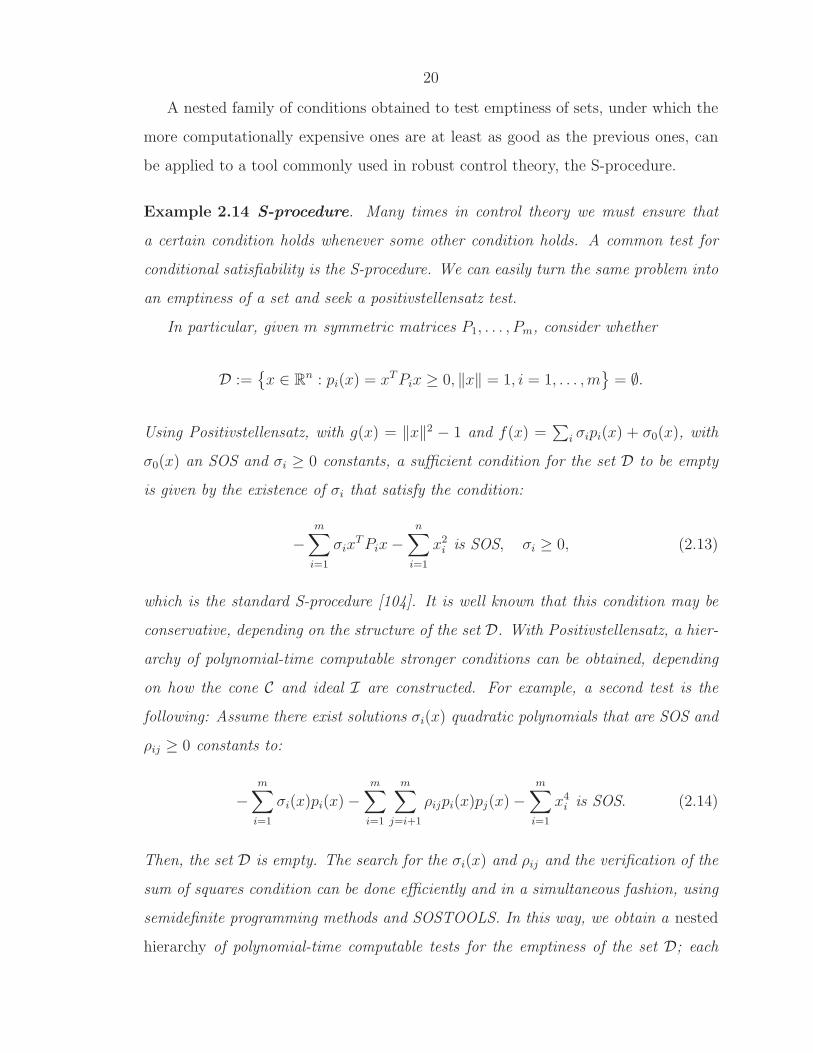
Example 2.14 S-procedure. Many times in control theory we must ensure that
a certain condition holds whenever some other condition holds. A common test for
conditional satisfiability is the S-procedure. We can easily turn the same problem into
an emptiness of a set and seek a positivstellensatz test.
In particular, given m symmetric matrices P1, . . . , Pm, consider whether
D :=x ∈ R
n : pi(x) = xTPix ≥ 0, ‖x‖ = 1, i = 1, . . . ,m
= ∅.
Using Positivstellensatz, with g(x) = ‖x‖2 − 1 and f(x) =∑
i σipi(x) + σ0(x), with
σ0(x) an SOS and σi ≥ 0 constants, a sufficient condition for the set D to be empty
is given by the existence of σi that satisfy the condition:
−m∑
i=1
σixTPix−
n∑
i=1
x2i is SOS, σi ≥ 0, (2.13)
which is the standard S-procedure [104]. It is well known that this condition may be
conservative, depending on the structure of the set D. With Positivstellensatz, a hier-
archy of polynomial-time computable stronger conditions can be obtained, depending
on how the cone C and ideal I are constructed. For example, a second test is the
following: Assume there exist solutions σi(x) quadratic polynomials that are SOS and
ρij ≥ 0 constants to:
−m∑
i=1
σi(x)pi(x) −m∑
i=1
m∑
j=i+1
ρijpi(x)pj(x) −m∑
i=1
x4i is SOS. (2.14)
Then, the set D is empty. The search for the σi(x) and ρij and the verification of the
sum of squares condition can be done efficiently and in a simultaneous fashion, using
semidefinite programming methods and SOSTOOLS. In this way, we obtain a nested
hierarchy of polynomial-time computable tests for the emptiness of the set D; each

21
test is always at least as powerful as the standard one, and often strictly stronger.
In the sequel, we will come across various S-procedure type conditions which
we test using SOSTOOLS in the framework given above. Instead of using constant
multipliers such as the unknowns σi in (2.13), we will be using higher order multipliers
such as the σi(x) in (2.14) – condition that is at least as strong as (2.13) to test the
emptiness of the set D.
2.3 Conclusion
In this chapter, we have developed the algorithmic and mathematical tools that will
be used in the rest of the thesis for the analysis of nonlinear systems. These center on
the sum of squares decomposition and positivstellensatz – tools that may be used to
produce new tests that generalize the S-procedure for testing conditional satisfiability.
In the next chapters we will use the SOS decomposition to test nonnegativity
and we will formulate Lyapunov and S-procedure type SOS conditions for analysis
of nonlinear systems. We will then search for Lyapunov functions or multipliers that
satisfy those conditions using semidefinite programming.
22
Chapter 3
Systems Described by OrdinaryDifferential EquationsT yuqr jèretai, jermän yÔqetai,Ígrän aÎanetai, karfalèon notzetai.<Hrkleito
Cold things become warm, and what is warm cools;what is wet dries, and the parched is moistened.
Heracletus
In this chapter, we will investigate how various analysis questions for nonlinear
systems described by Ordinary Differential Equations (ODEs) can be answered using
sums of squares (SOS). ODEs have been an important tool for modeling the physical
world, ranging from simple mechanical and electrical systems to chemical processes
and simplified aircraft dynamics. They have also been the primary tool for modeling
components in biological networks or multi-agent systems. Usually, the far-from-
equilibrium behavior of such systems is of greater interest than the local ‘linearized’
properties, and most analysis tools for such systems center in what are now known
as ‘Lyapunov methods’, named after A. M. Lyapunov. The main feature of these
techniques is that system properties are assessed without solving the underlying model
equations, but rather through the construction of a function of state (a Lyapunov
function) that satisfies certain conditions.
In this chapter, we develop an efficient algorithmic procedure to analyze nonlinear
systems described by ODEs that evolve under constraints such as equality, inequality
and integral type. This allows robust stability analysis, input-output analysis, as

23
well as analysis of non-polynomial systems to be performed in a unified manner.
The techniques we will be using are based on the sum of squares decomposition and
Positivstellensatz, as they were introduced in Chapter 2.
3.1 Introduction
Systems which appear in electrical or mechanical engineering and even biology are
usually modeled by a finite number of coupled first-order Ordinary Differential Equa-
tions (ODEs) of the form:
x1 = f1(t, x1, . . . , xn),
x2 = f2(t, x1, . . . , xn),
......
xn = fn(t, x1, . . . , xn),
where xi denotes the derivative of xi with respect to time, and xi are the state
variables. We use vector notation to describe this system. Let x ∈ Rn and let
f : [0,∞) × Rn → R
n. Then, the above can be written as:
x = f(t, x). (3.1)
If f(t, x) is piecewise continuous in t and satisfies a local Lipschitz condition in x,
then the existence and uniqueness of the solutions is guaranteed locally [35].
In this chapter, we will concentrate on systems that are autonomous, i.e., take the
form
x = f(x), (3.2)
where f : D → Rn is locally Lipschitz in a domain D ⊂ R
n. Suppose x∗ is an
equilibrium point of (3.2), i.e. f(x∗) = 0. Without loss of generality, we assume that
0 is an equilibrium – a simple change of coordinates can achieve this – and we are
interested in the stability properties of this equilibrium. There are different notions

24
of stability of equilibria which are usually characterized using Lyapunov arguments.
Here, we concentrate on stability and asymptotic stability ; ‖ · ‖ denotes a norm in Rn.
Definition 3.1 The equilibrium x = 0 of (3.2) is:
• Stable, if for each ǫ > 0 there is δ = δ(ǫ) > 0 such that
‖x(0)‖ < δ ⇒ ‖x(t)‖ < ǫ, ∀ t ≥ 0.
• Asymptotically stable if it is stable and δ can be chosen such that
‖x(0)‖ < δ ⇒ limt→∞
x(t) = 0.
We can see that these definitions of stability involve ǫ − δ formulations, which
at first give the impression that a complete description of the flow of the vector
field is required to answer stability questions. It is fortunate that in many cases
stability can be proved directly by exhibiting an energy-like function, now called a
Lyapunov function [35, 107]. This is Lyapunov’s direct method. Under some technical
conditions, the existence of this function was also proved necessary for asymptotic
stability [27]. More precisely, the conditions are stated in the following theorem:
Theorem 3.2 ([35]) Consider the system (3.2), and let D ⊆ Rn be a neighborhood
of the origin. If there is a continuously differentiable function V : D → R such that
the following two conditions are satisfied:
1. V (x) > 0 for all x ∈ D \ 0 and V (0) = 0, i.e., V (x) is positive definite in D;
2. −V (x) = −∂V∂xf(x) ≥ 0 for all x ∈ D, i.e., V (x) is negative semidefinite in D;
then the origin is a stable equilibrium. If in condition (2) above, V (x) is negative
definite in D, then the origin is asymptotically stable. If D = Rn and V (x) is radially
unbounded, i.e., V (x) → ∞ as ‖x‖ → ∞, then the result holds globally.

25
In the case of linear time-invariant systems
x = Ax, (3.3)
the stability properties can be characterized by the locations of the eigenvalues λi of
the matrix A, or equivalently, through a Lyapunov argument as follows:
Theorem 3.3 [35] The matrix A is a stability matrix; that is Reλi < 0 for all
eigenvalues λi of A if and only if for any given positive definite matrix Q there exists
a positive definite matrix P that satisfies:
PA+ ATP = −Q. (3.4)
P is unique, and V = xTPx is a Lyapunov function for (3.3).
We see that the construction of the Lyapunov function in the case of linear sys-
tems is reduced to solving an appropriate Algebraic Lyapunov Equation (3.4). Al-
ternatively, P can be obtained by solving two Linear Matrix Inequality (LMI) [10]
conditions:
P > 0,
ATP + PA < 0.
A feasible P exists if and only if A is Hurwitz. LMIs are constraints in semidefinite
programs [96], which can be solved using algorithms with a worst-case polynomial
time complexity. This makes them particularly attractive for computation.
The absence of a direct methodology for constructing Lyapunov functions for
nonlinear systems led to the development of other methods for assessing nonlinear
system properties. For example, in Lyapunov’s indirect method, one proceeds by
linearizing the vector field about the equilibrium and the (local) stability proper-
ties of the original nonlinear system are inferred from the stability properties of the
linearized system. However, this procedure is inconclusive when the linearized sys-

26
tem has imaginary axis eigenvalues and the result is valid anyway only locally. Other
methodologies involve absolute stability theory [19], Linear Parameter Varying (LPV)
embeddings [23, 86, 53], Integral Quadratic Constraint (IQC) formulations [47] and
others.
In this chapter, we will build on the methodology introduced in [66] and we will
show how to use the sum of squares decomposition to analyze different classes of
systems described by ODEs using Lyapunov methodologies. There are mainly two
reasons why there has been no algorithmic methodology for constructing the Lya-
punov functions V (x) for so long. On one hand, the ‘terms’ that should appear in
V (x) are not known a priori, and on the other hand, testing the nonnegativity condi-
tions in Theorem 3.2 is a difficult task even in the case in which they are polynomial.
We can get to the bottom of the first problem by resorting to intuition and prior
knowledge of energy-like terms that are likely to appear in V (x). As far as the sec-
ond problem is concerned, this is closely related to the fact that testing polynomial
nonnegativity when the degree is greater than or equal to 4 is an NP-hard problem,
as was mentioned in the previous chapter [50].
For concreteness, let us assume that f(x) is a polynomial vector field. Suppose
that we also wish to construct a V (x) that is also polynomial in x. In this case,
the two conditions in Theorem 3.2 become polynomial nonnegativity conditions. To
circumvent the difficult task of testing them, we can restrict our attention to cases in
which the two conditions admit SOS decompositions. Note that even if the coefficients
of a polynomial Lyapunov candidate V are unknown, we can still search for them so
that the two Lyapunov conditions are satisfied, as was explained in the previous
chapter.
To impose that V (x) should be positive definite rather than positive semi-definite,
we construct an auxiliary positive definite ‘shaping’ function ϕ(x) as follows:
ϕ(x) =n∑
i=1
d∑
j=1
ǫijx2ji ,
m∑
j=1
ǫij ≥ γ ∀ i = 1, . . . , n, γ > 0, ǫij ≥ 0 ∀ i, j (3.5)
This makes ϕ(x) > 0, i.e., positive definite. If we impose V (x) − ϕ(x) to be a SOS,

27
obviously
V (x) − ϕ(x) ≥ 0 ⇒ V (x) ≥ ϕ(x) > 0. (3.6)
Therefore, we have
Proposition 3.4 Given a polynomial V (x) of degree 2d, let ϕ(x) be given by Equa-
tion (3.5). Then, the condition
V (x) − ϕ(x) is a sum of squares (3.7)
guarantees the positive definiteness of V (x).
In the case of global stability, i.e., for D = Rn, the conditions in Theorem 3.2 can
then be formulated directly as SOS conditions. Therefore, we have the following sum
of squares program:
Program 3.5 To construct a Lyapunov function for system (3.2),
Find a polynomial V (x), V (0) = 0
and a positive definite function ϕ(x) of the form (3.5)
such that
V (x) − ϕ(x) is SOS (3.8)
− ∂V
∂xf(x) is SOS (3.9)
Then V (x) is a Lyapunov function for system (3.2) and the zero equilibrium of (3.2)
is globally stable.
The above program guarantees that V (x) is positive definite and also that V (x) is
negative semidefinite; therefore V (x) is a Lyapunov function that proves stability of
the origin of system (3.2). Note also that by construction ϕ(x) is radially unbounded;
therefore, V (x) will also be radially unbounded, and the stability property holds

28
globally [35]. Also, if condition (3.9) is replaced by
−∂V∂x
f(x) − ψ(x) is SOS, (3.10)
where ψ(x) is a positive definite polynomial constructed as per (3.5), then V (x) is
negative definite and the origin is globally asymptotically stable.
Below is an example of how the construction of a Lyapunov function is performed
using SOSTOOLS.
Example 3.6 Consider the system
x1 = −x1 + x32 − 3x3x4
x2 = −x1 − x32
x3 = x1x4 − x3
x4 = x1x3 − x34,
which has the only equilibrium at the origin. As a first attempt, we will try to construct
a quadratic Lyapunov function of the form V =∑4
i=1
∑4j=i aijxixj where the aij’s are
the unknowns. We search for V that satisfy the conditions in Program 3.5.
It turns out that a Lyapunov function of the above form does not exist (the cor-
responding semidefinite program is infeasible), so we will next search for a quartic
Lyapunov function. One then finds a Lyapunov function that satisfies conditions
(3.8) and (3.10), and thus proves global asymptotic stability of the origin. To three
significant figures, this reads:
V = 1.12x1x2x23 − 0.785x1x2 + 0.713x3
2x1 + 0.500x1x2x24 + 0.768x4
4
+1.64x21 + 1.76x2
3 + 0.392x22 + 1.63x2
4 + 1.69x21x
22 + 0.557x4
3
+0.724x31x2 + 0.181x4
1 + 1.07x42 + 0.561x2
1x23 + 1.61x2
2x23
+0.525x21x
24 + 0.969x2
2x24 + 0.569x2
3x24 − 0.251x4x3x1 + 0.432x4x3x2.
The above can be obtained by using the findlyap command in SOSTOOLS.

29
3.2 Stability of Constrained Systems
In this section, we extend Lyapunov’s theorem to systems that evolve under equality,
inequality, and integral constraints. This is a very general class of systems, special
cases of which are differential algebraic equations, robust stability analysis and per-
formance formulations. It will also allow us to treat non-polynomial vector fields
exactly.
Inequality constraints arise naturally when considering positive systems : systems
with inherently positive states, e.g., a chemical reaction in which the concentrations
of the reactants are positive. The same type of constraints can be used to describe
uncertain parameter sets for the study of robust stability of systems in the presence
of parametric uncertainty.
On the other hand, systems evolving over a manifold described by a set of equal-
ity constraints arise in a plethora of cases, and are also called differential algebraic
equations or descriptor systems [16]. Examples of equality constraints are holonomic
(configuration) constraints in mechanical systems and conservation laws – in electrical
networks in the form of current balance and in chemical engineering in the form of
mass balance. Sometimes it is possible to back-substitute and reduce the system to
an ordinary differential equation, but this usually results in more complicated vector
fields of higher order. In some other cases, this is not possible and a differential index
theory was developed as a measure of this singularity [91]. Equality constraints also
prove useful in robust stability analysis where they appear as constraints guaranteeing
that the equilibrium of the system is at the origin.
The last type of constraints that are going to be incorporated is of integral type,
in particular Integral Quadratic Constraints (IQCs) [47]. They provide a framework
rich enough to encapsulate many types of uncertainty and unmodelled dynamics:
dynamic, time-varying and L2 bounded uncertainty, just to name a few. Moreover,
one can formulate performance calculations using IQCs such as L2 input-output gain
estimation.

30
Consider the nonlinear system
x = f(x, u), (3.11)
with the following inequality, equality, and integral constraints that are satisfied by
x and u:
ai1(x, u) ≤ 0, for i1 = 1, ..., N1, (3.12)
bi2(x, u) = 0, for i2 = 1, ..., N2, (3.13)
∫ T
0ci3(x, u)dt ≤ 0, for i3 = 1, ..., N3, and ∀ T ≥ 0. (3.14)
Here x ∈ Rn is the state of the system, and u ∈ R
m is a collection of auxiliary variables
(such as inputs, non-polynomial functions of states, uncertain parameters, etc). We
assume that f(x, u), apart from the required Lipschitz conditions for existence of
solutions, has no singularity in D, where D ⊂ Rn+m is defined as
D = (x, u) ∈ Rn+m | ai1(x, u) ≤ 0, bi2(x, u) = 0, for all i1 and i2.
Without loss of generality, it is also assumed that f(x, u) = 0 for x = 0 and u ∈ D0u,
where
D0u = u ∈ R
m|(0, u) ∈ D.
The following theorem is an extension of Lyapunov’s stability theorem, and can be
used to prove that the origin is a stable equilibrium of the above system. It uses a
technique reminiscent of the well-known S-procedure [104] in nonlinear and robust
control theory, that was discussed in Example 2.14.
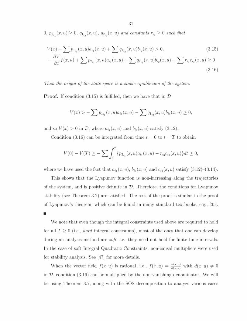
Theorem 3.7 [62] Suppose that for system (3.11), there exist functions V (x), p1i1(x, u) ≥
31
0, p2i1(x, u) ≥ 0, q1i2
(x, u), q2i2(x, u) and constants ri3 ≥ 0 such that
V (x) +∑
p1i1(x, u)ai1(x, u) +
∑
q1i2(x, u)bi2(x, u) > 0, (3.15)
− ∂V
∂xf(x, u) +
∑
p2i1(x, u)ai1(x, u) +
∑
q2i2(x, u)bi2(x, u) +
∑
ri3ci3(x, u) ≥ 0
(3.16)
Then the origin of the state space is a stable equilibrium of the system.
Proof. If condition (3.15) is fulfilled, then we have that in D
V (x) > −∑
p1i1(x, u)ai1(x, u) −
∑
q1i2(x, u)bi2(x, u) ≥ 0,
and so V (x) > 0 in D, where ai1(x, u) and bi2(x, u) satisfy (3.12).
Condition (3.16) can be integrated from time t = 0 to t = T to obtain
V (0) − V (T ) ≥ −∑
∫ T
0
p2i1(x, u)ai1(x, u) − ri3ci3(x, u)dt ≥ 0,
where we have used the fact that ai1(x, u), bi2(x, u) and ci3(x, u) satisfy (3.12)–(3.14).
This shows that the Lyapunov function is non-increasing along the trajectories
of the system, and is positive definite in D. Therefore, the conditions for Lyapunov
stability (see Theorem 3.2) are satisfied. The rest of the proof is similar to the proof
of Lyapunov’s theorem, which can be found in many standard textbooks, e.g., [35].
We note that even though the integral constraints used above are required to hold
for all T ≥ 0 (i.e., hard integral constraints), most of the ones that one can develop
during an analysis method are soft, i.e. they need not hold for finite-time intervals.
In the case of soft Integral Quadratic Constraints, non-causal multipliers were used
for stability analysis. See [47] for more details.
When the vector field f(x, u) is rational, i.e., f(x, u) = n(x,u)d(x,u)
with d(x, u) 6= 0
in D, condition (3.16) can be multiplied by the non-vanishing denominator. We will
be using Theorem 3.7, along with the SOS decomposition to analyze various cases

32
of systems with constraints. The procedure is similar to the one for the case of
unconstrained systems described in the previous section, and is based on relaxing
the conditions in Theorem 3.7 to SOS conditions. For this, we need to make some
assumptions, some of which will be removed in the sequel.
• The vector field fx(x, u) is assumed to be polynomial or rational, and the con-
straint functions ai1(x, u), bi2(x, u), ci3(x, u) are assumed to be polynomial. This
assumption will be removed in a later section through a recasting process.
• We search for bounded degree polynomial Lyapunov function V and multipliers
pi1 , qi1 , i1 = 1, . . . , N1 and pi2 , qi2 , i2 = 1, . . . , N2.
To make the above concrete, in order to use Theorem 3.7 and the sum of squares
decomposition, we have the proposition below.
Proposition 3.8 Suppose that for system (3.1) with f(x, u) = n(x,u)d(x,u)
where n(x, u)
and d(x, u) are polynomials and d(x, u) > 0 in D, there exist polynomial functions
V (x), p1i1(x, u), p2i1
(x, u), q1i2(x, u), q2i2
(x, u), a positive definite function ϕ(x) of
the form given in Equation 3.5 and constants ri3 ≥ 0 such that
V (x) +∑
p1i1(x, u)ai1(x, u) +
∑
q1i2(x, u)bi2(x, u) − ϕ(x) is SOS, (3.17)
p1i1(x, u), p2i1
(x, u) are SOS for i1 = 1, . . . , N1, (3.18)
d(x, u)
−∂V
∂xf(x, u) +
∑p2i1
(x, u)ai1(x, u)
+∑q2i2
(x, u)bi2(x, u) +∑ri3ci3(x, u)
is SOS. (3.19)
Then the origin of the state space is a stable equilibrium of the system.
The polynomials V (x), p1i1(x, u), p2i1
(x, u), q1i2(x, u), q2i2
(x, u), the constants ri3
and the positive definite function ϕ(x) can be constructed using SOSTOOLS [75],
and a program similar to Program 3.5 can be constructed.
It was mentioned that the particular class of systems with constraints that we
consider is rich enough to include as special cases various important analysis problems
in control theory. The rest of the chapter concentrates on some of these problems.

33
3.3 Estimating the Region of Attraction
In many instances, non-global stability analysis may be the objective, i.e., when
dealing with physical models with positivity constraints on the states (often referred
to as positive systems [42]), or when several equilibria or limit cycles are present. In
such cases, one may define regions of interest using inequality constraints.
For example, let us consider local stability analysis of the zero equilibrium of
x = f(x). Define the following inequality constraint on x:
a(x) , xTx− ξ ≤ 0, (3.20)
where ξ is a positive constant. Then local stability of the zero equilibrium can be
tested using the next corollary.
Corollary 3.9 Suppose for the system x = f(x) and the inequality constraint a(x) ≤0 given in (3.20) there exist a polynomial function V (x) and SOS polynomials p1(x), p2(x)
such that
V (x) + p1(x)a(x) − ϕ(x) is SOS,
− ∂V
∂xf(x) + p2(x)a(x) is SOS,
where ϕ(x) is as defined in Equation (3.5). Then the zero equilibrium of the system
is stable.
A problem of particular interest is estimation of the region of attraction of an
equilibrium. An estimate of the region of attraction is the largest level set of V (x)
obtained from the previous corollary which can ‘fit’ in the region described by a(x) ≤0. More specifically, given a Lyapunov function V (x) and a domain D in which a
Lyapunov function satisfying the conditions of asymptotic stability was constructed,
we seek a γ > 0 such that Ωγ = x ∈ Rn|V (x) ≤ γ is bounded and strictly contained
in D; then Ωγ is an estimate of the region of attraction. In order to get the maximum
value of γ, we can formulate the problem as one of testing emptiness of a set as

34
follows:
x ∈ Rn : V (x) < γ, a(x) = 0 = ∅ (3.21)
Positivstellensatz conditions take the form:
(N∑
i=1
x2i
)r
(V (x) − γ) + p(x)a(x) is a SOS (3.22)
where r is a non-negative integer and p(x) is a polynomial. Therefore, the task of
finding the maximum γ can be formulated as the following sum of squares program:
Program 3.10 Program to find the maximum γ such that x ∈ Rn|V (x) < γ ⊂
x ∈ Rn|a(x) ≤ 0:
Given V (x), a(x), maximize γ and find a non-negative integer r
and a polynomial p(x) such that(
N∑
i=1
x2i
)r
(V (x) − γ) + p(x)a(x) is a SOS.
In order to find good estimates of the region of attraction, one has to iterate
between V (x) and a(x).
Example 3.11 Consider the Van der Pol equation in reverse time:
x1 = −x2 (3.23)
x2 = x1 − (1 − x21)x2 (3.24)
The phase plane is shown in Figure 3.1(a); the presence of an unstable limit cy-
cle makes the stability of the only equilibrium local. In this case, we are interested
in determining how far from the origin we can choose an initial condition and the
trajectory will still converge to the origin. To obtain an estimate of the region of
attraction of the zero equilibrium of (3.23–3.24), we first initialize a(x) = xTx − ξ,
and search for V (x) of order 2 such that V (x) > 0 everywhere and V (x) < 0 in D,
performing a search on ξ. Obviously, at some point, V (x) = 0; therefore, we need to

35
−2.5 −2 −1.5 −1 −0.5 0 0.5 1 1.5 2 2.5−3
−2
−1
0
1
2
3
x1
x 2
The Van Der Pol system
−2.5 −2 −1.5 −1 −0.5 0 0.5 1 1.5 2 2.5−3
−2
−1
0
1
2
3
x1
x 2
Regions of Attraction for the Van der Pol system
Lyapunov order 2Lyapunov order 4Lyapunov order 6Lyapunov order 8
(a) (b)
Figure 3.1: The Van der Pol system in reverse time, with estimates of the region ofattraction of the stable equilibrium.
find the maximum γ such that V (x) − γ is completely contained in the set V (x) ≤ 0.
We then set a(x) = V (x) − γ, and increase the order of V (x) by 2. We can then
find a new Lyapunov function of this order adjusting γ, iterating between V (x) and
a(x). Estimates of the region of attraction in the form V (x) ≤ γ were constructed for
different degree V (x), shown in Figure 3.1(b).
3.4 Analysis of Systems with Non-Polynomial Vec-
tor Fields
Thus far, we have concentrated on systems that are described by polynomial vector
fields. It is true that physical systems, the functionality of which is in the focus of
many research areas, seldom are modeled by polynomial vector fields.
In this section, we will build on a recasting process [82] that produces a polynomial
system description from a non-polynomial one, with state dimension at least the same
as the original system or higher. The stability properties of the original system can
be concluded from the analysis of the recasted system [63]. To describe the original
system faithfully, constraints of the form xn+1 = F (x1, ..., xn) that are created when
new variables are introduced should be taken into account. These constraints define

36
an n-dimensional manifold on which the solutions to the original differential equations
lie. In general such constraints cannot be converted into polynomial forms, even
though sometimes there exist polynomial constraints that are induced by the recasting
process. For example:
• Two variables introduced for trigonometric functions such as x2 = sinx1, x3 =
cosx1 are constrained via x22 + x2
3 = 1.
• Introducing a variable to replace a power function such as x2 =√x1 induces
the constraints x22 − x1 = 0, x2 ≥ 0.
• Introducing a variable to replace an exponential function such as x2 = exp(x1)
induces the constraint x2 ≥ 0.
We will identify two different classes of systems. We consider systems with non-
polynomial vector fields that under a change of variables are transformed into poly-
nomial with:
1. Only polynomial equality constraints;
2. Non-polynomial equality constraints.
A particular example of case (1) above is the simple pendulum, which is described
by:
d
dt
θ
ω
=
ω
−glsin θ
where g is the gravitational constant, l is the length of the pendulum, ω its angular
velocity and θ the angular deviation of the bead from the vertical. Setting x1 = sin θ
and x2 = cos θ, one can easily rewrite the above system as
d
dt
x1
ω
x2
=
x2ω
−glx1
−x1ω
x21 + x2
2 = 1

37
where the constraint x21 +x2
2 = 1 is a polynomial equality in (x1, x2) that restricts the
3-D recasted system to the original 2-D system.
However, in some cases (case (2) above), this technique results in a series of
equality constraints that are not polynomial equalities, for example, relating sin(θ)
and θ. These appear many times because of modeling descriptions. For example, in
order to model enzymatic reactions in biological systems [48], it is common practice
to use vector fields with non-rational powers, in the Michaelis-Menten sense. Also,
the model of an aircraft in longitudinal flight contains trigonometric nonlinearities of
the angle of attack and pitch angle, but in the same equations, one usually captures
the coefficients of lift and drag as polynomial descriptions of these variables. The
stability analysis of the closed loop system using the above methodology becomes
difficult, as the same variable appears both in polynomial and non-polynomial terms.
The same is true in the case of analysis of chemical processes, where the temperature
appears in the energy equation both as a state and also exponentiated in Arrhenius
law for the reaction rate.
Suppose that for a nonpolynomial system
z = f(z) (3.25)
which has an equilibrium at the origin, the recasted system obtained using a recasting
procedure is written as
˙x1 = f1(x1, x2), (3.26)
˙x2 = f2(x1, x2), (3.27)
where x1 = (x1, ..., xn) = z are the state variables of the original system, x2 =
(xn+1, ..., xn+m) are the new variables introduced in the recasting process, and f1(x1, x2),
f2(x1, x2) are polynomial in their arguments.
We denote the constraints that arise directly from the recasting process (i.e., the

38
polynomial ones) by
x2 = F (x1), (3.28)
and those that arise indirectly (the non-polynomial ones) by
G1(x1, x2) = 0, (3.29)
G2(x1, x2) ≤ 0, (3.30)
where F , G1, andG2 are column vectors of functions with appropriate dimensions, and
the equalities or inequalities hold entry-wise. We should keep in mind that constraints
(3.29)–(3.30) are satisfied only when x2 = F (x1) are substituted to (3.29)–(3.30). We
assume that all functions involved are polynomials in their arguments.
Proving stability of the zero equilibrium of the original system (3.25) amounts to
proving that all trajectories starting close enough to z = 0 will remain close to this
equilibrium point. This can be accomplished by finding a Lyapunov function V (z)
that satisfies the conditions of Lyapunov’s stability theorem. Here we use the recasted
system to construct a Lyapunov function that proves stability of the equilibrium of
the original system. Sufficient conditions that guarantee the existence of a Lyapunov
function are stated in the following proposition.
Proposition 3.12 Let D1 ⊂ Rn and D2 ⊂ R
m be open sets such that 0 ∈ D1
and F (D1) ⊆ D2. Furthermore, define x2,0 = F (0). If there exists a function
V : D1 × D2 → R and column vectors of functions λ1(x1, x2), λ2(x1, x2), σ1(x1, x2),

39
and σ2(x1, x2) with appropriate dimensions such that
V (0, x2,0) = 0, (3.31)
V + λT1G1 + σT1 G2 − φ(x1, x2) ≥ 0 ∀(x1, x2) ∈ D1 ×D2, (3.32)
− ∂V
∂x1
f1 −∂V
∂x2
f2 + λT2G1 + σT2 G2 ≥ 0 ∀(x1, x2) ∈ D1 ×D2, (3.33)
σ1(x1, x2) ≥ 0 ∀(x1, x2) ∈ Rn+m, (3.34)
σ2(x1, x2) ≥ 0 ∀(x1, x2) ∈ Rn+m, (3.35)
for some scalar function φ(x1, x2) with φ(x1, F (x1)) > 0 ∀x1 ∈ D1 \ 0, then z = 0
is a stable equilibrium of (3.25).
Proof. Define V (z) = V (z, F (z)). From (3.31) and (3.32), it is straightforward to
verify that the first Lyapunov condition is satisfied by V (z). In fact, from (3.29)–
(3.30), (3.32) and (3.34), we have that
V (x1, x2) ≥ φ(x1, x2) − λT1G1 − σT1 G2 ≥ φ(x1, x2) ∀(x1, x2) ∈ D1 ×D2.
Since φ(z, F (z)) > 0 ∀z ∈ D1 \0 and F (D1) ⊆ D2, it follows that V (z) > 0 ∀z ∈D1 \ 0.
Finally, by the chain rule of differentiation we have
∂V
∂z(z)f(z) =
∂V
∂x1
(z, F (z))f1(z, F (z)) +∂V
∂x2
(z, F (z))f2(z, F (z)),
and using the same argument as above in conjunction with (3.29)–(3.30), (3.33) and
(3.35), we see that the second Lyapunov condition is satisfied. Therefore, V (z) is a
Lyapunov function for (3.25) and z = 0 is a stable equilibrium of the system.
The above non-negativity conditions can be relaxed to appropriate sum of squares
conditions so that they can be algorithmically verified using semidefinite program-
ming, as discussed earlier in this chapter. This leads the way to an algorithmic con-
struction of the Lyapunov function V . For this purpose, the set D1 ×D2 is captured

40
as a semialgebraic set:
D1 ×D2 = (x1, x2) ∈ Rn × R
m : GD(x1, x2) ≥ 0,
where GD(x1, x2) is a column vector of polynomials and the inequality is satisfied
entry-wise.
Let us now give an example of how this methodology can be used.
Example 3.13 (Continuously Stirred Tank Reactor) Chemical reactors are
the most important unit in a chemical process. Here, we consider the analysis of the
dynamics of a perfectly mixed, diabatic, continuously stirred tank reactor (CSTR) [3].
We also assume a constant volume – constant parameter system for simplicity.
The reaction taking place in the CSTR is a first-order exothermic irreversible
reaction A → B. After balancing mass and energy, the reactor temperature T and
the concentration of species A in the reactor CA evolve as follows:
CA =F
V(CAf
− CA) − k0e−∆E
RT CA (3.36)
T =F
V(Tf − T ) − ∆H
ρcpk0e
−∆ERT CA − UA
V ρcp(T − Tj) (3.37)
where F is the volumetric flow rate, V is the reactor volume, CAfis the concentration
of A in the freestream, k0 is the pre-exponential factor of Arrhenius law, ∆E is the
reaction activation energy, R is the ideal gas constant, Tf is the feed temperature,
−∆H is the heat of reaction (exothermic), ρ is the density, cp is the heat capacity, U
is the overall heat transfer coefficient, A is the area for heat exchange, and Tj is the
jacket temperature. For the analysis, we use the values shown in Table 3.1.
The equilibrium of the above system is given by (CA0 , T0) = (8.5636, 311.171). We
employ the following transformation: x1 = CA/CA0 − 1, x2 = T/T0 − 1; this serves
two purposes: first it moves the equilibrium to the origin, and second, it rescales the

41
Parameter Units Nominal Value
F/V hr−1 1k0 hr−1 9703×3600
−∆H kcal/kgmol 5960∆E kcal/kgmol 11843ρcp kcal/(m3 C) 500Tf
C 25CAf
kgmol/m3 10
UA/V kcal/(m3 C hr) 150Tj
C 25
Table 3.1: Parameter values for the Continuously Stirred Tank Reactor (CSTR)system.
state to reduce numerical ill-conditioning. The transformed system then becomes:
x1 =F
V
(CAf
CA0
− (x1 + 1)
)
− k0e− ∆E
RT0(x2+1) (x1 + 1)
x2 =F
V
(TfT0
− (x2 + 1)
)
− ∆HCA0
ρcpT0
k0e− ∆E
RT0(x2+1) (x1 + 1) − UA
V ρcp
(
(x2 + 1) − TjT0
)
Note that the system has an exponential term; the recasting will yield an indirect
constraint, as discussed earlier in this section. Define the state x3 = e∆Ex2
RT0(x2+1) − 1.
Then an extra equation in the analysis would be
x3 =∆E
RT0(x2 + 1)2(x3 + 1)x2
under the constraint that x3 > −1.
Then the full system, after we use the equilibrium relationship simplifies to:
x1 = −FVx1 − k0e
− ∆ERT0 (x1x3 + x1 + x3) (3.38)
x2 = −FVx2 −
∆HCA0
ρcpT0
k0e− ∆E
RT0 (x1x3 + x1 + x3) −UA
V ρcpx2 (3.39)
x3 =∆E
RT0(x2 + 1)2(x3 + 1)x2 (3.40)
This system is now of the form (3.26)–(3.27), with x1 = (x1, x2) and x2 = x3. To

42
7.6 7.8 8 8.2 8.4 8.6 8.8 9 9.2305
310
315
320
CA
T
CSTR system
Figure 3.2: Lyapunov function level curves for the Continuously Stirred Tank Reactorsystem.
proceed, we define the set D1 as:
D1 = (x1, x2) ∈ R2 : |x1| ≤ γ1, |x2| ≤ γ2
and then define the set D2 as
D2 = x3 ∈ R : (x3 − e−∆Eγ2
RT0(−γ2+1) − 1)(x3 − e∆Eγ2
RT0(γ2+1) − 1) ≤ 0
Then the system is ready for analysis as per Proposition 3.12. For γ1 = 0.12 and
γ2 = 0.05, a quartic Lyapunov function can be constructed for the system described
by Equations (3.38)–(3.40) using Proposition 3.12. Here the following φ(x) is used:
φ(x) =2∑
i=1
∑
j=2,4
ǫi,jxji +
4∑
j=1
ǫ3,jxj3,
with
ǫ1,2 + ǫ1,4 − 0.1 ≥ 0
ǫ2,2 + ǫ2,4 + ǫ3,1 + ǫ3,2 + ǫ3,3 + ǫ3,4 − 0.1 ≥ 0.
The level curves of the constructed Lyapunov function are shown in Figure 3.2.

43
As mentioned earlier, it is common practice in modeling biological reaction path-
ways to ‘lump’ enzymatic reactions consisting of three species into a single equation
in the Michaelis-Menten sense. The simplified system dynamics are obtained by a
methodology similar to singular perturbation methods in nonlinear control. Many
times, the ‘fitting’ is done based on experimental data, which results in non-integer
hill function coefficients. We will illustrate the technique with an example of biological
significance: regulation and autocatalysis in yeast glycolysis.
Example 3.14 Consider a simple biochemical reaction pathway consisting of two
metabolites, represented by the state variables x1 and x2. The product of the first
enzymatic reaction is the substrate for the second reaction, and the final output affects
the production of x1. The equations become:
x1 = xm2 − 1 + k
x1 + kx1 (3.41)
x2 =1 + k
x1 + kx1 − cxm2 − (1 − c)
1 + k
x2 + kx2 (3.42)
The free parameters in the model are k, m, and c. The sign of m determines the effect
of x2 on the production of x1. The system has an equilibrium point at x1 = x2 = x3 =
1 that is independent of the parameters. Linearization about this equilibrium gives the
system:
d
dt
δx1
δx2
=
− kk+1
m
kk+1
−cm− (1 − c) kk+1
δx1
δx2
Linear stability analysis asserts that stability is retained for 0 ≤ c ≤ 1, k−km−m ≥ 0
and k(2 − c) + cm(k + 1) ≥ 0, if we assume that k > 0. The stability region then
becomes:
k ≥ m1−m
for 0 ≤ m < 1
k ≥ −cm2+cm−c
for c−2c
≤ m < 0
(3.43)
We can translate the equilibrium of the system given by Equations (3.41–3.42) to

44
the origin by employing the transformation y1 = x1 − 1, y2 = x2 − 1 to get:
y1 = (y2 + 1)m − 1 + k
1 + y1 + k(y1 + 1)
y2 =1 + k
1 + y1 + k(y1 + 1) − c(y2 + 1)m − (1 − c)
1 + k
1 + y2 + k(y2 + 1)
If m is integer, then this system is polynomial. If m is not integer, then one can
proceed as in the CSTR example and try to analyze it directly. To illustrate a special
case when having non-integer (but rational) powers, consider m = 1/3. Denote
z = (y2 + 1)(1/3) − 1
Then we have the system
y1 = z + 1 − 1 + k
1 + y1 + k(y1 + 1) (3.44)
y2 =1 + k
1 + y1 + k(y1 + 1) − c(z + 1) − (1 − c)
1 + k
1 + y2 + k(y2 + 1) (3.45)
z =z + 1
3(y2 + 1)y2 (3.46)
(z + 1)3 = (y2 + 1) (3.47)
i.e., a 3-D system restricted by one equality constraint. The system is now in a DAE
formulation. We set c = 0.5 and k = 1 and use SOSTOOLS to construct a Lyapunov
function for this system, whose level curves are shown in Figure 3.3. In this figure,
‘+’ denotes the equilibrium point, solid lines are trajectories with initial conditions
indicated by ‘o’, arrows denote vector field and dashed lines are level curves of the
Lyapunov function.
In this example, m is an important parameter, and we wish to analyze robust
stability of the above system when m and k are allowed to vary. If we consider
stability analysis for −0.2 ≤ y1 ≤ 0.2 and −0.2 ≤ y2 ≤ 0.2, then we can approximate
(y2 + 1)m = 1 +my2 +m(m− 1)
2y2
2 + u(m, y2)

45
0.8 0.85 0.9 0.95 1 1.05 1.1 1.15 1.20.8
0.85
0.9
0.95
1
1.05
1.1
1.15
x1
x 2
Stability of metabolism system
Figure 3.3: Stability of the yeast glycolysis system.
and we can ‘cover’ the residual u by:
u(m, y2) = pmy22, p ∈ [−0.08, 0.06]
The system then becomes:
y1 = 1 +my2 +m(m− 1)
2y2
2 + pmy22 −
1 + k
1 + y1 + k(y1 + 1) (3.48)
y2 =1 + k
1 + y1 + k(y1 + 1) − c(1 +my2 +
m(m− 1)
2y2
2 + pmy22)
−(1 − c)1 + k
1 + y2 + k(y2 + 1) (3.49)
There are now three parameters in the system description, namely p, m and k. We
wish to prove stability of the equilibrium for the stable parameter set. To achieve this,
we construct two Lyapunov functions as shown in Figure 3.4: one for m ≥ 0 and one
for −m ≥ 0. In each region, there are five inequality constraints that we can write:
two on the state variables:
a1 , (y1 − 0.2)(y1 + 0.2) ≤ 0
a2 , (y2 − 0.2)(y2 + 0.2) ≤ 0,

46
one describing p ∈ [−0.08, 0.06]:
a3 , (p+ 0.08)(p− 0.06) ≤ 0,
and two describing the m−−k space; for m ≥ 0 we have:
a4 , −k + km+m+ 1 ≤ 0
a5 , m(m− 0.9) ≤ 0,
and for m ≤ 0 we have:
a4 , −1.5k − 0.5m(k + 1) + 1 ≤ 0
a5 , m(m+ 2.5) ≤ 0.
Using these constraints, the sum of squares program can be constructed and solved
with the aid of SOSTOOLS. The Lyapunov function V (y1, y2;m, p, k) for two ranges
of parameters, as well as the parameter region are shown in Figure 3.4. In this
figure, the shaded region in the center figure shows the parameter set for which a
parameterized Lyapunov function was constructed, and the region of stability given by
Equation (3.43). The figure on the left corresponds to a parameter set in which m is
negative, which results in system oscillations — the figure on the right corresponds
to another parameter set in which m is positive. In both cases, the level curves of a
Lyapunov function are shown dashed.
3.5 Robust Stability Analysis
The framework that we presented in this chapter allows the analysis of robustness of
systems with parametric and/or dynamic uncertainty.
In the case of parametric uncertainty, some of the auxiliary variables u in The-
orem 3.7 may now be taken to be parameters. Additionally, some other auxiliary
variables can be used to account for the location of the equilibrium of interest, as the

47
0.8 0.9 1 1.10.8
0.85
0.9
0.95
1
1.05
1.1
1.15
x1
x 2
k = 8, m = −2
0.8 0.9 1 1.10.8
0.85
0.9
0.95
1
1.05
1.1
1.15
x1
x 2
k = 15, m = 0.85
−3 −2.5 −2 −1.5 −1 −0.5 0 0.50
2
4
6
8
10
12
14
16
18
20
unstable
Parameter set
m
k
unstable
Lyapunov function constructed in this region
Figure 3.4: Robust stability of the yeast glycolysis system.
location of the equilibrium of a nonlinear system usually changes when the parame-
ters are varied. The use of equality and inequality constraints in this case is natural.
The region of the parameter space that is of interest can be described by inequality
constraints, and if the equilibrium moves as the parameters change, one can impose
an equality constraint on the corresponding auxiliary variables.
Dynamic uncertainty, on the other hand, can be characterized using integral con-
straints [47]. For example, an uncertain but L2-norm bounded feedback operator
relating x and u can be represented by the IQC
∫ T
0
(γxTx− uTu)dt ≥ 0.
Stability of the whole system can then be verified using Theorem 3.7.
The Lyapunov functions that we will be constructing may be parameterized by
the parameters. The introduction of new, unknown coordinates makes the size of the
resulting semidefinite programs grow fast. However, in some special cases, one can
structure these multipliers and functions so as to reduce the size of the semidefinite
programs and increase the numerical conditioning.
Here we consider a simple model that describes the phenomenon of heat shock in
E-coli, developed in [20].

48
Parameter Value
Kd 3αd 0.015η(T ) 10 @ T1 & 60 @ T2
α0 0.03αs 3Ks 0.05Ku 0.0254K(T ) 40 @ T1 & 80 @ T2
Kfold 6000Pt 2 × 10⁶
Table 3.2: Parameter values for the model of Heat Shock in E-coli.
Example 3.15 A simple description for the reduced order heat shock model is:
dDt
dt= Kd
St
1 + KsDt
1+KuUf
− αdDt
dStdt
= η(T ) − α0.St − αs
KsDt
1+KuUf
1 + KsDt
1+KuUf
St
dUfdt
= K(T )[Pt − Uf ] − [K(T ) +Kfold]Dt (3.50)
where Dt is the total number of chaperones, St is the total number of σ factors and
Uf is the amount of unfolded proteins. The rest are parameters that are tabulated in
Table 3.2.
In this example, we consider the problem of robust stability for the system under
parametric uncertainty. We first non-dimensionalize the states of (3.50) by their
equilibrium values (Dt0 , St0 , Uf0), followed by a shifting of the equilibrium of the system
to the origin, as it was done for the CSTR example. This yields a system with states
(x1, x2, x3) that is better conditioned, in the sense that the states are of the same order
of magnitude:
dx1
dt= f1(x1, x2, x3) − αdx1
dx2
dt= η(T ) − α0x2 − f2(x1, x2, x3) (3.51)
dx3
dt= K(T )[Pt − x3] −KTotx1

49
with f1(x1, x2, x3) = Kdx2
1+Ksx1
1+Kux3
and f2(x1, x2, x3) = αsx2
Ksx11+Kux3
1+Ksx1
1+Kux3
, and where Kd =
KdSt0/Dt0, Ks = KsDt0, Ku = KuUf0, η = η/St0, Pt = Pt/Uf0 and KTot =
Dt0(K(T ) +Kfold)/Uf0.
A simple simulation reveals that the dynamics of the third state x3 are much faster
than those of x2 and x1. Such stiffness (large differences in time scales) creates ill-
conditioning in the resulting semidefinite programme. In our analysis, we investigate
a quasi steady-state approximation by setting dx3
dt= 0, which results in a differential-
algebraic system.
To proceed, we first define the region D in the state-space where a Lyapunov func-
tion is to be constructed:
D = xi ∈ R : (xi − xi0)2 − γ2
i ≤ 0, i = 1, 2 (3.52)
with γi = 0.2, xi0 denoting the equilibrium of the i-th state. For robust stability analy-
sis purposes, we pick two important parameters, η and αs. η depicts the feedforward
gain, while αs forms part of the feedback gain. We ask whether the equilibrium of the
system described by (3.50) is stable for all values of η and αs in a certain range for
T = T1:
P = η, αs ∈ R2 : (η − η0)
2 − (γ3η0)2 ≤ 0, (αs − αs0)
2 − (γ4αs0)2 ≤ 0, (3.53)
with γ3 and γ4 measuring the percentage variation. As these parameters change, the
equilibrium of the system also changes and the other equilibria may cross through
the region D. In order to fix the equilibrium at the origin, we impose two equality
constraints of the form:
αdαsKsx210− Kd(η(T1) − α0x20)
(
1 + Ku
(
Pt −KTot
K(T1)x10)
))
= 0
KsKd(η(T1) − α0x20) − αsKs(Kdx20 − αdx10) = 0
Note that the vector field is rational, but this case can be treated by using Theorem

50
0.9 0.95 1 1.05 1.10.8
0.85
0.9
0.95
1
1.05
1.1
1.15
x1
x 2
η = 0.6 η0, α
s = 0.6 α
s0
0.9 0.95 1 1.05 1.10.8
0.85
0.9
0.95
1
1.05
1.1
1.15
x1
x 2
η = 1.4 η0, α
s = 1.4 α
s0
0 0.1 0.2 0.3 0.41
1.5
2
2.5
3
3.5
4
4.5
5
η
α s
(η0,α
s0
)(η0,α
s0
)
(0.6η0,0.6α
s0
)
(1.4η0,1.4α
s0
)
Parameter Space
Figure 3.5: Robust stability of the model of Heat Shock in E-coli.
3.7, by multiplying out by the (non-vanishing) common denominator of the vector
field. Robust stability analysis is achieved by constructing a parameter-dependent
Lyapunov function, using the results in proposition 3.8 and SOSTOOLS. We start
with a quadratic Lyapunov function V that is not parameterized by any parameters;
in this case, we can prove stability for γ3 = γ4 = 0.45. When the Lyapunov function
is parameterized by αs and η, we can construct a Lyapunov function for γ3 = γ4 =
0.53. We see that by increasing the complexity of the certificate, we can construct a
Lyapunov function for a larger parameter range. The equilibrium is stable for even
larger parameter sets, but the other equilibrium in the system (which is unstable)
approaches the equilibrium of interest. To get a larger parameter set, we need to
reduce the size of the region D and increase the order of the certificate we seek to
construct. Figure 3.5 shows the level curves of the Lyapunov function for two sets of
parameters in a parameter set with γ3 = γ4 = 0.53.
3.6 Stability of Switching Systems
In this section, we show how the sum of squares decomposition can be used to con-
struct Lyapunov-type certificates for switching systems. These are systems that have
dynamics that are described by a set of continuous time differential equations in
conjunction with a discrete event process. Previous results on stability analysis of
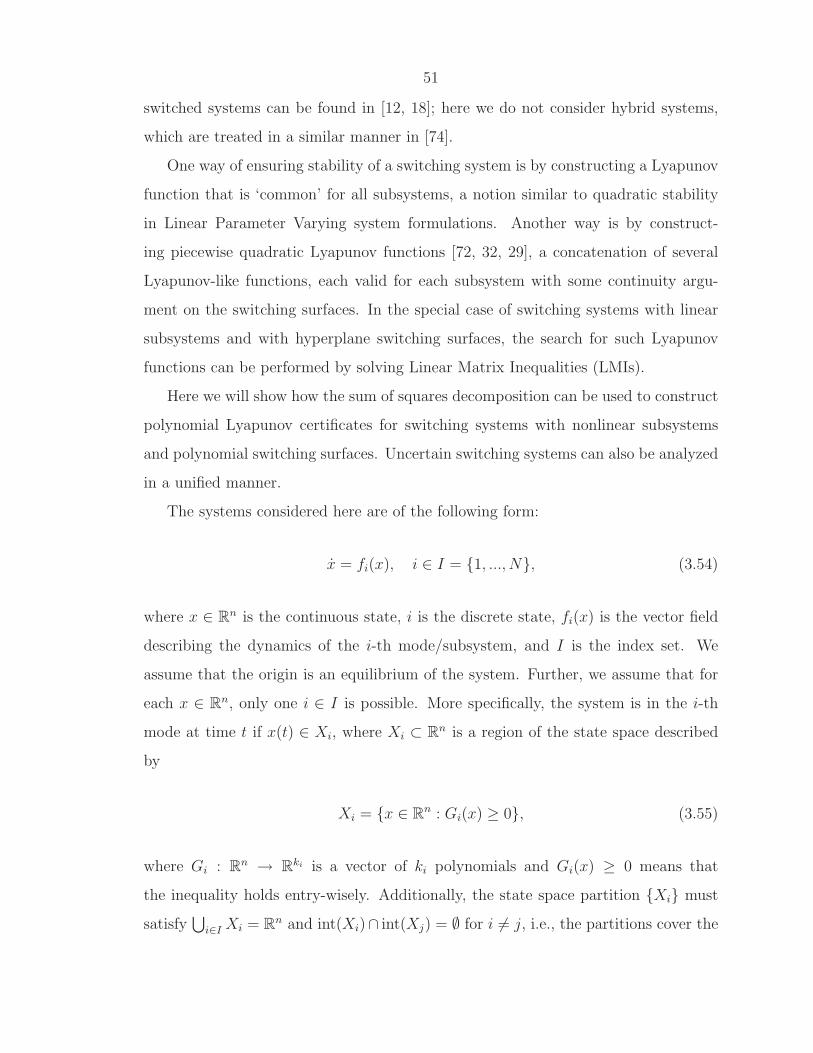
51
switched systems can be found in [12, 18]; here we do not consider hybrid systems,
which are treated in a similar manner in [74].
One way of ensuring stability of a switching system is by constructing a Lyapunov
function that is ‘common’ for all subsystems, a notion similar to quadratic stability
in Linear Parameter Varying system formulations. Another way is by construct-
ing piecewise quadratic Lyapunov functions [72, 32, 29], a concatenation of several
Lyapunov-like functions, each valid for each subsystem with some continuity argu-
ment on the switching surfaces. In the special case of switching systems with linear
subsystems and with hyperplane switching surfaces, the search for such Lyapunov
functions can be performed by solving Linear Matrix Inequalities (LMIs).
Here we will show how the sum of squares decomposition can be used to construct
polynomial Lyapunov certificates for switching systems with nonlinear subsystems
and polynomial switching surfaces. Uncertain switching systems can also be analyzed
in a unified manner.
The systems considered here are of the following form:
x = fi(x), i ∈ I = 1, ..., N, (3.54)
where x ∈ Rn is the continuous state, i is the discrete state, fi(x) is the vector field
describing the dynamics of the i-th mode/subsystem, and I is the index set. We
assume that the origin is an equilibrium of the system. Further, we assume that for
each x ∈ Rn, only one i ∈ I is possible. More specifically, the system is in the i-th
mode at time t if x(t) ∈ Xi, where Xi ⊂ Rn is a region of the state space described
by
Xi = x ∈ Rn : Gi(x) ≥ 0, (3.55)
where Gi : Rn → R
ki is a vector of ki polynomials and Gi(x) ≥ 0 means that
the inequality holds entry-wisely. Additionally, the state space partition Xi must
satisfy⋃
i∈I Xi = Rn and int(Xi)∩ int(Xj) = ∅ for i 6= j, i.e., the partitions cover the

52
whole of Rn and are non-overlapping. A switching surface between the i-th and j-th
modes, i.e., a boundary between Xi and Xj, is given by
Sij = x ∈ Rn : hij(x) = 0, (3.56)
for some hij : Rn → R. Note that even though the direction of transition for a partic-
ular x ∈ Sij can be determined from the vector fields fi(x) and fj(x), it is assumed
in our analysis that such a characterization is not performed a priori. Also, systems
with infinitely fast switching such as those that have sliding modes are excluded from
our discussion. We also assume that the functions fi, Gi, and hij are polynomials, for
otherwise, we can change coordinates to render the system polynomial as explained
earlier.
3.6.1 Common Lyapunov Functions
We will first consider stability of the system (3.54) under arbitrary switching. A
sufficient condition for such stability is the existence of a common global Lyapunov
function for all fi’s, as summarized in the following theorem.
Theorem 3.16 Suppose that for the set of vector fields fi, there exists a polynomial
V (x) such that V (0) = 0 and
V (x) > 0 ∀x 6= 0, (3.57)
∂V
∂xfi(x) < 0 ∀x 6= 0, i ∈ I, (3.58)
then the origin of the state space of the system (3.54) is globally asymptotically stable
under arbitrary switching.
The proof of this theorem is obvious and is omitted. If the vector fields are linear
and V (x) = xTPx, then the above conditions correspond to the LMIs for quadratic
stability [10]. For higher degree polynomial vector fields and Lyapunov functions, the
search for V (x) can also be performed using semidefinite programming by formulating

53
−0.6 −0.4 −0.2 0 0.2 0.4 0.6 0.8 1−1
−0.8
−0.6
−0.4
−0.2
0
0.2
0.4
0.6
0.8
1
x1
x 2
Stability under arbitrary swithcing
Figure 3.6: Stability of a switching system under arbitrary switching by constructinga common Lyapunov function.
the conditions as sum of squares conditions. The higher degree test is generally less
conservative than the quadratic test, as in many cases global higher degree Lyapunov
functions exist for systems that do not possess a global quadratic Lyapunov function.
Example 3.17 Consider the system x = fi(x), x =[
x1 x2
]T
, with
f1(x) =
−5x1 − 4x2
−x1 − 2x2
, f2(x) =
−2x1 − 4x2
20x1 − 2x2
.
It can be proven using a dual semidefinite program that no global quadratic Lyapunov
function exists for this system [32]. Nevertheless, a global sextic Lyapunov function
V (x) = 19.861x61 + 11.709x5
1x2 + 14.17x41x
22 + 4.2277x3
1x32 + 8.3495x2
1x42 − 1.2117x1x
52
+ 1.0421x62
exists, and therefore the system is asymptotically stable under arbitrary switching (see
Figure 3.6). In this figure, solid trajectories correspond to system f1, dashed ones
correspond to system f2. The dotted curves are level curves of the common Lyapunov
function.

54
3.6.2 Piecewise Polynomial Lyapunov Functions
Proving stability of an equilibrium of a switching system by constructing a common
Lyapunov function may be conservative, in particular when the switching rule is
known and included in the system description. In this case, stability can be proven
by constructing piecewise polynomial Lyapunov functions, i.e., a concatenation of
several polynomial functions Vi(x) (also termed Lyapunov-like functions), typically
corresponding to the state space partition Xi. The Lyapunov-like function Vi(x)
and its time derivative along the trajectory of the i-th mode are required to be
positive and negative definite respectively, only within Xi. Such conditions can be
accommodated using the S-procedure by using the descriptions for the sets Xi given
in (3.55) and the switching surfaces (3.56). Note again that the multipliers used
to adjoin such conditions can be polynomials instead of just constants as it was
mentioned in Example 2.14. Moreover, to ensure continuity of the Lyapunov function
on the switching surface between modes i and j, we can impose the condition
Vi(x) + cij(x)hij(x) − Vj(x) = 0,
where cij(x) is a polynomial.
Summing up, we have the following Theorem:
Theorem 3.18 Consider the switched system (3.54)–(3.56). Assume that there exist
polynomials Vi(x), cij(x), with Vi(0) = 0 if 0 ∈ Xi, and vectors of polynomials ai(x) ≥0, bi(x) ≥ 0, such that
Vi(x) − aTi (x)Gi(x) > 0 ∀x 6= 0, i ∈ I, (3.59)
∂Vi∂x
fi(x) + bTi (x)Gi(x) < 0 ∀x 6= 0, i ∈ I, (3.60)
Vi(x) + cij(x)hij(x) − Vj(x) = 0 ∀i, j. (3.61)
Then the origin of the state space is globally asymptotically stable. A Lyapunov func-

55
tion that proves this is the piecewise polynomial function V (x) defined by
V (x) = Vi(x), if x ∈ Xi. (3.62)
The proof of this theorem is based on the fact that the functions Vi are Lyapunov-like
functions for the corresponding subsystems in the regions in which they are defined.
Concatenation of these Lyapunov functions to form V (x), and the continuity of the
value of the Vi’s along the switching surface guarantees that along the trajectories of
the system, the value of V (x) does not increase.
Here we present an example that involves a switching system with nonlinear sub-
systems and a polynomial switching surface.
Example 3.19 Consider the system
x1
x2
=
−2x3
1 − x2
x1 − 2x2x21
for x31 − x2 > 0
x1
x2
=
−2x1x
22 − x2
x1 + px1x2 − x2
for x31 − x2 ≤ 0
Setting p = 4, we can construct a sextic Lyapunov function that proves global stability;
the level curves are shown in Figure 3.7. In that figure the trajectories are shown in
solid thin lines, and the switching surface as a solid thick line for p = 4. Alternatively,
consider the case in which p is unknown. A quadratic Lyapunov function proves
stability of the zero equilibrium for p ∈ [−2.82, 2.8]. A sextic one gives stability for
p ∈ [−2.82, 7.6] and one of order 8 gives stability for p ∈ [−2.82, 15.9]. Note that for
p < 2.82, two other equilibria appear in the second system which make the stability of
the origin only local.
3.7 Performance Analysis
In this section, we are concerned with performance analysis of uncertain nonlinear
models, and how it can be performed using sum of squares techniques. Previous

56
−1.5 −1 −0.5 0 0.5 1 1.5−6
−4
−2
0
2
4
6
x1
x 2
Switching System
Figure 3.7: Stability of a switching system with predefined switching, using aLyapunov-like function.
attempts to analyze performance of such systems concentrated on LPV system repre-
sentations and the discretization of the resulting infinite-dimensional Parameterized
LMIs (PLMIs). Again, this approach does not guarantee that the original PLMI
problem is feasible, as no discretization is fine enough.
In this section, we wish to obtain upper bounds on the L2 induced norm of the
system from an external input to a performance output using SOS. The L2 induced
norm is a measure of the worst energy amplification between input and output as the
system trajectory and the uncertain parameters vary within their specified bounded
regions. For uncertain systems with state-space constraints, it is also important
to characterize the reachable set from a bounded energy input. This way, we can
associate the set of external inputs to a region in the state-space which is guaranteed
to contain the state trajectory for the given amount of uncertainty. Then, for that
set of external inputs, the L2 induced norm from input to output can be calculated.
In this section, we concentrate on the following class of systems:
x = f(x, u; θ) (3.63)
y = h(x, u; θ) (3.64)

57
where x ∈ Rn, y ∈ R
q, u ∈ Rm, θ ∈ Θ ⊂ R
p where Θ is given by:
Θ = θ ∈ Rp |gi(θ) ≤ 0, i = 1, . . . , k1 (3.65)
The function f is locally Lipschitz in (x, u) and h is continuous in (x, u) for x ∈ D,
where D ⊂ Rn be a domain that contains the equilibrium state x = 0 that we define
by
D = x ∈ Rn |gi(x) ≤ 0, i = k1 + 1, . . . , S (3.66)
and for u ∈ D0 where D0 is a domain that contains u = 0.
First, consider the problem of calculating reachable sets for the system’s state
trajectory when it is driven with an input of energy ǫ. We follow the notation in [10],
and denote the set Ruǫ as the set of reachable states with inputs of energy ǫ for the
system (3.63–3.64):
Ruǫ ,
x(T )
∣∣∣∣(x, u) satisfy (3.63), x(0) = 0,
∫ T
0
uTu ≤ ǫ, T ≥ 0
. (3.67)
An estimate of the reachable set is the ǫ level set of an appropriate Lyapunov function
V (x), i.e., Ruǫ ⊂ x ∈ Rn|V (x) ≤ ǫ, which is contained in D:
Proposition 3.20 For the system given by (3.63), let there exist a polynomial func-
tion V (x) and a positive definite function φ(x) so that
1. V (x) − φ(x) ≥ 0
2. ∂V∂xf(x, u; θ) ≤ uTu for all x ∈ D and θ ∈ Θ
3. V (x) ≤ ǫ ⊂ D
Then the set V (x) ≤ ǫ contains the reachable set when the input satisfies ‖u‖2 < ǫ.
Proof. The first two conditions guarantee that V (x) is a Lyapunov function for the
unforced system. When u 6= 0, condition (2) becomes dVdt
≤ uTu. Integrating this
from 0 to T , we get:
V (x(T )) − V (x(0)) ≤∫ T
0
uTudt

58
Since V (x(0)) = V (0) = 0, we have
V (x(T )) ≤∫ T
0
uTudt ≤ ǫ
for every T ≥ 0 and every u such that∫ T
0uTudt ≤ ǫ. Condition (3) guarantees that
x ∈ Rn|V (x) ≤ ǫ is a subset of the set D, and therefore the set V (x) ≤ ǫ is an
estimate of the reachable set.
The conditions in Proposition 3.20 can be tested using the sum of squares de-
composition, by relaxing the non-negativity conditions to the existence of a sum of
squares decomposition. The third condition can be easily converted into a set empti-
ness argument which can be tested using positivstellensatz and the sum of squares
decomposition, as it was done in the case of obtaining estimates for the region of
attraction. This leads to the following Program:
Program 3.21 An algorithm to bound the reachable set with ǫ-energy inputs:
Maximize ǫ
and find a non-negative integer r, a polynomial V (x),
a positive definite function φ(x), sums of squares pi(x, θ), i = 1, . . . , S,
and sums of squares qi(x), i = k1, . . . , S
such that
V (x) − φ(x) is SOS
− ∂V
∂xf(x, u) + uTu+
S∑
i=1
pi(x, θ)gi is SOS
‖x‖2r(V (x) − ǫ) +S∑
i=k1
qi(x)gi is SOS
Then the reachable set is contained in the set V (x) ≤ ǫ.
Now that we can associate the energy of the external input to a region in the state-
space that is guaranteed to contain the state trajectory, we are ready to calculate the

59
input to output gain (the L2 gain). This is the maximum ratio of output to input
energy, i.e.,
sup‖u‖2 6=0
‖y‖2
‖u‖2
starting at x(0) = 0, where ‖u‖22 =
∫∞
0uTudt. It can be estimated as follows:
Proposition 3.22 Consider the system given by (3.63–3.64). Let there exist a poly-
nomial V (x), a positive number γ and a positive definite function φ(x) such that
1. V (x) − φ(x) ≥ 0,
2. −∂V∂xf(x, u; θ) − yTy + γuTu ≥ 0
for x ∈ D and θ ∈ Θ. Then the L2 gain of the system given by (3.63–3.64) is less
than√γ.
Proof. Condition (2) above implies that
−dVdt
− yTy + γuTu ≥ 0.
Integrating this from 0 to T , we get:
V (x(0)) − V (x(T )) ≥∫ T
0
(yTy − γuTu)dt
From condition (1) and from the fact that x(0) = 0, we have that V (x(0)) = V (0) = 0
and V (x(T )) ≥ 0. Therefore,
∫ T
0
(yTy − γuTu)dt ≤ 0
and so ∫ T
0yTydt
∫ T
0uTudt
≤ γ. (3.68)
We conclude that√γ is an upper bound on the L2 gain.

60
A similar sum of squares program can be formulated in this case, too. We will
demonstrate our results on a model of the short-period dynamics of an F/A-18 air-
craft, equipped with a nonlinear dynamic inversion control law.
Example 3.23 An uncertain model approximating the F/A-18 short-period dynamics
is derived in [64]:
q
∆α
=
0 1
IyyMα(α)unc
1 + cos (α)mVo
Zq(α)unccos (α)mVo
Zα(α)unc
q
∆α
+
1IyyMǫ(α)unc
cos (α)mVo
Zǫ(α)unc
∆e.
(3.69)
The symbol q denotes the pitch rate, α the angle of attack, e the elevator deflection,
Iyy the moment of inertia and m the mass of the aircraft. The model is valid for an
equilibrium point characterized by the speed V0 and altitude h0 for a range of α. The
signals ∆α = α−αo and ∆e = e−eo represent deviations from the equilibrium values
αo and eo.
The terms Mα(α), . . . , Zǫ(α) are aerodynamic derivatives – polynomial functions
of α – obtained by data fitting of experimental data (usually obtained from wind tunnel
tests). Because of this, their value is, in general, uncertain. It is also dependent on
the flight conditions, etc. Therefore, we introduce weighted, additive uncertainty on
the aerodynamic coefficients for these moments and forces as shown below.
Mα(α)unc = Mα(α) + MαwMαδMα
,
Mǫ(α)unc = Mǫ(α) + MǫwMǫδMǫ
,
Zq(α)unc = Zq(α) + ZqwZqδZq
,
Zα(α)unc = Zα(α) + ZαwZαδZα
,
Zǫ(α)unc = Zǫ(α) + ZǫwZǫδZǫ.
The w’s are positive numbers and the constant terms Mα, . . . , Zα, Zǫ are the average
moment or force over the specific range of α. The δ’s satisfy |δi| ≤ 1. Also, consider a
simple nonlinear dynamic inversion control law [21, 13] for the uncertain, short-period
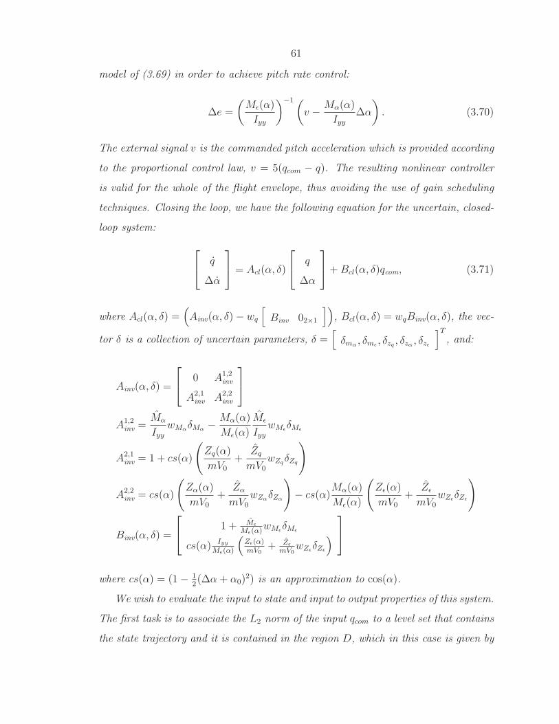
61
model of (3.69) in order to achieve pitch rate control:
∆e =
(Mǫ(α)
Iyy
)−1(
v − Mα(α)
Iyy∆α
)
. (3.70)
The external signal v is the commanded pitch acceleration which is provided according
to the proportional control law, v = 5(qcom − q). The resulting nonlinear controller
is valid for the whole of the flight envelope, thus avoiding the use of gain scheduling
techniques. Closing the loop, we have the following equation for the uncertain, closed-
loop system:
q
∆α
= Acl(α, δ)
q
∆α
+Bcl(α, δ)qcom, (3.71)
where Acl(α, δ) =(
Ainv(α, δ) − wq
[
Binv 02×1
])
, Bcl(α, δ) = wqBinv(α, δ), the vec-
tor δ is a collection of uncertain parameters, δ =[
δmα, δmǫ
, δzq, δzα
, δzǫ
]T
, and:
Ainv(α, δ) =
0 A1,2
inv
A2,1inv
A2,2inv
A1,2inv
=Mα
IyywMα
δMα− Mα(α)
Mǫ(α)
Mǫ
IyywMǫ
δMǫ
A2,1inv
= 1 + cs(α)
(
Zq(α)
mV0
+ZqmV0
wZqδZq
)
A2,2inv
= cs(α)
(
Zα(α)
mV0
+ZαmV0
wZαδZα
)
− cs(α)Mα(α)
Mǫ(α)
(
Zǫ(α)
mV0
+ZǫmV0
wZǫδZǫ
)
Binv(α, δ) =
1 + Mǫ
Mǫ(α)wMǫ
δMǫ
cs(α) Iyy
Mǫ(α)
(Zǫ(α)mV0
+ Zǫ
mV0wZǫ
δZǫ
)
where cs(α) = (1 − 12(∆α+ α0)
2) is an approximation to cos(α).
We wish to evaluate the input to state and input to output properties of this system.
The first task is to associate the L2 norm of the input qcom to a level set that contains
the state trajectory and it is contained in the region D, which in this case is given by

62
0 2 4 6 8 10 120
0.05
0.1
0.15
0.2
0.25
0.3
∆ α in degrees
ε
Guaranteed range of ∆ α for an input of energy ||qcom
||2 < ε
Nominalw = 0.1w = 0.2w = 0.3w = 0.4w = 0.5
0 2 4 6 8 10 121
1.2
1.4
1.6
1.8
2
2.2
2.4
∆ α in degrees
γ
Upper bound of induced L2 norm from q
com to q for an input of energy ||q
com||
2 < ε
w = 0.1w = 0.2w = 0.3w = 0.4w = 0.5
(a) (b)
Figure 3.8: Performance analysis of an F/A-18 aircraft model: input-to-state andinput-to-output gain estimates.
D = ∆α : −0.166 rad ≤ ∆α ≤ 0.166 rad. This can be done using Program 3.21,
multiplying out the Lyapunov derivative criterion by the non-vanishing denominator
of the vector field to render the expression polynomial. The result, with different sizes
of uncertainty, is shown in Figure 3.8(a). For example, when w = 0.1 for any pitch
rate reference satisfying ||qcom||2 < 0.15, it is guaranteed that the angle of attack will
not deviate by more than 6 degrees from its value at the equilibrium.
After the reachable set is obtained, a bound on the input to output L2 gain can
be found using Proposition 3.22. The results, with different sizes of uncertainty are
shown in Figure 3.8(b). The results on the bound of the induced L2 norm must be
interpreted in conjunction with the previous results in Figure 3.8(a). The combination
of the results in Figures 3.8(a) and 3.8(b) (by ignoring the ∆α information) allows
us to plot the upper bound on the induced L2 norm as a function of the L2 norm of
the reference input and thus, verify the nonlinear behavior of the controller. This is
shown in Figure 3.9, where the degradation of performance with increasing uncertainty
is evident.

63
0 0.05 0.1 0.15 0.2 0.251
1.5
2
2.5
ε
γ
Upper bound of induced L2 norm from q
com to q for an input of energy ||q
com||
2 < ε
w = 0.1w = 0.2w = 0.3w = 0.4w = 0.5
Figure 3.9: Performance analysis of an F/A-18 aircraft model: input-to-output gainestimates.
3.8 Conclusion
In this chapter, we have shown how the sum of squares decomposition and positivstel-
lensatz can be used to analyze systems described by Ordinary Differential Equations.
Generally speaking, this methodology is an extension of the well-studied Linear Ma-
trix Inequality techniques for the analysis of linear systems to nonlinear systems and
most of the results that we presented follow logically from this. We have seen how
robust stability analysis, obtaining estimates of the region of attraction, ensuring
the stability of switched systems and performance evaluation can be performed in a
unified manner.
In the next chapter we will investigate how the sum of squares decomposition
can be used to analyze a particular class of infinite dimensional systems: time-delay
systems.

64
Chapter 4
Systems Described by FunctionalDifferential Equations >Arga m thr psh kaka Sìlwn
Delay is the mother of all evilSolon
In this chapter, we concentrate on Functional Differential Equations, another class
of differential equations also known as time-delay systems. They are an important
modeling tool for systems that involve transport and propagation of data, such as
communication systems, but also for modeling maturation and growth in population
dynamics. The interest in time delay systems has been intensified recently [81], as they
provide the simplest adequate modeling framework for network congestion control for
the Internet, which is the topic of the next chapter. In general, the presence of delays
may induce undesirable effects such as instabilities and oscillations, so ignoring them
may lead to the wrong conclusions about the system’s properties.
In this chapter, we will develop algorithmic, Lyapunov-based methodologies for
analysis of time-delay systems, based on the sum of squares technique. We start
our investigation by considering the construction of Lyapunov-Krasovksii functionals
for linear systems, where the structure of the functional necessary and sufficient for
stability is known, but its construction is difficult, and we will show how the sum of
squares decomposition can be used to construct it. We will then turn to nonlinear
time delay systems and consider delay-independent and delay-dependent stability
analysis. Robust stability is also addressed, through the construction of parameterized
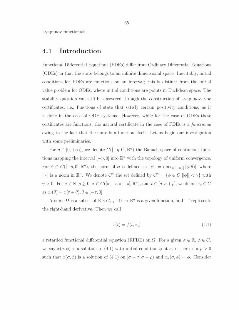
65
Lyapunov functionals.
4.1 Introduction
Functional Differential Equations (FDEs) differ from Ordinary Differential Equations
(ODEs) in that the state belongs to an infinite dimensional space. Inevitably, initial
conditions for FDEs are functions on an interval; this is distinct from the initial
value problem for ODEs, where initial conditions are points in Euclidean space. The
stability question can still be answered through the construction of Lyapunov-type
certificates, i.e., functions of state that satisfy certain positivity conditions, as it
is done in the case of ODE systems. However, while for the case of ODEs these
certificates are functions, the natural certificate in the case of FDEs is a functional
owing to the fact that the state is a function itself. Let us begin our investigation
with some preliminaries.
For η ∈ [0,+∞), we denote C([−η, 0],Rn) the Banach space of continuous func-
tions mapping the interval [−η, 0] into Rn with the topology of uniform convergence.
For φ ∈ C([−η, 0],Rn), the norm of φ is defined as ‖φ‖ = maxθ∈[−η,0] |φ(θ)|, where
| · | is a norm in Rn. We denote Cγ the set defined by Cγ = φ ∈ C|‖φ‖ < γ with
γ > 0. For σ ∈ R, ρ ≥ 0, x ∈ C([σ− τ, σ+ρ],Rn), and t ∈ [σ, σ+ρ], we define xt ∈ C
as xt(θ) = x(t+ θ), θ ∈ [−τ, 0].
Assume Ω is a subset of R×C, f : Ω 7→ Rn is a given function, and ‘ ˙ ’ represents
the right-hand derivative. Then we call
x(t) = f(t, xt) (4.1)
a retarded functional differential equation (RFDE) on Ω. For a given σ ∈ R, φ ∈ C,
we say x(σ, φ) is a solution to (4.1) with initial condition φ at σ, if there is a ρ > 0
such that x(σ, φ) is a solution of (4.1) on [σ − τ, σ + ρ) and xσ(σ, φ) = φ. Consider

66
the class of autonomous delayed differential equations, i.e.,
x(t) = f(xt). (4.2)
We say (4.2) is linear if f(xt) is linear in xt. In this chapter, we concentrate on au-
tonomous time-delay systems with discrete delays, so f(xt) = f(x(t), x(t−τ1), . . . , x(t−τr)) where τi are the discrete delays in the system. Without loss of generality, we
assume that 0 is a steady-state for the system.
Just as in the case of ODEs, the existence and uniqueness of solutions of (4.2)
is guaranteed if f(φ) is continuous in φ in an open subset Ω of C. Continuous
dependence of the solution on initial conditions and parameters can also be proven
under certain assumptions. Here we concentrate on a few stability definitions of the
steady-state of (4.2), which we assume to be at 0.
Definition 4.1 The trivial solution of (4.2) is called
1. stable if for any ǫ > 0 there is a δ = δ(ǫ) such that |x(φ)| ≤ ǫ for any initial
condition φ ∈ Ω; otherwise it is termed unstable;
2. asymptotically stable if it is stable and there is a γ > 0 such that limt→∞ x(t;φ) =
0 for any initial condition φ ∈ Ωγ. The set of initial functions φ for which
limt→∞ x(t;φ) = 0 is called the domain of attraction of the trivial solution.
Establishing the stability of the steady-state is a rather difficult task if f is a
nonlinear function of (x(t), x(t−τ1), . . . , x(t−τr)). Even in the linear case, establishing
the stability boundary, i.e., the exact values of τi for which stability is retained is NP-
hard [26]. Just as in the case of nonlinear systems described by Ordinary Differential
Equations (ODEs), a Lyapunov argument can be formulated that proves useful when
many, incommensurate delays appear in the system.
Consider a continuous functional V : C → R and define:
V (φ) = limh→0+
1
h[V (xh(φ)) − V (φ)]
67
the derivative of V along a solution of (4.2). Assume f : Ω → Rn is completely con-
tinuous and f(0) = 0. We then have the following Lyapunov-Krasovskii theorem [28]:
Theorem 4.2 For (4.2), assume f is completely continuous and f(0) = 0. Fur-
ther, assume there exist a(s) and b(s) nonnegative continuous, a(0) = b(0) = 0,
lims→∞ a(s) = +∞ and V : Ω → R continuous satisfying:
V (φ) ≥ a(|φ(0)|) in Ω
V (φ) ≤ b(|φ(0)|) in Ω.
Then the solution x = 0 of (4.2) is stable, and every solution is bounded. If in
addition, b(s) > 0 for s > 0, then x = 0 is asymptotically stable.
We note that apart from the Lyapunov-Krasovskii theorem for stability analysis,
there is the Lyapunov-Razumikhin theorem which uses functions as the certificates
for stability instead of functionals. When using functionals, the Lyapunov-Krasovskii
theorem requires that the derivative along solutions decrease monotonically; such
a requirement makes finding a Lyapunov functional a rather difficult task, since the
space C is much more complicated than Rn, and one has no control of the relationship
of |x(t)| and |x(t+ θ)|, θ ∈ [−τ, 0]. Razumikhin’s theorem uses functions and studies
their rate of change along solutions.
Let V : Rn → R is a positive definite continuously differentiable function. Its
derivative along the solution of (4.2) takes the form:
V (x(t)) =∂V (x)
∂xf(xt) (4.3)
Note that the right hand side is a functional, although V is a function. From the
definition of stability, we know that if xt is initially inside a ball of radius δ in C, then
for it to escape that ball, it has to reach the boundary at some time t∗. Therefore
|x(t∗)| = δ, and |x(t+ θ)| < δ for θ ∈ [−τ, 0), and d|x(t∗)|dt
≥ 0. Razumikhin’s theorem
rules out this case.

68
Theorem 4.3 Consider the functional differential equation given by (4.2), where f
maps bounded sets of C into bounded sets of Rn. Suppose u, v, w : R
+ 7→ R+ are
continuous, nondecreasing functions, u(s), v(s) positive for s > 0, u(0) = 0, v(0) = 0
and v strictly increasing. If there is a continuous function V : Rn 7→ R such that:
1. u(‖x‖) ≤ V (x) ≤ v(‖x‖), x ∈ Rn
2. V (x) ≤ −w(‖x‖) if V (x(t+ θ)) < p(V (x(t))), ∀ θ ∈ [−τ, 0]
Then the trivial solution of (4.2) is stable.
In this chapter, as in the previous one, we are interested in algorithmic method-
ologies for constructing Lyapunov-type certificates. The convexity in constructing
the Lyapunov functions in the previous chapter was important in this endeavor. Here
we have presented two Lyapunov theorems; it is easy to see that the conditions in
Theorem 4.2 are convex, whereas those in Theorem 4.3 are not because of the deriv-
ative condition and its connection to the Lyapunov certificate itself. The Lyapunov-
Krasovskii theorem can be used to construct simple Lyapunov functionals for linear
systems by solving a set of Linear Matrix Inequalities [37]. Under convexification
assumptions, the Lyapunov-Razuminkin criteria can also be tested by solving LMIs,
but are in general more conservative than the Lyapunov-Krasovskii ones [26].
LMIs were used for both delay-dependent and delay-independent stability analysis
of linear time-delay systems, a classification based on the persistence of stability as
the delay is increased. We say that a system is delay-independent stable, if, generally
speaking, the stability property is retained for all positive (finite) values of the delays
in the system, i.e., the system is robust with respect to the delay size. On the other
hand, we say that a system is delay-dependent stable if the stability is preserved
for some values of delays and is lost for some others. The existence of complete
quadratic Lyapunov-Krasovskii functionals necessary and sufficient for strong delay-
independent and delay-dependent stability of linear time-delay systems is well known
and so is their structure [78], but there is an inherent difficulty in constructing them.
They result in infinite-dimensional parameterized LMIs which are difficult to solve.

69
In this chapter, we will use the sum of squares technique for the construction of
Lyapunov-Krasovskii functionals for linear and nonlinear time delay systems [58]. The
SOS decomposition will be used not only for solving the infinite dimensional LMIs
in the linear case, but also for constructing Lyapunov functionals with polynomial
kernels for nonlinear time delay systems.
4.2 Analysis of Linear Time-Delay Systems
A question that the reader may pose at this point, is why do we investigate the
stability analysis of linear time-delay systems when it is well known that the sum of
squares technique can answer similar questions about nonlinear systems in a unified
manner. The answer to this question is twofold. First, the conditions for stability
of linear time-delay systems are in the form of parameterized LMIs (PLMIs) which
are difficult to solve in general. We will take this opportunity to show how the sum
of squares technique can be used to solve PLMIs, and comment on how the sparsity
structure that appears naturally can be taken advantage of when solving the sum of
squares program. On the other hand, it is important to appreciate that we now seek
to construct functionals rather than functions, and the structure that one should
consider is not a polynomial parametrization, but a ‘function’ of polynomials; we
therefore need strong intuition in what structures we should choose. A lot is known
about ‘complete’ (i.e., necessary and sufficient for stability) Lyapunov structures for
linear time-delay systems, and therefore we investigate the stability of linear systems
first, which can help us choose structures for nonlinear systems later on.
Consider a linear instantiation of (4.2) with one discrete delay of the form:
x(t) = A0x(t) + A1x(t− τ) = f(x(t), x(t− τ)) (4.4)
with an initial condition x0(θ) = φ(θ), θ ∈ [−τ, 0], φ ∈ C. The delay τ is assumed to
be constant, x(t) ∈ Rn and A0, A1 are known real constant matrices of appropriate
dimensions. The case in which the Ai are parameter-dependent can also be treated

70
in a unified manner.
We have the following version of Theorem 4.2 for the asymptotic stability of the
above system.
Theorem 4.4 [26] The system described by Equation (4.4) is asymptotically stable
if there exists a bounded quadratic Lyapunov functional V (xt) such that for some
ǫ1 > 0, ǫ2 > 0 it satisfies:
V (xt) ≥ ǫ1‖x(t)‖2 (4.5)
and its derivative along the system trajectory satisfies
V (xt) ≤ −ǫ2‖x(t)‖2. (4.6)
For the case of ODEs, it is well known that a Lyapunov function for the generic
linear ODE system of the form x = Ax with A Hurwitz would be V = xTPx where
P is a positive definite matrix satisfying ATP +PA < 0. P can be found numerically
by solving this set of Linear Matrix Inequalities [10].
In the same spirit, the search for structures that are ‘complete’, i.e., produce
necessary and sufficient conditions for stability of linear time-delay systems has been
under research in the past. For example, for the case of what is called strong delay-
independent stability [7], the class of such Lyapunov functions has been completely
characterized:
Example 4.5 For system (4.4) a Lyapunov-Krasovskii candidate that would yield a
delay-independent condition is
V (xt) = x(t)TPx(t) +
∫ 0
−τ
x(t+ θ)TSx(t+ θ)dθ
Sufficient conditions on V (xt) to be positive definite are P > 0, S ≥ 0. For V (xt) < 0
we require
ATP + PA+ S PA1
AT1 P −S
< 0,

71
i.e., the conditions for stability (see Theorem 4.4) can be written as a Linear Matrix
Inequality (LMI) with P and S as the unknowns.
The Lyapunov functional used above may not suffice to prove stability for a gen-
eral delay-independent stable system, as the proposed structure is not adequate for the
stability proof. Instead, the Lyapunov structure in [6] has been proven to be ‘com-
plete’ for strong delay-independent stability in the case of linear time delay systems.
Denoting
zk(t) = [x(t), x(t− τ), . . . , x(t− (k − 1)τ)] (4.7)
the complete structure in the single delay case is
Vk(xt) = a1(zk(t)) +
∫ 0
−τ
b1(zk(t+ θ))dθ (4.8)
where a1 and b1 are quadratic polynomials in their arguments.
As far as delay-dependent stability is concerned, the structures of Lyapunov-
Krasovskii functionals that are necessary and sufficient for delay-dependent stability
are known, but difficult to construct. The complete Lyapunov functional [78, 26] has
the following form:
V (xt) = xT (t)Px(t) + xT (t)
∫ 0
−τ
P1(θ)x(t+ θ)dθ +
∫ 0
−τ
xT (t+ θ)P T1 (θ)dθx(t)
+
∫ 0
−τ
∫ 0
−τ
xT (t+ θ)P2(θ, ξ)x(t+ ξ)dξdθ +
∫ 0
−τ
xT (t+ θ)Qx(t+ θ)dθ
(4.9)
with appropriate conditions on P, P1, P2, etc, to guarantee positivity of V . The con-
dition V < 0 implies that the matrices P, P1, P2 have to satisfy a complicated system
of algebraic, ordinary and partial differential equations with appropriate boundary
conditions [78]. If one wanted to write the above conditions as LMI conditions, he
would get a set of infinite-dimensional LMIs for which there are not many known
algorithms for efficient computation. A rather complicated discretization scheme was
proposed in [26] to solve these PLMIs.
72
In this chapter, we consider structures similar to the complete quadratic Lyapunov-
Krasovskii functional (4.9) for which we construct certificates in which the kernels
(matrices P1, P2, etc) are polynomials in the variables (θ, ξ). As we increase the order
of the polynomial kernels, the delay-dependent stability conditions obtained analyt-
ically (i.e., using frequency domain methods) can be approached. To proceed, we
use Theorem 4.4 and consider the following Lyapunov functional which resembles the
complete Lyapunov functional (4.9):
V (xt) = a0(x(t)) +
∫ 0
−τ
∫ 0
−τ
a1(θ, ξ, x(t), x(t+ θ), x(t+ ξ))dθdξ
+
∫ 0
−τ
∫ t
t+θ
a2(x(ζ))dζdθ +
∫ 0
−τ
∫ t
t+ξ
a3(x(ζ))dζdξ (4.10)
where by a1(θ, ξ, x(t), x(t + θ), x(t + ξ)), we mean a polynomial in θ, ξ, x(t), x(t + θ)
and x(t+ ξ) of bounded degree, which is quadratic with respect to x(t), x(t+ θ) and
x(t+ ξ) and allowed to be any order in θ and ξ. Such polynomials are called bipartite
and have a special structure [24]. The polynomials a0, a2 and a3 are quadratic in
their arguments. In other words,
a1(θ, ξ, x(t), x(t+ θ), x(t+ ξ)) =
x(t)
x(t+ θ)
x(t+ ξ)
T
a1(θ, ξ)
x(t)
x(t+ θ)
x(t+ ξ)
where a1(θ, ξ) is a polynomial matrix in (θ, ξ). The time derivative of V (xt) along f
given by (4.4) is:
V (xt) =da0
dx(t)f +
∫ 0
−τ(a1(0, ξ, x(t), x(t), x(t + ξ)) − a1(−τ, ξ, x(t), x(t − τ), x(t + ξ))) dξ
+
∫ 0
−τ(a1(θ, 0, x(t), x(t + θ), x(t)) − a1(θ,−τ, x(t), x(t + θ), x(t − τ))) dθ
+
∫ 0
−τ
∫ 0
−τ
(∂a1
∂x(t)f − ∂a1
∂θ− ∂a1
∂ξ
)
dθdξ
+
∫ 0
−τ(a2(x(t)) − a2(x(t + θ))) dθ +
∫ 0
−τ(a3(x(t)) − a3(x(t + ξ))) dξ
73
=1
τ2
∫ 0
−τ
da0dx(t)f + τ2 ∂a1
∂x(t)f − τ2 ∂a1∂θ − τ2 ∂a1
∂ξ + τa2(x(t)) + τa3(x(t))
−τa3(x(t + ξ)) − τa1(−τ, ξ, x(t), x(t − τ), x(t + ξ))
+τa1(0, ξ, x(t), x(t), x(t + ξ)) + τa1(θ, 0, x(t), x(t + θ), x(t))
−τa2(x(t + θ)) − τa1(θ,−τ, x(t), x(t + θ), x(t − τ))
dθdξ
In order to ensure positive definiteness of V and negative definiteness of V , we can
impose these conditions on the kernels of the integral expressions. Positivity of a
kernel of an integral is a conservative test for the positivity of the integral itself and
we will see later on how to relax this conservativeness.
By structuring the polynomial a1 and testing positivity of V as explained above,
it is easy to see that the resulting SOS conditions will be parameterized LMIs in
(θ, ξ). However, for notational simplicity, we will be working at the polynomial level
- This essentially means that PLMIs can be solved by turning them into polynomial
expressions and asking for the latter to be SOS.
Sufficient conditions for stability of the system can be found in the following
proposition:
Proposition 4.6 Consider the system given by Equation (4.4). Denote xτ = x(t−τ),xθ = x(t+θ), xξ = x(t+ξ) and x = x(t) for brevity. Suppose we can find polynomials
a0(x) a1(θ, ξ, x, xθ, xξ), a2(x(ζ)) and a3(x(ζ)) and a positive constant ǫ such that the
following conditions hold:
1. a0(x) − ǫ‖x‖2 ≥ 0,
2. a1(θ, ξ, x, xθ, xξ) ≥ 0, ∀θ, ξ ∈ [−τ, 0],
3. a2(x(ζ)) ≥ 0, a3(x(ζ)) ≥ 0,
4. da0
dxf+τ 2 ∂a1
∂xf−τ 2 ∂a1
∂θ−τ 2 ∂a1
∂ξ+τa2(x)−τa2(xθ)+τa3(x)−τa3(xξ)+τa1(0, ξ, x, x, xξ)−
τa1(−τ, ξ, x, xτ , xξ) + τa1(θ, 0, x, xθ, x)− τa1(θ,−τ, x, xθ, xτ ) ≤ −ǫ‖x‖2, ∀θ, ξ ∈[−τ, 0].
Then the system described by Equation (4.4) is asymptotically stable.

74
Proof. The first three conditions impose that:
V (xt) ≥ ǫ‖x(t)‖2.
Similarly, the fourth condition, and the discussion before the statement of the propo-
sition imply that
V (xt) ≤ −ǫ‖x(t)‖2
for some ǫ > 0. Therefore, from the statement of Theorem 4.4, the system (4.4) is
asymptotically stable.
Condition (2) in the above proposition asks for a1 to be non-negative only for a
certain θ and ξ interval. To impose the conditions θ ∈ [−τ, 0], ξ ∈ [−τ, 0], we use a
process similar to the S-procedure, as it was discussed in Chapter 2. The polynomial
a1 is required to be non-negative only when g1 , θ(θ + τ) ≤ 0 and g2 , ξ(ξ + τ) ≤ 0
are satisfied, which can be tested as follows:
a1 + p1g1 + p2g2 ≥ 0 (4.11)
where p1 and p2 are sums of squares of degree 2 in x, xθ and xξ and of bounded degree
in θ and ξ. This will retain the bipartite structure of the whole expression, which will
be taken advantage of in the computation. The same can be done with Constraint
(4) in the above proposition.
In order to reduce conservativeness of the test – in that the positivity of the kernel
is too strong a condition for the positivity of the integral – we can introduce terms
with polynomial kernels that integrate to zero and add them to these expressions.

75
Such terms would be, in condition (1):
∫ 0
−τ
∫ 0
−τ
b(θ, ξ, x(t), x(t+ θ), x(t+ ξ))dθdξ
,
∫ 0
−τ
∫ 0
−τ
x(t)
x(t+ θ)
x(t+ ξ)
T
b11(θ, ξ) b12(ξ) b13(θ)
b12(ξ) b22(ξ) 0
b13(θ) 0 b33(θ)
x(t)
x(t+ θ)
x(t+ ξ)
dθdξ = 0 (4.12)
and similarly for the derivative condition, we have:
∫ 0
−τ
∫ 0
−τ
c(θ, ξ, x(t), x(t− τ), x(t+ θ), x(t+ ξ))dθdξ
,
∫ 0
−τ
∫ 0
−τ
x(t)
x(t− τ)
x(t+ θ)
x(t+ ξ)
T
c11(θ, ξ) c12(θ, ξ) c13(ξ) c14(θ)
c12(θ, ξ) c22(θ, ξ) c23(ξ) c24(θ)
c13(ξ) c23(ξ) c33(ξ) 0
c14(θ) c24(θ) 0 c44(θ)
x(t)
x(t− τ)
x(t+ θ)
x(t+ ξ)
dθdξ = 0
(4.13)
The computational complexity of this method increases as the order of the poly-
nomials a1 with respect to ξ and θ are increased. However, for reducing the size and
better conditioning of the SDP, one should take advantage of the bipartite structure
of a1 (i.e., the fact that even though a1 might be of degree n > 2, it is always of
degree 2 in all variables, but possibly ξ and θ). For more details on how sparsity
can be exploited, see [66] and the references therein. SOSTOOLS has routines that
exploit the sparse bipartite structure to reduce the size of the resulting LMIs.
The system with delay τ can therefore be tested for stability by solving the fol-

76
lowing SOS program:
Find polynomials a0(x), a1(θ, ξ, x, xθ, xξ), a2(x(ζ)), a3(x(ζ)), ǫ > 0
and Sums of Squares qi,j(θ, ξ, x, xθ, xξ) for i, j = 1, 2
and polynomials b(θ, ξ, x, xθ, xξ) and c(θ, ξ, x, xτ , xθ, xξ) of the form (4.12) and (4.13)
such that
a0(x) − ǫ‖x‖2 is SOS,
a1(θ, ξ, x, xθ, xξ) +2∑
j=1
q1,jgi(θ, ξ) + b(θ, ξ, x, xθ, xξ) is SOS,
a2(x(ζ)) is SOS, (4.14)
a3(x(ζ)) is SOS,
−da0
dxf(xt) − τ 2 ∂a1
∂xf(xt) + τ 2 ∂a1
∂θ+ τ 2 ∂a1
∂ξ− τa1(0, ξ, x, x, xξ)
+τa1(−τ, ξ, x, xτ , xξ) − τa1(θ, 0, x, xθ, x(t))
+τa1(θ,−τ, x(t), xθ, xτ ) − τa2(x) − τa3(x) + τa2(xθ) + τa3(xξ)
−ǫ‖x‖2 +∑2
j=1 q2,jgi(θ, ξ) + c(θ, ξ, x, xτ , xθ, xξ)
is SOS.
∫ 0
−τ
∫ 0
−τ
b(θ, ξ, x(t), x(t+ θ), x(t+ ξ))dθdξ = 0
∫ 0
−τ
∫ 0
−τ
c(θ, ξ, x(t), x(t− τ), x(t+ θ), x(t+ ξ))dθdξ = 0
Note that the above procedure can be extended to handle systems with more than
one delay. A different Lyapunov structure may then be required.
We now present an example to investigate stability of a linear time delay system.
Example 4.7 The following two dimensional system that has been analyzed exten-
sively in the past, and the various LMI tests that were developed by researchers were

77
Order of a1 in θ and ξ 0 1 2 3 4 5 6max τ 4.472 5.17 5.75 6.02 6.09 6.15 6.16
Table 4.1: Constructing a Lyapunov-Krasovksii functional of a linear time-delay sys-tem.
tested against this example.
x1(t) = −2x1(t) − x1(t− τ) , f1
x2(t) = −0.9x2(t) − x1(t− τ) − x2(t− τ) , f2
The system is asymptotically stable for τ ∈ [0, 6.17]. The best bound on τ that can
be obtained without using the discretization method in [26] was τmax = 4.3588 in
[65]. Using V (xt) given by (4.1), we can test the maximum delays given in Table 4.1.
In this table, the values of τmax for different degree polynomials a1 in θ and ξ are
tabulated. We see that as the order of a1 with respect to θ and ξ is increased, better
delay sizes can be tested that approach the analytical one. We see that as the order
of the polynomials is increased, the LMI conditions we can obtain are better, but this
is at the expense of computational complexity.
Robust stability of linear time delay systems with respect to parametric uncer-
tainty can also be treated by constructing parameterized Lyapunov-Krasovskii func-
tionals. We will show how to do this for the case of nonlinear time-delay systems.
4.3 Nonlinear Time Delay Systems
In this section, we concentrate on delay-independent and delay-dependent stability
analysis of nonlinear time delay systems with or without parametric uncertainty.
These quite complex system descriptions can be treated using the sum of squares
technique in a unified way.
Previous attempts to analyze stability of nonlinear time delay systems centered on
manual constructions of Lyapunov-Razumikhin functions [38] and sometimes Lyapunov-
Krasovskii functionals. The main examples in this area were coming from population

78
dynamics, but as we will see in the next chapter, a renewed interest was shown in
nonlinear functional differential equations because of research in network congestion
control.
4.3.1 Delay-Independent Stability
Delay-independent stability for nonlinear systems has been investigated deeply un-
der Lyapunov-Razumikhin conditions [45]. In [92], connections between appropriate
Lyapunov-Razumikhin conditions and Input-to-State Stability small-gain are made,
and relaxed Razumikhin-type conditions guaranteeing global asymptotic stability
are derived. In [7], a relationship between a criterion obtained using a Lyapunov-
Krasovskii functional and the delay-independent small gain theorem is established
for a special class of nonlinear time-delay systems. The delay-independent stabil-
ity property is conservative, in the sense that the system may still be stable in a
delay-dependent fashion if the condition of stability is violated, but it is used a lot in
controller synthesis for delay systems where the size of the delay is uncertain.
In general, finding the proper structure for a Lyapunov functional involves some
guessing, especially in the case of nonlinear systems. Building on our work from the
linear case, we consider the construction of polynomial (i.e., of any order instead of
just quadratic) kernel Lyapunov-Krasovskii functionals, by formulating relevant sum
of squares conditions. For delay-independent stability we will be using the following
two structures of Lyapunov functionals,
V1,k(xt) = a1(zk(t)) +
∫ 0
−τ
b1(zk(t+ θ))dθ (4.15)
V2(xt) = a2(x(t)) +
∫ 0
−τ
b2(x(t+ θ))dθ (4.16)
where zk is defined by (4.7) for a system with one discrete delay given by
x(t) = f(x(t), x(t− τ)), (4.17)

79
We assume that f is a nonlinear, polynomial function of its arguments, although
this is not a significant restriction as argued in the previous chapter. It is assumed
without any loss of generality that 0 is a steady-state of the system.
The functional V1,k is the functional given by Equation (4.8), but we will be using
it to analyze stability of nonlinear systems. In functional V2, we allow a2 and b2
to be polynomials of bounded degree instead of just quadratics. Related to V1,k we
introduce the following notation for delayed versions of f :
fjτ = f(xt−jτ )
where f0 = f . Stability tests for the two cases can be derived, and are summarized
in the following proposition:
Proposition 4.8 Consider a time-delay system described by Equation (4.17). The
steady-state x = 0 is globally delay-independent stable if
1. Case 1: There exist polynomial functions a1(zk(t)) and b1(zk(t)) and a positive
definite function ϕ1(zk(t)) such that:
(a) a1(zk(t)) − ϕ1(zk(t)) ≥ 0,
(b) b1(zk(t+ θ)) ≥ 0,
(c)dV1,k
dt=∑k−1
j=0∂a1
∂x(t−jτ)fjτ + b1(zk(t)) − b1(zk(t− τ)) ≤ 0.
2. Case 2: There exist polynomial functions a2(x(t)) and b2(x(t+θ)) and a positive
definite function ϕ2(x(t)) such that
(a) a2(x(t)) − ϕ2(x(t)) ≥ 0,
(b) b2(x(t+ θ)) ≥ 0,
(c) dV2
dt= ∂a2
∂x(t)f + b2(x(t)) − b2(x(t− τ)) ≤ 0.
Proof. Consider first V1,k, and Case 1 above. The fist two constraints impose that
V1,k ≥ ϕ1(zk(t)) > 0, so the first Lyapunov-Krasovskii condition is satisfied. The

80
derivative of V1,k along the trajectories of system (4.17) is:
V1,k =k−1∑
j=0
∂a1
∂x(t− jτ)fjτ + b1(zk(t)) − b1(zk(t− τ))
Under the third condition in Case 1, the above derivative is non-positive. Therefore, if
all three conditions are satisfied, the system given by (4.17) is stable; since the delay
size does not appear explicitly in the above conditions, then the system is stable,
independent of delay.
The proof for Case 2 is similar.
The conditions in the above proposition can be tested using the sum of squares
decomposition, by relaxing the ‘≥’ conditions to the existence of a sum of squares
decomposition, as it was done in the previous chapter.
Example 4.9 Consider the system:
x1 = −x1(t) + x22(t− τ), x2 = −x2(t)
This system is delay-independent stable, and we prove this by constructing a Lyapunov
functional of the form V2 (given by Equation (4.16)) with a2 and b2 polynomials of
bounded degree. Note that now x(t) = [x1(t), x2(t)]T . When a2 and b2 are second
order polynomials, no certificate is found. However, when their order is increased, a
certificate of stability is obtained. In fact, the two conditions become
V (xt) = x22(t) +
3
4x2
1(t) + (0.5x1(t) + x22(t))
2 +
∫ 0
−τ
x42(t+ θ)dθ.
−V (xt) = (x1(t) + x22(t) − x2
2(t− τ))2 + 2x22(t) +
+x22(t)x
22(t− τ) + 2(x2
2(t) +1
4x1(t))
2 +14
16x1(t)
2.
To get this certificate, only a few SOSTOOLS commands are required.
Nonlinear systems may have more than one equilibria. In this case, we have to
81
use the region Ω in Theorem 4.2. For this, we define the set:
Ω = xt ∈ C : ‖xt‖ = sup−τ≤θ≤0
|x(t+ θ)| ≤ γ.
In particular, this means that |x(t + θ)| ≤ γ, ∀ θ ∈ [−τ, 0], where | · | is the ∞-
norm. This is a set of inequalities which can be adjoined using the extension to the
S-procedure that was introduced in Chapter 2. Suppose for concreteness that one
wants to use the Lyapunov functional V2(xt) given by (4.16) to prove stability for a
system described by (4.17) locally, i.e., under the additional constraint that
|x(t+ θ)| ≤ γ, ∀ θ. (4.18)
In particular this gives rise to the following conditions:
h1i := (xi(t) − γ)(xi(t) + γ) ≤ 0,
h2i := (xi(t− τ) − γ)(xi(t− τ) + γ) ≤ 0.
Then we have the following result, when we consider the Lyapunov functional (4.16):
Proposition 4.10 Let 0 be a steady state of system (4.17), and let there exist poly-
nomial functions a2(x(t)) and b2(x(t)), a positive definite function φ(x(t)) and non-
negative multipliers pi(x(t)), q1i(x(t), x(t− τ)) and q2i(x(t), x(t− τ)) such that:
1. a2(x(t)) − ϕ(x(t)) +∑
i pih1i ≥ 0,
2. b2(x(t+ θ)) ≥ 0,
3. −dVdt
+∑
i(q1ih1i + q2ih2i) ≥ 0.
Then the steady state is delay-independent stable.
Proof. While x(t) satisfies h1i ≤ 0 and pi(x(t)) is a SOS, we have:
V (xt) = V0(x(t)) +
∫ 0
−τ
V1(x(t+ θ))dθ ≥ ϕ(x(t)) −∑
i
pih1i > 0,

82
and so the first Lyapunov condition is satisfied. The same is true for the derivative
condition, so the steady state (4.17) is delay-independent stable.
A similar proposition can be written using the structure (4.15). A sum of squares
program can be constructed, based on the above proposition. We will now look at
delay-dependent stability for these systems.
4.3.2 Delay-Dependent Stability
In this case the stability of the system changes as the delay, seen as a parameter,
varies. Therefore a different type of Lyapunov functionals has to be used to allow
for the delay size to appear explicitly in the stability conditions. For nonlinear time
delay systems analysis we can use functionals with structures resembling the complete
Lyapunov structure for delay-dependent stability (4.9) for linear systems. Consider
the following functional:
V (xt) = a0(x(t)) +
∫ 0
−τ
a1(θ, x(t), x(t+ θ))dθ +
∫ 0
−τ
∫ t
t+θ
a2(x(ζ))dζdθ (4.19)
for the system of the form (4.17). The first term is added to impose positive defi-
niteness of V and the last term is added for convenience, as it will be used in the
derivative condition to ‘complete the squares’. Sufficient conditions for the (global)
stability of the zero steady state can then be formulated as follows:
Proposition 4.11 Let 0 be a steady state for the system given by (4.17). Denote
x = x(t), xτ = x(t− τ), xθ = x(t+ θ). Let there exist polynomials a0(x), a1(θ, x, xθ)
and a2(x(ζ)) and a positive definite polynomial ϕ(x) such that:
1. a0(x) − ϕ(x) ≥ 0,
2. a1(θ, x, xθ) ≥ 0 for θ ∈ [−τ, 0],
3. a2(x(ζ)) ≥ 0,
4. τ ∂a1
∂xf + da0
dxf − τ ∂a1
∂θ+ τa2(x) − τa2(xθ) + a1(0, x, x) − a1(−τ, x, xτ ) ≤ 0 for
θ ∈ [−τ, 0].
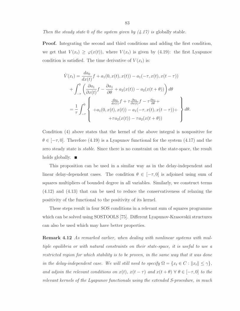
83
Then the steady state 0 of the system given by (4.17) is globally stable.
Proof. Integrating the second and third conditions and adding the first condition,
we get that V (xt) ≥ ϕ(x(t)), where V (xt) is given by (4.19): the first Lyapunov
condition is satisfied. The time derivative of V (xt) is:
V (xt) =da0
dx(t)f + a1(0, x(t), x(t)) − a1(−τ, x(t), x(t− τ))
+
∫ 0
−τ
(∂a1
∂x(t)f − ∂a1
∂θ+ a2(x(t)) − a2(x(t+ θ))
)
dθ
=1
τ
∫ 0
−τ
da0
dx(t)f + τ ∂a1
∂x(t)f − τ ∂a1
∂θ+
+a1(0, x(t), x(t)) − a1(−τ, x(t), x(t− τ))+
+τa2(x(t)) − τa2(x(t+ θ))
dθ.
Condition (4) above states that the kernel of the above integral is nonpositive for
θ ∈ [−τ, 0]. Therefore (4.19) is a Lyapunov functional for the system (4.17) and the
zero steady state is stable. Since there is no constraint on the state-space, the result
holds globally.
This proposition can be used in a similar way as in the delay-independent and
linear delay-dependent cases. The condition θ ∈ [−τ, 0] is adjoined using sum of
squares multipliers of bounded degree in all variables. Similarly, we construct terms
(4.12) and (4.13) that can be used to reduce the conservativeness of relaxing the
positivity of the functional to the positivity of its kernel.
These steps result in four SOS conditions in a relevant sum of squares programme
which can be solved using SOSTOOLS [75]. Different Lyapunov-Krasovskii structures
can also be used which may have better properties.
Remark 4.12 As remarked earlier, when dealing with nonlinear systems with mul-
tiple equilibria or with natural constraints on their state-space, it is useful to use a
restricted region for which stability is to be proven, in the same way that it was done
in the delay-independent case. We will still need to specify Ω = xt ∈ C : ‖xt‖ ≤ γ,and adjoin the relevant conditions on x(t), x(t− τ) and x(t+ θ) ∀ θ ∈ [−τ, 0] to the
relevant kernels of the Lyapunov functionals using the extended S-procedure, in much

84
the same way that the conditions θ ∈ [−τ, 0] can be adjoined in Conditions (2) and
(4) of Proposition 4.11.
4.3.3 Robust Stability Analysis Under Parametric Uncer-
tainty
Robust stability under parametric uncertainty can be treated in a unified way. Con-
sider a time-delay system of the form (4.2) with an uncertain parameter p:
z(t) = f(zt, p), (4.20)
where p ∈ P , where P is given by
P = p ∈ Rm |qi(p) ≥ 0, i = 1, . . . , N , (4.21)
i.e., the uncertainty set is captured by certain inequalities. Let x(t) = z(t)−z0. Then
we have:
x(t) = f(xt + z0, p) (4.22)
0 = f(z0, p) (4.23)
which has the steady state x∗ at the origin. The stability of this system (which
has a DAE form) can be handled by constructing a Parameter Dependent Lyapunov
functional. Consider the functional (modified from (4.19)):
V (xt, p) = a0(x(t), p) +
∫ 0
−τ
a1(θ, x(t), x(t+ θ), p)dθ +
∫ 0
−τ
∫ t
t+θ
a2(x(ζ), p)dζdθ.
(4.24)
Then we have the following proposition:
Proposition 4.13 Consider the system given by (4.22), where p ∈ P as defined
by (4.21). Denote x = x(t), xτ = x(t − τ), xθ = x(t + θ). Suppose that there exist

85
polynomials a0(x, p), a1(θ, x, xθ, p) and a2(x(ζ), p) and a positive definite function ϕ(x)
such that the following conditions hold for p ∈ P :
1. a0(x, p) − ϕ(x) ≥ 0,
2. a1(θ, x, xθ, p) ≥ 0 ∀ θ ∈ [−τ, 0],
3. a2(x(ζ), p) ≥ 0,
4. a1(0, x, x, p)−a1(−τ, x, xτ , p)+ da0
dx(t)f+τa2(x, p)−τa2(xθ, p)+τ
∂a1
∂xf−τ ∂a1
∂θ≤ 0,
∀ θ ∈ [−τ, 0] and when (4.23) is satisfied.
Then the steady state 0 of the system given by (4.22–4.23) is robustly globally uni-
formly stable for all p ∈ P .
The proof is similar to the one given earlier. It is based on functional (4.24) and is
omitted. The equality constraints given by (4.23) that may arise during the transfor-
mation process can be adjoined using appropriate polynomial multipliers, as explained
in Chapter 3. State-space constraints for local stability analysis can also be adjoined
in a unified manner.
4.4 Stability Analysis of a Predator-Prey Model
A simple model of predator-prey interactions is
x = bx− k1xy, y = k2xy − σy,
where x and y are the prey and predator populations, b is the rate of increase of
prey, k1 and k2 are the coefficients of the effect of predation on x and y and σ is
the death rate of y. The cause of death of the prey is due to predation alone, and
the growth of the predator population has as the only limitation the number of prey.
These equations give rise to Lotka-Volterra predator-prey cycles, but the model is
not biologically meaningful because it is conservative, giving rise to a family of closed
trajectories rather than a single limit cycle [48].

86
The above equations describe ideal populations that can react instantaneously
to any change in the environment. In real populations, this change comes with a
delay that represents maturation of the predator population. A more realistic set of
equations is [101]:
x(t) = x(t)[b− ax(t) − k1y(t)],
y(t) = −σy(t) + k2x(t− τ)y(t− τ),
where −ax(t)2 limits the growth of the prey, and τ ≥ 0 is a constant capturing the
average period between death of prey and birth of a subsequent number of predators.
Assumption 4.14 a, b, k1, k2 and σ are positive.
The equilibria (x∗, y∗) of the above system are:
(x∗, y∗) = (0, 0), (x∗, y∗) = (b/a, 0),
(x∗, y∗) =
(σ
k2
,bk2 − aσ
k1k2
)
. (4.25)
We are only interested in the steady state given by (4.25).
Assumption 4.15 (bk2 − aσ) > 0.
Assumption 4.15 ensures that the steady state (4.25) is in the first quadrant. We now
shift the coordinates to (x1, x2) = (x− σk2, y − bk2−aσ
k1k2) to get:
x1(t) =
[
x1(t) +σ
k2
]
[−ax1(t) − k1x2(t)] (4.26)
x2(t) = −σx2(t) + σx2(t− τ) +bk2 − aσ
k1
x1(t− τ) + k2x1(t− τ)x2(t− τ) (4.27)
We can linearize the above system about (0, 0) to get:
x1(t) =σ
k2
[−ax1(t) − k1x2(t)] (4.28)
x2(t) = −σx2(t) + σx2(t− τ) +bk2 − aσ
k1
x1(t− τ) (4.29)

87
For the linearised system, we have the following result:
Proposition 4.16 Consider the system (4.28–4.29) under the assumptions (4.14,4.15).
Then if (bk2 − 3aσ) < 0, the zero steady state is stable independent of the delay. If
(bk2 − 3aσ) > 0, the zero steady state is stable if the delay satisfies τ < τ ∗ and is
unstable otherwise, where τ ∗ is given by:
τ ∗ =1
ωatan
[
ω(aσ2 − ωk2)k2 − σ(2aσ + bk2)(k2 + a)
k2σω2(k2 + a) + (2aσ − bk2)(aσ2 − ωk2)
]
and ω solves
ω4 +a2σ2
k22
ω2 +σ2
k22
(bk2 − aσ)(3aσ − bk2) = 0.
Proof. In the absence of delay, and under the two assumptions, the system is as-
ymptotically stable. Substituting s = jω in the characteristic equation and separating
real and imaginary parts we get:
−ω2 +aσ2
k2
= σω sin(ωτ) + σ
(2aσ
k2
− b
)
cos(ωτ)
σ
[
1 +a
k2
]
ω = σω cos(ωτ) − σ
(2aσ
k2
− b
)
sin(ωτ)
Squaring the two equations and adding we get:
ω4 +a2σ2
k22
ω2 +σ2
k22
(bk2 − aσ)(3aσ − bk2) = 0. (4.30)
Denoting p1 = a2σ2
k22
and p2 = σ2
k22(bk2 − aσ)(3aσ − bk2), the roots of this equation are:
ω2 = −p1
2±√
p21 − 4p2
2. (4.31)
Under assumption 4.15, if (bk2−3aσ) < 0 (i.e p2 > 0), then there are no real solutions
to (4.30). Since the steady state is stable when the delay is zero, and there is no ω
for which poles cross to the RHP, we conclude that (4.28–4.29) is delay-independent
stable.
Under assumption 4.15 and (bk2 − 3aσ) > 0, then p2 < 0 and one of the two

88
roots of (4.31) is positive and the other one is negative. Therefore, the poles cross
the imaginary axis at only one ω. There is no possibility for stability reversal. If ω
is the solution to the above equation, then at τ = τ ∗ given in the statement of the
Proposition a Hopf bifurcation occurs; the system is stable for τ < τ ∗ and unstable
for τ > τ ∗.
We now analyze the nonlinear description of the system (4.26–4.27) using the
methodology that was developed in the previous sections. We choose as nominal
values for the parameters σ = 10, a = 1, k1 = 1, and k2 = 3.
4.4.1 Delay-Independent Stability Analysis
The system (4.26–4.27) has many equilibria, and so we need to define a region around
the zero steady state to obtain a stability condition (this is the region Ω in Theorem
4.2). We let
|x1t| ≤ γ1x
∗, |x2t| ≤ γ2y
∗, (4.32)
where the steady state (x∗, y∗) is given by (4.25). We consider b to be a parameter
in the problem. From Proposition 4.16, the linear version of this system is delay-
independent stable when aσk2
< b < 3aσk2
. For the given values of a, σ and k2, the
system is delay-independent stable for 10/3 < b < 10. For the purpose of calculating
(x∗, y∗), we use a value of b = 20/3. The steady state (0, 0) of system (4.26–4.27)
does not move as b changes; however, the other two equilibria cross through the region
defined by (4.32). If we choose γ1 = γ2 = 0.1, then no other steady state enters this
region for 11/3 < b < 10.
We consider the following Lyapunov structure:
V (xt) = a0(x1(t), x2(t), b) +
∫ 0
−τ
a1(x1(t+ θ), x2(t+ θ), b)dθ.
We use a variant of Proposition 4.13 to obtain parameter regions for which robust
delay-independent stability of the origin can be proven. When the order of a0 is second
order and a1 is 4th order, we can construct V (xt) for 4.56 ≤ b ≤ 7.11. When they

89
are 4th order and 6th order respectively, then this region becomes 3.67 ≤ b ≤ 9.95,
which is essentially the full interval.
4.4.2 Delay-Dependent Stability Analysis
Now we will analyze the system in the delay-dependent parameter regime for b = 15.
Given these parameters, τ ∗ = 0.0541. The system has several equilibria and so
we use the same constraints on x1 and x2 on the state-space given by (4.32) with
γ1 = γ2 = 0.1.
We can construct the Lyapunov functional V (xt) given by (4.19) with a1 0th order
with respect to θ, and 2nd order with respect to the rest of the variables for τ = 0.04.
When a1 is quartic with respect to all variables but θ (which is kept at 0 order), then
we can construct this V (xt) for τ = 0.053. The corresponding SDP is bigger as the
functional is more complicated, but we see that stability for a delay size close to the
stability boundary can be tested.
4.5 Conclusion
In this chapter, we presented a methodology to construct Lyapunov-Krasovskii func-
tionals for time delay systems based on the sum of squares decomposition. As far as
linear systems are concerned, this is tantamount to solving PLMIs using SOS. For
nonlinear systems, the construction is entirely algorithmic and is done using the same
tools.
The above methods can be easily extended to systems with many delays, either
commensurate or not. Still a judicious choice for the structure of the Lyapunov
functional would be required. Functional differential equations of neutral type can
also be treated in a unified way.
In the next chapter, we will consider the global stability of an arbitrary intercon-
nection of systems described by FDEs in the framework of network congestion control
for the Internet.

90
Chapter 5
Large Scale Systems: NetworkCongestion Control
3︷︸︸︷>Ae 1
︷︸︸︷å 4︷ ︸︸ ︷Jeä 1
︷︸︸︷å 5︷ ︸︸ ︷Mèga 9
︷ ︸︸ ︷GewmetreØPltwna π ≃ 3.14159
God Ever GeometrizesPlato
This chapter comes to complete the right hand side of the picture shown in Fig-
ure 1.1. We illustrate how scalable stability of ODE and FDE system interconnections
can be guaranteed for the case of network congestion control for the Internet.
The need for congestion control emerged in the mid-1980s, when a phenomenon
known as ‘congestion collapse’ resulted in unreliable file transfer. In 1988, Jacob-
son [31] proposed a congestion control scheme for the Internet, an admittedly inge-
nious design. The shortcomings of this scheme and its successors such as TCP Reno
and Vegas have only recently become apparent: they are not scalable to arbitrary
networks with very large capacities and time-delays. The technological advances –
reflected in the introduction of high bandwidth-delay product links – have revealed
that the thus far functional scheme unfortunately results in under-utilization of the
network’s resources, and theoretical analyses have shown the appearance of instabil-
ities in the transmission rates.
The need for designing new network congestion control schemes for the Internet
has steered the development of a mathematically rigorous methodological framework

91
in which the rather complicated design requirements can be accounted for to facilitate
design. In this chapter, we review briefly the methodological framework that was
developed, as well as how decentralized network congestion control schemes could
be designed to be functional, irrespective of the size of the network and the links’
capacities. The design is performed at two levels: first, the problem of sharing the
available bandwidth in a fair and efficient way is formulated as a resource allocation
program, the optimal solution of which is then the desired equilibrium point of the
overall system; thereafter, the task is to choose the dynamics of the sources and links
in the network so as to drive the system’s trajectories to that equilibrium (hence to
the optimum) in a scalably stable way.
This design recipe yielded several congestion control schemes, one of which is Fast
AQM Scalable TCP (FAST). The desired scalability properties, including scalability
with respect to the size of the delays in the network were proven for the delayed but
linearized system. This chapter is devoted to the solution of one of the most intriguing
problems: that of proving scalable nonlinear stability in the presence of heterogeneous
delays. The way we provide a proof of this property is through the construction of
a Lyapunov-Krasovskii functional, a tool that was presented in the previous chapter.
The proof is constructive and can be extended to other network congestion control
schemes such as primal schemes, as we will see in the sequel. This construction would
not be possible if the structure of the system was not taken into account.
5.1 Introduction
Internet congestion control [89] is a distributed algorithm to allocate available re-
sources to competing sources so as to avoid congestion collapse by ensuring that link
capacities are not exceeded. This problem can be formulated as a fully centralized
resource allocation program which however can be decomposed into a primal and a
dual problem by introducing duality-based price signals [34]. In this manner, conges-
tion signals seen as dual variables are generated at the Active Queue Management
(AQM) part of the algorithm implemented at the links; the congestion measure is

92
usually based on either delay or packet loss. On the other hand, the source rates can
be thought of as the primal variables which are adapted at the Transmission Control
Protocol (TCP) part of the algorithm, according to the size of the price signals. The
AQM and TCP algorithms have dynamics that aim to drive the congestion signals
and the source rates exactly at, or approximately close to, the optimum point of the
distributed resource allocation optimization problem [41].
The structure of the dynamics that are chosen for TCP and AQM are usually
based on a gradient algorithm to guarantee convergence [34]; when the delays that
are ubiquitously present in the system are ignored, a Lyapunov function argument can
be used to verify the global attractivity of the optimal point for arbitrary network
sizes. It is nonetheless appreciated that the simplest adequate model for network
congestion control is in the form of nonlinear deterministic delay-differential equa-
tions [85, 44, 54]: delays cannot be ignored as in general, their presence results in
degradation of performance or even instabilities. Indeed, stability is an important
measure of the functionality of the system. Without stability, transmission rates os-
cillate, which could result in a reduction in the link utilization; ‘mice’ packets, i.e.,
short-lived small packets on which congestion control is difficult get dropped; and
predictability of the behavior of the system is lost. On the other hand, the introduc-
tion of increasing bandwidth-delay product links in the network calls for protocols
whose performance properties scale with the network size, the Round Trip Time and
the link capacities [56].
It is unfortunate that the tools for analysis of the system behavior at the nonlinear
model level with heterogeneous delays do not scale well with the problem size. In
fact, most scalable analysis procedures in network congestion control center on the
investigation of the stability properties of the linearizations of the nonlinear equations,
using for example, the generalized Nyquist criterion developed in [97] the result in [56],
and [33].
There are significant results on the stability analysis of nonlinear Functional Dif-
ferential Equations (FDEs), also known as Time Delay Systems (TDSs) [28, 36]. The
motivating examples have predominantly come from population dynamics – an area

93
in which the effect of delay cannot be neglected [38]. This and other research areas
have motivated the development of hand-crafted methodologies for specific classes of
time delay systems at the nonlinear level. Lyapunov-based constructions have been
used in Internet Congestion Control [99, 100, 17, 46], but also, new tools have been
introduced such as passivity theory formulations [102]. The analysis procedure that
is usually followed is centered on simple network topologies. The difficulty lies in the
construction of the Lyapunov certificates, and the conservativeness of the results is
usually due to their type: Lyapunov-Razumikhin functions or Lyapunov-Krasovskii
functionals.
In order to obtain a scalable proof methodology for network congestion control
schemes, one has to take advantage of the structure of the system and construct
Lyapunov type certificates manually. In this chapter, we will describe a methodology
based on Lyapunov-Krasovskii functionals to prove stability of so-called ‘primal’ and
‘dual’ nonlinear congestion control schemes with delays, making particular reference
to Fast AQM Scalable TCP (FAST), a network congestion control scheme that was
developed in [56]. We will build up the methodology starting from the linear case
with delays and generalizing to the full nonlinear system with/without delays. The
stability result we obtain holds for arbitrary network topologies [59]. It is, however,
restricted to the structure of the Lyapunov functional constructed and is therefore
conservative compared to the result from the linearization.
We then turn to a general framework of primal network congestion control schemes,
and show that our result extends to that case in a unified way. However, when specific,
simple topologies and non-structured congestion control schemes are investigated, the
stability result can be obtained by resorting to the methodology presented in the pre-
vious chapter, using the sum of squares decomposition and SOSTOOLS. We present
an example at the end of this chapter that illustrates how this can be done.

94
5.2 Problem Formulation
Consider a network of L communication links shared by S sources. For this network,
we define a routing matrix R by:
Rli =
1 if source i uses link l
0 otherwise. (5.1)
Each source i has an associated transmission rate xi. All sources whose flow passes
through resource l contribute to the aggregate rate yl for resource l, the rates being
added with some forward time delay τ fi,l. Hence, we have:
yl(t) =S∑
i=1
Rlixi(t− τ fi,l) , rf (xi, τfi,l) (5.2)
The resources l react to the aggregate rate yl by setting congestion information pl,
the price at resource l. This is the Active Queue Management part of the picture
that is to be designed. The prices of all the links that source i uses are aggregated to
form qi, the aggregate price for source i, again through a delay τ bi,l:
qi(t) =L∑
l=1
Rlipl(t− τ bi,l) , rb(pl, τbi,l) (5.3)
The prices qi can then be used to set the rate of source i, xi, which completes the
picture shown in Figure 5.1. The forward and backward delays can be combined to
yield the Round Trip Time (RTT):
τi = τ fi,l + τ bi,l, ∀ l (5.4)
The capacity of link l is given by cl. The functions f and g shown in Figure 5.1 are
the source law and the link law, respectively. This setting is universal, and the only
information missing is the structure of the two control laws that describe how the ith

95
-
?
6
TCP AQMxi = fi(xi, qi, τi)
yl = rf(xi, τfi,l)
yl
plqi
xi
qi = rb(pl, τbi,l)
pl = gl(yl, pl, cl)
Figure 5.1: The Internet as an interconnection of sources and links through delays.
source reacts to the price signal qi that it sees
xi = fi(xi, qi, τi), (5.5)
and how the lth router reacts to the aggregate rate yl it observes
pl = gl(yl, pl, cl). (5.6)
Here fi models TCP algorithms (e.g., Reno or Vegas) and gl models AQM algorithms
(e.g., RED, REM).
In order to understand the meaning of the variables pl, let us consider the prop-
erties of the equilibrium of this system, which we assume is given by the vector
quantities x∗, y∗, p∗, q∗. We have the following relationships from (5.2) and (5.3):
y∗ = Rx∗, q∗ = RTp∗.
We now assume that as the aggregate price signal at equilibrium q∗i increases, then
the demanded transmission rate at the source should decrease, i.e., the two are related
by
x∗i = Fi(q∗i ),
where Fi is a positive, strictly monotone decreasing function, which is the solution of
fi(x∗i , q
∗i ) = 0 where fi is given by Equation (5.5). Alternatively, one can think that

96
the sources have a certain utility if allowed a certain transmission rate, the utility
satisfying:
U ′i(xi) = F−1
i (xi).
This relationship implies that Ui(xi) is a monotonically increasing strictly concave
function. Under these assumptions, the equilibrium rate x∗i for each source solves
maxxi≥0
Ui(xi) − xiq∗i , (5.7)
which means that the sources are trying to maximize their profit: maximize their
utility, and at the same time, minimize the cost of having high rates; q∗i can be
thought of as the price per unit flow that the sources have to pay. Different protocols
correspond to different Utility functions Ui, and to different dynamic laws (5.5–5.6)
that attempt in a decentralized way to reach the appropriate equilibrium. For this
reason this framework allows comparability of different designs.
The role of prices is to coordinate the actions of individual sources so as to align
individual optimality with social optimality, i.e., to ensure that the solution of (5.7)
also solves the network resource allocation problem
maxxi≥0
S∑
i=1
Ui(xi)
s.t.S∑
i=1
Rlixi ≤ cl, ∀ l = 1, . . . , L, (5.8)
where the inequality constraint is the natural limitation that the sum of all transmis-
sion rates through link l has to be less than or equal to its capacity. The uniqueness
of the optimal solution to the above problem is guaranteed since the Ui are strictly
concave functions and the program is convex. The above optimization problem can-
not be solved in a decentralized way, as the source rates are coupled in the shared
links through the inequality constraints and solving for x∗ would require cooperation
among possibly all sources. To solve it in a distributed manner over a large network,
we can decompose it into a primal problem that the sources are trying to solve and

97
a dual that the links are trying to solve, regarding the source rates xi as primal vari-
ables and the prices set by the links pl as the dual variables. Specifically, consider
the Lagrangian for program (5.8):
L(x, p) =∑
i
Ui(xi) −∑
l
pl(yl − cl)
=∑
i
(
Ui(xi) − xi∑
l
Rlipl
)
+∑
l
plcl,
where pl ≥ 0. The dual problem can then be written as
minpl≥0
maxxi≥0
∑
i
(
Ui(xi) − xi∑
l
Rlipl
)
+∑
l
plcl.
By the properties of the dual solution and the fact that the programs are convex,
at the optimum p∗ the xi that maximizes the individual profit (5.7) is the same as
the unique solution to the network problem (5.8). If the equilibrium prices p∗ are
made to align with the Lagrange multipliers, the individual optima – computed in a
decentralized fashion by the sources – will align with the global optima of (5.8).
The dynamical system defined by (5.5–5.6) with delays ignored aims to drive the
system close to or exactly at the optimal point (x∗, p∗), using well-known gradient
algorithms. For example, from the Karush-Kuhn-Tucker conditions, the solution of
the dual problem satisfies:
xi − U′−1i (qi) = 0
pl(yl − cl) = 0
and pl ≥ 0, as the dual variables are non-negative. To obtain the pl and xi, one can
use the following algorithm at each link, which is a gradient algorithm:
pl(t) =
[yl − clcl
]+
pl
, [gl]+pl, (5.9)
xi = U ′−1i (qi), (5.10)

98
where [f(x)]+x means
[f(x)]+x =
f(x) x > 0
max(f(x), 0), x = 0.
After [34], it is customary to call ‘dual’ the congestion control scheme with dynamics
at the links and a static source law - such as the one shown above; and ‘primal’ the
congestion control scheme with dynamics at the sources and a static link law. If both
source and link laws have dynamics, the scheme is termed ‘primal-dual’.
For both the dual and the primal algorithms, the stability properties of the un-
delayed systems can be obtained by constructing Lyapunov functions that scale with
the system size based on the barrier functions of the optimization strategies. Put
another way, the gradient algorithm results in a weighted gradient system, i.e., for
the primal case, there is a potential function V so that xi = −κi ∂V∂xi[89]. Taking
advantage of this structure, a scalable stability proof can be obtained.
When delays are introduced, the analysis becomes more complicated, and a scal-
able proof methodology for analysis of such congestion control schemes is difficult in
the nonlinear case. The generalized Nyquist criterion can be used for the lineariza-
tion of these systems, as it is scalable in the case of congestion control as explained
in [97]. Here we will show how the analysis of congestion control schemes captured by
nonlinear delay-differential equations can be performed in a scalable manner, treating
both the presence of heterogeneous delays in the system and the nonlinearities explic-
itly. The tools we will be using are Lyapunov-Krasovski functionals [36], which are
the relevant Lyapunov-based tools for functional differential equations as Lyapunov
functions are for ordinary differential equations. We will set them equal to the Lya-
punov functions used in the undelayed systems, plus some simple integral terms. We
will illustrate how the special structure of the system helps in the scalability of the
Lyapunov certificate for the linear case, and then concentrate in the nonlinear case
for which sufficient conditions for arbitrary topologies will be derived. The analy-
sis is performed for a dual algorithm and a primal algorithm, and scalable stability

99
conditions are obtained.
The routing matrix R is assumed fixed and full row rank. This means that there
are no algebraic constraints between link flows, i.e., they can vary independently by
choice of source flows xi. As a consequence, equilibrium prices are uniquely deter-
mined.
5.3 Dual Congestion Control Schemes
Combining (5.1–5.4) and (5.9–5.10), the system has the following closed loop dynam-
ics:
pl(t) =
[S∑
i=1
Rli
clU ′−1i
(L∑
m=1
Rmipm(t− τ fi,l − τ bi,m)
)
− 1
]+
pl
(5.11)
We also denote h = maxi,l,m:Rmi=Rli=1τ fi,l + τ bi,m, and Cn = C([−h, 0],Rn) the
Banach space of continuous functions mapping [−h, 0] into Rn with the topology of
uniform convergence. We assume that the initial condition is non-negative, i.e.,
p(θ) = φ(θ) ≥ 0, θ ∈ [−h, 0], φ ∈ CL.
This guarantees that the solutions to (5.11) satisfy pl(t) ≥ 0 for all time as a result
of the projection nonlinearity.
A particular congestion control scheme that we will be investigating is FAST, in
which the sources are assumed to have the following Utility function:
Ui(xi) =τiMi
αixi
(
1 − logxixi
)
, (5.12)
where Mi =∑L
l=1Rli, αi are (positive) source gains and xi are source constants. Since
xi = U′−1i (qi), we have:
xi = xie−
αiqiMiτi
which implies that xi ≤ xi, since qi ≥ 0.
To investigate the linearization of (5.11), we assume that R refers to bottleneck

100
links only, and for non-bottleneck links pl = 0. This gives the system
pl(t) =S∑
i=1
L∑
m=1
RliRmi
U ′′i (x∗i )cl
pm(t− τ fi,l − τ bi,m), (5.13)
where cl is a target capacity set just below the true capacity cl of link l and ∗ denotes
equilibrium quantities. For this system, the following result is known:
Theorem 5.1 [56] Let the matrix R that denotes the routing matrix in relation to
the bottleneck links be full row rank. Then the system given by (5.13) is asymptotically
stable if
1
cl
S∑
i=1
RliMiτi|U ′′
i (x∗i )|<π
2. (5.14)
In particular, for the Utility function given by (5.12), the above condition reduces to
αi ≤ π/2, which is a decentralized condition on the sources’ gains.
In the case of FAST, there are a number of undetermined parameters, xi. We can
choose
xi = x∗i eαiq∗iMiτi = x∗i e
αiLm=1 Rmip∗m
Miτi (5.15)
so that y∗l =∑S
i=1Rlix∗i . Also at the equilibrium y∗l = cl (or p∗l = 0 and y∗l < cl), we
therefore haveS∑
i=1
Rlix∗i ≤ cl. (5.16)
If we wanted to impose fairness so that the sources would have the same rates around
some nominal price value q∗i , then the x∗i would be equal to each other.
5.3.1 Stability of the Linearization
In this section, we aim to obtain a Lyapunov-based construction to prove a result
similar to Theorem 5.1. It is true that frequency domain methodologies many times
result in more accurate descriptions of the stability boundaries and are scalable for
the special case of Internet Congestion Control [56]. Lyapunov-based arguments are
more difficult to make, and many times are more conservative, but prove useful when
considering the stability of nonlinear time-delay systems. In order to construct a

101
scalable Lyapunov-Krasovskii functional, we take advantage of the structure of the
system, as will be evident in the proof of the theorem which is constructive. Important
in this quest is the following undelayed version of (5.13):
pl(t) =S∑
i=1
L∑
m=1
RliRmi
U ′′i (x∗i )cl
pm(t) (5.17)
Theorem 5.2 Let the matrix R that denotes the routing matrix in relation to the
bottleneck links be full row rank. Then the system given by (5.13) is asymptotically
stable if
1
cl
S∑
i=1
RliMiτi|U ′′
i (x∗i )|< 1. (5.18)
Proof. Consider the function
V1(p) =1
2
S∑
i=1
Aiτi
(L∑
l=1
Rlipl
)2
(5.19)
First, note that V1 > 0 since R is full rank. The derivative of (5.19) along the
trajectories of system (5.13) can be computed to be:
V1(p) = −L∑
l=1
clplpl,u = −L∑
l=1
clp2l −
L∑
l=1
clpl(pl,u − pl),
where pl,u is the undelayed version of (5.13) given by (5.17). To proceed, we use the
Leibniz rule to distribute the delay over an interval. For example, we have:
pl(t− τ) = pl(t) −d
dt
∫ 0
−τ
pl(t+ θ)dθ.
This gives
pl =S∑
i=1
L∑
m=1
RliRmi
U ′′i (x∗i )cl
pm(t− τ fi,l − τ bi,m) = pl,u −S∑
i=1
L∑
m=1
RliRmi
U ′′i (x∗i )cl
∫ 0
−τfi,l−τb
i,m
pm(t+ θ)dθ.

102
Putting everything together, we have:
V1(p) = −L∑
l=1
clp2l −
L∑
l=1
S∑
i=1
L∑
m=1
RliRmi
U ′′i (x∗i )
∫ 0
−τfi,l−τb
i,m
plpm(t+ θ)dθ.
Now let us concentrate on the second term:
−L∑
l=1
S∑
i=1
L∑
m=1
RliRmi
U ′′i (x∗i )
∫ 0
−τfi,l−τb
i,m
plpm(t+ θ)dθ
≤ 1
2
L∑
l=1
S∑
i=1
L∑
m=1
RmiRli(τfi,l + τ bi,m)
|U ′′i (x∗i )|
p2l +
1
2
L∑
l=1
S∑
i=1
L∑
m=1
RmiRli
|U ′′i (x∗i )|
∫ 0
−τfi,l−τb
i,m
p2m(t+ θ)dθ,
where the inequality 2ab ≤ a2 + b2 was used. Now consider the following functional
term:
V2 =1
2
L∑
l=1
S∑
i=1
L∑
m=1
RmiRli
|U ′′i (x∗i )|
∫ 0
−τfi,l−τb
i,m
∫ t
t+θ
p2m(ζ)dζdθ. (5.20)
Then
V2 =1
2
L∑
l=1
S∑
i=1
L∑
m=1
RmiRli(τfi,l + τ bi,m)
|U ′′i (x∗i )|
p2l −
1
2
L∑
l=1
S∑
i=1
L∑
m=1
RmiRli
|U ′′i (x∗i )|
∫ 0
−τfi,l−τb
i,m
p2m(t+ θ)dθ
Let V = V1 + V2. Then we get
V ≤ −L∑
l=1
clp2l +
L∑
l=1
S∑
i=1
L∑
m=1
RmiRli(τfi,l + τ bi,m)
|U ′′i (x∗i )|
p2l .
The coefficient of each term p2l is
− cl +S∑
i=1
RliMiτi|U ′′
i (x∗i )|
Therefore if1
cl
S∑
i=1
RliMiτi|U ′′
i (x∗i )|< 1 (5.21)

103
for all l then V ≤ 0, V is a Lyapunov-Krasovksii functional and the conditions of
stability [28] are satisfied. The set S = φ ∈ CL : V (φ) = 0 is the set
S =
φ :S∑
i=1
L∑
m=1
RliRmi
U ′′i (x∗i )cl
φm(−τ fi,l − τ bi,m) = 0, l = 1, . . . , L
.
The largest set in S that is invariant with respect to the system satisfies pl = 0
∀l = 1, . . . , L, i.e. pl = K, a constant. But the only constant φ that is in S is the
zero equilibrium. Therefore, the equilibrium of the system is asymptotically stable
by an extension of LaSalle’s theorem (Theorem 5.3.1 in [28]) for arbitrary networks
and delays, provided condition (5.18) is satisfied and R is full rank.
The Lyapunov-Krasovskii functional that we have constructed introduced some
conservativeness with respect to the result in Theorem 5.1, but is scalable to the size
of the system. In particular, the right hand side of the inequality in Theorem 5.1 is
π/2 and was obtained using frequency domain arguments. The bound that we obtain
is 1, and is a result of the structure of the Lyapunov functional that is used. More
complicated, ‘richer’ structures may yield stronger bounds.
In the case of FAST, for which the Utility function is given by (5.12), we have the
following corollary:
Corollary 5.3 Let the matrix R that denotes the routing matrix in relation to the
bottleneck links be full row rank. Then FAST linearized about the equilibrium is as-
ymptotically stable if
αi < 1.
Proof. The Utility function for FAST is given by (5.12). This gives:
|U ′′i (x∗i )| =
Miτiαix∗i

104
Condition (5.18) then becomes:
1
cl
S∑
i=1
RliMiτi|U ′′
i (x∗i )|< 1
⇒ 1
cl
S∑
i=1
Rliαix∗i < 1
which is guaranteed if αi < 1 since∑S
i=1Rlix∗i ≤ cl.
5.3.2 Nonlinear Stability Analysis
The nonlinear system is given by Equation (5.11). Now R denotes the full routing
matrix with non-bottleneck links (rows) included but is still full row rank so that
equilibrium prices are uniquely determined. The existence and uniqueness of solutions
of (5.11) is assumed.
5.3.2.1 Nonlinear Undelayed Model
The closed loop system with delays equal to zero is:
pl(t) =
[S∑
i=1
Rli
clU ′−1i
(L∑
m=1
Rmipm(t)
)
− 1
]+
pl
= [gl(p)]+pl
(5.22)
We have the following theorem:
Theorem 5.4 For fixed full rank R, the (unique) equilibrium of (5.22) is asymptot-
ically stable for all non-negative initial conditions.
Proof. Consider the following function:
V (p) =L∑
l=1
(cl − y∗l )pl +S∑
i=1
∫ qi
q∗i
(x∗i − U ′−1i (Q))dQ, (5.23)
105
This function is positive definite for p ≥ 0, with a minimum at the equilibrium [89].
Differentiating V (p) with respect to time, we get
V (p) = −L∑
m=1
cmgm(p)[gm(p)]+pm≤ 0.
Now V (p) = 0 only when gm(p) = 0 or gm(p) < 0 and pm = 0. This can only happen
at the equilibrium of interest. Therefore, we obtain asymptotic stability. Moreover,
V is radially unbounded; the equilibrium is globally (i.e., for pl ≥ 0) asymptotically
stable.
The above result is the basic building block that ensures the scalability of the
results. In the next subsection, we will build on the construction of scalable Lyapunov-
Krasovskii functionals for the linear case, to construct similar certificates for the
nonlinear case.
5.3.2.2 Nonlinear Delayed Model
In order to ensure stability for arbitrary topologies with delays, we will use a Lya-
punov argument using our result on the linearization. Most handcrafted attempts
center on Lyapunov-Razumikhin functions for analysis of simple network topolo-
gies [17, 99], or the extraction of delay-independent stability conditions for arbi-
trary networks [105]. Lyapunov-Razumikhin functions, although an attractive tool
for handcrafted stability analysis for nonlinear time delay systems because of their
simplicity to construct manually, are known to yield conservative results compared
to the ones that Lyapunov-Krasovskii functionals produce [28]. The intuition be-
hind this is that Lyapunov-Krasovskii functionals respect the fact that the system
is evolving on a function space, and so the Lyapunov certificate should be a func-
tional; Lyapunov-Razumikhin functions attempt to assess the stability of an infinite
dimensional system using finite dimensional arguments – an attempt that is inher-
ently conservative. Here we construct a Lyapunov-Krasovskii functional that scales
with the system size.
Recall that the Utility function is a continuously differentiable, non-decreasing,

106
strictly concave function. Therefore, U ′′i (xi) < 0 everywhere. Let γi be the lower
bound for |U ′′i (xi)|, so that
|U ′′i (xi)| ≥ γi > 0, ∀ i (5.24)
γi here serves as a global (i.e., for xi ≥ 0) Lipschitz constant for U′−1i as:
∣∣∣∣
(
U′−1i (q)
)′∣∣∣∣=
∣∣∣∣
1
U′′
i (x)
∣∣∣∣≤ 1
γi(5.25)
This means that:∣∣∣U
′−1i (q2) − U
′−1i (q1)
∣∣∣ ≤ 1
γi|q2 − q1| (5.26)
We then have the following result:
Theorem 5.5 The equilibrium of the system described by (5.11) is globally (for pl ≥0) asymptotically stable for arbitrary delays, provided that
1
cl
S∑
i=1
RliMiτiγi
< 1 (5.27)
and the matrix R is an arbitrary full rank, fixed routing matrix.
Proof. Consider V1 = V given by (5.23). From the argument in the proof of Theorem
5.4, V1 > 0 apart at the equilibrium, and is radially unbounded. Now
V1(p) = −L∑
l=1
clgl,u[gl]+pl
= −L∑
l=1
clgl[gl]+pl−
L∑
l=1
cl[gl]+pl(gl,u − gl),
where gl,u(p) corresponds to the undelayed version of unprojected (5.11), the unpro-

107
jected Equation (5.22). The second term is equal to:
−L∑
l=1
cl[gl]+pl(gl,u − gl)
≤L∑
l=1
S∑
i=1
Rli|[gl]+pl|∣∣∣∣∣U ′−1i
(L∑
m=1
Rmipm(t)
)
− U ′−1i
(L∑
m=1
Rmipm(t− τ fi,l − τ bi,m)
)∣∣∣∣∣
≤L∑
l=1
S∑
i=1
L∑
m=1
RmiRli
γi|[gl]+pl
|∣∣∣pm(t) − pm(t− τ fi,l − τ bi,m)
∣∣∣
≤L∑
l=1
S∑
i=1
L∑
m=1
RmiRli
γi
∫ 0
−τfi,l−τb
i,m
|[gl]+pl||pm(t+ θ)|dθ,
where global Lipschitz continuity and the Leibniz rule were used (note that p ≥ 0).
The rest of the proof is similar to the proof of Theorem 5.2. The candidate Lyapunov-
Krasovskii functional is given by V = V1 + V2 where
V2(p) =L∑
l=1
S∑
i=1
L∑
m=1
RliRmi
2γi
∫ 0
−τfi,l−τb
i,m
∫ t
t+θ
p2m(ζ)dθdζ.
Then we have:
V =L∑
l=1
[
−clgl[gl]+pl+
S∑
i=1
RliMiτiγi
[gl]
+pl
2
]
Now V ≤ 0 under the condition:
−cl +S∑
i=1
RliMiτiγi
< 0
This implies that V ≤ 0, and stability of the equilibrium follows for pl ≥ 0 ∀ l =
1, . . . , L. The set S = φ ∈ CL : V = 0 is the set for which [gl]+pl
= 0, i.e., for
l = 1, . . . , L we have either
S∑
i=1
Rli
clU ′−1i
(L∑
m=1
Rmiφm(−τ fi,l − τ bi,m)
)
= 1
108
or
∑Si=1
Rli
clU ′−1i
(∑L
m=1Rmiφm(−τ fi,l − τ bi,m))
< 1,
φl(−τ fi,l − τ bi,m) = 0
for l = 1, . . . , L. The largest invariant set in S satisfies pl = 0, i.e. pl = K, a constant.
The only constant solution in S is the (unique) equilibrium (either p∗l = 0 and y∗l < cl
or pl = p∗l ). Therefore, the asymptotic stability of the equilibrium can be proven
using an extension to LaSalle’s theorem (Theorem 5.3.1 in [28]). Since V is radially
unbounded, the equilibrium of the system is globally (i.e., for pl ≥ 0) asymptotically
stable for arbitrary networks and delays, provided that condition (5.27) is satisfied
and R is full rank.
For the special case of FAST, we have the following corollary:
Corollary 5.6 The equilibrium of FAST is globally (for pl ≥ 0) asymptotically stable
for arbitrary delays and network topologies, provided that
αi <xixi
(5.28)
and the matrix R is an arbitrary full rank, fixed routing matrix.
Proof. For FAST, the Utility function is given by (5.12); this gives the following
value for γi:
γi =τiMi
αixi
since xi ≤ xi. Therefore, condition (5.27) of Theorem 5.5 becomes:
1
cl
S∑
i=1
Rliαixi < 1
Therefore, a sufficient condition for stability is
αi <x∗ixi.
109
for R full rank.
Remark 5.7 Another approach would be to get a local result, i.e., valid for all initial
conditions in some level set of the Lyapunov functional V . In the case of FAST, one
can bound the term (gl,u − gl) using a local Lipschitz constant:
|gl,u − gl| =
∣∣∣∣∣
S∑
i=1
Rlix∗i
cl
(
e−αi
Lm=1 Rmi[pm(t)−p∗]
Miτi − e−αi
Lm=1 Rmi[pm(t−τi)−p∗]
Miτi
)∣∣∣∣∣
≤S∑
i=1
Rliαix∗i ki
Miτicl
∣∣∣∣∣
L∑
m=1
Rmi[pm(t) − pm(t− τi)]
∣∣∣∣∣,
where ki > 1 is a constant resulting from the Lipschitz approximation. If f(x) =
e−
αiMiτi
x, then
|f ′(x)| =αiMiτi
∣∣∣e
−αi
Miτix∣∣∣ ≤ αiki
Miτi.
The bigger ki is, the larger the region x around x = 0 it can ‘cover’, which can reflect
on the level set of V in which initial conditions will tend to the equilibrium. If the proof
methodology that was presented here is used, the bound αi <1ki
is obtained; this means
that the bigger ki is, the smaller the value of αi for which stability can be proven. The
maximal level set of the Lyapunov functional (giving a region of attraction) will be a
function of the ki.
Remark 5.8 For single-link single-source we get
p =
[x
ce−
ατp(t−τ) − 1
]+
p
.
A simple change of variables z(t) = xce−
ατp(t)−1, ignoring the projection and rescaling
of time results in the system gives:
z = −α[z(t) + 1]z(t− 1) (5.29)
Equation (5.29) is Hutchinson’s Equation, a well-known population dynamics model
that models a single species striving for a common food. The delay represents the

110
maturation of the population. The linearization of this system about the zero equilib-
rium is stable for α < π/2 ≃ 1.57. In [103], E. M. Wright managed to prove global
stability of the equilibrium of the nonlinear system for α < 37/24 = 1.54 if the initial
condition satisfies z(t + θ) ≥ −1, θ ∈ [−1, 0) with z(0) > −1 (which corresponds to
a non-negative price p) by looking at the properties of the solution of (5.29). How-
ever, this result is difficult to scale for arbitrary population interactions – a similar
problem to the arbitrary network topology case. Existence and uniqueness of solutions
of (5.11) can be established in a similar way [38, 55].
The above treatment may seem to have come from intuition, but in fact, it can be
generalized to other congestion control algorithms. In the next section we consider the
stability analysis of primal congestion control schemes in a delay-dependent fashion,
complimentary to the delay-independent result obtained in [105].
5.4 Primal Congestion Control Schemes
In the case of primal congestion control schemes, the sources have dynamics, whereas
the pricing function at the links is static. The optimization framework is used in
this case too, to provide a means for designing the control laws. The condition for
optimality from the resource allocation problem formulation is given by:
U ′i(x
∗i ) − q∗i = 0.
For the primal case, we consider a gradient control algorithm to drive the source
dynamics to achieve this optimality condition. We therefore have the following link
and source laws [34, 89]:
pl = fl(yl)
xi = κi(xi)(U′i(xi) − qi)

111
where fl is a strictly increasing function, such that fl > 0, f ′l > 0. In particular, the
following law has been proposed in [98]:
pl(t) = fl(yl(t))
xi = κixi(t− τi)
[
1 − qiU ′i(xi)
]
The closed loop dynamics for the whole network then become:
xi = κixi(t− τi)
1 −∑L
l=1Rlifl
(∑S
j=1Rljxj(t− τ bi,l − τ fj,l))
U ′i(xi)
(5.30)
The initial conditions for (5.30) are non-negative functions defined on C([−h, 0],RS),
where h = maxhi and
hi = maxj,l:Rli=Rlj=1
τ bi,l + τ fj,l. (5.31)
5.4.1 Stability of the Linearization
The linearization of (5.30) about the equilibrium x∗i is:
xi =κix
∗i
q∗iU
′′
i (x∗i )xi −κix
∗i
q∗i
L∑
l=1
Rlip′∗l
S∑
j=1
Rljxj(t− τ bi,l − τ fj,l) (5.32)
where q∗i = U′−1i (x∗i ), y
∗l =
∑Ll=1Rlix
∗i and p
′∗l = f ′
l (y∗l ).
We have the following result, similar to the one in Theorem 5.2:
Theorem 5.9 System (5.32) is asymptotically stable if R is full rank and
κiτiq∗i
L∑
l=1
Rliy∗l p
′∗l < 1, ∀ i.
We note that the result in [98] has π/2 in the RHS, and is obtained using frequency
domain methods.
112
Proof. Consider the following function:
V1 = −1
2
S∑
i=1
U′′
i (x∗i )x2i +
1
2
L∑
l=1
p′∗l
(S∑
j=1
Rljxj(t)
)2
This is positive definite, as R is full rank. The undelayed version of (5.32) is
xi = κix∗iq∗i
[
U′′
i (x∗i )xi −L∑
l=1
Rlip′∗l
S∑
j=1
Rljxj
]
.
We have:
V1 = −S∑
i=1
q∗iκix∗i
xixi,u = −S∑
i=1
q∗iκix∗i
x2i −
S∑
i=1
q∗iκix∗i
xi(xi,u − xi)
where xi,u denotes the undelayed version. We now manipulate the second term as in
the proof of Theorem 5.2 to get:
−S∑
i=1
q∗iκix∗i
xi(xi,u − xi) =S∑
i=1
L∑
l=1
Rlip′∗l
S∑
j=1
Rlj
∫ 0
−τbi,l−τf
j,l
xixj(t+ θ)dθ
where the Leibniz rule was used to distribute the delay over an interval. Using the
inequality ab ≤ k2a2 + 1
2kb2 for k > 0, we have:
−S∑
i=1
q∗iκix∗i
xi(xi,u − xi)
≤S∑
i=1
L∑
l=1
S∑
j=1
RljRli
2p′∗l (τ bi,l + τ fj,l)kijx
2i +
S∑
i=1
L∑
l=1
S∑
j=1
RljRli
2kijp′∗l
∫ 0
−τbi,l−τf
j,l
x2j(t+ θ)dθ
where kij are constants. Introduce now the following functional:
V2 =S∑
i=1
L∑
l=1
S∑
j=1
RljRli
2kijp′∗l
∫ 0
−τbi,l−τf
j,l
∫ t
t+θ
x2j(ζ)dζdθ

113
This then satisfies:
V2 =S∑
i=1
L∑
l=1
S∑
j=1
RljRli(τbi,l + τ fj,l)
2kijp′∗l x
2j −
S∑
i=1
L∑
l=1
S∑
j=1
RljRli
2kijp′∗l
∫ 0
−τbi,l−τf
j,l
x2j(t+ θ)dθ
Now let V = V1 + V2, and kij =x∗jx∗i
√τiτj
. Then:
V ≤ −S∑
i=1
q∗iκix∗i
x2i +
L∑
l=1
S∑
j=1
RljRli
2p′∗l (τi + τj)
√τiτj
x∗jx∗ix2i
Stability is guaranteed if V ≤ 0, i.e., if each i satisfies:
κiq∗i
L∑
l=1
S∑
j=1
RljRlix∗jp
′∗l
(τi + τj)
2
√τiτj< 1
Since (τi + τj) ≥ 2√τiτj, stability is also guaranteed by
κiτiq∗i
L∑
l=1
S∑
j=1
RljRlix∗jp
′∗l < 1. (5.33)
In order to prove asymptotic stability, we use a LaSalle argument in the same way as
it was done in the proof of Theorem 5.2. The set S = φ ∈ CS : V (φ) = 0 is the set
S =
φ :L∑
l=1
Rlip′∗l
S∑
j=1
Rljφj(−τ bi,l − τ fj,l) = U′′
i (x∗i )φi, i = 1, . . . , S
.
The largest set in S that is invariant with respect to the system satisfies xi = 0
∀i = 1, . . . , S, i.e. xi = K, a constant. But the only constant φ that is in S is the
zero equilibrium. Therefore, the equilibrium of the system is asymptotically stable
by an extension of LaSalle’s theorem (Theorem 5.3.1 in [28]) provided (5.33) holds
and R is full rank.
We remark that the proof is very similar to the one for Theorem (5.2), apart
from two steps: the way the quadratic inequality a2 + b2 ≥ 2ab is used, and the last
step where, in order to treat the delays τi and τj, one has to use another inequality
114
argument.
5.4.2 Nonlinear Stability Analysis
The nonlinear system is given by Equation (5.30), and the existence and uniqueness
of solutions is assumed. To ensure stability for arbitrary topologies in the nonlinear
case with delays, we have to use a Lyapunov based argument similar to the one we
used in the linearization. The system to be analyzed is described by Equation (5.30).
Further, consider the undelayed version of (5.30):
xi = κixi(t− τi)
1 −∑L
l=1Rlifl
(∑S
j=1Rljxj(t))
U ′i(xi)
(5.34)
Before we proceed, recall that Ui(xi) are strictly concave, non-decreasing functions
and fl(yl) are strictly increasing functions, such that fl > 0, f ′l > 0. This inevitably
means that xi are upper bounded, as shown in the following proposition:
Proposition 5.10 Let xi(t) be a solution of (5.30). Then there is a T > 0 such
that, for t ≥ T , xi(t) < U′−1i
(∑L
l=1Rlifl(0))
= xi.
Proof. First, note that
U′−1i
(L∑
l=1
Rlifl(0)
)
> U′−1i
(L∑
l=1
Rlifl(y∗l )
)
= U′−1i (q∗i ) = x∗i .
If xi(t) ≥ x∗i ∀i for all large t, say t ≥ T , then xi ≤ 0 for t ≥ T and hence
limt→∞ xi(t) = x∗i . Thus, we may assume xi(t) are oscillatory about x∗i . Let t > 2hi,
where hi is defined by (5.31) be such that xi(t) > x∗i and xi(t) = 0, i.e., a maximum
of the trajectory. Then we have:
U ′i(xi(t)) =
L∑
l=1
Rlifl
(S∑
j=1
Rljxj(t− τ bi,l − τ fj,l)
)
115
Therefore,
xi(t) = U′−1i
(L∑
l=1
Rlifl
(S∑
j=1
Rljxj(t− τ bi,l − τ fj,l)
))
< U′−1i
(L∑
l=1
Rlifl(0)
)
.
This completes the proof.
Let xi(t) ≤ xi where xi is defined in the above proposition. Similarly, define
yl =∑S
i=1Rlixi so that yl(t) ≤ yl. Then we have:
Theorem 5.11 The non-zero equilibrium of (5.30) is globally (i.e., for xi > 0) as-
ymptotically stable, provided R is full rank and
κiτiU ′i(xi)
S∑
j=1
Rliylf′l (yl) < 1. (5.35)
Proof. Consider a function of the form:
V1 = −S∑
i=1
[Ui(xi) − Ui(x∗i )] +
L∑
l=1
∫ PSj=1Rljxj
y∗l
fl(Y )dY
This function is positive definite and radially unbounded. Then we have:
V1 = −S∑
i=1
[
U ′i(xi) −
L∑
l=1
Rlifl
(S∑
i=1
Rljxj
)]
xi
= −S∑
i=1
U ′i(xi)
κixi(t− τ)xi,uxi = −
S∑
i=1
U ′i(xi)
κixi(t− τ)
(x2i + xi(xi,u − xi)
)
where (5.34) is the undelayed version of Equation (5.30). Now
−S∑
i=1
U ′i(xi)
κixi(t− τ)xi(xi,u − xi) =
S∑
i=1
L∑
l=1
Rlifl
(S∑
j=1
Rljxj(t)
)
xi
−S∑
i=1
L∑
l=1
Rlifl
(S∑
j=1
Rljxj(t− τ bi,l − τ fj,l)
)
xi
≤S∑
i=1
S∑
j=1
L∑
l=1
RliRljf′l (yl)
∫ 0
−τbi,l−τf
j,l
|xi||xj(t+ θ)|dθ

116
as fl is globally Lipschitz continuous and strictly increasing. The rest of the proof is
the same as in the linear case. Since xi < xi, we have:
U ′i(xi) > U ′
i(xi)
from the strict concavity of Ui and therefore V can be written as follows:
V ≤ −S∑
i=1
U ′i(xi)
κixi(t− τ)x2i +
S∑
i=1
L∑
l=1
S∑
j=1
RljRli
2f ′l (yl)(τi + τj)
√τiτj
xjxix2i
≤ −S∑
i=1
U ′i(xi)
κixix2i +
L∑
l=1
S∑
j=1
RljRli
2f ′l (yl)(τi + τj)
√τiτj
xjxix2i
Therefore, stability is retained if
κiτiU ′i(xi)
S∑
j=1
Rliylf′l (yl) < 1.
Asymptotic stability follows from LaSalle’s argument in a similar way as in the proof
of Theorem 5.5. Hence, the system is globally asymptotically stable for arbitrary
networks and delays provided (5.35) is satisfied and R is full rank.
5.5 A Primal-Dual Congestion Control Scheme
The above ‘manual’ constructions of scalable proofs for arbitrary networks have taken
advantage of the structure of the dynamics to guide the choice of the Lyapunov
certificate. In some cases, this is not possible because the dynamics are designed in
an ad-hoc way.
The two congestion control schemes that we analyzed in this chapter have dis-
advantages. The main drawback of the dual control law is that it puts a restriction
on the sources’ demand curves, as the source law is static. Moreover, a pure primal
congestion control scheme has no control over the pricing functions that can be used.
A congestion control scheme that has dynamics, both at the sources and links

117
could alleviate this problem. Such a scheme is called primal-dual, and was developed
in [57]. Apart from qi, yl and pl given by Equations (5.3), (5.2) and (5.9) respectively,
we have:
xi(t) = xm,ieξie
−αiqi(t)
Miτi (5.36)
ξi(t) =βiτi
[U ′i(xi(t)) − qi(t)] (5.37)
where Ui(xi) is the utility function of source i and βi is a parameter. The following
result on the stability of the linearized system is known:
Theorem 5.12 [57] Assume that for every source i, τi ≤ τ . Then the system
described by Equations (5.1–5.4), (5.9) and (5.36–5.37), with αi < π/2 and z =
βiMi
αi= η
τfor η ∈ (0, 1) small enough depending on α ≥ αi, the closed loop system is
linearly stable.
A Lyapunov argument that will scale with the system size may be difficult in this
case, as the parameters βi are tuned so as to provide for slow adaptation of the source
to its own utility function characteristic. It is fortunate that the tools that we have
developed in the previous chapter that use the sum of squares decomposition can be
used instead, but only for small network topologies [60]. We note that the system
equations are not polynomial in the variables, but if we write the system dynamics
in other system variables, we obtain the following description:
xi(t) = xi
(βiτi
[U ′i(xi(t)) − qi(t)] −
αiMiτi
qi(t)
)
qi(t) =∑
l
Rli
cl
(∑
j
Rljxj(t− τ fj,l − τ bi,l) − cl
)
where we have ignored the projection nonlinearity.
This formulation is suitable if the one-way delay is available, although in many
special cases, the RTT appears naturally in the delay combinations. We also put a
bound on the delay size so that the RTT delay is equal to τ , and we assume the
overbound on the one-way delay to be half of the overbound on the RTT. We choose
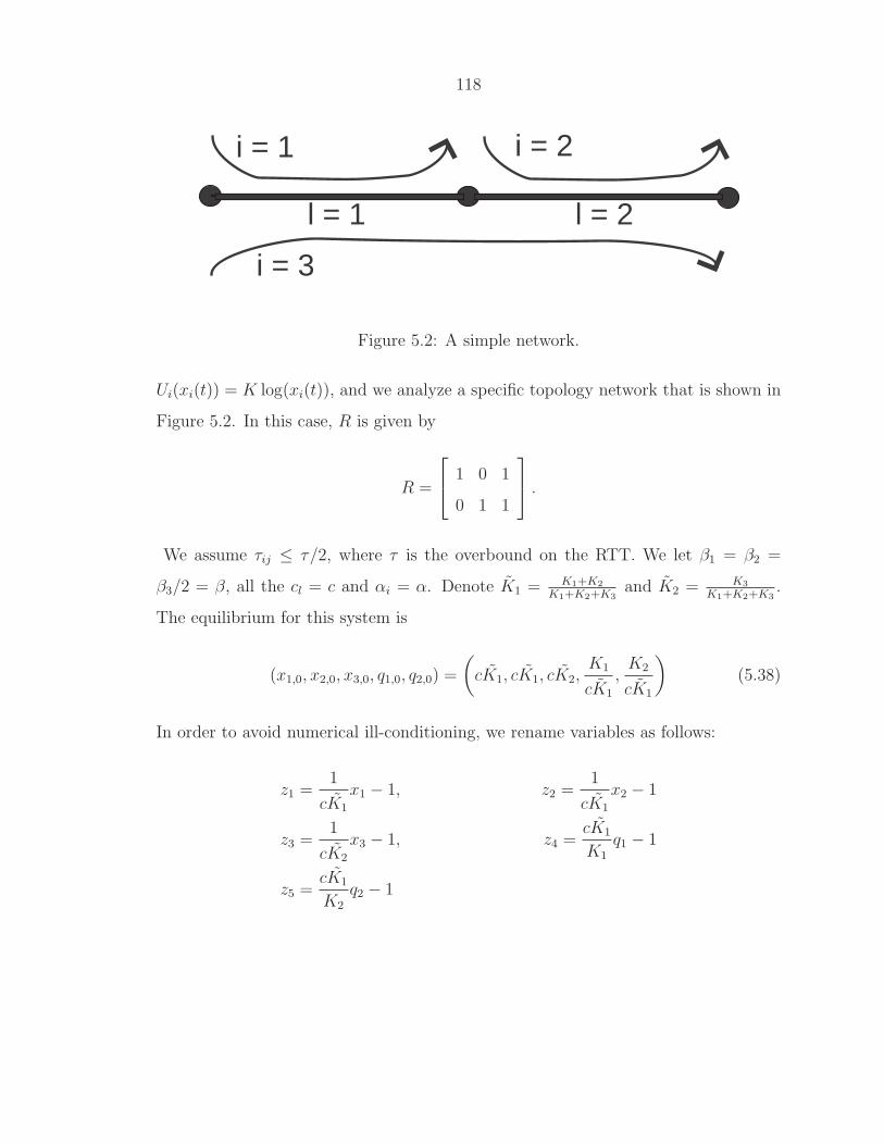
118
i = 1 i = 2
i = 3
l = 1 l = 2
Figure 5.2: A simple network.
Ui(xi(t)) = K log(xi(t)), and we analyze a specific topology network that is shown in
Figure 5.2. In this case, R is given by
R =
1 0 1
0 1 1
.
We assume τij ≤ τ/2, where τ is the overbound on the RTT. We let β1 = β2 =
β3/2 = β, all the cl = c and αi = α. Denote K1 = K1+K2
K1+K2+K3and K2 = K3
K1+K2+K3.
The equilibrium for this system is
(x1,0, x2,0, x3,0, q1,0, q2,0) =
(
cK1, cK1, cK2,K1
cK1
,K2
cK1
)
(5.38)
In order to avoid numerical ill-conditioning, we rename variables as follows:
z1 =1
cK1
x1 − 1, z2 =1
cK1
x2 − 1
z3 =1
cK2
x3 − 1, z4 =cK1
K1
q1 − 1
z5 =cK1
K2
q2 − 1

119
This change of variables gives the equations:
z1(t) = −K1β1
K1cτ[z1(t) + z4(t) + z1(t)z4(t)] −
α
τ[z1(t) + 1][K2z3(t− τ) + K1z1(t− τ)]
z2(t) = −K2β2
K1cτ[z2(t) + z5(t) + z2(t)z5(t)] −
α
τ[z2(t) + 1][K2z3(t− τ) + K1z2(t− τ)]
z3(t) = − β3
K1cτ[(z3z4 + z3 + z4)K1 + (z3z5 + z3 + z5)K2]
− α
2τ[z3(t) + 1][z1(t− τ)K1 + z2(t− τ)K1 + 2z3(t− τ)K2]
z4(t) =K1c
K1
(K1z1(t− τ) + K2z3(t− τ))
z5(t) =K1c
K2
((K1 +K2)z2(t− τ) +K3z3(t− τ))
We use c = 40, α = 1, τ = 0.2, and we calculate β = 0.64ατMi
and we let K1 = 15,
K2 = 20, K3 = 25. Using the technique developed in Chapter 4 based on the sum of
squares decomposition, we can construct a Lyapunov functional of the form
V1(zt) = a0(z1(t), z2(t), z3(t), z4(t))
+
∫ 0
−τ
a1(z1(t), z1(t+ θ), z2(t), z2(t+ θ), z3(t), z3(t+ θ), z4(t), z5(t))dθ
+
∫ 0
−τ
∫ t
t+θ
a2(z1(ζ), z2(ζ), z3(ζ))dζdθ,
with polynomials a0, a1 of second order and a2 of order four for
0 < x1t≤ 2.3x1,0, 0 < x2t
≤ 2.3x2,0,
0 < x3t≤ 2.3x3,0, q1 > 0, q2 > 0.
This proves that the network shown in Figure 5.2 with the aforementioned congestion
control algorithm is stable for τ = 0.2.

120
5.6 Conclusion
In this chapter, we have presented a methodology to construct Lyapunov certificates
for different congestion control algorithms to verify their stability properties for ar-
bitrary network topologies. The nonlinear conditions are delay dependent and of the
same form as the ones for the linearized system.
The structure of the system has helped greatly in obtaining simple scalable stabil-
ity conditions. More complicated functional structures can be less conservative, at the
expense of being more complicated; this has been observed when constructing these
functionals algorithmically using LMIs in the linear case, but also in the nonlinear
case using SOSTOOLS for simple network topologies.

121
Chapter 6
Systems Described by PartialDifferential Equations
T pnta reØ kaÈ oudèn mènei<Hrkleito Everything flows, nothing abides
Heracletus
In the previous two chapters, we were primarily concerned with the stability analy-
sis of small-scale and large-scale infinite dimensional systems described by Functional
Differential Equations. A natural question to ask is whether the proposed algorith-
mic methodology, which is based on the sum of squares decomposition, can be used
for the algorithmic analysis of systems described by Partial Differential Equations
(PDEs). Such system descriptions come about naturally in e.g. fluid dynamics and
heat transfer, areas in which the spatial dimension of the problem cannot be ignored.
We begin this chapter with a brief presentation of some background material on
the stability analysis of systems described by PDEs. We then consider a problem of
particular interest from fluid mechanics, that of stability of shear flows. In particular,
we prove that the Navier-Stokes equations in cylindrical coordinates subject to axi-
ally constant initial conditions and perturbations are globally stable for all Reynolds
numbers R. We note, however, that the transient energy growth of the system scales
as R3. Therefore even though streamlined flows can be made stable for arbitrary
Reynolds numbers, the system becomes susceptible to the effect of disturbances and

122
uncertainties.
We then describe briefly how the analysis of parabolic PDE systems can be per-
formed algorithmically using the sum of squares decomposition of multivariate poly-
nomials.
6.1 Introduction
The analysis of systems described by Partial Differential Equations has been con-
sidered to be a very difficult task, not only because of their infinite dimensional
nature [71, 30, 2], but also because of the complicated and sometimes mystifying
underlying theory. A comprehensive discussion on the methods for analysis of linear
PDEs can be found in [15]. There are also some results, mostly on a case-by-case
basis, on nonlinear PDE systems.
In this section we will present background material on the stability properties
of distributed parameter systems, and in the later sections we will investigate the
stability of systems arising in fluid mechanics and heat transfer.
First, we define the notion of a dynamical system (nonlinear semigroup) on a
complete metric space C with metric ‘dist’, as the family of maps S(t) : C → C, t ≥0 such that:
• For each t ≥ 0, S(t) is continuous from C to C,
• For each x ∈ C, t→ S(t)x is continuous,
• S(0) = I on C,
• S(t)(S(τ)x) = S(t+ τ)x for all x ∈ C and τ, t ≥ 0.
Such a semigroup defines a dynamical system on C. For any x ∈ C, let γ(x) =
S(t)x, t ≥ 0 denote the orbit (or positive semi-orbit) through x. We say x is an
equilibrium point if γ(x) = x. γ(x) is a periodic orbit if there exists a p > 0
such that γ(x) = S(t)x, 0 ≤ t ≤ p 6= x. An orbit γ(x) (or sometimes, the
point x) is stable if for any ǫ > 0 there exists δ(ǫ) > 0 such that for all t ≥ 0,

123
dist(S(t)x, S(t)y) < ǫ whenever dist(x, y) ≤ δ(ǫ), y ∈ C. An orbit γ(x) is unstable
if it is not stable. An orbit γ(x) is uniformly asymptotically stable if it is stable and
also there is a neighbourhood B = y ∈ C : dist(x, y) < r such that
dist(S(t)y, S(t)x) → 0 as t→ ∞
uniformly for y ∈ B.
Similarly to the case of ODEs and FDEs, a Lyapunov function can be used to
verify stability:
Definition 6.1 Let S(t), t ≥ 0 be a dynamical system on C. A Lyapunov function
is a continuous real-valued function V on C such that
V (x) , limt→0+
1
tV (S(t)x) − V (x) ≤ 0
for all x ∈ C, not excluding the possibility V (x) = −∞. Henceforth we use the
notation ‖x− y‖ = distx, y, as we will be use the induced topology of some Banach
space.
Having defined what a Lyapunov function is, we now state Lyapunov’s theorem
for this type of systems:
Theorem 6.2 Let S(t), t ≥ 0 be a dynamical system on C, and let 0 be an equi-
librium point in C. Suppose V is a Lyapunov function which satisfies V (0) = 0,
V (x) ≥ c(‖x‖) for x ∈ C, ‖x‖ = distx, 0, where c(·) is a continuous strictly
increasing function, c(0) = 0 and c(r) > 0 for r > 0. Then 0 is stable. If in ad-
dition V (x) ≤ −c1(‖x‖) where c1(·) is also continuous, increasing and positive with
c1(0) = 0, then 0 is uniformly asymptotically stable.
Also, in the same way as for ODEs and FDEs, we can define invariant sets, ω-limit
sets and state a LaSalle-type theorem. Although there is a converse theorem, finding
a Lyapunov function in any particular case is usually a difficult task.
With these definitions in place, we now turn our attention to examples from fluid
mechanics and heat transfer. In the next section, we consider a Hagen-Poiseuille pipe

124
flow with axially constant perturbations and initial conditions, for which we show
that the laminar flow is globally stable independent of the Reynolds number. We
demonstrate nonetheless, that the transient energy amplification of the background
disturbances scales as R3. This means that for this model there are no bifurcations
to instability, however the large amplification of the background disturbances which
was also observed in the linearization is still present. Therefore streamlining the flow
has as a consequence an increase in fragility to disturbances and uncertainties.
6.2 Global Stability of Axially Constant Perturba-
tions in Hagen-Poiseuille Flow
Hydrodynamic stability is an old research area and came about when the famous
pipe experiments performed by Reynolds [79] and his observations on the transition
of viscous fluid flow from laminar to turbulent were later on investigated theoretically
by Orr [52] and Sommerfeld [88]. More than a century later, these observations still
pose one of the most intriguing problems in fluid mechanics: what is the mechanism
for transition? In his original paper, Reynolds made an important observation: there
is no single ‘critical’ value below which flow is laminar and above which it becomes
turbulent. In his own words:
...the critical velocity was very sensitive to disturbance in the water before
entering the tubes. This at once suggested the idea that the condition
might be one of instability for disturbances of a certain magnitude and
stability for smaller disturbances.
In fact, by making sure that the disturbances were minimized, Reynolds was able
to keep the flow laminar up to values of Reynolds number R approaching 13000.
Subsequently, even more refined experiments have pushed this figure to R > 105, and
all theoretical evidence [83] suggests that fully developed flow down the pipe is stable
to disturbances at any finite value of R, no matter how large. If no great care is taken
to minimize disturbances, transition typically occurs at R ∼ 2000.

125
The experimental observation comes to contradict the theoretical explanation for
Hagen-Poiseuille flow in a pipe, something that is not experienced for the Rayleigh-
Benard convection and Taylor-Couette flow. Classical stability and bifurcation theory
could not explain the same phenomenon in plane Couette flow either, i.e. flow between
two parallel plates: the solution of the Orr-Sommerfeld equation predicts stability for
all Reynolds numbers, which disagrees strongly with the experimental observation.
The disagreement between the experiment and linearized theory is usually attributed
to nonlinear effects, but recently a new explanation has been asserted.
In a series of papers [95, 1, 22] and in [84] it has been shown that for shear flows,
the operator of the linearized Navier-Stokes is non-normal. This means that even
for a stable flow, transient disturbances can achieve very large values before even-
tually decaying, suggesting a mechanism for transition at Reynolds numbers signifi-
cantly smaller than those predicted by the stability of the Orr-Sommerfeld equation.
The large background energy amplification is due to the non-normality of the Orr-
Sommerfeld operator, and the corresponding non-orthogonality of its eigenfunctions.
In the case of pipe flow, the mathematical analysis has revealed that the Hagen-
Poiseuille laminar flow profile is linearly stable with respect to disturbances for all
Reynolds numbers [83]. In particular, it has been demonstrated that maximum back-
ground energy amplification is obtained for axially-constant perturbations with an
azimuthal wave number of m = 1. The initial form of the perturbations is that of
streamwise rolls. After a short time, the streamwise velocity component becomes
dominant. The perturbations take the form of spanwise modulation of the basic flow
leading to the formation of streaks which were observed in other shear flows.
In this section, we concentrate on Hagen-Poiseuille flow in a pipe with axially
constant 3-D perturbations. The flow is driven by a constant pressure gradient. The
fact that the perturbations are axially constant restricts the model to 2-D with 3
velocity components, which we will call a 2D/3C model. This is in line with the
observations that the most energy amplifying disturbances are axially constant and
produce axial structures. We show that the laminar solution of the 2D/3C model
is globally stable for all Reynolds numbers R by exhibiting a Lyapunov function.

126
The transient energy growth scales as R3, which agrees with the result from the
linearization. A similar result has been obtained for Couette flow [8].
6.2.1 The Equations of Motion
We begin our investigation by reformulating the Navier-Stokes equations in cylindrical
coordinates into the 2D/3C system of interest. Denote the radial, azimuthal and axial
coordinates by (r, θ, z) and the corresponding velocity components of v by (vr, vθ, vz).
In these coordinates the convective time derivative is:
v · ∇ = vr∂
∂r+vθr
∂
∂θ+ vz
∂
∂z,
and the Laplacian operator is
∆ = ∇2 =1
r
∂
∂r
(
r∂
∂r
)
+1
r2
∂2
∂θ2+
∂2
∂z2.
The Navier-Stokes equations of motion in these coordinates become:
∂vr∂t
+ vr∂vr∂r
+vθr
∂vr∂θ
+ vz∂vr∂z
− v2θ
r= −∂p
∂r+
1
R
(
∆vr −vrr2
− 2
r2
∂vθ∂θ
)
∂vθ∂t
+ vr∂vθ∂r
+vθr
∂vθ∂θ
+ vz∂vθ∂z
+vθvrr
= −1
r
∂p
∂θ+
1
R
(
∆vθ +2
r2
∂vr∂θ
− vθr2
)
∂vz∂t
+ vr∂vz∂r
+vθr
∂vz∂θ
+ vz∂vz∂z
= −∂p∂z
+1
R∆vz
1
r
∂(rvr)
∂r+
1
r
∂vθ∂θ
+∂vz∂z
= 0,
along with boundary conditions for a pipe of radius r = 1 and infinite length:
uz(1, θ, z, t) = 0, uz(0, θ, z, t) =−dp/dzR
,
ur(1, θ, z, t) = 0, ur(0, θ, z, t) = 0,
uθ(1, θ, z, t) = 0, uθ(0, θ, z, t) = 0.
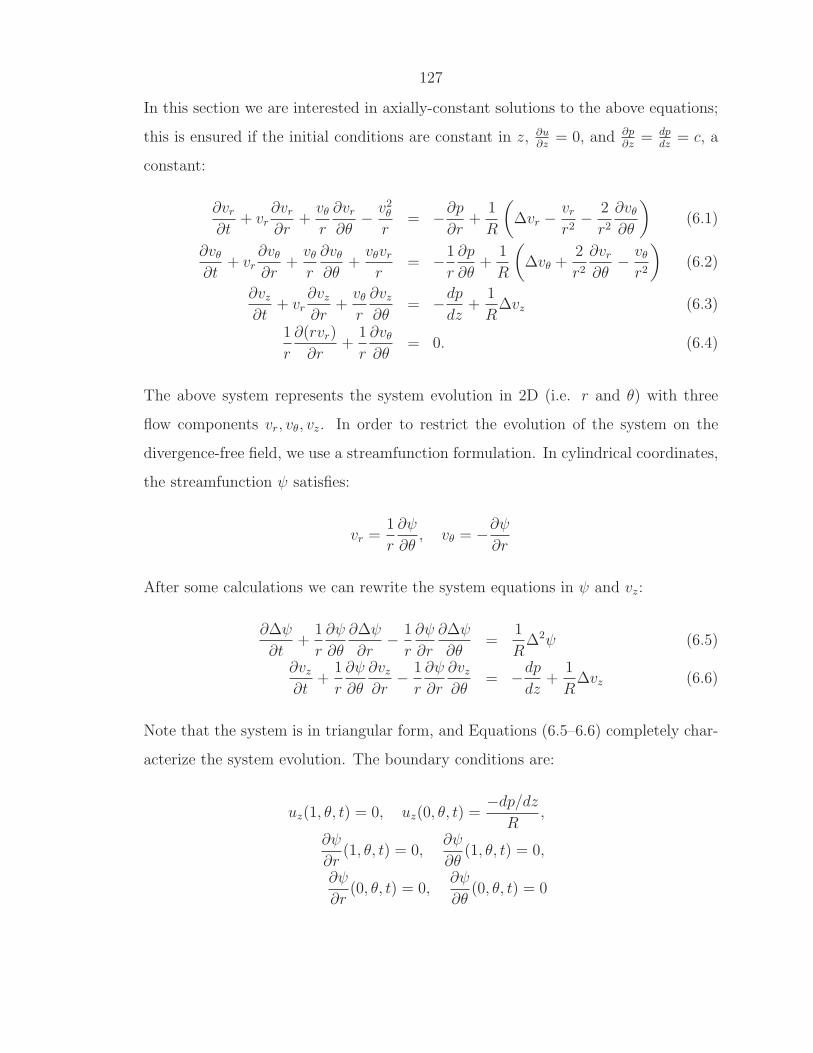
127
In this section we are interested in axially-constant solutions to the above equations;
this is ensured if the initial conditions are constant in z, ∂u∂z
= 0, and ∂p∂z
= dpdz
= c, a
constant:
∂vr∂t
+ vr∂vr∂r
+vθr
∂vr∂θ
− v2θ
r= −∂p
∂r+
1
R
(
∆vr −vrr2
− 2
r2
∂vθ∂θ
)
(6.1)
∂vθ∂t
+ vr∂vθ∂r
+vθr
∂vθ∂θ
+vθvrr
= −1
r
∂p
∂θ+
1
R
(
∆vθ +2
r2
∂vr∂θ
− vθr2
)
(6.2)
∂vz∂t
+ vr∂vz∂r
+vθr
∂vz∂θ
= −dpdz
+1
R∆vz (6.3)
1
r
∂(rvr)
∂r+
1
r
∂vθ∂θ
= 0. (6.4)
The above system represents the system evolution in 2D (i.e. r and θ) with three
flow components vr, vθ, vz. In order to restrict the evolution of the system on the
divergence-free field, we use a streamfunction formulation. In cylindrical coordinates,
the streamfunction ψ satisfies:
vr =1
r
∂ψ
∂θ, vθ = −∂ψ
∂r
After some calculations we can rewrite the system equations in ψ and vz:
∂∆ψ
∂t+
1
r
∂ψ
∂θ
∂∆ψ
∂r− 1
r
∂ψ
∂r
∂∆ψ
∂θ=
1
R∆2ψ (6.5)
∂vz∂t
+1
r
∂ψ
∂θ
∂vz∂r
− 1
r
∂ψ
∂r
∂vz∂θ
= −dpdz
+1
R∆vz (6.6)
Note that the system is in triangular form, and Equations (6.5–6.6) completely char-
acterize the system evolution. The boundary conditions are:
uz(1, θ, t) = 0, uz(0, θ, t) =−dp/dzR
,
∂ψ
∂r(1, θ, t) = 0,
∂ψ
∂θ(1, θ, t) = 0,
∂ψ
∂r(0, θ, t) = 0,
∂ψ
∂θ(0, θ, t) = 0

128
where dp/dz is the pressure drop driving the flow which is constant along the axial
direction, as otherwise vz would be a function of z. We further denote τ = t/R,
Ψ(τ) = Rψ(τR) and
V (τ) =Rvz(τR)
−dp/dz .
Multiplying (6.5) by R2 and (6.6) by R, and scaling time by 1R
we get:
∆Ψτ = −1
rΨθ∆Ψr +
1
rΨr(∆Ψ)θ + ∆2Ψ (6.7)
Vτ = −1
rΨθVr +
1
rΨrVθ + ∆V + 1 (6.8)
where from now on we denote Ψτ , ∂Ψ∂τ
, etc. The new boundary conditions are
V (1, θ, τR) = 0, V (0, θ, τR) = 1,
Ψr(1, θ, τR) = 0, Ψθ(1, θ, τR) = 0,
Ψr(0, θ, τR) = 0, Ψθ(0, θ, τR) = 0
Note that these equations are independent of R, and therefore the stability properties
of the system, which will be of interest later on, are independent of the Reynolds
number.
Before moving on, we present a solution to the above equations that corresponds
to vr = vθ = 0. We have, from the definition of the Ψ equations, that Ψ(r, θ) = c, a
constant. Therefore the stationary solution for V becomes:
∆V = −1. (6.9)
Of course V = V (r, θ) and is not a function of z, a result following from the continuity
equation. For the fully developed flow, we have, from the momentum equations:
0 = −dpdr
= −dpdθ
0 = −dpdz
+1
R
(1
r
∂
∂r
(
r∂V
∂r
)
+1
r2
∂2V
∂θ2
)

129
Since V does not vary with z, it follows that dpdz
must be constant, as mentioned
earlier. Taking symmetry into consideration, we have also that ∂V∂θ
= 0. Solving
the resulting elliptic equation and applying the boundary condition we get as the
steady-state solution:
V =1
4(1 − r2)
Therefore the steady state of the fully developed laminar flow is a paraboloid.
6.2.2 Global Stability Analysis
The energy of the 2-D system describing the Ψ evolution is:
EΨ =1
2π
∫ 1
0
∫ π
−π
(v2r + v2
θ
)rdrdθ =
1
2π
∫ 1
0
∫ π
−π
(1
r2Ψ2θ + Ψ2
r
)
rdrdθ
= −1
2〈Ψ,∆Ψ〉,
where ∆ is the Laplacian operator in cylindrical coordinates and the inner product
is given by:
〈f, g〉 , π
∫ 1
0
∫ π
−π
f(r, θ)g(r, θ)rdrdθ (6.10)
Now taking the derivative with respect to τ we have:
dEΨ
dτ= −1
2
d
dτ〈Ψ,∆Ψ〉 = −1
2〈Ψτ ,∆Ψ〉 − 1
2〈Ψ,∆Ψτ 〉 = −〈Ψ,∆Ψτ 〉
= −⟨
Ψ,−1
rΨθ(∆Ψ)r +
1
rΨr(∆Ψ)θ
⟩
−⟨Ψ,∆2Ψ
⟩
= −⟨Ψ,∆2Ψ
⟩= −〈∆Ψ,∆Ψ〉 < 0
where the last equality follows from a careful integration by parts. The term <
Ψ,−1rΨθ(∆Ψ)r + 1
rΨr(∆Ψ)θ > is identically zero:
⟨
Ψ,1
rΨθ(∆Ψ)r −
1
rΨr(∆Ψ)θ
⟩
= π
∫ 1
0
∫ π
−π
Ψ (Ψθ(∆Ψ)r − Ψr(∆Ψ)θ) drdθ
= π
∫ 1
0
∫ π
−π
(d
dr(ΨΨθ∆Ψ) − d
dθ(ΨΨr∆Ψ)
)
drdθ
= 0

130
which follows by integration by parts and considering the boundary conditions for Ψ.
This asserts that V is a Lyapunov function, and so global L2 stability of the Ψ = 0
solution is proven.
To investigate the stability of the overall system, consider (6.8) with the steady-
state V removed. Abusing notation, we denote this by V :
Vτ = −1
rΨθVr +
1
rΨrVθ + ∆V − 1
rV rΨθ
with zero boundary conditions. Consider now the kinetic energy:
EV =1
2π
∫ 1
0
∫ π
−π
V 2rdrdθ =1
2〈V, V 〉 =
1
2‖V ‖2
with the same inner product as before. The rate of change of EV with time is:
dEVdτ
= 〈Vτ , V 〉 =
⟨
−1
rΨθVr +
1
rΨrVθ, V
⟩
+
⟨
∆V − 1
rV rΨθ, V
⟩
=
⟨
∆V − 1
rV rΨθ, V
⟩
≤ λ(∆)‖V ‖2 +
∥∥∥∥
1
rV rΨθ
∥∥∥∥‖V ‖ =
(
λ(∆)‖V ‖ +
∥∥∥∥
1
rV rΨθ
∥∥∥∥
)
‖V ‖
≤(
λ(∆)‖V ‖ +
∥∥∥∥
1
rV r
∥∥∥∥∞
‖Ψθ‖)
‖V ‖
where λ(∆) is the maximum eigenvalue of ∆, which is a negative definite operator,
i.e. λ(∆) < 0. Here we have used that⟨−1rΨθVr + 1
rΨrVθ
⟩is zero identically:
⟨
−1
rΨθVr +
1
rΨrVθ
⟩
= π
∫ 1
0
∫ π
−π
V
(
−1
r
∂Ψ
∂θ
∂V
∂r+
1
r
∂Ψ
∂r
∂V
∂θ
)
rdrdθ
= π
∫ 1
0
∫ π
−π
(
−V ∂Ψ
∂θ
∂V
∂r+ V
∂Ψ
∂r
∂V
∂θ
)
drdθ
= π
∫ 1
0
∫ π
−π
(
− d
dθ(V VrΨ) +
d
dr(V VθΨ)
)
drdθ
= 0
This follows by integration by parts and considering the boundary conditions for Ψ

131
and V . Therefore whenever ‖V ‖ is such that:
‖V ‖ ≥ −∥∥1rV r
∥∥∞‖Ψθ‖
λ(∆)= k‖Ψθ‖
where k is a constant, then EV is non-increasing. We see that dEV
dτdoes not decrease
monotonically to zero, but it may increase before eventually decreasing. However
‖Ψθ‖ → 0 as time evolves as shown earlier, and therefore ‖V ‖ → 0 eventually. In
order to make this argument more concrete, we now show using a Lyapunov argument
that a modified energy-based function can be used as a Lyapunov function for the
whole system. For this purpose, consider the following functional:
Wα(Ψ, V ) = α2EΨ + EV
Then from our earlier calculations we have:
d
dτWα = −α2
⟨∆2Ψ,Ψ
⟩+ 〈∆V, V 〉 −
⟨1
rV rΨθ, V
⟩
≤ α2λ(∆)(‖Ψθ‖2 + ‖Ψr‖2) + λ(∆)‖V ‖2 +
∥∥∥∥
1
rV r
∥∥∥∥∞
‖Ψθ‖‖V ‖
Now −∆ is a strictly coercive operator, and therefore λ(∆) = −β2 < 0. We now
write
d
dτWα ≤ −α2β2‖Ψr‖2 − β2 (α‖Ψθ‖ − ‖V ‖)2 − 2β2α‖Ψθ‖‖V ‖ +
∥∥∥∥
1
rV r
∥∥∥∥∞
‖Ψθ‖‖V ‖
Which is guaranteed to be negative definite if 2β2α−∥∥1rV r
∥∥∞> 0, i.e.
α > −∥∥1rV r
∥∥∞
2λ(∆).
This guarantees that Wα is a Lyapunov function and the equilibrium of the system,
i.e. the laminar flow profile V is globally asymptotically stable.

132
6.2.3 Energy Scaling
Consider now the total transient energy growth E :
E , Eψ + Ev =
∫ ∞
0
Eψ + Evdt
where v = vz − v, and v denotes the laminar flow profile. From the nondimension-
alization we see that Eψ(0) = 1R2EΨ(0), and
∫∞
0Eψ(t)dt = 1
R
∫∞
0EΨ(τ)dτ . Similarly,
EV (0) = Ev(0), and∫∞
0Ev(t)dt = R
∫∞
0EV (τ)dτ .
Consider the case in which V (0) = 0. The ratio of output to input energy is:
g(Ψ) ,
∫∞
0EV (τ)dτ
∫∞
0EΨ(τ)dτ
This has a finite upper bound as the numerator is bounded, for Ψ 6= 0. Because of the
triangular structure of the equations of motion, g(Ψ) is only a function of the initial
condition in Ψ, i.e. Ψ(0). It also satisfies g(Ψ(0)) = g(ψ(0)). Therefore we have:
Ev = R
∫ ∞
0
EV (τ)dτ = Rg(Ψ(0))
∫ ∞
0
EΨ(τ)dτ = Rg(ψ(0))
∫ ∞
0
EΨ(τ)dτ
Moreover we have:
EψEψ(0)
=1R
∫∞
0EΨ(τ)dτ
1R2EΨ(0)
= R
∫∞
0EΨ(τ)dτ
EΨ(0)
Similarly:
EvEψ(0)
=Rg(Ψ(0))
∫∞
0Eψ(τ)dτ
1R2EΨ(0)
= R3g(ψ(0))
∫∞
0EΨ(τ)dτ
EΨ(0)
Therefore in total:
EEψ(0)
=(R +R3g(ψ(0))
)∫∞
0EΨ(τ)dτ
EΨ(0)
This shows that the total energy growth scales with R3, as the last fraction is inde-

133
pendent of R.
We summarize our findings in the following theorem:
Theorem 6.3 Consider the 2D/3C model (6.5–6.6). Then the following are true:
1. The Hagen-Poiseuille flow V = 14(1− r2) is globally asymptotically stable for all
Reynolds numbers R.
2. For initial conditions (v(0) = 0, ψ(0) 6= 0) the total transient energy growth is
given by:E
Eψ(0)= k
(R +R3g(ψ(0))
)(6.11)
for some k independent of R.
The above analysis means that streamlining can evade bifurcations to instability,
and produce a flow that is stable irrespective of the Reynolds number. At the same
time, nonetheless, the amplification of disturbances and background noise scales like
R3, i.e. the robustness properties of the system deteriorate significantly. This ‘robust
yet fragile’ principle is observed in many other systems in engineering and biology.
6.3 An Algorithmic Analysis Methodology for PDE
systems
In this section we will consider the algorithmic construction of Lyapunov functions
for systems described by PDEs. The methodology we use is based on the sum of
squares decomposition, just as in the case of ODEs and FDEs.
The procedure we consider is as follows. First, we propose a Lyapunov functional
structure V , and we impose positive definiteness by ensuring non-negativity of its
kernel, just as in the case of FDEs. The system dynamics come into play when V
is considered. The boundary conditions appear naturally when the resulting expres-
sion is integrated by parts, which, as seen in the previous section, helps greatly in
‘completing’ the squares and simplifying terms.

134
The above methodology is illustrated through an example. Consider the system
ut = uxx + λu3 + αu (6.12)
u(±1, t) = 0
with λ ≤ 0. This is the heat equation with forcing. From the linearization of this
system about the zero steady state, stability is guaranteed for α < π2/4.
Here we are interested in constructing a Lyapunov function of the form
V (u) =
∫ 1
−1
a(u(η, t), η)dη (6.13)
where a is a polynomial in its arguments, at least quadratic in u. We would expect
that as the order of a with respect to η and u is increased, better bounds on α can
be obtained, and this is the case, as we will see in the sequel.
Consider now dV (u)dt
:
dV (u)
dt=
∫ 1
−1
∂a
∂uut(η, t)dη =
∫ 1
−1
∂a
∂u
(uηη + λu3 + αu
)dη (6.14)
We mentioned earlier that integration by parts of the derivative condition is important
in ensuring its non-negativity, as in this way the boundary conditions are taken into
consideration. For example, in our case, the following expression is true:
∫ 1
−1
∂a
∂uuηη + u2
η
∂2a
∂u2− u
[∂3a
∂u2∂ηuη +
∂3a
∂uη∂η2
]
dη = 0
This is a result of integration by parts of the term∫ 1
−1∂a∂uuηηdη, where we have used
the fact that u ∂2a∂u∂η
∣∣∣
1
−1= 0 and uη
∂a∂u
∣∣1
−1= 0 since a is a polynomial at least quadratic
in u. Therefore the first term in (6.14) will be replaced by the rest of the terms in
the above expression, as in itself, it cannot contribute to the negative definiteness of
(6.14).

135
Notice that the following is also true:
∫ 1
−1
ηnu2dη = −∫ 1
−1
nηnu2dη − 2
∫ 1
−1
ηn+1uuηdη
i.e.,
∫ 1
−1
[(1 + n)ηnu2 + 2ηn+1uuη
]dη = 0
We then have the following proposition:
Proposition 6.4 Let there be polynomials a(u, η) and a positive definite function ϕ
such that the following hold:
1. a(u, η) − ϕ(u) ≥ 0 when η ∈ [−1, 1],
2. λ ∂a∂uu3 + α ∂a
∂uu − u2
η∂2a∂u2 + u
[∂3a∂u2∂η
uη + ∂3a∂uη∂η2
]
≤ 0 when η ∈ [−1, 1] and (1 +
n)ηnu2 + 2ηn+1uuη = 0 is satisfied.
Then the steady-state of system (6.12) is stable.
The two conditions guarantee the existence of a Lyapunov functional, given by (6.13),
that is positive definite and whose derivative is negative definite, guaranteeing stabil-
ity in L2. The criteria (1) and (2) in the proposition can be tested by adjoining the
conditions η ∈ [−1, 1] and the equality constraint in (2) using a technique similar to
the S-procedure, as it was done earlier in this thesis.
Recall that the stability condition from the linearization is α < π2/4. We introduce
a parameter measuring conservativeness, ρ as follows:
ρ(degree of a wrt η) = 1 −(
4α
π2for which a V can be constructed
)
(6.15)
Then for the functional shown in Equation (6.13), ρ varies as shown in Table 6.1.
We see that as the order of the polynomial a(u, η) is increased with respect to η, the
conservativeness is reduced, and the construction is entirely algorithmic.

136
Order of a wrt η 0 2 4 6 8 10 12 14 16ρ 1 0.5 0.32 0.20 0.15 0.11 0.08 0.07 0.06
Table 6.1: Stability analysis of a parabolic PDE system.
The above example shows how stability can be tested for systems described by
parabolic PDEs. The boundary conditions come into play through integration by
parts, a procedure that can be automated algorithmically. A problem that we face
is that many times, certain structures are better than others, and we need to choose
these judiciously, which is also the case for nonlinear FDEs.
6.4 Conclusion
In this chapter, we considered the problem of investigating the stability properties
of systems described by Partial Differential Equations. We have introduced some
stability notions, as well as a Lyapunov theorem for testing the stability properties
of a system.
We then showed how the axially constant solutions of the Navier Stokes equations
in cylindrical shear flow are globally stable, while they still retain an R3 growth on
the background noise, giving a ‘robust, yet fragile’ interpretation to the transition
from laminar to turbulent pipe flow.
We also demonstrated how the construction of Lyapunov functionals for PDEs
can be done algorithmically, using the sum of squares of multivariate polynomials
and semidefinite programming.

137
Chapter 7
Conclusions>Edìkei d meØzìn ti eÒnai tÀ Xenof¸nti...KaÈ tqa d koÔousi bo¸ntwn tÀnstratiwtÀn Jlatta jlatta kaÈ pareggu°ntwn...>EpeÈ dà fkonto pnte âpÈ tä kron,ântaÜja d perièballon ll lou dakrÔnonte .Xenof¸nto , Kjodo twn murwnIt seemed to Xenophon that there was something very important... Soon they heardthe soldiers shouting: The Sea! The Sea! and passing it along... And when they
came to the peak, then they embraced one another, weeping.Xenophon, Exodus
In this thesis, we have shown how the sum of squares technique can be used
to analyze nonlinear systems algorithmically, for system descriptions ranging from
simple Ordinary Differential Equations to simple Functional and Partial Differential
Equations. Then, we investigated the scalable analysis of large-scale interconnections
of subsystems described by Ordinary and Functional Differential Equations in relation
to congestion control for the Internet.
Before closing, we will give a summary of the main results presented and discuss
briefly future research directions.
7.1 Summary
In this thesis, we have seen the following results:
• In Chapter 3, we investigated how the algorithmic analysis of nonlinear systems

138
described by Ordinary Differential Equations can be performed using sum of
squares techniques. We considered a general class of systems evolving over in-
equality, equality and integral constraints. As particular cases, we have shown
how the region of attraction of an equilibrium can be estimated, how robust
stability analysis can be performed and how non-polynomial systems can be
treated. Moreover, we have shown how to analyze stability of switching sys-
tems and have presented how performance analysis of nonlinear systems can be
performed. Illustrative examples from biology and aerospace were used to show
the effectiveness of the methodology.
• In Chapter 4, we moved to another class of differential equations, that of Func-
tional Differential Equations. In this case, even the algorithmic analysis of
linear system descriptions poses a challenge, and we have shown how the sum
of squares technique can be used to construct algorithmically the relevant Lya-
punov functionals. We then considered the stability and robust stability of
nonlinear time delay systems, which can be performed in a unified way. Finally,
an illustrative example from ecology was considered.
• In Chapter 5, we considered network congestion control for the Internet, which is
a large-scale interconnection of subsystems described by Functional Differential
Equations to form a network. We produced a Lyapunov argument for the
analysis of the linearization, as well as the full global stability for arbitrary
topologies, delays and link capacities for FAST, a network congestion control
scheme. A more general class of TCP/AQM schemes was also considered. The
structure of the system and the judicious choice of dynamics have guided the
choice of the Lyapunov certificate.
• In Chapter 6, we considered the stability analysis of systems described by Par-
tial Differential Equations. We have introduced some stability notions, as well
as a Lyapunov theorem for testing the stability properties of such systems.
We then showed how the axially constant solutions of the Navier-Stokes equa-
tions in cylindrical shear flow are globally stable, while they still retain an R3

139
growth on the background noise. This shows how streamlined flows can be made
nonlinearly stable for arbitrary Reynolds numbers, at the expense of fragility
to disturbances. The chapter concluded with an algorithmic methodology for
constructing Lyapunov functionals for PDEs using the sum of squares decom-
position.
7.2 Future Research Directions
We would now like to mention a few pointers for future research. The work done so
far has swept horizontally various system descriptions and has presented algorithmic
solutions to analysis type questions. It would be interesting to investigate techniques
for algorithmic synthesis of control laws with or without guaranteed cost. The prob-
lem of synthesis is, in general, more complex than the problem of systems analysis.
In this case, both Lyapunov [76] and density function formulations [77] have been
considered, but alternative methodologies should be sought.
In the area of systems described by Ordinary Differential Equations, important
remains the concept of stiffness in ODEs and how this can be alleviated when seeking
algorithmic constructions using sum of squares. Singular perturbation methods can
provide some insight on how the Lyapunov function can be structured so that the
resulting semidefinite programming conditions are numerically well-conditioned [35].
In the area of infinite dimensional systems, and in particular systems described
by Partial Differential Equations, certain problems from fluid mechanics should be
investigated. In particular, for high shear flows [84], still unexplained is the effect of
drag reduction due to additives [43]. It is remarkable that a small amount of polymer
additives can have a significant effect on the drag reduction [4, 5]. This effect is
not entirely due to the change in the viscocity of the polymer/solvent solution – the
viscoelastic properties of the continuum are believed to play an important role.
We have seen in the previous chapter how the sum of squares technique opens new
possibilities for the analysis of systems described by PDEs, and we expect that these
methodologies will have a broader application to systems of infinite dimension in the
140
future. The tools that are currently used for analysis of PDE systems mostly center
on discretization, which can never answer questions about the system exactly, and
sometimes is computationally expensive. At least conceptually, the PDE description
of a system is simpler and richer at the same time. The sum of squares technique is
a methodology that opens new, unexplored possibilities and a unique perspective for
future research in Partial Differential Equations.
Beyond stability analysis of steady-states for parabolic PDEs, other analysis ques-
tions can be answered, such as obtaining functional output estimates for PDEs. This
information is important for determining acceptable mesh sizes in computational
methods [70]. These and other areas are particularly important, such as obtaining
bounds on functional outputs of the Fokker-Planck equation for stochastic systems
analysis.
It is appreciated that large scale networks and distributed parameter systems
provide the same modeling framework for systems with arbitrarily sized topologies.
A way to see this intuitively is as follows. Most analysis procedures for parabolic
PDE systems are related to discretization. This results in large-scale systems, each
node in the mesh having certain dynamics depending on its neighbors and the dis-
cretization scheme. We are definitely more comfortable working with the large-scale
system resulting from discretization — at least computers are, since they can simu-
late finite dimensional descriptions. But most of our questions cannot be answered
by discretization alone, and in any case the PDE system description is simpler, at
least conceptually. It is perhaps time that we put more effort in understanding the
properties of PDE systems directly, producing reliable analysis algorithms that do
not use discretization, so that invaluable information about infinitely large systems
can be obtained at a low computational cost.

141
Bibliography
[1] B. Bamieh and M. Dahleh. Energy amplification in channel flows with stochastic
excitation. Physics of Fluids, 13(11):3258–3269, 2001.
[2] S. P. Banks. State-space and frequency-domain methods in the control of dis-
tributed parameter systems. Peter Peregrinus Ltd., London, UK, 1983.
[3] B. W. Bequette. Process Dynamics. Modeling, Analysis and Simulation.
Prentice-Hall, 1998.
[4] R. B. Bird, R. C. Armstrong, and O. Hassager. Dynamics of Polymeric Liquids,
Vol 1. John Wiley & Sons Inc., second edition, 1987.
[5] R. B. Bird, C. F. Curtiss, R. C. Armstrong, and O. Hassager. Dynamics of
Polymeric Liquids, Vol 2. John Wiley & Sons Inc., second edition, 1987.
[6] P.-A. Bliman. Lyapunov equation for the stability of linear delay systems of re-
tarded and neutral type. IEEE Transactions on Automatic Control, 47(2):327–
335, 2002.
[7] P.-A. Bliman. Stability of non-linear delay systems: delay-independent small
gain theorem and frequency domain interpretation of the Lyapunov-Krasovskii
method. International Journal of Control, 75(4):265–274, 2002.
[8] K. M. Bobba, B. Bamieh, and J. C. Doyle. Highly optimized transitions to tur-
bulence. In Proceedings of the 41st IEEE Conference on Decision and Control,
2002.

142
[9] J. Bochnak, M. Coste, and M.-F. Roy. Real Algebraic Geometry. Springer-
Verlag, Berlin, 1998.
[10] S. Boyd, L. El Ghaoui, E. Feron, and V. Balakrishnan. Linear Matrix In-
equalities in System and Control Theory. Society for Industrial and Applied
Mathematics (SIAM), 1994.
[11] R. P. Braatz, P. M. Young, J. C. Doyle, and M. Morari. Computational complex-
ity of µ calculation. IEEE Transactions on Automatic Control, 39(5):1000–1002,
1994.
[12] M. S. Branicky. Multiple Lyapunov functions and other analysis tools for
switched and hybrid systems. IEEE Transactions on Automatic Control,
43(4):475–482, 1998.
[13] J. D. Bugajski and F. D. Enns. Nonlinear control law with application to high
angle of attack flight. Journal of Guidance, Control and Dynamics, 15(3):761–
767, 1992.
[14] M. D. Choi, T. Y. Lam, and B. Reznick. Sum of squares of real polynomials.
Proceedings of Symposia in Pure Mathematics, 58(2):103–126, 1995.
[15] R. F. Curtain and H. J. Zwart. An Introduction to Infinite-Dimensional Linear
Systems Theory. Springer-Verlag, Berlin, 1981.
[16] L. Dai. Singular Control Systems. Springer-Verlag, New York, 1989.
[17] S. Deb and R. Srikant. Global stability of congestion controllers for the Internet.
IEEE Transactions on Automatic Control, 48(6):1055–1060, 2003.
[18] R. A. DeCarlo, M. S. Branicky, S. Pettersson, and B. Lennartson. Perspectives
and results on the stability and stabilizability of hybrid systems. Proceedings
of the IEEE, 88(7):1069–1082, 2000.
[19] C. A. Desoer and M. Vidyasagar. Feedback Systems: Input-Output Properties.
Academic Press, New York, 1975.

143
[20] H. El-Samad, S. Prajna, A. Papachristodoulou, M. Khammash, and J. Doyle.
Model invalidation and robustness analysis of the bacterial heat shock response
using SOSTOOLS. In Proceedings of the 42nd IEEE Conference on Decision
and Control, 2003.
[21] D. Enns, D. Bugajski, R. Hendrick, and G. Stein. Dynamic inversion: an
evolving methodology for flight control design. International Journal of Control,
59(1):71–91, 1992.
[22] B. F. Farrell and P. J. Ioannou. Stochastic forcing of the linearized Navier-
Stokes equations. Physics of Fluids A, 5(11):2600–2609, 1993.
[23] E. Feron, P. Apkarian, and P. Gahinet. Analysis and synthesis of robust control
systems via parameter-dependent Lyapunov functions. IEEE Transactions on
Automatic Control, 41(7):1041–1046, 1996.
[24] K. Gatermann and P. A. Parrilo. Symmetry groups, semidefinite programs, and
sums of squares. Journal of Pure and Appl. Algebra, 192(1–3):95–128, 2004.
[25] M. X. Goemans and D. P. Williamson. Improved approximation algorithms
for maximum cut and satisfiability problems using semidefinite programming.
Journal of Association for Computing Machinery, 42(6):1115–1145, 1995.
[26] K. Gu, V. L. Kharitonov, and J. Chen. Stability of Time-Delay Systems.
Birkhauser, 2003.
[27] W. Hahn. Stability of Motion. Springer-Verlag, New York, 1967.
[28] J. K. Hale and S. M. V. Lunel. Introduction to Functional Differential Equations.
Applied Mathematical Sciences (99). Springer-Verlag, 1993.
[29] A. Hassibi and S. P. Boyd. Quadratic stabilization and control of piecewise-
linear systems. In Proceedings of the American Control Conference, 1998.
[30] D. Henry. Geometric Theory of semilinear parabolic equations. Springer-Verlag,
Berlin, 1981.

144
[31] V. Jacobson. Congestion avoidance and control. Proceedings
of ACM SIGCOMM, 1988. An updated version is available at
ftp://ftp.ee.lbl.gov/papers/congavoid.ps.Z.
[32] M. Johansson and A. Rantzer. Computation of piecewise quadratic Lya-
punov functions for hybrid systems. IEEE Transactions on Automatic Control,
43(4):555–559, 1998.
[33] R. Johari and D. Tan. End-to-end congestion control for the Internet: Delays
and stability. IEEE/ACM Transactions on Networking, 9(6):818–832, 2001.
[34] F. Kelly, A. Maulloo, and D. Tan. Rate control in communication networks:
shadow prices, proportional fairness and stability. Journal of the Operational
Research Society, 49:237–252, 1998.
[35] H. K. Khalil. Nonlinear Systems. Prentice Hall, Inc., second edition, 1996.
[36] V. Kolmanovskii and A. Myshkis. Introduction to the Theory and Applications
of Functional Differential Equations. Kluwer Academic Publishers, 1999.
[37] V. B. Kolmanovskii, S.-I. Niculescu, and J.-P. Richard. On the Lyapunov-
Krasovskii functionals for stability analysis of linear delay systems. Interna-
tional Journal of Control, 72(4):374–384, 1999.
[38] Y. Kuang. Delay Differential Equations with Applications in Population Dy-
namics. Academic Press, 1993. Mathematics in Science and Engineering (191).
[39] J. B. Lasserre. Global optimization with polynomials and the problem of mo-
ments. SIAM J. Optim., 11(3):796–817, 2001.
[40] M. Laurent and S. Poljak. On a positive semidefinite relaxation of the cut
polytope. Linear Algebra and Its Applications, 223/224:439–461, 1995.
[41] S. H. Low and D. E. Lapsley. Optimization flow control, I: basic algorithm and
convergence. IEEE/ACM Transactions on Networking, 1999.
145
[42] D. G. Luenberger. Introduction to Dynamic Systems: Theory, Models and
Applications. Wiley, 1979.
[43] J. L. Lumley. Drag reduction by additives. Ann. Rev. Fluid Mech., 1:367–384,
1969.
[44] M. Mathis, J. Semske, J. Mahdavi, and T. Ott. The macroscopic behavior of
the TCP congestion avoidance algorithm. Computer Communication Review,
27(3):67–82, 1997.
[45] F. Mazenc and S.-I. Niculescu. Lyapunov stability analysis for nonlinear delay
systems. Systems and Control Letters, 42:245–251, 2001.
[46] F. Mazenc and S.-I. Niculescu. Remarks on the stability of a class of TCP-like
congestion control models. In Proceedings of the 42nd IEEE Conference on
Decision and Control, 2003.
[47] A. Megretski and A. Rantzer. System analysis via Integral Quadratic Con-
straints. IEEE Transactions on Automatic Control, 42(6):819–830, 1997.
[48] J. D. Murray. Mathematical Biology. Springer-Verlag, second edition, 1993.
[49] R. Murray. Control in an information rich world, 2003. Report of the Panel on
Future Directions in Control, Dynamics and Systems (Edited).
[50] K. G. Murty and S. N. Kabadi. Some NP-complete problems in quadratic and
nonlinear programming. Mathematical Programming, 39:117–129, 1987.
[51] Y. Nesterov and A. Nemirovskii. Interior-point Polynomial Algorithms in Con-
vex Programming. Society for Industrial and Applied Mathematics (SIAM),
Philadelphia, PA, 1994.
[52] W. M. Orr. The stability or instability of the steady motions of a perfect liquid
and of a viscous liquid. Proc. Roy. Irish Acad. A, 27:9–68,69–138, 1907.

146
[53] A. Packard. Gain scheduling via linear fractional transformations. Systems and
Control Letters, 22:79–92, 1994.
[54] J. Padhye, V. Firoiu, D. Towsley, and J. Kurose. Modeling TCP throughput:
A simple model and its empirical validation. In ACM Sigcomm, 2001.
[55] F. Paganini. A global stability result in network flow control. Systems and
Control Letters, 46:165–172, 2002.
[56] F. Paganini, J. Doyle, and S. Low. Scalable laws for stable network congestion
control. In Proceedings of the 40th IEEE Conference on Decision and Control,
2001.
[57] F. Paganini, Z. Wang, S. H. Low, and J. C. Doyle. A new TCP/AQM for stable
operation in fast networks. In Proceedings of IEEE Infocom, 2003.
[58] A. Papachristodoulou. Analysis of nonlinear time delay systems using the sum
of squares decomposition. In Proceedings of the American Control Conference,
2004.
[59] A. Papachristodoulou. Global stability analysis of a TCP/AQM protocol for
arbitrary networks with delay. In Proceedings of the 43rd IEEE Conference on
Decision and Control, 2004.
[60] A. Papachristodoulou, J. C. Doyle, and S. H. Low. Analysis of nonlinear delay
differential equation models of TCP/AQM protocols using sums of squares. In
Proceedings of the 43rd IEEE Conference on Decision and Control, 2004.
[61] A. Papachristodoulou, L. Li, and J. C. Doyle. Methodological frameworks for
largescale network analysis and design. ACM SIGCOMM Computer Commu-
nications Review, 34(3):7–20, 2004.
[62] A. Papachristodoulou and S. Prajna. On the construction of Lyapunov functions
using the sum of squares decomposition. In Proceedings IEEE Conference on
Decision and Control, 2002.

147
[63] A. Papachristodoulou and S. Prajna. Analysis of non-polynomial systems us-
ing the sum of squares decomposition. To appear in Positive Polynomials in
Control, Springer-Verlag, 2004.
[64] C. Papageorgiou. Robustness Analysis of Nonlinear Dynamic Inversion Con-
trol Laws for Flight Control Applications. PhD thesis, Cambridge University
Engineering Department, Cambridge, UK, 2003.
[65] P. Park. A delay-dependent stability criterion for systems with uncertain time-
invariant delays. IEEE Transactions on Automatic Control, 44:876–877, 1999.
[66] P. A. Parrilo. Structured Semidefinite Programs and Semialgebraic
Geometry Methods in Robustness and Optimization. PhD thesis, Cal-
ifornia Institute of Technology, Pasadena, CA, 2000. Available at
http://www.control.ethz.ch/~parrilo/pubs/index.html.
[67] P. A. Parrilo. An explicit construction of distinguished representations of poly-
nomials nonnegative over finite sets, 2002. IfA Technical Report AUT02-02,
available at http://control.ee.ethz.ch/~parrilo/pubs/index.html.
[68] P. A. Parrilo. Semidefinite programming relaxations for semialgebraic problems.
Mathematical Programming Series B, 96(2):293–320, 2003.
[69] P. A. Parrilo and B. Sturmfels. Minimizing polynomial functions. In Work-
shop on Algorithmic and Quantitative Aspects of Real Algebraic Geometry in
Mathematics and Computer Science, 2001.
[70] A. Patera and J. Peraire. A general Lagrangian formulation for the computation
of a-posteriori finite element bounds. Chapter in Error Estimation and Adaptive
Discretization Methods in CFD, 25, 2002. Eds: T. Barth & H. Deconinck,
Lecture Notes in Computational Science and Engineering.
[71] A. Pazy. Semigroups of Linear Operators and Applications to Partial Differen-
tial Equations. Springer-Verlag, Berlin, 1983.

148
[72] S. Pettersson and B. Lennartson. Stability and robustness of hybrid systems.
In Proceedings of the 35th IEEE Conference on Decision and Control, 1996.
[73] V. Powers and T. Wormann. An algorithm for sums of squares of real polyno-
mials. Journal of Pure and Applied Linear Algebra, 127:99–104, 1998.
[74] S. Prajna and A. Papachristodoulou. Analysis of switched and hybrid systems
– beyond piecewise quadratic methods. In Proceedings of the American Control
Conference, 2003.
[75] S. Prajna, A. Papachristodoulou, and P. A. Parrilo. SOS-
TOOLS – Sum of Squares Optimization Toolbox, User’s
Guide. Available at http://www.cds.caltech.edu/sostools and
http://www.mit.edu/~parrilo/sostools, 2002.
[76] S. Prajna, A. Papachristodoulou, and F. Wu. Nonlinear control synthesis by
sum of squares optimization: A Lyapunov-based approach. In Proceedings of
the Asian Control Conference, 2004.
[77] A. Rantzer and P. A. Parrilo. On convexity in stabilization of nonlinear systems.
In Proceedings of the 39th IEEE Conference on Decision and Control, 2000.
[78] M. Y. Repin. Quadratic Lyapunov functionals for systems with delay. Prik.
Mat. Meh., 29:564–566, 1965.
[79] O. Reynolds. An experimental investigation of the circumstances which deter-
mine whether the motion of water shall be direct or sinuous, and of the law
of resistance in parallel channels. Phil. Trans. Roy. Soc. London, 174:935–982,
1883.
[80] B. Reznick. Some concrete aspects of Hilbert’s 17th problem. Preprint, available
at http://www.math.uiuc.edu/Reports/reznick/98-002.html, 1999.
[81] J.-P. Richard. Time-delay systems: An overview of some recent advances and
open problems. Automatica, 39:1667–1694, 2003.

149
[82] M. A. Savageau and E. O. Voit. Recasting nonlinear differential equations as S-
systems: a canonical nonlinear form. Mathematical Biosciences, 87(1):83–115,
1987.
[83] P. J. Schmid and D. S. Henningson. Optimal energy density growth in Hagen-
Poiseuille flow. Journal on Fluid Mechanics, 277:197–225, 1994.
[84] P. J. Schmid and D. S. Henningson. Stability and Transition in Shear Flows.
Applied Mathematical Sciences (142) Springer-Verlag New York Inc., 2001.
[85] S. Shakkottai and R. Srikant. How good are deterministic fluid models of In-
ternet congestion control. In Proceedings of IEEE Infocom, 2002.
[86] J. Shamma and M. Athans. Analysis of gain scheduled control for nonlinear
plants. IEEE Transactions on Automatic Control, 35(8):898–907, 1990.
[87] N. Z. Shor. Class of global minimum bounds of polynomial functions. Cyber-
netics, 23(6):731–734, 1987.
[88] A. Sommerfeld. Ein beitrag zur hydrodynamischen erklaerung der turbulenten
fluessigkeitsbewegungen. Atti del 4 Congresson Internazionale Dei Matematici,
3:116–124, 1908.
[89] R. Srikant. The Mathematics of Internet Congestion Control. Birkhauser, 2003.
[90] J. F. Sturm. Using SeDuMi 1.02, a MATLAB toolbox for optimization over
symmetric cones. Optimization Methods and Software, 11–12:625–653, 1999.
Available at http://fewcal.kub.nl/sturm/software/sedumi.html.
[91] D. Tarraf and H. Asada. On the nature and stability of differential-algebraic
systems. In Proceedings of the American Control Conference, 2002.
[92] A. R. Teel. Connections between Razumikhin-type theorems and the ISS nonlin-
ear small gain theorems. IEEE Transactions on Automatic Control, 43(7):960–
964, 1998.

150
[93] K. C. Toh, R. H. Tutuncu, and M. J. Todd. SDPT3 - a MATLAB soft-
ware package for semidefinite-quadratic-linear programming, 1999. Available
at http://www.math.nus.edu.sg/ mattohkc/sdpt3.html.
[94] G. Toulouse and J. Vannimenus. On the connection between spin glasses and
gauge field theories. Physics Reports, 67(1):47–54, 1980.
[95] L. N. Trefethen, A. E. Trefethen, S. C. Reddy, and T. A. Driscoll. Hydrodynamic
stability without eigenvalues. Science, 261:578–584, 1993.
[96] L. Vandenberghe and S. Boyd. Semidefinite programming. SIAM Review,
38(1):49–95, 1996.
[97] G. Vinnicombe. On the stability of end-to-end congestion control for the In-
ternet. Technical report, Cambridge University, CUED/F-INFENG/TR.398,
December 2000.
[98] G. Vinnicombe. On the stability of networks operating TCP-like congestion
control. In Proceedings of IFAC World Congress, 2002.
[99] Z. Wang and F. Paganini. Global stability with time-delay in network congestion
control. In Proceedings of the 41st IEEE Conference on Decision and Control,
2002.
[100] Z. Wang and F. Paganini. Global stability with time-delay of a primal-dual
congestion control. In Proceedings of the 42nd IEEE Conference on Decision
and Control, 2003.
[101] P. J. Wangersky and W. J. Cunningham. Time lag in prey-predator population
models. Ecology, 38(1):136–139, 1957.
[102] J. Wen and M. Arcak. A unifying passivity framework for network flow control.
IEEE Transactions on Automatic Control, 49(2):162–174, 2004.
[103] E. M. Wright. A non-linear difference-differential equation. Journal fur die
Reine und Angewandte Mathematik, 194:66–87, 1955.
151
[104] V. A. Yakubovic. S-procedure in nonlinear control theory. Vestnik Leningrad
University, 4(1):73–93, 1977. English translation; original Russian publication
in Vestnik Leningradskogo Universiteta, Seriya Matematika, Leningrad, Russia,
1971, pp. 62–77.
[105] L. Ying, G. Dullerud, and R. Srikant. Global stability of Internet congestion
controllers with heterogeneous delays. In Proceedings of the American Control
Conference, 2004.
[106] K. Zhou, J. C. Doyle, and K. Glover. Robust and Optimal Control. Prentice-
Hall, Inc., Upper Saddle River, NJ, 1996.
[107] V. Zubov. Methods of A.M. Lyapunov and their Application. P. Noordhoff Ltd,
Groningen, The Netherlands, 1964.