scalable analysis of stochastic process algebra models - school of
TRANSCRIPT

Scalable Analysis of Stochastic
Process Algebra Models
Mirco Tribastone
TH
E
U N I V E R S
I TY
OF
ED I N B U
RG
H
Doctor of Philosophy
Laboratory for Foundations of Computer Science
School of Informatics
University of Edinburgh
2010


Abstract
The performance modelling of large-scale systems using discrete-state approaches is
fundamentally hampered by the well-known problem of state-space explosion, which
causes exponential growth of the reachable state space as a function of the num-
ber of the components which constitute the model. Because they are mapped onto
continuous-time Markov chains (CTMCs), models described in the stochastic process
algebra PEPA are no exception. This thesis presents a deterministic continuous-state
semantics of PEPA which employs ordinary differential equations (ODEs) as the under-
lying mathematics for the performance evaluation. This is suitable for models consist-
ing of large numbers of replicated components, as the ODE problem size is insensitive
to the actual population levels of the system under study. Furthermore, the ODE is
given an interpretation as the fluid limit of a properly defined CTMC model when the
initial population levels go to infinity. This framework allows the use of existing results
which give error bounds to assess the quality of the differential approximation. The
computation of performance indices such as throughput, utilisation, and average re-
sponse time are interpreted deterministically as functions of the ODE solution and are
related to corresponding reward structures in the Markovian setting.
The differential interpretation of PEPA provides a framework that is conceptually
analogous to established approximation methods in queueing networks based on mean-
value analysis, as both approaches aim at reducing the computational cost of the anal-
ysis by providing estimates for the expected values of the performance metrics of in-
terest. The relationship between these two techniques is examined in more detail in
a comparison between PEPA and the Layered Queueing Network (LQN) model. Gen-
eral patterns of translation of LQN elements into corresponding PEPA components are
applied to a substantial case study of a distributed computer system. This model is
analysed using stochastic simulation to gauge the soundness of the translation. Fur-
thermore, it is subjected to a series of numerical tests to compare execution runtimes
and accuracy of the PEPA differential analysis against the LQN mean-value approxima-
tion method.
Finally, this thesis discusses the major elements concerning the development of a
software toolkit, the PEPA Eclipse Plug-in, which offers a comprehensive modelling en-
vironment for PEPA, including modules for static analysis, explicit state-space explo-
ration, numerical solution of the steady-state equilibrium of the Markov chain, stochas-
tic simulation, the differential analysis approach herein presented, and a graphical
framework for model editing and visualisation of performance evaluation results.
iii

Acknowledgements
This thesis would not have been possible without the support of my wife Paola. She
gave me the stimulus to come to Edinburgh in spite of my initial reluctance to leave
a somewhat more prudent career path in Italy. With hindsight, she was right, as it
usually happens to her. Along the way, she has helped me overcome my latent laziness
by setting an example of high standards of productivity I still keep aspiring to. At the
same time, she was there with me to remind me that there are also other important
things in life than work. The frequent video-calls home have been very helpful in
maintaing strong links with my roots. I thank my parents and relatives for the effort in
concealing their sorrow for me leaving home to pursue my studies abroad.
I am not good enough at saying in words how grateful I am to Jane Hillston and
Stephen Gilmore. I admire them in many respects. As researchers, it has been a real
pleasure to work with them all these years. I have learnt from them a great deal,
most important the discipline for conducting research and for presenting the results
properly. As advisors, I cannot thank them enough for their constant presence, for their
patience, and for dispensing praises and criticisms in the right doses. They successfully
established a group which provides a stimulating and serene working environment.
I will miss our weekly meetings that involved serious research as well as enjoyable
moments of fun.
Last but not least, I would like to acknowledge the financial support that I received
through the EU-funded project SENSORIA. There I have had the pleasure to be working
with some of the finest computer scientists in Europe, and I consider myself very lucky
for such a great opportunity of personal and professional growth.
iv

Declaration
I declare that this thesis was composed by myself, that the work contained herein is
my own except where explicitly stated otherwise in the text, and that this work has not
been submitted for any other degree or professional qualification except as specified.
An extended abstract of Chapter 4 appeared in [144]. Chapter 6 is based on work
presented in [140,145]. Chapter 7 includes parts which appeared in [46,139,141,142].
Chapter 8 illustrates concepts discussed in [94].
(Mirco Tribastone)
v


Table of Contents
List of Figures xi
List of Tables xiii
Table of Notation xv
1 Introduction 1
2 Background 5
2.1 Performance Evaluation with Markov Processes . . . . . . . . . . . . . . 5
2.1.1 Markov Chains . . . . . . . . . . . . . . . . . . . . . . . . . . . . 5
2.1.2 Numerical Solution . . . . . . . . . . . . . . . . . . . . . . . . . . 7
2.1.3 Lumpability . . . . . . . . . . . . . . . . . . . . . . . . . . . . . . 8
2.2 Queueing Networks . . . . . . . . . . . . . . . . . . . . . . . . . . . . . . 9
2.3 Stochastic Petri Nets . . . . . . . . . . . . . . . . . . . . . . . . . . . . . 11
2.4 Stochastic Automata Networks . . . . . . . . . . . . . . . . . . . . . . . 12
3 PEPA 13
3.1 Process Algebra for Performance Evaluation . . . . . . . . . . . . . . . . 13
3.2 Introduction to PEPA . . . . . . . . . . . . . . . . . . . . . . . . . . . . . 14
3.3 Aggregation Techniques . . . . . . . . . . . . . . . . . . . . . . . . . . . 19
3.4 Deterministic Approximations . . . . . . . . . . . . . . . . . . . . . . . . 20
3.4.1 Fluid-Flow Approximation . . . . . . . . . . . . . . . . . . . . . . 20
3.4.2 Differential Models for Computational Systems Biology . . . . . . 24
3.4.3 Related Work . . . . . . . . . . . . . . . . . . . . . . . . . . . . . 25
4 Fluid Flow Semantics 27
4.1 Population Models for PEPA . . . . . . . . . . . . . . . . . . . . . . . . . 28
4.2 Population-Based Operational Semantics . . . . . . . . . . . . . . . . . . 31
4.2.1 Preliminary Definitions . . . . . . . . . . . . . . . . . . . . . . . . 31
4.2.2 Structured Operational Semantics . . . . . . . . . . . . . . . . . . 36
vii

4.2.3 Parametric Derivation Graph . . . . . . . . . . . . . . . . . . . . 38
4.2.4 Extraction of the Generating Functions . . . . . . . . . . . . . . . 40
4.3 Fluid Limit of the CTMC . . . . . . . . . . . . . . . . . . . . . . . . . . . 41
4.3.1 Density Dependency . . . . . . . . . . . . . . . . . . . . . . . . . 41
4.3.2 Lipschitz Continuity . . . . . . . . . . . . . . . . . . . . . . . . . 42
4.4 Case Study . . . . . . . . . . . . . . . . . . . . . . . . . . . . . . . . . . 44
4.4.1 Three-Tier Distributed Application . . . . . . . . . . . . . . . . . 44
4.4.2 Numerical Results . . . . . . . . . . . . . . . . . . . . . . . . . . 47
4.5 Conclusion . . . . . . . . . . . . . . . . . . . . . . . . . . . . . . . . . . 49
4.5.1 Passive Synchronisation . . . . . . . . . . . . . . . . . . . . . . . 49
4.5.2 Error Probabilities . . . . . . . . . . . . . . . . . . . . . . . . . . 50
5 Computing Performance Indices from Fluid Models 53
5.1 The Markov Reward Model Framework . . . . . . . . . . . . . . . . . . . 54
5.2 Fluid Approximation of Reward Structures . . . . . . . . . . . . . . . . . 55
5.3 Action Throughput . . . . . . . . . . . . . . . . . . . . . . . . . . . . . . 58
5.3.1 Location-Aware Throughput . . . . . . . . . . . . . . . . . . . . . 60
5.4 Capacity Utilisation . . . . . . . . . . . . . . . . . . . . . . . . . . . . . . 61
5.4.1 Motivation . . . . . . . . . . . . . . . . . . . . . . . . . . . . . . 61
5.5 Average Response Time . . . . . . . . . . . . . . . . . . . . . . . . . . . 64
5.5.1 Little’s Law . . . . . . . . . . . . . . . . . . . . . . . . . . . . . . 65
5.5.2 General formulation . . . . . . . . . . . . . . . . . . . . . . . . . 67
5.6 Numerical Validation . . . . . . . . . . . . . . . . . . . . . . . . . . . . . 69
5.6.1 Methodology . . . . . . . . . . . . . . . . . . . . . . . . . . . . . 70
5.6.2 Validation of Example 1 . . . . . . . . . . . . . . . . . . . . . . . 70
5.6.3 A More Complex Model . . . . . . . . . . . . . . . . . . . . . . . 71
5.7 Discussion . . . . . . . . . . . . . . . . . . . . . . . . . . . . . . . . . . . 74
6 Relating Layered Queueing Networks and PEPA 81
6.1 Overview of Layered Queueing Networks . . . . . . . . . . . . . . . . . . 82
6.2 PEPA Interpretation of LQNs . . . . . . . . . . . . . . . . . . . . . . . . . 84
6.2.1 Processor . . . . . . . . . . . . . . . . . . . . . . . . . . . . . . . 85
6.2.2 Activity and Request . . . . . . . . . . . . . . . . . . . . . . . . . 86
6.2.3 Execution Graph . . . . . . . . . . . . . . . . . . . . . . . . . . . 88
6.2.4 Task . . . . . . . . . . . . . . . . . . . . . . . . . . . . . . . . . . 92
6.2.5 Network . . . . . . . . . . . . . . . . . . . . . . . . . . . . . . . . 92
6.2.6 Performance Measures . . . . . . . . . . . . . . . . . . . . . . . . 95
6.3 Validation . . . . . . . . . . . . . . . . . . . . . . . . . . . . . . . . . . . 96
viii

6.3.1 Accuracy of the Translation . . . . . . . . . . . . . . . . . . . . . 97
6.3.2 Comparison of Simulation Approaches . . . . . . . . . . . . . . . 98
6.3.3 Comparison of Approximate Techniques . . . . . . . . . . . . . . 100
6.4 Discussion . . . . . . . . . . . . . . . . . . . . . . . . . . . . . . . . . . . 104
7 Tool Support 107
7.1 Overview . . . . . . . . . . . . . . . . . . . . . . . . . . . . . . . . . . . 107
7.1.1 The Eclipse Framework . . . . . . . . . . . . . . . . . . . . . . . 107
7.1.2 Architecture of the PEPA Eclipse Plug-in . . . . . . . . . . . . . . 108
7.2 Pepato . . . . . . . . . . . . . . . . . . . . . . . . . . . . . . . . . . . . . 109
7.2.1 Concrete Syntax . . . . . . . . . . . . . . . . . . . . . . . . . . . 111
7.2.2 Static Analysis . . . . . . . . . . . . . . . . . . . . . . . . . . . . 112
7.2.3 State-Space Exploration . . . . . . . . . . . . . . . . . . . . . . . 116
7.2.4 Steady-State Analysis . . . . . . . . . . . . . . . . . . . . . . . . 128
7.2.5 Calculation of Markovian Rewards . . . . . . . . . . . . . . . . . 128
7.2.6 Differential Analysis . . . . . . . . . . . . . . . . . . . . . . . . . 131
7.3 The Graphical User Interface . . . . . . . . . . . . . . . . . . . . . . . . . 135
7.3.1 Contributions to Other Plug-ins . . . . . . . . . . . . . . . . . . . 135
7.3.2 Abstract Syntax Tree View . . . . . . . . . . . . . . . . . . . . . . 136
7.3.3 State-Space View . . . . . . . . . . . . . . . . . . . . . . . . . . . 136
7.3.4 Markovian Analysis and and Graph View . . . . . . . . . . . . . . 138
7.3.5 Experimenting with Markovian Analysis . . . . . . . . . . . . . . 139
7.3.6 Differential Analysis . . . . . . . . . . . . . . . . . . . . . . . . . 139
7.4 Related Work . . . . . . . . . . . . . . . . . . . . . . . . . . . . . . . . . 141
8 Conclusions 147
8.1 Combined Markovian and Differential Analysis . . . . . . . . . . . . . . 147
8.1.1 Model Debugging . . . . . . . . . . . . . . . . . . . . . . . . . . . 148
8.1.2 Estimation of Performance Bounds . . . . . . . . . . . . . . . . . 148
8.1.3 Advantages of Simulation for Analysing Large-Scale Systems . . . 149
8.1.4 A Modelling Workflow for PEPA Population Models . . . . . . . . 150
8.2 Future Work . . . . . . . . . . . . . . . . . . . . . . . . . . . . . . . . . . 151
A Differential Equations of Case Studies 153
A.1 Case Study of Section 4.4 . . . . . . . . . . . . . . . . . . . . . . . . . . 153
A.2 Case Study of Section 5.6.3 . . . . . . . . . . . . . . . . . . . . . . . . . 155
B Complete PEPA Model of Chapter 6 157
ix

Bibliography 161
x

List of Figures
4.1 Example 1 (from Section 3.2) . . . . . . . . . . . . . . . . . . . . . . . . 29
4.2 Density of component P in Example 1 . . . . . . . . . . . . . . . . . . . 32
4.3 Population-based parametric structured operational semantics of PEPA . 35
4.4 Parametric derivation graph of Example 1 . . . . . . . . . . . . . . . . . 40
4.5 PEPA model of a three-tier distributed application . . . . . . . . . . . . . 45
4.6 Error probabilities for Example 1 . . . . . . . . . . . . . . . . . . . . . . 50
5.1 Deterministic trajectories for the densities of components P and Q in
Example 1 for two distinct configurations . . . . . . . . . . . . . . . . . 56
5.2 State space of Example 1 for NP = NQ = 1 . . . . . . . . . . . . . . . . . 62
5.3 Markovian capacity utilisations for Example 1 . . . . . . . . . . . . . . . 64
5.4 Schematic representation of the system used for the application of Little’s
law to PEPA models . . . . . . . . . . . . . . . . . . . . . . . . . . . . . . 65
5.5 Derivation graph of a sequential component . . . . . . . . . . . . . . . . 66
5.6 Markovian average response time calculation for Example 1 . . . . . . . 69
5.7 Validation of T huseCpu . . . . . . . . . . . . . . . . . . . . . . . . . . . . . 77
5.8 Validation of T huseDb . . . . . . . . . . . . . . . . . . . . . . . . . . . . . 78
5.9 Experiments ordered by decreasing approximation error at n = 10 . . . . 79
6.1 LQN model of a distributed application. . . . . . . . . . . . . . . . . . . 83
6.2 Translation of an LQN Processor. . . . . . . . . . . . . . . . . . . . . . . 86
6.3 Translation of PFileServer. . . . . . . . . . . . . . . . . . . . . . . . . . . 86
6.4 Translation of an LQN Activity. . . . . . . . . . . . . . . . . . . . . . . . 87
6.5 Translation of activity write. . . . . . . . . . . . . . . . . . . . . . . . . . 88
6.6 Activity diagram representing the behaviour of the PEPA components
involved in a LQN fork/join synchronisation . . . . . . . . . . . . . . . . 91
6.7 Translation of an LQN Task . . . . . . . . . . . . . . . . . . . . . . . . . 93
6.8 Translation of task FileServer . . . . . . . . . . . . . . . . . . . . . . . . 93
6.9 Translation of a Layered Queuing Network . . . . . . . . . . . . . . . . . 93
xi

6.10 Temporal evolution of the utilisation of the processors of configuration
B5 over the first two time units . . . . . . . . . . . . . . . . . . . . . . . 105
7.1 Architecture of the PEPA Eclipse Plug-in . . . . . . . . . . . . . . . . . . 108
7.2 Architecture of Pepato. . . . . . . . . . . . . . . . . . . . . . . . . . . . . 110
7.3 Document object model of PEPA. . . . . . . . . . . . . . . . . . . . . . . 112
7.4 Concrete syntax accepted by the PEPA Eclipse Plug-in. . . . . . . . . . . 113
7.5 Class diagram of the data structures used for the bottom-up state space
derivation . . . . . . . . . . . . . . . . . . . . . . . . . . . . . . . . . . . 119
7.6 Class diagram of the Markovian rewards available in Pepato . . . . . . . 129
7.7 Class diagram of the data structures for the bottom-up exploration of the
parametric derivation graph . . . . . . . . . . . . . . . . . . . . . . . . . 133
7.8 The PEPA Eclipse Plug-in at a glance . . . . . . . . . . . . . . . . . . . . 136
7.9 Abstract Syntax Tree view . . . . . . . . . . . . . . . . . . . . . . . . . . 137
7.10 State Space view . . . . . . . . . . . . . . . . . . . . . . . . . . . . . . . 138
7.11 State-space filters . . . . . . . . . . . . . . . . . . . . . . . . . . . . . . . 139
7.12 Single-step Navigator . . . . . . . . . . . . . . . . . . . . . . . . . . . . . 140
7.13 Markovian analysis Wizard . . . . . . . . . . . . . . . . . . . . . . . . . . 141
7.14 The three tabs in the Performance Evaluation view . . . . . . . . . . . . 142
7.15 Graph view . . . . . . . . . . . . . . . . . . . . . . . . . . . . . . . . . . 142
7.16 Experimentation . . . . . . . . . . . . . . . . . . . . . . . . . . . . . . . 143
7.17 Differential Analysis view . . . . . . . . . . . . . . . . . . . . . . . . . . 144
7.18 Differential Analysis menu in the PEPA Eclipse Plug-in . . . . . . . . . . 144
7.19 User interface for the computation of differential performance metrics . 145
A.1 PEPA model of a three-tier distributed application . . . . . . . . . . . . . 154
xii

List of Tables
3.1 Markovian semantics of PEPA . . . . . . . . . . . . . . . . . . . . . . . . 18
4.1 Aggregated state-space sizes for the three-tier application model . . . . . 46
4.2 Comparison between the expected value of the Markov process and the
ODE solution at time t = 20.0 . . . . . . . . . . . . . . . . . . . . . . . . 48
5.1 The set of subvectors µli and µl
i for the sequential component in Fig. 5.5 . 68
5.2 Average approximation errors for Example 1 over a sample of 200 model
instances . . . . . . . . . . . . . . . . . . . . . . . . . . . . . . . . . . . 71
5.3 Number of the 200 model instances of Example 1 with error less than 5% 71
5.4 State space sizes for some configurations of (5.29) . . . . . . . . . . . . 74
5.5 Comparison between the approximation errors of the performance in-
dices in (5.30) . . . . . . . . . . . . . . . . . . . . . . . . . . . . . . . . 75
5.6 Number of model instances with approximation error less than 5% . . . 76
5.7 Approximation errors of the performance indices in (5.30) . . . . . . . . 76
5.8 Number of model instances with approximation error less than 5%. The
Markovian rewards are computed by stochastic simulation . . . . . . . . 76
6.1 Summary of notation. . . . . . . . . . . . . . . . . . . . . . . . . . . . . 85
6.2 Sensitivity of rate ν in the PEPA model of Figure 6.1 . . . . . . . . . . . . 97
6.3 Accuracy of the translation of the LQN in Figure 6.1 . . . . . . . . . . . . 99
6.4 Concurrency level configurations of the LQN model in Figure 6.1 . . . . 100
6.5 Comparison of stochastic simulation approaches . . . . . . . . . . . . . . 101
6.6 Comparison between MVA and fluid-flow analysis . . . . . . . . . . . . . 102
6.7 Evaluation of the stiffness of the fluid-flow analysis with respect to ν . . 103
7.1 Standard and aggregated state-space sizes of the model in Fig. 7.4 . . . 127
8.1 Evaluation of performance bounds for the PEPA model of Chapter 6 . . . 149
xiii


Table of Notation
Symbol Meaning
α,β, . . . ∈ A Action types of a PEPA model
P,P′,Q, . . . PEPA components
r,r1,s, . . . ∈ R>0 Rates of a PEPA activity
rα(P) Apparent rate of α in P (Markovian semantics)
ds(P) Derivative set of P
Ci, j j-th derivative of the i-th component in the
numerical vector form, 1≤ i≤ NC,1≤ j ≤ Ni
ξi, j Coordinate in ξ ∈ Zd for population level Ci, j
ξki, j Coordinate of the population vector at the k-th state of the CTMC
r?α (P,ξ) Parametric apparent rate of α in P
ds?(P) Parametric derivative set of P
ϕα(·, l) Generating function for action α and jump l ∈ Zd
δ ∈ Zd Density vector (initial state of the CTMC)
Xn(t) Family of CTMCs with initial state Xn(0) = nδ
x(t) Dependent variable of the ODE
V (·) Vector field of the underlying ODE
π(t) Probability distribution of a CTMC at time t
(t = ∞ for a steady-state distribution)
ρ(ω) : Rd → R Reward function. ω is Xn(t) (Markovian setting)
or x(t) (deterministic setting)
E [·] Expectation of a random variableP−−→ Convergence in probability for a succession of random variablesE−−→ Convergence in mean for a succession of random variables
xv


Chapter 1
Introduction
Performance evaluation is concerned with the analysis of the dynamic behaviour of a
system to study the amount of work processed with respect to time. In particular, com-
puter performance evaluation focusses on hardware/software systems. Common mea-
sures of interest include response time, which measures the time taken by the system
to process some unit of work; throughput, giving the frequency at which work is done;
and utilisation, the proportion of time that a component is busy serving some request.
The choice of the performance evaluation tool which is most appropriate to a specific
study depends upon the architectural characteristics as well as the development stage
of the system under consideration. Early analysis is typically conducted on a model, ei-
ther because the actual system has not been developed or is incomplete. In such a case,
the model is mainly used for prediction. One notable example is capacity planning,
which is conducted to estimate the processing power needed to meet assigned quality-
of-service agreements. At later stages, performance evaluation is essential for optimal
fine-grained tuning of the system’s parameters. Here, evaluation may be carried out
directly on the actual system, for example by means of field measurements.
This thesis is concerned with performance evaluation techniques based on ana-
lytical models, where the dynamics of the systems under study is associated with
a mathematical structure whose solution gives the performance estimates of inter-
est. Continuous-time Markov chains (CTMCs) are an established mathematics for the
quantitative analysis of systems, partly because a long record of successfully validated
case studies [91] and well understood solution techniques based on linear algebra,
amenable to efficient computer implementation [136]. However, as with most discrete-
state analysis techniques, the major drawback is the well-known problem of state-space
explosion, i.e., the state space of the chain grows exponentially with the number of
individuals in the system. This problem is only partially alleviated by ingenious re-
search on largeness avoidance, devoted to exploiting symmetries in the model in order
1
2 Chapter 1. Introduction
to obtain smaller (i.e., lumped) CTMCs which still preserve most of the information on
the stochastic behaviour of the original process [29], or largeness tolerance, whereby
efficient methods for the storage and the solution of very large chains are sought (e.g.,
disk-based solvers [56]).
The problem of state-space explosion is particularly detrimental when modelling
large-scale systems. At a reasonable level of abstraction, such systems may be described
as population models, i.e., they consist of large populations of statistically identical in-
dividuals. For instance, a typical software server is implemented as a multi-threaded
application where a thread handling a request for service may be regarded as being
indistinguishable from any other. In real-life applications, clients of such systems are
usually in the order of thousands (or even millions) and for most practical purposes
they can also be assumed to have identical behaviour. A stochastic treatment of these
models by numerical solution of the associated Markov chain is only feasible for rel-
atively small (and often unrealistic) population sizes. Difficulties in the computation
also arise when one employs analysis methods which avoid explicit state enumeration.
For instance, stochastic simulation has lower space requirements, however it may re-
quire very long execution runtimes due to the usually large number of independent
replications necessary for statistical significance of the results.
An alternative approach to performance evaluation may be offered by deterministic
models, which use ordinary differential equations (ODEs) as the underlying mathemat-
ical structure. Here, the temporal evolution of the population of inherently discrete en-
tities is approximated in a continuous fashion. As a result, large-scale models are much
easier to handle because the actual population size of the system under study does not
impact on the ODE representation. Despite their apparently contrasting modelling ap-
proach, in many circumstances it is possible to establish a very useful relationship of
convergence between the stochastic and deterministic representation, where the ODE
is interpreted as the fluid limiting behaviour of a family of CTMCs associated with the
model under evaluation and parametrised by a system variable [103]. For instance, this
property justifies the use of ODEs for the deterministic modelling of chemical reactions
(which admit an accurate Markov chain representation under specific conditions [76])
when the volume of the solution is sufficiently large [105]; in systems biology the fa-
mous Lotka-Volterra model of a predator-prey system (e.g., [149]) may be viewed as
the continuous interpretation of an associated CTMC when the number of individuals is
high [103]. In computing disciplines, this relationship has been used in the continuous
approximation of queueing systems [114] and routing protocols (e.g., [34,153]).
This thesis focuses on a differential-equation representation of population-based
performance models described in the process calculus PEPA [92]. As with most stochas-

3
tic process calculi, the language has a semantics which maps onto a CTMC for the quan-
titative analysis, which is therefore prone to the same state-space explosion problem
discussed above. Previous research has been devoted to exploiting the rich framework
of equivalence relations defined over the process-algebraic terms for inducing a lumped
Markov chain [79], and to defining efficient stochastic simulation algorithms [24]. The
main contribution of this thesis is to demonstrate that there exists a result of con-
vergence between a Markovian representation of PEPA and an associated differential
interpretation. This objective is pursued by developing an operational semantics for
the language—called population-based semantics—which leads to a compact symbolic
representation of a family of CTMCs underlying the model and its corresponding ODE
fluid limit. This semantics provides a formal account of earlier approaches to deter-
ministic interpretations of PEPA (e.g., [93]), and substantially extends their scope of
applicability by incorporating all the operators of the language and removing earlier
assumptions on the syntactical structure of the models amenable to this analysis.
The solution to a properly defined initial value problem of the ODE gives an ap-
proximation to the time-course evolution of the probability distribution of the CTMC
of the PEPA model. For some performance studies however this information cannot
be used directly to reason about performance. Instead, typical indices of performance
may be expressed using suitable reward structures, i.e., functions which assign to each
state of the chain a real number (the reward) which may interpreted as giving the level
of performance (or alternatively, the cost) when the system is in that state. Clearly,
the evaluation of a reward requires the knowledge of the probability distribution of the
associated CTMC, therefore in the Markovian setting this analysis presents similarly
problematic computational issues when dealing with large population models. With
this respect, this thesis examines under which conditions the evaluation of such rewards
over the population-based family of CTMCs enjoys convergence to a deterministic esti-
mate which is a function of the ODE limit. Within this framework are characterised the
notions of throughput, utilisation, and response time for a PEPA model.
The major advantage in employing the differential interpretation of PEPA is with
regard to the efficiency of the analysis, which is often many orders of magnitude faster
than the stochastic treatment (either by simulation or by numerical solution) of the
corresponding CTMC. Conceptually, this approach is analogous to the approximate
solution methods of queueing networks based on mean-value analysis for the compu-
tation of steady-state performance estimates. This thesis investigates this analogy in
more detail, discussing a comparison between PEPA and the Layered Queueing Net-
work (LQN) model, a modelling technique which captures rich forms of behaviour of
distributed computer systems such as multiple resource possession, software and hard-
4 Chapter 1. Introduction
ware contention, probabilistic branching, and fork/join synchronisation. Each element
of the LQN model is given an interpretation as a PEPA component and interactions be-
tween distinct elements are expressed as synchronisation actions in PEPA. The indices
of performance available in the LQN model are translated into corresponding PEPA
reward structures. This process-algebraic interpretation of the LQN model is practi-
cally applied to a case study of a distributed system, which is analysed to assess the
relative strengths and weaknesses of the approximate solution techniques of the two
formalisms.
Thesis organisation Chapter 2 gives a basic overview of Markov chains and related
high-level modelling techniques for performance evaluation, discussing the research
concerned with tackling state-space explosion. Chapter 3 presents background material
for PEPA with particular focus on the topic of deterministic approximation. Chapter 4
presents the population-based semantics and proves the result of convergence to an
ODE limit. The evaluation of deterministic reward structures is discussed in Chapter 5.
The case study comparing this approach with the Layered Queueing Network model
is presented in Chapter 6. The theory developed in this thesis was implemented in a
software toolkit, the PEPA Eclipse Plugin, which features comprehensive support for the
language. The numerical results reported here were obtained using this tool. The tool
architecture and its components of major interest are discussed in Chapter 7. Finally,
Chapter 8 concludes the thesis by summarising the main results and suggesting possible
future avenues of research. The complete differential equation models of the examples
examined in this thesis are provided in the Appendix.

Chapter 2
Background
This chapter provides a basic introduction to the theory of Markov processes (Sec-
tion 2.1). Stochastic process algebras are put into a more general context by discussing
three other well-known modelling techniques for performance evaluation: queueing
networks (Section 2.2), stochastic Petri nets (Section 2.3), and stochastic automata
networks (Section 2.4). Despite many notational and semantic differences, they all
provide a means of shielding the modeller from a direct description of the problem in
terms of the underlying stochastic process. Constructing a description of the problem
at that level would typically be tedious and error-prone. Instead, high-level languages
such as these provide a framework where models may be expressed more naturally in
terms of entities which are more closely related to the actual physical system under
consideration. Emphasis will be given in this overview to the main measures taken to
tackle state-space explosion in these formalisms.
2.1 Performance Evaluation with Markov Processes
This section gives an introductory account of Markov processes with the intention of
highlighting the computational implications of the analysis; a more formal and detailed
treatment can be found in many of the books available on this topic (e.g., [98,117]).
2.1.1 Markov Chains
Let S be a finite set of size N. Each element s ∈ S is called a state and S is called the
state space. Let X(n),n ∈ N0 be a stochastic process taking values in S. This process is
said to be a discrete-time Markov chain (DTMC) if the following property holds:
PX(n+1) = sn+1 |X(n) = sn,X(n−1) = sn−1, . . . ,X(0) = s0=
PX(n+1) = sn+1 |X(n) = sn , for all n and s0,s1, . . . ,sn+1 ∈ S.
5

6 Chapter 2. Background
The one-step conditional probability of making a transition from state si to state s j at
step n, denoted by pi, j(n), is defined as:
pi, j(n) = P
X(n+1) = s j |X(n) = si
, for all si,s j ∈ S
with the condition ∑ j pi, j(n) = 1. The DTMC is said to be homogeneous if these transition
probabilities do not depend on n. Thus, it is possible to write
pi, j = P
X(n+1) = s j |X(n) = si
,∀n ∈ N0,si,s j ∈ S.
Let P = [pi, j]N×N (probability matrix), πk(n) = PX(n) = sk and π(n) = [π1(n),π2(n),
. . . ,πN(n)]. By the law of total probability,
π(n+1) = π(n)P (2.1)
Given an initial probability distribution π(0), the probability distribution at any step
π(n) can be obtained by applying (2.1) recursively, yielding
π(n) = π(0)Pn (2.2)
The stationary distribution π of a DTMC is defined as
π = limn→∞
π(n)
If such a limit exists, π is the solution to the following system of linear equationsπP = π
∑i πi = 1(2.3)
where the first equation imposes the condition of invariance of the distribution in the
limit and the second equation requires that π be a probability distribution.
Similar definitions apply for a continuous-time Markov chain (CTMC), where the
stochastic process is indexed by reals instead of integers, denoted by X(t), t ∈ R≥0. In
particular, the Markov condition is now written as
PX(tn+1) = sn+1 |X(tn) = sn,X(tn−1) = sn−1, . . . ,X(t0) = s0=
PX(tn+1) = sn+1 |X(tn) = sn , for all tn+1 > tn > .. . > t0 and s0,s1, . . . ,sn+1 ∈ S
and the transition probabilities for a non-homogeneous CTMC are
pi, j(t,θ) = P
X(θ) = s j |X(t) = si
,∀si,s j ∈ S,θ > t.
The class that will be mostly considered in this thesis is that of homogeneous CTMCs,
where the above probabilities only depend upon the difference θ− t ≡ ∆t, i.e.,
pi, j(∆t) = P
X(t +∆t) = s j |X(t) = si
,∀si,s j ∈ S,∆t > 0.

2.1. Performance Evaluation with Markov Processes 7
These probabilities are fixed such that the probability that the process makes a transi-
tion in a time interval ∆t from si to s j, i 6= j, is proportional to ∆t, i.e.,
pi, j(∆t) = qi, j∆t +o(∆t), i 6= j (2.4)
where qi, j is a nonnegative real. Then, for every i,
PX(t +∆t) = si |X(t) = si= 1−∑i 6= j
P
X(t +∆t) = s j |X(t) = si
= 1−∑i 6= j
qi, j∆t +o(∆t)
hence
pi,i(∆t) = 1−∑i6= j
qi, j∆t +o(∆t). (2.5)
The quantities qi, j, i 6= j and qi,i = −∑i 6= j qi, j are interpreted as the transition rates for
the process, which is thus completely characterised by the transition (or probability)
matrix Q = [qi, j]N×N . Let π(t) = [π1(t),π2(t), . . . ,πN(t)] be the probability distribution of
the chain at time t. Calculating πi(t+∆t)−πi(t)∆t via (2.4–2.5) and taking the limit ∆t → 0
yields the following equation (in matrix form):
dπ(t)dt
= π(t)Q (2.6)
which, for an initial distribution π(0), has solution
π(t) = π(0)eQt . (2.7)
The stationary (or steady-state) probability distribution π is defined as
π = limt→+∞
π(t)
If this stationary distribution exists, it is obtained by setting the derivatives of (2.6) to
zero and imposing that the solution be a probability distribution, yielding the equationsπQ = 0
∑i πi = 1(2.8)
2.1.2 Numerical Solution
Equations (2.7) and (2.8) (and similarly (2.2) and (2.3)) are the fundamental tools
for the study of the behaviour of the Markov process, and much research has focussed
over the years on developing efficient solution techniques. Equation (2.7) essentially
requires the computation of a matrix exponential. Clearly, a naive approach is only
feasible for small matrices, since in general it requires multiplication of full matrices
even if the original problem Q is sparse (as is the case in most performance evalua-
tion applications). In [115], Moler and Van Loan examine nineteen different solution

8 Chapter 2. Background
methods, discussing their properties and related problems of round-off errors, trun-
cation, and conditioning. For large state spaces, a popular method is uniformisation
(e.g., [126,137]), in which an approximation is based on a truncated Taylor series ex-
pansion (with quantifiable error bounds) of the matrix exponential P = 1α
Q+ I, where
α = maxi|qi,i| and I is the identity matrix of size N. The matrix P has only nonnegative
terms lying in the range [0,1], which yields much higher numerical stability than a simi-
lar Taylor expansion of the matrix Q. However, each iteration of the algorithm requires
one matrix-vector multiplication of size N, which makes this approach practically appli-
cable only for moderately large models. Furthermore, the computation becomes even
more onerous when the transient probability distribution is to be computed at various
time points (e.g., cfr. [138]).
Problems of scalability also arise for the numerical solution of (2.8) [136]. Itera-
tive approaches requiring one matrix-vector multiplication per iteration are preferred
over direct solution methods based on Gaussian elimination (which run in O(N3) time),
and some are particularly suitable for parallelisation. Effective out-of-memory storage
techniques (e.g., [12, 56]) have widened the scope of applicability of Markovian anal-
ysis for systems up to about one billion states. However, as well as the typically large
computation effort required, one should be wary of potential numerical problems when
analysing such large models [13].
2.1.3 Lumpability
Used in conjunction with efficient numerical solvers, aggregation techniques can effec-
tively help to tackle state space explosion. The idea is to partition the original state
space into M groups (ideally M N) and construct an aggregated Markov chain in
which each state subsumes all the states of the original chain within a partition group.
In ordinary lumpability, the partition is chosen such that, for any two states si,si′ within
a given group, the sum of the transition rates from si to all states of another partition
group is equal to the sum of the transition rates from si′ to the same group [98]. A
number of results relating the transient and stationary distributions of the aggregated
Markov chain with the corresponding distributions of the overall Markov chain have
been provided in [29].
Lumpability has been studied in many performance modelling situations. In par-
ticular, much attention has been paid to the problem of exploiting symmetries in high-
level formalisms which induce lumpable partitions in the underlying Markov chains. Of
crucial importance are techniques which do not require generating the overall Markov
chain, which may often be prohibitive in terms of time and space. Indeed, the most ef-
ficient algorithm for optimal state-space lumping has been shown to run in O(K logN),

2.2. Queueing Networks 9
where K is the number of transitions of the chain [57].
2.2 Queueing Networks
The simplest form of a queueing network is termed a queueing system and consists of
one service station with one or more independent servers, accepting a flow of customers
which await service in a queue if all servers are busy, and leave the system after they are
served. Queueing systems have been studied extensively and a rich body of literature
is available (e.g., [73,99,109,130]).
A queueing system is completely characterised by five attributes, usually repre-
sented in the Kendall notation A/B/X/Y/Z, where:
A describes the arrival process, such as Markovian (i.e., Poisson), deterministic,
Erlang, or a more general phase-type distribution.
B describes the distribution of service times.
X is the number of independent servers.
Y is the maximum queue size (excluding the places at the servers).
Z is the queue discipline, determining how customers in the queue are selected for
service when one server is available to process further requests. Typical examples
are First Come First Served, Last Come First Served, Processor Sharing, Random
Order.
When the number of customers in the queue exceeds Y then other incoming clients are
not accepted. For many analytical results to apply the queue size must be of infinite
size, capturing a situation in which the queue has the capacity to grow as large as it
needs to accommodate all incoming requests. Under assumptions of independent and
exponential distributions for arrivals and service times (which may be relaxed to more
general distributions via suitable phase-type approximations), a queueing system is rep-
resented by an underlying CTMC in which a state gives the customer population count.
For specific classes of systems, e.g., M/M/1 (Poisson arrivals, exponentially distributed
service times, single-server with infinite queue length and First Come First Served pol-
icy), M/M/m (m independent servers), or M/M/∞ (infinite number of servers), the
solution for the equilibrium distribution admits a closed form. Many performance met-
rics may be readily evaluated from this closed-form solution.
Queueing networks model a set of interconnected service stations with a population
of customers moving through the network according to some routing policy. Given a
Markovian queueing network, if it admits external arrivals (an open network) then
10 Chapter 2. Background
the state space is infinite and analytical closed-form solutions exist only for specific
cases which exhibit certain regularities. Furthermore, in the case of closed networks,
where customers neither arrive nor leave the system, the cardinality of the state space
grows very rapidly with the number of service centres and the customer population.
For instance, a Markovian queueing network with S service centres and C customers
has(S+C−1
C
)states, making the analysis computationally intractable even for relatively
small networks.
One of the most important results aimed at tackling this problem is the product-
form solution, available for a large class of queueing networks [11, 35, 37, 81, 97]. In
networks exhibiting product form the stationary distribution of the underlying Markov
process can be computed without having to solve the associated system of linear equa-
tions (2.8). For a network with state c = (c1,c2, . . . ,cS), where ck,1≤ k ≤ S, denotes the
number of customers at the k-th service station, the solution π(c) has the general form
π(c) =1G
d(c)S
∏k=1
gk(ck),
where G is a normalising constant, d depends on the network parameters and gk is a
function of the characteristics of the k-th station. Intuitively, a product-form solution
describes the probability distribution of the entire system as the product of quantities
which are functions of the constituent service centres. This rationale has cross-fertilised
into other performance evaluation formalisms with a semantically defined notion of
compositionality, as discussed later in this chapter.
Except for cases in which G has a closed-form solution, the complexity for its com-
putation is generally of the order of the state space size (all the non-normalised proba-
bilities have to be summed over). The convolution theorem [30] can be used to reduce
the solution effort by providing an efficient recursive formulation for G. The computa-
tion of G is avoided altogether with mean-value analysis [127] at the cost of giving only
the expectations of the stochastic variables of interest. However, in these and other re-
lated methods (e.g., [52, 53, 108]) the computational cost grows rapidly as a function
of some important model parameters such as the customer population or the number
of distinct classes of customer behaviour [120]. To overcome this problem, alternative
approaches such as the Linearizer [36] or the Bard and Schweitzer [10,131] algorithms
have gained popularity as very efficient approximate solution techniques.
The widespread acceptance of queueing theory in the software performance eval-
uation community has fostered a large body of research on extending this theory to
capture the dynamics which naturally emerge from complex distributed software sys-
tems. A fundamental contribution of this line of inquiry is the notion of layered servers.
In Woodside’s Stochastic Rendezvous Network model servers may also act as clients
2.3. Stochastic Petri Nets 11
for services offered by other lower-level servers. In addition, a service may consist of
two or more phases, in which the first phase models the time between the request and
the corresponding reply to the client, whereas the subsequent ones describe server-
side independent computation [151]. Rolia’s Method of Layers proposes a similar
approach for the description of software/hardware models with layers and resource
contention [128]. The Layered Queueing Network (LQN) model has been shown to
include all these features and to support further extensions, including activity graphs
for sequence, conditional (probabilistic) branching, fork/join semantics, and quorum
consensus synchronisation [68].
It is worth emphasising that all these analysis techniques are only concerned with
stationary probability distributions (and related performance indices). If transient anal-
ysis is to be performed, then the standard tools discussed in Section 2.1.2 (if the queue
is Markovian) or simulation appear to be the most viable routes. As anticipated in
Chapter 1, a comparison between the performance evaluation approach presented in
this thesis and queueing networks (in particular, the LQN model) is presented in Chap-
ter 6.
2.3 Stochastic Petri Nets
Stochastic Petri nets are a conservative extension of classical Petri nets with the notion
of time associated with each transition [116]. By assuming exponentially distributed
activities, the reachability graph of the net has a stochastic interpretation in terms of
a CTMC. The modelling paradigm with Petri nets is an alternative to that of queueing
networks, and is particularly suitable to capture common execution policies in concur-
rent systems such as fork/join synchronisation and exclusive access. These features are
more difficult to capture using product form queueing networks.
Numerous extensions have been proposed over the last two decades to enrich the
expressiveness of this formalism. The most notable contribution is that of Generalised
Stochastic Petri nets [6], which introduces the notion of immediate transitions. This
is a particularly useful device to distinguish the behaviour of transitions which take
time and others which denote the execution of some logical condition, whose duration
in the actual system is negligible compared to the time-scale of the non-immediate
transitions of the net. Several lines of research have been pursued to increase the
solution capabilities for large-sized models, including the identification of structural
product-form criteria (e.g., [9, 50, 89]) and extensions (called Stochastic Well Formed
Petri Nets) in which symmetries are detected at the syntactic level, allowing for a direct
construction of the lumped state space [39].

12 Chapter 2. Background
2.4 Stochastic Automata Networks
Stochastic automata networks are particularly suitable for modelling distributed sys-
tems [121]. A system is represented by a collection of automata, each representing a
sequential entity evolving through a set of local states. The transitions between states
are determined by two classes of events: a local event causes the transition of one sin-
gle automaton in isolation, i.e., without cooperation with other agents; synchronising
events change the state of two or more automata simultaneously. The transitions are as-
sociated with rates such that, under the Markovian assumption, the automata network
gives rise to an underlying CTMC.
The problem of state-space explosion is partially mitigated by the use of a tensor
(Kronecker) form, which permits a much more compact representation of the generator
matrix than the explicit enumeration of the reachable states of the system. The vector-
matrix multiplications needed for transient and steady-state analysis of the Markov
chain are also expressed in tensor algebra, leading to solution methods with relatively
low memory requirements. Despite further research aimed at improving memory and
computation time [16,65], Kronecker algorithms still require that at least the probabil-
ity vector be stored in memory, thus limiting their applicability when the cardinality of
the state space is very large.1 A symmetry reduction technique based on lumping has
been provided for networks with replicated automata [15].
1This remark also applies to other formalisms which admit similar tensor algebra representations—forinstance, superposed stochastic automata, a subclass of Generalised Stochastic Petri Net [60].

Chapter 3
PEPA
The purpose of this chapter is twofold. First, it gives an overview (in Section 3.2) of the
stochastic process algebra PEPA, with emphasis on the notions which will be used in the
subsequent chapters of this thesis. Second, it reviews previous work regarding efficient
analysis techniques. Section 3.3 discusses the approaches developed in the Markovian
setting while Section 3.4 is concerned with deterministic approximations via ordinary
differential equations.
3.1 Process Algebra for Performance Evaluation
In the pioneering work by Milner [113] and Hoare [95], process algebras were devel-
oped as formal languages for the qualitative modelling of systems based on distributed
computation. The rich body of theory available in this context prompted many re-
searchers to extend process algebras with concepts intended for performance evalua-
tion, reminiscent of a somewhat similar development made by the Petri net research
community. The term stochastic process algebra refers to an extension of classical pro-
cess algebras with the notion of exponentially distributed activities, giving rise to a
reachability graph which is isomorphic to a CTMC. The powerful results in the classical
setting—most notably, bisimulation techniques to reason about equivalences between
processes—are recovered by stripping away the rate information in the stochastic inter-
pretation. Furthermore, novel time-aware notions of equivalence have been shown to
have important implications with respect to the underlying Markov process. For exam-
ple, Hillston showed that the strong equivalence relation induces a lumpable partition
of the Markov process [92].
Numerous stochastic process algebras have been developed, including PEPA [92],
TIPP [82], EMPA [17], and the stochastic π-calculus [124]. The fundamental mod-
elling paradigm is based on the notion of agents which engage in activities. Distinct
13

14 Chapter 3. PEPA
agents run in parallel if their activities do not require interaction with the environment
(i.e., other agents), otherwise a synchronisation barrier coordinates the execution of
an activity shared among two or more agents.1
3.2 Introduction to PEPA
A complete description of PEPA is available in Hillston’s book [92]. Here, the main
concepts of the language are described by means of a running example, which will be
also used in the remainder of this thesis for illustrative purposes. PEPA is a CSP-like
stochastic process algebra supporting the following operators.
Prefix
(α,r).E denotes a process which performs an action of type α and behaves as E subse-
quently. The activity rate r is taken from R>0∪n> : n ∈N. If r ∈R>0 then the activity
is associated with an exponential distribution with mean duration 1/r. The special
symbol > specifies a passive rate and may be used to model unbounded capacity. The
natural n expresses a weight which is useful to assign relative execution probabilities
to passive activities with the same type (e.g., in a choice, see below). When n is not
specified it is assumed n = 1. The duration of an activity involving passive rates is de-
termined by the active rate of some other synchronising component in the system. The
set of all the activities (α,r) in a PEPA model is denoted by Act and the set of all action
types is denoted by A .
Choice
E + F specifies a component which behaves either as E or as F. The activities of both
operands are enabled and the choice will behave as the operand which first completes
(race condition). For instance, given the choice component (α,r).E +(β,s).F with r,s ∈R>0, it behaves as E (resp., F) with probability r/(r + s) (resp., s/(r + s)).
Constant
Adef= E is used for recursion. Cyclic definitions are useful to impose steady-state be-
haviour of the underlying Markov process. For instance, letting r,s be positive reals,
the component Adef= (α,r).(β,s).A denotes a process which cycles forever executing an
α-activity and a β-activity sequentially.
1Unifying approaches aiming at capturing the similarities across stochastic process algebras have beenproposed recently [55,100].

3.2. Introduction to PEPA 15
Cooperation
E BCL
F is the compositional operator of PEPA. Components E and F synchronise over
the set of action types in set L; other actions are performed independently. For exam-
ple, (α,r1).(β,s).E BCα
(α,r2).(γ, t).F is a composition of two processes which execute α
cooperatively. Then, they perform actions β and γ independently and behave as E and
F, respectively.
Cooperating components need not have a common view of the duration of shared
actions. The semantics of PEPA specifies that the rate of a shared action is the slowest
of the individual rates of the synchronising components, e.g., min(r1,r2) in the example
above.
The parallel operator ‖ is sometimes used as shorthand notation for a cooperation
over an empty set, i.e., BC/0
. The notation E[N] indicates N independent copies of a
component E and will be used as the abbreviated form of E ‖ E ‖ · · · ‖ E︸ ︷︷ ︸N
. Clearly, this is
only for syntactic convenience and no expressiveness is added by this compact repre-
sentation.
Hiding
E/L relabels the activities of E with the silent action τ for all types in L. Thus,((α,r1) .E/
α)BCα
(α,r2).F does not cooperate over α because the process in the left-hand side of
the cooperation performs a transition (τ,r1) to E.
Grammar
An interesting class of PEPA models comprises those which can be generated by the
following two-level grammar:
S ::= (α,r).S | S +S | AS, ASdef= S
C ::= S | C BCL
C | C/L | AC, ACdef= C
(3.1)
The first production defines sequential components, i.e., processes which only exhibit
sequential behaviour (by means of the prefix operator), with branching (by means of
the choice operator). The second production defines model components, in which the
interactions between the sequential components are expressed through the cooperation
and hiding operators. The system equation designates the model component that de-
fines the environment which embraces all of the behaviour of the system under study.
In the remainder, system equations are denoted with constants such as System. Models
from this grammar satisfy a necessary condition for the irreducibility of the underly-
16 Chapter 3. PEPA
ing CTMC [92, Theorem 3.5.3]. Unless otherwise stated, only such models will be
considered throughout this thesis.
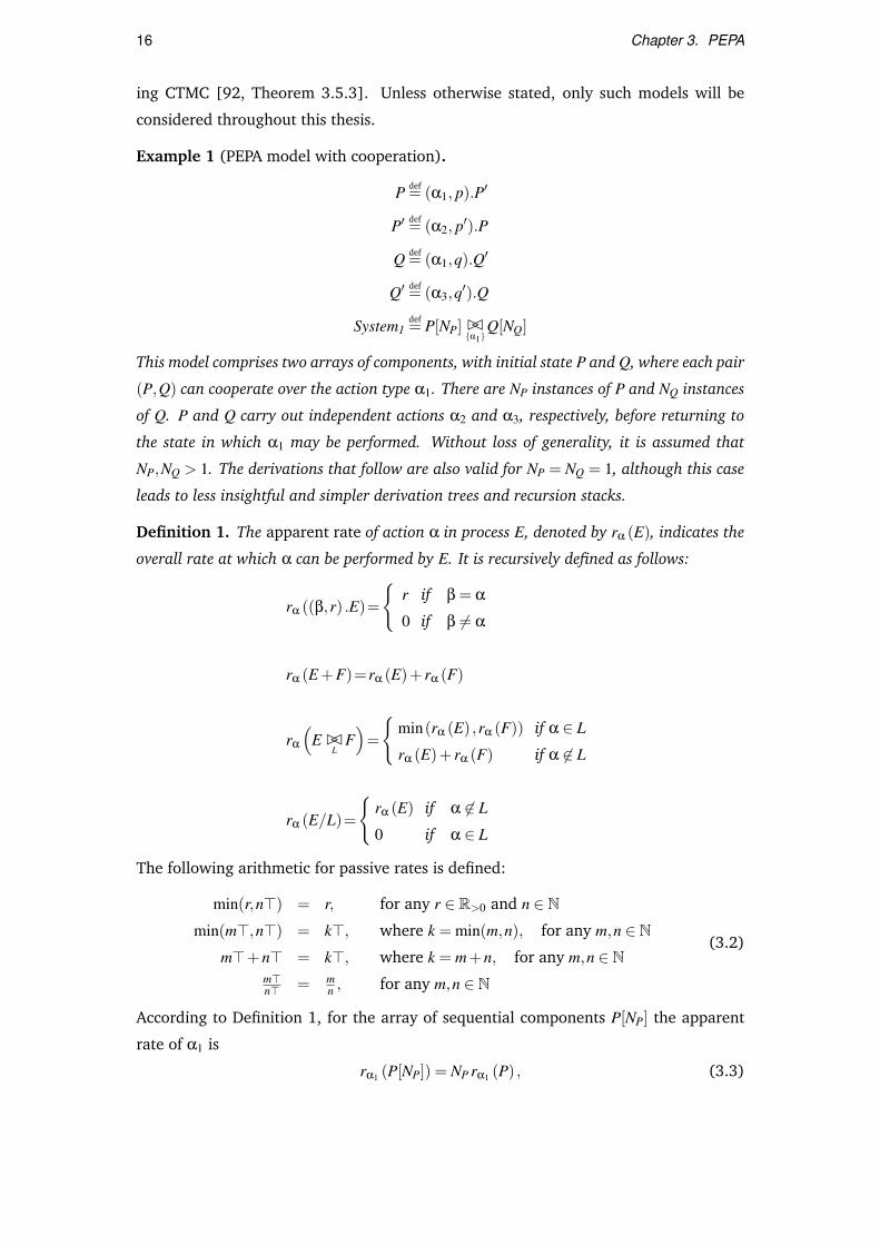
Example 1 (PEPA model with cooperation).
P def= (α1, p).P′
P′ def= (α2, p′).P
Q def= (α1,q).Q′
Q′ def= (α3,q′).Q
System1def= P[NP] BC
α1Q[NQ]
This model comprises two arrays of components, with initial state P and Q, where each pair
(P,Q) can cooperate over the action type α1. There are NP instances of P and NQ instances
of Q. P and Q carry out independent actions α2 and α3, respectively, before returning to
the state in which α1 may be performed. Without loss of generality, it is assumed that
NP,NQ > 1. The derivations that follow are also valid for NP = NQ = 1, although this case
leads to less insightful and simpler derivation trees and recursion stacks.
Definition 1. The apparent rate of action α in process E, denoted by rα (E), indicates the
overall rate at which α can be performed by E. It is recursively defined as follows:
rα ((β,r) .E)=
r if β = α
0 if β 6= α
rα (E +F)=rα (E)+ rα (F)
rα
(E BC
LF)
=
min(rα (E) ,rα (F)) if α ∈ L
rα (E)+ rα (F) if α 6∈ L
rα (E/L)=
rα (E) if α 6∈ L
0 if α ∈ L
The following arithmetic for passive rates is defined:
min(r,n>) = r, for any r ∈ R>0 and n ∈ Nmin(m>,n>) = k>, where k = min(m,n), for any m,n ∈ N
m>+n> = k>, where k = m+n, for any m,n ∈ Nm>n> = m
n , for any m,n ∈ N
(3.2)
According to Definition 1, for the array of sequential components P[NP] the apparent
rate of α1 is
rα1 (P[NP]) = NP rα1 (P) , (3.3)

3.2. Introduction to PEPA 17
and this holds for any α ∈ A and any NP because all the cooperation sets amongst such
components are empty.
The semantics of PEPA is defined in the style of Plotkin’s Structured Operational
Semantics [122] and is shown in Table 3.1. Given a PEPA component E, the operational
semantics induces the derivative set2, denoted by ds(E), which is the set of the possible
states reachable from E. The term local derivative denotes a state reachable from a
sequential component (which is itself a sequential component, as can be seen from
(3.1)). A derivation graph whose nodes are in ds(E) and arcs in ds(E)×Act × ds(E)
indicates all the transitions between each pair of derivatives of E. Arcs are taken with
multiplicity corresponding to the number of distinct inference trees which give the same
transition. The derivation graph is ultimately mapped onto a CTMC in which each state
corresponds to a derivative in ds(E).
The states reachable from the system equation System1 in Example 1 are obtained
by constructing derivation trees which begin with the transitions enabled by the con-
stituting sequential components. By rules S0 and A0 the following two transitions can
be inferred for P and Q:
P(α1,p)−−−→ P′ (3.4)
Q(α1,q)−−−→ Q′ (3.5)
The dynamic behaviour of the leftmost component P of the array can be collected by
NP−1 applications of rule C0. The first application has the form:
P(α1,p)−−−→ P′
P ‖ P(α1,p)−−−→ P′ ‖ P
Then, for 1≤ i≤ NP−2, the other NP−2 applications are of type
P ‖ P[i](α1,p)−−−→ P′ ‖ P[i]
P ‖ P[i] ‖ P(α1,p)−−−→ P′ ‖ P[i] ‖ P
For i = NP−2, the conclusion of this rule may be written as
P[NP](α1,p)−−−→ P′ ‖ P[NP−1] (3.6)
The behaviour of the leftmost component Q can be collected in a similar way, leading
to a transition in the form
Q[NQ](α1,q)−−−→ Q′ ‖ Q[NQ−1] (3.7)
2The term derivative is intended in PEPA to denote a reachable state of a component. It is not to beconfused with the notion of derivative in calculus, which will be used for the deterministic interpretationof the stochastic process underlying a PEPA model.

18 Chapter 3. PEPA
Table 3.1: Markovian semantics of PEPA (from [92]).
Prefix
S0 :(α,r).E
(α,r)−−→ E
Choice
S1 :E
(α,r)−−→ E′
E +F(α,r)−−→ E′+F
S2 :F
(α,r)−−→ F′
E +F(α,r)−−→ E +F′
Cooperation
C0 :E
(α,r)−−→ E′
E BCL
F(α,r)−−→ E′ BC
LF
, α 6∈ L
C1 :F
(α,r)−−→ F′
E BCL
F(α,r)−−→ E BC
LF′
, α 6∈ L
C2 :E
(α,r1)−−−→ E′ F(α,r2)−−−→ F′
E BCL
F(α,R)−−−→ E′ BC
LF′
, α ∈ L R =r1
rα(E)r2
rα(F)min(rα(E),rα(F))
Hiding
H0 :E
(α,r)−−→ E′
E/L(α,r)−−→ E′/L
, α 6∈ L H1 :E
(α,r)−−→ E′
E/L(τ,r)−−→ E′/L
, α ∈ L
Constant
A0 :E
(α,r)−−→ E′
A(α,r)−−→ E′
, Adef= E
Finally, by applying rule C2 to (3.6) and (3.7),
P[NP] BCα1
Q[NQ](α1,R)−−−→ P′ ‖ P[NP−1] BC
α1Q′ ‖ Q[NQ−1] (3.8)
where, by rule C2 and (3.3),
R =p
rα1 (P[NP])q
rα1 (Q[NQ])min(rα1 (P[NP]) ,rα1 (Q[NQ]))
=p
NP rα1 (P)q
NQ rα1 (Q)min(NP rα1 (P) ,NQrα1 (Q))
=p
NP pq
NQ qmin(NP p,NQ q)
=1
NP
1NQ
min(NP p,NQ q)
(3.9)

3.3. Aggregation Techniques 19
The conclusion of (3.8) is not the only transition enabled by the System1, because each
individual component P can be paired with each component Q to carry out action α1.
Hence, P[NP] BCα1
Q[NQ] enables NP×NQ transitions to distinct states of type
P ‖ · · · ‖ P ‖ P′ ‖ P ‖ · · · ‖ P︸ ︷︷ ︸NP sequential components
BCα1
Q ‖ · · · ‖ Q ‖ Q′ ‖ Q ‖ · · · ‖ Q︸ ︷︷ ︸NQ sequential components
(3.10)
which only differ in the locations of the components P′ and Q′. Since each transition
occurs at rate R, the exit rate from P[NP] BCα1
Q[NQ] is
NP×NQ×R = min(NP p,NQq) (3.11)
and the factor 1/(NP×NQ) is the probability that one specific pair of components makes
that transition.
3.3 Aggregation Techniques
Each of the states of kind (3.10), say P′ ‖ P[NP−1] BCα1
Q′ ‖ Q[NQ−1], has transitions to
(NP− 1)× (NQ− 1) distinct states in which there are two copies of P′, (NP− 2) copies
of P, two copies of Q′, and (NQ − 2) copies of Q. Similarly, each state, say P′[2] ‖P[NP − 2] BC
α1Q′[2] ‖ Q[NQ − 2], has transitions to (NP − 2)× (NQ − 2) distinct states in
which there are three copies of P′, (NP−3) copies of P, three copies of Q′, and (NQ−3)
copies of Q. Overall, this model will have a state space of cardinality 2NP+NQ , clearly
unsatisfactory for large-scale models.
The aggregation technique presented in [79] goes a long way toward alleviating
this problem. At the core of this algorithm is a strong notion of equivalence in PEPA
called isomorphism [92, Definition 6.2.2]. Informally, it states that two components E
and E′ are isomorphic (written E = E′) if there is a one-to-one correspondence between
the derivatives of E and those of E′ such that corresponding derivatives enable the
same activities (i.e., same action types and rates), and the resulting derivatives are in
the same correspondence. An equational law for isomorphism states that, for any E and
F, E ‖ F = F ‖ E [92, Proposition 6.3.4]. The aggregation algorithm uses this equational
law to determine a canonical representation of a derivative in which the constituting se-
quential components are arranged in some fixed order (e.g., lexicographical order). All
derivatives which have the same canonical representation form an equivalence class. In
this way a partition is induced in the derivative set of a PEPA model. The corresponding
partition in its underlying Markov chain satisfies the lumpability condition, therefore
this aggregated CTMC may be used for performance evaluation instead of the (much
larger) original one.
20 Chapter 3. PEPA
For instance, by assuming that the lexicographical order is such that P′ < P and
Q′ < Q, the NP ×NQ distinct states of (3.10) are members of the same equivalence
class, represented by their canonical representation P′ ‖ P[NP − 1] BCα1
Q′ ‖ Q[NQ − 1].
In the aggregated CTMC, the initial state System1def= P[NP] BC
α1Q[NQ] will have a single
transition to this canonical state, with a rate which is the sum of all rates to each of
the members of the equivalence class, i.e. (3.11) as discussed above. The reduction
achieved by this algorithm depends on the structure of the model under study. Overall,
in Example 1, the exponential growth in the non-aggregated state space is simplified
to a state space cardinality polynomial in NP and NQ (the state space size is (NP +1)×(NQ +1)). However, Markovian analysis may still be impractical when high population
levels or models with more complex structure are considered.
3.4 Deterministic Approximations
3.4.1 Fluid-Flow Approximation
A radical approach to tackling state-space explosion is to abandon the traditional Marko-
vian interpretation in favour of an alternative view in which the inherently discrete
changes of state are approximated in a continuous fashion. In the context of PEPA, the
seminal paper which prompted a considerable amount of research in this direction pro-
posed a deterministic interpretation in the form of a set of coupled ordinary differential
equations [93]. This approach is based on the observation that copies of isomorphic
sequential components composed in parallel can be regarded as being of the same type.
This is because they evolve through the same derivative set and the dynamic behaviour
of one copy is not affected by the state of the other isomorphic copies, but it only de-
pends upon the interactions with other components of different type. For instance, in
the composition P ‖ P′, P (resp., P′) enables (α1, p) (resp., (α2, p′)) regardless of the ac-
tivities enabled by P′ (resp., P). In Example 1 two component types may be identified,
respectively the left-hand side and the right-hand side of the non-empty cooperation
BCα1
.
Based on this, it is possible to define an alternative state representation, called the
numerical vector form (NVF). The PEPA process describing the evolution of all com-
ponents of the same type has the generic form (assuming a suitable lexicographical
order for the canonical form) E1[K1] ‖ E2[K2] ‖ · · · ‖ EN [KN ], where E1,E2, . . .EN are the
local derivatives of the sequential component and K1,K2, . . .KN are the corresponding
number of copies exhibiting that derivative. Thus, the state may be completely charac-
terised by the vector (K1,K2, . . . ,KN), assuming an arbitrary but fixed mapping of local
derivatives onto coordinates of the vector. It is interesting to note that the length of

3.4. Deterministic Approximations 21
the vector does not depend on the actual component counts, but only on the size of the
derivative set of the component type, which can be determined without recourse to the
derivation of the full state space of the system. The initial state of Example 1 (which is
P[NP] BCα1
Q[NQ]) may be represented by:
(NP,0) BCα1
(NQ,0) (3.12)
which states that there are NP copies of derivative P, no copies of P′, NQ copies of
derivative Q, and no copies of Q′. The NVF may be simplified further by observing that
the cooperation structure needs not be recorded if the model is specified according to
the two-level grammar (3.1). Models in such a form enjoy the property that they do
not spawn processes during the evolution of the system, e.g., processes of the form
(α,r).(E ‖ E) are not allowed. Additionally, the language has no primitives for the
dynamic configuration of hiding and cooperation sets. Thus, the number of sequential
components remains fixed across the entire state space and the behaviour is completely
determined by the local derivatives of each sequential component. This property, in
conjunction with the notion of component type discussed above, allows for a simpler
state descriptor. The description (3.12) can be reduced to the following NVF
(NP,0,NQ,0), (3.13)
with no loss of information provided that the static cooperation structure is recorded
separately. The adoption of the NVF brings about no significant advantages over the use
of the canonical form—apart from being a more parsimonious data structure for stor-
age, their underlying CTMCs are isomorphic. However, the purpose here is to replace
each discrete counter variable in the NVF with a continuous counterpart governed by
an ordinary differential equation. The procedure for achieving this is illustrated here
by means of Example 1.
The canonical state P′ ‖ P[NP − 1] BCα1
Q′ ‖ Q[NQ − 1] may be represented as (NP −1,1,NQ − 1,1) in the NVF, and this state is reached from (3.13) with the following
transition:
(NP,0,NQ,0)α1,min(NP p,NQq)−−−−−−−−−−→ (NP−1,1,NQ−1,1) (3.14)
This transition says that there is (on average) a unitary decrease in the number of
components P and Q after 1/min(NP p,NQq) time units. Notice that the transition rate is
a function of the current component counts. In general, by letting xE(t) be the variable
which counts the number of components exhibiting the derivative E at time t, it is
possible to write the decrease in the number of components over some finite interval
of time ∆t:
xP(t +∆t)− xP(t) =−min(xP(t)p,xQ(t)q)∆t (3.15)

22 Chapter 3. PEPA
Analogously, the same decrement is observed for the variable xQ:
xQ(t +∆t)− xQ(t) =−min(xP(t)p,xQ(t)q)∆t (3.16)
Correspondingly, the population levels of P′ and Q′ are increased by the same quantity:
xP′(t +∆t)− xP′(t) = min(xP(t)p,xQ(t)q)∆t
xQ′(t +∆t)− xQ′(t) = min(xP(t)p,xQ(t)q)∆t(3.17)
Dividing both sides of (3.15–3.17) by ∆t and taking the limit ∆t → 0 gives rise to a
contribution min(xP(t)p,xQ(t)q) to the following system of coupled ordinary differential
equations:
dxP(t)dt
=−min(xP(t)p,xQ(t)q)+ . . .
dxQ(t)dt
=−min(xP(t)p,xQ(t)q)+ . . .
dxP′(t)dt
= min(xP(t)p,xQ(t)q)+ . . .
dxQ′(t)dt
= min(xP(t)p,xQ(t)q)+ . . .
(3.18)
The ellipsis indicate that the ODE representation is only partial, because this system
only captures the relative changes of the population levels due to the execution of the
shared action α1. The contributions from the execution of the independent activities α2
and α3 can be extracted in a similar way. If there are xP′(t) (resp., xQ′(t)) components
of type P′ (resp., Q′) at time t, the population level is decreased by one at a rate which
is the product xP′(t)p′ (resp., xQ′(t)q′) and the component which makes the transition
will subsequently behave as P (resp., Q). Including these contributions in (3.18) will
give rise to the following system:
dxP(t)dt
=−min(xP(t)p,xQ(t)q)+ xP′(t)p′
dxQ(t)dt
=−min(xP(t)p,xQ(t)q)+ xQ′(t)q′
dxP′(t)dt
= min(xP(t)p,xQ(t)q)− xP′(t)p′
dxQ′(t)dt
= min(xP(t)p,xQ(t)q)− xQ′(t)q′
(3.19)
The procedure described in [93] can be used to automatically infer the differen-
tial model by static inspection of the model description. A set of coupled differential
equations is straightforwardly obtained via an intermediate object called the activity
diagram (or the equivalent representation termed the activity matrix), constructed to
collect the information about which action type influences which local derivative and
in which direction (i.e., whether the local derivative carries out the activity or if it is the

3.4. Deterministic Approximations 23
resulting derivative of some other sequential component performing the action). The
automatic procedure from [93] imposes five main restrictions to the syntactic structure
of models amenable to this analysis.3
Assumption 1. The hiding operator is not supported.
Assumption 2. Sequential components of distinct types must cooperate over all shared
action types.
For instance, given three distinct sequential components E, F, and G such that
Edef= (α,r).E′, F
def= (α,r).F′, and Gdef= (α,r).G′, the model
(E[NE] ‖ F[NF]
)BCα
G[NG], for
any NE,NF,NG ∈ N, cannot be analysed because the action type α is not in the cooper-
ation set between E[NE] and F[NF]. However, this pattern of cooperation is useful in
many circumstances. For instance, in a classical client/server scenario, E and F may
represent two distinct classes of clients (exhibiting perhaps different behaviour in their
other local states E′ and F′) which communicate with a group of servers G, where α
is the action which describes the interaction. Unfortunately this problem cannot be
circumvented by trivial changes to the model. For instance, a misleading fix could
consider two distinct action types αE and αF and modifying the process definitions as
follows: Edef= (αE,r).E′, F
def= (αF,r).F′, and Gdef= (αE,r).G′ +(αF,r).G′. With the system
equation(E[NE] ‖ F[NF]
)BC
αE ,αF G[NG], this model still allows E and F to cooperate with
G independently of each other because G enables both action types αE and αF . In
addition, Assumption 2 is met because E and F do not share any action type. The
behaviour of the original system with respect to α would be recovered by considering
the aggregated behaviour of αE and αF in the new model. However, the agreement is
only qualitative—in particular, the initial state has two different overall exit rates, i.e.,
r min(NE +NF,NG) for action α in the original model and r(
min(NE,NG)+min(NF,NG))
for actions αE and αF in the modified one.
Assumption 3. The same action type cannot be enabled by two distinct local states of the
same sequential component.
For instance, the model E[NE] BCα
F[NF], with Edef= (α,r).E′,E′ def= (α,r).E,F
def= (α,r).F′
would not be accepted. A possible solution similar to that proposed above—consisting
in replacing the two α-actions in E and E′ with two distinct action types enabled simul-
taneously by F—would not agree quantitatively with the original model.
Assumption 4. Prefixes must have active rates.
3In fact, it may be applied to Example 1 only if p = q. In the light of further developments of the theorydiscussed later in this section, the derivations presented here for p 6= q are still sensible.

24 Chapter 3. PEPA
Assumption 5. Two synchronising components must have the same local view of the rate
of the shared activity.
As a consequence, a cooperation in the form (α,rE).E BCα
(α,rF).F is not amenable
to fluid-flow approximation if rE 6= rF. Scenarios with asymmetric capacities occur
frequently in practical applications. For instance, with respect to the same client/server
model discussed above, the local rates for the shared activity may be associated with the
bandwidth available for the communication. At a suitable level of model abstraction, a
server’s local rate for α being higher than the client’s may capture the observation that
the server may be capable of carrying out the communication faster than the client, but
the minimum-rate semantics of PEPA will ensure that the delay is dominated by the
slowest of the participating components.
3.4.2 Differential Models for Computational Systems Biology
A similar translation procedure to [93] is given in [32] for a special class of PEPA
models considered for the analysis of signalling pathways. In such models, a sequen-
tial component represents a reactant in a biochemical network and it must be defined
with two states, describing the behaviour for high and low concentrations [31]. The
derivatives exhibited at high concentration indicate the chemical reactions in which
the reactant is consumed (thus transitioning to the state with low concentration). Con-
versely, the low-concentration state has derivatives corresponding to reactions in which
the reactant is produced (thus transitioning to the state with high concentration). In
either case, the chemical reactions are associated with the action types of the sequential
components’ derivatives. The final model consists of as many sequential components
as the distinct reactants in the network. The cooperation structure in the system equa-
tion is then used to define the reactions—if two components are the reagents of some
reaction, this is captured by a cooperation combinator whose action set includes the
shared action type for that reaction.
A deeply influential paper for the work developed in the present thesis is [72], in
which an extension to the cooperation combinator is used to accommodate the biolog-
ically interesting mass-action kinetics. Here, the nature of the relationship between the
differential equation model and the stochastic process is investigated for the first time,
and the authors show the the ODE may be regarded as the fluid limiting behaviour of
a sequence of increasingly detailed CTMCs. Informally, at the coarsest level of detail
is a representation in which the reactant’s concentration is represented by two discrete
states (called levels), as in the case of high and low concentration discussed above.
Finer granularity is given by increasing the number of levels; the (finite) concentration
interval of a species is divided into non-overlapping sub-intervals of equal length such

3.4. Deterministic Approximations 25
that each level corresponds to one sub-interval. The authors prove that in the limit
as the number of levels goes to infinity the stochastic process is not distinguishable
from the ODE solution. This is an application of a general result of convergence due
to Kurtz [103], which will be also used in this thesis (therefore it will be discussed in
more detail in the next chapter).
It is worthwhile pointing out that in these works concerned with applications to
computational systems biology the syntactical restrictions presented in the previous
section are not removed because the so-reduced language is sufficiently expressive for
most practical purposes in this context. (In fact, in [32] a further restriction is imposed
by considering only two-state sequential components.) This remark also applies to [14]
in which the treatment of self-looping components, i.e., components in the form Edef=
(α,r).E, is modified to better capture the behaviour of epidemiological models.
3.4.3 Related Work
Diffusion Approximation of Queueing Networks
In queueing theory, the approach which most resembles the deterministic interpreta-
tion of PEPA is concerned with diffusion approximation. The discrete-state stochastic
process governing the queue length is approximated by a (continuous-state) Brown-
ian motion with drift. Although this process is still stochastic, the probability density
function is now analytically tractable since it has a closed form as the solution to the
Kolmogorov diffusion (partial differential) equation (also called the Fokker-Plank equa-
tion). This approximation is valid for generally distributed independent and identically
distributed service and interarrival times and is shown to match the discrete-state pro-
cess very well when such distributions are exponential. This approach, extended to
open and closed queueing networks, is used to study the transient and asymptotic
regimes [101,102]. Of particular importance are the boundary conditions to the diffu-
sion equation, which must be imposed to keep the approximation process in a meaning-
ful region (for instance, non-negative values of the queue size). This implies that such
approximations can be usefully applied under specific circumstances—termed heavy-
traffic assumptions—which impose saturation or near-saturation behaviour of the queue
(i.e., similar arrival and service rates) [74].
Fluid Approaches for Stochastic Petri Nets
A Fluid Stochastic Petri net is a formalism developed to incorporate continuously chang-
ing quantities in an ordinary Generalised Stochastic Petri Net [96]. The places of the net
are partitioned into discrete and fluid places. Discrete places are ordinary places marked

26 Chapter 3. PEPA
with non-negative natural numbers, while fluid places have a marking whose domain is
the non-negative reals, interpreted as a continuously changing fluid level. In addition to
ordinary arcs connecting discrete places, fluid places are connected to timed transitions
via continuous arcs. A flow rate function describes the (possibly marking-dependent)
rate at which the fluid flows from a timed transition to a fluid place. The analysis of
a Fluid Stochastic Petri nets is carried out by solving an associated fluid model. The
discrete part of the net has the usual interpretation of a Generalised Stochastic Petri
net, hence it is characterised by a CTMC. The dynamics of the fluid may be viewed as
a stochastic process modulated by the CTMC, and its behaviour is governed by a set
of partial differential equations, for which several transient and steady-state solution
methods have been devised [38,83,132] (cfr. [84] for a review of this field).
A more closely related approach is that of Continuous Petri Nets [7], in which all
places and transitions are fluid. The behaviour of the net, i.e., the temporal evolution
of the marking process, is deterministically governed by a set of coupled ordinary dif-
ferential equations. For a study on the relationship between this formalism and the
continuous interpretation of PEPA, the reader is referred to [69,70].
Differential Equations in Stochastic Process Algebras
The topic of deterministic interpretation of process algebra models has received much
attention recently. Cardelli has investigated the relationship between the continuous-
and the discrete-state representation of the Chemical Ground Form, a subset of the
stochastic π-calculus used for the modelling of chemical reactions obeying the mass-
action kinetics [33]. A route toward fluid-flow approximation similar to that of PEPA
has been followed in the context of the stochastic Concurrent Constraint Programming
process algebra. In [22] a mapping to ordinary differential equations is established;
in [21], these equations are shown to correspond to the first-order approximation of
the Chapman-Kolmogorov equations of the corresponding process and in [23] it is
shown that convergence in the sense of Kurtz holds. In the context of computational
systems biology, a similar relationship has been studied in [40] with regard to Bio-PEPA,
a process algebra based on PEPA explicitly developed for the modelling of biochemical
systems [41,42].
The opposite perspective is provided by the continuous π-calculus [107], a variant
of the π-calculus for the modelling of biochemical networks in which the operational
semantics is given directly in terms of a differential equation model (with an associated
CTMC which is suggested to follow directly from the semantics).
Chapter 4
Fluid Flow Semantics
This chapter develops a fluid-flow semantics for PEPA. This work follows the line of
research presented in Section 3.4, providing three main novel contributions:
1. The applicability of the fluid-flow approximation is extended by removing the
syntactical restrictions discussed in Section 3.4.1.
2. Unlike previous approaches, the semantics is not given directly in terms of an un-
derlying ODE. Instead, using the same structured operational style as the original
interpretation in [92], the semantics gives rise to a CTMC with state descriptor in
the NVF. For this reason it is called the population-based semantics. However, this
approach does not involve the exploration of the (potentially very large) state
space because the chain is only described symbolically by means of generating
functions, i.e., functions of the state descriptor which characterise the transitions
of any state of the chain.1 This compact representation is sufficient to construct
an associated ODE.
3. The relationship between the ODE which is defined in this way and the CTMC
derived from the population-based semantics is a profound one. For any PEPA
model, the ODE is shown to be the deterministic limiting behaviour of a suitably
defined sequence of population-based CTMCs. This asymptotic regime is of prac-
tical interest, as demonstrated by an extensive numerical investigation on a case
study.
The chapter is structured as follows. Section 4.1 sets up the framework within
which the population-based semantics is developed and gives an illustrative example
of the result of deterministic convergence used for the fluid interpretation. Section 4.2
presents the population-based semantics for PEPA, and its properties are proved in
1The term generating function used throughout this thesis is not to be confounded with the usualdefinition of probability-generating function of a discrete random variable in probability theory.
27

28 Chapter 4. Fluid Flow Semantics
Section 4.3. Section 4.4 is concerned with an empirical study on the quality of the
approximation of the differential equation to the Markov process. Section 4.5 presents
concluding remarks about the nature of passive synchronisation in the fluid interpreta-
tion and the computation of theoretical error probabilities of the approximation.
4.1 Population Models for PEPA
Let ξ ∈ Zd be the state descriptor of a PEPA model in the NVF. The operational se-
mantics developed in this chapter leads to the derivation of generating functions of the
CTMC, i.e., functions of the state descriptor which give the transition rates between all
the reachable states of the system. These functions are parametrised by action types
to record the additional information of which action type is associated with a transi-
tion. Let l ∈ Zd be the transition jump, i.e., the transition moves from state ξ to ξ + l.
The generating functions are denoted by ϕα(ξ, l) : Rd → R and give the transition rate
for a jump l and an activity of type α ∈ A . Thus, the entry in the generator matrix
corresponding to the transition from ξ to ξ+ l, denoted by qξ,ξ+l, can be written as
qξ,ξ+l = ∑α∈A
ϕα(ξ, l).
The summation across A captures the fact that distinct action types may contribute to
a transition to the same target state, e.g., (α,r).E +(β,s).E. These transitions are kept
distinct in the labelled transition system of PEPA, because it records the action type in
addition to the transition rate, but they collapse onto the same entry in the underlying
generator matrix. We use the notation
ϕ(ξ, l)≡ ∑α∈A
ϕα(ξ, l)
to indicate the overall contribution to the transition. The extraction of the generat-
ing functions from the PEPA model usually presents very little computational challenge
because the environment collected via the inference rules in the population-based op-
erational semantics abstracts away from the actual component counts of the system
under study. From ϕ(ξ, l) it is possible to construct a vector field V (x) defined as
V (x) = ∑l∈Zd
lϕ(x, l) (4.1)
and an associated ODEdx(t)
dt= V (x(t)). (4.2)
This formulation makes it possible to establish a property of convergence for PEPA
models according to the interpretation by Kurtz [103], [104], [105]. The result used

4.1. Population Models for PEPA 29
Pdef= (α1, p).P′
P′def= (α2, p′).P
Qdef= (α1,q).Q′
Q′ def= (α3,q′).Q
System1def= P[NP] BC
α1Q[NQ]
Figure 4.1: Example 1 (from Section 3.2)
here states that the solution to a properly defined initial value problem with (4.2) is the
fluid limiting behaviour of a family of CTMCs in the sense of the following theorem.
Theorem 1 (cfr. [103], Theorem 3.1). Let Xn(t) be a family of density dependent
CTMCs, i.e., a sequence of chains with parameter n ∈ N taking values in Zd such that the
infinitesimal generator entries for Xn(t), denoted by qξ,ξ+l, can be described as
qξ,ξ+l = n ·ϕ(ξ/n, l). (4.3)
Suppose that:
1. The functions ϕ(x, l) are continuous.
2. There exists an open set O⊂ Rd and a constant L ∈ R such that:
(a) ‖V (x)−V (y)‖< L‖x− y‖ , x,y ∈ O
(b) supx∈O ∑l∈Zd ‖l‖ϕ(x, l) < ∞
(c) limk→∞ supx∈O ∑‖l‖>k ‖l‖ϕ(x, l) = 0
Then, for every solution to the initial value problem of (4.2) subject to
x(0) = x0 and x(t) ∈ O, 0≤ t ≤ T
the family Xn(t) converges to x(t) in the sense that
limn→∞
Xn(0)/n = x0 =⇒∀ε > 0 limn→∞
P(
supt≤T
‖Xn(t)/n− x(t)‖> ε
)= 0. (4.4)
Let us now use Example 1 (reported again in Fig. 4.1 for the sake of convenience)
to illustrate the rationale behind the approach and give an intuitive interpretation of
the result of convergence. The generating functions are obtained by reducing System1
to a much smaller model component red (System1) (where the function red(·) will be
formally introduced in the next section). This component extracts the structure of

30 Chapter 4. Fluid Flow Semantics
the system by disregarding the information about the multiplicities of the replicated
components:
red (System1)def= P BC
α1Q
The sequential components P and Q in this equation are not interpreted as single
entities, but as representatives of classes of behaviour. The state descriptor in the
NVF is formed by computing the local derivatives of each sequential component in
red(System1)—this procedure is of negligible computational cost because the behaviour
of such components is usually simple, and the state space growth arises from the inter-
leaving of their concurrent behaviours. A NVF with the same component mapping as
in Section 3.3 may be used—i.e., ξ ∈ Z4 and ξ1,ξ2,ξ3,ξ4 are the component counts of
the local derivatives P,P′,Q,Q′, respectively.
The population-based semantics will generate a derivation graph for red (System1),
and a transition in this derivation graph gives information about a generating function
of the CTMC. For instance, the following generating function is obtained for α1:
ϕα1 (ξ,(−1,1,−1,1)) = min(pξ1,qξ3) (4.5)
which intuitively means: if there are ξ1 components P and ξ3 components Q, each being
able to perform the shared action α1 at rate p and q, respectively, then the overall rate
of execution for the activity is the minimum (by the cooperation rule) of the two rates at
which the action can be performed by the populations of the synchronising components
(by additivity of apparent rate calculation). Let ξ = (NP,0,NQ,0) (i.e., the initial state
of Example 1), then (4.5) implies the CTMC transition
ξ = (NP,0,NQ,0)(α1,min(NP p,NQq))−−−−−−−−−−−→ ξ+(−1,1,−1,1) = (NP−1,1,NQ−1,1) (4.6)
Other transitions of the derivation graph will represent the behaviour of the sequential
components in state P′ and Q′, leading to the following generating functions, respec-
tively
ϕα2 (ξ,(1,−1,0,0)) = p′ξ2 (4.7)
and
ϕα3 (ξ,(0,0,1,−1)) = q′ξ4. (4.8)
The non-zero elements of the jump vector indicate which component derivatives are
involved in the transition. With regard to the shared action α1, all sequential compo-
nents are subjected to change in their population levels, because of the transitions of
the single components (3.4) and (3.5) which record a decrease of P and Q and a cor-
responding increase of P′ and Q′. Finally, (4.5), (4.7) and (4.8) can be used to extract

4.2. Population-Based Operational Semantics 31
the underlying ODE (4.2), which is, in components:
dx1(t)dt = −min(px1(t),qx3(t))+ p′x2(t)
dx2(t)dt = min(px1(t),qx3(t))− p′x2(t)
dx3(t)dt = −min(px1(t),qx3(t))+q′x4(t)
dx4(t)dt = min(px1(t),qx3(t))−q′x4(t)
(4.9)
Notice that this differential equation is equal to (3.19), obtained with arguments
of deterministic approximation of exponentially distributed activities with their means.
A family of population-based CTMCs Xn(t) can be systematically associated with a
PEPA model by taking a density vector, denoted by δ ∈ Zd , which is interpreted as
giving the relative proportions between the distinct sequential components. By letting
δ = (NP,0,NQ,0), the sequence of CTMCs is such that the initial population levels are
multiples of δ, i.e.,
Xn(0) = n ·δ, for all n.
This corresponds to increasingly large initial population levels as a function of n. For
instance, X1(t) represents the original population-based CTMC, X2(t) is the CTMC un-
derlying the model with initial state P[2NP] BCα1
Q[2NQ], and so on. Since by construction
limn→∞ Xn(0)/n = δ, the result of convergence (4.4) intuitively states that, asymptoti-
cally, a sample path of the CTMC Xn(t) may be well approximated by n · x(t), over any
finite time interval, where x(t) is the solution to the initial value problem of the ODE
(4.9) with x(0) = δ. A pictorial representation of this result is given in Fig. 4.2, which
shows that the ODE is a closer approximation to sample paths of Xn(t)/n for increasingly
large n, with excellent accuracy at n = 1000.
4.2 Population-Based Operational Semantics
Models are specified according to the two-level grammar (3.1). The present operational
semantics does not deal directly with passive rates, thus Assumption 4 of Section 3.4
still holds. However, a discussion on extensions to incorporate passive synchronisa-
tion is proposed in Section 4.5.1, after the semantics is presented. None of the other
assumptions of Section 3.4 are required.
4.2.1 Preliminary Definitions
As discussed above, the interpretation of a PEPA model against the population-based
structured operational semantics begins with considering a system equation which does
not record the multiplicities of independent replicated sequential components. Any

32 Chapter 4. Fluid Flow Semantics
0 0.5 1 1.5 2 2.5 30.4
0.6
0.8
1
1.2
1.4
1.6
1.8
2
Time
Den
sity
ODEn=10n=100n=1000
Figure 4.2: Density of component P in Example 1. One realisation of the scaled Markov chain
Xn(t)/n over the first three time units becomes closer to the solution of the ODE as n increases.
Parameter set: p = 1.0, p′ = 0.5,q = 2.0,q′ = 4.0,δ = (2,0,1,0)
PEPA component may be compacted in such a way. Here isomorphism is used to estab-
lish whether two distinct sequential components are equivalent.
Definition 2 (Reduced Context). The reduced context of a PEPA component E, denoted
by red(E), is recursively defined as follows:
red ((α,r) .E) = (α,r) .E
red (E +F) = E +F
red(A) = red(E), if A def= E
red(E BCL
F) =
red(E) if L = /0∧E = F∧E,F are sequential components
red(E) BCL
red(F) otherwise
red(E/L) = red(E)/L
The reduced context considers one representative single sequential component E
in place of the cooperation E ‖ F if the two cooperating processes are isomorphic se-
quential components. Thus, because of this equivalence relation between these compo-
nents, the first case for the cooperation operator in Definition 2 could also read red(F).
Clearly, the two arrays P[NP] and Q[NQ] in Example 1 are recursively reduced to single
sequential components P and Q, respectively and
red(System1) = P BCα1
Q, (4.10)
as illustrated above. Notice that the same context reduction (4.10) would be obtained
if the system equation was replaced with(P[NP−KP]‖P′[KP]
)BCα1
(Q[NQ−KQ]‖Q′[KQ]
), (4.11)

4.2. Population-Based Operational Semantics 33
for any 1 ≤ KP ≤ NP and 1 ≤ KQ ≤ NQ. Here the (NP −KP) P components would be
reduced to P as before. Furthermore, the cooperation P ‖ P′ would be reduced to P
as well, since P and P′ are isomorphic because they are two local derivatives of the
same sequential component. Similar arguments hold for the isomorphism between Q
and Q′. Therefore, the two model equations will give rise to the same underlying ODE
although with two different initial value problems, as determined by the population
levels specified in the equations.
It is worthwhile pointing out that Definition 2 also allows for two or more instances
of a sequential component to appear in the reduced context of a PEPA model. For
example, we have that
red((
P[NP] BCα1
Q[NQ])‖ P[N′
P])
=(P BC
α1Q
)‖ P
This supports the intuitive observation that the leftmost array of P components will be-
have differently from the rightmost array. In this instance, the action α1 of the leftmost
array is executed in cooperation with a Q component, whereas it is an independent
action with regard to the rightmost array because of the empty cooperation set.
In the remainder we consider a PEPA model for which the context reduced form Mis already known. This minimal form contains the necessary information to determine
the state descriptor in NVF, and is analogous to a Petri net without any marking.
Definition 3 (Numerical Vector Form). Let NC be the number of distinct sequential com-
ponents in M . Let Ci be the derivative set of the i-th component, i = 1,2, . . . ,NC and let
Ni be its size, i.e., Ni = |Ci|. Let Ci, j denote the j-th derivative of the i-th component,
j = 1,2, . . . ,Ni. The state descriptor in the NVF, denoted by ξ ∈ Zd ,d = ∑NCi=1 Ni, assigns a
coordinate, denoted by ξi, j, to each local derivative Ci, j and indicates the number of copies
in the system which exhibit that derivative.
Definition 4 (Initial State of the CTMC). The initial state of the CTMC is denoted by
δ ∈ Zd and gives an initial population level δi, j ≥ 0 to each local derivative Ci, j. Without
loss of generality we exclude the case in which all the derivatives of a sequential component
are set to 0, by subjecting δ to the condition ∑Nik=1 δi,k > 0, for all i.
Sometimes the element ξi, j is conveniently referred to by a single subscript ξk, i.e.,
an implicit mapping is assumed from each sequential component Ci, j to a coordinate
1 ≤ k ≤ d in the population vector. For instance, with regard to Example 1, NC = 2,
C1 = P,P′, and C2 = Q,Q′. Furthermore, the following mappings are used: C1,1 7→P,
C1,2 7→P′, C2,1 7→Q, C2,2 7→Q′. Using the same ordering as in Section 4.1, the initial state
in Example 1 is (NP,0,NQ,0) whereas it is (NP−KP,KP,NQ−KQ,KQ) in (4.11). When a
superscript is used, it refers to a state of the CTMC. Thus, ξmi, j indicates the population
count of the sequential component Ci, j in the m-th state of the CTMC.

34 Chapter 4. Fluid Flow Semantics
As with the Markovian interpretation, at the core of this semantics is the notion of
apparent rate. Here this concept is modified to take into account the interpretation of
the reduced context described above.
Definition 5 (Parametric Apparent Rate). Consider a process E composed of sequential
components Ci, j. The parametric apparent rate of action type α in component E, denoted
by r?α (E,ξ), defines the overall rate at which the action type α can be performed by com-
ponent E as a function of the current population sizes ξ of the sequential components of
the system:
r?α
(E BC
LF,ξ
)=
min(r?
α (E,ξ) ,r?α (F,ξ)) if α ∈ L
r?α (E,ξ)+ r?
α (F,ξ) if α 6∈ L
r?α (E/L,ξ) =
r?
α (E,ξ) if α 6∈ L
0 if α ∈ L
r?α (Ci, j,ξ) =
Ni
∑k=1
rα(Ci,k)ξi,k
The first two cases are structurally and syntactically similar to their counterparts
in the Markovian semantics, rα(E BCL
F) and rα(E/L). For a sequential component of
the reduced context, the definition of parametric apparent rate exploits the property in
(3.3) that it can be expressed as the product of the current population size expressed
in the state descriptor and the apparent rate of a single sequential component. In ad-
dition, the behaviour of the other derivatives in the same derivative set of Ci, j is taken
into account because of the interpretation of M . As already discussed, each sequen-
tial component in M represents an array of identical components, evolving through
the local derivatives Ci,k, 1 ≤ k ≤ Ni. In any state of the CTMC there may be one or
more components exhibiting each such derivative. These components will compete to
participate in a shared action α, and the probability that the action is completed by
each derivative will be proportional to the population level of that derivative and the
individual rate of execution. Thus, the apparent rate calculated in this manner reflects
the potential contribution to the action by any concurrent sequential component. This
summation is legitimate due to the property of additivity which holds for the apparent
rates for non-cooperating components.
The set of functions generated by r?α (·,ξ) is denoted by F = [Rd −→R≥0], a function
space with values in the nonnegative reals because passive actions are not allowed.

4.2. Population-Based Operational Semantics 35
Sequential Component (Promotion Rule)
S?0 :
Ci,j(α,r)−−→ Ci,j′ Ci, j ∈ Ci
Ci,j(α,rξi, j)−−−−→? Ci,j′
Cooperation
C?0 :
E(α,r(ξ))−−−−→? E′
E BCL
F(α,r(ξ))−−−−→? E′ BC
LF
, α 6∈ L
C?1 :
F(α,r(ξ))−−−−→? F′
E BCL
F(α,r(ξ))−−−−→? E BC
LF′
, α 6∈ L
C?2 :
E(α,r1(ξ))−−−−−→? E′ F
(α,r2(ξ))−−−−−→? F′
E BCL
F(α,r(ξ))−−−−→? E′ BC
LF′
, α ∈ L,
r(ξ) =r1(ξ)
r?α (E,ξ)
r2(ξ)r?
α (F,ξ)min(r?
α (E,ξ) ,r?α (F,ξ))
Hiding
H?0 :
E(α,r(ξ))−−−−→? E′
E/L(α,r(ξ))−−−−→? E′/L
, α 6∈ L
H?1 :
E(α,r(ξ))−−−−→? E′
E/L(τ,r(ξ))−−−−→? E′/L
, α ∈ L
Constant
A?0 :
E(α,r(ξ))−−−−→? E′
A(α,r(ξ))−−−−→? E′
, Adef= E
Figure 4.3: Population-based parametric structured operational semantics of PEPA. Transitions
are denoted by the symbol −→? to distinguish them from the Markovian transitions in PEPA
which carry reals instead of functions.

36 Chapter 4. Fluid Flow Semantics
4.2.2 Structured Operational Semantics
The population-based parametric structured operational semantics for PEPA is shown
in Fig. 4.3. Let C be the set of PEPA processes composed of Ci, j. Let L be the la-
belling alphabet, i.e., L = A×F . The rules induce a parametric multi-transition system,
(C ,L ,−→?) ,−→?⊆ C ×L ×C , which records the multiplicity of a transition between two
components. As with the Markovian semantics of PEPA, this requirement is necessary
in order to calculate the transition rates correctly.
The rule for sequential components S?0 constructs the relationship between the two
semantics. The premise is a transition of the Markovian semantics for a single sequen-
tial component. By construction of C the right hand side of the transition is in the same
derivative set, i.e., Ci,j(α,r)−−→ Ci′,j′ ⇒ i = i′. Such a transition is said to be promoted to an
inference for the population-based semantics—the premise describes the behaviour of
a single sequential component, whereas the conclusion gives the collective dynamics of
the population of components Ci,j. This population evolves at an overall rate which is
the product of the individual rate and the number of components exhibiting this local
derivative.
The other rules are syntactically similar to their counterparts in the Markovian se-
mantics. However, in all cases the derivations carry as rates functions of F instead
of reals. The following derivation tree gives a transition for the shared activity with
regard to the reduced context of Example 1.
P(α1,p)−−−→ P′
P(α1,pξ1,1)−−−−−−→? P′
S?0
Q(α1,q)−−−→ Q′
Q(α1,qξ2,1)−−−−−→? Q′
S?0
P BCα1
Q(α1,min(pξ1,1,qξ2,1))−−−−−−−−−−−−−→? P′ BC
α1Q′
C?2 (4.12)
The following two examples present cases which could not be handled by the de-
terministic interpretation introduced in [93]. The rules for cooperation can be used to
derive the rate for shared actions which can be performed by two distinct local deriva-
tives of the same sequential component (cfr. Assumption 3, Section 3.4), as shown by
P in the following.
Example 2 (Distinct local states enabling the same activity type).
ξ1,1 P def= (α1, p).P′
ξ1,2 P′ def= (α2, p′).P′′
ξ1,3 P′′ def= (α1, p′′).P
ξ2,1 Q def= (α1,q).Q′
ξ2,2 Q′ def= (α3,q′).Q
System2def= P[NP] BC
α1Q[NQ]

4.2. Population-Based Operational Semantics 37
(Alongside the process definitions are the corresponding coordinates in the population
vector.) The local derivatives P and P′′ perform the shared action at parametric rate ξ1,1 p
and ξ1,3 p′′, respectively. Similarly, the parametric rate for Q is ξ2,1q. Rule C?2 says that each
local state evolves at a rate which is weighted by their relative probabilities of execution,
i.e., ξ1,1 p/(pξ1,1 + p′′ξ1,3) and p′′ξ1,3/(pξ1,1 + p′′ξ1,3).
Rules C?0 and C?
1 allow two distinct sequential components not to cooperate over the
set of shared action types (cfr. Assumption 2), as illustrated by the following example.
Example 3 (Implicit Choice).
ξ1,1 P def= (α1, p).P′
ξ1,2 P′ def= (α2, p′).P
ξ2,1 R def= (α1,r).R′
ξ2,2 R′ def= (α4,r′).R
ξ3,1 Q def= (α1,q).Q′
ξ3,2 Q′ def= (α3,q′).Q
System3def=
(P[NP] ‖ R[NR]
)BCα1
Q[NQ]
Components P and R may both perform an activity of type α1, although the system
equation does not enforce synchronisation between them because their cooperation set
is empty. In our semantics, two deduction trees for α1 can be inferred which represent
the interactions between components P and Q, and R and Q. The deduction tree for
the interaction between P and Q is:
P(α1,p)−−−→ P′
P(α1,pξ1,1)−−−−−−→? P′
S?0
P ‖ R(α1,pξ1,1)−−−−−−→? P′ ‖ R
C?0
Q(α1,q)−−−→ Q′
Q(α1,qξ3,1)−−−−−→? Q′
S?0
(P ‖ R) BCα1
Q(α1, f1(ξ))−−−−−−→? (P′ ‖ R) BC
α1Q′
C?2,
where
f1(ξ) =pξ1,1
r?α1
(P‖R,ξ)qξ3,1
r?α1
(Q,ξ)min
(r?
α1(P‖R,ξ) ,r?
α1(Q,ξ)
)=
pξ1,1
pξ1,1 + rξ2,1min(pξ1,1 + rξ2,1,qξ3,1)
The deduction tree for the transition
(P ‖ R) BCα1
Q(α1, f2(ξ))−−−−−→?
(P ‖ R′
)BCα1
Q′
can be similarly inferred in the obvious way, where
f2(ξ) =pξ2,1
pξ1,1 + rξ2,1min(pξ1,1 + rξ2,1,qξ3,1)
Notice that f1(ξ) + f2(ξ) = min(pξ1,1 + rξ2,1,qξ3,1), which represents the total activity
rate for α1.

38 Chapter 4. Fluid Flow Semantics
4.2.3 Parametric Derivation Graph
All the inference trees presented in the previous section are concerned with the deriva-
tion of transitions from the initial state M . However, this information is not sufficient to
obtain the behaviour of the entire system under consideration, because the derivatives
of the initial state under the Markovian semantics only give the first-step behaviour of
the process. The collective behaviour of the system is represented by the notions of
derivative set and derivation graph of M in the population-based semantics, which are
defined in a similar way to their counterparts in the Markovian semantics.
Definition 6 (Parametric Derivative Set). The parametric derivative set of M , denoted
by ds?(M ), is the smallest set of PEPA components which satisfies the following conditions:
• M ∈ ds?(M )
• If E ∈ ds?(M ) and there exists E(α,r(ξ))−−−−→? E′ then E′ ∈ ds?(M )
Notice that the indicator function can be applied to each E ∈ ds?(M ) because it is
a composition through the combinators of PEPA of sequential components Ci, j, each of
which has the coordinate (i, j) in the NVF by Definition 3. We use the following notion
of indicator function to obtain the local states exhibited by a derivative in ds?(M ).
Definition 7 (Indicator Function). Let 1i, j ∈ Zd denote a vector whose elements are all
zero except for the coordinate corresponding to the derivative Ci, j, which is set to one.
Let E ∈ ds?(M ). The indicator of E, denoted by ind(E), returns a vector whose non-zero
elements correspond to the indices in the population vector of the sequential components
in E. It is defined as follows:
ind(Ci, j) = 1i, j
ind(A) = ind(E), if A def= E
ind(E BCL
F) = ind(E)+ ind(F)
ind(E/L) = ind(E)
In the third definition, the operator + denotes the usual summation of vectors and
is not to be confused with the choice operator of PEPA. In Example 1 we have that
ind(P BCα1
Q) = (1,0,1,0).
The derivative set ds?(M ) is of crucial importance for the development of the
population-based semantics. Each derivative E ∈ ds?(M ) identifies a specific kind of
behaviour, i.e., the interactions amongst the sequential components when they exhibit
the local states indicated by ind(E). For instance, in Example 1 the semantics will give
transitions for the generic state(P[ξ1,1] ‖ P′[ξ1,2]
)BCα1
(Q[ξ2,1] ‖ Q′[ξ2,2]
)(4.13)

4.2. Population-Based Operational Semantics 39
although the component P BCα1
Q subsumes information only about the transitions be-
tween the ξ1,1 components in state P and the ξ2,1 components in state Q. As observed
above (cfr. (3.9)), the transition between each such pair of sequential components can
be expressed parametrically as a function of their population levels and the behaviour
of the individual sequential components involved. The other kinds of behaviour which
are simultaneously enabled by (4.13) are obtained by the other elements of ds?(M ).
In Example 1, the inference tree in (4.12) implies P′ BCα1
Q′ ∈ ds?(M ). The transitions
from this component are concerned with the interactions between the ξ1,2 components
exhibiting state P′ and the ξ2,2 components in state Q′. These can be obtained from the
following two inference trees:
P′(α2,p′)−−−−→ P
P′(α2,p′ξ1,2)−−−−−−→? P
P′ BCα1
Q′ (α2,p′ξ1,2)−−−−−−→? P BCα1
Q′(4.14)
Q′ (α3,q′)−−−−→ Q
Q′ (α3,q′ξ2,2)−−−−−−→? Q
P′ BCα1
Q′ (α3,q′ξ2,2)−−−−−−→? P′ BCα1
Q(4.15)
The construction of the parametric derivative set is completed by the inference of the
transitions for P BCα1
Q′ and P′ BCα1
Q:
Q′ (α3,q′)−−−−→ Q
Q′ (α3,q′ξ2,2)−−−−−−→? Q
P BCα1
Q′ (α3,q′ξ2,2)−−−−−−→? P BCα1
Q(4.16)
P′(α2,p′)−−−−→ P
P′(α2,p′ξ1,2)−−−−−−→? P
P′ BCα1
Q(α2,p′ξ1,2)−−−−−−→? P BC
α1Q
(4.17)
Finally, the notion of parametric derivation graph encompasses the complete behaviour
of the system.
Definition 8 (Parametric Derivation Graph). Given a parametric derivative set ds?(M ),
the parametric derivation graph of M , denoted by D?(M ) is a labelled directed multi-
graph (V,A) with vertices V ∈ ds?(M ) and arcs A ∈ ds?(M )×L×ds?(M ) where the num-
ber of occurrences of an arc, denoted by m, is equal to the number of distinct inference trees
for a transition.
The inference trees (4.12), (4.14), (4.15), (4.16), and (4.17) give rise to the para-
metric derivation graph depicted in Fig. 4.4 (each arc has multiplicity one).

40 Chapter 4. Fluid Flow Semantics
P !"α1
Q ′
P !"α1
Q P ′ !"α1
Q ′
P ′ !"α1
Qα2, p′ξ1,2
α3, q′ξ2,2
α1,min (pξ1,1, qξ2,1)
α2, p′ξ1,2
α3, q′ξ2,2
Figure 1: Test
1Title: State machine :Tags: Manual, Automata, GraphsAnother examle from the manual.— Author: Till Tantau — Source: The PGF/TikZ manual
1[:]
1
Figure 4.4: Parametric derivation graph of Example 1
4.2.4 Extraction of the Generating Functions
The arcs of the parametric derivation graph can be used to construct the generating
functions of the underlying population-based CTMC, as straightforwardly as the deriva-
tion graph in the original semantics gives rise to the underlying Markov process. An arc
E(α,r(ξ))−−−−→? E′ ∈ A implies a generating function in the form ϕα(ξ, l) = m · r(ξ), where m
is the multiplicity of the arc and the jump vector l indicates the sequential components
whose population levels change due to the transition. The jump vector is taken from
the inspection of the source and target components of the transition. The population
levels of sequential components in the source component are subjected to a decrease
by one. Correspondingly, the population levels in the target component are increased
by the same quantity. This is captured by the following definition.
Definition 9 (Extraction of the Generating Functions). Let M be a PEPA model with
parametric derivative graph D?(M ). The generating functions of the underlying population-
based CTMC are as follows:
ϕα(ξ, l) =
m · r(ξ) if ∃ E(α,r(ξ))−−−−→? E′ ∈ A and l = 0d − ind(E)+ ind(E ′)
0 otherwise
where 0d is the zero-vector in Zd .
It is possible to verify that the generating functions derived according to this def-
inition coincide with those formulated in (4.5–4.8) for Example 1. Notice that two
distinct transitions in the parametric derivation graph may give rise to the same gen-
erating functions. For instance, (4.14) and (4.17) imply the generating function (4.7).
4.3. Fluid Limit of the CTMC 41
However, both transitions express the same kind of behaviour, i.e., the possibility for
components of kind P′ to perform action α2, regardless of the states of the components
in the right hand side of the cooperation. As discussed in Section 4.1 the fact that the
components exhibiting states Q and Q′ are not involved in this transition is reflected
by their corresponding elements in the jump vector being equal to zero. This property
emerges from the calculation of the jump vector in Definition 9, as any sequential com-
ponent which is present in both sides of a transition is such that the negative entry −1
(due to the presence in the lhs) cancels out the positive entry +1 (due to the presence
in the rhs) in the component’s corresponding coordinate. (A similar remark can be
applied to the symmetric case of (4.15) and (4.16), which define the same function
(4.8).)
4.3 Fluid Limit of the CTMC
This section is concerned with verifying that the population-based semantics satisfies
the conditions of Theorem 1.
4.3.1 Density Dependency
In order to prove (4.3) we begin by proving the following property for parametric
apparent rates.
Lemma 1. Let r?α (E,ξ) be the parametric apparent rate of action type α in process E. For
any n ∈ N and α ∈ A ,
r?α (E,ξ) = n · r?
α (E,ξ/n)
Proof. We proceed by structural induction over Definition 5. For the base case, we have
that
r?α (Ci, j,ξ) =
Ni
∑k=1
rα(Ci,k)ξi,k = nNi
∑k=1
rα(Ci,k)ξi,k/n = n · r?α (E,ξ/n)
The inductive step follows by observing that density dependency is preserved by the
functions min and summation.
This lemma is used to prove that the same property is enjoyed by the parametric
rates which label the transitions in the population-based semantics.
Lemma 2. If E(α,r(ξ))−−−−→? E′ then, for any n ∈ N, r(ξ) = n · r(ξ/n)
Proof. We prove this by structural induction over the structured operational semantics
in Fig. 4.3. The base case S?0 is obvious. The less straightforward case is that of rule C?
2
42 Chapter 4. Fluid Flow Semantics
where the rate function does not carry over to the conclusion. Combining the induction
hypothesis on r1(ξ) and r2(ξ) and the previous lemma for r?α (E,ξ) and r?
α (F,ξ),
r(ξ) =r1(ξ)
r?α (E,ξ)
r2(ξ)r?
α (F,ξ)min(r?
α (E,ξ) ,r?α (F,ξ))
=n · r1(ξ/n)
n · r?α (E,ξ/n)
n · r2(ξ/n)n · r?
α (F,ξ/n)min(n · r?
α (E,ξ/n) ,n · r?α (F,ξ/n))
=r1(ξ/n)
r?α (E,ξ/n)
r2(ξ/n)r?
α (F,ξ/n)n ·min(r?
α (E,ξ/n) ,r?α (F,ξ/n)) = n · r(ξ/n)
Observing that ϕ(x, l) is a summation of functions which satisfy the previous lemma,
the following proposition holds.
Proposition 1. Let M be a PEPA model with generating functions ϕ(x, l) derived according
to Definition 9. The elements of the generator matrix are such that they verify (4.3).
4.3.2 Lipschitz Continuity
Observing that Lipschitz continuity is preserved by summation, in order to verify that
the vector field (4.1) is Lipschitz it suffices to prove that any parametric rate generated
by the semantics is Lipschitz. As with density dependence, we check that the property
holds for apparent rates.
Lemma 3. Let r?α (E,ξ) be the parametric apparent rate of action type α in process E.
There exists a constant L ∈ R such that for all x,y ∈ Rd ,x 6= y,
‖r?α (E,x)− r?
α (E,y)‖‖x− y‖
≤ L
Proof. This is proven by using the supremum norm ‖x‖= maxi |xi| and structural induc-
tion over the Definition 5.
Base case
∥∥r?α (Ci, j,x)− r?
α (Ci, j,y)∥∥ =
∥∥∥∥∥ Ni
∑k=1
rα(Ci,k)(xi,k− yi,k)
∥∥∥∥∥≤ Ni
∑k=1
rα(Ci,k)‖x− y‖
Inductive Step
Case r?α
(E BC
LF, ·
)= min(r?
α (E, ·) ,r?α (F, ·)), α ∈ L follows because the minimum of two
Lipschitz functions (by the induction hypothesis) is also Lipschitz.
Case r?α
(E BC
LF, ·
)= r?
α (E, ·)+r?α (F, ·) ,α 6∈ L. This is Lipschitz with constant L = LE +LF ,
where LE and LF are the Lipschitz constants of E and F, respectively, which exist by the
induction hypothesis.
Case r?α (E/L, ·). The function 0 is Lipschitz. The other case follows by the induction
hypothesis.

4.3. Fluid Limit of the CTMC 43
Lemma 4. If E(α,r(x))−−−−→? E′ then r(x)≤ r?
α (E,x)
Proof. We prove this by structural induction. The most interesting case is that of coop-
eration.
Rule C?0 (Rule C?
1 is symmetric)
r(x) = r1 ≤ r?α (E,x)≤ r?
α (E,x)+ r?α (F,x)≡ r?
α
(E BC
LF,x
)
Rule C?2
r(x) =r1(x)
r?α (E,x)
r2(x)r?
α (F,x)min(r?
α (E,x) ,r?α (F,x))
≤ 1 ·1 ·min(r?α (E,x) ,r?
α (F,x))≡ r?α
(E BC
LF,x
)
By combining Lemma 3 and 4, by structural induction over the semantic rules,
Proposition 2. If E(α,r(x))−−−−→? E′ then r(x) is Lipschitz continuous.
Proposition 3 (Boundedness of the ODE solution). Let x(t),0 ≤ t ≤ T satisfy the initial
value problem dxdt = V (x(t)),x(0) = δ, specified from a PEPA model according to (4.1) and
Definition 4. Then, for all t, ∑Nij=1 xi, j(t) = ∑
Nij=1 δi, j, for any 1≤ i≤ NC.
Proof. Consider the construction of the vector field V (x) and observe that initially
V (x) = 0 implies that
Ni
∑j=1
dxi, j(t)dt
= 0, for any 1≤ i≤ NC. (4.18)
By Definition 9, a generating function ϕα(ξ, l) is implied by a transition E(α,r(ξ))−−−−→? E′.
Because of the two-level grammar, both E and E′ have the same compositional structure
as the initial state M . Therefore, let C1, j1 ,C2, j2 , . . . ,CNC, jNCbe the local states of the se-
quential components of E and C1,k1 ,C2,k2 , . . . ,CNC,kNCbe the local states of the sequential
components of E′. For any 1≤ i≤ NC there are two cases. If ji = ki then the elements of
the jump vector l corresponding to the i-th sequential component are zero, thus (4.18)
holds. If ji 6= ki then −ϕα(ξ, l) is added to the component of the vector field (i, ji) and
+ϕα(ξ, l) is added to the component (i,ki), and (4.18) still holds. By Proposition 2 and
Cauchy-Lipschitz theorem, the solution to the initial value problem is unique. This so-
lution must satisfy (4.18) which implies ∑Nij=1 xi, j(t) = Ki for all t and some constant Ki,
1≤ i≤ NC. From the initial condition, ∑Nij=1 xi, j(0) = ∑
Nij=1 δi, j ≡ Ki, as required.

44 Chapter 4. Fluid Flow Semantics
Theorem 2. Let x(t),0 ≤ t ≤ T satisfy the initial value problem dxdt = V (x(t)),x(0) = δ,
specified from a PEPA model according to (4.1) and Definition 4. Let Xn(t) be a family
of CTMCs with parameter n ∈ N generated according to Definition 9 and let Xn(0) = n ·δ.
Then,
∀ε > 0 limn→∞
P(
supt≤T
‖Xn(t)/n− x(t)‖> ε
)= 0.
Proof. The proof is based on checking that the conditions of Theorem 1 are satisfied
by any PEPA model. Proposition 2 establishes that the parametric rates are globally
Lipschitz in Rd . Thus, in Theorem 1, Condition (1) is satisfied and (2a) holds for any
open O ⊂ Rd . By Proposition 3 the trajectory of the ODE solution is bounded hence
the set O may be chosen to be bounded, therefore verifying condition (2b). Finally
condition (2c) is trivially verified by observing that the components of the jump vectors
in PEPA take values in −1,0,1, therefore ϕ(x,k) = 0 for sufficiently large k.
4.4 Case Study
In this section we apply the population-based semantics of PEPA to a more complex
PEPA model. We carry out numerical tests to assess the agreement between the deter-
ministic approximation and the stochastic process.
4.4.1 Three-Tier Distributed Application
The model, shown in Fig. 4.5, describes a three-tier distributed application. The pro-
cess definitions prefixed with Cl : indicate the client behaviour, which performs a syn-
chronous request to the system and interposes some thinking time between successive
requests. Clients communicate with server components, denoted by the prefix Sr : , over
the shared action types request and reply. The component Sr :Wait illustrates two classes
of request. Upon receiving a request, the information is retrieved via a database query
with probability pfresh; conversely, the server uses some cached data with probability
1−pfresh, modelled as a reply without access to the database. A server may also experi-
ence some recoverable error, which requires retrieving information from the database
in order to be able to accept further requests. When a database query is executed, the
server checks whether the information is up-to-date. With probability 1−pok this check
fails and the server forces an update of the dataset, by performing the action write. A
database server thread, denoted by the prefix Db : , is modelled as a two-state com-
ponent. The state Db : Wait exposes the two operations provided to the clients, while
the state Db : Update models some internal action which needs to be taken after every
operation. The system also comprises a robot component, denoted by the prefix Rb : ,

4.4. Case Study 45
Client
Cl :Requestdef= (request,rc:request).Cl :Wait
Cl :Waitdef= (reply,rc:reply).Cl :Think
Cl :Thinkdef= (think,rc:think).Cl :Request
Server
Sr :Waitdef= (request,pfreshrs:request).Sr :Fresh
+(request,(1−pfresh)rs:request).Sr :Reply
+(fail,rs:fail).Sr :Repair
Sr :Freshdef= (read,pokrs:read).Sr :Reply
+(read,(1−pok)rs:read).Sr :Force
Sr :Forcedef= (force,rs:force).Sr :Write
Sr :Writedef= (write,rs:write).Sr :Reply
Sr :Replydef= (reply,rs:reply).Sr :Wait
Sr :Repairdef= (read,rs:read).Sr :Wait
Database
Db :Waitdef= (read,rd:read).Db :Update
+(write,rd:write).Db :Update
Db :Updatedef= (update,rd:update).Db :Wait
Robot
Rb :Gatherdef= (crawl,rr:crawl).Rb :Write
Rb :Writedef= (write,rr:write).Rb :Gather
SystemAppdef= Cl :Request[Nc] BC
request,reply((Sr :Wait[Ns] ‖ Rb :Gather[Nr]
)BC
read,write
Db :Wait[Nd ])/read,write
Figure 4.5: PEPA model of a three-tier distributed application

46 Chapter 4. Fluid Flow Semantics
Table 4.1: Aggregated state-space sizes for the three-tier application model
Nc,Ns,Nr,Nd 1 2 4 8 9 10
State-space size 32 315 7350 382239 800800 1574573
describing the behaviour of a program which routinely writes to the database after
gathering some data (modelled via the state Rb :Gather).
This model employs all of the operators of the language and features forms of inter-
actions which were not allowed in earlier approaches to deterministic approximation:
• Sequential components participating in shared activities may specify distinct local
rates (e.g., rc:request and pfreshrs:request).
• Two distinct local derivatives of the same sequential component may perform the
same action type (e.g., Sr :Fresh and Sr :Repair).
• Two distinct sequential component may compete for the same shared activitiy
(e.g., Sr :Write and Rb :Write).
• Support for hiding (e.g., here, read and write need not be seen by the client com-
ponents).
The use of large population levels in models of this kind is justified by interpreting
each distinct sequential component as a distinct process or thread of execution. Thus,
Cl :Request[Nc] indicates the total workload on the system, and the use of parallel com-
position expresses independence amongst the clients. Sr : Wait[Ns] is the thread pool
instantiated for the application server. Similarly, Db : Wait[Nd ] is the thread pool pro-
vided by the database. Note that this model of concurrency is in agreement with actual
policies implemented by most web and database servers.
In practice, it is not unusual to have applications with hundreds of clients or multi-
threaded servers with large pool sizes. However, such large-scale systems are difficult
to analyse due to state space growth which is usually rapid. For instance, Table 4.1
shows the state space sizes in the NVF up to a maximum population size of ten. Even
with this effective state-space reduction in place the state space is still more than 1.5
million states when low numbers of replications are present. Clearly, explicit state-
space enumeration makes the analysis intractable for scenarios with larger population
sizes. An alternative approach in order to avoid onerous storage requirements consists
of employing stochastic simulation. However, if on the one hand this reduces mem-
ory complexity dramatically, on the other it usually involves long execution times to
compute a statistically significant number of samples.

4.4. Case Study 47
4.4.2 Numerical Results
The validation tests were conducted on the following reduced model MApp obtained
from SystemApp:
MApp = Cl :Request BCrequest,reply
((Sr :Wait ‖ Rb :Gather
)BC
read,writeDb :Wait
)/read,write
The underlying ODE model is fully shown in Appendix A.1. Two hundred randomly
generated instances of this PEPA model were constructed by drawing the values of the
rate parameters from uniform distributions in ]0,50] and the values of the probabili-
ties pfresh and pok from uniform distributions in ]0,1[. The initial densities of the local
derivatives which do not appear in MApp were set to zero. The remaining densities
were chosen at random between one and eight. Each model instance implies a family
of CTMCs Xn(t) and the corresponding ODE. The dynamics of the Markov processes
at n = 1, n = 10, n = 50 and n = 100 were compared against the solution to the ODE.
As an indicative measure of the quality of the approximation, the percentage relative
errors between the expected value of the scaled Markov process Xn(t)/n and the deter-
ministic trajectory x(t) were calculated for each coordinate i of the NVF at any given
time point, according to the following equation:
%Errorin(t) =
∣∣∣∣∣E[X i
n(t)/n]− xi(t)
E [X in(t)/n]
∣∣∣∣∣×100 (4.19)
The results discussed in this section are provided for t = 20.0, arbitrarily chosen as a
representative time point of the process since similar behaviour can also be observed for
other time points. The analyses were conducted using the Pepato library, available from
the PEPA Eclipse Plug-in software package [139]. For the sake of consistency, Gillespie’s
stochastic simulation algorithm (cfr. [75]) was employed for all values of n, although in
principle the CTMCs for n = 1 could be solved numerically given their relatively small
state space sizes. The simulations were terminated when the 95% confidence intervals
were within 10% of the statistical averages. The ODEs were numerically integrated
using a fifth-order Range-Kutta solver [61].
The validation results are reported in Table 4.2. Each coordinate of the popula-
tion vector behaves quantitatively differently. For instance, the deterministic estimates
of the database and robot components are significantly more precise than the other
sequential components. Nevertheless, in general the average approximation errors as
well as their variance across the validation set decrease with n. These results also
indicate that the deterministic approximation is sufficiently accurate for most practi-
cal purposes even at relatively low population levels. In particular, the scale factors
n ≥ 10 correspond to model instances with realistically sized pool sizes, i.e., hundreds

48 Chapter 4. Fluid Flow Semantics
Table 4.2: Comparison between the expected value of the Markov process and the ODE solution
at time t = 20.0. For each value of n and each coordinate in the NVF are listed the average
percentage relative errors and the 5% and 95% percentiles across the validation set of 200
randomly generated model instances
Componentn = 1 n = 10
5% Avg. 95% 5% Avg. 95%
Cl :Request 0.09% 19.62% 74.20% 0.01% 5.15% 29.09%
Cl :Wait 0.22% 17.09% 59.36% 0.03% 1.97% 7.57%
Cl :Think 0.70% 31.13% 87.57% 0.09% 2.96% 9.92%
Sr :Wait 0.31% 13.02% 50.49% 0.06% 2.46% 9.66%
Sr :Fresh 0.56% 20.21% 60.54% 0.09% 3.74% 12.81%
Sr :Force 1.20% 31.02% 85.57% 0.29% 4.39% 11.49%
Sr :Write 0.95% 27.68% 80.39% 0.21% 4.14% 12.38%
Sr :Reply 0.26% 24.69% 71.60% 0.07% 3.70% 13.10%
Sr :Repair 0.16% 13.19% 50.63% 0.01% 2.77% 11.37%
Db :Wait 0.01% 3.64% 20.21% 0.01% 0.77% 3.66%
Db :Update 0.04% 4.04% 17.08% 0.03% 1.07% 4.33%
Rb :Gather 0.05% 4.00% 16.56% 0.02% 1.09% 3.54%
Rb :Write 0.03% 2.82% 15.60% 0.02% 1.03% 3.12%
Componentn = 50 n = 100
5% Avg. 95% 5% Avg. 95%
Cl :Request 0.01% 1.87% 8.73% 0.01% 1.16% 4.85%
Cl :Wait 0.02% 0.76% 2.60% 0.02% 0.55% 1.70%
Cl :Think 0.06% 1.71% 6.00% 0.07% 1.62% 5.16%
Sr :Wait 0.05% 1.24% 4.56% 0.05% 1.23% 4.14%
Sr :Fresh 0.03% 2.09% 7.03% 0.06% 1.82% 5.68%
Sr :Force 0.22% 3.63% 9.17% 0.21% 3.27% 7.80%
Sr :Write 0.12% 2.91% 9.26% 0.10% 2.64% 8.91%
Sr :Reply 0.04% 1.69% 4.70% 0.05% 1.48% 5.44%
Sr :Repair 0.01% 1.32% 5.32% 0.02% 0.90% 3.92%
Db :Wait 0.01% 0.43% 1.70% 0.01% 0.38% 1.33%
Db :Update 0.01% 0.79% 2.93% 0.01% 0.81% 2.76%
Rb :Gather 0.02% 0.95% 3.23% 0.02% 0.89% 3.52%
Rb :Write 0.02% 0.91% 3.01% 0.01% 0.89% 3.00%

4.5. Conclusion 49
of clients and server threads. In these cases the ODE solutions behave very well on
average, with worst-case situations which give acceptable errors. Furthermore, as al-
ready observed in [93], ODE analysis is much less expensive than CTMC analysis—in
this study the numerical integration of the ODE was found to be about four orders of
magnitude faster, executing in tens of milliseconds on average.
4.5 Conclusion
4.5.1 Passive Synchronisation
The result of convergence discussed above only holds for models with active synchro-
nisation. PEPA also allows passive activities, whose rate is denoted by the symbol >.
Informally, the meaning of a passive component is that the rate is determined by some
other (active) cooperating component. For instance, replacing the definition of Q with
Qdef= (α1,>).Q′ in Example 1 yields a model in which the rate of α1 is determined by
P only. According to the arithmetic of passive rates in Equation (3.2), the analogue of
(3.9) in this case is
Rpas =p
NP p>
NQ>min(NP p,NQ>) =
pNQ
,
which would suggest a similar transition to (4.6) in the NVF of type
(NP,0,NQ,0)(α1,NP p)−−−−−→ (NP−1,1,NQ−1,1) (4.20)
However, unlike (4.6), this transition is enabled if NQ = 0, which leads to a mean-
ingless state of the chain because one component is negative. Instead, the presence
of passive components can be correctly captured by the following generating function
(see also [28] for a similar treatment):
ϕα1 (ξ,(−1,1,−1,1)) =
ξ1 p if ξ2 6= 0
0 if ξ2 = 0
Such a function is clearly discontinuous, hence it does not satisfy one condition for the
applicability of Kurtz’s theorem (in fact, the existence and uniqueness of the solution is
not even guaranteed by the condition of Lipschitz continuity on the vector field).
Our semantics can be extended in order to accommodate passive rates. With re-
spect to this example, the strategy consists in using a continuous generating function
ϕα1 (ξ,(−1,1,−1,1)) = ξ1 p and defining an exit time for the ODE, i.e. by setting T of
Theorem 2 as T = inft : x1(t) > 0∧ x3(t) = 0. Thus, solutions to the ODE are accepted
until the deterministic process is in such a state that there are active components capa-
ble of carrying out the shared actions but there are no cooperating passive components

50 Chapter 4. Fluid Flow Semantics
0 20 40 60 80 10010
−30
10−20
10−10
100
t0
Err
or P
roba
bilit
y
n=1000n=10000n=100000
Figure 4.6: Error probabilities (4.21) for Example 1. The following parameter set was used:
p = 0.01,q = 0.02, p′ = 0.05,q′ = 0.01,δ = (10,0,20,0),ε = 0.1. The y-axis is in logarithmic
scale
(notice that if x1(t) = 0 the shared activity is not enabled regardless of the population
level x3(t)).
Our approach can also incorporate the alternative treatment presented in [88], in
which a model with passive cooperation is translated into an equivalent one with active
synchronisation, yielding better results with regard to the agreement with the underly-
ing Markov process. Thus, a model with passive synchronisation may be subjected to
this transformation process before the population-based semantics is applied.
4.5.2 Error Probabilities
Kurtz’s theorem gives a result of asymptotic convergence and it was used to justify the
nature of the deterministic interpretation. Section 4.4 presented an empirical study
on quantifying the approximation error by comparing the ODE solution against the
expected value of the corresponding Markov process. Although they give confidence
on the applicability of differential analysis to realistically sized large-scale systems,
those findings are clearly model-dependent.
The question of establishing theoretical results for error probabilities has been stud-
ied by Darling and Norris [54]. It is possible to show that the CTMCs generated by the
population-based semantics of PEPA satisfy the conditions under which the following
bound for the error probability holds (cfr. [54, Theorem 4.2]):
P(
supt≤t0
‖Xn(t)/n− x(t)‖> ε
)≤ 2de−γ2/(2At0) +P(Ωc
0 +Ωc1 +Ω
c2) (4.21)

4.5. Conclusion 51
where d is the length of the state descriptor, γ = εe−Kt0/3, K is the Lipschitz constant
of the vector field. The events Ω0,Ω1,Ω2 are not described here for simplicity, as we
seek to provide a simpler version because it can be shown that Ω0 = Ω1 = Ω and that a
sufficient condition for Ω2 = Ω is
A≥ QJ2eγJ/(At0) (4.22)
where Q is the maximum transition rate of the CTMC and J is an upper bound for the
norm of the jump (the latter being easily known by the fact that the population-based
CTMC has jumps of size one). Therefore, this choice of A ensures that P(Ωc0 +Ωc
1 +Ωc2)=
0. The behaviour of the error probability is exemplified in Fig. 4.6, where, using the
supremum norm, it is calculated for Example 1 as a function of n and t0. Perhaps unsur-
prisingly, the error probability is well controlled by n. For instance, the approximation
error is more than 0.1 with probability less or equal to 10−10 until t ≈ 4 at n = 103,
t ≈ 29 at n = 104, and t ≈ 58 at n = 105. On the other hand, the trend suggests that for
relatively small n, say n = 10, the bound is meaningful only over a short time interval.
Furthermore, for any fixed n, the error probability does not behave satisfactorily as a
function of t0, as small changes of t0 may lead to changes in the error probability of
some orders of magnitude.
Nevertheless, under some circumstances the computation of theoretical bounds in
this manner can be of practical interest. It is not difficult to envisage an automatic
procedure that, given the vector field of the ODE underlying a PEPA model, calculates
its Lipschitz constant and the maximum transition rate Q, producing the error prob-
abilities for any desired time horizon t0 and error tolerance ε. Equation (4.21) could
also be useful to reason about the rate of convergence of the approximation error as a
function of n. However, writing the right-hand side of (4.21) as an explicit function of
n is difficult because (4.22), which depends on n through the maximum transition rate
Q, is transcendental. Indeed the results presented in Fig. 4.6 were obtained through
numerical interpolation of (4.22).

Chapter 5
Computing Performance Indices from
Fluid Models
The underlying ODE of a PEPA model may be referred to as a structured fluid model to
emphasize that the process calculus terms can be mapped onto structural elements of
the ODE. That is, each local derivative of a sequential component is assigned a state
variable and the synchronisation activities between components result in non-zero gen-
erating functions in the ODE vector field. This relationship permits the specification of
performance measures directly in terms of the process algebra model, from which the
definitions of rewards in the Markovian and deterministic interpretations can be ob-
tained. The operational semantics of the language provides a framework for verifying
properties which can be used to prove convergence of Markovian rewards to their corre-
sponding deterministic evaluations. This framework is employed to define and reason
about the convergence to fluid estimates of three fundamental indices of performance:
throughput, utilisation, and average response time, thus relating PEPA to other widely-
used formalisms for quantitative analysis. In particular, the definition of throughput
is analogous to that in stochastic Petri nets. On the other hand, utilisation is able to
express the behaviour of blocked resources and is similar to the notion of queue util-
isation. Throughput and population level information are combined in order to apply
Little’s law for the computation of steady-state average response time.
These indices are shown to enjoy asymptotic convergence to their deterministic es-
timates although this relation cannot be used for the quantitative assessment of the
accuracy of the approximation. Here convergence is studied by means of numerical
tests on a large array of PEPA models. Measures of throughput, utilisation, and average
response times for such models are evaluated both deterministically and stochastically
and the errors between the two estimates are computed. This investigation gives confi-
dence that the deterministic evaluation behaves satisfactorily at low population levels
53

54 Chapter 5. Computing Performance Indices from Fluid Models
and show good rate of convergence with increasing problem sizes.
This chapter is organised as follows. Section 5.1 presents background material on
the computation of performance indices from Markov models. The main theoretical re-
sults of convergence of the performance rewards are presented in Section 5.2. Through-
put, capacity utilisation and average response time are motivated and formally defined
in Section 5.3, 5.4 and 5.5, respectively. Section 5.6 presents the results of numerical
validation for low population levels of the running example and of a more computa-
tionally challenging model with faster rate of state-space growth. Finally, Section 5.7
gives concluding remarks.
5.1 The Markov Reward Model Framework
In many performance modelling situations, the probability distribution of a CTMC can-
not directly provide valuable insight into the behaviour of the system. Rather, perfor-
mance indices are usually described by means of reward structures, functions which
associate real-valued rewards to each state of the CTMC. Rewards of this kind are
defined by a function ρ : X → R of the state space of a CTMC X(t). Alternatively,
rewards may be assigned to state transitions, in which case they are called reward im-
pulses. The stochastic process ρ(X(t)) is called a reward model. Reward models have a
long tradition in performability analysis, which is concerned with the composite evalu-
ation of performance and reliability measures of degradable computer systems [111].
Performability metrics may be defined through ρ. The accumulated reward Y (t) is a
transient measure which gives the area under ρ(X(t)), i.e.,
Y (t) def=Z t
0ρ(X(s))ds (5.1)
and the time-averaged reward W (t) divides the accumulated reward over the length of
the time period,
W (t) def=Y (t)
t. (5.2)
For example, the most basic form of availability may consist of a reward structure Av
which assigns the reward 1.0 to each operational state of the chain and 0 to the non-
operational states (e.g., [135, 148]). Thus, E [Av(t)] gives the average instantaneous
availability of the system at time t and the total availability over the interval [0, t] is
given by E[R t
0 ρ(Av(s))ds]. Considerable attention has been paid to the evaluation of the
cumulative distribution of Y (t)—an extensive review of solution techniques is provided
in [112] (in particular Section 3.3).
Clearly, the framework of Markov reward models may be used for the evaluation of
purely performance-related measures. This appeared as early as in 1978 in the work of

5.2. Fluid Approximation of Reward Structures 55
Beaudry where the notion of computation availability is related to the expected value of
a reward structure called computation capacity, which gives the amount of processing
power of a system at any point in time. Trivedi et al. give a taxonomy of performance
evaluation reward models in [148], which includes examples of throughput [111],
bandwidth specification [135], and average response time [152].
When the CTMC is inferred from a model specification language, it is of utmost
importance to be able to define the Markov reward model directly in terms of the
constituents of the high-level description [87]. This question has been investigated, for
instance, in the context of stochastic activity networks [129] and generalised stochastic
Petri nets [20]. This problem also arises in PEPA and has previously been considered
in logical terms [49]. In this respect, the first contribution of this chapter is to de-
fine notions of throughput, capacity utilisation, and average response time as reward
structures which may be transparently inferred from the process algebraic description
through the population-based semantics. As a practical consequence, this approach is
not tied to a particular model and can be easily implemented in a software tool, as
will be discussed in Chapter 7. More important is the question of characterising under
which conditions the PEPA reward model admits a deterministic approximation of the
form ρ(x(t)), i.e., whether the reward structure ρ applied to the ODE underlying a PEPA
model is an approximation of the reward model ρ(Xn(t)) for sufficiently large n. This
relationship has a crucial implication because it permits estimations of performance
indices at a dramatically reduced computational cost.
5.2 Fluid Approximation of Reward Structures
To illustrate that the ODE solution x(t) is not always sufficient to gain insight into the
performance characteristics of the model, consider, for instance, two configurations of
Example 1, in which all rates of one instance (i.e., p, p′, q, q′) are doubled with respect
to the rates of the other instance. The solutions to the underlying ODE (3.19), depicted
in Fig. 5.1 for xP(t) and xQ(t), reveal similar behaviour in the steady state (here, after
t ≈ 50). Indeed, it is possible to show that any pair of instances such that the rates
of one instance are multiples (with the same factor) of the rates of the other instance
have the same equilibrium distribution of the underlying CTMC (hence, of the density
process). However, this fails to capture the basic intuition that one model should be
faster than the other, because of the rate configurations used. As will be shown in
Section 5.3, the different behaviours of these two models are captured by the reward
structure for the calculation of throughput. The remainder of this section is concerned
with a general set-up of the framework within which will be defined all the reward

56 Chapter 5. Computing Performance Indices from Fluid Models
0 20 40 600.5
1
1.5
2
2.5
3
Time
Pop
ulat
ion
Den
sity
PQ
(a) Slow model
0 20 40 600.5
1
1.5
2
2.5
3
Time
Pop
ulat
ion
Den
sity
PQ
(b) Fast model
Figure 5.1: Deterministic trajectories for the densities of components P and Q in Example 1
for two distinct configurations. (a) and (b) have the same initial density but the rates in (b) are
obtained by doubling the rates in (a).
structures presented in this chapter.
The reward structures considered here will be functions ρ : Rd → R. The domain
Rd follows from the fact that a state of a CTMC derived from the population-based
semantics of PEPA is a vector in Zd . Let ρk be the reward rate associated with a state of
the CTMC ranged over by k. Given a probability distribution π(t), the expected value
of the performance metric is calculated concisely as:
Performance Index = E [ρ(X(t))] = ∑k
πk(t)ρ(ξk) (5.3)
where ξk denotes the k-th state of the population-based CTMC.
Example 4. The expected population level of the sequential component Ci, j can be inter-
preted as the performance metric induced by the projection function Pi, j : Rd →R,Pi, j(ω) =
ωi, j,
E [Pi, j(X(t))] = ∑k
πk(t)ξki, j
The deterministic approximation of a reward model may be related to the family of
CTMCs Xn(t) defined in Theorem 1. Under the conditions imposed in the theorem,
the convergence property (4.4) implies that, for any fixed t, the sequence of random
variables Xn(t)/n converges in probability toward x(t) (as observed, e.g., in [123]):
limn→∞
P(|Xn(t)/n− x(t)|> ε
)= 0, for every ε > 0 (5.4)
From now on, the convergence (5.4) will be denoted by the usual notation P−−→, e.g.,
Xn(t)/n P−−→ x(t). The main objective of this section is to determine under which con-
ditions convergence in probability of the density process implies convergence for the

5.2. Fluid Approximation of Reward Structures 57
reward model in the form ρ(Xn(t)/n) → ρ(x(t)). This constitutes the formal justifica-
tion of the use of the deterministic approximation for the computation of performance
metrics from PEPA models. The reasoning will be mostly based upon the Continuous
Mapping theorem, which ensures convergence in probability for functions of stochastic
variables.
Theorem 3 (Continuous Mapping (cfr. [19], Section 29)). Let Yn be a random variable
with ranges in Rd and YnP−−→ c,c ∈ Rk. Let g : Rd → Rk be continuous at c. Then,
g(Yn)P−−→ g(c).
This result is directly applicable to study the convergence of ρ(Xn(t)/n) toward
ρ(x(t)) by letting Yn(t) = Xn(t)/n, for any t. Unfortunately, this theorem establishes the
convergence of ρ(Xn(t)/n), while the performance index of interest for a CTMC of a
PEPA model is expressed in terms of ρ(Xn(t)) (cfr. (5.3)). Therefore, metric specifica-
tions will be restricted to reward structures which are not explicitly dependent upon
the scaling factor n. In other words, the reward structure ρ must satisfy the condition
that there exists some ρ′ such that
ρ(Xn(t)/n) =ρ(Xn(t))
ρ′(n). (5.5)
Then, the asymptotic convergence in probability ρ(Xn(t)/n) P−−→ ρ(x(t)) intuitively means
that, for sufficiently large n,
ρ(Xn(t))≈ ρ′(n)ρ(x(t)), (5.6)
which gives an approximate estimate of ρ(Xn(t)) in terms of the deterministic quantity
ρ(x(t)), as required. The performance metrics defined in this paper are developed
within this framework. Specifically, they will be expressed in terms of the generating
functions, i.e., ρ(ω) = ρ(ϕα(ω, l)), hence the verification of these conditions can be
derived from the properties of ϕ. This is particularly useful because ϕ has been proven
to be continuous and to give rise to a family of density-dependent CTMCs. In particular,
the latter property meets the condition in (5.5), since
ϕα(Xn(t)/n, l) =ϕα(Xn(t), l)
n, ∀ l ∈ Zd ,α ∈ A (5.7)
Although these results are important from a theoretical standpoint for the justifica-
tion of the use of the differential reward evaluation, they do not provide estimates of
the approximation error for finite scale factors. The problem of assessing the accuracy
quantitatively is clearly of great significance in most applications. In particular, it is
often important to establish the accuracy for small scale factors because even for such

58 Chapter 5. Computing Performance Indices from Fluid Models
factors the associated CTMC may be too large to permit feasible numerical solution
and thus deterministic estimates constitute the only form of evaluation available. Un-
fortunately, theoretical bounds developed in the context of density dependent Markov
chains (cfr. Section 4.5.2) cannot be used here because in general ρ(Xn(t)) does not
enjoy the Markov property (cfr., e.g., [98]). Here, the accuracy for finite scale factors
will be gauged more pragmatically by making a direct comparison between the expec-
tation of the Markovian reward and its corresponding deterministic evaluation, using
the following notion of percentage relative error:
Error % =∣∣∣∣E [ρ(Xn(t)/n)]−ρ(x(t))
E [ρ(Xn(t)/n)]
∣∣∣∣×100 =∣∣∣∣E [ρ(Xn(t))]−ρ′(n)ρ(x(t))
E [ρ(Xn(t))]
∣∣∣∣×100 (5.8)
5.3 Action Throughput
Throughput is a performance metric which has counterparts in other formalisms for
quantitative evaluation. In queueing theory, it is associated with a station and denotes
the frequency of service; in stochastic Petri nets, it indicates the frequency of firing of
a transition. In PEPA, throughput measures the frequency of execution of an action
type. Based on the definition provided later in this Section, action throughput is more
adequate for the comparison between the two systems in Fig. 5.1—the steady-state
throughputs of the model in Fig. 5.1b are twice as much as the throughputs of the
model in Fig. 5.1a, as one would intuitively expect from the inspection of the two
model definitions.
Action throughput is introduced in [92] for the original Markovian interpretation
of the language, which assigns a PEPA component Pk to each state of the underlying
CTMC. For a probability distribution π(t) of the CTMC, the throughput of an action type
α ∈ A is defined as
∑k
πk(t) tk, tk = ∑(α,r)∈Act(Pk)
r (5.9)
where Act(Pk) denotes the set of activities enabled by component Pk. The reward
sums over all the rates of the activities which are labelled with the action type α.
An equivalent formulation for the CTMC in the population-vector form is given by
observing that the generating functions can be interpreted as the counterpart of the
activity multiset. Each jump size denotes the frequency of a distinct activity, hence
summing over all the activities of type α gives the throughput of interest for each state.
Thus, the Markovian reward is ∑k πk(t)∑l∈Zd ϕα
(ξk, l
)which is induced by the following
definition.
Definition 10. The reward function for the action throughput of α, denoted by T hα(ω),
5.3. Action Throughput 59
is
T hα(ω) = ∑l∈Zd
ϕα (ω, l)
From this definition, the corresponding deterministic reward is calculated as
T hα(x(t)) = ∑l∈Zd
ϕα (x(t) , l)
Throughput enjoys a stronger notion of convergence than convergence in probabil-
ity, i.e., convergence in mean (written E−−→):
limn→∞
E [T hα(Xn(t)/n)−T hα(x(t))] = 0, for any t and α.
A sufficient condition for convergence in mean of a succession of random variables
which enjoy convergence in probability is provided by the following
Theorem 4 (Dominated Convergence). If YnP−−→ Y and Yn is uniformly bounded, i.e.,
there exists M such that |Yn|< M almost surely, then YnE−−→ Y .
Theorem 5. Let Xn(t) be the sequence of random variables of the density process of a
PEPA model, for any fixed t. Let α ∈ A . If T hα is continuous at x(t) then,
T hα (Xn(t)/n) E−−→ T hα(x(t)).
Proof. By Theorem 3 we have that T hα (Xn(t)/n) P−−→ T hα(x(t)) because by definition,
throughput is a sum of generating functions which are Lipschitz continuous. There-
fore, in order to prove convergence in mean it is sufficient to check for uniform bound-
edness of T hα (Xn(t)/n). Using the same arguments as in Proposition 3, the family
of CTMCs Xn(t) is such that a coordinate ξi, j of the population vector for the n-th
CTMC takes values in
0,1, . . . ,∑Nik=1 nδi,k
, hence Xn(t) may be bounded by a closed
(d-dimensional) interval which depends on δ (and does not depend on n). On that
interval the Extreme Value Theorem (e.g. [66], Theorem 11.22), holds because of the
continuity of T hα. Therefore, T hα(Xn(t)/n) is also bounded, as required to complete
the proof.
The property in (5.5) is trivially satisfied because it holds for the generating functions
(cfr. Lemma 3). In particular, it holds that T hα(Xn(t)/n) = T hα(Xn(t))/n for any α ∈ Aand n ∈ N. With regard to Example 1, the following reward functions are defined:
T hα2(ω) = p′ω2 (5.10)
T hlog(ω) = q′ω4 (5.11)
T hα1(ω) = min(pω1,qω3) (5.12)
These equations may be used, for instance, to reveal the difference in the behaviours
of the two models illustrated in Fig. 5.1—in particular, given the steady-state regime,
the faster model has twice as much throughput as the slower one.
60 Chapter 5. Computing Performance Indices from Fluid Models
5.3.1 Location-Aware Throughput
According to Definition 10, throughput is a system-related measure as it does not take
account of the identity of the sequential components involved. However, the formula-
tion can be refined so as to include location awareness and to restrict the estimation
of throughput to a subset of components Ci, j in the system. Let C be such a subset,
L(C ) gives the subset of jumps l related to transitions in which the elements of C are
involved. Such transitions are obtained by considering all the jumps l for which −1 is
present in one of the coordinates in the population vector corresponding to the deriva-
tives in C . As observed above, li, j =−1 indicates that the population of the component
Ci, j is decreased by one because of the transition, i.e., the activity is being performed
by the component. Thus,
L(C ) =
l ∈ Zd : li, j =−1∧Ci, j ∈ C. (5.13)
The location-aware throughput of α with respect to C , denoted by T hα(ω |C ), is
T hα(ω |C ) = ∑l∈L(C )
ϕα (ω, l) . (5.14)
In addition to preserving continuity, it is straightforward to see that, for any C and α,
T hα(ω |C )≤ T hα(ω), for any ω. Location-aware throughput is not useful in Example 1
because any sequential component is always involved in the activities which it enables.
For instance, the action α1 is carried out by both Q and P, and the sets of independent
actions enabled by the two components are disjoint. Suppose now that the definition
of P′ in Example 1 is replaced with
P′def= (α3, p′).P,
i.e., the action type α2 is replaced by α3. This gives rise to an identical underlying differ-
ential equation although the generating function associated with the above definition
is now
ϕα3
(ξ,(1,−1,0,0)
)= p′ξ2
in place of ϕα2
(ξ,(1,−1,0,0)
)= p′ξ2. Since the action set in the cooperation opera-
tor is not changed, the activities α3 performed by P′ and Q′ are carried out without
synchronisation. In this modified model, the location-aware throughputs of action α3
are
T hα3
(ω |P,P′
)= p′ω2
T hα3
(ω |Q,Q′
)= q′ω4
and
T hα3(ω) = T hα3
(ω |P,P′
)+T hα3
(ω |Q,Q′
).

5.4. Capacity Utilisation 61
Another useful application of location-aware throughput is in cases where there are
two components performing a shared action with a third component, independently
from each other. Consider for instance the following definition of another client
Rdef= (α1,r).R′
R′def= (α4,r′).R
and the system equation
System′ def= (P[NP] ‖ R[NR]) BCα1
Q[NQ]
(An analogous scenario will be discussed in more detail in Section 5.6.) The compo-
nents P and R will be mapped onto two distinct coordinates in the population vector
representation. The empty cooperation set between them indicates no cooperation, but
each component will independently perform the action α1 with Q. In this case the es-
timates T hα1
(ω |P
)and T hα1
(ω |R
)disaggregate the overall throughput T hα1 into
the throughputs of two constituting interactions between P and Q, and R and Q.
5.4 Capacity Utilisation
Capacity utilisation is a performance metric which may be associated with a sequential
component to indicate the proportion of time that it engages in some activity, either
independently or in synchronisation with other components. This is analogous to the
definition of utilisation in queueing networks, which denotes the proportion of time
that a service centre serves a customer. This section gives an informal interpretation
of capacity utilisation in PEPA, presents its definition with respect to the framework
developed in Section 5.2, and applies this notion to the running example.
5.4.1 Motivation
The question of how often a device is utilised in a system arises frequently in perfor-
mance studies. A device that is under-utilised may represent wasteful consumption of
resources, whilst devices with utilisation close to unity may indicate overload and a
bottleneck which affects the system’s overall behaviour. For instance, let us consider
Example 1, and suppose one is interested in the utilisation of the sequential component
in the left hand side of the cooperation C1 = P,P′ (similarly, let C2 = Q,Q′). For sim-
plicity, let us consider the simple case NP = NQ = 1, which gives rise to a state space
representation in the NVF shown in Fig. 5.2. Let πk be the value of some probability
distribution for state ξk,1≤ k ≤ 4.
It is interesting to note that although the sub-vector for C1 is the same in ξ1 and ξ3,
the behaviour of the two states is profoundly different. In ξ1, both C1 and C2 enable α1,

62 Chapter 5. Computing Performance Indices from Fluid Models
ξ3
ξ1 ξ2
ξ4(α2, p′)
(α3, q′)
(α1,min (p, q))
(α2, p′)
(α3, q′)
Figure 1: Test
1Title: State machine :Tags: Manual, Automata, GraphsAnother examle from the manual.— Author: Till Tantau — Source: The PGF/TikZ manual
1[:]
1
State P P′ Q Q′
ξ1 1 0 1 0
ξ2 0 1 0 1
ξ3 1 0 0 1
ξ4 0 1 1 0
Figure 5.2: State space of Example 1 for NP = NQ = 1
whereas in ξ3 the activity cannot be carried out because it is not enabled by C2. Similar
considerations apply with respect to the behaviour of C2. In this case, (1,0) is the same
sub-vector in ξ1 and ξ4 although action α1 cannot be carried out in ξ4 because it is not
enabled by C1. Therefore, an intuitive requirement for the notion of capacity utilisation
is that it take account of these different dynamic behaviours across the state space.
In addition, it is also natural to assign a unitary capacity utilisation to independent
actions, to capture the observation that they are always enabled and their execution is
not dependent upon the behaviour of other components of the system.
A rather crude reward structure for the capacity utilisation of C1 may be:
Capacity Utilisation of C1 = 1π1 +1π2 +0π3 +1π4 (5.15)
where 1 is assigned to ξ1 because the shared action can be performed, and to ξ2 and
ξ4 because C2 is engaged in an independent action. However, this definition fails to
account for potential under-utilisation arising from the execution of α1. The definition
of P may be interpreted as that of a component which can perform the action at the
maximum rate of p. According to the semantics of PEPA, the corresponding transition
from ξ1 to ξ2 occurs at the rate min(p,q). Therefore, the value min(p,q)/p seems better
suited to measure the fraction of the upload capacity of C1 that is consumed in state ξ1.
In general, the reward assigns a fraction to each state of the CTMC. The numerator
of this fraction measures the total activity rate enabled, whereas the denominator indi-
cates the maximum rate exhibited by the component. This latter quantity corresponds
to the component’s apparent rate, denoted by rα(·) (cfr. Definition 1). Thus, the unitary
values of capacity utilisation for ξ2 and ξ4 may be interpreted as the fraction p′/p′.
Clearly, independent actions are always assigned unitary utilisation. Hence, (5.15) can
be revised as
Capacity Utilisation of C1 =min(p,q)
pπ1 +1π2 +0π3 +1π4 (5.16)
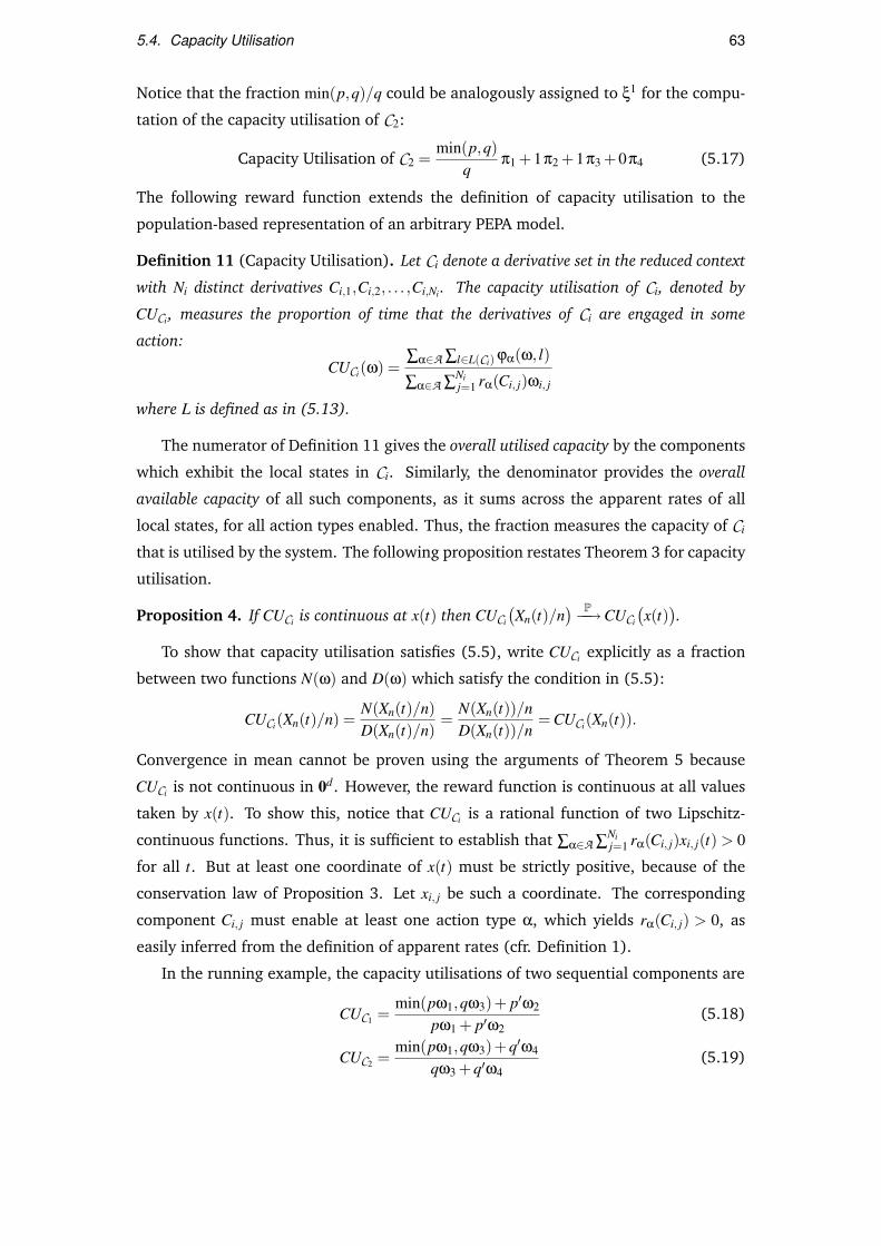
5.4. Capacity Utilisation 63
Notice that the fraction min(p,q)/q could be analogously assigned to ξ1 for the compu-
tation of the capacity utilisation of C2:
Capacity Utilisation of C2 =min(p,q)
qπ1 +1π2 +1π3 +0π4 (5.17)
The following reward function extends the definition of capacity utilisation to the
population-based representation of an arbitrary PEPA model.
Definition 11 (Capacity Utilisation). Let Ci denote a derivative set in the reduced context
with Ni distinct derivatives Ci,1,Ci,2, . . . ,Ci,Ni . The capacity utilisation of Ci, denoted by
CUCi , measures the proportion of time that the derivatives of Ci are engaged in some
action:
CUCi(ω) =∑α∈A ∑l∈L(Ci) ϕα(ω, l)
∑α∈A ∑Nij=1 rα(Ci, j)ωi, j
where L is defined as in (5.13).
The numerator of Definition 11 gives the overall utilised capacity by the components
which exhibit the local states in Ci. Similarly, the denominator provides the overall
available capacity of all such components, as it sums across the apparent rates of all
local states, for all action types enabled. Thus, the fraction measures the capacity of Ci
that is utilised by the system. The following proposition restates Theorem 3 for capacity
utilisation.
Proposition 4. If CUCi is continuous at x(t) then CUCi
(Xn(t)/n
) P−−→CUCi
(x(t)
).
To show that capacity utilisation satisfies (5.5), write CUCi explicitly as a fraction
between two functions N(ω) and D(ω) which satisfy the condition in (5.5):
CUCi(Xn(t)/n) =N(Xn(t)/n)D(Xn(t)/n)
=N(Xn(t))/nD(Xn(t))/n
= CUCi(Xn(t)).
Convergence in mean cannot be proven using the arguments of Theorem 5 because
CUCi is not continuous in 0d . However, the reward function is continuous at all values
taken by x(t). To show this, notice that CUCi is a rational function of two Lipschitz-
continuous functions. Thus, it is sufficient to establish that ∑α∈A ∑Nij=1 rα(Ci, j)xi, j(t) > 0
for all t. But at least one coordinate of x(t) must be strictly positive, because of the
conservation law of Proposition 3. Let xi, j be such a coordinate. The corresponding
component Ci, j must enable at least one action type α, which yields rα(Ci, j) > 0, as
easily inferred from the definition of apparent rates (cfr. Definition 1).
In the running example, the capacity utilisations of two sequential components are
CUC1 =min(pω1,qω3)+ p′ω2
pω1 + p′ω2(5.18)
CUC2 =min(pω1,qω3)+q′ω4
qω3 +q′ω4(5.19)

64 Chapter 5. Computing Performance Indices from Fluid Models
0 20 40 60 80 1000
0.2
0.4
0.6
0.8
1
NQ
Cap
acity
Util
isat
ion
q = 1.0q = 2.0
(a) C1
0 20 40 60 80 1000
0.2
0.4
0.6
0.8
1
NQ
Cap
acity
Util
isat
ion
q = 1.0q = 2.0
(b) C2
Figure 5.3: Markovian capacity utilisations for Example 1
As a practical application, Fig. 5.3a shows a steady-state capacity utilisation (5.18)
in the Markovian setting with respect to the parameters q and NQ. Two values for the
rate q were considered, i.e., 1.0 and 2.0, and NQ was varied between 1 and 100. All the
other parameters of the system were set as follows: p = 1.0, p′ = 100.0,q′ = 50.0 and
NP = 10. Here, the utilisation increases in the region 1≤ NQ ≤ 10 because the ten com-
ponents C1 are increasingly likely to find C2 to cooperate with. Clearly, when NQ > 10
the probability of finding an available C2 component is so high that the capacity of C1 is
fully utilised. Figure 5.3b shows the sensitivity analysis of (5.19). Qualitatively, the tra-
jectory of the two curves is in agreement with the intuition that, as NQ increases, each
of the sequential components is less utilised on average. A particularly interesting point
is NQ = 10, i.e., there are as many C1 as C2 components. When q = 1.0 they have the
same rate for the shared action, and the high capacity utilisation (i.e., 0.992) obtained
in this case highlights that each pair is very likely to be engaged in the synchronised
activity. However, the same model with q = 2.0 yields a capacity utilisation of about
50%—this is explained by the fact that the capacity of C2 is twice as much as that of C1.
5.5 Average Response Time
Throughput and capacity utilisation are meaningful performance metrics at every time
point of the system. Indeed, it is possible to define the notion of peak and minimum
across a finite time interval, or to normalise these metrics with respect to the time-frame
of interest, e.g. as in (5.2). Instead, the notion of average response time discussed in
this section can only be applied to systems under equilibrium conditions because it is
based on Little’s law [110], providing the response time as a function of a specific kind
of location-aware throughput and of the steady-state population levels of the model’s

5.5. Average Response Time 65
Figure 5.4: Schematic representation of the system used for the application of Little’s law to
PEPA models
sequential components.
5.5.1 Little’s Law
In its general formulation, Little’s law considers a system under steady-state conditions
with L users, arriving at rate λ and subject to an average waiting time W . The law
states that
L = λW. (5.20)
Here, this relation is used to determine W = L/λ, i.e., the average response time is
estimated from the computation of population levels and action throughputs, which
can be obtained as discussed in the previous sections. A slightly simpler formulation of
Little’s law requires the computation of only one estimate and may be applied for closed
systems such as in Fig. 5.4. The system comprises a total population of N users. The
arrival rate for service is λ, the average service time is W , and each user spends some
time Z between successive admissions into the system. Under steady-state conditions,
the following holds
N = λ(Z +W ) (5.21)
which can be used to give W = N/λ− Z. Note that (5.21) is obtained by applying
(5.20) to the system comprising the thinking stations and the service, observing that
the waiting time is the sum of the average waiting times in the two sub-systems. This
expression requires the calculation of λ, since N and Z are model parameters.
The PEPA model of Example 1 can be thought of as an instance of the system consid-
ered in Fig. 5.4. The thinking stations are represented by the number of components
which exhibit the local derivative P′, whilst the service centre comprises the compo-
nents which exhibit the local derivatives P, Q, and Q′. The total number of users is
N = NP, and the average thinking time Z = 1/p′. Finally, the arrival rate at the service

66 Chapter 5. Computing Performance Indices from Fluid Models
S1
S2 S3
S1
S2
t1
t2
t3
t4
t5
t6 t7
t8t9
Figure 1: Test
1
Figure 5.5: Derivation graph of a sequential component. The local derivatives are partitioned
into S = S1,S2 and S = S1,S2,S3, interpreted as the component being inside and outside the
system, respectively. Thus, transitions t3 and t7 are paths of entry into the system. Conversely,
the system is exited via t8
centre λ is calculated as the steady-state action throughput of α2. Thus, the average
response time can be calculated as follows
W =NC
T hα2(∞)− 1
p′. (5.22)
This formulation can be applied to both semantics, and the throughput can be calcu-
lated as discussed in Section 5.3. Interestingly, many descriptions of user behaviour in
concurrent systems are amenable to this form of analysis:
Asynchronous Send
α→ Send → α
Synchronous Send
α→ Send → Receive→ α
Send/Reply
α→ Send → Receive→ Reply→ α
where Send, Receive, and Reply may express suitable synchronisation activities with
communication partners to model message exchange. In all cases a user is modelled
as a cyclic sequential component in which one local derivative, e.g., P′, is interpreted
as the user being outside the system whilst all the other derivatives are associated with
actions performed within the system.
Such a syntactic structure of the user component has been assumed in previous
work on this topic (e.g., [45]), though it cannot be used for more complex user de-
scriptions. For instance, Fig. 5.5 shows the derivation graph of one such sequential
component, in which multiple paths of entry and exit are defined. The following section
is concerned with the development of a general formulation for the average response
time which does not require any assumption for the applicability of the analysis.
5.5. Average Response Time 67
5.5.2 General formulation
Let Ci be the component of the reduced context representing the user with respect to
whom the average response time is to be computed. Let Si ⊂ Ci,Si 6= /0 be the subset of
derivatives which indicate the presence of the user in the system, Si induces a binary
partition Si,Si. The derivatives in Si denote the states in which the user is outside
the system. Let µli and µl
i be the subsets of the jump vector l corresponding to the
population levels of Si and Si, respectively. By the population-based semantics of PEPA,
the number of non-zero elements in µli ∪ µl
i can be either zero or two. There cannot
be only one non-zero element because this would imply an increase (resp., decrease)
in the population level of some derivative without a corresponding decrease (resp.,
increase) in the population level of some other derivative. However, this is clearly
not allowed by the fact that the derivation graphs of the sequential components are
strongly connected—the dynamic creation or destruction of sequential components is
not possible. These non-zero elements must be −1 and +1, because the transition
records unitary changes in the population levels. Thus, there are five cases according
to the location of the non-zero elements:
• −1,+1 6∈ µli ∪ µl
i indicates a jump in which the population levels of Ci are not
affected (for instance, an independent action performed by some other sequential
component in the system).
• −1,+1 ∈ µli indicates a transition within the system in which the user is en-
gaged.
• −1,+1 ∈ µli is the symmetric case in which user is engaged, though the activity
takes place outside the system.
• −1 ∈ µli and +1 ∈ µl
i represents the departure of one user from the system,
as the population level of some component in Si is decreased by one, with a
corresponding increase observed for the population of some component in Si.
• −1 ∈ µli and +1 ∈ µl
i is the subset of jumps of interest with respect to the
computation of the average response time, as it represents the arrival of users
into the system. The population level of some component in Si is increased by
one, and, correspondingly, the population of some component in Si is decreased.
The set of jumps for the sequential component in Fig. 5.5 is shown in Table 5.1. The
following two definitions specify how to calculate the throughput of arrivals and the
average number of users in a PEPA model.

68 Chapter 5. Computing Performance Indices from Fluid Models
Table 5.1: The set of subvectors µli and µl
i for the sequential component in Fig. 5.5. Transi-
tions t3 and t7 indicate the entry of a user into the system, because a population level in µli is
incremented by one and, correspondingly, a population level in µli is decreased by one.
Transitionµl
i µli
Si1 Si
2 Si1 Si2 Si3
t1 0 0 −1 +1 0
t2 0 0 −1 0 +1
t3 +1 0 −1 0 0
t4 0 0 +1 −1 0
t5 0 0 0 −1 +1
t6 0 0 0 +1 −1
t7 0 +1 0 0 −1
t8 −1 0 +1 0 0
t9 +1 −1 0 0 0
Definition 12. The throughput of the arrivals of Si into the system, denoted by λSi , is the
sum of the throughputs, for all action types, across all transitions such that −1 ∈ µli and
+1 ∈ µli:
λSi(ω) = ∑α∈A ,−1∈µl
i ,+1∈µli
ϕα(ω, l) (5.23)
Definition 13. The average number of users in the system, denoted by LSi , is
LSi(ω) = ∑Ci, j∈Si
ωi, j (5.24)
Using the same arguments as in Theorem 5, the following proposition holds.
Proposition 5. λSi(Xn(t)/n) E−−→ λSi(x(t)),LSi(Xn(t)/n) E−−→ LSi(x(t)), for any Si ⊂ Ci,Si 6= /0.
Based on this result, the following approximation for the calculation of the fluid
response time will be used:
LSi(x(t))λSi(x(t))
≈ E [LSi(Xn(t)/n)]E [λSi(Xn(t)/n)]
=E [LSi(Xn(t))]/nE [λSi(Xn(t))]/n
=E [LSi(Xn(t))]E [λSi(Xn(t))]
(5.25)
where the first equality follows directly from Definitions 12 and 13, and the rightmost
fraction corresponds to the definition of average response time for the n-th Markov
chain of the family of PEPA models. As stated above, although this calculation is in
principle applicable to any time point, it is only meaningful under steady-state con-
ditions. In Example (1), the partition Si = P,Si = P′ gives rise to the following

5.6. Numerical Validation 69
0 10 20 30 40 500
20
40
60
80
NP
Ave
rage
Res
pons
e T
ime
q’=0.2q’=2.0
Figure 5.6: Markovian average response time calculation for Example 1
definitions of LSi and λSi for the average response time of C1
LSi(ω) = ω1 (5.26)
λSi(ω) = p′ω2 (5.27)
Figure 5.6 shows an example of (CTMC-based) average response time calculation for
this model, experimenting with population levels of C1 ranging from 1 to 50 and two
values for rate q′. In all cases NQ was kept fixed at 10. As expected, the response
time does not change significantly when the population level of C1 is less than that of
C2. By contrast, a dramatic increase is observed when the number of C1 components
is significantly more than the number of C2 components. Clearly, increasing q′ reduces
the response time although it does not impact on its qualitative behaviour.
5.6 Numerical Validation
This section presents numerical validations of the performance metrics introduced in
the previous sections, and is divided in two parts. Section 5.6.2 is concerned with the
validation of Example 1. Section 5.6.3 examines a more complex model, which has the
following features:
• Use of the choice operator to describe alternative behaviour.
• More structured system equation, comprising five sequential components and a
pattern of composition similar to that described in Section 5.3.1.
• Faster rate of state-space growth.
• Unlike Example 1, the average response times cannot be calculated using the
simplified formulation (5.21).

70 Chapter 5. Computing Performance Indices from Fluid Models
5.6.1 Methodology
The model descriptions were parametrised by the activity rates and the population
level density. A set of 200 model instances is obtained by assigning randomly chosen
parameters drawn from uniform distributions. The objective of this approach is to mea-
sure the quality of the deterministic approximation on a broad spectrum of behaviours,
from models which exhibit poor indices (i.e., low capacity utilisation or high average
response times) to those with good performance. Each model instance was analysed
stochastically for three scale factors. As the state space size grows very quickly with this
parameter, the choice of the actual scale factors used in those tests strongly depended
on the feasibility of the solution of the CTMCs.
The validation regarded performance estimates at equilibrium—this is necessary
for the computation of average response times whereas steady-state measures were
just taken as representative conditions for the calculation of throughput and capacity
utilisation since any other time point shows similar behaviour. Detection of steady-state
regime of the differential process was based on a condition of relative error between
two successive ODE integration steps. A tolerance of 1× 10⁶ was used in this study.
Stochastic simulation was carried out using the method of batch means.
5.6.2 Validation of Example 1
The instances of this model were obtained by drawing from uniform distributions in
[0.1,50] for all rates (i.e., p, p′,q,q′) and considering densities of the kind (A,0,B,0),
where A and B were chosen at random in 1,2, . . . ,5. This choice implies that the
initial local states of the two derivatives are P and Q, respectively. The scale factors
used in this validation were 1,10,50. For example, a model with density (2,0,1,0)
was analysed three times, each with the following initial population levels: (2,0,1,0),
(20,0,10,0), and (100,0,50,0). Thus, the model instance with the largest state space
has 63001 states, obtained with scale factor n = 50 and density (5,0,5,0) (the rate
parameters have no impact on the size of the CTMC).
Table 5.2 shows the average approximation errors for some performance indices
defined in the previous sections. The results confirm that better agreement is obtained
as the scaling factor is increased. In this example, the approximation is already sat-
isfactory at n = 1, and it is excellent at n = 50 (with an average error of less than 1%
for all performance indices). Finally, Table 5.3 shows the number of model instances
whose approximation error is less than 5%, demonstrating that the quality of the error
is consistent across all model instances.

5.6. Numerical Validation 71
Table 5.2: Average approximation errors for Example 1 over a sample of 200 model instances
n T hα1 CUC1 CUC2 W
1 4.87% 7.84% 7.87% 8.43%
10 0.51% 1.22% 1.11% 1.28%
50 0.08% 0.21% 0.19% 0.01%
Table 5.3: Number of the 200 model instances of Example 1 with error less than 5%
n T hα1 CUC1 CUC2 W
1 147 106 112 131
10 196 189 188 191
50 200 200 200 200
5.6.3 A More Complex Model
This model comprises the description of two distinct classes of users, C1 and C2, de-
fined as follows (alongside the definitions are the corresponding coordinates in the
population vector):
ξ1 C1 :Thinkdef= (think,(1−p)pdb t1).C1 :UseDb
+ (think,(1−p)p′db t1).C1 :UseCpu
+ (think,pt1).C1 :Think′
ξ2 C1 :UseCpudef= (useCpu,c1).C1 :Think
ξ3 C1 :UseDbdef= (useDb,d1c1).C1 :Think
ξ4 C1 :Think′def= (think, t′1).C1 :UseCpu
ξ5 C2 :Thinkdef= (think,qdb t2).C2 :UseDb
+ (think,q′db t2).C2 :UseCpu
ξ6 C2 :UseCpudef= (useCpu,c2).C2 :Think
ξ7 C2 :UseDbdef= (useDb,d2c2).C2 :Think
The use of the choice operator in C1 : Think and C2 : Think allows the specification of
conditional behaviour. The action think is performed at rates t1 and t2 by C1 and C2
respectively. With probability p, C1 moves into a second thinking state, C1 :Think′. With
probability 1−p the component may behave either as C1 :UseDb, with probability pdb,
or as C1 :UseCpu, with probability p′db = 1−pdb. The behaviour of C2 is similar, although

72 Chapter 5. Computing Performance Indices from Fluid Models
the second thinking process is not exhibited. Both components may perform the actions
useDb and useCpu although with different local rates. Specifically the rates of useDb are
expressed as ratios, i.e., d1 and d2, of the rates of useCpu. If d1 < 1 then the behaviour
of C1 is such that it requires longer data-bound activities. Conversely, if d2 > 1 then C2
carries out longer (i.e., slower) CPU-bound operations. The states UseCpu and UseDb of
the two classes of components are synchronisation points with the following two-state
server components
ξ8 Cpu :Executedef= (useCpu,c).Cpu :Log
ξ9 Cpu :Logdef= (log, lc).Cpu :Execute
ξ10 Db :Executedef= (useDb,d).Db :Log
ξ11 Db :Logdef= (log, ld).Db :Execute
The action type log represents a synchronising activity with the component
ξ12 Logger :Logdef= (log, l).Logger :Log
The resource-sharing nature of this activity is captured by the composition
(Cpu :Execute ‖ Db :Execute) BClog
Logger :Log (5.28)
Finally, the description of the whole system under study combines (5.28) with the user
components
Systemdef= (C1 :Think[NC1 ] ‖ C2 :Think[NC2 ])
BCuseCpu,useDb
((Cpu :Execute[NC] ‖ Db :Execute[ND])
BClog
Logger :Log[NL])
(5.29)
The densities used for this validation were of the form (A,0,0,0,B,0,0,C,0,D,0,E),
where A,B,C,D,E were chosen randomly in 1,2,3. As in Section 5.6.2, the rate
values were drawn from uniform distributions in [0.1,50]. The ratios d1 and d2 were
drawn from uniform distributions in [0,1] and [1,10], respectively. The following reward

5.6. Numerical Validation 73
functions were used for the validation:
T huseCpu(ω) = min(c1ω2 + c2ω6,cω8)
CUCpu(ω) =min(c1ω2 + c2ω6,cω8)+ lcω9
cω8 + lcω9
T huseDb(ω) = min(d1c1ω3 +d2c2ω7,dω10)
CUDb(ω) =min(d1c1ω3 +d2c2ω7,dω10)+ ldω11
dω10 + ldω11
LC1(ω) = ω2 +ω3
λC1(ω) = (1−p)t1ω1 + t′1ω4
LC2(ω) = ω6 +ω7
λC2(ω) = t2ω5
(5.30)
where Ci = Ci :UseCpu,Ci :UseDb , i = 1,2. LC1 and λC1 (respectively, LC2 and λC2) are
combined as in (5.25) for the calculation of the average response time WC1 (respectively,
WC2). The throughput measures refer to the aggregate throughput of the actions useCpu
and useDb, but similar results could be obtained by considering the location-aware
throughputs of the two distinct classes of users.
This model is computationally more demanding than Example 1. Table 5.4 shows
the size of the state space for different configurations, suggesting that the analytical
solution of the CTMC with scale factors n = 10 and n = 50, as conducted in the previous
model, is impractical. For these factors, the CTMC was solved by simulation, using the
approach described in [24]. Each model instance was simulated until the confidence
interval of the equilibrium distribution dropped below 5% of the statistical mean. The
accuracy of this simulation set-up was assessed by computing the approximation errors
of the performance indices with both the simulated results and the numerical solutions
of the CTMC for the equilibrium distribution, for scale factors n = 1, n = 2, and n = 3.
(The largest CTMC has 1210000 states and is obtained for A = B = C = D = E = 3
and n = 3.) The comparison between the approximation errors computed with the
simulated results and those obtained by numerical solution, reported in Tables 5.5 and
5.6, show good agreement, although stochastic simulation generally overestimates the
error.
These results also confirm the behaviour observed in the validation of Example 1,
as the error decreases with larger scale factors. This is further supported by the calcu-
lation of the approximation errors (using stochastic simulation only) for scale factors
n = 10, n = 20, and n = 50, as shown in Tables 5.7 and 5.8, which show very good
accuracy for a large fraction of model instances at n = 50. The nature of the approxi-
mation is examined in more detail in Fig. 5.7, which plots the error of T huseCpu for all
tests, tracking the three worst model instances for each scale factor. Perhaps unsur-
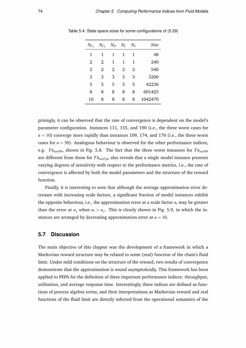
74 Chapter 5. Computing Performance Indices from Fluid Models
Table 5.4: State space sizes for some configurations of (5.29)
NC1 NC2 ND NC NL Size
1 1 1 1 1 48
2 2 1 1 1 240
2 2 2 2 2 540
3 3 3 3 3 3200
5 5 5 5 5 42236
8 8 8 8 8 601425
10 8 8 8 8 1042470
prisingly, it can be observed that the rate of convergence is dependent on the model’s
parameter configuration. Instances 111, 155, and 190 (i.e., the three worst cases for
n = 10) converge more rapidly than instances 109, 174, and 176 (i.e., the three worst
cases for n = 50). Analogous behaviour is observed for the other performance indices,
e.g. T huseDb, shown in Fig. 5.8. The fact that the three worst instances for T huseDb
are different from those for T huseCpu also reveals that a single model instance presents
varying degrees of sensitivity with respect to the performance metrics, i.e., the rate of
convergence is affected by both the model parameters and the structure of the reward
function.
Finally, it is interesting to note that although the average approximation error de-
creases with increasing scale factors, a significant fraction of model instances exhibit
the opposite behaviour, i.e., the approximation error at a scale factor ni may be greater
than the error at n j when ni > n j. This is clearly shown in Fig. 5.9, in which the in-
stances are arranged by decreasing approximation error at n = 10.
5.7 Discussion
The main objective of this chapter was the development of a framework in which a
Markovian reward structure may be related to some (real) function of the chain’s fluid
limit. Under mild conditions on the structure of the reward, two results of convergence
demonstrate that the approximation is sound asymptotically. This framework has been
applied to PEPA for the definition of three important performance indices: throughput,
utilisation, and average response time. Interestingly, these indices are defined as func-
tions of process algebra terms, and their interpretations as Markovian reward and real
functions of the fluid limit are directly inferred from the operational semantics of the

5.7. Discussion 75
Table 5.5: Comparison between the approximation errors of the performance indices in (5.30)
computed with numerical solution of the CTMC (columns labelled with NUM) and stochastic
simulation (columns labelled with SIM)
Performance indexn = 1 n = 2 n = 3
NUM SIM NUM SIM NUM SIM
T huseCpu 11.96% 12.35% 5.95% 6.15% 3.99% 4.40%
T huseDb 15.20% 15.71% 7.41% 7.73% 4.85% 5.78%
CUCpu 14.81% 14.83% 9.38% 9.36% 7.01% 7.00%
CUDb 21.36% 21.39% 12.70% 12.83% 9.25% 9.39%
WC1 32.66% 32.52% 20.00% 19.90% 14.45% 14.79%
WC2 23.67% 23.70% 14.83% 15.02% 11.06% 11.33%
language. Owing to the formality of the language, these results of convergence are not
tied to a particular PEPA model, but they hold in general.
The quality of the agreement between the Markovian reward and the correspond-
ing deterministic estimate for finite scale factors depends on the structure of the model.
The simple model of Example 1 shows excellent approximation at n = 50, where all
randomly generated instances have a percentage relative error less than 5%. This is
obtained by analysing small-sized CTMCs (i.e., no larger than 63000 states), which
gives confidence on the accuracy for larger population levels. Similar results are ob-
served for the model in Section 5.6.3, which shows a much more severe state-space
explosion problem. A comparison between the results from simulation and those from
the numerical solution of the CTMC confirms that the stochastic simulation approach
adopted for the validation of this model is accurate.
Unfortunately, theoretical bounds such as those discussed in Section 4.5.2 do not
apply to the performance indices discussed in this chapter because functions of Markov
chains do not in generally enjoy the Markov property [85,98]. However, the numerical
results presented here confirm the validity of ODE analysis for the estimation of indices
of performance. Importantly, this kind of analysis is possible at a very low computa-
tional effort: for the model in Section 5.6.3 at n = 3, the average execution time for
the analysis of the ODE model was 0.35s on an ordinary desktop machine, as opposed
to over 13s required for the numerical solution of the CTMC and the calculation of the
reward. One should expect longer execution times for the evaluation of the transient
probability distribution over a large time interval, and dramatic growth on memory and

76 Chapter 5. Computing Performance Indices from Fluid Models
Table 5.6: Number of model instances with approximation error less than 5%, computed using
the numerical solution of the CTMC for the equilibrium distribution (columns labelled with NUM)
and stochastic simulation (columns labelled with SIM)
T huseCpu T huseDb CUCpu CUDb WC1 WC2
n NUM SIM NUM SIM NUM SIM NUM SIM NUM SIM NUM SIM
1 79 78 66 63 76 78 55 54 52 46 46 48
2 119 122 105 103 109 110 80 80 84 84 80 80
3 145 140 137 130 123 121 106 102 97 96 97 94
Table 5.7: Approximation errors of the performance indices in (5.30). The Markovian rewards
are computed by stochastic simulation
n T huseCpu T huseDb CUCpu CUDb WC1 WC2
10 1.78% 2.57% 2.62% 3.59% 5.06% 5.27%
20 1.45% 2.35% 1.59% 2.31% 3.06% 3.55%
50 1.16% 1.78% 0.91% 1.30% 2.16% 2.25%
time requirements for the analysis of larger CTMCs. Alternatively, resorting to stochas-
tic simulation leads to a drastic reduction of memory footprint, though this is offset by
heavier time requirements to obtain a statistically significant number of samples. In-
deed, the average execution time for the simulation and the calculation of performance
indices of a model instance in Section 5.6.3 was about 2000s, i.e., about five orders of
magnitude slower than the deterministic evaluation.
The extraction of fluid performance measures from PEPA has been considered in [25],
where the authors introduce a slight variant to the language in order to be able to ex-
Table 5.8: Number of model instances with approximation error less than 5%. The Markovian
rewards are computed by stochastic simulation
n T huseCpu T huseDb CUCpu CUDb WC1 WC2
10 177 168 165 159 146 150
20 188 171 183 171 173 164
50 196 183 196 189 179 178

5.7. Discussion 77
0 50 100 150 2000
5
10
15
Experiment Number
Per
cent
age
Rel
ativ
e E
rror
←155 ←190 ←111
(a) Scale factor n = 10
0 50 100 150 2000
5
10
15
Experiment Number
Per
cent
age
Rel
ativ
e E
rror
←155 ←183
←190
(b) Scale factor n = 20
0 50 100 150 2000
5
10
15
Experiment Number
Per
cent
age
Rel
ativ
e E
rror
←109
←174 ←176
(c) Scale factor n = 50
Figure 5.7: Validation of T huseCpu
press time-to-absorption measures. The comparison against the corresponding stochas-
tic analysis is only empirical and does not make use of properties of convergence be-
tween the two interpretations. By contrast, the throughput and average response-time
calculations presented in [45] and [43] can be shown to be embodied in the present
framework.

78 Chapter 5. Computing Performance Indices from Fluid Models
0 50 100 150 2000
5
10
15
20
25
Experiment Number
Per
cent
age
Rel
ativ
e E
rror
←174
←111
←125
(a) Scale factor n = 10
0 50 100 150 2000
5
10
15
20
25
Experiment Number
Per
cent
age
Rel
ativ
e E
rror
←31 ←189 ←174
(b) Scale factor n = 20
0 50 100 150 2000
5
10
15
20
25
Experiment Number
Per
cent
age
Rel
ativ
e E
rror
←43
←103
←89
(c) Scale factor n = 50
Figure 5.8: Validation of T huseDb

5.7. Discussion 79
0 50 100 150 2000
10
20
30
40
50
60
Experiment Number
Per
cent
age
Rel
ativ
e E
rror
n=10n=20n=50
(a) T huseCpu
0 50 100 150 2000
10
20
30
40
50
60
Experiment Number
Per
cent
age
Rel
ativ
e E
rror
n=10n=20n=50
(b) T huseDb
0 50 100 150 2000
10
20
30
40
50
60
Experiment Number
Per
cent
age
Rel
ativ
e E
rror
n=10n=20n=50
(c) CUCpu
0 50 100 150 2000
10
20
30
40
50
60
Experiment Number
Per
cent
age
Rel
ativ
e E
rror
n=10n=20n=50
(d) CUDb
0 50 100 150 2000
10
20
30
40
50
60
Experiment Number
Per
cent
age
Rel
ativ
e E
rror
n=10n=20n=50
(e) WC1
0 50 100 150 2000
10
20
30
40
50
60
Experiment Number
Per
cent
age
Rel
ativ
e E
rror
n=10n=20n=50
(f) WC2
Figure 5.9: Experiments ordered by decreasing approximation error at n = 10 (solid line). A
percentage of model instances shows greater approximation errors with increasing scale factors


Chapter 6
Relating Layered Queueing Networks
and PEPA
As discussed in Chapter 2, one of the major advantages in using queueing models is the
availability of computationally efficient and scalable solution methods based on mean-
value analysis (MVA) for the evaluation of performance indices such as throughput,
utilisation and response time of hardware/software systems. In the paper by Herzog
and Rolia [90], this is related to the features of stochastic process algebras. The two
modelling techniques are presented as achieving orthogonal goals. Despite the compu-
tational advantage, queueing networks require a somewhat fixed level of abstraction
because the system is expressed at the level of processing resources and users that
queue for service. On the other hand, the small yet powerful set of primitives of pro-
cess algebras may capture the typical behaviour of software systems more naturally. For
example, a unit of computation may be associated with a prefix, conditional branching
may be represented by the choice operator, looping may be obtained by recursion, and
passing the locus of control may be indicated with cooperation. At the cost of a typ-
ically more expensive computation, process algebra models may yield a very accurate
and detailed representation of the system under study, and the range of quantitative
and qualitative characteristics is usually wider.
In light of the theoretical developments presented in the previous chapters of this
thesis, the relationship between process algebras and queueing models may be con-
sidered from a different perspective. The interpretation of a PEPA model against the
deterministic differential semantics aims at achieving efficiency improvements analo-
gously to the use of MVA methods in queueing networks. It is therefore of interest to
examine whether a process-algebraic interpretation of a model using the same level
of abstraction as a queueing network yields benefits with regard to the efficiency and
the accuracy of the quantitative analysis. Specifically, this chapter relates PEPA to the
81

82 Chapter 6. Relating Layered Queueing Networks and PEPA
Layered Queueing Network (LQN) model. The LQN semantics of layered multi-class
servers, resource contention, multiplicity of threads and processors are given an inter-
pretation in terms of components of a PEPA model in such a way that the benefits of the
deterministic approximation are best exploited—i.e., independent replicas of the same
LQN entity are represented as independent copies of the same sequential components.
The soundness of the translation is validated through a case study of a distributed
computer system and the numerical results are used to discuss the relative strengths
and weaknesses of the different forms of analysis available in both approaches, i.e.,
simulation, MVA, and differential approximation.
Section 6.1 gives an overview of the LQN model. Section 6.2 presents a methodol-
ogy for mapping LQN elements into PEPA processes, covering many important features
such as multiplicity of classes of servers, multithreaded and multiprocessor compu-
tation, synchronicity of service requests, and the fork/join paradigm for concurrent
behaviour. It also discusses how to obtain corresponding indices in the PEPA model
for utilisation and average response time. The overall methodology—which is general
and thus can be implemented for automatic translations—is practically applied to a
case study of a distributed system. In Section 6.3, this model is used to validate the
translation and compare all forms of analysis available for the two techniques on the
basis of accuracy, computational cost, and richness of the result set. Finally, concluding
remarks are presented in Section 6.4.
6.1 Overview of Layered Queueing Networks
This section gives an informal overview of the LQN model by means of a running ex-
ample. The reader is referred to [68] (and the rich bibliography therein) for a more
detailed treatment. Figure 6.1 shows a LQN of a distributed application which fea-
tures all of the elements considered in this chapter. Servers (called tasks) are drawn
as stacked parallelograms and their multiplicity is indicated within angular brackets
alongside the task’s name. For instance, File Server<1> denotes one single thread of
execution for the file server. A task is deployed onto a processor, depicted as a circle
connected to the task. Concurrency levels for processors are denoted similarly to tasks.
Distinct kinds of services (called entries) exposed by a task are represented by small
parallelograms drawn inside the task. Each entry is associated with an execution graph
consisting of atomic units of computation called activities, drawn as rectangles. Ac-
tivities are arranged through operators for sequencing (directed arrows), conditional
branching/merging (small circle with the + symbol) and fork/join synchronisation
(small circle with the & symbol). Each activity is characterised by a service time

6.1. Overview of Layered Queueing Networks 83
Figure 6.1: LQN model of a distributed application.

84 Chapter 6. Relating Layered Queueing Networks and PEPA
demand on the processor with which the task is associated, indicated within square
brackets. For the sake of graphical convenience, execution graphs which consist of a
single activity are not explicitly drawn, and the activity’s execution demand is directly
shown within the associated entry. In Figure 6.1 only the execution graphs of entry
visit and buy are drawn. The former models an activity which accesses some cached
information, after which it performs an internal activity with probability 0.95, or a
more expensive external activity with probability 0.05. In the entry buy, after prepare
is performed the two activities packaging and shipping are executed in parallel. When
they both finish, display is executed.
Layering of services is modelled by means of requests made from an activity to an
entry in another task in the network. Requests are indicated by directed arrows and
may be of two kinds: synchronous, with closed arrowheads, and asynchronous, with
open arrowheads. Each request is labelled with a number between parentheses, which
gives the number of requests per execution. This can be interpreted deterministically
or as the mean of a geometric distribution. The total number of requests performed by
an activity determines the distribution of its execution demand. The total demand is
divided into slices whose duration is drawn from independent exponential distributions
with mean equal to the ratio between total execution demand and total number of
requests. The execution of one slice is interposed between successive requests to other
entries. Reference tasks are tasks which do not accept requests and they are used to
model system workload.
For entries which accept synchronous requests, their overall behaviour may be sub-
divided into two phases. The first phase models the computation carried out from the
receipt of the request until the reply to the caller. Such a reply is denoted as a dashed
arrow pointing to the activity’s entry. All the activities in the execution graph that
follow the replying entry are part of the second phase, indicating an autonomous con-
tinuation during which the caller is not blocked. Execution graphs consisting of two
activities such that each represents the behaviour of one phase can be conveniently
drawn in a compact form, as illustrated by write in Figure 6.1. The execution demand
for each phase is drawn inside the entry within square brackets. The requests from
multi-phase entries are labelled with pairs, in which the i-th element represents the
number of requests made by the activity in the i-th phase.
6.2 PEPA Interpretation of LQNs
The main rationale behind the PEPA interpretation of LQNs presented in this section
is to exploit the inherent concurrent behaviour of replicated tasks and processors, and

6.2. PEPA Interpretation of LQNs 85
Table 6.1: Summary of notation.
Symbol Meaning Variables
A Set of LQN activities a
E Set of LQN entries e
K Synchronicity type. K = sync,async k
P Set of LQN processors p
T Set of LQN tasks t
act(p) : P → 2A Set of activities executed on p
act−1(a) : A → P Process on which a is executed
dem(a) : A → R≥0 Total execution demand of activity a
ent(t) : T → 2E Set of entries in task t
mpr(p) : P → N Multiplicity of processor p
mtk(t) : T → N Multiplicity of task t
rep(a) : A → E The entry to which activity a replies (may be /0)
req(a) : A → 2E×N×K Set of requests made by activity a (e,n,k)
N(a) = ∑(e,n,k)∈req(a) n Total number of requests made during activity a
model those as copies of identical sequential components in the process-algebra model.
Thus, if T is the sequential component which describes the behaviour of a task thread,
then the whole server is described as T[N], where N is the multiplicity of the server
in the LQN model. The empty cooperation set between two copies of the same com-
ponent represents a reasonable assumption of independence between the behaviour of
two distinct threads of execution. Analogously, two distinct copies of the same proces-
sor will be assumed to behave independently from each other. Clearly, the main benefit
in using this form of replication of behaviour is that the model has a convenient NVF
representation, and, when interpreted against the population-based semantics, the size
and structure of the underlying differential equation is not dependent upon the ac-
tual population levels of the system. The interpretation of each LQN element is now
discussed in more detail. Table 6.1 summarises the notation used in this section.
6.2.1 Processor
The template for the translation of a single processor p is illustrated in Figure 6.2,
showing a cyclic two-state sequential component. The first state Procp models an activ-
ity which grants exclusive access to the processor. The rate ν for this action is assumed

86 Chapter 6. Relating Layered Queueing Networks and PEPA
Procpdef= (acquirep,ν).Execp
Execpdef= ∑
a∈act(p):dem(a)>0
(a,(N(a)+1)/dem(a)
).Procp
Figure 6.2: Translation of an LQN Processor.
PFileServer′def= (acquirepfs,ν).PFileServer′′
PFileServer′′def= (read,1/0.01).PFileServer′
+(write1,1/0.001).PFileServer′
+(write2,3/0.04).PFileServer′
+(get,1/0.01).PFileServer′
+(update,1/0.01).PFileServer′
Figure 6.3: Translation of PFileServer.
to be much faster than any other activity in the system. The impact of this rate on the
performance results will be examined in Section 6.3.1.
The second state Execp enables all the actions corresponding to the activities which
are executed on p, by means of the choice operator. Each activity phase is mapped onto
a distinct action type in PEPA and the rate of execution reflects the fragmentation of the
computation into slices. For any activity a, the rate of execution of a slice is denoted by
s(a) and it is equal to (cfr. process Execp in Figure 6.2):
s(a) =
(N(a)+1)/dem(a) if dem(a) > 0
0 if dem(a) = 0
Notice that this interpretation produces a concise description for a processor, whose
number of sequential components does not depend upon the distinct classes of service
enabled. For example, the translation of a PFileServer is shown in Figure 6.3. The
activity rate 3/0.04 for write2 is determined as the total number of computation slices
(i.e., 3, because the corresponding entry makes two external requests) divided by the
total execution demand, i.e., 0.04 time units.
6.2.2 Activity and Request
An LQN activity subsumes a sequence of PEPA prefixes, whose length is determined
by the number of outgoing requests and their synchronicity. A synchronous call is

6.2. PEPA Interpretation of LQNs 87
Acta1
def= Acqa.Acta2
Actai+1
def=
Synca,ei . · · · .Synca,ei︸ ︷︷ ︸
ni
.Actai+2 if ki = sync
Asynca,ei . · · · .Asynca,ei︸ ︷︷ ︸ni
.Actai+2 if ki = async
(ei,ni,ki) ∈ req(a), for all 1≤ i < |req(a)|
CASE rep(a) = /0:
Acta|req(a)|+2
def= Enda
CASE rep(a) 6= /0:
Acta|req(a)|+2
def= ∑
(replya′,rep(a),ν).Enda|∃(e,n,k) ∈ req(a′) : e = rep(a),∀a′ ∈ A
Figure 6.4: Translation of an LQN Activity.
modelled with a sequence of two prefixes which model the request and the reply. The
PEPA action type for the request has the form requesta,e, where a is the activity from
which the request originates and e is the entry called by a. Similarly, the action type for
the reply has the form replya,e. An asynchronous call is represented with a single prefix
of type requesta,e.
The PEPA process corresponding to the LQN activity interposes executions of slices
of a between requests. The rates for requests and replies are here set to ν, i.e., it is
assumed that the delay for message exchange is negligible with respect to the execution
demands on the processors. With respect to the LQN interpretation, this means that
the rate of transition of jobs between queues is very fast (although not instantaneous
as per the classical assumption in queueing networks). The following snippets of PEPA
descriptions will be useful for the translation of an activity:
Acqa ≡
(
acquireact−1(a),ν)
.(a,s(a)) if s(a) > 0
ε if s(a) = 0
Synca,e ≡ (requesta,e,ν) .(replya,e,ν) .Acqa
Asynca,e ≡ (requesta,e,ν) .Acqa
where Acqa models the access to a processor and the execution of a slice of activity a. It
is an empty string ε if the activity has no execution demand (with the usual properties
of concatenations of empty strings with arbitrary PEPA definitions). Synca,e and Asynca,e
model the sequences of prefixes for synchronous and asynchronous requests (followed
by slice executions), respectively.

88 Chapter 6. Relating Layered Queueing Networks and PEPA
FIRST PHASE
Write′1def= (acquirepfs,ν).(write1,1/0.001).Write′2
Write′2def= (replysave,write,ν).EndWrite′
SECOND PHASE
Write′′1def= (acquirepfs,ν).(write2,3/0.04).Write′′2
Write′′2def= (requestwrite2,get,ν).(replywrite2,get,ν).(acquirepfs,ν).(write2,3/0.04).Write′′3
Write′′3def= (requestwrite2,update,ν).(replywrite2,update,ν).(acquirepfs,ν).(write2,3/0.04).EndWrite′′
Figure 6.5: Translation of activity write.
The translation of an LQN activity is shown in Figure 6.4. The first process definition
Acta1 models the first slice execution. If the activity replies to a synchronous request then
the last constant models the replies. The corresponding action types are given by all
LQN activities which make requests to the entry in which a is executed. The constant
Enda is left unspecified and it is defined according to the structure of the LQN, as
discussed in Section 6.2.3. As a concrete application, the translation of write is given
in Figure 6.5. Recalling the semantics of implicit activity invocation, write represents
two distinct activities, here denoted by write1 and write2. Activity write1 does not
make requests to the lower-level server but it replies to requests to entry write made
by get. Activity write2 is the autonomous continuation which makes two synchronous
requests to the entries get and update of task Backup.
6.2.3 Execution Graph
The interpretation of execution graphs follows the rationale behind the translation of
UML activity diagrams into PEPA models presented in [146]. (The reader is referred to
that paper for a detailed algorithmic description.) This section presents a conceptual
view of the approach, focussing on the main differences with respect to the original
work. The analogue of a UML action node in the LQN context is an activity, which rep-
resents the atomic unit of computation in an execution graph. However, while an action
node is translated into a single PEPA prefix, an activity is translated into a sequential
component with several local derivatives. Nevertheless, the two representations have
in common that they exhibit some form of sequential computation. For the purposes of
the translation, this sequential behaviour may be collectively summarised by the two
PEPA constants that define the initial and the final state (i.e., Acta1 and Enda in the LQN
model). Such definitions are modified in order to combine distinct activities according

6.2. PEPA Interpretation of LQNs 89
to the semantics of the execution graph.
For activity/execution graphs, the translation algorithm identifies a number of con-
current control flows. Flows are created by means of fork nodes (called And-Forks in
the LQN model). For each entry there will be at least one flow, called the main flow,
which executes the initial activity of the entry’s execution graph. The overall model of
an execution graph can be written in the form Main BCL
S, where S is an arbitrary PEPA
process consisting of the sequential components which model the remaining control
flows, called secondary flows.
Precedence
The operator of precedence models the behaviour of one activity being executed after
the previous one terminates. It is visually represented by directed arrows connecting
two elements of the graph and it can also be implicitly defined by second-phase entries.
The notion of precedence in PEPA is represented by letting the final state of the preced-
ing element coincide with the initial state of the subsequent one. For instance, the two
phases of the entry write—represented in Figure 6.5 as two unrelated sequential com-
ponents with no notion of precedence relationship—are transformed into a sequence
of activities by letting EndWrite′def= Write′′1 (recall that EndWrite′ was left intentionally
unspecified for this purpose).
Probabilistic Branching
The translation of probabilistic branching (called Or-fork in the LQN model) involves
manipulating all of the activities enabled in the final state of its predecessor and re-
trieving the information about the constant names which define the initial states of all
the successors of the node. According to the template for a basic activity in Figure 6.4,
cache is translated into a sequential component in the simple form
Cache1def= (acquireps,ν).(cache,1/0.001).EndCache.
Being the predecessor of a branching operator, its last activity cache is replaced with a
PEPA choice as follows:
(cache,1/0.001).EndCache→
(cache,0.95×1/0.001).Internal1
+(cache,0.05×1/0.001).External1
This component is capable of performing the activity cache at the original rate 1/0.001
(obtained as the sum of the two alternative behaviours), but with probability 0.95 and
0.05 it then behaves as one of its successors, i.e., Internal1 and External1, respectively.

90 Chapter 6. Relating Layered Queueing Networks and PEPA
Alternative behaviours may merge back into one (Or-join operator). This is trans-
lated in PEPA by letting all of the final states of the merging elements coincide with
the initial state of the merged behaviour. Or-join nodes are not used in the running
example.
Fork/Join Synchronisation
The presence of a fork/join synchronisation mechanism implies that an entry has ex-
plicit concurrent behaviour. This is captured in PEPA by assigning a sequential com-
ponent to each distinct concurrent control flow. Such flows perform the activities au-
tonomously and synchronise over action types corresponding to fork and join nodes in
the execution graph. A basic activity is uniquely assigned to one flow and the algorithm
keeps track of the initial state of all flows. This is necessary to define the constituting
sequential components in a cyclic manner. The initial activity of an entry’s execution
graph is said to start the main control flow of the entry. All subsequent activities are
executed within the same control flow as is the case for the entry visit. Conversely, the
entry buy has three control flows. In addition to the main one started by prepare, two
further are spawned by the fork operator. Their initial states are Prepare1, Pack1, and
Ship1, respectively defined as follows:
Prepare1def= (acquireps,ν).(prepare,1/0.01).EndPrepare
Pack1def= (acquireps,ν).(pack,1/0.03).EndPack
Ship1def= (acquireps,ν).(ship,1/0.01).EndShip
As with probabilistic branching, the translation of a fork operator takes as input the
set of activities enabled by the final state of the incoming flow and the set of initial
states of the spawned flows. Each activity in the former set is prefixed with a fork
activity, carried out at rate ν, indicating a negligible rate of spawning new processes.
Each state in the latter set is instead modified so as to have fork as the first enabled
activity. For instance, the PEPA component corresponding to the basic activity prepare
is modified to become
Prepare1def= (acquireps,ν).(prepare,1/0.01).ForkPrepare
ForkPreparedef= (fork1,ν).EndPrepare
where the subscript in the action fork1 is used to uniquely assign a type to each fork
node in the execution graph, for instance by mapping them into integers. Similarly,
Pack1 and Ship1 are prefixed with the fork1, i.e.,
Pack1def= (fork1,ν).(acquireps,ν).(pack,1/0.03).EndPack
Ship1def= (fork1,ν).(acquireps,ν).(ship,1/0.01).EndShip

6.2. PEPA Interpretation of LQNs 91
Figure 6.6: Activity diagram representing the behaviour of the PEPA components involved in a
LQN fork/join synchronisation
At a join, the algorithm resolves the unspecified final constants of its incoming flows,
by making them synchronise over a join activity (performed at rate ν) and subsequently
cycle back to the flows’ initial states. In the example,
EndPackdef= (join1,ν).Pack1
EndShipdef= (join1,ν).Ship1
An intuitive representation of the collective behaviour of the processes involved
in a fork/join synchronisation is shown in Figure 6.6, which presents a UML activity
diagram where each node is a PEPA derivative. The derivatives for forks and joins are
implicitly expressed by the vertical graphs in the diagram.
The translation of a join is also responsible for resolving the unspecified final con-
stant of the incoming flow at the matching fork, to capture the following semantics:
at a fork, the incoming flow of execution spawns as many flows as the number of suc-
cessors, and it is suspended until all of them have terminated; then, it behaves as the
flow corresponding to the outgoing edge at the matching join. In the example, the
component
Display1def= (acquireps,ν).(display,1/0.001).EndDisplay
models the behaviour of the outgoing edge of the join. The unspecified constant
EndPrepare is defined as follows:
EndPreparedef= (join1,ν).Display1
Overall Model of an Execution Graph
Finally, the complete model of an execution graph is represented as a composition of
all the flows’ sequential components, cooperating over the action types for forking and
joining. The definitions of the secondary flows are not modified any further, thus they
are instantiated with suitable replication according to the multiplicity of the task to
which the execution graph belongs. Instead, the definitions of the main flow will be
altered when translating an LQN task, during which its multiplicity will be adjusted. In

92 Chapter 6. Relating Layered Queueing Networks and PEPA
the example, the PEPA model of the execution graph for buy is:
Prepare1 BCL
(Pack1[2] BC
LShip1[2]
), L = fork1, join1
The overall behaviour of visit, consisting of a single flow of control is simply represented
by the flow’s initial state Cache1. In the remainder, the overall model of an execution
graph will be denoted by the component Maine BCLe
Sece, where Maine is the behaviour
of the main flow, without information on its multiplicity, and Sece comprises all the
secondary flows, with proper multiplicites. The cooperation set Le consists of fork/join
actions in which the main flow is involved throughout its execution. Under conditions
of balanced branching (i.e., each flow spawned at a fork eventually joins), only one
constant corresponding to the final behaviour of the main flow will be left unspecified—
for instance, Merge in visit, EndDisplay in Buy, and EndWrite′′ in write. For an entry e
such a constant will be denoted by Laste.
6.2.4 Task
A reference task, here denoted by t∗, has the same behaviour as its unique entry, de-
noted by e∗. Instead, a non-reference task is modelled as a PEPA process which initially
enables the activities corresponding to the invocations of all its entries, modelled as an
initial choice component. When one of these activities is chosen, the process behaves
as the initial state of the main flow of the execution graph corresponding to that entry.
Then, after all activities in that execution graph are performed, the task component
returns to its initial state in which any entry may be executed. The pattern of transfor-
mation of a task is shown in Figure 6.7. For instance, the complete translation of the
non-reference task FileServer is given in Figure 6.8. The entry read starts executing
upon the receipt of either of two messages from external or think, modelled as two
distinct prefixes in the initial choice which behave as the same component Read1 (the
actual behaviour of the entry is independent from the originator of the request).
6.2.5 Network
The complete LQN is represented by a PEPA cooperation which arranges all the com-
ponents as inferred above and introduces the concurrency levels for the entries’ main
flows and the processors. The pattern of translation is shown in Figure 6.9. The def-
inition Compt describes the overall behaviour of a multithreaded server with multiple
entries. The task behaviour Taskt (subsuming all the main flows of a task’s entries)
is instantiated with the concurrency level of the task. It is composed in parallel with
a number of other components, each collecting the behaviour of a secondary control

6.2. PEPA Interpretation of LQNs 93
REFERENCE TASK
Taskt∗def= Maine∗
Laste∗def= Taskt∗
NON-REFERENCE TASK
Tasktdef= ∑
(requesta,e,ν).Maine |∃(e,n,k) ∈ req(a) : e ∈ ent(t),∀a ∈ A
Laste
def= Taskt, for each e ∈ ent(t)
Figure 6.7: Translation of an LQN Task
FileServerdef= (requestexternal,read,ν).Read1
+(requestthink,read,ν).Read1
+(requestsave,write1 ,ν).Write′1
Read1def= (acquirepfs,ν).(read,1/0.01).EndRead
EndReaddef= FileServer
Write′1def= . . .
. . . (cfr. Figure 6.5)
EndWrite′′def= FileServer
Figure 6.8: Translation of task FileServer
Comptdef= Taskt[mtk(t)] BC
L
(Sece1
BC/0
Sece2BC
/0· · · BC
/0Sece|ent(t)|
)where L =
S|ent(t)|i=1 Lei , for all t ∈ T
LQNdef=
(Compt1
BCM
Compt2 · · · BCM Compt|T |
)BC∗(
Procp1 [mpr(p1)] BC/0
Procp2 [mpr(p2)] BC/0· · ·
BC/0
Proc|P |[mpr(p|P |)]),
where, M = ∗−S
p∈P acquirep.
Figure 6.9: Translation of a Layered Queuing Network

94 Chapter 6. Relating Layered Queueing Networks and PEPA
flow for each entry of the task. The cooperation sets between secondary flows of dis-
tinct entries are empty because no form of communication is possible between two
entries within the same task—an entry’s activity may only request service from another
task of the network. Conversely, Taskt is composed with all its secondary flows over a
cooperation set which includes all the fork/join action types in which the main flow of
any task’s entry is involved.
The definitions Compt are combined together using cooperation sets which can be
denoted by the same expression M. However, notice that the actual instantiations are
all different because of the dependence of the set ∗ upon the operands of the coopera-
tion. In fact, it is possible to show that all such sets are pairwise disjoint. Observe that,
by construction, all the acquirep action types are not contained in the sets M. Any pair
of components of type Compt does not exhibit the same action type for the execution of
a basic activity, since each activity belongs to only one task. The same fork/join action
type cannot be exhibited because these activities are executed within the same task, and
distinct fork/join nodes give rise to distinct action types in the PEPA model. Thus, the
only potential elements of M are the action types for message exchange requesta,e and
replya,e. The fact that sets with such action types are pairwise disjoint follows immedi-
ately from the uniqueness of activity and entry names in the LQN and can be proven
by structural induction. For an arbitrary composition of three components Compt, i.e.,
Compt1BC
MCompt2
BCM
Compt3 ,
component Compt1 may enable request/reply actions with subscripts (a′,e′), (a′′,e′′), . . . ,
where e′,e′′, . . . ∈ ent(t1) and a,b, . . . are basic activities. If some action with subscript
(a,e) was present in both cooperation sets then it would mean that both Compt2 and
Compt3 can perform the same basic activity a, which is a contradiction. Then, assuming
that the property holds for a cooperation among n > 3 components
Compt1BC
MCompt2
BCM
Compt3BC
M· · · BC
MComptn ,
in order to prove that it holds for n+1 components
Compt1BC
MCompt2
BCM
Compt3BC
M· · · BC
MComptn
BCM
Comptn+1 ,
it suffices to prove that the cooperation set M in position · · ·ComptiBC
MCompti+1 · · · is
disjoint from the cooperation set · · ·ComptnBC
MComptn+1 , for all 1 ≤ i ≤ n− 1. Suppose
that for some i ComptiBC
MCompti+1 has some action in common with the set in Comptn
BCM
Comptn+1 . This implies that the action must be a request/reply action with sub-
script (a,e), e ∈ ent(tn+1), because it belongs to the set ComptnBC
MComptn+1 , and that
e ∈ ent(ti+1), which is a contradiction because i + 1 6= n + 1 but one entry must belong
6.2. PEPA Interpretation of LQNs 95
to only one task. This property is of crucial importance because it guarantees that at
most two distinct components Compt synchronise for message exchange.
The group of task components is finally combined with the group of processors, each
taken with its own multiplicity. Processors do not cooperate with each other because
any execution slice must be performed on a single processor. However, the cooperation
set between all task components and all processors records the fact that any task may
be deployed on any processor, but the actual processor p which executes a given activity
a will be the only one which exhibits a in its state Execp (cfr. Figure 6.2).
The complete PEPA model for the LQN in Figure 6.1 is shown in Appendix B.
6.2.6 Performance Measures
This section is concerned with relating the notion of processor utilisation and average
response time defined in the LQN model to the corresponding performance indices
available from the analysis of the PEPA model. Such metrics will be used in Section 6.3
to quantitatively assess the soundness of the translation.
Utilisation
In the LQN model, utilisation is a performance measure which indicates the mean
number of busy processors at equilibrium. Hence, it is a value between zero and the
multiplicity of a processor. More fine-grained results can be obtained by computing
the distinct contributions from each of the activities which run on the processor. In
the PEPA model, the overall utilisation for a processor p is the mean number of com-
ponents which are in state Execp (cfr. Figure 6.2). However, this information alone is
not sufficient to obtain the contributions from each of the activities. In order to do so,
given an activity a ∈ act(p), it is necessary to compute the population levels of all the
sequential components which perform execution slices of a on the processor p. Then,
the processor utilisation due to the execution of a is given as the sum across all such
population levels. If an activity has two phases, the total contribution is the sum of the
contributions of each phase. For instance, the utilisation of processor PFileServer due
to the execution of write is obtained by inspection of the sequential components in Fig-
ure 6.5. The utilisation during the first phase is obtained as the number of sequential
components which behave as (write1,1/0.001).Write′2, whereas the utilisation during the
second phase is the sum of the population levels of the following three sequential com-
ponents: (write2,3/0.04).Write′′2, (write2,3/0.04).Write′′3, and (write2,3/0.04).EndWrite′′2.
It is worth noting that the estimation of processor utilisation is directly obtainable from
the components of the state descriptor in the NVF. Hence, this calculation does not

96 Chapter 6. Relating Layered Queueing Networks and PEPA
require the use of the reward structures discussed in Chapter 5.
Average Response Time
The LQN model provides the average response time for the execution of a task’s entry,
which denotes the overall time spent to carry out all of the basic activities of that entry,
including the time spent for requests to other servers in the network. Unlike LQN
utilisation, this metric cannot be derived directly from the NVF representation of PEPA.
However, it can be computed using the definition of average response time proposed in
Chapter 5. For instance, for the average response time for the entry visit, the following
local derivatives of the sequential component for Server are regarded as making up the
user population (cfr. Section 5.5.2):
Cache1def= (acquireps,ν).Cache′1
Cache′1def= (cache,0.95×1/0.001).Internal1 +(cache,0.05×1/0.001).External1
Internal1def= (acquireps,ν).(internal,1/0.001).Internal2
External1def= (acquireps,ν).(external,2/0.001).External2
External2def= (requestexternal,read,ν).(replyexternal,read,ν).
(acquireps,ν).(external,2/0.001).External3
(6.1)
This sequence of actions encompasses all of the basic activities carried out during the
execution of visit, but it does not include the time spent during the transmission of the
request and the reply messages (actions requestthink,visit and replythink,visit).
6.3 Validation
The model in Figure 6.1 was used to conduct a validation study on the quality of
the translation. The notion of accuracy used throughout this section is given by the
difference between the performance measure obtained from the LQN model and the
corresponding estimate (as discussed in Section 6.2.6) from the PEPA model, according
to the following definition of percentage relative error:
Error % =∣∣∣∣PEPA metric−LQN metric
LQN metric
∣∣∣∣×100.
This study considered all of the analysis techniques available in both formalisms,
with emphasis on the issue of scalability, i.e., the resilience of the solution methods to
increases in the size of the model under consideration. Here, scalability was studied
empirically by estimating the incremental cost (i.e., runtime) of solving models which
maintain the same topology but with increasingly large resource concurrency levels of
some of its components. The performance metrics of interest were:

6.3. Validation 97
Table 6.2: Sensitivity of rate ν in the PEPA model of Figure 6.1. First row: reference values.
Other rows: relative differences with respect to first row
ν U(PServer) U(write) W (visit)
Reference values
1.2×10⁸ 1.4763 0.3848 0.00364
Relative differences
1.2×10⁴ 1.6691% 1.6691% 5.2696%
1.2×10⁵ 0.1692% 0.1692% 0.5245%
1.2×10⁶ 0.0168% 0.0168% 0.0052%
1.2×10⁷ 0.0015% 0.0015% 0.0049%
• U(PServer), the overall processor utilisation of PServer.
• U(write), the contribution of action write to the processor utilisation of PFile-
Server.
• W (visit), the average response time for the entry visit.
The results were obtained with the PEPA Eclipse Plug-in (discussed in Chapter 7)
and the Layered Queueing Network Solver software package [125]. For statistical sig-
nificance, the execution times of all analyses presented here were averaged over ten
independent runs on an ordinary desktop machine.
6.3.1 Accuracy of the Translation
The exact form of analysis of PEPA models is the numerical solution of the underlying
Markov chain, which was compared against simulation of the LQN using the method
of batch means with automatic blocking and imposing a termination condition of 1%
radius at 95% confidence intervals. These are the parameters used for the simulation
of all LQN models. Given the rapid growth of the state space of the Markov chain with
increasing population sizes, the multiplicity of tasks and processors was kept low in
this validation study. However, insight into the sensitivity of the accuracy was given
by varying the execution demands in the model, which do not have an impact on the
cardinality of the state space.
A crucial element in the PEPA model is ν, the only parameter which has no coun-
terpart in the LQN model. Because of its semantics illustrated in the previous section,

98 Chapter 6. Relating Layered Queueing Networks and PEPA
ν is to be chosen such that the duration of the activities associated with this rate is
negligible with respect to all other activities in the system. Table 6.2 shows the results
of a sensitivity analysis conducted across an array of increasingly large values of ν. The
slowest rate considered for this analysis, i.e., 1.2× 10⁴, is equal to twenty times the
fastest individual rate in the LQN model (i.e., one slice execution of external). The
results in the table are reported as the percentage relative differences with respect to
the performance results of the model with ν = 1.2×10⁸. The error trends for the utilisa-
tion indices are similar and this may be due to the fact that both are linearly related to
the population levels of the system. The different behaviour for the average response
time may be due to a non-linear form “error propagation”, as it is computed as a frac-
tion of a linear function, i.e., the population levels of the users in the system, and a
generally non-linear function, as the throughput may contain minimum expressions).
Indeed, comparing the reference case with the model with ν = 1.2× 10⁴ showed that
the numerator of the fraction had an error of about 3.6%, whereas the denominator
had an error of about 1.67%. Further analysis on the nature of this approximation
was not conducted, but the results presented in this table were used to gain confidence
that even for relatively large values of ν the accuracy is very good, with discrepancies
considerably less than one percent in most cases.
The level of precision obtained for ν = 1.2× 10⁸ was used for the comparison be-
tween the numerical solution for the steady-state distribution of the CTMC of the PEPA
model and the stochastic simulation of the LQN model. The results are presented in
Table 6.3, which compares the two models for different execution demands and mul-
tiplicity of resources. Using the original concurrency levels, the accuracy improves by
reducing the rates of cache. This may be related to the fact that the entries of Server
have increasingly similar overall execution demands. Configurations A6 and A7, fea-
turing slightly larger population levels, present more accurate results. Overall, there is
good agreement between the two models, and despite the rather large numerical error
in some instances, their qualitative behaviour is compatible. The results show similar
error trends for the utilisation estimates U(PServer) and U(write). The accuracy for
W (visit) is consistently better, with errors less than 4% in all cases.
6.3.2 Comparison of Simulation Approaches
The evaluation of large-scale versions of this model cannot be based on explicit enu-
meration of the state space because of its exponential growth as a function of the
concurrency levels of the components. This section compares the stochastic simulation
of PEPA models against that of LQN networks. The CTMC derived from the population-
based semantics can be solved by Gillespie’s simulation algorithm [76], using an ap-

6.3. Validation 99
Table 6.3: Accuracy of the translation of the LQN in Figure 6.1 (numerical solution for the equi-
librium distribution of the CTMC in PEPA vs. simulation of the LQN). (a) Model configurations.
(b) Analysis results
Configuration Id Concurrency configurationExecution demands
dem(cache) dem(write1)
A1 Original Model 0.0001 0.0010
A2 Original Model 0.0010 0.0010
A3 Original Model 0.0100 0.0010
A4 Original Model 0.1000 0.0010
A5 Original Model 0.1000 0.0600
A6 All concurrency levels set to 2 0.0010 0.0010
A7 All concurrency levels set to 2 0.1000 0.0600
(a)
MeasureConfiguration
A1 A2 A3 A4 A5 A6 A7
U(P
Serv
er)
PEPA 1.4681 1.4763 1.5561 1.8465 1.5839 1.8440 1.7267
LQN 1.3029 1.3210 1.4002 1.7484 1.5047 1.6904 1.6851
Error 12.68% 11.76% 11.13% 5.61% 5.26% 9.09% 2.47%
U(w
rite
) PEPA 0.3894 0.3848 0.3462 0.1666 0.3486 0.4806 0.3801
LQN 0.3450 0.3433 0.3126 0.1572 0.3302 0.4407 0.3704
Error 12.86% 12.09% 10.75% 6.02% 5.56% 9.07% 2.60%
W(v
isit) PEPA 0.00276 0.00364 0.0126 0.1021 0.1028 0.00295 0.1019
LQN 0.00283 0.00376 0.0128 0.1022 0.1027 0.00307 0.1020
Error 2.47% 3.19% 1.41% 0.01% 0.13% 3.91% 0.16%
(b)

100 Chapter 6. Relating Layered Queueing Networks and PEPA
Table 6.4: Concurrency level configurations of the LQN model in Figure 6.1
ComponentConfiguration
B1 B2 B3 B4 B5
Client 2 10 50 200 1000
Server 2 2 8 20 100
FileServer 2 2 8 20 50
Backup 2 2 8 20 30
PClient 2 2 2 10 30
PServer 2 2 2 10 30
PFileServer 2 2 2 10 30
proach similar to that presented in [24]. For this study, five instances of the model in
Figure 6.1 were obtained by varying the multiplicity of tasks and processors, as listed
in Table 6.4. The simulation of the PEPA models was conducted using the same param-
eters of the LQN simulation, i.e., method of batch means terminating when the 95%
confidence levels were within 1% of the average of the observed quantities.
Table 6.5 shows the expectations of the three performance indices and the average
runtimes measured. The agreement improves with increasing population sizes, giving
approximation errors less than 5% in all instances except configuration B1. The results
confirm the correlation between the error trends of the utilisation estimates which was
observed in Table 6.3. The PEPA stochastic simulation algorithm is less sensitive to
the problem size. For instance, the largest model was about twice as costly as the
smallest one (whose population levels are about two orders of magnitude smaller),
as opposed to a corresponding increase by a factor of over 300 in the runtime of the
LQN simulation. However, in absolute terms LQN simulation was much faster than
PEPA simulation in the configurations B1 to B4, with runtimes of the same order of
magnitude only for configuration B5.
6.3.3 Comparison of Approximate Techniques
This section discusses the MVA approach for LQNs and the fluid-flow approximation of
PEPA based on ordinary differential equations. Similarly to the previous section, the
comparison considers the computational cost as well as the accuracy of these forms
of analysis using the model configurations listed in Table 6.4. The default parame-
ters of the LQN analytical solver were not satisfactory for this study, instead Conway’s

6.3. Validation 101
Table 6.5: Comparison of stochastic simulation approaches
MeasureConfiguration
B1 B2 B3 B4 B5U
(PSe
rver
)
PEPA 1.8437 1.8768 1.9986 9.9932 29.9792
LQN 1.6903 1.8030 1.9994 10.0000 30.0000
Error 9.07% 4.09% 0.04% 0.07% 0.07%
U(w
rite
) PEPA 0.47667 0.48976 0.51989 2.60831 7.81188
LQN 0.44096 0.46979 0.52066 2.60620 7.81970
Error 8.10% 4.25% 0.15% 0.08% 0.10%
W(v
isit) PEPA 0.0029626 0.0032327 0.0734965 0.028232 0.064852
LQN 0.0030678 0.0031620 0.0754888 0.027989 0.061714
Error 3.43% 2.23% 2.64% 0.87% 5.08%
(a) Performance estimates and percentage relative errors
ToolConfiguration
B1 B2 B3 B4 B5
LQN 42 s 106 s 420 s 2128 s 12864 s
PEPA 5165 s 3773 s 3757 s 8624 s 12115 s
(b) Execution times
algorithm [51] was used. Furthermore, as suggested in the user manual of the Lay-
ered Queueing Network Solver package [67], the solver option stop-on-message-loss was
turned on to deal with the asynchronous requests at Server. The differential equations
were numerically integrated using the Java implementation of the adaptive step-size
fitfh-order Dormand-Prince algorithm [61] provided by Patterson and Spiteri [119].
The algorithm was modified to detect convergence to equilibrium using the same ap-
proach discussed in Section 5.6.1: the termination condition was based on a criterion
of relative convergence, setting a threshold of 1×10⁻⁶ for the L1 norm of the difference
of the solution vectors of two successive integration steps. The initial-value problems
associated with these models were found to be stiff with respect to the values of ν.
The results presented in Table 6.6a were calculated for ν = 1.2× 10⁴. The simulation

102 Chapter 6. Relating Layered Queueing Networks and PEPA
Table 6.6: Comparison between MVA and differential-equation analysis (ν = 1.2×10⁴)
MeasureConfiguration
B1 B2 B3 B4 B5
U(P
Serv
er)
PEPA Value 1.98616 1.98616 1.98616 9.93082 29.7924
Error 17.50% 10.16% 0.66% 0.69% 0.69%
LQN Value 1.26297 1.38183 2.36364a 9.05149 24.235
Error 25.28% 25.36% 18.54% 9.48% 19.21%
U(w
rite
)
PEPA Value 0.517693 0.517690 0.517692 2.58845 7.76536
Error 17.40% 10.20% 0.57% 0.68% 0.69%
LQN Value 0.329205 0.360150 0.616152 2.35928 6.31687
Error 25.34% 23.34% 15.50% 9.47% 19.22%
W(v
isit) PE
PA Value 0.00391137 0.00391131 0.0840782 0.0306368 0.0662695
Error 27.50% 23.70% 11.38% 9.46% 7.38%
LQN Value 0.00830393 0.00975129 0.0543038 0.0120020 0.0241729
Error 170.68% 208.39% 28.06% 57.11% 60.83%
aThis is an inappropriate estimate because it exceeds the processor concurrency level, set to two. This
finding has been reported to the tool authors.
(a) Performance estimates and percentage relative errors calculated with respect to the simulation results
of the LQN shown in Table 6.5
ToolConfiguration
B1 B2 B3 B4 B5
LQN 0.26 s 0.26 s 0.62 s 2.72 s 19.96 s
PEPA 8.61 s 8.52 s 37.28 s 34.99 s 64.81 s
(b) Execution times

6.3. Validation 103
Table 6.7: Evaluation of the stiffness of the fluid-flow analysis with respect to ν. Runtime compar-
isons and relative errors between the PEPA performance calculated with ν = 1.2×10⁴ (shown
in Table 6.6a) and ν = 1.2×10⁵
ConfigurationRelative accuracy
Slow-down factorU(PServer) U(write) W (visit)
B1 0.62% 0.62% 0.23% 7.0
B2 0.62% 0.62% 0.20% 8.0
B3 0.62% 0.62% 0.64% 7.3
B4 0.62% 0.62% 0.57% 7.8
B5 0.62% 0.62% 0.60% 8.0
of the LQN was regarded as being the true model of the system, thus the reported
percentage errors were calculated with respect to the LQN estimates reported in Ta-
ble 6.5. In these instances, fluid-flow analysis is consistently more accurate than MVA.
The error trend of the fluid-flow approximation of PEPA reflects the findings presented
in Chapter 4 and 5, i.e., the approximation behaves better as the population sizes in
the system increase. The estimates of W (visit) are not fully satisfactory in both cases,
although the analysis with PEPA gives acceptable results (within 10%) for configura-
tions B4 and B5. The computational cost of fluid-flow analysis is low and independent
from the population sizes. The different execution times reported in Table 6.6b are due
to the different lengths of the transient period in the models (indeed, in all cases the
execution time for the integration of one time unit was about 3.7 seconds). To consider
the impact of the relatively low value of ν used, fluid-flow analysis was repeated for
ν = 1.2×10⁵. Table 6.7 reports the relative percentage accuracy and the increase in the
computational cost, measured as the ratio between the runtime for ν = 1.2×10⁵ and the
runtime for ν = 1.2×10⁴. This cost grows proportionally with the relative increase of ν.
However, given the negligible accuracy improvement, the model with ν = 1.2×10⁴ may
be considered to be a better candidate in the trade-off between accuracy and solution
efficiency.
In contrast to fluid-flow analysis, the execution runtimes for MVA were dependent
upon the system size, although they were in general significantly faster than fluid-flow
analysis (between about four and thirty times for configurations B1–B4 and executing
with comparable runtime for configuration B5). According to other experiences pub-
lished in the literature [68], models with such approximation errors as those reported

104 Chapter 6. Relating Layered Queueing Networks and PEPA
here can be considered as being problematic with respect to the applicability of MVA,
and in general one should expect more accurate results (i.e., within 5%). Nevertheless,
these slightly large approximation errors in such particularly unfavourable instances
are an adequate price to pay for the high efficiency of this solution technique.
6.4 Discussion
The interpretation of LQNs as PEPA process algebra models supports a generous subset
of the LQN model, including: synchronous and asynchronous request types, multi-
plicity of tasks and processors, two-phase activities, and execution graphs for the de-
scription of sequentiality, conditional branching, and fork/join synchronisation. Future
work will be concerned with extending this approach to other features not considered
here, such as looping in execution graphs, synchronisation based on quorum consensus
mechanisms, and forwarded replies (whereby the reply of one entry is delegated to
some other entry in the network). The interpretation of the request count parameter
corresponds to the deterministic semantics of the LQN model, i.e., the request is per-
formed exactly the number of times shown in the request label. This may be extended
to include requests with geometrical distributions. Furthermore, here all execution
demands are assumed to be distributed exponentially, although the LQN model sup-
ports activities with arbitrary variance. This extension can be included in the present
approach by using suitable phase-type distributions.
The numerical investigation suggests that the PEPA translation of LQN models of-
fers complementary rather than competing analysis techniques for the performance
evaluation of software systems. The original semantics of PEPA permits explicit enu-
meration of the complete state space of the model, enabling forms of analysis, e.g.,
model-checking, which do not require the solution of a performance model, but nev-
ertheless give insight into the qualitative behaviour of the system. In relatively small
models for which the numerical solution of the underlying Markov chain is feasible,
other indices of performance are possible beyond those considered in the LQN model.
For instance, the technology of stochastic probes for PEPA supports passage-time anal-
ysis in which complex passages over the Markov chain can be described using a rich
language based on regular expressions over the model’s process-algebraic terms [8].
As observed in Table 6.5, the rapid growth of the LQN simulation time with in-
creasing concurrency levels indicates that PEPA stochastic simulation is preferred for
the analysis of systems with many independent replicas, for which results are provided
with very good accuracy. Conversely, LQN simulation is the method of choice when the
multiplicities levels are relatively low, since the execution runtimes may be some orders

6.4. Discussion 105
0 0.5 1 1.5 20
5
10
15
20
25
30
35
40
Time
Utilis
atio
n
U(PClient)U(PSserver)U(PFileSystem)
Figure 6.10: Temporal evolution of the utilisation of the processors of configuration B5 over the
first two time units
of magnitude smaller. More interesting is the comparison between MVA and fluid-flow
analysis. Fluid-flow analysis behaved remarkably well in the instances analysed in Sec-
tion 6.3.3, especially in cases exhibiting components with an appreciable number of
replicas. Under these conditions, it gave sufficiently accurate estimates for the aver-
age response time W (visit) which proved otherwise difficult to approximate. Fluid-flow
analysis has stronger resilience to increases in the mutiplicity levels, since the runtime
span between configuration B1 and B5 is narrower than that observed for MVA. For
this reason it is more desirable than MVA for very large systems. In smaller models
fluid-flow analysis appears to be less advantageous because of its higher computational
cost. Nevertheless, it may be still preferred over MVA in situations where transient
measures of performance are required, as they can be extracted from the solution of
the differential equation over a finite time interval. This information can be used to
reason about different quantitative characteristics, such as warm-up periods (defined
as the time interval necessary to reach equilibrium from some initial condition) and
peak throughputs and utilisations. An example is shown in Figure 6.10, which plots
the temporal evolution of the utilisation of the processors over the first two time units
for the model configuration B5, clearly identifying PServer as the bottleneck of the
system since almost all (i.e., 29.74) of the available processors are kept busy after a
warm-up period of about 0.02 time units.


Chapter 7
Tool Support
The PEPA Eclipse Plug-in is the software toolkit for PEPA which implements the analysis
techniques presented in the previous chapters. It provides support for the modelling
process from the early stages of model development and debugging through to au-
tomating the experimentation process and culminating in visualisation of numerical
results in the form of graphs and charts [139, 141, 142, 143]. This chapter is con-
cerned with a detailed discussion of the tool, with focus on the design principles and
algorithms developed for the core functionality concerning Markovian and differential
analysis. Much effort has been devoted to addressing ease of maintainability and ac-
commodating further enhancement and reuse, as will be demonstrated by an overview
of third-party libraries and tools which have connections with the PEPA Eclipse Plug-in.
7.1 Overview
7.1.1 The Eclipse Framework
Eclipse is a software platform written primarily in Java. Initially developed by IBM, it
is now open source and is managed by the Eclipse foundation [63]. Eclipse comprises
a run-time environment (Equinox) compliant with the OSGi standard [118], based on
an extensible architecture. A plug-in is a software component that adds functionality to
Equinox. The Eclipse foundation has developed and made freely available a rich set of
plug-ins that deliver an integrated development environment (IDE) for this framework.
The IDE itself is extensible through the same plug-in mechanism; for instance, one of
the most popular plug-in projects for the Eclipse IDE is JDT [64], a powerful toolkit for
Java development. The IDE revolves around the notion of workbench, which represents
the main container of the Eclipse user interface. An Eclipse workspace contains a menu
bar, a tool bar, a status bar, and a collection of editors and views. The two latter
components are used as a presentation layer to some underlying business model. An
107

108 Chapter 7. Tool Support
Figure 7.1: Architecture of the PEPA Eclipse Plug-in. Beneath the human-readable component
name (in bold) is the Java namespace. The components within the rounded rectangle are
dependent upon the Eclipse platform whereas Pepato and PEPA Command Line are deployed
as standard Java packages.
editor is used to alter the underlying model of its registered types while a view presents
contextual information.
7.1.2 Architecture of the PEPA Eclipse Plug-in
The PEPA Eclipse Plug-in comprises contributions to the Eclipse platform for the de-
velopment and the analysis of PEPA performance models. Its architecture, depicted
in Fig. 7.1, is organised as a set of components which perform various PEPA-related
tasks. In the spirit of Eclipse, the PEPA Eclipse Plug-in exhibits loosely coupled intra-
and inter-component interaction, which allows for clear separation of interfaces from
their implementations and provides a robust framework for interchangeability.
The central element of the PEPA Eclipse Plug-in is Pepato, discussed in Section 7.2, a
pure Java library which exposes an application programming interface for all of the core
modelling tasks. Pepato may be accessed via a command-line interface, particularly use-
ful to reduce the memory footprint of the graphical user interface when analysing larger
models. When developing for Eclipse, it is a recommended practice to separate out core
functionality of a service and its contributions to the user interface into (at least) two
distinct plug-ins. This allows the core functionality to be used in a context in which

7.2. Pepato 109
the user interface is not necessary or even not available. Eclipse Core exposes Pepato to
the platform, and its main role is to provide a mapping between files managed within
Eclipse and PEPA-related objects. In particular, it is based on the Eclipse Resources
plug-in, which implements a file-system layer for the Eclipse workspace on top of the
native file system of the underlying operating system. This facilitates the management
of events related to changes in the state of workspace files. For example, listeners may
be installed on files to be notified when a file being edited is saved. Eclipse Core regis-
ters listeners for PEPA model files, which trigger the automatic execution of the PEPA
parser and the static analysis routines when the model is saved. The plug-in Common
has similar ancillary nature. It provides necessary support to the other plug-ins of the
system, encapsulating pieces of commonly-used functionality such as routines for path
manipulation, services that handle the progress of long-running tasks, and frameworks
for plotting tools. EMF Support provides a meta-model of PEPA for the Eclipse Modelling
Framework, which may be used for data interchange and meta-model transformation
within the platform [2]. The plugin Eclipse UI, discussed in Section 7.3, provides all of
the elements for the graphical user interface of the PEPA Eclipse Plug-in, including a
text editor for PEPA models and several related views for displaying analysis results.
A user manual and a developer guide are provided in HTML format through PEPA
Help, as an extension of the Eclipse Help system. This is the standard mechanism for
documenting plug-ins in Eclipse, which has two major benefits for the user: i) the
documentation for all the installed plug-ins is located in a central repository, easily
accessible from the IDE; and ii) the user interface can be enriched with hot-keys and
hyperlinks to the relevant pages.
7.2 Pepato
The class diagram in Fig. 7.2 shows the components of Pepato discussed in this section.
The main access point to the library is the facade class (cfr. [71]) PepaTools. The root
object is Model, the abstract syntax tree of a PEPA model, which can be either generated
from a text file via the method PepaTools.parse, or created directly as an in-memory
model via the programming interface. The complete document object model of PEPA
is shown in Fig. 7.3. Static analysis of the model description is available through the
method doStaticAnalysis, whose details are discussed at length in Section 7.2.2. The
support classes OptionMap and IProgressMonitor are used extensively throughout the
library. The former acts as a centralised resource for storing user-accessible settings
such as solver types and parameters whereas the latter offers an interface for controlling
long-running operations such as the exploration of the state space and the numerical

110 Chapter 7. Tool Support
Figure 7.2: Architecture of Pepato.
7.2. Pepato 111
solution of the underlying mathematical representation.
The method PepaTools.getBuilder returns an instance of IStateSpaceBuilder
which may be invoked for the explicit enumeration of the state space of the model. The
implementation Builder and its associated object MarkovianExplorer are discussed
in Section 7.2.3.3. A state-space builder returns an instance of IStateSpace, which
represents the central interface for Markovian analysis in Pepato. Steady-state analysis
of the underlying Markov chain is accessible via the method PepaTools.getSolver.
The architecture for differential analysis follows an analogous route. The method
PepaTools.getParamGraphBuilder returns an instance of IParamGraphBuilder which
is responsible for the computation of the underlying parametric derivation graph of the
PEPA model, represented by the interface IParametricDerivationGraph. The imple-
mentation ParamGraphBuilder, similar in spirit to the Markovian analogue Builder, is
discussed in Section 7.2.6. The most notable method of a parametric derivation graph
is getFunctions, which returns the list of generating functions of the model. These are
used within the method PepaTools.getODESolver to create an instance of IODESolver.
In contrast to ISolver, the solution of the differential equation returns the time-course
trajectory. Therefore, the solve method accepts an interface ICallback, which is noti-
fied of any time point computed during the numerical integration.
7.2.1 Concrete Syntax
The concrete syntax accepted by the tool is here presented by means of a running
example, which is shown in Fig. 7.4. Its main features are listed below.
• Rate declarations and action types must start with a lowercase letter. They may
contain underscores and digits.
• Process declarations must start with an uppercase letter. They may also contain
underscores and digits.
• Arithmetic expressions are supported in declarations of rates and activities. The
usual operators +, -, *, / are supported with the obvious semantics.
• The model’s system equation is implicitly given by the last unnamed declaration
in the model description. The PEPA combinator is implemented by specifying the
cooperation set between angular brackets <>.
• Comments follow the style of the C/C++ language, i.e., // followed by a line
termination character, or enclosed by /* and */.
• Arrays of processes are specified in the form Process[N], where N is a natural
number. The symmetry reduction algorithm implemented in the PEPA Eclipse

112 Chapter 7. Tool Support
Figure 7.3: Document object model of PEPA.
Plug-in exploits the isomorphism between these processes to construct the lumped
Markov processes. In addition, an array may have the form Process[param],
where Process is a process identifier and param is a parameter identifier which
can be evaluated to a natural. This format is to be used should the modeller
require performing sensitivity analysis over different sizes of the array.
7.2.2 Static Analysis
Static analysis is used for checking the well-formedness of a model and detecting po-
tential problems as early as possible in the modelling life cycle, particularly prior to
inferring the derivation graph of the system. Basic checks include detection of unused
declarations of rates and processes, or process identifiers which are used but never de-

7.2. Pepato 113
/* Parameter declarations */
p = 0.1;
q = 2.0;
r = 0.2 * q;
s = 3.0;
t = 4.0;
u = 5.0;
v = 6.0;
w = 7.0;
n cpu = 4; // Array length parameter
/* Sequential component Process */
Process1 = (think, p * q).Process2 + (think, (1 - p) * q).Process3;
Process2 = (use cpu, r).Process1;
Process3 = (use db, s).Process1;
/* Sequential component CPU */
CPU1 = (use cpu, t).CPU2;
CPU2 = (reset cpu, u).CPU1;
/* Sequential component DB */
DB1 = (use db, v).DB2;
DB2 = (reset db, w).DB1;
/* System equation */
Process1[8] <use cpu, use db> ((CPU1[n cpu] <> DB1[4]) / <reset cpu,reset db>)
Figure 7.4: Concrete syntax accepted by the PEPA Eclipse Plug-in.
fined.1 Other less straightforward static analysis is concerned with the detection of:
(i) potential local deadlocks, i.e., the inability of a sequential component to engage
in a shared activity; (ii) transient local derivatives of sequential components; and (iii)
unnecessary declarations of action types in cooperation and hiding sets. In order to
perform these checks, the model’s abstract syntax tree is iteratively walked to create
two support data structures: complete action type set and used constant set.
Definition 14 (Complete Action Type Set). The complete action type set of a PEPA com-
ponent P, denoted by act(P), is the set of all action types which may be carried out by P
1It is worthwhile noting that rate identifiers must be declared before use. However, there is no suchrule with regard to process identifiers, so as to allow seamless description of recursive behaviour.
114 Chapter 7. Tool Support
during its evolution. It is recursively defined as follows:
act(A)
= act(P), if A def= P
act((α,r).P
)= α∪act
(P)
act(P+Q
)= act
(P)∪act
(Q
)act
(P BC
LQ
)= act
(P)∪act
(Q
)act
(P/L
)= act
(P)−L
Syntactic Abbreviation Incidentally, the function act is also used to compile out the
special cooperation set <*>. For instance, P <*> Q is replaced with P <L> Q, where
L = act(P)∩act
(Q
), i.e., the two processes are enforced to cooperate over all common
action types.
Definition 15 (Used Constant Set). The used constant set of a PEPA component P, de-
noted by def (P), is the set of all PEPA constants which are visited by P during its evolution.
It is recursively defined as follows:
def(A)
= A∪def(P), if A def= P
def((α,r).P
)= def
(P)
def(P+Q
)= def
(P)∪def
(Q
)def
(P BC
LQ
)= def
(P)∪def
(Q
)def
(P/L
)= def
(P)
For instance, the following sets are computed for each process definition of the
model in Fig. 7.4:
act(Process1
)= act
(Process2
)= act
(Process3
)= think,use cpu,use db
act(CPU1
)= act
(CPU2
)= use cpu,reset cpu
act(DB1
)= act
(DB2
)= use db,reset db
def(Process1
)= def
(Process2
)= def
(Process3
)= Process1,Process2,Process3
def(CPU1
)= def
(CPU2
)= CPU1,CPU2
def(DB1
)= def
(DB2
)= DB1,DB2
Definition 16 (Potential Local Deadlock). A component P BCL
Q is said to have a potential
local deadlock on α ∈ L if α 6∈ act(P)∩act
(Q
)and α ∈ act
(P BC
LQ
).
The definition of a potential local deadlock captures a condition that may occur
when either P or Q cannot proceed because they may perform an action α ∈ L but the
synchronising partner does not exhibit α. For instance, consider (α,r).(β,s).P BCβ
Q,

7.2. Pepato 115
for any P and Qdef= (γ, t).Q. Clearly, β satisfies the condition of local deadlock and
indeed, after the left-hand side of the cooperation performs the independent action
α, (β,s).P BCβ
Q executes (independent) γ-actions only. The condition is not sufficient
to conclude that one cooperating process does not ever enable any transition. For
instance, let Pdef= (α,r).P+(β,r).P. Now, P BC
βQ has a potential local deadlock on β, but
the top-level process interleaves α- and γ-actions indefinitely. Furthermore, note that
a cooperation without potential local deadlock may lead to an actual deadlock, i.e., it
may not enable any transition, as is the case in P BCα,β
Q where Pdef= (α,r).(β,s).P and
Qdef= (β, t).(α,u).Q.
Definition 17 (Redundant Action). An action α ∈ L is said to be redundant in P/L if
α 6∈ act(P). Similarly, α ∈ L is redundant in P BC
LQ if α 6∈ act
(P BC
LQ
).
For instance, β is redundant in P/α,β, Pdef= (α,r).P and in P BC
α,βQ where Q
def=
(α,s).Q. It is interesting to note that a non-redundant action may never be enabled by
a process. For instance, consider the following model:
P1def= (α,r).P2 +(β,s).P2
P2def= (α,r).P1
Q1def= (α, t).Q2
Q2def= (α, t).Q1 +(β,u).Q1
The component P1 BCα,β
Q1 only enables a α-transition to P2 BCα,β
Q2, which in turn enables
another α-transition to P1 BCα,β
Q1, without ever carrying out a β-action.
Transient Local Derivatives Consider the model component P1 defined as follows:
P1def= (α,r).P2
P2def= (β,s).P3
P3def= (γ, t).P2
(7.1)
This system initially performs an activity of α and then alternates activities of type β
and γ. In this sense, P1 is said to be a transient local derivative. Such a situation can be
statically checked via the procedure described in Algorithm 1. The set of process iden-
tifiers T returns those which are flagged as transient local derivatives. The inequality
X 6= A in line 3 is to be intended as a lexicographical relation between the identifiers.
Hence, it is possible that the behaviour of a transient local derivative may still be ob-
served indefinitely — e.g., consider again (7.1) where P3def= (α,r).P2. This performs
activity α at rate r without ever returning to derivative P1.
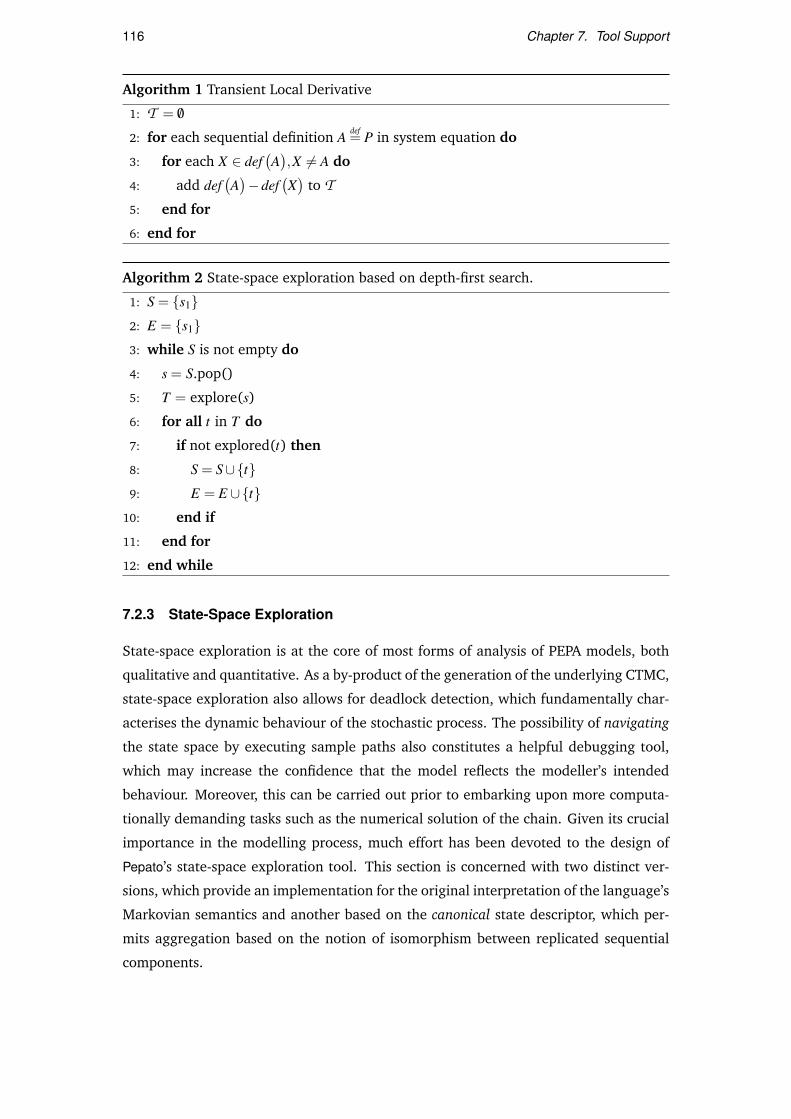
116 Chapter 7. Tool Support
Algorithm 1 Transient Local Derivative
1: T = /0
2: for each sequential definition Adef= P in system equation do
3: for each X ∈ def(A),X 6= A do
4: add def(A)−def
(X)
to T5: end for
6: end for
Algorithm 2 State-space exploration based on depth-first search.
1: S = s12: E = s13: while S is not empty do
4: s = S.pop()
5: T = explore(s)
6: for all t in T do
7: if not explored(t) then
8: S = S∪t9: E = E ∪t
10: end if
11: end for
12: end while
7.2.3 State-Space Exploration
State-space exploration is at the core of most forms of analysis of PEPA models, both
qualitative and quantitative. As a by-product of the generation of the underlying CTMC,
state-space exploration also allows for deadlock detection, which fundamentally char-
acterises the dynamic behaviour of the stochastic process. The possibility of navigating
the state space by executing sample paths also constitutes a helpful debugging tool,
which may increase the confidence that the model reflects the modeller’s intended
behaviour. Moreover, this can be carried out prior to embarking upon more computa-
tionally demanding tasks such as the numerical solution of the chain. Given its crucial
importance in the modelling process, much effort has been devoted to the design of
Pepato’s state-space exploration tool. This section is concerned with two distinct ver-
sions, which provide an implementation for the original interpretation of the language’s
Markovian semantics and another based on the canonical state descriptor, which per-
mits aggregation based on the notion of isomorphism between replicated sequential
components.

7.2. Pepato 117
7.2.3.1 Exploration by depth-first search
Pepato explores the state space of a model by employing depth-first search according to
Algorithm 2. The initial state s1 is extracted from the model’s definition, and is used to
initialise a stack S and a set of explored states E. For each state s popped off the stack,
the set of its reachable states T is computed by applying the semantic rules of PEPA.
Finally, if a reachable state t ∈ T has not been explored, then it is pushed onto S. The
algorithm terminates when the stack S is empty.
7.2.3.2 State representation
Given the two-level grammar supported by Pepato, the cooperation structure of the
system equation is static across the entire state space, hence it needs not be recorded
in the state descriptor. This property leads to a more parsimonious representation
consisting of an array of PEPA components, whose length, here denoted by NC, is equal
to the number of sequential components declared in the system equation. Without
loss of generality, the remainder of this section assumes a system equation comprising
at least of the cooperation operator. For any model, the value of NC is determined
by visiting the binary cooperation tree representing the system equation and counting
its leaves. The correspondence between an element of the array and its location in
the cooperation tree is maintained by assuming a fixed visit policy of the tree (in the
following, this will be pre-order traversal).
For instance, the initial state s1 of the model in Fig. 7.4 is represented as follows:
s1 = [Process1,Process1,Process1,Process1,Process1,Process1,Process1,Process1,
CPU1,CPU1,CPU1,CPU1,DB1,DB1,DB1,DB1]
This process enables a transition think enabled by the leftmost sequential component
Process1, which subsequently behaves as Process2. The state descriptor of the target
process is thus
[Process2,Process1,Process1,Process1,Process1,Process1,Process1,Process1,
CPU1,CPU1,CPU1,CPU1,DB1,DB1,DB1,DB1],
in which all but the first identifier are unchanged. (Clearly, since any Process1 in s1
may perform the same action, this will give rise to eight distinct transitions consisting
of all the permutations of the sub-vector [Process2,Process1,Process1,Process1,Process1,
Process1,Process1,Process1] of the first eight coordinates of the state descriptor.)

118 Chapter 7. Tool Support
Notation In the remainder of this chapter the following notation will be used. A state
of the underlying Markov chain is denoted by si, 1≤ i≤ NS. (The tool supports Markov
chains of finite size, and a sufficient condition for this is given by the use of the two-
level grammar [92].) The sequential component at position j in state si will be denoted
by si, j, 1≤ j ≤ NC.
7.2.3.3 Bottom-up exploration
The rules of PEPA in the Structured Operational Semantics style can be naturally im-
plemented as a recursive algorithm. For instance, in order to determine the derivatives
of a cooperation, those of the two cooperating components need to be computed, lead-
ing to a recursion which exits when the derivative of a prefix is to be computed (i.e.,
the axiom of the semantics). In a similar fashion, the computation of apparent rates
may also be carried out recursively. This approach corresponds to a top-down visit of
the cooperation tree—from the top-level cooperation operator to the sequential com-
ponents at each leaf. However, PEPA models obtained by the two-level grammar are
such that the cooperation structure of a state—hence, the structure of the recursion
stack for its exploration—is fixed throughout the state-space exploration process. For
this reason, the two-level grammar lends itself well to an alternative sequential version
of the exploration algorithm which statically records the cooperation structure of the
model and determines the derivatives of the components in the reverse order of the re-
cursive structure. This is the approach that will be discussed in detail here. It is termed
the bottom-up exploration algorithm because the cooperation tree is visited from the
leaves (i.e., the constituting sequential components) up to the root (i.e., the top-level
cooperation denoting the system equation).
A diagram with the most relevant classes employed by the algorithm is depicted in
Fig. 7.5 (cfr. also Fig. 7.2 for a larger context). The first-step derivatives are stored
as arrays of MarkovianTransition instances, holding a reference to the action iden-
tifier, the target process and the transition rate, represented as a Java primitive type
double. Passive apparent rates are encoded as negative doubles, whose absolute val-
ues correspond to the passive weights. A MarkovianStructuralElement is an abstract
representation of an element of the cooperation structure of the system equation.
The current process to be explored associated with a structural element is manipu-
lated using the methods getState and setState. The method getDerivatives returns
the first-step derivatives of the current process associated with the structural element
(held in the field derivatives) and the apparent rates are accessed using the methods
getApparentRate and setApparentRate. PEPA’s hiding operator is not represented as
a subclass of MarkovianStructuralElement, rather a hiding set may be associated with

7.2. Pepato 119
Figure 7.5: Class diagram of the data structures used for the bottom-up state space deriva-
tion. The prefix Markovian is used in some class names to explicitly distinguish them from the
analogous classes used for the extraction of the differential equation model, as discussed in
Section 7.2.6
the hidden process using the hidingSet field. A leaf in the cooperation tree is repre-
sented by an instance of MarkovianComponent. A crucial piece of information held in
this class is the index of the state descriptor associated with the sequential component,
accessed via the methods getIndex and setIndex. An instance of MarkovianOperator
corresponds to a cooperation operator in the system equation and holds references to
the cooperation set and the two operands. The method compose is called to calculate
the apparent rates and the derivatives of the cooperation given the current operand
references.
Set-up The instantiation of the model’s structural elements and their ordering for
sequential computation are carried out during an initialisation phase of the algorithm,
which is also responsible for the construction of the state descriptor of the Markov
chain. The system equation is visited in a top-down pre-order manner. An instance
of MarkovianOperator is created for each cooperation node visited and pushed onto a
stack SO. A MarkovianComponent is created for each sequential component, associated
with the proper coordinate of the state descriptor via setIndex, and appended to a list
LC. When the visit terminates, the state descriptor is generated as an array of the same
size as LC, each element of which is uniquely mapped to a leaf in the system equation.
The elements of SO are popped off the stack and inserted into a list LO such that the

120 Chapter 7. Tool Support
first element of the list is the last visited operator during the exploration of the system
equation. Since the first operator has clearly two sequential components as its children,
it is possible to compute its derivatives and apparent rates without recursion. Similarly,
when those are calculated, the second operator of LO has the necessary information
to compute its own apparent rates and derivatives, and so on until the last operator
of LO, the top-level cooperation in the system equation, is visited. In the remainder,
the elements of LO are denoted by ok, 1 ≤ k ≤ NMO and the elements of LC by c j,
1≤ j ≤ NMC.2
The initialisation phase also operates an optimisation aimed at avoiding unneces-
sary repeated computations of the first-step derivatives and the apparent rates of the
sequential components in the system, which are usually needed several times in the
course of state-space exploration. Instead, this information is computed only once and
stored in suitable maps, denoted by R and D. The term R(S,α) gives the apparent
rate of action type α in the sequential component S, while D(S) returns the first-step
derivatives of the component. It is worthwhile pointing out that populating these maps
usually presents little computational effort with respect to the cost of exploring the en-
tire state space. Indeed, the maps are constructed by inspection of the PEPA model’s
definitions and this process does not depend upon the system equation. Conversely,
the size of the state space grows combinatorially with the number of sequential com-
ponents declared in the system equation.
Example The following example will be used to illustrate the various stages of the
bottom-up exploration algorithm. The system equation is adapted from the model in
Fig. 7.4, for simplicity consisting of fewer copies of the sequential components:
(Process1 ‖ Process1) BCuse cpu,use db
(CPU1 ‖ DB1)/reset cpu,reset db (7.2)
The initialisation phase produces three instances of MarkovianOperator. Operator o1
represents the parallel composition between the two distinct copies of Process1, which
are assigned indices 1 and 2 of the state descriptor. Operator o2 is associated with
the cooperation CPU1 ‖ DB1 (which are assigned indices 3 and 4), with a non-empty
hiding set which stores the action types reset cpu and reset db. Finally, o3 represents the
overall system equation represented by the cooperation BCuse cpu,use db
, and it has o1 and
o2 as its left and right child, respectively. The list of sequential components has four
elements and the corresponding state descriptor for the initial state of the system s1 is
[Process1,Process1,CPU1,DB1]. For each sequential component in the model definition,
2In this implementation, NMC = NC, i.e., the number of instances of MarkovianComponent is equal tothe number of sequential components in the system. This will not hold for the implementation of theaggregation algorithm, as discussed in Section 7.2.3.4.

7.2. Pepato 121
the maps R and D are computed as follows:
R(Process1, think) = 2.0
R(Process2,use cpu) = 0.4
R(Process3,use db) = 3.0
R(CPU1,use cpu) = 4.0
R(CPU2,reset cpu) = 5.0
R(DB1,use db) = 6.0
R(DB2,reset db) = 7.0
D(Process1) = (think,0.2,Process2),(think,1.8,Process3)
D(Process2) = (use cpu,0.4,Process1)
D(Process3) = (use db,3.0,Process1)
D(CPU1) = (use cpu,4.0,CPU2)
D(CPU2) = (reset cpu,5.0,CPU1)
D(DB1) = (use db,6.0,DB2)
D(DB2) = (reset db,7.0,DB1)
(7.3)
Method explore The procedure for determining the first-step derivatives of a state
si is described in Algorithm 3. It begins with updating the state of the elements of
LC, by invoking setState on each of them. This method, illustrated in Algorithm 4,
takes as input the current state to be explored and extracts the local state at the state
descriptor coordinate associated with it. Then, it updates the internal references to
the apparent rates and the first-step derivatives using the pre-computed maps D and R.
However, the entries are modified to take account of the hiding set associated with the
component as this structural information cannot be inferred from the model’s process
definitions. (The model in (7.2) does not have hiding operators applied to sequential
components, therefore the apparent rates and derivatives are a mere copy of the entries
in D and R.) The method compose in MarkovianOperator, shown in Algorithm 5, is
the implementation of the PEPA semantic rules for cooperation.
Given the initial state of the model (7.2), o1.compose() has the effect of setting
o1.currentState to Process1 ‖ Process1. Observing that the set of hidden actions is

122 Chapter 7. Tool Support
Algorithm 3 explore(si)
1: for j = 1 to NMC do
2: c j.setState(si)
3: end for
4: for k = 1 to NMO do
5: ok.compose()
6: end for
7: return oNMO .getDerivatives()
empty, the following derivatives are then obtained:
o1.derivatives = (think,0.2,Process2 ‖ Process1), (lines 13–15)
(think,1.8,Process3 ‖ Process1), (lines 13–15)
(think,0.2,Process1 ‖ Process2), (lines 16–18)
(think,1.8,Process1 ‖ Process3) (lines 16–18)
In a similar fashion, o2.currentState is set to CPU1 ‖ DB1 and the following deriva-
tives are computed:
o2.derivatives = (use cpu,4.0,CPU2 ‖ DB1),(use db,6.0,CPU1 ‖ DB2)
Finally, the state transitions are obtained as the derivatives of o3. There are no deriva-
tives such that the conditions in line 7 and 16 of Algorithm 5 are verified. Conversely,
the condition in line 13 is verified for all the derivatives of o1. Therefore, observing
that the action think is not hidden, it holds that
o3.derivatives =
(think,0.2,Process2 ‖ Process1 BCuse cpu,use db
(CPU1 ‖ DB1)/reset cpu,reset db),
(think,1.8,Process3 ‖ Process1 BCuse cpu,use db
(CPU1 ‖ DB1)/reset cpu,reset db)
(think,0.2,Process1 ‖ Process2 BCuse cpu,use db
(CPU1 ‖ DB1)/reset cpu,reset db)
(think,1.8,Process1 ‖ Process3 BCuse cpu,use db
(CPU1 ‖ DB1)/reset cpu,reset db)
Since all of the transitions involve non-shared actions, the apparent rates computed at
o1 and o2 — respectively, (think,4.0) and (use cpu,4.0),(use db,6.0) — are not used
during the visit of o3.
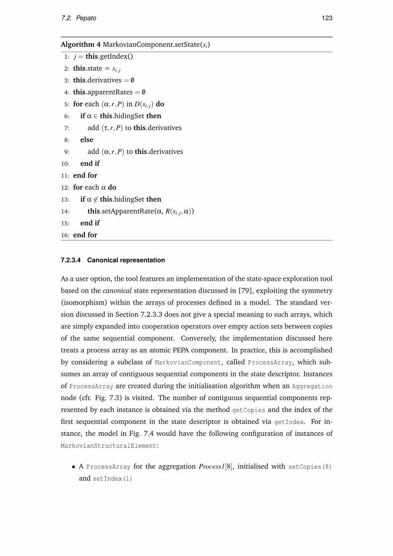
7.2. Pepato 123
Algorithm 4 MarkovianComponent.setState(si)
1: j = this.getIndex()
2: this.state = si, j
3: this.derivatives = /0
4: this.apparentRates = /0
5: for each (α,r,P) in D(si, j) do
6: if α ∈ this.hidingSet then
7: add (τ,r,P) to this.derivatives
8: else
9: add (α,r,P) to this.derivatives
10: end if
11: end for
12: for each α do
13: if α 6∈ this.hidingSet then
14: this.setApparentRate(α, R(si, j,α))
15: end if
16: end for
7.2.3.4 Canonical representation
As a user option, the tool features an implementation of the state-space exploration tool
based on the canonical state representation discussed in [79], exploiting the symmetry
(isomorphism) within the arrays of processes defined in a model. The standard ver-
sion discussed in Section 7.2.3.3 does not give a special meaning to such arrays, which
are simply expanded into cooperation operators over empty action sets between copies
of the same sequential component. Conversely, the implementation discussed here
treats a process array as an atomic PEPA component. In practice, this is accomplished
by considering a subclass of MarkovianComponent, called ProcessArray, which sub-
sumes an array of contiguous sequential components in the state descriptor. Instances
of ProcessArray are created during the initialisation algorithm when an Aggregation
node (cfr. Fig. 7.3) is visited. The number of contiguous sequential components rep-
resented by each instance is obtained via the method getCopies and the index of the
first sequential component in the state descriptor is obtained via getIndex. For in-
stance, the model in Fig. 7.4 would have the following configuration of instances of
MarkovianStructuralElement:
• A ProcessArray for the aggregation Process1[8], initialised with setCopies(8)
and setIndex(1)

124 Chapter 7. Tool Support
Algorithm 5 compose()
1: L = this.cooperationSet
2: this.setState(this.getLeft().getState() BCL
this.getRight().getState())
3: this.derivatives = /0
4: this.apparentRates = /0
5: l = this.getLeft().getDerivatives()
6: r = this.getRight().getDerivatives()
7: for each((α,a,P),(β,b,Q)
)∈ l× r such that α = β∧α ∈ L do
8: appLeft = this.getLeft().getApparentRate(α)
9: appRight = this.getRight().getApparentRate(α)
10: rate = aappLeft
bappRight min(appLeft,appRight)
11: add (α,rate,P BCL
Q) to this.derivatives
12: end for
13: for each (α,a,P) ∈ l such that α 6∈ L do
14: add (α, a, P BCL
this.getRight().getState()) to this.derivatives
15: end for
16: for each (β,b,Q) ∈ r such that β 6∈ L do
17: add (β, b, this.getLeft().getState() BCL
Q) to this.derivatives
18: end for
19: for each (γ,rate,P BCL
Q) ∈ this.derivatives do
20: if γ 6∈ this.hidingSet then
21: currentRate = this.getApparentRate(γ)
22: this.setApparentRate(γ, currentRate + rate)
23: else
24: remove (γ, rate, P BCL
Q) from this.derivatives
25: add (τ, rate, P BCL
Q) to this.derivatives
26: end if
27: end for
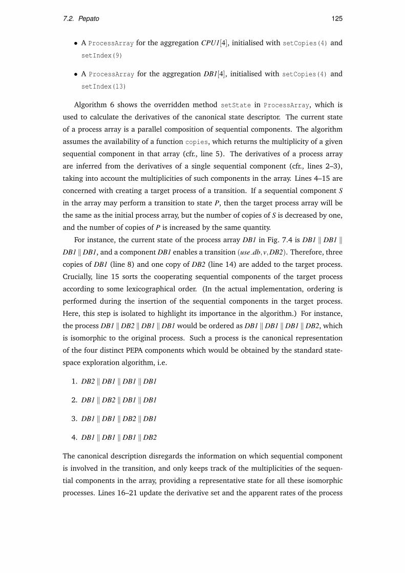
7.2. Pepato 125
• A ProcessArray for the aggregation CPU1[4], initialised with setCopies(4) and
setIndex(9)
• A ProcessArray for the aggregation DB1[4], initialised with setCopies(4) and
setIndex(13)
Algorithm 6 shows the overridden method setState in ProcessArray, which is
used to calculate the derivatives of the canonical state descriptor. The current state
of a process array is a parallel composition of sequential components. The algorithm
assumes the availability of a function copies, which returns the multiplicity of a given
sequential component in that array (cfr., line 5). The derivatives of a process array
are inferred from the derivatives of a single sequential component (cfr., lines 2–3),
taking into account the multiplicities of such components in the array. Lines 4–15 are
concerned with creating a target process of a transition. If a sequential component S
in the array may perform a transition to state P, then the target process array will be
the same as the initial process array, but the number of copies of S is decreased by one,
and the number of copies of P is increased by the same quantity.
For instance, the current state of the process array DB1 in Fig. 7.4 is DB1 ‖ DB1 ‖DB1 ‖DB1, and a component DB1 enables a transition (use db,v,DB2). Therefore, three
copies of DB1 (line 8) and one copy of DB2 (line 14) are added to the target process.
Crucially, line 15 sorts the cooperating sequential components of the target process
according to some lexicographical order. (In the actual implementation, ordering is
performed during the insertion of the sequential components in the target process.
Here, this step is isolated to highlight its importance in the algorithm.) For instance,
the process DB1 ‖DB2 ‖DB1 ‖DB1 would be ordered as DB1 ‖DB1 ‖DB1 ‖DB2, which
is isomorphic to the original process. Such a process is the canonical representation
of the four distinct PEPA components which would be obtained by the standard state-
space exploration algorithm, i.e.
1. DB2 ‖ DB1 ‖ DB1 ‖ DB1
2. DB1 ‖ DB2 ‖ DB1 ‖ DB1
3. DB1 ‖ DB1 ‖ DB2 ‖ DB1
4. DB1 ‖ DB1 ‖ DB1 ‖ DB2
The canonical description disregards the information on which sequential component
is involved in the transition, and only keeps track of the multiplicities of the sequen-
tial components in the array, providing a representative state for all these isomorphic
processes. Lines 16–21 update the derivative set and the apparent rates of the process

126 Chapter 7. Tool Support
array. Here, the transition rates of a single sequential component are multiplied by the
number of components which enable the same action.
Algorithm 6 ProcessArray.setState(si)
1: this.state = si, j ‖ si, j+1 ‖ · · · ‖ si, j+this.getCopies()−1
2: for each distinct sequential component S in c.currentState do
3: for each (α,r,P) in D(S) do
4: target = /0
5: multiplicity = copies(this.currentState, S)
6: for each distinct sequential component S′ in this.currentState do
7: if S′ = S then
8: add (multiplicity-1) S′ components to target
9: else
10: add (multiplicity) S′ components to target
11: end if
12: end for
13: targetMultiplicity = copies(this.state, P)
14: add (targetMultiplicity+1) P components to target
15: order(target)
16: if α ∈ this.hidingSet then
17: add (τ,multiplicity× r, target) to this.derivatives
18: else
19: add (α,multiplicity× r, target) to this.derivatives
20: add multiplicity× r to this.apparentRates(α)
21: end if
22: end for
23: end for
7.2.3.5 Discussion
The state-space aggregation algorithm based on the canonical representation may be
very effective, making it possible to analyse models which would be otherwise in-
tractable with the standard exploration tool. For instance, Table 7.1 compares the
state-space sizes obtained with both implementations of the model in Fig. 7.4. The
benefits from aggregation are dramatic even at such small multiplicity levels, as the
state space may be reduced by up to four orders of magnitude.
The current implementation of the aggregation algorithm is sub-optimal in that it
only aggregates replicated components cooperating over empty action sets. Further-

7.2. Pepato 127
Table 7.1: Standard and aggregated state-space sizes of the model in Fig. 7.4
Multiplicity levels State-space sizes
Process1 CPU1 DB1 Standard form Canonical Form
2 2 2 144 54
3 3 3 1728 160
4 4 4 20736 375
5 4 4 62208 525
6 4 4 186624 700
7 4 4 559872 900
8 4 4 1679616 1125
more, the modeller is required to explicitly express which components to aggregate via
the use of the process array operator. Therefore, the system equation
Process1[8] BCuse cpu,use db
(CPU1[4] ‖ DB1[4]
)is treated differently from the equation
Process1[8] BCuse cpu,use db
(CPU1[4] ‖ DB1[2] ‖ DB1[2]
)although the theoretical canonical representation algorithm would give rise to the same
aggregated Markov chain. For instance, the process DB1 ‖ DB1 ‖ DB2 ‖ DB2 in the
former model is represented by the following three distinct states in the latter model
1. DB1 ‖ DB1 ‖ DB2 ‖ DB2
2. DB1 ‖ DB2 ‖ DB1 ‖ DB2
3. DB2 ‖ DB2 ‖ DB1 ‖ DB1
because each process array is considered in isolation — in this case, this has the effect
of increasing the state space size to 2025 states.
Despite these limitations, the implementation is adequate for effective aggregation
in a large class of PEPA models — namely, those population models which have been
considered in previous chapters of this thesis. In these circumstances, optimal com-
paction of distinct arrays of isomorphic components, as in the example above, can be
easily spotted by the modeller in order to achieve further aggregation.

128 Chapter 7. Tool Support
7.2.4 Steady-State Analysis
Most of the functionality for the analysis of the underlying Markov chain is available
through the IStateSpace interface, whose principal methods are illustrated in Fig. 7.2.
Implementations of this interface define specialised data structures for holding the
derivation graph of the PEPA model. This graph has more information than is needed
for the construction of the generator matrix of the chain because it also records the
action labels for each transition. For instance, the derivation graph of the simple pro-
cess Pdef= (α,r).Q+(β,s).Q will maintain one transition for each operand of the choice,
whereas the generator matrix will record a single transition to Q at rate r + s. Because
of this difference, a design requirement of the tool was that the derivation graph and
generator matrix be represented separately using loosely coupled interfaces. In the
implementation, IStateSpace adopts the Adapter design pattern to return generator
matrices (i.e., via the method getGenerator). In so doing Markov chain solvers are
not tied to a particular representation, but may ask for implementations which are
best suited to the solution technique (e.g., sparse implementation with row or column
access).
The current version of Pepato performs steady-state analysis of the Markov chain. A
lightweight adapter around the Matrix Toolkit for Java [3] provides access to the following
solution methods (as implementations of the ISolver interface):
• Gaussian elimination
• Conjugate gradient
• Conjugate gradient squared
• Biconjugate gradient
• Biconjugate gradient stabilised
• Generalised minimal residual
• Iterative refinement
• Quasi-minimal residual
7.2.5 Calculation of Markovian Rewards
Pepato is equipped with a range of routines for the calculation of common performance
metrics over the steady-state probability distribution of the underlying Markov chain.
The main components which constitute this framework are illustrated in Fig. 7.6. A
category of metrics is concerned with the probability mass of a subset of state space

7.2. Pepato 129
Figure 7.6: Class diagram of the Markovian rewards available in Pepato
which matches certain conditions. Pepato has the notion of filters to define such sets,
grouped into two categories: state-based and transition-based. The former are used to
specify conditions which must hold on the local states of the sequential components of
the PEPA process. The latter match states according to properties on their incoming or
outgoing transitions.
The tool supports the following state-based filters:
Local State Filter This takes as input a local state of a sequential component P, an
integer K, and a relational operator ∈ <,≤,=,>,≥, 6=. It returns the set of
states in which the number of sequential components in state P, denoted by #P,
satisfies the relation #P K. In the sample PEPA model, a performance metric
of interest could be the probability of finding all the CPUs in their state CPU2,
representing a situation in which no computation can be processed in the system.
This can be queried by using the local state filter #CPU2 = 4.
Pattern Matching Filter A more expressive way of filtering based on local states is
available through a pattern-matching filter. For example, the expression P| ∗ |Qmatches states with three sequential components that have the first component
in state P and the third component in state Q. The wildcard operator ∗ is used to
indicate any local state in a position. The same query as above is represented by
the following expression:

130 Chapter 7. Tool Support
Algorithm 7 Throughput(α,Σ,π)
1: throughput = 0
2: for each si ∈ Σ do
3: for each (β,r,P) ∈ transitions(si) do
4: if β = α then
5: throughput = throughput+πi× r
6: end if
7: end for
8: end for
*|*|*|*|*|*|*|*|CPU2|CPU2|CPU2|CPU2|*|*|*|*
Unnamed State Filter Consider the definition
Pdef= (α,r).(β,s).Q
The local state (β,s).Q is called unnamed because it is not defined through a
constant. The modeller may want to use unnamed local states because their
behaviour is of secondary importance for the performance analysis. This filter
returns the set of states in which all its sequential components are not in an
unnamed state.
Probability Threshold Filter This filter may be applied to match states whose steady-
state probability is above or below a given threshold.
A transition-based filter takes as input an action type and the direction of the transition
(i.e. incoming or outgoing). It filters states which have transitions of the given direction
labelled with the given action type. Both kinds of filter can be combined using boolean
operators.
Pepato has native support for the calculation of three commonly used performance
metrics: throughput, utilisation, and mean population levels. Algorithm 7 describes
how to compute the throughput of an action type α for a probability distribution π over
a state space Σ. The total rate of execution of a given action type α at one state of the
chain is multiplied by the probability of being in that state. The sum across all states
gives the average number of activities of type α which are performed in a unit of time.
This metric is accessed via the method IStateSpace.getThroughput, which returns an
array of instances of ThroughputResult, containing the throughputs for each non-silent
action type in the model.
Utilisation is associated with each sequential component of a PEPA model and gives
the fraction of its lifetime that is spent in a particular local state. Recalling the rep-

7.2. Pepato 131
Algorithm 8 Utilisation(Σ,π)
1: for each si ∈ Σ do
2: for 1≤ j ≤ NC do
3: U j(si, j) = U j(si, j)+πi
4: end for
5: end for
resentation discussed in Section 7.2.3.2, utilisation is calculated for each coordinate
j,1≤ j ≤ NC of the state descriptor, and it is represented as a map of sequential compo-
nents si, j to real values. Such quantities are denoted by U j(si, j) (i.e., the utilisation at
coordinate j of the sequential component si, j) in Algorithm 8, which shows the pseu-
docode for their computation. Finally, for a given sequential component si, j, the sum
of its utilisation figures across all the coordinates of the state descriptor gives the mean
population level of si, j in the system. The method IStateSpace.geUtilisation re-
turns an array of instances of UtilisationResult, containing the utilisation maps for
each sequential component. The maps are represented as arrays of LocalStateResult,
associating a local derivative with its utilisation value.
7.2.6 Differential Analysis
Being syntactically similar to the Markovian interpretation, the implementation of the
differential semantics can reuse some of the components discussed in Section 7.2.3.3.
The process of extracting the underlying differential equation from a PEPA model con-
sists of the following steps:
1. Verification of preconditions
2. Context reduction
3. Preparation of the bottom-up exploration structure
4. Exploration of the derivation graphs of all sequential components
5. Exploration of the parametric derivation graph
The initial step rejects PEPA models with passive rates, as discussed in Section 3.4
(Assumption 4). Context reduction is carried out by replacing a process array with
a single sequential component. In this respect, the implementation is coarser than
Definition 2 (in Section 4.2) because the process P[N1] ‖ P[N2] is reduced to P ‖ P in-
stead of P, thus yielding a differential equation in which a number of components of
the size of the derivation graph of P is redundant. However, such a situation can be

132 Chapter 7. Tool Support
easily avoided by the modeller via visual inspection of the system equation. The con-
struction of the data structures for the bottom-up exploration takes place during con-
text reduction. The class diagram in Fig. 7.7 shows that these objects are structurally
similar to their counterparts in the Markovian state-space exploration (cfr. Fig. 7.5).
The visit of a sequential component or a process array gives rise to an instance of a
ParametricComponent, whereas a ParametricOperator is constructed for each coop-
eration in the system equation. The main difference with respect to the Markovian
analysis is the treatment of rates, which are handled symbolically using the class hier-
archy under Expression, instead of being represented as real values. Symbolic rates
are built from the rates in the Markovian transitions of the sequential components.
This information is given by the map D(S) discussed in Section 7.2.3.3, which is com-
puted during the initialisation of the algorithm. The procedure for the generation of
the derivatives of a ParametricComponent is shown in Algorithm 9. Lines 12–21 are
concerned with initialising the apparent rates of the component. Similarly to a sequen-
tial component in the Markovian interpretation, these apparent rates are computed
only once and cached for repeated uses by instances of ParametricOperator using the
method getApparentRate during the entire exploration process.
The structural elements of the bottom-up exploration algorithm and the Markovian
derivation graphs of all sequential components are sufficient to generate the numerical
vector form representation. Each distinct local state of the sequential component rep-
resented by a ParametricComponent is assigned a unique coordinate in the numerical
vector form, which can be obtained via the method getCoordinate(Process). Deriva-
tives of a ParametricComponent may be calculated by retrieving the Markovian rate of
execution, wrapping it around a Rate expression, and multiplying the expression by the
coordinate which represents the sequential component. (The same procedure can be
used for the computation of apparent rates.) The treatment of a ParametricOperator
is carried out verbatim as in Algorithm 5, where all the rate manipulations are now
assumed to be symbolic. The initial state in the numerical vector form is computed
from the initial population levels recorded in ParametricComponent and Algorithms 2
and 3 are applied similarly to obtain the parametric derivation graph of the model.
The process of context reduction applied to the model in Fig. 7.4 results in the
following context for the generation of the underlying differential equation:
Process1 BCuse cpu,use db
(CPU1 ‖ DB1)/reset cpu,reset db
The following instances of ParametricStructuralElement are created:
• An instance c1 of ParametricComponent with setIndex(1) associated with Process1.
This has the effect of allocating three coordinates in the state descriptor in the
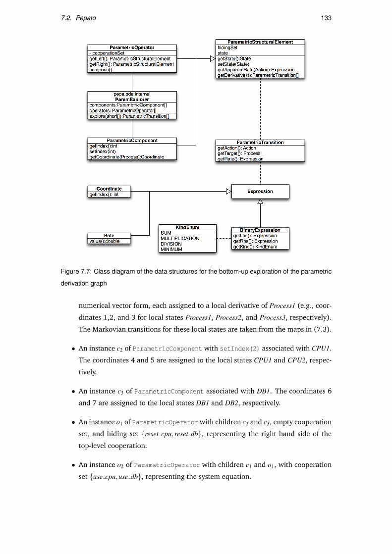
7.2. Pepato 133
Figure 7.7: Class diagram of the data structures for the bottom-up exploration of the parametric
derivation graph
numerical vector form, each assigned to a local derivative of Process1 (e.g., coor-
dinates 1,2, and 3 for local states Process1, Process2, and Process3, respectively).
The Markovian transitions for these local states are taken from the maps in (7.3).
• An instance c2 of ParametricComponent with setIndex(2) associated with CPU1.
The coordinates 4 and 5 are assigned to the local states CPU1 and CPU2, respec-
tively.
• An instance c3 of ParametricComponent associated with DB1. The coordinates 6
and 7 are assigned to the local states DB1 and DB2, respectively.
• An instance o1 of ParametricOperator with children c2 and c3, empty cooperation
set, and hiding set reset cpu,reset db, representing the right hand side of the
top-level cooperation.
• An instance o2 of ParametricOperator with children c1 and o1, with cooperation
set use cpu,use db, representing the system equation.

134 Chapter 7. Tool Support
Algorithm 9 ParametricComponent.setState(si)
1: j = this.getIndex()
2: this.state = si, j
3: this.derivatives = /0
4: for each (α,r,P) in D(si, j) do
5: parametricRate = new Multiplication(new Rate(r), this.getCoordinate(si, j) )
6: if α ∈ this.hidingSet then
7: add (τ,parametricRate,P) to this.derivatives
8: else
9: add (α,parametricRate,P) to this.derivatives
10: end if
11: end for
12: if executed for the first time then
13: this.apparentRates = /0
14: for each local state si, j′ ∈ ds(si, j) do
15: for each action type α 6∈ this.hidingSet do
16: rateExpr = new Rate(R(si, j′ ,α)
17: parametricRate = new Multiplication(rateExpr, this.getCoordinate(si, j′) )
18: add parametricRate to this.apparentRate(α)
19: end for
20: end for
21: end if
Upon calling setState on each parametric component, the following derivatives
will be available to o1 and o2:
c1.getDerivatives() = (think,0.2×ξ1,Process2),(think,1.8×ξ1,Process3)
c2.getDerivatives() = (use cpu,4.0×ξ4,CPU2)
c3.getDerivatives() = (use db,6.0×ξ6,DB2)
where ξ represents the state descriptor in the numerical vector form. Therefore, the
derivatives of o1 and o2 will be computed as follows:
o1.getDerivatives() = (use cpu,4.0×ξ4,CPU2 ‖ DB1),(use db,6.0×ξ6,CPU1 ‖ DB2)
o2.getDerivatives() = (think,0.2×ξ1,Process2 BCuse cpu,use db
(DB1 ‖ CPU1)/reset cpu,reset db),
(think,1.8×ξ1,Process3 BCuse cpu,use db
(DB1 ‖ CPU1)/reset cpu,reset db)

7.3. The Graphical User Interface 135
The derivatives of o2 are used to determine the parametric derivation graph of the
model. For instance, the transition
Process1 BCuse cpu,use db
(DB1 ‖ CPU1)/reset cpu,reset db (think,0.2×ξ1)−−−−−−−−→?
Process2 BCuse cpu,use db
(DB1 ‖ CPU1)/reset cpu,reset db
implies the generating function
ϕthink(ξ,(−1,+1,0,0,0,0,0)
)= 0.2×ξ1
where the jump (−1,+1,0,0,0,0,0) may be computed via invocations of the method
getCoordinate of ParametricComponent.
Evaluation of fluid performance metrics The fluid performance metrics discussed in
Chapter 5 are implemented as realisations of the interface ICallback (cfr. Fig. 7.2).
Details on the elements of graphical user interface employed for setting the parameters
of the analysis may be found in Section 7.3.6.
7.3 The Graphical User Interface
Eclipse UI contains all the user interface contributions to the Eclipse IDE. It features an
editor, which is automatically associated by the workbench to workspace files with the
.pepa extension. The editor has syntax highlighting and supports graphical annota-
tions (markers) for problems encountered during the modelling process. Tasks to be
performed on the PEPA model being edited are shown in the top-level menu bar, and
a number of views are connected to the editor. A customisable arrangement of all the
views of interest to a PEPA modeller is provided in the PEPA perspective. The remain-
der of this section is concerned with a detailed discussion of the views and the actions
available under the Eclipse UI plug-in.
7.3.1 Contributions to Other Plug-ins
The Navigator view is used to navigate the Eclipse workspace. Workspace files with the
.pepa extension are associated with the PEPA synchronisation icon in the editor and
registered with the PEPA editor. The Problems view is populated automatically with
syntax error and static analysis messages. The plug-in defines two levels of severity: a
warning allows the user to continue the analysis, whereas an error must be fixed. The
Console view provides verbose information on the status of a PEPA model. In particular,
it displays execution times of the various stages of analysis and provides hyperlinks
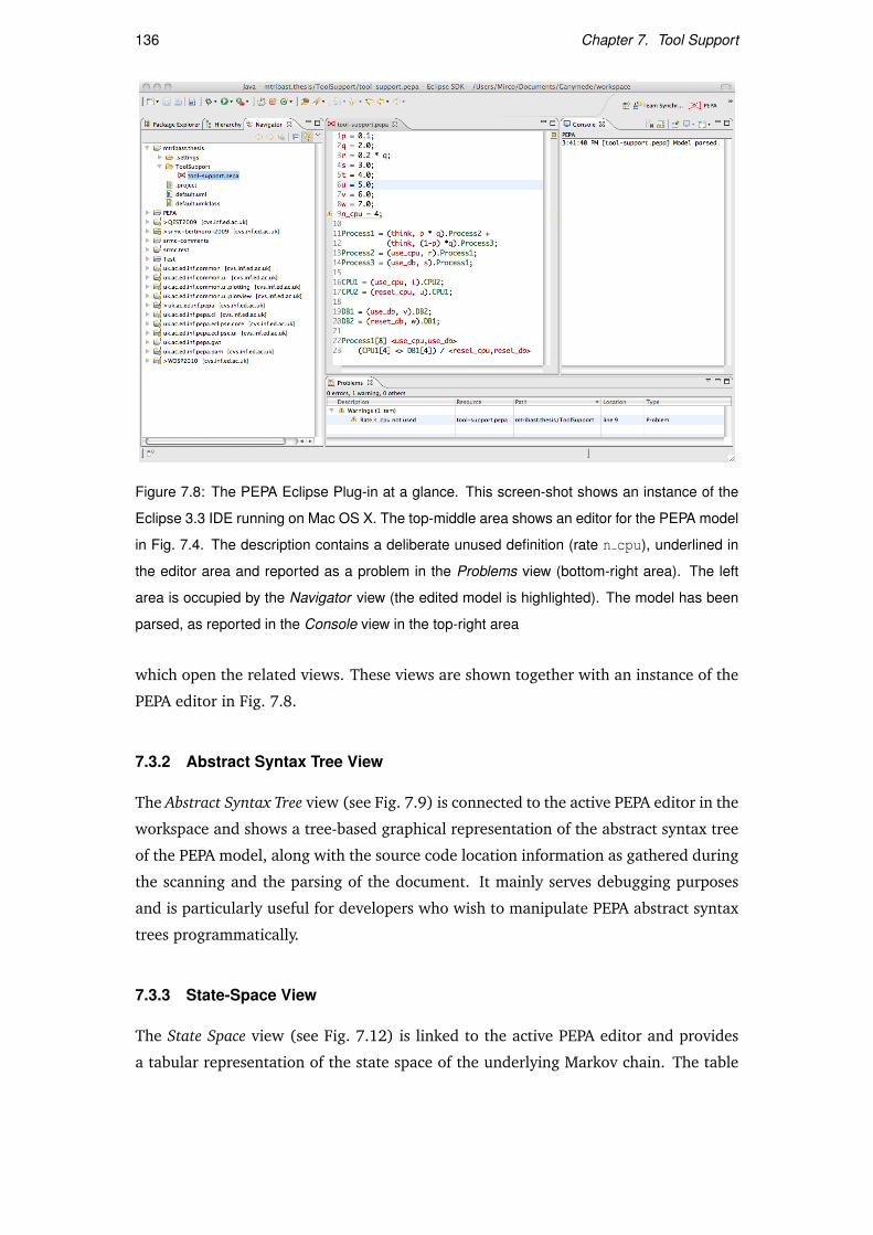
136 Chapter 7. Tool Support
Figure 7.8: The PEPA Eclipse Plug-in at a glance. This screen-shot shows an instance of the
Eclipse 3.3 IDE running on Mac OS X. The top-middle area shows an editor for the PEPA model
in Fig. 7.4. The description contains a deliberate unused definition (rate n cpu), underlined in
the editor area and reported as a problem in the Problems view (bottom-right area). The left
area is occupied by the Navigator view (the edited model is highlighted). The model has been
parsed, as reported in the Console view in the top-right area
which open the related views. These views are shown together with an instance of the
PEPA editor in Fig. 7.8.
7.3.2 Abstract Syntax Tree View
The Abstract Syntax Tree view (see Fig. 7.9) is connected to the active PEPA editor in the
workspace and shows a tree-based graphical representation of the abstract syntax tree
of the PEPA model, along with the source code location information as gathered during
the scanning and the parsing of the document. It mainly serves debugging purposes
and is particularly useful for developers who wish to manipulate PEPA abstract syntax
trees programmatically.
7.3.3 State-Space View
The State Space view (see Fig. 7.12) is linked to the active PEPA editor and provides
a tabular representation of the state space of the underlying Markov chain. The table

7.3. The Graphical User Interface 137
Figure 7.9: Abstract Syntax Tree view. The node corresponding to the first process definition in
Fig. 7.8 is highlighted. It defines a choice whose left-hand side component is a prefix, whose
action type is think. The target of this activity is the process Process2. Each node is labelled
with source-code location information between brackets (line number and index of the initial
character corresponding to the node)
is populated automatically when the state space exploration is invoked from the cor-
responding top-level menu item. A row represents a state of the Markov chain, each
cell in the table showing the local state of a sequential component, using the state
representation discussed in Section 7.2.3.2. A further column displays the steady-state
probability distribution if one is available. A toolbar menu item provides access to the
user interface for managing state space filters. When a set of filter rules is activated,
the excluded states are removed from the table. The probability mass of the states that
match the filters is automatically computed and shown in the view (see Fig. 7.11). Fil-
ter rules are assigned names and made persistent across workspace sessions. From the
toolbar the user can invoke a wizard dialogue box to export the transition system and
one to import the steady-state probability distribution as computed by external tools.
The view also has a Single-step Navigator, a tool for navigating the transition system
of the Markov chain. It can be opened from any state of the chain and its layout is as
follows. In an external window are displayed the state description of the current state
and two tables. The tables show the set of states for which there is a transition to or

138 Chapter 7. Tool Support
Figure 7.10: State Space view. The model in Fig. 7.4 is solved for all population levels set to two,
therefore each state has six sequential components. The last column shows the steady-state
probability distribution
from the current state. The tables are laid out similarly to the view’s main table. In
addition, the action types that label a transition are shown in a further column. The
user can navigate backwards and forwards by selecting any of the states listed.
7.3.4 Markovian Analysis and and Graph View
A wizard dialogue box accessible from the top-level menu bar guides the user through
the process of performing steady-state analysis on the Markov chain. The user can
choose between an array of iterative solvers and tune their parameters as needed (see
Fig. 7.13). Performance metrics are calculated automatically and displayed in the Per-
formance Evaluation view. It has three tabs showing the results of the aforementioned
reward structures, i.e., utilisation, throughput, and population levels (see Fig. 7.14).
Throughput and population levels are arranged in a tabular fashion, whereas utilisation
is shown in a two-level tree in which each top-level node corresponds to a sequential
component and its children are its local states.
The Performance Evaluation view can feed input to the Graph view, a general-
purpose view available in the plug-in for visualising charts. Throughputs and pop-
ulation levels are shown as bar charts and a top-level node of the utilisation tree is
shown as a pie chart (see Fig. 7.15). As with any kind of graph displayed in the view,
several converting options are available. The graph can be exported to PDF or SVG and
the underlying data can be extracted into a comma-separated value text file.

7.3. The Graphical User Interface 139
(a) Filter editor (b) Filtered state space
Figure 7.11: State-space filters. (a) In the filter editor the user may choose to display only such
states of the model in Fig. 7.12 that their steady-state probability is greater than 0.03. The
filtered state space and its probability mass are shown in (b)
7.3.5 Experimenting with Markovian Analysis
An important stage in performance modelling is sensitivity analysis, i.e. the study of
the impact that certain parameters have on the performance of the system. A wizard
dialogue box is available in the plug-in to assist the user with the set-up of sensitivity
analysis experiments over the models (see Fig. 7.16). The parameters that can be
subjected to this analysis are the rate definitions and number of replications of the array
of processes in the system equation. The performance metrics that can be analysed are
throughput, utilisation, or population levels. If the model has filter rules defined, the
probability mass of the set of filtered states can be used as a performance index as
well. The tool allows the set-up of multiple experiments of two kinds: one-dimensional
(performance metric vs. one parameter) or two-dimensional (performance metric vs.
two parameters changed simultaneously). The results of the analysis are shown in the
Graph view as line charts.
7.3.6 Differential Analysis
The Differential Analysis view is linked to the active PEPA editor in the workspace and
shows the set of generating functions extracted from the model. These are constructed
automatically but the derivation process may be interrupted by the user should the
differential representation be particularly expensive. Figure 7.17 shows the contents
of the view for the model in Figure 7.4. The generating functions are arranged in a
tabular format. The first column shows the action type, followed by the jump vector of
the function according to the underlying numerical vector format representation. The
last column shows the parametric rate of execution, where the coordinates of the state
descriptor are explicitly indicated using the identifiers of the sequential components
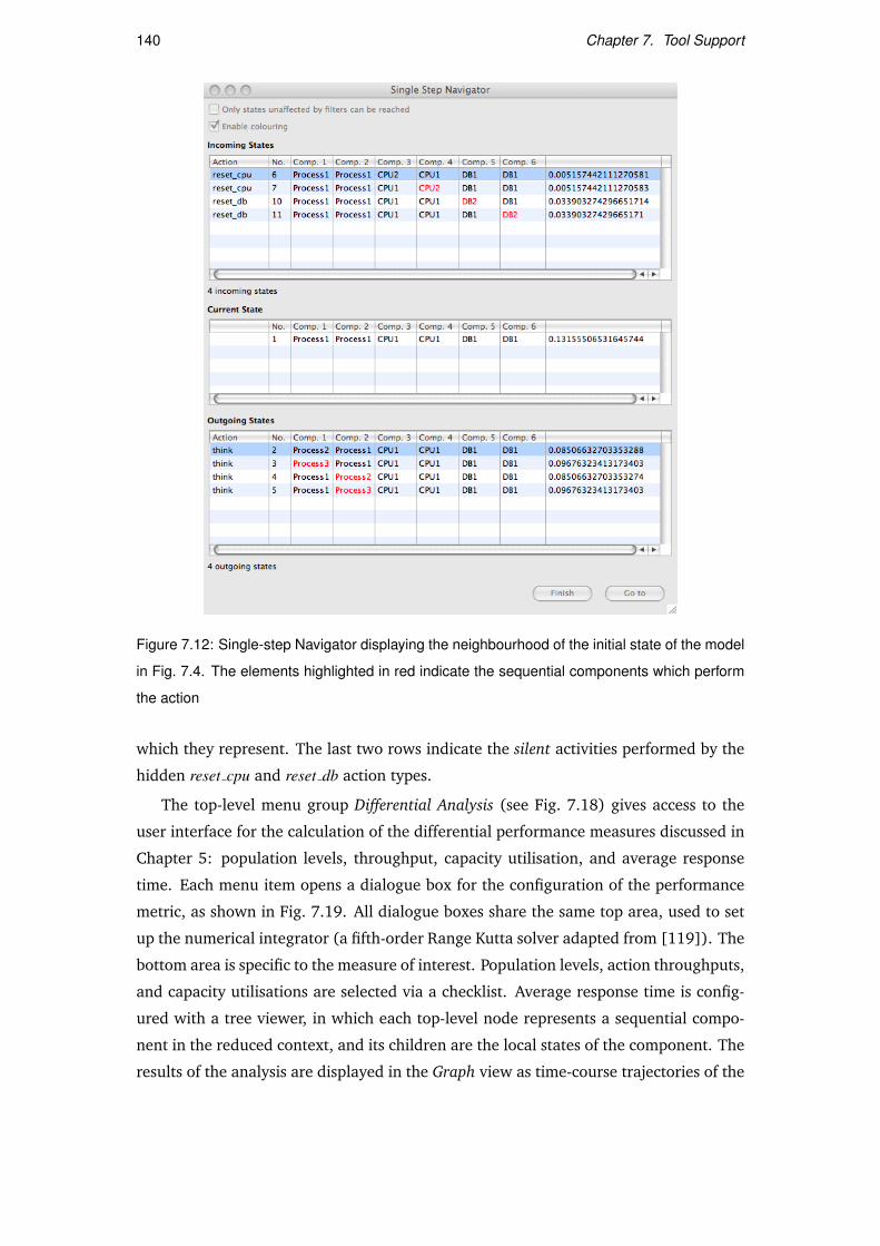
140 Chapter 7. Tool Support
Figure 7.12: Single-step Navigator displaying the neighbourhood of the initial state of the model
in Fig. 7.4. The elements highlighted in red indicate the sequential components which perform
the action
which they represent. The last two rows indicate the silent activities performed by the
hidden reset cpu and reset db action types.
The top-level menu group Differential Analysis (see Fig. 7.18) gives access to the
user interface for the calculation of the differential performance measures discussed in
Chapter 5: population levels, throughput, capacity utilisation, and average response
time. Each menu item opens a dialogue box for the configuration of the performance
metric, as shown in Fig. 7.19. All dialogue boxes share the same top area, used to set
up the numerical integrator (a fifth-order Range Kutta solver adapted from [119]). The
bottom area is specific to the measure of interest. Population levels, action throughputs,
and capacity utilisations are selected via a checklist. Average response time is config-
ured with a tree viewer, in which each top-level node represents a sequential compo-
nent in the reduced context, and its children are the local states of the component. The
results of the analysis are displayed in the Graph view as time-course trajectories of the
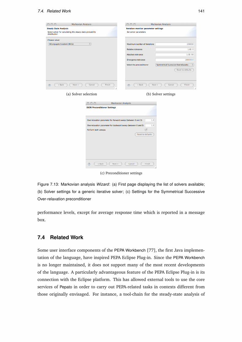
7.4. Related Work 141
(a) Solver selection (b) Solver settings
(c) Preconditioner settings
Figure 7.13: Markovian analysis Wizard : (a) First page displaying the list of solvers available;
(b) Solver settings for a generic iterative solver; (c) Settings for the Symmetrical Successive
Over-relaxation preconditioner
performance levels, except for average response time which is reported in a message
box.
7.4 Related Work
Some user interface components of the PEPA Workbench [77], the first Java implemen-
tation of the language, have inspired PEPA Eclipse Plug-in. Since the PEPA Workbench
is no longer maintained, it does not support many of the most recent developments
of the language. A particularly advantageous feature of the PEPA Eclipse Plug-in is its
connection with the Eclipse platform. This has allowed external tools to use the core
services of Pepato in order to carry out PEPA-related tasks in contexts different from
those originally envisaged. For instance, a tool-chain for the steady-state analysis of

142 Chapter 7. Tool Support
(a) Utilisation (b) Throughput (c) Population
Figure 7.14: The three tabs in the Performance Evaluation view
(a) Bar chart for population levels (b) Pie chart for utilisation
Figure 7.15: Graph view: (a) Example of a bar chart showing the mean population levels of the
components in the steady state; (b) Pie chart for utilisation
PEPA models inputted as text files has been built for the Sensoria Development Envi-
ronment [4,150], a framework based on a loosely-coupled service-oriented architecture
for the integration and orchestration of tools for the modelling, development, and de-
ployment of service-oriented software systems. Pepato is used in conjunction with the
Eclipse implementation of the UML2 meta-model [1] for supporting automatic extrac-
tion of performance models from annotated UML activity diagrams [140] and sequence
diagrams [147]. The programming interface for the Graph View is being used by the
Eclipse Bio-PEPA Plugin [62], which implements a variant of PEPA for the modelling
and analysis of biochemical networks [42]. Pepato’s abstract syntax tree and Marko-
vian analysis packages are used to provide support for stochastic model checking and
aggregation by abstraction [133,134]. Software support for SRMC (the Sensoria Refer-
ence Markovian Calculus [47,48]), an extension of PEPA aimed at modelling large-scale
service-oriented systems, is built on top of the PEPA Eclipse Plug-in [5].
The Imperial PEPA Compiler [26] and its successor, the International PEPA Com-

7.4. Related Work 143
(a) (b)
(c) (d)
Figure 7.16: Experimentation: (a) Selection of parameters amenable to sensitivity analysis; (b)
Range set-up; (c) Performance metric set-up; (d) Visualisation of results in the Graph view
piler (ipc, see [44]) provide an orthogonal command-line-based implementation of
PEPA language. The original purpose of this tool was to provide a bridge to the
tools DNAmaca/HYDRA for transient and steady-state analysis of very large Markov
chains [27, 59]. The main difference with respect to the PEPA Eclipse Plug-in is that
ipc enables the computation of passage-time quantiles, i.e., the cumulative distribution
function of the time to traverse a set of states of the Markov chain, particularly useful
for the analysis of response-time measures. The set of states of interest is determined
using the technology of stochastic probes, i.e., observational model components gener-
ated from a regular expression-based specification language [8].
PEPA is also integrated into PRISM for the model checking of the underlying Markov
chain against properties expressed in Continuous Stochastic Logic (CSL) [106]. The

144 Chapter 7. Tool Support
Figure 7.17: Differential Analysis view
Figure 7.18: Differential Analysis menu in the PEPA Eclipse Plug-in
integration also provides access to the efficient numerical solutions of PRISM based on
binary decision diagrams and sparse matrix representation. PRISM has been applied
successfully to a number of PEPA case studies, e.g., [78,80].

7.4. Related Work 145
(a) Population levels (b) Throughput
(c) Capacity utilisation (d) Average response time
Figure 7.19: User interface for the computation of differential performance metrics


Chapter 8
Conclusions
The major contribution of this thesis has been a formal semantic account of the fluid-
flow approximation of PEPA models. Unlike earlier work on this subject, a system of
coupled ordinary differential equations is fully characterised by the generating functions
extracted by interpreting the model against the population-based semantics. Although
this semantics is still Markovian, this thesis has mainly emphasised the scalability prop-
erties of the related deterministic interpretation, highlighting the fundamental insensi-
tivity of the cost of differential analysis with respect to increasing population sizes of
the system under study. The asymptotic results of convergence and the empirical tests
on the accuracy of the approximation have given much confidence on the applicability
of this approach.
8.1 Combined Markovian and Differential Analysis
Clearly, for problems of manageable size the explicit enumeration of the derivative
graph of the model remains the preferred route to performance evaluation, because
the numerical solution of the underlying Markov chain using traditional linear-algebra
techniques is the most precise form of analysis available (except for closed-form solu-
tions which are known only for special and relatively simple cases). Nevertheless, the
increasing computational difficulty in handling large-scale systems does not necessarily
imply that a Markovian approach is not without use even in these circumstances. In
fact, the unique capability of PEPA to address both a discrete and a continuous-state
interpretation may be effectively exploited for a combined and complementary use of
both analysis techniques.
147

148 Chapter 8. Conclusions
8.1.1 Model Debugging
A possible use of the discrete-state representation of a large-scale system may be for
the purposes of model debugging. This is intended as a form of validation that gives
confidence that the model dynamics matches the modeller’s intended behaviour. For
such a study, the direct use of the differential representation may be counterintuitive
since the evolution of the system is not provided in terms of the intrinsically discrete
representation of the process-algebraic description. Instead, this reasoning may be
carried out more effectively by direct inspection of the derivation graph obtained from
the stochastic semantics. Interestingly, the chain needs not be solved if the modeller is
only interested in qualitative properties of the system.
One of its simplest forms of debugging is the interactive exploration of the deriva-
tion graph using tools such as the Single-step Navigator presented in Section 7.3.3 (cfr.
Fig. 7.12). This tool requires that the complete state space be explored in order to
populate the set of states that have transitions to any given state. However, it is not
difficult to envisage a much less demanding alternative which does not provide this
functionality, restricting itself to showing only the set of reachable states from a given
state. In this manner, the state space needs not be explored in advance, but the tool
would need to compute upon demand only the neighbourhood of the states visited by
the user. Even for large models, the computational cost of this operation is usually
acceptable.
For instance, with respect to the PEPA model of the LQN system proposed in Chap-
ter 6, state-space navigation may be used to verify that whenever a Server thread
carries out an action of type cache, i.e., when it is in the state Cache′1 shown in (6.1),
then one Client thread component must be in a state in which it is waiting for one of
the three synchronous calls to the entry visit. (Using initial concurrency levels such
that explicit enumeration is feasible, this check can be practically carried out by means
of the action- and state-based filters presented in Section 7.3.3.) It must be pointed
out that this approach is informal and necessarily not exhaustive. In practice it is often
beneficial to use model checking techniques to test the validity of logical expressions
which represent the desired properties of correctness of the system under study.
8.1.2 Estimation of Performance Bounds
In addition to the qualitative analysis presented above, the discrete-state representa-
tion of PEPA may be used for the derivation of precise performance bounds. In most
cases, such as all the examples presented in this thesis, the model may be regarded as
a reactive system that performs some computation when triggered by other cooperat-

8.1. Combined Markovian and Differential Analysis 149
Table 8.1: Evaluation of performance bounds for the PEPA model of Chapter 6. The rate pa-
rameters are set as in Figure 6.1 and all other concurrency levels are set to one.
Number of Client threads U(PClient) U(PServer) U(PFileServer)
1 0.052 0.823 0.379
2 0.055 0.864 0.398
3 0.056 0.876 0.404
ing active components. These active components usually capture the behaviour of the
actual users in the real system. When the initial population counts of the active com-
ponents are unitary, the model describes a situation in which there is no contention for
the system’s resources. In these conditions the overall state space is usually of man-
ageable size, therefore the performance estimates can be calculated precisely and can
be interpreted as representing the upper bounds on the performance attainable by the
system. It should be noted that resource contention may still be present in these mod-
els, but it is due to architectural constraints on the reactive modules, e.g., two threads
executing on the same processor. The classification of a sequential component as an
active or a reactive entity is left to the modeller. This information cannot be inferred
automatically from the model description since the semantics of PEPA does not encode
explicitly the role of initiator and receiver of a synchronisation action.
The PEPA interpretation of the LQN model lends itself well to this form of analysis.
Here the modeller can distinguish three classes of components: the active components
are the sequential components which model the Client threads; all the other thread
components are passive, if they service requests from other threads, or active, if they
in turn make requests to other threads and processors. The processor components can
be regarded as being purely passive, in that they only carry out computation when
explicitly acquired by the threads. Therefore, a meaningful derivation of optimistic
performance estimates may be based on the evaluation of the system performance
when there is only one Client thread in the system. Such a study is illustrated in
Table 8.1, which confirms that the utilisation of the processors is indeed the lowest in
that case.
8.1.3 Advantages of Simulation for Analysing Large-Scale Systems
The execution runtimes presented in this thesis refer to sequential implementations of
the ODE solver and the CTMC simulator. Although not studied here, the gap in the com-

150 Chapter 8. Conclusions
putational efficiency between these two techniques can be dramatically reduced if one
considers alternative implementations designed to run on massively parallel architec-
tures. This is because stochastic simulation is an embarassingly parallelizable problem,
since the independent runs can be run on separate processors and very little coordi-
nation is needed among such runs. One master process is usually required to gather
the simulation results, compute confidence intervals, and determine the convergence
criteria. In this context, a comparison study between the efficiency of parallel versions
of ODE and CTMC analysis would be beneficial and is left as a topic for future work.
Despite its higher computational cost, stochastic simulation is potentially more in-
formative than ODE analysis because it can provide the probability distributions of
the stochastic variables under observation (although this adds to the computational
complexity both in terms of memory and time due to the larger amount of data that is
needed). This more detailed information can be desired in later stages of the modelling
process when a more informative characterisation of the system is required.
8.1.4 A Modelling Workflow for PEPA Population Models
In conclusion, one can devise the following modelling workflow for large-scale pop-
ulation models which encompasses all of the forms of analysis to which PEPA can be
subjected:
1. Model development Definition of the system components and the synchronisation
sets among them. This stage can be assisted by static analysis to search for com-
mon modelling mistakes. In some cases deadlock detection may be conducted
prior to state-space exploration [58].
2. Qualitative analysis Study of the functional characteristics of the model, allowing
for the detection of problems that cannot be discovered statically. Informal ap-
proaches include running state- and action-based filters over the state space (if
explicit enumeration is feasible) and interactive simulation of execution traces.
More formally, model checking techniques can be employed.
3. Evaluation of performance bounds If the performance estimates are to be com-
pared against given quality-of-service agreements, evaluating optimistic perfor-
mance bounds may be used to reject models that do not meet such prerequisites
even under the most optimistic conditions of no contention from users for the
system’s resources.
4. Large-scale analysis with ODEs The low computational cost of differential analy-
sis makes it particularly suitable for the investigation of problems that involve the

8.2. Future Work 151
exploration of large parameter spaces. Instances of such problems include sen-
sitivity analysis, e.g., studying the impact that changes to parameter values have
on the system performance, and optimisation, e.g., finding the optimal system
configuration that minimises a given cost function.
5. Refinement with stochastic simulation Once enough confidence on the correct-
ness of the model is built, stochastic simulation may be employed for a detailed
characterisation of the system, e.g., the computation of higher moment statistics.
8.2 Future Work
Although the deterministic interpretation of PEPA proposed in this thesis has extended
the scope of applicability of ODE analysis of earlier approaches, there are still a number
of modelling situations of practical interest which cannot be described satisfactorily
with PEPA. This section discusses a few topics of future work with this respect.
Synchronisation among isomorphic components
A PEPA model whose reduced context features synchronisation between identical com-
ponents in the form A BCL1
A · · · BCLk
A, for non-empty synchronisation sets L1,L2, . . . ,Lk, can
be theoretically subjected to fluid-flow interpretation. However, the resulting popula-
tion model is not meaningful because it does not correctly capture the actual behaviour
of the system in the large scale. In particular, the associated population model would
be in the form A[N1] BCL1
A[N2] · · · BCLk
A[Nk+1], i.e., it is such that the overall population of
components A results partitioned in groups of components within which communica-
tion is not possible (because the components are composed in parallel with empty coop-
eration sets). Further research is needed in this area because communication between
identical components is a reasonable modelling abstraction to study the behaviour of
several interesting (and complex) distributed systems, e.g., peer-to-peer networks and
other similar communication protocols.
Modelling user workload
As shown in the examples provided throughout this thesis, the performance evaluation
of a system may be conducted under the assumption of a special class of user behaviour
specification, namely that of a closed workload in which a (fixed) population of users
are assumed to cyclically interact with the system, possibly interposing some think
time between successive requests. This is a consequence of the two-level grammar for
PEPA, which prohibits definitions in the form Adef= (born,r).(A ‖ A′) which could provide
152 Chapter 8. Conclusions
a simple description of a component that spawns new processes. In particular, this
would model a Poisson workload of users of type A′ with exponentially distributed
interarrival times (with rate r), a common assumption in many performance modelling
studies.
Multiscale models
The treatment of the LQN model developed in Chapter 6 has highlighted the presence
of distinct activities occurring at rates which are separated by many orders of magni-
tude. One recurring case is the use of very fast activities to enforce exclusive access to
processors and to model the passing of the locus of control from one software thread
to another. Such multiscale behaviour is not exclusive to those models that translate
queueing networks, but it manifests itself in general when there are activities which
denote purely logical operations or whose duration is negligible (e.g., context switch
in multitasking processors), as well as others which carry significant delays (e.g., net-
work data transfer). Although such models do not present difficulties from a theoretical
standpoint, as observed in Chapter 6 they may give rise to numerical problems because
of stiffness. A possible way of tackling this problem would be to develop alternative
(perhaps approximate) versions of the model in which the behaviour of fast activities
is not expressed directly with a specific action but is instead incorporated in activi-
ties whose rates are of a similar order of magnitude. It should be noted however that
the solution of stiff problems would greatly benefit from using numerical integrators
specifically designed to handle such cases (e.g., implicit methods [86]). The implemen-
tation of these solvers within the PEPA Eclipse Plug-in, which currently supports only an
explicit Dormand-Prince integrator, is the subject of future work.

Appendix A
Differential Equations of Case Studies
A.1 Case Study of Section 4.4
The model is reported again in Figure A.1 for convenience; alongside each sequential
component is the corresponding coordinate in the NVF.
dx1(t)dt
=−min(rc:requestx1(t),rs:requestx4(t))+ rc:thinkx3(t)
dx2(t)dt
= min(rc:requestx1(t),rs:requestx4(t))−min(rc:replyx2(t),rs:replyx8(t))
dx3(t)dt
=−rc:thinkx3(t)+min(rc:replyx2(t),rs:replyx8(t))
dx4(t)dt
=−min(rc:requestx1(t),rs:requestx4(t))− rs:failx4(t)+min(rc:replyx2(t),rs:replyx8(t))
+rs:readx9(t)
rs:readx9(t)+ rs:readx5(t)min(rs:readx9(t)+ rs:readx5(t),rd:readx10(t))
dx5(t)dt
=− rs:readx5(t)rs:readx9(t)+ rs:readx5(t)
min(rs:readx9(t)+ rs:readx5(t),rd:readx10(t))
+pfresh min(rc:requestx1(t),rs:requestx4(t))
dx6(t)dt
= (1−pok)rs:readx5(t)
rs:readx9(t)+ rs:readx5(t)min(rs:readx9(t)+ rs:readx5(t),rd:readx10(t))
−rs:forcex6(t)
dx7(t)dt
=− rs:writex7(t)rs:writex7(t)+ rr:writex13(t)
min(rs:writex7(t)+ rr:writex13(t),rd:writex10(t))
+ rs:forcex6(t)
dx8(t)dt
=−min(rc:replyx2(t),rs:replyx8(t))+(1−pfresh)min(rc:requestx1(t),rs:requestx4(t))
+pokrs:readx5(t)
rs:readx9(t)+ rs:readx5(t)min(rs:readx9(t)+ rs:readx5(t),rd:readx10(t))
+rs:writex7(t)
rs:writex7(t)+ rr:writex13(t)min(rs:writex7(t)+ rr:writex13(t),rd:writex10(t))
153

154 Appendix A. Differential Equations of Case Studies
ξ1 Cl :Requestdef= (request,rc:request).Cl :Wait
ξ2 Cl :Waitdef= (reply,rc:reply).Cl :Think
ξ3 Cl :Thinkdef= (think,rc:think).Cl :Request
ξ4 Sr :Waitdef= (request,pfreshrs:request).Sr :Fresh
+ (request,(1−pfresh)rs:request).Sr :Reply
+ (fail,rs:fail).Sr :Repair
ξ5 Sr :Freshdef= (read,pokrs:read).Sr :Reply
+ (read,(1−pok)rs:read).Sr :Force
ξ6 Sr :Forcedef= (force,rs:force).Sr :Write
ξ7 Sr :Writedef= (write,rs:write).Sr :Reply
ξ8 Sr :Replydef= (reply,rs:reply).Sr :Wait
ξ9 Sr :Repairdef= (read,rs:read).Sr :Wait
ξ10 Db :Waitdef= (read,rd:read).Db :Update
+ (write,rd:write).Db :Update
ξ11 Db :Updatedef= (update,rd:update).Db :Wait
ξ12 Rb :Gatherdef= (crawl,rr:crawl).Rb :Write
ξ13 Rb :Writedef= (write,rr:write).Rb :Gather
SystemAppdef= Cl :Request[Nc] BC
request,reply((Sr :Wait[Ns] ‖ Rb :Gather[Nr]
)BC
read,write
Db :Wait[Nd ])/read,write
Figure A.1: PEPA model of a three-tier distributed application
dx9(t)dt
=− rs:readx9(t)rs:readx9(t)+ rs:readx5(t)
min(rs:readx9(t)+ rs:readx5(t),rd:readx10(t))
+min(rc:replyx2(t),rs:replyx8(t))
dx10(t)dt
= rd:updatex11(t)−min(rs:readx9(t)+ rs:readx5(t),rd:readx10(t))
−min(rs:writex7(t)+ rr:writex13(t),rd:writex10(t))
dx11(t)dt
=−rd:updatex11(t)+min(rs:readx9(t)+ rs:readx5(t),rd:readx10(t))
+min(rs:writex7(t)+ rr:writex13(t),rd:writex10(t))
dx12(t)dt
=−rr:crawlx12(t)
+rr:writex13(t)
rs:writex7(t)+ rr:writex13(t)min(rs:writex7(t)+ rr:writex13(t),rd:writex10(t))
dx13(t)dt
= rr:crawlx12(t)
− rr:writex13(t)rs:writex7(t)+ rr:writex13(t)
min(rs:writex7(t)+ rr:writex13(t),rd:writex10(t))

A.2. Case Study of Section 5.6.3 155
A.2 Case Study of Section 5.6.3
dx1(t)dt
=−t1x1(t)+c1x2(t)
c1x2(t)+ c2x6(t)min(c1x2(t)+ c2x6(t),cx8(t))
+d1c1x3(t)
d1c1x3(t)+d2c2x7(t)min(d1c1x3(t)+d2c2x7(t),dx10(t))
dx2(t)dt
= t′1x4(t)+(1−p)p′db t1x1(t)−c1x2(t)
c1x2(t)+ c2x6(t)min(c1x2(t)+ c2x6(t),cx8(t))
dx3(t)dt
= (1−p)pdb t1x1(t)−d1c1x3(t)
d1c1x3(t)+d2c2x7(t)min(d1c1x3(t)+d2c2x7(t),dx10(t))
dx4(t)dt
= pt1x1(t)− t′1x4(t)
dx5(t)dt
=−t2x5(t)+c2x6(t)
c1x2(t)+ c2x6(t)min(c1x2(t)+ c2x6(t),cx8(t))
+d2c2x7(t)
d1c1x3(t)+d2c2x7(t)min(d1c1x3(t)+d2c2x7(t),dx10(t))
dx6(t)dt
= q′db t2x5(t)−c2x6(t)
c1x2(t)+ c2x6(t)min(c1x2(t)+ c2x6(t),cx8(t))
dx7(t)dt
= qdb t2x5(t)−d2c2x7(t)
d1c1x3(t)+d2c2x7(t)min(d1c1x3(t)+d2c2x7(t),dx10(t))
dx8(t)dt
=−min(c1x2(t)+ c2x6(t),cx8(t))+lcx9(t)
lcx9(t)+ ldx10(t)min(lcx9(t)+ ldx10(t), lx12(t))
dx9(t)dt
= min(c1x2(t)+ c2x6(t),cx8(t))−lcx9(t)
lcx9(t)+ ldx10(t)min(lcx9(t)+ ldx10(t), lx12(t))
dx10(t)dt
=−min(d1c1x3(t)+d2c2x7(t),dx10(t))
+ldx10(t)
lcx9(t)+ ldx10(t)min(lcx9(t)+ ldx10(t), lx12(t))
dx11(t)dt
= min(d1c1x3(t)−d2c2x7(t),dx10(t))
− ldx10(t)lcx9(t)+ ldx10(t)
min(lcx9(t)+ ldx10(t), lx12(t))
dx12(t)dt
= 0


Appendix B
Complete PEPA Model of Chapter 6
CLIENT (REFERENCE TASK)
Client1def= (acquirepc,ν).(think,8/0.01).Client2
Client2def= (requestthink,visit,ν).(replythink,visit,ν).(acquirepc,ν).(think,8/0.01).Client3
Client3def= (requestthink,visit,ν).(replythink,visit,ν).(acquirepc,ν).(think,8/0.01).Client4
Client4def= (requestthink,visit,ν).(replythink,visit,ν).(acquirepc,ν).(think,8/0.01).Client5
Client5def= (requestthink,buy,ν).(replythink,buy,ν).(acquirepc,ν).(think,8/0.01).Client6
Client6def= (requestthink,notify,ν).(acquirepc,ν).(think,8/0.01).Client7
Client8def= (requestthink,save,ν).(replythink,save,ν).(acquirepc,ν).(think,8/0.01).Client9
Client9def= (requestthink,read,ν).(replythink,read,ν).(acquirepc,ν).(think,8/0.01).Client1
SERVER
Serverdef= (requestthink,visit,ν).Cache1 +(requestthink,buy,ν).Prepare1
+(requestthink,notify,ν).Notify1 +(requestthink,save,ν).Save1
Cache1def= (acquireps,ν).
[(cache,0.95×1/0.001).Internal1 +(cache,0.05×1/0.001).External1
]Internal1
def= (acquireps,ν).(internal,1/0.001).Internal2
Internal2def= (replythink,visit,ν).EndInternal
EndInternaldef= Server
External1def= (acquireps,ν).(external,2/0.001).External2
External2def= (requestexternal,read,ν).(replyexternal,read,ν).(acquireps,ν).(external,2/0.001).External3
External3def= (replythink,visit,ν).EndExternal
EndExternaldef= Server
157

158 Appendix B. Complete PEPA Model of Chapter 6
Prepare1def= (acquireps,ν).(prepare,1/0.01).ForkPrepare
ForkPreparedef= (fork1,ν).EndPrepare
EndPreparedef= (join1,ν).Display1
Display1def= (acquireps,ν).(display,1/0.001).Display2
Display2def= (replythink,buy,ν).EndDisplay
EndDisplaydef= Server
Notify1def= (acquireps,ν).(notify,1/0.08).EndNotify
EndNotifydef= Server
Save1def= (acquireps,ν).(save,2/0.02).Save2
Save2def= (requestsave,write,ν).(replysave,write,ν).(acquireps,ν).(save,2/0.02).Save3
Save3def= (replythink,save,ν).EndSave
EndSavedef= Server
SERVER’S SECONDARY FLOWS
Pack1def= (fork1,ν).(acquireps,ν).(pack,1/0.03).EndPack
EndPackdef= (join1,ν).Pack1
Ship1def= (fork1,ν).(acquireps,ν).(ship,1/0.01).EndShip
EndShipdef= (join1,ν).Ship1
FILESERVER
FileServerdef= (requestthink,read,ν).Read1
+(requestexternal,read,ν).Read1
+(requestsave,write1 ,ν).Write′1
Read1def= (acquirepfs,ν).(read,1/0.01).Read2
Read2def= (replythink,read,ν).EndRead +(replyexternal,read,ν).EndRead
EndReaddef= FileServer
Write′1def= (acquirepfs,ν).(write1,1/0.001).Write′2
Write′2def= (replysave,write1 ,ν).EndWrite′
EndWrite′def= Write′′1
Write′′1def= (acquirepfs,ν).(write2,3/0.04).Write′′2
Write′′2def= (requestwrite2,get,ν).(replywrite2,get,ν).(acquirepfs,ν).(write2,3/0.04).Write′′3
Write′′3def= (requestwrite2,update,ν).(replywrite2,update,ν).(acquirepfs,ν).(write2,3/0.04).EndWrite′′
EndWrite′′def= FileServer

159
BACKUP
Backupdef= (requestwrite2,get,ν).Get1
+(requestwrite2,update,ν).Update1
Get1def= (acquirepfs,ν).(get,1/0.01).Get2
Get2def= (replywrite2,get,ν).EndGet
EndGetdef= Backup
Update1def= (acquirepfs,ν).(update,1/0.01).Update2
Update2def= (replywrite2,update,ν).EndUpdate
EndUpdatedef= Backup
PCLIENT
PClient′def= (acquirepc,ν).PClient′′
PClient′′def= (think,8/0.01).PClient′
PSERVER
PServer′def= (acquireps,ν).PServer′′
PServer′′def= (cache,1/0.001).PServer′+(internal,1/0.001).PServer′
+(external,2/0.001).PServer′+(prepare,1/0.01).PServer′
+(pack,1/0.03).PServer′+(ship,1/0.01).PServer′+(display,1/0.001).PServer′
PFILESERVER: (cfr. Figure 6.3)
COMPLETE LAYERED QUEUEING NETWORK(Client[2] BC
M1
(Server[2] BC
L1Pack1[2] BC
L2Ship1[2]
)BCM2
FileServer[1] BCM3
Backup[1])
BCM4
(PClient[2] BC
/0PServer[2] BC
/0PFileServer[2]
),
M1 =
requestthink,visit,replythink,visitrequestthink,buy,replythink,buy,requestthink,notify,
requestthink,save,replythink,save
L1 = L2 =
fork1, join1
M2 =
requestthink,read,replythink,read,requestexternal,readreplyexternal,read,
requestsave,write1 ,replysave,write1
M3 =
requestwrite2,get,replywrite2,get,requestwrite2,update,
replywrite2,update
M4 =
acquirepc, think,acquireps,cache, internal,external,
prepare,pack,ship,display,notify,display,acquirepfs,
read,write,get,update


Bibliography
[1] “Eclipse Model Development Tools (MDT): UML2 and UML2 Tools,” http://www.eclipse.org/modeling/mdt/?project=uml2.
[2] “Eclipse Modelling Framework Project,” http://www.eclipse.org/modeling/emf.
[3] “Matrix Toolkit for Java,” http://code.google.com/p/matrix-toolkits-java/.
[4] “Sensoria Development Environment,” http://svn.pst.ifi.lmu.de/trac/sct.
[5] “SRMC: the Sensoria Reference Markovian Calculus. Download page,” http://groups.inf.ed.ac.uk/srmc/download.html.
[6] M. Ajmone-Marsan, G. Conte, and G. Balbo, “A Class of Generalized Stochas-tic Petri Nets for the Performance Evaluation of Multiprocessor Systems,” ACMTrans. Comput. Syst., vol. 2, no. 2, pp. 93–122, 1984.
[7] H. Alla and R. David, “Continuous and Hybrid Petri Nets,” Journal of Circuits,Systems, and Computers, vol. 8, no. 1, pp. 159–188, 1998.
[8] A. Argent-Katwala, J. Bradley, and N. Dingle, “Expressing performance require-ments using regular expressions to specify stochastic probes over process alge-bra models,” in Proceedings of the Fourth International Workshop on Softwareand Performance. Redwood Shores, California, USA: ACM Press, Jan. 2004, pp.49–58.
[9] G. Balbo, S. Bruell, and M. Sereno, “Product Form Solution for GeneralizedStochastic Petri Nets,” IEEE Transactions on Software Engineering, vol. 28, no. 10,pp. 915–932, 2002.
[10] Y. Bard, “Some extensions to multiclass queueing network analysis,” in Proceed-ings of the Third International Symposium on Modelling and Performance Evalua-tion of Computer Systems. Amsterdam, The Netherlands: North-Holland Pub-lishing Co., 1979, pp. 51–62.
[11] F. Baskett, K. M. Chandy, R. R. Muntz, and F. G. Palacios, “Open, closed, andmixed networks of queues with different classes of customers,” J. ACM, vol. 22,no. 2, pp. 248–260, 1975.
[12] A. Bell and B. R. Haverkort, “Distributed disk-based algorithms for model check-ing very large Markov chains,” Form. Methods Syst. Des., vol. 29, no. 2, pp.177–196, 2006.
[13] ——, “Untold horrors about steady-state probabilities: What reward-based mea-sures won’t tell about the equilibrium distribution,” in EPEW, ser. Lecture Notesin Computer Science, K. Wolter, Ed., vol. 4748. Springer, 2007, pp. 2–17.
161
162 Bibliography
[14] S. Benkirane, J. Hillston, C. McCaig, R. Norman, and C. Shankland, “Improvedcontinuous approximation of PEPA models through epidemiological examples,”Electronic Notes in Theoretical Computer Science, vol. 229, no. 1, pp. 59–74, 2009.
[15] A. Benoit, L. Brenner, P. Fernandes, and B. Plateau, “Aggregation of stochas-tic automata networks with replicas,” in Proc. 4th Int. Conference on NumericalSolution of Markov Chains (NSMC), 2003, pp. 145–166.
[16] A. Benoit, B. Plateau, and W. J. Stewart, “Memory-efficient Kronecker algorithmswith applications to the modelling of parallel systems,” Future Generation Comp.Syst., vol. 22, no. 7, pp. 838–847, 2006.
[17] M. Bernardo and R. Gorrieri, “Extended Markovian Process Algebra,” in CON-CUR, ser. Lecture Notes in Computer Science, U. Montanari and V. Sassone, Eds.,vol. 1119. Springer, 1996, pp. 315–330.
[18] M. Bernardo and J. Hillston, Eds., Formal Methods for Performance Evaluation,7th International School on Formal Methods for the Design of Computer, Commu-nication, and Software Systems, SFM 2007, Bertinoro, Italy, May 28-June 2, 2007,Advanced Lectures, ser. Lecture Notes in Computer Science, vol. 4486. Springer,2007.
[19] P. Billingsley, Probability and Measure, 3rd ed. Wiley, 1995.
[20] A. Bobbio, “Petri nets generating Markov reward models for perfor-mance/reliability analysis of degradable systems,” in Modeling Techniques andTools for Computer Performance Evaluation. Proceedings of the Fourth Interna-tional Conference,, R. Puigjaner, Ed., Palma, Spain, 1988, pp. 353–365.
[21] L. Bortolussi, “On the approximation of stochastic concurrent constraint pro-gramming by master equation,” Electr. Notes Theor. Comput. Sci., vol. 220, no. 3,pp. 163–180, 2008.
[22] L. Bortolussi and A. Policriti, “Stochastic concurrent constraint programmingand differential equations,” Electr. Notes Theor. Comput. Sci., vol. 190, no. 3, pp.27–42, 2007.
[23] ——, “Dynamical systems and stochastic programming: To ordinary differentialequations and back,” T. Comp. Sys. Biology, vol. 11, pp. 216–267, 2009.
[24] J. T. Bradley and S. T. Gilmore, “Stochastic simulation methods applied to asecure electronic voting model,” Electr. Notes Theor. Comput. Sci., vol. 151, no. 3,pp. 5–25, 2006.
[25] J. T. Bradley, R. Hayden, W. J. Knottenbelt, and T. Suto, “Extracting responsetimes from fluid analysis of performance models,” in SIPEW ’08: Proceedings ofthe SPEC international workshop on Performance Evaluation. Berlin, Heidelberg:Springer-Verlag, 2008, pp. 29–43.
[26] J. Bradley, N. Dingle, S. Gilmore, and W. Knottenbelt, “Derivation of passage-time densities in PEPA models using IPC: The Imperial PEPA Compiler,” in Pro-ceedings of the 11th IEEE/ACM International Symposium on Modeling, Analysisand Simulation of Computer and Telecommunications Systems, G. Kotsis, Ed. Uni-versity of Central Florida: IEEE Computer Society Press, Oct. 2003, pp. 344–351.

Bibliography 163
[27] ——, “Extracting passage times from PEPA models with the HYDRA tool: Acase study,” in Proceedings of the Nineteenth annual UK Performance EngineeringWorkshop, S. Jarvis, Ed., University of Warwick, July 2003, pp. 79–90.
[28] J. Bradley, S. Gilmore, and J. Hillston, “Analysing distributed internet wormattacks using continuous state-space approximation of process algebra models,”Journal of Computer and System Sciences, vol. 74, no. 6, pp. 1013–1032, Septem-ber 2008.
[29] P. Buchholz, “Exact and Ordinary Lumpability in Finite Markov Chains,” Journalof Applied Probability, vol. 31, no. 1, pp. 59–75, 1994.
[30] J. P. Buzen, “Computational algorithms for closed queueing networks with ex-ponential servers,” Commun. ACM, vol. 16, no. 9, pp. 527–531, 1973.
[31] M. Calder, S. Gilmore, and J. Hillston, “Modelling the Influence of RKIP on theERK Signalling Pathway Using the Stochastic Process Algebra PEPA,” in Pro-ceedings of the BioConcur Workshop on Concurrent Models in Molecular Biology,A. Ingolfsdottir and H. R. Nielson, Eds., London, England, 2004, pp. 26–41.
[32] ——, “Automatically deriving ODEs from process algebra models of signallingpathways,” in Computational Methods in Systems Biology, 2005.
[33] L. Cardelli, “On process rate semantics,” Theor. Comput. Sci., vol. 391, no. 3, pp.190–215, 2008.
[34] A. Chaintreau, J.-Y. L. Boudec, and N. Ristanovic, “The age of gossip: spatialmean field regime,” in SIGMETRICS/Performance, J. R. Douceur, A. G. Green-berg, T. Bonald, and J. Nieh, Eds. ACM, 2009, pp. 109–120.
[35] K. M. Chandy and A. J. Martin, “A characterization of product-form queuingnetworks,” J. ACM, vol. 30, no. 2, pp. 286–299, 1983.
[36] K. M. Chandy and D. Neuse, “Linearizer: A heuristic algorithm for queueingnetwork models of computing systems,” Commun. ACM, vol. 25, no. 2, pp. 126–134, 1982.
[37] K. Chandy, J. Howard Jr., and D. Towsley, “Product form and local balance inqueueing networks,” J. ACM, vol. 24, no. 2, pp. 250–263, 1977.
[38] D. Chen, Y. Hong, and K. S. Trivedi, “Second-order stochastic fluid models withfluid-dependent flow rates,” Performance Evaluation, vol. 49, no. 1-4, pp. 341 –358, 2002.
[39] G. Chiola, C. Dutheillet, G. Franceschinis, and S. Haddad, “Stochastic well-formed colored nets and symmetric modeling applications,” IEEE Transactionson Computers, vol. 42, no. 11, pp. 1343–1360, 1993.
[40] F. Ciocchetta, A. Degasperi, J. Hillston, and M. Calder, “Some InvestigationsConcerning the CTMC and the ODE Model Derived from Bio-PEPA,” Electron.Notes Theor. Comput. Sci., vol. 229, no. 1, pp. 145–163, 2009.
[41] F. Ciocchetta and J. Hillston, “Bio-PEPA: An Extension of the Process AlgebraPEPA for Biochemical Networks,” Electr. Notes Theor. Comput. Sci., vol. 194,no. 3, pp. 103–117, 2008.

164 Bibliography
[42] ——, “Bio-PEPA: A framework for the modelling and analysis of biological sys-tems,” Theor. Comput. Sci., vol. 410, no. 33-34, pp. 3065–3084, 2009.
[43] A. Clark, A. Duguid, S. Gilmore, and J. Hillston, “Espresso, a Little Coffee,”in Process Algebra and Stochastically Timed Activities (PASTA), Edinburgh, UK,2008.
[44] A. Clark, “The ipclib PEPA Library,” in Fourth International Conference on theQuantitative Evaluation of Systems (QEST). Edinburgh, Scotland, UK: IEEEComputer Society, 17–19 September 2007, pp. 55–56.
[45] A. Clark, A. Duguid, S. Gilmore, and M. Tribastone, “Partial Evaluation of PEPAModels for Fluid-Flow Analysis,” in Computer Performance Engineering, 5th Euro-pean Performance Engineering Workshop (EPEW), ser. Lecture Notes in ComputerScience, N. Thomas and C. Juiz, Eds., vol. 5261. Springer, 2008, pp. 2–16,invited paper.
[46] A. Clark, S. Gilmore, J. Hillston, and M. Tribastone, Formal Methods for Perfor-mance Evaluation: the 7th International School on Formal Methods for the Designof Computer, Communication, and Software Systems, SFM 2007. Bertinoro, Italy:Springer-Verlag, May–June 2007, vol. 4486, ch. Stochastic Process Algebras, pp.132–179.
[47] A. Clark, S. Gilmore, and M. Tribastone, “Service-Level Agreements for Service-Oriented Computing,” in WADT, ser. Lecture Notes in Computer Science, A. Cor-radini and U. Montanari, Eds., vol. 5486. Springer, 2008, pp. 21–36.
[48] ——, “Scalable analysis of scalable systems,” in Fundamental Approaches to Soft-ware Engineering (FASE), ser. LNCS, M. Chechik and M. Wirsing, Eds., no. 5503.York, UK: Springer-Verlag, March 2009, invited paper.
[49] G. Clark, S. Gilmore, and J. Hillston, “Specifying performance measures forpepa,” in ARTS, ser. Lecture Notes in Computer Science, J.-P. Katoen, Ed., vol.1601. Springer, 1999, pp. 211–227.
[50] J. L. Coleman, W. Henderson, and P. G. Taylor, “Product form equilibrium dis-tributions and a convolution algorithm for stochastic Petri nets,” Perform. Eval.,vol. 26, no. 3, pp. 159–180, 1996.
[51] A. Conway, “Fast approximate solution of queueing networks with multi-serverchain-dependent fcfs queues,” in Modeling Techniques and Tools for ComputerPerformance Evaluation, R. Puigjaner and D. Potier, Eds. New York: Plenum,1989, pp. 385–396.
[52] A. E. Conway, E. de Souza e Silva, and S. S. Lavenberg, “Mean value analysisby chain of product form queueing networks,” IEEE Trans. Computers, vol. 38,no. 3, pp. 432–442, 1989.
[53] A. E. Conway and N. D. Georganas, “RECAL—a new efficient algorithm for theexact analysis of multiple-chain closed queuing networks,” J. ACM, vol. 33, no. 4,pp. 768–791, 1986.
[54] R. Darling and J. Norris, “Differential equation approximations for Markovchains,” Probability Surveys, vol. 5, pp. 37–79, 2008.

Bibliography 165
[55] R. de Nicola, D. Latella, M. Loreti, and M. Massink, “Rate-based transition sys-tems for stochastic process calculi,” in ICALP (2), ser. Lecture Notes in ComputerScience, S. Albers, A. Marchetti-Spaccamela, Y. Matias, S. E. Nikoletseas, andW. Thomas, Eds., vol. 5556. Springer, 2009, pp. 435–446.
[56] D. D. Deavours and W. H. Sanders, “An Efficient Disk-Based Tool for SolvingLarge Markov Models,” Perform. Eval., vol. 33, no. 1, pp. 67–84, 1998.
[57] S. Derisavi, H. Hermanns, and W. H. Sanders, “Optimal state-space lumping inMarkov chains,” Inf. Process. Lett., vol. 87, no. 6, pp. 309–315, 2003.
[58] J. Ding, “A new deadlock checking algorithm for pepa,” in 8th Workshop onProcess Algebra and Stochastically Timed Activities (PASTA), 2009, non refereed.
[59] N. J. Dingle, P. G. Harrison, and W. J. Knottenbelt, “Hydra: Hypergraph-baseddistributed response-time analyzer,” in PDPTA, H. R. Arabnia and Y. Mun, Eds.CSREA Press, 2003, pp. 215–219.
[60] S. Donatelli, “Superposed stochastic automata: a class of stochastic Petri netswith parallel solution and distributed state space,” Performance Evaluation,vol. 18, no. 1, pp. 21 – 36, 1993.
[61] J. Dormand and P. Prince, “A family of embedded Runge-Kutta formulae,” Jour-nal of Computational and Applied Mathematics, vol. 6, no. 1, pp. 19–26, March1980.
[62] A. Duguid, “An Overview of the Bio-PEPA Eclipse Plug-in,” in 8th Workshop onProcess Algebra and Stochastically Timed Activities (PASTA), 2009, non refereed.
[63] Eclipse Foundation, http://eclipse.org.
[64] ——, “Eclipse Java development tools,” http://www.eclipse.org/jdt.
[65] P. Fernandes, B. Plateau, and W. J. Stewart, “Efficient descriptor-vector multipli-cations in stochastic automata networks,” J. ACM, vol. 45, no. 3, pp. 381–414,1998.
[66] P. Fitzpatrick, Advanced Calculus, 2nd ed. AMS Bookstore, 2009.
[67] G. Franks, P. Maly, M. Woodside, D. Petriu, and A. Hubbard, “Layered QueueingNetwork Solver and Simulator User Manual,” http://www.sce.carleton.ca/rads/lqns, 2005.
[68] G. Franks, T. Omari, C. M. Woodside, O. Das, and S. Derisavi, “Enhanced mod-eling and solution of layered queueing networks,” IEEE Trans. Software Eng.,vol. 35, no. 2, pp. 148–161, 2009.
[69] V. Galpin, “Continuous approximation of PEPA models and Petri nets,” in Pro-ceedings of the European Simulation and Modelling Conference (ESM 2008), LeHavre, France, 27-29 October 2008, pp. 492–499.
[70] ——, “Continuous approximation of PEPA models and Petri nets,” InternationalJournal of Computer Aided Engineering and Technology, 2009, to appear.
[71] E. Gamma, R. H. amd Ralph Johnson, and J. Vlissides, Design Patterns: ReusableElements of Object-Oriented Software. Addison-Wesley, 1995.
166 Bibliography
[72] N. Geisweiller, J. Hillston, and M. Stenico, “Relating continuous and discretePEPA models of signalling pathways,” Theor. Comput. Sci., vol. 404, no. 1-2, pp.97–111, 2008.
[73] E. Gelenbe and I. Mitrani, Analysis and Synthesis of Computer Systems. AcademicPress, 1980.
[74] E. Gelenbe, “On approximate computer system models,” J. ACM, vol. 22, no. 2,pp. 261–269, 1975.
[75] D. T. Gillespie, “Exact stochastic simulation of coupled chemical reactions,” TheJournal of Physical Chemistry, vol. 81, no. 25, pp. 2340–2361, 1977.
[76] D. Gillespie, “Exact stochastic simulation of coupled chemical reactions,” Journalof Physical Chemistry, vol. 81, no. 25, pp. 2340–2361, December 1977.
[77] S. Gilmore and J. Hillston, “The PEPA Workbench: A Tool to Support a Pro-cess Algebra-based Approach to Performance Modelling,” in Proceedings of theSeventh International Conference on Modelling Techniques and Tools for ComputerPerformance Evaluation, ser. Lecture Notes in Computer Science, no. 794. Vi-enna: Springer-Verlag, May 1994, pp. 353–368.
[78] S. Gilmore, J. Hillston, L. Kloul, and M. Ribaudo, “Software performance mod-elling using PEPA nets,” in Proceedings of the Fourth International Workshop onSoftware and Performance. Redwood Shores, California, USA: ACM Press, Jan.2004, pp. 13–24.
[79] S. Gilmore, J. Hillston, and M. Ribaudo, “An efficient algorithm for aggregatingPEPA models,” IEEE Transactions on Software Engineering, vol. 27, no. 5, pp.449–464, May 2001.
[80] S. Gilmore and L. Kloul, “A unified tool for performance modelling and predic-tion,” in Proceedings of the 22nd International Conference on Computer Safety, Re-liability and Security (SAFECOMP 2003), ser. LNCS, S. Anderson, B. Littlewood,and M. Felici, Eds., vol. 2788. Springer-Verlag, 2003, pp. 179–192.
[81] W. J. Gordon and G. F. Newell, “Closed queuing systems with exponentialservers,” Operations Research, vol. 15, no. 2, pp. 254–265, 1967.
[82] N. Gotz, U. Herzog, and M. Rettelbach, “TIPP - A Stochastic Process Algebra,” inProc. of the Workshop on Process Algebra and Performance Modelling, J. Hillstonand F. Moller, Eds. Department of Computer Science, University of Edinburgh,May 1993.
[83] M. Gribaudo and R. Gaeta, “Efficient steady-state analysis of second-order fluidstochastic Petri nets,” Performance Evaluation, vol. 63, no. 9-10, pp. 1032 – 1047,2006.
[84] M. Gribaudo and M. Telek, “Fluid models in performance analysis,” in SFM, ser.Lecture Notes in Computer Science, M. Bernardo and J. Hillston, Eds., vol. 4486.Springer, 2007, pp. 271–317.
[85] L. Gurvits and J. Ledoux, “Markov property for a function of a markov chain:A linear algebra approach,” Linear Algebra and its Applications, vol. 404, pp.85–117, 2005.

Bibliography 167
[86] E. Hairer and G. Wanner, Solving Ordinary Differential Equations II. Stiff andDifferential-Algebraic Problems, second revised ed. Springer, 1996.
[87] B. Haverkort and K. Trivedi, “Specification techniques for Markov reward mod-els,” Discrete Event Dynamic Systems, vol. 3, no. 2–3, pp. 219–247, July 1993.
[88] R. Hayden and J. T. Bradley, “Fluid semantics for passive stochastic process al-gebra cooperation,” in VALUETOOLS’08, Sept. 2008.
[89] W. Henderson and P. Taylor, “Embedded Processes in Stochastic Petri Nets,” IEEETransactions on Software Engineering, vol. 17, no. 2, pp. 108–116, 1991.
[90] U. Herzog and J. A. Rolia, “Performance validation tools for software/hardwaresystems,” Perform. Eval., vol. 45, no. 2-3, pp. 125–146, 2001.
[91] P. V. Hilgers and A. Langville, MAM 2006: Markov Anniversary Meeting. BosonBooks, 2006, ch. The five greatest applications of Markov chains.
[92] J. Hillston, A Compositional Approach to Performance Modelling. CambridgeUniversity Press, 1996.
[93] ——, “Fluid flow approximation of PEPA models,” in Proceedings of the SecondInternational Conference on the Quantitative Evaluation of Systems. Torino, Italy:IEEE Computer Society Press, Sept. 2005, pp. 33–43.
[94] J. Hillston, M. Tribastone, and S. Gilmore, “Stochastic process algebras: Fromindividuals to populations,” to appear in Computer Journal.
[95] C. Hoare, Communicating Sequential Processes. Prentice-Hall, 1985.
[96] G. Horton, V. G. Kulkarni, D. M. Nicol, and K. S. Trivedi, “Fluid stochastic Petrinets: Theory, applications, and solution techniques,” European Journal of Oper-ational Research, vol. 105, no. 1, pp. 184 – 201, 1998.
[97] J. R. Jackson, “Jobshop-like queueing systems,” Management Science, vol. 10,no. 1, pp. 131–142, 1963.
[98] J. Kemeny and J. Snell, Finite Markov Chains. Van Nostrand, 1960.
[99] L. Kleinrock, Queueing Systems—Theory. Wiley-Interscience, 1975, vol. 1.
[100] B. Klin and V. Sassone, “Structural operational semantics for stochastic processcalculi,” in FoSSaCS, ser. Lecture Notes in Computer Science, R. M. Amadio, Ed.,vol. 4962. Springer, 2008, pp. 428–442.
[101] H. Kobayashi, “Application of the Diffusion Approximation to Queueing Net-works I: Equilibrium Queue Distributions,” J. ACM, vol. 21, no. 2, pp. 316–328,1974.
[102] ——, “Application of the Diffusion Approximation to Queueing Networks II:Nonequilibrium Distributions and Applications to Computer Modeling,” J. ACM,vol. 21, no. 3, pp. 459–469, 1974.
[103] T. G. Kurtz, “Solutions of ordinary differential equations as limits of pure Markovprocesses,” J. Appl. Prob., vol. 7, no. 1, pp. 49–58, April 1970.

168 Bibliography
[104] ——, “Limit theorems for sequences of jump Markov processes approximatingordinary differential processes,” J. Appl. Prob., vol. 8, no. 2, pp. 344–356, 1971.
[105] ——, “The relationship between stochastic and deterministic models for chem-ical reactions,” The Journal of Chemical Physics, vol. 57, no. 7, pp. 2976–2978,1972.
[106] M. Z. Kwiatkowska, G. Norman, and D. Parker, “Prism: Probabilistic symbolicmodel checker,” in Computer Performance Evaluation / TOOLS, ser. Lecture Notesin Computer Science, T. Field, P. G. Harrison, J. T. Bradley, and U. Harder, Eds.,vol. 2324. Springer, 2002, pp. 200–204.
[107] M. Kwiatkowski and I. Stark, “The continuous pi-calculus: A process algebrafor biochemical modelling,” in CMSB, ser. Lecture Notes in Computer Science,M. Heiner and A. M. Uhrmacher, Eds., vol. 5307. Springer, 2008, pp. 103–122.
[108] S. S. Lam and Y. L. Lien, “A tree convolution algorithm for the solution of queue-ing networks,” Commun. ACM, vol. 26, no. 3, pp. 203–215, 1983.
[109] S. S. Lavenberg, Computer Performance Modelling Handbook. Academic Press,1983.
[110] J. Little, “A Proof of the Queuing Formula: L = λW ,” Operations Research, vol. 9,no. 3, pp. 383–387, 1961.
[111] J. Meyer, “On evaluating the performability of degradable computing systems,”Computers, IEEE Transactions on, vol. C-29, no. 8, pp. 720–731, Aug. 1980.
[112] J. F. Meyer, “Performability: a retrospective and some pointers to the future,”Performance Evaluation, vol. 14, no. 3-4, pp. 139 – 156, 1992.
[113] R. Milner, Communication and Concurrency. Prentice-Hall, 1989.
[114] M. Mitzenmacher, “The power of two choices in randomized load balancing,”Ph.D. dissertation, University of California at Berkeley, Department of ComputerScience, Berkeley, CA, 1996.
[115] C. Moler and C. V. Loan, “Nineteen dubious ways to compute the exponential ofa matrix, twenty-five years later,” SIAM Review, vol. 45, no. 1, pp. 3–49, 2003.
[116] M. K. Molloy, “Performance Analysis Using Stochastic Petri Nets,” IEEE Trans.Computers, vol. 31, no. 9, pp. 913–917, 1982.
[117] J. Norris, Markov Chains, ser. Cambridge Series in Statistical and ProbabilisticMathematics. Cambridge University Press, 1998.
[118] OSGi Alliance, “OSGi specifications,” http://www.osgi.org/Specifications/HomePage.
[119] M. Patterson and J. Spiteri, “odeToJava Library,” http://www.netlib.org/ode/odeToJava.tgz.
[120] K. R. Pattipati, M. M. Kostreva, and J. L. Teele, “Approximate mean value anal-ysis algorithms for queuing networks: Existence, uniqueness, and convergenceresults,” J. ACM, vol. 37, no. 3, pp. 643–673, 1990.

Bibliography 169
[121] B. Plateau and K. Atif, “Stochastic Automata Network for Modeling Parallel Sys-tems,” IEEE Transactions on Software Engineering, vol. 17, no. 10, pp. 1093–1108, 1991.
[122] G. D. Plotkin, “A structural approach to operational semantics,” J. Log. Algebr.Program., vol. 60-61, pp. 17–139, 2004.
[123] P. Pollet, “On a model for interference between searching insect parasites,” J.Austral. Math. Soc. Ser. B, vol. 32, no. 2, pp. 133–150, 1990.
[124] C. Priami, “Stochastic pi-calculus,” Comput. J., vol. 38, no. 7, pp. 578–589, 1995.
[125] Real-Time and Distributed Systems group, Department of Systems and Com-puter Engineering, University of Carleton, “LQNS software package,” http://www.sce.carleton.ca/rads/lqns.
[126] A. Reibman and K. Trivedi, “Numerical transient analysis of Markov models,”Comput. Oper. Res., vol. 15, no. 1, pp. 19–36, 1988.
[127] M. Reiser and S. S. Lavenberg, “Mean-value analysis of closed multichain queu-ing networks,” J. ACM, vol. 27, no. 2, pp. 313–322, 1980.
[128] J. A. Rolia and K. C. Sevcik, “The method of layers,” IEEE Trans. Software Eng.,vol. 21, no. 8, pp. 689–700, 1995.
[129] W. H. Sanders and J. Meyer, “A unified approach for specifying measures of per-formance, dependability, and performability,” Dependable Computing for CriticalApplications, pp. 215–247, 1990.
[130] C. Sauer and K. Chandy, Computer systems performance modeling. EnglewoodCliffs, NJ: Prentice-Hall, 1980.
[131] P. Schweitzer, “Approximate analysis of multiclass closed networks of queues,”in International Conference on Stochastic Control and Optimization, Amsterdam,June 1979, pp. 25–29.
[132] B. Sericola, “Transient analysis of stochastic fluid models,” Performance Evalua-tion, vol. 32, no. 4, pp. 245 – 263, 1998.
[133] M. Smith, “Abstraction and Model Checking in the Eclipse PEPA Plug-In,” in 8thWorkshop on Process Algebra and Stochastically Timed Activities (PASTA), 2009,non refereed.
[134] ——, “A Tool for Abstraction and Model Checking of PEPA Models,” to appear.
[135] R. Smith, K. Trivedi, and A. Ramesh, “Performability analysis: measures, analgorithm, and a case study,” Computers, IEEE Transactions on, vol. 37, no. 4, pp.406–417, Apr 1988.
[136] W. Stewart, Introduction to the Numerical Solution of Markov Chains. PrincetonUniversity Press, 1994.
[137] W. J. Stewart, “Performance modelling and markov chains,” in SFM, ser. Lec-ture Notes in Computer Science, M. Bernardo and J. Hillston, Eds., vol. 4486.Springer, 2007, pp. 1–33.

170 Bibliography
[138] ——, Probability, Markov Chains, Queues, and Simulation. Princeton UniversityPress, 2009.
[139] M. Tribastone, A. Duguid, and S. Gilmore, “The PEPA Eclipse Plug-in,” Perfor-mance Evaluation Review, vol. 36, no. 4, pp. 28–33, March 2009.
[140] M. Tribastone and S. Gilmore, “Automatic Extraction of PEPA Performance Mod-els from UML Activity Diagrams Annotated with the MARTE Profile,” in Proceed-ings of the Seventh International Workshop on Software and Performance (WOSP).Princeton, New Jersey, USA: ACM, June 2008.
[141] M. Tribastone, “The PEPA Plug-in Project,” in Fifth Workshop on Process Alge-bra and Stochastically Timed Activities (PASTA), London, United Kingdom, June2006, non refereed.
[142] ——, “Bottom-Up Beats Top-Down Hands Down,” in Sixth Workshop on ProcessAlgebra and Stochastically Timed Activities (PASTA), Edinburgh, United Kingdom,July 2007, non refereed.
[143] M. Tribastone, “The PEPA Plug-in Project,” in Fourth International Conferenceon the Quantitative Evaluation of Systems. Edinburgh, United Kingdom: IEEEComputer Society Press, September 2007, pp. 53–54.
[144] M. Tribastone, “Differential Analysis of PEPA Models,” in Eight Workshop onProcess Algebra and Stochastically Timed Activities (PASTA), Edinburgh, UnitedKingdom, August 2009, non refereed.
[145] ——, “Relating layered queueing networks and process algebra models,” inWOSP/SIPEW ’10: Proceedings of the first joint WOSP/SIPEW international con-ference on Performance engineering. New York, NY, USA: ACM, 2010, pp. 183–194.
[146] M. Tribastone and S. Gilmore, “Automatic extraction of PEPA performance mod-els from UML activity diagrams annotated with the MARTE profile,” in Pro-ceedings of the 7th International Workshop on Software and Performance, WOSP,A. Avritzer, E. J. Weyuker, and C. M. Woodside, Eds. Princeton NJ, USA: ACM,2008, pp. 67–78.
[147] ——, “Automatic Translation of UML Sequence Diagrams into PEPA Models,” inFifth International Conference on the Quantitative Evaluaiton of Systems (QEST2008). Saint-Malo, France: IEEE Computer Society, 14–17 September 2008,pp. 205–214.
[148] K. S. Trivedi, J. K. Muppala, S. P. Woolet, and B. R. Haverkort, “Compositeperformance and dependability analysis,” Performance Evaluation, vol. 14, no.3-4, pp. 197 – 215, 1992.
[149] V. Volterra, “Variations and fluctuations of the number of individuals in animalspecies living together,” Animal Ecology, 1931.
[150] M. Wirsing, M. M. Holzl, L. Acciai, F. Banti, A. Clark, A. Fantechi, S. Gilmore,S. Gnesi, L. Gonczy, N. Koch, A. Lapadula, P. Mayer, F. Mazzanti, R. Pugliese,

Bibliography 171
A. Schroeder, F. Tiezzi, M. Tribastone, and D. Varro, “SensoriaPatterns: Aug-menting Service Engineering with Formal Analysis, Transformation and Dynam-icity,” in ISoLA, ser. Communications in Computer and Information Science,T. Margaria and B. Steffen, Eds., vol. 17. Springer, 2008, pp. 170–190.
[151] C. M. Woodside, “Throughput calculation for basic stochastic rendezvous net-works,” Perform. Eval., vol. 9, no. 2, pp. 143–160, 1989.
[152] L. T. Wu, “Operational models for the evaluation of degradable computing sys-tems,” SIGMETRICS Performance Evaluation Review, vol. 11, no. 4, pp. 179–185,1982.
[153] X. Zhang, G. Neglia, J. Kurose, and D. Towsley, “Performance modeling of epi-demic routing,” Computer Networks, vol. 51, no. 10, pp. 2867 – 2891, 2007.