scalable and e ective polyhedral auto-transformation
TRANSCRIPT

Scalable and Effective Polyhedral Auto-transformation
Without Using Integer Linear Programming
A THESIS
SUBMITTED FOR THE DEGREE OF
Doctor of Philosophy
IN THE
Faculty of Engineering
BY
Aravind Acharya N
Computer Science and Automation
Indian Institute of Science
Bangalore – 560 012 (INDIA)
August, 2020


© Aravind Acharya N
August, 2020
All rights reserved


DEDICATED TO
Sri. B S Gopalakrishnamurthy and Smt. Parimala
Acknowledgements
I am extremely grateful to my advisor Dr. Uday Reddy Bondhugula, for all the support and
encouragement throughout my association here at the Muticore Computing Lab (MCL). He
has always been open to discussions and has provided me the necessary freedom to explore
various ideas (no matter how stupid they were!). I am indebted to him for providing me an
opportunity to work with him as a project assistant soon after my masters, which enhanced
my desire to pursue a PhD in the area of polyhedral compilation. He has been extremely
motivating throughout the course and I was extremely fortunate to have him as an advisor.
His initial support in the development of Pluto+ not only deepened my understanding of
polyhedral compilation but also helped me understand the internals of Pluto, which was
very essential for the implementation of the techniques described in this thesis. I was ex-
tremely fortunate to have Prof. Albert Cohen as a collaborator throughout the course of my
PhD. The discussions with him both at ENS and IISc have been very fruitful and insightful.
In fact, discussions in the Parkas laboratory and the garden at ENS, Rue de Ulm, Paris, were
the foundation of the core components of this thesis. Further interactions with him over
email and in person have significantly contributed to the refinement and enhancement of
the ideas that are presented in the thesis. I consider myself to be extremely privileged to
have both Dr. Uday Reddy Bondhugula and Dr. Albert Cohen as my mentors during my
PhD.
In the development of the compiler framework described in the thesis, I have used a

Acknowledgements ii
large number of open source projects. I thank the developers and contributors of Pluto,
ISL, PET, Candl, OpenScop, PIP, ClooG, GLPK PoCC and PPCG. I am grateful to Intel and
Gurobi Inc., for providing the educational licenses of Intel C Compiler and Gurobi optimizer
respectively. Thanks to Martin Kong and Sanyam Mehta for sharing their implementation,
without which, the quantitative evaluation of this work would have remained incomplete.
I have been very fortunate to have received the guidance of inspiring faculty throughout
my education. I would like to thank each and every faculty in the department of Computer
Science and Automation, IISc, for various interesting courses that they have offered some of
which I have been fortunate credit or audit during my Masters and my PhD. In particular, I
would like to thank Dr. Matthew Jacob and Dr. Arkaprava Basu for very insightful courses
in computer architecture. I would like to thank Dr. Uday Reddy Bondhugula and Dr. Y N
Srikant for the compiler course which provided me the necessary understanding of compiler
optimizations. I am thankful to Dr Vittal Rao for an interesting course on linear algebra
which provided me the necessary mathematical background to understand and visualize
polyhedral loop transformation techniques. I was fortunate to have Dr. K V Raghavan
as my masters advisor who inspired and motivated me to pursue my PhD. I also thank
him and Dr. Deepak D’Souza for providing me the necessary theoretical background on
dataflow analysis in the program analysis and verification course. Special thanks to Dr.
Deepak D’Souza for being my supervisor when Dr. Uday was on a sabbatical. I would like
to thank N R Prashanth, compiler tree technologies, for an excellent course on compilers
during my B.E at SJCE, which was the primary motivation for me to join higher studies after
my bachelors. He was extremely helpful during my GATE preparations and also has been
motivating me throughout my post-graduate studies. I am also thankful to Jayaram Sir,
PPEC, Bhadravathi for igniting my interests in computer science thorough his interesting
computer classes during my school days.
During the entire course of my PhD, I had the opportunity to interact with a very tal-

Acknowledgements iii
ented, motivated and enthusiastic lab mates. For all the various discussions, agreements
and disagreements, I am thankful to Chandan, Roshan, Thejas, Vinayaka, Irshad, Vinay, Ku-
mudha, Somashekar, Arvind, Anoop, Harshil, Karan, Kingshuk, Siddarth, Abhinav Jangda,
Abhinav Baid and Shubham. Thanks to Adarsh Patil for joining the discussions and provid-
ing useful feedback, even though he was not the member of MCL.
I would like to thank Mrs. Padmavati, Mrs. Suguna, Mrs. Meenakshi, Mrs. Nishita
and Kushel, the office staff at CSA, for helping me out with all the administrative tasks in
a very efficient way. I also thank all the sys-admins and web-admins for maintaining the
computing facility at CSA.
I have received travel grants from various organizations funding my visits to ENS, Paris
and to attend various conferences. I thank CEFIPRA and INRIA for funding my visits to
ENS, Paris. I also thank Microsoft Research, India and ACM for funding my travel to PPoPP
2015. My travel to PLDI 2018 was funded by Google India and ACM. I thank once again for
all these organizations for providing financial support for my travel. I thank the Ministry of
Human Resource Development (MHRD) for providing scholarship throughout my PhD.
I was fortunate to have made a large set of friends during the course of my stay here
at IISc. Thanks to the members of ”The Sangha" for all the fun we had during our various
trips, dinners, birthday parties and many more. Thanks to Chandan and Linda for making
my stay at Paris a comfortable and memorable one.
Life outside academics in IISc was very pleasant. In particular, friends on tennis court,
namely, Varun, Nitin, Chandru, Aditya, Chirag, Roy, Rachit,Prof Narashimhan, Madhav,
Nireekshit, and the younger guys Prof. Ambarish Ghosh, Prof. Siddarth Sarma provided
all the necessary distractions from the academic world. I thank Gymkhana staff and admin-
istration for providing the necessary facilities for relaxing a stressed mind. My time on the
mess table was also well spent with discussion on various topics outside computer science
— credits to my friends Chaitranjali, Sathya, Dutta, Raman, Archana, Nishant and Chandan.

Acknowledgements iv
I am grateful to the committee members and cooks in A-Mess for providing healthy food. I
also thank Mr. Dhananjay, the physiotherapist at IISc health centre, for helping me with a
speedy recovery from a back injury.
Finally, I would like to thank my parents, Dr. Narayana Acharya and Dr. Anjana Acharya,
my brother Subramanya Acharya and my fiancée Vibha Udupa for all the support, with-
out which, this memorable journey would not have started. A special thank you to all my
cousins here in Bengaluru who accommodated me in very short notices when I wanted a
break.
Thank you.

Abstract
In recent years, polyhedral auto-transformation frameworks have gained significant interest
in general-purpose compilation, because of their ability to find and compose complex loop
transformations that extract high performance from modern architectures. These frame-
works automatically find loop transformations that either enhance locality, parallelism or
minimize latency or a combination of these. Recently, focus has also shifted on develop-
ing intermediate representations, like MLIR, where complex loop transformations and data-
layout optimizations can be incorporated efficiently in a single common infrastructure.
Polyhedral auto-transformation frameworks typically rely on complex Integer Linear
Programming (ILP) formulations to find affine loop transformations. However, construc-
tion and solving these ILP problems is time consuming, which increases the compilation
time significantly. Secondly, loop fusion heuristics in these auto-transformation frameworks
are ad hoc, and modeling loop fusion efficiently would further degrade compilation time.
In this thesis, we provide a relaxation of the ILP formulation in the Pluto algorithm. We
identify certain interesting correlations between the solution of this ILP formulation and its
relaxation. We observe that sub-optimalities that arise due to relaxation manifest as spu-
rious loop skewing transformations that lead to significant loss of performance. In spite of
these sub-optimalities, we observe that the relaxed formulation can be used as a light-weight
check for tileability and existence of communication free loop nests.
Using some results of the relaxed formulation, in this thesis, we propose a framework
Abstract vi
called Pluto-lp-dfp, that decomposes the problem of finding an affine transformation into
three phases, namely, (1) loop permutation and fusion (2) loop scaling and shifting and (3)
loop skewing. At each phase, the framework solves Linear Programming (LP) formulations
instead of ILPs. The decoupled structure of the framework also simplifies the construction of
constraints, thereby leading to significant compile time improvements. The first two phases
interact with each other via valid permutations, which allows loop fusion to be modeled in
presence of loop scaling and shifting transformations. We provide a new data structure
called the Fusion Conflict Graph (FCG) that encodes valid permutations and allows loop fu-
sion to be modeled in presence of loop permutations. A vertex in the FCG corresponds
to a dimension of a statement in the program. An edge is added between two vertices if
the corresponding two dimensions can not be fused and permuted to the outermost level.
We provide a graph coloring heuristic to find valid permutations for every statement in the
program. With a clustering heuristic that groups the vertices of the FCG, we present three
different greedy fusion models, namely, (1) max-fuse, which aims at maximal fusion (2) typed-
fuse, which is parallelism-preserving fusion heuristic (3) hybrid-fuse, which is a combination
of typed-fuse and max-fuse variants. We also provide a characterization of time-iterated
stencil dependence patterns that have tile-wise concurrent start, and employ a different
fusion scheme in such program segments. We compare the performance of Pluto-lp-dfp
framework with the state-of-the-art polyhedral auto-parallelizers namely Pluto, PoCC and
PPCG on benchmarks from PolyBench and NAS parallel benchmark suites. The Pluto-lp-
dfp framework provides improvements of 461×, 1.4×, 2.2× over PoCC, PPCG, and Pluto
respectively in compilation time. The transformed codes were faster than the codes gener-
ated by PoCC, PPCG and an improved version of Pluto by geomean factors of 1.8×, 5.8×
and 7% respectively.

Publications based on this Thesis
• Aravind Acharya, Uday Bondhugula and Albert Cohen, Effective Loop Fusion in Polyhe-
dral Compilation using Fusion Conflict Graphs, in ACM Transactions on Architecture and
Code Optimization (TACO), accepted.
• Aravind Acharya, Uday Bondhugula and Albert Cohen, Polyhedral Auto-transformation
with No Integer Linear Programming. In Proceedings of ACM SIGPLAN Symposium on
Programming Language Design and Implementation (PLDI), Philadelphia, PA USA,
pages 529-542, June 2018.
Other related publications
• Uday Bondhugula, Aravind Acharya and Albert Cohen, The Pluto+ Algorithm: A Prac-
tical Approach for Parallelization and Locality Optimization of Affine Loop Nests. In ACM
Transactions on Programming Languages and Systems (TOPLAS), volume 38, issue 3,
pages 12:1-12:32, April 2016.
• Irshad Pananilath, Aravind Acharya, Vinay Vasista and Uday Bondhugula, An Opti-
mizing Code generator for a Class of Lattice Boltzmann Computations. In ACM Transactions
on Architecture and Code Optimization (TACO), volume 12, issue 2, pages 14:1-14:23,
July 2015.
• Aravind Acharya and Uday Bondhugula, Pluto+: Near-complete Modeling of Affine trans-
Publications based on this Thesis viii
forms for Parallelism and Locality. In proceedings of ACM SIGPLAN Symposium on
Principles and Practice of Parallel Programming (PPoPP), San Francisco, CA, USA,
pages 54-64, Jan 2015.
Software based on this thesis
The auto-transformation framework based on this thesis has been integerated with latest
upstream version of Pluto, and is available for download in the following repository:
https://github.com/bondhugula/pluto


Contents
Acknowledgements i
Abstract v
Publications based on this Thesis vii
Contents x
List of Figures xiv
List of Tables xvi
List of Symbols xvii
1 Introduction 1
1.1 Affine Transformation Frameworks . . . . . . . . . . . . . . . . . . . . . . . . . 2
1.1.1 Polyhedral Model . . . . . . . . . . . . . . . . . . . . . . . . . . . . . . . 3
1.2 Shortcomings of Polyhedral Frameworks . . . . . . . . . . . . . . . . . . . . . 5
1.2.1 Large Compilation Times . . . . . . . . . . . . . . . . . . . . . . . . . . 6
1.2.2 Modeling Loop Fusion . . . . . . . . . . . . . . . . . . . . . . . . . . . . 7
1.3 The Pluto-lp-dfp Framework . . . . . . . . . . . . . . . . . . . . . . . . . . . . 8
1.4 Contributions of the Thesis . . . . . . . . . . . . . . . . . . . . . . . . . . . . . 12

CONTENTS xi
2 Background 15
2.1 Notation and Background on Polyhedral Compilation . . . . . . . . . . . . . . 15
2.2 The Pluto Algorithm . . . . . . . . . . . . . . . . . . . . . . . . . . . . . . . . . 22
2.2.1 Avoiding the Zero Solution . . . . . . . . . . . . . . . . . . . . . . . . . 24
2.2.2 Enforcing Linear Independence . . . . . . . . . . . . . . . . . . . . . . . 24
2.2.3 Illustration . . . . . . . . . . . . . . . . . . . . . . . . . . . . . . . . . . . 25
2.2.4 Loop Fusion Heuristic in Pluto . . . . . . . . . . . . . . . . . . . . . . . 28
2.3 Scalability of the Pluto Algorithm . . . . . . . . . . . . . . . . . . . . . . . . . . 29
3 Relaxing Integrality Constraints in the Pluto Algorithm 31
3.1 Theoretical Results . . . . . . . . . . . . . . . . . . . . . . . . . . . . . . . . . . 32
3.2 Practical Issues in Using Pluto-lp . . . . . . . . . . . . . . . . . . . . . . . . . . 37
3.3 Complexity of Pluto-lp . . . . . . . . . . . . . . . . . . . . . . . . . . . . . . . . 41
3.4 Scaling Rational Solutions to Integral Solutions . . . . . . . . . . . . . . . . . . 42
3.5 Preliminary Experimental Results . . . . . . . . . . . . . . . . . . . . . . . . . . 45
3.5.1 Impact of ILP Solvers and Relaxation on Constraint Solving Times . . 46
4 Pluto-lp-dfp Framework 50
4.1 Overview of the Pluto-lp-dfp Framework . . . . . . . . . . . . . . . . . . . . . . 51
4.2 Valid Permutations . . . . . . . . . . . . . . . . . . . . . . . . . . . . . . . . . . 52
4.3 Loop Scaling and Shifting . . . . . . . . . . . . . . . . . . . . . . . . . . . . . . 55
4.3.1 Illustration: . . . . . . . . . . . . . . . . . . . . . . . . . . . . . . . . . . 57
4.3.2 Correctness of Algorithm 2 . . . . . . . . . . . . . . . . . . . . . . . . . 59
4.3.3 Need for the Cost Function . . . . . . . . . . . . . . . . . . . . . . . . . 60
4.3.4 Complexity of Algorithm 2 . . . . . . . . . . . . . . . . . . . . . . . . . 61
4.4 Skewing Post Pass for Permutability . . . . . . . . . . . . . . . . . . . . . . . . 62
4.4.1 Illustration of Loop Skewing in Pluto-lp-dfp . . . . . . . . . . . . . . . 65
CONTENTS xii
4.4.2 Soundness and Completeness of the Skewing Phase . . . . . . . . . . . 67
4.4.3 Complexity of the Skewing Phase . . . . . . . . . . . . . . . . . . . . . 68
4.5 Comparison of Transformations Found by Pluto and Pluto-lp-dfp . . . . . . . 69
4.6 Correctness and Complexity of the Pluto-lp-dfp Framework . . . . . . . . . . 70
5 Valid Permutations 72
5.1 Finding Valid Permutations . . . . . . . . . . . . . . . . . . . . . . . . . . . . . 72
5.1.1 Fusion Conflict Graph . . . . . . . . . . . . . . . . . . . . . . . . . . . . 73
5.1.2 Construction of the Fusion Conflict Graph . . . . . . . . . . . . . . . . 75
5.1.3 Coloring the Fusion Conflict Graph . . . . . . . . . . . . . . . . . . . . 80
5.2 Clustering . . . . . . . . . . . . . . . . . . . . . . . . . . . . . . . . . . . . . . . 83
5.2.1 Construction of the FCG with Clustering . . . . . . . . . . . . . . . . . 84
5.2.2 Coloring SCC Clustered FCG . . . . . . . . . . . . . . . . . . . . . . . . 85
5.2.3 Correctness . . . . . . . . . . . . . . . . . . . . . . . . . . . . . . . . . . 89
5.3 Typed Fusion . . . . . . . . . . . . . . . . . . . . . . . . . . . . . . . . . . . . . 91
5.3.1 FCG Construction and Coloring . . . . . . . . . . . . . . . . . . . . . . 92
5.3.2 Stencil Characterization . . . . . . . . . . . . . . . . . . . . . . . . . . . 96
5.4 Hybrid Fusion . . . . . . . . . . . . . . . . . . . . . . . . . . . . . . . . . . . . . 100
5.5 Time complexity of Finding Valid Permutations . . . . . . . . . . . . . . . . . 102
6 Pluto-lp-dfp Toolchain 104
6.1 Intra-tile Optimizations . . . . . . . . . . . . . . . . . . . . . . . . . . . . . . . 106
6.2 Unroll and Jam Optimizations . . . . . . . . . . . . . . . . . . . . . . . . . . . . 109
7 Experimental Evaluation 111
7.1 Experimental Setup . . . . . . . . . . . . . . . . . . . . . . . . . . . . . . . . . . 112
7.2 Benchmark Selection . . . . . . . . . . . . . . . . . . . . . . . . . . . . . . . . . 114
7.3 Impact on Auto-transformation Times . . . . . . . . . . . . . . . . . . . . . . . 114

CONTENTS xiii
7.3.1 Breakdown of Auto-transformation Times in Pluto-lp-dfp . . . . . . . 117
7.3.2 Impact of Clustering on Auto-transformation times of Pluto-lp-dfp . . 118
7.4 Performance Evaluation . . . . . . . . . . . . . . . . . . . . . . . . . . . . . . . 121
7.5 Summary of Results . . . . . . . . . . . . . . . . . . . . . . . . . . . . . . . . . . 126
8 Related Work 128
8.1 Scalability of Polyhedral Frameworks . . . . . . . . . . . . . . . . . . . . . . . 128
8.2 Related Work on Fusion . . . . . . . . . . . . . . . . . . . . . . . . . . . . . . . 133
9 Conclusions and Future Work 137
9.1 Conclusions . . . . . . . . . . . . . . . . . . . . . . . . . . . . . . . . . . . . . . 137
9.2 Future Directions . . . . . . . . . . . . . . . . . . . . . . . . . . . . . . . . . . . 139
Bibliography 142

List of Figures
2.1 Heat-1d example. . . . . . . . . . . . . . . . . . . . . . . . . . . . . . . . . . . . 16
2.2 Loop skewing in heat-1d representing the transformation (t, i)→ (t, t + i). . . 18
2.3 Valid loop fusion transformations for a code snippet from the gemver kernel
of PolyBench benchmark suite. . . . . . . . . . . . . . . . . . . . . . . . . . . . 20
2.4 Pluto’s ILP formulation for the outermost hyperplane of heat-1d kernel. . . . 27
3.1 Constraints from the heat-1d stencil benchmark . . . . . . . . . . . . . . . . . 38
4.1 Pluto-lp-dfp stages/components. . . . . . . . . . . . . . . . . . . . . . . . . . . 51
4.2 Example permutations for a code snippet from gemver benchmark of the
PolyBench benchmark suite. . . . . . . . . . . . . . . . . . . . . . . . . . . . . . 54
4.3 Finding loop scaling and shifting factors from a valid permutation. . . . . . . 56
4.4 Tiling validity constraints and dependence distance bounding constraints for
code shown in Figure 4.3a . . . . . . . . . . . . . . . . . . . . . . . . . . . . . . 58
4.5 Need for cost function in the scaling and shifting phase. . . . . . . . . . . . . . 61
4.6 Skewing in heat-2d benchmark. . . . . . . . . . . . . . . . . . . . . . . . . . . . 65
5.1 Our approach to find a valid permutation. . . . . . . . . . . . . . . . . . . . . . 74
5.2 FCG construction. . . . . . . . . . . . . . . . . . . . . . . . . . . . . . . . . . . . 79
5.3 Coloring the FCG of the program shown in Figure 5.2 using Algorithm 5. . . 82
5.4 Transformed code for the input program shown in Figure 5.2a. . . . . . . . . . 83
LIST OF FIGURES xv
5.5 Greedy clustering heuristic in fdtd-2d. . . . . . . . . . . . . . . . . . . . . . . . 88
5.6 Fusion resulting in loss of parallelism with Algorithm 6 and Pluto. . . . . . . 92
5.7 Typed fusion in cases where parallelism is inhibited by loop shifting. . . . . . 95
5.8 Typed fusion in multi-statement stencils. . . . . . . . . . . . . . . . . . . . . . 96
5.9 Typed fusion in gemver. . . . . . . . . . . . . . . . . . . . . . . . . . . . . . . . 100
5.10 Transformation of code snippet from gemver kernel with hybrid fusion. . . . 102
6.1 Pluto-lp-dfp toolchain. . . . . . . . . . . . . . . . . . . . . . . . . . . . . . . . . 105
6.2 Intra-tile optimizations in 2mm benchmark from PolyBench. . . . . . . . . . . 108
7.1 Breakdown of auto-transformation times in Pluto-lp-dfp framework with hybrid-
fuse model for selected benchmarks from NAS benchmarks suite. . . . . . . . 118
7.2 Normalized FCG construction and coloring times. . . . . . . . . . . . . . . . . 119
7.3 Speedup of different auto-transformation frameworks on stencil benchmarks
from PolyBench benchmark suite. . . . . . . . . . . . . . . . . . . . . . . . . . . 123
7.4 Speedup of different auto-transformation frameworks on selected linear alge-
bra benchmarks from PolyBench benchmark suite. . . . . . . . . . . . . . . . . 124
7.5 Benchmarks from PolyBench on which we observe performance degradation. 125

List of Tables
3.1 Constraint solving times for pluto-ilp with different solvers. . . . . . . . . . . . 47
7.1 Experimental setup. . . . . . . . . . . . . . . . . . . . . . . . . . . . . . . . . . . 112
7.2 Compilation (automatic transformation) times in seconds. Cases in which
auto-transformation framework did not terminate in 10 hours or ran out of
memory are marked with a ’-’. . . . . . . . . . . . . . . . . . . . . . . . . . . . . 115
7.3 Execution times on 16 cores (in seconds). Cases in which auto-transformation
frameworks did not find a transformation in 10 hours or ran out of memory
are marked with a ’-’. For benchmarks marked with a ’*’, PPCG generated
codes were compiled with gcc-8. . . . . . . . . . . . . . . . . . . . . . . . . . . 122
8.1 Summary of various fusion heuristics available in polyhedral auto-transformation
frameworks. . . . . . . . . . . . . . . . . . . . . . . . . . . . . . . . . . . . . . . 134

List of Symbols
IS Iteration space of a statement S
IS Dimensionality of a statement S
� Lexicographically greater than
G〈GV , GE〉 Data Dependence graph
De Dependence polyhedron for the dependence e
Z Set of Integers
N Set of Natural numbers
φiS Hyperplane at a level i for a statement S
cSij Transformation coefficient corresponding to dimension
j at a level i for a statement S
TS Affine transformation for a statement S
zi Optimal solution of Pluto ILP
zr Optimal solution of Pluto LP
P Set of program parameters
C Set of connected components in the DDG
I Convex-Independent set
F〈FV , FE〉 Fusion Conflict Graph
Si Vertex of the FCG corresponding to a dimension i of a
statement S

List of Symbols xviii
P A permutation matrix
ψ Set of constraints
S Set of statements or set of SCCs in the DDG, depending
on the context

Chapter 1
Introduction
Computer architectures have evolved significantly in the past two decades. They have mul-
tiple processing cores on chip, and deeper memory hierarchies to meet the increasing de-
mands of complex applications. These cores also exploit parallelism available due to a sin-
gle instruction being executed on multiple data elements (SIMD) using vector / SIMD units.
Multiple cores on chip and SIMD units cater to the increasing compute demand of programs.
The deeper memory hierarchies have large caches to exploit the spatial and temporal behav-
ior of programs with high bandwidth requirements. Programs from various domains like
scientific computing, image processing, machine learning among many others try to exploit
maximum performance from these cores.
In the recent times, the clock frequency of processors is not increasing significantly and
the number of transistors on chip are not doubling every two years. In other words, free
performance improvements that were ensured due to enhancements in processor technol-
ogy, have diminished. Hence, programs have to be optimized to efficiently use to on chip
resources. However, manually optimizing programs is hard and error prone. Secondly,
evolving architectures and algorithms place a significant burden on programmers to effi-
ciently optimize their programs for every new architecture. Optimized libraries like Intel
1.1. Affine Transformation Frameworks 2
MKL [MKL], Intel DNN MKL [Int], cuBLAS [cuB], cuDNN [cuD] reduce this burden, a bit,
by providing optimized implementations of commonly used operations for vendor specific
architecture. However, in these cases, the providers of these optimized libraries bear the
burden of writing optimized implementations for new architectures. Moreover, optimized
library routines may not be available for new algorithms, in which case, the programmer has
manually write an optimized implementation to achieve high performance. Hence, there is
a need for optimized compilers, both in the areas of domain-specific and general-purpose
compilation. These compilers should be able to parallelize programs and optimize them to
exploit the available on chip resources. In this thesis, we focus on general-purpose compil-
ers.
1.1 Affine Transformation Frameworks
It is well known that most of time is spent in executing a small fragment of code. These small
fragments typically appear in loop nests of programs. Hence, optimizing these loop nests is
critical in achieving high performance. A common practice is to write a sequential program
and then manually parallelize the loop nests in the program. Programming models like
OpenMP, which are supported by most modern day general-purpose compilers like GCC,
ICC, LLVM, provide pragmas that can be used to annotate the parallel loops (or parallel sec-
tions of code) and parallelization is actually done by the compiler. However, this approach
may not be feasible in many cases, where detection of parallel loops may not be manually
possible in the first place. Secondly, there many be opportunities for efficiently parallelizing
the loop nests after performing certain loop transformations. Manually performing these
optimizations is hard and error prone, and hence, compilers that find loop transformations
to efficiently parallelize and optimize programs are essential.
Automatic parallelization frameworks have gained significant interests in recent times as
they require no programmer effort in the context of parallelization. These frameworks find

1.1. Affine Transformation Frameworks 3
loop transformations that result in parallel loops whenever possible and generate parallel
code automatically. These frameworks ensure that the semantics of the transformed pro-
gram is identical to the semantics of the original program, thereby providing a correctness
guarantee. Such complex program transformations are easier to be applied at a high level
the information about loop structure is available. Hence intermediate representations like
MLIR [MLI19], nGraph [CBB+18], have been been proposed where loop and data-layout
transformations can be applied seamlessly on a single common infrastructure. In this thesis,
we consider a class of optimization frameworks that focus on optimization of affine loop nests
for performance on multicore CPUs.
Affine transformation frameworks target optimization of affine loop nests aka. Static Con-
trol Parts (SCoPs) in the program. A loop nest is called affine, if the loop bounds and ar-
ray access functions are affine functions of loop iterator variables and program parameters.
These transformation frameworks can model a rich class of loop reorderings like loop per-
mutation, loop skewing, loop shifting, loop scaling, loop tiling (blocking) and combinations
of these. Auto-transformation frameworks that were proposed initially focused on finding
legal unimodular affine loop transformations [ST92, Ban94, WL91], however they still lacked
the ability to model the complete space of affine loop transformations. For example diamond
tiling transformation for stencils [BPB12], loop scaling transformations that improve locality
of image processing pipelines that contain up-sampling and down-sampling operations, can
not be modeled by these unimodular transformation frameworks.
1.1.1 Polyhedral Model
The polyhedral model allows modeling of complex affine transformations using an elegant
mathematical abstraction of affine loop nests. It reasons about ordering of dynamic state-
ment instances in a well defined integer space. Dependences between two iterations are
captured using a dependence polyhedra, which can be viewed as a conjunction of constraints.
This mathematical representation of dependences in the polyhedral model, allows both intra
1.1. Affine Transformation Frameworks 4
and inter-statement dependences to be modeled precisely. Polyhedral auto-transformation
frameworks that find loop transformations ensure that the dependence relations (a.k.a con-
straints representing the dependence polyhedra) are not violated. A loop transformation in
the polyhedral model can be viewed as an affine transformation of the iteration space of a
statement, which is the space of dynamic instances of a statement. It also allows to define
properties of loops in the transformed space, that enables to efficiently find parallel loops,
perform loop tiling etc., among many other loop optimizations. Moreover, affine loop trans-
formations preserve collinearity of points in space. This allows automatic code generators
like CLooG [Clo04], ISL [Ver13], OMEGA [KMP+96], to generate code from the abstract rep-
resentation after transformation using techniques that traverse the transformed space in a
specific order. Thus the ability polyhedral model to visualize loop transformations at a very
abstract level, efficiently model the space of affine transformations and generate code from
the abstract representation makes it a very powerful tool for finding efficient loop transfor-
mations.
In the polyhedral model, dependences in an affine loop nest are represented using inte-
ger polyhedra, which can also be viewed as a conjunction of constraints. These constraints
are Presburger relations between source and target iterations. A legal transformation must
satisfy the dependences in the transformed space, which are also represented using a set
of linear constraints. Note that, there may exist many possible legal transformations and a
polyhedral compiler must choose one of these. A large number of polyhedral loop optimiz-
ers with different cost models have been proposed in the literature [Fea92a, Fea92b, LL98,
LCL99, BBK+08, VMBL12, KVS+13]. These algorithms find affine transformations that ei-
ther maximize parallelism, maximize parallelism and locality while considering other crite-
ria, or minimize latency and have been widely used in various research compilers and tools.
These algorithms typically model their optimization criteria as the objective function of an
Integer Linear Programming (ILP) formulation. The constraints in these ILP formulations

1.2. Shortcomings of Polyhedral Frameworks 5
ensure that any dependence in the program is not violated in the transformed space. Thus,
the transformations found by polyhedral auto-transformation frameworks are guaranteed
to be correct by construction.
The auto-transformation algorithms of Pluto [BHRS08], Pluto+ [BAC16], ISL [Ver10], and
R-Stream [VMBL12, MVW+11] are among the state-of-the-art algorithms to find affine trans-
formations. These algorithms use an ILP-based framework driven by an objective that en-
codes dependence distance minimization among other criteria. This objective intuitively trans-
lates to maximizing locality by placing dependent iterations as close to each other as pos-
sible. Pluto finds transformation hyperplanes level by level from outermost to innermost
while looking for tileable bands. This process ensures that communication-free loop nests
are obtained whenever they exist, without any changes to the cost model. Once the transfor-
mation is found by the Pluto algorithm, the transformed loop nest is tiled with rectangular
tiles, there by, improving the cache behavior. Alternate cost models for finding affine trans-
formations have been used by Kong et al. [KVS+13], Vasilache et al. [VMBL12], and in the
ISL’s scheduler. Efforts have been made to incorporate these auto-transformation algorithms
in general-purpose compilers like Graphite in GCC [PCB+06] and Polly in LLVM [GGL12].
However, Graphite lacks a complete end-to-end complex auto-transformation algorithm like
Pluto, where as, Polly in LLVM remains as an optional pass during compilation. This is be-
cause these auto-transformation algorithms have high compilation times, which we describe
in the next section.
1.2 Shortcomings of Polyhedral Frameworks
In this section we describe the shortcomings of the state-of-the-art polyhedral automatic
transformation frameworks.
1.2. Shortcomings of Polyhedral Frameworks 6
1.2.1 Large Compilation Times
Polyhedral auto-transformation frameworks rely on ILP formulations to find efficient loop
transformations. The complexity of finding a loop transformation is exponential in the num-
ber of variables seen by the ILP solver. These frameworks have typically relied on Integer
Linear Programming (ILP) formulations instead of Linear Programming (LP) formulations
for one or more of the following reasons:
• for the program sizes that were of interest for initial exploration, ILP-based models
were reasonably fast (for a few statements to at most a few tens of statements),
• code generators have supported integer coefficients in the schedules (although it was
an implementation issue to support rationals), and
• constraints and objectives used to model and obtain transformations were only mean-
ingful for integer coefficients.
Hence, using linear programming with exact real or floating-point arithmetic has been largely
unexplored. In recent years, the issue of scalability with ILP-based models has become quite
evident.
The ILP formulation in Pluto does not scale to affine loop nests with hundreds of loops,
resulting in significant time to find transformations. For example, optimizing a hotspot of
the LU benchmark which has 108 statements, Pluto takes over 8 hours to find a transforma-
tion automatically. Mehta et al. [MY15] concluded that, the bottlenecks in the Pluto algo-
rithm were primarily due to the ILP itself and the complex construction of constraints in the
ILP formulation. The number of variables in the ILP formulation in Pluto is approximately
equal to the sum of the number of loops surrounding a statement. This makes the Pluto
algorithm exponential in the number of statements in the program. Secondly, the Pluto algo-
rithm enforces the transformation hyperplanes of a statement to be linearly independent of
1.2. Shortcomings of Polyhedral Frameworks 7
each other, in order to provide certain correctness guarantees of the transformed space. The
construction of linear independence constraints is the most time consuming step in the Pluto
algorithm. There have been recent works that involve statement clustering [Bag15, MY15] to
reduce the number statements seen by auto-transformation framework. These approaches
not only reduce the number of variables in the ILP solver, but also, reduce the number of
linear independence constraints to be constructed. However, these approaches tend to post-
pone the problem of scalability rather than completely avoiding the ILP formulation. To the
best of our knowledge, no effort has yet been made to directly address this scalability issue,
without using other techniques that may reduce the number of statements or loops.
1.2.2 Modeling Loop Fusion
Polyhedral affine transformation frameworks model a rich class of complex affine loop re-
orderings. These frameworks incorporate various cost models to optimize programs for
various architectures using the objective function in the ILP formulation. Although complex
loop transformations can be modeled seamlessly in these frameworks, they lack the infras-
tructure to efficiently model loop fusion without significant compile-time overheads. For
example, the nature of the ILP formulation in Pluto along with its objective which is to im-
prove locality, naturally favors fusion even at the expense of loss of parallelism. Heuristics
used by the Pluto algorithm for loop distribution are adhoc and loop nests are distributed
only when the ILP formulation in the Pluto algorithm fails to find a solution. Efforts have
been made to systematically incorporate parallelism preserving fusion heuristics in the Pluto
algorithm, but they are achieved at the expense of solving more number of ILP formulation,
which directly translates to increase in compilation time. On the other hand, older and tradi-
tional loop transformation approaches that do not rely on the polyhedral model, incorporate
efficient loop fusion heuristics [KM93, SG91, Ken00, MS97, KM92]. The primary objective of
these loop fusion models is to maximize maximize locality and parallelism. However, these
approaches are primarily restricted to perfect loop nests and rely on direction or distance

1.3. The Pluto-lp-dfp Framework 8
vectors. Modeling dependences via polyhedral dependences are more precise than direc-
tion vectors, and hence, these frameworks lack the ability to precisely model loop trans-
formations as well, and often make conservative approximations. Therefore, a polyhedral
auto-transformation framework to efficiently model fusion of imperfectly nested loops in
conjunction with transformations such as loop permutation, scaling, and shifting, without
significant compile time overhead has been missing.
The focus of this thesis to provide a polyhedral auto-transformation framework that ad-
dresses the scalability issues stemming from the ILP formulation itself and also incorpo-
rate loop fusion efficiently alongside other affine loop transformations. The transformation
framework is expected to find affine loop transformations quickly, with significant improve-
ments in auto-transformation time over the state-of-the-art polyhedral auto-transformation
frameworks like Pluto, PPCG and PoCC. Moreover, the improvements in compilation time
will only be meaningful if the performance of the generated code is on at least on par with
(and preferably better than) the performance of codes generated by these compilers. Hence,
the polyhedral auto-transformation framework that we present in this thesis aims at finding
efficient loop transformations, while scaling to loop nests with tens to hundereds of state-
ments.
1.3 The Pluto-lp-dfp Framework
In this thesis, we first explore an approach that does not rely on ILP to find loop transfor-
mations automatically. We first study the relaxation of integer constraints on transformation
coefficients of polyhedral statements in the Pluto algorithm, as it is used in some form or the
other in state-of-the-art polyhedral auto-transformation frameworks. This relaxation results
in a Linear Program (LP) that is polynomial in the sum of the number of loops surrounding
each statement in the program. In the rest of this chapter, a routine or a framework is said to
a polynomial time complexity when the time complexity of the routine or the framework is

1.3. The Pluto-lp-dfp Framework 9
polynomial in the sum of the number of loops surrounding each statement in the program.
Code generators and analytical models assume the affine schedules to map to an in-
teger space, we need a systematic solution to derive a feasible (and good) transformation
with integer coefficients from the result of the relaxed LP formulation. We first observe
that the solutions of the relaxed ILP formulation in Pluto are rational and these rational
solutions obtained by the LP formulation can be scaled to integers without violating any
dependences, and without interfering with the objective function, albeit with some imple-
mentation caveats. We identify connections between the relaxed LP formulation and the
original ILP in the Pluto algorithm. In some cases, the relaxed formulation may yield sub-
optimal solutions, which we observe are associated with unnecessary skewing. However,
in spite of this sub-optimality, we show that the relaxation will always succeed in finding
communication-free parallel loops whenever they exist. We also note that the relaxed ap-
proach can be used for detection of tileable loop nests. We use these properties extensively
in designing the new auto-transformation framework.
While the Pluto-algorithm uses an ILP to model the entire space of affine loop transfor-
mations, the Pluto-lp-dfp framework breaks the auto-transformation phase in the Pluto-lp-
dfp framework into three components namely,
• loop permutation and fusion,
• loop scaling and shifting,
• loop skewing.
The first component looks for valid permutations of the loop nest. Using valid permutations,
we model loop fusion in presence of loop scaling and loop shifting transformations. The
loop scaling and shifting factors for the valid permutation found in the first phase are found
in the second phase of the Pluto-lp-dfp framework. The last phase introduces loop skewing
if and only if loop skewing enables loop tiling. Each stage in this decoupled formulation uses

1.3. The Pluto-lp-dfp Framework 10
an LP formulation instead of an ILP. Thus, the time complexity of the auto-transformation
phase in the Pluto-lp-dfp framework is polynomial in the number of statements, provided
valid permutations in the first phase are found in polynomial time. Apart from relying on
LP formulations for auto-transformation, the decoupling in Pluto-lp-dfp framework also has
the following advantages:
• it overcomes the sub-optimalities that arise due to relaxation of the ILP formulation in
the Pluto algorithm that manifested as spurious loop skewing transformations.
• it simplifies the construction of constraints in the Pluto algorithm. More precisely,
it avoids the construction of linear independence constraints because linear indepen-
dence of loop transformations is encoded by the decoupling itself — the nature of the
transformations found at each stage ensure linear independence of affine loop trans-
formations.
The first phase of the Pluto-lp-dfp framework makes decisions on loop fusion in ad-
dition to finding loop permutations. As identified by Pouchet et al. [PBB+10], loop fu-
sion has to performed efficiently in the initial stages, which in turn enables efficient loop
transformations to be found in the later for each fused loop nest. Because of this, the
auto-transformation framework should ideally model all possible valid fusion opportuni-
ties. Then, cost models can be incorporated to find a good loop fusion strategy among
various valid fusion combinations. With this objective, we design a data structure called
the Fusion Conflict Graph (FCG) to find valid loop permutations while modeling loop fusion.
The vertices in the FCG correspond to dimensions of statements, which intuitively repre-
sents the loops surrounding a statement in the program. There exists an edge between two
vertices Si1 and Sj
2 if fusing the i loop of S1 with the j loop of S2 violates some dependence
whose source and target statements are either S1 or S2. We identify that a set of vertices that
form a convex independent set in the fusion conflict graph represents valid permutations of

1.3. The Pluto-lp-dfp Framework 11
the program. For the construction of the FCG, we rely on LP formulations. We then propose
a statement clustering heuristic to cluster the vertices of the FCG. For the clustered FCG, we
describe a greedy convex coloring routine that colors the vertices of the FCG is a specific order
to find convex independent sets. Thus, using the FCG, we model loop fusion in presence of
loop permutations, loop scaling and loop shifting transformations.
Incorporating parallelism preserving loop fusion heuristics in polyhedral automatic trans-
formation frameworks, without increase in compilation time, has been a challenge. We
incorporate two parallelism preserving loop fusion heuristics called typed-fuse and hybrid-
fuse. These parallelism preserving heuristics are incorporated by adding parallelism prevent-
ing edges in the FCG. The typed fuse variant that we describe is similar to the loop fusion
model described by Kennedy and McKinley [KM93]. This fusion model does not fuse loops
whenever there is loss of parallelism. The hybrid fuse model is the default fusion model in
Pluto-lp-dfp that performs typed fusion at outer levels. At an inner level, in cases where
parallel loops have been found at some outer level, the fusion heuristic ignores parallelism
preserving edges in the FCG and greedily fuses as many statements as possible in order
to improve locality. However, these fusion heuristics do not perform well in the case pro-
grams with time-iterated stencil dependence patterns. Hence, we provide a characterization
of stencil dependence patterns based on existence of tile-wise concurrent start, absence of
communication free parallel loop nests and presence of near-neighbor dependences. We
use a different heuristic in such program segments, so that the transformations that allow
tile-wise concurrent start can be obtained.
We evaluated the performance of the proposed Pluto-lp-dfp framework on benchmarks
for PolyBench [Pol10] and NAS parallel benchmark [NPB11] suites. Benchmarks from Poly-
Bench have been widely used for evaluating the performance of Polyhedral auto-transformation
frameworks and hence, the goal would be to perform at least on par with the state-of-the-
art polyhedral auto-parallelizers. Selected benchmarks from NAS parallel benchmark suite

1.4. Contributions of the Thesis 12
have been previously studied by Mehta et al. [MY15] to evaluate the scalability of polyhedral
auto-transformation frameworks. In these benchmarks, our goal was to achieve significant
improvements in compilation time. From our experiments on benchmarks from NAS bench-
mark suite, we observe that Pluto-lp-dfp is faster than Pluto by a factor of 234×. On these
benchmarks, PoCC+ [PoC19], which is the implementation of Kong et al. [KP19], failed to
find a transformation in a reasonable amount of time. Even on smaller benchmarks from
PolyBench suite, Pluto-lp-dfp was faster PoCC+ by a factor of 461×. We also observe that
incorporating parallelism-preserving loop fusion heuristics incur an additional overhead of
≈ 5.2%, demonstrating the effectiveness of the FCG in modeling loop fusion. In addition to
these improvements in compilation time, we also observe that the codes generated by Pluto-
lp-dfp were faster an improved version of Pluto by 7%, with a maximum performance im-
provement of 2.6×, on benchmarks from PolyBench suite. Pluto-lp-dfp also outperformed
PoCC+ by 1.8× in terms performance of generated codes.
1.4 Contributions of the Thesis
The contributions of the thesis are as follows:
1. To the best of our knowledge, we are the first to provide an LP-based approach for
polyhedral compilation of loop nests, capable of determining schedules competitive
with the state-of-the-art optimizers.
2. We identify correlations between the solutions of the ILP and the relaxed LP formu-
lations of Pluto and demonstrate that the relaxed formulation can be used as a light-
weight check for tileability and communication free parallel loops.
3. We propose a new, polynomial time (in the number of statements), auto-transformation
framework, called Pluto-lp-dfp, that decomposes the affine scheduling problem into
loop fusion and permutation, loop scaling and shifting, and loop skewing components.
1.4. Contributions of the Thesis 13
4. We present the fusion conflict graph and its application to the embedding of traditional
loop fusion models into the Pluto algorithm for automatically finding profitable affine
loop transformations.
5. We introduce a clustering heuristic to group the vertices of the FCG. Using the clus-
tered FCG, we implement a simple greedy polynomial time loop fusion heuristic called
max-fuse. This clustering also enables to find loop permutations in polynomial time.
6. We also incorporate parallelism-preserving loop fusion heuristics to work in tandem
with loop permutation, loop scaling and loop shifting transformations in a polyhedral
auto-transformation framework.
7. We provide a characterization for time-iterated stencils that have tile-wise concurrent
start and apply a different fusion heuristic for program segments that contain these
stencil patterns as a part of a single auto-transformation algorithm.
8. Our fusion model, when implemented in the Pluto-lp-dfp framework, outperforms the
current state-of-the-art polyhedral transformation frameworks both in terms of com-
pilation time and performance of transformed codes.
The rest of this thesis is organized as follows: Chapter 2 provides the necessary back-
ground on polyhedral compilation and the ILP formulation in Pluto. Chapter 3 provides
both theoretical and experimental results surrounding the relaxation of the ILP formula-
tion in the Pluto algorithm. In Chapter 4, the details of the Pluto-lp-dfp framework is de-
scribed by treating the first phase of the Pluto-lp-dfp framework as a blackbox that pro-
vides a permutation. Our approach to find loop permutations using the fusion conflict
graph is provided in Chapter 5. This chapter also describes the clustering heuristic and
details the realization of parallelism-preserving loop fusion heuristics in the Pluto-lp-dfp
framework. Chapter 6 provides the end-to-end workflow of the Pluto-lp-dfp framework.

1.4. Contributions of the Thesis 14
Our experiments results that demonstrate Pluto-lp-dfp outperforms state-of-the-art poly-
hedral auto-parallelizers with respect to both compilation time and performance of trans-
formed programs, are provided Chapter 7. In Chapter 8, we provide details on previous
approaches that have addressed the scalability issue in polyhedral compilation. Along with
these, approaches that have tried to model loop fusion in polyhedral auto-transformation
frameworks are also described. Finally, Chapter 9 presents the conclusions of the thesis and
provides insight into some future directions.
Chapter 2
Background
In this chapter, we introduce notation and terminology used in the thesis. We provide back-
ground on affine transformations, polyhedral compilation and the current ILP formulation
used in Pluto.
2.1 Notation and Background on Polyhedral Compilation
A polyhedral compiler framework has a statement-centric view of the program. Each state-
ment in an iteration space is modeled with integer sets called index sets or the domain of
the statement. Let IS denote the index set of a statement S. Consider the example program
shown in Figure 2.1a. The index set IS of the only statement in the loop nest is given by,
IS = {[t, i] : 0 ≤ t ≤ T, 0 ≤ i ≤ N}, (2.1)
where i and j are the original loop iterator variables of the statement S, and N and T are
program parameters. These index sets represent the set of statement instances that are exe-
cuted by the program. A dynamic instance of the statement S is given by the iteration vector
of S. An iteration vector~is of S has mS components, each corresponding to a loop surround-
ing the statement S, from outermost to innermost. The number of components in ~iS is also

2.1. Notation and Background on Polyhedral Compilation 16
for(t = 0; t < T+1; t++) {for(i = 1; i < N + 1; i++) {
A[(t+1)%2][i]=0.25*(A[t%2][i+1]-2.0*A[t%2][i]+A[t%2][i-1]);
}}
(a) Heat-1d kernel.
j1 2 3 4 . . . N
t
0
1
2
3
...T
(b) Iteration space.
Figure 2.1: Heat-1d example.
called the dimensionality of the statement S. Iteration vectors for the heat-1d kernel are rep-
resented as filled circles in Figure 2.1b. Given two iteration vectors~i and ~j we say that~i is
lexicographically greater than~j, denoted by~i �~j, if the following condition holds:
(i0, i1, . . . , in) � j0, j1, . . . , jn ⇐⇒ (i0 > j0) ∨ (i0 = j0 ∧ (i1, . . . , in) � (j1, . . . , jn)).
Statement instances given by these iteration vectors are executed according to their lexi-
cographic ordering. For the heat 1-d example, the lexicographic ordering of the iteration
vectors corresponds to traversing the iteration space shown in Figure 2.1b from left to right
and bottom to top, which corresponds to iterations defined by t and i loops shown in Fig-
ure 2.1a. Programs that we consider have affine loop nests, a.k.a, static control paths (SCoPs),
i.e, loop bounds and array access functions are affine combinations of the outer loop iterator
variables and program parameters. A loop around a statement S corresponds to hyperplane
in the iteration space of S.
Two statements S and T are said to be data dependent if there are instances ~iS and ~iT such
that, ~iS and ~iT access the same location and one of the accesses is a write. A Data Dependence

2.1. Notation and Background on Polyhedral Compilation 17
Graph (DDG), G〈GV , GE〉, is a graph whose vertices are the set of statements in the pro-
gram. A data dependence between two statements in the program corresponds to an edge in
the DDG. Data dependences are precisely represented in a polyhedral auto-transformation
framework using dependence polyhedra which are a conjunction of constraints. These con-
straints can also be viewed as a relation between source and target iterations. These relations
are affine combinations of loop iterator variables of the source and target iterations, program
parameters which are symbols and do not change in the polyhedral part of the program be-
ing analyzed and existentially quantified variables. If De is the dependence polyhedron
associated with an edge e of the data dependence graph, then an iteration~t of a statement
T is dependent on an iteration~s of a statement S if and only if 〈~s,~t〉 ∈ De. The union of all
dependence polyhedra represents the set of all dependences in the program. The set of all
dependences for the heat-1d program shown in Figure 2.1a is given by three dependence
vectors (1, 0), (1, 1) and (1,−1), which are represented using arrows in Figure 2.1b.
An affine transformation in the polyhedral model is an affine combination of the loop
iterators and program parameters. A one-dimensional affine transformation φS for the state-
ment S can expressed as:
φS(~iS) = (c1, c2, . . . , cmS).(~iS) + (d1, . . . dp).(~p) + c0,
c0, c1, . . . cmS , d1, . . . dp ∈ Z.
Each statement has its own set of ci’s and di’s and are called transformation coefficients
corresponding to the loop iterator variables and the program parameters respectively. A
sequence of φ’s for each statement represents a multi-dimensional affine transformation.
2.1. Notation and Background on Polyhedral Compilation 18
i0 1 2 3 . . . N
j
0
1
2
3
4
...M
Figure 2.2: Loop skewing in heat-1d representing the transformation (t, i)→ (t, t + i).
Formally, a multi-dimensional affine transformation for a statement S can be defined as:
TS(~i) =
φ1S(~i)
φ2S(~i)
...
φdS(~i)
=
cS11 cS
12 . . . cS1mS
cS21 cS
22 . . . cS2mS
...... . . .
...
cSd1 cS
d2 . . . cSdmS
~iS +
cS10
cS20...
cSd0
(2.2)
where each row of TS represents a one dimensional affine transformation and d ≥ mS. The
matrix of transformation coefficients is called the transformation matrix. Each row i of the
transformation matrix is referred to as the transformation at a level i. A transformation at a
level i for a statement S can also be viewed as a hyperplane at the level i which is represented
using the notation φiS or ~hi
S. For simplicity, we drop the subscript S or the superscript i in
places where the meaning is clear from the context. Note that, the total number of rows in
the transformation matrix can be larger than the dimensionality of the statement. However,
the rank of the transformation matrix must have a full column rank in order to provide
correctness guarantees of the transformed space.
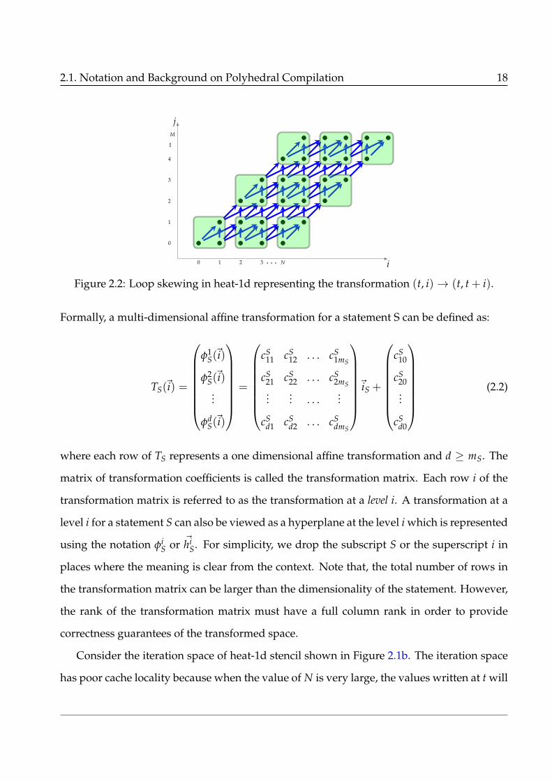
Consider the iteration space of heat-1d stencil shown in Figure 2.1b. The iteration space
has poor cache locality because when the value of N is very large, the values written at t will

2.1. Notation and Background on Polyhedral Compilation 19
be evicted from the cache and will not be available in cache for reads during the iteration
t+ 1 resulting in significant loss. Loop tiling (blocking) is a technique which is used to improve
locality in loop nests. Rectangular tiling can not be done on the above loop nest because
dependence vectors have both positive and negative components. However, if we skew the
loop nest with the transformation:
T(i, j) =
1 0
1 1
·i
j
+
0
0
, (2.3)
every dependence will have non-negative components as shown in Figure 2.2, and hence,
the loop nest can be tiled. The above transformation, at the outermost level, corresponds
to the affine transformation, in which, the transformation coefficient c11 = 1, c12 = 0 and
c10 = 0. At the second level, the transformation coefficient c21 = 1, c22 = 1, and c20 = 0,
representing a loop skewing transformation. While referring the transformation at a given
level we omit the first number in the subscript. We use the notation TS(t, i) → (t, t + i),
as a shorthand, to represent the transformation shown in Equation 2.3. The transformed
iteration space is shown in Figure 2.2.
Modeling loop distribution: Loop distribution in polyhedral frameworks is modeled us-
ing scalar hyperplanes. A hyperplane at a level i for a statement S is said to be scalar, if every
transformation coefficient for the statement S, cSi is zero, for all 1 ≤ i ≤ mS. This corresponds
to trivial hyperplane for the statement S at a level i or a constant function. Therefore, the
dimensionality of the transformation matrix TS given by d in Equation 2.2, can be greater
than mS, and is used to model loop distributions at various levels. Note that, the value of cS0
can be different for different statements. The statements that are distributed have different
values of cS0 when compared with each other and the ordering of statements after distribu-
tion is given by the increasing order of corresponding c0s. Any transformation with any
possible nesting structure of the loop nest can be represented with 2× mS + 1 rows in the

2.1. Notation and Background on Polyhedral Compilation 20
for(i=0; i<N; i++)for(j=0; j<N; j++)
A[i][j] = A[i][j] + u1[i]*v1[j] + u2[i]*v2[j];
for(i=0; i<N; i++)for(j=0; j<N; j++)
x[i] = x[i] + beta* A[j][i]*y[j];
(a) Gemver Code snippet from PolyBench kernel.
TS1(i, j)→ (0, i, j)TS2(i, j)→ (0, i, j)
(b) Transformation repre-senting full distribution.
for(i=0; i<N; i++) {for(j=0; j<N; j++)
A[j][i] = A[j][i] + u1[i]*v1[j] + u2[i]*v2[j];
for(j=0; j<N; j++)x[i] = x[i] + beta* A[j][i]*y[j];
}
(c) Distribution at level 1.
TS1(i, j)→ (j, 0, i)TS2(i, j)→ (i, 1, j)
(d) Transformation for loopdistribution at level 1.
for(i=0; i<N; i++)for(j=0; j<N; j++) {
A[j][i] = A[j][i] + u1[i]*v1[j] + u2[i]*v2[j];x[i] = x[i] + beta* A[j][i]*y[j];
}
(e) Perfect loop nest.
TS1(i, j)→ (j, i, 0)TS2(i, j)→ (i, j, 1)
(f) Transformation for fullfusion.
Figure 2.3: Valid loop fusion transformations for a code snippet from the gemver kernel ofPolyBench benchmark suite.
transformation matrix. Figure 2.3 provides an example program and few valid transforma-
tions illustrating fusion at different levels.
Iterations in the transformed space are executed in the lexicographic order. Hence, loop
distribution using scalar hyperplanes naturally models this ordering. For example, the
transformation shown in Figure 2.3b, indicates that all iteration of S1 should be executed
before the first instance of S2, which precisely models distribution of loops surrounding
statements S1 and S2 at the outermost level.
Definition 2.1 (Dependence satisfaction) A dependence from a statement Si to a statement Sj rep-
resented by an edge e in the data dependence graph, is satisfied at a level ` if and only if ` meets the

2.1. Notation and Background on Polyhedral Compilation 21
condition
∀k.1 ≤ k ≤ `− 1, φkSj(~t)− φk
Si(~s) = 0∧ φ`
Sj(~t)− φ`
Si(~s) ≥ 1, 〈~s,~t〉 ∈ De,
where De represents the dependence polyhedron associated with the edge e.
Intuitively, a dependence d is satisfied at a level `, if ` is the first level in the transformation
that distinguishes the source and the target iterations of the dependence d.
Definition 2.2 (Legal transformation) A multi-dimensional affine loop transformation is said to be
legal or correct, if and only if
TSs(~t)− TSj(~s) �~0, 〈~s,~t〉 ∈ De∀e ∈ GE
Informally, a transformation is legal if all the dependences in the transformed space are
lexicographically positive. In other words, if a dependence is lexicographically negative in
the transformed space, then the transformation is said to violate a dependence.
Definition 2.3 (Outer Parallel loop) A transformation at a level ` is said to be parallel if and only if
φ`Sj(~t)− φ`
Si(~s) = 0, 〈~s,~t〉 ∈ De, ∀e ∈ GE.
An outer parallel loop is such that, if it is placed at the outermost level and parallelized, all
the dependences are satisfied at the inner levels and the resulting loop nest is communication
free. Hence, a loop nest with outer parallel loop is called as a communication free loop nest.
A loop at a level l is said to be inner parallel if and only if
φ`Sj(~t)− φ`
Si(~s) = 0, 〈~s,~t〉 ∈ De,
2.2. The Pluto Algorithm 22
were De represents the dependence polyhedron of an edge e corresponding to any depen-
dence that is not satisfied till level `− 1.
Definition 2.4 (Permutable Band) Transformation hyperplanes at levels l, l + 1, . . . , l + n form a
permutable band if they satisfy the condition:
∀k.l ≤ k ≤ l + n, φkSj(~t)− φk
Si(~s) ≥ 0, 〈~s,~t〉 ∈ De,
where De represents the dependence polyhedron of a dependence that is unsatisfied till level l − 1.
It is easy to see that loops that form a permutable band can be permuted among themselves.
If all the levels in the transformation form a permutable band, then the loop nest is said to
be fully permutable. A fully permutable loop nest can be rectangluarly tiled. In the rest of
this thesis, we refer to rectangular tiling as tiling of the loop nest. For the example shown
in Figure 2.1, the transformation (t, i) → (t, t + i) satisfies all dependences at the outermost
level and the inner loop is parallel. The above transformation yields a fully permutable loop
nest, and hence, the loop nest can be tiled. The tiled iteration space is shown in Figure 2.2.
The goal of polyhedral auto-transformation frameworks is to find the transformation ma-
trix, in particular, the transformation coefficients for each level, for every statement in the
program. Many affine loop transformation frameworks have been proposed in literature
with various objectives. These objectives include maximizing parallelism, locality, minimiz-
ing latency along with other factors. In the next section, we will discuss the details of the
Pluto algorithm [BHRS08] which has been used in some form or the other in many state-of-
the-art affine transformation frameworks like LLVM-Polly, ISL and PPCG.
2.2 The Pluto Algorithm
Pluto [BHRS08, BBK+08] is a source-to-source, polyhedral auto-transformation tool that op-
timizes affine loop nests in the input program, by finding affine loop transformations that

2.2. The Pluto Algorithm 23
maximize locality and parallelism. Given the index sets of statements in the program, and
dependences in the form of dependence polyhedra, the Pluto algorithm iteratively finds lin-
early independent hyperplanes. The hyperplanes found, try to minimize the dependence
distance. This objective is formulated as an Integer Linear Programming (ILP) problem,
which we provide in the rest of this section.
The Pluto algorithm iteratively finds hyperplanes from outermost to innermost looking
for tileable bands. That is, every hyperplane satisfies the tiling validity constraint shown in
(2.4), for every dependence 〈~s,~t〉 ∈ DSi→Sj :
φSj(~t)− φSi(~s) ≥ 0. (2.4)
The objective function used by the Pluto algorithm tries to minimize the dependence
distances using a bounding function shown in (2.5):
φSj(~t)− φSi(~s) ≤ ~u · ~p + w. (2.5)
The intuition behind this upper bound on dependence distances is as follows: dependence
distances are bounded by loop iterator variables, that are, in turn, bounded by program pa-
rameters. Therefore, one can choose large enough values for ~u to obtain an upper bound.
Note that, constraints shown in Equations 2.4 and 2.5 can be non-linear in certain cases and
are linearized by the application of Farkas Lemma [Sch86]. In order to minimize depen-
dence distances, the Pluto algorithm tries to minimize this upper bound. This is achieved
by finding the lexicographically smallest ~u and w as shown in (2.6):
minimize≺(~u, w, . . . , cSi , . . . ), (2.6)
where cSi represents transformation coefficients of the statement S. The lexicographically

2.2. The Pluto Algorithm 24
smallest solution can be found using PIP [Fea88]. We refer to the lexicographically smallest
solution (~u, w) as lexmin of (~u, w). Note that, well-known ILP solvers like GLPK [GNU],
Gurobi [GO16] and CPLEX [IBM] do not provide a lexmin function. However, in practice,
lexmin can be implemented as a weighted sum objective as shown in (2.7):
minimize b1.~u + b2.w + b3.c1 + · · ·+ cms + c0, (2.7)
where each bi is orders of magnitude smaller than bi−1.
2.2.1 Avoiding the Zero Solution
The tiling validity constraints and the dependence bounding constraints from (2.4) and (2.5)
have a trivial zero vector solution. Construction of trivial solution avoidance constraints in
the full space of integral solutions is complex and has to be modeled as in Pluto+ [BAC16] by
the introduction of binary decision variables. Therefore, as a trade off, the Pluto algorithm
restricts all transformation coefficients (of φ′Ss) to non-negative integers. This restriction al-
lows the trivial zero vector solution for the coefficients of φS to be avoided with the constraint
shown in (2.8):mS
∑i=0
ci ≥ 1. (2.8)
2.2.2 Enforcing Linear Independence
Affine transformations have to be one-to-one mappings in order for them to specify a com-
plete schedule. This property also guarantees the satisfaction of all dependences in the
transformed space, in the case of Pluto algorithm. The Pluto algorithm thus enforces lin-
ear independence of hyperplanes statement-wise. This is modeled by finding a basis for
the null space of hyperplanes already found. The next hyperplane to be found must have a
component in this null space. The exact modeling of this constraint is described in [BAC16].
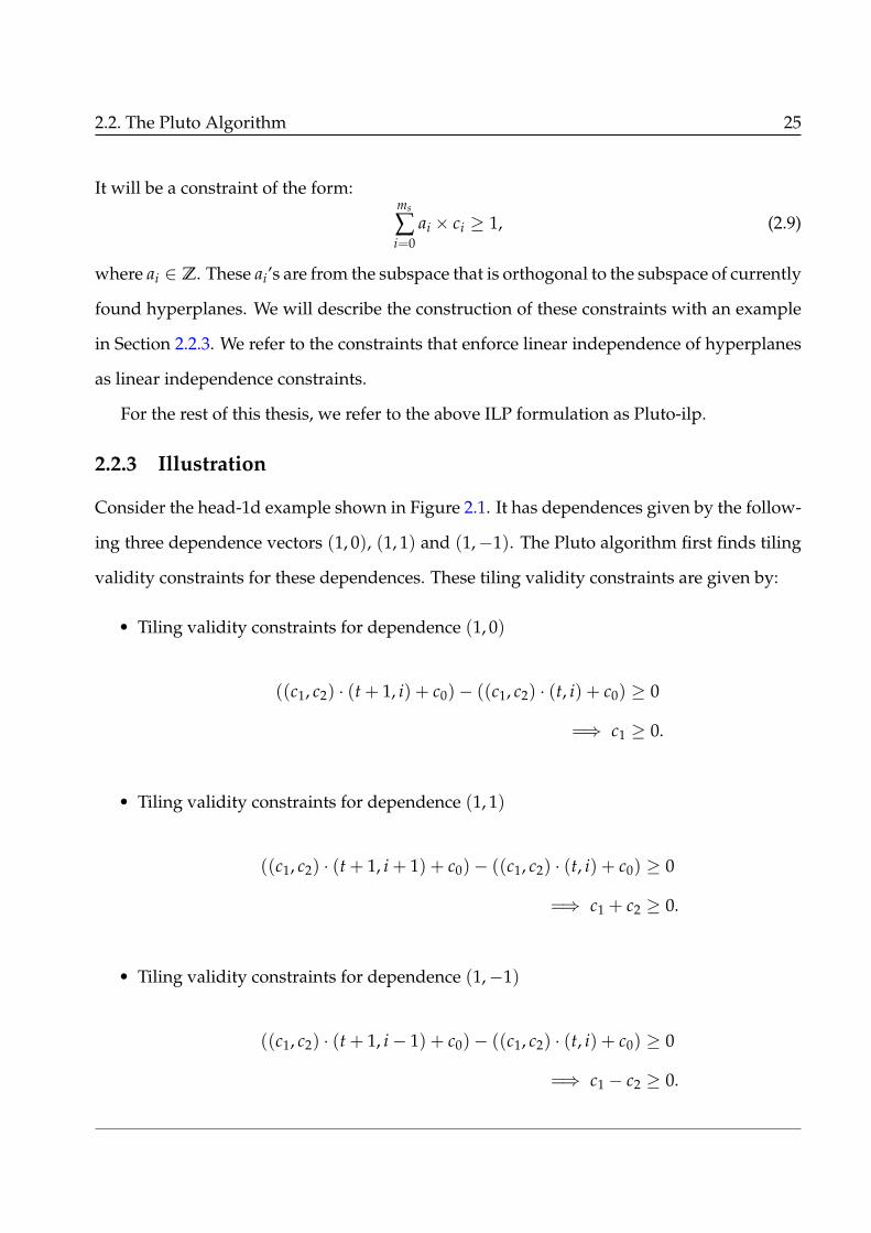
2.2. The Pluto Algorithm 25
It will be a constraint of the form:ms
∑i=0
ai × ci ≥ 1, (2.9)
where ai ∈ Z. These ai’s are from the subspace that is orthogonal to the subspace of currently
found hyperplanes. We will describe the construction of these constraints with an example
in Section 2.2.3. We refer to the constraints that enforce linear independence of hyperplanes
as linear independence constraints.
For the rest of this thesis, we refer to the above ILP formulation as Pluto-ilp.
2.2.3 Illustration
Consider the head-1d example shown in Figure 2.1. It has dependences given by the follow-
ing three dependence vectors (1, 0), (1, 1) and (1,−1). The Pluto algorithm first finds tiling
validity constraints for these dependences. These tiling validity constraints are given by:
• Tiling validity constraints for dependence (1, 0)
((c1, c2) · (t + 1, i) + c0)− ((c1, c2) · (t, i) + c0) ≥ 0
=⇒ c1 ≥ 0.
• Tiling validity constraints for dependence (1, 1)
((c1, c2) · (t + 1, i + 1) + c0)− ((c1, c2) · (t, i) + c0) ≥ 0
=⇒ c1 + c2 ≥ 0.
• Tiling validity constraints for dependence (1,−1)
((c1, c2) · (t + 1, i− 1) + c0)− ((c1, c2) · (t, i) + c0) ≥ 0
=⇒ c1 − c2 ≥ 0.

2.2. The Pluto Algorithm 26
Since the dependences are constant, the dependence distances are not parametric. Hence,
~u in Equation 2.5 is zero. Note that, this can be inferred by the application of Farkas lemma as
well. The coefficients corresponding to the loop iterator variables cancel out and hence the
Farkas multipliers that contain the variables representing the loop parameters, that come
from loop bounds, will be inferred to be zero. Thus, the dependence distance bounding
constraints are given by:
• Dependence distance bounding constraints for dependence (1, 0)
((c1, c2).(t + 1, i) + c0)− ((c1, c2).(t, i) + c0) ≤ w
=⇒ w− c1 ≥ 0.
• Dependence distance bounding constraints for dependence (1, 1)
((c1, c2).(t + 1, i + 1) + c0)− ((c1, c2).(t, i) + c0) ≤ w
=⇒ w− c1 − c2 ≥ 0.
• Dependence distance bounding constraints for dependence (1,−1)
((c1, c2).(t + 1, i− 1) + c0)− ((c1, c2).(t, i) + c0) ≤ w
=⇒ w− c1 + c2 ≥ 0.
The trivial solution avoiding constraint is given by
c1 + c2 ≥ 1.
For the first hyperplane, there are no hyperplanes found before. Hence the linear indepen-

2.2. The Pluto Algorithm 27
lexmin(u1, u2, w, c1, c2)subject to :
c1 ≥ 0c1 + c2 ≥ 0c1 − c2 ≥ 0w− c1 ≥ 0
w− c1 − c2 ≥ 0w− c1 + c2 ≥ 0
c1 + c2 ≥ 1c1 + c2 ≥ 1
u1 ≥ 0u2 ≥ 0w ≥ 0c0 ≥ 0c1 ≥ 0c2 ≥ 0
First hyperplane : (c0, c1) = (1, 0)Second hyperplane : (c0, c1) = (1, 1)
Figure 2.4: Pluto’s ILP formulation for the outermost hyperplane of heat-1d kernel.
dence of the hyperplane to be found is enforced using the constraint,
c1 + c2 ≥ 1.
Since the Pluto algorithm restricts the transformation coefficients to be in the non-negative
half space, it also enforces a lower bound of zero on the transformation coefficients. The ILP
formulation solved by the Pluto algorithm to find the first hyperplane for the heat-1d kernel
is shown in Figure 2.4. The lexicographically smallest solution to this ILP formulation corre-
sponds to the hyperplane~t at the outermost level. Now, to find the second hyperplane, Pluto
constructs constraints that enforce the newly found hyperplane to have a component in the
null space of the hyperplanes that have already been found. For the above example, the
hyperplane is represented by the vector (1, 0). Since the second component of this vector is
zero, Pluto enforces the second hyperplane to have a non-zero component along dimension
i by adding the constraint
c2 ≥ 1, (2.10)
in the above ILP formulation. Note that, the linear independence constraint used for the
previous hyperplane (shown in blue) is replaced with the one shown in Equation 2.10. This
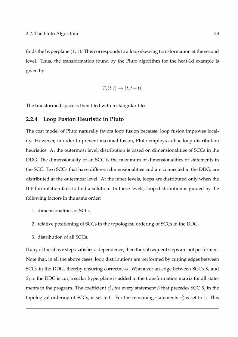
2.2. The Pluto Algorithm 28
finds the hyperplane (1, 1). This corresponds to a loop skewing transformation at the second
level. Thus, the transformation found by the Pluto algorithm for the heat-1d example is
given by
TS(t, i)→ (t, t + i).
The transformed space is then tiled with rectangular tiles.
2.2.4 Loop Fusion Heuristic in Pluto
The cost model of Pluto naturally favors loop fusion because, loop fusion improves local-
ity. However, in order to prevent maximal fusion, Pluto employs adhoc loop distribution
heuristics. At the outermost level, distribution is based on dimensionalities of SCCs in the
DDG. The dimensionality of an SCC is the maximum of dimensionalities of statements in
the SCC. Two SCCs that have different dimensionalities and are connected in the DDG, are
distributed at the outermost level. At the inner levels, loops are distributed only when the
ILP formulation fails to find a solution. In these levels, loop distribution is guided by the
following factors in the same order:
1. dimensionalities of SCCs,
2. relative positioning of SCCs in the topological ordering of SCCs in the DDG,
3. distribution of all SCCs.
If any of the above steps satisfies a dependence, then the subsequent steps are not performed.
Note that, in all the above cases, loop distributions are performed by cutting edges between
SCCs in the DDG, thereby ensuring correctness. Whenever an edge between SCCs Si and
Sj in the DDG is cut, a scalar hyperplane is added in the transformation matrix for all state-
ments in the program. The coefficient cS0 , for every statement S that precedes SCC Sj in the
topological ordering of SCCs, is set to 0. For the remaining statements cS0 is set to 1. This

2.3. Scalability of the Pluto Algorithm 29
loop fusion heuristic in Pluto does not consider other factors like parallelism into account.
In the rest of the thesis, whenever we say that a loop nest is distributed, the same procedure
of adding scalar hyperplanes is followed.
2.3 Scalability of the Pluto Algorithm
The complexity of solving the ILP formulation in Pluto is exponential in the number of
variables seen by the ILP solver. The ILP formulation in Pluto has
|P|+ 1 + ∑S∈P
(mS + 1)
variables, where P is the set of parameters in the program. Thus, solving this ILP formula-
tion is exponential in the sum of dimensionalities of polyhedral statements in the program.
In the rest of this thesis, whenever we say that an algorithm is polynomial or exponential,
we mean that the algorithm is polynomial or exponential in the sum total of dimensionali-
ties of polyhedral statements seen by the auto-transformation framework. Though solving
this ILP formulation is exponential in general, for the scheduling algorithms that are often
used in the polyhedral compilation, the observed time complexity has been shown to be
O(V5) [Fea06, UC13, MY15], where V is the number of variables in the ILP formulation.
Mehta et al. [MY15] identified this ILP formulation and the construction of linear indepen-
dence constraints as major bottlenecks in Pluto’s algorithm. Efforts to address this scala-
bility have been primarily directed towards reducing the number of variables seen by the
Pluto’s ILP formulation via statement clustering [MY15, Bag15] or by projecting out vari-
ables [PMB+16]. However, this tends to postpone the problem of scalability. For example,
there exist programs where the clustering heuristics proposed by Mehta et al. [MY15] re-
sults in clusters with a small number of statements, and hence, the impact of clustering on
auto-transformation times is diminished.
In the rest of this thesis, we propose a framework that overcomes both the bottlenecks
2.3. Scalability of the Pluto Algorithm 30
by (1) relaxing integer constraints in Pluto-ILP and (2) decoupling the problem of finding
permutations and fusion, from other loop transformations. This decomposition, which uses
an LP formulation at each stage, does not require the construction of linear independence
constraints, there by providing a scalable auto-transformation framework that uses the poly-
hedral model. The decoupling also allows the modeling of loop fusion alongside other loop
transformations like loop permutation and loop shifting. We also demonstrate that various
loop fusion models can be incorporated seamlessly in our auto-transformation framework.
The rest of the thesis provides the details on the proposed auto-transformation framework
Pluto-lp-dfp and evaluates it on previously studied benchmarks.
Chapter 3
Relaxing Integrality Constraints in the
Pluto Algorithm
The Pluto algorithm described in Chapter 2 finds affine transformation hyperplanes from the
outermost level to the innermost. At each level, the algorithm finds hyperplanes that min-
imize dependence distances, by formulating an ILP problem. The number of variables and
constraints in the ILP increases with the number of statements in the program. The problem
is NP-hard in the number of variables seen by the ILP solver. This ILP formulation results in
an auto-transformation framework which is exponential in the number of statements in the
program resulting in large compilation (auto-transformation) times in the case of loop nests
with hundreds of statements. In order to reduce this complexity, in this chapter, we study
the effect of relaxing the integer constraint on the variables of this ILP formulation.
When the variables in Pluto’s ILP formulation are modeled as reals instead of integers,
the trivial solution avoidance constraints and the linear independence constraints shown in
Equations (2.8) and (2.9), do not model the full space of non-negative real numbers. The
complete space of non-negative reals is modeled by changing constraints in (2.8) and (2.9)

3.1. Theoretical Results 32
to strict inequalities:mS
∑i=0
ci > 0,mS
∑i=0
ai × ci > 0, (3.1)
where ai ∈ Z is a constant. We refer to this relaxed formulation as pluto-lp, while pluto-ilp
will be used to refer to the original ILP formulation of Pluto (cf. Chapter 2). Note that it is
not directly possible to encode the above constraints, and we do not do this. Instead, we
will use the original constraints in the LP formulation. However, before we propose that,
we discuss a few results surrounding the relaxed version of the formulation when the linear
independence and the trivial solution avoidance constraints precisely model the complete
space of real solutions as shown in Equation 3.1.
In this chapter, we first present key results that can be obtained by relaxing the ILP for-
mulation in Pluto while solving for a hyperplane. We provide a routine to infer solutions to
the ILP formulation in Pluto using the solutions of the relaxed formulation, thus avoiding
the ILP based approach. We identify certain interesting properties that are preserved in the
relaxed formulation even in presence of certain sub-optimalities.
3.1 Theoretical Results
We now present various theorems relating the solutions of pluto-lp to those of pluto-ilp. We
first assume that the trivial solution avoidance constraints and the linear independence en-
forcing constraints model the complete space of real transformation coefficients as shown
in Equation 3.1. The tiling validity constraints and the dependence distance bounding con-
straints are same as the ones used in pluto-ilp as shown in Equations 2.4 and 2.5 respectively.
The objective of pluto-lp is same as that of of the objective of pluto-ilp, which is to find the
minimize the dependence distances as shown in Equation 2.6.
We first note through Lemma 3.1 that, if the constraints in pluto-lp are satisfiable, then its
optimal solution is rational.
Lemma 3.1 The optimal solution to pluto-lp, when it exists, is rational.

3.1. Theoretical Results 33
The above lemma follows from the fact that coefficients of all variables in the LP formulation
of Pluto are integers; thus the solutions of pluto-lp are rational. For the rest of this thesis,
we refer to the optimal rational solution of pluto-lp as the solution of pluto-lp. Note that,
even when a few more constraints are added to the constraints of Pluto-lp, as long as the
coefficients of variables in the newly added constraints are integers, Lemma 3.1 continues to
hold.
Theorem 3.1 If ~z is a solution to the relaxed Pluto formulation (pluto-lp), then for any constant
k ≥ 1, k×~z is also a valid solution to the constraints in pluto-lp.
The intuition behind the proof of this theorem is as follows: ~z is a solution to pluto-lp and
hence will satisfy the tiling validity constraints (Equation 2.4). Therefore, for every depen-
dence 〈~s,~t〉 ∈ De,
φSj(~t)− φSi(~s) ≥ 0
=⇒ (k× φSj)(~t)− (k× φSi)(~s) ≥ 0,
where Si, Sj are the source and the target statements of the dependence and k ≥ 1. Infor-
mally, scaling the rational hyperplane will also scale up the dependence distance between
the source and the target iterations by the same scaling factor and will not violate any de-
pendence. It is easy to see that scaling the rational solution with k ≥ 1 will not violate any
linear independence constraints shown in (3.1). The formal proof of Theorem 3.1 is given
below.
Proof: From Lemma 3.1, we know that, if a solution exists, then the optimal value of the ob-
jective corresponds to a rational solution of pluto-lp. Now, we need to prove that, scaling the
solutions of pluto-lp will not violate the constraints. Consider the tiling validity constraints

3.1. Theoretical Results 34
in (2.4). φSi and φSj are one dimensional affine transformations. Therefore,
φSj(~t)− φSi(~s) ≥ 0 =⇒ k× φSj(~t)− k× φSi(~s) ≥ 0
where k ≥ 1. Therefore, the scaled solution of pluto-lp will represent a hyperplane that will
not violate the tiling validity constraints. The dependence distance bounding constraints in
Equation (2.5) are bounded above by ~u and w, which are variables in the pluto-lp formula-
tion. The values of ~u and w are can also be scaled up, and these scaled up values still remain
to be an affine combination of program program parameters as shown:
k× φSj(~t)− k× φSi(~s) ≥ k× ~u + k× w.
The trivial solution avoidance constraints and the linear independence enforcing constraints
given in (3.1) can not be violated by scaling the solutions. That is, if ci’s are the solutions to
pluto-lp and k ≥ 1, then from (3.1) it follows that for each statement S,
mS
∑i=0
ci > 0 ⇐⇒mS
∑i=0
k× ci > 0
and,mS
∑i=0
ai × ci > 0 ⇐⇒mS
∑i=0
ai × k× ci > 0.
Therefore scaling the solutions of pluto-lp with a factor k ≥ 1, will not violate the constraints.
�
Note that the theorem holds for all k > 0 when the linear independence constraints
and the trivial solution avoidance constraints are modeled precisely as in (3.1). However,
we are interested in scaling rational solutions to integers. The integer solution, if it exists,
must be lexicographically greater than the rational solution. Therefore, we prove it for k ≥
1. Moreover, the constraints in (3.1) cannot be modeled in a solver as discussed later in
Section 3.2. In those cases, one can only scale the solutions with a value of k ≥ 1 and not

3.1. Theoretical Results 35
with any value k > 0.
Corollary 3.1 proves that a solution of pluto-lp can be used to infer the solutions of pluto-
ilp. This result is used extensively in Algorithms 2, 3 that form the core components of the
new transformation approach presented in this thesis.
Corollary 3.1 There exists a solution to pluto-lp if and only if there exists a solution to pluto-ilp.
Proof: The necessary condition is trivially true since every integral solution in the space of
pluto-ilp is in the space of pluto-lp as well. For the sufficient condition, by Theorem 3.1, the
rational solutions of pluto-lp can be scaled to integers by choosing the LCM of the denomi-
nators of the solutions as the scaling factors without violating any dependences. The integer
hyperplane found through scaling will continue to be linearly independent of previously
found hyperplanes. Therefore, this scaled solution will be in the space of pluto-ilp. � Con-
straints corresponding to dependences of a connected component in a DDG impose bounds
on one another. Hence coefficients corresponding to different connected components, that
are obtained by pluto-lp, can be scaled by different factors. This naturally calls us to look
for scaling factors for each connected component in the DDG independently. In the rest of
this section, we prove results only for a single connected component. However, they can be
easily extended to multiple connected components, as each connected component results in
a disjoint set of constraints in LP and ILP formulations of the Pluto algorithm.
We identify relations between the objective value and solutions of pluto-lp and the objec-
tive of pluto-ilp under the assumption that the linear independence constraints and the trivial
solution avoidance constraints are modeled precisely. This is an interesting theoretical result
to have, though the practical issues in realizing it are discussed in Section 3.2. Assuming that
the full space of rational solutions is modeled precisely, we observe that the optimal solution
to the relaxed Pluto algorithm (pluto-lp) can be scaled to an integral solution to pluto-ilp such
that (1) the objective of the scaled (integral) solution will be equal to the objective of optimal
solution of pluto-ilp. (2) For each statement S, the hyperplane found by pluto-ilp will be a

3.1. Theoretical Results 36
scaled up version of the hyperplane found by pluto-lp. Though, we do not use these results
in our implementation, these are applicable in a futuristic setting where constraint solvers
allow to specify a small rational number which is greater than zero.
Theorem 3.2 The optimal solution to the relaxed Pluto algorithm (pluto-lp) can be scaled to an
integral solution to pluto-lp such that the objective of the scaled (integral) solution will be equal to
the objective of optimal solution of pluto-ilp.
Proof: By Theorem 3.1, we know that scaling the rational solutions of pluto-lp, will result in
a solution does not violate any constraints. Let zi and zr be the value of the optimal objective
values for solutions to pluto-ilp and pluto-lp respectively. Let cs be the smallest scaling factor
that scales solutions of pluto-lp to integers. Let z′i = cs × zr be the value obtained from by
scaling the optimal real solution of pluto-lp to an integral one. Note that cs ≥ 1; otherwise,
the real solution would not be optimal. Now we prove that z′i ≤ zi. Consider z′r given by
z′r = zi/cs
=⇒ zr ≤ z′r(∵ zr is the optimal solution to pluto-lp)
=⇒ cs × zr ≤ cs × z′r (∵ cs ≥ 1 and zr, z′r ≥ 0)
=⇒ z′i ≤ zi.
This proves that the optimal (minimum) objective of pluto-lp after scaling to integer coeffi-
cients will be less than or equal to that of of pluto-ilp. However, the objective of the relaxed
formulation after scaling cannot be strictly less than that of pluto-ilp (otherwise, pluto-ilp’s
solution, zi would not be an optimal one). Therefore, the optimal objective of pluto-lp after
scaling up, is equal to the optimal objective of pluto-ilp. �
Theorem 3.2 states that the objective function of pluto-lp will evaluate to a scaled down
value of the objective function of pluto-ilp. In Theorem 3.3, we prove that the hyperplane
found by pluto-lp will be a scaled down version of the hyperplane found by pluto-ilp.

3.2. Practical Issues in Using Pluto-lp 37
Theorem 3.3 Let ~hi = (c1, . . . , cn) be the optimal solution for pluto-ilp. Then, the optimal solution
to pluto-lp, ~hr, is such that ~hr = ~hi/cs where cs ≥ 1.
Proof: Let zi and zr be the optimal values of the objective found by pluto-ilp and pluto-lp
respectively. Let cs be the smallest scaling factor that scales every component of ~hr to an
integer. Note that cs ≥ 1 (otherwise, ~hr would not have been optimal solution). Let zi be
the solution obtained by the hyperplane ~hi. Let z′r = zi/cs. Note that z′r can be obtained by
dividing all the components of ~hi by cs. Now we have the following cases:
• Case 1: If zr = z′r then we have nothing to prove.
• Case 2: Consider the case zr < z′r. Let ~h′i = ~hr × cs, and let z′i be the objective value
with h′i. z′i = zr × cs (due to the nature of (2.5)). Since the optimal objective value for
pluto-ilp was found to be zi, z′i ≥ zi. Now if we scale down each component of ~hi by cs,
we get a solution that has an objective value lower than zr. This is a contradiction.
Therefore, zr = z′r in all cases, and z′i = zi. Since both ~hi and ~h′i have the same optimal
objective value and given that the lexmin provides a unique optimal solution, ~h′i = ~hi, and
~hr = ~hi/cs. � Theorems 3.2 and 3.3 assume that trivial solution avoidance constraints and
linear independence constraints precisely model the space of rational solutions. However,
this is not possible with the current LP solvers. Therefore, in the next section, we discuss the
issues in realizing pluto-lp in practice.
3.2 Practical Issues in Using Pluto-lp
As per the theorems presented in the previous section, it would appear that pluto-lp could
be readily used by scaling its rational solutions — to replace pluto-ilp and thus overcome the
need to use ILP altogether. However, in this section, we discuss issues encountered in that
process.

3.2. Practical Issues in Using Pluto-lp 38
The rational solutions of pluto-lp after scaling with give the solutions of pluto-ilp if and
only if linear independence constraints and trivial solution avoidance constraints model the
complete space rational solutions as shown in (3.1). However, these constraints cannot be
represented as “≥” constraints. Doing so in (2.8) and (2.9) will exclude some rational solu-
tions. More precisely, these constraints, when modeled imprecisely, will exclude infinites-
imally small positive values that are closer to zero. This is because the rational space is
“dense”, which makes it hard to model rational numbers that are strictly greater than zero.
Therefore, the relaxed LP formulation after scaling up to integers will end up giving sub-
optimal solutions in the integral space. These sub-optimal solutions usually manifest as
unnecessary loop skewing transformations, which may result in significant loss of perfor-
mance.
−c2 + c1 ≥ 0c1 ≥ 0c2 + c1 ≥ 0u ≥ 0u + w− c1 ≥ 0u + w− c2 − c1 ≥ 0u + w− c1 ≥ 0u + w + c2 − c1 ≥ 0
u ≥ 0w ≥ 0c1 ≥ 0c2 ≥ 0c0 ≥ 0c2 + c1 ≥ 1c2 + c1 ≥ 1
Dependences:(1, 0), (1, 1), (1,−1)pluto-ilp solution:u = 0, w = 1, c2 = 0,c1 = 1, c0 = 0pluto-lp solution:u = 0, w = 1, c2 = 0.5,c1 = 0.5, c0 = 0
Figure 3.1: Constraints from the heat-1d stencil benchmark
For example, consider the constraints given in Figure 3.1. These are pluto-ilp constraints
for the first (outermost) hyperplane of the heat-1d non-periodic stencil shown in Figure 2.1.
Here ~u is one dimensional; therefore is represented as a scalar variable u in Figure 3.1. The
code has a single statement in the two dimensional loop nest. c1 and c2 are the coefficients
corresponding to the time dimension t and the space dimension i respectively. The last
two constraints are trivial solution avoidance constraint and linear independence constraint
respectively. Rest of them establish tiling validity and enforce a upper bound on the depen-
dence distances. The hyperplane (c1, c2) = (1, 0) is found by pluto-ilp with the values of
u = 0 and w = 1 (without diamond tiling support).

3.2. Practical Issues in Using Pluto-lp 39
When the integer constraints on the coefficients are relaxed, pluto-lp finds the solution
(c1, c2) = (0.5, 0.5) with the value of w = 1 and u = 0. However, when we scale the solutions
to integers, we get a value of u = 0 and w = 2 which is higher than the objective of pluto-ilp.
However the solution (u = 0, w = 0.5, c1 = 0.5, c2) would have been ideal because (1) it
is lexicographically smaller than the one found by pluto-ilp. (2) after scaling with a scaling
factor of 2, we would have got the same solution as that of pluto-ilp. Unfortunately, the
solution is not in the space of all valid transformations because the trivial solution avoidance
constraint and the linear independence constraints (2.8 and 2.9) do not model the space of
all rational solutions.
Note that scaling down the RHS of the trivial solution avoidance constraints and linear
independence constraints to say 0.1 (which now includes (c1, c2) = (0.5, 0) in the space) will
not solve the issue. This is because one can scale down the solution to (c1, c2) = (0.05, 0.05)
and still end up with the hyperplane (c1, c2) = (1, 1). The solution (c1, c2) = (0.05, 0) will
still not be present in the space. The hyperplane (1, 1) found by pluto-lp does not satisfy the
dependence (1,−1), and hence, must be satisfied at the innermost level, resulting in a fully
sequential loop nest. However, the hyperplane (1, 0) found by pluto-ilp in the first level,
satisfies all the dependences and the innermost loop is parallel. Therefore, it is absolutely
essential to get rid of these sub-optimalities in pluto-lp. For example, for the heat-2d bench-
mark, we observe that pluto-lp finds a schedule that is 10× slower (on 16 cores) than the
schedule found by pluto-ilp. Our approach to overcome these sub-optimalities is described
in Chapter 4.
As mentioned above, sub-optimal loop skewing transformations can be found as a conse-
quence of using the relaxed LP formulation that imprecisely models the real space of trans-
formation coefficients. In spite of this imprecise modeling, there are certain interesting prop-
erties that are retained in the relaxation of pluto-ilp.
Theorem 3.4 The relaxed formulation, pluto-lp (in each permutable band), finds a outer parallel

3.2. Practical Issues in Using Pluto-lp 40
hyperplane if and only if pluto-ilp finds a outer parallel hyperplane.
Proof: There exists a parallel hyperplane if and only if ~u = ~0 and w = 0 in the ILP for-
mulation of Pluto. Note that ~u.̇~p + w gives an upper bound on the dependence distance for
every dependence. Each component of ~u, and w, are lower bounded by zero. Therefore, the
smallest value of ~u.~p + w is 0. The objective of the relaxed LP formulation is to minimize the
values of ~u and w. At the outermost level, any solution that exists in the space of pluto-ilp
is also present in the space of pluto-lp. Therefore the solution found by pluto-lp will fall into
one of the two following cases.
1. The solution found by pluto-lp is same as the solution found by pluto-ilp. In this case,
there is nothing to prove.
2. pluto-lp finds a fractional solution with ~u =~0 and w = 0. In this case, by Theorem 3.1,
one can scale the real (rational) solution to an integral one, without violating any con-
straints. This scaling will neither change the value of ~u nor w because they were found
to be equal to zero.
The “only if” part of the proof follows from Case 2 in the above argument. �
As a consequence of Theorem 3.4, existence of communication free parallel hyperplanes
can be inferred using an LP formulation instead of an ILP formulation. Secondly, the the-
orem can also be used to check if fusion statements from two strongly connected compo-
nents with outermost parallel loops results in a sequential loop nest. ILP based approaches
have been adapted in auto-transformation frameworks like ISL and PPCG for incorporating
parallelism-preserving fusion heuristics. However, Theorem 3.4 shows that equivalent re-
sults can be obtained by an LP based approach as well. Later in Chapter 5, we also use this
result to find dimensions of loops nests that are parallel, and to come up with parallelism
preserving heuristics for loop fusion.
While Theorem 3.4 proved the property of a single hyperplane at the outermost level,

3.3. Complexity of Pluto-lp 41
Theorem 3.5 proves that both pluto-lp and pluto-ilp find tileable bands of the same width, i.e,
the outermost permutable band found by both pluto-lp and pluto-ilp will contain the same
number of hyperplanes.
Theorem 3.5 Given a loop nest of dimensionality m, if pluto-ilp finds d ≤ m permutable hyper-
planes, then pluto-lp also finds d permutable hyperplanes.
Proof: Let us assume that pluto-lp finds k hyperplanes and let k 6= d. We prove Theorem 3.5
by contradiction. Let us assume that k > d. The k linearly independent hyperplanes found
by pluto-lp can be scaled to integers. These scaled solutions will continue to be linearly
independent as scaling transformations will not affect linear independence. Therefore these
correspond to k linearly independent in the integer space. This means that there existed k
linearly independent solutions in the integer space. Since the validity constraints remain the
same at each level, there exits only d linearly independent solutions as found by pluto-ilp.
This is a contradiction to the assumption that k > d.
Suppose k < d, then we know that there are d linearly independent solutions to the tiling
validity constraints in the integer space. These are valid linearly independent solutions in
the rational space. Therefore, it is a contradiction to our assumption k < d. Therefore, pluto-
lp will find d linearly independent solutions to the tiling validity constraints. �
A sufficient condition for tileability is that the loop nest is fully permutable. Is such cases,
both pluto-ilp and pluto-lp find m linearly independent hyperplanes. Therefore, pluto-lp can
also be used as a fast and robust tileability check for a given loop nest.
3.3 Complexity of Pluto-lp
In this section, we will discuss the complexity of finding a rational solution to the LP fromu-
lation in Pluto-lp, i.e the effect of relaxing the integrality constraints in the Pluto algorithm
on its time complexity. Let S be the set of all statements in the program. The Pluto algorithm
has an observed time complexity of O(|S|5) [Fea06, UC13]. This quintic complexity is still

3.4. Scaling Rational Solutions to Integral Solutions 42
high for an auto-transformation algorithm to efficiently scale to programs with large num-
ber of statements. By relaxing the integrality constraints in the ILP formulation of the Pluto
algorithm, the time complexity of the Pluto-lp scheduling algorithm reduces to O(|S|3).
Even though the simplex algorithm, which is used by most LP solvers in practice, has an
exponential worst-case time complexity, it is considered to be highly scalable. Moreover,
interior-point methods for solving LP formulations with V variables in O(V3) time, has
been proposed in literature [Vai89]. Hence for the purposes of complexity analysis, in the
rest of the thesis, we assume that the time complexity of solving an LP formulation isO(V3).
Therefore, the scheduling algorithm in Pluto-lp has a time complexity of O(|S|3).
Note that, the transformation hyperplanes obtained using pluto-lp formulation are ratio-
nals. However, polyhedral code generators like ClooG [Clo04] require integral transforma-
tion coefficients for code generation. In the next section, we describe a routine to scale the
rational solutions obtained by pluto-lp to integers.
3.4 Scaling Rational Solutions to Integral Solutions
The solutions of pluto-lp are rational. Polyhedral code generators require integer coefficients
for schedules. Once solutions to pluto-lp are found, we thus need to find scaling factors that
when multiplied with the solutions of pluto-lp will yield integers. It is possible to design
simple algorithms that scale the rational numbers to integers using dynamic programming.
However, for programming convenience, we solve the scaling problem robustly by formu-
lating a small mixed integer programming (MIP) problem. This scaled solution will not
violate any dependences as proved in Theorem 3.1. We will show that time spent here is
negligible. Since the MIP approach here is chosen for convenience (instead of another poly-
nomial time heuristic), we still claim that our entire approach is free of ILP.
The MIP formulation to infer integer solutions from rational solutions of pluto-lp is simple
and straightforward as shown in Algorithm 1.

3.4. Scaling Rational Solutions to Integral Solutions 43
Algorithm 1: SCALE (SOL, G, P)Input : A solution sol to pluto-lp and the DDG G for the program P.Output: Integer solutions that are scaled versions of the rational solutions from
pluto-lp
1 obj←|C|∑
k=1ck where ck is scaling factor for kth connected component in G, ck ∈ Q.
2 ψ← true3 foreach S ∈ S do4 k← connected component to which S belongs in G.5 foreach i = 0 to ms do6 ψ← ψ ∧ {cS
i = ck × sol(i, S)}, where cSi ∈ Z
7 foreach i = 1 to |C| do8 ψ← ψ ∧ {ck ≥ 1}9 isol← MIP-SOLVE(ψ, obj)
10 Update the hyperplanes of all statements with isol.
Let k be the connected component to which the statement S belongs and ck be the scaling
factor. For each dimension i of a statement S, let sol(i, S) be the solution obtained by pluto-lp.
A scaling constraint (line 6) is added per dimension of every statement that scales sol(i, S) to
cSi . By further constraining cS
i to integer and the scaling variable ck to be greater than or equal
to 1, we ensure that integer transformation coefficients are obtained. Note that the shifting
coefficient cS0 for each statement is also being scaled. There can be multiple valid scaling
factors that scale the solution of pluto-lp to an integral one. However, the minimum scaling
factor for each connected component is naturally desired. Therefore, the sum of the scaling
factors corresponding to each connected component is minimized (line 1). These constraints
are solved using an MIP solver (line 9) like GLPK or Gurobi.
For example, consider the constraints from heat-1d example shown in Figure 2.4 for the
first hyperplane. The pluto-lp algorithm finds the solution u = 0, w = 1, c1 = 0.5, c2 =
0.5, c0 = 0. Since there is a single statement in the program there is a single vertex in the DDG
G of P with a single connected component. Let cs be the scaling factor for this connected
component. In case of multiple connected components, we will have multiple scaling factors
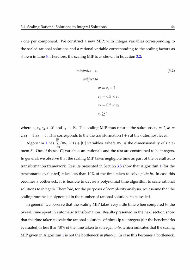
3.4. Scaling Rational Solutions to Integral Solutions 44
- one per component. We construct a new MIP; with integer variables corresponding to
the scaled rational solutions and a rational variable corresponding to the scaling factors as
shown in Line 6. Therefore, the scaling MIP is as shown in Equation 3.2:
minimize cs (3.2)
subject to
w = cs × 1
c1 = 0.5× cs
c2 = 0.5× cs
cs ≥ 1
where w, c1, c2 ∈ Z and cs ∈ R. The scaling MIP thus returns the solutions cs = 2, w =
2, c1 = 1, c2 = 1. This corresponds to the the transformation t + i at the outermost level.
Algorithm 1 has|S|∑
i=1(mSi + 1) + |C| variables, where mSi is the dimensionality of state-
ment Si. Out of these, |C| variables are rationals and the rest are constrained to be integers.
In general, we observe that the scaling MIP takes negligible time as part of the overall auto
transformation framework. Results presented in Section 3.5 show that Algorithm 1 (for the
benchmarks evaluated) takes less than 10% of the time taken to solve pluto-lp. In case this
becomes a bottleneck, it is feasible to devise a polynomial time algorithm to scale rational
solutions to integers. Therefore, for the purposes of complexity analysis, we assume that the
scaling routine is polynomial in the number of rational solutions to be scaled.
In general, we observe that the scaling MIP takes very little time when compared to the
overall time spent in automatic transformation. Results presented in the next section show
that the time taken to scale the rational solutions of pluto-lp to integers (for the benchmarks
evaluated) is less than 10% of the time taken to solve pluto-lp, which indicates that the scaling
MIP given in Algorithm 1 is not the bottleneck in pluto-lp. In case this becomes a bottleneck,

3.5. Preliminary Experimental Results 45
it appears feasible to devise alternate heuristics, that may be ad-hoc in nature, but work
well in practice. One approach would be to infer rational numbers (with small numerators
and denominators) from the real solutions. Another would be to approximate ratios of the
coefficients with rational numbers with small integer numerators and denominators. The
validity of the obtained solution can later be anyway verified quickly.
3.5 Preliminary Experimental Results
In this section, we first provide details on the time taken by four different ILP solvers to solve
the ILP formulation in Pluto-ilp. We then provide the impact of relaxation on constraint
solving times of both Pluto-lp and Pluto-ilp. Though our detailed experimental setup is
described in Chapter 7, we provide some necessary details here to describe the observations
from our preliminary experiments. All our experments were conducted on a 16 core dual
socket Intel Xeon 4110 CPU running at 2.10 GHz. The machine had a total memory of 256
GB DDR4 with a memory transfor rate of 2666 MT per second. We measured the time taken
by the following four solvers to find a solution to the ILP in Pluto’s formulation.
1. Parametric Integer Programming (PIP) [Fea88] is an ILP solver that has been widely
used in polyhedral compilation.
2. Integer Set Library (ISL) [Ver13] is the ILP solver that has been gained lot of interest in
recent times with its ability to find polyhedral schedules, and the lexmin function.
3. GNU Linear Programming Kit (GLPK) [GNU] is an open-source ILP solver that sup-
ports Mixed Integer Programming (MIP) along with ILP and LP formulations. We
used GLPK version 4.65 to solve ILP formulations in pluto-ilp and LP formulations in
pluto-lp. The lexmin objective function was encoded as a weighted sum objective, as
described in Chapter 2.
4. Gurobi [GO16] is a commercial ILP solver which also supports ILP and LP formula-

3.5. Preliminary Experimental Results 46
tions. We used the version 9.0 with an academic license in our experiments. Even in
this case, the lexmin function was encoded as a weight sum objective in case of both
Pluto-ilp and Pluto-lp.
We evaluate the impact of relaxation on benchmarks from PolyBench [Pol10] and hotspots
of BT LU and SP benchmarks from NAS Parallel Benchmark suites. The hotspots from NAS
benchmakarks were previously used by Mehta et al [MY15] for studying the scalability of
the Pluto algorithm.
3.5.1 Impact of ILP Solvers and Relaxation on Constraint Solving Times
In this section, we present the impact of various ILP solvers on the auto-transformation
times of the Pluto algorithm. Note that both PIP and ISL have a lexmin function and hence
the objective function used by Pluto-ilp when using these solvers is the lexmin function
shown in Equation 2.6. However, GLPK and Gurobi do not have a lexmin function and
hence, the objective function used in these solvers is a weighted sum objective shown in
Equation 2.7. Hence the comparison of different solvers is not on the same ILP formulation,
which is unfair. However, our goal was to measure the impact ILP solvers on the auto-
transformation time of the Pluto algorithm. Moreover, for all the benchmarks, both GLPK
and Gurobi found the same transformation as PIP and ISL, while using the weighted sum
objective instead of the lexmin. In the rest of the thesis, though for theoretical reasoning the
lexmin objective is used, for all practical purposes, we assume that the results obtained via
the weighted sum objective in the ILP or LP formulation is same as the solution obtained
using the by using the lexmin objective function. The secondary reason to compare with
GLPK and Gurobi is that, these solvers provide support for LP formulations along with
ILPs, whereas ISL and PIP do not support LPs. Hence, for a fair comparison between Pluto-
lp and Pluto-ilp we want to use a solver that supports both ILP and LP formulations.
In Table 3.1 we detail the time taken to solve the ILP formulation in Pluto by various

3.5. Preliminary Experimental Results 47
Table 3.1: Constraint solving times for pluto-ilp with different solvers.
BenchmarkNumber of
pip isl glpk gurobiTotal
stmts loops deps time
2mm 4 10 13 1.6× 10⁻⁴ 2.9× 10⁻³ 4.1× 10⁻⁴ 0.017 0.0193mm 6 15 19 2.8× 10⁻⁴ 5.0× 10⁻³ 5.2× 10⁻⁴ 0.035 0.043atax 4 6 11 4.3× 10⁻⁵ 8.3× 10⁻⁴ 1.9× 10⁻⁴ 0.024 0.005bicg 4 6 10 4.1× 10⁻⁵ 7.6× 10⁻⁴ 2.3× 10⁻⁴ 0.026 0.005cholesky 4 8 17 3.8× 10⁻⁴ 6.5× 10⁻³ 6.7× 10⁻⁴ 0.015 0.029correlation 15 22 46 5.1× 10⁻⁴ 0.015 6.3× 10⁻⁴ 0.029 0.161covariance 8 15 27 1.9× 10⁻⁴ 4.6× 10⁻³ 4.1× 10⁻⁴ 0.032 0.033doitgen 3 10 13 3.3× 10⁻⁴ 3.9× 10⁻³ 6.2× 10⁻⁴ 0.041 0.023durbin 10 10 50 5.8× 10⁻⁴ 6.8× 10⁻³ 7.4× 10⁻⁴ 0.033 0.049fdtd-2d 4 11 29 6.0× 10⁻⁴ 7.1× 10⁻³ 1.2× 10⁻³ 0.017 0.045floyd-warshall 1 3 61 6.0× 10⁻⁵ 6.4× 10⁻³ 2.9× 10⁻⁴ 0.011 0.017gemm 2 5 6 4.3× 10⁻⁵ 8.5× 10⁻⁴ 2.7× 10⁻⁴ 0.009 0.005gemver 4 7 12 6.3× 10⁻⁵ 1.7× 10⁻³ 2.8× 10⁻⁴ 0.034 0.007gesummv 5 7 14 5.4× 10⁻⁵ 1.1× 10⁻³ 2.3× 10⁻⁴ 0.007 0.006gramschmidt 7 14 28 6.6× 10⁻⁴ 8.1× 10⁻³ 7.7× 10⁻⁴ 0.023 0.065heat-3d 2 8 52 1.9× 10⁻³ 0.011 5.1× 10⁻³ 0.045 0.083jacobi-1d 2 4 20 1.5× 10⁻⁴ 1.5× 10⁻³ 5.0× 10⁻⁴ 0.028 0.009jacobi-2d 2 6 38 6.0× 10⁻⁴ 4.5× 10⁻³ 1.5× 10⁻³ 0.015 0.033lu 3 8 14 3.0× 10⁻⁴ 8.8× 10⁻³ 7.7× 10⁻⁴ 0.018 0.025mvt 2 4 6 2.3× 10⁻⁵ 5.9× 10⁻⁴ 1.7× 10⁻⁴ 0.007 0.002seidel-2d 1 3 29 7.5× 10⁻⁵ 1.2× 10⁻³ 4.5× 10⁻⁴ 0.028 0.012symm 4 10 23 3.4× 10⁻⁴ 4.2× 10⁻³ 6.4× 10⁻⁴ 0.020 0.028syr2k 2 5 6 4.3× 10⁻⁵ 8.0× 10⁻⁴ 2.2× 10⁻⁴ 0.009 0.004syrk 2 5 6 4.1× 10⁻⁵ 7.8× 10⁻⁴ 2.3× 10⁻⁴ 0.009 0.004trisolv 3 4 11 4.8× 10⁻⁵ 8.3× 10⁻⁴ 3.9× 10⁻⁴ 0.028 0.004trmm 2 5 8 5.0× 10⁻⁵ 9.0× 10⁻⁴ 2.5× 10⁻⁴ 0.008 0.006
bt 48 149 824 0.472 6.164 0.061 0.108 297.4lu 106 325 2896 8.996 53.576 0.498 0.379 3.1× 10⁵
sp 50 155 836 0.534 7.353 0.065 0.108 402.6
solvers. For the benchmarks listed in the first column, columns two, three and four give
the number of statements, the number of loops and the number of dependences in the loop
nest. The next four columns provide the time taken (in seconds) by PIP, ISL, GLPK and
Gurobi solvers respectively to solve the ILP formulation in Pluto. These columns do not
include the time taken for the construction of constraints. The last column gives the total
auto-transformation time with GLPK as the ILP solver. The last three rows in the table

3.5. Preliminary Experimental Results 48
correspond to benchmarks from NAS parallel benchmark suite and the rest correspond to
benchmarks from PolyBench. We observe that for smaller benchmarks from PolyBench,
both PIP and GLPK are faster than ISL and Gurobi. Gurobi, being a commercial solver,
involves additional overhead during start-up. This overhead involves checking of licenses
along with some I/O operations which mask the constraint solving time in case of small
ILPs. However, in case of rhs routine from the LU benchamark of the NAS benchmark suite,
which has 108 of statement in the loop nest, Gurobi is faster than other solvers. In other
benchmarks from the NAS benchmark suite, both GLPK and Gurobi are orders of magnitude
faster than PIP and ISL. Note that, irrespective of the solver used, the auto-transformation
times are significantly higher when compared to ILP solving times. This is primarily due to
the construction of linear independence constraints. Thus the constraint solving time alone,
does not appear to be the bottleneck in the ILP formulation of Pluto. The relaxation of the ILP
formulation will reduce constraint solving times, which are only a small fraction of the total
auto-transformation time. Therefore, we hypothesize that, integer relaxation and usage of a
commercial solver like Gurobi, will have significant impacts on auto-transformation times
in any of the following scenarios:
• the number of variables in the ILP are higher,
• the ILP formulation does not restrict transformation coefficients to be non-negative,
• the ILP formulation is different and relatively more complex than Pluto. An example
of such an ILP formulation is the one used by Kong et al. [KP19] in PoCC+. However,
the legality of relaxation on their ILP formulation remains unexplored.
For the experiments mentioned in rest of the thesis, GLPK is used as the default solver
for solving both ILP and LP formulations. From the experiments described in this section,
we can conclude that relaxing the ILP alone will not improve the scalability of the Pluto
algorithm and an auto-transformation framework that completely avoids the construction

3.5. Preliminary Experimental Results 49
of linear independence constraints is absolutely essential.

Chapter 4
Pluto-lp-dfp Framework
In this chapter, we propose a new auto-transformation framework called Pluto-lp-dfp to ad-
dress the limitations of the Pluto-lp formulation. The Pluto-lp formulation, described in
Chapter 3, suffers from the following drawbacks:
• it involves the construction of linear independence constraints, which is the most time
consuming step in Pluto’s auto-transformation framework, and
• sub-optimality issues arising in pluto-lp manifest as spurious loop skewing transforma-
tions. These spurious loop skewing transformations, as observed, inhibit parallelism
at inner levels, thereby significantly reducing performance (over 10× on 16 cores).
However, penalizing loop skewing transformations in the relaxed formulation is not possi-
ble. Even in the integer space, penalizing loop skewing transformations while incorporating
loop scaling is a hard problem.
The Pluto-lp-dfp framework that we propose in this section, addresses both issues by de-
coupling the affine transformation phase into a sequence of simpler transformations. More
specifically, the new auto-transformation approach, decouples the problem of finding an
affine transformation into three steps: (a) loop fusion and permutation, (b) loop scaling and
shifting transformations, and (c) post processing skewing transformation. This decoupling
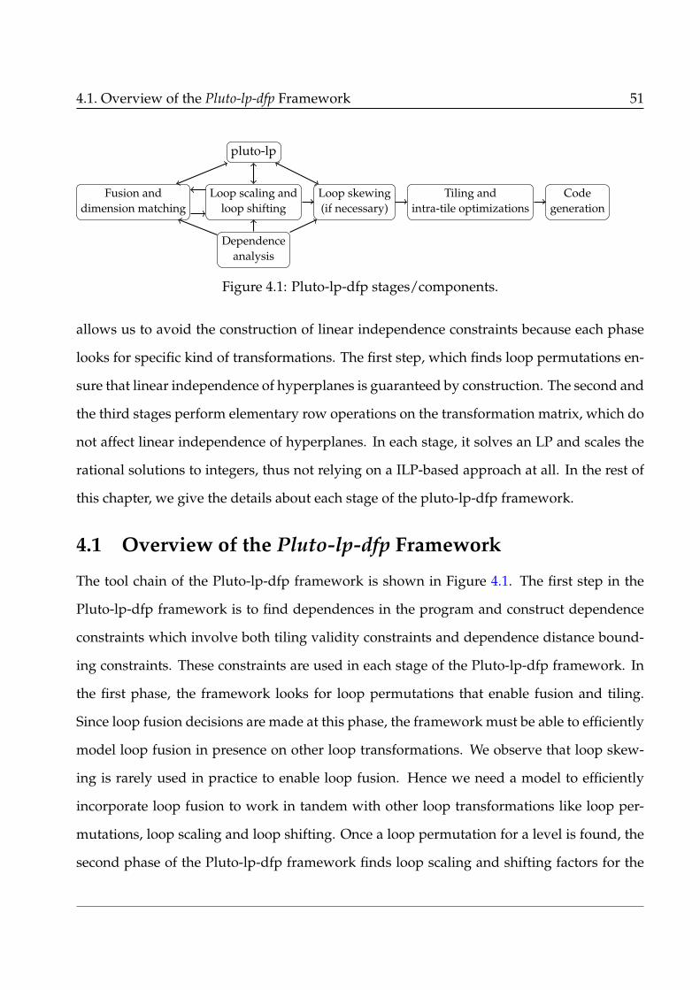
4.1. Overview of the Pluto-lp-dfp Framework 51
Dependenceanalysis
Loop scaling andloop shifting
Fusion anddimension matching
Loop skewing(if necessary)
Tiling andintra-tile optimizations
Codegeneration
pluto-lp
Figure 4.1: Pluto-lp-dfp stages/components.
allows us to avoid the construction of linear independence constraints because each phase
looks for specific kind of transformations. The first step, which finds loop permutations en-
sure that linear independence of hyperplanes is guaranteed by construction. The second and
the third stages perform elementary row operations on the transformation matrix, which do
not affect linear independence of hyperplanes. In each stage, it solves an LP and scales the
rational solutions to integers, thus not relying on a ILP-based approach at all. In the rest of
this chapter, we give the details about each stage of the pluto-lp-dfp framework.
4.1 Overview of the Pluto-lp-dfp Framework
The tool chain of the Pluto-lp-dfp framework is shown in Figure 4.1. The first step in the
Pluto-lp-dfp framework is to find dependences in the program and construct dependence
constraints which involve both tiling validity constraints and dependence distance bound-
ing constraints. These constraints are used in each stage of the Pluto-lp-dfp framework. In
the first phase, the framework looks for loop permutations that enable fusion and tiling.
Since loop fusion decisions are made at this phase, the framework must be able to efficiently
model loop fusion in presence on other loop transformations. We observe that loop skew-
ing is rarely used in practice to enable loop fusion. Hence we need a model to efficiently
incorporate loop fusion to work in tandem with other loop transformations like loop per-
mutations, loop scaling and loop shifting. Once a loop permutation for a level is found, the
second phase of the Pluto-lp-dfp framework finds loop scaling and shifting factors for the

4.2. Valid Permutations 52
permutation found in the first stage. Intuitively the first two stages of the framework can
be assumed to work as follows: the scaling and shifting phase requests for a valid permuta-
tion (described formally in Section 4.2) for a given level, from the first stage. While finding
the valid permutation, loop fusion / distribution decisions are also made. Then, the first
stage returns a permutation for which loop scaling and shifting factors are guaranteed to
exist and these factors are found by the second stage of the Pluto-lp-dfp framework using
an LP-formulation, which are then scaled to integers. Once permutations for all the levels,
and the associated loop scaling and shifting factors are found, the Pluto-lp-dfp framework
introduces loop skewing if and only if loop skewing enables loop tiling. This is important in
cases like stencils, where loop skewing enables loop tiling and further enables tile-wise con-
current start via diamond tiling [BPB12]. If the third phase finds outer-parallel hyperplanes,
these hyperplanes are moved to outer levels of the transformed loop nest. In the rest of this
chapter, we describe in detail, each of these steps in the Pluto-lp-dfp framework.
4.2 Valid Permutations
For the rest of this chapter, the reader can treat the first phase as a black box that provides a
valid permutation to the scaling and shifting phase. However, in this section, we provide the
semantics of this blackbox. We formally define the semantics of valid permutations and also
illustrate that choosing a good permutation is a critical step in the Pluto-lp-dfp framework.
Later in Chapter 5 we describe the details on how this black box can be efficiently realized
in practice.
The first stage of the Pluto-lp-dfp framework provides a valid permutation at each level.
Intuitively, a permutation at a level ` is said to be valid if there exist loop scaling and shifting
factors for the permutation such that the resulting transformation after scaling and shifting
will not violate any dependence. Note that, valid permutation for a statement S is rep-
resented by a permutation matrix P, which has only one non-zero entry per row and per

4.2. Valid Permutations 53
column of P. Every non-zero entry of P is 1. Thus, a valid permutation represents linearly
independent transformation hyperplanes along the canonical axes of the iteration space.
Definition 4.1 (Valid Permutation). A permutation P for a statement S is valid, if and only
if for each level `, the hyperplane φ at level `, which corresponds to the `th row of P, satisfies the
condition:
∃k1, k2, k3, k4 ∈N.((k1 × φSt)(~t) + k2)− ((k3 × φSs)(~s) + k4) ≥ 0,
for every dependence 〈~s,~t〉 ∈ DSs→St .
In Definition 4.1, k1 and k3 are called the loop scaling factors while k2 and k4 are called the
loop shifting factors. The values of these scaling and shifting factors for each level in the
permutation are found in the second second phase of the Pluto-lp-dfp framework and is
described in Section 4.3
Illustration: Consider the code snippet from the gemver kernel show in Figure 4.2a. The
code has two statements S1 and S2, each in a two dimensional iteration space. Dependence
constraints for the code snippet are shown in Figure 4.2d. Here c1 corresponds to the trans-
formation coefficient of dimension i and c2 corresponds to the transformation coefficient of
dimension j. The first permutation is valid and corresponds to the hyperplanes (1,0) for
statement S1 and (0, 1) for the statement S2 at the outermost level. This is easy to verify by
substituting, cS11 = 1 , cS2
2 = 1 and the other coefficients to zero. This assignment will have
a value of u and w that will satisfy the constraints. Similarly, one can verify that constraints
in Figure 4.2d are unsatisfiable with cS11 = 1 , cS2
1 = 1, which corresponds to the invalid
permutation shown in Figure 4.2b. In general, it is sufficient to check for the satisfiability
of tiling validity constraints alone, which do not involve ~u and w. However, we use depen-
dence distance bounding constraints as well, and the benefits of this are in mentioned in
Chapter 5. Note that, the second permutation is invalid because there does exist any loop

4.2. Valid Permutations 54
for(i=0; i<N; i++)for(j=0; j<N; j++)
A[i][j] = A[i][j] + u1[i]*v1[j]+ u2[i]*v2[j]; //S1
for(i=0; i<N; i++)for(j=0; j<N; j++)
x[i] = x[i] +beta* A[j][i]*y[j]; //S2
(a) Gemver code.
Valid permutation:TS1 : (i, j)→ (i, j)TS2 : (i, j)→ (j, i)
Invalid permutation:TS1 : (i, j)→ (i, j)TS2 : (i, j)→ (i, j)
Permutation with outer parallelism:TS1 : (i, j)→ (j, i)TS2 : (i, j)→ (i, j)
(b) Permutations of the loop nest.
S1
S2
(c) DDG of code snippet in Figure 4.2a.
−cS11 − cS1
2 + cS21 + cS2
2 ≥ 0
−cS11 + cS2
2 ≥ 0
−cS12 + cS2
1 ≥ 0
−cS10 + cS2
0 ≥ 0
+cS22 ≥ 0
+u− cS22 ≥ 0
+u ≥ 0
+u + cS12 − cS2
1 ≥ 0
+u + cS11 − cS2
2 ≥ 0
+u + cS11 + cS1
2 − cS21 − cS2
2 ≥ 0
+u + w + cS10 − cS2
0 ≥ 0
+2u + w− cS22 ≥ 0
(d) Dependence Constraints.
Figure 4.2: Example permutations for a code snippet from gemver benchmark of the Poly-Bench benchmark suite.

4.3. Loop Scaling and Shifting 55
scaling and shifting factors which will result in a transformation that satisfies the depen-
dence constraints. The last permutation involves loop interchange for the first statement
and fuses with the second statement. This transformation results in a fused loop nest with
an outer parallel loop. Hence, from the example, it is clear there exist many possible valid
permutations and a cost model to determine a profitable one is essential.
Valid permutations also have an added advantage; they allow complex loop fusion heuris-
tics to be modeled in conjunction with loop permutation, loop scaling and loop shifting
transformations. We leverage this advantage to model loop fusion efficiently in our affine
transformation framework. However, for the rest of this chapter, we will assume that the
permutation black box will provide a valid permutation. The details on the approach fol-
lowed in Pluto-lp-dfp to find profitable permutations will be provided in Chapter 5 along
with the details of the permutation black box.
Given the polyhedral representation of a program, the permutation black box provides
a valid loop permutation. The theoretical results presented at the end of this chapter hold
for any black box that provides a valid permutation for all the statements in the loop nest. For
example, the approach followed by Shirako et al. [SPS14] can also be used as an alternative
with minor modifications.
4.3 Loop Scaling and Shifting
The first phase of the Pluto-lp-dfp framework yields a valid permutation. In this section,
we describe our approach to find loop scaling and shifting factors for each level in the in-
put permutation. Since loop fusion/distribution decisions are also made by the black box,
correct loop scaling and shifting coefficients have to be found. Consider the example pro-
gram shown in Figure 4.3a. Let us assume that the black box gives a valid permutation
(i, j)→ (i, j) for both the statements. Note that, the i loop (or dimension i) of both the state-
ments can be fused without violating any dependences. However, fusing dimension j of
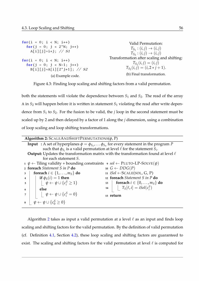
4.3. Loop Scaling and Shifting 56
for(i = 0; i < N; i++)for(j = 0; j < 2*N; j++)
A[i][j]=i+j; // S1
for(i = 0; i < N; i++)for(j = 0; j < N-1; j++)
B[i][j]=A[i][2*j+1]; // S2
(a) Example code.
Valid Permutation:TS1 : (i, j)→ (i, j)TS2 : (i, j)→ (i, j)
Transformation after scaling and shifting:TS1(i, j) = (i, j)
TS2(i, j) = (i, 2 ∗ j + 1).
(b) Final transformation.
Figure 4.3: Finding loop scaling and shifting factors from a valid permutation.
both the statements will violate the dependence between S1 and S2. The read of the array
A in S2 will happen before it is written in statement S1 violating the read after write depen-
dence from S1 to S2. For the fusion to be valid, the j loop in the second statement must be
scaled up by 2 and then delayed by a factor of 1 along the j dimension, using a combination
of loop scaling and loop shifting transformations.
Algorithm 2: SCALEANDSHIFTPERMUTATIONS(φ, P)Input : A set of hyperplanes φ = φS1 , . . . φSn for every statement in the program P
such that φSi is a valid permutation at level ` for the statement Si.Output: Updates the transformation matrix with the transformation found at level `
for each statement S.1 ψ← Tiling validity + bounding constraints2 foreach Statement S in P do3 foreach i ∈ {1, . . . , mS} do4 if φS(i) = 1 then5 ψ← ψ ∪ {cS
i ≥ 1}6 else7 ψ← ψ ∪ {cS
i = 0}
8 ψ← ψ ∪ {cS0 ≥ 0}
9 sol← PLUTO-LP-SOLVE(ψ)10 G ← DDG(P)11 iSol←SCALE(SOL, G, P)12 foreach Statement S in P do13 foreach i ∈ {0, . . . , mS} do14 TS[`, i] = iSol(cS
i )
15 return
Algorithm 2 takes as input a valid permutation at a level ` as an input and finds loop
scaling and shifting factors for the valid permutation. By the definition of valid permutation
(cf. Definition 4.1, Section 4.2), these loop scaling and shifting factors are guaranteed to
exist. The scaling and shifting factors for the valid permutation at level ` is computed for

4.3. Loop Scaling and Shifting 57
each statement of the program P. The output of Algorithm 2 is a transformation for every
statement in the program. This new transformation may be a combination of loop scaling
and loop shifting transformations for the permutation found in the first phase, as shown
in Figure 4.3. Let φS represent the hyperplane along the canonical axes that represents the
valid permutation for the statement S at the level `. The algorithm collects tiling validity and
dependence distance bounding constraints for every dependence in P, i.e, for every edge in
the DDG of P (line 1). Then, for each statement S, if some component i of φS has a non-zero
value, the lower bound of cSi is set to 1 (line 5) otherwise, the coefficient is set to zero (line 7).
The algorithm then sets the lower bound of the shifting coefficient cS0 to be zero (line 8). The
routine PLUTO-LP-SOLVE in line 9, solves the set of constraints that are given as input an LP
formulation with same the objective function as pluto-lp with is to find the lexmin of ~u and
w. The reason for using the above objective function is described in Section 4.3.3. This LP is
guaranteed to have a solution because the input permutation is valid. The rational solutions
are scaled to integral solutions using Algorithm 1 (line 11). The resulting integral solution
will not violate any dependences according to Theorem 3.1. Using these integral solutions
represent the transformation at level ` and transformation matrices for each statement S is
populated in Line 14.
4.3.1 Illustration:
Consider the code snippet shown in Figure 4.3a. Let us assume that the permutation black-
box gave the permutation (i) → (i) The permutation at the first level corresponds to the
hyperplane (1, 0) for both S1 and S2. The tiling validity constraints and dependence dis-
tance bounding constraints are shown in Figure 4.4. At the outermost level, the permutation
black-box returns the hyperplane (1,0) for both the statements. Algorithm 2 adds the con-
straints
cS11 ≥ 1, cS2
1 ≥ 0, cS10 ≥ 0, cS2
0 ≥ 0, cS12 = 0, cS2
2 = 0

4.3. Loop Scaling and Shifting 58
−cS11 − 2cS1
2 + cS21 + cS2
2 ≥ 0− cS1
1 − cS12 − cS1
0 + cS21 + cS2
0 ≥ 0− cS1
1 + cS21 ≥ 0
− 2cS12 + cS2
2 ≥ 0− cS1
2 − cS10 + cS2
0 ≥ 0
+u ≥ 0+ u + 2cS1
2 − cS22 ≥ 0
+ u + cS11 − cS2
1 ≥ 0+ u + cS1
1 + 2cS12 − cS2
1 − cS22 ≥ 0
+ 2u + w + cS12 + cS1
0 − cS20 ≥ 0
+ 2u + w + cS11 + cS1
2 + cS10 − cS2
1 − cS20 ≥ 0
Figure 4.4: Tiling validity constraints and dependence distance bounding constraints forcode shown in Figure 4.3a.
to the tiling validity and dependence distance bounding constraints and solves them as an
LP. This gives the solution cS11 = 1, cS2
2 = 1 and all other variables in the LP formulation are
assigned the value 0. This corresponds to the transformation (1, 0) for both the statements at
the outermost level. For the second level, the permutation blackbox gives the transformation
(0, 1) for both S1 and S2. Now the algorithm adds the constraints
cS12 ≥ 1, cS2
2 ≥ 0, cS10 ≥ 0, cS2
0 ≥ 0, cS11 = 0, cS2
1 = 0
to the tiling validity and dependence distance bounding constraints show in Figure 4.4.
These constraints are then solved as an LP which gives, and after scaling give the solution
cS12 = 1, cS2
2 = 2 and cS20 = 1. This corresponds a loop scaling and shifting transformation
for the second statement. The final transformation after scaling and shifting phase of the
Pluto-lp-dfp framework for both the statements is given by
TS1 =
1 0
0 1
·i
j
+
0
0
=
i
j
and
TS2 =
1 0
0 2
·i
j
+
0
1
=
i
2 ∗ j + 1
.
The scaling and shifting phase in the Pluto-lp-dfp framework finds loop scaling and shift-

4.3. Loop Scaling and Shifting 59
ing factors level by level. Another design choice would be to find valid permutations for all
levels and then find the scaling and shifting factors for each level individually. This leads
to complete decoupling of the fusion and permutation phase from the scaling and shifting
phase of the Pluto-lp-dfp framework. However, we do not implement it this way because,
the permutation phase would have to maintain additional meta-data on the loop fusion (or
distribution) decisions made at each level and communicate it to the scaling and shifting
phase. This overhead does not exist if both permutation black box and the scaling and shift-
ing phase operate on a per level in a coupled fashion. This is merely an implementation
choice but for the purposes of understanding and analysis of the framework, these phases
can be studied in a decoupled manner.
4.3.2 Correctness of Algorithm 2
Algorithm 2 finds the scaling and shifting factors for the valid permutation provided by
the permutation black box level by level. In this section, we prove that the transformation
obtained by the scaling and shifting phase will not violate any dependence in input program.
Theorem 4.1 Given a program P and a valid permutation φ for a level `, the transformation found
by Algorithm 2 does not violate any dependence.
Proof: The input to Algorithm 2 is a valid permutation φ. By definition of valid permu-
tations (refer Definition 4.1), loop scaling and shifting factors that do not violate any de-
pendences are guaranteed to exist. The variables ~u and w have the same semantics as in
Pluto’s ILP formulation and they do not restrict the space of valid solutions. Hence the LP
formulation is guaranteed to have a solution such that the tiling validity constraints are sat-
isfied. Then, by Corollary 3.1 there exists an integral solution as well. This integral solution
is found by Algorithm 1. Scaling the rational solutions of Pluto-lp to integral solutions will
not violate any dependences according to Theorem 3.1. Therefore, the transformation found
by Algorithm 2 at the level ` will not violate any dependences. �
4.3. Loop Scaling and Shifting 60
The result of Theorem 4.1 can be extended to every level of the program P and hence, the
output of the scaling and shifting phase for the Pluto-lp-dfp framework is a valid transfor-
mation for every statement in the program. In Theorem 4.2 we prove that the transformation
found for every statement in the program by Algorithm 2 consists of linearly independent
hyperplanes at every level.
Theorem 4.2 The transformation hyperplanes of each statement that are obtained by Algorithm 2
are linearly independent with respect to each other.
Proof: The input to Algorithm 2 is a valid permutation for a given level. As mentioned in
Section 4.2, valid permutations for a statement S at each level, provided by the permutation
black-box, are linearly independent with respect to the permutations at the previous levels.
In other words, valid permutations at each level forms a row of a permutation matrix. Thus
by definition, these hyperplanes obtained by the permutation black box for each statement
are linearly independent. Algorithm 2 scales the permutation and shifts it by a constant
offset. These operations do not affect linear independence of hyperplanes. Therefore, the
hyperplanes found by Algorithm 2 for every statement are linearly independent. �
As a consequence of Theorem 4.2, the output of the the scaling and shifting phase is a
transformation of the program which does not violate any dependences. Moreover, these
transformation hyperplanes satisfy every loop carried dependence in the transformed pro-
gram. Thus, with the help of some domain knowledge, if it is known that loop skewing is
not necessary, the first two stages of the Pluto-lp-dfp framework can be used to find affine
loop transformations.
4.3.3 Need for the Cost Function
Algorithm 2 finds valid transformations for the input program. It might appear that the
objective function used in the LP formulation, which is to minimize dependence distances,
is not essential. In this section, we illustrate the need for this cost function with an example.

4.3. Loop Scaling and Shifting 61
Consider the code shown in Figure 4.5a. Let us assume that the permutation black box
for(i=0;i<N;i++)A[i] = i; // S1
for(i=1;i<=N;i++)B[i] = A[i-1]; // S2
(a) Example code.
Possible transformation:TS1(i) = TS2(i) = (i)
Transformation for a parallel loop nest:TS1(i) = (i + 1)TS2(i) = (i)
(b) Possible transformations.
Figure 4.5: Need for cost function in the scaling and shifting phase.
gave the permutation TS1(i) = TS2 = (i). This permutation fused both the statements. The
dependence between S1 and S2 will then be carried by the loop i, thus making it sequential.
Now, the scaling and shifting phase has at least two possible solutions:
1. shifting factor of both S1 and S2 is 0 and the loop nest can be fused
2. the shifting factor of S1 is 1 and the shifting factor of S2 is 0. This introduces a delay of
1 for S1 with respect to S2 along dimension i.
The first solution results in a loop carried dependence, making the i loop sequential. Using
Pluto’s cost function will find the second solution and the dependence between S1 and S2
will now be a loop independent dependence in the fused loop nest, thus resulting in a par-
allel loop. Similarly, there are applications (involving up-sampling and down sampling) in
the image processing domain where loop scaling results in a tileable, parallel, loop nest.
4.3.4 Complexity of Algorithm 2
Algorithm 2 solves an LP with the same as the number of variables as pluto-lp which is given
by
v = np + 1 + ∑S∈P
(mS + 1),

4.4. Skewing Post Pass for Permutability 62
where np is the number of parameters in the program (which is also the number of compo-
nents in ~u), a single variable for w, and for each statement, there are mS + 1 transformation
coefficients one per dimension of the statement and the shifting coefficient. This LP formu-
lation has tiling validity constraints, dependence distance bounding constraints, and one
additional constraint per variable. Note that, an LP formulation has a time complexity of
O(n3), where n is the number of variables in the LP formulation. Hence, the time complex-
ity of Algorithm 2 is O(v3). This scaling routine is called m times, where m is the maximum
of dimensionalities of all statements in the program. Thus the complexity of the scaling
and shifting phase of the Pluto-lp-dfp framework is O(m × v3). This is polynomial in the
number of statements of the program.
4.4 Skewing Post Pass for Permutability
The output of Algorithm 2 is a transformation that does not include loop skewing. However,
there are classes of programs, like time-iterated stencils, for which loop skewing transforma-
tions enable loop tiling, yielding significant performance gains due to improved cache reuse.
Further, tile-wise concurrent start in stencils can also be achieved in stencil computations via
diamond tiling [BPB12]. In order to incorporate loop skewing transformations, in this sec-
tion, we describe a post processing step that introduces skewing at each level, provided it
enables loop tiling.
The intuition behind the approach is as follows: a dimension j inhibits rectangular tiling
of a loop nest if it has positive and negative components for some set of dependences in
the program. We try to make all the dependences have non-negative components along j, if
possible, by skewing it with outer dimensions that satisfy those dependences that have neg-
ative components along j. Algorithm 3 describes the loop skewing step to enable rectangular
tiling. The algorithm introduces skews in the DDG on a per-SCC basis (line 3). For each SCC
S, the algorithm introduces loop skews level by level from outermost to innermost. Note,
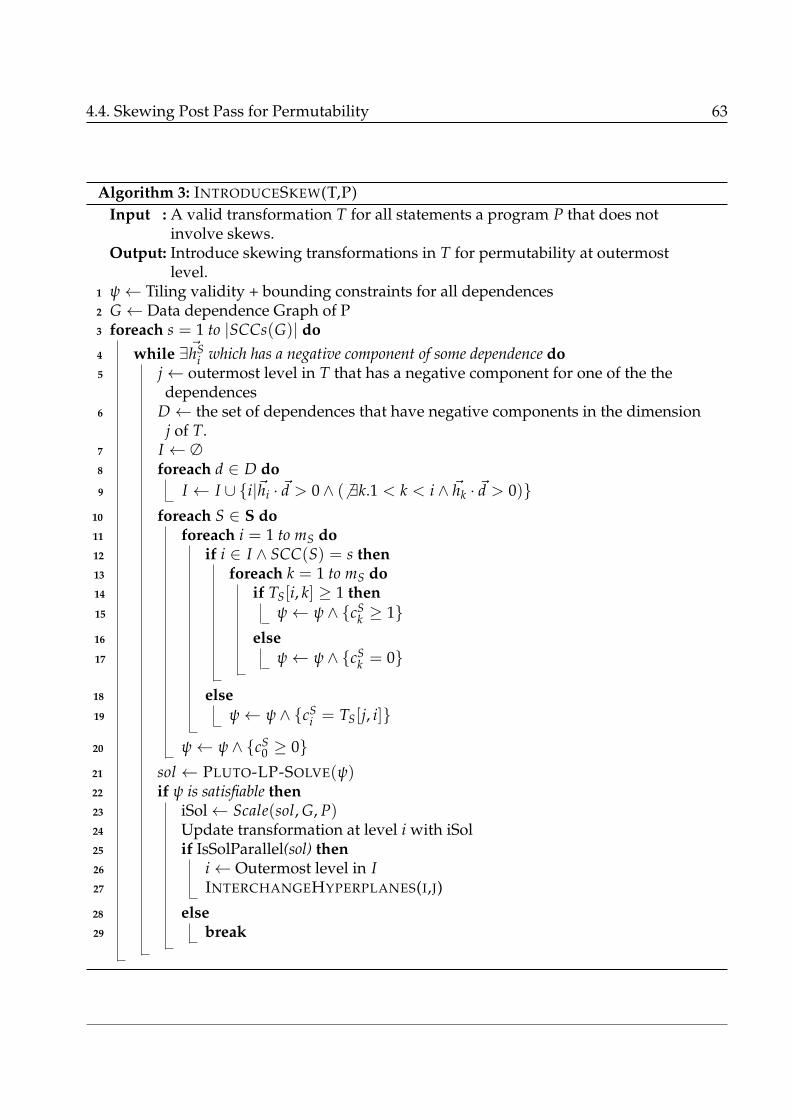
4.4. Skewing Post Pass for Permutability 63
Algorithm 3: INTRODUCESKEW(T,P)Input : A valid transformation T for all statements a program P that does not
involve skews.Output: Introduce skewing transformations in T for permutability at outermost
level.1 ψ← Tiling validity + bounding constraints for all dependences2 G ← Data dependence Graph of P3 foreach s = 1 to |SCCs(G)| do4 while ∃~hS
i which has a negative component of some dependence do5 j← outermost level in T that has a negative component for one of the the
dependences6 D ← the set of dependences that have negative components in the dimension
j of T.7 I ← ∅8 foreach d ∈ D do9 I ← I ∪ {i|~hi · ~d > 0∧ ( 6 ∃k.1 < k < i ∧ ~hk · ~d > 0)}
10 foreach S ∈ S do11 foreach i = 1 to mS do12 if i ∈ I ∧ SCC(S) = s then13 foreach k = 1 to mS do14 if TS[i, k] ≥ 1 then15 ψ← ψ ∧ {cS
k ≥ 1}16 else17 ψ← ψ ∧ {cS
k = 0}
18 else19 ψ← ψ ∧ {cS
i = TS[j, i]}
20 ψ← ψ ∧ {cS0 ≥ 0}
21 sol ← PLUTO-LP-SOLVE(ψ)22 if ψ is satisfiable then23 iSol← Scale(sol, G, P)24 Update transformation at level i with iSol25 if IsSolParallel(sol) then26 i← Outermost level in I27 INTERCHANGEHYPERPLANES(I,J)
28 else29 break

4.4. Skewing Post Pass for Permutability 64
that the outermost level will not have a negative component for any dependence. Let j be
the first level that has a negative component for at least one dependence given by:
(∃~d.~d · ~hj < 0) ∧ (@[email protected] ≤ k < j ∧ hk · ~d < 0),
where ~d represents a dependence whose source and target statements belong to the same
SCC S, and ~hj is the hyperplane at level j. Let D be the set of dependences that have neg-
ative components at level j. Every dependence in D must be satisfied at some outer level i
according to the equation:
I = {i|∃~d ∈ D,~hi · ~d ≥ 1∧ ∀k.0 ≤ k < i ∧ ~hk · ~d = 0},
that is, every hyperplane at some level in the set I will satisfy some dependence in the set
D. This set of levels I is collected in lines (lines 8-9). To enable rectangular tiling, algorithm
tries to make dependences in D have positive component at level j by skewing it with the
hyperplane that satisfied the dependence at an outer level i ∈ I using an LP formulation. In
this LP formulation, the lower bound of a transformation coefficient cSk is set to 1 provided
• statement S belongs to the current SCC, and
• the hyperplane at level i has a non-zero component in dimension k, i.e, the ith row of
the transformation matrix of statement S has a non-zero entry in column k (line 15).
The lower bound of the shifting factor cS0 of the statement S is reset to 0 (line 20). For state-
ments that do not belong to the current SCC, the algorithm does not change the input trans-
formation (line 19). These constraints are solved along with tiling validity constraints and
dependence distance bounding constraints for all the dependences. This LP formulation
has the same objective function as Pluto, which is to minimize the dependence distance for
every dependence. The resulting rational solution will be scaled to integers using Algo-
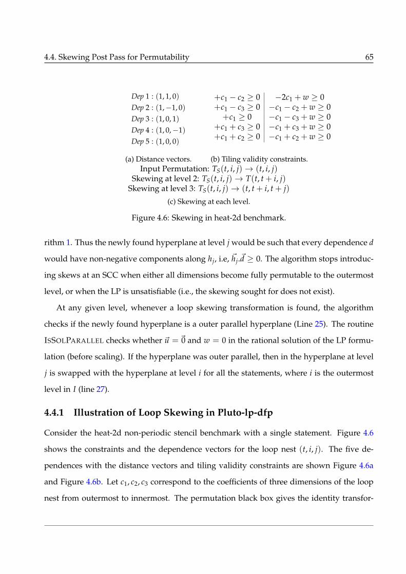
4.4. Skewing Post Pass for Permutability 65
Dep 1 : (1, 1, 0)Dep 2 : (1,−1, 0)Dep 3 : (1, 0, 1)Dep 4 : (1, 0,−1)Dep 5 : (1, 0, 0)
(a) Distance vectors.
+c1 − c2 ≥ 0 −2c1 + w ≥ 0+c1 − c3 ≥ 0 −c1 − c2 + w ≥ 0+c1 ≥ 0 −c1 − c3 + w ≥ 0
+c1 + c3 ≥ 0 −c1 + c3 + w ≥ 0+c1 + c2 ≥ 0 −c1 + c2 + w ≥ 0
(b) Tiling validity constraints.Input Permutation: TS(t, i, j)→ (t, i, j)
Skewing at level 2: TS(t, i, j)→ T(t, t + i, j)Skewing at level 3: TS(t, i, j)→ (t, t + i, t + j)
(c) Skewing at each level.
Figure 4.6: Skewing in heat-2d benchmark.
rithm 1. Thus the newly found hyperplane at level j would be such that every dependence d
would have non-negative components along hj, i.e, ~hj.~d ≥ 0. The algorithm stops introduc-
ing skews at an SCC when either all dimensions become fully permutable to the outermost
level, or when the LP is unsatisfiable (i.e., the skewing sought for does not exist).
At any given level, whenever a loop skewing transformation is found, the algorithm
checks if the newly found hyperplane is a outer parallel hyperplane (Line 25). The routine
ISSOLPARALLEL checks whether ~u = ~0 and w = 0 in the rational solution of the LP formu-
lation (before scaling). If the hyperplane was outer parallel, then in the hyperplane at level
j is swapped with the hyperplane at level i for all the statements, where i is the outermost
level in I (line 27).
4.4.1 Illustration of Loop Skewing in Pluto-lp-dfp
Consider the heat-2d non-periodic stencil benchmark with a single statement. Figure 4.6
shows the constraints and the dependence vectors for the loop nest (t, i, j). The five de-
pendences with the distance vectors and tiling validity constraints are shown Figure 4.6a
and Figure 4.6b. Let c1, c2, c3 correspond to the coefficients of three dimensions of the loop
nest from outermost to innermost. The permutation black box gives the identity transfor-

4.4. Skewing Post Pass for Permutability 66
mation, and the scaling and shifting phase finds the loop scaling and shifting factors to be
1 and 0 respectively, which does not change the input permutation. With this transforma-
tion, rectangular tiling can not be performed on the loop nest because because dimension i
has a negative component for the second dependence and a positive component for the first
dependence. This is the first level that is considered for skewing. Since, both these depen-
dences are satisfied at the outermost level t, the algorithm tries to skew the hyperplane at
level 2 with the hyperplane at level 1. It adds the constraints
c1 ≥ 1,
c2 ≥ 1,
c3 = 0,
c0 ≥ 0,
to the tiling validity constraints (Figure 4.6b) and solves it as an LP with the with the same
objective as that of Pluto. This gives the solution c1 = 1, c2 = 1 and c3 = 0 which does not
change after scaling. This corresponds to the hyperplane t + i at level 2. This new hyper-
plane is permutable to the outermost level. Similarly, the last component of dependence 4 is
made non-negative by skewing the third dimension with the first dimension. This provides
the t + j at the third level. The final transformation is given by
(t, i, j)→ (t, t + i, t + j),
which is the same as the transformation found by Pluto-ilp. Further, both Pluto and Pluto-lp-
dfp finds diamond tiling hyperplanes using the approach provided by Bandishti et al. [BPB12],
which yields the hyperplane
(t, i, j)→ (t− i, t + i, t + j),

4.4. Skewing Post Pass for Permutability 67
and enables tile-wise concurrent start after loop tiling.
4.4.2 Soundness and Completeness of the Skewing Phase
In this section, we first prove that Algorithm 3 will not violate any dependence and will not
affect the linear independence of hyperplanes.
Theorem 4.3 Given a program P and a valid transformation TS for every statement S in P, loop
skewing introduced by Algorithm 3 is such that
1. it does not violate any dependence, and
2. the transformation hyperplanes of S, after loop skewing, continue to be linearly independent
provided the hyperplanes in TS are linearly independent.
Proof: The input to Algorithm 3 is a valid transformation consisting of linearly indepen-
dent hyperplanes at each level. If the loop nest is already tileable, then the dependence
vectors of all dependences will have non-negative components in all dimensions and Algo-
rithm 3 will not introduce any skews. In case a skew is introduced at a level j, the resulting
hyperplane for each statement S will satisfy the tiling validity constraints. This ensures that
no dependence is violated. Also, the new hyperplane continues to be linearly independent
to other hyperplanes of S after skewing because, the newly found hyperplane corresponds
to an elementary row operation of the transformation matrix. Hence, the the transforma-
tion found by Algorithm 3 will not violate any dependence and gives a transformation with
linearly independent hyperplanes. �
Algorithm 3 also has certain interesting properties with respect to the transformation
found before and after skewing. If the resulting loop is not parallel, the transformation
found by Algorithm 3 does not change dependence satisfaction, i.e, if a dependence d was
satisfied at a level ` before loop skewing was introduced, then the dependence d continues
to be satisfied at level ` after the transformation. In cases where outer parallel hyperplanes
4.4. Skewing Post Pass for Permutability 68
are found, the level at which the dependences are satisfied will be pushed to the lower levels
because, the outer parallel loops are permuted to outer levels.
In Theorem 4.4, we prove the completeness of the loop skewing phase in Pluto-lp-dfp.
That is, the loop skewing transformations in Pluto-lp-dfp framework are introducing only if
it enables loop tiling.
Theorem 4.4 Given a valid transformation T for a program P, Algorithm 3 does not introduce any
skewing transformations in cases where T was tileable with rectangular tiles.
Proof: A loop nest can be tiled with rectangular tiles when all the dependences have non-
negative components along all dimensions. Algorithm 3 tries to introduce a skew only when
there is a negative component for at least one dependence d at a level ` of T. This means
that the hyperplane at level ` can not be permuted to the outermost level. This is a contra-
diction to our assumption that the input transformation T is tileable with rectangular tiles.
Therefore, Algorithm 3 would not introduce loop skewing, if the the transformation T was
not tileable. �
4.4.3 Complexity of the Skewing Phase
Algorithm 3 introduces skews on a per-SCC basis, level by level. Let us assume every state-
ment in the program is of dimensionality m. At each level, the algorithm solves an LP with
(m + 1)× |S| variables. For each SCC m LPs are solved and therefore the time complexity
of finding loop skewing transformations for each SCC is given by O(m4|S|3), assuming the
time complexity of solving an LP formulation with n variables is O(n3). The number of
SCCs for a given program is upper bounded by the number of statements. Therefore, the
time complexity of the skewing phase is O(m4|S|4).
4.5. Comparison of Transformations Found by Pluto and Pluto-lp-dfp 69
4.5 Comparison of Transformations Found by Pluto and Pluto-
lp-dfp
The Pluto algorithm models the full space of affine loop transformations in the non-negative
orthant, where as, the Pluto-lp-dfp framework models affine transformations in a decou-
pled fashion. Let us assume that both Pluto and Pluto-lp-dfp use the same fusion model
described in Section 2.2.4. It is very easy to see that every solution in the space of Pluto-lp-
dfp is also present in the space of transformations modeled by Pluto. However, Pluto-lp-dfp
does not model the full space of affine transformations. In this section, we provide intuitions
on the the kind of transformations that can not be found by Pluto-lp-dfp with examples.
1. Consider a 3-d loop nest with a single statement S and dependences given by the fol-
lowing dependence vectors (2, 0, 0), (1, 1, 0), and (1, 1,−1). Let (t, i, j) be the valid
permutation obtained by the permutation blackbox. Algorithm 2 finds the loop scal-
ing and shifting factors to be 1 and 0 respectively. In our approach, we skew the third
dimension with the dimension that satisfies the dependences that have negative com-
ponents along j, which is the dimension t, and find the transformation TS(t, i, j) →
(t, i, t + j). However, Pluto finds the transformation TS(t, i, j) → (i + j, t, i), because
it has a dependence distance of 1 at the outer most level. We will not be able to find
the transformation i + j at any level because the third dependence is satisfied at level 1
and not at the second level. One can also construct similar examples where the trans-
formation i + j might result in an outer parallel loop and Pluto-lp-dfp might miss this
transformation completely. Such issues arise because the permutation blackbox is not
aware that the loop skewing step will find a communication free parallel loop. Imple-
mentation of such a blackbox is not discussed in this thesis. Thus, even though both
Pluto and Pluto-lp-dfp perform loop skewing to enable loop tiling, the skewing factors
might differ based on the valid permutation obtained in the first phase.

4.6. Correctness and Complexity of the Pluto-lp-dfp Framework 70
2. Pluto-lp-dfp introduces loop skewing only when loop skewing enables loop tiling.
However, in rare cases, loop skewing might also enable loop fusion but not loop tiling.
In cases, Pluto’s cost model might find a fused loop nest with a loop skewing transfor-
mation, where as, Pluto-lp-dfp will distribute the loop nests. We will discuss one such
example in Chapter 7.
3. The permutation black-box, like the one that we describe in Chapter 5, might not have
the capability to choose permutations based on dependence distances. It might end up
favoring permutations that enable outer parallelism and may not distinguish the rest.
Therefore, even when restricted to loop permutations, transformations found by both
Pluto and Pluto-lp-dfp might differ.
4.6 Correctness and Complexity of the Pluto-lp-dfp Frame-
work
In this section, we prove the correctness of the Pluto-lp-dfp framework and provide the
time complexity of the Pluto-lp-dfp framework. The Pluto-lp-dfp framework decouples the
auto-transformation step of the Pluto algorithm into three phases. In the first step, a valid
permutation is found using a permutation blackbox. The second phase finds loop scaling and
shifting transformations for the permutation found by the black-box. By the semantics of the
black-box these scaling and shifting factors are guaranteed to exist. Then, by Theorems 4.1
and 4.2, the transformation obtained will not violate any dependences and the transforma-
tion hyperplanes will be linearly independent. Then, loop skewing is introduced in final
step only if it enables loop tiling. According to Theorem 4.3, the skews introduced will not
violate any dependence and the transformation hyperplanes continue to be linearly inde-
pendent. Thus, the correctness of the transformations found by Pluto-lp-dfp framework
follows directly from Theorems 4.1, 4.2 and 4.3.

4.6. Correctness and Complexity of the Pluto-lp-dfp Framework 71
Pluto-lp-dfp framework uses LP formulations to find loop scaling and shifting factors
as well as to introduce loop skewing transformations whenever they enable tiling. As de-
scribed in Sections 4.3.4 and 4.4.3, both scaling and and shifting phase, and loop skewing
phase are polynomial in the number of statements. Thus, the Pluto-lp-dfp framework finds
a transformation in polynomial time provided, valid loop permutations are found in poly-
nomial time. We describe our approach to find valid loop permutations in Chapter 5.
Statement clustering heuristics that have been proposed ([MY15], [Bag15]), are orthog-
onal to the decomposition of the scheduling problem in Pluto-lp-dfp. We hypothesize that
these clustering heuristics tend to postpone the problem of scalability of the Pluto-algorithm
by reducing the number of variables seen by the ILP solver rather than eliminating ILP it-
self. These statement clustering heuristics can be easily incorporated as a pre-processing
step, before fusion and dimension matching, and we provide one such statement clustering
heuristic in Chapter 5.

Chapter 5
Valid Permutations
The Pluto-lp-dfp framework described in Chapter 4 used a black-box to find a valid permu-
tation. In this chapter, we provide our approach to find a valid permutation. Note that, the
first phase of the Pluto-lp-dfp not only finds valid permutations, but also takes decisions on
loop fusion. Hence, the permutation blackbox should be able to model various loop fusion
opportunities. This chapter describes the implementation of our approach to find valid per-
mutations and is organized as follows: in Section 5.1, we describe our approach to find valid
permutations using a data structure called Fusion Conflict graph. We introduce a clustering
technique in Section 5.2 to cluster the vertices of the FCG and provide a polynomial time
approach to find valid permutations. Then, in Sections 5.3 and 5.4, we provide two polyno-
mial time, parallelism-preserving, fusion heuristics and incorporate them seamlessly in the
Pluto-lp-dfp framework.
5.1 Finding Valid Permutations
In this section, we describe our approach to find a valid permutation in the Pluto-lp-dfp
framework. According to Definition 4.1, a permutation P is said to be valid if there are loop
scaling and loop shifting factors for each level in P, such that the resulting transformation
after scaling and shifting, will not violate any dependences. The objective of finding a good

5.1. Finding Valid Permutations 73
permutation is to enhance locality by enabling loop tiling, fusion and to improve parallelism.
Since loop fusion/distribution decisions are also made at this stage, a framework which
allows to model various fusion opportunities is desirable. With this objective, we present a
data structure called the fusion conflict graph, which aids in efficiently modeling loop fusion,
while looking for valid permutations.
5.1.1 Fusion Conflict Graph
In this section, we provide the formal definition of the fusion conflict graph and its properties
that enable us to find valid permutations. A fusion conflict graph (FCG) is an undirected
graph F〈V, E〉, where the set of vertices is given by V = {S11, S2
1, . . . , SmS11 , S1
2, . . . , SmSnn }, i.e,
each vertex corresponds to a dimension of a statement in the program. An edge between
Sis and Sj
t represents that the ith dimension of Ss and jth dimension of St can not be fused
together and permuted to the outermost level. If the loop nest can be fully permuted, then
it can be tiled as well. Hence, an edge in the fusion conflict graph encodes invalidity of loop
fusion and tileability.
Once the FCG is constructed, the objective is to find convex independent sets of the FCG.
Definition 5.1 (Convex independent set) Given a fusion conflict graph, we say that an independent
set I of the fusion conflict graph is convex, if for each Sit ∈ I , the following condition holds:
∀Ss.(Ss, St) ∈ GE, ∃Sjs ∈ I , (5.1)
where GE is an edge in the DDG.
Intuitively, if a vertex of the FCG corresponding to a dimension i of a statement St is present
in I , then, for every predecessor Ss of St in the DDG, there must exist some vertex Sjs in I .
Each convex independent set represents the set of vertices that can be fused and permuted to
the outermost level. Any pair of non-adjacent vertices Sis, Sj
t ∈ I , indicate that fusing these

5.1. Finding Valid Permutations 74
Construct FCG Color FCG with m colors
Rebuild FCG
Update FCG
Valid permutation
Data Dependence Graph
Dependence constraints
Figure 5.1: Our approach to find a valid permutation.
dimensions will not violate any dependence between Ss and St. Convexity of I ensures that
transitivity of dependences is not violated. We obtain a convex independent set by a convex
coloring of the FCG. Given a fusion conflict graph, we say that the coloring of the fusion
conflict graph is convex, if the vertices with the same color form a convex independent set.
In the rest of the thesis, we refer to convex coloring of the FCG as coloring of the FCG.
We later prove formally in Section 5.2.3 that convex independent sets obtained via convex
coloring correspond to valid permutations.
Overview: The overview of our approach is shown in Figure 5.1. The first step is to con-
struct the fusion conflict graph using the dependence graph and dependence constraints
(described in Section 5.1.2). We use the term dependence constraints to represent union
of tiling validity constraints and dependence distance bounding constraints given in Equa-
tions 2.4 and 2.5. After constructing the FCG, it is colored level by level. In order to enforce
convexity on the coloring routine, we use the topological ordering on SCCs in the DDG to
drive the coloring algorithm. The upper bound on the number of colors to be used for col-
oring is given by m, where m is the maximum of dimensionalities of all statements in the
program. This establishes a mapping of colors to dimensions of the loop nest. We assume
that the colors are ordered; ordering of colors gives the permutation for every statement
from the outermost level to the innermost. If the loop nest can be completely fused and
tiled, then FCG can be successfully colored with m colors. The vertices that obtain the same
color represent the dimensions that can be fused and permuted to the outermost level. FCG
may not be colorable with m colors, either due to a permute preventing or a fusion prevent-

5.1. Finding Valid Permutations 75
ing dependence. If coloring with a color c failed due to a permute preventing dependence,
dependences that are satisfied at outer levels are removed and the FCG is rebuilt. Now,
the dimension corresponding to vertices that are colored with c can be permuted only with
the loops at lower levels. Intuitively, rebuilding the FCG marks the beginning of a per-
mutable band of loops. If coloring failed due to a fusion preventing dependence, loops are
distributed and the DDG and the FCG are updated. When coloring of FCG fails, it marks
one of the following:
1. if coloring fails due to a intra-SCC permute preventing dependence, then it marks the
beginning of a new permutable band of loops at the current level, or,
2. if coloring fails due to a inter-SCC fusion or permute preventing dependence, then the
loop nests are distributed at this level. The statements in these SCCs remain fused up
to the current level that is being colored and will be distributed at this level.
Details of this coloring step are given in Section 5.1.3. Once all the vertices are colored, the
ordering of colors can be used to obtain the permutation.
5.1.2 Construction of the Fusion Conflict Graph
In this section, we describe the construction of the fusion conflict graph. Recall that, each
dimension of a statement in the program corresponds to a vertex in the FCG. An edge in the
FCG represents the dimensions that can not be fused and permuted to the outermost level.
Algorithm 4 incrementally constructs the fusion conflict graph by adding edges between
vertices of the FCG in the following stages:
• intra-statement permute preventing edges,
• inter-statement fusion and permute preventing edges,
• inter-statement edges between statements that are independent and,

5.1. Finding Valid Permutations 76
• intra-statement edges between dimensions of the same statement.
Algorithm 4: CONSTRUCTFUSIONCONFLICTGRAPH
Input : Dependence Graph G〈GV , GE〉Output: Fusion Conflict Graph F〈FV , FE〉
1 foreach S ∈ GV do2 ADDPERMUTEPREVENTINGEDGES(S)
3 foreach pair of statements (Ss, St) such thats > t do
4 ADDINTERSTMTEDGES(Ss, St)
5 G∗〈GV , G∗E〉 ← TRANSITIVECLOSURE(G)6 foreach pair of statements (Ss, St) do7 if (Ss, St) /∈ G∗E ∧ (St, Ss) /∈ G∗E then8 foreach i ∈ 1 . . . mSs do9 foreach j ∈ 1 . . . mSt do
10 FE ← FE ∪ {(SiS, Sj
S)}
11 foreach S ∈ GV do12 foreach i ∈ 1 . . . mS do13 FE ← FE ∪ {(Si, Sj)|i 6= j ∧ 1 ≤ j ≤
mS}
14 return F15 function
ADDPERMUTEPREVENTINGEDGES(Stmt S)16 ψs ← All intra statement dep constraints
for S foreach i ∈ 1 . . . mS do17 if ((cS
i ≥ 1) ∧ ψs) is infeasible then18 FE ← FE ∪ {(Si, Si)}
19 function ADDINTERSTMTEDGES(Ss, St)20 ψst ← Dep constraints for all deps
between Ss and St21 foreach i ∈ 1 . . . mSs do22 foreach j ∈ 1 . . . mSt do23 if ((cSs
i ≥ 1∧ cStj ≥ 1) ∧ ψst) is
infeasible then24 FE ← FE ∪ {(Si
s, Sjt)}
Adding intra-statement edges: Algorithm 4 adds intra-statement permute preventing edges
in the routine ADDPERMUTEPREVENTINGEDGES, for each dimension of a statement S. These
edges appear as self-edges on the vertices of the FCG. Using the DDG G, the routine collects
all intra-statement dependences for S as shown in Equation 5.2:
DS ≡ {De|e = (S, S) ∈ GE}, (5.2)
where e is a self edge on a statement S in G. For each dependence in DS, dependence con-
straints are constructed, which include both tiling validity constraints and dependence dis-
tance bounding constraints and is denoted by ψs in Algorithm 4 (line 16). If a dimension i is
not permutable to the outermost level, then it must have a negative component along i for at

5.1. Finding Valid Permutations 77
least one intra-statement dependence. To find if i is permutable to the outermost level, we set
the lower bound of the coefficient ciS, to 1. Coefficients corresponding to other dimensions of
S, except c0S (loop shifting coefficient), are set to zero. Note that, none of the transformation
coefficients are constrained to be integers. The satisfiability of these constraints is checked
using an LP formulation with the same objective as Pluto. As described in Lemma 3.1, the
solution of this LP formulation is rational. This solution can be further scaled to integers
without violating dependences according to Theorem 3.1, because the newly added con-
straints either define lower bounds for variables or constrain them to zero and neither of
these are violated by scaling. Hence, the existence of a rational solution implies that there
exists an integer solution and vice versa. Therefore, if these constraints are unsatisfiable,
then dimension i is not permutable. Hence, we add a self edge on the vertex Si in the FCG
(line 18) which prevents coloring of the vertex i in the coloring phase. This edge will be re-
moved only when permute preventing dependences are satisfied at some outer level and the
FCG is reconstructed. Note that, if we are considering just feasibility of constraints, depen-
dence distance bounding constraints can be removed in the above formulation. However,
we intend to solve these constraints as an LP with the same objective as Pluto, because it
allows us to model parallelism preserving loop fusion heuristics alongside loop permuta-
tions, loop scaling and loop shifting transformations, which we describe in Section 5.3. The
objective function of the Pluto algorithm is meaningful only when dependence distances are
upper bounded, and therefore, dependence distance bounding constraints are essential. In
the rest of this thesis, whenever we check the satisfiability of a set of constraints, we solve
the constraints using an LP, with the same objective function as the Pluto algorithm.
Adding inter-statement edges: Algorithm 4 adds inter-statement permute and fusion pre-
venting edges in the routine ADDINTERSTMTEDGES. For each pair of statements Ss and St
that are adjacent in the DDG G, it collects all dependences (both intra and inter-statement

5.1. Finding Valid Permutations 78
dependences) between them according to Equation 5.3:
Dst ≡ {De|e = (Ss, St) ∈ GE ∨ e = (St, Ss) ∈ GE}. (5.3)
Validity of fusing dimension i of Ss with dimension j of St and permuting to the outermost
level is checked by solving dependence constraints ψst along with the constraints cis ≥ 1
and cjt ≥ 1 (line 23). Coefficients corresponding to other dimensions of statements Ss and St,
apart from the shifting coefficient, are set to zero. The shifting coefficients c0s and c0
t are lower
bounded by 0. If the above constraints are unsatisfiable, then, an edge is added between Sis
and Sjt in the FCG. This is because, fusing dimension i of Ss with dimension j of St will
violate some dependence between Ss and St. Again, the satisfiability of these constraints are
checked with an LP formulation with the same objective as Pluto.
Fusing two statements that do not have any reuse tend to pollute caches, resulting in
increase of conflict and capacity misses, increased register pressure and so on. Therefore, to
avoid fusion in such cases, we first construct the transitive closure of the DDG. This adds
edges between statements that are transitively dependent on each other. For every pair of
vertices (Ss, St), if they are not adjacent in the transitive closure of DDG, i.e, if
(Ss, St) /∈ G∗E ∨ (St, Ss) /∈ G∗E,
then fusion preventing edges are added between each and every dimension of Ss and St in
the FCG (lines 6-10). Addition of these edges ensure that statements that are not dependent
are distributed at the outermost level itself. These edges are added only when the FCG is
constructed for the first time and the above step is skipped during subsequent reconstruc-
tions of the FCG to avoid unnecessary distribution of statements at the inner levels.
Finally, the algorithm adds edges between vertices of the FCG that correspond to dimen-
sions the same statement (line 13), ensuring that two dimensions of the same statement are

5.1. Finding Valid Permutations 79
for(i=0; i<N; i++)for(j=0; j<N; j++)
A[i][j]=i+j; \\ S1
for(i=0; i<N; i++)for(j=0; j<N; j++)
B[i][j]=A[j][i]; \\ S2
for(i=0; i<N; i++)for(j=0; j<N; j++)
C[i][j]=A[i][j]+B[N-i][j]; \\ S3
(a) Example code.
S1
S2
S3
(b) DDG.
S1
S2
S3
i j
(c) FCG.
Figure 5.2: FCG construction.
not given the same color.
Illustration: Consider the example shown in Figure 5.2a. The code has three statements
with each statement in a two dimensional loop nest. Therefore, the corresponding FCG
shown in Figure 5.2c has a six vertices. The DDG corresponding to the example code is
shown in Figure 5.2b. There are no intra-statement dependences in the program and hence
intra-statement permute preventing edges are not added. Then the algorithm adds inter-
statement fusion and permuting preventing edges in the routine ADDINTERSTMTEDGES.
For example, the loop i of S1 cannot be fused with loop i of S2 because fusing it will violate
the RAW dependence between S1 and S2. More specifically, the read A[j][i] would read a
stale value in the statement S2, and hence, an edge is added between vertex Si1 and Si
2 in the
FCG. All intra-statement fusion and permute preventing edges are shown as solid lines in
Figure 5.2c. In the example, all statements are dependent and therefore no inter-statement
edges are added between statements that do not have a path between them in the DDG.
Finally edges between dimensions of the same statement are added and shown as dashed
lines in Figure 5.2c.

5.1. Finding Valid Permutations 80
5.1.3 Coloring the Fusion Conflict Graph
In this section, we provide details of our convex coloring algorithm to obtain convex inde-
pendent sets of the fusion conflict graph. We assume that SCCs in the DDG are numbered
according to a topological ordering of SCCs. Vertices of the FCG are colored by the topo-
logical ordering of the SCCs to which the statements belong. The coloring routine is driven
by the topological ordering of SCCs to enforce convexity of the independent set obtained
via coloring. We also assume that the colors are ordered, with smaller numbered colors
representing outer dimensions.
Algorithm 5 colors the vertices of the FCG, one color at a time starting from the first SCC
in the topological order. The routine COLORSCC (line 5) tries to color the vertices of the
FCG corresponding to the statements SCC i in the DDG. It returns true if the coloring suc-
ceeds for the SCC i; else it returns false. If there are many dimensions that can be colored,
it colors the outermost dimension in the original program order. At the outermost level,
the coloring of the first SCC will succeed. This is because, for any given SCC i, there exists
at least one dimension which fuses every statement in SCC i without violating any depen-
dences. However, coloring of any subsequent SCC might fail at any level. This will either
be due to a permute preventing dependence or a fusion preventing dependence. To dis-
tinguish the above two cases, the routine ISPERMUTEPREVENTING checks if vertices of the
FCG corresponding to dimensions of statements in SCC i can be colored in isolation. If not,
the routine returns false, indicating that, coloring in Line 5 failed due to permute preventing
edge in the FCG. Algorithm 5 removes dependences that are satisfied at the outer levels and
reconstructs the FCG (lines 7,8). If coloring failed due to a fusion preventing edge, that is,
the routine ISPERMUTEPREVENTING returned false, we distribute the current SCC and the
subsequent SCCs from the previous SCCs. We also update the DDG and the FCG by remov-
ing the edges corresponding to the dependences that are satisfied due to this distribution
(lines 20-23). Note that, the routine COLORSCC can fail for a maximum of two times for

5.1. Finding Valid Permutations 81
Algorithm 5: COLORFCGInput : FCG F〈FV , FE〉 and DDG G〈GV ,GE〉 of a program P.Output: Performs a convex coloring of the FCG, finds a valid permutation level by
level and then finds loop scaling and shifting factors for the permutation.using Algorithm 2.
1 maxColors← max{ms : s ∈ S}2 foreach c ∈ 1 . . . maxColors do3 foreach i = 1 to |SCCs(DDG)| do4 V ← set of vertices in SCC i of G5 while ¬ColorSCC(V,c,F) do6 if ISPERMUTEPREVENTING (V, C,
F) then7 Update DDG by removing
deps satisfied at outer levels8 F ← CONSTRUCTFUSION-
CONFLICTGRAPH(G)9 else
10 UPDATEDDGFCG(i, G, F)
11 φ←ADDPERMUTATION(c, F, G)12 SCALESHIFTPERMUTATIONS(φ, P)
13 function ISPERMUTEPREVENTING(vertices V,color c, FCG F)
14 F′V = {Si ∈ FV |S ∈ V}// Get the induced subgraph in F by F′V
15 F′ = F[F′V ]16 if ColorSCC(V,color, F′) then17 return true
18 return false
19 function UPDATEDDGFCG(scc1, DDG G,FCG F)
20 V1 = {S ∈ GV |get_scc(S) < scc1}21 V2 = {S ∈ GV |get_scc(S) ≥ scc1}22 FE = FE − {(Si
1, Sj2)|S1 ∈ V1 ∧ S2 ∈ V2}
23 GE = GE − {(Si, Sj)|Si ∈ V1 ∧ Sj ∈ V2}24 function ADDPERMUTATION(color c, FCG F,
DDG G, program P)25 foreach S ∈ P do26 foreach i ∈ 1, . . . mS do27 if Si is colored c then28 φi
S ← 1
29 else30 φi
S ← 0
any given SCC; once due to a permute preventing edge in the SCC and once due to a fusion
preventing edge. Thus, the loop in Line 5 is guaranteed to terminate. Algorithm 5 colors
all SCCs of the DDG with a color c. This corresponds to a valid permutation at the level l,
which we prove formally in Section 5.2.3. The loop scaling and shifting factors for the valid
permutation at level l are found immediately (line 12), using the scaling and shifting routine
SCALESHIFTPERMUTATIONS described in Section 4.3. Once loop scaling and shifting factors
are found, Algorithm 5 colors the FCG with the color c + 1.
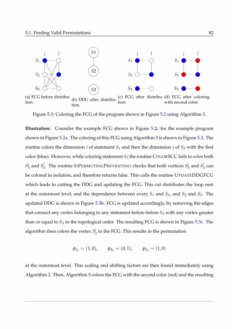
5.1. Finding Valid Permutations 82
S1
S2
S3
i j
(a) FCG before distribu-tion.
S1
S2
S3
(b) DDG after distribu-tion.
S1
S2
S3
i j
(c) FCG after distribu-tion.
S1
S2
S3
i j
(d) FCG after coloringwith second color.
Figure 5.3: Coloring the FCG of the program shown in Figure 5.2 using Algorithm 5.
Illustration: Consider the example FCG shown in Figure 5.2c for the example program
shown in Figure 5.2a. The coloring of this FCG using Algorithm 5 is shown in Figure 5.3. The
routine colors the dimension i of statement S1 and then the dimension j of S2 with the first
color (blue). However, while coloring statement S3 the routine COLORSCC fails to color both
Si3 and Sj
3. The routine ISPERMUTINGPREVENTING checks that both vertices Si3 and Sj
3 can
be colored in isolation, and therefore returns false. This calls the routine UPDATEDDGFCG
which leads to cutting the DDG and updating the FCG. This cut distributes the loop nest
at the outermost level, and the dependence between every S1 and S3, and S2 and S3. The
updated DDG is shown in Figure 5.3b. FCG is updated accordingly, by removing the edges
that connect any vertex belonging to any statement before before S3 with any vertex greater
than or equal to S3 in the topological order. The resulting FCG is shown in Figure 5.3c. The
algorithm then colors the vertex Si3 in the FCG. This results in the permutation
φS1 = (1, 0), φS2 = (0, 1), φS3 = (1, 0)
at the outermost level. This scaling and shifting factors are then found immediately using
Algorithm 2. Then, Algorithm 5 colors the FCG with the second color (red) and the resulting

5.2. Clustering 83
for (i=0; i<N; i++) {for (j=0; j<N; j++) {
A[i][j] = i+j; \\ S1B[j][i] = A[i][j]; \\ S2}
}
for (i=0; i<N; i++)for (j=0; j<N; j++)
C[i][j] = A[i][j] + B[N-i][j]; \\ S3
Figure 5.4: Transformed code for the input program shown in Figure 5.2a.
coloring is shown in Figure 5.3d which corresponds to the permutation
φS1 = (0, 1), φS2 = (1, 0), φS3 = (0, 1),
at the second level. The scaling and shifting factors will be found to be 1 and 0 respectively
for all the statements by Algorithm 2. The transformed code is shown in Figure 5.4.
The coloring routine described in Algorithm 5 is exponential in the size of the SCCs in
the DDG. Moreover, if there exist many possible valid colorings for an SCC, then selecting
one of these valid colorings becomes tedious. Suppose the goal is to locally fuse as many
successors as possible for a given SCC S, then in the worst case, one would have to enumer-
ate all possible colorings for every successor of S and then decide the dimension of S to be
colored. Therefore, in Section 5.2, we provide a clustering heuristic which not only results in
a polynomial time SCC coloring routine, but also makes way for simplistic implementation
of greedy coloring heuristics.
5.2 Clustering
In this section, we describe a clustering heuristic to cluster the vertices of the FCG based
on SCCs in the DDG. We then present a polynomial time greedy coloring heuristic which
can be efficiently implemented using the clustered FCG. Later, in Section 5.3, we show how

5.2. Clustering 84
a parallelism-preserving fusion heuristic can be seamlessly incorporated in the clustered
FCG, without affecting the coloring routine.
5.2.1 Construction of the FCG with Clustering
Algorithm 6: BUILDSCCCLUSTERFCG
Input : Dependence Graph G〈GV , GE〉Output: Fusion Conflict Graph F〈FV , FE〉
1 foreach SCCs S ∈ G do2 ADDPERMUTEPREVENTINGEDGES(S)
3 foreach pair of Sccs (Ss, St) such that s < t do4 ψst ← GETINTERSCCDEPCST(Ss, St)5 foreach i ∈ 1 . . . dim(Ss) do6 foreach j ∈ 1 . . . dim(St) do7 ψij ←
∧S∈Ss
(ciS ≥ 1)
∧S∈St
(cjS ≥
1) ∧ ψst8 if ψij is infeasible then9 FE ← FE ∪ {(Si
s, Sjt)}
10 foreach Sccs S ∈ G do11 foreach i ∈ 1 . . . dim(S) do12 FE ← FE ∪ {(Si, Sj)|i 6= j ∧ 1 ≤ j ≤
mS}
13 return F14 function
ADDPERMUTEPREVENTINGEDGES(SCC S)15 ψs ← All intra SCC dep constraints for
SCC S16 foreach i ∈ 1 . . . dim(S) do17 ψi ←
∧S1∈S
(ciS1≥ 1) ∧ ψs
18 if ψi is infeasible then19 FE ← FE ∪ {(Si, Si)}
Our clustering heuristic is based on the observation that, for every statement in the SCC,
there exists at least one dimension i that fuses all the statements of the SCC without violating
the tiling validity constraints. Therefore, if we assume that every statement in an SCC gets
the same transformed schedule, at a given level, then all statements within an SCC can be
clustered. We define dimensionality of an SCC to be the maximum of dimensionalities of all
statements in the SCC. Each vertex in the clustered FCG corresponds to a dimension of an
SCC in the DDG. Algorithm 6 depicts the construction of SCC clustered FCG. It is similar
to Algorithm 4 but with a few minor changes. Addition of permute preventing edges is
performed on a per-SCC basis by considering the intra-SCC dependences. For a given SCC

5.2. Clustering 85
S, the algorithm first collects intra-SCC dependence constraints according to the formula
DS ≡∧
e∈DDG(De|SCC(Src(e)) = SCC(Dest(e)) = S),
where the functions Src(e) and Dest(e) return the source and destination statements of the
an edge e in the DDG, and the function SCC(V) returns the SCC to which the vertex V
belongs in the DDG. Note that all the statements in the SCC are assumed to have the same
schedule, and hence, the lower bound of ci’s of all statements in the SCC are set to 1 (line 17)
while checking the permutability of a dimension i. Inter-SCC edges for every pair SCCs in
the DDG, by considering both intra and inter-SCC dependences (lines 3-9) according to the
equation
D ≡∧
e∈DDG(De|SCC(Src(e)), SCC(Dest(e)) ∈ {Ss, St}).
These edges are added for every pair of dimensions (i, j) of SCCs (Ss, St). Lower bounds
of transformation coefficients corresponding to i and j of all statements in SCCs Ss and St
are set to 1. Transformation coefficients corresponding to all other dimensions, apart from
the shifting coefficient, are constrained to 0. Satisfiability of these constraints are checked
with an LP formulation, in the same way as Algorithm 4, and edges in the FCG are added if
the constraints are unsatisfiable. Algorithm 6 also adds edges in the FCG between vertices
corresponding to SCCs that are not connected in the DDG (not shown in pseudocode). It
also adds edges between vertices corresponding to dimensions of the same SCC (line 12).
5.2.2 Coloring SCC Clustered FCG
Coloring of the clustered FCG is very similar to Algorithm 5. The obvious difference in
semantics of the coloring routine is that, when a vertex of the clustered FCG is colored, it
defines a permutation for every statement in the SCC, instead of a single statement. Now

5.2. Clustering 86
Algorithm 7: COLORCLUSTERFCGInput : FCG F〈FV , FE〉 and DDG G〈GV , GE〉 of a program POutput: Performs a convex coloring of the FCG, finds a valid permutation level by
level and then finds loop scaling and shifting factors for the permutation.using Algorithm 2.
1 maxColors← max{ms : s ∈ S}2 foreach c ∈ 1 . . . maxColors do3 foreach i = 1 to |SCCs(DDG)| do4 while ¬ColorSCC(i,c,F) do5 if ISPERMUTEPREVENTING(I, F)
then6 Update DDG by removing
deps satisfied at outer levels7 F ← CONSTRUCTFUSION-
CONFLICTGRAPH(G)8 else9 UPDATEDDGFCG(i, G, F)
10 φ←ADDPERMUTATION(c, F, G)11 SCALESHIFTPERMUTATIONS(φ, P)
12 function ISPERMUTEPREVENTING(Scc S,FCG F)
13 if @j ∈ {1, . . . , dim(S)}|(Sj, Sj) ∈ FE then14 return False
15 else16 return True
17 function UPDATEDDGFCG(scc1, DDG G,FCG F)
18 V1 = {S ∈ GV |get_scc(S) < scc1}19 V2 = {S ∈ GV |get_scc(S) ≥ scc1}20 FE = FE − {(Si
1, Sj2)|S1 < scc1∧ S2 ≥
scc1}21 GE = GE − {(Si, Sj)|Si ∈ V1 ∧ Sj ∈ V2}22 function ADDPERMUTATION(color c, FCG F,
DDG G, program P)23 foreach S ∈ P do24 foreach i ∈ 1, . . . mS do25 if Si is colored c then26 φi
S ← 1
27 else28 φi
S ← 0
the routine COLORSCC will have m choices to color a vertex. Since the permutation for
statements within the SCC is fixed, it does not consider any choices for statements within
the SCC. Apart from yielding a polynomial time coloring heuristic, clustering also has the
following advantages: (1) simplification of permutability check in Line 6 of Algorithm 5,
and (2) greedy coloring heuristics can be employed in a simplistic manner.
Algorithm 7 colors the vertices of the clustered FCG based on topological ordering of the
SCCs. The coloring routine COLORSCC in line 4 now checks if the vertex corresponding to a
dimension of SCC i can be colored from outermost to innermost. Therefore, the routine has
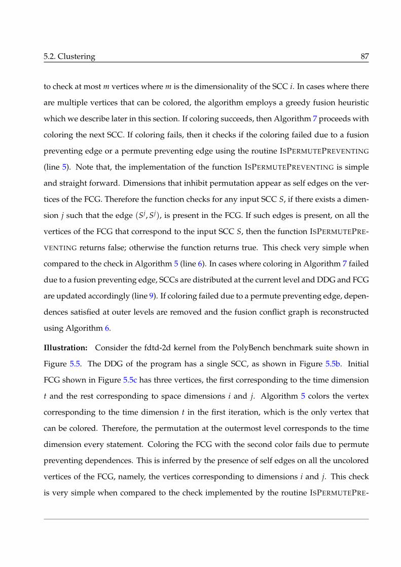
5.2. Clustering 87
to check at most m vertices where m is the dimensionality of the SCC i. In cases where there
are multiple vertices that can be colored, the algorithm employs a greedy fusion heuristic
which we describe later in this section. If coloring succeeds, then Algorithm 7 proceeds with
coloring the next SCC. If coloring fails, then it checks if the coloring failed due to a fusion
preventing edge or a permute preventing edge using the routine ISPERMUTEPREVENTING
(line 5). Note that, the implementation of the function ISPERMUTEPREVENTING is simple
and straight forward. Dimensions that inhibit permutation appear as self edges on the ver-
tices of the FCG. Therefore the function checks for any input SCC S, if there exists a dimen-
sion j such that the edge (Sj, Sj), is present in the FCG. If such edges is present, on all the
vertices of the FCG that correspond to the input SCC S, then the function ISPERMUTEPRE-
VENTING returns false; otherwise the function returns true. This check very simple when
compared to the check in Algorithm 5 (line 6). In cases where coloring in Algorithm 7 failed
due to a fusion preventing edge, SCCs are distributed at the current level and DDG and FCG
are updated accordingly (line 9). If coloring failed due to a permute preventing edge, depen-
dences satisfied at outer levels are removed and the fusion conflict graph is reconstructed
using Algorithm 6.
Illustration: Consider the fdtd-2d kernel from the PolyBench benchmark suite shown in
Figure 5.5. The DDG of the program has a single SCC, as shown in Figure 5.5b. Initial
FCG shown in Figure 5.5c has three vertices, the first corresponding to the time dimension
t and the rest corresponding to space dimensions i and j. Algorithm 5 colors the vertex
corresponding to the time dimension t in the first iteration, which is the only vertex that
can be colored. Therefore, the permutation at the outermost level corresponds to the time
dimension every statement. Coloring the FCG with the second color fails due to permute
preventing dependences. This is inferred by the presence of self edges on all the uncolored
vertices of the FCG, namely, the vertices corresponding to dimensions i and j. This check
is very simple when compared to the check implemented by the routine ISPERMUTEPRE-

5.2. Clustering 88
for(t = 0; t < tmax; t++) {for(j = 0; j < ny; j++)
ey[0][j] = t; \\ S1for (i = 1; i < nx; i++)
for (j = 0; j < ny; j++)ey[i][j]=ey[i][j]-0.5*(hz[i][j]-hz[i-1][j]); \\ S2
for (i = 0; i < nx; i++)for (j = 1; j < ny; j++)
ex[i][j] = ex[i][j]-0.5*(hz[i][j]-hz[i][j-1]); \\ S3for (i = 0; i < nx; i++)
for (j = 0; j < ny; j++)hz[i][j]=hz[i][j]-0.7*(ex[i][j+1]-ex[i][j]+ey[i+1][j]-ey[i][j]); \\ S4
}
(a) Fdtd-2d benchmark.
S1
S2
S3
S4
(b) DDG.
S1
t i j
(c) Initial FCG.
S1
S2
S3
S4
t i j
(d) FCG after reconstruction.
TS1(t, i)→ (t, i),TS2(t, i, j)→ (t, j, i),TS3(t, i, j)→ (t, j, i),TS4(t, i, j)→ (t, j, i)
(e) Valid permutation.
Figure 5.5: Greedy clustering heuristic in fdtd-2d.

5.2. Clustering 89
VENTING in Algorithm 5. The presence of permute preventing edges leads to removal of
dependences that are satisfied at the outermost level (shown in blue in Figure 5.5b). The
updated DDG now has a single statement in every SCC. The reconstructed FCG is shown in
Figure 5.5d. Algorithm colors the only remaining dimension in SCC 1, and then, while col-
oring a vertex of SCC 2, it has two choices. Coloring vertex Si2 with the second color would
enable us to color Si3 only, whereas coloring Sj
2, would enable coloring both Sj3 and Sj
4. Here,
the routine COLORSCC chooses the vertex which enables coloring of maximum number of
successor SCCs in the topological order, which, in this example, is the vertex Sj2. This greedy
coloring heuristic can be implemented in the clustered FCG in a simplistic manner, whereas,
in the unclustered approach, we would have to look for coloring of vertices corresponding to
statements within a given SCC as well as its successors. The final coloring obtained is shown
in Figure 5.5d, which corresponds to the permutation shown in Figure 5.5e. This permuta-
tion leads to loop skewing and enables diamond tiling in the later stages of the Pluto-lp-dfp
framework.
5.2.3 Correctness
In this section, we describe the correctness of our approach to find valid permutations using
clustered FCG. The coloring routine described in Algorithm 5, which colors the unclustered
FCG, also colors on the FCG on a per SCC basis. Each SCC is colored atomically, i.e, there
does not exist a situation in which some vertices of corresponding to statements of a given
SCC S are colored with a color c and some vertices are not colored. Therefore, the proofs
that we provide here also hold for the unclustered approach as well.
We first prove that for a given SCC, there exists at least one dimension that fuses all the
statements of the SCC, without violating any dependences. This is the assumption on which
our clustering heuristic is based.
Theorem 5.1 Given a DDG G of a program P, for each SCC S in G, there exists at least one dimen-

5.2. Clustering 90
sion i that fuses all statements in S, without violating any dependences.
The intuition behind the proof of Theorem 5.1 is that, every statement in an SCC must be
surrounded by at least one loop i that carries a dependence along the back-edge. Since the
input program is correct, this loop does not violate any dependence in the SCC and will
satisfy the dependence constraints of all intra-SCC dependences.
Proof: We prove Theorem 5.1 by contradiction. Let us assume that there does not exist
any dimension i that fuses all statements belonging to SCC S, without violating any depen-
dences. However, in the input program, since the vertices are part of an SCC, there must ex-
ist a loop i, which carries a dependence along the back edge. This loop i fuses all statements
in S. Since the input program is correct, the dimension i will not violate any dependence,
and therefore, will satisfy the dependence constraints for all dependences in the SCC. �
The consequence of Theorem 5.1 is that, for every SCC S in the DDG, there exists a vertex
v corresponding to some dimension i of S in the FCG without a self edge, at the outermost
level. If there is a single SCC in the program, then v can be colored with the color c and
this corresponds to a valid permutation at a particular level. The greedy coloring heuristic
described in Section 5.2.2, is driven by a topological ordering of SCCs in the DDG, and
therefore, the set of vertices that have the same color form a convex independent set. In
Theorem 5.2 we prove that any convex independent set of the FCG found by the greedy
coloring algorithm, corresponds to a valid permutation for every statement in the input
program.
Theorem 5.2 Every convex independent set I of the FCG F, corresponds to a valid permutation for
the set of statements in the program P.
Proof: Let S = {S1, . . . , SN} be the SCCs in the DDG whose corresponding vertices are
present in I , i.e, S = {S|∃j.1 ≤ j ≤ dim(S) ∧ Sj ∈ I}. Without loss of generality, let us
assume that the dimension i of every SCC in S is present in I . Let c be the color used for col-
oring at a level `. We will prove that, at any point of time in the coloring routine, whenever a

5.3. Typed Fusion 91
vertex Sim of the FCG is colored with c (analogous to adding Si
m to I), the set of vertices that
are already colored with c (analogous to elements in I) represents a valid permutation for
statements in those SCCs whose vertices corresponding to dimension i have been colored.
We will assume that it is valid to color Sim with c and the routine COLORSCC has succeeded.
If Sim was the first vertex added to I , then by Theorem 5.1, it is a valid permutation. Let
Sim be the mth vertex added to I . Let k j be the loop shifting factor required to shift and fuse
dimension i of SCCs Sj and Sj−1, where j < m. Let k be the maximum shifting factor, which
is required to fuse SCC Sm with its predecessors in the DDG. We make an observation that
if two SCCs are connected in the DDG, then the target SCC can be delayed further by a loop
shifting transformation without violating any dependences. Therefore, when Sim is colored
with c, there exists an integer k′ = k2 + k3 + · · ·+ km−1 + k, that will be a valid loop shifting
factor for every statement in Sm. Hence, there exists a loop shifting factor for every statement
in every SCC of S such that dependences are not violated. The existence of loop scaling fac-
tors can also be proved in a similar way. Once all the SCCs are colored, I corresponds to a
valid permutation for every statement in the program. �
Theorem 5.2 proves that a convex independent set of the FCG obtained via convex color-
ing represents a valid permutation. The scaling and shifting factors for the permutation are
found using the the routine SCALESHIFTPERMUTATIONS described in Section 4.3.
5.3 Typed Fusion
The approach described in Section 5.2 constructs the FCG and the coloring heuristic greedily
fuses as many statements as possible, under a given loop. However this fusion strategy is
not desirable because it may inhibit parallelism. For example consider the example program
shown in Figure 5.6a. The two statements are distributed and each loop is parallel. The fu-
sion algorithm described in Section 5.2, as well as the default fusion heuristic in Pluto, fuses
the two statements and the fused loop nest shown in Figure 5.6b code results is sequen-

5.3. Typed Fusion 92
for(i=0;i<N;i++)A[i] = 2*i;
for(i=1;i<N;i++)B[i] = A[i-1] + A[i-2];
(a) Example code.
A[0] = 2*0;for(i=1;i<N;i++) {
A[i] = 2*i;B[i] = A[i-1] + A[i];
}
(b) Transformed code with Algorithm 6.
Figure 5.6: Fusion resulting in loss of parallelism with Algorithm 6 and Pluto.
tial. Incorporating parallelism preserving loop fusion heuristics in polyhedral compilers
like Pluto would require solving an exponential number of ILPs, thereby, resulting in very
large compilation times, making it practically infeasible for adaption in general-purpose
compilers like LLVM.
In this section, we provide a variant of typed fusion developed by Kennedy and McKin-
ley [KM93], which ensures that loop fusion does not result in loss of parallelism. The typed
fusion heuristic allows fusion of a subset of loops that preserve parallelism when compared
to the approach described in Section 5.2, in particular, it allows only the subset of valid loop
fusion opportunities where there is no loss of parallelism. Hence, our approach would be
to add more edges in the FCG. More specifically, we add parallelism preventing edges during
the construction of the FCG, in addition to permute and fusion preventing edges.
5.3.1 FCG Construction and Coloring
Algorithm 8 provides details on construction of the FCG, which is very similar to Algo-
rithm 6. The routine ADDPERMUTEPREVENTINGEDGES, in addition to adding permute pre-
venting edges, adds parallelism preventing edges on vertices that correspond to serial di-
mensions (line 26). For a given SCC S, the routine ADDPERMUTEPREVENINGEDGES, solves
the same set of constraints as Algorithm 6, as a Linear Program (LP) with the same objective
as Pluto (line 24), which is to find lexmin ~u, w. If a non-zero solution for ~u or w is obtained,
then a parallelism preventing self-edge is added on the vertex Si in the FCG. In addition to
adding parallelism preventing edges, the routine also marks an SCC as parallel if there is at

5.3. Typed Fusion 93
Algorithm 8: BUILDFCGTYPED
Input : Dependence Graph G〈GV , GE〉Output: Fusion Conflict Graph F〈FV , FE〉
1 foreach SCCs S ∈ G do2 ADDPERMUTEPREVENTINGEDGES(S)
3 foreach pair of Sccs (Ss, St) such that s < t do4 ψst ← GETINTERSCCDEPCST(Ss,St)5 foreach i ∈ 1 . . . dim(Ss) do6 foreach j ∈ 1 . . . dim(St) do7 ψij ←
∧S∈Ss
(cSi ≥ 1) ∧ ∧
S∈St
cSj ≥
1∧ ψst8 if ψij is infeasible then9 FE ← FE ∪ {(Si
s, Sjt)}
10 else11 sol← PLUTOLPSOLVE(ψ1)12 if sol(~u, w) 6=~0∧
isParallel[Ss] ∨ isParallel[St]then
13 FE ← FE ∪ {(Si, Sj)}
14 Add edges betweeen sequential and parallelSCCs
15 Add scale and shift conflict edges16 return F17 function
ADDPERMUTEPREVENTINGEDGES(SCC S)18 ψs ← All intra SCC dep constraints for S19 foreach i ∈ 1 . . . dim(S) do20 ψi ←
∧S1∈S
cS1i ≥ 1∧ ψs
21 if ψi is infeasible then22 FE ← FE ∪ {(Si, Si)}23 else24 sol← PLUTOLPSOLVE(ψ1)25 if sol(~u, w) 6=~0 then26 FE ← FE ∪ {(Si, Si)}27 else28 isParallel[S]← true

5.3. Typed Fusion 94
least one parallel dimension along the canonical axes (Line 28) by checking if at least one of
the LPs during addition of permute preventing edges has a solution with ~u =~0 and w = 0.
Thus, after adding preventing edges, parallel SCCs would also be marked. Then, the algo-
rithm adds inter-SCC fusion and permute preventing edges for every pair of adjacent SCCs
(Ss, St) (lines 3-13). Parallelism preventing edges are also added if fusing two dimensions
of Ss and St in the DDG does not result in a parallel loop (line 13). This is again achieved
by checking the solution of the LP formulation. Parallelism preventing edges are also added
between vertices of the FCG that correspond to dimensions of sequential and parallel SCCs
(line 14). Analogous to Algorithm 6, Algorithm 8 also adds edges between SCCs that are not
connected and between vertices corresponding to the dimensions of the same SCC. For the
example shown in Figure 5.6, Algorithm 8 adds a parallelism preventing edge between Si1
and Si2, thereby, distributing the loop nests without resulting in loss of parallelism.
Parallelism can also be lost by fusing SCCs that require different loop scaling or shifting
factors. For example, consider the code shown in Figure 5.7a. Statements S1 and S2 can be
fused together by shifting S1 by 1 with respect to loop i, while preserving parallelism, and
similarly S2 and S3 can be fused with by shifting S2 by 1 with respect to i. However, if all
three statements are fused, then the resulting fused loop nest will not be parallel. This is
because, S2 should be delayed from S3 by 1 and S1 should be delayed by 1 with respect to S2
thereby resulting a net delay of 2 for the statement S1 with respect to S3. However, S1 can be
fused with S3 only with a delay of 1, while preserving parallelism. In order to account for
such conflicting shifts, we add shift conflict edges in the FCG (Line 15 in Algorithm 8). This
routine traverses SCCs in the reverse topological order, while summing up the shifts. The
shifts for a pair of statements are computed during the addition of inter-SCC edges using
the solution of the LP formulation (Line 11). Whenever the routine detects a conflicting shift,
i.e two different shifting factors for fusing two dimensions of any two statements, it adds a
parallelism preventing edge between dimensions of SCCs that requires a larger shift. In

5.3. Typed Fusion 95
for(i=0;i<N;i++)A[i] = 2*i; \\ S1
for(i=1;i<N;i++)B[i] = A[i-1] + i; \\ S2
for(i=2;i<N;i++)C[i] = B[i-1] + A[i-1]; \\
S3
(a) Example code.
S1
S2
S3
i
(b) FCG.
A[0] = 0;for(i=1;i<N;i++) {
A[i] = 2*i; \\ S1B[i] = A[i-1] + i; \\ S2
}for(i=2;i<N;i++)
C[i] = B[i-1] + A[i-1]; \\ S3
(c) Transformed code.
Figure 5.7: Typed fusion in cases where parallelism is inhibited by loop shifting.
the above example parallelism preventing edge is added between Si1 and Si
3 (dashed edge
in Figure 5.7b). A similar approach is followed to add scale conflict edges in the FCG. The
transformed code in which the statements S1 and S2 are fused and statement S3 is distributed
is shown in Figure 5.7c.
Once the FCG is constructed, we use the greedy coloring heuristic described in Sec-
tion 5.2.2 to find convex independent sets. In case of typed fusion, the coloring heuristic
also ensures that if there exists a parallel hyperplane along the canonical axes, it is found
at the outermost level, resulting in a communication-free loop nest. We illustrate this in
Section 5.4 with an example. Note that, in cases where communication free loop nests are
obtained by loop skewing, the skewing phase will ensure that parallel hyperplanes that are
found after skewing are moved to the outermost level if they correspond to communication-
free hyperplanes. Thus, by adding parallelism preventing edges in the FCG, we not only
accomplish the objective of inhibiting fusion that results in parallelism, but also ensure that

5.3. Typed Fusion 96
for(t = 0; t < T; t++) {for(i = 1; i < N-1; i++)
for(j = 1; j < N-1; j++)B[i][j]=0.2*(A[i][j]+A[i][j-1]+A[i][1+j]
+A[1+i][j]+A[i-1][j]); \\ S1for(i = 1; i < N-1; i++)
for(j = 1; j< N-1; j++)A[i][j]=0.2*(B[i][j]+B[i][j-1]+ B[i][1+j]
+B[1+i][j]+B[i-1][j]); \\ S2}
(a) Jacobi-2d code snipet from PolyBench.
S1
t i j
(b) Initial FCG.
S1
S2
t i j
(c) FCG after reconstruc-tion.
Figure 5.8: Typed fusion in multi-statement stencils.
good permutations with communication free hyperplanes are found whenever they exist.
5.3.2 Stencil Characterization
The typed fuse heuristic described in Section 5.3 distributes loop nests when fusion leads
to loss of parallelism. However, there are scenarios where this distribution might result
in a loss of performance. For example, consider the FCG constructed by Algorithm 8 for
the jacobi-2d benchmark from the PolyBench benchmark suite shown in Figure 5.8b. The
coloring algorithm first colors the vertex corresponding to the time dimension in the FCG.
Coloring fails while coloring with the second color due to the permute preventing edges
in the FCG which results in updating the DDG by removing the dependences satisfied by
the outer level and FCG is reconstructed. Algorithm 8 adds parallelism preventing edges
between vertices that correspond to dimension i of SCCs S1 and S2 as shown in Figure 5.8c.
Now, coloring fails while coloring dimension i of SCC 2 due to a parallelism preventing
edge, leading to distribution of SCCs 1 and 2. This distribution disables diamond tiling in
stencils, resulting in performance degradation of 3× to 5×, due to poor locality. In the rest
of this section, we characterize stencil dependence patterns that have tile-wise concurrent
start.
Though time-iterated stencils lack outer parallelism, concurrent start can be enabled with

5.3. Typed Fusion 97
diamond tiling [BPB12], thereby avoiding pipeline start-up and drain phases. These stencil
patterns are local to SCCs and have the following properties:
1. dependences span the entire iteration space, or equivalently, there does not exist an
outer parallel hyperplane,
2. there is a face with concurrent start, and,
3. along a hyperplane that is normal to the face with concurrent start, all dependences
are short, i.e., the dependence distances are not parametric.
Our approach to formalize these properties and incorporate them as a part of a single auto-
transformation algorithm is described in the rest of the section.
Existence of communication-free loop nest: For each SCC S, we first check if the SCC
has an outer parallel parallel hyperplane by solving an LP formulation. The constraints in
this LP formulation include the tiling validity constraints, dependence distance bounding
constraints and trivial solution avoidance constraints as shown:
lexmin (~u, w)
subject to : φ(~t)− φ(~s) ≥ 0,
φ(~t)− φ(~s) ≤ ~u · ~p + w,
∀T ∈ S,mT
∑i=1
cTi ≥ 1, (5.4)
where~s and~t are source and target iterations of a dependence whose source and target state-
ments belong to the SCC S. The last constraint in Equation 5.4, added for every statement T
in SCC S, represents trivial solution avoidance constraint for each statement T in the SCC S.
Note that, this LP formulation differs from the Pluto-lp formulation described in Chapter 3
by not adding linear independence constraints. This is because, for the outermost hyper-
5.3. Typed Fusion 98
plane (or communication free hyperplane), linear independence constraints and trivial solu-
tion avoiding constraints are the same and hence adding linear independence constraints is
redundant. These constraints are solved with the same objective function as Pluto. If there
exists a parallel hyperplane, then in the solution of the LP formulation, (~u, w) = (~0, 0) (c.f,
Theorem 3.4). Hence, if an outer parallel hyperplane is found, then, the SCC is not marked
as a stencil.
Face allowing concurrent start: SCCs that have stencil dependence patterns have a face
that allows concurrent start. Therefore for each SCC S that does not have an outer parallel
hyperplane, we find the face ~f that allows concurrent start, as described by Bondhugula
et al. [BBP17]. This is a generalization of the single statement case proposed previously by
Krishnamoorthy et al. [KBB+07]. This face with concurrent start satisfies the condition ~f .~d ≥
1 for all intra-SCC dependences. We use an LP formulation instead on an ILP formulation
proposed by Bondhugula et al. [BBP17]. If there is no face that allows concurrent start, then
the SCC is not classified as a stencil. We will refer to the face that allows concurrent start as
~f for the rest of this section.
Short dependences: SCCs with stencil dependence patterns have short dependence dis-
tances, i.e, non parametric dependence distances, along the hyperplane that is that is normal
to the phase that allows concurrent start. We find a hyperplane~h that is normal to ~f using
the LP formulation:
minimize (w)
subject to : ~h · ~f = 0,
∀~d ∈ DS.− w ≤~h · ~d ≤ w,
0 ≤ w ≤ 10, (5.5)

5.3. Typed Fusion 99
where DS represents the set of all intra-SCC dependences for the SCC S. The first constraint
in the LP formulation ensures that~h is normal to ~f . The constraint −w ≤~h · ~d ≤ w, enforces
non-parametric upper and lower bounds on dependence distance for each dependence. This
constraint can be linearized by the application of Farkas lemma [Sch86]. The last constraint
enforces an upper bound on w in the non-negative half space. A solution to the above LP is
a hyperplane along which the dependence distances are constant and are bounded by w. If
there does not exist a solution to the above LP formulation, then it implies that there does
not exist an hyperplane that is normal to ~f along which the dependence distances are short.
A more precise characterization would be to solve the LP formulation in Equation 5.5 for
every hyperplane~h that is orthogonal to ~f , because, with a single LP, Equation 5.5 classifies
an SCC with dependences (1,+,−1), (1,−,−1), (1, 0, 1), (1, 0,−1) as a stencil. This can be
acheieved by iteratively adding orthogonality constraints for after finding each hyperplane
~h to the above LP formulation. However, for the benchmarks that we studied, a single LP
formulation shown in Equation 5.5 was sufficient and the experments described in Chapter 7
solve a single LP formulation shown in Equation 5.5.
Therefore, for a given SCC that does not have an outer parallel hyperplane and has a
face ~f that allows concurrent start, if there exists a solution to the LP formulation shown
in Equation 5.5, then the SCC is classified as a stencil. As a pre-processing step, we first
mark and separate SCCs in the DDG that are classified as stencils. This separation of SCCs
is performed by cutting the DDG. Let S be an SCC that is marked as a stencil. Every inter
SCC dependence for which the source or the target statements are outside the SCC S is sat-
isfied by loop distribution. Then, during the construction of the FCG, for each SCC S that is
marked as a stencil, parallelism preventing edges are not added during FCG construction by
Algorithm 8. Hence, even in the case of typed fusion, we do not distribute multi-statement
stencils to enable tile-wise concurrent start via diamond tiling.

5.4. Hybrid Fusion 100
for(i=0; i<N; i++)for(j=0; j<N; j++)
A[i][j] = A[i][j] + u1[i]*v1[j] + u2[i]*v2[j];
for(i=0; i<N; i++)for(j=0; j<N; j++)
x[i] = x[i] + beta* A[j][i]*y[j];
(a) Gemver code snippet.
S1
S2
(b) DDG.for(i=0; i<N; i++) {
for(j=0; j<N; j++)A[j][i] = A[j][i] + u1[i]*v1[j] + u2[i]*v2[j];
for(j=0; j<N; j++)x[i] = x[i] + beta* A[j][i]*y[j];
}
(c) Transformed gemver code snippet.
S1
S2
i j
(d) FCG.
Figure 5.9: Typed fusion in gemver.
5.4 Hybrid Fusion
In this section, we discuss a fusion model called hybrid fusion. This model is a combination
of max-fuse model and the typed-fuse model. The typed-fuse model described in Section 5.3
enables parallelism preserving loop fusion alongside loop permutations, loop scaling and
loop shifting transformations. However, typed fuse model can distribute loops leading to
loss of locality. The hybrid fusion model that we propose in this section, overcomes this
drawback of typed fusion by performing typed fusion until a parallel hyperplane is found
for a given SCC. Then it performs max-fusion at the inner levels to improve locality. We
illustrate this model with an example.
Consider the code snippet from the gemver kernel from the PolyBench benchmark suite
shown in Figure 5.9a. Both loops i and j of the statement S1 are parallel. The i loop of
the second statement is parallel while the j loop of the second statement carries an intra-
statement dependence. The DDG for the code snippet is shown in Figure 5.9b. The fusion

5.4. Hybrid Fusion 101
conflict graph constructed using Algorithm 8, shown in Figure 5.9d has parallelism prevent-
ing edges (Si1, Sj
2) and (Sj2, Sj
2) in the FCG, along with other fusion and permute preventing
edges. The greedy coloring routine described in Algorithm 7 colors the vertex Sj1 and Si
2 with
the first color (green). This corresponds to a loop interchange for the the first statement. Note
that, the vertex Si1 is not chosen for coloring because if Si
1 is chosen for coloring, no vertex
from statement S2 in the FCG can be colored, whereas coloring Sj1 will enable coloring vertex
Sj2 as well. Therefore, the greedy choice enables parallel loops to be found at outer levels in
case of typed fusion. Then while coloring with the second color, the coloring routine colors
vertex Si1 and distributes the two statements before coloring the vertex Sj
2. The transformed
code is shown in Figure 5.9c. In the transformed code, if the innermost loops of statements
S1 and S2 are fused, then the access A[j][i] will have register reuse. However, due to
the presence of parallelism preventing edge (Si1, Sj
2) the coloring algorithm distributes these
statements at the innermost level.
In the hybrid-fuse model, the coloring routine checks that both statements S1 and S2
have a parallel loop at the outermost level. Hence, while coloring with the second color, the
hybrid fuse model ignores the parallelism preserving edge between these two statements,
and the coloring proceeds without distribution of loops at the inner level. Intuitively, the
it can be assumed that the coloring routine removes parallelism preventing edges between
SCCs for which a parallel hyperplane has already been found. For the above example, col-
oring with the second color is analogous to coloring the FCG shown in Figure 5.10a. The
hybrid fuse fusion model fuses both the statements at the innermost level by ignoring the
parallelism preventing edge. The transformation found by hybrid fusion model is given by
TS1(i, j)→ (j, i), TS2(i, j)→ (i, j).
The resulting transformed code is shown in Figure 5.10b.
The hybrid fusion heuristic finds parallel loops at outer levels because it performs typed

5.5. Time complexity of Finding Valid Permutations 102
S1
S2
i j
(a) FCG during col-oring with secondcolor.
for(i=0; i<N; i++)for(j=0; j<N; j++) {
A[j][i] = A[j][i] + u1[i]*v1[j] + u2[i]*v2[j];x[i] = x[i] + beta* A[j][i]*y[j];
}
(b) Transformed code with hybrid fusion.
Figure 5.10: Transformation of code snippet from gemver kernel with hybrid fusion.
fusion at the outermost level. Just like typed-fuse model described in Section 5.3, the hybrid
fuse model does not add parallelism preventing for SCCs that are classified as stencils and
performs max-fusion for these SCCs. Once, parallel hyperplanes are found for non-stencil
SCCs, the objective of the fusion model shifts towards maximizing locality by using the
max-fuse heuristic. We use hybrid-fuse model as the default fusion model in the Pluto-lp-
dfp framework. Before we provide the details on the entire Pluto-lp-dfp compiler toolchain
is provided in Chapter 6, we provide on complexity of finding valid permutations in the
next section.
5.5 Time complexity of Finding Valid Permutations
In this section, we provide the time complexity of our approach to find valid permutations
using the clustered approach which incorporates the greedy fusion heuristic, as described in
Section 5.2.
The input to our approach for finding valid permutations is the data dependence graph
G. Let S denote the set of all statements in the program and S denote the set of all SCCs in
the DDG. We will assume that the complexity of solving an LP formulation is O(n3) where
n is the number of variables in the LP formulation. To simplify the notation, without loss of
generality, let us assume that every SCC in the DDG is of dimensionality m. The construction
of FCG by Algorithm 6 has m× |S| LP formulations for the addition of permute preventing

5.5. Time complexity of Finding Valid Permutations 103
edges — one LP per dimension of an SCC. For the addition of inter-SCC edges in the FCG,
|S|2×m2 LP formulations are solved. Each of these LPs have |S| × (m + 1) variables. Hence
the construction of the FCG is of the order of O(|S|5m5) because the number of statements
in the program P is of the same order as the number of SCCs in the DDG of P. The coloring
routine in the clustered approach checks only m vertices to conclude if coloring failed due
to a fusion preventing edge or a permute preventing edge. The greedy choice for coloring a
vertex is made by looking at all convex successors of a given SCC. Hence, for a given SCC,
the complexity of coloring is of the order of O(|S| × m2). Every SCC in the DDG has to
be colored with a given color. Therefore, the coloring routine has the time complexity of
O(|S|2m2). Each of these steps might have to be repeated at most m times and hence the
complexity of finding a valid permutation is O(|S|5m6), which is the complexity of adding
inter-SCC edges in the FCG. With a valid permutation found in polynomial time, the Pluto-
lp-dfp framework finds a schedule in polynomial time. The above discussion also holds for
the typed-fuse and hybrid-fuse variants, because, both Algorithms 6 and 8 rely on the same
LP formulation and the same coloring routine, with some minor modifications that do not
affect the time complexity, in the case of hybrid-fusion.

Chapter 6
Pluto-lp-dfp Toolchain
In this chapter, we provide the workflow of the Pluto-lp-dfp framework. Pluto-lp-dfp is a
polyhedral auto-transformation framework that takes polyhedral dependences as an input
and outputs tiled, OpenMP parallelized C code. The framework uses the same front end
and the backend of Pluto [Plu08] and is shown in Figure 6.1. The modifications that were
made to the Pluto’s toolchain are mentioned in blue boxes.
Pluto and Pluto-lp-dfp frameworks take inputs from either a C source or in the form
of dependences and statement domains that are specified using isl_maps and isl_sets re-
spectively. From the C source, polyhedral representations can be extracted either using
Clan [Basb] or Pet [VG12] frontends. Dependences from these programs are then extracted
using Candl [Basa] or ISL [Ver13]. Once, polyhedral dependences dependences are obtained,
Pluto and Pluto-lp-dfp diverge in the auto-transformation phase. While, the Pluto algorithm
uses an ILP formulation to find the transformation coefficients, the auto-transformation
phase in Pluto-lp-dfp framework first constructs identifies the and marks the SCCs that are
classified as stencils as described in Section 5.3.2. Once stencil SCCs are marked, the SCC
clustered fusion conflict graph is constructed using Algorithm 8. During the construction
of the FCG parallelism preventing edges are added for non-stencil SCCs to prevent fusion

105
Dependenceanalysis
Polyhedralrepresentation
C Source
Loop scaling andloop shifting
Fusion andpermutation
Loop Skewing(if necessary)
Stencilcheck
Looptiling
Intra-tileoptimizations
ASTgeneration
Unroll and jamoptimzations
OptimizedC code
FCG construction and coloring
CLooG
LP formulations
Figure 6.1: Pluto-lp-dfp toolchain.
that leads to loss of parallelism. Then coloring the FCG begins and the coloring algorithm
employs the greedy fusion heuristic described in Section 5.2.2 with locally maximizes the
number of dimensions to be fused. Since, the hybrid fuse model performs typed fusion at
the outer levels and max-fusion at the inner levels, the coloring routine also marks the SCCs
for which a parallel hyperplane has already been found. For the marked SCCs, parallelism
preventing fusion edges are ignore at the inner level leading to max-fusion strategy adapted
at the inner levels. For SCCs that are marked as stencils, the max-fusion strategy is used by
default and parallelism preventing edges are not added by the FCG construction routine. If
coloring fails at any level, then Pluto-lp-dfp framework either distributes the SCCs or recon-
structs the SCCs depending on whether coloring failed due to a permute preventing edge
or a fusion preventing edge. When the FCG is rebuilt, the dependences satisfied at the outer
levels are removed. This rebuilding of the FCG is analogous to unclustering the vertices of
the FCG and a fresh set of edges are added. During rebuilding the FCG, the information
regarding colors of vertices before rebuilding are propagated to the newly constructed FCG
and the coloring will proceed. Once vertices corresponding to all SCCs are colored, the loop
6.1. Intra-tile Optimizations 106
scaling and shifting factors for the permutation at the current level obtained by coloring are
found. This cycle is repeated until for m times, where m is the maximum of dimensionali-
ties of all statements in the program. Then, the Pluto-lp-dfp framework finds loop skewing
transformations at the if and only if it enables loop tiling. In case communication free hy-
perplanes are found during the introduction of loop skews, these hyperplanes are moved
to outer levels. Note that, the entire auto-transformation phase in Pluto-lp-dfp relies on LP
formulations and scales the rational solutions of LP formulations to integers.
Once a transformation is found by Pluto-lp-dfp (or Pluto), tileable bands are computed
and loop tiling is performed. This is where the toolchain of Pluto-lp-dfp merges with the
toolchain of Pluto. The tiled loop nest is then subjected to intra-tile optimizations to exploit
spatial locality and enable vectorization. After performing intra-tile optimizations, AST is
generated from polyhedral schedules using CLooG [Clo04]. Unroll jamming is performed
on the ClooG AST using a cost model. In the rest of this chapter, we describe the cost models
used for intra-tile optimizations and unroll jamming and are common to both Pluto and
Pluto-lp-dfp.
6.1 Intra-tile Optimizations
The cost model incorporated in Pluto and the default hybrid fusion model in Pluto-lp-dfp
favor outer parallel loops. However, each core in a modern multicore CPU exploits data-
parallelism in loop nests through SIMD/vector units. Many modern compilers generate
SIMD instructions for statements in the innermost loop if they are parallel and have zero or
unit stride accesses. Hence, it necessary for an auto-transformation framework like Pluto to
transform the loop nests such that parallel loops are present as the innermost loops and the
accesses in the innermost loop have zero or unit strides. In this section, we describe the intra-
tile optimizations that are used in both Pluto and Pluto-lp-dfp. Note that, the cost model by
itself is not the contribution of the author of the thesis but is included for the purpose of

6.1. Intra-tile Optimizations 107
completeness.
Pluto performs intra-tile optimizations on the tiled loop nest by permuting the intra-tile
iterators. Note that, as the loop nest is tiled, they can be permuted as well. Hence, intra-tile
optimizations of Pluto permute the intra-tile loop iterators with a cost model, on a per band
basis. For each permutable band (referred to as a band from here-after), Pluto computes the
following for a given intra-tile loop `:
• a, the total number of accesses under `,
• s, the total number of accesses that would have spatial reuse if ` is made the innermost
loop,
• t, the total number of accesses for which the loop iterator of ` does not appear in the
access function, i.e, these accesses are invariant with respect to `, and
• v, a parameter indicating whether ` is vectorizable. The value of v is 1 if the loop is
parallel and all accesses under the loop ` have either stride zero or an unit stride.
After computing these accesses, Pluto computes the cost of making a loop ` as the innermost
using the formula
score = (2× s + 4× t + 8× v− 16× (a− s− t)) ∗ ×|S`|, (6.1)
where S` denotes the set of statements that are nested under the loop `. Intuitively this cost
function, assigns a higher score to loops that have vectorizable accesses at the innermost
level. The intra-tile loop loop in the band with the highest score is made the innermost. This
intra-tile optimization pass was previously available in Pluto.
The intra-tile optimization pass in Pluto assigns the same intra-tile iteration hyperplanes
for all the statements in the a given permutable band. However, this may miss out on certain
cases, which we illustrate in this section. Consider the 2mm benchmark kernel from the

6.1. Intra-tile Optimizations 108
for(i = 0; i < I; i++)for(j = 0; j < J; j++)
for(k = 0; k < K; ++k)tmp[i][j] += alpha * A[i][k] * B[k][j];
for(i = 0; i < I; i++)for(j = 0; j < L; j++)
for(k = 0; k < J; ++k)D[i][j] += tmp[i][k] * C[k][j];
(a) Code from 2mm kernel.
TS1 : (i, j, k)→ (i/32, j/32, 0, k/32, i, j, 0, k)TS2 : (i, j, k)→ (i/32, k/32, 1, j/32, i, k, 1, j)
(b) Transformation found by Pluto.
Figure 6.2: Intra-tile optimizations in 2mm benchmark from PolyBench.
PolyBench suite shown in Figure 6.2a. The transformation found by Pluto after tiling is
shown in Figure 6.2b. The transformation found by Pluto, enables vectorization for the
statement S2 but not statement S1. This is because the intra-tile optimization pass enforces
the same intra-tile schedule for all the statements in a permutable band and in this case, both
the statements fall in the same permutable band of loops because they share the at least one
inter-tile iterator. However, note that, the two statements are distributed at level 3 indicated
by the scalars 0 and 1 in the transformation. This says that the tile iterators of the loops at the
first two levels are fused and then the statements are distributed. This means that the two
statements do not share any intra-tile iterators. We make the observation that, whenever two
statements in a permutable band of loops do not share a single intra-tile iterator, then these
two statements can have different intra-tile permutations. That is, the intra-tile schedules
for two statements that do not share a single intra-tile iterator can be different. Hence, we
relax the restriction of Pluto’s intra-tile optimization pass so that statements with at least one
common intra-tile iterator have the same intra-tile schedule, as opposed to all statements in

6.2. Unroll and Jam Optimizations 109
the permutable band. With this relaxation, we find the transformation,
TS1 : (i, j, k)→ (i/32, j/32, 0, k/32, i, 0, k, j)
TS2 : (i, j, k)→ (i/32, k/32, 1, j/32, i, 1, k, j),
which enables vectorization of both statements leading to significant performance gains.
6.2 Unroll and Jam Optimizations
Loop tiling is known to improve reuse in caches. In addition to improving reuse in caches,
register reuse can also be exploited to further improve performance. In order to exploit
register reuse, we rely on unroll jamming loops of a loop nest. In this section, we describe
the cost model used for unroll jamming.
The objective of unroll jamming a loop is to improve register reuse. Loops for unroll
jamming are chosen based on the following criteria:
1. The loop being unroll jammed must be the part of a fully permutable loop nest. This
condition can be relaxed and any loop from the innermost permutable band can be
unroll jammed as well.
2. The loop correspond to an intra-tile iterator. Unroll jamming an inter-tile iterator might
lead to accessing data from a different tile, and hence, may increase the number of
cache misses. Therefore, we restrict unroll jam to intra-tile iterators only.
3. The loop that is being unroll jammed must not be the innermost loop. This restriction
is because, we want the innermost loop to be vectorized by the host compiler. Register
reuse for the innermost loop will be exploited via vectorization. There might be dif-
ferent vectorization strategies some of them exploit register reuse via register shuffles;
but efficient vectorization strategies are orthogonal to the contributions of thesis.
6.2. Unroll and Jam Optimizations 110
4. The loop to be unroll jammed must have some temporal reuse. If the loop does not
have temporal reuse, then register reuse will not be exploited in such cases. Unrolling
such a loop will lead to increased register pressure and might result in generation of
spill code by the native compiler which will result in loss of performance.
5. Finally, the number of distinct accesses in the innermost level must not increase beyond
a particular threshold. Again, increased number of distinct accesses in the innermost
level will result in generation of spill code which, will negate the advantages of unroll
jamming. The threshold is computed using the equation
score = 32− (a× ufactor− t× (u f actor− 1)),
where a represents the total number of accesses at the innermost level and t represents
the number of invariant accesses at the innermost loop. Intuitively, a × ufactor - t ∗
×ufactor− 1 is an estimate for the number of registers needed at the innermost loop.
This score is computed for every loop that satisfies the above criteria, and if the score
is positive for a loop `, then unroll jamming the loop is marked for unroll and jam. The
constant value 32 in the above equation was derived through using empirical results.
Loops that are satisfy the above criteria are unroll jammed using CLooG’s AST. Note that,
multiple loops may satisfy the above criterion and in such cases we unroll jam all of them.
This cost model is not restricted to proper loop nests and hence our implementation has the
capability to unroll jam improper loop nests as well. After unroll jamming loops in CLooG’s
AST, OpenMP parallel C code is generated from the AST.
In the next chapter, we will describe the impact of Pluto-lp-dfp framework on auto-
transformation times of Pluto and also compare the performance of the generated codes
with state-of-the-art polyhedral auto-transformation frameworks.

Chapter 7
Experimental Evaluation
In this chapter, we provide the details of our experiments. We implemented our auto-
transformation framework, pluto-lp-dfp, in Pluto, basing it on its git version [Plu08]. The
objective of our experimental evaluation was to provide details on the following queries:
1. How do the auto-transformation times of Pluto-lp-dfp compare with that of Pluto,
especially in programs with tens to hundreds of statements?
2. What is the impact of decoupling on the performance of the transformed codes? In par-
ticular, how do the codes generated by various fusion models in Pluto-lp-dfp compare
with the codes generated by Pluto?
3. What is the additional overhead of incorporating parallelism preserving heuristics like
typed-fuse (described in Section 5.3) and hybrid-fuse (described in Section 5.4) on the
auto-transformation times of the max-fuse variant?
4. What is the impact of SCC based clustering heuristics on auto-transformation times?
In the rest of this chapter, we provide details of our experimental setup and provide quanti-
tative comparison of the proposed Pluto-lp-dfp framework with the state-of-the-art polyhe-
dral auto-parallelizers.

7.1. Experimental Setup 112
Table 7.1: Experimental setup.
Processor Intel Xeon Silver 4110 @ 2.10GHz (Skylake-SP)Cores 16LLC 11.2 MB
Memory 256GB DDR4, 2666 MT/sOS Centos 7.6 (Linux kernel 3.10.0-957.1.3.el7.x86_64)
Compiler Intel C Compiler 19.0.4Flags -O3, -xHost, -ansi-alias, -ipo, -fp-model precise
7.1 Experimental Setup
All our experiments were performed on a 16 core, dual socket (8 cores per socket), Intel
Xeon Silver 4110 CPU (based on the Skylake-SP micro-architecture) running at 2.10 GHz.
OpenMP threads in the auto-transformed codes were explicitly pinned to cores 0 to 15 and
thus SMT was not utilized. We used Intel C Compiler (icc) to compile the codes generated
by PoCC+, Pluto and Pluto-lp-dfp. The detailed experimental setup is provided in Table 7.1.
We compare the performance of Pluto-lp-dfp with the state-of-the-art polyhedral auto-
parallelizers namely the recent the work of Kong et al. [KP19], which we refer to as PoCC+ [PoC19],
PPCG, and an improved version of Pluto. The improvements to Pluto included enhance-
ments to intra-tile optimization heuristics and implementation of unroll and jam optimiza-
tions which were described in Chapter 6. We provide the impact of these improvements on
the performance of codes generated by Pluto, by comparing with an older version of Pluto
(version 0.11.) from December 2018, which is similar to the one used by Kong et al. [KP19],
for their comparison. All the auto-transformation frameworks were built with gcc-8.3.0.
We used GLPK (version 4.65) as LP package with Pluto-lp-dfp. We used GLPK to solve
ILPs in Pluto and LPs in Pluto-lp-dfp. PoCC+ and PPCG do not have support for GLPK
and hence, pip was used as a solver with PoCC+ and isl as the solver with PPCG. Note that,
GLPK does not offer the lexmin objective and hence in Pluto, we model the lexmin function
as a weighted sum objective. Hence, the weights of the variables in the ILP formulation

7.1. Experimental Setup 113
that occur in the objective are tuned for Pluto’s lexmin function. A high integer tolerance
of 0.01 was used to neutralize the effects of rational to float conversions in LP solver for the
scaling routine (Algorithm 1). The flags –lastwriter, –glpk, –tile and –parallel
were used with Pluto, and Pluto-lp-dfp. We used the flags –tile, –target=c –openmp to
generate OpenMP parallelized CPU codes using PPCG. The flags to be used with PoCC+
was obtained via private communication from the authors. We used a default tile size of 32
with Pluto, Pluto-lp-dfp and PPCG for all the benchmarks.
Optimized C codes corresponding the polyhedral schedules found by Pluto and Pluto-
lp-dfp were generated using ClooG [Clo04]. Unroll and jam optimizations were performed
on the ClooG AST and OpenMP parallelized C code was generated. We used a default un-
roll jam factor of 8 with both Pluto-lp-dfp and Pluto. This factor was found by empirical
evaluation and it was found to be the best across all benchmarks. PoCC+ also implements
unroll jamming of statements in the innermost loop using its own intermediate AST repre-
sentation. However, its implementation is currently limited to unroll jamming of a single
loop containing a single statement, and whose trip count is a multiple of the unroll jam fac-
tor. Both Pluto and Pluto-lp-dfp support multi-loop unroll jam of improper loop nests via
ClooG’s AST.
Fusion models : We implemented the following three fusion models in Pluto-lp-dfp:
1. max-fuse variant that uses clustering and greedy coloring heuristics described in Sec-
tion 5.2,
2. typed-fuse variant that performs parallelism preserving fusion by adding parallelism
preventing edges, as discussed in Section 5.3, and
3. hybrid-fuse variant that performs typed fusion at outer levels and max fusion at inner
levels, as described in Section 5.4.

7.2. Benchmark Selection 114
7.2 Benchmark Selection
Selected benchmarks from NAS Parallel benchmark (NPB) suite and PolyBench 4.2 [Pol10]
suites were used for experimental evaluation. From the NAS Parallel benchmark suite, we
selected the BT, LU and SP benchmarks; the routine rhs being the hot spot in each of them.
The C versions of the NAS parallel benchmarks are obtained from [NPB11]. These bench-
marks from NPB suite have large number of statements in their loop nests ranging from few
10s of statements to 100 statements in case of rhs routine in the LU benchmark. These rou-
tines were also used by Mehta et al. [MY15] to study the scalability of the Pluto algorithm.
Benchmarks from PolyBench has been widely used to study the performance of Polyhedral
auto-transformation frameworks. The ADI benchmark in PolyBench was not chosen for
evaluation because the benchmark has a decrementing loop. The dependence analysis in
Pluto’s toolchain can not extract dependences from such loops.
The goal of our experiments is to have significant compile time improvements with
Pluto-lp-dfp over Pluto in benchmarks from NAS, and to match or out-perform state-of-the-
art polyhedral auto-parallelizers on benchmarks from PolyBench. In particular, the paral-
lelism preserving fusion heuristics that we proposed, namely typed and hybrid fusion, must
not incur significant compile time overheads when compared to the max-fusion variant in
Pluto-lp-dfp. We use the Clan [Basb] front-end of Pluto to extract polyhedral representation
of programs from the C source. PET [VG12] was used to extract polyhedral representation
from the source code in case of PPCG.
7.3 Impact on Auto-transformation Times
In Table 7.2, we detail the impact of our fusion models on auto-transformation times of
the Pluto-lp-dfp framework. In particular, our goal was to measure the compile-time over-
head of typed and hybrid fusion variants over the max-fuse variant. The second and third

7.3. Impact on Auto-transformation Times 115
Table 7.2: Compilation (automatic transformation) times in seconds. Cases in which auto-transformation framework did not terminate in 10 hours or ran out of memory are markedwith a ’-’.
Benchmark PPCG PoCC+ PlutoPluto-lp-dfp hybrid-fuse speedup
max-fuse typed-fuse hybrid-fuse PoCC+ Pluto
2mm 0.019 15.81 0.019 0.011 0.014 0.014 1138.32 1.3393mm 0.034 72.13 0.043 0.020 0.025 0.026 2823.06 1.700atax 0.011 2.100 5.1× 10⁻³ 4.0× 10⁻³ 5.5× 10⁻³ 5.1× 10⁻³ 408.81 0.993bicg 0.008 1.763 4.1× 10⁻³ 3.6× 10⁻³ 5.0× 10⁻³ 4.7× 10⁻³ 373.14 1.031cholesky 0.012 5.750 0.029 0.007 0.011 0.011 518.91 2.593correlation 0.054 463.2 0.161 0.036 0.044 0.043 10798.3 3.762covariance 0.037 58.09 0.033 0.017 0.019 0.018 3153.63 1.805doitgen 0.027 - 0.023 0.013 0.015 0.015 - 1.551durbin 0.048 15.81 0.049 0.011 0.014 0.014 1129.71 3.507fdtd-2d 0.043 20.59 0.045 0.029 0.040 0.040 508.91 1.113floyd-warshall 0.009 1.982 0.017 0.018 0.022 0.022 89.30 0.763gemm 0.007 1.626 4.6× 10⁻³ 4.0× 10⁻³ 5.3× 10⁻³ 5.1× 10⁻³ 321.38 0.919gemver 0.009 1.636 6.7× 10⁻³ 4.0× 10⁻³ 5.6× 10⁻³ 5.4× 10⁻³ 300.97 1.247gesummv 0.013 2.372 5.9× 10⁻³ 4.2× 10⁻³ 5.6× 10⁻³ 5.2× 10⁻³ 455.81 1.143gramschmidt 0.067 39.81 0.065 0.016 0.019 0.019 2084.67 3.416heat-3d 0.508 63.58 0.083 0.102 0.133 0.134 476.09 0.618jacobi-1d 0.009 1.096 0.009 0.008 0.012 0.012 94.50 0.771jacobi-2d 0.033 7.276 0.033 0.034 0.046 0.046 156.81 0.701lu 0.013 4.607 0.025 0.006 0.010 0.010 484.44 2.605mvt 0.002 0.271 0.002 0.002 0.003 0.003 93.27 0.844seidel-2d 0.013 4.217 0.012 0.018 0.021 0.021 203.97 0.598symm 0.022 19.82 0.028 0.012 0.015 0.015 1319.82 1.843syr2k 0.006 1.150 3.8× 10⁻³ 3.5× 10⁻³ 4.5× 10⁻³ 4.3× 10⁻³ 267.75 0.901syrk 0.006 1.131 4.0× 10⁻³ 3.6× 10⁻³ 4.5× 10⁻³ 4.4× 10⁻³ 258.05 0.905trisolv 0.006 0.615 3.9× 10⁻³ 2.9× 10⁻³ 3.9× 10⁻³ 3.9× 10⁻³ 157.63 1.000trmm 0.007 1.811 5.6× 10⁻³ 4.9× 10⁻³ 6.4× 10⁻³ 6.2× 10⁻³ 282.12 0.880
bt 2.18 - 297.41 3.04 3.25 3.24 - 91.83lu 129.67 - 30.7× 10³ 25.53 26.29 26.20 - 1172.7sp 3.16 - 402.68 3.17 3.38 3.39 - 118.90
7.3. Impact on Auto-transformation Times 116
columns list the auto-transformation times of PoCC+ and Pluto, the fourth fifth and sixth
columns provide the auto-transformation times of max-fuse, typed-fuse and hybrid-fuse
variants in the Pluto-lp-dfp framework respectively. The last two columns in Table 7.2 pro-
vide the speedups of the hybrid fuse variant in Pluto-lp-dfp over PoCC+ and Pluto with
respect to compilation time. The auto-transformation times in case of the Pluto-lp-dfp frame-
work include time taken for identifying stencil dependence patterns in SCCs, FCG construc-
tion and coloring time (Algorithms 4 and 5), time taken to find loop scaling and shifting
factors, and time taken by the loop skewing phase. PoCC+ does not have support for ei-
ther Gurobi [GO16] or GLPK, which are the LP solvers used by the Pluto-lp-dfp framework.
Moreover, the ILP formulation in PoCC+ is significantly more complex than the ILP for-
mulation in Pluto. Hence, in order to nullify the effects of the ILP solver, we ignore the
constraint solving times in PoCC+, whereas, include these in the automatic transformation
times for Pluto and Pluto-lp-dfp.
We first observe that the construction of constraints in PoCC+ is significantly slower than
Pluto-lp-dfp. The fusion variants in Pluto-lp-dfp are over 104 times faster than PoCC+ in the
correlation benchmark. The hybrid-fuse variant, which is the best performing variant among
the rest in terms of execution time, has a geomean speedup of 461× over PoCC+. In case of
NAS benchmarks, we observe that PoCC+ did not terminate in over 10 hours for any bench-
mark. The max-fuse variant of Pluto-lp-dfp is faster than Pluto by a geomean factor of 246×.
Even typed and hybrid fusion variants are faster than Pluto by a factor of 234×. We also ob-
serve that max-fuse, typed-fuse and hybrid-fuse variants are faster than Pluto by 60%, 25%
and 27% respectively across all benchmarks. We note that PPCG is significantly faster than
Pluto in terms of auto-transformation time and is comparable to the auto-transformation
time of Pluto-lp-dfp. This is because they model the linear independence in a different way
than Pluto as described by Verdoolaege and Janssens [VJ17]. The implementation in PPCG
incrementally searches for optimal solutions of the ILP formulation in a linearly independent

7.3. Impact on Auto-transformation Times 117
subspace instead of modeling the full space of linearly independent solutions before solving
the ILP. The consequence of incremental modeling of linear independent solutions on the
transformations found by PPCG remains unexplored. Even with this incremental model-
ing, we observe that Pluto-lp-dfp is faster than PPCG by a geomean factor 1.41× across all
benchmarks and 4.5× in the largest case. In Section 7.4 we show that codes generated by
PoCC+, Pluto and Pluto-lp-dfp significantly outperform the codes generated by PPCG, thus
indicating that PPCG is far from the state-of-the-art for polyhedral compilation for multicore
CPUs.
We observe that typed-fuse and hybrid-fuse variants are slower than max-fuse due to
the application of Farkas lemma and more LP calls to identify SCCs with stencil dependence
patterns.Note that, typed fuse and hybrid fuse variants are slower than max-fuse by≈ 5.2%,
demonstrating that, using the FCG, complex fusion models can be incorporated in Pluto-
lp-dfp, without significant compile time overhead. Moreover, these fusion models scale
efficiently to loop nests with large number of statements.
7.3.1 Breakdown of Auto-transformation Times in Pluto-lp-dfp
Figure 7.1 provides the times taken by each stage of the Pluto-lp-dfp framework with hybrid-
fuse fusion model. Note that, we provide the breakdowns only for the NAS benchmarks be-
cause the auto-transformation times in benchmarks are higher when compared to the bench-
marks from PolyBench. The graph represents the fraction of auto-transformation times
taken by each stage in the Pluto-lp-dfp framework. The time taken to find the permutation
accounts for almost half the time taken for finding a transformation for the given program
and includes cost of construction and coloring of the fusion conflict graph. This is primar-
ily because, the addition of intra-statement permute and fusion preventing edges involves
solving a large number of ILP formulations. Introduction of loop skewing is the second
most time consuming step. In our implementation, we construct direction vectors for every
dependence to find tiling preventing dependences, i.e, dependences that have some nega-
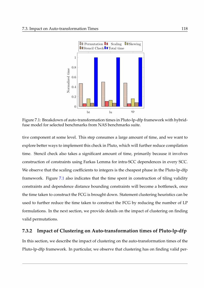
7.3. Impact on Auto-transformation Times 118
bt lu sp
0
0.2
0.4
0.6
0.8
1
Normalized
time
Permutation Scaling SkewingStencil Check Total time
Figure 7.1: Breakdown of auto-transformation times in Pluto-lp-dfp framework with hybrid-fuse model for selected benchmarks from NAS benchmarks suite.
tive component at some level. This step consumes a large amount of time, and we want to
explore better ways to implement this check in Pluto, which will further reduce compilation
time. Stencil check also takes a significant amount of time, primarily because it involves
construction of constraints using Farkas Lemma for intra-SCC dependences in every SCC.
We observe that the scaling coefficients to integers is the cheapest phase in the Pluto-lp-dfp
framework. Figure 7.1 also indicates that the time spent in construction of tiling validity
constraints and dependence distance bounding constraints will become a bottleneck, once
the time taken to construct the FCG is brought down. Statement clustering heuristics can be
used to further reduce the time taken to construct the FCG by reducing the number of LP
formulations. In the next section, we provide details on the impact of clustering on finding
valid permutations.
7.3.2 Impact of Clustering on Auto-transformation times of Pluto-lp-dfp
In this section, we describe the impact of clustering on the auto-transformation times of the
Pluto-lp-dfp framework. In particular, we observe that clustering has on finding valid per-
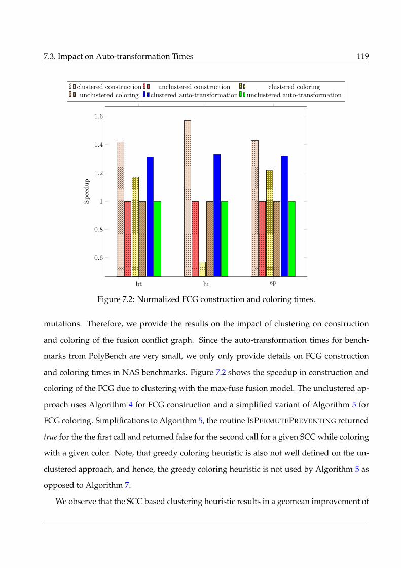
7.3. Impact on Auto-transformation Times 119
bt lu sp
0.6
0.8
1
1.2
1.4
1.6
Speedup
clustered construction unclustered construction clustered coloringunclustered coloring clustered auto-transformation unclustered auto-transformation
Figure 7.2: Normalized FCG construction and coloring times.
mutations. Therefore, we provide the results on the impact of clustering on construction
and coloring of the fusion conflict graph. Since the auto-transformation times for bench-
marks from PolyBench are very small, we only only provide details on FCG construction
and coloring times in NAS benchmarks. Figure 7.2 shows the speedup in construction and
coloring of the FCG due to clustering with the max-fuse fusion model. The unclustered ap-
proach uses Algorithm 4 for FCG construction and a simplified variant of Algorithm 5 for
FCG coloring. Simplifications to Algorithm 5, the routine ISPERMUTEPREVENTING returned
true for the the first call and returned false for the second call for a given SCC while coloring
with a given color. Note, that greedy coloring heuristic is also not well defined on the un-
clustered approach, and hence, the greedy coloring heuristic is not used by Algorithm 5 as
opposed to Algorithm 7.
We observe that the SCC based clustering heuristic results in a geomean improvement of
7.3. Impact on Auto-transformation Times 120
1.47× in FCG construction time. This is because, clustering reduces the number of LP prob-
lems that are solved during the construction of the FCG. The FCG coloring time in case of
LU benchmarks increases significantly in case of LU benchmark due to the greedy coloring
heuristic. In case of LU, we observe that for a given SCC there are a large number of convex
successors that can be colored but it remains valid to color only a few of them. Hence, the
greedy coloring heuristic takes longer than the simplified implantation of Algorithm 5. We
observe that our clustering contributed to an improvement of 1.31× in auto-transformation
time over the unclustered approach.
The clustering technique described by Mehta et al [MY15] does not allow efficient mod-
eling of loop distribution. On a slightly different experimental setup1, we observed that
their clustering technique, along with variable liberalization [MY16] provided an improve-
ment 3.5× on the NAS benchmarks considered for evaluation. The fusion model that we
considered for this experiment was the same as in scalefuse, and we found the same trans-
formation as that of scalefuse in these cases. However, since their clustering heuristic did
not allow modeling of loop distribution efficiently, we did not incorporate the it in the Pluto-
lp-dfp framework. Hotspots from hsmoc and lorentz routines in zeusmp benchmark of the
SPEC CPU 2006 benchmark suite studied by Mehta et al. [MY15] were also considered for
experimental evaluation. However the results from these benchmarks are not included in
this thesis because tools like Scalefuse and PolyOpt-Fortran were not maintained during the
submission of this thesis. Hence, quantitative evaluation of both compile time and execu-
tion time was not possible with the fusion heuristics in Pluto-lp-dfp. These experiments
demonstrated that, with the same fusion heuristic like Pluto in Pluto-lp-dfp, on the SPEC
benchmarks, Pluto-lp-dfp was faster than Pluto by a geomean factor of 180×. The reader is
encouraged to refer to the PLDI paper [ABC18] for further details.
1These experiments were performed on a sandybridge machine and the complete experimental setup isdescribed in [ABC18]. Scalefuse, which had the implementation of Mehta et al [MY15] was not maintainedand hence it was impossible to reproduce the results in the current experimental setup.

7.4. Performance Evaluation 121
7.4 Performance Evaluation
The execution times on 16 cores of all fusion models are listed in Table 7.3. The second col-
umn provides the execution times of the codes generated by PPCG [PPC13]. Note that for
benchmarks that are marked with a ’*’, the codes generated by PPCG could not be com-
piled with icc. Therefore, in these cases we used gcc-8 to compile transformed codes gen-
erated by PPCG. The third column provides the execution times for codes generated by
an older version of Pluto (version 0.11.4-463). This version is similar to the version used
by Kong et al. [KP19] for their comparison of PoCC+ with Pluto. The fourth and the fifth
columns present the execution times of the codes generated by PoCC+ and the recent ver-
sion of Pluto (version 0.11.4-920) that includes improved intra-tile optimizations and unroll
and jam heuristics (c.f. Chapter 6). Columns 5-7 correspond to the execution times of max-
fuse, typed-fuse and hybrid-fusion variants implemented in the Pluto-lp-dfp framework.
The last three rows correspond to benchmarks from the NAS benchmark suite while the rest
correspond to benchmarks from PolyBench. From Columns 3 and 5, we observe that these
optimizations result in a significant performance improvement over the older version of
Pluto by a geomean factor of 1.4× and over 3× in benchmarks like 2mm and 3mm. This im-
proved version of Pluto is used as the baseline for the comparison of Pluto-lp-dfp with Pluto,
unless specified otherwise. The first observation that we make is that PPCG is significantly
slower than PoCC+, Pluto, and the fusion variants in Pluto-lp-dfp. The codes generated by
Pluto-lp-dfp faster than the transformed codes generated by PPCG by a geomean factor of
5.8× across all benchmarks. This is primarily due to the cost model in PPCG and it also
lacks the support to generate vector pragmas. In the rest of this section, we only present the
details on comparison of Pluto-lp-dfp with PoCC+ and Pluto.
Figure 7.3 provides the speedup of PoCC+ and the fusion variants in Pluto-lp-dfp with
respect the Pluto, for the stencil benchmarks in PolyBench on which diamond tiling was
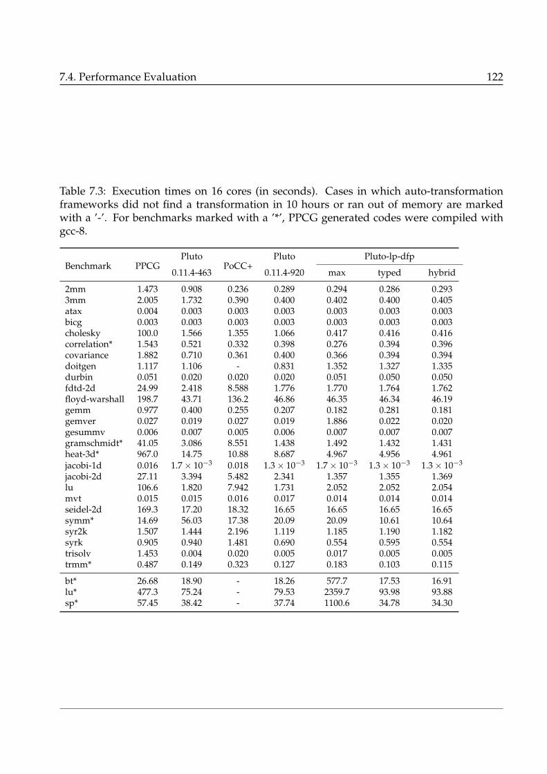
7.4. Performance Evaluation 122
Table 7.3: Execution times on 16 cores (in seconds). Cases in which auto-transformationframeworks did not find a transformation in 10 hours or ran out of memory are markedwith a ’-’. For benchmarks marked with a ’*’, PPCG generated codes were compiled withgcc-8.
Benchmark PPCGPluto
PoCC+Pluto Pluto-lp-dfp
0.11.4-463 0.11.4-920 max typed hybrid
2mm 1.473 0.908 0.236 0.289 0.294 0.286 0.2933mm 2.005 1.732 0.390 0.400 0.402 0.400 0.405atax 0.004 0.003 0.003 0.003 0.003 0.003 0.003bicg 0.003 0.003 0.003 0.003 0.003 0.003 0.003cholesky 100.0 1.566 1.355 1.066 0.417 0.416 0.416correlation* 1.543 0.521 0.332 0.398 0.276 0.394 0.396covariance 1.882 0.710 0.361 0.400 0.366 0.394 0.394doitgen 1.117 1.106 - 0.831 1.352 1.327 1.335durbin 0.051 0.020 0.020 0.020 0.051 0.050 0.050fdtd-2d 24.99 2.418 8.588 1.776 1.770 1.764 1.762floyd-warshall 198.7 43.71 136.2 46.86 46.35 46.34 46.19gemm 0.977 0.400 0.255 0.207 0.182 0.281 0.181gemver 0.027 0.019 0.027 0.019 1.886 0.022 0.020gesummv 0.006 0.007 0.005 0.006 0.007 0.007 0.007gramschmidt* 41.05 3.086 8.551 1.438 1.492 1.432 1.431heat-3d* 967.0 14.75 10.88 8.687 4.967 4.956 4.961jacobi-1d 0.016 1.7× 10⁻³ 0.018 1.3× 10⁻³ 1.7× 10⁻³ 1.3× 10⁻³ 1.3× 10⁻³
jacobi-2d 27.11 3.394 5.482 2.341 1.357 1.355 1.369lu 106.6 1.820 7.942 1.731 2.052 2.052 2.054mvt 0.015 0.015 0.016 0.017 0.014 0.014 0.014seidel-2d 169.3 17.20 18.32 16.65 16.65 16.65 16.65symm* 14.69 56.03 17.38 20.09 20.09 10.61 10.64syr2k 1.507 1.444 2.196 1.119 1.185 1.190 1.182syrk 0.905 0.940 1.481 0.690 0.554 0.595 0.554trisolv 1.453 0.004 0.020 0.005 0.017 0.005 0.005trmm* 0.487 0.149 0.323 0.127 0.183 0.103 0.115
bt* 26.68 18.90 - 18.26 577.7 17.53 16.91lu* 477.3 75.24 - 79.53 2359.7 93.98 93.88sp* 57.45 38.42 - 37.74 1100.6 34.78 34.30

7.4. Performance Evaluation 123
heat-3d jacobi-1d jacobi-2d fdtd-2d
0.5
1
1.5
Speedup
PoCC Pluto max-fuse typed-fuse hybrid-fuse
Figure 7.3: Speedup of different auto-transformation frameworks on stencil benchmarksfrom PolyBench benchmark suite.
possible. In case of jacobi-1d/2d, heat-3d, fdtd-2d), both Pluto and all our fusion models in
Pluto-lp-dfp perform better than PoCC+ because of diamond tiling. Pluto-lp-dfp performs
better than Pluto in case of multi-statement, time-iterated stencils (heat-3d, jacobi-2d) due to
a better transformation that increases the L1 hit rate. For example, in case of jacobi-2d, Pluto
finds the transformation
TS1(t, i, j)→ (2t− i, 2t + i, 2t + j)
TS2(t, i, j)→ (2t− i + 1, 2t + i + 1, 2t + j + 1),
which then tiled. Note that, the above transformation after tiling enables tile-wise concur-
rent start. Pluto-lp-dfp on the other hand finds the transformation
TS1(t, i, j)→ (2t− i, 2t + i, 2t + i + j)

7.4. Performance Evaluation 124
2mm 3mm gemm cholesky gramschmidt
0
0.5
1
1.5
2
2.5
Speedup
PoCC Pluto max-fuse typed-fuse hybrid-fuse
Figure 7.4: Speedup of different auto-transformation frameworks on selected linear algebrabenchmarks from PolyBench benchmark suite.
TS2(t, i, j)→ (2t− i + 1, 2t + i + 1, 2t + i + j + 1),
which involves more skewing at the innermost level. We first tuned the stencil benchmarks
for tile sizes and then measured the profiled the best performing variant for analysis of cache
behavior. Tile sizes were tuned in the space of 8, 16,32, 64, 128, 256 for each dimension, to
ensure that the default tile size of 32 was not favoring the transformation found by Pluto-
lp-dfp. The best performing variant was then profiled with perf during which we observed
that the L1 hit rate was better with the transformation found by Pluto-lp-dfp.
Figure 7.4 provides the speedup of linear algebra benchmarks from PolyBench for cases
where a significant difference in performance was observed. The first observation that we
make here is that the performance of PoCC+ is comparable to tiled codes generated by the

7.4. Performance Evaluation 125
doitgen durbin
0
0.2
0.4
0.6
0.8
1Speedup
PoCC Pluto max-fuse typed-fuse hybrid-fuse
Figure 7.5: Benchmarks from PolyBench on which we observe performance degradation.
improved version of Pluto in all cases other than gramschmidt. This is because in bench-
marks that involve matrix multiplications, the performance of tiled codes can be matched
register tiling via unroll jam optimizations. Note that, our improvements to intra-tile op-
timization heuristics and implementation of unroll and jam optimization, enabled us to
closely match the performance of PoCC+ in cases like 2mm, 3mm and gramschmidt. In
cholesky, we observe that transformation found by Pluto-lp-dfp improves register reuse by
enabling unroll jam of loops. This was not possible with the transformation found by Pluto,
because the transformation found by Pluto resulted in triangular loop nests.
Figure 7.5 lists the benchmarks in which the codes generated by Pluto-lp-dfp have a
degradation in performance. In doitgen, Pluto-lp-dfp finds a scaled up version of the trans-
formation found by Pluto. Such transformations are found by Pluto-lp-dfp in cases where
there exist spurious loop carried dependences due to updates to a loop private variable.
This issue can either be addressed by a code-generator, or by incorporating techniques like
variable liberalization [MY16] or live range re-ordering [VC16] in the auto-transformation

7.5. Summary of Results 126
framework, to remove such spurious dependences. In case of durbin, all our fusion variants
find a parallel loop at the innermost level. However, this inner parallel loop not only has
significant OpenMP synchronization cost, but also suffers from load imbalance, because, it
traverses a triangular domain. However, Pluto finds a transformation in which loop skew-
ing enables loop fusion, resulting in loss of parallelism. Thus the loop nest found by Pluto
is not parallelized using OpenMP. We profiled our code using Intel’s VTune and identified
OpenMP synchronization cost to be primary reason for loss of performance. To further
strengthen our claim, all the fusion variants were able to match the performance of the Pluto
generated code, in a single threaded execution. In future, we would like to have a model to
identify scenarios where parallelizing a loop with OpenMP results in performance degrada-
tion.
7.5 Summary of Results
In this section we summarize the results of our experiments. We first observe that the Pluto-
lp-dfp framework is significantly faster than state-of-the-art polyhedral auto-transformation
frameworks in terms of compile time. The default hybrid-fuse fusion model in the Pluto-lp-
dfp framework is faster than Pluto by a geomean factor of 2.2× in compilation time, with
more significant gains on larger NAS benchmarks and over 1000× in the largest case. On
these large cases PoCC+ did not terminate in a reasonable amount of time. Even when
restricted to PolyBench suite, our framework was faster than PoCC+ by 461×. We also ob-
served that incorporation of parallelism preserving fusion incurred a mere additional over-
head of ≈ 5.2% on compilation time. These massive improvements in compilation time are
meaningful only when there is no loss of performance. In terms of execution time, Pluto-lp-
dfp outperforms PoCC+ by 1.8× and PPCG by 5.8×. The intra-tile optimization heuristics
and multi-loop unroll and jam optimizations described in Chapter 6 improved the perfor-
mance of the then existing version of Pluto by a factor of 1.4×. The Pluto-lp-dfp framework

7.5. Summary of Results 127
is faster than this optimized version of Pluto by 7%. In the best case, we observe a perfor-
mance improvement of 2.6×. Thus, the Pluto-lp-dfp framework achieves our objective our
obtaining high performance with low compilation times, while efficiently modeling paral-
lelism preserving loop fusion heuristics in polyhedral compilation.

Chapter 8
Related Work
In this chapter, we discuss the related work around scalability of polyhedral compilation
and then in Section 8.2, we discuss the literature around loop fusion both in traditional and
polyhedral compilation.
8.1 Scalability of Polyhedral Frameworks
The first set of works on using affine schedules to improve performance were those by
Feautrier [Fea92a, Fea92b]. Feautrier’s schedules aimed at greedily satisfying dependences
as early as possible to obtain minimum latency schedules. Feautrier’s approach to find
multi-dimensional schedules [Fea92b] involves binary decision variables, and it thus can
only be relaxed to an Mixed Integer Programming (MIP) formulation instead of an LP for-
mulation. Feautrier’s schedules did not consider tiling or coarse-grained parallelization op-
portunity, and are thus very different from the ones found by Pluto [BBK+08, BHRS08].
The consequence of relaxing the ILP formulation in Feautrier’s multi-dimensional affine
scheduling formulation to a MIP formulation remains unexplored. However, Feautrier [Fea06]
identified the scalability issues in this ILP formulation and proposed a solution to optimize
the large programs by
8.1. Scalability of Polyhedral Frameworks 129
1. reducing the number of Farkas multipliers during the construction of dependence con-
straints using Gaussian elimination,
2. replacing the simplex algorithm with a different elimination algorithm that exploits
the sparsity of dependence constraints.
3. individually optimizing small program chunks.
All these methods aim at reducing the number of variables seen by the ILP solver, along
with exploiting the structure of constraints generated by polyhedral scheduling algorithms.
These approaches are orthogonal to the approach presented in the paper and can be incor-
porated in Pluto-lp-dfp to further improve auto-transformation times.
Several polyhedral frameworks have either relied on variants of Feautrier’s scheduling
approach, Pluto’s scheduling algorithm (ref Chapter 2), or a combination of these [VJC+13].
Vasilache [Vas07] modeled the space of multi-dimensional schedules using a single ILP for-
mulation, and has been extended to model driven and iterative approaches [PBB+10, KP19].
However, the ILP formulation is relatively more complex than the one in Pluto, and its im-
pact on compilation times was demonstrated in Chapter 7.
Variants of the scheduling algorithm in Pluto and the multi-dimensional algorithm by
Vasilache [Vas07] have been extended to model spatial and temporal reuse in order to ex-
ploit efficient vectorization [VMBL12, KVS+13]. The approach of Vasilache et al. [VMBL12]
restricts the space of affine transformations such that the innermost loop has stride-0 or
stride-1 accesses. Kong et al. [KVS+13] on the other hand, introduce a polyhedral reschedul-
ing step. The first scheduling step involves finding a transformation for the program using
the Pluto algorithm [BHRS08], then tileable loops are detected and parametrically [BHT+10]
tiled, and then, partial and full tiles are separated. In the second step, the intra-tile itera-
tors of full tiles obtained in the first step, are subjected to intra-tile rescheduling. The newly
found intra-tile schedule tries to maximize fine-grained parallelism, maximize unit stride

8.1. Scalability of Polyhedral Frameworks 130
and stride-0 references, and penalize unaligned loads and stores. Both these approaches
involve solving more ILPs that contain decision variables per dependence. Therefore, the
number of variables in these ILP formulations is significantly large. Relaxing integrality
constraints in such formulations is outside the scope of this work. In the case of Pluto algo-
rithm, we were able to relax it to an LP formulation, while seeking tileable bands. Moreover,
in Pluto, we were able to efficiently model intra-tile optimizations using heuristics with-
out solving ILPs (refer Chapter 6). We also observe that these heuristics are sufficient to
match or outperform state-of-the-art polyhedral auto-parallelizers in terms of performance
of transformed codes, as demonstrated by our experiments described in Chapter 7.
Several tiling strategies have been incorporated in the state-of-the-art polyhedral com-
pilers like Pluto and PPCG. Bandishti et al. [BPB12] introduced diamond tiling, which was
later generalized by Bondhugula et. al [BBP17], to enable tile-wise concurrent start in sten-
cils as rescheduling step in Pluto. Prior to that, overlapped tiling and split tiling techniques
were used to enable tile-wise concurrent start in stencils, by altering the transformations
obtained by Pluto [KBB+07]. Hexagonal tiling, which can be viewed as an extension of
diamond tiling by allowing hexagonal shaped tiles instead of diamond tiles, was intro-
duced by Grosser et al. [GCH+14] for tiling stencil computations on GPUs. Overlapped
tiling [RKBA+13, MVB15, HPS12] has been studied in the context of domain specific compi-
lation for both stencils and image processing applications for both CPUs and GPUs. Efforts
to reduce redundant computation that arise due to overlapped tiling have been made by hi-
erarchical tiling schemes that perform overlapped tiling at inner level and rectangular tiling
at outer levels [ZGG+12, ZGP15]. Very recently, Zhao and Cohen [ZC19] proposed flex-
tended tiling, in which tile shapes can be asymmetric/scalene trapezoids, by deriving tighter
bounds on the amount of redundant computation. Their approach integrates affine transfor-
mations like loop fusion and permutation, among many others, with storage optimizations
like, scratchpad allocation, in a general-purpose compiler, thereby yielding performance

8.1. Scalability of Polyhedral Frameworks 131
that is comparable with diamond tiling on CPUs and hexagonal/hybrid tiling on GPUs.
All these tiling techniques rely on Pluto’s or Feautrier’s scheduling algorithm, and hence
suffer from the scalability issues described in this thesis. It is a part of our future work,
to study the impact of incorporating overlapped tiling instead of loop skewing in the last
auto-transformation stage of the Pluto-lp-dfp compiler.
Recent efforts explored ways to improve the scalability of Pluto by reducing the num-
ber of variables in its ILP formulation. Pradelle et al. [PMB+16] hierarchically project out
dimensions (per level of tiling) of the dependence polyhedron with a focalisation operator.
This operator projects out the outer dimensions while intra-tile optimizations are performed
and vice-versa. Every focalization operator is associated with a defocalisation operator that
reintroduces the dimensions that were projected out by the focalization operator. This ap-
proach was implemented in R-Stream compiler [RST08], which relies on Feautrier’s schedul-
ing constraints. Their approach does not address the scalability problem stemming from the
ILP formulation and the construction of linear independence constraints.
Mehta et al. [MY15] and Baghdadi [Bag15] propose statement clustering heuristics to re-
duce the number of statements seen by the polyhedral optimizer. All the statements within
a cluster will have a single set of transformation coefficients and hence get the same trans-
formation. The statement clustering heuristic of Mehta et al. [MY15], clusters successive
statements that have the same iteration domain into an O-molecule (optimization molecule).
This heuristic is slightly more generic than basic block clustering used in LLVM-Polly; for ex-
ample, in cases where statements in consecutive loop nests have the same iteration domain,
these statements are clustered into an O-molecule. They also employ dependence conden-
sation techniques, where only a sufficient set of dependences are considered, reducing the
taken for the construction of tiling validity and dependence distance bounding constraints.
Though they achieve significant compile time improvements over the Pluto algorithm, their
approach inhibits opportunities for loop distribution. Moreover, these compilation time im-
8.1. Scalability of Polyhedral Frameworks 132
provements are tightly coupled with the ability to construct O-molecules with a large num-
ber of statements. We observed that on some large image processing pipelines, their cluster-
ing heuristic fails to form large clusters, which results in auto-transformation times similar
to that of Pluto. This is because, even after clustering, the auto-transformation framework
still relies on the ILP formulation and the construction of linear independence constraints.
On the other hand, the Pluto-lp-dfp framework completely avoids these major bottlenecks
in the Pluto algorithm.
The SCC based clustering approach proposed by Baghdadi [Bag15], was able to find the
same set of transformations as Pluto, apart from a few practically harmless loop shifting
transformations. Their clustering heuristic clusters statements in an SCC that belong to a
same basic block. This results in smaller clusters than our clustering heuristic described in
Section 5.2. This is because, their approach does not have the ability to uncluster during
the auto-transformation phase, where as, in Pluto-lp-dfp, unclustering is performed during
the reconstruction of the FCG. Statement clustering approaches are orthogonal to the pro-
posed framework and the advantages of integrating these heuristics was demonstrated in
Chapter 7.
Upadrasta and Cohen [UC13] explored yet another angle to improve the scalability of
affine scheduling: by approximating LP problems into lower complexity sub-polyhedral fea-
sibility problems (e.g., octagons). This complementary approach remains currently limited
in its ability to model optimization problems, and its implementation and further evaluation
remains to be explored.
Shirako et al. [SPS14] decompose the affine scheduling problem into polyhedral and AST
based transformation stages. The output of their polyhedral stage is a valid transformation
consisting of loop permutation and loop shifting transformations. This can be used as an
alternative for the permutation black box part of our approach, and the scaling and shift-
ing phase can be skipped. However, their transformations do not consider loop scaling to

8.2. Related Work on Fusion 133
enable fusion. Also, their approach can not be relaxed to an LP because, their polyhedral
phase relies on Feautrier’s multi-dimensional scheduling constraints [Fea92b] involving bi-
nary decision variables. Their fusion heuristic is guided by the distinct lines model [Sar97]
which considers cache occupancy and tries the minimize the number of conflict misses in
the cache, along with other factors. Their approach relies on traditional AST based methods
for loop skewing and loop tiling and hence are limited to tiling of perfect loop nests. The
proposed Pluto-lp-dfp framework is a pure polyhedral framework which does not have the
restrictions of traditional loop transformation approaches and has precise dependence infor-
mation in the form of dependence polyhedra, and hence, it allows loop skewing and loop
tiling to be modeled in a more generic fashion.
8.2 Related Work on Fusion
Traditionally loop fusion and distribution has been studied in the context of maximizing
parallelism and locality. Seminal work by Kennedy and McKinley on parallelism preserv-
ing loop fusion or typed fusion [KM92, KM93] involved fusing loops that have the same type
(parallel or sequential). Optimal loop fusion has been proven to be NP-complete [KM93] and
Darte [Dar00, Dar99] established NP-completeness for a broader class of loop fusion prob-
lems. Both polynomial time and optimal solutions have been proposed for the weighted
loop fusion problem [Ken00, MS97]. All these approaches do not consider loop fusion in
conjunction with other loop transformations like loop permutation, loop scaling and shift-
ing.
Sarkar and Gao [SG91] use interference graphs to model loop reversals and loop permu-
tations to enable loop fusion. These graphs have two vertices per dimension of a statement.
Edges in these graphs are analogous to edges in the FCG. However, their model does not
consider transformations that involve loop shifting or loop scaling to enable fusion. Their
primary objective is to improve reuse and enable scalarization of arrays and do not consider

8.2. Related Work on Fusion 134
Table 8.1: Summary of various fusion heuristics available in polyhedral auto-transformationframeworks.
Fusion heuristic Parallelism-preserving More ILPs Implementation status
Smart-fuse 7 7 Default in PlutoMax-Fuse 7 7 Available in PlutoNo-Fuse 7 7 Available in PlutoWise-fuse 3 3 UnavailableTyped-fuse 3 3 Default in ISL/PPCG
parallelism in their objective. To model loop reversals in the FCG, we can extend the FCG by
duplicating its vertices to model reversals, similar to interference graphs. However, we ob-
serve that, in practice, transformations like loop scaling and loop shifting enable loop fusion
in large number of cases when compared to loop reversals.
Polyhedral compilers like LLVM Polly [GZA+11], Pluto, PPCG [VJC+13], model loop
distribution with various heuristics. PPCG fuses two SCCs only if it preserves parallelism
by solving more number of ILPs. Hence, even with certain heuristics, implementation of
parallelism-preserving fusion models in a polyhedral compiler would involve solving a sig-
nificantly large number of ILP formulations, resulting in large auto-transformation times.
Loop fusion heuristics in Pluto are adhoc and do not consider any optmization criteria as
described in Chapter 2. A summary of these fusion heuristics is provided in Table 8.1. Us-
ing the FCG we were able to model parallelism preserving loop fusion heuristics to work
alongside other affine loop transformations in a polyhedral compilation framework with-
out significant compilation time overhead, as evidenced by our experiments described in
Chapter 7.
Mehta et al. [MLY14] provide a loop fusion heuristic in the polyhedral framework called
wisefuse, which is similar to typed fusion. Their approach fuses two SCCs only if there is
reuse and also ensures that the resulting loop nest remains parallel. Their approach de-
tects if a hyperplane found by Pluto resulted in loss of parallelism and if so, it discards the
hyperplane found, distributes the SCCs, and then, finds a new hyperplane using Pluto’s al-

8.2. Related Work on Fusion 135
gorithm. This adds more compile time overhead to the existing auto-transformation times
of Pluto (refer Table 7.2).
The recent work of Kong and Pouchet [KP19], which we referred to as PoCC+ in Chap-
ter 7, obtains significant performance benefits over the then existing version of Pluto (version
0.11.4-85), which we were able to reproduce. They exploit register reuse by unroll and jam-
ming loops, due to which, the benefits of cache tiling diminish. Their loop transformations
are guided by a series of objectives based on the characteristics of the program. Experimental
results therein concluded that excellent performance improvements could be achieved with-
out actually performing loop tiling. We implemented unroll and jam optimizations in Pluto
(and Pluto-lp-dfp) to exploit register reuse and also improved intra-tile optimization heuris-
tics. These optimizations, in addition to loop tiling, not only enabled us to closely match the
performance of PoCC+ with default tile sizes on benchmarks like 2mm and 3mm, but also
achieve overall performance improvement over PoCC+ with both Pluto and Pluto-lp-dfp.
Tuning for tile sizes will further improve our performance over PoCC+. This re-establishes
the need for loop tiling and also motivates further research on tile size selection models. To
the best of our knowledge, they are the first to incorporate a model to characterize stencils
in a general-purpose compiler. Their characterization classifies an SCC as a stencil if the
condition
is_stencil∧ Ndep ≤ 3×m
evaluates to true, where Ndep represents the number of dependences in the SCoP, m is the
maximum of dimensionalities of all statements in the SCoP, and the predicate isstencil is true
if at least half the number of statements in the SCoP refer to at least two neighboring points
in the iteration space of the same statement. This characterization can be restricted to a per-
SCC basis rather than the entire SCoP with minor modifications. However, it is based on
the number of dependences and the number of statements in the SCoP and does not take
into account tile-wise concurrent start, constant dependence vectors, absence of communi-

8.2. Related Work on Fusion 136
cation free parallel loops, which are characteristics of time-iterated stencils, as described in
Section 5.3.2. Note that, in case of stencil benchmarks, significant performance gains were
obtained primarily enabling of tile-wise concurrent start by diamond tiling, which is our
characterization takes into account. Finally, the construction of constraints in PoCC+ is rel-
atively more expensive, resulting in very high auto-transformation times, as evidenced by
our experiments in Section 7.3.
Fusion on coarser grained operators has been widely implemented in domain-specific
compilers like Halide [RKBA+13], XLA [XLA17], and Polymage [MVB15]. Such fusion is
more general than traditional loop fusion since the former could lead to redundant compu-
tation and impact intermediary storage in different ways. XLA implements operator fusion
on its intermediate representation relying on the type of operators. In Halide and Polymage,
stages of an image processing pipeline are fused greedily, based on reuse and the amount of
redundant computation [MAS+16, JB18] among other factors.

Chapter 9
Conclusions and Future Work
In this chapter we conclude the thesis by reiterating the contributions of the thesis and
provide insights on some possible future extensions to the proposed Pluto-lp-dfp auto-
transformation framework.
9.1 Conclusions
Loop optimizations are known to provide significant performance gains in applications from
various domains. Therefore, automatic loop transformation frameworks have become more
popular to extract performance on modern architectures and meet the increasing compute
and memory requirements of complex algorithms. Polyhedral auto-transformation frame-
works have the ability to model a rich class of affine loop transformations with objectives.
However, these frameworks still remained as optional passes in general-purpose compilers
like LLVM, because these frameworks did not scale to programs with hundreds of state-
ments. This thesis not only focused on improving the scalability of the widely used Pluto
algorithm to programs with hundreds of statements, but also provided a way to model com-
plex loop fusion heuristics in polyhedral auto-transformation frameworks.
The scalability issues in the Pluto algorithm has been traditionally known to arise from
the ILP formulation and the associated combinatorially expensive construction of linear in-

9.1. Conclusions 138
dependence constraints. Hence, in this thesis, we first studied the effects of relaxing the
integrality constraints on the variables in the ILP formulation of the Pluto algorithm. We
showed that relaxing the ILP formulation in Pluto results in rational solutions, that can be
scaled to integers without violating any dependences. However, the sub-optimalities that
arise due to this relaxation manifested as loop skewing transformations that degraded per-
formance significantly in some cases. In spite of these sub-optimalities, we showed that the
relaxed formulation can be used as a light-weight check for existence of communication free
parallel hyperplanes and tileability of the loop nest. On the contrary, the relaxed formula-
tion still involved the construction of linear independence constraints that played a key role
in the scalability of the Pluto algorithm.
In order to overcome the sub-optimalities arising due to relaxation of the ILP formulation
and avoid the construction of linear independence constraints, we designed an automatic
transformation algorithm within the polyhedral framework. This new framework, Pluto-
lp-dfp, addressed the key scalability issue in polyhedral compilation by decomposing the
auto-transformation phase into the following three stages: 1) loop fusion and permutation,
2) loop scaling and shifting, and 3) loop skewing. In each stage, the Pluto-lp-dfp frame-
work relied on LP formulations instead of ILP and completely avoided the construction
of linear independence constraints by reorganizing the construction of affine transforma-
tions. Experimental results demonstrated that, the proposed reorganization does not miss
any profitable transformations for benchmarks from NAS and PolyBench benchmark suites.
A consequence of decoupling the construction of polyhedral loop transformations allowed
loop fusion to be modeled in conjunction with other loop transformations like loop permu-
tation, loop scaling and loop shifting. Loop fusion in Pluto-lp-dfp was modeled using a
data structure called the fusion conflict graph (FCG). We proved that convex independent
sets that were obtained using a convex coloring routine corresponded to valid loop permu-
tations, and these valid permutations allowed various loop fusion heuristics to be modeled

9.2. Future Directions 139
efficiently using the FCG. Then, we proposed clustering heuristics that allowed us to im-
plement greedy fusion models, in particular, fusion models that did not result in loss of
parallelism. We also characterized dependence patterns exhibited by time-iterated stencils
that have tile-wise concurrent start. This characterization allowed to use different fusion
heuristics in such program segments. Thus, the Pluto-lp-dfp framework allows seamless
integration of complex loop fusion heuristics in polyhedral compilation as a part of a single
auto-transformation algorithm.
Our experiments demonstrated that Pluto-lp-dfp was faster than Pluto by a factor of
234× on larger NAS benchmarks in compilation time, without sacrificing performance of
executed codes. Even while considering the smaller benchmarks from PolyBench, Pluto-
lp-dfp was faster than Pluto by a factor of 2.2× and PoCC+ by a factor of 461×. We also
demonstrated that incorporating greedy parallelism preserving loop fusion heuristics did
not incur significant compile time overhead. These improvements in compilation time came
along with an improvement in performance of generated codes. The hybrid fusion model in
Pluto-lp-dfp outperforms PPCG, PoCC+, and an improved version of Pluto by a by geomean
factors of 5.8×, 1.8× and 7% respectively. Thus, Pluto-lp-dfp framework complementary to
other recent approaches in the subject of scalability of polyhedral auto-transformation and
allows integration of these approaches. Pluto-lp-dfp not only advances state-of-the-art in
polyhedral compilation but also introduces other research opportunities, some of which we
detail in the next section.
9.2 Future Directions
In this section, we provide some insights into some possible future extensions.
Further reducing compilation times: We would further reduce the compilation times of
Pluto-lp-dfp by improving the clustering heuristic. If not the clustering heuristic described
by Mehta et al. [MY15], we hypothesize that a more careful clustering along similar lines

9.2. Future Directions 140
would reduce the compilation times further. Secondly, we in our previous experiments, we
had observed that applying loop distribution heuristic of Pluto at the outermost level, even
before the construction of the FCG, reduces the time taken to construct the FCG by a factor
of 1.5×. This is because, it reduces the number of LP formulations during the construction
of the FCG. Incorporating such loop distribution strategies at the outermost level while con-
sidering certain optimization criteria is a part of our future work. In order to reduce the
overall compilation time in Pluto-lp-dfp, in addition to reducing FCG construction time, the
time taken to construct polyhedral dependence constraints (tiling validity and dependence
distance bounding constraints) by the application of Farkas Lemma has to reduced. One can
identify a minimal set of dependences to be satisfied in order to ensure correctness, however
a more interesting approach would be to rely on a mixture of experts approach. Loop opti-
mizations on certain parts of the program can be performed by traditional approaches by
using dependence vectors, and polyhedral dependences can be used in certain other parts.
Optimizing loops with a mix of polyhedral and traditional loop transformation approaches
applied on different program segments is currently unexplored.
Modeling loop fusion: The loop fusion models that we proposed here only considered
parallelism into account. However, loop fusion can increase register pressure and also re-
duce the performance of prefetchers if the fusion model is very aggressive. In future we
would like to model these factors into cost model, more likely during the coloring phase
of the Pluto-lp-dfp framework. We would also like to incorporate other cost models like
weighted loop fusion [Ken00, MS97] in the Pluto-dfp framework. In other words, we would
like to evaluate the performance of older approaches to loop fusion in a polyhedral environ-
ment. Using the FCG, Pluto-lp-dfp is able to unify the benefits of traditional and polyhe-
dral loop transformations, and hence, is a good candidate to be incorporated into a multi-
abstraction-level infrastructure like MLIR.

9.2. Future Directions 141
Extensions to overlapped tiling: Overlapped tiling has been proven to be effective in es-
pecially in the domains of image processing and machine learning. However, the adoption
of this tiling strategy in general-purpose compilation has not gained much popularity in
state-of-the-art polyhedral compilers. This is primarily due to large overhead of redun-
dant computation that might arise in general purpose programs. As observed by Vasista
et al [VNBB17], even within the class of stencils, performance of diamond tiled and over-
lap tiled codes vary significantly. Moreover, apart from time-iterated stencils, it is unclear
whether loop skewing performs better than codes with overlapped tiling. Using the sten-
cil characterization provided in Section 5.3.2, one can not only distinguish between lower
and higher dimensional stencils (higher dimensional stencils have high over head of redun-
dant computation in case of overlapped tiling), but also replace the loop skewing phase in
the Pluto-lp-dfp benchmarks with overlapped tiling in cases where it is considered to be
profitable.
Extensions to Domain Specific Languages (DSLs): We plan to apply our fusion model to
DSLs like PolyMage and TensorFlow-XLA where loop fusion strategies are predefined and
operator fusion heuristics have been studied. These operation fusion heuristics not only
aim at exploring reuse, at times, even with the expense of redundant computation, but also
optimize for storage by using small buffers to store intermediate results, if necessary. In
such cases, fusion models would to consider many different criteria, as described by Jangda
et al. [JB18]. We would like to extend the FCG to model operation fusion in DSLs to optimize
for storage and performance in a unified manner.

Bibliography
[ABC18] Aravind Acharya, Uday Bondhugula, and Albert Cohen. Polyhedral auto-
transformation with no integer linear programming. In Proceedings of the 39th
ACM SIGPLAN Conference on Programming Language Design and Implementation,
PLDI 2018, pages 529–542, New York, NY, USA, 2018. ACM.
[BAC16] Uday Bondhugula, Aravind Acharya, and Albert Cohen. The pluto+ algorithm:
A practical approach for parallelization and locality optimization of affine loop
nests. ACM Trans. Program. Lang. Syst., 38(3):12:1–12:32, April 2016.
[Bag15] Mohamed Riyadh Baghdadi. Improving tiling, reducing compilation time, and ex-
tending the scope of polyhedral compilation. Theses, Université Pierre et Marie
Curie - Paris VI, September 2015.
[Ban94] Utpal Banerjee. Unimodular Transformations, pages 67–112. Springer US, Boston,
MA, 1994.
[Basa] Cédric Bastoul. Candl: The Chunky Analyzer for Dependences in Loops.
[Basb] Cédric Bastoul. Clan: The Chunky Loop Analyzer. The Clan User guide.
[BBK+08] Uday Bondhugula, M. Baskaran, Sriram Krishnamoorthy, J. Ramanu-
jam, A. Rountev, and P. Sadayappan. Automatic transformations for
communication-minimized parallelization and locality optimization in the

BIBLIOGRAPHY 143
polyhedral model. In International conference on Compiler Construction (ETAPS
CC), 2008.
[BBP17] U. Bondhugula, V. Bandishti, and I. Pananilath. Diamond tiling: Tiling tech-
niques to maximize parallelism for stencil computations. IEEE Transactions on
Parallel and Distributed Systems, 28(5):1285–1298, May 2017.
[BHRS08] Uday Bondhugula, Albert Hartono, J. Ramanujam, and P. Sadayappan. A prac-
tical automatic polyhedral parallelizer and locality optimizer. In ACM SIG-
PLAN symposium on Programming Languages Design and Implementation (PLDI),
pages 101–113, 2008.
[BHT+10] Muthu Manikandan Baskaran, Albert Hartono, Sanket Tavarageri, Thomas
Henretty, J. Ramanujam, and P. Sadayappan. Parameterized tiling revisited.
In Proceedings of the 8th Annual IEEE/ACM International Symposium on Code Gen-
eration and Optimization, CGO ’10, page 200–209, New York, NY, USA, 2010.
Association for Computing Machinery.
[BPB12] Vinayaka Bandishti, Irshad Pananilath, and Uday Bondhugula. Tiling stencil
computations to maximize parallelism. In Supercomputing, pages 40:1–40:11,
2012.
[CBB+18] Scott Cyphers, Arjun K. Bansal, Anahita Bhiwandiwalla, Jayaram Bobba,
Matthew Brookhart, Avijit Chakraborty, William Constable, Christian Convey,
Leona Cook, Omar Kanawi, Robert Kimball, Jason Knight, Nikolay Korovaiko,
Varun Kumar Vijay, Yixing Lao, Christopher R. Lishka, Jaikrishnan Menon, Jen-
nifer Myers, Sandeep Aswath Narayana, Adam Procter, and Tristan J. Webb.
Intel ngraph: An intermediate representation, compiler, and executor for deep
learning. CoRR, abs/1801.08058, 2018.

BIBLIOGRAPHY 144
[Clo04] The Chunky Loop Generator, 2004. http://www.cloog.org.
[cuB] Dense Linear Algebra on GPUs. https://developer.nvidia.com/cublas.
[cuD] NVIDIA CUDA Deep Neural Network library.
https://developer.nvidia.com/cudnn.
[Dar99] A. Darte. On the complexity of loop fusion. In 1999 International Conference on
Parallel Architectures and Compilation Techniques (Cat. No.PR00425), pages 149–
157, Oct 1999.
[Dar00] Alain Darte. On the complexity of loop fusion. Parallel Computing, 26(9):1175–
1193, 2000.
[Fea88] P. Feautrier. Parametric integer programming. RAIRO Recherche Opérationnelle,
22(3):243–268, 1988.
[Fea92a] P. Feautrier. Some efficient solutions to the affine scheduling problem: Part I,
one-dimensional time. International Journal of Parallel Programming, 21(5):313–
348, 1992.
[Fea92b] P. Feautrier. Some efficient solutions to the affine scheduling problem: Part II,
multidimensional time. International Journal of Parallel Programming, 21(6):389–
420, 1992.
[Fea06] Paul Feautrier. Scalable and structured scheduling. International Journal of Par-
allel Programming, 34(5):459–487, Oct 2006.
[GCH+14] Tobias Grosser, Albert Cohen, Justin Holewinski, P. Sadayappan, and Sven Ver-
doolaege. Hybrid hexagonal/classical tiling for gpus. In Proceedings of Annual
IEEE/ACM International Symposium on Code Generation and Optimization, CGO

BIBLIOGRAPHY 145
’14, pages 66–75, New York, NY, USA, 2014. Association for Computing Ma-
chinery.
[GGL12] Tobias Grosser, Armin Groesslinger, and Christian Lengauer. Polly: Performing
polyhedral optimizations on a low-level intermediate representation. Parallel
Processing Letters, 22(04), 2012.
[GNU] GNU. GLPK (GNU Linear Programming Kit).
https://www.gnu.org/software/glpk/.
[GO16] Inc. Gurobi Optimization. Gurobi optimizer reference manual, 2016.
[GZA+11] Tobias Grosser, Hongbin Zheng, Ragesh Aloor, Andreas Simbürger, Armin
Größlinger, and Louis-Noël Pouchet. Polly – Polyhedral Optimization in
LLVM. In Proceedings of the First International Workshop on Polyhedral Compila-
tion Techniques (IMPACT), 2011, 2011.
[HPS12] Justin Holewinski, Louis-Noël Pouchet, and P. Sadayappan. High-performance
code generation for stencil computations on gpu architectures. In Proceedings of
the 26th ACM International Conference on Supercomputing, ICS ’12, pages 311–320,
New York, NY, USA, 2012. Association for Computing Machinery.
[IBM] IBM. CPLEX Optimizer. https://www.ibm.com/analytics/cplex-optimizer.
[Int] Intel(R) Math Kernel Library for Deep Neural Networks.
http://intel.github.io/mkl-dnn/.
[JB18] Abhinav Jangda and Uday Bondhugula. An effective fusion and tile size model
for optimizing image processing pipelines. In Proceedings of the 23rd ACM SIG-
PLAN Symposium on Principles and Practice of Parallel Programming, PPoPP ’18,
pages 261–275, New York, NY, USA, 2018. ACM.
BIBLIOGRAPHY 146
[KBB+07] Sriram Krishnamoorthy, Muthu Baskaran, Uday Bondhugula, J. Ramanujam,
A. Rountev, and P. Sadayappan. Effective Automatic Parallelization of Stencil
Computations. In ACM SIGPLAN PLDI, July 2007.
[Ken00] K. Kennedy. Fast greedy weighted fusion. In ACM International conference on
Supercomputing, 2000.
[KM92] K. Kennedy and K. McKinley. Optimizing for Parallelism and Data Locality. In
Proc. 1992 ACM International Conference on Supercomputing, pages 323–334, 1992.
[KM93] K. Kennedy and K. McKinley. Maximizing loop parallelism and improving data
locality via loop fusion and distribution. In Languages and Compilers for Parallel
Computing, pages 301–320, 1993.
[KMP+96] Wayne Kelly, Vadim Maslov, William Pugh, Evan Rosser, Tatiana Shpeisman,
and Dave Wonnacott. The Omega calculator and library, version 1.1.0. 1996.
[KP19] Martin Kong and Louis-Noël Pouchet. Model-driven transformations for multi-
and many-core cpus. In Proceedings of the 40th ACM SIGPLAN Conference on
Programming Language Design and Implementation, PLDI 2019, pages 469–484,
New York, NY, USA, 2019. ACM.
[KVS+13] Martin Kong, Richard Veras, Kevin Stock, Franz Franchetti, Louis-Noël
Pouchet, and P. Sadayappan. When polyhedral transformations meet simd code
generation. In ACM SIGPLAN conference on Programming Language Design and
Implementation (PLDI), June 2013.
[LCL99] A. Lim, Gerald I. Cheong, and Monica S. Lam. An affine partitioning algorithm
to maximize parallelism and minimize communication. In ACM International
Conference on Supercomputing (ICS), pages 228–237, 1999.

BIBLIOGRAPHY 147
[LL98] A. Lim and Monica S. Lam. Maximizing parallelism and minimizing synchro-
nization with affine partitions. Parallel Computing, 24(3-4):445–475, 1998.
[MAS+16] Ravi Teja Mullapudi, Andrew Adams, Dillon Sharlet, Jonathan Ragan-Kelley,
and Kayvon Fatahalian. Automatically scheduling halide image processing
pipelines. ACM Transactions on Graphics, 35(4):83:1–83:11, July 2016.
[MKL] Intel math kernel library (MKL). http://software.intel.com/en-us/intel-mkl.
[MLI19] Multi-Level Intermediate Representation Compiler Infrastructure, 2019.
https://github.com/tensorflow/mlir.
[MLY14] Sanyam Mehta, Pei-Hung Lin, and Pen-Chung Yew. Revisiting loop fusion in
the polyhedral framework. In Proceedings of the 19th ACM SIGPLAN Symposium
on Principles and Practice of Parallel Programming, PPoPP ’14, pages 233–246, New
York, NY, USA, 2014. ACM.
[MS97] Nimrod Megiddo and Vivek Sarkar. Optimal weighted loop fusion for parallel
programs. In symposium on Parallel Algorithms and Architectures, pages 282–291,
1997.
[MVB15] Ravi Teja Mullapudi, Vinay Vasista, and Uday. Bondhugula. Polymage: Auto-
matic optimization for image processing pipelines. In International Conference
on Architectural Support for Programming Languages and Operating Systems (ASP-
LOS), 2015.
[MVW+11] Benoît Meister, Nicolas Vasilache, David Wohlford, Muthu Baskaran, Allen Le-
ung, and Richard Lethin. R-Stream Compiler. In Encyclopedia of Parallel Com-
puting, pages 1756–1765. Springer, 2011.

BIBLIOGRAPHY 148
[MY15] Sanyam Mehta and Pen-Chung Yew. Improving compiler scalability: Optimiz-
ing large programs at small price. In ACM SIGPLAN Conference on Programming
Language Design and Implementation, pages 143–152, 2015.
[MY16] Sanyam Mehta and Pen-Chung Yew. Variable liberalization. ACM Transactions
on Architecture and Code Optimization, 13(3):23:1–23:25, August 2016.
[NPB11] SNU NAS Parallel Benchmark Suite, 2011.
http://aces.snu.ac.kr/software/snu-npb/.
[PBB+10] Louis-Noël Pouchet, Uday Bondhugula, Cédric Bastoul, Albert Cohen, J. Ra-
manujam, and P. Sadayappan. Combined iterative and model-driven optimiza-
tion in an automatic parallelization framework. In Supercomputing (SC’10), New
Orleans, LA, November 2010.
[PCB+06] Sébastian Pop, Albert Cohen, Cédric Bastoul, Sylvain Girbal, P. Jouvelot, G.-A.
Silber, and N. Vasilache. GRAPHITE: Loop optimizations based on the polyhe-
dral model for GCC. In Proc. of the 4th GCC Developer’s Summit, Ottawa, Canada,
June 2006.
[Plu08] PLUTO: A polyhedral automatic parallelizer and locality optimizer for multi-
cores, 2008. https://github.com/bondhugula/pluto.
[PMB+16] B. Pradelle, B. Meister, M. Baskaran, A. Konstantinidis, T. Henretty, and
R. Lethin. Scalable hierarchical polyhedral compilation. In 2016 45th Interna-
tional Conference on Parallel Processing (ICPP), pages 432–441, Aug 2016.
[PoC19] The Polyhedral Compiler Collection, 2019. Obtained via private communica-
tion.
[Pol10] Polybench suite, 2010. http://polybench.sourceforge.net.

BIBLIOGRAPHY 149
[PPC13] Polyhedral parallel code generator, 2013. https://github.com/Meinersbur/ppcg,
Version 0.08.2.
[RKBA+13] Jonathan Ragan-Kelley, Connelly Barnes, Andrew Adams, Sylvain Paris, Frédo
Durand, and Saman Amarasinghe. Halide: a language and compiler for opti-
mizing parallelism, locality, and recomputation in image processing pipelines.
In PLDI, pages 519–530, 2013.
[RST08] RSTREAM - High Level Compiler, Reservoir Labs, 2008.
http://www.reservoir.com.
[Sar97] V. Sarkar. Automatic selection of high-order transformations in the ibm xl for-
tran compilers. IBM J. Res. Dev., 41(3):233–264, May 1997.
[Sch86] Alexander Schrijver. Theory of Linear and Integer Programming. John Wiley &
Sons, 1986.
[SG91] Vivek Sarkar and Guang R. Gao. Optimization of array accesses by collective
loop transformations. In Proceedings of the 5th International Conference on Super-
computing, ICS ’91, pages 194–205, New York, NY, USA, 1991. ACM.
[SPS14] Jun Shirako, Louis-Noël Pouchet, and Vivek Sarkar. Oil and water can mix: An
integration of polyhedral and ast-based transformations. In Proceedings of the
International Conference for High Performance Computing, Networking, Storage and
Analysis, SC ’14, pages 287–298, Piscataway, NJ, USA, 2014. IEEE Press.
[ST92] Vivek Sarkar and Radhika Thekkath. A general framework for iteration-
reordering loop transformations. In Proceedings of the ACM SIGPLAN 1992
Conference on Programming Language Design and Implementation, PLDI ’92, pages
175–187, New York, NY, USA, 1992. Association for Computing Machinery.

BIBLIOGRAPHY 150
[UC13] Ramakrishna Upadrasta and Albert Cohen. Sub-polyhedral scheduling using
(Unit-)two-variable-per-inequality polyhedra. In ACM SIGPLAN-SIGACT Sym-
posium on Programming Languages (POPL), Rome, Italy, January 2013.
[Vai89] P. M. Vaidya. Speeding-up linear programming using fast matrix multiplica-
tion. In 30th Annual Symposium on Foundations of Computer Science, pages 332–
337, 1989.
[Vas07] Nicolas Vasilache. Scalable Program Optimization Techniques in the Polyhedral
Model. PhD thesis, Université de Paris-Sud, INRIA Futurs, September 2007.
[VC16] Sven Verdoolaege and Albert Cohen. Live-range reordering. In International
workshop on Polyhedral Compilation Techniques (IMPACT), 2016.
[Ver10] Sven Verdoolaege. ISL: An Integer Set Library for the Polyhedral Model. In
Komei Fukuda, Joris Hoeven, Michael Joswig, and Nobuki Takayama, editors,
Mathematical Software - ICMS 2010, volume 6327, pages 299–302. Springer, 2010.
[Ver13] Sven Verdoolaege. Integer Set Library, 2013. An integer set library for program
analysis.
[VG12] Sven Verdoolaege and Tobias Grosser. Polyhedral extraction tool. In Interna-
tional workshop on Polyhedral Compilation Techniques (IMPACT), 2012.
[VJ17] Sven Verdoolaege and Gerda Janssens. Scheduling for ppcg, 2017.
[VJC+13] Sven Verdoolaege, Juan Carlos Juega, Albert Cohen, José Ignacio Gómez, Chris-
tian Tenllado, and Francky Catthoor. Polyhedral parallel code generation for
CUDA. ACM Trans. on Architecture and Code Optimization (TACO), January 2013.
[VMBL12] Nicolas Vasilache, Benoit Meister, Muthu Baskaran, and Richard Lethin. Joint

BIBLIOGRAPHY 151
scheduling and layout optimization to enable multi-level vectorization. In In-
ternational workshop on Polyhedral Compilation Techniques (IMPACT), 2012.
[VNBB17] Vinay Vasista, Kumudha Narasimhan, Siddharth Bhat, and Uday Bondhugula.
Optimizing geometric multigrid method computation using a dsl approach. In
Proceedings of the International Conference for High Performance Computing, Net-
working, Storage and Analysis, SC ’17, New York, NY, USA, 2017. Association for
Computing Machinery.
[WL91] M. Wolf and M. S. Lam. A loop transformation theory and an algorithm to max-
imize parallelism. IEEE Transactions on Parallel and Distributed Systems, 2(4):452–
471, 1991.
[XLA17] Optimizing compiler for machine learning, 2017.
https://www.tensorflow.org/xla.
[ZC19] Jie Zhao and Albert Cohen. Flextended tiles: A flexible extension of overlapped
tiles for polyhedral compilation. ACM Trans. Archit. Code Optim., 16(4), Decem-
ber 2019.
[ZGG+12] Xing Zhou, Jean-Pierre Giacalone, María Jesús Garzarán, Robert H. Kuhn, Yang
Ni, and David Padua. Hierarchical overlapped tiling. In Proceedings of the Tenth
International Symposium on Code Generation and Optimization, CGO ’12, pages
207–218, New York, NY, USA, 2012. Association for Computing Machinery.
[ZGP15] Xing Zhou, María J. Garzarán, and David A. Padua. Optimal parallelogram
selection for hierarchical tiling. ACM Transactions on Architecture and Code Opti-
mization, 11(4), January 2015.