scalable frequent sequence mining with flexible ... · frequent sequence mining (fsm) is a data...
TRANSCRIPT
Scalable Frequent Sequence MiningWith Flexible Subsequence Constraints
Alexander Renz-WielandTechnische Universitat Berlin
Matthias BertschUniversitat Mannheim
Rainer GemullaUniversitat Mannheim
Abstract—We study scalable algorithms for frequent sequencemining under flexible subsequence constraints. Such constraintsenable applications to specify concisely which patterns are ofinterest and which are not. We focus on the bulk synchronousparallel model with one round of communication; this modelis suitable for platforms such as MapReduce or Spark. Wederive a general framework for frequent sequence mining underthis model and propose the D-SEQ and D-CAND algorithmswithin this framework. The algorithms differ in what data arecommunicated and how computation is split up among workers.To the best of our knowledge, D-SEQ and D-CAND are thefirst scalable algorithms for frequent sequence mining withflexible constraints. We conducted an experimental study onmultiple real-world datasets that suggests that our algorithmsscale nearly linearly, outperform common baselines, and offeracceptable generalization overhead over existing, less generalmining algorithms.
I. INTRODUCTION
Frequent sequence mining (FSM) is a data mining task thatfinds frequent subsequences in a sequence database. FSM isubiquitous in applications, including natural language process-ing [19], information extraction [12], web usage mining [29],market-basket analysis [28], and computational biology [9].
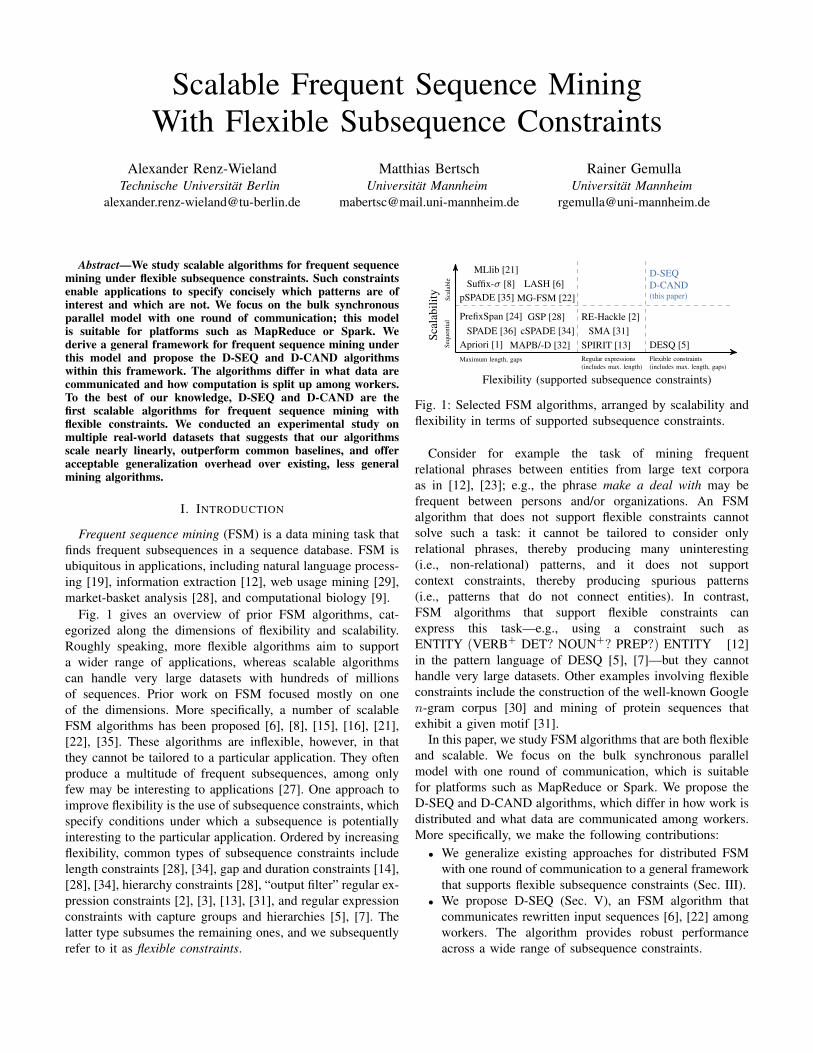
Fig. 1 gives an overview of prior FSM algorithms, cat-egorized along the dimensions of flexibility and scalability.Roughly speaking, more flexible algorithms aim to supporta wider range of applications, whereas scalable algorithmscan handle very large datasets with hundreds of millionsof sequences. Prior work on FSM focused mostly on oneof the dimensions. More specifically, a number of scalableFSM algorithms has been proposed [6], [8], [15], [16], [21],[22], [35]. These algorithms are inflexible, however, in thatthey cannot be tailored to a particular application. They oftenproduce a multitude of frequent subsequences, among onlyfew may be interesting to applications [27]. One approach toimprove flexibility is the use of subsequence constraints, whichspecify conditions under which a subsequence is potentiallyinteresting to the particular application. Ordered by increasingflexibility, common types of subsequence constraints includelength constraints [28], [34], gap and duration constraints [14],[28], [34], hierarchy constraints [28], “output filter” regular ex-pression constraints [2], [3], [13], [31], and regular expressionconstraints with capture groups and hierarchies [5], [7]. Thelatter type subsumes the remaining ones, and we subsequentlyrefer to it as flexible constraints.
Flexibility (supported subsequence constraints)
Scal
abili
ty
Maximum length, gaps Regular expressions(includes max. length)
Flexible constraints(includes max. length, gaps)
Sequ
entia
lSc
alab
le
Apriori [1]SPADE [36]
PrefixSpan [24]
MAPB/-D [32]cSPADE [34]
GSP [28]
SPIRIT [13]SMA [31]
RE-Hackle [2]
DESQ [5]
pSPADE [35]Suffix-σ [8]
MLlib [21]
MG-FSM [22]LASH [6]
(this paper)D-CANDD-SEQ
Fig. 1: Selected FSM algorithms, arranged by scalability andflexibility in terms of supported subsequence constraints.
Consider for example the task of mining frequentrelational phrases between entities from large text corporaas in [12], [23]; e.g., the phrase make a deal with may befrequent between persons and/or organizations. An FSMalgorithm that does not support flexible constraints cannotsolve such a task: it cannot be tailored to consider onlyrelational phrases, thereby producing many uninteresting(i.e., non-relational) patterns, and it does not supportcontext constraints, thereby producing spurious patterns(i.e., patterns that do not connect entities). In contrast,FSM algorithms that support flexible constraints canexpress this task—e.g., using a constraint such asENTITY (VERB+ DET? NOUN+? PREP?) ENTITY [12]in the pattern language of DESQ [5], [7]—but they cannothandle very large datasets. Other examples involving flexibleconstraints include the construction of the well-known Googlen-gram corpus [30] and mining of protein sequences thatexhibit a given motif [31].
In this paper, we study FSM algorithms that are both flexibleand scalable. We focus on the bulk synchronous parallelmodel with one round of communication, which is suitablefor platforms such as MapReduce or Spark. We propose theD-SEQ and D-CAND algorithms, which differ in how work isdistributed and what data are communicated among workers.More specifically, we make the following contributions:• We generalize existing approaches for distributed FSM
with one round of communication to a general frameworkthat supports flexible subsequence constraints (Sec. III).
• We propose D-SEQ (Sec. V), an FSM algorithm thatcommunicates rewritten input sequences [6], [22] amongworkers. The algorithm provides robust performanceacross a wide range of subsequence constraints.
T1: a1cdcbT2: eea1ea1ebT3: cdcbT4: a2dbT5: a1a1b
(a) Sequence db.
A
a1 a2
b
c d e
(b) Item hierarchy
w f(w,Dex)
b 5A 4d 3a1 3c 2e 1a2 1
(c) Item freq.
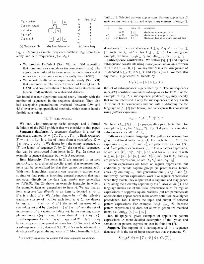
Fig. 2: Running example. Sequence database Dex, item hier-archy, and item frequencies f(w,Dex).
• We propose D-CAND (Sec. VI), an FSM algorithmthat communicates candidates (in compressed form). Thealgorithm is tailored to more selective constraints and itmines such constraints more efficiently than D-SEQ.
• We report results of an experimental study (Sec. VII)that examines the relative performance of D-SEQ and D-CAND and compares them to baseline and state-of-the-art(specialized) methods on real-world datasets.
We found that our algorithms scaled nearly linearly with thenumber of sequences in the sequence database. They alsohad acceptable generalization overhead (between 0.9x and4.3x) over existing specialized methods, which cannot handleflexible constraints.
II. PRELIMINARIES
We start with introducing basic concepts and a formaldefinition of the FSM problem that we consider in this paper.
Sequence database. A sequence database is a set1 ofsequences, denoted D =
{T1, T2, . . . , T|D|
}. Each sequence
T = t1t2 . . . t|T | is a list of items from a vocabulary Σ ={w1, w2, . . . , w|Σ|
}. We denote by ε the empty sequence, by
|T | the length of sequence T , by Σ∗ the set of all sequencesthat can be constructed from items in Σ. Fig. 2a shows anexample sequence database Dex with 5 sequences.
Item hierarchy. The items in Σ are arranged in an itemhierarchy, i. e., a directed acyclic graph that expresses howitems can be generalized (or that they cannot be generalized).With item hierarchies, analysts can succinctly express con-straints or find patterns involving general concepts that maynot occur directly in the data (e.g., make may generalizeto V ERB). Fig. 2b shows an example hierarchy in which,for example, item a1 generalizes to item A. We say that anitem u generalizes directly to an item v, denoted u ⇒ v,if u is a child of v. We further denote by ⇒∗ the reflexivetransitive closure of ⇒. For each item w ∈ Σ, we denoteby anc(w) = {w′ | w ⇒∗ w′ } the set of ancestors of w(including w) and by desc(w) = {w′ | w′ ⇒∗ w } the set ofdescendants of w (again, including w). In our running exam-ple, we have anc(a1) = { a1, A } and desc(A) = {A, a1, a2 }.
Subsequence. Let S = s1s2 . . . s|S| and T = t1t2 . . . t|T |be two sequences composed of items from Σ. We say that S isa subsequence of T , denoted S v T , if S can be obtained bydeleting and/or generalizing items in T . More formally, S v T
1To simplify exposition, we assume that input sequences are distinct.
TABLE I: Selected pattern expressions. Pattern expression Ematches any item t ∈ inE and outputs any element of outE(t).
E inE outE(t) Description
. t ∈ Σ { ε } Match any item, empty output(.↑) t ∈ Σ anc(t) Match any item, output ancestors(w) t ∈ desc(w) { t } Match any desc. of w, output matched item
if and only if there exist integers 1 ≤ i1 < i2 < · · · < i|S| ≤|T | such that tij ⇒∗ sj for 1 ≤ j ≤ |S|. Continuing ourexample, we have a1a1b v T5 and Ab v T5, but a1e 6v T5.
Subsequence constraints. We follow [5], [7] and expresssubsequence constraints using subsequence predicates of formπ : Σ∗ × Σ∗ → { 0, 1 }. We say that S is a π-subsequence ofT , denoted S vπ T , if S v T and π(S, T ) = 1. We then alsosay that T π-generates S. Denote by
Gπ(T ) = {S | S vπ T }
the set of subsequences π-generated by T . The subsequencesin Gπ(T ) constitute candidate subsequences for FSM. For theexample of Fig. 2, a subsequence predicate πex may specifythat we are interested in only the subsequences that begin withA or one of its descendants and end with b. Adopting the thelanguage of [5], [7] (see below), we can express this constraintusing pattern expression
πex = .∗(A)[(.↑).∗]∗(b).∗
We have Gπex(T5) = { a1a1b, a1Ab, a1b } . Note that, for
example, b v T5 but b 6vπexT5. Fig. 3 depicts the candidate
subsequences for all T ∈ Dex.Pattern expression language. The pattern expression lan-
guage is defined inductively: (1) For each item w ∈ Σ, theexpressions w, w=, w↑, and w↑= are pattern expressions. (2) .and .↑ are pattern expressions. (3) If E is a pattern expression,so are (E), [E], [E]∗, [E]+, [E]?, and for all n,m ∈ N withn ≤ m, [E]{n}, [E]{n, }, and [E]{n,m}. (4) If E1 and E2
are pattern expressions, so are [E1E2] and [E1|E2].Pattern expressions are based on regular expressions, but
additionally include capture groups (in parentheses), hierar-chies (by omitting =), and generalizations (using ↑ and ↑=).Intuitively, pattern expressions work like regular expressions:when they match, they output what is captured and may gener-alize along the hierarchy (optionally via ↑, always via ↑=). Thelanguage makes use of the usual precedence rules for regularexpressions to suppress square brackets (but not parentheses);operators that appear earlier in the above definition have higherprecedence. Tab. I shows the input and output of selectedpattern expressions. For example, Aa1b 6vπex
T5, becausepattern expression (A) does not allow to generalize matcheditems, i.e., out(A)(a1) = { a1 }.
Tab. III (page 9) gives examples of application patternexpressions. A more detailed description of the syntax andsemantics of pattern expressions can be found in [7].
Support. The support of a subsequence S in a sequencedatabase D is the set of input sequences that π-generate S:
Supπ(S,D) = {T ∈ D | S ∈ Gπ(T ) } .
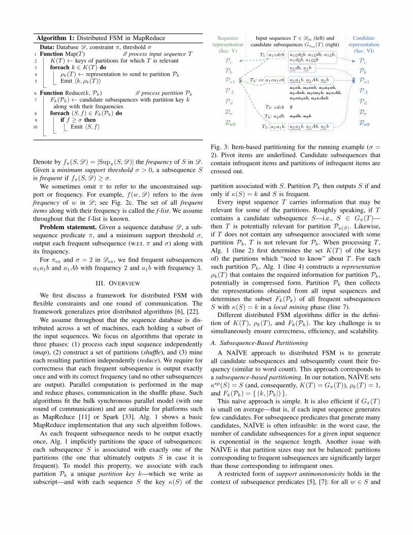
Algorithm 1: Distributed FSM in MapReduceData: Database D , constraint π, threshold σ
1 Function Map(T ) // process input sequence T2 K(T )← keys of partitions for which T is relevant3 foreach k ∈ K(T ) do4 ρk(T )← representation to send to partition Pk
5 Emit 〈k, ρk(T )〉
6 Function Reduce(k, Pk) // process partition Pk
7 Fk(Pk)← candidate subsequences with partition key kalong with their frequencies
8 foreach (S, f) ∈ Fk(Pk) do9 if f ≥ σ then
10 Emit 〈S, f〉
Denote by fπ(S,D) = |Supπ(S,D)| the frequency of S in D .Given a minimum support threshold σ > 0, a subsequence Sis frequent if fπ(S,D) ≥ σ.
We sometimes omit π to refer to the unconstrained sup-port or frequency. For example, f(w,D) refers to the itemfrequency of w in D ; see Fig. 2c. The set of all frequentitems along with their frequency is called the f-list. We assumethroughout that the f-list is known.
Problem statement. Given a sequence database D , a sub-sequence predicate π, and a minimum support threshold σ,output each frequent subsequence (w.r.t. π and σ) along withits frequency.
For πex and σ = 2 in Dex, we find frequent subsequencesa1a1b and a1Ab with frequency 2 and a1b with frequency 3.
III. OVERVIEW
We first discuss a framework for distributed FSM withflexible constraints and one round of communication. Theframework generalizes prior distributed algorithms [6], [22].
We assume throughout that the sequence database is dis-tributed across a set of machines, each holding a subset ofthe input sequences. We focus on algorithms that operate inthree phases: (1) process each input sequence independently(map), (2) construct a set of partitions (shuffle), and (3) mineeach resulting partition independently (reduce). We require forcorrectness that each frequent subsequence is output exactlyonce and with its correct frequency (and no other subsequencesare output). Parallel computation is performed in the mapand reduce phases, communication in the shuffle phase. Suchalgorithms fit the bulk synchronous parallel model (with oneround of communication) and are suitable for platforms suchas MapReduce [11] or Spark [33]. Alg. 1 shows a basicMapReduce implementation that any such algorithm follows.
As each frequent subsequence needs to be output exactlyonce, Alg. 1 implicitly partitions the space of subsequences:each subsequence S is associated with exactly one of thepartitions (the one that ultimately outputs S in case it isfrequent). To model this property, we associate with eachpartition Pk a unique partition key k—which we write assubscript—and with each sequence S the key κ(S) of the
Sequencerepresentation
(Sec. V)
Input sequences T ∈ Dex (left) andcandidate subsequences Gπex
(T ) (right)Candidate
representation(Sec. VI)
PcPcPbPbPa1Pa1
PAPAPdPdPePePa2Pa2
a1cdcbT1: a1cdcb, a1cdb, a1cb,a1dcb, a1ccb
a1db, a1b
a1ea1ebT2: ee a1a1b, a1Ab, a1b
a1eb, a1eeb, a1a1eb,a1Aeb, a1ea1b, a1eAb,a1ea1eb, a1eAeb
cdcbT3: ∅
a2dbT4: a2db, a2b
a1a1bT5: a1a1b, a1Ab, a1b
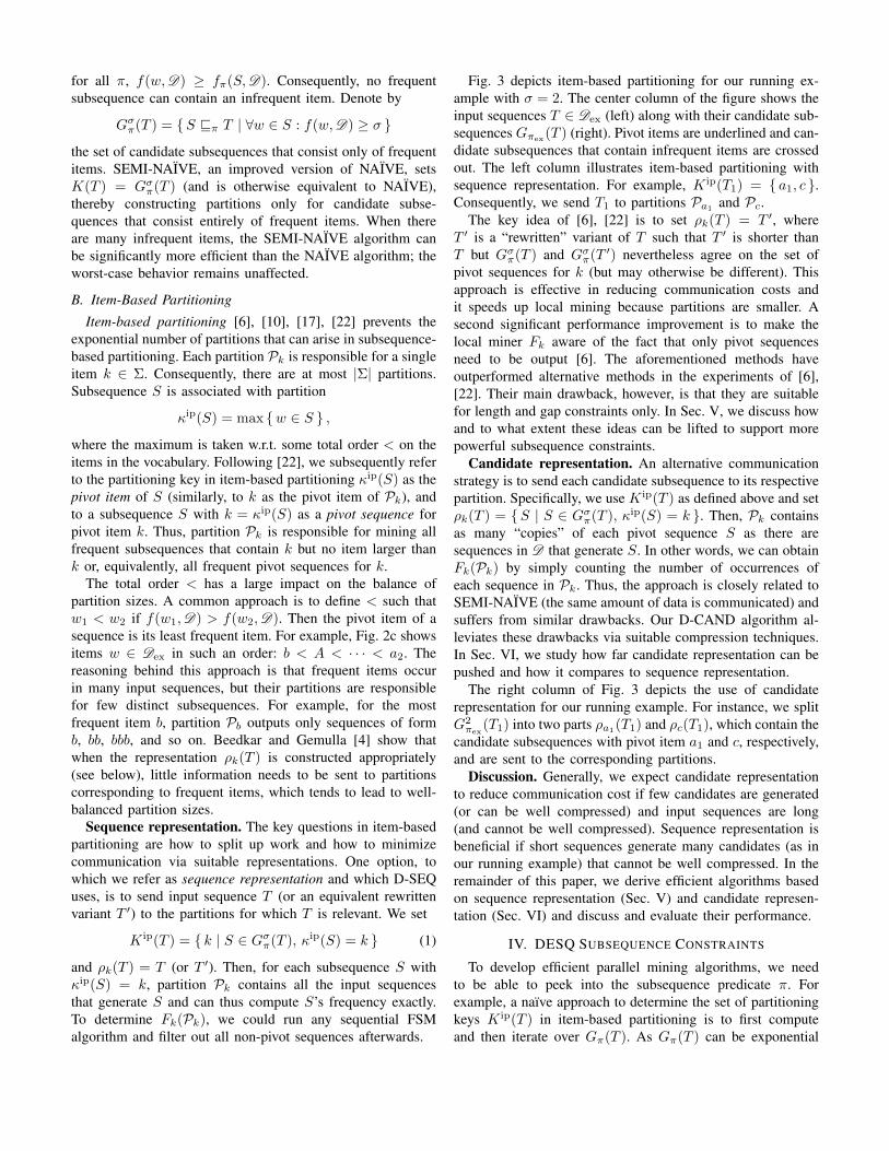
Fig. 3: Item-based partitioning for the running example (σ =2). Pivot items are underlined. Candidate subsequences thatcontain infrequent items and partitions of infrequent items arecrossed out.
partition associated with S. Partition Pk then outputs S if andonly if κ(S) = k and S is frequent.
Every input sequence T carries information that may berelevant for some of the partitions. Roughly speaking, if Tcontains a candidate subsequence S—i.e., S ∈ Gπ(T )—then T is potentially relevant for partition Pκ(S). Likewise,if T does not contain any subsequence associated with somepartition Pk, T is not relevant for Pk. When processing T ,Alg. 1 (line 2) first determines the set K(T ) of (the keysof) the partitions which “need to know” about T . For eachsuch partition Pk, Alg. 1 (line 4) constructs a representationρk(T ) that contains the required information for partition Pk,potentially in compressed form. Partition Pk then collectsthe representations obtained from all input sequences anddetermines the subset Fk(Pk) of all frequent subsequencesS with κ(S) = k in a local mining phase (line 7).
Different distributed FSM algorithms differ in the defini-tion of K(T ), ρk(T ), and Fk(Pk). The key challenge is tosimultaneously ensure correctness, efficiency, and scalability.
A. Subsequence-Based Partitioning
A NAIVE approach to distributed FSM is to generateall candidate subsequences and subsequently count their fre-quency (similar to word count). This approach corresponds toa subsequence-based partitioning. In our notation, NAIVE setsκsp(S) = S (and, consequently, K(T ) = Gπ(T )), ρk(T ) = 1,and Fk(Pk) = { (k, |Pk|) }.
This naıve approach is simple. It is also efficient if Gπ(T )is small on average—that is, if each input sequence generatesfew candidates. For subsequence predicates that generate manycandidates, NAIVE is often infeasible: in the worst case, thenumber of candidate subsequences for a given input sequenceis exponential in the sequence length. Another issue withNAIVE is that partition sizes may not be balanced: partitionscorresponding to frequent subsequences are significantly largerthan those corresponding to infrequent ones.
A restricted form of support antimonotonicity holds in thecontext of subsequence predicates [5], [7]: for all w ∈ S and
for all π, f(w,D) ≥ fπ(S,D). Consequently, no frequentsubsequence can contain an infrequent item. Denote by
Gσπ(T ) = {S vπ T | ∀w ∈ S : f(w,D) ≥ σ }
the set of candidate subsequences that consist only of frequentitems. SEMI-NAIVE, an improved version of NAIVE, setsK(T ) = Gσπ(T ) (and is otherwise equivalent to NAIVE),thereby constructing partitions only for candidate subse-quences that consist entirely of frequent items. When thereare many infrequent items, the SEMI-NAIVE algorithm canbe significantly more efficient than the NAIVE algorithm; theworst-case behavior remains unaffected.
B. Item-Based Partitioning
Item-based partitioning [6], [10], [17], [22] prevents theexponential number of partitions that can arise in subsequence-based partitioning. Each partition Pk is responsible for a singleitem k ∈ Σ. Consequently, there are at most |Σ| partitions.Subsequence S is associated with partition
κip(S) = max {w ∈ S } ,
where the maximum is taken w.r.t. some total order < on theitems in the vocabulary. Following [22], we subsequently referto the partitioning key in item-based partitioning κip(S) as thepivot item of S (similarly, to k as the pivot item of Pk), andto a subsequence S with k = κip(S) as a pivot sequence forpivot item k. Thus, partition Pk is responsible for mining allfrequent subsequences that contain k but no item larger thank or, equivalently, all frequent pivot sequences for k.
The total order < has a large impact on the balance ofpartition sizes. A common approach is to define < such thatw1 < w2 if f(w1,D) > f(w2,D). Then the pivot item of asequence is its least frequent item. For example, Fig. 2c showsitems w ∈ Dex in such an order: b < A < · · · < a2. Thereasoning behind this approach is that frequent items occurin many input sequences, but their partitions are responsiblefor few distinct subsequences. For example, for the mostfrequent item b, partition Pb outputs only sequences of formb, bb, bbb, and so on. Beedkar and Gemulla [4] show thatwhen the representation ρk(T ) is constructed appropriately(see below), little information needs to be sent to partitionscorresponding to frequent items, which tends to lead to well-balanced partition sizes.
Sequence representation. The key questions in item-basedpartitioning are how to split up work and how to minimizecommunication via suitable representations. One option, towhich we refer as sequence representation and which D-SEQuses, is to send input sequence T (or an equivalent rewrittenvariant T ′) to the partitions for which T is relevant. We set
K ip(T ) = { k | S ∈ Gσπ(T ), κip(S) = k } (1)
and ρk(T ) = T (or T ′). Then, for each subsequence S withκip(S) = k, partition Pk contains all the input sequencesthat generate S and can thus compute S’s frequency exactly.To determine Fk(Pk), we could run any sequential FSMalgorithm and filter out all non-pivot sequences afterwards.
Fig. 3 depicts item-based partitioning for our running ex-ample with σ = 2. The center column of the figure shows theinput sequences T ∈ Dex (left) along with their candidate sub-sequences Gπex
(T ) (right). Pivot items are underlined and can-didate subsequences that contain infrequent items are crossedout. The left column illustrates item-based partitioning withsequence representation. For example, K ip(T1) = { a1, c }.Consequently, we send T1 to partitions Pa1 and Pc.
The key idea of [6], [22] is to set ρk(T ) = T ′, whereT ′ is a “rewritten” variant of T such that T ′ is shorter thanT but Gσπ(T ) and Gσπ(T ′) nevertheless agree on the set ofpivot sequences for k (but may otherwise be different). Thisapproach is effective in reducing communication costs andit speeds up local mining because partitions are smaller. Asecond significant performance improvement is to make thelocal miner Fk aware of the fact that only pivot sequencesneed to be output [6]. The aforementioned methods haveoutperformed alternative methods in the experiments of [6],[22]. Their main drawback, however, is that they are suitablefor length and gap constraints only. In Sec. V, we discuss howand to what extent these ideas can be lifted to support morepowerful subsequence constraints.
Candidate representation. An alternative communicationstrategy is to send each candidate subsequence to its respectivepartition. Specifically, we use K ip(T ) as defined above and setρk(T ) = {S | S ∈ Gσπ(T ), κip(S) = k }. Then, Pk containsas many “copies” of each pivot sequence S as there aresequences in D that generate S. In other words, we can obtainFk(Pk) by simply counting the number of occurrences ofeach sequence in Pk. Thus, the approach is closely related toSEMI-NAIVE (the same amount of data is communicated) andsuffers from similar drawbacks. Our D-CAND algorithm al-leviates these drawbacks via suitable compression techniques.In Sec. VI, we study how far candidate representation can bepushed and how it compares to sequence representation.
The right column of Fig. 3 depicts the use of candidaterepresentation for our running example. For instance, we splitG2πex
(T1) into two parts ρa1(T1) and ρc(T1), which contain thecandidate subsequences with pivot item a1 and c, respectively,and are sent to the corresponding partitions.
Discussion. Generally, we expect candidate representationto reduce communication cost if few candidates are generated(or can be well compressed) and input sequences are long(and cannot be well compressed). Sequence representation isbeneficial if short sequences generate many candidates (as inour running example) that cannot be well compressed. In theremainder of this paper, we derive efficient algorithms basedon sequence representation (Sec. V) and candidate represen-tation (Sec. VI) and discuss and evaluate their performance.
IV. DESQ SUBSEQUENCE CONSTRAINTS
To develop efficient parallel mining algorithms, we needto be able to peek into the subsequence predicate π. Forexample, a naıve approach to determine the set of partitioningkeys K ip(T ) in item-based partitioning is to first computeand then iterate over Gπ(T ). As Gπ(T ) can be exponential
q0 q1 q2
.
(A)
.
(.↑)
(b)
.δ0
δ1
δ2
δ3
δ4
δ5
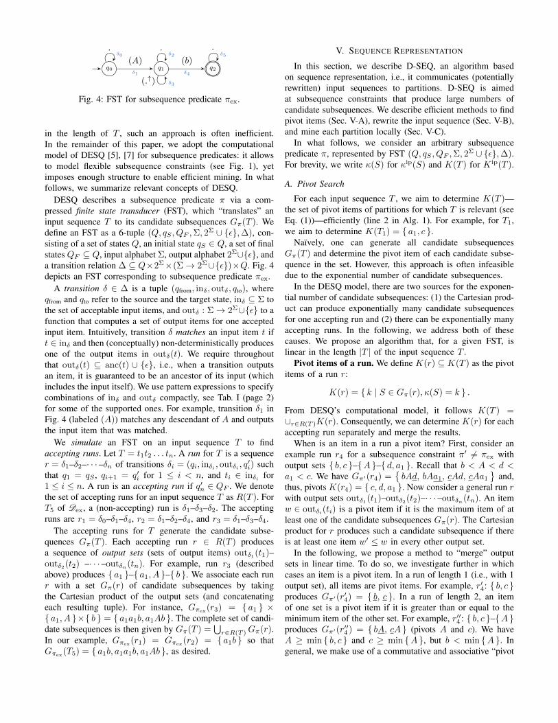
Fig. 4: FST for subsequence predicate πex.
in the length of T , such an approach is often inefficient.In the remainder of this paper, we adopt the computationalmodel of DESQ [5], [7] for subsequence predicates: it allowsto model flexible subsequence constraints (see Fig. 1), yetimposes enough structure to enable efficient mining. In whatfollows, we summarize relevant concepts of DESQ.
DESQ describes a subsequence predicate π via a com-pressed finite state transducer (FST), which “translates” aninput sequence T to its candidate subsequences Gπ(T ). Wedefine an FST as a 6-tuple (Q, qS , QF ,Σ, 2
Σ ∪ {ε},∆), con-sisting of a set of states Q, an initial state qS ∈ Q, a set of finalstates QF ⊆ Q, input alphabet Σ, output alphabet 2Σ∪{ε}, anda transition relation ∆ ⊆ Q×2Σ×(Σ→ 2Σ∪{ε})×Q. Fig. 4depicts an FST corresponding to subsequence predicate πex.
A transition δ ∈ ∆ is a tuple (qfrom, inδ, outδ, qto), whereqfrom and qto refer to the source and the target state, inδ ⊆ Σ tothe set of acceptable input items, and outδ : Σ→ 2Σ∪{ε} to afunction that computes a set of output items for one acceptedinput item. Intuitively, transition δ matches an input item t ift ∈ inδ and then (conceptually) non-deterministically producesone of the output items in outδ(t). We require throughoutthat outδ(t) ⊆ anc(t) ∪ {ε}, i.e., when a transition outputsan item, it is guaranteed to be an ancestor of its input (whichincludes the input itself). We use pattern expressions to specifycombinations of inδ and outδ compactly, see Tab. I (page 2)for some of the supported ones. For example, transition δ1 inFig. 4 (labeled (A)) matches any descendant of A and outputsthe input item that was matched.
We simulate an FST on an input sequence T to findaccepting runs. Let T = t1t2 . . . tn. A run for T is a sequencer = δ1–δ2–· · · –δn of transitions δi = (qi, inδi , outδi , q
′i) such
that q1 = qS , qi+1 = q′i for 1 ≤ i < n, and ti ∈ inδi for1 ≤ i ≤ n. A run is an accepting run if q′n ∈ QF . We denotethe set of accepting runs for an input sequence T as R(T ). ForT5 of Dex, a (non-accepting) run is δ1–δ3–δ2. The acceptingruns are r1 = δ0–δ1–δ4, r2 = δ1–δ2–δ4, and r3 = δ1–δ3–δ4.
The accepting runs for T generate the candidate subse-quences Gπ(T ). Each accepting run r ∈ R(T ) producesa sequence of output sets (sets of output items) outδ1(t1)–outδ2(t2) –· · · –outδn(tn). For example, run r3 (describedabove) produces { a1 }–{ a1, A }–{ b }. We associate each runr with a set Gπ(r) of candidate subsequences by takingthe Cartesian product of the output sets (and concatenatingeach resulting tuple). For instance, Gπex
(r3) = { a1 } ×{ a1, A }×{ b } = { a1a1b, a1Ab }. The complete set of candi-date subsequences is then given by Gπ(T ) =
⋃r∈R(T )Gπ(r).
In our example, Gπex(r1) = Gπex(r2) = { a1b } so thatGπex(T5) = { a1b, a1a1b, a1Ab }, as desired.
V. SEQUENCE REPRESENTATION
In this section, we describe D-SEQ, an algorithm basedon sequence representation, i.e., it communicates (potentiallyrewritten) input sequences to partitions. D-SEQ is aimedat subsequence constraints that produce large numbers ofcandidate subsequences. We describe efficient methods to findpivot items (Sec. V-A), rewrite the input sequence (Sec. V-B),and mine each partition locally (Sec. V-C).
In what follows, we consider an arbitrary subsequencepredicate π, represented by FST (Q, qS , QF ,Σ, 2
Σ ∪ {ε},∆).For brevity, we write κ(S) for κip(S) and K(T ) for K ip(T ).
A. Pivot Search
For each input sequence T , we aim to determine K(T )—the set of pivot items of partitions for which T is relevant (seeEq. (1))—efficiently (line 2 in Alg. 1). For example, for T1,we aim to determine K(T1) = { a1, c }.
Naıvely, one can generate all candidate subsequencesGπ(T ) and determine the pivot item of each candidate subse-quence in the set. However, this approach is often infeasibledue to the exponential number of candidate subsequences.
In the DESQ model, there are two sources for the exponen-tial number of candidate subsequences: (1) the Cartesian prod-uct can produce exponentially many candidate subsequencesfor one accepting run and (2) there can be exponentially manyaccepting runs. In the following, we address both of thesecauses. We propose an algorithm that, for a given FST, islinear in the length |T | of the input sequence T .
Pivot items of a run. We define K(r) ⊆ K(T ) as the pivotitems of a run r:
K(r) = { k | S ∈ Gπ(r), κ(S) = k } .
From DESQ’s computational model, it follows K(T ) =∪r∈R(T )K(r). Consequently, we can determine K(r) for eachaccepting run separately and merge the results.
When is an item in a run a pivot item? First, consider anexample run r4 for a subsequence constraint π′ 6= πex withoutput sets { b, c }–{A }–{ d, a1 }. Recall that b < A < d <a1 < c. We have Gπ′(r4) =
{bAd, bAa1, cAd, cAa1
}and,
thus, pivots K(r4) = { c, d, a1 }. Now consider a general run rwith output sets outδ1(t1)–outδ2(t2)–· · · –outδn(tn). An itemw ∈ outδi(ti) is a pivot item if it is the maximum item of atleast one of the candidate subsequences Gπ(r). The Cartesianproduct for r produces such a candidate subsequence if thereis at least one item w′ ≤ w in every other output set.
In the following, we propose a method to “merge” outputsets in linear time. To do so, we investigate further in whichcases an item is a pivot item. In a run of length 1 (i.e., with 1output set), all items are pivot items. For example, r′4: { b, c }produces Gπ′(r′4) = { b, c }. In a run of length 2, an itemof one set is a pivot item if it is greater than or equal to theminimum item of the other set. For example, r′′4 : { b, c }–{A }produces Gπ′(r′′4 ) = { bA, cA } (pivots A and c). We haveA ≥ min { b, c } and c ≥ min {A }, but b < min {A }. Ingeneral, we make use of a commutative and associative “pivot
merge” function ⊕ to determine the pivot items of two outputsets U and Q (with ε < w for w ∈ Σ):
U⊕Q = {ω ∈ U | ω ≥ min(Q) }∪{ω ∈ Q | ω ≥ min(U) } .
As we have to check for minimum items in every other set,we apply ⊕ repeatedly, see Th. 1. For example, we find thepivot items of r4 as K(r4) = { b, c } ⊕ {A } ⊕ { d, a1 }.
Theorem 1: The pivot items K(r) of run r with output setsoutδ1(t1)–outδ2(t2)–· · · – outδ|T |(t|T |) can be computed by
K(r) = outδ1(t1)⊕ outδ2(t2)⊕ · · · ⊕ outδ|T |(t|T |).
As there are at most |Σ| items in each output set, we cancompute ⊕ in time O(Σ) using appropriate data structures.For a run of length |T |, total computation time reduces fromO(|Σ||T |) via computation of Gπ(r) to O(|T ||Σ|) using Th. 1.
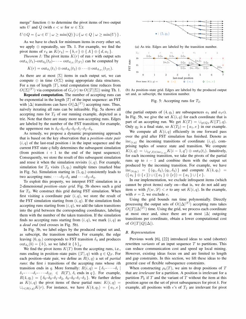
Repeated computation. The number of accepting runs canbe exponential in the length |T | of the input sequence: an FSTwith |∆| transitions can have O(|∆||T |) accepting runs. Thus,naıvely iterating all runs can be infeasible. Fig. 5a shows allaccepting runs for T2 of our running example, depicted as atrie. Note that there are many more non-accepting runs. Edgesare labeled by the number of the FST transition; for example,the uppermost run is δ0–δ0–δ0–δ0–δ1–δ2–δ4.
As remedy, we propose a dynamic programming approachthat is based on the key observation that a position–state pair(i, q) of the last-read position i in the input sequence and thecurrent FST state q fully determines the subsequent simulation(from position i + 1 to the end of the input sequence).Consequently, we store the result of this subsequent simulationand reuse it when the simulation revisits (i, q). For example,simulation for T2 visits (5, q1) multiple times (marked bluein Fig. 5a). Simulation starting in (5, q1) consistently leads totwo accepting runs: · · · –δ2–δ4 and · · · –δ3–δ4.
To exploit this property, we interpret FST simulation in a2-dimensional position–state grid. Fig. 5b shows such a gridfor T2. We construct this grid during FST simulation. Whenfirst visiting a coordinate pair (i, q), we store the result ofthe FST simulation starting from (i, q). If the simulation findsaccepting runs starting from (i, q), we add the taken transitionsinto the grid between the corresponding coordinates, labelingthem with the number of the taken transition. If the simulationfinds no accepting runs starting from (i, q), we mark (i, q) asa dead end (red crosses in Fig. 5b).
In Fig. 5b, we label edges by the produced output set and,as subscript, the transition number. For example, the edgeleaving (6, q1) corresponds to FST transition δ4 and producesoutδ4(b) = { b }, so we label it { b }4.
We find the pivot items K(T ) from the accepting runs, i.e.,runs ending in position–state pairs (|T |, q) with q ∈ QF . Foreach position–state pair, we define as R(i, q) a set of partialruns: the first i transitions of the accepting runs whose ithtransition ends in q. More formally: R(i, q) = { δ1– · · · –δi |δ1– · · · –δi– · · · –δ|T | ∈ R(T ), δi ends in q }. For example,R(4, q1) = { δ0–δ0–δ1–δ2, δ0–δ0–δ1–δ3 }. We further defineas K(i, q) the pivot items of these partial runs: K(i, q) =∪r∈R(i,q)K(r). For instance, we have K(4, q1) = { a1, e }
: (5, q1)
0 0 0 0 1 2 43 41
2 2 2 43 432 43 4
3
2 2 43 432 43 4
(a) As trie. Edges are labeled by the transition number.
Pivot items K(i, q) = : { ε } : { a1 } : { a1, e }
{ε}0 {ε}0 {ε}0 {ε}0
{a1}1{a1}1 {ε}2
{e}3
{ε}2
{a1, A}3
{ε}2
{e}3 {b}4
last-read position0 1 2 3 4 5 6 7
T2: e e a1 e a1 e b
FST
stat
e
q0
q1
q2
(b) As position–state grid. Edges are labeled by the produced outputset and, as subscript, the transition number.
Fig. 5: Accepting runs for T2.
(the partial outputs of (4, q1) are subsequences a1 and a1e).In Fig. 5b, we give the set K(i, q) for each coordinate that ispart of an accepting run. We get K(T ) = ∪q∈QFK(|T |, q).Only q2 is a final state, so K(T2) = { a1, e } in our example.
We compute all K(i, q) efficiently in one forward passover the grid after FST simulation has finished. Denote asinc(i,q) the incoming transitions of coordinate (i, q), com-prising tuples of source state and transition. We computeK(i, q) = ∪(q′,δ)∈inc(i,q)K(i − 1, q′) ⊕ outδ(ti). Intuitively,for each incoming transition, we take the pivots of the partialruns up to i − 1 and combine them with the output setproduced by the incoming transition. For example, we haveinc(4,q1) = { (q1, δ2), (q1, δ3) } and compute K(4, q1) =({ a1 } ⊕ { ε }) ∪ ({ a1 } ⊕ {e}) = { a1 } ∪ { e }.
In our implementation, we exclude infrequent items (whichcannot be pivot items) early on—that is, we do not add anyitem w with f(w,D) < σ to any set K(i, q). In the example,with σ = 2, we exclude e.
Using the grid bounds run time polynomially. Directlyprocessing the output sets of O(|∆||T |) accepting runs takesO(|T ||∆||T |) time. Using the grid, we process each coordinateat most once and, since there are at most |∆| outgoingtransitions per coordinate, obtain a lower computational costof O(|T ||Q||∆|).
B. Representation
Previous work [6], [22] introduced ideas to send (shorter)rewritten variants of an input sequence T to partitions. Thiscan reduce communication cost and speed up local mining.However, existing ideas focus on and are limited to lengthand gap constraints. In this section, we lift these ideas to thegeneral case of flexible subsequence constraints.
When constructing ρk(T ), we aim to drop positions of Tthat are irrelevant for a partition. A position is irrelevant for apartition Pk if T and the variant of T without the item at thisposition agree on the set of pivot subsequences for pivot k. Forexample, all positions with e’s of T2 are irrelevant for pivot
PrefixPrefix (frequent)Prefix (not expanded)ExpansionProjected database
ε a1
a1A a1Ab
a1a1 a1a1b
a1a1ea1b
a1c
a1d
a1e
T1, 0, q0T2, 0, q0T5, 0, q0
T1, 1, q1T2, 3, q1T5, 1, q1
T2, 5, q1T5, 2, q1
T2, 7, q2T5, 3, q2
T2, 5, q1T5, 2, q1
T2, 7, q2T5, 3, q2
T1, 5, q2T2, 7, q2T5, 3, q2 T1, 2, q1
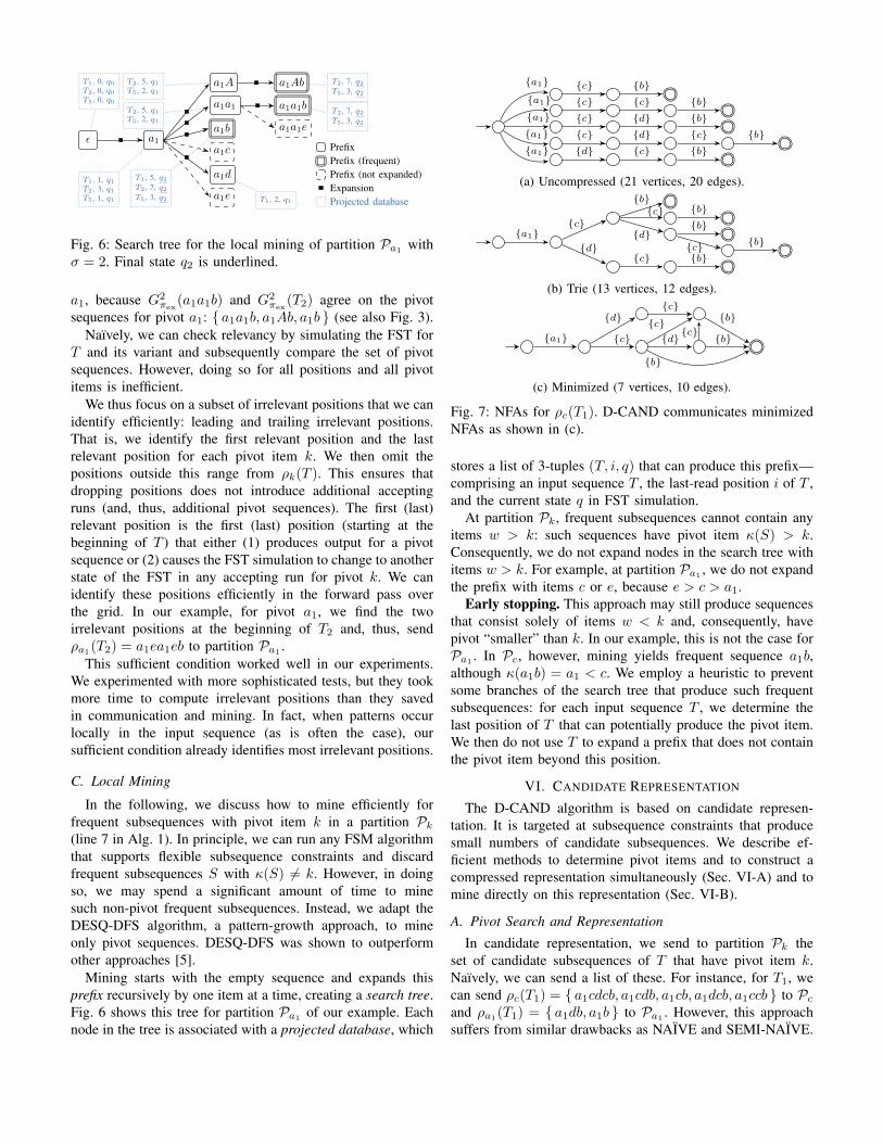
Fig. 6: Search tree for the local mining of partition Pa1 withσ = 2. Final state q2 is underlined.
a1, because G2πex
(a1a1b) and G2πex
(T2) agree on the pivotsequences for pivot a1: { a1a1b, a1Ab, a1b } (see also Fig. 3).
Naıvely, we can check relevancy by simulating the FST forT and its variant and subsequently compare the set of pivotsequences. However, doing so for all positions and all pivotitems is inefficient.
We thus focus on a subset of irrelevant positions that we canidentify efficiently: leading and trailing irrelevant positions.That is, we identify the first relevant position and the lastrelevant position for each pivot item k. We then omit thepositions outside this range from ρk(T ). This ensures thatdropping positions does not introduce additional acceptingruns (and, thus, additional pivot sequences). The first (last)relevant position is the first (last) position (starting at thebeginning of T ) that either (1) produces output for a pivotsequence or (2) causes the FST simulation to change to anotherstate of the FST in any accepting run for pivot k. We canidentify these positions efficiently in the forward pass overthe grid. In our example, for pivot a1, we find the twoirrelevant positions at the beginning of T2 and, thus, sendρa1(T2) = a1ea1eb to partition Pa1 .
This sufficient condition worked well in our experiments.We experimented with more sophisticated tests, but they tookmore time to compute irrelevant positions than they savedin communication and mining. In fact, when patterns occurlocally in the input sequence (as is often the case), oursufficient condition already identifies most irrelevant positions.
C. Local Mining
In the following, we discuss how to mine efficiently forfrequent subsequences with pivot item k in a partition Pk(line 7 in Alg. 1). In principle, we can run any FSM algorithmthat supports flexible subsequence constraints and discardfrequent subsequences S with κ(S) 6= k. However, in doingso, we may spend a significant amount of time to minesuch non-pivot frequent subsequences. Instead, we adapt theDESQ-DFS algorithm, a pattern-growth approach, to mineonly pivot sequences. DESQ-DFS was shown to outperformother approaches [5].
Mining starts with the empty sequence and expands thisprefix recursively by one item at a time, creating a search tree.Fig. 6 shows this tree for partition Pa1 of our example. Eachnode in the tree is associated with a projected database, which
{a1} {c} {b}{a1} {c} {c} {b}{a1} {c} {d} {b}{a1} {c} {d} {c} {b}{a1} {d} {c} {b}
(a) Uncompressed (21 vertices, 20 edges).{b}
{a1}{c}
{c} {b}
{d}{b}
{c} {b}{d}{c} {b}
(b) Trie (13 vertices, 12 edges).{c}
{a1} {c}
{d}
{d}{c}
{b}{c}
{b}
{b}
(c) Minimized (7 vertices, 10 edges).
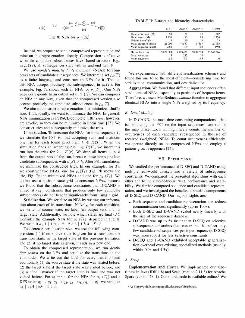
Fig. 7: NFAs for ρc(T1). D-CAND communicates minimizedNFAs as shown in (c).
stores a list of 3-tuples (T, i, q) that can produce this prefix—comprising an input sequence T , the last-read position i of T ,and the current state q in FST simulation.
At partition Pk, frequent subsequences cannot contain anyitems w > k: such sequences have pivot item κ(S) > k.Consequently, we do not expand nodes in the search tree withitems w > k. For example, at partition Pa1 , we do not expandthe prefix with items c or e, because e > c > a1.
Early stopping. This approach may still produce sequencesthat consist solely of items w < k and, consequently, havepivot “smaller” than k. In our example, this is not the case forPa1 . In Pc, however, mining yields frequent sequence a1b,although κ(a1b) = a1 < c. We employ a heuristic to preventsome branches of the search tree that produce such frequentsubsequences: for each input sequence T , we determine thelast position of T that can potentially produce the pivot item.We then do not use T to expand a prefix that does not containthe pivot item beyond this position.
VI. CANDIDATE REPRESENTATION
The D-CAND algorithm is based on candidate represen-tation. It is targeted at subsequence constraints that producesmall numbers of candidate subsequences. We describe ef-ficient methods to determine pivot items and to construct acompressed representation simultaneously (Sec. VI-A) and tomine directly on this representation (Sec. VI-B).
A. Pivot Search and Representation
In candidate representation, we send to partition Pk theset of candidate subsequences of T that have pivot item k.Naıvely, we can send a list of these. For instance, for T1, wecan send ρc(T1) = { a1cdcb, a1cdb, a1cb, a1dcb, a1ccb } to Pcand ρa1(T1) = { a1db, a1b } to Pa1 . However, this approachsuffers from similar drawbacks as NAIVE and SEMI-NAIVE.
q0 q1
q2
q3{a1}
{a1, A} {b}
{b}
Fig. 8: NFA for ρa1(T5).
Instead, we propose to send a compressed representation andmine on this representation directly. Compression is effectivewhen the candidate subsequences have shared structure. E.g.,in ρc(T1), all subsequences start with a1 and end with b.
We use nondeterministic finite automata (NFAs) to com-press sets of candidate subsequences. We interpret a set ρk(T )as a finite language and construct an NFA for it. That is,this NFA accepts precisely the subsequences in ρk(T ). Forexample, Fig. 7a shows such an NFA for ρc(T1). One NFAedge corresponds to an output set outδi(ti). We can compressan NFA in any way, given that the compressed version alsoaccepts precisely the candidate subsequences in ρk(T ).
We aim to construct a representation that minimizes shufflesize. Thus, ideally, we want to minimize the NFA. In general,NFA minimization is PSPACE-complete [18]. Tries, however,are acyclic, so they can be minimized in linear time [25]. Weconstruct tries and subsequently minimize the tries.
Construction. To construct the NFAs for input sequence T ,we simulate the FST to find accepting runs and maintainone trie for each found pivot item k ∈ K(T ). When thesimulation finds an accepting run r ∈ R(T ), we insert thisrun into the tries for k ∈ K(r). We drop all items w > kfrom the output sets of the run, because these items producecandidate subsequences with κ(S) > k. After FST simulation,we minimize the constructed tries. In our example, for T1,we construct two NFAs: one for ρc(T1) (Fig. 7b shows thetrie, Fig. 7c the minimized NFA) and one for ρa1(T1). Wedo not use a position–state grid to construct NFAs, becausewe found that the subsequence constraints that D-CAND isaimed at (i.e., constraints that produce only few candidatesubsequences) do not benefit significantly from using a grid.
Serialization. We serialize an NFA by writing out informa-tion about each of its transitions. Naıvely, for each transition,we write its source state, its label (an output set), and itstarget state. Additionally, we note which states are final (F).Consider the example NFA for ρa1(T5), depicted in Fig. 8.We write 0 a1 1 | 1 a1A 2 | 2 b 3 | 1 b 3 | F : 3.
To decrease serialization size, we use the following com-pression: (1) if no source state is given for a transition, thetransition starts in the target state of the previous transitionand (2) if no target state is given, it ends in a new one.
To obtain the compressed representation, we run depth-first search on the NFA and serialize the transitions in thevisit order. We write out the label for every transition andadditionally (1) the source state if the state was visited before,(2) the target state if the target state was visited before, and(3) a “final” marker if the target state is final and was notvisited before. For example, for the NFA for ρa1(T5) and aDFS order q0 → q1, q1 → q2, q2 → q3, q1 → q3, we serializea1 | a1A | bF | 1 b 3.
TABLE II: Dataset and hierarchy characteristics.
NYT AMZN AMZN-F CW50
Total sequences (M) 50 21 21 567Total items (M) 1 130 83 83 10 774Unique itemsa (M) 8 10 10 23Max. sequence length 21 000 44 557 44 557 20 993Mean sequence length 22.8 3.9 3.9 19.0
Hierarchy items 9 874 089 9 903 422 9 894 624 22 642 566Max. ancestors 3 282 10 1Mean ancestors 2.8 5.1 3.5 1.0
We experimented with different serialization schemes andfound this one to be the most efficient—considering time forserialization, communication, and deserialization.
Aggregation. We found that different input sequences oftensend identical NFAs, especially to partitions of frequent items.Therefore, we use a MapReduce combine function to aggregateidentical NFAs into a single NFA weighted by its frequency.
B. Local Mining
In D-CAND, the most time-consuming computations—thatis, simulating the FST on the input sequences—are run inthe map phase. Local mining merely counts the number ofoccurrences of each candidate subsequence in the set ofreceived (weighted) NFAs. To count occurrences efficiently,we operate directly on the compressed NFAs and employ apattern-growth approach [24].
VII. EXPERIMENTS
We studied the performance of D-SEQ and D-CAND usingmultiple real-world datasets and a variety of subsequenceconstraints. We compared the presented algorithms with eachother and to the state-of-the-art w.r.t. performance and scala-bility. We further compared sequence and candidate represen-tation, and we investigated the benefits of specific componentsof D-SEQ and D-CAND. Our major insights are:
• Both sequence and candidate representation can reducecommunication cost significantly (up to 100x).
• Both D-SEQ and D-CAND scaled nearly linearly withthe size of the sequence database.
• D-CAND was up to 5x faster than D-SEQ on selectivesubsequence constraints (i.e., constraints that select onlyfew candidate subsequences per input sequence). D-SEQwas more robust for less selective constraints.
• D-SEQ and D-CAND exhibited acceptable generaliza-tion overhead over existing, specialized methods (usuallywithin 0.9x and 4.3x).
A. Setup
Implementation and cluster. We implemented our algo-rithms in Java (JDK 1.8) and Scala (version 2.11.8) for ApacheSpark (version 2.0.1). Our source code is available online.2 We
2At https://github.com/rgemulla/desq/tree/distributed.
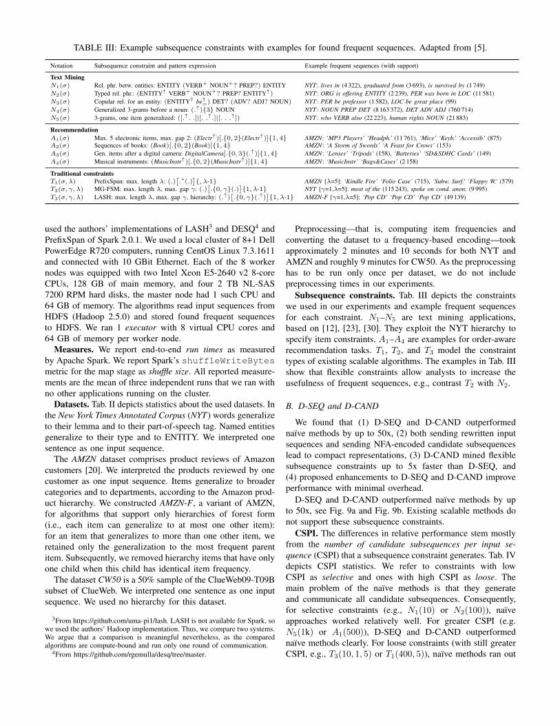
TABLE III: Example subsequence constraints with examples for found frequent sequences. Adapted from [5].
Notation Subsequence constraint and pattern expression Example frequent sequences (with support)
Text MiningN1(σ) Rel. phr. betw. entities: ENTITY (VERB+ NOUN+? PREP?) ENTITY NYT: lives in (4 322), graduated from (3 693), is survived by (1 749)N2(σ) Typed rel. phr.: (ENTITY↑ VERB+ NOUN+? PREP? ENTITY↑) NYT: ORG is offering ENTITY (2 239), PER was born in LOC (11 581)N3(σ) Copular rel. for an entity: (ENTITY↑ be↑=) DET? (ADV? ADJ? NOUN) NYT: PER be professor (1 582), LOC be great place (99)N4(σ) Generalized 3-grams before a noun: (.↑){3} NOUN NYT: NOUN PREP DET (8 163 372), DET ADV ADJ (760 714)N5(σ) 3-grams, one item generalized: ([.↑. .]|[. .↑.]|[. . .↑]) NYT: who VERB also (22 223), human rights NOUN (21 883)
RecommendationA1(σ) Max. 5 electronic items, max. gap 2: (Electr↑)[.{0, 2}(Electr↑)]{1, 4} AMZN: ‘MP3 Players’ ‘Headph.’ (11 761), ‘Mice’ ‘Keyb.’ ‘Accessib.’ (875)A2(σ) Sequences of books: (Book)[.{0, 2}(Book)]{1, 4} AMZN: ‘A Storm of Swords’ ‘A Feast for Crows’ (153)A3(σ) Gen. items after a digital camera: DigitalCamera[.{0, 3}(.↑)]{1, 4} AMZN: ‘Lenses’ ‘Tripods’ (158), ‘Batteries’ ‘SD&SDHC Cards’ (149)A4(σ) Musical instruments: (MusicInstr↑)[.{0, 2}(MusicInstr↑)]{1, 4} AMZN: ‘MusicInstr’ ‘Bags&Cases’ (2 158)
Traditional constraintsT1(σ, λ) PrefixSpan: max. length λ: (.)
[.∗(.)
]{, λ-1} AMZN [λ=5]: ‘Kindle Fire’ ‘Folio Case’ (715), ‘Subw. Surf.’ ‘Flappy W.’ (579)
T2(σ, γ, λ) MG-FSM: max. length λ, max. gap γ: (.)[.{0, γ}(.)
]{1, λ-1} NYT [γ=1,λ=5]: most of the (115 243), spoke on cond. anon. (9 995)
T3(σ, γ, λ) LASH: max. length λ, max. gap γ, hierarchy: (.↑)[.{0, γ}(.↑)
]{1, λ-1} AMZN-F [γ=1,λ=5]: ‘Pop CD’ ‘Pop CD’ ‘Pop CD’ (49 139)
used the authors’ implementations of LASH3 and DESQ4 andPrefixSpan of Spark 2.0.1. We used a local cluster of 8+1 DellPowerEdge R720 computers, running CentOS Linux 7.3.1611and connected with 10 GBit Ethernet. Each of the 8 workernodes was equipped with two Intel Xeon E5-2640 v2 8-coreCPUs, 128 GB of main memory, and four 2 TB NL-SAS7200 RPM hard disks, the master node had 1 such CPU and64 GB of memory. The algorithms read input sequences fromHDFS (Hadoop 2.5.0) and stored found frequent sequencesto HDFS. We ran 1 executor with 8 virtual CPU cores and64 GB of memory per worker node.
Measures. We report end-to-end run times as measuredby Apache Spark. We report Spark’s shuffleWriteBytesmetric for the map stage as shuffle size. All reported measure-ments are the mean of three independent runs that we ran withno other applications running on the cluster.
Datasets. Tab. II depicts statistics about the used datasets. Inthe New York Times Annotated Corpus (NYT) words generalizeto their lemma and to their part-of-speech tag. Named entitiesgeneralize to their type and to ENTITY. We interpreted onesentence as one input sequence.
The AMZN dataset comprises product reviews of Amazoncustomers [20]. We interpreted the products reviewed by onecustomer as one input sequence. Items generalize to broadercategories and to departments, according to the Amazon prod-uct hierarchy. We constructed AMZN-F, a variant of AMZN,for algorithms that support only hierarchies of forest form(i.e., each item can generalize to at most one other item):for an item that generalizes to more than one other item, weretained only the generalization to the most frequent parentitem. Subsequently, we removed hierarchy items that have onlyone child when this child has identical item frequency.
The dataset CW50 is a 50% sample of the ClueWeb09-T09Bsubset of ClueWeb. We interpreted one sentence as one inputsequence. We used no hierarchy for this dataset.
3From https://github.com/uma-pi1/lash. LASH is not available for Spark, sowe used the authors’ Hadoop implementation. Thus, we compare two systems.We argue that a comparison is meaningful nevertheless, as the comparedalgorithms are compute-bound and run only one round of communication.
4From https://github.com/rgemulla/desq/tree/master.
Preprocessing—that is, computing item frequencies andconverting the dataset to a frequency-based encoding—tookapproximately 2 minutes and 10 seconds for both NYT andAMZN and roughly 9 minutes for CW50. As the preprocessinghas to be run only once per dataset, we do not includepreprocessing times in our experiments.
Subsequence constraints. Tab. III depicts the constraintswe used in our experiments and example frequent sequencesfor each constraint. N1–N5 are text mining applications,based on [12], [23], [30]. They exploit the NYT hierarchy tospecify item constraints. A1–A4 are examples for order-awarerecommendation tasks. T1, T2, and T3 model the constrainttypes of existing scalable algorithms. The examples in Tab. IIIshow that flexible constraints allow analysts to increase theusefulness of frequent sequences, e.g., contrast T2 with N2.
B. D-SEQ and D-CAND
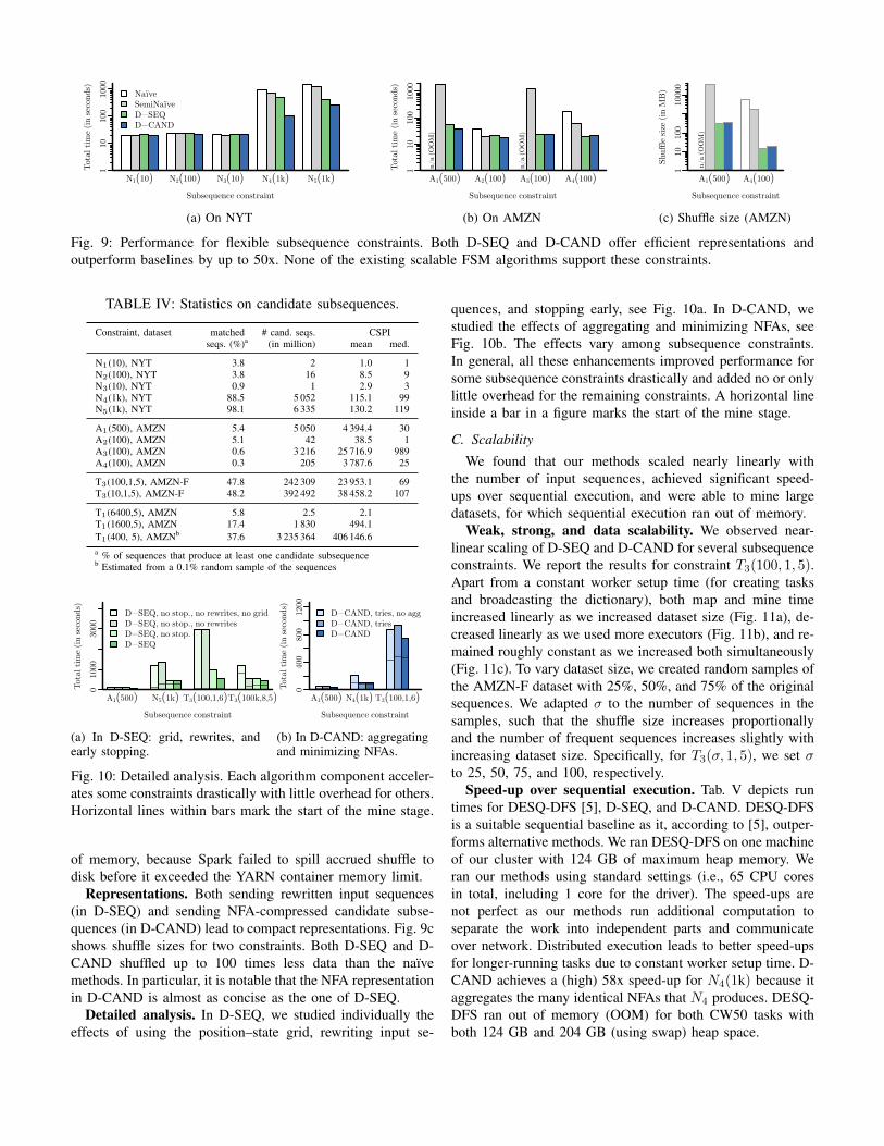
We found that (1) D-SEQ and D-CAND outperformednaıve methods by up to 50x, (2) both sending rewritten inputsequences and sending NFA-encoded candidate subsequenceslead to compact representations, (3) D-CAND mined flexiblesubsequence constraints up to 5x faster than D-SEQ, and(4) proposed enhancements to D-SEQ and D-CAND improveperformance with minimal overhead.
D-SEQ and D-CAND outperformed naıve methods by upto 50x, see Fig. 9a and Fig. 9b. Existing scalable methods donot support these subsequence constraints.
CSPI. The differences in relative performance stem mostlyfrom the number of candidate subsequences per input se-quence (CSPI) that a subsequence constraint generates. Tab. IVdepicts CSPI statistics. We refer to constraints with lowCSPI as selective and ones with high CSPI as loose. Themain problem of the naıve methods is that they generateand communicate all candidate subsequences. Consequently,for selective constraints (e.g., N1(10) or N2(100)), naıveapproaches worked relatively well. For greater CSPI (e.g.N5(1k) or A1(500)), D-SEQ and D-CAND outperformednaıve methods clearly. For loose constraints (with still greaterCSPI, e.g., T3(10, 1, 5) or T1(400, 5)), naıve methods ran out
N1(10) N2(100) N3(10) N4(1k) N5(1k)
Subsequence constraint
Tot
al t
ime
(in
seco
nds)
110
100
1000
NaïveSemiNaïveD−SEQD−CAND
(a) On NYT
A1(500) A2(100) A3(100) A4(100)
Subsequence constraint
Tot
al t
ime
(in
seco
nds)
110
100
1000
n/a
(OO
M)
n/a
(OO
M)
(b) On AMZN
A1(500) A4(100)
Subsequence constraint
Shuf
fle s
ize
(in
MB
)
110
100
1000
0
n/a
(OO
M)
(c) Shuffle size (AMZN)
Fig. 9: Performance for flexible subsequence constraints. Both D-SEQ and D-CAND offer efficient representations andoutperform baselines by up to 50x. None of the existing scalable FSM algorithms support these constraints.
TABLE IV: Statistics on candidate subsequences.
Constraint, dataset matched # cand. seqs. CSPIseqs. (%)a (in million) mean med.
N1(10), NYT 3.8 2 1.0 1N2(100), NYT 3.8 16 8.5 9N3(10), NYT 0.9 1 2.9 3N4(1k), NYT 88.5 5 052 115.1 99N5(1k), NYT 98.1 6 335 130.2 119
A1(500), AMZN 5.4 5 050 4 394.4 30A2(100), AMZN 5.1 42 38.5 1A3(100), AMZN 0.6 3 216 25 716.9 989A4(100), AMZN 0.3 205 3 787.6 25
T3(100,1,5), AMZN-F 47.8 242 309 23 953.1 69T3(10,1,5), AMZN-F 48.2 392 492 38 458.2 107
T1(6400,5), AMZN 5.8 2.5 2.1T1(1600,5), AMZN 17.4 1 830 494.1T1(400, 5), AMZNb 37.6 3 235 364 406 146.6a % of sequences that produce at least one candidate subsequenceb Estimated from a 0.1% random sample of the sequences
A1(500) N5(1k) T3(100,1,6) T3(100k,8,5)
Subsequence constraint
Tot
al t
ime
(in
seco
nds)
010
0030
00
D−SEQ, no stop., no rewrites, no gridD−SEQ, no stop., no rewritesD−SEQ, no stop.D−SEQ
(a) In D-SEQ: grid, rewrites, and ...early stopping.
A1(500) N4(1k) T3(100,1,6)
Subsequence constraint
Tot
al t
ime
(in
seco
nds)
040
080
012
00
D−CAND, tries, no agg.D−CAND, triesD−CAND
(b) In D-CAND: aggregatingand minimizing NFAs.
Fig. 10: Detailed analysis. Each algorithm component acceler-ates some constraints drastically with little overhead for others.Horizontal lines within bars mark the start of the mine stage.
of memory, because Spark failed to spill accrued shuffle todisk before it exceeded the YARN container memory limit.
Representations. Both sending rewritten input sequences(in D-SEQ) and sending NFA-compressed candidate subse-quences (in D-CAND) lead to compact representations. Fig. 9cshows shuffle sizes for two constraints. Both D-SEQ and D-CAND shuffled up to 100 times less data than the naıvemethods. In particular, it is notable that the NFA representationin D-CAND is almost as concise as the one of D-SEQ.
Detailed analysis. In D-SEQ, we studied individually theeffects of using the position–state grid, rewriting input se-
quences, and stopping early, see Fig. 10a. In D-CAND, westudied the effects of aggregating and minimizing NFAs, seeFig. 10b. The effects vary among subsequence constraints.In general, all these enhancements improved performance forsome subsequence constraints drastically and added no or onlylittle overhead for the remaining constraints. A horizontal lineinside a bar in a figure marks the start of the mine stage.
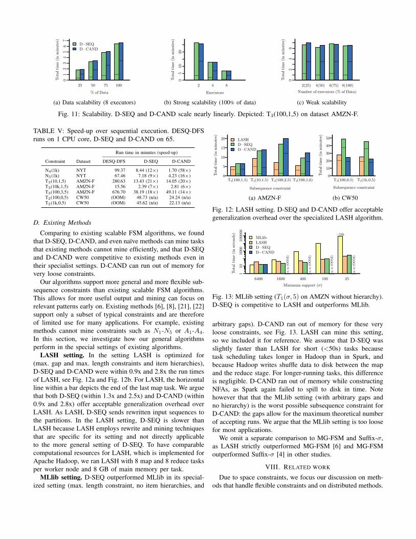
C. Scalability
We found that our methods scaled nearly linearly withthe number of input sequences, achieved significant speed-ups over sequential execution, and were able to mine largedatasets, for which sequential execution ran out of memory.
Weak, strong, and data scalability. We observed near-linear scaling of D-SEQ and D-CAND for several subsequenceconstraints. We report the results for constraint T3(100, 1, 5).Apart from a constant worker setup time (for creating tasksand broadcasting the dictionary), both map and mine timeincreased linearly as we increased dataset size (Fig. 11a), de-creased linearly as we used more executors (Fig. 11b), and re-mained roughly constant as we increased both simultaneously(Fig. 11c). To vary dataset size, we created random samples ofthe AMZN-F dataset with 25%, 50%, and 75% of the originalsequences. We adapted σ to the number of sequences in thesamples, such that the shuffle size increases proportionallyand the number of frequent sequences increases slightly withincreasing dataset size. Specifically, for T3(σ, 1, 5), we set σto 25, 50, 75, and 100, respectively.
Speed-up over sequential execution. Tab. V depicts runtimes for DESQ-DFS [5], D-SEQ, and D-CAND. DESQ-DFSis a suitable sequential baseline as it, according to [5], outper-forms alternative methods. We ran DESQ-DFS on one machineof our cluster with 124 GB of maximum heap memory. Weran our methods using standard settings (i.e., 65 CPU coresin total, including 1 core for the driver). The speed-ups arenot perfect as our methods run additional computation toseparate the work into independent parts and communicateover network. Distributed execution leads to better speed-upsfor longer-running tasks due to constant worker setup time. D-CAND achieves a (high) 58x speed-up for N4(1k) because itaggregates the many identical NFAs that N4 produces. DESQ-DFS ran out of memory (OOM) for both CW50 tasks withboth 124 GB and 204 GB (using swap) heap space.
25 50 75 100
% of Data
Tot
al t
ime
(in
min
utes
)
01
23
45
67
D−SEQD−CAND
(a) Data scalability (8 executors)
2 4 8
Executors
Tot
al t
ime
(in
min
utes
)
05
1020
(b) Strong scalability (100% of data)
2(25) 4(50) 6(75) 8(100)
Number of executors (% of Data)
Tot
al t
ime
(in
min
utes
)
02
46
(c) Weak scalability
Fig. 11: Scalability. D-SEQ and D-CAND scale nearly linearly. Depicted: T3(100,1,5) on dataset AMZN-F.
TABLE V: Speed-up over sequential execution. DESQ-DFSruns on 1 CPU core, D-SEQ and D-CAND on 65.
Run time in minutes (speed-up)
Constraint Dataset DESQ-DFS D-SEQ D-CAND
N4(1k) NYT 99.37 8.44 (12×) 1.70 (58×)N5(1k) NYT 67.46 7.18 (9×) 4.23 (16×)T3(10,1,5) AMZN-F 280.63 13.43 (21×) 14.05 (20×)T3(10k,1,5) AMZN-F 15.56 2.39 (7×) 2.81 (6×)T3(100,3,5) AMZN-F 676.70 38.19 (18×) 49.11 (14×)T2(100,0,5) CW50 (OOM) 48.73 (n/a) 24.24 (n/a)T2(1k,0,5) CW50 (OOM) 45.62 (n/a) 22.13 (n/a)
D. Existing Methods
Comparing to existing scalable FSM algorithms, we foundthat D-SEQ, D-CAND, and even naıve methods can mine tasksthat existing methods cannot mine efficiently, and that D-SEQand D-CAND were competitive to existing methods even intheir specialist settings. D-CAND can run out of memory forvery loose constraints.
Our algorithms support more general and more flexible sub-sequence constraints than existing scalable FSM algorithms.This allows for more useful output and mining can focus onrelevant patterns early on. Existing methods [6], [8], [21], [22]support only a subset of typical constraints and are thereforeof limited use for many applications. For example, existingmethods cannot mine constraints such as N1-N5 or A1-A4.In this section, we investigate how our general algorithmsperform in the special settings of existing algorithms.
LASH setting. In the setting LASH is optimized for(max. gap and max. length constraints and item hierarchies),D-SEQ and D-CAND were within 0.9x and 2.8x the run timesof LASH, see Fig. 12a and Fig. 12b. For LASH, the horizontalline within a bar depicts the end of the last map task. We arguethat both D-SEQ (within 1.3x and 2.5x) and D-CAND (within0.9x and 2.8x) offer acceptable generalization overhead overLASH. As LASH, D-SEQ sends rewritten input sequences tothe partitions. In the LASH setting, D-SEQ is slower thanLASH because LASH employs rewrite and mining techniquesthat are specific for its setting and not directly applicableto the more general setting of D-SEQ. To have comparablecomputational resources for LASH, which is implemented forApache Hadoop, we ran LASH with 8 map and 8 reduce tasksper worker node and 8 GB of main memory per task.
MLlib setting. D-SEQ outperformed MLlib in its special-ized setting (max. length constraint, no item hierarchies, and
T3(100,1,5) T3(10,1,5) T3(100,2,5) T3(100,1,6)
Subsequence constraint
Tot
al t
ime
(in
min
utes
)
0
5
10
15
20 LASHD−SEQD−CAND
(a) AMZN-F
T2(100,0,5) T2(1k,0,5)
Subsequence constraint
Tot
al t
ime
(in
min
utes
)
0
10
20
30
40
50
(b) CW50
Fig. 12: LASH setting. D-SEQ and D-CAND offer acceptablegeneralization overhead over the specialized LASH algorithm.
6400 1600 400 100 25
Minimum support (σ)
Tot
al t
ime
(in
seco
nds)
110
1000
1000
00MLlibLASHD−SEQD−CAND
>24h
n/a
(OO
M)
n/a
(OO
M)
n/a
(OO
M)
n/a
(OO
M)
Fig. 13: MLlib setting (T1(σ, 5) on AMZN without hierarchy).D-SEQ is competitive to LASH and outperforms MLlib.
arbitrary gaps). D-CAND ran out of memory for these veryloose constraints, see Fig. 13. LASH can mine this setting,so we included it for reference. We assume that D-SEQ wasslightly faster than LASH for short (<50s) tasks becausetask scheduling takes longer in Hadoop than in Spark, andbecause Hadoop writes shuffle data to disk between the mapand the reduce stage. For longer-running tasks, this differenceis negligible. D-CAND ran out of memory while constructingNFAs, as Spark again failed to spill to disk in time. Notehowever that that the MLlib setting (with arbitrary gaps andno hierarchy) is the worst possible subsequence constraint forD-CAND: the gaps allow for the maximum theoretical numberof accepting runs. We argue that the MLlib setting is too loosefor most applications.
We omit a separate comparison to MG-FSM and Suffix-σ,as LASH strictly outperformed MG-FSM [6] and MG-FSMoutperformed Suffix-σ [4] in other studies.
VIII. RELATED WORK
Due to space constraints, we focus our discussion on meth-ods that handle flexible constraints and on distributed methods.

Subsequence constraints. There exist many approachesfor constraining which subsequences should be consideredfor mining. GSP [28] introduced minimum and maximumgap constraints as well as sliding windows for time-annotatedsequences. cSpade [34] supports length, gap, and item con-straints. Wu et al. [32] studied periodic wild card gaps. Regularexpressions as “output filter” were proposed in the SPIRITfamily of algorithms [13], RE-Hackle [2], and SMA algo-rithms [31]. Such filters are evaluated on only the subsequence,but not the input sequence, so that context constraints cannotbe specified. DESQ [5], [7] extends regular expressions withcontextual constraints by considering both input sequence andsubsequence as input for evaluating constraints. Our methodsuse the DESQ framework to specify and evaluate constraints.However, DESQ is a sequential algorithm and, consequently,does not scale to large datasets.
Scalable mining. To mine large datasets efficiently, parallelalgorithms have been developed for shared [35] and distributedmemory architectures [15], [16], but without support forconstraints or hierarchies. Apache Spark’s MLlib library [21]features a distributed version of PrefixSpan [24] for distributedFSM with sequences of itemsets, but without support forhierarchies or subsequence constraints other than maximumsubsequence length. It uses prefix-based partitioning; that is,it recursively partitions sequences by their first items. Thus,it runs multiple rounds of communication. In the context ofitemset mining, Savasare et al. [26] proposed to partition inputs(instead of outputs). Their approach has the drawback that allcandidates need to be communicated to all workers.
Most closely related to our work is a group of distributedsequential pattern mining algorithms targeted towards theMapReduce programming model: Suffix-σ [8], MG-FSM [4],[22], and LASH [6]. Suffix-σ mines subsequences of consec-utive items in one MapReduce step with suffix-partitioning.However, it does not support gaps. MG-FSM and LASH aredistributed FSM algorithms with maximum gap and maximumlength constraints. They use item-based partitioning and se-quence representation with specialized rewrite techniques. Themethods are inspired by item-based partitioning for parallelitemset mining [10], [16]. LASH extends MG-FSM with itemhierarchies and introduces a technique to focus local miningon pivot sequences. According to [6], LASH outperforms MG-FSM. MG-FSM and LASH inspired D-SEQ, which is moregeneral. D-SEQ supports many more types of subsequenceconstraints, including the ones of MG-FSM and LASH.
IX. CONCLUSION
We described D-SEQ and D-CAND, the first two FSMalgorithms that are scalable and support flexible subsequenceconstraints. We demonstrated that they can mine varied typesof subsequence constraints efficiently, scale nearly linearly,and offer acceptable generalization overhead over existing,specialized methods.
ACKNOWLEDGMENT
This work was supported by a Software Campus grant ofthe German Ministry of Education and Research (01IS17052).
REFERENCES
[1] R. Agrawal and R. Srikant. Mining sequential patterns. ICDE ’95.[2] H. Albert-Lorincz and J. Boulicaut. Mining frequent sequential patterns
under regular expressions: a highly adaptative strategy for pushingconstraints. SDM ’03.
[3] C. Antunes and A. Oliveira. Inference of sequential association rulesguided by context-free grammars. ICGI ’02.
[4] K. Beedkar, K. Berberich, R. Gemulla, and I. Miliaraki. Closing thegap: Sequence mining at scale. TODS, 40(2):8:1–8:44, 2015.
[5] K. Beedkar and R. Gemulla. DESQ: Frequent sequence mining withsubsequence constraints. ICDM ’16.
[6] K. Beedkar and R. Gemulla. LASH: Large-scale sequence mining withhierarchies. SIGMOD ’15.
[7] K. Beedkar, R. Gemulla, and W. Martens. A unified framework forfrequent sequence mining with subsequence constraints. To appear inTODS.
[8] K. Berberich and S. Bedathur. Computing N-gram statistics in MapRe-duce. EDBT ’13.
[9] A. Brazma, I. Jonassen, J. Vilo, and E. Ukkonen. Pattern discovery inbiosequences. ICGI ’98.
[10] G. Buehrer et al. Toward terabyte pattern mining: An architecture-conscious solution. PPoPP ’07.
[11] J. Dean and S. Ghemawat. MapReduce: Simplified data processing onlarge clusters. OSDI ’04.
[12] A. Fader, S. Soderland, and O. Etzioni. Identifying relations for openinformation extraction. EMNLP ’11.
[13] M. Garofalakis, R. Rastogi, and K. Shim. SPIRIT: Sequential patternmining with regular expression constraints. VLDB ’99.
[14] F. Giannotti, M. Nanni, and D. Pedreschi. Efficient mining of temporallyannotated sequences. SDM ’06.
[15] V. Guralnik, N. Garg, and G. Karypis. Parallel tree projection algorithmfor sequence mining. Euro-Par ’96.
[16] V. Guralnik and G. Karypis. Parallel tree-projection-based sequencemining algorithms. Parallel Computing, 30(4):443–472, 2004.
[17] J. Han, J. Pei, and Y. Yin. Mining frequent patterns without candidategeneration. SIGMOD ’00.
[18] T. Jiang and B. Ravikumar. Minimal NFA problems are hard. SIAMJournal on Computing, 22(6):1117–1141, 1993.
[19] A. Lopez. Statistical machine translation. ACM Computing Surveys,40(3):8:1–8:49, 2008.
[20] J. McAuley, R. Pandey, and J. Leskovec. Inferring networks ofsubstitutable and complementary products. KDD ’15.
[21] X. Meng et al. MLlib: Machine learning in Apache Spark. The Journalof Machine Learning Research, 17(1):1235–1241, 2016.
[22] I. Miliaraki et al. Mind the gap: Large-scale frequent sequence mining.SIGMOD ’13.
[23] N. Nakashole, G. Weikum, and F. Suchanek. PATTY: A taxonomy ofrelational patterns with semantic types. EMNLP-CoNLL ’12.
[24] J. Pei et al. PrefixSpan: Mining sequential patterns efficiently by prefix-projected pattern growth. ICDE ’01.
[25] Dominique Revuz. Minimisation of acyclic deterministic automata inlinear time. Theoretical Computer Science, 92(1):181–189, 1992.
[26] A. Savasere, E. Omiecinski, and S. Navathe. An efficient algorithm formining association rules in large databases. VLDB ’95.
[27] K. Smets and J. Vreeken. Slim: Directly mining descriptive patterns.SDM ’12.
[28] R. Srikant and R. Agrawal. Mining sequential patterns: Generalizationsand performance improvements. EDBT ’96.
[29] J. Srivastava et al. Web usage mining: Discovery and applications ofusage patterns from web data. SIGKDD Explorations, 1(2):12–23, 2000.
[30] Google Ngram Viewer Team. Google Books Ngram Viewer. https://books.google.com/ngrams/info, 2013. Accessed: 2018-10-10.
[31] R. Trasarti, F. Bonchi, and B. Goethals. Sequence mining automata: Anew technique for mining frequent sequences under regular expressions.ICDM ’08.
[32] Y. Wu et al. Mining sequential patterns with periodic wildcard gaps.Applied Intelligence, 41(1):99–116, 2014.
[33] M. Zaharia et al. Spark : Cluster computing with working sets. HotCloud’10.
[34] M. Zaki. Sequence mining in categorical domains: incorporatingconstraints. CIKM ’00.
[35] M. Zaki. Parallel sequence mining on shared-memory machines. Journalof Parallel and Distributed Computing, 61(3):401–426, 2001.
[36] M. Zaki. SPADE: An efficient algorithm for mining frequent sequences.Machine Learning, 42(1-2):31–60, 2001.