��

��

Scalar Optimization

�

��

��

Organization

�� What kind of optimizations are useful�

�� Program analysis for determining opportunities for optimization�

data�ow analysis�

� lattice algebra

� solving equations on lattices

� applications to data�ow analysis

�� Speeding up data�ow analysis�

� exploitation of structure

� sparse representations� control dependence� SSA form� sparse

data�ow evaluator graphs

�

��

��

Optimizations performed by most compilers

� Constant propagation� replace constant�valued variables with

constants

� Common sub�expression elimination� avoid re�computing value

if value has been computed earlier in program

� Loop invariant removal� move computations into less frequently

executed portions of program

� Strength reduction� replace expensive operations �like

multiplication� with simpler operations �like addition�

� Dead code removal� eliminate unreachable code and code that

is irrelevant to output of program�

��

��

Optimization example�

DO J � �����

DO I � �����

A�I�J� � �

If we assume columnmajor order of storage� and bytes per array

element�

Address of A�I�J� � BaseAddress�A� �J�������� �I����

� BaseAddress�A � J��� � I� �

� Only the term I � depends on I �� rest of computation is

invariant in the inner loop and can be hoisted out of it�

� Further hoisting of invariant code is possible since only the subterm

J � �� depends on J �

� Since I and J are incremented by � each time through the loop�

expressions like I � and J � �� can be strength reduced by

replacing them with additions��

��

��

Pseudo�code for original loop nest�

DO J � �����

DO I � �����

t � BaseAddress�A� � J��� � I� �

STORE�t���

Pseudo�code for optimized loop nest�

t� � BaseAddress�A� �

DO J � �����

t� � t� � ��

t� � t�

DO I � �����

t� � t� �

STORE�t���

�

��

��

Terminology

� A de�nition of a variable is a statement that may assign to

that variable� De�nitions of x�

�i� x � �

�ii� F�x�y� �call by reference�

In second example� invocation of F may write to x�

so to be safe� we declare invocation to be a

definition of x

� A use of a variable is a statement that may read the

value of that variable Uses of x�

�i� y � x � �

�ii� F�x�z�

�

��

��

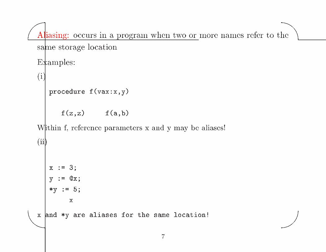
Aliasing� occurs in a program when two or more names refer to the

same storage location�

Examples�

�i�procedure f�vax x�y�

����

���f�z�z� ��� f�a�b����

Within f� reference parameters x and y may be aliases�

�ii ��

x � ��

y � �x�

�y � ��

����x���

x and �y are aliases for the same location�

�

��

��

Our position�

We will not perform analysis for variables that may be aliased such

�reference parameters� local variables whose addresses have been

taken� etc���

This implies we can determine syntactically where all de�nitions

and uses of a variable are�

More re�ned approach� perform alias analysis�

�

��

��

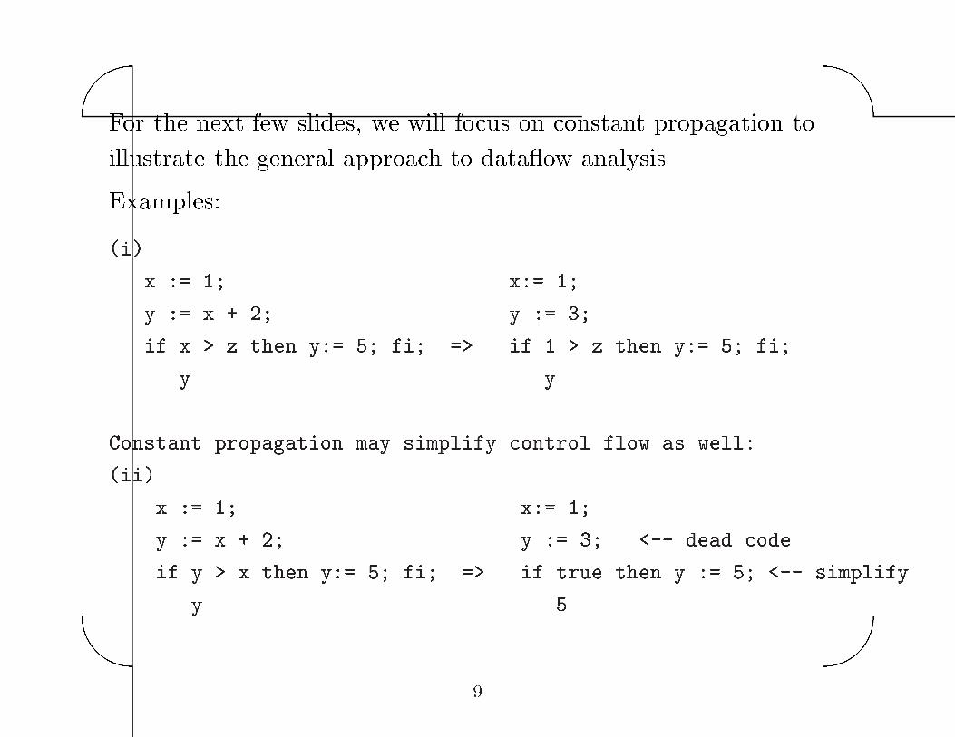
For the next few slides� we will focus on constant propagation to

illustrate the general approach to data�ow analysis�

Examples�

�i���� ���

x � �� x � ��

y � x �� y � ��

if x � z then y � �� fi� �� if � � z then y � �� fi�

���y��� ���y���

Constant propagation may simplify control flow as well

�ii���� ���

x � �� x � ��

y � x �� y � �� � dead code

if y � x then y � �� fi� �� if true then y � �� � simplify

���y��� �������

��

��

Why do opportunities for constant propagation arise in programs

� constant declarations for modularity

� macros

� procedure inlining� small methods in OO languages

� machine�speci�c values

�

��

��

Overview of algorithm�

� Build the control �ow graph of program�

makes �ow of control in program explicit

�� Perform �symbolic evaluation to determine constants�

�� Replace constant�valued variable uses by their values and

simplify expressions and control �ow�

��

��

��

Step� build the control �ow graph �CFG��

Example�

x �� ��

y �� x���

if �y � x� then y �� �� fi�

y

��

��

��

1

1

1 3

1

3

5

51

x := 1

START

y:= x + 2

y > x

y := 5

merge

...y....

control flow graph (CFG)

state vectorson CFG edges

��

��

��

Algorithm for building CFG� easy� only complication being break�s

and GOTO�s �need to identify jump targets�

Basic Block� straight�line code without any branches or merging of

control �ow

Nodes of CFG� statements�or basic blocks��switches�merges

Edges of CFG� represent possible control �ow sequence

��

��

��

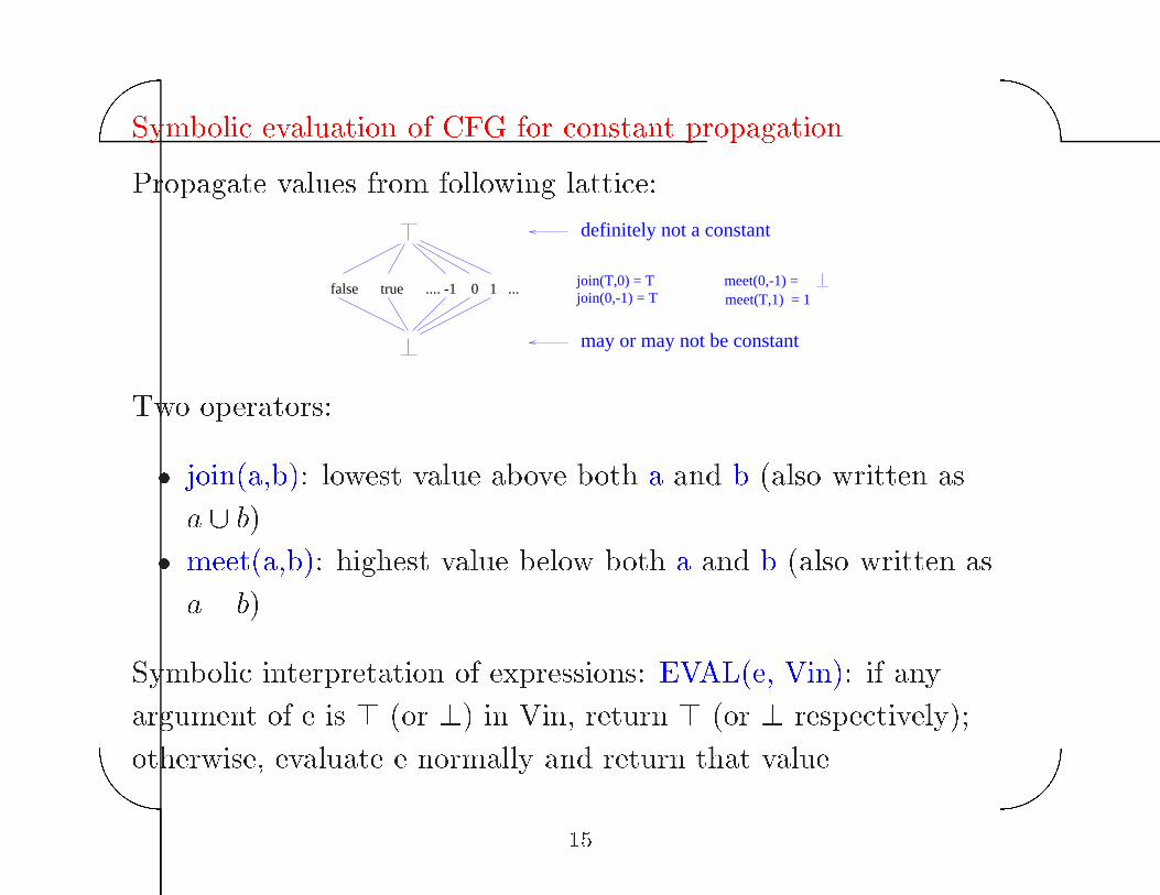
Symbolic evaluation of CFG for constant propagation

Propagate values from following lattice�

false true .... -1 0 1 ...

definitely not a constant

may or may not be constant

join(T,0) = Tjoin(0,-1) = T

meet(0,-1) = meet(T,1) = 1

Two operators�

� join�a�b�� lowest value above both a and b �also written as

a � b�

� meet�a�b�� highest value below both a and b �also written as

a � b�

Symbolic interpretation of expressions� EVAL�e� Vin�� if any

argument of e is � �or �� in Vin� return � �or � respectively��

otherwise� evaluate e normally and return that value

��

��

��

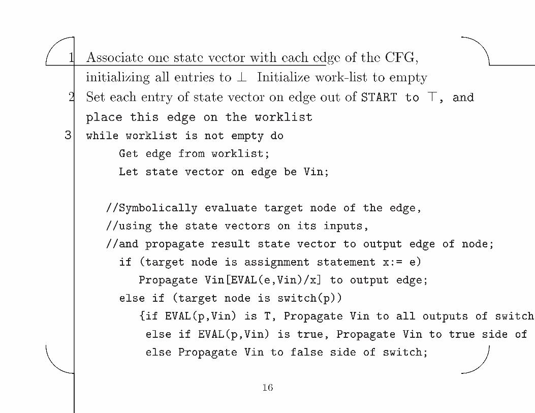
� Associate one state vector with each edge of the CFG�

initializing all entries to �� Initialize work�list to empty�

�� Set each entry of state vector on edge out of START to �� and

place this edge on the worklist

� while worklist is not empty do

Get edge from worklist�

Let state vector on edge be Vin�

��Symbolically evaluate target node of the edge�

��using the state vectors on its inputs�

��and propagate result state vector to output edge of node�

if �target node is assignment statement x � e�

Propagate Vin�EVAL�e�Vin��x� to output edge�

else if �target node is switch�p��

�if EVAL�p�Vin� is T� Propagate Vin to all outputs of switch

else if EVAL�p�Vin� is true� Propagate Vin to true side of

else Propagate Vin to false side of switch�

��

��

��

�

else ��target node is merge

Propagate join of state vectors on all inputs to output�

If this changes the output state vector� enqueue output edge

on worklist�

od�

��

��

��

Running example�1

1

1 3

1

3

5

51

x := 1

START

y:= x + 2

y > x

y := 5

merge

...y....

control flow graph (CFG)

state vectorson CFG edges

��

��

��

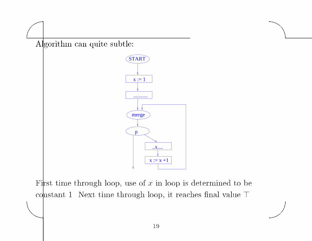
Algorithm can quite subtle�

x := 1

START

...........

p

x := x +1

merge

..x....

First time through loop� use of x in loop is determined to be

constant � Next time through loop� it reaches �nal value ��

�

��

��

Complexity of algorithm�

Height of lattice � � �� each state vector can change value � � V

times�

So while loop in algorithm is executed at most � � E � V times�

Cost of each iteration� O�V ��

So overall algorithm takes O�EV �� time�

�

��

��

Questions�

� Can we use same work�list based algorithm with di�erent

lattices to solve other analysis problems

� Can we improve the e�ciency the algorithm

Need to separate what is being computed from how it is being

computed �� use algebras once again��

��

��

��

Lattice algebraic approach to data�ow analysis

Abstractly� our work�list algorithm can be viewed as one solution

procedure for solving a set of lattice algebraic equations�

Data�ow lattices�

� partially order set of �nite height

� meet and join operations with appropriate algebraic properties

are de�ned for all pairs of values from po�set�

These properties imply that the lattice has a least and a greatest

element�

��

��

��

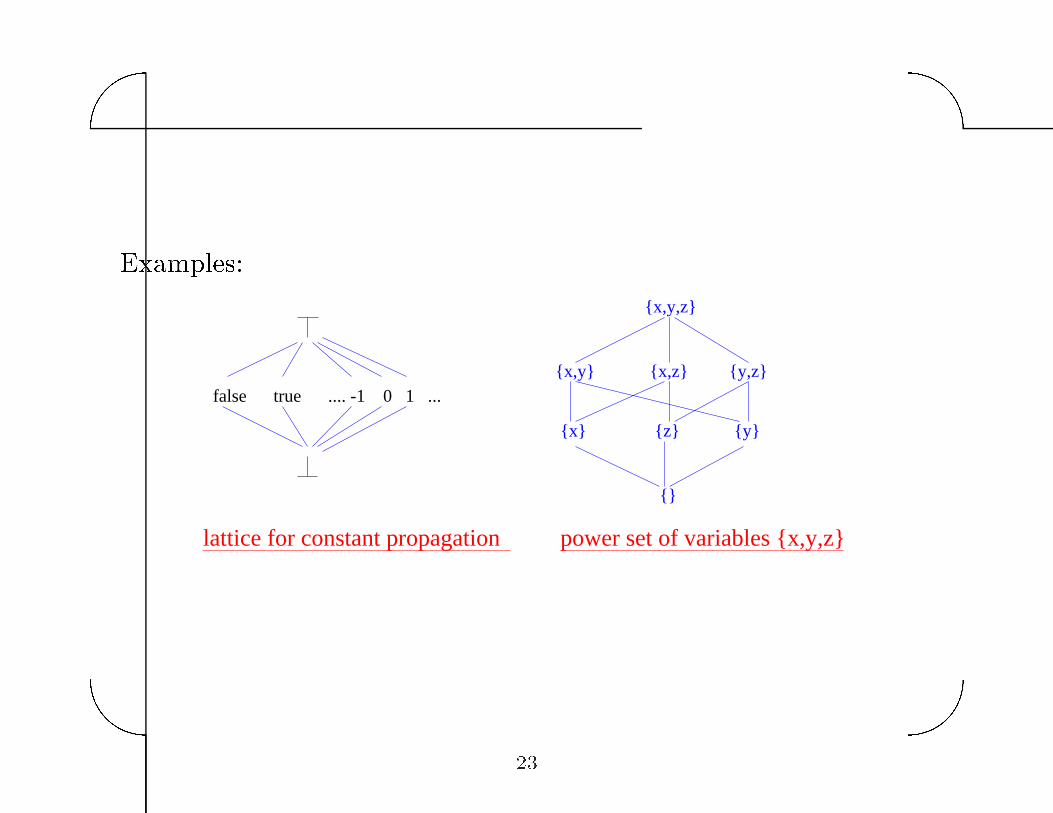
Examples�

false true .... -1 0 1 ...

{x,y,z}

{x,y} {x,z} {y,z}

{y}{x} {z}

{}

lattice for constant propagation power set of variables {x,y,z}��

��

��

Monotonic function� If D is a partially ordered set and f � D � D�

f is said to be monotonic if x � y �� f�x� � f�y��

Intuitively� if the input of a monotonic function is increased� the

output either stays the same or increases as well�

Examples of monotonic functions on CP lattice�

� identity� f�x� � x

� bottom function� f�x� � �

� constant function� f�x� � �

Examples of non�monotonic functions on CP lattice�

f�x� � if �x �� �� then else ���

��

��

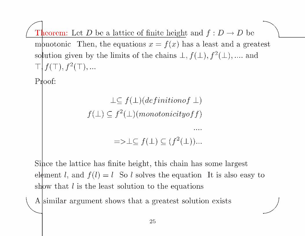
Theorem� Let D be a lattice of �nite height and f � D � D be

monotonic� Then� the equations x � f�x� has a least and a greatest

solution given by the limits of the chains �� f���� f����� ���� and

�� f���� f����� ����

Proof�

�� f����definitionof ��

f��� � f�����monotonicityoff�����

���� f��� � �f��������

Since the lattice has �nite height� this chain has some largest

element l� and f�l� � l� So l solves the equation� It is also easy to

show that l is the least solution to the equations�

A similar argument shows that a greatest solution exists�

��

��

��

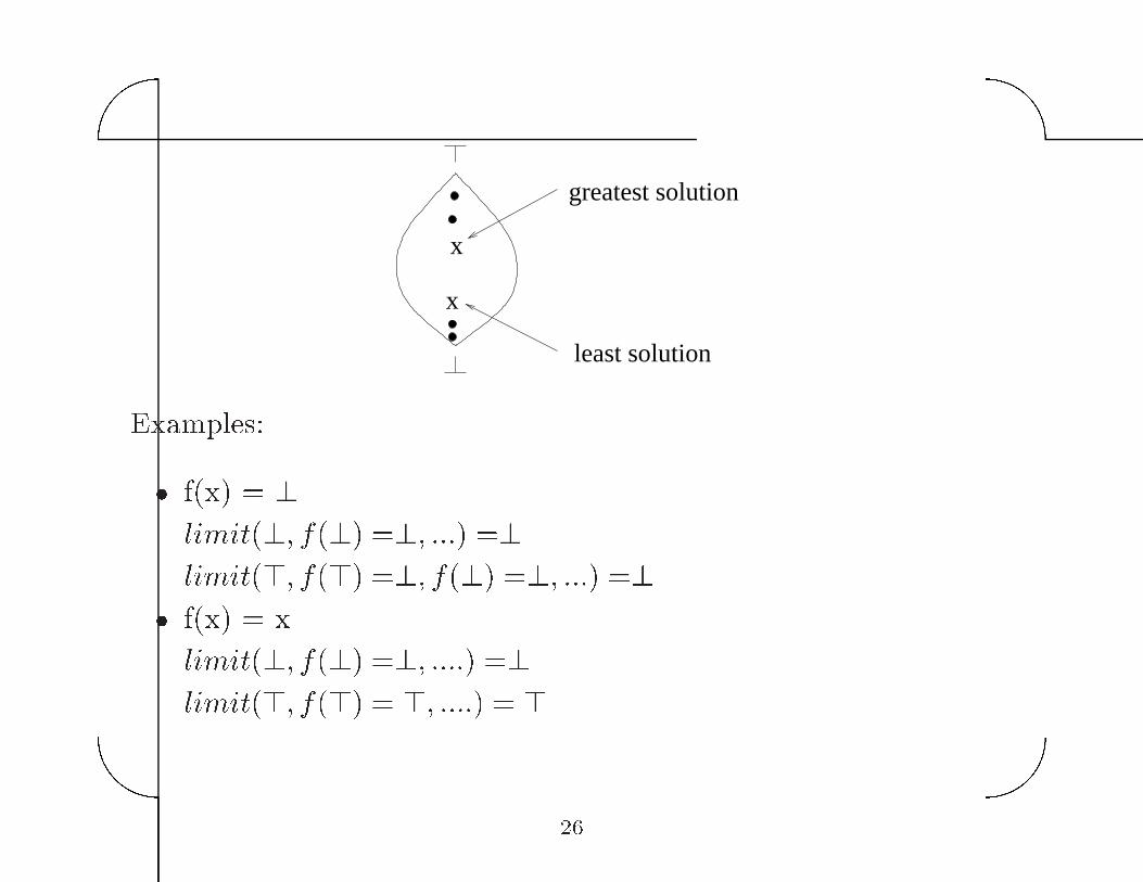
greatest solution

least solution

x.

x

Examples�

� f�x� � �

limit��� f��� ��� ���� ��

limit��� f��� ��� f��� ��� ���� ��

� f�x� � x

limit��� f��� ��� ����� ��

limit��� f��� � �� ����� � ���

��

��

Corollary�

If f � g� h etc are monotonic functions� the system of equations

x � f�x� y� z����

y � g�x� y� z� ���

z � h�x� y� z� �������

has least and greatest solutions given by the limits of the obvious

chains �eg� least solution is obtained by starting with � for all

variables� substituting into right hand sides to get new values for

all variables� and iterating till convergence occurs��

��

��

��

Connection between constant propagation and lattice equations�

iterative procedure is just a method to solve lattice equations�

S0 = [T,T]

S1 = S0{1 / x}S2 = S1{2 / y }S3 = if (S2[y] < S2[x]) or (S2[y]=T) or (S2[x] = T) then S2 else S3 .....S6 = S4 U S5......

x := 1

START

y:= x + 2

y > x

y := 5

merge

...y....

S0

S1

S2

S3

S4

S5

S6

(2 variables)S0, S1, S2,..... : CxC

Lattice: Ctrue false ... -1 0 1 ....

��

��

��

Question� since equations have many solutions in general� which

one should we compute

For CP� least solution gives more accurate information than other

solutions�

x := 1

START

merge

y := ...

p(y)

...x...

[1,T]

[T,T]

[T,T]

[T,T]

[T,T]

[T,T]

[T,T]

[1,T]

[1,T]

[1,T]

[1,T]

[1,T]

[.....]: least solution

[.....]: greatest solution

In general� if con�uence operator is join� compute least solution�

otherwise compute greatest solution�

�

��

��

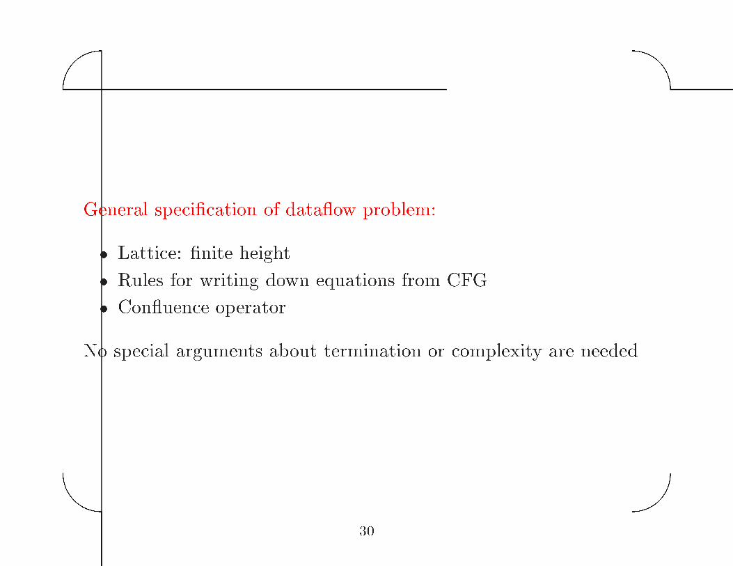
General speci�cation of data�ow problem�

� Lattice� �nite height

� Rules for writing down equations from CFG

� Con�uence operator

No special arguments about termination or complexity are needed�

�

��

��

Constant propagation is example of

FORWARD�FLOW�ALL�PATHS problem�

Intuitively� data is propagated forward in CFG� and value is

constant at a point p only if it is the same constant for all paths

from start to p�

General classi�cation of data�ow problems�

reaching definitions

very busy expressions live variables

constant propagation

available expressions

BACKWARD

FORWARD

ALL PATHS ANY PATH

��

��

��

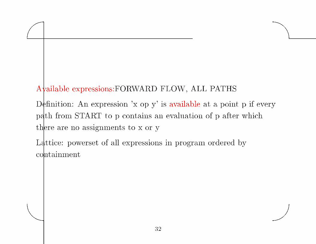
Available expressions�FORWARD FLOW� ALL PATHS

De�nition� An expression �x op y� is available at a point p if every

path from START to p contains an evaluation of p after which

there are no assignments to x or y�

Lattice� powerset of all expressions in program ordered by

containment

��

��

��

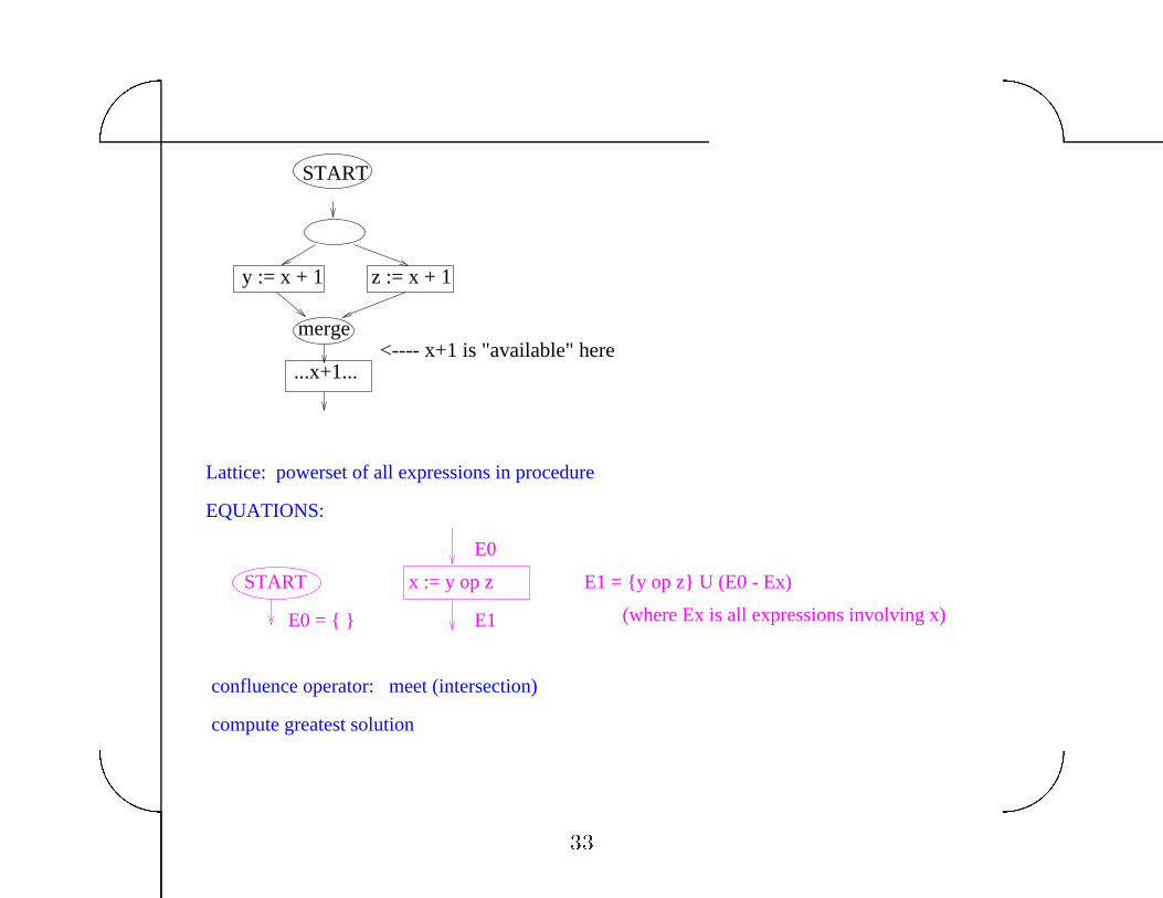
y := x + 1 z := x + 1

merge

...x+1...

START

<---- x+1 is "available" here

x := y op z

E0

E1

E1 = {y op z} U (E0 - Ex)

(where Ex is all expressions involving x)

START

E0 = { }

EQUATIONS:

Lattice: powerset of all expressions in procedure

confluence operator: meet (intersection)

compute greatest solution

��

��

��

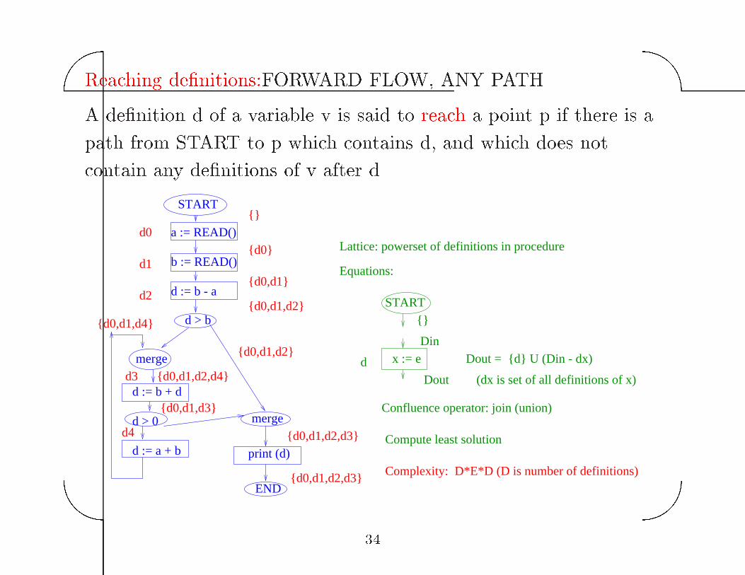
Reaching de�nitions�FORWARD FLOW� ANY PATH

A de�nition d of a variable v is said to reach a point p if there is a

path from START to p which contains d� and which does not

contain any de�nitions of v after d�

a := READ()

b := READ()

d := b - a

d := b + d

d > 0

d := a + b

merge

print (d)

START

merge

d > b

END

d0

d1

d2

{}

{d0}

{d0,d1}

{d0,d1,d2}

{d0,d1,d2}

{d0,d1,d4}

d3

d4

{d0,d1,d2,d4}

{d0,d1,d3}

{d0,d1,d2,d3}

{d0,d1,d2,d3}

Lattice: powerset of definitions in procedure

Equations:

START{}

x := eDin

Dout

Dout = d {d} U (Din - dx)

(dx is set of all definitions of x)

Compute least solution

Confluence operator: join (union)

Complexity: D*E*D (D is number of definitions)

��

��

��

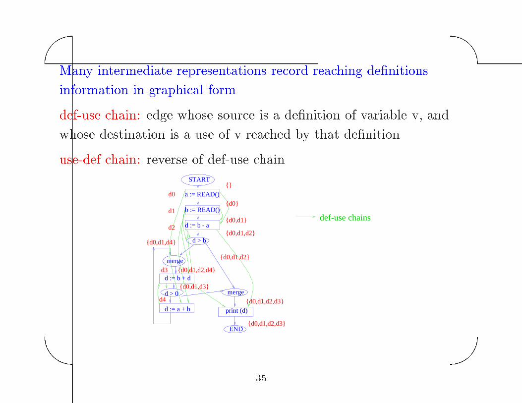
Many intermediate representations record reaching de�nitions

information in graphical form�

def�use chain� edge whose source is a de�nition of variable v� and

whose destination is a use of v reached by that de�nition

use�def chain� reverse of def�use chain

a := READ()

b := READ()

d := b - a

d := b + d

d > 0

d := a + b

merge

print (d)

START

merge

d > b

END

d0

d1

d2

{}

{d0}

{d0,d1}

{d0,d1,d2}

{d0,d1,d2}

{d0,d1,d4}

d3

d4

{d0,d1,d2,d4}

{d0,d1,d3}

{d0,d1,d2,d3}

{d0,d1,d2,d3}

def-use chains

��

��

��

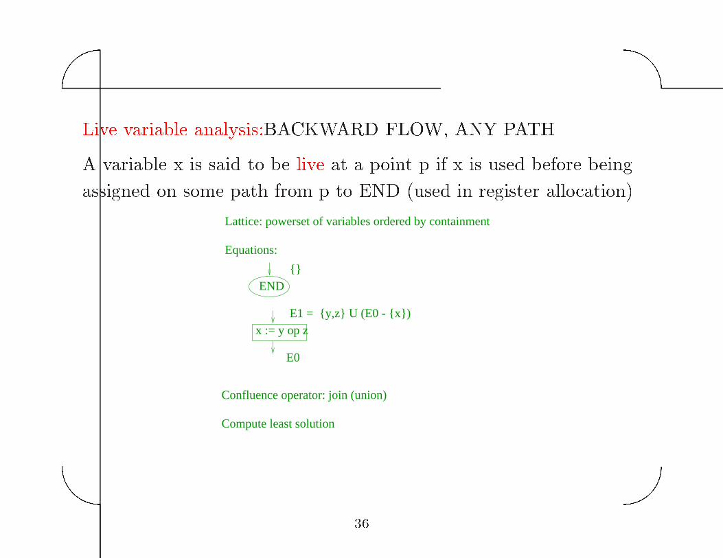
Live variable analysis�BACKWARD FLOW� ANY PATH

A variable x is said to be live at a point p if x is used before being

assigned on some path from p to END �used in register allocation��

Lattice: powerset of variables ordered by containment

Equations:

END

{}

x := y op z

E0

E1 = {y,z} U (E0 - {x})

Confluence operator: join (union)

Compute least solution

��

��

��

Very busy expressions�FORWARD FLOW� ALL PATHS

An expression e �� y op z� is said to be very busy at a point p if it

is evaluated on every path from p to END before an assignment to

y or z�

Lattice: powerset of expressions ordered by containment

Equations:

END

{}

x := y op z

E0

E1 = {y op z} U (E0 - Ex)

Compute greatest solution

(Ex is set of expressions containing x)

Confluence operator: meet (intersection)

��

��

��

Pragmatics of data�ow analysis�

� Compute and store information at basic block level�

� Use bit vectors to represent sets�

Question� can we speed up data�ow analysis

Two approaches�

� exploit structure in control �ow graph

� exploit sparsity

��

��

��

Optimizing Data�ow Analaysis

�

��

��

Constant propagation on CFG� O�EV ��

Reaching de�nitions on CFG� O�EN��

Available expressions on CFG� O�EA��

Two approaches to speeding up data�ow analysis�

� exploit structure in the program

� exploit sparsity in the data�ow equations� usually� a data�ow

equation involves only a small number of data�ow variables

�

��

��

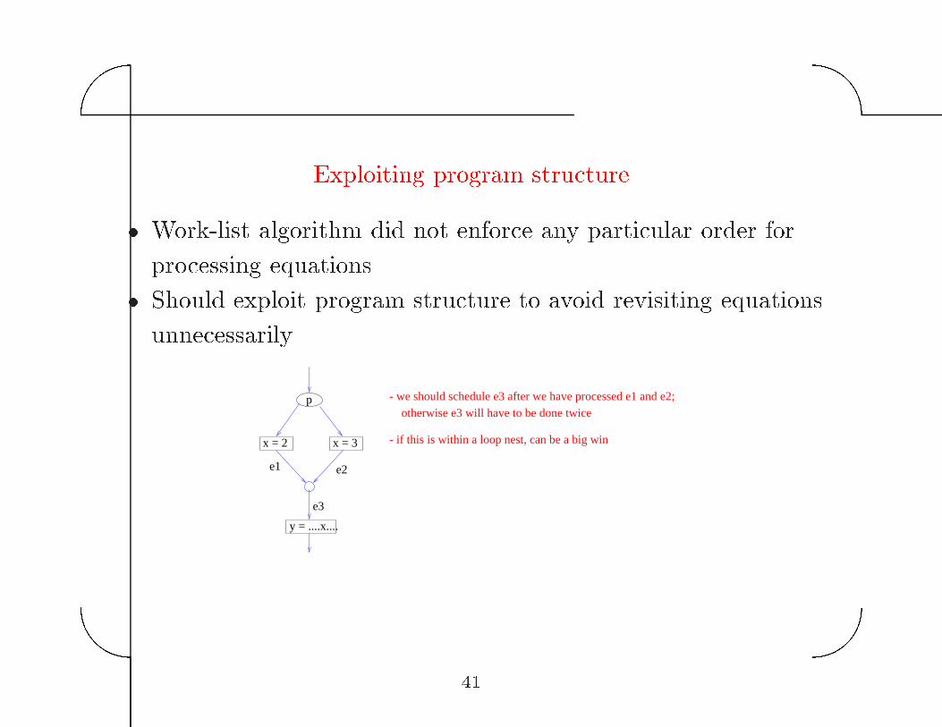
Exploiting program structure

� Work�list algorithm did not enforce any particular order for

processing equations

� Should exploit program structure to avoid revisiting equations

unnecessarily

p

y = ....x....

x = 2 x = 3

e1 e2

e3

- we should schedule e3 after we have processed e1 and e2; otherwise e3 will have to be done twice

- if this is within a loop nest, can be a big win��

��

��

General approach to exploiting structure� elimination

� Identify regions of CFG that can be preprocessed by collapsing

region into a single node with the same input�output behavior

as region

� Solve data�ow equations iteratively on the collapsed graph�

� Interpolate data�ow solution into collapsed regions�

What should be a region

� basic�blocks

� basic�blocks� if�then�else� loops

� intervals

� ����

Structured programs� limit in which no iteration is required

��

��

��

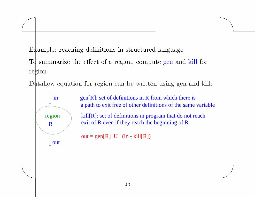
Example� reaching de�nitions in structured language

To summarize the e�ect of a region� compute gen and kill for

region�

Data�ow equation for region can be written using gen and kill�

in

out

region

R

gen[R]: set of definitions in R from which there is a path to exit free of other definitions of the same variable

kill[R]: set of definitions in program that do not reach

out = gen[R] U (in - kill[R])

exit of R even if they reach the beginning of R��

��

��

a = b + cd

R

p

R1 R2

R1

R2

p

R1

R

R

R

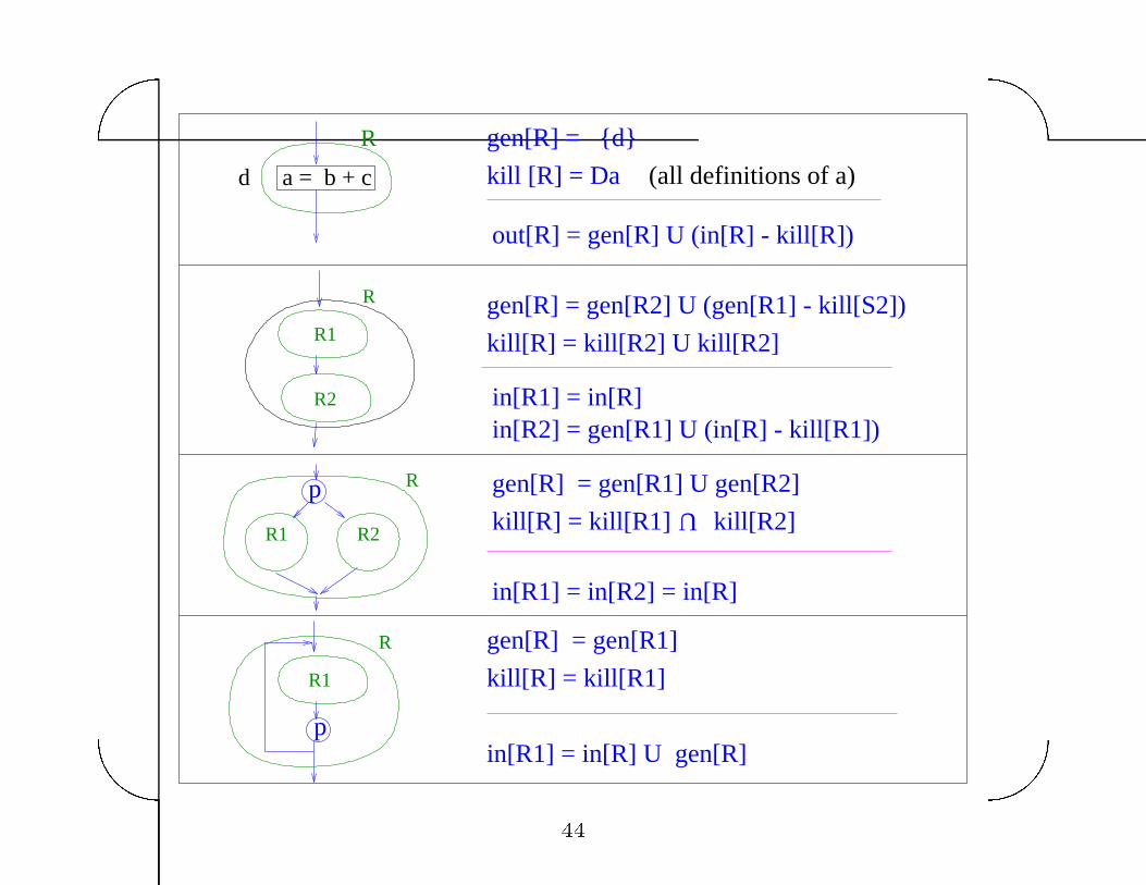
gen[R] = {d}

kill [R] = Da (all definitions of a)

out[R] = gen[R] U (in[R] - kill[R])

gen[R] = gen[R2] U (gen[R1] - kill[S2])

kill[R] = kill[R2] U kill[R2]

gen[R] = gen[R1] U gen[R2]

kill[R] = kill[R1]

U

kill[R2]

gen[R] = gen[R1]

kill[R] = kill[R1]

in[R2] = gen[R1] U (in[R] - kill[R1])in[R1] = in[R]

in[R1] = in[R2] = in[R]

in[R1] = in[R] U gen[R]

��

��

��

Observations�

� For structured programs� we can solve data�ow problems like

reaching de�nitions purely by elimination �without any

iteration� �complexity� O�EV ���

� For structured programs� we can even solve the data�ow

problem directly on the abstract syntax tree �no need to build

the control �ow graph��

� For less structured programs �like reducible programs�� we

must build the control �ow graph to identify regions like

intervals� but there is still no need to iterate�

��

��

��

Exploiting sparsity to speed up data�ow analysis

Example� constant propagation

� CFG algorithm for constant propagation used control �ow

graph to propagate state vectors�

� Propagating information for all variables in lock�step forces a

lot of useless copying information from one vector to another

�consider a variable that is de�ned at top of procedure and

used only at bottom��

Solution�

� do constant propagation for each variable separately

� propagate information directly from de�nitions to uses�

skipping over irrelevant portions of control �ow graph

Subtle point� in what order should we process variables

��

��

��

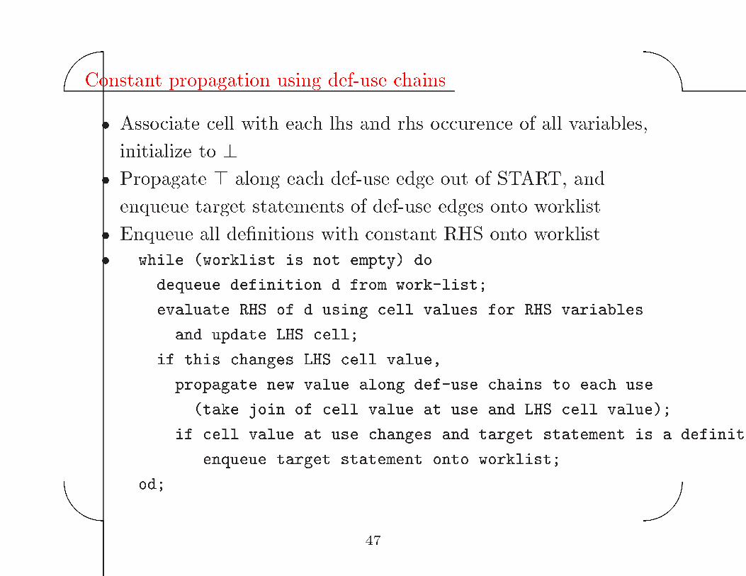
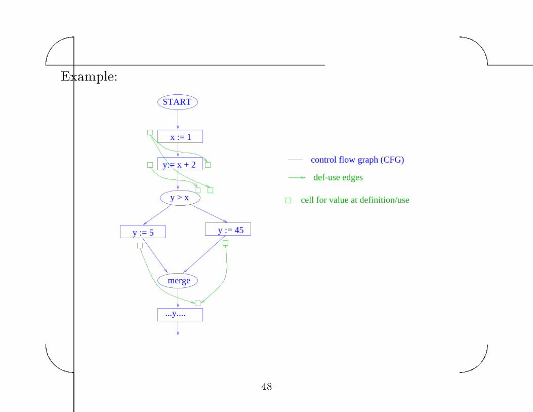
Constant propagation using def�use chains

� Associate cell with each lhs and rhs occurence of all variables�

initialize to ��

� Propagate � along each def�use edge out of START� and

enqueue target statements of def�use edges onto worklist�

� Enqueue all de�nitions with constant RHS onto worklist�

� while �worklist is not empty� do

dequeue definition d from worklist�

evaluate RHS of d using cell values for RHS variables

and update LHS cell�

if this changes LHS cell value�

propagate new value along defuse chains to each use

�take join of cell value at use and LHS cell value��

if cell value at use changes and target statement is a definit

enqueue target statement onto worklist�

od�

��

��

��

Example�

x := 1

START

y:= x + 2

y > x

merge

...y....

y := 45y := 5

control flow graph (CFG)

def-use edges

cell for value at definition/use

��

��

��

Complexity� O�sizeofdef � usechains�

This can be as large O�N�V � where N is size of set of CFG nodes�

However� with SSA form� can be reduced to O�EV ��

Problem with algorithm� loss of accuracy�

Propagation along def�use chains cannot determine directly that

y�� �� is dead code� so last use of y is not marked constant�

One possibility� repeated cycles of reaching de�nition computation�

constant propagation and dead code elimination�

Is there a better way

Key idea�

� �nd unreachable statements during constant propagation

� do not propagate values out of unreachable de�nitions

�

��

��

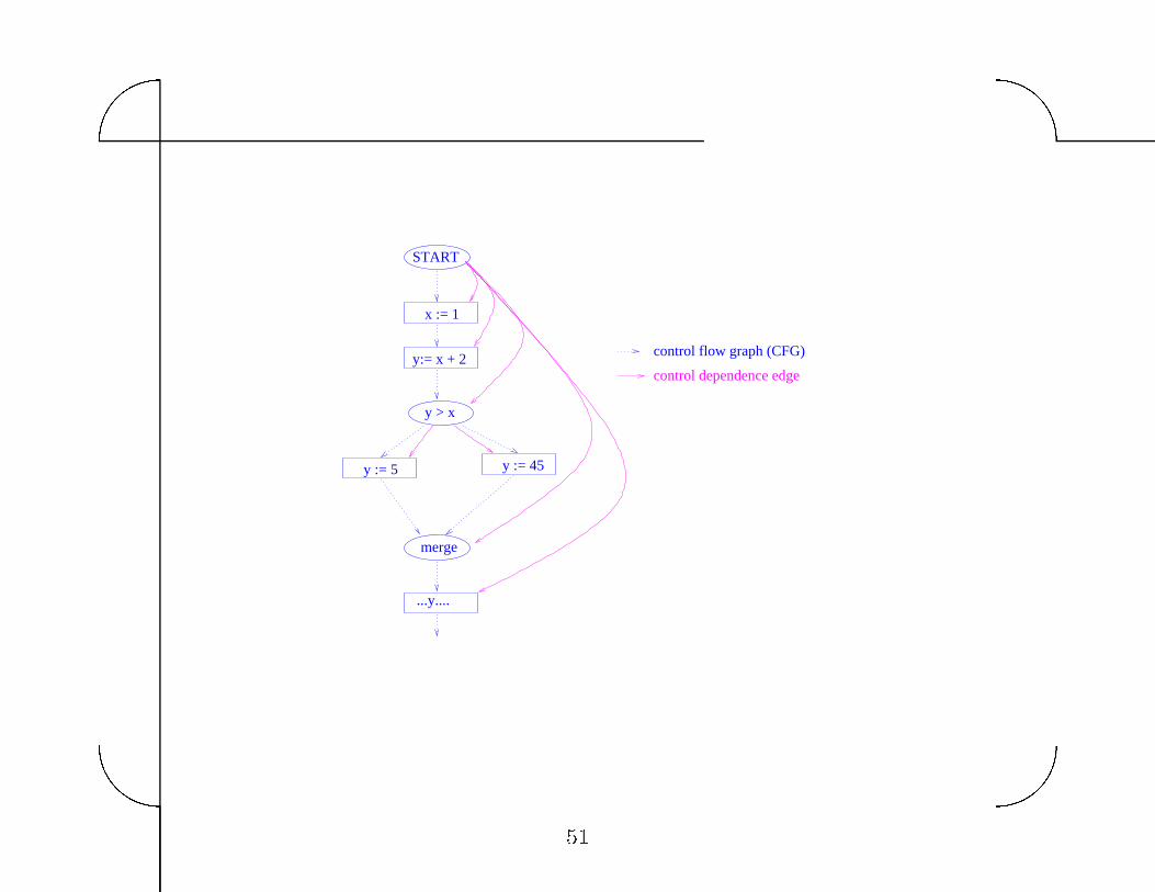
One approach� use control dependence and def�use chains

Intuitive idea of control dependence� Node n is control dependent

on predicate p if p determines whether n is executed�

Convention� assume START is a predicate so unconditionally

executed statements are control dependent on START�

CDG� Control dependence graph�

��

��

x := 1

START

y:= x + 2

y > x

merge

...y....

y := 45y := 5

control flow graph (CFG)

control dependence edge

��

��

��

Algorithm� Propagate �liveness along control dependence edges

while propagating constants along def�use chains�

x := 1

START

y:= x + 2

y > x

merge

...y....

y := xy := 5

control dependence edges

def-use chains

��

��

��

Constant propagation

� Associate cell with each lhs and rhs occurence of all variables�

and with each statement� initialized to �

� Propagate � along each def�use edge and control dependence

edge out of START� If value in any target cell changes� enqueue

target statement onto worklist�

� while �worklist is not empty� do

dequeue statement d from worklist�

if control dependence cell of statement is ��top�

switch �type of d�

case �definition�

�Evaluate RHS of d using cell values for RHS variables

and update LHS cell�

If this changes LHS cell value�

propagate new value along defuse chains to each use

�take join of cell value at use and LHS cell value��

��

��

��

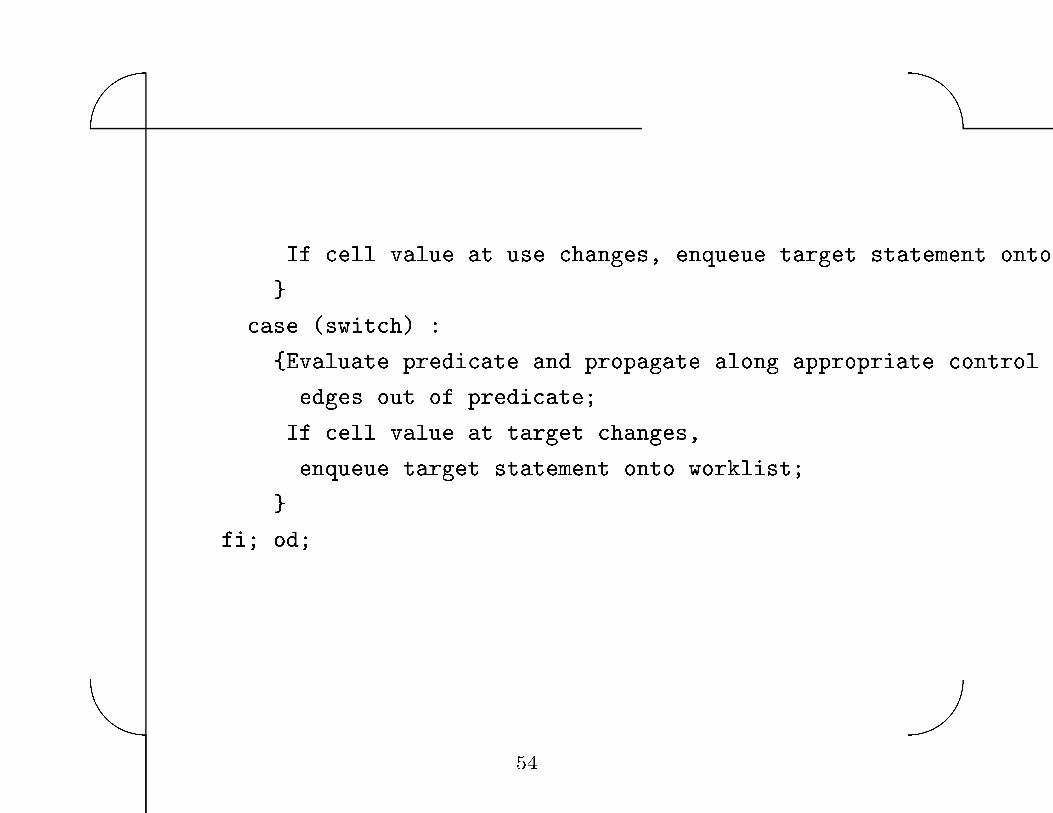
If cell value at use changes� enqueue target statement onto

�case �switch�

�Evaluate predicate and propagate along appropriate control d

edges out of predicate�

If cell value at target changes�

enqueue target statement onto worklist�

�

fi� od�

��

��

��

Observations�

� We do not propagate information out of dead �unreachable�

statements�

� However� precision of information is still not as good as CFG

algorithm� we still propagate information out of statements

that are executed but are irrelevant to output �other sort of

dead statements� as in Slide ���

� Need an algorithm to compute control dependence in general

graphs�

� Size of CDG� O�EN� �can be reduced�

��

��

��

Solutions�

� Require that a variable assigned on one side of a conditional be

assigned on both sides of conditional �by inserting dummy

assignments of form x �� x�� Programmers don�t want to do

this�

� Make compiler insert dummy assignments� Hard to �gure out

in presence of unstructured control �ow�

� Use SSA form� ensure that every use is reached by exactly one

de�nition by inserting ��functions at merges to combine

multiple reaching de�nitions���

��

��

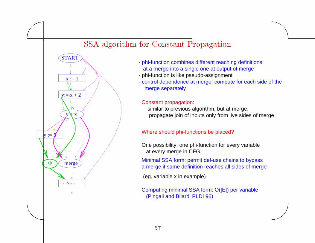
SSA algorithm for Constant Propagation

x := 1

START

y:= x + 2

y > x

y := 5

merge

...y....

Φ

- phi-function is like pseudo-assignment

One possibility: one phi-function for every variable at every merge in CFG.

- phi-function combines different reaching definitions at a merge into a single one at output of merge

- control dependence at merge: compute for each side of the merge separately

Constant propagation:

Where should phi-functions be placed?

similar to previous algorithm, but at merge, propagate join of inputs only from live sides of merge

Computing minimal SSA form: O(|E|) per variable (Pingali and Bilardi PLDI 96)

(eg. variable x in example)

Minimal SSA form: permit def-use chains to bypassa merge if same definition reaches all sides of merge

��

��

��

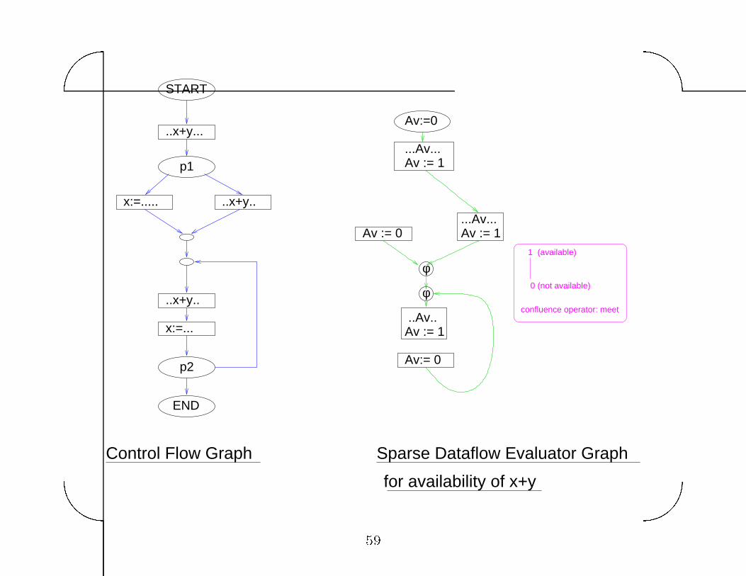
Same idea can be applied to other data�ow analysis problems

� perform data�ow analysis for each sub�problem separately �eg�

for each expression separately in available expressions problem�

� build a sparse graph in which only statements that modify or

use data�ow information for sub�problem are present� and solve

in that

Sparse data�ow evaluator graph can be built in O�jEj� time per

problem �Pingali and Bilardi PLDI����

��

��

��

..x+y...

START

p1

p2

x:=..... ..x+y..

..x+y..

x:=...

END

Control Flow Graph

Av := 1

Av:=0

Av := 0 Av := 1

Av := 1

Av:= 0

...Av...

...Av...

..Av..

φ

φconfluence operator: meet

(not available)

(available)1

0

Sparse Dataflow Evaluator Graph

for availability of x+y

�

��

��

Advantage� sparse graph is usually small and acyclic

Disadvantage� need to solve each sub�problem separately

Many optimizing compilers now use sparse data�ow evaluation

graphs �eg� Intel�s compilers for Merced��

�