scale-based normalization of spectral data. - fred...
TRANSCRIPT

Scale-based normalization of spectral data.
Timothy W. Randolph
Department of BiostatisticsUniversity of Washington
Seattle, WA, 98195206-667-1079
206-667-7998 (fax)[email protected]
November 16, 2005
Abstract
Classification of data that arise as signals or images often requires a standard-ization step so that information extracted from biologically equivalent signals canbe quantified for comparison across classes. Differences in global trend, total en-ergy, high-frequency noise and/or local background can arise from variabilities dueto instrumentation or conditions during data collection. This article considers somecommon ways in which such variation is adjusted for and introduces a generalizationof the popular “standard normal variate” transformation. Examples from three typesof spectroscopy data illustrate the method and its properties.
Keywords: normalization, spectroscopy, preprocessing, standard normal variate, wavelet.
1

1 Introduction
An increasing number of data types being used in the search for disease markers have the
form of spectra, curves or images. These include flow cytometry, liquid chromatography,
elastic light fluorescence and a variety of spectroscopies (near infrared (NIR), light scat-
tering, Raman) [7, 9]. Use of these data for classifying disease status typically requires
some form of normalization that allows for an effective comparison across a heterogeneous
set of samples. Indeed, the data from these highly sensitive instruments can be influenced
by subtle changes in settings or conditions and hence are often contaminated by noise, or
more precisely, non-discriminatory sample-specific signal ranging from broadband back-
ground to high-frequency jitter. In this note we consider some common forms of variability,
review some ways in which they are often handled and then introduce an approach that
adjusts for both global background and local variabilities. We have in mind data from
spectroscopy instrumentations, but the ideas discussed are relevant to signals and images
of many types.
The point of normalization is to perform numerically that which was not able to be
performed physically during data collection; that is, recover exact replicates when no bio-
logical differences exist. Ideally, the sources of non-disease related variation are identified
before attempting to adjust for them. Absent this, some exploratory analysis, in addi-
tion to careful attention to experimental design, is necessary. In a classical univariate
setting one often looks to see how two treatments are manifest in a single individual or
unit, thereby allowing one to account for extraneous within-unit variation. Similarly, to
determine the within-unit variability in a set of spectra before normalization, an impor-
tant first step is to create a set of spectra that are nominally replicates (from the same
biological sample) but collected under a range of conditions—different collection days,
technicians, instrument drift, weather conditions, etc. This seems obvious, but as technol-
ogy advances and highly-refined instrumentation moves from a role similar to that of the
laboratory microscope—where the trained eye of an experienced researcher automatically
sifts through uninformative signal—to that of a high-throughput data generator, the temp-
2

tation is to “shoot first and ask questions later.” Indeed, given a wealth of measurements
it is tempting to think that sorting out signal from noise should be straightforward. The
problem is that when a single datum consists of tens of thousands of correlated values, it
is not obvious which parts of its complex structure reflect informative biologically-related
signal. And even if one has a reasonable description of this signal, a post-hoc analysis of
variance can still be difficult.
In view of this, we consider the problem of normalizing a data set consisting of m spec-
tra, {Si}mi=1, all presumed to contain the exact same biological information, but having
been collected from a range of experimental conditions. For convenience we will assume
each spectrum is a function of intensity measurements S(t) taken at times (or pixel lo-
cations) t in an interval I = [0, 1] (in practice measurements are discretely sampled at
tki , ki = 1, ..., n, where I ⊂ Rp). A time-warping alignment or registration of features
is sometimes needed so that measurements across spectra (Si(t) vs. Sj(t), i 6= j) can be
appropriately compared. We assume this is has been done and focus only on normalization
of intensity.
The goal is to transform these nominally equivalent spectra into m exact replicates,
S̃i ≡ S̃, i = 1, ..., m. This problem has infinitely many solutions including some that
are useless (such as multiplying each spectrum by zero) and some that are minimally
useful (such as transforming each spectrum to a constant; e.g., the grand mean inten-
sity from the entire group). Indeed, a transformation of Si to S̃ should retain as much
information as possible for subsequent use in discrimination between samples. A more
reasonable transformation would be to match each spectrum to the mean spectrum,
M(t) := 1m
∑i Si(t), as in a multiplicative scatter correction [6] which involves a regression
of the form S̃i(t) = ai + biM(t). However, this may not be helpful in applications where
the goal is to normalize a large set of heterogeneous data since even a within-class mean
spectrum might be an inappropriate, or at least attenuated, reference spectrum. One aim
of this note is to retain an empirical approach that does not depend on matching the spec-
tra to an external reference signal. There is, of course, no universally optimal procedure
3
for this problem since the answer depends on how the noise enters the data, which varies
by platform and implementation.
We begin in Section 2 by establishing notation for several assumptions about how noise
versus signal is represented and review some simple methods for normalization. Following
this, Section 3 introduces a method that simultaneously extends the most common of
these methods, bypasses the need for others (such as smoothing and modeling baseline
trends) and incorporates derivative information into the normalization process. Examples
involving spectra from three types of instrumentation are presented in Section 4.
2 Common normalizations of spectra
Let S0 denote a nominal spectrum uncorrupted by noise, and let {Si}mi=1 be the set of
replicate spectra, each consisting of some transformation of S0. The goal is to transform
each replicate to a common signal, Si 7→ S̃i ≡ S̃. Here, S̃ is not necessarily equal to, or even
an estimate of, S0, rather it may be any function that characterizes informative properties
common to the data set. The list that follows mathematically describes some obvious
ways in which variation enters these data and the methods most commonly used to adjust
for them. In practice, some combination of these adjustments would be recommended.
A host of articles have studied the effects of these, and other, preprocessing methods for
calibration of NIR spectra; see, e.g., [3, 5, 18].
Constant shift. If the replicates exhibit a simple vertical offset between spectra so that
Si(t) = S0(t) + ci, the goal is met by subtracting a sample-specific constant from each;
e.g., S̃ := Si −mint∈I{Si(t)}, or S̃ := Si − S̄i, where S̄i denotes the mean of Si on I.
Scaling. If each spectrum contains a different amount of energy (variance), large in-
tensities are magnified more than low intensities: Si(t) = ηi · S0(t). Dividing each spec-
trum by its total energy ||S||2 = (∫I S(t)2 dt)1/2 produces a set of unit-length vectors,
S̃i := Si/||Si||2 = S0/||S0||2. In fact any norm, || · ||, defined on a vector space containing
the spectra will achieve the goal by producing a unit vector in this normed vector space:
4
300 400 500 600 700 8001
1.5
2
2.5
3
3.5
4
4.5
5
5.5
x 104
inte
nsity
(arb
itrar
y un
its)
Raman shift
(a)
300 400 500 600 700 800
−1
0
1
norm
aliz
ed in
tens
ity
Raman shift
(b)
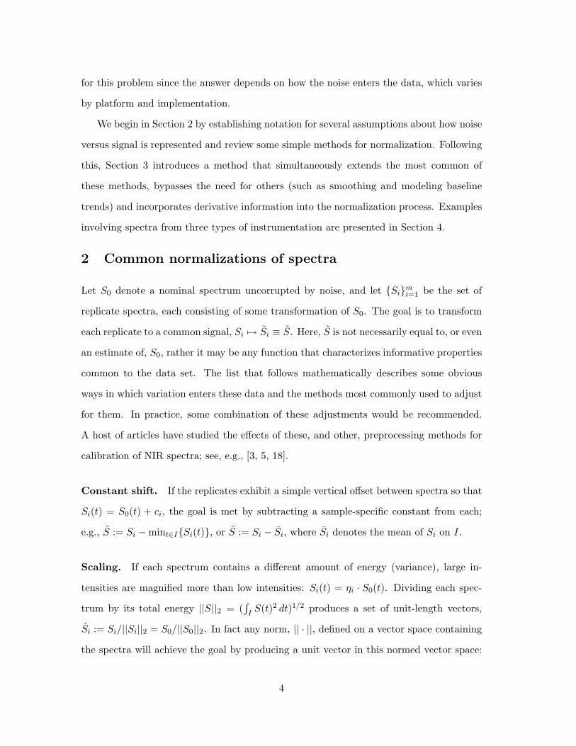
Figure 1: (a) 50 raw surface-enhanced Raman spectra collected on two days, as indicatedby the two colors. (b) The same set of spectra after applying the SNV normalization toeach.
S̃ = S0/||S0|| (||S̃|| = 1).
Standard normal variate. With the goal of both centering (producing mean-zero spec-
tra) and scaling, the popular standard normal variate (SNV) transformation was intro-
duced [2] as:
S̃i(t) := (Si(t)− S̄i)/√
var(Si). (1)
Since var(S) ∝ ||S − S̄||22, the transformation (1) is equivalent to a total-energy scal-
ing applied to a centered signal. In [8] this scaling is put in the context of a family of
normalization procedures, all of which arise from minimizing the variation of S̃i about
a mean, the most common being the multiplicative scatter correction [6] which takes the
form S̃i(t) = (M(t)− ai)/bi.
Figure 1 illustrates a relatively successful application of the SNV transformation to
a set of surface-enhanced Raman spectra. These 50 spectra came from the same bio-
logical sample collected on two different days [16]. The spectra from the two days (as
indicated by color) are biologically identical yet easily distinguished in Figure 1(a) prior
to normalization in Figure 1(b).
5

Baseline correction. A common method of adjusting for a non-constant but low-
frequency baseline is to fit a quadratic function (or other polynomial) Pi, to each spectrum
and use the difference as the normalized spectrum (e.g., [3]). The assumption in this de-
trending step is that Si(t) = S0(t) + Pi(t), where Pi(t) = ait2 + bit + ci, so the adjustment
S̃ := Si − Pi achieves the goal. If a more localized background exists, such as a broad
fluorescence bump as may appear in Raman spectra (see, e.g., [19]), a more refined model
for Pi would be needed.
Smoothing. If the difference between spectra is known to be a random process, Si(t) =
S0(t) + εi(t), then normalization has the additional complication that any adjustments,
S̃i ≈ S̃, are at best approximate in each case. A variety of smoothing (local-averaging)
techniques may be used to obtain a denoised set of essentially equal spectra. The literature
on this important topic is vast; for an example of a wavelet-based smoothing method
applied to Raman spectra, see [4].
Differentiation. Derivatives of spectra play a useful role in processing spectroscopy
signals and algorithms for numerical differentiation are nearly as common as algorithms
for smoothing [15, 12]; see [10] for an introductory discussion. Their use can contribute
to discrimination, resolution enhancement and detrending. For the latter, note that a
quadratic background, Pi, is removed by the second derivative since if Si(t) = S0(t)+Pi(t),
then S′′i (t) = S′′0 (t), so S̃i := S′′i achieves the goal. However, numerical differentiation is
sensitive to high-frequency noise and without sufficient smoothing the process produces a
substantially poorer signal-to-noise ratio than in the original signal. For computation of
numerical derivatives, a window is chosen, the width being dependent on several factors:
the resolution of the instrument (sampling rate); the derivative being estimated (the second
derivative involves a wider window); assumptions about the scale (or width) of informative
features; the intensity of the random process noise (a lower signal-to-noise ratio requires
a wider window).
6
3 Scale-based normalization
The global adjustments made by the SNV transformation (the mean and standard de-
viation) are an attempt to adjust for the fact that features in one signal are offset and
magnified versions of those in another. In the case of unequal and nonconstant trends,
however, no constant scaling factor will transform one signal into another without first
accurately removing these trends. We now introduce a more general and flexible version of
the standard normal variates normalization that is less rigidly tied to either the global vari-
ance or baseline trend of a spectrum. This scale-based approach is based on locally-defined
signal content and includes the SNV normalization as a special case. It allows for greater
control over the extraction of localized signal by exploiting a multiscale decomposition of
each spectrum. Flexibility is implemented by limiting the scales of content extracted and
using only the variance of these portions of the signal. Using all scales coincides with the
SNV normalization whereas restricting scales allows one to bypass high-frequency noise,
wide-scale background and/or global trend without explicitly modelling any of these. As
illustrated by the examples in Section 4, there are several circumstances—i.e., ways in
which noise enters the signals—for which a scale-based normalization may be preferable.
3.1 Mulitscale decomposition
Wavelet-based multiscale analysis of spectral data has been used by several authors for
background correction [17], noise removal [4] and filtering and feature selection [1]. These
approaches are based on the idea that these signals are composed of various scales, or fre-
quency ranges, of information. Moreover, unfolding these scales of content in a time-scale
representation facilitates the process of sorting through informative versus uninformative
signal. The goal here is similar, but of particular interest is the fact that the variance of a
signal is also faithfully decomposed by a wavelet decomposition. For detailed discussions
of wavelet analysis see, e.g., the expository article [14] or the comprehensive text [11]. A
very brief description of a wavelet decomposition follows.
For convenience, it will be assumed that the domain I of a signal S is an interval
7

in R that has been discretely sampled at n “time” points. For this brief discussion, it
is assumed that n = 2j , for some integer j, but in practice this is not necessary. The
discrete wavelet transform (DWT), denoted here by W, comes from a dyadic subsampling
in both time and scale. In time, the dyadic scales roughly correspond to window widths
2j (j = 1, ..., log2 n), while for each fixed j a wavelet coefficient function Wj consists of
n/2j values that result from convolving translates of a scale-j wavelet function with S.
A similar scaling coefficient function, Vj , results from convolving translates of a scale-j
scaling function with S. Properties of the scaling function imply that Wj roughly records
local averages in S.
Equally important to this wavelet analysis is a synthesis. That is, one can form the so-
called detail functions via Dj = W−1(Wj), from which the signal S can be recovered. More
specifically, S can be decomposed into a ladder of detail functions, Dj , each containing
information related to local changes in S occurring on intervals of width 2j : D1 is the
result of extracting changes in S that occur across a 21-unit domain. Writing A1 = S−D1
expresses the approximation after D1 is removed. Similarly, changes in S that occur across
a 2j-unit domain lead to a scale-j detail function, Dj . Continuing through J steps results
in the decomposition
S(t) = AJ(t) +J∑
j=1
Dj(t). (2)
Figure 2 illustrates the concept with one Raman spectrum and a decomposition into
five detail functions, D1, ..., D5, and the remaining approximation function, A5. This
decomposition was performed using the Haar wavelet family; the inset shows a scale-4
Haar wavelet, its shape helping to emphasize the fact that local differences were extracted.
Important properties of this decomposition include the following.
i) The detail functions Dj are mean-zero signals which are, roughly speaking, indepen-
dent of global background. Moveover, features in the original signal (such as local
maxima and inflections) align exactly with events in the detail functions.
8

300 350 400 450 500 550 600 650 700 750 800
D1
D2
D3
D4
D5
A5
S
Figure 2: A multiscale decomposition of a noisy version of a Raman spectrum S (gray)using a Haar wavelet; this wavelet function at scale four is shown in the inset. The detailfunctions, D1 to D5 are shown top to bottom, and the scale-5 approximation appearssuperimposed on S.
ii) A complete decomposition of variance in the signal is preserved by the decomposition:
||S||22 =J∑
j=1
||Wj ||22 + ||VJ ||22 =J∑
j=1
||Dj ||22 + ||AJ ||22. (3)
iii) Using a wavelet having d vanishing moments extracts signal content that is orthog-
onal to all polynomials of degree less than d: if P is a polynomial of degree less than
d and S = S0 + P , then for each j, the wavelet coefficient functions Wj for S and
S0 are equal.
iv) When the wavelet has d vanishing moments, then each scale-j wavelet coefficient
function, Wj , is equal to the dth-order derivative of an averaging of S over a domain
proportional to the jth scale.
If one uses a portion of the decomposition (4), say Dk + ... + DJ , then the analysis
of variance in equation (3) allows a SNV-type transformation that restricts attention to
these scales of signal content:
S̃ = S̃k,J :=Dk + ... + DJ√
var(Dk + ... + DJ)=
Dk + ... + DJ√||Dk||22 + ... + ||DJ ||22
(4)
9

A special case of (4) is the SNV normalization (1) which is recovered by using k = 1 and
J = log2 n. Indeed, in this case AJ = S̄ so the numerator is D1+...+DJ = S−AJ = S−S̄,
while the denominator is the standard deviation of S. Using k > 1 and/or J < log2 n
generalizes (1) to a normalization based on any specific set of scales. The transformation
S 7→ S̃ defined by (4) will be referred to as a scale-based normalization (SBN). The SNV
normalization will be denoted by S̃SNV (= S̃1,J , for J = log2 n). Useful properties of this
normalization result from properties (i)–(iv) of the wavelet decomposition:
a) Interpretation is straightforward since property (i) implies a direct correspondence
between features in S and events in S̃k,J .
b) The need to model a global baseline is eliminated. Indeed, each Di has zero mean
and, by property (iii), S̃k,J is blind to a polynomial background in S when an
appropriate choice of wavelet family is used.
c) Restricting k and J to an appropriate subset of scales produces a normalization
that is less influenced by either high-frequency noise or broadband variation than
SNV. Consequently, local background influences are diminished or removed without
modelling them.
d) A consequence of (iv) is that even in the presence of high-frequency noise, S̃k,J
provides a stable extraction of derivative information. In particular, smoothing is
not a necessary precursor to extracting first or second derivative information which
is an important property when the raw data contains high-frequency noise.
4 Examples of normalizing spectroscopy signals
We consider three different types of spectral signals, the first from a study on the de-
tectability of post-translational modifications in small peptides using surface-enhanced
Raman spectroscopy [16]. A second type comes from near infrared spectroscopy. These
are inherently smoother, yet apparently have different background properties. In each
case, the Daubechies-4 wavelet family (two vanishing moments) was used in producing the
10

SBN transformations. A third example involves MALDI (matrix assisted laser desorption
and ionization) time-of-flight mass spectrometry data where the Haar wavelet family (one
vanishing moment) is used.
4.1 Raman spectra
Figure 1 illustrates the SNV normalization applied to a set of surface-enhanced Raman
spectra. As a means of illustrating properties of the SBN, a simulated polynomial trend
and local background was added to one of these spectra and then processed using SNV
and SBN for k = 4, J = 5. Figure 3(a) shows the two spectra, the simulated background
B (the sum of a quadratic polynomial and an exponential), and the result of adding this
background to one of these spectra. Figures 3(b) and 3(c) show results of the SNV and SBN
transformations, respectively. The SNV normalization is affected by the local background
in the region near wavelength 500. The SBN transformations of S2 and S3 = S2 + B are
essentially identical and nearly coincide with that of S1. The primary differences in these
occur near the ends of the spectra (wavelengths less than 350 and greater than 750); these
are the result of edge effects related to the wavelet transformation.
For reference, we note that the spectra S1 and S2 also appear in Figure 1(a), one from
each of the two days of data collection (same color coding). The background in Figure 3(a)
is of the form B(t) = a1t2+a2t+a3+b1e
−b2(t−200)2 . Figure 4(a) exhibits the same set of 50
spectra from Figure 1(a) after being perturbed by the addition of 50 different backgrounds,
SBi = Si +Bi, where each Bi a random perturbation of B, the coefficients a1, a2, a3, b1 and
b2 chosen from a uniform distribution. Figure 4(b) shows both the SNV and SBN versions
of these signals. Of note is the tight agreement shown by SBN for the spectra within each
day. On the other hand, there are enhanced differences between these two days near 640
and 740. These differences are apparent to a lesser extent in Figure 1.
11

300 400 500 600 700 800
1
2
3
4
5
6
x 104
(a)
300 400 500 600 700 800
−1
0
1
(b)
300 400 500 600 700 800
−1
0
1
2
(c)
Figure 3: (a) A simulated background B, two Raman spectra S1 (gray) and S2 (black),and a modification, S3 = S2 + B (red). (b) The same three signals after applying theSNV normalization to each. (c) The transformation of these three signals using SBN withk = 3, J = 5.
12

350 400 450 500 550 600 650 700 750
2
3
4
5
6
7
8
9
x 104
(a)
350 400 450 500 550 600 650 700 750
−2
−1
0
1
2
(b)
Figure 4: (a) The 50 Raman spectra from Figure 1(a), each perturbed by the additionof a different background (see text). The gray and black colors indicate the two differentcollection days. (b) Two normalizations of the spectra in (a): SNV in the background(black and gray) and SBN with k = 3, J = 5 (dark blue and light blue).
4.2 Near infrared spectra
The next example consists of NIR spectra from pharmaceutical tablets. These come from a
published “ShootOut” data set for the 2002 International Diffuse Reflectance Conference.1
A small random sampling of seven spectra was selected in order to illustrate the flexibility
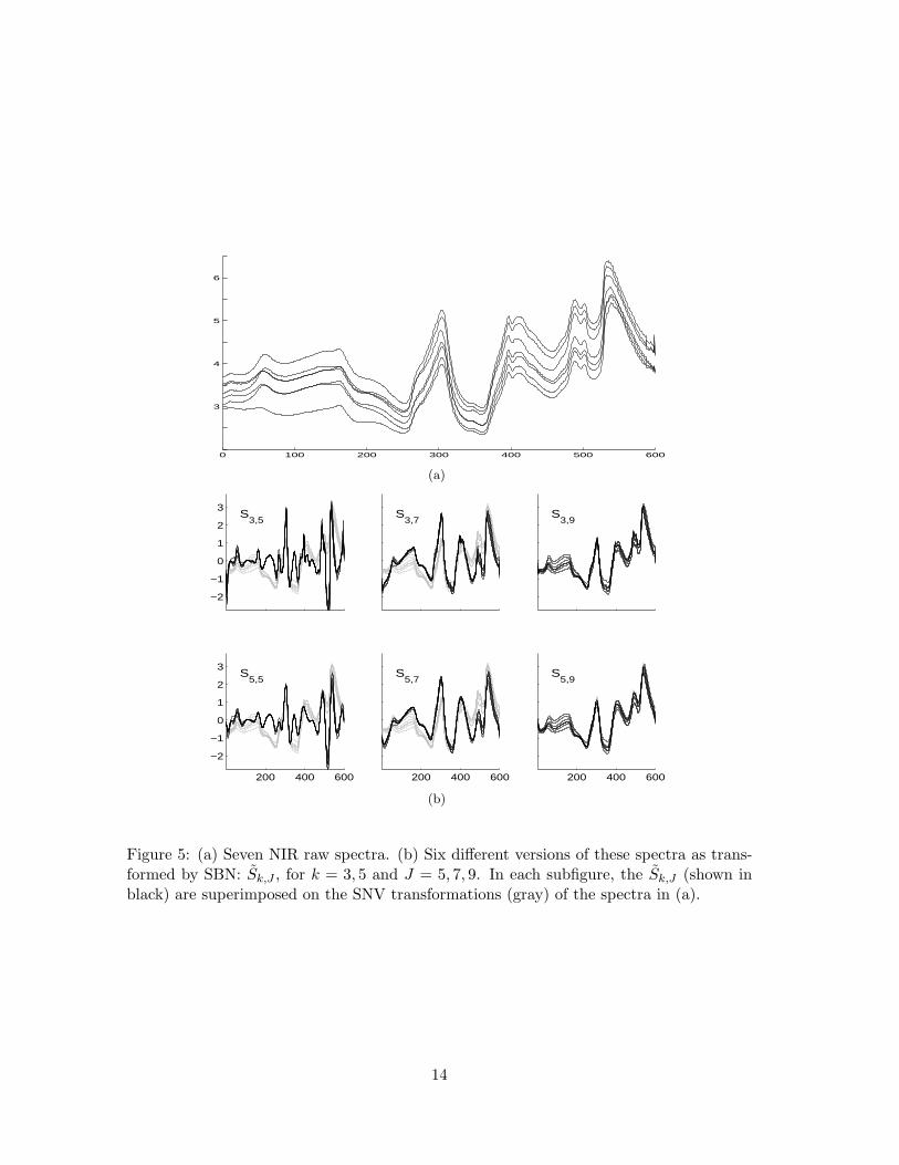
introduced by a scale-based normalization applied to these data. Figure 5(a) shows the
raw spectra and Figure 5(b) shows six different SBN transformations: S̃k,J , for k = 3, 5
and J = 5, 7, 9. In each case the plots are superimposed on the SVN transformations
of these spectra. Note that S̃3,9 and S̃5,9 essentially reproduce the SVN transformation.
Indeed, these are close approximations to S̃1,9 = S̃SNV since the raw spectra are relatively
smooth and contain little scale-1 through scale-4 content. At the finest scales, as in S̃3,5,
subtle local features are magnified, whereas a focus on midrange scales via S̃3,7 or S̃5,7
produces both a resolution enhancement and a tight agreement in this set of spectra.
4.3 MALDI-TOF spectra
Five MALDI mass spectrometry spectra from the same biological sample that were ob-
tained during a dilution experiment [13] are graphed in Figure 6 after being normalized in1www.idrc-chambersburg.org/shootout 2002.htm
13
0 100 200 300 400 500 600
3
4
5
6
(a)
−2
−1
0
1
2
3S
3,5
S
3,7
S
3,9
200 400 600
−2
−1
0
1
2
3S
5,5
200 400 600
S
5,7
200 400 600
S
5,9
(b)
Figure 5: (a) Seven NIR raw spectra. (b) Six different versions of these spectra as trans-formed by SBN: S̃k,J , for k = 3, 5 and J = 5, 7, 9. In each subfigure, the S̃k,J (shown inblack) are superimposed on the SNV transformations (gray) of the spectra in (a).
14
1.96 1.98 2 2.02 2.04 2.06 2.08 2.1
x 104
0
1
2
3
4
5
inte
nsity
(arb
itrar
y un
its)
time of flight
(a)
1.96 1.98 2 2.02 2.04 2.06 2.08 2.1
x 104
0
1
2
inte
nsity
(arb
itrar
y un
its)
time of flight
(b)
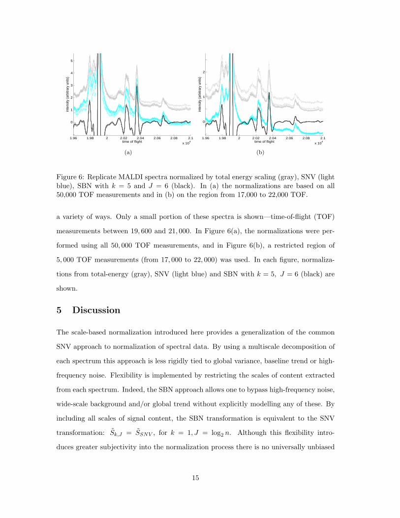
Figure 6: Replicate MALDI spectra normalized by total energy scaling (gray), SNV (lightblue), SBN with k = 5 and J = 6 (black). In (a) the normalizations are based on all50,000 TOF measurements and in (b) on the region from 17,000 to 22,000 TOF.
a variety of ways. Only a small portion of these spectra is shown—time-of-flight (TOF)
measurements between 19, 600 and 21, 000. In Figure 6(a), the normalizations were per-
formed using all 50, 000 TOF measurements, and in Figure 6(b), a restricted region of
5, 000 TOF measurements (from 17, 000 to 22, 000) was used. In each figure, normaliza-
tions from total-energy (gray), SNV (light blue) and SBN with k = 5, J = 6 (black) are
shown.
5 Discussion
The scale-based normalization introduced here provides a generalization of the common
SNV approach to normalization of spectral data. By using a multiscale decomposition of
each spectrum this approach is less rigidly tied to global variance, baseline trend or high-
frequency noise. Flexibility is implemented by restricting the scales of content extracted
from each spectrum. Indeed, the SBN approach allows one to bypass high-frequency noise,
wide-scale background and/or global trend without explicitly modelling any of these. By
including all scales of signal content, the SBN transformation is equivalent to the SNV
transformation: S̃k,J = S̃SNV , for k = 1, J = log2 n. Although this flexibility intro-
duces greater subjectivity into the normalization process there is no universally unbiased
15

method that optimally adjusts for all manners in which variation enters the data; careful
experimental design and exploratory study of signal content is required in this and every
normalization process.
Extracting individual scales of content is implemented through a wavelet multiscale
decomposition. Since a wavelet transform acts as differential operator, an added benefit
is the potential resolution enhancement obtained by extracting derivative information
without the need to first smooth each spectrum. This is particularly important when the
raw spectra contain high-frequency noise since the use of derivatives, though common in
the analysis of spectral data, is primarily limited to relatively smooth spectra due to the
potential instability of numerical differentiation procedures.
Examples from three types of instrumentation illustrate some of the properties of a
scale-based normalization. Simulating a variety of random backgrounds in a large set
of Raman spectra, the first example contrasts the SNV transformation with its scale-
restricted cousin, SBN. Using a set of NIR spectra, a second example exhibits the results
from of a wide range of SBN transformations. Finally, a set of MALDI mass spectrometry
spectra, each having 50,000 intensity measurements illustrates the robustness of SBN with
respect to global properties in the data.
Acknowledgements
This research was financially supported by National Institutes of Health grant GM67211.
Additional support from CA086368 is gratefully acknowledged.
References
[1] B. R. Bakshi, Multiscale analysis and modeling using wavelets, Journal of Chemomet-
rics 13 (1999), 415–434.
[2] R. J. Barnes, M. S. Dhanoa, and S. Lister, Standard normal variate transformation
and de-trending of near-infrared diffuse reflectance spectra, Applied Spectroscopy 43
(1989), no. 5, 772–777.
16

[3] M. Blanco, J. Coello, H. Iturriaga, S. Maspoch, and C. D. L. Pezuela, Effect of data
preprocessing methods in near-infrared diffuse reflectance spectroscopy for the determi-
nation of the active compound in a pharmaceutical preparation, Applied Spectroscopy
51 (1997), no. 2, 240–246.
[4] T. T. Cai, D. Zhang, and D. Ben-Amotz, Enhanced chemical classification of raman
images using multiresolution wavelet transformation, Applied Spectroscopy 55 (2001),
no. 9, 1124–1130.
[5] A. Candolfi, R. De Maesschalck, D. Jouan-Rimbaud, P. A. Hailey, and D. L. Massart,
The influence of data pre-processing in the pattern recognition of excipients near-
infrared spectra, Journal of Pharmaceutical and Biomedical Analysis 21 (1999), 115–
132.
[6] P. Geladi, D. MacDougall, and H. Martens, Linearization and scatter-correction for
near-infrared reflectance spectra of meat, Applied Spectroscopy 39 (1985).
[7] R. S. Gurjar, V. Backman, L. T. Perelman, I. Georgakoudi, K. Badizadegan, I. Itzkan,
and R. Dasari M. S. Feld, Imaging human epithelial properties with polarized lightscat-
tering spectroscopy, Nature Medicine 7 (2001), no. 11, 1245–1248.
[8] I. S. Helland, T. Naes, and T. Isaksson, Related versions of the multiplicative scatter
correction method for preprocessing spectroscopic data, Chemometrics and Intelligent
Laboratory Systems 29 (1995), 233–241.
[9] M. MacRae, Rays of hope: Spectroscopy as an emerging tool for cancer diagnostics
and monitoring, Spectroscopy 18 (2003), no. 10, 14–19.
[10] H. Mark and J. Workman, Derivatives in spectroscopy, Part III–computing the deriva-
tive, Spectroscopy 18 (2003), no. 4, 106–111.
[11] D. B. Percival and A. T. Walden, Wavelet methods for time series analysis, Cambridge
University Press, Cambridge, UK, 2000.
17
[12] W. H. Press, S. A. Teukolsky, W. T. Vetterling, and B. P. Flannery, Numerical recipes
in c, the art of scientific computing, 2nd ed., Cambridge University Press, Cambridge,
UK, 1992.
[13] T. Randolph, B. Mitchell, D. McLerran, P. Lampe, and Z. Feng, Quantifying peptide
signal in MALDI-TOF mass spectrometry data, Molecular and Cellular Proteomics
(2005), in press.
[14] P. Sajda, A. Laine, and Y. Zeevi, Multi-resolution and wavelet representations for
identifying signatures of disease, Disease Markers 18 (2002), no. 5–6, 339–363.
[15] A. Savitzky and M.J.E. Golay, Smoothing and differentiation of data by simplified
least squares pro,cedures, Analytical Chemistry 36 (1964), 1627–1639.
[16] N. Sundararajana, D. Mao, S. Chan, T-W. Koo, X. Su, L. Sun, J. Zhang, K b. Sung,
M. Yamakawa, P. R. Gafken, T. Randolph, D. McLerran, Z. Feng, A. A. Berlin, and
M. B. Roth, Ultra-sensitive detection and analysis of post-translational modifications
using surface enhanced raman spectroscopy (SERS), (2005), submitted.
[17] H.-W. Tan and S. D. Brown, Wavelet analysis applied to removing non-constant,
varying spectroscopic background in multivariate calibration, Journal of Chemometrics
16 (2002), 228–240.
[18] M. Zeaiter, J.-M. Roger, and V. Bellon-Maurel, Robustness of models developed by
multivariate calibration. Part II: The influence of pre-processing methods, Trends in
Analytical Chemistry 24 (2005), no. 5, 437–445.
[19] D. Zhang and D. Ben-Amotz, Enhanced chemical classification of raman images in the
presence of strong fluorescence interference, Applied Spectroscopy 54 (2000), no. 9,
1379–1383.
18