scalelength of disc galaxies - diva portal

Mon. Not. R. Astron. Soc. 406, 1595–1608 (2010) doi:10.1111/j.1365-2966.2010.16812.x

Scalelength of disc galaxies

Kambiz Fathi,1,2� Mark Allen,3 Thomas Boch,3 Evanthia Hatziminaoglou4

and Reynier F. Peletier5

1Stockholm Observatory, Department of Astronomy, Stockholm University, AlbaNova Center, 106 91 Stockholm, Sweden2Oskar Klein Centre for Cosmoparticle Physics, Stockholm University, 106 91 Stockholm, Sweden3Observatoire de Strasbourg, UMR 7550, Strasbourg 67000, France4European Southern Observatory, Karl-Schwarzschild-Str. 2, 85748 Garching bei Munchen, Germany5Kapteyn Astronomical Institute, Postbus 800, 9700 AV Groningen, the Netherlands

Accepted 2010 April 7. Received 2010 April 2; in original form 2010 February 18

ABSTRACTWe have derived disc scalelengths for 30 374 non-interacting disc galaxies in all five SloanDigital Sky Survey (SDSS) bands. Virtual Observatory methods and tools were used to define,retrieve and analyse the images for this unprecedentedly large sample classified as disc/spiralgalaxies in the LEDA catalogue. Cross-correlation of the SDSS sample with the LEDAcatalogue allowed us to investigate the variation of the scalelengths for different types ofdisc/spiral galaxies. We further investigate asymmetry, concentration and central velocitydispersion as indicators of morphological type, and are able to assess how the scalelengthvaries with respect to galaxy type. We note, however, that the concentration and asymmetryparameters have to be used with caution when investigating type dependence of structuralparameters in galaxies. Here, we present the scalelength derivation method and numeroustests that we have carried out to investigate the reliability of our results. The average r-banddisc scalelength is 3.79 kpc, with an rms dispersion of 2.05 kpc, and this is a typical valueirrespective of passband and galaxy morphology, concentration and asymmetry. The derivedscalelengths presented here are representative for a typical galaxy mass of 1010.8±0.54 M�, andthe rms dispersion is larger for more massive galaxies. Separating the derived scalelengths fordifferent galaxy masses, the r-band scalelength is 1.52 ± 0.65 kpc for galaxies with total stellarmass 109–1010 M� and 5.73 ± 1.94 kpc for galaxies with total stellar mass between 1011 and1012 M�. Distributions and typical trends of scalelengths have also been derived in all theother SDSS bands with linear relations that indicate the relation that connect scalelengths inone passband to another. Such transformations could be used to test the results of forthcomingcosmological simulations of galaxy formation and evolution of the Hubble sequence.

Key words: galaxies: structure.

1 IN T RO D U C T I O N

The exponential scalelength of a galaxy disc is one of the mostfundamental parameters to determine its morphological structureas well as to model its dynamics, and the fact that the light distribu-tions are exponential makes it possible to constrain the formationmechanisms (Freeman 1970). The scalelength determines how thestars are distributed throughout a disc, and can be used to deriveits mass distribution, assuming a specific M/L ratio. Ultimately,this mass distribution is the primary constraint for determining theformation scenario (e.g. Lin & Pringle 1987; Dutton 2009, andreferenced therein), which dictates the galaxy’s evolution. As the

�E-mail: [email protected]

galaxy evolves, substructures such as bulges, pseudo-bulges, bars,rings and spiral arms may build up, and this will then considerablychange the morphology of the host discs (Combes & Elmegreen1993; Elmegreen et al. 2005; Bournaud, Elmegreen & Elmegreen2007). The scalelength value is intimately connected to the cir-cular velocity of the galaxy halo, which in turn relates closely tothe angular momentum of the halo in which the disc is formed(Dalcanton, Spergel & Summers 1997; Mo, Mao & White 1998).Up to the last few years, cosmological simulations were limitedto rather low resolution, were discs and spheroids were barely re-solved, and generally limited to high redshifts, so reproducing real-istic disc scalelengths for modern galaxies was clearly out of reach.The current simulations reach resolutions that allow resolving thediscs from high redshift down to redshift zero, and subtle mech-anisms changing the disc masses and scalelengths can be studied

C© 2010 The Authors. Journal compilation C© 2010 RAS

1596 K. Fathi et al.

(e.g. Ceverino, Dekel & Bournaud 2010; Governato et al. 2010;Martig & Bournaud 2010; Schaye et al. 2010), thus calling for acomprehensive observational determination of these parameters totest the state of the art cosmological simulations.

Previous observations of NGC, UGC and low surface brightnessgalaxies have shown that scalelengths span over a range of three or-ders of magnitudes (e.g. Boroson 1981; Romanishin, Strom & Strom1983; van der Kruit 1987; Schombert et al. 1992; Knezek 1993; deJong 1996). Any physical galaxy formation scenario should be ableto explain this wide range of values while simultaneously explainingthe similarities among disc galaxies throughout this range.

Analytic disc formation scenarios predict that, in cases whereangular momentum is conserved, the disc scalelength is determinedby the angular momentum profile of the initial cloud (Lin & Pringle1987), and the scalelength in a viscous disc is set by the interplaybetween star formation and dynamical friction (Silk 2001). Theseprocesses form the basis of a galaxy’s gravitational potential, anddetermine the strength of gravitational perturbations, the locationof resonances in the disc, the formation and evolution of spiralarms and bars, kinematically decoupled components in centres ofgalaxies, and the dynamical feeding of circumnuclear starbursts andnuclear activity (e.g. Elmegreen et al. 1996; Fathi 2004; Knapen2004; Kormendy & Kennicutt 2004).

Photometrically, one generally derived this scalelength by az-imuthally averaging profiles of the surface brightness which is inturn decomposed into a central bulge and an exponential disc, andwhen spatial resolution allows other components such as one orseveral bars and rings can be taken into account.

As images in different bands probe different optical depths and/orstellar populations, it is likely that a derived scalelength value shoulddepend on waveband, and these effects may vary as a function ofgalaxy type where different amounts of dust and star formation areexpected. Dusty discs are more opaque, resulting in larger scale-length values in bluer bands when compared with red and/or in-frared images. Similar effects can also be caused by differencesin the stellar populations. Differences in scalelength as a func-tion of passband can therefore be used to derive information aboutthe stellar structure and contents of galactic discs. Both the ef-fects of stellar populations and dust extinction have been subjectto much discussion over the years (e.g. Simien & de Vaucouleurs1983; Kent 1985; Valentijn 1990; Peletier et al. 1994, 1995; vanDriel et al. 1995; Beckman et al. 1996; Courteau 1996; Baggett,Baggett & Anderson 1998; Cunow 1998, 2001, 2004; Graham 2001;Graham & de Blok 2001; Prieto et al. 2001; Giovanelly &Haynes 2002; MacArthur, Courteau & Holtzman 2003; Graham &Worley 2008). A detailed and extensive analysis of the dust effectshas also been presented for a few tens of galaxies in Holwerda(2005) and subsequent papers by this author, however, as noted byPeletier et al. (1994) and van Driel et al. (1995), the scalelengthalone in different wavelengths in small sample cannot be used tobreak the age/metallicity and dust degeneracies. Investigating thescalelength variation as a function of inclination for large numbersof galaxies is necessary to distinguish between the effects of dustand stellar populations.

The common denominator in all the previous studies is theroughly comparable sample sizes (at most few hundred galaxies).Most studies have so far analysed individual galaxies, or sam-ples containing a few tens, and in unique cases a few hundred(e.g. Knapen & van der Kruit 1991; Courteau 1996) galaxies. Al-though a number of great results from studies with the Sloan DigitalSky Survey (SDSS; York et al. 2000) in the last years have appeared,

these works have not studied the astrophysical parameters targetedhere.

As a part of a European Virtual Observatory1 Astronomical In-frastructure for Data Access (Euro-VO AIDA) research initiative,we have undertaken a comprehensive analysis of the scalelengthin disc galaxies using an unprecedentedly large sample of discgalaxies. We have used the Virtual Observatory (VO) tools to re-trieve data in all (u, g, r, i and z) bands from the sixth SDSS majordata release (DR6; Adelman-McCarthy et al. 2008) which includesimaging catalogues, spectra and redshifts freely available. We usethe LEDA2 catalogue (Paturel et al. 2003) to retrieve morphologicalclassification information about our sample galaxies, and those withtypes defined as Sa or later are hereafter refereed to as disc galaxies(distribution of both samples is presented in Fig. 1).

In the present paper, we present the data retrieval and analysismethod used to automatically derive the scalelengths for a sample ofdisc galaxies which contains 56 096 objects (described in Section 2),and after rigorous tests described in Section 3, we find that a subsetof 30 374 of these can be called reliable following these criteria.The scalelengths presented here relate only to the disc components,and we have tried to avoid the regions that could be dominated bythe bulge component, in order to avoid complications related to theuncertainties of bulge–disc decomposition procedure (as demon-strated in e.g. Knapen & van der Kruit 1991). In Section 4 wepresent the first results based on our unprecedentedly large sampleof galaxies and finally discuss their implications in Section 5.

2 SAMPLE G ALAXIES FROM SDSS

2.1 First selection criteria

The DR6 provides imaging catalogues, spectra and redshifts for thethird and final data release of SDSS-II, an extension of the originalSDSS consisting of three subprojects: the Legacy Survey, the SloanExtension for Galactic Understanding and Exploration and a Su-pernova Survey. The SDSS Catalogue Archive Server Jobs System3

allow for a sample selection based on a number of useful morpho-logical and spectroscopic parameters provided for all objects. Weuse these parameters and make a first selection of the entire SDSSDR6 sample. Various VO methods were investigated to perform thedownload of the SDSS images, and the SkyView4 was chosen forthis task. This service has the advantage of being able to create fitscut outs centred at a given sky coordinate and with a given size.Moreover, SkyView is able to rescale the image backgrounds tothe same level, hence correcting for background level differencesbetween the SDSS tiles.

The image size is an important parameter to achieve a reliablesky subtraction which is necessary to derive realistic scalelengths,thus we require that the images cover an area at least three timesthe size of each galaxy. To optimize the data handling and keep lowdata transfer time from SkyView, we chose a constant image sizeof 900 × 900 pixels to be sampled for all galaxies, still being ableto achieve a reliable sky subtraction. With these specifications, theimage size is 3.2 MB with the typical download time of 16 s per

1http://www.euro-vo.org2http://leda.univ-lyon1.fr3http://casjobs.sdss.org4http://skyview.gsfc.nasa.gov

C© 2010 The Authors. Journal compilation C© 2010 RAS, MNRAS 406, 1595–1608

Scalelength of disc galaxies 1597

0 5 10 15 20

-20

0

20

40

60

80

100L

ED

A D

eclin

atio

n (

J2

00

0)

698800 galaxies

0 5 10 15 20

0

20

40

60

80

SD

SS

De

clin

atio

n (

J2

00

0) 56096 galaxies

0 5 10 15 20Right Ascension (J2000)

0

20

40

60

80

SD

SS

De

clin

atio

n (

J2

00

0) 30374 galaxies

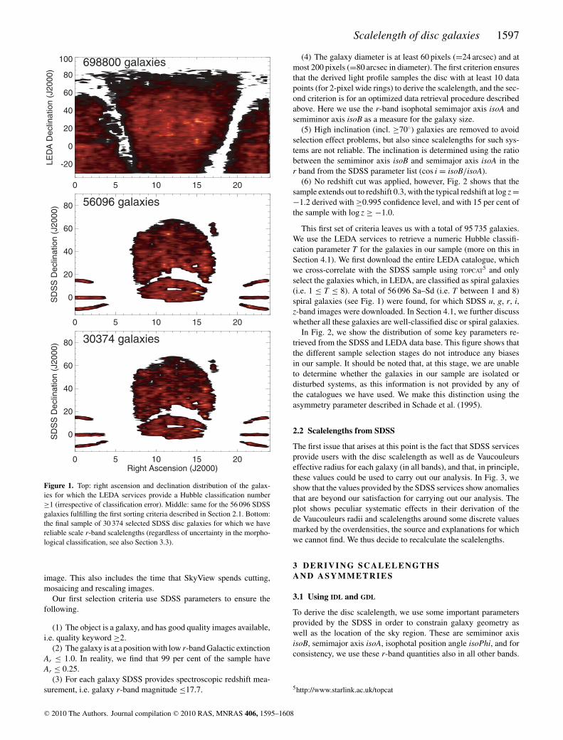
Figure 1. Top: right ascension and declination distribution of the galax-ies for which the LEDA services provide a Hubble classification number≥1 (irrespective of classification error). Middle: same for the 56 096 SDSSgalaxies fulfilling the first sorting criteria described in Section 2.1. Bottom:the final sample of 30 374 selected SDSS disc galaxies for which we havereliable scale r-band scalelengths (regardless of uncertainty in the morpho-logical classification, see also Section 3.3).

image. This also includes the time that SkyView spends cutting,mosaicing and rescaling images.

Our first selection criteria use SDSS parameters to ensure thefollowing.

(1) The object is a galaxy, and has good quality images available,i.e. quality keyword ≥2.

(2) The galaxy is at a position with low r-band Galactic extinctionAr ≤ 1.0. In reality, we find that 99 per cent of the sample haveAr ≤ 0.25.

(3) For each galaxy SDSS provides spectroscopic redshift mea-surement, i.e. galaxy r-band magnitude ≤17.7.

(4) The galaxy diameter is at least 60 pixels (=24 arcsec) and atmost 200 pixels (=80 arcsec in diameter). The first criterion ensuresthat the derived light profile samples the disc with at least 10 datapoints (for 2-pixel wide rings) to derive the scalelength, and the sec-ond criterion is for an optimized data retrieval procedure describedabove. Here we use the r-band isophotal semimajor axis isoA andsemiminor axis isoB as a measure for the galaxy size.

(5) High inclination (incl. ≥70◦) galaxies are removed to avoidselection effect problems, but also since scalelengths for such sys-tems are not reliable. The inclination is determined using the ratiobetween the semiminor axis isoB and semimajor axis isoA in ther band from the SDSS parameter list (cos i = isoB/isoA).

(6) No redshift cut was applied, however, Fig. 2 shows that thesample extends out to redshift 0.3, with the typical redshift at log z =−1.2 derived with ≥0.995 confidence level, and with 15 per cent ofthe sample with log z ≥ −1.0.

This first set of criteria leaves us with a total of 95 735 galaxies.We use the LEDA services to retrieve a numeric Hubble classifi-cation parameter T for the galaxies in our sample (more on this inSection 4.1). We first download the entire LEDA catalogue, whichwe cross-correlate with the SDSS sample using TOPCAT5 and onlyselect the galaxies which, in LEDA, are classified as spiral galaxies(i.e. 1 ≤ T ≤ 8). A total of 56 096 Sa–Sd (i.e. T between 1 and 8)spiral galaxies (see Fig. 1) were found, for which SDSS u, g, r, i,z-band images were downloaded. In Section 4.1, we further discusswhether all these galaxies are well-classified disc or spiral galaxies.

In Fig. 2, we show the distribution of some key parameters re-trieved from the SDSS and LEDA data base. This figure shows thatthe different sample selection stages do not introduce any biasesin our sample. It should be noted that, at this stage, we are unableto determine whether the galaxies in our sample are isolated ordisturbed systems, as this information is not provided by any ofthe catalogues we have used. We make this distinction using theasymmetry parameter described in Schade et al. (1995).

2.2 Scalelengths from SDSS

The first issue that arises at this point is the fact that SDSS servicesprovide users with the disc scalelength as well as de Vaucouleurseffective radius for each galaxy (in all bands), and that, in principle,these values could be used to carry out our analysis. In Fig. 3, weshow that the values provided by the SDSS services show anomaliesthat are beyond our satisfaction for carrying out our analysis. Theplot shows peculiar systematic effects in their derivation of thede Vaucouleurs radii and scalelengths around some discrete valuesmarked by the overdensities, the source and explanations for whichwe cannot find. We thus decide to recalculate the scalelengths.

3 D E R I V I N G SC A L E L E N G T H SAND ASYMMETRI ES

3.1 Using IDL and GDL

To derive the disc scalelength, we use some important parametersprovided by the SDSS in order to constrain galaxy geometry aswell as the location of the sky region. These are semiminor axisisoB, semimajor axis isoA, isophotal position angle isoPhi, and forconsistency, we use these r-band quantities also in all other bands.

5http://www.starlink.ac.uk/topcat



12 13 14 15 16 17 18Magnitude (r-band)

0

1000

2000

3000

4000

Co

un

ts

14 16 18 20 22Magnitude (u-band)

0

1000

2000

3000

Co

un

ts

0 20 40 60 80Inclination (r-band)

0

1000

2000

3000

Co

un

ts

0.0 0.1 0.2 0.3 0.4 0.5 0.6Galactic Extinction (r-band)

0

2000

4000

6000

8000

Co

un

ts

0.00 0.05 0.10 0.15 0.20 0.25 0.30Spectroscopic Redshift

0

2000

4000

6000

8000

Co

un

ts

0 100 200 300 400Velocity Dispersion

0

2000

4000

6000

Co

un

ts

30 40 50 60 70 80 90 100Major Axis (r-band)

0

4.0•103

8.0•103

1.2•104

Co

un

ts

0 2 4 6 8Morphological Type from LEDA

0

4.0•103

8.0•103

1.2•104

Co

un

ts

Figure 2. Distribution of some key parameters retrieved from the SDSS data base and morphological types from LEDA (bottom right). The filled histogramsare the 56 096 disc galaxies described in Section 2.1, and the open histograms show the distributions of the final 30 374 galaxies for which we derive reliablescalelengths. The distribution of the sample remains unchanged.

0.0 0.2 0.4 0.6 0.8 1.0 1.2 1.4Scale Length from SDSS [log(arcsec)]

0.0

0.2

0.4

0.6

0.8

1.0

1.2

1.4

de

Va

uco

ule

urs

Ra

diu

s f

rom

SD

SS

[lo

g(a

rcse

c)]

1 33 65

Figure 3. Density plot of the de Vaucouleurs effective radius (y-axis) versusexponential disc radius (x-axis) provided by the SDSS service for the entiredisc galaxy sample. The odd clustering of the data (overdensities arounddiscrete values) show the strong systematic effects in these two parametersprovided by the SDSS team.

Our scalelength derivation routine uses standard IDL routines, thoughdue to license limitations this code can only be executed once, andhence is estimated to take a long time to run. Using one single IDL

session, we would need 47 d to derive the scalelengths for the entiresample, thus in order to speed up the process, we decided to run thiscomputation on a cluster of machines located at Centre de Donneesastronomiques de Strasbourg CDS. Since the freely available IDL

virtual machine does not allow one to launch batch queries, andsince installing an IDL licence on each cluster node was not anoption, we used the open source clone of IDL, GNU Data Language(GDL; Coulais et al. 2009). We found out that a few IDL functionswere either missing or behaving improperly, thus requiring minortweaking in our code. Then, we ran both IDL and GDL code on thesame subset of SDSS images, in order to check the reliability of theGDL output.

Once the GDL code was installed on each node of the cluster, the56 096 SDSS images were put to an iRods6 installation deployedat CDS. Finally, the scalelength computation was launched on thecluster, using the following architecture.

(i) A JAVA program holds the list of galaxies to process, and – foreach object of this list – sends a message to the cluster, asking tospawn a new job (i.e. launch the corresponding computation).

6iRods (www.irods.org) is a distributed data management system, whichprovides a distributed storage environment to easily store and share files.



(ii) The cluster master node receives the request, and dispatchesit to the cluster node with the smallest CPU load.

(iii) The cluster node then downloads from iRods the u, g, r, i, zimages corresponding to the galaxy to process, runs the GDL codeand sends back the computed result to iRods.

(iv) If the computation fails, it will be resent to another node untilsuccess.

The CDS cluster has proven to be very stable and reliable, thoughsome problems were found in the dispatching algorithm, resultingsometimes in overloading some of the nodes while some others wereidle. Four nodes of the cluster were dedicated to our computation.As the total computation time is roughly proportional to the numberof involved nodes, allocating 10 times more nodes would havedecreased this time by a factor of 10. This would only be true if thecomputation service were to be close to the data, so that the transfer

time would be negligible with respect to the computation time. Intheory, on the CDS cluster, with four dedicated nodes, we shouldhave been able to process 11 200 galaxies d−1, however, in reality,the cluster only processed between 8500 and 9000 galaxies d−1,which could be explained by some inefficiency in the dispatchingalgorithm. To conclude, using the CDS, we have been able to derivethe scalelengths for all 56 090 galaxies in all five SDSS bands inless than a week.

3.2 The procedure

The procedure to derive scalelength and calculate asymmetry pa-rameters from the SDSS images is illustrated in Fig. 4 and carriesout the following steps.

r-band ID: 587730816827981899

-100 0 100arcsec

-100

0

100

arc

se

c

Masked and sky subtrcated

-100 0 100arcsec

-100

0

100

arc

se

c

Asym= 0.41 rd=28.2 rdSDSS=9.0

0 20 40 60 80arcsec

28

26

24

22

20

r-b

an

d μ

r-band ID: 587728665042616383

-100 0 100arcsec

-100

0

100

arc

se

c


-100 0 100arcsec

-100

0

100

arc

se

c


0 10 20 30 40 50 60 70arcsec

30

28

26

24

22

20

r-b

an

d μ

r-band ID: 588011218064769056

-100 0 100arcsec

-100

0

100

arc

se

c


-100 0 100arcsec

-100

0

100

arc

se

c


0 20 40 60 80 100 120arcsec

26

24

22

20

18

r-b

an

d μ

Figure 4. Three randomly selected galaxies for which we illustrate the procedure for deriving the scalelength (see Section 3). For each galaxy, the left-handpanel shows the r-band image and the ellipse with axis-ratio isoB/isoA. The middle panel shows the sky-subtracted image, the sky region 2.0 ± 0.25 × isoAoutlined by two corresponding ellipses and the SEXTRACTOR sources masked. The right-hand panel shows the light profile using the zero-point from the SDSS,and linear fit to the disc region as described in Section 3. At the top of this panel, the asymmetry parameter, our derived disc scalelength (black linear fit) andthe scalelength from SDSS (arbitrarily shifted red line) are stated.



(i) Reading the image and assigning the pre-determined r-bandparameters from a file that contains all SDSS parameters for theentire sample.

(ii) Selecting the sky region as the ellipse encompassing the range2.0 ± 0.25 × isoA. This is marked as a darker shaded region in therightmost panels in Fig. 4. The mean value of this region, usingTukey’s bi-weight mean formalism described in Mosteller & Tukey(1977), is used to calculate the sky level for sky subtraction as wellas setting the background level.

(iii) To remove foreground stars and point sources from the im-age, we extract point sources with SEXTRACTOR (Bertin & Arnouts1996), by selecting all point sources that are larger than 4 pixelsin size and more than 3σ above the background level. All pixelsbelonging to these sources are then masked out, and we note thatour selection could include bright star-forming regions and smallbackground galaxies in these sources.

(iv) Using the asymmetry parameter definition of Schade et al.(1995) and Conselice (2003), we calculate the asymmetry parame-ter:

A =∑

‖I − I180‖/ ∑

I , (1)

where I is the sky subtracted galaxy image intensity and I180 is thatfor the image rotated by 180◦ around the galaxy centre. It should benoted here that the asymmetry criterion applied here removes ongo-ing mergers and galaxies with companions at a projected distanceof about twice the galaxy radius, and here we take the results ofConselice (2003) at face value, that A ≥ 0.35 means that the systemis disturbed.

(v) Using the isoB, isoA, isoPhi parameters from SDSS, we thensection each galaxy into 2-pixel wide ellipses oriented at the ma-jor axis position angle isoPhi and with minor-to-major axis ratiob/a = isoB/isoA. The bi-weighted mean surface brightness valuewithin each ellipse is calculated to compile the galactocentric sur-face brightness profile μ(r) for each galaxy.

In spatially resolved systems, surface brightness profiles are com-monly fitted by a multiple of parametric functions in order to de-scribe the contribution of different components to the observedprofile. A de Vaucouleurs (r1/4; de Vaucouleurs 1948) or Sersic(r1/n; Sersic 1968) law is typically used for the innermost part ofthe disc, and for the outer parts an exponential function of the form

μ(r) = μ0 + 1.086r

rd(2)

is used, where μ0 is the central surface brightness, r is the galac-tocentric radius and rd is the disc scalelength of the outer disc.In addition to these two components, other functions may be usedto fit the halo component, bars, rings and other structures in thegalaxies (e.g. Prieto et al. 2001), and the fits can be applied toone-dimensional light profiles or directly on two-dimensional im-ages (Byun & Freeman 1995). Here we fit equation (2) to the one-dimensional surface brightness profiles.

Running the fully automated fitting algorithm on all retrievedimages, we found a number of artefacts which cause problems forapplying the code successfully. These include the following.

(i) SkyView does not deliver the image for the galaxy in all bands,i.e. a blank image has been transferred and stored. The first querydelivered 892 blank images, and a second query on the blank imagesdelivered successfully less than 1 per cent of the images.

(ii) The galaxy is positioned such that there are no adjacent tilesobserved yet, and thus a large part of the retrieved image is filledby SkyView with blank pixels.

(iii) The galaxy is too faint in a given band to deliver reliablesurface brightness profile, i.e. the linear fit results in a negativeslope.

(iv) Man-made satellites passing too close to the galaxy position.

3.3 Reliable scalelengths

Saturated stars near the objects cannot be masked properly usingSEXTRACTOR (due to undetermined source radii). Moreover, stronggalaxy interactions and noisy images introduce errors in the derivedscalelengths. We select randomly a few hundred images for whichwe plot the surface brightness profiles with corresponding linearfits. Visual inspection showed that the routine runs as expected.Saturated stars, if far away from a galaxy (farther than 2.25 ×isoA, i.e. the outermost sky pixel) do not introduce any errors inthe derived parameters as they are not considered at any stage. Ifclose to a galaxy, they can be regarded as interactions. Interactionsbetween galaxies can be quantified following. Conselice (2003)and Conselice et al. (2003) who found that interacting or merginggalaxies mostly have asymmetry parameter A ≥ 0.35.

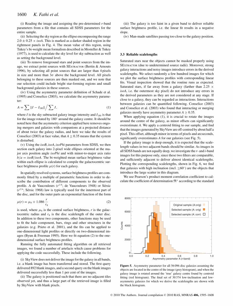
When applying equation (1), it is crucial to rotate the imagesaround the centre of the galaxy, as minor offsets can significantlyoverestimate A. We apply a centroid fitting to our sample, and findthat the images generated by SkyView are off-centred by about half apixel. This offset, although minor in terms of pixels and arcseconds,significantly overestimates A for our galaxies (see Fig. 5).

If the galaxy image is deep enough, it is expected that the scale-length values in two adjacent bands should be similar. As images inall SDSS bands are not equally deep, we investigate the r- and i-bandimages for this purpose only, since these two filters are comparable,and sufficiently adjacent to deliver almost identical scalelengths.Plotting the corresponding scalelengths, shown in Fig. 6, we findthat galaxies with high inclination (incl. ≥60◦) are the objects thatintroduce the large scatter in this diagram.

We use Pearson’s product moment correlation coefficient to cal-culate the coefficient of determination R2 according to the standard

0.0 0.2 0.4 0.6 0.8 1.0Asymmetry parameter A (r-band)

0

2000

4000

6000

8000

Co

un

ts

Original sample (A:orig)

Selected sample (A: orig)

Selected sample (A: corr)

Figure 5. Asymmetry parameter for all 56 096 disc galaxies assuming theobjects are located in the centre of the image (grey histogram), and when thegalaxy image is rotated around the ‘true’ galaxy centre found by centroidfitting (red histogram). The final set of 30 374 low-inclination and low-asymmetry galaxies for which we derive the scalelengths are shown withthe black histogram.



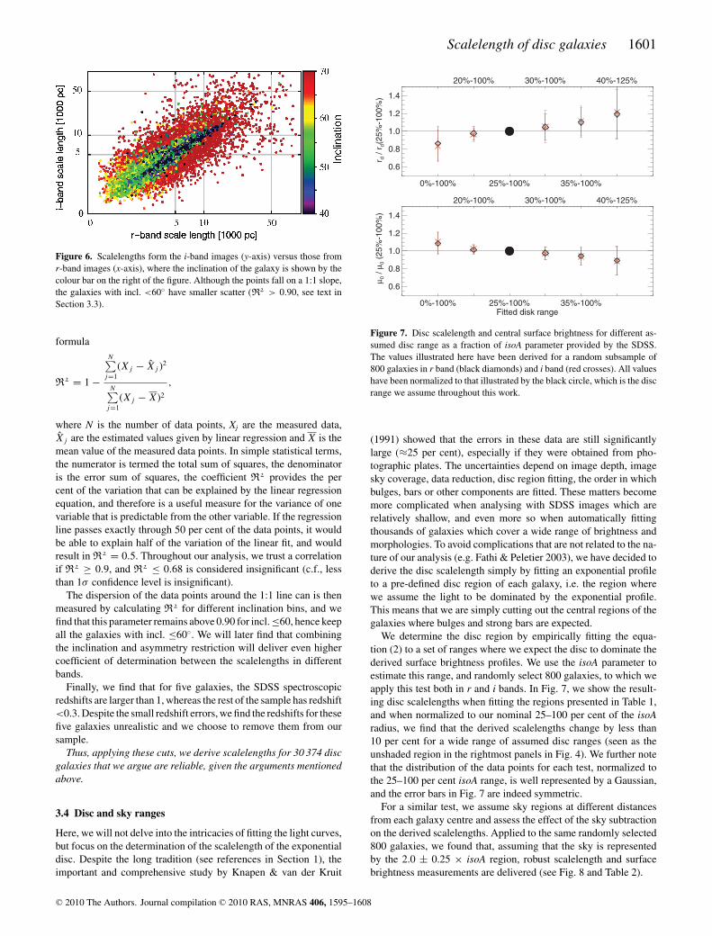
Figure 6. Scalelengths form the i-band images (y-axis) versus those fromr-band images (x-axis), where the inclination of the galaxy is shown by thecolour bar on the right of the figure. Although the points fall on a 1:1 slope,the galaxies with incl. <60◦ have smaller scatter (R2 > 0.90, see text inSection 3.3).

formula

R2 = 1 −

N∑j=1

(Xj − Xj )2

N∑j=1

(Xj − X)2

,

where N is the number of data points, Xj are the measured data,Xj are the estimated values given by linear regression and X is themean value of the measured data points. In simple statistical terms,the numerator is termed the total sum of squares, the denominatoris the error sum of squares, the coefficient R2 provides the percent of the variation that can be explained by the linear regressionequation, and therefore is a useful measure for the variance of onevariable that is predictable from the other variable. If the regressionline passes exactly through 50 per cent of the data points, it wouldbe able to explain half of the variation of the linear fit, and wouldresult in R2 = 0.5. Throughout our analysis, we trust a correlationif R2 ≥ 0.9, and R2 ≤ 0.68 is considered insignificant (c.f., lessthan 1σ confidence level is insignificant).

The dispersion of the data points around the 1:1 line can is thenmeasured by calculating R2 for different inclination bins, and wefind that this parameter remains above 0.90 for incl. ≤60, hence keepall the galaxies with incl. ≤60◦. We will later find that combiningthe inclination and asymmetry restriction will deliver even highercoefficient of determination between the scalelengths in differentbands.

Finally, we find that for five galaxies, the SDSS spectroscopicredshifts are larger than 1, whereas the rest of the sample has redshift<0.3. Despite the small redshift errors, we find the redshifts for thesefive galaxies unrealistic and we choose to remove them from oursample.

Thus, applying these cuts, we derive scalelengths for 30 374 discgalaxies that we argue are reliable, given the arguments mentionedabove.

3.4 Disc and sky ranges

Here, we will not delve into the intricacies of fitting the light curves,but focus on the determination of the scalelength of the exponentialdisc. Despite the long tradition (see references in Section 1), theimportant and comprehensive study by Knapen & van der Kruit

0%-100% 25%-100% 35%-100%

0.6

0.8

1.0

1.2

1.4

rd / r

d(2

5%

-100%

)

20%-100% 30%-100% 40%-125%

0%-100% 25%-100% 35%-100%Fitted disk range

0.6

0.8

1.0

1.2

1.4

μ0 / μ

0 (

25%

-100%

)

20%-100% 30%-100% 40%-125%

Figure 7. Disc scalelength and central surface brightness for different as-sumed disc range as a fraction of isoA parameter provided by the SDSS.The values illustrated here have been derived for a random subsample of800 galaxies in r band (black diamonds) and i band (red crosses). All valueshave been normalized to that illustrated by the black circle, which is the discrange we assume throughout this work.

(1991) showed that the errors in these data are still significantlylarge (≈25 per cent), especially if they were obtained from pho-tographic plates. The uncertainties depend on image depth, imagesky coverage, data reduction, disc region fitting, the order in whichbulges, bars or other components are fitted. These matters becomemore complicated when analysing with SDSS images which arerelatively shallow, and even more so when automatically fittingthousands of galaxies which cover a wide range of brightness andmorphologies. To avoid complications that are not related to the na-ture of our analysis (e.g. Fathi & Peletier 2003), we have decided toderive the disc scalelength simply by fitting an exponential profileto a pre-defined disc region of each galaxy, i.e. the region wherewe assume the light to be dominated by the exponential profile.This means that we are simply cutting out the central regions of thegalaxies where bulges and strong bars are expected.

We determine the disc region by empirically fitting the equa-tion (2) to a set of ranges where we expect the disc to dominate thederived surface brightness profiles. We use the isoA parameter toestimate this range, and randomly select 800 galaxies, to which weapply this test both in r and i bands. In Fig. 7, we show the result-ing disc scalelengths when fitting the regions presented in Table 1,and when normalized to our nominal 25–100 per cent of the isoAradius, we find that the derived scalelengths change by less than10 per cent for a wide range of assumed disc ranges (seen as theunshaded region in the rightmost panels in Fig. 4). We further notethat the distribution of the data points for each test, normalized tothe 25–100 per cent isoA range, is well represented by a Gaussian,and the error bars in Fig. 7 are indeed symmetric.

For a similar test, we assume sky regions at different distancesfrom each galaxy centre and assess the effect of the sky subtractionon the derived scalelengths. Applied to the same randomly selected800 galaxies, we found that, assuming that the sky is representedby the 2.0 ± 0.25 × isoA region, robust scalelength and surfacebrightness measurements are delivered (see Fig. 8 and Table 2).



Table 1. Disc scalelength and central surface brightness for different assumed disc range as a fraction of isoA as illustrated in Fig. 7. The valuespresented here have been derived for a random subsample of 800 galaxies with formal errors given in brackets, and all values are normalized tothe scalelength derived in the range 25–100 per cent.

Fitted isoA range (r band) rdrd(25–100 per cent) (r band) μ0

μ0(25–100 per cent) (i band) rdrd(25–100 per cent) (i band) μ0

μ0(25–100 per cent)

0–100 per cent 0.91(0.19) 0.87(0.18) 1.07(0.12) 1.09(0.12)20–100 per cent 0.98(0.08) 0.97(0.07) 1.02(0.05) 1.03(0.05)25–100 per cent 1 1 1 130–100 per cent 1.07(0.15) 1.09(0.18) 0.97(0.07) 0.96(0.08)30–100 per cent 1.14(0.27) 1.12(0.17) 0.93(0.12) 0.93(0.09)40–120 per cent 1.20(0.28) 1.25(0.29) 0.87(0.16) 0.87(0.16)

150%-200% 200%-250% 250%-300%

0.90

0.95

1.00

1.05

1.10

rd / r

d(1

75%

-225%

)

175%-225% 225%-275%

150%-200% 200%-250% 250%-300% Sky range

0.90

0.95

1.00

1.05

1.10

μ0 / μ

0(1

75%

-225%

)

175%-225% 225%-275%

Figure 8. Disc scalelength and central surface brightness for different as-sumed sky range as a fraction of isoA parameter provided by the SDSS. Thevalues illustrated here have been derived for a random subsample of 800galaxies in r band (black diamonds) and i band (red crosses). The valueshave been normalized to that illustrated by the black circle, which is the skyrange we assume throughout this work.

3.5 Scalelengths in u, g, r, i, z bands

Although the SDSS is one of the most influential and ambitiousastronomical surveys, the depth of its images in all bands are notequal. Here we have chosen to analyse only the galaxies for whichSDSS provides spectroscopic redshifts (in order to investigate theredshift evolution the parameters we derived), where SDSS is com-plete for r-band magnitude <17.7. The images in other bands arenot equally deep and/or complete to this magnitude limit, partlydue to the significantly different transmission curves for the differ-ent filters. Including atmospheric extinction and detector efficiency,the peak quantum efficiency of the system in u and z bands are

≈10 per cent, g and i bands ≈35 per cent and r band ≈50 per cent.Thus it is necessary to apply a magnitude cut which varies depend-ing on the band, fainter than which we are not able to derive reliablescalelengths.

For each pair of SDSS filters, we expect that the scalelengthvariation larger than a factor of 1.5 is unphysical. We determinethe magnitude limit for a pair of filters by plotting the scalelengthratio versus magnitude in one of the bands (see Fig. 9), and scanthe values from the brighter to the fainter levels in fixed bins of0.2 mag. Once we reach a magnitude where less than 95 per centof the scalelength ratios is smaller than 0.67 or larger than 1.5 (i.e.above or below the horizontal dotted lines in Fig. 9), we stop thescan and select this value for the faintest magnitude level in thatband for which we trust the scalelengths. As shown in Fig. 9, thisprocedure very clearly demonstrates the noise in different bands,and how the values presented in Table 3 have been established. Inthe given examples, the scalelengths in r band when compared to iband are complete to an r-band magnitude of 17.70 (indicated by thearrow), and the u versus z band is complete to a u-band magnitudeof 16.29 (indicated by the arrow).

4 R ESULTS

4.1 Scalelength versus morphology

The morphological classification scheme of Sandage (1961) is de-signed based on visual inspection of basic features of galaxies whichrelates them to their formation and evolution histories. While thisclassification scheme is somewhat subjective, in the past years, nu-merous efforts have been made to define quantitative versions of thisclassification scheme (e.g. Burda & Feitzinger 1992; Doi, Fukugita& Okamura 1993; Abraham et al. 1996; Yamauchi et al. 2005).

The numeric morphological types presented in the LEDA cata-logue are a compilation of the morphological types encoded in the deVaucouleurs scale as well as the luminosity class (van den Bergh’sdefinition). There is also information about the presence of barsand rings, but we do not consider these for the present paper mostly

Table 2. Disc scalelength and central surface brightness for different assumed sky range as a fraction of isoA as illustratedin Fig. 8. The values presented here have been derived for a random subsample of 800 galaxies, normalized to the skyrange 2.00 ± 0.25, with formal errors given in brackets.

Fitted sky range (r band) rdrd(2.0±0.25) (r band) μ0

μ0(2.0±0.25) (i band) rdrd(2.0±0.25) (iband) μ0

μ0(2.0±0.25)

1.75 ± 0.25 0.99(0.03) 0.99(0.03) 1.00(0.01) 1.00(0.01)2.00 ± 0.25 1 1 1 12.25 ± 0.25 1.00(0.03) 1.01(0.04) 1.00(0.01) 1.00(0.02)2.50 ± 0.25 1.01(0.05) 1.01(0.07) 1.00(0.02) 1.00(0.03)2.75 ± 0.25 1.01(0.06) 1.01(0.09) 1.00(0.03) 1.00(0.04)



12 13 14 15 16 17r-band magnitude from SDSS

0.0

0.5

1.0

1.5

2.0

r-b

and r

d / i-b

and r

d

14 15 16 17 18 19 20u-band magnitude from SDSS

0

1

2

3

4

5

6

u-b

and r

d / z

-band r

d

Figure 9. Scalelength ratio versus magnitude for two pairs from Table 3.Bins of 0.2 mag are used to scan the data points ‘from left to right’, and whenless than 95 per cent of the ratios are inside the dotted lines, that magnitudelimit is taken to be the faintest magnitude where we trust the scalelengthsfor these two bands. Here we show the best case r, i pair (top) and the worstcase u, z pair (bottom). In each panel, the arrow indicates the cutting limitpresented in Table 3.

Table 3. Magnitude cuts applied to the final sample of 30 374 galaxies asdescribed in Section 3. To apply the cut to each pair, a plot similar to Fig. 9was set up, and the magnitude cut was decided accordingly.

Filter pair Upper magnitudes Number of galaxies

g and r g < 17.70 and r < 17.70 30 201g and i g < 19.95 and i < 16.65 30 371g and z g < 17.70 and z < 15.53 27 319r and i r < 17.70 and i < 16.65 30 374r and z r < 17.70 and z < 15.53 27 329i and z i < 15.89 and z < 15.53 27 264

u and g u < 16.79 and g < 14.94 847u and r u < 16.54 and r < 13.56 132u and i u < 16.79 and i < 13.14 123u and z u < 16.29 and z < 12.78 88

since this information is only available for minor fraction of the sam-ple. More details about the classification of galaxies can be foundin the Level 5 of the NASA/IPAC Extragalactic Database (NED).The morphological types of LEDA have been compiled using fromVorontsov-Velyaminov, Arkipova & Kranogorskaja (1963–1974),Nilson (1973), Lauberts (1982), de Vaucouleurs et al. (1991) andLoveday (1996).

We select only the galaxies which are classified using the numerictype = 1 (i.e. Sa) up to and including numeric type = 8 (i.e. Sdm).Most of the values presented in Fig. 2 are subject to errors largerthan 1, typically smaller for fainter galaxies, but they seem not

2.0 2.5 3.0 3.5 4.0 4.5 5.0log(Scale Length [parsec])

1

10

100

1000

10000

Counts

2 4 6 8Morphological Type

2.5

3.0

3.5

4.0

4.5

5.0

Scale

Length

[lo

g(p

ars

ec)]

ugriz

Figure 10. Top: distribution of the reliably derived r-band scalelengths forthe entire sample of 30 374 galaxies (dotted histogram) and the 309 mor-phologically well classified galaxies (solid histogram). Bottom: scalelengthversus morphological type for the 309 galaxies which have been morpholog-ically classified accurately. The r band has been used with the scalelengthin u, g, i, z bands, i plotted in the middle panel. The error bars for all bandsare comparable, and here we only show these for the r-band values.

to depend much on other parameters such as asymmetry, redshift,etc. To analyse the dependency of the parameters with respect tomorphological type, we strictly only use the galaxies for whichthe morphological type error is smaller than 0.5. These are 309galaxies from our final sample of 30 374 galaxies, for which weinvestigate how the scalelength and asymmetry parameter dependson morphology.

Typically, scalelengths for disc galaxies are not expected to de-pend on Hubble morphological type (de Jong 1996; Graham & deBlok 2001) for types ranging between 1 and 6. Here, we analyseour derived values in this context first by only using the galaxiesfor which we only find morphological classifications with corre-sponding errors smaller than 0.5, i.e. the 309 galaxies explained inSection 4.1. In Fig. 10, we plot the r-band scalelength and mor-phological types, and find that our sample is fully consistent withprevious results showing that the absolute value of the scalelengthis independent of type. We transform the scalelength to parsec unitsby using the spectroscopic redshifts provided by the SDSS and ig-nore local flows. Our scalelength values agree with those derivedby previous authors (e.g. van der Kruit 1987; de Jong 1996; Cunow2001); we find that the average r-band scalelength for the entiresample is 3.79 ± 2.05 kpc, and that for the 309 galaxies with reli-able morphology is 3.3 ± 1.6 kpc (see top panel of Fig. 10). Furtherdiscussion is provided in Section 4.2, and the errors are root meansquare (rms) values.

In combination with the mass determination described in Sec-tion 4.3, we find that the mass does play a certain role in thebehaviour of Fig. 10. Although out to type T = 6 scalelengthare constant, the later type galaxies (T > 6) are generally thoseof lower mass, and hence in agreement with Fig. 11. However,



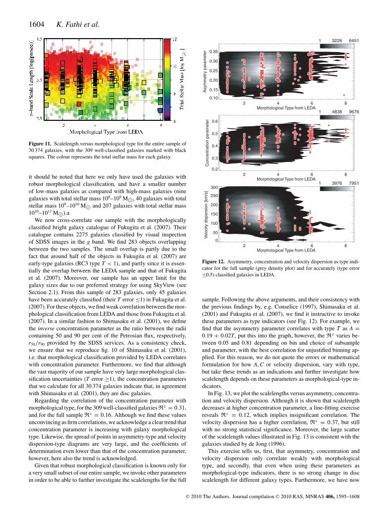
Figure 11. Scalelength versus morphological type for the entire sample of30 374 galaxies, with the 309 well-classified galaxies marked with blacksquares. The colour represents the total stellar mass for each galaxy.

it should be noted that here we only have used the galaxies withrobust morphological classification, and have a smaller numberof low-mass galaxies as compared with high-mass galaxies (ninegalaxies with total stellar mass 108–109 M�, 40 galaxies with totalstellar mass 109–1010 M� and 207 galaxies with total stellar mass1010–1011 M�).a

We now cross-correlate our sample with the morphologicallyclassified bright galaxy catalogue of Fukugita et al. (2007). Theircatalogue contains 2275 galaxies classified by visual inspectionof SDSS images in the g band. We find 283 objects overlappingbetween the two samples. The small overlap is partly due to thefact that around half of the objects in Fukugita et al. (2007) areearly-type galaxies (RC3 type T < 1), and partly since it is essen-tially the overlap between the LEDA sample and that of Fukugitaet al. (2007). Moreover, our sample has an upper limit for thegalaxy sizes due to our preferred strategy for using SkyView (seeSection 2.1). From this sample of 283 galaxies, only 45 galaxieshave been accurately classified (their T error ≤1) in Fukugita et al.(2007). For these objects, we find weak correlation between the mor-phological classification from LEDA and those from Fukugita et al.(2007). In a similar fashion to Shimasaku et al. (2001), we definethe inverse concentration parameter as the ratio between the radiicontaining 50 and 90 per cent of the Petrosian flux, respectively,r50/r90 provided by the SDSS services. As a consistency check,we ensure that we reproduce fig. 10 of Shimasaku et al. (2001),i.e. that morphological classification provided by LEDA correlateswith concentration parameter. Furthermore, we find that althoughthe vast majority of our sample have very large morphological clas-sification uncertainties (T error ≥1), the concentration parametersthat we calculate for all 30 374 galaxies indicate that, in agreementwith Shimasaku et al. (2001), they are disc galaxies.

Regarding the correlation of the concentration parameter withmorphological type, for the 309 well-classified galaxies R2 = 0.31,and for the full sample R2 = 0.16. Although we find these valuesunconvincing as firm correlations, we acknowledge a clear trend thatconcentration parameter is increasing with galaxy morphologicaltype. Likewise, the spread of points in asymmetry-type and velocitydispersion-type diagrams are very large, and the coefficients ofdetermination even lower than that of the concentration parameter,however, here also the trend is acknowledged.

Given that robust morphological classification is known only fora very small subset of our entire sample, we invoke other parametersin order to be able to further investigate the scalelengths for the full

2 4 6 8Morphological Type from LEDA

0.10

0.15

0.20

0.25

0.30

0.35

Asym

me

try p

ara

me

ter

1 3226 6451


0.2

0.3

0.4

0.5

0.6

Co

nce

ntr

atio

n p

ara

me

ter

1 4838 9676


0

50

100

150

200

250

300

Ve

locity d

isp

ers

ion

[km

/s]

1 3976 7951

Figure 12. Asymmetry, concentration and velocity dispersion as type indi-cator for the full sample (grey density plot) and for accurately (type error≤0.5) classified galaxies in LEDA.

sample. Following the above arguments, and their consistency withthe previous findings by, e.g. Conselice (1997), Shimasaku et al.(2001) and Fukugita et al. (2007), we find it instructive to invokethese parameters as type indicators (see Fig. 12). For example, wefind that the asymmetry parameter correlates with type T as A =0.19 + 0.02T , put this into the graph, however, the R2 varies be-tween 0.05 and 0.81 depending on bin and choice of subsampleand parameter, with the best correlation for unjustified binning ap-plied. For this reason, we do not quote the errors or mathematicalformulation for how A, C or velocity dispersion, vary with type,but take these trends as an indications and further investigate howscalelength depends on these parameters as morphological-type in-dicators.

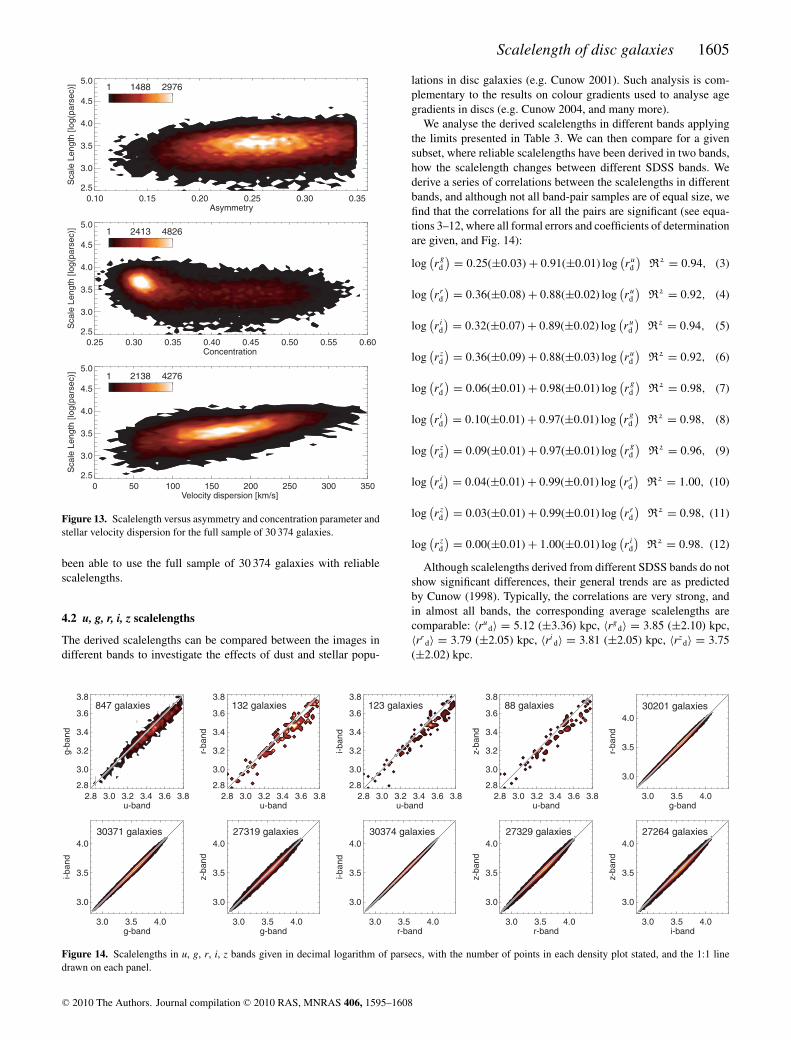
In Fig. 13, we plot the scalelengths versus asymmetry, concentra-tion and velocity dispersion. Although it is shown that scalelengthdecreases at higher concentration parameter, a line-fitting exercisereveals R2 = 0.12, which implies insignificant correlation. Thevelocity dispersion has a higher correlation, R2 = 0.37, but stillwith no strong statistical significance. Moreover, the large scatterof the scalelength values illustrated in Fig. 13 is consistent with thegalaxies studied by de Jong (1996).

This exercise tells us, first, that asymmetry, concentration andvelocity dispersion only correlate weakly with morphologicaltype, and secondly, that even when using these parameters asmorphological-type indicators, there is no strong change in discscalelength for different galaxy types. Furthermore, we have now



0.10 0.15 0.20 0.25 0.30 0.35Asymmetry

2.5

3.0

3.5

4.0

4.5

5.0S

ca

le L

en

gth

[lo

g(p

ars

ec)] 1 1488 2976

0.25 0.30 0.35 0.40 0.45 0.50 0.55 0.60Concentration

2.5

3.0

3.5

4.0

4.5

5.0

Sca

le L

en

gth

[lo

g(p

ars

ec)] 1 2413 4826

0 50 100 150 200 250 300 350Velocity dispersion [km/s]

2.5

3.0

3.5

4.0

4.5

5.0

Sca

le L

en

gth

[lo

g(p

ars

ec)] 1 2138 4276

Figure 13. Scalelength versus asymmetry and concentration parameter andstellar velocity dispersion for the full sample of 30 374 galaxies.

been able to use the full sample of 30 374 galaxies with reliablescalelengths.

4.2 u, g, r, i, z scalelengths

The derived scalelengths can be compared between the images indifferent bands to investigate the effects of dust and stellar popu-

lations in disc galaxies (e.g. Cunow 2001). Such analysis is com-plementary to the results on colour gradients used to analyse agegradients in discs (e.g. Cunow 2004, and many more).

We analyse the derived scalelengths in different bands applyingthe limits presented in Table 3. We can then compare for a givensubset, where reliable scalelengths have been derived in two bands,how the scalelength changes between different SDSS bands. Wederive a series of correlations between the scalelengths in differentbands, and although not all band-pair samples are of equal size, wefind that the correlations for all the pairs are significant (see equa-tions 3–12, where all formal errors and coefficients of determinationare given, and Fig. 14):

log(r

g

d

) = 0.25(±0.03) + 0.91(±0.01) log(ru

d

)R2 = 0.94, (3)

log(rr

d

) = 0.36(±0.08) + 0.88(±0.02) log(ru

d

)R2 = 0.92, (4)

log(ri

d

) = 0.32(±0.07) + 0.89(±0.02) log(ru

d

)R2 = 0.94, (5)

log(rz

d

) = 0.36(±0.09) + 0.88(±0.03) log(ru

d

)R2 = 0.92, (6)

log(rr

d

) = 0.06(±0.01) + 0.98(±0.01) log(r

g

d

)R2 = 0.98, (7)

log(ri

d

) = 0.10(±0.01) + 0.97(±0.01) log(r

g

d

)R2 = 0.98, (8)

log(rz

d

) = 0.09(±0.01) + 0.97(±0.01) log(r

g

d

)R2 = 0.96, (9)

log(ri

d

) = 0.04(±0.01) + 0.99(±0.01) log(rr

d

)R2 = 1.00, (10)

log(rz

d

) = 0.03(±0.01) + 0.99(±0.01) log(rr

d

)R2 = 0.98, (11)

log(rz

d

) = 0.00(±0.01) + 1.00(±0.01) log(ri

d

)R2 = 0.98. (12)

Although scalelengths derived from different SDSS bands do notshow significant differences, their general trends are as predictedby Cunow (1998). Typically, the correlations are very strong, andin almost all bands, the corresponding average scalelengths arecomparable: 〈ru

d〉 = 5.12 (±3.36) kpc, 〈rgd〉 = 3.85 (±2.10) kpc,

〈rrd〉 = 3.79 (±2.05) kpc, 〈ri

d〉 = 3.81 (±2.05) kpc, 〈rzd〉 = 3.75

(±2.02) kpc.

2.8 3.0 3.2 3.4 3.6 3.8u-band

2.8

3.0

3.2

3.4

3.6

3.8

g-b

and

847 galaxies

2.8 3.0 3.2 3.4 3.6 3.8u-band

2.8

3.0

3.2

3.4

3.6

3.8

r-band

132 galaxies

2.8 3.0 3.2 3.4 3.6 3.8u-band

2.8

3.0

3.2

3.4

3.6

3.8

i-band

123 galaxies

2.8 3.0 3.2 3.4 3.6 3.8u-band

2.8

3.0

3.2

3.4

3.6

3.8

z-b

and

88 galaxies

3.0 3.5 4.0g-band

3.0

3.5

4.0

r-band

30201 galaxies

3.0 3.5 4.0g-band

3.0

3.5

4.0

i-band

30371 galaxies

3.0 3.5 4.0g-band

3.0

3.5

4.0

z-b

and

27319 galaxies

3.0 3.5 4.0r-band

3.0

3.5

4.0

i-band

30374 galaxies

3.0 3.5 4.0r-band

3.0

3.5

4.0

z-b

and

27329 galaxies

3.0 3.5 4.0i-band

3.0

3.5

4.0

z-b

and

27264 galaxies

Figure 14. Scalelengths in u, g, r, i, z bands given in decimal logarithm of parsecs, with the number of points in each density plot stated, and the 1:1 linedrawn on each panel.



We further find that these numbers are consistent withe.g. Courteau (1996), de Jong (1996) and de Grijs (1998) whopresented an extensive analysis of deep images of 349, 86 and 45spiral galaxies, respectively. It should be noted that the sample ofde Grijs (1998) is a sample of edge-on galaxies, which explainsthe relatively insignificant variations found in our analysis, as op-posed to theirs. Furthermore, their wavelength range, from B to K,is larger than with SDSS data. In an attempt to extend these resultsto compare with near-infrared results, we also cross-correlated oursample with the Two Micron All Sky Survey (2MASS) J-, H-, K-band images. We applied the code presented in Section 3 and foundthe 2MASS images are too shallow to yield anything presentable.

4.3 Scalelength versus stellar mass

We retrieve stellar masses for our sample galaxies by cross-matchingour sample with the publically available sample of Kauffmann et al.(2003) and Brinchmann et al. (2004), and find stellar masses for30 126 (i.e. almost all our sample) galaxies. These authors havecalculated total stellar masses for nearly a million SDSS galaxiesbased on photometry of the outer regions of the galaxies with modelsthat produce dust-corrected star formation rates and use upgradedstellar population synthesis spectra for the continuum subtraction.As noted by these authors, comparison between the stellar massesderived from photometry and spectra from the central regionsshows that the fits to the photometry are more constrained at lowmass since the emission-line contribution makes the line index fitsless well constrained. Since the spectroscopic masses are based onfibre spectra from SDSS, which cover only a fraction of the galaxies,we opt to use the stellar masses from photometry.

In Fig. 15 we illustrate the scalelength as a function of total stellarmass, and find that larger mass galaxies have larger scalelengths.Moreover, we find that this increase is accompanied by a largerspread in scalelength. Galaxies with total stellar mass less than108 M� have average r-band scalelength of 238 ± 94 pc, galax-ies with total stellar mass between 109 and 1010 M� have average

Figure 15. Total stellar mass distribution of our sample is illustrated inthe top panel, and the scalelength versus mass diagram shows the expectedbehaviour in the bottom panel. The colour code shows the r-band abso-lute magnitude derived from the SDSS apparent r-band magnitude. Thehistogram and the scatter plot illustrate the same mass range.

scalelength of 1.52 ± 0.65 kpc, and galaxies with total stellar massbetween 1011 and 1012 M� have average scalelength of 5.73 ±1.94 kpc. All points in Fig. 15 are also colour coded to show theconsistently increasing intrinsic absolute magnitude for larger stel-lar mass galaxies.

5 D ISCUSSION

We have derived reliable scalelengths for 30 374 disc/spiral galax-ies, with no sign of ongoing interaction or disturbed morphology,in all five u, g, r, i and z bands from SDSS DR6 images. Cross-correlation of the SDSS sample with the LEDA catalogue has en-abled us to investigate the variation of the scalelengths for differenttypes of disc/spiral galaxies. Although the typical scalelength in uband is 35 per cent larger than that in the r band, the scalelengthsin the g, r, i and z bands are similar and only become smaller on theaverage for late morphological types. This result remains consis-tent when using by-eye morphological classification or when usingasymmetry parameter, concentration parameter or velocity disper-sion as an indicator for galaxy morphological type. Our samplespans a range of total stellar masses between 106.6 and 1012.2 M�with a typical galaxy mass of 1010.8±0.54 M�, and shows that thewhile scalelength increases for more massive galaxies, the scale-length spread also increases with galaxy mass. Overall, these resultsare in full agreement with the recent work by Courteau et al. (2007).

Scalelength variations between bands are commonly studied tobetter understand the content and distribution of different stellarpopulations, metals and/or dust. A colour gradient is expected toincrease from early-type spirals to late-type spirals, mainly due toextinction, which increases to later types. However, for Scd galaxiesor later the colour gradient becomes smaller, because of decreasingamount of extinction (see e.g. Peletier & Balcells 1996; de Grijs1998).

Changes in galaxy scalelength in different wavelengths can beattributed to extinction by moderate amounts of dust, with ra-dial metallicity and age gradients as other contributing factors(Elmegreen & Elmegreen 1984; Peletier et al. 1994; Beckman et al.1996). All these parameters will probably change as a function ofredshift, enabling us to measure the variation of intrinsic scale-length with cosmological epoch. It is expected that the opacity ofdisc galaxies is expected to have been systematically higher in thepast (e.g. Dwek 1998; Pei, Fall & Hauser 1999). The fact that theobserved radial colour vary little suggests strongly that stellar pop-ulation effects are not important here. Dust effects are studied byusing radiative transfer models which take into account scatteringas well as absorption by dust, and observationally by investigatingthe scalelength ratio in different bands as a function of inclination,i.e. optical depth. However, there are some degeneracies. Any ten-dency of the stars in the outer parts of discs to be bluer would tendto result in underestimated dust content. Any tendency of the dustto concentrate towards the centre would result in an overestimate ofthe bluer scalelengths, and would not be distinguishable photomet-rically from a tendency of the stars in the outer disc to be bluer (cf.Pohlen & Trujillo 2006; Azzolini, Trujillo & Beckman 2008; Erwin,Pohlen & Beckman 2008). Peletier et al. (1994, 1995) found thatscalelength ratios could change, due to stellar population changes,by a factor of approximately 1.1–1.2 from blue to near-infrared (Kband). This would correspond to a factor of about 1.03–1.06 from gto z. Since these numbers are very small, a very accurate analysis isneeded to derive conclusions from the SDSS data base. Our resultsseem to first order in agreement with these numbers.



The derived scalelengths and our presentation of the transfor-mation coefficients for converting observed scalelengths from oneSDSS band to another, furthermore, are meant to be useful tools totest the results of cosmological galaxy formation models, whethernumerical or semi-analytical.

In the future, we plan to add the stored parameters form theGalaxy Zoo7 project to obtain a larger sample with morphologicalclassifications (at this stage, detailed morphologies are not avail-able), but also compare scalelength as a function environment, nu-clear activity and colour gradients (e.g. comparing the sample withthat of Hatziminaoglou et al. 2005). Many more parameters can befurther investigated, and with the data and the derived parameters athand, we now have the capability to continue this project in variousand potentially unforeseeable directions.

AC K N OW L E D G M E N T S

This work made use of EURO-VO software, tools and services. TheEURO-VO has been funded by the European Commission through con-tract numbers RI031675 (DCA) and 011892 (VO-TECH) under the6th Framework Programme and contract number 212104 (AIDA),under the 7th Framework Programme. We also acknowledge the useof NASA’s SkyView facility (http://skyview.gsfc.nasa.gov) locatedat NASA Goddard Space Flight Center, the usage of the Hyper-Leda data base (http://leda.univ-lyon1.fr) and the TOPCAT software(http://www.starlink.ac.uk/topcat/). KF acknowledges support fromthe Swedish Research Council (Vetenskapsradet), and the hospital-ity of ESO-Garching where parts of this work were done. KF also ac-knowledges support from Sergio Gelato for computer support, andfruitful discussions with Robert Cumming and Genoveva Micheva.Finally, we thank the referee Frederic Bournaud for insightful andencouraging comments which helped improve our manuscript.

Funding for the SDSS and SDSS-II has been provided by the Al-fred P. Sloan Foundation, the Participating Institutions, the NationalScience Foundation, the US Department of Energy, the NationalAeronautics and Space Administration, the Japanese Monbuka-gakusho, the Max Planck Society and the Higher Education FundingCouncil for England. The SDSS website is http://www.sdss.org/

The SDSS is managed by the Astrophysical Research Consor-tium for the Participating Institutions. The Participating Institu-tions are the American Museum of Natural History, AstrophysicalInstitute Potsdam, University of Basel, University of Cambridge,Case Western Reserve University, University of Chicago, DrexelUniversity, Fermilab, the Institute for Advanced Study, the JapanParticipation Group, Johns Hopkins University, the Joint Institutefor Nuclear Astrophysics, the Kavli Institute for Particle Astro-physics and Cosmology, the Korean Scientist Group, the ChineseAcademy of Sciences (LAMOST), Los Alamos National Labora-tory, the Max Planck Institute for Astronomy (MPIA), the MaxPlanck Institute for Astrophysics (MPA), New Mexico State Uni-versity, Ohio State University, University of Pittsburgh, Universityof Portsmouth, Princeton University, the United States Naval Ob-servatory and the University of Washington.

REFERENCES

Abraham R. G., van den Bergh S., Glazebrook K., Ellis R. S., Santiago B.X., Surma P., Griffiths R. E., 1996, ApJS, 107, 1

7http://www.galaxyzoo.org

Adelman-McCarthy J. K. et al., 2008, ApJS, 175, 297Azzolini R., Trujillo I., Beckman J. E., 2008, ApJ, 679, L69Baggett W. E., Baggett S. M., Anderson K. S. J., 1998, AJ, 116, 1626Beckman J. E., Peletier R. F., Knapen J. H., Corradi R. L. M., Gentet L. J.,

1996, ApJ, 467, 175Bertin E., Arnouts S., 1996, A&AS, 117, 393Boroson T., 1981, ApJS, 46, 177Bournaud F., Elmegreen B. G., Elmegreen D. M., 2007, ApJ, 670, 237Brinchmann J., Charlot S., White S. D. M., Tremonti C., Kauffmann G.,

Heckman T., Brinkmann J., 2004, MNRAS, 351, 1151Burda P., Feitzinger J. V., 1992, A&A, 261, 697Byun Y. I., Freeman K. C., 1995, ApJ, 448, 563Ceverino D., Dekel A., Bournaud F., 2010, MNRAS, 404, 2151Combes F., Elmegreen B. G., 1993, A&A, 271, 391Conselice C. J., 1997, PASP, 109, 1251Conselice C. J., 2003, ApJS, 147, 1Conselice C. J., Bershady M. A., Dickinson M., Papovich C., 2003, ApJ,

126, 1183Coulais A., Schellens M., Gales J., Arabas S., Boquier M., Chanial P.,

Messmer P., 2009, in Proc. 19th Conference on Astronomical DataAnalysis Software and Systems, Sapporo, Japan

Courteau S., 1996, ApJS, 103, 363Courteau S., Dutton A., van den Bosch F. C., MacArthur L. A., Dekel A.,

McIntosh D. H., Dale D. A., 2007, ApJ, 671, 203Cunow B., 1998, A&AS, 129, 593Cunow B., 2001, MNRAS, 323, 130Cunow B., 2004, MNRAS, 353, 477Dalcanton J. J., Spergel D. N., Summers F. J., 1997, ApJ, 482, 659de Grijs R., 1998, MNRAS, 299, 595de Jong R. S., 1996, A&A, 313, 45de Vaucouleurs G., 1948, Ann. Astrophys., 11, 247de Vaucouleurs G., de Vaucouleurs A., Corwin H. G., Jr, Buta R. J., Paturel

G., Fouque P., 1991, Third Reference Catalogue of Bright Galaxies,Vols 1–3. Springer-Verlag, Berlin

Doi M., Fukugita M., Okamura S., 1993, MNRAS, 264, 832Dutton A., 2009, MNRAS, 396, 141Dwek E., 1998, ApJ, 501, 643Elmegreen D. M., Elmegreen B. G., 1984, ApJS, 54, 127Elmegreen B. G., Elmegreen D. M., Chromey F. R., Hasselbacher D. A.,

Bissell B. A., 1996, AJ, 111, 2233Elmegreen B. G., Elmegreen D. M., Vollbach D. R., Foster E. R., Ferguson

T. E., 2005, ApJ, 634, 101Erwin P., Pohlen M., Beckman J. E., 2008, AJ, 135, 20Fathi K., 2004, PhD thesis, Groningen UniversityFathi K., Peletier R. F., 2003, A&A, 407, 61Freeman K. C., 1970, ApJ, 160, 811Fukugita M. et al., 2007, AJ, 134, 579Giovanelli R., Haynes M., 2002, ApJ, 571, L107Governato F. et al., 2010, Nat, 463, 203Graham A. W., 2001, MNRAS, 326, 543Graham A. W., de Blok W. J. G., 2001, ApJ, 556, 177Graham A. W., Worley C. C., 2008, MNRAS, 388, 1708Hatziminaoglou E. et al., 2005, MNRAS, 364, 47Holwerda B., 2005, PhD thesis, Groningen UniversityKauffmann G. et al., 2003, MNRAS, 341, 33Kent S. M., 1985, ApJS, 59, 115Knapen J. H., 2004, in ASSL Vol. 319, Penetrating Bars Through Masks of

Cosmic Dust, p. 189Knapen J. H., van der Kruit P. C., 1991, A&A, 248, 57Knezek P., 1993, PhD thesis, Univ. MassachusettsKormendy J., Kennicutt R. C., Jr, 2004, ARA&A, 42, 603Lauberts A., 1982, The ESO/Uppsala Survey of the ESO(B) Atlas. Kluwer,

DordrechtLin D. N. C., Pringle J. E., 1987, MNRAS, 225, 607Loveday J., 1996, MNRAS, 278, 1025MacArthur L. A., Courteau S., Holtzman J. A., 2003, ApJ, 582, 689Martig M., Bournaud F., 2010, ApJ, 714, L275Mo H. J., Mao S., White S. D., 1998, MNRAS, 295, 319



Mosteller F., Tukey J., 1977, Data Analysis and Regression. Addison-Wesley, Reading, MA

Nilson P., 1973, Uppsala General Catalogue of Galaxies. Uppsala Astron.Obs. Annaler, Band 6

Paturel G., Petit C., Prugniel P., Theureau G., Rousseau J., Brouty M.,Dubois P., Cambresy L., 2003, A&A, 412, 45

Pei Y. C., Fall S. M., Hauser M. G., 1999, ApJ, 522, 604Peletier R. F., Balcells M., 1996, in Minniti D., Rix H.-W., eds, ESO/MPA

Proc., Spiral Galaxies in the Near-IR. Springer-Verlag, Berlin, p. 48Peletier R. F., Valentijn E. A., Moorwood A. F. M., Freudling W., 1994,

A&AS, 108, 621Peletier R. F., Valentijn E. A., Moorwood A. F. M., Freudling W., Knapen

J. H., Beckman J. E., 1995, A&A, 300, L1Pohlen M., Trujillo I., 2006, A&A, 454, 759Prieto M., Aguerri J. A. L., Varela A. M., Munoz-Tunn C., 2001, A&A, 367,

405Romanishin W., Strom K. M., Strom S. E., 1983, ApJS, 53, 105Sandage A., 1961, The Hubble Atlas of Galaxies. Carnegie Institution of

Washington, WashingtonSchade D., Lilly S. J., Crampton D., Hammer F., Le Fevre O., Tresse L.,

1995, ApJ, 451, L1Schaye J. et al., 2010, MNRAS, 402, 1536

Schombert J. M., Bothun G. D., Schneider S. E., McGaugh S. S., 1992, AJ,103, 1107

Sersic J. L., 1968, Atlas de Galaxias Australes. Observatorio Astronomico,Cordoba

Shimasaku K. et al., 2001, AJ, 122, 1238Silk J., 2001, MNRAS, 324, 313Simien F., de Vaucouleurs G., 1983, in Athanassoula E., ed., Proc. IAU

Symp. 100, Internal Kinematics and Dynamics of Galaxies. Reidel,Dordrecht, p. 375

Valentijn E. A., 1990, Nat, 346, 153van der Kruit P. C., 1987, A&A, 173, 59van Driel W., Valentijn E. A., Wesselius P. R., Kussendrager D., 1995, A&A,

298, 41Vorontsov-Velyaminov B. A., Arkipova V. P., Kranogorskaja A. A., 1963–

1974, Morphological Catalogue of Galaxies. Trudy Sternberg Stat. Astr.Inst., Moscow, 32, 33, 34

Yamauchi C. et al., 2005, ApJ, 130, 1545York D. G. et al., 2000, AJ, 120, 1579

This paper has been typeset from a TEX/LATEX file prepared by the author.


scalelength of disc galaxies - diva portal

Documents