Scaling of heat transfer augmentation due to mechanical distortions in hypervelocityboundary layersW. Flaherty and J. M. Austin

Citation: Physics of Fluids (1994-present) 25, 106106 (2013); doi: 10.1063/1.4826476 View online: http://dx.doi.org/10.1063/1.4826476 View Table of Contents: http://scitation.aip.org/content/aip/journal/pof2/25/10?ver=pdfcov Published by the AIP Publishing Articles you may be interested in Interaction of a vortex ring with a natural convective layer Phys. Fluids 26, 083602 (2014); 10.1063/1.4891985 Particle image velocimetry measurements of the interaction of synthetic jets with a zero-pressure gradientlaminar boundary layer Phys. Fluids 22, 063603 (2010); 10.1063/1.3432133 Purely analytic solutions of the compressible boundary layer flow due to a porous rotating disk with heat transfer Phys. Fluids 21, 106104 (2009); 10.1063/1.3249752 Wall heat transfer effects on Klebanoff modes and Tollmien–Schlichting waves in a compressible boundary layer Phys. Fluids 21, 024106 (2009); 10.1063/1.3054155 Laminar boundary layer response to rotation of a finite diameter surface patch Phys. Fluids 15, 101 (2003); 10.1063/1.1526663

This article is copyrighted as indicated in the article. Reuse of AIP content is subject to the terms at: http://scitation.aip.org/termsconditions. Downloaded to IP:

131.215.70.231 On: Wed, 24 Sep 2014 22:46:36

PHYSICS OF FLUIDS 25, 106106 (2013)

Scaling of heat transfer augmentation due to mechanicaldistortions in hypervelocity boundary layers

W. Flaherty and J. M. AustinDepartment of Aerospace Engineering, University of Illinois, Urbana, Illinois 61801, USA

(Received 22 March 2013; accepted 2 October 2013; published online 30 October 2013)

We examine the response of hypervelocity boundary layers to global mechanical dis-tortions due to concave surface curvature. Surface heat transfer and visual boundarylayer thickness data are obtained for a suite of models with different concave surfacegeometries. Results are compared to predictions using existing approximate methods.Near the leading edge, good agreement is observed, but at larger pressure gradients,predictions diverge significantly from the experimental data. Up to a factor of fiveunderprediction is reported in regions with greatest distortion. Curve fits to the exper-imental data are compared with surface equations. We demonstrate that reasonableestimates of the laminar heat flux augmentation may be obtained as a function ofthe local turning angle for all model geometries, even at the conditions of greatestdistortion. This scaling may be explained by the application of Lees similarity. Asa means of introducing additional local distortions, vortex generators are used toimpose streamwise structures into the boundary layer. The response of the large scalevortices to an adverse pressure gradient is investigated. Surface streak evolution isvisualized over the different surface geometries using fast response pressure sensitivepaint. For a flat plate baseline case, heat transfer augmentation at similar levels toturbulent flow is measured. For the concave geometries, increases in heat transfer byfactors up to 2.6 are measured over the laminar values. The scaling of heat trans-fer with turning angle that is identified for the laminar boundary layer response isfound to be robust even in the presence of the imposed vortex structures. C© 2013 AIPPublishing LLC. [http://dx.doi.org/10.1063/1.4826476]

I. INTRODUCTION

Concave surface curvature can introduce significant distortion to compressible boundary layerflows due to multiple, potentially coupled, effects including an adverse pressure gradient, bulk flowcompression, and possible centrifugal instabilities, see, for example, White,1 Saric,2 and Smits andDussauge.3 Solution strategies for the compressible boundary layer equations in the presence of apressure gradient have been investigated by numerous researchers, and approximate methods havebeen developed that can provide insight into the dominant mechanisms. Only a few of these methodstreat heat transfer effects.

One such approximate method for boundary layer calculations was developed by Cohen andReshotko.4 Stewartson’s transformation was applied to the compressible boundary layer equationsand unity Prandtl number; linear viscosity-temperature relationship and an isothermal surface wereassumed. Thwaites5 correlation was used to develop an approximate solution method.6 In the caseof a favorable pressure gradient, agreement was within 2% of predictions based on a perturbationmethod,7 however for an adverse pressure gradient with an insulated wall, significant departure fromperturbation theory was observed for predictions of skin friction and heat transfer. As noted by theauthors, this departure appears consistent with the limitations of small-pressure gradient perturbationtheory applied to a highly distorted flow, where their more general formation may be more reliable.No comparison with experimental data was reported.

The effects of self-induced pressure gradients due to viscous interaction for compressible, flat-plate boundary layers were examined by Li and Nagamatsu.8 They arrived at their approach after

1070-6631/2013/25(10)/106106/19/$30.00 C©2013 AIP Publishing LLC25, 106106-1

This article is copyrighted as indicated in the article. Reuse of AIP content is subject to the terms at: http://scitation.aip.org/termsconditions. Downloaded to IP:

131.215.70.231 On: Wed, 24 Sep 2014 22:46:36

106106-2 W. Flaherty and J. M. Austin Phys. Fluids 25, 106106 (2013)

determining that the compressible pressure gradient parameter can be related to the incompressibleform, assuming the flow is hypersonic (implying a small change in fluid velocity across the shock)and isentropic. This method was extended to include surface curvature by Bertram and Feller.9

Reasonable agreement was obtained between computed results and experimental heat flux data fora favorable pressure gradient over a blunted flat plate. The Bertram and Feller method was modifiedby Crawford to accommodate a more general pressure profile.10 Theoretical results were comparedwith experimental data for concave and convex shapes with a blunt leading edge. Good agreementwas observed between theory and experiment, though the theory slightly over predicted heat flux inmost cases. Though the available data set contained regions with strong adverse pressure gradients,predictions were only generated for favorable pressure gradient data.

In a study of heat transfer over blunted bodies with favorable pressure gradients, Lees identifiedthat at hypersonic flight conditions the gas density near the surface is much higher than outsidethe boundary layer, and as a consequence the velocity and enthalpy profiles near the surface aremuch less sensitive to the pressure gradient than to the local pressure, leading to “local similarity”(Sec. III B 2).11 Combining the local flat plate similarity theory of Lees11 with the Newton-Busemannpressure approximation, Cheng12 developed a theoretical model to predict boundary layer quantitieson blunted flat plates at an angle of attack in hypersonic flow. This method was extended to curvedsurfaces by Stollery.13 He found that the use of the Newton-Busemann pressure law caused largescale, non-physical oscillations, but these could be mitigated by substitution of the tangent-wedgepressure approximation. With the modified Cheng method, Stollery obtained good agreement be-tween predictions and pressure measurements over a cubic concave ramp in a hypersonic gun tunnel.This method was again tested by Mohammadian14 and compared with schlieren, surface pressure,and heat transfer data for a Mach 12.25 flow over a cubic ramp with cold wall. Near the leading edge,the modified Cheng method predictions agreed closely with heat transfer measurements, but by 4in. downstream of the leading edge, in the region of larger turning angles (18◦), the two divergedrapidly, with the theoretical model far over-predicting the experimental heat flux. In the presence ofthe strong adverse pressure gradient, Mohammadian proposed that the assumption of local flat platesimilarity may fail and strong normal pressure gradients may exist.

The discrepancies in the predictions of heat transfer using approximate methods for boundarylayers subjected to strong distortions due to adverse pressure gradients, and the sparsity of exper-imental data in these same flows, motivated the present study. We focus on hypervelocity flowswhere thermochemical processes may have a significant impact on boundary layer structure andstability, as previously demonstrated predominantly for flat plate boundary layers. For example,thermochemical equilibrium and nonequilibrium have been shown to affect boundary layer stabilitythrough modifications both to the mean flow and to the frequency and amplitude of growth rates.15–17

Numerical predictions of surface heat flux at hypervelocity conditions are challenged by the accuracywith which gas and surface reaction rates are known, see, for example, Park18 and Miller et al.19

Destabilization of a compressible boundary layer over a concave surface has also been demon-strated to augment the heat flux and skin friction significantly in turbulent boundary layer flows.Experiments by Donovan20 in a Mach 2.9 turbulent flow showed the absolute wall shear stressincreased by about 125% and the skin friction by about 77% over a concave wall. When comparedto a previous study21 of a flat plate boundary layer with the same pressure gradient imposed, theturbulence levels and skin friction were amplified by an additional 60%–70% due to the curva-ture. Experimental measurements indicated that the observed augmentation was not only due tothe streamline curvature, adverse pressure gradients, and bulk compression, but these effects werecoupled with strong amplification of the turbulent stresses. Fernando and Smits22 investigated a flatplate with an imposed pressure gradient equal to that over a curved ramp. Significant differences inthe velocity profiles and Reynolds stresses were measured, and an increase in the wall friction of17% for the curved surface was reported. Ekoto et al.23 studied the response of a turbulent boundarylayer in a Mach 2.86 flow to favorable and combined pressure gradients caused by surface curvature.Local mechanical distortions in the form of two types of patterned roughness on the wall werealso introduced and quantitative characterization of the interaction between turbulent flow structuresand associated production mechanisms were carried out for the different combinations of local andglobal distortions.

This article is copyrighted as indicated in the article. Reuse of AIP content is subject to the terms at: http://scitation.aip.org/termsconditions. Downloaded to IP:

131.215.70.231 On: Wed, 24 Sep 2014 22:46:36

106106-3 W. Flaherty and J. M. Austin Phys. Fluids 25, 106106 (2013)

Discrete roughness elements or protuberances can introduce local mechanical distortion andvortices to the boundary layer. Multiple different roughness geometries were investigated byWhitehead.24 Oil flow patterns showed upstream flow separation and multiple vortex filamentswhich were wrapped around the protuberance and swept downstream to form horseshoe vortexstructures. The effects of a discrete protuberance have been investigated by Sedney,25 among others.For high speed flow, transition to turbulence was not necessarily observed even when the roughnessheight was comparable to the boundary layer thickness. In these cases where laminar flow wasmaintained, the flowfield was still significantly distorted by the vortices generated by the roughnesselement. A single protuberance in a hypersonic flow was examined experimentally by Danehy et al.26

and numerically by Chang and Choudhari.27 The simulations showed that vorticity is formed in therecirculation region in front of the roughness element, and the resulting vortex filament propagatesdownstream as a horseshoe vortex after wrapping around the sides of the protuberance. Almostno vortex shedding over the element was observed, and the spanwise influence was determined toextend almost five roughness diameters away from the element.

In the present work, we investigate the response of hypervelocity boundary layers to a regionof concave surface curvature. A suite of models with different surface geometries and final turningangles are selected. We first examine the response of laminar boundary layers and carry out acomparative study of the heat flux augmentation. In addition, vortex generators are used to introducestreamwise structures into the boundary layer as a model problem to examine the interaction of globaland local mechanical distortions. Diagnostics include surface heat transfer and visual boundary layerprofile measurements, as well as pressure sensitive paint visualizations of streak patterns created bythe imposed vortices.

II. EXPERIMENTAL SETUP

A. Facility description and test conditions

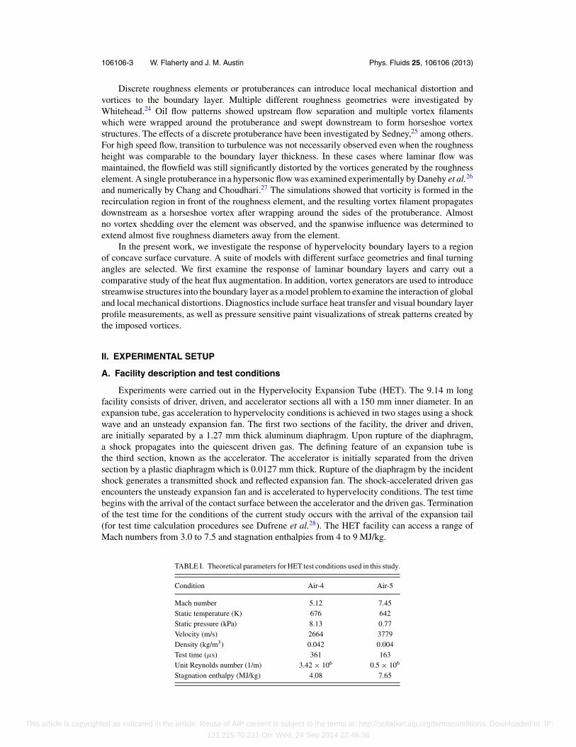
Experiments were carried out in the Hypervelocity Expansion Tube (HET). The 9.14 m longfacility consists of driver, driven, and accelerator sections all with a 150 mm inner diameter. In anexpansion tube, gas acceleration to hypervelocity conditions is achieved in two stages using a shockwave and an unsteady expansion fan. The first two sections of the facility, the driver and driven,are initially separated by a 1.27 mm thick aluminum diaphragm. Upon rupture of the diaphragm,a shock propagates into the quiescent driven gas. The defining feature of an expansion tube isthe third section, known as the accelerator. The accelerator is initially separated from the drivensection by a plastic diaphragm which is 0.0127 mm thick. Rupture of the diaphragm by the incidentshock generates a transmitted shock and reflected expansion fan. The shock-accelerated driven gasencounters the unsteady expansion fan and is accelerated to hypervelocity conditions. The test timebegins with the arrival of the contact surface between the accelerator and the driven gas. Terminationof the test time for the conditions of the current study occurs with the arrival of the expansion tail(for test time calculation procedures see Dufrene et al.28). The HET facility can access a range ofMach numbers from 3.0 to 7.5 and stagnation enthalpies from 4 to 9 MJ/kg.

TABLE I. Theoretical parameters for HET test conditions used in this study.

Condition Air-4 Air-5

Mach number 5.12 7.45Static temperature (K) 676 642Static pressure (kPa) 8.13 0.77Velocity (m/s) 2664 3779Density (kg/m3) 0.042 0.004Test time (μs) 361 163Unit Reynolds number (1/m) 3.42 × 106 0.5 × 106

Stagnation enthalpy (MJ/kg) 4.08 7.65

This article is copyrighted as indicated in the article. Reuse of AIP content is subject to the terms at: http://scitation.aip.org/termsconditions. Downloaded to IP:

131.215.70.231 On: Wed, 24 Sep 2014 22:46:36

106106-4 W. Flaherty and J. M. Austin Phys. Fluids 25, 106106 (2013)

TABLE II. Model specifications. G is the Goertler number at the initiationof curvature.

Model Radius (mm) Turning angle (deg) Curvature length (mm) G

Flat plate . . . 0 0 . . .Curved10 908 10.5 165 6.4Curved16 350 16 100 10.3Curved25 330 25 140 10.6Curved30 113 30 57 18.1Cubic32 . . . 32 165 2

Two test conditions, denoted as Air-4 and Air-5, were selected for this study. The Air-4 testcondition has a Reynolds number and test time which are on the high end of what is attainable inthe tube. The Air-5 condition has a much lower Reynolds number and test time, but has a higherMach number than the Air-4 condition. Theoretical free stream conditions calculated using unsteady,one-dimensional gas dynamics for both test conditions are given in Table I. For more informationon the design, operation, and verification of the HET, refer to Dufrene et al.28

B. Experimental models

A suite of six interchangeable models were used for this study. Details of the model geometriesare given in Table II, together with the nomenclature used in this paper. A sketch of the model withbasic features highlighted is shown in Figure 1. Models were chosen to span a range of turningangles, therefore covering multiple imposed distortions of different strengths. The surface equationsof these models were also varied (i.e., cubic or quadratic). The Curved16 model was designed toreplicate the model used in Donovan et al.20 Curved10, Curved16, Curved25, and Cubic32, denotedin this work as the “large” models have a 248 mm long and 65 mm wide footprint. These models usedthe same mounting system so that the surface geometry could be exchanged without introducing anyvariable leading edge effects. The sting mounting system incorporated a sharp leading edge followedby a 83 mm flat plate section, which allowed the boundary layer to develop before encounteringany modification to the surface geometry. A thermocouple was placed in the flat plate region ofeach model, creating a common data point to ensure there was no unexpected variation in the testcondition. As a baseline case, a flat plate model could also be mounted to replace the concavegeometries.

The models also included a location to mount a row of diamond vortex generators 76 mmbehind the leading edge of the model (right at the beginning of curvature) (Figure 2(a)). The strip ofvortex generators consisted of 11 elements spaced evenly along the span of the model. One elementwas located along the centerline of the model. The vortex generators were based on the design ofBerry et al.29 These diamond roughness elements were scaled to two boundary layer thicknesses(boundary layer thickness at 76 mm from the leading edge was estimated to be around 1.27 mm), asshown in Figure 2(b). Some parameters of interest to roughness elements are listed in Table III.

Due to the decreased test time in the Air-5 test condition in the HET, it was not possible toestablish steady flow over the larger models. Curved30 was designed as a shorter (“small”) model

FIG. 1. Sketch highlighting major features of the curved ramp models.

This article is copyrighted as indicated in the article. Reuse of AIP content is subject to the terms at: http://scitation.aip.org/termsconditions. Downloaded to IP:

131.215.70.231 On: Wed, 24 Sep 2014 22:46:36

106106-5 W. Flaherty and J. M. Austin Phys. Fluids 25, 106106 (2013)

FIG. 2. (a) Model of the vortex generator strip mounted in the flat plate. (b) Model of a single vortex generator element.

such that data could be obtained for the Air-5 condition. A decreased radius of curvature was used forthis model to achieve a measurable increase in heat transfer over the shorter distance. Unfortunately,the decreased radius of curvature for the Curved30 model also results in the formation of a shocknearer the boundary layer in the Air-4 condition, thus this model was only tested in Air-5. TheCurved30 model has a footprint 129 mm long and 65 mm wide. It was designed with a shorter (25.4mm) flat plate region behind the leading edge. A simplified sketch highlighting the basic features ofthe flow over the curved models is shown in Figure 3.

C. Diagnostics, flow establishment, and uncertainty

Multiple diagnostic techniques were applied in this study: coaxial thermocouples for heat trans-fer measurements, pressure sensitive paint for surface streak visualization, and schlieren imaging.Coaxial thermocouples are very common sensors used for the measurement of the surface temper-ature histories in impulse facilities. The temperature difference can be post-processed to determinethe heat flux to the model. The thermocouples used in these experiments are based on the design ofSanderson.30 They are coaxial, 2.4 mm in diameter, type E (constantan-chromel), and mount flushwith the surface of the model. Due to the short test times in the HET, it can be assumed that thesurface of the model is isothermal. This assumption helps simplify the analysis of the thermocoupledata. This type of thermocouple gage has been used extensively in the T5 reflected shock tunnelat GALCIT,30–32 where a response frequency of around a megahertz has been demonstrated. Asa baseline case, heat transfer measurements over a flat plate in the Air-4 condition are shown inFigure 4. Data are compared with a calculation based on the model of Hayne33 on compressible,laminar flat-plate boundary layers. Agreement between the data and prediction is generally good.

The time to establish a steady flow over the model was calculated using the method describedby Gupta,34 and the corresponding sections of the heat flux record were discarded before processingthe data. Though Gupta’s analysis was carried out for a flat plate in an expansion tube facility,Holden35 reports that the same establishment times were applicable to concave ramps. Figure 5shows a representative heat transfer trace. The extent of the horizontal lines indicates the applicabletest times both with and without the correction to remove the establishment time from the idealtest time. There is a resulting difference in the average heat transfer value over the time considered.These sample data are also an indication of the degree of variation in the heat flux due to signaloscillation during the test time.

TABLE III. Vortex generator parameters.

Parameter Value

Rek 8755Reθ 504k/δ 2

This article is copyrighted as indicated in the article. Reuse of AIP content is subject to the terms at: http://scitation.aip.org/termsconditions. Downloaded to IP:

131.215.70.231 On: Wed, 24 Sep 2014 22:46:36

106106-6 W. Flaherty and J. M. Austin Phys. Fluids 25, 106106 (2013)

FIG. 3. Sketch of experimental setup and flow features over a concave curved surface.

Davis31 identified two main sources of uncertainty for the thermocouple gages. First, there iserror in the voltage-to-temperature conversion due to uncertainty in the NIST temperature conversiontables. Davis reports this to be 1.7% in the temperature change, which corresponds directly to a 1.7%error in the heat flux. Second, uncertainty in the thermal properties of the thermocouple materialswas determined by Davis to be 8%. The uncertainties due to heat transfer fluctuations over theaveraging window were taken into account by calculating a 95% confidence interval for each datapoint (Eq. (1)). Where ε is the absolute uncertainty, σ is the standard deviation, and n is the numberof samples. The total uncertainty of each data point (combining the temperature conversion, materialproperty, and fluctuation uncertainties) was less than 12%. More information on the implementationand validation of these gages in the HET can be found in the authors’ previous work:36

ε = 1.96σ√n

. (1)

Pressure sensitive paints (PSPs) provide full-field data over a three-dimensional surface, asignificant advantage over point gage measurements. In this study, a porous-polymer PSP wasused (provided by Innovative Scientific Solutions, Inc.) which had a response time on the order of30–50 μs.37, 38

FIG. 4. Baseline measurements of heat transfer for a laminar boundary layer over a flat plate section of the full length of themodels. Experimental data are compared with predictions based on the model of Hayne33 and are in reasonable agreement.

This article is copyrighted as indicated in the article. Reuse of AIP content is subject to the terms at: http://scitation.aip.org/termsconditions. Downloaded to IP:

131.215.70.231 On: Wed, 24 Sep 2014 22:46:36

106106-7 W. Flaherty and J. M. Austin Phys. Fluids 25, 106106 (2013)

FIG. 5. A representative heat transfer trace highlighting the effect of including a correction to remove the establishment timeon the calculated mean heat transfer value.

Schlieren imaging was used to visualize the boundary layer development over the models.Schlieren images show a distinct white line near the surface of the model, which previous studieshave shown is due to the density gradient at the edge of the boundary layer.39 In order to extracta quantitative visual boundary layer thickness, images were processed utilizing a MATLAB edgedetection algorithm. An in-house code was then used to determine the shortest distance between thesurface vector and the boundary layer vector at each downstream location. This distance necessarilylies along a vector perpendicular to the surface of the model. Schlieren images were also used to checkthat the location of shock formation did not interfere with the boundary layer over the curved surfaces.

III. RESULTS: LAMINAR BOUNDARY LAYERS

A. Visual boundary layer thickness measurements

The visual boundary layer thickness developing over the initial flat plate portion of the modelsis shown in Figure 6(a). The measured thickness is in reasonable agreement with a

√x scaling,

as expected for laminar boundary layers outside the viscous interaction region. For the Curved30model, it is possible to visualize both the initial flat plate section, as well as most of the modelcurvature (Figure 6(b)). The boundary layer initially grows over the flat plate portion of the model,then just after the beginning of curvature, there is an inflection point in the visual boundary layerthickness and it begins to thin.

Mohammadian14 found that for surface geometries with the form y ∼ xn, for values of n > 3/2 theboundary layer will be supercritical (i.e., with increasing pressure, the boundary layer thickness willdecrease). For supercritical conditions, the outer, supersonic layer of the boundary layer is thinningfaster than the subsonic streamtube near the surface is thickening due to the pressure gradient.40

For all the concave ramp cases presented in this work the value of n was two or greater. Thus, theobserved supercritical behavior of the boundary layer is consistent with theoretical predictions.

For all curved models other than Curved30, field-of-view limitations allowed boundary layermeasurements to be obtained only over the curved portions of the model (specifically from around100 mm behind the leading edge to 180 mm behind the leading edge). Figure 7 shows the boundary

This article is copyrighted as indicated in the article. Reuse of AIP content is subject to the terms at: http://scitation.aip.org/termsconditions. Downloaded to IP:

131.215.70.231 On: Wed, 24 Sep 2014 22:46:36

106106-8 W. Flaherty and J. M. Austin Phys. Fluids 25, 106106 (2013)

(a) (b)

FIG. 6. Schlieren images and measured visual boundary layer thickness (δ) over (a) flat plate and (b) Curved30.

layer profiles from the four larger curved models on the same scale. The boundary layers on all fourmodels are of similar thickness near the beginning of curvature, as expected since all begin with thesame initial flat plate section. The smallest decrease in boundary layer thickness is observed over theCurved10 model, which is consistent with the fact it has the largest radius of curvature. Boundarylayer profiles over Curved16 and Curved25 are similar, both in magnitude and slope, consistentwith the fact that the models have very similar surface equations. There is an inflection point in thevisual boundary layer thickness for Curved16 and Curved25 near 140 mm (θ = 9.5◦). The inflectionpoint may be an indication that the boundary layer is beginning to separate.40 It should be notedthat although the experimental data including visual boundary layer thickness and schlieren images,heat transfer and pressure measurements along the surface, show no evidence of separation alongthe other models, it cannot be ruled out. The Cubic32 model shows a non-constant decrease in theboundary layer thickness, which is expected since the cubic surface has a non-constant radius of

(a) (b)

(c) (d)

FIG. 7. Measurements of visual boundary layer thickness over the large curved models. (a) Curved10, (b) Curved16, (c)Curved25, and (d) Cubic32.

This article is copyrighted as indicated in the article. Reuse of AIP content is subject to the terms at: http://scitation.aip.org/termsconditions. Downloaded to IP:

131.215.70.231 On: Wed, 24 Sep 2014 22:46:36

106106-9 W. Flaherty and J. M. Austin Phys. Fluids 25, 106106 (2013)

curvature. Near the beginning of curvature (where the radius would be largest) the boundary layerover Cubic32 exhibits a response similar to that over Curved10, but further downstream the boundarylayer begins to thin more rapidly as the radius of curvature decreases.

B. Heat transfer measurements

Surface heat transfer measurements for the flow over each model are presented inFigures 8(a)–8(e). For the four large models, the data presented are obtained in the Air-4 testcondition; for Curved30, the data presented are obtained in the Air-5 test condition. For all modelsconsidered in this study, significant augmentation in the heat transfer was measured over the sectionswith concave surface curvature. For the model with the smallest final turning angle, Curved10, theheat flux increased by a factor of about two, while for the other models, the heat flux increased byfactors between approximately eight and 12.

Non-dimensional heat flux, StRe1/2, where St is the Stanton number and Re is the Reynoldsnumber, versus distance downstream for one sample data set is shown in Figure 9, together withthe predictions using the approximate methods of Cohen and Reshotko,6 Bertram and Feller,9 andCrawford.10 For the Stanton number calculation the heat transfer was non-dimensionalized by thefreestream properties and the total enthalpy difference. The experimental data and all three predic-tions are in reasonable agreement for modest pressure gradients closer to the leading edge. However,at increasing distance from the leading edge, all three approximate methods severely underpredictthe experimentally measured heat transfer. Significant divergence occurs by approximately 150 mmfrom the leading edge, which corresponds to an x/δ of 94 and a turning angle of θ = 11◦. In thisregion, where the distortion to the boundary layer becomes large, the model assumptions become in-creasingly invalid, and the heat transfer augmentation is underpredicted by the approximate solutionsby up to a factor of about five. In view of the poor agreement between experiments and approximatepredictions of heat transfer augmentation at larger pressure gradients, we examine possible scalingsof the experimental data over the range of surface geometries considered.

1. Heat transfer scaling with surface geometry

Curve fits were calculated for the experimental heat transfer profiles for each model geometryand are shown as solid lines in Figures 8(a)–8(e). To determine the optimal curve fit, multiplepolynomial fits were generated with increasing order. Above a certain order, the R2 value no longerimproved. The optimal fit was determined by the lowest order polynomial for which there was nofurther increase in the R2 value. These optimal curve fits suggested that the functional form of theheat transfer increase was of the same polynomial order as the surface equation of the model. Forexample, for the Curved16 model, the surface equation is a quadratic, as is the optimal fit to the heattransfer data.

To quantify this observation, scaled surface equations were calculated based on the surfaceequations of the models. As an example, if the model surface was described by Eq. (2), then a curvefit was determined using Eq. (3). The coefficients a and b were then selected to obtain the best fitbetween the scaled surface equation and the experimental data. Table IV lists the values of the a andb coefficients obtained in matching these curves for each model, together with an R2 assessment ofthe fit. Each of these scaled surface fits are plotted in Figures 8(a)–8(e) as a dashed line:

y = c1x2 + c2x + c3, (2)

q = a(c1x2 + c2x + c3) + b. (3)

The same procedure was applied to the heat transfer data obtained for the Curved30 model,Figure 8(d), at a different test condition. The surface equations for the large models are shownin Figure 10(a), and the measured heat transfer values and the scaled surface fits are shown inFigure 10(d). Generally, good agreement is observed between the curve fits based on the surfacegeometry and the heat transfer data. Trends in heat transfer augmentation over the different surfacegeometries are captured.

This article is copyrighted as indicated in the article. Reuse of AIP content is subject to the terms at: http://scitation.aip.org/termsconditions. Downloaded to IP:

131.215.70.231 On: Wed, 24 Sep 2014 22:46:36

106106-10 W. Flaherty and J. M. Austin Phys. Fluids 25, 106106 (2013)

(a)

(c) (d)

(e)

(b)

FIG. 8. Experimental heat transfer data for boundary layers developing over the different surface geometries. The solid lineis a optimal curve fit to the heat transfer data, while the dashed line is the surface equation of the model with a linear scalingapplied. (a) Curved10, (b) Curved16, (c) Curved25, (d) Curved30, and (e) Cubic32.

2. Heat transfer scaling with turning angle

Heat transfer data for each model are plotted versus the local turning angle (Figure 11). Whenturning angle, rather than distance from the leading edge, is considered, the heat transfer data forall the larger ramps collapse. The external static pressure variation with the local turning angle can

This article is copyrighted as indicated in the article. Reuse of AIP content is subject to the terms at: http://scitation.aip.org/termsconditions. Downloaded to IP:

131.215.70.231 On: Wed, 24 Sep 2014 22:46:36

106106-11 W. Flaherty and J. M. Austin Phys. Fluids 25, 106106 (2013)

FIG. 9. Comparison of experimental heat flux data over the Curved16 model with approximate methods of Cohen andReshotko,4 Bertram and Feller,9 and Crawford.10 Agreement near the leading edge is reasonable, but the predictions divergesharply from the experimental data around 150 mm (θ = 11◦) downstream from the leading edge.

be calculated using the method of characteristics, and compared to the combined heat transfer datafor all the models (shown as the solid line in Figure 11). The pressure profile captures the trend ofthe heat transfer, indicating that the effect of the curvature and pressure gradient acts locally, andthe variation in the heat transfer with the turning angle is related to the isentropic compression ofthe flow.

In a study of laminar heat transfer over blunted bodies at hypersonic flight conditions, Lees11

examined the magnitude of the pressure gradient term. Following Lees and assuming similarity, themomentum and energy equations become

(C f ′′)′ + f f

′′ + 2s̃

ue

due

ds̃

[ρe

ρ− (

f ′)2]

= 0, (4)

(C

Prg′

)′+ f g′ + u2

e

2hse

[2C

(1 − 1

Pr

)f ′ f

′′]′

= 0, (5)

where C = ρμ/ρeμe, f ′ = u/ue, g = hs/hse, hs is the total enthalpy, u is the velocity parallel tothe surface, s̃ is the transformed coordinate about the body surface, and subscripts e and w refer

TABLE IV. Curve fit parameters used to scale the model geometry surfaceequations to compare with curve fits to the heat transfer data. R is theregression coefficient.

Model a b R2

Curved10 65.5 0.35 0.83Curved16 315.9 0.16 0.92Curved25 317.4 − 0.13 0.97Curved30 152.1 0.50 0.87Cubic32 80.0 − 0.44 0.93

This article is copyrighted as indicated in the article. Reuse of AIP content is subject to the terms at: http://scitation.aip.org/termsconditions. Downloaded to IP:

131.215.70.231 On: Wed, 24 Sep 2014 22:46:36

106106-12 W. Flaherty and J. M. Austin Phys. Fluids 25, 106106 (2013)

(a) (b)

(c) (d)

FIG. 10. (a) Model surface equations. (b) Pressure profiles for each model geometry calculated using the method of charac-teristics. (c) Mach number profiles for each geometry calculated with method of characteristics. (d) Experimental heat transfermeasurements (symbols) and curve fits (solid lines) generated based on the model surface equations as described in the text.

to boundary layer edge and wall quantities. At hypersonic flight speeds, taking the difference inmolecular weight across the boundary layer into account, Lees notes that

ρe

ρ� hs

hse= g, (6)

then for gw � 1

g � gw + (1 − gw)u

ue� u

ue= f ′. (7)

The pressure gradient term in the brackets in the momentum equation thus becomes [u/ue − (u/ue)2],which, as evaluated by Lees, is zero at the surface and boundary layer edge and reaches a maximumvalue of 0.25 through the boundary layer. Thus, in the case of a highly cooled wall, where the densityat the surface is much greater than at the boundary layer edge, Lees finds that to “an excellent firstapproximation,” the influence of the pressure gradient can be neglected in comparison with the localpressure. The collapse of the heat transfer data in the present study supports this conclusion, evenin the case of an adverse pressure gradient with strong boundary layer distortion, when the externalpressure distribution is calculated using the method of characteristics.

This article is copyrighted as indicated in the article. Reuse of AIP content is subject to the terms at: http://scitation.aip.org/termsconditions. Downloaded to IP:

131.215.70.231 On: Wed, 24 Sep 2014 22:46:36

106106-13 W. Flaherty and J. M. Austin Phys. Fluids 25, 106106 (2013)

FIG. 11. Heat transfer data for laminar boundary layers over all models versus the local turning angle. The solid line is thepressure distribution calculated using the method of characteristics.

The scaling obtained in the present study was compared with available data from a previousstudy by Mohammadian14 (Figure 12(a)). In that study, heat transfer was measured over a ramp with acubic surface equation in a Mach 12.25 flow in a hypersonic gun tunnel. For clarity, in this figure, datafrom repeat experiments are averaged and displayed as a single point. The data of Mohammadianalso appear to be in good agreement with the present experiments and data reduction strategy.For Figure 12(a), the Stanton number is calculated using the freestream conditions and stagnationenthalpy differential. Non-dimensionalization can also be performed with the boundary layer edge

(a) (b)

FIG. 12. (a) Comparison of nondimensional heat transfer data to results from a previous study in a different facility.14 Goodagreement is observed when all data are plotted against the local turning angle of the curved surface. Each point representsthe average of repeat experiments. Non-dimensionalization calculated using freestream quantities. (b) Nondimensionalheat transfer data recalculated using edge quantities rather than freestream. Reasonable estimates of heat transfer indicatefreestream quantities were most likely used.

This article is copyrighted as indicated in the article. Reuse of AIP content is subject to the terms at: http://scitation.aip.org/termsconditions. Downloaded to IP:

131.215.70.231 On: Wed, 24 Sep 2014 22:46:36

106106-14 W. Flaherty and J. M. Austin Phys. Fluids 25, 106106 (2013)

rather than the freestream quantities (Figure 12(b)). From the information in Mohammadian, it couldnot be determined which quantities were used, but based on reasonable estimates of heat transferthe authors believe it is correct to non-dimensionalize by the freestream values.

IV. RESULTS: BOUNDARY LAYERS WITH ADDITIONAL LOCAL DISTORTIONDUE TO IMPOSED VORTEX STRUCTURES.

Boundary layers with streamwise vortices imposed by passive vortex generators are investigatedboth to examine the effects of additional local distortion and as a model problem for the evolutionof large scale vortices subjected to adverse pressure gradients. For the baseline flat plate case,Figure 13, surface streaks are observed to form directly behind the vortex generators. Previousstudies by Whitehead24 and Berry et al.29 identify similar structures in oil-flow visualization asbeing caused by vortices generated from similar roughness elements. Some distance downstream,the streaks are no longer clearly evident in the images. In order to determine the location at whichthe streaks were no longer apparent, the images were converted into binary at multiple cutoffs. Twocutoffs were then selected, the one just before the streaks were entirely saturated white, and thepoint just before the streaks were entirely saturated black. The streamwise extent of the streaks was

FIG. 13. Pressure sensitive paint visualization of streaks behind the vortex generators for the baseline flat plate model. Thewhite region corresponds to location of heat transfer gages where no paint data were collected. The bottom of the imagecorresponds to 10 mm above the model centerline.

FIG. 14. Comparison of heat flux distributions over a flat plate both with (�) and without (�) imposed streamwise vortices.Each point represents the average of repeat experiments.

This article is copyrighted as indicated in the article. Reuse of AIP content is subject to the terms at: http://scitation.aip.org/termsconditions. Downloaded to IP:

131.215.70.231 On: Wed, 24 Sep 2014 22:46:36

106106-15 W. Flaherty and J. M. Austin Phys. Fluids 25, 106106 (2013)

FIG. 15. Pressure sensitive paint visualization of the evolution of streaks on over a concave surface (Curved16). The bottomof the image corresponds to 10 mm above the model centerline.

determined for each image, and used to set the limits on where the structures fade from the image.For the flat plate, this range begins about 5 cm downstream of the vortex generators. It is not possiblefrom the surface pressure paint data to determine if this is caused by the vortices breaking down orlifting off the surface.

A comparison of the heat transfer profiles for the boundary layer developing over the flat platewith and without vortex generators is presented in Figure 14. Significant heat flux augmentation isobserved with the presence of the imposed structures, even at locations where the streaks are nolonger visible in the PSP image. The laminar boundary layer heat flux agrees well with a predictionbased on Hayne et al.33 With the vortex generators installed, the heat transfer data are in betteragreement with the prediction of Van Driest II for turbulent flows.41 This should not be taken asa claim that the flow is turbulent, rather that the augmentation due to the presence of streamwisevortices is equivalent to that of a turbulent flow.

The PSP images of the Curved16 model with the vortex generators installed is shown inFigure 15. The flow features here are noticeably different from the flat plate case. The streaks are

FIG. 16. Spanwise pressure distributions at 187 mm behind the leading edge extracted from PSP images of Curved16 model.Solid line is data taken with the vortex generator array installed, while the dashed line is data taken with no vortex generatorarray installed.

This article is copyrighted as indicated in the article. Reuse of AIP content is subject to the terms at: http://scitation.aip.org/termsconditions. Downloaded to IP:

131.215.70.231 On: Wed, 24 Sep 2014 22:46:36

106106-16 W. Flaherty and J. M. Austin Phys. Fluids 25, 106106 (2013)

(c) (d)

(a) (b)

FIG. 17. Comparison of heat transfer distributions over all four large models both with (◦) and without (•) imposedstreamwise vorticity. Each point represents the average of repeat experiments. (a) Curved16, (b) Curved10, (c) Curved25,and (d) Cubic32.

visible on the surface for a significantly longer extent, to almost 11 cm behind the vortex generators,and the structures also appear to curve towards the edges of the model. Heat transfer data for theboundary layer developing over the Curved16 model both with and without imposed vortices areshown in Figure 17(a). For turning angles up to approximately 10◦ there is an augmentation to theheat transfer in the case of imposed structures. After a turning angle of 10◦, however, the heat transferrelaxes to below the undisturbed values. It is possible this is caused by three-dimensional effects,and we note that a Mach cone emanating from the two corners of the leading edge would converge atapproximately 153 mm downstream. Cross sections of the surface pressure data were examined andshowed no detectable spanwise pressure gradient. Figure 16 shows representative spanwise pressurecross sections taken at 187 mm behind the leading edge on the Curved16 model, both with andwithout the vortex generator array installed. The pressure resolution of the PSP was calculated tobe 0.1 kPa, thus smaller pressure gradients may be present. Additionally, the complexity of the flowcould lead to interactions between the vortices, surface curvature, and adverse pressure gradient thatcannot be detected with the current diagnostics, and could contribute to the reduction in heat transfer.

Similar trends are observed in the data from the Curved25 and Cubic32 models (Figures 17(c)and 17(d)). In contrast, the data for Curved10 with and without vortex generators installed showthat at all measurement locations, the disturbed boundary layer exhibits increased heat transfer. For

This article is copyrighted as indicated in the article. Reuse of AIP content is subject to the terms at: http://scitation.aip.org/termsconditions. Downloaded to IP:

131.215.70.231 On: Wed, 24 Sep 2014 22:46:36

106106-17 W. Flaherty and J. M. Austin Phys. Fluids 25, 106106 (2013)

FIG. 18. Comparison of heat transfer distributions as a function of local turning angle for all surface geometries for boundarylayers with imposed streamwise vortex structures. Each data point represents the average of repeat experiments.

Curved16, Curved25, and Cubic32, the transition turning angle where the disturbed boundary layerheat flux decreases to the undisturbed levels is between 10◦ and 12◦.

A. Data reduction for models with imposed vortex structures

Heat transfer data for boundary layers with imposed vortex structures developing over the curvedsurfaces are shown in Figure 18 for each of the large models. Perhaps surprisingly, as for the laminarboundary layers, the data for all surface geometries collapse when the heat transfer is plotted as afunction of the local turning angle of the surface. Even in the presence of additional distortions tothe boundary layer, the scaling of heat flux with local turning angle identified for laminar boundarylayers appears to be robust.

V. CONCLUSIONS

In this work, the response of hypervelocity boundary layers to global mechanical distortionsdue to concave surface curvature was investigated experimentally. Heat transfer and visual boundarylayer thickness data were obtained over six model geometries with different surface equations andfinal turning angles. Models were designed to be interchangeable to avoid variable leading edgeeffects and to allow an initial laminar flat plate boundary layer to develop. Measurements of visualboundary layer thickness confirmed that, as predicted by theory, the boundary layer over each ofthe concave surfaces was supercritical and thinning. For the Curved16 and Curved25 models, aninflection point was observed at 140 mm downstream of the leading edge (corresponding to a turningangle of θ = 9.5◦ and x/δ of 97), possibly indicating the beginning of separation.

Significant augmentation in the surface heat transfer over baseline flat plate values was observedfor all curvatures. Comparison of heat transfer data with approximate model predictions showedgood agreement in regions of modest pressure gradient near the leading edge, but significant under-

This article is copyrighted as indicated in the article. Reuse of AIP content is subject to the terms at: http://scitation.aip.org/termsconditions. Downloaded to IP:

131.215.70.231 On: Wed, 24 Sep 2014 22:46:36

106106-18 W. Flaherty and J. M. Austin Phys. Fluids 25, 106106 (2013)

prediction of experimental values in regions of greatest distortion. In view of this poor agreement,possible scalings of the experimental data were investigated. Curve fits to the experimental data werefound to reproduce the polynomial order of the surface equations. The heat transfer data obtainedfor all of the large model geometries were found to collapse when plotted versus local turning anglerather than downstream distance. The collapsed data were compared with the pressure distributioncalculated using the method of characteristics. Good agreement was obtained, indicating that a localscaling based on the pressure distribution and the concept of Lees’ similarity can be used to predictthe heat flux augmentation even in the cases of greatest distortion at the conditions of this study.

As a model problem to study the evolution of vortices, streamwise vortices were imposedinto the boundary layer. The effects of the additional local distortion were investigated. Surfacestreaks, visualized using pressure sensitive paint, were observed to persist significantly further overa curved surface than a flat plate. For the baseline flat plate case, heat transfer augmentation dueto the imposed structures was comparable to turbulent levels. For the curved surface, increasesin heat transfer by factors up to 2.6 over laminar values were measured where the turning anglewas less than approximately 10◦. The heat transfer data for boundary layers with imposed vortexstructures developing over all large models were compared. Data for all surface curvatures collapseas a function of the turning angle, as for the laminar boundary layers. Comparisons of the scalingwith local turning angle and with the current heat transfer data were made with previous studieswhere possible, with good agreement.

ACKNOWLEDGMENTS

This work was funded through the Air Force Office of Scientific Research Young InvestigatorAward No. FA9550-08-1-0172 with Dr. John Schmisseur as program manager. The authors wouldlike to thank Ryan Fontaine, Dr. Manu Sharma, Andrew Knisely, and Dr. Andy Swantek for theircontributions to this work.

1 F. M. White, Viscous Fluid Flow, 3rd ed. (McGraw Hill, 2006).2 W. S. Saric, “Gortler vortices,” Annu. Rev. Fluid Mech. 26, 379–409 (1994).3 A. J. Smits and J. P. Dussauge, Turbulent Shear Layers in Supersonic Flow (Springer, New York, 2006).4 C. B. Cohen and E. Reshotko, “Similar solutions for the compressible laminar boundary layer with heat transfer and

pressure gradient,” NACA Report No. 1293, 1956.5 B. Thwaites, “Approximate calculation of the laminar boundary layer,” Aeronaut. Q. 1, 245–280 (1949).6 C. B. Cohen and E. Reshotko, “The compressible boundary layer with heat transfer and arbitrary pressure gradient,” NACA

Report No. 1294, 1956.7 G. M. Low, “The compressible laminar boundary layer with heat transfer and small pressure gradient,” NACA Report No.

TN-3028, 1953.8 T. Li and H. T. Nagamatsu, “Hypersonic viscous flow on a noninsulated flat plate,” GALCIT Report No. 25, 1955.9 M. H. Bertram and W. V. Fuller, “A simple method for determining heat transfer, skin friction, and boundary-

layer thickness for hypersonic laminar boundary-layer flows in a pressure gradient,” NASA Report No. TM 5-24-59l,1959.

10 D. H. Crawford, “Pressure and heat transfer on blunt curved plates with concave and convex surfaces in hypersonic flow,”NASA Report No. TN D-4367, 1968.

11 L. Lees, “Laminar heat transfer over blunt nosed bodies at hypersonic flight speeds,” Jet Propul. 26, 259 (1956).12 H. K. Cheng, J. G. Hall, T. C. Golian, and A. Hertzberg, “Boundary-layer displacement and leading-edge bluntness effects

in high-temperature hypersonic flow,” J. Aerosp. Sci. 28(5), 353–381 (1961).13 J. L. Stollery, “Hypersonic viscous interaction on curved surfaces,” J. Fluid Mech. 43(3), 497–511 (1970).14 S. Mohammadian, “Viscous interaction over concave and convex surfaces at hypersonic speeds,” J. Fluid Mech. 55(1),

163–175 (1972).15 M. R. Malik and J. D. Anderson, Jr.,“Real gas effects on hypersonic boundary layer stability,” Phys. Fluids A 3(5), 803–821

(1991).16 G. Stuckert and H. L. Reed, “Linear disturbances in hypersonic, chemically reacting shock layers,” AIAA J. 32(7),

1384–1393 (1994).17 M. L. Hudson, N. Chokani, and G. V. Candler, “Linear stability of hypersonic flow in thermochemical nonequilibrium,”

AIAA J. 35(6), 958–964 (1997).18 C. Park, Nonequilibrium Hypersonic Aerothermodynamics (Wiley Interscience, New York, 2000).19 J. H. Miller, J. C. Tannehill, G. Wadawadigi, T. A. Edwards, and S. L. Lawrence, “Computation of hypersonic flows with

finite catalytic walls,” J. Thermophys. Heat Transfer 9(3), 486–493 (1995).20 J. F. Donovan, E. F. Spina, and A. J. Smits, “The structure of a supersonic boundary layer subject to concave wall curvature,”

J. Fluid Mech. 259, 1–24 (1994).

This article is copyrighted as indicated in the article. Reuse of AIP content is subject to the terms at: http://scitation.aip.org/termsconditions. Downloaded to IP:

131.215.70.231 On: Wed, 24 Sep 2014 22:46:36

106106-19 W. Flaherty and J. M. Austin Phys. Fluids 25, 106106 (2013)

21 D. R. Smith and A. J. Smits, “A study of the effects of curvature and compression on the behavior of a supersonic turbulentboundary layer,” Exp. Fluids 18, 363–369 (1995).

22 E. M. Fernando and A. J. Smits, “A supersonic turbulent boundary layer in an adverse pressure gradient,” J. Fluid Mech.211, 285–307 (1990).

23 I. W. Ekoto, R. D. W. Bowersox, T. Beutner, and L. Goss, “Response of supersonic turbulent boundary layers to local andglobal mechanical distortions,” J. Fluid Mech. 630, 225–265 (2009).

24 A. H. Whitehead, Jr., “Flow-field and drag characteristics of several boundary-layer tripping elements in hypersonic flow,”NASA Report No. TN D-5454, 1969.

25 R. Sedney, “A survey of the effects of small protuberances on boundary-layer flows,” AIAA J. 11(6), 782–792 (1973).26 P. M. Danehy, A. P. Garcia, S. Borg, A. A. Dyakonov, S. A. Berry, J. A. Inman, and D. W. Alderfer, “Fluorescence

visualization of hypersonic flow past triangular and rectangular boundary-layer trips,” AIAA Paper No. 2007-536,2007.

27 C. Chang and M. M. Choudhari, “Hypersonic viscous flow over large roughness elements,” AIAA Paper No. 2009-173,2009.

28 A. Dufrene, M. Sharma, and J. M. Austin, “Design and characterization of a hypervelocity expansion tube facility,” J.Propul. Power 23(6), 1185–1193 (2007).

29 S. A. Berry, A. H. Auslender, A. D. Dilley, and J. F. Calleja, “Hypersonic boundary-layer trip development for Hyper-X,”J. Spacecr. Rockets 38(2), 853–864 (2001).

30 S. R. Sanderson, “Shock wave interaction in hypervelocity flow,” Ph.D. thesis (California Institute of Technology, Pasadena,CA, 1995).

31 J. Davis, “High-enthalpy shock/boundary-layer interaction on a double wedge,” Ph.D. thesis (California Institute ofTechnology, Pasadena, CA, 1999).

32 A. Rasheed, “Passive hypervelocity boundary layer control using an ultrasonically absorptive surface,” Ph.D. thesis(California Institute of Technology, Pasadena, CA, 2001).

33 M. J. Hayne, D. J. Mee, S. L. Gai, and T. J. McIntyre, “Boundary layers on a flat plate at sub- and superorbital speeds,” J.Thermophys. Heat Transfer 21(4), 772–779 (2007).

34 R. N. Gupta, “An analysis of the relaxation of laminar boundary layer on a flat plate after passage of an interface withapplication to expansion-tube flows,” NASA Report No. TR-397, 1973.

35 M. S. Holden, T. P. Wadhams, G. J. Smolinski, M. G. Maclean, J. Harvey, and B. J. Walker, “Experimental and numericalstudies on hypersonic vehicle performance in the LENS shock and expansion tunnels,” AIAA Paper No. 2006-125, 2006.

36 W. Flaherty and J. M. Austin, “Comparative surface heat transfer measurements in hypervelocity flow,” J. Thermophys.Heat Transfer 25(1), 180–183 (2011).

37 W. Flaherty, J. Crafton, G. Elliott, and J. M. Austin, “Application of fast pressure sensitive paint in hypervelocity flow,”AIAA Paper No. 2011-848, 2011.

38 W. Flaherty and J. M. Austin, “Experimental investigation of mechanical distortions to hypersonic boundary layers,”in 28th International Symposium on Shock Waves Symposium (The University of Manchester, Manchester, 2011), PaperNo. 2431.

39 D. R. Chapman, D. M. Kuehn, and H. K. Larson, “Investigation of separated flows in supersonic and subsonic streamswith emphasis on the effect of transition,” NACA Report No. TN-1356, 1957.

40 M. S. Holden and J. R. Moselle, “Theoretical and experimental studies of the shock wave-boundary layer interaction oncompression surfaces in hypersonic flow,” Cornell Aeronautical Lab Report No. CAL-AF-2410-A-1, 1970.

41 E. R. Van Driest, “Turbulent boundary layers in compressible fluids,” J. Aeronaut. Sci. 18, 145–160 (1951).

This article is copyrighted as indicated in the article. Reuse of AIP content is subject to the terms at: http://scitation.aip.org/termsconditions. Downloaded to IP:

131.215.70.231 On: Wed, 24 Sep 2014 22:46:36