scaling up infrastructure spending in the philippines… · savard scaling up infrastructure...

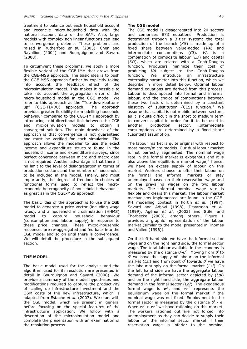
INTERNATIONAL JOURNAL OF MICROSIMULATION (2010) 3(1) 43-59

Scaling Up Infrastructure Spending in the Philippines: A CGE Top-

Down Bottom-Up Microsimulation Approach

Luc Savard GREDI, Faculté d‟administration, Université de Sherbrooke, 2500 Bld de l‟Université, Sherbrooke, Québec, Canada, J1K 2R1; email: [email protected]

ABSTRACT: In this paper we use a top-down bottom-up CGE microsimulation model with endogenous labour supply and unemployment to explore the impact of scaling up infrastructure spending in the Philippines. In the current debate on the importance of scaling up infrastructure to stimulate growth, some analysts raise concerns about potential negative macroeconomic impacts (Dutch disease). This study aims to provide some insight into this debate by extending the analysis to include distributional analysis. We draw from the infrastructure productivity literature to postulate positive productive

externalities of new infrastructure and from Fay and Yepes (2003) to include operating and maintenance costs associated with new infrastructure. We investigate two fiscal tools and foreign aid as mechanisms to fund the new infrastructure and associated costs. The distributional analysis is performed with FGT indices and growth incidence curves. Our results reveal that infrastructure spending reduces poverty. Foreign aid is shown to be the most equitable funding mechanism, whereas a value added tax provides

the strongest poverty reduction.

Keywords: Investment externalities, infrastructure, foreign aid, fiscal reforms, poverty, CGE, microsimulation. INTRODUCTION

Since Aschauer (1989) and Munnell (1990) stressed the important role of the public sector in funding infrastructure to stimulate economic development, a vast literature has dealt with this issue. Theoretical models and empirical studies have attempted to shed some light on this relationship. Some authors believed that a decline

in productivity would be induced by slow expansion of public infrastructure investment (Bergman and Suan 1996; and Binder and Smith

1997). In policy circles, the role of infrastructure was somewhat neglected in the context of the stabilization and structural adjustment programs

of the mid-eighties and nineties. For many international institutions and developing countries the focus was directed at liberalizing trade, improving macroeconomic balances and reacting to various external shocks. With improvements in these areas yet sluggish results in terms of poverty reduction in many countries, the end of

the nineties saw major changes in development strategies by international financial institutions (IFI), development partners and governments of developing countries. According to Estache (2007), infrastructure appears to be returning to the research agenda of

development economists. This reflects a change in priorities of developing country governments, IFIs and multi- and bilateral donor agencies bringing infrastructure back to the top of the policy agenda. The Asian Development Bank organized a major conference entitled “Infrastructure

Development: Private Solutions for the Poor” in October 2002 in Manila. This conference dealt with issues such as making infrastructure projects pro-poor, increasing private sector participation to scale up infrastructure and strengthening and increasing pro-poor public-private infrastructure partnerships. It built on a May 2000 conference

organized by the Department for International Development (DFID-UK) and the World Bank. The

World Bank‟s world development report published in 2001 is another important illustration of this change, as is the implementation in many developing countries of Poverty Reduction Strategy Programs (PRSPs). More recently the Asian Development Bank (2009) published a report on investing in sustainable infrastructure to

improve lives. Since the turn of the century, poverty has been at the centre of all development strategies. In many developing countries, growth

is constrained by infrastructure bottlenecks and this is reflected in many investment climate surveys in which infrastructure ranks as the top

priority (Estache, 2007).1 Recently, governments of developing countries and various development partners have been investigating the determinants of poverty and the most effective roads out of poverty. One important determinant that has been identified is

improvements in productivity. Education has received great attention as a tool to improve labour productivity. As a result, significant investments have been made, and major reforms have been implemented, to improve education in developing countries. At the same time, more and more analysts have raised the issue of

deteriorated or obsolete infrastructure in developing countries as a stumbling block for growth. In many countries, infrastructure growth has not kept up with economic and demographic growth and in some instances infrastructure was not even maintained. This situation has led many

analysts to return to the literature linking public expenditure to infrastructure. These stakeholders have argued that major investments to scale up infrastructure levels would transform their role from a constraint to an engine of growth that would contribute indirectly to poverty reduction in the long term.

SAVARD Scaling up infrastructure spending in the Philippines 44

At the same time, some researchers, such as

Gupta et al. (2006), Foster and Killick (2006) and Mckinley (2005), have suggested that scaling up

aid could have negative macroeconomic consequences, notably through Dutch disease (i.e., in which foreign inflows contribute to a real exchange rate appreciation that adversely affects

a country‟s international competitiveness). These conclusions have been challenged by others in empirical studies such as Berg et al. (2007) for five Sub-Saharan African countries, Li and Rowe (2007) for Tanzania and Mongardini and Rayner (2009) for a panel of 28 Sub-Saharan African countries. Many researchers have also

investigated the impacts or challenges of scaling up aid to achieve the Millennium Development Goals (MDG), notably Bourguignon and Sundberg (2006) and Hailu (2007). Although the debate has not been settled, concern for risks associated with a large scaling up of aid (for infrastructure or

other expenditures) continues to prevail in many

policy circles. Others argue that significant infrastructure spending may result in inflation and a resulting loss of competitiveness. There is also an important body of literature dealing with the crowding-out

effects of public investment. Finally, some authors have raised concerns over the excessive operation and maintenance (O&M) cost burden of increased public infrastructure. In a recent comprehensive report sponsored jointly by the African Development Bank, the

World Bank and the Agence Française pour le Développement, edited by Foster and Briceño-Garmendia (2010), it was found that half of Africa‟s growth was generated by infrastructure.

In the report, the authors argue that improved infrastructure will accelerate urbanization, which has been the engine for growth in many countries,

and will also improve regional integration. They focus on the potential contribution to the growth of various forms of infrastructure such as information and communication technologies, electricity, transportation (in a broad sense), water, irrigation and sanitation. They further

decompose the respective contributions of investments in roads, railway, ports and airports. The report also investigates the impact on poverty, the role of institutions and the various options available. The main contribution of this report is to provide an estimate of infrastructure spending in Africa needed to achieve optimal

growth rates. This price tag is estimated at 93

billion per year, of which one third is required for O&M. In this paper we provide a comparative analysis of funding mechanisms to finance infrastructure investment and associated O&M costs. We build

on work by Adam and Bevan (2006), Levy (2007) and Estache et al. (2007), who explore how infrastructure investments funded through foreign aid can contribute to Dutch disease. In their 2006 paper, Adam and Bevan show that the impact of Dutch disease can be attenuated if non-tradable

sectors also benefit from infrastructure investment

externalities. They construct an aggregate model and apply it to Uganda to verify this. We extend

this idea by dropping the dichotomous classification of sectors as tradable and non-tradable. We also introduce an additional element by imposing increases in public expenditure to

maintain and repair the new public infrastructure as in Estache et al. (2007). We investigate fiscal policy and foreign aid as possible funding mechanisms. We further extend previous work by introducing distributional analysis with poverty indices and growth incidence curves. For this purpose, we adopt a top-down/bottom-up CGE

microsimulation approach. The paper is structured as follows: we present the CGE top-down/bottom approach in the context of CGE microsimulation approaches, then set forth our model and resolution strategy and present our

simulations, followed by an examination of macro

and distributional analysis. We end the paper with our concluding remarks and possible extensions. CGE MICROSIMULATION APPROACHES

Three main approaches have been used to study the impacts of macro reforms on income distribution and poverty. The first and most commonly used one is the representative household approach (CGE-RH), the second is the top-down, layered or microsimulation sequential approach (CGE-MSS), and the third is usually

referred to as the CGE integrated multi-household (CGE-IMH) (see Davies (2009) for a detailed description of these approaches).

Without going into a complete review of these approaches, we wish to highlight a few of their drawbacks in order to situate the contribution of

the Top-down/bottom-up approach. First, despite extensive applications for distributive analysis, the CGE-RH has been strongly criticized for its inability to capture intra group changes in distribution (see Savard (2005) and Robilliard et al. (2008) for an elaboration of this critique). The

main drawback of the CGE-MSS approach is that it does not fully take into account the feedback effects to the CGE model of household behaviour in the microsimulation model. In fact, when micro-household behaviour aggregates perfectly, this approach implicitly integrates the feedback effect. However, when household behaviour does not

aggregate perfectly, the aggregation error is lost

in the process.2 The interesting question is to know the size of this aggregation error. If the aggregation error is small, not taking it into account is unlikely to bias results, but this is not the case if the error is relatively large. This critique of the CGE-MSS approach has been

highlighted in two literature reviews of macro-micro modelling for poverty analysis (Hertel and Reimer (2005) and Bourguignon and Spadaro (2006)). The third approach is the CGE-IMH, which is theoretically sound but presents a few challenges. First, it requires significant data


treatment to balance out each household account

and reconcile micro-household data with the national account data of the SAM. Also, large

models with complex non linear functions can lead to convergence problems. These problems are raised in Rutherford et al. (2005), Chen and Ravallion (2004) and Bourguignon and Savard

(2008). To circumvent these problems, we apply a more flexible variant of the CGE-IMH that draws from the CGE-MSS approach. The basic idea is to push the CGE-MSS approach further by explicitly taking into account the feedback effect of the

microsimulation model. This makes it possible to take into account the aggregation error of the micro-household model in the CGE model. We refer to this approach as the “Top-down/bottom-up” (CGE-TD/BU) approach. The approach provides greater flexibility for modelling household

behaviour compared to the CGE-IMH approach by

introducing a bi-directional link between the CGE and microsimulation models to obtain a convergent solution. The main drawback of the approach is that convergence is not guaranteed and must be verified for each simulation. The approach allows the modeller to use the exact

income and expenditure structure found in the household income and expenditure surveys, since perfect coherence between micro and macro data is not required. Another advantage is that there is no limit to the level of disaggregation in terms of production sectors and the number of households to be included in the model. Finally, and most

importantly, the degree of freedom in choices of functional forms used to reflect the micro-economic heterogeneity of household behaviour is as great as in the CGE-MSS approach.

The basic idea of the approach is to use the CGE model to generate a price vector (including wage

rates), and a household microsimulation (HHMS) model to capture household behaviour (consumption and labour supply) in response to these price changes. These micro-household responses are re-aggregated and fed back into the CGE model and so on until there is convergence.

We will detail the procedure in the subsequent section. THE MODEL The basic model used for the analysis and the

algorithm used for its resolution are presented in

detail in Bourguignon and Savard (2008). We provide a summary of the model hypotheses and modifications required to capture the productivity of scaling up infrastructure investment and the O&M costs of the new infrastructure, which is adapted from Estache et al. (2007). We start with

the CGE model, which we present in general before focusing on the special features of the infrastructure application. We follow with a description of the microsimulation model and complete the presentation with an examination of the resolution process.

The CGE model

The CGE model is disaggregated into 20 sectors and comprises 873 equations. Production is

determined through a 3-tier system: the total production of the branch (XS) is made up of a fixed share between value-added (VA) and intermediate consumptions (CI). VA is a

combination of composite labour (LD) and capital (KD), which are related with a Cobb-Douglas function. Producers minimize their cost of producing VA subject to the Cobb-Douglas function. We introduce an infrastructure externality parameter into this function, which we describe in more detail below. Optimal labour

demand equations are derived from this process. Labour is decomposed into formal and informal labour, and the choice of combinations between these two factors is determined by a constant elasticity of substitution (CES) function.3 We assume that capital is not mobile between sectors,

as it is quite difficult in the short to medium term

to convert capital in order for it to be used in another production sector. Intermediate consumptions are determined by a fixed share (Leontief) assumption. The labour market is quite original with respect to

most macro/micro models. Our dual labour market is not perfectly segmented. The nominal wage rate in the formal market is exogenous and it is also above the equilibrium market wage;4 hence, we have an excess supply of labour on this market. Workers choose to offer their labour on the formal and informal markets or stay

unemployed based on their reservation wage and on the prevailing wages on the two labour markets. The informal nominal wage rate is flexible and clears this market. The labour market

mechanisms implemented are found in the CGE-RH modelling context in Fortin et al. (1997), Savard and Adjovi (1998), Devarajan et al.

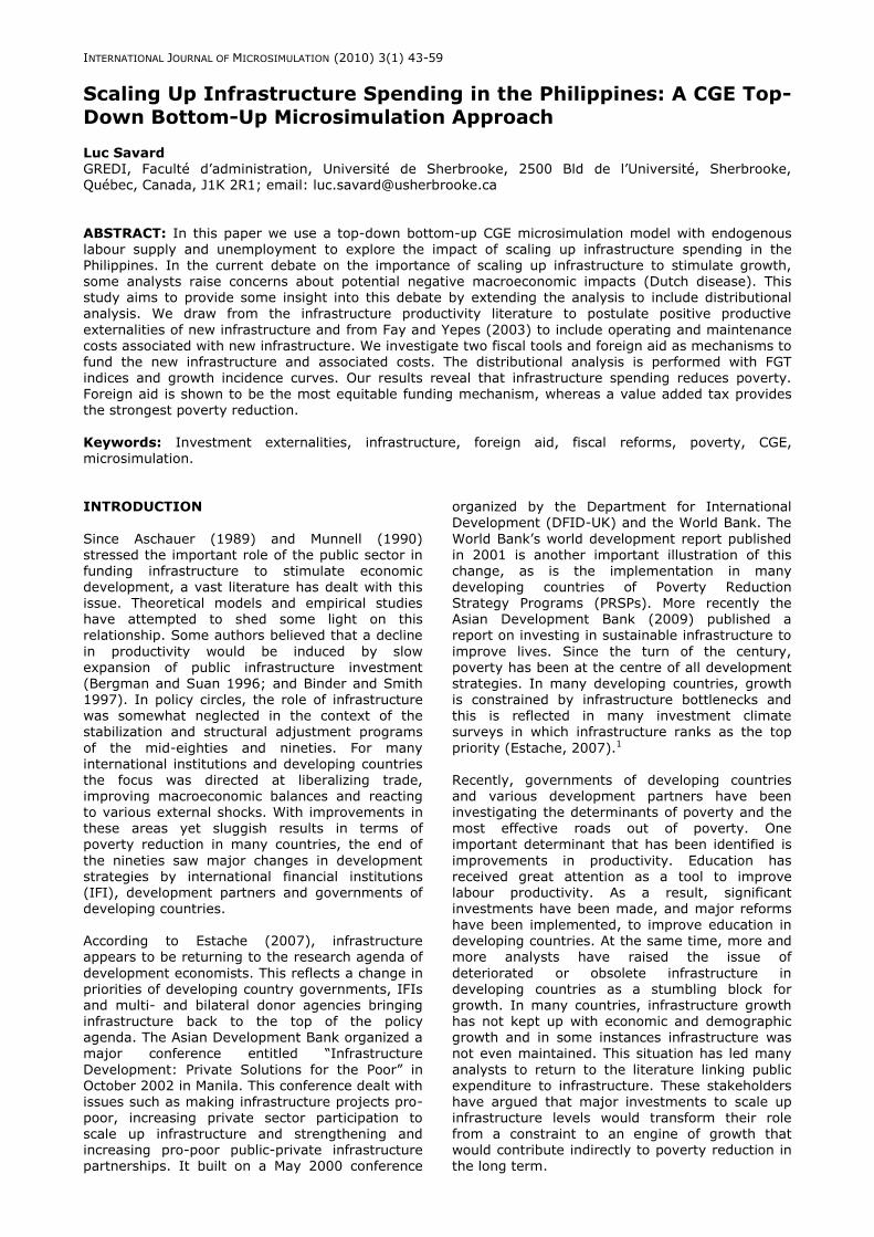
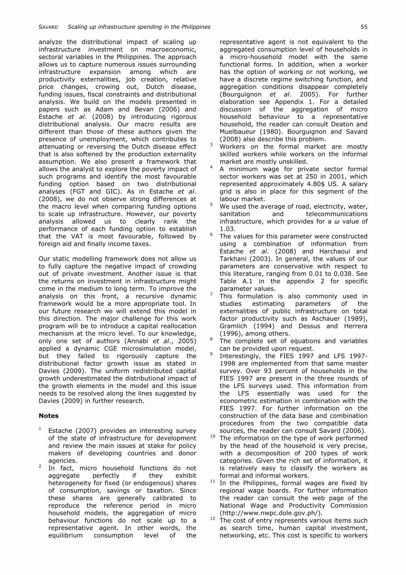
(1999), Agénor et al. (2003) and Stifel and Thorbecke (2003), among others. Figure 1 provides a graphic representation of the labour market (similar to the model presented in Thomas and Vallée (1996)).

On the left hand side we have the informal sector wage and on the right hand side, the formal sector wage. The total labour available in the economy is measured by the distance 0i-0f. Moving from 0i to 0f we have the supply of labour on the informal market (Lsi) and from point 0f towards 0i we have the labour supply on the formal market (Lsf). On

the left hand side we have the aggregate labour

demand of the informal sector depicted by (Ldi) and on the right hand side, the aggregate labour demand in the formal sector (Ldf). The exogenous formal wage is w1, and w1* represents the equilibrium wage on the formal market if the nominal wage was not fixed. Employment in the

formal sector is measured by the distance 0f - e. When w1 > w1* we have rationing on this market. The workers rationed out are not forced into unemployment as they can decide to supply their labour on the informal sector market if their reservation wage is inferior to the nominal


Figure 1 Labour market representation informal wage. The rationed unemployed are

measured by the distance e – d and the waiting

unemployment, by the distance b – d. Further details are provided in the presentation of the microsimulation model further on. We only have one representative household in the CGE model and its income is composed of wage payments (from the two labour categories),

capital payments, dividends and transfers from other agents. As opposed to what we would find in the CGE-IMH approach, the labour endowment is endogenous (as stated above), although this is only factored in the micro model. Workers can move in and out of unemployment as well as

between the formal and informal markets but these movements will be computed in the microsimulation model and transferred into the CGE model in the resolution procedure.

The key assumptions to capture the impact of infrastructure spending concern their production

externalities and the government budget constraint to fund O&M costs. A complete description of the model can be found in Estache et al. (2007). This first equation (1.1) is the government budget constraint (equation 1.1) where government income (Yg) is spent on public services or expenditures (G) and on government

savings (Sg), which will be used entirely for public investment.

(1.1)

We assume that public spending is exogenous and

that public savings (the budget surplus) is

implicitly exogenous as it is equal to public investment, which is exogenous. Hence, to fund new public infrastructure, the government will need an endogenous source of revenue such as a tax instrument or a foreign transfer (aid). We introduce an additional assumption, namely that

an increase in public infrastructure investment will generate higher O&M costs for the government. We draw this assumption from the estimations of Fay and Yepes (2003).5 The externality equation (1.2) is the other

important assumption, given its role in increasing

the total productivity of factors in the value added

equation (1.3). For this, we draw on the vast literature linking public infrastructure to private sector factor productivity, including Dumont and Mesplé-Somps (2000) in a CGE context, although our externality function does not include private investment. This function was also used in Estache et al. (2008). The function defining the externality

is the following:

(1.2)

where θi is the externality or sectoral productivity effect, which is a function of the ratio of new public investment (Itp) over past public investment (Itpo) with a sector-specific elasticity

(ξi).6 The externality is introduced in the value

added (Vai) equation:

(1.3)

where Ai is the scale parameter, Ldi, the labour demand, Kdi, the capital demand, and α, the Cobb-Douglas parameter. Hence, an increase in θi represents a Hicks neutral productivity improvement, like the one modelled in Yeaple and

Golub (2007).7 With this formulation, the infrastructure investment can act as a source of comparative advantage because the function is sector specific. Commodity markets are balanced through adjustments in market prices. The current account

balance is fixed; accordingly, the nominal

exchange rate varies to allow the real exchange rate to clear the current account balance. The GDP deflator is used as the numeraire in the model. We also assume in a standard manner that the Philippines is a small open economy. Armington‟s

(1969) assumption is adopted for the demand of imported goods (imperfect substitution with constant elasticity of substitution function (CES)) and constant elasticity of transformation (CET) functions are used to model export supply.8

b d e

f

w1

0i 0

f

w1 w

2

Ldi

Lsi

Ldf

Lsf

w1*

c g


The household microsimulation model

(HHMS) The construction of the household microsimulation

model (HHMS) relies on data for all of the 39,520 households from the 1997 Family Income and Expenditure Survey (FIES) and on three rounds of the Labour Force Survey (LFS) run between 1997

and 1998.9 The HHMS comprises a representation of household income structures and expenditure behaviour as well as their labour supply decisions. Household consumption is modelled with a linear expenditure demand system (LES). We use the calibration method proposed by Dervis et al. (1982). Savings and income tax rates are

calibrated according to the observed data in the survey. All transfers received and paid are exogenous. We consider that capital endowments are fixed at the levels observed in the 1997 FIES. In the FIES, we have information on the sector of activity of the household head and on the amount

of non-wage income. This allows for a mapping of

the sector of origin for household capital income. Based on information from the FIES and LFS, we classified wage earners into formal and informal workers according to the category of work specified in the survey.10

Our labour market mechanism is drawn from the Roy (1951) model, which was revisited by Heckman and Sedlacek (1985) and further enriched by Magnac (1991). We selected the non competitive version of the models presented by Magnac (1991), as it includes a formal and informal market with unemployment. The formal

market in non competitive; it has a rigid nominal wage and workers face a cost of entry to access this market. The fixed formal wage is above the market equilibrium wage, which creates excess

supply on this market. The rigid wage can reflect various interventions on the labour market such as labour union contracts, efficiency wages and

regulated wages.11 The labour supply model is estimated with the two-step Heckman procedure. More details on the labour supply model and the results of the estimation results can be found in Bourguignon and Savard (2008). The estimated model allows us to compute the worker-specific

cost of entry, the reservation wage and the potential wage. Each of these elements is used in constructing our labour supply in the HHMS. The key feature of the labour supply model is the introduction of an endogenous labour supply, but it also serves to compute changes in income,

consumption and welfare changes at the

household level. We introduce mobility between the three statuses of workers and potential workers, namely informal work, formal work and unemployment. The transformation at the micro level allows us to allocate changes in labour supply to the informal sector and unemployment

in the HHMS model. We now describe how we go from the labour supply model to our HHMS model to construct our two labour supplies. For the formal market, we construct two queues. The first concerns the formal sector workers who

can be laid off in the context of a decrease in

formal labour demand generated by the CGE model. The second concerns unemployed and

informal market workers who supply their labour to the formal market when formal labour demand increases in the CGE model. We assume that firms have perfect knowledge of the workers‟

productivity (implicitly their potential wage). If formal labour demand increases, workers are drawn from the queue of informal and unemployed workers. To be included in the queue, two conditions from our labour supply model must be satisfied by workers: the formal wage minus

the cost of entry into the formal sector must be greater than both the reservation wage of the worker and the informal wage.12 Workers satisfying these two conditions are then ranked based on their potential wage and formal sector firms recruit the most qualified workers from this

queue.

In the presence of a decrease in formal sector labour demand, the least productive formal sector workers, based on their potential wage computed from the labour supply model, will be laid off. The destination of laid off workers depends on the

reservation wage of the workers compared to the prevailing informal sector wage. If the reservation wage is above the informal wage the workers become unemployed, and if it is lower they supply their labour to the informal market. The reservation wage check with the informal sector wage is not only applied to laid off workers in the

formal sector but also to active informal sector workers and the unemployed; the change in informal wage can modify the status of either. This procedure provides us with the new labour

endowments in the HHMS to compute the new income level, expenditure and change in welfare. The final step in the HHMS consists in computing

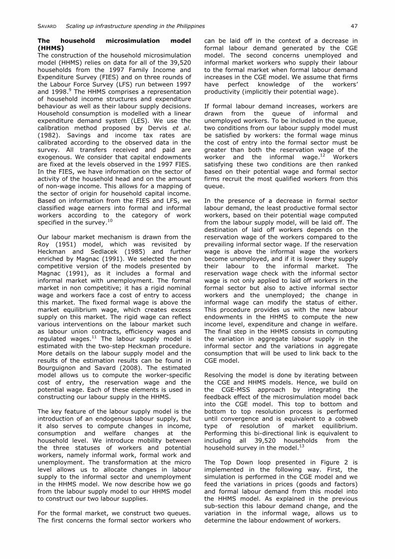
the variation in aggregate labour supply in the informal sector and the variations in aggregate consumption that will be used to link back to the CGE model. Resolving the model is done by iterating between

the CGE and HHMS models. Hence, we build on the CGE-MSS approach by integrating the feedback effect of the microsimulation model back into the CGE model. This top to bottom and bottom to top resolution process is performed until convergence and is equivalent to a cobweb type of resolution of market equilibrium.

Performing this bi-directional link is equivalent to

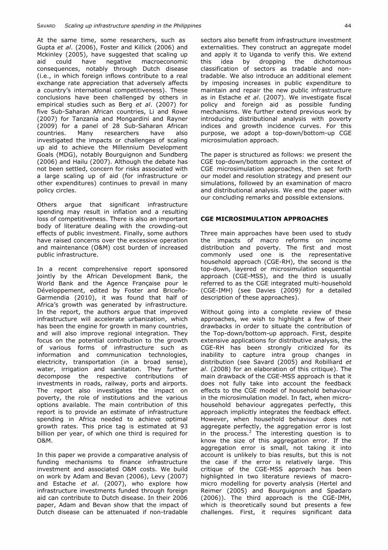
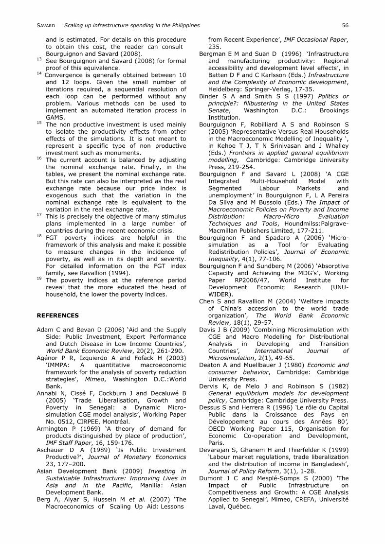
including all 39,520 households from the household survey in the model.13 The Top Down loop presented in Figure 2 is implemented in the following way. First, the simulation is performed in the CGE model and we

feed the variations in prices (goods and factors) and formal labour demand from this model into the HHMS model. As explained in the previous sub-section this labour demand change, and the variation in the informal wage, allows us to determine the labour endowment of workers.


Figure 2 Resolution procedure of the TD/BU approach

Once this is done, we can determine the new income and consumption level of each household. We then aggregate consumption and informal labour supply and compute the variations in these

two variables. These variations are finally introduced into the CGE module where aggregate consumption and informal labour supply is exogenous. We repeat this loop until converging results are obtained for these two variables.14 We know that there are conditions that satisfy the

stability of the cobweb resolution approach and these conditions also apply to the resolution of the TDBU approach. Our application of the CGE-TDBU approach to the Philippines is programmed with GAMS software. Our CGE model has 873 equations and endogenous variables, whereas the

microsimulation model has 829,920 equations

with 829,920 endogenous variables. THE SIMULATIONS In order to analyze the macro and distributional impacts of scaling up infrastructure investment

under different funding mechanisms, we contrast two types of infrastructure investments; a non productive one and a productive one.15 These simulations are well justified in the context of the economic crisis and the larger debate on scaling up infrastructure in developing countries described

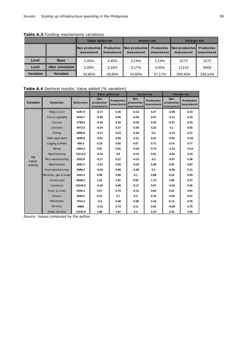
in the introduction. We simulate an increase of 30 percent in public investment on infrastructure with respect to the level of investment in the reference period. We compare three funding mechanisms

consisting of increases in the value added tax rate, the income tax rate and foreign aid. It is important to highlight that the effective tax rates

observed in the SAM are relatively small in the reference period: between 2 and 3 percent for the two weighted average tax rates. Hence, the increase in these taxes required to fund the program is large in percentage terms, but not in nominal terms. The increases necessary for the three funding schemes are presented in Table A.3

in the appendix. Productive externalities contribute to increased economic activity, which

increases government revenues. Hence, the funding requirements are not equal to the direct investment and O&M costs.

IMPACT ANALYSIS OF THE SCENARIOS A comparative analysis of productive and non-productive investments under three funding mechanisms allows us to highlight the most

efficient funding mechanism. We explore the effect on different macroeconomic and sectoral variables in addition to the distributional impacts. To simplify the presentation, we focus on the macroeconomic variables and the key sectoral impacts contributing to welfare and distributional

impacts, namely market prices and returns to

factors. We compare funding options throughout the section. We concentrate on productive investments with a brief comparative analysis to non productive investments at the end of the section. Distribution analysis follows in the subsequent section. When looking at results (Tables 1 to 3), it is important to keep in mind

that our current account balance is fixed.16 Before moving on to the specific simulations, we can begin with a few general comments. First, the impacts on GDP and most macro variables are relatively modest. This results from the fact that,

in nominal terms, the 30% increase in public investment is not large compared to size of the economy (0.48%). However, this is not an important issue as we are mostly interested in the

comparative analysis between the different scenarios. The second point is that all simulations produce a positive impact on GDP, although the

non productive simulations produce a very small impact. This positive effect comes in part from the productivity gains of the infrastructure but also from the economic activity generated by these investments.17 The positive effect helps create employment in the construction sector and in the public services to operate and maintain this new

infrastructure. The sectors supplying goods and services more intensively to these two sectors,

Top Module CGE

Endogenous (P, Y, Q, Ldfa)

Exogenous (C, Lsi, w1)

Output to HHMS module (P,Ldfa,w

2)

Loop to

Ct-Ct+1 1x10-7

and Lsit-Lsit+1 1x10-7

Bottom module (HHMS) Endogenous (Y, C, Lsi, Uc)

Exogenous (P, w1, w

2, Ldf

a)

Output to CGE (C, Lsi)

C : Household consumption

P : Price vector

w1: Formal wage

w2: Informal wage

Y : Household income

Q : Supply of goods

Ldfa : Aggregate demand (formal)

Lsi : Informal labor supply

Uc : unemployment rate


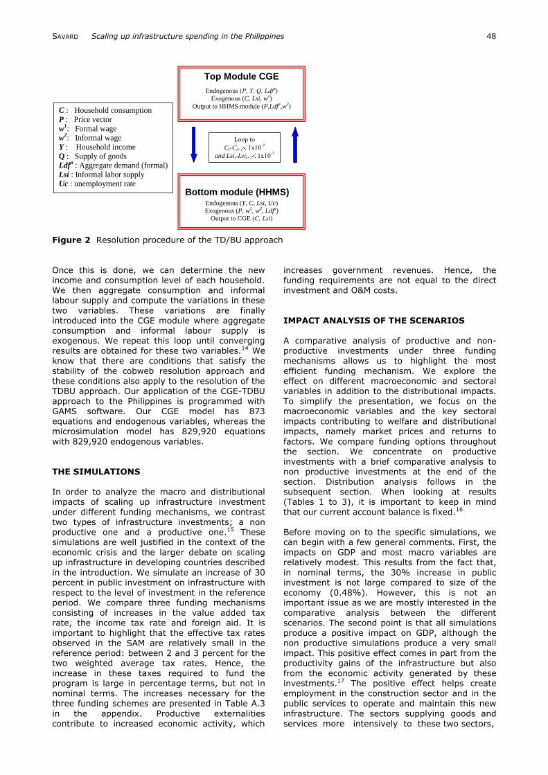
Table 1 Macroeconomic results (% variations)

Source: Values computed by the author

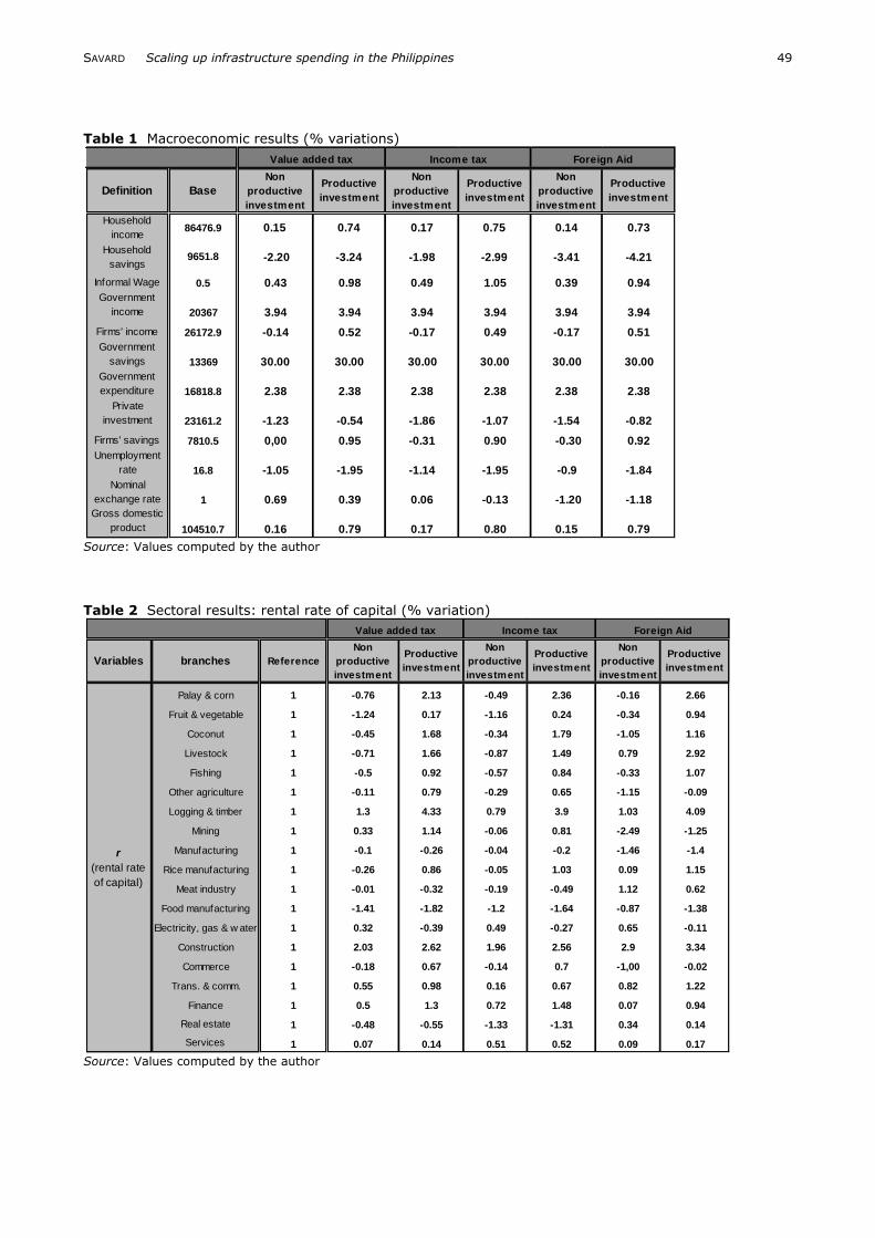
Table 2 Sectoral results: rental rate of capital (% variation)


Definition Base

Non

productive

investment

Productive

investment

Non

productive

investment

Productive

investment

Non

productive

investment

Productive

investment

Household

income86476.9 0.15 0.74 0.17 0.75 0.14 0.73

Household

savings9651.8 -2.20 -3.24 -1.98 -2.99 -3.41 -4.21

Informal Wage 0.5 0.43 0.98 0.49 1.05 0.39 0.94

Government

income 20367 3.94 3.94 3.94 3.94 3.94 3.94

Firms' income 26172.9 -0.14 0.52 -0.17 0.49 -0.17 0.51

Government

savings 13369 30.00 30.00 30.00 30.00 30.00 30.00

Government

expenditure 16818.8 2.38 2.38 2.38 2.38 2.38 2.38

Private

investment 23161.2 -1.23 -0.54 -1.86 -1.07 -1.54 -0.82

Firms' savings 7810.5 0,00 0.95 -0.31 0.90 -0.30 0.92

Unemployment

rate 16.8 -1.05 -1.95 -1.14 -1.95 -0.9 -1.84

Nominal

exchange rate 1 0.69 0.39 0.06 -0.13 -1.20 -1.18Gross domestic

product 104510.7 0.16 0.79 0.17 0.80 0.15 0.79

Value added tax Income tax Foreign Aid

Variables branches Reference

Non

productive

investment

Productive

investment

Non

productive

investment

Productive

investment

Non

productive

investment

Productive

investment

Palay & corn 1 -0.76 2.13 -0.49 2.36 -0.16 2.66

Fruit & vegetable 1 -1.24 0.17 -1.16 0.24 -0.34 0.94

Coconut 1 -0.45 1.68 -0.34 1.79 -1.05 1.16

Livestock 1 -0.71 1.66 -0.87 1.49 0.79 2.92

Fishing 1 -0.5 0.92 -0.57 0.84 -0.33 1.07

Other agriculture 1 -0.11 0.79 -0.29 0.65 -1.15 -0.09

Logging & timber 1 1.3 4.33 0.79 3.9 1.03 4.09

Mining 1 0.33 1.14 -0.06 0.81 -2.49 -1.25

Manufacturing 1 -0.1 -0.26 -0.04 -0.2 -1.46 -1.4

Rice manufacturing 1 -0.26 0.86 -0.05 1.03 0.09 1.15

Meat industry 1 -0.01 -0.32 -0.19 -0.49 1.12 0.62

Food manufacturing 1 -1.41 -1.82 -1.2 -1.64 -0.87 -1.38

Electricity, gas & w ater 1 0.32 -0.39 0.49 -0.27 0.65 -0.11

Construction 1 2.03 2.62 1.96 2.56 2.9 3.34

Commerce 1 -0.18 0.67 -0.14 0.7 -1,00 -0.02

Trans. & comm. 1 0.55 0.98 0.16 0.67 0.82 1.22

Finance 1 0.5 1.3 0.72 1.48 0.07 0.94

Real estate 1 -0.48 -0.55 -1.33 -1.31 0.34 0.14

Services 1 0.07 0.14 0.51 0.52 0.09 0.17

r

(rental rate

of capital)



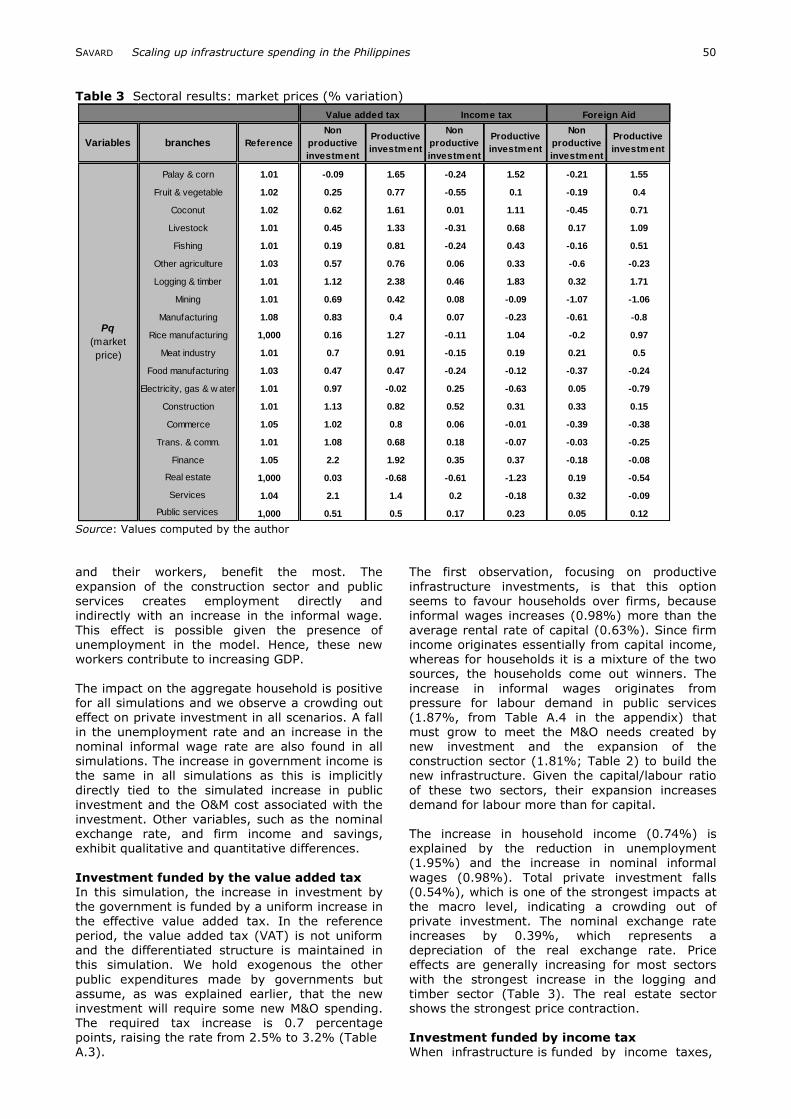
Table 3 Sectoral results: market prices (% variation)

Source: Values computed by the author and their workers, benefit the most. The

expansion of the construction sector and public services creates employment directly and indirectly with an increase in the informal wage.

This effect is possible given the presence of unemployment in the model. Hence, these new workers contribute to increasing GDP.

The impact on the aggregate household is positive for all simulations and we observe a crowding out effect on private investment in all scenarios. A fall in the unemployment rate and an increase in the nominal informal wage rate are also found in all simulations. The increase in government income is the same in all simulations as this is implicitly

directly tied to the simulated increase in public investment and the O&M cost associated with the investment. Other variables, such as the nominal exchange rate, and firm income and savings, exhibit qualitative and quantitative differences.

Investment funded by the value added tax In this simulation, the increase in investment by the government is funded by a uniform increase in the effective value added tax. In the reference period, the value added tax (VAT) is not uniform and the differentiated structure is maintained in this simulation. We hold exogenous the other

public expenditures made by governments but assume, as was explained earlier, that the new investment will require some new M&O spending. The required tax increase is 0.7 percentage points, raising the rate from 2.5% to 3.2% (Table A.3).

The first observation, focusing on productive

infrastructure investments, is that this option seems to favour households over firms, because informal wages increases (0.98%) more than the

average rental rate of capital (0.63%). Since firm income originates essentially from capital income, whereas for households it is a mixture of the two sources, the households come out winners. The

increase in informal wages originates from pressure for labour demand in public services (1.87%, from Table A.4 in the appendix) that must grow to meet the M&O needs created by new investment and the expansion of the construction sector (1.81%; Table 2) to build the new infrastructure. Given the capital/labour ratio

of these two sectors, their expansion increases demand for labour more than for capital. The increase in household income (0.74%) is explained by the reduction in unemployment (1.95%) and the increase in nominal informal

wages (0.98%). Total private investment falls (0.54%), which is one of the strongest impacts at the macro level, indicating a crowding out of private investment. The nominal exchange rate increases by 0.39%, which represents a depreciation of the real exchange rate. Price effects are generally increasing for most sectors

with the strongest increase in the logging and timber sector (Table 3). The real estate sector shows the strongest price contraction. Investment funded by income tax When infrastructure is funded by income taxes,


Non

productive

investment

Productive

investment

Non

productive

investment

Productive

investment

Non

productive

investment

Productive

investment

Palay & corn 1.01 -0.09 1.65 -0.24 1.52 -0.21 1.55

Fruit & vegetable 1.02 0.25 0.77 -0.55 0.1 -0.19 0.4

Coconut 1.02 0.62 1.61 0.01 1.11 -0.45 0.71

Livestock 1.01 0.45 1.33 -0.31 0.68 0.17 1.09

Fishing 1.01 0.19 0.81 -0.24 0.43 -0.16 0.51

Other agriculture 1.03 0.57 0.76 0.06 0.33 -0.6 -0.23

Logging & timber 1.01 1.12 2.38 0.46 1.83 0.32 1.71

Mining 1.01 0.69 0.42 0.08 -0.09 -1.07 -1.06

Manufacturing 1.08 0.83 0.4 0.07 -0.23 -0.61 -0.8

Rice manufacturing 1,000 0.16 1.27 -0.11 1.04 -0.2 0.97

Meat industry 1.01 0.7 0.91 -0.15 0.19 0.21 0.5

Food manufacturing 1.03 0.47 0.47 -0.24 -0.12 -0.37 -0.24

Electricity, gas & w ater 1.01 0.97 -0.02 0.25 -0.63 0.05 -0.79

Construction 1.01 1.13 0.82 0.52 0.31 0.33 0.15

Commerce 1.05 1.02 0.8 0.06 -0.01 -0.39 -0.38

Trans. & comm. 1.01 1.08 0.68 0.18 -0.07 -0.03 -0.25

Finance 1.05 2.2 1.92 0.35 0.37 -0.18 -0.08

Real estate 1,000 0.03 -0.68 -0.61 -1.23 0.19 -0.54

Services 1.04 2.1 1.4 0.2 -0.18 0.32 -0.09

Public services 1,000 0.51 0.5 0.17 0.23 0.05 0.12

Pq

(market

price)



the effective income tax rate rises from 2.2% to

3.0% (a 37% increase). The macro results are quite similar to the previous simulation with main

differences observed for the nominal exchange rate, with an appreciation of 0.13% compared to a depreciation of 0.39% in the previous simulation, indicating a very slight Dutch disease effect. There

is also more crowding out as total investment decreases more (1.07%) compared to the previous simulation (0.54%). The slightly stronger negative impact on firm income is the source of this difference. The other macro level results largely resemble the VAT-funded scenario.

For the rental rate of capital, the qualitative effects are the same as in the previous simulation, although the weighted average increase is slightly weaker (0.60%, compared to 0.63%). Some sectoral differences are observed in the returns to capital. Market price variations (Table 3) are

smaller for most sectors and qualitative

differences are observed in six sectors with the largest gap for the service sector passing from a 1.4% increase for the VAT scenario to a 0.18% decrease in this case. These stronger differences at the market price will have distributional impacts further on.

Investment funded by foreign aid At the macro level, the main difference is observed for the nominal exchange rate, which is not surprising insofar as the current account balance is fixed and an increase in foreign aid thus requires an appreciation of the exchange rate. The

Dutch disease effect is thus greater than in the income tax simulation. The unemployment rate decreases less compared to the previous two simulations. Other macro results are almost

identical to the other simulations. The market price and rental rate of capital are

more sensitive to this funding scheme and we have many qualitative changes in the sectoral impacts compared to the first two scenarios. The differences are greater when we compare these results with the VAT scenario. These stronger price differences should have a distributional

impact on the income side (rental rate of capital) and on the consumption side (market prices). Comparing productive and non productive infrastructure We note a weaker positive effect on GDP, household income and firm income in the non-

productive investment scenarios. This is not

surprising as we built in this difference. As was the case for productive investments, the choice of funding mechanism does not have much impact on the macro results. However, the crowding out effect is almost doubled in the non productive investment scenarios, compared to productive

investments. For price variations (market price and rental rate of capital) the effects are quite different. For the VAT funding option, nine out of the nineteen sectors exhibit a qualitative change in terms of the

impacts on the rental rate of capital. For all

agricultural sectors, the difference is strong, ranging from a 0.9% improvement for other

agriculture to a 2.89% improvement in the palay and corn sector. The pattern of differences between the income tax scenarios is similar to that of the VAT simulations. The foreign aid

scenarios generate closer results, with only five sectors exhibiting qualitative differences. Moreover, the quantitative gap between the productive and non productive scenarios is weaker with foreign aid financing. As for market price variations, we observe many differences between non productive and productive options with

between five (VAT) and eight (foreign aid) qualitative differences. There is no clear trend that can be observed either. Before moving on to the distributional impact of our policies, we can summarize the key effects

that will play an important role. VAT funding will

have a tendency to favour sectors in which initial VAT rates were lower and, consequently, households that consume a lower share of goods and services with high VAT rates in the reference period. Workers and owners of capital in the sectors with higher VAT rates will experience a

stronger negative impact. Moving on to the income tax scenario, on the income side we will have a stronger negative impact on households that pay income taxes. As a result, the price of goods consumed by households with higher income decrease more compared to the first scenario. The price effect may dominate the

income effect for certain households. Foreign aid financing produces a price and income effect via the appreciation of the exchange rate given the fixed current account balance. This will favour

consumers of imported goods on the price side. On the income side, the non tradable sectors will be favoured and hence capital owners and

workers used intensively in these sectors will benefit the most. The final impact is a combination of these more direct effects and indirect effects captured by all assumptions and interactions in the model. It is

also important to note that, contrary to many CGE microsimulation models, we capture discrete changes in income, and not only marginal changes in income, with workers moving in and out of unemployment and between the formal and informal sectors. This can produce unusual distributional effects. For example, a relatively rich

household in the reference period can become

unemployed after simulation and lose a large portion of its income. DISTRIBUTIONAL ANALYSIS

For the distributional analysis, we apply poverty indices and compute growth incidence curves. The poverty index chosen (FGT) is the additively decomposable P proposed by Foster, Greer and

Thorbecke (1984).18 To complete the distributional analysis, we computed the growth incidence curve


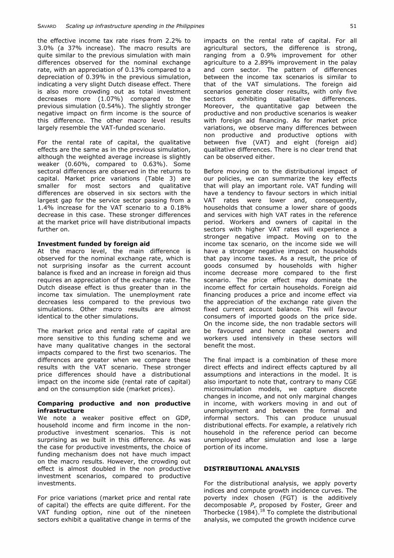
Table 4 Poverty index results (% variation)

Source: Values computed by the author. Notes: See Table A.2 for educational codes

(GIC) proposed by Ravallion and Chen (2003).

Poverty analysis We use the change in household welfare, measured by change in real income, to evaluate the impact of the policy on each household. This approach has the advantage of taking into account the price and income effects simultaneously. This approach is quite standard in the context of

macro-micro CGE analysis. The CGE top-down/bottom-up model generates post simulation changes in welfare at the household level that are used for poverty analysis. Households can be grouped into various socio-economic categories for the analysis, which can be repeated for the

base period and each simulation. For our application, we group households based on the education level of the household head.

The first point we can make is that poverty impacts are relatively small (Table 4). As we highlighted in the macro analysis, this comes from

the relatively small nominal increase in public investment, but we can still draw interesting conclusions on relative impacts between productive and non productive investments and between the three funding schemes. Starting at the national level, with non productive investments, we observe a decrease in poverty

only for the VAT scenario. This reduction is

observed for the three poverty indices, ranging from 0.26% for the headcount index (FGT-0) to

0.30% for poverty severity (FGT-2). The income tax and foreign aid scenarios for non productive investment produce an increase in poverty severity ranging up to 1.33% for the income tax option and 0.88% for foreign aid. This is interesting in that GDP and aggregate household income increased in both those scenarios. This

illustrates the importance of using a microsimulation approach to determine the distributional and welfare impact of such reforms. The option generating the greatest increases in poverty is the income tax option.

Productive investments reduce poverty under all funding mechanisms, but produce a similar pattern in that the best option is the VAT, which

produces reductions in poverty ranging from 0.86% for the headcount index to 1.57% for the severity index. The least positive option is the income tax, which generates a poverty reduction

of around 0.2% for all three indices. This result is not surprising insofar as the households absorb fully and directly the funding option as a negative income effect. Foreign aid provides an intermediary option, with reductions of 0.41% for the headcount index and a drop of 0.60% for the severity index.

Poverty index

Code- education Base

Non productive investment

Productive investment





FGT-0 National 0.311 -0.26 -0.86 0.67 -0.19 0.49 -0.41 FGT-1 National 0.096 -0.27 -1.29 1.05 -0.20 0.68 -0.52 FGT-2 National 0.04 -0.30 -1.57 1.33 -0.22 0.88 -0.6

0 0.564 -0.36 -1.08 0.51 0.07 0.71 0.2 1 0.501 -0.37 -0.89 0.31 -0.26 0.27 -0.61 2 0.384 -0.29 -0.8 0.70 -0.26 0.3 -0.42 3 0.317 0.35 -0.71 1.52 0.27 1.38 -0.30 4 0.184 -0.34 -0.94 0.85 -0.33 0.2 -0.54 5 0.092 -0.47 -0.83 1.58 -0.35 1.35 0.40 6 0.021 -0.42 -0.42 -0.42 -0.42 3.54 -0.42

0 0.185 -0.19 -0.99 0.96 -0.05 0.92 -0.09 1 0.168 -0.24 -1.19 0.94 -0.20 0.61 -0.50 2 0.116 -0.30 -1.36 1.05 -0.23 0.62 -0.61 3 0.090 -0.32 -1.37 1.15 -0.17 0.79 -0.51 4 0.048 -0.31 -1.56 1.29 -0.22 0.71 -0.71 5 0.022 -0.26 -1.65 1.60 -0.11 1.05 -0.57 6 0.005 -0.49 -1.87 1.43 -0.24 1.51 -0.20 0 0.08 -0.25 -1.32 1.25 -0.09 1.14 -0.18 1 0.075 -0.27 -1.48 1.23 -0.23 0.82 -0.58 2 0.048 -0.32 -1.64 1.34 -0.26 0.82 -0.70 3 0.035 -0.36 -1.66 1.41 -0.20 0.95 -0.64 4 0.018 -0.31 -1.78 1.57 -0.23 0.93 -0.76 5 0.007 -0.28 -2.01 1.92 -0.19 1.22 -0.78 6 0.002 -0.38 -1.83 1.83 0.00 2.12 0.24

FGT-0

FGT-1

FGT-2

Foreign Aid Value added tax Income tax


Moving on to the decomposition analysis, we

observe a relatively uniform qualitative impact across the 7 household types – by education of

household head – for non productive investments. We only observe two cases of qualitative differences, namely for the VAT simulation, in which the poverty headcount increases for group 3

whereas other households benefit from a reduction in poverty indices, and the income tax simulation, where the headcount for group 6 falls by 0.42% whereas other households experience an increase in poverty indices. For the VAT simulation, we can identify a weak trend favouring the most educated households. For the income tax

option, the most educated groups (4, 5 and 6) have the largest poverty increase when using the poverty gap and severity indices. For the foreign aid funding scheme, the groups suffering the least are groups 1 and 2 for the three indices with one exception for FGT-0 where the most favoured

group is group 4.

The productive investment provides more interesting results. For the VAT option, the headcount index indicates that the least educated would be most advantaged, while the poverty gap and severity indices reveal a more regressive

option in which most educated households benefit the most.19 When the income tax serves as the funding mechanism, we cannot find a clear trend. Each indicator provides a different picture. The headcount index seems to favour the most educated and group 3 is faced with a 0.27% increase in poverty. In terms of the poverty gap

(FGT-1), we observe the most positive effects for group 6, and the least positive effects for groups 5 and 0. Poverty severity favours group 2, 1 and 4, and groups 6 and 0 are the losers. For the foreign

aid simulation, we seem to have a clearer winner with group 4 being top or second in terms of positive impact and group 0 being last or second

to last for all indices. Interestingly, group 5 has the worst situation for the headcount index and the best when using the severity index.

When comparing each funding option we can

clearly conclude that the VAT is the most favourable option both at the national level and

when looking at household decomposition results. Moreover, all groups benefit for all indices. In addition, the poverty reduction impact is quite large given the weak changes in macro and

sectoral variables. The foreign aid option also dominates the income tax option for the poverty depth and severity indices. For the headcount index, two groups (group 0 and 4) suffer more with the foreign aid compared to the income tax option. For the other groups, the foreign aid option is more favourable.

Comparing the micro distributional results with poverty results illustrates the importance of using a CGE microsimulation approach since the income tax option is the most favourable when looking at aggregate variables such as GDP, aggregate

household income, informal wage and

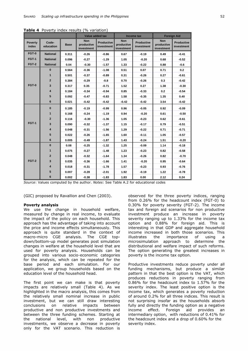
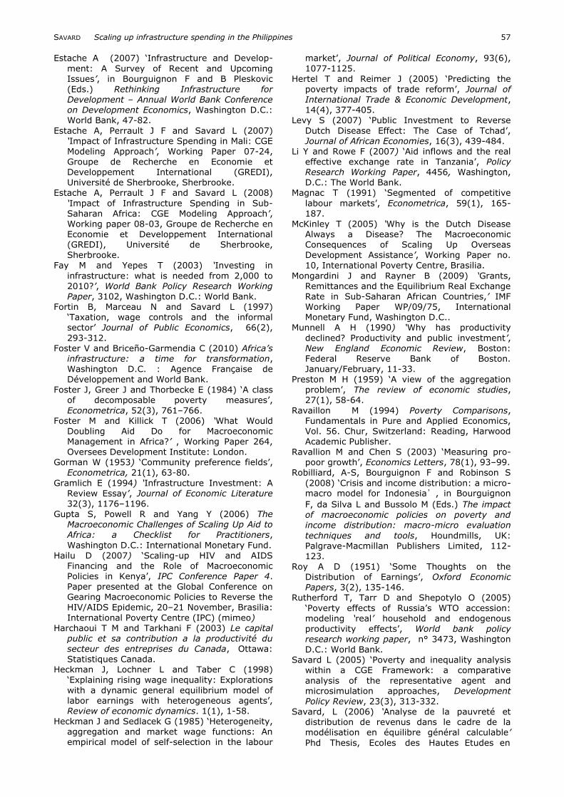
unemployment, whereas it is the least favourable in terms of poverty impacts. Growth incidence curves We computed the GIC for the three productive scenarios (Figure 3 to 5). A caveat must be

highlighted for comparison of the two tools used. In the first case, households remain in the same group whereas for the GIC curves, a household in the top of the distribution can drop to the bottom and this is not fully captured given that the approach compares households at a specific rank and not the households before and after the

simulation. The two tools are thus complementary. It is interesting to note that in the first scenario

(Value Added Tax), we observe in Figure 3 the largest gains at the two extremes of the distribution. If we remove the bottom and top two

deciles, we note a slightly positive GIC. This is consistent with the decomposition of poverty analysis in which more educated households seem


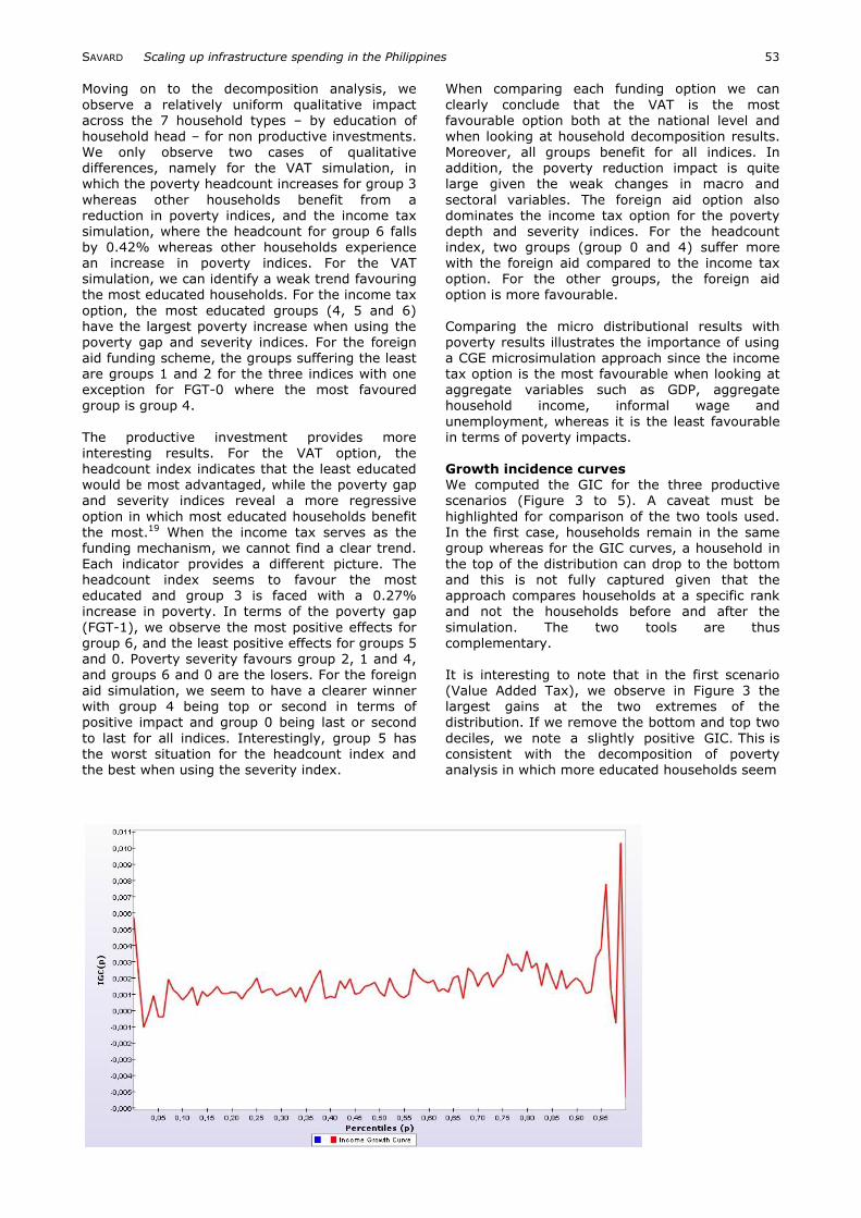
Figure 3 Income growth curve: VAT-funded productive infrastructure

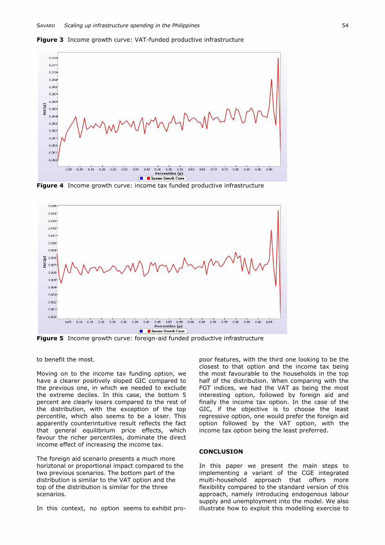
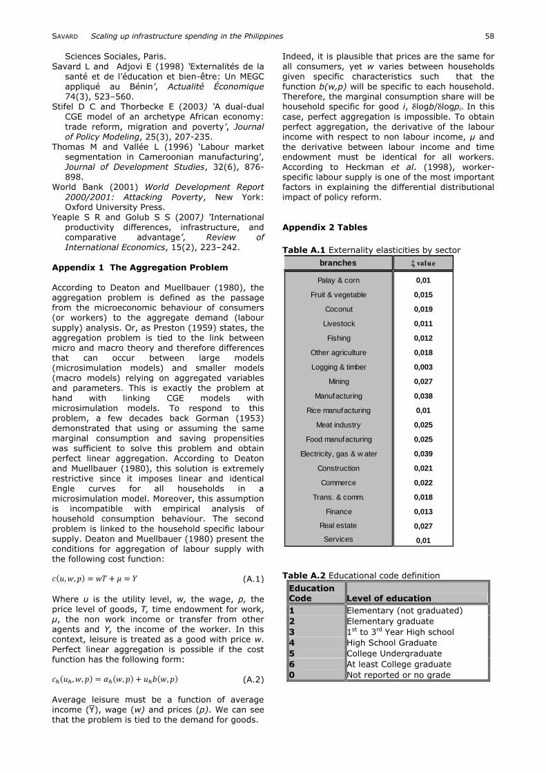
Figure 4 Income growth curve: income tax funded productive infrastructure

Figure 5 Income growth curve: foreign-aid funded productive infrastructure to benefit the most. Moving on to the income tax funding option, we

have a clearer positively sloped GIC compared to the previous one, in which we needed to exclude the extreme deciles. In this case, the bottom 5 percent are clearly losers compared to the rest of the distribution, with the exception of the top percentile, which also seems to be a loser. This

apparently counterintuitive result reflects the fact

that general equilibrium price effects, which favour the richer percentiles, dominate the direct income effect of increasing the income tax. The foreign aid scenario presents a much more horiztonal or proportional impact compared to the

two previous scenarios. The bottom part of the distribution is similar to the VAT option and the top of the distribution is similar for the three scenarios. In this context, no option seems to exhibit pro-

poor features, with the third one looking to be the closest to that option and the income tax being the most favourable to the households in the top

half of the distribution. When comparing with the FGT indices, we had the VAT as being the most interesting option, followed by foreign aid and finally the income tax option. In the case of the GIC, if the objective is to choose the least regressive option, one would prefer the foreign aid

option followed by the VAT option, with the

income tax option being the least preferred. CONCLUSION In this paper we present the main steps to

implementing a variant of the CGE integrated multi-household approach that offers more flexibility compared to the standard version of this approach, namely introducing endogenous labour supply and unemployment into the model. We also illustrate how to exploit this modelling exercise to


analyze the distributional impact of scaling up

infrastructure investment on macroeconomic, sectoral variables in the Philippines. The approach

allows us to capture numerous issues surrounding infrastructure expansion among which are productivity externalities, job creation, relative price changes, crowing out, Dutch disease,

funding issues, fiscal constraints and distributional analysis. We build on the models presented in papers such as Adam and Bevan (2006) and Estache et al. (2008) by introducing rigorous distributional analysis. Our macro results are different than those of these authors given the presence of unemployment, which contributes to

attenuating or reversing the Dutch disease effect that is also softened by the production externality assumption. We also present a framework that allows the analyst to explore the poverty impact of such programs and identify the most favourable funding option based on two distributional

analyses (FGT and GIC). As in Estache et al.

(2008), we do not observe strong differences at the macro level when comparing funding options to scale up infrastructure. However, our poverty analysis allowed us to clearly rank the performance of each funding option to establish that the VAT is most favourable, followed by

foreign aid and finally income taxes. Our static modelling framework does not allow us to fully capture the negative impact of crowding out of private investment. Another issue is that the returns on investment in infrastructure might come in the medium to long term. To improve the

analysis on this front, a recursive dynamic framework would be a more appropriate tool. In our future research we will extend this model in this direction. The major challenge for this work

program will be to introduce a capital reallocation mechanism at the micro level. To our knowledge, only one set of authors (Annabi et al., 2005)

applied a dynamic CGE microsimulation model, but they failed to rigorously capture the distributional factor growth issue as stated in Davies (2009). The uniform redistributed capital growth underestimated the distributional impact of the growth elements in the model and this issue

needs to be resolved along the lines suggested by Davies (2009) in further research. Notes 1 Estache (2007) provides an interesting survey

of the state of infrastructure for development

and review the main issues at stake for policy

makers of developing countries and donor agencies.

2 In fact, micro household functions do not aggregate perfectly if they exhibit heterogeneity for fixed (or endogenous) shares of consumption, savings or taxation. Since

these shares are generally calibrated to reproduce the reference period in micro household models, the aggregation of micro behaviour functions do not scale up to a representative agent. In other words, the equilibrium consumption level of the

representative agent is not equivalent to the

aggregated consumption level of households in a micro-household model with the same

functional forms. In addition, when a worker has the option of working or not working, we have a discrete regime switching function, and aggregation conditions disappear completely

(Bourguignon et al. 2005). For further elaboration see Appendix 1. For a detailed discussion of the aggregation of micro household behaviour to a representative household, the reader can consult Deaton and Muelbaueur (1980). Bourguignon and Savard (2008) also describe this problem.

3 Workers on the formal market are mostly skilled workers while workers on the informal market are mostly unskilled.

4 A minimum wage for private sector formal sector workers was set at 250 in 2001, which represented approximately 4.80$ US. A salary

grid is also in place for this segment of the

labour market. 5 We used the average of road, electricity, water,

sanitation and telecommunications infrastructure, which provides for a ω value of 1.03.

6 The values for this parameter were constructed

using a combination of information from Estache et al. (2008) and Harchaoui and Tarkhani (2003). In general, the values of our parameters are conservative with respect to this literature, ranging from 0.01 to 0.038. See Table A.1 in the appendix 2 for specific parameter values.

7 This formulation is also commonly used in studies estimating parameters of the externalities of public infrastructure on total factor productivity such as Aschauer (1989),

Gramlich (1994) and Dessus and Herrera (1996), among others.

8 The complete set of equations and variables

can be provided upon request. 9 Interestingly, the FIES 1997 and LFS 1997-

1998 are implemented from that same master survey. Over 93 percent of households in the FIES 1997 are present in the three rounds of the LFS surveys used. This information from

the LFS essentially was used for the econometric estimation in combination with the FIES 1997. For further information on the construction of the data base and combination procedures from the two compatible data sources, the reader can consult Savard (2006).

10 The information on the type of work performed

by the head of the household is very precise,

with a decomposition of 200 types of work categories. Given the rich set of information, it is relatively easy to classify the workers as formal and informal workers.

11 In the Philippines, formal wages are fixed by regional wage boards. For further information

the reader can consult the web page of the National Wage and Productivity Commission (http://www.nwpc.dole.gov.ph/).

12 The cost of entry represents various items such as search time, human capital investment, networking, etc. This cost is specific to workers


and is estimated. For details on this procedure

to obtain this cost, the reader can consult Bourguignon and Savard (2008).

13 See Bourguignon and Savard (2008) for formal proof of this equivalence.

14 Convergence is generally obtained between 10 and 12 loops. Given the small number of

iterations required, a sequential resolution of each loop can be performed without any problem. Various methods can be used to implement an automated iteration process in GAMS.

15 The non productive investment is used mainly to isolate the productivity effects from other

effects of the simulations. It is not meant to represent a specific type of non productive investment such as monuments.

16 The current account is balanced by adjusting the nominal exchange rate. Finally, in the tables, we present the nominal exchange rate.

But this rate can also be interpreted as the real

exchange rate because our price index is exogenous such that the variation in the nominal exchange rate is equivalent to the variation in the real exchange rate.

17 This is precisely the objective of many stimulus plans implemented in a large number of

countries during the recent economic crisis. 18 FGT poverty indices are helpful in the

framework of this analysis and make it possible to measure changes in the incidence of poverty, as well as in its depth and severity. For detailed information on the FGT index family, see Ravallion (1994).

19 The poverty indices at the reference period reveal that the more educated the head of household, the lower the poverty indices.

REFERENCES

Adam C and Bevan D (2006) „Aid and the Supply Side: Public Investment, Export Performance and Dutch Disease in Low Income Countries‟, World Bank Economic Review, 20(2), 261-290.

Agénor P R, Izquierdo A and Fofack H (2003) „IMMPA: A quantitative macroeconomic

framework for the analysis of poverty reduction strategies‟, Mimeo, Washington D.C.:World Bank.

Annabi N, Cissé F, Cockburn J and Decaluwé B (2005) „Trade Liberalisation, Growth and Poverty in Senegal: a Dynamic Micro-simulation CGE model analysis‟, Working Paper

No. 0512, CIRPEE, Montréal.

Armington P (1969) „A theory of demand for products distinguished by place of production‟, IMF Staff Paper, 16, 159-176.

Aschauer D A (1989) „Is Public Investment Productive?‟, Journal of Monetary Economics 23, 177–200.

Asian Development Bank (2009) Investing in Sustainable Infrastructure: Improving Lives in Asia and in the Pacific, Manilla: Asian Development Bank.

Berg A, Aiyar S, Hussein M et al. (2007) „The Macroeconomics of Scaling Up Aid: Lessons

from Recent Experience‟, IMF Occasional Paper,

235. Bergman E M and Suan D (1996) „Infrastructure

and manufacturing productivity: Regional accessibility and development level effects‟, in Batten D F and C Karlsson (Eds.) Infrastructure and the Complexity of Economic development,

Heidelberg: Springer-Verlag, 17-35. Binder S A and Smith S S (1997) Politics or

principle?: filibustering in the United States Senate, Washington D.C.: Brookings Institution.

Bourguignon F, Robilliard A S and Robinson S (2005) „Representative Versus Real Households

in the Macroeconomic Modelling of Inequality „, in Kehoe T J, T N Srinivasan and J Whalley (Eds.) Frontiers in applied general equilibrium modelling, Cambridge: Cambridge University Press, 219-254.

Bourguignon F and Savard L (2008) „A CGE

Integrated Multi-Household Model with

Segmented Labour Markets and unemployment’ in Bourguignon F, L A Pereira Da Silva and M Bussolo (Eds.) The Impact of Macroeconomic Policies on Poverty and Income Distribution: Macro-Micro Evaluation Techniques and Tools, Houndmilss:Palgrave-

Macmillan Publishers Limited, 177-211. Bourguignon F and Spadaro A (2006) „Micro-

simulation as a Tool for Evaluating Redistribution Policies‟, Journal of Economic Inequality, 4(1), 77-106.

Bourguignon F and Sundberg M (2006) „Absorptive Capacity and Achieving the MDG‟s‟, Working

Paper RP2006/47, World Institute for Development Economic Research (UNU-WIDER).

Chen S and Ravallion M (2004) „Welfare impacts

of China‟s accession to the world trade organization‟, The World Bank Economic Review, 18(1), 29-57.

Davis J B (2009) ‘Combining Microsimulation with CGE and Macro Modelling for Distributional Analysis in Developing and Transition Countries’, International Journal of Microsimulation, 2(1), 49-65.

Deaton A and Muellbauer J (1980) Economic and

consumer behavior, Cambridge: Cambridge University Press.

Dervis K, de Melo J and Robinson S (1982) General equilibrium models for development policy, Cambridge: Cambridge University Press.

Dessus S and Herrera R (1996) ‘Le rôle du Capital Public dans la Croissance des Pays en

Développement au cours des Années 80’,

OECD Working Paper 115, Organisation for Economic Co-operation and Development, Paris.

Devarajan S, Ghanem H and Thierfelder K (1999) „Labour market regulations, trade liberalization and the distribution of income in Bangladesh‟,

Journal of Policy Reform, 3(1), 1-28. Dumont J C and Mesplé-Somps S (2000) ‘The

Impact of Public Infrastructure on Competitiveness and Growth: A CGE Analysis Applied to Senegal’, Mimeo, CREFA, Université Laval, Québec.


Estache A (2007) „Infrastructure and Develop-

ment: A Survey of Recent and Upcoming Issues’, in Bourguignon F and B Pleskovic

(Eds.) Rethinking Infrastructure for Development – Annual World Bank Conference on Development Economics, Washington D.C.: World Bank, 47-82.

Estache A, Perrault J F and Savard L (2007) ‘Impact of Infrastructure Spending in Mali: CGE Modeling Approach’, Working Paper 07-24, Groupe de Recherche en Economie et Developpement International (GREDI), Université de Sherbrooke, Sherbrooke.

Estache A, Perrault J F and Savard L (2008)

‘Impact of Infrastructure Spending in Sub-Saharan Africa: CGE Modeling Approach’, Working paper 08-03, Groupe de Recherche en Economie et Developpement International (GREDI), Université de Sherbrooke, Sherbrooke.

Fay M and Yepes T (2003) ‘Investing in

infrastructure: what is needed from 2,000 to 2010?’, World Bank Policy Research Working Paper, 3102, Washington D.C.: World Bank.

Fortin B, Marceau N and Savard L (1997) „Taxation, wage controls and the informal sector‟ Journal of Public Economics, 66(2),

293-312. Foster V and Briceño-Garmendia C (2010) Africa’s

infrastructure: a time for transformation, Washington D.C. : Agence Française de Développement and World Bank.

Foster J, Greer J and Thorbecke E (1984) „A class of decomposable poverty measures‟,

Econometrica, 52(3), 761–766. Foster M and Killick T (2006) ‘What Would

Doubling Aid Do for Macroeconomic Management in Africa?’ , Working Paper 264,

Oversees Development Institute: London. Gorman W (1953) „Community preference fields‟,

Econometrica, 21(1), 63-80.

Gramlich E (1994) ‘Infrastructure Investment: A Review Essay’, Journal of Economic Literature 32(3), 1176–1196.

Gupta S, Powell R and Yang Y (2006) The Macroeconomic Challenges of Scaling Up Aid to Africa: a Checklist for Practitioners,

Washington D.C.: International Monetary Fund. Hailu D (2007) „Scaling-up HIV and AIDS

Financing and the Role of Macroeconomic Policies in Kenya‟, IPC Conference Paper 4. Paper presented at the Global Conference on Gearing Macroeconomic Policies to Reverse the HIV/AIDS Epidemic, 20–21 November, Brasilia:

International Poverty Centre (IPC) (mimeo)

Harchaoui T M and Tarkhani F (2003) Le capital public et sa contribution a la productivité du secteur des entreprises du Canada, Ottawa: Statistiques Canada.

Heckman J, Lochner L and Taber C (1998) „Explaining rising wage inequality: Explorations

with a dynamic general equilibrium model of labor earnings with heterogeneous agents‟, Review of economic dynamics. 1(1), 1-58.

Heckman J and Sedlacek G (1985) „Heterogeneity, aggregation and market wage functions: An empirical model of self-selection in the labour

market‟, Journal of Political Economy, 93(6),

1077-1125. Hertel T and Reimer J (2005) „Predicting the

poverty impacts of trade reform‟, Journal of International Trade & Economic Development, 14(4), 377-405.

Levy S (2007) „Public Investment to Reverse

Dutch Disease Effect: The Case of Tchad‟, Journal of African Economies, 16(3), 439-484.

Li Y and Rowe F (2007) „Aid inflows and the real effective exchange rate in Tanzania‟, Policy Research Working Paper, 4456, Washington, D.C.: The World Bank.

Magnac T (1991) „Segmented of competitive

labour markets‟, Econometrica, 59(1), 165-187.

McKinley T (2005) ‘Why is the Dutch Disease Always a Disease? The Macroeconomic Consequences of Scaling Up Overseas Development Assistance’, Working Paper no.

10, International Poverty Centre, Brasilia.

Mongardini J and Rayner B (2009) ‘Grants, Remittances and the Equilibrium Real Exchange Rate in Sub-Saharan African Countries,’ IMF Working Paper WP/09/75, International Monetary Fund, Washington D.C..

Munnell A H (1990) ‘Why has productivity

declined? Productivity and public investment’, New England Economic Review, Boston: Federal Reserve Bank of Boston. January/February, 11-33.

Preston M H (1959) „A view of the aggregation problem‟, The review of economic studies, 27(1), 58-64.

Ravaillon M (1994) Poverty Comparisons, Fundamentals in Pure and Applied Economics, Vol. 56. Chur, Switzerland: Reading, Harwood Academic Publisher.

Ravallion M and Chen S (2003) „Measuring pro-poor growth‟, Economics Letters, 78(1), 93–99.

Robilliard, A-S, Bourguignon F and Robinson S

(2008) „Crisis and income distribution: a micro-macro model for Indonesia’, in Bourguignon

F, da Silva L and Bussolo M (Eds.) The impact of macroeconomic policies on poverty and income distribution: macro-micro evaluation

techniques and tools, Houndmills, UK: Palgrave-Macmillan Publishers Limited, 112-123.

Roy A D (1951) „Some Thoughts on the Distribution of Earnings‟, Oxford Economic Papers, 3(2), 135-146.

Rutherford T, Tarr D and Shepotylo O (2005)

„Poverty effects of Russia‟s WTO accession: modeling ‘real’ household and endogenous

productivity effects‟, World bank policy research working paper, n° 3473, Washington D.C.: World Bank.

Savard L (2005) „Poverty and inequality analysis within a CGE Framework: a comparative

analysis of the representative agent and microsimulation approaches, Development Policy Review, 23(3), 313-332.

Savard, L (2006) ‘Analyse de la pauvreté et distribution de revenus dans le cadre de la modélisation en équilibre général calculable’

Phd Thesis, Ecoles des Hautes Etudes en


Sciences Sociales, Paris.

Savard L and Adjovi E (1998) ‘Externalités de la santé et de l‟éducation et bien-être: Un MEGC

appliqué au Bénin’, Actualité Économique 74(3), 523–560.

Stifel D C and Thorbecke E (2003) ‘A dual-dual CGE model of an archetype African economy:

trade reform, migration and poverty’, Journal of Policy Modeling, 25(3), 207-235.

Thomas M and Vallée L (1996) „Labour market segmentation in Cameroonian manufacturing‟, Journal of Development Studies, 32(6), 876-898.

World Bank (2001) World Development Report

2000/2001: Attacking Poverty, New York: Oxford University Press.

Yeaple S R and Golub S S (2007) ‘International productivity differences, infrastructure, and comparative advantage’, Review of International Economics, 15(2), 223–242.

Appendix 1 The Aggregation Problem According to Deaton and Muellbauer (1980), the aggregation problem is defined as the passage from the microeconomic behaviour of consumers (or workers) to the aggregate demand (labour

supply) analysis. Or, as Preston (1959) states, the aggregation problem is tied to the link between micro and macro theory and therefore differences that can occur between large models (microsimulation models) and smaller models (macro models) relying on aggregated variables and parameters. This is exactly the problem at

hand with linking CGE models with microsimulation models. To respond to this problem, a few decades back Gorman (1953) demonstrated that using or assuming the same

marginal consumption and saving propensities was sufficient to solve this problem and obtain perfect linear aggregation. According to Deaton

and Muellbauer (1980), this solution is extremely restrictive since it imposes linear and identical Engle curves for all households in a microsimulation model. Moreover, this assumption is incompatible with empirical analysis of household consumption behaviour. The second

problem is linked to the household specific labour supply. Deaton and Muellbauer (1980) present the conditions for aggregation of labour supply with the following cost function:

(A.1)

Where u is the utility level, w, the wage, p, the

price level of goods, T, time endowment for work, µ, the non work income or transfer from other agents and Y, the income of the worker. In this context, leisure is treated as a good with price w. Perfect linear aggregation is possible if the cost function has the following form:

(A.2)

Average leisure must be a function of average income (Y), wage (w) and prices (p). We can see that the problem is tied to the demand for goods.

Indeed, it is plausible that prices are the same for

all consumers, yet w varies between households given specific characteristics such that the

function b(w,p) will be specific to each household. Therefore, the marginal consumption share will be household specific for good i, logb/ logpi. In this

case, perfect aggregation is impossible. To obtain perfect aggregation, the derivative of the labour income with respect to non labour income, µ and

the derivative between labour income and time endowment must be identical for all workers. According to Heckman et al. (1998), worker-specific labour supply is one of the most important factors in explaining the differential distributional impact of policy reform.

Appendix 2 Tables

Table A.1 Externality elasticities by sector

Table A.2 Educational code definition

Education Code Level of education

1 Elementary (not graduated)

2 Elementary graduate

3 1st to 3rd Year High school

4 High School Graduate

5 College Undergraduate

6 At least College graduate

0 Not reported or no grade

branches ξ value

Palay & corn 0,01

Fruit & vegetable 0,015

Coconut 0,019

Livestock 0,011

Fishing 0,012

Other agriculture 0,018

Logging & timber 0,003

Mining 0,027

Manufacturing 0,038

Rice manufacturing 0,01

Meat industry 0,025

Food manufacturing 0,025

Electricity, gas & w ater 0,039

Construction 0,021

Commerce 0,022

Trans. & comm. 0,018

Finance 0,013

Real estate 0,027

Services 0,01


Table A.3 Funding mechanisms variations

Table A.4 Sectoral results: Value added (% variation)


Non productive

investment

Productive

investment

Non productive

investment

Productive

investment

Non productive

investment

Productive

investment

Level Base 2,45% 2,45% 2,19% 2,19% 2272 2272

Level After simulation 3,28% 3,16% 3,17% 3,00% 11142 9909

Variation Variation 33,80% 28,80% 43,80% 37,17% 390,40% 336,14%



Non

productive

investment

Productive

investment

Non

productive

investment

Productive

investment

Non

productive

investment

Productive

investment

Palay & corn 5197.9 -0.17 0.25 -0.14 0.27 -0.08 0.33

Fruit & vegetable 4210.7 -0.26 0.06 -0.26 0.07 -0.11 0.19

Coconut 1789.5 -0.35 0.42 -0.33 0.43 -0.57 0.23

Livestock 4473.5 -0.24 0.27 -0.29 0.22 0.1 0.55

Fishing 3996.8 -0.17 0.23 -0.19 0.2 -0.13 0.27

Other agriculture 1845.8 -0.22 0.09 -0.31 0.01 -0.62 -0.25

Logging & timber 856.5 0.19 0.82 0.07 0.71 0.14 0.77

Mining 1604.3 0.01 0.91 -0.18 0.74 -1.23 -0.14

Manufacturing 13112.5 -0.16 0.9 -0.14 0.91 -0.82 0.34

Rice manufacturing 2022.9 -0.17 0.27 -0.13 0.3 -0.07 0.36

Meat industry 2081.2 -0.12 0.55 -0.19 0.48 0.25 0.87

Food manufacturing 3696.2 -0.54 0.06 -0.49 0.1 -0.36 0.21

Electricity, gas & w ater 2341.3 0.06 0.85 0.1 0.88 0.15 0.93

Construction 6848.2 1.01 1.81 0.93 1.74 1.56 2.27

Commerce 15149.5 -0.18 0.66 -0.17 0.67 -0.54 0.36

Trans. & comm. 5206.4 0.07 0.79 -0.12 0.62 0.22 0.91

Finance 3580.5 0.13 0.7 0.2 0.76 -0.02 0.57

Real estate 7314.2 -0.2 0.48 -0.55 0.16 0.14 0.76

Services 6960 -0.12 0.72 0.11 0.91 -0.09 0.75

Public services 12222.8 1.86 1.87 2.2 2.15 2.33 2.26

Va

(value

added)


scaling up infrastructure spending in the philippines… · savard scaling up infrastructure...

Documents