Scatterometer backscatter uncertainty due to wind variability1

Marcos Portabella and Ad Stoffelen

KNMI, Postbus 201, 3730 AE De Bilt, The Netherlands

Phone: +31 30 2206568, Fax: +31 30 2210843

e-mail: portabel@knmi.nl, stoffelen@knmi.nl

Abstract

Wind retrieval from scatterometer backscatter measurements is not trivial. A good assessment

of the different measurement uncertainties inherent in scatterometer systems is very important

for successful wind retrieval and quality control. One source of these uncertainties, i.e., the

geophysical noise, is dominated by the sub-cell wind variability. Although the latter is known

to dominate the total measurement noise at low winds, no attempt to fully model such effect

has yet been performed. In this paper, a simple method to derive a model of geophysical noise

for the European remote sensing satellite (ERS) scatterometer is proposed. It is assumed that

this noise is mainly due to the spatial distribution of the backscatter footprints and the wind

variability within the wind vector cell. In a simulation experiment these parameters were

varied and the values for which the simulation compares best to real data in the 3D

1 IEEE Trans. Geosci. Rem. Sens., Vol. 44, No. 11, pp. 3356-3362, 2006. © Institute of Electrical and Electronics Engineers.

1

measurement space were selected. The resulting geophysical noise model is dependent on

wind speed and across sub-satellite track location. The empirical method presented here is

straightforward and could be applied to other scatterometer systems.

1 Introduction

Scatterometer wind observations have proven important for a wide variety of applications,

including nowcasting, short-range forecasting and mesoscale numerical weather prediction

(NWP) data assimilation [1], [2], [3], [4], [5]. A related paper [6] addresses the problem of

deriving a wind field from scatterometer measurements, showing that the total wind

sensitivity of the scatterometer measurements is dominant in determining the appropriate

ambiguous wind solutions, i.e., for inversion of the Geophysical Model Function (GMF).

However, for computing the probability of these solutions, precise knowledge of the error

properties is required. Moreover, to determine the likelihood of gross error for Quality

Control (QC) purposes, the expected uncertainty is very valuable [7], [8], [9]. This paper

deals with the modelling of the expected scatterometer error. The spatial sampling

characteristics as well as the instrumental error of the system need to be taken into account. A

quantitative expression of these uncertainties needs to be established for a successful retrieval

of wind probability and quality information.

A Gaussian distributed measurement error is commonly assumed, characterized by the error

parameter Kp, a dimensionless (%) value representing two different sources of error: the so-

called geophysical noise (Kpgeoph), i.e., noise caused by the physical interaction of the radar

2

signal and the propagation/scattering media, and the instrument noise (Kpinstr), i.e., noise

produced by the technical properties of the radar.

For every scatterometer system, an instrument error model has been derived [10], [11], [12].

This error is commonly taken Gaussian and ranges from about 3% to 5%.

Modelling the geophysical error is not a trivial exercise since all the geophysical effects that

are not modelled by the GMF and contribute to the radar backscatter uncertainty have to be

taken into account. GMF imperfections, wave field variability, wave fetch, atmospheric

stability, and rain (among others) are known to contribute to the backscatter uncertainty.

However, at scatterometer footprint sizes (a few tens of kilometres), these effects marginally

contribute to the total geophysical error except for some special or “pathetic” cases (about 5%

of the times) such as confused sea state, high spatial and temporal wind variability (nearby

fronts or low-pressure systems), or rain (particularly problematic for Ku-band scatterometry).

In these cases the quality of the retrieved winds is seriously compromised and for which

quality control (QC) procedures to reject such data have been developed, e.g., [7], [9], [13].

For nominal wind cases, i.e., cases where the backscatter value is mainly related to a local

wind in equilibrium with the sea (about 95% of the times), the geophysical error is mainly due

to the wind variability within the wind vector cell (WVC) and the non-uniform spatial

averaging inherent in the radar measurement1 (see Fig. 1). In this paper, we focus on such

nominal cases.

1 In the NWP data assimilation context, errors such as Kpgeoph are known as spatial representativeness error, but applied on analysis resolution cell level rather than on WVC level [10].

3

Wind variability and spatial context

The scatterometer GMF expresses the spatially averaged backscatter measurement to the

spatially averaged wind vector, the spatially averaged incidence and azimuth angles, the

frequency and the polarization of the radar beam. When analysing wind variability and non-

uniform spatial averaging, an important aspect of the GMF is its dependence on spatial

resolution.

Shankaranarayanan and Donelan [14] show a significant dependence of the GMF wind speed

on spatial resolution at low wind speed, mainly due to wind variability. They show that

laboratory-scale GMFs can be matched to satellite scatterometer scale GMFs with differences

at low wind speed. In line with [14], Stoffelen et al. [15] also show a GMF resolution

dependence on the wind direction. These observations can be explained by the following

illustrative example:

For a given scatterometer, its set of M σ° measurements at a certain WVC defines a GMF

surface in a M-dimensional σ° space for varying speed and direction. For the ERS triplets,

i.e., fore, mid and aft backscatter (respectively, σ1°, σ2°, and σ3°), this surface has the shape

of a double-folded cone in the 3D measurement space [7]. A cross section of the ERS cone

roughly represents a constant wind speed cut. For simplicity, the cross section shown in Fig. 2

only shows a single folded manifold. Let’s now assume that there are two triplets at certain

(e.g., Field of View or FoV) spatial resolution that are averaged into a lower (e.g., WVC)

spatial resolution triplet and that the wind variability associated with the resolution difference

is only present in the wind direction. The relationship between the wind variability (Δv) and

the wind direction difference (Δφ) is given by the following equation:

4

fv /Δ=Δφ , (1)

such that for a fixed wind speed (f) of 4 m/s and Δv of 0.5 m/s and 1 m/s, the resulting values

of Δφ are 0.125 radians (7.2°) and 0.25 radians (14.4°) respectively. Fig. 2 shows two FoV

triplets (black dots) with a certain Δφ (associated with the wind variability) located on a

defined GMFFoV (black ellipse). The averaged WVC triplet (grey dot) is better represented by

the GMFWVC (grey ellipse) than the GMFFoV. The GMF difference increases with the wind

variability (represented here by Δφ).

In the general case, the wind speed and the wind direction are inter-related in the GMF and,

consequently, a more complicated GMF resolution dependence as the one described here

exists. However, it is clear that the GMF is resolution dependent.

Relevance of Kp noise in wind retrieval

Provided that both the instrument and the geophysical errors are Gaussian distributed and

uncorrelated, the total Kp can be formulated (for any given measurement) in the following

way

22instrgeoph KpKpKp += (2)

The most common approach used for scatterometer wind inversion is the Bayesian approach,

which leads to the so-called Maximum Likelihood Estimator (MLE) technique [7], [16], [17].

For the ERS scatterometer, the following simplified MLE function is minimized [7]:

(∑=

−=3

1

2

31

isioi zzMLE ) (3)

5

where i is the measurement index, is the transformed backscatter measurement,

and is the transformed backscatter simulated through the GMF. Different wind

speed and direction trial values are used in the GMF in order to minimize the MLE.

Neglecting the GMF uncertainty, the following equation is used , where

6.1)( ooioiz σ=

6.1)( osisiz σ=

6.1)( iosioiz εσ += iε is

the backscatter error with relative error osi

iiKp σ

ε= , to determine the expectation value of

Eq. 3 by using a Taylor expansion:

(∑=

⋅⋅>=<3

1

26.131

iisi KpzMLE ) (4)

The MLE inversion technique is also used for the National Aeronautics and Space

Administration (NASA) scatterometer (NSCAT) [18] and the SeaWinds scatterometer [19],

albeit using a slightly different formulation [16] and therefore a slightly different expectation

value [8]. The expected MLE (Eq. 4) is very valuable for QC purposes [7], [8], [9]. Moreover,

it can be used to scale the computed MLE (Eq. 3) to relate it to the posterior probability of the

ambiguous wind solutions [20], which is a very important input for the ambiguity removal

(AR) of the scatterometer winds in the following way [21], [22]:

><−

∝ )(2)(

)( s

s

zMLEzMLE

s ezp (5)

The assessment of the Kp noise information is essential for a successful wind retrieval. In this

respect, extensive work has been done in characterizing the instrument noise, i.e., Kpinstr (see

Eq. 2), for different scatterometer systems [23]. Stoffelen and Anderson [7] made a

preliminary attempt to characterize the geophysical noise (Kpgeoph) by subjectively estimating

the scatter of triplets in the 3D ERS measurement space, whereas Figa and Stoffelen [24]

6

associated the geophysical noise to wind variability for NSCAT. Here, the effect of wind

variability on the backscatter uncertainty is analysed in more detail.

In order to compensate for the lack of a geophysical noise model, several statistical

approaches have been developed [9], [24]. Following these, the mean MLE in wind speed

bins can be computed for each WVC. The resulting values can be used as an additional

normalization factor in Eq. 3. Note that Eq. 3 measures the Euclidian distance of the measured

triplet σoio to the solution manifold σsi

o in a transformed measurement space (z space). Figs. 3

and 4 show examples of cross sections through this 3D measurement space, where measured

triplets are distributed around an elliptic solution manifold. As the noise increases (relative to

the size of the ellipse), the ellipse gets blurred and filled in (e.g., Fig. 4a). True triplets from

the top may be moved, due to noise, towards the bottom of the ellipse. Their Euclidian

distance to the ellipse (MLE) may be small while their error is large. This aliasing problem

results in a mean MLE that under-predicts the true noise in the measurement data. If the MLE

is normalized by its mean to compute the solution probability, it would, due to the exponential

relationship (see Eq. 5), result in an exaggerated relative probability range.

In this paper, a more physically-based rather than statistically-based approach is proposed to

account for the effect of wind variability, i.e., a geophysical noise model. Such a model has

been developed for the European Remote Sensing Satellite (ERS) scatterometer system [10].

However, the same approach may be used for other scatterometer systems as well.

7

2 Determination of geophysical noise parameters

As mentioned before, it is assumed that the geophysical noise is caused by the sub-WVC

spatial wind variability and the non-uniform illumination by the radar beam of the WVC area.

Although the backscatter measurements may be regularly spaced over the WVC, the total

illumination pattern will be spatially non-uniform and different for each beam. In particular,

for ERS, several sub-cell resolution σ° measurements are averaged to produce a single σ°

measurement for every beam (i.e., fore, mid, and aft). These sub-cell footprints or FoVs are

centered in different locations of the WVC (see Fig. 1) and observe somewhat different winds

due to wind variability. Therefore, the geophysical noise will depend on both the sub-WVC

wind variability and the number of independent σ° (FoV) samples. In fact the geophysical

noise depends on the ratio between the wind variability and the square root of the number of

independent samples, i.e., both parameters have a similar effect on the geophysical noise, but

with opposite trends.

Cone cross section visualization

In order to derive the geophysical noise, a simulation of the backscatter triplets (i.e., σ1°, σ2°,

and σ3°) is performed and compared to distributions of measured triplets. In the simulation

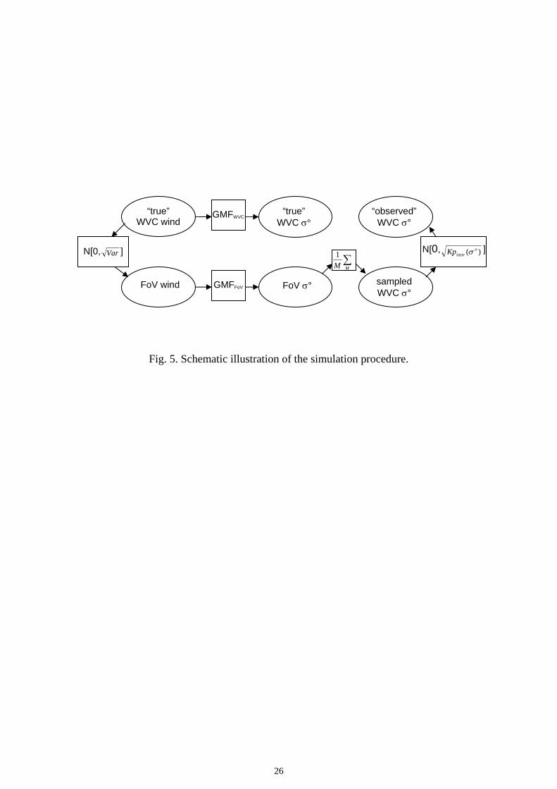
(see diagram in Fig. 5), we assume as input a Gaussian distributed “true” WVC wind centered

at 0 m/s with a standard deviation (SD) of 6 m/s in the wind components (i.e., N[0,6]). Then,

for each input “true” WVC wind vector, we simulate the “perturbed” wind sample values

8

corresponding to the different FoVs (i.e., FoV wind), where the perturbations are drawn from

a normal distribution with specified wind component variability, Var, (i.e., N[0, Var ]). From

the FoV wind samples, we compute FoV σ° samples using the CMOD-5 GMF [25] as

GMFFoV and compute their mean value (i.e., ∑MM

1 ) to obtain the sampled WVC σ°. Both the

sampling number M and wind variability Var are free parameters in the simulation. In

practice, since the two parameters have a similar effect (as already discussed), one of them,

i.e., the sampling number, is set to a fixed approximate value, i.e., M = 8 σ° samples. A

realistic instrument noise value per beam and WVC number1 is used at the end of the

simulation and its variance added as a random component (i.e., N[0, )( oinstrKp σ ]) to each

sampled WVC σ° to get the “observed” WVC σ°. It is noted that adding M times this noise

variability (N[0, )( oinstrKpM σ⋅ ]) at the FoV level (i.e., before the sample averaging)

results in a very similar “observed” WVC σ°. Finally, the set of “observed” WVC

{σ1°,σ2°,σ3°} constitute the simulated triplets.

Fig. 3 shows the real and simulated triplets that belong to a particular cross section of the

cone2. The GMF cone cross section used in the simulation is also shown (grey line). The

uppermost triplets correspond to winds blowing along the mid beam (upwind/downwind),

whereas at the lowest points the wind blows roughly across the mid beam direction

(crosswind) [7].

At low winds, there is a noticeable GMF misfit since most of the real triplets are located

within the CMOD-5 cone cross section (not shown). In this paper, however, the emphasis is

not on determining the GMF error, but rather on determining the wind-variability induced

1 Such value corresponds to the mean of the ESA-product estimated instrument noise values, obtained over 2004 and ranging between 2.6% and 4%. 2 Both the real and the simulated distributions correspond to a uniform wind direction distribution.

9

backscatter uncertainty. Therefore, to perform a proper visual comparison between real and

simulated triplet distributions, it is best to remove the GMF error. This is done by modifying

the CMOD-5 GMF (CMOD5-mod) such that the resulting section better fits the real triplet

distribution (see grey ellipse in Fig. 3a). The modification consists in a reduction by 2/3 of the

GMF B2 term, which accounts for the upwind/crosswind asymmetry [25].

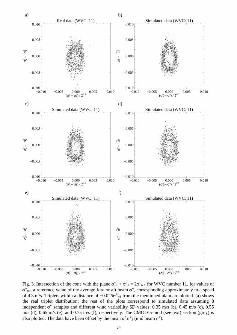
Figs. 3b to 3f show the CMOD5-mod simulated triplet distributions, accounting for different

wind variability values. Fig 3d is the simulation which resembles best the real data (Fig. 3a).

The other simulations show either too little (Figs. 3b and 3c) or too much (Figs. 3e and 3f)

noise. Fig. 3d corresponds to a wind variability Standard Deviation (SD) of 0.55 m/s.

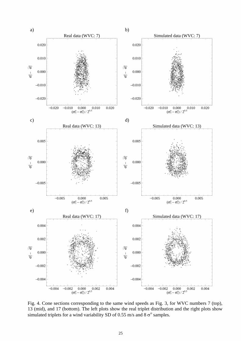
Fig. 4 shows more cone cross section comparisons between the real and simulated triplets

with a wind variability SD of 0.55 m/s for the same wind speed as Fig. 3 but for WVC

numbers 7 (top plots), 13 (mid plots) and 17 (bottom plots). The CMOD-5 GMF misfit with

respect to the real triplet distributions at low winds is also present (not shown). As in Fig. 3,

we use a modified GMF, CMOD5-mod (grey ellipse), to plot the simulated triplets (right

plots). As before, there is a good agreement between real (left plots) and simulated (right

plots) triplets.

Moreover, at higher wind speed (i.e., 6 m/s and above) cone cross sections, there is a very

good agreement between the real and simulated data (not shown). However, here the relative

contribution of the geophysical noise to the total noise is smaller (i.e., the instrument noise

dominates the total Kp in Eq. 2), as expected from our parameter selection. At lower speeds,

there is reasonable agreement. However, since the scattering of the triplets is of comparable

size to the diameter of the cone section, the analysis is more difficult. Some inconsistency

between real and simulated triplets appears (not shown) for the innermost WVCs (i.e., WVC

numbers 1 to 3), where the instrument noise seems larger than specified for all wind speeds.

10

At such WVCs, the backscatter has maximum incidence angle sensitivity. In the simulation,

no incidence angle variation within the same WVC is assumed. Perhaps, the existing

(although small) incidence angle variation is the reason for the excess noise.

Overall, a value of 0.55 m/s could be assumed as the most realistic wind variability value with

an uncertainty of ±0.05 m/s (10%). The selected geophysical noise parameters are therefore

0.55 m/s for wind variability SD and M = 8 independent σ° samples.

3 Analysis of the geophysical noise model

In order to further analyse the geophysical noise model, the impact of the geophysical noise

parameters derived in section 2 on the mean sampled WVC σ° value and its uncertainty (SD)

in terms of dependences on wind speed, wind direction, and incidence angle is studied. For

any input “true” wind vector and incidence angle, a “true” WVC σ° and a distribution of

sampled WVC σ°s (see diagram in Fig. 5), corresponding to a FoV wind (component)

variability SD of 0.55 m/s and a total of M = 8 independent σ° samples within a WVC (i.e., in

line with the results of section 2), are computed. Both the “true” WVC σ° and the FoV σ°

(used to compute the sampled WVC σ°) are computed with CMOD-5 GMF, i.e., GMFWVC =

GMFFoV, since no resolution-dependent GMF is available. This analysis is performed over a

wide range of WVC wind speeds [0-20 m/s], wind directions [0°-360°], and incidence angles

[16°-66°].

Generally, there appears to be no significant difference between the mean of the sampled

WVC σ° distribution and the “true” WVC σ° as a function of wind speed or incidence angle

11

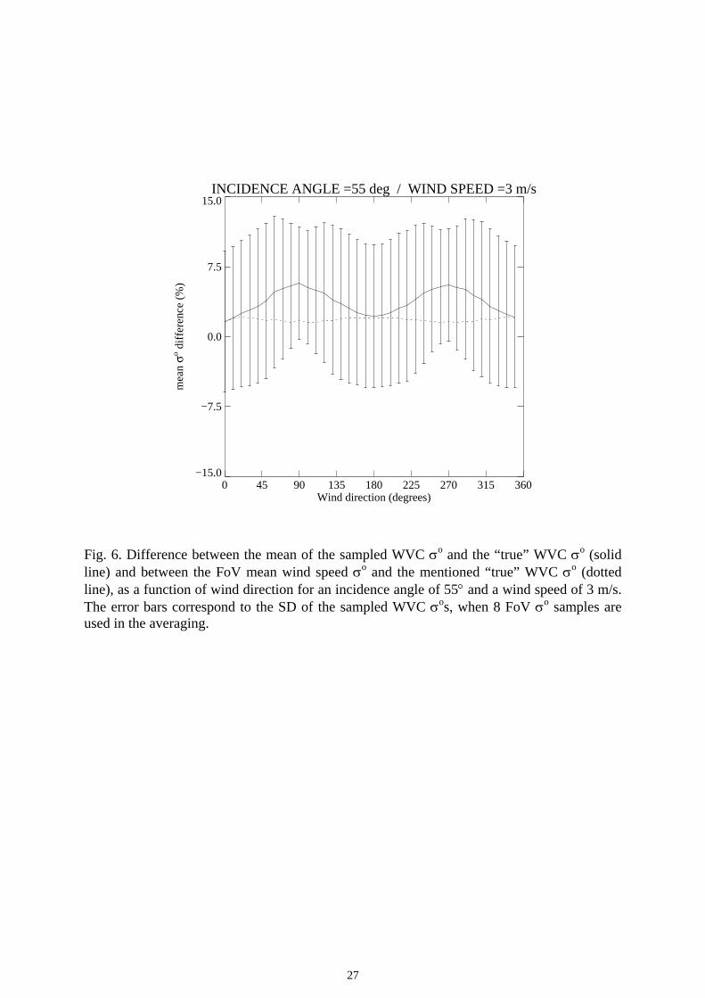
(not shown) since wind speed sensitivity is quasi-linear. However, there are some significant

differences (biases) as a function of wind direction, especially for high incidence angles and

low winds, e.g., see the solid line in Fig. 6. These biases appear due to the non-linear wind

direction dependence of the GMF and the fact that the same GMF (CMOD-5) was used to

compute both the FoV σ° and the “true” WVC σ° (i.e., GMFWVC = GMFFoV in diagram of

Fig. 5). As discussed in Fig. 2, for a true upwind direction, the wind direction perturbation

will tend to result in a sampled WVC σ° lower than the corresponding “true” WVC σ°. The

same holds for downwind and the opposite for crosswind. The effect is most pronounced at

high incidence angle and low winds, since here the wind direction sensitivity is relatively high

and, due to the low speeds, the wind direction perturbations are also relatively high.

It is interesting exercise to examine the behaviour of the σ° corresponding to the FoV mean

wind speed as a function of wind direction. The wind speed corresponding to the mean of the

FoV wind components is smaller than the mean of the FoV wind speeds (i.e., FoV mean wind

speed), especially at low winds. Since we assume Gaussian wind component error

distributions, the mean of the FoV wind components is on average very similar to the wind

components of the “true” WVC wind (see Fig. 5), and therefore can be used instead. The

dotted lines in Fig. 6 represent the difference between the σo corresponding to the FoV mean

wind speed1 and the σo corresponding to the “true” WVC wind, i.e., the “true” WVC σo. The

actual bias of the mean σ° distribution is represented by the difference between the solid and

the dotted lines and not by the differences between the solid line and the line y = 0. Clearly

the σ° corresponding to the FoV mean wind speed is closer to the “truth”.

1 The “true” WVC wind direction and incidence angle values are also used as input to compute this σ°.

12

The deviations of the mean sampled WVC σ° from the “true” WVC σ° (solid line) are, in

practice, taken into account in the GMF fit to real scatterometer σ° data. Therefore, these

biases do not exist in reality and have no impact on the quality of wind retrieval. They show

though the already discussed GMF dependence on spatial resolution due to the sub-WVC

wind variability. As a consequence, the scatterometer GMF should not be blindly applied to a

sensor with different spatial resolution, .e.g., the Synthetic Aperture Radar (SAR), without

further consideration (e.g., [14]).

The SD of the sampled WVC σ° distribution represents uncertainty in terms of geophysical

noise. Although some dependence on wind direction is also present (e.g., Fig. 4), it is

generally small as compared to the total Kp. It therefore is neglected and the geophysical error

SD is computed over all wind directions.

Fig. 7 shows the geophysical error SD surface (Kpgeoph) as a function of wind speed and

incidence angle. Dependences on wind speed and incidence angle are clearly discernible (see

shape of Fig. 7). For a given Kpinstr value (typically between 2.6% and 4%), the total Kp can

be easily derived using Eq. 2. Dependences on both the wind speed and the WVC number are

evident. As shown in Fig. 7, the error (total Kp) is generally dominated by the instrument

noise at medium and high winds. These results are in line with a preliminary work presented

by Stoffelen and Anderson [7], showing that the backscatter variability for medium and high

winds is about 3-4% (i.e., mostly instrument noise), whereas for low winds it substantially

increases.

Finally, the impact of the 10% uncertainty in wind variability SD (see section 2) is assessed.

As expected, the uncertainty in the geophysical noise is about 10%, except for winds lower

than 3 m/s, where it monotonically decreases down to 1% at 1 m/s. Taking into account the

13

characteristics of the total Kp described above, this uncertainty has little impact on the total

Kp.

4 Summary

The characterization of the different backscatter uncertainties, i.e., the instrument noise and

the geophysical noise, is of great importance for scatterometer wind retrieval. In particular,

expected σ° uncertainty is needed to compute the solution probability and useful for QC

purposes. The sub-WVC wind variability is known to contribute to the backscatter uncertainty

(especially at low winds). In this paper, this effect is analysed and modelled. A geophysical

noise model for scatterometers is proposed and applied to ERS.

Through visualization of the 3D measurement space, real triplets are compared to simulated

triplets for different geophysical error model parameter values. The parameters that better

represent the real triplet distributions are selected and used as geophysical error model. As the

simulations well reproduce the real data, the derived geophysical error model is validated for

different WVC numbers and wind speeds. For NSCAT or SeaWinds, sections of the solution

surface through a 4D space could be made [15] for validation of a similar error model.

The backscatter uncertainty due to wind variability is, as expected, increasing with decreasing

wind speeds. The uncertainty is also wind direction dependent. However, this dependence is

small and therefore neglected in the proposed geophysical error model. This is in line with

earlier MLE normalization schemes [9], [24].

14

Portabella and Stoffelen [22] show the importance of the derived geophysical noise model for

ERS ambiguity removal purposes. In particular, they use Eq. 5 to determine the probability of

each ambiguous solution of being the true wind. The probability information can then be used

in more sophisticated AR schemes, such as the Royal Netherlands Meteorological Institute

(KNMI) 2D variational analysis (2D-VAR) [21].

In this paper, a constant or mean global wind variability value is assumed, which can be used

to scale the MLE. However, the wind variability may vary depending on the region, e.g.,

tropics, extra-tropics, semi-enclosed seas, or weather. By analysing these scaled MLEs, such

different wind variability regimes may be determined.

Finally, the approach followed in this paper to derive a geophysical noise model for

scatterometers can also be applied more generally to systems combining several FoVs in a

pixel, in case of appreciable sub-pixel variability.

Acknowledgments

This work is funded by the European Space Agency under the project contract number

18041/04/NL/AR, in collaboration with the Institute for Applied Remote Sensing (IFARS).

The software used in this work has been developed by the EUMETSAT SAFs, involving

several colleagues at KNMI. We greatly appreciate the two reviewers who helped to improve

the paper.

15

References

[1] Isaksen, L., and Janssen, P.A.E.M., “Impact of ERS scatterometer winds in ECMWF’s

assimilation system,” Quart. J. R. Met. Soc., vol. 130, pp. 1793-1814, 2004.

[2] Stoffelen, A., “Timely ERS-2 scatterometer winds for weather nowcasting,” Proc. of

Envisat & ERS Symposium (ESA SP-572, April 2005), Salzburg, Austria, September 2004.

[3] Stoffelen, A., and Anderson, D., “Ambiguity removal and assimilation of scatterometer

data,” Quart. J. R. Met. Soc., vol. 123, pp. 491-518, 1997.

[4] Stoffelen, A., Van Beukering, P., “Implementation of improved ERS scatterometer data

processing and its impact on HIRLAM short range weather forecasts,” Report NRSP-2/97-06,

Beleidscomissie Remote Sensing, The Netherlands, 1997.

[5] Undén, P., Kelly, G., Le Meur, D., and Isaksen, L., “Observing system experiments with

the 3D-Var assimilation system,” Technical Memorandum No. 244, European Centre for

Medium-Range Weather Forecasts (ECMWF), Reading, United Kingdom, 1997.

[6] Stoffelen, A., and Portabella, M., “On Bayesian scatterometer wind inversion,” IEEE

Trans. Geosci. Rem. Sens., vol. 44, no. 6, pp. 1523-1533, 2006.

[7] Stoffelen, A., and Anderson, D., “Scatterometer data interpretation: measurement space

and inversion,” J. Atmos. and Oceanic Technol., vol. 14(6), 1298-1313, 1997.

[8] Portabella, M., and Stoffelen, A., “Characterization of residual information for SeaWinds

quality control,” IEEE Trans. Geosci. Rem. Sens., vol. 130, no. 596, pp. 127-152, 2004.

16

[9] Portabella, M., and Stoffelen, A., “Rain detection and quality control of SeaWinds,” J.

Atm. and Ocean Techn., vol. 18, no. 7, pp. 1171-1183, 2001.

[10] Attema, E. P. W., “The active microwave instrument on board the ERS-1 satellite,” Proc.

IEEE, vol. 79, pp. 791-799, 1991.

[11] Spencer, M.W., Wu, C., and Long, D.G., “Tradeoffs in the design of a spaceborn

scanning pencil beam scatterometer: application to SeaWinds,” IEEE Trans. Geosci. Rem.

Sens., vol. 35, no. 1, pp. 115-126, 1997.

[12] Long, D.G., and Spencer, M.W., “Radar backscatter measurement accuracy for a

spaceborne pencil-beam wind scatterometer with transmit modulation,” IEEE Trans. Geosci.

Rem. Sens., vol. 35, no. 1, pp. 102-114, 1997.

[13] Huddleston, J.N., and Stiles, B.W., “Multidimensional histogram (MUDH) rain flag”,

version 2.1, Jet Propulsion Laboratory, available at http://podaac-

www.jpl.nasa.gov/quikscat/, September 2000.

[14] Shankaranarayanan, K., and Donelan, M.A., “A probabilistic approach to scatterometer

model function verification,” J. Geophys. Res., vol. 106(C9), pp. 19969-19990, 2001.

[15] Stoffelen, A., de Vries, J., and Voorrips, A., “Towards the real-time use of QuikSCAT

winds,” Final Report USP-2/00-26, Beleidscomissie Remote Sensing, The Netherlands,

September 2000.

[16] Pierson, W.J., “Probabilities and statistics for backscatter estimates obtained by a

scatterometer,” J. Geophys. Res., vol. 94, no. C7, pp. 9743-9759, 1989.

17

[17] Cornford, D., Csató, L., Evans, D. J., and Opper, M., “Baysian analysis of the

scatterometer wind retrieval inverse problems: some new approaches,” J. R. Statist. Soc. B,

vol. 66, no. 3, pp. 609-626, 2004.

[18] Naderi, F. M., Freilich, M. H., and Long, D. G., “Spaceborne radar measurement of wind

velocity over the ocean: an overview of the NSCAT scatterometer system,” Proc. IEEE, vol.

79, pp. 850-866, 1991.

[19] Spencer, M. W., Wu, C., and Long, D. G., “Tradeoffs in the design of a scapceborne

scanning pencil beam scatterometer: application to SeaWinds,” IEEE Trans. on Geoscience

and Rem. Sens., vol. 35(1), pp. 115-126, 1997.

[19] Long, D. G., “Wind measurement resolution for a scanning pencil beam scatterometer,”

in Proc. Int. Geosci. Remote Sensing Symp., Pasadena, CA, pp. 948-952, Aug. 8-12, 1994.

[20] Stiles, B.W., Pollard, B.D., Dunbar, R.S., “Direction interval retrieval with thresholded

nudging,” IEEE Trans. Geosci. Rem. Sens., vol. 40, no. 1, pp. 79-89, 2002.

[21] Portabella, M., and Stoffelen, A., “A probabilistic approach for SeaWinds data

assimilation,” Quart. J. R. Met. Soc., vol. 130, no. 596, pp. 127-152, 2004.

[22] Portabella, M., and Stoffelen, A., “Study of an objective performance measure for

spaceborne wind sensors,” ESTEC contract, no. 18041/04/NL/AR, Netherlands, 2004.

[23] Cavanié, A., and Ezraty, R., “Evaluation of Kp on central and lateral antennas of NSCAT

over Arctic sea ice,” in Proc. of ADEOS/NSCAT Working Team Meeting, Maui, Hawaii, pp.

70-74, November 10-14, 1997.

18

[24] Figa, J., and Stoffelen, A., “On the assimilation of Ku-band scatterometer winds for

weather analysis and forecasting”, IEEE Trans. on Geoscience and Rem. Sens. (special issue

on Emerging Scatterometer Applications), vol. 38 (4), pp. 1893-1902, 2000.

[25] Hersbach, H., A. Stoffelen, and S. de Haan, “The improved C-band ocean geophysical

model function CMOD-5,” J. Geophys. Res. – Oceans, # 2005JC002931, provisionally

accepted for publication on August 1, 2006.

19

List of Figures

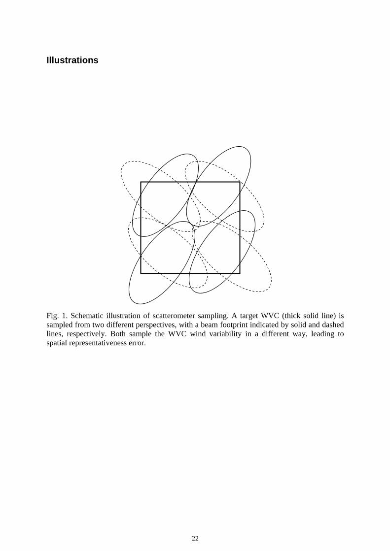
Fig. 1. Schematic illustration of scatterometer sampling. A target WVC (thick solid line) is

sampled from two different perspectives, with a beam footprint indicated by solid and dashed

lines, respectively. Both sample the WVC wind variability in a different way, leading to

spatial representativeness error.

Fig. 2. Schematic illustration of the wind variability effect on the GMF. The GMF on

footprint (FoV) level (black ellipse) is sampled twice (black dots) over different wind scenes

within the WVC. As a result, the WVC averaged backscatter (grey dot) moves away from the

FoV GMF, and the GMF on WVC level (grey ellipse) has a reduced harmonic oscillation.

Similar effects due to GMF surface curvature exist as a function of wind speed.

Fig. 3. Intersection of the cone with the plane σo1 + σo

3 = 2σoref for WVC number 11, for

values of σoref, a reference value of the average fore or aft beam σo, corresponding

approximately to a speed of 4.3 m/s. Triplets within a distance of ±0.025σoref from the

mentioned plain are plotted. (a) shows the real triplet distribution; the rest of the plots

correspond to simulated data assuming 8 independent σo samples and different wind

variability SD values: 0.35 m/s (b), 0.45 m/s (c), 0.55 m/s (d), 0.65 m/s (e), and 0.75 m/s (f),

respectively. The CMOD-5-mod section (grey) is also plotted. The data have been offset by

the mean of σo2 (mid beam σo).

20

Fig. 4. Cone sections corresponding to the same wind speeds as Fig. 3, for WVC numbers 7

(top), 13 (mid), and 17 (bottom). The left plots show the real triplet distribution and the right

plots show simulated triplets for a wind variability SD of 0.55 m/s and 8 σo samples.

Fig. 5. Schematic illustration of the simulation procedure.

Fig. 6. Difference between the mean of the sampled WVC σo and the “true” WVC σo (solid

line) and between the FoV mean wind speed σo and the mentioned “true” WVC σo (dotted

line), as a function of wind direction for an incidence angle of 55° and a wind speed of 3 m/s.

The error bars correspond to the SD of the sampled WVC σos, when 8 FoV σo samples are

used in the averaging.

Fig. 7. Geophysical noise as a function of wind speed and incidence angle. The speed binning

is 1 m/s and the angle binning is 1°.

21

Illustrations

Fig. 1. Schematic illustration of scatterometer sampling. A target WVC (thick solid line) is sampled from two different perspectives, with a beam footprint indicated by solid and dashed lines, respectively. Both sample the WVC wind variability in a different way, leading to spatial representativeness error.

22

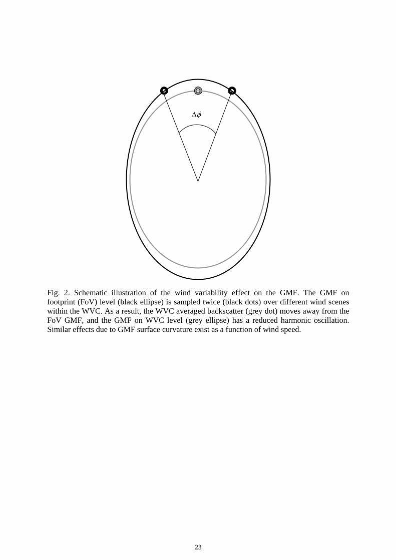
Fig. 2. Schematic illustration of the wind variability effect on the GMF. The GMF on footprint (FoV) level (black ellipse) is sampled twice (black dots) over different wind scenes within the WVC. As a result, the WVC averaged backscatter (grey dot) moves away from the FoV GMF, and the GMF on WVC level (grey ellipse) has a reduced harmonic oscillation. Similar effects due to GMF surface curvature exist as a function of wind speed.

φΔ

23

a) b) Real data (WVC: 11) Simulated data (WVC: 11)

−0.010 −0.005 0.000 0.005 0.010(σο

3 − σο1) / 20.5

−0.010

−0.005

0.000

0.005

−0.010 −0.005 0.000 0.005 0.010(σο

3 − σο1) / 20.5

−0.010

−0.005

0.000

0.005

0.010σο 2 −

⎯σο 2

0.010

σο 2 − ⎯

σο 2

c) d)

Simulated data (WVC: 11)

−0.010 −0.005 0.000 0.005 0.010(σο

3 − σο1) / 20.5

−0.010

−0.005

0.000

0.005

0.010

σο 2 − ⎯

σο 2

Simulated data (WVC: 11)

−0.010 −0.005 0.000 0.005 0.010(σο

3 − σο1) / 20.5

−0.010

−0.005

0.000

0.005

0.010σο 2 −

⎯σο 2

e) f)

Simulated data (WVC: 11)

−0.010 −0.005 0.000 0.005 0.010(σο

3 − σο1) / 20.5

−0.010

−0.005

0.000

0.005

0.010

σο 2 − ⎯

σο 2

Simulated data (WVC: 11)

−0.010 −0.005 0.000 0.005 0.010(σο

3 − σο1) / 20.5

−0.010

−0.005

0.000

0.005

0.010

σο 2 − ⎯

σο 2

Fig. 3. Intersection of the cone with the plane σo1 + σo

3 = 2σoref for WVC number 11, for values of

σoref, a reference value of the average fore or aft beam σo, corresponding approximately to a speed

of 4.3 m/s. Triplets within a distance of ±0.025σoref from the mentioned plain are plotted. (a) shows

the real triplet distribution; the rest of the plots correspond to simulated data assuming 8 independent σo samples and different wind variability SD values: 0.35 m/s (b), 0.45 m/s (c), 0.55 m/s (d), 0.65 m/s (e), and 0.75 m/s (f), respectively. The CMOD-5-mod (see text) section (grey) is also plotted. The data have been offset by the mean of σo

2 (mid beam σo).

24

a) b) Real data (WVC: 7)

−0.020 −0.010 0.000 0.010 0.020(σο

3 − σο1) / 20.5

−0.020

−0.010

0.000

0.010

0.020

σο 2 − ⎯

σο 2

Simulated data (WVC: 7)

−0.020 −0.010 0.000 0.010 0.020(σο

3 − σο1) / 20.5

−0.020

−0.010

0.000

0.010

0.020

σο 2 − ⎯

σο 2

c) d)

Real data (WVC: 13)

−0.005 0.000 0.005(σο

3 − σο1) / 20.5

−0.005

0.000

0.005

σο 2 − ⎯

σο 2

Simulated data (WVC: 13)

−0.005 0.000 0.005(σο

3 − σο1) / 20.5

−0.005

0.000

0.005

σο 2 − ⎯

σο 2

e) f)

Real data (WVC: 17)

−0.004 −0.002 0.000 0.002 0.004(σο

3 − σο1) / 20.5

−0.004

−0.002

0.000

0.002

0.004

σο 2 − ⎯

σο 2

Simulated data (WVC: 17)

−0.004 −0.002 0.000 0.002 0.004(σο

3 − σο1) / 20.5

−0.004

−0.002

0.000

0.002

0.004

σο 2 − ⎯

σο 2

Fig. 4. Cone sections corresponding to the same wind speeds as Fig. 3, for WVC numbers 7 (top), 13 (mid), and 17 (bottom). The left plots show the real triplet distribution and the right plots show simulated triplets for a wind variability SD of 0.55 m/s and 8 σo samples.

25

N[0, )( oinstrKp σ ]

“observed” WVC σ°

N[0, Var ]

“true” WVC wind

GMFWVC“true”

WVC σ°

FoV wind FoV σ° sampled WVC σ°

GMFFoV

∑MM

1

Fig. 5. Schematic illustration of the simulation procedure.

26

INCIDENCE ANGLE =55 deg / WIND SPEED =3 m/s

0 45 90 135 180 225 270 315 360Wind direction (degrees)

−15.0

−7.5

0.0

7.5

15.0

mea

n σο d

iffe

renc

e (%

)

Fig. 6. Difference between the mean of the sampled WVC σo and the “true” WVC σo (solid line) and between the FoV mean wind speed σo and the mentioned “true” WVC σo (dotted line), as a function of wind direction for an incidence angle of 55° and a wind speed of 3 m/s. The error bars correspond to the SD of the sampled WVC σos, when 8 FoV σo samples are used in the averaging.

27

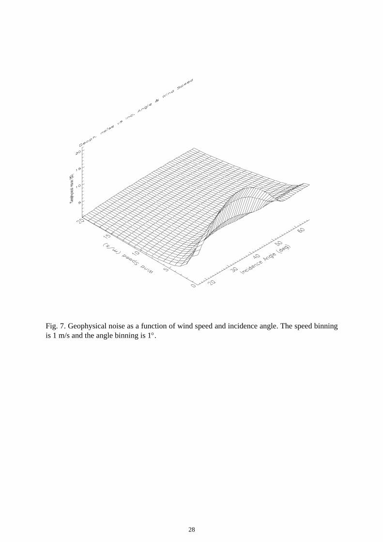
Fig. 7. Geophysical noise as a function of wind speed and incidence angle. The speed binning is 1 m/s and the angle binning is 1°.

28

Biographies

Ad Stoffelen was born on February 25, 1962, in the Netherlands. He

received the M.Sc. degree in physics in 1987 from the Technical

University of Eindhoven, The Netherlands, and the Ph.D. degree from

University of Utrecht, Utrecht, The Netherlands, in 1998.

He is currently with the Royal Netherlands Meteorological Institute

(KNMI), de Bilt, The Netherlands, and has worked on scatterometer data interpretation,

inversion, calibration, validation, quality monitoring, and assimilation in global and regional

weather forecast models. Other involvements include the European Doppler wind light

detection and ranging (LIDAR) in space program, and ozone data assimilation.

Marcos Portabella received the B.Sc. degree in Physics in 1994,

with a specialization in atmospheric physics, from the University of

Barcelona, Barcelona, Spain; the M.Sc. in Space Studies in 1995,

with a specialization in Remote Sensing, from the Institute of Space

Studies of Catalonia, Barcelona, Spain; and the Ph.D. degree in

Physics in 2002, from the University of Barcelona, Spain.

He has worked at the European Space Agency (ESA) on wind retrievals from satellite radar

systems, such as scatterometers and synthetic aperture radars (SAR). He is currently with the

Royal Netherlands Meteorological Institute (KNMI), de Bilt, The Netherlands, and has

worked on scatterometer data interpretation, inversion and quality control. He is also

29

collaborating on sea surface salinity retrievals from satellite L-band radiometry (SMOS) with

the Marine Sciences Institute (CSIC), Barcelona, Spain.

30