sccm user's guide - department of physicsatmosp.physics.utoronto.ca/.../sccm_doc.pdf · sccm...

SCCM User's Guide http://www.cgd.ucar.edu/cms/sccm/userguide.html

1 of 24 01/11/2004 2:38 PM

SCCM User 's GuideVersion 1.2

January 1999

J. J. Hack, J. A. Pedretti and J. C. Petch

Contents1. Introduction

1.1 Basic Description of the NCAR CCM SCCM Framework1.2 Potential for solution differences across CCM program libraries

2. Building SCCM2.1 Preliminary Setup2.2 Obtaining the Source Code and Datasets2.3 Explanation of the SCCM Subdirectory Organization2.4 Configuring the Makefile2.5 Making the SCCM Executable2.6 Running SCCM2.7 Changing between CCM versions2.8 Optional Configurations2.9 Troubleshooting

3. The User Interface3.1 Overview3.2 Starting SCCM / The Main Window3.3 Loading Datasets3.4 Setting Options3.5 Monitoring and Modifying a Field3.6 Running the Model3.7 Saving Data3.8 Post-Run Analysis3.9 Restarting3.10 Command Line Options

4. Modifying the Code4.1 Adding New Model Source Code Files4.2 Adding New Fields to View or Save4.3 Model Initialization

5. Using SCCM with an IOP Dataset5.1 Introduction5.2 The Standard IOP Dataset for SCCM5.3 A Detailed Example Using SCCM With an IOP Dataset

5.3.1 Changing and Initializing the Model


2 of 24 01/11/2004 2:38 PM

5.3.2 Running the Model6. AcknowledgementsAppendix A: Format of SCCM NetCDF Datasets

1. Introduction

Numerical modeling of the climate system and its sensitivity to anthroprogenic forcing is a highly complex scientific problem. Progresstoward accurately representing our climate system using global numerical models is primarily paced by uncertainties in therepresentation of non-resolvable physical processes, most often treated by what is known as physical parameterization. A principalexample of the parameterization problem is how to accurately include the overall effects of moist processes, i.e., the variouscomponents of the hydrologic cycle, into the governing meteorological equations. Since water in any phase is a strongly radiativelyactive atmospheric constituent, and since changes in water phase are a major source of diabatic heating in the atmosphere, thelarge-scale moisture field plays a fundamental role in the maintenance of the general circulation and climate. Clouds themselves are acentral component in the physics of the hydrologic cycle since they directly couple dynamical and hydrological processes in theatmosphere through the release of the latent heat of condensation and evaporation, through precipitation, and through the verticalredistribution of sensible heat, moisture and momentum. They play a comparable role in the large-scale thermodynamic budget throughthe reflection, absorption, and emission of radiation and also play an important role in the chemistry of the Earth's atmosphere.Evaluating the many parametric approaches which attempt to represent these types of processes in atmospheric models can be bothscientifically complex and computationally expensive.

An alternative approach to testing climate model parameterizations in global atmospheric models is in what are called single-columnmodels or SCMs. As the name suggests, an SCM is analogous to a grid column of a more complete global climate model, where theperformance of the parameterized physics for the column is evaluated in isolation from the rest of the large-scale model. Various formsof "observations" can be used to specify the effects of neighboring columns, as well as selected effects of parameterized processes(other than those being tested) within the column, such as surface energy exchanges. The SCM approach lacks the more completefeedback mechanisms available to an atmospheric column imbedded in a global model, and therefore cannot provide a sufficientlythorough framework for evaluating competing parametric techniques. It can, however, provide an inexpensive first look at thecharacteristics of a particular parameterization approach without having to sort out all the complex nonlinear feedback processes thatwould occur in a global model.

Because of the large computational expense associated with evaluating new parameterizations using a complete atmospheric generalcirculation model, we have developed a highly flexible and computationally inexpensive single column modeling environment for theinvestigation of parameterized physics targeted for global climate models. In particular, this framework is designed to facilitate thedevelopment and evaluation of physical parameterizations for the NCAR Community Climate Model (CCM). The SCM modelingenvironment provides a framework for making initial assessments of physical parameterization packages and allows for theincorporation of both in situ forcing datasets [e.g., Atmospheric Radiation Measurement (ARM) data] and synthetic, user-specified,forcing datasets, to help guide the refinement of parameterizations under development. Diagnostic data which can be used to evaluatemodel performance can also be trivially incorporated. The computational design of the SCM framework allows assessments of both thescientific and computational aspects of the physics parameterizations for the NCAR CCM because the coding structures at the physicsmodule levels are identical. We believe that this framework will have widespread utility and will help to enrich the pool of researchersworking on the problem of physical parameterization since few have access to or can afford to test new approaches in atmosphericGCMs. Another strength of our approach is that it will provide a common framework in which to investigate the scientificrequirements for the successful parameterization of subgrid-scale processes.

1.1 Basic descr iption of the NCAR CCM SCCM Framework

The NCAR single-column CCM (SCM) is a one-dimensional time-dependent model in which the local time-rate-of-change of thelarge-scale state variables (e.g., temperature, moisture, momentum, cloud water, etc.) depends on specified horizontal fluxdivergences, a specified vertical motion field (from which the large-scale vertical advection terms are evaluated), and subgrid-scalesources, sinks and eddy transports. The subgrid-scale contributions are determined by the particular collection of physicalparameterizations being investigated. Because an SCM lacks the horizontal feedbacks that occur in complete three-dimensional modelsof the atmosphere, the governing equations are only coupled (incompletely) through the parameterized physics. In a practical sense thismeans that the thermodynamic and momentum components of the governing equations are generally independent of one another,where typical configurations of the SCM would consider each of these budgets independently. The thermodynamic configurationconsists of


3 of 24 01/11/2004 2:38 PM

(1),

(2),

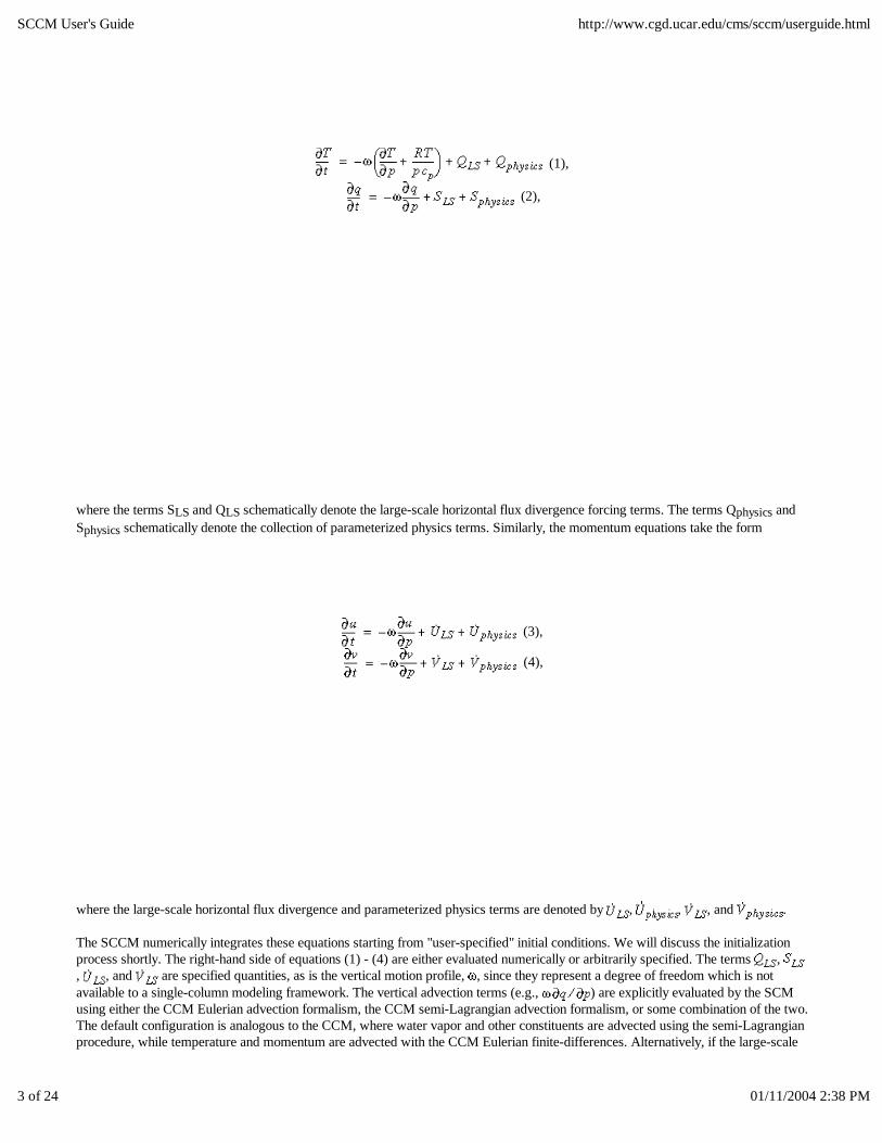
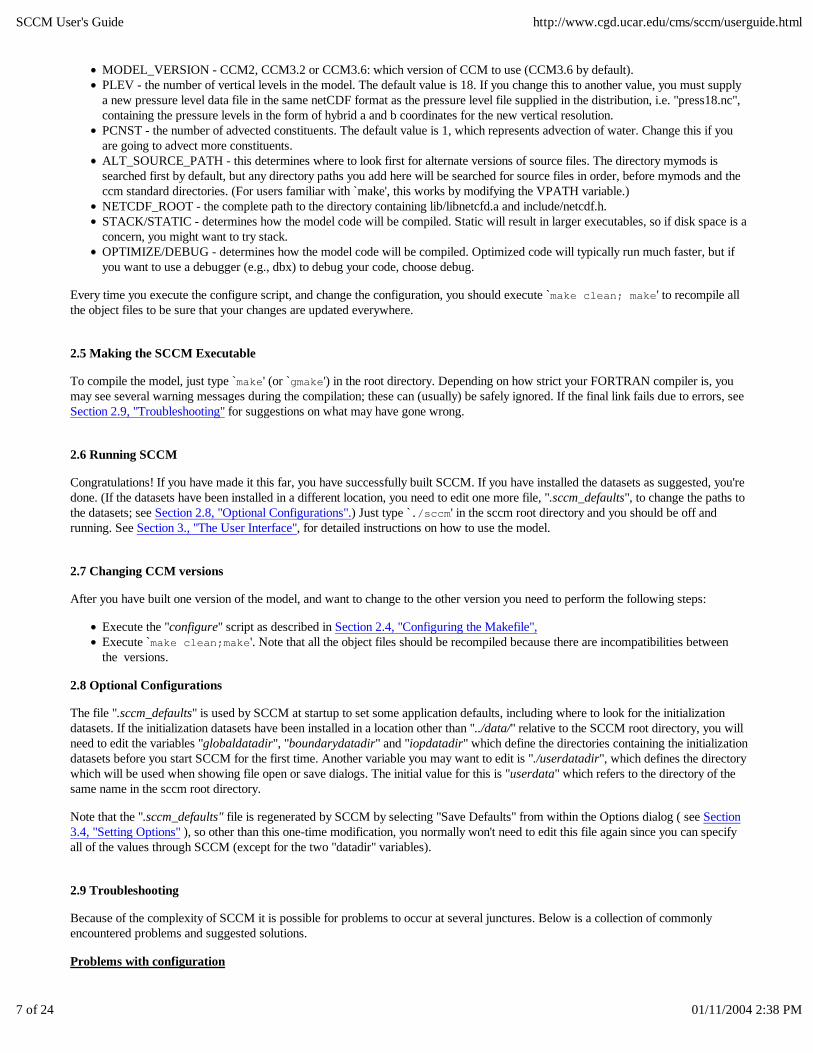
where the terms SLS and QLS schematically denote the large-scale horizontal flux divergence forcing terms. The terms Qphysics andSphysics schematically denote the collection of parameterized physics terms. Similarly, the momentum equations take the form

(3),

(4),

where the large-scale horizontal flux divergence and parameterized physics terms are denoted by , , , and .

The SCCM numerically integrates these equations starting from "user-specified" initial conditions. We will discuss the initializationprocess shortly. The right-hand side of equations (1) - (4) are either evaluated numerically or arbitrarily specified. The terms , , , and are specified quantities, as is the vertical motion profile, , since they represent a degree of freedom which is notavailable to a single-column modeling framework. The vertical advection terms (e.g., ) are explicitly evaluated by the SCMusing either the CCM Eulerian advection formalism, the CCM semi-Lagrangian advection formalism, or some combination of the two.The default configuration is analogous to the CCM, where water vapor and other constituents are advected using the semi-Lagrangianprocedure, while temperature and momentum are advected with the CCM Eulerian finite-differences. Alternatively, if the large-scale


4 of 24 01/11/2004 2:38 PM

vertical advection terms are available in any of the SCCM forcing datasets, the user can modify the SCCM dynamical driver to usethese terms in place of the default large-scale vertical advection calculation. Note, all large-scale terms on the right-hand side of eq. (1)- (4) are defined as a positive tendency in any of the datasets provided with the SCCM. For example, the large-scale vertical advectionterm would be defined exactly as it appears on the right hand side of equation (2) in all datasets. This sign convection isconsistent with the way in which the large-scale advection information is provided for ARM Intensive Observing Period observationsused for single-column modeling applications.

Finally, the remaining physical parameterization terms are explicitly evaluated using the standard CCM physics packages (eitherCCM2 or CCM3) or an alternative physical parameterization package as configured by the user. The coding constructs (e.g., callingtree, parameter lists, etc.) are identical to what is contained in the CCM. The SCCM operates in one of two standard modes. The firstmode allows the user to select an arbitrary atmospheric column from anywhere on the globe. The SCCM will build an initial conditionfor this column (along with all the necessary boundary datasets, such as surface properties, ozone path lengths, etc.) from one of twodata sources. Presently these data sources are monthly average climatological properties from ECMWF analyses or frommodel-generated (i.e., CCM3) results. At this point in time, the horizontal flux divergence forcing tendencies are specified to be zerowhen using this configuration of the SCCM. There are some important modeling implications for the solutions when specifying a zerohorizontal forcing. They will be discussed in future versions of this document, along with alternative ways of treating these terms. Thesecond mode of operation makes use of what we refer to as Intensive Observing Period (IOP) data. This data provides transient forcinginformation to the SCM physics, where the source of such data will most frequently be from observational field programs such asGATE, ARM, and TOGA COARE. An alternative to field program data might be a synthetically generated dataset designed to stresscertain aspects of a parameterization technique. We expect that such datasets would generally incomplete when it comes to providingall the data required to initialize and integrate the SCCM. Therefore, when using the IOP option, the SCCM first builds an initialcondition using the appropriate climatological profiles and surface quantities using global analysis data, and incorporates theappropriate model-specific boundary condition data for the column closest to where the IOP data is located. It then overwrites this datawith whatever IOP data is available. In this way the model is guaranteed to have all the data necessary to perform a numericalintegration. This procedure may introduce inconsistencies in the initial and boundary value states which could result in undesirablesystematic errors in the solution. Once again, this puts the burden on the user to completely understand what has been assumed for thepurpose of integrating the SCCM using IOP data. At the moment, the IOP datasets consist of the GATE dataset, a TOGA COAREdataset (ascii data for both were obtained from the CSU single-column modeling web site:http://kiwi.atmos.colostate.edu/scm/scm.html), and an ARM dataset (for which the ascii data was obtained from the from the ARMintercomparison web site: http://wetfly.llnl.gov/scm/scm_intercomp/). Over time, we will assemble additional IOP forcing datasetsfrom new field experiments, revisions of existing IOP datasets, and will explore the use of GCM and analysis-generated forcing inregions where detailed observational data may not exist. See Table 1 for a summary of the format of the SCCM NetCDF datasets.

1.2 Potential for solution differences across CCM program librar ies

There have been several releases of the SCCM, some of which have incorporated changes to the GUI only, and others that haveincluded GUI updates along with the latest CCM program library. Generally speaking, updates to the CCM program library includeonly roundoff changes in the implementation. However, in some cases, minor algorithmic changes may also be included, such as in thecase of the CCM3.6 program library. Experience has shown that both roundoff and algorithmic changes can introduce nontrivialdifferences in the solutions produced by the SCCM. For example, the old and new solutions will track each other to a high degree ofaccuracy and suddenly diverge, resulting in fundamentally different solution characteristics. This is a property of branch points in thephysics codes that can result in non-deterministic solutions, and should not necessarily be cause for alarm. Once a significantdifference is introduced in an SCCM solution because of a branch point, the lack of dynamical feedbacks can limit the chances that thesolutions will once again converge. When large solution differences occur with a migration across CCM code libraries, it is importantto carefully examine the time evolution of the differences to ensure that they are not attributable to an incorrect setup of the new SCCMversion (e.g., not properly incorporating user changes to the physics libraries). An example of different solution characteristics isshown below. The solutions represent the temperature error time series for two different versions of the CCM3 physics algorithmswhen forced with the ARM Summer 1995 IOP dataset.


5 of 24 01/11/2004 2:38 PM

TDIFF (version a)

TDIFF (version b)

2. Building SCCM

2.1 Preliminary Setup

Make sure that you have at least 100 Mb of disk space available on your local disk for building sccm and installing the requireddatasets. SCCM relies on netCDF version 3 to read and write datasets so you must have the netCDF library libnetcdf.a installed onyour system. Information about netCDF can be found at http://www.unidata.ucar.edu/packages/netcdf/index.html. Precompiledbinaries are available by anonymous ftp from ftp.unidata.ucar.edu/pub/binary/<system-type>/netcdf-3.3.1.tar.Z (N.B.: the Linuxprecompiled binary at this site is incompatible with the fortran compiler; you can download a compatible version here). SCCM outputis in standard netCDF format, so in addition to the basic plotting capabilities of SCCM, you can use any plotting utility thatunderstands netCDF files (e.g., "ferret") to analyze its output. The configuration script will look for netCDF in the usual places (e.g.,/usr/local), but in the case that it is installed in an unusual location and the configure script can't find it, you will need to know where itis installed. If you can't locate netCDF on file system, your system administrator should be able to help you.

Building SCCM depends on the following utilities:

cpp - the C preproccessor; standard on every unix system.Gnu make - Gnu's freely available version of make. This may be installed variously as gnumake, gmake, or make. To find out ifa particular version of make is the Gnu version, type `make - v '. In case it is not installed on your system, information onobtaining the source code for Gnu make is available at http://www.fsf.org/order/ftp.html.C and FORTRAN77 compilers - standard on most systems (NB: Linux users must purchase the Portland Group f77 compilerpgf77 (g77 is not an option)).

2.2 Obtaining the Source Code and Datasets

Use Netscape or your favorite web browser to download the SCCM source code and datasets. Open the URL:http://www.cgd.ucar.edu/cms/sccm/sccm.html and follow the links for downloading the source and datasets. The size of the completedistribution, including datasets, is appoximately 100 mb. Once you have downloaded the files to your local machine you will need toextract them. The file sccm-<version>.<system>.tar.gz contains SCCM source code for compiling the model and a precompiled


6 of 24 01/11/2004 2:38 PM

binary for the user interface (sccmgui). This file is a compressed tar file which must be uncompressed and "untarred" as follows:

gunzi p - c sccm- <ver si on>. <syst em>. t ar . gz | t ar xvf -

This will create the directory `sccm-<version>' containing the SCCM source code and configuration files and user interface binary"sccmgui".

The file "sccm-1.2.datasets.tar" contains all of the datasets required by SCCM. It is not compressed and can be untarred with thefollowing command:

t ar xvf sccm. dat aset s. t ar

It is recommended that you untar the sccm.datasets tar file in the same directory that you untarred the sccm.code tar file (i.e., theparent directory of sccm). If you don't perform any of the optional configurations described below in Section 2.8, "OptionalConfigurations", SCCM will expect to find the datasets in the directory `../data/' relative to the directory from which the SCCMexecutable is run. Alternatively, you can make a symbolic link from the directory in which you installed the datasets, to a directorycalled `data' in sccm's parent directory. For example, if the datasets are located in "/home/model/data" and SCCM is located in "/home/jsmith/ccm/sccm", use the command

l n - s / home/ model / dat a/ home/ j smi t h/ ccm/ dat a

The precompiled binary "sccmgui" that is included in the distribution should work on most systems: before you proceed, you should tryexecuting it by typing ". / sccmgui ." You should see a window popup which says, "ERROR: Cannot connect to sccm (not running?)."If you don't see this window there is a problem and you will need to compile the user interface separately (see below). The list ofsystems for which precompiled binaries are available includes Solaris 2.4 (SunOS 5.4), AIX 4.2, OSF1 3.2, IRIX 6.2, HP-UX 10.20,and Linux 2.0. If you are unsure what system you are working on, the output from the command "uname - sr " will give the name andrelease of the operating system. If your system version is lower than those specified above, you may have problems, but later releasesshould work alright.

The source for the user interface is also available to interested parties. However, it is not necessary or recommended that you obtainthis. If you feel you are a competent C++ programmer and want to modify the interface code to suit your own particular needs, sendmail to [email protected] for details on how to obtain the complete user interface source code.

2.3 Explanation of the SCCM Subdirectory Organization

Untarring the source distribution will result in the creation of the sccm root directory the files `sccmgui', `configure', `INSTALL', and`GNUmakefile' and the subdirectories described below.

init - model initialization code shared between the different model versions.ccm2 - CCM2 model code and GNUmakefileccm3.2 - CCM3.2 model code and GNUmakefileccm3.6 - CCM3.6 model code and GNUmakefilemymods - default location for your modified model codeobj - configuration file, object filesuserdata - default location for data files generated by sccmlib - files needed by NCAR Graphics routineshtml - location of SCCM User's Guide (this document) and home page in html format.utils - separate stand-alone utilities.

Users will mainly be concerned with the model directories, the userdata directory, and the configure shell script.

2.4 Configur ing the Makefile

The user must configure the Makefile for the desired target architecture. Currently supported architectures are IBM RS6000/AIX,DEC Alpha/OSF1, SUN SPARC/Solaris, HP 9000/HP-UX, Intel PC/Linux and SGI/IRIX. All of the site-specific configuration isdone by executing the script "configure" in the sccm root directory (type `. / conf i gur e'). You will be asked to supply values for afew parameters as described below; just press return to select the default value. The configure script will then test your system'sFORTRAN and C compilers to make certain they work properly together.

You will need to supply values for the following variables:


7 of 24 01/11/2004 2:38 PM

MODEL_VERSION - CCM2, CCM3.2 or CCM3.6: which version of CCM to use (CCM3.6 by default).PLEV - the number of vertical levels in the model. The default value is 18. If you change this to another value, you must supplya new pressure level data file in the same netCDF format as the pressure level file supplied in the distribution, i.e. "press18.nc",containing the pressure levels in the form of hybrid a and b coordinates for the new vertical resolution.PCNST - the number of advected constituents. The default value is 1, which represents advection of water. Change this if youare going to advect more constituents.ALT_SOURCE_PATH - this determines where to look first for alternate versions of source files. The directory mymods issearched first by default, but any directory paths you add here will be searched for source files in order, before mymods and theccm standard directories. (For users familiar with `make', this works by modifying the VPATH variable.)NETCDF_ROOT - the complete path to the directory containing lib/libnetcfd.a and include/netcdf.h.STACK/STATIC - determines how the model code will be compiled. Static will result in larger executables, so if disk space is aconcern, you might want to try stack.OPTIMIZE/DEBUG - determines how the model code will be compiled. Optimized code will typically run much faster, but ifyou want to use a debugger (e.g., dbx) to debug your code, choose debug.

Every time you execute the configure script, and change the configuration, you should execute `make cl ean; make' to recompile all the object files to be sure that your changes are updated everywhere.

2.5 Making the SCCM Executable

To compile the model, just type `make' (or `gmake') in the root directory. Depending on how strict your FORTRAN compiler is, youmay see several warning messages during the compilation; these can (usually) be safely ignored. If the final link fails due to errors, seeSection 2.9, "Troubleshooting" for suggestions on what may have gone wrong.

2.6 Running SCCM

Congratulations! If you have made it this far, you have successfully built SCCM. If you have installed the datasets as suggested, you'redone. (If the datasets have been installed in a different location, you need to edit one more file, ".sccm_defaults", to change the paths tothe datasets; see Section 2.8, "Optional Configurations".) Just type `. / sccm' in the sccm root directory and you should be off andrunning. See Section 3., "The User Interface", for detailed instructions on how to use the model.

2.7 Changing CCM versions

After you have built one version of the model, and want to change to the other version you need to perform the following steps:

Execute the "configure" script as described in Section 2.4, "Configuring the Makefile",Execute `make cl ean; make'. Note that all the object files should be recompiled because there are incompatibilities betweenthe versions.

2.8 Optional Configurations

The file ".sccm_defaults" is used by SCCM at startup to set some application defaults, including where to look for the initializationdatasets. If the initialization datasets have been installed in a location other than "../data/" relative to the SCCM root directory, you will need to edit the variables "globaldatadir", "boundarydatadir" and "iopdatadir" which define the directories containing the initializationdatasets before you start SCCM for the first time. Another variable you may want to edit is "./userdatadir", which defines the directorywhich will be used when showing file open or save dialogs. The initial value for this is "userdata" which refers to the directory of thesame name in the sccm root directory.

Note that the ".sccm_defaults" file is regenerated by SCCM by selecting "Save Defaults" from within the Options dialog ( see Section3.4, "Setting Options" ), so other than this one-time modification, you normally won't need to edit this file again since you can specifyall of the values through SCCM (except for the two "datadir" variables).

2.9 Troubleshooting

Because of the complexity of SCCM it is possible for problems to occur at several junctures. Below is a collection of commonlyencountered problems and suggested solutions.

Problems with configuration


8 of 24 01/11/2004 2:38 PM

Problem: When you execute the configure script, the script will not accept your choice of a NetCDF directory even though youknow that it contains "libnetcdf.a" and "netcdf.inc."

Solution: Most likely, the problem is with the naming of the directories which contain the library and include file. The configurescript is expecting the library to be in a subdirectory called "lib" and the include file to be in a subdirectory called "include." Ifyour particular installation has a different directory structure, just make a directory called "netcdf" in the directory that containsthe sccm root directory, make two subdirectories called "lib" and "include" and copy the files "libnetcdf.a" and "netcdf.inc" into the two new subdirectories "lib" and "include" respectively (or make symbolic links). Execute ". / conf i gur e" again, and thistime it will find them automatically.

Problems with Makefiles

Problem: When you execute make, you get an error message along the lines of: "make: Fat al er r or : No ar gument s t o

bui l d."

Solution: The error message indicates that you are not using the Gnu version of make. To check if a particular version of makeis a Gnu version, try typing `make - v ' (or `gmake -v', etc). You should get a message saying, "GNU Make version ...". If youdon't, then ask your system administator for help. Note that the makefile in the root directory is named GNUmakefile. This isbecause the syntax of the makefile can only be interpreted by Gnu make.

Problem: When you execute make, you get an error "* * * No r ul e t o make t ar get ` header . h' , needed by

` f i l e. d' . St op. "

Solution: The dependency files in the obj directory are inconsistent with your file system and you need to force them to bereconstructed. Execute `r m obj / * . d' and then `make'.

Problem: When building on Linux platforms, you get unresolved reference errors at the final link stage that refer to netCDFlibrary functions (e.g., nf_open, nf_close, etc.).

Solution: The error message indicates that you have the wrong version of the netCDF library "libnetcdf.a" installed. Theprecompiled version of the library that is available on the Unidata ftp site was built using a compiler which is incompatible withpgf77. You can download a compatible version here.

Problems with execution

Problem: On startup, SCCM shows a warning message, "Error encountered while loading SCCM startup defaults file.sccm_defaults" followed by the message, "Fatal: Couldn't load start-up defaults file .sccm_defaults," and then quits.

Solution: This usually indicates that there is a problem with the paths to the datasets in the defaults file; a more explicit messageis written to the terminal. You may need to edit the file .sccm_defaults to change the paths/filenames to reflect the location of thedatasets on your systems.

Problem: SCCM seems to start, but nothing appears on your monitor.

Solution: This may be a problem with your DISPLAY environment variable. If it is set to ":0.0" or ":0" you need to change thisto "unix:0" (using `set env DI SPLAY uni x: 0').

Problem: When attempting to use the post-plotting function, SCCM generates a number of error messages regarding failedGKS color requests, and then aborts.

Solution: There is a bug in some versions of NCAR graphics that causes it to abort when there are not enough colors availableto display the requested colors. One solution is to reduce the number of colors that your workstation is using. Many workstationsonly have 256 colors available, and some applications grab a very large number of them, e.g., Netscape. Try quitting from theseapplications and trying the post-plot again.

Problem: SCCM is in the middle of a model run when it suddenly crashes without generating any error message.

Solution: There is probably more than one condition that could trigger this problem, but certainly one cause could be a bad datavalue in your dataset. SCCM performs only modest data integrity checking while it is reading in datasets. Non-physical datavalues will usually be input to the model without generating errors. The result of this is often a floating point division errorsomewhere in the model code, many levels removed from where the bad data value is first used. One method of tracking downthe problem is to use the diagnostic features of SCCM's user interface: bring up plot windows showing T, Q, etc., and during a


9 of 24 01/11/2004 2:38 PM

run and look for strange values appearing. Also, the CCM model code may generate error messages on the standard output thatcan point you in the right direction.

Problem: SCCM crashes on startup with a bus error.

Solution: An incorrectly formed call to addfield() can cause this. If you pass the wrong number or kind of arguments toaddfield(), the compiler and linker won't catch it because there is no type checking of parameters in FORTRAN. Use a debuggerto track down exactly where SCCM is crashing, and if it is in a call to addfield(), there is likely to be a problem with theparameters. See Section 4.2, "Adding New Fields to View or Save" for more details on the addfield() call syntax.

Problem: SCCM does not seem to be using the correct source files.

Solution: This might be caused by an incorrectly specified ALT_SOURCE_PATH variable (set by the configure script). Makeuses this variable to find the source files to compile by searching the list in order to find the first occurrence of a given file. Tosee the list of directories that make is searching, type `make showpat h'. To see the list of source files with paths that are beingused, type `make showsr c '. Try rerunning the configure script.

Problem: SCCM will not save the history file in the directory that you specified.

Solution: This can be caused by specifying a directory that does not exist; that you don't have write permission in; that is full; orthat is on a separate filesystem. Try specifying a different pathname.

***Note: In addition to the problems and solutions given below, occasionally problems occur that have no easily explainablecause, often when parts of the code have been recompiled. At this point you should try to rebuild everything from scratch bytyping `make cl ean' and then `make'.

3. The User Inter face

3.1 Overview

The SCCM interface is meant to provide the user with an intuitive tool for dataset selection and modification, model execution andpost plotting of model output. Typically, an SCCM session consists of the following tasks:

Loading DatasetsSelecting Save FieldsMonitoring/Modifying a FieldSaving Initial ConditionsRunning the ModelPlotting Saved Data

SCCM also has the ability to "restart" the model from a previously loaded set of data. The following sections describe these tasks.

3.2 Star ting SCCM / The Main Window

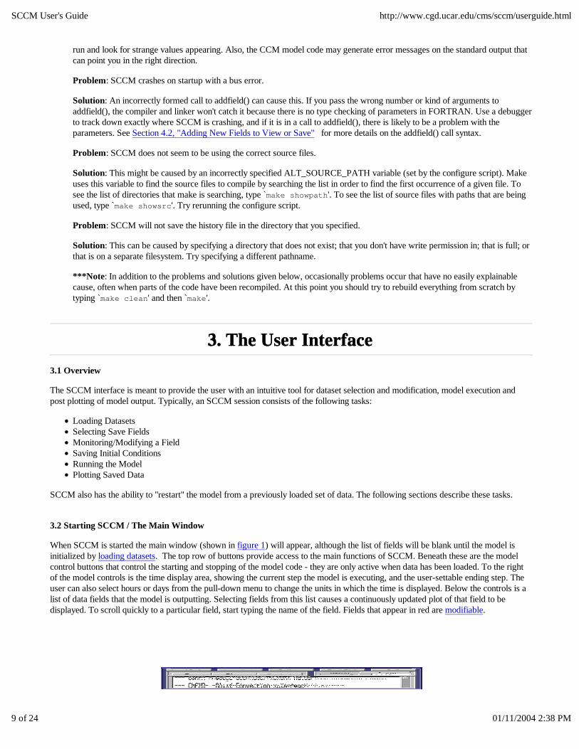
When SCCM is started the main window (shown in figure 1) will appear, although the list of fields will be blank until the model isinitialized by loading datasets. The top row of buttons provide access to the main functions of SCCM. Beneath these are the modelcontrol buttons that control the starting and stopping of the model code - they are only active when data has been loaded. To the rightof the model controls is the time display area, showing the current step the model is executing, and the user-settable ending step. Theuser can also select hours or days from the pull-down menu to change the units in which the time is displayed. Below the controls is alist of data fields that the model is outputting. Selecting fields from this list causes a continuously updated plot of that field to bedisplayed. To scroll quickly to a particular field, start typing the name of the field. Fields that appear in red are modifiable.


10 of 24 01/11/2004 2:38 PM

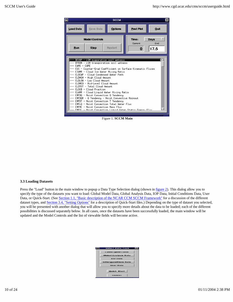
Figure 1. SCCM Main

3.3 Loading Datasets

Press the "Load" button in the main window to popup a Data Type Selection dialog (shown in figure 2). This dialog allow you tospecify the type of the datasets you want to load: Global Model Data, Global Analysis Data, IOP Data, Initial Conditions Data, UserData, or Quick-Start. (See Section 1.1, "Basic description of the NCAR CCM SCCM Framework" for a discussion of the differentdataset types, and Section 3.4, "Setting Options" for a description of Quick-Start files.) Depending on the type of dataset you selected,you will be presented with another dialog that will allow you to specify more details about the data to be loaded; each of the differentpossibilities is discussed separately below. In all cases, once the datasets have been successfully loaded, the main window will beupdated and the Model Controls and the list of viewable fields will become active.


11 of 24 01/11/2004 2:38 PM

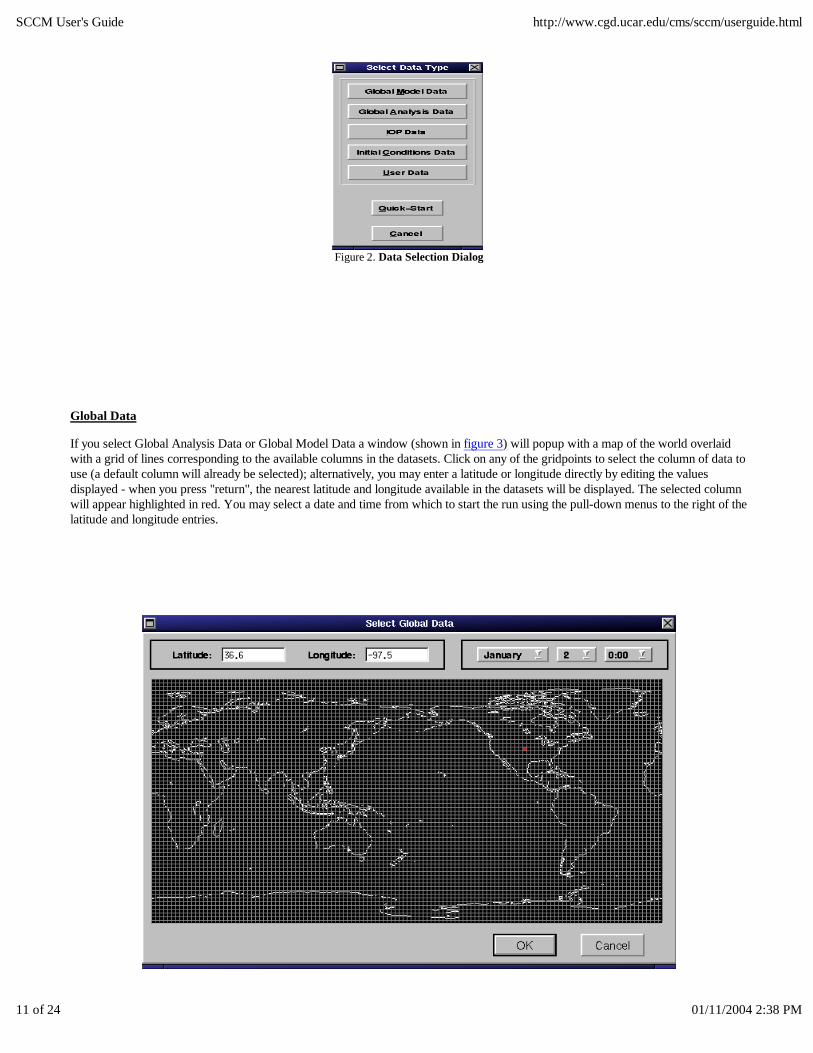
Figure 2. Data Selection Dialog

Global Data

If you select Global Analysis Data or Global Model Data a window (shown in figure 3) will popup with a map of the world overlaidwith a grid of lines corresponding to the available columns in the datasets. Click on any of the gridpoints to select the column of data touse (a default column will already be selected); alternatively, you may enter a latitude or longitude directly by editing the valuesdisplayed - when you press "return", the nearest latitude and longitude available in the datasets will be displayed. The selected columnwill appear highlighted in red. You may select a date and time from which to start the run using the pull-down menus to the right of thelatitude and longitude entries.


12 of 24 01/11/2004 2:38 PM

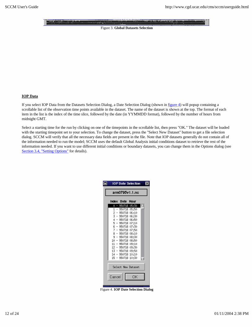
Figure 3. Global Datasets Selection

IOP Data

If you select IOP Data from the Datasets Selection Dialog, a Date Selection Dialog (shown in figure 4) will popup containing ascrollable list of the observation time points available in the dataset. The name of the dataset is shown at the top. The format of eachitem in the list is the index of the time slice, followed by the date (in YYMMDD format), followed by the number of hours frommidnight GMT.

Select a starting time for the run by clicking on one of the timepoints in the scrollable list, then press "OK." The dataset will be loadedwith the starting timepoint set to your selection. To change the dataset, press the "Select New Dataset" button to get a file selectiondialog. SCCM will verify that all the necessary data fields are present in the file. Note that IOP datasets generally do not contain all ofthe information needed to run the model; SCCM uses the default Global Analysis initial conditions dataset to retrieve the rest of theinformation needed. If you want to use different initial conditions or boundary datasets, you can change them in the Options dialog (seeSection 3.4, "Setting Options" for details).

Figure 4. IOP Date Selection Dialog


13 of 24 01/11/2004 2:38 PM

User Data

User datasets are similar to IOP datasets, but only provide data for an arbitrary number of fields. Like IOP datasets, they may contain atime series of values to force the model, or they may contain only a single timepoint to provide an initial condition. Forcing data forfields that are required by the model that are not provided in the User Data will be extracted from the Global Analysis dataset.

If you select User Data from the Datasets Selection Dialog, a standard file selection dialog will popup to allow you to select a usercreated file to use. The IOP date selection dialog will pop up to allow you to select a starting date within the user dataset, assumingthere is more than one timepoint in the file.

3.4 Setting Options

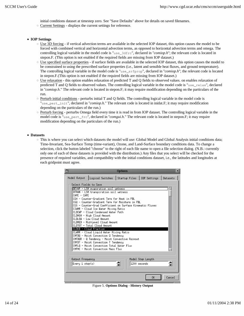
From the main window, click on Options to pop up the Options tab dialog (shown in figure 5) from where you control all of thecustomizable features of SCCM. The various options are organized into the four categories listed below. When you click `OK', themodel will be reinitialized with the new settings. Clicking cancel will close the dialog without making any changes. Note that you canonly change options after a dataset has been chosen, and at the start of a run.

History OutputSelect Fields to Save - all of the fields that are highlighted in this list will be output to the history file innetCDF format.Output Frequency - sets the frequency at which SCCM writes history data to disk. Whether this is an instantaneous oraverage value is controlled by one of the arguments provided in the addfield call for each individual field.Model Step Length - sets the length of the time step used in the model. If you edit the value directly (by typing it in, asopposed to using the arrows), you need to press <RETURN> to make your changes take effect.

Set Model Logical SwitchesThere are 12 switches that you can set in the GUI whose values are passed to the model code. In the model code, they areavailable as the array of logicals named "swi t ch" in the common block defined in "comgui.h". To use them, you need toinclude the file "comgui.h" in your source code, and test the value of the logical as in "i f ( swi t ch( 1) . eq. . t r ue.

) t hen . . . . ". The descriptive name that you can assign to them in this dialog is not available in the model code, but isincluded in the SCCM history files. Depressing the button sets the corresponding switch array element to . TRUE. This feature allows you to modify the model behavior without recompiling.

Startup FilesSet Defaults - saves the model datasets, latitude, longitude, saved fields list, save frequency, endstep, timeformat, andswitch states to the SCCM defaults file ".sccm_defaults" so that every time you start up SCCM, you will start off withthose options set the way you like. All initialization datesets except for IOP datasets are saved as filenames without paths,i.e., they are assumed to reside in the "data" directory in the usual location. IOP datasets are saved using full pathnames,so they can be located anywhere on your filesystem.Quick-Start Files - saves the current configuration to a file of your choosing, allowing you to start SCCM from this file ata later date with the same settings. To start SCCM using a quick-start file named "foobar.scm", you would type `sccm

f oobar . scm' or if SCCM was already running, you would press "Load Data" in the main window, then select theQuick-Start option in the following dialog. Quick-Start filenames are included in the NetCDF history file under theattribute "case". See "Save Defaults" above for details on saved filenames.Initial Conditions Dataset - saves all the attributes mentioned above, and also saves the fields that you have modified usingthe field plot discussed below in Section 3.5, "Monitoring and Modifying a Field". To use the file as input in a latersession, choose "Initial Conditions" from the Load Data selection dialog, and select the desired file. You can only create an


14 of 24 01/11/2004 2:38 PM

initial conditions dataset at timestep zero. See "Save Defaults" above for details on saved filenames.Current Settings - displays the current settings for reference.

IOP Settings

Use 3D forcing - if vertical advection terms are available in the selected IOP dataset, this option causes the model to beforced with combined vertical and horizontal advection terms, as opposed to horizontal advection terms and omega. Thecontrolling logical variable in the model code is "use_3df r c", declared in "comiop.h"; the relevant code is located instepon.F. (This option is not enabled if the required fields are missing from IOP dataset.)Use specified surface properties - if surface fields are available in the selected IOP dataset, this option causes the model tobe constrained to using the prescribed surface properties (i.e., latent and sensible heat fluxes, and ground temperature).The controlling logical variable in the model code is "use_sr f pr op", declared in "comiop.h"; the relevant code is locatedin stepon.F.(This option is not enabled if the required fields are missing from IOP dataset.)Use relaxation - this option enables relaxation of predicted T and Q fields to observed values. on enables relaxation ofpredicted T and Q fields to observed values. The controlling logical variable in the model code is "use_r el ax", declared in "comiop.h." The relevant code is located in stepon.F; it may require modification depending on the particulars of therun.Perturb initial conditions - perturbs initial T and Q fields. The controlling logical variable in the model code is"use_per t _i ni t ", declared in "comiop.h." The relevant code is located in inidat.F; it may require modificationdepending on the particulars of the run.)Perturb forcing - perturbs Omega field every time it is read in from IOP dataset. The controlling logical variable in themodel code is "use_per t _f r c", declared in "comgui.h." The relevant code is located in stepon.F; it may requiremodification depending on the particulars of the run.)

Datasets

This is where you can select which datasets the model will use: Global Model and Global Analysis initial conditions data;Time-Invariant, Sea-Surface Temp (time-variant), Ozone, and Land-Surface boundary conditions data. To change aselection, click the button labeled "choose" to the right of each file name to open a file selection dialog. (N.B.: currentlyonly one of each of these datasets is provided with the distribution.) Any files that you select will be checked for thepresence of required variables, and compatibility with the initial conditions dataset, i.e., the latitudes and longitudes ateach gridpoint must agree.

Figure 5. Options Dialog - History Output


15 of 24 01/11/2004 2:38 PM

3.5 Monitor ing and Modifying a Field

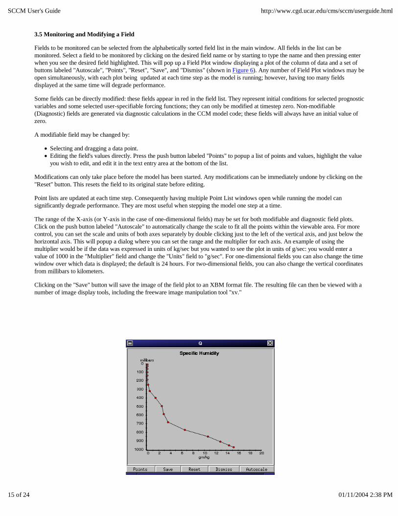
Fields to be monitored can be selected from the alphabetically sorted field list in the main window. All fields in the list can bemonitored. Select a field to be monitored by clicking on the desired field name or by starting to type the name and then pressing enterwhen you see the desired field highlighted. This will pop up a Field Plot window displaying a plot of the column of data and a set ofbuttons labeled "Autoscale", "Points", "Reset", "Save", and "Dismiss" (shown in Figure 6). Any number of Field Plot windows may beopen simultaneously, with each plot being updated at each time step as the model is running; however, having too many fieldsdisplayed at the same time will degrade performance.

Some fields can be directly modified: these fields appear in red in the field list. They represent initial conditions for selected prognosticvariables and some selected user-specifiable forcing functions; they can only be modified at timestep zero. Non-modifiable(Diagnostic) fields are generated via diagnostic calculations in the CCM model code; these fields will always have an initial value ofzero.

A modifiable field may be changed by:

Selecting and dragging a data point.Editing the field's values directly. Press the push button labeled "Points" to popup a list of points and values, highlight the valueyou wish to edit, and edit it in the text entry area at the bottom of the list.

Modifications can only take place before the model has been started. Any modifications can be immediately undone by clicking on the"Reset" button. This resets the field to its original state before editing.

Point lists are updated at each time step. Consequently having multiple Point List windows open while running the model cansignificantly degrade performance. They are most useful when stepping the model one step at a time.

The range of the X-axis (or Y-axis in the case of one-dimensional fields) may be set for both modifiable and diagnostic field plots.Click on the push button labeled "Autoscale" to automatically change the scale to fit all the points within the viewable area. For morecontrol, you can set the scale and units of both axes separately by double clicking just to the left of the vertical axis, and just below thehorizontal axis. This will popup a dialog where you can set the range and the multiplier for each axis. An example of using themultiplier would be if the data was expressed in units of kg/sec but you wanted to see the plot in units of g/sec: you would enter avalue of 1000 in the "Multiplier" field and change the "Units" field to "g/sec". For one-dimensional fields you can also change the timewindow over which data is displayed; the default is 24 hours. For two-dimensional fields, you can also change the vertical coordinatesfrom millibars to kilometers.

Clicking on the "Save" button will save the image of the field plot to an XBM format file. The resulting file can then be viewed with anumber of image display tools, including the freeware image manipulation tool "xv."


16 of 24 01/11/2004 2:38 PM

Figure 6. Plot Window

3.6 Running the Model

Any time after the data is loaded the model can be run. To start the model, push the button labeled "Run" in the main window (shownin Figure 1). The model will start time-stepping and will continue until the value of the current time reaches the ending time. To stopthe model before it reaches the end press the button again and the model will halt. It is also possible to advance the model one step at atime by clicking on the "Step" button; continuing to depress the "Step" button will result in the model single-stepping repeatedly untilthe button is released.

3.7 Saving Data

SCCM always saves the output of the model to the "userdata" subdirectory with the name ".sccmhist.tmp.nnnn" where "nnnn" is the process id. At any time after the model has stopped running, whether it stops by itself after reaching the end time or because youpressed the Run/Stop button, you can change the name and location of the the history file by clicking the "Save Data" button in themain window. You will be asked to provide a filename for the history file, with the default location of the userdata directory. It issuggested that you use one ending in ".nc" because the post-plotting dialog filters files to choose from using the filter "*.nc". If youcontinue to run the model after saving the data, the saved history file will continue to be updated until the model stops. Note that if youdo not change the filename from its default, it will be overwritten on the next run. Also see the comments about saving data in Section4.2, "Adding New Fields to View or Save."

3.8 Post-Run Analysis

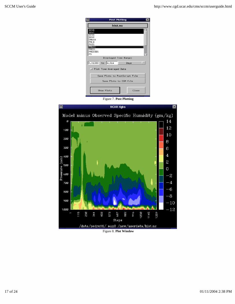
SCCM utilizes NCAR graphics to produce contour plots of saved field data. Post plots are produced from field data that has beensaved to a history file. Press the "Post Plot" button in the SCCM main window (shown in Figure 1) to pop up the "Post Plotting" window (shown in Figure 7). Select the fields for which you want to create plots from the popup menu labeled "Field", then click onthe "Show Plots" button; a window will pop up for each field selected, displaying a color contour plot or line plot of the field (shown inFigure 8). You may resize the windows, change the time range which will be displayed, or show the average value at each level overthe selected time interval; in all cases, press "Show Plots" to update the windows. To close a window, deselect it from the list, andpress the "Show Plots" button. More than one history file may be viewed at the same time: just click on the Post Plot button again,open up another file, and select the fields you want to see; this feature is helpful if you want to compare the results from two differentruns. You may also save the plots in CGM or Postscript format: just click on either of the "Save Plot to <format> File" buttons.


17 of 24 01/11/2004 2:38 PM

Figure 7. Post Plotting

Figure 8. Plot Window


18 of 24 01/11/2004 2:38 PM

3.9 Restar ting

To restart the model at time step zero, press the "Restart Button" in the main window. This will cause the model to be initialized withthe same conditions it was started with, including any changes that were made to modifiable fields. If you save a history file at the endof a run, restarting will not affect it; you may save as many history files as you like (useful if you change the value of one of the ModelLogical Switches between runs).

3.10 Command L ine Options

SCCM supports the following command line options: sccm [ - ng [ - o<out put f i l e>] [ - t <t i mest eps>] ] [ <st ar t - up f i l e>]

-ng: run sccm without the graphical user interface. If this option is specified, the name of a startup file must be provided.-o<outputfile>: save output history file in "outputfile."-t<steps>: run the model for "steps" timesteps.-r<repetitions>: repeat model run, output is saved in <outputfile>0, <outputfile>1, ....,<outputfile>repetitions-1<startupfile>: the file containing the model startup parameters. The startup files can be created by selecting the "CreateQuick-start" option in the Options Dialog. Quick-start files are plain text files, so it is possible to modify a quick-start file createdby sccm as long as the same format for the individual entries is maintained.

4. Modifying the Code

4.1 Adding New Files to the Model director ies

To add files containing new code to the model directories, you may place the new file in with the original source, place it in themymods directory, or place it in a new directory of your choosing (providing that you have added it to the ALT_SOURCE_PATHvariable described in Section 2.4, "Configuring the Makefile"). All that remains to do is to type `make'.

4.2 Adding New Fields to View or Save

To add new fields to the list of fields that you can view or save, you must edit init/bldfld.F and add new calls to addfield(). The formatof a call to addfield() is as follows:

cal l addf i el d( ' f i el d_name' , ' f i el d l ongname' , ' pl ot uni t s ' , ' st d uni t s ' , $ pl ot _mul t i pl i er , mi n_r ange, max_r ange, SHOW/ DONTSHOW, $ DI AGNOSTI C/ MODI FI ABLE, AVERAGE/ I NSTANEOUS, si ze, dummy)

where:

field_name = (Abbreviated) name of the field you want to add (must not contain any spaces). field long name = Full name of the field. std units = Units of measure used in the model code, and in the history file . plot units = Units of measure in which the field will be displayed in the GUI. plot_multiplier = Multiplication factor for displaying in non-std units in field plots. min_range = The minimum of the data range to display in plots. max_range = The maximum of the data range to display in plots. SHOW/DONTSHOW = Flag indicating whether to list the field in the main window. DIAGNOSTIC/MODIFIABLE = Flag indicating whether the field is diagnostic. AVERAGE/INSTANTANEOUS = Flag indicating whether to output averaged values to the history file, or to use theinstantaneous values. size = The size of the field: 1 if single level, plev if multilevel.


19 of 24 01/11/2004 2:38 PM

dummy = variable of type REAL that is not used (kept for backwards compatibility).

The plot multiplier, min range, and max range are used by the plotting routine to set the default display parameters. For example, ifyou have a field "foobar" that is expressed in kg/m2 in the dataset, but you would like to see it displayed in g/m2 in a Plot Window,you would set the multiplier to 1000, enter "kg/m2" as the std units pararameter, and enter "g/m2" as the "plot units" parameter. Usethe min range and max range to set the range of the x-axis in the plotting window. If you use the value 0.0 for both range parameters,the plotting routine will use the range -100 to +100 for the x-axis. These parameters only change the default display parameters: youcan still change these values at any time while you are viewing a particular field during a run. Also, they do not have any effect on theway in which the data is saved: the data is always saved in the same standard units used in the model input data files.

The DIAGNOSTIC flag indicates this field is diagnostic as opposed to modifiable/prognostic. User-defined fields will always bediagnostic.

The AVERAGE/INSTANTANEOUS flag is used to control how the GUI outputs the fields data to the history file. For example, if thesave frequency set in the GUI is 6, then once every 6 timesteps, the saved fields will be written out to the history file. AVERAGEfields will have the values for the preceding 6 timesteps averaged before outputting, whereas INSTANEOUS fields will have theinstantaneous value at that timestep output. Note that if on a given step, outfld is not called for a particular field (for example if thatsection of the code is not reached on that timestep), then the value that was output from the last outfld call will be written to the historyfile.

Note that addfield() is a C function located in the file outfld.c in the `init' subdirectory. Addfield() initializes the fieldlist in the userinterface and makes it possible to save and view fields. It is the user interface that performs all saving of data to files. To output afields's values, you need to make a call to outfld() at the relevant point in the model code. The call to outfld() takes the following form:

call outfld(`field-name', data-variable, size, lat, hbuf)

The variables `lat' and `hbuf' are unused by SCCM, but are left in for compatibility with the full CCM code so that files modified in theSCCM can be moved with minimum changes into the full CCM versions, i.e., SCCM doesn't care what you pass for these arguments.

4.3 Model Initialization

Initialization of the model in SCCM differs somewhat from the standard CCM3 initialization. It has been slightly simplified due to thedifferent nature of SCCM compared to the full CCM3. In CCM3, the calls to the major initialization routines "inital," "inti," "initext"and "intht" occur in the main program ccm3.F; they are called just once per run. In contrast, in SCCM the calls to the above routinesoccur in init_model.F in the same order, but they may be called repeatedly, once for each time the model is initialized via the userinterface (e.g., after selecting new datasets, or restarting). Additionally, some of the initialization routines found in CCM3 are absentfrom SCCM, primarily those relating to initialization of file input/output devices, and the decomposition of space into latitudes andlongitudes. As a general rule, if some initialization of the model needs to be performed before the time-stepping routine is invoked,init_model.F is the best place to put the necessary initialization code.

5. Using SCCM with an IOP Dataset


20 of 24 01/11/2004 2:38 PM

5.1 Introduction

This section describes the contents and standard format of the Intensive Observation Period (IOP) datasets available for SCCM, and atypical example of how the model is used with this type of data. In this section it is assumed that the IOP dataset has already beencreated; sample IOP datasets are distributed with SCCM.

An IOP dataset can provide a large amount of information for use with a single column model. For many users it is likely that some ofthe available data will not be used to force the model, in which case it may be used as a method of validating SCCM output. Forexample, the ground temperature within SCCM can be constrained to the value measured during the IOP or it can be predicted. If themodel predicts the ground temperature then the value in the IOP dataset can be used to `validate' the models prediction. In general theless data used to constrain the model the more validating diagnostics will be available.It may be the case that some fields required forforcing SCCM are not available in the IOP dataset; if this is the case then the user should decide on the best method for dealing withthis situation. For example, if the horizontal wind speed is not available the user must decide if this field will have a strong influence ontheir investigation; if so, then the dataset is not suitable for their use. If, however, the horizontal wind speed is of only secondaryimportance, then they may decide to use a climatological value which should be included in the dataset or read into the model at therelevant time.

5.2 The Standard IOP Dataset for SCCM

As a general guide, the terms used to force or constrain SCCM can be separated into the 3 following categories.

Essential [E] - the SCCM cannot function satisfactorily without this information.Important [I] - these terms are important in forcing the SCCM but it can be run without them if some basic assumptions aremade. It is important for the user to understand what assumptions are made if the terms are missing, and the effect this will haveon the model.Optional [O] - these are terms which are not required by the SCCM but may be included to constrain the model physics or forcethe model in a format other than its basic form, i.e., latent and sensible heat may be predicted by SCCM or prescribed by theIOP dataset.

For some users, some of the essential fields may be replaced with a climatology or other prescribed values. This depends on validationtechniques and the principles being investigated by the user.

Table 2 shows the essential, important and optional forcing terms for a typical SCCM IOP dataset. This dataset can be expanded uponby the user to contain any number of other fields but the list is complete for any currently available datasets. The datasets used inSCCM must be in NetCDF format (Rew et al., 1993) and Table 2 describes the NetCDF long and short names which should be used(when creating a dataset for use in SCCM it is essential that short name used is identical to that shown). Surface values such as groundtemperature should be a function of time only, profiles such as temperature should be a function of pressure level (top down) and timerespectively. If any of the essential [E] terms are missing then the dataset can not be used in the IOP format.

If any of the important [I] terms are missing then the model will display a warning and replace these with a default value. For pt, u andv zero will be used; a missing pt will influence the interpolation of omega onto model levels and interfaces, a missing u or v willinfluence parts of SCCM physics. If the Tg or Ts are missing then they will be set to the temperature at the lowest level; a missing Tswill influence the temperature interpolation onto the lowest model level, a missing Tg will influence some of the model physics such asradiation. If any of the substitutions described here are not suitable for a users experiments then the user should include the valuesrequired in the IOP dataset.

The optional [O] terms, shflx and lhflx can be included to constrain the surface physics in the model (the ground temperature can beused in this way but is categorized as important [I] because it is required as an initial condition). The hydrometeor terms are rarelyavailable in IOP datasets but may be included if a bulk microphysical scheme is incorporated into SCCM.

5.3 A Detailed Example Using SCCM With an IOP Dataset.

In the following example we will make 2 versions of the model, run SCCM using IOP data, and compare the results.

5.3.1 Changing and Initializing the Model

Here it is assumed that we have a working version of the standard SCCM and we are going to modify it. In this example we will add anew condensation scheme called `foobar.F', which for one experiment will replace the standard `cond.F'. The file foobar.F contains a


21 of 24 01/11/2004 2:38 PM

tracer which should be advected, and a variable àcr', the autoconversion rate which we will use as a diagnostic. The autoconversion

rate is a function of height and time and has SI units of (s-1). The diagnostic should be saved in its SI units but can be viewed in themore intuitive units of g/kg/hr. To do this the following steps should be taken:

Add the file foobar.F to the mymods directory.Add a call to àddfield()' in the file initial/bldfld.F as follows:

cal l addf i el d( ' ACR' , ' Aut oconver si on Rat e' , ' g/ kg/ hr ' , ' s- 1' , 3. 6e6, 0. , 2. , $ ACTI VE, DI AGNOSTI C, I NSTANTANEOUS, pl ev, dummy )

where 3.6e6 is the conversion factor between s-1 and g/kg/hr, and 0 to 2 is a conservative range for viewing this field.

Add a call to òutfld()' in mymods/foobar.F as follows:

cal l out f l d( ' ACR' , acr , pl ev, l at , hbuf )

Note that `lat' and `hbuf' are not used in SCCM, and are only included for compatibility with the full CCM code; they can bereplaced with any variables of the right type.

Make a copy of the file àphys.F', and edit it to include a call to `foobar' next to the call to `cond'. A logical statement around the2 schemes can be used to control which scheme is to be used, using one of the switches described in Section 3.4, "SettingOptions." We'll use switch(2). Save the modified version of àphys.F' in the `mymods' directory .Since there is an additional tracer associated with foobar.F, PCONST must be changed from 1 to 2. This is done by executingthe configure script and assigning a value of 2 to PCNST.

Rebuild the model by typing `make'.

We should now be able to run two versions of the column model, a standard version or a version which uses foobar.F. Eitherversion can be run by turning switch number 2 on or off in the options dialog.

5.3.2 Running the Model

Once we have the new code in place under the control of the `foobar switch' we can then run the model. For this example we will usethe ARM IOP dataset which is distributed with SCCM. This is the Summer 1995 IOP from the ARM Southern Great Plains (SGP)site. For this example we will choose a 10 day period beginning on the 20th of July. We will concentrate on Temperature, and SpecificHumidity as diagnostics.

The following is a brief guide to running the model:

From the Main window select `Load Data' button.Select ÌOP Data'.If the default is not àrm0795v1.nc', use `Select New Dataset' to choose this.Scroll through the dates and select the description `128 - 950720 00:10' to select a starting time of 00:10 GMT on July 20, 1995.Select Òptions' from the Main window. Select `T - Temperature', and `Q - Specific Humidity' from the list of saved fields(these may already be highlighted). Change the description of switch 2 in the Logical Switches section to "foobar" so that you


22 of 24 01/11/2004 2:38 PM

will know what the switch settings mean when you get around to analyzing the history data at a later time. Leave the switchturned off for now.Change the time display to display days instead of hours, then set the ending time to 10 days.Select `Run' from the model controls. When the model is finished, select `Save' and give the name `standard.nc'.Select `Restart' from the Main window.Select `Options' and change the foobar switch to the `on' (depressed) position.Run the model again for 10 days, saving the history file at the end, using the name `foobar.nc'.

Once the model has finished the postplotting routine can be used to examine the two history files, or you can quit from SCCM and usea tool of preference to examine the data. Differencing the files `standard.nc' and `foobar.nc' (using some netCDF tool) can provideinformation on the influence foobar.F had on SCCM.

6. Acknowledgements

The authors wish to acknowledge contributions to earlier versions of the SCCM modeling tool made by Mike Hoswell and DavidEnce. This work has been supported by the Computer Hardware Advanced Mathematics Model Physics (CHAMMP) program and theClimate Change Prediction Program (CCPP) which are administered by the Office of Energy Research under the Office of Health andEnvironmental Research in the Department of Energy Environmental Sciences Division.

Appendix A: Format of SCCM NetCDF Datasets

Table 1: Required Dimensions and Variables in SCCM NetCDFDatasets

Dataset Type Dimensions Required Variables

Global Model lon, lev, lat,time

lon, lat, lev, time, date, datesec, hyam, hyai,hybi, hybm, PHIS, U, V, T, PS, ORO, TS1,TS2, TS3, TS4, OMEGA

Global Analysis

lon, lev, lat,time

lon, lat, lev, time, date, datesec, hyam, hyai,hybi, hybm, PHIS, U, V, T, PS, ORO, OMEGA

IOP lon, lev, lat,time

lon, lat, lev, phis, tsec, T, q, bdate, divT,divq, Ps, omega

LSM lon, lat, time numlon, latixy, longxy, surf2d, soic2d,silt2d, clay2d, pctlak, pctwet


23 of 24 01/11/2004 2:38 PM

Ozone lon, lev, lat,time

lat, lev, time, date, datesec, OZONE

Pressure lev hyam, hyai, hybi, hybm

Time Variant lon, lev, lat,time

date, datesec, SST

Time Invariant

lon, lev, lat,time

ALBVSS, ALBVSW, ALBNIS, ALBNIW,FRCTST, RGHNSS, EVAPF, VEGTYP, SNWJAN, SNWJLY, SGH

User lon, lev, lat,time

bdate, lon, lat, lev, tsec

Table 2: The Various Terms Included in the Standard IOPDatasets Used for Forcing SCCM

Short Name

Long Name Type Units

nbdate [E]

Base Date long yymmdd

time [E] Time after 0Z on nbdate long s

lev [E] Pressure Levels float Pa

lat [E] Latitude float deg N

lon [E] Longitude float deg E

phis [E] Surface Geopotential float m/s2

t [E] Temperature float K

divt [E] Horizontal T Advective Tendency float K/s

vertdivt [O]

Vertical T Advective Tendency float K/s

q [E] Specific Humidity float kg/kg

divq [E] Horizontal Q Advective Tendency float kg/kg/s

vertdivq [O]

Verical Q Advective Tendency float kg/kg/s

ps [E] Surface Pressure float Pa

omega [E]

Vertical Pressure Velocity float Pa/s

Ptend [I] Surface Pressure Tendency float Pa/s


24 of 24 01/11/2004 2:38 PM

u [I] U Windspeed float m/s

v [I] V Windspeed float m/s

tg [O] Ground Temperature float K

ts [O] Surface Air Temperature float K

shflx [O] Surface Sensible Heat Flux float W/m2

lhflx [O] Surface Latent Heat Flux float W/m2

This document last updated February 5, 1999. Send comments to [email protected].

sccm user's guide - department of physicsatmosp.physics.utoronto.ca/.../sccm_doc.pdf · sccm...

Documents