scenario analysis in risk management -...
TRANSCRIPT

Bertrand K. Hassani
Scenario Analysis in Risk ManagementTheory and Practice in Finance

Scenario Analysis in Risk Management

Bertrand K. Hassani
Scenario Analysis in RiskManagementTheory and Practice in Finance
123

Dr. Bertrand K. HassaniGlobal Head of Research and
Innovation - Risk MethodologyGrupo SantanderMadrid, Spain
Associate ResearcherUniversité Paris 1 Panthéon SorbonneLabex ReFiParis, France
The opinions, ideas and approaches expressed or presented are those of the author and donot necessarily reflect Santander’s position. As a result, Santander cannot be held responsiblefor them. The values presented are just illustrations and do not represent Santander losses,exposures or risks.
ISBN 978-3-319-25054-0 ISBN 978-3-319-25056-4 (eBook)DOI 10.1007/978-3-319-25056-4
Library of Congress Control Number: 2016950567
© Springer International Publishing Switzerland 2016This work is subject to copyright. All rights are reserved by the Publisher, whether the whole or part ofthe material is concerned, specifically the rights of translation, reprinting, reuse of illustrations, recitation,broadcasting, reproduction on microfilms or in any other physical way, and transmission or informationstorage and retrieval, electronic adaptation, computer software, or by similar or dissimilar methodologynow known or hereafter developed.The use of general descriptive names, registered names, trademarks, service marks, etc. in this publicationdoes not imply, even in the absence of a specific statement, that such names are exempt from the relevantprotective laws and regulations and therefore free for general use.The publisher, the authors and the editors are safe to assume that the advice and information in this bookare believed to be true and accurate at the date of publication. Neither the publisher nor the authors orthe editors give a warranty, express or implied, with respect to the material contained herein or for anyerrors or omissions that may have been made.
Printed on acid-free paper
This Springer imprint is published by Springer NatureThe registered company is Springer International Publishing AG Switzerland

To my sunshines, Lila, Liam and Jihane
To my parents, my brother, my family, myfriends and my colleagues without whom Iwould not be where I am
To Pr. Dr. Dominique Guégan, who believedin me. . .

Preface
The objective of this book is to show that scenario analysis in financial institutionscan be addressed in various ways depending on what we would like to achieve.There is not one method better than the other; there are just methods moreappropriate in some particular situations.
I heard so many times opinionated people selecting a scenario strategy overanother because everyone was doing it; that is not the appropriate answer andmay lead to selecting an inappropriate methodology and consequently to unusableresults. Even worse, the managers may lose faith in the process and tell everyonethat scenario analysis for risk management is useless.
Therefore, in this book, I am presenting various approaches to perform scenarioanalysis; some are relying on quantitative approaches; others are more qualitative,but once again, none of them are better than another. Each of them has some prosand cons and depends on the maturity of your risk framework, the type of riskthat banks are willing to assess and manage and the information available. I triedto present them in the simplest way possible and to keep only the essence of themethodologies as in any case; eventually, the managers will have to fine-tune them,making them their own approach. I hope this book will inspire them. One of myobjectives was also to make supposedly complicated methodologies accessible toany risk managers. Indeed, these would just need to have a basic understanding ofmathematics.
Note that I implemented all the methodologies I am presenting in this book,and all the figures presented are my own. Most of them have been implementedin professional environments to answer practical issues. Therefore, I am givingsome tools for risk managers to address scenario analysis, I am providing leadsfor researchers to start proposing solutions to address them and I hope that theclear perspective of combining the methodologies will lead to future academic andprofessional developments.
vii

viii Preface
As failures of risk management related to failures of scenario analysis pro-grammes may have disastrous impacts, note that all the proceedings of this bookare going to charities to contribute to the relief of suffering people.
Global Head of Research and Innovation - Bertrand K. HassaniRisk MethodologyGrupo SantanderMadrid, Spain
Associate ResearcherUniversité Paris 1 Panthéon SorbonneLabex ReFiParis, France

Biography
Bertrand is a risk measurement and management specialist (Credit, Market, Oper-ational, Liquidity, Counterparty etc.) for SIFIs. He is also an active associateresearcher at Paris Pantheon-Sorbonne University. He wrote several articles dealingwith Risk Measures, Risk Modelling, and Risk Management. He is still studyingto obtain the D.Sc. degree (French H.D.R.). He spent two years working in theBond/Structure notes market (Eurocorporate), four years in the banking industryin a Risk Management/Modelling department (BPCE) and one year as a SeniorRisk Consultant (Aon-AGRC within Unicredit in Milan). He is currently workingfor Santander where he successively held the Head of Major Risk Managementposition (San UK), the Head of Change and Consolidated Risk Managementposition (San UK), the Global Head of Advanced and Alternative Analyticsposition (Grupo Santander) and is now Global Head of Research and Innovations(Grupo Santander) for the risk division. In this role, Bertrand aims at developingnovel approaches to measure risk (financial and non-financial) and integrating themin the decision-making process of the bank (business orientated convoluted risk
ix

x Biography
management), relying on methodologies coming from the field of data science(data mining, machine learning, frequentist statistics, A.I., etc.).

Contents
1 Introduction . . . . . . . . . . . . . . . . . . . . . . . . . . . . . . . . . . . . . . . . . . . . . . . . . . . . . . . . . . . . . . . . . 11.1 Is this War? . . . . . . . . . . . . . . . . . . . . . . . . . . . . . . . . . . . . . . . . . . . . . . . . . . . . . . . . . . . 11.2 Scenario Planning: Why, What, Where, How, When. . . . . . . . . . . . . . 21.3 Objectives and Typology .. . . . . . . . . . . . . . . . . . . . . . . . . . . . . . . . . . . . . . . . . . . . 41.4 Scenario Pre-requirements .. . . . . . . . . . . . . . . . . . . . . . . . . . . . . . . . . . . . . . . . . . 61.5 Scenarios, a Living Organism . . . . . . . . . . . . . . . . . . . . . . . . . . . . . . . . . . . . . . . 71.6 Risk Culture . . . . . . . . . . . . . . . . . . . . . . . . . . . . . . . . . . . . . . . . . . . . . . . . . . . . . . . . . . 8References .. . . . . . . . . . . . . . . . . . . . . . . . . . . . . . . . . . . . . . . . . . . . . . . . . . . . . . . . . . . . . . . . . . . 10
2 Environment . . . . . . . . . . . . . . . . . . . . . . . . . . . . . . . . . . . . . . . . . . . . . . . . . . . . . . . . . . . . . . . . 112.1 The Risk Framework .. . . . . . . . . . . . . . . . . . . . . . . . . . . . . . . . . . . . . . . . . . . . . . . . 112.2 The Risk Taxonomy: A Base for Story Lines . . . . . . . . . . . . . . . . . . . . . . . 122.3 Risk Interactions and Contagion.. . . . . . . . . . . . . . . . . . . . . . . . . . . . . . . . . . . . 142.4 The Regulatory Framework .. . . . . . . . . . . . . . . . . . . . . . . . . . . . . . . . . . . . . . . . . 17References .. . . . . . . . . . . . . . . . . . . . . . . . . . . . . . . . . . . . . . . . . . . . . . . . . . . . . . . . . . . . . . . . . . . 23
3 The Information Set: Feeding the Scenarios . . . . . . . . . . . . . . . . . . . . . . . . . . . . 253.1 Characterising Numeric Data . . . . . . . . . . . . . . . . . . . . . . . . . . . . . . . . . . . . . . . . 27
3.1.1 Moments . . . . . . . . . . . . . . . . . . . . . . . . . . . . . . . . . . . . . . . . . . . . . . . . . . . . 283.1.2 Quantiles . . . . . . . . . . . . . . . . . . . . . . . . . . . . . . . . . . . . . . . . . . . . . . . . . . . . 293.1.3 Dependencies . . . . . . . . . . . . . . . . . . . . . . . . . . . . . . . . . . . . . . . . . . . . . . . 29
3.2 Data Sciences . . . . . . . . . . . . . . . . . . . . . . . . . . . . . . . . . . . . . . . . . . . . . . . . . . . . . . . . . 303.2.1 Data Mining. . . . . . . . . . . . . . . . . . . . . . . . . . . . . . . . . . . . . . . . . . . . . . . . . 303.2.2 Machine Learning and Artificial Intelligence . . . . . . . . . . . . . 323.2.3 Common Methodologies . . . . . . . . . . . . . . . . . . . . . . . . . . . . . . . . . . . 34
References .. . . . . . . . . . . . . . . . . . . . . . . . . . . . . . . . . . . . . . . . . . . . . . . . . . . . . . . . . . . . . . . . . . . 36
4 The Consensus Approach . . . . . . . . . . . . . . . . . . . . . . . . . . . . . . . . . . . . . . . . . . . . . . . . . . 394.1 The Process . . . . . . . . . . . . . . . . . . . . . . . . . . . . . . . . . . . . . . . . . . . . . . . . . . . . . . . . . . . 404.2 In Practice . . . . . . . . . . . . . . . . . . . . . . . . . . . . . . . . . . . . . . . . . . . . . . . . . . . . . . . . . . . . 43
4.2.1 Pre-workshop . . . . . . . . . . . . . . . . . . . . . . . . . . . . . . . . . . . . . . . . . . . . . . . 444.2.2 The Workshops . . . . . . . . . . . . . . . . . . . . . . . . . . . . . . . . . . . . . . . . . . . . . 45
xi

xii Contents
4.3 For the Manager . . . . . . . . . . . . . . . . . . . . . . . . . . . . . . . . . . . . . . . . . . . . . . . . . . . . . . 464.3.1 Sponsorship .. . . . . . . . . . . . . . . . . . . . . . . . . . . . . . . . . . . . . . . . . . . . . . . . 474.3.2 Buy-In .. . . . . . . . . . . . . . . . . . . . . . . . . . . . . . . . . . . . . . . . . . . . . . . . . . . . . . 484.3.3 Validation . . . . . . . . . . . . . . . . . . . . . . . . . . . . . . . . . . . . . . . . . . . . . . . . . . . 484.3.4 Sign-Offs . . . . . . . . . . . . . . . . . . . . . . . . . . . . . . . . . . . . . . . . . . . . . . . . . . . . 48
4.4 Alternatives and Comparison . . . . . . . . . . . . . . . . . . . . . . . . . . . . . . . . . . . . . . . . 49References .. . . . . . . . . . . . . . . . . . . . . . . . . . . . . . . . . . . . . . . . . . . . . . . . . . . . . . . . . . . . . . . . . . . 50
5 Tilting Strategy: Using Probability Distribution Properties . . . . . . . . . . . 515.1 Theoretical Basis . . . . . . . . . . . . . . . . . . . . . . . . . . . . . . . . . . . . . . . . . . . . . . . . . . . . . 52
5.1.1 Distributions . . . . . . . . . . . . . . . . . . . . . . . . . . . . . . . . . . . . . . . . . . . . . . . . 525.1.2 Risk Measures . . . . . . . . . . . . . . . . . . . . . . . . . . . . . . . . . . . . . . . . . . . . . . 565.1.3 Fitting . . . . . . . . . . . . . . . . . . . . . . . . . . . . . . . . . . . . . . . . . . . . . . . . . . . . . . . 585.1.4 Goodness-of-Fit Tests . . . . . . . . . . . . . . . . . . . . . . . . . . . . . . . . . . . . . . 61
5.2 Application . . . . . . . . . . . . . . . . . . . . . . . . . . . . . . . . . . . . . . . . . . . . . . . . . . . . . . . . . . . 625.3 For the Manager: Pros and Cons . . . . . . . . . . . . . . . . . . . . . . . . . . . . . . . . . . . . 65
5.3.1 Implementation . . . . . . . . . . . . . . . . . . . . . . . . . . . . . . . . . . . . . . . . . . . . . 655.3.2 Distribution Selection . . . . . . . . . . . . . . . . . . . . . . . . . . . . . . . . . . . . . . 665.3.3 Risk Measures . . . . . . . . . . . . . . . . . . . . . . . . . . . . . . . . . . . . . . . . . . . . . . 66
References .. . . . . . . . . . . . . . . . . . . . . . . . . . . . . . . . . . . . . . . . . . . . . . . . . . . . . . . . . . . . . . . . . . . 67
6 Leveraging Extreme Value Theory . . . . . . . . . . . . . . . . . . . . . . . . . . . . . . . . . . . . . . . 696.1 Introduction .. . . . . . . . . . . . . . . . . . . . . . . . . . . . . . . . . . . . . . . . . . . . . . . . . . . . . . . . . . 696.2 The Extreme Value Framework.. . . . . . . . . . . . . . . . . . . . . . . . . . . . . . . . . . . . . 71
6.2.1 Fisher–Tippett Theorem .. . . . . . . . . . . . . . . . . . . . . . . . . . . . . . . . . . . 726.2.2 The GEV . . . . . . . . . . . . . . . . . . . . . . . . . . . . . . . . . . . . . . . . . . . . . . . . . . . . 726.2.3 Building the Data Set . . . . . . . . . . . . . . . . . . . . . . . . . . . . . . . . . . . . . . . 746.2.4 How to Apply It? . . . . . . . . . . . . . . . . . . . . . . . . . . . . . . . . . . . . . . . . . . . 75
6.3 Summary of Results Obtained .. . . . . . . . . . . . . . . . . . . . . . . . . . . . . . . . . . . . . . 776.4 Conclusion .. . . . . . . . . . . . . . . . . . . . . . . . . . . . . . . . . . . . . . . . . . . . . . . . . . . . . . . . . . . 79References .. . . . . . . . . . . . . . . . . . . . . . . . . . . . . . . . . . . . . . . . . . . . . . . . . . . . . . . . . . . . . . . . . . . 79
7 Fault Trees and Variations . . . . . . . . . . . . . . . . . . . . . . . . . . . . . . . . . . . . . . . . . . . . . . . . . 817.1 Methodology . . . . . . . . . . . . . . . . . . . . . . . . . . . . . . . . . . . . . . . . . . . . . . . . . . . . . . . . . 827.2 In Practice . . . . . . . . . . . . . . . . . . . . . . . . . . . . . . . . . . . . . . . . . . . . . . . . . . . . . . . . . . . . 83
7.2.1 Symbols . . . . . . . . . . . . . . . . . . . . . . . . . . . . . . . . . . . . . . . . . . . . . . . . . . . . . 837.2.2 Construction Steps . . . . . . . . . . . . . . . . . . . . . . . . . . . . . . . . . . . . . . . . . . 867.2.3 Analysis . . . . . . . . . . . . . . . . . . . . . . . . . . . . . . . . . . . . . . . . . . . . . . . . . . . . . 887.2.4 For the Manager . . . . . . . . . . . . . . . . . . . . . . . . . . . . . . . . . . . . . . . . . . . . 897.2.5 Calculations: An Example . . . . . . . . . . . . . . . . . . . . . . . . . . . . . . . . . 89
7.3 Alternatives . . . . . . . . . . . . . . . . . . . . . . . . . . . . . . . . . . . . . . . . . . . . . . . . . . . . . . . . . . . 907.3.1 Failure Mode and Effects Analysis . . . . . . . . . . . . . . . . . . . . . . . . 917.3.2 Root Cause Analysis . . . . . . . . . . . . . . . . . . . . . . . . . . . . . . . . . . . . . . . 917.3.3 Why-Because Strategy . . . . . . . . . . . . . . . . . . . . . . . . . . . . . . . . . . . . . 927.3.4 Ishikawa’s Fishbone Diagrams. . . . . . . . . . . . . . . . . . . . . . . . . . . . . 937.3.5 Fuzzy Logic . . . . . . . . . . . . . . . . . . . . . . . . . . . . . . . . . . . . . . . . . . . . . . . . . 94
References .. . . . . . . . . . . . . . . . . . . . . . . . . . . . . . . . . . . . . . . . . . . . . . . . . . . . . . . . . . . . . . . . . . . 95

Contents xiii
8 Bayesian Networks . . . . . . . . . . . . . . . . . . . . . . . . . . . . . . . . . . . . . . . . . . . . . . . . . . . . . . . . . 978.1 Introduction .. . . . . . . . . . . . . . . . . . . . . . . . . . . . . . . . . . . . . . . . . . . . . . . . . . . . . . . . . . 978.2 Theory . . . . . . . . . . . . . . . . . . . . . . . . . . . . . . . . . . . . . . . . . . . . . . . . . . . . . . . . . . . . . . . . 100
8.2.1 A Practical Focus on the Gaussian Case. . . . . . . . . . . . . . . . . . . 1038.2.2 Moving Towards an Integrated System: Learning . . . . . . . . 104
8.3 For the Managers . . . . . . . . . . . . . . . . . . . . . . . . . . . . . . . . . . . . . . . . . . . . . . . . . . . . . 106References .. . . . . . . . . . . . . . . . . . . . . . . . . . . . . . . . . . . . . . . . . . . . . . . . . . . . . . . . . . . . . . . . . . . 108
9 Artificial Neural Network to Serve Scenario Analysis Purposes . . . . . . 1119.1 Origins . . . . . . . . . . . . . . . . . . . . . . . . . . . . . . . . . . . . . . . . . . . . . . . . . . . . . . . . . . . . . . . . 1129.2 In Theory . . . . . . . . . . . . . . . . . . . . . . . . . . . . . . . . . . . . . . . . . . . . . . . . . . . . . . . . . . . . . 1139.3 Learning Algorithms . . . . . . . . . . . . . . . . . . . . . . . . . . . . . . . . . . . . . . . . . . . . . . . . . 1149.4 Application . . . . . . . . . . . . . . . . . . . . . . . . . . . . . . . . . . . . . . . . . . . . . . . . . . . . . . . . . . . 1169.5 For the Manager: Pros and Cons . . . . . . . . . . . . . . . . . . . . . . . . . . . . . . . . . . . . 119References .. . . . . . . . . . . . . . . . . . . . . . . . . . . . . . . . . . . . . . . . . . . . . . . . . . . . . . . . . . . . . . . . . . . 120
10 Forward-Looking Underlying Information: Working withTime Series . . . . . . . . . . . . . . . . . . . . . . . . . . . . . . . . . . . . . . . . . . . . . . . . . . . . . . . . . . . . . . . . . . 12310.1 Introduction .. . . . . . . . . . . . . . . . . . . . . . . . . . . . . . . . . . . . . . . . . . . . . . . . . . . . . . . . . . 12310.2 Methodology . . . . . . . . . . . . . . . . . . . . . . . . . . . . . . . . . . . . . . . . . . . . . . . . . . . . . . . . . 124
10.2.1 Theoretical Aspects. . . . . . . . . . . . . . . . . . . . . . . . . . . . . . . . . . . . . . . . . 12510.2.2 The Models . . . . . . . . . . . . . . . . . . . . . . . . . . . . . . . . . . . . . . . . . . . . . . . . . 131
10.3 Application . . . . . . . . . . . . . . . . . . . . . . . . . . . . . . . . . . . . . . . . . . . . . . . . . . . . . . . . . . . 135References .. . . . . . . . . . . . . . . . . . . . . . . . . . . . . . . . . . . . . . . . . . . . . . . . . . . . . . . . . . . . . . . . . . . 139
11 Dependencies and Relationships Between Variables . . . . . . . . . . . . . . . . . . . 14111.1 Dependencies, Correlations and Copulas . . . . . . . . . . . . . . . . . . . . . . . . . . . 142
11.1.1 Correlations Measures . . . . . . . . . . . . . . . . . . . . . . . . . . . . . . . . . . . . . . 14211.1.2 Regression . . . . . . . . . . . . . . . . . . . . . . . . . . . . . . . . . . . . . . . . . . . . . . . . . . 14411.1.3 Copula .. . . . . . . . . . . . . . . . . . . . . . . . . . . . . . . . . . . . . . . . . . . . . . . . . . . . . . 151
11.2 For the Manager . . . . . . . . . . . . . . . . . . . . . . . . . . . . . . . . . . . . . . . . . . . . . . . . . . . . . . 155References .. . . . . . . . . . . . . . . . . . . . . . . . . . . . . . . . . . . . . . . . . . . . . . . . . . . . . . . . . . . . . . . . . . . 157
Index . . . . . . . . . . . . . . . . . . . . . . . . . . . . . . . . . . . . . . . . . . . . . . . . . . . . . . . . . . . . . . . . . . . . . . . . . . . . . . . 159

Chapter 1Introduction
1.1 Is this War?
Scenarios have been used for years in many areas (economics, military, aeronautics,public health, etc.) and are far from being limited to the financial industry. Scenariosare a postulated sequence or development of events, a summary of the plot of a play,including information about its stakeholders, characters, locations, scenes, weather,etc., i.e., anything that could contribute to make it more realistic. One of the keyaspects of scenario analysis is the fact that starting from one set of assumptionsit is possible to evaluate and map various outcome of a particular situation. Whilein this book we will limit ourselves to the financial industry for our applicationsand examples, it would be an extreme prejudice not to inspire ourselves fromwhat we could use from other industries in terms of methodologies, procedures orregulations.
Indeed, to illustrate the importance of scenario analysis in our world, let’sstart with famous historical examples combining geopolitics and military strategy.The greatest leaders in the history of mankind based their decisions on theoutcome of scenarios, Pearl Harbor attack was one of the outcomes of the scenarioanalysed by Commanders Mitsuo Fuchida and Minoru Genda considering thattheir objective was to make US naval forces inoperative for 6 months at least(Burbeck, 2013). Sir Winston Churchill analysed the possibility of attacking theSoviet Union with Americans and West Germans as allied after World War II(Operation Unthinkable—Lewis 2008). Scenarios are a very useful and powerfultool to analyse all potential future outcomes and prepare ourselves for them. Froma counter terrorism point of view, the protection scheme of nuclear plants fromterrorist attacks is clearly the result of a scenario analysis, for example, in Francesquadron of fighter pilots are ready to take off and intercept an airborne potentialthreat in less than 15 min. It is also really important to understand that the riskassessment resulting from a scenario analysis may result in the acceptance of thisrisk. The nuclear plant located in Fessenheim, next to the Switzerland border has
© Springer International Publishing Switzerland 2016B.K. Hassani, Scenario Analysis in Risk Management,DOI 10.1007/978-3-319-25056-4_1
1

2 1 Introduction
been built in a seismic area, but the authorities came to the conclusion that the riskwas acceptable, besides it is one of the oldest nuclear plants in France and one maythink the likelihood of a failure and age are correlated.1
In the military, most equipments are the results of either field experience orscenarios or past failure, but in many industries, contrary to the financial sector,we may not have the opportunity to wait for a failure to be able to identify an issueand fix it, and therefore learn from it as in other industries such as aeronautics orpharmaceutical if a failure occurs or a faulty product is released, people’s lives areat risk.
Now, focusing on scenario analysis within financial institutions, this one hasusually one of the following forms. The first form is stress testing (Rebonato,2010). Stress testing aims at assessing multiple outcomes resulting from adversestories of different magnitude, for instance, likely, mild and worse case scenariorelying on macroeconomic variables. Indeed, it is quite frequent to analyse aparticular situation with respect to how would macroeconomic variables evolve.The second form relates to operational risk management as prescribed in the currentregulation,2 where scenarios are required for capital calculations (Pillar I and PillarII—Rippel and Teply 2011). The recent crisis taught us that banks failing dueto extreme incidents may dramatically impact the real economy, indeed, SociétéGénérale rogue tading, a massive operational risk resulted in a massive marketrisk materialisation as all the prices went down simultaneously, in a huge lackof liquidity as the interbanking market was failing (banks were not funding eachothers) and consequently in the well-known credit crunch as banks were not fundingthe real economy, the whole occurring within the context of the subprime crisis.Impacted companies were suffering and some relatively healthy went even bankrupt.The last use of scenarios is related to general risk management. It is probably themost useful use of scenario analysis as it is not necessary a regulatory demand and assuch would only be used by risk managers to improve their risk framework removingthe pressure of a potential higher capital charge.
1.2 Scenario Planning: Why, What, Where, How, When. . .
Presenting scenario analysis in its globality and not only in the financial industry,the following paragraph presents a military scenario planning. In this book, wedraw a parallel between the scenario process in the Army and in a financialinstitution. The scenario planning as suggested in Aepli et al. (2010) is summarisedbelow. It can be broken down in 12 successive steps of equal importance and we
1The idea behind these example is neither to generate any controversy nor to feed any conspiracytheory but to refer to examples which should talk to the largest number of readers.2Note that though the regulation might change, scenarios should still be required for riskmanagement purposes.

1.2 Scenario Planning: Why, What, Where, How, When. . . 3
would recommend risk managers to keep them in mind undertaking such a process(International Institute for Environment and Development (IIED) 2009; GregoryStone and Redmer, 2006).
1. Decide on the key question to be answered by the analysis. This allows creatingthe framework for the analysis and condition the next points.
2. Set both time and scope of the analysis, i.e. place the scenario in a period oftime, define the environment and precise the condition.
3. Identify and select major stakeholders to be engaged, i.e. people at theorigination of the risk, responsible or accountable, or impacted by it.
4. Map basic trends and driving forces such as industry, economic, political,technological, legal and societal trends. Evaluate to what extent these trendsaffect the issues to be analysed.
5. Find key uncertainties, assess the presence of relationships between the drivingforces and rule out any inappropriate scenarios.
6. Group the linked forces and try to operate a reduction of the forces to the mostrelevant.
7. Identify the extreme outcomes of the driving forces. Check the consistency andthe plausibility of these ones with respect of the time frame, the scope and theenvironment of the scenario and stakeholders behaviours.
8. Define and write out the scenarios. The narrative is very important as it will bea reference for all the stakeholders, i.e., a common ground for analysis.
9. Identify research needs (e.g. data, information, elements supporting the stories,etc.).
10. Develop quantitative methods. Depending on the objectives, methodologiesmay have to be refined or developed. This is the book main focus and it providesmultiple examples, but these are not exhaustive.
11. Assess the scenarios implementing for example one of the strategies presentedin this book, such as the consensus approach.
12. Transform the outcome of the scenario analysis into key management actionsto prevent, control or mitigate the risks.
These steps are almost applicable as such to perform a reliable scenario analysis ina financial institution. None of the questions should be a priori left aside.
Remark 1.2.1 An issue to bear in mind during the scenario planning phase of theprocess which may impact the model selection and the selection of the stakeholdersis what we would refer to as the seniority bias. This is something we observedfacilitating the workshops, even if you have the best experts of a topic in theroom, the presence of a more senior person might lead to a self-censorship. Peoplemay censor themselves due to threats against them or their interests from theirline manager, shareholders, etc. Self-censor occurs when employees deliberatelydistort their contributions either to please the more senior manager or by fear of himwithout any other pressure than their own perception of the situation.

4 1 Introduction
1.3 Objectives and Typology
Now that we have presented examples of scenarios, a fundamental question needto be raised: up to what extent the scenario should be real? Indeed what afinancial institution should focus on? A science fiction type of scenario such as ameteor striking the building, except a reliable business continuity plan is not reallymanageable. Another example relates to something that already happened, and theinstitution has now good controls in place to prevent or mitigate the issue andtherefore did not suffer any incident in the past 20 years. Should it have a scenario?Obviously, these questions are both rhetorical and provocative. What is the point ofa scenario if the outcome is not manageable or is already fully controlled, we do notlearn anything from the process, it might be considered a waste of time. Indeed, it isimportant that in its scenario selection process a bank identify its immediate largestexposures, those which could have a tremendous impact in the short term, even ifthe event is assessed in the longer term, and prioritise those requiring an immediateattention.
Remark 1.3.1 The usual denomination “1 in 100 years” scenario characterises a tailevent, but there is no information about when the event may occur. Indeed, contraryto the common mistake, 1 in 100 years refers to a large magnitude not to the datethe scenario may materialise itself. Indeed, this one may occur the next day.
Scenario analysis may have a high impact on regulatory capital calculations(operational risks) but this is not the focal point of this books, scenario analysisshould be used for management thoroughly anyway. We would argue that scenarioanalysis is the purest risk management tool as if a risk materialises it is not a riskany more, in the best case, it is an incident. Consequently, contrary to people mainlydealing with the aftermath (accountant, for instance, except for what relates toprovisions), risk managers deal with exposures, i.e., a position which may ultimatelyresult in some damages for financial institutions. These may be financial losses (butnot necessarily if the risk is insured), reputational impact, etc. The most importantis that actually, a risk may never materialise in an incident. We may draw a parallelbetween the risk and a volcano. Indeed, an incident is the crystallisation of a risk, sometaphorically, it is the eruption of the volcano (especially is this one is consideredasleep). But this eruption may not engender any damages or losses if the lava is onlycoming on one side and nothing is on its path, it may even generate some positivethings as it may provide some good fertiliser. However, if the eruption results in aglowing cloud which destroys everything on its path, the impact might be dramatic.
The ultimate objective of the scenario analysis is to prevent and/or mitigate risksand losses, therefore, in a first stage, it is important to identify the risks, to makesure that controls are in place to prevent incidents, and if they still materialise,mitigate the losses. At the risk of sounding overly dramatic, it is really importantthat financial institutions follow a rigorous process as eventually, we are discussingthe protection of the consumer, the competitiveness of the bank and the security ofthe financial system.

1.3 Objectives and Typology 5
To make this book more readable and to help risk managers sorting issuesin a simple scenario taxonomy, we propose the following classification. Themost destructive risks a financial institution has to bear are those we will labelConventional Warfare, Over Confident, Black Swans, Dinosaurs and Chimera.By “conventional warfare”, we are talking about the traditional risk, those youwould face on a “Business as Usual” basis, such as credit risk and market risk.Taken independently, they are not usually leading to dramatic issues and thebank address then permanently, but when an event transforms their non-correlatedbehaviour into highly correlated one, i.e., each and every individual component failssimultaneously, they might be dramatic (and may fall in the last category). The OverConfident label refers to types of incidents which have already materialised but themagnitude was really low, or it led to a near miss therefore practitioners assumedthat their framework was functioning until we have a similar but larger incident.The Black Swan is as reference to Nassim Taleb’s book, entitled the Black Swan(Taleb, 2010). The allegory of the Black Swan was, no one could ever believe thatBlack Swans existed until someone saw one. For a financial institution it is “therisk that can never materialise in a target entity” type of scenario, but only purelack of experience made us make that judgment. The Dinosaur is the risk that theinstitution thought did not exist anymore but suddenly “comes back to life” andstomps on the financial institution. This is typically the exposure to the back bookfinancial institutions are experiencing. The last one is the Chimera, the mythologicalbeast, the one which is not supposed to exist, it is the impossible, the things that donot make sense a priori. Here, we know it can happen, we just do not believe it willsuch as the Fessenheim nuclear plant example before, a meteor striking the buildingor a rogue wave which until the middle of the twentieth century was consider asnonexistent by scientist, despite having been reported by multiple witnesses. Thedifference between the Black Swan and the Chimera types of scenarios is that theBlack Swan did exist we just did not know it, we did not even think about thepossible existence of a Black Swan, while the Chimera is not supposed to exist,we do not want to believe it can happen even if we could imagine it, as it ismythological, and we have not been able to understand the underlying phenomenonyet.
Scenarios can both find their roots in endogenous and exogenous issues. Exam-ples of endogenous risk are those due to the intrinsic way of doing business, ofcrating value, of dealing with customers, etc. Exogenous risks are those havingexternal roots such as terrorist attacks and earthquakes. The main problem withendogenous risk is that we may be able to point fingers at people if we experiencesome failures and therefore, we may have an adverse incentive as these peoplemay not want anyone to discover that there is a potential issue in their area. Whileexogenous risk, we may experience another problem, in the sense that sometimenot much can be done to control it, though awareness is still important. The humanaspect of scenario analysis briefly discussed here is really important and shouldalways be bore in mind. As if the process is not clearly explained and the peopleworking in the financial institution do not buy in then we will face a major issue, thescenarios will not be reliable as they will not be performed properly, they would do

6 1 Introduction
them because it is compulsory, but they will never try to obtain any usable outcomeas for them it is a waste of time. The first step of a good scenario process is to teachand train people on why scenarios are useful, how to deal with them, in other wordsto market the process. The objective is to embedded the process. The best evidenceof an embedded process is the transformation of a demanded “tick the box” kind ofprocess to scenarios analysis performed by business unit themselves without beingrequested to do so as it became part of their culture.
Another question which is worth addressing in the process is the moment whenwe should capture the controls already in place. Indeed, facilitating a scenarioanalysis, you will often hear the following answer to the question “do you havea risk?”, “no, we have controls in place”. To what, the manager should reply, youhave controls because you have a risk. This comes from the confusion made betweeninherent and residual risk. Indeed, the inherent risk is the one the entity faces, theone it has before putting any controls or mitigants in place. The residual risk isthe one the financial institution faces after the controls. The one that will faceeven if the mitigants are functioning. Performing a scenario analysis, it is reallyimportant working with inherent risk in a first step, otherwise our perception of therisk might be biased. Indeed, let’s assume we would rather work with the residualrisk, then your control is failing, you would never have captured the real exposure,and therefore would have assumed you were safe when you were not. Therefore,we would recommend working with the inherent risk in the first place and capturingthe impact of the control in a second stage. The inherent risk will also support theinternal process of prioritisation.
Another question arise, should scenarios be analysed independently one fromthe other or should we adopt a holistic methodology? Obviously here it not onlydepends on the quality and the availability of the information, inputs, experts, timingand feasibility, but also on the type of scenario you are interested in analysing.Indeed, if your scenario is for stress testing purposes and a contagion channel hasbeen identified between various risks, you would need to capture this phenomenonotherwise the full exposure will not be taken into account and your scenario willnot be representative of the threat. Now, if you are only working on a limited scopekind of scenarios and you only have a few weeks to do the analysis you may want toadopt an alternative strategy. Note that holistic approaches are usually highly inputconsuming.
1.4 Scenario Pre-requirements
One of the key success factors of scenario analysis is the analysis of the underlyinginputs, for instance, the data. These are analysed prior to the scenario analysis,this is the starting point to evaluate the extreme exposure. No one should everunderestimate the importance of data in scenario analysis, in both what it bringsand the limitations associated. Indeed, the information used for scenario analysis,obtained internally (losses, customer data, etc.) or externally (macroeconomicvariables, external LGD, etc.) are key to the reliability of the scenario analysis,

1.5 Scenarios, a Living Organism 7
but some major challenges may arise that could limit the use of these data andworse may mislead people owning the scenarios, i.e., responsible for evaluating theexposures and dealing with the outcomes. Some of the main issues we would needto discuss are
• Data security: It is the issue of individual privacy. While using the data we haveto be careful not to threaten the character confidential of most data.
• Data integrity: Clearly, data analysis can only be as good as the data relying upon.A key implementation challenge is integrating conflicting or redundant data fromdifferent sources. A data validation process should be undertaken. This is theprocess of ensuring that a program operates on clean, correct and useful data,checking the correctness, the meaningfulness and the security of data used asinput into the system.
• Stationarity analysis: In mathematics and statistics, a stationary process is astochastic process whose joint probability distribution does not change whenshifted in time. Consequently, moments such as mean and variance, if they exist,do not change over time and do not follow any trends. In other words, we canrely on past data to predict the future (up to certain extent).
• Technical obsolescence: The requirement we all have to store large quantity ofdata drives technological innovation in storage. This results in fast advances instorage technology. However, the technologies that used to be the best not solong ago are rapidly discarded by both suppliers and customers. Proper migrationstrategies have to be anticipated at the risk of not being able to access the dataanymore.
• Data relevance: How old should be the data? Can we assume a single horizonof analysis for all the data or depending on the question we are interested inanswering, should we use different horizons? This question is almost rhetoricalas obviously we need to use the data that are appropriate and consistent with whatwe would be interested in analysing. It also means that the quantity of data andtheir reliability depends on the possibility to use outdated data.
1.5 Scenarios, a Living Organism
It is extremely important to understand that scenario analysis is like a livingorganism. It is alive, self feeding, evolving and may become something completelydifferent from what we originally intended to achieve. It is possible to draw aparallel between a recurring scenario analysis process in a company and the theoryof evolution of Charles Darwin (up to a certain extent). Darwin’s general theorypresumes the development of life from non-life and stresses a purely naturalistic(undirected) descent with modification (Darwin, 1859). Complex creatures evolvefrom more simplistic ancestors naturally over time. These mutations are passed onto the next generation. Over time, beneficial mutations accumulate and the result isan entirely different organism. In a bank, it is the same, the mutation is embedded

8 1 Introduction
in the genetic code, as in the savana, the bank that is going to survive the longer isnot the biggest or the strongest, but the one the most likely to adapt, and scenarioallows adaptation through understanding of the environment.
Darwin’s theory of evolution is a slow gradual process. Darwin wrote, “Naturalselection acts only by taking advantage of slight successive variations; she can nevertake a great and sudden leap, but must advance by short and sure, though slowsteps” formed by numerous, successive, slight modifications. The transcription ofthe evolution into a financial institution tells us that scenarios may evolve slowly,but they will evolve as long as practices. A scenario to be plausible should capturethe largest number of impacts and interactions. As for Darwin’s theoretical startingpoint for evolution, the starting point of a scenario analysis process is always quitegross, but by digging more and more every time, learning from experience, thisheuristic process would lead to better ways of assessing the risk, better outcomes,better controls, etc.
Indeed, we usually observe that the scenario analysis process in a financialinstitution mature in parallel of the framework. The first time the process isundertaken, this one is never based on the most advanced strategy, the latestmethodologies and does not necessarily provide the most precise results. But thisphase is really important and necessary as it is the ignition phase, i.e., the onethat triggers a cultural change in terms of risk management procedure. The processwill constantly evolve towards the most appropriate strategy for the target financialinstitution as the stakeholders will own the process.
Scenario is not a box ticking process.
1.6 Risk Culture
It is widely agreed that failures of culture (Ashby et al., 2013), which permittedexcessive and uncontrolled risk-taking and a loss of focus on end customer, wereat the heart of the financial crisis. The cultural dimensions of risk-taking andcontrol in financial organisations have been widely discussed, arguing that, forall the many formal frameworks and technical modelling expertise of modernfinancial risk management, risk-taking behaviour and a questionable ethics weremisunderstood by individuals, companies and regulators. The growing interest infinancial institution risk culture since 2008 has been symptomatic of a desire toreconnect risk-taking, related management and appropriate return. The couple risk-return which somehow has been forgotten came back not as a couple but as a singlepolymorphic organism in which risk and return are indivisible elements.
When risk culture change programs were being led by risk functions the reshap-ing of the organisational risk management was at the centre of these programs. Riskculture is a way of framing and perceiving risk issues in an organisation. In addition,risk culture is itself a composite of a number of interrelated factors involving manytrade-offs. Risk culture is not static but dynamic, a continuous process which repeatsand renews itself constantly. The risk culture is permanently subject to shocks that

1.6 Risk Culture 9
lead to permanent questioning. The informal aspect is probably the most important,i.e., small behaviours and habits which in the aggregate constitute the state ofrisk culture. Note that risk culture can be taken in a more general sense, as riskculture is what makes us fasten our seat-belts in our cars. Risk culture is usuallytransorganisational, and different risk cultures may be found within organisations oracross the financial industry.
The most fundamental issue at stake in the risk culture debate is an organisationsself-awareness of its balance between risk-taking and control. It is clear thatmany organisational actors prior to the financial crisis were either unaware of,or indifferent to, the risk profile of the organisation as a whole as soon as thereturn generated was appropriate or sufficient according to their own standard.Indeed, inefficient control functions and revenue-generating functions consideredmore important created an unbalanced relationship leading to the disaster we know.The risk appetite framework now helps articulating these relationships with moreclarity.
The risk culture discussion shows the desire to make risk and risk management amore prominent feature of organisational decision-making and governance, withthe embedded idea to move towards a more convoluted risk framework, i.e., aframework in which the risk department is engaged before rather than after abusiness decision is made. The usual structure of the risk management frameworkcurrently relies on
• a three Lines of Defence backbone• risk oversight units and capabilities and• increased attention to risk information consolidation and aggregation.
Risk representatives engage directly with the businesses, acting as trusted advisors;they usually propose risk training programs and general awareness-raising activities.Naturally this is only possible if the risk function is credible. The former approachinvolves acting on the capabilities of the risk function and in developing greaterbusiness fluency and credibility. Combining the independence of the second lineof defence and the construction of partnerships might be perceived as inconsistent,though one may argue that an effective supervision requires proper explanations andclear statements of the expectations to the supervisee. Consequently, they need tohave good relationships and regular interactions (structured or ad-hoc).
According to Ashby et al. (2013), two kinds of attitude have been observedtowards interactions: enthusiastic and realistic. The former are developing toolson their own, and are investing time and resource in building informal internalnetworks. Realists have a tendency to think that too much interaction can inhibitdecision-making. Realists have more respect for the lines of defense models thanenthusiasts who continually work across first and second lines. Limits and relatedrisk management policies and rules unintentionally become a system in their ownright. The impact of history and collective memory of past incidents should not beunderestimated as this is a constituting part of the culture of the company and maydrive future risk management behaviours.

10 1 Introduction
Regulation has undoubtedly been a big driver of risk culture change programmes.Though a lot of organisations were frustrated about the weigh of the regulatorydemand, they had no choice but to cooperate and most of them sooner or latteraccepted the new regulatory climate and worked with it more actively; however, itis still unclear if the extent of the regulatory footprint on the business has been fullyunderstood.
Behaviour alteration related to cultural change requires repositioning customerservice at the centre of financial institutions activities, and good behaviour shouldbe incentivised for faster changes. Martial artists say that it requires 1000 repetitionsof a single move to make it a reflex, and 10,000 thousands to change it. Therefore itis critical to adjust behaviours before it becomes a reflex.
Scenario analysis will impact the risk culture within a financial institution as itwill change the perception of some risks and will consequently lead to the creation,the amendment or enhancement of controls, leading themselves to the reinforcementof the risk culture. As mentioned previously, scenarios will evolve and the riskculture will evolve simultaneously. We believe that the current three line of defencemodel will slowly fade away as the empowerment of the first line will grow.
References
Aepli, P., Summerfield, E., & Ribaux, O. (2010). Decision making in policing: Operations andmanagement. Lausanne: EPFL Press.
Ashby, S., Palermo, T., & Power, M. (2013). Risk culture in financial organisations - a researchreport. London: London School of Economics.
Burbeck, J. (2013). Pearl Harbor - a World War II summary. http://www.wtj.com/articles/pearl_harbor/.
Darwin, C. (1859). On the origin of species by means of natural selection, or the preservation offavoured races in the struggle for life (1st ed.). London: John Murray.
Gregory Stone, A., & Redmer, T. A. O. (2006). The case study approach to scenario planning.Journal of Practical Consulting, 1(1), 7–18.
International Institute for Environment and Development (IIED). (2009). In Profiles of tools andtactics for environmental mainstreaming. Scenario planning, No. 9.
Lewis, J. (2008). Changing direction: British military planning for post-war strategic defence (2nded.). London: Routledge.
Rebonato, R. (2010). Coherent stress testing: A Bayesian approach to the analysis of financialstress. London: Wiley.
Rippel, M., & Teply, P. (2011). Operational risk - scenario analysis. Prague Economic Paper, 1,23–39.
Taleb, N. (2010). The black swan: The impact of highly improbable (2nd ed.). New York: RandomHouse and Penguin.

Chapter 2Environment
2.1 The Risk Framework
As introduced in the previous chapter, risk management is a central element ofbanking—integrating risk management practices into processes, systems and cultureis key. As a proactive partner to senior management, risk management value lies insupporting and challenging them to align the business control environment with thebank’s strategy by measuring and mitigating risk exposure and therefore contribut-ing to optimal return for stakeholders. For instance, some banks invested heavilyin understanding customer behaviour through new systems initially designed forfraud detection, which is now being leveraged beyond compliance to address moreeffective customer service.
The risk department of an organisation keeps its people up-to-date on problemsthat have happened to other financial institutions, allowing it to take a more proactiveapproach. As mentioned previously, the risk framework of a financial institution isusually split into three layers, usually referred to as three lines of defense. The firstline which is in the business is supposed to manage the risks, the second line issupposed to control the risks and the third line characterised by the audit departmentis supposed to oversee. The target is to embed the risk framework, i.e., empower thefirst line of defence to identify, assess, manage, report, etc. Ultimately, each andevery person working in the bank is a risk manager, and any piece of data is a riskdata.
Contrary to what the latest regulatory documents suggest, there is no one-size-fits-all approach to risk management—as every company has a framework specificto its own internal operating environment. A bank should aim for integrated riskframeworks and models supporting behavioural improvements. Understanding therisks should mechanically lead to a better decision-making process and to betterperformance, i.e., better or more efficient returns (in the portfolio theory sense—Markowitz 1952).
© Springer International Publishing Switzerland 2016B.K. Hassani, Scenario Analysis in Risk Management,DOI 10.1007/978-3-319-25056-4_2
11

12 2 Environment
Banks’ risk strategy drives the management framework as it sets the tone forrisk appetite, policies, controls and “business as usual” risk management processes.Policies should be efficiently and effectively cascaded at all levels as long as acrossthe entity to ensure a homogeneous risk management.
The risk governance is the process by which the Board of Directors setsobjectives, oversees the framework and the management execution. A successfulrisk strategy is equivalent to the risk being embedded at every level of a financialinstitution. Governance sets the precedence for strategy, structure and execution. Anideal risk management process ensures that organisational behaviour is consistentwith its risk appetite or tolerance, i.e., the risk an institution is willing to take togenerate a particular return. In other words, the risk appetite has two components:risk and return. Through the risk appetite process, we see that risk managementclearly informs business decisions.
In financial institutions, it is necessary to evaluate the risk management effective-ness regularly to ensure its quality in the long term, and to test stressed situationsto ensure its reliability when extreme incidents materialise. Here, we realise thatscenario analysis is inherent to risk management as we are talking about situationswhich never materialised.
The appropriate risk management execution requires risk measurement toolsrelying on the information obtained through risk control self-assessments, datacollection, etc., to better replicate the company risk profile. Indeed, appropriate riskmitigation and internal control procedures are established in the first line such thatthe risk is mitigated. “Key Risk Indicators” are established to ensure timely warningis received prior to the occurrence of an event (COSO, 2004).
2.2 The Risk Taxonomy: A Base for Story Lines
In this section we present the main risks to which scenario analysis is usually or canbe applied in financial institutions. This list is non-exhaustive but gives a good ideaof the task to be accomplished.
Starting with credit risk, this one is defined as the risk of default on a debtthat may arise from a borrower failing to make contractual payments, such as theprincipal and/ or the interests. The loss may be total or partial. Credit risk can itselfbe split as follows:
• Credit default risk is the risk of loss arising from a debtor being unable to pay itsdebt. For example, if the debtor is more than 90 days past due on any materialcredit obligation. A potential story line would be an increase in the probability ofdefault of a signature due to a decrease in the profit generated.
• Concentration risk is the risk associated with a single type of counterparty(signature or industry) having the potential to produce losses large enough tolead to the failure of the financial institution. An example of story line would be

2.2 The Risk Taxonomy: A Base for Story Lines 13
a breach in concentration appetite due to a position taken by the target entity forthe sake of another entity of the same group.
• Country risk is the risk of loss arising from a sovereign state freezing foreigncurrency payments or defaulting on its obligations. The relationship betweenthis risk, macroeconomics and countries stability is non-negligible. Political riskanalysis lies at the intersection between politics and business, and it deals withthe probability that political decisions, events or conditions significantly affectthe profitability of a business actor or the expected value of a given economicaction. An acceptable story line would be the bank has invested in a country inwhich the government has changed and has nationalised some of the companies.
Market risk is the risk of a loss in positions arising from movements in marketprices. This one can be split between,
• Equity risk: the risk associated with changes in stock or stock index prices.• Interest rate risk: the risk associated with changes in interest rates.• Currency risk: the risk associated with changes in foreign exchange rates.• Commodity risk: the risk associated with changes in commodity prices.• Margining risk results from uncertain future cash outflows due to margin calls
covering adverse value changes of a given position.
A potential story line would be a simultaneous drop in all indexes, rates and currencyof a country due to a sudden decrease of GDP.
Liquidity risk is the risk that given a certain period of time, a particular financialasset cannot be traded quickly enough without impacting the market price. Astory line could be a portfolio of structured notes that was performing correctlyis suddenly crashing as the index on which they have been built is dropping, butthe structured notes have no market and therefore the products can only be sold at ahuge loss. It might make more sense to analyse the liquidity risk at the micro level(portfolio level). Regarding this risk of illiquidity at the macro level, considering thata bank is transforming the money with a short duration such as savings into moneywith a longer one through lending, a bank is operating a maturity transformation.This ends up in banks having an unfavourable liquidity position as they do nothave access to the money they lent while the money they owe to customer can bewithdrawn at any time on demand. Through “asset and liability management”, banksare managing this mismatch, however, and we cannot emphasise enough this point,this implies that banks are structurally illiquid (Guégan and Hassani, 2015).
Operational risk is defined as the risk of loss resulting from inadequate or failedinternal processes, people and systems or from external events. This definitionincludes legal risk, but excludes strategic and reputational risk (BCBS, 2004). Italso includes other classes of risk, such as fraud, security, privacy protection, cyberrisks, physical, environmental risks and currently one of the most dramatic, conductrisk. Contrary to other risks such as those related to credit or market, operationalrisks are usually not willingly incurred nor are they revenue driven (i.e. they arenot resulting from a voluntary position), they are not necessarily diversifiable, butthey are manageable. An example of story line would be the occurrence of a roguetrading on the “delta one” desk on which a trader took an illegal position. Note that

14 2 Environment
for some bank this might not be a scenario as it happened, but for others it might bean interesting case to test their resilience.
Financial institutions misconduct or perception of misconduct leads to con-duct risk. Indeed, the terminology “conduct risk” gathers various processes andbehaviours which fall into operational risk Basel category 4 (Clients, Productsand Business Practices), but goes beyond as it generally implies a non-negligiblereputational risk. Conduct risk can lead to huge losses, usually resulting fromcompensations, fines or remediation costs and the reputational impact (see below)might non negligible. Contrary to other operational risks, conduct risk is connectedto the activity of the financial institution, i.e. the way the business is driven.
Legal risk is a component of operational risk. It is the risk of loss which isprimarily caused by a defective transaction, a claim, a change in law, an inadequatemanagement of non-contractual rights, a failure to meet non-contractual obligationsamong other things (McCormick, 2011). Some may define it as any incidentimplying a litigation.
Model risk is the risk of loss resulting from using models to make decisions(Hassani, 2015). Understanding this risk partly as probability and partly as impactprovides insight into other risk measured. A potential story line would be amodel not properly adjusted due to a paradigm shift in the market leading to aninappropriate hedge of some positions.
Reputational risk is a risk of loss resulting from damages to a firm’s reputationin terms of revenue, operating costs, capital or regulatory costs, or destruction ofshareholder value, resulting from an adverse or potentially criminal event even if thecompany is not found guilty. In that case, a good reputational risk scenario would bea loss of income due to the discovery that the target entity is funding illegal activitiesin a banned country. Once again, for some banks this might not be as scenario as theincident already materialised, but the lesson learnt might be useful for others.
The systemic risk defines itself as the risk of collapse of an entire financialsystem, as opposed to the risk associated with the failure of one of its componentwithout jeopardising the entire system. The financial system instability engenderedpotentially caused or exacerbated by idiosyncratic events or conditions in financialintermediaries may lead to the destruction of the system (Piatetsky-Shapiro, 2011).The materialisation of a systemic risk implies the presence of interdependenciesin the financial system, i.e. the failure of a single entity may trigger a cascadingfailure, which could potentially bankrupt or bring down the entire system or market(Schwarcz, 2008).
2.3 Risk Interactions and Contagion
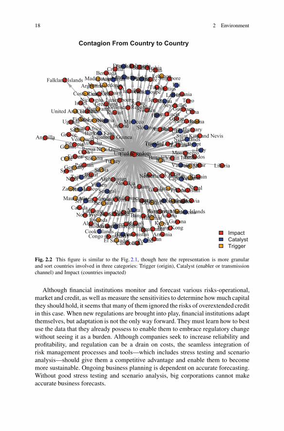
It is not possible to discuss scenario analysis without addressing contagion effects.Indeed, it is not always possible or appropriate to deal with a particular risk andanalysing it in silo. It is important to capture the impact of a risk over another, i.e.,a spread or a spillover effect.

2.3 Risk Interactions and Contagion 15
In fact this aspect is too often left aside when it should be at the centre of thetopic. Combined effect due to contagion can lead to larger losses than the sum of theimpact of each components taken separately. Consequently, capturing the contagioneffect between the risks may be a first way of tackling systemic risks.
Originally, financial contagion referred to the spread of market disturbances fromone country to the other. Financial contagion is a natural risk for countries whosefinancial systems are integrated in international financial markets as obviously whatoccurs in a country would mechanically impact the other in a way or another. Theimpact is usually proportional to the incident, in other words, the larger the issue,the larger the impact on the other countries belonging to the same system unlesssome mitigants are in place to at least confine the smaller exposures. The contagionphenomenon is usually one of the main components explaining that a crisis is notcontained and may pass across borders and affect an entire region of the globe.
Financial contagion may occur at any level of a particular economy and may betriggered by various things. Note that lately, banks have been at the conjunction of adramatic contagion process (subprime crisis), but inappropriate political decisionmay lead to even larger issues. At the domestic level, usually the failure of adomestic bank or financial intermediary triggers a transmission when it defaults oninterbank liabilities and sells assets in a fire sale, thereby undermining confidencein similar banks. International financial contagion, which happens in both advancedand developing economies, is the transmission of a financial crisis across financialmarkets to directly and indirectly connected economies. However, in today’sfinancial system, due to both cross-regional and cross-border operations of banks,financial contagion usually happens simultaneously at the domestic level and acrossborders.
Financial contagion usually generates financial volatility and may damage theeconomy of countries. There are several branches of classifications that explainthe mechanism of financial contagion, which are spillover effects and financialcrisis that are caused by the influence of the four agents’ behaviour. These aregovernments, financial institutions, investors and borrowers (Dornbusch et al., 2000)
The first branch, spillover effects, can be seen as a negative externality. Spillovereffects are also known as fundamental-based contagion. These effects can occurglobally, i.e., affecting several countries simultaneously, or regionally, only impact-ing adjacent countries. The larger the countries, the more global the effect is thegeneral rule. Conversely, the smaller countries are those triggering regional effects.Though some debates arose regarding the difference between co-movements andcontagion, here we will state that if what happen in a particular location directly orindirectly impact the situation in another geographical region, with a time lag1 then,we should refer to it as contagion.
At the micro level, from a risk management perspective, contagion should beconsidered when the materialisation of a first risk (say operational risk) triggers thematerialisation of subsequent risk (for instance, market or credit). This is typically
1This one might be extremely short.

16 2 Environment
what happened in Société Générale rogue trading issue as briefly discussed in theprevious chapter.
From a macroeconomic point of view, contagion effects have repercussions onan international scale transmitted through channels such as trade links, competitivedevaluations and financial links. “A financial crisis in one country can lead to directfinancial effects, including reductions in trade credits, foreign direct investment, andother capital flows abroad”. Financial links come from globalisation since countriestry to be more economically integrated with global financial markets. Many authorshave analysed financial contagions. Allen and Gale (2000) and Lagunoff andSchreft (2001) analyse financial contagion as a result of linkages among financialintermediaries.
Trade links are another type of shock that has its similarities to common shocksand financial links. These types of shocks are more focused on its integrationcausing local impacts. Kaminsky and Reinhart (2000) document the evidence thattrade links in goods and services and exposure to a common creditor can explainearlier crises clusters, not only the debt crisis of the early 1980s and 1990s, but alsothe observed historical pattern of contagion.
Irrational phenomenon might also cause financial contagion. Co-movementsare considered irrational when there is no global shock triggering and interde-pendence channeling. The cause is related to one of the four agents’ behaviourspresented earlier. Contagion causes are increased risk aversion, lack of confidenceand financial fears. Transmission channel can be through typical correlations orliquidation processes (i.e. sell in one country to fund a position in another) (Kingand Wadhwani, 1990; Calvo, 2004).
Remark 2.3.1 Investor’s behaviour seems to be one of the biggest issues that canimpact a country’s financial system.
So to summarise, a contagion may be caused by:
1. Irrational co-movements related to crowed psychology (Shiller, 1984; Kirman,1993)
2. Rational but excessive co-movements3. Liquidity problems4. Information asymmetry and coordination problems5. Shift of equilibrium6. Change in the international financial system, or in the rules of the game7. Geographic factors or neighbourhood effect (De Gregorio and Valdes, 2001)8. The developments of sophisticated financial products, such as credit default
swaps and collateralised debt obligations which spread the exposure across theworld (sub-prime crisis).
Capturing interactions and contagion effects leads to analysing financial crises.The term financial crisis refers to a variety of situations resulting in a loss ofpaper wealth, which may ultimately affect the real economy. An interesting wayof representing financial contagion can be done extending models used to representepidemics as illustrated by Figs. 2.1 and 2.2.

2.4 The Regulatory Framework 17
Financial Crisis: Contagion From A Country To Another
ll
ll ll
ll
llllll
ll
ll
ll
llllllll
llllll
ll
ll
ll
ll
ll
ll
ll
ll
ll
llll
ll
ll
ll
ll
ll
llll
ll
ll
llll
ll
llll
ll
ll
ll
ll
ll
ll
ll
llllll
ll
ll
llllll
ll
ll
ll
llll
llll
ll
ll
llll
ll
ll
ll
ll
ll
ll
ll
ll
ll
ll
ll
ll
ll
ll
ll
ll
ll
llll ll
ll
ll
ll
ll
ll
llll
llll
ll
ll
llll
ll
ll
ll
ll
ll
ll
ll
ll
ll
ll
ll
ll
ll
ll
ll
ll
ll
ll
llll
ll
ll
ll
ll
ll
ll
ll
ll
ll
ll
ll
ll
ll
llll
ll
ll
ll
ll
ll
llll
ll
ll
ll
ll
ll
ll
ll
llll
llll
ll
ll
llll
ll
ll
ll
llll
ll
llll ll
llll
ll
ll
ll
llll
ll
ll
ll
ll
ll
ll
ll
ll
ll ll
ll
ll llll
llll
ll
ll
ll llll
ll
ll
llllll
ll
ll
ll
ll
ll ll
llll
ll ll
ll
ll
ll
llllllll
llll
ll
llll
ll
ll
llll
ll
USAUKFranceChinaBrazil
Fig. 2.1 In order to graphically represent a financial contagion, I inspired myself from a modelcreated to represent the way epidemies move from a specific geographic region to another(Oganisian, 2015)
2.4 The Regulatory Framework
In this section, we will briefly discuss the regulatory framework surroundingscenario analysis. Indeed, scenario analysis can be found in multiple regulatoryprocesses, such as stress testing and operational risk management and not only fromthe financial industry. As it has been introduced in the previous sections, we believethat some precision regarding stress testing might be useful to understand the scopeof the pieces of regulations below.
The stress-testing term generally refers to examining how a company’s financesrespond to an extreme scenario. The stress-testing process is important for prudentbusiness management, as it looks at the “what if” scenarios companies needto explore to determine their vulnerabilities. Since the early 1990s, catastrophemodelling, which is a form of scenario analysis for providing insight into themagnitude and probabilities of potential business disasters, has become increasinglysophisticated. Regulators globally are increasingly encouraging the use of stresstesting to evaluate capital adequacy (Quagliariello, 2009).
18 2 Environment
Contagion From Country to Country
ll
ll
ll
ll
ll
ll
ll
ll
ll
ll
ll
ll
ll
ll
ll
llll
ll
ll
ll
ll
ll
llll
ll
ll
ll
ll
ll
ll
llll
llll
ll
ll
ll
ll
ll
ll
ll
ll
ll
ll
ll
ll
ll
ll
ll
ll
ll
ll
ll
ll
ll
ll
ll
ll
ll
ll
ll
ll
ll
ll
ll
ll
ll
ll
ll
ll
ll
ll
ll
ll
ll
llll
ll
ll
ll
ll
ll
ll
ll
ll
ll
ll
ll ll
ll
ll
ll
ll
ll
ll
ll
ll
ll
llll
ll
ll
ll
ll
ll
ll
ll
ll
ll
llll
ll
ll
ll
ll
ll ll
ll
ll
ll
ll
ll
ll
ll
ll
ll
ll
ll
ll
ll
ll
ll
ll
ll
ll
ll
ll
ll
ll
ll
ll
ll
ll
ll ll
ll
ll
ll
ll
ll
ll
ll
ll
ll
ll
ll
ll
ll
ll
ll
ll
ll
ll
llll
ll
ll
ll
Afghanistan
Algeria
Angola
Antigua and Barbuda
Argentina
Armenia
Australia
Austria
Azerbaijan
Bahamas
Bahrain
Bangladesh
Barbados
Belarus
Belgium
Belize
Bermuda
Bolivia
Bosnia and Herzegovina
Botswana
Brazil
British Virgin Islands
BulgariaBurkina Faso
Burma
Cambodia
Cameroon
Canada
Cape Verde
Chile
ChinaColombia
Congo (Kinshasa)
Cook Islands
Costa Rica
Croatia
Cuba
Cyprus
Czech Republic
Denmark
Djibouti
Dominican Republic
Ecuador
Egypt
El Salvador
Equatorial Guinea
Eritrea
Ethiopia
Fiji
Finland
France
French Polynesia
Gabon
Georgia
Germany
Ghana
Greece
Greenland
Guadeloupe
Guam
Guatemala
Guernsey
Guyana
Haiti
Honduras
Hong Kong
Hungary
India
Indonesia
Iran
Iraq
Ireland
Israel
Italy
Jamaica
JapanJersey
Jordan
Kazakhstan
Kenya
Kuwait
Kyrgyzstan
Laos
Latvia
Lebanon
Liberia
Lithuania
Luxembourg Macau
Madagascar
Malawi
Malaysia
Maldives
Malta
Mauritania
Mauritius
Mexico
Montenegro
MoroccoMozambique
NA
Nepal
Netherlands Antilles
Netherlands
New Caledonia
New Zealand
Nicaragua
Niger
Nigeria
Northern Mariana IslandsNorway
Oman
Pakistan
Panama
Papua New Guinea
ParaguayPeru
Philippines
Poland
Portugal
Puerto Rico
Qatar
Romania
Russia
Rwanda
Saint Kitts and Nevis
Saint Lucia
Saudi Arabia
Senegal
Serbia
Seychelles
Singapore
Slovakia
Slovenia
Somalia
South Africa
South Korea
Spain
Sri Lanka
Sudan
Sweden
Switzerland
Taiwan
Tajikistan Tanzania
Thailand
Togo
Trinidad and Tobago
Tunisia
Turkey
Turkmenistan
Tuvalu
Uganda
Ukraine
United Arab Emirates
United Kingdom
Uruguay
Uzbekistan
Vanuatu
Venezuela
Vietnam
Virgin Islands
Western Sahara
YemenZambia
United States
Anguilla
Falkland Islands
ImpactCatalystTrigger
Fig. 2.2 This figure is similar to the Fig. 2.1, though here the representation is more granularand sort countries involved in three categories: Trigger (origin), Catalyst (enabler or transmissionchannel) and Impact (countries impacted)
Although financial institutions monitor and forecast various risks-operational,market and credit, as well as measure the sensitivities to determine how much capitalthey should hold, it seems that many of them ignored the risks of overextended creditin this case. When new regulations are brought into play, financial institutions adaptthemselves, but adaptation is not the only way forward. They must learn how to bestuse the data that they already possess to enable them to embrace regulatory changewithout seeing it as a burden. Although companies seek to increase reliability andprofitability, and regulation can be a drain on costs, the seamless integration ofrisk management processes and tools—which includes stress testing and scenarioanalysis—should give them a competitive advantage and enable them to becomemore sustainable. Ongoing business planning is dependent on accurate forecasting.Without good stress testing and scenario analysis, big corporations cannot makeaccurate business forecasts.

2.4 The Regulatory Framework 19
One approach is to view the business from a portfolio perspective, with capitalmanagement, liquidity management and financial performance integrated into theprocess. Comprehensive stress testing and scenario analysis must take into accountall risk factors, including credit, market, liquidity, operational, funding, interest,foreign exchange and trading risks. To these must be added operational risks due toinadequate systems and controls, insurance risk (including catastrophes), businessrisk factors (including interest rate, securitisation and residual risks), concentrationrisk, high impact low-probability events, cyclicality and capital planning.
In the following paragraphs, we extract quotes from multiple regulatory docu-ments or international associations discussing scenario analysis requests to empha-sise how important the process is considered. We analysed documents from multiplecountries and multiple industries. These documents are also used to give someperspectives and illustrate the relationships between scenario analysis, stress testingand risk management.
In IAA (2013), the International Actuarial Association points out the differencesbetween scenario analysis and stress testing: “A scenario is a possible futureenvironment, either at a point in time or over a period of time. A projection ofthe effects of a scenario over the time period studied can either address a particularfirm or an entire industry or national economy. To determine the relevant aspects ofthis situation to consider, one or more events or changes in circumstances may beforecast, possibly through identification or simulation of several risk factors, oftenover multiple time periods. The effect of these events or changes in circumstancesin a scenario can be generated from a shock to the system resulting from a suddenchange in a single variable or risk factor. Scenarios can also be complex, involvingchanges to and interactions among many factors over time, perhaps generated by aset of cascading events. It can be helpful in scenario analysis to provide a narrative(story) behind the scenario, including the risks (events) that generated the scenario.Because the future is uncertain, there are many possible scenarios. In additionthere may be a range of financial effects on a firm arising from each scenario. Theprojection of the financial effects during a selected scenario will likely differ fromthose seen using the modeler’s best expectation of the way the current state of theworld is most likely to evolve. Nevertheless, an analysis of alternative scenarios canprovide useful information to involved stakeholders. While the study of the effectof likely scenarios is useful for business planning and for the estimation of expectedprofits or losses, it is not useful for assessing the impact of rare and/or catastrophicfuture events, or even moderately adverse scenarios. A scenario with significant orunexpected adverse consequences is referred to as a stress scenario.”
“A stress test is a projection of the financial condition of a firm or economyunder a specific set of severely adverse conditions that may be the result of severalrisk factors over several time periods with severe consequences that can extendover months or years. Alternatively, it might be just one risk factor and be shortin duration. The likelihood of the scenario underlying a stress test has been referredto as extreme but plausible.”

20 2 Environment
Analysing the case of the United Kingdom, a firm must carry out an ICAAP inaccordance with the PRA’s rules. These include requirements on the firm to assess,on an ongoing basis the amounts, types and distribution of capital that it considersadequate to cover the level and nature of the risks to which it is exposed. Thisassessment should cover the major sources of risks to the firm’s ability to meetits liabilities as they fall due, and should incorporate stress testing and scenarioanalysis. If a firm is merely attempting to replicate the PRA’s own methodologies, itwill not be carrying out its own assessment in accordance with the ICAAP rules.The ICAAP should be documented and updated annually by the firm, or morefrequently if changes in the business, strategy, nature or scale of its activities oroperational environment suggest that the current level of financial resources is nolonger adequate.
Specifically PRA (2015) says that firms have “to develop a framework for stresstesting, scenario analysis and capital management that captures the full range ofrisks to which they are exposed and enables these risks to be assessed against arange of plausible yet severe scenarios. The ICAAP document should outline howstress testing supports capital planning for the firm”.
In the European Union (Single Supervisory Mechanism jurisdiction), the RTS(EBA, 2013)—and later the final guideline (EBA, 2014)—is prepared taking intoaccount the FSB Key Attributes of Effective Resolution Regimes for Financial Insti-tutions and current supervisory practices. The draft RTS covers the key elements andessential issues that should be addressed by institutions when developing financialdistress scenarios against which the recovery plan will be tested.
Quoting: “Drafting a recovery plan is a duty of institutions or groups undertakenprior to a crisis in order to assess the potential options that an institution or agroup could itself implement to restore financial strength and viability shouldthe institution or group come under severe stress. A key assumption is thatrecovery plans shall not assume that extraordinary public financial support wouldbe provided.
The plan is drafted and owned by the financial institution, and assessed by therelevant competent authority or authorities. The objective of the recovery plan isnot to forecast the factors that could prompt a crisis. Rather it is to identify theoptions that might be available to counter; and to assess whether they are sufficientlyrobust and if their nature is sufficiently varied to cope with a wide range of shocksof different natures. The objective of preparing financial distress scenarios is todefine a set of hypothetical and forward-looking events against which the impactand feasibility of the recovery plan will be tested. Institutions or groups should usean appropriate number of system wide financial distress scenarios and idiosyncraticfinancial distress scenarios to test their recovery planning. More than one of eachscenario is useful, as well as scenarios that combine both systemic and idiosyncraticevents. Financial distress scenarios used for recovery planning shall be designedsuch that they would threaten failure of the institution or group, in the case recoverymeasures are not implemented in a timely manner by the institution or group”.

2.4 The Regulatory Framework 21
Article 4. Range of scenarios of financial distress
1. The range of scenarios of financial distress shall include at least one scenario for each of thefollowing types of events:
(a) a system wide event;(b) an idiosyncratic event;(c) a combination of system wide and idiosyncratic events which occur simultaneously and
interactively.
2. In designing scenarios based on system wide events, institutions and groups shall take intoconsideration the relevance of at least the following system wide events:
(a) the failure of significant counterparties affecting financial stability;(b) a decrease in liquidity available in the interbank lending market;(c) increased country risk and generalised capital outflow from a significant country of
operation of the institution or the group;(d) adverse movements in the prices of assets in one or several markets;(e) a macroeconomic downturn.
3. In designing scenarios based on idiosyncratic events, institutions and groups shall take intoconsideration the relevance of at least the following idiosyncratic events:
(a) the failure of significant counterparties;(b) damage to the institution’s or group’s reputation;(c) a severe outflow of liquidity;(d) adverse movements in the prices of assets to which the institution or group is predomi-
nantly exposed;(e) severe credit losses;(f) a severe operational risk loss.
“These Guidelines aim at specifying the range of scenarios of severe macroe-conomic and financial distress against which institutions shall test the impact andfeasibility of their recovery plans. The recovery plans detail the arrangements whichinstitutions have in place and the early action steps that would be taken to restoretheir long-term viability in the event of a material deterioration of financial situationunder severe stress conditions. When the consultation was launched, there was anexisting mandate in the Bank Recovery and Resolution Directive (BRRD) for theEBA to develop technical standards for the range of scenarios to be used by firms totest their recovery plans. During legislative process the mandate has been amendedand the EBA was asked to develop Guidelines instead”.
In Australia, the Australian Prudential Regulation Authority(APRA) wererequesting the following from banks with respect to the implementation ofoperational risk models (APRA, 2007). “Banks intending to apply the AdvancedMeasurement Approach (AMA) to Operational Risk are required to use scenarioanalysis as one of the key data inputs into their capital model. Scenario analysisis a forward-looking approach, and it can be used to complement the banks’ shortrecorded history of operational risk losses, especially for low frequency highimpact events (LFHI). A common approach taken by banks is to ask staff withrelevant business expertise to estimate the frequency and impact for the plausible

22 2 Environment
scenarios that have been identified. A range of techniques is available for elicitingthese assessments from business managers and subject matter experts, each withits own strengths and weaknesses. More than 30 years of academic literature isavailable in the area of eliciting probability assessments from experts. Much ofthis literature is informed by psychologists, economists and decision analysts, whohave done research into the difficulties people face when trying to make probabilityassessments. The literature provides insight into the sources of uncertainty and biassurrounding scenario assessments, and the methods available for their mitigation.”The purpose of APRA (2007) was “to increase awareness of the techniques that areavailable to ensure scenario analysis is conducted in a structured and robust manner.Banks should be aware of the variety of methods available, and should considerapplying a range of techniques as appropriate”.
Besides, the COAG (Council of Australian Governments) Energy Council inCOAG (2015) requires some specific scenario analysis: “The Council tasked offi-cials with a scenario analysis exercise and to come back to it with recommendations,if necessary, about the need for further work. At its July 2015 meeting, theCouncil considered these recommendations and tasked officials to further explorethe implications of key issues that emerged from the initial stress-testing exercise.This piece of work is being considered as part of the Council’s strategic workprogram to ensure regulatory frameworks are ready to cope with the effects ofemerging technologies”. This is an example of scenario analysis requirement forrisk management in an industry different from the financial sector.
In the USA, in the nuclear industry, the US Nuclear Regulatory Commission(NRC) requested scenario analysis in USNRC (2004) and USNRC (2012). “TheU.S. Nuclear Regulatory Commission (NRC) will use these Regulatory AnalysisGuidelines (“Guidelines”) to evaluate proposed actions that may be needed to pro-tect public health and safety. These evaluations will aid the staff and the Commissionin determining whether the proposed actions are needed, in providing adequatejustification for the proposed action, and in documenting a clear explanation of whya particular action was recommended. The Guidelines establish a framework for(1) identifying the problem and associated objectives, (2) identifying alternativesfor meeting the objectives, (3) analysing the consequences of alternatives, (4)selecting a preferred alternative, and (5) documenting the analysis in an organisedand understandable format. The resulting document is referred to as a regulatoryanalysis”.
Specifically for the financial industry, “the Comprehensive Capital Analysis andReview (CCAR) (Fed, 2016b) is an annual exercise by the Federal Reserve to assesswhether the largest bank holding companies operating in the United States havesufficient capital to continue operations throughout times of economic and financialstress and that they have robust, forward-looking capital-planning processes thataccount for their unique risks”.
As part of this exercise, the Federal Reserve evaluates institutions’ capitaladequacy, internal capital adequacy assessment processes and their individual plansto make capital distributions, such as dividend payments or stock repurchases.Dodd-Frank Act (Fed, 2016a) stress testing (DFAST)—a complementary exercise
References 23
to CCAR—is a forward-looking component conducted by the Federal Reserveand financial companies supervised by the Federal Reserve to help assess whetherinstitutions have sufficient capital to absorb losses and support operations duringadverse economic conditions.
While DFAST is complementary to CCAR, both efforts are distinct testing exer-cises that rely on similar processes, data, supervisory exercises and requirements.The Federal Reserve coordinates these processes to reduce duplicative requirementsand to minimise regulatory burden.
International organisations such as the Food and Agriculture Organisation ofthe United Nations use scenarios. In FAO (2012), they state that “a scenario is acoherent, internally consistent and plausible description of a possible future stateof the world. Scenarios are not predictions or forecasts (which indicate outcomesconsidered most likely), but are alternative images without ascribed likelihoods ofhow the future might unfold. They may be qualitative, quantitative or both. Anoverarching logic often relates several components of a scenario, for example, astoryline and/or projections of particular elements of a system. Exploratory (ordescriptive) scenarios describe the future according to known processes of change,or as extrapolations of past trends. Normative (or prescriptive) scenarios describe aprespecified future, optimistic, pessimistic or neutral and a set of actions that mightbe required to achieve (or avoid) it. Such scenarios are often developed using aninverse modelling approach, by defining constraints and then diagnosing plausiblecombinations of the underlying conditions that satisfy those constraints”.
This last section provided a snapshot of the regulatory environment surroundingscenario analysis. In our discussion, we do not really distinguish scenario analysisfrom stress testing as this one requires and rely similar methodologies to beeffective.
References
Allen, F., & Gale, D. (2000). Financial contagion. Journal of Political Economy, 108(1), 1–33.APRA. (2007). Applying a structured approach to operational risk scenario analysis in Australia.
Sydney: Australian Prudential Regulation Authority.BCBS. (2004). International convergence of capital measurement and capital standards. Basel:
Bank for International Settlements.Calvo, G. A. (2004). Contagion in emerging markets: When wall street is a carrier. In E. Bour, D.
Heymann, & F. Navajas (Eds.), Latin American economic crises: Trade and labour (pp. 81–91).London, UK: Palgrave Macmillan.
COAG. (2015). Electricity network economic regulation; scenario analysis. In Council of Aus-tralian Governments, Energy Council, Energy Working Group, Network Strategy WorkingGroup.
COSO. (2004). Enterprise risk management - integrated framework executive summary. InCommittee of Sponsoring Organizations of the Treadway Commission.
De Gregorio, J., & Valdes, R.O. (2001). Crisis transmission: Evidence from the debt, tequila, andAsian flu crises. World Bank Economic Review, 15(2), 289–314.

24 2 Environment
Dornbusch, R., Park, Y., & Claessens, S. (2000). Contagion: Understanding how it spreads. TheWorld Bank Research Observer, 15(2), 177–197.
EBA. (2013). Draft regulatory technical standards specifying the range of scenarios to be usedin recovery plans under the draft directive establishing a framework for the recovery andresolution of credit institutions and investment firms. London: European Banking Authority.
EBA. (2014). Guidelines on the range of scenarios to be used in recovery plans. London: EuropeanBanking Authority.
FAO. (2012). South Asian forests and forestry to 2020. In Food and Agriculture Organisation ofthe United Nations.
Fed. (2016a). 2016 supervisory scenarios for annual stress tests required under the Dodd-Frankact stress testing rules and the capital plan rule. Washington, DC: Federal Reserve Board.
Fed. (2016b). Comprehensive capital analysis and review 2016 summary instructions. Washington,DC: Federal Reserve Board.
Guégan, D., & Hassani, B. (2015). Stress testing engineering: The real risk measurement? In A.Bensoussan, D. Guégan, & C. Tapiero (Eds.), Future perspectives in risk models and finance.New York: Springer.
Hassani, B. (2015). Model risk - from epistemology to management. Working paper, UniversitéParis 1.
IAA. (2013). Stress testing and scenario analysis. In International Actuarial Association.Kaminsky, G. L., & Reinhart, C. M. (2000). On crises, contagion, and confusion. Journal of
International Economics, 51(1), 145–168.King, M. A., & Wadhwani, S. (1990). Transmission of volatility between stock markets. Review of
Financial Studies, 3(1), 5–33.Kirman, A. (1993). Ants, rationality, and recruitment. Quarterly Journal of Economics, 108(1),
137–156.Lagunoff, R. D., & Schreft, S. L. (2001). A model of financial fragility. Journal of Economic
Theory, 99(1), 220–264.Markowitz, H. M. (1952). Portfolio selection. The Journal of Finance, 7(1), 77–91.McCormick, R. (2011). Legal risk in the financial markets (2nd ed.). Oxford: Oxford University
Press.Oganisian, A. (2015). Modeling ebola contagion using airline networks in R. www.r-bloggers.com.Piatetsky-Shapiro, G. (2011). Modeling systemic and sovereign risk. In A. Berd (Ed.), Lessons
from the financial crisis (pp. 143–185). London: RISK Books.PRA. (2015). The internal capital adequacy assessment process (ICAAP) and the supervisory
review and evaluation process (SREP). In Prudential Regulation Authority, Bank of England.Quagliariello, M. 2009. Stress-testing the banking system - methodologies and applications.
Cambridge: Cambridge University Press.Schwarcz, S. L. (2008). Systemic risk. Georgetown Law Journal, 97(1), 193–249.Shiller, R. J. (1984). Stock prices and social dynamics. Brookings Papers on Economic Activity,
1984(2), 457–498.USNRC. (2004). Regulatory analysis guidelines of the U.S. nuclear regulatory commission. In
NUREG/BR-0058, U.S. Nuclear Regulatory Commission.USNRC. (2012). Modeling potential reactor accident consequences - state-of-the-art reactor con-
sequence analyses: Using decades of research and experience to model accident progression,mitigation, emergency response, and health effects. In U.S. Nuclear Regulatory Commission.

Chapter 3The Information Set: Feeding the Scenarios
A point needs to be made absolutely clear before any further presentation. None ofthe methodologies presented in the following chapters can be used if these are notfed by appropriate inputs. Therefore, we will start this chapter characterising anddefining data, then we will discuss pre-processing these inputs to make them readyfor further processing.
Data are a set of qualitative or quantitative pieces of information. Data areengendered or obtained by both observation and measurement. They are collected,reported, analysed and visualised. Data as a general concept refers to the factthat some existing information or knowledge is represented in some form suitablefor better or different processing. Raw data, or unprocessed data, are a collectionof numbers and characters; data processing commonly occurs by stages, and theprocessed data from one stage may become the raw data of the next one. Field dataare raw data that is collected in an uncontrolled environment. Experimental dataare data generated within the context of a scientific investigation by observationand recording, in other words these are data generated carrying out an analysisor implementing a model. It is important to understand, in particular for scenarioanalysis, that the data used to support the process are not most of the time numericvalues. Indeed, these are usually pieces of information gathered to support a storyline, such as articles, media, incidents experienced by other financial institutions orexpert perceptions.
Indeed, specifying the definition, data are any facts, numbers or text that can beprocessed. Nowadays, organisations are capturing and gathering growing quantitiesof data in various formats. We can split the data in three categories:
• operational or transactional data such as, sales, cost, inventory, payroll andaccounting
• non-operational data, such as industry sales, forecast data and macroeconomicdata
• meta data—data about the data itself, such as logical database design or datadictionary definitions
© Springer International Publishing Switzerland 2016B.K. Hassani, Scenario Analysis in Risk Management,DOI 10.1007/978-3-319-25056-4_3
25
26 3 The Information Set: Feeding the Scenarios
Recent regulatory documents, for instance, the Risk Data Aggregation (BCBS,2013b) aims at ensuring the quality of the data used for regulatory purposes.However, one may argue that any piece of data could be used for regulatorypurposes, consequently, this piece of regulation should lead in the long term toa wider capture of data for risk measurement and consequently to better riskmanagement.
Indeed, BCBS (2013b) requires that the information banks used in decision-making process capture all risks accurately as well as timely. This piece ofregulation sets out principles of effective and efficient risk management by pushingbanks to adopt the right systems and develop the right skills and capabilities insteadof ticking regulatory boxes to be compliant at a certain date.
It is important to understand that this piece of regulation cannot be dealt with insilo. It has to be regarded as part of the larger library of regulations. This paragraphprovides some illustrations, indeed, BCBS 239 compliance is required to ensurea successful Comprehensive Capital Analysis and Review (CCAR—Fed 2016) inthe USA, a Firm Data Submission Framework (FDSF—BoE 2013) in the UK, theEuropean Banking Authority stress tests (EBA, 2016) or the Fundamental Reviewof the Trading Book (FRTB—BCBS 2013a). The previous chapter introduced inmore details some of these regulatory processes. The resources required for theseexercises are quite significant and should not be underestimated. If banks are notable to demonstrate compliant solutions for data management, data governanceacross the multiple units such as risk, finance and the businesses, these will have tochange their risk measurement strategies and as a corollary their risk framework. Inthe short term, these rules may imply larger capital charges for financial institutions,but in the long term the better risk management processes implied by this regulationshould help reducing capital charges for bank using internal model, or at least thebanks exposures.
With the level of change implied, BCBS 239 might be considered as the coreof regulatory transformation. However, banks task to make evolve their operatingmodel remains significant and adapting their technology infrastructures will not bestraightforward. However, both banks and regulators acknowledge the challenges.The principles are an enabler to transform the business strategically speaking, tosurvive in the new market environment. Furthermore, combining BCBS 239 specificrequirements and business as usual tasks across, business units and geographicallocations will not be easy and will require appropriate change management.
In the meantime, a nebula emerged, usually referred to as big data. Big datais a broad term for data sets so large or complex that traditional data processingapplications are inadequate. Challenges include analysis, capture, cleansing, search,sharing, storage, transfer, visualisation and information privacy. The term oftenrefers simply to the use of predictive analytics or other certain advanced methodsto extract valuable information from data, and rarely to a particular size of dataset. Accuracy in big data may lead to more confidence in the decision-makingprocess and consequently improvement in operational efficiency, reduction of costsand better risk management.

3.1 Characterising Numeric Data 27
Data analysis is the key to the future of banking, our environment will move fromtraditional to rational though a path which might be emotional. Data analysis allowslooking at a particular situation from different angles. Besides the possibilities areunlimited as long as the underlying data are of good quality. Indeed, data analysismay lead to the detection of correlations, trends, etc., and can be used in multipleareas and industries. Dealing with large data sets is not necessarily easy. Most of thetime it is quite complicated as many issues arise related to data completeness, sizeor reliability of the IT infrastructure.
In otherwords, “big data” combines capabilities, users objectives, tools deployed,methodologies implemented. The field evolves quickly as what is considered bigdata one year becomes “business as usual” the next (Walker 2015). Depending onthe organisation, the infrastructure to put in place will not be the same as the needsare not identical from an entity to another, e.g., parallel computing is not alwaysnecessary. There is no “one-size fits all” infrastructure.
3.1 Characterising Numeric Data
Before introducing any methodological aspects, it is necessary to discuss how torepresent and characterise the data. Here we will focus on numerical data, it isimportant to bear in mind that, as mentioned previously, the information used forscenario analysis should not be limited to these kinds of data.
Understanding numerical data boils down to statistical analysis. This task can bebroken down into the following:
1. Describe the nature of the data, in other words what data are we working on? Thisfirst point is quite important as practitioners usually have a priori understandingsof the data, they have some expertise relying on their experience and thereforecan help and orientate the characterisation of the data.
2. Explore the relationship of the data with the underlying population, i.e., up towhat extent is the sample representative of a population?
3. Create, fit or adjust a model on the sample so this one would be representative ofthe underlying population, i.e., fit the data and extract or extrapolate the requiredinformation.
4. Assess the validity of the model, for example, using goodness-of-fit tests.
In this section, we will introduce some concepts that will be helpful understandingthe data and will support the selection of the appropriate scenario analysis strategy.Indeed, most numerical data sets can be represented by an empirical distribution.These distributions can be described in various way using moments, quantiles orhow the data interacts with each others. Therefore, we will briefly introduce thesenotions in the following sections (the latter will actually be discussed in subsequentchapters).

28 3 The Information Set: Feeding the Scenarios
3.1.1 Moments
In mathematics, a moment is a specific quantitative measure of the shape of a set ofpoints. If these points are representative of a density of probability, then first momentis the mean, the second moment is the variance, the third moment is the skewnessmeasuring the asymmetry of the distribution and the fourth the kurtosis providingsome information regarding the thickness of the tails through the flattening of thedistribution.
For a bounded distribution of mass or probability, the collection of all themoments uniquely determines the distribution. The nth moment of a continuousfunction f .x/ defined on R given c 2 R is
�n DZ 1
�1.x � c/n f .x/ dx: (3.1.1)
The moment1 of a function usually refers to the above expression considering c D 0.The nth moment about zero or raw moment of a probability density function
f .x/ is the expected value of Xn. For the second and higher moments, the centralmoments are usually used rather than the moments about zero, because they provideclearer information about the distribution’s shape. The moments about its mean �are called central moments; these describe the shape of the function, independentlyof translation.
It is actually possible to define other moments such as the nth inverse momentabout zero E ŒX�n� or the nth logarithmic moment about zero E Œlnn.X/�.
If f is a probability density function, then the value of the previous integral iscalled the nth moment of the probability distribution. More generally, if F is acumulative probability distribution function of any probability distribution, whichmay not have a density function, then the nth moment of the probability distributionis given by the Riemann–Stieltjes integral
�0n D E ŒXn� D
Z 1
�1xn dF.x/ (3.1.2)
where X is a random variable, F.X/ its cumulative distribution and E denotes theexpectation.
When
E ŒjXnj� DZ 1
�1jxnj dF.x/ D1; (3.1.3)
then the moment does not exist (we will see example of such problems in Chap. 5with the Generalised Pareto and the ˛-stable distributions and with the Generalised
1Moments can be defined in a more general way than only considering real.

3.1 Characterising Numeric Data 29
Extreme Value distribution in Chap. 6). If the nth moment exists so does the .n�1/thmoment as well as all lower-order moments.
Note that the zeroth moment of any probability density function is 1, since
Z 1
�1f .x/dx: D 1 (3.1.4)
3.1.2 Quantiles
Quantiles divide a set of observations into groups of equal sizes. There is onequantile less than the number of groups created, for example, quartiles have onlythree points that allow dividing a dataset into four groups of equal size of 25 %. Ifthere are ten different buckets each of them representing 10 %, we will talk aboutdecile.
More generally quantiles are values that split a finite set of values into q subsetsof equal sizes. There are q � 1 of the q-quantiles, one for each integer k satisfying0 < k < q. In some cases the value of a quantile may not be uniquely determined,for example, for the median of a uniform probability distribution on a set of evensize. Quantiles can also be applied to continuous distributions, providing a way togeneralise rank statistics to continuous variables. When the cumulative distributionfunction of a random variable is known, the q-quantiles are the application of thequantile function (the inverse function of the cumulative distribution function) to
the valuesn1q ;
2q ; : : : ;
.q�1/q
o.
Understanding the quantiles of a distribution is particularly important as it isa manner to represent the way the data are positioned. Indeed, the larger thequantiles at a particular point, the larger the risk. Indeed, quantiles are the theoreticalfoundation of the Value-at-Risk and the Expected Shortfall which will be developedin the next chapter. Quantiles are in fact risk measures, therefore are very usefulfor evaluating exposures to a specific risk as soon as we have enough informationto ensure the robustness of these quantiles, i.e., if we have not many data, then theoccurrence of an event will materially impact the quantiles. Note that this situationmight be acceptable for tail events, but this is generally not the case for risks morerepresentative of the body of the distribution.
3.1.3 Dependencies
In statistics, a dependence depicts any statistical relationship between sets of data.Correlation refers to any statistical relationships involving dependence. Correlationsare useful because they can indicate a predictive relationship that can be exploited.

30 3 The Information Set: Feeding the Scenarios
There are several correlation coefficients, often denoted � or � , measuringthe degree of correlation. The most common of these is the Pearson correlationcoefficient, which is only sensitive to a linear relationship between two variables.Alternative correlation coefficients have been developed to deal with the problemscaused by the Pearson correlation. These correlations will be presented in details inChap. 11.
Dependencies embrace many concepts such as correlations, autocorrelations,copula, contagion and causal chain. Understanding them will help understandinghow an incident materialises as an early warning, what indicator could be used priorthe materialisation and what could lead to this one, supporting the implementationof controls. As a corollary, understanding the causal effect will help supporting theselection of the strategy to implement for scenario analysis purposes.
3.2 Data Sciences
The previous paragraphs built the path to introduce data sciences. Most methodolo-gies presented in the next chapters either rely or are introduced somehow in thissection. Data science is a generic term gathering data mining, machine learning,artificial intelligence, statistics, etc., under a single banner.
3.2.1 Data Mining
Data mining (Hastie et al., 2009) is a field belonging to computer science. Thepurpose of data mining is to extract information from data sets and transform theminto an understandable structure with respect to the ultimate use of these data.The embedded computational process of discovering patterns in large data setscombines methods from artificial intelligence (Russell and Norvig, 2009), machinelearning (Mohri et al., 2012), statistics, and database systems and management. Theautomatic or semi-automatic analysis of large quantities of data permits to detectinteresting patterns such as clusters (Everitt et al., 2011), anomalies, dependenciesand the outcome of the analysis can then be perceived as the essence or thequintessence of the original input data, and may be used for further analysis inmachine learning, predictive analytics or more traditional modelling.
Usually, the term data mining refers to the process of analysing raw data andsummarising them into information used for further modelling. In data mining thedata are analysed from many different dimensions. More precisely, data miningaims at finding correlations or dependence patterns between multiple fields inlarge relational databases. The patterns, associations or relationships among all thisdata can provide information usable to prepare and support the scenario analysisprogram of a financial institution. While the methodologies, the statistics and themathematics behind are not new, until very recently and innovations in computer

3.2 Data Sciences 31
processing, disk storage and statistical software data mining were not reaching thegoal set.
Advances in data capture, processing power, data transmission and storagecapabilities are enabling organisations to integrate their various databases intodata warehouses or data lakes. Data warehousing is a process of centralised datamanagement and retrieval. Data warehousing, like data mining, is a relatively newterm although the concept itself has been around for years. Data warehousingrepresents an ideal vision of maintaining a central repository of all organisationaldata. Centralisation of data is needed to maximise user access and analysis. Datalakes in some sense generalise the concept and allow structured and unstructureddata as well as any piece of information (PDF documents, emails, etc.) that are notnecessarily instantly usable for pre-processing.
Until now, data mining was mainly used by companies with a strong consumerfocus, in other words, retail, financial, communication and marketing organisations(Palace, 1996). These types of companies were using data mining to analyserelationships between endogenous and exogenous factors such as, price, productpositioning, economic indicators, competition or customer demographics, as wellas their impacts on sales, reputation, corporate profits, etc. Besides, it permittedsummarising the information analysed. It is interesting to note that nowadays retailerand suppliers have joined forces to analyse even more relationships at a deeper level.The National Basketball Association developed a data mining application to supporta more efficient coaching. Billy Bean from the Oackland Athletics used data miningand statistics to select the players forming his team.
Data mining enables analysing relationships and patterns in stored data based onopen-ended user queries. Generally, any of four types of relationships are sought:
• Classes: This is the simplest kind of relationship, as stored data is used to analysesubgroups.
• Clusters: Data items are gathered according to logical relationships related totheir intrinsic characteristics. More generally, a cluster analysis aims at groupinga set of similar objects (in some sense) in one particular group (Everitt et al.,2011).
• Associations: Data can be analysed to identify associations. Association rulelearning is intended to identify strong rules discovered in databases measuringhow interesting they are for our final purpose (Piatetsky-Shapiro, 1991).
• Sequential patterns: Data are analysed to forecast and anticipate behaviours,trends or schemes, such as the likelihood of a purchase given what someone hasalready the product in his Amazon basket.
Data mining consists in several major steps. We would recommend following thesesteps to make sure that the data used to support the scenario analysis (if some dataare used) are appropriate and representative of the risk to be assessed.
• Data capture: In a first step data are collected from various sources and gatheredin a data base.

32 3 The Information Set: Feeding the Scenarios
• Data pre-processing, i.e., before proper mining:
– Data selection: Given the ultimate objective, only a subset of the data availablemight be necessary for further analysis.
– Data cleansing and anomalies detection: Collected data may contain errors,may be incomplete, inconsistent, outdated, erroneous, etc. These issues needto be identified, investigated and dealt with prior to any further analysis.
– Data transformation: Following the previous stage, the data are not ready formining, these require transformation such as kernel smoothing, aggregation,normalisation and interpolation.
• Data processing is only possible once the data have been cleansed and are fit forpurpose. This step combines,
– Outlier detection, i.e., an observation point that is distant (in some sense)from other observations. Note that we make the distinction between an outlierand an extreme value, as an outlier is related to a sample while an extremevalue is related to the whole set of value possible a realisation could take.Though large, an extreme value is normal while an outlier might be abnormal.An extreme value is usually an outlier in a sample when an outlier is notnecessarily an extreme value.
– Relationship analysis, as indicated before, gathering the data with similarcharacteristics, classification or analysing interactions.
– Pattern recognition, such as regression analysis, time series analysis anddistributions.
– Summarisation and knowledge presentation: This step deals with visualisa-tion, as one should beware that key aspects are not lost during the process andthe results exhibited are representative.
• Decisions making process integration: This step enables using the knowledgeobtained from the previous manipulations, the analysis. This is the ultimateobjective of data mining.
Remark 3.2.1 The infrastructure required to be able to mine the data is drivenby two main technological aspect, and these should not be underestimated as thereliability of the analysis directly depends on the quality of the infrastructure, asboth the size of the database and the query complexity require more or less powerfulsystem. The larger the quantity of data to be processed and the more complex thequeries, the more powerful the system required.
3.2.2 Machine Learning and Artificial Intelligence
Once these data have been analysed and formatted, these can be further used forprediction, forecasting and evaluation, in other words, for modelling.

3.2 Data Sciences 33
Machine learning deals with the study of pattern recognition and computa-tional learning theory in artificial intelligence. Machine learning aims at buildingalgorithms that can learn from data and make predictions from them, i.e., whichoperate dynamically adapting themselves to changes in the data, not only relying onstatistics but also on mathematical optimisation. Automation is the keyword of thisparagraph, the objective is to make machines think by possibly mimicking the wayhuman brains function (see Chap. 10).
Machine learning tasks are usually classified into four categories (Russell andNorvig, 2009) depending on the inputs and the objectives:
• In supervised learning (Mohri et al., 2012), the goal is to infer a general rule fromexample data mapped to the desired output. The example data are usually calledtraining data. These consist in couples input and desired output or supervisorysignal. Once the algorithm analysed the training data and inferred the function, itcan be used to map new examples and generalise its use to previously unknownsituations. Optimally, algorithms should perfectly react to new instances inproviding an unbiased and accurate outcome, e.g., a methodology outcomeswhich reveal to be accurate once they can be compared with the future realoccurrences.
• The second possibility is unsupervised learning in which no training data aregiven to the learning algorithm, consequently it will have to extract patterns fromthe input. Unsupervised learning can actually be used to find hidden structuresand patterns embedded within the data. Therefore, unsupervised learning aimsat inferring a function describing hidden patterns from unlabelled data (Hastieet al., 2009). In the case of unsupervised learning, it is complicated to evaluatethe quality of the solution as initially no benchmark is available.
• When the initial training information (i.e. data and/or targets) is incomplete, aintermediate strategy called semi-supervised learning main be used.
• In reinforcement learning (Sutton and Barto, 1998), a program interacts andevolves within a dynamic environment in which it is supposed to achieve aspecific task. However, as for unsupervised learning, there is no training dataand no benchmark. This approach aims at learning what to do, i.e., how to mapsituations to actions, so as to optimise a numerical function, i.e., the output. Thealgorithm has to discover which actions lead to the best output signal by tryingthem. These strategies allow capturing situations in which actions may affect allsubsequent steps with or without any delay, which might be of interest.
Another way of classifying machine learning strategies is by desired output(Bishop, 2006). Indeed, we will illustrate that classification briefly introducing somestrategies and methodologies used in the next chapters. Our objective is to show howinterconnected all the methodologies are as one may leverage on some of them toachieve other purposes. Indeed all the methodologies belonging to data sciences canbe used as a base for scenario analysis.
The first methodology (we actually presented in the previous section) is theclassification in which inputs are divided in at least two different classes, and thelearning algorithm has to assign unseen inputs to at least one of these classes. This

34 3 The Information Set: Feeding the Scenarios
is a good example of supervised learning but it could be adapted and fall in thesemi-supervised alternative. The second methodology is the regression which alsobelongs to the supervised learning, which focuses on the relationship between adependent variable and at least one independent variable (Chap. 11). In clustering,inputs have to be divided into groups of similar data. Contrary to classification, thegroups are unknown a priori therefore this methodology belongs to the unsupervisedstrategies. Density estimation (Chap. 5) provides the distribution of input data andbelongs by essence to the family of unsupervised learnings, though if we usea methodology such as Bayesian inference it would be more a semi-supervisedstrategy.
As mentioned before machine learning is closely related to optimisation. Mostlearning problems are formulated as optimising (i.e. minimising or maximising) anobjective function. Objective functions express the difference between the output ofthe trained model and the actual values. Contrary to data mining, machine learningdoes not only aim at detecting patterns or for a good adjustment of a model to somedata but to a good adjustment of this model to previously unknown situations, whichis a far more complicated task. Machine learning models goal is accurate predictiongeneralising patterns originally detected and refined by experience.
3.2.3 Common Methodologies
Machine learning and data mining often rely on identical methodologies and/oroverlap quite significantly though having different objectives. As mentioned in theprevious paragraphs, machine learning aims at prediction using properties learnedfrom training data while data mining focuses on the discovery of unknown patternsembedded in the data. In this section, we briefly introduce methodologies used indata mining and machine learning as some of them will be implemented in the nextchapters as scenario analysis requires first analysing data to identify the importantpatterns embedded and second to make prediction from them. The following listis far from being exhaustive; however, it provides a good sample of traditionalmethodologies:
• Decision tree learning (deVille, 2006) is a predictive model. The purpose isto predict the values of a target variable based on several inputs, which aregraphically represented by nodes. Each edge of a node leads to children,respectively, representing each of the possible values the variable can takegiven the input provided. A decision tree may be implemented for classificationpurposes or for regression purposes, respectively, to identify to which class theinput belongs or to evaluate a real outcome (prices, etc.). Some examples ofdecision tree strategies are Bagging decision trees (Breiman, 1996), RandomForest classifier, Boosted Trees (Hastie et al., 2009) or Rotation forest. In Chap. 7,a related strategy (a fault tree) has been implemented, though in our case the rootwill be reverse engineered.

3.2 Data Sciences 35
• Association rule learning aims at discovering hidden or embedded relationshipsbetween variables in databases. To assess how interesting and significant theserelationships are, various measures have to be implemented, this step is crucial toavoid misleading outcomes and conclusions, such as Confidence, All-confidence(Omiecinski, 2003), Collective strength (Aggarwal and Yu, 1998), Conviction(Brin et al., 1997), Leverage (Piatetsky-Shapiro, 1991) among others. Multiplealgorithms have been developed to generate association such as Apriori algorithm(Agrawal and Srikant, 1994), Eclat algorithm (Zaki, 2000) and FP-growthalgorithm (Han et al., 2000).
• Artificial neural networks are learning algorithms that are inspired by the struc-ture and the functional aspects of biological neural networks, i.e., brains. Modernneural networks are non-linear statistical data modelling tools. They are usuallyused to model complex relationships between inputs and outputs, to find patternsin data or to capture the statistical structure in an unknown joint probabilitydistribution between observed variables. Artificial neural networks are generallypresented as systems of interconnected “neurons” which exchange messagesbetween each other. The connections have numeric weights that can be tunedbased on experience, making them adaptive to inputs and capable of learning.Neural networks might be used for function approximation, regression analysis,time series, classification, including pattern recognition, filtering, clustering,among others. Neural networks are discussed in more details and applied inChap. 9. Note that the current definition of deep learning consists in usingmultiple layer neural networks (Deng and Yu, 2013).
• Inductive logic programming (Muggleton, 1991; Shapiro, 1983) uses logicprogramming as a uniform representation for input examples, backgroundknowledge and hypotheses. Given an encoding of both background knowledgeand examples provided as a logical database of facts, the system will derivea logic program that implies all positive and no negative examples. Inductivelogic programming is frequently used in bioinformatics and natural languageprocessing.
• Support vector machines (Ben-Hur et al., 2001; Cortes and Vapnik, 1995) aresupervised learning models in which algorithms analyse data and recognisepatterns, usually used for classification and regression analysis. Given a set oftraining data, each of them associated with one of two categories, the algorithmbinarily assigns new examples to one of these. This methodology is quite pow-erful though it requires fully labelled input data. Besides, the parameterisation isquite complicated to interpret. This strategy can also be extended to more thantwo classes, though the algorithm is more complex. The literature provides uswith other interesting extension such as support vector clustering an unsupervisedversion, or the transductive support vector machines a semi-supervised versionor the structured support vector machine among others.
• Cluster analysis (Huang, 1998; Rand, 1971) consists in assigning observationsinto subsets (clusters) so that each subset is similar according to some criteria.Clustering is a method of unsupervised learning. Cluster analysis depicts thegeneral task to be solved. This can be achieved carrying out various methods

36 3 The Information Set: Feeding the Scenarios
which significantly differ in their definition of what constitutes a cluster andhow to determine them. Both the appropriate clustering algorithm and the properparameter settings depend on the data considering the intended use of the results.Cluster analysis is an iterative process of knowledge discovery involving trial anderror. Indeed, it will often be necessary to fine tune the data pre-processing andthe model parameters until the results are appropriate according to a prespecifiedset of criteria. Usual methodologies are Connectivity models, Centroid models,Distribution models, Density models, Subspace models, Group models andGraph-based models.
• A Bayesian network is a probabilistic graphical model that represents a setof random variables and their conditional independence through a directedacyclic graphic (DAG). The nodes either represent random variable, observablequantities, latent variables, unknown parameters or hypotheses. Edges representconditional dependencies; nodes that are not connected represent variables thatare conditionally independent from each other. Each node is associated with aprobability function that takes, as input, a particular set of values from the parentnodes, and provides the probability (or distribution) of the variable representedby the node. Multiple extensions of Bayesian networks have been developedsuch as dynamic Bayesian networks or influence diagram. Bayesian networksare introduced in more details in Chap. 8.
• In similarity and metric learning (Chechik et al., 2010), the learning algorithmis provided with a couple of training sets. The first contains similar objects,while the second contains dissimilar ones. Considering a similarity function (i.e.a particular objective function) the objective is to measure how similar are newdata coming. Similarity learning is an area of supervised machine learning inartificial intelligence. It is closely related to regression and classification (seeChap. 11). These kinds of algorithms can be used for face recognition to preventimpersonation fraud, for example.
• Genetic algorithms (Goldberg, 2002; Holland, 1992; Rand, 1971)—A geneticalgorithm (GA) is a heuristic search that imitates the natural selection process(see Chap. 1), and uses methods such as mutation, selection, inheritance andcrossover to generate new genotype in order to find solutions to a problem, suchas optimisation or search problems. While genetic algorithms supported the evo-lution of the machine learning field, in return machine learning techniques havebeen used to improve the performance of genetic and evolutionary algorithms.
References
Aggarwal, C. C., & Yu, P. S. (1998). A new framework for itemset generation. In Symposium onPrinciples of Database Systems, PODS 98 (pp. 18–24).
Agrawal, R. & Srikant, R. (1994). Fast algorithms for mining association rules in large databases.In J.B. Bocca, M. Jarke, & C. Zaniolo (Eds.), Proceedings of the 20th International Conferenceon Very Large Data Bases (VLDB) (pp. 487–499).
BCBS. (2013a). Fundamental review of the trading book: A revised market risk framework. Basel:Basel Committee for Banking Supervision.

References 37
BCBS. (2013b). Principles for effective risk data aggregation and risk reporting. Basel: BaselCommittee for Banking Supervision.
Ben-Hur, A., Horn, D., Siegelmann, H. T., & Vapnik, V. (2001). Support vector clustering. Journalof Machine Learning Research, 2, 125–137.
Bishop, C. M. (2006). Pattern recognition and machine learning. Berlin: Springer.BoE. (2013). A framework for stress testing the UK banking system. London: Bank of England.Breiman, L. (1996). Bagging predictors. Machine Learning, 24(2), 123–140.Brin, S., Motwani, R., Ullman, J. D., & Tsur, S. (1997). Dynamic itemset counting and implication
rules for market basket data. In ACM SIGMOD record, June 1997 (Vol. 26, No. 2, pp. 255–264).New York: ACM.
Chechik, G., Sharma, V., Shalit, U., & Bengio, S. (2010). Large scale online learning of imagesimilarity through ranking. Journal of Machine Learning Research, 11, 1109–1135.
Cortes, C., & Vapnik, V. (1995). Support-vector networks. Machine Learning, 20(3), 273–297.Deng, L., & Yu, D. (2013). Deep learning methods and applications. Foundations and Trends in
Signal Processing, 7(3–4), 197–387.deVille, B. (2006). Decision trees for business intelligence and data mining: Using SAS enterprise
miner. Cary: SAS Press.EBA. (2016). 2016 EU wide stress test - methodological note. London: European Banking
Authority.Everitt, B. S., Landau, S., Leese, M., & Stahl, D. (2011). Cluster analysis (5th ed.). New York:
Wiley.Fed. (2016). Comprehensive capital analysis and review 2016 summary instructions. Washington,
DC: Federal Reserve Board.Goldberg, D. (2002). The design of innovation: Lessons from and for competent genetic algorithms.
Norwell: Kluwer Academic Publishers.Han, J., Pei, J., & Yin, Y. (2000). Mining frequent patterns without candidate generation. In ACM
SIGMOD record (Vol. 29, No. 2, pp. 1–12). New York: ACM.Hastie, T., Tibshirani, R., & Friedman, J. (2009). The elements of statistical learning: Data mining,
inference, and prediction. New York: Springer.Holland, J. (1992). Adaptation in natural and artificial systems. Cambridge: MIT.Huang, Z. (1998). Extensions to the k-means algorithm for clustering large data sets with
categorical values. Data Mining and Knowledge Discovery, 2, 283–304.Mohri, M., Rostamizadeh, A., & Talwalkar, A. (2012). Foundations of machine learning. Cam-
bridge: MIT.Muggleton, S. (1991). Inductive logic programming. New Generation Computing, 8(4), 295–318.Omiecinski, E. R. (2003). Alternative interest measures for mining associations in databases. IEEE
Transactions on Knowledge and Data Engineering, 15(1), 57–69.Palace, W. (1996). Data mining: What is data mining? www.anderson.ucla.edu/faculty_pages/
jason.frand.Piatetsky-Shapiro, G. (1991). Discovery, analysis, and presentation of strong rules. In G. Piatetsky-
Shapiro & W. Frawley (Eds.), Knowledge discovery in databases (pp. 229–248). Menlo Park:AAAI.
Rand, W. M. (1971). Objective criteria for the evaluation of clustering methods. Journal of theAmerican Statistical Association, 66(336), 846–850.
Russell, S., & Norvig, P. (2009). Artificial intelligence: A modern approach (3rd ed.). London:Pearson.
Shapiro, E. Y. (1983). Algorithmic program debugging. Cambridge: MIT.Sutton, R. S., & Barto, A. G. (1998). Reinforcement learning: An introduction. Cambridge:
A Bradford Book/MIT.Walker, R. (2015). From big data to big profits: Success with data and analytics. Oxford: Oxford
University Press.Zaki, M. J. (2000). Scalable algorithms for association mining. IEEE Transactions on Knowledge
and Data Engineering, 12(3), 372–390.

Chapter 4The Consensus Approach
In this chapter, we will present the so-called consensus approach in which thescenarios are analysed in a workshop and a decision is made if a consensus isreached.
Formally, consensus decision-making is a group process in which membersgather, discuss, agree, implement and support afterwards, a decision in the bestinterest of the whole, in that case the whole can be an entity, a branch, a group,etc. A consensus is an acceptable resolution, i.e., a common ground that mightnot be optimal for each individual but it is the smallest common denominator.In other words, it is a general agreement and the term consensus describes boththe decision and the process. Therefore, the consensus decision-making processinvolves deliberations, finalisation and the effects of the application of the decision.
For scenario analysis purposes, this is typically the strategy implied when aworkshop is organised and the experts gathered are supposed to evaluate a potentialexposure together. Coming back to the methodology itself, being a decision-makingprocess, the consensus strategy (Avery, 1981; Hartnett, 2011) aims to be all of thefollowing:
1. Agreement seeking—The objective is to reach the largest possible number ofendorsements and approvals or at least no dramatic antagonism. The keywordbeing “seeking” as it is not given that a unanimous position will be reached.
2. Collaborative—Members of the panels discuss proposals to reach global decisionthat at least tackles the largest numbers of participants concerns. Once again, itis highly unlikely that all the issues will be tackled through this process thoughit should be at least attempted to do so.
3. Cooperative—Participants should not be competing for their own benefit, theobjective is to reach the best possible decision for the greater good (up to a certainextent). In our case, this strategy is particularly appropriate if the global exposureis lower for all participants when they collaborate than when they do not, inother words, if the outcome altogether is lower than the sum of all parties. Here,a game theory aspect is appearing as we can draw a parallel between consensus
© Springer International Publishing Switzerland 2016B.K. Hassani, Scenario Analysis in Risk Management,DOI 10.1007/978-3-319-25056-4_4
39
40 4 The Consensus Approach
agreement seeking and a generalised version of the prisoner’s dilemma (Fehr andFischbacher, 2003).
4. Balanced—All members are allowed to express their opinions, present theirviews and propose amendments. This process is supposed to be democratic.This will be discussed in the manager’s section as the democratic character ofa company is still to be demonstrated.
5. Inclusive—As many stakeholders as possible should be involved as soon as theyadd-value to the conversation. Their seniority should not be the only reason oftheir presence in the panel. It is really important that the stakeholders are openminded and able to put their seniority aside to listen to other people despite theirpotential youth or lack of experience.
6. Participatory—All decision-makers are required to propose ideas. This point is acorollary of the previous one. No one should be sitting in the conference roomfor the sake of being there. Besides, ideas proposed should be constructive, i.e.,they should be solution seeking and not destruction oriented.
4.1 The Process
Now that the necessary principles to reach a consensus have been presented, we canfocus on the process to be implemented.
As mentioned previously, the objective of the process is to generate widespreadlevels of participation and agreement. There are variations regarding the degreeof agreement necessary to finalise a group decision, i.e., to determine if it isrepresentative of the group decision. However, the deliberation process demandsincluding any individual proposal. Concerns and alternatives raised or proposed byany group member should be discussed as this will usually lead to the amendmentof the proposal. Indeed, each individual’s preferences should be voiced so thatthe group can incorporate all concerns into an emerging proposal. Individualpreferences should not obstruct the progress of the group. A consensus processmakes a concerted attempt to reach full agreement.
There are multiple stepwise models supporting the consensus decision-makingprocess. They merely vary in what these steps require as long as on how decisionsare finalised. The basic model involves collaboratively generating a proposal,identifying unsatisfied concerns and then modifying the proposal to generate asmuch agreement as possible. The process described in this paragraph and theprevious can be summarised in the following six step process which can either circleor exit with a solution:
1. A discussion is always the initial step. A moderator and a coordinator are usuallyrequired to ensure that the discussions are going in the right direction and are notdiverging.
2. A proposal should result from the discussion, i.e., an initial optimal position(likely to be sub-optimal in a first stage though).

4.1 The Process 41
3. All the concerns should be raised, considered and addressed the best waypossible. If these are show-stoppers it is required to circle back to the first stepbefore moving to the next step.
4. Then the initial proposal should be revised. (It might be necessary to go throughthe second or the third point again, as new issues might arise and these should bedealt with).
5. Then the level of support is assessed. If the criterion selected is not satisfied, thenit is necessary to circle back at least to point 3 and 4.
6. Outcomes and key decisions: This level represents the agreement. It is reallyimportant to bear in mind that we cannot circle back and forth indefinitely, as adecision is ultimately required. It is necessary that after some time (or a numberof iterations) the proposal is submitted to an arbitral committee to rule.
Depending on the company culture, the sensitivity of the scenarios or the temperof the participants, the agreement level required to consider that we successfullyreached a consensus may differ. Various possibilities are generally accepted toassess if the general consensus has been reached, these are enumerated in whatfollows:
• The ultimate goal is the unanimous agreement (Welch Cline, 1990), however,reaching this one is highly unlikely especially if the number of participants islarge as the number of concerns raised is at least proportional to the number ofparticipants. But if the number of participant is limited, it is probably the strategywhich should be selected.
• Another possibility is to obtain unanimity minus a certain number of disagree-ments. This may overcome some issues, though it is necessary to make sure thatissues overruled are not show-stoppers.
• Another possibility is the use of majority thresholds (qualified, simple, etc.). Thisalternative strategy is very close to what you would expect from a poll requiringa vote (Andersen and Jaeger, 1999). It is important (and that point is valid for allthe strategies presented in this book) that the consensus only ensure the qualityof the decision made to a certain extent.
• The last possibility is a decision made by the executive committee or anaccountable person. This option should only be considered in last resort as in ourexperience this may antagonise participants and jeopardise the implementationof the decision.
Each of the previous possibilities has pros and cons, for instance, trying to reachunanimous decisions allows participants the option of blocking the process, but, onthe other hand, if the consensus is reached the likelihood of this one leading to agood decision is higher. Indeed, unless someone steps back for irrational reason, themicro economist would say that they all maximised their utility.
The rules of engagement for such a solution have to be properly stated prior theworkshop otherwise, we may end up with a solution in which the participants are leftin a closed environment forbidden to leave the room until they found an agreement.In principle, with this strategy, the group is placed over and above the individual,

42 4 The Consensus Approach
and it is in the interest of each individual to compromise for the greater good, andboth dissenters and aligned participants are mechanically encourage to collaborate.No one has a veto right in the panel. Common “blocking rules” are as follows:
• Limiting the option to block consensus to issues that are fundamental tothe group’s mission or potentially disastrous to the group, though it is oftencomplicated to draw the line.
• Providing an option for those who do not support a proposal to “stand aside”rather than block.
• Requiring two or more people to block for a proposal to be put aside.• Requiring the blocking party to supply an alternative proposal or at least an
outlined solution.• Limiting each person’s option to block consensus to a handful of times in a given
session.
Unanimity is achieved when the full group consents to a decision. Giving consentdoes not necessarily mean the proposal being considered is one’s first choice.Group members can vote their consent to a proposal because they choose tocooperate with the direction of the group, rather than insist on their personalpreference. This relaxed threshold for a yes vote can help make unanimity easierto achieve. Alternatively, a group member can choose to stand aside. Standing asidecommunicates that while a participant does not necessarily support a group decision,he does not wish to block it.
Note that critics of consensus blocking have a tendency to object to giving thepossibility to individuals to block proposals widely accepted by the group. Theybelieve that this can result in a group experience of widespread disagreement, theopposite of a consensus process’s primary goal. Further, they believe group decisionmaking may stagnate by the high threshold of unanimity. Important decisions maytake too long to make, or the status quo may become virtually impossible to change.The resulting tension may undermine group functionality and harm relationshipsbetween group members as well as the future execution of the decision (Heitzig andSimmons, 2012).
Defenders of consensus blocking believe that decision rules short of unanimitydo not ensure a rigorous search for full agreement before finalising decisions. Theyvalue the commitment to reach unanimity and the full collaborative effort thisgoal requires. They believe that under the right conditions unanimous consent isachievable and the process of getting there strengthens group relationships. In ouropinion, these arguments are only justifiable if we do not have any time constraint,which realistically almost never happens.
The goals of requiring unanimity are only fully realised when a group issuccessful in reaching it. Thus, it is important to consider what conditions make fullagreement more likely. Here are some of the most important factors that improvethe chances of successfully reaching unanimity:
• Small group size: The smaller the size of the group, the easier the consensus willbe reached, however, the universality of the decision might become questionable,
4.2 In Practice 43
as one may wonder if this small group is representative of the entire entity towhich will be applied the decision.
• Clear common purpose: The objective should be clearly stated to avoid divergingdiscussions.
• High levels of trust: This is a prerequisite. If people do not trust each other or themethodology owner, they will question the proposals and the decisions made. Orworse, they will undermine the process.
• Participants well trained in consensus processes: training is key in the sensethat we should explain people what is expected from them before the workshop.The lack of training inevitably results in participants not handling properly theconcepts, misunderstanding the process, scenario not properly analysed and as aresult a waist of participants’ time.
• Participants willing to put the best interest of the group before their own,therefore, it may take time to reach a consensus. Patience is a virtue. . .
• Participants willing to spend sufficient time in meetings.• Appropriate facilitation and preparation: particularly in the long term. If the
workshops are led by unskilled people, the seriousness and the professionalismof the process will be questioned. Note that the time of preparation of a workshopshould not be underestimated. The general rule is the more thorough the groundwork, the smoother the workshops.
• Multiplying decisions rules to avoid blockages might also be a good idea,particularly when the scenario to be analyse is complex.
Most institutions implementing a consensus decision-making process considernon-unanimous decision rules. The consensus process can help prevent problemsassociated with Robert’s Rules of Order or top-down decision making (Robert,2011). This allows hierarchical organisations to benefit from the collaborativeefforts of the whole group and the resulting joint ownership of final proposals.A small business owner may convene a consensus decision-making discussionamong her staff to generate proposals of changes to the business. However, afterthe proposal is given the business owner may retain the authority to accept or rejectit, obviously up to a certain extent. Note that if a person accountable rejects adecision representative of the group, he might put himself in a difficult positionas his authority would be questioned.
The benefits of consensus decision making are lost if the final decision is madewithout regard to the efforts of the whole group. When group leaders or majorityfactions reject proposals that have been developed with widespread agreement of agroup, the goals of consensus decision making will not be realised.
4.2 In Practice
Applying this methodology within financial institutions, the goal is to obtaina consensus on key values (usually percentiles or moments) through scenarioworkshops, for instance, the biggest exposure in 10, 40 and/or 100 years, for each

44 4 The Consensus Approach
risk subject to analysis. A story line representing each horizon ought to be selectedconsistently with entity risk profile discussed in the previous chapter, and will bepresented to the businesses for evaluation. The business stakeholders will be chosenwith regard to the business area in which the selected risk may materialise, on theone hand, and the business area supposed to control that risk (these two areas mightbe identical), on the other hand.
4.2.1 Pre-workshop
The type of scenario analysis discussed in that chapter requires multiple steps.The first one being the identification of the scenarios to be analysed. In this firststage the previous chapter dealing with data analysis might be useful as it shouldprovide stakeholders with benchmarks and key metrics to support their selection.The department responsible for the scenario analysis program in any given entity—it might be the risk department or more specifically the operational risk department,or a strategic department—is also usually in charge of the ground work, the materialfor the workshops and the workshops facilitation themselves.
These departments are supposed to define the question to be answered and toformulate the issue to be analysed (see Chap. 1 - Scenario Planning). They suggestthe story lines, but they do not own them, ownership lies with the stakeholdersor more specifically with the risk owners (Fig. 4.1). Owners are fully entitled toamend, modify or change the scenarios to be analyse if they believe that they arenot representative of the target issue to be analysed.
Before scheduling the workshop, a set of scenarios should be written and poten-tially pre-submitted depending on the maturity of the business experts regarding thatprocess. These scenarios should consider both technical and organisational aspectduring the analysis.
Remark 4.2.1 It is really important to understand that scenario analysis is necessaryto find a solution to a problem, raising the issues is just a step towards solving it.
To organise the workshops, the presence of three kinds of people is necessary, aplanning manager, a facilitator and the experts. The facilitator guarantees that theworkshops are held in a proper fashion, for example, ensuring that all participantshave the same time allowed for expressing their views, or that the discussion is notdiverging. Experts should be knowledgeable, open minded and good communicatorswith an overview of their field. The person responsible for planning has the overallresponsibility of making sure that the process is transparent and has been clearlycommunicated to the experts before the workshop. As mentioned before, one of thekey success factor is that the process is properly documented and communicated tothe stakeholders, in particular what is expected from them.

4.2 In Practice 45
Fig. 4.1 Illustration (for example) of a pre-workshop template
4.2.2 The Workshops
A scenario workshop is a meeting in which business representatives and riskfacilitator discuss the question to answer, i.e., the risk to analyse. The participantscarry out assessments of risk materialisation impact, outcomes and aftermath as longas solutions to these problems such as controls, mitigants and monitoring indicators(KRI or KPI, for instance) (Fig. 4.2).
In the workshop, the scenarios are used as visions, and as a source of inspiration.The participants are asked to criticise and comment them to enable the developmentof visions of their own—and not necessarily to choose among, or prioritise thescenarios.
The risk facilitator has the duty of correcting misunderstandings and factualerrors, but is not allowed to influence the views of the business representatives asthese ones are the owners of the scenarios, and the complete independence needs tobe observed. The risk facilitators should only make sure that the question is properlyaddressed by the business stakeholders, to prevent them from going off track.
The process is guided by a facilitator and takes place in “role” groups, “theme”groups and plenary sessions. Dialogue among participants with different knowledge,views and experience is central. Various techniques can be used to ensure gooddiscussions and the production of actionable results.
The scenario facilitators have four principal objectives:
• to ease the conversation, making sure that all participants have an opportunity toexpress themselves;
• to comment on, and criticise the scenarios to make sure that the scenarios arerepresentative of the risk profile of the target perimeter;

46 4 The Consensus Approach
Fig. 4.2 Illustration (for example) of a workshop supporting template
• to develop and deepen participants proposals;• to develop plans of action such as controls, mitigants and insurances.
During the workshop, if a secretary has not been designated, the participants mustnominate someone. The minutes of the workshop are quite important though forobvious reason these might be complicated to take (especially if the debate has atendency to diverge), but these need to be as complete as possible, highlightingthe key points and the intermediate conclusions. These will be used for futurereferences, to improve the process and to show to the Audit department how thescenario analysis has been performed (audit trail) (Wang and Suter, 2007).
4.3 For the Manager
Scenarios are supposed to support strategic decision-making processes (Postma andLiebl, 2005), i.e., long-term establishment risk frameworks, therefore misleadingconclusion arising from this process may be dramatic. In this section, the keys for areliable process are being discussed, for instance, sponsorship, buy-in and sign-offsfrom the owner before the validation.

4.3 For the Manager 47
4.3.1 Sponsorship
In this section, we discuss the question of sponsorship of the scenario program. Themost important tasks an executive sponsor has to achieve are the following (Fed,2016; Prosci, 2009):
• Take the lead in establishing a budget and assigning the right resources for theproject including, (1) set priorities and balance between project work and day-to-day work, (2) ensure that the appropriate budget is allocated, (3) appoint anexperienced change manager to support the process.
• Be active with the project team throughout the project: (1) support the definitionof the program and the scope, (2) attend key meetings, (3) set deadlines andexpectations, (4) control deliverables, (5) make himself available to the teammembers and (6) set expectations and hold the team accountable, (7) transform avision into objectives.
• Engage and create support with other senior managers: (1) represent the projectin front of its peers, (2) enure that key stakeholders are properly trained, (3) sellthe process to other business leaders and ensure good communication, (4) holdmid-level managers accountable, (5) form, lead and drive a steering committeeof key stakeholders and (6) ensure that resistance from other senior managers isdealt with prior the initialisation of the process.
• Be an active and visible spokesperson for the change: (1) help the team under-stand the political landscape and hot spots, (2) use authority when necessary.
Participants cited the following areas as the most common mistakes made byexecutive sponsors that they would advise other senior managers to avoid. Notethat each one of them may lead to a failing scenario analysis
• Not visibly supporting the change throughout the entire process. The sponsorshould ensure that he does not become disconnected from the project.
• Abdicating responsibility or delegating too much.• Not communicating properly to explain why the task undertaken is necessary.• Failing to build a coalition of business leaders and stakeholders to support the
project.• Moving on to the next change before the current change is in place or changing
priorities too soon after the project has started.• Underestimating resistance of managers and not addressing this one properly.• Failing to set expectations with mid-level managers and front-line supervisors
related to the change and change process.• Spending too little time on the project to keep it on track and with the project
team to help them overcome obstacles.

48 4 The Consensus Approach
4.3.2 Buy-In
Employees buy-in is when employees are committed to the mission and/or goals setby their company, and/or also find the day-to-day work personally meaningful. Buy-in promotes engagement and a willingness to go the extra mile on the job (Davis,2016).
Most of the time, when a request is made from a perfect stranger, even thosewho comply will give the person asking a really odd look. The main reason whyso few comply, and those who do still show reluctance, is that no one knows whythey are supposed to do something on demand, especially if doing so seems ratherpointless. They are not committed to following the instruction, and have thus not“bought into” the goal of the request. Now, if you were asked to do something thatyou know is important, or that you feel committed to doing, you would very likelycomply because you buy into the aims and goals underlying the request. In fact,you would comply willingly, and perhaps even eagerly, because of how much therequest echoes with you.
Obtaining stakeholders buy-in provide more assurance that the process will leadto decision of better quality as they would be committed to the success of theprocess.
4.3.3 Validation
The validation aspect is also very important as the idea is to tackle the issuesmentioned earlier such as the fact that potentially the consensus would lead tosub-optimal outcomes and therefore would have a limited reliability. Indeed, thiswould jeopardise future use of scenarios but even more dramatically may limit theapplicability or the usefulness of the process in terms of risk management.
One way to validate would be to use a challenger-champion approach (Hassani,2015; BoE, 2013) and therefore to implement, for example, one or more strategiessuggested in the next chapters. The second is to use internal and external dataavailable as benchmarks.
4.3.4 Sign-Offs
All projects need at some stage or other a formal sign-off. This step of the processis the final stamp given by people ultimately accountable. This is the guarantee thatthe consensus is now accepted by top executives (Rosenhead, 2012).
It is rather important to note that following the workshops and therefore the selec-tion of the rules, a pre sign-off should be provided, i.e., mid to top managers in thescale of accountability should sign-off the results as they are, before any challenge

4.4 Alternatives and Comparison 49
process or any piece of validation as this would demonstrate the ownership of thescenarios. This demonstrates that the accountability of the materialisation of thesescenarios lies with them. Furthermore, speaking from experience and from a morepragmatic point of view, if someone does not pre sign-off the initial outcome andthese are challenged following the validation process, for instance this one requirethat the scenario has to be reviewed, the managers will be reluctant to sign them offafterwards, and the entire process will be jeopardised.
4.4 Alternatives and Comparison
In this section, we aim at discussing the limitations of the strategies as long aspotential alternative solutions. If an entity has adopted a book of rules (or policies)for conducting its meetings, it is still free to adopt its own rules which supersedeany rules in the adopted policy with which they conflict. The only limitations mightcome from the rules in a parent organisation or from the law. Otherwise, the policiesare binding on the society.
Consensus decision making is an alternative to commonly practiced non-collaborative decision-making processes. Robert’s Rule of Order (Robert, 2011),for instance, is a process used in many institution. Robert’s Rules objective is tostructure the debate. Proposals are then submitted to a vote for selection and/orapproval. This process does not aim at reaching a full agreement, nor does it enableor imply some collaboration among a group of people or the inclusion concernsfrom the minority in the resulting proposals. The process involves adversarialdebate and consequently the apparition of confronting parties. This may impact therelationships between groups of people and undermine the capability of a group tocarry out the controversial decision.
Besides, as implied before, consensus decision making is an alternative to thehierarchical approach in which the group implements what the top managementdeems appropriate. This decision-making process does not include the participationof all interested stakeholders. The leaders may gather inputs, but the group ofintended stakeholders are not participating to the key decisions. There is no coalitionformation and agreement of a majority is not an objective. However, it is importantto nuance that this does not necessarily mean that the decision is bad.
The process may induce rebellion or complaisance from the group memberstowards the top managers and therefore may lead to a split of the larger groupinto two factions. The success of the decision to be implemented is also relyingon the strength, the authority or the power of the senior management. Indeed, seniormanagers challenged by subordinated people may lead to the poor implementationof key decisions, especially if they do not openly challenge the senior manager.Besides, the resulting decisions may overlook important concerns of those directlyaffected resulting in poor group relationship dynamics and implementation prob-lems.

50 4 The Consensus Approach
Consensus decision making addresses the problems observed in the previous twoalternatives. To summarise, the consensus approach should lead to better decisionsas the inputs of various stakeholders are considered, consequently issued proposalsare more likely to tackle most concerns and issues raised during the workshops andtherefore be more reliable for the group. In this collaborative process the wider theagreement, the better the implementation of the resulting decision. As corollary therelationships quality, the cohesion and the collaboration among or between factions,groups of people or departments would largely be enhanced.
To conclude this chapter, more elaborate models of consensus decision makingexist as this field is in perpetual evolution such as consensus-oriented decision-making model (Hartnett, 2011), however, as they are not the focal point of thisbook, we refer the reader to the appropriate bibliography.
References
Andersen, I.-E., & Jaeger, B. (1999). Scenario workshops and consensus conferences: Towardsmore democratic decision-making. Science and Public Policy, 26(5), 331–340.
Avery, M. (1981). Building united judgment: A handbook for consensus decision making. NorthCharleston: CreateSpace Independent Publishing Platform.
BoE. (2013). A framework for stress testing the UK banking system. London: Bank of England.Davis, O. (2016). Employee buy-in: Definition & explanation. study.com/academy.Fed. (2016). Comprehensive capital analysis and review 2016 summary instructions. Washington,
DC: Federal Reserve Board.Fehr, E., & Fischbacher, U. (2003). The nature of human altruism. Nature, 425(6960), 785–791.Hartnett, T. (2011). Consensus oriented decision-making. Gabriola Island: New Society Publishers.Hassani, B. (2015). Model risk - From epistemology to management. Working paper, Université
Paris 1.Heitzig, J., & Simmons, F. W. (2012). Some chance for consensus: Voting methods for which
consensus is an equilibrium. Social Choice and Welfare, 38(1), 43–57.Postma, T., & Liebl, F. (2005). How to improve scenario analysis as a strategic management tool?
Technological Forecasting and Social Change, 72, 161–173.Prosci (2009). Welcome to the change management tutorial series.
www.change-management.com/tutorial-change-sponsorship.htm.Robert, H. M. (2011). Robert’s rules of order newly revised (11th ed.). Philadelphia: Da Capo
Press.Rosenhead, R. (2012). Project sign off - do people really know what this means? www.
ronrosenhead.co.uk.Wang, H., & Suter, D. (2007). A consensus-based method for tracking: Modelling background
scenario and foreground appearance. Pattern Recognition, 40(3), 1091–1105.Welch Cline, R. J. (1990). Detecting groupthink: Methods for observing the illusion of unanimity.
Communication Quarterly, 38(2), 112–126.

Chapter 5Tilting Strategy: Using Probability DistributionProperties
As implied in the previous chapter, scenario analysis cannot be disconnected fromthe concept of statistical distributions. Indeed, by using the term scenarios, we arespecifically dealing with situation that never materialised in a target institution eitherat all or at least in magnitude, therefore the exposure analysed cannot be dissociatedfrom a likelihood. A scenario is nothing more than the realisation of a randomvariable, and as such follows the distribution representative of the underlying lossgenerating process. A probability distribution (or probability mass function fordiscrete random variables) assigns a probability to each measurable subset of thepossible outcomes of a story line.
Considering the data analysis solutions provided in the previous chapters, itis possible to fit some distributions and to use these distributions to model thescenarios. Indeed, the scenarios can be represented by tilting the parametersobtained fitting the distributions. These parameters are usually representative ofsome characteristics of the underlying data, for instance, the mean, the median,the variance, the skewness, the kurtosis, the location, the shape, the scale, etc.Therefore, the scenarios can be applied to these parameters, for example, the mediantraditionally representative of a typical loss might be increased by 20 % and wecould re-evaluate consistently other risk measures to understand such an impact onthe global exposure.
By tilting, we cause the slope to raising one end, or inclining another. Theparameters of the distributions are impacted positively or negatively to represent thescenario to be analysed. Then the impact on the risk measure is assessed. Thereforein this chapter, we will analyse the theoretical foundations of such an approach,i.e., the distributions, the estimation procedure and the risk measures. Besides, wewill provide some illustrations related to real cases. A last section will provide themanagers with pros and cons to use this approach as long as the methodologicalissues.
© Springer International Publishing Switzerland 2016B.K. Hassani, Scenario Analysis in Risk Management,DOI 10.1007/978-3-319-25056-4_5
51

52 5 Tilting Strategy: Using Probability Distribution Properties
5.1 Theoretical Basis
In this section we introduce the concepts required to implement a tilting strategy, forinstance, the distribution and the risk measures as long as the estimation approachesrequired to parametrise these distributions.
5.1.1 Distributions
This section proposes several alternatives for the fitting of a proper distributionto the information set related to a risk (losses, incidents, etc.). Understanding thedistributions characterising each risk is necessary to understand the associatedmeasures. The elliptical domain (Gaussian or Student distribution) should not beleft aside, but has its properties are well known, we will focus on distributions whichare asymmetric and leptokurtic such as the generalised hyperbolic distributions(GHD), the generalised Pareto distributions or the extreme value distributionsamong others.1 But before discussing parametric distributions, we will introducenon-parametric approaches as these allow representing the data as they are and maysupport the selection of a parametric distribution if necessary.
Non-parametric statistics are a very useful and practical alternative to representthe data (Müller et al., 2004), either using a histogram or a kernel density. A his-togram (Silverman, 1986) gives a good representation of the empirical distribution,but the kernel density has the major advantage of enabling the transformation of adiscrete empirical distribution into a continuous one (Wand and Jones, 1995).
To introduce this method, we give the density estimator formula. Let X1; : : : ;Xn
be an empirical distribution. Its unknown density function is denoted f , and weassume that f has continuous derivatives of all order required, denoted f 0; f 00; : : :.Then the estimated density of f is
Of .xI h/ D 1
nh
nXiD1
K
�x � Xi
h
�; (5.1.1)
where K is the kernel function satisfyingR C1
�1 K.t/dt D 1,R C1
�1 tK.t/dt D 0
andR C1
�1 t2K.t/dt D k2 ¤ 0, k2 is a constant denoting the variance of the kerneldistribution and h is the bandwidth.
The choice of the kernel nature has no particular importance; however, theresulting density is very sensitive to the bandwidth selection. The global error ofthe density estimator Of .xI h/ may be measured by the mean square error (MSE):
MSE. Of .xI h// D EŒ Of .xI h/� f .x/�2 (5.1.2)
1Note that the elliptic domain is part of the GH family.

5.1 Theoretical Basis 53
This one can be decomposed,
MSE. Of .xI h// D Var. Of .xI h//� .EŒ Of .xI h/�� f .x//2; (5.1.3)
where,
biash.x/ D EŒ Of .xI h/� � f .x/ (5.1.4)
DZ C1
�1K.t/. f .x � ht/ � f .x//dt (5.1.5)
D 1
2h2f 00.x/k2 C higher-order terms in h; (5.1.6)
is the bias, and the integrated square bias is approximately,
Z C1
�1biash.x/
2dx � 1
4h4k22
Z C1
�1f 00.x/2dx: (5.1.7)
Var Of .xI h/ D 1
nhf .x/
Z C1
�1K.t/2dtC O.
1
n/ (5.1.8)
� 1
nhf .x/
Z C1
�1K.t/2dt: (5.1.9)
is the variance of the estimator, and the integrated variance is approximately,
Z C1
�1Var Of .xI h/dx � 1
nh
Z C1
�1K.t/2dt: (5.1.10)
Indeed, estimating the bandwidth, we face a trade-off between the bias and thevariance, but this decomposition allows easier analysis and interpretation of theperformance of the kernel density estimator.
The most widely used way of placing a measure on the global accuracy of Of .xI h/is the mean integrated squared error (MISE):
MISE. Of .xI h// DZ C1
�1EŒ Of .xI h/� f .x/�2dx (5.1.11)
DZ C1
�1MSE. Of .xI h//dx (5.1.12)
DZ C1
�1biash.x/
2dxCZ C1
�1Var Of .xI h/dx: (5.1.13)
But, as the previous expressions depend on the bandwidth, it is difficult tointerpret the influence of this one on the performance of the kernel, therefore, we

54 5 Tilting Strategy: Using Probability Distribution Properties
derive an approximation of the MISE which is the asymptotic MISE or AMISE,
AMISE. Of .xI h// D 1
nh
Z C1
�1K.t/2dtC 1
4h4k22
Z C1
�1f 00.x/2: (5.1.14)
Let #.K.t// D R C1�1 t2K.t/dt and �. f .x// D R C1
�1 f .x/2dx, for any squareintegrable function f , then the relation (5.1.14) becomes
AMISE. Of .xI h// D 1
nh�.K.t//C 1
4h4k22�. f 00.x//: (5.1.15)
The minimisation of the AMISE with respect to the parameter h permits theselection of the appropriate bandwidth. As the optimal bandwidth selection is not inthe core of this book, we will only refer the reader to the bibliography includedin this section. Now that the non-parametric distributions have been properlyintroduced, we can present other families of distributions that will be of interestfor the methodology presented in this chapter.
The GHD is a continuous probability distribution defined as a mixture ofan inverse Gaussian distribution and a normal distribution. The density functionassociated with the GHD is
f .x; �/ D .�=ı/p2K.ı�/
eˇ.x��/K�1=2.˛pı2 C .x � �/2/
.pı2 C .x � �2/=˛/1=2� ; (5.1.16)
with 0 � jˇj < ˛. This class of distributions is very interesting as it relies on fiveparameters. If the shape parameter is fixed then several well-known distributionscan be distinguished:
1. D 1: Hyperbolic distribution2. D �1=2: NIG distribution3. D 1 and � ! 0: Normal distribution4. D 1 and � ! 1: Symmetric and asymmetric Laplace distribution5. D 1 and �! ˙�: Inverse Gaussian distribution6. D 1 and j�j ! 1: Exponential distribution7. �1 < < �2: Asymmetric Student8. �1 < < �2 and ˇ D 0: Symmetric Student9. � D 0 and 0 < <1: Asymmetric Normal Gamma distribution
The four other parameters can then be associated with the first four momentspermitting a very good fit of the distributions to the corresponding losses as itcaptures all intrinsic features of these ones.
The next interesting class of distribution permits to model extremes relying on adata set defined above a particular threshold. Let X a r.v. with distribution functionF and right end point xF and a fixed u < xF. Then,
Fu.x/ D PŒX � u � xjX > u�; x � 0;

5.1 Theoretical Basis 55
is the excess distribution function of the r.v. X (with the df F) over the threshold u,and the function
e.u/ D EŒX � ujX > u�
is called the mean excess function of X which can play a fundamental role in riskmanagement. The limit of the excess distribution has the distribution G� defined by:
G�.x/ D(1 � .1C �x/�
1� � ¤ 0;
1 � e�x � D 0; :
where,
x � 0 � � 0;0 � x � � 1
�� < 0; :
The function G�.x/ is the standard generalised Pareto distribution (Pickands, 1975;Danielsson et al., 2001; Luceno, 2007). One can introduce the related location-scalefamily G�; ;ˇ.x/ by replacing the argument x by .x � /=ˇ for 2 R, ˇ > 0. Thesupport has to be adjusted accordingly. We refer to G�; ;ˇ.x/ as GPD.
The next class of distributions is the class of ˛-stable distributions (McCulloch,1996) defined through their characteristic function also relying on several param-eters. For 0 < ˛ � 2, � > 0, ˇ 2 Œ�1; 1� and � 2 RC, S˛.�; ˇ; �/ denotesthe stable distribution with the characteristic exponent (index of stability) ˛, thescale parameter � , the symmetric index (skewness parameter) ˇ and the locationparameter �. S˛.�; ˇ; �/ is the distribution of a r.v. X with characteristic function,
EŒeixX � D�
exp.i�x � �˛jxj˛.1 � iˇsign.x/ tan.˛=2/// ˛ ¤ 1;exp.i�x � � jxj.1C .2=/iˇsign.x/ ln jxj// ˛ D 1 ;
(5.1.17)
where x 2 R, i2 D �1, sign.x/ is the sign of x defined by sign.x/ D 1 if x >0, sign.0/ D 0 and sign.x/ D �1 otherwise. A closed form expression for thedensity f .x/ of the distribution S˛.�; ˇ; �/ is available in the following cases: ˛ D 2(Gaussian distribution), ˛ D 1 and ˇ D 0 (Cauchy distribution) and ˛ D 1=2 andˇ D C=�1 (Levy distributions). The index of stability ˛ characterises the heavinessof the stable distribution S˛.�; ˇ; �/.
Finally we introduce the g-and-h random variable Xg;h obtained transforming thestandard normal random variable with the transformation function Tg;h:
Tg;h.y/ D(
exp.gy/�1g exp. hy2
2/ g ¤ 0;
y exp. hy2
2/ g D 0 :
(5.1.18)

56 5 Tilting Strategy: Using Probability Distribution Properties
Thus
Xg;h D Tg;h.Y/;when Y � N.0; 1/:
This transformation allows for asymmetry and heavy tails. The parameter gdetermines the direction and the amount of asymmetry. A positive value of gcorresponds to a positive skewness. The special symmetric case which is obtainedfor g D 0 is known as h distribution. For h > 0 the distribution is leptokurtic withthe mass in the tails increasing with h.
Now with respect to the risks we need to assess if the estimates and the fitting ofthe univariate distributions is adapted to the data sets. The models will be differentdepending on the kind of risks we would like to investigate.
It is important to bear in mind that the distributions presented in this chapterare non- exhaustive, and other kind of distributions might be more appropriate inspecific situations. We focused on these distributions as their characteristics makethem appropriate to capture risk data properties, in particular the asymmetry andthe thickness of the tails. Besides, in the next chapter, we present another scenariostrategy relying on generalised extreme value distributions.
5.1.2 Risk Measures
Scenario analysis for risk management cannot be departed from the concept of riskmeasure, as there is no risk management without measurement, in other words, toevaluate the quality of the risk management, this one needs to be benchmarked.
Initially risks in financial institutions were evaluated using the standard deviation.Nowadays, the industry moved towards quantile-based downside risk measuresincluding the Value-at-Risk (VaR˛ for confidence level ˛) or Expected Shortfall.The VaR˛ measures the losses that may be expected for a given probability, andcorresponds to the quantile of the distribution which characterises the asset or thetype of events for which the risk has to be measured, while the ES represents theaverage loss above the VaR. Consequently, the fit of an adequate distribution to therisk factor is definitively an important task to obtain a reliable risk measure.
The definitions of these two risks measures are recalled below:
Definition 5.1.1 Given a confidence level ˛ 2 .0; 1/, the VaR˛ is the relevantquantile2 of the loss distribution, VaR˛.X/ D inffx j PŒX > x� 6 1 � ˛g Dinffx j FX.x/ > ˛g where X is a risk factor admitting a loss distribution FX .
2VaR˛.X/ D q1�˛ D F�1X .˛/.

5.1 Theoretical Basis 57
Definition 5.1.2 The Expected Shortfall (ES˛) is defined as the average of all losseswhich are equal or greater than VaR˛:
ES˛.X/ D 1
1 � ˛Z 1
˛
VaR˛dp
The Value-at-Risk initially used to measure financial institutions market risk waspopularised by Morgan (1996). This measure indicates the maximum probable lossgiven a confidence level and a time horizon.3 The expected shortfall has a number ofadvantages over the VaR˛ because it takes into account the tail risk and fulfills thesub-additive property. It has been widely dealt with in the literature, for instance, inArtzner et al. (1999), Rockafellar and Uryasev (2000, 2002) and Delbaen (2000).
Nevertheless even if regulators require banks to use the VaR˛ and recently theES˛ to measure their risks and ultimately provide the capital requirements to avoidbankruptcy these risk measures are not entirely satisfactory:
• They provide a risk measure for an ˛ which is too restrictive considering the riskassociated with the various financial products.
• The fit of the distribution functions can be complex or inadequate in particularfor the practitioners who want to follow regulatory guidelines (Basel II/IIIguidelines). Indeed, in the operational risk case, the suggestions is to fit a GPDwhich does not correspond very often to a good fit and its implementation turnsout to be difficult.
• It may be quite challenging to capture extreme events, when taking into accountthese events in modelling the tails of the distributions is determinant.
• Finally all the risks are computed considering unimodal distributions which maybe unrealistic in practice.
Recently several extensions have been analysed to overcome these limitationsand to propose new routes for the risk measures. These new techniques are brieflyrecalled and we refer to Guégan and Hassani (2015) for more details, developmentsand applications:
• Following our proposal we suggest the practitioners to use several ˛ to obtaina spectrum of their expected shortfall and to visualise the evolution of the ESwith respect to these different values. Then, a unique measure can be providedmaking a convex combination of these different ES with appropriate weights.This measure is called spectral measure (Acerbi and Tasche, 2002).
• In the univariate approach if we want to take into account information containedin the tails we cannot restrict to the GPD as suggested in the guidelines providedby the regulators. As mentioned before, there exist other classes of distributions
3The VaR˛ is sometimes referred to as the “unexpected” loss.

58 5 Tilting Strategy: Using Probability Distribution Properties
which are very interesting, for instance, the generalised hyperbolic distribu-tion (Barndorff-Nielsen and Halgreen, 1977), the extreme value distributionsincluding the Gumbel, the Frechet and the Weibull distributions (Leadbetter,1983), the ˛-stable distributions (Taqqu and Samorodnisky, 1994) or the g-and-hdistributions (Huggenberger and Klett, 2009) among others.
• Nevertheless the previous distributions are not always sufficient to properly fit theinformation in the tails and another approach could be to build new distributionsshifting the original distribution on the right or left parts in order to take adifferent information in the tails. Wang (2000) proposes such a transformationof the initial distribution which provides a new symmetrical distribution. Seredaet al. (2010) extend this approach to distinguish the right and left part of thedistribution taking into account more extreme events. The function applied tothe initial distribution for shifting is called a distortion function. This idea isinteresting as the information in the tails is captured in a different way using theprevious classes of distributions.
• Nevertheless when the distribution is shifted with a function close to the Gaussianone as in Wang (2000) and Sereda et al. (2010) the shifted distribution remainsunimodal. Thus we propose to distort the initial distribution with polynomials ofodd degree in order to create several humps in the distributions. This permits tocatch all the information in the extremes of the distributions, and to introduce anew coherent risk measure �.X/ computed under the g ı f .x/ distribution whereg is the distortion operator and f .x/ the initial distribution (FX represent thecumulative distribution function), thus we get
�.X/ D EgŒF�1X .x/jF�1
X .x/ > F�1X .ı/�: (5.1.19)
All these previous risk measures can be included within a scenario analysisprocess or a stress-testing strategy.
5.1.3 Fitting
In order to use the distributions presented above and the associated risk measuresdiscussed in the previous section, their parameters have to be estimated, i.e.,the parameters allowing an appropriate representation of the phenomenon to bemodelled. In the next paragraphs, several methodologies which could be imple-mented, depending on the situation (i.e. the data, the properties of the distributions,etc.), to estimate the parameters of the distributions selected, are presented. Thefirst methodology to be presented is the maximum likelihood estimation (MLE)(Aldrich, 1997). This one can be formalised as follows:
Let x1; x2; : : : ; xn be n independent and identically distributed (i.i.d.) observa-tions, of probability density function f .:j�/, where � is a vector of parameters. Inorder to use the maximum likelihood approach, the joint density function for all

5.1 Theoretical Basis 59
observations is specified. For an i.i.d. sample, this one is
f .x1; x2; : : : ; xn j �/ D f .x1 j �/ � f .x2j�/ � � � � � f .xn j �/: (5.1.20)
Then the likelihood function is obtained using x1; x2; : : : ; xn as parameters of thisfunction, whereas � becomes the variable:
L.� I x1; : : : ; xn/ D f .x1; x2; : : : ; xn j �/ DnY
iD1f .xi j �/: (5.1.21)
In practice a monotonic and strictly increasing transformation using a logarithmfunction makes it easier to use and does not change the outcome of the methodology:
lnL.� I x1; : : : ; xn/ DnX
iD1ln f .xi j �/; (5.1.22)
or the average log-likelihood,
O D 1
nlnL: (5.1.23)
O estimates the expected log-likelihood of a single observation in the model. O� is orare the value(s) that maximises O.� Ix/. If a maximum does exist, then the estimator is
f O�mleg farg max�2‚
O.� I x1; : : : ; xn/g; (5.1.24)
For some distributions the maximum likelihood estimator can be written as a closedform formula, while for some others a numerical method has to be implemented.
Bayesian estimation may be used to fit the distribution, though this one will onlybe briefly introduced here as the maximum likelihood estimator coincides with themost probable Bayesian estimator (Berger, 1985) given a uniform prior distributionon the parameters. Note that Bayesian philosophy differs from the more traditionalfrequentist approach. Indeed, the maximum a posteriori estimate of � is obtainedmaximising the probability of � given the data:
P.� j x1; x2; : : : ; xn/ D f .x1; x2; : : : ; xn j �/P.�/P.x1; x2; : : : ; xn/
(5.1.25)
where P.�/ is the prior distribution of the parameter � and where P.x1; x2; : : : ; xn/
is the probability of the data averaged over all parameters. Since the denominator isindependent of � , the Bayesian estimator is obtained maximising f .x1; x2; : : : ; xn j�/P.�/ with respect to � . If the prior P.�/ is a uniform distribution, the Bayesianestimator is obtained maximising the likelihood function f .x1; x2; : : : ; xn j �/as presented above. We only wanted to introduce that aspect of the maximum

60 5 Tilting Strategy: Using Probability Distribution Properties
likelihood estimator to show how everything is related. Indeed, the Bayesianframework will be discussed in a subsequent chapter. Note that Bayesian estimationmight be quite powerful in situations where the number of data points is very small.
Multiple variations of the maximum likelihood already exist such as quasimaximum likelihood (Lindsay, 1988), restricted maximum likelihood (Patterson andThompson, 1971) or the penalised maximum likelihood (Anderson and Blair, 1982),and these may be more appropriate in some particular situations.
Another popular alternative approach to estimate parameters is the generalisedmethod of moments (Hansen, 1982). This one can be formalised as follows:
Consider a data set fzt;tD1;:::;Tg representing realisations of a random variable.This random variable follows a distribution which is driven by an unknownparameter (or set of parameters) � 2 ‚. In order to be able to apply GMM, g.zt; �/
are required such that
m.�0/ EŒg.zt; �0/� D 0; (5.1.26)
where E denotes expectation. Moreover, the function m.�/must differ from zero for� ¤ �0. The basic idea behind the GMM is to replace the theoretical expected valueEŒ:� with its empirical sample average:
Om.�/ 1
T
TXtD1
g.zt; �/ (5.1.27)
and then to minimise the norm of this expression with respect to � . The � value (orset of values) minimising the norm of the expression above is our estimate for �0.
By the law of large numbers, Om.�/� EŒg.z;�/�Dm.�/ for large data sample, and thuswe expect that Om.�0/ � m.�0/D�. The GMM looks for a number O� which would makeOm. O� / as close to zero as possible.4 The properties of the resulting estimator will
depend on the particular choice of the norm function, and therefore the theory ofGMM considers an entire family of norms, defined as
k Om.�/k2W D Om.�/0 W Om.�/; (5.1.28)
where W is a positive-definite weighting matrix, and Om0 denotes the transpositionof Om. In practice, the weighting matrix W is obtained using the available data set,which will be denoted as OW. Thus, the GMM estimator can be written as
O� D arg min�2‚
�1
T
TXtD1
g.zt; �/
�0OW�1
T
TXtD1
g.zt; �/
�(5.1.29)
4The norm of m, denoted as jjmjj, measures the distance between m and zero.

5.1 Theoretical Basis 61
Under suitable conditions this estimator is consistent, asymptotically normal, andwith the appropriate weighting matrix OW also asymptotically efficient.
5.1.4 Goodness-of-Fit Tests
To ensure the quality of a distribution adjustment, this one has to be assessed.Indeed, an inappropriate fitting will mechanically lead to inappropriate outcomes.
Therefore, goodness-of-fit tests have to be implemented. The goodness of fit ofa statistical model describes how well it fits a set of observations. Goodness-of-fit measures summarise the discrepancy between observed values and the valuesexpected using the tested model. Four of the most common tests are presentedbelow, the Kolmogorov–Smirnov test (Smirnov, 1948), the Anderson–Darling test(Anderson and Darling, 1952), the Cramér–von-Misses test (Cramér, 1928) and thechi-square test (Yates, 1934).
For the first one, i.e., the Kolmogorov–Smirnov test, the empirical distributionfunction Fn for n i.i.d. observations Xi is defined as
Fn.x/ D 1
n
nXiD1
IŒ�1;x�.Xi/ (5.1.30)
where IŒ�1;x�.Xi/ is the indicator function, equal to 1 if Xi � x and 0 otherwise. Thestatistic for a given cumulative distribution function F.x/ is
Dn D supxjFn.x/ � F.x/j (5.1.31)
where supx is the supremum of the set of distances. Glivenko–Cantelli theorem(Tucker, 1959) tells us that Dn converges to 0 almost surely in the limit whenn goes to infinity, if the data comes from distribution F.x/. Kolmogorov andDonsker (Donsker, 1952) strengthened this result, providing the convergence rate.In practice, the statistic requires a relatively large number of data points to properlyreject the null hypothesis.
Then, the Anderson–Darling and Cramér–von Mises tests can be presented. Bothstatistics belong to the class of quadratic empirical distribution function. Let F bethe assumed distribution, and Fn the empirical cumulative distribution function, thenboth statistics measure the distance between F and Fn:
nZ 1
�1.Fn.x/ � F.x//2 w.x/ dF.x/; (5.1.32)
where w.x/ is a weighting function. When w.x/ D 1, the previous equationrepresents the Cramér–von Mises statistic. The Anderson–Darling test is based on a

62 5 Tilting Strategy: Using Probability Distribution Properties
different distance
A D nZ 1
�1.Fn.x/� F.x//2
F.x/ .1 � F.x//dF.x/; (5.1.33)
for which the weight function is given by w.x/ D ŒF.x/ .1 � F.x//��1. As aconsequence, the Anderson–Darling statistic puts more weight on the tail than theCramér–von Misses. This might be of interest considering the fat-tailed distributionspresented earlier.
Remark 5.1.1 These tests are non-parametric, i.e., the larger the number of datapoints the lower the chance of the tests to accept the distributions. This could be amajor drawback as the other way around is also true, the lower the number of datapoints the larger the chance that the test is going to accept the distribution. Howeverin this case the robustness of the fitting would be highly questionable.
While previous tests are usually preferred to evaluate the fit of continuousdistributions to a data sample, the next test is usually implemented on discretedistributions, and might be of interest to compare two data samples. Indeed, in thisparagraph, the �2 test statistic is presented. Mathematically, the statistic is given asfollows:
�2 DnX
iD1
.Oi � Ei/2
EiD N
nXiD1
pi
�Oi=N � pi
pi
�2: (5.1.34)
where Oi is the number of observations of type i, N is total number of observations,Ei D Npi D the theoretical frequency of type i, asserted by the null hypothesisthat the fraction of type i in the population is pi and n is the number of buckets ofpossible outcomes.
In reality this statistic is the Pearson’s cumulative test statistic, which asymptot-ically approaches a �2 distribution. The �2 statistic can then be used to calculate ap-value by comparing the value of the statistic to a �2 distribution. The number ofdegrees of freedom, which has to be used to compute the appropriate critical value,is equal to the number of buckets n � p.
5.2 Application
In this section, we propose to show the impact on parameters of some scenariosand we represent the shift and the distortion of the distributions as long as theimpacts on percentiles and risk measures. Therefore, we will take a right skewedand leptokurtic data sets, i.e., the tail is asymmetric on the right and this one is fatterthan the equivalent tail of a Gaussian distribution.

5.2 Application 63
Split Data
Losses
Freq
uenc
y
0 50,000 100,000 150,000 200,000
010
,000
20,0
0030
,000
Fig. 5.1 This figure represents three types of data, as illustrated, these data sets combined (asdiscussed in the first section) may lead to multimodal distribution
Combination of Data
Losses
Freq
uenc
y
0 50,000 100,000 150,000 200,000
010
,000
20,0
0030
,000
40,0
0050
,000
60,0
00
Fig. 5.2 This figure is represent the same data as the previous one, though, here the data are notjuxtaposed but combined
Following the process described in the previous paragraphs, in a first step weuse a histogram to represent the data, to see how these are empirically distributed.Figure 5.1 represents the data. As shown these data are representative of the samestory line but triggered from three different processes. The three colours representthe distributions of each data set taken independently, while Fig. 5.2 represents thehistogram of the data once combined.
It is interesting to note that the empirical distributions taken independently havecompletely different features. This is something not particularly unusual dependingon the granularity of the event we are interested in modelling, for example, if weare interested in analysing the exposure of the target financial institution to externalfraud, these may be combining cyber attacks, credit card frauds, Ponzi schemes,credit application fraud and so on and so forth. Consequently it is not unlikely to beconfronted to multimodal distributions.

64 5 Tilting Strategy: Using Probability Distribution Properties
0 50,000 100,000 150,000 200,000
0e+0
01e
−05
2e−0
53e
−05
4e−0
55e
−05
Kernel Density Adjusted on the Data
Losses
Prob
abilit
ies
Fig. 5.3 This figure represents how the empirical distributions should have been modelled if thedata were not combined
0 50,000 100,000 150,000 200,000
0.0e
+00
5.0e
−06
1.0e
−05
1.5e
−05
2.0e
−05
2.5e
−05
Kernel Density Adjusted on Combined Data
Losses
Prob
abilit
ies
Fig. 5.4 This figure illustrates a kernel density estimation on the combined data set
Once these have been represented, the first strategy to be implemented to fit thedata is a kernel density estimation. In that case, assuming an Epanechnikov kernel,it is possible to see that the shape of the densities adjusted on each individualdistribution (Fig. 5.3), as long as the one adjusted on the combined data sets(Fig. 5.4), is similar to the histogram represented in Fig. 5.2. Therefore these couldbe adequate solutions to characterise the initial distribution. However, as thesemethodologies are non-parametric, it is not possible to shock the parameters, butthe shape of the represented distribution may help selecting the right family asintroduced earlier in this chapter.
Therefore, once the right distribution has been selected, such as a lognormal, an˛-stable or any other suitable distribution, we can compare the fittings. Figure 5.5shows on a single plot different adjustments. As depicted depending on the

5.3 For the Manager: Pros and Cons 65
0.00
0.05
0.10
0.15
0.20
Losses
Prob
abilit
ies
X1
X2
X3
X4
1000 5,264,106 15,790,316 26,316,527 36,842,737 47,368,948 57,895,158 68,421,369
Fig. 5.5 In this figure four distributions are represented illustrating how data would be fittedand represented by these distributions. This figure illustrates how by tilting the data, we couldmove from an initial thin tailed distribution (X1) to a fat-tailed distribution (X4). The fat-tailrepresentation will lead by construction to higher risk measures
adjustment, we will capture slightly different characteristics of the underlyingdata, and therefore different scenario values for a given distribution. Note that thegoodness-of-fit tests described in the previous section may support the selectionof a distribution over another, however, practitioners expertise may also contributeto the selection particularly in the case of emerging risks, i.e., risk which nevermaterialised or for which no data has ever been collected yet.
Besides, Fig. 5.5 also illustrates the fact that considering the same data set,fitting different distributions may lead to various risk measures. For instance, inour example, 57,895,158 euros represents the 95th percentile of X1 (the VaR), the96th of X2, the 99th of X3 and the 75th of X4.
Finally, for a given percentile the scenarios may be evaluated, as long asvarious risk measures. It is important to note that in the case of multimodaldistributions, distortion risk measure, combination of distributions or a generalisedPareto distribution might be very useful in practice.
5.3 For the Manager: Pros and Cons
5.3.1 Implementation
In this section, we discuss the pros and cons of the methodology from a managerpoint of view, and in particular the added value of the methodology. Indeed, thismethodology is very useful in some cases but it is not appropriate in others. Theright question once again is what are the objectives? For example, for some stress-testing purposes, this is quite powerful as some of the distributions have propertiesthat can capture asymmetric shocks, extremes values, etc.
66 5 Tilting Strategy: Using Probability Distribution Properties
However, the managers would need to have an understanding of probabilities,statistics and mathematics. He would have to understand the limitations of theapproach. Alternatively, the manager could rely on a quant team. Furthermore,the tilts have to rely on some particular rationale led by business owners, externaldata or regulatory requirement. They also would have to transform these pieces ofinformation into parameters.
In other words, the engineering behind is more complicated, however, in someparticular situation it is able to capture multiple features of a particular risk.The training of practitioners and business owners is essential and primordial, asotherwise the outcome will never be transformed in key management actions as themethodology might be seen as too complicated or worse, not representative.
The understanding of the parameter transformation induced by a scenario maysometimes be quite difficult to handle as it may be dramatically different from aclass of distributions to another. Therefore the selection of the distribution used tomodel a risk plays a major role, and this one might be heavily challenged by the topmanagement if the process is not properly elaborated and documented.
5.3.2 Distribution Selection
As the name suggests, the generalised hyperbolic family has a very generalform combining various distributions, for instance, the Student’s t-distribution,the Laplace distribution, the hyperbolic distribution, the normal-inverse Gaussiandistribution, the variance-gamma distribution, among others. It is mainly applied toareas requiring the capture of larger probabilities in the tails, property the normaldistribution does not possess. However, the five parameters required may make thisdistribution complicated to fit.
To apply the second distribution presented above, the GPD, the choice of thethreshold might be extremely complicated (Guégan et al., 2011). Besides, theestimation of the shape parameter may lead to infinite mean models (shape superiorto 1) which might be complicated to use in practice.
Finally, stable distributions generalise the central limit theorem to random vari-ables without second moments. Once again, we might experience some problemsas if ˛ � 1, the first moment does not exist, and therefore the distribution might beinappropriate in practice.
5.3.3 Risk Measures
VaR has been controversial since 1994, date of its creation by Morgan (1996).Indeed, the main issue is that VaR is not sub-additive (Artzner et al., 1999). In otherwords, the VaR of a combined portfolio can be larger than the sum of the VaRs ofits components.

References 67
VaR users agree that this one can be misleading if misinterpretated:
1. Referring to the VaR as a “worst-case” is inappropriate as it represents a lossgiven a probability.
2. By making VaR reduction the central concern of risk management, practitionerswould miss the point, as though it is important to reduce the risk, it might bemore important to understand what happen if the VaR is breached.
3. When losses are extremely large, it is sometimes impossible to define the VaR asthe level of losses for which a risk manager starts preparing for anything.
4. A VaR based on inappropriate assumptions such as always using a Gaussian dis-tribution no matter the risk profle, or fitting any other inappropriate distribution tomodel a specific risk might have dramatic consequences as the risk taken mightnot be properly evaluated.
Consequently, the VaR may lead to excessive risk-taking for financial insti-tutions, as practitioners focus on the manageable risks near the centre of thedistribution and ignore the tails. Besides, it has the tendency to create an incentive totake “excessive but remote risks” and could be catastrophic when its use engendersa false sense of security among senior executives.
Finally, as discussed in Guégan and Hassani (2016), depending on the chosendistributions, VaR˛ can be lower than ESˇ , with ˇ > ˛. Therefore, the riskmeasure selected or the level of confidence does not ensure with certainty that themeasurement will be conservative.
References
Acerbi, C., & Tasche, D. (2002). On the coherence of expected shortfall. Journal of Banking andFinance, 26(7), 1487–1503.
Aldrich, J. (1997). R. A. fisher and the making of maximum likelihood 1912–1922. StatisticalScience, 12(3), 162–176.
Anderson, J. A., & Blair, V. (1982). Penalized maximum likelihood estimation in logisticregression and discrimination. Biometrika, 69(1), 123–136.
Anderson, T. W., & Darling, D. A. (1952). Asymptotic theory of certain “goodness-of-fit” criteriabased on stochastic processes. Annals of Mathematical Statistics, 23(2), 193–212.
Artzner, P., Delbaen, F., Eber, J. M., & Heath, D. (1999). Coherent measures of risk. MathematicalFinance 9(3), 203–228.
Barndorff-Nielsen, O., & Halgreen, C. (1977). Infinite divisibility of the hyperbolic and general-ized inverse Gaussian distributions. Zeitschrift für Wahrscheinlichkeitstheorie und verwandteGebiete, 38(4), 309–311.
Berger, J. O., (1985). Statistical decision theory and Bayesian analysis. New York: Springer.Cramér, H. (1928). On the composition of elementary errors. Scandinavian Actuarial Journal,
1928(1), 13–74.Danielsson, J., et al. (2001). Using a bootstrap method to choose the sample fraction in tail index
estimation. Journal of Multivariate Analysis, 76, 226–248.Delbaen, F. (2000). Coherent risk measures. Blätter der DGVFM 24(4), 733–739.Donsker, M. D. (1952). Justification and extension of Doob’s heuristic approach to the
Kolmogorov–Smirnov theorems. Annals of Mathematical Statistics, 23(2), 277–281.

68 5 Tilting Strategy: Using Probability Distribution Properties
Guégan, D., & Hassani, B. (2015). Distortion risk measures or the transformation of unimodaldistributions into multimodal functions. In A. Bensoussan, D. Guégan, & C. Tapiro (Eds.),Future perspectives in risk models and finance. New York: Springer.
Guégan, D., & Hassani, B. (2016). More accurate measurement for enhanced controls: VaR vsES? In Documents de travail du Centre d’Economie de la Sorbonne 2016.15 (Working Paper)[ISSN: 1955-611X. 2016] <halshs-01281940>.
Guégan, D., Hassani, B. K. & Naud, C. (2011). An efficient threshold choice for the computationof operational risk capital. The Journal of Operational Risk, 6(4), 3–19.
Hansen, L. P. (1982). Large sample properties of generalized method of moments estimators.Biometrika, 50(4), 1029–1054.
Huggenberger, M., & Klett, T. (2009). A g-and-h Copula approach to risk measurement inmultivariate financial models, University of Mannheim, Germany, Preprint
Leadbetter, M. R. (1983). Extreme and local dependence in stationary sequences. Zeitschrift fürWahrscheinlichkeitstheorie und Verwandte Gebiete, 65, 291–306.
Lindsay, B. G. (1988). Composite likelihood methods. Contemporary Mathematics, 80, 221–239.Luceno, A. (2007). Likelihood moment estimation for the generalized Pareto distribution.
Australian and New Zealand Journal of Statistics, 49, 69–77.McCulloch, J. H. (1996). On the parametrization of the afocal stable distributions. Bulletin of the
London Mathematical Society, 28, 651–655.Müller, M., Sperlich, S., & Werwatz, A. (2004). Nonparametric and semiparametric models.
Springer series in statistics. Berlin: Springer.Patterson, H. D., & Thompson, R. (1971) Recovery of inter-block information when block sizes
are unequal. Biometrika, 58(3), 545–554.Pickands, J. (1975). Statistical inference using extreme order statistics. Annals of Statistics, 3,
119–131.Morgan, J. P. (1996). Riskmetrics technical document.Rockafellar, R. T., & Uryasev, S. (2000). Optimization of conditional value-at-risk. Journal of
Risk, 2(3), 21–41.Rockafellar, R. T., & Uryasev, S. (2002). Conditional value at risk for general loss distributions.
Journal of Banking and Finance, 26(7), 1443–1471.Sereda, E. N., et al. (2010). Distortion risk measures in portfolio optimisation. Business and
economics (Vol. 3, pp. 649–673). Springer, New YorkSilverman, B. W. (1986). Density estimation for statistics and data analysis. London: Chapman
and Hall/CRC.Smirnov, N. (1948). Table for estimating the goodness of fit of empirical distributions. Annals of
Mathematical Statistics, 19, 279–281.Taqqu, M., & Samorodnisky, G. (1994). Stable non-Gaussian random processes. New York:
Chapman and Hall.Tucker, H. G. (1959). A generalization of the Glivenko-Cantelli theorem. The Annals of
Mathematical Statistics, 30(3), 828–830.Wand, M. P., & Jones, M. C. (1995). Kernel smoothing. London: Chapman and Hall/CRC.Wang, S. S. (2000). A class of distortion operators for pricing financial and insurance risks. Journal
of Risk and Insurance, 67(1), 15–36.Yates, F. (1934). Contingency table involving small numbers and the �2 test. Supplement to the
Journal of the Royal Statistical Society, 1(2), 217–235.

Chapter 6Leveraging Extreme Value Theory
6.1 Introduction
Relying on Guégan and Hassani (2012) proposal, in this chapter, we suggest anapproach to build a data set focusing specifically on extreme events arising fromany risks. We will show that using an alternative approach which focuses on extremeevents may be more relevant and more reliable for risk measurement purposes. Wediscuss here the type of information to be considered to be able to behave in theextreme value theory framework.
The solution is based on the knowledge that has been gained by risk managerswho experience risks on a daily basis from their root causes to their consequences.Indeed, in a three line of defense configuration, the first line managing the risk, i.e.,facing these issues, dealing with them, controlling and mitigating these situationsand their corresponding exposures, gathers a lot of experience and understandingof these problems. Their knowledge of these events leads to the construction ofa new data set which by its analysis and its results may be used in parallel tomore traditional approaches. This statement makes the potential flaws quite obvious,indeed the more mature the risk framework and the larger number of risk managers,the better the information gathered, the more reliable the approach. The converse isunfortunately also valid.
As implied, we first consider the expertise of local risk managers who are theguardian of the system efficiency, and provide the department responsible for thepermanent control of the system, useful information. Some of them collect thelosses and the incidents, others have in charge deploying some plans to preventoperational risks, therefore they have a real experience of these risks and are ableto anticipate them. Their opinions incorporate different types of information suchas what behaviours are important to consider, the persistence, the seasonality, thecycles and so on; how strong is the activity in a specific entity in a particular period;how efficient and effective are the measures and the mitigants in place to preventthese risks, etc. We have a real opportunity to use their expertise several times a year
© Springer International Publishing Switzerland 2016B.K. Hassani, Scenario Analysis in Risk Management,DOI 10.1007/978-3-319-25056-4_6
69
70 6 Leveraging Extreme Value Theory
either to understand the evolution of the risks, or to estimate a capital allocation orin a forward looking exercise, i.e., the scenario analysis in our case.
In this approach we are not working with traditional data sets, in the sense thatthese are not a combination of losses, incidents or market data, in other words eventswhich already occurred. These are representative of the risk perception of the marketexperts. Besides, collecting the data does not ensure that we will get any extremepoints.
Actually, we may argue that working with historical data sets biases our visionof extreme events as their frequency is much lower than for regular events (smalland medium sized) and does not reflect the real risk exposures. Consequently,large losses are difficult to model and analyse with traditional approaches. Asolution stands in modelling extreme events in a specific framework which has beenspecifically created to capture them, for instance, considering the generalised Paretodistribution to model the severities (Pickands, 1975; Coles, 2004; Guégan et al.,2011), as presented in the previous chapter. Nevertheless, this last method requireslarge data sets to ensure the robustness of the estimations. It might be complicatedto fit these distributions whose information is contained in the tails using historicaldata, a possibility is to build a scenario data set based on expert opinions.
Traditionally, to assess the scenarios, workshops are organised within financialinstitutions as introduced in the fourth chapter of this book. According to the risktaxonomy consistent with the target entity risk profile, some story lines representingthe major exposures are proposed to a panel of business experts who are supposed toevaluate them. As for the consensus approach, the session leader may ask the largestloss that may occur in a number of years, 10, 25, 50, etc. Then, the informationprovided can be transformed into distribution percentiles. However, contrary to theconsensus approach, we do not seek an agreement, we are actually more interestedin gathering the individual opinions of each business experts.
Indeed, in this strategy each and every opinion matters and if we are not boundto use a consensus approach, then we should select this methodology as it tackles atonce almost all the issues identified in the previous chapters.
From a more human behaviour point of view, because of human nature, somemore charismatic person may take over the session and prevent the others fromgiving their opinions (see the seniority bias in Chap. 1), whereas their experiencemay lead to different assessments, as they may come from different business units.These facts may be seen as drawbacks, but in fact it is a real opportunity to capture alot of information and to have an alternative, creating another set of data to explorethe behaviour of extreme risk events. Why should we eclipse some experts’ opinion?Indeed, by labelling them experts, we mechanically acknowledge and recognisetheir understanding and experience of the risks. Not trusting them would be similarto not trusting the first officer in a plane and only relying on the captain no matterwhat, even if this one cannot fly the plane. It does not make any sense to hire expertsif these are not listened to.
The information obtained from the experts may be heterogeneous because theydo not have the same experience, the same information quality or the same location.This might be seen as a drawback, but in our case, if justified by the various

6.2 The Extreme Value Framework 71
exposures, this heterogeneity is what we are looking for, up to a certain extent.In order to reduce the impact of huge biases, we will only keep the maximum valueobserved or forecasted for a particular event type occurring on a particular businessunit in a specific period of time (a week, a month, etc.). Therefore, each expert is toprovide several maxima, for each risk class of the approved taxonomy, and also fordifferent levels of granularity and prespecified horizon.
The objective is to provide risk measures associated with the various risk ofthe taxonomy built with these data sets. As soon as we work with sequences ofmaxima, we will consider the extreme value theory (EVT) results (Leadbetter et al.,1983; Resnick, 1987; Embrechts et al., 1997; Haan and Ferreira, 2010) to computethem. We focus on the theoretical framework that under some regularity conditions,a series of maxima follows a generalised extreme value (GEV) distribution givenin (6.2.2).1
6.2 The Extreme Value Framework
Extreme value theory is a statistical framework created to deal with extremedeviations from the median of probability distributions (extreme values). Theobjective is to assess, from a given ordered sample of a given random variable,the probability of extreme events.
Two approaches exist in practice regarding extreme value. The first methodrelies on deriving block maxima (minima) series, i.e., the largest value observedat regular intervals. The second method relies on extracting the peak values reachedduring any period, i.e., values exceeding a certain threshold and is referred to asthe “Peak Over Threshold” method (POT) (Embrechts et al., 1997) and can leadto several or no values being extracted in any given year. This second method isactually more interesting to fit a generalised Pareto distribution as presented in theprevious chapter. Indeed, using over a threshold, the analysis involves fitting twodistributions: one for the number of events in a basic time period and a second forthe exceedances. The fitting of the tail here can rely on Pickands (1975) and Hill(1975). We will not focus on this strategy in this chapter.
Regarding the first approach, the analysis relies on a corollary of the resultsof the Fisher–Tippett–Gnedenko theorem, leading to the fit of the generalisedextreme value distribution as the theorem relates to the limiting distributions for theminimum or the maximum of a very large collection of realisation of i.i.d. randomvariables obtained from an unknown distribution. However, distributions belongingto the maximum domain of attraction of this family of distributions might also beof interest as the number and the type of incident may actually lead to differentdistributions anyway.
1The parameters of the GEV distributions are estimated by maximum likelihood (Hoel, 1962).

72 6 Leveraging Extreme Value Theory
This strategy is particularly interesting as it allows capturing the possibleoccurrences of extreme incidents which are high-profile, hard-to-predict, rare eventsand beyond normal expectations. The way the workshops are led may help dealingwith psychological biases which may push people to refuse the reality of anexposure as it never happened or because for them it cannot happen (denial).Usually, they have the reflex to look at past data, but the fact that it did not happenbefore does not mean that it will not happen in the future.
6.2.1 Fisher–Tippett Theorem
In statistics, the Fisher–Tippett–Gnedenko theorem2 is a fundamental result ofextreme value theory (almost the founding result) regarding asymptotic distributionof extreme order statistics. The maximum of a sample of normalised i.i.d. randomvariables converges to one of three possible distributions: the Gumbel distribution,the Fréchet distribution or the Weibull distribution.
This theorem (enounced below) is to maxima what the central limit theorem isto averages, though the central limit theorem applies to the sample average of anydistribution with finite variance, while the Fisher–Tippet–Gnedenko theorem onlystates that the distribution of normalised maxima converges to a particular class ofdistributions. It does not state that the distribution of the normalised maximum doesconverge.
We denote X a random variable (r.v.) with a cumulative distribution function(c.d.f.) F. Let X1; : : : ;Xn be a sequence of independent and identically distributed(i.i.d.) r.v., and let Mn D max.X1; : : : ;Xn/. Then, the Fisher and Tippett (1928)theorem says:
Theorem 6.2.1 If there exists constants cn > 0 and dn 2 R, then
P�
�Mn � dn
cn� x
�D Fn.cnxC dn/
d! H� (6.2.1)
for some non-degenerate distribution H� . Then H� belongs to the generalisedextreme value distribution presented in the following section.
6.2.2 The GEV
While some aspects of extreme value theory have been discussed in the previouschapter, here we will present its application in a different context and theoreticalframework.
2Sometimes known as the extreme value theorem.

6.2 The Extreme Value Framework 73
In probability theory and statistics, the generalised extreme value (GEV) distri-bution (sometimes called the Fisher–Tippet distribution) is a family of continuousprobability distributions developed within extreme value theory combining theGumbel, Fréchet and Weibull families also known as type I, II and III extreme valuedistributions.
The generalised extreme value distribution has cumulative distribution function
F.xI�; �; �/ D exp
��h1C �
�x � ��
�i�1=��(6.2.2)
for 1 C �.x � �/=� > 0, where � 2 R is the location parameter, � > 0 the scaleparameter and � 2 R the shape parameter. Thus for � > 0, the expression just givenfor the cumulative distribution function is valid for x > � � �=�, while for � < 0 itis valid for x < �C �=.��/. For � D 0 the expression just given for the cumulativedistribution function is not defined and is replaced taking the limit as � ! 0 by,
F.xI�; �; 0/ D expn� exp
��x � �
�
�o; (6.2.3)
without any restriction on x.The resulting density function is
f .xI�; �; �/ D 1
�
h1C �
�x � ��
�i.�1=�/�1exp
��h1C �
�x � ��
�i�1=��
(6.2.4)
again, for x > ���=� in the case � > 0, and for x < �C�=.��/ in the case � < 0.The density is zero outside of the relevant range. In the case � D 0 the density ispositive on the whole real line and equal to
f .xI�; �; �/ D 1
�exp
h��x � �
�
�iexp
n� exp
h��x � �
�
�io: (6.2.5)
The first four moments as long as the mode and the median are
• Mean -8<ˆ:�C � �.1��/�1
�if � ¤ 0; � < 1;
�C � � if � D 0;1 if � � 1;
(6.2.6)
where � is Euler’s constant.

74 6 Leveraging Extreme Value Theory
• Median -
(�C � .ln 2/���1
�if � ¤ 0;
� � � ln ln 2 if � D 0:(6.2.7)
• Mode -
(�C � .1C�/���1
�if � ¤ 0;
� if � D 0:(6.2.8)
• Variance -8<ˆ:�2 .g2 � g21/=�
2 if � ¤ 0; � < 12;
�2 2
6if � D 0;
1 if � � 12;
(6.2.9)
where gk D �.1 � k�/.• Skewness -
8ˆ<ˆ:
g3�3g1g2C2g31.g2�g21/
3=2 if � > 0;
� g3�3g1g2C2g31.g2�g21/
3=2 if � < 0;12
p6�.3/
3if � D 0:
(6.2.10)
where �.x/ is Riemann zeta function• Excess kurtosis -
8<ˆ:
g4�4g1g3C6g2g21�3g41.g2�g21/
2� 3 if � ¤ 0; � < 1
4;
125
if � D 0;1 if � � 1
4:
(6.2.11)
6.2.3 Building the Data Set
In order to apply the methodology, the first step is to build the data set, consideringfor example a banking group which possesses several branches, subsidiaries andlegal entities all over the world. Note that this kind of structure is typical ofwhat we can find with systematically important financial institutions (SIFIs) orlarge insurance companies. In each branch, subsidiary, legal entity or businessunit, the group has experts responsible for managing the risks, the so-called firstline of defense. This methodology is particularly appropriate for operational risk

6.2 The Extreme Value Framework 75
management as the Basel Matrix provides each and every entity with a basetaxonomy of the risks (BCBS, 2004).
We assume that we have i D 1; : : : ; p subsidiaries or branches, each one beingrepresented by a risk manager. This manager can provide j D 1; : : : ; n quotationsper risk in a year (for instance) or any relevant period of time. Thus, for a given date,we can have np quotations for a risk type. These quotations can also be obtained fordifferent level of granularity. Then, these np quotations per risk provide a data setwhich corresponds to a sequence we will refer to as a maxima data set (MDS).
Remark 6.2.1 Once the data collection process properly explained to risk managers,the information can be collected by email or through the risk management system,they do not necessarily need to meet on a regular basis. Consequently, thismethodology is particularly appropriate for large, complex and global companiesan relatively costless.
6.2.4 How to Apply It?
Given the MDS created in the previous section, we will estimate the parameters ofthe GEV distribution whose density is given by Eq. (6.2.4).
As mentioned before, this distribution contains the Fréchet distribution for � > 0,the Gumbel distribution for � D 0 and the Weibull distribution for � < 0 (Fisherand Tippett, 1928; Gnedenko, 1943). Therefore, the shape parameter � governs thetail behaviour of the distribution. The sub-families defined above have the followingcumulative distribution functions:
Gumbel or type I extreme value distribution (� D 0)
F.xI�; �; 0/ D e�e�.x��/=�
for x 2 R: (6.2.12)
Fréchet or type II extreme value distribution, if � D ˛�1 > 0
F.xI�; �; �/ D(0 x � �e�..x��/=�/�˛ x > �:
(6.2.13)
Reversed Weibull or type III extreme value distribution, if � D �˛�1 < 0
F.xI�; �; �/ D(
e�.�.x��/=�/˛ x < �
1 x � � (6.2.14)
where � > 0.
Remark 6.2.2 Though we are working with maxima, the theory is equally valid forminima. Indeed, a generalised extreme value distribution can be fitted the same way.

76 6 Leveraging Extreme Value Theory
Remark 6.2.3 Considering the variable change t D � � x, the ordinary Weibulldistribution is mechanically obtained. Note that the change of variable provides astrictly positive support. This is due to the fact that the Weibull distribution usuallypreferred to deal with minima. The distribution has an additional parameter and istransformed so that the distribution has an upper bound rather than a lower bound.
Remark 6.2.4 In terms of support specificity, the Gumbel distribution is unlimited,the Fréchet distribution has a lower limit, while the GEV version of the Weibulldistribution has an upper limit.
Remark 6.2.5 It is interesting to note that if � > 1 in (6.2.2), then the distributionhas no first moment, as for the GPD presented in the previous chapter. This propertyis fundamental in the applications, because in these latter cases we cannot usethe GEV—in our application as some of the risk measure cannot be calculated.Therefore, we have to pay attention to the value of the parameter (�).3
It is interesting to note that the distributions might be linked. Indeed, assuminga type II cumulative distribution function of a random variable X, with positivesupport, i.e., F.xI 0; �; ˛/, then the cumulative distribution function of ln X is of typeI, with the following form F.xI ln �; 1=˛; 0/. Similarly, if the cumulative distributionfunction of X is of type III, and negative support, i.e., F.xI 0; �;�˛/, then thecumulative distribution function of ln.�X/ is of type I, with the following formF.xI � ln �; 1=˛; 0/.
Besides, as stated earlier, many distributions are related to the GEV:
• If X � GEV.�; �; 0/, then mX C b � GEV.m�C b; m�; 0/• If X � Gumbel.�; �/ (Gumbel distribution), then X � GEV.�; �; 0/• If X � Weibull.�; �/ (Weibull distribution), then �
�1 � � ln X
�
�GEV.�; �; 0/
• If X � GEV.�; �; 0/, then � exp.�X����/ � Weibull.�; �/ (Weibull distribu-
tion)• If X � Exponential.1/ (Exponential distribution), then � � � ln X �
GEV.�; �; 0/• If X � GEV.˛; ˇ; 0/ and Y � GEV.˛; ˇ; 0/ , then X � Y � Logistic.0; ˇ/
(Logistic distribution)• If X � GEV.˛; ˇ; 0/ and Y � GEV.˛; ˇ; 0/ , then X C Y � Logistic.2˛; ˇ/
3The estimation procedure is a very important aspect of the approach. Under regular conditionsthe maximum likelihood estimate can be unbiased, consequently, if it is possible to use it, it willnot make any sense opting for another approach. Unfortunately, this approach may lead to aninfinite estimated mean model. To avoid this problem we can use a “probability weighted moment”estimation approach, as this would have enabled constraining the shape parameter within Œ0; 1�.But, as discussed in the following sections we will see that estimation procedures are not the mainproblem because they are linked to the information set used.

6.3 Summary of Results Obtained 77
6.3 Summary of Results Obtained
In this section, the main results obtained in Guégan and Hassani (2012) aresummarised to illustrate the approach.4
In this paper, the information provided by the expects is sorted according to theBasel taxonomy for operational risk which has three level of granularity (BCBS,2004).
• In a first risk category of the Basel Matrix, for instance, the “Payment andSettlement”/“Internal Fraud” cell, the estimated value for � is 4:30 for the firstlevel of granularity. Consequently, this estimated GEV distribution has an infinitemean and is therefore inapplicable. Working on the second level of granularity,even if the � value decreases, it remains larger than 1 and therefore the fittedGEV distribution cannot be used for risk management purposes, or at least theoutcomes might be very complicated to justify. This means that we need toconsider a lower level of granularity to conclude: the third one, for instance.Unfortunately, this information set is not available for the present exercise. Sothe methodology is not always applicable, particularly if the data are not adapted.
• The second application is far more successful. Indeed the application to the“Retail Banking”/“Clients, Products and Business Practices/Improper Businessor Market Practice” cell, disaggregating the data set from the first to thesubsequent level of granularity, i.e., from the highest level of granularity to thelowest, the value of � increases from � D 0:02657934 to � D 0:04175584 forthe first subcategory, � D 3:013321 for the second subcategory, � D 0:06523997for the fourth subcategory and � D 0:08904748 for the fifth. Again, the influenceof the data set built for estimation’s purpose is highlighted. The aggregation ofdifferent risk natures—the definition behind this sub-event covers many kinds ofincidents—in a single cell cannot permit to provide an adequate risk measure.For the first level of granularity, � is less than 1 and this is probably due to thefact that the corresponding information set is biased by the combination of data.In this specific case, we have four cells in the second level of granularity forwhich some quotations are available, i.e., the bank may consider that some majorthreats may arise from these categories, as the result, working at a lower level ofgranularity tends to make sense. Note that the data for the third subcategory atthe second level of granularity were not available.
• In a successful third case, the methodology has been applied to the cell “Paymentand Settlement”/“Execution, Delivery and Process Management”. In this case,� D 2:08 for the first level of granularity, and � D 0:23 for the subcategoryquoted at the next level, i.e., the “Payment and Settlement”/“Vendors andSuppliers” cell. Note that some cells are empty, because the banks top riskmanagers dealt with these risks in different ways and did not ask quotations to therisk managers. In these situations, we would recommend switching to alternative
4Note that this methodology has been tested and/ or is used in multiple large banking group.

78 6 Leveraging Extreme Value Theory
methodologies. We also noted in our analysis that the shape parameter � waspositive in all cases, thus the quotations’ distributions follow Fréchet distributionsgiven in relationship (6.2.2).
Thus, using MDS from different cells permit to anticipate incidents, losses,corresponding capital requirements and prioritise key management decisions to beundertaken. Besides it shows the necessity to have precise information.
In the summarised piece of analysis, comparing the risk measures obtained usingexperts opinion with the ones obtained from the collected losses using the classicalloss distribution approach (LDA) (Lundberg, 1903; Frachot et al., 2001; Guégan andHassani, 2009), we observe that even focusing on extreme losses, the methodologyproposed in this chapter does not always provide larger risk measures than thoseobtained implementing more traditional approaches. This outcome is particularlyimportant as it means that using an appropriate framework even focusing on extremeevents does not necessarily imply that the risk measures will be higher. This tacklesone of the main clichés regarding the over conservativeness of the EVT and riskmanagers should be aware of that feature.
On the other hand, the EVT approach vs the LDA (Frachot et al., 2001) whichrelies on past incidents, even if the outcomes may vary, the ranking of these oneswith respect to the class of incidents is globally maintained. Regarding the volatilitybetween the results obtained from the two methods, we observe that the experts tendto provide quotations embedding the entire information available at the momentthey are giving their quotations as well as their expectations, whereas historicalinformation sets are biased by the delays between the moment an incident occurred,is detected and the moment it has been entered in the collection tool.
Another reason explaining the differences between the two procedures is thefact that experts anticipate the loss maximum values with respect to the internalpolicy of risk management, such that the efficiency of the operational risk controlsystem, the quality of the communication from the top management or the lackof insight regarding a particular risk, or the effectiveness of the risk framework.For example, on the “Retail Banking” business line for the “Internal Fraud” eventtype, a VaR of 7,203,175 euros using experts opinions is obtained against a VaR of190,193,051 euros with the LDA. The difference between these two amounts maybe interpreted as a failure inside the operational risk control system to prevent thesefrauds.5
The paper summarised highlighted the importance to consider an a prioriknowledge of the experts associated with an a posteriori backtesting based oncollected incidents.
5Theoretically, the two approaches (Experts vs. LDA) are different, therefore this way of thinkingmay be easily challenged, nevertheless it might lead practitioners to question their system ofcontrol.

References 79
6.4 Conclusion
In this chapter, a new methodology based on experts opinions and extreme valuetheory to evaluate risks has been developed. This method does not suffer fromnumerical methods and provide analytical risk measures, though GEV’s parametersestimation might sometimes be challenging.
With this method, practitioner’s judgements have been transformed into com-putational values and risk measures. The information set might only be biased bypeople’s personality, risk aversion and perception, but not by obsolete data. It isclear that these values include an evaluation of the risk framework and might beused to evaluate how the culture is embedded.
The potential unexploitability of the GEV (� > 1) may just be caused by the factthat several risk types are mixed in a single unit of measure, for example, “Theftand Fraud” and “System Security” within the “External Fraud” event type. Butfrom splitting the data set some other challenges may appear, as this will require aprocedure to deal with the dependencies, such as the approach presented in Guéganand Hassani (2013).
However, it is important to bear in mind that the reliability of the results mainlydepends on the risk management quality and particularly on the risk managerscapability to work as a team.
References
BCBS. (2004). International convergence of capital measurement and capital standards. Basel:Bank for International Settlements.
Coles, S. (2004). An introduction to statistical modeling of extreme values. Berlin: Springer.Embrechts, P., Klüppelberg, C., & Mikosh, T. (1997). Modelling extremal events: For insurance
and finance. Berlin: Springer.Fisher, R. A., & Tippett, L. H. C. (1928). Limiting forms of frequency distributions of the largest or
smallest member of a sample. Proceedings of the Cambridge Philological Society, 24, 180–190.Frachot, A., Georges, P., & Roncalli, T. (2001). Loss distribution approach for operational risk.
Working paper, GRO, Crédit Lyonnais, Paris.Gnedenko, B. V. (1943). Sur la distribution limite du terme d’une série aléatoire. Annals of
Mathematics, 44, 423–453.Guégan, D., & Hassani, B. K. (2009). A modified Panjer algorithm for operational risk capital
computation. The Journal of Operational Risk, 4, 53–72.Guégan, D., & Hassani, B. K. (2012). A mathematical resurgence of risk management: An extreme
modeling of expert opinions. To appear in Frontier in Economics and Finance, Documents detravail du Centre d’Economie de la Sorbonne 2011.57 - ISSN:1955-611X.
Guégan, D., & Hassani, B. K. (2013). Multivariate VaRs for operational risk capital computa-tion: A vine structure approach. International Journal of Risk Assessment and Management(IJRAM), 17(2), 148–170.
Guégan, D., Hassani, B. K., & Naud, C. (2011). An efficient threshold choice for the computationof operational risk capital. The Journal of Operational Risk, 6(4), 3–19.
Haan, L. de, & Ferreira, A. (2010). Extreme value theory: An introduction. Springer Series inOperations Research and Financial Engineering. New York: Springer.

80 6 Leveraging Extreme Value Theory
Hill, B. M. (1975). A simple general approach to inference about the tail of a distribution. Annalsof Statistics, 3, 1163–1174.
Hoel, P. G. (1962). Introduction to mathematical statistics (3rd ed.). New York: Wiley.Leadbetter, M. R., Lindgren, G., & Rootzen, H. (1983). Extreme and related properties of random
sequences and series. New York: Springer.Lundberg, F. (1903). Approximerad framställning av sannolikhetsfunktionen Aterförsäkring av
kollektivrister. Uppsala: Akad. Afhandling. Almqvist och Wiksell.Pickands, J. (1975). Statistical inference using extreme order statistics. Annals of Statistics, 3, 119–
131.Resnick, S. I. (1987). Extreme values, regular variation, and point processes. New York: Springer.

Chapter 7Fault Trees and Variations
In order to analyse the process leading to a failure, we have seen various strategies.In this chapter we are presenting another approach which is also very intuitive andwould obtain business buy-in as it is by design, built and informed by risk owners:the fault tree analysis (FTA) (Barlow et al., 1975; Roberts et al., 1981; Ericson,1999a; Lacey, 2011). This methodology relies on a binary system which makes theunderlying mathematics quite simple and easy to implement.
Therefore, the FTA is a top down, deductive (and not inductive) failure analysisin which an undesired state of a system is analysed using Boolean logic to combinea series of lower-level events (DeLong, 1970; Larsen, 1974; Martensen and Butler,1975; FAA, 1998). This methodology is mainly used in fields of both safety andreliability engineering to analyse how systems may fail, to mitigate and manage therisks or to determine event rates of a safety accident or a particular system levelfailure. This methodology is directly applicable to financial institutions (Benner,1975; Andrews and Moss, 1993; Vesely, 2002; Lacey, 2011).
To be more specific regarding how FTA can be used the following enumerationshould be enlightening:
1. understand the logic, events and conditions as well as their relationships leadingto an undesired event (i.e. root cause analysis (RCA)).
2. show compliance with the system safety and reliability requirements.3. identify the sequence of causal factors leading to the top event.4. monitor and control the safety performance to design safety requirements.5. optimise resources.6. assist in designing a system. Indeed, the FTA may be used to design a system
while identifying the potential causes of failures.7. identify and correct causes of the undesired event. The FTA is a diagnosis tool.8. quantify the exposure by calculating the probability of the undesired event (risk
assessment).
© Springer International Publishing Switzerland 2016B.K. Hassani, Scenario Analysis in Risk Management,DOI 10.1007/978-3-319-25056-4_7
81

82 7 Fault Trees and Variations
Any complex system is subject to potential failures as a result of subsystemsfailing. However the likelihood and the magnitude of a failure can often bemitigated by improving the system design. FTA allows drawing the relationshipsbetween faults, subsystems and redundant safety design elements by creating a logicdiagram of the overall system. Note that FTA has a global coverage, i.e., it permitsdealing with failures, fault events, normal events, environmental effects, systems,subsystems, system components (hardware, software, human and instructions),timing (mission time, single phase and multi phase) and repair.
The undesired outcome is located at the top of a tree such as, for example, thefact that there is no light in the room. Working backward it is possible determinethat this could happen if the power is off or the lights are not functioning. Thiscondition is a logical OR. Considering the branch analysing when the power isoff, this may happen if the network is down or if a fuse is burnt. Once again,we are in the presence of another logical OR. On the other part of the tree, thelights might be burnt. Assuming there are three lights, these should all be burntsimultaneously, i.e., light 1, light 2 and light 3 are burnt. Here the relationshiptakes the form of a logical AND. When fault trees events are associated with failureprobabilities, it is possible to calculate the likelihood of the undesired event to occur.When a specific event impacts several subsystems, it is called a common cause(or common mode). On the diagram, this event will appear in several locations ofthe tree. Common causes mechanically embed dependencies between events. Thecomputation of the probabilities in a tree containing common causes is slightlymore complicated than in trees for which events are considered independent. Toavoid creating some confusion, we will not address that issue in this chapter andrefers to the bibliography provided.
The diagram is usually drawn using conventional logic gate symbols. The pathbetween an event and a causal factor in the tree is called a cut set. The shortestcredible way from the fault to the triggering event is usually referred to as a minimalcut set.
Some industries use both fault trees and event trees. An event tree starts froman undesired causal issue and climbs up a tree to a series of final consequences(bottom-up approach). Contrary to the FTA, an event tree is an inductive process forinvestigation and therefore may be used for scenario analysis (Woods et al., 2006),though the problem here we do not know a priori which extreme event we want toanalyse as this one may change while we are climbing the tree.
7.1 Methodology
In a fault tree, events are associated with probabilities, e.g., a particular failure mayoccur at some constant rate . Consequently, the probability of failure depends onthe rate and the moment of occurrence t:
P D 1� exp.�t/ (7.1.1)
P � t, t < 0:1.

7.2 In Practice 83
Fault trees are generally normalised to a given time interval.Unlike traditional logic gate diagrams in which inputs and outputs may only take
TRUE or FALSE values, the gates in a fault tree output probabilities are related tothe set operations of Boolean logic. Given a gate, the probability of the output eventdepends on the probabilities of the inputs.
An AND gate is a combination of independent events, i.e., the probability of anyinput event to an AND gate is not impacted by any other input linked to the samegate. The AND gate is equivalent to an intersection of sets in mathematics, and theprobability is given by:
P.A \ B/ D P.A/P.B/ (7.1.2)
An OR gate can be represented by a union of sets:
P.A [ B/ D P.A/C P.B/� P.A\ B/ (7.1.3)
If the probabilities of a failure on fault trees are very small (negligible), P.A \ B/may be discarded in the calculations.1 As a result, the output of an OR gate may beapproximated by:
P.A[ B/ � P.A/C P.B/;P.A\ B/ � 0; (7.1.4)
assuming that the two sets are mutually exclusive. An exclusive OR gate representsthe probability that one or the other input, but not both, occurs:
P.A N[B/ D P.A/C P.B/� 2P.A \ B/ (7.1.5)
As before, if P.A \ B/ is considered negligible, it might be disregarded. Conse-quently, the exclusive OR gate has limited value in a fault tree.
7.2 In Practice
7.2.1 Symbols
The basic symbols used in FTA are grouped as events, gates and transfer symbols(Roberts et al., 1981).
Remark 7.2.1 Depending on the software used these symbols may vary as theymay have been borrowed from alternative approaches to represent causality suchas circuit diagrams.
1It becomes an error term.

84 7 Fault Trees and Variations
Basic Event External Event UndevelopedEvent
ConditioningEvent
IntermediateEvent
Fig. 7.1 Event taxonomy
Event symbols are used for primary events and intermediate (or secondary)events. Primary events are not developed any further on the fault tree. Intermediateevents are located after the output of a gate. The event symbols are represented inFig. 7.1.
The primary event symbols are typically used as follows:
• Basic event—failure or error root.• External event—exogenous impact (usually expected).• Undeveloped event—an event for which we do not have enough information or
which has no impact on our analysis of the main problem.• Conditioning event—conditions affecting logic gates.
Gate symbols describe the relationship between input and output events. Thesymbols are derived from Boolean logic symbols (Parkes, 2002; Givant and Halmos,2009). These are represented in Fig. 7.2.
The gates work as follows:
• OR gate—the output occurs if any input occurs• AND gate—the output occurs only if all inputs occur• Exclusive OR gate—the output occurs if exactly one input occurs• Priority AND gate—the output occurs if the inputs occur in a specific sequence
specified by a conditioning event• Inhibit gate—the output occurs if the input occurs under an enabling condition
specified by a conditioning event.
In a first step, it is necessary to explain the difference between a fault and afailure. A failure is related to a basic component, it is the result of an internal

7.2 In Practice 85
OR Gate
Priority AND Gate
Exclusive OR Gate
Inhibit Gate
AND Gate
Transfer In Transfer Out
Fig. 7.2 Gate taxonomy
mechanism pertaining to the component in question, while a fault corresponds to theundesired state of a component, resulting from a failure, a chain of failures and/orchain of faults which can be further broken down. It is important to note that thecomponent may function correctly but at the wrong time, potentially engenderingitself a bigger issue (Roland and Moriarty, 1990).
A primary event (fault or failure) is an issue that cannot be defined further downthe tree, i.e., at a lower level. A secondary event (fault or failure) is a failure thatcan be defined at a lower level but not in details. A command fault/failure is a faultstate that is commanded by an upstream fault/failure such as a normal operation ofa component in an inadvertent or untimely manner. In other words, the normal butundesired state of a component at a particular point in time.
To clarify subsequent readings of the bibliography provided for instance, wedefine in the following paragraphs some other terms that are traditionally used suchas multiple occurring event (MOE) or failure mode that occurs in more than oneplace in the fault tree, also known as a redundant or repeated event. A multipleoccurring branch (MOB) is a tree branch that is used in more than one place inthe fault tree. All of the basic events within the branch would actually be multipleoccurring events. A branch is a subsection of the tree, similar to a limb on a real tree.A module is a subtree or branch. An independent subtree that contains no outsideMOE or MOB and is not an MOB itself.
Regarding the cut set terms, a cut set is a set of events that together cause thetree top undesired event to occur, the minimal cut set (MCS) is characterised by theminimum number of events that can still cause the top event. A super set is a cutset that contains an MCS plus additional events to cause the top undesired event.The critical path is the highest probability cut set that drives the top undesired eventprobability. The cut set order is the number of components in a cut set. A cut set

86 7 Fault Trees and Variations
truncation is the fact of not considering particular segments during the evaluationof the fault tree. Cut sets are usually truncated when they exceed a specific orderand/or probability.
A transfer event indicates a subtree branch that is used elsewhere in the tree.A transfer always involves a gate event node on the tree, and is symbolicallyrepresented by a triangle. The transfer has various purposes such as (1) starts anew page (for plots), (2) indicates where a branch is used in various places in thesame tree, but is not repeatedly drawn (internal transfer) (MOB) and (3) indicatesan input module from a separate analysis (external transfer).
Transfer symbols are used to connect the inputs and outputs of related fault trees,such as the fault tree of a subsystem to its system. Figure 7.3 exhibits an example ofsimple FTA regarding a building on fire.
7.2.2 Construction Steps
The construction of a fault tree is an iterative process, which has 6 clearly definedsteps, for instance (Ericson, 1999b):
1. Review the gate event under investigation2. Identify all the possible causes of this event and ensure that none are missed3. Identify the cause–effect relationship for each event4. Structure the tree considering your findings5. Ensure regularly that identified events are not repeated6. Repeat the process for the next gate.
While informing each gate node involves a three steps:
• Step 1—Immediate, necessary and sufficient (INS)• Step 2—Primary, secondary and command (PSC)• Step 3—State of the system or component.
Analysing this first step in detail, the question to be answered is are thefactors INS to cause the intermediate event? Immediate means that we do notskip past events, necessary means that we only include what is actually necessaryand sufficient means that we do not include more than the minimum necessary.Regarding the second step, it is necessary to consider the fault path for each enablingevent and identify each causing event identifying if they are primary fault, secondaryfaults or command faults (or even induced fault or sequential fault). Then, it ispossible to structure the subevents and gate logic from the path type. Finally, thethird step requires answering the question is the intermediate event a state of thesystem or a state of the component. If it is a “state of the component” we are at thelowest level of that issue, while if the answer to the previous question is “state ofthe system”, this implies subsequent or intermediate issues.

7.2 In Practice 87
Fig. 7.3 Simple fault tree: this fault tree gives a simplified representation of what could lead toa building on fire. In this graph, we can see that the building is on fire if and only if a fire hasbeen triggered, the safety system malfunctioned and the doors have been left open. Analysis the“Fire Triggered” node located in the upper right part of the diagram, this one results from threepotential issues, for instance, a faulty electrical appliance, someone smoking in the building or anarsonist, while the safeguard system is not functioning if the smoke alarms are not going off or thefire extinguishers are not functioning

88 7 Fault Trees and Variations
7.2.3 Analysis
An FTA can be modelled in different manners, the usual way is summarised below.A single fault tree permits analysing only one undesired event but this one may besubsequently fed into another fault tree as a basic event. Whatever the nature of theundesired event, an FTA is applicable as the methodology is universal.
FTA analysis involves five steps (note that each and every steps should beproperly documented):
1. Define the undesired event to study
• Identify the undesired event to be analysed, and draft the story line leading tothat event.
• Analyse the system and the threat. i.e. what might be the consequences of thematerialisation of the undesired event. This step is necessary to prioritise thescenarios to be analysed.
2. Obtain an understanding of the system
• Obtain the intermediate probabilities of failure to be fed into the fault tree inorder to evaluate the likelihood of materialisation of the undesired event.
• Analyse the courses, i.e., the critical path, etc.• Analyse the causal chain, i.e. obtain a prior understanding of what conditions
are necessary and intermediate events have to occur to lead to the materialisa-tion of the undesired event.
3. Construct the fault tree
• Replicate the causal chain identified in the previous step of the analysis, fromthe basic events to the top
• Use the appropriate gates where necessary, OR, AND etc. (see section 7.2.1.)
4. Evaluate the fault tree
• Evaluate the final probability of the undesired event to occur• Analyse the impact of dealing with the causal factors. This is a “what if” stage
during which we identify the optimal positioning of the controls.
5. Control the hazards identified
• Key management actions (what controls should be put in place).
The implementation of appropriate key management actions is the end game of aproper scenario analysis. The objective is to manage and if possible, mitigate thepotential threats.

7.2 In Practice 89
7.2.4 For the Manager
The main positive aspects of FTA are the following:
• It’s a visual model representing cause/effect relationships• It is easy to learn, do and follow and consequently easy to present to the senior
management of the financial institution.• It models complex system relationships in an understandable manner
– Follows paths across system boundaries– Combines hardware, software, environment and human interaction
• As presented in section 7.1, it is a simple probability model.• Is scientifically sound
– Boolean algebra, logic, probability, reliability– Physics, chemistry and engineering
• Commercial softwares are available and are generally not too costly• FT’s can provide value despite incomplete information• It is a proven technique.
However, these methodologies should not be considered as
• a hazard analysis, as this approach is deductive and not inductive targeting theroot cause. This may seem obvious considering that the methodology is topdown.
• a failure mode and effects analysis (FMEA) which is a bottom-up single threadanalysis.
• an un-reliability analysis. It is not an inverse success tree.• a model of all system failures as it only includes issues and failures relevant with
respect to the analysis of the top event.• a absolute representation of the reality too. It is only the representation of a
perception of the reality.
Alternatives are actually presented in the next sections.
7.2.5 Calculations: An Example
In this subsection, the objective is to outline the calculations, i.e., to evaluate theprobability of the top event to occur assuming the probabilities of the bottom eventsare known. We use the fault tree presented in Fig. 7.3. Let’s assume the trigger eventsin the bottom have the following probabilities:
• Outdated fire extinguisher: 1e10�6• Faulty fire extinguisher: 1e10�6• Battery remained unchecked: 1e10�6

90 7 Fault Trees and Variations
• Faulty smoke detector: 1e10�6• Doors left open: 1e10�5• Unapproved device plugged: 1e10�5• Approved device untested: 1e10�6• Employee smoked in the building: 7e10�6• Arsonist: 3e10�6
Therefore applying the formulas provided above, the likelihood of having:
• A fire extinguisher not functioning = P(Outdated fire extinguisher) + P(Faultyfire extinguisher) = 1e10�6 + 1e10�6 = 2e10�6
• A smoke detector not functioning = P(Battery remained unchecked) + P(Faultysmoke detector) = 1e10�6 + 1e10�6 = 2e10�6
• A faulty electrical device = P(Unapproved device plugged) + P(Approved Deviceuntested) = 1e10�5 + 1e10�6 = 11e10�6
Moving to the next level, the likelihood of having:
• A fire undetected and unattacked = P(fire extinguisher not functioning) + P(Asmoke detector not functioning) = 2e10�6 + 2e10�6 = 4e10�6
• A fire triggered = P(Arsonist) + P(Employee smoked in the building) + P(A faultyelectrical device) = 3e10�6 + 7e10�6 + 11e10�6 = 21e10�6
Therefore, the likelihood of having a fire spreading and therefore having a buildingon fire is given by:
• Building on fire = P(A fire triggered) x P(A fire undetected and unattacked) xP(Doors left open) = 4e10�6 x 21e10�6 x 1e10�5 = 8:4e10� 16
7.3 Alternatives
As discussed before, the FTA is a deductive methodology, in other words it is atop-down method aiming at analysing the effects of initiating faults or failures andevents on a top and final incident given a complex system. This differs from variousalternatives that are briefly introduced in the following for consideration, such as theFMEA, which is an inductive, bottom-up analysis method which aims at analysingthe effects of single component or function failures on equipment or subsystems,the dependence diagram (DD) (also known as reliability block diagram (RBD)or success tree analysis), the RCA, why-because analysis (WBA) or Ishikawadiagrams.

7.3 Alternatives 91
7.3.1 Failure Mode and Effects Analysis
The FMEA might be used to systematically analyse postulated component failuresand identify the resultant effects on system operations. The analysis might berepresented by a combination of two sub-components, the first being the FMEA,and the second, the criticality analysis (Koch, 1990). All significant failure modesfor each element of the system should be included for the system to be reliable.FMEA primary benefit is the early identification of all critical system failure andthese can be mitigated by modifying the design at the earliest; therefore, the FMEAshould be done at the system level initially and later extended to lower levels.
The major benefits of FMEA are the following:
• Maximise the chance of designing a successful process.• Assessing potential failure mechanisms, failure modes and their impacts allow
ranking them according to their severity and their likelihood of occurrence. Thisleads to the prioritisation of the issues to be dealt with.
• Early identification of single points of failure critical to the success of a projector a process, for instance.
• Appropriate method to evaluate controls effectiveness.• “In-flight” issue identification and troubleshooting procedures.• Criteria for early planning of tests.• Easy to implement.
7.3.2 Root Cause Analysis
RCA aims at solving problems by dealing with their origination (Wilson et al., 1993;Vanden Heuvel et al., 2008; Horev, 2010; Barsalou, 2015). A root cause definesitself by the fact that if it is removed from a causal sequence, the final undesirableevent does not occur; whereas a causal factor affects an event’s outcome, but is not aroot cause as it does not prevent the undesired event from occurring. Though dealingwith a causal factor usually benefits an outcome, such as reducing the magnitude ofa potential loss, it does not prevent it. Note that several measures may effectivelydeal with root causes.
RCA allows methodically identifying and correcting the root causes of events,rather than dealing with the symptoms. Dealing with root causes has for ultimateobjective to prevent problem recurrence. However, RCA users acknowledge that thecomplete prevention of a corrective action might not always be achievable.
The analysis is usually done after an event has occurred, therefore the insights inRCA make it very useful to feed a scenario analysis process. It is indeed compatiblewith the other approaches presented in this book. RCA can be used to predict afailure and is a prerequisite to manage the occurrence effectively and efficiently.

92 7 Fault Trees and Variations
The general principles and usual goal of the RCA are the following:
1. to identify the factors leading to the failure: magnitude, location, timing,behaviours, actions, inactions or conditions.
2. to prevent recurrence of similar harmful outcomes, focusing on what has beenlearnt from the process.
3. RCA must be performed systematically as part of an investigation. Root causesidentified must be properly documented.
4. The best solution to be selected is the one that is the most likely to prevent therecurrence of a failure at the lowest cost.
5. Effective problem statements and event descriptions are a must to ensure theappropriateness of the investigations conducted.
6. Hierarchical clustering data-mining solutions can be implemented to capture rootcauses (see Chap. 3).
7. The sequence of events leading to the failures should be clearly identified,represented and documented to support the most effective positioning of controls.
8. Transform a reactive culture into a forward-looking culture (see Chap. 1).However, the cultural changes implied by the RCA might not be welcome gentlyas it may lead to the identification of personnel’s accountability. The associationof the RCA with a no blame culture might be required as well as a strongsponsorship (see Chap. 4).
The quality of RCA depends on the data quality as well as its capability touse them and transform the outcome into management actions. One of the mainissues that RCA may suffer is the so-called analyst bias, i.e., the selection andthe interpretation of the data supporting a prior opinion. The process transparencyshould be ensured to avoid that problem. Note that RCA, as most of the factormodels presented in this book, are highly data consuming (Shaqdan et al., 2014).
However, the RCA is not necessarily the best approach to estimate the likelihoodand the magnitudes of future impacts.
7.3.3 Why-Because Strategy
The why-because analysis has been developed to analyse accidents (Ladkin andLoer, 1998). It is an a posteriori analysis which aims at ensuring objectivity,verifiability and reproducibility of results. A why-because graph presents causalrelationships between factors of an accident. It is a directed acyclic graph in whichthe factors are represented by nodes and relationships between factors by directededges.
“What?” is always the first question to ask. It is usually quite easy to define asthe consequences are understood. The following steps are an iterative process todetermine each and every potential causes. Once the causes of the accident havebeen identified, formal tests are applied to all potential cause–effect relationships.

7.3 Alternatives 93
This process can be broken down for each cause identified until the targeted level isreached, such as the level of granularity the management can have an effect on.
Remark 7.3.1 For each node, each contributing cause must be a necessary conditionto cause the accident, while all of causes taken together must be sufficient to cause it.
In the previous paragraph, we mentioned the use of some tests to evaluate hownecessary the potential causes are necessary or sufficient. Indeed, the counterfactualtest addresses the root character of the cause, i.e., is the cause necessary for theincident to occur. Then, the causal sufficiency test deals with the combination ofcauses and aims at analysing whether a set of causes are sufficient for an incidentto occur, and therefore help identifying missing causes. Causes taken independentlymust be necessary, and all causes taken together must be sufficient.
This solution is straightforward and may support the construction of scenarios,but it might not be particularly efficient to deal with situations that never crystallised.Good illustration of WBAs can be found in Ladkin (2005)
7.3.4 Ishikawa’s Fishbone Diagrams
Ishikawa diagrams are causal diagrams depicting the causes of a specific eventcreated by Ishikawa (1968) for quality management purposes. Ishikawa diagramsare usually used to design a product and to identify potential factors causing a biggerproblem. As illustrated this methodology can easily be extended to operational riskor conduct risk scenario analysis, for example. Causal factors are usually sorted intogeneral categories. These traditionally include
1. People: Anyone involved in the process.2. Process: How the process is performed- policies, procedures, rules, regulations,
laws, etc.3. Equipment: Tools required to achieve a task.4. Materials: Raw materials used to produce the final product (in our case these
would be risk catalysts).5. Management and measurements: Data used to evaluate the exposure.6. Environment: The conditions to be met so the incident may happen.
Remark 7.3.2 Ishikawa’s diagram is also known as a fishbone diagram because ofits shape, similar to the side view of a fish skeleton.
Cause-and-effect diagrams are useful to analyse relationships between multiplefactors, and the analysis of the possible causes provides additional informationregarding the processes behaviour. As in Chap. 4, potential causes can be definedin workshops. Then, these groups can then be labeled as categories of the fishbone,in our case, we used the traditional ones to illustrate what the analysis of a fireexposure would look like (Fig. 7.4).

94 7 Fault Trees and Variations
Equipment Process People
Fire Extinguisher People Smoking Arsonist
Smoke Detector Doors left open Employee
Fire doors Plugging electric device Fire response unit
Security
Carpet Combustants Calibration
Papers Humidity Triggers
Devices' plastic Tempeture Scenarios
Materials Environment Measurement & Management
Building on Fire
Fig. 7.4 Ishikawa diagram illustration
7.3.5 Fuzzy Logic
In this section, we present a methodology that has been widely used at the earlystages of scenario analysis for risk management: fuzzy logic. In fuzzy logic, valuesrepresenting the “truth” of a variable is a real number lying between 0 and 1contrary to Boolean logic in which the “truth” can only be represented by 0 or1. The objective is to capture the fact that the “truth” is a conceptual objective andcan only be partially reached, and therefore the outcome of an analysis may rangebetween completely true and completely false (Zadeh, 1965; Biacino and Gerla,2002; Arabacioglu, 2010).
Classical logic does not permit to capture situation in which answers may vary,in particular when we are dealing with people’s perceptions, and only a spectrumof answers may lead to a consensual “truth”, which should converge to the “truth”.This approach makes a lot of sense, when we only have a partial information at ourdisposal.
Most people are instinctively apply “fuzzy” estimates in daily situation, basedupon previous experience, to determine how to park their car in a very narrow space,for example.

References 95
Fuzzy logic systems can be very powerful when input values are not availableor are not trustworthy, and can be used and adapted in a workshop such as thosedescribed in Chap. 4, as this method aims for a consensus.
Cipiloglu Yildiz (2008) provides the following algorithm to implement a fuzzylogic:
1. Define the linguistic variables, i.e., variable that represents some characteristicsof an element (color, temperature, etc.). This variable takes words as values.
2. Build the membership functions which represents the degree of truth.3. Design the rulebase i.e. the set of rules, such as IF-THEN rules etc.4. Convert input data into fuzzy values using the membership functions.5. Evaluate the rules in the rulebase.6. Combine the results of each rule evaluated in the previous step.7. Convert back the output data into non-fuzzy values so these can be used for
further processing or management in our case.
References
Andrews, J. D., & Moss, T. R. (1993). Reliability and risk assessment. London: Longman Scientificand Technical.
Arabacioglu, B. C. (2010). Using fuzzy inference system for architectural space analysis. AppliedSoft Computing, 10(3), 926–937.
Barlow, R. E., Fussell, J. B., & Singpurwalla, N. D. (1975). Reliability and fault tree analysis,conference on reliability and fault tree analysis. UC Berkeley: SIAM Pub.
Barsalou, M. A. (2015). Root cause analysis: A step-by-step guide to using the right tool at theright time. Boca Raton: CRC Press/Taylor and Francis.
Benner, L. (1975). Accident theory and accident investigation. In Proceedings of the Society of AirSafety Investigators Annual Seminar.
Biacino, L., & Gerla, G. (2002). Fuzzy logic, continuity and effectiveness. Archive for Mathemat-ical Logic, 41(7), 643–667.
Cipiloglu Yildiz, Z. (2008). A short fuzzy logic tutorial. http://cs.bilkent.edu.tr/~zeynep.DeLong, T. (1970). TA fault tree manual. (Master’s thesis) Texas A and M University.Ericson, C. (1999a). Fault tree analysis - a history. In Proceedings of the 17th International Systems
Safety Conference.Ericson, C. A., (Ed.) (1999b). Fault tree analysis. www.thecourse-pm.com.FAA. 1998. Safety risk management. In ASY-300, Federal Aviation Administration.Givant, S. R., & Halmos, P. R. (2009). Introduction to Boolean algebras. Berlin: Springer.Horev, M. (2010). Root cause analysis in process-based industries. Bloomington: Trafford
Publishing.Ishikawa, K. (1968). Guide to quality control. Tokyo: Asian Productivity Organization.Koch, J. E. (1990). Jet propulsion laboratory reliability analysis handbook. In Project Reliability
Group, Jet Propulsion Laboratory, Pasadena, California JPL-D-5703.Lacey, P. (2011). An application of fault tree analysis to the identification and management of
risks in government funded human service delivery. In Proceedings of the 2nd InternationalConference on Public Policy and Social Sciences.
Ladkin, P. (2005). The Glenbrook why-because graphs, causal graphs, and accimap. Workingpaper, Faculty of Technology, University of Bielefeld, German.
Ladkin, P., & Loer, K. (1998). Analysing aviation accidents using WB-analysis - an application ofmultimodal reasoning. (AAAI Technical Report) SS-98-0 (pp. 169–174)

96 7 Fault Trees and Variations
Larsen, W. (1974). Fault tree analysis. Picatinny Arsenal (Technical Report No. 4556).Martensen, A. L., & Butler, R.W. (1975). The fault-tree compiler. In Langely Research Center,
NTRS.Parkes, A. (2002). Introduction to languages, machines and logic: Computable languages, abstract
machines and formal logic. Berlin: Springer.Roland, H. E., & Moriarty, B. (Eds.), (1990). System safety engineering and management. New
York: Wiley.Shaqdan, K., et al. (2014). Root-cause analysis and health failure mode and effect analysis: Two
leading techniques in health care quality assessment. Journal of the American College ofRadiology, 11(6), 572–579.
Vanden Heuvel, L. N., Lorenzo, D. K., & Hanson, W. E. (2008). Root cause analysis handbook: Aguide to efficient and effective incident management (3rd ed.). New York: Rothstein Publishing.
Vesely, W. (2002). Fault tree handbook with aerospace applications. In National Aeronautics andSpace Administration.
Vesely, W. E., Goldberg, F. F., Roberts, N. H., & Haasl, D. F. (1981). Fault tree handbook (No.NUREG-0492). Washington, DC: Nuclear Regulatory Commission.
Wilson, P. F., Dell, L. D., Anderson, G. F. (1993). Root cause analysis: A tool for total qualitymanagement (Vol. SS-98-0, pp. 8–17). Milwaukee: ASQ Quality Press.
Woods, D. D., Hollnagel, D. D., & Leveson, N. (Eds.). (2006). Resilience engineering: Conceptsand precepts (New Ed ed.). New York: CRC Press.
Zadeh, L. A. (1965). Fuzzy sets. Information and Control, 8(3), 338–353.

Chapter 8Bayesian Networks
8.1 Introduction
This chapter introduces Bayesian belief and decision networks (Koski and Noble,2009) as quantitative tools for risks measurement and management. Bayesiannetworks are a powerful statistical tool which can be applied to risk managementin financial institutions at various stages (Pourret et al., 2008). As stated in the thirdchapter, this methodology belongs to the field of data science and can be applied tovarious situations beyond scenario analysis.
To effectively and efficiently manage risks, influencing factors from triggers tocatalyst must be clearly identified. Once the key drivers have been identified, thesecond stage regards the controls in place to mitigate these risks and ideally toreduce the exposures. But before initiating these tasks, and assuming that the riskappetite of the company has been taken into account, three main components need tobe analysed: those are control effectiveness, potential negative impact of the controlson associated risks and cost of these controls (Alexander, 2003):
1. Effectiveness: Bayesian network factor modelling may help understanding theimpact of a factor (control, risk or trigger) on the overall exposure. The Bayesiannetworks are designed to deal with such situations.
2. Dependency: It is possible that the reduction of one risk increases the risksin another area or a different kind of risks. The Bayesian networks providepractitioners with a solution to analyse that possibility. This aspect is particularlyimportant for practitioners as most of the time, dealing with risk implies varioustrade-offs and usually requires to compromise.
3. Cost: Would controls cost reduce the risk significantly to at least cover theinvestment? This question is fully related to the question of firm risk appetite.Do we want to accept the risk, or are we willing to offset it?
© Springer International Publishing Switzerland 2016B.K. Hassani, Scenario Analysis in Risk Management,DOI 10.1007/978-3-319-25056-4_8
97

98 8 Bayesian Networks
Addressing now the core topic of this chapter, we can start with the defi-nition of a Bayesian network. A Bayesian network is a probabilistic graphicalmodel representing random variables and their conditional dependencies (hence theBayesian terminology) via a directed acyclic graph (DAG). Formally, the nodesrepresent random variables in the Bayesian sense, i.e., these may be observablequantities, latent variables, unknown parameters, hypotheses, etc. Arcs or edgesrepresent conditional dependencies; nodes that are not connected represent variablesthat are conditionally independent from each other. Each node is associated witha probability function which takes a particular set of values from the node’sparent variables, and returns the probability of the variable represented by thenode. Figure 8.1 illustrates a simple Bayesian network presenting how three initialconditionally independent variables may lead to an issue.
The node where the arc originates is called the parent, while the node where thearc ends is called the child. In our example (Fig. 8.1), A is a parent of C, and C isa child of A. Nodes that can be reached from other nodes are called descendants.Nodes that lead a path to a specific node are called ancestors. Here, C and E aredescendents of B, and B and C are ancestors of E. Note that children cannot beits own ancestor or descendent. Bayesian networks will generally include tablesproviding the probabilities for the true/false values of the variables. The main pointof Bayesian networks is to allow for probabilistic inference (Pearl, 2000) to beperformed. This means that the probability of each value of a node in the Bayesiannetwork can be computed when the values of the other variables are known. Also,because independence among the variables is easy to recognise since conditionalrelationships are clearly defined by graphic edges, not all joint probabilities in theBayesian system need to be calculated in order to make a decision.
In order to present Bayesian network practically, we will rely on a simpleexample related to IT failures as depicted in Fig. 8.2. Assuming that two events in theIT department could lead to a business disruption and a subsequent financial loss:
A B
C
D
E
F
Fig. 8.1 Illustration: a simple directed acyclic graph—this graph contains six nodes from A to F.C depends on A and B, F depends on D, E depends on C and F and t hrough these nodes A, Band D
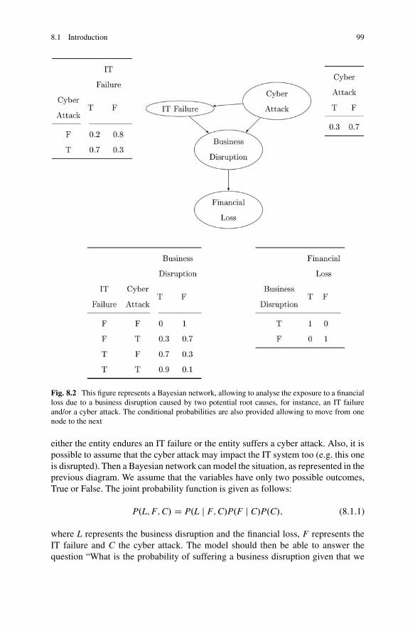
8.1 Introduction 99
Fig. 8.2 This figure represents a Bayesian network, allowing to analyse the exposure to a financialloss due to a business disruption caused by two potential root causes, for instance, an IT failureand/or a cyber attack. The conditional probabilities are also provided allowing to move from onenode to the next
either the entity endures an IT failure or the entity suffers a cyber attack. Also, it ispossible to assume that the cyber attack may impact the IT system too (e.g. this oneis disrupted). Then a Bayesian network can model the situation, as represented in theprevious diagram. We assume that the variables have only two possible outcomes,True or False. The joint probability function is given as follows:
P.L;F;C/ D P.L j F;C/P.F j C/P.C/; (8.1.1)
where L represents the business disruption and the financial loss, F represents theIT failure and C the cyber attack. The model should then be able to answer thequestion “What is the probability of suffering a business disruption given that we

100 8 Bayesian Networks
had a cyber attack?” by using the conditional probability formula and summing overall nuisance variables:
P.C D T j L D T/ D P.L D T;C D T/
P.L D T/DP
F2fT;Fg P.L D T;F;C D T/PF;C2fT;Fg P.L D T;F;C/
:
(8.1.2)
Using the expansion for the joint probability function P.L;F;C/ and the condi-tional probabilities as presented in the diagram, we can compute any combination.For example,
P.L D T;F D T;C D T/ D P.L D T j F D T;C D T/P.F D T j C D T/P.C D T/
which leads to 0:9 � 0:7 � 0:3 D 0:189. Or,
P.L D T;F D T;C D F/ D P.L D T j F D T;C D F/P.F D T j C D F/P.C D F/
which leads to 0:7 � 0:2 � 0:7 D 0:098. Then the numerical results are
P.C D T j L D T/ D 0:189TTT C 0:027TFT
0:189TTT C 0:098TTF C 0:027TFT C 0:0TFF� 68:78%:
8.2 Theory
In this section, we will address the Bayesian network from a theoretical point ofview, not only focusing on our problem, i.e., scenario analysis, but also discussing itsuse beyond scenario analysis, or in other words, its use for automated and integratedrisk management.
The first point to introduce is the concept of joint probability, i.e., the probabilitythat a series of events will happen subsequently or simultaneously. The jointprobability distribution can be expressed either in terms of a joint cumulativedistribution function or in terms of a joint probability density function in thecontinuous case or joint probability mass function in the discrete case.1 These in turncan be used to find two other types of distributions: the marginal distributions givingthe probabilities for any of the variables, and the conditional probability distributionfor the remaining variables.
The joint probability mass function of two discrete random variables X, Y isgiven by
P.X D x and Y D y/ D P.Y D y j X D x/ � P.X D x/ D P.X D x j Y D y/ � P.Y D y/;
(8.2.1)
1Chapter 11 provides alternative solution to build joint probability functions.

8.2 Theory 101
where P.Y D y j X D x/ is the probability of Y D y given that X D x. Thegeneralisation to n discrete random variables X1;X2; : : : ;Xn which is
P.X1 D x1; : : : ;Xn D xn/ D P.X1 D x1/P.X2 D x2 j X1 D x1/
� P.X3 D x3 j X1 D x1;X2 D x2/ � � � �� P.Xn D xn j X1 D x1;X2 D x2; : : : ;Xn�1 D xn�1/
In parallel, the joint probability density function fX;Y.x; y/ for continuous randomvariables is
fX;Y.x; y/ D fYjX.y j x/fX.x/ D fXjY.x j y/fY.y/ ; (8.2.2)
where fYjX.yjx/ and fXjY.xjy/ give the conditional distributions of Y given X D x andof X given Y D y, respectively, and fX.x/ and fY.y/ give the marginal distributionsfor X and Y, respectively.
In the case of a Bayesian network, the joint probability of the multiple variablescan be obtained from the product of individual probabilities of the nodes:
P.X1; : : : ;Xn/ DnY
iD1P.Xi j parents.Xi// : (8.2.3)
The second requirement to understand how the network is functioning is under-standing Bayes’ theorem (Bayes and Prince, 1763), expressed as:
P.AjI; S/ D P.AjS/ � P.IjA; S/P.IjS/ ; (8.2.4)
where our belief in assumption A can be refined given the additional informationavailable I as long as secondary inputs S. P.AjI; S/ is the posterior probability, i.e.,the probability of A to be true considering the initial information available as long asthe added information. P.AjS/ is the prior probability or the probability of A beingtrue given S. P.IjA; S/ is the likelihood component and gives the probability of theevidence assuming that both A and S are true. Finally, the last term P.IjS/ is calledthe expectedness, or how expected the evidence is, given only S. It is independentof A, therefore it is usually considered as a scaling factor, and may be rewritten as
P.IjS/ DnXi
P.IjAi; S/ � P.AijS/; (8.2.5)
where i denotes the index of a particular assumption Ai, and the summation is takenover a set of hypotheses which are mutually exclusive and exhaustive. It is importantto note that all these probabilities are conditional. They specify the degree of

102 8 Bayesian Networks
belief in propositions assuming that some other propositions are true. Consequently,without prior determination of the probability of the previous propositions, theapproach cannot be functioning.
Going one step further, we can now briefly present the statistical inference.Given some data x, and parameter � , a simple Bayesian analysis starts with aprior probability p.�/ and likelihood p.x j �/ to compute a posterior probabilityp.� j x/ / p.x j �/p.�/ (Shevchenko, 2011).
Usually the prior distributions depend on other parameters ' (not mentioned inthe likelihood), referred to as hyperparameters. So, the prior p.�/ must be replacedby a likelihood p.� j '/, and a prior p.'/ on the newly introduced parameters ' isrequired, resulting in a posterior probability
p.�; 'jx/ / p.xj�/p.�j'/p.'/: (8.2.6)
The process may be repeated multiple times if necessary; for example, the parame-ters ' may depend in turn on additional parameters , which will require their ownprior. Eventually the process must terminate, with priors that do not depend on anyother unmentioned parameters.2
For example, suppose we have measured the quantities x1; : : : ; xn, each withnormally distributed errors of known standard deviation � ,
xi � N.�i; �2/: (8.2.7)
Suppose we are interested in estimating �i. An approach would be to estimate the�i using a maximum likelihood approach; since the observations are independent,the likelihood factorises and the maximum likelihood estimate is simply
�i D xi: (8.2.8)
However, if the quantities are not independent, a model combining the �i is requiredsuch as,
xi � N.�i; �2/; (8.2.9)
�i � N.'; �2/ (8.2.10)
with improper priors ' �, � �2 .0;1/. When n � 3, this is an identified model(i.e. there exists a unique solution for the model’s parameters), and the posteriordistributions of the individual �i will tend to converge towards their common mean.3
2The symbol / means proportional too, and to draw a parallel with the previous paragraph relatedto Bayes’ theorem, we see that the scaling factor does not have any impact in the research of theappropriate values for the parameters.3This shrinkage is a typical behaviour in hierarchical Bayes’ models (Wang-Shu, 1994).

8.2 Theory 103
8.2.1 A Practical Focus on the Gaussian Case
In order to specify the Bayesian network and therefore represent the joint probabilitydistribution, the probability distribution for X conditional upon X’s parents has tobe specified for each node X. These distributions may take any form, though it iscommon to work with discrete or Gaussian distributions since these simplifies thecalculations.
In the following we develop the Gaussian case because of the so-called conjugateproperty. Indeed, if the posterior distributions p.� jx/ are in the same family as theprior probability distribution p.�/, the prior and posterior are then called conjugatedistributions, and the prior is called a conjugate prior for the likelihood function. TheGaussian distribution is conjugate to itself with respect to its likelihood function.Consequently, the conjugate prior of the mean vector is another multivariate normaldistribution, and the conjugate prior of the covariance matrix is an inverse-Wishartdistribution W�1 (Haff, 1979). Suppose then that n observations have been gathered
X D fx1; : : : ; xng � N .�;†/ (8.2.11)
and that a conjugate prior has been assigned, where
p.�;†/ D p.� j †/ p.†/; (8.2.12)
where
p.� j †/ � N .�0;m�1†/; (8.2.13)
and
p.†/ �W�1.‰ ; n0/: (8.2.14)
Then,
p.� j †;X/ � N�
nNxCm�0nCm ; 1
nCm †�;
p.† j X/ � W�1 �‰ C nSC nmnCm .Nx ��0/.Nx � �0/
0; nC n0;
(8.2.15)
where
Nx D n�1nX
iD1xi;
S D n�1nX
iD1.xi � Nx/.xi � Nx/0:
(8.2.16)

104 8 Bayesian Networks
If N-dimensional x is partitioned as follows:
x Dx1x2
�with sizes
q � 1
.N � q/ � 1�
(8.2.17)
and accordingly � and † are partitioned as follows:
� D�1
�2
�with sizes
q � 1
.N � q/ � 1�
(8.2.18)
† D†11 †12
†21 †22
�with sizes
q � q q � .N � q/
.N � q/ � q .N � q/ � .N � q/
�(8.2.19)
then, the distribution of x1 conditional on x2 D a is multivariate normal .x1jx2 Da/ N.�;†/ where
N� D �1 C†12†�122 .a � �2/ (8.2.20)
and covariance matrix
† D †11 �†12†�122 †21: (8.2.21)
This matrix is the Schur complement (Zhang, 2005) of †22 in †. This means thatto compute the conditional covariance matrix, the overall covariance matrix need tobe inverted, the rows and columns corresponding to the variables being conditionedupon have to be dropped, and then inverted back to get the conditional covariancematrix. Here †�1
22 is the generalised inverse of †22.
8.2.2 Moving Towards an Integrated System: Learning
In the simplest case, a Bayesian network is specified by an expert and is then usedto perform inference, as briefly introduced in the first section. In more complicatedsituations, the network structure and the parameters of the local distributions mustbe learned from the data.
As discussed in Chap. 4, Bayesian networks are part of the machine learningfield of research. Originally developed by Rebane and Pearl (1987) the automatedlearning relies on the distinction between the three possible types of adjacent tripletsallowed in a DAG:
• Type 1: X ! Y ! Z• Type 2: X Y ! Z• Type 3: X ! Y Z

8.2 Theory 105
Type 1 and type 2 are both independent given Y, therefore, they are indis-tinguishable. On the other hand, Type 3 can be uniquely identified as X and Zare marginally independent and all other pairs are dependent. Thus, while therepresentations of these three triplets are identical, the direction of the arrows definesthe causal relationship and is therefore of particular importance. Algorithms havebeen developed to determine the structure of the graph in a first step and orient thearrows according to the conditional independence observed in a second step (Vermaand Pearl 1991; Spirtes and Glymour 1991; Spirtes et al. 1993; Pearl 2000).
Alternatively, it is possible to use structural learning methods which requirea scoring function and a search strategy, such as a Markov Chain Monte Carlo(MCMC) to avoid being trapped in local minima. Another method consists in focus-ing on the sub-class of models, for which the MLE have a closed form, supportingthe discovery of a consistent structure for hundreds of variables (Petitjean et al.,2013).
Nodes and edges can be added using rule-based machine learning techniques,inductive logic programming or statistical relational learning approaches (Nassifet al., 2012, 2013).
Often the conditional distributions require a parameter estimation, using, forexample, a maximum likelihood approach (see Chap. 5) though any maximisationproblem (likelihood or posterior probability) might be complex if some variablesare unobserved. To solve this problem the implementation of the expectation–maximisation algorithm, which iteratively alternates evaluating expected valuesof the unobserved variables conditional on observed data, and maximising thecomplete likelihood (or posterior) assuming that previously computed expectedvalues are correct, is particularly helpful. Alternatively it is possible estimate theparameters by treating them as additional unobserved variables and to compute a fullposterior distribution over all nodes conditional upon observed data, but this usuallyleads to large dimensional models, which are complicated to implement in practice.
Bayesian networks are complete models capturing relationships between vari-ables and can be used to evaluate probabilities at various stages of the causal chain.Computing the posterior distribution of variables considering the information gath-ered about them is referred to as probabilistic inference. To summarise, a Bayesiannetwork allows automatically applying Bayes’ theorem to complex problems.
The most common exact inference methods are: (1) variable elimination, whicheliminates either by integration or summation the non-observed non-query variablesone by one by distributing the sum over the product; (2) clique tree propagation(Zhang and Yan 1997), which stores in computers memory the computation sothat multiple variables can be queried simultaneously and new evidence propagatedquickly; (3) and recursive conditioning which allow for a space-time trade-off andmatch the efficiency of variable elimination when enough space is used (Darwiche2001). All of these methods see their complexity growing with the network’s treewidth.
The most common approximate inference algorithms are importance sampling,stochastic MCMC simulation, mini-bucket elimination, loopy belief propagation,

106 8 Bayesian Networks
generalised belief propagation and variational methods (MacKay, 2003; Hassaniand Renaudin, 2013).
8.3 For the Managers
In this section, we discuss the added value of Bayesian networks for risk practition-ers. As these are some kind of models, the possibilities are almost unlimited as longas the information and the strategies used to feed the nodes are both accurate andappropriate. Indeed, the number of nodes leading to an outcome can be as large aspractitioners would like though it will require more research to feed the probabilitiesrequired for each node.
The network in Fig. 8.3 shows how starting from a weak IT system, we mayanalyse the likelihood of putting customers data at risk and therefore getting aregulatory fine, of losing customer due to the reputational impact, of suffering anopportunistic rogue trading incident, up to the systemic incident. In that example, wecan see a macro contagion mimicking a bit the domino effect observed after SocieteGenerale rogue trading incident in 2008. Note that each node can be analysed and/orinformed by either discrete or continuous distributions. It is also interesting to notehow the two illustrations in this chapter start from similar underlying issues thoughaim at analysing different scenarios (i.e., comparing Figs. 8.2 and 8.3).
The key to the use of this network is the evaluation of the probabilities andconditional probabilities at each node. Note once again that this kind of method-ology is highly data consuming, as to be reliable we need evidence and information
Credit Crunch
Customers Data At Risk
Financial Loss
Financial Loss due to defaults
Impact on Reputation
Liquidity IssueLoss of Customers
Market Confidence Impact
Real Economy not funded
Regulatory Fine
Rogue Trading
Weak IT Systems
Fig. 8.3 In this figure, we illustrate the possibility to analyse the cascading outcomes resultingfrom a weak IT System, i.e. the likelihood of putting customers data at risk and therefore gettinga regulatory fine, of losing customers due to the reputational impact and in parallel analyse theprobability of suffering an opportunistic rogue trading incident, implementing a Bayesian Network

8.3 For the Managers 107
supporting these probabilities, otherwise it would be highly judgemental andtherefore likely to be unreliable. Besides, to be used for risk assessment, the rightquestions need to be asked, indeed, are we interested in the potential loss amount orthe probability of failure? In other words, what is our target?
One advantage of Bayesian networks is that it is intuitively easier for a managerto build, to explain and to understand direct dependencies and local distributionsthan complete joint distributions, and to defend it in front of senior managers. In thefollowing, the pros and cons of the methodology are detailed.
The advantages of Bayesian networks are as follows:
• Bayesian networks represent all the relationships between variables in a systemwith connecting arcs. It is quite simple for a professional to build his own causalnetwork representative of the risk he is trying to model, from the triggers to thecontagion nodes up to the outcome in case of the materialisation of the risk, e.g.,loss, system failure, time of recovery, etc.
• It is simple to identify dependent and independent nodes. This would help, forexample, determining where some more controls should be put in place andprioritise the tasks.
• Bayesian networks are functioning even if the data sets are incomplete as themodel takes into account dependencies between all variables. This makes it fasterto implement and allows practitioners to use multiple sources of information toinform the nodes.
• Bayesian networks can map scenarios where it is not feasible/practical tomeasure all variables due to system constraints. Especially in situations wherethey are integrated in a machine learning environment and the mapping isidentified automatically.
• They can help reaching order out of chaos on complicated models (i.e. containingmany variables).
• They can be used for any system model—from all known parameters to unknownparameters.
However, and from a more scenario centric perspective, the limitations ofBayesian networks are as follows (Holmes, 2008):
• All branches must be calculated in order to calculate the probability of any onebranch. That might be highly complicated, and the impact on the global outcomesof the model of a node that is not properly informed may be leading to unreliableresults and therefore may potentially mislead the management.
• The second problem regards the quality and the extent of the prior beliefs used inBayesian inference processing. A Bayesian network is only as useful as this priorknowledge is reliable. Either an excessively optimistic or pessimistic expectationof the quality of these prior beliefs will distort the entire network and invalidatethe results. Related to this concern is the selection of the statistical distributioninduced in modelling the data. Selecting the proper distribution model to describethe data has a notable effect on the quality of the resulting network.
• It is difficult, computationally speaking, to explore a previously unknownnetwork. To calculate the probability of any branch of the network, all branches

108 8 Bayesian Networks
must be calculated. While the resulting ability to describe the network can beperformed in linear time, this process of network discovery is a hard task whichmight either be too costly to perform, or impossible given the number andcombination of variables.
• Calculations and probabilities using Bayes’ rule and marginalisation can becomecomplex, therefore calculation should be undertaken carefully.
• System’s users might be keen to violate the distribution of probabilities uponwhich the system is built.
References
Alexander, C. (2003). Managing operational risks with Bayesian networks. Operational Risk:Regulation, Analysis and Management, 1, 285–294.
Bayes, T., & Prince, R. (1763). An essay towards solving a problem in the doctrine of chance. Bythe late Rev. Mr. Bayes, communicated by Mr. Price, in a letter to John Canton, M. A. and F.R. S. Philosophical Transactions of the Royal Society of London, 53, 370–418.
Darwiche, A. (2001). Recursive conditioning. Artificial Intelligence, 126(1–2), 5–41.Haff, L. R. (1979). An identity for the Wishart distribution with applications. Journal of
Multivariate Analysis, 9(4), 531–544.Hassani, B. K., & Renaudin, A. (2013). The cascade Bayesian approach for a controlled
integration of internal data, external data and scenarios. Working Paper, Université Paris 1.ISSN:1955-611X [halshs-00795046 - version 1].
Holmes, D. E. (Ed.). (2008). Innovations in Bayesian networks: Theory and applications. Berlin:Springer.
Koski, T., & Noble, J. (2009). Bayesian networks: An introduction (1st ed.). London: Wiley.MacKay, D. (2003). Information theory, inference, and learning algorithms. Cambridge: Cam-
bridge University Press.Nassif, H., Wu, Y., Page, D., & Burnside, E. (2012). Logical differential prediction Bayes net,
improving breast cancer diagnosis for older women. In AMIA Annual Symposium Proceedings(Vol. 2012, p. 1330). American Medical Informatics Association.
Nassif, H., Kuusisto, F., Burnside, E. S., Page, D., Shavlik, J., & Costa, V. S. (2013). Scoreas you lift (SAYL): A statistical relational learning approach to uplift modeling. In JointEuropean conference on machine learning and knowledge discovery in databases, September2013 (pp. 595–611). Berlin/Heidelberg: Springer.
Pearl, J. (Ed.). (2000). Causality: Models, reasoning, and inference. Cambridge: CambridgeUniversity Press.
Petitjean, F., Webb, G. I., & Nicholson, A. E. (2013). Scaling log-linear analysis to highdimensional data. In International Conference on Data Mining, Dallas, TX (pp. 597–606).
Pourret, O., Naim, P., & Marcot, B. (Eds.). (2008). Bayesian networks: A practical guide toapplications (1st ed.). London: Wiley.
Rebane, G., & Pearl, P. (1987). The recovery of causal poly-trees from statistical data. InProceedings 3rd Workshop on Uncertainty in AI, Seattle, WA.
Shevchenko, P. V. (2011). Modelling operational risk using Bayesian inference. Berlin: Springer.Spirtes, P., & Glymour, C. N. (1991). An algorithm for fast recovery of sparse causal graphs. Social
Science Computer Review, 9(1), 62–72.Spirtes, P., Glymour, C. N., & Scheines, R. (1993). Causation, prediction, and search. New York:
Springer.

References 109
Verma, T., & Pearl, J. (1991). Equivalence and synthesis of causal models. In P. Bonissoneet al. (Eds.), UAI 90 Proceedings of the Sixth Annual Conference on Uncertainty in ArtificialIntelligence. Amsterdam: Elsevier.
Wang-Shu, L. (1994). Approximate Bayesian shrinkage estimation. Annals of the Institute ofStatistical Mathematics, 46(3), 497–507.
Zhang, F. (2005). The Schur complement and its applications. New York: Springer.Zhang, N. L., & Yan, L. (1997). Independence of causal influence and clique tree propagation. In
Proceedings of the thirteenth conference on uncertainty in artificial intelligence, August 1997(pp. 481–488). Los Altos: Morgan Kaufmann Publishers Inc.

Chapter 9Artificial Neural Network to Serve ScenarioAnalysis Purposes
Artificial neural networks (ANN), though inspired by the way brains are func-tioning, have been largely replaced by approaches based on statistics and signalprocessing, but the philosophy remains the same. Consequently and as brieflyintroduced in the third chapter, artificial neural networks are a family of statisticallearning models.
An artificial neural network is an interconnected group of nodes (“neurons”)mimicking neural connections in a brain, though it is not clear to what degreeartificial neural networks mirror brain functions. As represented in Fig. 9.1 a circularnode characterises an artificial neuron and an arrow depicts the fact that the outputof one neuron is the input of the next. They are used to estimate or approximatefunctions that can depend on a large number of inputs. The connections haveweights that can be modified, fine tuned or adapted according to experience or newsituations: this is the learning scheme.
To summarise the process, neurons are activated when they receive a signal, i.e.,a set of information. After being weighted and transformed, the activated neuronspass the modified information, message or signal onto other neurons. This process isreiterated until an output neuron is triggered, which determines the outcome of theprocess. Neural networks (Davalo and Naim 1991) have been used to solve multipletasks that cannot be adequately addressed using ordinary rule-based programming,such as handwriting recognition (Matan et al. 1990), speech recognition (Hintonet al. 2012) or climate change scenario analysis (Knutti et al. 2003), among others.
Neural networks are a family or class of processes that have the followingcharacteristics:
• It contains weights which are modified during the process based on the newinformation available, i.e., numerical parameters that are tuned by a learningalgorithm.
• It allows approximating non-linear functions of their inputs.• The adaptive weights are connection strengths between neurons, which are
activated during training and prediction by the appropriate signal.
© Springer International Publishing Switzerland 2016B.K. Hassani, Scenario Analysis in Risk Management,DOI 10.1007/978-3-319-25056-4_9
111

112 9 Artificial Neural Network to Serve Scenario Analysis Purposes
X4
X3
X2
X1
Output
1 1
Fig. 9.1 This figure illustrates a neural network. In this illustration, only one hidden layer hasbeen represented
9.1 Origins
In this section we will briefly provide an historical overview of artificial neuralnetworks.
McCulloch and Pitts (1943) created a computational model for neural networksbased on mathematics and algorithms usually referred to as threshold logic. Thisapproach led to the split of neural network research in two different axis. The firstfocused on biological processes in the brain, while the second aimed at applyingneural networks to artificial intelligence. Psychologist (Hebb 1949) created thetypical unsupervised learning rule referred to as Hebbian learning, later leading tonew neuroscience models. Hebbian network was simulated for the first time at theMIT by Farley and Clark (1954) using an ancestor of the computer1 and later thiswork was extended by Rochester et al. (1956).
Then Rosenblatt (1958) created the perceptron, a two-layer computer learningnetwork algorithm using additions and subtractions, created for pattern recognitionpurposes; however, this one could not be properly processed at the time. It is onlywhen Werbos (1974) created the back-propagation algorithm that it was possibleprocessing situation previously impossible to model with the perceptron. Besidesthis new algorithm revived the use of ANN as it solved the exclusive-or issue.However, the use of ANN was still limited due to the lack of processing power.
It is only in the early 2000s that neural networks really came back to life with thetheoretisation of the deep learning (Deng and Yu 2014).
To summarise, as presented ANN are far from being new, but the computationpower necessary has only been made recently available.
1Turing’s B machine already existed (sic!).

9.2 In Theory 113
9.2 In Theory
Neural network models in artificial intelligence are essentially mathematical modelsdefining a function f W X ! Y (i.e. y D f .x/) or a distribution over X or both X andY.
The first layer contains input nodes which transfer data to the subsequent layersof neurons via synapses until the signal reaches the output neurons. The mostcomplex architecture has multiple layers of neurons, various input neurons layersand output neurons. The synapses embed weight parameters that modify the data inthe calculations.
An ANN relies on three important features:
• The connection between the different layers of neurons• The learning process (i.e. updating the weights)• The activation function which transforms the weighted inputs into transferable
values.
Mathematically, the network function f .x/ is a combination of other functionsgi.x/, which might themselves be a combination of other functions. This networkstructure representation using arrows is straightforward to represent the synapticconnections, i.e., the variable relationships. Besides, f .x/ is traditionally representedas a non-linear weighted sum:
f .x/ D K
Xi
wigi.x/
!; (9.2.1)
where K is the prespecified activation function (Wilson 2012).In the traditional probabilistic view, the random variable F D f .G/ depends on
the random variable (r.v.) G D g.H/, which itself relies upon the r.v. H D h.X/depending on the r.v. X.
Considering this architecture, the components of individual layers are indepen-dent from each other. Therefore some intermediate operations can be performed inparallel.
Networks used in this chapter are referred to as feed forward, as their graph isa directed acyclic graph (DAG) as the Bayesian networks presented in the previouschapter.
Neural networks are very interesting as they can learn, i.e., given a problem anda class of functions F, the learning process uses a set of observations to find theoptimal2 subset of functions f � 2 F solving the problem, achieving the task orassessing the likely outcome of a scenario storyline.
This requires defining an objective function C W F ! R such that, for the optimalsolution f �, C. f �/ � C. f /8f 2 F (i.e. no solution is better than the optimal
2According to prespecified criteria.

114 9 Artificial Neural Network to Serve Scenario Analysis Purposes
solution). The objective function C is very important as it measures the distanceof a particular solution from an optimal solution given the task to be achieved. Theobjective function has to be a function of the input data and is usually defined as astatistic that can only be approximated.
While it is possible to define some ad hoc objective function, it is highly unusual.A specific objective function is traditionally used, either because of its desirableproperties (e.g. convexity) or because the formulation of the problem led to it, i.e.,this one depends on the desired task.
9.3 Learning Algorithms
Training a neural network model essentially means selecting one model from theset of allowed models that minimise the objective function criterion. There arenumerous algorithms available for training neural network models; most of themcan be viewed as a straightforward application of optimisation theory and statisticalestimation. Most of the algorithms used in training artificial neural networks employsome form of gradient descent, using backpropagation to compute the actualgradients. This is done by simply taking the derivative of the objective function withrespect to the network parameters and then changing those parameters in a gradient-related direction. The backpropagation training algorithms are usually classified inthree categories: steepest descent (with variable learning rate, with variable learningrate and momentum, with resilient backpropagation), quasi-Newton (Broyden–Fletcher–Goldfarb–Shanno, one step secant, Levenberg–Marquardt) and conjugategradient (Fletcher–Reeves update, Polak–Ribiére update, Powell–Beale restart,scaled conjugate gradient) (Forouzanfar et al. 2010).
Evolutionary methods (Rigo et al. 2005), gene expression programming (Ferreira2006), simulated annealing (Da and Xiurun 2005), expectation–maximisation, non-parametric methods and particle swarm optimisation (Wu and Chen 2009) are somecommonly used methods for training neural networks.
Perhaps the greatest advantage of ANNs is their ability to be used as an arbitraryfunction approximation mechanism that “learns” from observed data. However,using them is not so straightforward, and a relatively good understanding of theunderlying theory is essential.
Obviously, the approximation accuracy will depend on the data representationand the application. Complex models tend to lead to problems with learning. Indeed,there are numerous issues with learning algorithms. Almost any algorithm will workwell with the correct hyperparameters for training on a particular fixed data set.However, selecting and tuning an algorithm for training on unseen data requires asignificant amount of experimentation.
If the model’s, objective function and learning algorithm are selected appropri-ately the resulting ANN might be quite robust. With the correct implementation,ANNs might be used naturally for online learning and large data set applications.

9.3 Learning Algorithms 115
Their simple structure and the existence of mostly local dependencies exhibited inthe structure allows for fast parallel implementations.
The utility of artificial neural network models lies in the fact that they can beused to infer a function from observations. This is particularly useful in applicationswhere the complexity of the data or task makes the design of such a function byhand impractical. Indeed, the properties presented in the next paragraphs supportthe capability of Neural Networks to capture particular behaviors embedded withindata sets and infer a function from it.
Artificial neural network models have a property called “capacity”, which meansthat they can model any function despite the quantity of information, its type or itscomplexity.
Addressing the question of convergence is complicated since it depends on anumber of factors: (1) many local minima may exist, (2) it depends on the objectivefunction and the model, (3) the optimisation method used might not converge whenstarting far from a local minimum, (4) for a very large number of data points orparameters, some methods become impractical.
In applications where the goal is to create a system which works well in unseensituations, the problem of overtraining has emerged. This arises in convoluted orover-specified systems when the capacity of the network significantly exceeds theneeded free parameters.
There are two schools of thoughts to deal with that issue. The first suggests usingcross-validation and similar techniques to check for the presence of overtrainingand optimally select hyperparameters such as to minimise the generalisation error.The second recommends using some form of regularisation. This is a concept thatemerges naturally in a probabilistic framework, where the regularisation can beperformed by selecting a larger prior probability over simpler models; but also instatistical learning theory, where the goal is to minimise over two quantities: the“empirical risk” and the “structural risk”, which roughly corresponds to the errorover the training set and the predicted error in unseen data due to overfitting.
Supervised neural networks that use a mean squared error (MSE) objectivefunction can use formal statistical methods to determine the confidence of thetrained model. The MSE on a validation set can be used as an estimate for variance.This value can then be used to calculate the confidence interval of the output of thenetwork, assuming a normal distribution. A confidence analysis made this way isstatistically valid as long as the output probability distribution stays the same andthe network is not modified.
It is also possible to assign a generalisation of the logistic function, referred toas the softmax activation function so that the output can be interpreted as posteriorprobabilities (see Chap. 8).
The softmax activation function is
yi D exiPcjD1 exj
: (9.3.1)

116 9 Artificial Neural Network to Serve Scenario Analysis Purposes
9.4 Application
In this section, our objective is to apply neural network to scenario analysis. Indeedscenario analysis includes many tasks that can be independently performed byneural networks such as function approximation, regression analysis, time seriesprediction, classification (pattern and sequence recognition), novelty detection andsequential decision making and can also be used in data processing for tasks suchas mining, filtering, clustering, knowledge discovery in databases, blind sourceseparation and compression. After training, the networks could predict multipleoutcomes from unrelated inputs (Ganesan 2010).
Applications of neural networks to risk management are not new. Indeed, Trippiand Turban (1992) provide multiple chapters presenting methodologies using neuralnetworks to predict bank failures. In this book, the neural network strategy is alsocompared to more traditional approaches. Relying on the results presented in thesechapters, we see that neural networks can be used as follows.
Considering that neural networks are relying on units. Each unit u receives inputssignals from other units, aggregates these signals based on the input function Ui andgenerates an output signal based on an output Oi. The output signal is then directedto other units consistently with the topology of the network. Although the form ofinput/ output functions at each node has no constraint other than to be continuousand differentiable, using the function obtained from Rumelhart et al. (1996):
Ui DX
j
wijOj C i (9.4.1)
and
Oi D 1
1C eUi; (9.4.2)
where
1. Ui D input of unit i,2. Oi D output of unit i,3. wij D connection weight between unit i and j,4. i = bias of unit i
Here, the neural network can be represented by a weighted directed graph wherethe units introduced in the previous paragraph represent the nodes and the linksrepresent connections. To the links are assigned the weights of the correspondingconnection. A special class of neural networks referred to as feedforward networksare used in the chapters in question.
A feedforward network contains three types of processing units, for instance,input, output and hidden. Input units, initialising the network, receive the seed infor-mation from some data. Hidden units do not directly interact with the environment,

9.4 Application 117
they are invisible, though they are located in the subsequent intermediate layers.Finally, output units provide signals to the environment and are located in the finallayers. Note that layers can be skipped, but we cannot move backward.
The weight vector W, i.e., weights associated with the connections, is the coreof the neural network. W represents what a neural knows and permits respondingto any input provided. “A feedforward network with an appropriate W can be usedto model the casual relationship between a set of variables”. The fitting and thesubsequent learning is done by modifying the connections’ weights.
Determining the appropriate W is not usually easy, especially when the charac-teristics of the entire population are barely known. As mentioned previously, thenetwork is trained using examples. The objective is to obtain a set of weights Wleading to the best fit of the model to the data used initially. The backpropagationalgorithm has been selected here to perform the learning as it is able to train multi-layer networks. Its effectiveness comes from the fact that it is capable of exploitingregularities and exceptions contained in the initial sample. The backpropagationalgorithm consists in two phases: forward-propagation and backward-propagation.
Mechanically speaking, let s be a training sample, each piece of informationdescribed by an input vector Xi D .xi1; xi2; : : : ; xim/ and an output vector Di D.di1; di2; : : : din/, 1 � i � s. In forward propagation, Xi is fed to the input layer, andan output Yi D .yi1; yi2; : : : ; yin/ is obtained using W, in other words Y D f .W/where f characterises any appropriate function. The value of Yi is then comparedwith the desired output Di by computing the squared error ..yij � dij/
2/, 1 � i � n,for each output unit. Output differences are aggregated to form the error functionSSE (sum squared error).
SSE DsX
iD1
nXjD1
.yij � dij/2
2: (9.4.3)
The objective is to minimise the SSE with respect to W so that all input vectorsare correctly mapped into their corresponding output vectors. As a matter of fact,the learning process can be considered as a minimisation problem with objectivefunction SSE defined in the space of W, i.e., arg maxW SSE:
The second phase consists in evaluating the gradient of the function in the weightspace to locate the optimal solution. Both direction and magnitude change �wij ofeach wij are obtained using
�wij D �ıSSE
ıwij�; (9.4.4)
where 0 < � < 1 is a parameter controlling the convergence rate of the algorithm.The sum squared error calculated in the first phase is propagated back, layer
by layer, from the output units to the input units in the second phase. Weightadjustments are obtained through propagation at each level. As Ui, Oi and SSE arecontinuous and differentiable, ıSSE=ıwij can be evaluated at each level applying

118 9 Artificial Neural Network to Serve Scenario Analysis Purposes
the following chain rule:
ıSSE
ıwijD ıSSE
ıOi
ıOi
ıUi
ıUi
ıwij: (9.4.5)
In this process, W can be updated in two manners. For instance, either W is updatedsequentially for each couple .Xi;Di/, or considering the aggregation of �wij after acomplete run of all examples. For each iteration of the back-propagation algorithm,the two phases are executed until the SSE converges.
In this book neural networks offer a viable alternative for scenario analysis. Herethis model is applied to bankruptcy prediction. In Trippi and Turban (1992), theresults exhibited for neural networks show a better predictive accuracy than thoseobtained from implementing a linear discriminant model, a logistic regression,a k nearest neighbour strategy and a decision tree. Applying their model to theprediction of bank failures, the authors have modified the original backpropagationalgorithm to capture prior probabilities and misclassification. Indeed, the errorof misclassifying a failed bank into the non-failed group (type I error) is moresevere than the other way. The original function SSE is generalised to SSEw bymultiplying each error term by Zi, in other word by weighting it. The comparison ofthe methodologies is based on a training set with an equal proportion of failed andnon-failed banks, though quite often, the number of defaults constitutes a smallerportion of the whole population than the non-failed entities. The matching processmay bias the model, consequently, they recommended the entire population to beused as the training set. As actually mentioned in earlier chapters, neural networkscan be helpful to identify a single group from a large set of alternatives.
Alternatively, Fig. 9.2 provides another application of neural networks with twohidden layers. In that model, the data provided are related to cyber security. The
1.10785−6.64
463
−3.0
7072
3.53
224
34.3
0726
Number_Of_Daily_Users
−2.28388
−10.69908
−4.6
3794
−24.
3645
3
0.19
203
Quality_Of_Security_Checks
−0.4526
53.98013−2.48
443
37.8
9733
1.31
05
Traffic_To_Unwanted_Addresses
0.83524
−41.54127
4.40744
−27.9
2341
−12.
5082
Level_Of_Formation_Of_Managers
−1.51758
51.37852
2.110322.03342
−19.
2720
5
Number_Of_Security_Patches
−0.3445310.60307
−2.79519
22.1320354.41
594
Number_Of_Malware_Attack
−5.73499−16.94477
−2.93554
14.55174
23.98356
Budget_Security_Program
−1.321734.876672.44388
−7.87106
−5.30881Industry_Reputation
−2.1703748.37499−0.77594
−1.48015
11.31625Antivirus_Updates
1.16316
16.3
3257
−0.32507
3.44
61
−0.46964
−9.00374
−0.03826
−3.63973
−0.76176
−4.54531
2.80832
−3.93509
Losses
0.788366.48083
0.47507
9.71124
−11.10332
1
−0.00758
−1.28865
1
−0.11184
1
Fig. 9.2 This figure illustrates a neural network applied to IT security issues, consideringinformation coming from anti-virus updates frequency, industry reputation (how likely it is to bethreatened), the budget of security programs within financial institutions, the number of malwareattack, the number of security patches, the level of training of managers, the traffic to unwantedaddresses, the quality of security checks and the number of daily users

9.5 For the Manager: Pros and Cons 119
objective is to evaluate the likelihood of a financial loss. The information regardinganti-virus updated, industry reputation, budget of the security program, number ofmalware attacks, number of security patches, level of formation of the managers,traffic to unwanted addresses, quality of security checks and number of daily usersis used as input.
Implementing a strategy as described before, the weights are calculated for eachand every connections. Then moving from a layer to another, we can evaluate theprobability of a loss related to cyber attacks given the initial issues identified.
In our second example, we are already moving toward deep learning strategiesas the neural network has two layers.
9.5 For the Manager: Pros and Cons
In this section we discuss the main issues and advantages of implementing a neuralnetwork strategy for scenario analysis purposes, starting with the issues.
To be properly applicable neural networks require sufficient representative datato capture the appropriate underlying structure which will allow a generalisation tonew situations. These issues can be dealt with in various manners such as randomlyshuffling the training data, using a numerical optimisation or reclassifying the data.
From a computational and IT infrastructure point of view, to implement large,efficient and effective neural network strategies, considerable processing and storageresources are required (Balcazar 1997). Simulating even the most simplified neuralnetwork may require filling large database and may consume huge amounts ofmemory and hard disk space. Besides, neural network methodologies will usuallyrequire some simulations to deal with the signal transmission between the neurons—and this may need huge amounts of CPU processing power and time.
Though, neural networks methodologies are questioned as it is possible to createa successful net without understanding how it works. However it is arguable that anunreadable table that a useful machine could read would still be well worth having(NASA 2013). Indeed, the discriminant capability of a neural network is difficult toexpress in symbolic form. However, neural networks are limited if one wants to testthe significance of individual inputs.
Remark 9.5.1 In that case we are somehow already talking about artificial intelli-gence.
Other limitations reside in the fact that there is no formal method to derive anetwork configuration for a given classification task. Although it was shown thatonly one hidden layer is enough to approximate any continuous functions, thenumber of hidden units can be arbitrarily large, the risk of overfitting the network isreal especially if the size of the training sample is insufficient. Researchers exploringlearning algorithms for neural networks are uncovering generic principles allowinga successful fitting, learning, analysis and prediction. A new school of thoughtsactually consider that hybrid models (combining neural networks and symbolic
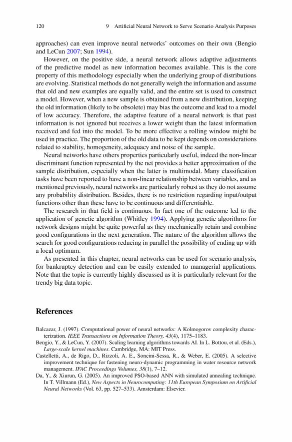
120 9 Artificial Neural Network to Serve Scenario Analysis Purposes
approaches) can even improve neural networks’ outcomes on their own (Bengioand LeCun 2007; Sun 1994).
However, on the positive side, a neural network allows adaptive adjustmentsof the predictive model as new information becomes available. This is the coreproperty of this methodology especially when the underlying group of distributionsare evolving. Statistical methods do not generally weigh the information and assumethat old and new examples are equally valid, and the entire set is used to constructa model. However, when a new sample is obtained from a new distribution, keepingthe old information (likely to be obsolete) may bias the outcome and lead to a modelof low accuracy. Therefore, the adaptive feature of a neural network is that pastinformation is not ignored but receives a lower weight than the latest informationreceived and fed into the model. To be more effective a rolling window might beused in practice. The proportion of the old data to be kept depends on considerationsrelated to stability, homogeneity, adequacy and noise of the sample.
Neural networks have others properties particularly useful, indeed the non-lineardiscriminant function represented by the net provides a better approximation of thesample distribution, especially when the latter is multimodal. Many classificationtasks have been reported to have a non-linear relationship between variables, and asmentioned previously, neural networks are particularly robust as they do not assumeany probability distribution. Besides, there is no restriction regarding input/outputfunctions other than these have to be continuous and differentiable.
The research in that field is continuous. In fact one of the outcome led to theapplication of genetic algorithm (Whitley 1994). Applying genetic algorithms fornetwork designs might be quite powerful as they mechanically retain and combinegood configurations in the next generation. The nature of the algorithm allows thesearch for good configurations reducing in parallel the possibility of ending up witha local optimum.
As presented in this chapter, neural networks can be used for scenario analysis,for bankruptcy detection and can be easily extended to managerial applications.Note that the topic is currently highly discussed as it is particularly relevant for thetrendy big data topic.
References
Balcazar, J. (1997). Computational power of neural networks: A Kolmogorov complexity charac-terization. IEEE Transactions on Information Theory, 43(4), 1175–1183.
Bengio, Y., & LeCun, Y. (2007). Scaling learning algorithms towards AI. In L. Bottou, et al. (Eds.),Large-scale kernel machines. Cambridge, MA: MIT Press.
Castelletti, A., de Rigo, D., Rizzoli, A. E., Soncini-Sessa, R., & Weber, E. (2005). A selectiveimprovement technique for fastening neuro-dynamic programming in water resource networkmanagement. IFAC Proceedings Volumes, 38(1), 7–12.
Da, Y., & Xiurun, G. (2005). An improved PSO-based ANN with simulated annealing technique.In T. Villmann (Ed.), New Aspects in Neurocomputing: 11th European Symposium on ArtificialNeural Networks (Vol. 63, pp. 527–533). Amsterdam: Elsevier.

References 121
Davalo, E., & Naim, P. (1991). Neural networks. MacMillan computer science series. London:Palgrave.
Deng, L., & Yu, D. (2014). Deep learning: Methods and applications. Foundations and Trends inSignal Processing, 7(3–4), 1–199.
Farley, B. G., & Clark, W. A. (1954). Simulation of self-organizing systems by digital computer.IRE Transactions on Information Theory 4(4), 76–84.
Ferreira, C. (2006). Designing neural networks using gene expression programming. In A. Abra-ham, et al. (Eds.), Applied soft computing technologies: The challenge of complexity (pp. 517–536). New York: Springer.
Forouzanfar, M., Dajani, H. R., Groza, V. Z., Bolic, M., & Rajan, S. (2010). Comparison of feed-forward neural network training algorithms for oscillometric blood pressure estimation. In 20104th international workshop on soft computing applications (SOFA), July 2010 (pp. 119–123).New York: IEEE.
Ganesan, N. (2010). Application of neural networks in diagnosing cancer disease using demo-graphic data. International Journal of Computer Applications, 1(26), 76–85.
Hebb, D. (1949). The organization of behavior. New York: Wiley.Hinton, G., Deng, L., Yu, D., Dahl, G. E., Mohamed, A. R., Jaitly, N., et al. (2012). Deep neural
networks for acoustic modeling in speech recognition: The shared views of four researchgroups. IEEE Signal Processing Magazine, 29(6), 82–97.
Knutti, R., Stocker, T. F., Joos, F., & Plattner, G. K. (2003). Probabilistic climate change projectionsusing neural networks. Climate Dynamics, 21(3–4), 257–272.
Matan, O., Kiang, R. K., Stenard, C. E., Boser, B., Denker, J. S., Henderson, D., et al. (1990).Handwritten character recognition using neural network architectures. In Proceedings of the4th USPS advanced technology conference, November 1990 (pp. 1003–1011).
McCulloch, W., & Pitts, W. (1943). A logical calculus of ideas immanent in nervous activity.Bulletin of Mathematical Biophysics, 5(4), 115–133.
NASA (2013). NASA neural network project passes milestone. www.nasa.gov.Rochester, N., Holland, J., Haibt, L., & Duda, W. (1956). Tests on a cell assembly theory of the
action of the brain, using a large digital computer. IRE Transactions on Information Theory,2(3), 80–93.
Rosenblatt, F. (1958). The perceptron: a probabilistic model for information storage and organiza-tion in the brain. Psychological Review, 65(6), 386–408.
Rumelhart, D. E., Hinton, G. E., & Williams, R. J. (1996). Learning representations by backprop-agating errors. Nature, 323, 533–536.
Sun, R. (1994). A two-level hybrid architecture for common sense reasoning. In R. Sun &L. Bookman (Eds.), Computational architectures integrating neural and symbolic processes.Dordrecht: Kluwer Academic Publishers.
Trippi, R. R., & Turban, E. (Eds.), (1992). Neural networks in finance and investing: Using artificial intelligence to improve real-world performance. New York: McGraw-Hill Inc.
Werbos, P. J. (1974). Beyond regression: New tools for prediction and analysis in the behavioralsciences. Ph.D. thesis, Harvard University.
Whitley, D. (1994). A genetic algorithm tutorial. Statistics and computing, 4(2), 65–85.Wilson, W. (2012). The machine learning dictionary. www.cse.unsw.edu.au/~billw.Wu, J., & Chen, E. (2009). A novel nonparametric regression ensemble for rainfall forecasting
using particle swarm optimization technique coupled with artificial neural network. In H. Wang,et al. (Eds.), 6th International Symposium on Neural Networks. Berlin: Springer.

Chapter 10Forward-Looking Underlying Information:Working with Time Series
10.1 Introduction
In order to capture serially related events, banks may need to consider the completedependence scheme. This is the reason why this chapter focuses on time series. It isimportant to note that the presence of autocorrelation is not compulsory, sometimesthe independence assumption should not be rejected a priori. Indeed, if there is nostatistical evidence to reject the assumption of independence, then this one shouldnot be rejected for the sake of it. Besides, these dependencies may take variousforms and may be detected on various time steps. We will come back to that pointin the next paragraphs. In this chapter, we assume that serial dependence existsand we model it using time series processes (McCleary 1980; Hamilton 1994; Boxet al. 2015). In many cases, the scenario analysis has to integrate macro-economicalfactors, and here time series models are particularly useful. The literature on thistopic is colossal (in the bibliography of this chapters as well as the previous we willfind some interesting articles). But strategies relying on time series should not belimited to macro-economic factors or stock indexes for instance. In this chapter, weillustrate the models with applications, but in order not to bias the manager trying toimplement the methodologies presented we do not emphasise the data to which weapplied them, though in this case they were macro-economic data.
Our objective is to capture the risks associated with the loss intensity whichmay increase during crises or turmoils, taking into account correlations, embeddeddynamics and large events thanks to adequate distributions fitted on the residuals.Using time series permit capturing the embedded autocorrelation phenomenonwithout losing any of the characteristics captured by traditional methodologies suchas fat tails.
Consequently, a time series is a sequence of data points, typically consistingin successive measurements made over a period of time. Time series are usuallyrepresented using line charts. A traditional application of time series processes isforecasting, which in our language can be translated into scenario analysis. Time
© Springer International Publishing Switzerland 2016B.K. Hassani, Scenario Analysis in Risk Management,DOI 10.1007/978-3-319-25056-4_10
123

124 10 Forward-Looking Underlying Information: Working with Time Series
series analysis aims at extracting meaningful statistics and other characteristics ofthe data. Time series forecasting consists in using a model to predict future valuesbased on past observations and embedded behaviours.
Time series are ordered by construction, as data are collected and sorted withrespect to a relevant date, occurrence, accounting, etc. This makes time seriesanalysis distinct from cross-sectional studies or regressions (see Chap. 11), in whichthere is no natural ordering of the observations for the first, and a classificationper type or characteristic more than a natural ordering for the second. Timeseries analysis also differs from spatial data analysis where to each observationis associated a geographical location. A stochastic model for a time series can beimplemented to capture the fact that observations close together in time will bemore closely related than observations further apart, but this is not always the caseas discussed a bit further in this chapter. In addition, the natural one-way ordering oftime leads to the fact that each value is expressed as a function of past values. Timeseries analysis is applicable to various data type as soon as these are associated withtime periods (continuous data, discrete numeric data, etc.)
Time series analysis usually belongs to one of the two following classes:frequency-domain and time-domain methods (Zadeh, 1953). The former includespectral analysis and recently, wavelet analysis; the latter include autocorrelationand cross-correlation analysis. We will focus on the second type. Additionally,we may split time series analysis techniques into parametric and non-parametricmethods. Parametric approaches assume that the underlying stationary stochasticprocess can be captured using a strategy relying on a small number of parameters.Here, estimating the parameters of this model is a requirement. Non-parametricapproaches, on the contrary, explicitly estimate the covariance or the spectrum ofthe process without assuming that the process has any particular structure. Methodsof time series analysis may also be divided into linear and non-linear, and univariateand multivariate. In this chapter we will focus in particular on parametric modelsand will illustrate univariate approaches. The next chapter may be used to extendthe solutions provided here to multivariate processes.
10.2 Methodology
Practically to build a model closer to reality, the assumption of independencebetween the data points may have to be relaxed. Thus, a general representation ofthe losses .Xt/t is 8t,
Xt D f .Xt�1;:::/C "t: (10.2.1)
There exist several models to represent various patterns and behaviour. Variationsin the level of a process using the following approaches or a combination of themcan be obtained. Time series processes can be split into various classes, each ofthem having their own variations, for instance, the autoregressive (AR) models, the

10.2 Methodology 125
integrated (I) models and the moving average (MA) models. These three classesdepend linearly on past data points (Gershenfeld, 1999). Combinations of these leadto autoregressive moving average (ARMA) and autoregressive integrated movingaverage (ARIMA) models. The autoregressive fractionally integrated moving aver-age (ARFIMA) model combines and enlarges the scope of the previous approaches.VAR1 strategies are an extension of these classes to deal with vector-valued data(multivariate time series), besides these might be extended to capture exogenousimpacts.
Non-linear strategies might also be of interest as empirical investigations haveshown that using predictions derived from non-linear models, over those fromlinear models, might be more appropriate (Rand 1971 and Holland 1992). Amongthese non-linear time series models those capturing the evolution of variance overtime (heteroskedasticity) are of particular interest. These models are referred to asautoregressive conditional heteroskedasticity (ARCH) and the library of variationcontains a wide variety of representation such as GARCH, TARCH, EGARCH,FIGARCH and CGARCH. The changes in variability are related to recent pastvalues of the observed series.
10.2.1 Theoretical Aspects
Originally the theory has been built on two sets of conditions, for instance,stationarity and its generalisation, ergodicity. However, ideas of stationarity must beexpanded: strict stationarity and second-order stationarity. Models can be developedunder each of these conditions, but in the latter case the models are usually regardedas partially specified. Nowadays, many time series models have been developed todeal with seasonally stationary or non-stationary series.
10.2.1.1 Stationary Process
In mathematics and statistics, a stationary process stricto sensus is a stochasticprocess whose joint probability distribution does not change when shifted in time.Consequently, moments (see Chap. 3) such as the mean and variance, if these exist,do not change over time and do not follow any trends. Practically, raw data areusually transformed to become stationary.
Mathematically, let fXtg be a stochastic process and let FX.xt1C� ; : : : ; xtkC� /represent the c.d.f. of the joint distribution of fXtg at times t1 C �; : : : ; tk C � . Then,fXtg is strongly stationary if, for all k, for all � , and for all t1; : : : ; tk,
FX.xt1C� ; : : : ; xtkC� / D FX.xt1 ; : : : ; xtk /: (10.2.2)
Since � does not affect FX.�/, FX is not a function of time.
1Vector autoregression.

126 10 Forward-Looking Underlying Information: Working with Time Series
10.2.1.2 Autocorrelation
Statistically speaking, the autocorrelation of a random process describes the corre-lation between values of the process at different times. Let X be a process whichreiterates in time, and t represents a specific point in time, then Xt is the realisationof a given run of the process at time t. Suppose that the mean �t and variance �2texist for all times t, then the definition of the autocorrelation between times s andt is
R.s; t/ D EŒ.Xt � �t/.Xs � �s/�
�t�s; (10.2.3)
where E is the expected value operator. Note that this expression cannot be evaluatedfor all time series as the variance may be zero (e.g. for a constant process), infinite ornonexistent. If the function R is computable, the returned value in the range Œ�1; 1�,where 1 indicates a perfect correlation and �1 a perfect anti-correlation.
If Xt is a wide-sense stationary process, then � and �2 are not time-dependent.The autocorrelation only depends on the lag between t and s, i.e., the time-distancebetween two values. Therefore the autocorrelation can be expressed as a function ofthe time-lag � D s � t, i.e.,
R.�/ D EŒ.Xt � �/.XtC� � �/��2
; (10.2.4)
an even function as R.�/ D R.��/.
10.2.1.3 White Noise
The framework in which we are evolving implies that observed data series arethe combination of a path dependent process (some may say “deterministic”) andrandom noise (error) terms. Then an estimation procedure is implemented to param-eterise the model using observations. The noise (error) values are assumed mutuallyuncorrelated with a mean equal to zero and the same probability distribution, i.e.,the noise is white. Traditionally, a Gaussian white noise is assumed, i.e. the errorterm follows a Gaussian distribution, but it is possible to have the noise representedby other distributions and the process transformed.
If the noise terms underlying different observations are correlated, then theparameters are still unbiased, however, uncertainty measures will be biased. Thisis also true if the noise is heteroskedastic, i.e., if its variance varies over time. Thisfact may lead to the selection of an alternative time series process.

10.2 Methodology 127
10.2.1.4 Estimation
There are many ways of estimating the coefficients or parameters, such as theordinary least squares procedure or the method of moments (through Yule–Walkerequations).
For example, the AR. p/ model is given by the equation
Xt DpX
iD1'iXt�i C "t; (10.2.5)
where 'i, i D 1; : : : ; p denotes the coefficients. As a direct relationship existsbetween the model coefficients and the covariance function of the process, theparameters can be obtained from the autocorrelation function. This is performedusing the Yule–Walker equations.
The Yule–Walker equations (Yule and Walker, 1927) correspond to the followingset:
�m DpX
kD1'k�m�k C �2" ım;0; (10.2.6)
where m D 0; : : : ; p, leading to p C 1 equations. Here �m is the autocovariancefunction of Xt, �" is the noise standard deviation and ım;0 is the Kronecker deltafunction.
As the last part of an individual equation is non-zero only if m D 0, the set ofequations can be solved by representing the equations for m > 0 matricially, i.e.,
2666664
�1�2
�3:::
�p
3777775D
2666664
�0 ��1 ��2 : : :�1 �0 ��1 : : :�2 �1 �0 : : ::::
::::::: : :
�p�1 �p�2 �p�3 : : :
3777775
2666664
'1'2
'3:::
'p
3777775
(10.2.7)
which can be solved for all f'mIm D 1; 2; : : : ; pg. The remaining equation for m D0 is
�0 DpX
kD1'k��k C �2" ; (10.2.8)
which, once f'mIm D 1; 2; : : : ; pg are known, can be solved for �2" .

128 10 Forward-Looking Underlying Information: Working with Time Series
Alternatively, AR parameters are determined by the first pC 1 elements �.�/ ofthe autocorrelation function. The full autocorrelation function can then be derivedby recursively calculating
�.�/ DpX
kD1'k�.k � �/: (10.2.9)
The Yule–Walker equations provide several ways of estimating the parameters of anAR. p/model, by replacing the theoretical covariances with estimated values.
Alternative estimation approaches include maximum likelihood estimation.Indeed, two distinct variations of maximum likelihood methods are available. In thefirst, the likelihood function considered corresponds to the conditional distributionof later values in the series given the initial p values in the series. In the second, thelikelihood function considered corresponds to the unconditional joint distributionof all the values in the observed series. Significant differences in the results of theseapproaches may be observed depending on the length of the series, or if the processis almost non-stationarity.
10.2.1.5 Seasonality
As mentioned before, time series data are collected at regular intervals, implyingthat some peculiar schemes might be observed multiple times over a long period.Indeed, some patterns tend to repeat themselves over known, fixed periods of timewithin the data set. These might characterise seasonality, seasonal variation, periodicvariation or periodic fluctuations (risk cycle).
Seasonality may be the result of multiple factors and consists in periodic,repetitive and relatively regular, and predictable patterns of a time series. Seasonalitycan repeat on a weekly, monthly or quarterly basis, these periods of time arestructured while cyclical patterns extend beyond a single year and may not repeatthemselves over fixed periods of time. It is necessary for organisations to identifyand measure seasonal variations within their risks to support strategical plans andto understand their true exposure and not the exposures point in time, indeed if arelationship such as “the volume impact the exposure” (credit card fraud is a goodexample, as the larger the number of credit card sold, the larger the exposure),if the volumes tend to increase, the risk tends to increase, the seasonality in thevolume will mechanically imply larger losses, but it does not necessarily mean thatthe institution is facing more risks.
Multiple graphical techniques can be used to detect seasonality: (1) a runsequence plot, (2) a seasonal plot (each season is overlapped), (3) a seasonalsubseries plot, (4) multiple box plots, (5) an autocorrelation plot (ACF) can helpidentify seasonality or (6) seasonal index measuring the difference between aparticular period and its expected value.

10.2 Methodology 129
A simple run sequence plot is usually a good first step to analyse time seriesseasonality. Although seasonality appears more clearly on the seasonal subseriesplot or the box plot, besides the seasonal subseries plot exhibit the evolutions ofthe seasons over time contrary to the box plot but the box plot is more readable forlarge data sets.
Seasonal, seasonal subseries and box plots rely on the fact that seasonal periodsare known, e.g., for monthly data we have 12-regular period in a year. However, ifthe period is unknown, the autocorrelation plot is probably the best solution. If thereis significant seasonality, the autocorrelation plot should show regular pikes (i.e. atthe same period every year).
10.2.1.6 Trends
Dealing with time series, the analysis of the tendencies in the data related tomeasurements to the times at which they occurred is really important. In particular, itis useful to understand if measurements exhibiting increasing or decreasing patternsare statistically distinct from random behaviours.2
Considering a data set for modelling purposes, various functions can be chosento represent them. Assuming the data are unknown, then the simplest function (onceagain) to fit is an affine function (Y D aX C b) for which the magnitudes are givenon the vertical axis, while the time is represented in abscissa.
Once the strategy has been selected, the parameters need to be estimated usuallyimplementing a least-squares approach, as presented earlier in this book. Applyingit to our case we obtain the following equation,
Xt
˚Œ.atC b/� yt�
2�; (10.2.10)
where yt are the observed data, and a and b are to be estimated. The differencebetween yt and at C b provides the residual set. Therefore, yt D at C b C "t issupposed to be able to represent any set of data (though the error might be huge).If the errors are non-stationary, then the non-stationary series yt is referred to astrend stationary. It is usually simpler if the "’s are identically distributed, but if itis not the case and some points are less certain than other a weighted least squaremethodology can be implemented to obtain more accurate parameters.
In most cases, for a simple time series, the variance of the error term is calculatedempirically by removing the trend from the data to obtain the residuals. Once the“noise” of the series has been properly captured, the significance of the trend can beaddressed by making the null hypothesis that the trend a is not significantly differentfrom 0.
The presented methodology has been the subject of criticisms related to the non-linearity of the time trend, the impact of this non-linearity on the parameters, the
2In the latter case, homogeneity problems may have to be dealt with.

130 10 Forward-Looking Underlying Information: Working with Time Series
possible variation in the linear trend or the spurious relationships, leading to asearch for alternative approaches to avoid an inappropriate use in model adjustment.Alternative approaches involve unit root tests and cointegration techniques (Engleand Granger 1987; Cameron 2005).
The augmented Dickey–Fuller (ADF) test (Dickey and Said, 1984) is thetraditional test to detect a unit root in a time series sample. It is a revised versionof the Dickey–Fuller test (Dickey and Fuller, 1979) for more challenging timeseries models. The statistic is represented by a negative number. The lower it is,the stronger the rejection of the hypothesis that there is a unit root at some level ofconfidence.
The testing procedure for the ADF test is the same as for the Dickey–Fuller testbut it is applied to the model
�yt D ˛ C ˇt C �yt�1 C ı1�yt�1 C � � � C ıp�1�yt�pC1 C "t; (10.2.11)
where ˛ is a constant, ˇ the coefficient on a time trend and p the lag order ofthe autoregressive process. Remark that setting ˛ D 0 and ˇ D 0 is equivalentcorresponds to modelling a random walk, only setting ˇ D 0 leads to modelling arandom walk with a drift.
Remark 10.2.1 Note that the order of the lags (p) permits to capture high orderautoregressive processes. The order has to be determined either using the t-value ofthe coefficient or using the Akaike criterion (AIC) (Akaike, 1974), the Bayesianinformation criterion (BIC) (Schwarz, 1978) or the Hannan–Quinn informationcriterion (Hannan and Quinn, 1979).
The null hypothesis � D 0 is tested against the alternative � < 0. The test statistic
DF� D O�SE. O�/ (10.2.12)
is then computed, and compared to the relevant critical value for the Dickey–Fullertest. A test statistic lower than the critical value implies a rejection of the nullhypothesis, i.e., the absence of a uniroot.
A widely used alternative is the Kwiatkowski–Phillips–Schmidt–Shin (KPSS)3
test (Kwiatkowski et al., 1992) which tests the null hypothesis that a time seriesis stationary around a deterministic trend. The series is the sum of deterministictrend, random walk and stationary error, and the test is the Lagrange multipliertest of the hypothesis that the random walk has zero variance. The founding paperactually states that by testing both unit root hypothesis and stationarity hypothesissimultaneously, it is possible to distinguish series that appear to be stationary, seriesthat have a unit root and series for which the data are not sufficiently informative tobe sure whether they are stationary or integrated.
3The KPSS is included in many statistical softwares (R, etc.).

10.2 Methodology 131
10.2.2 The Models
In this section we present various models as long as their theoretical properties. Itis interesting to note that the phenomenon captured here is path dependent, in thesense that the next occurrence is related to the previous ones.
• Autoregressive model: the notation AR(p) refers to the autoregressive model oforder p. The AR(p) model is written
Xt D cCpX
iD1'iXt�i C "t; (10.2.13)
where '1; : : : ; 'p are parameters, c is a constant and the random variable "t
represents a white noise.The parameters of the model have to be constrained to ensure the model
remains stationary. AR processes are not stationary if j'ij � 1.• Moving average model: the notation MA(q) refers to the moving average model
of order q:
Xt D �C "t CqX
iD1�i"t�i (10.2.14)
where the �1; : : : ; �q are the parameters of the model, � equals EŒXt� and the"t; "t�1; : : : are white noise error terms. In this process the next value of Xt buildsup on past combined errors.
• ARMA model: the notation ARMA(p, q) refers to the model with p autoregres-sive terms and q moving average terms. This model contains the AR(p) andMA(q) models,
Xt D cC "t CpX
iD1'iXt�i C
qXiD1
�i"t�i: (10.2.15)
The ARMA models were popularised by Box and Jenkins (1970).• In an ARIMA model, the integrated part of the model includes the lag operator.1 � B/ (where B stands for back shift operator) raised to an integer power, e.g.,
.1 � B/2 D 1 � 2BC B2; (10.2.16)
where
B2Xt D Xt�2; (10.2.17)

132 10 Forward-Looking Underlying Information: Working with Time Series
so that
.1 � B/2Xt D Xt � 2Xt�1 C Xt�2: (10.2.18)
Both ARFIMA and ARIMA (Palma, 2007) models have the same form,though, d 2 N
C for the ARIMA while d 2 R.
1 �
pXiD1
�iBi
!.1 � B/d Xt D
1C
qXiD1
�iBi
!"t: (10.2.19)
ARFIMA models have the intrinsic capability to capture long range depen-dencies, i.e., the fact that present data points are linked to information captured along time ago.
• ARCH(q): "t denotes the error terms which in our case are the series terms. These"t are divided into two pieces: a stochastic component zt and a time-dependentstandard deviation �t,
"t D �tzt: (10.2.20)
The random variable zt is a strong white noise process. The series �2t isformalised as follows:
�2t D ˛0 C ˛1"2t�1 C � � � C ˛q"2t�q D ˛0 C
qXiD1
˛i"2t�i; (10.2.21)
where ˛0 > 0 and ˛i � 0, i > 0.It is possible to adjust an ARCH(q) model on a data set implementing an
ordinary least squares approach (see previous section). Zaki (2000) designed amethodology to test for the lag length of ARCH errors relying on the Lagrangemultiplier, proceeding as follows:
1. Fit the autoregressive model AR(q) yt D a0 C a1yt�1 C � � � C aqyt�q C "t Da0 CPq
iD1 aiyt�i C "t.2. Regress O"2t on an intercept and q lagged values:
O"2t D O0 CqX
iD1O i O"2t�i; (10.2.22)
where q is the ARCH lags length.3. The null hypothesis corresponds to ˛i D 0 for all i D 1; : : : ; q if there is no
ARCH components. On the contrary, the alternative hypothesis states that weare in the presence of an ARCH if at least one ˛i is significant.
Considering a sample of n residuals and a null hypothesis of no ARCHerrors, the test statistic NR2 follows a �2 distribution with q degrees of

10.2 Methodology 133
freedom, where N represents the number of equations fitting the residuals vsthe lags (i.e. N D n � q ). If NR2 > �2q, the null hypothesis is rejected. Thisrejection leads to the conclusion that there is an ARCH effect in the ARMAmodel. If NR2 < �2q table value, the null hypothesis is accepted.
• GARCH: Taking the ARCH model above, if an ARMA model characterisesthe error variance, a generalised autoregressive conditional heteroskedasticity(GARCH), Bollerslev (1986) model is obtained.
In that case, the GARCH (p, q) model (where p is the order of the GARCHterms �2 and q is the order of the ARCH terms "2) is given by
�2t D ˛0C˛1"2t�1C� � �C˛q"2t�qCˇ1�2t�1C� � �Cˇp�
2t�p D ˛0C
qXiD1
˛i"2t�iC
pXiD1
ˇi�2t�i:
(10.2.23)
To test for heteroskedasticity in econometric models, the White (1980) test isusually implemented. However, when dealing with time series data, this meansto test for ARCH errors (as described above) and GARCH errors (below).
The lag length p of a GARCH. p; q/ process is established in three steps:
1. Adjust the AR(q) model
yt D a0 C a1yt�1 C � � � C aqyt�q C "t D a0 CqX
iD1aiyt�i C "t: (10.2.24)
2. Evaluate the autocorrelations of "2 by
� DPT
tDiC1.O"2t � O�2t /.O"2t�1 � O�2t�1/PTtD1.O"2t � O�2t /2
: (10.2.25)
The asymptotic standard deviation of �.i/ is 1pT
. If yt > � we are in thepresence of GARCH errors. The total number of lags is obtained iteratively usingLjung–Box Q-test (Box and Pierce, 1970). The Ljung–Box Q-statistic followsa �2 distribution with n degrees of freedom assuming the squared residuals"2t are uncorrelated. It is recommended to consider up to T
4values of n. The
null hypothesis of the test considers that there is no ARCH or GARCH errors.A rejection of the null leads to the conclusion that such errors exist in theconditional variance.
– NGARCH: Engle and Ng (1991) introduced a non-linear GARCH (NGARCH)also known as non-linear asymmetric GARCH(1,1) (NAGARCH).
�2t D ! C ˛. "t�1 � � �t�1/2 C ˇ �2t�1; (10.2.26)
where ˛ , ˇ � 0 ; ! > 0.

134 10 Forward-Looking Underlying Information: Working with Time Series
– IGARCH: In the integrated generalised autoregressive conditionalheteroskedasticity model the persistent parameters sum up to one, and bringsa unit root in the GARCH process. The condition for this is
pXiD1
ˇi CqX
iD1˛i D 1: (10.2.27)
– EGARCH (Nelson, 1991): The exponential generalised autoregressiveconditional heteroskedastic is another form of the GARCH model. TheEGARCH(p,q) is characterised by:
log �2t D ! CqX
kD1ˇkg.Zt�k/C
pXkD1
˛k log �2t�k; (10.2.28)
where g.Zt/ D �Zt C .jZtj � E.jZtj//, �2t is the conditional variance, !, ˇ,˛, � and are coefficients and Zt is a representation of the error term whichmay take multiple forms. g.Zt/ allows the sign and the magnitude of Zt to havedifferent effects on the volatility.
Remark 10.2.2 As log �2t can take negative values the restrictions on param-eters are limited.
– GARCH-in-mean (Kroner and Lastrapes 1993): In this model a heteroskedas-ticity term is added in the mean equation of the GARCH, such that,
yt D ˇxt C �t C "t; (10.2.29)
where "t is still the error term.– Asymetric GARCH:
� QGARCH (Sentana, 1995): The quadratic GARCH (QGARCH) model isparticularly useful for scenario analysis as it captures asymmetric effectsof positive and negative shocks. In the example of a GARCH(1,1) model,the residual process �t is
"t D �tzt; (10.2.30)
where zt is i.i.d. and
�2t D K C ˛ "2t�1 C ˇ �2t�1 C � "t�1 (10.2.31)
� GJR-GARCH (Glosten et al., 1993): The Glosten–Jagannathan–RunkleGARCH version also models asymmetry in the ARCH. As previously"t D �tzt where zt is i.i.d., but
�2t D K C ı �2t�1 C ˛ "2t�1 C � "2t�1It�1; (10.2.32)
where It�1 D 0 if "t�1 � 0 , and It�1 D 1 if "t�1 < 0.

10.3 Application 135
� TGARCH model (Rabemananjara and Zakoian, 1993): The thresholdGARCH uses the conditional standard deviation instead of the conditionalvariance:
�t D K C ı �t�1 C ˛C1 "
Ct�1 C ˛�
1 "�t�1; (10.2.33)
where "Ct�1 D "t�1 if "t�1 > 0 , and "C
t�1 D 0 if "t�1 � 0. Likewise,"�
t�1 D "t�1 if "t�1 � 0, and "�t�1 D 0 if "t�1 > 0.
– the Gegenbauer process (Gray et al., 1989):
f .Xt�1;:::/ D1X
jD1 j"t�j; (10.2.34)
where j are the Gegenbauer polynomials which may represented as follows:
j DŒ j=2�XkD0
.�1/k�.dC j� k/.2 /j�2k
�.d/�.kC 1/�. j� 2kC 1/ ;
� represents the Gamma function, d and are real numbers to be estimated,such that 0 < d < 1=2 and j j < 1 to ensure stationarity. When D 1, we obtain the AutoRegressive Fractionally Integrated (ARFI) model,(Guégan, 2003; Palma, 2007) or Fractionally Integrated (FI(d)) model withoutautoregressive terms.
Remark 10.2.3 The fGARCH model (Hentschel, 1995) combines other GARCHmodel in its construction making him potentially useful when we want to testmultiple approaches simultaneously.
10.3 Application
In this section, we illustrate some of the models presented in the previous section aslong as some of their properties. Starting from Fig. 10.1 representing an autocorre-lation function (ACF). This one presents a rapid decay towards zero characterisingan autoregressive function.
Figure 10.2 exhibits an AR(2) process with two parameters �1 D 1 and �2 D0:5 which ensure the stationarity of the underlying model. In that case, the eventoccurring in Xt is related to the two previous occurrences recorded in Xt�1 and Xt�2.In real life applications, losses generated by identical generating processes usuallylead to that kind of situations. It is also important to note that even if the series isreally volatile, this one may still be stationary as soon as the moments remain stableover time.

136 10 Forward-Looking Underlying Information: Working with Time Series
0 1 2 3 4 5 6 7
−0.2
0.0
0.2
0.4
0.6
0.8
1.0
Lag
ACF
ACF Weekly Aggregated Series
Fig. 10.1 This figure represents an autocorrelation function (ACF). This one presents a rapiddecay towards zero characterising an autoregressive function
AR(2) φ1 = 0.5 φ2 = 0.4
Time
x
0 200 400 600 800 1000
−6−4
−20
24
Fig. 10.2 This figure exhibits an AR(2) process with two parameters �1 D 0:5 and �2 D 0:4
which ensure the stationarity of the underlying model. In that case, the event occurring in Xt isrelated to the two previous occurrences recorded in Xt�1 and Xt�2
Figure 10.3 represents an ARIMA process, i.e., a process that contains anintegrated autoregressive model and a MA process. Once again, though the aspectseems erratic, the data generated are still stationary.
Figure 10.4 presents the ACF and the PACF of an AR(2) process as the topquadrant exhibits an ACF plot quickly decreasing to zero denoting an autogressiveprocess and the bottom quadrant exhibits the partial autocorrelation function (PACF)of the series, showing the order of the process. Indeed, only the two first lags aresignificantly different from zero.
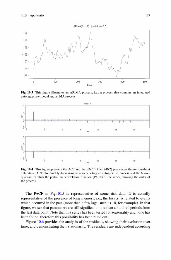
10.3 Application 137
ARIMA(1, 1, 1) φ = 0.5 θ = 0.5
Time
x
0 100 200 300 400 500
−10
010
2030
4050
Fig. 10.3 This figure illustrates an ARIMA process, i.e., a process that contains an integratedautoregressive model and an MA process
0 5 10 15 20 25 30
−0.5
0.0
0.5
1.0
Series: x
LAG
ACF
0 5 10 15 20 25 30
−0.5
0.0
0.5
1.0
LAG
PAC
F
Fig. 10.4 This figure presents the ACF and the PACF of an AR(2) process as the top quadrantexhibits an ACF plot quickly decreasing to zero denoting an autogressive process and the bottomquadrant exhibits the partial autocorrelation function (PACF) of the series, showing the order ofthe process
The PACF in Fig. 10.5 is representative of some risk data. It is actuallyrepresentative of the presence of long memory, i.e., the loss Xt is related to eventswhich occurred in the past (more than a few lags, such as 10, for example). In thatfigure, we see that parameters are still significant more than a hundred periods fromthe last data point. Note that this series has been tested for seasonality and none hasbeen found, therefore this possibility has been ruled out.
Figure 10.6 provides the analysis of the residuals, showing their evolution overtime, and demonstrating their stationarity. The residuals are independent according

138 10 Forward-Looking Underlying Information: Working with Time Series
0 1 2 3 4 5 6 7
−0.1
0.0
0.1
0.2
0.3
Lag
Parti
al A
CF
PACF Weekly Aggregated Series
Fig. 10.5 The PACF represented here exhibits the presence of long memory, i.e., the loss Xt isrelated to events which occurred a long time ago
Standardized Residuals
Time1880 1900 1920 1940 1960 1980 2000
−2−1
01
2
5 10 15 20
−0.2
0.0
0.2
0.4
ACF of Residuals
LAG
ACF
ll
l
ll
l
l
l
l
l
l
lll
ll
l
l
l
l
l
l
l
l
ll
l
l
l
l
l
l
l
l
l
l
l
l
l
l
ll
l
l l
l
l
ll
l
l
l
ll
l
l
l
ll
l
ll
l l
l
l
l
l
l
l
l
l
l
l
l
ll
l
l
ll
l
l
l
l
l
l
l
l
l
l
l
ll
ll
l
l
l
l
l
l
l
l
l
ll
l
l
l
l
l
l
l
l
l
l
l
l
l
l
l
l
l
l
l
ll
l
l
−2 −1 0 1 2
−2−1
01
2
Normal Q−Q Plot of Std Residuals
Theoretical Quantiles
Sam
ple
Qua
ntile
s
ll
l
l
ll
l
l l l
l l
ll
l
ll
l
5 10 15 20
0.0
0.2
0.4
0.6
0.8
1.0
p values for Ljung−Box statistic
lag
p va
lue
Fig. 10.6 Following the adjustment of a SARIMA model to macro-economic data (selected forillustration purposes), this figure provides the analysis of the residual, showing their evolution overtime, and demonstrating their stationarity. The residuals are independent according to the ACFand the QQ-plot advocate that the residuals are normally distributed, and the Ljung-Box statisticprovides evidence that the data are independent
to the ACF and the QQ-plot advocates that the residuals are normally distributed.The Ljung–Box statistic provides evidence that the data are independent.
Time series are particularly interesting as once it has been established that Xt
is related to past incidents, and we are interested in a particular scenario, thenthe scenarios can be analysed by shocking the time series, the parameters or thedistribution representing the residuals.

References 139
Indeed, leveraging on strategies presented in previous chapters such as changingthe distribution of �t from a Gaussian to a more fat-tailed distribution, we wouldbe able to capture asymmetric and/or more extreme behaviours. (Note that it isnecessary to transform the residuals to these have a mean equal to zero).
Besides, the multiple processes presented in this chapter, such as those capturingthe intrinsic of the data or of the residuals allow modelling changes in risk patterns,i.e., the fact that these evolve over time. As stated in the first chapter, risks asthe scenarios reflecting them are living organisms. They are in perpetual motion,therefore depending on the risk to be modelled, multiple combinations of theprevious models are possible, and these may help capturing multiple risk behaviourssimultaneously, and therefore can be a powerful tool to analyse scenarios.
References
Akaike, H. (1974). A new look at the statistical model identification. IEEE Transactions onAutomatic Control, 19(6), 716–723.
Bollerslev, T. (1986). Generalized autoregressive conditional heteroskedasticity. Journal of Econo-metrics, 31(3), 307–327.
Box, G., & Jenkins, G. (1970). Time series analysis: Forecasting and control. San Francisco, CA:Holden-Day.
Box, G. E. P., & Pierce, D. A. (1970). Distribution of residual autocorrelations in autoregressive-integrated moving average time series models. Journal of the American Statistical Association,65, 1509–1526.
Box, G. E., Jenkins, G. M., Reinsel, G. C., & Ljung, G. M. (2015). Time series analysis:Forecasting and control. New York: Wiley.
Cameron, S. (2005). Making regression analysis more useful, II. Econometrics. Maidenhead:McGraw Hill Higher Education.
Dickey, D. A., & Fuller, W. A. (1979). Distribution of the estimators for autoregressive time serieswith a unit root. Journal of the American Statistical Association, 74(366), 427–431.
Dickey, D. A., & Said, S. E. (1984). Testing for unit roots in autoregressive-moving average modelsof unknown order. Biometrika, 71(366), 599–607.
Engle, R. F., & Granger, C. W. J. (1987). Co-integration and error correction: Representation,estimation and testing. Econometrica, 55(2), 251–276.
Engle, R. F., & Ng, V. K. (1991). Measuring and testing the impact of news on volatility. Journalof Finance, 48(5), 1749–1778.
Gershenfeld, N. (1999). The nature of mathematical modeling. New York: Cambridge UniversityPress.
Glosten, L. R., Jagannathan, D. E., & Runkle, D. E. (1993). On the relation between the expectedvalue and the volatility of the nominal excess return on stocks. The Journal of Finance, 48(5),1779–1801.
Gray, H., Zhang, N., & Woodward, W. (1989). On generalized fractional processes. Journal ofTime Series Analysis, 10, 233–257.
Guégan, D. (2003). Les chaos en finance. Approche statistique. Paris: Economica.Hamilton, J. D. (1994). Time series analysis (Vol. 2). Princeton: Princeton University Press.Hannan, E. J., & Quinn, B. G. (1979). The determination of the order of an autoregression. Journal
of the Royal Statistical Society, Series B, 41(2), 190–195.Hentschel, L. (1995). All in the family nesting symmetric and asymmetric GARCH models.
Journal of Financial Economics, 39(1), 71–104.Holland, J. (1992). Adaptation in natural and artificial systems. Cambridge, MA: MIT.

140 10 Forward-Looking Underlying Information: Working with Time Series
Kroner, K. F., & Lastrapes, W. D. (1993). The impact of exchange rate volatility on internationaltrade: reduced form estimates using the GARCH-in-mean model. Journal of InternationalMoney and Finance, 12(3), 298–318.
Kwiatkowski, D., Phillips, P. C., Schmidt, P., & Shin, Y. (1992). Testing the null hypothesis ofstationarity against the alternative of a unit root: How sure are we that economic time serieshave a unit root?. Journal of Econometrics, 54(1–3), 159–178.
McCleary, R., Hay, R. A., Meidinger, E. E., & McDowall, D. (1980). Applied time series analysisfor the social sciences. Beverly Hills, CA: Sage.
Nelson, D. B. (1991). Conditional heteroskedasticity in asset returns: A new approach. Economet-rica, 59(2), 347–370.
Palma, W. (2007). Long-memory time series: Theory and methods. New York: Wiley.Rabemananjara, R., & Zakoian, J. M. (1993). Threshold ARCH models and asymmetries in
volatility. Journal of Applied Econometrics, 8(1), 31–49.Rand, W. M. (1971). Objective criteria for the evaluation of clustering methods. Journal of the
American Statistical Association, 66(336), 846–850.Schwarz, G. E. (1978). Estimating the dimension of a model. Annals of Statistics, 6(2), 461–464.Sentana, E. (1995). Quadratic ARCH models. The Review of Economic Studies, 62(4), 639–661.White, H. (1980). A heteroskedasticity-consistent covariance matrix estimator and a direct test for
heteroskedasticity. Econometrica, 48(4), 817–838.Yule, U., & Walker, G. (1927). On a method of investigating periodicities in disturbed series, with
special reference to Wolfer’s sunspot numbers. Philosophical Transactions of the Royal Societyof London, Series A, 226, 267–298.
Zadeh, L. A. (1953). Theory of filtering. Journal of the Society for Industrial and AppliedMathematics, 1, 35–51.
Zaki, M. J. (2000). Scalable algorithms for association mining. IEEE Transactions on Knowledgeand Data Engineering, 12(3), 372–390.

Chapter 11Dependencies and Relationships BetweenVariables
In this chapter we address the topic of the capture of dependencies, as these areintrinsically connected to scenario analysis. Indeed, as implied in the previouschapters, the materialisation of large losses usually results from multiple issues,faults or failures occurring simultaneously. As seen, in some approaches, themagnitude of the correlations and the dependencies are not explicitly evaluatedthough they are the core of some strategies such as neural networks or Bayesiannetworks. Here, we discuss the concepts of correlation and dependencies explicitly,i.e., these are measured and specific models or functions are built, in order to capturethem and reflect them in risk measurement.
Statistically speaking, a dependence is a relationship between random variablesor data sets (at least two). The related concept of correlation refers to statisticalrelationships embedding dependencies. Correlations are useful as they indicate arelationship that can be exploited in practice for forecasting purposes, for example.However, statistical dependence does not necessarily imply the presence of a causalrelationship. Besides, issues related to non-linear behaviours may arise. These willbe developed in the following paragraphs.
Formally, dependencies refer to any situation in which random variables donot satisfy a mathematical condition of probabilistic independence, which mayseem quite obvious, though this definition implies that the emphasis is made onindependence, therefore if the variables are not independent, these are somehowdependent. The literature counts several correlation measures and coefficients(usually denoted � or �) allowing to evaluate the degrees of these relationships. Themost famous of these is Pearson (1900) correlation coefficient, which captures linearrelationships between two variables. This measure is usually what practitionersand risk managers have in mind when the question of correlation is addressed, forinstance, the related coefficient takes its values between�1 and 1. Other correlationcoefficients have been developed to address issues related to the Pearson approachsuch as the capture of non-linear relationships and the correlations between morethat 2 factors simultaneously.
© Springer International Publishing Switzerland 2016B.K. Hassani, Scenario Analysis in Risk Management,DOI 10.1007/978-3-319-25056-4_11
141

142 11 Dependencies and Relationships Between Variables
In this chapter, we will present the theoretical foundations of the various conceptssurrounding dependencies—from correlations to copula and regressions, as wellas the characteristics and properties which may help practitioners analysing riskscenarios. We will also illustrate them with figures and examples.
11.1 Dependencies, Correlations and Copulas
11.1.1 Correlations Measures
Starting with the theoretical foundations of the methodologies related to dependencemeasurement, these will be discussed from the most common to the most advanced.And therefore, as mentioned before, the most common is the Pearson’s correlationcoefficient. It is obtained by dividing the covariance of the two variables by theproduct of their respective standard deviations.
Mathematically speaking, let .X;Y/ be a couple of random variables withexpected values �X and �Y , standard deviations �X and �Y and covariance �.X;Y/then the Pearson correlation coefficient is given by:
�.X;Y/ D �.X;Y/
�X�YD EŒ.X � �X/.Y � �Y /�
�X�Y; (11.1.1)
where E denotes the expected value and �x;y represents the covariance between Xand Y.
Obviously the Pearson correlation is only defined if both standard deviations(i.e. the second moments—see Chap. 3) of each random variable exists, are finiteand non-zero. It is also interesting to note that �.X;Y/ D �.Y;X/ and consequently thevalues are independent from the variables order.
The Pearson correlation ranges from C11 in the case of a perfect correlation to�1 representative of a perfect anticorrelation, i.e. when X increases, Y decreases insame magnitude (Dowdy et al. 2011). All the other values belonging to that rangeindicates various degrees of linear dependencies between the variables. When thecoefficient is equal to zero the variables are assumed uncorrelated. � > 0 impliesthat the random variables are evolving concomitantly while � < 0 implies that therandom variables are evolving conversely (Fig. 11.1).
A well-known issue related to Pearson’s approach can be stated as follows.Independent variables imply � D 0, but the converse is not true as this approach onlycaptures linear dependencies. As a result, non-linear dependencies are disregardedand this may lead to dreadful modelling inaccuracies.
A first alternative to Pearson’s correlation is the Spearman correlation coefficient(Spearman 1904), which is defined as the Pearson correlation coefficient between
1The Cauchy–Schwarz inequality (Dragomir 2003) implies that this correlation coefficient cannotexceed 1 in absolute value.

11.1 Dependencies, Correlations and Copulas 143
the ranked variables. For example, considering a data sample containing n datapoints, the data points Xi;Yi are ranked and become xi; yi, and � is calculated asfollows:
�.X;Y/ D 1 � 6Pı2i
n.n2 � 1/ : (11.1.2)
where ıi D xi � yi characterises the difference between ranks. Ties are assigneda rank equal to their positions’ average in the ascending order of the values. Forexample, let .x1; y1/, .x2; y2/; : : : ; .xn; yn/ be a set of observations of the jointrandom variables X and Y, respectively, such that all xi and yi are unique. Anycouple .xi; yi/ and .xj; yj/ are considered concordant if xi > xj and yi > yj or ifxi < xj and yi < yj. Conversely they are discordant, if xi > xj and yi < yj or ifxi < xj and yi > yj. If xi D xj or yi D yj, the pair is none of the previous alternative.
In parallel, Kendall’s � coefficient (Kendall 1938), another alternative to Pear-son’s coefficient is defined as:
� D .number of concordant couples/ � .number of discordant couples/12n.n � 1/ :
(11.1.3)
The denominator denotes the number of combinations, as a result � 2 Œ�1; 1�. Ifthe two rankings are perfectly matching the coefficient equals 1, if these are notmatching whatsoever, the coefficient equals �1. If X and Y are independent, thenthe coefficient tends to zero.
Another alternative is Goodman and Kruskal’s � (Goodman and Kruskal 1954),also measuring the rank correlation. The quantity G presented below is an estimateof � . This requires Ns the number of concordant pairs, Nd, the number of discordantcouples. Note that “ties” are not considered and are therefore dropped. Then
G D Ns � Nd
Ns C Nd: (11.1.4)
G can be seen as the maximum likelihood estimator for � :
� D Ps � Pd
Ps C Pd; (11.1.5)
where Ps and Pd are the probabilities that a random couple of observations willposition itself in the same or opposite order, respectively, when ranked by bothvariables.
Critical values for the � statistic are obtained using the Student t distribution, asfollows:
t � G
sNs C Nd
n.1 �G2/; (11.1.6)

144 11 Dependencies and Relationships Between Variables
where n is the number of observations, i.e., n is usually different from
n ¤ Ns C Nd; (11.1.7)
11.1.2 Regression
While in the first section we were discussing the measurement of correlations, inthat section, we are discussing another way of capturing dependencies, analysing theinfluence of a variable on another for forecast or prediction purposes (for instance):the regressions (Mosteller and Tukey 1977 and Chatterjee and Hadi 2015).
Therefore, regression analysis aims at statistically estimating relationshipsbetween variables. Many techniques are available to capture and to analyserelationships between a dependent variable and one or more independent variables.2
Regression permits analysing how a dependent variable evolves when any ofthe independent variables varies, while other independent variables remain fixed.Besides, regression analysis allows estimating, the conditional expectation of thedependent variable given the independent variables, the quantile, or the conditionaldistribution of the dependent variable given the independent variables. The objectivefunction, i.e., the regression function is expressed as a function of independentvariables which can in turn be represented by a probability distribution (Figs. 11.1,11.2, 11.3, and 11.4).
Bonus
Income
Office Hours
Market Volume
Losses
Adventurous Positions
Number of People on the Desk
Desk Volume
Experience
Economics
Controls
Front Office Risk Analysis
Fig. 11.1 This figure shows correlations pair by pair. The circle represents the magnitude ofthe correlations. These are equivalent to a correlation matrix, providing an representation of thePearson correlations. This figure allows to analyse pairwise correlations between various elementsrelated to a rogue trading in the front office
2Sometimes called predictors.

11.1 Dependencies, Correlations and Copulas 145
ll
l
l
l
ll
l
l
ll
l
l
l
ll
l
l
l
l
lll
ll
l
l
l
l
l
l
ll
l
l
l
l
2 3 4 5 6
0.5
1.0
1.5
2.0
Scatterplot
Controls
Loss
es
Fig. 11.2 This figure is a scatterplot representing losses with respect to controls. Here, we havethe expected behaviour, i.e., the level of losses decreases when the level of controls increases
3D Scatterplot
10 15 20 25 30 35 40
50
100
150
200
250
300
350
400
12
34
56
7
Office Hours
Controls
Des
k Vo
lum
e
lll
l
l
l
l
l
l
l
l l
l
l
l
l
l
l
l
l
l
l
ll
l
l
l
l
l
l
l
l
Fig. 11.3 This figure is similar to Fig. 11.2, i.e., this is a scatterplot, though compared to theprevious figure, this one represents three variables
Regression analysis is particularly interesting for forecasting purposes. Note that(once again) these strategies belong to the field of machine learning. Regressionanalysis allows detecting the independent variables related to the dependent variableand these relationships may be causal. But this methodology is to be implementedwith caution as it is easy to obtain spurious correlations and interpret them as if theywere real. Besides, we need to bear in mind that correlation does not necessarilyimply causation.
As mentioned previously, many regression techniques exist. These can be splitinto two families: the parametric methods which rely on a set of parameters to beestimated from the data (e.g. the linear regression or the ordinary least squares

146 11 Dependencies and Relationships Between Variables
Office Hours
0.5 1.0 1.5 2.0
ll
l
l
l l
l
ll
lll
l
l
l l
l
l
l
l
l
ll
l
l
ll
l
l
l
l
l
l l
l
l
l l
l
ll
lll
l
l
ll
l
l
l
l
l
ll
l
l
l l
l
l
l
l
l
1 2 3 4 5 6 7 8
1520
2530
35
ll
l
l
ll
l
ll
lll
l
l
ll
l
l
l
l
l
ll
l
l
l l
l
l
l
l
l
0.5
1.0
1.5
2.0
l
l
l
l
l
l
l
ll
l
l
l
ll
ll
l
l
ll
l
l
l
ll
l
l
l
l
ll
l
Lossesl
l
l
l
l
l
l
l l
l
l
l
ll
ll
l
l
ll
l
l
l
ll
l
l
l
l
ll
l
l
l
l
l
l
l
l
ll
l
l
l
ll
ll
l
l
ll
l
l
l
ll
l
l
l
l
ll
l
l
l
ll
l
l
l
l
l
l
l
l
l
l
l
l
l
l
l
l
l
l
l
l
l
l
l
ll
l
l
l
l
l
ll
l
l
l
l
l
l
l
l
l
l
l
l
l
l
l
l
l
l
l
l
l
l
l
l l
l
l
l
Adventurous Positions
3.5
4.5
5.5
6.5
l
l
l l
l
l
l
l
l
l
l
l
l
l
l
l
l
l
l
l
l
l
l
l
l
l
l
l l
l
l
l
15 20 25 30 35
12
34
56
78
ll
l
l
l
l
l
ll
l
l
lll
lll
l
l
ll
ll
l
l
l
ll
l
l
l
l
ll
l
l
l
l
l
ll
l
l
ll l
l ll
l
l
ll
l l
l
l
l
ll
l
l
l
l
3.5 4.0 4.5 5.0 5.5 6.0 6.5
l l
l
l
l
l
l
l l
l
l
lll
lll
l
l
ll
ll
l
l
l
ll
l
l
l
l
Number of People on the Desk
Simple Scatterplot Matrix
Fig. 11.4 This figure illustrates a scatter plot matrix, plotting pairwise relationships betweencomponents of rogue trading issues
regression), and the non-parametric regressions which rely on a specified set offunctions.
The most useful models are described in the following paragraphs, these may allbe formally expressed as,
Y � f .X;ˇ/; (11.1.8)
where Y is the dependent variable, X represents independent variables and ˇ
characterises a set of parameters. Besides, the approximation symbol denotes thepresence of an error term. The approximation is usually mathematically formalisedas E.YjX/ D f .X; ˇ/. To implement the regression analysis, the function f must bespecified as this one characterises the relationship between Y and X, which doesnot rely on the data. If unknown f is chosen according to other criteria such as itspropensity to capture and mimic a desired pattern.
To be applicable, the data must be sufficient, i.e., the number of data points (n)has to be superior to the number of parameters (k) to be estimated. If n < k, themodel is underdetermined. If n D k and f is linear, the problem is reduced tosolving a set of n equations with n unknown variables which has a unique solution.3
However, if f is non-linear the system may not have any solution or on the contrarywe may have many solutions. If N > k, then we have enough information to robustlyestimate a unique value for ˇ, the regression model is overdetermined.
Minimising the distance between the measured and the predicted values ofthe dependent variable Y (least squares minimisation) with respect to ˇ is oneof the most common ways to estimate these parameters. Note that under certain
3The factors have to be linearly independent.

11.1 Dependencies, Correlations and Copulas 147
statistical assumptions, the model uses the surplus of information to providestatistical information about the unknown parameters ˇ and the predicted valuesof the dependent variable Y, such as confidence intervals.
The main assumptions in simple regression analysis which are common to allstrategies presented in the following are
• The sample is representative of the population.• The error term is a random variable with a mean equal to zero conditional on the
explanatory variables.• The independent variables are measured with no error.• The independent variables are linearly independent.• The errors are uncorrelated.• The error terms are homoskedastic (the variance is constant over time).
Now that the main features of regressions have been presented, we will presentsome particular case that might be useful in practice. The first model presentedis the linear regression. This model presents itself in a form where the dependentvariable, yi, is a linear combination of the parameters. For example, in a simplelinear regression to model n data points there is one independent variable: xi , andtwo parameters, ˇ0 (the intercept) and ˇ1:
• Affine function (Figs. 11.2 and 11.3):
yi D ˇ0 C ˇ1xi C "i; i D 1; : : : ; n: (11.1.9)
Adding a term in x2i to the previous equation, we obtain• Parabolic function:
yi D ˇ0 C ˇ1xi C ˇ2x2i C "i; i D 1; : : : ; n: (11.1.10)
The expression is still linear but is now quadratic. In both cases, "i is an errorterm and the subscript i refers to a particular observation. Multiple linear regressionsare built the same way, however, these contain several independent variables orfunctions of independent variables.
Fitting the first model to some data, we obtain O0 and O1 the estimates,respectively, of ˇ0 and ˇ1. Equation (11.1.9), becomes
byi D O0 C O1xi: (11.1.11)
The residuals represented by �i D yi � Oyi are the difference between the valueof the dependent variable predicted by the model, byi, and the true value of thedependent variable, yi. As mentioned above, the popular method of estimation forthese cases, the ordinary least squares, relies on the minimisation of the squared

148 11 Dependencies and Relationships Between Variables
residuals formalised as follows (Kutner et al. 2004):
SSE DnX
iD1�2i : (11.1.12)
A set of linear equations in the parameters are solved to obtain O0; O1. For a simpleaffine regression, the least squares estimates are given by
b1 D
P.xi � Nx/.yi � Ny/P.xi � Nx/2 and b0 D Ny � b1 Nx; (11.1.13)
where Nx represent the mean of the xi values, and Ny the mean of the yi values. Theestimate of the variance of the error terms is given by the mean square error (MSE):
O�2" DSSE
n � p: (11.1.14)
where p represents the number of regressors. The denominator is replaced by .n �p � 1/ if an intercept is used. The standard errors are given by
O�ˇ0 D O�"s1
nC Nx2P
.xi � Nx/2 (11.1.15)
O�ˇ1 D O�"s
1P.xi � Nx/2 : (11.1.16)
These can be used to create confidence intervals and test the parameters.The previous regression models can be generalised. Indeed, the general multiple
regression model contains p independent variables:
yi D ˇ1 C ˇ2xi2 C � � � C ˇpxip C "i; (11.1.17)
where xij is the ith observation on the jth independent variable. The residuals can bewritten as
"i D yi � O1xi1 � � � � � Opxip: (11.1.18)
Another very popular regression widely used in risk management is the logisticregression which has a categorical dependent variable (Cox 1958 and Freedman2009). The logistic model is used to estimate the probability of a binary responsebased on some predictor(s), i.e., 0 or 1.
The logistic regression measures the relationship between the categorical depen-dent variable and some independent variable(s), estimating the probabilities using

11.1 Dependencies, Correlations and Copulas 149
the c.d.f. of the logistic distribution. The residuals of this model are logisticallydistributed.
The logistic regression is a particular case of the generalised linear model andthus analogous to the linear regression presented earlier. However, the underlyingassumptions are different from those of the linear regression. Indeed, the conditionaldistribution y j x is a Bernoulli distribution rather than a Gaussian distribution,because the dependent variable is binary, and the predicted values are probabilitiesand are therefore restricted to the interval Œ0; 1�.
The logistic regression can be binomial, ordinal or multinomial. In a binomiallogistic regression only two possible outcomes can be observed for a dependentvariable. In a multinomial logistic regression we may have more than two possibleoutcomes. In an ordinal logistic regression the dependent variables are ordered.
The logistic regression is traditionally used to predict the odds of obtaining “true”(1) to the binary question based on the values of the independent variables. The oddsare given by the ratio, probability of obtaining a positive outcome divided by theprobability of obtaining “false” (0).
As implied previously, here, most assumptions of the linear regression do nothold. Indeed, the residuals cannot be normally distributed. Furthermore, linearregression may lead to predictions making no sense for a binary dependent variable.To convert a binary variable into a continuous one which may take any real value,the logistic regression uses the odds of the event happening for different levels ofeach independent variable, the ratio of those odds and then takes the logarithm ofthat ratio. This function is usually referred to as logit.
The logit function is then fitted to the predictors using linear regression analysis.The predicted value of the logit is then transformed into predicted odds usingthe inverse of the natural logarithm, i.e., the exponential function. Although theobserved dependent variable in a logistic regression is a binary variable, the relatedodds are continuous.
The logistic regression can be translated into finding the set of ˇ parameters thatbest fit:
y D 1ifˇ0 C ˇ1xC " > 0 (11.1.19)
y D 0; otherwise; (11.1.20)
where " is an error distributed by the standard logistic distribution.4
ˇ parameters are usually obtained by maximum likelihood (see Chap. 5).The logistic function is useful and actually widely used in credit risk measure-
ment as it can take any input value, the output will always be between zero and one,and consequently can be interpretable as a probability.
4The associated latent variable is y0 D ˇ0 C ˇ1x C ". Note that " is not observed consequently y0is not observed.

150 11 Dependencies and Relationships Between Variables
Formalising the concept presented before, the logistic function �.t/ is defined asfollows:
�.t/ D et
et C 1 D1
1C e�t: (11.1.21)
Let t be a linear function of a single variable x (the extension to multiple variableis trivial), then t is
t D ˇ0 C ˇ1x (11.1.22)
then, the logistic function can be rewritten as
F.x/ D 1
1C e�.ˇ0Cˇ1x/ : (11.1.23)
F(x) can be regarded as the probability of the dependent variable equaling a“success”. The inverse of the logistic function, g, the logit (log odds):
g.F.x// D ln
�F.x/
1 � F.x/
�D ˇ0 C ˇ1x; (11.1.24)
and equivalently, after exponentiating both sides:
F.x/
1 � F.x/D eˇ0Cˇ1x: (11.1.25)
g.�/ is the logit function. Here g.F.x// is equivalent to the linear regressionexpression, ln denotes the natural logarithm, F.x/ is the probability that thedependent variable equals “true” considering a linear combination of the predictors.F.x/ shows that the probability of the dependent variable to represent a success isequal to the value of the logistic function of the linear regression expression. ˇ0 isthe intercept from the linear regression equation (the value of the criterion whenthe predictor is equal to zero). ˇ1x is the regression coefficient and e denotes theexponential function.
From above we can conclude that the odds of the dependent variable leading toa success is given by
odds D eˇ0Cˇ1x: (11.1.26)

11.1 Dependencies, Correlations and Copulas 151
11.1.3 Copula
While in the first section we have measured the dependence, in the second we havecaptured the impact of a variable on another, in this section, we propose buildingmultivariate functions.
Following (Guegan and Hassani 2013), a robust way to measure the dependencebetween large data sets is to compute their joint distribution function using copulafunctions. Indeed, a copula is a multivariate distribution function linking a largedata sets through their standard uniform marginal distributions (Sklar 1959; Bedfordand Cooke 2001; Berg and Aas 2009). The literature often states that the useof copulas is complicated in high dimensions except when implementing ellipticstructures (Gaussian or Student) (Gourier et al. 2009). However, they fail to captureasymmetric shocks. For example, using a Student copula with three degrees offreedom5 to capture a dependence between the largest losses (as implied by theregulation (EBA 2014)), would also be translated into higher correlations betweenthe smallest losses. An alternative is found in Archimedean copulas (Joe 1997)which are interesting as they are able to capture the dependence embedded indifferent parts of the marginal distributions. The marginal distributions might bethose presented in Chap. 5. However, as soon as we are interested in measuringa dependence between more than two sets (Fig. 11.4), the use of this class ofcopulas becomes limited as these are usually driven by a single parameter. Thereforetraditional estimation methods may fail to capture the intensity of the “true”dependence. Therefore, a large number of multivariate Archimedean structures havebeen developed, for instance, the fully nested structures, the partially nested copulasand the hierarchical ones. Nevertheless, all these structures have restrictions on theparameters and impose only using an Archimedean copula at each node (junction)making their use limited in practice. Indeed, the parameters have to decrease as thelevel of nesting increases.
An intuitive approach proposed by Joe (1997), based on a pair-copula decom-position, might be implemented (Kurowicka and Cooke 2004; Dissmann et al.2013). This approach rewrites the n-density function associated with the n-copula,as a product of conditional marginal and copula densities. All the conditioningpair densities are built iteratively to get the final one representing the completedependence structure. The approach is easy to implement,6 and has no restrictionfor the choice of functions and their parameters. Its only limitation is the numberof decompositions we have to consider as the number of vines grows exponentiallywith the dimension of the data sample and thus requires the user to select a vine
5A low number of degrees of freedom imply a higher dependence in the tail of the marginaldistributions.6A recent packages has been developed to carry out this approach - for instance the R packageVineCopula (Schepsmeier et al. https://github.com/tnagler/VineCopula) and the R package vines(Gonzalez-Fernandez et al. https://github.com/yasserglez/vines).

152 11 Dependencies and Relationships Between Variables
from nŠ2
possible vines (Antoch and Hanousek 2000; Bedford and Cooke 2002;Brechmann et al. 2012; Guégan and Maugis 2011).
To be more accurate the formal representation of copulas is defined in thefollowing way. Let X D ŒX1;X2; : : : ;Xn� be a vector of random variables, with jointdistribution F and marginal distributions F1;F2; : : : ;Fn, then (Sklar 1959) theoreminsures the existence of a function C mapping the individual distributions F1; : : : ;Fn
to the joint one F:
F.x/ D C.F1.x1/;F2.x2/; : : : ;Fn.xn//;
where x D .x1; x2; : : : ; xn/. we call C a copula.The Archimedean nested type is the most intuitive way to build n-variate
copulas with bivariate copulas, and consists in composing copulas together, yieldingformulas of the following type for n D 3:
F.x1; x2; x3/ D C�1;�2 .F.x1/;F.x2/;F.x3//
D C�1.C�2 .F.x1/;F.x2//;F.x3//;
where �i; i D 1; 2 is the parameter of the copula. This decomposition can be doneseveral times, allowing to build copulas of any dimension under specific constraints(Figs. 11.5 and 11.6).
To present the vine copula method, we use here the density decomposition andnot the distribution function as before. Denoting f the density function associatedwith the distribution F, then the joint n-variate density can be obtained as a productof conditional densities. For n D 3, we have the following decomposition:
f .x1; x2; x3/ D f .x1/ � f .x2jx1/ � f .x3jx1; x2/;
where
f .x2jx1/ D c1;2.F.x1/;F.x2// � f .x2/;
and c1;2.F.x1/;F.x2// is the density copula associated with the copula C which linksthe two marginal distributions F.x1/ and F.x2/. With the same notations we have
f .x3jx1; x2/ D c2;3j1.F.x2jx1/;F.x3jx1// � f .x3jx1/D c2;3j1.F.x2jx1/;F.x3jx1// � c1;3.F.x1/;F.x3// � f .x3/:
Then,
f .x1; x2; x3/ Df .x1/ � f .x2/ � f .x3/� c1;2.F.x1/;F.x2// � c1;3.F.x1/;F.x3//� c2;3j1.F.x2jx1/;F.x3jx1//:
(11.1.27)

11.1 Dependencies, Correlations and Copulas 153
That last formula is called vine decomposition (Fig. 11.7). Many other decompo-sitions are possible using different permutations. Details can be found in Berg andAas (2009), Guégan and Maugis (2010) and Dissmann et al. (2013).
In the applications below, we focus on these vine copulas and in particular theD-vine whose density f .x1; : : : ; xn/ may be written as,
nYkD1
f .xk/
n�1YjD1
n�jYiD1
c�;i;iCjjiC1;:::;iCj�1.F.xijxiC1; : : : ; xiCj�1/;F.xiCjjxiC1; : : : ; xiCj�1//:
(11.1.28)Other vines exist such as the C-vine:
nYkD1
f .xk/
n�1YjD1
n�jYiD1
c�;i;iCjj1;:::;j�1.F.xjjx1; : : : ; xj�1/;F.xjCijx1; : : : ; xj�1//;
(11.1.29)
where index j identifies the trees, while i runs over the edges in each tree (Figs. 11.5,11.6, and 11.7).
Cabcd (Cabc , ud)
Cabc (C ab , u c )
Cab(ua , ub)
ua ub uc ud
Fig. 11.5 Fully nested copula illustration
C abcd (C ab , Ccd )
C ab(ua , ub) Ccd (uc , ud)
ua ub uc ud
Fig. 11.6 Partially nested copula illustration

154 11 Dependencies and Relationships Between Variables
Cabc (C ab , Cbc )
C ab(ua , ub) Cbc(ub, u c )
ua ub uc
Fig. 11.7 Three-dimensional D-vine illustration: it represents another kind of structure we couldhave considering a decomposition similar to (11.1.27), considering the CDFs
ll
l
l
l
l
l
l
l
l
l
l
ll
l
l
l
l
l
l
l
l
l
l
l
l
l
l
l
l
l
l
l
l
l
l
l l
lll
l
l
l
l
l
l
ll
l
l
l
l
l
l
ll
l
l
l
l
l
l
l
l
l
ll
l
l
l
ll
l
l
l
l
l
l
l
l
l
l
ll
l
l
l
l
l
l
l
l
l
l
l
l
l
l
l l
l
l
l
l
l
l
l
l
l
l
ll
l
l
l
l
l
l
l
l
l
ll
l
l
l
l
l
ll
l
l
l
l
l
l
ll
l
l
l
l
l
l
l
l
l l
l
l
l
l
l
l
ll
l
l
l
l
l
l
l
l
l
l
l
l l l
l
l
l
l
l
l
l
l
l
l
l
ll
l
l
l
l
l
l
l
l
l
l
l
l
l
l
l
l
ll
l
l
l
ll
l
l
l
l
ll
l
l
ll
l
l
l
l
l
l
l
l
l
l
l
l
l
l
l
l
l
ll
l
ll
ll
ll
l
l
l
l
l
l
l
ll
l
l
l
ll
l
l
l
l
l
l
l
l
ll
l
l
l
l
l
l
ll
l
l
l
l
l
l
l
l
l
l
ll
l
l
l
l
l
l
l
l
l
l
l
l
l
l
l
l
l
l
l
l
l
l
ll
l
l
l
l
l
ll
l
l
l
l
l ll
l
l
l
l
l
l
l
l
l
l
l
l
l
l
l
l
l
l
l
l
l
l
l
l
l
ll
l
l
l
l
l
ll
ll
l
l
ll
l
l
l
l
l
l
l
l
l
l
l
l
ll
ll
l
l
l
l
l
l
l
l
l
l
l
l
ll
l
l
l
l
l
l
l
l
l
l
l
l
l
l
l
ll
l
l
ll
l
l
l
l
l
l
l
l
l
l
l
l
ll
l
l
ll
l
l
l
l
l
l
l
l
l
l
l
l
l
l
l
l
l
l
l
l
l
l
l l
l
l
l
l
ll
l
l
ll
l
l
l
l
l
l
l
l
l
l
l
l
l
l
ll
l
l
l
l
l
l
l
l
l
l
ll
l
l
l
l
l
l
l
l
l
l
l
l
l
l
l
l
l
l
l
l
ll
l
l
l
l
ll
l
l
l
l
l
ll
l
l
l
l
l
l
l
l
l
l
l
l
l
l
l
l
l
l
l
l
l
l l
l
l
l
l
l
l
l
l
l l
l
ll
l
l
l
l
l l
l
l
l
l
l
l
l
l
l
l
l
l
l
l
l
l
l
l
ll
l
l
l
l
l
l
l
l
l
l
ll
l
l
l l
l
l
l
l
l
l
l
ll
l
l
l
l
l l
l
l
l
l
l
l
l
l
l
l
l
ll
l
l
l
l
l
l
l
l
l
l
ll
l
l
l
ll
l
l
l
l
l
l
l
l
l
l
l
l
l
l
l
l
l
l
l
ll
l
l
l
l
l
l l
l
l
l
l
l
l
l
l
l
l
l
l
l
l
l
l
l
l
l
l
l
l
l
l
l
l
l
l
l
l
l
ll
l
l
l
l
l
l
l
ll
l
l
l
l
l
l
l
l
l
l
l
l
ll
l
l
l
l
l
l
l
l
l
l
l
l
l
l
l
l
ll
l
l
l
l
l
l
ll
l
l
l
ll
l
l
l
l
l
l
l
ll
l
l
l
l
l
l
l
ll
ll
l
l
l
l
l
l
l
l
ll
ll
l
l
l
l
l
ll
l
l
l
l
l
l
l
l
l
l
l
l
l
l
l
l
l
l
l
l
l
l
ll
l
l
l
l
l
l
l
ll
l
l
l
l
l
ll
l
lll
l
l
l
l
l l
l
l
l
l
l
l
l
l
ll
l
l
l
l
l
l
l
l
l
l
l
l l
l
l
l
l
l
l
l
l
l
l
ll
l l
l
l
l
l
l
l
l
l
l
l
l
l
l
l
ll
l
l
l
l
l
l
l
l
l
l
l
l
l
l
l
l
l
l
l
l
ll
l
l
l
l
l
l
l
l
l
l
l
l
l
l
ll
l
l
ll
l
ll
l
l
l
l
l
l
l
l
l
l
l
l
l
l
l
l
l
l
l
l
l
l
ll
l
l
l
l
ll
ll
l
l
l
l
l
l
l
l
l
l
l
l
l
l
l
l
l
l
l
l
l
l
ll
l
l
l
l
l
l
l
l ll
l
l
l
l
l
l
l
l
l
l
l
ll
l
l
l
l
l
l
l
l
ll
l
l
l
ll
l
l
l
l
l
l
l
l ll
l
l
l
l
l
l
l
l
l
l
l
ll
l
l
l
l
l
l
l
l
l
l
l
l
l
l
l
l
l
l
ll
l
l
l
l
ll
l
l
l
l l
l
l
l
l
l
l
ll
l
l
l
l
l
l
l
l
lll l
l
l
l
l
l
l
l
l
l
l
l
ll
l
l
l
l
l
l
l
l
l
l
ll
l
ll
l
l
l
l
l
l
l
l
ll
l
l
l
l
l
l
l
l
l
l
l
l
l
l
l
l
l
l
l
l
l
l
l
l
l
l
l
l
l
l
l
l
l
l
l
l
l
l
l
l
l
l
l
l
l
l
l
ll
l
l
l
l
l
l
l
l
l
l
l
l
l
l
l
l
l
l
l
l
l l
l
l
l
l
l
l
l
l
l
l
l
l
ll
l
l
l
l
l
l
l
l l
l
l
l
l
l
l
l
l
l
l
l
ll
l
l
l
l
l
l
l
l
l
l
l
l
l
l
l
l
l
l
l
l
l
l
l
l
l
l
l
l
l
l
l
l
l
l
l
ll
l l
ll
l
l
l
l
l
ll
l
l
l
l
l
l
l
l
l
l
l
l
l
l
l
l
l
l
l
l
l
l
l
l
l
l
l
l
l
l
l
l
l
l
l
l
l
l
l
l
l
l
l
l
l
ll
l
l
l
l
l
ll
l
l
l
l
l
l
ll
l
ll
l
l
l
l
l
ll
l
ll
l
l
l
l
l
l
l
l
l
l
l
l
l
l
l
l
l
l
l
l
l ll
l
l
l
l
l
l
l
l
l
l
l
l
l
l
l
l
l
l
l
l
l
l
l
l
ll
l
l
ll
ll
l
l
l
l
ll
l
l
l
l
l
l
l
l
l
l
l
l
l
l
l
l
l
l
l
l
l
l
l
ll
l
l
l
l
l
ll
l
ll
l
l
l
l
l
l
l
ll
l
l
l
l
l
l
ll
l
l
l
l
l
l
l
l
l
l
l
l
l
l
l
l
l
l
l
l
l
ll
l
l
l
l
l
l
l
l
l
l
l
l
l
l
l
l
l
l
l
l
l
l
l
ll
l ll
ll
l
l
l
l
l
l
l
l
l
l
l
l
l
l
l
l
l
l
l
l
l
l
l
l
l
l
l
l
l
l
l
l
l
l
l
l
l
l
l
l
l
l
l
l
l
ll
l
l
l
ll
l
ll
l
l
l
l
l
l
ll
l
l
l
l
ll
l
l
l
ll
l
l
l
l
l
ll
l
l
l
l
l
l
l
l
l
l
l
l
l
l
ll
l
l
l
l
l
l
l
l
l
l
l
l
l
l
l
l
l
l
l
l
l
l
l
l
l
l
l
l
l
l
l
l
l
l
l
l
l
l
l
l
l
l
l
l
l
l
l
l
l
l
l l
l
l
l
l
l
l
l
l
l
l
l
l
l
l
l
l
l
l
l
l
l
l
l
l
l
l
ll
l
l
l
l
l
l
l
l
l
l
l
l
l
l
l
ll
l
ll
l
l
l
l
l
l
l
l
lll
l
l
l
l
l
l
l
l
l
l
l
l
l
ll
l
l
l
l
l
l
l
l
l
l
l
l
l
l
l
l
l
l
l
l
l
l
l
l
l
l
l
l
l
l
l
l
l
l
l
l
l
l
l
l
l
l
l
l
l
ll
l
l
l
l
l
l
l
l
l
l
l
l
l
l
l
l
l
l
l
l
ll
l
l
ll
l
l
l
l
l
l
l
l
ll
l
l
l
l
l
l
l
l
l
l
l
l
l
l
l
l
l
l
l
l
l
l
ll
l
l
ll
l
l
l
l
l
l
l
l
l
l
l
l
l
l
l
l
l
l
l
l
l
l
l
l
l
l
l
l
l
l
l
l
l
l
l
l
l
l
l
ll
l
l
l
l
l
l
l
l
l
l
l
l
l
ll
ll
l
l
l
l
l
l
l
l
l
l
l
l
l
l
ll
l
l
l
l
l
l
l
l
ll
l
l
l
l
l
l
l
l
l
l
l
l
l
l
l
l
l
l
l
l
l
l
l
l
l
l
ll l
l
l
ll
l
l
l
l
l
ll
l
l
l
l
l
l
l
l
l
l
l
l
l
l
l
l
l
l
l
l l
l
l
l
l
l
l
l l
l
l
ll
l
l
l
l
l
ll
l
l
l
l
l
l
l
l
l
l
l l
l
l
l
l
l
l
l
l
l
l
l
l
l
l
l
l
l
l
l
l
l
l
ll
l
l
l
l
l
l
l
l
l
l
l
ll
l
l
l
l
l
l
l
l
ll
l
l
l
l
l
l
ll
l
l
l
l
l
l
ll
ll
l
l
l
l
l
l
l
l
l
l
l
l
l
l
l
l
l
l
l
l
l
l
l
l
l
l l
ll
l l
l
l
l
ll
l
l
l
l
l
l
l
l
l
l
l
l
l
l
l
l
l
l
l
l
l
l
l
l
ll
l
l
l
ll
l
l
ll
l
l
l
l
l
l
l
l
l
l
l
l
l
l
l
l
ll
l
l
l
l
l
l
l
l
l
l
l
l
l
l
l
l
l
l
l
l
l
l
l
l
l
l
l
ll
l
l
ll
l ll l
l
l
l
l
l
l
l
l
l
l
l
l
ll
l
l
l l
l
l
l
ll
l
l
l
l
l
l
l
l
l
l
l
l
ll
ll
l
l
l
l
l
l
l
ll
l
l
l
l
l l
l
l
l
l
l
l
l
l
l
l
l
l
l
l
l
ll
l
l l
l
l
l
l l
l
l
l
l
l
l
l
l
l
l
l
l
l
l
l
l
l
l
l
l
l
l
l
ll
l
l
l
l
l
l
l
l
l
l
l l
l
ll
l
l
l
ll
lll
l
l
ll
l
l
l
l
l
l
l
l
l
l
l
l
l
ll
l
l
ll
ll
l
l
l
l
ll
l
ll
l
l
l
l
l
l
l
l
l
l
l
l
l
l
ll
l
ll
l
l
l
l
l
l
lll
l
ll
l
l
l
l l
l
ll
l
l ll
l
l
ll
l
l
l
l
l
l
l
l
l
l
l
l
l
l
l
l
l
l
l
l
l
l
l
l
l
l
l
l
l
l
l
l
l
l
l
l
l
l
l
l
l
l
l
l
l
l
l
l
l
l
l
l
ll
l
l
l
l
l
ll
l
l
l
l
l
l
l
l l
l
l
l
l
l
l
l
l
l
l
l
l
l
l
l
l
l
l
l
l
l
l
l
l
l
l
l
l
l
ll
l
l
l
l
l
l
l
l
l
l
l
l
l
l
l
l
l
l
l
l
l
l
l
l
l
l
l
l
l
l
l
l
l
l
l
l
l
l
l
l
l
l
l
l
l
l
l
l
l
l
l l
l
l
ll
l
l
l
ll
l
l
l
l
l
l
l
l
l
l
l
l
l
l
l
ll
l
ll
lll
l
l
l
ll
l
l
ll
l
l
l
l
l
l
l
l
ll
l
l
l
l
ll
l
l
l
l
l
l
l
l
l
l
l
l
l
l
l
l
l
l
l
l
ll
l
l
l
l
l
l
l
l l
l
l
l
l
l
l
l
l
l
l
l
ll
l
l
l
l
l
l
l
l
l
l
l
l
l
ll
l
ll
l
l
l
ll
l
l
l
l
l
l
l
l
l
l
l
l
l
l
l
l
l
l
l
l
l
l
l
l
l
l
l
l
l
l
ll
ll
l
l
l
l
l
l
l
l
l
l
l
l
l
l
l
ll
ll
l
l
l
l
l
l
l
l
l
l
l
l
l
l
l
l
l
l
l
l
l
l
l
l
l
l
l
ll
l
l
ll
l
l
l
l
ll
l
l
l
l
l l
l
l
l
l
l
l
l
l
l
l
l
l
ll
l
l
l
l
l
l
l
l
l
ll
l
l
l
l
l
l
l
l
l
l
l
l
l
l
l
l
l
l
l
l
l
l
l
l
l
l
l
l
l
l
l
l
l
l
l
l
l
l
l
l
l
l
l
l
l
l
l
l
l
l
l
l
l
l
l
l
l
l
l
l
l
l
l
l
l
l
l
l
l
l
l
l
l
l
l
l
l
l
l
l
ll
l
l
l
l
l
l
l
l
l
l
l
l
l
l
l
l
l
l
l
l
ll
l
l
l
ll
l
l
l
l
l
l
l
l
l
l
ll
l
l
l
l
l
l
l
l
l
l
l
l
l
l
l
l
l
l
ll
ll
l
l
l
l
l
l
l
l
l
l
l
l
l
l
l
l
l
l
l
l
l
l
l
l
l
l
l
l
l
l
l
l
l
l
l
l
l
l
l
l
l
l
l
l
l
l
l
l
l
l
l
l
l
l
l
l
l
l
ll
l
l
ll l
l
l
l
l
l
ll
l
l
l
ll
l
l
l
l
l
l
l
l
l
l
l
ll
l
l
l
l
l
l
l
l
l
l
l
l
l
l
l
ll
l
l
l
l
l
l
l
l
l
l
l l
l
l
l
l
l
l
l
l
ll
l
l
l
l
l
l l
l
l
l
l
l
l
l
l
l
l
l
l
l
l
l
l
l
l
l
l
l
l
l
ll
l
l
l
l
l
l
l
l
l
l
l
l
ll
l
l
l
l
l
ll
l
l
l
l
l
l
l
l
l
l
l
l
l
l
l
l
l
l
l
l
l
l
l
ll
l
l
l
l
l
l
l
ll
l
l
l
l
l
l
l
l
l
l l
l
l
l
ll
l
l
l
l
ll
l
l
ll
l
l
l
l
l
ll
l
l
l
l
l
l
ll
l
l
l
l
l
l
l
l
l
l
l
l
l
l
l
l
l
l
l
l
l
l
l
l
l
l
l
l
l
l
l
l
l
l
l
l
l
l
l
l
l
l
l
l
l
l
l
l
l
l
l
l
l
l
l
l
l
l
l
l
l
l
l
l
l
l
l
l
l
l
l
l
l
ll
l
l
l l
l
l
l
l
l
l
l
l l
l
l
l
ll
ll
l
ll
ll
l
l
l
ll
l
l
l
l
l
l
l
l
l
l
l
ll
l
l
ll
ll
l
l
l
lll
l
l
l
l
l
l
l
l
l
l
l
l
l
l
l
l
l
ll
l
l
l
l
l
l
l
l
ll
l
l
l
l
l
l
l
l
l
l
ll
l
l
l
l
l
l
l
l
l
l
l
l
l
l
l
l
l
l
ll
l
l
l
l
l
ll
ll
l
l
l
l
l
l
l
l
l
l
l
l
l
l
l
l
l
l
l
l
l
l
l
l
l
l
l
l
l
l
l
l
l
l
l
l
l
ll
ll
l
l
l
l
l
l
l l
l
l
l
ll
l
ll
l
l
l
l
ll
l
l
ll
l
l l
l
l
l
l
l
l
l
ll
l
l
l
l
l
l
l
l
l
l
ll
l
l
l
l
l
ll
l
l
l
l
l
l
l
l
l
l
l
l
l
l
l
l
l
l
l
l
l
l
l
l
l
l
l
l
l
l
l
l
l
l
l
l
ll
l
l
l l
l
l
l
l
l
l
l
l
ll
l
l
l
l
l
l
l
l
l
l
l
l
l
l
l
l
l
ll
l
l
l
l
lll
l
l
l
l
l
l
l l
l
ll
l
l
l
l
l
l
l
l
l
l
l
l l
l
ll
l
l
l
l
l
l
l
l
l
l
l
l
l
l
l
l
l
l
l
l
l
l
l
l
l
l
l
l
l
l
l
l
l
l l
l
l
l
l
ll
l
l
l
l
l
l
l
l
l
l
l
l
l
l
l
l
l
l l
l
l
l
l
l
l
l
l
l
l
l
ll
l
l
l l
l
l
l
l
l
l
l
l
l
l
l
l
l
l
l
l
l
l
l
l
l
l
l
l
l
l
l
l
l
l
l
l
l
l
l
l
l
l
l
l
l
l
l
l
l
l
l
l
l
l
l
l
l
ll
l
l
l
l
l
l
l
l
l
l
l
l
l
l
l
ll
l
l
l
l
l
l
l
l
l
l
l
l
l
l
l
l
l lll
l
l
l
l
l
l
l l
l
l
l
l
l
l
l
l
l
l
l
l
l
l
l
l
l
l
l
ll
l
l
l
l
ll
l
l
l
l
ll
l
l
l
ll
l
l
l
l
l
l
l
l
l
l
l
l
l
l
l
l
l
l
l
l
ll
l
l
l
l
l
l
l
l
l
l
ll
ll
l
l
ll
l
l
l
l
l
l
l
l
l
l
l
l
l
l
l
l
l
l
l
l
l
l
l
l
l
l
ll
l
l
l
l
l
l
l
l
l
ll
l
l
l
l
l
l
l
ll
l
l
l l
l
l
l
l
l
l
l
l
l
l
l
l
l
l
l
l
l
l
l
l
l
l
l
l
l
l
l
l
l
l
l
l
l
l
l
l
l
l
l
ll
l
l
ll
l
l
l
l
l
l
l
l
l
l
ll
l
l
l
l
l
l
l
l
l
l
l
l
l
l
l
l
l
l
l
l
ll
l
l
l
l
l
l l l
l
l
l
l
l
l
l
l
l
l
l
l
l
l
l
l
l
l
l
l
l
l
ll
l
l
l
l
l
l
l
l
l
l
l
l
l
l
l
l
l l
l
l
l
l
l
l
l
l
l
l
l
l
l
l
l
l
l
l
l
l
l
ll
l
l
l
l
l
l
l
l
l
l
ll
l
l
ll
l
l
l
l
l
l
l
l
l
l
l
l
l
l
l
l
l
l
l
l
l
l
l
ll
l l
l
l
l
l
l
l
l
l
l
l
l
l
l
l
l
ll
l
l
ll
l
l
l
l
l
l
l
l
l
l
l
l
l
l
ll l
l
l
l
l
l
l
l
l
l
l l
l
l
ll
l
l
ll
l
l
l
l
l
l
l
l
l
l
l
l
l
l
l
l
l
l
l
l
l
l
l
l
l
l
l
l
l
l
l
l
l
l l
l
l
l
l
l
l
l
l
l
l
l
l
l
ll
l
l
l
l
l
l
l
l
l
ll
l
ll
l
l
l
l
l
l
l
l
l
ll
l
l
l
l
l
l
l
l
l
l
l
l
l
l
l
l
l
l
l
l
l
ll
l
l
l
ll
l
l
l
l
l
l
l
l
l
l
l
l
l
l
l
l
ll
l
l
l
l
l
l
l
ll
l
l
l
l
l
l
l
l
l
l
l
l
l
l
l
l
l
l
l
l
l
l
l
ll
l
l
l
l
l
l
l
l
l
l
l
l l
l
l
l
l
l
l
l
l
l
l
l
l
l
l
l
l
l
l
l
l
l
l
l
l
l
l
l
l
l
l
l
l
l
l
l l
l
l
l
l
l
l
ll
l
ll
l
l
l
l
l
l
l
l
l
l
l
ll
l
l
l
l
l
l
l
l
l
l
l
l
lll
l
l
l
l
l
ll
l
l
l
l
l
l
l
lll
l
l
l
l
l
ll
l
l
l
l
l
l
l
l
l
l
l
l
l
ll
l
l
ll
l
l
ll
l
l
l
l
l
l
l
ll
l
l
l
l
l
l
l
l
l
l
l
l
l
l
l
l
l
l
l
l
l
l
l
l
l
l
l
l
l
l
l
l
l
l
l
l
ll
l
l
l
l
l
l
l
l l
l
l
l
l
l
l
ll
l
l
ll
l
l
l
l
l
l
l
l
l
l
l
l
l
l
l
l
l
l
l
l
l
l
l
l
l
l
l
l
l
l
l
l
l
l
l
l
l
l
l
l
l
l
l
l
l
l
l
l
l
l
l
l
l
l
ll
l
l
l
l
l
l
l
l
l
l
l
l
l
ll
l
ll
l
l
lll l
l
l
l
l
l
l
l
l
l
l
l
l
l
l
l
l
l
l
l
l
l
l
ll
l
l
l
l
l
l
l
l
l
l
l
l
l
l
l
l
l
l
l
l
l
l
l
l
l
l
ll
l
l
l
l
l
l
l
l
l
l
l
l
l
l
l
l
l
l
l
l l
l
l
l
l
l
l
l
l
ll
l
l
l
l
l l
l
l
l
l
l
l
l
l
l
l
l
l
ll
l
l
l ll
l
l
l
ll
ll
ll
l
l
l
l
l
l
l
l
l
l
l
l
lll
l
l
l
l
l
ll
l
ll
l
l l
l
ll
l
l
l
l
l
l
l
l
l
l
l
l
l
l
l
l
ll
l
l
l
l
l
l
l
l
l
l
l
l
l
l
l
l
l
l
l
l
l
l
l
l
l
l
l
l
l
l
l
l
l
l
l
l
l
l
l
l
l
l
l
l
l
l
l
l
l
l
l
l
l
l
l
l
l
l
ll
l
l
l
l
l
l
l
ll
l
l
l
l
l
l
l
l
l
l
l
l
l
l
l
l
l
l
l
l
l
l
l
l
l
l
l l
l
l
l
l
l
l
l
l
l
l
l
l
l
l
l
l
l
l
l
l
l
l
l
l
l
l
l
l
l
l
l
l
l
l
l
l
l
l l
ll
l
l
l
l
l
l l
l
l
l
l
l
l
l
l
l
l
l
l
l
l
l
l
l
l
l
l
l
l
0.0 0.2 0.4 0.6 0.8 1.0
0.0
0.2
0.4
0.6
0.8
1.0
Gumbel
X
Y
l
l
l
l
l
l
l
l
l
l
l
l
l
ll
l
l
l
l
l
l
l
l
l
l
l
l
l
ll
l
l
l
l
l
l
l
l
ll
l
l
l
l
ll
l
l
l
l
l
l
l
l
l
l
l
l
l
l
l
l
l
l
l
l
ll
l
l
l
l
l
ll
l
l
l
l
l
l
l
l
l
l
l
l
l
l
ll
l
l
l
l
l
l
l
l
l
l
l
l
l
l
l
l
l
l
l
ll
l
l
l
l
l
l
l
l
l
l
ll
l
l
ll
l
l
l
l
l
l
l l
l
l
l
l
l
l
l
l
l
l
l
l
l
l
l
l
l
l
l
l
l
l
ll
l
l
l
l
l
l
l
l
l
l
l
l
l
l
l
l
l
l
l
l
l
l
l
l
l
l
l
l
l
l l
l
l
l
l
l
l
l
l
l
ll
l
l
l
l
l
l
l
l
ll
l
l
l
l
l
l
l
l
l
l
l
l
l l
l
l
l
l
l
ll
l
l
l
l
l
l
l
l
l
l
l
l
l
ll
l
l
l
l
l
l
l
l
l
l
l
l
ll
l
l
l
l
l
l
l
l
l
l
l
l
ll
l
l
l
l
l
l
l
l
l
l
l
l
l
l
ll
ll
l
l
l
l
l
ll
l
l
l
l
l
l
l
l
l
l
l
l
l
l
l
l
l
l
l
l
l
l
l
l
l
l
l
l
l
l
l
l
l
l
l
l
l
l
l
l
l
l
l
l
l
l
l
l
l
l
l
l
l
l
l
l
l
l
l
l
l
l
l
l
l
l
l
l
l
l
l
l
l
l
l
l
l
l
l
l
l
l
l
l
ll
l
l
l
l
l
l
l
ll
l l
l
l
l
l
l
l
l
l
l
l
l l
l
l
l
l
l
l
l
l
l
lll
l
l
l
l
l
l
l
l
l
l
ll
l
l
l
l
l
l
l l
l
l
l
l
l
l
l
l
l
l
l
l l
l
l
l
l
l
l
l
l
l
l
ll
l
ll
l
l
ll
l
l
l
l
l
l
l
l
l
l
l l
l
l
l
l
l l
l
l
ll
l
l
l ll
l
l
l
l
l
l
l
ll
l
l
l
l
l
l
l
l
l
l
ll
l
l
l
l
l
l
ll
l
l
l
l
l
l
ll
l
l
l
l
l
l
l
l
l
l
l
l
l
l
l
l
l
l
l l
l
l
ll
l
l
l
l
l
l
l
l
l
l
l
l
l
l
l
l
l
l
l
l
ll
l
l
l
l
l
l
l
l
l
l
l
l
l
ll
l
l
l
l
ll
ll
l
l
ll l
l
l
ll
l ll
l
l
l
l
l
l
l
l
l
l
l
l
l
l
l
l
l
l
l
l
l
l
l
l
l
l l
l
l
l
l
l
l
l
l l l
l
l
l
l
l
l
l
l
l
llll l
l
l
ll
l
l
l
l
l
l
l
l
l
l
l
l
l
l
l
l
l
l
l
l
l
l
l
ll
l
ll
l
ll
l
l
l
l
l
l
ll
l l
l
l
l
l
l
l
l
l
l
l
l
l
l
l
l
l
l
l
l
l
l
l
l
l
l
l
l
l
ll
l
l
l
l
l
l
l
l
l
l
l
l
l
l
l
l
l
l
l
l
l
l
l
l
ll
l
l
l
ll
ll
l
l
l
l
ll
l
l
l
l
l
l
l
l
l
l
l
l
ll
l
l
l
l
l
l
l
ll
ll
l
l
l
l
l
l
l l
ll
l
l
ll
l
l
l
l
l
l
l
l
ll
l
l
l
l
ll
l
l
l
l
l
l
l
l
l
l
l
ll l
l
l
l
l
l
l
l
l
l
l
l
l
l
l
l
l
ll
l
l
l
l
l
l
l
ll
l
ll
l
l
ll
l
l
l
ll
l
l
l
l
l
l
l
l
l
l
l
l
l
l
l
l
l
l
l
ll
l
l
l
l
l
l l
l
l
l
l
l
l
l
l
l l
l
l
l
l
l
l
l
l
l
l
l
l
l
l
l
l
ll
l
l
l
l
l
l
l
l
l
l
l
l
l
l
l
l
ll
l
ll
ll
l
l l
l
l
l
l
l
l
l
l
l
l
l
l
l
l
l
l
l
l
l
l
l
l
l
l
l
l
l
l
l
l
ll
l
l
l
l
l
l
l
l
l
l
ll
l
l
l
l
l
l
l
l
ll
l
l
l
l
l
l
l
l
l
l
l
l
l
l
l
l
l
l
l
l
l
l
l
l
l
l
l
l
l
l
l
l
ll
l
l
l
l
l
l
l
l
l
l
l
l
l
l
l
ll
l
l
l
l
l
l
l
l
l
l
l
l
l
l
l
l
l
l
l
l
l
l
l
l
l
l
ll
l
l
l
l
l
l
l
l
l
l
l
l
l
l
l
l
l
l
l
l
l
l
l
ll
l
l
l
l
l
l
l
l
l
l
l
l
l
l
l
l
l
l
l
l
ll
l
l
l l
l
l
l
ll
l
l
l
l
l
l
l
l
l
l
l
l
l
l
l
l
l
l
l
l
l l
l
l
l
l
l
l
l
l
l
l
l
l
l
l
l
l
l
l
l
lll
l
l
l
l
l
l
l
l
l
l
ll
l
l
l
l
l
l
l
ll
l
l
l ll
l
l
l
l
l
l
l
l
l
l
l
l
l
l
ll
l
l
l
l
ll
l
l
l
l
l
l
l
l
l
l
ll
l
l
l
l
l
l
l
l
l
l
l
l
l
l
l
l
l
l
l
l
l
ll
l
l
l
l
l
l
l
l
ll
l
l
l
l
l
l
l
l
l
l
l
l
l
l
ll
ll
l
l
l
l
ll
l
l
l
l
l
l
l
l
l
l
l
l
l
l
ll
l
l
l
l
l
l
l
ll
l
l
ll
ll
l
l
l
l
l
l
l
l
l
l
l
l
l
lll
ll
l
l
l
l
l
l
l
l
l
l
l
l
l
ll
l
ll
l
l
l
l
l
l
l
l
l
l
l
l
l
l l
l
l
l
l
l
l
l
l
l
l
l
l
l
ll
l
l
l
l
ll
ll
l
l
l
l
l
l
l
l
l
l
l
l
l
l
l
l
l
l
l
l
l
l
ll
l
l
l
l
l
l
l
l
l
l
l
l
l
l
l
l
l
l
l
l
l
l
l
l
l
l
l
l
l
l
l
l
l
l
l
ll
l
l
l
l
l
l
l
l
l
l
ll
l
l
l
l
l
ll
l
l
l
l
l
l
l
l
l
l
l
l
l
l
l
l
l
l
l
l
l
l
l
l
l
ll
l
l
l
l
l
l
l
l
l
l
l
l
l
l
l
l
l
ll
l
l
l
l
l
l
ll
l
l
l
l
l
l
l
l
l
l
l
l
l
l
l
l
l
l
l
l
l
l
l
l
l
l
l
ll
l
l
l
l
l
l
l
ll
l
l
l
l
l
ll
l
ll
l
l
l
l
ll
l
l
l
l
l l
l
l
l
l
l
l
l
l
l
l
l
l
l
l
l
l
ll
l
l
l
ll
l
ll
l
l
l
l
l
l
l
l
l
ll
ll
ll
l
ll
l
l
l
l
l
l
l
l
l
ll
l
l
l
l
l
l
l
l
l
l
l
l
l
l
l
l
l
l
l
l
l
l
l
l
l
l
l
l
l
l
l
l
l
l
l
l
l
l
l
l
l
l
ll
l
l
l
l
l
l
ll
l l
l
l
ll
l
l
l
l
l
l
l
l
l
l
l
l l
l
l
l
l
l
l
l
l
l
l
l
l
l
l
l
l
l
l
l
ll
l
l
ll
l
l
l
l
l
l
l
l
l
l
l
l
lll
l
l
l
l
l
l
l
l
l
ll
l
l
l
l
l
l
l
l
l
l
l
l
l
l
l
l
l
l
l
l
l
l
l
l
l
l
l
l
l
l
ll
l l
l
l
l
l
l
l
l
l l
ll
l
l
l
l
l
l
l
l
l
l
ll
l
l
l
l
l
l
l
ll
l
l
l
l
l
l
l
l
l
l
l
l
l
l
ll
l
l
l
l
l
l
l
ll
l
l
l
l
ll
ll
l
l
l
l
l
l
l
l
l
l
l
ll
l
l
l
ll
l
l
l
l
ll
l
l
l
l
l
l
l
l
l
l
ll
l
l
l
l
l
l
l
l
l
l
l
l
l
l
l
l
l
l
l
l
l
l
l
l
l
l
l
l
l
l
l
l
l
l
l
l
l
l
l
l
l
l
l
l
l
l
l
l
l
ll
l
l
ll
l
l
l
l
l
l
l
l
l
l
l
l
l
l
l
l
l
l
l
l
l
l
l
l
l
l
l
l
l
l
l
l
l
l
l
l
l
l
l
l
l
l
l
l
l
l
l
l
l
l
ll
l
ll
ll
l
l
l
l
l
l
ll
l
l
l
l
l
l
l
l
l
l
l
l
l
l
l
l
l
l
l
l
l
l l
l
l
l
l
ll
l
l
l
l
l
l
l
l
l
l
ll
ll
l
l
l
l
l
l
l
l
l
l
l
l
ll
l
l
l
ll
l
l
l
l
l
l
l
l
l
l
l
l
l
l
l
ll
l
l
l
l
l
l
l
ll
l
l
l
l
l
l
l
l
ll
l
l
l
l
l
l
l
l
l
l
l
l
l
l
l
l
l
l
l
l
l
l
ll
l
l
l
l
ll
l
l
l
l
ll l
l
l
l
l
l
l
l
ll
l
l
l
l
l
l
l
l
l
l
l
l
l
l
l
l
l
l
l
l
l
l
l
ll
l
l
ll
l
l
l
ll
l
l
l
l
l
l
l
l
l
l
l
l
l
l
l
l
l
l
l
l
l
l
l
l
l
l
l
l
l
l
l
l
ll
l
l
l
l
l
l
l
l
ll
l
l
l
l
l
l
l
l
l
l
l
l
l
l
l
l
l
l
l
l
ll
l
l
l
l
l
l
l
l
l
l
ll
l
l
l
l
l
l
l
l
l
l
l
l
l
l
l
ll
l
l
l
l
l
l
l
l
l
l
l
l
l
l
l
l
l
l
l
ll
l
l
l
l
l
l
l
l
ll
ll
l l
l
l
l
l
l
l
ll
l
l
l
l
l
l
l
l
l
l
l
ll
l
l
l
l
l
l
l
l
ll
ll
l
l
l
l
l
l
l
l
l l
l
l
l
l
l
l
l
l
ll
l l
l
l
ll
l
l
l
l
ll
ll
l
l l
l
l
l
ll
l
l
l
l
l
l
l
l
l
l
l
l
ll
l
l
l lll
l
l
l
l
l
l
l
l
l
l
l
l
l
l
l
l l
l
l
l
l
l
l
l
ll
l
lll
l
l
l
l
l
l
l
l
l
l
ll
l
l
l
ll
l
l
l
l
ll
ll
l
l
l
l
l
l
l
l
ll
l
l
l
l
l
ll
l
l
l
l
l
l
l
l
ll
l
l
l
ll
ll
l
l
l
l
l
l
l
l
l
l
l
l
l
l
l
l
ll
l
l
l
l
l
l
l
l
l
l
ll
l
ll
l
l
l
l
l
l
l
l
l
l
l
l
l
l
l
l
l
l
l
l
l
l
l
l
l
l
l
l
l
l
l
l
l
l
l
ll
l
ll
l
l
l
l
l
l
l
l
l
l
l
ll
l l
l
l
l
l
l
l l
l
ll
l
l
l
l
l
l
l
l
l
l
ll
l
l
l
l
ll
l
l
l
l
l
ll
ll
l
l
l
l
l
l
l
l
l
l
l
l
l
l
l
l
l
l
l
l
l
l
l
ll
ll
l
l
l
l
l l
ll
l
l
l
l
l
l
l
ll
l
l
l
l
l
l
l
l
l
ll
l
l
l
l
l
l
l
l
l
l
l
l
l
l
l
l
l
l
l l
l
l
l
l
l
l
l
l
l
l
l
l l
l
l
l
l
l
l
l
l
l
l
l
l
l
l
l
l
l
l
l
l
l
ll
l
l
l
l
l
l
l l
l
l
l
l l
l
l
l
l
l
l
l
l
l
l
l
l
l
l
l
l
l
l
l
l
l
l
ll
l
l
l
l l
l
l
l
l l l
l
l
l
l
l
l
l
l
l
l
llll
l
l
l
l
l
l
l
l
l
l
l
l
l
l
l
l
l
l
l l
l
l
l
l
l
l
l
l
l
l
l
l
l
l l
l
l
ll
l
l
ll
l
l
l
l
l
l
l
l
l
l
l
l
l
ll
l
l
l
l
l
l
l
l
l
l
l
l
l
l
l
l
l
l
l
ll
l
l
l l
l
l
l
l
l
l
l
l
l
l
l
l
l
l
l
l
l
l
l
l
l
ll
l
ll
ll
l
l
l
l
l
l
l
l
l
l
l
l
l
l
l
l
l
l
l
l
l
l
l
l
l
l
l
l
l
l
l
l
l
l
l
l
l
l
l
l
l
l
l
l
l
l
l
l
l l
l
l
l
l
l
l
l
l
l
l
l
l
l
l
l
l
l
l
l
l
l
l
l
l
l
l
l
l
ll
l
l
l
l
l
ll
l
l
l
l
l
l
l
l
l
l
l
ll
l
l
l
l
ll
l
l
l
l
l
l
l
l
l
l
l
l
l
l
l
l
l
l
l
l
ll
l
l
l
l
l
l
l
l
l
l
l
l
l
l
l
l
l
l
l
l l
l
l
l
ll
l
l
l
l
l
l
l
l
l
l
l l
l
l
l
ll
l
l
l
l
l
l
l
l
l
l
l
l
l
l
l
ll
l
l
l
l
l
l
l
ll
l
l
l
l
l
l
l
l
l
l
l
l
l
l
l
l
l
l
l
l
l
l
l
l
l
l
l
l
l
l
l
l
l
l
l
ll
l
ll
ll
l
l
l
l
l
l
l
l
l
l l
l
l
l
l
l
l
l
l
l
l
l
l
l
l
l
l
l
l
l
l
l
l
l
l
l
l
l
l
l
l
l
l
l
l
l
l
l
l
l
l
l
l
ll
l
l
l
ll
l
l
l
l
l
l
l
l
l
l
l
l
l
l
l
l
l
ll
l
l
l
l
l
l
l
l
l
l
l
l
ll
l
l
l
l
l
l
l
l
l
lll
l
l
l
l
l
l
l
l
l
l
l
l
l
l
l
l
l
l
l
l
l
l
l
l
l l
l
l
ll
l
l
l
l
l
ll
l
l
l
l
l
l
l
l
l
l
l
l
l
l
l
l
l
l
l
l
l
l
l
l
l
l
l
l
l
l
l
l
l
l
l
l
l
l
l
l
l
l
l
l
l
l
l
l
l
l
l
l
l
l
l
l
l
l
l
l
l
l
l
l
l
l
l
l
l
l
l
l
l
l
l
l
l
l
l
l
l
l
l
l
ll
l
l
l
l
l
l
l
l
l
ll
l
l
l
l
l
l
l
l
l
l
l
l
l
l
l
l
l
ll
l
l
l
l
l
l
l
l
l
l
l
l
l
l
l
l
l
l
ll
l
l
l
l
l
l
l
l
l
l
l
l
l
l
l
l
l
l
l
l
l
l
l
l
l
l
l
l
ll
l
l
l
l
l
l
l
l
l
l
l
l
l
l
l
l
l
l
l
l
l
l
ll
l
l
l
l
l
l
l
l
l
l
l
l
l
l
l
l
l
l
l
l
l
l
l
l
l
l
l
l
l
l
l
l
l
l
l
l
ll
l
l
l
l
l
l
l
l
l
lll
l
l
l
l
l
l
l
l
l
l
l
l
l
l
l
l
l
l
l
l
l
l
l
l
l
ll
l
l
ll
l
ll
l
l
l
l
l
l
l
l
l
l
l
l
l
l
l
l
l
ll
l
l
l
l
ll
l
l
l
l
l
ll
l
l
l
l
l
l
ll
ll
l
l
l
l
l
l
l
l
l
l
l
l
l
l
l
l
l
l
l
l
l
l
ll
l
l
l
l
l
l
l l
l
l
l
l
l
l
l
l
l
l
l
l
l
l
l
l
l
ll
l
l
l
l
l
l
ll
l
l
l
l
l
l
l
l
l
l
l
l
l
l
l
l
l
l
l
l
l
l
l
l
l
l
l
l l
l
l
ll
l
l
l
l
ll
l
l
l
l
l
l
ll
l
l
l
l
l
l
l
l
l
l
l
ll
ll
l
l
l
l
l
l
l
l
l
l
l
l
l
l
l
l
l
l
l
l
ll
l
l
l
l
l
l
l
l
l
l
l
l
ll
l
l
l
l
l
l
l
l
l
l
l
l
l
ll
l
l
l
ll
l
l
l
l
l
l
l
l
l
l
l
l
l
l
l
l
l
l
l
l
l
l
l
l
l
l
l
l
l
ll
l
l
l
l
l
l
l
l
l
l
l
l
l
l
l
l
l
l
l
l
ll
ll
l
l
l
l
l
l
l
l
l
l
l
l
l
l
l
l
l
l
l
l l
l
ll
l
l
l
l
l
l
l
l
l
l
l
l
l
l
l
l
l
l
l
l
l
l
l
l
l
l
ll
l
l
l
l
l
l
l
l
ll
l
ll
l
l l
ll
ll
ll
ll
l
ll
l
l
ll
l
l
l l
l
l
l
l
l
l
l
ll
ll
l
l
l
l
l
l
l
l
l
l
l
l
l
l
l
l
l
l
l
l
ll
l
l
l
ll
l
l
l
l
l
l
l
ll
l
l
l
ll
l
l
l
l
ll
l
l
l
ll
l
l
l
l
l
l
l
l
l
l
ll
l
l
l
ll
l
l
l
ll
l
ll
l
l
l l
l
l
l
l
l
l
l
l
l
l
l
l
l
l
l
l
l
l
l
l
ll
l
ll
l
l
l
l
l
l
l
l
l
l
l
l
l
l
l
l
l
l
ll
l
ll
l
l
l
ll
l
l
l
l
l
l
l
l
ll
ll
l l
l
l
l
l
l
l
l
l
l
l
l
l
l
l
l
l
l
l
l
l
l
l
l
ll
l
l
ll
l
l
l
l
l
l
l
l
l
l
l
l
l
l
l
l
l
l
l
l
l
l
l
l
l
ll
ll
l
l
l
l
l
l
l
l
l
l
l
ll
l
ll
l
l
l
l
l
l
l
l
l
l
l
l
l
l
l
l
l
l
l
l
l
l
l
l
l
l
l
l
l
l
l
l
ll
l
l
l
l
l
l
l
l
l
l
l
l
l
l
l
l
l
l
l
l
l
l
l
l
l
l
l
l
ll
l
l
l
l
l
ll
l
l
ll
l
l
l
l
ll
l
l
l
l
l
l
l
l
l
l
l
l
ll
ll
l
l
l
l
l
l
l
l
l
l
l
l
l
l
l
l
l
l
l
ll
l
l
l
l
ll
l
l
l
l
l
l
l
l
l
l
l
l
l
ll
l
l
l
l
l
l
l
l
l
l
l
l
l
l
l l
l l
l
l
l
l
l
l
l
l
ll
l
l
l
l
l
l
ll
l
l
l
l
l
l
l
ll
l
l
l
l
l
l
l
l
l
l
l
ll
l
l
l
l
l
l
l
l
ll
l
l
l
l
l
l
l
l
l
l
l
l
l
l
lll
l
l
l
l
l
l
l
l
l
l
l
l l
l
l
l
l
l
l
l
l
l
l
l
lll
l l
l
l
lll
l
l
l
l
l
l
l
l
l
ll
l
l
l
l
l
l
l
l
l
l
l
l
l
l
ll
l
l
l
l
l
l
l
ll
l
l
l
l
ll
l
l
l
l
l
l
l
l
l
l
l
l
l
l
l
l
l
ll
l
l
l
l
l
l
l
l
l
l
l
l
l
l
l l
l
l
l
l
l
l
l
l
l
l
l ll
l
l
l
l
l
l
l
l
l
l
l
ll
l
l
l
l
l
l
l
l
l
l
l
ll
l
l
l
l
l
l
l
l
l
l
l
l
l
l
ll
l
l
l
l
l
l
l
l
l
l
l
l
l
l
l
l
l
ll
ll
l
l
l
l l
l
ll
l
ll
l
l
l
l
l
l
l
l
l
l
l
l
l
l
l
l
ll
l
l
l
ll
l
l
l
l
l
l
l
l
l
l
l
l
l
l
l
l
l
l
l
l
l
l
ll
ll
l
l
l
l
l
ll
l
l
l
l
l
l
l
l
l
l
l
l
l
l
l
l
l
l
l
l
l
l
l
l
l
l
l
ll
l
l
l
l
l
l
l l
l
l
l
l
l
l
l
l
l
l
l
l
l
l
l
l
l
l
l
l
l
l
l
l
l
l
l
l
l
ll
l
ll
l
l
l
l
l
l
l
l
l
l
l
l
l
l
l
l
l
l
l
l
l
l
l
ll
l
l
l
ll
l
l
l
l
ll
l
l
l
l
l
l
l
l
l
l
l
l
l
l
ll
l
l
l
l
l
l
l
l
l
l
l
l
l
l
l
l
l
l
l
l
l
l
l
l
l
l
l
l
l
l
l
l
l
l
l
l
l
l
l
l
l
l
l
l
l
ll
l
l
l
l
l
l
l
l
ll
l
l
l
l
l
l
l
l
l
l
l
l
l
l
l
l
l
l
l
l
l
l
l l
l
l
l
l
l
l
l
l
l
l
l
l
l
l
l
l
ll
l
l
l
l
l
l
l
l
ll
ll
l
l
l
l
l
l
l
l
l
l
ll
l
ll
l
l
l
l
l
l
l
l
l l
l
l
l
l
l
l
l
l
l
l
l
l
l
l
l
l
l
l
l
l
l
l
l
l
l
l
l
l
l
l
ll
l
l
l
l
l
l
l
l
l
l
l
l
l
l
l
l
l
l
l
l
l
ll
l
l
l
0.0 0.2 0.4 0.6 0.8 1.0
0.0
0.2
0.4
0.6
0.8
1.0
Galombos
X
Y
l
l
l
ll
l
ll
l
l
l
l
l
l
l
l
l
l
l
l
l
l
l
ll
l
l
l
l
l
l
l
l
l
l
l
l
l
l
l
l
l
l
l
l
l
ll
l
lll
l
l
l
l
l
l
l
l
l
l
l
l
l
l
l
l
l
l
l
l
l
l
l
l
l
l
l
l
l
l
l
l
l
l
l
l
l
l
l
l
l
l
l
l
l
l
l
l
l
l
l
l
l
l l
l
l
l
l
l
l
l
l
l
l
l
ll
l
l
l l
l
l
l
l
l
l
l
l
l
l
ll
l
l
l
l
l
l
l
l
l
ll
l
l
l
l
l
l
l
l
l
l
l
l
l
l
l
l
l
l
l
l
l
l
l
l
l
l
l
l
l
l
l
ll
l
l
l
l
l
l
l
l
l
l
l
l
l
ll
l
l
l
l
ll
l
l
l
l
l
l
l
ll
ll
l
l
l
l
l
l
l
l
l
l
ll
l
l
l
l
l
l ll
l
l
l
l
ll
l
l
l
l
l
l
l
l
l
l
ll
l
l
l
l
l
l
l
l
l
l
l
l
ll
l
l
l
l
l
l
l
l
l
l
l
l
l
l
l
l
l
l
l
l
l
l
l
l
l
l l
l
l
l
l
l
l
l
l
l
l
l
l
l
l
l
l
l
l
l
l
l
l
l
l
l
l
l
l
l
l
l
l
l
l
l
l
l
l
ll
l
l
l
l
l
ll
l
l
l
l
l
l
l
l
l
l
l
l
l
l
l
l
l
ll
l
l
l
l
l
l
l
l
l
l
l
l
l
l
l
l
l
l
l
l
l
l
l
l l
l
l
l
l
l
l
ll
l l
l
l
l
l
l
l
l
l
l
l
l
l
l
lll
l
l
l
l
l
l
l
ll
l
l
l
l
l
l
l
l
l
l
l
l
l
l
l
l
l
l
l
ll
l
l
l
l
l
l
l
l
l
l
l
ll
l
ll
l
l
l
l
l
l
l
l
l
l
l
l
l l
l
l
l
l
l
l
l
l
l
l
l
ll
l
l
l
ll
l
l
l
ll
l
l
l
l
ll
l
l
l
l
l
l
l
ll
l
l
l
l
l
l l
l
l
l
l
l
l
l
ll
l
l
l
l
l
l
l l
l
l
l
l
l
l
l
l
l
l
l
l
l
l
l
l
l l
l
l
l
l
l
l
l
l
l
l
l
l
ll
l
l
l
l
l
l
l
l
l
l
l l
l
l
l
l
ll
l
l
l
l
l
l
l
l
l
l
l
l
l
l
l
l
l
l
l
l
l
l
l
l
l
l
l
l
l
l
l
l
l
l
l
l
l
l
l
l
l
l
l
l
l
l
l
l
l
l
l
ll
l
l
l
l
l
l
l
l
l
l
l
ll
l
l
l
l
l
l
l
l
ll l
l
l
l
l
ll
l
l
l
l
l
l
l
l
l
lll
l
l
l
l
l
l
l
l
l
l
l
l
l
l
l
l
l
l
ll
l
l
l
ll
l
l
l
l
l
l
l
l
l
l
l
l
l
l
l
l
ll
l
ll
ll
l
l
l
l
l
l
l
l
l
l
l
ll
l
l
l
l
l
l
l
l
l
l
l
l
l
l
l
l
l
l
l
l
l
l
l
l
l
l
l
ll
l
l
l
l
l
l
l
ll
ll
l
l
l
l
ll
l
l
l
l
l
l
l
l
ll
l
l
ll
ll ll
l
l
l
l
l
l
l
l
l
l
l
l
l
ll
l
l
l
l
l
l
l
l
l
l
l
l
l
l
l
l
ll
l
l
l
l
l l
ll
l
l
l
l
l
l
l
l
l l
l
l
l
ll
l
l
l
l
l
l
l
l
l
l
l
l
l
l
l
l
l
l
l
l
l
ll
l
ll
l
l
l
l
l
l
l
l
l
l
l
l
l
l
l
l
ll
l
l
l
l l
l
l
l
l
l
l
l
l
l
l
ll
l
l
l
l
l
l
l
l
l
l
l
l
l
l
l
l
l
ll
l
l
l
l l
l
l
l
l
l
l l
l
l
l
l
l
l
l
l
l
l
ll
l
l
l
l
ll
l
l
l
l
l
ll
l
l
l
l
l
l
l
l
l
l
l
l
l
l l
l
l
l
l
l
l
l
l
l
ll
l
l
l
l
l
l
l
l
l
ll
l
ll
l
l
l
l
l
l
l
l
l
l
l
l
l
l
l
l
l
l
l l
l
l
l
l
l
l
l
l
l
l
l
l
ll
l
l
l
l
l
l
l
l
l
l
l
l
l
l l
l
l
l
ll
l
l
ll
l
l
l
l
l
l
l
l
l
l
l
ll
l
l
l
l
ll
l
l
l
l
l
l
l
l
l
l
l
l
l
l
l
l
l
ll
l l
l
l
l
l
l
l
l
l
l
l
l
l
l
l
l
l
l
l
l
l
l
l
l
l
l
l
l
l
l
l
l
l
l
l
l
l
l
l
l
l
ll l
l
l
l
l
l
l
l
l
l
l
l
l
l
l
l
l
l
l
l
l
l
l
l
l
l
l
l
l
l
l
l
l
l
l
l
l
l
l
l
l
l
l
l
l
l
l
l
l
l
l
l
l
l
l
l
l
l
l
l
ll
l
l
l
l
l
l
l
l
l
l
l
l
l
l
l
ll
l
ll
l
l
l
l
l
l
l
l
ll
l
l
l
l
l
l
l
l
l
l
l
l
l
l
l
l
l
ll
l
l
l
l
l
l
l
l
l
l
ll
l
l
l
l
ll
l
l
l
l
l
l
l
l
l
l
l
l
l
l
l
l
l
l
l
l
l
l
l
l
l
l
l
l
l
l
l
l
l
l
l
l
l
l
l
l
l
l
l
l
l
l
l
l
l
l
l
l
l
l
l
l
l
l
ll
l
l
l
l
l
l
l
l
l
l
l
l
ll
l
l
l
l
l
l
l
l
l
l
l
l
l
l
l
ll
l
l
l
l
l
l
l
l
l
l
l
l l
l
l
l
l
l
l
l
l
l
l
l
l
l
l
l
l
l
l
l
l
l
l
l
l
l
l
l
l
l
l
l
l
l
l
l
l
l
l
l
l
l l
l
l
l
l
l
l
l
l
l
l
l
l
l
l
l
l
l
l
l
l
l
l
l
l
l
l
l
l
l
l l
l
l
l
l
l
l
l
l
l
l
l
l
l
l
l
ll
l
l
l
l
l
l
l
l
l
l
l
l
l
l
ll
l
l
l
l
l
l
l
l
ll
l
l
l
l
l
l
l
l
l
l
l
l
l
l
l
l
l
l
l
l
l
l
l
l
l
l
l
l
l
ll
l
l
l
l
l
l
l
l
l
l
l
ll
l
l
l
l
l
l
l
l
l
ll
l
l
l
l
l
ll
l
l
l
l
l
l
l
l
l
l
l
l
l
l
l
l
l
l
l
l
l
l
l
l
l
l
ll
l
ll
l
l
l
l
l
l
l
l
l
l
ll
l
l l
l
l
l
l
ll
l
l
l l
l
l
l
l
l
l
ll
ll
l
l
l
l
l l
l
l
l
l
l
l
l
l
l l
l
l
l
l
ll
l
l
l
l
l
l
l
l
l
l
l
l
l
l
l l
l
l
l
l
l
l
l
l
l
l
ll
l
l
l
l
l
l
l
l
l
l
l
l
l
l
l
l
l
l
l
l
l
l
l
l
l
l
l
l
l
l
l
l
l
l
l
l
l
l
l
l l
l
ll
l
l
l
l
l
l
l
ll
l
l
ll
l
l
l
l
l
l
l
l
l
l
l
l
l
ll
l
l
l
ll
l
l
l
l
l
ll
l
l
l
l
ll
l
l
l
l
l
l
l
ll
l
l
l
l
l
l
ll
l
l
l
l
l
ll
l
l
l
l
l
l
l l
l
l
l
l
l
l
l
ll
l
l
l
l
l
l
l
l
ll
l
l
l
l
l
ll
l
l
l
l
l
l
l
l
l
l
l
l
l
l
l
l
l
l
l
l
l
l
l
l
l
l
l
l
l
l
l
l
l
l
l
l
l
l
l
l
l
l
l
l
l
l
l
l
ll
l
l
ll
l l
l
l
l
l
ll
l
l
l
l
l
l
l
l
l
l
l
l
l
l
l
l
l
l
l
ll
l
l
l
l
l
l
l
l
l
l
l
l
l l
l
l
l
l
l
l
l
l
l
l
l
l
l
l
l
l
l
l
l
ll
l
l
l
l
l
l
l
l
l
l
l
l
l
l
l
l
l
l
l
l
l
l
l
l
l
ll
l
l
l
l
l
l
l
l
l
l
l
l
l
l
ll
ll
l
l
l
l
l
ll
l
l
l
l
l
l
l
l
l
l
l
l
l
l
ll
l
l
l
ll
l
l
l
l
l
l
l
ll
l
l
l
l
l
l
l
l
l
l
l
l
l
l
l
l
l
l
l
l
l
l
l
l
l
l
l
l
l
l
l
l
l
l
l
l
l
l
ll
l
l
l
l
l
l
l
ll
l
l
l
l
l
l
l
l
l
l
l
l
l
l
l
l
l
l
l
l
l
l
l
l l
l
l
l
l
l
l
l
l
l
l
l
l
l
l
l
l
l
l
l
l
l
l
l
l
l
l
ll
l
l
l
l
l
l
l
l
l
l
l
l
l
l
l
l
l
l
l
ll
l
ll
l
l
ll
l
l
l
l
l
l
l
l
l
l
l
l
l
ll
l
l
l
l
l
l
l
l
l
l
l
l
l
l
l
l
l
l
l
l
l
l
l
l
l
l
l
l
l
l
l
l
l
l
l
l
l
l
l
l
l
l
l
l
l
l
l
l
l
l
l
l
l
l
l
l
l
l
l
l
l
l
l
l
l
l
l
l
l
l l
l
l
l
l
l
l
l
l
l
l
l
l
l
l
l
l
l
l
lll
l
l
l
l
l
l
l l
l
l
l
l
l
l
l
l
l
ll
l
l
l
l
l
l
l
l
l
l
l
l
l
l
ll
l
l
l
l
l
l
l
l
l
l
l
l
l
l
l
l
l
l
l
l
l
l
ll
l
l
l
l
l
l
l
l
l
l
l
l
l
l
l
l
l
l
l
l
l
l
l
l
l
l
l
l
l
l
l
l
l
l
l
l
ll
l
l
l
l
l
ll
l
l
l
l
l
l
l
l
l
l
l
l
l
l
l
l
l
l
l
l
l
l
l
l
l
l
l
l
l
l
l
l
l
l
l
l
l
l
l
l
l
l
l
l
l l
l
ll
l
l
l
l
l
l
l
l
l
l
l
l
l
l
l
l
l
l
l
l
l
l
ll l
l
l
l
l
l
l
ll
l
l
l
l
l l
l
l
l
l
ll
l
l
l
l
l
l
l
ll
l
l
l
l
l
l
l
l
l
l
ll
l
l
l
l
l
l
l
l
l
l
l
l
l
l
l
l
l
l
l
l
l
l
l
l
l
l
l
ll
l
l
l
l
l
l
l
l
l
l
l
l
l
ll
l
l
l
l
l
l
ll
l
l
l
l
l
l
l
l
l
l
l
l
l
l
l
l
l
l
l
l
l
l
l l
l
ll
l
l
l
lll
l
l
l
l
l
l
l
l
l
l
l
l
l
l
l
l
l
l
ll
l
l
l
l
l
l
l
l
ll
l
l
l
l
l l
ll
l
l
ll
l
l
l
l
l
l
l
l
ll
l l
l
l
l
l
l
l
l
ll
l
ll
l
l
l
l
l
l
l
l
l
l
l
l
l
l l
l
ll
l
l
l
l
l
l
l
l
ll
l
l
l
l
l
l
l
l
l
l
l
l
l
l
l
ll
l
l
l
l
l
l
l
ll
ll l
l
l
l
l
l
l
l l
l
l
l
ll
l
l
l
l
l
l
l
l
l
l
ll
l
l
l
l
l
l
l
l
l
l
ll
l
l
l
l
l
l
l
l
l
l
l
l
l
l
l
l
l
l
l
l ll
l
l
l
l
l
l
l
l
l
l
l
l
l
l
l
l
l
l
l
l
l
l l
l
l
l
l
l
ll
l
l
ll
l
l
l
l
l
l
l
l
l
l
ll
l
ll
l
l
l
l
ll
l
l
ll
l
l
l
l
l
l
l
l
l
l
l
l
l
l
l
l
l
l
l
l
l
l
l
l
l
ll
l
ll
l
l
l
l
l
l
l
l
l
l
l
l
l
l
l
l
l
l
l
l
l
l
l
l
l
l
l
l
l
lll
l
l
l
l
l
l
l
l
l
l
l
l
l
l
l
l
l
l
ll
l
l
l
l
l
l
l
l
l
l
l
l
l
l
l
l
l
l
l
l
l
l
l
l
l
l
l
l
l
l
l
l
l
l
l
l
l
l
l
l
l
l
l
l
l
l
l
ll
l
l
l
l
l
l
l
l
l
l
lll
ll
l
l
l
l
l
l
l
l
l
l
l
l
ll
l
l
ll
l
l
l
l
l
l
l
l
l
l
l
ll
ll
l
l
l
l
l
l
l
l
l
l
l
l
l
l
l
l
l
l
l
l
l
ll
l
ll
l
l
l
l
l
l
l
l
l
l
l
l
l
l
l
l
l
l
l
l
l
l
l
l
l
l
ll
l
l
l
l
l
l
l
l
l
l
l
l
l
ll
l
l
l
l
l
l
l
l
l
l
l
ll
l
l
l
l
l
l
l
l
l
l
l
l
l
l
l
l
l
l
l
l
l
l l
ll
l
l
l
l
ll
ll
l
l
l
l
l
l
l
l
l
l
l
l
l
l
l
l
l
l
l
l
l
l
l
l
l
l
l
l
l
ll
l
l
l
l
l
l
ll l
l
l
ll
ll
ll
l
l
l
l
l
l
l
l
ll
ll
l
l
l
l
l
l
l
l
l
l l
l
l
l
l
l
l
l
l
l
l
l
l
l
l
l
l
l
l
l
ll
l
l
l
l
l
l
ll
l
ll
l
ll
l
l
l
l
l
ll
l
l
l
l
l
l
l
l
l
l
l
l
l
l
l
l
l
l
l
l
l
l
l
l
l
l
l
l
l
ll
l
l
l
l
l
l
ll
l
l
l
l
ll
l
l
l
l
l
l
l
l
ll
ll
l
l
l
l
l
l
l
l
l
l
l
l
l
l
l
l
l
l
ll
l
ll
l
l
l
l
l
l
l
l
l
l
l
l
l
l
l
l
l
l
l
l
l
l
l
ll
l
l
l
l
l
l
l
l
l
l
l
l
l
ll
l
l
l
l
l
l
ll
l
l
l
l
l
l
l
ll
l
l
l
l
l
ll
l
l
l
l
l
ll
ll
l
lll
l l
l
l
l
l
l
l
l
l
l
l
l
l
l
l
l
l
l
l
l
l
l
l
l
l
l
l
l
l
l
l
l
l
l
l
l
l
l
l
l
l
l
l
l
l
l
l
l
l
l
l l
l
l
l
l
l
l
l
l
l
l
l
l
ll
l
l
l
l
l
l
l
l
l
l
ll
l
l
l
l
l
l
l
l
l
l
l
l
l
l
l
l
l
l
l
l
l
l
l
l
l
l
l
l
l
l l
l
ll
l
l
ll
l
l
l
l
l
l
l
l
l
l
l
l
l
l
l
l
l
l
l
l
l
l
l
l
l
l
ll
l
l
l l
ll
l
l
l
l
l
l
l
l
l
l
l
l
l
l
l
l
l
l
l
l
l
l
l
l
l
l
l
l
l
l l
l
l
l
l
l
ll
l
l
ll
l
l
ll
l
l
l
l
l
l
l
l
l
l
l
l
l
ll
ll
l
l
ll
l
l
l
l
l
l
ll
l
l
l
l
l
l
l
l
l
l
l
l
l
l
l
l
l
l
l
l
l
l
l
l
l
l
l
l
l
l
l
l
l
l
ll
l
l
l
l
ll
l
l
l l
l
l
l
l
l
l
l
l
l
l
l
l
l
l
l
l
l
l
l
l
l
l
l
l
l
l
l
l
l
ll
l
l
l
l
l
l
l
l
l
l
l
l
l
l
l
l
l
l
l
l
l
l
l
l
ll
l
l
l
l
l
l
l
l
l
l
l
l
l
l
l
l
l
l
l
l
l
l
l
l
l
l
l
l
l
l
l
l
l
l
l
l
l
l
l
l
l
l
l
l
l
l
l
l
l
l
l
l
l
l
l
l
l
l
ll
l
ll
l
l
l
l
l
l
l
l
l
l l
l
l
l
l
l
l
l
l
l
l
l
l
l
l
l
l
l
l
l
ll
l
l
l
l
l
l
l
l
l
l
l
l
l
l
l
ll
l
l
l
l
l
l
l
l
l
l
l
l
l
l
l
l
l
l
l
ll
l
l
l
l
l
ll
l
l
l l
l
l
l
l
l
l
l
l
l
l
l
l
l l
l
l
l
l
l
l
l
l
l
l
l
l
l
l
l
l
l
ll
l
l
l
l
l
l
l
l
l
l
l
l
ll
l
l
l
lll
ll
l
l
l
l
l
l
l
l
l
l
l
l
l
l
l
l
l
l
l
l
l
l
l
l
l
ll
l
l
l
l
ll
l
l
l
l
l
l
ll
l
l
l
l
l
l
l
l
l
l
l
l
l
l
l
l
l
l
l
l
l
ll
ll
l
l
l
l
l
l
l
l
l
l
l
l
l
l
l
l
l
l
l
l
l
l
l
l
l
l
l
l
ll
ll
l
l
l
l
l
l
l
l l
l
l
l
l
l
ll
l
l
l
l
l
l
l
l
l
l
l
l
l
ll
l
l
l
l
l
l
l
l
l
l
l
l
l
l
l
l
l
l
l
l
l
l
l
l
ll
l
l
l
l
l
ll
l
l
l
l
l
l l
l
l
ll
l
l
l
l
l
l
l
l
l
ll
l
l
l
l
l
l l
l
l
l
l
l
l
l
ll
l
l
l
l
l l
l
l
l
l
ll
l
l
l
l
l
l
l
l
l
l
l
lll
l
l
l
ll
l
l
l
l
l
l
l
l
l
l
l
l
l
l
l
l
l
l
l
l
l
l
l
l
l
l
l
l
l
ll
l
l
l
l
l
l
l
l
l
l
l
l
l
l
l
l
ll
l l
l
l
l
l
l
l
l
l
l
ll
ll
l
l
l
l
l
l
l
l
l
l
l
l
l
l
l
l
l
l
l
l
l
l
l
l
l
l
ll
l
l
l
ll
ll
ll
l
l
l
l
l
l
l
l
l
l
l
l l
l
l
l
l
l
l
l
l
l
l
l
l
l
l
l
l
l
l
l
l
l
l
l
l
l
l
l
l
l
ll
l
l
l
l
l
l
l
l
l
l
l
l
ll
l
l
l
l
ll
ll
ll
ll
l
l
l
l
l
l
ll
l
l
l
l
l
l
l
ll
l
l
l
l
l
l
l
l
l
l
l
l
l
l
l
l
l
l
l
l
l
l
ll
l
l
l
l
l
l
l
ll
l
l
l
l
l
l
l
ll
l
l
l
ll
l
l
l
l
l
l
l
l
l
l
l
ll
ll
l
l
l
l
l
l
l
l
l
l
l
l
l
l
l
l
l
l
l
l
ll
l
l
ll
l
l
l
l
l
l
l
l l l
l
l
l
l
l
l
l
l
l
l
l
l
l
l
l
l
l
ll
l
l
l
l
ll
l
l
l
l
l
l
l
l
l
l
l
l
l
l
l
l
l
l
l
l
l
l
l
l
l
l
l
l
l
l
l
l
l
l
l l
l
l
l
l
l
ll
l
l
l
l
l
l
l
l
l
l
l
l
ll
l
l
l
ll
ll
l
l
l
ll
l
l
l
l
l
l
l
l
l
l
ll
l
l
ll
l
l
l
l
l
l
l
l
l
ll
l
l
l
ll
l
l
l
l
l
l
l
l
l
l
l
l
l
l
l
l
l
l
l
l
l
l
l
l
ll
l
l
l
l
l
ll
l
l
l
l
l
l
l
l
l
l
l
l
l ll
l
ll
l
l
l
l
l
l l
l
l
l
ll
l
l
l
l
l
ll
l
l
l
l
l
l
ll
l
l
l
l
l
l
l
l
l
l
l
l
l
l
l
l
l
l
l
l
l
l
l
l
l
l
l
lll
l
l
l
l
l
l
l
l
ll
l
l
l
l
l
l
l
l
l l
l
l
l
ll
l
l
ll
l
l
l
l
l
l
l
l
l
l
l
l
l
l
l
l
l
l
l
l
l
l
l
l
l
l
l
l
l
l
l
l
l
l
l
l
ll
l
l
l
l
l
ll
l
l
l
l
l
l
l
l
l
ll
l
l
l
l
ll
l
l
ll
l
l
l
l
l ll
l
l
l
l
l
l
l
l
l
l
l
l
l
l
l
l
l
l
l
l
l
l
l
l
l
l
l
l
l
l
l
l
l
l
l
l
l
l
l
l
l
l
l
l
l
l
l
l
ll
l
l
l
l
l
l
l
l
l
l
l
l
l
l l
l
l
ll
l
l
ll
ll
l
ll
l
l
l
l
l
l
ll
l
l
l
l
ll
l
l
l
ll
l
ll
l
l
l
ll
l
l
l
l
l
l
l
l
l
l
l
l
l
l
l
l
l
l
l
l
l
l
l
l
l
l
l
l
l
l
ll
ll
l
l
l
l
l
l
l
l
l
l
l
l
l
l
l
ll
l
l
l
l
l
l
ll
l
l
l
l
l
l
l
l
l
l
l
l
l l
l
l
l
ll
l
l
l
l
l
ll
l
lll
l
l
l
l
l
ll
l
l
l
l
l
l
l
l
l
ll
l
l
l
l
l
l
l
l
l
l
l
l
l
ll
l l
l
l
l
l
l
l
l
l
l
l
l
l
l
l l
l
0.0 0.2 0.4 0.6 0.8 1.0
0.0
0.2
0.4
0.6
0.8
1.0
Gaussian
X
Y
l
ll
l
l
l
l
l
ll
l
l
l
l
l
l
l
l l
l
l
l
l
l
l
l
l
l
l ll
l
l
l
l
l
l
l
l
l
l
l
l
l
l
l
l
l
l
l
l
l
l
l
l
l
ll
l
l
l
l
l
l
l
l
l
l
l
l
ll
l
l
l
l
l
l
l
l
l
l
l
l
l
l
ll
l
l
l
l
l
l
l
l
l
l
l
l
l
l
l
l
l
l
l
l
l
l
l
l
l
l
l
l
l
l
l
l
l
l
ll
l
l
l
l
l
l
l
l
l
l
l
l
l
l
l
l
l
l
l
l
l
l
l
l
ll
l
l
l
l
l
l
l
l
l
l
ll
l l
l
l
l
l
l
l
l
l
ll
l
l
l
l
l
l
l
l
ll l
l
l
l
l
l
l
l
l
l
l
l
l
l
l
l
l
l
l l
l
ll
l l
l
ll
l
l
l
ll
l
l
l
l
l
l
l
l
ll
l
l
l
l
l
l
l
l
l
l
l
l
l
l
l
l
l
l
l
l
l
l
l
l
l
l
l
ll
l
l
l
l
l
l
l
l
l
l
l
l
l
l
l
l
ll
l
l
l
l
l
l
l
l
l
l
l
l
l
l
l
l
l
l
l
l
l
l
l
l
l
l
l
l
l
l
l
l l
l
l
l
l
l
l
l
l
l
ll
l
l
l
l
l
l
l
l
lll
l
l
l
l
l
l
l
l
l
l
l
l
l
l
l
l
l
l
l
l
l
l
l l
l
l
l
l
l
l
l
l
l
l
ll
l
l
l
l
l
l
l
l
l
l
l
l
l
l
l
ll
l
l
l
l
l
l
l
l
l
l
l
l
l
l
ll
l
l
l
l
l l
l
l
l
l
l
l
l
l
l
l
l
l
l
l
l
l
l
l
l
l
l
l
l
l
l
l
l
l
l
l
l
l
l
l
l
l
l
l
l
l
l
l
l
l
l
l
ll
l
l
l
l
l
ll
l
l
l
l
l
l
l
ll
l
l
l
l
l
l
l
l
l
l
l
l
l
l
l
l
ll
l
l
l
l
l
l
l
l
l
l
l
l
l
ll
l
l
l
l
l
l
l
l
l
l
l
l
ll
l
l
l
l
l
l
l l
l
l
l
l
l
ll
l
l
l
l
l
l
l
ll
l
l
l
l
l
l
l
l
l
l
l
l
l
l
l
l
l
l
l
l
l
l
l
l
l
l
l l
l
l
l
l
l
l
l
l
l
l
l
l
l
l
l
l
l
l
l
l
l
l
l
l
l
l
l
l
l l
l
l
l
l
ll
l
l
l
l
l
l
l
l
ll
l ll
l
l
l
l
l
l
l
l
l
l
l
l l
l
l
l l
l
l
l
l
l
l
l l
l
l
l
l l
l
l
l
l
l
l
l
l
l
l
l
l
l
l
l
l
l
l
l
l
l
l
l
l
l
l
l
l
l
l
l
l
ll
l
l
l
l
l
l
l
l
ll
l
l
l
lll
l l
l
l
l
l
l
l
l
l
l
l
l
l
ll
l
l
l
l
l
l
l
l l
l
l
l
l
l
l
l
ll
l
l
l
l
l
l
l
l
l
l
l
ll
l
l
l
l
l
l
l
l
ll
l
l
l
l
l
l
l
l
l
l
l
l
l
l
l
l
l
l
l
ll
l l
l
l
l
l
l
l
l
l
l
l
l
ll
l
l
l
l
l
l
l
l
l
l
l
l
l
l
l
l
l
l
l
l
l
l
l
l
l
l
l
ll
l
ll
l
l
l
l
l
l
l
l
l
l
l
l
l
l
l
l
l
l
l
l l
l
l
l
l
l
l
l
l
l
l
l
l
l
l
l
l
ll
l
l
l
l
l
l
l
l
l
l
l
ll
l
l
l
l
l
l
l
ll
l
l
l
l
l
l
l
l
l
l
l
l
l
l l
l
l
l
l
l
l
l
l
l
l
l
l
l
l
l
l
l ll
l
l
l
l
l
l
l
l
l
l
l
l
l
l
l
l
ll
l
l
l
l
l
l
l
l
l
l
l
l
l
l
l
l
l
l
l
l
l
l
l
l
l
l
l
l
l
l
l
l
l
l
l
l
l
l
l
ll
l
ll
l
l
l l
l
l
l
l
l
l
l
l
ll
l
l
l
l
l
l
l
l
ll
l
l
l
l l
l
l
l
l
l
l
l
l
l
l
l
l
l l
l
l
l
l
l
l
l
l
l
l
l
l
l
l
l
l
l
l
l
l
ll
l
l
l
l
l
ll
l
l
l
ll
l
l
l
l
l
l
l
l
l
l
l
l
l
ll
l
l
l
l
l
l
l
l l
l
ll
l
l
l
l
l
l
l
l
l
l
l
l
l
l
l
l
l
l
l
l
l
l
l l
l
ll
l
l
l
ll
l
l
l
ll
l
l
l
ll
ll
l
l
l
l
l
l
l
ll
l
l
l
l
l
l
l
l
l
l
l
l
l
l
l
ll
l
l
l
l
l
l
l
l
l
l
l l
l
l
l
l
l
ll
ll
l
l
l l
l
l
l
l
l
l
ll
l
l
l
l
l l
l
l
l
l
l
l
l
l
ll
ll
ll
l
l
l
l
l
l
l
ll
l
l
l
l
l
l
l
l
l
l l
l
l
l
l
l
l
l
l
l
l
l
l
l
ll
l
l
l
l
l
l
ll l
l
l
l
l
l
l
l
l
l
l
l
l
l
l
l
l
l
l
l
ll
l
l
l
l
l
l
l
l
l l
l
l
l
l
l
l
l
l
l
l
ll
l
l
l
l
ll
l
l l
l
l
l
l
l
l
l
l
l
ll l
l
l
l
l
l
l
l
l
l
l
l
l
l
l
ll
l
l
l
l
l
l
l
ll
l
l
l
l
l
l
l
l
l
l
l
l
l
l
l
l
l
l
l
l
l
l
l
l
l
l
l
l
l
l
l
l
l
l
l
l
l
ll
l
l
l
ll
l
l
l
l
l
l
l
l
l
l
l
lll
l
l
l
l
l
l
ll
l
l
l
l
l
l
l
l
l
l
l
l
l
l
l
l
ll
l
l
l
l
l
l
l
l
ll
l
l
ll
l
l
l
l
l
l
l
ll
l
l
l
l
l
l
l
l
l
l
l
l
l
l
l
l
l
l
l l
ll
l
l
l
l
l
l
l
l
l
l
l
l
l
l
l
l
l
l
l
l
l
l
l l
l
l
l
l
l
ll
l
l
l
l
l
l
ll
l
l
ll
l
l
l
l
l
l
l
ll
ll
l
l
l
l
ll
l
l
l
l
l
ll
l
l
l
l
l
l
l
l
l
l
l
l
l
l
l
l
l
l
l
l
l
l
l
l
l
l
l
l
l
l
l
l
l
l
l
l
l
l
l
l
l
l
l
l
ll
l
l
l
l
l
l
l
l
l
l
l
l
l
l
l
l
l
l
l
l
l
l
l
ll
l l
l
l
l
l
ll
l
l
l
l
l l
l
ll
l
l
l
l
l
l
l
ll
l
l
l
l
l
l
l
l
l
l
l
l
l
l
l
l
l
l
l
l
l
l
l
l
ll
l
l
l
l
l
l
l
l
l
l
l
l
l
l
l
l
l
l
l
l
l
l
ll
l
l
l
l
l
l
l
l
l
l
l
l
l
l
l
ll
l
l
l
ll
l
ll
l
l
l
l
l
l
l
l
l
l l
l
l
l
l
l
l
l
l
l
l
ll
l
l
ll
l
l
ll
l
ll
l
l
l
l
l
l
l
l
l
l
l
l
l
l
ll
l
l
l
l
l
ll
l
l
l
l
l l
l
l
l
l
l
ll
l
ll
ll
l
l l
l
l
l
l
l
ll
l
ll
l
l
l
l
l
l
l
l
ll
l
l
l
l
l
l
l
l
l
l
l
ll
l
l
l
l
l
l
l
l
l ll
l
l
l
l
l
l
l
l
l
l
l
l
l
l
l
l
l
l
l
l
l
l
ll
l
l
l
l
l
l
l
l
ll
l
l
l
ll
l
l
ll l
l
l l
l
l
l
l
l
l
l
l
ll
l
l
l
l
l
l
ll
ll
l
l
l
l
l
l
l
l
l
l
l
l
l
l
l
l
l
l l
l
l
l
l
l
l
l
l
l
l
l
l
l
l
ll
l
l
l
l l
l
l
l
l
l
l
l
l
l
l
l
l
l
l
ll l
l
l
l
l
l l
l
l
l
l
l
l
l
l
l
l
l
l
ll
l
l
ll
ll
l
l
l
l
l
l
l
l l
l
ll
l
l
l
l
l
l
l
l
l
l
l
l
l
l
l
l
l
l
l
ll
l
l
l
l
l
l
l
l
l
l
ll
ll
l
l l l
l
l l
l
l
l
l
l
l
l
l
l
l
l
l
l
l
l
l
l
l
l
l
l
l
l
l
l
l
l
l
l
l
l
l
ll
l
l
l
l
ll
l
l
l
l
l
l l
l
l
l
l
l
l
l
ll
ll
l
l
l
ll
l
ll
l
l
l
l
l
l
l
l
l
l
ll
l l
ll
l
l
l
l
l
l
l
l
l
l
l
l
l
l
l
l
l
l
l
l
ll
l
l
l
l
l
l
l
lll
l
l
l
l
l
l
l l
l
l
l
l
l
l
l
l
ll
l
l
l
l
l
l
l
l
l
ll
l
l
l
l
l
l
l
ll l
l
l
l
ll
l
l
l
l
l
l
l
l
l
l
l
l
l
l
l
l
ll
l
l
l
l
l
l
l
l
l
l
l
l
l
l
l
l
ll
l
l
l
l
l
l
l
l
l
l
l
l
ll
l
l
l
l
l
l
l
l
l
l
l
l
l
l
l
l
l
l
l
l
l
l
l
ll
l
l
l
l
l
l
l
l
ll
l
l
l l
l
l
ll
l
l
l
l
l
l
l
l
l
l
l
l
l
ll
l
l
l
l
l
l
l
l
l
l
l
l
ll
l
l
l
ll
l
l
l
l
l
l
l
l
l
ll
l
l
l
l
l
l
l
l
l
l
l
l
l l
l
l
l
l
l
l l
l
l
l
l
l
ll
l
l
l
l
l
l
l
l
l
l
l
l
l
l
ll
l
l
l
l
l
l
l
l
l
l
l
l
l
l
l
ll
l
l
ll
l
l
l
l
l
l
l
l
l
l
l
l
ll
l
l
l
l
l
l
ll
l
l
l
l
l
l
l
l
l
l
ll
l
l
l
l
ll
l
l
l
ll
l
l
l
l
l
l
l
l
l
l
l
l
l
ll l
l
l
l
l
l
l
l
l
l
l
l
ll
l l
l
l
l
l
l
l
l
l
l
l
l
l
l
l
l
l
l
l
ll
l
l
ll l
l
l
l
l
l
l
l
l
l
l
l
l
l
l
ll
ll
l
l
l
l
l
l
l
l
l
l
l
l
l
l
l
lll
l
l
ll
l
l
l
l
l
l
l
l
l
l
l
l
l
l
l
l
l
l
ll
l
l
l
l
l
l
ll
ll
ll
l
l
l
l
l
l
l
l
l
l
l
l
l
l
l
l
l
l
l
l
l
l
l
l
l
l
l
l
l
l
l
l
l
l
l
l
l
l
l
ll
l
l
l
l
l
l
l
l
l
l
l
l
l
l
ll
l
l
l
l
l
l
l
l
l
l
l
l
l
l
l
l
l
l
ll
l
l
l
l
l
l
l
l
l
l
l
l
l
l
l
l
l
l
l
l
l
l
l
l
l
l
l
l
l
l
l
l
l
l
l
l
l
l
l
l
l
l
l
l
ll
l
l
l
l
l
l
l
l
l
l
l
l
l
l
l
ll
l
l
l
l
l
l
l
l
l
l
l
l
l
l
l
l
l
l
l
ll
l
ll
l
l
l
l
l
l
l
l
l
l
l
l
l
l
l
l
l
l
l
l
l
l
l
l
l
l
l
l
l
l
ll l
l
l
l
ll
l
l
l
l
l
l
l
l
l
l
l
l
l
l
l
l
l
l
l
l
l
ll
l
l
l
l
l
l
l
l l
l
l
l
l
ll
l
l
l
l
ll
l
l
l
l
l
l l
l
l
l
l
l
ll
l
l
l l
l
l
l
l
l
l
l
l
l
l
l
l
ll
ll
l
l
l
l
l
l
l
l
l
l
l
l
l
l
l
l
l
l
l
l
l
l
l
l
l
l
l
l
ll
l
l
l
l
l
l
l
l
l
ll
l
l
l
l
l
l
l
ll
l
l
l
l
l
l
l
l
l
l
l
l
l
l
ll
l
l
ll
l
l
l
l
l
l
l
l
l
l
l
l
l
l
l
l
l
l
l l
l
l
l
l
l
l
l
ll
l
l
l
l
l
ll
l
l
l
l
l
l
l
l
l
ll
l
l
l
l
l
l
l
l
l
l
ll
l
l
l
l
l l
l
l
l
l
l
l
l
l
l
ll
l
l
l
l
l
l
l
l
l
l
l
l
l
l
l
l
l
l
l
l
l
l
l
l
l
l
l
l
l
l
l
l
l
l
l
l
l
ll
l
l
ll
l
l
ll
l
l l
l
l
l
l
l
l
l
l
l
l
l l
l
l
l
l
l
l
l
l
l
l
l
l
l
l
l l
l
l
l
l
l
l
l
l
l
l
l
l
l
l
l
l
l
l
l
l
l
l
ll
l
l
l
l l
l
l
l
l
l
l
l
l
l
l
l
ll
l
l
l
l
ll
l
l
ll
l
l
ll
l
ll
l
l
l
l
l
l l
l
l
l
ll
l
l
l
l
ll
ll
l
l
l
l
l
l
l
l l
l
l
l
ll
l
l
l
l
l
l
l
l
l
l
l
l
l
l
l
l
l
ll
l
l
l
l
l
l
l
l
ll
l
l
l
l
l
l
l
l
l
ll
l
l
ll
l
l
l
l
l
l
l
l
l
l
l
l
l
l
l
l
l
l
l
l
l
l
l
l
l
l
l
ll
l
l
l
ll
l
l
l
l
l
l
l
l
l
l
l
l
l
l
l
l
l
l
l
l
l
l
l
l
l
l
l
l
l
l
ll
l
l
l
l
l
l
l
ll
l
l
l
l
l
l
l
l
l
l
l
l
l
l
l
l
l
l
ll
l
l
l
l
l
l
l
l
l
l
l
l
l
ll
l
l
l
l
l
l
l
l
l
l
ll
l
l
ll
ll
l
l
l
l
l
l
l
l
l
ll
l
l
l
ll
l
l
l
ll
ll
l
l
l
l
l
l
l
l
l
l
l
l
l
l
ll
l
l
l
l
l
l
l
l
l
ll
l
ll
l
l
l
l
l
l
l
ll
l
l
l
l
l
ll
l
l
ll
ll
l
l
l
l
ll
l l
l
l
l
l
l
l
l
l
l
l
l
l
l
l
ll
l
ll
l
l
l
l
l
l
l
l
l
l
l
ll
l
l
l
l
l
l
l
l
l
l
l
l
l
l
l
l
l
l
l
l
l
l
l
l
ll
l
ll
l
l
l
l
l
l
l
l
l
l
l
l
l
l
l
l
l
l
l
l
l
l
l
ll
l
l
l
l
l
l
l
l
l
l
l
l
ll
l
l
l
l
l
l
l
l
l
l
l l
l
l
l
l
l
l
l
l
l
l
l
l
l
l
ll
l
l
l
l
l
l
l
l
l
l
l
l
l
l
l
l
l
l
l
l
l
l
l
l
l
l
l
l
l
l
l
l
l
l
l
l
l
l
l
l
l
l
l
l
l
l
l
l
l
l
l
l
l
l
l
l
l
l
l
ll
l
l
l
l
l
l
l
l
l
l
l
l
l
l
l
l
l
l l
l
l
l
l
l
l
l
l
l
l
l
l
l
l
l
l
l
l
l
l
ll
l
l
l
l
l
ll
l
l
l
l
l
l
l
l
l
l
l
l
l
l
l
l
l
l
l l
l
l
l
l
l
l
ll
l l
l
l
l
l
l
l
l
ll
l
l
l
l
l
l
l
l
l
l
l
l
l
l
l
l
l
l
l
l
l
l
l
l
l
l
l
l
l
l
l
ll
l
l
l
l
l
l
l
l
ll
l l
l
ll
l
l
l
ll
l
l
l
l
l
l
l
l
l
l
l
l
l
l
ll
l
l
l
l
l
l
l
l
l
l
l
l
l
l
l
l
l
l
l
l
l
ll
l
l
l
l
l
l
l
ll
l
l
l
l
l
l
l
l
l
l
l
ll
l
l
l
l
l
l
l
l
l
l
l
l
l
l
l
l
l
l
l
l
l l
l
l
ll
l
l
l
l
l
l
l
l
l
l
l
l
l
l
l
l
l
l
l
l
l
l
l
l
l
l
l
l
l
l
l
ll
l
l
l
l
l
l
l
l
l
l
l
l
l
l
l
l
l
l
l
ll
l
l
l
l
l
l
l
l
l
l
l
l l
l
l
l
ll
l
l
l
l
l
ll
l
ll
l
l
l
l
l
l
l
l
l
l
l
ll
l
l
l
l
l
l
l
l
l
l
l
l
ll
ll
l
l
l
l
l
l
l l
l
l
l
l
l
l
ll
l
l
l
l
l
l
l
l
l
l
l
l
l
l
l
l l
l
l
l
l
l
ll
l
l
l
l
l
l
l
l
l
l l
l
l
l
l
l
l
l
ll
l
l
l
l
l
ll
l
l
l
l
l
l
l
l
l
ll
l
l
l
l
l
l
l
l
l
l
l
l
l
ll
l
l
l
l
l
l
l
l
l
l
l
l
l
l
l
l
ll
l
ll
l
l
l
l
l
l
l
l
ll
l
ll
l
l
l
l
l
l
ll
l
l
l
l l
l
l
l
l
l
l
l
l
l
l
ll
l
l
l
l
l
l
l
l
l
l
l
l
l
ll
l
l
l
l
l
l
l
l l
l
l
l
l
l
l
l
l
l
l
l
l
l
l
l
ll
l
ll
l
l
l
l
l
l
l
l
l
l
l
l
l
l
l
ll
l
l l
l
ll
l
l
l
l
l
l
l
l
l
l l
l
l
l
l
l
ll
l
l
l
l
l
l
l
l
l
l
l
l
l
l
l
l
l
l
l
l
l
l
l ll
l
ll
l
l
l
l l
l
l
l
l
l
l
l
l
l
l
l
l
l
l
l
l
l
l
l
l
l
l
l
l
l
l
l
l
l
l
l
l
l
l
l
l
l
l
l
l
l
l
l
ll
l
l
l
l
l
l
l
l
l
l
l
ll
ll
l
l
l
l
l
l
l
l
l
l
ll
ll
l l
l
l
l
ll
l
l
l
l
l
l
l
l
l
l
l
l
l
l
ll
l
l
l
l
l
ll
l
l
l
l
l
l
l
l
l
l
l
l
l
l
l
ll
l
l
l
l
l
l
l
l
l
l
l
l
l
l
ll
l
l
l
l
l
l
l
l
ll
l
l
l
l
ll
l
l
l
l
l
l
l
l
l
l
l
l
l
l
l
l
l
l
l
l
l
l
l
l
l
ll
l
l
l
l
l
l
l
l
l
l
l
l
l
l
l
l
l
ll
l
l
l
l
l
l
l
l
l
l
l
l
ll
l
l
l
l
l
l
l
l
l
ll
l
l
l
l
l
l
l
l
l
l
l
l
l
l
l
ll
l
l
l
l
ll
l l
l
l
l
l
l
l
l
l
ll
l
l
l
l
l
l
l
l
l
l
l
l
l
l
l
ll
l
l
ll
l
l
l
l
l
ll
l
l
l
l
l
l
l
l l
l
l
l
l
ll
l
l
l
l l
l
l
l
l
l
l
ll
l
l
l
l
l
l
l
l
l
l
l
l
ll
l
l
l
l
l
l
l l
l
l
l
l
l
l
l
l
l
l
l
l
l
l
l
l
l l
l
l
l
l
l
l
l
l
l
ll
l
l
l
l
l
l
l
l
l
l
l
l
l
l
l
l
l
l
l
l
l
l
l
ll
l
l
l
l
l
l
l
l
l
l
l
l
l
l
ll
l
l
l
l
l
l
l
l
l
l
l
l
l
l
ll
l
l l
l
l
l
l
l
l
l
l
l
l
l
l
l
l
l
l
l
l
ll
l
l
l
l
l
l
l
l
ll
l
l
l
l
ll
l
l
l
l
l
l
l
l
l
l
l
l
l
l
l
l
l l
l
ll
l
l
ll
l
l
l
l
l
l
l
l
l
l
l
ll
l
l
l l
l
l
l
l
l
l
l
l
l
l
l
l
ll
l
l
l
l
l
ll
l
l l
l
l
l
l
l
l
l
l
l
l l
l
l
l
l
l
l
l
l
l
l
ll
l
l
l
l
l
l
l
l
l
l
l
l
l
l
l
l
l
l
l
l
l
l
l
l
l
l
l
l
l
l
l
l
l
l
l
l
l
l
l
l
l
ll
l
l
l
ll
l
l
l
l
l
l
ll
l
l
l
l
l
l
l
l
l
l
ll
l
l
l
l
l
l
l
l
l
l
l
l
l
l
l
l
l
l
l
l
l
l
l
l
l l
ll
l
l
l
l
ll
l
l
l
ll
l
l
l
l
l
l
l
l
l
l
l
l
l
l
ll
l
l l
l
l
ll
l
l
l
l
l
l
l
l
l
l
l
l
l
l
l
l
l
l l
l
l
l
l
l
l
l
l
l
l
l
l l
l
l
l
l
l
l
l
l
l
l
l l
l
l
l
l
l
l
l
l
l
l
l
ll
l
l
l
l
ll
l
l
l
l
l
l
l
l
l
l
l
l
l
l
l
l
l
l
l
l
l
ll
l
l
l
ll
l
l
l
l
l
l
l
l
l
l
l
l
l
0.0 0.2 0.4 0.6 0.8 1.0
0.0
0.2
0.4
0.6
0.8
1.0
Clayton
X
Y
Fig. 11.8 This figure represents four types of copulas. Starting from the top left hand corner,the Gumbel copula which is an Archimedean copula is upper tail dependent. The top right-handcorner copula is the Galambos, an extreme value copula. The bottom left-hand corner representsthe Gaussian copula belonging to the elliptic family. Mathematically this copula is the inverse ofthe multivariate Gaussian distribution. The last one represents the Clayton copula, an Archimedeancopula which is lower tail dependent
Some usual copulas (Fig. 11.8) are provided in the following (Ali et al. 1978; Joe1997; Nelsen 2006):
• Gaussian: Cˆ†.u/ D ‚†.‚
�1.u1/; : : : ; ‚‹1.ud//, † being a correlation matrix.• Student-t: Ct
†;v.u/ D t†;v.t�1v .u1/; : : : ; t�1v .ud//, † being a correlation matrixand v the number of degrees of freedom.
• Ali–Mikhail–Haq: uv1��.1�u/.1�v/ , � 2 Œ�1; 1/.
• Clayton: max
˚u�� C v�� � 1I 0���1=� , � 2 Œ�1;1/nf0g� 2 Œ�1;1/nf0g.
• Frank: � 1�
logh1C .exp.��u/�1/.exp.��v/�1/
exp.��/�1i, � 2 Rnf0g.
• Gumbel: exph� �.� log.u//� C .� log.v//�
1=�i, � 2 Œ1;1/.
• Joe: 1 � .1 � u/� C .1 � v/� � .1 � u/� .1 � v/� �1=� , � 2 Œ1;1/.

11.2 For the Manager 155
11.2 For the Manager
In this section, we will discuss points that are to be remembered when thesemethodologies are implemented. Following the structure of the chapter, we startwith the correlation coefficients in particular the most commonly used, the Pearsoncorrelation which measures the strength of linear association between two variables.The first interesting point is that outliers can heavily influence linear correlationcoefficients and may lead to spurious correlations between two quantitative vari-ables. Besides, Pearson’s correlation relates to covariances, i.e., variables movingtogether, but it does not mean that a real relation exists.
Besides, the correlation coefficient is a numerical way to quantify the relationshipbetween two variables and is always between �1 and 1, thus �1 < � < 1. Largercorrelation coefficients, i.e., closer to 1 suggest a stronger relationship between thevariables, whilst closer to 0 would suggest weaker ones. This leads to outcomes easyto interpret.
It is important to remember that correlation coefficients do not imply causality.If two variables are strongly correlated, it does not mean that the first is responsiblefor the other’s occurrence and conversely.
Now, discussing the performance of regression analysis methods in practice,this depends on the data-generating process, and the model used to representthem. As the first component, i.e., the data-generating process is usually unknown,the appropriateness of the regression analysis depends on the assumptions maderegarding this process. These are sometimes verifiable if enough data are available.Regression models for prediction are often useful even when the assumptions aremoderately violated, although they may not perform optimally, but we shouldbeware misleading results potentially engendered in these situations.
Sensitivity analysis, such as variation from the initial assumptions may helpmeasuring the usefulness of the model and its applicability.
Now focusing on the use of copulas, it is important to understand that thoughthey are powerful tools they are not the panacea. Some would actually argue thatthe application of the Gaussian copula to CDOs acted as catalyst in the spreadingof the sub-prime crisis, even though the limitations of copula functions such as thelack of dependence dynamics and the poor representation of extreme events weretried to be addressed.
Note that Gaussian and Student copulas have another problem, despite beingwidely used these are symmetric structure, i.e., if we have asymmetric negativeshocks, these will be automatically transferred on the other side. In other words, ifonly large negative events have a tendency to occur simultaneously, the structurewill also consider that large positive events also occur simultaneously which asmentioned previously might not be the case.
Alternative briefly presented in this chapter are not necessary easier to use, as theparametrisation might be complicated.
Further to the brief discussions regarding the presented methodology, as they arerelated to the analysis of correlations, we thought it might be of interest to brieflyaddress and illustrate the exploratory data analysis methodologies, for instance,
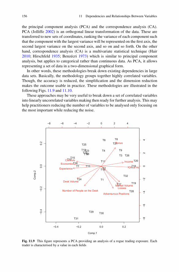
156 11 Dependencies and Relationships Between Variables
the principal component analysis (PCA) and the correspondence analysis (CA).PCA (Jolliffe 2002) is an orthogonal linear transformation of the data. These aretransferred to new sets of coordinates, ranking the variance of each component suchthat the component with the largest variance will be represented on the first axis, thesecond largest variance on the second axis, and so on and so forth. On the otherhand, correspondence analysis (CA) is a multivariate statistical technique (Hair2010; Hirschfeld 1935; Benzécri 1973) which is similar to principal componentanalysis, but applies to categorical rather than continuous data. As PCA, it allowsrepresenting a set of data in a two-dimensional graphical form.
In other words, these methodologies break down existing dependencies in largedata sets. Basically, the methodology groups together highly correlated variables.Though, the accuracy is reduced, the simplification and the dimension reductionmakes the outcome usable in practice. These methodologies are illustrated in thefollowing Figs. 11.9 and 11.10.
These approaches may be very useful to break down a set of correlated variablesinto linearly uncorrelated variables making then ready for further analysis. This mayhelp practitioners reducing the number of variables to be analysed only focusing onthe most important while reducing the noise.
−0.4 −0.2 0.0 0.2
−0.4
−0.2
0.0
0.2
Comp.1
Com
p.2
T1
T2
T3
T4T5
T6
T7
T8
T9
T10
T11
T12
T13
T14T15
T16T17
T18
T19
T20
T21
T22T23
T24
T25
T26
T27
T28
T29 T30
T31
T32
−8 −6 −4 −2 0 2 4
−8−6
−4−2
02
4
Office HoExperience
Economics
Desk VolumeMarket Volume
Controls
Bonus
Income
Losses
Adventurous PositionsNumber of People on the Desk
Fig. 11.9 This figure represents a PCA providing an analysis of a rogue trading exposure. Eachtrader is characterised by a value in each fields

References 157
Dimension 1 (4%)
Dim
ensi
on 2
(4%
)
−6 −4 −2 0 2 4 6
−2−1
01
23
ll
l
l
l
l
l
l
l
l
l
l
l
l
l
l
l
l
l l
l
ll
l
ll
l
l
l
l
l
1.622.07
2.26
2.28
2.44
2.75
2.82.85
3.22
3.38
3.44
3.47
3.53
3.6
3.61
3.62
3.88
3.9
3.914.03
4.24
4.34.32
4.36
4.494.51
4.56
4.6
5.75
6.04
6.3
0.090.170.20.26
0.320.34
0.44
0.480.67
0.68
0.740.75
0.79
0.910.96
1.02
1.121.131.21
1.321.381.56
1.621.681.73
1.751.95
Fig. 11.10 This figure represents a CA providing an analysis of a rogue trading exposure
References
Ali, M. M., Mikhail, N. N., & Haq, M. S. (1978). A class of bivariate distributions including thebivariate logistic. Journal of Multivariate Analysis 8, 405–412.
Antoch, J., & Hanousek, J. (2000). Model selection and simplification using lattices. CERGE-EIWorking Paper Series (164).
Bedford, T., & Cooke, R. M. (2001). Probability density decomposition for conditionally depen-dent random variables modeled by vines. Annals of Mathematics and Artificial Intelligence, 32,245–268.
Bedford, T., & Cooke, R. (2002). Vines: A new graphical model for dependent random variables.The Annals of Statistics, 30(4), 1031–1068.
Benzécri, J.-P. (1973). L’Analyse des Données. Volume II: L’Analyse des Correspondances. Paris:Dunod.
Berg, D., & Aas, K. (2009). Models for construction of multivariate dependence - a comparisonstudy. The European Journal of Finance, 15, 639–659.
Brechmann, E. C., Czado, C., & Aas, K. (2012). Truncated regular vines in high dimensions withapplication to financial data. Canadian Journal of Statistics, 40(1), 68–85.
Capéraà, P., Fougères, A. L., & Genest, C. (2000). Bivariate distributions with given extreme valueattractor. Journal of Multivariate Analysis, 72, 30–49.
Chatterjee, S., & Hadi, A. S. (2015). Regression analysis by example. New York: Wiley.Cox, D. R. (1958). The regression analysis of binary sequences (with discussion). Journal of Royal
Statistical Society B, 20, 215–242.Dissmann, J., Brechmann, E. C., Czado, C., & Kurowicka, D. (2013). Selecting and estimating
regular vine copulae and application to financial returns. Computational Statistics & DataAnalysis, 59, 52–69.
Dowdy, S., Wearden, S., & Chilko, D. (2011). Statistics for research (Vol. 512). New York: Wiley.Dragomir, S. S. (2003). A survey on Cauchy–Bunyakovsky–Schwarz type discrete inequalities.
JIPAM - Journal of Inequalities in Pure and Applied Mathematics, 4(3), 1–142.EBA. (2014). Draft regulatory technical standards on assessment methodologies for the advanced
measurement approaches for operational risk under article 312 of regulation (eu), no. 575/2013.London: European Banking Authority.
Freedman, D. A. (2009). Statistical models: Theory and practice. Cambridge: Cambridge Univer-sity Press.

158 11 Dependencies and Relationships Between Variables
Galambos, J. (1978). The asymptotic theory of extreme order statistics. Wiley series in probabilityand mathematical statistics. New York: Wiley.
Gonzalez-Fernandez, Y., Soto, M., & Meys, J. https://github.com/yasserglez/vines.Goodman, L. A., & Kruskal, W. H. (1954). Measures of association for cross classifications.
Journal of the American Statistical Association, 49(268), 732–764.Gourier, E., Farkas, W., & Abbate, D. (2009). Operational risk quantification using extreme value
theory and copulas: from theory to practice. The Journal of Operational Risk 4, 1–24.Guégan, D., & Maugis, P.-A. (2010). New prospects on vines. Insurance Markets and Companies:
Analyses and Actuarial Computations, 1, 4–11.Guégan, D., & Maugis, P.-A. (2011). An econometric study for vine copulas. International Journal
of Economics and Finance, 2(1), 2–14.Guegan, D., & Hassani, B. K. (2013). Multivariate vars for operational risk capital computation:
a vine structure approach. International Journal of Risk Assessment and Management, 17(2),148–170.
Hair, J. F. (2010). Multivariate data analysis. Pearson College Division.Hirschfeld, H. O. (1935). A connection between correlation and contingency. Proceedings of
Cambridge Philosophical Society, 31, 520–524.Joe, H. (1997). Multivariate models and dependence concepts. Monographs on statistics, applied
probability. London: Chapman and Hall.Jolliffe, I. (2002). Principal component analysis. New York: Wiley.Kendall, M. (1938). A new measure of rank correlation. Biometrika, 30(1–2), 81–89.Kurowicka, D. and Cooke, R. M. (2004). Distribution - Free continuous bayesian belief nets.
In Fourth international conference on mathematical methods in reliability methodology andpractice. New Mexico: Santa Fe.
Kutner, M. H., Nachtsheim, C. J., & Neter, J. (2004). Applied linear regression models (4th ed.).Boston: McGraw-Hill/Irwin.
Mendes, B., de Melo, E., & Nelsen, R. (2007). Robust fits for copula models. Communications inStatistics: Simulation and Computation, 36, 997–1017
Mosteller, F., & Tukey J. W. (1977). Data analysis and regression: A second course in statistics.Addison-Wesley series in behavioral science: Quantitative methods. Reading, MA: Addison-Wesley.
Nelsen, R. B. (2006). An introduction to copulas. Springer series in statistics. Berlin: Springer.Pearson, K. (1900). On the criterion that a given system of deviations from the probable in the case
of a correlated system of variables is such that it can be reasonably supposed to have arisenfrom random sampling. Philosophical Magazine Series 5, 50(302), 157–175.
Schepsmeier, U., Stoeber, J., Christian Brechmann, E., Graeler, B., Nagler, T., Erhardt, T., et al.https://github.com/tnagler/VineCopula.
Sklar, A. (1959). Fonctions de répartition à n dimensions et leurs marges. Publication Institute ofStatistics, 8, 229–231.
Spearman, C. (1904). The proof and measurement of association between two things. AmericanJournal of Psychology, 15, 72–101.

Index
AActivation, 113Adaptive weights, 111Advanced measurement approach (AMA), 21Agreement, 39–43, 49, 50, 70Ancestors, 7, 98, 112Approximation, 35, 54, 114–115, 120, 146Autocorrelation, 123, 124, 126, 136, 137Autoregressive conditional heteroskedasticity
(ARCH), 125, 132Autoregressive fractionally integrated moving
average (ARFIMA)autoregressive (AR), 124, 127, 128,
131–133, 135–137autoregressive integrated moving average
(ARIMA), 125, 131, 132, 136, 137autoregressive moving average (ARMA),
125, 131moving average (MA), 125, 131, 136, 137
BBack propagation, 114Balanced, 40Bayesian
estimation, 59, 60network, 36, 97–108, 113
Bayes theorem, 101, 102, 105BCBS 239, 26Big data, 26, 27, 120Black Swan, 5Blocking rules, 42Block maxima, 71Boolean, 81, 83, 84, 89, 94Buy-in, 46, 48, 81
CCapital analysis and review (CCAR), 22, 26Chimera, 5Cleansing, 26, 32Clusters, 16, 30, 31, 34–36, 92, 116Collaborative, 39, 40, 42, 43, 49, 50Computation, 30, 82, 105, 107, 112, 119Concentration risk, 12Concerns, 39–41, 49, 50, 67, 107Conditional dependencies, 36, 98Conduct risk, 93Conjugate prior, 103Consensus, 39–50, 70, 95Construction, 9, 65, 69, 86–87, 93, 124, 135Contagion, 6, 14–18, 30, 106, 107Control, 3–6, 8–12, 19, 25, 30, 44–47, 69, 78,
81, 88, 91, 92, 97, 107, 117, 145Cooperative, 39Copula
Archimedean, 151, 152Clayton, 154Elliptic, 52, 151, 154Frank, 22, 154Galambos, 151, 154Gaussian, 154, 155Gumbel, 154Joe, 151, 154student, 151, 154, 155
CorrelationGoodman and Krushal, 143Kendall, 143Pearson, 30, 141, 142, 155Spearman, 142
Correspondence analysis, 156Country risk, 13, 21
© Springer International Publishing Switzerland 2016B.K. Hassani, Scenario Analysis in Risk Management,DOI 10.1007/978-3-319-25056-4
159

160 Index
Credit risk, 5, 12, 149Cut set, 82, 85, 86
DData
lake, 31mining, 30–32, 34, 92science, 30–33, 97
Dependence(ies), 29–30, 36, 79, 82, 90, 97, 98,107, 115, 123, 141–157
Dependence diagram, 90Descendents, 98Dickey-fuller, 130Directed acyclic graph (DAG), 36, 98, 104, 113Discussion, 9, 23, 40, 43–45, 155Distribution
alpha-stable, 28, 55, 65elliptic, 52, 151, 154extreme value, 29, 52, 56, 58, 71–73, 75gamma, 54, 66Gaussian, 54, 55, 62, 103, 149, 154generalised hyperbolic, 52, 58, 66generalised Pareto, 28, 52, 55, 70, 71Laplace, 54, 66NIG, 54non-parametric, 52, 54, 62, 64student, 52, 66, 143
Dodd-Frank Act stress testing (DFAST), 22
EEfficiency (efficient), 11, 12, 26, 31, 61, 69, 91,
93, 97, 105, 119Estimation, 19, 34, 51, 52, 56, 58–60, 64, 66,
70, 76, 77, 79, 105, 114, 126–128,147, 151
Evolution, 7, 8, 36, 50, 57, 70, 114, 125, 129,137, 138
Expected shortfall (ES), 29, 56, 57Experts, 3, 6, 8, 21, 25, 27, 39, 44, 65, 69–71,
74, 78, 79, 104Extreme value theory, 69–79
FFacilitation (facilitator), 43–45Failure mode and effect analysis (FMEA), 89,
90Failures, 2, 5, 8, 12, 14, 15, 20, 21, 78, 81–85,
88–92, 98, 99, 106, 107, 116, 141Fault, 2, 34, 81–94, 141Fault tree analysis (FTA), 81–94
Fisher–Tippett–Gnedenko, 71, 72Fitting, 51, 52, 56, 58–62, 64, 65, 67, 71, 117,
119, 133, 147Forecasting, 18, 32, 123, 141, 145Fréchet distribution, 58, 72, 75, 76, 78Fuzzy logic, 94–95
GGates, 82–86, 88Gegenbauer, 135Generalised autoregressive conditional
heteroskedasticity (GARCH)EGARCH, 125, 134GARCH-M, 134IGARCH, 134
Generalised method of moments, 60Genetic algorithms, 36, 120Goodness of fit, 27, 61–62, 65Governance, 9, 12, 26Gradient, 114, 117Gumbel distribution, 72, 75, 76
IIncident, 2, 4, 5, 9, 12, 14, 15, 25, 30, 52,
69–72, 77, 78, 90, 93, 106, 138Inclusive, 40Inductive logic, 35, 105Inference, 34, 98, 102, 104, 105, 107Infinite mean, 66Information, 1, 4, 6, 9, 12, 16, 19, 25–36, 52,
57, 58, 66, 69, 70, 75–79, 84, 89, 93,94, 101, 105–107, 111, 115–120,123–139, 146, 147
Inherent risk, 6Initialisation, 47Inputs, 6, 7, 21, 25, 30, 33–36, 49, 50, 83, 84,
86, 95, 101, 111, 114, 116, 119, 120,149
Integrated system, 104–106Integration, 16, 18, 32, 105, 130Interactions, 8, 9, 14–17, 19,
32, 89Internal capital adequacy assessment process
(ICAAP), 20Ishikawa diagrams, 90, 93–94
KKwiatkowski–Phillips–Schmidt–Shin (KPSS),
130

Index 161
LLatent variables, 36, 98, 149Learning, 8, 30–34, 36, 104–107, 111–119,
145Least-square, 129Legal risk, 13, 14Learning
semi-supervised, 33, 34supervised, 33–35, 112unsupervised, 33–35, 112
Liquidity risk, 13Logic, 23, 25, 31, 35, 81–84, 86, 89, 94–95,
105, 112
MMarket risk, 5, 13, 57Markov Chain Monte Carlo (MCMC), 105Maxima data set, 75Maximum likelihood estimation, 128Mean, 7, 28, 49, 51–53, 55, 66, 72, 73, 76–78,
86, 98, 102–104, 114, 115, 125, 126,128, 133, 134, 139, 147, 148, 155
Mean square error, 52, 148Meta data, 25Military, 1, 2Minutes, 46Model risk, 14Moderator, 40Moment, 6, 7, 27–29, 43, 54, 60, 66, 73, 76,
78, 82, 114, 125, 127, 135, 142
NNested copula, 151Networks
Bayesian, 36, 97–108, 113neural, 35, 111–120, 141
Neural network. See NetworksNeuron, 35, 111, 115, 119Nodes, 34, 36, 86, 87, 92, 93, 98, 99, 101, 103,
105–107, 111, 113, 116, 151Numeric data, 27–30, 124
OObjective function, 34, 36, 113, 114, 144Observable quantities, 36, 98Odds, 48, 58, 149, 150Operational risk, 2, 4, 13–15, 17, 19, 21, 44,
57, 69, 74, 77, 78, 93Optimisation, 33, 34, 36, 114, 115, 119Origins, 7, 15, 30, 34, 58, 91, 98, 104, 112,
118, 125
PPattern, 16, 30–35, 112, 116, 124, 128, 129,
139, 146Perceptron, 112, 115Planning, 2, 3, 18–20, 22, 44, 91Posterior, 101–103, 105, 115Principal component analysis, 156Prior, 6, 9, 12, 20, 30, 32, 41, 47, 59, 92,
101–103, 107, 115, 118Processing, 25, 26, 31, 32, 35, 36, 94, 107,
111, 112, 116, 119
QQuantiles, 27, 29, 56, 144
RRank, 29, 78, 91, 143, 154Regression
linear, 145, 149, 150logistic, 118, 148, 149
Regulation, 1, 2, 10, 17, 18, 21, 26, 93Reputational risk, 14Requirements, 7, 20, 22, 26, 57, 66, 78, 81, 101Residual risk, 6, 19Residuals, 6, 19, 123, 129, 132, 137, 148–149Risk
culture, 8–10data aggregation, 26framework, 2, 9, 11–12, 26, 46, 69, 78, 79measures, 12, 14, 26, 29, 51, 52, 56–58, 62,
65–67, 69, 71, 76–79, 141, 149owner, 44, 81
Root cause analysis, 81, 91–92Rule of order, 49
SSeasonality, 69, 128–129, 137Seniority bias, 3, 70Shape, 28, 51, 54, 64, 66, 73, 75, 76, 78, 93Signal, 33, 111, 113, 116, 119Sign-offs, 46, 48–49Sklar, A., 151, 152Softmax activation function, 115Spill-over, 14, 15Sponsorship, 46, 47, 92Stationarity (stationary process), 7, 125, 128,
130, 135–138Stepwise, 40Stress testing, 2, 6, 17–20, 22, 23, 58, 65Sum of squared error (SSE), 117, 118, 148Supervised neural network, 115

162 Index
Support vector machines, 35Symbols, 82–84, 86, 102, 119, 146Synaptic connection, 113Systemic risk, 14, 15
TTaxonomy, 5, 12–14, 70, 71, 75, 77, 84, 85Three lines of defense, 11Tilting, 51–67Time series, 32, 35, 116, 123–139Training, 9, 33–36, 43, 66, 111, 114–119Tree, 34, 82–95, 105, 118, 153Trends, 3, 7, 23, 27, 31, 120, 125, 129–130Trust, 9, 43, 70Typology, 4–6
UUnanimous (Unanimity), 39, 41–43Uni-root, 130, 134
VValidation, 7, 46, 48, 49, 115Value at risk (VaR), 56, 57, 66, 67, 78Variance, 7, 28, 51–53, 66, 72, 74, 115,
125–129, 133–135, 147, 148, 156Vines, 151–154Vote, 41, 49
WWeibull distribution, 58, 72, 75, 76White noise, 126, 131, 132Why-because analysis, 90, 92Workshop, 3, 39, 41, 43–46, 48, 50, 70, 72, 93,
95
YYule–Walker, 127, 128