scharr public health evidence report 9/file/preschool... · scharr public health evidence report...
TRANSCRIPT
ScHARR Public Health Evidence Report 9.4
Promoting the social and emotional wellbeing of vulnerable pre-school children
Economic outcomes of early years programmes and interventions designed to promote cognitive, social and emotional development among vulnerable
children and families.
Part 1 - Econometric analysis of UK longitudinal data sets
Authors: Mónica Hernández Alava, Gurleen Popli, Silvia Hummel, Jim Chilcott
Public Health Collaborating Centre
2
Commissioned by:
NICE Centre for Public Health Excellence
Produced by: ScHARR Public Health Collaborating Centre
Correspondence to: Vivienne Walker School of Health and Related Research (ScHARR) University of Sheffield Regent Court 30 Regent Street Sheffield S1 4DA [email protected]
This report should be referenced as follows: Mónica Hernández Alava, Gurleen Popli, Silvia Hummel, Jim Chilcott. (2011) Economic outcomes of early years programmes and interventions designed to promote cognitive, social and emotional development among vulnerable children and families. Part 1 - Econometric analysis of UK longitudinal data sets. ScHARR Public Health Evidence Report 9.4
© 2011 ScHARR (School of Health and Related Research) University of Sheffield
ISBN 1900752093

3
About the ScHARR Public Health Collaborating Centre
The School of Health and Related Research (ScHARR), in the Faculty of Medicine, Dentistry and
Health, University of Sheffield, is a multidisciplinary research-led academic department with
established strengths in health technology assessment, health services research, public health,
medical statistics, information science, health economics, operational research and mathematical
modelling, and qualitative research methods. It has close links with the NHS locally and nationally
and an extensive programme of undergraduate and postgraduate teaching, with Masters courses
in public health, health services research, health economics and decision modelling.
ScHARR is one of the two Public Health Collaborating Centres for the Centre for Public Health
Excellence (CPHE) in the National Institute for Health and Clinical Excellence (NICE) established
in May 2008. The Public Health Collaborating Centres work closely with colleagues in the Centre
for Public Health Excellence to produce evidence reviews, economic appraisals, systematic
reviews and other evidence based products to support the development of guidance by the public
health advisory committees of NICE (the Public Health Interventions Advisory Committee (PHIAC)
and Programme Development Groups).
Contribution of Authors
Mónica Hernández Alava, Gurleen Popli, Silvia Hummel were the authors. Jim Chilcott was the
senior lead.
Acknowledgements
This report was commissioned by the Centre for Public Health Excellence of behalf of the National
Institute for Health and Clinical Excellence. The views expressed in the report are those of the
authors and not necessarily those of the Centre for Public Health Excellence or the National
Institute for Health and Clinical Excellence. The final report and any errors remain the
responsibility of the University of Sheffield. Elizabeth Goyder and Jim Chilcott are guarantors.
The analyses in this work are based wholly or in part on analysis of data from the 1970 British
Cohort Study (BCS) and the Millennium Cohort Study (MCS). The data was deposited at the UK
Data Archive by the Centre for Longitudinal Studies at the Institute of Education, University of
London. BCS and MCS are funded by the Economic and Social Research Council (ESRC). Data
on the highest educational qualification obtained by cohort members in the BCS was provided by
Jon Johnson at the Centre for Longitudinal Studies.

4
Contents
1 Introduction 5
2 Econometric analysis: datasets and methodology 5
2.1 Choice of data set 5
2.2 Early childhood: analysis from the MCS 7
2.3 Long run outcomes: analysis from the BCS 12
3 Results 14
3.1 MCS Results 14
3.2 BCS Results 16
3.3 Limitations of the analysis: 17
4 References 19
Appendix 1 Schematic diagram representing the econometric analysis methods 21
Appendix 2 Econometric models: specification and derived equations for predictions 22
Appendix 3 Millennium Cohort Study Question Response Categories 23
Appendix 4 Millennium Study Model Results 25
Appendix 5 BCS Model Results 29
5
1. Introduction
It is now widely accepted that the ‘early years’1 matter, with children from disadvantaged
backgrounds having a lower probability of completing their education, higher probability of being
involved in crime and lower life time earnings potential (Patterson et al 1990; Heckman and
Masterov 2007). Poverty is often associated with lower cognitive development and higher
behavioural problems in children as young as 5 years (Bor et al 1997; Feinstein 2003).
Interventions have been trialled in the UK with the aim of improving outcomes for infants,
particularly from vulnerable populations. These studies are the subject of an accompanying
systematic review (Systematic review of UK evaluation studies of the effectiveness of early years
programmes and interventions designed to promote cognitive, social and emotional development
among vulnerable children and families). All of these studies had limited follow-up of between 12
and 18 months, the majority reporting outcomes when children were still in infancy. Analysis of
longitudinal data of children through to adulthood was therefore undertaken with the following
objectives:
- to understand the factors determining the formation of ability in early childhood;
- establish a link between early childhood development and adult outcomes;
- to allow the effects of childhood interventions on long term outcomes to be predicted.
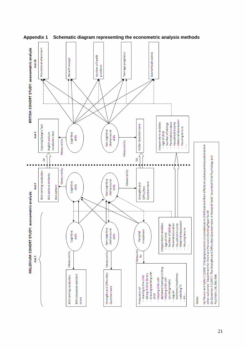
To accomplish the first two objectives, two econometric models were developed and estimated
using two nationally representative UK longitudinal data sets, the Millennium Cohort Study (MCS)
and the 1970 British Cohort Study (BCS). The resulting models were used to predict outcomes at
age 5 and at age 38 (details in Appendix 2), with and without interventions to be able to fulfil the
third objective. The final step was the development of a mathematical model to estimate the
economic consequences of the interventions. The use of the models developed in the econometric
analysis in an economic model to determine the long term outcomes of the intervention are
described in a separate document - Part 2.
1 While it is widely accepted that ‘early years’ matter, what we mean by ‘early years’ is not well defined.
Figures often quoted in the literature are: ‘from conception to age six’ (McCain and Mustard 1999), ‘first eight years’ (Cunha et al 2006); and ‘up to the age of ten’ (Hopkins and Bracht 1975).

6
2. Econometric analysis: datasets and methodology
2.1 Choice of data set:
There are four datasets for the UK which follow children from birth. In reverse chronological order,
these are:
MCS:
- This dataset is nationally representative;
- has information on relevant measures from birth;
- is the most recent and thus most relevant for the children growing up now.
BCS:
- This dataset is nationally representative;
- does not have the relevant information from birth (so cannot be used for modelling
childhood outcomes): it started collecting information on cognitive and non-cognitive
measures from the age of 5;
- is the most recent available for the adult outcomes.
Avon Longitudinal Study of Parents and Children (ALSPAC) 2:
- This dataset is not nationally representative (has under representation of poor and non-
white families);
- does not have as detailed measures of cognitive and non-cognitive assessment of children
as MCS.
The 1958 National Child Development Study (NCDS) 3:
- This dataset is not nationally representative (has under representation of ethnic minorities);
- started collection of information on ‘educational and social development’ only from age 7;
- has longer follow up for modelling adult outcomes, but is from an earlier cohort than BCS,
reflecting less well the UK society of today.
For the analysis undertaken here we use the MCS and BCS. The two main reasons for the using
these datasets are their epidemiological coverage (i.e. these surveys are nationally representative)
and their temporal applicability (i.e. these are the most recent surveys, so most relevant for the
current population). Furthermore, the MCS is the only dataset which follows children from birth
and oversamples children from disadvantaged backgrounds, which means it is the only dataset
which gives us enough observations to perform an empirical analysis on disadvantaged/vulnerable
children.
2 For details on ALSPAC see www.bristol.ac.uk/alspac.
3 For details on NCDS see www.cls.ioe.ac.uk.
7
To understand the factors determining the formation of ability in early childhood we used the MCS.
MCS has a set of variables relevant to our analysis including cognition, behaviour, and parental
behaviour, as well as a range of socio-economic variables collected when infants were aged 9
months, 3, 5 and 7 years. As the cohort was enrolled in the year 2000 it has the advantage of
being relatively recent. To establish the link between the early childhood development and the
adult outcomes the BCS was chosen. BCS is an older cohort which has many more years follow
up, allowing outcomes such as educational attainment and income in adulthood (age 38) to be
used in the analysis. The follow-up is not as long as the NCDS (1958), but when using longitudinal
data there is always a balance between length of follow up and relevance. Given that by the age
of 38 the vast majority of individuals’ life course is established, education completed, and
work/career trajectory set, the BCS was selected for the present analysis.
2.2 Early childhood: analysis from the MCS
The first econometric model is based on the MCS. The MCS is a multi-disciplinary research
project following the lives of around 19,000 children born in the UK in 2000/1.4 Four waves are
available to date, at ages 9 months (2001/2), 3 years (2004/5), 5 years (2006) and 7 years (2008).
For the analysis carried out here we make use of the information contained within the 2nd (age 3)
and the 3rd (age 5) waves.
Reasons for choosing the 2nd (age 3) wave:
- In wave 1 of the MCS the children are 9 months old. While there are measures of physical
development and health of the child up till this point, there are not very many measures of
cognitive and behavioural measures available. Wave 2, when the children are 3 years old, is
the first wave when the cognition and behavioural measures are available. Also the majority of
studies reporting effect sizes do so at age 3.
Reason for choosing the 3rd (age 5) wave:
- This is the wave that can be linked up with the BCS for the long-run analysis as we have data
from both surveys when children are 5. In the BCS we have information about cognitive and
behavioural development of the children from age 5 onwards. The next wave of the BCS was
carried out when the children were 10 years old but the latest wave of the MCS is when
children were 7 years old. Consequently, 5 is the only age at which we can link the data from
both datasets.
4 http://www.cls.ioe.ac.uk
8
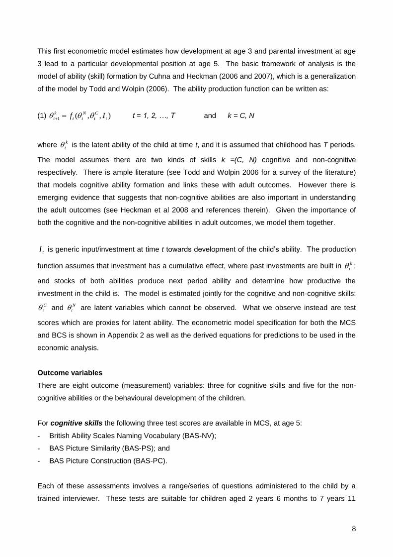
This first econometric model estimates how development at age 3 and parental investment at age
3 lead to a particular developmental position at age 5. The basic framework of analysis is the
model of ability (skill) formation by Cuhna and Heckman (2006 and 2007), which is a generalization
of the model by Todd and Wolpin (2006). The ability production function can be written as:
(1) ),,(1 t
C
t
N
tt
k
t If t = 1, 2, …, T and k = C, N
where k
t is the latent ability of the child at time t, and it is assumed that childhood has T periods.
The model assumes there are two kinds of skills k =(C, N) cognitive and non-cognitive
respectively. There is ample literature (see Todd and Wolpin 2006 for a survey of the literature)
that models cognitive ability formation and links these with adult outcomes. However there is
emerging evidence that suggests that non-cognitive abilities are also important in understanding
the adult outcomes (see Heckman et al 2008 and references therein). Given the importance of
both the cognitive and the non-cognitive abilities in adult outcomes, we model them together.
tI is generic input/investment at time t towards development of the child’s ability. The production
function assumes that investment has a cumulative effect, where past investments are built in k
t ;
and stocks of both abilities produce next period ability and determine how productive the
investment in the child is. The model is estimated jointly for the cognitive and non-cognitive skills:
C
t and N
t are latent variables which cannot be observed. What we observe instead are test
scores which are proxies for latent ability. The econometric model specification for both the MCS
and BCS is shown in Appendix 2 as well as the derived equations for predictions to be used in the
economic analysis.
Outcome variables
There are eight outcome (measurement) variables: three for cognitive skills and five for the non-
cognitive abilities or the behavioural development of the children.
For cognitive skills the following three test scores are available in MCS, at age 5:
- British Ability Scales Naming Vocabulary (BAS-NV);
- BAS Picture Similarity (BAS-PS); and
- BAS Picture Construction (BAS-PC).
Each of these assessments involves a range/series of questions administered to the child by a
trained interviewer. These tests are suitable for children aged 2 years 6 months to 7 years 11

9
months. BAS assessment captures the cognitive abilities and educational achievements of the
children.
Non-cognitive skills is often a generic term which in the economic literature on ‘skill formation’ is
used to indicate social and emotional well-being of the individuals (children in our case). Often the
only reliable measures available for non-cognitive skill formation are indices of behavioural
development; and this is what we use here. To assess the behavioural development of the
children a Strength and Difficulties Questionnaire (SDQ) is used. The SDQ is a part of self-
completion questionnaire filled by the main carer of the child (in almost all the cases this would be
the mother/mother figure). The SDQ has 25 questions, designed to capture the behavioural
attributes of 3 to 16 year olds. For each question, the main interviewee can respond with: not true,
somewhat true, certainly true and can't say. The 25 questions can be grouped to assess children
on five different scales:
- Emotion Symptoms Scale (often seem worried, unhappy, are easily scared, are nervous of
new situations and complain of headaches, stomach aches etc.),
- Conduct Problems (temper tantrums, obedient, fights with other children etc.),
- Hyperactivity Scale (restless, easily distracted, fidgety, etc.),
- Peer Problems (tends to play alone, picked on or bullied by other children etc.), and
- Pro-social Scale (share with others, kind and helpful, etc.).
For the first four of these scales a higher number indicates worse behavioural problems. Often in
the literature the first four components of SDQ are aggregated to reach an index of behavioural
problems. While this is useful and helps in interpretation, it ignores the important information that
is provided by the fifth component, pro-social. In our approach we use all the five components.
We do not use any arbitrary weights in combining these, instead we use structural equation
modelling (see Heckman et al 2008 and Kiernan et al 2010 for details) to estimate the latent
measure of behavioural problems, where all the components are standardized such that in all of
them a higher number indicates more behavioural problems to aid interpretation. Any other
standardization will lead to the same results.
Explanatory variables
The explanatory variables for the age 5 outcomes are as follows.
- Age 3 scores on two tests for cognitive skills: British Ability Scales Naming Vocabulary (BAS-
NV) and Bracken School Readiness (BSR) Assessment. BSR assessment measures the
comprehension of 308 educational concepts in 11 categories. For the MCS only 6 categories
were used -- colours, letters, numbers/counting, sizes, comparisons, and shapes.
- Age 3 scores on the five behavioural scales.

10
Questions are answered by the main carer of the child (which in the majority of cases is the
mother, and will be referred to as such). Unless otherwise specified the questions are asked at
both age 3 and age 5. The response categories for each question are shown in Appendix 3.
- How often do you read to the child?
- How often does child paint/draw at home?
- How often help child learn alphabet?
The above question is asked at age 3. Its equivalent question for age 5 is: how often is the
child helped with reading?
- How often is the child helped with writing? This is asked only at age 5.
- Regular bedtime:
At age 3 the question asked is: child has regular bedtimes?
At age 5 the question asked is: regular bedtime on term-time weekdays?
- TV watching:
At age 3 the question asked is: hours a day child watches tv/videos?
At age 5 the question asked is: hours per term-time weekday watching tv/dvd?
- Smack child if being naughty?
- Shout at child if being naughty?
- The Pianta parenting scale (this is available at age 3 only):
Positive parenting items are:
1. I share an affectionate, warm relationship with the Child
2. Child will seek comfort from me
3. Child values his/her relationship with me
4. When praised Child beams with pride
5. Child spontaneously shares information about himself/herself
6. is easy to be in tune with what the Child is feeling
7. Child shares his/her feelings and experiences with me
Negative parenting items are:
1. Child and I always seem to be struggling with each other
2. Child easily becomes angry with me
3. Child remains angry or is resistant after being disciplined
4. Dealing with the Child drains my energy
5. When the Child wakes up in a bad mood, I know we’re in for a long and difficult
day
6. The Child’s feelings towards me can be unpredictable or can change suddenly
7. The Child is sneaky or manipulative with me
8. Child uncomfortable with physical affection

11
Question asked of the father/father figure in the household:
- How often do you read to the child?
Other variables:
- Age of the child, to the nearest tenth of the year, for both ages 3 and 5. This is the age when
the test was administered to the child. The tests conducted at an early age are sensitive to the
age of the child – a month’s difference in age can imply different development.
- Number of siblings in the household.
- Mother’s education: this is a dummy variable, taking value 1 if the mother has an NVQ level 4
or above; 0 otherwise. Overseas education is coded as 0.
- Kessler psychological distress scale (mother).
Variables initially entered in the analysis, but found to be largely insignificant were: regular meal
times, taking the child to the library, count/maths with the child. Including them does not change
the results in any way, and they were dropped from the final model.
The analysis was undertaken in a subset of the MCS data – the children in the poor households. A
child is defined to be in poverty if the household income is below 60% of contemporary median
income; this classification is provided in the MCS. Poverty status of the child is defined at age 3 in
this analysis. Plewis (2008) found only few and small effects on children’s attainment and
behaviour of changes in their families’ economic circumstances as they grow up. As the estimation
was done for the poor and the non-poor sample separately, income was not included as one of the
control variables. Including income, as a control variable, does not alter the results qualitatively.
There are two main reasons for undertaking the analysis only on the poor sample: (1) The primary
purpose of the analysis is to estimate how effective interventions with vulnerable infants and their
families may be on outcomes, and these children have potentially different development gradients
(Feinstein 2003). (2) There is no standard definition of ‘vulnerable’. The study scope refers to a
range of socio-economic, parental health and behavioural risk factors, without defining at what
level increased risk or vulnerability arises. The intervention studies also varied in their
identification of populations. However low income or poverty is a strong recurring theme in both
the selection of families or areas for interventions (for example Ford 2009, Toroyan 2003, Wiggins
2004), and in studies identifying risk factors for poor child outcomes identified in Review 3
(Summary review of cohort studies on the factors relating to risk of children experiencing cognitive,
social and emotional difficulties) Poverty is also associated with many other risk factors such as
lone parenthood, unemployment, substance abuse and poor health.
12
2.3 Long run outcomes: analysis from the BCS
A second econometric model was estimated to enable us to make a link between development and
other relevant socio-economic variables at age 5 and adult achievement (measured at age 38)
using the BCS. The BCS is a longitudinal cohort survey designed and conducted by the Centre for
Longitudinal Studies (CLS) of the Institute of Education, University of London, and the fieldwork
was carried out at the National Centre for Social Research (NatCen). The work was funded by the
Economic and Social Research Council. The BCS is a continuing, multi-disciplinary longitudinal
study which takes as its subjects all those living in England, Scotland and Wales who were born in
one particular week in April 1970.
The econometric analysis makes use of information contained within 4 different waves of the BCS.
Most of the analysis was undertaken using data from the waves at age 5 years (wave 2: the five-
year follow-up, 1975) and the latest available wave at age 38 (wave 8). In cases where data was
unavailable in these waves or needed supplementing, wave 3 (the 10-year follow-up) and wave 6
(the 29-year follow-up survey) were also used as noted below. Following on the analysis of the
MCS, measures of both cognitive and non-cognitive skills, information on parental behaviour and a
range of other relevant socio-economic variables when the children were 5 years old were used.
These measures were linked to a range of economic outcomes (see details below) observed when
the cohort members were interviewed in 2008 (age 38). The equations for all the outcomes are
estimated jointly, but separately for males and females. This second econometric model is not
restricted to the sample of disadvantaged/vulnerable children. Unfortunately, the BCS does not
provide information on household income at age 5 and therefore disadvantaged/vulnerable
children cannot be singled out reliably at this age. The first information on household income
appears in the third wave of the study when children are age 10. However, household income is
given within a very small number of bands each covering a high proportion of the sample. Even if
we are prepared to make the strong assumption that the disadvantage/vulnerable position is
perfectly persistent over time, the small number of bands prevents us from being able to split the
sample reliably although the information contained in this variable is used in the analysis to signal
cases of extreme poverty (see below for details). The sample size is also relatively small if we were
to split it by income as well as gender.
Outcome variables:
A total of five outcome variables were used in the analysis. Three outcomes for both males and
females: highest NVQ level from an academic or vocational qualification attained by the age of 38,
being in receipt of benefits at 38, and number of health problems at 38. In addition, teenage
pregnancy and being economically active at the age of 38 are also used as outcomes for females
and for males respectively. Being economically active is not used as an outcome for females given

13
the problems of self selection into participation in the labour force for women, requiring a much
more detailed and lengthy study than the analysis carried out here. The variables were specified as
follows:
- Educational attainment at 38: highest NVQ level from an academic or vocational qualification –
coding as the level number, 0, 1, up to 5 where 5 could be NVQ at level 5 or 6 (these are not
distinguished in the dataset).
- Benefit receipt: dummy equal to one if the respondent is in receipt of Income Support or other
state benefits excluding state pension, child benefit and tax credit.
- Number of health problems at 38. Health problems identified in the survey include: asthma or
wheezy bronchitis, hayfever/sneeze/runny nose, diabetes, convulsion, fit, epileptic seizure,
recurrent backache, etc., cancer or leukaemia, problems with hearing, eyesight problems, high
blood pressure, migraine, eczema/other skin problem, chronic fatigue syndrome, period or
other problems, stomach/bowels/gall bladder, problems with bladder/kidneys, cough/bringing
up phlegm, depression. The variable is a simple count of the number of health problems and it
does not control for the severity of these.
- Economically active at 38 (males only): dummy equal to one if the cohort member is
economically active, zero otherwise.
- Teenage pregnancy defined as having a live birth before the age of 18. Full pregnancy
histories were collected at age 29. At age 38 full pregnancy histories were collected of those
cohort members who had not been interviewed at age 29.
Explanatory variables
All explanatory variables used in the BCS analysis but one come from the 5-year follow-up when
the cohort members were aged 5. The variables are described below.
For cognitive skills the following two tests are available in the BCS at age 5:
- Copying Designs Test score which assesses children’s visual-motor coordination.
- English Picture Vocabulary Test (survey design) adaptation by Brimer and Dun (1962) of the
American Peabody picture vocabulary test. The BCS gives standardised scores.
The BCS includes one measure of the behavioural development of the child:
- The Rutter scale. A higher score indicates behaviour adjustment problems. The Rutter score is
an index made up of a number of behaviour items. Non-response on some of the items will
tend to produce lower scores. In the analysis we dropped any score which had more than 5
missing items to avoid problems with artificially low scores: this still leaves over 99% of the

14
sample. We experimented with a lower cut-off point but the direction of the effects was not
affected by this.
Other explanatory variables used in the analysis are as follows.
- Age of the child when the tests where conducted. This is the same variable used in the MCS
analysis to control for the sensitivity of the tests to the different developmental stages of the
children.
- Psychiatric problems in the mother as measured by a score of 7 or more on the Malaise score.
- Number of other children in the household.
- Average hours per day (Monday-Friday) of TV watching coded as follows:
1: less than 1 hour
2: at least 1 hour but less than 3 hours
3: 3 or more hours.
- Number of days the child was read to in the past week:
0: not at all
2: once/twice a week
3: several times a week
4: every day.
- Mother’s education is defined as a binary variable that takes the value of one if the mother had
a degree or a certificate of education when the child was 5 years of age and zero otherwise.
Unfortunately the BCS does not have information about household income until the children are 10
years old. The analysis uses a poverty dummy defined as one if at age 10 the household income
was less than £99 per week and zero otherwise. This dummy covers 35% of children in the survey
with the lowest household income at the age of 5. The income variable is banded with fairly large
bands. Adding one more band to the poverty variable would result in over 70% of the sample being
included in the dummy and, therefore, not suitable as a poverty indicator.
In the analysis, highly insignificant variables were dropped using an extremely conservative
criteria. For each outcome, only those variables with an associated p-value of 0.70 or higher for
both males and females were dropped. The estimated parameter values and significance is not
affected by this. The econometric model specification as well as the derived predicting equations
for use in the economic model are shown in Appendix 2.
3. Results
3.1 MCS Results
Tables reporting the variable coefficients and their P-values are shown in Appendix 4.

15
Table 1 gives us the relationship between cognition and behavioural development at age 3 with
those at age 5:
- Cognitive (behavioural) development at age 3 has a positive and a significant effect on
cognitive (behavioural) development at 5.
- Higher cognitive development at age 3 is associated with less behavioural problems at age 5,
though the effect is not significant at the conventional levels (i.e. p<0.10).
- Behavioural development at age 3, does not seem to be associated with the cognitive
development at age 5.
The key findings above are similar to those found in the literature. A study by Cunha and
Heckman (2008), using the US data and a model similar to the one used here, also finds a strong
evidence of persistence, over time, in both cognitive and behavioural development.
Table 2 gives us the relationship between the other explanatory variables and cognitive and
behavioural development at age 3. Similarly Table 3 gives us the relationship between the other
explanatory variables and cognitive and behavioural development at age 5.
Many of the variables measured when the infant is aged 3 are significant when predicting cognition
and behaviour at age 3, and some are highly significant (p<0.001). On the whole the estimated
parameters have the intuitively expected sign, with the possible exceptions of the positive effect of
“shouting” on cognition, and negative effect of helping the child learn the alphabet on behaviour.
Factors at age 3 which were highly significant in predicting cognition at age 3 are number of
siblings, mother’s education, mother reading to child and positive parenting behaviour. Mother’s
education is also highly significant in the prediction of lower levels of poor behaviour, as is positive
parenting, whilst negative parenting has a negative effect on child behaviour.
- Maternal depression is negatively associated with cognitive scores, and positively associated
with behavioural problems. This is consistent with the findings of Kiernan and Huerta (2008)5.
- Among the activities that parent’s do with their children (reading, painting, etc.) it is reading (by
both father and mother) which has the strongest link with the development of the child.
Reading activities enhance the cognitive scores and lower the observed behavioural problems
in the child. This is consistent with the findings of Kiernan and Huerta (2008).
- Positive parenting (PPS) is associated with higher cognitive scores and lower behavioural
problems. This is consistent with the findings of Kiernan and Huerta (2008) and Kiernan and
Mensah (2010)6.
5 Kiernan and Huerta (2008) use the MCS wave 2 (age 3).

16
- Negative parenting (NPS) is associated with higher behavioural problems, while it does not
have a statistically significant association with cognition.
While there is evidence of self-productivity (or persistence over time) in both cognition and
behavioural problems, as seem in Table 1, fewer variables measured at age 5 are significant in
predicting cognitive and behavioural outcomes at age 5. One reason for this may be that by age 5
the child is in school and factors related to school become relatively more important. The few
significant variables include: helping child with writing (counter-intuitively a negative effect) and
shouting for cognition. Mother’s psychological distress and TV watching predicted behavioural
problems, whilst reading to the child was protective.
3.2 BCS Results
We find that some of the relationships from 5 years to adult outcomes are weak as has previously
been highlighted in the literature. Heckman et al (2006) for example find that the relationship is
much stronger when using 16-20 years as the linking age instead of 10. It is likely that a much
better link could be found if the data in the MCS extended for a longer period. An additional
problem is the paucity of data in the BCS during the early years when compared to the MCS. For
example, information of household income is not available until the cohort members are 10. The
exact figure is not recorded in the survey, only an interval is given with a small number of intervals
covering a large range. There are also a lot less variables recorded in the BCS that can be used as
indicators of parental investment in the child. A table showing the estimated coefficients and their
significance is shown in Appendix 5. On the whole the estimated parameters have the expected
sign when they are significant at conventional significance levels. In a few cases they have a
counterintuitive sign but tend not to be significant. The results for all the outcomes are summarised
below.
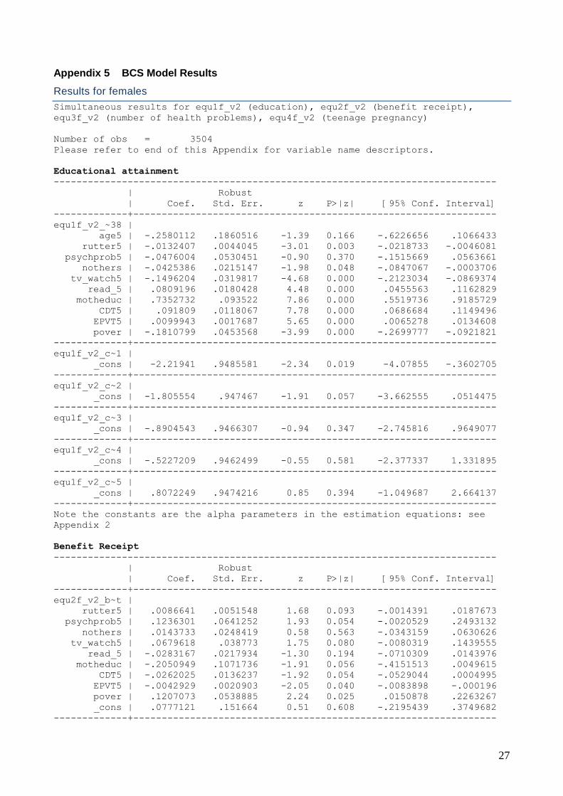
- Educational attainment. We find that for both males and females the probability of having the
highest NVQ level at age 38 depends positively on the levels of cognitive development, on the
frequency of the child being read to and on mother’s education. The probability of having the
highest NVQ level at 38 decreases with the level of behavioural problems of the child and with
the number of other children in the household. This probability is also lower if the mother had
psychiatric problems and if the household was in poverty, as measured by our poverty dummy.
Although the direction of the effect of psychiatric problems of the mother is as expected, this
variable is not significant at conventional levels for either males or females.
6 Kiernan and Mensah (2010) use the MCS wave 3 (age 5). The positive parenting score that these authors
use is a composite of positive pianta scale (age 3) and other parenting activities (reading to the child, etc. at age 5).

17
- Benefit receipt. We find that for both males and females higher behavioural problems,
psychiatric problems in the mother, longer TV watching times, and being in poverty when
young are associated with a higher probability of being in receipt of benefits at 38. The
reading frequency to the child, mother’s education and the levels of cognitive development are
associated with lower probabilities of receiving benefit at age 38. The only exception is the sign
of the English Picture Vocabulary Test for males which has a counterintuitive sign, but is
however highly insignificant.
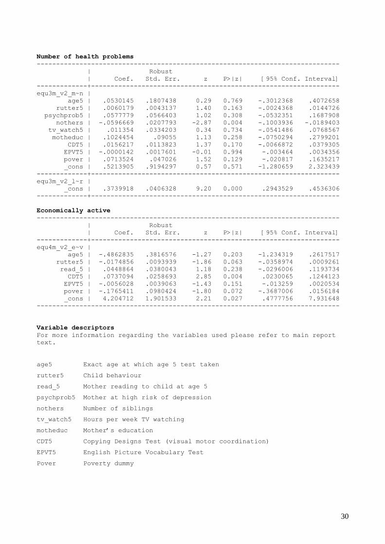
- Number of health problems. This relationship is particularly uncertain which is likely due to
the nature of the variable we are using in the analysis. The survey does not contain detailed
information of health problems, only self-reported information on whether the individual suffers
from each of a number of health conditions. These conditions represent a broad spectrum of
severity. In addition, there is substantial variability in severity between the included conditions.
Thus, the combined score is itself a relatively crude measure. Furthermore, age 38 is still
relatively young for the emergence of chronic health problems. The results show that the only
significant variable at conventional levels is the number of other children in the household
which has a negative effect on the number of health problems.
- Teenage pregnancies (females only). As expected, higher behavioural problems, psychiatric
problems in the mother, number of other children in the household, longer TV watching times,
and being in poverty when young are associated with a higher probability of a teenage
pregnancy. The reading frequency to the child, mother’s education and the levels of cognitive
development are associated with lower probabilities of receiving benefit at age 38.
- Economically active (males only). This relationship has a number of highly insignificant
variables. However, this is expected given the high proportion of males in the sample who are
economically active. Higher behavioural problems and being in poverty when young are
associated with a lower probability of being economically active at age 38. The reading
frequency to the child and the levels of cognitive development as measured by the Copying
Designs Test are associated with a higher probability of being economically active at age 38.
The level of cognitive development as measured by the English Picture Vocabulary Test seems
to have a counterintuitive sign although it does not appear to be significant as conventional
significance levels.
3.3 Limitations of the analysis:
Apart from the usual noise/ error associated with estimated parameters in any econometric
analysis, the following are the limitations of this analysis that should be kept in mind:
18
- Other than the test scores for cognitive ability, a lot of the data used here is self-reported,
mainly by mother. Some of the variables are more prone to systematic misreporting than
others.
- The relationship between the observables (e.g. test scores) and the unobservables (e.g. latent
cognitive ability of the child), is fraught with measurement errors in both the MCS and BCS
analysis. While the approach used in the MCS analysis (dynamic factor analysis) limits this
problem it cannot completely eliminate it.
- The skill production function (i.e. the relationship between cognitive development at age 3 with
that at age 5; and similarly for the behavioural development) is assumed to be linear (results in
Table 1). This may not be the case. (However, evidence from the simulations carried out by
Cunha and Heckman (2008) seem to indicate that the linear production function is not a limiting
assumption).
- Endogeneity of inputs: in the MCS model we have assumed that parenting behaviour
influences child’s development; it could be that child’s development is influencing the parenting
environment (see Kiernan and Huerta, 2008). For example reading more to the child is
associated with a higher cognitive score of the child; but it could be that parents read more to
the child who is inherently more able and interested. Similarly, endogeneity problems are also
present in the BCS analysis and need to be considered in the interpretation of the results.
Taking endogeneity into account will tend to reduce the size of the long run effect.
- Long-run linkages: we are using the information in the BCS at age 5, to make long-run
predictions (age 38) because it is the only age the two surveys have in common. One can not
assume a linear trajectory from age 5 to age 38 because at age 5 children are still developing
at a very high pace. Studies by Cunha and Heckman (2008) and Heckman et al (2006)
indicate that the best possible way to make long run predictions is:
o Make them frequently before the mid-teens. Cunha and Heckman (2008) make
predictions in three stages: from ages (I) 6-7 to 8-9, (II) 8-9 to 10-11 and (III) 10-11
to 12-13.
o From mid-teens the long run predications make more sense. Heckman et al (2006)
make predictions from age 14 to age 30. Here too however the analysis has to take
into account the endogeneity of the choices related to: schooling, occupational
choices, fertility etc.
19
4 References Bor, W., J.M. Najman, M.J. Andersen, M. O’Callaghan, G.M. Williams, and B.C. Behrens, (1997), ‘The Relationship Between Low Family Income and Psychological Disturbance in Young Children: An Australian Longitudinal Study’, Australian and New Zealand Journal of Psychiatry, 31(5): 664–75.
Cunha, F. and J.J. Heckman (2006), ‘Investing in Young People,’ Working Paper, University of Chicago.
Cunha, F. and J.J. Heckman (2007), ‘The technology of skill formation,’ American Economic Review, vol. 97(2), pp.31-47.
Cunha, F. and J.J. Heckman (2008), ‘Formulating, Identifying and Estimating the Technology of Cognitive and Noncognitive Skill Formation,’ Journal of Human Resources, vol. 43(4), pp. 738-782. Cunha, F., J.J. Heckman, L. Lochner and D. Masterov (2006), ‘Interpreting the Evidence on Life Cycle Skill Formation,’ in Handbook of the Economics of Education, edited by E. Hanushek and F. Welch, pp. 697-812, North Holland: Amsterdam.
Feinstein, L. (2003) ‘Inequality in the Early Cognitive Development of British children in the 1970 Cohort’, Economica 70(277): 73–97. Heckman, J.J., J. Strixrud and S. Urzua (2006), ‘The Effects of Cognitive and Noncognitive Abilities on Labor Market Outcomes and Social Behavior, Journal of Labor Economics, vol. 24(3), pp. 411-482.
Heckman, J.J. and D.V. Masterov (2007), ‘The productivity argument for investing in young children,’ Review of Agricultural Economics, vol. 29(3), pp.446-493.
Hopkins, K.D. and G.H. Bracht (1975), ‘Ten-Year Stability of Verbal and Nonverbal IQ Scores,’ American Educational Research Journal, Vol. 12(4), pp. 469-477. Kiernan, K.E. and M.C. Huerta (2008), ‘Economic deprivation, maternal depression, parenting and children’s cognitive and emotional development in early childhood,’ The British Journal of Sociology, vol. 59(4), pp. 783-806. Kiernan, K.E. and F.K. Mensah (2010), ‘Poverty, family resources and children’s early educational attainment: the mediating role of parenting,’ British Educational Research Journal, available online 26th February 2010. McCain, M.N and J.F. Mustard (1999), Reversing the Real Brain Drain: Early Years Study, Final Report, Toronto: Ontario Children’s Secretariat.
Patterson, C.J., J.B. Kupersmidt and N.A. Vaden (1990), ‘Income level, gender, ethnicity, and household composition as predictors of children’s school-based competence,’ Child Development, vol. 61(2), pp.485-494.
Todd, P.E. and K.I. Wolpin (2006), ‘The Production of Cognitive Achievement in Children: Home, School and Racial Test Score Gaps,’ Working Paper, University of Pennsylvania.
Ford, R.M., S.J.P. McDougall, and D. Evans (2009). Parent-delivered compensatory education for children at risk of educational failure: Improving the academic and self-regulatory skills of a Sure Start preschool sample. British Journal of Psychology, 100(Pt 4), 773-797.

20
Toroyan, T., A. Oakley, G. Laing, I. Roberts, M. Mugford, and J. Turner (2004). The impact of day care on socially disadvantaged families: an example of the use of process evaluation within a randomized controlled trial. Child: Care, Health and Development, 30 691-698.
Wiggins, M., A. Oakley, I. Roberts, H. Turner, L. Rajan, H. Usterberry, R. Mujica, and M. Mugford, (2004). The Social Support and Family Health Study: a randomised controlled trial and economic evaluation of two alternative forms of postnatal support for mothers living in disadvantaged inner-city areas. Health Technology Assessment, 8(32), 1-+.
Plewis, I and C. Kallis, (2008). Changing economic circumstances in childhood and their effects on subsequent educational and other outcomes. DWP Working Paper No. 49. http://www.dwp.gov.uk/asd/asd5/report_abstracts/wp_abstracts/wpa_049.asp
21
Appendix 1 Schematic diagram representing the econometric analysis methods

22
Appendix 2 Econometric models: specification and derived equations for predictions. Please see attachment

23
Appendix 3 Millennium Cohort Study Question Response Categories Questions are answered by the main carer of the child (which in the majority of cases is the
mother, and will be referred to as such). Unless otherwise specified the questions are asked at
both age 3 and age 5:
- How often do you read to the child?
0 = Not at all
1 = Once/twice/less a month
2 = once/twice a week
3 = Several times a week
4 = Every day
- How often does child paint/draw at home?
0 = Never
1 = Occasionally
2 = once\twice a week
3 = Several times a week
4 = Every day
- How often help child learn alphabet?
The above question is asked at age 3. Its equivalent question for age 5 is: how often is the
child helped with reading?
0 = Never
1 = Occasionally
2 = once\twice a week
3 = Several times a week
4 = Every day
- How often is the child helped with writing? This is asked only at age 5.
0 = Never
1 = Occasionally
2 = once\twice a week
3 = Several times a week
4 = Every day

24
- Regular bedtime:
At age 3 the question asked is: child has regular bedtimes?
At age 5 the question asked is: regular bedtime on term-time weekdays?
0 = never or almost never
1 = sometimes
2 = usually
3 = always
- TV watching:
At age 3 the question asked is: hours a day child watches tv/videos?
At age 5 the question asked is: hours per term-time weekday watching tv/dvd?
0 = None
1 = Up to one hour
2 = [1,3) hours
3 = >3 hours
- Smack child if being naughty?
0 = Never
1 = Rarely
2 = >1 a month
- Shout at child if being naughty?
0 = Never
1 = Rarely
2 = >1 a month
Question asked of the father/father figure in the household:
- How often do you read to the child?
0 = Not at all
1 = Once/twice/less a month
2 = once/twice a week
3 = Several times a week
4 = Every day

25
Appendix 4 Millennium Study Model Results
Please refer to end of this Appendix for variable name descriptors.
TABLE 1
Cognition at Age 5
Two-Tailed
Estimate S.E. Est./S.E. P-Value
Cognition at Age 3 0.539 0.032 17.121 0.000
Behaviour at Age 3 0.000 0.026 0.001 0.999
Behaviour at Age 5
Two-Tailed
Estimate S.E. Est./S.E. P-Value
Cognition at Age 3 -0.031 0.024 -1.253 0.210
Behaviour at Age 3 0.388 0.045 8.639 0.000
TABLE 2
Cognition at Age 3
Two-Tailed
Estimate S.E. Est./S.E. P-Value
AGE_age3 0.179 0.183 0.980 0.327
BDOTHS -0.133 0.033 -4.059 0.000
MEDU_age3 0.572 0.127 4.512 0.000
KESS_age3 -0.016 0.008 -2.010 0.044
MREAD_age3 0.210 0.039 5.401 0.000
PREAD_age3 0.077 0.029 2.624 0.009
PAINT_age3 0.076 0.044 1.730 0.084
ALPH_age3 0.064 0.028 2.255 0.024
REGBED_age3 0.135 0.039 3.439 0.001
TV_age3 -0.032 0.058 -0.559 0.576
SMACK_age3 -0.009 0.055 -0.163 0.871
SHOUT_age3 0.182 0.075 2.413 0.016
PPS 0.092 0.014 6.391 0.000
NPS -0.004 0.007 -0.578 0.563
Behavioural at Age 3
Two-Tailed
Estimate S.E. Est./S.E. P-Value
AGE_age3 0.025 0.182 0.136 0.892
BDOTHS 0.006 0.032 0.187 0.852
MEDU_age3 -0.341 0.087 -3.920 0.000
KESS_age3 0.023 0.009 2.652 0.008
MREAD_age3 -0.076 0.032 -2.398 0.016
PREAD_age3 -0.064 0.025 -2.572 0.010
PAINT_age3 -0.015 0.037 -0.406 0.685
ALPH_age3 0.051 0.025 2.060 0.039
REGBED_age3 -0.028 0.041 -0.691 0.490
TV_age3 0.121 0.047 2.570 0.010
SMACK_age3 0.051 0.054 0.946 0.344
SHOUT_age3 -0.031 0.063 -0.485 0.628
PPS -0.060 0.013 -4.515 0.000
NPS 0.110 0.009 12.835 0.000

26
TABLE 3
Cognition at Age 5
Two-Tailed
Estimate S.E. Est./S.E. P-Value
AGE_age5 -0.189 0.095 -1.976 0.048
CDOTHS 0.008 0.020 0.402 0.688
MEDU_age5 0.003 0.059 0.055 0.956
KESS_age5 0.000 0.006 0.023 0.982
MREAD_age5 0.017 0.023 0.728 0.466
PREAD_age5 0.009 0.019 0.467 0.641
PAINT_age5 0.024 0.024 0.996 0.319
READ_age5 -0.019 0.026 -0.746 0.456
WRIT_age5 -0.034 0.017 -2.015 0.044
REGBED_age5 0.018 0.024 0.768 0.443
TV_age5 0.008 0.036 0.207 0.836
SMACK_age5 0.025 0.034 0.727 0.467
SHOUT_age5 0.087 0.041 2.096 0.036
Behavioural at Age 5
Two-Tailed
Estimate S.E. Est./S.E. P-Value
AGE_age5 -0.072 0.083 -0.869 0.385
CDOTHS -0.033 0.020 -1.629 0.103
MEDU_age5 0.026 0.052 0.503 0.615
KESS_age5 0.041 0.006 7.383 0.000
MREAD_age5 0.007 0.027 0.266 0.790
PREAD_age5 -0.002 0.016 -0.123 0.902
PAINT_age5 0.023 0.023 1.007 0.314
READ_age5 -0.055 0.028 -1.989 0.047
WRIT_age5 0.024 0.019 1.275 0.202
REGBED_age5 0.009 0.027 0.314 0.754
TV_age5 0.087 0.034 2.567 0.010
SMACK_age5 0.032 0.032 0.998 0.318
SHOUT_age5 0.050 0.042 1.187 0.235
Variable descriptors
AGE Actual age test taken at ages 3 and 5
B/CDOTHS Number of siblings at ages 3 and 5
MEDU Mother’s education
KESS Kessler (psychological distress scale (mother).
MREAD Mother read to child
PREAD Father read to child
PAINT Paint with child
ALPH Help child with alphabet(age 3)
READ Help child with reading (age 5)
WRIT Help child with writing(age 5)
REGBED Regular bedtimes
TV TV viewing
SMACK Smack child
SHOUT Shout at child
PPS Positive Pianta (parent-child) relationship Scale
NPS Negative Pianta (parent-child) relationship Scale
27
Appendix 5 BCS Model Results
Results for females
Simultaneous results for equ1f_v2 (education), equ2f_v2 (benefit receipt),
equ3f_v2 (number of health problems), equ4f_v2 (teenage pregnancy)
Number of obs = 3504
Please refer to end of this Appendix for variable name descriptors.
Educational attainment
------------------------------------------------------------------------------
| Robust
| Coef. Std. Err. z P>|z| [95% Conf. Interval]
-------------+----------------------------------------------------------------
equ1f_v2_~38 |
age5 | -.2580112 .1860516 -1.39 0.166 -.6226656 .1066433
rutter5 | -.0132407 .0044045 -3.01 0.003 -.0218733 -.0046081
psychprob5 | -.0476004 .0530451 -0.90 0.370 -.1515669 .0563661
nothers | -.0425386 .0215147 -1.98 0.048 -.0847067 -.0003706
tv_watch5 | -.1496204 .0319817 -4.68 0.000 -.2123034 -.0869374
read_5 | .0809196 .0180428 4.48 0.000 .0455563 .1162829
motheduc | .7352732 .093522 7.86 0.000 .5519736 .9185729
CDT5 | .091809 .0118067 7.78 0.000 .0686684 .1149496
EPVT5 | .0099943 .0017687 5.65 0.000 .0065278 .0134608
pover | -.1810799 .0453568 -3.99 0.000 -.2699777 -.0921821
-------------+----------------------------------------------------------------
equ1f_v2_c~1 |
_cons | -2.21941 .9485581 -2.34 0.019 -4.07855 -.3602705
-------------+----------------------------------------------------------------
equ1f_v2_c~2 |
_cons | -1.805554 .947467 -1.91 0.057 -3.662555 .0514475
-------------+----------------------------------------------------------------
equ1f_v2_c~3 |
_cons | -.8904543 .9466307 -0.94 0.347 -2.745816 .9649077
-------------+----------------------------------------------------------------
equ1f_v2_c~4 |
_cons | -.5227209 .9462499 -0.55 0.581 -2.377337 1.331895
-------------+----------------------------------------------------------------
equ1f_v2_c~5 |
_cons | .8072249 .9474216 0.85 0.394 -1.049687 2.664137
-------------+----------------------------------------------------------------
Note the constants are the alpha parameters in the estimation equations: see
Appendix 2
Benefit Receipt
------------------------------------------------------------------------------
| Robust
| Coef. Std. Err. z P>|z| [95% Conf. Interval]
-------------+----------------------------------------------------------------
equ2f_v2_b~t |
rutter5 | .0086641 .0051548 1.68 0.093 -.0014391 .0187673
psychprob5 | .1236301 .0641252 1.93 0.054 -.0020529 .2493132
nothers | .0143733 .0248419 0.58 0.563 -.0343159 .0630626
tv_watch5 | .0679618 .038773 1.75 0.080 -.0080319 .1439555
read_5 | -.0283167 .0217934 -1.30 0.194 -.0710309 .0143976
motheduc | -.2050949 .1071736 -1.91 0.056 -.4151513 .0049615
CDT5 | -.0262025 .0136237 -1.92 0.054 -.0529044 .0004995
EPVT5 | -.0042929 .0020903 -2.05 0.040 -.0083898 -.000196
pover | .1207073 .0538885 2.24 0.025 .0150878 .2263267
_cons | .0777121 .151664 0.51 0.608 -.2195439 .3749682
-------------+----------------------------------------------------------------

28
Number of health problems
------------------------------------------------------------------------------
| Robust
| Coef. Std. Err. z P>|z| [95% Conf. Interval]
-------------+----------------------------------------------------------------
equ3f_v2_m~n |
age5 | .2446242 .2308929 1.06 0.289 -.2079176 .6971661
rutter5 | .0057937 .0049933 1.16 0.246 -.0039929 .0155804
psychprob5 | .0548895 .0650777 0.84 0.399 -.0726605 .1824395
nothers | -.0948362 .0221247 -4.29 0.000 -.1381999 -.0514725
tv_watch5 | .0390748 .0382477 1.02 0.307 -.0358892 .1140389
motheduc | .0817377 .0960768 0.85 0.395 -.1065694 .2700448
CDT5 | -.0118173 .013906 -0.85 0.395 -.0390726 .015438
EPVT5 | .0009276 .002088 0.44 0.657 -.0031648 .0050201
pover | -.0663853 .0524777 -1.27 0.206 -.1692398 .0364691
_cons | -.0208919 1.177536 -0.02 0.986 -2.32882 2.287036
-------------+----------------------------------------------------------------
equ3f_v2_l~r |
_cons | .6962201 .0394246 17.66 0.000 .6189492 .7734909
-------------+----------------------------------------------------------------
Teenage pregnancy
------------------------------------------------------------------------------
| Robust
| Coef. Std. Err. z P>|z| [95% Conf. Interval]
-------------+----------------------------------------------------------------
equ4f_v2_t~g |
age5 | .397334 .3809806 1.04 0.297 -.3493742 1.144042
rutter5 | .0137368 .0093589 1.47 0.142 -.0046063 .0320799
psychprob5 | .1124631 .1117229 1.01 0.314 -.1065097 .3314359
nothers | .113243 .0390126 2.90 0.004 .0367798 .1897062
tv_watch5 | .1438558 .0684168 2.10 0.035 .0097613 .2779503
read_5 | -.1157883 .0346549 -3.34 0.001 -.1837107 -.0478658
motheduc | -.2819257 .3615056 -0.78 0.435 -.9904638 .4266123
CDT5 | -.0295679 .0265106 -1.12 0.265 -.0815278 .022392
EPVT5 | -.0030923 .003831 -0.81 0.420 -.010601 .0044163
pover | .1793648 .0938555 1.91 0.056 -.0045887 .3633183
_cons | -4.052269 1.9114 -2.12 0.034 -7.798545 -.3059942
------------------------------------------------------------------------------

29
Appendix 5 continued BCS Model Results
Results for males
Simultaneous results for equ1m_v2 (education), equ2m_v2 (benefit receipt),
equ3m_v2 (number of health problems), equ4m_v2 (economically active)
Number of obs = 3602
Education
------------------------------------------------------------------------------
| Robust
| Coef. Std. Err. z P>|z| [95% Conf. Interval]
-------------+----------------------------------------------------------------
equ1m_v2_~38 |
age5 | -.2588501 .2572503 -1.01 0.314 -.7630514 .2453511
rutter5 | -.0042447 .004264 -1.00 0.320 -.0126021 .0041127
psychprob5 | -.0363015 .0560986 -0.65 0.518 -.1462527 .0736498
nothers | -.0936954 .0223999 -4.18 0.000 -.1375985 -.0497923
tv_watch5 | -.0428762 .034543 -1.24 0.215 -.1105793 .024827
read_5 | .0750645 .019509 3.85 0.000 .0368276 .1133013
motheduc | .5787598 .0928323 6.23 0.000 .3968118 .7607078
CDT5 | .095413 .0118451 8.06 0.000 .0721969 .118629
EPVT5 | .0057965 .0018159 3.19 0.001 .0022375 .0093555
pover | -.1844068 .0490579 -3.76 0.000 -.2805584 -.0882551
-------------+----------------------------------------------------------------
equ1m_v2_c~1 |
_cons | -2.003194 1.305017 -1.53 0.125 -4.56098 .5545926
-------------+----------------------------------------------------------------
equ1m_v2_c~2 |
_cons | -1.649208 1.303677 -1.27 0.206 -4.204367 .9059518
-------------+----------------------------------------------------------------
equ1m_v2_c~3 |
_cons | -.8376686 1.303258 -0.64 0.520 -3.392008 1.71667
-------------+----------------------------------------------------------------
equ1m_v2_c~4 |
_cons | -.4030576 1.303113 -0.31 0.757 -2.957112 2.150996
-------------+----------------------------------------------------------------
equ1m_v2_c~5 |
_cons | .9693265 1.302662 0.74 0.457 -1.583843 3.522496
-------------+----------------------------------------------------------------
Note the constants are the alpha parameters in the estimation equations: see
Appendix 2
Benefit Receipt
------------------------------------------------------------------------------
| Robust
| Coef. Std. Err. z P>|z| [95% Conf. Interval]
-------------+----------------------------------------------------------------
equ2m_v2_b~t |
rutter5 | .0011251 .0053022 0.21 0.832 -.009267 .0115171
psychprob5 | .0371475 .0690781 0.54 0.591 -.0982431 .1725381
nothers | -.012773 .0266491 -0.48 0.632 -.0650044 .0394583
tv_watch5 | .1517344 .0417533 3.63 0.000 .0698994 .2335694
read_5 | -.0346686 .0227871 -1.52 0.128 -.0793305 .0099932
motheduc | -.1702395 .1155891 -1.47 0.141 -.3967899 .0563109
CDT5 | -.036079 .014112 -2.56 0.011 -.063738 -.0084199
EPVT5 | .0003133 .0022039 0.14 0.887 -.0040063 .0046329
pover | .0817404 .0585608 1.40 0.163 -.0330366 .1965174
_cons | -.3884712 .1617289 -2.40 0.016 -.705454 -.0714884
-------------+----------------------------------------------------------------
30
Number of health problems
------------------------------------------------------------------------------
| Robust
| Coef. Std. Err. z P>|z| [95% Conf. Interval]
-------------+----------------------------------------------------------------
equ3m_v2_m~n |
age5 | .0530145 .1807438 0.29 0.769 -.3012368 .4072658
rutter5 | .0060179 .0043137 1.40 0.163 -.0024368 .0144726
psychprob5 | .0577779 .0566403 1.02 0.308 -.0532351 .1687908
nothers | -.0596669 .0207793 -2.87 0.004 -.1003936 -.0189403
tv_watch5 | .011354 .0334203 0.34 0.734 -.0541486 .0768567
motheduc | .1024454 .09055 1.13 0.258 -.0750294 .2799201
CDT5 | .0156217 .0113823 1.37 0.170 -.0066872 .0379305
EPVT5 | -.0000142 .0017601 -0.01 0.994 -.003464 .0034356
pover | .0713524 .047026 1.52 0.129 -.020817 .1635217
_cons | .5213905 .9194297 0.57 0.571 -1.280659 2.323439
-------------+----------------------------------------------------------------
equ3m_v2_l~r |
_cons | .3739918 .0406328 9.20 0.000 .2943529 .4536306
-------------+----------------------------------------------------------------
Economically active
------------------------------------------------------------------------------
| Robust
| Coef. Std. Err. z P>|z| [95% Conf. Interval]
-------------+----------------------------------------------------------------
equ4m_v2_e~v |
age5 | -.4862835 .3816576 -1.27 0.203 -1.234319 .2617517
rutter5 | -.0174856 .0093939 -1.86 0.063 -.0358974 .0009261
read_5 | .0448864 .0380043 1.18 0.238 -.0296006 .1193734
CDT5 | .0737094 .0258693 2.85 0.004 .0230065 .1244123
EPVT5 | -.0056028 .0039063 -1.43 0.151 -.013259 .0020534
pover | -.1765411 .0980424 -1.80 0.072 -.3687006 .0156184
_cons | 4.204712 1.901533 2.21 0.027 .4777756 7.931648
------------------------------------------------------------------------------
Variable descriptors
For more information regarding the variables used please refer to main report
text.
age5 Exact age at which age 5 test taken
rutter5 Child behaviour
read_5 Mother reading to child at age 5
psychprob5 Mother at high risk of depression
nothers Number of siblings
tv_watch5 Hours per week TV watching
motheduc Mother’s education
CDT5 Copying Designs Test (visual motor coordination)
EPVT5 English Picture Vocabulary Test
Pover Poverty dummy