Scheduling: Exact Methods

ECE 5775 (Fall’17)High-Level Digital Design Automation

▸ Sign up for the first student-led discussions today– One slot remaining– Presenters for the 1st session will meet with instructor on

Tuesday 9/19– Form groups on CMS by tomorrow (9/15) 11:59pm

▸ HW 1 due tomorrow at 11:59pm

▸ Lab 2 to be released tomorrow

1

Announcements

2

Example: Basic Blocks and CFG

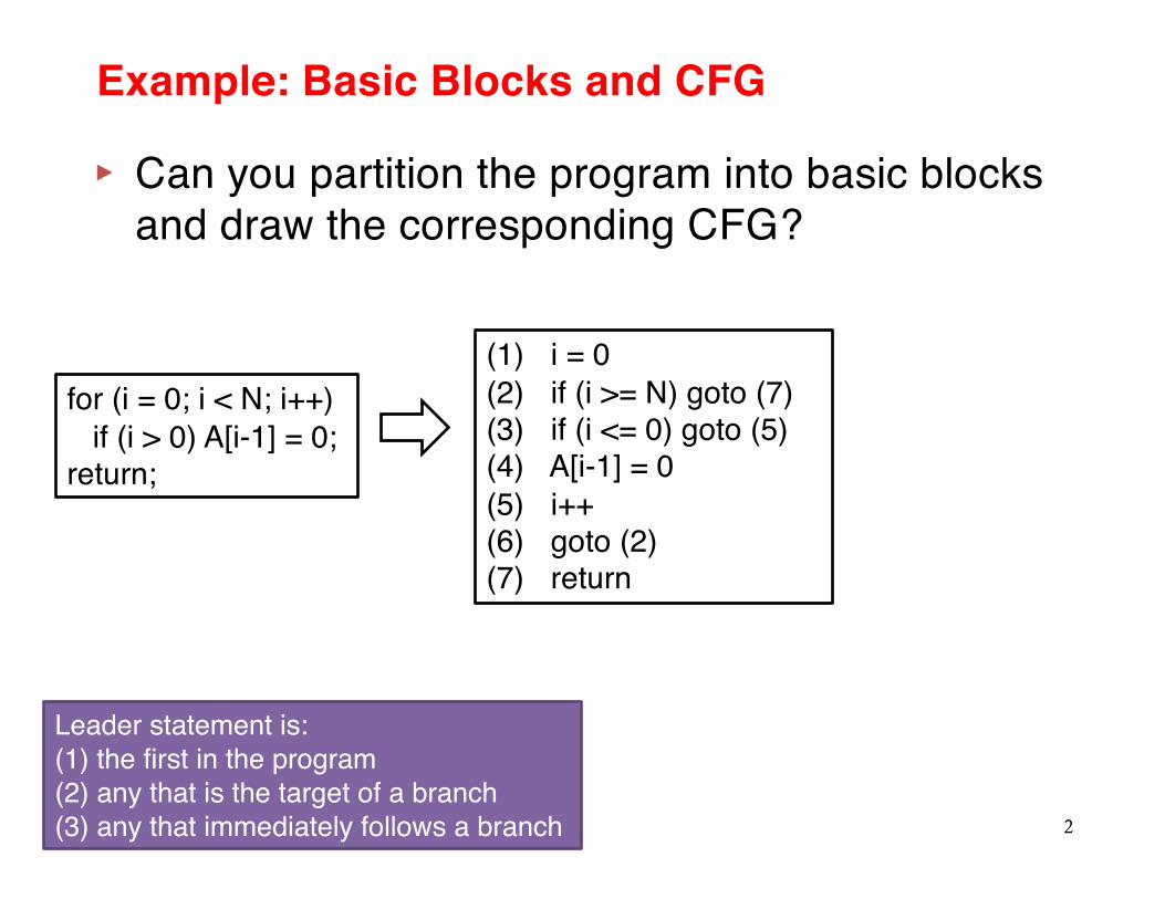
(1) i = 0(2) if (i >= N) goto (7)(3) if (i <= 0) goto (5)(4) A[i-1] = 0(5) i++(6) goto (2)(7) return

for (i = 0; i < N; i++)if (i > 0) A[i-1] = 0;

return;

▸ Can you partition the program into basic blocks and draw the corresponding CFG?

Leader statement is: (1) the first in the program(2) any that is the target of a branch (3) any that immediately follows a branch

3

Review: Dominator Tree and Dominance Frontier

B01234567

B0

B1

B2 B3

B4

B6

B7

B5

Dominance frontiersCFG

DF–1776671

For each convergence point X in the CFGFor each predecessor, Y, of X in the CFG

Run up to Z=IDOM(X) in the dominator tree,adding X to DF(N) for each N between [Y, Z)

Algorithm to compute DF set

B0

B1

B2 B3

B4B6

B5

B7

Dominator tree

4

Example: PHI Node Placement

X = …

X = …B0

B1

B2 B3

B4

B6

B7

B5

CFG

▸ X are defined in B0 and B4 in non-SSA form▸ Can you identify all the basic blocks where ϕ-nodes

need to be inserted for X in the SSA form?

B01234567

DF–1776671

▸ Unconstrained scheduling – ASAP and ALAP

▸ Constrained scheduling – Resource constrained scheduling (RCS)– Exact formulations with integer linear programming (ILP)

5

Agenda

High-level Programming Languages

(C/C++, OpenCL, SystemC, ...)

Parsing

Transformations

RTLgeneration

S0

S1

S2

S0

S1

S2

ab

z

d

3 cycles

*–

Control data flow graph (CDFG)

Finite state machines with datapath

BB3

BB1

BB2

BB4

T F

+

-

*+

*

if (condition) {…

} else {t1 = a + b;t2 = c * d;t3 = e + f;t4 = t1 * t2;z = t4 – t3;

}

Scheduling Binding

Allocation

Review: A Typical HLS Flow

6

Intermediate Representation (IR)

Scheduling in High-Level Synthesis

▸ Scheduling: a central problem in HLS– Introduce clock boundaries to untimed or partially timed input

specification– Significant impact on QoR

• Frequency• Latency• Throughput• Area• Power…

7

Scheduling: Untimed to Timed Latency Area Throughput

Untimed Combinational Sequential Pipelined

+

+

in1

+

out1

in2 in3 in4

+

+

in1

+

out1

in2 in3 in4

add

clk1

addclk

AAt1Td3t

*3/

1 ==

tclk ≈ dadd + dsetupT2 =1/ (3* tclk )A2 = Aadd + 2*Areg regadd

clk3

setupaddclk

AAAtT

ddt

*6*3/1

3 +==

+

+

+

in

+

out

3

2

1

4

3

2

1 2

1

( )in4in3,in2,in1,fout1=

in1

+

out1

in2 in3 in4

REG

8

Control-Data Flow Graph

▸ Control data flow graph (CDFG)– Generated by a compiler front end

from high-level description– Nodes

• Operations (and pseudo operations)– Directed edges

• Data edges, control edges, precedence edges

▸ Without control flow, the basic structure is a data flow graph (DFG)

9

Scheduling Input

xl = x+dx;ul = u-3*x*u*dx-3*y*dxyl = y+u*dxc = xl<a;x = xl; u = ul; y = yl;

+´´´´

´ ´ + <-

-

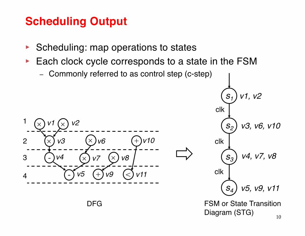
▸ Scheduling: map operations to states▸ Each clock cycle corresponds to a state in the FSM

– Commonly referred to as control step (c-step)

10

Scheduling Output

+

´

´

´´

´

´

+ <

-

-

1

2

3

4

v2v1

v3

v4

v5

v6

v7 v8

v9

v10

v11

s1

s2

s3

s4

v1, v2

v3, v6, v10

v4, v7, v8

v5, v9, v11

clk

clk

clk

DFG FSM or State Transition Diagram (STG)

▸ Only consideration: dependence

▸ As soon as possible (ASAP) – Schedule an operation to the earliest possible step

▸ As late as possible (ALAP)– Schedule an operation to the earliest possible step, without

increasing the total latency

11

Unconstrained Scheduling

12

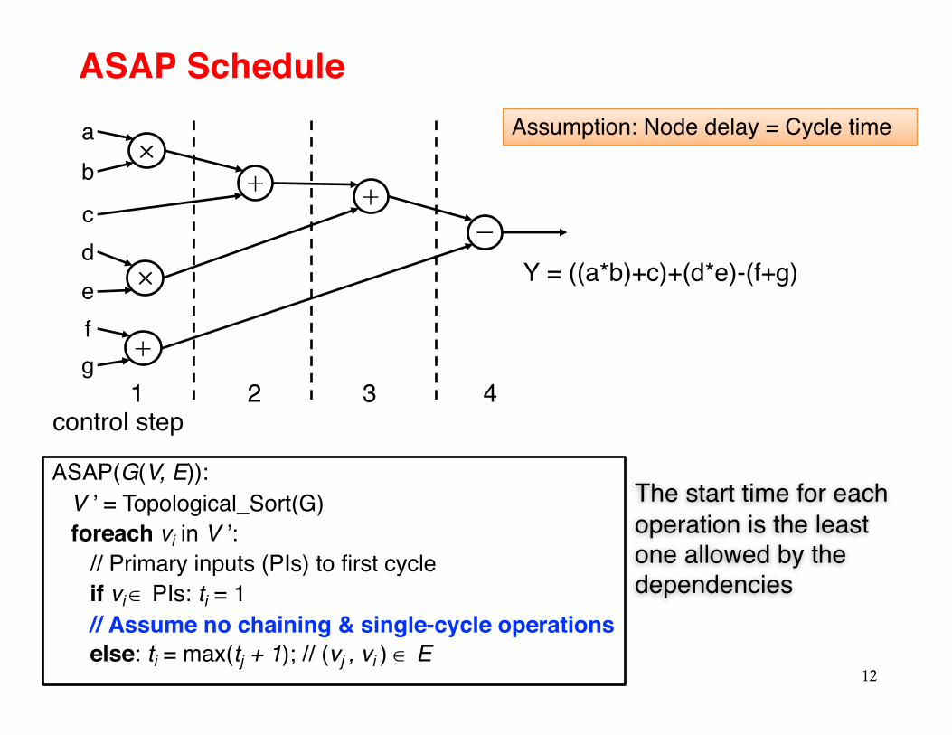
Y = ((a*b)+c)+(d*e)-(f+g)

The start time for each operation is the least one allowed by the dependencies

ASAP(G(V, E)):V ’ = Topological_Sort(G)foreach vi in V ’:

// Primary inputs (PIs) to first cycleif vi Î PIs: ti = 1// Assume no chaining & single-cycle operationselse: ti = max(tj + 1); // (vj , vi ) Î E

control step2 3 41

×

×

+

+ +−

ab

cdefg

ASAP ScheduleAssumption: Node delay = Cycle time

13

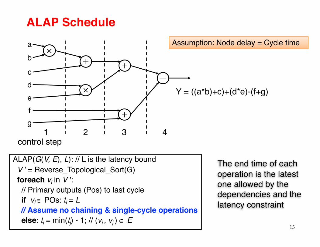
The end time of each operation is the latest one allowed by the dependencies and the latency constraint

ALAP(G(V, E), L): // L is the latency boundV ’ = Reverse_Topological_Sort(G)foreach vi in V ’:// Primary outputs (Pos) to last cycleif vi Î POs: ti = L// Assume no chaining & single-cycle operationselse: ti = min(tj) - 1; // (vi , vj ) Î E

control step

×

×

+

+ +−

2 3 41

ab

cdefg

Y = ((a*b)+c)+(d*e)-(f+g)

ALAP ScheduleAssumption: Node delay = Cycle time

14

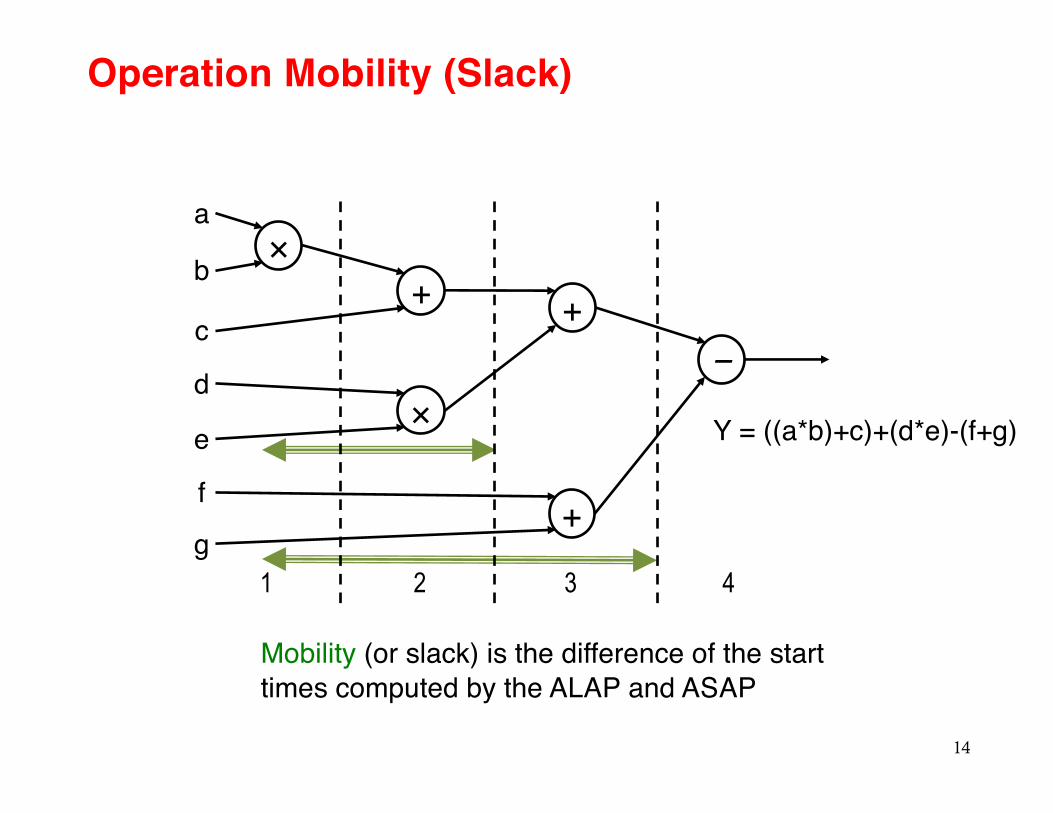
Operation Mobility (Slack)

Y = ((a*b)+c)+(d*e)-(f+g)

Mobility (or slack) is the difference of the start times computed by the ALAP and ASAP

×

×

+

+ +−

2 3 41

a

b

c

d

e

f

g

▸ Constrained scheduling– General case NP-hard– Resource-constrained scheduling (RCS)

• Minimize latency given constraints on area or resources– Time-constrained scheduling (TCS)

• Minimize resources subject to bound on latency

▸ Exact methods– Integer linear programming (ILP)– Hu’s algorithm for a very restricted problem

▸ Heuristics– List scheduling– Force-directed scheduling– SDC-based scheduling…

15

Constrained Scheduling

▸ Linear programming (LP) solves the problem of maximizing or minimizing a linear objective function subject to linear constraints

– Efficiently solvable both in theory and in practice

▸ Integer linear programming (ILP): in addition to linear constraints and objective, the values for the variables have to be integer

– NP-Hard in general (A special case, 0-1 ILP)– Modern ILP solvers can handle problems with nontrivial size

▸ Enormous number of problems can be expressed in LP or ILP

16

Linear Programming

17

Canonical Form of ILPmaximize c1x1+c2x2+…+cnxn // objective functionsubject to // linear constraints

a11x1+a12x2+…+a1nxn £ b1a21x1+a22x2+…+a2nxn £ b2….am1x1+am2x2+…+amnxn £ bmxi ≥ 0xi Î Z

maximize cTx // c = (c1, c2, …, cn) subject to

Ax ≤ b // A is a mxn matrix; b = (b1, b2, …, bn)x ≥ 0 andxi Î Z

Vector form

18

Example: Course Selection Problem

▸ A student is about to finalize her course selection for the coming semester, given the following information:

– Minimum credits / semester: 8

Schedule Credits Est. workload

1. Big data analytics MW 2:00-3:30pm

3 8 hrs

2. How to build a start-up TT 2:00-3:00pm 2 4 hrs

3. Linear programming MW 9:00-11:00am

4 10 hrs

4. Analog circuits TT 1:00-3:00pm 4 12 hrs

Question: Which courses to take to minimize the amount of work?

▸ Define decision variables (i = 1, 2, 3, 4):

▸ The total expected work hours:▸ The total credits taken:▸ Account for the schedule conflict:

▸ Complete ILP formulation (in canonical form):minimize 8x1+4x2+10x3+12x4

s.t. 3x1+2x2+4x3+4x4 ≥ 8x2+x4 ≤ 1xi Î {0,1}

19

ILP Formulation for Course Selection

xi =1 if course i is taken0 if not

!"#

$#

Time CRs Work

1. Big data MW 2-3:30pm

3 8 hrs

2. Start-up TT 2-3pm 2 4 hrs

3. Linear prog. MW 9-11am

4 10 hrs

4. Analog TT 1-3pm 4 12 hrs

8x1+4x2+10x3+12x4

3x1+2x2+4x3+4x4x2+x4 ≤ 1

▸ When functional units are limited– Each functional unit can only perform one operation

at each clock cycle• e.g., if there are only K adders, no more than K additions can

be executed in the same c-step

▸ A resource-constrained scheduling problem for DFG – Given the number of functional units of each type,

minimize latency – NP-hard problem

20

Resource Constrained Scheduling (RCS)

▸ Use binary decision variables– xik = 1 if operation i starts at step k, otherwise = 0.

• i = 1, 2, ..., N : N is the total number of operations• k = 1, ..., L : L is the given upper bound on latency

ILP Formulation of RCS

ti = kxikk=1

L

∑

21

ti indicates the start time of operation i

▸ Linear constraints:

– Unique start times:

– Dependence must be satisfied (no chaining)

ILP Formulation of RCS: Constraints (1)

xik =1, i =1,2,...,Nk∑

t j ≥ ti + di +1:∀(vi,vj )∈ E⇒ k x jkk∑ ≥ k xik +

k∑ di +1

22

vj must not start before vi completes since vj depends on vi

Start Time vs. Time(s) of Execution

▸ di : latency of operation i– di = 0 indicates single-cycle combinational logic

▸ When di = 0, then the following questions are the same:– Does operation i start at step k – Is operation i running at step k

▸ But if di > 0, then the two questions should be formulated as:

– Does operation i start at step k• Check if xik = 1 hold

– Is operation i running at step k • Check if the following hold?

23

xill=k−di

k

∑ =1?

▸ Is v9 (d9 = 2) running at step 6?If and only if x9,6 + x9,5 + x9,4 equals 1

▸ Note:– Only one (if any) of the above three cases can happen– To meet resource constraints, we have to ask the same question

for ALL steps, and ALL operations of that type

456

x9,4=1

v9

456

x9,5=1

v9v9

456

x9,6=1

24

Operation vi Still Running at Step k ?

▸ Linear constraints:

– Unique start times:

– Dependence must be satisfied (no chaining)

– Resource constraints

ILP Formulation of RCS: Constraints (2)

xik =1, i =1,2,...,Nk∑

t j ≥ ti + di +1:∀(vi,vj )∈ E⇒ k x jkk∑ ≥ k xik +

k∑ di +1

25

RT(vi) : resource type ID of operation vi (between 1~nres)ar is the number of available resources for resource of type r

xill=k−di

k

∑i:RT (vi )=r∑ ≤ ar, r =1,...,nres, k =1,...,L

▸ Students presenting next Thursday are expected to set up an appointment with the instructor

▸ Next lecture: More scheduling algorithms

26

Before Next Lecture

▸ These slides contain/adapt materials developed by– Ryan Kastner (UCSD)

27

Acknowledgements