Schema Design and Implementation of

the Grasp-Related Mirror Neuron System

Erhan Oztop and Michael A. Arbib

erhan@java.usc.edu, arbib@pollux.usc.edu

USC Brain Project

University of Southern California

Los Angeles, CA 90089-2520

http://www-hbp.usc.edu/

Abstract Mirror neurons within a monkey's premotor area F5 fire not only when the monkey performs a certain

class of action but also when the monkey observes another monkey (or the experimenter) perform a

similar action (Gallese et al. 1996; Rizzolatti et al. 1996a) . It has thus been argued that these neurons are

crucial for understanding of actions by others. We offer the Hand-State Hypothesis as a new explanation

of the evolution of this capability, hypothesizing that these neurons first evolved to augment the

"canonical" F5 neurons (active during self-movement based on observation of an object) by providing

visual feedback on "hand state", relating the shape of the hand to the shape of the object. We then

introduce the MNS (Mirror Neuron System) model of F5 and related brain regions. The existing FARS

(Fagg-Arbib-Rizzolatti-Sakata) model (Fagg and Arbib 1998) represents circuitry for visually-guided

grasping of objects, linking parietal area AIP with F5 canonical neurons. The MNS model extends the AIP

visual pathway by also modeling pathways, directed toward F5 mirror neurons, which match arm-hand

trajectories to the affordances and location of a potential target object. We present the basic schemas for

the MNS model, then aggregate them into three "grand schemas" − Visual Analysis of Hand State, Reach

and Grasp, and the Core Mirror Circuit − for each of which we present a useful implementation. With this

implementation we show how the mirror system may learn to recognize actions already in the repertoire

of the F5 canonical neurons. We show that the connectivity pattern of mirror neuron circuitry can be

established through training, and that the resultant network can exhibit a range of novel, physiologically

interesting, behaviors during the process of action recognition. We train the system on the basis of final

grasp but then observe the whole time course of mirror neuron activity, yielding predictions for

neurophysiological experiments under conditions of spatial perturbation, altered kinematics, and

ambiguous grasp execution which highlight the importance of the timing of mirror neuron activity.

1 INTRODUCTION

1.1 The Mirror Neuron System for Grasping

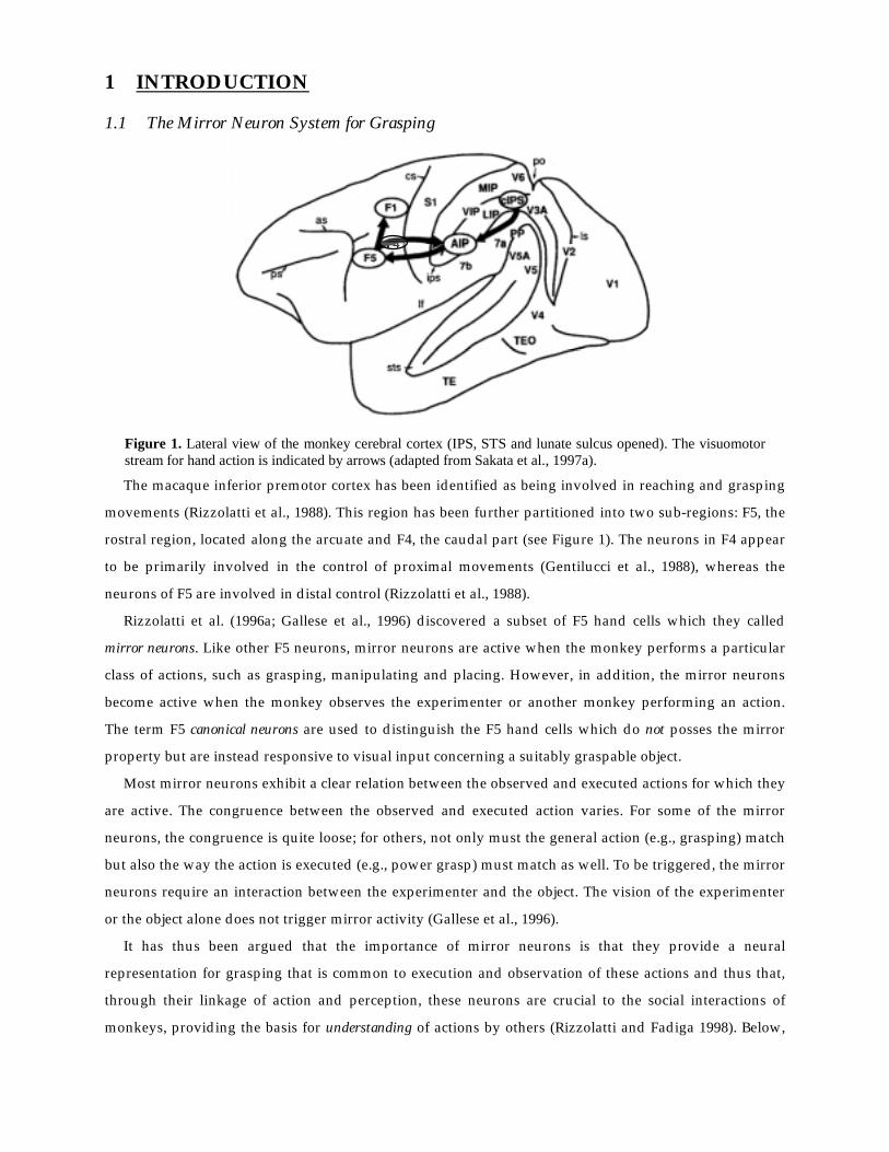
Figure 1. Lateral view of the monkey cerebral cortex (IPS, STS and lunate sulcus opened). The visuomotor stream for hand action is indicated by arrows (adapted from Sakata et al., 1997a).

The macaque inferior premotor cortex has been identified as being involved in reaching and grasping

movements (Rizzolatti et al., 1988). This region has been further partitioned into two sub-regions: F5, the

rostral region, located along the arcuate and F4, the caudal part (see Figure 1). The neurons in F4 appear

to be primarily involved in the control of proximal movements (Gentilucci et al., 1988), whereas the

neurons of F5 are involved in distal control (Rizzolatti et al., 1988).

Rizzolatti et al. (1996a; Gallese et al., 1996) discovered a subset of F5 hand cells which they called

mirror neurons. Like other F5 neurons, mirror neurons are active when the monkey performs a particular

class of actions, such as grasping, manipulating and placing. However, in addition, the mirror neurons

become active when the monkey observes the experimenter or another monkey performing an action.

The term F5 canonical neurons are used to distinguish the F5 hand cells which do not posses the mirror

property but are instead responsive to visual input concerning a suitably graspable object.

Most mirror neurons exhibit a clear relation between the observed and executed actions for which they

are active. The congruence between the observed and executed action varies. For some of the mirror

neurons, the congruence is quite loose; for others, not only must the general action (e.g., grasping) match

but also the way the action is executed (e.g., power grasp) must match as well. To be triggered, the mirror

neurons require an interaction between the experimenter and the object. The vision of the experimenter

or the object alone does not trigger mirror activity (Gallese et al., 1996).

It has thus been argued that the importance of mirror neurons is that they provide a neural

representation for grasping that is common to execution and observation of these actions and thus that,

through their linkage of action and perception, these neurons are crucial to the social interactions of

monkeys, providing the basis for understanding of actions by others (Rizzolatti and Fadiga 1998). Below,

F4F4F4F4

we offer the Hand-State Hypothesis, suggesting that this important role is an exaptation of a more

primitive role, namely that of providing feedback for visually-guided grasping movements. We will then

develop the MNS (Mirror Neuron System) model and show that the system can exploit its ability to relate

self-hand movements to objects to recognize the manual actions being performed by others, thus yielding

the mirror property. We also conduct a number of simulation experiments with the model and show that

these yield novel predictions, suggesting new neurophysiological experiments to further probe the

monkey mirror system. However, before introducing the Hand-State Hypothesis and the MNS model, we

first outline the FARS model of the circuitry that includes the F5 canonical neurons and provides the

conceptual basis for the MNS model.

1.2 The FARS Model of Parietal-Premotor Interactions in Grasping Studies of the anterior intraparietal sulcus (AIP; Figure 1) revealed cells that were activated by the

sight of objects for manipulation (Taira et al., 1990; Sakata et al., 1995). In addition, this region has very

significant recurrent cortico-cortical projections with area F5 (Matelli, 1994; Sakata, 1997). In their

computational model for primate control of grasping (the FARS – Fagg-Arbib-Rizzolatti-Sakata – model),

Fagg and Arbib (1998) analyzed these findings of Sakata and Rizzolatti to show how F5 and AIP may act

as part of a visuo-motor transformation circuit, which carries the brain from sight of an object to the

execution of a particular grasp. In developing the FARS model, Fagg and Arbib (1998) interpreted the

findings of Sakata (on AIP) and Rizzolatti (on F5), as AIP representing the grasps afforded by the object

and F5 selecting and driving the execution of the grasp. The term affordance (adapted from Gibson, 1966)

refers to parameters for motor interaction that are signaled by sensory cues without invocation of high-

level object recognition processes). The model also suggests how F5 may use task information and other

constraints encoded in prefrontal cortex (PFC) to resolve the action opportunities provided by multiple

affordances. Here we emphasize the essential components of the model (Figure 2) that will form part of

the current version of the MNS model presented below. We focus on the linkage between viewing an

affordance of an object and the generation of a single grasp.

AIP

F5

dorsal/ventral streams

Task Constraints (F6)

Working Memory (46)

Instruction Stimuli (F2)

Task Constraints(F6)Working Memory(46)Instruction Stimuli(F2)

AIPDorsalStream:Affordances

IT

VentralStream:Recognition

Ways to grabthis “thing”

“It’s a mug”PFC

Figure 2. AIP extracts the affordances and F5 selects the appropriate grasp from the AIP ‘menu’. Various biases are sent to F5 by Prefrontal Cortex (PFC) which relies on the recognition of the object by Inferotemporal Cortex (IT). The dorsal stream through AIP to F5 is replicated in the current version of the MNS model; the influence of IT and PFC on F5 is not analyzed further in the present paper.

1. The dorsal visual stream (parietal cortex) extracts parametric information about the object being

attended. It does not "know" what the object is; it can only see the object as a set of possible affordances.

The ventral stream (from primary visual cortex to inferotemporal cortex, IT), by contrast, recognize what

the object is and passes this information to prefrontal cortex (PFC) which can then, on the basis of the

current goals of the organism and the recognition of the nature of the object, bias F5 to choose the

affordance appropriate to the task at hand.

2. AIP is hypothesized as playing a dual role in the seeing/reaching/grasping process, not only

computing affordances exhibited by the object but also, as one of these affordances is selected and

execution of the grasp begins, serving as an active memory of the one selected affordance and updating

this memory to correspond to the grasp that is actually executed.

3. F5 is hypothesized as first being responsible for integrating task constraints with the set of grasps

that are afforded by the attended object in order to select a single grasp. After selection of a single grasp,

F5 unfolds this represented grasp in time to perform the execution.

4. In addition, the FARS model represents the way in which F5 may accept signals from areas F6 (pre-

SMA), 46 (dorsolateral prefrontal cortex), and F2 (dorsal premotor cortex) to respond to task constraints,

working memory, and instruction stimuli, respectively, and how these in turn may be influenced by

object recognition processes in IT (see Fagg and Arbib 1988 for more details), but these aspects of the

FARS model are not involved in the current version of the MNS model.

2 THE HAND-STATE HYPOTHESIS The key notion of the MNS model is that the brain augments the mechanisms modeled by the FARS

model for recognizing the grasping-affordances of an object (AIP) and transforming these into a program

of action by mechanisms which can recognize an action in terms of the hand state which makes explicit

the relation between the unfolding trajectory of a hand and the affordances of an object. Our radical

departure from all prior studies of the mirror system is to hypothesize that this system evolved in the first

place to provide feedback for visually-directed grasping, with the social role of the mirror system being

an exaptation as the hand state mechanisms become applied to the hands of others as well as to the hand

of the animal itself. We first introduce the notions of virtual fingers and opposition space and then define

the hand state.

2.1 Virtual Fingers

Figure 3. Each of the 3 grasp types here is defined by specifying two "virtual fingers", VF1 and VF2, which are groups of fingers or a part of the hand such as the palm which are brought to bear on either side of an object to grasp it. The specification of the virtual fingers includes specification of the region on each virtual finger to be brought in contact with the object. A successful grasp involves the alignment of two "opposition axes": the opposition axis in the hand joining the virtual finger regions to be opposed to each other, and the opposition axis in the object joining the regions where the virtual fingers contact the object. (Iberall and Arbib 1990.)

As background for the Hand-State Hypothesis, we first present a conceptual analysis of grasping.

Iberall and Arbib (1990) introduced the theory of virtual fingers and opposition space. The term virtual finger

is used to describe the physical entity (one or more fingers, the palm of the hand, etc.) that is used in

applying force and thus includes specification of the region to be brought in contact with the object (what

we might call the "virtual fingertip"). Figure 3 shows three types of opposition: those for the precision

grip, power grasp, and side opposition. Each of the grasp types is defined by specifying two virtual

fingers, VF1 and VF2, and the regions on VF1 and VF2 which are to be brought into contact with the

object to grasp it. Note that the "virtual fingertip" for VF1 in palm opposition is the surface of the palm,

while that for VF2 in side opposition is the side of the index finger. The grasp defines two "opposition

axes": the opposition axis in the hand joining the virtual finger regions to be opposed to each other, and the

opposition axis in the object joining the regions where the virtual fingers contact the object. Visual

perception provides affordances (different ways to grasp the object); once an affordance is selected, an

appropriate opposition axis in the object can be determined. The task of motor control is to preshape the

hand to form an opposition axis appropriate to the chosen affordance, and to so move the arm as to

transport the hand to bring the hand and object axes into alignment. During the last stage of transport,

the virtual fingers move down the opposition axis (the "enclose" phase) to grasp the object just as the

hand reaches the appropriate position.

2.2 The Hand-State Hypothesis We assert as a general principle of motor control that if a motor plant is used for a task, then a

feedback system will evolve to better control its performance in the face of perturbations. We thus ask, as

a sequel to the work of Iberall and Arbib (1990), what information would be needed by a feedback

controller to control grasping in the manner described in the previous section. Note that we do not model

this feedback control in the present paper. Rather, we offer the following hypothesis.

The Hand-State Hypothesis: The basic functionality of the F5 mirror system is to elaborate the

appropriate feedback – what we call the hand state – for opposition-space based control of manual

grasping of an object. Given this functionality, the social role of the F5 mirror system in understanding

the actions of others may be seen as an exaptation gained by generalizing from self-hand to other's-hand.

The key to the MNS model, then, is the notion of hand state as encompassing data required to

determine whether the motion and preshape of a moving hand may be extrapolated to culminate in a

grasp appropriate to one of the affordances of the observed object. Basically a mirror neuron must fire if

the preshaping of the hand conforms to the grasp type with which the neuron is associated; and the

extrapolation of hand state yields a time at which the hand is grasping the object along an axis for which

that affordance is appropriate.

Our current representation of hand state defines a 7-dimensional trajectory

F(t) = (d(t), v(t), a(t), o1(t), o2(t), o3(t), o4(t))

with the following components (see Figure 4):

The three components are hand configuration parameters:

a(t): Index finger-tip and thumb-tip aperture

o3(t), o4(t): The two angles defining how close the thumb is to the hand as measured relative to the

side of the hand and to the inner surface of the palm

The remaining four parameters relates the hand to the object. o1 and o2 components represent the

orientation of different components of the hand relative to the opposition axis for the chosen affordance

in the object whereas d and v represents the kinematics properties of the hand with reference to the target

location.

o1(t): The cosine of the angle between the object axis and the (index finger tip – thumb tip) vector

o2(t): The cosine of the angle between the object axis and the (index finger knuckle – thumb tip) vector

d(t): distance to target at time t

v(t): tangential velocity of the wrist

Figure 4. The components of hand state F(t) = (d(t), v(t), a(t), o1(t), o2(t), o3(t), o4(t)). Note that some of the components are purely hand configuration parameters (namely v,o3,o4,a) whereas others are parameters relating hand to the object.

In considering the last 4 variables, note that only one or two of them will be relevant in generating a

specific type of grasp, but they all must be available to monitor a wide range of possible grasps. We have

chosen a set of variables of clear utility in monitoring the successful progress of grasping an object, but do

not claim that these and only these variables are represented in the brain. Indeed, the brain's actual

representation will be a distributed neural code, which we predict will correlate with such variables, but

will not be decomposable into a coordinate-by-coordinate encoding. However, we believe that the explicit

definition of hand state offered here will provide a firm foundation for the design of new experiments in

kinesiology and neurophysiology.

The crucial point is that the availability of the hand state to provide feedback for visually-directed

grasping makes action recognition possible. Notice that we have carefully defined the hand state in terms

of relationships between hand and object (though the form of the definition must be subject to future

research). This has the benefit that it will work just as well for measuring how the monkey’s own hand is

Velocity (v(t))

Axis disparity 2 (arccos(o2(t)))

Axis disparity 1 (arccos(o1(t)))

Distance (d(t))

Aperture (a(t))

Thumb angle 2 (o4(t))

Thumb angle 1 (o3(t)) Grasp Axis

Object opposition axis

Hand opposition axis (thumb, index fingertip)

Hand opposition axis (thumb, index knuckle)

moving to grasp an object as for observing how well another monkey’s hand is moving to grasp the

object. This, we claim, is what allows self-observation by the monkey to train a system that can be used

for observing the actions of others and recognizing just what those actions are.

3 THE MNS (MIRROR NEURON SYSTEM) MODEL We now present a high level view of the MNS (Mirror Neuron System) model in terms of the set of

interacting schemas (functional units; Arbib 1981; Arbib et al. 1998, Chapter 3) shown in Figure 5, which

define the MNS (Mirror Neuron System) model of F5 and related brain regions. The connectivity of the

model is constrained by the existing neurophysiology and neuroanatomy of the monkey brain, but except

for AIP and F5 the anatomical localization of schemas is not germane to the simulations presented in the

current paper. In Figure 4, solid arrows denote neuroanatomically established connections while dashed

arrows indicate connections postulated for computational completeness. Detailed discussion of the

pertinent data is postponed to later papers in which more detailed neural modeling of other brain regions

takes center stage. The F5 grasp-related neurons are divided between (i) F5 mirror neurons which are,

when fully developed, active during certain self-movements of grasping by the monkey and during the

observation of a similar grasp executed by others, and (ii) F5 canonical neurons, namely those active

during self-movement but not during the observation of grasping by others. The subsystem of the MNS

model responsible for the visuo-motor transformation of objects into affordances and grasp

configurations, linking AIP and F5 canonical neurons, corresponds to a key subsystem of the FARS model

reviewed above. Our task is to complement the visual pathway via AIP by pathways directed toward F5

mirror neurons, which allow the monkey to observe arm-hand trajectories and match them to the

affordances and location of a potential target object. We will then show how the mirror system may learn

to recognize actions already in the repertoire of the F5 canonical neurons. In short, we will provide a

mechanism whereby the actions of others are "recognized" based on the circuitry involved in performing

such actions. The Methods section provides the details of the implemented schemas and the Results

section confronts the overall model with virtual experiments and produces testable predictions.

STS 7a

Handshaperecognition

Hand-Objectspatial relationanalysis

Object affordance-hand stateassociation

Objectaffordanceextraction

Actionrecognition(MirrorNeurons)

Motorprogram(Grasp)

Motorexecution

MirrorFeedback

Integratetemporalassociation

7bF5canonical

AIP

M 1

F5mirror

Object features

Objectlocation

Motorprogram(Reach)F4

M IP/LIP/VIP

Visu

al C

orte

xcIPS

Handmotiondetection

Figure 5. The MNS (Mirror Neuron System) model. (i) Top diagonal: a portion of the FARS model. Object features are processed by AIP to extract grasp affordances, these are sent on to the canonical neurons of F5 that choose a particular grasp. (ii) Bottom right. Recognizing the location of the object provides parameters to the motor programming area F4 which computes the reach. The information about the reach and the grasp is taken by the motor cortex M1 to control the hand and the arm. (iii) New elements of the MNS model: Bottom left are two schemas, one to recognize the shape of the hand, and the other to recognize how that hand is moving. Just to the right of these is the schema for hand-object spatial relation analysis. It takes information about object features, the motion of the hand and the location of the object to infer the relation between hand and object. (iv) The center two regions marked by the gray rectangle form the core mirror circuit. This complex associates the visually derived input (hand state) with the motor program input from region F5canonical neurons during the learning process for the mirror neurons. (Solid arrows: Established connections; Dashed arrows: postulated connections. Details of the ascription of specific schemas to specific brain regions is deferred to a later paper.)

3.1 Overall Function In general, the visual input of the monkey represents a complex scene. However, we here sidestep

much of this complexity by assuming that the brain extracts two salient sub-scenes, a stationary object

and in some cases a (possibly) moving hand. The overall system operates in two modes:

(i) Prehension: In this mode, the view of the stationary object is analyzed to extract affordances; then

under prefrontal influence F5 may choose one of these to act upon, commanding the motor apparatus to

perform the appropriate reach and grasp based on parameters supplied by the parietal cortex. The FARS

model captures the loop linking F5 and AIP together with the role of prefrontal cortex in modulating F5

activity, based in part on object recognition processes culminating in inferotemporal cortex (Figure 2). In

the MNS model, we incorporate the F5 and AIP components from FARS (top diagonal of schemas in

Figure 5), but omit the roles of IT and PFC from the present analysis.

(ii) Action recognition: In this mode, the view of the stationary object is again analyzed to extract

affordances, but now the initial trajectory and preshape of an observed moving hand must be

extrapolated to determine whether the current motion of the hand can be expected to culminate in a

grasp of the object appropriate to one of its affordances.

We will not prespecify all the details of the MNS schemas but will instead offer a learning model

which, given a grasp that is already in the motor repertoire of the F5 canonical neurons, can yield a set of

F5 mirror neurons trained to be active during such grasps as a result of self-observation of the monkey's

own hand grasping the target object. Consistent with the Hand-State Hypothesis, the result will be a

system whose mirror neurons can respond to similar actions observed being performed by others. The current

implementation of the MNS model exploits learning in artificial neural nets.

The heart of the learning model is provided by the Object affordance-hand state association schema and

the Action recognition (mirror neurons) schema. These form the core mirror (learning) circuit, marked by the

gray slanted rectangle in Figure 5, which mediates the development of mirror neurons via learning. The

simulation results of this article will focus on this part of the model. The Methods section presents in

detail the neural network structure of the core circuit. As we note further in the Discussion section, this

leaves open many problems for further research, including the development of a basic action repertoire

by F5 canonical neurons through trial-and-error in infancy and the expansion and refinement of this

repertoire throughout life.

3.2 Individual Schemas Explained In this section, we present the input, output and function for each of the schemas in Figure 5.

However, as will be made clear when we come to the discussion of Figure 6 below, we will not attempt in

this paper the modeling of these individual schemas but will instead discuss the implementation of three

"grand schemas", each of which provides the composite functionality of several of the individual schemas

of Figure 5. Nonetheless, it seems worth providing the more detailed specifications here both to ground

the definition of the grand schemas and to set the stage for the more detailed neurobiological modeling

promised for our later papers.

Object Features schema: The output of this schema provides a coarse coding of geometrical features of

the observed object. It thus provides suitable input to AIP and other regions/schemas.

Object Affordance Extraction schema: This schema transforms its input, the coarse coding of

geometrical features of the observed object provided by the Object features schema, into a coarse coding

for each affordance of the observed object.

Motor Program (Grasp) schema: We identify this schema with the canonical F5 neurons, as in FARS

model. Input is provided by AIP's coarse coding of affordances for the observed object. We assume that

the output of the schema encodes a generic motor program for the AIP-coded affordances. This output

drives the Action-recognition (Mirror neurons) schema as well as the hand control functions of the Motor

execution schema

Object Location schema: The output of this schema provides, in some body-centered coordinate

frame, the location of the center of the opposition axis for the chosen affordance of the observed object.

Motor Program (Reach) schema: The input is the position coded by the Object location schema, while

the output is the motor command required to transport the arm to bring the hand to the indicated

location. This drives the arm control functions of the Motor execution schema.

The Motor Execution schema determines the course of movements via activity in primary motor cortex

M1 and "lower" regions.

We now turn to the truly novel schemas which define the Mirror Neuron System (MNS) model:

The Action Recognition schema – which is meant to correspond to the mirror neurons of area F5 –

receives two inputs in our model. One is the motor program selected by the Motor program schema; the

other comes from the Object affordance-hand state association schema. This schema learns to integrate the

output of the Object affordance-hand state association schema to form the correct mirror response by

exploiting the motor program information signaled by the F5 canonical neurons (Motor program schema).

We next review the schemas which (in addition to the previously presented Object features and Object

affordance extraction schemas) implement the visual system of the model:

The Hand Shape Recognition schema takes as input a picture of a hand, and its output is a

specification of the hand shape, which thus forms some of the components of the hand state. In the

current implementation these are a(t), o3(t) and o4(t). Note also that we implicitly assume that the schema

includes a validity check to verify that the picture does contain a hand.

The Hand Motion Detection schema takes as input a sequence of pictures of a hand and returns as

output the velocity estimate of the hand. The current implementation tracks only the wrist velocity,

supplying the v(t) component of the hand state.

Finally, we present the schemas that combine observations of hand shape and movements with

observation of object affordances to drive the action recognition (mirror neuron) circuitry.

The Hand-Object spatial relation analysis schema receives object-related signals from the Object

features schema, as well as input from the Object Location, Hand shape recognition and Hand motion detection

schemas. Its output is a set of vectors relating the current hand preshape to a selected affordance of the

object. The schema computes such parameters as the distance of the object to the hand, and the disparity

between the opposition axes of the object and the hand. Thus the hand state components o1(t), o2(t), and

d(t) are supplied by this schema. The Hand-Object spatial relation analysis schema is needed because, for

most (but not all) mirror neurons in the monkey, a hand mimicking a matching grasp would fail to elicit

the mirror neuron's activity unless the hand's trajectory were taking it toward an object with a grasp that

matches one of the affordances of the object. The output of this visual analysis is relayed to the Object

affordance-hand state association schema which drives the F5 mirror neurons whose output is a signal

expressing confidence that the observed trajectory will extrapolate to match the observed target object

using the grasp encoded by that mirror neuron.

The Object affordance-hand state association schema combines all the hand related information as

well as the object information available. Thus the inputs to the schema are from Hand shape recognition

(components a(t), o3(t), o4(t)), Hand motion detection (component v(t)), Hand-Object spatial relation analysis

(o1(t), o2(t), d(t)) and from Object affordance extraction schemas. As will be explained below, the schema

needs a learning signal (mirror feedback). This signal is relayed by the Action recognition schema and, is

basically, a copy of the motor program passed to the Action recognition schema itself. The output of this

schema is a distributed representation of the object and hand state match (in our implementation the

representation is not pre-specified but shaped by the learning process). The idea is to match the object

and the hand state as the action progresses during a specific observed reach and grasp. In the current

implementation, time is unfolded into a spatial representation of "the trajectory until now" at the input of

the Object affordance-hand state association schema, and the Action recognition schema decodes the

distributed representation to form the mirror response (in our implementation the decoding is not pre-

specified but is the result of the back-propagation learning). In any case, the schema has two operating

modes. First is the learning mode where the schema tries to adjust its efferent and afferent weights to

ensure the right activity in the Action recognition schema. The second mode is the forward mode where it

maps the hand state and the object affordance into a distributed representation to be used by the Action

recognition schema.

The key question for our present modeling will be to account for how learning mechanisms may shape

the connections to mirror neuron in such a way that an action in the motor program repertoire of the F5

canonical neurons may become recognized by the mirror neurons when performed by others.

To conclude this section, we note that our modeling is subject to two quite different tests: (i) its overall

efficacy in explaining behavior and its development, which can be tested at the level of the schemas

(functional units) presented in this article; and (ii) its further efficacy in explaining and predicting

neurophysiological data. As we shall see below, certain neurophysiological predictions are possible given

the current work, even though the present implementation relies on relatively abstract artificial neural

networks.

4 METHODS

4.1 Schema Implementation We do not implement the schemas of Figure 5 individually, but instead partition them into the three

"grand schemas" of Figure 6(a) as follows:

Visual Analysisof Hand State

CoreMirrorCircuit

Reach and Grasp Schema

Core Mirror Circuit

Vis

ual I

nput

Object Affordance

Grasp Command

Hand State

Action CodeHand State

Action Code

Object Affordance

Grasp Command

(a)

(b)

Figure 6. (a) For purposes of simulation, we aggregate the schemas of the MNS (Mirror Neuron System) model of Figure 5 into three "grand schemas" for Visual Analysis of Hand State, Reach and Grasp, Core Mirror Circuit. (b) For detailed analysis of the Core Mirror Circuit, we dispense with simulation of the other 2 grand schemas and use other computational means to provide the three key inputs to this grand schema.

Grand Schema 1: Visual Analysis of Hand State

• Hand shape recognition schema

• Hand-Object spatial relation analysis schema

• Hand motion detection schema

Grand Schema 2: Reach and Grasp

• Object Features schema

• Object Location schema

• Object Affordance Extraction schema

• Motor Program (Grasp) Schema

• Motor Program (Reach) Schema

• Motor Execution schema

Grand Schema 3: Core Mirror Circuit

• Object affordance-hand state association schema

• Action recognition schema

Only in a few cases it is possible to identify individual schemas (such as the Action recognition schema)

in a schema group implementation.

4.2 Grand Schema 1: Visual Analysis of Hand State To extract hand parameters from a view of a hand, we try to recover the configuration of a model of

the hand being seen. The hand model is a three dimensional 14 degrees of freedom (DOF) kinematic

model, with a 3-DOF joint for the wrist, two 1-DOF joints (metacarpophalangeal and

distalinterphalangeal) for each of four fingers, and finally a 1-DOF joint for the metacarpophalangeal

joint, and a 2-DOF joint for the carpometacarpal joint of the thumb. Note the distinction between "hand

configuration" which gives the joint angles of the hand considered in isolation, and the "hand state"

which comprises 7 parameters relevant to assessing the motion and preshaping of the hand relative to an

object. Thus the hand configuration provides some, but not all, of the data needed to compute the hand

state.

To lighten the load of building a visual system to recognize hand features, we mark the wrist and the

articulation points of the hand with colors. We then use this color-coding to help recognize key portions

of the hand and use this result to initiate a process of model matching. Thus the first step of the vision

problem is color segmentation, after which is followed by the task of recovering the three dimensional

hand shape.

4.2.1 Color Segmentation and Feature Extraction

One needs color segmentation to locate the colored regions on the image. Gray level segmentation

techniques cannot be used in a straightforward way because of the vectorial nature of color images

(Lambert and Carron, 1999). Split-and-Merge is a well-known image segmentation technique in image

processing (see Sanka et al., 1993), recursively splitting the image into smaller pieces until some

homogeneity criterion is satisfied. In our case, it corresponds to having the same color in a region. To

decide whether a region is (approximately) of the same color one needs to compare the color values in the

region. However, RGB (Red-Green-Blue) space is not well suited for this purpose. HSV (Hue-Saturation-

Value) space is better suited for the task as hue in segmentation processes usually corresponds to human

perception and ignores shading effects (see Russ, 1998, chapters 1 and 6). However, the segmentation

system we implemented with HSV space, although better than RGB version, was not satisfactory for our

purposes. Therefore, we designed a system that can learn the best color space itself.

Figure 7(a) shows the training phase of the color expert system, which is a (one hidden-layer) feed-

forward network with sigmoidal activation function. The learning algorithm is back-propagation with

momentum and adaptive learning rate. The given image is put through a smoothing filter to reduce noise

in the image before training. Then the network is given around 100 training samples each of which is a

pair of ((R, G, B), perceived color code) values. The output color code is a vector consisting of all zeros

except for one component corresponding to the perceived color of the patch. Basically, the training builds

an internal non-linear color space on which it can unambiguously tell the perceived color. This training is

done only at the beginning of a session to learn the colors used on the particular hand. Then the network

is fixed as the hand is viewed in a variety of poses.

Preprocessing(Color Expert)

Features

Color segmentation System augmented with the trained neural network

Hand image for trainingNeural Network Training

Hand Image input for actual segmentation

Color segmentation using the Color Expert

Network Weights

(a)

(b)

One hidden layer feed-forward neural network

Figure 7. (a) Training the color expert. The trained network will be used in the subsequent phase for segmenting image. (b) The hand image (different from training sample) is fed to the augmented segmentation program. The color decision during segmentation is done by consulting to the Color Expert. Note that the smoothing step is performed before the segmentation (not shown).

Figure 7(b) illustrates the actual segmentation process using the Color Expert to find each region of a

single (perceived) color (see Appendix A1 for details). The output of the algorithm is then converted into

a feature vector with a corresponding confidence vector (giving a confidence level for each component in

the feature vector). Each finger is marked with two patches of the same color. Sometimes it may not be

possible to determine which patch corresponds to the fingertip and which to the knuckle. In those cases

the confidence value is set to 0.5. If a color is not found (e.g., the patch may be obscured), a zero value is

given for the confidence. If a unique color is found without any ambiguity then the confidence value is

set to 1. The segmented centers of regions (color markers) are taken as the approximate articulation point

positions. To convert the absolute color centers into a feature vector we simply subtract the wrist position

from all the centers found and put the resulting relative (x,y) coordinate into the feature vector (but the

wrist is excluded from the feature vector as the positions are specified with respect to the wrist position).

4.2.2 3D Hand Model Matching

Our model matching algorithm uses the feature vector generated by the segmentation system to attain a

hand configuration and pose that would result in a feature vector as close as possible to the input feature

vector (Figure 8). The scheme we use is a simplified version of Lowe’s (1991); see Holden (1997) for a

review of other hand recognition studies.

Result of feature extraction

Feature Vector

Initial Configuration of Hand Model

Final Configuration of Hand Model

Figure 8. Illustration of the model matching system. Left: markers located by feature extraction schema. Middle: initial and Right: final stages of model matching. After matching is performed a number of parameters for the Hand state are extracted from the matched 3D model.

The matching algorithm is based on minimization of the distance between the input feature and model

feature vector, where the distance is a function of the two vectors and the confidence vector generated by

segmentation system. Distance minimization is realized by a hill climbing in feature space. The method

can handle occlusions by starting with "don't cares" for any joints whose markers cannot be clearly

distinguished in the current view of the hand

The distance between two feature vectors F and G is computed as follows:

gi

fiii CCGFGFD 2)(),( −=

where subscripting denotes components and Cf, Cg denotes the confidence vectors associated with F and

G. Given this result of the visual processing – our Hand shape recognition schema – we can clearly read off

the following components of the hand state, F(t):

a(t): Aperture of the virtual fingers involved in grasping

o3(t), o4(t): The two angles defining how close the thumb is to the hand as measured relative to the

side of the hand and to the inner surface of the palm (see Figure 4).

The other 4 components of F(t):

d(t): distance to target at time t, and

v(t): tangential velocity of the wrist

o1(t): Angle between the object axis and the (index finger tip – thumb tip) vector

o2(t): Angle between the object axis and the (index finger knuckle – thumb tip) vector

constitute the tasks of the Hand-Object spatial relation analysis schema and the Hand motion detection

schema. These require visual inspection of the relation between hand and target, and visual detection of

wrist motion, respectively. It is clear that they pose minor challenges for visual processing compared with

those we have solved in extracting the hand configuration. We thus have completed our exposition of the

(non-biological) implementation of Visual Analysis of Hand State, the first of our three "grand schemas".

However, when we turn to modeling the Core Mirror Circuit (Grand Schema 3) to simplify computation

we will not use this implementation of Visual Analysis of Hand State to provide the necessary input but

instead, we will use synthetic output generated by the reach/grasp simulator to emulate the values that

could be extracted with this visual system. We now describe the reach/grasp simulator.

4.3 Grand Schema 2: Reach and Grasp We next discuss a simulator that corresponds to the whole reach and grasp command system shown at

the right of the MNS diagram (Figure 5). The reach/grasp simulator that we have developed lets us move

from the representation of the shape and position of a (virtual) 3D object and the initial position of the

(virtual) arm and hand to a trajectory that successfully results in a simulated grasping of the object. In

other words the simulator plans a grasp and reach trajectory and executes it in a simulated 3D world. The

adaptive learning of motor control and trajetory planning is widely studied (for example Kawato et al.,

1987; Kawato and Gomi, 1992; Jordan and Rumelhart 1992; Karniel and Inbar, 1997; Breteler et al., 2001).

Also experimental studies of human prehension lead to models of reach and grasp, including our work

(Hoff and Arbib, 1993) and others (see Wolpert and Ghahramani, 2000 for a review). However, in

implementing the Reach and Grasp schema, we do not attempt to learn the motor control task and

include neither the dynamics aspects of the simulated arm nor the biological basis of reaching and

grasping. The sole purpose of our simulator is to create an environment where we can generate

kinematically realistic actions to drive the learning circuit that we describe in the next section. A similar

reach and grasp system was proposed (Rosenbaum et al., 1999) where a movement is planned based on

the constraint hierarchy, relying on obstacle avoidance and candidate posture evaluation processes

(Meulenbroek et al. 2001). However, the arm and hand model was much simpler than ours as the arm

was modeled as a 2D kinematics chain. Our Reach/Grasp Simulator is a non-neural extension of FARS

model functionality to include the reach component. It controls a virtual 19 degrees DOF arm/hand (3 at

the shoulder, 1 for elbow flexion/extension, 3 for wrist rotation, 2 for each finger joints with additional 2

DOFs for thumb one to allow the thumb to move sideways, and the other for the last joint in the thumb)

and provides routines to perform realistic grasps. The simulator solves the inverse kinematics problem by

simulated gradient descent with noise added to the gradient. The model achieves the bell shape velocity

profile and the aperture profiles observed in humans and monkeys. Within the simulator, it is possible to

adjust the target position; size and target identity using a GUI or automatically by the simulator as, for

example, in training set generation.

Normalized time

Hand state values

d(t)

o3(t)

o4(t)

a(t)

v(t)o2(t)

o1(t)0.0 1.0

(normalized to 0.0 – 1.0 range)

Figure 9. (Left) The final state of arm and hand achieved by the reach/grasp simulator in executing a power grasp on the object shown. (Right) The hand state trajectory read off from the simulated arm and hand during the movement whose end-state is shown at left. The hand state components are: d(t), distance to target at time t; v(t), tangential velocity of the wrist; a(t), Index and thumb finger tip aperture; o1(t), cosine of the angle between the object axis and the (index finger tip – thumb tip) vector; o2(t), cosine of the angle between the object axis and the (index finger knuckle – thumb tip) vector; o3(t), The angle between the thumb and the palm plane; o4(t), The angle between the thumb and the index finger.

Figure 9 (left) shows the end state of a power grasp, while Figure 9 (Right) shows the time series for

the hand state associated with this simulated power grasp trajectory. For example, the curve labeled d(t)

show the distance from the hand to the object decreasing until the grasp is completed; while the curve

labeled a(t) show how the aperture of the hand first increases to yield a safety margin larger than the size

of the object and then decreases until the hand contacts the object with the aperture corresponding to the

width of the object along the axis on which it is grasped.

Figure 10. Grasps generated by the simulator. (a) A precision grasp. (b) A power grasp. (c) A side grasp.

Figure 10(a) shows the virtual hand/arm holding a small cube in a precision grip in which the index

finger (or a larger "virtual finger") opposes the thumb. The power grasp (Figure 10(b)) is usually applied

to big objects and characterized by the hand’s covering the object, with the fingers as one virtual finger

opposing the palm as the other. In a side grasp (Figure 10(c)), the thumb opposes the side of another

finger. To clarify the type of heuristics we use to generate the grasp, Appendix A2 outlines the grasp

planning and execution for a precision pinch.

Our goal in the next section, will be to present our model of the core mirror schema. The results section

will then show that it is indeed possible for the schema to learn to associate the relationship observed

between an object and the hand of an observed actor with the movement executed by the self, which

would yield the same behavior. In the brain of a monkey, the hand state trajectories for a grasp executed

by another monkey, or a human, would be extracted by analysis of the visual input. Although the

previous section has demonstrated the design of schemas to extract the hand configuration from the

visual input, we will instead use the hand/grasp simulator to produce both (i) the visual appearance of

such a movement for our inspection, and (ii) the hand state trajectory associated with the movement.

Especially, for training we need to generate and process too many grasp actions, which makes it

impractical to use the visual processing system without special hardware as the computational time

requirement is too high. Thus, in the rest of this study we will use these simulated hand state trajectories

so that we can concentrate on the action recognition system without keeping track of details of visual

processing.

4.4 Grand Schema 3: Core Mirror Circuit The Core Mirror Circuit comprise two schemas

• Object affordance-hand state association schema, and

• Action recognition schema.

As diagrammed in Figure 6(b) our detailed analysis of the Core Mirror Circuit does not require

simulation of the other 2 grand schemas Visual Analysis of Hand State and Reach and Grasp that

represent the neural process in the brain of the observing monkey, i.e., the monkey we are modeling.

Rather, we only need to ensure that it receives the appropriate inputs. Thus, we supply the object

affordance (actually, we conduct experiments to compare performance with and without an explicit input

which codes object affordance) and grasp command directly to the network at each trial. The Hand State

input is more interesting. Rather than provide visual input to the Visual Analysis of Hand State schema

and have it compute the hand state input to the Core Mirror Circuit, we use our reach and grasp

simulator to simulate the performance of the observed primate – and from this simulation we extract (as

shown in Section 4.3) both a graphical display of the arm and hand movement that would be seen by the

observing monkey, as well as the hand state trajectory that would be generated in his brain. We thus use

the time-varying hand state trajectory generated in this way to provide the input to the model of the Core

Mirror Circuit of the observing monkey without having to simultaneously model his Visual Analysis of

Hand State. Thus, we have implemented the Core Mirror Circuit in terms of neural networks using as

input the synthetic data on hand state that we gather from our reach and grasp simulator. Figure 13

shows an example of the recognition process together with the type of information supplied by the

simulator.

4.4.1 Neural Network Details

In our implementation we used a feed-forward neural network with one hidden layer. In contrast to

the previous sections, we can here identify the parts of the neural network as schemas in a one-to-one

fashion. The hidden layer of the neural network used corresponds to the Object affordance-hand state

association schema, while the output layer of the network corresponds to the Action recognition schema (i.e.,

we identify the output neurons with the F5 mirror neurons). In the following formulation MR (mirror

response) represents the output of the Action recognition schema, MP (motor program) denotes the target

of the network (copy of the output of Motor Program (Grasp) schema). X denotes the input vector applied to

the network, which is the transformed Hand State (and the object affordance). The transformation

applied is described in the next subsection. The learning algorithm used is back propagation (Rumelhart

et al., 1986) with momentum term. The formulation is adapted from (Hertz et al., 1991).

Activity propagation (Forward pass)

= ∑ ∑j k

kjkiji XwgWgMR

Learning weights from input to hidden layer

( )

WW

MRMPXwgWgW

whereWWtWW

old

iij k

kjkijij

oldijijijij

=

−

′=

++=

∑ ∑δ

µδη ,)(

Learning weights from hidden to output layer

jkoldjk

kk

kjkjk

oldjkjkjkjk

ww

XXwgw

wherewwtww

=

′=

++=

∑δ

µδη ,)(

The squashing function g we used was )1/(1)( xexg −+= . η and µ are the learning rate and the

momentum coefficient respectively. In our simulations, we adapted η during training such that if the

output error was consistently decreasing then we increased η . Otherwise we decreased η . We kept µ

as a constant set to 0.9. W is the 3x(6+1) matrix of real numbers representing the hidden-to–output

weights. w is the 6x(210+1) (6x(220+1) in explicit affordance coding case) matrix of real numbers

representing the input to hidden weights, and X is the 210+1 (220+1 in explicit affordance coding case)

component input vector representing the hand state (trajectory) information (The extra +1 comes from the

fact that the formulation we used hides the bias term required for computing the output of a unit in the

incoming signals as a fixed input clamped to 1)

4.4.2 Temporal to Spatial Transformation

The input to the network was formed in a way to allow encoding of temporal information without the

use of a dynamic neural network, and solved the scaling problem. The input at any time represented the

entire input from the start of the action until the present time t. To form the input vector, each of the

seven components of the hand state trajectory to time t is fitted by a cubic spline (see Kincaid and Cheney

1991 for a formulation), and the splines are then sampled at 30 uniformly spaced intervals. The hand state

input is then a vector with 210 components: 30 samples from the time-scaled spline fitted to the 7

components of the hand-state time series. Note then that no matter what fraction t is of the total time T of

the entire trajectory, the input to the network at time t comprises 30 samples of the hand-state uniformly

distributed over the interval [0, t]. Thus the sampling is less densely distributed across the trajectory-to-

date as t increases from 0 to T.

Nor

mal

ized

ape

rtur

e

0.66 1.0Normalized time

0.0

Action seen so far

1.0

0.0

Figure 11. The scaling of an incomplete input to form the full spatial representation of the hand state As an example, only one component of the hand state, the aperture is shown. When the 66 percent of the action is completed, the pre-processing we apply effectively causes the network to receive the stretched hand state (the dotted curve) as input even though the actual hand state information accessible is represented by the solid curve (the dashed curve shows the remaining, unobserved part of the hand state).

Figure 11 demonstrates the preprocessing we use to transform time varying hand state components into

spatial code. In the figure only a single component (the aperture) is shown as an example. The curve

drawn by the solid line indicates the available information when the %66 of the grasp action is

completed. In reality a digital computer (so the simulator) runs in discrete time steps, so actually, we

construct the continuous curve by fitting a cubic spline to the collected samples for the value represented

(aperture value in this case). Then we resample 30 points from the (solid) curve to form a vector of size

30. In effect, this presents the network the stretched spline shown by the dotted curve. This method has

the desirable property of avoiding the time scaling problem, that is the problem of establishing the

equivalence of actions that last longer than the shorter ones, as it is the case for a grasp for an object far

from to the hand compared to a grasp to a closer object. In Figure 11, the dashed curve shows the future

(inaccessible to the observer at time=0.66) time course of the aperture. By comparing the dotted curve

(what the network sees) with the “solid + dashed” curve (the actual trajectory of the aperture) we can see

how much the network’s input is distorted. As the action gets closer to its end the discrepancy between

the curves tends to zero. Thus, our preprocessing gives rise to an approximation to the final

representation when a certain portion or more of the input is seen. The Figure 12, shows the temporal

evolution of the spatial input the network receives.

%40 completed %50 completed %66 completed

%80 completed %90 completed %100 completed

Normalized time Normalized timeNormalized time

Normalized time Normalized time Normalized time

Nor

mal

ized

ape

rtur

eN

orm

aliz

ed a

pert

ure

Nor

mal

ized

ape

rtur

eN

orm

aliz

ed a

pert

ure

Nor

mal

ized

ape

rtur

eN

orm

aliz

ed a

pert

ure

Figure 12. The solid curve shows the effective input that the network receives as the action progresses. At each simulation cycle the scaled curves are sampled (30 samples each) to form the spatial input for the network. Towards the end of the action the networks input gets closer to the final hand state.

4.4.3 Neural Network Training

The training set was constructed by making the simulator perform various grasps in the following

way.

(i) The objects used were a cube of changing size (scaled randomly by 0.5 –1.5), a disk (approximated

as a thin prism), a ball (approximated as a dodecahedron) again scaled randomly by a number between

0.75 and 1.5. In this particular trial, we did not change the disk size. In the training set formation, a certain

object always received a certain grasp (unlike the testing case).

(ii) The target locations were chosen form the surface patch of a sphere centered on the shoulder joint.

The patch is defined by bounding meridian and parallel lines. The extent of the meridian and parallel

lines was from -45° to 45°. The step chosen was 15°. Thus the simulator made 7x7=49 grasps per object.

The unsuccessful grasp attempts were discarded from the training set. For each successful grasp, two

negative examples were added to the training set in the following way. The inputs (group of 30) for each

parameter are randomly shuffled. In this way, the network was forced to learn the order of activity

within a group rather than learning the averages of the inputs (note that the shuffling does not change

mean and variance). The second negative pattern was used to stress that the distance to target was

important. The target location was perturbed and the grasp was repeated (to the original target position).

Finally, our last modification in the backpropagation training algorithm was to introduce a random

input pattern (totally random; no shuffling) on the fly during training and ask the network to produce

zero output for those patterns. This way we not only biased the network to be as silent as possible during

ambiguous input presentation but also gave the network a higher chance to reach global minima.

It should be emphasized that the network was trained using the complete trajectory of the hand state

(analogous to adjusting synapses after the self grasp is completed). During testing, in contrast, the

prefixes of a trajectory were used (analogous to predictive response of mirror neurons while observing a

grasp action). The network thus yielded a time-course of activation for the mirror neurons. As we shall

see in the Results section, initial prefixes yields little or no mirror neuron activity, and ambiguous

prefixes may yields transient activity of the “wrong” mirror neurons.

We thus need to make two points to highlight the contribution of this study:

1. It is, of course, trivial to train a network to pair complete trajectories with the final grasp type.

What is interesting here is that we can train the system on the basis of final grasp but then observe

the whole time course of mirror neuron activity, yielding predictions for neurophysiological

experiments by highlighting the importance of the timing of mirror neuron activity.

2. Again, it is commonly understood that the training method used here, namely back-propagation,

is not intended to be a model of the cellular learning mechanisms employed in cerebral cortex.

This might be a matter of concern were we intending to model the time course of learning, or

analyze the effect of specific patterns of neural activity or neuromodulation on the learning

process. However, our aim here is quite different: we want to show that the connectivity of mirror

neuron circuitry can be established through training, and that the resultant network can exhibit a

range of novel, physiologically interesting, behaviors during the process of action recognition.

Thus, the actual choice of training procedure is purely a matter of computational convenience, and

the fact that the method chosen is non-physiological does not weaken the importance of our

predictions concerning the timing of mirror neuron activity.

5 RESULTS In this study, we experimented with two types of network. The first has only the hand state as the

network input. We call this version the non-explicit affordance coding network since the hand state will often

imply the object affordance in our simple grasp world, though this will not be the case in general. The

second network we experimented with – the explicit affordance coding network − has affordance coding as

one set of its inputs. The number of hidden layer units in each case was chosen as 6 and there were 3

output units, each one corresponding to a recognized grasp.

5.1 Non-explicit Affordance Coding Experiments We first present results with the MNS model implemented without an explicit object affordance input

to the core mirror circuit. We then study the effects of supplying an explicit object affordance input.

5.1.1 Grasp Resolution

In Figure 13, we let the (trained) model observe a grasp action. Figure 13(a) demonstrates the executed

grasp by giving the views from three different angles to show the reader the 3D trajectory traversed. In

Figure 13(b), we presented the extracted hand state (left) and the response of the (trained) core mirror

network (right). In this example, the network was able to infer the correct grasp without any ambiguity as

a single curve corresponding to the observed grasp reaches a peak and the other two units’ output are

close to zero during the whole action. The horizontal axis for both figures is such that the onset of the

action and the completion of the grasp are scaled to 0 and 1 respectively. The vertical axis in the hand

state plot represents a normalized (min=0, max=1) value for the components of the hand state whereas in

the output plot represents the average firing rate of the neurons (no firing = 0, maximum firing = 1). The

plotting scheme that is used in Figure 13 will be used in later simulation results.

(a)

(b) d(t)

o3(t)

o4(t)a(t)

v(t)

o2(t)o1(t)

0.0 1.0Normalized time

Hand state values normalized to 0.0 – 1.0 range

Normalized time 1.00.0

Firi

ng r

ate

0.0

1.0

Figure 13. (a) A single grasp trajectory viewed from three different angles to clearly show its 3D pattern. The wrist trajectory during the grasp is marked by square traces, with the distance between any two consecutive trace marks traveled in equal time intervals. (b) Left: The input to the network. Each component of the hand state is labelled. (b) Right: How the network classifies the action as a power grasp: squares: power grasp output; triangles: precision grasp; circles: side grasp output. Note that the response for precision and side grasp is almost zero.

It is often impossible (even for humans) to classify a grasp at a very early phase of the action. For

example, the initial phases of a power grasp and precision grasp can be very similar. Figure 14

demonstrates this situation where the model changes its decision during the action and finally reaches

the correct result towards the end of the action. To create this result we used the "outer limit" of the

precision grasp by having the model perform a precision grasp for a wide object (using the wide

opposition axis). Moreover, the network had not been trained using this object for precision grasp. In

Figure 14(b), the curves for power and precision grips cross towards the end of the action, which shows

the change of decision of the network.

(a) (b)

Power grasp

Normalized time 1.00.0

Firi

ng r

ate

0.0

1.0

Precision grasp

Figure 14. Power and precision grasp resolution. The conventions used are as in the previous figure. (a) The curves for power and precision cross towards the end of the action showing the change of decision of the network. (b) The left shows the initial configuration and the right shows the final configuration of the hand.

5.1.2 Spatial Perturbation

As the next step we wanted to analyze how the model will perform if we present improper grasp

actions as the input to the network. For this purpose, we carried out two virtual experiments. In the first

one, we made a fake grasp action that did not meet the object (i.e., the distance never reached zero). Since

we constructed the training set to stress the importance of distance, we expected that network response

would decrease with increased perturbation of target location. Figure 15 shows an example of such a

case. However, the network's performance was not homogeneous over the workspace: for some parts of

the space the network would yield a strong mirror response even with comparatively large perturbation.

This could be due to the small size of the training set. However, interestingly, the network’s response had

some specificity in terms of the direction of the perturbation. If the object’s perturbation direction were

similar to the direction of hand motion then the network would be more likely to disregard the

perturbation (since the trajectory prefix would then approximate a prefix of a valid trajectory) and signal

a good grasp. Note that the network reduces its output rate as the perturbation increases, however the

decrease is not linear and after a critical point it sharply drops to zero. The critical perturbation level also

depends on the position in space.

Firi

ng r

ate

Normalized time1.00.0

0.0

1.0

Firi

ng r

ate

Normalized time 1.0

0.0

1.0

0.0

Figure 15. (Top) Strong precision grip mirror response for a reaching movement with a precision pinch. (Bottom) Spatial location perturbation experiment. The mirror response is greatly reduced when the grasp is not directed at a target object. (Only the precision grasp related activity is plotted. The other two outputs are negligible.)

5.1.3 Altered Kinematics

Normally, the simulator produces bell-shaped velocity profiles along the trajectory of the wrist. In our

next experiment, we tested action recognition by the network for an aberrant trajectory generated with

constant arm joint velocities. The change in the kinematics does not change the path generated by the

wrist. However the trajectory (i.e., time course along the path) is changed and the network is capable of

detecting this change (Figure 16). The notable point is that the network acquired this property without

our explicit intervention (i.e. the training set did not include any negative samples for altered velocity

profiles). This is because the input to the network at any time comprises 30 evenly spaced samples of the

trajectory up to that time. Thus, changes in velocity can change the pattern of change exhibited across

those 30 samples. The extent of this property is again dependent on spatial location.

Normalized time 1.00.0

Firi

ng r

ate

0.0

1.0

Normalized time 1.00.0Fi

ring

rat

e0.0

1.0

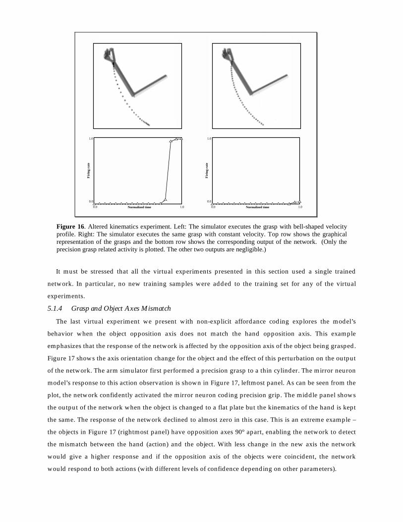
Figure 16. Altered kinematics experiment. Left: The simulator executes the grasp with bell-shaped velocity profile. Right: The simulator executes the same grasp with constant velocity. Top row shows the graphical representation of the grasps and the bottom row shows the corresponding output of the network. (Only the precision grasp related activity is plotted. The other two outputs are negligible.)

It must be stressed that all the virtual experiments presented in this section used a single trained

network. In particular, no new training samples were added to the training set for any of the virtual

experiments.

5.1.4 Grasp and Object Axes Mismatch

The last virtual experiment we present with non-explicit affordance coding explores the model’s

behavior when the object opposition axis does not match the hand opposition axis. This example

emphasizes that the response of the network is affected by the opposition axis of the object being grasped.

Figure 17 shows the axis orientation change for the object and the effect of this perturbation on the output

of the network. The arm simulator first performed a precision grasp to a thin cylinder. The mirror neuron

model’s response to this action observation is shown in Figure 17, leftmost panel. As can be seen from the

plot, the network confidently activated the mirror neuron coding precision grip. The middle panel shows

the output of the network when the object is changed to a flat plate but the kinematics of the hand is kept

the same. The response of the network declined to almost zero in this case. This is an extreme example –

the objects in Figure 17 (rightmost panel) have opposition axes 90° apart, enabling the network to detect

the mismatch between the hand (action) and the object. With less change in the new axis the network

would give a higher response and if the opposition axis of the objects were coincident, the network

would respond to both actions (with different levels of confidence depending on other parameters).

Normalized time 1.00.0

Firi

ng r

ate

0.0

1.0

1.0Normalized time0.0

Firi

ng r

ate

0.0

1.0

Figure 17. Grasp and object axes mismatch experiment. Rightmost: the change of the object from cylinder to a plate (an object axis change of 90 degrees). Leftmost: the output of the network before the change (the network turns on the precision grip mirror neuron). Middle: the output of the network after the object change. (Only the precision grasp related activity is plotted. The other two outputs are negligible.)

5.2 Explicit affordance coding experiments Now we switch our attention to the explicit affordance coding network. Here we want to see the effect

of object affordance on the model’s behavior. The new model is similar to that given before except that it

not only has inputs encoding the current prefix of the hand state trajectory, but also has a constant input

encoding the relevant affordance of the object under current scrutiny. Thus, both the training of the

network, and the performance of the trained network will exhibit effects of this additional, affordance,

input.

Due to the simple nature of the objects studied here, the affordance coding used in the present study

only encodes the object size. In general, one object will have multiple affordances. The ambiguity then

would be solved using extra cues such as the contextual state of the network. We chose a coarse coding of

object size with 10 units. Each unit has a preferred value; the firing of a unit is determined by the

difference of the preferred value and the value being encoded. The difference is passed through a non-

linear decay function by which the input is limited to 0 to 1 range (the larger the difference, the smaller

the firing rate). Thus, the explicit affordance coding network has 220 inputs (210 hand state inputs, plus

10 units coarse coding the size). The number of hidden layer units was again chosen as 6 and there were

again 3 output units, each one corresponding to a recognized grasp.

We have seen that the MNS model without explicit affordance input displayed a biasing effect of

object size in the Grasp Resolution subsection of Section 5.1; the network was biased toward power grasp

while observing a wide precision pinch grasp (the network initially responded with a power grasp

activity even though the action was a precision grasp). The model with full affordance replicates the

grasp resolution behavior seen in Figure 12. However, we can now go further and ask how the temporal

behavior of the model with explicit affordance coding reflects the fact that object information is available

throughout the action. Intuitively, one would expect that the object affordance would speed up the grasp

resolution process (which is actually the case as will be shown in Figure 19).

In the following 2 subsections we look at the effect of affordance information in two cases: (i) where

we study the response to precision pinch trajectories appropriate to a range of object sizes; and (ii) where

on each trial we use the same time-varying hand state trajectory but modify the object affordance part of

the input. In each case, we are studying the response of a network that has been previously trained on a

set of normal hand-state trajectories coupled with the corresponding object affordance (size) encoding.

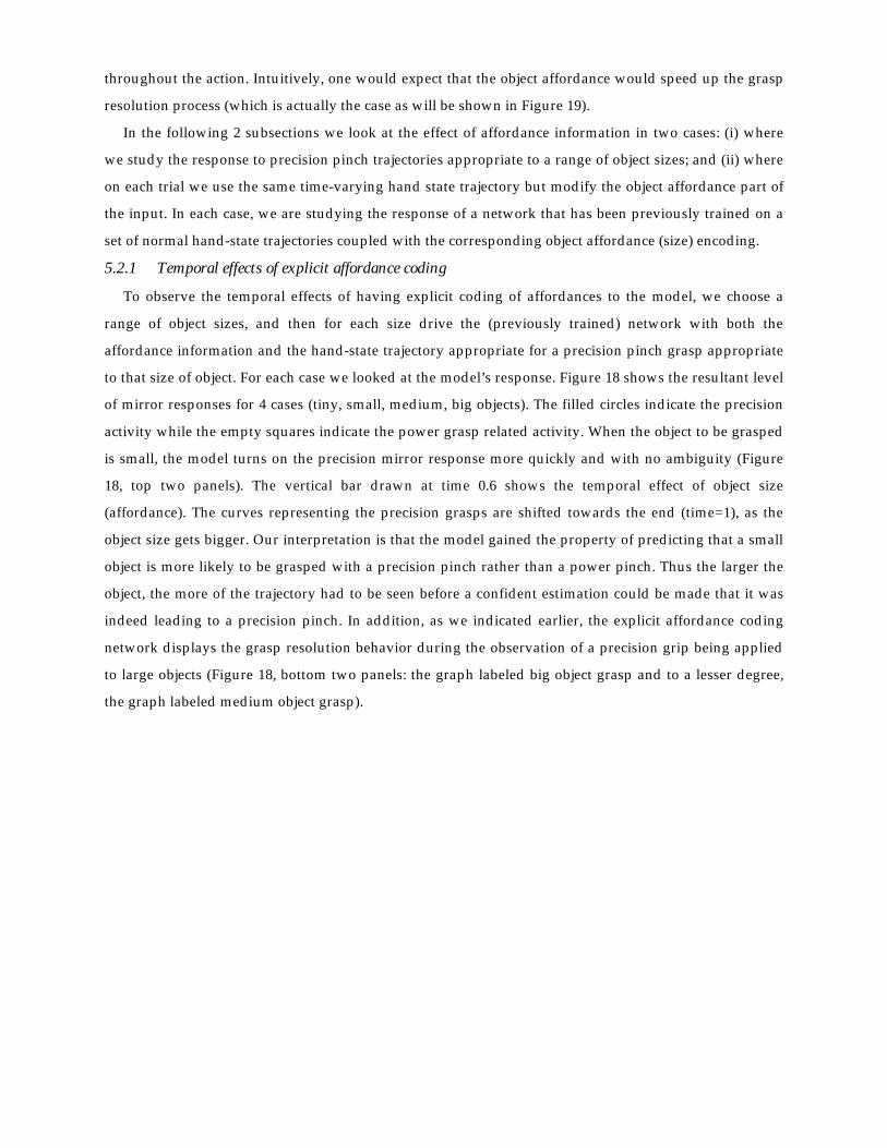
5.2.1 Temporal effects of explicit affordance coding

To observe the temporal effects of having explicit coding of affordances to the model, we choose a

range of object sizes, and then for each size drive the (previously trained) network with both the

affordance information and the hand-state trajectory appropriate for a precision pinch grasp appropriate

to that size of object. For each case we looked at the model’s response. Figure 18 shows the resultant level

of mirror responses for 4 cases (tiny, small, medium, big objects). The filled circles indicate the precision

activity while the empty squares indicate the power grasp related activity. When the object to be grasped

is small, the model turns on the precision mirror response more quickly and with no ambiguity (Figure

18, top two panels). The vertical bar drawn at time 0.6 shows the temporal effect of object size

(affordance). The curves representing the precision grasps are shifted towards the end (time=1), as the

object size gets bigger. Our interpretation is that the model gained the property of predicting that a small

object is more likely to be grasped with a precision pinch rather than a power pinch. Thus the larger the

object, the more of the trajectory had to be seen before a confident estimation could be made that it was

indeed leading to a precision pinch. In addition, as we indicated earlier, the explicit affordance coding

network displays the grasp resolution behavior during the observation of a precision grip being applied

to large objects (Figure 18, bottom two panels: the graph labeled big object grasp and to a lesser degree,

the graph labeled medium object grasp).

Figure 18. The plots show the level of mirror responses of the explicit affordance coding object for an observed precision pinch for four cases (tiny, small, medium, big objects). The filled circles indicate the precision activity while the empty squares indicate the power grasp related activity

We also compared the general response time of the non-explicit affordance coding implementation

with the explicit coding implementation. The network with affordance input is faster to respond than the

previous one. Moreover, it appears that − when affordance and grasp type are well correlated − having

access to the object affordance from the beginning of the action not only lets the system make better

Normalized time 1.00.0

Firi

ng r

ate

0.0

1.0

Figure 19. The solid curve: the precision grasp output, for the non-explicit affordance case, directed to a tiny object. The dashed curve: the precision grasp output of the model to the explicit affordance case, for the same object.

Tiny object grasp Small object grasp

Medium object grasp Big object grasp

predictions but also smoothes out the neuron responses. Figure 19 summarizes this: it shows the

precision response of both the explicit and non-explicit affordance case for a tiny object (dashed and solid

curves respectively).

5.2.2 Teasing Apart the Hand State and Object Affordance Components

We now look at the case where the hand state trajectory is incompatible with the affordance of the

observed object. In Figure 20, the plot labeled medium object shows the system output for a precision grasp

directed to a medium-sized object whose affordance is supplied to the network. We then repeatedly input

the hand state trajectory generated for this particular action but in each trial use an object affordance

discordant with the observed trajectory affordance (i.e., using a reduced or increased size of the object).

The plots in Figure 20 show the change of the output of the model due to the change in the affordance.

The results shown in these plots tell us two things. First, the recognition process becomes fuzzier as the

object gets bigger because the larger object sizes biases the network towards the power grasp. In the

extreme case the object affordance can even overwhelm the hand state and switch the network decision to

power grasp (Figure 20, graph labeled biggest object). Moreover, for large objects, the large discrepancy

between the observed hand state trajectory and the size of the objects results in the network converging

on a confident assessment for neither grasp.

Tiny object Small object Medium object

Big object Bigger object Biggest object

Figure 20. Empty squares indicate the precision grasp related cell activity, while the filled squares represent the power grasp related cell activity. The grasps show the effect of changing the object affordance, while keeping a constant hand state trajectory. In each case, the hand-state trajectory provided to the network is appropriate to the medium-sized object, but the affordance input to the network encodes the size shown. In the case of the biggest object affordance, the effect is enough to overwhelm the hand state’s precision bias.

Secondly, the resolution point (the crossing-point of the precision and power curves) shows an

interesting temporal behavior. It may be intuitive to think that as the object gets smaller the network’s

precision decision gets quicker and quicker (similar to what we have seen in the previous section).

However, although this is the case when the object is changing size from big to small, it is not the case

when the object size is getting medium to tiny (i.e., the crossing time has a local minimum between the

two extreme object sizes, as opposed to being at the tiny object extreme). Our interpretation is that the

network learned an implicit parameter related to the absolute value of the difference of the hand aperture

and the object size such that the maximum firing is achieved when the difference is smallest, that is when

the hand trajectory matches best with the object. This will explain why the network has quickest

resolution for a size between the biggest and the smallest sizes.

0 50 100 150 200 250Object size

0.70

0.75

0.80

0.85

0.90

0.95

1.00

Tim

e of

cro

ssin

g

300

Figure 21. The graph is drawn to show the decision switch time versus object size. The minimum is not at the boundary, that is, the network will detect a precision pinch quickest with a medium object size. Note that the graph does not include a point for "Biggest object" since there is no resolution point in this case (see the final panel of Figure 19).

Figure 21 shows the time of resolution versus object size in graphical form. We emphasize that the

model easily executes the grasp recognition task when hand-state trajectory matches object affordance.

We do not include all the results of these control trials, as they are similar to the cases mentioned in the

previous section.

6 DISCUSSION

6.1 The Hand-State Hypothesis Because the mirror neurons within monkey premotor area F5 fire not only when the monkey performs

a certain class of actions but also when the monkey observes similar actions, it has been argued that these

neurons are crucial for understanding of actions by others. Indeed, we agree with the importance of this

role and indeed have built upon it elsewhere.

Rizzolatti et al. (1996b) used a PET study to show that Broca's region is activated by observation of

hand gestures. They showed that both grasping observation and object prehension yield highly

significant activation in the rostral part of Broca's area (a significant part of the human language system)

as compared to the control condition of object observation. Moreover, Massimo Matelli (in Rizzolatti and

Arbib 1998) demonstrated a homology between monkey area F5 and area 45 in the human brain (Broca's

area comprises areas 44 and 45). Such observations led Rizzolatti and Arbib (1998), building on Rizzolatti

et al. (1996a) to formulate:

The Mirror System Hypothesis: Human Broca’s area contains a mirror system for grasping which is

homologous to the F5 mirror system of monkey, and this provides the evolutionary basis for language

parity - i.e., an utterance means roughly the same for both speaker and hearer. This adds a neural

“missing link” to the tradition that roots speech in a prior system for communication based on manual

gesture.

Arbib (2001) then refines this hypothesis by showing how evolution might have bridged from an

ancestral mirror system to a "language ready" brain via increasingly sophisticated mechanisms for

imitation of manual gestures as the basis for similar skills in vocalization and the emergence of

protospeech. In some sense, then, the present paper can be seen as extending these evolutionary concerns

back in time. Our central aim was to give a computational account of the monkey mirror system by

asking (i) What data must the rest of the brain supply to the mirror system? and (ii) How could the mirror

system learn the right associations between classification of its own movements and the movement of

others? In seeking to ground the answer to (i) in earlier work on the control of hand movements (Iberall

and Arbib 1990) we were led to extend our evolutionary understanding of the mirror system by offering:

The Hand-State Hypothesis: The basic functionality of the F5 mirror system is to elaborate the

appropriate feedback – what we call the hand state – for opposition-space based control of manual

grasping of an object. Given this functionality, the social role of the F5 mirror system in understanding

the actions of others may be seen as an exaptation gained by generalizing from self-hand to other's-hand.

The Hand-State Hypothesis provides a new explanation of the evolution of the "social capability" of

mirror neurons, hypothesizing that these neurons first evolved to augment the "canonical" F5 neurons

(active during self-movement but not during the observation of grasping by others) by providing visual

feedback on "hand state", relating the shape of the hand to the shape of the object.

6.2 Neurophysiological Predictions We introduced the MNS (Mirror Neuron System) model of F5 and related brain regions as an

extension of the FARS model of circuitry for visually-guided grasping of objects that links parietal area

AIP with F5 canonical neurons. The MNS model as diagrammed in Figure 4 includes hypotheses as to

how different brain regions may contribute to the functioning of the mirror system, and the region by

region analysis of neural circuitry remains a target for current research and future publications. However,

the implementation here took a different approach, aggregating these regions into three "grand schemas"

− Visual Analysis of Hand State, Reach and Grasp, and the Core Mirror Circuit − for each of which we

present a detailed implementation. To justify the claim that the model exhibits neurophysiologically

interesting, behaviors, we must look more carefully at the structure of the implementation, stressing that

it is only the activity of mirror neurons in the Core Mirror Circuit for which we make this claim. We

developed the Visual Analysis of Hand State schema simply to the point of demonstrating algorithms

powerful enough to take actual video input of a hand (though we simplified the problem somewhat by

using colored patches) and produce hand state information. The Reach and Grasp schema then

represented all the functionality for taking the location and affordance of an object and determining the

motion of a hand and arm to grasp it. However, the aim in the present paper was not to model the neural

mechanisms involved in these processes, but rather to do something more subtle and more useful for the

simulation of the Core Mirror Circuit (Figure 6(b)): we showed that if we used the Reach and Grasp

schema to generate an observed arm-hand trajectory (i.e., to represent the reach and grasp generator of

the monkey or human being observed), then that simulation could directly supply the corresponding

hand-state trajectory, and we thus use these data so that we can analyze the Core Mirror Circuit schema

in isolation from the Visual Analysis of Hand State.

Moreover, this hand state input was presented to the network in a way to avoid the use of a dynamic

neural network. To form the input vector, each of the seven components of the hand state trajectory, up to

the present time t, is fitted by a cubic spline. Then this spline is sampled at 30 uniformly spaced intervals;

i.e., no matter what fraction t is of the total time T of the entire trajectory, the input to the network at time

t comprises 30 samples of the hand-state uniformly distributed over the interval [0, t]. The network is

trained using full trajectory of the hand state in a specific grasp; the training set pairs each such hand

state history as input with the final grasp type as output. On contrary, when testing the model with

various grasp observations, the input to the network was the hand state trajectory that was available up

to that instant. This exactly parallels the way the biological system (the monkey) receives visual (object

and hand) information: When the monkey performs a grasp, the learning can take place after the

observation of the complete (self) generated visual stimuli. On the other hand, in the observation case the

monkey mirror system predicts the grasp action based on the partial visual stimuli (i.e. before the grasp is

completed). The network thus yields a time-course of activation for the mirror neurons, yielding

predictions for neurophysiological experiments by highlighting the importance of the timing of mirror

neuron activity. We saw that initial prefixes will yield little or no mirror neuron activity, and ambiguous

prefixes may yield transient activity of the “wrong” mirror neurons.

Since our aim was to show that the connectivity of mirror neuron circuitry can be established through

training, and that the resultant network can exhibit a range of novel, physiologically interesting,

behaviors during the process of action recognition, the actual choice of training procedure is purely a

matter of computational convenience, and the fact that the method chosen, namely back-propagation, is

non-physiological does not weaken the importance of our predictions concerning the timing of mirror

neuron activity.

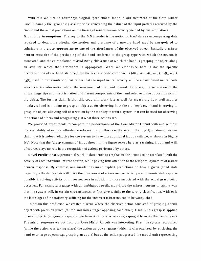
With this we turn to neurophysiological "predictions" made in our treatment of the Core Mirror

Circuit, namely the "grounding assumptions" concerning the nature of the input patterns received by the

circuit and the actual predictions on the timing of mirror neuron activity yielded by our simulations.

Grounding Assumptions: The key to the MNS model is the notion of hand state as encompassing data

required to determine whether the motion and preshape of a moving hand may be extrapolated to

culminate in a grasp appropriate to one of the affordances of the observed object. Basically a mirror

neuron must fire if the preshaping of the hand conforms to the grasp type with which the neuron is

associated; and the extrapolation of hand state yields a time at which the hand is grasping the object along

an axis for which that affordance is appropriate. What we emphasize here is not the specific

decomposition of the hand state F(t) into the seven specific components (d(t), v(t), a(t), o1(t), o2(t), o3(t),

o4(t)) used in our simulation, but rather that the input neural activity will be a distributed neural code

which carries information about the movement of the hand toward the object, the separation of the

virtual fingertips and the orientation of different components of the hand relative to the opposition axis in

the object. The further claim is that this code will work just as well for measuring how well another

monkey’s hand is moving to grasp an object as for observing how the monkey’s own hand is moving to

grasp the object, allowing self-observation by the monkey to train a system that can be used for observing

the actions of others and recognizing just what those actions are.

We provided experiments to compare the performance of the Core Mirror Circuit with and without

the availability of explicit affordance information (in this case the size of the object) to strengthen our

claim that it is indeed adaptive for the system to have this additional input available, as shown in Figure

6(b). Note that the "grasp command" input shown in the figure serves here as a training input, and will,

of course, plays no role in the recognition of actions performed by others.

Novel Predictions: Experimental work to date tends to emphasize the actions to be correlated with the

activity of each individual mirror neuron, while paying little attention to the temporal dynamics of mirror

neuron response. By contrast, our simulations make explicit predictions on how a given (hand state

trajectory, affordance) pair will drive the time course of mirror neuron activity – with non-trivial response

possibly involving activity of mirror neurons in addition to those associated with the actual grasp being

observed. For example, a grasp with an ambiguous prefix may drive the mirror neurons in such a way

that the system will, in certain circumstances, at first give weight to the wrong classification, with only

the late stages of the trajectory sufficing for the incorrect mirror neuron to be vanquished.

To obtain this prediction we created a scene where the observed action consisted of grasping a wide

object with precision pinch (thumb and index finger opposing each other). Usually this grasp is applied

to small objects (imagine grasping a pen from its long axis versus grasping it from its thin center axis).

The mirror response we got from our Core Mirror Circuit was interesting. First, the system recognized

(while the action was taking place) the action as power grasp (which is characterized by enclosing the

hand over large objects; e.g. grasping an apple) but as the action progressed the model unit representing

precision pinch started to get active and the power grasp activity started to decline. Eventually the Core

Mirror Circuit settled on the precision pinch. This particular prediction is testable and indeed suggests a

whole class of experiments. The monkey has to be presented with unusual or ambiguous grasp actions

that require a “grasp resolution”. For example, the experimenter can grasp a section of banana using

precision pinch from its long axis. Then we would expect to see activity from power grasp related mirror

cells followed by a decrease of that activity accompanied by increasing activity from precision pinch

related mirror cells.

The other simulations we made leads to different testable predictions such as the mirror response in

case of a spatial perturbation (showing the monkey a fake grasp where the hand does not really meet the

object) and altered kinematics (perform the grasp with different kinematics than usual). The former is in

particular a justification of the model, since in the mirror neuron literature it has been reported that the

spatial contact of the hand and the object is almost always required for the mirror response (Gallese et al.,

1996). On the other hand the altered kinematics result predicts that an alteration of the kinematics will

cause a decrease in the mirror response. We have also noted how a discrepancy between hand state

trajectory and object affordance may block or delay the system from classifying the observed movement.

In summary, we have conducted a range of simulation experiments – on grasp resolution, spatial

perturbation, altered kinematics, temporal effects of explicit affordance coding, and analysis of

compatibility of the hand state to object affordance – which demonstrate that the present model is not

only of value in providing an implemented high-level view of the logic of the mirror system, but also

serves to provide interesting predictions ripe for neurophysiological testing, as well as suggesting new

questions to ask when designing experiments on the mirror system. However, we must note that this

study has excluded some actions (such as tearing and twisting) for which mirror activity has been

observed. As new neurophysiological studies on monkeys expand the range of actions for which the

temporal response of the mirror system is delimited, we will expand our model to explain the new

findings and suggest yet further classes of experiments to probe the structure and function of the mirror

system – as well as increasing the set of brain regions in Figure 4 for which increasingly realistic neural

models are made available.

Acknowledgments This work was supported in part by a Human Frontier Science Program grant to Arbib which made

possible extensive discussions of data on the mirror system with Giacomo Rizzolatti, Vittorio Gallese and

Massimo Matelli, to whom we express our gratitude. Writing of the paper was also supported in part by

an ARC-IREX grant to Robyn Owens for the study of "Hand Movement Recognition and Language:

Assistive Technologies and Neural Mechanisms" while Arbib was a Visiting Professor in the Computer

Science Department at the University of Western Australia.

7 REFERENCES Arbib MA (1981) Perceptual Structures and Distributed Motor Control. In: Brooks VB, (eds) Handbook of

Physiology, Section 2: The Nervous System, Vol. II, Motor Control, Part 1. American Physiological

Society, pp. 1449-1480

Arbib MA (2001) The Mirror System, Imitation, and the Evolution of Language. In Nehaniv C,

Dautenhahn K (eds) Imitation in Animals and Artifacts. The MIT Press, to appear

Arbib MA, Érdi P, Szentágothai J (1998) Neural Organization: Structure, Function and Dynamics.

Cambridge, MA: A Bradford Book/The MIT Press

Breteler MDK, Gielen SCAM, Meulenbroek RGJ (2001) End-point constraints in aiming movements: effect

of approach angle and speed. Biological Cybernetics 85: 65-75

Fagg AH, Arbib MA (1998) Modeling parietal--premotor interactions in primate control of grasping.

Neural Networks 11:(7-8) 1277-1303

Gallese V, Fadiga L, Fogassi L, Rizzolatti G (1996) Action recognition in the premotor cortex. Brain 119:

592-609

Gentilucci M, Fogassi L, Luppino G, Matelli M, Camarda R, Rizzolatti G (1988). Functional Organization

of Inferior Area 6 in the Macaque Monkey I. Somatotopy and the Control of Proximal Movements.

Experimental Brain Research 71: 475-490

Gibson JJ (1966) The Senses Considered as Perceptual Systems. Allen and Unwin

Hertz J, Krogh A, Palmer RG (1991) Introduction to the Theory of Neural Computation. Addison Wesley

Hoff B, Arbib MA (1993) Models of trajectory formation and temporal interaction of reach and grasp.

Journal of Motor Behavior 25: 175-192

Holden EJ (1997) Visual Recognition of Hand Motion. Ph.D. Thesis, Department of Computer Science,

University of Western Australia.

Iberall T, Arbib MA (1990) Schemas for the Control of Hand Movements: An Essay on Cortical

Localization. In Goodale MA (ed) Vision and action: the control of grasping. Norwood, NJ: Ablex, pp.

163-180

Jordan MI, Rumelhart DE (1992) Forward models: supervised learning with distal teacher. Cognitive

Science 16: 307-354

Karniel A, Inbar GF (1997) A model for learning human reaching movements. Biological Cybernetics 77:

173-183

Kawato M, Furukawa K, Suzuki R (1987) A hierarchical neural-network model for control and learning of

voluntary movement. Biological Cybernetics 57: 169-185

Kawato M, Gomi H (1992) A computational model of four regions of the cerebellum based on feedback-

error-learning. Biological Cybernetics 68:95-103

Kincaid D, Cheney W, (1991) Numerical Analysis. Brooks/Cole Publishing

Lambert P, Carron T (1999) Symbolic fusion of luminance-hue-chroma features for region segmentation.

Pattern Recognition 32: 1857-1872

Lowe, DG (1991) Fitting parameterized three-dimensional models to images. IEEE Transactions on

Pattern Analysis and Machine Intelligence 13(5): 441-450

Matelli M, Luppino G, Murata A, Sakata H (1994) Independent anatomical circuits for reaching and

grasping linking the inferior parietal sulcus and inferior area 6 in macaque monkey. Soc. Neurosci.

Abstr. 20: 404.4

Meulenbroek RGJ, Rosenbaum DA, Jansen C, Vaughan J, Vogt S (2001) Multijoint grasping movements.

Experimental Brain Research, online: DOI 10.1007/s002210100690

Rizzolatti G, and Arbib MA (1998) Language Within Our Grasp. Trends in Neurosciences, 21(5): 188-194.

Rizzolatti G, Camarda R, Fogassi L, Gentilucci M, Luppino G, Matelli M (1988) Functional Organization

of Inferior Area 6 in the Macaque Monkey II. Area F5 and the Control of Distal Movements.

Experimental Brain Research 71: 491-507

Rizzolatti G, Fadiga L (1998) Grasping objects and grasping action meanings: the dual role of monkey

rostroventral premotor cortex (area F5). In Sensory Guidance of Movement, Novartis Foundation

Symposium 218. Chichester: Wiley, pp. 81-103.

Rizzolatti G, Fadiga L, Gallese, V, and Fogassi, L (1996a) Premotor cortex and the recognition of motor

actions. Cogn Brain Res 3: 131-141

Rizzolatti G, Fadiga L, Matelli M, Bettinardi V, Perani D, Fazio F (1996b) Localization of grasp

representations in humans by positron emission tomography: 1. Observation versus execution.

Experimental Brain Research 111: 246-252.

Rosenbaum DA, Meulenbroek RGJ, Vaughan J, Jansen C (1999) Coordination of reaching and grasping by

capitalizing on obstacle avoidance and other constraints. Experimental Brain Research 128: 92-100

Rumelhart DE, Hinton GE, Williams RJ (1986) Learning internal representations by error propagation. In

Rumelhart DE, McClelland JL and PDP group (eds) Parallel distributed processing Vol. 1:

Foundations. pp. 151-193

Russ JC (1998) The Image Processing Handbook. CRC press LLC, FL: Boca Raton

Sakata H, Taira M, Murata A, Mine S, (1995) Neural mechanisms of visual guidance of hand action in the

parietal cortex of the monkey. Cerebral Cortex 5(5): 429-38

Sakata H, Taira M, Kusunoki M, Murata A, Tanaka Y (1997) The parietal association cortex in depth

perception and visual control of action. Trends in Neuroscience 20: 350-357

Sanka M, Hlavac V, Boyle R (1993) Image Processing, Analysis and Machine Vision. Chapman and Hall,

London.

Taira M, Mine S, Georgopoulos A P, Murata A, Sakata H (1990) Parietal Cortex Neurons of the Monkey

Related to the Visual Guidance of Hand Movement. Experimental Brain Research 83: 29-36.

Wolpert DM, Ghahramani Z (2000) Computational principles of movement neuroscience. Nature

Neuroscience 3: 1212-1217

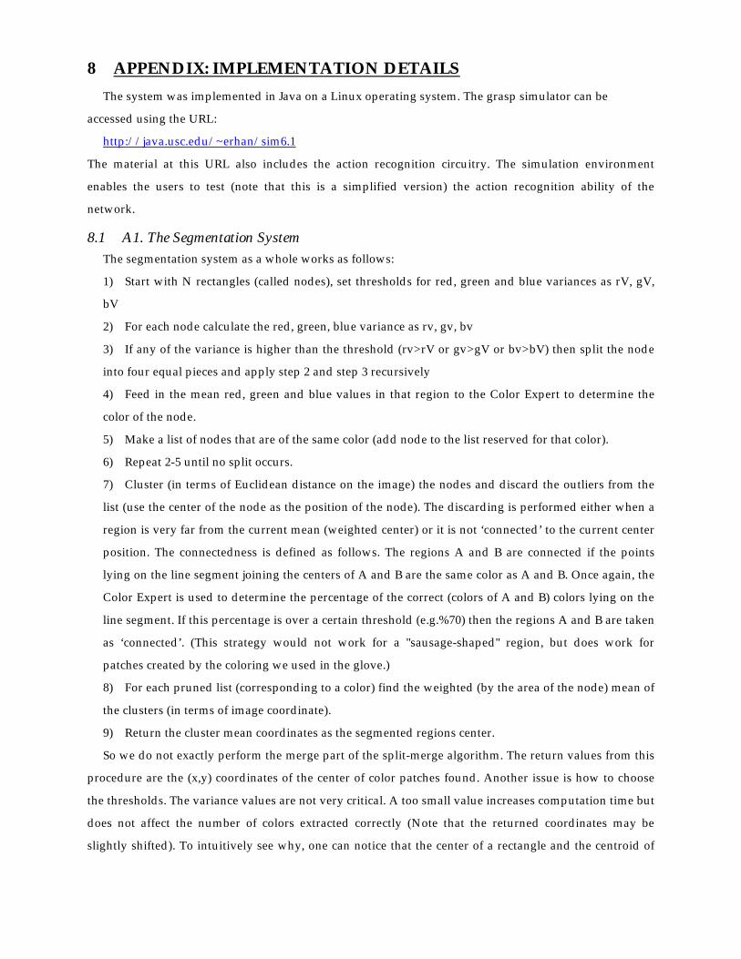
8 APPENDIX: IMPLEMENTATION DETAILS The system was implemented in Java on a Linux operating system. The grasp simulator can be

accessed using the URL:

http://java.usc.edu/~erhan/sim6.1

The material at this URL also includes the action recognition circuitry. The simulation environment

enables the users to test (note that this is a simplified version) the action recognition ability of the

network.

8.1 A1. The Segmentation System The segmentation system as a whole works as follows:

1) Start with N rectangles (called nodes), set thresholds for red, green and blue variances as rV, gV,

bV

2) For each node calculate the red, green, blue variance as rv, gv, bv

3) If any of the variance is higher than the threshold (rv>rV or gv>gV or bv>bV) then split the node

into four equal pieces and apply step 2 and step 3 recursively

4) Feed in the mean red, green and blue values in that region to the Color Expert to determine the

color of the node.

5) Make a list of nodes that are of the same color (add node to the list reserved for that color).

6) Repeat 2-5 until no split occurs.

7) Cluster (in terms of Euclidean distance on the image) the nodes and discard the outliers from the

list (use the center of the node as the position of the node). The discarding is performed either when a

region is very far from the current mean (weighted center) or it is not ‘connected’ to the current center

position. The connectedness is defined as follows. The regions A and B are connected if the points

lying on the line segment joining the centers of A and B are the same color as A and B. Once again, the

Color Expert is used to determine the percentage of the correct (colors of A and B) colors lying on the

line segment. If this percentage is over a certain threshold (e.g.%70) then the regions A and B are taken

as ‘connected’. (This strategy would not work for a "sausage-shaped" region, but does work for

patches created by the coloring we used in the glove.)

8) For each pruned list (corresponding to a color) find the weighted (by the area of the node) mean of

the clusters (in terms of image coordinate).

9) Return the cluster mean coordinates as the segmented regions center.

So we do not exactly perform the merge part of the split-merge algorithm. The return values from this

procedure are the (x,y) coordinates of the center of color patches found. Another issue is how to choose

the thresholds. The variance values are not very critical. A too small value increases computation time but

does not affect the number of colors extracted correctly (Note that the returned coordinates may be

slightly shifted). To intuitively see why, one can notice that the center of a rectangle and the centroid of

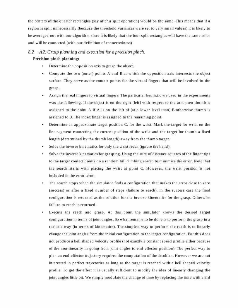
the centers of the quarter rectangles (say after a split operation) would be the same. This means that if a

region is split unnecessarily (because the threshold variances were set to very small values) it is likely to

be averaged out with our algorithm since it is likely that the four split rectangles will have the same color

and will be connected (with our definition of connectedness)

8.2 A2. Grasp planning and execution for a precision pinch. Precision pinch planning:

• Determine the opposition axis to grasp the object.

• Compute the two (outer) points A and B at which the opposition axis intersects the object

surface. They serve as the contact points for the virtual fingers that will be involved in the

grasp.

• Assign the real fingers to virtual fingers. The particular heuristic we used in the experiments

was the following. If the object is on the right [left] with respect to the arm then thumb is

assigned to the point A if A is on the left of [at a lower level than] B otherwise thumb is

assigned to B. The index finger is assigned to the remaining point.

• Determine an approximate target position C, for the wrist. Mark the target for wrist on the

line segment connecting the current position of the wrist and the target for thumb a fixed

length (determined by the thumb length) away from the thumb target.

• Solve the inverse kinematics for only the wrist reach (ignore the hand).

• Solve the inverse kinematics for grasping. Using the sum of distance squares of the finger tips

to the target contact points do a random hill climbing search to minimize the error. Note that

the search starts with placing the wrist at point C. However, the wrist position is not

included in the error term.

• The search stops when the simulator finds a configuration that makes the error close to zero

(success) or after a fixed number of steps (failure to reach). In the success case the final

configuration is returned as the solution for the inverse kinematics for the grasp. Otherwise

failure-to-reach is returned.

• Execute the reach and grasp. At this point the simulator knows the desired target

configuration in terms of joint angles. So what remains to be done is to perform the grasp in a

realistic way (in terms of kinematics). The simplest way to perform the reach is to linearly

change the joint angles from the initial configuration to the target configuration. But this does

not produce a bell shaped velocity profile (not exactly a constant speed profile either because

of the non-linearity in going from joint angles to end effector position). The perfect way to

plan an end-effector trajectory requires the computation of the Jacobian. However we are not

interested in perfect trajectories as long as the target is reached with a bell shaped velocity

profile. To get the effect it is usually sufficient to modify the idea of linearly changing the

joint angles little bit. We simply modulate the change of time by replacing the time with a 3rd

order polynomial that will match our constraints for time (starts at 0 climbs up to 1

monotonically). Note that we are still working in the joint space and our method may suffer

from the non-linearity in transforming the joint angles to end effector coordinates. However,

our empirical studies showed that a satisfactory result, for our purposes, could be achieved

with this strategy.