schema versioning in data warehouses: enabling cross...
TRANSCRIPT
Schema Versioning in Data Warehouses:
Enabling Cross-Version Querying via Schema
Augmentation ⋆
Matteo Golfarelli a Jens Lechtenborger b,∗ Stefano Rizzi a
Gottfried Vossen b
aDEIS, University of Bologna, Italy
bDept. of Information Systems, University of Muenster, Germany
Abstract
As several mature implementations of data warehousing systems are fully opera-tional, a crucial role in preserving their up-to-dateness is played by the ability tomanage the changes that the data warehouse (DW) schema undergoes over time inresponse to evolving business requirements. In this paper we propose an approachto schema versioning in DWs, where the designer may decide to undertake someactions on old data aimed at increasing the flexibility in formulating cross-versionqueries, i.e., queries spanning multiple schema versions. First, we introduce a repre-sentation of DW schemata as graphs of simple functional dependencies, and discussits properties. Then, after defining an algebra of schema graph modification opera-tions aimed at creating new schema versions, we discuss how augmented schematacan be introduced to increase flexibility in cross-version querying. Next, we showhow a history of versions for DW schemata is managed and discuss the relationshipbetween the temporal horizon spanned by a query and the schema on which it canconsistently be formulated.
Key words: data warehousing, schema versioning, cross-version querying, schemaaugmentation
⋆ A preliminary version of this paper appeared in the Proc. 3rd Workshop on Evo-lution and Change in Data Management, 2004.∗ Corresponding author. Address: Dept. of Information Systems, Leonardo-Campus3, 48149 Muenster, Germany. Tel.: +49-251-8338158, Fax: +49-251-8338159
Email addresses: [email protected] (Matteo Golfarelli),[email protected] (Jens Lechtenborger), [email protected](Stefano Rizzi), [email protected] (Gottfried Vossen).
Preprint submitted to Elsevier Science 7 September 2005

1 Introduction
Data Warehouses (DWs) are databases specialized for business intelligenceapplications and can be seen as collections of multidimensional cubes centeredon facts of interest for decisional processes. A cube models a set of events,each identified by a set of dimensions and described by a set of numericalmeasures. Typically, for each dimension a hierarchy of properties expressesinteresting aggregation levels. A distinctive feature of DWs is that of storinghistorical data; hence, a temporal dimension is always present.
Data warehousing systems have been rapidly spreading within the industrialworld over the last decade, due to their undeniable contribution to increasingthe effectiveness and efficiency of decision making processes within businessand scientific domains. This wide diffusion was supported by remarkable re-search results aimed at increasing querying performance [17,33], at improvingthe quality of data [34], and at refining the design process [14] on the onehand, as well as by the quick advancement of commercial tools on the other.
Today, as several mature implementations of data warehousing systems arefully operational within medium to large contexts, the continuous evolutionof the application domains is bringing to the forefront the dynamic aspectsrelated to describing how the information stored in the DW changes over timefrom two points of view:
• At the data level: Though historical values for measures are easily storeddue to the presence of temporal dimensions that timestamp the events,the multidimensional model implicitly assumes that the dimensions and therelated properties are entirely static. This assumption is clearly unrealisticin most cases; for instance, a company may add new categories of productsto its catalog while others can be dropped, or the category of a product maychange in response to the marketing policy.
• At the schema level: The DW schema may change in response to the evolv-ing business requirements. New properties and measures may become nec-essary (e.g., a subcategory property could be added to allow more detailedanalysis), while others may become obsolete. Even the set of dimensionscharacterizing a cube may be required to change.
Note that, in comparison with operational databases, temporal issues are morepressing in DWs since queries frequently span long periods of time; thus, it isvery common that they are required to cross the boundaries of different ver-sions of data and/or schema. Besides, the criticality of the problem is obviouslyhigher for DWs that have been established for a long time, since unhandledevolutions will determine a stronger gap between the reality and its represen-tation within the database, which will soon become obsolete and useless.
2
So far, research has mainly addressed changes at the data level, i.e., changes ininstances of aggregation hierarchies (the so-called slowly-changing dimensions[21]), and some commercial systems already allow to track changes in data andto effectively query cubes based on different temporal scenarios. For instance,SAP-BW [32] allows the user to choose which version of the hierarchies to usewhile querying (e.g., aggregate the sales according to the categories that weretrue on 1/1/2000). On the other hand, schema versioning in DWs has onlypartially been explored and no dedicated commercial tools or restructuringmethods are available to the designer. Thus, both an extension of tools andsupport for designers are urgently needed.
Indeed, according to the frequently cited definition of a DW by Inmon [18]one of the characteristic features of a DW is its non-volatility, which meansthat data is integrated into the DW once and remains unchanged afterwards.Importantly, this feature implies that the re-execution of a single query willalways produce a single consistent result. In other words, past analysis resultscan be verified and then inspected by means of more detailed OLAP sessionsat any point in time. While commercial solutions may support non-volatilityin the presence of changes at the data level (e.g., SAP-BW under the term“historical truth”), non-volatility in the presence of changes at the schema levelhas not received much attention. In fact, it is easy to see that the ability tore-execute previous queries in the presence of schema changes requires accessto past schema versions.
In this paper we propose an approach to schema versioning in DWs, specifi-cally oriented to support the formulation of cross-version queries, i.e., queriesspanning multiple schema versions. Our main contributions are the following:
(1) Schema graphs are introduced in order to univocally represent DW sche-mata as graphs of simple functional dependencies, and an algebra of graphoperations to determine new versions of a DW schema is defined. Impor-tantly, our graph model captures the core of all multidimensional datamodels proposed previously.
(2) The issues related to data migration, i.e., how to consistently move databetween schema versions, are discussed. In particular, a dichotomy in thetreatment of fact instances and dimension instances is established.
(3) Augmented schemata are introduced in order to increase flexibility incross-version querying. The augmented schema associated with a versionis the most general schema describing the data that are actually recordedfor that version and thus are available for querying purposes.
(4) The sequencing of versions to form schema histories in presence of aug-mented schemata is discussed, and the relationship between the temporalhorizon spanned by a query and the schema on which it can consistentlybe formulated is analyzed. Based on the notion of schema intersection, anovel approach towards cross-version querying is defined.
3
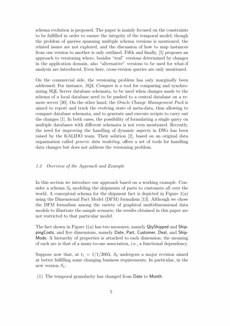
The remainder of this paper is outlined as follows. We discuss related work inSubsection 1.1, and we give an overview of our approach and present a moti-vating example in Subsection 1.2. In Section 2 we propose a graph-based rep-resentation of DW schemata. In Section 3 we describe the elementary changesa schema may undergo, while in Section 4 we show how these changes cre-ate new versions. In Section 5 we discuss how versions are concatenated intohistories. In Section 6 we focus on cross-version querying, and we draw theconclusions in Section 8.
1.1 Related Work
1.1.1 Temporal Databases
A large part of the literature on schema versioning in relational databases issurveyed in [31]. With reference to terminology introduced in [19] our approachis framed as schema versioning since past schema definitions are retained sothat all data may be accessed both retrospectively and prospectively throughuser-definable version interfaces; additionally, with reference to [31] we aredealing with partial schema versioning as no retrospective update is allowedto final users. Note that, in contrast, schema evolution allows modificationsof the schema without loss of data but does not require the maintenance of aschema history.
As to querying in the presence of multiple schema versions, while TSQL2 [35]only allows users to punctually specify the schema version according to whichdata are queried, queries spanning multiple schema versions are considered in[10] and [15].
1.1.2 Data Warehouse Evolution and Versioning
In the DW field, a number of approaches for managing slowly-changing di-mensions were devised (see for instance [11,25,38]).
As to schema evolution/versioning, mainly five approaches can be found inthe literature. First, in [29], the impact of evolution on the quality of thewarehousing process is discussed in general terms, and a supporting meta-model is outlined. Second, in [37] a prototype supporting dimension updatesat both the data and schema levels is presented, and the impact of evolutionson materialized views is analyzed. Third, in [7,6], an algebra of basic operatorsto support evolution of the conceptual schema of a DW is proposed, and theeffect of each operator on the instances is analyzed. In all these approaches,versioning is not supported and the problem of querying multiple schemaversions is not mentioned. Fourth, in [12], the COMET model to support
4
schema evolution is proposed. The paper is mainly focused on the constraintsto be fulfilled in order to ensure the integrity of the temporal model; thoughthe problem of queries spanning multiple schema versions is mentioned, therelated issues are not explored, and the discussion of how to map instancesfrom one version to another is only outlined. Fifth and finally, [5] proposes anapproach to versioning where, besides “real” versions determined by changesin the application domain, also “alternative” versions to be used for what-ifanalysis are introduced. Even here, cross-version queries are only mentioned.
On the commercial side, the versioning problem has only marginally beenaddressed. For instance, SQL Compare is a tool for comparing and synchro-nizing SQL Server database schemata, to be used when changes made to theschema of a local database need to be pushed to a central database on a re-mote server [30]. On the other hand, the Oracle Change Management Pack isaimed to report and track the evolving state of meta-data, thus allowing tocompare database schemata, and to generate and execute scripts to carry outthe changes [1]. In both cases, the possibility of formulating a single query onmultiple databases with different schemata is not even mentioned. Recently,the need for improving the handling of dynamic aspects in DWs has beenraised by the KALIDO team. Their solution [2], based on an original dataorganization called generic data modeling, offers a set of tools for handlingdata changes but does not address the versioning problem.
1.2 Overview of the Approach and Example
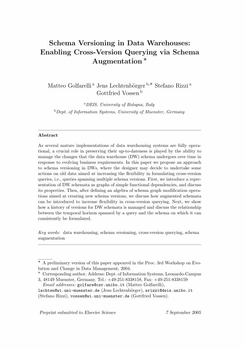
In this section we introduce our approach based on a working example. Con-sider a schema S0 modeling the shipments of parts to customers all over theworld. A conceptual schema for the shipment fact is depicted in Figure 1(a)using the Dimensional Fact Model (DFM) formalism [13]. Although we chosethe DFM formalism among the variety of graphical multidimensional datamodels to illustrate the sample scenario, the results obtained in this paper arenot restricted to that particular model.
The fact shown in Figure 1(a) has two measures, namely QtyShipped and Ship-
pingCosts, and five dimensions, namely Date, Part, Customer, Deal, and Ship-
Mode. A hierarchy of properties is attached to each dimension; the meaningof each arc is that of a many-to-one association, i.e., a functional dependency.
Suppose now that, at t1 = 1/1/2003, S0 undergoes a major revision aimedat better fulfilling some changing business requirements. In particular, in thenew version S1:
(1) The temporal granularity has changed from Date to Month.
5

Category
SHIPMENT
QtyShippedShippingCostsDM
City
Customer
Deal
TermsIncentive
Ship Mode
AllowanceSType
Carrier
Container
Part
Brand
Type
Size
Region
Nation
Year
Month
Date
SaleDistrict
Subcategory
Category
City
Customer
Deal
TermsIncentive
Ship Mode
AllowanceSType
Carrier
Container
Part
Brand
Type
Size
Region
Nation
Year
Month
SaleDistrict
SHIPMENT
QtyShippedShippingCostsDM
(a) (b)
Subcategory
Year
Month
Category
Deal
Incentive
ShipFrom
Allowance
Container
Part
Brand
Type
Size
City
Customer
Region
Nation
SaleDistrict
Terms
PartDescr
SHIPMENT
QtyShippedShipping CostsLITShippingCostsEUShipppingCostsDM
(c)
Fig. 1. Conceptual schemata for three versions of the shipment fact: S0 (a), S1 (b),and S2 (c)
(2) A classification into subcategories has been inserted into the part hierar-chy.
(3) A new constraint has been modeled in the customer hierarchy, statingthat sale districts belong to nations, and that for each customer the nationof her sale district is the nation of her city.
(4) The incentive has become independent of the shipment terms.
Then, at t2 = 1/1/2004, another version S2 is created as follows:
(1) Two new measures ShippingCostsEU and ShippingCostsLIT are added.(2) The ShipMode dimension is eliminated.(3) A ShipFrom dimension is added.(4) A descriptive attribute PartDescr is added to Part.
The conceptual schemata for S1 and S2 are depicted in Figure 1(b,c).
Within a system not supporting versioning, at the time of change all datawould be migrated to the new schema version. On the other hand, if thesystem supports versioning, all previous schema versions will still be availablefor querying together with the data recorded during their validity time. In thiscase, the user could be given the possibility of deciding which schema versionis to be used to query data. For instance, the 2002 data could be queried underschema S1, introduced in 2003; in particular, one might ask for the distribution
6

of the shipping costs for 2002 according to subcategories, introduced in 2003.
In our approach, the schema modifications occurring in the course of DWoperation lead to the creation of a history of schema versions. All of theseversions are available for querying purposes, and the relevant versions for aparticular analysis scenario may either be chosen explicitly by the user orimplicitly by the query subsystem. The key idea is to support flexible cross-version querying by allowing the designer to enrich previous versions using theknowledge of current schema modifications. For this purpose, when creatinga new schema version the designer may choose to create augmented schematathat extend previous schema versions to reflect the current schema extension,both at the schema and the instance level.
To be more precise, let S be the current schema version and S ′ be the newversion. Given the differences between S and S ′, a set of possible augmentationactions on past data are proposed to the designer; these actions may entailchecking past data for additional constraints or inserting new data based onuser feedback. (Details are presented in Subsection 4.2.) The set of actions thedesigner decides to undertake leads to defining and populating an augmentedschema SAUG, associated with S, that will be used instead of S, transparentlyto the final user, to answer queries spanning the validity interval of S. Impor-tantly, SAUG is always an extension of S, in the sense that the instance of Scan be computed as a projection of SAUG.
Consider, for instance, the schema modification operation that introduces at-tribute Subcategory, performed at time t1 = 1/1/2003 to produce version S1.For all parts still shipped after t1 (including both parts introduced after t1and parts already existing before t1), a subcategory will clearly have to bedefined as part of data migration, so that queries involving Subcategory canbe answered for all shipments from t1 on. However, if the user is interestedin achieving cross-version querying on years 2002 and 2003, i.e., if she asks toquery even old data (shipments of parts no longer existing at t1) on Subcate-
gory, it is necessary to:
(1) define an augmented schema for S0, denoted SAUG0 , that contains the new
attribute Subcategory;(2) (either physically or virtually) move old data entries from S0 to SAUG
0 ;and
(3) assign the appropriate values for Subcategory to old data entries in SAUG0 .
This process will allow queries involving Subcategory to be answered on olddata via the instance of SAUG
0 . Note that, while the first two steps are entirelymanaged by the versioning system, the last one is the designer’s responsibility.
As another example, consider adding the constraint between sale districtsand nations. In this case, the designer could ask the system to check if the
7

functional dependency between SaleDistrict and Nation holds on past datatoo (it might already have been true when S0 was created, but might havebeen missed at design time; or it could be enforced via data cleansing): if so,the augmented schema SAUG
0 will be enriched with this dependency, whichincreases the potential for roll-up and drill-down operations during OLAPsessions.
2 Formal Representation of DW Schemata
In this section we define notation and vocabulary, and we recall results on sim-ple FDs that form the basis for the graph-theoretic framework used throughoutthis paper.
2.1 Simple Functional Dependencies
We assume the reader to be familiar with the basics of relational databasesand FDs. Following standard notation (see, e.g., [26]), capital letters from thebeginning (respectively ending) of the alphabet denote single (respectively setsof) attributes, “≡” denotes equivalence of sets of FDs, and F+ is the closureof the FDs in F .
An FD X → Y is simple if |X| = |Y | = 1 (note that simple FDs have alsobeen called unary [9]). Given a set F of simple FDs over X we say that Fis acyclic (respectively cyclic) if the directed graph (X,F ) (i.e., the graphthat contains the attributes in X as nodes and that contains an arc (A,B) ifA → B ∈ F ) is acyclic (respectively cyclic).
Finally, we recall that a set F of FDs is canonical if [26]: 1
• every FD X → Y ∈ F satisfies |Y | = 1,• F is left-reduced, i.e., for each FD X → A ∈ F there is no Y $ X such
that Y → A ∈ F+, and• F is nonredundant, i.e., there is no F ′ $ F such that F ′ ≡ F .
For every set F of FDs there is at least one canonical cover, i.e., a canonicalset F 0 of FDs such that F ≡ F 0 [26].
1 Canonical sets are called minimal in [36], while the notion of minimality of [26]has a different meaning.
8

2.2 Schema Graphs
In order to talk about schema versioning, we first have to fix a representa-tion for DW schemata on top of which operations for schema modificationscan be defined. In this section, we introduce a graph-based representation forschemata called schema graph, which captures the core of multidimensionalmodels such as the DFM. Intuitively, in line with [23], a DW schema is a di-rected graph, where the nodes are attributes (either properties or measures),and arcs represent simple FDs of a canonical cover. The representation ofDW schemata in terms of graphs allows us to define schema modifications bymeans of four elementary graph manipulations, namely adding and deletingof nodes and arcs, and to analyze the schema versioning problem in a simpleand intuitive setting. Besides, as shown in [22], it provides a considerable sim-plification over hyper-graph based approaches that have previously been usedto represent schemata involving general FDs (see, e.g., [4]).
Formally, we represent a DW schema in terms of one or more schema graphs.
Definition 1 (Schema Graph) A schema graph is a directed graph S =(U , F ) with nodes U = {E} ∪ U and arcs F , where
(1) E is called fact node and represents a placeholder for the fact itself (mean-ing that its values are the single events that have occurred, i.e., the singletuples of the fact table);
(2) U is a set of attributes (including properties and measures);(3) F is a set of simple FDs defined over {E} ∪ U in the DW schema;(4) E has only outgoing arcs, and there is a path from E to every attribute
in U .
S is called canonical schema graph if F is canonical.
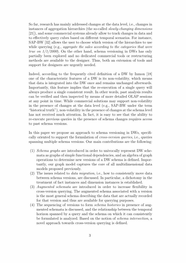
Canonical schema graphs for the shipment facts in Figure 1 are shown inFigure 2.
Throughout this paper we assume that schema graphs satisfy the universalrelation schema assumption (URSA) [26], which is a standard assumption inrelational database design. URSA ties an attribute name to its semantics, i.e.,among the set of schema graphs describing the DW schema all occurrencesof an attribute name are assumed to have the same meaning. Thus, in ourexample, the two different concepts “type of part” and “type of ship mode” arerepresented in terms of two attributes with distinct names (Type and SType);on the other hand, the attributes occurring in the Part hierarchy are allowedto appear with the same names in other schema graphs if those schema graphsdeal with the same part concept (which will be the case for other versions ofshipment facts or, e.g., invoice or revenue related facts).
9

(a)
(b)
QtyShippedQtyShipped ShippingCostsDMShippingCostsDM
MonthMonth
YearYear BrandBrand
ContainerContainer
TypeType
SubcategorySubcategory
SizeSize
PartDescr
AllowanceAllowance TermsTerms
IncentiveIncentive
DealDeal ShipFromShipFrom
Shipment
CustomerCustomer
SaleDistrictSaleDistrict
NationNation
RegionRegion
CityCity
CategoryCategory
ShippingCostsEUShippingCostsEU
ShippingCostsLITShippingCostsLIT
PartPart
(c)
Fig. 2. Schema graphs S0 (a), S1 (b), and S2 (c)
Finally, we note that, with reference to the multidimensional model, an FDf ∈ F has an impact on the semantics of attributes as follows:
(1) f = E → A
10

• A may be a dimension. Since the values of E represent single events, inthis case f expresses the fact that each event is related to exactly onevalue for each dimension.
• A may be a measure. In this case f represents the fact that each eventis associated with exactly one value for each measure.
(2) f = B → A• B may be a dimension or a property, and A a property. In this case, B →
A models a many-to-one association within a hierarchy (for instance,B is City and A is Nation). From the implementation point of view, thismeans that the correspondence between each value of B and exactlyone value of A is explicitly stored in the database (for instance, withina dimension table of a star schema).
• B may be a measure, and A a derived measure. In this case, B →A models the fact that A can be derived from B (for instance, B isthe daily fluctuation of a share and A is its absolute value). From theimplementation point of view, there are two choices: Either store A asa separate attribute, which introduces redundant data in the DW butmay be advantageous if the computation of A from B is expensive; orstore a function in the meta-data repository allowing A to be computedfrom B on-the-fly.
In view of these observations it should be clear that the questions whetheran attribute defines (1) a measure or a dimension and (2) a derived mea-sure or a property cannot be answered based on our graph representation.Thus, this additional information is recorded in the meta-data repository (seeSection 2.5).
2.3 Reduced Schema Graphs
In comparison with general schema graphs, the class of canonical schemagraphs has the important advantage of providing a non-redundant, i.e., com-pact schema representation. On the other hand, in order to obtain uniqueresults for schema modification operations, we also need to make sure thatwe are dealing with a uniquely determined representation. This section showshow any schema graph can be put in a uniquely determined canonical formcalled reduced schema graph.
We begin by observing that, for acyclic sets of simple FDs, canonical coversare uniquely determined and can be computed via transitive reduction:
Definition 2 (Transitive Closure and Reduction) Let U be a set of at-tributes, and F be a set of simple FDs over U . The transitive closure of F ,denoted F ∗, is inductively defined as follows:
11

(1) f ∈ F =⇒ f ∈ F ∗
(2) A → B ∈ F ∗ ∧ B → C ∈ F ∗ =⇒ A → C ∈ F ∗
A transitive reduction of F is a minimal set F− of simple FDs over U suchthat F ∗ = (F−)∗.
To illustrate the differences between transitive closure F ∗ and closure F+ ofFDs F , we observe that by definition F ∗ contains only simple FDs. In contrast,if the FDs in F involve two or more attributes then F+ contains additionalnon-simple FDs (exponential in the number of attributes) that are implied byF ∗.
Example 1 For F = {A → B,B → C} we have:
F ∗ = {A → B,B → C,A → C}
F+ = {A → B,B → C,A → C,
A → A,AB → A,AC → A,ABC → A,
B → B,AB → B,AC → B,BC → B,ABC → B,
C → C,AB → C,AC → C,BC → C,ABC → C}
As shown in [3], in case of acyclic graphs the transitive reduction F− isuniquely determined and F− ⊆ F . Besides, from [22] we recall that F− isa canonical cover of F . Thus, if F is acyclic, the reduced schema graph forS = (U , F ) is S− = (U , F−).
On the other hand, in real-world scenarios acyclicity of FDs may not be givenas cycles occur in at least the following two cases:
• Descriptive properties. Though most associations between properties of DWschemata have many-to-one multiplicity, in some cases they may have one-to-one multiplicity. Typically, this happens when a property is associatedwith one or more univocal descriptions (e.g., the technical staff may referto products by their codes while sale agents may use product names).
• Derived measures. Two measures may be derivable from each other by ap-plying some fixed formula (for instance, Euros and Italian Liras can betransformed back and forth by applying constant conversion factors).
The following example shows that canonical covers are no longer unique ifFDs are cyclic.
Example 2 Consider measures A1 and A2 whose values are derivable fromeach other (such as item prices listed in two currencies), i.e., we have cyclicFDs A1 → A2 and A2 → A1, and a measure A3 that can be derived fromA1 and also from A2 (such as an item tax that is computed from the price).
12

Hence, we have a set F of FDs {A1 → A2, A2 → A1, A1 → A3, A2 → A3}, andit is easily verified that {A1 → A2, A2 → A1, A1 → A3} and {A1 → A2, A2 →A1, A2 → A3} are both canonical covers of F .
In the remainder of this section we show how a uniquely determined reducedform for schema graphs can be determined even in the presence of cyclic FDs[22]. Consider a schema graph S = (U , F ), where F is neither necessarilycanonical nor acyclic. The relation ≡F on U defined by
A ≡F B iff A → B ∈ F+ ∧ B → A ∈ F+
for A,B ∈ U is an equivalence relation; U/≡Fis used to denote the set of
equivalence classes induced by ≡F on U . Then, we consider the acyclic directedgraph where each node is one equivalence class X ∈ U/≡F
and an arc goesfrom X to Y , X 6= Y , if there are attributes A ∈ X and B ∈ Y such thatA → B ∈ F . The transitive reduction of this graph, called the equivalentacyclic schema graph for S and denoted by Sa = (U/≡F
, F a), is acyclic (byconstruction) and uniquely determined (as transitive reduction is unique foracyclic graphs). Now, let <S be a total order on U (e.g., user-specified orsystem-generated based on some sorting criterion such as attribute creationtimestamp or attribute name).
Definition 3 (Implicit FDs) Let U be a set of attributes with total order<S, let F be a (possibly redundant and/or cyclic) set of simple FDs over U ,and let X = {A1, . . . , An} ∈ U/≡F
, n ≥ 1. Let A1 <S A2 <S . . . <S An be theordering of attributes in X according to <S. The implicit FDs for X (w.r.t.<S) are given by FX = {A1 → A2, A2 → A3, . . . , An−1 → An, An → A1}.
Definition 4 (Reduced Schema Graph) Let S = (U , F ) be a schema graphand Sa = (U/≡F
, F a) be the equivalent acyclic schema graph for S. The re-
duced schema graph for S is the directed graph S− = (U , F−), where
F− =⋃
X→Y ∈F a
{min X → min Y } ∪⋃
X∈U/≡F
FX .
From [3,22] we know that the reduced schema graph S− = (U , F−) for S isa uniquely determined transitive reduction of S, and F− is a canonical coverof F . In the remainder of this paper, given a set F of simple FDs, we will use“−” to denote the reduction operator that produces the uniquely determinedcanonical cover F− of F according to Definition 4.
Example 3 Consider the schema graph S2 in Figure 2(c), where Part hasan equivalent property PartDescr and shipping costs are expressed in EU, LIT,and DM. The reduced form for S2, based on the total order induced by attributenames, is shown in Figure 3.
13

QtyShipped ShippingCostsDM
Month
Year Brand
Container
Type
Subcategory
Size
PartDescr
Allowance Terms
Incentive
Deal ShipFrom
Shipment
Customer
SaleDistrict
Nation
Region
City
Category
ShippingCostsEU
ShippingCostsLIT
Part
Fig. 3. Reduced form for schema graph S2
2.4 Projection on Schema Graphs
Given a set F of FDs over attributes U and given X ⊆ U , the projection ofF to X is given by πX(F ) := {A1 → A2 ∈ F+ | A1A2 ⊆ X}. Based on theresults of [23] and [22], in this section we show that the projection operationπ is closed on schema graphs. The importance of this result lies in the factthat it allows us to use projection to define precisely the effect of the deletionof an attribute from a schema graph (cf. Definition 6 later on). Indeed, whendeleting an attribute our aim is to retain “as much information concerningFDs as possible”, which is suitably formalized via π. However, as projectionis defined as subset of a closure, the following challenges (which are visible inExample 1 above) arise in applying π directly:
(1) In general the projection of a set of simple FDs involves non-simple FDs,which are outside our framework.
(2) The result of the closure may grow exponentially in the number of in-volved attributes.
In our setting of simple FDs, however, the following results hold.
Lemma 1 ([23]) Let U be a set of attributes, let F be a set of simple FDs overU , and let A ∈ U and X ⊆ U such that X 6= ∅, A /∈ X, and X → A ∈ F+.Then there is a sequence of n ≥ 2 attributes A1, . . . , An ∈ U such that A1 ∈ X,An = A, and Ai → Ai+1 ∈ F , 1 ≤ i ≤ n − 1.
Lemma 2 ([22]) Let U be a set of attributes, F be a set of simple FDs overU , and X ⊆ U . Let FX = πX(F )0 and F ′
X = {A1 → A2 ∈ F ∗ | A1A2 ⊆ X}−.
(1) FX contains only simple FDs.(2) FX ≡ F ′
X .
14

In view of Lemma 2, from now on we assume that, for a set F of simple FDs,projection is defined as πX(F ) := {A1 → A2 ∈ F ∗ | A1A2 ⊆ X}, which bydefinition is a simple set of FDs.
Theorem 1 Let S = (U , F ) be a schema graph, and let X ⊆ U such thatE ∈ X. Then (X, {A1 → A2 ∈ F ∗ | A1A2 ⊆ X}−) is a reduced schema graph.
PROOF. Let FX1= πX(F ) = {A1 → A2 ∈ F ∗ | A1A2 ⊆ X} and FX2
= F−X1
.We have to verify that (X,FX2
) is a schema graph, i.e., that (i) FX2is a set
of simple FDs, (ii) E has only outgoing arcs in FX2, and (iii) there is a path
in FX2from E to every attribute in X2. Once we have established (i)–(iii),
the remaining claims follow as for any set F0 of simple FDs the set F−0 is by
construction a uniquely determined canonical cover. First, (i) follows from thefact that by definition FX1
contains only simple FDs. Hence, by constructionFX2
= F−X1
contains only simple FDs as well. Now, concerning (ii) we notethat E has only outgoing arcs in F and hence in F ∗. Moreover, by definitionπ only removes FDs from F ∗, which implies that E has only outgoing arcs inFX1
. As FX2is a canonical cover of FX1
the claim follows. Concerning (iii),let A ∈ X. We have to show E → A ∈ F ∗
X2, from which the claim follows by
Lemma 1. As there is a path from E to A in F we have E → A ∈ F ∗, and bydefinition of projection we find E → A ∈ FX1
, which implies E → A ∈ F ∗X2
and ends the proof.
2.5 Meta-Data
The formalism of schema graphs captures just that core of multidimensionalschemata which we need as basis to define a powerful schema modificationalgebra in the next section. Nevertheless, we assume that schema graphs aremanaged as part of a larger meta-data repository, which contains all kindsof schema information, in particular, information that is not captured in ourgraph notation.
For example, for all versions of schema graphs defined over time the meta-data repository includes specifications of attribute domains, classifications ofattributes into dimensions, measures, and properties, summarizability typesor restriction levels of measures (cf. [24]), derivation specifications for derivedmeasures, and summarizability constraints (cf. [13,23]). In particular we as-sume that, in accordance with what several OLAP tools do, each measure isassociated with exactly one aggregation operator for each dimension. Thus,measures are not just attributes: they have some built-in semantics, coded inmeta-data, that states how they will be aggregated along each hierarchy.
15

3 Schema Modification Algebra
Our proposal towards schema versioning rests upon four simple schema mod-ification operations, namely AddA() to add a new attribute, DelA() to deletean existing attribute, AddF() to add an arc involving existing attributes (i.e.,an FD), and DelF() to remove an existing arc. For each of these operationswe define its effect on the schema. Note that, from now on, we will alwaysconsider schema graphs in their reduced form, and thus use the terms schemaand reduced schema graph interchangeably.
In addition to the four schema modification operations defined below, we as-sume that there are (1) an operation to create an initial schema S = ({E}, ∅)that contains only the fact node without attributes or arcs and (2) an oper-ation to delete an existing schema. We do not consider these operations anyfurther.
In order to specify schema modification operations formally, let S = (U , F )be a schema. For each modification operation M(Z) (where M is AddA or DelAand Z is an attribute, or M is AddF or DelF and Z is an FD), we define thenew schema New(S,M(Z)) obtained when applying M on current schema S.
Definition 5 Let S = (U , F ) be a reduced schema graph, and let A be anattribute. Then we have:
New(S, AddA(A)) := (U ∪ {A}, (F ∪ {E → A})−)
We call attention to the fact that in Definition 5 we do not distinguish thecases whether A does already occur in S = (U , F ) or not. Indeed, on theone hand Definition 5 implies that S remains unchanged if A does alreadyoccur in S. On the other, if A is a newly inserted attribute then it is directlyconnected by an arc to the fact node E. 2 Besides, when adding an attribute,the designer will be required to specify whether it is a measure or a property;this information will be recorded in meta-data.
Definition 6 Let S = (U , F ) be a reduced schema graph, and let A ∈ U bean attribute. Then we have:
New(S, DelA(A)) := (U \ {A}, πU\{A}(F )−)
2 The unrestricted usage of AddA might introduce homonym conflicts, i.e., the de-signer could try to add an attribute although another attribute with the same namebut a different meaning occurs somewhere else. To avoid such conflicts, in an imple-mentation the meta-data repository needs be checked whether some schema versioncontains an attribute with the same name.
16

Thus, in view of Theorem 1 the deletion of attribute A is defined by removingA and retaining FDs not involving A via projection.
Definition 7 Let S = (U , F ) be a reduced schema graph, and let f = A1 →A2 be an FD involving attributes in U . Then we have:
New(S, AddF(f)) := (U , (F ∪ {f})−)
We note that the insertion of a new FD may introduce redundancies, whichare removed via reduction “−”.
Definition 8 Let S = (U , F ) be a reduced schema graph, and let f = A1 →A2 be an existing FD in F , where A1 6= E. Let
F ′ = F \ {f}
∪ {A0 → A2 | (∃A0 ∈ U) A0 → A1 ∈ F}
∪ {A1 → A3 | (∃A3 ∈ U) A2 → A3 ∈ F}
Then we have:New(S, DelF(f)) := (U , (F ′)−)
The intuition underlying Definition 8 is as follows: First, the specified FDf = A1 → A2 gets deleted via set difference. Then, previous transitive depen-dencies are retained by adding (i) FDs to A2 from all nodes A0 determiningA1 (possibly A0 = E) and (ii) FDs from A1 to all nodes A3 determined by A2.
We note that the “appropriate” deletion of FDs is more intricate than it mightseem at first sight. For example, we cannot simplify the deletion of an FD fby defining the new set of FDs to be (F+ \ {f})0 (recall that F 0 denotes thecanonical cover of F ). Indeed, given A1 → A2 ∈ F we have A1X → A2 ∈ F+
for an arbitrary set X. Although A1X → A2 is not left-reduced with respectto F , it may be left-reduced with respect to F+ \ {f}, which implies that(F+ \{f})0 is not guaranteed to be a set of simple FDs. Consider for instanceF = {E → A1, E → A2, A2 → A3} and DelF(A2 → A3): here, we haveA1A2 → A3 ∈ F+, and A1A2 → A3 is also contained in (F+ \ {A2 → A3})
0,which does not correspond to the users’ intuition. Moreover, we observe thatif we tried to define deletion of an FD via (F ∗ \{f})− (to get rid of non-simpleFDs), we were still facing a severe problem: Users would be unable to deletea single FD from a cycle involving three or more attributes, as the FD to beremoved would be implied by the remaining FDs. Thus, users would be unableto pull out attributes from cycles involving three or more attributes. With ourdefinition, none of these problems arises.
Example 4 The sequence of operations applied in order to arrive at S1 start-
17
Part
Category
TypeBrand
Shipment
Container
Size
Subcategory Part
TypeBrand
Subcategory
Category
Shipment
Container
Size
...(c)
... ...Part
TypeBrand
Shipment
Container
Size
Category Subcategory
...(a)
... ...
(b)
.........
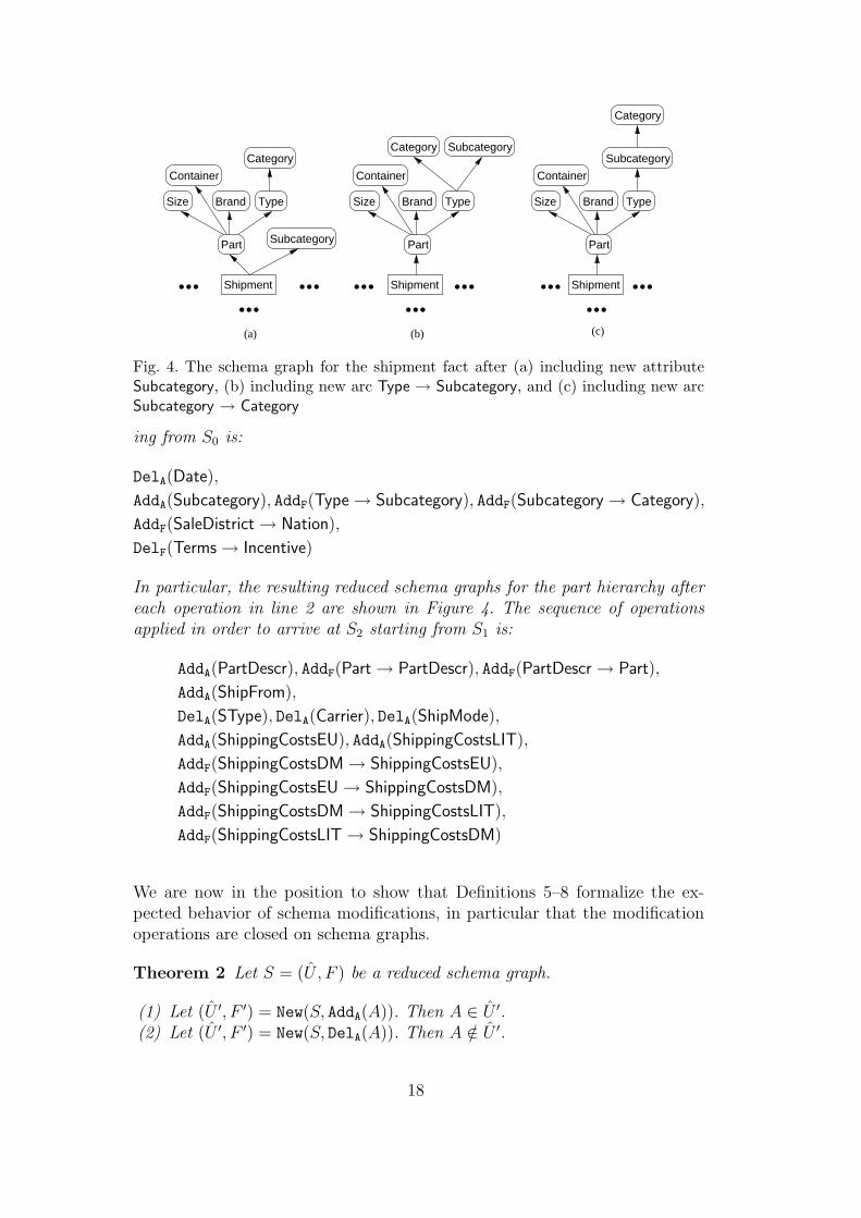
Fig. 4. The schema graph for the shipment fact after (a) including new attributeSubcategory, (b) including new arc Type → Subcategory, and (c) including new arcSubcategory → Category
ing from S0 is:
DelA(Date),
AddA(Subcategory), AddF(Type → Subcategory), AddF(Subcategory → Category),
AddF(SaleDistrict → Nation),
DelF(Terms → Incentive)
In particular, the resulting reduced schema graphs for the part hierarchy aftereach operation in line 2 are shown in Figure 4. The sequence of operationsapplied in order to arrive at S2 starting from S1 is:
AddA(PartDescr), AddF(Part → PartDescr), AddF(PartDescr → Part),
AddA(ShipFrom),
DelA(SType), DelA(Carrier), DelA(ShipMode),
AddA(ShippingCostsEU), AddA(ShippingCostsLIT),
AddF(ShippingCostsDM → ShippingCostsEU),
AddF(ShippingCostsEU → ShippingCostsDM),
AddF(ShippingCostsDM → ShippingCostsLIT),
AddF(ShippingCostsLIT → ShippingCostsDM)
We are now in the position to show that Definitions 5–8 formalize the ex-pected behavior of schema modifications, in particular that the modificationoperations are closed on schema graphs.
Theorem 2 Let S = (U , F ) be a reduced schema graph.
(1) Let (U ′, F ′) = New(S, AddA(A)). Then A ∈ U ′.(2) Let (U ′, F ′) = New(S, DelA(A)). Then A /∈ U ′.
18
(3) Let (U ′, F ′) = New(S, AddF(f)). Then f ∈ F ′+.(4) Let (U ′, F ′) = New(S, DelF(f)). Then f /∈ F ′+.
Additionally, in all of the above cases, (U ′, F ′) is a reduced schema graph.
PROOF. Statements (1), (2), and (3) follow immediately from Definitions 5,6, and 7, respectively. Statement (4) follows from Definition 8, observing thatF is canonical and hence in particular nonredundant. It remains to show that(U ′, F ′) is a reduced schema graph, i.e., that (a) F ′ is a set of simple FDs,(b) E has only outgoing arcs and there is a path from E to every attributein U ′, and (c) (U ′, F ′) is in reduced form. For AddA, AddF, and DelF, (a) and(b) are immediate. For DelA, (a) and (b) follow from Theorem 1. For allfour operations, (c) follows immediately from the definition of the reductionoperator “−”.
Intuitively, Theorem 2 states that our schema modification operations pre-serve valid schema graphs and are guaranteed to produce non-redundant anduniquely determined results.
4 Versions
We call a version a schema that reflects the business requirements during agiven time interval, called its validity, that starts upon schema creation timeand extends until the next version is created. 3 The validity of the currentversion, created at time t, is [t, +∞]. A version is populated with the eventsoccurring during its validity and can be queried by the user.
A new version is the result of a sequence of modification operations, which wecall schema modification transaction, or simply transaction. In analogy to theusual transaction concept, intermediate results obtained after applying singleschema modifications are invisible for querying purposes. Moreover, interme-diate schemata are neither populated with events, nor are they associated withaugmented schemata.
A transaction produces (1) a new version and (2) an augmented schema foreach previous version, all of which are (either physically or virtually) populatedwith data. In Subsection 4.1 we address (1), in particular we discuss how thenew version is populated. In Subsection 4.2 we address (2), i.e., we illustrate
3 In accordance with [27] we argue that there is no need to distinguish valid timefrom transaction time in the context of schema versioning.
19

how augmented schemata are created at the end of transactions in order toincrease flexibility in cross-version querying.
4.1 Data Migration
Given version S, let the sequence of operations M1(Z1), . . . ,Mh(Zh) be theexecuted schema modification transaction. Then, the new version S ′ is de-fined by executing the modification operations one after another, i.e., S ′ =New(Sh,Mh(Zh)), where S1 = S and Si = New(Si−1,Mi−1(Zi−1)) for i =2, . . . , h.
In order to populate S ′, it is necessary to carry out some migration actionsto consistently move data from the previous version to the new one. If S ′ iscreated at time t, migration actions involve the data that are valid at t, i.e.,data whose validity spans both S and S ′. Importantly, in the DW context thevalidity may be defined differently for two categories of data, namely events(in the star schema, tuples of fact tables) and instances of hierarchies (tuplesof dimension tables):
• Events occur at a particular moment in time. Consistently with [20], weassume that the validity of an event that occurs at time te is the zero-lengthinterval [te, te]; thus, an event naturally conforms to exactly one version(the one valid at te). Consequently, when a new version S ′ is created, whileall future events will necessarily conform to S ′, no data migration will berequired for past events. (Note that this is a consequence of the fact that,in a versioning approach, all past versions are retained together with theirdata. Conversely, in the approach to schema evolution in DWs described in[7], migration is carried out also for events: in fact, in evolution past versionsare not retained.)
• Instances of hierarchies are generally valid during time intervals (e.g., a partis valid from the time it is first shipped to the time it is declared obsolete),so their validity may span different versions. Thus, if S ′ is created at time t,for each hierarchy instance that is valid at t it may be necessary to migrateit from S to S ′.
In order to determine the migration actions to be performed after a transac-tion, independently of the specific sequence of modification operations thatimplements the transaction, we define the net effect for attributes and FDswith reference to the transaction. Let S ′ = (U ′, F ′) be the new version ob-
20

Table 1Migration actions associated to added or deleted attributes/FDs
Element Condition Migration action
A ∈ Diff+
A (S, S′) (E → A) 6∈ F ′ A is property Add values for A
A ∈ Diff−
A (S, S′) (E → A) 6∈ F ′ A is property delete A
f ∈ Diff+
F (S, S′) - enforce f
tained by applying the transaction to version S = (U , F ). Then we define:
Diff+A (S, S ′) := U ′ \ U (set of added attributes)
Diff+F (S, S ′) := F ′ \ F ∗ (set of added FDs)
Diff−A (S, S ′) := U \ U ′ (set of deleted attributes)
We note that it is not necessary to define Diff−F (S, S ′) (set of deleted FDs)since no action needs to be performed for deleted FDs. In fact, if an FD getsdeleted then a constraint on previous instances gets removed; thus, there isno need for alignment of previous instances with the new schema version.
The migration actions associated with the elements in Diff+A (S, S ′), Diff−A (S, S ′),
and Diff+F (S, S ′) are reported in Table 1 and defined in the following. All of
these actions are supported and managed by the versioning system, under thedesigner guidance where required.
(1) Add values for A: A new property A has been added to a hierarchy. Eachvalid hierarchy instance is migrated to S ′ by providing values for A. Forinstance, when property Subcategory is added, then all currently validsubcategory values must be recorded under S ′.
(2) Delete A: Property A has been deleted, so its values are simply droppedfrom all valid instances migrated to S ′.
(3) Enforce f : A new FD f has been added. We distinguish two cases: (1)If the new FD involves two already existing properties, it is necessary tocheck if f holds for all valid instances and possibly to enforce it in S ′ bymodifying, under the user guidance, the values of one or both propertiesinvolved in f . (2) If the new FD involves a new property A (i.e., one thathas just been added), then the values for A must be provided in such away that this FD is satisfied. For instance, when Subcategory is addedto the part hierarchy as in Figure 4 (c), then each valid part type in S2
must be associated with exactly one subcategory and all types includedin each subcategory must belong to the same category.
In all cases not covered by the table, no action needs to be performed. Infact, the impact of adding or deleting a measure or a dimension is restrictedto events, which are not involved in migration as explained above; finally,deleting an FD requires no change on hierarchy instances.
21

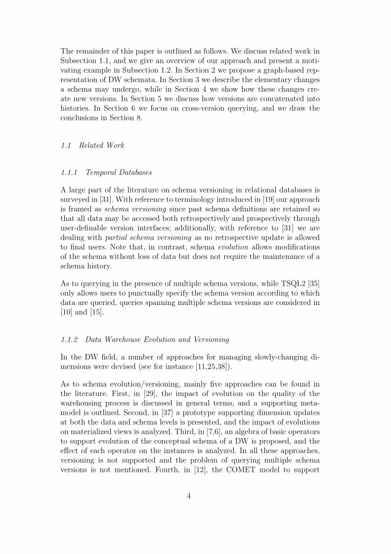
Fig. 5. Dimension tables for customers and parts in the shipment example, beforeand after time t1
Again, we emphasize that in a versioning approach all past versions must beretained. Thus, for each migrated hierarchy instance, both versions of data willbe available for querying: the one conforming to schema S, used for accessingthe events that occurred before time t, and the one conforming to S ′, used foraccessing the events that occurred after t.
Example 5 In the shipment example, at time t1 = 1/1/2003 the new versionS1 is created from version S0. Among other things, this transaction entailsadding Subcategory to the part hierarchy (consistently with the FDs Type →Subcategory and Subcategory → Category) and adding an FD from SaleDistrict
to Nation. Figure 5 shows the data in the dimension tables for customers andparts just before t1 and some months after t1. After t1 each dimension table hastwo copies, belonging to S0 and S1 respectively. Fields from and to express thevalidity of parts (for instance, they may have been introduced to manage partsas a slowly-changing dimension), while customers are assumed to be alwaysvalid. At time t1, all the valid parts (those whose to timestamp is open) aremigrated to S1 and their subcategory is added; then, in February, part ♯3 isdismissed and, in April, a new part (♯6) is inserted. As to customers, all ofthem are migrated. Since the new FD SaleDistrict → Nation does not hold forMidEurope, the sale district of customer ♯1 is modified in S1. Note that, at t1,
22

the open timestamps of parts are closed: in fact, from a conceptual point ofview, it is clear that instances cannot survive their schema.
4.2 Augmentation
Let S ′ = (U ′, F ′) be the new version obtained by applying, at time t, a transac-tion to version S = (U , F ). Let Si be a previous version (possibly, Si coincideswith S itself), and SAUG
i be its augmented schema. While migration involvesthe data whose validity spans both S and S ′, the augmentation of Si—whichdetermines the new augmented schema for Si—involves the data whose valid-ity overlaps with the validity of Si. Thus, while migration is only performedon hierarchy instances that are valid at time t, augmentation also concerns theevents that occurred before t and the hierarchy instances that were no morevalid at t.
As in migration, also here the possible actions do not depend on the specificsequence of modification operators applied, but on the net effect for attributesand FDs with reference to the transaction. More specifically:
• If attribute A has been added in the course of the transaction, i.e., if A ∈Diff+
A (S, S ′), then the designer may want to include A in the augmentedschema for Si to enable cross-version queries involving A.
• If f is a new FD, i.e., if f = A → B ∈ Diff+F (S, S ′), then the designer may
want to include f in the augmented schema for Si to enable cross-versionroll-up and drill-down operations involving A and B.
In this respect, we call attention to the fact that we only consider augmenta-tions in response to operations that add attributes or FDs: in fact, the utilityof augmenting the current version with deleted attributes/FDs seems highlyquestionable. 4 On the one hand, we do not see why a designer should firstdelete an attribute only to state that data associated with this attribute shouldbe maintained in an augmented schema. On the other, we assume that dele-tions of FDs are triggered by real-world events that invalidate these FDs (thedeletion of valid FDs reduces the information of a schema without need, whichdoes not seem reasonable); hence, there is no way, not even in an augmentedschema, to maintain these FDs.
Now, we define the augmentation operation Aug(SAUGi , S, S ′) that (further)
augments the augmented schema SAUGi = (Ui, Fi) based on the designer’s
choice in response to the schema change from S to S ′. Let DiffA(S, S ′) and
DiffF(S, S ′) be the subsets of Diff+A (S, S ′) and Diff+
F (S, S ′), respectively,
4 Designers can, of course, delete attributes and FDs from schema versions. Thepoint is that such deletions do not lead to augmentations.
23

Table 2Augmentation actions associated to added attributes/FDs
Element Condition Augm. action
A is measure estimate values for A
(E → A) ∈ Fi
A is dimension disaggregate measure values
A is derived measure compute values for AA ∈ DiffA(S, S′)
(E → A) 6∈ Fi
A is property add values for A
f ∈ DiffF(S, S′) - check if f holds
including only the attributes and FDs the designer has chosen to augment.We note that all attributes occurring in FDs of DiffF(S, S ′) must be contained
in Ui ∪ DiffA(S, S ′), as only those FDs can be augmented whose attributesoccur in the augmented schema. 5 Then the new augmented version for Si isdefined as follows:
Aug(SAUGi , S, S ′) := (Ui ∪ DiffA(S, S ′), (Fi ∪ πUi∪DiffA(S,S′)(DiffF(S, S ′)))−)
The augmentation actions associated with each element in DiffA(S, S ′) and
DiffF(S, S ′) are reported in Table 2 and defined as follows.
(1) Estimate values for A: A new measure A has been added. To enablecross-version querying, the designer provides values for A for the eventsrecorded under Si, typically by deriving an estimate based on the values ofthe other measures. For instance, when measure Discount is added to theshipment fact, if the discount applied depends on the shipped quantitybracket, its values for past events may be easily estimated from measureQty shipped.
(2) Disaggregate measure values: A new dimension A has been added. To en-able cross-version querying, the designer must disaggregate past eventsby A according to some business rule or by adopting a statistical inter-polation approach that exploits multiple summary tables to deduce thecorrelation between measures [28]. For instance, a likely reason for addingdimension ShipFrom is that, while in the past all shipments were madefrom the same warehouse w, now they are occasionally made from otherwarehouses: in this case, all past events can be easily related to w.
(3) Compute values for A: A derived measure A has been added; by definitionof derived measure, the values of A for past events are computed byapplying some known computation to another measure.
5 If an attribute A occurs in an FD to be augmented but not in Ui ∪ DiffA(S, S′)then the system should warn the designer that she probably forgot to augment A.In this case, the designer needs to revise her choices concerning potential actionsaccordingly.
24
(4) Add values for A: A new property A has been added, so the designermay provide values for A. For instance, when Subcategory is added, thedesigner may provide values for all subcategories.
(5) Check if f holds: A new FD f has been added. As for migration, wedistinguish two cases. (1) If f involves two already existing attributes,it is necessary to check whether f , that was added for S ′, also holdsfor Si; this can be automatically done by inspecting the instance of Si.For instance, when SaleDistrict → Nation is added, the system checksthat no sale district including customers from different nations exists.If the check fails, the designer is warned: f cannot be augmented sincethis would require to change the reality as recorded in the past. (2) If finvolves a new attribute A (i.e., one that has just been added), then thevalues for A must be provided in such a way that f is satisfied.
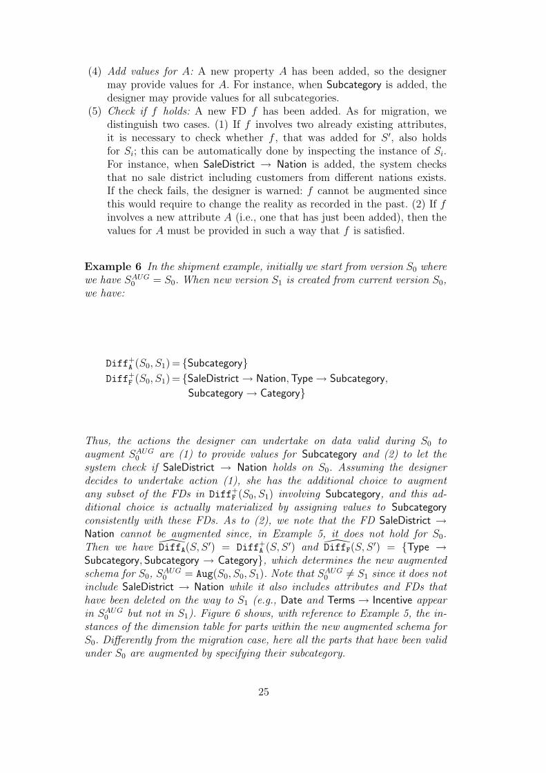
Example 6 In the shipment example, initially we start from version S0 wherewe have SAUG
0 = S0. When new version S1 is created from current version S0,we have:
Diff+A (S0, S1) = {Subcategory}
Diff+F (S0, S1) = {SaleDistrict → Nation, Type → Subcategory,
Subcategory → Category}
Thus, the actions the designer can undertake on data valid during S0 toaugment SAUG
0 are (1) to provide values for Subcategory and (2) to let thesystem check if SaleDistrict → Nation holds on S0. Assuming the designerdecides to undertake action (1), she has the additional choice to augmentany subset of the FDs in Diff+
F (S0, S1) involving Subcategory, and this ad-ditional choice is actually materialized by assigning values to Subcategory
consistently with these FDs. As to (2), we note that the FD SaleDistrict →Nation cannot be augmented since, in Example 5, it does not hold for S0.Then we have DiffA(S, S ′) = Diff+
A (S, S ′) and DiffF(S, S ′) = {Type →Subcategory, Subcategory → Category}, which determines the new augmentedschema for S0, SAUG
0 = Aug(S0, S0, S1). Note that SAUG0 6= S1 since it does not
include SaleDistrict → Nation while it also includes attributes and FDs thathave been deleted on the way to S1 (e.g., Date and Terms → Incentive appearin SAUG
0 but not in S1). Figure 6 shows, with reference to Example 5, the in-stances of the dimension table for parts within the new augmented schema forS0. Differently from the migration case, here all the parts that have been validunder S0 are augmented by specifying their subcategory.
25

Fig. 6. Augmented dimension table for parts in the shipment example
5 Versioning
In this section we consider schema versioning based on sequences of versionsas defined in the previous section, which influence the history of schemata andaugmented schemata. Formally, a history is a sequence H of one or more triplesrepresenting versions of the form (S, SAUG, t), where S is a version, SAUG isthe related augmented schema, and t is the start of the validity interval of S:
H = ( (S0, SAUG0 , t0), . . . , (Sn, S
AUGn , tn) ),
where n ≥ 0 and ti−1 < ti for 1 ≤ i ≤ n. Note that, in every history, for thelast triple (Sn, S
AUGn , tn) we have SAUG
n = Sn as augmentation only enrichesprevious versions using knowledge of the current modifications.
Given version S0 created at time t0, the initial history is
H = ((S0, SAUG0 , t0)),
where SAUG0 = S0. Schema modifications then change histories as follows. Let
H = ((S0, SAUG0 , t0), . . . , (Sn−1, S
AUGn−1 , tn−1), (Sn, S
AUGn , tn)) be a history, and
let Sn+1 be the new version at time tn+1 > tn; then the resulting history H ′ is
H ′ = ( (S0, Aug(SAUG0 , Sn, Sn+1), t0), . . . ,
(Sn, Aug(SAUGn , Sn, Sn+1), tn),
(Sn+1, SAUGn+1 , tn+1) ).
where SAUGn+1 := Sn+1.
We point out that a schema modification might potentially change any or allaugmented schemata contained in the history. E.g., adding a new FD at timen + 1, which has been valid but unknown throughout the history, may leadto a “back propagation” of this FD into every augmented schema in the his-tory. Moreover, note that new augmentations of previous schemata are basedon the augmented schemata as recorded in the history, not on the schematathemselves. Thus, augmentations resulting from different modifications areaccumulated over time, resulting in augmented schemata whose informationcontent—and, hence, potential for answering queries—is growing monotoni-cally with every modification.
26

We close this section by observing that, assuming to rely on a relational DBMS,a relevant choice concerns how to physically implement augmented schemataand histories. In the literature two approaches are proposed: namely single-pooland multi-pool [15]. In a single-pool implementation all schemata are associ-ated with a unique, shared, extensional repository, so that the same objectscannot have different values for the same properties when “viewed” throughdifferent schemata. On the other hand, in a multi-pool implementation eachschema is associated with a “private” extensional data pool; different datapools may contain the same objects having (possibly) completely indepen-dent representations and evolutions. Although the multi-pool solution maylook more flexible at a first glance, a single-pool solution has usually beenconsidered satisfactory for implementation as it limits the storage space over-head due to coexistence of multiple schemata. Both solutions do support ourapproach; however, a detailed comparison is outside the scope of this paper.
6 Querying Across Versions
In this section we discuss how our approach to versioning supports cross-version queries, i.e., queries whose temporal horizon spans multiple versions.
Preliminarily, we remark that OLAP sessions in DWs are aimed at effectivelysupporting decisional processes, thus they are characterized by high dynamicsand interactivity. A session consists of a sequence of queries, where each queryq is transformed into the next one q′ by applying an OLAP operator. Forinstance, starting from a query asking for the total quantity of parts of eachtype shipped on each month, the user could be interested in analyzing inmore detail a specific type: thus, she could apply a drill-down operator toretrieve the total quantity of each part of that type shipped on each month.Then, she could apply the roll-up operator to measure how many items ofeach part were shipped on the different years in order to catch a glimpse ofthe trend. Hence, since OLAP operators mainly navigate the FDs expressedby the hierarchies in the multidimensional schema, specifying the version forquery formulation in the OLAP context does not only mean declaring whichattributes are available for formulating the next query q′, but also representingthe FDs among attributes in order to determine how q′ can be obtained fromthe previous query q.
In this sense, the formulation context for an OLAP query is well representedby a schema graph. If the OLAP session spans a single version, the schemagraph is the associated one. Conversely, when multiple versions are involved,a schema under which all data involved can be queried uniformly must bedetermined. In our approach, such a schema is univocally determined by thetemporal interval T covered by the data to be analyzed, as the largest schema
27
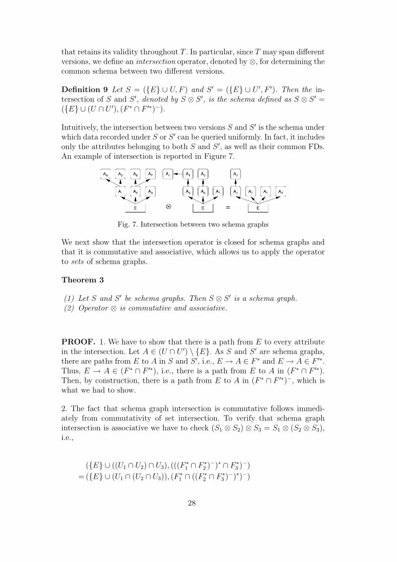
that retains its validity throughout T . In particular, since T may span differentversions, we define an intersection operator, denoted by ⊗, for determining thecommon schema between two different versions.
Definition 9 Let S = ({E} ∪ U, F ) and S ′ = ({E} ∪ U ′, F ′). Then the in-tersection of S and S ′, denoted by S ⊗ S ′, is the schema defined as S ⊗ S ′ =({E} ∪ (U ∩ U ′), (F ∗ ∩ F ′∗)−).
Intuitively, the intersection between two versions S and S ′ is the schema underwhich data recorded under S or S ′ can be queried uniformly. In fact, it includesonly the attributes belonging to both S and S ′, as well as their common FDs.An example of intersection is reported in Figure 7.
Fig. 7. Intersection between two schema graphs
We next show that the intersection operator is closed for schema graphs andthat it is commutative and associative, which allows us to apply the operatorto sets of schema graphs.
Theorem 3
(1) Let S and S ′ be schema graphs. Then S ⊗ S ′ is a schema graph.(2) Operator ⊗ is commutative and associative.
PROOF. 1. We have to show that there is a path from E to every attributein the intersection. Let A ∈ (U ∩ U ′) \ {E}. As S and S ′ are schema graphs,there are paths from E to A in S and S ′, i.e., E → A ∈ F ∗ and E → A ∈ F ′∗.Thus, E → A ∈ (F ∗ ∩ F ′∗), i.e., there is a path from E to A in (F ∗ ∩ F ′∗).Then, by construction, there is a path from E to A in (F ∗ ∩ F ′∗)−, which iswhat we had to show.
2. The fact that schema graph intersection is commutative follows immedi-ately from commutativity of set intersection. To verify that schema graphintersection is associative we have to check (S1 ⊗ S2) ⊗ S3 = S1 ⊗ (S2 ⊗ S3),i.e.,
({E} ∪ ((U1 ∩ U2) ∩ U3), (((F∗1 ∩ F ∗
2 )−)∗ ∩ F ∗3 )−)
= ({E} ∪ (U1 ∩ (U2 ∩ U3)), (F∗1 ∩ ((F ∗
2 ∩ F ∗3 )−)∗)−)
28

Clearly, equality in the first component (i.e., attributes) follows from associa-tivity of set intersection. Concerning equality in the second component (i.e.,FDs) we establish the following facts for all sets F , F1, and F2 of simple FDs:(a) (F−)∗ = F ∗ and (b) F ∗
1 ∩ F ∗2 = (F ∗
1 ∩ F ∗2 )∗
Afterwards equality in the second component is derived as follows for F1, F2, F3:
(((F ∗1 ∩ F ∗
2 )−)∗ ∩ F ∗3 )−
(a)= ((F ∗
1 ∩ F ∗2 )∗ ∩ F ∗
3 )−(b)= ((F ∗
1 ∩ F ∗2 ) ∩ F ∗
3 )−
= (F ∗1 ∩ (F ∗
2 ∩ F ∗3 ))−
(b)= (F ∗
1 ∩ (F ∗2 ∩ F ∗
3 )∗)−(a)= (F ∗
1 ∩ ((F ∗2 ∩ F ∗
3 )−)∗)−
Fact (a) follows immediately from the observation that path reachability re-mains invariant under transitive reduction (Definition 2) and schema graphreduction (Definition 4). Concerning fact (b) we have to show f ∈ F ∗
1 ∩F ∗2 for
f ∈ (F ∗1 ∩ F ∗
2 )∗. (The other inclusion is trivial.) Let A1 → An ∈ (F ∗1 ∩ F ∗
2 )∗.Due to the inductive definition of “∗” we either have A1 → An ∈ (F ∗
1 ∩ F ∗2 ),
in which case there is nothing to show, or there are A1, . . . , An for n ≥ 3such that Ai → Ai+1 ∈ (F ∗
1 ∩ F ∗2 ), 1 ≤ i ≤ n − 1. In the latter case we
have Ai → Ai+1 ∈ F ∗1 and Ai → Ai+1 ∈ F ∗
2 , 1 ≤ i ≤ n − 1. Thus, we haveA1 → An ∈ (F ∗
j )∗ = F ∗j , j = 1, 2. Consequently, we have A1 → An ∈ (F ∗
1 ∩F ∗2 ),
which concludes the proof.
In view of Theorem 3 a common schema for cross-version querying can nowbe defined as follows based on schema intersection.
Definition 10 Given a history H and a (not necessarily connected) temporalinterval T , we call the span of T on H the set
Span(H,T ) = {SAUGi | (Si, S
AUGi , ti) ∈ H ∧ [ti, ti+1[ ∩ T 6= ∅}
(conventionally assuming tn+1 = +∞).
Given a history H and a temporal interval T , the common schema on H alongT is defined as Com(H,T ) =
⊗Span(H,T ) SAUG
i .
Let q be the last query formulated, and T be the interval determined by thepredicates in q on the temporal hierarchy (if no predicate is present thenT =] −∞, +∞[). The formulation context for the next query q′ is expressedby the schema graph Com(H,T ). Note that the OLAP operator applied totransform q into q′ may entail changing T into a new interval T ′; in this case,the formulation context for getting a new query q′′ from q′ will be defined byCom(H,T ′).
29

QtyShipped ShippingCostsDM
Month
Year Brand
Container
Type
Subcategory
Size
PartDescr
Allowance Terms
Incentive
Deal ShipFrom
Shipment
Customer
SaleDistrict
Nation
Region
City
Category
ShippingCostsEU
ShippingCostsLIT
Part
Fig. 8. Formulation contexts for the query in Example 7 without augmentation (inplain lines) and with augmentation (in plain and dashed lines)
Example 7 Let H = ((S0, SAUG0 , t0), (S1, S
AUG1 , t1), (S2, S
AUG2 , t2)) be the his-
tory for the shipment fact (recall that we have t1 = 1/1/2003 and t2 =1/1/2004), and let q = “Compute the total quantity of each part categoryshipped from each warehouse to each customer nation since July 2002”. Thetemporal interval of q is T = [7/1/2002, +∞[, hence Span(H,T ) = {S0, S1, S2}.Fig. 8 shows the formulation context, defined by SAUG
0 ⊗SAUG1 ⊗SAUG
2 , in twosituations: when no augmentation has been made, and when all possible aug-mentations have been made.
First of all, we observe that q is well-formulated only if ShipFrom has beenaugmented for both previous versions, since otherwise one of the required at-tributes does not belong to the formulation context.
Then we observe that, for instance, (1) drilling down from Category to Sub-
category will be possible only if subcategories and their relationship with cate-gories have been established also for 2002 data; (2) drilling down from Nation
to SaleDistrict will be possible only if the FD from sale districts to nationshas been verified to hold also before 2003, which is the assumption underlyingFig. 8.
Finally, we note that if ShippingCostsEU is augmented (which is particularlysimple due to the existence of constant conversion factors) then queries involv-ing ShippingCostsEU can be evaluated over any time period, although shippingcosts were recorded exclusively in DM until t2. Moreover, we point out thatthe augmentation of the derived measure ShippingCostsEU can be implementedat virtually no storage cost (e.g., in terms of a view that applies the constantconversion factor).
We close this section with some remarks about query rewriting over versions.Due to addition or removal of dimensions, the granularity of a given mea-
30

Table 3Summarizability issues with disaggregation
monthly
Product Month Stock
p1 Jan-2003 10...
......
p1 Jun-2003 10
p1 Jul-2003 20...
......
p1 Dec-2003 20
daily
Product Day Stock
p1 01-Jan-2003 10...
......
p1 30-Jun-2003 10
p1 01-Jul-2003 20...
......
p1 31-Dec-2003 20
sure M (meant as the combination of dimensions under which its values arerecorded) may change from one version to the other. Thus, a given cross-version query q may require aggregation on some (finer) version S ′, and noaggregation on some (coarser) one S ′′. Importantly, the aggregation operatorused to summarize M on S ′ is the one associated with M in the meta-datarepository. If at some time, during augmentation, the designer decides to dis-aggregate M , it is obviously necessary that this is done consistently with thisaggregation operator, i.e., in such a way that reaggregating M at the originalgranularity exactly returns the original values.
Disaggregation also brings to the foreground some subtle summarizability is-sues. We recall from [16] that aggregate functions are either distributive oralgebraic or holistic. Repeated applications of a distributive aggregate func-tion (e.g., SUM) during a sequence of roll-up operations lead to the correctfinal result. If an aggregate function is not distributive, i.e., if it is algebraic(e.g., AVG) or holistic (e.g., Median), then in general the repeated applica-tion during a sequence of roll-up operations leads to an incorrect result. Now,consider an initial schema version S where some measure is recorded under anon-distributive aggregate function, e.g., average quantities in stock (measureStock) are recorded per product and month. Next, in the new version S ′ thesequantities are recorded at a finer granularity, e.g., per product at the end ofeach day. If the designer chooses to augment data associated with S to reflectthis change, then according to Table 2 measure Stock has to be disaggregatedto obtain daily values. Here, daily values can be obtained easily by just usingthe original monthly measure as new daily measure for each day of the month,as shown in Table 3. Clearly, in this way the averages of the daily measuresper month yield the original monthly measures. However, it is less clear how aroll-up aggregation to the year level should be computed. In fact, as the firsthalf of a year (i.e., 01-Jan until 30-Jun) has 181 days while the second one(i.e., 01-Jul until 31-Dec) has 184, the aggregation of daily measures to levelyear will yield a different result (181·10+184·20
365≈ 15.04) than the aggregation of
31
monthly measures to level year (6·10+6·2012
= 15). Following our above argumen-tation concerning non-distributive aggregate functions, one might think thattaking averages of daily measures to level year (with result 15.04) should becorrect, while averaging the average monthly values (with result 15) should beavoided. Nevertheless, we recall that the monthly values are the ones that werereally recorded in the system, while the daily ones were obtained by disaggre-gation during augmentation. In particular, on schema version S users mightalready have seen the value 15 computed from monthly values. As augmen-tation should not introduce inconsistencies by changing the results of queries,we must make sure that in this particular scenario the daily values are notused to compute the aggregates per year.
We envisage the following two alternative approaches to deal with inconsisten-cies arising from roll-up operations involving disaggregated measures. First,the query subsystem could simply warn the user whenever disaggregated mea-sures have contributed to a query result. Second, and more ideally, the querysubsystem could try to avoid the use of disaggregated measures in roll-up ag-gregations. For example, in the above scenario roll-up operations beyond themonth level would always be computed from monthly measures but not fromdaily ones. However, a systematic analysis of how to avoid the use of disaggre-gated measures in general and of disaggregated and derived ones in particularstill needs to be done.
7 Computational Complexity
To support our approach towards schema versioning, some central operationshave to be implemented. The aim of this section is to indicate that all of theseoperations can be implemented efficiently (i.e., by means of polynomial timealgorithms), which suggests that our approach can indeed be used in an inter-active design and versioning process. We point out that we do not try to deriveexact complexity bounds; instead, we just point out some well-known poly-nomial time algorithms that could be used in an ad-hoc implementation. (Inparticular, we do not address possibly more efficient incremental algorithms.)
It should not come as a surprise that the complexity of computing transitivereductions underlies the following analysis. Consequently, we recall from [3]that each graph has a transitive reduction that can be computed in polynomialtime and, moreover, that the complexity of computing transitive reductionsis of the same complexity as computing transitive closures (which can becomputed in O(n3) time using Warshall’s algorithm where n is the number ofthe graph’s nodes).
(1) Schema graph reduction. To compute the reduced schema graph S− of S
32

the following procedure can be applied: (a) The strongly connected com-ponents of S are identified in linear time (see., e.g., [8]). (b) The equiva-lent acyclic schema graph Sa = (U/≡F
, F a) for S is constructed from thestrongly connected components of S in polynomial time via transitive re-duction. (c) The reduced schema graph S− = (U , F−) is computed fromSa = (U/≡F
, F a) in polynomial time according to Definition 4.(2) Projection. To compute a projection πX(F ) according to Lemma 2 a
subset of a transitive closure has to be selected, which can be done inpolynomial time.
(3) Schema modification operations. Operation AddA requires adding the at-tribute to the current schema, which is done in constant time. OperationDelA can be seen as a composition of projection followed by reduction,both of which are polynomial time as we have seen already. OperationsAddF and DelF each require a single reduction, which can be done inpolynomial time.
(4) Schema augmentation. Augmentation requires the computation of Diff+A
and Diff+F , which involve standard (polynomial time) set operations and
transitive closures. Afterwards, augmentation proceeds in terms of (poly-nomial time) modification operations on augmented schema versions.
(5) Schema intersection. Schema intersection ⊗ is defined in terms of a com-position of set operations, transitive closure, and reduction; hence, it canbe computed in polynomial time as well.
8 Conclusions and Further Remarks
In this paper we have presented an approach towards DW schema version-ing. Importantly, our approach relies on a conceptually simple graph modelthat captures the core of state-of-the-art data models for DWs. Based on thestandard graph operations of transitive closure and reduction, we have de-fined four intuitively appealing schema modification operations in the contextof graphical DW schemata. We have shown how single schema modificationslead to a history of versions that contain augmented schemata in addition to“ordinary” schemata, and we have defined an intersection operator that allowsus to determine whether a given query, possibly spanning several versions, canbe answered based on the information contained in augmented schemata.
As a side remark, we note that our approach can also be used for horizon-tal benchmarking, where a company compares its own performance againstcompetitors’ performance. E.g., in our sample scenario assume that there isanother company shipping similar products but according to a different geo-graphical classification. To include the competitor’s shipments for horizontalbenchmarking, all one has to do is to (a) create a new schema version, (b) addthe competitor’s geographical classification, e.g., in terms of a new alternative
33

aggregation path such as Customer → CompetitorSaleDistrict → Competitor-
Region, and (c) augment previous schema versions with the new aggregationpath.
Appropriate schema versioning and in particular schema augmentation in-volves considerable manual work by DW administrators. Nevertheless, we arenot aware of “simpler” viable alternatives. E.g., one could be tempted to try(a) to express augmented information in terms of views over new data and (b)to answer cross-version queries based on established techniques for answer-ing queries using views. However, this approach is infeasible for the followingreason: Consider the insertion of a new dimensional attribute such as Sub-
category at time t1 into the Part hierarchy in our sample scenario. To enablecross-version queries involving Subcategory on schema versions prior to t1,somehow Subcategory values have to be “found” for Part instances prior to t1,even for parts that do not exist any longer after t1. Clearly, those parts donot occur in versions after t1 and hence they do neither occur in views overversions after t1. Consequently, a manual assignment of subcategories to partscannot be avoided if cross-version queries need to be supported. (Note that anautomated assignment of default or null values would not increase the analysispotential.)
Next, we observe that our approach to versioning can be regarded as “pure”since data never gets deleted. In particular, if an attribute A is deleted byDelA then a new version is created whose schema does not contain A anylonger; hence, A-values will not be stored for new data any longer. However,previous versions and augmented schemata still contain A, and their associatedinstances contain values for A, which allows us to answer queries involving Aon old data.
While this fully complies with the idea of versioning [19,31], for practical pur-poses designers might want to delete data physically to free disk space. Thiscould be easily achieved in at least two ways. First, designers might want todelete entire (old) versions and their associated data, which can be imple-mented by deleting appropriate data entries and/or tables of those schematafrom the database. Second, designers might want to erase individual attributesfrom the history of versions (as if the attributes never existed). In this case,all tables (belonging to versions and augmented schemata for those versions)containing the specified attribute have to be altered to drop those attributes.
Finally, we remark that our approach to DW schema versioning provides aninitial step that covers the majority of schema elements occurring in real worlddata warehouses. However, future research is necessary to include side con-cepts such as (1) cross-dimensional attributes (e.g., an attribute VAT that isfunctionally determined by the pair of attributes product and location is across-dimensional attribute) and (2) derived measures that can be computed
34

from sets of other measures. Indeed, both concepts go beyond our assumptionof simple FDs and require general FDs that could be represented by usinga schema hyper-graph, where hyper-arcs go from sets of attributes to singleattributes. The generalization of our approach to the setting of hyper-graphsremains an open issue.
Acknowledgements
The authors would like to thank the reviewers whose careful reading andconstructive remarks helped to improve the presentation.
References
[1] Oracle change management pack. Technical report, Oracle Technical WhitePaper, 2000.
[2] KALIDO dynamic information warehouse - a technical overview. Technicalreport, KALIDO White Paper, 2004.
[3] A. V. Aho, M. R. Garey, and J. D. Ullman. The transitive reduction of adirected graph. SIAM Journal on Computing, 1(2):131–137, 1972.
[4] G. Ausiello, A. D’Atri, and D. Sacca. Graph algorithms for functionaldependency manipulation. Journal of the ACM, 30(4):752–766, 1983.
[5] B. Bebel, J. Eder, C. Koncilia, T. Morzy, and R. Wrembel. Creation andmanagement of versions in multiversion data warehouse. In Proc. SAC, pages717–723, Nicosia, Cyprus, 2004.
[6] M. Blaschka. FIESTA - A framework for schema evolution in multidimensional
databases. PhD thesis, Technische Universitat Munchen, Germany, 2000.
[7] M. Blaschka, C. Sapia, and G. Hofling. On schema evolution in multidimensionaldatabases. In Proc. DaWaK, pages 153–164, 1999.
[8] T. H. Cormen, C. Stein, R. L. Rivest, and C. E. Leiserson. Introduction to
Algorithms. McGraw-Hill, 2001.
[9] S. S. Cosmadakis and P. C. Kanellakis. Functional and inclusion dependencies:A graph theoretic approach. In Proc. 3rd PODS, pages 29–37, 1984.
[10] C. De Castro, F. Grandi, and M. R. Scalas. On schema versioning in temporaldatabases. In S. Clifford and A. Tuzhilin, editors, Recent advances in temporal
databases, pages 272–294. Zurich, Switzerland, 1995.
[11] J. Eder and C. Koncilia. Changes of dimension data in temporal datawarehouses. In Proc. DaWaK, pages 284–293, 2001.
35

[12] J. Eder, C. Koncilia, and T. Morzy. The COMET metamodel for temporal datawarehouses. In Proc. CAiSE, pages 83–99, 2002.
[13] M. Golfarelli, D. Maio, and S. Rizzi. The Dimensional Fact Model: a conceptualmodel for data warehouses. Int. Journal of Cooperative Information Systems,7(2-3):215–247, 1998.
[14] M. Golfarelli and S. Rizzi. A methodological framework for data warehousedesign. In Proc. 1st DOLAP Workshop, pages 3–9, Washington, 1998.
[15] F. Grandi. A relational multi-schema data model and query language for fullsupport of schema versioning. In Proc. 10th SEBD, Isola d’Elba, Italy, 2002.
[16] J. Gray, S. Chaudhuri, A. Bosworth, A. Layman, D. Reichart, M. Venkatrao,F. Pellow, and H. Pirahesh. Data Cube: A relational aggregation operatorgeneralizing group-by, cross-tab, and sub totals. Data Mining and Knowledge
Discovery, 1(1):29–53, 1997.
[17] H. Gupta, V. Harinarayan, A. Rajaraman, and J.D. Ullman. Index selectionfor OLAP. In Proc. ICDE, pages 208–219, 1997.
[18] W. H. Inmon. Building the Data Warehouse. John Wiley & Sons, 3rd edition,2002.
[19] C. Jensen, J. Clifford, R. Elmasri, S. K. Gadia, P. J. Hayes, and S. Jajodia.A consensus glossary of temporal database concepts. ACM SIGMOD Record,23(1):52–64, 1994.
[20] C. Jensen et al. The consensus glossary of temporal database concepts. InO. Etzion, S. Jajodia, and S. Sripada, editors, Temporal Databases: Research
and Practice, pages 367–405. Springer, 1998.
[21] R. Kimball, L. Reeves, M. Ross, and W. Thornthwaite. The data warehouse
lifecycle toolkit. John Wiley & Sons, 1998.
[22] J. Lechtenborger. Computing unique canonical covers for simple fds viatransitive reduction. Information Processing Letters, 92(4):169–174, 2004.
[23] J. Lechtenborger and G. Vossen. Multidimensional normal forms for datawarehouse design. Information Systems, 28(5):415–434, 2003.
[24] H. Lenz and A. Shoshani. Summarizability in OLAP and statistical databases.In Proc. 9th SSDBM, pages 132–143, 1997.
[25] C. Letz, E. Henn, and G. Vossen. Consistency in data warehouse dimensions.In Proc. IDEAS, pages 224–232, 2002.
[26] D. Maier. The theory of relational databases. Computer Science Press, 1983.
[27] E. McKenzie and R. Snodgrass. Schema evolution and the relational algebra.Information Systems, 15(2):207–232, 1990.
[28] E. Pourabbas and A. Shoshani. Answering joint queries from multiple aggregateOLAP databases. In Proc. 5th DaWaK, Prague, 2003.
36
[29] C. Quix. Repository support for data warehouse evolution. In Proc. DMDW,1999.
[30] Red-Gate Software. Compare and synchronize SQL database structures, 2004.
[31] J. Roddick. A survey of schema versioning issues for database systems.Information and Software Technology, 37(7):383–393, 1995.
[32] SAP. Multi-dimensional modeling with BW: ASAP for BW accelerator.Technical report, SAP America Inc. and SAP AG, 2000.
[33] D. Theodoratos and M. Bouzeghoub. A general framework for the view selectionproblem for data warehouse design and evolution. In Proc. DOLAP, McLean,2000.
[34] D. Theodoratos and M. Bouzeghoub. Data currency quality satisfaction in thedesign of a data warehouse. International Journal of Cooperative Information
Systems, 10(3):299–326, 2001.
[35] TSQL2 Language Design Committee. The TSQL2 Temporal Query Language.Kluwer Academic Publishers, 1995.
[36] J. D. Ullman. Database and Knowledge-Base Systems, volume 1. ComputerScience Press, 1988.
[37] A. Vaisman, A. Mendelzon, W. Ruaro, and S. Cymerman. Supportingdimension updates in an OLAP server. In Proc. CAiSE, pages 67–82, 2002.
[38] J. Yang. Temporal data warehousing. PhD thesis, Stanford University, 2001.
37