schematron schema inference - univerzita karlovaholubova/dp/kozak.pdf · název práce: schematron...
TRANSCRIPT

Charles University in Prague
Faculty of Mathematics and Physics
MASTER THESIS
Michal Kozák
Schematron Schema Inference
Department of Software Engineering
Supervisor of the master thesis: RNDr. Irena Mlýnková, Ph.D.
Study programme: Informatics
Specialization: Software Systems
Prague 2011

I would like to thank to my supervisor, RNDr. Irena Mlýnková, Ph.D., for her guidance,
helpful suggestions, study materials and the time she spend reading and correcting my
English. It helped me a lot.

I declare that I carried out this master thesis independently, and only with the cited sources,
literature and other professional sources.
I understand that my work relates to the rights and obligations under the Act No. 121/2000
Coll., the Copyright Act, as amended, in particular the fact that the Charles University in
Prague has the right to conclude a license agreement on the use of this work as a school
work pursuant to Section 60 paragraph 1 of the Copyright Act.
In ........ date ............ signature

Název práce: Schematron Schema Inference
Autor: Michal Kozák
Katedra / Ústav: Katedra softwarového inženýrství
Vedoucí diplomové práce: RNDr. Irena Mlýnková, Ph.D., Katedra softwarového inženýrství
Abstrakt: XML je populární jazyk pro výměnu dat. Mnoho dokumentů však nemá svůj popis schématu nebo je tento popis neaktuální. Tato práce navazuje na práce o automatickém odvozování schémat XML dokumentů a zaměřuje se na odvozování schémat pro Schematron.
Schematron je jazyk, který validuje XML dokumentu pouze pomocí pravidel, ne jako celou gramatiku, jako je typické pro DTD nebo XML Schema. Jelikož oblast generování schémat Schematronu není příliš prozkoumaná, tato práce analyzuje základní problémy, navrhuje několik postupů a popisuje jejich výhody a nevýhody.
Klíčová slova: XML, XML schéma, Odvozování XML, Schematron
Title: Schematron Schema Inference
Author: Michal Kozák
Department / Institute: Department of Software Engineering
Supervisor of the master thesis: RNDr. Irena Mlýnková, Ph.D., Department of Software Engineering
Abstract: XML is a popular language for data exchange. However, many XML documents do not have their schema or their schema is outdated. This thesis continues on the field of automatic schema inferring for set of XML documents and focuses on Schematron schema inferring.
Schematron is a language that validates XML documents with rules, it does not compare the document against a grammar like DTD, and XML Schema does. Because the field of Schematron schema generation is not so much explored, this thesis analyzes basic problems, suggests several approaches and describes their advantages and disadvantages.
Keywords: XML, XML schema, XML inferring, Schematron

Contents
1 Introduction ........................................................................................................................ 1
1.1 Motivation ................................................................................................................... 1
1.2 Description of this thesis ............................................................................................. 1
1.3 Structure of the work .................................................................................................. 2
2 Used technologies ............................................................................................................... 3
2.1 XML .............................................................................................................................. 3
2.1.1 Syntax ................................................................................................................... 3
2.1.2 Namespaces ......................................................................................................... 5
2.2 XPath ............................................................................................................................ 7
2.2.1 Syntax ................................................................................................................... 7
2.2.2 XPath 2.0 ............................................................................................................ 10
2.3 DTD ............................................................................................................................ 10
2.4 XML Schema .............................................................................................................. 11
2.4.1 Syntax ................................................................................................................. 12
2.4.2 Summary of XSD ................................................................................................. 14
2.5 RELAX NG ................................................................................................................... 14
2.5.1 XML Syntax ......................................................................................................... 14
2.5.2 Summary of RELAX NG ....................................................................................... 18
2.6 Schematron ................................................................................................................ 19
2.6.1 Versions of Schematron ..................................................................................... 19
2.6.2 Language definition ............................................................................................ 19
2.6.3 Difference from other schema languages .......................................................... 25
3 Basic Definitions ................................................................................................................ 31
3.1 Formal Languages Theory .......................................................................................... 31
3.1.1 Basic definitions ................................................................................................. 31

3.2 Regular expressions and finite automata .................................................................. 33
3.2.1 Non-deterministic finite state automata ........................................................... 35
Theorem 1 Automata equivalence ................................................................................ 36
3.3 Regular tree grammars and Hedges .......................................................................... 36
3.3.1 Local tree grammars and languages .................................................................. 40
3.3.2 Single-Type tree grammars and languages ........................................................ 41
3.3.3 Regular tree automata ....................................................................................... 42
4 Taxonomy .......................................................................................................................... 45
4.1 DTD ............................................................................................................................ 45
4.2 XML Schema .............................................................................................................. 45
4.3 Relax NG..................................................................................................................... 46
4.4 Schematron ................................................................................................................ 46
5 Transforming hedges to Schematron schema .................................................................. 49
5.1 Definitions .................................................................................................................. 49
5.2 Limitations ................................................................................................................. 50
5.3 Step 1 – Context generation ...................................................................................... 50
5.3.1 Trivial solution .................................................................................................... 50
5.3.2 K-ancestors ......................................................................................................... 52
5.3.3 Absolute path without a recursion .................................................................... 53
5.3.4 Single recursion in production rules .................................................................. 54
5.3.5 Recursion with deterministic content ................................................................ 59
5.3.6 Context for each hedge of grammar .................................................................. 67
5.4 Step 2 – Boundary rules ............................................................................................. 69
5.5 Step 3 – order checks ................................................................................................ 71
5.5.1 Basic idea of the algorithm ................................................................................. 72
5.5.2 Problem analysis................................................................................................. 74

5.5.3 Algorithm ............................................................................................................ 75
5.6 Summary .................................................................................................................... 84
6 XML Schema inferring ....................................................................................................... 86
6.1 iXSD ............................................................................................................................ 86
6.1.1 Algorithm ............................................................................................................ 87
6.1.2 Summary ............................................................................................................ 93
7 Implemented solution ....................................................................................................... 94
7.1 Data limitations ......................................................................................................... 94
7.2 Usage of iXSD ............................................................................................................. 95
7.2.1 Inferred grammar ............................................................................................... 95
7.3 Schematron schema generation ................................................................................ 95
7.4 Experimental data sets .............................................................................................. 96
7.5 Conclusion ............................................................................................................... 101
8 Related work ................................................................................................................... 103
8.1 Inferring xml schema definitions from xml data ..................................................... 103
8.2 Even an Ant Can Create an XSD ............................................................................... 103
8.3 Automatic Construction of an XML Schema for a Given Set of XML Documents ... 104
8.4 Optimization and Refinement of XML Schema Inference Approaches ................... 104
8.5 Efficient Detection of XML Integrity Constraints ..................................................... 105
9 Conclusion ....................................................................................................................... 106
9.1 Future work ............................................................................................................. 106
10 Bibliography ................................................................................................................. 108
11 Appendix – Content of the CD ..................................................................................... 111
12 Appendix Program usage ............................................................................................ 112
12.1 iXSD .......................................................................................................................... 112
12.2 Schematron Generator ............................................................................................ 112

13 Appendix - attachments .............................................................................................. 114

1
1 Introduction
1.1 Motivation
In the current world communication holds a very important role. In the computer
world if two entities want to communicate they can accomplish it in many formats.
One of the mostly used is the Extensible Markup Language (XML) [9].
XML is used in many areas and for many purposes and often between different
subjects. Each XML document can have a different structure. To express the
structure and validate a document against it, XML schema languages were created.
Just to name some of them – DTD[9], XML Schema[12] and Relax NG[3]. These
schema languages describe the structure of a valid XML document and thus
allowing a safe data exchange.
The use of XML schemas is not mandatory and even if they exist, they can outdate
real fast. The problem emerges – how to automatically create an XML schema for a
set of documents. There have been many works on this problem. But most of them
focused on creating a complex grammar. These complex grammars validate the
whole document from its root to every leaf. This kind of validation is often slow and
also not needed.
What if we want to split the validation into several steps? In each step check a
different aspect of the document? What if we want to validate only a specific
construct and leave the rest of the document unchecked? These demands were not
easily satisfied. Rick Jellife created in 1999 a new schema language for XML
validation – Schematron. It uses rules that are able to check only specific parts of an
XML document. Schematron is distinct to grammar based schema languages and
the ability to automatically generate its schema would be interesting.
1.2 Description of this thesis
In this thesis we will introduce a method to infer a Schematron schema from a set
of XML documents. We analyze different aspect of Schematron schema generation.
Since the automatic inferring of XML documents is not a new problem, we will

2
introduce only a single method that we will use in our experimental
implementation.
In our experimental implementation we generate a grammar using the introduced
inferring method. We allow the user to modify the grammar. The grammar is then
transformed into Schematron schema by the use of our algorithm.
1.3 Structure of the work
This chapter presented a motivation and a brief description for this thesis. In
Chapter 2 we introduce used technologies (XML, grammar languages, etc.). In
Chapter 3 we define formalisms from the language theory. The expressive power of
schema languages is compared in Chapter 4. Chapter 5 is the core part of this thesis
presenting an analysis and algorithms for Schematron schema generation. Chapter
6 analyzes XML schema inferring and introduces a single method. In Chapter 7 we
describe our experimental implementation and its results. Chapter 9 contains
summary and also suggestions for possible future work that could not be done in
this thesis. The last part of this thesis is the Appendix that contains a brief user
guide.
3
2 Used technologies
In this chapter we introduce current technologies that are compared and
referenced later in this thesis. These descriptions introduce the technologies only in
main features. It is not the aim of this thesis to provide the full definition of these
technologies.
2.1 XML
In this chapter we define what XML, XML validation and a schema language is. The
Extensible Markup Language (XML) is a text-based language standardized by the
W3C1. XML was derived from SGML [14] that was too complex and thus too difficult
to implement. XML is simpler but preserves the expressive power. For full definition
of XML please refer to [9].
XML is used to describe structured information. XML is a meta-language; it defines
only the syntax how to describe the information but not a concrete way how to do
it. XML is used in many places for many purposes: sharing data (between people,
between programs), communication (e.g. WSDL2), storing data …
2.1.1 Syntax
XML syntax is easy. Here we define basic terms. To full definition of XML, please see
[9]:
Definition 2.1.1. Tag is a markup construct that begins with “<” and ends
with “>”. There are three types of tags – a start tag, an end tag and
an empty tag. The difference between these tags is the existence and
location of the character “/”. Start tag has none, end tag has it right
after “<” and empty tag has it right before the “>”.
There are limitations for characters that are allowed in the tag name. For full
definition of allowed name please see [9].
1World Wide Web consortium
http://www.w3.org 2 WSDL – Web Service Description Language
http://en.wikipedia.org/wiki/WSDL

4
Definition 2.1.2. Element is the building stone of any XML document. It
begins with a start-tag and ends with a corresponding end-tag or it
consists only of a single empty-tag. The names of the tags must match
and is case-sensitive. The data (if any) between the start-tag and end-
tag is called the content of an element. The content can be text or other
elements or both. These elements are called child elements.
Example 2.1.1. XML markup example
<paragraph style=”normal”>
Here starts some text. <bold>This part is Important!</bold> <newline />
Some more text on the next line.
</paragraph>
Example 2.1.1 contains three elements: paragraph, bold and newline. Elements bold
and newline are within the content of the element paragraph and thus they are child
elements. Element newline is formed only of empty-tag and has no content.
Definition 2.1.3. Attribute is a name-value pair located within a start-tag
or an empty-tag. The value must be always quoted.
Example 2.1.1 contains one attribute style that is located in the start-tag of the
element paragraph. The attribute style has the value “normal“.
Definition 2.1.4. An XML document is well-formed if it contains exactly one
root element and all elements are terminated within their parent
element’s content. (They must be correctly nested)
Example 2.1.2. Not a well-formed document
<doc>
<A><B></A></B>
</doc>
Example 2.1.2 is not well-formed because elements A and B are not correctly nested.
Note that the order of elements is generally significant; on the contrary the order of
attributes of an element is not.

5
Definition 2.1.5. An XML document is valid if and only if it is well-formed
and meets some other constraints. These constraints are defined by a
schema language. The process of determination whether the
document is valid is called validation.
Example 2.1.3. Well-formed XML document
<doc>
<para>
Here is some text of paragraph 1. <bold>Important information </bold>
</para>
<para>
Here is text of a next paragraph.
</para>
</doc>
We can see an example of a well-formed document. The root element is doc, it has
two child elements called para that have mixed content of text and element bold
(that can be seen in the first paragraph).
2.1.2 Namespaces
Some XML documents have their content from multiple sources – some elements
belong to a group A, other elements to group B. As the result the names of
elements (or attributes) can collide. Each group has its own schema and we need to
determine what schema to use for validation of every specific element. That is the
situation where namespaces are used.
Definition 2.1.6. Namespace is a context that holds information (e.g.
schema) for logically connected data.
6
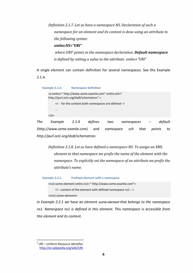
Definition 2.1.7. Let us have a namespace NS. Declaration of such a
namespace for an element and its content is done using an attribute in
the following syntax:
xmlns:NS=”URI”
where URI3 points to the namespace declaration. Default namespace
is defined by setting a value to the attribute xmlns=”URI”
A single element can contain definition for several namespaces. See the Example
2.1.4.
Example 2.1.4. Namespace definition
<a xmlns=” http://www.some.examle.com” xmlns:sch=” http://purl.oclc.org/dsdl/schematron” >
<!-- for the content both namespaces are defined-->
…
</a>
The Example 2.1.4 defines two namespaces – default
(http://www.some.examle.com) and namespace sch that points to
http://purl.oclc.org/dsdl/schematron.
Definition 2.1.8. Let us have defined a namespace NS. To assign an XML
element to that namespace we prefix the name of the element with the
namespace. To explicitly set the namespace of an attribute we prefix the
attribute’s name.
Example 2.2.1. Prefixed element with a namespace
<ns1:some-element xmlns:ns1=” http://www.some.examle.com”>
<!-- content of the element with defined namespace ns1 -->
</ns1:some-element>
In Example 2.2.1 we have an element some-element that belongs to the namespace
ns1. Namespace ns1 is defined in this element. This namespace is accessible from
this element and its content.
3 URI – Uniform Resource identifier
http://en.wikipedia.org/wiki/URI

7
2.2 XPath
XPath (XML Path language) [6, 7] is a query language for XML. XPath serves to
address parts of an XML document, allowing navigation in the XML document and
mining values of element, their attributes, etc. XPath is widely used by other
languages and tools (XSLT, XQuery …). Here we introduce the basics of XPath –
syntax, XPath-axis and some of its functions.
2.2.1 Syntax
Here we introduce the syntax of XPath 1.0, its queries and how they are evaluated.
An XML document is represented as a tree, where the root node of the tree is the
XML document itself and the root node has only one child – the root element of the
XML document.
Definition 2.2.1. An XPath node is the smallest XML fragment addressable
by XPath.
There are several types of XPath nodes:
Root nodes
Element nodes
Text nodes
Attribute nodes
Nodes for comments, processing instructions, namespaces…
Each XML document has only one root node and, as mentioned above, it is pointing
to the document itself. An element node represents an element in an XML
document but not its content. A text node represents the text content of an
element’s content model (The text is concatenated from each text node that is
located in the content model of the element). An attribute node represents
element’s attributes.
Definition 2.2.2. An XPath axis is a relation that specifies what nodes will
be selected from a current context.

8
There are several types of axes which are listed below. For each description of
an XPath axis we suppose we have selected a context node U that expresses the
relative position.
Self – returns the current node U.
Parent – returns the parent node of U.
Ancestor – returns all ancestors of U. (All nodes that are present on path
from U to the root node, excluding U)
Ancestor-or-self – returns the result of ancestor axis plus U.
Child – returns direct child nodes of U.
Descendant – returns all descendants of U, excluding U.
Descendant-or-self – returns descendants of U, including U.
Preceding-sibling – returns all siblings (elements that have the same parent
element) that precede U in the XML document.
Preceding – returns all elements that precede U in the XML document,
excluding the ancestors of U.
Following-siblings – returns all siblings (elements that have the same parent
element) that follow U in the XML document.
Following – returns all nodes that follow U in the XML document, excluding
the descendants of U.
Attribute – selects the attributes of U.
Namespace – selects the namespace nodes of U.
Definition 2.2.3. Node test tests the type or name of a node.
Definition 2.2.4. Predicate allows for specifying more complex conditions
for a node. It is written in square parenthesis and allows using of
negation (not), and and or operators.
Predicate can contain another XPath query and (or) use some of the built-in
functions of XPath. (e.g. count, location, position…)
Example 2.2.2. Predicate example
[1] - selects the first node from node set

9
[child] – has a child element “child”
[@id = 500] – has an attribute “id” with a value of 500.
Definition 2.2.5. Location step is a function that returns a set of nodes. It
has the form of:
axis::node-test predicate1 predicate2 … predicateN,
where axis is an XPath axis and it is optional, the default axis is the child
axis, node-test is required and predicates are optional. If the axis is
omitted the double-colon is also omitted.
Example 2.2.3. Examples of location steps
child::book[count(para) > 1]
Example 2.2.3 returns all children of the current node that have the name book and
each returned book must have at least one child element para.
Definition 2.2.6. Location path is a sequence (can be empty) of location
steps concatenated with “/”.
Location path is sometimes called path or query.
Definition 2.2.7. Absolute location path is a location path that begins with
a “/”. The context for absolute path is always the root node.
Example 2.2.4. Absolute location path
/ - absolute path that selects only the root node (no location steps)
/* - selects all children of the root node – document root (there is always only one document root)
In Example 2.2.4 the second path selects any child node of the root node. The
asterisk (*) select any node that has a name. Each element or attribute has a name.
Definition 2.2.8. Relative location path is a location path without “/” at
the beginning. Relative path must have specified a context set of nodes.
Example 2.2.5. Relative location path examples
Let us use Example 2.1.3 (Well-formed XML document), let the context node be the
root element “doc”. The following relative location path
para/bold/text()

10
would return the text node (the text) of the element bold that is the child of element
para that is the child of the context node.
descendant::bold/parent::para
descendant::para[bold]
Both paths return the element para that has a child element bold.
XPath abbreviations
The mostly used axes have their abbreviations.
Child <-> /
Descendant-or-self::node()/ <-> //
self <-> .
parent::node() <-> ..
attribute <-> @
Example 2.2.6. Example of abbreviations
/doc <-> /child:doc
bold/.. <-> bold/parent::node()
//bold <-> /descendat-or-self::node()/bold
2.2.2 XPath 2.0
The next version of XPath – version 2.0 brings new features like data types, more
built-in functions, ordered sequences and regular expressions [8]. Due to space
limitations it is left to the reader for his or her interests to read [8] for more
information.
2.3 DTD
The Document Type Definition (DTD) is a schema language. It allows to define
constrains for SGML family of languages and contrary to later schema languages it
does not use XML. It describes the constraints for every element and its content [9]-
Chapter 2.8.
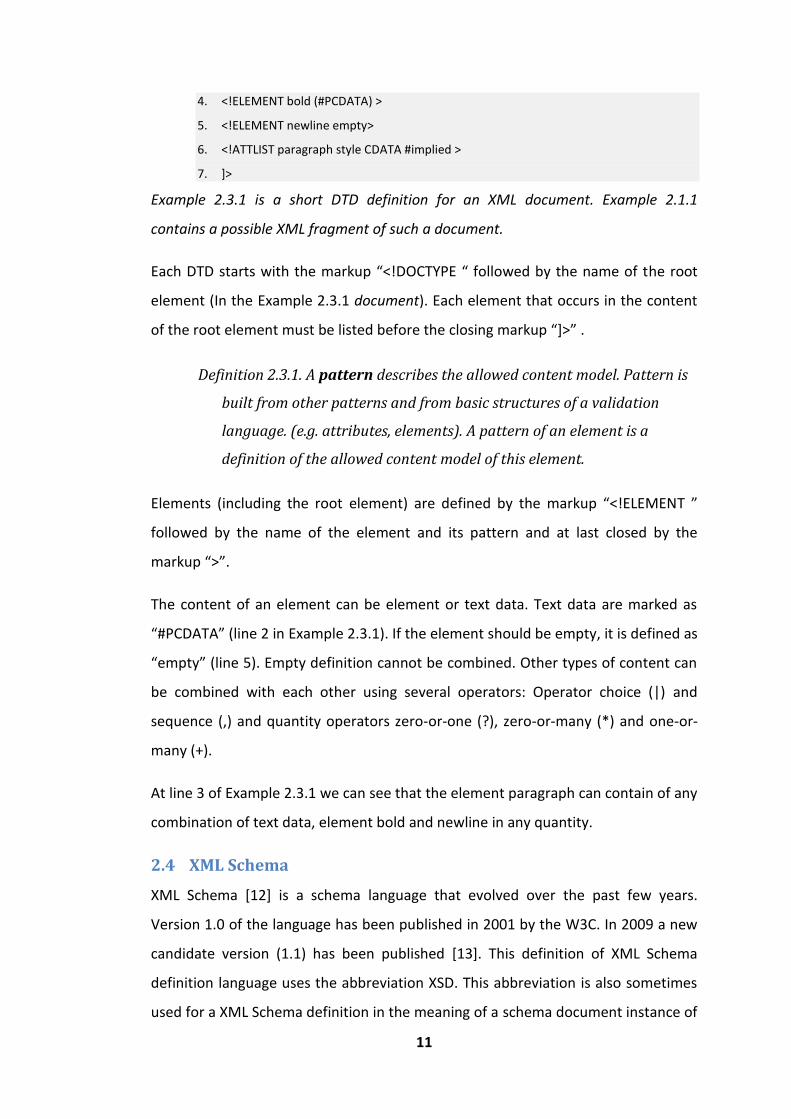
Example 2.3.1. A DTD example
1. <!DOCTYPE document [
2. <!ELEMENT title (#PCDATA) >
3. <!ELEMENT paragraph (#PCDATA | bold | newline)* >
11
4. <!ELEMENT bold (#PCDATA) >
5. <!ELEMENT newline empty>
6. <!ATTLIST paragraph style CDATA #implied >
7. ]>
Example 2.3.1 is a short DTD definition for an XML document. Example 2.1.1
contains a possible XML fragment of such a document.
Each DTD starts with the markup “<!DOCTYPE “ followed by the name of the root
element (In the Example 2.3.1 document). Each element that occurs in the content
of the root element must be listed before the closing markup “]>” .
Definition 2.3.1. A pattern describes the allowed content model. Pattern is
built from other patterns and from basic structures of a validation
language. (e.g. attributes, elements). A pattern of an element is a
definition of the allowed content model of this element.
Elements (including the root element) are defined by the markup “<!ELEMENT ”
followed by the name of the element and its pattern and at last closed by the
markup “>”.
The content of an element can be element or text data. Text data are marked as
“#PCDATA” (line 2 in Example 2.3.1). If the element should be empty, it is defined as
“empty” (line 5). Empty definition cannot be combined. Other types of content can
be combined with each other using several operators: Operator choice (|) and
sequence (,) and quantity operators zero-or-one (?), zero-or-many (*) and one-or-
many (+).
At line 3 of Example 2.3.1 we can see that the element paragraph can contain of any
combination of text data, element bold and newline in any quantity.
2.4 XML Schema
XML Schema [12] is a schema language that evolved over the past few years.
Version 1.0 of the language has been published in 2001 by the W3C. In 2009 a new
candidate version (1.1) has been published [13]. This definition of XML Schema
definition language uses the abbreviation XSD. This abbreviation is also sometimes
used for a XML Schema definition in the meaning of a schema document instance of

12
the XML Schema. If not said otherwise we will use the XSD as the abbreviation of
XML Schema Definition Language.
In this thesis we work with version 1.0 of XSD. Nowadays it is one of the most
commonly used schema languages. It was created because DTD was not strong
enough (bad support for foreign keys, missing data types and namespaces…) but
there are many principles that are similar to DTD.
2.4.1 Syntax
XSD defines the allowed content of an XML document based on defining parent-
child relationship. It defines the allowed content for the root element and its
attributes. Recursively defines the child elements of root and their children.
Definition 2.4.1. XSD file is an XML document with the root element
schema and the namespace “http://www.w3.org/2001/XMLSchema”.
Data types
XSD supports many built-in data types (e.g. boolean, int, double, date, string…) and
allows for defining user-defined types as well. There are two types of data types in
XSD - simple and complex data types.
All embedded XSD types are simple types. A user can create new simple types using
extension or restriction of another simple type or just by defining a list of allowed
values. Simple types are used to store simple values like text, amount of money,
post code… but not a structured data – elements or attributes. For that purpose
complex data types are used.
Example 2.4.1. Simple types in XSD
<xsd:element name=”familyName” type=”xsd:string” />
<xsd:simpleType name=”postCodeType”>
<xsd:restriction base=”xsd:string”>
<xsd:length value=”5” />
</xsd:restriction>
</xsd:simpleType>
<xsd:element name=”postCode” type=”postCodeType” />

13
In Example 2.4.1 we define a simple type for the post code of an address. It is based
on string and we limit its length to 5 characters.
Complex data types are used to store a complex (structured) element content –
containing multiple elements and (or) attributes. A child element may be defined
directly in the definition of its parent element. It is also possible to define its exact
occurrence by using minOccurs and maxOccurs attributes. An item can be made
optional by setting minOccurs to “0”.
There are generally three options to define complex types: deriving from a simple
type (we use simple type with attributes), from a complex type or defining a new
complex type. Deriving from an existing data type is done via extension or
restriction. For purposes of this thesis we show the definition of a brand new
complex type.
Defining the pattern for a complex type is done with pattern operator sequence,
choice or all. These operators control the order of their patterns.
Operator sequence ensures that child patterns are validated against the
order they are listed in their definition. The content of this operator is
limited to pattern element, sequence and choice.
Operator choice selects only one pattern from its child patterns. The content
of this operator is limited to pattern element, sequence, choice and all.
Operator all validates its pattern in any order. The occurrence of patterns
can be set to at most once. This feature is not directly in DTD, but it can be
still expressed by a more complex pattern definition. However the content
of this operator is limited only to elements (Chapter 3.8.2 in [12] also note
the containts in Chapter 3.9.6). These constraints ensure a deterministic
data model.
Example 2.4.2. Complex type example
<xs:element name=”person”>
<xs:complexType>
<xs:sequence>
<xs:element name=”firstName” type=”xs:string” />

14
<xs:element name=”middleName” minOccurs=”0” type=”xs:string” />
<xs:element name=”lastName” type=”xs:string” />
<xs:choice>
<xs:element name=”passportNo” type=”xs:string” />
<xs:element name=”IDCardNo” type=”xs:string” />
</xs:choice>
</xs:sequence>
</xs:complexType>
</xs:element>
In Example 2.4.2 we define a pattern for element “person”. The pattern consists of
a sequence of elements firstName, optional middleName and lastName and a choice
of elements passportNo and IDCardNo.
2.4.2 Summary of XSD
XSD allows for complex definition of a schema for an XML document. It supports
more user friendly features like “all” operator or better support for foreign keys,
and data types. As we will see in Chapter 4, the expressive power of XSD is stronger
than of DTD. Some features of XSD are merely a syntactic sugar (like the operator
all).
2.5 RELAX NG
RELAX NG [3] is another schema language. It was created by merging two former
schema languages – RELAX CORE [15] and TRex [16]. RELAX NG language has a
strong mathematical background. Its schemas can be written in two forms: XML or
“compact”; these two forms can be translated to each other without the loss of
important information. In this chapter we will introduce the basic aspects of XML
syntax of RELAX NG.
2.5.1 XML Syntax
RELAX NG has similar syntax as XSD, but as we will see in Chapter 4, that RELAX NG
is stronger than XSD. It also supports namespaces.
Example 2.5.1. RELAX NG simple example
<element name="addressBook">
<zeroOrMore>
<element name="card">

15
<choice>
<element name="name">
<text/>
</element>
</choice>
<choice>
<element name="email">
<text/>
</element>
</choice>
</element>
</zeroOrMore>
</element>
In this example we define pattern for element “addressBook”. It contains zero or
more elements “card”. Each “card” contain either element “name” or element
“email”.
Elements are defined using the element element. Their pattern is defined by
patterns below.
element
attribute
group
interleave
optional
choice
zeroOrMore
oneOrMore
data types
Group pattern connects its child patterns in serial order. Interleave pattern on the
contrary allows its child patterns to be in any order (with no limitation to the child
patterns) but every pattern must be present. Optional pattern allows a pattern to
be omitted. Choice pattern selects only one of its child patterns. ZeroOrMore

16
pattern repeats zero or more times. OneOrMore pattern repeats one or more
times.
RELAX NG supports data types like XSD does. In fact, it allows the usage of data
types from XSD and their parameterization.
Name classes
Both the DTD and XSD allow the definition of elements only by specification of a
name or type (in case of XSD). They are unable to define schema like “The root
element can have only this pattern regardless its name” because in the schema we
do not know the name (or type) of the root element and we do not want to define
it.
RELAX NG has a feature called “name classes”. This feature allows for defining
elements and attributes anonymously or with some restrictions. Normally we would
use the name attribute or element. To define a pattern for more than a single name
we do not give elements (or attributes) their name but we use one of following
elements specifying their name class:
anyName
nsName
choice
Construct anyName defines that the element (or attribute) can have any name. It
can be restricted by nsName or name elements, see Example 2.5.2. There we define
an element that can have any name except for name “root” and must not have the
default namespace.
Example 2.5.2. anyName name class example
<element>
<anyName>
<except>
<name>root</name>
<nsName ns=”” />
</except>
</anyName>

17
<!—more definition of content -->
</element>
In Example 2.5.2 we define a name class for an element pattern. The element can
have any name from non-default namespace except the name root.
Construct nsName specifies the allowed namespace for a name. Again the
namespace can be restricted by an element except. Choice (in context of name
class) allows combining of previous options.
Example 2.5.3. nsName name class example
<element>
<nsName ns=” http://www.someNameSpace.com”>
<except>
<name>root</name>
</except>
</nsName>
<!—more definition of content -->
</element>
The allowed name for Example 2.5.3 is any name, except the name root, from the
namespace “http://www.someNameSpace.com“.
Example 2.5.4. choice name class example
<element>
<choice>
<name>root</name>
<name>document</name>
<nsName ns=”” />
</choice>
<!—more definition of content -->
</element>
In Example 2.5.4 we define three possible options for name of this pattern – “root”,
“document” or the default namespace.
Definition 2.5.1. Co-constraint or Co-occurrence constraint is a set of
rules that control what markup (elements or attributes) can co-occur
together. [5]
18
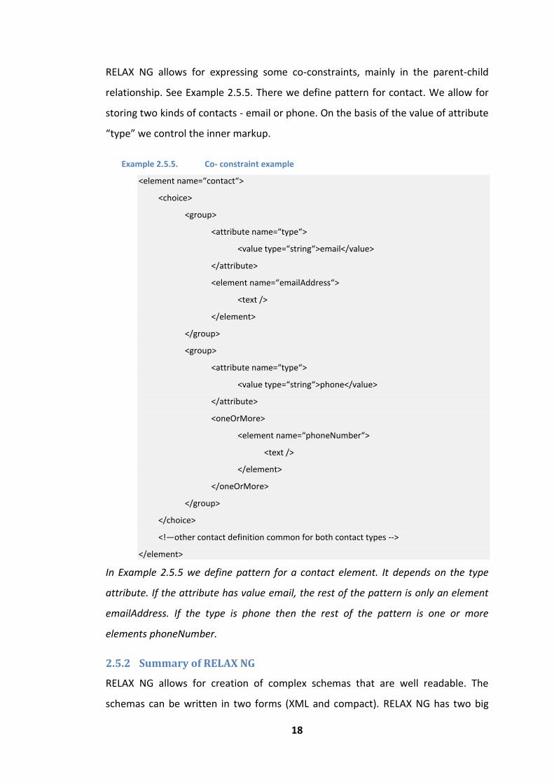
RELAX NG allows for expressing some co-constraints, mainly in the parent-child
relationship. See Example 2.5.5. There we define pattern for contact. We allow for
storing two kinds of contacts - email or phone. On the basis of the value of attribute
“type” we control the inner markup.
Example 2.5.5. Co- constraint example
<element name=“contact“>
<choice>
<group>
<attribute name=“type“>
<value type=“string“>email</value>
</attribute>
<element name=“emailAddress“>
<text />
</element>
</group>
<group>
<attribute name=“type“>
<value type=“string“>phone</value>
</attribute>
<oneOrMore>
<element name=“phoneNumber“>
<text />
</element>
</oneOrMore>
</group>
</choice>
<!—other contact definition common for both contact types -->
</element>
In Example 2.5.5 we define pattern for a contact element. It depends on the type
attribute. If the attribute has value email, the rest of the pattern is only an element
emailAddress. If the type is phone then the rest of the pattern is one or more
elements phoneNumber.
2.5.2 Summary of RELAX NG
RELAX NG allows for creation of complex schemas that are well readable. The
schemas can be written in two forms (XML and compact). RELAX NG has two big

19
advantages: name classes and co-constraints. Contrary to XML Schema there is
another advantage – non-determinism. RELAX NG has stronger expressive power
than XSD or DTD.
2.6 Schematron
Schematron is an XML validation language [2]. It defines rules that validate
documents by presence or absence of XML patterns. These rules are short, simple
and allow for printing user friendly messages.
2.6.1 Versions of Schematron
Schematron was developed by Rick Jellife in 1999. Since then many implementation
were created and the language itself evolved. We will describe the most common
variants.
Schematron 1.5
Version 1.5 of Schematron was built by Rick Jellife and contains of two-stage XSLT
1.0 transformation. The first transformation transforms a Schematron definition
into new XSLT transformations these are then run to validate XML documents. It is
easy-to-use but uses only XSLT 1.0 as a query language.
ISO Schematron
Schematron has been standardized by ISO/DSDL [17] project as ISO/IEC 19757-3. It
brings new ideas and extends and changes Schematron 1.5. The main differences
are support for more query languages, variables, abstract patterns and new URI.
In this thesis we will use ISO Schematron if not stated otherwise.
Schematron 1.6
This version of Schematron is the transition between Schematron 1.5 and ISO
Schematron.
2.6.2 Language definition
The syntax for Schematron is fairly easy. A full RELAX NG schema for Schematron
can be found at [2]. We will explain here the most important features and
constructs.
20
Schematron understands namespaces and thus we can combine Schematron with
other namespace-aware schema languages. The namespace definition for
Schematron is located on [18].
As said at the beginning of this chapter, ISO Schematron can use different query
languages – this means, we can create schemas that query using XSLT 1.0 [19], XSLT
1.1 [20], XSLT 2.0 [21], XQuery [22], XPath [6] or XPath 2.0 [8]. The full list of
supported implementations can be found in the ISO Schematron definition and
depends on the implementation used. The list of supported query languages of each
implementation may differ because new query languages can be supported if they
implement a set of rules that corresponds to Schematron definition. The definition
of a query language “queryBinding” is located in the element “schema” and can be
omitted.
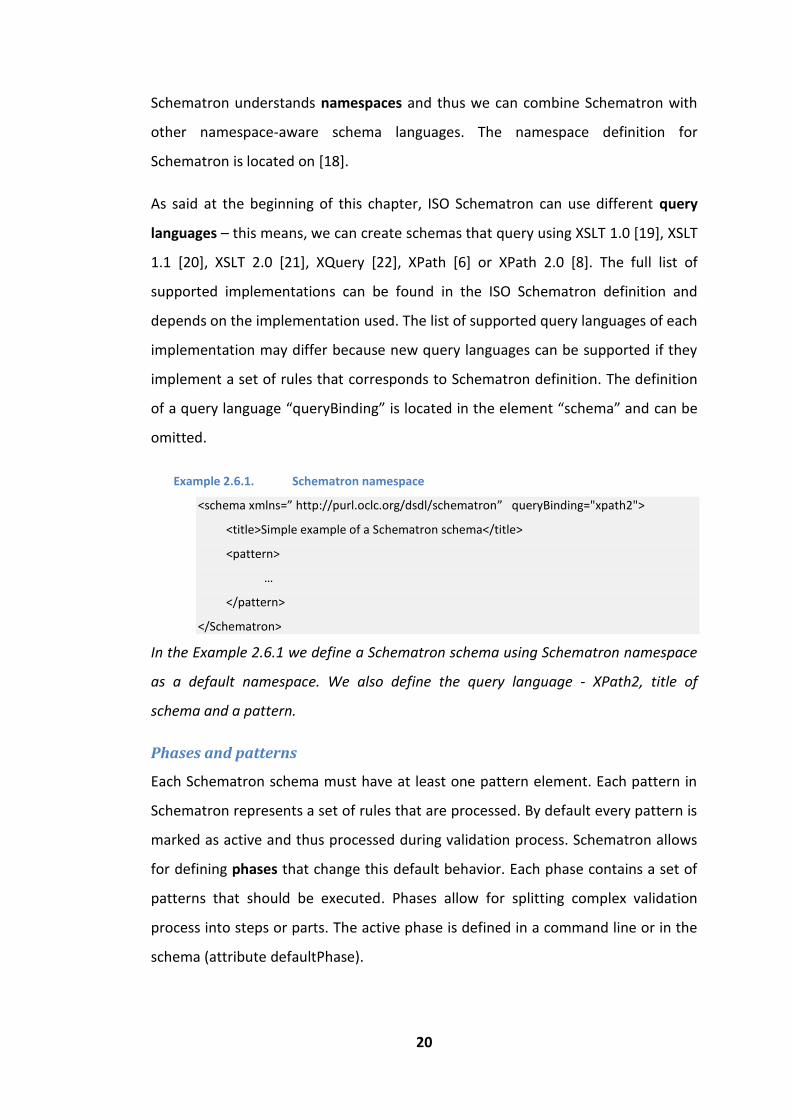
Example 2.6.1. Schematron namespace
<schema xmlns=” http://purl.oclc.org/dsdl/schematron” queryBinding="xpath2">
<title>Simple example of a Schematron schema</title>
<pattern>
…
</pattern>
</Schematron>
In the Example 2.6.1 we define a Schematron schema using Schematron namespace
as a default namespace. We also define the query language - XPath2, title of
schema and a pattern.
Phases and patterns
Each Schematron schema must have at least one pattern element. Each pattern in
Schematron represents a set of rules that are processed. By default every pattern is
marked as active and thus processed during validation process. Schematron allows
for defining phases that change this default behavior. Each phase contains a set of
patterns that should be executed. Phases allow for splitting complex validation
process into steps or parts. The active phase is defined in a command line or in the
schema (attribute defaultPhase).

21
Example 2.6.2. Schematron phases
<schema xmlns=”http://purl.oclc.org/dsdl/schematron“ defaultPhase=”simpleValidation“>
<title>Example of a Schematron phases</title>
<phase id=”simpleValidation”>
<active pattern=”simple_index_validation” />
<active pattern=”word_blacklist” />
</phase>
<phase id=”complexValidation”>
<active pattern=”word_blacklist” />
<active pattern=”complex _validation” />
</phase>
<pattern id=”simple_index_validation”>… </pattern>
<pattern id=”word_blacklist”>… </pattern>
<pattern id=”complex_validation”>… </pattern>
</Schematron>
Schema definition in Example 2.6.2 contains three patterns
(simple_index_validation, word_blacklist and complex_validation) and two phases
(simpleValidation and complexValidation). The default phase is the
simpleValidation. If the default phase is selected, it processes the
simple_index_validation and word_blacklist patterns.
There are three types of patterns in Schematron – normal, abstract and “is-a”
pattern. Normal pattern contains a set of rules and if active, it processes them.
Abstract pattern also contains rules, but must have specified the attribute
abstract=”true”. They may use undefined variables (they are defined by a caller “is-
a” pattern). “Is-a” pattern does not contain any rules. It contains attribute “is-a”
with reference to an abstract pattern. They may contain “param” elements that
define the values of all undefined variables of the abstract pattern.
Example 2.6.3. Patterns
<schema xmlns=” http://purl.oclc.org/dsdl/schematron ">
<pattern abstract=”false”>
<!—normal pattern, id and abstract=”false” are optional -->
<rule>…</rule>
</pattern>
<pattern id=”normal_pattern”>
<!—another normal pattern -->

22
<rule>…</rule>
</pattern>
<pattern abstract=”true” id=”abstract1”>
<!—abstract pattern must have an id-->
<rule>…</rule>
</pattern>
<pattern is-a=”abstract1”>
<!—is-a pattern of abstract pattern abstract1-->
<param name=”…” value=”…”>
</pattern>
</Schematron>
Example 2.6.3 contains four patterns. The first two are normal patterns. Each
defines one rule. The third pattern is an abstract pattern. The last one is a “is-a”
pattern.
Rules and assertions
Schematron validation capability is based on its rules. Each pattern must contain at
least one. Each rule must have a context in which it runs assertions. Schematron
contains two types of assertions: positive - asserts – and negative - reports. If any
assertion of the rule fails the rule fails and the document is marked as invalid. Note
that as the result of this paragraph Schematron allows for both positive and
negative validation.
Definition 2.6.1. An Assertion, in the context of XML validation, is a
statement about an XML fragment. A positive assertion succeeds if the
statement of the assertion succeeds. A negative assertion succeeds if
the statement fails.
Example 2.6.4. Assertions
<schema xmlns=” http://purl.oclc.org/dsdl/schematron” queryBinding="xpath2">
<pattern>
<rule context=”//book”>
<assert test=”title”>Every book must have an element title</assert>
<report test=”descendant::book”>Book cannot contain any other book element</report>
</rule>
</pattern>

23
</Schematron>
In Example 2.6.4 we have a single rule that contains two assertions about every
book in the tested XML document. Positive (assert) that checks that every book has
an element title. Negative assertion (report) that tests there are no book elements
that would contain other book element in its content.
Diagnostic and value-of
Schematron assertions – assert and report – both contain a user-defined text of
assertion - Example 2.6.4. This text can be enriched by the construct “value-of”.
Value-of queries a value in the validated document and returns it. See Example
2.6.5.
Example 2.6.5. Assertions with value-of
<schema xmlns=” http://purl.oclc.org/dsdl/schematron” queryBinding="xpath2">
<pattern>
<rule context=”//book”>
<assert test=”@id”>Every book must have an id</assert>
<assert test=”title”>The book with id <value-of select=”@id” /> must have an element title</assert>
<report test=”descendant::book”>Book cannot contain any other book element</report>
</rule>
</pattern>
</Schematron>
In Example 2.6.5 we have changed Example 2.6.4. We added an assert for attribute
ID and extended the assert testing the title. Now if the title assert fails it prints the
ID of the book that is missing the title.
Sometimes we would need to print the same message repeatedly for multiple
assertions, like help. For this purpose we can use the diagnostic construct.
Diagnostics generate text and can be referenced from Schematron assertions. If the
assertion fails, it prints its message and then it prints the diagnostic. The diagnostic
construct can contain the “value-of” construct. Its context is the context of the
assertion that called the diagnostic.

24
Example 2.6.6. Diagnostics
<schema xmlns=” http://purl.oclc.org/dsdl/schematron” queryBinding="xpath2">
<pattern>
<rule context=”//book”>
<assert test=”@id” diagnostics=” printHelp“>Every book must have an id</assert>
<assert test=”title” diagnostics=” printHelp“>The book with id <value-of select=”@id” /> must have an element title</assert>
<report test=”book” diagnostics=” printHelp“>Book cannot have any other book</report>
</rule>
</pattern>
<diagnostics>
<diagnostic id=“printHelp“>
For more information, see the validation requirements for this document. www.example.com/documentantation
</diagnostic>
</diagnostics>
</Schematron>
Example 2.6.6: We have extended Example 2.6.5 with the usage of diagnostics. Each
assertion now prints the same help.
Variables and let construct
Schematron allows creating variables and using them in later queries. Schematron
variables are created with the let construct.
Let construct contains only two attributes name and value. Name attributes defines
the name of variable, the value attribute defines its value. Variables are addressed
with their name prefixed with “$”. See Example 2.6.7.
Example 2.6.7. Let construct
<rule context=”//book”>
<let name=”book-position” value=”count(preceding-siblings::book) + 1” />
<assert test=”@id” diagnostics=” printHelp“>Book at position <value-of select=”$book-position” /> must have defined an id</assert>
</rule>
Example 2.6.7 shows the usage of let construct. We define a rule and store the count
of preceding books. It the book does not have the id attribute, the assertion will
contain the position of the book.

25
Let construct is allowed as a child of schema, phase, pattern and rule. The context
for value expression of the let construct is the rule context for rule, or document
root otherwise.
2.6.3 Difference from other schema languages
Schematron is not a classical XML validation language (like DTD, RELAX NG or XML
Schema) that must define the whole structure of the XML document (regular
grammar) they validate. Schematron defines rules for patterns that validate the
document - we create only rules we are interested in. The number of these rules
can be significantly lower and because of that the whole Schematron document can
be smaller. See Example 2.6.9 for example of DTD. In Example 2.6.10 there is a
Schematron definition for the same file. Other main advantages of Schematron are
that we can define relationships between XML markups (co-constraints) and define
rules for general usage (name classes of RELAX NG, but less restricted) See Example
2.6.13 where we create a rule for the root node independently its name.
Example 2.6.8. Book list example – xml fragment
<books>
<book id=”1”>
<author>Božena Němcová</author>
<title>Babička: obrazy venkovského života</title>
</book>
<book id=”2”>
<author>Karel Čapek</author>
<title>Krakatit</title>
</book>
<book id=”3”>
<author>Erich Maria Remarque</author>
<title>Im Westen nichts Neues</title>
</book>
</books>
In Example 2.6.8 we have an XML fragment from a book database. This fragment is
a part of a bigger XML document. In this example there are three books, each book
has an id attribute (values 1, 2, 3) and elements author and title.

26
Example 2.6.9. DTD definition for the book list
<!DOCTYPE books [
<!ELEMENT books (book*)>
<!ELEMENT book (author+, title)>
<!ELEMENT author (#PCDATA)>
<!ELEMENT title (#PCDATA)>
<!ATTLIST book id CDATA #REQUIRED>
]>
In Example 2.6.9 there is a DTD definition for xml fragment from Example 2.6.8.
Note that the DTD allows a book element to have more authors, this cannot be
anticipated from the fragment we have.
Example 2.6.10. Schematron definition
<schema xmlns="http://purl.oclc.org/dsdl/schematron”>
<title>A simple Schematron definition</title> <pattern> <rule context=”book”> <assert test=”title”>Book must have a title</assert> <assert test=”author”>Book must have at least one author</assert> <assert test=”@id”>Book misses attribute ID.</assert> </rule> </pattern>
</schema>
Example 2.6.10 shows the Schematron definition for the XML fragment of Example
2.6.8. It has only one pattern that contains only one rule. This definition checks only
the presence of required attributes, but does not check the order or the occurrence
of elements and attributes. It is for the simplicity of this example. Schematron also
allows for printing defined assertation messages.
Advantages of Schematron
The real strength of Schematron is the ability to define all kinds of relationships we
know from XPath–axes (e.g. “following”, “descendant-or-self”). The classical
grammar languages are able to define only parent/child and sibling relationships.
Notable features:
Co-constraints: Making a constraint about nodes (XPath) based on a
presence or a value of another node(s). (Element-to-element , attribute-to-
element and attribute-to-attribute)

27
Example 2.6.11: There are two elements min and max. We define that the
value of element min must be lower than or equal to the value of element
max.
Example 2.6.12: If there is an attribute A, the parent element must be C or D
otherwise.
Making general constraints for elements (like name classes in RELAX NG, but
stronger).
Example 2.6.13: The root element must have a specific form - in this example
a date attribute. If the document is valid, the date information is printed.
(Note that we do not need to know what the name of the root element is.)
An author of a Schematron schema writes his own messages for asserts. This
is an advantage during validation as it allows explaining the error and can
give hints for correction.
Example 2.6.11. Co-constraints example
<schema xmlns="http://purl.oclc.org/dsdl/schematron”>
<title>A simple check for limit values </title> <pattern> <rule context=”limit”> <assert test=”max > min”>Value of Max(<value-of select="max"/>) should be greater than the value of Min (<value-of select="max"/>)</assert>
</rule> </pattern>
</schema>
In this example we check values of two elements – min and max.
Example 2.6.12. Parent element check example
<?xml version="1.0" encoding="utf-8"?>
<schema xmlns="http://purl.oclc.org/dsdl/schematron">
<title>Simple parent check</title>
<pattern>
<rule context="//*[@A and parent::*]">
<assert test="parent::C">Only element "C" can have a child element with attribute "A"</assert>
</rule>
<rule context="//*[not(@A) and parent::*]">
<assert test="parent::D">The only allowed parent element for an element without attribute "A" is element "D"</assert>
28
</rule>
</pattern>
</schema>
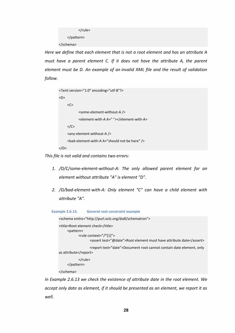
Here we define that each element that is not a root element and has an attribute A
must have a parent element C. If it does not have the attribute A, the parent
element must be D. An example of an invalid XML file and the result of validation
follow.
<?xml version="1.0" encoding="utf-8"?>
<D>
<C>
<some-element-without-A />
<element-with-A A=" "></element-with-A>
</C>
<any-element-without-A />
<bad-element-with-A A="should not be here" />
</D>
This file is not valid and contains two errors:
1. /D/C/some-element-without-A: The only allowed parent element for an
element without attribute "A" is element "D".
2. /D/bad-element-with-A: Only element "C" can have a child element with
attribute "A".
Example 2.6.13. General root constraint example
<schema xmlns="http://purl.oclc.org/dsdl/schematron”>
<title>Root element check</title> <pattern> <rule context=”/*[1]”> <assert test=”@date”>Root element must have attribute date</assert>
<report test=”date”>Document root cannot contain date element, only as attribute</report>
</rule> </pattern>
</schema>
In Example 2.6.13 we check the existence of attribute date in the root element. We
accept only date as element, if it should be presented as an element, we report it as
well.

29
Disadvantages of Schematron
The language is relatively young and is still evolving. There are many
implementations and versions; however thanks to the standardization of ISO
Schematron, this should be solved.
The Schematron is not suitable for defining and checking the whole structure of an
XML document, mainly the order or cardinality of elements. (We mean the
construct “sequence” from XSD or “group” from RELAX NG.) For this purpose it is
recommended to use a grammar language like RELAX NG, XML Schema or DTD.
Note that Schematron definitions can be placed into XSD or RELAX NG schema and
thus enhances the validation capability of that validation language. In Example
2.6.14 we show an example of a Schematron definition in an XSD schema (Version
1.0). Schematron definitions are placed in the “appinfo” element. Please note that
version 1.1 of XML Schema allows for defining its own constructs of asserts. In this
thesis, we consider only XML Schema of the version 1.0.
Example 2.6.14. Schematron within XML Schema 1.0
<?xml version="1.0"?>
<xsd:schema xmlns:xsd="http://www.w3.org/2001/XMLSchema"
targetNamespace="http://www.demo.org"
xmlns="http://www.demo.org"
xmlns:sch="http://purl.oclc.org/dsdl/schematron"
elementFormDefault="qualified">
<xsd:annotation>
<xsd:appinfo>
<sch:title>Schematron validation</sch:title>
<sch:ns prefix="d" uri="http://www.demo.org"/>
</xsd:appinfo>
</xsd:annotation>
<xsd:element name="Limits">
<xsd:annotation>
<xsd:appinfo>
<sch:pattern">
<sch:rule context="d: Limits">
<sch:assert test="d:max > d:min" diagnostics="lessThan">MAX should be greater than MIN.</sch:assert>
</sch:rule>

30
</sch:pattern>
<sch:diagnostics>
<sch:diagnostic id="lessThan">Error! Max is less than Min.
Max = <sch:value-of select="d:max"/>
Min = <sch:value-of select="d:min"/>
</sch:diagnostic>
</sch:diagnostics>
</xsd:appinfo>
</xsd:annotation>
<xsd:complexType>
<xsd:sequence>
<xsd:element name="min" type="xsd:integer"/>
<xsd:element name="max" type="xsd:integer"/>
</xsd:sequence>
</xsd:complexType>
</xsd:element>
</xsd:schema>
This example connects XML Schema with Schematron schema. We extend the
Example 2.6.11.

31
3 Basic Definitions
In this chapter we introduce basic definitions that are used later in this thesis. The
definitions are taken from theoretical computer science, Language and Automata
theory. After the basic definitions we formally define regular expressions that were
more or less used in the previous chapter and will be used more in this and later
chapters. Later on we introduce definitions for hedges and regular tree automata
and grammars. At the end of this chapter we define subclasses of regular tree
languages. This chapter is based on [1], [10], [11] and [23].
3.1 Formal Languages Theory
In this chapter we introduce the basics of language theory and regular trees. We
start with basic terms like alphabet, word, language and grammar and introduce the
Chomsky hierarchy.
3.1.1 Basic definitions
Definition 3.1.1. An alphabet ∑ is any finite set of symbols (or letters).
Finite sequence of symbols over an alphabet ∑ is called a word. Empty
word is denoted by λ.
The set of all words over an alphabet ∑ is denoted by ∑*.
Definition 3.1.2. A formal language L over an alphabet ∑ is a subset of ∑*.
A formal language can be defined in several ways: set of words, or by some
formalism like grammar, regular expression or an automaton.
Example 3.1.1. Example of an alphabet, word and a language
Let us have ∑ = all small letters. (That is informally written ∑ = [a-z]).
A word over the ∑ can be “hi”, “a”, “aab”, or any other combination of letters from this alphabet.
We can define language L to be a set of words {a, ab, abb, abbb, …}

32
Definition 3.1.3. Let us have a word w ∊∑ and i ∊ N, the i-th power of a
word w. We denote as a sequence ⏟
. More formally power is
a function P(w,i), defined as:
P(w,0) = λ
P(w,1) = w
P(w,n) = wP(w, n-1)
Example 3.1.2. Power of words
( )
Example 3.1.2 shows the usage of the power function and the result of applying it to
three words.
Definition 3.1.4. A formal grammar G is tuple G=(N, T, S, P), where N is a
finite set of non-terminal symbols, T ∊∑ is a finite set of terminal
symbols that is disjoint from N, S ∈ N is the starting non-terminal and P
is a finite set of production rules of the form (N ⋃ T)*N(N ⋃ T)* →
(N ⋃ T)*
Definition 3.1.5. The language of a formal grammar G=(N, T, S, P), denoted
as L(G), is a set of all words over ∑ that are generated by repeated
application of production rules to S until there are no non-terminal
symbols left.
Example 3.1.3. Production rule
Let us have grammar G1 = (N1, T1, S, P1), where N1 = {S, A, B}, T1 = {a, b} and P1 contains the following production rules:
S→A | B
A→a | aB
B→b | bB
The generated language L(G1) = {a, b, ab, bb, abb, bbb,…}.
Example 3.1.3 shows a definition of grammar G1 and the language L(G1).

33
Chomsky Hierarchy
Chomsky Hierarchy[23] classifies formal grammars into four categories based on the
complexity of production rules they use. The higher the category is, the stricter the
production rules are.
Type 0 – unrestricted grammars – include all formal grammars from
Definition 3.1.4. They generate exactly all languages that can be recognized
by a Turing machine.
Type 1 – context-sensitive grammars – have production rules of the form:
aXb → axb, where a,b ∈ (N ⋃ T)*, x ∈ (N ⋃ T)+ and X ∈ N. The rule S → λ is
allowed only if the non-terminal S does not appear on the right side of any
production rule. These formal grammars generate context-sensitive
languages.
Type 2 – context-free grammars – have production rules of the form: X →
w, where X ∈ N and w ∈ (N ⋃ T)*. They generate context-free languages.
Type 3 – regular grammars – have production rules of the form: X → xY or X
→ x, where X,Y ∈ N and x ∈ T. The rule S → λ is allowed only if the non-
terminal S does not appear on the right side of any production rule. This
category of grammars is recognized by a finite state automaton. These
formal grammars generate regular languages. The regular languages can be
also obtained by regular expressions.
3.2 Regular expressions and finite automata
Regular expressions describe a regular language. They have the same expressive
power as a regular grammar. We first introduce the definition of regular
expressions, some informal examples and, finally, a formal definition of regular
expression evaluation is introduced.
Definition 3.2.1. Regular expression R is a sequence over an alphabet
∑ ⋃ {?, *, +, |, (,), “,”}, where ? is the zero-or-one operator, * is the zero-
or-more operator, + is the one-or-more operator, | is the choice
operator, “,” is a sequence operator and (,) are grouping parenthesis.

34
The test if a word is described by a regular expression is called matching. For regular
expression there is often used the abbreviation regex. The sequence operator “,” is
sometimes omitted. E.g. The regex “a,b” equals to “ab”.
We can use regular expression for Example 3.1.3 and define the language L(G1) as
L(G1) = (a|b)b*.
We now informally describe what each regular expression operator does.
Grouping parenthesis (,) change the scope of operators. Normally operator
matches only single preceding (or following) symbol, if there are grouping
parenthesis then the operator matches the whole content of the
parenthesis.
Operator | matches either a preceding or a following symbol.
Quantity operators ?, * and + specify how often the preceding symbol (or
group) can occur.
o Operator ? zero-times or once.
o Operator * zero or many times.
o Operator + one or many times.
Example 3.2.1. Regular expressions
R1 = “ab?c” matches {abc, ac}
R2 = “b|c” matches {b, c}
R3 = “abc*” matches {ab, abc, abcc, …}
R4= “abc+” matches {abc, abcc, abccc,…}
R5 = “a(b|c)+” matches {ab, ac, abb, abc, acb, acc,…}
Now we formally describe the evaluation (matching) of regular expression.
We denote the set of all regular expressions R over and alphabet A as RegExp(A).
Let us have R, R1, R2 ∈ RegExp(A) and a ∈ A. The language of regular expression is
defined by induction:
R = λ, L(R) = { λ }
R = a, L(R) = {a}
R = R1 R2 (sequence) L(R) = {uv | u ∈ L(R1), v ∈ L(R2)}
R = R1 | R2 (choice) L(R) = L(R1) ⋃ L(R2)

35
R = R1? L(R) = L(R1) ⋃ {λ}
R = R1+ L(R) = ⋃ { | ∈ ( ) ∈
R = R1* L(R) = { λ } ⋃ L(R1+)
R = (R1) L(R) = L(R1)
3.2.1 Non-deterministic finite state automata
In the previous chapter we have showed one way to express the Regular grammars
(Type 3 in the Chomsky hierarchy). In this chapter we show a different approach
using finite state automata.
Definition 3.2.2. [26]Nondeterministic finite state automaton (NFA) is a
tuple ( ) where
Q is a finite non-empty set of states
X is a finite non-empty alphabet
is transition function ( ), where P(Q) is the power set of
Q
is the set of starting states and
is the set of final states.
Definition 3.2.3. [26]We say that a word is accepted by NFA
( ), if there exists a sequence that
∈ and
∈ ( ) for and
∈ .
For the later use we define a theorem of automata equivalence. For that we need to
define automaton homomorphism.
Definition 3.2.4. [26]Let us have two NFAs and . We say that the
transition is (automaton) homomorphism if and only if:
( ) , that means ∈ ∈ ( ) ∈ ∈
( ) ,
( ( )) ( ( ) ) and
( ) ( ).

36
Here we used transition on a set we define it as follows: ( ) means
∈ ∈ ( ) ∈ ∈ ( ) .
Theorem 1 Automata equivalence
[26] If there exists automata homomorphism between finite NFAs and
, then and are equivalent.
Proof
Finite iteration
Let us have ( ( )) ( ( ) ) and ∈
∈ ( ) ( ) ∈ for some ∈
( ( )) ∈
( ( ) ) ∈
( ) ∈
∈ ( )
Lemma 1 Each regular expression R can be converted to a NFA so that
( ) ( ).
Proof
There are two ways shown in [26]. We will not show here the whole proof, only the
basic idea. For each symbol ∈ we create an elementary NFA (accepting empty
or single-letter languages). We merge these elementary NFA based on regex
operations.
3.3 Regular tree grammars and Hedges
Now we will define grammar that is used to describe the tree-like documents, such
as XML. This chapter is based on [10] and [11].

37
XML documents are special, they have only one root element. Each element can
have multiple children (elements, attributes…). Without any loss of generality, we
will now consider that XML document consists only of elements. Attributes, text
content, namespaces… can be all considered as special elements with no children.
Our simplified XML document is a tree – it has only one root, elements are nodes
and leaves.
In literature, regular tree grammars are often used for definition of tree languages.
We will introduce here their definition. However, as it may look that XML
documents are well expressed with regular tree grammar, we will show later in this
chapter, that this is not true. Therefore, we introduce hedges and their grammars
and languages.
Definition 3.3.1. [11] A ranked alphabet is a couple (F, Arity) where F is a
finite set and Arity is a mapping from F into . The arity of a symbol
∈ is Arity(f).
A ranked alphabet defines an arity for each symbol. Based on their arity we can call
them variables, unary, binary … n-ary operators. Before we introduce regular tree
grammar, we will define term and tree.
Definition 3.3.2. A term t over an alphabet A and a set of variables X is
defined in the form of:
t := a(t1, t2,… tn), or t:=x
where a ∈ A and t1, t2,… tn are terms over A, n>= 0 and x ∈ X.
For ranked alphabet the number n is equal to Arity(a).
We denote set of all terms over an alphabet A and variables X as Term(A,X).
Definition 3.3.3. A ground term g over an alphabet A is a term from
Term(A, ). We denote set of all ground terms over A as
GroundTerm(A).
Ground term is in fact a term without a variable.
Definition 3.3.4. A tree t over an alphabet A is a subset of GroundTerm(A).

38
We denote set of all trees over an alphabet ∑ as T(∑).
Next we introduce the definition of regular tree grammar from [11]. We will use this
definition for comparison with hedges.
Definition 3.3.5. [11] Regular tree grammar G over ranked alphabet is a
tuple (S, N, F, R) where
S is a starting symbol, S∊ N, Arity(S)=0
N is a finite set of non-terminals over a ranked alphabet
F is a finite set of terminal symbols from a ranked alphabet and
R: ( ), where X is set of variables
Hedges
[10] defines regular tree grammars over an alphabet with infinite arity. [11]
contains second definition of regular tree grammars over unranked alphabet. These
definitions of tree grammar are sometimes called hedges.
Using ranked alphabet for XML documents is problematic – elements (terminal
symbols) must correspond to their arity, but an XML document generally does not
limit the number of children of elements. That is the reason we will use unranked
alphabet.
An unranked alphabet is nothing more than just a normal alphabet defined at the
beginning of Chapter 3.
The order of elements in XML may or may not be important. For example for
structured data the order is not important, but for an XML document (e.g.
XHTML[24]) the order may be important. Let us have an XML document with a root
element a and sub trees t1, t2… tn, we can depict the document as a(t1, t2… tn). Now
comes the question, how to call all the sub-trees of the element a. A set of trees is a
forest, but a set does not reflect the order. That is why the term hedge is used.
Hedge is a sequence of trees. Hedges are used for definition of formalism that is
connected with XML.

39
There are many definitions of hedge grammars. We will use the one from [10],
there it is called regular tree grammar, but it is also a hedge grammar definition.
Definition 3.3.6. Regular hedge grammar G is a tuple (N, T, S, P) where:
N is a finite set of non-terminals,
T is a finite set of terminals over an unranked alphabet,
S is a set of start symbols, where S ⊂ N,
P is a finite set of production rules of the form , where
∈ ∈ and r is a regular expression over N. X is the left-hand
side, a r is the right-hand side, and r is the content model of this
production rule.
We abbreviate rules of the form of X to the form X . Some definitions of
hedges use parenthesis to separate the regular expression from the label (non-
terminal). We will use this one.
As said before, hedge grammars are used for unranked ordered trees. An extension
for unranked unordered trees could be defined by extending the regular
expressions by introducing an interleave (shuffle) operator. See reference [11] for
more details.
In this thesis we will use the term regular grammar when we do not want to
distinguish between ordered and unordered trees and hedges for ordered trees.
Both tree definitions are used over an unranked alphabet, if not stated otherwise.
Example 3.3.1. Regular hedge grammar
G1 = (N1, T1, S1, P1),
N1 = {Milestone, MandatoryTask, OptionalTask, MandatoryData, Data}
T1 = {milestone, task, data}
S1 = {Milestone}
P1 = { Milestone→milestone (MandatoryTask OptionalTask*), MandatoryTask→ task(MandatoryData), OptionalTask → task (Data), MandatoryData → mandatorydata (λ), Data → data (λ)}.
In Example 3.3.1 we show a grammar for milestone that contains tasks. The first
task is mandatory, others are only optional.

40
Each grammar generates a language. We introduce here the formal definition from
[10] for a regular tree language.
Definition 3.3.7. [10] An interpretation I of a tree t against a regular
tree grammar G is a mapping from each node e in t to a non-terminal
denoted I(e), such, that:
I(eroot) is a start symbol where eroot is the root of t, and
for each node e and its subordinates e0, e1, …, ei there exists a
production rule X→ a r such that
I(e) is X,
the terminal (label) of e is a, and
I(e0)I(e1)…I(ei) matches r.
Definition 3.3.8. A tree t is generated by a regular tree grammar G if there
is an interpretation of t against G. [10]
Definition 3.3.9. A regular tree language is the set of trees generated by a
regular tree grammar. [10]
3.3.1 Local tree grammars and languages
Local tree grammar is a restricted sub-class for a regular tree grammar. The
interpretation is simplified, because each terminal (label) has associated one and
only one non-terminal (there is no competition between non-terminals). This
chapter is based on [10].
Definition 3.3.10. Let us have grammar G = (N, T, S, P). Let
such that
P1 has the form of X → a r1, P2 has the form of Y → a r2, where .
Then we say the non-terminals X and Y compete with each other.
Example 3.3.2. Competing non-terminals
G2 = (N,T,S,P), where
N= {Database, Man, Woman, ManData, WomanData}
T = {database, person, manData, womanData}
S = { Database }
P = {Database → database (Man| Woman )*, Man → person (ManData), Woman → person (WomanData), ManData → manData (λ), WomanData → womanData (λ)}
41
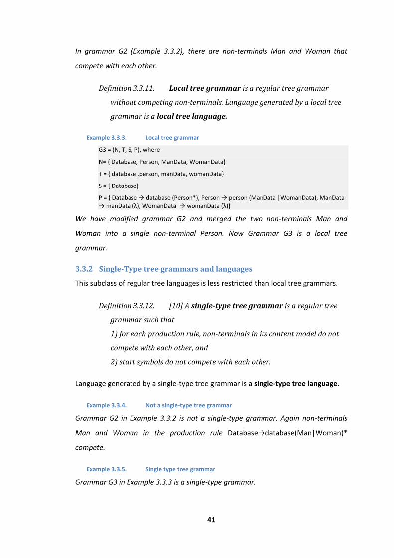
In grammar G2 (Example 3.3.2), there are non-terminals Man and Woman that
compete with each other.
Definition 3.3.11. Local tree grammar is a regular tree grammar
without competing non-terminals. Language generated by a local tree
grammar is a local tree language.
Example 3.3.3. Local tree grammar
G3 = (N, T, S, P), where
N= { Database, Person, ManData, WomanData}
T = { database ,person, manData, womanData}
S = { Database}
P = { Database → database (Person*), Person → person (ManData |WomanData), ManData → manData (λ), WomanData → womanData (λ)}
We have modified grammar G2 and merged the two non-terminals Man and
Woman into a single non-terminal Person. Now Grammar G3 is a local tree
grammar.
3.3.2 Single-Type tree grammars and languages
This subclass of regular tree languages is less restricted than local tree grammars.
Definition 3.3.12. [10] A single-type tree grammar is a regular tree
grammar such that
1) for each production rule, non-terminals in its content model do not
compete with each other, and
2) start symbols do not compete with each other.
Language generated by a single-type tree grammar is a single-type tree language.
Example 3.3.4. Not a single-type tree grammar
Grammar G2 in Example 3.3.2 is not a single-type grammar. Again non-terminals
Man and Woman in the production rule Database→database(Man|Woman)*
compete.
Example 3.3.5. Single type tree grammar
Grammar G3 in Example 3.3.3 is a single-type grammar.

42
Example 3.3.6. Single-type tree grammar, not local tree grammar
G4 = (N, T, S, P), where
N = {Database, Men, Man, Women, Woman, ManData, WomanData}
T = {database, men, women, person, manData, womanData}
S = { Database }
P = {Database → database (Men Women ), Men→men (Man*), Women→women (Woman*), Man → person (ManData), Woman → person (WomanData), ManData → manData (λ), WomanData → womanData (λ)}
Grammar G4 is a single-type tree grammar, but not a local tree grammar. Non-
terminals Man and Woman compete, but they do not occur together in any content
model.
3.3.3 Regular tree automata
Regular tree languages are recognized by finite regular tree automata. We
introduce a definition of finite hedge regular tree automata here. This section is
based on [11]. Some basic facts about automata can be found also in [10].
In previous section we have defined tree over ranked alphabet using ground term.
For the definition of hedge automata below, we will redefine the tree using a bit
different way. The following definitions are taken from [11].
Definition 3.3.13. A finite (ordered) tree t over ∑ as partial function t:
N* → ∑ with domain written Pos(t) satisfying following:
1. Pos(t) is finite, nonempty and prefix-closed,
2. ∈ ( ) { | ∈ ( ) { for some .
Function Pos(t) returns all positions of nodes in a tree t. Position “pk” is the k-th
child of a node at the position p. Generally an i-th child of a node x has the position
defined as iPos(x). Again we denote set of all trees over an alphabet ∑ as T(∑).
Example 3.3.7. Tree and Pos()
t=a(ab(cb)) r - Position of nodes
a 1
a b 11 12
c b 121 122

43
In Example 3.3.7 we have tree t=a(ab(cb)) and a tree r from the same domain. The
nodes of tree r are labeled by the Pos function. The value of t(11) is a – the first child
of the root. The value of t(121) equals to c.
Now we define hedge automata.
Definition 3.3.14. [11] A nondeterministic finite hedge automaton
(NFHA) over alphabet ∑ is a tuple A = (Q, ∑, Qf , P) where Q is a finite
set of states, Qf Q is a set of final states, and P is a finite set of
transition rules of the following form:
a(R) → q
where R ∈ RegExp(Q), a ∈ ∑ and q ∈
This definition defines bottom-up automata. That means that we process the leaves
of a tree first and then we move up the tree towards the root.
Example 3.3.8. Example of NFHA
We want to define NFHA that accepts such trees that have a node c that contains somewhere in its descendants a node containing two children b. For example a tree t = c(ba(cbab)).
A1= (Q, ∑, Qf , P), where
Q = {q, q1, q2, qf}
∑ = {a,b,c}
Qf = { qf }
Rules are:
a(Q*) → q a(Q* q1 Q* q1 Q*) → q2 a(Q* q2 Q*) → q2 a(Q* qc Q*) → qc
b(Q*) → q1 b(Q* q1 Q* q1 Q*) → q2 b(Q* q2 Q*) → q2 b(Q* qc Q*) → qc
c(Q*) → q c(Q* q1 Q* q1 Q*) → qf c(Q* q2 Q*) → qf c(Q* qc Q*) → qc
In Example 3.3.8 we have defined NFHA with 12 rules. We mark nodes labeled by b
with state q1. At the next layer, this state is transformed to state q2 (if it contains at
least two q1) or back to default state q. Please note the non-determinism here. Even
if there are two children b of a node, there exists a rule that assigns a default state
q, but also a rule that assigns a state q2.
Next we define the run of the NFHA. For that we use the new definition of tree and
the Pos() function.

44
Definition 3.3.15. [11] A run of NFHA A= (Q, ∑, Qf , P) on a tree t ∈
T(∑) is a tree r ∈ T(Q) with the same domain as t such that for each
node p∈Pos(r) it a t( ) and r( ) t ere is a transition rule a( )
→ q of A with r(p1)…r(pn) ∈ ere n denotes t e number of
successors of p.
Definition 3.3.16. [11] An unranked tree t is accepted by NFHA A if
there is a run r of A on t whose root is labeled by a final state. The
language L(A) of A is the set of all unranked trees accepted by A.
In Example 3.3.8 we have defined a NFHA A1. For a tree t = c(ba(cbab)) A1 assigns a
set of states s={ q, q1, qf}. The tree t is accepted by A1 because there is a final state
qf in s.
We have defined nondeterministic bottom-up hedge automaton, let us define a
deterministic one.
Definition 3.3.17. [11] A deterministic finite hedge automaton
(DFHA) is a finite hedge automaton A = (Q, ∑, Qf , P) such that for all
rules a(R1) → q1 and a(R2) → q2 either or q1 = q2.
The automaton A1 from Example 3.3.8 is not deterministic.

45
4 Taxonomy
In this chapter we compare the power of schema languages: DTD, XML Schema,
Relax NG and Schematron. We assign each of them to a class of regular tree
grammars. This chapter is based on [10] and [11].
4.1 DTD
Based on definition of DTD in [9], DTD requires a deterministic content model and
more importantly contains the following restriction: “For Compatibility, it is an error
if the content model allows an element to match more than one occurrence of an
element type in the content model” [9]. Said in other words, an element - terminal
– cannot have more than one corresponding non-terminal in an XML document.
This is the definition of a local tree language.
4.2 XML Schema
We show that XML Schema corresponds to a single-type tree language. We present
here the general idea. Proofs and examples can be found in [10] and [11].
One of the main features of XML Schema contrary DTD is the declaration and usage
of types. XML Schema allows for elements with the same name to have different
types and thus content model. Types allow XML Schema to overcome limitations of
DTD (local tree language) and define for the same name of element different types
of content.
The Usage of types is limited by a constraint called the “Element Declarations
Consistent” [12]. This constraint says that all elements from the content model of
an element that have the same name and namespace must also have the same
type. E.g. there cannot be two book elements next to each other each having
a different type.
The above constraint corresponds to the limitation of the single-type tree grammar
and, thus, XML Schema belongs to the class of single-type tree languages.

46
4.3 Relax NG
We show the basic idea, that any regular tree grammar can be expressed in Relax
NG. The construction of the schema can be found in [10] (However in [10] it is
described for Relax Core and TRex, but modifying the process for Relax NG is
straightforward).
Relax NG does not impose any restrictions for the content model. Its patterns
(sequence, choice, one-or-more, zero-or-more) in the content model can be easily
transformed to a regular expression. The pattern interleave can be also transformed
to a regular expression. See the shuffle operator in [11].
4.4 Schematron
In previous chapters we classified DTD, XML Schema and Relax NG to their sub-class
of regular tree language. To our best knowledge there is only little or no work that
would classify Schematron to a sub-class of regular tree grammar. We found some
recommendations and general algorithms for expressing schema models with
Schematron in the blog of Rick Jelliffe [25].
In this thesis we introduce an algorithm for transformation of hedges into
Schematron rules – Chapter 5. It this chapter we assign a sub-class of regular tree
grammar to Schematron. We show that the expressive power of Schematron
depends on the used query language.
Analysis
First we identify the differences of Schematron that concern the expressive power
of validation and later we compare those.
The main difference between Schematron and other schema languages is the usage
of rules. Classical grammar schema languages (like Schema or Relax NG) also use
rules, but they do not name them like that. Grammar schema languages define
types and elements. These definitions are in fact rules that validate the content.
However, there is one big difference between the rules of Schematron and
grammar schema languages – finding the context for the rule.

47
Identifying the context in grammar schema languages is trivial; we follow the
structure of the document either from root to leaves or opposite. The previously
processed elements identify the rule (or the set of rules) that should be used to
validate current element. Note the previously identified elements create the
context for the rules to come; that is the general idea of the validation algorithms.
However, Schematron identifies the context for each rule independently. That
means that the expressive power of Schematron is limited by the expression
strength of the used query language.
The second aspect of validation is the validation of the content. From the formal
definitions we know that the content for a regular grammar is expressed by a
regular expression. So if the query language is able to express regular expressions,
there should not be a problem.
We have shown that the expressive power depends on the expressive power of the
query language – how well it can identify hedge. For the purpose of this thesis we
will discuss the strength of XPath 1.0.
XPath 1.0 works only with the element names. So if we want to identify a path in a
document, we have to translate types to their element names. This is one obstacle.
The other one is that XPath 1.0 does not support regular expressions. In this thesis
we use XPath 1.0 and we try to emulate the regular expressions. It can be done in
the most cases but do not know if it is doable in all cases. This disadvantage could
be removed by the use of XPath 2.0. However, there still persists the problem of
context matching. In our analysis in Chapter 5 we discuss several ways how this
could be done.
Even with the regex support, XPath is not able to identify all possible contexts. We
can see that on the grammar G1 from Example 3.3.1. There are two types
MandatoryTask and OptionalTask. Both use the label task, both are children of the
same type. In the Example 3.3.1 the mandatory task is only the first child, but we
could modify this grammar so it could be at any position. In that case XPath is not
able to tell apart these two types.
48
We have shown a case where Schematron with XPath is not able to find context
correctly. So there are two possible candidates for sub-class of regular tree
grammar: local or single-type.
The context of local language is trivial, the names of element types are unique and
XPath can handle these.
Lemma 2 Schematron with XPath with regex support is able to express single-
type tree grammar.
The idea of proof is simple. We show the basic idea of construction of an XPath path
for a single-type tree grammars.
Proof
Let us have a single-type grammar G with a starting type S.
We also know, that each child type of any type has unique label among its siblings.
For any type T, we create unique paths from starting type S to every occurrence of T
in the grammar. Each step in a path uniquely identifies one of child types of the
previous parent type. (Single-type grammar)
Summary
We have shown that the expressive power of Schematron mainly depends on the
used query language. We have shown that if we are using XPath with regular
expression support, Schematron is able to express single-type tree grammar.

49
5 Transforming hedges to Schematron schema
In this chapter we introduce algorithm for generating Schematron rules for a hedge.
We use XPath 1.0 since it is widely spread, but we also suggest the possibility of
using XPath 2.0.
We may encounter some limitations. As we will show, Schematron may not be ideal
for expression general ordered unranked trees, since the schema for expressing
that may be bigger than the schemas of classical grammar schema languages (e.g.
Relax NG, DTD).
We divide the transformation process of a hedge into three steps. Step 1 will
generate the correct context for rules that will be checked by steps 2 and 3. Step 2
controls the correct sum of children and step 3 matches the order of children to the
regex of the hedge.
5.1 Definitions
Here we define terms that will be referenced in the following steps of the
algorithm.
Let us have a hedge regular grammar G = (N, T, S, P) and a hedge a ( )
where ∈ ∈ ∈ ∈ ( ).
Definition 5.1.1. We denote production set S to be the set of all non-
terminals that occur in R.
Two examples of production sets are show below in Example 5.1.1.
Example 5.1.1. Example of a hedge h and S
(B?C+)
{
(BB?C*D*C)
{
Example 5.1.1 shows examples of hedges h1, h2 and their production sets S1 and S2.
Definition 5.1.2. We denote the translate function that
assigns a terminal to a non-terminal.

50
Function trans is in fact a production rule without the regex part. Note that there
can exist different hedges g, h that have the same terminal, i.e. trans(g) = trans(h).
5.2 Limitations
Before we describe the algorithm itself we introduce two limitations for the
algorithm that the grammar or the XML document must meet.
1) All sibling elements (sharing the same parent) with the same name must
be of the same type.
This constraint is similar to the “Element Declaration Consistent” [12] from XML
Schema. In other words if there is an element of type A, all its siblings with the same
name must have the same type A.
2) If there is a recursion within the derivation sequence of a non-terminal,
the recursion sub-sequence must be deterministic.
The second limitation is deeper explained in Chapter 5.3.5. This restriction is
needed because of the lack of regex support of XPath 1.0.
5.3 Step 1 – Context generation
The correct context for rules is absolutely necessary for the algorithm to work
correctly. The context is used to match an element in an XML document to a hedge
h from grammar G. The context is used for constraints generated by steps 2 and 3.
At first we show a trivial solution and discuss its disadvantages. Later we introduce a
more complex and reliable algorithm also including formal definitions and proofs of
correctness.
5.3.1 Trivial solution
The first thing that can come to a mind is the idea to generate context using relative
path and match only the element and maybe some of its ancestors.
Example 5.3.1. Trivial context matching
(B?C+)
XPath context: “//a”
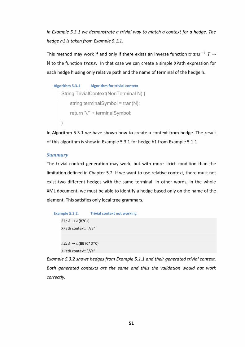
51
In Example 5.3.1 we demonstrate a trivial way to match a context for a hedge. The
hedge h1 is taken from Example 5.1.1.
This method may work if and only if there exists an inverse function
to the function . In that case we can create a simple XPath expression for
each hedge h using only relative path and the name of terminal of the hedge h.
Algorithm 5.3.1 Algorithm for trivial context
String TrivialContext(NonTerminal N) {
string terminalSymbol = tran(N);
return ”//” + terminalSymbol;
}
In Algorithm 5.3.1 we have shown how to create a context from hedge. The result
of this algorithm is show in Example 5.3.1 for hedge h1 from Example 5.1.1.
Summary
The trivial context generation may work, but with more strict condition than the
limitation defined in Chapter 5.2. If we want to use relative context, there must not
exist two different hedges with the same terminal. In other words, in the whole
XML document, we must be able to identify a hedge based only on the name of the
element. This satisfies only local tree grammars.
Example 5.3.2. Trivial context not working
(B?C+)
XPath context: “//a”
(BB?C*D*C)
XPath context: “//a”
Example 5.3.2 shows hedges from Example 5.1.1 and their generated trivial context.
Both generated contexts are the same and thus the validation would not work
correctly.

52
5.3.2 K-ancestors
This method is used for schema inferring in [27]. It is based on real data properties.
Our trivial solution from Chapter 5.3.1 is, in fact, a specific case of this approach. In
this chapter we will not describe the inferring method – it is described in Chapter 6.
The key idea is to identify context based on the element name and the name of K
closest ancestors. For K = 2 it is the name of the element and the name of the
parent. The trivial solution is a special case of this solution where K = 1.
Example 5.3.3. Example for K-ancestor solution
K = 2
G5 = (N, T, S, P), where
N= { Database, Person, Data}
T = { database ,person, data}
S = { Database}
P = { Database → database (Person*), Person → person (Data),Data → data(λ) }
XPath context for Person: “//database/person”
XPath context for Data: “//person/data”
Example 5.3.3 shows an XPath for identifying the context of the non-terminal Person
and Data.
Algorithm 5.3.2 Algorithm for K-ancestors
String K_AncestorContext(NonTerminal N, int K) {
var ancestors = get first K ancestors element names from N;
string xpath = “/”;
foreach(var name in ancestors in reverse order) {
xpath += “/” + name;
}
return xpath;
}
Summary
Similarly to trivial context generation, K-ancestor solution offers fast and
comfortable way to identify context. On the other hand K-ancestor solution may not
identify some context correctly –e.g. if we have K = 1 the situation is the same as for

53
trivial context. However, the real world data (described in [27]) show that more
than 98% of context matching could be expressed with this solution and the K equal
to 2 or 3.
5.3.3 Absolute path without a recursion
In the previous chapters we showed a trivial ways to identify a context and showed
that these approaches are limited. In this chapter we introduce a more reliable, less
restricted way to identify the correct context. We will use absolute paths to identify
it.
This approach is sufficient for general cases of grammar that do not contain
recursion in hedge transformation or only simple recursion.
Definition 5.3.1. We denote the derivation sequence DA for non-terminal A
to be a sequence of non-terminals produced by production rules that
transformed the starting non-terminal to the non-terminal A of the
hedge h.
Definition 5.3.2. We say that the derivation sequence DA contains a
recursion if there is at least one non-terminal ∈ that occurs more
than once in DA. We say the recursion is a simple recursion if there are
no other non-terminals between any two occurrences of ∈ .
Simple recursion is a sequence where the repetition of a single symbol is not
interrupted by any other.
Multiple derivation sequences may exist for the same non-terminal. Without loss of
generality, we suppose there exists only one such sequence. If more sequences
exist, we can always merge their generated path expressions.
Definition 5.3.3. We denote derivation sequence of terminals DTA for
non-terminal A to be a sequence of terminals defined by the formula
∈ ( ). Derivation sequence of terminals is a translated
derivation sequence DA.

54
The basic idea for generation of an absolute path is the following. When we want to
find a context for hedge h, there exists a sequence DTA of terminals. This sequence
contains terminals that match an absolute path from the root element (that
matches the terminal of the starting symbol) to an element a of the hedge h.
Example 5.3.4. Example of an absolute path without recursion
G6 = (N, T, S, P), where
N = { Database, Person, Data}
T = { database ,person, data}
S = { Database}
P = { Database → database (Person*), Person → person (Data),Data → data(λ) }
DData = (Database, Person, Data),
DTData = (database, person, data), XPathData = “/database/person/data”
Example 5.3.4 shows the derivation sequence for the non-terminal Data and the
respective absolute XPath.
Algorithm for absolute path is trivial. We join the derivation sequence of terminals
with “/”. Please note that the derivation sequence is always deterministic. If there
should be a non-deterministic step (e.g. operator “?” or “|”) in derivation process
from starting hedge to hedge h, we generate several deterministic sequences and
merge all of their results.
5.3.4 Single recursion in production rules
In Example 5.3.4 we showed a simple example for absolute path context using only
the child axis. However, there can be situations when the length of a derivation
sequence (based on Definition 5.2) is not limited. This happens when there is a
recursion in hedges. See Example 5.3.5. In this chapter we introduce algorithm for
dealing with simple recursions that are special cases of recursions with
deterministic content discussed in Chapter 5.3.5.
Example 5.3.5. Absolute path with simple recursion
G7 = (N, T, S, P), where
N= {Indent, Text}
T = {tab, text}
S = {Indent}
P = {Indent→ tab (Indent|Text), Text→ text(λ) }

55
DTText = (tab, tab, …, tab, text)
1) XPathText = “//tab/text” <!—intuitive but not working -->
2) XPathText = “//tab[count(ancestor::tab) = count(ancestor::*)]/text” <!-- working -->
Example 5.3.5 shows an example of a grammar with recursion in its production
rules. There are presented two XPath expressions: 1) with only descendant-or-self
axis and 2) with descendant-or-self axis and a condition checking the count of
ancestors. Expression 1) will find any elements tab, including illegal sequences like
(tab, tab, some-other-element, tab, text). Expression 2) locates only sequences that
match the sequence DTtext.
We have introduced the problem and we extend Definition 5.3.1 to express
recursion in derivation sequence.
Definition 5.3.4. We denote the derivation regular expression DRA for
non-terminal ∈ to be a word over Regex(N) that represents all
derivation sequences of DA .
DRA is able to express several derivation sequences with a single finite word. DRTA is
defined similarly.
Definition 5.3.5. We denote the derivation regular expression for
terminals DTRA for non-terminal ∈ to be a word over Regex(T) –
regular expression over terminals T of grammar G. DRTA is converted
from DRA by the formula:
∈ ∈ ( )
∈ .
We can re-define simple recursion using the derivation regular expression.
Definition 5.3.6. We say that derivation regular expression DRA contains
only simple recursion if and only if all regular operators + and * in
DRA are applied to a single symbol and not to a group.

56
Definition 5.3.7. Let us have a derivation regular expression DR and an xml
fragment F. We denote foreign elements foreign(DR, F) to be such
elements that have to be removed from F in order to be matched by the
DR.
Since x+ can be expressed as xx*, without the loss of generality we can assume that
all simple recursions consist of the form x*.
In Example 5.3.5 we can see path expressions for simple sequences. Now we
introduce the algorithm for XPath generation for grammar with simple hedge
recursion.
This algorithm creates XPath expression that matches undisturbed sequence (that
may not be limited) of elements in the parent/child relation. Since we have only
simple recursion and thus the repeating sequence consists of only single terminal,
our work is fairly easy.
Since XPath 1.0 does not support regular expressions, we have to use the
descendant-or-self axis with constraint on the ancestors. We create a constraint
that will ensure that we will find only such descendants that have no element other
than the element from the simple recursion.
The input is the DRTA for the simple recursion. As denoted in this chapter, without
the loss of generality the DRTA will have the form of “x*”.
The constraint is implemented using the count function, ancestor and descendant
axes. The context for XPath evaluation must be taken at the start of recursion. Now
the algorithm:
Algorithm 5.3.3 Context for simple recursion
/** Creates let statements under the PaternElement context and returns xPath expression that expresses the context
*/
string CreateSimpleContext(string DRTA, int iterationStartPosition, Context PaternElement) {
string subDRTA = DRTA.subSequence(0, iterationStartPosition);

57
string xPathContext;
int recursionIndex = findSimpleRecursion(subDRTA);
if (recursionIndex > -1) {
//there is at least one simple recursion before the one we want to analyze, e.g. “a* b x*”
xPathContext = CreateSimpleContext(subDRTA, recursionIndex, PaternElement);
} else {
//only absolute path, e.g. “a b c” => “a/b/c”
xPathContext = CreateAbsoluteContext(subDRTA);
}
//create two let statements for variables that will be used in generated xPath
//variable for all ancestors
string allCountVar = createUnitVariable(“allCount”);
//form: <let name=” allCountVar” value=” count(xPathContext/ancestor::*)” />
createLetVariable(allCountVar, xPathContext, “*”);
string iterationCharacter = DRTA.getIterationCharacter(iterationPosition);
//variable only for iterationCharacter occurences
string charCountVar = createUnitVariable(iterationCharacter + “Count”);
createLetVariable(charCountVar, xPathContext, iterationCharacter);
//return prefix//x[(count(ancestor::x) - $xCount) = (count(ancestor::*) - $allCount)]
return string.Format(“{0}//{1}[(count(ancestor::{1}) – {2}) = (count(ancestor::*) – {3})]”, xPathContext, iterationCharacter, charCountVar, allCountVar);
}
We summarize the above algorithm in short: We store into two variables counts of
ancestors - any ancestor (allCount) and ancestors that are x (xCount). Since we

58
generate a Schematron schema we use the let construct for creating these
variables. We generate the XPath expression for context: //x[(count(ancestor::x) -
$xCount) = (count(ancestor::*) - $allCount)]
Lemma 3 Algorithm 5.3.3 matches only the single recursion.
Let us prove that this algorithm does what it is supposed to. We use the absurdum
proof.
Proof
Let us have a derivation sequence (x0, … xi-1, yi, xi+1, … xk) for some ∈
. Let us assume that this sequence is matched with our algorithm. Without
loss of generality we assume that the variables allCount and xCount are equal to 0.
Let us choose any ∈ . The element xj follows yi since . From the
sequence we can see that xj has j preceding elements from which there are j-1
occurrences of element x. The constrain count(ancestor::xj) = count(ancestor::*) is
thus false and XPath should not match the element xj.
Note that the variables allCount and xCount allows us to ignore any sequence (any
ancestors) before start of the simple recursion since they correct the equation
correctly on both sides.
We have introduced the Algorithm 5.3.3 for simple recursion. See Example 5.3.6 for
the result of this algorithm. The algorithm works also in cases when there are
multiple simple recursions in serial order.
For cases when there is only absolute path before the simple recursion, the
variables xCount and allCount are not necessary since the counts can be counted in
generation time.
Example 5.3.6. Derivation sequence with prefix
DRTText = book paragraph tab+ text
<schema xmlns="http://purl.oclc.org/dsdl/schematron" queryBinding="xpath">
…
<pattern>
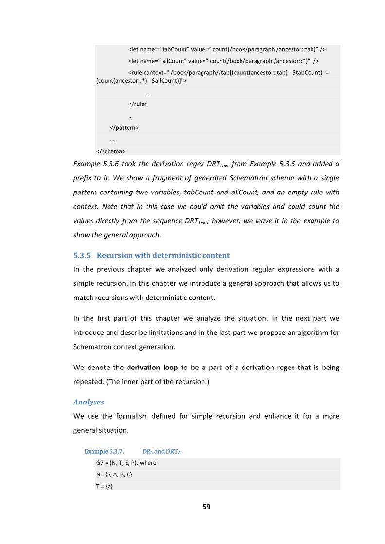
59
<let name=” tabCount” value=” count(/book/paragraph /ancestor::tab)” />
<let name=” allCount” value=” count(/book/paragraph /ancestor::*)” />
<rule context=" /book/paragraph//tab[(count(ancestor::tab) - $tabCount) = (count(ancestor::*) - $allCount)]">
…
</rule>
…
</pattern>
…
</schema>
Example 5.3.6 took the derivation regex DRTText from Example 5.3.5 and added a
prefix to it. We show a fragment of generated Schematron schema with a single
pattern containing two variables, tabCount and allCount, and an empty rule with
context. Note that in this case we could omit the variables and could count the
values directly from the sequence DRTText; however, we leave it in the example to
show the general approach.
5.3.5 Recursion with deterministic content
In the previous chapter we analyzed only derivation regular expressions with a
simple recursion. In this chapter we introduce a general approach that allows us to
match recursions with deterministic content.
In the first part of this chapter we analyze the situation. In the next part we
introduce and describe limitations and in the last part we propose an algorithm for
Schematron context generation.
We denote the derivation loop to be a part of a derivation regex that is being
repeated. (The inner part of the recursion.)
Analyses
We use the formalism defined for simple recursion and enhance it for a more
general situation.
Example 5.3.7. DRA and DRTA
G7 = (N, T, S, P), where
N= {S, A, B, C}
T = {a}
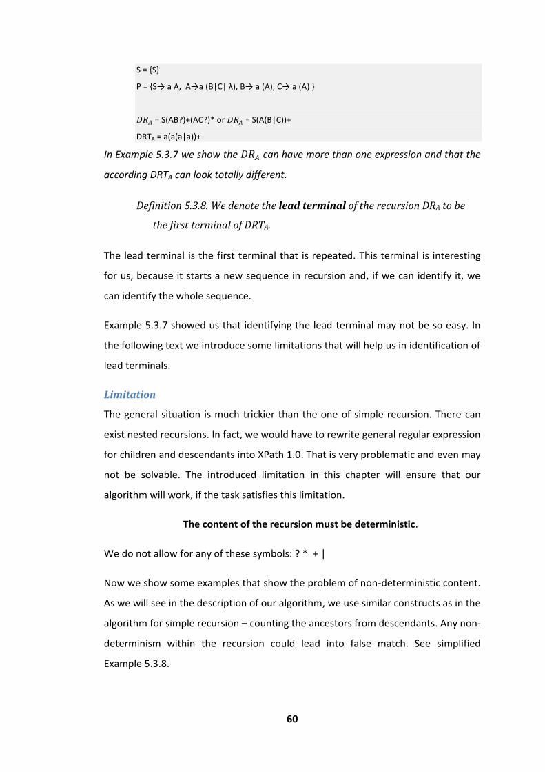
60
S = {S}
P = {S→ a A, A→a (B|C| λ), B→ a (A), C→ a (A) }
= S(AB?)+(AC?)* or = S(A(B|C))+
DRTA = a(a(a|a))+
In Example 5.3.7 we show the can have more than one expression and that the
according DRTA can look totally different.
Definition 5.3.8. We denote the lead terminal of the recursion DRA to be
the first terminal of DRTA.
The lead terminal is the first terminal that is repeated. This terminal is interesting
for us, because it starts a new sequence in recursion and, if we can identify it, we
can identify the whole sequence.
Example 5.3.7 showed us that identifying the lead terminal may not be so easy. In
the following text we introduce some limitations that will help us in identification of
lead terminals.
Limitation
The general situation is much trickier than the one of simple recursion. There can
exist nested recursions. In fact, we would have to rewrite general regular expression
for children and descendants into XPath 1.0. That is very problematic and even may
not be solvable. The introduced limitation in this chapter will ensure that our
algorithm will work, if the task satisfies this limitation.
The content of the recursion must be deterministic.
We do not allow for any of these symbols: ? * + |
Now we show some examples that show the problem of non-deterministic content.
As we will see in the description of our algorithm, we use similar constructs as in the
algorithm for simple recursion – counting the ancestors from descendants. Any non-
determinism within the recursion could lead into false match. See simplified
Example 5.3.8.
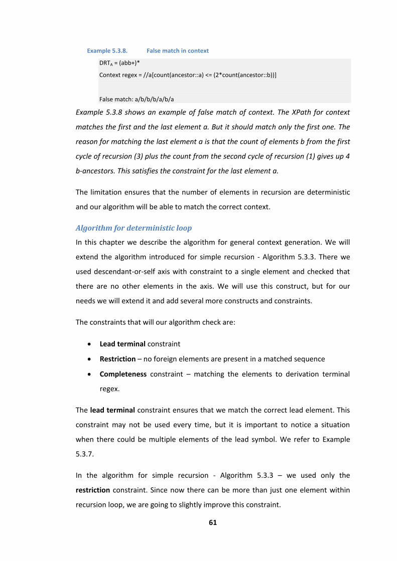
61
Example 5.3.8. False match in context
DRTA = (abb+)*
Context regex = //a[count(ancestor::a) <= (2*count(ancestor::b))]
False match: a/b/b/b/a/b/a
Example 5.3.8 shows an example of false match of context. The XPath for context
matches the first and the last element a. But it should match only the first one. The
reason for matching the last element a is that the count of elements b from the first
cycle of recursion (3) plus the count from the second cycle of recursion (1) gives up 4
b-ancestors. This satisfies the constraint for the last element a.
The limitation ensures that the number of elements in recursion are deterministic
and our algorithm will be able to match the correct context.
Algorithm for deterministic loop
In this chapter we describe the algorithm for general context generation. We will
extend the algorithm introduced for simple recursion - Algorithm 5.3.3. There we
used descendant-or-self axis with constraint to a single element and checked that
there are no other elements in the axis. We will use this construct, but for our
needs we will extend it and add several more constructs and constraints.
The constraints that will our algorithm check are:
Lead terminal constraint
Restriction – no foreign elements are present in a matched sequence
Completeness constraint – matching the elements to derivation terminal
regex.
The lead terminal constraint ensures that we match the correct lead element. This
constraint may not be used every time, but it is important to notice a situation
when there could be multiple elements of the lead symbol. We refer to Example
5.3.7.
In the algorithm for simple recursion - Algorithm 5.3.3 – we used only the
restriction constraint. Since now there can be more than just one element within
recursion loop, we are going to slightly improve this constraint.

62
The restriction constraints checks only that there are no foreign elements; the
completeness constraint checks that all terminals from derivation terminal regex
are matched to elements within the recursion, thus no elements are missing and all
elements are in correct order. This will ensure that we ignore all other permutated
sequences.
The algorithm will match all possible lead terminals in the descendant axis and
identify the correct ones. We have to ignore all other terminals that are neither a
part of the recursion, nor the lead terminal (e.g. another terminal with the same
name as the lead terminal but occurring inside the recursion loop at a different
position). We will describe the algorithm in three parts – each for a constraints
described above. Each part will produce a predicate for XPath.
To identify the lead terminal we count the ancestor elements that match the lead
terminal and modulo the value. Part I can be omitted if the lead terminal occurs
only once within the recursion loop.
Algorithm 5.3.4 Algorithm for recursion Part I – Modal Count
string GetModuloConstraint (DRT terminalRegex, Context PaternElement) {
string LeadTerminal = getLeadingTerminal(terminalRegex);
int moduloCount = terminalCountInRecursion(terminalRegex, LeadTerminal);
//variable lead terminal occurences
string leadTerVar = createUnitVariable(“modulo” + LeadTerminal);
//form: <let name=”leadTerVar” value=”count(ancestor::x)” />
createLetVariable(leadTerVar, xPathContext, iterationCharacter);
//return (count(ancestor:: ) - $modulo_x) mod ∑ = 0
return string.Format(“(count(ancestor::{0}) – {1}) mod {2} = 0”,
LeadTerminal,
leadTerVar,
ModuloCount);

63
}
Lemma 4 Algorithm 5.3.4 finds the correct lead terminals.
Proof
Since we do not allow any nondeterministic behavior within the recursion loop, the
number of terminals that have the same name as the lead terminal is fixed.
Example 5.3.9. Example for algorithm for recursion part I - The lead terminal
DRTA = (aa)*
Generated predicate:
P1 = count(ancestor::a) mod 2 = 0
Context:
//a[P1]
Example 5.3.9 shows a predicate for matching the lead terminal a.
Algorithm 5.3.5 is based on Algorithm 5.3.3 for simple recursion. The Algorithm
5.3.3 was used only for simple recursion, and, thus it checks only a single element.
We enhance it to support checking of multiple elements. The description is brief;
please look at the algorithm for simple recursion first.
Algorithm 5.3.5 Algorithm for recursion Part II - restriction
string CreateRestrictionContext(string DRTA, string xPathContext, Context PaternElement) {
//we create n + 1 variables, where n is the number of distinc terminals in DRTA
string allCountVar = createUnitVariable(“allCount”);
//form: <let name=” allCountVar” value=” count(xPathContext/ancestor::*)” />
createLetVariable(allCountVar, xPathContext, “*”);
string result = “”;
foreach (var terminalCharacter in distinct terminals of DRTA) {
string charCountVar = createUnitVariable(terminalCharacter + “Count”);
createLetVariable(charCountVar, xPathContext, terminalCharacter);

64
if (result != “”) {
result += “ + “;
}
result += string.Format(“(count(ancestor::{0}) – {1})”, terminalCharacter, charCountVar);
}
result += string.Format(“ = count(ancestor::*) – {0}”, allCountVar);
return result;
}
The proof of correctness is very similar to that presented for Algorithm 5.3.3.
Example 5.3.10. Example for algorithm Path II - Restriction
DRTA = (abcb)*
Generated predicate:
P2 = (count(ancestor::a) + count(ancestor::b) + count(ancestor::c)) = count(ancestor::*)
Context:
//a[P2]
Example 5.3.10 shows a generated predicate for restriction constraint. For simplicity
we do not use variables since the DRTA has no prefix before the recursion.
The following part of our algorithm generates the completeness constraint about
the internal structure of the recursion loop.
The aim of Algorithm 5.3.6 is to check that the internal structure of the recursion
loop matches the regular expression of DRTA. The generated conditions by this part
of the algorithm will ensure that the loop contains all necessary elements and that
they are in a correct order. Since the loop itself is deterministic, the problem ahead
is simplified.
To check the internal structure of a recursion loop, we use nested child condition. In
a single condition we check the child, grandchild, great-grandchild… of the lead
terminal. We denote this condition as the structural check.

65
The generated constrain will check the count of ancestor lead terminals against the
count elements found by the structural check.
We transform the deterministic loop into the structural check:
leading_symbol[child[grand-child[…[leading _symbol]]]
The final parent-child check is matching the lead symbol of the following recursion
loop.
We count the number of occurrences of the lead terminal in the loop. We will
internally denote this constant as $LeadingSymbolCount.
Thanks to the facts that the loop is deterministic, we can afford to check the
internal structure by a single nested XPath condition. We have transformed the
loop e.g. “abcad” into the XPath a[b[c[a[d[a]]]]]. The generated condition will be the
following:
count(ancestor::a) = $LeadingSymbolCount * count(ancestor::a[b[c[a[d[a]]]]])
The DRTA for the loop is abcad, the lead symbol is thus a and the constant
$LeadingSymbolCount expresses the number of symbols of the lead terminal within
the recursion loop. Here it is equal to two.
Algorithm 5.3.6 Algorithm for recursion Part III – minimal validity and order
String generateStructuralCheck(string DRTA) {
string terminal = getLastTerminal(DRTA);
string prefix = getPrefixWithoutLastTerminal(DRTA);
if (prefix == “”) {
return terminal;
} else {
return string.format(“{0}[{1}]”, terminal, generateStructuralCheck(prefix));
}
}
/** parameter DRTA contains only the body of recursion, not a prefix

66
*/
String getCompletenessConstraint(string DRTA) {
string leadTerminal = getFirstTerminal(DRTA);
int LeadingSymbolCount = count(leadTerminal, DRTA);
string structuralCheck = generateStructuralCheck(DRTA + leadTerminal);
return string.format(“count(ancestor::{0}) = {1} * count({2})”, leadTerminal, LeadingSymbolCount, structuralCheck);
}
Lemma 5 Algorithm 5.3.6 identifies only the lead terminals preceded by a
complete deterministic recursion body and the recursion body is in the
correct order.
Proof
The structural check ensures that the matched lead terminal is followed by
elements in the correct order and none is missing.
The final part of the structural check – the condition that checks the lead terminal
of the next recursion loop - ensures that structural check checks the whole
structure of the loop. (Not only a part of it).
The algorithm for more general recursions consists of three parts. Each part focuses
on a different problem. All together it ensures that the recursion with a
deterministic loop can be identified.
Summary
We have shown the algorithm for more general cases. However, we do not allow
non-deterministic content in the recursion loop, because XPath 1.0 has only very
limited support for regular expression matching.
Algorithm 5.3.6 could be improved to allow some non-deterministic content. The
way to do so is to split the single XPath sequence into more parts and for each non-
determinism check all possible children/sub-sequences. The main obstacle is that
there could accumulate some sub-sequences in the previous loops and these sub-

67
sequences could falsely satisfy the condition for loops that have these sub-
sequences missing – see Example 5.3.8.
5.3.6 Context for each hedge of grammar
We have introduced several algorithms, i.e. several ways to create the context for a
hedge in the grammar G. In this chapter we identify cases where each of the
algorithms should be applied.
Let us have a grammar G = (N, T, S, P) and a set of hedges. We create a directed
graph ⃗ = (V, E), where V is a set of vertices and V = N, E is a set of edges and E = {
| ∈ ∈ }. Edges of the graph express the derivation process of the
grammar.
The idea of Algorithm 5.3.7 is as follows. We have the starting set of non-terminals
from the grammar. This starting set can be extended at the beginning by non-
completing non-terminals. We use the BFS (breadth-first search) algorithm from the
starting set of non-terminals to process all non-terminals/vertices. We use BFS so
that we can utilize the already generated context of preceding vertices.
Algorithm 5.3.7 Context for grammar
void CreateContext(grammar G) {
DGraph = createDirectedGraphFromGrammar(G);
foreach(var start in G.S) {
BFS(start, G);
}
}
void BFS (vertex Start, grammar G) {
fifo f = new fifo();
fifo.push(Start);
while (not fifo.empty()) {
vertex V = lifo.pop();
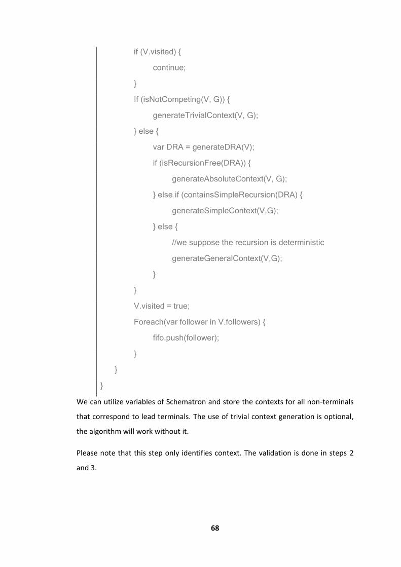
68
if (V.visited) {
continue;
}
If (isNotCompeting(V, G)) {
generateTrivialContext(V, G);
} else {
var DRA = generateDRA(V);
if (isRecursionFree(DRA)) {
generateAbsoluteContext(V, G);
} else if (containsSimpleRecursion(DRA) {
generateSimpleContext(V,G);
} else {
//we suppose the recursion is deterministic
generateGeneralContext(V,G);
}
}
V.visited = true;
Foreach(var follower in V.followers) {
fifo.push(follower);
}
}
}
We can utilize variables of Schematron and store the contexts for all non-terminals
that correspond to lead terminals. The use of trivial context generation is optional,
the algorithm will work without it.
Please note that this step only identifies context. The validation is done in steps 2
and 3.
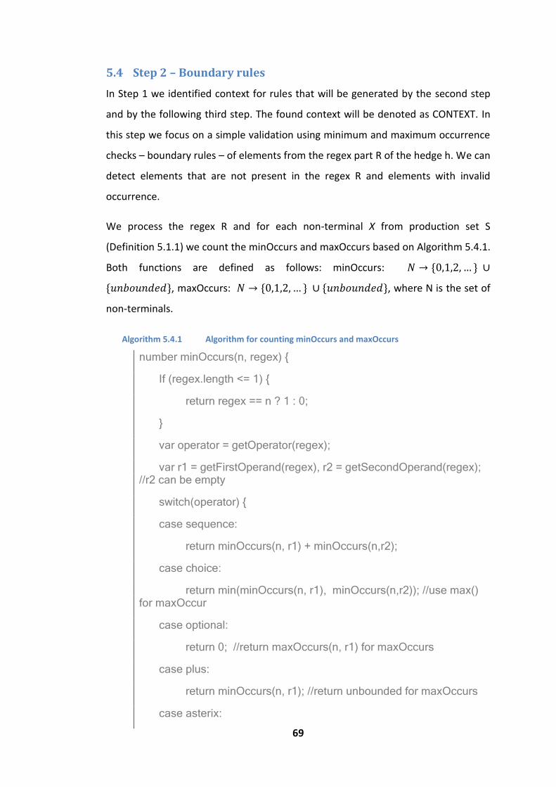
69
5.4 Step 2 – Boundary rules
In Step 1 we identified context for rules that will be generated by the second step
and by the following third step. The found context will be denoted as CONTEXT. In
this step we focus on a simple validation using minimum and maximum occurrence
checks – boundary rules – of elements from the regex part R of the hedge h. We can
detect elements that are not present in the regex R and elements with invalid
occurrence.
We process the regex R and for each non-terminal X from production set S
(Definition 5.1.1) we count the minOccurs and maxOccurs based on Algorithm 5.4.1.
Both functions are defined as follows: minOccurs: {
{ , maxOccurs: { { , where N is the set of
non-terminals.
Algorithm 5.4.1 Algorithm for counting minOccurs and maxOccurs
number minOccurs(n, regex) {
If (regex.length <= 1) {
return regex == n ? 1 : 0;
}
var operator = getOperator(regex);
var r1 = getFirstOperand(regex), r2 = getSecondOperand(regex); //r2 can be empty
switch(operator) {
case sequence:
return minOccurs(n, r1) + minOccurs(n,r2);
case choice:
return min(minOccurs(n, r1), minOccurs(n,r2)); //use max() for maxOccur
case optional:
return 0; //return maxOccurs(n, r1) for maxOccurs
case plus:
return minOccurs(n, r1); //return unbounded for maxOccurs
case asterix:

70
return 0: //return unbounded for maxOccurs
case group:
return minOccurs(n,r1);
}
}
In Algorithm 5.4.1 we use a pseudo-code and recursively parse the regular
expression until we get to a single non-terminal. Based on regex operator used, we
process the result of the inner regular expression. Note that we count with
unsinged integers and the special value ‘unbounded’. Any add operation with this
special value return again the value ‘unbounded’.
The function maxOccurs is very similar and the differences are stated in the code of
function minOccurs.
Example 5.3.11. Example of minOccurs and maxOccurs
minOccurs(B, B?C+) = 0 minOccurs(C, B?C+) = 1
maxOccurs(B, B?C+) = 1 maxOccurs(C, B?C+) = unbounded
minOccurs(B, BB?C*D*C) = 1 minOccurs(C, BB?C*D*C) = 1
maxOccurs(B, BB?C*D*C) = 2 maxOccurs(C, BB?C*D*C) = unbounded
In Example 5.3.11 we show on regular expression from Example 5.1.1 the values
returned by function minOccurs and maxOccurs.
We abbreviate the function calls of minOccurs and maxOccurs by allowing leaving
out the second parameter. The default value is the regex R of hedge h.
Now we get to the rule generation. With defined function minOccurs and
maxOccurs we can generate rules for hedge h. We use the function of XPath count.
First we check that there are no illegal children with a single rule:
∑ ( ( )) (
∈
ild )
Where child::* is an XPath expression for any child element from current context.

71
Next, we generate a rule for each non-terminal from S to check the bounds
(minimum occurrence and maximum occurrence):
⋁{ ( ( )) ( ) ( ( )) ( )
∈
Note that we may skip the maximum bound check, if maxOccurs equals to the value
‘unbounded’. The same fact can be applied to minOccurs and the value 0.
Example 5.3.12. Boundary rules for hedge h1
<rule context=”CONTEXT”>
<assert test=”(count(b) + (count(c) ) = count(child::*)”>There are illegal children of element a. Only elements b and c are allowed.</assert>
<!—min and max bounds check -->
<assert test=” count(b) <= 1”>Element a can have at most one child element b.</assert>
<assert test=”count(c) >= 1”>Element a must have child element c with minimum occurrence of 1.</assert>
</rule>
Example 5.3.12 contains generated Schematron rules for hedge h1 from Example
5.1.1. We assume that trans(B) = b and trans(C) = c.
5.5 Step 3 – order checks
In step 2 we generate constraints for boundary counts of elements. For unordered
unranked trees these rules would be sufficient. However, we are generating rules
for ordered unranked trees and that is why we need Step 3.
XPath 1.0 does not support regular expressions, the only thing we can do is to
construct several rules that use XPath-axes (preceding, following, etc.) and try to
express the regular expression with it. The full expression of a hedge using
Schematron rules can be found in Chapter 2.2. The basic idea is taken from [25].
We recapitulate in short what we want to do. We have a hedge h with a regular
expression R for its content. We want to generate rules that check that the content
(the child elements) match the regular expression.
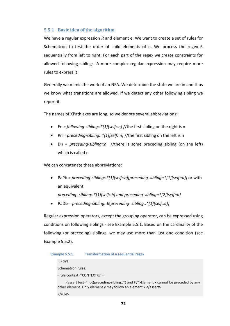
72
5.5.1 Basic idea of the algorithm
We have a regular expression R and element e. We want to create a set of rules for
Schematron to test the order of child elements of e. We process the regex R
sequentially from left to right. For each part of the regex we create constraints for
allowed following siblings. A more complex regular expression may require more
rules to express it.
Generally we mimic the work of an NFA. We determine the state we are in and thus
we know what transitions are allowed. If we detect any other following sibling we
report it.
The names of XPath axes are long, so we denote several abbreviations:
Fn = following-sibling::*[1][self::n] //the first sibling on the right is n
Pn = preceding-sibling::*[1][self::n] //the first sibling on the left is n
Dn = preceding-sibling::n //there is some preceding sibling (on the left)
which is called n
We can concatenate these abbreviations:
PaPb = preceding-sibling::*[1][self::b][preceding-sibling::*[1][self::a]] or with
an equivalent
preceding- sibling::*[1][self::b] and preceding-sibling::*[2][self::a]
PaDb = preceding-sibling::b[preceding- sibling::*[1][self::a]]
Regular expression operators, except the grouping operator, can be expressed using
conditions on following siblings - see Example 5.5.1. Based on the cardinality of the
following (or preceding) siblings, we may use more than just one condition (see
Example 5.5.2).
Example 5.5.1. Transformation of a sequential regex
R = xyz
Schematron rules:
<rule context=”CONTEXT/x”>
<assert test=”not(preceding-sibling::*) and Fy”>Element x cannot be preceded by any other element. Only element y may follow an element x.</assert>
</rule>

73
<rule context=”CONTEXT/y”>
<assert test=”Fz”>Element y must be followed by an element z. </assert>
</rule>
<rule context=”CONTEXT/z”>
<assert test=”not(following-sibling::*)”>Element z cannot be followed by any other element. </assert>
</rule>
In Example 5.5.1 we expressed a simple regex that contains only a sequence of three
elements – x, y and z. We created three rules with help of abbreviation defined at
the beginning of step 2. Each rule checks the follower to match the following
element from regex. We also added border conditions for elements at the beginning
and end of the regex.
Example 5.5.2. Transformation of a regex with a non-trivial cardinality
R = x+yz?
<rule context=”CONTEXT/x”>
<assert test=”(not(preceding-sibling::*) or Py) and (Fx or Fy)”>Element x cannot be preceded by any other element. Element x must be followed by other element x or by an element y.</assert>
</rule>
<rule context=”CONTEXT/y”>
<assert test=”Fz or not(following-sibling::*)”>Element y may be followed only by an element z or no element.</assert>
</rule>
<rule context=”CONTEXT/z”>
<assert test=”not(following-sibling::*)”> Element z cannot be followed by any other element. </assert>
</rule>
Example 5.5.2 extends Example 5.5.1. We have added a non-trivial cardinality for
elements x and z. The regex allows a sequence of elements x at the beginning and
makes the element z optional. The first and second rules must be extended to
capture the new conditions – element x must be the first element or be preceded by
another element x and must be followed by x or y. Element y must be followed by an
element z, or be the last element. Only the last (third) rule remains the same,
because the element z (if present) can be only the last element.

74
In Example 5.5.1, Example 5.4 and Example 5.5.2 we demonstrated the idea of
generating rules for regular expression. Now we describe the problem in more
detail.
5.5.2 Problem analysis
The Schematron rules are independent of each other and thus make sequential
processing of a regex more complicated. The main problem is to match an element
to a part of a regex. If we succeed in identifying the correct position in the regex,
the testing of the following sibling is fairly easy.
Elements with multiple occurrences in the regex represent the main problem - see
Example 5.5.3. We have to distinguish them using only XPath 1.0.
Example 5.5.3. Double occurrence of an element in a regex
R = a?a?
L(R) = {λ, a, aa}
In Example 5.5.3 we can see a regex that contains two occurrences of a, each one is
optional. The word “a” generated by the regex R is generated by either the first or
the second element a.
In order to simplify the work with this task, we transform the regex to NFA [26].
Each state in the NFA can have multiple paths (words) to access it (or produce the
state). In Example 5.5.3 the first element a is produced only by the empty word λ
and the second element a is produced by words λ and a. Note that both elements a
are produced by the empty word λ, but only the second one is produced also by a
word a. This illustrates the general problem – each state is produced by a set of
words, different states can have non-empty intersection of these sets.
Definition 5.5.1. Let us have a NFA = ( ). We denote the
production set of the state ∈ as ( ) { ∈
| ( ) .
Using this definition we can write the production sets for states for regex in
Example 5.5.3 as Product(a1) = { λ} and Product(a2) = {λ, a}.

75
Let us have two states p and q that have a non-empty intersection P of their
production sets. When we receive a word from P, the active state of the NFA can be
either p or q. This means that the next allowed state can be the follower of either
state p or q.
The solution for our problem with multiple elements in a regex is the following.
When we have an element x that is present in the regex R more than once, we
compute the production sets for each occurrence of x and intersect them. We
merge the rules for words that are in some intersection, since they are not
differentiable.
5.5.3 Algorithm
We have a regex R and want to create Schematron rules for validation. We analyzed
the problem in the previous chapter. Now we introduce our algorithm for
transforming the regex into Schematron rules.
Algorithm 5.5.1 Transformation of regular expression to Schematron rules
void generateRules (regex R, context C) {
var terminals = getTerminalSet(R);
foreach(var terminal in terminals) {
if (count(terminal, R) == 1) {
generateSimpleRule(terminal, R, C);
} else {
generateComplexRule(terminal, R, C);
}
}
}
void generateSimpleRule (string T, regex R, context C) {
var element = getElement(T, R); //find the corresponding element for terminal in R
var followers = getFollowers(element, R);

76
writeRule(T, null, followers); //there are no conditions for this terminal
}
void generateComplexRule (string T, regex R, context C) {
var paths = getPaths(T, R); //find all paths that lead from states of terminal T to the start of Regex.
var prefixAutomaton = PrefixAutomaton.EMPTY;
foreach(var path in paths) {
mergeNFA(prefixAutomaton, path);
}
foreach(var terminalState in prefixAutomaton.outputs) {
var condition = getCondition(terminalState);
var followers = getFollowers(terminalState, mergedNFA);
writeRule(T, condition, followers);
}
}
Let us describe Algorithm 5.5.1. We generate rules for each terminal in the regular
expression. If the terminal has only a single occurrence in the regex, we generate a
single rule without any complex conditions. Otherwise we have to tell apart each
occurrence of this terminal in the regex since the followers may differ.
In method generateComplexRule we find a list of all words that lead to the terminal
(see the production set from Definition 5.5.1). Multiple words can lead to the same
terminal. To find all the words we can use a NFA with reverted production function
and keep the found words represented as an automaton. We will merge those
automatons into a single prefix automaton. This automaton will serve as the source
for conditions to tell apart terminals T at different positions in the given regex R.
In the above paragraph and also in Algorithm 5.5.2 we use the term prefix
automaton. It is an extended NFA that contains one additional symbols in the input
alphabet – ^. Symbol ^ means the same as in the common regex usage - no

77
preceding symbol. In the prefix automaton we have two categories of states –
whether they have a transition to a following state (node state) or not (leaf state).
Algorithm 5.5.2 Merging NFA of terminals
void mergeNFA(prefixA aut, NFA nfa) {
var mapping = initMapping();
var mapped = mapping[nfa.startingState];
if (mapped != null && mapped != aut.start) {
update mapping with mergeAutomatonStates(aut.start, mapped);
} else {
Add new mapping for nfa.startingState and aut.start
}
doMerge(nfa.startingState);
}
void doMerge (NFAState startingState) {
var mapping = initMapping();
var lifo = LIFO.emptyLifo;
lifo.push(startingState);
while (not lifo.isEmpty()) {
var state = lifo.pop();
var automatonState = mapping[state];
switch(automatonState.type) {
case NODE:
foreach(var trans in state.forwardTransitions) {
if (automatonState.hasTransition(trans.letter) {
handleExistingTransition(automatonState, lifo, trans);
} else {
createNewTransition(automatonState, lifo, trans);

78
}
}
break;
case LEAF:
if (automatonState.nfaReference.isEmpty()) {
automatonState.nfaReference.add(state);
} else if (isDifferentNFA (automatonState.nfaReference[0], state)) {
// the same prefix part, we need to update this state
lifo.push(state); //repeat the evaluation for this state, after this leaf is processed (either changed to NODE or FINAL_LEAF);
var leafState = automatonState.nfaReference[0];
if (leafState.forwardTransitions.length > 0) {
automatonState.type = NODE;
lifo.push(leafState);
} else {
automatonState.type = FINAL_LEAF;
}
}
break;
case FINAL_LEAF:
automatonState.nfaReference.add(state);
break;
}
}
}
void createNewTransition (AState automatonState, LIFO lifo, Transition trans) {
if (mapping.contains(trans.finalState)) {

79
automatonState.connectToState(mapping[trans.finalState]);
} else {
var createdState = automatonState.createTransitionState(trans.letter);
//asociate the newly created automaton state with the NFA state
addMapping(trans.finalState, createdState);
}
lifo.push(trans.finalState);
}
void handleExistingTransition (AState automatonState, LIFO lifo, Transition trans) {
var foundAState = automatonState.forwardTransitions[trans.letter];
if (no mapping for trans.finalState) {
//this state in NFA is was not yet visited, associate it with this automaton state
trans.finalState.image = foundAState;
addMapping(trans.finalState, foundAState);
lifo.push(trans.finalState);
} else if (trans.finalState.image != foundAState) {
//state from NFA cannot point to two different automaton states -> merge them
var mergedAState = mergeAutomatonStates(trans.finalState.image, foundAState);
updateMapping(trans.finalState, mergedAState);
lifo.push(trans.finalState);
} else {
//already visited
}
}

80
AState mergeAutomatonStates(AState state1, AState state2) {
//state LEAF may change to NODE or FINAL_LEAF, we need to be certain of the outcome
If (state1.type == LEAF) {
doMerge(state1.nfaReference[0]);
}
If (state2.type == LEAF) {
doMerge(state2.nfaReference[0]);
}
//now we have only type NODE or FINAL_LEAF
If (state1.type == FINAL_LEAF || state2.type == FINAL_LEAF) {
//merge into single FINAL_LEAF, destroy possible following states in the automaton
state1.type = FINAL_LEAF;
state1.nfaReference.add(state2.nfaReference);
state1.removeTransitions();
state1.replaceState(state2);
} else {
//both states are of type NODE, merge their followers recursivly
state1.nfaReference.add(state2.nfaReference);
state1.replaceState(state2);
foreach (var trans in state1.forwardTransitions) {
if (state2.hasTransition(trans.letter) {
trans.finalState = mergeAutomatonStates(trans.finalState, state2.transition[trans.letter]); //recursive merge
state2.removeTransition(trans.letter);
}
}
//add the rest of the transition from state 2
state1.forwardTransitions.add(state2.forwardTransitions);

81
}
return state1;
}
In Algorithm 5.5.2 we introduce the algorithm to create a prefix automaton. The
prefix is constructed from the position of the terminal in regex R in the direction to
the beginning of the regex R. We want to find unique suffixes of prefixes or to know
that some prefixes cannot be decided.
In our prefix automaton the leaf states will contain a reference to NFA of terminals
and their follower list. Any leaf state identifies a word that identifies a specific
terminal.
This algorithm starts in the state that represents the terminal in the NFA and the
starting state of the prefix automaton. We simulate all the paths from the NFA in
the prefix automaton and add new states to it. We connect states from processed
NFA to the states of the automaton – to detect cycles. Each state from NFA can
have at most one connection to a state in the automaton.
Now we can build the prefix automaton. Example 5.5.4 shows a process of building
the automaton step by step.
Example 5.5.4. Building the prefix automaton
R = abca, indexed: R = a1b1c1a2
NFA:
a b c a
S F
Path for
a1: a^ a2: acba^ b1: ba^ b2: cba^
The construction of the prefix automaton for a:
I. There is only an empty automaton, containing only the starting state that represents the terminal a. It is LEAF.
S LEAF is associated with a1, the processing for a1 ends for now

82
II. Processing a2. The starting state is also a LEAF for a1. The NFA (path) for a1 contains another symbol: ^. We change the type of the starting state to NODE. And process a1 further.
III. We create a new state for a1 – LEAF for symbol ^. The processing for a1 ends here.
^ (a1)
S
IV. We continue processing of a2. We create a new state (LEAF) for symbol b and end. We do not need to continue, since we found unique suffixes of prefixes for both a1 and a2.
^ (a1)
S
c (a2)
Example 5.5.4 show the work of Algorithm 5.5.2 – the creation of a prefix
automaton for terminal a.
Conditions generation
After creation of the prefix automaton we can start to generate rules. From the
prefix automaton we know what states are easily distinguishable and what states
are similar (share the same output state). We do use the word similar, because if
there exists a cycle on a path from automaton start to the output state, there can
also exist a hidden condition for the repetition counts. Each of the similar states can
have a different repetition condition. See Example 5.5.5.
Example 5.5.5. Example of similar states in prefix automaton
R = (a+b)|((aa)+c), indexed = (a1+b)|((a2a3)+c)
Final prefix automaton:
^ (a1,a2,a3)
S
a
Example 5.5.5 shows that even a distinct occurrence of a terminal in a regex can be
merge into a single state in the prefix automaton. We must not express this

83
situation by only a single rule (as it may look correct at first sight) since symbol “c”
can only occur after even number of symbols “a”.
If there is no cycle in the path, we can generate the Schematron rule for that
terminal of the output state. See Example 5.5.6.
Example 5.5.6. Schematron rules for simple prefix automaton
R = abca, indexed: R = a1b1c1a2
Prefix automaton:
^ (a1)
S
c (a2)
Tell-apart condition for a1: no-preceding
Tell-apart condition for a2: c
Followers of a1: b
Followers of a2: none
Schematron rules:
<rule context=”CONTEXT/a[not(preceding-sibling::*)]”>
<assert test=”Fb”> Only element b may follow after an element a.</assert>
</rule>
<rule context=”CONTEXT/a[Pc]”>
<assert test=”not(following-sibling::*)”> Element a cannot be followed by any other element.</assert>
</rule>
Example 5.5.6 shows the generation of rules and conditions from prefix automaton
created in Example 5.5.4.
Cycle handling
Example 5.5.5 showed us that our algorithm is not perfect. However, we will not
show a solution for this problem in this thesis and leave it for a future work.
Future optimizations
There are several aspects that can be done to improve the performance of
generated rules. This chapter is merely for motivation purposes for future work.

84
As we saw in Example 5.5.5 it can happen that more occurrences merge in the
prefix automaton, leaving only a single rule and thus does not need additional
condition like other complex rules.
Another feature of our algorithm is that for each output state of the prefix
automaton there is generated a rule with a single Schematron assert. Again this
could be improved by merging similar rules and adjusting asserts.
Another possible optimization would be the use of XPath 2.0. XPath 2.0 supports
regexes that would help greatly in Schematron schema generation. However, using
a simple regex for validating content has a downside –asserts are simplified and will
not tell the user where exactly an error is.
5.6 Summary
We have shown that expressing hedges with XPath1.0 is possible, but contains
some limitations. In this chapter we summarize these limitations and identify the
sub-class of regular grammar that we can express.
We introduced three-step algorithm. Step 1 generates correct context for later
steps. Steps 2 and 3 generate Schematron rules. All steps introduce a limitation for
the content – we are unable to differentiate types. Thus we cannot allow two
different types for a single element in the same content model, i.e. we do not allow
competition between non-terminals. This restricts the grammar to a Single Type
tree grammar.
Step 1 introduces another limitation. It does not allow for any non-determinism in
the recursion of the grammar. This is limited neither by a local tree grammar, nor by
a Single type grammar. However, as we will see in the next chapter, the k-ancestor
approach offers a nice way to handle the most real-world data.
Step 3 matches regular expression of a hedge. We have shown an approach that
uses XPath 1.0. We also showed that there are some cases where our algorithm
may not work – i.e. tell apart odd and even number of preceding siblings. Step 3 can
be omitted if we want to generate rules for unordered hedges.

85
The expression strength of our algorithm is thus limited by step 1 and 3. In may be
possible to improve the algorithm from step 3 and utilize it also for step 1 and lift
some limitations, but that is a possible task for a future work.

86
6 XML Schema inferring
This chapter describes ways of XML schema inferring. We will not go into deep
details, because this problem has been analyzed many times before, but we will
describe single method more deeply since we use it in our implementation. A
deeper analysis can be found for example in [28] and [29].
There are two different general approaches to XML schema inferring – heuristic
approach and grammar-inferring approach.
Heuristic approaches come from practical needs. They utilize empiric observations
and are more human-oriented. Results of heuristic approach are created by
generalization of a simple schema based on empiric observations (e.g. if an element
occurs three or more times, we denote it as unbounded). Based on this fact, the
inferred schemas cannot be assigned to a specific type of grammar.
Grammar-inferring approaches are based on a theoretical basis. Each method of
this family generates defined grammar type. However, based on the Gold’s theorem
[31], the language cannot be learned only from positive examples. As such, there
has to be typically some user input to direct the algorithm to the result.
6.1 iXSD
This algorithm was introduced in [30]. It is a grammar-inferring approach that
generates single-type grammar (in the form of XML Schema - XSD).
The authors of this method analyzed the real world data and came with two
following observations:
Locality [30]: The content model of an element in more than 98% of XSDs in
practice turns out not to depend on the whole labeled path from the root to
the element, but only on the k last element names in that path, with
typically .
Single occurrence [30]: The regular expressions in more than 99% of XSDs in
practice are of a very specific form: each element name occurs at most once
in them.

87
We use these observations in the following definitions.
Definition 6.1.1. We denote an XML document k-local if any of its content
models depends at most on the last k labels of ancestors.
Definition 6.1.2. We denote single occurrence regular expression (SORE)
to be a regular expression ∈ ( ), where each symbol ∈ is
present at most once.
Example 6.1.1. SORE
S1 = a+b?c is SORE
S2 = aa? is NOT SORE
Example 6.1.1 shows two regular expressions. The first one (S1) is a SORE expression,
but the second one (S2) is not because there are two occurrences of a.
The iXSD algorithm supposes that the input set of XML documents is k-local and
contains only content models expressible by single occurrence regular expressions.
6.1.1 Algorithm
The algorithm of iXSD consists of two steps – iLocal and Reduce. iLocal identifies all
k-local content models and creates types of them. Reduce step merges similar-
enough types.
For the needs of the algorithm we define several terms.
Definition 6.1.3. We denote paths(f) for an XML fragment f to be a set of all
labeled paths starting at root element in f.
Definition 6.1.4. We denote k-path | of path p to be a path formed by the
last k labels of path p. Two paths p and q are k-equivalent if | | .
Example 6.1.2. XML fragment and paths
F :=
<library>
<documents>
<book>
<title>Krakatit</title>
<author>Karel Čapek</author>

88
</book>
<book>
<title>Big encyclopedia </title>
<author>Some author 1</author>
<author>Some author 2</author>
<summary>Some summary of the Big Encyclopedia</summary>
</book>
<article>
<title>Some technical article</title>
< author >Author </ author >
<summary>Summary of this technical article</summary>
</article>
</documents>
</ library>
paths(F) = { , library, library documents, library documents book, library documents book title, library documents book author, library documents book summary, library documents article, library documents article title, library documents article author, library documents article summary}
2-paths(F) = { , library, library documents, documents book, book title, book author, book summary, documents article, article title, article author, article summary}
Example 6.1.2 shows a XML fragment and all paths and 2-paths.
Definition 6.1.5. We define strings(f, p) , where f is an XML fragment and p
is a path, to be the a set of all names of element directly below an
occurrence identified by the path p.
If the path p in the string(f, p) is a k-path we use the term k-strings(f, | ).
Example 6.1.3. K-string example
2-strings(F, documents book) = {title author, title author author summary}
1-strings(F, author) = { , , , , }
Example 6.1.3 shows the usage of function string on the XML fragment from
Example 6.1.2.
Now we have basic definitions and can proceed to the main algorithm.
Algorithm 6.5.3 iLocal
Types iLocal (int K, XMLFragments[] C) {
var paths = paths(C);

89
var types = create type for each unique k-path from paths;
foreach(type t in types) {
//create single occurrence automata
t.soa = iSOA(k-strings(C, t.kPath));
//convert the automata to SORE
t.regex = createSore(t.soa);
}
Foreach( path (p,a) in paths) {//(p,a) consist of a path ‘p’ and a label ‘a’
Type[ | ].addTypeMapping(a, types[( )| ]);
}
return types;
}
Automata iSOA(string [][] labels) {
var aut = create empty SOA;
var uniqueNames = getUniqueNames(labels);
aut.createVertices(uniqueNames);
foreach (string[] labelSet in labels) {
let labeSet have the form of (s1, s2, …, sn)
aut.connectVertices ((aut.start, s1), (s1, s2),…(sn, aut.out));
}
return aut;
}
The iLocal - Algorithm 6.5.3 – creates types based on their K-path. Note that there
will be more types than necessary. E.g. all empty elements with different k-paths
will have different types, but they could easily have only a single type – empty. We
will thus post-process the result of iLocal and merge the same types using the
Minimalize algorithm.
Example 6.1.4. Ilocal results
Types generates by iLocal on F (Example 6.1.2 ) and k = 2:

90
, library, library documents, documents book, document article, book title, book author, book summary, article name, article author, article summary
Example 6.1.4 shows the types that will be found on the XML fragment from
Example 6.1.2. Note that e.g. types book title, book author, article name could be
merged into the same type since they contain only text data.
Algorithm 6.5.4 Minimalize
Void minimalize(Types T, Type ignore, XMLFragments[] C) {
while(exists Type ∈ ) {
If (setsEqual(k-strings(C, t.kPath), k-string(C, s.kPath)) {
foreach(Type k that contains mapping to t) {
k.changeMapping(a, s);
}
T.removeType(t);
}
}
}
Example 6.1.5. Output of Minimalize
Minimalize on the result of Example 6.1.4 will return these types:
, library, library documents, documents book, document article, book title
Example 6.1.5 shows the minimalization of equal types of iLocal algorithm from
Example 6.1.4. Note that there is significantly less types now. All types with empty
content were merged into a single type with kPath book title.
After running the iLocal and Reduce algorithms, we have set of types that are each
unique. The next step – Reduce - will identify similar types and merge them. For
that we will define the distance of types.
We have to modify the iSOA algorithm. Each edge will contain a number usage –
how many words from k-strings used this edge. Let as have a look on the adapted
iSOA.
Algorithm 6.5.5 Adapted iSOA
Automata iSOA(string [][] labels) {
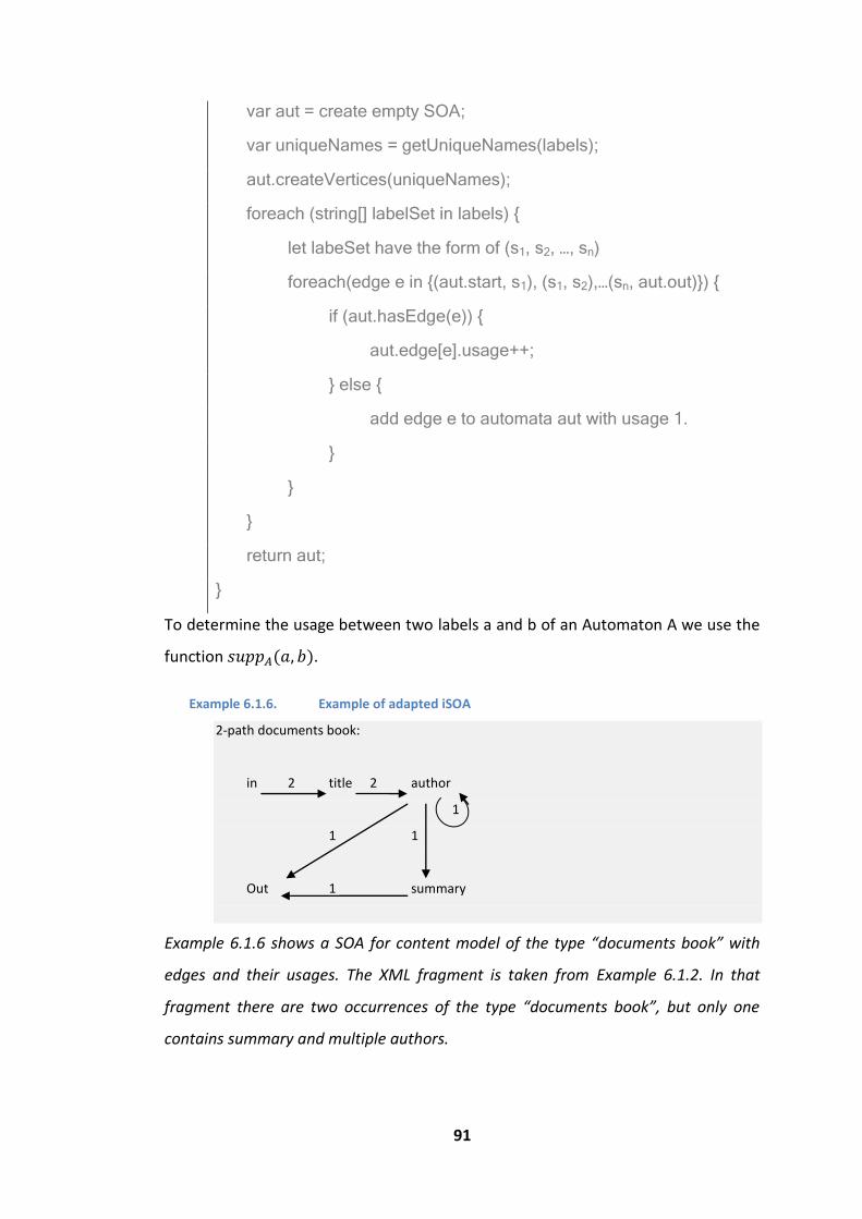
91
var aut = create empty SOA;
var uniqueNames = getUniqueNames(labels);
aut.createVertices(uniqueNames);
foreach (string[] labelSet in labels) {
let labeSet have the form of (s1, s2, …, sn)
foreach(edge e in {(aut.start, s1), (s1, s2),…(sn, aut.out)}) {
if (aut.hasEdge(e)) {
aut.edge[e].usage++;
} else {
add edge e to automata aut with usage 1.
}
}
}
return aut;
}
To determine the usage between two labels a and b of an Automaton A we use the
function ( ).
Example 6.1.6. Example of adapted iSOA
2-path documents book:
in 2 title 2 author
1
1 1
Out 1 summary
Example 6.1.6 shows a SOA for content model of the type “documents book” with
edges and their usages. The XML fragment is taken from Example 6.1.2. In that
fragment there are two occurrences of the type “documents book”, but only one
contains summary and multiple authors.
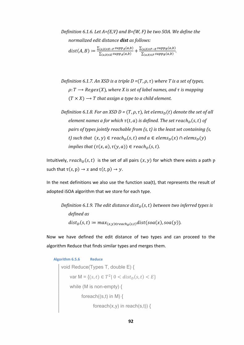
92
Definition 6.1.6. Let A=(E,V) and B=(W, F) be two SOA. We define the
normalized edit distance dist as follows:
( ) ∑ ( )( )∈
∑ ( )( )∈
∑ ( )( )∈
∑ ( )( )∈ .
Definition 6.1.7. An XSD is a triple D =( ) where T is a set of types,
( ), where X is set of label names, and is mapping
( ) that assign a type to a child element.
Definition 6.1.8. For an XSD D = ( ), let ( ) denote the set of all
element names a for which ( ) is defined. The set ( ) of
pairs of types jointly reachable from (s, t) is the least set containing (s,
t) such that ( ) ∈ ( ) and ∈ ( ) ( )
implies that ( ( ) ( )) ∈ ( ).
Intuitively, ( ) is the set of all pairs ( ) for which there exists a path p
such that ( ) and ( ) .
In the next definitions we also use the function soa(t), that represents the result of
adopted iSOA algorithm that we store for each type.
Definition 6.1.9. The edit distance ( ) between two inferred types is
defined as
( ) ( )∈ ( ) ( ( ) ( )).
Now we have defined the edit distance of two types and can proceed to the
algorithm Reduce that finds similar types and merges them.
Algorithm 6.5.6 Reduce
void Reduce(Types T, double E) {
var M = {( ) ∈ | ( )
while (M is non-empty) {
foreach((s,t) in M) {
foreach(x,y) in reach(s,t)) {

93
x.soa = x.soa y.soa;
y.soa = x.soa;
foreach(a in elems(y) – elems(x)) {
x.addTypeMapping(a, y.mapping[a]);
}
foreach(a in elems(x) – elems(y)) {
y.addTypeMapping(a, x.mapping[a]);
}
}
recompute M = {( ) ∈ | ( )
}
}
Foreach(type t in T) {
t.regex = createSore(t.soa);
}
Minimalize(T);
}
We demonstrate the work of the Reduce algorithm on an example.
Example 6.1.7. Reduce demonstration
Reduce on the result of Example 6.1.5 with E=0.5 will return these types:
, library, library documents, documents book, book title.
It merged types
s = documents book and t = documents article
since Dist(s,t) = ⁄
6.1.2 Summary
The iXSD algorithm recognizes a single type grammar. It is able to identify types
based on a definable context and not only on element names. The iXSD uses two
parameters – k for the size of the context and E for the sensitivity for type merging.
94
7 Implemented solution
In previous chapters we analyzed and described a lot of algorithms. In this chapter
we introduce our implementation for Schematron schema inferring.
Our goal is to infer a Schematron schema out of a set of XML documents. Our
solution is divided into two parts – grammar inferring and Schematron schema
generation. For the grammar inferring part we use the iXSD algorithm described in
Chapter 6.1. For the Schematron schema generation part we use our three part
algorithm from Chapter 5.
The reason for splitting our solution into two independent parts is because of the
nature of Schematron. The inferred grammar can contain types that we are not
interested in, or some types may not have been identified correctly. With our
approach, the user can fix and simplify the inferred schema and thus gaining a
better control of the output. Another advantage is that a user may choose a
different inferring tool.
Our solution is written in C# over .NET Framework 3.5 as two separate command
line applications. The usage is described in the appendix.
7.1 Data limitations
Since we use the iXSD algorithm, we expect that the data follow the two
observations – locality and single occurrence. If the data will not support these two
expectations, the result may be too general since the iXSD algorithm will always try
to return SORE content models.
Our algorithm from Chapter 5 comes with two limitations on the input grammar.
The first limitation – single type – is trivially fulfilled by the fact that the iXSD
algorithm produces single type grammar. The second – determinism in derivation
sequence – will be resolved by the k-local feature of the iXSD that will be used also
in the context matching of our Schematron schema generation.

95
7.2 Usage of iXSD
In our solution we used the core of the iXSD algorithm as described in Chapter 6.1.
The only difference from the intended usage of the iXSD is the form of the inferred
grammar. We do not use XML Schema but a very simple form of grammar
description. The Relax NG schema for inferred grammars can be found in the
appendix.
7.2.1 Inferred grammar
The result of the step 1 of our solution is an XML document referenced as the
inferred grammar. It contains two sets of definitions – types and elements.
The type definitions describe the whole inferred grammar. Each definition contains
the description of its own content model, the names of child elements and their
types. The section is similar to a Relax NG or XSD schema in the meaning that it
defines all the hedges of the documents.
The other section - elements - contains constrains for content models of XML
documents. Based on K ancestors it references a type that should be used to
validate the content. This approach lets user to validate only a specific parts of XML
documents and thus a more Schematron-like approach.
Relax NG schema for inferred grammar can be found on the CD and in the
Appendix.
The second part of our solution – Schematron schema generation – uses constrains
from elements.
7.3 Schematron schema generation
The Schematron schema generation consists of three parts: context matching,
boundary rules and order check.
In this thesis we discussed several ways of context matching. Because of the locality
observation of the iXSD algorithm, we choose the k-ancestor approach.

96
Although the inferred grammar of the iXSD algorithm should contain only SORE
content models, our solution supports also simple multi-occurrence regular
expressions. This support is limited as discussed in Chapter 5.
7.4 Experimental data sets
We used our solution on experimental data taken from real world. We present two
data sets. Each set is presented in the same folder structure. It contains folder for
grammars where all schemas and inferred grammars are stored and a folder for
XML data.
The inferred schema (produced by step 1 of our solution) is named
InferredGrammar.xml. The generated Schematron schema is named
schematronSchema.sch. For all of our experimental data sets we use the default
settings for grammar inferring (k=2, E=0.3).
Data set 1
This data set contains XML representation of a very common book – the Bible. We
do not have any schema, just a single XML document. The XML document has a
simple internal structure see Example 7.4.1. The full version of the XML document
can be found on the CD.
Example 7.4.1. XML fragment of the Bible data set
<book title="Genesis">
<chapter number="1">
<verse number="1">In the beginning God created the heaven and the earth.</verse>
<verse number="2">And the earth was without form, and void; and darkness [was] upon the face of the deep. And the Spirit of God moved upon the face of the waters.</verse>
<verse number="3">And God said, Let there be light: and there was light.</verse>
…
</chapter>
…
</book>
Example 7.4.1 shows an XML fragment - the first verses of the first book of the Bible.

97
Example 7.4.2. Inferred grammar for Bible
<schema>
<definitions>
<definition name="chapter">
<oneOrMore>
<element name="verse" type="ValueOrEmpty" />
</oneOrMore>
</definition>
<definition name="ValueOrEmpty">
<empty />
</definition>
<definition name="book">
<oneOrMore>
<element name="chapter" type="chapter" />
</oneOrMore>
</definition>
</definitions>
<elements>
…
<element ofType="chapter">
<location>
<parent name="chapter">
<parent name="book" />
</parent>
</location>
</element>
</elements>
</schema>
In Example 7.4.2 we part of the inferred grammar for the first data set. The full
version of the grammar can be found on the CD.
As we can see in Example 7.4.2, the inferred grammar for Bible is also simple. All
content models are single occurrence and thus we should not have any difficulties
in Schematron schema generation.
Example 7.4.3. Schematron schema for data set 1
<schema xmlns="http://purl.oclc.org/dsdl/schematron">
<pattern>

98
<rule context="//book/chapter">
<assert test="count(verse) >= 1">There must be at least 1 element(s) "verse".</assert>
<assert test="(count(verse)) = count(child::*)">There are illegal elements. Only elements "verse" are allowed</assert>
</rule>
<!--rules for checking regex regex "verse+"-->
<rule context="//book/chapter/verse">
<assert test="following-sibling::*[1][self::verse] or not(following-sibling::*)">Element "verse" can only be followed by "verse" or cannot be followed by any other element</assert>
</rule>
</pattern>
<pattern>
<rule context="//chapter/verse">
<assert test="count(child::*) = 0">No children are allowed.</assert>
</rule>
</pattern>
</schema>
Example 7.4.3 shows part of the generated Schematron schema. The full version of
the Schematron schema can be found on the CD.
The generated Schematron schema contains one pattern for each element
definition in the inferred grammar. Each pattern consists of several rules
constraining the corresponding grammar type.
Data set 2
In the second data set we initially had only XSD schema (schema.xsd) for NASC
arrays. The XSD contains choices, sequences and types. There are more types than
in the data set 1. Because the both the inferred grammar and the corresponding
Schematron schema are too big we will show only small interesting XML fragments
as examples. All the referenced files can be found on the CD.
Based on the XSD we generated two sample XML documents – the first with
random choice and repetition and the second one without repetition.
The inferred grammar is bigger this time. It contains 23 types and about 130
element definitions. Schematron schema for this bigger grammar is also supplied

99
and it works. Note that there are some examples of multi occurrence content
models. However for better performance the inferred grammar should be
simplified.
Example 7.4.4. Complex definition from the inferred grammar for data set 2
<definition name="Source">
<choice>
<oneOrMore>
<element name="StockCode" type="ValueOrEmpty" />
</oneOrMore>
<group>
<element name="Individual" type="ValueOrEmpty" />
<choice>
<element name="Organism" type="ValueOrEmpty" />
<group>
<element name="IndivGeneChar" type="ValueOrEmpty" />
<optional>
<element name="GeneticBackground" type="ValueOrEmpty" /> </optional>
</group>
</choice>
</group>
<group>
<element name="invitroTreat" type="Other" />
<element name="CellLineSource" type="ValueOrEmpty" />
<optional>
<element name="Age" type="ValueOrEmpty" />
</optional>
</group>
<group>
<optional>
<element name="SeperationTechnique" type="Other" />
</optional>
<element name="CellLineSource" type="ValueOrEmpty" />
<optional>
<element name="Age" type="ValueOrEmpty" />
</optional>
</group>

100
<group>
<element name="IndivGeneChar" type="ValueOrEmpty" />
<optional>
<element name="GeneticBackground" type="ValueOrEmpty" />
</optional>
</group>
<group>
<element name="Other" type="Other" />
<element name="CellSourceType" type="Other" />
</group>
</choice>
</definition>
Example 7.4.4 is a typical example of a multi-occurrence content model. E.g. the
type StockCode or IndivGeneChar is occurring more than once.
We can see some suspicious type definitions in the inferred grammar. We can also
notice some multi-occurring content models. See Example 7.4.4. This is caused by a
small set of input XML documents and their small variability and also by the
complex type used to generate the data. Our implementation of the iXSD algorithm
was not able to simplify enough the regex of this type. Thanks to this fact, we can
demonstrate the ability of basic multi-occurrence support of our Schematron
schema generation.
Example 7.4.5. Multi-occurrence support of Schematron schema generation
<!-- Symbol IndivGeneChar: -->
<!--Warning: support for multi-occurence symbols is not fully implemented-->
<rule context="//Extract/Source/IndivGeneChar[not(preceding-sibling::*)]">
<assert test="following-sibling::*[1][self::GeneticBackground] or not(following-sibling::*)">Element "IndivGeneChar" can only be followed by "GeneticBackground" or cannot be followed by any other element</assert>
</rule>
<rule context="//Extract/Source/IndivGeneChar[preceding-sibling::*[1][self::Individual]]">
<assert test="following-sibling::*[1][self::GeneticBackground] or not(following-sibling::*)">Element "IndivGeneChar" can only be followed by "GeneticBackground" or cannot be followed by any other element</assert>
</rule>
Shows part of the regex-checking rules for multi-occurring element IndivGeneChar.
Our algorithm detected two occurrences with different prefixes. However, notice
101
that the following asserts are identical and thus the generation process could be
further improved.
In the inferredGrammarSimplified.xml we removed element definitions of type
ValueOrEmpty and Other. Only this simple removal of the two most common (and
trivial) element types reduced the number of element definitions to 26. Based on
the user preferences the inferred grammar could be simplified further.
7.5 Conclusion
Our solution works on the most data from the real world – we use the iXSD
algorithm. See Chapter 6.1 for more details about the properties of the real world
data. However, we could see that both the inferred grammar and the generated
Schematron schema are often bigger than necessary.
The most trivial comparison is by the file sized of the schemas of the second
experimental data set: XSD Schema – 20kB, inferredGrammar - 23kB,
inferredGrammarSimplified - 13kB, SchematronSchema – 71kb,
SchematronSchemaSimplified - 51kB. We must note that the original XSD schema
also contains comments and attributes definitions that are not contained in the
inferredGrammar nor in the SchematronSchema.
Our implementation is a proof of concept that a Schematron schema can be
generated for set of XML documents. For the real-world usage the generator should
be optimized and the inferred grammar reduced.
We did not compare the effectiveness of the validation between Schematron and
other languages, but based on the file sizes of the schemas we recommend that
Schematron is used only for validation of some interesting parts of XML documents
and not for the validation of the whole document.
There is another interesting feature of our implementation. We can see that the
most rules come from the regex matching. If we could reduce their number the
resulting Schematron schema would be greatly simplified. This could be done by
two approaches – firstly we could use a different query language with a regex

102
support, secondly we could allow any-order groups in the regex definition and thus
skipping the regex matching altogether.

103
8 Related work
There has been research already done on the field of XML schema inference. In this
chapter we describe in short the most related work on this field. For a much bigger
overview of XML inferring methods we recommend the [32].
8.1 Inferring xml schema definitions from xml data
Paper [30] analyses the properties of real world XML documents and defines two
most common properties - locality and single occurrence. Based on those two
properties it introduces the iXSD algorithm. Since we described this approach in
Chapter 6.1, we will no redefine the whole algorithm again. We will only summarize
the basic idea.
Locality property means that each content model depends only on the last K
ancestors. Single occurrence states that content models consists only of single
occurrence regular expressions (each terminal is present at most once). The iXSD
algorithm identifies types based on the locality property and merges the similar
types. The output is a single-type tree grammar in the form of an XSD.
8.2 Even an Ant Can Create an XSD
Paper [33] introduces the Schema miner. This approach generates an XSD. It is a
heuristic approach and allows inferring elements with the same name but with a
different structure. It is also able to infer unordered sequences in a content model.
This approach exploits the ACO (Ant Colony Optimization, [34], [35]), sk-string, (k,h)-
context and MDL-principle. The ACO is a heuristics that is able to find a suboptimal
solution. It uses “ants” that search the space S of possible solutions. Ants try to find
an optimal solution; each found solution is evaluated by the MDL principle. Each ant
does only predefined amount of steps before it dies. In each step an ant searches a
subspace of S for a local suboptimum. Based on how good a found solution is, the
ant gives a positive feedback – pheromones. The following iterations of other ant
adjust their search based on the amount of pheromones.
SK-string method is used for finding and merging equivalent states. It is a more
relaxed form of Nerode equivalence. The Nerode equivalence says that two states p

104
and q are equivalent if the sets of all paths leading to terminal states are equivalent.
For the simplicity sk-string compares only s most probable k-strings. K-string returns
only paths of the length K or shorter that lead to a terminal state.
Definition 8.1.1. A regular language L is k-contextual, if there exists a finite
automaton A s.t. L = L(A) and for any two states pk, qk of A and all input
symbols a1a2…ak: if there are two states p0 q0 of A s. t. ( )
and ( ) , then .
Definition 8.1.2. A regular language L is k-contextual, if there exists a finite
automaton A s.t. L = L(A) and for any two states pk, qk of A and all input
symbols a1a2…ak: if there are two states p0 q0 of A s. t. ( ) ,
( ) , …, ( ) and ( ) , ( ) , …,
( ) then for every i s. t. .
8.3 Automatic Construction of an XML Schema for a Given Set of
XML Documents
Thesis [29] enhances the Schema miner from previous chapter and introduces the
Schema builder. The aim of Schema builder is to allow user interaction and
recognize inheritance between types. Another improvement is that Schema builder
matches elements with different name but similar structure.
User can preview identified types and adjust their regular expressions. However,
the main addition of the user interaction is the ability to define inheritance between
types.
8.4 Optimization and Refinement of XML Schema Inference
Approaches
Another work that builds upon paper [33] is [36]. The author focusses on the fact,
that many XML documents have some schema, but that schema is outdated, invalid
or not complete. He proposes a method of inferring an updated schema from the
old one. The benefit of this approach is that the new schema is enforced not to
deviate much from the old one.
105
Another goal of this work is to develop a finer MDL metric. The newly proposed
MDL metric should prefer simpler schemas.
8.5 Efficient Detection of XML Integrity Constraints
It is common that XML data have some integrity constraints. Even if these
constraints are known, there may be some XML documents that violate some of the
constraints. The work [37] discusses the problem of correcting these violations with
the least modification as possible to the input documents.
The author introduces repair groups for different types of violations. Each repair
action from a repair group is weighted and the least invasive is chosen. Another
aspect of the this work is that the algorithm allows user input.

106
9 Conclusion
This thesis has brought a way to infer a Schematron schema for a set of XML
documents. We have introduced Schematron in deeper, because it uses a different
way of XML validation – it uses rules instead of grammar validation. Schematron
supports more query languages, we chose XPath 1.0, since the support from third
parties implementations of Schematron validators is the most common for XPath
1.0.
To our best knowledge, there has not been much work on automatic Schematron
schema generation. Because of this fact we focused on analyzing and describing
different ways of transforming a single type grammar to Schematron rules. This is
the main part of this thesis and more future work can be based on it.
Since there have been works on automatic XML schema inferring (e.g. [28] or [29]),
we reduced the analysis of existing inferring methods to a single representative –
the iXSD algorithm. We used the iXSD algorithm later in our implementation.
Our implementation consists of grammar inferring part and of a Schematron
schema generation part. User interaction is supported, since the user can modify
the inferred simple grammar description or even write its own.
At the end we show some experimental results.
9.1 Future work
In this thesis there are some areas that we did not discuss at all or only a little.
Some new areas came up as we proceeded with our analysis. These areas can bring
new results and improve the current results. We will try to describe them in short in
the following paragraphs.
One of the main areas that have not been touch is negative examples handling.
Schematron (in contrast to other major validation languages) is able to express and
check negative constraints. Current inferring methods use only positive examples. It
would be interesting to be able to define negative constraints.

107
Schematron supports more query languages. We used XPath 1.0 since it is widely
supported. We were limited by the use of XPath 1.0 in algorithms mainly because of
the lack of regex support. However, other query languages can work better – like
XPath 2.0. They bring new possibilities to match elements and thus they could
greatly improve and simplify our algorithms.
There is another a way to reduce the number of generated rules and simplify the
Schematron schema - by introducing any-order alternative for a group (like XS:any
in XML Schema). In current implementation the majority of generated rules are for
regex checking and thus, for unordered content models, these rules could be left
out.
Our algorithm suggests a way to handle multi-occurrence content models with the
help of prefix automata. However, this method is not fully completed since it does
not handle all cases – mainly the length of repeated loops. Also there is some place
to improve the generated queries and simplify them.
Lastly, the whole Schematron schema is not optimized. It can query multiple times
the same elements or on the other hand uses too much variables. We think that this
could be improved. Also the generated schema is too big and not all elements must
be checked. The inferred grammar could be automatically optimized.

108
10 Bibliography
[1] Introduction to automata theory, languages, and computation, John E.
Hopcroft, Rajeev Motwani, Jeffrey D. Ullman,
[2] Schematron, Eric van der Vlist, March 2007, ISBN: 978-0-596-55874-1
http://www.schematron.com
[3] (Relax NG homepage) http://www.relaxng.org , 2010.
[4] Relax NG book, Eric van der Vlist, December 2003, ISBN: 0596004214
http://books.xmlschemata.org/relaxng
[5] W3C wiki http://esw.w3.org/Co-occurrence_constraints
[6] XML Path Language (XPath) Version 1.0, W3C http://www.w3.org/TR/xpath,
16 November 1999
[7] Technologie XML, RNDr. Irena Mlýnkova, Ph.D , Martin Nečaský, Ph.D., 2010
http://www.ksi.mff.cuni.cz/~mlynkova/prg036/slajdy/PRG036_XPath1.pdf
[8] W3C, XML Path Language (XPath) Version 2.0 (Second edition),
http://www.w3.org/TR/xpath20/, 14 December 2010
[9] W3C, Extensible Markup language (XML) 1.0 fifth edition,
http://www.w3.org/TR/REC-xml/, 26 November 2008
[10] Makoto Murata, Dongwon Lee, Murali Mani, and Kohsuke
Kawaguchi. 2005. Taxonomy of XML schema languages using formal
language theory. ACM Trans. Internet Technol. 5, 4 (November 2005)
[11] H. Comon, M. Dauchet, R. Gilleron, F. Jacquemard, C. Löding, S. Tison
and M. Tommasi. Tree automata techniques and applications.
https://gforge.inria.fr/projects/tata/, November 18 2008.
[12] W3C, XML Schema Part 1: Structures Second Edition,
http://www.w3.org/TR/xmlschema-1, 28 October 2004
[13] W3C, W3C XML Schema Definition Language (XSD) 1.1 Part 1:
Structures, http://www.w3.org/TR/xmlschema11-1/, 3 December 2009
[14] W3C, On SGML and HTML, http://www.w3.org/TR/REC-
html40/intro/sgmltut.html
[15] M. Murata, “RELAX (Regular Language description for XML)”,
http://www.xml.gr.jp/relax/, October 2000

109
[16] J. Clark, “TREX – Tree Regular Expressions for XML”,
http://www.thaiopensource.com/trex/, 2001
[17] ISO JTC1/SC34, Document Schema Definition Languages,
http://www.dsdl.org/, March 2010
[18] Schematron namespace http://purl.oclc.org/dsdl/schematron
[19] W3C, XSL Transformations (XSLT) Version 1.0,
http://www.w3.org/TR/xslt, 16 November 1999
[20] W3C, XSL Transformations (XSLT) Version 1.1,
http://www.w3.org/TR/xslt11/, 24 August 2001
[21] W3C, XSL Transformations (XSLT) Version 2.0
http://www.w3.org/TR/xslt20/, 23 January 2007
[22] W3C, XQuery 1.0: An XML Query Language,
http://www.w3.org/TR/xquery/, 3 January 2011
[23] Michal Chytil, Automaty a gramatiky, 1. Vyd. Praha : Státní
nakladatelství technické literatury, 1984. -- 331 s
[24] W3C, XHTML ™ 1.0 The Extensible HyperText Markup Language
(Second Edition), http://www.w3.org/TR/xhtml1/#xhtml, 26 January 2000,
revised 1 August 2002
[25] Rick Jeliffe, Converting Models to Schematron, November 16 2006,
http://www.oreillynet.com/xml/blog/2006/11/converting_content_models_
to_s.html
[26] R. Barták: Automaty a gramatiky:
http://kti.mff.cuni.cz/~bartak/automaty/, 2001
[27] Geert Jan Bex, Frank Neven, and Stijn Vansummeren. Inferring xml
schema definitions from xml data. In VLDB '07: Proceedings of the 33rd
international conference on Very large data bases, pages 998–1009. VLDB
Endowment, 2007.
[28] Automatická konstrukce schématu pro množinu XML dokumentů,
Ondřej Vošta, Master Thesis, Department of Software Engineering, Charles
University in Prague, 2005
110
[29] Automatic Construction of an XML Schema for a Given Set of XML
Documents, Julie Vyhnanovská, Master Thesis, Department of Software
Engineering, Charles University in Prague, 2009
[30] Geert Jan Bex, Frank Neven, and Stijn Vansummeren. Inferring xml
schema definitions from xml data. In VLDB '07: Proceedings of the 33rd
international conference on Very large data bases, pages 998–1009. VLDB
Endowment, 2007.
[31] E. Mark Gold: Language identification in the limit. 1967. Information
and Control, 10(5): 447-474
[32] Irena Mlýnková, XML Schema Inferrence: A Study, Department of
Software Engineering, Charles University in Prague
[33] O. Vosta, I. Mlynkova, and J. Pokorny. Even an Ant Can Create an XSD.
In DASFAA'08: Proc. of the 13th Int. Conf. on Database Systems for Advance
Applications, LNCS, pages 35-50. Springer, 2008.
[34] M. Dirigo, A. Calorni and V. Maniezzo, Positive feedback as a search
strategy. Technical Report 91-016, Dipartimento di Elettronica, Politecnico di
Milano, Milan, Italy, 1991
[35] R. K. Wong and J. Sankey, On Structural Inference for XML Data,
Technical Report UNSW-CSE-TR-0313, School of Computer Science, The
University of New South Wales, 2003.
[36] Michal Klempa, Optimization and Refinement of XML Schema
Inference Approaches, Master Thesis, Department of Software Engineering,
Charles University in Prague, 2011
[37] Michal Švirec, Efficient Detection of XML Integrity Constraints,
Master Thesis, Department of Software Engineering, Charles University in
Prague, 2011

111
11 Appendix – Content of the CD
The CD is part of this thesis. It contains this text, implementation, data sets and
Relax NG schema for inferred grammar. Implementation is divided into two projects
of Visual Studio 2010 – iXSD implementation and Schematron schema generator.
Experimental data set contains data sets and also an Ant build file for running
Schematron schemas on the input XML documents.
content.txt text of this chapter
text – A directory with the pdf file with the text of this thesis
src – A directory with sources for our implementation and Relax NG schema
for the inferred grammars.
bin – A directory with binaries of our implementation
experimental data – A directory for experimental data sets

112
12 Appendix Program usage
In this chapter we describe the usage of our implemented solution. The solution is
divided into two parts iXSD.exe and SchemaGenerator.exe.
For help, run any program with the “-h” parameter.
Both binaries require RegularExpression.dll to be present in the run content and
support for .NET framework 3.5.
12.1 iXSD
The iXSD.exe infers the grammar out of the input set of XML documents and
generates the inferred grammar. The recognized parameters are:
Usage: [-h] [-k INTEGER] [-e DOUBLE] [-o OutputFile] (inputFile)*
Where:
-h prints help and terminates
-k is the number of ancestors to identify a type.
-e is the number (0 – 1.0) for merging similar types (see Chapter 6.1).
-o is the name of created output file. If not provided, standard output will
be used
Any following parameters are considered to be names of input XML
documents
There must be provided at least one filename. All other parameters are optional.
12.2 Schematron Generator
The binary takes the inferred grammar (most likely from the iXSD part) and
generates Schematron schema out of it. The recognized parameters are:
Usage: [-h] [-i inputFile] [-o OutputFile]
Where:
-h prints help and terminates
-i specifies the location of inferred grammar. If not provided standard input
is used.

113
-o specifies the location for the generated Schematron schema. If not
provided, schema is printed to standard output.
All parameters are optional.
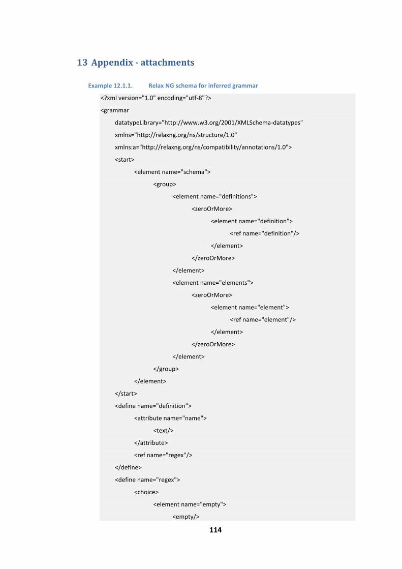
114
13 Appendix - attachments
Example 12.1.1. Relax NG schema for inferred grammar
<?xml version="1.0" encoding="utf-8"?>
<grammar
datatypeLibrary="http://www.w3.org/2001/XMLSchema-datatypes"
xmlns="http://relaxng.org/ns/structure/1.0"
xmlns:a="http://relaxng.org/ns/compatibility/annotations/1.0">
<start>
<element name="schema">
<group>
<element name="definitions">
<zeroOrMore>
<element name="definition">
<ref name="definition"/>
</element>
</zeroOrMore>
</element>
<element name="elements">
<zeroOrMore>
<element name="element">
<ref name="element"/>
</element>
</zeroOrMore>
</element>
</group>
</element>
</start>
<define name="definition">
<attribute name="name">
<text/>
</attribute>
<ref name="regex"/>
</define>
<define name="regex">
<choice>
<element name="empty">
<empty/>

115
</element>
<element name="element">
<attribute name="name">
<text/>
</attribute>
<optional>
<attribute name="type">
<text/>
</attribute>
</optional>
</element>
<element name="optional">
<ref name="regex"/>
</element>
<element name="zeroOrMore">
<ref name="regex"/>
</element>
<element name="oneOrMore">
<ref name="regex"/>
</element>
<element name="choice">
<group>
<ref name="regex"/>
<oneOrMore>
<ref name="regex"/>
</oneOrMore>
</group>
</element>
<element name="group">
<group>
<ref name="regex"/>
<oneOrMore>
<ref name="regex"/>
</oneOrMore>
</group>
</element>
</choice>
</define>

116
<define name="element">
<attribute name="ofType">
<text/>
</attribute>
<element name="location">
<ref name="location"/>
</element>
</define>
<!-- Location serves to locate elements in XML document and to identify their type without the need to define grammar for the whole XML-->
<define name="location">
<element name="parent">
<choice>
<group>
<attribute name="name">
<text/>
</attribute>
<optional>
<ref name="location"/>
</optional>
</group>
<element name="none">
<empty/>
</element>
</choice>
</element>
</define>
</grammar>
Relax NG schema for our inferred grammar.