school bus idling and mobile diesel emissions testing
TRANSCRIPT
Rowan University Rowan University
Rowan Digital Works Rowan Digital Works
Theses and Dissertations
10-31-2003
School bus idling and mobile diesel emissions testing: effect of School bus idling and mobile diesel emissions testing: effect of
fuel type and development of a mobile test cycle fuel type and development of a mobile test cycle
Jason Scott Hearne Rowan University
Follow this and additional works at: https://rdw.rowan.edu/etd
Part of the Mechanical Engineering Commons
Recommended Citation Recommended Citation Hearne, Jason Scott, "School bus idling and mobile diesel emissions testing: effect of fuel type and development of a mobile test cycle" (2003). Theses and Dissertations. 1319. https://rdw.rowan.edu/etd/1319
This Thesis is brought to you for free and open access by Rowan Digital Works. It has been accepted for inclusion in Theses and Dissertations by an authorized administrator of Rowan Digital Works. For more information, please contact [email protected].
School Bus Idling and Mobile Diesel Emissions Testing: Effectof Fuel Type and Development of a Mobile Test Cycle
Jason Scott Hearne
A THESIS
PRESENTED TO THE FACULTY
OF ROWAN UNIVERSITY
IN CANDIDACY FOR THE DEGREE
OF MASTER OF SCIENCE
RECOMMENDED FOR ACCEPTANCE
BY THE DEPARTMENT OF MECHANICAL ENGINEERING
COLLEGE OF ENGINEERING
October 2003
School Bus Idling and Mobile Diesel Emissions Testing: Effect of Fuel
Type and Development of a Mobile Test Cycle
Prepared by:
Jason Scott Hearne
Approved by:
Professor Anthony J. Marchese
Rowan University
Thesis Advisor
Professor Robert P. Hesketh
Rowan University
Thesis Reader
Professor H. Clay Gabler
Rowan University
Thesis Reader
Professor John C. Chen
Chair, Mechanical Engineering
Rowan University
ii

© Copyright by Jason Hearne, 2003. All rights reserved.
iii.
111

ABSTRACT
The New Jersey Department of Transportation (NJDOT) is currently sponsoring a
research study at Rowan University to develop strategies for reducing diesel emissions
from mobile sources such as school buses and class 8 trucks (classified as a heavy- duty
truck of more than 33,000 lbs.). This thesis presents the results of an investigation
performed to measure school bus idle emissions in a controlled environmental chamber.
This thesis also presents the results of mobile school bus testing that has been performed
to quantify the emission reduction capabilities of various alternative fuels, such as
biodiesel, ultra low sulfur diesel, and a blend of the two, when used to fuel school buses
that are representative of those currently in use in the state of NJ.
To measure emissions from school buses during idling conditions, three school
buses equipped with an International T444E, an International DT466E, and a Cummins
5.9L B series engine were instrumented and tested at the Aberdeen Test Center at the
Aberdeen Proving Grounds in Maryland. To simulate a wide variety of idling situations,
tests were conducted at four different ambient temperatures (20°F, 40°F, 65°F and 85°F)
and relative humidity ranging from 37 to 90%. In addition to quantifying school bus
emissions during idling conditions, another objective of the school bus idling experiments
was to develop a NOx humidity correlation for use in mobile school bus emissions
testing, the first phase of which is presented herein. The results of the idle testing provide
evidence that the measured CO emissions decrease from 10% to 40% with increasing
ambient temperature. The measured NOx emissions under similar conditions vary by
school bus and therefore a single correlation could not be developed that accurately
corrects NOx emission for all three buses. Rather, an engine specific correction factor
was developed for each school bus engine. The results also show that current NOx
correction standards fail at lower temperatures suggesting that caution should be used
when performing mobile emissions testing.
To ensure repeatability of testing under conditions that accurately reproduce actual
school bus operating conditions, a new composite mobile school bus cycle was
developed. The cycle was developed by acquiring Global Positioning System (GPS) data
from actual school bus routes from 5 different municipalities within the state of New
iv
Jersey.
For both the mobile and idle tests, exhaust gas emission measurements were made
using a Sensors Semtech-D to measure CO, CO2, NO2 , NO, 02, and HC, along with a
Sensors PM-300 to measure Particulate Matter. In addition to the exhaust emissions
measurements, operating parameters such as instantaneous vehicle speed, engine speed,
percent load and fuel flow rate were acquired from the engine electronic control module
(ECM) during testing.
The mobile emissions results presented in this thesis focus mainly on a comparison
of alternative fuels on mobile emissions acquired during the new mobile test cycle that
was developed as part of this study. The results of the mobile testing prove that the
Rowan University Composite School Bus Cycle (RUCSBC) is a repeatable mobile test
cycle when run during the same operating conditions. The results of mobile testing show
a decrease in HC emissions for the alternative fuels tested for all buses of 7% to 43%.
NOx emissions were only slightly affected by alternative fuels by 0% to 10%. A 20%
biodiesel blend and ultra low sulfur diesel reduced CO and PM emissions by 30% to 40%
for the T444E and Cummins, but showed no affect on the DT466E bus. The ultra low
sulfur diesel and biodiesel blend provided significant reductions in CO and PM by 70%
and 50%, respectively, for the T444E and a 22% reduction in PM for the DT466E.
Finally, in addition to the tests conducted at the Aberdeen Testing Center (ATC), a
series of on-road tests were performed using school buses presently in service on actual
operating routes. Specifically, four International DT466E school buses were tested at the
Medford, New Jersey School District, a district that has been operating half of their
school bus fleet on biodiesel for the past five years.
v

For Mom and Dad, Family, and Danielle.
vi
ACKNOWLEDGEMENTS
My sincerest thanks to my graduate advisors, Dr. Anthony Marchese and Dr. Robert
P. Hesketh. This thesis could not have been completed without their knowledge, support,
and guidance throughout the entire project. Also I would like to extend extreme
appreciation to the project sponsor, NJDOT, and project manager Henry Schweber.
Added thanks to Dr. Gabler and Dr. Hesketh for reading this thesis. I would also like to
thank all of the Aberdeen, Maryland testing staff, especially Todd Morris (T' Mo) for all
he contributed to the project.
I would also like to thank Gil and Carol Hearne, my parents, and the rest of my
family for understanding that time away from home was well spent. A special thanks
goes out to my friends for their continued support, especially my Holly Court roommate
Lew Clayton, my officemate Doug Gabauer, my teammate Andy Toback, and my
overseas warrior Dan Peterson. And finally, I would like to thank my beautiful and
loving girlfriend Danielle Baldwin, who has kept me in line for the over a year now and
will hopefully continue to do so.
vii
TABLE OF CONTENTS
A bstract ........................ ....................................................... iv
D edication .................. ...................................................................... vi
A cknow ledgm ents.................................................................................. ii
Table of C ontents .................... . ..... .... ... .. ... ........................ viii
List of Figures ..... .. .. ......... ... ... ..... .................................. xi
L ist of T ables ................... .... ... .. ..... ... ..... ............................. xiii
1. Introduction................................................................................................................. 11.1. B ackground ......................................................................................................... 11.2. Literature Search ................................................................................................ 31.3. G oal of Study .................................................................................................... 6
1.3.1. Project Sponsor NJDOT ................................................ 61.3.2. State Implementation Plan ..................................................................... 6
1.3.3. Project Research Team - Rowan University............................................... 7
1.4. Emissions/ Emission Measurement ......................................... .. 81.4.1. Diesel Emissions ..................................................... 8
1.4.2. EPA Diesel Emissions Regulation History ............................................ 101.4.3. Units of Measure for Emissions.............................................................. 13
1.4.4. Em issions Testing ................................................................................... 151.4.4.1. Engine Dynamometer Emissions Testing ........................................ 151.4.4.2. Chassis Dynamometer Emissions Testing ........................................ 171.4.4.3. Mobile In-Use Emissions Testing..................................................... 20
1.5. Diesel Emission Reduction Strategies .............................................................. 221.5.1. A lternative Fuels ....................................................................................... 231.5.2. P articulate T raps ....................................................................................... 26
1.6. Thesis O rganization .......................................................................................... 302. Experimental Procedure and Equipment .................................................................. 32
2.1. Introduction ...................................................................................................... 322.2. Rationale for School Bus Selection .................................................................. 32
2.2.1. School Bus Types in N J............................................................................ 322.2.2. Engine Specifications................................................................................ 35
2.2.2.1. 1997 International T-444E ................................................................ 352.2.2.2. 1997 International DT-466E ............................................................. 36
viii
2.2.2.3. 1996 Ford Cum m ins 5.9 L ISB Series .............................................. 37
2.3. A berdeen Test Center ....................................................................................... 41
2.3.1. Test Track ................................................................................................. 41
2.3.2. Environm ental Testing Cham ber .............................................................. 41
2.3.3. Chem istry Lab........................................................................................... 42
2.4. Bus Instrum entation .......................................................................................... 43
2.4.1. Instrum entation Table ............................................................................... 44
2.4.2. Electronic Control M odule (ECM ) ........................................................... 45
2.4.3. Sensors Inc. Sem tech-D ............................................................................ 47
2.4.4. Sensors Inc. PM -300................................................................................. 56
2.4.5. AD O CS A TC D ata A cquisition System ................................................... 58
2.4.6. D ata M anagem ent ..................................................................................... 59
3. Development of a New Mobile Emissions Test Cycle for School Buses ............. 61
3.1. Introduction....................................................................................................... 61
3.2. Literature Review .............................................................................................. 62
3.3. Procedure for Generating a New Mobile Cycle... . .................... 66
3.3.1. Types of School D istricts /Regions........................................................... 67
3.3.2. GPS M apping: Experim ental Procedure ................................................... 70
3.3.3. D ata Reduction/Cycle D evelopm ent......................................................... 73
4. Rowan On Road Medford Township School Bus Testing........................................ 81
4.1. Introduction....................................................................................................... 81
4.2. Purpose of M edford Study ................................................................................ 81
4.3. Medford School District Biodiesel Program . ................. 82
4.4. Experimental Setup: Test Procedure.................................................................84
4.5. Test Results ....................................................................................................... 85
4.5.1. M edford Fuel Consum ption/Total W ork .................................................. 85
4.5.2. M edford Em issions ................................................................................... 88
5. School Bus Idle Em issions........................................................................................ 93
5.1. Introduction....................................................................................................... 93
5.2. Literature Search ............................................................................................... 94
5.2.1. H D D V Study............................................................................................. 94
5.2.2. School Bus Idling...................................................................................... 96
5.3. Experim ental Procedure: Test M atrix ............................................................... 96
5.4. Test Results ....................................................................................................... 99
5.4.1. Fuel consum ption...................................................................................... 99
5.4.2. Em issions ................................................................................................ 100
ix
5.4.2.1. CO2 Emissions ................................................................................ 1025.4.2.2. CO Emissions.................................................................................. 1035.4.2.3. NOx Emissions ................................................................................ 104
5.4.2.4. HC Emissions.................................................................................. 1065.4.2.5. PM Emissions ................................................................................. 1075.4.2.6. Experimental Results -NOx correction.......................................... 108
6. School Bus M obile Emissions Testing (ATC).................................................. 1146.1. Introduction..................................................................................................... 1146.2. Experimental Procedure: Test M atrix ............................................................. 1146.3. Test Results ..................................................................................................... 115
6.3.1. Raw data and NOx Correction Factors .................................................... 1176.3.2. T444E Emissions ........................................................................... .. ....... 1206.3.3. DT466E Emissions ................................... ..... ...................... 122
6.3.4. Cummins 5.9L Emissions ....................................................................... 1246.3.5. Mobile Emission Test Results (g/bhp-hr) ............................................... 126
7. Conclusions and Future W ork . . ... ............................................................ 1287.1. Conclusions..................................................................................................... 128
7.1.1. Idle . ......................................................................................................... 1287.1.2. Mobile ..................................................................................................... 1297.1.3. Thesis . ..................................................................................................... 130
7.2. Future W ork .................................................................................................... 1318. R eferences ............................................................................................................... 133
x
LIST OF FIGURES
Figure 1: US EPA Emissions Standards Timeline for HDDV's for NOx and HC ........... 12
Figure 2: US EPA Emissions Standards Timeline for HDDV's for PM........................... 13
Figure 3: Engine dynamometer in-use ............................................................................. 17
Figure 4: Water brake dynamometer installed in ground ................................................. 19
Figure 5: Schematic of a diesel particulate filter .............................................................. 27
Figure 6: Johnson Matthey CRT diesel particulate filter.................................................. 28
Figure 7: International T-444E diesel engine ................................................................... 36
Figure 8: International DT-466E diesel engine ............................................................... 36
Figure 9: Cummins 5.9 L B Series diesel engine.............................................................. 37
Figure 10: T-444E engine lug curve ................................................................................. 38
Figure 11: DT-466E engine lug curve .............................................................................. 39
Figure 12: Cummins 5.9 L engine lug curve .................................................................... 40
Figure 13: Environmental testing chamber 4.................................................................... 42
Figure 14: Sensors inc. Semtech-D mobile emissions analyzer ....................................... 48
Figure 15: Internal layout of Semtech-D unit 54 ................................................................ 48
Figure 16: Sensor's Inc. PM-300 particulate analyzer ...................................................... 57
Figure 17: Excel graph of PM data separated by bins ...................................................... 58
Figure 18: ADvanced Onboard Computer System (ADOCS) .......................................... 59
Figure 19: City Suburban Heavy Vehicle Route .............................................................. 64
Figure 20: Central Business District Cycle....................................................................... 66
Figure 21: New Jersey Population Breakdown by Urban and Rural Regions62 ............... 70
Figure 22: G arm in GPSM AP76S...................................................................................... 71
Figure 23: Pittsgrove Township GPS Map ....................................................................... 72
Figure 24: Pittsgrove School District velocity vs. time profile ........................................ 73
Figure 25: The Rowan University Composite School Bus Cycle ................................... 77
Figure 26: Rowan University Cycle Separated by Representative Regions ..................... 77
Figure 27: Speed Trace of Two Separate Runs of the RUCSBC .................................... 79
Figure 28: Speed Trace of Two Separate Runs of the RUCSBC (Reduced Axis)........... 79
Figure 29: NOx Concentration Trace of Two Separate Runs of the RUCSBC ................ 80
xi
Figure 30: NOx Concentration Trace of Two Separate Runs of the RUCSBC (Reduced
A x is).......................................................................................................................... 8 0
Figure 31: Medford Township's biodiesel operated school bus fleet............................... 83
Figure 32: Medford biodiesel storage tank ........................................ .................... 83
Figure 33: Speed Trace of Simulated Medford School Bus Route................................... 85
Figure 34: Fuel Consumption for Medford school buses tested ....................................... 85
Figure 35: Work for Medford school buses tested............................................................ 87
Figure 36: Fuel Consumption as a function of work for Medford school buses tested.... 88
Figure 37: Average emissions results for the 4 different Medford buses tested ............... 90
Figure 38: Typical NOx emissions during a test ............................................................... 98
Figure 39: Fuel consumption rates for the three buses tested ......................................... 100
Figure 40: Measured CO 2 emissions during idling for school bus with DT466E engine.
.................................................................................................................................. 10 2
Figure 41: Effect of ambient temperature on CO emissions.......................................... 103
Figure 42: NOx emissions during idling conditions for school bus with T444E engine. 104
Figure 43: NOx emissions during idling conditions for school bus with DT466E engine.
............ .... ... ............. ....... ... . .... ...................... ........ 10 5
Figure 44: NOx emissions during idling conditions for school bus with Cummins 5.9 L
engine ...................................................................................................................... 105
Figure 45: Effect of ambient temperature on HC emissions........................................... 106
Figure 46: Uncorrected NOx emissions (ppm) for the school bus with DT466E engine.
.................................................................................................................................. 1 10
Figure 47: Corrected NOx emissions using the SAE J1243 correction factor ............... 111
Figure 48: Corrected NOx emission data using the CFR40 86.1342-90 ......................... 111
Figure 49: Engine specific corrected NOx emissions for the DT466E .......................... 112
Figure 50: Raw emissions data from RUCSBC............................................................. 116
Figure 51: Raw NOx emissions data correction factor comparison for T444E .............. 118
Figure 52: Average mobile emissions results for the International T444E .................... 121
Figure 53: Average mobile emissions results for the International DT466E ................. 123
Figure 54: Average mobile emissions results for the Cummins 5.9L............................. 125
xii

LIST OF TABLES
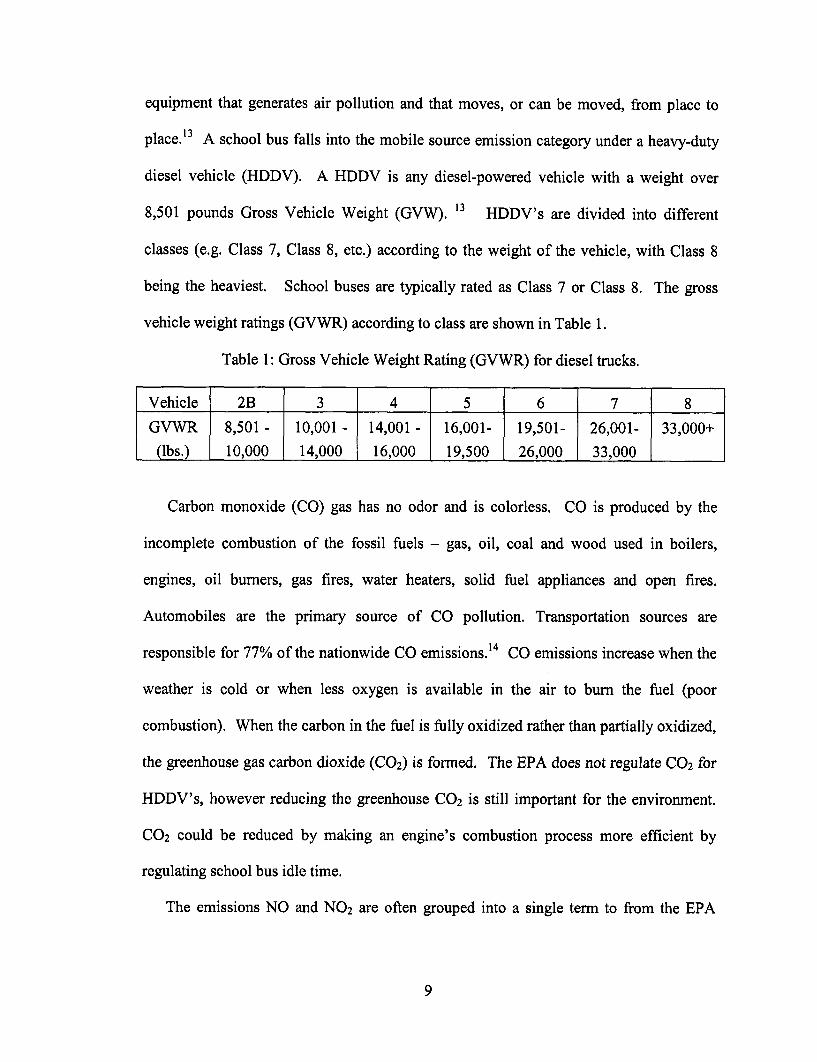
Table 1: Gross Vehicle Weight Rating (GVWR) for diesel trucks ................................... 9
Table 2: EPA Emission Standard History for HDDV's.................................................... 13
Table 3: Engine types used in NJ School Districts ........................................................... 33
Table 4: Engine selection for school bus emissions testing.............................................. 35
Table 5: School bus emissions testing instrumentation ................................................... 44
Table 6 Prototypical NJ School Bus Districts6 2' .............................................................. 69
Table 7: Statistical Information on Microtrip Categories ............................................... 74
Table 8: Microtrip Times for a Cycle with a Minimum of 20 Minutes ............................ 76
Table 9: Vehicle and engine data for Medford school buses investigated ..................... 84
Table 10: Medford fuel consumption and work ............................................................... 88
Table 11: Vehicle and testing condition parameters for the four different Medford buses
tested ........................................................................................................................... 8 9
Table 12: Average emissions results for the four different Medford buses tested measured
in g/m ile...................................................................................................................... 89
Table 13: Average emissions results for the four different Medford buses tested measured
in g/bhp-hr and ppm concentration ...................................................... 89
Table 14: Environmental test matrix for each bus ............................................................ 97
Table 15: Emission results from environmental chamber testing................................... 101
Table 16: Average PM for the three bus engines tested ............................................... 107
Table 17: Engine specific values for SAE 1243 correlation........................................... 113
Table 18: Test m atrix for each school bus ...................................................................... 115
Table 19: Fuel properties for fuels tested at ATC........................................................... 116
Table 20: Average concentrations and various NOx corrections for T444E .................. 118
Table 21: Average concentrations and various NOx corrections for DT466E................ 119
Table 22: Average concentrations and various NOx corrections for Cummins .............. 120
Table 23: Alternative fuel reductions in emission levels when compared to #2 diesel.. 122
Table 24: Alternative fuel reductions in emission levels when compared to #2 diesel.. 124
Table 25: Alternative fuel reductions in emission levels when compared to #2 diesel.. 126
Table 26: Comparison of test results with 2007 standards ............................................. 127
xiii
1. Introduction
1.1. Background
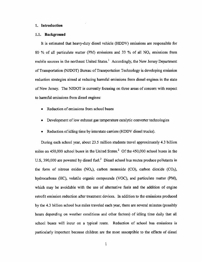
It is estimated that heavy-duty diesel vehicle (HDDV) emissions are responsible for
80 % of all particulate matter (PM) emissions and 33 % of all NOx emissions from
mobile sources in the northeast United States.' Accordingly, the New Jersey Department
of Transportation (NJDOT) Bureau of Transportation Technology is developing emission
reduction strategies aimed at reducing harmful emissions from diesel engines in the state
of New Jersey. The NJDOT is currently focusing on three areas of concern with respect
to harmful emissions from diesel engines:
* Reduction of emissions from school buses
* Development of low exhaust gas temperature catalytic converter technologies
* Reduction of idling time by interstate carriers (HDDV diesel trucks).
During each school year, about 23.5 million students travel approximately 4.3 billion
miles on 450,000 school buses in the United States. 2 Of the 450,000 school buses in the
U.S, 390,000 are powered by diesel fuel.3 Diesel school bus routes produce pollutants in
the form of nitrous oxides (NOx), carbon monoxide (CO), carbon dioxide (CO2),
hydrocarbons (HC), volatile organic compounds (VOC), and particulate matter (PM),
which may be avoidable with the use of alternative fuels and the addition of engine
retrofit emission reduction after treatment devices. In addition to the emissions produced
by the 4.3 billion school bus miles traveled each year, there are several minutes (possibly
hours depending on weather conditions and other factors) of idling time daily that all
school buses will incur on a typical route. Reduction of school bus emissions is
particularly important because children are the most susceptible to the effects of diesel
1
emissions, which can cause respiratory disease and bring about long-term conditions such
as asthma.3
The current emissions regulations for school buses are lenient enough that newer
school buses are able to operate legally with no after treatment devices or alternative
fuels sources. In 2004 and again in 2007, more stringent emission standards are being
put in place by the federal government that will mandate the use of some after treatment
for new HDDV's in order to meet the new standards. NJ regulations that mandate school
buses to be in service for a maximum of twelve years allows for school bus engines
manufactured before 2007 to possibly remain in service until 2019 without complying
with the 2007 standards. Many state organizations, engine manufactures, universities,
and research facilities are conducting research projects to find the most inexpensive and
effective way to meet the new standards before they are put into place in the upcoming
years.
This thesis presents results of an experimental study aimed at evaluating emission
reduction strategies for diesel powered school buses. Three school buses, which were
purchased by NJDOT, were instrumented and tested at the U.S. Army Aberdeen Test
Center (ATC). The most advanced mobile emission measurement equipment was
purchased to measure the harmful emission levels from the school buses. The school
buses were tested using a mobile test cycle, developed as part of the study and described
in this thesis.
There is currently a lack of mobile testing cycles for school buses, so a NJ composite
school bus mobile testing cycle, the Rowan University Composite School Bus Cycle
(RUCSBC) was created for the testing. A variety of fuel types were tested to determine
2
the cleanest burning fuel type for the NJ school bus duty cycle (e.g. rural, urban, etc.) that
was developed. Previous research in the heavy-duty diesel emission reduction field has
been conducted in research labs on engine and/or chassis dynamometers. Testing for this
project was conducted entirely with the vehicle mobile or on-road on a test track at the
Aberdeen Testing Center running the RUCSBC. Another important aspect of this
research is to gain an understanding on how temperature and humidity effects emissions,
specifically NOx. In the following section, a review of prior literature is presented.
1.2. Literature Search
In recent years several experimental and theoretical studies have been performed on
diesel emission reduction strategies. Each of these studies has focused on emission
reduction strategies by performing tests on a chassis or an engine dynamometer. The
majority of previous studies were mainly performed on different HDDV's other than
school buses. The few previous studies on school buses did not use testing cycles that
were initially developed for school bus operation. This thesis presents the results of a
new experimental mobile emission reduction study using a newly developed school bus
mobile testing cycle. A review of several previous emissions studies is provided in the
following sections.
As stated previously, there has been only a limited number of school bus emission
studies ever reported in the literature. One of the first school bus emissions studies took
place in 1978 and evaluated tailpipe CO emissions only. 4 In this earlier study, school
buses were tested for CO levels over a 10-month evaluation period to determine whether
or not there were any serious CO intrusion problems or indications of potential problems
on a small sample of the nation's school buses. Test results from the study showed, based
3
on a maximum safe exposure level of 20 ppm, that 7.2% of the buses tested exceeded this
level, and 5.4% of the buses tested had maximum CO readings over 50 ppm.
In 1995, the Northeast Florida Regional Planning Council, together with the National
Biodiesel Board compared four alternative fuel sources to # 2 diesel in one of the sector
school bus fleets. 5 These tests did not consider varying weather conditions or any direct
comparison of a bus running identical cycles. The alternative fuels tested in this study
were: biodiesel (B20 and B100), compressed natural gas (CNG), liquefied natural gas
(LNG) and liquefied petroleum gas (LPG). The study concluded that relative to diesel,
each of the four fuels tested had significantly lower emissions. B20 reduced CO and PM
by 12 % and HC by 20 %. B100 reduced CO and PM by 50 % and HC by 70 %. This
study also showed biodiesel resulted in significant reductions of unburned HC, CO, and
PM. NOx emissions stayed the same or were slightly increased. The study concluded that
biodiesel blends could compete effectively with other alternative fuels when life cycle,
total fleet costs are considered.
Another study conducted in 1997, and followed up in 1999, evaluated diesel
emissions, from a variety of vehicle classes several of which were school buses. The
study evaluated the initial effects of a retrofitted diesel oxidation catalyst technology and
also the effects of the device two-years later. In this study chassis dynamometer
emissions testing and in-use emissions testing were employed with and without a
retrofitted catalyst technology using the New York Composite and Central Business
District cycles, further detailed in Chapter 3.6 The results of the study found that the
diesel oxidation catalyst reduced total PM by 20 to 50 %, CO by 45 to 93 %, and HC by
50 to 90 %.
4
In another study, West Virginia University characterized the emissions of a fleet of
school buses in Indio, Ca. In this fleet, both 8.3 L Cummins natural gas engines and
conventional 8.3 L diesel engines were tested. Their results showed that the natural gas
engines had lower emissions in PM and NOx (46 % and 12 %, respectively), but higher
emissions of HC (50 %) compared to the diesel engine.7 A remote sensing study of CO
and HC emissions from school buses was initiated to develop emissions factors but
results of this study have not been reported.8
The most recent study involving school buses was completed by collaboration
between ARCO, West Virginia University, Johnson Matthey, and Engelhard. 9 The
program evaluated ultra-low-sulfur diesel fuels and passive diesel particulate filters
(DPFs) in truck and bus fleets operating in southern California. In this study exhaust
emissions, fuel economy and operating cost data were collected for the test vehicles, and
compared with baseline control vehicles. The evaluation of exhaust emissions took place
prior to testing and also one year after installation of the filters. For all fleets tested
including school buses, the test vehicles retrofitted with the DPFs reduced PM emissions
by more than 90% when operated on ULSD when compared to the control vehicles
having factory mufflers and operated on a typical California diesel fuel.
The San Diego School Bus Pilot program is currently testing 30 school buses. Five of
the 30 buses are equipped with the Johnson-Matthey CRT filter and the other five buses
are fitted with the competing Engelhard DPX filter technology. The second part of the
California school bus pilot program is using a test fleet of 39 school buses from the Los
Angeles Unified School District, the Anaheim Union High School district, and the Hemet
Unified School district. In this program, 13 buses have been retrofitted with Johnson-
5
Matthey CRT filter system, thirteen buses retrofitted with Englehard DPX filter
technology and at least one with Ceryx Quadcat system. The remaining buses are using
low-sulfur ECD diesel fuel and no filter system.' 0
1.3. Goal of Study
1.3.1. Project Sponsor NJDOT
NJDOT is committed to the support and implementation of air quality friendly
transportation projects and programs and is continually looking for new strategies and
initiatives that could provide emission reduction benefits. Through studies conducted by
various agencies, NJDOT recognizes the potential value of the reduction of mobile and
idle emissions from school buses in its efforts to support and implement air quality
friendly projects. A grant from NJDOT is responsible for the work conducted on the
emission reduction study by a team of Rowan University faculty and students.
1.3.2. State Implementation Plan
In response to the Section 109 of the Clean Air Act, the US Environmental Protection
Agency (USEPA) established the National Ambient Air Quality Standards (NAAQS).
The NAAQS monitors various pollutants, known as "criteria" pollutants, which adversely
affect human health (primary) and welfare (secondary). The primary and secondary
transportation-related criteria pollutants include Ozone (03) and its precursors, lead,
volatile organic compounds (VOC) and oxides of nitrogen (NOx), particulate matter
(PM), sulfur dioxide (SO 2), and carbon monoxide (CO).
Each state is required to submit to the EPA a State Implementation Plan or SIP, which
is a collection of strategies/ commitments that explain how the State will achieve the air
quality standards, set by the Federal Clean Air Act. In New Jersey, the Department of
6
Environmental Protection (NJDEP) is the agency responsible for assembling and
submitting the SIP to the USEPA. The SIP includes strategies and commitments for
stationary (factories, etc) and mobile (on and off-road vehicles, auto inspections, etc.)
sources. The New Jersey Department of Transportation (NJDOT) provides input to the
mobile source portion of the SIP.
New Jersey is regulated under region 2 air quality standards, which also includes New
York, Puerto Rico, and the Virgin Islands. Region 2 is one of the most urban regions
found in the Unites States. Approximately 30 million residents are concentrated in the
Region 2 urban areas, in which 85 percent of the 30 million live in New York and New
Jersey, mainly in the New York - New Jersey metropolitan area". When the NJDEP
produces a draft of the SIP that contains proposed strategies for improved air quality they
first propose the SIP in a public process. The next step is to formally adopt the SIP and
submit it the USEPA for approval to the Code of Federal Regulations (Title 40, Part
52)12. After approval by the USEPA the state's SIP becomes federally enforceable.
1.3.3. Project Research Team - Rowan University
The main goal of the Rowan University research team was to provide NJDOT with
adequate results to formulate an effective SIP. The project also will act as a foundation
for future emission related projects presented to Rowan University in the future. The
Rowan University research team was responsible for researching emissions reduction
literature, obtaining the test vehicles, researching reduction strategies, providing testing
instrumentation and the reduction strategies, analyzing the data collected from the ATC
personnel testing the buses, and finally recommending the most effective emission
reduction strategies to the NJDOT. To date the project has produced two master theses
7
for Rowan Engineering graduate students, five Society of Automotive Engineers (SAE)
conference papers, and provided an engineering clinic projects for eleven undergraduate
students for three semesters. During this time, students were given the opportunity to
travel to a remote testing facility at the U.S. Army Aberdeen Test Center where
instrumentation and testing of the school buses occurred.
1.4. Emissions/ Emission Measurement
This research focuses on the EPA regulated emissions from HDDV's: CO, NOx, HC,
and PM. In addition, the greenhouse gas CO2 is also examined. The EPA has regulated
HDDV emissions since 1970, and has since slowly reduced the allowable level of each
pollutant to the future standards of 2007. School buses stay in a school district's fleet for
a maximum of 13 years by law, so by 2007 school buses from as early as 1994 could still
be operating in a district's fleet. All emission testing takes place using a testing system
such as an engine dynamometer, chassis dynamometer, or mobile in-use emissions. When
testing using these different systems the units used to analyze the experimental data
becomes an important factor in developing conclusions. The research presented herein,
focuses on experimental data taken from mobile in-use emissions testing, however it
should be noted that the other two methods of testing (engine and chassis) have
advantages and disadvantages that are relevant to consider when forming conclusions.
1.4.1. Diesel Emissions
Mobile sources contribute significantly to air pollutants such as carbon monoxide CO,
carbon dioxide CO2, nitrogen oxide NO, nitrogen dioxide NO2 , particulate matter PM,
and hydrocarbons HC. A mobile source is defined as any variety of vehicle, engine, or
8
equipment that generates air pollution and that moves, or can be moved, from place to
place. 3 A school bus falls into the mobile source emission category under a heavy-duty
diesel vehicle (HDDV). A HDDV is any diesel-powered vehicle with a weight over
8,501 pounds Gross Vehicle Weight (GVW). 13 HDDV's are divided into different
classes (e.g. Class 7, Class 8, etc.) according to the weight of the vehicle, with Class 8
being the heaviest. School buses are typically rated as Class 7 or Class 8. The gross
vehicle weight ratings (GVWR) according to class are shown in Table 1.
Table 1: Gross Vehicle Weight Rating (GVWR) for diesel trucks.
Vehicle 2B 3 4 5 6 7 8
GVWR 8,501 - 10,001 - 14,001 - 16,001- 19,501- 26,001- 33,000+
(lbs.) 10,000 14,000 16,000 19,500 26,000 33,000
Carbon monoxide (CO) gas has no odor and is colorless. CO is produced by the
incomplete combustion of the fossil fuels - gas, oil, coal and wood used in boilers,
engines, oil burners, gas fires, water heaters, solid fuel appliances and open fires.
Automobiles are the primary source of CO pollution. Transportation sources are
responsible for 77% of the nationwide CO emissions.'4 CO emissions increase when the
weather is cold or when less oxygen is available in the air to bur the fuel (poor
combustion). When the carbon in the fuel is fully oxidized rather than partially oxidized,
the greenhouse gas carbon dioxide (CO2) is formed. The EPA does not regulate CO2 for
HDDV's, however reducing the greenhouse CO 2 is still important for the environment.
CO2 could be reduced by making an engine's combustion process more efficient by
regulating school bus idle time.
The emissions NO and NO2 are often grouped into a single term to from the EPA
9
regulated emission NOx, or oxides of nitrogen. The EPA regulates NOx emissions as a
whole and does not regulate individual oxides of nitrogen. NOx emissions are produced
during the combustion of fuels at high temperatures. 14 NOx is formed from a variety of
mobile highway sources (e.g. HDDV's), non-road sources (e.g. marine and locomotives)
and stationary sources (e.g. factories and power plants). Prior research has shown that at
higher ambient and combustion temperatures there is an increase in NOx. Hydrocarbons
(HC) are produced differently with increasing combustion temperature than NOx;
increasing combustion temperature will lower HC emissions. HC emissions result from
when fuel molecules in the engine do not bur or bur only partially.
The final regulated emission by the EPA is particulate matter (PM). PM is
microscopic particles or liquid droplets suspended in the air that can contain a variety of
chemical components. Low combustion temperatures and non-stoichiometric oxygen
conditions result in incompletely burned fuel, and various concentrations of particulates
largely of carbon composition. These particulates consist of elemental carbon (EC),
organic carbon (OC), metals from fuel and engines wear, and sulfates with bound water.
15,16 The National Ambient Air Quality Standard (NAAQS) for particulates are divided
into two size groupings. For particulate matter less than 10 ptm, the NAAQS limits the
annual average of particulates to 50 plg/m 3 and the 24 hour average to 150 4Lg/m 3. For
particulate matter 2.5 pm and smaller the NAAQS annual average is 15 pg/m3 and the 24
hour average is 65 4tg/m 3 .
1.4.2. EPA Diesel Emissions Regulation History
Since diesel engine emissions have been classified by the International Agency for
Research on Cancer as a Group 2A carcinogen (probably carcinogenic to Humans) the
10
EPA began regulating emissions. 17 Since 1970 the EPA has been regulating certain
emissions from HDDV (including school buses). The EPA regulates the following
pollutants from mobile sources:
* Total Hydrocarbons (HC)
* Oxides of nitrogen (NOx)
* Particulate matter (PM)
* Carbon monoxide (CO)
From 1970 to 1974 however, only opacity levels of smoke for acceleration and lugging
(laboring the engine in too high a gear) were regulated. In 1974, CO and a combined HC
+ NOx regulation were put into effect as well as tighter smoke standards. Combining HC
and NOx emissions were an attempt to ease the transition into regulated emissions for
engine manufacturers. The CO limit was introduced at 40 g/bhp-hr and the HC + NO,
was introduced at 16 g/bhp-hr. The emissions standards again tightened in 1979 with CO
emission levels tightened to 25 g/bhp-hr. Also in 1979, a choice of 5 g/bhp-hr HC + NO,
or HC of 1.5 g/bhp-hr combined with a 10 g/bhp-hr HC + NOx was introduced for the
first time.
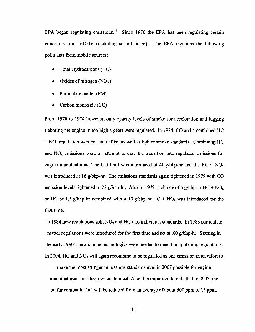
In 1984 new regulations split NOx and HC into individual standards. In 1988 particulate
matter regulations were introduced for the first time and set at .60 g/bhp-hr. Starting in
the early 1990's new engine technologies were needed to meet the tightening regulations.
In 2004, HC and NOx will again recombine to be regulated as one emission in an effort to
make the most stringent emissions standards ever in 2007 possible for engine
manufacturers and fleet owners to meet. Also it is important to note that in 2007, the
sulfur content in fuel will be reduced from an average of about 500 ppm to 15 ppm,
11

which will also be helpful when using particulate traps that require ultra low sulfur fuel.
Figure 1 and Figure 2 show the EPA emission standard timelines from 1974 to model
year 2007 for NOx, HC, and a HC and NOx combination and a timeline for PM,
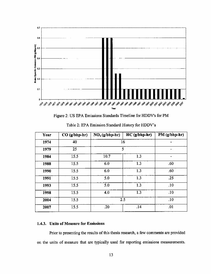
respectively. A complete listing of emission regulations since 1970 is shown in Table 2.
ONOx + HC
F1 6
gure 1: US| EI E|-----issions--Standards------------for----- f mNOx
SHC
14
& 12
. 10l
EUJ
8
0.V)
6m
4
Year
Figure 1: US EPA Emissions Standards Timeline for HDDV's for NOx and HC
12
0.6
D. U.I-
. 0.4.2
EUJ ...
E
V u,a A
0.1
0
Year
Figure 2: US EPA Emissions Standards Timeline for HDDV's for PM
Table 2: EPA Emission Standard History for HDDV's
Year CO (g/bhp-hr) NO, (g/bhp-hr) HC (g/bhp-hr) PM (g/bhp-hr)
1974 40 16
1979 25 5
1984 15.5 10.7 1.3
1988 15.5 6.0 1.3 .60
1990 15.5 6.0 1.3 .60
1991 15.5 5.0 1.3 .25
1993 15.5 5.0 1.3 .10
1998 15.5 4.0 1.3 .10
2004 15.5 2.5 .10
2007 15.5 .20 .14 .01
1.4.3. Units of Measure for Emissions
Prior to presenting the results of this thesis research, a few comments are provided
on the units of measure that are typically used for reporting emissions measurements.
13
II
*
VA
--
F-----By
I -
IIII IIII[ILr T7I . . . . . I . . I I / I , I I T. . I . I I III. I . . . . .

Results from emissions testing can be manipulated in several different ways based on
how the emission units are reported. For example, the current EPA regulations specify
heavy-duty diesel emission limits in terms of brake-specific emissions, with units of
grams per brake horse power-hour (g/ bhp-hr) or equivalently in metric units of grams per
kilowatt-hr (g/kW-hr). Total vehicle emissions in g/hr scales proportionally to engine size
(hp). The g/bhp-hr emission unit allows for comparison between emissions from non-
road sources (lawn mower, boat, etc.) to a class 8 truck. Other emissions units commonly
used in prior research are g/mile and g/hour. For the purpose of this research, results will
be reported in g/bhp-hr and g/mile for mobile testing or g/hr for school bus idling where
the miles are always zero.
Brake specific emissions (g/bhp-hr) are the mass flow rate of the pollutant per
unit power output. Time-specific emissions, or grams of pollutant per unit time, are
required to compute these measurements (calculations are shown in Chapter 2).
Emissions from an internal combustion engine are commonly measured as a
concentration (corresponds to the mole fraction multiplied by 106 or the percent
multiplied by 102, respectively) from a dilution tunnel in ppm or percent by volume.' 8
Concentration is converted to mass using a mass balance on the gas being emitted from
the exhaust pipe. Procedures for performing this calculation are given in the Code of
Federal Regulations (CFR) by multiplying the mole fraction of the pollutant by the
mixing volume measured in the dilution tunnel (device where the engine exhaust and
dilution air are mixed together) and multiplying by the density of the pollutant and
subtracting the background emissions measured during the test. 19 The work from the
vehicle is obtained from the engine torque and is further discussed in Chapter 2.
14

1.4.4. Emissions Testing
Emissions are tested by applying a known load to an engine or vehicle and by
sampling the engine exhaust. Loads can be applied to an engine in a variety of ways,
such as a dynamometer system or by mobile in-use testing of the engine installed in a
vehicle. A dynamometer system is used to measure the mechanical power an engine can
produce against known loads. There are two categories of dynamometers: engine and
chassis. Each of theses types of emissions testing is described in the following section.
The majority of testing in the present study was performed using mobile testing; however
the past practice required by EPA was to certify a new engine on an engine
dynamometer.
1.4.4.1. Engine Dynamometer Emissions Testing
An engine dynamometer is a dynamometer test system that is used to simulate road
conditions and loads in stationary settings to gather data about the engine's performance
under those conditions. With an engine dynamometer the engine is installed on a test
system, which is more convenient to work with and has greater accuracy than if the
engine were installed in a vehicle. In the engine dynamometer system, the engine is
supposed to simulate performance characteristics as if the engine were actually being
used in the vehicle. Power is usually measured at the flywheel (mounted at the rear of the
crankshaft and used to store up rotational energy during the power impulses of the
engine20) of the engine when using an engine dynamometer, which is difficult when using
a chassis dynamometer or mobile testing. As described in the following sections,
measuring the power at the flywheel gives the actual power produced by the engine
however, because it results in no transmission or driveline losses to influence the results.
15

An engine dynamometer is typically operated with a specific software package provided
by a vendor. A typical engine dynamometer test system is shown in Figure 3.
A disadvantage for the EPA inspectors when using an engine dynamometer is the
need for the missing vehicle subsystems required for engine operation. Such subsystems
including: fuel supply, electrical supply, exhaust extraction, air flow for cooling and for
combustion air, coolant temperature control, and throttle actuation are required to
maintain control over the engine.
Testing for emissions with an engine dynamometer significantly lacks some real
conditions that influence emission results from a vehicle. The lack of real conditions on
the engine dynamometer provides the engine manufacturer an opportunity to manipulate
engine emissions. Emission influencing factors such as temperature and humidity, wind
resistance, frictions from the tires and road, driveline losses, real vehicle accelerations
and decelerations, etc. are almost impossible to simulate with an engine dynamometer.
Installing emission reduction after treatment devices such as particulate filters is possible
with an engine dynamometer, but installation of these devices when the engine is in the
vehicle is more practical for emission testing. The engine dynamometer is currently used
however, for HDDV emission certification in the United States.
16
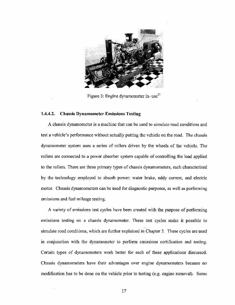
Figure 3: Engine dynamometer in-use 21
1.4.4.2. Chassis Dynamometer Emissions Testing
A chassis dynamometer is a machine that can be used to simulate road conditions and
test a vehicle's performance without actually putting the vehicle on the road. The chassis
dynamometer system uses a series of rollers driven by the wheels of the vehicle. The
rollers are connected to a power absorber system capable of controlling the load applied
to the rollers. There are three primary types of chassis dynamometers, each characterized
by the technology employed to absorb power: water brake, eddy current, and electric
motor. Chassis dynamometers can be used for diagnostic purposes, as well as performing
emissions and fuel mileage testing.
A variety of emissions test cycles have been created with the purpose of performing
emissions testing on a chassis dynamometer. These test cycles make it possible to
simulate road conditions, which are further explained in Chapter 3. These cycles are used
in conjunction with the dynamometer to perform emissions certification and testing.
Certain types of dynamometers work better for each of these applications discussed.
Chassis dynamometers have their advantages over engine dynamometers because no
modification has to be done on the vehicle prior to testing (e.g. engine removal). Some
17
disadvantages associated with using a chassis dynamometer include the inability to
achieve repeatable measurements due to such factors as driveline losses or tire wear,
pressure and temperature. Another disadvantage to the chassis dynamometer is that,
although it includes some parameters that are not present in engine dynamometer testing
such as driveline losses and wheel friction, it still lacks the real conditions (changing
temperature and humidity, wind resistance, road conditions, etc.) mobile testing can
provide.
In order for a dynamometer to simulate road conditions, it must have a means of
applying load to the rollers, which the wheels of the vehicle ride on. The water brake is
one type of braking system that is used for this purpose. The water brake produces a load
by pumping water. The pump is driven from the rollers, which the tires of the vehicle
being tested ride on. The characteristics of the pump can be changed to apply varying
degrees of load to the rollers. The advantages of a water brake are that the system is
easy to maintain and relatively inexpensive. The water brake dynamometer can also be
operated for extended periods of time because the system is actively cooled.22 The
disadvantage of a water brake is that it cannot apply a load at zero RPM and is slow to
respond to quick changes in load conditions. Another disadvantage is that it requires a
significant amount of hardware installed on the premises in addition to the dynamometer
itself. Since the water brake dynamometer uses a water pump to apply load, it requires an
ample water supply and drainage to remove the used water. In many cases a cooling
tower is needed to lower the temperature of the exhaust water before it is returned to the
environment. The water brake dynamometer is intended for applications that require the
dynamometer to be run for extended periods of time and have facilities that can
18
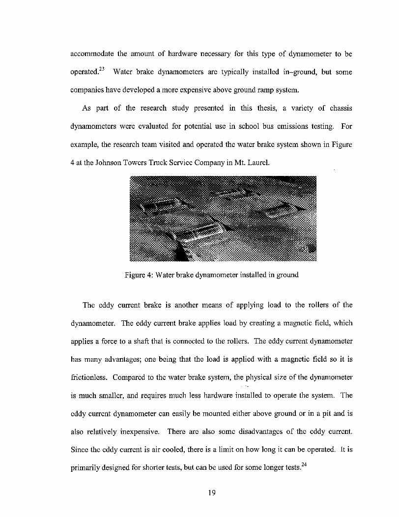
accommodate the amount of hardware necessary for this type of dynamometer to be
operated.2 3 Water brake dynamometers are typically installed in-ground, but some
companies have developed a more expensive above ground ramp system.
As part of the research study presented in this thesis, a variety of chassis
dynamometers were evaluated for potential use in school bus emissions testing. For
example, the research team visited and operated the water brake system shown in Figure
4 at the Johnson Towers Truck Service Company in Mt. Laurel.
Figure 4: Water brake dynamometer installed in ground
The eddy current brake is another means of applying load to the rollers of the
dynamometer. The eddy current brake applies load by creating a magnetic field, which
applies a force to a shaft that is connected to the rollers. The eddy current dynamometer
has many advantages; one being that the load is applied with a magnetic field so it is
frictionless. Compared to the water brake system, the physical size of the dynamometer
is much smaller, and requires much less hardware installed to operate the system. The
eddy current dynamometer can easily be mounted either above ground or in a pit and is
also relatively inexpensive. There are also some disadvantages of the eddy current.
Since the eddy current is air cooled, there is a limit on how long it can be operated. It is
primarily designed for shorter tests, but can be used for some longer tests.2 4
19
The third type of system used to apply load for a chassis dynamometer is the electric
motor brake or AC dynamometer. The electric motor applies a load via direct coupling
with the rollers on the dynamometer. The motor can then apply a load to the rollers by
providing a resistive force on the axel of the rollers. The electric motor dynamometer is
capable of running almost any test that has been created. It can apply a load to the rollers
at zero RPM, which none of the other brake systems are capable of. The primary
disadvantage of the electric motor dynamometer is that it is very expensive; almost eight
times that of the water brake and over ten times that of the eddy current.25 Electric motor
dynamometers can perform complicated real-world driving cycles that the other chassis
dynamometers cannot, however the electric motor dynamometers are so expensive that
there are only two in the US.
1.4.4.3. Mobile In-Use Emissions Testing
The third and final type of emissions testing is mobile or in-use testing. A mobile
emissions test includes an engine installed in the test vehicle while on the road running a
prescribed test cycle. Mobile testing allows the school buses to be tested under
conditions that cannot be reproduced on any dynamometer, or within an environmental
chamber, but do allow for repeatable driving routes to be run.
Mobile testing was chosen as the research method for this project for several reasons.
The main reason was that the EPA plans to switch to mobile testing by 2010 for all of
their emissions testing.26 Mobile testing provides a more accurate and realistic account of
emissions actually from a vehicle while it is in-use, something an engine or chassis
dynamometer system in a lab will never be able to reproduce. Another reason why
mobile testing was chosen is due to the ease of installing emissions measuring equipment
20
and emissions reduction devices. There were no modifications necessary prior to vehicle
testing, the engine did not have to be removed, and the expense of a test system (engine
or chassis dynamometer) was not needed. Mobile emissions measurement equipment is
advanced enough to provide similar controls to those which were previously only
available for dynamometer testing, such as vehicle interface and driver assist routing aid,
which will be discussed later.
Previous research in the emissions field was done without the advantage of a test
track for mobile testing often forcing the researchers to work in the lab on an engine or
chassis dynamometer test system. At ATC there are several test track options for running
test cycles uninterrupted from outside influences, such as traffic and pedestrians.
Another important factor when choosing mobile testing was the fact that engine
manufacturers actually misrepresented emissions levels when testing their engines on
engine dynamometers. In 1998 the Department of Justice and the Environmental
Protection Agency found seven diesel engine manufacturers guilty of installing software
that disables pollution prevention control devices after completing EPA standard tests.
These companies are Caterpillar, Inc., Cummins Engine Company, Detroit Diesel
Corporation, Mack Trucks, Inc., Navistar International Transportation Corporation,
Renault, and Volvo Truck Corporation. Combined, these manufactures were ordered to
pay fines totaling $83.4 million, which is the largest civil penalty ever for violation of
environmental law.27 This penalty was also the third in a series actions brought against
engine companies that allow their ECM's to "selectively" prevent pollution. The first
exposure of the defeat device came in 1995 when the EPA and the Department of Justice
found GM guilty and penalized them $45 million. The American Honda Motor Co. was
21
penalized $267 million and the Ford Motor Co. for $7.8 million to conduct environmental
projects.2 8 Mobile testing eliminates any cheating by the engine manufacturers, since the
emissions being measured by the analyzer are after the certification tests and the
manufacturer does not have the ability to change the ECM programming.
A disadvantage to mobile testing is that the weather cannot be controlled (snow, rain,
heavy winds, etc.). Some emissions, particularly NOx, have been shown to be a strong
function of ambient conditions. Though these are real conditions HDDV's may undergo,
it makes for a difficult time for researchers and the vehicle's driver (trying to follow a
prescribed drive cycle) when testing for mobile emissions. Indeed, the human error
associated with the driver is another disadvantage of mobile testing. Though mobile
testing does not result in the wear and tear of chassis dynamometer on the vehicle, the
driver cycle repeatability is inferior to what can be accomplished on the chassis
dynamometer.
1.5. Diesel Emission Reduction Strategies
Several different emissions reduction technologies will be tested with mobile testing
over the course of the school bus emissions testing project. The technologies that are
going to be tested are the Johnson-Matthey CRT Particulate Trap, Engelhard DPX
Particulate Trap, PFC crank case breather, the PFC flux wave cell, and other various
technologies. Alternative fuels to be tested include #2 diesel, ultra-low sulfur diesel
(ULSD), biodiesel/# 2 diesel blends, and biodiesel/ULSD blends. The results from the
alternative fuel-testing portion of the project are presented in this research.
In an attempt to meet the stringent 2007 EPA emissions standards, all HDDV engines
will need an emission reduction technology. In the past 30 years of EPA emission
22
regulation engine manufacturers were able to meet the new standards by only changing
their engine designs (e.g. fuel injection systems, exhaust gas recirculation, and
electronically controlled engines). The most common types of emission reduction
strategies are after treatment devices (e.g. particulate traps) and alternative fuels. Fuel
additives and other reduction devices (e.g. Selective Catalytic Reduction, Diesel
Oxidization Catalysts, etc.) are also used, but are not as common and widely available as
particulate traps and some alternative fuels. In order to meet the new standards for
HDDV's the emission reduction technologies needed will be costly and usually come
with a fuel penalty. The research presented in this thesis will focus primarily on the
emissions reduction benefits from various alternative fuels. A follow on study is
currently underway that will focus on after treatment devices.
1.5.1. Alternative Fuels
An alternative fuel is defined as a fuel other than petroleum diesel or gasoline.29 The
purpose of an alternative fuel is to have a cleaner bur and produce lower emissions.
Alternative fuels will also reduce our reliance on imported oil. The most common
alternative fuels such as biodiesel and ultra low sulfur diesel (ULSD) have been shown to
reduce some diesel emissions significantly in cars and trucks. For this research, # 2
conventional petroleum diesel (low sulfur -360 ppm), B20 (20% by volume biodiesel,
80% by volume #2 conventional petroleum (-360 ppm) diesel), ultra low sulfur diesel
(-15 ppm), and a biodiesel-ultra low sulfur diesel (20% by volume biodiesel, 80% by
volume ultra low sulfur diesel (-15 ppm)) mixture were examined.
Biodiesel is an alternative fuel that is a cleaner-burning diesel replacement to # 2
diesel. Biodiesel is made from natural renewable sources such as new and used vegetable
23
oils and animal fats. The most common source of biodiesel in the US is soybeans.
Biodiesel can be used pure or in different blends with #2 conventional petroleum diesel.
These blends are classified by percent volume of biodiesel. For example, a blend of 20
percent biodiesel and 80 percent conventional petroleum diesel is called B20. Research
has shown that the best emission reductions for PM, HC, and CO come from higher
percent biodiesel blends and pure biodiesel, B100.3 5 One large obstacle in the widespread
use of biodiesel as a permanent petroleum diesel replacement is availability. Biodiesel
resources are estimated at about two billion gallons per year, which is considerably lower
than the 60 billion gallons used annually by the USA distillate market.3 0
One tradeoff when using pure biodiesel, B100, is that it can significantly increase
NOx depending on the duty cycle.31 The NOx increases when using biodiesel could be
caused by the higher fuel density and lower heating value of the fuel.32 Increasing
oxygen content in the fuel has caused significant increases in NOx in previous research.32
The NOx tradeoff is not a large concern, due to the low sulfur content of biodiesel (~24
ppm), which will work with NOx reducing technologies that require low sulfur fuel.
Biodiesel blends higher than B20 however, can cause problems with deterioration of
existing gaskets and could cause gelling in the winter. A basic mixing process called
splash blending creates a mixture of biodiesel and conventional petroleum diesel.
Biodiesel has a higher specific gravity (-. 88) than conventional petroleum diesel (-. 85),
so splash blending should involve mixing the biodiesel on top of the conventional
petroleum diesel.
Biodiesel has other advantages besides decreasing HC, PM, and CO emissions.
Every unit of energy needed to produce biodiesel results in 3.24 units of fuel energy,
24

while producing conventional petroleum diesel requires more energy to produce the fuel
than is generated. 33 As far as safety factors are concerned biodiesel has a higher
flashpoint than conventional petroleum diesel and is biodegradable and non-toxic. Also,
since biodiesel is renewable, CO2 reductions are indirectly created from the lifecycle of
biodiesel. Biodiesel also has no known blending problems when being mixed with
ULSD. Biodiesel also improves lubricity of the engine, where ULSD does not, and a
combination of biodiesel and ULSD would offset the loss of lubricity when using just
ULSD. ULSD and biodiesel both have higher cloud points than conventional petroleum
diesel, which could be a problem with gelling in colder weather conditions. The cloud
point of a clear distillate fuel is the temperature at which the fuel becomes hazy or cloudy
because of the appearance of wax crystals.34
In a comprehensive review compiling several separate biodiesel studies, the EPA
concluded that common blends of B20 reduced HC emissions by 20 %, PM emissions by
10 %, and CO emissions by 11 %.35 NOx emissions increased slightly in some engines (-
2%) and CO2 emissions showed little or no difference. Some school districts such as
Medford Township in NJ are already using B20 in half of their 44 buses 36. As part of the
present study, tests were performed on some of the buses in the Medford conventional
and biodiesel fueled fleet. The results from those tests are presented in Chapter 4.
Ultra low sulfur diesel (ULSD) is an alternative fuel made to have lees than 15-ppm
sulfur. ULSD will be the only diesel fuel allowed in the U.S. after 2006. PM emissions
have been shown to decrease slightly with the use of ULSD, however the real advantage
of the fuel comes when combining it with an emission after treatment technology. Since
sulfur has been known to poison catalysts it is required that ULSD be used for most
25
particulate traps and catalytic converters.
technologies significant reductions in some emissions have been reported.
The USEPA classifies ULSD as having no more than 15-ppm sulfur content, with the
current U.S. regulations allowing up to 500-ppm sulfur for diesel fuel used for highway
transportation. Previous studies show that ULSD by itself reduces HC emissions by
13 %, PM emissions by 13 %, CO emissions by 6 %, and NOx emissions by 3 %. With
the addition of a particulate filter, ULSD can reduce HC and CO emissions by 90 %, PM
emissions by 80%, and NOx emissions by 15 % to 20 %.33 Compared to conventional
petroleum diesel, a B20 biodiesel blend costs an additional $0.12 to $0.20 and ULSD
costs an additional $.05 to $0.15.33
1.5.2. Particulate Traps
Although exhaust after treatment tests have yet to be completed, a review of the
current status of available devices was conducted as part of the present research study. A
brief review is presented here. A diesel particulate filter or trap physically captures
particulates from the exhaust and prevents them from entering the atmosphere. The
Johnson Matthey Continuously Regenerating Technology (CRT) Particulate Filter and
the Engelhard DPX Catalyzed Diesel Particulate Filter are the only two diesel particulate
traps approved by the EPA for HDDV's as part of their verified after treatment
technology list3 7. A diesel particulate filter incorporates a filtering device to trap liquid
and solid particulates. Materials used to construct diesel particulate filter include ceramic
monoliths, wire mesh, woven silica fiber coils, ceramic foam, etc. A catalyst is used to
promote combustion of the carbon inside the filter, producing carbon dioxide.
The three types of particulate filters are "catalytic, "fuel-borne catalyst," and
26
When combining ULSD with these
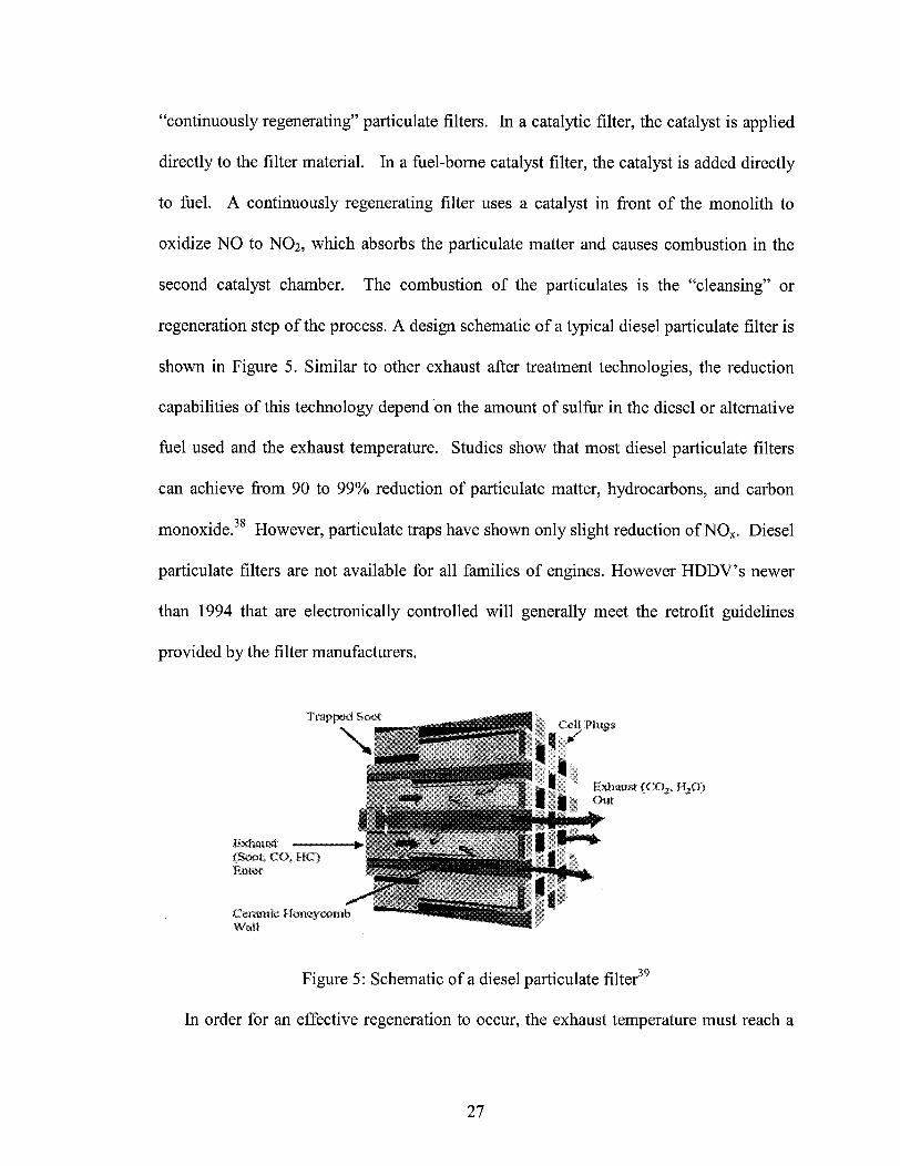
"continuously regenerating" particulate filters. In a catalytic filter, the catalyst is applied
directly to the filter material. In a fuel-borne catalyst filter, the catalyst is added directly
to fuel. A continuously regenerating filter uses a catalyst in front of the monolith to
oxidize NO to NO2, which absorbs the particulate matter and causes combustion in the
second catalyst chamber. The combustion of the particulates is the "cleansing" or
regeneration step of the process. A design schematic of a typical diesel particulate filter is
shown in Figure 5. Similar to other exhaust after treatment technologies, the reduction
capabilities of this technology depend on the amount of sulfur in the diesel or alternative
fuel used and the exhaust temperature. Studies show that most diesel particulate filters
can achieve from 90 to 99% reduction of particulate matter, hydrocarbons, and carbon
monoxide.3 8 However, particulate traps have shown only slight reduction of NOx. Diesel
particulate filters are not available for all families of engines. However HDDV's newer
than 1994 that are electronically controlled will generally meet the retrofit guidelines
provided by the filter manufacturers.
N
:Cktr--aiu k' 0-tip~ycomih
Watt~ 7c~:P~
Figure 5: Schematic of a diesel particulate filter39
In order for an effective regeneration to occur, the exhaust temperature must reach a
27
Iust tC.-Xie:l, 1,41Oi.")
temperature between 350-400 °C. If this exhaust temperature is not reached, the soot
collected in the filter is not combusted and the particulate trap becomes clogged. Another
disadvantage when using a particulate filter on an HDDV is the effect of sulfur in the
fuel. Sulfur inhibits the active sites on the catalyst, which results in a less active catalyst
and a higher exhaust temperature requirement for regeneration. The oxidation of SO2 to
S0 3 over the platinum oxidation catalyst takes place in preference to the oxidation of NO
to N0 240. Therefore, the NO oxidation reaction is inhibited, and the NO 2 is less available
to bum off the trapped soot.
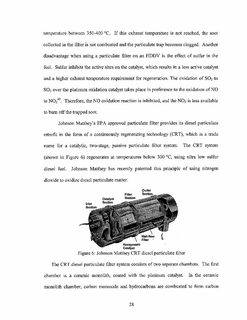
Johnson Matthey's EPA approved particulate filter provides its diesel particulate
retrofit in the form of a continuously regenerating technology (CRT), which is a trade
name for a catalytic, two-stage, passive particulate filter system. The CRT system
(shown in Figure 6) regenerates at temperatures below 300 °C, using ultra low sulfur
diesel fuel. Johnson Matthey has recently patented this principle of using nitrogen
dioxide to oxidize diesel particulate matter.
:ftiM
Figure 6: Johnson Matthey CRT diesel particulate filter
The CRT diesel particulate filter system consists of two separate chambers. The first
chamber is a ceramic monolith, coated with the platinum catalyst. In the ceramic
monolith chamber, carbon monoxide and hydrocarbons are combusted to form carbon
28
'11""B~
dioxide and water. The first stage also increases the proportion of nitrogen dioxide to
nitrogen oxide. In the second chamber the exhaust passes through another monolith,
which forces the exhaust through the pores. The remaining soot is trapped and burned off
by the nitrogen dioxide from the first stage. 41 Restrictions do exist for this technology
however, such as the exhaust gas temperature, the NOx to PM ratio, and sulfur content in
the diesel fuel. The restrictions are as follows: the exhaust gas temperature for the CRT
must be at least 275 °C, the sulfur content in the fuel must not exceed 50 ppm (ULSD has
a sulfur content of less than 15 ppm), and the exhaust NOx to PM ratio must be between
8:1 and 25:1 by weight. The minimum exhaust temperature has been determined by
studies such as the California Air Resources Board for post-1994 engine retrofits, and the
Diesel Emission Control - Sulfur Effects (DECSE) study on a CAT 3126 engine. The
high exhaust temperature is required for the filter regeneration to take place, which
according to California ARB must have a temperature of 270 °C for 40% of the operating
time of the filter. According to the DECSE report, the filter has shown to regenerate as
low as 300°C, provided that ultra low sulfur diesel fuel (15ppm) was used. ULSD must
be used with the CRT because the sulfur deteriorates regeneration. 42 Sulfur is an
inhibitor, which strongly competes with NO, in the exhaust. Thus, the active sites in the
catalyst become blocked by a competitive adsorption between sulfur dioxide and nitrogen
oxide. The result is a lower NO2 generation, and in order to obtain generation, the
exhaust temperature must be raised.4 3
Engelhard's EPA approved particulate filter provides its diesel particulate retrofit in
the form of a DPX catalyzed particulate filter. The DPX filter is a platinum and base
metal oxide catalyst-coated ceramic wall-flow filter. The catalyst coating is embedded
29

into the porous filter walls and oxidized the collected particulate matter, hydrocarbons,
and carbon monoxide from the exhaust.44
According to Engelhard Corporation the DPX filter delivers 70-98% PM reduction
and 70-98% carbon monoxide and hydrocarbon reductions. 4 5 The DPX particulate filter
is effective when used with sulfur fuel ranging from 5 PPM to 500 PPM, and no fuel
additives are required. Under such circumstances, oxidation catalyst technology in the
form of a muffler replacement would be more suitable and would deliver 25-50% PM
reduction, 50-80% hydrocarbon reduction, and 40-90% carbon monoxide reduction.
Engelhard Corporation also claims that the DPX Soot Filter requires an exhaust gas
temperature of 375°C for at least 25% of the time. 46
1.6. Thesis Organization
This thesis presents the results of an experimental study aimed at evaluating emission
reduction strategies for diesel powered school buses in New Jersey. Chapter 2 details the
experimental procedure used to acquire and analyze emissions data from the school
buses. The specifics of the emission measurement equipment, the testing location, the
test vehicles, and the data management are discussed in this chapter. Chapter 3 details
the development of a new mobile emissions test cycle for school buses. The test cycle
was developed using actual school bus route GPS data from distinct routes in NJ school
systems.
Chapter 4 describes preliminary testing of school buses in Medford, NJ. The
Medford School District is the first in the state of New Jersey to operate a majority of its
fleet on biodiesel. Testing was conducted solely by Rowan University on four Medford
school buses in an attempt to acquire as much emission data as possible. Chapter 5 details
30
the experimental testing conducted in the Aberdeen Testing Center environmentally
controlled chamber. The goal of the chamber testing was to evaluate the effects of
varying temperatures and humidity on an idling school bus. From the data, a correction
factor was developed for the buses to account for varying temperature and humidity as
encountered during mobile testing. School bus idling emissions data was also acquired
that could lead to further recommendations for the New Jersey SIP.
Chapter 6 details the experimental testing of alternative fuels in school buses
conducted on the Aberdeen Testing Center mobile testing track. Three school buses
were tested with three alternative fuel types and #2 conventional petroleum diesel to
evaluate the emission effects of alternative fuels on different engines. The school bus
tests were performed using the mobile test cycle created in Chapter 3. The NOx
emissions data collected was corrected for temperature and humidity using the correction
factor developed in Chapter 5. The biodiesel results from this ATC mobile test were
compared to the results previously obtained at the Medford Township School District
with buses that have been running on biodiesel for five years, as shown in Chapter 4.
Chapter 7 provides conclusions and suggestions for future work on both emission
reduction technologies for school buses and mobile school bus testing cycles.
31
2. Experimental Procedure and Equipment
2.1. Introduction
The purpose of this chapter is to describe the test vehicles, the test facilities, and the
equipment used to measure emissions for mobile and idle school bus testing. This
chapter will also provide information on how data collected from various instruments was
compiled and managed.
2.2. Rationale for School Bus Selection
An early challenge for the project was to choose three diesel engines typically found
in school buses across New Jersey for diesel emissions testing. Among the criteria
considered for the selection was availability of the buses, frequency of use of a particular
bus type in New Jersey, and popularity of engine type with respect to previous school bus
emission studies. Another important factor in bus selection was the age of the school
bus. Since school buses are replaced from a school districts fleet every 13 years, it was
important to stay in the scope of the project and chose a bus that would still be in service
for a significant time after completion of this study.
2.2.1. School Bus Types in NJ
One criteria for the selection of the school buses was developed after determining the
types of buses that are commonly used in New Jersey school systems. NJDOT provided
a comprehensive study of the engines used in school buses across the entire state. As
shown in Table 3, specific engine types were used in the study done by Polk Automotive
Intelligence of Detroit to organize buses from all NJ school districts. The three buses that
were ultimately chosen for emissions testing are shown in bold in Table 3. In addition to
the survey compiled by NJDOT, a survey was taken by Rowan University students in the
32
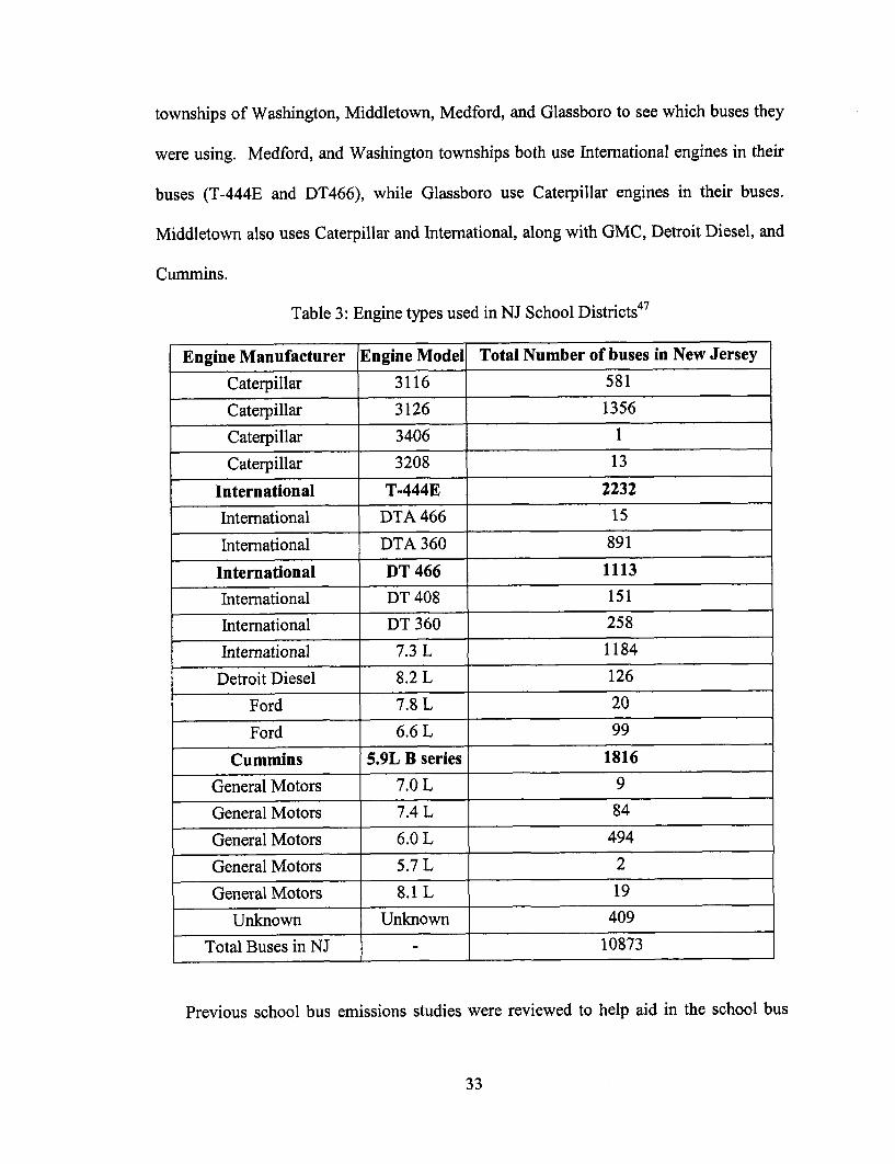
townships of Washington, Middletown, Medford, and Glassboro to see which buses they
were using. Medford, and Washington townships both use International engines in their
buses (T-444E and DT466), while Glassboro use Caterpillar engines in their buses.
Middletown also uses Caterpillar and International, along with GMC, Detroit Diesel, and
Cummins.
Table 3: Engine types used in NJ School Districts4 7
Engine Manufacturer Engine Model Total Number of buses in New Jersey
Caterpillar 3116 581
Caterpillar 3126 1356
Caterpillar 3406 1
Caterpillar 3208 13
International T-444E 2232
International DTA 466 15
International DTA 360 891
International DT 466 1113
International DT 408 151
International DT 360 258
International 7.3 L 1184
Detroit Diesel 8.2 L 126
Ford 7.8 L 20
Ford 6.6 L 99
Cummins 5.9L B series 1816
General Motors 7.0 L 9
General Motors 7.4 L 84
General Motors 6.0 L 494
General Motors 5.7 L 2
General Motors 8.1 L 19
Unknown Unknown 409
Total Buses in NJ 10873
Previous school bus emissions studies were reviewed to help aid in the school bus
33
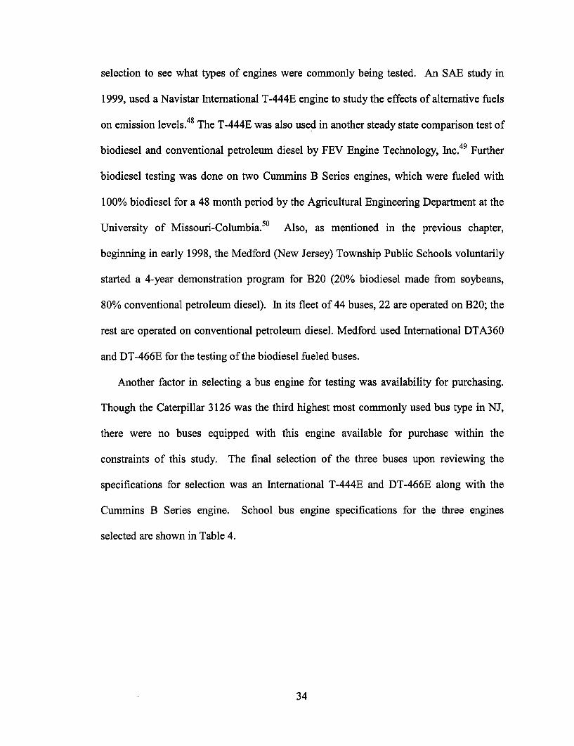
selection to see what types of engines were commonly being tested. An SAE study in
1999, used a Navistar International T-444E engine to study the effects of alternative fuels
on emission levels. 48 The T-444E was also used in another steady state comparison test of
biodiesel and conventional petroleum diesel by FEV Engine Technology, Inc.4 9 Further
biodiesel testing was done on two Cummins B Series engines, which were fueled with
100% biodiesel for a 48 month period by the Agricultural Engineering Department at the
University of Missouri-Columbia. 5 0 Also, as mentioned in the previous chapter,
beginning in early 1998, the Medford (New Jersey) Township Public Schools voluntarily
started a 4-year demonstration program for B20 (20% biodiesel made from soybeans,
80% conventional petroleum diesel). In its fleet of 44 buses, 22 are operated on B20; the
rest are operated on conventional petroleum diesel. Medford used International DTA360
and DT-466E for the testing of the biodiesel fueled buses.
Another factor in selecting a bus engine for testing was availability for purchasing.
Though the Caterpillar 3126 was the third highest most commonly used bus type in NJ,
there were no buses equipped with this engine available for purchase within the
constraints of this study. The final selection of the three buses upon reviewing the
specifications for selection was an International T-444E and DT-466E along with the
Cummins B Series engine. School bus engine specifications for the three engines
selected are shown in Table 4.
34
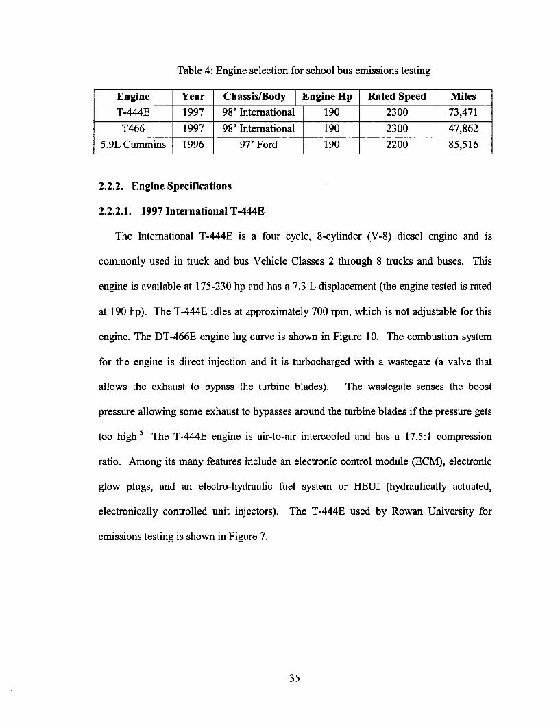
Table 4: Engine selection for school bus emissions testing
Engine Year Chassis/Body Engine Hp Rated Speed Miles
T-444E 1997 98' International 190 2300 73,471
T466 1997 98' International 190 2300 47,862
5.9L Cummins 1996 97' Ford 190 2200 85,516
2.2.2. Engine Specifications
2.2.2.1. 1997 International T-444E
The International T-444E is a four cycle, 8-cylinder (V-8) diesel engine and is
commonly used in truck and bus Vehicle Classes 2 through 8 trucks and buses. This
engine is available at 175-230 hp and has a 7.3 L displacement (the engine tested is rated
at 190 hp). The T-444E idles at approximately 700 rpm, which is not adjustable for this
engine. The DT-466E engine lug curve is shown in Figure 10. The combustion system
for the engine is direct injection and it is turbocharged with a wastegate (a valve that
allows the exhaust to bypass the turbine blades). The wastegate senses the boost
pressure allowing some exhaust to bypasses around the turbine blades if the pressure gets
too high.5 1 The T-444E engine is air-to-air intercooled and has a 17.5:1 compression
ratio. Among its many features include an electronic control module (ECM), electronic
glow plugs, and an electro-hydraulic fuel system or HEUI (hydraulically actuated,
electronically controlled unit injectors). The T-444E used by Rowan University for
emissions testing is shown in Figure 7.
35
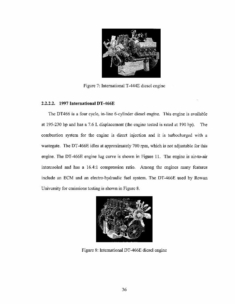
Figure 7: International T-444E diesel engine
2.2.2.2. 1997 International DT-466E
The DT466 is a four cycle, in-line 6-cylinder diesel engine. This engine is available
at 195-230 hp and has a 7.6 L displacement (the engine tested is rated at 190 hp). The
combustion system for the engine is direct injection and it is turbocharged with a
wastegate. The DT-466E idles at approximately 700 rpm, which is not adjustable for this
engine. The DT-466E engine lug curve is shown in Figure 11. The engine is air-to-air
intercooled and has a 16.4:1 compression ratio. Among the engines many features
include an ECM and an electro-hydraulic fuel system. The DT-466E used by Rowan
University for emissions testing is shown in Figure 8.
Figure 8: International DT-466E diesel engine
36
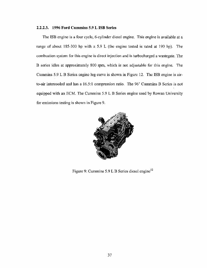
22.2.2.3. 1996 Ford Cummins 5.9 L ISB Series
The ISB engine is a four cycle, 6-cylinder diesel engine. This engine is available at a
range of about 185-300 hp with a 5.9 L (the engine tested is rated at 190 hp). The
combustion system for this engine is direct injection and is turbocharged a wastegate. The
B series idles at approximately 800 rpm, which is not adjustable for this engine. The
Cummins 5.9 L B Series engine lug curve is shown in Figure 12. The ISB engine is air-
to-air intercooled and has a 16.5:1 compression ratio. The 96' Cummins B Series is not
equipped with an ECM. The Cummins 5.9 L B Series engine used by Rowan University
for emissions testing is shown in Figure 9.
Figure 9: Cummins 5.9 L B Series diesel engine5 2
37

--.- TORQUE POWER
250
225
200
175
150
125 ;0
m100
75
50
25
0
600 800 1000 1200 1400 1600 1800 2000 2200 2400 2600 2800
Engine Speed (RPM)
Figure 10: T-444E engine lug curve
38
500
450
400
350
300
.0
E 250
200
150
100
50
c)

- - - TORQUE - POWER
ZOU
225
200
175
150
I
125 g0.
100 o
75
50
25
0600 800 1000 1200 1400 1600 1800 2000 2200 2400 2600 2800
Engine Speed (RPM)
Figure 11: DT-466E engine lug curve
39
500
450
400
350
300
* 250E12
200
150
100
50
0
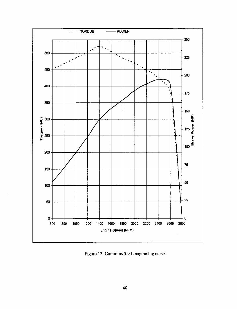
.... TORQUE POWER
250
500
450
400
350
8 300
E0
E 250
200
150
100
50
0
225
200
175
150
L
125 oa.
100 M
75
50
25
0600 800 1000 1200 1400 1600 1800 2000 2200 2400 2600 2800
Engine Speed (RPM)
Figure 12: Cummins 5.9 L engine lug curve
40
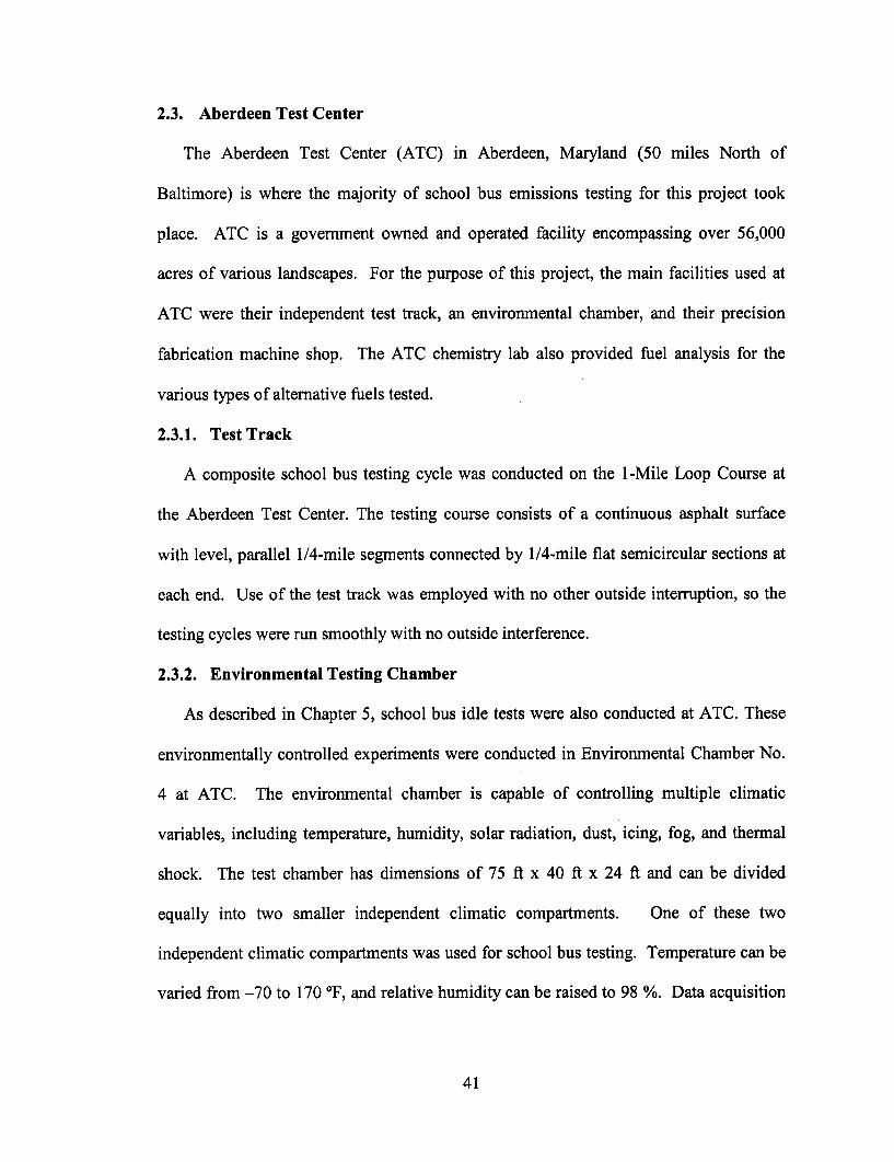
2.3. Aberdeen Test Center
The Aberdeen Test Center (ATC) in Aberdeen, Maryland (50 miles North of
Baltimore) is where the majority of school bus emissions testing for this project took
place. ATC is a government owned and operated facility encompassing over 56,000
acres of various landscapes. For the purpose of this project, the main facilities used at
ATC were their independent test track, an environmental chamber, and their precision
fabrication machine shop. The ATC chemistry lab also provided fuel analysis for the
various types of alternative fuels tested.
2.3.1. Test Track
A composite school bus testing cycle was conducted on the 1-Mile Loop Course at
the Aberdeen Test Center. The testing course consists of a continuous asphalt surface
with level, parallel 1/4-mile segments connected by 1/4-mile flat semicircular sections at
each end. Use of the test track was employed with no other outside interruption, so the
testing cycles were run smoothly with no outside interference.
2.3.2. Environmental Testing Chamber
As described in Chapter 5, school bus idle tests were also conducted at ATC. These
environmentally controlled experiments were conducted in Environmental Chamber No.
4 at ATC. The environmental chamber is capable of controlling multiple climatic
variables, including temperature, humidity, solar radiation, dust, icing, fog, and thermal
shock. The test chamber has dimensions of 75 ft x 40 ft x 24 ft and can be divided
equally into two smaller independent climatic compartments. One of these two
independent climatic compartments was used for school bus testing. Temperature can be
varied from -70 to 170 °F, and relative humidity can be raised to 98 %. Data acquisition
41
and control instrumentation are located in a separate in e room adjacent to the environmental
chamber 53 . Various views of chamber 4 are shown in Figure 13. 53
Figure 13: Environmental testing chamber 4
2.3.3. Chemistry Lab
The ATC Chemistry Fuels Testing Laboratory provided analysis on several properties
of diesel fuels. The ATC Chemistry Team Laboratory is certified by the Army Petroleum
Center as a fuel-testing laboratory.53 The lab followed ASTM D975-01, Standard
Specification for Diesel Fuel Oils, for the fuel testing. Properties of the fuels tested and
the ASTM Method in which they were tested are as follows:
* Distillation range: The range of temperature, usually determined at atmospheric
(Boiling Range) pressure by means of standard apparatus, over which boiling or
distillation of a liquid proceeds., tested using ASTM D 86.
* API gravity: An arbitrary scale expressing the gravity or density of liquid
42
petroleum products, tested using ASTM D 287.
* Flash point (closed and open cup): The temperature at which a combustible liquid
gives off just enough vapor to produce a vapor/air mixture that will ignite when a
flame is applied, tested using ASTM D 93.
* Cetane index %: A calculated value, derived from fuel density and volatility,
giving a reasonably close approximation to cetane number, tested using
ASTM D 4737.
* Particulate contamination
* Sulfur Content, tested using ASTM D 4294.
* Cloud point: The temperature at which wax first becomes visible when diesel fuel
is cooled under standardized test conditions.
* Pour point: The temperature at which the amount of wax out of solution is
sufficient to gel the fuel when tested under standard conditions.
* Freeze point
* Fuel Viscosity, tested using ASTM D 445.
* Density or specific gravity, tested using ASTM D 4052.
2.4. Bus Instrumentation
Table 5 is a summary school bus emission testing instrumentation proposed for these
tests. If a measurement was taken following an SAE standard testing measurement
method, the method is noted in Table 5. Exhaust gas emissions measurements will
include oxygen, CO, C0 2, NO2, NO, SO2, unburned hydrocarbons, and particulate
matter. In addition to tail pipe emissions, the intake air, ambient air, school bus interior,
and engine operating parameters were also monitored. The data was acquired using
43
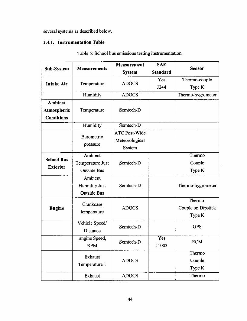
several systems as described below.
2.4.1. Instrumentation Table
Table 5: School bus emissions testing instrumentation.
Measurement SAESub-System Measurements Sensor
System StandardYes Thermo-couple
Intake Air Temperature ADOCSJ244 Type K
Humidity ADOCS Thermo-hygrometer
AmbientAtmospheric Temperature Semtech-D
Conditions
Humidity Semtech-D
ATC Post-WideBarometric
Meteorologicalpressure
System
Ambient ThermoSchool Bus
Extior Temperature Just Semtech-D CoupleExterior
Outside Bus Type K
Ambient
Humidity Just Semtech-D Thermo-hygrometer
Outside Bus
Thermo-Crankcase
Engine ADOCS Couple on Dipsticktemperature
Type K
Vehicle Speed/Semtech-D GPS
Distance
Engine Speed, YesSemtech-D ECM
RPM J1003
ThermoExhaust
ADOCS CoupleTemperature 1ple
Type K
Exhaust ADOCS Thermo
44
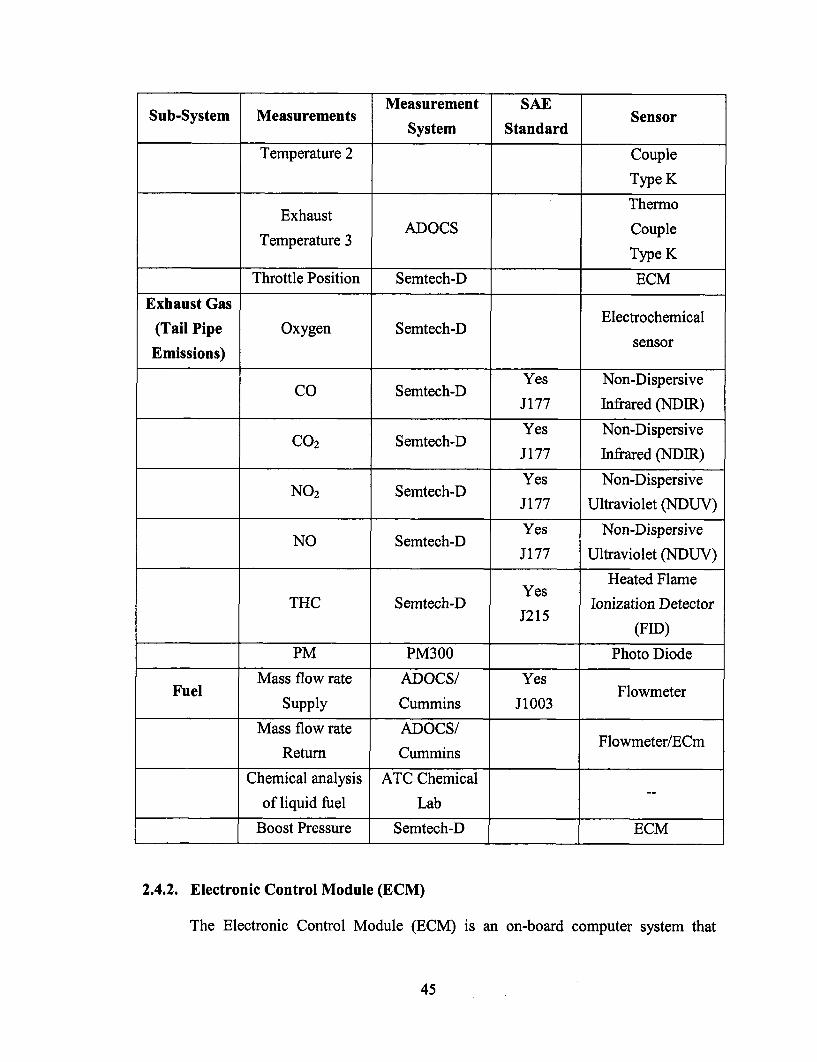
Measurement SAESub-System Measurements Sensor
System Standard
Temperature 2 Couple
Type K
ThermoExhaust
ADOCS CoupleTemperature 3
Type K
Throttle Position Semtech-D ECM
Exhaust GasElectrochemical
(Tail Pipe Oxygen Semtech-Dsensor
Emissions)
Yes Non-DispersiveCO Semtech-D
J177 Infrared (NDIR)
Yes Non-DispersiveCO2 Semtech-D
J177 Infrared (NDIR)
Yes Non-DispersiveNO2 Semtech-D
J177 Ultraviolet (NDUV)
Yes Non-DispersiveNO Semtech-D
J177 Ultraviolet (NDUV)
Heated FlameYes
THC Semtech-D Ionization DetectorJ215
(FID)
PM PM300 Photo Diode
Mass flow rate ADOCS/ YesFuel Flowmeter
Supply Cummins J1003
Mass flow rate ADOCS/Flowmeter/ECm
Return Cummins
Chemical analysis ATC Chemical
of liquid fuel Lab
Boost Pressure Semtech-D ECM
2.4.2. Electronic Control Module (ECM)
The Electronic Control Module (ECM) is an on-board computer system that
45
controls the opening and shutting of the intake and exhaust valves of an engine. The
ECM is generally mounted near the engine in the engine compartment and reads a variety
of signals. An ECM can also control engine performance parameters such as fuel
metering, ignition spark advance, air-fuel mixture, and the engine-cooling fan. There are
five individual parts to an ECM, the main one being the microprocessor. The
microprocessor consists of Random-access memory (RAM), Read-only memory (ROM),
Keep-alive memory (KAM), and several inputs and outputs.
Using an analog to digital converter, the ECM first converts information from the
input sensors to a form that it can use to process the data. The information is then sent to
the microprocessor where specifications that are stored in the memory chips are used to
form an assessment of vehicle conditions based upon the engine's performance. This
assessment is then sent to an actuator and an action occurs based upon the input of
information. The final information can then be uploaded onto a device (such as the
Semtech-D emissions unit read out screen) where the engine parameter information can
be processed and analyzed. Several parameters can be read from the ECM
microprocessor's RAM and KAM such as road speed, engine load, engine rpm, and fuel
consumption. The main difference between the RAM and KAM is that KAM will store
information even after the ignition is turned off.
Engine manufacturers have different service tools to access information from the
ECM through a data link. A data link provides a physical means for transmitting and
sorting electric signals. A data link consists of special electronic circuitry and electrical
connections. Connection points for electronic service tools are also part of the data link.
A data link adapter is a device that converts the SAE J1587/SAE J1708 or the SAE J1939
46
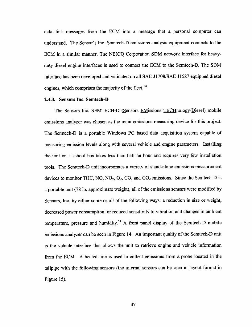
data link messages from the ECM into a message that a personal computer can
understand. The Sensor's Inc. Semtech-D emissions analysis equipment connects to the
ECM in a similar manner. The NEXIQ Corporation SDM network interface for heavy-
duty diesel engine interfaces is used to connect the ECM to the Semtech-D. The SDM
interface has been developed and validated on all SAE-J1708/SAE-J1587 equipped diesel
engines, which comprises the majority of the fleet.54
2.4.3. Sensors Inc. Semtech-D
The Sensors Inc. SEMTECH-D (Sensors EMissions TECHnology-Diesel) mobile
emissions analyzer was chosen as the main emissions measuring device for this project.
The Semtech-D is a portable Windows PC based data acquisition system capable of
measuring emission levels along with several vehicle and engine parameters. Installing
the unit on a school bus takes less than half an hour and requires very few installation
tools. The Semtech-D unit incorporates a variety of stand-alone emissions measurement
devices to monitor THC, NO, NO 2, 02, CO, and CO 2 emissions. Since the Semtech-D is
a portable unit (78 lb. approximate weight), all of the emissions sensors were modified by
Sensors, Inc. by either some or all of the following ways: a reduction in size or weight,
decreased power consumption, or reduced sensitivity to vibration and changes in ambient
temperature, pressure and humidity.54 A front panel display of the Semtech-D mobile
emissions analyzer can be seen in Figure 14. An important quality of the Semtech-D unit
is the vehicle interface that allows the unit to retrieve engine and vehicle information
from the ECM. A heated line is used to collect emissions from a probe located in the
tailpipe with the following sensors (the internal sensors can be seen in layout format in
Figure 15).
47
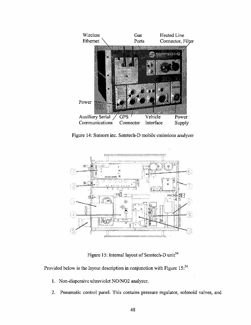
Heated LineConnector, Filter
Communications
Figure 14: Sensors inc.
<1ui
Connector Interface Supply
Semtech-D mobile emissions analyzer
.. ..... ...... ....... .... ... . ..... ..... ..... .... ... ........................;;.·;.·.
::B i i..~~~~~~~~~~~~~~~~~~~~~~~~~~~.....
X :1 I.,~ ~~ ~: :~ D
................ iii............ . ...... ~ ~.......... ........... ... ~ j::
.............................~ ~ ~ ~~ ~ ~ ~~~:~~~~:~~~:~~~:~~~:~~~u~~~ri·:l··rrr~~~~~~~~~~~~ru:~~~~~~~5··.......~~~~~~~~~~~~~~"~ ~ ~ ~~~......
Figure 15: Internal layout of Semtech-D unit 54
Provided below is the layout description in conjunction with Figure 15:54
1. Non-dispersive ultraviolet NO/N02 analyzer.
2. Pneumatic control panel. This contains pressure regulator, solenoid valves, and
48
WirelessEthernet \
GasPorts
Power
Auxilia
/
I
.. .. .. . ... .. .
.3i ~ ·~·~.~
i i"�X9·::"�':"8I i::
.,zi��s I
...'
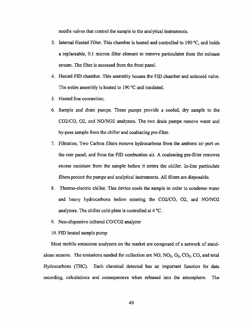
needle valves that control the sample to the analytical instruments.
3. Internal Heated Filter. This chamber is heated and controlled to 190 °C, and holds
a replaceable, 0.1 micron filter element to remove particulates from the exhaust
stream. The filter is accessed from the front panel.
4. Heated FID chamber. This assembly houses the FID chamber and solenoid valve.
The entire assembly is heated to 190 °C and insulated.
5. Heated line connection.
6. Sample and drain pumps. These pumps provide a cooled, dry sample to the
C02/CO, 02, and NO/N02 analyzers. The two drain pumps remove water and
by-pass sample from the chiller and coalescing pre-filter.
7. Filtration. Two Carbon filters remove hydrocarbons from the ambient air port on
the rear panel, and from the FID combustion air. A coalescing pre-filter removes
excess moisture from the sample before it enters the chiller. In-line particulate
filters protect the pumps and analytical instruments. All filters are disposable.
8. Thermo-electric chiller. This device cools the sample in order to condense water
and heavy hydrocarbons before entering the C02/CO, 02, and NO/N02
analyzers. The chiller cold-plate is controlled at 4 °C.
9. Non-dispersive infrared CO/C02 analyzer
10. FID heated sample pump
Most mobile emissions analyzers on the market are composed of a network of stand-
alone sensors. The emissions needed for collection are NO, NO2, 02, C02, CO, and total
Hydrocarbons (THC). Each chemical detected has an important function for data
recording, calculations and consequences when released into the atmosphere. The
49
Semtech-D uses a heated, insulated sample line to reduce the loss of THC. The heated
line is twelve feet in length and operates at 191 °C. Teflon is used as the wetted surface
of the line because of its high heat resistance and low absorbing properties. A heater is
wrapped around the Teflon line, which is molded inside a larger insulated flexible tube.54
The heated line is filtered at the inlet to prevent contamination from particulates.
Oxygen (02) is one of the two important reactants for internal combustion in air. 02
concentration is read using an electrochemical sensor by the Semtech-D gas analyzer.
Electrochemical sensors require the sample to be dry before passing over them. The
sensor detects the partial pressure of 02 in the stream and reports it electronically. This
technology is used in prior emission measurement devices and gas analyzer companies
are attempting to produce products that can continuously give accurate data. Other
emissions can also be measured using electrochemical sensors, but more advanced
techniques have been developed and are being used by the Semtech-D.
Sensors Inc.'s Non-Dispersive Ultraviolet (NDUV) system is currently the newest
technology for NOx. Sensor Inc. employs a dual NO and NO2 detection system based on
a plasma powered ultraviolet light to detect NO and NO2 separately. Previous attempts at
ultraviolet detection were hindered by the life of the ultraviolet light. The NDUV sensor
does not deteriorate like the electrochemical does over time. The most important
condition of NOx detection is the removal of water before the sensor where the exhaust
sample is dried with an ambient temperature coalescing filter followed by a
thermoelectric chiller. The heavy hydrocarbons found in the diesel exhaust sample are
removed from the sample along with a small amount of NO 2 (about 5% of sample) with
the water removal process to prevent contamination of the optics.
50
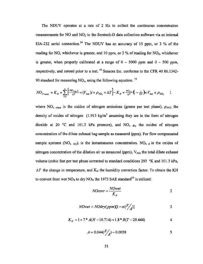
The NDUV operates at a rate of 2 Hz to collect the continuous concentration
measurements for NO and NO2 to the Semtech-D data collection software via an internal
EIA-232 serial connection.54 The NDUV has an accuracy of 15 ppm, or 3 % of the
reading for NO, whichever is greater, and 10 ppm, or 3 % of reading for NO2 , whichever
is greater, when properly calibrated at a range of 0 - 5000 ppm and 0 - 500 ppm,
respectively, and zeroed prior to a test. 54 Sensors Inc. conforms to the CFR 40 86.1342-
90 standard for measuring NOx, using the following equation. 19
NOXmass = KH X [ X (V T-K ( )X V X PNO 1i=l
where NOx mass is the oxides of nitrogen emissions (grams per test phase), PNO2 the
density of oxides of nitrogen (1.913 kg/m3 assuming they are in the form of nitrogen
dioxide at 20 °C and 101.3 kPa pressure), and NOx dry the oxides of nitrogen
concentration of the dilute exhaust bag sample as measured (ppm). For flow compensated
sample systems (NOx dy)i is the instantaneous concentration. NOx d is the oxides of
nitrogen concentration of the dilution air as measured (ppm), Vmix the total dilute exhaust
volume (cubic feet per test phase corrected to standard conditions 293 °K and 101.3 kPa,
AT the change in temperature, and KH the humidity correction factor. To obtain the KH
to convert from wet NOx to dry NOx the 1973 SAE standard 55 is utilized:
NOwetNOcorr = Nw 2
KH
NOwet = NOdry(ppm)[ - a(F/A)] 3
KH = 1 + 7 * A(H -10.714) +1.8 * B(T - 29.444) 4
A =0.044(F/) - 0.00385
51
B = -0.116( ) + 0.0053 6
where NOdry is the measured NOx emissions (ppm), a the atomic hydrogen to carbon
ratio (y/x in fuel with formula CxHy), F/A the fuel to air ratio (Dry Basis), H the specific
humidity (grams of H20/kg dry air), and T the intake air temperature (°C). The
temperature range for this correlation to work effectively is 70-115 °F. Ambient and
intake temperature and humidity are measured mainly for this reason. As described in
Chapter 5, a new correction was developed specifically for use with the school busses
tested here.
The AMBII Non-Dispersive Infrared (NDIR) analyzer is used by the Semtech-D to
measure CO and CO 2 emissions. This sensor also needs the incoming gas dried to
remove heavy hydrocarbons and water vapor that cause interference with the sensor. The
gas is dried in the same manner as the NOx analyzer with an ambient temperature
coalescing filter followed by a thermoelectric chiller. If the gas were not dried
interference would occur in the infrared channels. Unlike the NOx emission, the CO2 and
CO emissions do not require humidity corrections. The AMBII NDUV operates on a
continuous .83 Hz (1.2 second) data rate to collect concentration measurements of CO
and CO2 to the Semtech-D data collection software via an internal EIA-232 serial
connection. 54 The AMBII NDUV has an accuracy of 50 ppm, or 5 % of reading,
whichever is greater, when properly calibrated at a range of 1200 - 1500 ppm and zeroed
prior to a test. 54
While infrared and electrochemical cells may work for HC detection, the Flame
Ionized Detector (FID) employed in the SEMTECH-D is superior in measurment
52

sensitivity. While keeping a flame lit with hydrogen, a sample is passed over and
combusted. The concentration of the HC is then determined by the amount of sample
that bums. The FID fuel used for FID flame ignition is a 40/60 mixture of
hydrogen/helium. The user can also select a data rate of up to 4 Hz through the Semtech-
D application software. The AMBII NDIR has an accuracy of 5 ppm, or 1 % of reading,
whichever is greater, when properly calibrated at a range of 0 - 100 ppm and zeroed prior
to a test. 54
In order to calculate the widely accepted emissions units of grams per mile and grams
per brake horsepower, fuel flow rate is needed. Using injector pore size, the ECM can
measure fuel flow rate, which is the procedure used by Sensors Inc for Semtech-D.
Semtech-D relies on the ECM to provide fuel flow information in order to calculate
fuel flow rate and time specific mass emissions. The ECM determines the fuel flow rate
based on the real-time pulse width of the fuel injectors.5 Transient mass emissions are
thus calculated by multiplying the fuel specific emissions by the fuel flow rate (NO2 for
example) as follows:
NO2 (g/s) = NOfs (g_N02/g_fuel) x Fuelflow (g/s) 7
The total fuel consumption can then be calculated instantaneously from the volumetric
fuel flow rate and fuel density, which is supplied by the user. The ATC Chemical lab
provided fuel density of the fuels tested for this purpose. The fuel flow method of
computing mass emissions, CFR40 part 86.345-79 describes the fuel flow method for
mass emissions computations for diesel engine dynamometer testing, which is what was
used here. The Semtech-D unit also calculates torque to use for calculating emissions in
g/bhp-hr. Direct torque output is not available for any of the school buses used in this
53
project, so engine torque was computed by applying the percent load parameter with an
engine lug curve (maximum torque curve). The percent-load parameter is defined as:
% Load = (current engine torque)/ (maximum engine torque)
where the maximum engine torque is defined at the current engine RPM provided by the
ECM. The engine lug curves for the three buses tested were supplied by the engine
manufacturers International and Cummins. The lug curves define the maximum engine
torque for all engine speeds. Examples of engine lug curves for the engines tested can be
seen in Figure 10, Figure 11, and Figure 12. Using the fuel flow rate and torque
measurement it is possible to provide g/bhp-hr emissions units.
The Semtech-D unit is equipped with a compact flash reader, 2 Ethernet connections,
3 RS-232 connections, an RS-485, and two wireless connections. The two wireless
connections are designed for use with a laptop computer, and a personal desktop assistant
(PDA). The Semtech-D uses a graphical user interface (GUI) for control, monitoring,
and analysis of the data collected by the unit. The GUI is displayed on both the laptop
screen and the PDA screen while the unit is in use. The data collected is stored in two
locations in the Semtech-D. At the end of the test, the run data is loaded onto the laptop
and a copy of that data is saved on the compact flash card located on the front panel of
the Semtech-D. To validate vehicle speed from the ECM, an external GPS device
accompanies the Semtech-D. This device mounts outside of the vehicle to maximize
reception. When the data is processed, both ECM speed and GPS speed are represented
as columns in Microsoft Excel.
The Semtech-D can be calibrated at any time prior to actually running a test. The unit
contains 4 inputs for gas: the ambient port, span/audit port, the sample port, and zero air
54
port. The audit gases are run before and after a test is performed to ensure the sensors are
still reading accurately. The user has the option of recording the audit at all times. The
span gas is used before a test to calibrate the CO, CO2, NO, NO 2, and/or THC sensors.
The zero air port (pressure regulated) and ambient port (unregulated) is used before a test
to calibrate the 02 sensor. The sample port audits gas through the heated sample line and
can be used for any gas channel. For this project the span and zero air ports were used
for calibration. The procedure used for the sensors for start-up of the unit is as follows:
1. A zero calibration is performed after the equipment has been properly
warmed up. A zero is performed at the beginning of every test day.
2. An audit is performed at the beginning and end of every test to ensure
analyzer accuracy. Gas bottles with known concentrations are used for the
audit, where the all sensors must meet specified tolerances for a successful
test.
3. If any gas channels fail the audit, a span is necessary. A gas bottle of
known concentration is used and programmed into the Semtech-D unit.
The unit uses the known value to recalibrate the sensor.
4. After the zero, audit, and span if necessary operations are completed a test
is ready to be performed. After the test it is useful to perform another
audit to check the sensors for drifting. If any audit fails, the test will be
discarded.
The Semtech-D uses a Vehicle Interface (VI), which is not always common in
emission gas analyzers. However, communicating with the engine's ECM through the VI
allows the user to calculate the emission rates in grams per brake horsepower-hour, and
55
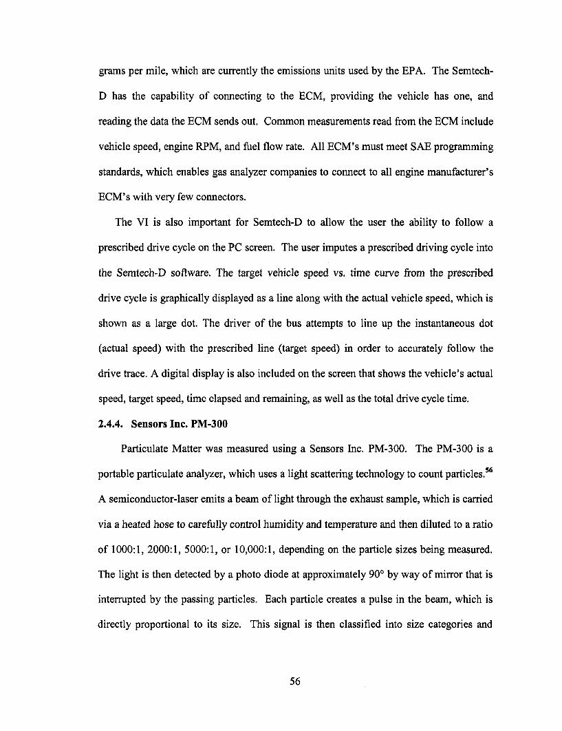
grams per mile, which are currently the emissions units used by the EPA. The Semtech-
D has the capability of connecting to the ECM, providing the vehicle has one, and
reading the data the ECM sends out. Common measurements read from the ECM include
vehicle speed, engine RPM, and fuel flow rate. All ECM's must meet SAE programming
standards, which enables gas analyzer companies to connect to all engine manufacturer's
ECM's with very few connectors.
The VI is also important for Semtech-D to allow the user the ability to follow a
prescribed drive cycle on the PC screen. The user imputes a prescribed driving cycle into
the Semtech-D software. The target vehicle speed vs. time curve from the prescribed
drive cycle is graphically displayed as a line along with the actual vehicle speed, which is
shown as a large dot. The driver of the bus attempts to line up the instantaneous dot
(actual speed) with the prescribed line (target speed) in order to accurately follow the
drive trace. A digital display is also included on the screen that shows the vehicle's actual
speed, target speed, time elapsed and remaining, as well as the total drive cycle time.
2.4.4. Sensors Inc. PM-300
Particulate Matter was measured using a Sensors Inc. PM-300. The PM-300 is a
portable particulate analyzer, which uses a light scattering technology to count particles.5 6
A semiconductor-laser emits a beam of light through the exhaust sample, which is carried
via a heated hose to carefully control humidity and temperature and then diluted to a ratio
of 1000:1, 2000:1, 5000:1, or 10,000:1, depending on the particle sizes being measured.
The light is then detected by a photo diode at approximately 90° by way of mirror that is
interrupted by the passing particles. Each particle creates a pulse in the beam, which is
directly proportional to its size. This signal is then classified into size categories and
56
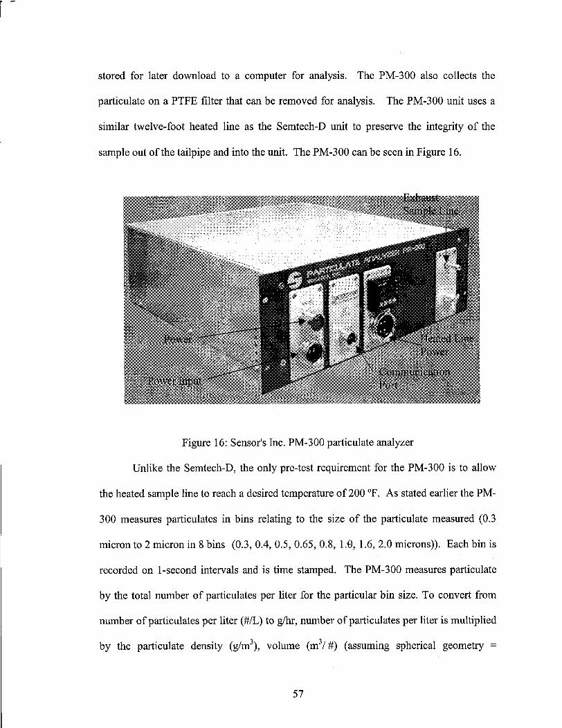
stored for later download to a computer for analysis. The PM-300 also collects the
particulate on a PTFE filter that can be removed for analysis. The PM-300 unit uses a
similar twelve-foot heated line as the Semtech-D unit to preserve the integrity of the
sample out of the tailpipe and into the unit. The PM-300 can be seen in Figure 16.
Figure 16: Sensor's Inc. PM-300 particulate analyzer
Unlike the Semtech-D, the only pre-test requirement for the PM-300 is to allow
the heated sample line to reach a desired temperature of 200 °F. As stated earlier the PM-
300 measures particulates in bins relating to the size of the particulate measured (0.3
micron to 2 micron in 8 bins (0.3, 0.4, 0.5, 0.65, 0.8, 1.0, 1.6, 2.0 microns)). Each bin is
recorded on 1-second intervals and is time stamped. The PM-300 measures particulate
by the total number of particulates per liter for the particular bin size. To convert from
number of particulates per liter (#/L) to g/hr, number of particulates per liter is multiplied
by the particulate density (g/m3 ), volume (m 3 /#) (assuming spherical geometry =
57
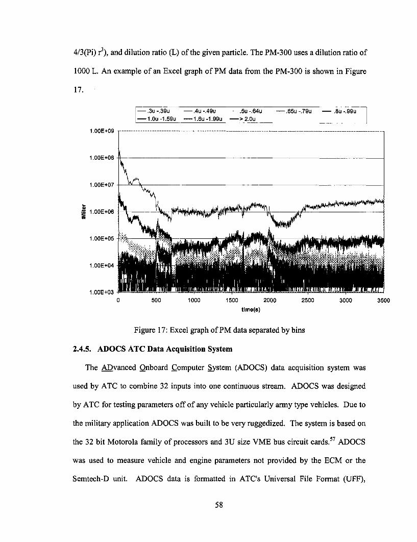
4/3(Pi) r3), and dilution ratio (L) of the given particle. The PM-300 uses a dilution ratio of
1000 L. An example of an Excel graph of PM data from the PM-300 is shown in Figure
17.
.3u -.39u - .4u -.49u .5u -.64u-- 1.0u-1.59u -- 1.6u-1.99u ->2.0u
1.UUt+UV
1.00E+08
1.00E+07
a 1.00E+06
1.00E+05
1.00E+04
1.00E+03
- .65u-.79u - .8u-.99u
0 500 1000 1500 2000 2500 3000 3500
time(s)
Figure 17: Excel graph of PM data separated by bins
2.4.5. ADOCS ATC Data Acquisition System
The ADvanced Onboard Computer System (ADOCS) data acquisition system was
used by ATC to combine 32 inputs into one continuous stream. ADOCS was designed
by ATC for testing parameters off of any vehicle particularly army type vehicles. Due to
the military application ADOCS was built to be very ruggedized. The system is based on
the 32 bit Motorola family of processors and 3U size VME bus circuit cards.5 7 ADOCS
was used to measure vehicle and engine parameters not provided by the ECM or the
Semtech-D unit. ADOCS data is formatted in ATC's Universal File Format (UFF),
58
l - - - -
l
�___�__
which can be easily converted to an Excel spreadsheet. ADOCS operates using a
Windows based user interface for easier interaction. An ADOCS Signal Conditioning
System (ASCS) is used to condition each of the 32 ADOCS channels being used. The
ASCS accepts inputs from pressure sensors, thermocouples, and displacement sensors as
well as outputs from pulse instrumentation and provides signal amplification, filtering,
and calibration.57 The complete ADOCS and ASCS system weighs approximately 32 lbs.
and dimensions of 9 inches width, 10.3 inches high, and 17 inches deep. A complete
ADOCS unit is shown in Figure 18.
Figure 18: ADvanced Onboard Computer System (ADOCS)
For the purpose of school bus emissions tesing, ADOCS was used for only a few
parameters. The Cummins bus had a fuel flow rate meter installed due to the lack of an
ECM. The fuel flow rate was recorded by ADOCS. Three thermocouples were used in
conjunction with ADOCS to measure the exhaust temperature at three distinct locations
along the tailpipe. The temperature at these locations are pertinent when designing
particulate traps where temperature can be an important factor.
2.4.6. Data Management
An important part in analyzing the data collected from up to three separate instrument
platforms is making certain the data is correctly referenced in time. All three units were
59
started at approximately the same time and all three units report data at 1 Hz. The
Semtech-D reports all of its data by exporting it directly into a single Excel spreadsheet.
The PM-300 provides a text file, which can be turned into a comma delimited Excel file
rather easily. ADOCS data is reported in Universal File Format (UFF), which also can be
quickly converted into an Excel spreadsheet. Since, for example, percent load (reported
by Semtech-D) is important in the concentration of particulates (PM-300) it was
important to have all data in a single Excel spreadsheet. All three pieces of equipment
provide time stamping, which is a definitive way to reference all three Excel files
compiled from the equipment into one single file for the analysis.
Data collected by ATC personnel during testing was sent electronically to Rowan for
analysis. Included with all data was a running log file that was up to date with the current
data being forwarded. Every log consisted of the following data: day of test, time of test
start and end, daily run number, fuel type, school bus type tested, equipment used, school
bus driver, success of audits, and any additional comments to describe the test run. The
data was then separated into folders named according to date and then data type (e.g. PM-
300, Semtech-D, audit, etc.).
60
3. Development of a New Mobile Emissions Test Cycle for School Buses
3.1. Introduction
This chapter describes the development of a new mobile emissions test cycle for
school buses. Also provided in this chapter is a literature search of previous test cycles, a
demographic breakdown of regions in NJ, and detailed bus routes of various NJ school
bus districts.
Federal regulation requires that all heavy-duty diesel vehicles (HDDV) complete an
engine certification process using the Transient FTP engine dynamometer cycle.58
Several emission-testing cycles, such as the Transient FTP, have been developed for
federal and private emission testing purposes. These HDDV testing cycles are based
upon speed versus time traces. Traditionally, diesel engine emissions are measured using
a cycle in a stationary position with the engine either in a vehicle on a chassis
dynamometer or the engine alone using an engine dynamometer (See Chapter 1). Mobile
emissions' testing consists of the engine emissions being measured from the mobile
vehicle being tested on the road. There are presently emission test cycles developed for
transit buses and delivery trucks, which are not approved or adopted by the EPA, using a
chassis dynamometer for the testing, but no cycles have been created for mobile testing.
Prior to the present study there existed a scarcity of emission test cycles developed
specifically for school buses. Moreover, mobile-on-road or in-use emissions testing is
relatively new to the emissions testing field, so a standard test cycle for mobile school
bus emissions testing was not available. Accordingly a new standard test cycle for mobile
school bus emissions testing was developed as part of the present study. The Rowan
61
University Composite School Bus Cycle (RUCSBC) was developed using actual global
positioning system (GPS) data from a variety of prototypical New Jersey school bus
routes. The school district routes were chosen based upon the population density of the
district, school age children population of the district, the total number of the district's
buses, and the total number of students in the district. The RUCSBC can be broken down
into three sections to represent the three common areas of the state: rural, suburban, and
urban. As described below, the RUCSBC was used to simulate a typical New Jersey
school bus route in order to compare baseline emissions to emissions with a variety of
fuel types.
3.2. Literature Review
The 2007 HDDV emission standards have lead to extensive testing of the vehicles
and their engines on both chassis and engine dynamometers. The extensive testing has
led to an increasing number of test cycles being created to represent some type of driving
pattern for the HDDV industry. Only a few test cycles have ever been created using
actual data collected from the vehicle during its normal operation. To date there has also
been no test cycle known created specifically for school bus mobile emissions testing.
This literature search is provided to show the function of current emission test cycles,
how the cycles were developed, and what the cycles were developed for.
West Virginia University (WVU) developed a route for delivery trucks using data
from actual delivery truck routes. The City Suburban Heavy Vehicle Route (CSHVR) 59
was designed to consider power-to-weight ratio of the vehicle running the route. A route
differs from a cycle in that a route allows the full power of the vehicle being tested to be
employed.59 In a route the vehicle follows a speed vs. distance trace allowing vehicles
62
with the ability of more rapid accelerations to finish the route in less time. A cycle is a
speed vs. time trace and should be completed in the same amount of time by every
vehicle regardless of its power or size.
The CSHVR was developed from data collected from Classes 7 and 8 delivery
trucks (from two different trucking companies, one based in Akron, Ohio and one from
Richmond Virginia). Speed vs. time data along with video recordings were collected for
the trucks for a total of approximately 60 hours. The data was broken down into a total
of 130 microtrips. The definition of a microtrip for this route was defined typically as
driving from one delivery site to another. The 130 microtrips were further separated into
categories: interstate freeway, suburban, city, and yard with the aid of the video taped
data.
All of the microtrips from the CSHVR were analyzed to determine the percentage of
time when the vehicle was accelerating, decelerating, and cruising. The idle time and
average velocity for each microtrip was also taken into account. The microtrips were
then randomly selected and concatenated using a computer program yielding 10,000
possible combinations. The constrained time range of the cycle was 1000-1600 seconds.
The most representative cycle was then determined using a route mean squared (rms)
approach using the following parameters: standard deviation of speed, average speed, and
percent cruise time. Each of the parameters chosen for the most representative cycle was
weighted evenly. These were all compared to the desired database values for each
category. The cycle with the lowest rms was chosen as the most representative cycle.
When performing the analyses, the idle time was removed and then added back in at the
end so that only the vehicles motion was characterized. In the WVU, individual driver
63
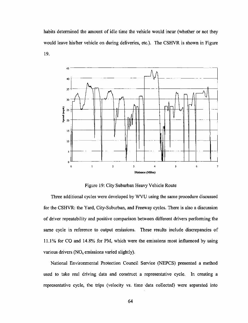
habits determined the amount of idle time the vehicle would incur (whether or not they
would leave his/her vehicle on during deliveries, etc.). The CSHVR is shown in Figure
19.
45
40
35
J 25
1u. 20
15
10
5
=1I I/I \
pII
III0 1 2 3 4 5 6 7
Distance (Miles)
Figure 19: City Suburban Heavy Vehicle Route
Three additional cycles were developed by WVU using the same procedure discussed
for the CSHVR: the Yard, City-Suburban, and Freeway cycles. There is also a discussion
of driver repeatability and positive comparison between different drivers performing the
same cycle in reference to output emissions. These results include discrepancies of
11.1% for CO and 14.8% for PM, which were the emissions most influenced by using
various drivers (NOx emissions varied slightly).
National Environmental Protection Council Service (NEPCS) presented a method
used to take real driving data and construct a representative cycle. In creating a
representative cycle, the trips (velocity vs. time data collected) were separated into
64
IIIt A ,II 1A lI
]J
TV
a A A7k1(LI J .\ r
I
AnAa_
AS T7 n-I or I .[
IU A
I /11 -/
iI 1-
1 t tI
I
I
-- I
t
I _ l l I h
11- I
11- -'1 I/
10I
C-i
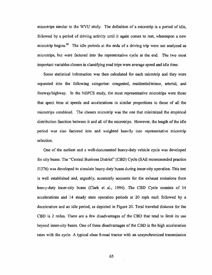
microtrips similar to the WVU study. The definition of a microtrip is a period of idle,
followed by a period of driving activity until it again comes to rest, whereupon a new
microtrip begins.60 The idle periods at the ends of a driving trip were not analyzed as
microtrips, but were factored into the representative cycle at the end. The two most
important variables chosen in classifying road trips were average speed and idle time.
Some statistical information was then calculated for each microtrip and they were
separated into the following categories: congested, residential/minor, arterial, and
freeway/highway. In the NEPCS study, the most representative microtrips were those
that spent time at speeds and accelerations in similar proportions to those of all the
microtrips combined. The chosen microtrip was the one that minimized the empirical
distribution function between it and all of the microtrips. However, the length of the idle
period was also factored into and weighted heavily into representative microtrip
selection.
One of the earliest and a well-documented heavy-duty vehicle cycle was developed
for city buses. The "Central Business District" (CBD) Cycle (SAE recommended practice
J1376) was developed to simulate heavy-duty buses during inner-city operation. This test
is well established and, arguably, accurately accounts for the exhaust emissions from
heavy-duty inner-city buses (Clark et al., 1994). The CBD Cycle consists of 14
accelerations and 14 steady state operation periods at 20 mph each followed by a
deceleration and an idle period, as depicted in Figure 20. Total traveled distance for the
CBD is 2 miles. There are a few disadvantages of the CBD that tend to limit its use
beyond inner-city buses. One of these disadvantages of the CBD is the high acceleration
rates with the cycle. A typical class 8-road tractor with an unsynchronized transmission
65
could not follow the CBD acceleration ramps successfully (Clark et al., 1994). The
Central Business District (CBD) Cycle is a chassis dynamometer testing procedure for
heavy-duty vehicles (SAE J1376). The CBD cycle represents a "sawtooth" driving
pattern, which includes 14 repetitions of a basic cycle composed of idle, acceleration,
cruise, and deceleration modes.
1 0
20
{ 15E
5
00 100 200 300 400 500 600
Time, s
Figure 20: Central Business District Cycle
3.3. Procedure for Generating a New Mobile Cycle
The first step in generating the mobile school bus cycle was to take actual GPS data
from a variety of prototypical school districts in NJ. In each case, a Garmin GPSMAP
765 Global Positioning System was placed on the school bus and activated at the
beginning of a normal bus route and stopped when the bus returned to school. There
were a total of five school bus districts examined from three different counties. These
districts were as follows: Deptford (Gloucester County), Pittsgrove (Salem County),
Medford (Burlington County), Washington Township (Gloucester County), and
Glassboro (Gloucester County).
In total, data from 11 different school bus routes (each referred to as a single "trip")
66
were acquired. Each trip was then separated into microtrips (sometimes called a
sequence). Each microtrip (or sequence) consists of a period of idle, followed by a
period of acceleration and deceleration, until the bus again comes to a complete stop at
which time the next microtrip starts.61 A total of 135 individual microtrips were
generated from the data. In addition, most of the trips contained a period of idle at the
end. For simplicity, the idle times were not included in any of the statistical analyses, but
were later factored into the developed cycle to accurately represent the typical idle a
school bus would incur.
3.3.1. Types of School Districts /Regions
The microtrips were separated into three categories based on the average speed of the
microtrip. Category A included the microtrips with a mean speed range of 0-20 mph,
category B a range of 20-35 mph, and category C a range of 35+ mph. Since idle is very
important in characterizing school bus driving behavior (typically many stops for child
pick-up/drop-off), idle were used in calculating the mean values of microtrip speed, thus
slightly reducing the averages.
Each of these categories (A, B, and C) were designed to represent a different type of
region in NJ: urban, suburban, and rural. An urban area would be considered to be most
densely populated and would reside predominantly within category A. Glassboro and
Washington Township (both located in predominately urban Gloucester County) are
classified as urban areas according to the NJ State Data Center 2000 report.6 2 These
urban area microtrips therefore have the lowest mean speed, the shortest duration,
shortest distance, and the largest percent of idle time at the beginning of each microtrip
(signifying more stops, made more often, with more children at each stop).
67
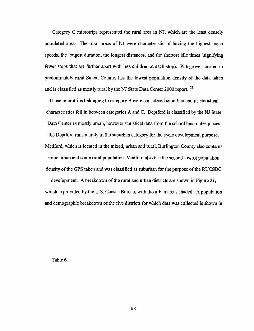
Category C microtrips represented the rural area in NJ, which are the least densely
populated areas. The rural areas of NJ were characteristic of having the highest mean
speeds, the longest duration, the longest distances, and the shortest idle times (signifying
fewer stops that are further apart with less children at each stop). Pittsgrove, located in
predominately rural Salem County, has the lowest population density of the data taken
and is classified as mostly rural by the NJ State Data Center 2000 report. 62
Those microtrips belonging to category B were considered suburban and its statistical
characteristics fell in between categories A and C. Deptford is classified by the NJ State
Data Center as mostly urban, however statistical data from the school bus routes places
the Deptford runs mainly in the suburban category for the cycle development purpose.
Medford, which is located in the mixed, urban and rural, Burlington County also contains
some urban and some rural population. Medford also has the second lowest population
density of the GPS taken and was classified as suburban for the purpose of the RUCSBC
development. A breakdown of the rural and urban districts are shown in Figure 21,
which is provided by the U.S. Census Bureau, with the urban areas shaded. A population
and demographic breakdown of the five districts for which data was collected is shown in
Table 6.
68
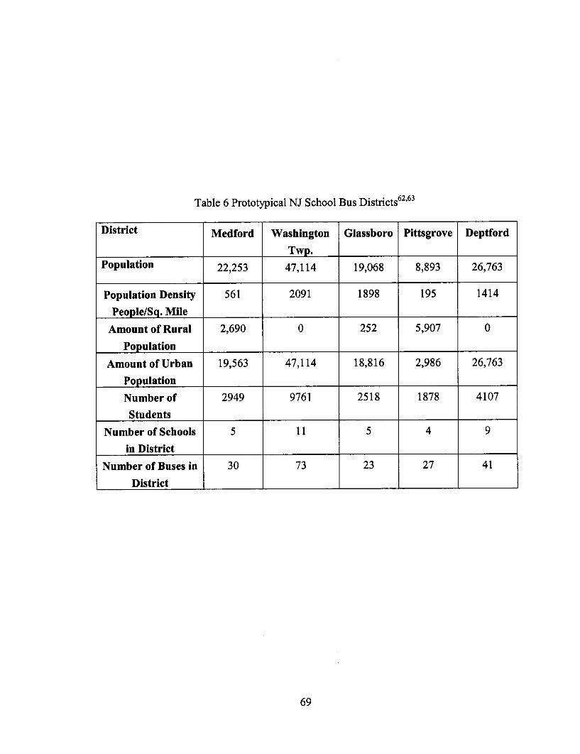
Table 6 Prototypical NJ School Bus Districts 62 '63
District Medford Washington Glassboro Pittsgrove Deptford
Twp.Population 22,253 47,114 19,068 8,893 26,763
Population Density 561 2091 1898 195 1414
People/Sq. Mile
Amount of Rural 2,690 0 252 5,907 0
Population
Amount of Urban 19,563 47,114 18,816 2,986 26,763
Population
Number of 2949 9761 2518 1878 4107
Students
Number of Schools 5 11 5 4 9
in District
Number of Buses in 30 73 23 27 41
District
69
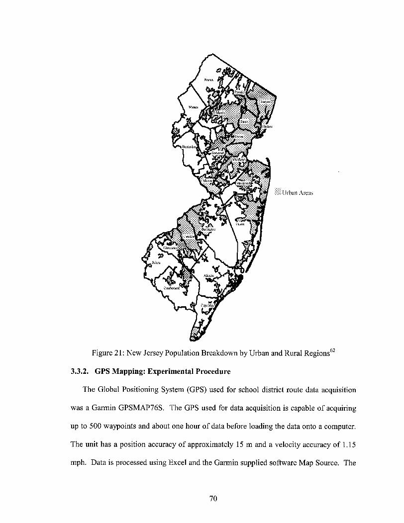
* t1..U rblan Areals
Figure 21: New Jersey Population Breakdown by Urban and Rural Regions62
3.3.2. GPS Mapping: Experimental Procedure
The Global Positioning System (GPS) used for school district route data acquisition
was a Garmin GPSMAP76S. The GPS used for data acquisition is capable of acquiring
up to 500 waypoints and about one hour of data before loading the data onto a computer.
The unit has a position accuracy of approximately 15 m and a velocity accuracy of 1.15
mph. Data is processed using Excel and the Garmin supplied software Map Source. The
70
I
GPS transfers data to a PC in the form of an Excel file, which includes the following
information: position, altitude, time, leg length, leg speed, leg time, total time, average
speed, and leg course. The Garmin GPSMAP76S unit is shown in Figure 22.
Figure 22: ( P76S
The GPS was placed on the school bus for each respective district. Data acquisition
started when the school bus driver started the bus for their route and ended when the
school bus was turned off for the same route. Waypoints were taken at specific locations
to mark the route and the school bus stops. The GPS was then connected to the serial
port on the computer through a PC cable and data was transferred in text format for
analysis. Data to create the cycle was taken in the form of a speed vs. time drive trace.
The speed vs. time drive traces for the Medford, Washington Township, Glassboro,
Pittsgrove, and Deptford school districts are shown in Appendix A.
In a similar format to the drive traces, data was_ transferred to the Map Source
software provided by the Garmin Company, which created an actual map of the school
bus route. The map created by the Map Source Software is similar to a common road
map except the drive trace of the school bus is highlighted and the school bus stops are
marked. Two maps are shown for the Washington Township and Pittsgrove school
71
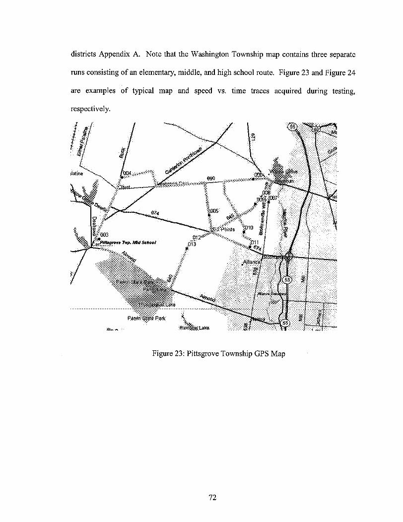
districts Appendix A. Note that the Washington Township map contains three separate
runs consisting of an elementary, middle, and high school route. Figure 23 and Figure 24
are examples of typical map and speed vs. time traces acquired during testing,
respectively.
Figure 23: Pittsgrove Township GPS Map
72
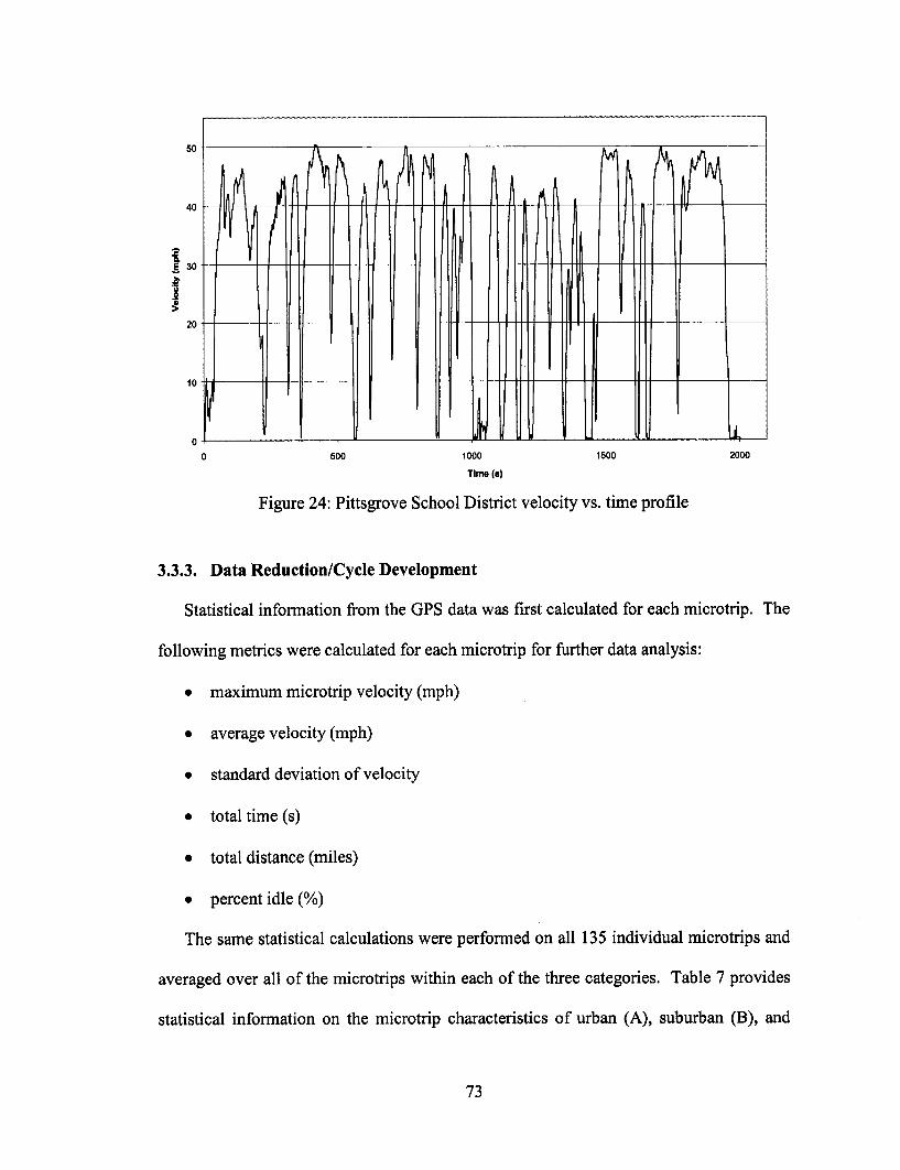
50
40
I.E 30
20
10
0 500 1000 1500 2000
Time (s)
Figure 24: Pittsgrove School District velocity vs. time profile
3.3.3. Data Reduction/Cycle Development
Statistical information from the GPS data was first calculated for each microtrip. The
following metrics were calculated for each microtrip for further data analysis:
* maximum microtrip velocity (mph)
* average velocity (mph)
* standard deviation of velocity
* total time (s)
* total distance (miles)
* percent idle (%)
The same statistical calculations were performed on all 135 individual microtrips and
averaged over all of the microtrips within each of the three categories. Table 7 provides
statistical information on the microtrip characteristics of urban (A), suburban (B), and
73
V I vii Id I II~~~~~1 II ISBS16:~~~~~~~~~~~~~~~~~~~~~~~~~~~~~~~~~~~~~~~~~~~~~~~~~~~~~~~~~~~~~~~~~~~~~~~~~~~~~~~~~~~~~~~~~~~~~~~~~~~~~~~~~~~~~~~~~~~~~~~~~~~~~
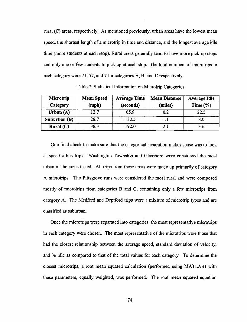
rural (C) areas, respectively. As mentioned previously, urban areas have the lowest mean
speed, the shortest length of a microtrip in time and distance, and the longest average idle
time (more students at each stop). Rural areas generally tend to have more pick-up stops
and only one or few students to pick up at each stop. The total numbers of microtrips in
each category were 71, 57, and 7 for categories A, B, and C respectively.
Table 7: Statistical Information on Microtrip Categories
Microtrip Mean Speed Average Time Mean Distance Average IdleCategory (mph) (seconds) (miles) Time (%)
Urban (A) 12.7 65.9 0.2 22.5
Suburban (B) 28.7 130.5 1.1 8.0
Rural (C) 38.3 192.0 2.1 3.6
One final check to make sure that the categorical separation makes sense was to look
at specific bus trips. Washington Township and Glassboro were considered the most
urban of the areas tested. All trips from these areas were made up primarily of category
A microtrips. The Pittsgrove runs were considered the most rural and were composed
mostly of microtrips from categories B and C, containing only a few microtrips from
category A. The Medford and Deptford trips were a mixture of microtrip types and are
classified as suburban.
Once the microtrips were separated into categories, the most representative microtrips
in each category were chosen. The most representative of the microtrips were those that
had the closest relationship between the average speed, standard deviation of velocity,
and % idle as compared to that of the total values for each category. To determine the
closest microtrips, a root mean squared calculation (performed using MATLAB) with
these parameters, equally weighted, was performed. The root mean squared equation
74
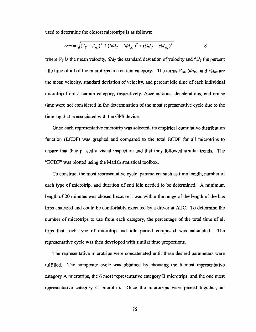
used to determine the closest microtrips is as follows:
rms = (VT - Vm, )2 + (Std, - Stdm )2 + (%IT - %Im )2 8
where VT is the mean velocity, Stdr the standard deviation of velocity and %IT the percent
idle time of all of the microtrips in a certain category. The terms Vmi, Stdmi, and %Imi are
the mean velocity, standard deviation of velocity, and percent idle time of each individual
microtrip from a certain category, respectively. Accelerations, decelerations, and cruise
time were not considered in the determination of the most representative cycle due to the
time lag that is associated with the GPS device.
Once each representative microtrip was selected, its empirical cumulative distribution
function (ECDF) was graphed and compared to the total ECDF for all microtrips to
ensure that they passed a visual inspection and that they followed similar trends. The
"ECDF" was plotted using the Matlab statistical toolbox.
To construct the most representative cycle, parameters such as time length, number of
each type of microtrip, and duration of end idle needed to be determined. A minimum
length of 20 minutes was chosen because it was within the range of the length of the bus
trips analyzed and could be comfortably executed by a driver at ATC. To determine the
number of microtrips to use from each category, the percentage of the total time of all
trips that each type of microtrip and idle period composed was calculated. The
representative cycle was then developed with similar time proportions.
The representative microtrips were concatenated until these desired parameters were
fulfilled. The composite cycle was obtained by choosing the 6 most representative
category A microtrips, the 6 most representative category B microtrips, and the one most
representative category C microtrip. Once the microtrips were pieced together, an
75

average idle was added to the end of the representative cycle consisting of 47 seconds,
which was the average duration of "end of run" idle time for all of the 11 bus routes. The
total duration of the RUCSBC cycle is 1241 seconds. See Table 8 for a breakdown of
category percentages pertaining to the desired time length of each category and the actual
length of each category in the RUCSBC.
Table 8: Microtrip Times for a Cycle with a Minimum of 20 Minutes
Microtrip Time Desired Time Obtained % Difference
Category (seconds) (seconds)
A 400.9 445 8.8
B 636.8 658 1.31
C 115.0 74 36.9
Idle Time 47.3 47 2.66
To ensure that the cycle was easy for a driver to follow and perform, an additional
idle period (10 seconds) was added at the beginning of the cycle and all of the idle
periods were zeroed (the GPS has an accuracy of 2mph). The velocity vs. time profile of
the RUCSBC can be seen in Figure 25. The RUCSBC (velocity vs. time) is also shown in
Figure 26 broken down into the three-microtrip categories urban (A), suburban (B), and
rural (C).
76
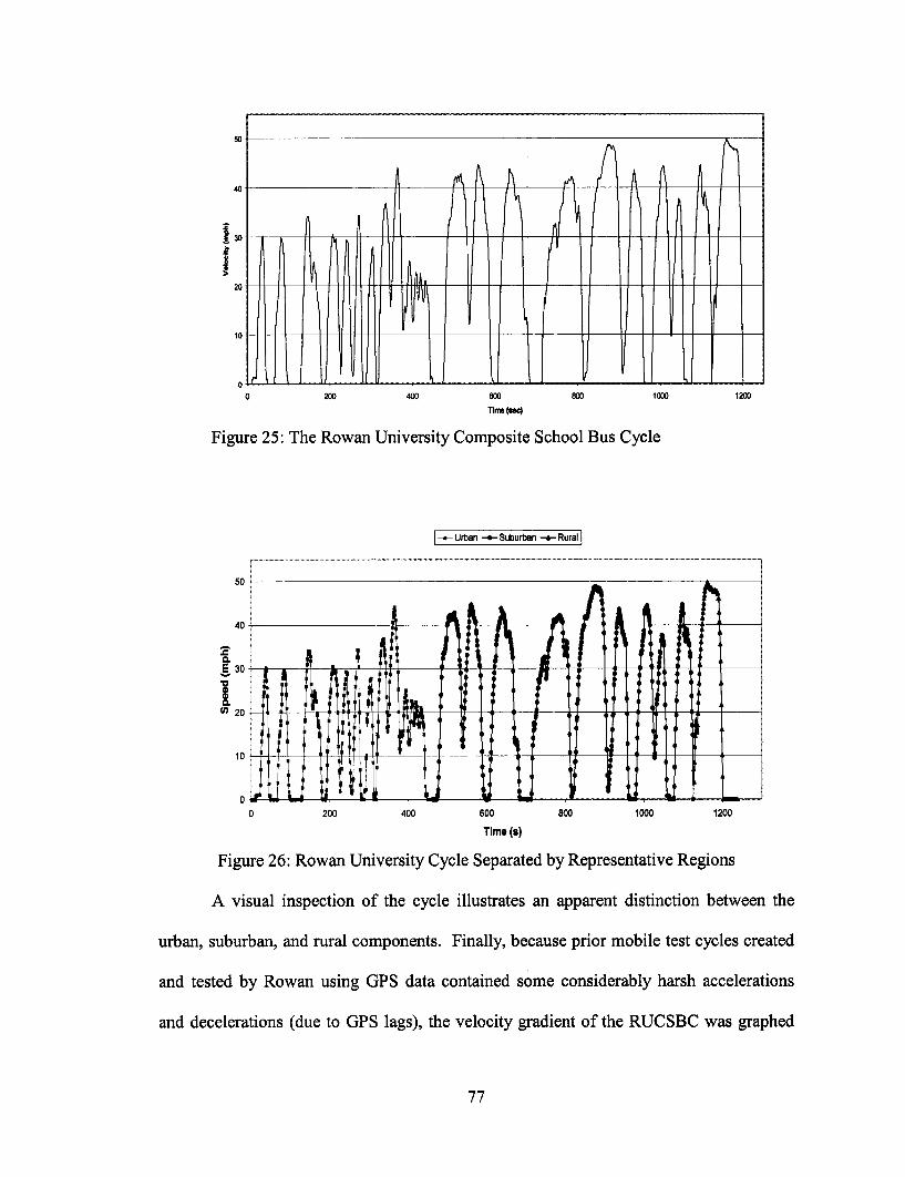
I£
0 200 400 600 800 100
Tlme (ec)
Figure 25: The Rowan University Composite School Bus Cycle
1200
|- -Urban -+-Suburban - Rural
r-1 ..--.. ....... ........................... -.. 1-1-1.... -.11 1- -- ....... ..I............... ..... i...... ... - ,........_- ff _,- , -."...,l- ',1-. ,1.11 ~ I. ..I ...........
SQ.
'a
I(0
50
40
30
20
10
n
0 200 400 600 800 1000 1200
Time (s)
Figure 26: Rowan University Cycle Separated by Representative Regions
A visual inspection of the cycle illustrates an apparent distinction between the
urban, suburban, and rural components. Finally, because prior mobile test cycles created
and tested by Rowan using GPS data contained some considerably harsh accelerations
and decelerations (due to GPS lags), the velocity gradient of the RUCSBC was graphed
77
50
40
5h.10 I-A-I
A I. I
*-,i ̂ i\ Ml
' Ai AI , AI AtI
i~ tiftt :l: If,~L ,__u__J. I I _I LJI
--

(using Matlab) and inspected. The areas with high accelerations and decelerations were
manually smoothed such that the maximum value was adjusted from approximately
0lmph/s to 7mph/s. This adjustment allowed the driver to follow the Semtech trace
provided by the ECM more smoothly and accurately.
An initial driving test of the cycle was performed successfully at the ATC 1-mile
loop. During the driving test it was shown that the same driver could execute the cycle
with adequate repeatability. The close repeatability of the driver following the Semtech
speed trace is shown in Figure 27, and again in Figure 28, which is a speed vs. time trace
of the RUCSBC driven on the 1-mile loop by the same driver using the DT466 bus. The
processed data also showed close comparison between the same two runs with respect
measured emissions, further proving the cycle's repeatability. Figure 29 and Figure 30
show the instantaneous NOx concentration measured during the two runs shown in Figure
27 and Figure 28. From Figure 29 and Figure 30 it is evident that during the idle periods
of the RUCSBC the NOx levels always returned to the same concentration and peaked at
similar positions during the cycle. From the emission and GPS data it was concluded that
the RUCSBC is a repeatable cycle when executed at conditions of similar temperature
and absolute humidity.
78
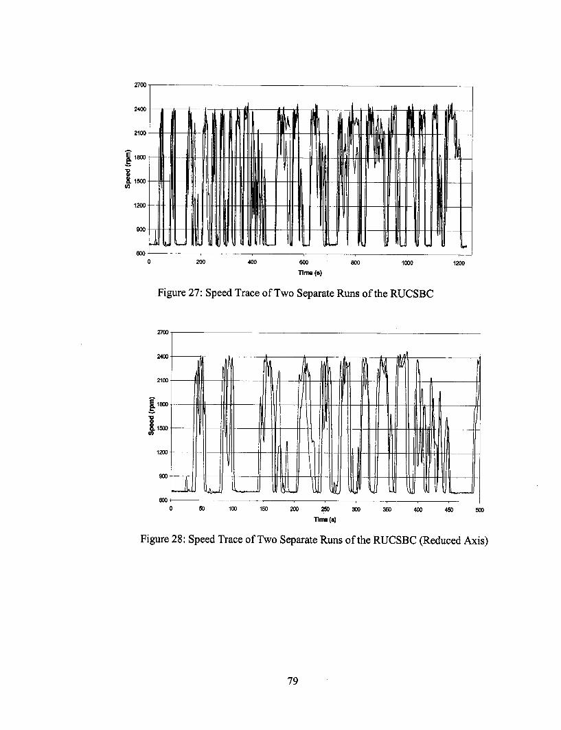
INl IIII II I I roll _
11I11
-1 l_. I _ ... ...... II1 I H 11 1
11-~ II U
L0 200 400 600 800 1000 1200
Time (s)
Figure 27: Speed Trace of Two Separate Runs of the RUCSBC
2700
MI.. I I/AA
- -i-jt-A-tji500 11A1200
MO/ /,lin ,il ,600^---------------------------, ______
0 50 100 150 200 250 30 360 400 450 500
wmn (s)
U I I.- BJ I1 1I
Figure 28: Speed Trace of Two Separate Runs of the RUCSBC (Reduced Axis)
79
2700
2400
2100
1800
1Uu -
1200-
900
fi L .A Ai I , M [I 1AII'I I I I . ~ q~ I , h I I 1 1111 11 I -Ii 11 III .
III 1 1 n 11111 1111I rlall II ll l Vi11 II H 111 1l!M~,'1nlllYll n1 IjI/fl N 1 1HIIH ilfllU l I I I I I II I I I I ll r llllilli i-ii iiIl.I I ..... I. .... t1 I III 1 II I 11 11111 L-
IIBt 11 ]kUA I
IN1
1111111lll 1 F,
I
60O
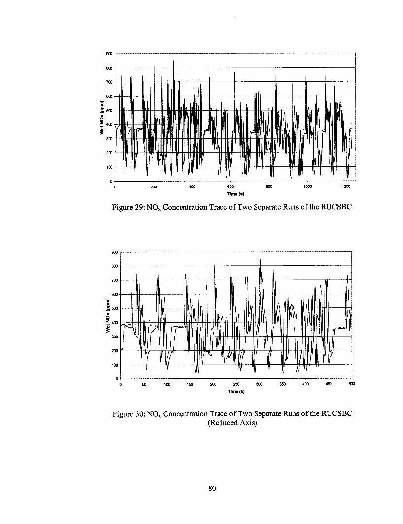
800
700
600
500
400
300
200
100
n
0 200 400 600
Time (s)
800 1000 1200
Figure 29: NOx Concentration Trace of Two Separate Runs of the RUCSBC
900
800 l
700
600
ox 400
200
100
0
0 50 100 150 200 250 300 350 400 450 500
Time (s)
Figure 30: NOx Concentration Trace of Two Separate Runs of the RUCSBC(Reduced Axis)
80
E9.C.
0zw
r~Ibob ---- -------~~~_~___
, , , II I. I I ,I .I I I, 1 1 t L I I I; 111 ilI T Ill~l J Jll l lll f ~ ll 'I[II 'I~il ll~ I1 ' 11 f illI l
I~~~{ I! t ,rQ IIl vII' 1 I Mii1 "I II

4. Rowan On Road Medford Township School Bus Testing
4.1. Introduction
This chapter provides emissions data taken from school buses in the Medford
Township School District running on #2 diesel and biodiesel. In conjunction with the
school bus emissions reduction study being performed at ATC, Rowan University
performed emissions testing at a local school district already running biodiesel. Since a
local school district (Medford, NJ) currently employs a B20 biodiesel blend to fuel 50%
of their fleet, actual on-road emissions data were acquired in addition to the tests
performed on the test track at ATC. The on-road tests were performed at the Medford
Township School District in Medford, NJ on four of the districts 44 buses. Over the past
five years, Medford has converted half of their 44-bus fleet to a blend of 20 percent
biodiesel and 80 percent petroleum (B20) purchased from World Energy Alternatives.
Since converting Medford has had no known problems with running biodiesel even at
temperatures of 11 degrees below zero36.
4.2. Purpose of Medford Study
In recent emission reduction programs for heavy-duty diesel engines, biodiesel has
become a popular alternative fuel for testing. In an effort to acquire as much emissions
data as possible, Rowan tested at the only school district in NJ and the surrounding area
running school buses on any mixture of biodiesel. Tests were performed in Medford in
the month of January on two separate occasions. Since 1997, Medford has run biodiesel
in almost half of their buses, but they had never had them tested for emissions to see if
their efforts in running on biodiesel were worthwhile. Rowan was able to provide
Medford with emissions data that could only otherwise be acquired by purchasing or
81
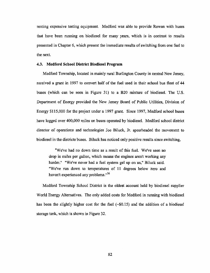
renting expensive testing equipment. Medford was able to provide Rowan with buses
that have been running on biodiesel for many years, which is in contrast to results
presented in Chapter 6, which present the immediate results of switching from one fuel to
the next.
4.3. Medford School District Biodiesel Program
Medford Township, located in mainly rural Burlington County in central New Jersey,
received a grant in 1997 to convert half of the fuel used in their school bus fleet of 44
buses (which can be seen in Figure 31) to a B20 mixture of biodiesel. The U.S.
Department of Energy provided the New Jersey Board of Public Utilities, Division of
Energy $115,000 for the project under a 1997 grant. Since 1997, Medford school buses
have logged over 400,000 miles on buses operated by biodiesel. Medford school district
director of operations and technologies Joe Biluck, Jr. spearheaded the movement to
biodiesel in the districts buses. Biluck has noticed only positive results since switching,
"We've had no down time as a result of this fuel. We've seen no
drop in miles per gallon, which means the engines aren't working any
harder." "We've never had a fuel system gel up on us," Biluck said.
"We've run down to temperatures of 11 degrees below zero and
haven't experienced any problems."3 6
Medford Township School District is the oldest account held by biodiesel supplier
World Energy Alternatives. The only added costs for Medford in running with biodiesel
has been the slightly higher cost for the fuel (-$0.15) and the addition of a biodiesel
storage tank, which is shown in Figure 32.
82
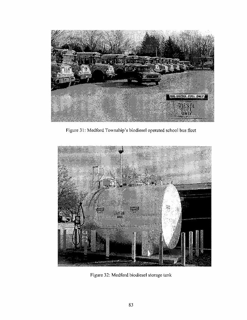
Figure 31: Medford Township's biodiesel operated school bus fleet
Figure 32: Medford biodiesel storage tank
83
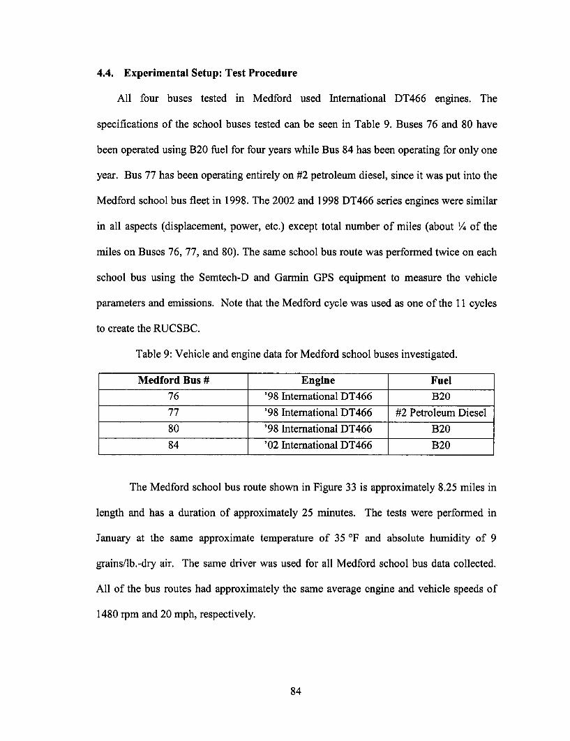
4.4. Experimental Setup: Test Procedure
All four buses tested in Medford used International DT466 engines. The
specifications of the school buses tested can be seen in Table 9. Buses 76 and 80 have
been operated using B20 fuel for four years while Bus 84 has been operating for only one
year. Bus 77 has been operating entirely on #2 petroleum diesel, since it was put into the
Medford school bus fleet in 1998. The 2002 and 1998 DT466 series engines were similar
in all aspects (displacement, power, etc.) except total number of miles (about ¼/4 of the
miles on Buses 76, 77, and 80). The same school bus route was performed twice on each
school bus using the Semtech-D and Garmin GPS equipment to measure the vehicle
parameters and emissions. Note that the Medford cycle was used as one of the 11 cycles
to create the RUCSBC.
Table 9: Vehicle and engine data for Medford school buses investigated.
Medford Bus # Engine Fuel76 '98 International DT466 B20
77 '98 International DT466 #2 Petroleum Diesel
80 '98 International DT466 B20
84 '02 International DT466 B20
The Medford school bus route shown in Figure 33 is approximately 8.25 miles in
length and has a duration of approximately 25 minutes. The tests were performed in
January at the same approximate temperature of 35 °F and absolute humidity of 9
grains/lb.-dry air. The same driver was used for all Medford school bus data collected.
All of the bus routes had approximately the same average engine and vehicle speeds of
1480 rpm and 20 mph, respectively.
84
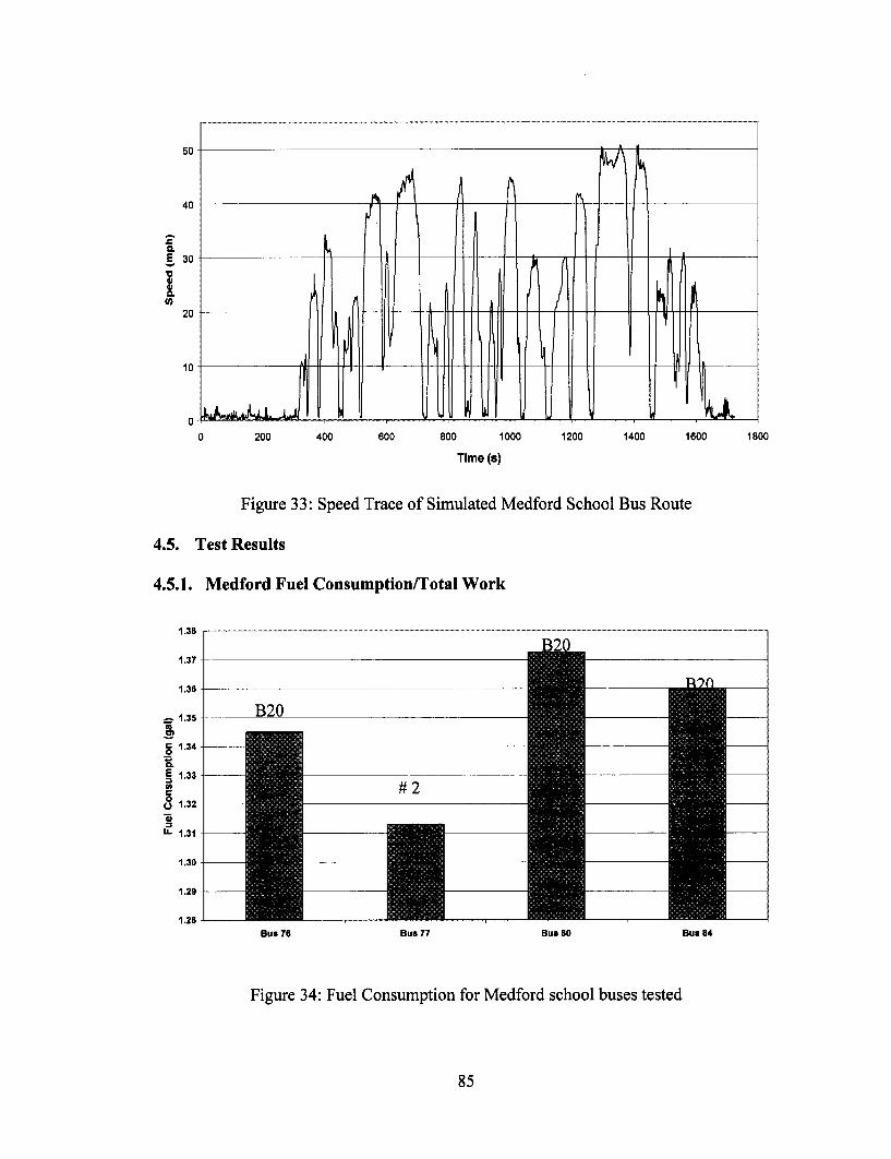
50
40
20
E 3o
10
010
o-
0 200 400 600 800 1000 1200 1400 1600
Time (s)
Figure 33: Speed Trace of Simulated Medford School Bus Route
4.5. Test Results
4.5.1. Medford Fuel Consumption/Total Work
1.38 -
1.37
1.3 -
1.35
c 1.34-0
E 1.33 -
C
1- 3LL 1.31 -
1.30 -
1.29
1.28 -
B20
#2
Bus 76 Bus 77 Bus 80 Bus 84
Figure 34: Fuel Consumption for Medford school buses tested
85
1800
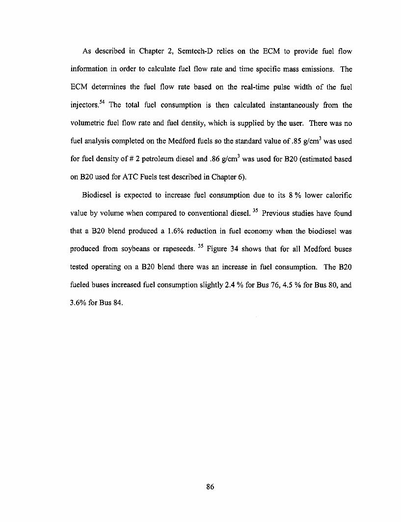
As described in Chapter 2, Semtech-D relies on the ECM to provide fuel flow
information in order to calculate fuel flow rate and time specific mass emissions. The
ECM determines the fuel flow rate based on the real-time pulse width of the fuel
injectors. 54 The total fuel consumption is then calculated instantaneously from the
volumetric fuel flow rate and fuel density, which is supplied by the user. There was no
fuel analysis completed on the Medford fuels so the standard value of .85 g/cm3 was used
for fuel density of # 2 petroleum diesel and .86 g/cm3 was used for B20 (estimated based
on B20 used for ATC Fuels test described in Chapter 6).
Biodiesel is expected to increase fuel consumption due to its 8 % lower calorific
value by volume when compared to conventional diesel.35 Previous studies have found
that a B20 blend produced a 1.6% reduction in fuel economy when the biodiesel was
produced from soybeans or rapeseeds. 35 Figure 34 shows that for all Medford buses
tested operating on a B20 blend there was an increase in fuel consumption. The B20
fueled buses increased fuel consumption slightly 2.4 % for Bus 76, 4.5 % for Bus 80, and
3.6% for Bus 84.
86
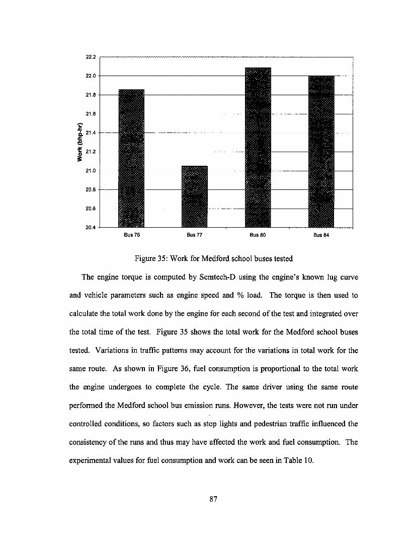
22.0
21.8
21.6
& 21.4 -
.0
E 21.2
21.0
20.8
20.6 -
20.4Bus 76 Bus 77 Bus 80 Bus 84
Figure 35: Work for Medford school buses tested
The engine torque is computed by Semtech-D using the engine's known lug curve
and vehicle parameters such as engine speed and % load. The torque is then used to
calculate the total work done by the engine for each second of the test and integrated over
the total time of the test. Figure 35 shows the total work for the Medford school buses
tested. Variations in traffic patterns may account for the variations in total work for the
same route. As shown in Figure 36, fuel consumption is proportional to the total work
the engine undergoes to complete the cycle. The same driver using the same route
performed the Medford school bus emission runs. However, the tests were not run under
controlled conditions, so factors such as stop lights and pedestrian traffic influenced the
consistency of the runs and thus may have affected the work and fuel consumption. The
experimental values for fuel consumption and work can be seen in Table 10.
87
n_ nZZ.Z
l
I
II
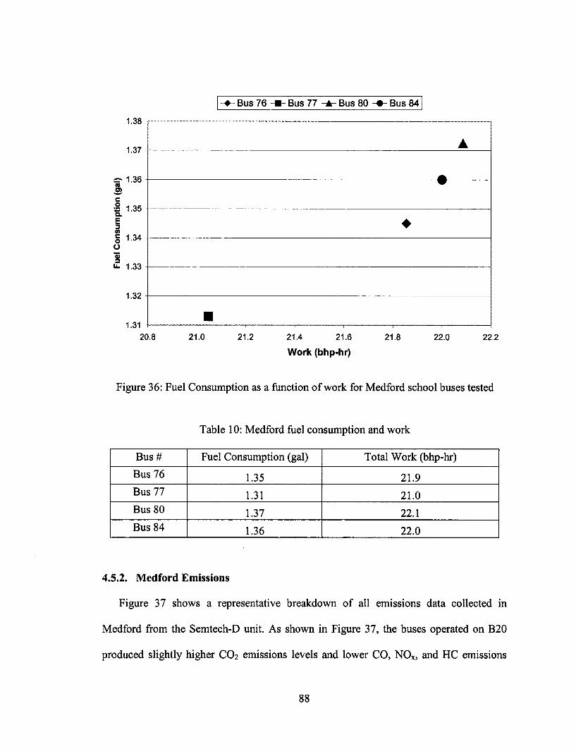
I -4 Bus 76 -U- Bus 77 -- Bus 80 -- Bus 841
1 . ... ..........-....... . _. .. .„.... .I
1.37 -A
- 1.36 -
C
I 1.35
E ·1.34
0
u. 1.33
1.32
1.31 -20.8 21.0 21.2 21.4 21.6 21.8 22.0 22.2
Work (bhp-hr)
Figure 36: Fuel Consumption as a function of work for Medford school buses tested
Table 10: Medford fuel consumption and work
Bus # Fuel Consumption (gal) Total Work (bhp-hr)
Bus 76 1.35 21.9
Bus 77 1.31 21.0
Bus 80 1.37 22.1
Bus 84 1.36 22.0
4.5.2. Medford Emissions
Figure 37 shows a representative breakdown of all emissions data collected in
Medford from the Semtech-D unit. As shown in Figure 37, the buses operated on B20
produced slightly higher CO2 emissions levels and lower CO, NOx, and HC emissions
88
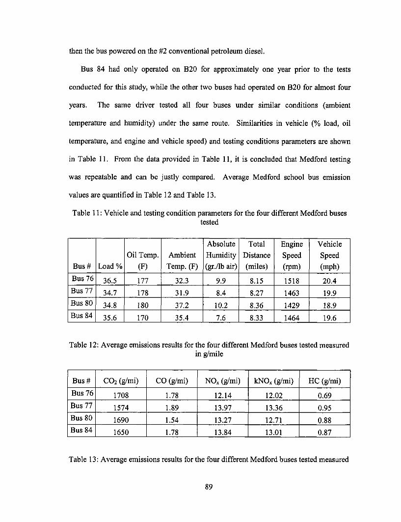
then the bus powered on the #2 conventional petroleum diesel.
Bus 84 had only operated on B20 for approximately one year prior to the tests
conducted for this study, while the other two buses had operated on B20 for almost four
years. The same driver tested all four buses under similar conditions (ambient
temperature and humidity) under the same route. Similarities in vehicle (% load, oil
temperature, and engine and vehicle speed) and testing conditions parameters are shown
in Table 11. From the data provided in Table 11, it is concluded that Medford testing
was repeatable and can be justly compared. Average Medford school bus emission
values are quantified in Table 12 and Table 13.
Table 11: Vehicle and testing condition parameters for the four different Medford busestested
Absolute Total Engine VehicleOil Temp. Ambient Humidity Distance Speed Speed
Bus # Load % (F) Temp. (F) (gr./lb air) (miles) (rpm) (mph)
Bus 76 36.5 177 32.3 9.9 8.15 1518 20.4Bus 77 34.7 178 31.9 8.4 8.27 1463 19.9Bus 80 34.8 180 37.2 10.2 8.36 1429 18.9Bus 84 35.6 170 35.4 7.6 8.33 1464 19.6
Table 12: Average emissions results for the four different Medford buses tested measuredin g/mile
Bus # CO2 (g/mi) CO (g/mi) NO, (g/mi) kNOx (g/mi) HC (g/mi)
Bus 76 1708 1.78 12.14 12.02 0.69Bus 77 1574 1.89 13.97 13.36 0.95Bus 80 1690 1.54 13.27 12.71 0.88Bus 84 1650 1.78 13.84 13.01 0.87
Table 13: Average emissions results for the four different Medford buses tested measured
89
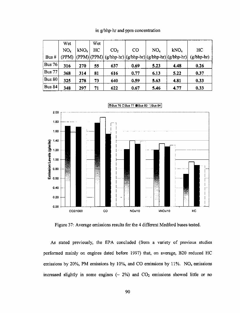
in g/bhp-hr and ppm concentration
Wet Wet
NOx kNOx HC CO2 CO NOx kNOx HC
Bus # (PPM) (PPM)(PPM) (g/bhp-hr) (g/bhp-hr) (g/bhp-hr) (g/bhp-hr) (g/bhp-hr)
Bus 76 316 270 55 637 0.69 5.23 4.48 0.26
Bus 77 368 314 81 616 0.77 6.13 5.22 0.37Bus 80 325 278 73 640 0.59 5.63 4.81 0.33Bus 84 348 297 71 622 0.67 5.46 4.77 0.33
I M Bus 76 O Bus 77 * Bus 80 ] Bus 84
Z.UU
1.80
1.60
T 1.40
E1.20
.5
' 1.00-I
0.80
0.60U, 0.60
0.40
0.20
0.00C02/1000 CO NOx/10 kNOx/10 HC
Figure 37: Average emissions results for the 4 different Medford buses tested.
As stated previously, the EPA concluded (from a variety of previous studies
performed mainly on engines dated before 1997) that, on average, B20 reduced HC
emissions by 20%, PM emissions by 10%, and CO emissions by 11%. NOx emissions
increased slightly in some engines (- 2%) and CO 2 emissions showed little or no
90
difference.3 5 In the present study, HC emissions showed some significant reductions with
the use of B20, particularly in Buses 76, which showed a reduction of 27.2 % when
compared to the baseline #2 diesel bus (Bus 77). These reductions are higher then those
found by the EPA cumulative study. However, Bus 80 and Bus 84 reduced HC emissions
by only 7.4 % and 8.4 %, respectively, which was slightly lower than given by the study.
CO emissions were slightly decreased by 6.1 % and 5.9 % with the use of B20 in Buses
76 and 84, respectively, when compared to the baseline #2 diesel bus (Bus 77). Bus 80
showed a much higher CO decrease than the other buses of 18.7 %. These decreases in
CO emissions were expected since the EPA report claimed that B20 was expected to
slightly reduce CO emissions.
NOx emissions showed slight reductions between 1.0 % and 13 % with the use of
B20. Semech's corrected NOx (kNOx) also slight reductions between 2.6 % and 10 %.
An SAE NOx correction factor for temperature and humidity was not used for the
Medford data because all tests were conducted within a close range of 5 °F and 2 gr./lb-
dry air, respectively. Previous work has found however, that NOx emissions generally
increase slightly with biodiesel. 32, 35 The NOx increases when using biodiesel could be
caused by the higher fuel density and lower heating value of the fuel.32 Increasing
oxygen content in the fuel has caused significant increases in NOx in previous research. 32
The NOx tradeoff is not a large concern however, due to the low sulfur content of
biodiesel (-24 ppm), which will work with NOx reducing technologies that require low
sulfur fuel.
The slight reduction of NOx emissions from the Medford biodiesel buses could be a
result of the B20 being mixed with kerosene for winterization. It is a common practice
91

for cold weather areas to mix kerosene with biodiesel to lower the cloud point of the fuel
to prevent gelling. Kerosene has a lower relative density (-0.80 g/cm3) when compared
to B20 (-0.86 g/cm3) and #2 petroleum diesel (-0.85 g/cm3). Kerosene also contains a
slightly higher heating value (20,000 btu/lb) when compared to biodiesel (17,500 btu/lb).
A previous study on the effect of kerosene in #2 petroleum diesel fuel found that the
addition of kerosene slightly reduces NOx and PM emissions and slightly raises CO and
HC emissions.6 4
The Medford data concurred with the EPA study that there was little change in CO2
emissions (between 2.4 % and 4.5 %) from using B20. However, the real savings in CO2
emissions comes from the fact that biodiesel is renewable, meaning the CO2 emission
released into the atmosphere when biodiesel is burned is recycled by growing plants,
which are later processed into fuel. A small percentage of tailpipe fossil CO 2 produced
from operating on biodiesel can be attributed to the methanol contribution, however
almost 95 % of the biodiesel created CO2 emission is tailpipe biomass CO2.6 5 A recent
government study shows that the use of biodiesel can reduce CO2 emissions by 78.45%
on a life cycle basis, which include emissions in the production of the fuel.65.
92
5. School Bus Idle Emissions
5.1. Introduction
In addition to implementing reduction technologies for mobile emissions from school
buses, NJDOT has also identified the reduction or elimination of school bus idling as a
potential component of future SIP's. There are approximately 11,000 school buses used
each day in the state of New Jersey.4 7 These school buses are often idled in the morning
prior to their initial bus route and in the afternoon while waiting to pick up the children to
take them home. School bus idling occurs for the following reasons:
* to keep the engine and fuel warm in cold weather,
* provide heat inside the bus in cold weather and,
* to provide power for lighting for safety purposes.
Heavy Duty Diesel Vehicle (HDDV) truck engine idling results in costly fuel
consumption and engine wear. Moreover, idling produces pollutants in the form of
nitrous oxides (NOx), carbon monoxide (CO), carbon dioxide (CO2), hydrocarbons (HC),
and particulate matter (PM), which may be avoidable with the reduction of unnecessary
idling. Indeed, unlike mobile emissions, which can at best be reduced through a variety
of costly technologies, idle emissions can be completely eliminated by eliminating
unnecessary idling.
School bus idle experiments were conducted at the United States Army Aberdeen
Test Center (ATC) in Aberdeen, Maryland. In the experiments described herein, three
school buses were tested in an environmental chamber where the ambient temperatures of
20°F, 40°F, 65°F, and 85°F and relative humidity were held constant. The objectives of
this study were as follows:
93
* quantify fuel consumption rates of school buses at idle,
* quantify school bus idle exhaust emissions at various temperatures and
humidity's,
* determine the effects of ambient temperature and humidity on school bus engine
idle emissions and fuel consumption, and
* create engine specific NOx correction factors for each school bus engine presently
undergoing mobile emissions reduction technologies testing in a parallel study.
5.2. Literature Search
5.2.1. HDDV Study
Previous idle emission studies on HDDV's have mainly been performed on heavy-
duty trucks. A significant fraction of diesel emissions can be attributed to HDDV's at idle
conditions during which power is being used for systems such as cabin heating or
cooling. In the spring of 2002, the U.S. Environmental Protection Agency, in
collaboration with the New Jersey Department of Transportation, the U.S. Army
Aberdeen Test Center, Oak Ridge National Laboratory and Rowan University initiated a
study to quantify the idling emissions and fuel consumption rates for HDDV trucks.
Testing was performed in an environmental chamber at ATC on five different class 8
trucks with model years ranging from 1990's to 2001. To simulate a wide variety of
idling situations, 38 tests were conducted at three different ambient temperatures (0°F,
65°F and 90°F), relative humidity ranging from 22 to 90% and idle speeds from 600 to
1200 RPM. Each test was conducted for approximately three hours during which HC,
NOx, CO, C 2O, 02, and PM emissions were monitored.
The test results show that the emission rates are a function of both the inlet
94
temperature and engine load. For example, a Detroit Diesel engine idling at 600 RPM
produced an average NO, emission of 54.8 g/hr for 0° F ambient temperature (with cabin
heater activated) to 105 g/hr at 90° F (with cabin air conditioner activated). The effect of
humidity was evidenced through a 15 to 20% decrease in NOx concentration when
relative humidity increased by a factor of three. However, the HDDV vehicles have
engines that are almost double the displacement of school bus engines. Therefore, these
values cannot be used to accurately estimate the emissions and fuel consumption from
school bus idling. Moreover, most school buses are not equipped with air conditioning
units, nor does a school bus have to power any appliances and/or refrigerate or heat
cargo.
The results from the HDDV truck idling study also show that ambient temperature
and humidity can have a significant effect on the formation of NOx gases. 66 Accordingly,
the present idle study was performed to accurately quantify emissions from school bus
idling for various temperature and humidity.
The present school bus idle emissions study is also an integral part of larger study
involving the characterization of emission reduction strategies using a mobile testing
procedure. As described in detail in Chapter 6 of this thesis, since the mobile emissions
testing is performed outdoors on a test track, the inlet air temperature and humidity is not
controlled. It is also well documented that NO, emissions are a strong function of
temperature and humidity.55 In order to eliminate the difference in NOx emissions created
by ambient temperature and humidity, correction factors are applied to the NOx data.
Therefore, in order to compare the effects of various emission reduction strategies and
alternative fuels, an accurate correction factor for NOx emissions needed to be developed.
95
5.2.2. School Bus Idling
The California Air Resources Board (CARB) conducted the only known study on
school bus idling. The study, titled "Airborne Toxic Control Measure to Limit School
Bus Idling and Idling at Schools," examines the estimated health effects from school bus
idle emissions in California.67 The study provides estimated idle emission values from
HDDV's and states that school bus idle emissions should be similar, but never measured
any actual idle emissions. The study also analyzes the effects of other diesel vehicles
(e.g. food delivery trucks, garbage trucks, official school use utility trucks, etc.) that
might be present on or around school grounds. The research herein provides measured
emissions and fuel consumption rates from various school buses operating under a variety
of controlled temperature and humidity conditions.
5.3. Experimental Procedure: Test Matrix
Three school buses were tested at the Aberdeen Test Center (ATC) in Aberdeen,
Maryland inside an environmental chamber. The environmental chamber is capable of
controlling multiple climatic variables, including temperature, humidity, solar radiation,
dust, icing, fog, and thermal shock. 68 The full climatic chamber dimensions are 75 ft x
40 ft x 24 ft, however only half of the chamber was used for this testing. In order to
simulate the range of humidity over the four temperatures, 33 tests were performed.
Engine data for each of the school buses utilized in the testing are shown in Table 4.
The test matrix of temperatures and corresponding humidity shown in Table 14 were
chosen based on typical temperatures seen by a New Jersey school bus during the course
of a school year. The test matrix was performed one time on each bus tested. The 85° F
and 40 % relative humidity (- 75 grains/lb. dry air absolute humidity) is the current
96
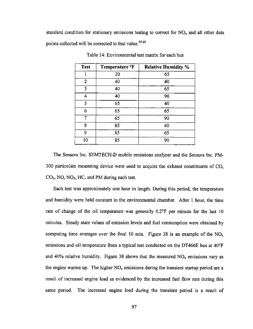
standard condition for stationary emissions testing to correct for NOx and all other data
points collected will be corrected to that value.55'6 9
Table 14: Environmental test matrix for each bus
Test Temperature °F Relative Humidity %1 20 65
2 40 40
3 40 65
4 40 90
5 65 40
6 65 65
7 65 90
8 85 40
9 85 65
10 85 90
The Sensors Inc. SEMTECH-D mobile emissions analyzer and the Sensors Inc. PM-
300 particulate measuring device were used to acquire the exhaust constituents of CO,
CO2, NO, NO2, HC, and PM during each test.
Each test was approximately one hour in length. During this period, the temperature
and humidity were held constant in the environmental chamber. After 1 hour, the time
rate of change of the oil temperature was generally 0.2°F per minute for the last 10
minutes. Steady state values of emission levels and fuel consumption were obtained by
computing time averages over the final 10 min. Figure 38 is an example of the NOx
emissions and oil temperature from a typical test conducted on the DT466E bus at 40°F
and 40% relative humidity. Figure 38 shows that the measured NOx emissions vary as
the engine warms up. The higher NOx emissions during the transient startup period are a
result of increased engine load as evidenced by the increased fuel flow rate during this
same period. The increased engine load during the transient period is a result of
97
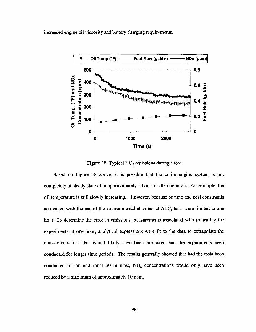
increased engine oil viscosity and battery charging requirements.
- Oil Temp (°F) - Fuel Row (gal/hr) NOx (ppm)
ou -x
. r 300-o °
di 200 -
E @o o 100
00
u.8
-0.6 V
a0
0.4 ~1
0.2U.
-n
0 1000 2000
Time (s)
Figure 38: Typical NO, emissions during a test
Based on Figure 38 above, it is possible that the entire engine system is not
completely at steady state after approximately 1 hour of idle operation. For example, the
oil temperature is still slowly increasing. However, because of time and cost constraints
associated with the use of the environmental chamber at ATC, tests were limited to one
hour. To determine the error in emissions measurements associated with truncating the
experiments at one hour, analytical expressions were fit to the data to extrapolate the
emissions values that would likely have been measured had the experiments been
conducted for longer time periods. The results generally showed that had the tests been
conducted for an additional 30 minutes, NOx concentrations would only have been
reduced by a maximum of approximately 10 ppm.
98
--- a n
-t---�---c--
I I V
5.4. Test Results
5.4.1. Fuel consumption
Fuel consumption at idle for HDDV engines can vary depending on the accessories
used. 66 Most school buses are not equipped with any air conditioning devices, but are
equipped with heaters for cold weather. The heater on a school bus contains three fans to
evenly distribute heat throughout the school bus. Operating these fans increases the total
load on the vehicle's engine and will increase the engine speed at idle. The increase in
engine speed in turn raises the fuel consumption. For the experiments reported herein,
the heater fans were not turned on. As shown in Figure 39, the fuel consumption rate
varies slightly with ambient temperature. The fuel consumption values for the Cummins
engine are slightly higher even though the Cummins engine size is 1.4L smaller. In
addition, the Cummins engine is not equipped with an ECM and therefore did not adjust
fuel injection rates accordingly under various climate changes in the chamber. As shown
in Figure 39, the three school buses tested consume an average of 0.5 gallons of fuel per
hour.
99
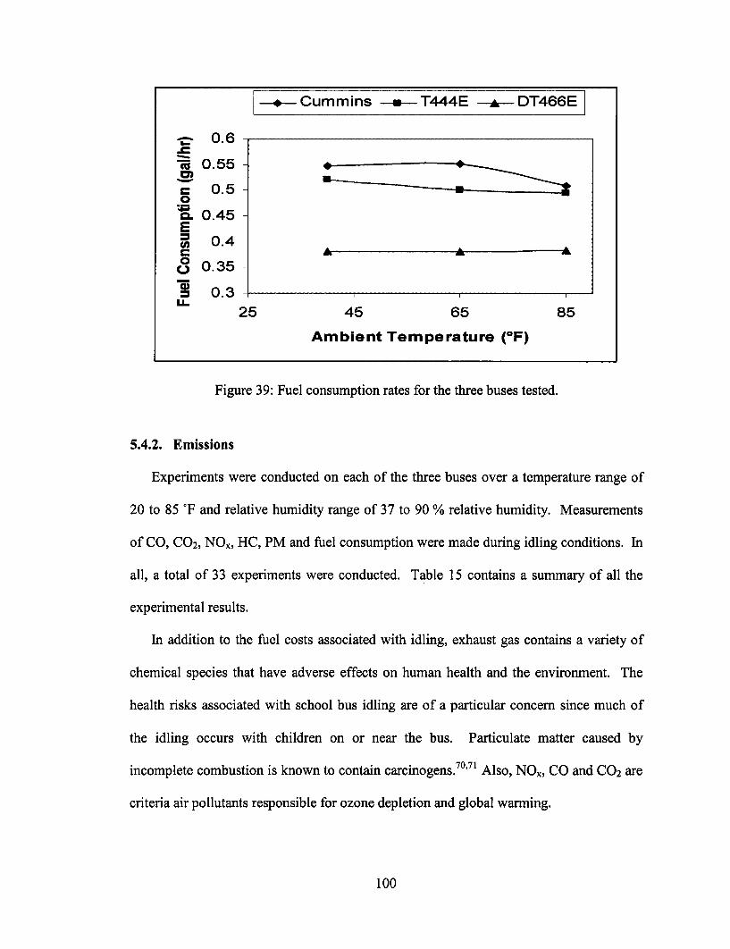
Figure 39: Fuel consumption rates for the three buses tested.
5.4.2. Emissions
Experiments were conducted on each of the three buses over a temperature range of
20 to 85 °F and relative humidity range of 37 to 90 % relative humidity. Measurements
of CO, CO2, NOx, HC, PM and fuel consumption were made during idling conditions. In
all, a total of 33 experiments were conducted. Table 15 contains a summary of all the
experimental results.
In addition to the fuel costs associated with idling, exhaust gas contains a variety of
chemical species that have adverse effects on human health and the environment. The
health risks associated with school bus idling are of a particular concern since much of
the idling occurs with children on or near the bus. Particulate matter caused by
incomplete combustion is known to contain carcinogens.70'71 Also, NOx, CO and CO 2 are
criteria air pollutants responsible for ozone depletion and global warming.
100
- -Cummins - T444E A DT466E
-C 0.6
X 0.55
C 0.5- "0
. 0.45EI 0.4
o 0.35
= 0.3 -U-
25 45 65 85
Ambient Temperature (°F)
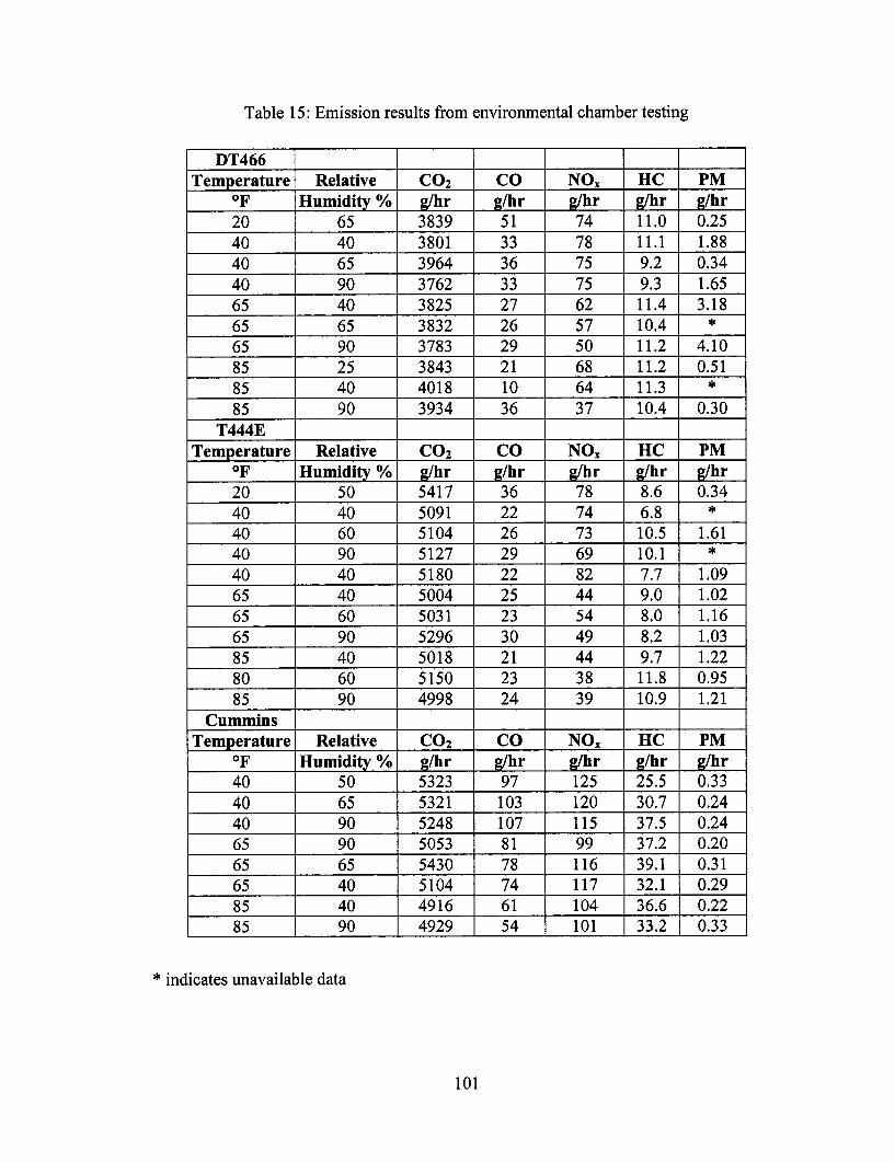
Table 15: Emission results from environmental chamber testing
DT466Temperature
OF
20404040656565858585
T444ETemperature
OF2040404040656565858085
CumminsTemperature
OF4040406565658585
RelativeHumidity %
65406590406590254090
RelativeHumidity %
5040609040406090406090
RelativeHumidity %
5065909065404090
* indicates unavailable data
101
C02g/hr3839380139643762382538323783384340183934
CO2
g/hr54175091510451275180500450315296501851504998
CO2g/hr53235321524850535430510449164929
COg/hr
51333633272629211036
COg/hr3622262922252330212324
COg/hr971031078178746154
NOxg/hr74787575625750686437
NOXg/hr7874736982445449443839
NOxg/hr12512011599116117104101
HCg/hr11.011.19.29.311.410.411.211.211.310.4
HCg/hr8.66.810.510.17.79.08.08.29.711.810.9
HCg/hr25.530.737.537.239.132.136.633.2
PMg/hr0.251.880.341.653.18
4.100.51
*
0.30
PMg/hr0.34
*
1.61
1.091.021.161.031.220.951.21
PMg/hr0.330.240.240.200.310.290.220.33
� I -
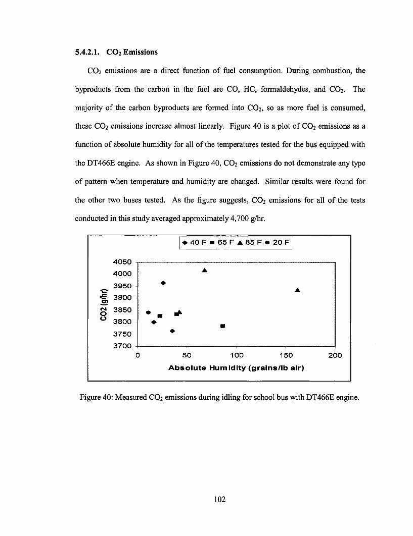
5.4.2.1. CO 2 Emissions
CO2 emissions are a direct function of fuel consumption. During combustion, the
byproducts from the carbon in the fuel are CO, HC, formaldehydes, and CO2. The
majority of the carbon byproducts are formed into CO2, so as more fuel is consumed,
these CO2 emissions increase almost linearly. Figure 40 is a plot of CO2 emissions as a
function of absolute humidity for all of the temperatures tested for the bus equipped with
the DT466E engine. As shown in Figure 40, CO2 emissions do not demonstrate any type
of pattern when temperature and humidity are changed. Similar results were found for
the other two buses tested. As the figure suggests, CO2 emissions for all of the tests
conducted in this study averaged approximately 4,700 g/hr.
Figure 40: Measured CO 2 emissions during idling for school bus with DT466E engine.
102
* 40 F * 65 F A 85 F 20 F
4050
4000 A
3950 -
E 3900
cm 3850
0 3800
3750
37000 50 100 150 200
Absolute Humidity (grains/lb air)

5.4.2.2. CO Emissions
CO emissions are caused by the incomplete combustion of the fuel in the engine.
Figure 41 shows the measured effect of ambient temperature on CO emissions of the
school buses at idle. As the ambient temperature increases, the cylinder temperature also
increases. This increase in cylinder temperature results in a more effective conversion of
CO to C0 2, thus more CO2 is created and in turn less CO is emitted. Since diesel engines
generally have excess oxygen and high combustion temperatures, CO emissions are
generally much lower than CO2 emissions. The Cummins engine produced the highest
CO emissions by almost double over the newer International T444E and DT466E
engines.
Figure 41: Effect of ambient temperature on CO emissions.
103
* DT466E * T444E A Cumrins
4n^\L u -
100 -
80
cm 600
40-
20 -
00 20 40 60 80 100
Ambient Temperature (°F)
,- ,I
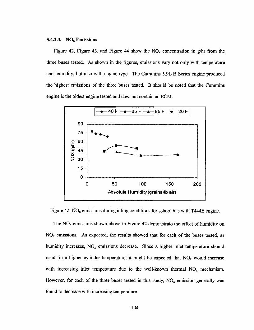
5.4.2.3. NO, Emissions
Figure 42, Figure 43, and Figure 44 show the NOx concentration in g/hr from the
three buses tested. As shown in the figures, emissions vary not only with temperature
and humidity, but also with engine type. The Cummins 5.9L B Series engine produced
the highest emissions of the three buses tested. It should be noted that the Cummins
engine is the oldest engine tested and does not contain an ECM.
Figure 42: NOx emissions during idling conditions for school bus with T444E engine.
The NOx emissions shown above in Figure 42 demonstrate the effect of humidity on
NOx emissions. As expected, the results showed that for each of the buses tested, as
humidity increases, NOx emissions decrease. Since a higher inlet temperature should
result in a higher cylinder temperature, it might be expected that NOx would increase
with increasing inlet temperature due to the well-known thermal NOx mechanism.
However, for each of the three buses tested in this study, NOx emission generally was
found to decrease with increasing temperature.
104
-- 40 F -- 65 F -- 85 F --- 20F
90
75 **..
-c 60
- 45-Do
z 30
15
0 - I I
0 50 100 150 200
Absolute Humidity (grains/lb air)
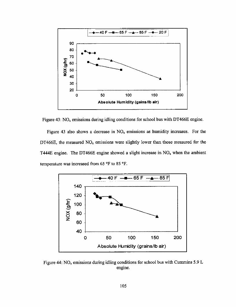
-- 40 F -9- 65F -- 85 F -- 20 F
Figure 43: NOx emissions during idling conditions for school bus with DT466E engine.
Figure 43 also shows a decrease in NOx emissions as humidity increases. For the
DT466E, the measured NOx emissions were slightly lower than those measured for the
T444E engine. The DT466E engine showed a slight increase in NOx when the ambient
temperature was increased from 65 °F to 85 °F.
--- 40F -- 65F -A 85FA^ A ^Ifu
120
- 100
o§ 80-
0 50 100 150 200
Absolute Huridity (grains/lb air)
Figure 44: NOx emissions during idling conditions for school bus with Cummins 5.9 Lengine.
105
z 60
40
nr . .YU
80
70
i 60-
5040z4 0
30
200 50 100 150 200
Absolute Humidity (gains/lb air)
.
I I I
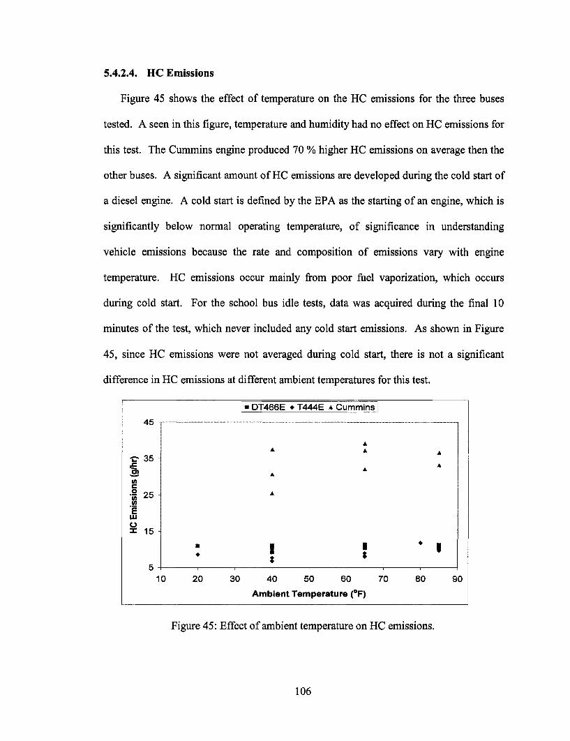
5.4.2.4. HC Emissions
Figure 45 shows the effect of temperature on the HC emissions for the three buses
tested. A seen in this figure, temperature and humidity had no effect on HC emissions for
this test. The Cummins engine produced 70 % higher HC emissions on average then the
other buses. A significant amount of HC emissions are developed during the cold start of
a diesel engine. A cold start is defined by the EPA as the starting of an engine, which is
significantly below normal operating temperature, of significance in understanding
vehicle emissions because the rate and composition of emissions vary with engine
temperature. HC emissions occur mainly from poor fuel vaporization, which occurs
during cold start. For the school bus idle tests, data was acquired during the final 10
minutes of the test, which never included any cold start emissions. As shown in Figure
45, since HC emissions were not averaged during cold start, there is not a significant
difference in HC emissions at different ambient temperatures for this test.
[ DT466E * T444E * CumminsAA _.to -
·. 35 -
U)
ECI 15-
5 -10 20 30 40 50 60 70 80 90
Ambient Temperature (°F)
AA A A
A
A
A
a |___________; I* ~ ~$ $
Figure 45: Effect of ambient temperature on HC emissions.
106
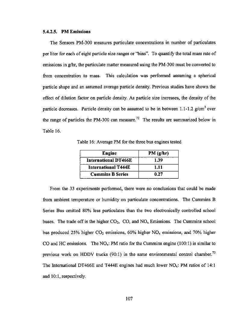
5.4.2.5. PM Emissions
The Sensors PM-300 measures particulate concentrations in number of particulates
per liter for each of eight particle size ranges or "bins". To quantify the total mass rate of
emissions in g/hr, the particulate matter measured using the PM-300 must be converted to
from concentration to mass. This calculation was performed assuming a spherical
particle shape and an assumed average particle density. Previous studies have shown the
effect of dilution factor on particle density. As particle size increases, the density of the
particle decreases. Particle density can be assumed to be in between 1.1-1.2 g/cm3 over
the range of particles the PM-300 can measure.72 The results are summarized below in
Table 16.
Table 16: Average PM for the three bus engines tested
Engine PM (g/hr)
International DT466E 1.39
International T444E 1.11
Cummins B Series 0.27
From the 33 experiments performed, there were no conclusions that could be made
from ambient temperature or humidity on particulate concentrations. The Cummins B
Series Bus emitted 80% less particulates than the two electronically controlled school
buses. The trade off is the higher C0 2, CO, and NOx Emissions. The Cummins school
bus produced 25% higher CO2 emissions, 60% higher NOx emissions, and 70% higher
CO and HC emissions. The NOx: PM ratio for the Cummins engine (100:1) is similar to
previous work on HDDV trucks (90:1) in the same environmental control chamber. 73
The International DT466E and T444E engines had much lower NOx: PM ratios of 14:1
and 10:1, respectively.
107
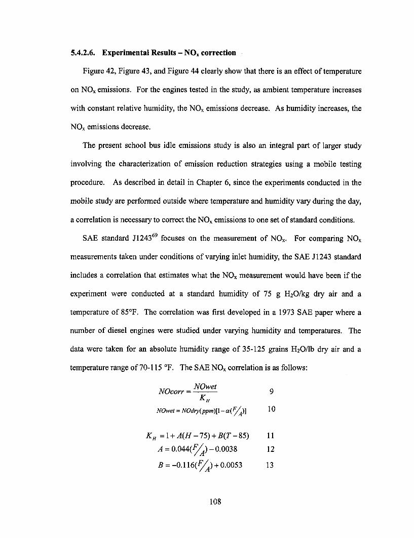
5.4.2.6. Experimental Results - NOx correction
Figure 42, Figure 43, and Figure 44 clearly show that there is an effect of temperature
on NOx emissions. For the engines tested in the study, as ambient temperature increases
with constant relative humidity, the NOx emissions decrease. As humidity increases, the
NOx emissions decrease.
The present school bus idle emissions study is also an integral part of larger study
involving the characterization of emission reduction strategies using a mobile testing
procedure. As described in detail in Chapter 6, since the experiments conducted in the
mobile study are performed outside where temperature and humidity vary during the day,
a correlation is necessary to correct the NO, emissions to one set of standard conditions.
SAE standard J124369 focuses on the measurement of NOx. For comparing NOx
measurements taken under conditions of varying inlet humidity, the SAE J1243 standard
includes a correlation that estimates what the NOx measurement would have been if the
experiment were conducted at a standard humidity of 75 g H 2O/kg dry air and a
temperature of 85°F. The correlation was first developed in a 1973 SAE paper where a
number of diesel engines were studied under varying humidity and temperatures. The
data were taken for an absolute humidity range of 35-125 grains H20/lb dry air and a
temperature range of 70-115 °F. The SAE NOx correlation is as follows:
NOcorr= NOwet 9KH
NOwet = NOdry(ppm)[1 - a(F/A)] 10
KH = 1+ A(H - 75) + B(T- 85) 11
A=0.044(F/) - 0.0038 12
B =-0.116(FA)+ 0.0053 13
108

where NOdr is the measured NOx emissions in ppm, a the hydrogen to carbon ratio (
y/x in fuel with formula CxHy), F/A the fuel to air ratio (dry basis), H the humidity in
grains of H 2 0/kg dry air and T the intake air temperature in °C.
The SAE correlation was created in order to create a NOx correction for all diesel
engines within a reasonable range of the ambient temperature and humidity constraints.
The CFR40 86.1342-90, which is another correlation that only corrects for humidity
variations, is as follows:
NO,,,o, = NOxmeasre * K' 141K' = 15
(1 - 0.0026 * (H - 75))
where H is the humidity in grains of H2 0 in grains/lb of dry air.
The CFR40 correlation is only recommended for use in a temperature range from
68°F-85°F. Weather conditions in New Jersey fall out of both the SAE and CFR
correlations. Moreover, since a wide variety of fuels, additives and exhaust gas after
treatment devices will be tested in the parallel mobile emissions study at ATC, it is likely
that tests will be conducted under a wider range of inlet air and humidity conditions than
that recommended for either the SAE or CFR40 standard. Accordingly, a new NOx
correlation was developed from the NOx measurements presented herein for use in the
mobile emissions testing described in Chapter 6. As described below, using a similar
equation to that presented in the SAE standard, three sets of"engine specific" correlation
coefficients were developed corresponding to the three engines tested in this study.
In Figure 46 below, the NOx emissions for the DT466E are shown uncorrected. The
figure shows that, although all tests were conducted during identical idle conditions, NOx
concentrations vary by as much as 100 ppm with respect to experiments conducted at the
109

SAE standard condition of 39 % RH and 85 °F.
Figure 46: Uncorrected NOx emissions (ppm) for the school bus with DT466E engine.
Since the CFR40 and SAE standards were developed for limited temperature and
humidity range, extreme caution should be exercised in their use for correcting data over
a wider range of conditions. This caution is of particular significance in light of the
recent trend toward mobile emissions testing. The following figures show that both the
SAE and CFR40 standards perform poorly outside their recommended range. In Figure
47 and Figure 48, the SAE and CFR correlations are used to correct the NOx emissions to
the standard of 85°F and 39% RH. The open symbols represent the uncorrected
measurements and the closed symbols represent the corrected measurements. An
effective correction factor would result in the closed symbols following a roughly
horizontal line at approximately 200 ppm. As show in Figure 47, the SAE 1243
correction factor actually increases the NOx concentration at lower temperatures. This
result underscores the danger in extending these correction factors outside the range for
which they were originally developed.
110
*40 F *65 F A85 F *20 F
290 -270 -
E 250-230 - ·
" 210 - *z 190 · A
170150 -
0.00 50.00 100.00 150.00 200.00
Absolute Humidity (gr./lb air)
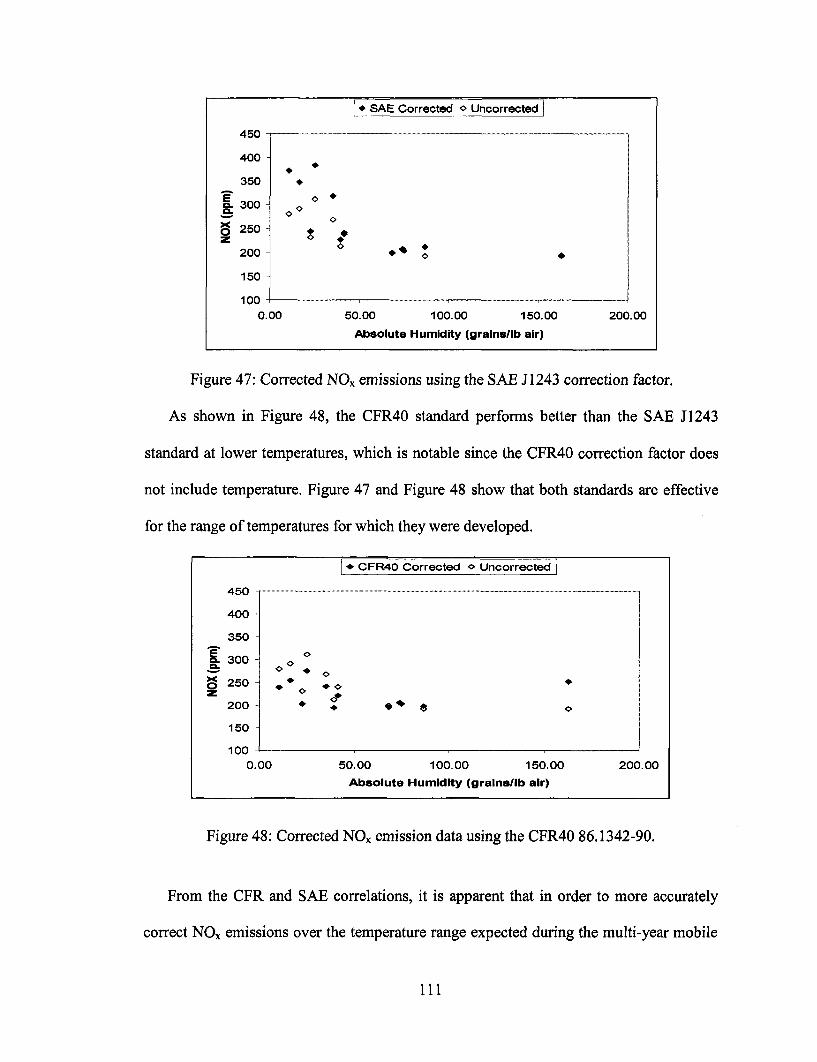
* SAE Corrected o Uncorrected
Figure 47: Corrected NOx emissions using the SAE J1243 correction factor.
As shown in Figure 48, the CFR40 standard performs better than the SAE J1243
standard at lower temperatures, which is notable since the CFR40 correction factor does
not include temperature. Figure 47 and Figure 48 show that both standards are effective
for the range of temperatures for which they were developed.
Figure 48: Corrected NOx emission data using the CFR40 86.1342-90.
From the CFR and SAE correlations, it is apparent that in order to more accurately
correct NOx emissions over the temperature range expected during the multi-year mobile
111
Q *Q.0
.0
.0 *, *.0
450
400 -
350
E 300
8 250z
200
150
1000.00 50.00 100.00 150.00 200.00
Absolute Humidity (grains/lb air)
| * CFR40 Corrected o Uncorrected |
A tn ............................. ...............................................................................................................................................................................................U - .. ....................................................................................................
400
350
F 300
| 25 0 - .o *250- o
200 $ .e o
150
1000.00 50.00 100.00 150.00 200.00
Absolute Humidity (gralns/lb air)
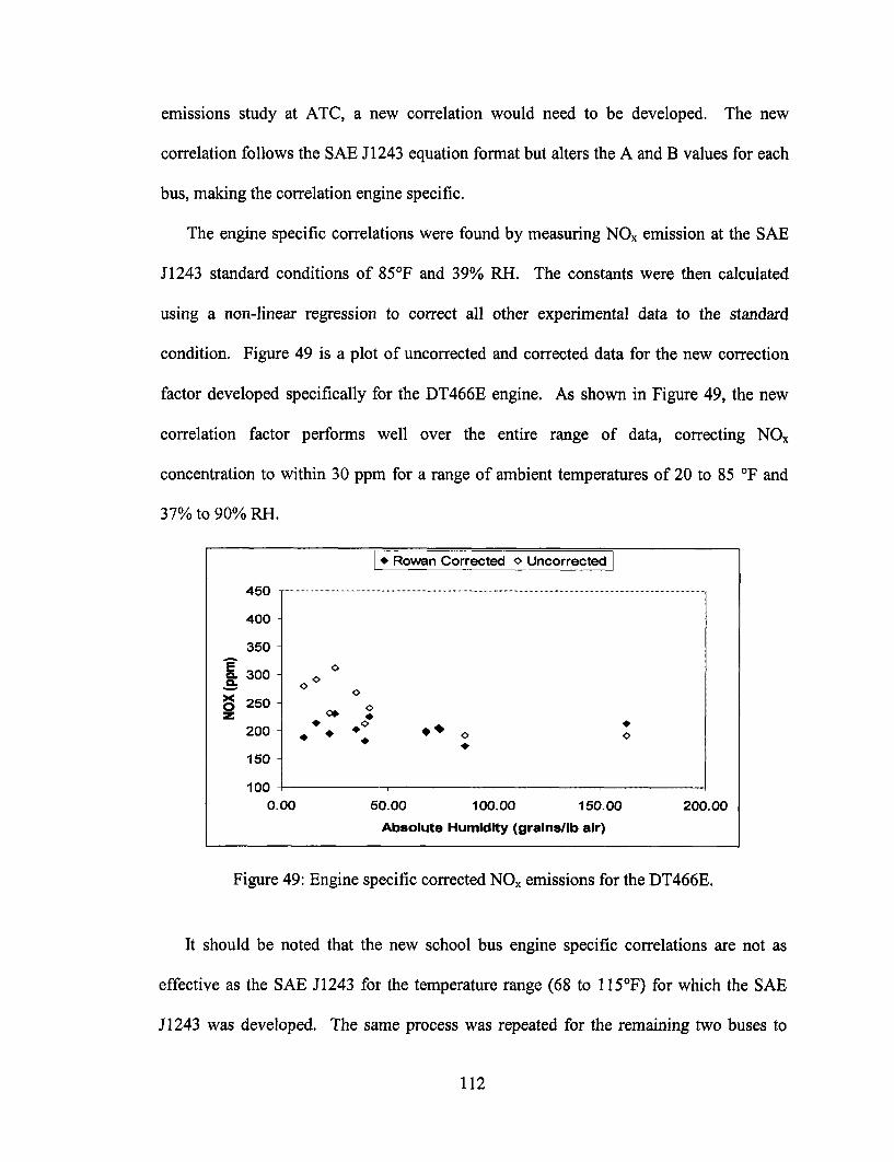
emissions study at ATC, a new correlation would need to be developed. The new
correlation follows the SAE J1243 equation format but alters the A and B values for each
bus, making the correlation engine specific.
The engine specific correlations were found by measuring NOx emission at the SAE
J1243 standard conditions of 85°F and 39% RH. The constants were then calculated
using a non-linear regression to correct all other experimental data to the standard
condition. Figure 49 is a plot of uncorrected and corrected data for the new correction
factor developed specifically for the DT466E engine. As shown in Figure 49, the new
correlation factor performs well over the entire range of data, correcting NOx
concentration to within 30 ppm for a range of ambient temperatures of 20 to 85 °F and
37% to 90% RH.
Figure 49: Engine specific corrected NOx emissions for the DT466E.
It should be noted that the new school bus engine specific correlations are not as
effective as the SAE J1243 for the temperature range (68 to 115°F) for which the SAE
J1243 was developed. The same process was repeated for the remaining two buses to
112
* Rowan Corrected o Uncorrected
A r -................. A.n Corrected .
400
350
E. 300
250* *
200 **o o
150
1000.00 50.00 100.00 150.00 200.00
Absolute Humidity (grains/lb air)
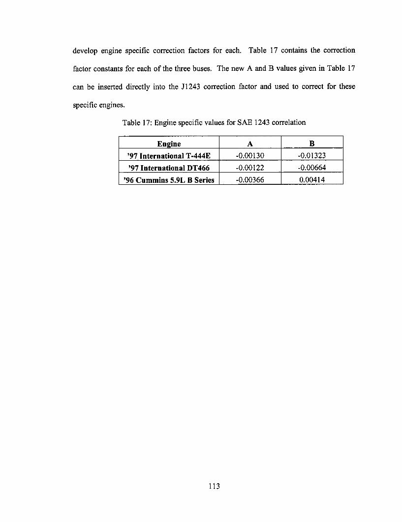
develop engine specific correction factors for each. Table 17 contains the correction
factor constants for each of the three buses. The new A and B values given in Table 17
can be inserted directly into the J1243 correction factor and used to correct for these
specific engines.
Table 17: Engine specific values for SAE 1243 correlation
Engine A B
'97 International T-444E -0.00130 -0.01323
'97 International DT466 -0.00122 -0.00664
'96 Cummins 5.9L B Series -0.00366 0.00414
113

6. School Bus Mobile Emissions Testing (ATC)
6.1. Introduction
Alternative fuels such as biodiesel and ultra low sulfur diesel (ULSD) have been
shown to reduce some diesel emissions in cars and trucks. The final phase of testing for
this thesis was mobile testing of various alternative fuels to evaluate the emissions
reduction advantages and disadvantages. The RUCSBC developed in Chapter 3 was used
as the mobile emissions testing cycle for the research. NOx emissions data collected
during mobile testing was corrected for temperature and humidity using the NOx
correction factor developed in Chapter 5. Finally, mobile emission results using various
alternative fuels, including B20, were compared to the test results from the Medford
Township School District discussed in Chapter 4.
6.2. Experimental Procedure: Test Matrix
Experiments were conducted on the 1-Mile Loop Course at the Aberdeen Test Center
in Aberdeen, Md. The course consists of a continuous asphalt surface with level, parallel
1/4-mile segments connected by 1/4-mile banked semicircular sections at each end. Data
acquisition and control instrumentation were located inside the school bus. Three
separate school buses were acquired and tested each with four different fuel
combinations. The vehicle and engine specifications for each school bus tested are listed
in Table 4. Each of the vehicles was tested with four fuels under the RUCSBC as seen in
the test matrix in Table 18. Each test consisted of a single RUCSBC cycle, which has a
duration of approximately 20 minutes during which HC, NO, NO2 , CO, C0 2, and PM
emissions were monitored.
The Sensors Inc. SEMTECH-D mobile emissions analyzer and the Sensors Inc. PM-
114
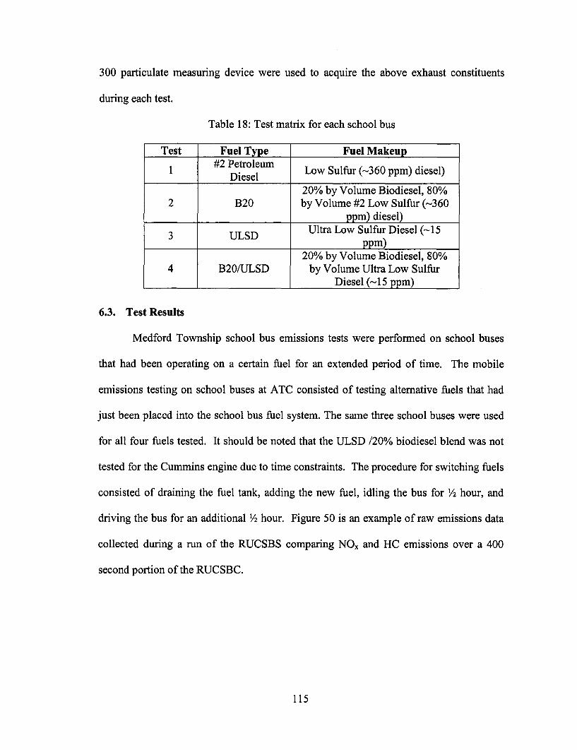
300 particulate measuring device were used to acquire the above exhaust constituents
during each test.
Table 18: Test matrix for each school bus
Test Fuel Type Fuel Makeup#2 Petroleum1 #2 Petroleum Low Sulfur (~360 ppm) diesel)
Diesel20% by Volume Biodiesel, 80%
2 B20 by Volume #2 Low Sulfur (-360ppm) diesel)
3 TcULSD Ultra Low Sulfur Diesel (-15ULSD ______ ppm)
20% by Volume Biodiesel, 80%4 B20/ULSD by Volume Ultra Low Sulfur
Diesel (-15 ppm)
6.3. Test Results
Medford Township school bus emissions tests were performed on school buses
that had been operating on a certain fuel for an extended period of time. The mobile
emissions testing on school buses at ATC consisted of testing alternative fuels that had
just been placed into the school bus fuel system. The same three school buses were used
for all four fuels tested. It should be noted that the ULSD /20% biodiesel blend was not
tested for the Cummins engine due to time constraints. The procedure for switching fuels
consisted of draining the fuel tank, adding the new fuel, idling the bus for Y2 hour, and
driving the bus for an additional i2 hour. Figure 50 is an example of raw emissions data
collected during a run of the RUCSBS comparing NOx and HC emissions over a 400
second portion of the RUCSBC.
115

k I
-- NOx -HC
I
I
'IVA
-___r ' u rI
0 50 100 150 200
Time (s)
250 300 350
Figure 50: Raw emissions data from RUCSBC
The following fuels were tested at ATC using the RUCSBC described above: # 2
petroleum diesel, ULSD, #B20, and ULSD/ 20 % biodiesel mixture. Fuels were analyzed
by the chemistry lab at ATC for density, cetane index #, viscosity, and sulfur %. Results
from the fuels tests are shown in Table 19.
Table 19: Fuel properties for fuels tested at ATC.
116
Ou -
500
c 4000
o 300
o0Z 200
100
0
140
120
100
80 o
40
20
400
Fuel Type #2 Diesel B20 ULSD
Density (g/cm 3) .8521 .8592 .8243
Cetane Index 45.2 46.5 42.5
Sulfur % .0431 .0409 .0049
Viscosity (mm 2/s) 2.40 2.60 1.60
J
w A
i l __ I II__
I f AA Ii f I
nn ,tLI ' I I
--- _ ------�
I
IJv
nt
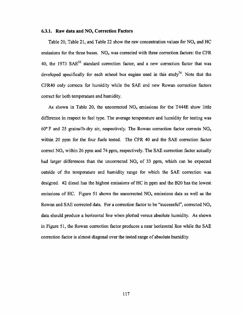
6.3.1. Raw data and NO, Correction Factors
Table 20, Table 21, and Table 22 show the raw concentration values for NOx and HC
emissions for the three buses. NOx was corrected with three correction factors: the CFR
40, the 1973 SAE 55 standard correction factor, and a new correction factor that was
developed specifically for each school bus engine used in this study7 4. Note that the
CFR40 only corrects for humidity while the SAE and new Rowan correction factors
correct for both temperature and humidity.
As shown in Table 20, the uncorrected NOx emissions for the T444E show little
difference in respect to fuel type. The average temperature and humidity for testing was
60° F and 25 grains/lb-dry air, respectively. The Rowan correction factor corrects NOx
within 20 ppm for the four fuels tested. The CFR 40 and the SAE correction factor
correct NOx within 26 ppm and 74 ppm, respectively. The SAE correction factor actually
had larger differences than the uncorrected NOx of 33 ppm, which can be expected
outside of the temperature and humidity range for which the SAE correction was
designed. #2 diesel has the highest emissions of HC in ppm and the B20 has the lowest
emissions of HC. Figure 51 shows the uncorrected NOx emissions data as well as the
Rowan and SAE corrected data. For a correction factor to be "successful", corrected NOx
data should produce a horizontal line when plotted versus absolute humidity. As shown
in Figure 51, the Rowan correction factor produces a near horizontal line while the SAE
correction factor is almost diagonal over the tested range of absolute humidity.
117
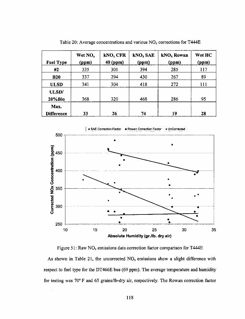
Table 20: Average concentrations and various NOx corrections for T444E
Wet NO, kNOX CFR kNO, SAE kNOx Rowan Wet HC
Fuel Type (ppm) 40 (ppm) (pp) (ppm)(ppm)#2 335 301 394 285 117
B20 337 294 430 267 89
ULSD 341 304 418 272 111
ULSD/
20%Bio 368 320 468 286 95
Max.
Difference 33 26 74 19 28
I * SAE Correction Factor * Rowan Correction Factor * UnCorrected I500
E450
Ic
* 40080
o 350z
300
0
25010 15 20 25 30 35
Absolute Humidity (gr./lb. dry air)
Figure 51: Raw NOx emissions data correction factor comparison for T444E
As shown in Table 21, the uncorrected NOx emissions show a slight difference with
respect to fuel type for the DT466E bus (69 ppm). The average temperature and humidity
for testing was 70° F and 65 grains/lb-dry air, respectively. The Rowan correction factor
118

also corrects NOx for the DT466E bus within 20 ppm for the four fuels tested. The CFR
40 and the SAE correction factor correct NOx within 12 ppm and 59 ppm, respectively. In
this case the temperature was within the SAE correction factor limit and absolute
humidity was slightly lower then the range, however the corrected NOx was still less than
the uncorrected data. #2 diesel and ULSD had the highest emissions of HC and the
ULSD/ 20 % biodiesel mixture had the lowest HC emissions.
Table 21: Average concentrations and various NOx corrections for DT466E
As shown in Table 22, the uncorrected NOx emissions show a slight difference in
respect to fuel type for the Cummins bus (65 ppm). The average temperature and
humidity for testing was 50°F and 15 grains/lb-dry air, respectively. The Rowan
correction factor corrects NOx for the DT466E bus within 54 ppm for the three fuels
tested. The CFR 40 and the SAE correction factor correct NOx within 47 ppm and 100
ppm, respectively. The SAE correction factor actually had larger differences than the
uncorrected NOx of 69 ppm, which can be expected outside of the temperature and
humidity range for which the SAE correction was designed. #2 diesel had the highest HC
emissions and the B20 again had the lowest HC emissions.
119
Wet NOx kNO, CFR kNO, SAE kNOx Rowan Wet HC
Fuel Type (ppm) 40 ( ppm) (ppm) (p p m) ( )
#2 377 334 474 299 102
B20 371 338 435 317 96
ULSD 308 334 415 319 103
ULSD/
20%Bio 308 326 426 303 82
Max.
Difference 69 12 59 20 21
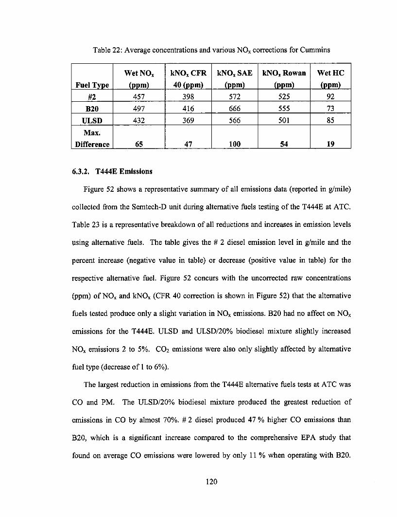
Table 22: Average concentrations and various NOx corrections for Cummins
6.3.2. T444E Emissions
Figure 52 shows a representative summary of all emissions data (reported in g/mile)
collected from the Semtech-D unit during alternative fuels testing of the T444E at ATC.
Table 23 is a representative breakdown of all reductions and increases in emission levels
using alternative fuels. The table gives the # 2 diesel emission level in g/mile and the
percent increase (negative value in table) or decrease (positive value in table) for the
respective alternative fuel. Figure 52 concurs with the uncorrected raw concentrations
(ppm) of NOx and kNOx (CFR 40 correction is shown in Figure 52) that the alternative
fuels tested produce only a slight variation in NOx emissions. B20 had no affect on NOx
emissions for the T444E. ULSD and ULSD/20% biodiesel mixture slightly increased
NOx emissions 2 to 5%. CO 2 emissions were also only slightly affected by alternative
fuel type (decrease of 1 to 6%).
The largest reduction in emissions from the T444E alternative fuels tests at ATC was
CO and PM. The ULSD/20% biodiesel mixture produced the greatest reduction of
emissions in CO by almost 70%. # 2 diesel produced 47 % higher CO emissions than
B20, which is a significant increase compared to the comprehensive EPA study that
found on average CO emissions were lowered by only 11 % when operating with B20.
120
Wet NOx kNOx CFR kNOx SAE kNO, Rowan Wet HC
Fuel Type (ppm) 40 (ppm)(ppm )(ppm )#2 457 398 572 525 92
B20 497 416 666 555 73
ULSD 432 369 566 501 85
Max.
Difference 65 47 100 54 19
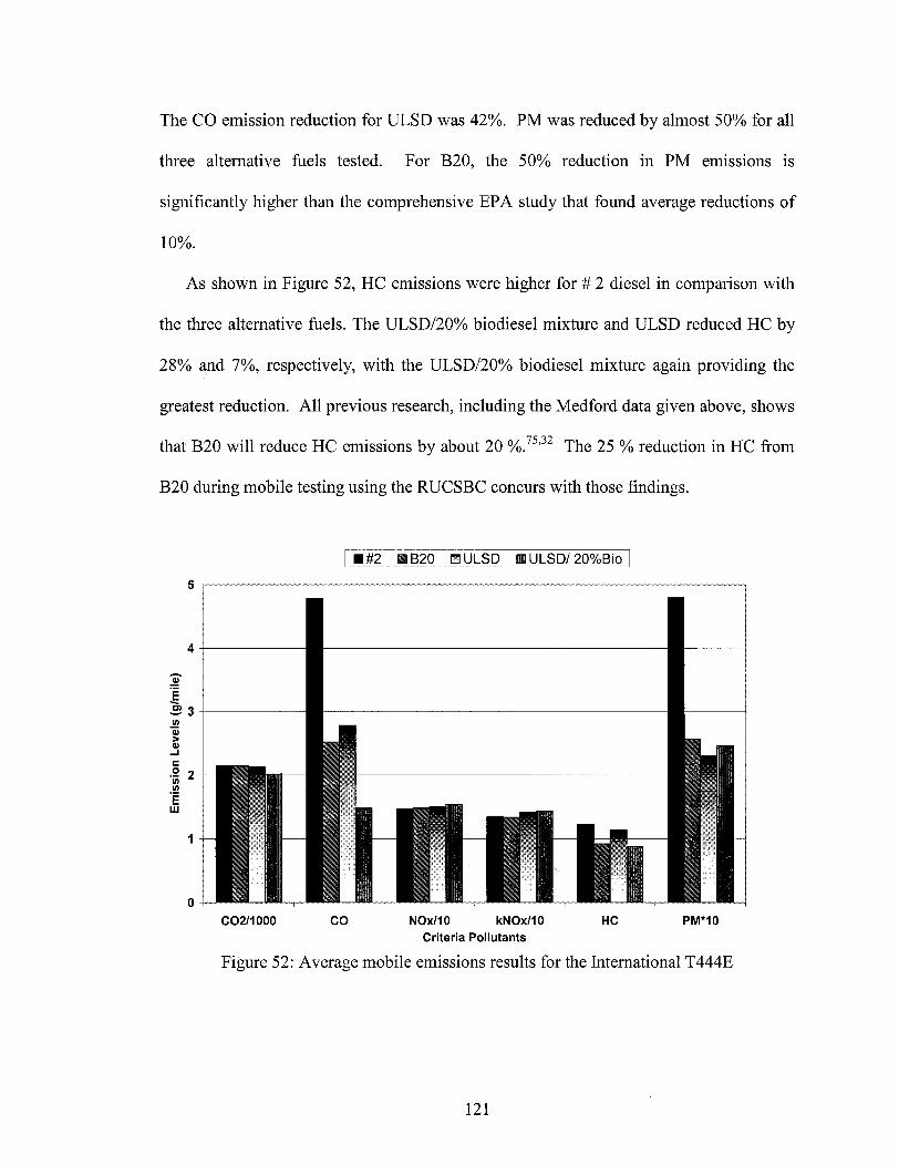
The CO emission reduction for ULSD was 42%. PM was reduced by almost 50% for all
three alternative fuels tested. For B20, the 50% reduction in PM emissions is
significantly higher than the comprehensive EPA study that found average reductions of
10%.
As shown in Figure 52, HC emissions were higher for # 2 diesel in comparison with
the three alternative fuels. The ULSD/20% biodiesel mixture and ULSD reduced HC by
28% and 7%, respectively, with the ULSD/20% biodiesel mixture again providing the
greatest reduction. All previous research, including the Medford data given above, shows
that B20 will reduce HC emissions by about 20 /%.7532 The 25 % reduction in HC from
B20 during mobile testing using the RUCSBC concurs with those findings.
*#2 *B20 DULSD mULSD/20%Bio
a)
4-
.E
1--l
.o 2._
ELU
n
C02/1000 CO NOx/10 kNOx/10 HC PM*10Criteria Pollutants
Figure 52: Average mobile emissions results for the International T444E
121
---- ------ - - - - - - - - -- -l-- - - - f
L
vI I T T ""T l

Table 23: Alternative fuel reductions in emission levels when compared to #2 diesel
% Reduction
# 2 (g/mile)
B20
ULSD
ULSD/20% Bio
2155
1
1
6
4.8
47
42
69
14.7
-1
-2
-5
13.5
1
-5
-6
1.2
25
7
28
0.480
47
49
48
6.3.3. DT466E Emissions
Figure 53 shows a representative summary of all emissions data (reported in g/mile)
collected from the Semtech-D unit during alternative fuels testing of the DT466E at ATC.
Table 24 is a representative breakdown of all reductions and increases in emission levels
using alternative fuels. The table gives the # 2 diesel emission level in g/mile and the
percent increase (negative value in table) or decrease (positive value in table) for the
respective alternative fuel. Figure 53 concurs with the uncorrected raw concentrations
(ppm) of NOx and kNOx (CFR 40 correction is shown in Figure 53) that the alternative
fuels tested produce only a slight variation in NOx emissions. B20 had no affect on NOx
emissions for the DT466E. ULSD and ULSD/20% biodiesel mixture decreased NOx
emissions 12 to 23%, almost four times more than the T444E bus. As shown in Table 24,
CO and CO2 emissions were also only slightly affected by alternative fuel type (decrease
of 7% to an increase of 8%).
The largest reduction in emissions from the DT466E alternative fuels tests at ATC
was HC emissions. The ULSD/20% biodiesel mixture again produced the greatest
reduction of emissions in HC by 43%. # 2 diesel produced 20% higher HC emissions
than B20, which is identical to the comprehensive EPA study that found on average HC
122
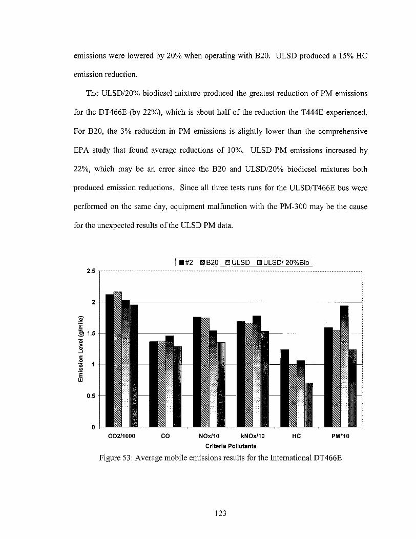
emissions were lowered by 20% when operating with B20. ULSD produced a 15% HC
emission reduction.
The ULSD/20% biodiesel mixture produced the greatest reduction of PM emissions
for the DT466E (by 22%), which is about half of the reduction the T444E experienced.
For B20, the 3% reduction in PM emissions is slightly lower than the comprehensive
EPA study that found average reductions of 10%. ULSD PM emissions increased by
22%, which may be an error since the B20 and ULSD/20% biodiesel mixtures both
produced emission reductions. Since all three tests runs for the ULSD/T466E bus were
performed on the same day, equipment malfunction with the PM-300 may be the cause
for the unexpected results of the ULSD PM data.
*#2 E B20 ULSD E ULSD/ 20%Bio
2 -
m 1.5-
0)
a, 1-EuJ
0.5
0 - Ir
C02/1000 CO NOx/10 kNOx/10 HC PM*10Criteria Pollutants
Figure 53: Average mobile emissions results for the International DT466E
123
2.5- .. ..... ..... ...... ..... ....... .... ..... ...... ..... .. ..... .. ... .. .. ...... ...... ... .. ..... .... .. ... .. ..... ...... ... .. .. ..... .... ..... ...... ..... ....... ..... ..... ..... ..... ... ... .. ... .. ..... .. .. ..... ...... ... .. ...... ..... ...... ........ ........ ... .. ... ......... ...1 ........ ... .. ...I. .... ...... ... .,. ..11 1 .... ....I ... I " ...... ...... .. ... .. ... .. ....I .......I. .. ...... .. ...... ..... .... .... .. .... I .. ... .. ... ..I. ... ..... .. .. .... .......I ... ... .
I
---7- -7- I-
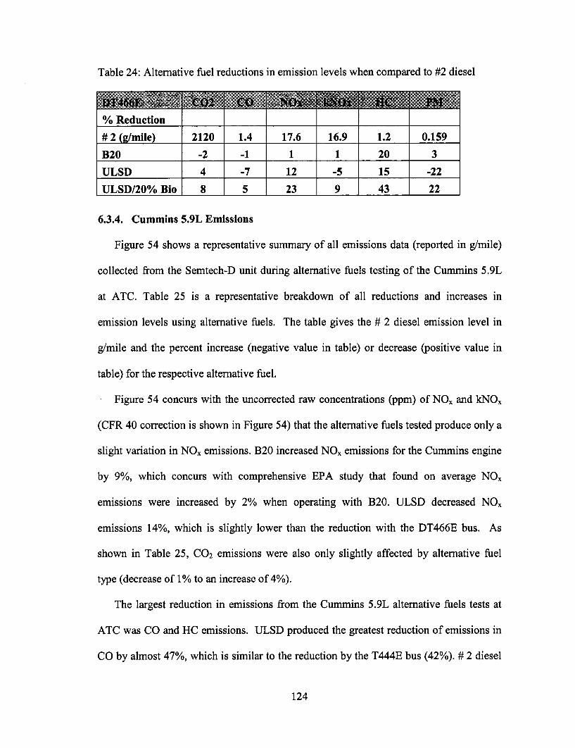
Table 24: Alternative fuel reductions in emission levels when compared to #2 diesel
�bT46� �% Reduction
# 2 (g/mile)
B20
ULSD
ULSD/20% Bio
2120
-2
4
8
1.4
-1
-7
5
17.6
1
12
23
16.9
1
-5
9
1.2
20
15
43
0.159
3
-22
22
6.3.4. Cummins 5.9L Emissions
Figure 54 shows a representative summary of all emissions data (reported in g/mile)
collected from the Semtech-D unit during alternative fuels testing of the Cummins 5.9L
at ATC. Table 25 is a representative breakdown of all reductions and increases in
emission levels using alternative fuels. The table gives the # 2 diesel emission level in
g/mile and the percent increase (negative value in table) or decrease (positive value in
table) for the respective alternative fuel.
Figure 54 concurs with the uncorrected raw concentrations (ppm) of NOx and kNOx
(CFR 40 correction is shown in Figure 54) that the alternative fuels tested produce only a
slight variation in NOx emissions. B20 increased NOx emissions for the Cummins engine
by 9%, which concurs with comprehensive EPA study that found on average NOx
emissions were increased by 2% when operating with B20. ULSD decreased NOx
emissions 14%, which is slightly lower than the reduction with the DT466E bus. As
shown in Table 25, CO2 emissions were also only slightly affected by alternative fuel
type (decrease of 1% to an increase of 4%).
The largest reduction in emissions from the Cummins 5.9L alternative fuels tests at
ATC was CO and HC emissions. ULSD produced the greatest reduction of emissions in
CO by almost 47%, which is similar to the reduction by the T444E bus (42%). # 2 diesel
124
�BB��
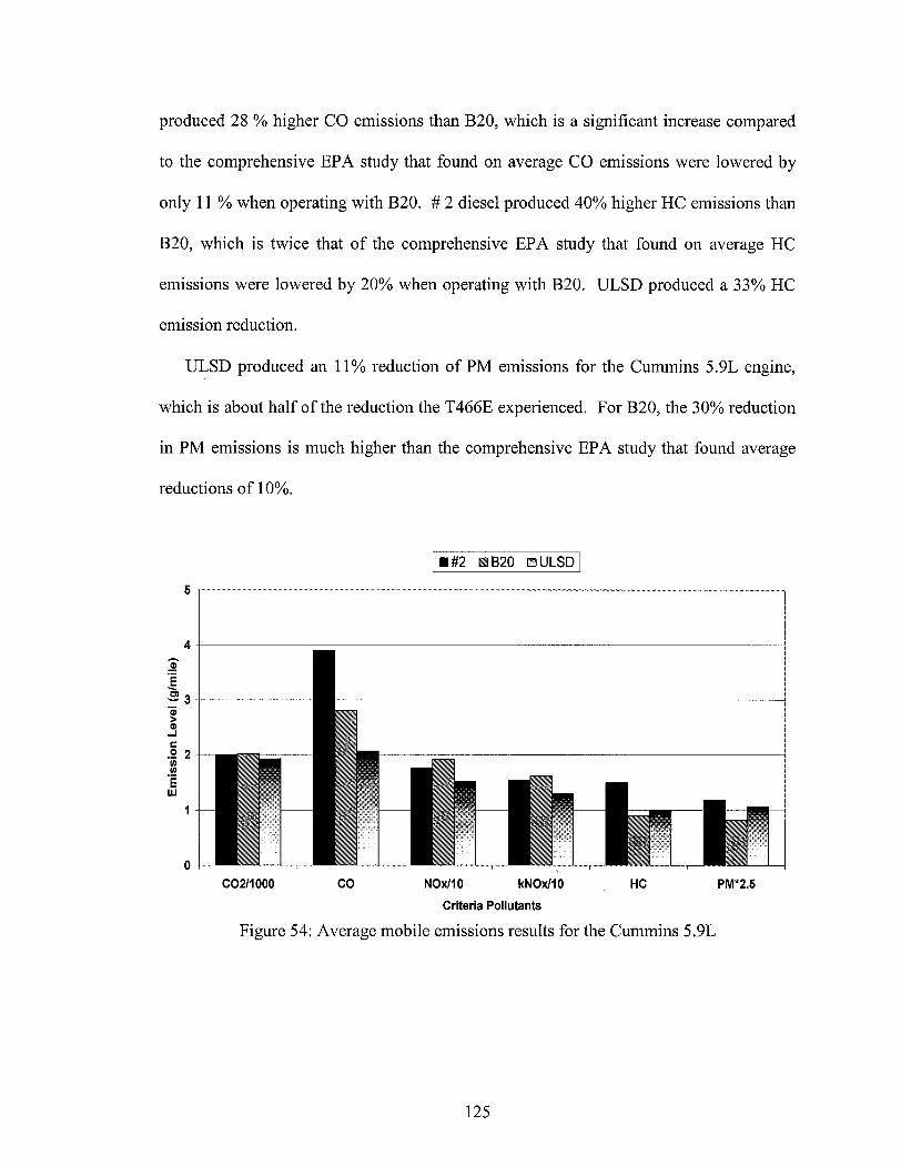
produced 28 % higher CO emissions than B20, which is a significant increase compared
to the comprehensive EPA study that found on average CO emissions were lowered by
only 11 % when operating with B20. # 2 diesel produced 40% higher HC emissions than
B20, which is twice that of the comprehensive EPA study that found on average HC
emissions were lowered by 20% when operating with B20. ULSD produced a 33% HC
emission reduction.
ULSD produced an 11% reduction of PM emissions for the Cummins 5.9L engine,
which is about half of the reduction the T466E experienced. For B20, the 30% reduction
in PM emissions is much higher than the comprehensive EPA study that found average
reductions of 10%.
1#2 E B20 C ULSD
4
.E
0
3J
.2 2
E
I1
0
C0211000 CO NOx/10 kNOx/10 HC I
Criteria Pollutants
Figure 54: Average mobile emissions results for the Cummins 5.9L
PM*2.5
125
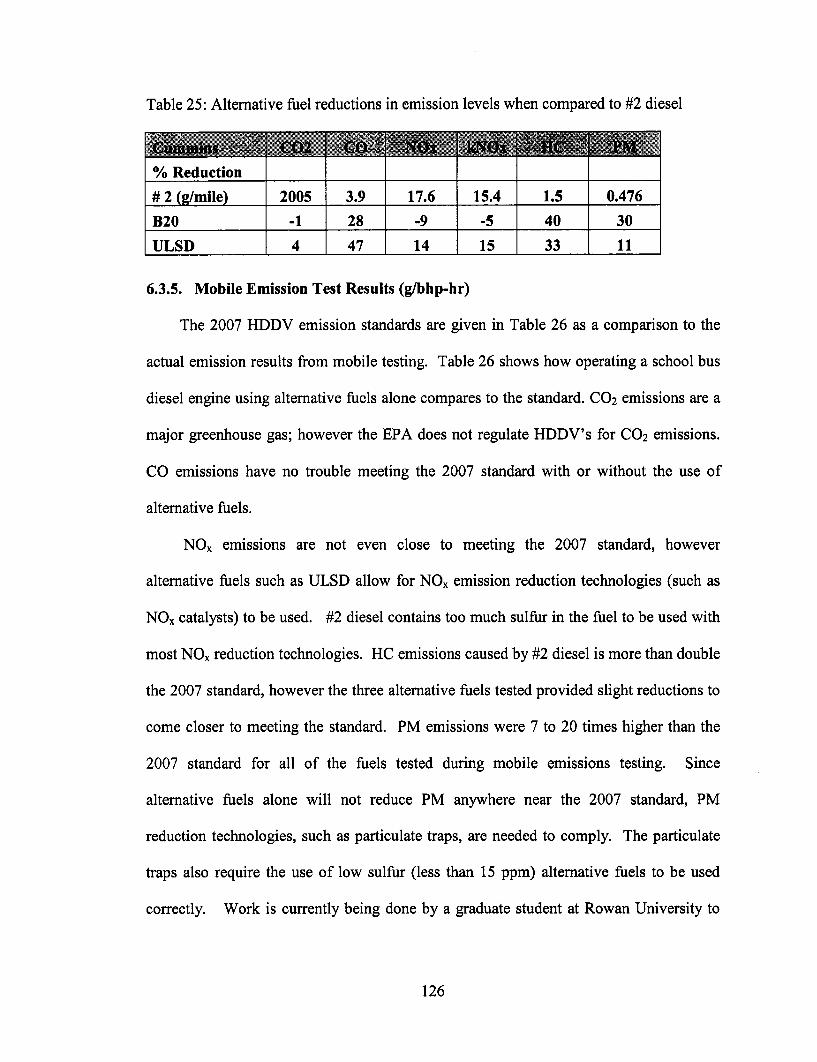
Table 25: Alternative fuel reductions in emission levels when compared to #2 diesel
% Reduction
# 2 (g/mile)
B20
ULSD
2005
-1
4
3.9
28
47
17.6
-9
14
15.4
-5
15
1.5
40
33
0.476
30
11
6.3.5. Mobile Emission Test Results (g/bhp-hr)
The 2007 HDDV emission standards are given in Table 26 as a comparison to the
actual emission results from mobile testing. Table 26 shows how operating a school bus
diesel engine using alternative fuels alone compares to the standard. CO2 emissions are a
major greenhouse gas; however the EPA does not regulate HDDV's for CO2 emissions.
CO emissions have no trouble meeting the 2007 standard with or without the use of
alternative fuels.
NOx emissions are not even close to meeting the 2007 standard, however
alternative fuels such as ULSD allow for NOx emission reduction technologies (such as
NOx catalysts) to be used. #2 diesel contains too much sulfur in the fuel to be used with
most NOx reduction technologies. HC emissions caused by #2 diesel is more than double
the 2007 standard, however the three alternative fuels tested provided slight reductions to
come closer to meeting the standard. PM emissions were 7 to 20 times higher than the
2007 standard for all of the fuels tested during mobile emissions testing. Since
alternative fuels alone will not reduce PM anywhere near the 2007 standard, PM
reduction technologies, such as particulate traps, are needed to comply. The particulate
traps also require the use of low sulfur (less than 15 ppm) alternative fuels to be used
correctly. Work is currently being done by a graduate student at Rowan University to
126
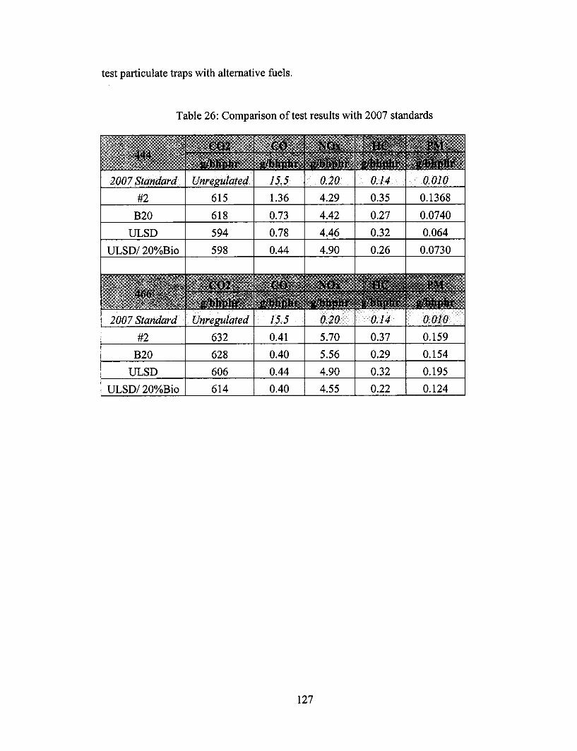
test particulate traps with alternative fuels.
Table 26: Comparison of test results with 2007 standards
2007 Standard
#2
B20
ULSD
ULSD/ 20%Bio
Unreulated
615
618
594
598
15.5
1.36
0.73
0.78
0.44
0.20
4.29
4.42
4.46
4.90
0.14 0.010
0.1368
0.0740
0.064
0.0730
#2 632 0.41 5.70 0.37 0.159
B20 628 0.40 5.56 0.29 0.154
ULSD 606 0.44 4.90 0.32 0.195
ULSD/ 20%Bio 614 0.40 4.55 0.22 0.124
127
0.35
0.27
0.32
0.26
7. Conclusions and Future Work
7.1. Conclusions
7.1.1. Idle
New Jersey is continuing its efforts to meet the National Ambient Air Quality
Standards (NAAQS) by investigating emission reduction strategies for school buses. One
such strategy is reducing idle emissions. Little data has been collected on school buses in
previous studies. In order to quantify the idling emissions, 33 tests were performed in an
environmental chamber to simulate idling conditions experience throughout the course of
a school year.
There are currently approximately 11,000 school buses in use in the state of NJ.
Based on the idle emissions measurements presented herein (assuming an average idle
time of one hr/day), the current NJ school bus fleet produces approximately 9.3 million
kg of CO2, 90,000 kg CO, 150,000 kg NOx, 35,000 kg HC and 2,145 kg PM per calendar
school year of 180 days.
In terms of the financial burden, a one-hour reduction of idling time per school bus
per day for each of the 11,000 buses in NJ would result in an annual statewide cost
savings of approximately $1.5 million. This calculation is based on an average school bus
fuel consumption of 0.5 gallons of diesel fuel per hour and a price of $1.50 for #2
diesel76.
In addition, the following conclusions were also found for the school buses tested in
this study:
* As fuel consumption increases, CO2 and CO emissions increase.
As ambient temperature increases, CO emissions decrease due to a more complete
128
conversion of CO to CO2.
* As expected, results showed that for each of the buses tested, as humidity
increased, NOx emissions decreased. For the most part as temperature increased,
NOx emissions also decreased.
* Hydrocarbon (HC) and Particulate matter (PM) measurements did not show any
relationship between temperature, humidity, or fuel consumption.
* The SAE J1243 and CFR 40 86.1342-90 correction factors for NOx emission
perform poorly when applied to temperature and humidity ranges outside those
for which they were developed, particularly when applied to experiments
conducted at low temperatures.
* A modification of the SAE J1243 correlation resulting in engine specific
correlation constants was created for the DT444E, DT466E, and Cummins 5.9L
school bus engines was successfully used for mobile school bus testing.
7.1.2. Mobile
With increasing pressure to meet the National Ambient Air Quality Standards
(NAAQS) set by USEPA, New Jersey continues to actively research and develop
strategies to help meet the standards, which may include alternative fuels and after
treatment devices. However, prior to the present study, very little data was available to
quantify emission levels for school buses under realistic mobile testing conditions.
Moreover, prior to the present study, there were no mobile testing cycles developed for
school buses to be tested. This study now provides a composite test cycle for school
buses as well as emissions data for three alternative fuels and # 2 petroleum diesel
acquired using a repeatable, mobile school bus cycle. The composite test cycle can also
129
be used for testing with a chassis dynamometer.
To obtain additional alternative fuel mobile emissions data, three B20 fueled buses
and one # 2 petroleum diesel fueled bus were tested on-road within the Medford, NJ
school district. In parallel to these tests, three buses were tested at the Aberdeen Test
Center using three alternative fuels and a baseline # 2 petroleum diesel. The following
major conclusions were found:
* CO 2 emissions were not affected by the alternative fuels tested; however
Biodiesel provides CO2 benefits because it is a renewable fuel.
* NOx emissions were slightly affected by the alternative fuels tested, however
ULSD and ULSD/20% Biodiesel allow for use of NOx reduction technologies.
* HC emissions were significantly reduced for all buses by all alternative fuels by 7
to 43%.
* B20 and ULSD reduced CO and PM emissions by an average of 30 - 40% for the
T444E and Cummins.
* ULSD/20% Biodiesel provided significant reductions in CO and PM emissions by
70% and 50%, respectively, for the T444E.
* ULSD/20% Bio reduced PM emissions by 22% for the DT466E.
* No affect of alternative fuels on CO emissions for the DT466E.
* B20 had no affect on PM emissions for the DT466E.
* ULSD raised PM emissions by 22% for the DT466E.
7.1.3. Thesis
Mobile emissions testing with alternative fuels and the study of idle emissions
provided significant research results for the school bus emissions field. ULSD and
130
ULSD/20% biodiesel was tested and compared to #2 diesel in three different school
buses for the first time. Results found that the ULSD/20% biodiesel mixture alone has
the ability to provide emission reductions and potential to combine with other emission
reduction technologies for further reductions. The first school bus mobile emissions
cycle to represent rural, urban, and suburban region of NJ was also created. These are the
major thesis conclusions:
* Regulation of school bus idling could provide significant emission reduction.
* The Rowan University NOx correction factor successfully corrects NOx emissions
over a wide range of temperatures and humidity's.
* The RUCSBC provides an accurate and repeatable composite school bus testing
cycle for a variety of regions, that can be used for future mobile testing or chassis
dynamometer testing.
* Alternative fuels have the potential to reduce emissions from diesel engines.
* Unfortunately, alternative fuels alone do not provide significant emission
reductions to meet 2007 standards.
* Future work includes incorporating the alternative fuels and the RUCSBC with
various after treatment devices and technologies such as NOx catalysts and
particulate traps.
7.2. Future Work
The research presented herein is the first phase of the Rowan/NJDOT diesel emission
reduction study. The next phase will be to mobile test existing diesel after treatment
devices, such as the Johnson Matthey CRT and Engelhard DPX particulate trap, among
other reduction strategies. The results of this testing will be compared to the results
131
presented in this paper in order to propose the most effective emission reduction method
for school buses. If further testing is required, a chassis dynamometer may be purchased
to further quantify emission-testing results. At the end of testing emission reduction
devices it is possible that higher blends (> B20) of biodiesel will be tested with
specifically designed gaskets for the engines.
When the most effective emission reduction strategies and combinations for NJ
school buses are found, they will be proposed to the NJDOT and NJ school districts. An
interactive website will then be developed for school districts to find the best reduction
strategies for their region and their particular school bus engine. The same mathematical
model that will be used on the website for emission calculations will also be sent out to
the schools as an interactive CD-ROM.
132

8. References
1 Heavy-Duty Engine Emissions in the Northeast", NESCAUM, May 1997.
2 "School Bus Safety: Crash Worthiness Research", National Highway Traffic Safety
Administration (NHTSA), April 2002.
3 "Clean School Bus USA", USEPA, http://www.epa.gov/otaq/schoolbus/basicinfo.htm,
viewed August 25 2003.
4 Clements, J.S., "School bus carbon monoxide intrusion", Off. State Vehicle. Program,
National Highway Traffic Safety Administration., Washington, DC, USA. Avail. NTIS.
Report (1978), (DOT-HS-803705; Order No. PB-291156), 60 pp.
5 Northeast Florida Regional Planning Council, viewed October 10, 2003.
http://www.nefrpc.org/AFVweb/case_study_6.htm.
6 Brown, K. F., Rideout, G.R., Turner, J.E., "Urban driving cycle results of retrofitted
diesel oxidation catalysts on heavy duty vehicles: one year later." SAE, [Spec. Publ.] SP
(1997), SP-1227 (Diesel Exhaust Aftertreatment 1997), 69-82.
7 Clark, N.N., Gautam, M., Wang, W., Boyce, J.A., Lyons, D.W., "Emissions
performance of natural gas and diesel fueled school buses with Cummins 8.3 liter
engines," ICE (Am. Soc. Mech. Eng.) (1999), 32-2 (Experimental Studies in Engines
and Natural Gas and Alternative Fuels, Vol. 2), 17-24.
8 Frey, H. Christopher, "Quantification of uncertainty in remote sensing-based school bus
CO and hydrocarbon emission factors." Proc., Annu. Meet. - Air Waste Manage. Assoc.
(1997), 90th RP14307/1-RP14307/16.
9 LeTavec, C., Uihlein, J., Vertin, K., Chatterjee, S., "Year-long evaluation of trucks and
buses equipped with passive diesel particulate filters", Paper # 2002-01-0433, SAE 2002
World Congress.
133
10 Diesel Technology Forum, Clean Diesel Solutions for Today's Engines", viewed
August 25,2003. http://www.dieselforum.org/retrofit/Schoolbus.html.
" EPA Region 2 State of the Environment 1998, viewed September 15, 2003.
http://www.epa.gov/region02/soer/
12 EPA Region 2 Air, State Implementation Plan, viewed September 15, 2003.
http ://www.epa.gov/region02/air/sip/
13 EPA OTAQ, Mobile Source Emissions - Past, Present, Future, viewed September 15,
2003. http://www.epa.gov/otaq/invntory/overview/examples.htm.
14 EPA Voluntary Diesel Retrofit Program, Overview, viewed September 15, 2003.
http://www.epa.gov/otaq/retrofit/glossary.htm.
15 Jarret, R.P., Clark, N.N. "Evaluation of Methods for Determining Continuous
Particulate Matter from Transient Testing of Heavy-Duty Diesel Engines." SAE
Technical Paper, 2001-01-3575, (2001)
16 Groves, J., Cain, J.R., "A Survey of Exposure to Diesel Engine Exhaust
Emissions in the Workplace." Elsevier Science Ltd on behalf of British Occupational
Hygiene Society, (2000)
17 IARC (International Agency for Reseearch on Cancer) Diesel and Gasoline Engine
Exhausts and some Nitroarenes. IARC, Lyon, France, ISBN 92 832 1246 0, 1998.
18 Bradley, B., "A Comparison of Steady State and Transient Emissions from a Heavy-
Duty Diesel Engine", A Thesis Presented to The College of Engineering and Mineral
Resources at West Virginia University, 2002.
19 Code of Federal Regulations, 40, Part 86, Subpart N, "Protection of Environment,"
U.S. Government Printing Office, 1998.
134
20 "Engine Mechanics, Engine Flywheel", viewed April 2004.
http://www.tpub.com/content/engine/14037/css/14037 107.htm
21 Diesel and Industrial Dynomite Dynamometers, viewed February, 2002.
http://www.land-and-sea.com/diesel-dynamometer/diesel-dvnamometer.htm
22 Personal contact, Hank Fulmer, Power Test Inc, January 2003.
23 Personal visit, Johnson and Towers Inc., Mt Laurel, NJ, January 2003.
24 Personal contact, Michael Caldwell, Mustang Dynamometers, January 2003.
25 Personal contact, Schenck Pegasus, January 2003.
26 Fleet Owner, "EPA's take on 2007", viewed September 15, 2003.
http://fleetowner.com/ar/fleet epas/.
27 EPA Civil Enforcement, "Fact Sheet Diesel Engine Settlement:, viewed September 20,
2003. http://www.epa.gov/compliance/civil/programs/caa/diesel/factsheet.html.
28 EPA National News," EPA Announce 1 Billion Dollar Settlement With Diesel Engine
Industry, viewed September 15, 2003.
http://yosemite.epa.gov/opa/admpress.nsf/b ab9f485b098972852562e7004dc686/93e9e6
51 adeed6b7852566a60069ad2e?OpenDocument
29 Dieselnet, Diesel Engine Glossary, viewed September 15, 2003.
http ://www.dieselnet.com/gl-a.html.
30 McCormick, R., "Renewable Diesel Fuels: Status of Technology and R&D Needs", US
DOE, 8th Diesel Emissions Reduction Conference (DEER), San Diego, CA, August
2002.
31 Official Site of the National Biodiesel Board, Biodiesel FAQ, viewed September 15,
2003. http://www.biodiesel.org/resources/faqs/.
135
32 Graboski, M.S., McCormick, R.L., "Combustion of Fat and Vegetable Oil Derived
Fuels in Diesel Engines", Prog. Energy Combustion Science Vol. 24 pp 125-164, 1998.
33 The Puget Sound Clean Cities Coalition, "Comparison to Biodiesel and Ultra Low
Sulfur Diesel", viewed August 25 2003.
http://www.pugetsoundcleancities.org/Biodiesel2.htm.
34Bunkerworld, Cloud Point Definition,
http://www.bunkerworld.com/technical/tech_pp_3.htm.
35 Assessment and Standards Division Office of Transportation and Air Quality U.S.
Environmental Protection Agency, "A Comprehensive Analysis of Biodiesel Impacts on
Exhaust Emissions", EPA420-P-02-001, Oct. 2002.
36 Personal Contact, Joe Biluck, Medford New Jersey School District Director of
Operations, January 2003.
37 "EPA Verified Retrofit Technologies", viewed October 2003.
http://www.epa.gov/otag/retrofit/retroverifiedlist.ht
38 Chatterjee, S. "Emission reductions and operational experiences with heavy-duty diesel
fleet vehicles retrofitted with continuously regenerated diesel particulate filters in
Southern California", Paper # SAE 2001-01-0512, SAE World Congress 2001.
39 "Catalyst-Based Diesel Particulate Filters and NOx Adsorbers: A Summary of the
Technologies and the Effects of Fuel Sulfur." Manufacturers of Emissions Controls
ASSN. Aug 14, 2000. http://www.meca.org
40 Warren, J. P., Allansson, R., Hawer, P.N., Wilkins, J.J. "Effects on after-treatment on
particulate matter when using the Continuously Regenerating Trap (CRTn)"
S491-006-1998.
4 1 Brace, Matthew. "Into the Trap. A new affordable exhaust filter system could hold the
key to significantly cleaner diesel emissions." Green Futures. Johnson Matthey.
136
42 DieselNet Technology Guide, "CRT Filter", viewed September 25, 2003.
http://www.dieselnet.com/tech/dpfcat.html.
43 "The Impact of Gasoline Fuel Sulfur on Catalytic Emission Control Systems."
Manufacturers of Emission Controls Association. Washington, DC. Sept 1998.
44 Vertin, K., Chandler, K., LeTavec, C., Goguen, S., Keshki-Hynnila, D., Chatterjee, S.,
Smith, G., Hallstrom, K. "Class 8 Trucks Operating On Ultra-Low Sulfur Diesel
With Particulate Filter Systems: A Fleet Start-Up Experience" 2000-02-2821
45 "Innovative Emissions Control Solutions for On-Highway Applications." Engelhard
Corporation, viewed October 31, 2002. http://www.engelhard.com.
46 Engelhard Corporation, "Engelhard Emission Control Products", viewed September
25, 2003. http://www.dieselnet.com/engelhard/produts.html.
47 "Survey of School Buses in NJ", Polk Automotive Intelligence of Detroit, March 2002.
48 Clark, Nigel N., et. al., "Transient Emissions Comparisons of Alternative Compression
Ignition Fuels." SAE Technical Paper 1999-01-1117 (1999).
49 Lat, R.J., "Emissions and performance characteristics of a 4-stroke, direct injected
diesel engine fueled with blends of biodiesel and low sulfur diesel fuel", Paper # SAE
950054, SAE International Congress and Expo, 1995.
50 Schumacher, L.,"100,000 miles of fueling 5.9L Cummins engines with 100%
biodiesel", Paper # SAE 962233, SAE International Truck and Bus Meeting and
Exposition 1996.
51 How Stuff Works, "How Turbos Work", viewed September 25, 2003.
http://auto.howstuffworks.com/turbo4.htm
52 Cummins Medium and Heavy Trucks, viewed September 25, 2003.
http://www.cummins.com/na/pages/en/products/trucks/isb.cfin.
137

53 Aberdeen Test Center Facilities/Capabilities Guide, viewed August 21, 2002.
http://www.atc.army.mil/fac_guide/ facilities/envcham4.html.
54 "Semtech-D Operator's Manual." Revision 5.1, Sensors, Inc.
55 Krause, S.R., Merrion, D.F., Green, G.L., "Effect of Inlet Air Humidity and
Temperature on Diesel Exhaust Emissions", International Automotive Engineering
Congress January 8, 1973. SAE Paper # 730213
56 "PM-300 Operator's Manual." Revision 5.1, Sensors, Inc.
57 Aberdeen Test Center Facilities/Capabilities Guide, viewed August 21, 2002.
http://www.atc.army.mil/facguide/facilities/facilities.html.
58 Emissions Standards Applicability and Test Cycles, viewed August 25, 2003
http://www.dieselnet.com/standards/us/hd.html.
59 Nine, R.D., N.N. Clark, J.J. Daley, C.M. Atkinson. "Development of a Heavy-Duty
Chassis Dynamometer Driving Route." Proc Instn Mech Engrs Vol. 213 Part D 1999.
60 Brown, Steve, Chris Bryett, Mike Mowle. "Proposed Diesel Vehicle Emissions
National Environmental Protection Measure Preparatory Work: In-Service Emissions
Preformance; Drive Cycle." National Environmental Protection Council Service
Corporation. EPA NSW, ISBN 0 642 32323 2. March 1999.
6 1 Davies, S., Sparks, S., Donnelly, J., "Identification of Typical Drive Cycles for Diesel
Vehicles: Final Report", CSIRO Mathematical and Informational Science Macquarie
University Campus, Feb 1999.
62 "Urban and Rural Population & Housing Units New Jersey, Counties, and
Municipalities 2000." New Jersey State Data Center, April 2003.
63 New Jersey Schools Elementary, middle and high school information, viewed August
15, 2003. http://www.greatschools.net/modperl/go/NJ.
138
64 Akasaka, Y., Suzuki, T., Sakurai, Y., "Exhaust Emissions of a DI Diesel Engine Fueled
with Blends of Biodiesel and Low Sulfur Diesel Fuel", International Fall Fuels &
Lubricants Meeting & Exposition, Oct. 1997. SAE Paper # 972998.
65 "Life Cycle Inventory of Biodiesel and Petroleum Diesel for Use in an Urban Bus,"
NREL/SR-580-24089 UC Category 1503, USDA & USDOE May 1998.
66 Pekula, N, B. Kuritz, J. Hearne, A. J. Marchese, R. P. Hesketh, "The Effect of Ambient
Temperature, Humidity, and Engine Speed on Idling Emissions from Heavy-Duty Diesel
Trucks," SAE 2003-01-0290.
67 Cook, B., "Airborne Toxic Control Measure to Limit School Bus Idling and Idling at
Schools", California Air Resources Board, December 2002.
68 Aberdeen Test Center Facilities/capabilities Guide, http://www.atc.army.mil/fac_guide/
facilities/envcham4.html, viewed August 21, 2002.
69 "Measurement of Carbon Monoxide, Carbon Dioxide, and Oxides of Nitrogen in
Diesel Exhaust." SAE J1243, (1995)
70 IARC (International Agency for Research on Cancer) Diesel and Gasoline Engine
Exhuasts and some Nitroarenes. IARC, Lyon, Frankce, ISBN 92 832 1246 0, 1998.
71 Groves, J. and J.R. Cain, "A Survey of Exposure to Diesel Engine Exhuast Emissions
in the Workplace," Ann. Occup. Hyg., 44(6) pp. 435-447 (2000).
72 Virtanen, Annele "Effective density of diesel exhaust particles as a function of size"
SAE 2002-01-0056, (2002).
73 Storey, J. Thomas, J., Lewis Sr., S. "Particulate Matter and Aldehyde Emissions from
Idling Heavy Duty Diesel Trucks", SAE Paper #2003-01-0289, SAE World Congress,
March 2003.
74 Toback, A.T., Hearne, J.S., Hesketh, R.P., Marchese, A.J., The Effect of Ambient
Temperature and Humidity on Idling Emissions from Diesel School Buses", SAE World
139
Congress, March 2004.
75 Assessment and Standards Division Office of Transportation and Air Quality U.S.
Environmental Protection Agency, "A Comprehensive Analysis of Biodiesel Impacts on
Exhaust Emissions", EPA420-P-02-001, Oct. 2002.
76 US Department of Energy, "Gasoline and Diesel Fuel Update", viewed August 16,
2003. http://tonto.eia.doe.gov/oog/info/gdu/gasdiesel.asp.
140
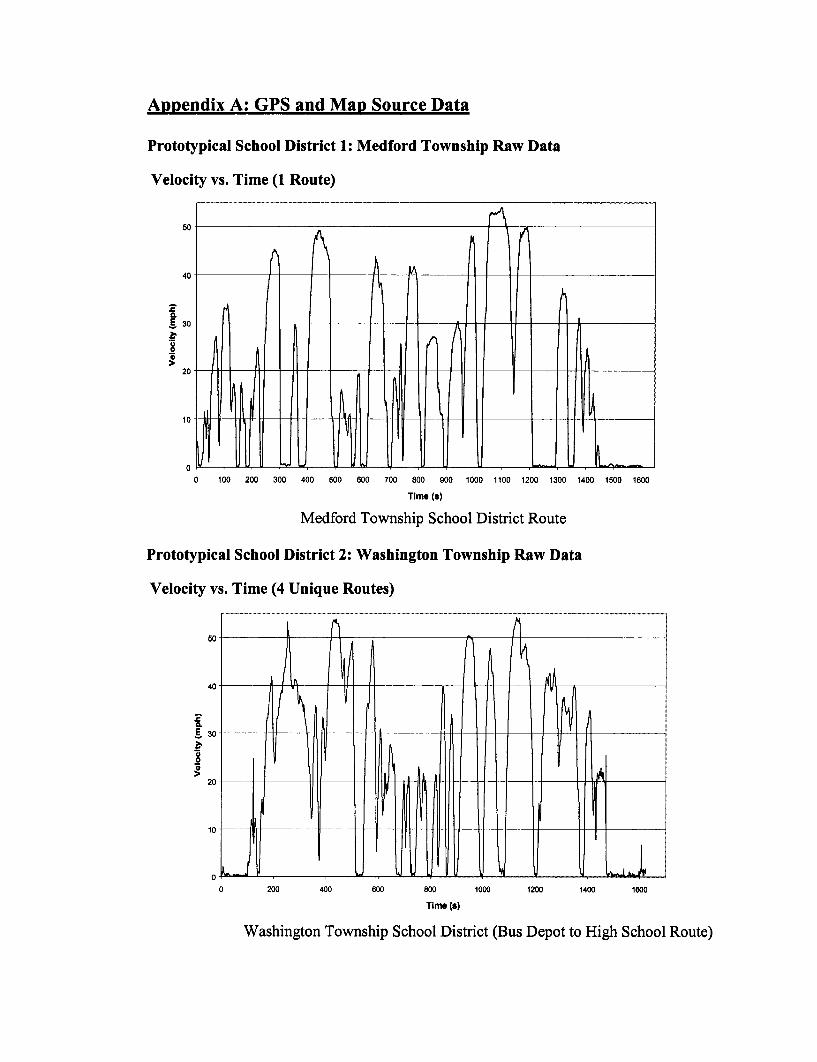
Appendix A: GPS and Map Source Data
Prototypical School District 1: Medford Township Raw Data
Velocity vs. Time (1 Route)
50
40
So.E 30
8
20
10
0
0 100 200 300 400 500 600 700 800 900 1000 1100 1200 1300 1400 1500 1600
Time (s)
Medford Township School District Route
Prototypical School District 2: Washington Township Raw Data
Velocity vs. Time (4 Unique Routes)
E
S
ou
40
30
20
10
0
0
I-n n
200 400 600 800 1000 1200 1400 1600
Time (s)
Washington Township School District (Bus Depot to High School Route)
AA M
, ~ .... I ,TT'P T rLlI
A dA
~WI I:AI 'I .I .I .
· · ·
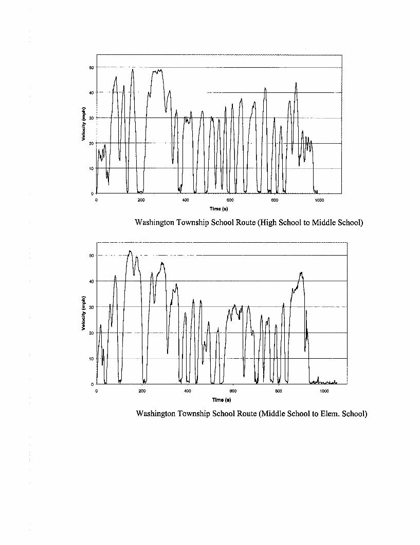
50
40 AA
30 oA -A A___
20 -
I,~~~~~AA
a 200 400 600 800 1000
Time (s)
Washington Township School Route (High School to Middle School)
..--- _. .. ... _.... __..
ou
40
30
20
10
Ih
0
EoLEa.
I
E
11
200 400 600 800 1000
Time (s)
Washington Township School Route (Middle School to Elem. School)
A fi . , AIJ fA . , A
/~tl __ ____'I_,-^ _ J I I M y / L
I
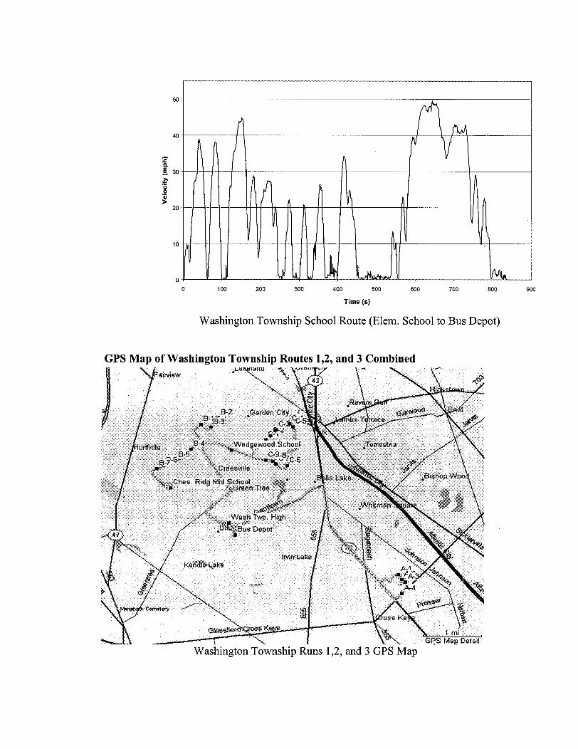
2.
E
._0
5U
40
30
20
10
0
0 100 200 300 400 500 600 700 800
Time (s)
Washington Township School Route (Elem. School to Bus Depot)
GPS Map of Washington Township Routes 1,2, and 3 Combined
900
-----------------I.... --------- ___________ -· -1---- 11-- 1
fV
- I
� A , I
I I k
I I
I I - I I
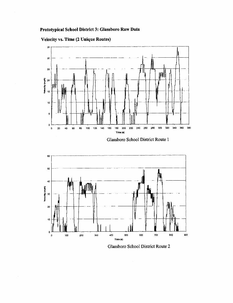
Prototypical School District 3: Glassboro Raw Data
Velocity vs. Time (2 Unique Routes)
II1 A-I
r'l II1 I rm I AII nII 11II II I I I`
II.~, i
II
U
I I-I I IIl I I I J
,~ 'I II Fl inI I I I Il"
If ifI I
0 20 40 60 80 100 120 140 160 180 200 220 240 260 280 300 320
Time (a)
Glassboro School District Route 1
om i ,wM. I
11 I 1 1
Jr
II
rI
I'340 360 380
h !1'1
Y
l,,
h ki i900200 300 400 500 800 700 800
Time (s)
Glassboro School District Route 2
30
I20
15
10
5
0
V _ "_
50
50
II I
- T7I
a1
30
20
n
d LI I 111 III
0 100
II I |
I j IOr L i nr
� d i . � 11
I 11 III t7I. . . . . I . I .
C _ __ 11 C II I inn*__I A_ L L_11_____ f IL_I 1I 11!,I-. .. _ . ... .. -_. ... _ - ei _ I I ._1fi
.. ..... .. .. .
I l B I l 1 R Il II
I
g
--̂ ., _ _ . _. _ . _ ..
,A, I4U
E6 j" 1illq, * I ,
IUlI I i·,
��------- --
I~ I
In
IIF
i ' i
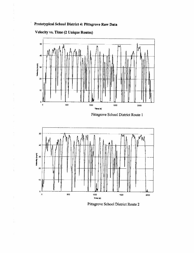
Prototypical School District 4: Pittsgrove Raw Data
Velocity vs. Time (2 Unique Routes)
50
40
10
0
0 500 1000 1500 2000
Time (s)
Pittsgrove School District Route 1
50
40
30
20
10
00 600 1000 1500
Time (s)
Pittsgrove School District Route 2
A
8_s
A
8
2000
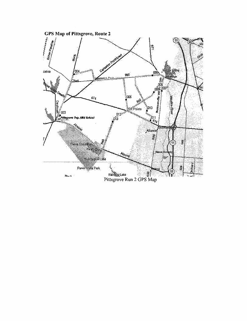
GPS Map of Pittsgrove, Route 2
i90
vs Tw.Md VSciool
Pittsgrove Run 2 GPS Map
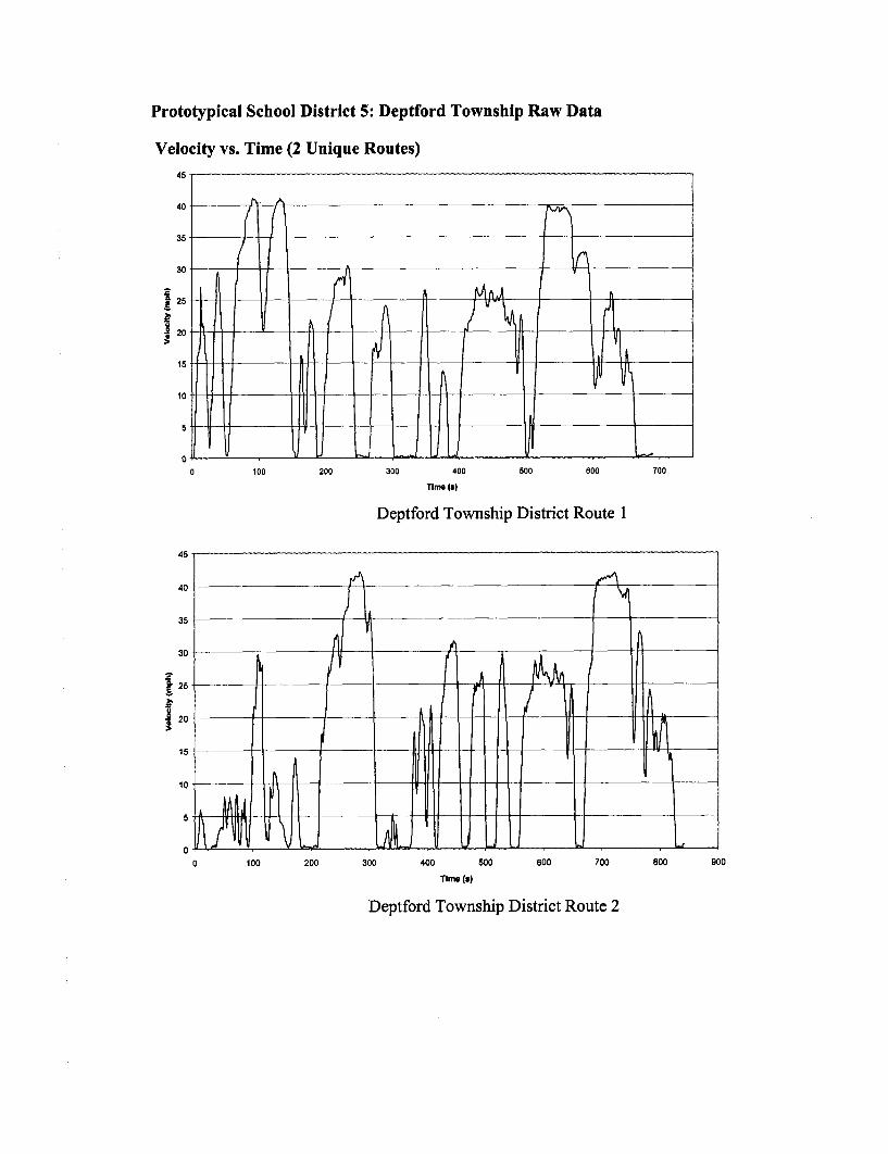
Prototypical School District 5: Deptford Township Raw Data
Velocity vs. Time (2 Unique Routes)
100 200 300 400 500 000 700
Time (s)
Deptford Township District Route 1
I, I r
.11 IIIIlI I
f . A A i
A~ltI)I
UfA I I
11 11
HII/1i I
\P !WU J JUV300 400 500
III I
I'XI i
600 700 800 900
Time (s)
Deptford Township District Route 2
4
4
3
3
2
1
5
15
IIFJrfIIII°t ̂ - -B-4 -- - 4--- - ----
0
n~ 11 'V.
45
40
35
30
25
i 20
15
10
5
0
0
IFA C
Id II
WA^l II 1
100 200
-- i^i- �-- f\--I---------
r-i'X^ ,I--
11 I .. .1 I
II ' I l I
In .
I it' - .w . _T - o l _X .:'' _ -
1
I I II
i10.II I
I I II I II Ii
A . I 11 l
._
_II , [ J
- -- X