school of economics working papers · than a power form of probability ... (cox and oaxaca, 1996,...
TRANSCRIPT

A Naïve Approach to Bidding
Paul Pezanis-Christou Hang Wu University of Adelaide National University of Singapore School of Economics Centre for Behavioural Economics
Working Paper No. 2017-03 March 2017
Copyright the authors
School of Economics
Working Papers ISSN 2203-6024
1
A naïve approach to bidding†
PAUL PEZANIS-CHRISTOU HANG WU
March 2017
Abstract: We propose a novel approach to the modelling of bidding behavior in pay-
your-bid auctions that builds on the presumption that bidders are mostly concerned with
losing an auction if they happen to have the highest signal. Our models assume risk
neutrality, no profit maximization and no belief about competitors’ behavior. They may
entail overbidding in first-price and all-pay auctions and we discuss conditions for the
revenue equivalence of standard pay-your-bid auctions to hold. We fit the models to the
data of first-price auction experiments and find that they do at least as well as Vickrey’s
benchmark model for risk neutral bidders. Assuming probability misperception or
impulse weighting (when relevant) improves their goodness-of-fit and leads to very
similar revenue predictions. An analysis of individuals’ heterogeneous behavioral traits
suggests that impulse weighting is a more consistent rationale for the observed behavior
than a power form of probability misperception.
Keywords: first-price auctions, all-pay auctions, impulse balance equilibrium,
overbidding, bounded rationality, probability distortion, regret, revenue equivalence,
experiments.
J.E.L. Classification: C44, C72, D44, D48, L2.
† We thank audiences at the University of Technology Sydney and the 2016 ANZWEE meetings in Brisbane for
useful comments, as well as Peter Katuščak, Fabio Michelucci, Axel Ockenfels and Jim Walker for access to
their data. Financial support from the Australian Research Council through a Discovery Project grant
(DP140102949) is gratefully acknowledged. The usual disclaimer applies.
Affiliations and email addresses:
Pezanis-Christou: University of Adelaide, School of Economics. Email: [email protected]
Wu: National University of Singapore, Center for Behavioural Economics. Email: [email protected]

2
Since Vickrey’s (1961) seminal paper, the task of bidding in auctions has been approached
from a game-theoretic perspective. While this approach organizes bidding behavior well in
auctions that entail a weakly dominant strategy such as the ascending-price format, its
relevance for the analysis of first-price, which entails complex strategic reasoning, has been
challenged by four decades of experimental research reporting ‘overbidding’, i.e., bidding
more than what the Symmetric Bayes Nash Equilibrium bidding strategy predicts (see Kagel,
1995 and 2008 for reviews). Remarkably, at the exception of Reinhard Selten’s Learning
Direction Theory which predicts qualitative changes in bidders’ round-to-round behavior (see
Selten and Buchta, 1998), the proposed rationales keep a strong game-theoretic flavor as they
all hinge upon some set of beliefs about competitors’ behavior. In this paper, we propose a
novel approach to the modelling of bidding behavior in standard pay-your-bid auctions with
independent private values that assumes no profit-maximization, no belief about competitors’
behavior, and which sheds a new light on Vickrey’s pioneering work.
Before spelling out our approach, we briefly review two basic features of the proposed
rationales for first-price auctions.1 First, they all assume the optimization of some objective
function. Following the recent debate on the modelling of bounded rationality in strategic
games (see Harstad and Selten, 2013, Crawford, 2013, and Rabin, 2013), we identify three
approaches to this exercise: (1) one that considers alternative specifications of the bidders’
preferences or utilities while assuming profit-maximization and belief-consistency, (2) one
that relaxes the latter assumption to study non-equilibrium type of best-responding behaviors,
e.g., rationalizable bidding (Battigali and Siniscalchi, 2003) and level-k (Crawford and
Irriberi, 2007), and (3) one that substitutes the usual maximization of expected profits with
the minimization of some loss function, as in learning models (Saran and Serrano, 2014) or
Impulse Balance Equilibrium (Ockenfels and Selten, 2005). Second, they all involve either (i)
some parameter(s) to be estimated, e.g., risk averse preferences (Cox, Smith and Walker,
1988), extent of best-responsiveness (Goeree, Holt and Palfrey, 2002), probability
misperception (Armantier and Treich, 2009a), depth-of-reasoning (Crawford and Irriberi,
2007) or reference-dependent loss aversion (Banerji and Gupta, 2014), and/or (ii) some
treatment variations to highlight a behavioral trait such as information-induced regret
(Ockenfels and Selten, 2005, Neugebauer and Selten, 2006, Engelbrecht-Wiggans and Katok,
1 Most experimental studies of bidding behaviour with incomplete information have dealt with first-price
auctions. See Dechenaux, Kovenock and Sheremeta (2015) for a review of experimental research on all-pay
auctions, contests and tournaments.

3
2007, 2008, Filiz and Ozbay, 2007) or non-best-responding behavior (Kirchkamp and Reiβ,
2011).
These rationales successfully explain some aspect of the observed behavior but their
investigations also reveal inconsistencies across experiments as well as empirical limitations.
Risk aversion, for example, is often used to explain overbidding in symmetric first-price but
it fails to do so in other formats that also cast a Bayes-Nash equilibrium argument, like third-
price auctions (Kagel and Levin, 1993) and asymmetric first-price auctions (Pezanis-
Christou, 2002). It also does not suit well the analysis of all-pay auctions since these may
imply negative payoffs. As for probability perceptions, Ratan (2015) investigates the effects
of displaying probabilities of winning conditional on the submitted bids in first-price auctions
and finds no evidence of bidders’ responsiveness to this information. Katuščak, Michelucci
and Zajíček (2015) and Ratan and Wen (2016) attempt to reproduce the findings of Filiz and
Ozbay (2007) about the effect of information-induced regret in one-shot first-price auctions
and find no support for it. It should further be noted that these rationales are hard to
disentangle when values are uniformly drawn since they yield the same linear equilibrium
strategy for some specification of risk aversion, probability misperception and information-
induced regret --- see Engelbrecht-Wiggans and Katok (2007, Footnote 4) and Pezanis-
Christou and Romeu (2016, Proposition 2). On the other hand, boundedly rational models
based on ‘rationalizability’ or ‘learning’ remain hard to assess empirically, whereas Quantal
Response Equilibrium and level-k provide stochastic point predictions (the variance of
bidders’ noisy behavior and the mean of their depth-of-reasoning, respectively) that imply
optimal distributions of bids rather than optimal bid point predictions. Lastly, the proposed
rationales typically require additional and hardly verifiable ad hoc common knowledge
assumptions, like the full specification of a non-atomic distribution of individual parameters,
to rationalize bidders’ heterogeneous behavior (Cox and Oaxaca, 1996, Chen and Plott, 1998,
and Palfrey and Pevniskaya, 2007, and Armantier and Treich, 2009a).
Our take on the modelling of this task assumes risk neutral preferences and no complex
strategic reasoning. It builds on the presumption that bidders are mostly concerned with
losing the auction if they happen to have the highest of all values. To address their concern,
we assume that bidders are prepared to bid up to the highest (unknown) value of the other
bidders, provided that it does not yield a loss; like what the weakly dominant bidding strategy
commands in an ascending-price auction. We believe that such assumptions are relevant to
the analysis of bidding behavior in real-world auctions. Next, to the difference of models that

4
assume some maximization of expected payoffs under some set of beliefs about competitors’
behavior, the individual decision-making models we propose assume that bidders minimize
some loss function without any such beliefs.
Our first model, NoR, equalizes the gain to be made in case of winning to an expected payoff
which we define as the expected difference between ones’ value and the highest of the others’
values, provided that it is smaller than ones’ value. This model is parameter-free and the
resulting bidding strategy shares properties of Vickrey’s Symmetric Bayes-Nash Equilibrium
(SBNE) strategy but implies a nonlinear overbidding. Our second model, nIBE (for naïve
IBE), casts an Impulse Balance Equilibrium argument inspired from Ockenfels and Selten
(2005). It assumes that bidders balance the expected impulses from winning with too high a
bid and from losing with too low a bid. In the absence of impulse weighting (i.e., bidders
equally weight the impulses from winning and from losing), nIBE is parameter-free and
yields the SBNE bidding strategy for risk neutral bidders. With impulse weighting, it implies
overbidding if bidders are more responsive to losing with too low a bid than to winning with
too high a bid, as in Ockenfels and Selten (2005). Finally, both NoR and nIBE can
accommodate idiosyncratic probability misperceptions, as defined in Cumulative Prospect
Theory, that are not common knowkledge.2
We test these models with the data of five experiments on first-price auctions with two or
four bidders, one-shot or repeated play, and with private values drawn from uniform or non-
uniform distributions. Overall, we find that in terms of parameter-free models, NoR largely
outperforms nIBE (or equivalently SBNE) in organizing bidding behavior and the seller’s
expected revenues in auctions with two bidders. Assuming probability misperception or
impulse weighting (when relevant) improves the models’ goodness-of-fits and yields very
similar revenue predictions; this holds for auctions with two and four bidders. Finally, an
analysis of the estimated individual behavioral traits indicates that impulse weights are
typically more concentrated at values characterizing an overbidding than probability
distortion estimates, thereby suggesting a more consistent rationale for the observed behavior.
The nest section presents our naïve approach and two models of bidding in first-price
auctions. Section 2 reviews the data and the estimation procedures and Section 3 reports the
outcomes. In Section 4, we extend nIBE to the analysis of ascending-price, descending-price
2 See Stott (2006) for a review of the functional forms of probability misperception used in Cumulative Prospect
Theory.

5
and all-pay auctions and we discuss conditions for the revenue equivalence to hold in the
presence of impulse weighting and probability misperception. Section 5 concludes.
1. Two models of naïve bidding in first-price auctions
1.1. The No-Regret model
Consider a first-price sealed-bid auction with 𝑛 > 1 bidders who compete for the purchase of
some commodity. Bidders' private values are identically and independently distributed
according to 𝐹, which has a common knowledge density 𝑓 defined on (0, �̅�].3 They know
their own value realizations but not those of their 𝑛 − 1 competitors. According to the first-
price auction rule, the highest bidder wins the object and pays her/his winning bid. In what
follows we will assume that bidders may display probability misperceptions that can be
characterized by some probability weighting function 𝜙 as defined in Cumulative Prospect
Theory.
Following the Bayes-Nash equilibrium argument of Vickrey (1961), bidders maximize their
expected utilities from winning the auction, assuming that they all use the same best-reply
function and they all distort probabilities according to 𝜙 which is common knowledge. Using
a fixed-point argument, the SBNE bidding strategy for first-price auctions reverts to
submitting a bid equal to the expectation of the second highest value of a sample of size 𝑛,
conditional on ones’ value 𝑣 being the highest. Denoting the (mis)perceived distribution of 𝑦
by 𝜙(𝐹(𝑦)𝑛−1), the SBNE strategy takes the following expression:
𝑏𝑁𝑎𝑠ℎ(𝑣) = 𝑣 −∫ 𝜙(𝐹(𝑦)𝑛−1)𝑣
0𝑑𝑦
𝜙(𝐹(𝑣)𝑛−1)
Our approach postulates that bidders are mostly concerned with losing the auction if they
happen to have the highest of all values. To avoid this concern, we assume that they are
prepared to bid up to the highest value (unknown) 𝑦 of the 𝑛 − 1 competitors, provided that
𝑦 ≤ 𝑣. Note that this is precisely how bidders are expected to behave in an ascending-price
auction since it is weakly dominant to stay in the bidding as long as the prevailing price is not
greater than ones’ value. In the context of sealed-bid first-price auctions for which only
3 We assume the lower end of 𝑓’s domain to be 𝑣 = 0 for expository convenience; all results extend to 𝑣 > 0.

6
overbidding is weakly dominated, bidders cannot update their bids and are required to make a
unique final offer to the seller. We define the bidder’s aspired expected payoff, 𝜋𝑁𝑅, as the
expected difference between 𝑣 and 𝑦 with 𝑦 ≤ 𝑣, that is:
𝜋𝑁𝑅 = ∫ (𝑣 − 𝑦)𝑣
0
𝑑𝜙(𝐹(𝑦)𝑛−1)
A NoR bidding strategy for first-price auctions, 𝑏𝑁𝑅(𝑣), is defined as the one that equalizes
the payoff to be made from winning, 𝑣 − 𝑏𝑁𝑅(𝑣), to 𝜋𝑁𝑅, so we have:
𝑣 − 𝑏𝑁𝑅(𝑣) = ∫ (𝑣 − 𝑦)𝑣
0
𝑑𝜙(𝐹(𝑦)𝑛−1) = ∫ 𝜙(𝐹(𝑦)𝑛−1)𝑣
0
𝑑𝑦
𝑏𝑁𝑅(𝑣) = 𝑣 −∫ 𝜙(𝐹(𝑦)𝑛−1)𝑣
0
𝑑𝑦
This bidding strategy shares features of 𝑏𝑁𝑎𝑠ℎ(𝑣) and has the following properties:
(i) 𝑏𝑁𝑅(𝑣) is monotone increasing in values, i.e., 𝜕𝑣𝑏𝑁𝑅(𝑣) > 0 for all 𝑣 ∈ (0, 𝑣), and
implies 𝑏𝑁𝑅(0) = 𝑏𝑁𝑎𝑠ℎ(0) and 𝑏𝑁𝑅(𝑣) = 𝑏𝑁𝑎𝑠ℎ(𝑣).
(ii) The difference ∆= 𝑏𝑁𝑅(𝑣) − 𝑏𝑁𝑎𝑠ℎ(𝑣) converges to 0 as 𝑛 → ∞.
(iii) In the absence of probability misperception, i.e., 𝜙(𝑝) = 𝑝 , 𝑏𝑁𝑅(𝑣) is ‘parameter-
free’ and implies a nonlinear overbidding. This follows from the term
∫ 𝜙(𝐹(𝑦)𝑛−1)𝑣
0𝑑𝑦 in 𝑏𝑁𝑅(𝑣) being smaller than the term
∫ 𝜙(𝐹(𝑦)𝑛−1)𝑣0 𝑑𝑦
𝜙(𝐹(𝑣)𝑛−1) in 𝑏𝑁𝑎𝑠ℎ(𝑣)
(which implies overbidding for all 𝑣 ∈ (0, 𝑣) ) and from 𝜕𝑣𝑣2 𝑏𝑁𝑅(𝑣) < 0 (which
implies concavity).
(iv) For a given 𝜙(. ), 𝑏𝑁𝑅(𝑣) implies ‘𝜙-overbidding’, i.e., bidding more than SBNE with
probability weighting function 𝜙 for all 𝑣 ∈ (0, 𝑣). When compared to the SBNE with
no probability misperception, 𝑏𝑁𝑅(𝑣) implies overbidding if:
∫ 𝐹(𝑦)𝑛−1𝑣
0
𝑑𝑦 > 𝐹(𝑣)𝑛−1∫ 𝜙(𝐹(𝑦)𝑛−1)𝑣
0
𝑑𝑦
Figure 1 displays the NoR bidding strategies and their properties for 𝑛 = 2 , assuming
uniformly distributed values on (0,1) and either the power form of probability misperception
𝜙(𝑝) = 𝑝𝛼 with 𝛼 > 0 or Prelec’s (1998) specification 𝜙(𝑝) = 𝑒−𝛽(ln(𝑝)𝛾) with 𝛽, 𝛾 > 0.

7
FIGURE 1: NOR AND SBNE BIDDING STRATEGIES FOR FIRST-PRICE AUCTIONS.
1.2. The naïve Impulse Balance Equilibrium model: nIBE
Before applying our naïve argument to Impulse Balance Equilibrium, we briefly sketch the
logic of IBE for first-price auctions as defined by Ockenfels and Selten (2005, OS). A bidder
with value 𝑣 will receive an upward impulse from losing the auction with a bid of 𝑥 and a
downward impulse upon winning the auction with a bid 𝑥 . With 𝐺(∙) standing for the
distribution of the highest of the 𝑛 − 1 other bids, the expected values of these impulses are
respectively equal to
𝑈(𝑣, 𝑥) = ∫ (𝑣 − 𝑧)𝑑𝐺(𝑧)𝑣
𝑥
and 𝐷(𝑣, 𝑥) = ∫ (𝑥 − 𝑧)𝑑𝐺(𝑧)𝑥
0
where 𝑈(𝑣, 𝑥) measures the anticipated regret of losing the auction with too low a bid 𝑥 and
where 𝐷(𝑣, 𝑥) measures the anticipated regret of winning the auction with too high a bid 𝑥.
In the IBE, 𝑥 solves 𝑈(𝑣, 𝑥) = 𝜆𝐷(𝑣, 𝑥), where 𝜆 stands for an impulse weighting parameter.
To solve the IBE, OS specify a linear relationship between values and bids so that the
solution must be of the form 𝑏∗(𝑣) = 𝑎𝑣 with 𝑎 > 0 . This assumption defines a
correspondence between 𝐺(∙) and the distribution of the highest of 𝑛 − 1 values, 𝐹(𝑣)𝑛−1,
that is essential to the determination of an IBE. 4 In what follows, we substitute this
assumption for our naïve argument: bidders mostly worry about losing the auction if they
happen to have the highest of 𝑛 values and are prepared to bid up to the highest unknown
value 𝑦 of the 𝑛 − 1 other bidders, provided that 𝑦 ≤ 𝑣. We also define the bidders’ upward
4 To determine the IBE, OS use this assumption and equalize the expectations of the impulses with respect to
values so that 𝑏𝐼𝐵𝐸(𝑣) is the solution to ∫ 𝑈(𝑣, 𝑥)𝑑𝑣 =1
0𝜆∫ 𝐷(𝑣, 𝑥)𝑑𝑣
1
0. We do not follow this approach and
determine instead the nIBE bidding strategy for each possible value, as when determining a SBNE bidding
strategy.

8
and downward impulses in terms of the expected distance between ones’ bid, 𝑥, and the
highest of the 𝑛 − 1 other values, 𝑦. Upon losing the auction, an upward impulse is triggered
by the regret of not having bid high enough to win the auction and is measured by the
distance between 𝑦 (which is larger than 𝑥) and ones’ bid 𝑥 . The expected value of this
upward impulse thus takes the following expression:
𝑈𝑛(𝑥) = ∫ (𝑦 − 𝑥)𝑑𝜙(𝐹(𝑦)𝑛−1)𝑣
𝑥
= 𝑣𝜙(𝐹(𝑦)𝑛−1) − 𝑥𝜙(𝐹(𝑦)𝑛−1) − ∫ 𝜙(𝐹(𝑦)𝑛−1)𝑑𝑦𝑣
0
+∫ 𝜙(𝐹(𝑦)𝑛−1)𝑑𝑦𝑥
0
Similarly, upon winning the auction, a downward impulse is triggered by the regret of having
won the auction with too high a bid and is measured by the distance between ones’ bid 𝑥
(which is larger than the highest of the other values, 𝑦) and 𝑦. The expected value of this
impulse takes the following expression:
𝐷𝑛(𝑥) = ∫ (𝑥 − 𝑦)𝑑𝜙(𝐹(𝑦)𝑛−1) = ∫ 𝜙(𝐹(𝑦)𝑛−1)𝑑𝑦𝑥
0
𝑥
0
At the nIBE, 𝑥∗ solves 𝑈𝑛(𝑥∗) = 𝜆𝐷𝑛(𝑥
∗) or equivalently, the following implicit equation
𝑥∗ = 𝑣 −∫ 𝜙(𝐹(𝑦)𝑛−1)𝑑𝑦𝑣
0
𝜙(𝐹(𝑣)𝑛−1)+ (1 − 𝜆)
∫ 𝜙(𝐹(𝑦)𝑛−1)𝑑𝑦𝑥∗
0
𝜙(𝐹(𝑣)𝑛−1)
The solution 𝑥∗ defines a function of 𝑣, 𝑏𝑛𝐼𝐵𝐸(𝑣), which has the following properties:
(i) When 𝜆 = 1, i.e., bidders equally weight upward and downward impulses, 𝑏𝑛𝐼𝐵𝐸(𝑣)
takes the same expression as 𝑏𝑁𝑎𝑠ℎ(𝑣). It thus follows that overbidding results if 𝜙
satisfies the star-shaped condition 𝜙(𝑝) < 𝑝𝜙′(𝑝) for 𝑝 ∈ (0,1), see Armantier and
Treich (2009b).
(ii) 𝑏𝑛𝐼𝐵𝐸(𝑣) is monotone increasing in 𝑣 for all 𝜆 > 0 (see Appendix 0).
(iii) The difference 𝑏𝑛𝐼𝐵𝐸(𝑣) − 𝑏𝑁𝑎𝑠ℎ(𝑣) converges to 0 as 𝑛 → ∞.
(iv) In the absence of probability misperception, 𝑏𝑛𝐼𝐵𝐸(𝑣) implies overbidding
(underbidding) for all 𝑣 ∈ (0, 𝑣) when 𝜆 < 1 (𝜆 > 1). This follows from the term
(1 − 𝜆) ∫ 𝐹(𝑦)𝑛−1𝑑𝑦𝑏𝑛𝐼𝐵𝐸(𝑣)
0/𝐹(𝑣)𝑛−1 being positive (negative) when 𝜆 < 1 (𝜆 > 1).
9
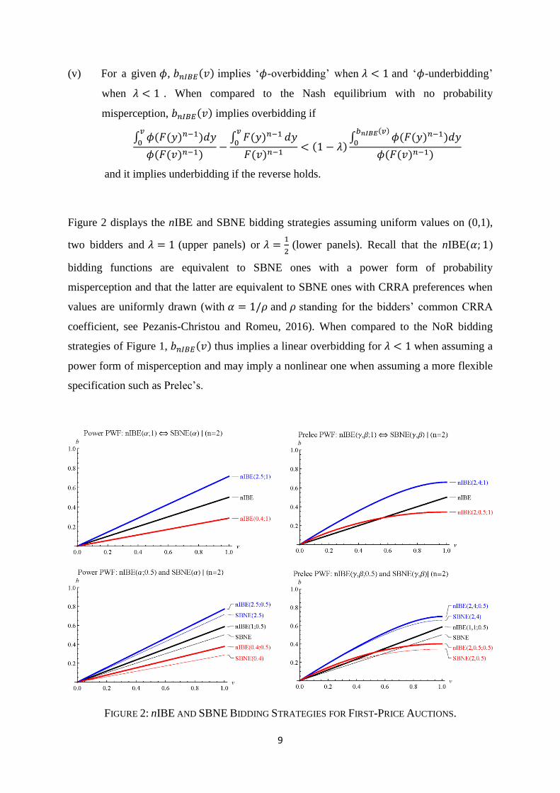
(v) For a given 𝜙, 𝑏𝑛𝐼𝐵𝐸(𝑣) implies ‘𝜙-overbidding’ when 𝜆 < 1 and ‘𝜙-underbidding’
when 𝜆 < 1 . When compared to the Nash equilibrium with no probability
misperception, 𝑏𝑛𝐼𝐵𝐸(𝑣) implies overbidding if
∫ 𝜙(𝐹(𝑦)𝑛−1)𝑑𝑦𝑣
0
𝜙(𝐹(𝑣)𝑛−1)−∫ 𝐹(𝑦)𝑛−1𝑣
0𝑑𝑦
𝐹(𝑣)𝑛−1< (1 − 𝜆)
∫ 𝜙(𝐹(𝑦)𝑛−1)𝑑𝑦𝑏𝑛𝐼𝐵𝐸(𝑣)
0
𝜙(𝐹(𝑣)𝑛−1)
and it implies underbidding if the reverse holds.
Figure 2 displays the nIBE and SBNE bidding strategies assuming uniform values on (0,1),
two bidders and 𝜆 = 1 (upper panels) or 𝜆 =1
2 (lower panels). Recall that the nIBE(𝛼; 1)
bidding functions are equivalent to SBNE ones with a power form of probability
misperception and that the latter are equivalent to SBNE ones with CRRA preferences when
values are uniformly drawn (with 𝛼 = 1/𝜌 and 𝜌 standing for the bidders’ common CRRA
coefficient, see Pezanis-Christou and Romeu, 2016). When compared to the NoR bidding
strategies of Figure 1, 𝑏𝑛𝐼𝐵𝐸(𝑣) thus implies a linear overbidding for 𝜆 < 1 when assuming a
power form of misperception and may imply a nonlinear one when assuming a more flexible
specification such as Prelec’s.
FIGURE 2: nIBE AND SBNE BIDDING STRATEGIES FOR FIRST-PRICE AUCTIONS.
10
2. Model comparisons
2.1. Data
We estimate our models with the data of five experiments on first-price auctions with two or
four bidders. The protocols of these experiments differ in many aspects (i.e., end-of-round
information feedback, number of rounds played, matching protocols, etc.) and are
summarized in Table 1. Katuščak, Michelucci and Zajíček (2015, KMZ henceforth) and Filiz
and Ozbay (2004, FO) dealt with one-shot auctions, controlling for the information feedback
and/or the number of bidders (𝑛 = {2,4}). The motivation to let participants play only once is
to prevent confounding effects from repeated play. Another distinctive feature of these
experiments is the use of the strategy method to collect bid data: participants in KMZ (FO)
were asked to submit a bid for each of six (ten) hypothetical values knowing that only one of
the (value, bid)-pairs will be randomly selected and implemented. KMZ also report on
treatments with a participant bidding against a SBNE robot (labelled 𝑛 = 2C in Table 2), as
well as on treatments replicating FO’s design. In both studies, winning or losing bids were
disclosed to bidders depending on them winning or losing the auction. In treatment MF (for
Minimal Feedback), participants were only informed about the win/lose outcome of the
auction and the winner knew the profit made. In LF (for Losers Feedback), the winning bid
was disclosed to losers whereas in WF (for Winners Feedback) the second highest bid was
disclosed to the winner.5 These studies were conducted to check whether bids are indeed
lower in the MF treatment than in the LF or WF ones.
Ockenfels and Selten (2005, OS), Isaac and Walker (1985, IW) and Chen, Katuščak and
Ozdenoren (2007, CKO) conducted repeated auctions and controlled for either the end-of-
round information feedback or the information about 𝐹 in different auction formats. OS
studied two-bidder auctions where participants bid in five consecutive auctions (days) with
the same value realisation and a different competitor before getting a new realisation for the
next five auctions (week). Participants were either provided information feedback on the
winning bid (treatment MF+) or they got to know the losing bid if they won the auction
(treatment WF). In IW, participants bid in fixed groups of four buyers and the information
feedback provided was either the full array of bids and the identification of bidders who
submitted them (treatment FF, for Full Feedback) or only the winning bid and the
5 To minimize the use of acronyms, we re-label treatments dealing with end-of-round information feedback
using KMZ’s notation when relevant, i.e., MF, LF and WF.

11
identification of the winner (treatment MF*). Both studies conjectured that the provision of
information feedback (WF or FF) in a repeated setting would yield lower bids when
compared to their respective Minimal Feedback treatments. Also, like most other
experimental studies on auctions, they assumed uniformly drawn values so that the SBNE
benchmark is linear in values. CKO relax this assumption and study sealed-bid auctions with
non-uniformly drawn values to assess the effect of ambiguity aversion/loving on bidders’
behaviour and on the seller’s revenues. In their K1 treatment, bidders knew that their
respective values were drawn from 𝐹1(𝑣) = (3
2𝑣) 𝕀
{0≤𝑣≤1
2}+ (
3
4+1
2(𝑣 −
1
2)) 𝕀
{1
2<𝑣≤1}
with
probability 𝛿 = 0.7 or from 𝐹2(𝑣) = (1
2𝑣) 𝕀
{0≤𝑣≤1
2}+ (
1
4+3
2(𝑣 −
1
2)) 𝕀
{1
2<𝑣≤1}
with
probability 1 − 𝛿. In their U1 treatment, participants were not informed about the probability
𝛿 and thus faced ambiguity regarding the generation of their values. CKO formalize this form
of ambiguity and show that it can be framed by the participants’ priors regarding the
distribution of 𝛿 and a weight of 𝛼 which captures ambiguity in an 𝛼-MEU setting. As the
resulting SBNE, NoR and nIBE bidding strategies are piece-wise linear in values, the
analysis of this data permits an assessment of the robustness of our models.
TABLE 1: SUMMARY OF EXPERIMENTAL DESIGNS.
Dataseta # Bidders
(𝑛) Interaction Treatments
# Groups
/Treatment
# Rounds
/Group
# Obs.
(Total) # Subjects
KMZ 2Cb One-Shot MF, LF, WF 72, 72, 72 1 1296 216
KMZ 2 One-Shot MF, LF, WF 36, 36, 36 1 1296 216
OS 2 Repeated MF+, WF 4, 4 140 13440 96
CKO 2 Repeated K1, U1 5, 5 30 2400 80
KMZ 4 One-Shot MF, LF 12, 12 1 576 96
KMZ 4Rc One-Shot MF, LF 12, 12 1 960 96
FO 4 One-Shot MF, LF, WF 7, 8, 9 1 960 96
IW 4 Repeated MF*, FF 10, 10 25 1988d 80 Note: a: KMZ: Katuščak, Michelucci and Zajíček (2015), OS: Ockenfels and Selten (2005), CKO: Chen, Katuščak and
Ozderonen (2007), FO: Filiz and Ozbay (2004), IW: Isaac and Walker (1985); b: one human bidder versus one Nash
computerized bidder; c: Replication of FO’s design; d: The data of IW/FF lacks twelve observations.
2.2. Procedures
As both NoR and nIBE yield closed-form bidding strategies when assuming a power form of
probability misperception, we conduct most of our analysis assuming 𝜙(𝑝) = 𝑝𝛼, with 𝛼 > 0.
We estimate our models with nonlinear least squares and compare their goodness-of-fits in
terms of the Akaike Information Criterion (AIC) corrected for the number of estimated
parameters and observations. As in repeated auctions, bidders interact with each other (via

12
their bids), we assume session-clustered standard errors, and we assume individually-
clustered ones when there is no interaction, as in one-shot auctions.
The estimation equation for the NoR bidding strategy, 𝑏𝑁𝑅(∙), has the following expression
when assuming uniform values on (0,1) and a Gaussian error term 휀:
𝑏𝑁𝑅(𝑣𝑖𝑗𝑡, 𝛼) = 𝑣𝑖𝑡 −𝑣𝑖𝑗𝑡
𝛼(𝑛−1)+1
1 + 𝛼(𝑛 − 1)+ 휀𝑖𝑗𝑡
where 𝑖 identifies bidders, 𝑗 stands for the auction session and 𝑡 stands for rounds. It takes an
additional parameter 𝛿 when values are drawn from non-uniform distributions 𝐹1 or 𝐹2 as in
CKO. Whether participants know 𝛿 or not, i.e., for both the K1 and U1 treatments, we get the
following two-piecewise nonlinear NoR bidding strategy: 6
𝑏𝑁𝑅(𝑣𝑖𝑗𝑡, 𝛼, 𝛿) = 𝜒1(𝑣𝑖𝑗𝑡, 𝛼, 𝛿)𝕀{0≤𝑣𝑖𝑗𝑡≤12}+ 𝜒2(𝑣𝑖𝑗𝑡, 𝛼, 𝛿)𝕀{1
2<𝑣𝑖𝑗𝑡≤1}
+ 휀𝑖𝑗𝑡
with
𝜒1(𝑣𝑖𝑗𝑡 , 𝛼, 𝛿) = 𝑣𝑖𝑗𝑡 −[𝑤(𝛿)3𝛼 + (1 − 𝑤(𝛿))]𝑣𝑖𝑗𝑡
𝛼+1
2𝛼(𝛼 + 1)
and
𝜒2(𝑣𝑖𝑗𝑡 , 𝛼, 𝛿) = 𝑣𝑖𝑗𝑡 −𝑤(𝛿) [(1 + 𝑣𝑖𝑗𝑡)
𝛼+1− (32)𝛼
] +1 − 𝑤(𝛿)
3 [(3𝑣𝑖𝑗𝑡 − 1)𝛼+1
+12𝛼]
2𝛼(𝛼 + 1)
For the K1 treatment, the estimation of 𝑏𝑁𝑅(𝑣𝑖𝑗𝑡, 𝛼, 𝛿) assumes 𝑤(𝛿) =𝛿𝛼
𝛿𝛼+(1−𝛿)𝛼.7 For the
U1 treatment, we follow CKO’s approach and use the probability misperception 𝛼-estimate
of the K1 treatment in the equation defining 𝑤(𝛿) and estimate 𝛿.
For the nIBE model, we focus attention on the estimation of constrained models with either
no impulse weight (𝜆 = 1, in which case we estimate the parameter 𝛼) or with no probability
misperception (𝛼 = 1, in which case we estimate the impulse weight 𝜆). This allows us to
assess the separate effects of probability misperception and of 𝜆 on the model’s goodness-of-
6 The details of the derivation of NoR’s and nIBE’s bidding strategy assuming CKO’s treatments K1 or U1 are
reported in Appendix A. 7 We used this normalization to make our results independent of whether the probability transformation
primarily applies to the event associated with 𝛿 or to the one associated with (1 − 𝛿). Estimating the models
assuming 𝑤(𝛿) = 𝛿𝛼 yields negligible differences that leaves our conclusions unchanged.
13
fit, and it alleviates the identification problem encountered when attempting to estimate all
parameters simultaneously. We will refer to these models as in nIBE(𝛼;1) and nIBE(1; 𝜆),
respectively. The estimating equation of nIBE(𝛼;1) admits the same closed-form solution as
the symmetric Nash equilibrium strategy, so:
𝑏𝑛𝐼𝐵𝐸(𝑣𝑖𝑗𝑡, 𝛼; 1) =𝛼(𝑛 − 1)
𝛼(𝑛 − 1) + 1𝑣𝑖𝑗𝑡 + 휀𝑖𝑗𝑡
As for nIBE(1;𝜆), the estimation equation takes the following closed-form expressions:
𝑏𝑛𝐼𝐵𝐸(𝑣𝑖𝑗𝑡 , 1; 𝜆 ) =1
1 + √𝜆𝑣𝑖𝑗𝑡 + 휀𝑖𝑗𝑡
𝑏𝑛𝐼𝐵𝐸(𝑣𝑖𝑗𝑡, 1; 𝜆 ) =1
2(√𝒜 −√8(√𝒜)
−1−𝒜)𝑣𝑖𝑗𝑡 + 휀𝑖𝑗𝑡
for 𝑛 = 2 and 4, respectively, and with 𝒜 = 2(1 − 𝜆)−2
3 [(1 + √𝜆)1
3 + (1 − √𝜆)1
3].
Assuming CKO’s K1 treatment and 𝑤(𝛿) =𝛿𝛼
𝛿𝛼+(1−𝛿)𝛼, we get the following two-piecewise
nonlinear model for nIBE(𝛼; 1, 𝛿):
𝑏𝑛𝐼𝐵𝐸(𝑣, 𝛼; 1,𝛿) = 𝜑1(𝑣𝑖𝑗𝑡, 𝛼, 𝛿)𝕀{0≤𝑣𝑖𝑗𝑡≤12}+𝜑2(𝑣𝑖𝑗𝑡, 𝛼, 𝛿)𝕀{12<𝑣𝑖𝑗𝑡≤1}
+ 휀𝑖𝑗𝑡
with
𝜑1(𝑣𝑖𝑗𝑡, 𝛼, 𝛿) =𝛼
𝛼 + 1𝑣𝑖𝑗𝑡
and
𝜑2(𝑣𝑖𝑗𝑡 , 𝛼, 𝛿) =
𝑤(𝛿) [(𝛼𝑣𝑖𝑗𝑡 − 1)(1 + 𝑣𝑖𝑗𝑡)𝛼+ (32)𝛼
] +1 − 𝑤(𝛿)
3 [(3𝛼𝑣𝑖𝑗𝑡 + 1)(3𝑣𝑖𝑗𝑡 − 1)𝛼−12𝛼]
𝑤(𝛿)(𝛼 + 1)(1 + 𝑣𝑖𝑗𝑡)𝛼+ (1 − 𝑤(𝛿))(𝛼 + 1)(3𝑣𝑖𝑗𝑡 − 1)𝛼
Here again, we estimate the constrained version 𝑏𝑛𝐼𝐵𝐸(𝑣, 𝛼, 1, 𝛿) with 𝑤(𝛿) =𝛿𝛼
𝛿𝛼+(1−𝛿)𝛼 in
the K1 treatment, and we use the 𝛼 - or 𝜆 -estimate of this treatment to estimate the 𝛿
14
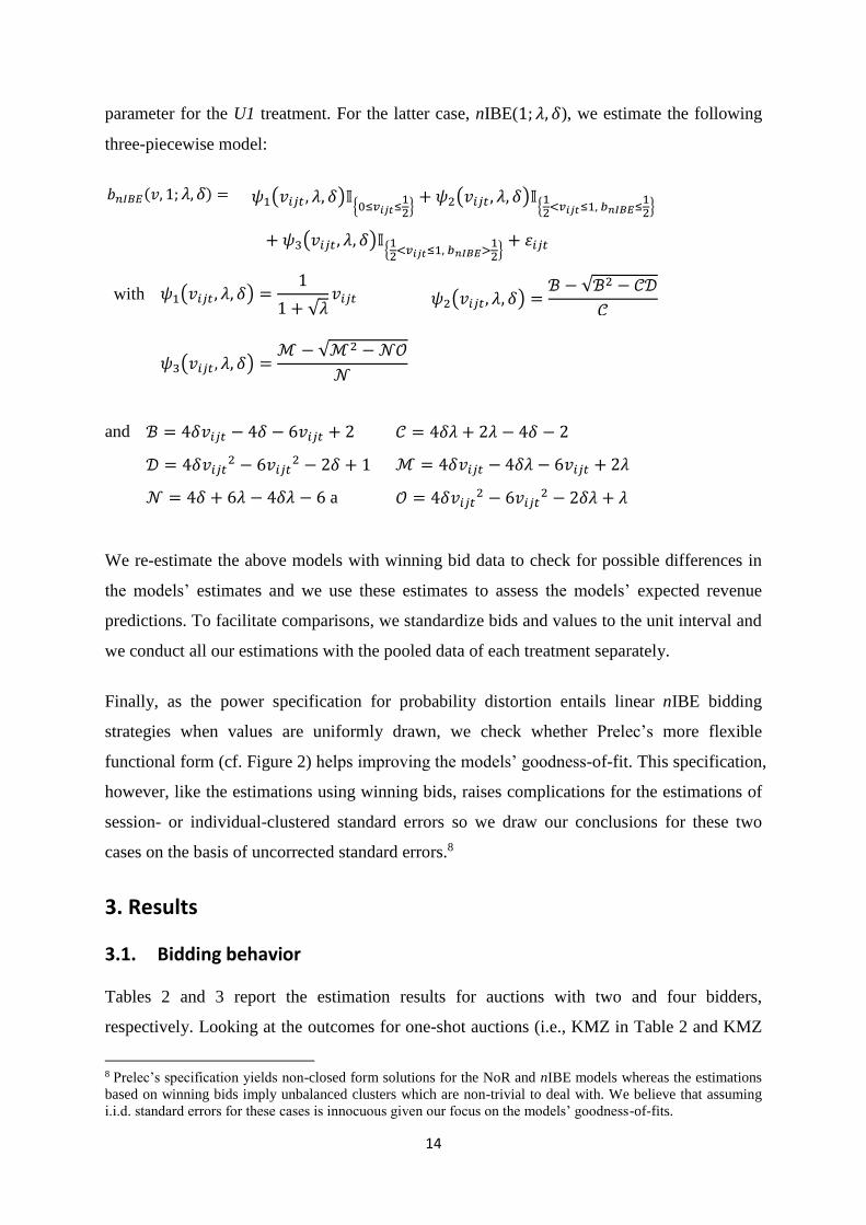
parameter for the U1 treatment. For the latter case, nIBE(1; 𝜆, 𝛿), we estimate the following
three-piecewise model:
𝑏𝑛𝐼𝐵𝐸(𝑣, 1; 𝜆,𝛿) = 𝜓1(𝑣𝑖𝑗𝑡 , 𝜆, 𝛿)𝕀{0≤𝑣𝑖𝑗𝑡≤12}+ 𝜓2(𝑣𝑖𝑗𝑡 , 𝜆, 𝛿)𝕀{1
2<𝑣𝑖𝑗𝑡≤1, 𝑏𝑛𝐼𝐵𝐸≤
12}
+ 𝜓3(𝑣𝑖𝑗𝑡 , 𝜆, 𝛿)𝕀{12<𝑣𝑖𝑗𝑡≤1, 𝑏𝑛𝐼𝐵𝐸>
12}+ 휀𝑖𝑗𝑡
with 𝜓1(𝑣𝑖𝑗𝑡 , 𝜆, 𝛿) =1
1 + √𝜆𝑣𝑖𝑗𝑡 𝜓2(𝑣𝑖𝑗𝑡, 𝜆, 𝛿) =
ℬ − √ℬ2 − 𝒞𝒟
𝒞
𝜓3(𝑣𝑖𝑗𝑡 , 𝜆, 𝛿) =
ℳ − √ℳ2 −𝒩𝒪
𝒩
and ℬ = 4𝛿𝑣𝑖𝑗𝑡 − 4𝛿 − 6𝑣𝑖𝑗𝑡 + 2 𝒞 = 4𝛿𝜆 + 2𝜆 − 4𝛿 − 2
𝒟 = 4𝛿𝑣𝑖𝑗𝑡2 − 6𝑣𝑖𝑗𝑡
2 − 2𝛿 + 1 ℳ = 4𝛿𝑣𝑖𝑗𝑡 − 4𝛿𝜆 − 6𝑣𝑖𝑗𝑡 + 2𝜆
𝒩 = 4𝛿 + 6𝜆 − 4𝛿𝜆 − 6 a 𝒪 = 4𝛿𝑣𝑖𝑗𝑡2 − 6𝑣𝑖𝑗𝑡
2 − 2𝛿𝜆 + 𝜆
We re-estimate the above models with winning bid data to check for possible differences in
the models’ estimates and we use these estimates to assess the models’ expected revenue
predictions. To facilitate comparisons, we standardize bids and values to the unit interval and
we conduct all our estimations with the pooled data of each treatment separately.
Finally, as the power specification for probability distortion entails linear nIBE bidding
strategies when values are uniformly drawn, we check whether Prelec’s more flexible
functional form (cf. Figure 2) helps improving the models’ goodness-of-fit. This specification,
however, like the estimations using winning bids, raises complications for the estimations of
session- or individual-clustered standard errors so we draw our conclusions for these two
cases on the basis of uncorrected standard errors.8
3. Results
3.1. Bidding behavior
Tables 2 and 3 report the estimation results for auctions with two and four bidders,
respectively. Looking at the outcomes for one-shot auctions (i.e., KMZ in Table 2 and KMZ
8 Prelec’s specification yields non-closed form solutions for the NoR and nIBE models whereas the estimations
based on winning bids imply unbalanced clusters which are non-trivial to deal with. We believe that assuming
i.i.d. standard errors for these cases is innocuous given our focus on the models’ goodness-of-fits.
15
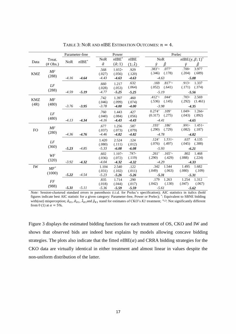
and FO in Table 3), it appears that in terms of goodness-of-fit of parameter-free models, NoR
always outperforms nIBE (or SBNE) when 𝑛 = 2 whereas it hardly ever does so when 𝑛 = 4.
Assuming a power form of probability misperception, we reach the opposite conclusion that
nIBE(𝛼; 1) outperforms NoR(𝛼), but assuming Prelec’s more flexible specification, we find
again that NoR(𝛾, 𝛽) outperforms nIBE(𝛾, 𝛽; 1) no matter 𝑛. Furthermore, the 𝛼-estimates of
nIBE(𝛼; 1) (𝜆-estimates of nIBE(1; 𝜆)) are all greater (smaller) than one which supports the
observed overbidding, and nIBE(𝛼; 1 ) generates the same goodness-of-fit measures as
nIBE(1; 𝜆) which suggests that both parameters explain the data equally well when they are
considered separately. The estimates also suggest that overbidding decreases with
competition. In addition, they are not significantly different across information treatments
when 𝑛 = 2, which is in line with KMZ findings that end-of-round information feedback
does not affect behaviour in one-shot first-price auctions. When 𝑛 = 4 , the effect of
information feedback on behaviour is mild in KMZ, and virtually absent in KMZ/4R. Since
the FO estimates for the LF treatment are twice those for the MF treatment and since the
latter are virtually identical to those of KMZ/4R/MF, our analysis supports KMZ’s conjecture
that FO’s findings for the LF treatment are most likely due to a subject-cohort bias.
The outcomes of repeated auctions (i.e., OS and CKO in Table 2 and IW in Table 3) indicate
that in terms of parameter-free models, NoR usually outperforms nIBE. When assuming a
power form of probability misperception, the OS data is best explained by NoR whereas the
IW and CKO data are best explained by nIBE with either probability misperception or
impulse weighting. The estimates of both models are then significantly different across
treatments in OS and IW but support the conjecture that information disclosure in repeated
first-price auctions yields lower bids. For these datasets, assuming Prelec’s specification
improves the models’ goodness-of-fits and makes them equivalent in terms of AIC statistics.
As for the U1 treatment of CKO, the 𝛿-estimates of the parameter-free variants of NoR and
nIBE suggest that participants bid as if their values were most likely drawn from the high
value distribution 𝐹2 whereas those obtained by assuming the 𝛼 -estimates of the K1
treatment are close to one and suggest that they bid as if values were most likely drawn from
the low value distribution 𝐹1. The poor performance of nIBE(1, 𝜆) also suggests that the
effect of ambiguity, as modelled by CKO, seems to override the one of impulse weighting.
Since the correspondence between a power form of distortion and CRRA preferences does
not hold for non-uniformly drawn values, we estimate the SBNE model for the CKO data

16
with CRRA preferences and find that it explains the data equally well as nIBE(𝛼, 1) or
nIBE(1, 𝜆) in the K1 treatment, and that it does marginally better than nIBE(𝛼, 1) in the U1
treatment. Finally, our 𝛿-estimate of .845 is virtually identical to the one of .8438 obtained by
CKO when using a subjective utility model so that our analysis leads to the same overall
conclusion as CKO regarding the effect of ambiguity on bidding behaviour in first-price
auctions.
TABLE 2: NOR AND nIBE ESTIMATION OUTCOMES: 𝑛 = 2.
Parameter-free Power Prelec
Data Treat. (# Obs.)
NoR nIBE* NoR
�̂�
nIBE*
(�̂�; 1) nIBE
(1; �̂�)
NoR
𝛾 �̂�
nIBE(𝛾, 𝛽; 1)*
𝛾 �̂�
KMZ
(2C)
MF
(432)
-4.32
-3.80
1.376
(.046)
-4.51
2.405
(.087)
-4.81
.173
(.012)
-4.81
.250
(.087)
0.396
(.435)
1.028▫
(.066)
2.388
(.095)
-4.79 -4.81
LF
(432)
-4.72
-4.10
1.295
(.035)
-4.91
2.240
(.058)
-5.43
.199
(.010)
-5.43
.824×▫
(.424)
.021×
(.035)
1.018▫
(.047)
2.229
(.064)
-5.43 -5.43
WF
(432)
-4.25
-3.76
1.402
(.049)
-4.45
2.462
(.090)
-4.80
.165
(.012)
-4.80
.498×▫
(.292)
.077×
(.106)
.936▫
(.062)
2.508
(.103)
-4.78 -4.80
KMZ MF
(432)
-4.38
-3.86
1.280
(.042)
-4.49
2.205
(.082)
-4.69
.206
(.015)
-4.69
.330
(.153)
.221×
(.241)
1.162
(.076)
2.130
(.086)
-4.70 -4.70
LF
(432)
-4.62
-4.06
1.229
(.036)
-4.72
2.107
(.065)
-5.02
.225
(.014)
-5.02
.453
(.192)
.112
(.110)
1.121▫
(.062)
2.046
(.070)
-5.03 -5.02
WF
(432)
-4.47
-3.93
1.289
(.040)
-4.61
2.222
(.075)
-4.88
.203
(.014)
-4.88
.503
(.249)
.083×
(.098)
1.105▫
(.066)
2.169
(.080)
-4.88 -4.88
OS MF+
(6720)
-4.85
-4.63
.838
(.005)
-4.97
1.368
(.010)
-4.87
.534
(.008)
-4.87
.539
(.018)
.850
(.005)
1.658
(.004)
1.139
(.010)
-5.03 -5.03
WF
(6720)
-4.41
-4.86
.631
(.004)
-5.04
.966
(.007)
-4.86
1.071
(.007)
-4.86
.655
(.020)
.659
(.004)
1.790
(.021)
.731
(.007)
-5.07 -5.07
Nash CRRA �̂�
CKO K1
(1200)
-4.27
-3.75
1.977
(.066)
-4.59
3.810
(.115)
-4.78
.140
(.007)
-4.79
.362
(.009)
-4.79
�̂� given: 𝛼 = 1 𝛼 = 1 𝛼 = �̂�𝐾1 𝛼 = �̂�𝐾1,
𝜆 = 1
𝛼 = 1,
𝜆 = �̂�𝐾1 𝜌 = �̂�𝐾1
U1
(1200)
.316
(.020)
-4.61
.000
(.022)
-4.48
.957
(.013)
-4.52
.971
(n.a.)
-4.71
.000
(.062)
-2.03
.845
(.021)
-4.76
Note: Session-clustered standard errors in parenthesis (i.i.d. for Prelec’s specification); AIC statistics in italics (bold figures
indicate the best AIC statistic for a given category: ‘Parameter-free’, ‘Power’ or ‘Prelec’; *: Equivalent to SBNE bidding
with(out) misperception; �̂�𝐾1, �̃�𝐾1, �̂�𝐾1 and �̂�𝐾1 stand for estimates of CKO’s K1 treatment; ×(▫): Not significantly different from
0 (1) at 𝛼 = 5%.
17
TABLE 3: NOR AND nIBE ESTIMATION OUTCOMES: 𝑛 = 4.
Parameter-free Power Prelec
Data Treat.
(# Obs.) NoR nIBE*
NoR
�̂�
nIBE*
(�̂�; 1) nIBE
(1; �̂�)
NoR
𝛾 �̂�
nIBE(𝛾, 𝛽; 1)*
𝛾 �̂�
KMZ MF
(288)
-4.16
-4.64
.568
(.027)
-4.43
1.032▫
(.056)
-4.63
.929
(.120)
-4.63
.383×▫
(.346)
.077×
(.178)
.788▫
(.204)
3.977
(.689)
-4.63 -5.08
LF
(288)
-4.59
-5.19
.660
(.028)
-4.77
1.217
(.053)
-5.25
.632
(.064)
.169
(.052)
.817×▫
(.641)
.913▫
(.171)
1.337
(.374)
-5.25 -5.19 -5.56
KMZ
(4R)
MF
(480)
-3.76
-3.95
.742
(.046)
-3.78
1.397
(.099)
-4.00
.460
(.074)
-4.00
.412×▫
(.536)
.044×
(.145)
.703▫
(.292)
2.569
(1.461)
-3.98 -4.35
LF
(480)
-4.13
-4.34
.760
(.040)
-4.16
1.443
(.084)
-4.43
.427
(.056)
-4.43
0.274×
(0.317)
.109×
(.275)
1.049▫
(.043)
1.266▫
(.892)
-4.41 -4.65
FO MF
(280)
-4.36
-4.76
.677
(.037)
-4.46
1.256
(.073)
-4.82
.587
(.079)
-4.82
.193×
(.290)
.186×
(.729)
.891▫
(.082)
1.451▫
(.187)
-4.78 -4.82
LF
(360)
-5.23
-4.85
1.420
(.080)
-5.33
2.524
(.111)
-6.08
.124
(.012)
-6.08
.124×
(.076)
1.531▫
(.497)
.637
(.045)
4.135
(.388)
-5.93 -6.21
WF
(320)
-3.92
-4.32
.602
(.036)
-4.04
1.107▫
(.072)
-4.32
.787▫
(.119)
.261×
(.290)
.165×▫
(.429)
.802
(.088)
1.468
(.224)
-4.32 -4.29 -4.33
IW MF*
(1000)
-5.22
-4.54
1.104
(.031)
-5.23
2.540
(.102)
-5.26
.122
(.011)
-5.26
.342
(.049)
1.544
(.063)
1.495
(.080)
1.682
(.109)
-5.31 -5.31
FF
(988)
-5.31
-5.11
.835
(.018)
-5.36
1.714
(.044)
-5.59
.290
(.017)
-5.59
.179
(.042)
1.263
(.130)
1.254
(.047)
1.312
(.067)
-5.61 -5.62
Note: Session-clustered standard errors in parenthesis (i.i.d. for Prelec’s specification); AIC statistics in italics (bold
figures indicate best AIC statistic for a given category: Parameter-free, Power or Prelec); *: Equivalent to SBNE bidding
with(out) misperception; �̂�𝐾1, �̃�𝐾1, �̂�𝐾1and �̂�𝐾1 stand for estimates of CKO’s K1 treatment; ×(▫): Not significantly different
from 0 (1) at 𝛼 = 5%.
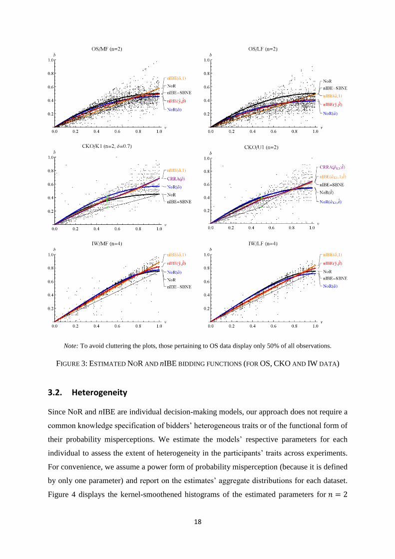
Figure 3 displays the estimated bidding functions for each treatment of OS, CKO and IW and
shows that observed bids are indeed best explains by models allowing concave bidding
strategies. The plots also indicate that the fitted nIBE(𝛼) and CRRA bidding strategies for the
CKO data are virtually identical in either treatment and almost linear in values despite the
non-uniform distribution of the latter.
18
Note: To avoid cluttering the plots, those pertaining to OS data display only 50% of all observations.
FIGURE 3: ESTIMATED NOR AND nIBE BIDDING FUNCTIONS (FOR OS, CKO AND IW DATA)
3.2. Heterogeneity
Since NoR and nIBE are individual decision-making models, our approach does not require a
common knowledge specification of bidders’ heterogeneous traits or of the functional form of
their probability misperceptions. We estimate the models’ respective parameters for each
individual to assess the extent of heterogeneity in the participants’ traits across experiments.
For convenience, we assume a power form of probability misperception (because it is defined
by only one parameter) and report on the estimates’ aggregate distributions for each dataset.
Figure 4 displays the kernel-smoothened histograms of the estimated parameters for 𝑛 = 2

19
(upper panel) and 𝑛 = 4 (lower panel). For auctions with 𝑛 = 2, the 𝛼-estimates of one-shot
sessions (KMZ) and CKO/K1 sessions are more evenly spread than those of repeated sessions
(OS) whereas the opposite holds for the 𝜆-estimates. For auctions with 𝑛 = 4, the 𝛼-estimates
of both one-shot and repeated auctions are spread out whereas the 𝜆 -ones are more
concentrated at 𝜆 < 1 in both cases (cf. FO and IW). Overall, at the exception of the OS data,
the plots suggest that participants’ 𝜆-estimates are far more are concentrated than their 𝛼-
estimates which suggests that the former are better identified than the latter.9
FIGURE 4: DISTRIBUTIONS OF ESTIMATED PARAMETERS FOR NOR AND nIBE.
3.3. Expected Revenues
We now assess the models’ expected revenue predictions when these are determined with the
NoR or nIBE parameter estimates obtained from winning bids. The estimation outcomes
(reported in Appendix B) indicate that in terms of parameter-free models, NoR outperforms
nIBE (or equivalently SBNE) six out of seven times when 𝑛 = 2 and seven out of nine times
9 To explain the atypical distributions of the 𝛼- and 𝜆-estimates in OS, we conjectured that this could be due to
their experimental design which had participants play with the same value for five days before getting a new
draw for the next five days (week). We therefore estimated the models with the data of the first or last day of
each week to check for differences that would witness non-constant bid-to-value ratios over days but found no
significant pattern to report. Also, the resulting distributions of first- and last-day estimates display the same
patterns as those reported in Figure 4.
20
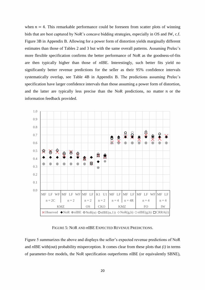
when 𝑛 = 4. This remarkable performance could be foreseen from scatter plots of winning
bids that are best captured by NoR’s concave bidding strategies, especially in OS and IW, c.f.
Figure 3B in Appendix B. Allowing for a power form of distortion yields marginally different
estimates than those of Tables 2 and 3 but with the same overall patterns. Assuming Prelec’s
more flexible specification confirms the better performance of NoR as the goodness-of-fits
are then typically higher than those of nIBE. Interestingly, such better fits yield no
significantly better revenue predictions for the seller as their 95% confidence intervals
systematically overlap, see Table 4B in Appendix B. The predictions assuming Prelec’s
specification have larger confidence intervals than those assuming a power form of distortion,
and the latter are typically less precise than the NoR predictions, no matter 𝑛 or the
information feedback provided.
FIGURE 5: NOR AND nIBE EXPECTED REVENUE PREDICTIONS.
Figure 5 summarizes the above and displays the seller’s expected revenue predictions of NoR
and nIBE with(out) probability misperception. It comes clear from these plots that (i) in terms
of parameter-free models, the NoR specification outperforms nIBE (or equivalently SBNE),
0.0
0.1
0.2
0.3
0.4
0.5
0.6
0.7
0.8
0.9
1.0
MF LF WF MF LF WF MF LF K1 U1 MF LF MF LF MF LF WF MF LF
n = 2C n = 2 n = 2 n = 2 n = 4 n = 4R n = 4 n = 4
KMZ OS CKO KMZ FO IW
Observed NoR nIBE NoR(α) nIBE(α,1)) NoR(g,b) nIBE(g,b) CRRA(r)

21
especially when 𝑛 = 2 , and (ii) assuming various forms of probability misperception or
homogenous CRRA preferences yield hardly any different revenue predictions.
4. Extensions to other pay-your-bid auctions
In this section, we extend our approach to the analysis of other pay-your-bid auctions and we
discuss conditions for their revenue equivalence to hold.
4.1. Ascending- and Descending-price auctions
In ascending-price auctions, the bidders’ major concern of ‘losing the auction if they happen
to have the highest values’ is easily addressed if they are prepared to bid up to the highest
value of their competitors, provided that it it does not incur a loss. Since this translates into
staying in the auction as long as the current price does not exceed ones’ value, the NoR and
nIBE models are irrelevant to the analysis of ascending-price auctions and the mere casting of
our naïve approach is sufficient to yield the well-established weakly dominant bidding
strategy for these auctions.
In descending-price auctions, the asset’s price is decreased over time until one of bidders
chooses to buy. The bidders’ dilemma therefore consists in choosing the lowest price at
which to buy the asset, given that choosing too low a price may result in being outbid by a
competitor. By discarding the time feature of these auctions and taking the normal form of
this dilemma, it immediately follows that applying our naïve approach to the analysis of
descending-price auctions yields the same NoR and nIBE bidding strategies as first-price
auctions.10
4.2. All-pay auctions
In all-pay auctions, the highest bidder wins and all bidders pay their bids. With such an
allocation rule, submitting a positive bid bears a risk of incurring a loss. Since our definition
of a naïve bidder’s aspired No-Regret expected profit, 𝜋𝑁𝑅, is independent of her bid, we
cannot derive a NoR bidding strategy for this format. However, we can define a naïve
Impulse Balance Equilibrium one. The nIBE argument leaves the definitions of 𝑈𝑛(𝑥) and
10 See Katok and Kwasnica (2008) who find evidence that the clock’s speed inversely affects the seller’s
expected revenues in descending-price auctions, which indicates that the strategic isomorphism of these format
does not hold anymore when the speed descending-prices is taking in to account.

22
𝐷𝑛(𝑥) for first-price auctions unchanged when it is applied to the analysis of all-pay auctions
but it generates an additional downward impulse, 𝐷1𝑛(𝑥, 𝑣), that is induced by the fact of
having to pay ones bid upon losing. This downward impulse is measured by the expected
distance between ones’ losing bid 𝑥 and the best ex-post bid, 𝑣 (= 0), provided the highest of
the 𝑛 − 1 other values is in (𝑣, 𝑣].
𝐷1𝑛(𝑥, 𝑣) = ∫ (𝑥 − 0)𝑑𝜙(𝐹(𝑦)𝑛−1𝑣
𝑣
= 𝑥(1 − 𝜙(𝐹(𝑦)𝑛−1)
At nIBE, we thus have 𝑈𝑛(𝑥∗) = 𝜆[𝐷𝑛(𝑥
∗) + 𝐷1𝑛(𝑥∗)]. The solution 𝑥∗ for a value 𝑣 solves
the following implicit equation:
𝑥∗ =𝑣𝜙(𝐹(𝑣)𝑛−1) − ∫ 𝜙(𝐹(𝑦)𝑛−1)𝑑𝑦 + (1 − 𝜆) ∫ 𝜙(𝐹(𝑦)𝑛−1)𝑑𝑦
𝑥∗
0
𝑣
0
𝜙(𝐹(𝑣)𝑛−1) + 𝜆[1 − 𝜙(𝐹(𝑣)𝑛−1)]
The solution 𝑥∗ is a function of 𝑣 that is the nIBE bidding strategy 𝑏𝑛𝐼𝐵𝐸𝐴 (𝑣). It has the
following properties:
(i) When 𝜆 = 1, 𝑏𝑛𝐼𝐵𝐸𝐴 (𝑣) boils down to the SBNE bidding strategy with distortion 𝜙:
𝑏𝑁𝑎𝑠ℎ(𝑣) = 𝑣𝜙(𝐹(𝑣)𝑛−1) − ∫ 𝜙(𝐹(𝑦)𝑛−1)𝑑𝑦
𝑣
0
Overbidding occurs if for all 𝑣 ∈ (0, 𝑣), we have:
𝑣 >∫ 𝜙(𝐹(𝑦)𝑛−1)𝑑𝑦𝑣
0− ∫ 𝐹(𝑦)𝑛−1𝑑𝑦
𝑣
0
𝜙(𝐹(𝑣)𝑛−1) − 𝐹(𝑣)𝑛−1
(ii) 𝑏𝑛𝐼𝐵𝐸𝐴 (𝑣) is monotone increasing in 𝑣 for all 𝜆 > 0 (see Appendix 0).
(iii) The difference ∆= 𝑏𝑛𝐼𝐵𝐸𝐴 (𝑣) − 𝑏𝑁𝑎𝑠ℎ(𝑣) converges to 0 as 𝑛 → ∞.
(iv) In the absence of probability misperception, 𝑏𝑛𝐼𝐵𝐸𝐴 (𝑣) implies an overbidding
(underbidding) when 𝜆 < 1 (𝜆 > 1). This follows from the sign of ∆ at 𝜆 < 1 (𝜆 > 1).
(v) In the presence of probability misperception, 𝑏𝑛𝐼𝐵𝐸𝐴 (𝑣) implies ‘𝜙-overbidding’ (‘𝜙-
underbidding’) when 𝜆 < 1 (𝜆 > 1). When compared to SBNE without probability
distortion, 𝑏𝑛𝐼𝐵𝐸𝐴 (𝑣) implies overbidding if, for all 𝑣 ∈ (0, 𝑣), we have:
𝑣𝜙(𝐹(𝑣)𝑛−1) − ∫ 𝜙(𝐹(𝑦)𝑛−1)𝑑𝑦𝑣
0
+ (1 − 𝜆)∫ 𝜙(𝐹(𝑦)𝑛−1)𝑑𝑦𝑏𝑛𝐼𝐵𝐸𝐴 (𝑣)
𝑣
> [𝑣𝐹(𝑣)𝑛−1 −∫ 𝐹(𝑦)𝑛−1𝑑𝑦𝑣
0
] {𝜙(𝐹(𝑣)𝑛−1) + 𝜆[1 − 𝜙(𝐹(𝑣)𝑛−1)]}
and it implies underbidding if the reverse holds.

23
Figure 6 displays the nIBE bidding strategies assuming two bidders with uniform values on
(0,1) and either a power or a Prelec form of probability distortion. The upper panels report
the nIBE bidding strategies assuming no impulse weighting (𝜆 = 1, in which case they are
equivalent to the SBNE ones) whereas the plots in the lower panels assume 𝜆 = 0.5 and
indicate overbidding. Note that for both specifications of bidders’ probability misperception
and for 𝜆 ≤ 1 , the nIBE bidding strategies may imply underbidding at low values and
overbidding at high ones. To this extent, our individual decision-making approach seems to
also organize the bidding patterns reported by Noussair and Silver (2006), Dechenaux and
Mancini (2008), and Hyndman, Ozbay and Sujarittanonta (2012).
FIGURE 6: nIBE AND SBNE BIDDING STRATEGIES FOR ALL-PAY AUCTIONS.
4.3. Revenue equivalence with 𝒏IBE bidders
We compare the seller’s expected revenues from ascending-price, descending-price, first-
price and all-pay auctions when assuming nIBE bidders. Clearly, when 𝜆 = 1 the nIBE
strategies for first-price, descending-price and all-pay (first-price) auctions coincide with the
SBNE ones with(out) probability misperception so that the revenue equivalence of these
formats holds when bidders use nIBE strategies. Furthermore, when compared to the

24
expected revenue of an ascending-price auction, which is equal to the expectation of the
second-highest value (of 𝑛 draws), it follows that first-price auctions are revenue superior
when 𝜙 satisfies the ‘star-shaped’ condition in first-price auctions and that all-pay auctions
are revenue superior if the condition to observe overbidding in all-pay auctions is fulfilled, cf.
property (i) in the previous section.
FIGURE 7: nIBE EXPECTED REVENUE DIFFERENCES.
25
When 𝜆 ≠ 1, the nIBE strategies for a first-price and all-pay auctions have no closed-form
solutions so the seller’s expected revenues must be numerically evaluated. Noting that they
are determined by the expected payment of the highest valued bidder in first-price auctions
and by summing the expected payments of the 𝑛 bidders in all-pay auctions, Figure 7
displays the expected revenue differences (∆) between (1) first-price and all-pay auctions
(upper panel), (2) first-price and ascending-price auctions (mid panel) and (3) all-pay and
ascending-price auctions (lower panel), assuming uniform values on [0,1], 𝑛 = {2,4} and
𝜙(𝑝) = 𝑝𝛼. The plots also report the (𝛼, 𝜆)-constellations for which both formats are revenue
equivalent (i.e., the shaded ∆= 0 surface) in each case and indicate that first-price auctions
usually generate higher expected revenues than the other formats.
5. Conclusion
We proposed a novel approach to the modelling of bidding behavior in pay-your-bid auctions
with independent private values that builds on a regret-avoidance argument and that assumes
no profit-maximization nor any belief about competitor’s behavior. Our models forgo the
complex strategic reasoning that underlies most of the received rationales for the observed
misbehavior and exploit the games’ stochastic features (i.e., the knowledge of bidders’
common distribution of values 𝐹 and ones’ own value realization 𝑣) as well as the extent of
competition. The resulting bidding strategies share properties of the Symmetric Bayes-Nash
Equilibrium one and we discuss conditions under which they are actually identical or imply
an equivalence of ascending, first-price and all-pay auctions in terms of the seller’s expected
revenues. Like Vickrey’s benchmark model, our models are essentially ‘parameter-free’; their
predictions are not affected by winners’ or losers’ information-feedback, and they may
accommodate behavioral traits such as probability misperception or impulse weighting (when
relevant). Our approach thus basically shows that the bid and revenue predictions of
Vickrey’s benchmark model for first-price and all-pay auctions may obtain without a game-
theoretic reasoning11 and that a simple parameter-free, individual decision-making model of
bidding in first-price auctions may organize the well-documented concave overbidding
pattern.
11 See Güth and Pezanis-Christou (2016) for the determination of a condition on the distribution of values 𝐹 to
obtain the SBNE strategy for first-price auctions in an indirect evolutionary context with no belief consistency
nor any knowledge about 𝐹.
26
We assess the explanatory power of the NoR and nIBE models with the data of five
experiments on first-price auctions with two and four bidders. We find that in terms of
parameter-free models, NoR fits the nonlinear overbidding pattern remarkably well and
clearly outperforms the Symmetric Bayes-Nash Equilibrium model in auctions with two
bidders, no matter if these auctions are one shot or repeated, or if they assume uniform or
non-uniform values. In auctions with four bidders, nIBE with either a power form of
probability misperception or impulse weighting performs as well as the Vickrey’s game-
theoretic benchmark in terms of goodness-of-fit, and assuming a more flexible form of
probability misperception further improves nIBE’s goodness-of-fit performance. Surprisingly,
however, the expected revenue predictions of these augmented NoR and nIBE models are
hardly ever significantly different, no matter if there are two or four bidders. Finally, we
show that despite a substantial heterogeneity in bidders’ traits, nIBE’s individual impulse
weighting estimates are usually more homogenous than its individual probability distortion
estimates, thereby suggesting more consistency across number of bidders, experimental
protocols (one-shot or repeated) and unambiguous distributions of values (uniform or non-
uniform). To this extent, besides the remarkable goodness-of-fit performance of the proposed
models, our approach to bidding also overcomes the problem of modelling heterogeneity in
game-like situations and could therefore be of interest to field studies of auctions.
References
Armantier O. and N. Treich, 2009a, “Probability misperception in games: An application to
the overbidding puzzle”, International Economic Review, 50(4), 1079-1102.
Armantier O. and N. Treich, 2009b, “Star-shaped probability weighting functions and
overbidding in first-price auctions”, Economics Letters, 104, 83-85.
Battigalli P. and M. Siniscalchi, 2003, “Rationalizable bidding in first-price auctions”, Games
and Economic Behavior, 45(1), 38-72.
Banerji A. and N. Gupta, 2014, “Detection, identification and estimation of loss aversion:
Evidence from an auction experiment”, American Economic Journal: Microeconomics, 6(1),
91-133.
Chen K.-Y. and C. Plott, 1998, “Nonlinear behavior in sealed bid first-price auctions”,
Games and Economic Behavior, 25, 34-78.
Chen Y., P. Katuščak and E. Ozdenoren, 2007, “Sealed bid auctions with ambiguity: Theory
and experiments”, Journal of Economic Theory, 136, 513-535.
Cox J., V. Smith and J. Walker, 1988, “Theory and individual behavior of first-price
auctions”, Journal of Risk and Uncertainty, 1, 61-99.

27
Crawford V., 2013, “Boundedly rational versus optimization-based models of strategic
thinking and learning in games”, Journal of Economic Literature, 51(2), 512-527.
Crawford V. and N. Iriberri, 2007, “Level-k auctions: Can a non-equilibrium model of
strategic thinking explain the winner's curse and overbidding in private-value auctions?”,
Econometrica, 75(6), 1721-1770.
Dechenaux E., D. Kovenock and R. Sheremeta, 2015, “A survey of experimental research on
contests, all-pay auctions and tournaments”, Experimental Economics, 18, 609-699.
Dechenaux and Mancini, 2008, “Auction-theoretic approach to modelling legal systems: an
experimental analaysis”, Applied Economics Research Bulletin, 2, 142-177.
Engelbrecht-Wiggans R. and Katok E., 2007, “Regret in auctions: theory and evidence”,
Economic Theory, 33(1), 81-101.
Engelbrecht-Wiggans R. and Katok E., 2008, “Regret and feedback information in first-price
sealed-bid auctions”, Management Science, 808-819.
Filiz E. and E. Ozbay, 2007, “Auctions with anticipated regret: theory and experiment”,
American Economic Review, 97(4), 1407-1418.
Güth W. and P. Pezanis-Christou, 2016, “Believing in correlated types in spite of
independence: An indirect evolutionary analysis”, Economics Letters, 1-3.
Hyndman K., E. Ozbay and P. Sujarittanonta, 2012, “Rent-seeking with regretful agents:
Theory and Experiment”, Journal of Economic Behavior and Organizations, 84, 866-878.
Isaac M. and J. Walker, 1985, “Information and conspiracy in sealed bid auctions”, Journal
of Economic Behavior and Organization, 6(2), 139-159.
Harstad R. and R. Selten, 2013, “Bounded-rationality models: Tasks to become intellectually
competitive”, Journal of Economic Literature, 51(2), 496-511.
Kagel J., 1995, “Auctions: a survey of experimental research” in Handbook of Experimental
Economics, Kagel J.H. and Roth A.E. (eds), Princeton University Press.
Kagel J., 2008, “Auctions: a survey of experimental research, 1995-2008” in Handbook of
Experimental Economics Vol. 2, Kagel J.H. and Roth A.E. (eds), Princeton University Press.
Kagel J. and D. Levin, 1993, “Independent private value auctions: bidder behaviour in first-,
second- and third-price auctions with varying numbers of bidders”, Economic Journal,
103(419), 868-879.
Katok E. and A. Kwasnica, 2008, “Time is money: The effect of clock speed on seller’s
revenue in Dutch auctions”, Experimental Economics, 11, 344-357.
Katuščak P., F. Michelucci and M. Zajíček, 2015, “Does feedback really matter in one-shot
first-price auctions”, Journal of Economic Behavior and Organization, 119, 139-152.
Kirchkamp O. and P. Rei, “Out-of-equilibrium bids in first-price auctions: wrong
expectations or wrong bids”, Economic Journal, 121, 1361-1397.
28
Neugebauer T. and R. Selten, 2006, “Individual behavior of first-price sealed-bid auctions:
the importance of information feedback in experimental markets”, Games and Economic
Behavior, 54, 183–204.
Noussair C. and J. Silver, 2006, “Behavior in all pay auctions with incomplete information”,
Games and Economic Behavior, 55, 189–206.
Ockenfels A. and R. Selten, 2005, “Impulse balance equilibrium and feedback in first-price
auctions”, Games and Economic Behavior, 51(1), 155-170.
Pezanis-Christou P., 2002, “On the impact of Low-Balling: Experimental results in
asymmetric auctions”, International Journal of Game Theory, 31(1), 69-89.
Pezanis-Christou P. and A. Romeu, 2016, “Structural analysis of first-price auction data:
insights from the laboratory”, University of Adelaide working paper #17/16.
Rabin M., 2013, “Incorporating limited rationality into economics”, Journal of Economic
Literature, 51(2), 528-543.
Ratan A., 2016, “Does regret matter in first-price auctions?”, Economics Letters, 143, 114-
117.
Ratan A. and Y. Wen, 2013, “Does displaying probabilities affect bidding in first-price
auctions”, Economics Letters, 126, 119-121.
Saran R. and R. Serrano, 2014, “Ex-post regret heuristics under private values (I): Fixed and
random matching”, Journal of Mathematical Economics, 54, 97-111.
Stott, H., 2006, “Cumulative prospect theory’s functional ménagerie”, Journal of risk and
Uncertainty, 32, 101-130.
Vickrey W., 1961, “Counterspeculation, auctions and competitive sealed tenders”, Journal of
Finance, 16, 8-37.

29
Appendix 0: Monotonicity of nIBE bidding strategies
0.1. First-price auctions
Proof: Consider the nIBE solution:
𝑥∗ = 𝑣 −∫ 𝜙(𝐹(𝑦)𝑛−1)𝑑𝑦𝑣
0
𝜙(𝐹(𝑣)𝑛−1)+ (1 − 𝜆)
∫ 𝜙(𝐹(𝑦)𝑛−1)𝑑𝑦𝑥∗
0
𝜙(𝐹(𝑣)𝑛−1).
Define 𝑧(𝑥∗(𝑣), 𝑣) as
𝑧(𝑥∗(𝑣), 𝑣) = 𝑥∗ − (1 − 𝜆)∫ 𝜙(𝐹(𝑦)𝑛−1)𝑑𝑦𝑥∗
0
𝜙(𝐹(𝑣)𝑛−1).
According to the nIBE solution, we thus have:
𝑧(𝑥∗(𝑣), 𝑣) = 𝑥∗ − (1 − 𝜆)∫ 𝜙(𝐹(𝑦)𝑛−1)𝑑𝑦𝑥∗
0
𝜙(𝐹(𝑣)𝑛−1)= 𝑣 −
∫ 𝜙(𝐹(𝑦)𝑛−1)𝑑𝑦𝑣
0
𝜙(𝐹(𝑣)𝑛−1)
We know that in the SBNE with(out) a probability distortion function 𝜙, the bidding strategy is
monotone increasing in 𝑣, so:
𝜕𝑧(𝑥∗(𝑣), 𝑣)
𝜕𝑣=𝜕𝑧(𝑥∗(𝑣), 𝑣)
𝜕𝑥
𝜕𝑥
𝜕𝑣> 0
For the nIBE bidding strategy to be monotone increasing in 𝑣, i.e., 𝜕𝑥
𝜕𝑣> 0, we thus need:
𝜕𝑧(𝑥∗(𝑣), 𝑣)
𝜕𝑥= 1 − (1 − 𝜆)
𝜙(𝐹(𝑥∗)𝑛−1)
𝜙(𝐹(𝑣)𝑛−1)> 0
which is always verified for 𝜆 > 0 since 𝜙(𝐹(𝑥∗)𝑛−1)
𝜙(𝐹(𝑣)𝑛−1)≤ 1.
0.2. All-pay auctions
Proof: Consider the nIBE solution:
𝑥∗ =𝑣𝜙(𝐹(𝑣)𝑛−1) − ∫ 𝜙(𝐹(𝑦)𝑛−1)𝑑𝑦 + (1 − 𝜆) ∫ 𝜙(𝐹(𝑦)𝑛−1)𝑑𝑦
𝑥∗
0
𝑣
0
𝜙(𝐹(𝑣)𝑛−1) + 𝜆[1 − 𝜙(𝐹(𝑣)𝑛−1)]
Rearranging terms, this is equivalent to:
𝑥∗(𝜙(𝐹(𝑣)𝑛−1) + 𝜆[1 − 𝜙(𝐹(𝑣)𝑛−1)]) − (1 − 𝜆)∫ 𝜙(𝐹(𝑦)𝑛−1)𝑑𝑦𝑥∗
0
= 𝑣𝜙(𝐹(𝑣)𝑛−1) − ∫ 𝜙(𝐹(𝑦)𝑛−1)𝑑𝑦𝑣
0

30
Define 𝑧(𝑥∗(𝑣), 𝑣) as
𝑧(𝑥∗(𝑣), 𝑣) = 𝑥∗(𝜙(𝐹(𝑣)𝑛−1) + 𝜆[1 − 𝜙(𝐹(𝑣)𝑛−1)]) − (1 − 𝜆)∫ 𝜙(𝐹(𝑦)𝑛−1)𝑑𝑦𝑥∗
0
According to the nIBE solution, we thus have:
𝑧(𝑥∗(𝑣), 𝑣) = 𝑣𝜙(𝐹(𝑣)𝑛−1) − ∫ 𝜙(𝐹(𝑦)𝑛−1)𝑑𝑦𝑣
0
.
We know that in the SBNE with(out) probability distortion, the bidding strategy is monotone
increasing in 𝑣, so:
𝜕𝑧(𝑥∗(𝑣), 𝑣)
𝜕𝑣=𝜕𝑧(𝑥∗(𝑣), 𝑣)
𝜕𝑥
𝜕𝑥
𝜕𝑣> 0.
For the nIBE bidding strategy to be monotone increasing in 𝑣, i.e., 𝜕𝑥
𝜕𝑣> 0, we thus need:
𝜕𝑧(𝑥∗(𝑣), 𝑣)
𝜕𝑥= 𝜙(𝐹(𝑣)𝑛−1) + 𝜆[1 − 𝜙(𝐹(𝑣)𝑛−1)] − (1 − 𝜆)𝜙(𝐹(𝑥∗)𝑛−1)
= 𝜆[1 − 𝜙(𝐹(𝑣)𝑛−1) + 𝜙(𝐹(𝑥∗)𝑛−1)] + [𝜙(𝐹(𝑣)𝑛−1) − 𝜙(𝐹(𝑥∗)𝑛−1)] > 0.
which is always verified for 𝜆 > 0.
31
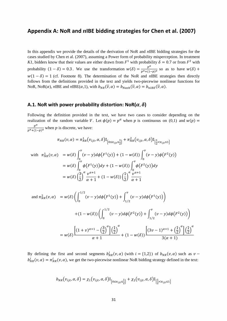
Appendix A: NoR and nIBE bidding strategies for Chen et al. (2007)
In this appendix we provide the details of the derivation of NoR and nIBE bidding strategies for the
cases studied by Chen et al. (2007), assuming a Power form of probability misperception. In treatment
K1, bidders know that their values are either drawn from 𝐹1 with probability 𝛿 = 0.7 or from 𝐹2 with
probability (1 − 𝛿) = 0.3 . We use the transformation 𝑤(𝛿) =𝑝𝛼
𝑝𝛼+(1−𝑝)𝛼 so as to have 𝑤(𝛿) +
𝑤(1 − 𝛿) = 1 (cf. Footnote 8). The determination of the NoR and nIBE strategies then directly
follows from the definitions provided in the text and yields two-piecewise nonlinear functions for
NoR, NoR(𝛼), nIBE and nIBE(𝛼,1), with 𝑏𝑁𝑅(𝑣, 𝛼) = 𝑏𝑁𝑎𝑠ℎ(𝑣, 𝛼) = 𝑏𝑛𝐼𝐵𝐸(𝑣, 𝛼).
A.1. NoR with power probability distortion: NoR(𝜶, 𝜹)
Following the definition provided in the text, we have two cases to consider depending on the
realization of the random variable 𝑉 . Let 𝜙(𝑝) = 𝑝𝛼 when 𝑝 is continuous on (0,1) and 𝑤(𝑝) =𝑝𝛼
𝑝𝛼+(1−𝑝)𝛼 when 𝑝 is discrete, we have:
𝜋𝑁𝑅(𝑣, 𝛼) = 𝜋𝑁𝑅1 (𝑣𝑖𝑗𝑡 , 𝛼, 𝛿)𝕀{0≤𝑣𝑖𝑗𝑡≤
12}+ 𝜋𝑁𝑅
2 (𝑣𝑖𝑗𝑡 , 𝛼, 𝛿)𝕀{12<𝑣𝑖𝑗𝑡≤1}
with 𝜋𝑁𝑅1 (𝑣, 𝛼) = 𝑤(𝛿)∫ (𝑣 − 𝑦)𝑑𝜙(𝐹1(𝑦)) + (1 − 𝑤(𝛿))∫ (𝑣 − 𝑦)𝜙(𝐹2(𝑦))
𝑣
0
𝑣
0
= 𝑤(𝛿)∫ 𝜙(𝐹1(𝑦))𝑑𝑦 + (1 − 𝑤(𝛿))∫ 𝜙(𝐹2(𝑦))𝑑𝑦
𝑣
0
𝑣
0
= 𝑤(𝛿) (
3
2)𝛼 𝑣𝛼+1
𝛼 + 1+ (1 − 𝑤(𝛿)) (
1
2)𝛼 𝑣𝛼+1
𝛼 + 1
and 𝜋𝑁𝑅2 (𝑣, 𝛼)
= 𝑤(𝛿) (∫ (𝑣 − 𝑦)𝑑𝜙(𝐹1(𝑦)) + ∫ (𝑣 − 𝑦)𝑑𝜙(𝐹1(𝑦))𝑣
1 2⁄
1 2⁄
0
)
+(1 − 𝑤(𝛿)) (∫ (𝑣 − 𝑦)𝑑𝜙(𝐹2(𝑦)) +∫ (𝑣 − 𝑦)𝑑𝜙(𝐹2(𝑦))
𝑣
1 2⁄
1 2⁄
0
)
= 𝑤(𝛿)[(1 + 𝑣)𝛼+1 − (
32)𝛼
] (12)𝛼
𝛼 + 1+ (1 − 𝑤(𝛿))
[(3𝑣 − 1)𝛼+1 + (12)𝛼
] (12)𝛼
3(𝛼 + 1)
By defining the first and second segments 𝑏𝑁𝑅𝑖 (𝑣, 𝛼) (with 𝑖 = {1,2} ) of 𝑏𝑁𝑅(𝑣, 𝛼) such as 𝑣 −
𝑏𝑁𝑅𝑖 (𝑣, 𝛼) = 𝜋𝑁𝑅
𝑖 (𝑣, 𝛼), we get the two-piecewise nonlinear NoR bidding strategy defined in the text:
𝑏𝑁𝑅(𝑣𝑖𝑗𝑡 , 𝛼, 𝛿) = 𝜒1(𝑣𝑖𝑗𝑡 , 𝛼, 𝛿)𝕀{0≤𝑣𝑖𝑗𝑡≤12}+ 𝜒2(𝑣𝑖𝑗𝑡 , 𝛼, 𝛿)𝕀{1
2<𝑣𝑖𝑗𝑡≤1}
32
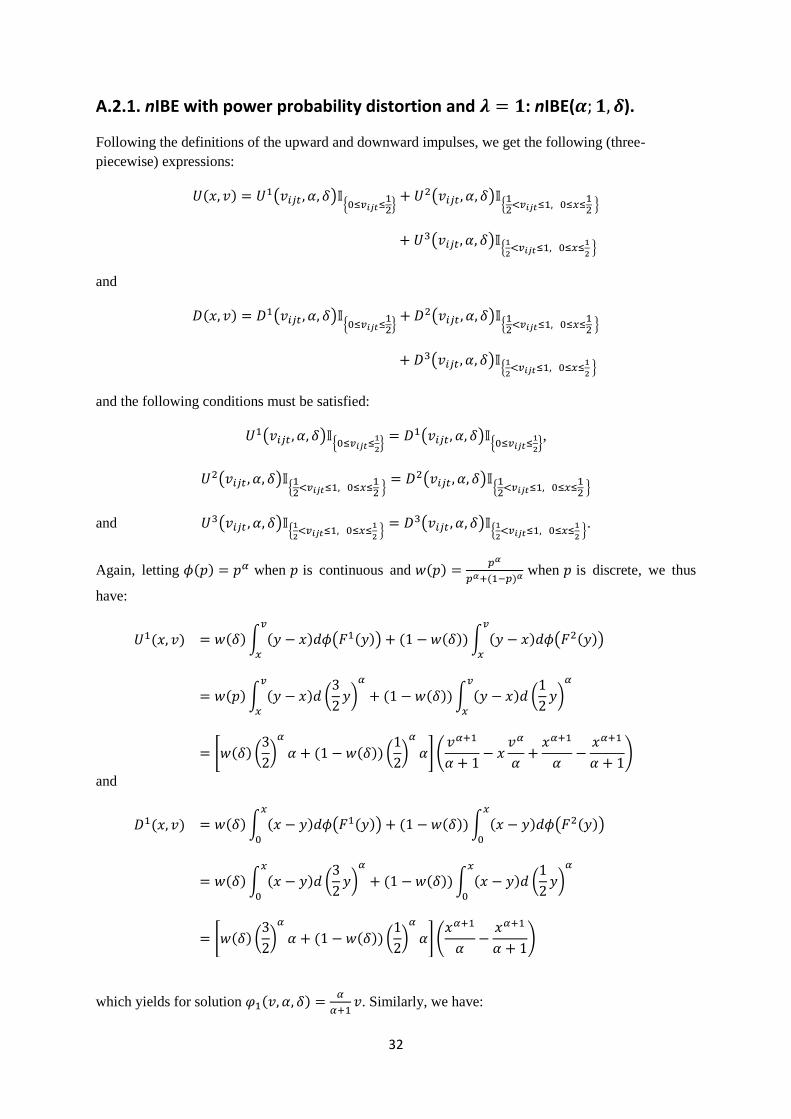
A.2.1. nIBE with power probability distortion and 𝝀 = 𝟏: nIBE(𝜶; 𝟏, 𝜹).
Following the definitions of the upward and downward impulses, we get the following (three-
piecewise) expressions:
𝑈(𝑥, 𝑣) = 𝑈1(𝑣𝑖𝑗𝑡 , 𝛼, 𝛿)𝕀{0≤𝑣𝑖𝑗𝑡≤12}+ 𝑈2(𝑣𝑖𝑗𝑡, 𝛼, 𝛿)𝕀{1
2<𝑣𝑖𝑗𝑡≤1, 0≤𝑥≤
12 }
+ 𝑈3(𝑣𝑖𝑗𝑡, 𝛼, 𝛿)𝕀{12<𝑣𝑖𝑗𝑡≤1, 0≤𝑥≤
1
2 }
and
𝐷(𝑥, 𝑣) = 𝐷1(𝑣𝑖𝑗𝑡 , 𝛼, 𝛿)𝕀{0≤𝑣𝑖𝑗𝑡≤12}+ 𝐷2(𝑣𝑖𝑗𝑡 , 𝛼, 𝛿)𝕀{1
2<𝑣𝑖𝑗𝑡≤1, 0≤𝑥≤
12 }
+ 𝐷3(𝑣𝑖𝑗𝑡 , 𝛼, 𝛿)𝕀{12<𝑣𝑖𝑗𝑡≤1, 0≤𝑥≤
1
2 }
and the following conditions must be satisfied:
𝑈1(𝑣𝑖𝑗𝑡 , 𝛼, 𝛿)𝕀{0≤𝑣𝑖𝑗𝑡≤1
2}= 𝐷1(𝑣𝑖𝑗𝑡 , 𝛼, 𝛿)𝕀{0≤𝑣𝑖𝑗𝑡≤
1
2},
𝑈2(𝑣𝑖𝑗𝑡 , 𝛼, 𝛿)𝕀{12<𝑣𝑖𝑗𝑡≤1, 0≤𝑥≤
12 }= 𝐷2(𝑣𝑖𝑗𝑡 , 𝛼, 𝛿)𝕀{1
2<𝑣𝑖𝑗𝑡≤1, 0≤𝑥≤
12 }
and 𝑈3(𝑣𝑖𝑗𝑡 , 𝛼, 𝛿)𝕀{12<𝑣𝑖𝑗𝑡≤1, 0≤𝑥≤
1
2 }= 𝐷3(𝑣𝑖𝑗𝑡 , 𝛼, 𝛿)𝕀{1
2<𝑣𝑖𝑗𝑡≤1, 0≤𝑥≤
1
2 }
.
Again, letting 𝜙(𝑝) = 𝑝𝛼 when 𝑝 is continuous and 𝑤(𝑝) =𝑝𝛼
𝑝𝛼+(1−𝑝)𝛼 when 𝑝 is discrete, we thus
have:
𝑈1(𝑥, 𝑣) = 𝑤(𝛿)∫ (𝑦 − 𝑥)𝑑𝜙(𝐹1(𝑦)) + (1 − 𝑤(𝛿))∫ (𝑦 − 𝑥)𝑑𝜙(𝐹2(𝑦))
𝑣
𝑥
𝑣
𝑥
= 𝑤(𝑝)∫ (𝑦 − 𝑥)𝑑 (3
2𝑦)𝛼
+ (1 − 𝑤(𝛿))∫ (𝑦 − 𝑥)𝑑 (1
2𝑦)𝛼𝑣
𝑥
𝑣
𝑥
= [𝑤(𝛿) (3
2)𝛼
𝛼 + (1 − 𝑤(𝛿)) (1
2)𝛼
𝛼](𝑣𝛼+1
𝛼 + 1− 𝑥
𝑣𝛼
𝛼+𝑥𝛼+1
𝛼−𝑥𝛼+1
𝛼 + 1)
and
𝐷1(𝑥, 𝑣) = 𝑤(𝛿)∫ (𝑥 − 𝑦)𝑑𝜙(𝐹1(𝑦)) + (1 − 𝑤(𝛿))∫ (𝑥 − 𝑦)𝑑𝜙(𝐹2(𝑦))
𝑥
0
𝑥
0
= 𝑤(𝛿)∫ (𝑥 − 𝑦)𝑑 (3
2𝑦)𝛼
+ (1 − 𝑤(𝛿))∫ (𝑥 − 𝑦)𝑑 (1
2𝑦)𝛼𝑥
0
𝑥
0
= [𝑤(𝛿) (3
2)𝛼
𝛼 + (1 − 𝑤(𝛿)) (1
2)𝛼
𝛼](𝑥𝛼+1
𝛼−𝑥𝛼+1
𝛼 + 1)
which yields for solution 𝜑1(𝑣, 𝛼, 𝛿) =𝛼
𝛼+1𝑣. Similarly, we have:
33
𝑈2(𝑥, 𝑣) = 𝑤(𝛿) (∫ (𝑦 − 𝑥)𝑑𝜙(𝐹1(𝑦)) + ∫ (𝑦 − 𝑥)𝑑𝜙(𝐹1(𝑦))𝑣
1 2⁄
1 2⁄
𝑥)
+ (1 − 𝑤(𝛿)) (∫ (𝑦 − 𝑥)𝑑𝜙(𝐹2(𝑦)) + ∫ (𝑦 − 𝑥)𝑑𝜙(𝐹2(𝑦))𝑣
1 2⁄
1 2⁄
𝑥)
= 𝑤(𝛿) ((3
2)𝛼𝛼)(
(1
2)𝛼+1
−𝑥𝛼+1
𝛼+1+𝑥𝛼+1−𝑥(
1
2)𝛼
𝛼)
+ 𝑤(𝛿) ((1
2)𝛼𝛼)(
(𝑣−𝑥)(𝑣+1)𝛼
𝛼+(1
2)𝛼+1
−(𝑣+1)𝛼+1
𝛼(𝛼+1)+(𝑥−
1
2)(3
2)𝛼
𝛼)
+(1 − 𝑤(𝛿)) ((1
2)𝛼𝛼)
(
(1
2)𝛼+1
−𝑥𝛼+1
𝛼+1+𝑥𝛼+1−𝑥(
1
2)𝛼
𝛼+(𝑣−𝑥)(3𝑣−1)𝛼
𝛼
+(1
2)𝛼+1
−(3𝑣−1)𝛼+1
3𝛼(𝛼+1)+(𝑥−
1
2)(1
2)𝛼
𝛼 )
and
𝐷2(𝑥, 𝑣) = 𝑤(𝛿) ∫ (𝑥 − 𝑦)𝑑(𝐹1(𝑦))𝛼+ (1 −𝑤(𝛿)) ∫ (𝑥 − 𝑦)𝑑(𝐹2(𝑦))
𝛼𝑥
0
𝑥
0
= 𝑤(𝛿) ((3
2)𝛼𝛼) (
𝑥𝛼+1
𝛼−𝑥𝛼+1
𝛼+1) + (1 − 𝑤(𝛿)) ((
1
2)𝛼𝛼) (
𝑥𝛼+1
𝛼−𝑥𝛼+1
𝛼+1)
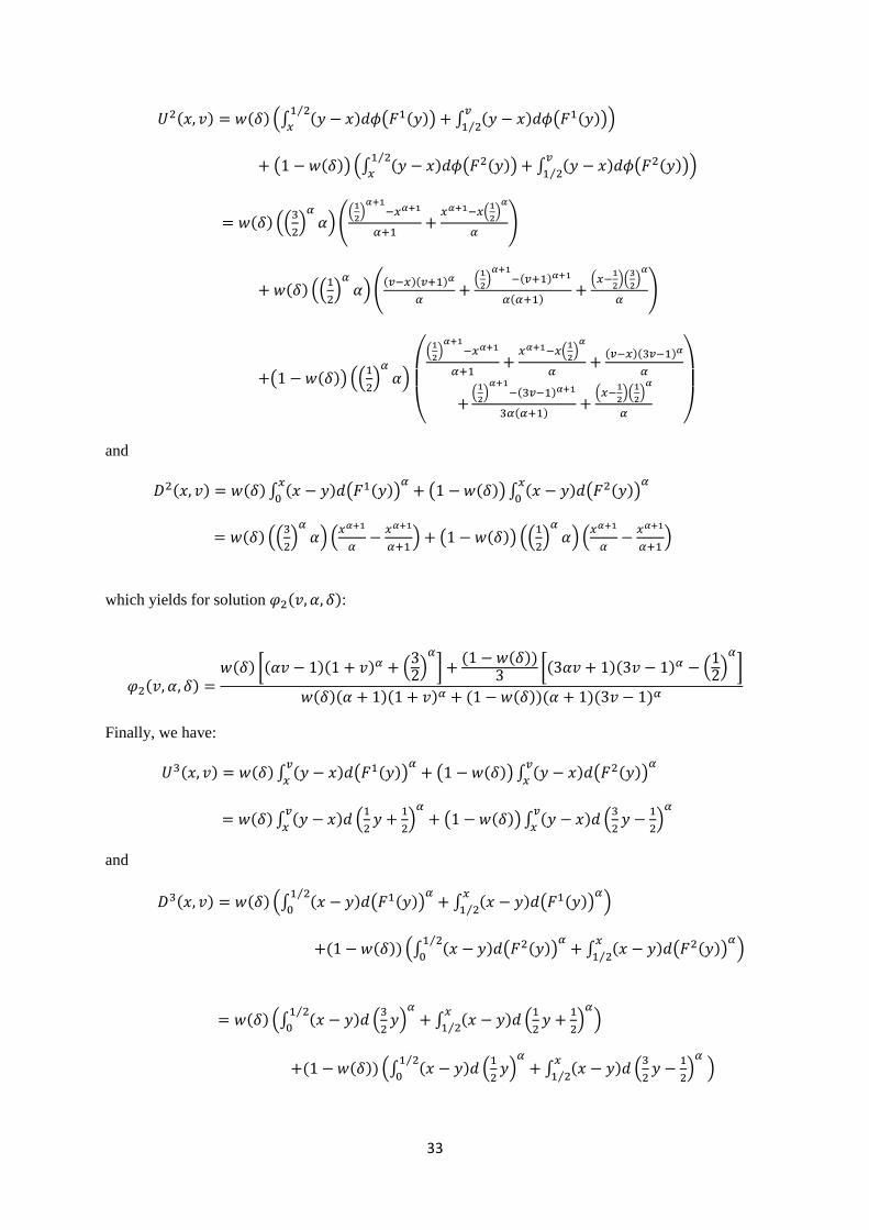
which yields for solution 𝜑2(𝑣, 𝛼, 𝛿):
𝜑2(𝑣, 𝛼, 𝛿) =𝑤(𝛿) [(𝛼𝑣 − 1)(1 + 𝑣)𝛼 + (
32)𝛼
] +(1 − 𝑤(𝛿))
3 [(3𝛼𝑣 + 1)(3𝑣 − 1)𝛼 − (12)𝛼
]
𝑤(𝛿)(𝛼 + 1)(1 + 𝑣)𝛼 + (1 − 𝑤(𝛿))(𝛼 + 1)(3𝑣 − 1)𝛼
Finally, we have:
𝑈3(𝑥, 𝑣) = 𝑤(𝛿) ∫ (𝑦 − 𝑥)𝑑(𝐹1(𝑦))𝛼+ (1 − 𝑤(𝛿)) ∫ (𝑦 − 𝑥)𝑑(𝐹2(𝑦))
𝛼𝑣
𝑥
𝑣
𝑥
= 𝑤(𝛿) ∫ (𝑦 − 𝑥)𝑑 (1
2𝑦 +
1
2)𝛼+ (1 − 𝑤(𝛿)) ∫ (𝑦 − 𝑥)𝑑 (
3
2𝑦 −
1
2)𝛼𝑣
𝑥
𝑣
𝑥
and
𝐷3(𝑥, 𝑣) = 𝑤(𝛿) (∫ (𝑥 − 𝑦)𝑑(𝐹1(𝑦))𝛼+ ∫ (𝑥 − 𝑦)𝑑(𝐹1(𝑦))
𝛼𝑥
1 2⁄
1 2⁄
0)
+(1 − 𝑤(𝛿)) (∫ (𝑥 − 𝑦)𝑑(𝐹2(𝑦))𝛼+ ∫ (𝑥 − 𝑦)𝑑(𝐹2(𝑦))
𝛼𝑥
1 2⁄
1 2⁄
0)
= 𝑤(𝛿) (∫ (𝑥 − 𝑦)𝑑 (3
2𝑦)𝛼+ ∫ (𝑥 − 𝑦)𝑑 (
1
2𝑦 +
1
2)𝛼𝑥
1 2⁄
1 2⁄
0)
+(1 − 𝑤(𝛿)) (∫ (𝑥 − 𝑦)𝑑 (1
2𝑦)𝛼+ ∫ (𝑥 − 𝑦)𝑑 (
3
2𝑦 −
1
2)𝛼
𝑥
1 2⁄
1 2⁄
0)
34
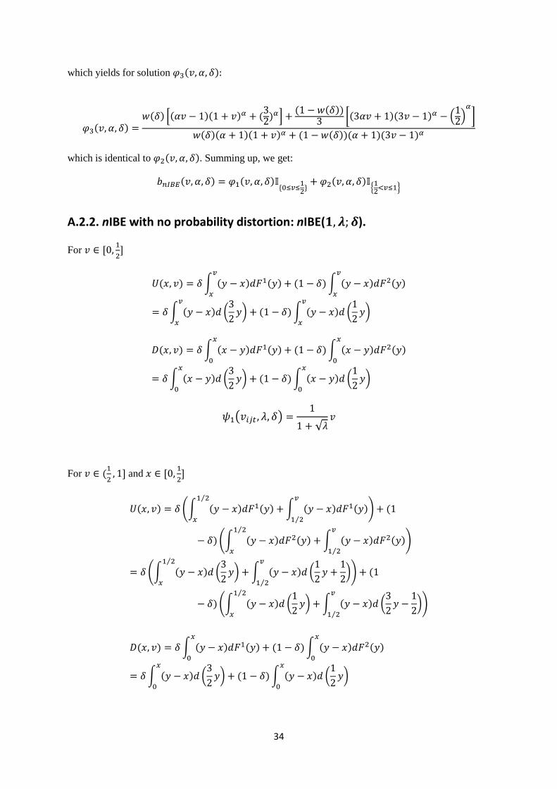
which yields for solution 𝜑3(𝑣, 𝛼, 𝛿):
𝜑3(𝑣, 𝛼, 𝛿) =𝑤(𝛿) [(𝛼𝑣 − 1)(1 + 𝑣)𝛼 + (
32)𝛼] +
(1 − 𝑤(𝛿))3 [(3𝛼𝑣 + 1)(3𝑣 − 1)𝛼 − (
12)𝛼
]
𝑤(𝛿)(𝛼 + 1)(1 + 𝑣)𝛼 + (1 − 𝑤(𝛿))(𝛼 + 1)(3𝑣 − 1)𝛼
which is identical to 𝜑2(𝑣, 𝛼, 𝛿). Summing up, we get:
𝑏𝑛𝐼𝐵𝐸(𝑣, 𝛼, 𝛿) = 𝜑1(𝑣, 𝛼, 𝛿)𝕀{0≤𝑣≤12}+ 𝜑2(𝑣, 𝛼, 𝛿)𝕀{1
2<𝑣≤1}
A.2.2. nIBE with no probability distortion: nIBE(𝟏, 𝝀; 𝜹).
For 𝑣 ∈ [0,1
2]
𝑈(𝑥, 𝑣) = 𝛿∫ (𝑦 − 𝑥)𝑑𝐹1(𝑦) + (1 − 𝛿)∫ (𝑦 − 𝑥)𝑑𝐹2(𝑦)𝑣
𝑥
𝑣
𝑥
= 𝛿∫ (𝑦 − 𝑥)𝑑 (3
2𝑦) + (1 − 𝛿)∫ (𝑦 − 𝑥)𝑑 (
1
2𝑦)
𝑣
𝑥
𝑣
𝑥
𝐷(𝑥, 𝑣) = 𝛿∫ (𝑥 − 𝑦)𝑑𝐹1(𝑦) + (1 − 𝛿)∫ (𝑥 − 𝑦)𝑑𝐹2(𝑦)𝑥
0
𝑥
0
= 𝛿∫ (𝑥 − 𝑦)𝑑 (3
2𝑦) + (1 − 𝛿)∫ (𝑥 − 𝑦)𝑑 (
1
2𝑦)
𝑥
0
𝑥
0
𝜓1(𝑣𝑖𝑗𝑡 , 𝜆, 𝛿) =1
1 + √𝜆𝑣
For 𝑣 ∈ (1
2, 1] and 𝑥 ∈ [0,
1
2]
𝑈(𝑥, 𝑣) = 𝛿 (∫ (𝑦 − 𝑥)𝑑𝐹1(𝑦) +∫ (𝑦 − 𝑥)𝑑𝐹1(𝑦)𝑣
1 2⁄
1 2⁄
𝑥
) + (1
− 𝛿)(∫ (𝑦 − 𝑥)𝑑𝐹2(𝑦) + ∫ (𝑦 − 𝑥)𝑑𝐹2(𝑦)𝑣
1 2⁄
1 2⁄
𝑥
)
= 𝛿 (∫ (𝑦 − 𝑥)𝑑 (3
2𝑦) + ∫ (𝑦 − 𝑥)𝑑 (
1
2𝑦 +
1
2)
𝑣
1 2⁄
1 2⁄
𝑥
) + (1
− 𝛿)(∫ (𝑦 − 𝑥)𝑑 (1
2𝑦) +∫ (𝑦 − 𝑥)𝑑 (
3
2𝑦 −
1
2)
𝑣
1 2⁄
1 2⁄
𝑥
)
𝐷(𝑥, 𝑣) = 𝛿∫ (𝑦 − 𝑥)𝑑𝐹1(𝑦) + (1 − 𝛿)∫ (𝑦 − 𝑥)𝑑𝐹2(𝑦)𝑥
0
𝑥
0
= 𝛿∫ (𝑦 − 𝑥)𝑑 (3
2𝑦) + (1 − 𝛿)∫ (𝑦 − 𝑥)𝑑 (
1
2𝑦)
𝑥
0
𝑥
0
35
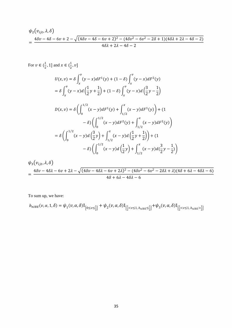
𝜓2(𝑣𝑖𝑗𝑡, 𝜆, 𝛿)
= 4𝛿𝑣 − 4𝛿 − 6𝑣 + 2 −√(4𝛿𝑣 − 4𝛿 − 6𝑣 + 2)2 − (4𝛿𝑣2 − 6𝑣2 − 2𝛿 + 1)(4𝛿𝜆 + 2𝜆 − 4𝛿 − 2)
4𝛿𝜆 + 2𝜆 − 4𝛿 − 2
For 𝑣 ∈ (1
2, 1] and 𝑥 ∈ (
1
2, 𝑣]
𝑈(𝑥, 𝑣) = 𝛿∫ (𝑦 − 𝑥)𝑑𝐹1(𝑦) + (1 − 𝛿)∫ (𝑦 − 𝑥)𝑑𝐹2(𝑦)𝑣
𝑥
𝑣
𝑥
= 𝛿∫ (𝑦 − 𝑥)𝑑 (1
2𝑦 +
1
2) + (1 − 𝛿)∫ (𝑦 − 𝑥)𝑑 (
3
2𝑦 −
1
2)
𝑣
𝑥
𝑣
𝑥
𝐷(𝑥, 𝑣) = 𝛿 (∫ (𝑥 − 𝑦)𝑑𝐹1(𝑦) +∫ (𝑥 − 𝑦)𝑑𝐹1(𝑦)𝑥
1 2⁄
1 2⁄
0
) + (1
− 𝛿)(∫ (𝑥 − 𝑦)𝑑𝐹2(𝑦) +∫ (𝑥 − 𝑦)𝑑𝐹2(𝑦)𝑥
1 2⁄
1 2⁄
0
)
= 𝛿 (∫ (𝑥 − 𝑦)𝑑 (3
2𝑦) +∫ (𝑥 − 𝑦)𝑑 (
1
2𝑦 +
1
2)
𝑥
1 2⁄
1 2⁄
0
) + (1
− 𝛿)(∫ (𝑥 − 𝑦)𝑑 (1
2𝑦) + ∫ (𝑥 − 𝑦)𝑑(
3
2𝑦 −
1
2)
𝑥
1 2⁄
1 2⁄
0
)
𝜓3(𝑣𝑖𝑗𝑡 , 𝜆, 𝛿)
= 4𝛿𝑣 − 4𝛿𝜆 − 6𝑣 + 2𝜆 −√(4𝛿𝑣 − 4𝛿𝜆 − 6𝑣 + 2𝜆)2 − (4𝛿𝑣2 − 6𝑣2 − 2𝛿𝜆 + 𝜆)(4𝛿 + 6𝜆 − 4𝛿𝜆 − 6)
4𝛿 + 6𝜆 − 4𝛿𝜆 − 6
To sum up, we have:
𝑏𝑛𝐼𝐵𝐸(𝑣, 𝛼, 1,𝛿) = 𝜓1(𝑣, 𝛼, 𝛿)𝕀{0≤𝑣≤12}+𝜓2(𝑣, 𝛼, 𝛿)𝕀{1
2<𝑣≤1, 𝑏𝑛𝐼𝐵𝐸≤
1
2}+𝜓3(𝑣, 𝛼, 𝛿)𝕀{1
2<𝑣≤1, 𝑏𝑛𝐼𝐵𝐸>
1
2}

36
Appendix B: NoR and nIBE estimation outcomes for winning bids.
TABLE 2B: NOR AND nIBE ESTIMATION OUTCOMES FOR WINNING BIDS: 𝑛 = 2.
Parameter-free Power Prelec
Data Treat. (# Obs.)
NoR nIBE* NoR
�̂�
nIBE*
(�̂�; 1)
nIBE
(1; �̂�)
NoR
𝛾 �̂�
nIBE(𝛾, 𝛽; 1)*
𝛾 �̂�
KMZ
(2C)
MF
(162)
-3.69
-3.10
1.675
(.103)
-4.09
2.922
(.232)
-4.06
.117
(.019)
-4.06
.479
(.168)
1.456
(.089)
.479
(.168)
1.456
(.089)
-4.11 -4.11
LF
(132)
-3.48
-3.08
1.535
(.117)
-3.70
2.435
(.225)
-3.71
.169
(.031)
-3.71
.363×
(.205)
1.277▫
(.209)
.363×
(.205)
1.277▫
(.209)
-3.73 -3.73
WF
(159)
-3.59
-3.07
1.724
(.118)
-3.95
3.101
(.264)
-4.04
.104
(.018)
-4.04
.191
(.082)
.872×▫
(1.503)
.191
(.082)
.872×▫
(1.503)
-4.04 -4.04
KMZ MF
(216)
-3.89
-3.38
1.381
(.070)
-4.07
2.206
(.139)
-4.01
.206
(.026)
-4.01
.523
(.146)
1.254
(.062)
.523
(.146)
1.254
(.062)
-4.09 -4.09
LF
(218)
-3.56
-3.11
1.483
(.085)
-3.76
2.370
(.171)
-3.71
.178
(.026)
-3.71
.573
(.177)
.1.337
(.081)
.573
(.177)
1.337
(0.081)
-3.77 -3.77
WF
(218)
-3.87
-3.37
1.367
(.070)
-4.02
2.228
(.141)
-4.01
.202
(.025)
-4.01
.421
(.133)
1.220
(.083)
.421
(.133)
1.220
(.083)
-4.06 -4.06
OS MF
(3375)
-4.76
-4.26
.937
(.008)
-4.77
1.438
(.015)
-4.59
.484
(.010)
-4.59
.699
(.033)
.927
(.007)
1.876
(.043)
1.278
(.016)
-4.79 -4.79
LF
(3373)
-4.37
-4.57
.704
(.006)
-4.82
1.021
(.010)
-4.57
.959
(.020)
-4.57
.843
(.038)
.711
(.006)
2.055
(.048)
.803
(.012)
-4.82 -4.82
Nash CRRA 𝜌
CKO K1
(600)
-3.78
-3.27
2.491
(.108)
-4.36
4.353
(.179)
-4.44
.122
(.008)
-4.42
.335
(.012)
-4.43
�̂� given → 𝛼 = 1 𝛼 = 1 𝛼 = �̂�𝐾1 𝛼 = �̂�𝐾1,
𝜆 = 1
𝛼 = 1,
𝜆 = �̂�𝐾1 𝜌 = �̂�𝐾1
U1
(600)
.223
(.025)
-4.46
.000
(.029)
-4.18
.811
(.076)
-4.38
.951
(n.a.)
-4.52
.000
(.062)
-1.71
.823
(.026)
-4.54
Note: Standard errors in parenthesis; AIC statistics in italics (bold figures indicate best AIC statistic for a given category:
‘Parameter-free’, ‘Power’ or ‘Prelec’); *: Equivalent to SBNE bidding with(out) misperception; �̂�𝐾1, �̃�𝐾1, �̂�𝐾1and �̂�𝐾1 stand for
estimates of CKO’s K1 treatment; ×(▫): Not significantly different from 0 (1) at 𝛼 = 5%.

37
TABLE 3B: NOR AND nIBE ESTIMATION OUTCOMES FOR WINNING BIDS: 𝑛 = 4.
Parameter-free Power Prelec
Data Treat.
(# Obs.) NoR nIBE*
NoR
�̂�
nIBE*
(�̂�; 1)
nIBE
(1; �̂�)
NoR
𝛾 �̂�
nIBE(𝛾, 𝛽; 1)*
𝛾 �̂�
KMZ MF
(72)
-4.35
-4.15
0.833
(.074)
-4.37
1.548
(.191)
-4.33
.364
(.101)
-4.33
.496
(.246)
1.131▫
(.210)
1.633
(.044)
0.959
(.005)
-4.39 -4.38
LF
(72)
-4.32
-4.03
0.901
(.084)
-4.31
1.662
(.221)
-4.25
.311
(.093)
-4.25
.552×
(.294)
1.144▫
(.225)
1.740
(.039)
1.015
(.168)
-4.31 -4.29
KMZ
(4R)
MF
(122)
-3.89
-3.51
1.871
(.281)
-4.06
3.395
(0.603)
-4.20
.066
(.025)
-4.20
6.115
(.811)
2.143×▫
(2.078)
0.874
(.224)
3.701
(0.925)
-4.34 -4.18
LF
(120)
-4.58
-4.02
1.356
(.108)
-4.69
2.445
(0.238)
-4.86
.133
(.028)
-4.86
n.a. n.a.
1.135
(0.172)
2.246
(0.311)
--- -4.85
FO MF
(71)
-4.43
-4.19
1.015▫
(.097)
-4.40
1.750
(.202)
-4.55
.277
(.071)
-4.55
.117
(.013)
.728×▫
(4.287)
1.150▫
(.228)
1.562▫
(.307)
-4.54 -4.53?
LF
(90)
-4.80
-4.01
1.950
(.157)
-5.57
3.415
(.242)
-6.28
.065
(.010)
-6.28
1.458×▫ (14.59)
.000×
(.007)
.851▫
(.091)
3.753
(.369)
-6.25 -6.28
WF
(80)
-4.61
-4.25
1.135▫
(.101)
-4.61
1.977
(.203)
-4.85
.211
(.048)
.680×▫
(2.336)
.007×
(.086)
1.026▫
(.178)
1.937
(.329)
-4.85 -4.83 -4.83
IW MF
(250)
-5.08
-4.07
1.401
(.055)
-5.39
2.771
(.157)
-5.39
.101
(.012)
-5.39
.411
(.089)
1.650
(.086)
1.550
(.006)
2.178
(.153)
-5.48 -5.48
LF
(247)
-5.43
-4.64
1.016
(.031)
-5.43
1.808
(.072)
-5.48
.258
(.023)
-5.48
.363
(.073)
1.382
(.069)
1.461
(.109)
1.348
(.091)
-5.58 -5.58
Note: Standard errors in parenthesis; AIC statistics in italics (bold figures indicate best AIC statistic for a given category:
‘Parameter-free’, ‘Power’ or ‘Prelec’); *: Equivalent to SBNE bidding with(out) misperception; ×(▫): Not significantly
different from 0 (1) at 𝛼 = 5%.
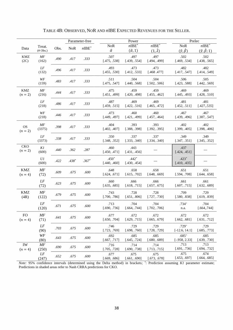
38
TABLE 4B: OBSERVED, NOR AND nIBE EXPECTED REVENUES FOR THE SELLER.
Parameter-free Power Prelec
Data Treat. (# Obs.)
Obs. NoR nIBE* NoR
�̂�
nIBE*
(�̂�, 1) nIBE*
(1, �̂�)
NoR
(𝛾, �̂�)
nIBE*
(𝛾, �̂�; 1)
KMZ
(2C)
MF
(162) .490 .417 .333
.507
[.475, .538]
.497
[.439, .554]
.497
[.494, .499]
.502
[.469, .534]
.502
[.438, .565]
LF
(132) .496 .417 .333
.493
[.455, .530]
.473
[.412, .533]
.473
[.468 .477]
.482
[.417, .547]
.482
[.414, .549]
WF
(159) .483 .417 .333
.511
[.475, .547]
.504
[.440, .568]
.504
[.502, .506]
.506
[.423, .588]
.505
[.442, .569]
KMZ
(𝑛 = 2)
MF
(216) .444 .417 .333
.475
[.451, .499]
.459
[.420, .498]
.459
[.455, .462]
.469
[.445, .493]
.469
[.428, .510]
LF
(218) .486 .417 .333
.487
[.459, .515]
.469
[.422, .516]
.469
[.465, .472]
.481
[.452, .511]
.481
[.427,.535]
WF
(218) .446 .417 .333
.473
[.449, .497]
.460
[.421, .499]
.460
[.457, .464]
.467
[.439, .496]
.467
[.387, .547]
OS
(𝑛 = 2)
MF
(3375) .398 .417 .333
.404
[.402, .407]
.393
[.388, .398]
.393
[.392, .395]
.402
[.399, .405]
.402
[.398, .406]
LF
(3373) .338 .417 .333
.350
[.348, .352]
.337
[.333, .340]
.337
[.334, .340]
.349
[.347, .351]
.349
[.345, .352]
CKO
(𝑛 = 2) K1
(600) .440 .362 .287
.460
[.450, .471]
.443
[.431, .456] ---
.437
[.424, .451] ---
U1
(600) .422 .438* .367*
.450*
[.440, .460]
.442*
[.430, .454] ---
.423*
[.410, .435] ---
KMZ
(𝑛 = 4)
MF
(72) .609 .675 .600
.648
[.624, .671]
.658
[.615, .702]
.658
[.648, .669]
.651
[.594, .708]
.651
[.644, .658]
LF
(72) .623 .675 .600
.660
[.635, .685]
.666
[.618, .715]
.666
[.657, .675]
.661
[.607, .715]
.661
[.632, .689]
KMZ
(4R)
MF
(122) .679 .675 .600
.743
[.700, .786]
.728
[.651, .806]
.728
[.727, .730]
.709
[.580, .838]
.729
[.619, .839]
LF
(120) .671 .675 .600
.713
[.690, .736]
.704
[.664, .744]
.704
[.702, .706]
.734×
n.a.
.704
[.664,.744]
FO
(𝑛 = 4)
MF
(71) .641 .675 .600
.677
[.650, .704]
.672
[.629, .715]
.672
[.665, .679]
.672
[.662, .681]
.672
[.631, .712]
LF
(90) .703 .675 .600
.746
[.723, .769]
.729
[.698, .760]
.729
[.728, .729]
.729×
[-12.6, 14.1]
.729
[.685, .773]
WF
(80) .643 .675 .600
.692
[.667, .717]
.685
[.645, .724]
.685
[.680, .689]
.685×
[-.958, 2.33]
.685
[.639, .730]
IW
(𝑛 = 4)
MF
(250) .690 .675 .600
.716
[.705, .728]
.714
[.690, .738]
.714
[.713, .715]
.713
[.691, .736]
.713
[.694, .732]
LF
(247) .652 .675 .600
.677
[.669, .686]
.675
[.661, .690]
.675
[.673, .678]
.675
[.653, .697]
.674
[.664, .685]
Note: 95% confidence intervals (determined using the Delta method) in brackets; *: Prediction assuming K1 parameter estimate;
Predictions in shaded areas refer to Nash CRRA predictions for CKO.

39
Note: To avoid cluttering the plots, those pertaining to OS data display only 50% of all observations.
FIGURE 3B: ESTIMATED NOR AND nIBE WINNING BID FUNCTIONS (OS, CKO AND IW).