school of engineering - core.ac.uk · abstract the scope of the current thesis is the comprehensive...

University of Liverpool

School of Engineering

Lattice Boltzmann modelling of immiscible

two-phase flows

The Thesis is submitted in accordance with the requirements of

Liverpool for the degree of Doctor in Philosophy

Author: Duo Zhang

August, 2015

This copy of the thesis has been supplied on condition that anyone who consults it is understood to

recognise that its copyright rests with its author and that no quotation from the thesis and no infor-

mation derived from it may be published without proper acknowledgement.

1

Abstract

The scope of the current thesis is the comprehensive understanding of the droplet im-

pact and spreading dynamics on flat and curved surfaces with the aim of simulating

high density ratio immiscible two phase flows in porous media. Understanding the

dynamic behavior of droplet impingement onto solid substrate can provide significant

information about the fluid flow dynamics in porous structures. The numerically study

process will be realized by using a high density ratio multi-phase lattice Boltzmann

model which is able to simulate multi-phase flows in complex systems. The interfacial

information between the two immiscible phases can be captured without tracking or

constructing the vapour-liquid interface. A three dimensional lattice Boltzmann mod-

el is applied on the study of the impaction of a liquid droplet on a dry flat surface

for a liquid-gas system with large density ratio. The impaction of liquid droplet on

a curved surface for the liquid-gas system with large density ratio and low kinematic

viscosity of the fluid is computed by a two-dimensional multi-relaxation-time (MRT)

interaction-potential-based lattice Boltzmann model based on the improved forcing

scheme. The dynamics behaviors of the spreading of the liquid droplet on the flat sur-

face as well as the impaction of the liquid droplet on a curved surface are computed,

followed by their dependence on the Reynolds number, Weber number, Galilei number

and surface characteristics. Moreover, an improved force scheme is proposed for the

three-dimensional MRT pseudopotential lattice Boltzmann model which is based on

the improved force scheme for the Single relaxation time (SRT) pseudopotential lat-

tice Boltzmann model and the Chapman-Enskog analysis. The validation for the new

developed three-dimensional multi-relaxation time lattice Boltzmann model is carried

out through Laplace’s law ad by achieving thermodynamic consistency. In addition,

the relationship between the fluid-solid interaction potential parameter Gw and the

contact angle is investigated for the new developed three-dimensional MRT lattice

Boltzmann model. The immiscible two-phase flow in porous media is carried out by

a two dimensional MRT lattice Boltzmann model. The porous media structures with

different geometrical properties are artificially generated by a Boolean model based on

a random distribution of overlapping ellipses/circles. Furthermore, the impact of geo-

metrical properties on the immiscible two-phase flows in porous media is investigated

in the pore scale. The lattice Boltzmann model results provide significant information

i

on the interface between the two immiscible phases in complex systems, it is easy to

apply for complex domains with bounce back boundary wall condition and be able to

handle multi-phase and multi-component flows without tracing the interfaces between

different phases.

Keywords: Multiphase flow, Lattice Boltzmann, High-density-ratio, Droplet impact, Porous media

ii

Contents

Abstract i

Contents v

List of Figures x

List of Tables x

Acknowledgement xi

Nomenclature xii

1 Introduction 1

1.1 Multiphase flows . . . . . . . . . . . . . . . . . . . . . . . . . . . . . . . 1

1.1.1 Droplet impingement on surfaces . . . . . . . . . . . . . . . . . . 1

1.1.2 Two-phase immiscible flows in porous media . . . . . . . . . . . 3

1.2 Numerical techniques for multiphase flows . . . . . . . . . . . . . . . . . 4

1.3 Lattice Boltzmann model . . . . . . . . . . . . . . . . . . . . . . . . . . 4

1.4 Thesis subject . . . . . . . . . . . . . . . . . . . . . . . . . . . . . . . . . 6

1.5 Elements of novelty . . . . . . . . . . . . . . . . . . . . . . . . . . . . . . 7

1.6 Progress of research . . . . . . . . . . . . . . . . . . . . . . . . . . . . . 8

1.7 Outline of the thesis . . . . . . . . . . . . . . . . . . . . . . . . . . . . . 8

2 Literature review 11

2.1 Continuum models for multiphase flows . . . . . . . . . . . . . . . . . . 11

2.2 Lattice Boltzmann modelling for multiphase flows . . . . . . . . . . . . . 13

2.3 Droplet impingement on solid surfaces . . . . . . . . . . . . . . . . . . . 16

2.4 Immiscible two-phase flow in porous media . . . . . . . . . . . . . . . . 20

3 Mathematical model 25

3.1 Shan-Chen multiphase model with Peng-Robinson equation of state . . 25

3.1.1 Pseudo-potential model . . . . . . . . . . . . . . . . . . . . . . . 25

3.1.2 Fluid-fluid cohesion . . . . . . . . . . . . . . . . . . . . . . . . . 26

iii

3.1.3 Fluid-solid adhesion and body force . . . . . . . . . . . . . . . . 27

3.2 Two-dimensional multi-relaxation time pseudopotential model . . . . . . 28

3.2.1 Incorporation of the force term . . . . . . . . . . . . . . . . . . . 28

3.2.2 Multi-relaxation-time LBM model . . . . . . . . . . . . . . . . . 29

3.3 New forcing scheme for the three-dimensional multi-relaxation time lattice-

Boltzmann model . . . . . . . . . . . . . . . . . . . . . . . . . . . . . . . 31

3.3.1 3D multi-relaxation-time LBM model for multi-phase flows . . . 31

3.3.2 Evaluation of surface tension . . . . . . . . . . . . . . . . . . . . 36

3.3.3 Evaluation of thermodynamic consistency . . . . . . . . . . . . . 37

3.3.4 Evaluation of the contact angle . . . . . . . . . . . . . . . . . . . 38

3.3.5 Conclusions . . . . . . . . . . . . . . . . . . . . . . . . . . . . . . 39

4 Droplet impingement on a solid surface 41

4.1 Dynamics of droplet impingement on a flat surface . . . . . . . . . . . . 41

4.1.1 Initial and boundary conditions . . . . . . . . . . . . . . . . . . . 41

4.1.2 Spreading of the liquid droplet . . . . . . . . . . . . . . . . . . . 42

4.1.3 Spreading of the liquid droplet with new forcing scheme . . . . . 48

4.1.4 Conclusions . . . . . . . . . . . . . . . . . . . . . . . . . . . . . . 51

4.2 Dynamics of droplet impingement on a cylindrical surface . . . . . . . . 53

4.2.1 Initial and boundary condition . . . . . . . . . . . . . . . . . . . 53

4.2.2 Dynamics of the film flow on the cylindrical surface . . . . . . . 54

4.2.3 Conclusions . . . . . . . . . . . . . . . . . . . . . . . . . . . . . . 61

4.3 Dynamics of droplet impact on the cylinder from 45 with horizon . . . 63

4.3.1 Dynamic behavior of droplet impact onto the side of the tube . . 63

4.3.2 Effect of contact angle . . . . . . . . . . . . . . . . . . . . . . . . 64

4.3.3 Effect of kinetic energy . . . . . . . . . . . . . . . . . . . . . . . 66

4.3.4 Conclusions . . . . . . . . . . . . . . . . . . . . . . . . . . . . . . 67

5 Immiscible two-phase flows in artificial porous media 69

5.1 Generation of the pore space . . . . . . . . . . . . . . . . . . . . . . . . 69

5.2 Model validation: viscous coupling in co-current flow in a two-dimensional

channel . . . . . . . . . . . . . . . . . . . . . . . . . . . . . . . . . . . . 71

5.3 The impact of the geometrical properties of porous media on the steady

state relative permeabilities on immiscible two-phase flows . . . . . . . . 74

5.3.1 Porosity effects . . . . . . . . . . . . . . . . . . . . . . . . . . . . 78

5.3.2 Surface area effects . . . . . . . . . . . . . . . . . . . . . . . . . . 83

5.3.3 Connectivity effects . . . . . . . . . . . . . . . . . . . . . . . . . 87

5.3.4 Conclusions . . . . . . . . . . . . . . . . . . . . . . . . . . . . . . 92

iv

6 Conclusions 94

6.1 Research summary & conclusions . . . . . . . . . . . . . . . . . . . . . . 94

6.2 Recommendations for future work . . . . . . . . . . . . . . . . . . . . . 97

A Derivation of there-dimensional macroscopic equations for D3Q19

model 99

B Generation of porous media with specific global Minkowski function-

als 103

C Measure of pore size distribution in artificial porous media 108

List of Publications 112

Bibliography 124

v

List of Figures

1.1 Six different outcomes of drop impact on a dry surface [2]. . . . . . . . . 2

1.2 Different lattice models for two- and three-dimensional simulations [8]. . 5

2.1 Sequence of images for drop impaction on five substrates:(a) U0 = 2.21m/s,

D0 = 40.9µm; (b) U0 = 4.36m/s,D0 = 48.8µm; (c) U0 = 12.2m/s,

D0 = 50.5µm [84]. . . . . . . . . . . . . . . . . . . . . . . . . . . . . . . 18

2.2 Impact of a droplet onto a spherical target [87]. . . . . . . . . . . . . . . 19

2.3 Snapshots of droplet spreading on a uniform hydrophilic surface with

the density ratio is 775[65]. . . . . . . . . . . . . . . . . . . . . . . . . . 19

2.4 Snapshots from steady-state two-phase flow experiments corresponding

to the main flow regimes (a) Large ganglion dynamics (LGD), (b) Small

ganglion dynamics (SGD), (c) Drop traffic flow (DTF), (d) Connected

pathway flow (CPF) [111]. . . . . . . . . . . . . . . . . . . . . . . . . . . 21

2.5 Snapshots of the nonwetting phase distribution under a higher capillary

number with Ca = 5 ∗ 10−4 [132]. . . . . . . . . . . . . . . . . . . . . . . 23

3.1 Evaluation of Laplace’s law, the slope is 0.3690; the intercept is 0.000002136;

and the coefficient of determination is 0.9999. . . . . . . . . . . . . . . . 36

3.2 Comparison of the numerical coexistence curves predicted by the im-

proved 3D MRT lattice Boltzmann model with the coexistence curves

given by the Maxwell construction. . . . . . . . . . . . . . . . . . . . . . 38

3.3 The relationship between Gw and contact angle θ. . . . . . . . . . . . . 39

3.4 Computational cross-section snapshots with different contact angles. . . 40

4.1 Computational domain for droplet impact on flat surface . . . . . . . . . 42

4.2 Computational snapshots of the droplet impact on a flat surface; We =

52, Re = 41, density ratio=240, contact angle=96. . . . . . . . . . . . . 43

4.3 Time evolution of the spread factor from the current lattice Boltzmann

model simulation. . . . . . . . . . . . . . . . . . . . . . . . . . . . . . . . 44

4.4 Time evolution of the spread factor in the kinematic phase from current

LBM simulation for six cases . . . . . . . . . . . . . . . . . . . . . . . . 45

vi

4.5 Comparison of the maximum spread factor predicted by the lattice Boltz-

mann model and various equations published in the literature. . . . . . 46

4.6 Time evolution of the spread factor for Oh = 0.177. . . . . . . . . . . . . 47

4.7 Time evolution of the spread factor for Re = 31.2 and θw = 96. . . . . 48

4.8 Influence of wettability on the spreading behavior. (Re = 31.2,We = 16,

density ratio is 313. . . . . . . . . . . . . . . . . . . . . . . . . . . . . . . 49

4.9 Computational snapshots of droplet impact on flat surface; We=19.34,

Re=92.4, density ratio=412, contact angle=89. . . . . . . . . . . . . . . 50

4.10 Time evolution of the spread factor from improved 3D MRT LBM sim-

ulation. . . . . . . . . . . . . . . . . . . . . . . . . . . . . . . . . . . . . 51

4.11 Maximum spread factor comparison with LBM simulation results and

prediction equation. . . . . . . . . . . . . . . . . . . . . . . . . . . . . . 52

4.12 Wettability influence on the spreading behavior.(Re=92.4, We=19.34,

density ratio is 412). . . . . . . . . . . . . . . . . . . . . . . . . . . . . . 53

4.13 The initial and boundary conditions in domain. . . . . . . . . . . . . . . 54

4.14 Computational snapshots of droplet impact on tube;We=12.51, Re=113.1,

density ratio=580, contact angle=60. . . . . . . . . . . . . . . . . . . . 55

4.15 Time evolution of film thickness at the north pole of the tube;We=12.51,

Re=113.1, density ratio=580, contact angle=60. . . . . . . . . . . . . . 56

4.16 Temporal variation of film thickness at the north pole of the tube for

different Reynolds number and Weber number with same kinematic vis-

cosity; τν=0.6, contact angle=60. . . . . . . . . . . . . . . . . . . . . . 57


different Reynolds number and Weber number with different kinematic

viscosity; contact angle=60. . . . . . . . . . . . . . . . . . . . . . . . . 58


different Reynolds number and Weber number with Ga=219.5, B0=3.42,

contact angle=60. . . . . . . . . . . . . . . . . . . . . . . . . . . . . . . 59


different Reynolds number and Weber number with Ga=3512, B0=3.42,

contact angle=60. . . . . . . . . . . . . . . . . . . . . . . . . . . . . . . 60


different Reynolds number and Weber number with Ga=3512, B0=3.42,

contact angle=60 and t⋆ = (tU0 + 0.5gt2)/D0. . . . . . . . . . . . . . . 61


different Weber number with contact angle=91 and Re=65.25. . . . . . 62

4.22 Computational snapshots of droplet impact on the side of tube;We=23.99,

Re=78.3, density ratio=580, Bond number=0.515, contact angle=107. 64

vii


Re=78.3, density ratio=580, Bond number=0.515, contact angle=75. . 65





5.1 Porous media corresponding to the properties shown in Table. 5.1. . . . 72

5.2 Schematic of two phase flow between two parallel plates. . . . . . . . . . 73

5.3 Relative permeabilities from LBM model and analytical solutions for the

wetting and non-wetting phases in a channel with M ≈ 95 and G = 10−8. 74

5.4 The initial co-current flow (left column) and the final steady-state (right

column) two-phase distribution patterns in the cases of Snw = 0.15,

Snw = 0.6 and Snw = 0.85 when G = 10−5. The non-wetting phase is

indicated by red colour, while blue colour represents the wetting phase. 76

5.5 Pore size (left column) and cumulative (right column) distributions of

porous structures 1 and 2 of Groups 1 and 2. . . . . . . . . . . . . . . . 77

5.6 The average superficial velocity of the non-wetting and wetting phases

as a function of time-step for two cases with different initial uniform

distribution; Snw = 0.85, G = 0.5× 10−6 and M ≈ 103. . . . . . . . . . 79

5.7 Normal (left column) and logarithmic (right column) plots of the relative

permeabilities as a function of the driving force G for structures 1 and

2 of Groups 1 and 2. . . . . . . . . . . . . . . . . . . . . . . . . . . . . . 80

5.8 Capillary number against the driving forceG for two-phase flow in porous

structures 1 and 2 of Groups 1 and 2. . . . . . . . . . . . . . . . . . . . 80

5.9 The average superficial velocity of the non-wetting and wetting phases

as a function of the time-step for two cases with different initial uniform

distributions; Snw = 0.6, G = 0.0000005 and M ≈ 103. . . . . . . . . . . 82

5.10 Relative permeabilities as a function of G in porous structures 1 and 2

of Groups 1 and 2; Snw = 0.6. . . . . . . . . . . . . . . . . . . . . . . . . 82


structures 1 and 2 of Groups 1 and 2; M ≈ 103 and Snw = 0.6 . . . . . 83





3 of Groups 1 and 2. . . . . . . . . . . . . . . . . . . . . . . . . . . . . . 85

5.14 Capillary number as a function of G for two-phase flow in artificial struc-

tures 1 and 3 of Groups 1 and 2. . . . . . . . . . . . . . . . . . . . . . . 85

viii


of Groups 1 and 2; Snw = 0.6. . . . . . . . . . . . . . . . . . . . . . . . . 87







4 of Groups 1 and 2. . . . . . . . . . . . . . . . . . . . . . . . . . . . . . 90

5.19 Magnified regions of structures 1 and 4 of Groups 1 and 2. . . . . . . . . 91


structures 1 and 4 of Group 1 and 2. . . . . . . . . . . . . . . . . . . . . 91


of Groups 1 and 2; Snw = 0.6. . . . . . . . . . . . . . . . . . . . . . . . . 92



B.1 Flow chart for the generation of the artificial porous media. . . . . . . . 103

C.1 Flow chart for determining the pore size distribution in the artificial

porous media. . . . . . . . . . . . . . . . . . . . . . . . . . . . . . . . . . 108

ix

List of Tables

4.1 Simulation parameters. . . . . . . . . . . . . . . . . . . . . . . . . . . . . 44

4.2 Simulation parameters for new forcing scheme. . . . . . . . . . . . . . . 50

5.1 Geometrical properties of the porous structures. . . . . . . . . . . . . . . 71

5.2 Fluid-fluid interfacial contour lengths per unit pixel. . . . . . . . . . . . 86

x

Acknowledgement

This work couldn’t have been accomplished without the guidance of my supervisors,

help from friends, and the support from my family.

I would never be able to fully express my gratitude to Prof. S. Gu and Dr. K. Papadikis,

for their guidance, encouragement, financial support. Dr. K. Papadikis is a great

problem solver. He supported many good suggestions on my research.

I would like to thank the department of civil engineering at Xi’an Jiaotong-University

and the department of Engineering at University of Liverpool for financial, academic

and providing me with first class computational resources for the implementation of

the current project.

I would also like to thank my friends Mr. Kiron Kumar, Mr. Lei Sun, Mr. Zhenhuan

Li, Miss Yina Liu and Miss Lu Zong. They provide me very important encouragement

during my graduate study.

Last but not least, I would like to express my profound gratitude from my deepest

heart to Miss Jin Zheng, my parents for their love and support through the years of

my PhD life.

xi

Nomenclature

Latin letters

Symbol DescriptionA areaa attraction parameterB0 Bond numberb repulsion parameterC contour lengthc ratio of lattice spacing and time stepcs lattice sound speedCa capillary numberD⋆ dimensionless spread factorD⋆max maximum dimensionless spread fac-

torD0 diameter of the spherical drop prior

to impactDmax maximum diameter of the contact

area of the drop on the substrateD⋆max maximum spreading factor

F α forcing termeα particle velocity in the αth directionF adhesion fluid-solid adhesion forceF body body forceF cohesion fluid-fluid cohesion forceF total total force on each particlefα particle distribution function along

the αth directionf eqα equilibrium distribution function

G(x,x′) Green’s function

Ga Galilei numberh⋆ dimensionless film thicknessI identity matrixjx component of the moment in x di-

rectionjy component of the moment in y di-

rectionjz component of the moment in z di-

rectionk relative permeability

xii

L contour length to square area ratioM viscosity ratio between nonwetting

phase and wetting phaseM transformation matrixm moment space of the density distri-

bution functionmeq moment space of the equilibrium

density distribution functionnw non-wetting phaseOh Ohnesorge numberp pressurePc critical pressure∇pi pressure gradient of fluid iq intensity of the germsr radius of thee dropletRe Reynolds numberRd random set of d dimensionS forcing term in multi-relaxation-

time lattice Boltzmann modelSi phase saturation of phase iS forcing term in the moment spacet⋆ dimensionless evolution time for

droplet spreading on surfaceδt time stepT temperatureTc critical temperatureU0 drop impaction speedueq equilibrium value of the velocityv velocity

v′

modified velocity in new forcing ter-m

vi superficial velocity of fluid iVν(Z) morphological measures of the indi-

vidual grainsw wetting phasewα weighting factorWe Weber number

x′

neighbor siteZi random object

Greek letters

Symbol Descriptionϵ constant in modified velocityθ contact angleθeq equilibrium contact angle

xiii

κ intrinsic permeability of the porousmedia

κr,i relative permeability of phase iΛ diagonal matrix of multi-relaxation

time lattice Boltzmann modelµi dynamic viscosity of fluid iµL liquid viscosityν kinetic viscosityΞi compact convex setρL liquid densityτ single relaxation timeσ surface tension of the interface be-

tween liquid and gasϕ phase fractionχ Euler characteristicχ mean value of the Euler characteris-

ticχ0 mean Euler characteristic, neglect-

ing the cavities inside solid clustersψ effective massΩ begingroup collision matrixω acentric factor

Abbreviations

BGK Bhatnagar-Gross-KrookCF-VOF color function volume-of-fluidC-LS conservative level setD2Q9 two dimension with nine speed directionsD3Q15 three dimension with fifteen speed directionsD3Q19 three dimension with nineteen speed directionsD3Q27 three dimension with twenty seven speed directionsDPD dissipative particle dynamicsEDM exact difference methodEOS equation of stateFCT flux-corrected transportLBM lattice Boltzmann MethodLGA lattice gas automataMD Molecular DynamicsMRT lattice-Boltzmann modelPEM Proton exchange membraneP-R Peng-RobinsonSRT Single relaxation timeSTOMP Subsurface transport over multiple phasesTCAT thermodynamically constrined averaging theoryVOF Volume of fluid

xiv

Chapter 1

Introduction

A brief introduction on the system of multiphase flow and the development of the lattice

Boltzmann model are included into this chapter. Then, the thesis subject and elements

of novelty are explained. Finally, the outline of the thesis describes the main contents

of each chapter.

1.1 Multiphase flows

In fluid mechanics, the term multi-phase flow is used to refer to any fluid flow consisting

of more than one phase or component. Multi-phase flows do not only occur in the

natural environment such as rainy or snowy winds, tornadoes, typhoons, air and water

pollution etc., but also in a variety of conventional and nuclear power plants, combustion

engines, flows inside the human body, oil and gas production and transport, chemical

industry etc. Multi-phase flow regimes can be grouped into four categories: gas-liquid

or liquid-liquid flows; gas-solid flows; liquid-solid flows; and three-phase flows.

1.1.1 Droplet impingement on surfaces

The droplet impingement on surfaces is an every day occurrence. Interactions between

drops and surfaces are a key element of a wide variety of phenomena encountered in

nature and engineering applications, such as rain drops falling on the ground, ink-jet

printing, spay cooling of hot surfaces (turbine blades, lasers, semiconductor chips),

quenching of aluminum alloys and steel, internal combustion engines (intake ducts of

gasoline engines or piston bowls in direct-injection diesel engines), spray painting and

coating, plasma spraying, and crop spraying. Microfabrication of structured materials,

solder bumps on printed circuit boards, and electric circuits in microelectronics pro-

duced by precision solder-drop dispensing, as well as liquid atomization and cleaning,

catalytic processing in fixed bed reactors and more recently in microfabrication and

microchannels [1]. Due to the various applications of droplet impingement on surfaces

in micro/nano-fluidic systems and its occurrence in a wide range of nature and engi-

neering, behavior of droplet impact on solid surface has been studied for more than a

1

century and remains both fundamentally and practically of interest.

Figure 1.1: Six different outcomes of drop impact on a dry surface [2].

The time evolution of the spreading phase after impact can be divided into three

main phases. In the first phase, an internal shock wave propagates at the very beginning

of the impact. Then, a spreading lamella is generated in the second phase. During

the last phase, the drop deforms in a pancake shape. The impingement outcomes

are dependent on several material properties and dynamic parameters [2]. Several

outcomes may occur as a result of droplet impact on a rigid dry surface, it may be

broadly classified as deposition, splashing and rebounding. Six possible outcomes were

observed by recent experimental study as shown in Fig. 1.1, namely deposition, prompt

splash, corona splash, receding break-up, partial rebound and complete rebound [2].

The splashing of droplet and secondary drops formation are obviously undesirable in

applications such as ink-jet printing and spray coating, while splashing may be desirable

in combustion chambers. Thus, a fundamental understanding of the dynamic behavour

of droplet impact onto solid surfaces and predicting its subsequent outcome are very

important to engineering applications.

2

1.1.2 Two-phase immiscible flows in porous media

Fluid flow in a porous medium is a common phenomenon in nature, and in many

fields of science and engineering. The understanding of immiscible two-phase flows

in porous media is of critical importance in industrial operations such as, enhanced

oil recovery, geologic CO2 sequestration, groundwater supply and remediation, proton

exchange membrane (PEM) fuel cells, catalytic processing in fixed bed reactors etc.

The importance of improving the understanding of such industrial processes arises from

the high amount of energy consumed by them. For example, a typical problem that

should be faced in oil recovery is the amount of unrecovered oil left in oil reservoirs by

traditional recovery techniques. A detailed understanding of the coupling of transport

phenomena and chemical reaction in porous media is important for the process in

catalytic reactors. However, in many cases the porous structure of the medium and

the fluid interactions are very complex. Due to the complexity of such systems, flow in

such porous media is usually investigated on a macroscopic scale, such as Darcy’s law.

The correlations between material characteristics, such as porosity and specific surface

area and flow properties were firstly discovered by Darcy [3]. Permeability is given by

the coefficient of linear response of the fluid to a non-zero pressure gradient in terms

of the flux induced. Then, conventional macro-scale multi-phase flow models in porous

media rely heavily on extensions of Darcy’s law, where each phase moves through its

own channel which is bounded only by the solid walls. The viscous coupling between the

two phases is ignored in this kind of approach. Under the assumptions described above

the relative permeability is taken to be only a function of the phase saturation Si [4].

The existence of the viscous coupling effect, which represents the momentum transfer

between the two phases, makes this simple extension of Darcy’s law highly questionable.

Several theoretical, experimental and numerical studies have revealed that two-phase

transport in porous media depends strongly on the interfacial morphology and fluid

dynamics near the interface. Hence the relative permeability for every phase does not

only depend on Si, but it is also a function of the pore geometry properties, capillary

number Ca, wetting angle, viscosity ratioM = µnw/µw and flow process (imbibition or

drainage). In addtion, several experimental and numerical methods investigate the flow

in porous media on micro-scale, commonly focus on the effective parameters constitutive

relationships. Different numerical approaches have been used to solve multiphase flow

in porous media at the pore scale, involving pore-network models, Lattice-Boltzmann

models, Lagrangian mesh-free methods and grid-based computational fluid dynamics

with fluid-fluid interface tracking and velocity-dependent contact angles. Microscopic

models provide not only an insight into the pore-scale dynamics, but also the effective

parameters for macroscopic models. Thus, a proper understanding of the immiscible

two-phase flows on the micro-scale can help improving the prediction of flow behavior

on the macro-scale and it extremely important for applied fields.

3

1.2 Numerical techniques for multiphase flows

Currently, numerical solutions to the fluid flow problem can be divided into three

scales including macroscale, mesoscale and microscale. In macroscale solution, the

governing equations are identified into an finite control volume. Then, the domain is

discretized into volume, grids, or elements depending on the method of solution. The

velocity, pressure and temperature of every point in space are stored in every node or

averaged over a finite volume. The continuum approach is more suitable to treat the

macroscopic phenomenon, while such an approach has difficulties to incorporate the

microscopic interactions, which are crucial in many microfluidic circumstances [5]. In

microscopic scale, the medium can be considered to be made of atoms or molecules

which collide with each other. The micro-scale calculations for such systems are based

on the Molecular Dynamics (MD) simulations. The fluid behaviours (trajectory and

velocity) are decided by the evolution of individual molecules interaction with each other

through intermolecular potentials. Temperature and pressure are related to the kinetic

energy of the particles (mass and velocity) and frequency of particles bombardment on

the boundaries [6]. Molecular Dynamics simulations can handle microscopic molecular

structures and interactions without introducing extra ingredients. However, the huge

computation demand limits its applications to a relatively large system. For example,

the work is limited to simulation on the 3 5 nm and 5 µs in the microsecond simulations

of spontaneous methane hydrate nucleation and growth [7]. In the molecular dynamics

simulations on flattening process with high temperature and high speed droplet, 200

h is required for a simulation in a period of 60 ps in a 40nm×40nm×2nm domain

with Pentium IV 3 GHz CPU and 1GB memory [8]. Sometimes, it is not important to

know the behavior of each molecule or atom, it is necessary to know the function that

can represent the behavior of many particles. Therefore, there exist several mesoscopic

methods between the macroscopic and microscopic approaches, such as the dissipative

particle dynamics (DPD) [9] and the lattice Boltzmann method (LBM). DPD is a mesh-

free particle-based method for fluids and other soft matters and can be considered as a

coarse-grained version of MD. The LBM utilizes the probability distribution function

to find a particle at a certain time and at a certain location. Therefore, the method

avoids tracking a separate molecule, but a whole ensemble of molecules, resulting in

the probability distribution function.

1.3 Lattice Boltzmann model

The lattice Boltzmann Method (LBM), as one of the mesoscopic methods, is the bridge

between micro-scale and macro-scale. The lattice Boltzmann method is a kinetic

theory-based numerical technique for solving transport problems. Unlike particle-based

methods such as Molecular Dynamics or Direct Simulation Monte Carlo, LBM does not

4

D2Q9 D3Q15

D3Q19 D3Q27

Figure 1.2: Different lattice models for two- and three-dimensional simulations [8].

consider each particle behaviour alone but behavior of a collection of particles as a unit

and the property of the collection of particles is represented by a distribution function.

Lattice Boltzmann model consists of two steps. The first one is a local step describing

the distribution of particle density due to the collisions at each grid node. The second

step, so called streaming step, is responsible for streaming of particles from the current

lattice nodes to the nearest nodes. A lattice model is uniquely identified by the number

of dimensions D and by the number of speeds Q. Currently, the most employed model

for two dimensional simulations is the D2Q9, while for three dimensional ones, models

with D3Q15, D3Q19 and D3Q27 [10] are available as shown in Fig. 1.2. There are

many native advantages for the lattice Boltzmann model. It is easy to apply for com-

plex domains (flows in porous media), easy to handle complex flows such as multi-phase

and multi-component flows without needing to trace the interfaces between different

phases. In addition, it can be adapted to parallel processesing computing.

5

The use of lattice Boltzmann method has been growing continuously in the last 30

years. Historically, LBM originated based on the lattice gas automata (LGA), which

can be seen as a simplified, fictitious version of Molecular Dynamics model [11]. In

these methods the fluid is considered by particles that move on a regular lattice which

often must be chosen in a special way. Lattice gas automata suffers from several na-

tive defects including the lack of Galilean invariance, presence of statistical noise and

exponential complexity for three-dimensional lattices [12]. In order to overcome the

deficiencies of lattice-gas methods and improve the situation, several lattice-Boltzmann

models were formulated. The statistical noise of LGA can be removed by replacing the

Boolean particle number with density distribution function. The first LBM is named

as nonlinear lattice-Boltzmann model [13] in which a mean-value representation of par-

ticles eliminated the problem of statistical noise. Then, a linearized enhanced-collision

method was developed to overcome the complexity of the lattice-gas collision opera-

tor used also in the lattice-Boltzmann models [14]. Furthermore, the inclusion of rest

particles and Maxwellian velocity distribution achieved the Galilean invariant macro-

scopic behaviour [15]. The appearance of the lattice Bhatnagar-Gross-Krook (BGK)

model make the LBM reach maturity and be widely used in industrial and academic

works. In the lattice BGK, the collision operator is based on the single-relaxation-time

approximation to the local equilibrium distribution [16]. In addition, the numerical

stability of LBM, especially in the high-Reynolds number simulations was increased by

the multi-relaxation time lattice-Boltzmann model (MRT).

1.4 Thesis subject

The subject of the current thesis is to numerically study the dynamics of droplet im-

pingement onto the solid phase and understanding the spreading process, as well as

the immiscible two-phase flows in porous media. The numerical investigation will be

performed by using a high density ratio multi-phase lattice Boltzmann model which

is capable of simulating multi-phase flows in complex systems. The lattice Boltzmann

model is able to capture interfacial information without tracking or constructing the

vapour-liquid interface. The Boolean model is applied to generate the artificial porous

media. The MATLAB language has been used as the computational platform for the

LB code development.

The main task of the current thesis is to get new significant insight on the physical

phenomena that govern the process of droplet impact onto solid surfaces, as well as the

fluid flow in porous media by using advanced lattice-Boltzmann methods in combina-

tion with numerical reconstructions of porous media. The ambition is to understand

in particular the dynamic behaviour of droplet impingement onto solid surfaces and

to identify the effects of the non-dimensional parameters (i.e. Re, We, Oh) on the

various stages of the process. In addition, the different flow mechanisms that corre-

6

spond to different flow regimes for two phases flows in porous media is investigated.

Finally, the impact of the geometrical properties of the porous media on the wetting

and non-wetting phase relative permeabilities is analyzed.

1.5 Elements of novelty

Several theoretical, experimental and numerical studies have been presented in the

literature to understand the process of droplet impingement onto solid phase. As a

modern method, lattice Boltzmann method (LBM) has attracted considerable attention

in simulating the droplet impingement on solid surfaces. Most of the LBM studies on

the droplet impingement onto solid surfaces are limited to low density ratio between

two phases and instability with a relaxation time τ less than 1. In current thesis,

a 3-dimensional lattice Boltzmann model is applied on the study of the impaction

of a liquid droplet on a dry flat surface for a liquid-gas system with large density

ratio. The simulations support the information about the influence of Reynolds number,

Weber number, Ohnesorge number and the target-to-drop size ratio on the impingement

process. Then, the impaction of liquid droplet on a curved surface for the liquid-gas

system with large density ratio and low kinematic viscosity of the fluid is simulated by

a two-dimensional multi-relaxation-time interaction-potential-based lattice Boltzmann

model based on the improved forcing scheme. In addition, an improved force scheme

is proposed for the three-dimensional MRT pseudopotential Lattice Boltzmann model

which is based on the improved force scheme for the Single relaxation time (SRT)

pseudopotential lattice Boltzmann model and the Chapman-Enskog analysis.

Experimental works and computational approaches have also revealed that two-phase

transport in porous media depends strongly on the interfacial morphology and fluid

dynamics near the interface. The previous numerical works on the relative permeability

of multi-phase flow in porous media are focus on the relationship between relative

permeability and capillary number, wetting angle, viscosity ratio. However, to the

best of our knowledge, there are no systematic LB numerical studies presented in the

literature that address the relationship between the geometrical properties and the

relative permeabilities for immiscible two-phase flows in pore-scale porous media. In

the current work, a two-dimensional high density ratio MRT lattice Boltzmann model

as a robust numerical method is used to study the immiscible two-phase flow in porous

media. The various flow mechanisms with different flow regimes and the dependence

of relative permeability for two phases on the geometrical properties of porous media

are reported. The porous media structures with different geometrical properties are

artificially generated by a Boolean model based on a random distribution of overlapping

ellipses/circles.

7

1.6 Progress of research

The research started with the reviewing of the literature on numerical modeling works

on the multi-phase flow in porous media, as well as the different lattice Boltzmann

models for multi-phase flows. It was found that lattice Boltzmann model is a robust

numerical model in simulating multiphase flow in complex porous systems caused by

its native advantages. Generally, the porous media is generated by packing union set

of grains with different shapes. Our simulation work began from studying the process

of droplet impingement onto flat surface and single spherical grain.

The following step was the code development after the basic idea of the project was

formed. Firstly, the code was developed for a 3-dimensional lattice Boltzmann model

based on the original Shan-Chen model and the improvements in the single-component

multiphase flow model reported by Yuan and Schaefer [17]. The impaction of a liquid

droplet on a dry flat surface and a curved surface for a liquid-gas system with large

density ratio was studied. In order to overcome the limitations of instability with a

relaxation time τ less tan 1, another MATLAB code was developed on the base of

a two-dimensional multi-relaxation-time interaction-potential-based lattice Botlzmann

model to study specifically the dynamic behavior of liquid droplet on a curved sur-

face for the liquid-gas system with large density ratio and low kinematic viscosity of

the liquid phase. Then, a three-dimensional multi-relaxation time lattice Boltzmann

model with an improved forcing scheme which can tolerate high density ratios and low

viscosity is proposed to extend the application of the multiphase lattice Boltzmann

model. At last, the developed code was applied to study the immiscible two-phase flow

in porous media, such as the flow mechanisms with different flow regimes, the impact

of the geometrical properties (volume fraction, solid phase contour length, solid phase

connectivity) of the porous media on the relative permeability. Due to the limitation of

computational capacity, the study on multiphase flow in porous media was conducted

in two dimensions.

1.7 Outline of the thesis

The thesis is organized in six main chapters.

The first chapter provides a brief introduction on the background and the history of

development of lattice Boltzmann model, as well as multiphase systems involving the

processes of droplet impingement on surface and two-phase immiscible flows in porous

media. The main research subject is illustrated, the different processes and physical

phenomena occurring in droplet impingement onto solid surfaces and immiscible two-

phase flows in porous media are explained. The elements of novelty and the significance

of the current research are also described. The chapter finishes with the discussion on

the progress of the research during the PhD time and the description of the outline of

8

the current thesis.

In the second chapter, the various computational models in the range of scientific com-

munity for multiphase flows are reviewed. Specifically, the lattice Boltzmann modeling

for multiphase flow is reviewed in this chapter. The review continues with the descrip-

tion of the previously published research work on the droplet impingement onto solid

surfaces, involving the experimental and numerical studies. The existing theoretical,

experimental and numerical studies on the interfacial coupling effect in the two-phase

flow in porous media are reviewed at the end of the second chapter.

The third chapter provides the detailed information of the lattice Boltzmann model

which was used as a numerical method in the current work. It starts with the descrip-

tion of the Shan-Chen multiphase model with Peng-Robinson equation of state, the

method of incorporation of the fluid-fluid cohesion force, fluid-solid adhesion force as

well as the body force into the pseudo-potential model. The chapter continues with the

description of the 2-dimensional multi-relaxation time pseudopotential model which can

tolerate high density ratios and low viscosity. The forcing schemes for the single relax-

ation time and multi relaxation time models are also provided in this section. Finally,

an improved force scheme is proposed for the three-dimensional MRT pseudopotential

lattice Boltzmann model.

The main content of the fourth chapter is the investigation of the liquid droplet im-

pact process on solid surface by using the SRT Shan-Chen multiphase model and the

MRT pseudopotential LBM with improved force scheme. The dynamic behaviours of

the spreading process of the liquid droplet on the flat surface and the impaction of the

liquid droplet on a curved surface are reported, followed by their dependence on the

Reynolds number, Weber number, Galilei number and surface characteristics.

The fifth chapter gives an insight on the flow mechanisms of the immiscible two-phase

flows in artificial porous media, as well as the effect of volume fraction, solid phase

contour length and connectivity on the wetting and non-wetting phase relative per-

meabilities. The pore size distribution for the artificial porous structures with various

Minkowski functionals is computed by a independent code developed in MATLAB. The

problem of how each different single Minkowski functional affects the relative perme-

abilities for both phases at various saturations of the non-wetting phase is addressed.

The sixth chapter of the thesis presents a general discussion and draws important con-

clusion from this research. Also recommendations for the future work are given at the

end of the thesis.

The six main chapters of the thesis are followed by three appendices.

Appendix A provides the derivation process of the three dimensional macroscopic e-

quations recovered from the improved forcing scheme.

Appendix B presents the flow chart and code for the generation of artificial porous

media with specific Minkowski functionals.

9

Appendix C presents the flow chart and code to explain the measure of pore size dis-

tribution in artificial porous media.

10

Chapter 2

Literature review

This chapter provides the review of the previous studies in the fields of numerical

modelling for multiphase flows with a special focus on lattice Boltzmann models. Also,

previous investigations including the theoretical, experimental and numerical studies

on the droplet impingement on solid surfaces and immiscible two-phase flow in porous

media are presented.

2.1 Continuum models for multiphase flows

Multiphase flows occur in many natural and industrial processes. However, the sim-

ulation of multiphase flows is a challenging task in the realm of computational fluid

dynamics due to the inherent complexity of the phenomena involved. The phases are

separated by an interface in gas-liquid and immiscible liquid-liquid flow. It is im-

possible to simulate the macroscopic two-fluid flows in chemical engineering with full

3D time-dependent interface resolving numerical modeling over sufficiently long time.

So, the detail of the interface are not resolved when simulation methods are used for

such problems. The Euler-Euler approach [18,19] and Euler-Lagrange [20] method are

widely used methods for computation of macroscopic two-phase flows. In the Euler-

Euler approach, a set of momentum and continuity equations is solved for each phase.

Coupling is achieved through the pressure and interphase exchange coefficients. The

Euler-Lagrange method is based on the point particle approach where the flow around

individual disperse elements of presumed shape is not resolved by the grid. The in-

terfacial transfer of momentum, heat and mass between the two immiscible phases are

relied on physical models derived from theoretical or experimental results for both two

methods.

In micro-scale, the importance of details of interface such as breakup or coalescence

appears and the physical models obtained for isolated fluid particles cannot be used.

For this reason, the Euler-Euler and Euler-Lagrange method do not play a significant

role for computation of two-fluid flows in micro-scale. In order to capture the informa-

tion of the interface between two immiscible phases, immiscible multiphase flows are

11

simulated by solving the macroscopic Navier-Stokes equations coupled with an appro-

priate technique to track the interface between different phases. Interface tracking can

be commonly classified into two categories: sharp interface methods [21,22] and diffuse

interface methods [23,24]. In the sharp interface method, different fluids are separated

by the sharp interface and fluid properties such as density and viscosity at the interface

are discontinuous, while the interface has a non-zero width and fluid properties vary

smoothly across the interface in the finite thickness method.

The sharp interface methods can be divided into two main groups depending on the

type of the mesh. The first group named as moving-mesh methods, such methods are

often based on the arbitrary Lagrangian-Eulerian formulation, where the interface is re-

solved by moving mesh [25–28]. In order to maintain good mesh quality thereby capture

the changing curvature and obtain computational efficiency, the local mesh adaptations

involving mesh coarsening and mesh refining need to be performed for both the interior

and the interface elements. However, complex algorithms are required to handle the

topological deformation of interface such as coalescence, break up and pinch-off [29].

In the second group of methods such as volume of fluid [30], level set [31,32] and front

tracking [33] in which the fixed grid is used for solving the Navier-Stokes equations

and the interface is represented and located by different data structures of functions.

These methods can be divided into two classes. In front-capturing methods including

the interface reconstruction Volume of fluid (VOF) method and level-set method, the

interface is implicitly embedded in a scalar field function defined on a fixed Eulerian

mesh, such as a Cartesian grid, while the interface is explicitly represented by La-

grangian particles and its dynamics is tracked by the motion of these particles in the

second category that is front-tracking method.

Three methods are classified into methods with diffuse interface method. It should

be noted that the finite thickness arises from numerical reasons in the colour function

VOF method and the conservative level set method, whereas the finite thickness stems

from physical modeling in the phase-field method. The color function volume-of-fluid

(CF-VOF) method rely on a colour function which can be considered as an approxima-

tion for the volume fraction function. Compared with the interface reconstruction VOF

method, the process of complex interface reconstruction is avoided. The color function

is solved by difference schemes. Hirt and Nichols [34] and Rudman [35] proposed the

scheme which is based on the multidimensional flux-corrected transport (FCT) algo-

rithm of Zalesak [36]. Bonometti and Magnaudet [37] also adopted the FCT scheme

to solve the colour-function equation in non-conservative form by three successive one-

dimensional steps. Another CF-VOF method is the high resolution interface capturing

scheme, which uses a nonlinear blend of upwind and downwind cell-face values. The

conservative level set (C-LS) method is developed by Olsson and Kreiss [38], combines

elements from the CF-VOF and level set method. A modification of the reinitialization

12

step was formulated in the follow-up study [39]. Because of the advantage in capturing

interfaces implicitly, the diffuse interface method has gained considerable attention in

recent years. In this method, the sharp interfaces is replaced by thin but nonzero thick-

ness transition regions in which the interfacial forces are smoothly distributed [40]. The

basic idea of diffuse interface method is to introduce an order parameter that varies

continuously over thin interfacial layers and is mostly uniform in the bulk phases. The

temporal evolution of the order parameter is governed by the Cahn-Hilliard equation.

2.2 Lattice Boltzmann modelling for multiphase flows

In recent years, the lattice-Boltzmann method (LBM) has attracted much attention as

an alternative way of simulating multiphase fluid flow problems [41]. Unlike conven-

tional computational fluid dynamics methods, which are based on the discretization

of macroscopic governing equations, the lattice Boltzmann model method is based on

microscopic models and mesoscopic kinetic equations in which the collective behavior

of the particle distribution function is used to simulate the continuum mechanics of

the system [17]. Also, for multiphase flows, the interface between different phases is

automatically maintained, hence its reconstruction or tracking is avoided [42].

There are several models developed for multicomponent flows during the last twenty

years. They are the Rothman and Keller’s colour method [43, 44], Shan and Chen’s

potential method [45], Swift et al.’s free energy method [46], He et al.’s phase field

method [47] and field mediator LB model which was proposed by Santos et al. [48].

The first multiphase LB model is the colour-gradient model proposed by Gunstensen

et al. [44] based on a lattice gas method [43]. In this model, the different phases or

components were labeled by different colours and the interparticle interactions are ex-

pressed by a local colour gradient associated with the density difference. The original

RK model was modified by Grunau et al. [49] to allow the simulation of variable density

and viscosity between two phases. However, the density ratio is restricted to around

one and the perturbation step can cause an anisotropic interfacial tension that induces

high spurious velocities near an interface [41]. Then, some improvements have been

made to model the interfacial tension and reduce the spurious velocities at the inter-

face based on the original RK colour model proposed by Gunstensen et al. [44]. The

concept of a continuum surface force was used by Lishchuk et al. [50] to model the

interfacial tension. It has been reported that the spurious currents can be greatly re-

duced and the isotropy of the interface can be improved. However, only equal density is

considered for both fluids in this model. Latva-Kokko and Rothman [51] found that the

non-physical behavior such as anisotropy and high spurious velocities at the interface

are caused by the original recoloring step performed at the interface of the fluids. A new

recoloring operators was proposed by [51] to reduce the non-physical behavior near the

interface. Reis and Phillips [52] developed a two-dimensional nine-velocity LB model

13

for immiscible binary fluids with variable viscosities and density ratios. The perturba-

tion operator was modified so that the model complies with the capillary stress tensor

within the macroscopic limit. Liu et al. [53] further extend the two-dimensional nine-

velocity LB model to three-dimensional. Leclaire et al. [54] combined the recoloring

operator of Latva-Kokko and Rothman [51] with the model of Reis and Phillips [52],

the maximal stable density ratios were increased for some basic test cases following

this modification. In addition, it was found that the multiple relaxation time (MRT)

collision operator can greatly improves the overall stability of the RK model for high

density and viscosity ratios [55].

Shan and Chen [45] proposed another type of multiphase LB model named as the pseu-

dopotential model in which an artificial interparticle potential was employed to describe

fluid interactions. It is well known that the original formulation of the Shan-Chen model

is limited to stability for low liquid to gas phase density ratios, and over a small range of

viscosities. Shan [56] realized that the discretization of the forcing term had insufficient

isotropy, thus increasing the order of the finite difference calculation which resulted in

a decrease in spurious velocities near the interface. On the basis of this method, Sbra-

gaglia et al. [57] developed an extended pseudopotential method which permits to tune

the equation of state and surface tension independently of each other. The spurious

velocity contributions of this extended model are shown to vanish in the limit of high

grid refinement and high order isotropy. Yuan and Schaefer [17] expressed that the

equation of state (EOS) plays an important role in achieving high-density ratios. The

form of the effective number density was changed in order to reproduce a more realistic

equation of state which result in the attainable density ratio from tens to thousands.

Guo et al. [58] analysed the effects of the discrete lattice on the inclusion of the force

term and proposed a scheme which resolve the effect. Furthermore, Kupershtokh [59]

introduced the exact difference method (EDM). Li et al. [60] proposed an improved

pseudopotential model which can achieve thermodynamic consistency and treat high

density ratio multiphase flows. In order to overcome the restriction of numerical in-

stabilities at low viscosities, the models which simulate high-density ratio flows are

extended to lower viscosities by employing multiple-relaxation-times [61–63].

Swift et al. [46] proposed the third type of multiphase LB model with the idea of

free energy. In this model, the interface behavior such as Cahn-Hilliard or Ginzbourg-

Landau were introduced by means of a free energy. The main feature of this model is

the direct inclusion of a nonideal pressure tensor and an external chemical potential

instead of the introduction of the additional collision operator. However, the short-

coming of the original model is the lack of Galilean invariance that was restored in the

later developed free-energy models [64, 65]. To overcome this difficulty of the numeri-

cal instabilities due to the high density ratio between two phases, Inamuro et al. [66]

proposed a model, based on the free energy method for multiphase flows with large

14

density ratio. However, Inamuro et al. [66] involves the solution of a Poisson equa-

tion, which decreased the simplicity of the usual LBM. Yan and Zu [67] reported a

new numerical scheme for the lattice Boltzmann method which combines the existing

models of Inamuro et al. [66] and Briant et al. [68] for calculating the liquid droplet

behavior on a partially wetted surface typical for gas-liquid systems with large den-

sity ratio. He et al. [47] developed a new multiphase LB model with the extension

and improvement of their former kinetic-theory-based model [69]. Two distribution

functions were employed, one of which calculates the velocity and pressure fields and

another evaluates the index function to track the interfaces between different fluids. As

pressure is smooth in the whole flow field, the high variation of particle distribution

function is avoided. Based on the LB model of He et al. [47], Lee and Lin [70] devel-

oped a stabilized scheme for the discrete Boltzmann equation for multiphase flows with

large density ratio. A stable discretization scheme and a second-order mixed differ-

ence scheme were proposed to calculated the forcing terms so that a large density ratio

can be reached. The LBE method [70] was applied to microscale drop impact on dry

surfaces. Recently, the lattice Boltzmann method [71] for immiscible multiphase flows

with large density ratio is extended to high Reynolds number flows using a multiple-

relaxation-time(MRT) collision operator. Zheng et al. [72, 73] found that the interface

capturing equation in all of the above-mentioned multiphase models cannot completely

recover the convective Cahn-Hilliard equation. To solve this problem, the interface is

naturally captured by minimizing the free energy functional [72] which can recover the

Cahn-Hilliard equation exactly. Combing this lattice Boltzmann equation for tracing

the interface and a free-energy lattice Boltzmann equation for solving the velocity field,

a lattice Boltzmann model for multiphase flows was developed by Zheng et al. [73].

However, Fakhari and Rahimian [74] found that the LB model of [73] is not capable

of dealing with two-phase flows with different densities and is mostly suitable for a

density-matched binary fluid. Since the particle distribution function is directly used

to measure the mean density, the effect of local density variation cannot be properly

considered in the momentum equation when the multiphase flow with density contrast

is solved. Fakhari and Rahimian proposed a multi-relaxation-time LB model which is

able to simulate multiphase flows with moderate density ratios and being consistent

with the Cahn-Hilliard equation by combining the lattice Boltzmann equation of Zheng

et al. [72] for interface capturing with the lattice Boltzmann equation of He et al. [47]

for the velocity and pressure fields. To remove the drawback of the original LB model

proposed by Zheng et al. [73], a transformation which is similar to the one used in the

Lee-Lin model [71] is introduced in the original Zheng et al.’s model to change the par-

ticle distribution function for the local density and momentum into that for the mean

density and momentum [75]. Recently, a new lattice Boltzmann model [76] is proposed

based on the phase-field theory to simulate incompressible binary fluids with density

15

and viscosity contrasts. The model utilized two lattice Boltzmann equations which

one for the interface capturing and the another for resolving hydrodynamic properties.

The lattice Boltzmann equation for interface capturing is based on the basic idea of

Zheng et al. [72],the performance is improved by introducing several modifications.New

equilibrium particle distribution functions are proposed for hydrodynamic properties,

this lattice Boltzmann equation for hydrodynamic properties is capable for recover

the divergence-free incompressible Navier-Stokes equations avoiding spurious interfa-

cial forces. Then, a phase-field-based multiple-relaxation-time lattice Boltzmann model

is proposed by Liang et al. [77]. Different from the previous work [76], a time-derivative

term is incorporated in the interfacial evolution equation which is able to recover the

the Cahn-Hilliard equation exactly. In addition, a modified pressure distribution func-

tion was introduced that resulted in the correct incompressible hydrodynamic equations

and simultaneously the pressure and velocity can be obtained explicitly.

The last multiphase flow LB model is named field mediator LB model, proposed by

Santos et al. [48]. The collision term was split into mutual and cross, long-range forces

were simulated by using field mediators. They have the advantage of being able to

incorporate binary diffusivity and therefore can be adapted to simulate miscible fluids.

2.3 Droplet impingement on solid surfaces

Rein [78] and Yarin [1] presented comprehensive reviews on the experimental and the-

oretical studies of the droplet impact dynamics onto the solid surface. Systematic

studies have been carried out by Rioboo et al [79]. Six possible outcomes of drop im-

pact on a dry surface were revealed, namely deposition, prompt splash, corona splash,

receding break-up, partial rebound and complete rebound. To systematically study the

dynamics of a spreading droplet, three major non-dimensional parameters are usually

employed, specifically the Weber number (We), Reynolds number (Re) and the Ohne-

sorge number (Oh) which is also directly related to We and Re. They are defined

as

We =ρLD0U

20

σ, (2.1)

Re =ρLD0U0

µL, (2.2)

Oh =µL√D0σρL

=

√We

Re, (2.3)

where U0 is the drop impaction speed, D0 is the diameter of the spherical drop prior

to impact, µL is the liquid viscosity, σ is surface tension of the interface between liquid

and gas, and the ρL is liquid density. The spread factor, which is an effect of the impact

16

process, is defined as the ratio of the total diameter of the spreading droplet (not the

lamella diameter) and the initial droplet diameter:

D⋆ =D

D0. (2.4)

Experimental and analytical investigations have been performed to study the time evo-

lution of the spread factor and to determine the correlation between the maximum

spreading factor and the Weber, Reynolds and Ohnesorge numbers [80–85]. The max-

imum spreading factor is defined as D⋆max = Dmax/D0, where Dmax is the maximum

diameter of the contact area of the drop on the substrate. Asai et al. [80] examined

the spreading of a micron size droplet from an inkjet printhead impacting on moving

paper and obtained a simple correlation formula to predict the maximum spreading

ratio. Scheller and Bousfield [81] showed that the contact angle effect on the spreading

film diameter is negligible for droplet Re >10, and that the maximum spread factor

follows the correlation given by Dmax = 0.61(Re2Oh)0.166. Roisman et al. [85] modeled

the drop impaction process to predict the evolution of the drop diameter. The model

accounts for the capillary force, viscosity and inertial effects, as well as the dynamic

contact angle. Micron drop impaction on smooth solid substrates was investigated by

Dong [86] over a wide range of impaction speeds, surface contact angles and drop di-

ameters as shown in Fig. 2.1. The experimental results were compared with several

existing equations for predicting maximum spreading. The prediction equation of Ro-

isman et al. [85] agrees well with the experimental results for both low and high We

impactions. The empirical equation of Scheller and Bousfield [81] also gave a good fit

even though the effect of the equilibrium contact angle was neglected.

Previously published work [87–89] has shown that the impaction of droplets onto

curved surfaces (e. g spheres), differs significantly from the impact of droplets on flat

surface. Hung and Yao [87] have carried out experiments on the impaction of water

droplets with diameters of 110, 350 and 680 µm on cylindrical wires. The effects of

droplet velocity and wire sizes were studied parametrically to reveal the impaction

characteristics. Hardalupas et al. [88] have conducted experiments on droplets of a

water-ethanol-glycerol solution in the size and velocity ranges of 160 < D < 230 µm

and 6 < U < 13 m/s respectively, impinging on the surface of a solid sphere with 0.8

- 1.3 mm diameter. The impinged droplet formed a crown which was influenced by

surface roughness, droplet kinematic and liquid properties. Bakshi et al. [89] have re-

ported experimental data and theoretical investigations on the impact of a droplet onto

a spherical target over a range of Reynolds numbers and target-to-drop size ratios. The

snapshots with increasing time are shown in Fig. 2.2. Three distinct temporal phases

of the film dynamics were found, namely the initial drop deformation phase, the iner-

tia dominated phase, and the viscosity dominated phase. The influence of the droplet

17

Figure 2.1: Sequence of images for drop impaction on five substrates:(a) U0 = 2.21m/s,D0 = 40.9µm; (b) U0 = 4.36m/s,D0 = 48.8µm; (c) U0 = 12.2m/s, D0 = 50.5µm [84].

Reynolds number and the target-to-drop size ratio on the dynamics of the film flow on

the surface of the target were conducted.

Recently, numerical investigations have drawn increasing attention in simulating the

impingement process, because experiments alone are not adequate enough to define the

governing physics [90]. Trapaga and Szekely [91] used a commercial code (FLOW-3D)

that incorporates the “volume of fluid”(VOF) method to study the impact of molten

particles in the thermal spray process. Bussmann et al. [92] studied the dynamics of

droplet impact on flat and inclined surfaces with a 3D VOF method. Pasandideh-Fard

et al. [93] developed a three-dimensional model which is an extension of finite-difference,

fixed-grid Eulerian model to simulated the impact of a 2mm diameter water droplet

landing with low velocity (∼ 1m/s) on tubes ranging in diameter from 0.5 to 6.35 mm.

Liu et al. [94] developed a fixed-grid, sharp interface method to simulate the droplet

impact and spreading on surfaces of arbitrary shape with a level-set method. Ge and

18

Figure 2.2: Impact of a droplet onto a spherical target [87].

Fan [95] studied the process of collision between an evaporative droplet and a high-

temperature particle in a riser reactor with a three-dimensional level-set method.

As a modern method, lattice Boltzmann method (LBM) has attracted considerable

Figure 2.3: Snapshots of droplet spreading on a uniform hydrophilic surface with thedensity ratio is 775[65].

19

attention in simulating the droplet impingement on solid surfaces. Gupta and Ku-

mar [96, 97] studied the droplet impingement on a flat solid surface at low density

ratios. Yan and Zu [67] reported a new numerical scheme for the lattice Boltzmann

method, which combines the existing model of Inamuro et al. [66] and Briant et al. [68]

for calculating the liquid droplet behavior on partial wetted surfaces, typical for large

density ratios gas-liquid systems. The snapshots of droplet spreading on a uniform

hydrophilic surface with 45 contact angle are shown in Fig. 2.3. Moreover, Fakhar

and Rahimian [74] found that the free-energy-based model [46] is not capable of dealing

with two-phase flows with different densities and is mostly suitable for binary fluids for

which the Boussinesq approximation holds. Until now, most of the studies focus on

flat and inclined solid surfaces. Few studies focus on the simulation of a droplet impact

on curved surfaces. Shen et al. [98] adopted the two-dimensional lattice Boltzmann

pseudo-potential method to simulate the droplets impacting on curved solid surfaces.

However, the gas-liquid density ratio is limited to unity.

2.4 Immiscible two-phase flow in porous media

In the past decades, several theoretical approaches have been developed to describe

viscously coupled multiphase flow in porous medium systems. A volume averaging

method was applied to Stokes equation to arrive at a modified theory which includes

viscous coupling effects between two fluid phases [99–101]. Marle [102] and Kalayd-

jian [103,104] employed an approach based on averaging and non-equilibrium thermo-

dynamics to develop analogous transport equations describing the immiscible two-phase

flow in isotropic media. A similar formulation named as generalized two-phase flow

model was produced from these different theoretical approaches and their integrated

form can be written as

vi = −2∑j=1

κκijµj

∇pj , (2.5)

where i and j indicate wetting phase or non-wetting phase. The generalized relative

permeability coefficients include two conventional coefficients, kr,nn and kr,ww and two

off-diagonal coefficients, kr,nw and kr,wn. Recently, the thermodynamically constrained

averaging theory (TCAT) was proposed for modeling multiphase flows by Gray and

Miller [105–107]. The TCAT approach is based on the work of Hassanizadeh and

Gray [108], Bowen [109], Klaydjian [103] and the importance of fluid-fluid interfaces in

multiphase systems has been distinguished and incorporated in model formulations.

Experimental research also attempted to quantify the interfacial coupling effect in the

two-phase flow in porous media. Avraam and Payatakes [110–112] performed a series

of experiments on a two-dimensional network of pore chambers and throats etched into

20

glass and explored the functional dependence of the relative permeability on the cap-

illary number, wettability, viscosity ratio, and the ratio of injection flow rates. Four

main flow regimes include large ganglion dynamics (LGD), small ganglion dynamics

(SGD), drop traffic flow (DTF) and connected pathway flow (CPF) are identified(Fig.

2.4). It has been revealed that the steady-state water and oil relative permeabilities

may differ substantially from the transient ones depending on the capillary number

and wettability by recent experimental research [113]. The dimensionless parameters

such as the capillary number and viscosity ratio can influence the capillary pressure

and the relative permeability functions [114, 115]. Tsakiroglou et al. [114, 115], and

Aggelopoulos and Tsakiroglou [116] presented the effect of pore space morphology on

the transport properties and the capillary pressure-relative permeability relationship.

It has been evident that non-random heterogeneities affect strongly the transient flow

pattern and the shape of capillary pressure and relative permeability curves.

In addition to the theoretical study and experimental work, several computational

a b

c d

Figure 2.4: Snapshots from steady-state two-phase flow experiments corresponding tothe main flow regimes (a) Large ganglion dynamics (LGD), (b) Small ganglion dynamics(SGD), (c) Drop traffic flow (DTF), (d) Connected pathway flow (CPF) [111].

approaches have been used for simulating multiphase flows in porous media. Ataie-

Ashitiani et al. [117–119] adopted a numerical simulator named Subsurface transport

over multiple phases (STOMP) and an implicit finite difference discretisation method

to evaluate the influence of porous media heterogeneity on the relative permeabilities.

21

The STOMP simulator based on the standard finite volume spatial discretisation was

used to investigate the effect of the variations in the nature, amount and distribution of

micro-heterogeneities on the capillary pressure-saturation-relative permeability curves

for dense non-aqueous phase liquids and water flow [120]. Further work revealed that

there are significant effects on the flow direction and the orientation of samples with

the high intensity of heterogeneity [121]. Another computational model which combines

the grid-based computational fluid dynamics method with interface tracking/capturing

and a contact angle model was reported for simulating multiphase flow in porous medi-

a [122–124]. In recent decades, network models have been used extensively to study a

huge range of transport phenomena in porous media [125]. The predictive capabilities

of network models have improved greatly with recent developments in constructing geo-

logically realistic pore networks from microstructure images [126,127]. Joekar-Niasar et

al. [128] adopted a quasi-static pore-network model to simulate the equilibrium states

of drainage and imbibition processes without solving the pressure field. The relation-

ships among interfacial area, capillary pressure, saturation and relative permeability

were investigated. A new dynamic pore-network model was developed and has been

applied on the research of two-phase flow in porous media [129–131].

In recent years, numerous investigations have shown that lattice Boltzmann models

are capable of simulating multiphase flows in complex porous systems [5, 132]. Com-

paring with the network models, the advantage of the lattice Boltzmann model is that

it can solve equations in an arbitrary pore space geometry and topology rather than in

a simplification of the pore space geometry [129]. Several models have been develope-

d for multiphase and multi-component flows during the last twenty years [43, 45–47].

Gunstensen and Rothman [133] investigated the flow of two immiscible fluids in two

different three-dimensional microscopic models under a range of applied force and non-

wetting fluid saturation by using the lattice Boltzmann model. The results implicated

that the generalized two-phase flow model may be a good model for describing the

fluid flow when the flow rate is high. A multi-relaxation time (MRT) approximation

has also been adopted to evaluated viscous coupling effects in immiscible two-phase

flow system [134]. Fig. 2.5 shows the snapshots of the non-wetting phase distribu-

tion with Ca = 5 ∗ 10−4. It was found that there is a strong correlation between the

relative permeability and capillary number, wettability, the fluid viscosities, and in-

terfacial area between the fluids. Yiotis et al. [135] applied the He-Shan-Doolen LB

model to study the immiscible two-phase flow in porous media and reported that the

relative permeability of the non-wetting phase may take values greater than unity due

to the ”lubricating” effect of the wetting films that cover the solid walls. The high-

density-ratio gas-liquid flow relative permeabilities change with the wetting saturation

Sw, capillary number Ca, and viscous ratio M in heterogeneous porous media has also

been studied by using the LB model [136]. Dou and Zhou [137] applied a LB model to

22

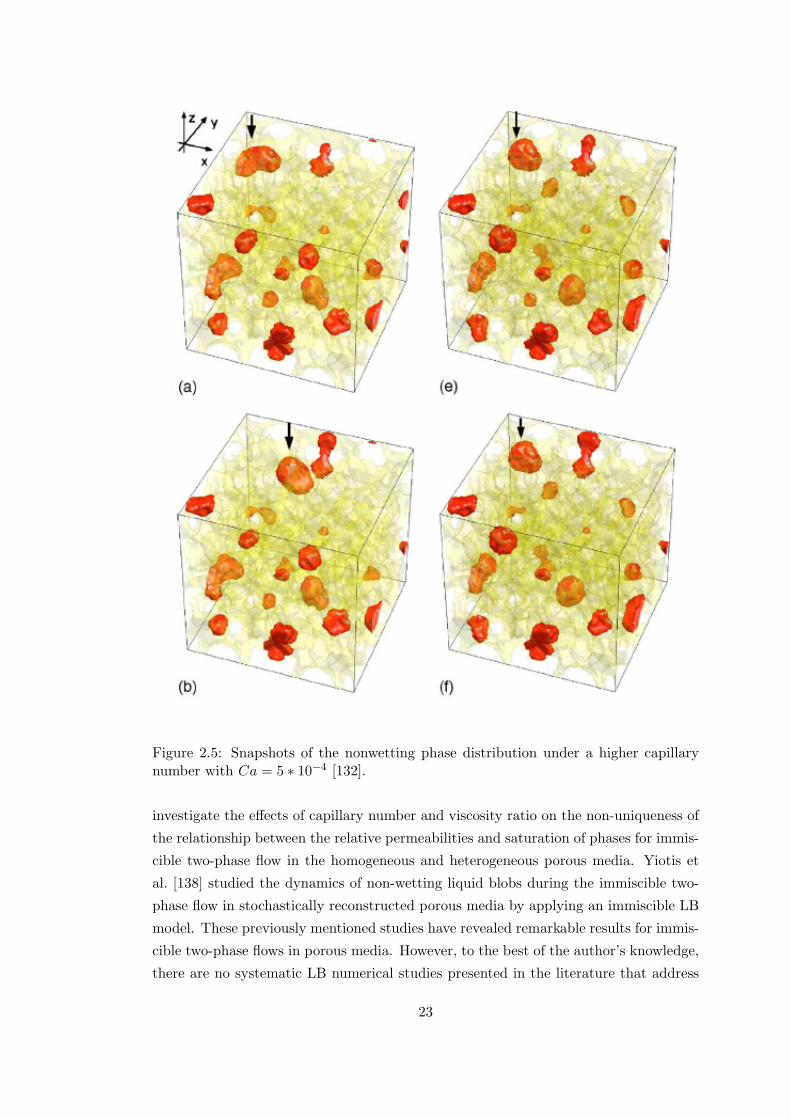
Figure 2.5: Snapshots of the nonwetting phase distribution under a higher capillarynumber with Ca = 5 ∗ 10−4 [132].

investigate the effects of capillary number and viscosity ratio on the non-uniqueness of

the relationship between the relative permeabilities and saturation of phases for immis-

cible two-phase flow in the homogeneous and heterogeneous porous media. Yiotis et

al. [138] studied the dynamics of non-wetting liquid blobs during the immiscible two-

phase flow in stochastically reconstructed porous media by applying an immiscible LB

model. These previously mentioned studies have revealed remarkable results for immis-

cible two-phase flows in porous media. However, to the best of the author’s knowledge,

there are no systematic LB numerical studies presented in the literature that address

23

the relationship between the geometrical properties and the relative permeabilities for

immiscible two-phase flows in pore-scale porous media.

24

Chapter 3

Mathematical model

3.1 Shan-Chen multiphase model with Peng-Robinson e-quation of state

3.1.1 Pseudo-potential model

The particle distribution function is governed by the discretized Boltzmann equation

with single relaxation time for the collision term [139]:

fα(x+ eαδt, t+ δt) = fα(x, t)−1

τ[fα(x, t)− feqα (x, t)], (3.1)

where fα is the particle distribution function along the αth direction, feqα is equilibrium

distribution function, δt is the time step, eα is the particle velocity in the αth direction,

τ is the single relaxation time. The viscosity in the LBM model is given by

ν = (τ − 1

2)c2sδt, (3.2)

where cs = c/√3 is the lattice sound speed, and c = δx/δt is the ratio of lattice spacing

δx and time step δt. The equilibrium distribution function feqα (x, t) can be calculated

from

f eqα = ρwα[1 +eα · ueq

c2s+

(eα · ueq)2

2c4s− ueq · ueq

2c2s], (3.3)

where wα is the weighting factor. In this paper, the D3Q19 model is adopted for the

3-dimensional simulations. The weighting factor and discrete velocity for D3Q19 are

given by

[e0, e1, e2, e3,e4,e5,e6,e7,e8,e9,e10, e11, e12, e13, e14, e15, e16,e17, e18

]= 0 1 −1 0 0 0 0 1 1 −1 −1 1 −1 1 −1 0 0 0 0

0 0 0 1 −1 0 0 1 −1 1 −1 0 0 0 0 1 1 −1 −10 0 0 0 0 1 −1 0 0 0 0 1 1 −1 −1 1 −1 1 −1

,(3.4)

25

wα =

1/3, α = 0;1/18, α = 1, 2, . . . , 6;1/36, α = 7, 8, . . . , 18;

(3.5)

The local density and local momentum are given by

ρ(x, t) =

N∑α=0

fα(x, t), (3.6)

and

ρu(x, t) =

N∑α=0

eαfα(x, t). (3.7)

The equilibrium value of the velocity ueq used in eq. (3.3) is given by

ueq = u+τF total

ρ(x). (3.8)

In eq. (3.8), F total = F cohesion + F adhesion + F body is the total force on each particle,

here including the fluid-fluid cohesion force F cohesion, the fluid-solid adhesion force

F adhesion and the body force F body.

3.1.2 Fluid-fluid cohesion

It is commonly accepted that the segregation of different phases is microscopically due

to the long-range interaction force between the particles at site x and the particles at

neighbor sites x′[45]. The interaction force is defined as

F cohesion(x) = −ψ(x)∑x′

G(x,x′)ψ(x

′)(x

′ − x), (3.9)

where G(x,x′) is Green’s function and satisfies G(x,x

′) = G(x

′,x). It reflects the

intensity of the interparticle interactions and is given by

G(x,x′) =

g, |x− x

′ | = 1,

g/2, |x− x′ | =

√2,

0, otherwise.

(3.10)

In eq. (3.9), ψ(x) is the effective mass, which is a function of the local density and

can be varied to reflect different fluid and fluid mixture behaviors, as represented by

various equations. The equation of state (EOS) of the system is given by

p = c2sρ+c02g[ψ(ρ)]2. (3.11)

and the effective mass can be defined as:

26

ψ(ρ) =

√2(p− c2sρ)

c0g, (3.12)

where c0=6.0 for the D3Q19, and p is the pressure. In Yuan and Schaefer’s study [17],

five different EOS were compared, and it was found that Peng-Robinson (PR) EOS

provided the maximum density ratio while maintaining small spurious currents around

the interface. Hence, the P-R EOS was adopted in our following multi-phase flow

research, and can be expressed as:

p =ρRT

1− bρ− aα(T )ρ2

1 + 2bρ− b2ρ2, (3.13)

where

α(T ) = [1 + (0.37464 + 1.5422ω − 0.26992ω2)(1−√T/Tc)]

2. (3.14)

The attraction parameter a = 0.45724R2T 2c /pc, the repulsion parameter b = 0.0778RTc/pc,

and ω is the acentric factor. Tc and Pc are the critical temperature and critical pres-

sure respectively. The density ratio and interfacial surface tension are governed by the

temperature T , and parameters a and b respectively. Substituting eq. (3.13) into eq.

(3.12), we get

ψ(ρ) =

√√√√2( ρRT1−bρ −aα(T )ρ2

1+2bρ−b2ρ2 − c2sρ)

c0g. (3.15)

Unlike in the original SC model, the value of the coefficient of interaction strength, g,

becomes unimportant. Indeed, it is canceled out when eq. (3.12) is substituted into

eq. (3.9). The only requirement for g is to ensure that the term inside the square root

in eq. (3.12) is positive, (i.e g = sgn(p − c2sρ) has to be stored when eq. (3.12) is

computed).

3.1.3 Fluid-solid adhesion and body force

At the fluid-solid interface, the interaction between the fluid and solid needs to be

considered. Hence the force applied on a particle that comes in contact with the solid

wall is

F adhesion = −ρ(x)∑x′

Gw(x,x′)ρw(x

′)(x

′ − x), (3.16)

where Gw(x,x′) denotes the intensity of the fluid-solid interaction. For the D3Q19

model, it is defined as

Gw(x,x′) =

Gw, |x− x

′ | = 1,

Gw/2, |x− x′ | =

√2,

0, otherwise.

(3.17)

27

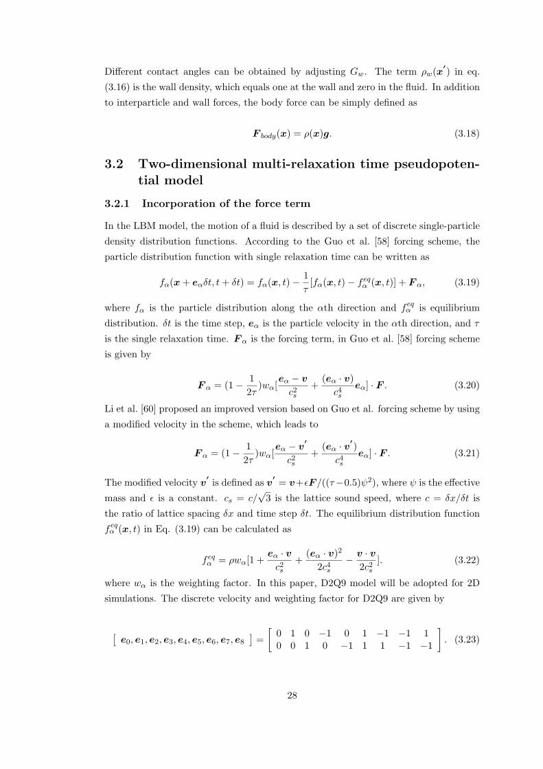
Different contact angles can be obtained by adjusting Gw. The term ρw(x′) in eq.

(3.16) is the wall density, which equals one at the wall and zero in the fluid. In addition

to interparticle and wall forces, the body force can be simply defined as

F body(x) = ρ(x)g. (3.18)

3.2 Two-dimensional multi-relaxation time pseudopoten-tial model

3.2.1 Incorporation of the force term

In the LBM model, the motion of a fluid is described by a set of discrete single-particle

density distribution functions. According to the Guo et al. [58] forcing scheme, the

particle distribution function with single relaxation time can be written as


τ[fα(x, t)− f eqα (x, t)] + F α, (3.19)

where fα is the particle distribution along the αth direction and f eqα is equilibrium

distribution. δt is the time step, eα is the particle velocity in the αth direction, and τ

is the single relaxation time. F α is the forcing term, in Guo et al. [58] forcing scheme

is given by

F α = (1− 1

2τ)wα[

eα − v

c2s+

(eα · v)c4s

eα] · F . (3.20)

Li et al. [60] proposed an improved version based on Guo et al. forcing scheme by using

a modified velocity in the scheme, which leads to

F α = (1− 1

2τ)wα[

eα − v′

c2s+

(eα · v′)

c4seα] · F . (3.21)

The modified velocity v′is defined as v

′= v+ϵF /((τ−0.5)ψ2), where ψ is the effective

mass and ϵ is a constant. cs = c/√3 is the lattice sound speed, where c = δx/δt is

the ratio of lattice spacing δx and time step δt. The equilibrium distribution function

feqα (x, t) in Eq. (3.19) can be calculated as

feqα = ρwα[1 +eα · vc2s

+(eα · v)2

2c4s− v · v

2c2s]. (3.22)

where wα is the weighting factor. In this paper, D2Q9 model will be adopted for 2D

simulations. The discrete velocity and weighting factor for D2Q9 are given by

[e0, e1, e2, e3, e4, e5, e6, e7, e8

]=

[0 1 0 −1 0 1 −1 −1 10 0 1 0 −1 1 1 −1 −1

]. (3.23)

28

wα =

4/9, α = 0;1/9, α = 1, 2, 3, 4;1/36, α = 5, 6, 7, 8;

(3.24)

The corresponding macroscopic density and velocity are calculated by

ρ(x, t) =

N∑α=0

fα(x, t). (3.25)

ρv(x, t) =

N∑α=0

eαfα(x, t) +F

2. (3.26)

where N is the number of discrete particle velocities. F = F cohesion+F adhesion+F body

is the total force on each particle, in this current study including fluid-fluid cohesion

F cohesion, fluid-solid adhesion force F adhesion and body force F body.

3.2.2 Multi-relaxation-time LBM model

In general the collision process involves multiple physical quantities that may relax

on different time scales, and information for those time scales can be given using a

collision matrix Ω instead of a single time scale τ in Eq. (3.19). As a result, Eq. (3.19)

is replaced by the following density distribution function:

fα(x+eαδt, t+δt) = fα(x, t)−∑β

Ωαβ [fβ(x, t)−f eqβ (x, t)]+(Sα(x, t)−0.5∑β

ΩαβSβ(x, t)).

(3.27)

where S is the forcing term in multi-relaxation-time LBM model which can be derived

from Eq. (3.20) or Eq. (3.21). The collision step in the velocity space is difficult to

perform. It is more convenient to perform the collision process in the momentum space.

Hence, Eq. (3.27) can be transformed to the following form,

fα(x+ eαδt, t+ δt) = fα(x, t)−M−1Λ[m(x, t)−meq(x, t)] +M−1(I − Λ

2)S(x, t).

(3.28)

where m and meq are the moment space of the density distribution function fα and

its equilibrium distribution f eqα respectively. It can be obtained from m = Mf and

meq = Mf eq respectively. M is the transformation matrix, which for D2Q9 is

M =

1 1 1 1 1 1 1 1 1−4 −1 −1 −1 −1 2 2 2 24 −2 −2 −2 −2 1 1 1 10 1 0 −1 0 1 −1 −1 10 −2 0 2 0 1 −1 −1 10 0 1 0 −1 1 1 −1 −10 0 −2 0 2 1 1 −1 −10 1 −1 1 −1 0 0 0 00 0 0 0 0 1 −1 1 −1

. (3.29)

29

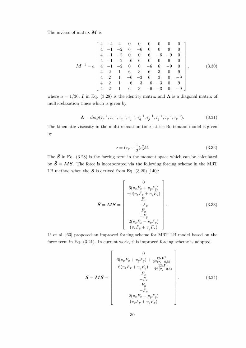
The inverse of matrix M is

M−1 = a

4 −4 4 0 0 0 0 0 04 −1 −2 6 −6 0 0 9 04 −1 −2 0 0 6 −6 −9 04 −1 −2 −6 6 0 0 9 04 −1 −2 0 0 −6 6 −9 04 2 1 6 3 6 3 0 94 2 1 −6 −3 6 3 0 −94 2 1 −6 −3 −6 −3 0 94 2 1 6 3 −6 −3 0 −9

, (3.30)

where a = 1/36, I in Eq. (3.28) is the identity matrix and Λ is a diagonal matrix of

multi-relaxation times which is given by

Λ = diag(τ−1ρ , τ−1

e , τ−1ζ , τ−1

j , τ−1q , τ−1

j , τ−1q , τ−1

ν , τ−1ν ). (3.31)

The kinematic viscosity in the multi-relaxation-time lattice Boltzmann model is given

by

ν = (τν −1

2)c2sδt. (3.32)

The S in Eq. (3.28) is the forcing term in the moment space which can be calculated

by S = MS. The force is incorporated via the following forcing scheme in the MRT

LB method when the S is derived from Eq. (3.20) [140]:

S = MS =

06(vxFx + vyFy)−6(vxFx + vyFy)

Fx−FxFy−Fy

2(vxFx − vyFy)(vxFy + vyFx)

. (3.33)

Li et al. [63] proposed an improved forcing scheme for MRT LB model based on the

force term in Eq. (3.21). In current work, this improved forcing scheme is adopted.

S = MS =

0

6(vxFx + vyFy) +12ϵF 2

Ψ2(τe−0.5)

−6(vxFx + vyFy)− 12ϵF 2

Ψ2(τζ−0.5)

Fx−FxFy−Fy

2(vxFx − vyFy)(vxFy + vyFx)

. (3.34)

30

3.3 New forcing scheme for the three-dimensional multi-relaxation time lattice-Boltzmann model

An improved force scheme is proposed for the three-dimensional MRT pseudopoten-

tial lattice Boltzmann model which is based on the improved force scheme for the

single relaxation time (SRT) pseudopotential lattice Botlzmann model ( [60]) and the

Chapman-Enskog analysis ( [141]). This three-dimensional multi-relaxation-time lat-

tice Boltzmann model can handle multiphase flows at high density ratios and low

viscosities. The proposed MRT multiphase model is evaluated by verifying Laplace’s

law and achieving thermodynamic consistency for a static droplet. Moreover, a rela-

tionship between the fluid-solid interaction potential parameter and the contact angle

is investigated.

3.3.1 3D multi-relaxation-time LBM model for multi-phase flows

In the LBM model, the motion of a fluid is described by a set of discrete single-

particle density distribution functions. According to the [58] forcing scheme, the lattice

Boltzmann equation with single relaxation time can be written as


τ[fα(x, t)− f eqα (x, t)] + F α, (3.35)

where fα is the particle distribution along the αth direction, feqα is the equilibrium

distribution, δt is the time step, eα is the particle velocity in the αth direction, τ is the

single relaxation time and F α is the forcing term. Li et al. [60] proposed an improved

version based on the Guo et al. [58] forcing scheme by using a modified velocity, which

leads to

F α = (1− 1

2τ)wα[

eα − v′

c2s+

(eα · v′)

c4seα] · F . (3.36)

The modified velocity v′is defined as v

′= v + ϵF /((τ − 0.5)ψ2), where ψ is the

effective mass and ϵ is a constant. F = F cohesion+F adhesion+F body is the total force on

each particle, including the fluid-fluid cohesion F cohesion, the fluid-solid adhesion force

F adhesion and the body force F body. The equilibrium distribution function feqα (x, t) is

expressed as [45]

feqα = ρwα[1 +eα · vc2s

+(eα · v)2

2c4s− v · v

2c2s], (3.37)

where wα is the weighting factor. In this study, the D3Q19 model is adopted for

the 3D simulations. The discrete velocity and the weighting factor for the D3Q19 are

given by Eq.3.4 and Eq.3.5

Generally, the collision process involves multiple physical quantities that may relax

on different time scales, and information for those time scales can be given using a

31

collision matrix Ω instead of a single time scale τ in Eq. (3.35). As a result, Eq. (3.35)

is replaced by the following lattice Boltzmann equation [142]:

fα(x+eαδt, t+δt) = fα(x, t)−∑β

Ωαβ [fβ(x, t)−f eqβ (x, t)]+(Sα(x, t)−0.5∑β

ΩαβSβ(x, t)),

(3.38)

where S is the forcing term in the multi-relaxation-time LBM model. From Eq. (3.36)

Sα = wα[eα − v

′

c2s+

(eα · v′)

c4seα] · F . (3.39)

Eq. (3.38) can be mapped onto the moment space by multiplying throughout by a

transformation matrix M [61]. Hence, Eq. (3.38) can be transformed into the following

form,

fα(x+ eαδt, t+ δt) = fα(x, t)−M−1Λ[m(x, t)−meq(x, t)] +M−1(I − Λ

2)S(x, t),

(3.40)where m and meq are the moment space of the density distribution function fα andits equilibrium distribution feqα . It can be derived from m = Mf and meq = Mf eq,respectively, where M is the transformation matrix. The matrix M for the D3Q19 is

M =

1 1 1 1 1 1 1 1 1 1 1 1 1 1 1 1 1 1 1−30 −11 −11 −11 −11 −11 −11 8 8 8 8 8 8 8 8 8 8 8 812 −4 −4 −4 −4 −4 −4 1 1 1 1 1 1 1 1 1 1 1 10 1 0 0 −1 0 0 1 1 0 −1 −1 0 1 1 0 −1 −1 00 −4 0 0 4 0 0 1 1 0 −1 −1 0 1 1 0 −1 −1 00 0 1 0 0 −1 0 1 0 1 −1 0 −1 −1 0 1 1 0 −10 0 −4 0 0 4 0 1 0 1 −1 0 −1 −1 0 1 1 0 −10 0 0 1 0 0 −1 0 1 1 0 −1 −1 0 −1 −1 0 1 10 0 0 −4 0 0 4 0 1 1 0 −1 −1 0 −1 −1 0 1 10 2 −1 −1 2 −1 −1 1 1 −2 1 1 −2 1 1 −2 1 1 −20 −4 2 2 −4 2 2 1 1 −2 1 1 −2 1 1 −2 1 1 −20 0 1 −1 0 1 −1 1 −1 0 1 −1 0 1 −1 0 1 −1 00 0 −2 2 0 −2 2 1 −1 0 1 −1 0 1 −1 0 1 −1 00 0 0 0 0 0 0 1 0 0 1 0 0 −1 0 0 −1 0 00 0 0 0 0 0 0 0 0 1 0 0 1 0 0 −1 0 0 −10 0 0 0 0 0 0 0 1 0 0 1 0 0 −1 0 0 −1 00 0 0 0 0 0 0 1 −1 0 −1 1 0 1 −1 0 −1 1 00 0 0 0 0 0 0 −1 0 1 1 0 −1 1 0 1 −1 0 −10 0 0 0 0 0 0 0 1 −1 0 −1 1 0 −1 1 0 1 −1

.

(3.41)

The M−1 is the inverse of matrix M . The equilibrium distribution functions meq in

the moment space are related to those in velocity space by

32

meq = Mf eq =

ρ

−11ρ+ 19jx2+jy2+jz2

ρ

3ρ− 112jx2+jy2+jz2

ρ

jx−2

3jxjy

−23jyjz

−23jz

2jx2−(jy2+jz2)ρ

−122jx2−(jy2+jz2)

ρjy2−jz2

ρ

−12jy2−jz2

ρjxjyρ

jyjzρ

jxjzρ

000

, (3.42)

where jx, jy and jz are the components of the momentum, jx=ρux, jy=ρuy and jz=ρuz.

I in Eq. (3.40) is the identity matrix and Λ is a diagonal matrix which is given by

Λ = diag(s1, s2, s3, s4, s5, s6, s7, s8, s9, s10, s11, s12, s13, s14, s15, s16, s17, s18, s19).

(3.43)

The bulk viscosity and kinematic viscosity in the multi-relaxation-time lattice Boltz-

mann model are given by

ξ =2

9(1

s2− 1

2), (3.44)

and

ν =1

3(1

sβ− 1

2), β = 10, 12, 14, 15, 16. (3.45)

Li et al. [60] showed that the numerical stability of the Shan-Chen and EDM schemes

is related to an additional term in their recovered macroscopic equations. Based on

the theoretical analysis, a SRT improved forcing scheme which is more stable than

Shan-Chen, Guo and EDM schemes was presented. The two dimensional macroscopic

equations recovered from the improved forcing scheme were shown in their study [60].

Similar to the two dimensional macroscopic equations, the macroscopic equations for

the three dimensional case are given by

∂tρ+ ∂x(ρvx) + ∂y(ρvy) + ∂z(ρvz) = 0, (3.46)

33

∂t(ρvx) + ∂x(ρvxvx) + ∂y(ρvxvy) + ∂z(ρvxvz) = −∂x(ρc2s) + Fx + ∂x(2ν[∂x(ρvx)−1

3∇ · (ρv)]

+ξ∇ · (ρv)) + ∂y(ν(∂x(ρvy) + ∂y(ρvx))) + ∂z(ν(∂x(ρvz) + ∂z(ρvx)))

−2G2c4ϵ∂x(|∇Ψ|2) +O(∂5),

(3.47)

∂t(ρvy) + ∂x(ρvxvy) + ∂y(ρvyvy) + ∂z(ρvyvz) = −∂y(ρc2s) + Fy + ∂x(ν(∂x(ρvy) + ∂y(ρvx)))

+∂y(2ν[∂y(ρvy)−1

3∇ · (ρv)] + ξ∇ · (ρv)) + ∂z(ν(∂y(ρvz) + ∂z(ρvy)))

−2G2c4ϵ∂y(|∇Ψ|2) +O(∂5),

(3.48)

∂t(ρvz) + ∂x(ρvxvz) + ∂y(ρvyvz) + ∂z(ρvzvz) = −∂z(ρc2s) + Fz + ∂x(ν(∂x(ρvz) + ∂z(ρvx)))

+∂y(ν(∂y(ρvz) + ∂z(ρvy))) + ∂z(2ν[∂z(ρvz −1

3∇ · (ρv))] + ξ∇ · (ρv))

−2G2c4ϵ∂z(|∇Ψ|2) +O(∂5),

(3.49)

where G and c are constants equal to 1, ϵ is a constant which can be adjusted to fit

the mechanical stability solution with the solution given by the Maxwell construction

as well as to enhance the numerical stability [60].

The corresponding macroscopic density and velocity are calculated by

ρ(x, t) =

N∑α=0

fα(x, t), (3.50)

and

ρv(x, t) =

N∑α=0

eαfα(x, t) +F

2, (3.51)

where N is the number of discrete particle velocities. According to Eqs. (A.45), (A.46),

(A.47), the pressure tensor is defined as

∇ · P new = ∇ · P + 2G2c4ϵ∇ · (|∇Ψ|2I), (3.52)

where

∇ · P = ∇ · (ρc2sI)− F . (3.53)

The term S in Eq. (3.40) is the forcing term in the moment space. In the current

work, a MRT force scheme which is able to recover the 3-dimensional macroscopic Eqs

(A.45), (A.46), (A.47) is proposed. According to the Chapman-Enskog analysis [141],

the 3D MRT force scheme is given by

34

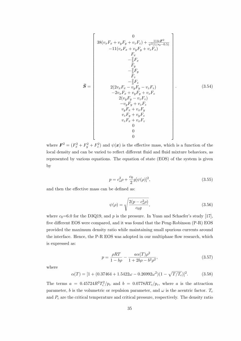
S =

0

38(vxFx + vyFy + vzFz) +114ϵF 2

ψ2(1/s2−0.5)

−11(vxFx + vyFy + vzFz)Fx

−23FxFy

−23FyFz

−23Fz

2(2vxFx − vyFy − vzFz)−2vxFx + vyFy + vzFz

2(vyFy − vzFz)−vyFy + vzFzvyFx + vxFyvzFy + vyFzvzFx + vxFz

000

. (3.54)

where F 2 = (F 2x + F 2

y + F 2z ) and ψ(x) is the effective mass, which is a function of the

local density and can be varied to reflect different fluid and fluid mixture behaviors, as

represented by various equations. The equation of state (EOS) of the system is given

by

p = c2sρ+c02g[ψ(ρ)]2, (3.55)

and then the effective mass can be defined as:

ψ(ρ) =

√2(p− c2sρ)

c0g, (3.56)

where c0=6.0 for the D3Q19, and p is the pressure. In Yuan and Schaefer’s study [17],

five different EOS were compared, and it was found that the Peng-Robinson (P-R) EOS

provided the maximum density ratio while maintaining small spurious currents around

the interface. Hence, the P-R EOS was adopted in our multiphase flow research, which

is expressed as:

p =ρRT

1− bρ− aα(T )ρ2

1 + 2bρ− b2ρ2, (3.57)

where

α(T ) = [1 + (0.37464 + 1.5422ω − 0.26992ω2)(1−√T/Tc)]

2. (3.58)

The terms a = 0.45724R2T 2c /pc and b = 0.0778RTc/pc, where a is the attraction

parameter, b is the volumetric or repulsion parameter, and ω is the acentric factor. Tc

and Pc are the critical temperature and critical pressure, respectively. The density ratio

35

and surface tension of the liquid is governed by the temperature T , and parameters a

and b respectively. Substituting Eq. (3.57) into Eq. (3.56), we get

ψ(ρ) =

√√√√2( ρRT1−bρ −aα(T )ρ2

1+2bρ−b2ρ2 − c2sρ)

c0g. (3.59)

Unlike in the original SC model, the value of the coefficient of the interaction strength g

becomes unimportant, because g is canceled out when calculating the interaction force

and pressure [17]. The requirement for g is to ensure that the term inside the square

root in Eq. (3.56) is positive, (i.e g = sgn(p − c2sρ) has to be stored when computing

Eq. (3.56)).

3.3.2 Evaluation of surface tension

0.01 0.02 0.03 0.04 0.05 0.060

0.005

0.01

0.015

0.02

0.025

1/r

∆p

LB simulationLeast−square linear fit

Figure 3.1: Evaluation of Laplace’s law, the slope is 0.3690; the intercept is 0.000002136;and the coefficient of determination is 0.9999.

The satisfaction of Laplace law is an important benchmark test. The Laplace law

for three dimensional states is

∆p = pin − pout =2σ

r, (3.60)

36

where pin and pout are the pressures inside and outside the droplet, respectively. ∆p,

σ, r are the pressure difference, surface tension coefficient and the radius of the droplet.

Stationary droplets with different radii are generated inside the domain with 120×120×120

lattice points and periodic boundary conditions to test if the results from simulations

follow Laplace’s law. The parameters are fixed at R=1, a=1/49, b=2/21, ω=0.344,

T=0.61Tc, sβ=1/0.6 and ϵ=0.3. The final droplet radius and pressure difference inside

and outside of the droplet are measured after 18000 time steps. The steady-state pres-

sure inside(pin) and outside the droplet(pout) is measured on nodes located away from

the interface since pressure values vary near it. The pressure jump is plotted as a func-

tion of the curvature in Fig. 3.1. The droplet radius, pressure difference and calculated

surface tension are all in lattice units. The square marker in Fig. 3.1 indicates the

results of the LB simulations whereas the solid line is the least-square linear fit. The

slope equals to 0.3592 which corresponds to a surface tension of 0.1845; the intercept

is 0.000002136; and the coefficient of determination is 0.9999. It is can be seen that

all points fit a straight line. The pressure difference between the inside and outside

of the droplet is proportional to the curvature. The agreement between the Laplace

law and the numerical simulation indicates that the 3D MRT LBM model with the

improved force scheme can handle the high density ratio multi-phase flow accurately.

However, as it occurs in other pseudopotential lattice Boltzmann models, the surface

tension in the current model cannot not be predicted in advance and can not be tuned

independently.

3.3.3 Evaluation of thermodynamic consistency

A series of numerical simulations of stationary droplets are conducted to validate the

proposed new 3D MRT lattice Boltzmann model. The problem of stationary droplets

with different values of T , can be used to compare the numerical coexistence curve with

the coexistence curve given by the Maxwell construction.

In order to verify the thermodynamic consistency, a stationary droplet with a radius of

r=25 is initially placed at the center of the domain with 100×100×100 lattice points.

Periodic boundary condition are applied on both sides of the domain. The parameters

are fixed at R=1, a=1/49, b=2/21, ω=0.344, sβ=1/0.6 and ϵ=0.3. The coexistence

curves are shown in Fig. 3.2. It can be seen that the simulation results are in good a-

greement with the results from the Maxwell construction. In addition to that, it can be

seen that the proposed MRT lattice Boltzmann model with the improved force scheme

works well at T/Tc=0.6, which corresponds to ρl/ρg = 863. This is a clear demonstra-

tion that the proposed 3D MRT lattice Boltzmann model is capable of handling large

density ratio multiphase flows and achieve thermodynamic consistency. According to

numerical experimentation with the single-relaxation-time model, the largest achiev-

able density ratio is approximately 150 for the case of sβ=1/0.6. In contrast to that,

37

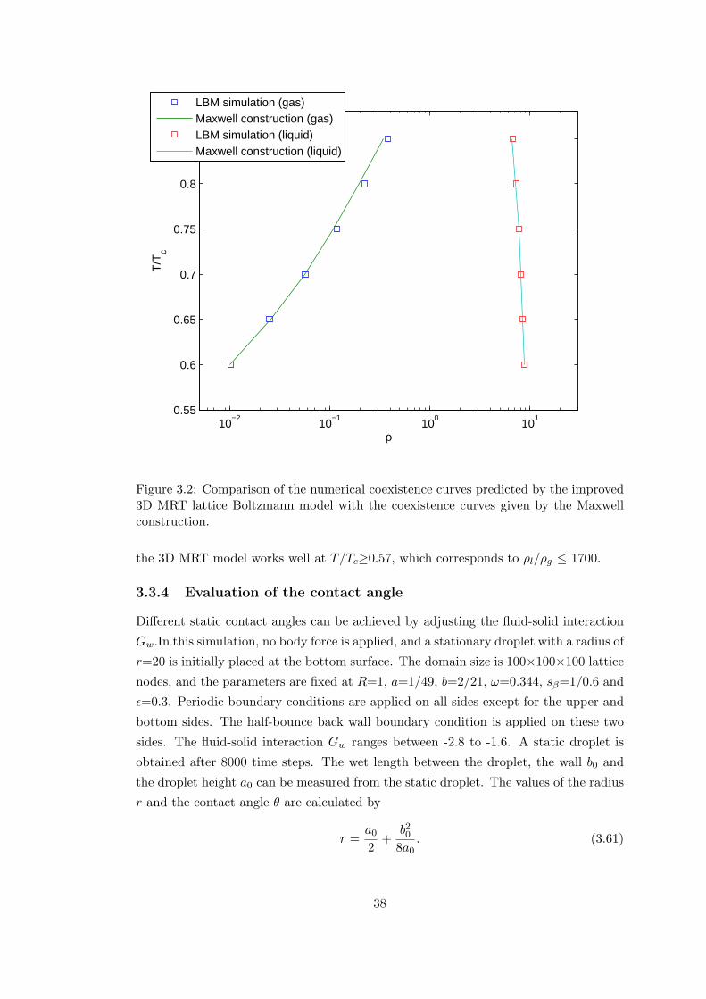
10−2

10−1

100

101

0.55

0.6

0.65

0.7

0.75

0.8

0.85

ρ

T/T

c

LBM simulation (gas)Maxwell construction (gas)LBM simulation (liquid)Maxwell construction (liquid)

Figure 3.2: Comparison of the numerical coexistence curves predicted by the improved3D MRT lattice Boltzmann model with the coexistence curves given by the Maxwellconstruction.

the 3D MRT model works well at T/Tc≥0.57, which corresponds to ρl/ρg ≤ 1700.

3.3.4 Evaluation of the contact angle

Different static contact angles can be achieved by adjusting the fluid-solid interaction

Gw.In this simulation, no body force is applied, and a stationary droplet with a radius of

r=20 is initially placed at the bottom surface. The domain size is 100×100×100 lattice

nodes, and the parameters are fixed at R=1, a=1/49, b=2/21, ω=0.344, sβ=1/0.6 and

ϵ=0.3. Periodic boundary conditions are applied on all sides except for the upper and

bottom sides. The half-bounce back wall boundary condition is applied on these two

sides. The fluid-solid interaction Gw ranges between -2.8 to -1.6. A static droplet is

obtained after 8000 time steps. The wet length between the droplet, the wall b0 and

the droplet height a0 can be measured from the static droplet. The values of the radius

r and the contact angle θ are calculated by

r =a02

+b208a0

. (3.61)

38

−3.5 −3 −2.5 −2 −1.5 −1

40

60

80

100

120

140

160

Gw

θ

simulationfitting

Figure 3.3: The relationship between Gw and contact angle θ.

and

θ = arctan(b0

2(r − a0)). (3.62)

The value of Gw is varied to obtain steady droplets with different contact angles. The

relationship between Gw and the contact angle θ is shown in Fig. 3.3. It can be seen

that the contact angles approximate to a linear function of Gw.

3.3.5 Conclusions

A three-dimensional multi-relaxation time (MRT) lattice Boltzmann model with an

improved forcing scheme is reported for the simulation of high liquid-to-gas density

ratio multiphase flows, based on the improved force scheme for the single relaxation

time (SRT) pseudopotential LBM [60] and the Chapman-Enskog analysis [141]. The

3D MRT lattice Boltzmann model is validated through Laplace’s law and by achiev-

ing thermodynamic consistency. Additionally, the relationship between the fluid-solid

interaction potential parameter Gw and the contact angle is investigated. It has been

observed that the contact angle is a linear function of Gw.

39

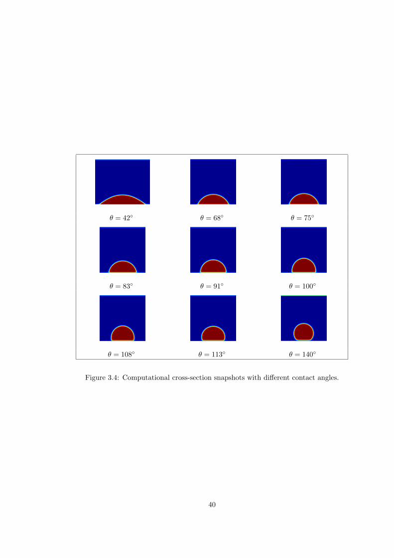
θ = 42 θ = 68 θ = 75

θ = 83 θ = 91 θ = 100

θ = 108 θ = 113 θ = 140

Figure 3.4: Computational cross-section snapshots with different contact angles.

40

Chapter 4

Droplet impingement on a solidsurface

In chapter 4, lattice Boltzmann model is applied on the study of the impaction of a

liquid droplet on a dry flat surface and a curved surface for a liquid-gas system with large

density ratio. The influence of Reynolds number, Weber number, Ohnesorge number,

Galilei number and surface characteristics on the impingement process is reported. The

results are compared with experimental data reported in the literature.

4.1 Dynamics of droplet impingement on a flat surface

The improved three-dimensional MRT lattice Boltzmann model and the 3-dimensional

lattice Boltzmann model based on the original Shan-Chen model [45] and the improve-

ments in the single-component multiphase flow model reported by Yuan and Schae-

fer [17] is employed to study the impaction of a liquid droplet on a flat surface.

4.1.1 Initial and boundary conditions

The 3-dimensional computational domain used in the simulations is shown in Fig. 4.1.

The domain size is 150*150*120 lattice nodes. Periodic boundary conditions are used

on the sides of the domain. That means that the particles leaving the domain through

a bounding face, will immediately re-enter the simulation region through the opposite

face. No-slip wall boundary conditions are used on the top and bottom boundaries

of the domain, while the half-way bounce-back scheme in LBM is applied on the wall

boundary. The domain size for each case is varied according to the initial size of the

droplet while the impact is assumed to be isothermal. By varying Gw, the wettability

of the flat surface can be controlled. The liquid-gas density ratio is determined by T

in eq. (3.13). In addition, the temperature T and other parameters (a,b) in eq. (3.13)

control the interfacial surface tension between the two fluids. The acentric factor ω is

set to be 0.344 in this simulation. Initially, the droplet is placed at the center of the

computational domain and is equilibrated for 10000 lattice time steps to achieve the

41

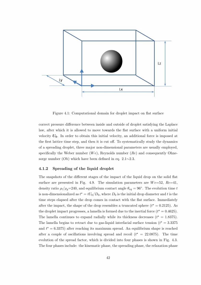
Figure 4.1: Computational domain for droplet impact on flat surface

correct pressure difference between inside and outside of droplet satisfying the Laplace

law, after which it is allowed to move towards the flat surface with a uniform initial

velocity U0. In order to obtain this initial velocity, an additional force is imposed at

the first lattice time step, and then it is cut off. To systematically study the dynamics

of a spreading droplet, three major non-dimensional parameters are usually employed,

specifically the Weber number (We), Reynolds number (Re) and consequently Ohne-

sorge number (Oh) which have been defined in eq. 2.1∼2.3.

4.1.2 Spreading of the liquid droplet

The snapshots of the different stages of the impact of the liquid drop on the solid flat

surface are presented in Fig. 4.9. The simulation parameters are We=52, Re=41,

density ratio ρl/ρg=240, and equilibrium contact angle θeq = 96. The evolution time t

is non-dimensionalized as t⋆ = tU0/D0, whereD0 is the initial drop diameter and t is the

time steps elapsed after the drop comes in contact with the flat surface. Immediately

after the impact, the shape of the drop resembles a truncated sphere (t⋆ = 0.2125). As

the droplet impact progresses, a lamella is formed due to the inertial force (t⋆ = 0.4625).

The lamella continues to expand radially while its thickness decreases (t⋆ = 1.8375).

The lamella begins to retract due to gas-liquid interfacial surface tension (t⋆ = 3.3375

and t⋆ = 6.3375) after reaching its maximum spread. An equilibrium shape is reached

after a couple of oscillations involving spread and recoil (t⋆ = 22.0875). The time

evolution of the spread factor, which is divided into four phases is shown in Fig. 4.3.

The four phases include: the kinematic phase, the spreading phase, the relaxation phase

42

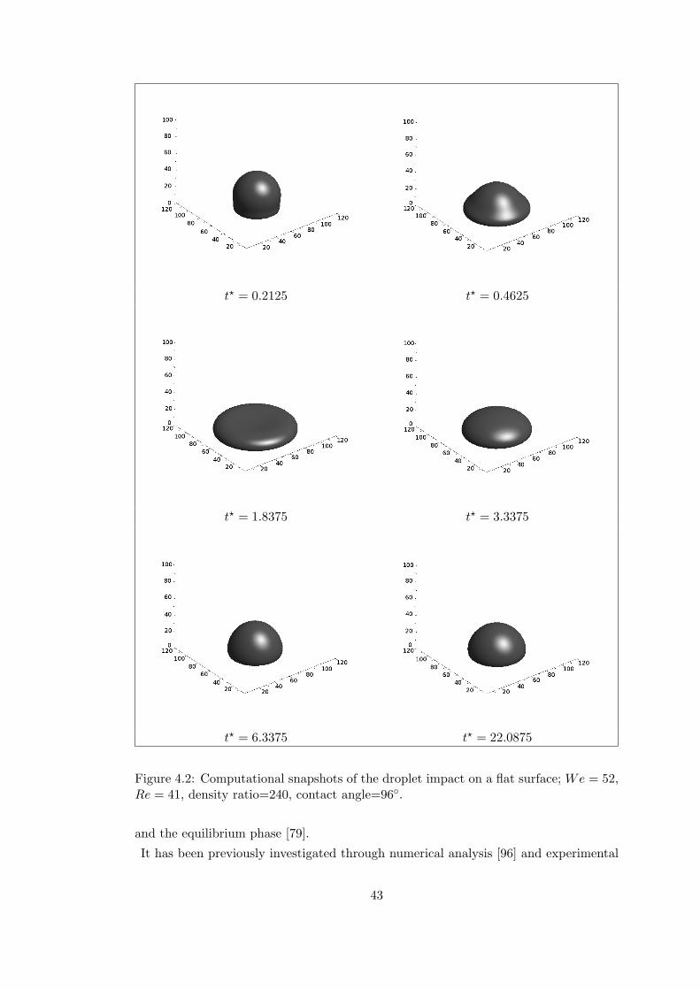
t⋆ = 0.2125 t⋆ = 0.4625

t⋆ = 1.8375 t⋆ = 3.3375

t⋆ = 6.3375 t⋆ = 22.0875

Figure 4.2: Computational snapshots of the droplet impact on a flat surface; We = 52,Re = 41, density ratio=240, contact angle=96.

and the equilibrium phase [79].

It has been previously investigated through numerical analysis [96] and experimental

43

10−2

10−1

100

101

102

0

0.2

0.4

0.6

0.8

1

1.2

1.4

1.6

1.8

2

non−dimensional time (t*)

non−

dim

ensi

onal

spr

ead

fact

or (

D*) Kinematic

Spreading

Relaxation

Equilibrium

Figure 4.3: Time evolution of the spread factor from the current lattice Boltzmannmodel simulation.

Table 4.1: Simulation parameters.

Reynolds number Weber number Density ratio Contact angle a b

27.72 10.86 240 90 2/49 2/2131.2 30.72 240 96 0.5/49 3.5/2141 52 240 96 0.5/49 3.5/2118.72 11.06 240 96 0.5/49 3.5/2154 104 114 104 0.5/49 3.5/2131.2 16 310 97 1/49 2/21

work [79] that the spread factor is proportional to√t⋆ in the kinematic phase. The

correlation factor is 2.8 from the experimental data by Rioboo et al. [79], while it equals

to 1.35 in the work of Gupta and Kumar [96]. According to the theoretical analysis the

correlation factor equals to 2. Fig. 4.4 shows the time evolution of the spread factor D⋆

in the kinematic phase (t⋆ << 1) for six different We and Re cases using the current

LBM model. The Weber number, Reynolds number, density ratio and wettability of

the surface for these six cases are illustrated in table. 4.1. A fitting curve has been

generated to yield D⋆ = 2√t⋆ which is the same as the theoretical result. It can be

44

0 0.02 0.04 0.06 0.08 0.1 0.12 0.14 0.160

0.1

0.2

0.3

0.4

0.5

0.6

0.7

0.8

0.9

1


non−

dim

ensi

onal

spr

ead

fact

or (

D*)

Re=27.72, We=10.86Re=31.2, We=30.72Re=41, We=52Re=18.72, We=11.06Re=54, We=104Re=31.2, We=16fitting curve

Figure 4.4: Time evolution of the spread factor in the kinematic phase from currentLBM simulation for six cases

observed from Fig. 4.4 that all cases behave similarly during the kinematic phase.

Therefore, the droplet spread factor in the kinematic phase is independent of the the

physical properties of the fluids and the wettability of the surface, while it is only a

function of the dimensionless time.

The maximum spread factor is obtained at the end of the spreading phase, which follows

the kinematic phase. It depends on the capillary force, viscosity and inertial effects as

well as the contact angle. Asai et al. [80] proposed a correlation for the maximum

spread factor which is given by

D⋆max = 1 + 0.48We0.5exp[−1.48We0.22Re−0.21]. (4.1)

Another maximum spread factor prediction equation was derived based on the energy

conservation equation and the viscous dissipation based on the linear velocity profile [82]

3

2

We

ReD⋆max

4 + (1− cosθ)D⋆max

2 − (We

3+ 4) = 0. (4.2)

The maximum spread factor prediction equation from Pasandideh-Fard et al. [83] is

also based on energy conservation equation, while the viscous dissipation was based on

45

the velocity profile of stagnation-point flow.

D⋆max =

√(We+ 12)/[3(1− cosθ) + 4We/

√Re]. (4.3)

In order to cover a large range of We and Oh numbers, Mao et al. [84] proposed an

empirical equation based on the energy conservation equation

[0.2Oh0.33We0.665 +1

4(1− cosθ)]D⋆

max2 +

2

3D⋆max

−1 =We

12+ 1. (4.4)

Scheller and Bousfield [81] generated a experimental equation to predict D⋆max given

by

D⋆max = 0.61(Re2Oh)0.166. (4.5)

102

103

100

OhRe2

Max

imum

spr

ead

fact

or

simulation dataScheller & Bousfield[81]Pasandideh−Far et al.[83]Asai et al.[80]Chandra & Avedisian[82]Mao et al.[84]

Figure 4.5: Comparison of the maximum spread factor predicted by the lattice Boltz-mann model and various equations published in the literature.

Although the effect of the equilibrium contact angle was neglected, the empirical

equation was in good agreement with Dong et al.’s [86] experiment. The maximum

spread factor predicted from our simulation results is compared with previous stud-

ies [80–84] in Fig. 4.5. It can be observed that the simulation results are in good agree-

ment with the predictions from the equations of Asai et al. [80] and Mao et al. [84]. A

good correlation with the results of Chandra and Avedisians’ [82] is also observed, es-

pecially at higher OhRe2 numbers, while minor deviations are present at lower OhRe2

46

numbers. Discrepancies can be seen between the numerical results and the predictions

from Pasandideh-Fard et al. [83], while the correlation of Scheller and Bousfield signifi-

cantly under predicts D⋆max especially for low OhRe2 numbers. These discrepancies can

mainly be attributed to the fact that Pasandideh-Fard et al’s. [83] evaluation of dissi-

pation is suitable for low Oh numbers, while Chandra and Avedisian’ [82] dissipation

evaluation becomes more suitable for high Oh numbers. This has also been pointed

out in the work of Mao et al. [84].

Simulations were conducted for a range of Weber and Reynolds numbers in this

10−2

10−1

100

101

102

0

0.5

1

1.5

2

2.5


non−

dim

ensi

onal

fact

or (

D*)

Re=31.20,We=30.72Re=41.00,We=52.00Re=18.72,We=11.06

(t*)0.5

Kinematic

Figure 4.6: Time evolution of the spread factor for Oh = 0.177.

study, while keeping the density ratio between liquid and gas, the wettability of the

surface and the Ohnesorge number (Oh) constant as 240, 96, and 0.177, respectively.

In Fig. 4.6, the time evolution of the droplet spreading process on a dry flat surface

for Oh=0.177 is shown. It can be seen that in the kinematic phase, D⋆ is proportional

to√t⋆ for all Reynolds numbers. The spreading phase depends on the Weber and

Reynolds numbers, which control both the maximum diameter and the time to achieve

it. Increasing the inertial force leads to an increase in the maximum spread factor. For

the lowest Reynolds number of 18.72, the maximum spread factor is 1.43, while the

maximum value is 1.72 when the Reynolds number is 41. Another observation from

Fig. 4.6 is that longer times are needed for the droplets to reach the peak diameter

47

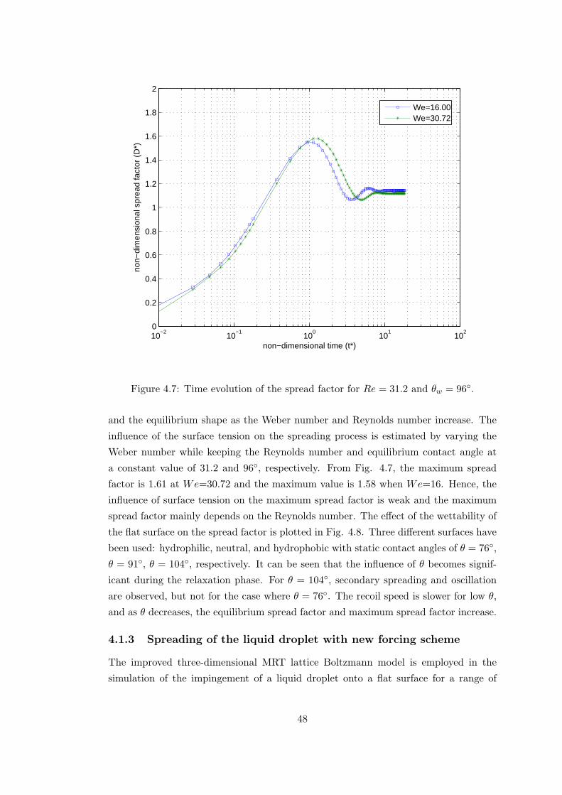
10−2

10−1

100

101

102

0

0.2

0.4

0.6

0.8

1

1.2

1.4

1.6

1.8

2


non−

dim

ensi

onal

spr

ead

fact

or (

D*)

We=16.00We=30.72

Figure 4.7: Time evolution of the spread factor for Re = 31.2 and θw = 96.

and the equilibrium shape as the Weber number and Reynolds number increase. The

influence of the surface tension on the spreading process is estimated by varying the

Weber number while keeping the Reynolds number and equilibrium contact angle at

a constant value of 31.2 and 96, respectively. From Fig. 4.7, the maximum spread

factor is 1.61 at We=30.72 and the maximum value is 1.58 when We=16. Hence, the

influence of surface tension on the maximum spread factor is weak and the maximum

spread factor mainly depends on the Reynolds number. The effect of the wettability of

the flat surface on the spread factor is plotted in Fig. 4.8. Three different surfaces have

been used: hydrophilic, neutral, and hydrophobic with static contact angles of θ = 76,

θ = 91, θ = 104, respectively. It can be seen that the influence of θ becomes signif-

icant during the relaxation phase. For θ = 104, secondary spreading and oscillation

are observed, but not for the case where θ = 76. The recoil speed is slower for low θ,

and as θ decreases, the equilibrium spread factor and maximum spread factor increase.

4.1.3 Spreading of the liquid droplet with new forcing scheme

The improved three-dimensional MRT lattice Boltzmann model is employed in the

simulation of the impingement of a liquid droplet onto a flat surface for a range of

48

0 2 4 6 8 10 12 14 16 18 200

0.2

0.4

0.6

0.8

1

1.2

1.4

1.6

1.8


non−

dim

ensi

onal

spr

ead

fact

or (

D*)

HydrophobicNeutralHydrophilic

Figure 4.8: Influence of wettability on the spreading behavior. (Re = 31.2, We = 16,density ratio is 313.

Weber and Reynolds numbers. The snapshots of the stages of the liquid drop impact

on the solid flat surface are presented in Fig. 4.9 for We=19.34, Re=92.4, density

ratio ρl/ρg=412, and equilibrium contact angle θeq = 89. The evolution time t is non-

dimensionalized as t⋆ = tU0/D0, where D0 is the initial drop diameter and t is the time

elapsed after the drop comes in contact with the flat surface. Immediately after the

impact, the shape of the drop resembles a truncated sphere (t⋆=0.167). As the liquid

drop continues to move downwards, a lamella is formed (t⋆=0.573). The lamella con-

tinues to grow radially while its thickness decreases (t⋆=1.157) until the surface tension

dominates the inertial force. The lamella begins to retract due to interfacial tension

after reaching a maximum spread factor (t⋆=1.67, t⋆=2.028, t⋆=2.625). Then, an equi-

librium shape is reached (t⋆=23.83) after a couple of oscillations involving spread and

recoil (t⋆=4.295, t⋆=7.159). The time evolution of the spread factor which is divided

into four phases is provided in Fig. 4.10. The spread factor is defined as the ratio of the

spreading diameter on the surface and the initial droplet diameter, D⋆ = D/D0. The

four phases include: the kinematic phase, the spreading phase, the relaxation phase

and the equilibrium phase [79].

The maximum spread factor is reached at the end of the spreading phase which fol-

49

t⋆ = 0.167 t⋆ = 0.573 t⋆ = 1.157

t⋆ = 1.67 t⋆ = 2.028 t⋆ = 2.625

t⋆ = 4.295 t⋆ = 7.159 t⋆ = 23.83

Figure 4.9: Computational snapshots of droplet impact on flat surface; We=19.34,Re=92.4, density ratio=412, contact angle=89.

case Reynolds number Weber number density ratio contact angle

data1 27.72 10.86 412 89

data2 31.2 16 412 96

data3 92.4 19.34 412 89

data4 168.75 26.90 716 89

data5 229.95 36.49 716 89

data6 18.72 11.06 412 96

Table 4.2: Simulation parameters for new forcing scheme.

lows the kinematic phase. It is dependent on the capillary force, viscosity and inertial

effects as well as the contact angle. [80] proposed a correlation which was given as

D⋆max = 1+ 0.48We0.5exp[−1.48We0.22Re−0.21]. Another maximum spread factor pre-

diction equation was produced as D⋆max = ((We + 12)/[3(1 − cosθ) + 4We/

√Re])0.5

based on the energy conservation equation in Pasandideh-Fard et al.’s study [83].

Scheller and Bousfield [81] derived an experimental equation to predict D⋆max given

by D⋆max = 0.61(Re2Oh)0.166. Although the effect of the equilibrium contact angle had

been neglected, the empirical equation gives a good fit with Dong et al.’s [86] exper-

iment. In order to validate the current 3D MRT LBM model, the maximum spread

50

10−2

10−1

100

101

102

0

0.5

1

1.5

2


non−

dim

ensi

onal

spr

ead

fact

or (

D*) Kinematic

Spreading

Relaxation

Equilibrium

Figure 4.10: Time evolution of the spread factor from improved 3D MRT LBM simu-lation.

factor for randomly chosenWe and Re cases from the current LBMmodel are compared

with the predictions from previous studies published in the literature [80, 81, 83](Fig.

4.11). The Weber number, Reynolds number, density ratio and surface wettability for

these six cases are given in table. 5.1. The simulation results are in good agreement

with the predictions of the equations from [80], [83] and [81].

The effect of the wettability of the flat surface on the spread factor is shown in Fig.

4.12. Three different surfaces have been used: hydrophilic, neutral, and hydrophobic

with static contact angles of θ = 76, θ = 89, θ = 106, respectively. It can be

seen that the influence of the contact angle θ becomes significant during the relaxation

phase. For θ = 106, the oscillation is more intense than for the case of θ = 76. Longer

time is required to achieve the equilibrium state for the case of hydrophobic surface.

As θ decreases, the equilibrium spread factor and maximum spread factor increase.

4.1.4 Conclusions

The liquid droplet impact on a flat surface has been simulated by a 3-dimensional lattice

Boltzmann model which can tolerate high density ratios. It has been shown that there

51

102

103

100

101

OhRe2

Max

imum

spr

ead

fact

or

Scheller & BousfieldAsai et al.Pasandideh−Fard et al.simulation data

Figure 4.11: Maximum spread factor comparison with LBM simulation results andprediction equation.

are four phases during the droplet impact on flat surface which include: the kinematic

phase, the spreading phase, the relaxation phase and the equilibrium phase. In the

kinematic phase, the droplet spread factor does not depend on the physical properties

of the fluids and surface wettability, and it is only a function of the non-dimensional

time (D⋆ = 2√t⋆). In the spreading phase, it is shown that increasing the inertia leads

to an increase in the maximum spread factor.

For given Oh, it can be seen that inertia controls the maximum diameter as well as

the time needed to reach the peak diameter in the spreading phase. Longer times are

needed to reach the equilibrium shape for high Weber and Reynolds numbers. It is

also found that the influence of surface tension on the maximum spread factor is weak,

while the influence of the wettability of the surface becomes significant during the re-

laxation phase. The secondary spread and oscillation appear for higher θ, while they

are absent for low θ under the same Reynolds and Weber numbers. As the contact

angle decreases, the equilibrium spread factor and maximum spread factor increase,

while the recoil speed becomes slower.

52

0 5 10 15 20 250

0.2

0.4

0.6

0.8

1

1.2

1.4

1.6

1.8

2


non−

dim

ensi

onal

spr

ead

fact

or (

D*)

NeutralHydrophobicHydrophilic

Figure 4.12: Wettability influence on the spreading behavior.(Re=92.4, We=19.34,density ratio is 412).

4.2 Dynamics of droplet impingement on a cylindricalsurface

In order to overcome the limitations of low density ratio and instability with a relaxation

time τ less than 1, a two-dimensional multi-relaxation-time interaction-potential-based

lattice Boltzmann model based on the improved forcing scheme which was reported by

Li et al. [60] and Peng-Robinson (P-R) equation of state [17] is proposed in this thesis.

The impaction of liquid droplet on a cylindrical surface for the liquid-gas system with

large density ratio and low kinematic viscosity of the fluid is simulated. The effect of the

Reynolds number, Weber number, Galilei number and surface characteristics on the dy-

namic behavior of droplet and film flow dynamics on the target surface are investigated.

4.2.1 Initial and boundary condition

A two-dimensional computational domain for simulation of droplet impact onto the

cylindrical surface from 90 with horizon is shown in Fig. 4.13. Non-slip wall boundary

condition is used on the solid surface and periodic boundary condition is used on all

53

Figure 4.13: The initial and boundary conditions in domain.

sides of the domain. Initially, the droplet is located several nodes away from the tube

and then directed towards the tube with initial velocity U0 after 50000 lattice time

steps.

4.2.2 Dynamics of the film flow on the cylindrical surface

Fig. 4.14 shows a sequence view of the impact of the droplet onto cylindrical surface

with Re=113.1, We=12.51, Bond number B0=1.2, density ratio ρl/ρg=580 and equi-

librium contact angle θ = 60. The Bond number is defined as B0 = ρlgD0/σ. The

evolution time t is non-dimensionalized as t⋆ = tU0/D0, where D0 is the initial drop

diameter, U0 is the initial velocity and t is the time steps elapsed after the drop contacts

the surface. From this figure, the formation of the liquid lamella around the surface of

54

t⋆ = 0.028 t⋆ = 0.090

t⋆ = 0.325 t⋆ = 3.60

t⋆ = 12.33 t⋆ = 44.83

Figure 4.14: Computational snapshots of droplet impact on tube; We=12.51,Re=113.1, density ratio=580, contact angle=60.

the target is clearly observed. At the beginning, the initial droplet deformation period

is observed. The upper portion of the droplet remains spherical under the action of

surface tension and moves with the impact velocity of the drop (t⋆ = 0.028 and t⋆ =

0.090). Then the liquid lamella appears around the surface of the tube with the liquid

continuing to flow downwards and the thickness of film at the pole of tube decreas-

ing gradually in this phase (t⋆ = 0.325 and t⋆ = 3.60). Finally, during phase 3, the

lamella begins to retract governed by the surface tension and almost reaches a residual

value (t⋆ = 12.33 and t⋆ = 44.83) after a couple of oscillations. The corresponding

temporal variation of the film thickness at the cylindrical surface is shown in Fig. 4.15

55

10−2

10−1

100

101

102

10−1

100


non−

dim

ensi

onal

thic

knes

s (h

*)

simulation resultsphase−1 fittingphase−2 fitting

Phase 2

Phase 1

Phase 3

Figure 4.15: Time evolution of film thickness at the north pole of the tube; We=12.51,Re=113.1, density ratio=580, contact angle=60.

with log-log axes. The film thickness is nondimensionalized with the initial impacting

droplet diameter as h⋆ = h/D0. Three distinct temporal phases of the film dynamics

can be clearly observed from this figure. The first phase is the droplet deformation

period in which the free surface of the deforming drop is negligibly influenced by the

presence of the target. Hence, the upper part of the droplet continues to move at the

impacting velocity resulting in the non-dimensional film thickness and time satisfy the

equation h⋆ = 1 − t⋆. In the second phase, inertial forces dominate the viscous forces

and surface tension, thus the temporal variation is given by the equation which yield

h⋆ = 0.33/(t⋆)0.9. There are diffent dynamic behavior for the first and second phase

reflecting from the different format for the equations describing the temporal viariation

of film thickness in first phase and second phase. In phase 3, the film thickness increases

under the action of surface tension and approaches a constant value due to the balance

of surface tension, viscous forces and gravity.

Simulations are performed for different values of droplet Reynolds number with

the same target-to-drop size ratio, wettability and kinematic viscosity to evaluate the

effect of Reynolds number on the dynamics of the film flow on the cylindrical surface.

Some new investigations are found comparing with the investigation from experimental

56

10−2

10−1

100

101

10−1

100


non−

dim

ensi

onal

thic

knes

s (h

*)

Re=217.5, We=46.27Re=147.9, We=21.39Re=184.44, We=33.27

Figure 4.16: Temporal variation of film thickness at the north pole of the tube fordifferent Reynolds number and Weber number with same kinematic viscosity; τν=0.6,contact angle=60.

research of Bakshi et al. [89]. In order to avoid the effect of gravity, the gravity force

is not included into this case. The influence of gravity on film flow dynamics will be

discussed in the next paragraph. In the experimental research of Bakshi et al. [89],

it has been observed that the non-dimensional temporal variation of film thickness for

different values of Reynolds number collapses onto a single curve in the first and second

phases. However, the Reynolds number is varied by changing the impact velocity with

same kinematic viscosity value in that study. The Weber number is also varied during

this process and both of the change of the Reynolds and Weber number affect this

process. A different behaviour might be observed when only the Reynolds number is

varied, while the Weber number is invariable. In order to verify this assumption, a

numerical investigation is conducted as follows. Firstly, the Reynolds number is varied

by changing the impact velocity, while the kinematic viscosity is kept constant. The

kinematic viscosity can be controlled by Eq. (3.32) and the τν is given by 0.6 for differ-

ent Reynolds number. The contact angle of surface is given as 60 which corresponds

to Gw = 2.9. Fig. 4.16 shows the time evolution of the film thickness at the cylindri-

cal surface for different Reynolds numbers. Fig. 4.16 shows that the non-dimensional

57

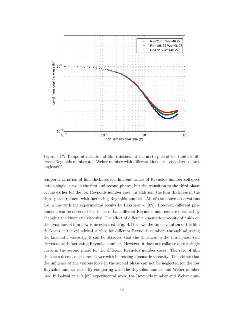
10−2

10−1

100

101

10−1

100


non−

dim

ensi

onal

thic

knes

s (h

*)

Re=217.5,We=46.27Re=108.75,We=46.27Re=72.5,We=46.27

Figure 4.17: Temporal variation of film thickness at the north pole of the tube for dif-ferent Reynolds number and Weber number with different kinematic viscosity; contactangle=60.

temporal variation of film thickness for different values of Reynolds number collapses

onto a single curve in the first and second phases, but the transition to the third phase

occurs earlier for the low Reynolds number case. In addition, the film thickness in the

third phase reduces with increasing Reynolds number. All of the above observations

are in line with the experimental results by Bakshi et al. [89]. However, different phe-

nomena can be observed for the case that different Reynolds numbers are obtained by

changing the kinematic viscosity. The effect of different kinematic viscosity of fluids on

the dynamics of film flow is investigated. Fig. 4.17 shows the time evolution of the film

thickness at the cylindrical surface for different Reynolds numbers through adjusting

the kinematic viscosity. It can be observed that the thickness in the third phase still

decreases with increasing Reynolds number. However, it does not collapse onto a single

curve in the second phase for the different Reynolds number cases. The rate of film

thickness decrease becomes slower with increasing kinematic viscosity. This shows that

the influence of the viscous force in the second phase can not be neglected for the low

Reynolds number case. By comparing with the Reynolds number and Weber number

used in Bakshi et al.’s [89] experimental work, the Reynolds number and Weber num-

58

10−2

10−1

100

101

10−1

100


non−

dim

ensi

onal

thic

knes

s (h

*)

Re=54.375,We=46.128Re=28.275,We=12.51

Figure 4.18: Temporal variation of film thickness at the north pole of the tube for differ-ent Reynolds number and Weber number with Ga=219.5, B0=3.42, contact angle=60.

ber in current numerical work is low. Thus, we call the Reynolds number and Weber

number in the present work as low Reynolds number and low Weber number. Actually,

even for the high Reynolds number case, the influence of the viscous force will appear

at the latter part of the second phase with the inertial force decreasing.

In the experimental study of Bakshi et al. [89], the effect of Reynolds number and

target-to-drop size ratio on the dynamics of film flow is investigated. In the current

simulation study, the influence of gravity and surface tension is investigated as well.

Four simulations divided into two groups with different Galiler number are conducted

to evaluate the effect of gravity on the temporal variatio nof film thickness. The time

evolution of the film thickness at the cylindrical surface with different Reynolds num-

bers at Galilei number 219.5 is shown in Fig. 4.18. The Galilei number is defined as

Ga = gD30/ν

2. It is clear from Fig. 4.18 that the temporal variation of film thickness

for different values of Reynolds number collapses onto a single curve in the first and

second phases, which shows that the influence of gravity can be neglected in the first

and second phases. However, decreasing the kinematic viscosity which corresponds to

an increase in the Galilei number results in a different phenomenon. Fig. 4.19 shows the

temporal variation of the film thickness for different Reynolds number at Galilei num-

59

10−2

10−1

100

101

10−1

100


non−

dim

ensi

onal

thic

knes

s (h

*)

Re=217.5,We=46.27Re=113.1,We=12.51

Figure 4.19: Temporal variation of film thickness at the north pole of the tube for differ-ent Reynolds number and Weber number with Ga=3512, B0=3.42, contact angle=60.

ber 3512. There are different observation comparing the simulation with Ga=219.5,

the effect of gravity on the temporal variation of flim thickness can be evaluated from

these two groups simulations. It can be seen that the influence of gravity on the second

phase appears with increasing Galilei number, while the rate of film thinning becomes

slower for the high Reynolds number case. This is because the influence of gravity is

not considered into the non-dimensional time. From Fig. 4.20, it is clear that when

evolution time t is non-dimensionalized as t⋆ = (tU0+0.5gt2)/D0, the non-dimensional

temporal variation of film thickness for varied Reynolds number collapses onto a single

curve again in the second phase. In order to evaluate the effects of the surface tension

on the dynamics of the film flow process, simulations were conducted for different val-

ues of Weber number while the wettability of solid surface and Reynolds number were

held constant as θ = 91 and 65.25. The gravity force is ignored in this case. In Fig.

4.21, the time evolution of the dynamics of film flow at the cylindrical surface with

varied Weber number is shown. It can be seen that the effect of surface tension can

be neglected in the first and second phases, and the rate of film thickness reduction is

the same. However, the surface tension dominates the inertial force at the end of the

second phase, the transition to the retraction phase occurs earlier for the low Weber

60

10−2

10−1

100

101

10−1

100


non−

dim

ensi

onal

thic

knes

s (h

*)

Re=217.5,We=46.27Re=113.1,We=12.51

Figure 4.20: Temporal variation of film thickness at the north pole of the tube for differ-ent Reynolds number and Weber number with Ga=3512, B0=3.42, contact angle=60

and t⋆ = (tU0 + 0.5gt2)/D0.

number case.

4.2.3 Conclusions

The liquid droplet impact on a curved target has been simulated by a two-dimensional

multi-relaxation time (MRT) lattice Boltzmann model which can tolerate high density

ratios and low viscosity. It is shown that three distinct temporal phases of the film

dynamics can be clearly observed from the simulation results which is consistent with

the experimental study of Bakshi et al. [89]. In the first phase, the non-dimensional film

thickness follows the correlation given by h⋆ = 1−t⋆. The inertia dominates the viscous

forces during the second phase, while the non-dimensional time and film thickness sat-

isfy the relation h⋆ = 0.33/(t⋆)0.9. In the third phase, the film thickness increases under

the action of the interfacial tension and almost reaches a constant value at last due to

the balance of surface tension, viscous force and gravity. The non-dimensional time

and film thickness curve for different values of Reynolds number collapses onto a single

curve in the first and second phases which is in line with the experimental results [89]

when the Reynolds number is controlled by the impact velocity. However, differen-

61

10−2

10−1

100

101

10−1

100


non−

dim

ensi

onal

thic

knes

s (h

*)

Re=65.25,We=10.4Re=65.25,We=16.61

Figure 4.21: Temporal variation of film thickness at the north pole of the tube fordifferent Weber number with contact angle=91 and Re=65.25.

t phenomena can be observed for the case that varied Reynolds number obtained by

changing the kinematic viscosity. It can be seen that the non-dimensional time and film

thickness curves for varied Reynolds number do not collapse onto a single curve in the

second phase, and the rate of film thickness reduction becomes slower with increasing

kinematic viscosity. Therefore, the influence of the viscous force in the second phase can

not be neglected for the low Reynolds number case. The effects of gravity and surface

tension on the dynamics of film flow are also investigated in the current paper. It is

found that the influence of gravity on the second phase appears with increasing Galilei

number, the rate of film thinning becomes slower for the high Reynolds number case

when evolution time is non-dimensionalized as t⋆ = tU0/D0, while the film thickness

reduction rate will remain the same when t⋆ = (tU0+0.5gt2)/D0. From the simulation

results, the effect of surface tension can be neglected at the first and second phases,

while the surface tension dominates the inertial force at the end of the second phase,

the transition to the retraction phase occurs earlier for low Weber numbers.

62

4.3 Dynamics of droplet impact on the cylinder from 45

with horizon

The dynamics of the film flow at the cylinder from 90 with horizon is investigated in

section 4.2. However, the droplet impact onto the side of the cylinder is a more common

phenomenon in industrial equipment. Especially in fixed bed and micro-channels, the

contact line between liquid and solid surface and dynamic behavior of the droplet are

important for the catalytic reaction process. In the following section, the dynamic

behavior of the droplet impact onto a cylindrical surface with its center offset from the

centerline of the tube is shown. The effects of the static contact angle, the Reynolds

number, and the Weber number are investigated. Non-slip wall boundary conditions

have been used on the sphere surface and periodic boundary conditions have been used

on all sides of the domain.

4.3.1 Dynamic behavior of droplet impact onto the side of the tube

Fig. 4.22 shows the snapshots of impact of a liquid droplet landing on a cylinder,

with Reynolds number of 78.3, Weber number of 23.99, Bond number of 0.515, density

ratio ρl/ρg of 580 and contact angle of 107. The droplet falls towards the cylinder

after 50000 lattice time steps, with its center offset by 65 nodes from the centerline

of the tube. The evolution time t is non-dimensionalized as t⋆ = tU0/D0, where t is

the number of time steps elapsed after the drop contacts the surface. Immediately

after impact, the process is similar with the first phase of the droplet impact onto

the cylinder, which is the initial drop deformation period (t⋆=0.078). Then the liquid

droplet spreads out on the surface of the cylinder. Since the impact point of the

droplet is off-set relative to the cylinder, the flow pattern is not symmetrical, and

the majority of the liquid flows downwards rather than towards the upper part of the

tube. The liquid lamella appears as the liquid flows in an upward manner towards

the north pole of the cylinder (t⋆=0.62). The upward motion tendency of the liquid is

captured at t⋆=0.853, where the droplet is pulled down by gravity. As a result of the

inertial force and gravity, the bulk of the droplet continues to flow downwards, being

stretched and growing longer and thinner (t⋆=1.55 and t⋆=3.1). However, with the

bulk of the liquid flowing downwards, the impact and potential energy of the droplet

are dissipated in overcoming the viscous flow effects and in spreading out its surface

area. Hence, the downward stretching is stopped at about t⋆=4.19, after which the

bulk droplet is pulled back onto the cylinder surface under the action of surface tension

force (t⋆=5.897). As the downward liquid flow increases and concentrates at the bottom

of the tube, the liquid droplet is stretched again under the action of the gravity and

inertia (t⋆=8.53). At the same time, the liquid droplet continues to move upwards along

the cylindrical surface after crossing the bottom of cylinder (t⋆=10.862). However, the

63

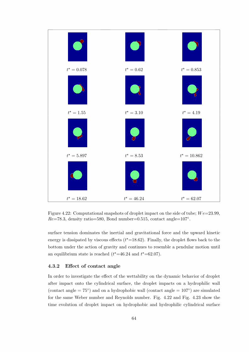
t⋆ = 0.078 t⋆ = 0.62 t⋆ = 0.853

t⋆ = 1.55 t⋆ = 3.10 t⋆ = 4.19

t⋆ = 5.897 t⋆ = 8.53 t⋆ = 10.862

t⋆ = 18.62 t⋆ = 46.24 t⋆ = 62.07

Figure 4.22: Computational snapshots of droplet impact on the side of tube;We=23.99,Re=78.3, density ratio=580, Bond number=0.515, contact angle=107.

surface tension dominates the inertial and gravitational force and the upward kinetic

energy is dissipated by viscous effects (t⋆=18.62). Finally, the droplet flows back to the

bottom under the action of gravity and continues to resemble a pendular motion until

an equilibrium state is reached (t⋆=46.24 and t⋆=62.07).

4.3.2 Effect of contact angle

In order to investigate the effect of the wettability on the dynamic behavior of droplet

after impact onto the cylindrical surface, the droplet impacts on a hydrophilic wall

(contact angle = 75) and on a hydrophobic wall (contact angle = 107) are simulated

for the same Weber number and Reynolds number. Fig. 4.22 and Fig. 4.23 show the

time evolution of droplet impact on hydrophobic and hydrophilic cylindrical surface

64

t⋆ = 0.078 t⋆ = 0.62 t⋆ = 1.55

t⋆ = 5.90 t⋆ = 6.83 t⋆ = 8.53

t⋆ = 15.52 t⋆ = 22.50 t⋆ = 41.18


respectively with density ratio ρl/ρg = 580, Re = 78.3 and We = 23.99. From Fig.

4.23, it can be observed that the contact line between the liquid and the solid surface

is longer for the hydrophilic case than for the hydrophobic one shown in Fig. 4.22. In

the case of hydrophilic wall, the contact line between the solid surface and the liquid is

increasing with the downward liquid flow and breaks up into two parts on the surface

after reaching a maximum contact line. Then the two droplets begin to retract due

to interfacial tension and move towards the bottom of the tube at the same time. At

t⋆=22.5, the two droplets merge together, where an equilibrium shape is reached at

t⋆=41.18. On the other hand, in the case of the hydrophobic wall (Fig. 4.22), there

is a process that the bulk of the droplet is stretched and grows longer and thinner

as it moves along the surface of the tube. After the maximum elongation has been

reached, surface tension dominates the recovery process and the droplet is attached to

the tube wall. However, in the case of the hydrophilic wall (Fig. 4.23), the stretching

and oscillation behavior is not as obvious as that in Fig. 4.22 and the time to reach

the equilibrium state is shorter than for a hydrophobic wall. This is because of the

longer contact line in the hydrophilic wall case. Thus, a higher proportion of the initial

impact energy is dissipated in overcoming the viscous effects and surface tension.

65

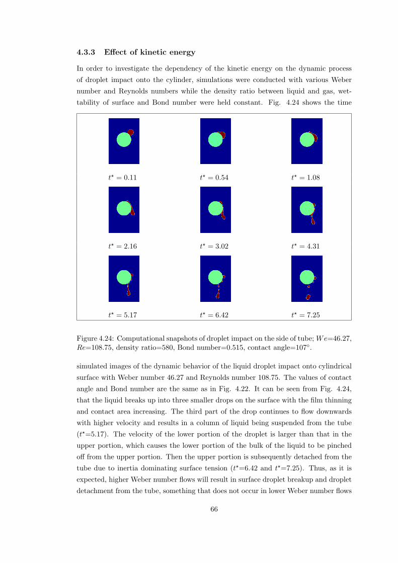
4.3.3 Effect of kinetic energy

In order to investigate the dependency of the kinetic energy on the dynamic process

of droplet impact onto the cylinder, simulations were conducted with various Weber

number and Reynolds numbers while the density ratio between liquid and gas, wet-

tability of surface and Bond number were held constant. Fig. 4.24 shows the time

t⋆ = 0.11 t⋆ = 0.54 t⋆ = 1.08

t⋆ = 2.16 t⋆ = 3.02 t⋆ = 4.31

t⋆ = 5.17 t⋆ = 6.42 t⋆ = 7.25


simulated images of the dynamic behavior of the liquid droplet impact onto cylindrical

surface with Weber number 46.27 and Reynolds number 108.75. The values of contact

angle and Bond number are the same as in Fig. 4.22. It can be seen from Fig. 4.24,

that the liquid breaks up into three smaller drops on the surface with the film thinning

and contact area increasing. The third part of the drop continues to flow downwards

with higher velocity and results in a column of liquid being suspended from the tube

(t⋆=5.17). The velocity of the lower portion of the droplet is larger than that in the

upper portion, which causes the lower portion of the bulk of the liquid to be pinched

off from the upper portion. Then the upper portion is subsequently detached from the

tube due to inertia dominating surface tension (t⋆=6.42 and t⋆=7.25). Thus, as it is

expected, higher Weber number flows will result in surface droplet breakup and droplet

detachment from the tube, something that does not occur in lower Weber number flows

66

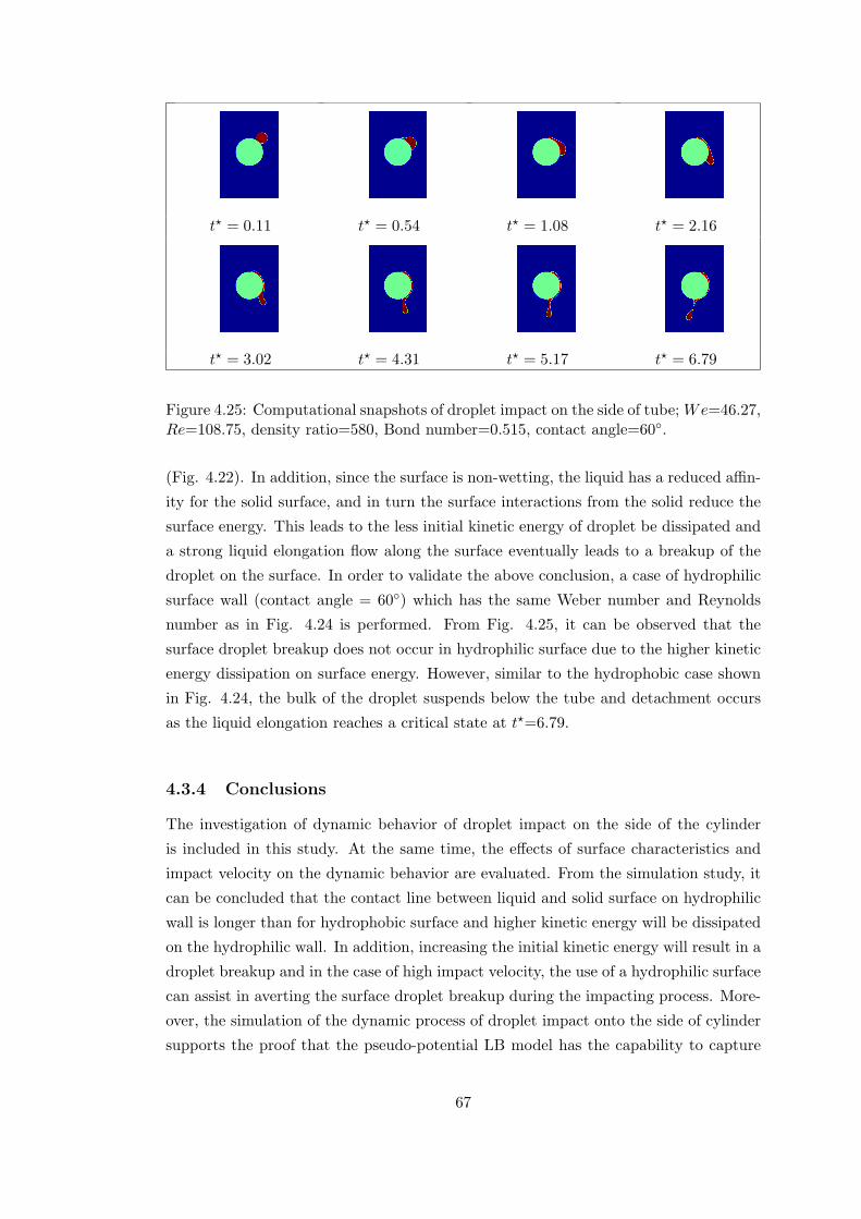
t⋆ = 0.11 t⋆ = 0.54 t⋆ = 1.08 t⋆ = 2.16

t⋆ = 3.02 t⋆ = 4.31 t⋆ = 5.17 t⋆ = 6.79


(Fig. 4.22). In addition, since the surface is non-wetting, the liquid has a reduced affin-

ity for the solid surface, and in turn the surface interactions from the solid reduce the

surface energy. This leads to the less initial kinetic energy of droplet be dissipated and

a strong liquid elongation flow along the surface eventually leads to a breakup of the

droplet on the surface. In order to validate the above conclusion, a case of hydrophilic

surface wall (contact angle = 60) which has the same Weber number and Reynolds

number as in Fig. 4.24 is performed. From Fig. 4.25, it can be observed that the

surface droplet breakup does not occur in hydrophilic surface due to the higher kinetic

energy dissipation on surface energy. However, similar to the hydrophobic case shown

in Fig. 4.24, the bulk of the droplet suspends below the tube and detachment occurs

as the liquid elongation reaches a critical state at t⋆=6.79.

4.3.4 Conclusions

The investigation of dynamic behavior of droplet impact on the side of the cylinder

is included in this study. At the same time, the effects of surface characteristics and

impact velocity on the dynamic behavior are evaluated. From the simulation study, it

can be concluded that the contact line between liquid and solid surface on hydrophilic

wall is longer than for hydrophobic surface and higher kinetic energy will be dissipated

on the hydrophilic wall. In addition, increasing the initial kinetic energy will result in a

droplet breakup and in the case of high impact velocity, the use of a hydrophilic surface

can assist in averting the surface droplet breakup during the impacting process. More-

over, the simulation of the dynamic process of droplet impact onto the side of cylinder

supports the proof that the pseudo-potential LB model has the capability to capture

67

interfacial topological changes like snap-off, which is a very important phenomenon for

the study of the two phase flows in porous media. In the multiphase flow in porous

media, a combination of low Ca values with low saturation of non-wetting phase leads

the appearance of large-ganlion dynamics regime. In the large-ganlion dynamics, in

which the non-wetting phase is totally disconnected in the form of ganglia. The previ-

ous study on the dynamic behavior of non-wetting phase blob depending on the solid

phase with different shape and different wettability is significative for the large-ganlion

dynamics regime in multiphase flow in porous media [110].

68

Chapter 5

Immiscible two-phase flows inartificial porous media

In this chapter, a two-dimensional high density ratio MRT LBM is applied to study the

impact of geometrical properties on the immiscible two-phase flows in porous media.

The porous media structures with different geometrical properties are artificially gener-

ated by a Boolean model based on a random distribution of overlapping ellipses/circles.

Firstly, the capability and accuracy of the high density ratio MRT LBM is evaluated

by simulating the immiscible two-phase co-current flow between two parallel plates.

Then, the immiscible two-phase flow in porous media with different non-wetting phase

saturation depending on the porosity, contour length and connectivity of solid phase in

porous media is addressed.

5.1 Generation of the pore space

In this section, the mathematical framework to quantify and generate the artificial

porous media is introduced. It has been demonstrated that the permeability of sedi-

mentary rock samples is very close to those of Boolean models [143]. Integral geometry

furnishes a suitable family of morphological descriptors, known as Minkowski function-

als [144, 145]. Minkowski functionals are defined for sets Ξ which can be written as

finite unions of compact convex sets Ξi, Ξ =∪ni=1 Ξi. In two dimensions there are

three Minkowski functionals, namely the area A, the contour length C and the Euler

characteristic χ which is the number of connected objects minus the number of enclosed

cavities. The Boolean model is a certain random set Z ⊂ Rd which is used to model

various random geometric patterns. The Boolean process can be realized in two sim-

ple steps: Firstly, points xi (called germs) are scattered randomly and independent of

each other across space according to a stationary Poisson process. Secondly, a random

object Zi which is called a grain is placed in every random point xi. An outcome of

the Boolean model is then generated as the union set of all such germ-grain pairs.

69

Z =∞∪i=1

(Zi + xi). (5.1)

We consider a two-component medium filling a square area S = l2. The global morphol-

ogy of this two-phase complex material is defined by the global Minkowski functionals

per unit area, namely: the solid phase fraction ϕ, the contour length to area ratio L

and the mean value of the Euler characteristic χ. The global morphology can be related

to a Boolean process defined by the morphological measures of the individual grains

Vν(Z) [146,147]

ϕ = 1− e−ρV0 , (5.2)

L

4= e−ρV0(1− e−ρV1), (5.3)

χ = e−ρV0(−1 + 2e−ρV1 − e−2ρV1−ρV2), (5.4)

where ρ is the intensity of the germs in the two dimensional porous media. In other

word, ρ is defined as the number of particles per area. The measures Vν are related to

the Minkowski functionals of individual grains which include the surface area A, the

contour length C and the Euler characteristic χ with a value of 1 for convex sets.

V0 = A/lu3, (5.5)

V1 = C/(4lu2), (5.6)

V2 = χ = 1, (5.7)

where lu is defined as lattice unit. Vν for an ensemble of n grains is given by averaged

values Vν=∑n

j=1 pjVvj , weighted by the probability of their occurrence, pj . In the

current work, the porous media are created by using uniform grains (circles or ellipses)

with same size.

Two groups including four artificial structures each with given values of the specific

global Minkowski functionals are generated. These values can be fixed arbitrarily in

an attempt to compare porous media with different geometric properties. The intrinsic

permeability, global Minkowski functionals, as well as the representative elementary

volume (REV) of the different artificial porous structures are shown in Table. 5.1. The

porous structures obtained with these properties are shown in Fig. 5.1. The Euler

characteristic [148] of the conducting phase (χ0) in Table. 5.1 is distinguished from the

χ, by neglecting the cavities inside the solid clusters which do not contribute to the fluid

70

flow. From these global morphological parameters and Eqs. (5.2-5.4) one can determine

the Minkowski functionals of individual grains with intensity ρ, and consequently the

generation of the artificial structures can be realized by a Boolean process. In some

cases the results of the global Minkowski functionals for a specific realization might

not be exactly the same as the predefined ones. In this case, the code should keep

looping until the structure with similar global Minkowski functionals compared with

the predefined ones is obtained (as shown in the Fig. B.1 in the appendix). The

deviation is controlled at a level of 0.1%.

5.2 Model validation: viscous coupling in co-current flowin a two-dimensional channel

In this section, the immiscible two-phase co-current flow between two parallel plates

to evaluate the accuracy of the MRT LBM is studied. In the immiscible two-phase

flow in porous media, the wetting phase typically attaches to and moves along the

solid surface in the form of films, while the non-wetting phase flows in the center of

the pores. Hence, for the simulation of immiscible two-phase flows in a 2D channel,

the non-wetting phase is sandwiched by the wetting phase which is in contact with the

solid walls as depicted in Fig. 5.2. The degree of saturation of each fluid phase can

be defined as the occupied width of the same fluid divided by the entire width of the

channel. Assuming a Poiseuille-type of flow in the channel, the analytical solutions for

the velocity distribution can be derived by solving the relevant Navier-Stokes equations

[136]:

u(x) =

G

2νwρw(l2 − x2), l′ < |x| < l,

G2νwρw

(l2 − l′2) + G2νnwρnw

(l′2 − x2), 0 < |x| < l′,(5.8)

where νw, νnw, ρw, ρnw are the kinematic viscosities and densities of the wetting non-

wetting phases respectively. The distance from the centreline between the two plates

Structure ϕ L χ0(10−3) κ REV(ϕ) REV(L) REV(χ0)

Group 1

1 0.3744 0.094 -0.536 4.4986 700 700 6002 0.3259 0.0928 -0.534 5.1601 600 600 5003 0.3738 0.0828 -0.537 6.5142 650 600 6004 0.3738 0.094 -0.711 5.6838 700 700 700

Group 2

1 0.3260 0.0988 -0.711 5.0936 500 700 6002 0.2641 0.0984 -0.717 5.5500 700 700 6003 0.3297 0.0844 -0.710 8.3375 600 700 6004 0.3294 0.0980 -0.925 6.6612 650 700 700

Table 5.1: Geometrical properties of the porous structures.

71

Group 1

Structure 1 Structure 2

Structure 3 Structure 4Group 2



Figure 5.1: Porous media corresponding to the properties shown in Table. 5.1.

72

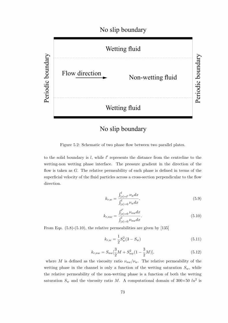
No slip boundary

No slip boundary

Per

iod

ic b

ou

nd

ary

Per

iod

ic b

ou

nd

ary

Wetting fluid

Wetting fluid

Non-wetting fluidFlow direction

Figure 5.2: Schematic of two phase flow between two parallel plates.

to the solid boundary is l, while l′ represents the distance from the centreline to the

wetting-non wetting phase interface. The pressure gradient in the direction of the

flow is taken as G. The relative permeability of each phase is defined in terms of the

superficial velocity of the fluid particles across a cross-section perpendicular to the flow

direction.

kr,w =

∫ l|x|=l′ νwdx∫ l|x|=0 νwdx

. (5.9)

kr,nw =

∫ l′|x|=0 νnwdx∫ l|x|=0 νnwdx

. (5.10)

From Eqs. (5.8)-(5.10), the relative permeabilities are given by [135]

kr,w =1

2S2w(3− Sw) (5.11)

kr,nw = Snw[3

2M + S2

nw(1−3

2M)], (5.12)

where M is defined as the viscosity ratio νnw/νw. The relative permeability of the

wetting phase in the channel is only a function of the wetting saturation Sw, while

the relative permeability of the non-wetting phase is a function of both the wetting

saturation Sw and the viscosity ratio M . A computational domain of 300×50 lu2 is

73

0 0.1 0.2 0.3 0.4 0.5 0.6 0.7 0.8 0.9 10

10

20

30

40

50

60

70

80

90

100

Sw

krnw

0 0.5 10

0.5

1

Sw

krw

LBM simulationsAnalytical solutions

Figure 5.3: Relative permeabilities from LBM model and analytical solutions for thewetting and non-wetting phases in a channel with M ≈ 95 and G = 10−8.

established. One lattice unit is defined as 1 lu. Periodic boundary conditions have been

used at the inlet and outlet of the domain and no-slip wall boundary conditions have

been applied to the top and bottom boundaries of the domain. A constant external

force (G = 5 × 10−8) has been added to each phase and the dynamic viscosity ratio

has been set to 95. The relative permeabilities of the wetting phase and non-wetting

phases from the numerical simulations and the analytical solutions are shown in Fig.

5.3. It can be seen that the simulation results are in good agreement with the results

from the analytical solutions.Therefore, it can be concluded that the MRT LBM model

can accurately predict the flow behaviour and fluid phase relative permeability of two

phase flows in porous media.

5.3 The impact of the geometrical properties of porousmedia on the steady state relative permeabilities onimmiscible two-phase flows

Following the validation of the MRT LBM with the 2D channel flow, the attention is

now focused on the simulation of the immiscible two-phase flow in 2D porous media

74

structures generated with different Minkowski functionals.

The eight artificial porous media are generated as shown in Fig. 5.1. The size of

every computational domain is 800×800 lu2 and the global Minkowski functionals for

each porous medium are given in table. 5.1. Periodic boundary conditions have been

applied in all directions, while no-slip wall boundary conditions have been used on the

solid surfaces. Initially, the wetting and non-wetting phases are uniformly-distributed

in the porous media such that the desired wetting saturation is obtained. Obtaining

different wetting saturation depends on the different choice for uniformly distributed

random variable. The constant external force G is applied on both fluids along the flow

direction. The reasons for using body forces instead of imposing a pressure gradient

as a driving force are that body forces are convenient to implement and also can avoid

capillary pressure gradients and saturation gradients along the flow direction [134].

Since we are interested in the impact of the geometrical properties on the two-phase

flow in porous media, the viscosity ratio between the two phases and the contact angle

are set to M ≈ 103 and θ = 180. The interfacial tension is 0.0044 and the density

ratio has been set to 103. It is assumed that the final steady state is achieved when

the following criterion is satisfied:√∑2x[ux(x, t)− ux(x, t− 10000)]∑

x ux(x)< 10−4, (5.13)

where ux is the macroscopic velocity along the flow direction x. The number of time

steps needed to achieve the steady state increases significantly as the wetting phase

saturation increases. This should be attributed to the wetting phase being less viscous

than the non-wetting phase [135]. In order to estimate the relative permeabilities for

both phases, the steady state superficial velocity of each phase is calculated. The rela-

tive permeabilities for the non-wetting phase and wetting phase are calculated following

the extension of Darcy’s law defined. The intrinsic permeability of a specific porous

medium is determined by Darcy’s law after applying a constant body force for a single

phase and setting the density of the other fluid equal to zero at all void locations.

In the case of immiscible two-phase flows in porous media, the interfacial geometry,

phase distribution patterns and dynamics vary with the fluid saturation. Fig. 5.4 shows

the initial and steady state two-phase distribution patters when the wetting saturations

are Snw = 0.15, Snw = 0.6 and Snw = 0.85. The geometrical properties of the selected

porous medium are ϕ = 0.3744, L = 0.094 and χ = −0.536 × 10−3. From Fig. 5.4,

it can be seen that the wetting phase is continuous, while the non-wetting phase is

disconnected and trapped into big pores as form of blobs when its saturation is 0.15.

For the case of Snw = 0.6, the non-wetting phase is partially connected, while the

wetting phase is still continuous. For the case of Snw = 0.85, the wetting phase covers

the solid surfaces, while the non-wetting phase is fully continuous and flows among

the wetting phase films. For this case, three flow regimes have been identified in the

75

Snw = 0.15

Snw = 0.6

Snw = 0.85

Figure 5.4: The initial co-current flow (left column) and the final steady-state (rightcolumn) two-phase distribution patterns in the cases of Snw = 0.15, Snw = 0.6 andSnw = 0.85 when G = 10−5. The non-wetting phase is indicated by red colour, whileblue colour represents the wetting phase.

previously published literature [133, 138]. A wetting phase Darcy-type regime can be

observed for very low levels of driving forces where the capillary pressure dominates

the viscous forces. At intermediate values of driving forces, which result to a corre-

sponding intermediate capillary number, the effect of viscous force becomes important

and a non-linear two-phase flow regime is observed. Further increase of the driving

force leads to a Darcy-type two-phase regime where the effect of capillary forces can

be neglected. It was observed that an increased viscosity ratio leads to an apparently

increased non-wetting phase relative permeability due to the lubricating effect of the

76

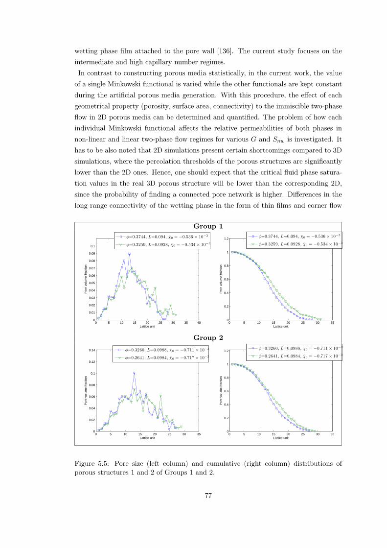
wetting phase film attached to the pore wall [136]. The current study focuses on the

intermediate and high capillary number regimes.

In contrast to constructing porous media statistically, in the current work, the value

of a single Minkowski functional is varied while the other functionals are kept constant

during the artificial porous media generation. With this procedure, the effect of each

geometrical property (porosity, surface area, connectivity) to the immiscible two-phase

flow in 2D porous media can be determined and quantified. The problem of how each

individual Minkowski functional affects the relative permeabilities of both phases in

non-linear and linear two-phase flow regimes for various G and Snw is investigated. It

has to be also noted that 2D simulations present certain shortcomings compared to 3D

simulations, where the percolation thresholds of the porous structures are significantly

lower than the 2D ones. Hence, one should expect that the critical fluid phase satura-

tion values in the real 3D porous structure will be lower than the corresponding 2D,

since the probability of finding a connected pore network is higher. Differences in the

long range connectivity of the wetting phase in the form of thin films and corner flow

Group 1

0 5 10 15 20 25 30 35 400

0.01

0.02

0.03

0.04

0.05

0.06

0.07

0.08

0.09

0.1

Lattice unit

Por

e vo

lum

e fr

actio

n

φ=0.3744, L=0.094, χ0 = −0.536 × 10−3

φ=0.3259, L=0.0928, χ0 = −0.534 × 10−3

0 5 10 15 20 25 30 350

0.2

0.4

0.6

0.8

1

1.2

Lattice unit

Por

e vo

lum

e fr

actio

n

φ=0.3744, L=0.094, χ0 = −0.536 × 10−3

φ=0.3259, L=0.0928, χ0 = −0.534 × 10−3

Group 2

0 5 10 15 20 25 30 350

0.02

0.04

0.06

0.08

0.1

0.12

0.14

Lattice unit

Por

e vo

lum

e fr

actio

n

φ=0.3260, L=0.0988, χ0 = −0.711 × 10−3

φ=0.2641, L=0.0984, χ0 = −0.717 × 10−3

0 5 10 15 20 25 30 350

0.2

0.4

0.6

0.8

1

1.2

Lattice unit

Por

e vo

lum

e fr

actio

n

φ=0.3260, L=0.0988, χ0 = −0.711 × 10−3

φ=0.2641, L=0.0984, χ0 = −0.717 × 10−3

Figure 5.5: Pore size (left column) and cumulative (right column) distributions ofporous structures 1 and 2 of Groups 1 and 2.

77

are also present.

5.3.1 Porosity effects

Geometrical properties

In order to investigate the effect of volume fraction, four artificial porous structures

(1 and 2 in Groups 1 and 2 of Table. 5.1) with different porosity but similar surface

area and connectivity have been generated. Capillary forces in two-phase flow in porous

media depend on the pore size distribution. The pore size distribution can be character-

ized through the computation of the density of the spherical contact distribution [149].

The distance of each pore pixel to the solid phase is determined by inserting discrete

circles with increasing diameters until they touch the solid phase. As a pixel close to

the wall can nevertheless be an element of a large circle centred at another position,

the size of each pore pixel could be computed as the diameter of the largest sphere that

includes this pore pixel. The pore size distributions together with their corresponding

cumulative distributions of the four artificial porous media are given in Fig. 5.5.

The cumulative distributions which are defined as the volume fraction of all pores with

pore size larger or equal to a certain diameter are shown in Fig. 5.5. It is evident that

the density of larger pore sizes is smaller in the structure with low porosity (i.e. larger

solid phase fraction ϕ) than in the structure with high porosity. Comparing structures

1 and 2 in each of group, the latter structure has larger porosity with the same con-

tour length and Euler characteristic as structure 1. Increased porous media porosity,

given that the rest of the Minkowski functionals are similar, indicates an increased

number/fraction of large pore sizes in the medium.

Fully connected flow

In order to verify that the results for the fully connected flow of the non-wetting phase

in porous media are not affected by the different initial uniform distribution of the

two phases, simulations with different random initial uniform distributions have been

carried out. Fig. 5.6 illustrates the average superficial velocity of the non-wetting and

wetting phases in artificial structure 1 as as function of the time-step for two cases with

different initial uniform distributions. It can be observed that the convergent superficial

velocity in both cases is similar. Therefore, the results for fully connected flow in porous

media will not be affected by the different initial uniform distribution of the two phases.

Generally though, the application of uniform distribution cannot reflect either drainage

or imbibition relative permeabilities which are dependent on history [150].

Fig. 5.7 shows the relative permeabilities of the wetting and non-wetting phases as

a function of the applied external force G. A set of simulations with high saturation of

the non-wetting fluid and a dynamic viscosity ratio of 103 in the two different structures

for each of group was performed. The saturation of the non-wetting phase was set up

78

0 2 4 6 8 10 12 14 16

x 104

0

0.2

0.4

0.6

0.8

1

1.2

1.4

1.6

1.8x 10

−4

Time steps

Ave

rage

flui

d ve

loci

ty

vw

case 1

vnw

case 1

vw

case 2

vnw

case 2

Figure 5.6: The average superficial velocity of the non-wetting and wetting phasesas a function of time-step for two cases with different initial uniform distribution;Snw = 0.85, G = 0.5× 10−6 and M ≈ 103.

as 0.85 in group 1, while Snw = 0.9 in group 2. It can be observed that the relative

permeabilities of the non-wetting phase in both media are significantly larger than

unity due to the lubricating effect. The relative permeabilities of the wetting phase are

significantly lower (very close to zero) in both artificial structures, caused by the film

flow around the solid surfaces as well as its low saturation. Figs. 5.7 and 5.8 show that

the flow rate of the non-wetting phase exhibits a non-linear behaviour at low driving

forces through all porous structures. In contrast to that, the relative permeabilities

seem to approach a constant value at higher levels of driving forces. This indicates

that as the driving force increases, the non-wetting phase is able to overcome capillary

pressures associated with the smaller pores in the structure and forms new additional

flow paths. The constant relative permeability for different levels of driving forces

indicates that there are no newly available flow paths in the structure and thus no

further increase is observed. Correlating the previously mentioned observations with

the pore size distribution in the different structures, it becomes evident that between

two porous media, the one with a higher density of small pores will experience a wider

non-linear region. This becomes more clear in the logarithmic plots of Fig. 5.7 as well

as the Capillary number vs driving force plots (Fig. 5.8). The non-linear effects of

the pore size distribution on the correlation of the relative permeability and Capillary

number (Ca = µnwvnw/σ) with the driving forces become more significant at lower

porosities of the porous media. It has to be noted that the pore body to pore throat

ratio is implicitly embedded into the pore volume distribution of each porous medium

and it is not incorporated as an explicit separate parameter in the system.

Fig. 5.7 shows that in the linear region the relative permeability of the non-wetting

79

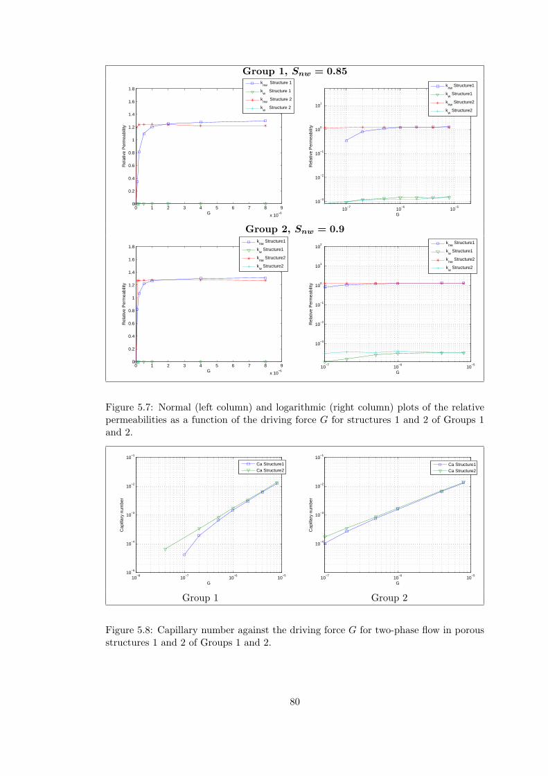
Group 1, Snw = 0.85

0 1 2 3 4 5 6 7 8 9

x 10−6

0

0.2

0.4

0.6

0.8

1

1.2

1.4

1.6

1.8

G

Rel

ativ

e P

erm

eabi

lity

k

nw Structure 1

kw

Structure 1

knw

Structure 2

kw

Structure 2

10−7

10−6

10−5

10−3

10−2

10−1

100

101

G

Rel

ativ

e P

erm

eabi

lity

k

nw Structure1

kw

Structure1

knw

Structure2

kw

Structure2

Group 2, Snw = 0.9

0 1 2 3 4 5 6 7 8 9

x 10−6

0

0.2

0.4

0.6

0.8

1

1.2

1.4

1.6

1.8

G

Rel

ativ

e P

erm

eabi

lity

k

nw Structure1

kw

Structure1

knw

Structure2

kw

Structure2

10−7

10−6

10−5

10−3

10−2

10−1

100

101

102

G

Rel

ativ

e P

erm

eabi

lity

k

nw Structure1

kw

Structure1

knw

Structure2

kw

Structure2

Figure 5.7: Normal (left column) and logarithmic (right column) plots of the relativepermeabilities as a function of the driving force G for structures 1 and 2 of Groups 1and 2.

10−8

10−7

10−6

10−5

10−5

10−4

10−3

10−2

10−1

G

Cap

illar

y nu

mbe

r

Ca Structure1Ca Structure2

10−7

10−6

10−5

10−4

10−3

10−2

10−1

G

Cap

illar

y nu

mbe

r


Group 1 Group 2

Figure 5.8: Capillary number against the driving force G for two-phase flow in porousstructures 1 and 2 of Groups 1 and 2.

80

phase in structure 1 is greater (≈ 1.3) than in structure 2 (≈ 1.2). It is found that in

this region the value of the surface ratios between fluid-fluid, non-wetting fluid-solid and

wetting fluid-solid are similar. The surface ratio between the non-wetting fluid-solid and

fluid-fluid approaches 0.015 for both structures in group 1, while it approaches a value of

0.1 in group 2. Hence, the difference in the values of the relative permeabilities between

structures 1 and 2 in Fig. 5.7 are not a result of the changes between the fluid-fluid, non-

wetting fluid-solid and wetting fluid-solid surface ratios. Fully connected flows of the

non-wetting phase in porous structures can be treated as pipe like flows once the linear

region is reached (i.e the influence of capillary pressure becomes negligible). In this case,

the flow rate of the non-wetting phase increases since the effective pore size decreases

due to the existence of a slip boundary caused by the film of the wetting phase covering

the solid phase. This observation is in great agreement with the research conducted

by Berg et al. [151] regarding pipe flows with slip at the wall. From Fig. 5.8 it can

be observed that the Capillary number presents a non-linear behaviour at low driving

forces in accordance with the non-wetting phase relative permeabilities. Moreover,

the Capillary number versus driving forces relationship approximately collapses onto a

single curve for the two structures at high levels of driving forces. However, the fact

that structure 1 presents similar Capillary numbers with structure 2 in that region, is

attributed to its lower intrinsic permeability, which further enhances capillary pressure

effects.

Partially connected flow

Fig. 5.9 shows the average superficial velocity of the non-wetting and wetting phases as

a function of the time-step for partially connected flow for two different initial uniform

distributions in porous structure 1. The convergent superficial velocity from the two

cases is similar, thus the results of the partially connected flow in porous media will

not be affected by the different initial uniform distribution of the two phases.

The wetting and non-wetting phase relative permeabilities are investigated at in-

termediate saturations (Snw = 0.6) and high levels of driving forces. As in the case of

fully connected flow, the two structures in each group possess the same Minkowski func-

tionals except for the solid phase fraction ϕ. As shown in Fig. 5.10, the non-wetting

phase relative permeability is higher for structure 2 in both groups. In contrast to

the fully connected flow regime, capillary pressure effects in partially connected flow

impose significant restrictions to the motion of the non-wetting phase due to the in-

creased fluid-fluid interfacial line. It becomes evident that the higher fraction of small

pores in the porous structures has a negative impact on the non-wetting phase relative

permeability at large driving forces due to capillary pressure effects. For partially con-

nected flow, the relative permeabilities of the non-wetting phase in structures 1 and 2

81

0 1 2 3 4 5 6

x 105

0

0.2

0.4

0.6

0.8

1

1.2

1.4x 10

−3

Time steps

Ave

rage

flui

d ve

loci

ty

v

w case 1

vnw

case 1

vw

case 2

vnw

case 2

Figure 5.9: The average superficial velocity of the non-wetting and wetting phases asa function of the time-step for two cases with different initial uniform distributions;Snw = 0.6, G = 0.0000005 and M ≈ 103.

0 0.5 1 1.5 2 2.5

x 10−6

0

0.1

0.2

0.3

0.4

0.5

0.6

0.7

0.8

0.9

G

Rel

ativ

e P

erm

eabi

lity

k

nw Structure 1

kw

Structure 1

knw

Structure 2

kw

Structure 2

0 0.5 1 1.5 2 2.5

x 10−6

0

0.1

0.2

0.3

0.4

0.5

0.6

0.7

0.8

0.9

G

Rel

ativ

e P

erm

eabi

lity

k

nw Structure 1

kw

Structure 1

knw

Structure 2

kw

Structure 2

Group 1 Group 2

Figure 5.10: Relative permeabilities as a function of G in porous structures 1 and 2 ofGroups 1 and 2; Snw = 0.6.

of Group 1 are ≈ 0.45 and ≈ 0.5 respectively, whereas for structures 1 and 2 of Group

2 are ≈ 0.5 and ≈ 0.53 respectively. The previously mentioned values are an average

approximation in the studied range of driving forces since all values show an increasing

trend as the driving forces increase. This phenomenon can be also noticed in Fig. 5.11

where the capillary number for structure 2 is higher in both groups for the same level

of driving forces. This comes in contrast with the observations in the fully connected

regime, where the higher fraction of small pores has a significant negative impact only

at low levels of driving forces by widening the non-linear region as described in section

5.3.1. However, at large driving forces, where the formation of new flow paths is nearly

saturated and pressure can be transmitted uninterruptedly through the non-wetting

82

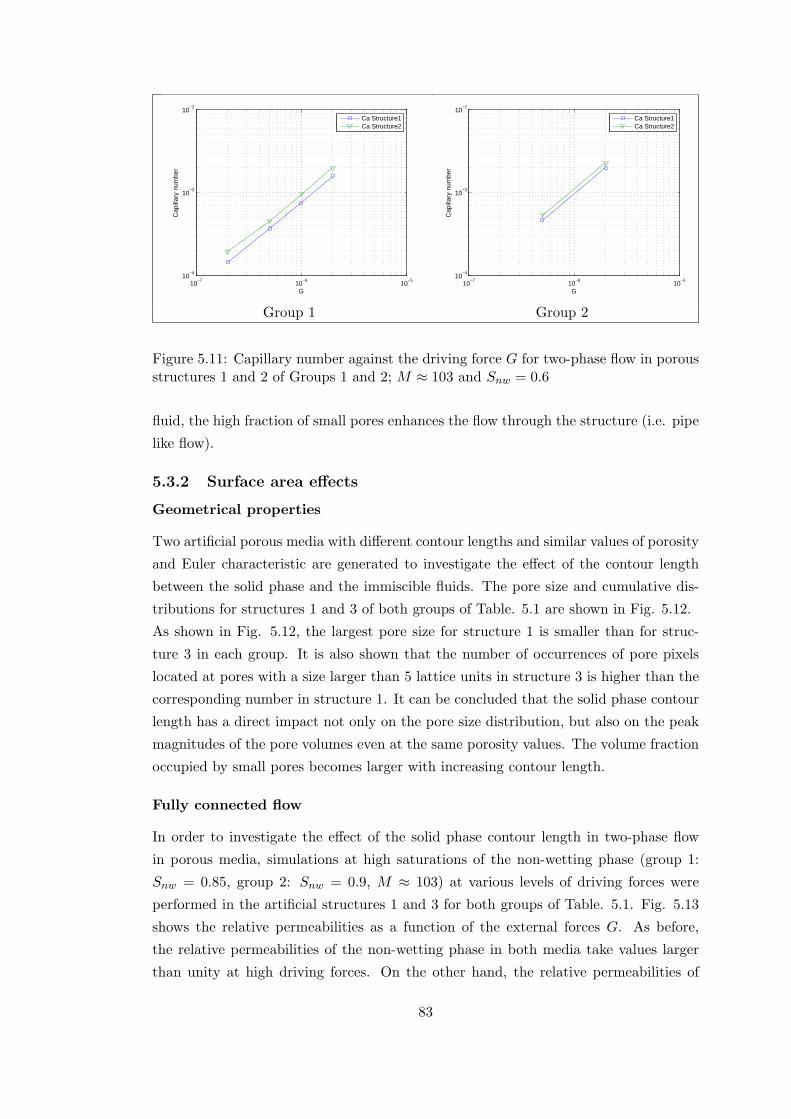
10−7

10−6

10−5

10−4

10−3

10−2

G

Cap

illar

y nu

mbe

r


10−7

10−6

10−5

10−4

10−3

10−2

G

Cap

illar

y nu

mbe

r


Group 1 Group 2

Figure 5.11: Capillary number against the driving force G for two-phase flow in porousstructures 1 and 2 of Groups 1 and 2; M ≈ 103 and Snw = 0.6

fluid, the high fraction of small pores enhances the flow through the structure (i.e. pipe

like flow).

5.3.2 Surface area effects


Two artificial porous media with different contour lengths and similar values of porosity

and Euler characteristic are generated to investigate the effect of the contour length

between the solid phase and the immiscible fluids. The pore size and cumulative dis-

tributions for structures 1 and 3 of both groups of Table. 5.1 are shown in Fig. 5.12.

As shown in Fig. 5.12, the largest pore size for structure 1 is smaller than for struc-

ture 3 in each group. It is also shown that the number of occurrences of pore pixels

located at pores with a size larger than 5 lattice units in structure 3 is higher than the

corresponding number in structure 1. It can be concluded that the solid phase contour

length has a direct impact not only on the pore size distribution, but also on the peak

magnitudes of the pore volumes even at the same porosity values. The volume fraction

occupied by small pores becomes larger with increasing contour length.


In order to investigate the effect of the solid phase contour length in two-phase flow

in porous media, simulations at high saturations of the non-wetting phase (group 1:

Snw = 0.85, group 2: Snw = 0.9, M ≈ 103) at various levels of driving forces were

performed in the artificial structures 1 and 3 for both groups of Table. 5.1. Fig. 5.13

shows the relative permeabilities as a function of the external forces G. As before,

the relative permeabilities of the non-wetting phase in both media take values larger

than unity at high driving forces. On the other hand, the relative permeabilities of

83

Group 1

0 5 10 15 20 25 30 35 400

0.01

0.02

0.03

0.04

0.05

0.06

0.07

0.08

0.09

0.1

Lattice unit

Por

e vo

lum

e fr

actio

n

φ=0.3744, L=0.094, χ0 = −0.536 × 10−3

φ=0.3738, L=0.0828, χ0 = −0.537 × 10−3

0 5 10 15 20 25 30 350

0.2

0.4

0.6

0.8

1

1.2

Lattice unit

Por

e vo

lum

e fr

actio

n

φ=0.3744, L=0.094, χ0 = −0.536 × 10−3

φ=0.3738, L=0.0828, χ0 = −0.537 × 10−3

Group 2

0 5 10 15 20 25 30 350

0.02

0.04

0.06

0.08

0.1

0.12

Lattice unit

Por

e vo

lum

e fr

actio

n

φ=0.3260, L=0.0988, χ0 = −0.711 × 10−3

φ=0.3297, L=0.0844, χ0 = −0.709 × 10−3

0 5 10 15 20 25 30 350

0.2

0.4

0.6

0.8

1

1.2

Lattice unit

Por

e vo

lum

e fr

actio

n

φ=0.3260, L=0.0988, χ0 = −0.711 × 10−3

φ=0.3297, L=0.0844, χ0 = −0.709 × 10−3


the wetting phase take values very close to zero. The flow rate through the structure

becomes linear at high driving forces, while it displays a non-linear behaviour at low

driving forces. It is evident that for structure 3 in each group, a lower pressure gradient

is needed for the flow to reach the linear flow region compared with the two-phase flow

in artificial structure 1. As shown in Fig. 5.12, the number of small pore sizes in

structure 1 is higher than in structure 3. This is an additional indication that the

required external force magnitude to reach the linear flow region is highly dependent

on the pore size distribution. However, the corresponding relative permeabilities of

the non-wetting phase are different from the previous case (i.e. effect of porosity).

For both groups, the relative permeabilities of the non-wetting phase in structure 3 are

greater than the relative permeabilities attained in structure 1 in the linear region. The

discrepancy between the two cases is attributed to the different fluid-fluid interfacial

lengths. Unlike the phase distributions in structures 1 and 2, where both have a similar

fluid-fluid interfacial length (i.e. similar solid phase contour length), the length of

the interface between the two phases in structure 3 is less than the length of the

84

Group 1, Snw = 0.85

0 1 2 3 4 5 6 7 8 9

x 10−6

0

0.2

0.4

0.6

0.8

1

1.2

1.4

1.6

1.8

G

Rel

ativ

e P

erm

eabi

lity

k

nw Structure 1

kw

Structure 1

knw

Structure 3

kw

Structure 3

10−7

10−6

10−5

10−3

10−2

10−1

100

101

G

Rel

ativ

e P

erm

eabi

lity

k

nw Structure1

kw

Structure1

knw

Structure3

kw

Structure3

Group 2, Snw = 0.9

0 1 2 3 4 5 6 7 8 9

x 10−6

0

0.2

0.4

0.6

0.8

1

1.2

1.4

1.6

1.8

G

Rel

ativ

e P

erm

eabi

lity

k

nw Structure1

kw

Structure1

knw

Structure3

kw

Structure3

10−7

10−6

10−5

10−3

10−2

10−1

100

101

102

G

Rel

ativ

e P

erm

eabi

lity

k

nw Structure1

kw

Structure1

knw

Structure3

kw

Structure3


10−8

10−7

10−6

10−5

10−5

10−4

10−3

10−2

10−1

G

Cap

illar

y nu

mbe

r


10−7

10−6

10−5

10−4

10−3

10−2

10−1

G

Cap

illar

y nu

mbe

r


Group 1 Group 2

Figure 5.14: Capillary number as a function of G for two-phase flow in artificial struc-tures 1 and 3 of Groups 1 and 2.

85

interface in structure 1 for both groups. The values of the fluid-fluid interfacial contour

Structure Fully connected flow Partially connected flow

Group 1

1 0.0758 0.04653 0.067 0.0405

Group 2

1 0.0869 0.04923 0.0763 0.0437

Table 5.2: Fluid-fluid interfacial contour lengths per unit pixel.

lengths for the different cases are given in Table. 5.2. It is evident that in the case

of fully connected flow of the non-wetting phase, the contour length of the fluid-fluid

interface depends on the the solid phase perimeter. In this specific case, the fluid-fluid

interfacial contour length in structure 1 of both groups is higher than in structure 3.

This eventually results in an increased viscous momentum exchange length between

the two phases, resulting in an elongated shear flow path (i.e. higher resistance in

the flow). Hence, for a given magnitude of the driving force, an increased fluid-fluid

interfacial contour length in particular porous medium results in a reduced value at its

linear region. Fig. 5.14 displays the relationship between the Capillary number with

driving forces. In accordance with the observations regarding the non-wetting phase

relative permeabilities, a wider non-linear region is observed at low driving forces for

structure 1 which tends to diminish as the driving force is increased. In contrast with

the effects of porosity, it can be observed that the Capillary number does not collapse

onto a single curve when the porous structures possess different solid phase contour

lengths. This indicates that the increased interfacial contour lengths result in lower

non-wetting phase velocities in the porous medium at the same levels of driving forces.


The dependence of the partially connected flow of the non-wetting phase on the perime-

ter of the solid phase in porous media is also investigated. Fig. 5.15 illustrates the rel-

ative permeabilities of the wetting and non-wetting phases under high levels of driving

forces and saturation of 60% for the non-wetting phase. The corresponding fluid-fluid

interfacial lengths for the partially connected flow are also shown in Table. 5.2 and can

be directly compared with the ones for the fully connected flow. The relative permeabil-

ities of the non-wetting phase are higher for structure 3 which has a shorter perimeter

of the solid phase. In addition, the effects of capillary forces and surface tension at

the fluid-fluid interface on the non-wetting phase are more intense in structure 1 since

it possesses a higher fraction of small pores and a longer fluid-fluid interfacial contour

length. This has a direct effect on the relationship of the Capillary number of the

86

different structures with driving forces as it is clearly shown in Fig. 5.16. Hence, it can

be concluded that porous structures of similar porosity and solid phase connectivity

but with lower solid phase contour length will significantly aid the prevalence of the

viscous forces over interfacial tension at the same magnitudes of driving forces.

5.3.3 Connectivity effects


The pore size and the corresponding cumulative distributions for structures 1 and 4 of

groups 1 and 2 are shown in Fig. 5.17. Each pair has similar values of porosity and solid

contour length, however different values of connectivity. It can be seen that the overall

distribution of pore sizes as well as their peak sizes are similar for the two structures

in each group. Looking at the cumulative pore size distribution, it is observed that the

volume fraction of all pores with size larger or equal to 18 lu in structure 1 is greater

than that in structure 4. The large pores in structure 4 are slightly smaller than those

in structure 1. However, within the margin of numerical accuracy on the porosity and

solid line contour length values, it can be concluded that the effect of connectivity on

the pore size distribution can be safely ignored. This result indicates that the two

phase flow observations will exclusively depend on the shape of the structure (i.e. the

topological space).


Fig. 5.18 shows the relative permeabilities of the wetting and non-wetting phases in

structure 1 and 4 of groups 1 and 2 as a function of the driving force G at high non-

wetting fluid saturations (Group 1; Snw = 0.85, Group 2; Snw = 0.9) and dynamic

viscosity ratio M ≈ 103. Neglecting pore size distribution effects (i.e. similar in both

0 0.5 1 1.5 2 2.5

x 10−6

0

0.1

0.2

0.3

0.4

0.5

0.6

0.7

0.8

0.9

G

Rel

ativ

e P

erm

eabi

lity

k

nw Structure 1

kw

Structure 1

knw

Structure 3

kw

Structure 3

0 0.5 1 1.5 2 2.5

x 10−6

0

0.1

0.2

0.3

0.4

0.5

0.6

0.7

0.8

0.9

1

G

Rel

ativ

e P

erm

eabi

lity

k

nw Structure 1

kw

Structure 1

knw

Structure 3

kw

Structure 3

Group 1 Group 2


87

10−7

10−6

10−5

10−4

10−3

10−2

G

Cap

illar

y nu

mbe

r


10−7

10−6

10−5

10−4

10−3

10−2

G

Cap

illar

y nu

mbe

r


Group 1 Group 2


structures from each group), it can be observed that the solid grain connectivity has

a significant impact on the range of the driving force necessary to reach the linear

flow region. More specifically, large values of the Euler characteristics imply a smaller

number of solid clusters formed by isolated or overlapping grains. Considering simi-

lar levels of grains, a small number of solid clusters indicates a higher morphological

complexity clusters in the porous structure. In this case, the larger value of the Euler

characteristic of structure 1 in both groups results in a higher complexity structure as

depicted in the magnified regions shown in Fig. 5.19. In the research of single phase

flow through porous materials, Scholz et al. [152] pointed out that the clusters with

complex morphology which are defined as extended clusters lead to tortuous stream-

lines and thus reduce the permeability of the porous medium. In the case of two-phase

flow in porous media, the extended clusters will give rise to strong resistance to the

non-wetting phase flow. The sharp corners tend to pin interfaces when the non-wetting

phase attempts to penetrate into the pores. Thus, greater driving forces are needed to

reach the linear region for structure 1 in each group, despite that the pore size distri-

bution is similar to structure 4. In contrast to the curve of the non-linear region, the

relative permeabilities in the linear region collapse onto a single curve with increasing

driving forces. Both structures in each of group possess similar pore size distribution

and fluid-fluid interfacial length. It can be concluded that the relative permeabilities

of the non-wetting phase in the linear region depend only on the pore size distribution

of the porous structure rather than the morphological characteristics of the conducting

phase. The influence of the resistance on the non-wetting phase caused by interface

pinning at the corner of external clusters disappear in the linear region as fully con-

nected paths are constructed. As shown in Fig. 5.20 the Capillary number presents a

non-linear behaviour at low driving forces, whereas a linear relationship is observed at

88

Group 1

0 5 10 15 20 25 30 35 400

0.01

0.02

0.03

0.04

0.05

0.06

0.07

0.08

0.09

0.1

Lattice unit

Por

e vo

lum

e fr

actio

n

φ=0.3744, L=0.094, χ0 = −0.536 × 10−3

φ=0.3738, L=0.094, χ0 = −0.711 × 10−3

0 5 10 15 20 25 300

0.2

0.4

0.6

0.8

1

1.2

Lattice unit

Por

e vo

lum

e fr

actio

n

φ=0.3744, L=0.094, χ0 = −0.536 × 10−3

φ=0.3738, L=0.094, χ0 = −0.711 × 10−3

Group 2

0 5 10 15 20 25 30 350

0.02

0.04

0.06

0.08

0.1

0.12

Lattice unit

Por

e vo

lum

e fr

actio

n

φ=0.3260, L=0.0988, χ0 = −0.711 × 10−3

φ=0.3294, L=0.0980, χ0 = −0.925 × 10−3

0 5 10 15 20 25 30 350

0.2

0.4

0.6

0.8

1

1.2

Lattice unit

Por

e vo

lum

e fr

actio

n

φ=0.3260, L=0.0988, χ0 = −0.711 × 10−3

φ=0.3294, L=0.0980, χ0 = −0.925 × 10−3


higher driving forces. Since the relative permeabilities of the two structures collapse

onto a single curve at high driving forces, the deviation in their capillary numbers is

attributed to their corresponding intrinsic permeabilities (i.e. lower for structure 1).

Thus higher driving forces are needed to overcome resistance effects for structures with

higher Euler characteristic, due to their increased morphological complexity which also

lowers their intrinsic permeability.


Simulations have also been performed in structures 1 and 4 of Groups 1 and 2 at

intermediate values of the non-wetting phase saturation (Snw = 0.6 and M ≈ 103)

at high levels of driving forces. As shown in Fig. 5.21, the relative permeabilities of

non-wetting phase are lower in structure 1 for both groups comparing with those in

structure 4 which has a lower χ0. This observation comes in contrast with the fully

connected flow case in which the relative permeabilities collapse onto a single curve at

higher levels of driving forces. The reason for the variance of the relative permeabilities

89

Group 1, Snw = 0.85

0 1 2 3 4 5 6 7 8 9

x 10−6

0

0.2

0.4

0.6

0.8

1

1.2

1.4

1.6

1.8

G

Rel

ativ

e P

erm

eabi

lity

knw

Structure 1

kw

Structure 1

knw

Structure 4

kw

Structure 4

10−7

10−6

10−5

10−3

10−2

10−1

100

101

G

Rel

ativ

e P

erm

eabi

lity

k

nw Structure1

kw

Structure1

knw

Structure4

kw

Structure4

Group 2, Snw = 0.9

0 1 2 3 4 5 6 7 8 9

x 10−6

0

0.2

0.4

0.6

0.8

1

1.2

1.4

1.6

1.8

G

Rel

ativ

e P

erm

eabi

lity

knw

Structure1

kw

Structure1

knw

Structure4

kw

Structure4

10−7

10−6

10−5

10−3

10−2

10−1

100

101

102

G

Rel

ativ

e P

erm

eabi

lity

k

nw Structure1

kw

Structure1

knw

Structure4

kw

Structure4


of the non-wetting phase should be attributed to the existence of extended clusters with

complex morphology in structure 1, since the pore size distribution and solid contour

length are similar. The resistance effect formed by the interface penetration into the

pores constructed with sharp and concave bulge cannot be neglected for the partially

connected flow of the non-wetting phase. Thus, it can be concluded that the relative

permeabilities of the non-wetting phase are higher for the porous media with lower

Euler characteristic of the conducting phase χ0 in the linear region. Ahmadlouydarab

et al. [123] has also observed that sharp corners tend to reduce the knw in relation to

the rounded geometry in the study of two-phase flow through corrugated tubes. This

effect is also reflected in Fig. 5.22, where significantly lower Capillary numbers are

observed for structure 1 due to the combined effects of reduced intrinsic permeability

and non-wetting phase relative permeability.

90

Group 1

Structure 1 Structure 4Group 2


Figure 5.19: Magnified regions of structures 1 and 4 of Groups 1 and 2.

10−8

10−7

10−6

10−5

10−5

10−4

10−3

10−2

10−1

G

Cap

illar

y nu

mbe

r


10−7

10−6

10−5

10−4

10−3

10−2

10−1

G

Cap

illar

y nu

mbe

r


Group 1 Group 2

Figure 5.20: Capillary number against the driving force G for two-phase flow in porousstructures 1 and 4 of Group 1 and 2.

91

0 0.5 1 1.5 2 2.5

x 10−6

0

0.1

0.2

0.3

0.4

0.5

0.6

0.7

0.8

0.9

G

Rel

ativ

e P

erm

eabi

lity

k

nw Structure 1

kw

Structure 1

knw

Structure 4

kw

Structure 4

0 0.5 1 1.5 2 2.5

x 10−6

0

0.1

0.2

0.3

0.4

0.5

0.6

0.7

0.8

0.9

1

G

Rel

ativ

e P

erm

eabi

lity

k

nw Structure 1

kw

Structure 1

knw

Structure 4

kw

Structure 4

Group 1 Group 2


10−7

10−6

10−5

10−4

10−3

10−2

G

Cap

illar

y nu

mbe

r


10−7

10−6

10−5

10−4

10−3

10−2

G

Cap

illar

y nu

mbe

r


Group 1 Group 2


5.3.4 Conclusions

In the present work, the effect of the geometrical properties of 2D porous media on the

relative permeabilities of the non-wetting phase for steady-state immiscible two-phase

flows was investigated. The simulations have been performed for various saturations

of the non-wetting phase using a two-dimensional MRT LBM which can tolerate high

density ratios. Two groups of four artificial porous structures with different Minkowski

functionals were generated with a Boolean model based on a random distribution of

overlapping ellipses/circles. The pore size distributions of each artificial structure was

computed. As expected, a higher fraction of small pores was found in the porous struc-

tures with longer solid phase contour length and higher solid phase fraction. It was

shown that the relative permeability of the non-wetting phase, knw, is much more sen-

92

sitive to the geometric properties of the porous media than the relative permeability of

the wetting phase, kw, for the cases of fully connected flow (Snw = 0.85 and Snw = 0.9)

and partially connected flow (Snw = 0.6).

In the case of fully connected flow, it was found that the flow rate of the non-wetting

fluid and the driving force exhibit highly non-linear relations at low force magnitudes,

while the relative permeabilities are almost constant, something that indicates linear

flows, when the driving forces were increased. It became clear that the external force

needed to reach the linear flow region is highly dependent on the pore size distribution

and solid phase connectivity of the porous structure. As the fraction of small pores

and the Euler characteristic of the conducting phase χ0 increases, the required external

force needed to reach the linear flow region also increases. The non-wetting phase can

be treated as a pipe flow once the linear region is reached, in which case the influence

of capillary pressure becomes negligible. This was found to give rise to increased non-

wetting phase relative permeabilities when porosity is the varied parameter (i.e. higher

with increasing fraction of small pores), whilst they were found to collapse onto a single

curve when the Euler characteristic (i.e. connectivity) was altered. On the other hand,

lower values were observed for porous structures that present larger solid phase contour

length.

At intermediate values of the non-wetting phase saturation (partially connected flow),

it was shown that the relative permeabilities are significantly reduced as the fraction of

small pores, the solid phase/interfacial contour length and Euler characteristic (high-

er morphological complexity) increase. It was observed that capillary pressure effects

become more significant as the fraction of small pores increases. Increased solid phase

contour length gives rise to an increased fluid-fluid interfacial length, which also affects

the relative permeabilities in a negative way. In addition, a larger value of the Euler

characteristic, implying a porous structure with higher morphological complexity, was

found to reduce the values of the non-wetting phase relative permeability. This phe-

nomenon was attributed to the resistance caused by the interface penetration into the

pores shaped with sharp and concave bulges.

93

Chapter 6

Conclusions

6.1 Research summary & conclusions

The primary motivation for the current research is to develop a numerical model that

will be able to simulate multi-phase flows in porous media. Traditional CFD meth-

ods are not suitable for pore scale simulations in porous media due to their inevitable

geometrical complexities. It is also a huge challenge for the continuum models to cap-

ture topological changes in the interface between wetting and non-wetting phase. As

a mesoscopic method, the pseudopotential lattice Boltzmann model has native advan-

tages to treat the multiphase flow in the complex systems without the need to trace

the interfaces between different phases. Hence, the pseudo-potential LB model was

chosen as the numerical model in current research. The research start from studying

the process of droplet impingement onto flat surface and single cylinder as most of

artificial packed porous media is composed of union set of grains with different shapes.

The understanding of the dynamic behaviour of the dynamic behavior of liquid droplet

on the solid phase will be useful and valuable in the efficient design and optimization

for the types of structured packing of artificial porous structure. Especially in large-

ganlion dynamics regime, the non-wetting phase is totally disconnected in the form

of ganglia. The study on the dynamic behavior of non-wetting phase blob depending

on the solid phase with different shape and different wettability is significative. Fur-

thermore, in order to overcome the limitation of low density ratio between two phases

and instability with a relaxation time τ less than 1 for the pesudopotential model,

an improved force scheme is proposed for the three-dimensional multi-relaxation time

pseudopotential lattice Boltzmann model. The investigation on the immiscible two

phases flow in porous media is carried out by the multi-relaxation time (MRT) lattice

Boltzmann model. Two groups including eight artificial structures with given values of

the specific global Minkowski functionals are generated by a Boolean model based on

a random distribution of overlapping ellipases/circles. An additional MATLAB code is

developed to measure the pore size distributions for every porous structure. The effects

of geometrical properties of pore structure on the pore size distribution, as well as the

94

immiscible two-phase flows in porous media are revealed.

As it is mentioned in the chapter 2, most of the LBM studies on the droplet impinge-

ment onto solid surfaces and the immiscible two phases in porous media are limited

to low density ratio between two phases and instability with a relaxation time τ less

than 1. In addition, previous numerical works on the immiscible two phase flows in

porous media focus on the influence of the properties of liquids, such as capillary num-

ber, wetting angle and viscosity ratio, while few previous publications revealed the

effect of the packed structure on the multi-phase flow in porous media. The under-

standing of the effect of the properties of porous structures on the multi-phase flow

has great significance for industrial operations such as, enhanced oil recovery, geolog-

ic CO2 sequestration, catalytic processing in trick bed reactors. In current study, the

process of liquid droplet impact onto solid phase is investigated by 2-dimensional and 3-

dimensional lattice Boltzmann model which can tolerate the high density ratio between

two phases. The simulations support the information about the influence of Reynolds

number, Weber number, Ohnesorge number and the target-to-drop size ratio on the

impingement process. Moreover, an improved force scheme is proposed for the three-

dimensional MRT pseudopotential lattice Boltzmann model which can simulate the

multi-phase flow with large density ratio and low kinematic viscosity. The immiscible

two phases flow in porous media is simulated by a MRT lattice Boltzmann model. The

properties of porous structures is decided by the global Minkowski functionals which

can be controlled by a Boolean process. So, the pore structure is characterized and the

relation between relative permeability with pore structure is constructed.

The study showed in section 3.3, that in order to handle multi-phase flows at high densi-

ty ratios and low viscosities in a efficient way, an improved force scheme is proposed for

the three-dimensional multi-relaxation time (MRT) pseudopotential lattice Boltzmann

model based on the improved force scheme for the single relaxation time (SRT) pseu-

dopotential lattice Botlzmann model [60] and the Chapman-Enskog analysis [141]. The

3-dimensional MRT lattice Boltzmann model is validated through following aspects.

• The satisfaction of Laplace law.

• Thermodynamic consistency verified.

• The contact angle is a linear function of fluid-solid interaction potential parameter

Gw.

In the chapter 4, lattice Boltzmann model was applied on studying the impaction of

a liquid droplet on a dry flat surface and a cylindrical surface for a liquid-gas system

with large density ratio and low viscosity. The dynamics behavior of droplet impact

on a flat surface was discussed in section 4.1.

• There are four phases during the droplet impact on flat surface including the

95

kinematic phase, the spreading phase, the relaxation phase and the equilibrium

phase.

• In the kinematic phase, the droplet spread factor depend on the non-dimensional

time rather than the physical properties.

• In the spreading phase, the maximum spread factor increases with increasing

inertia.

• In the spreading phase, the maximum diameter and the time needed to reach the

maximum diameter are decided by the inertia for given Ohnesorge number.

• In the relaxation phase, the wettability of the surface becomes significant.

• In the equilibrium phase, the time reaches the equilibrium shape is controlled by

Weber and Reynolds number.

In section 4.2. the liquid droplet impact on a cylindrical surface were modeled. It is

found:

• There are three distinct temporal phases of the film dynamics.

• In the first phase, the non-dimensional film thickness follows the correlation given

by h⋆ = 1− t⋆.

• In the second phase, the inertia dominates the viscous forces, the non-dimensional

film thickness follows the correlation given by h⋆ = 0.33/(t⋆)0.9.

• In the third phase, the film thickness increases under the action of the interfacial

tension and reaches a constant value at last.

• In the first and second phases, the non-dimensional time and film thickness curve

collapses onto a single curve for different values of Reynolds number.

• In the second phase, the influence of the viscous force cannot be neglected for the

low Reynolds number case.

• In the second phase, the influence of gravity appears with increasing Galilei num-

ber.

• In the first phase, the effect of surface tension can be neglected, while the surface

tension dominates the inertial force at the end of the second phase.

In section 4.3, the dynamics behaviour for the droplet impact onto the cylinder from 45

with horizon was modeled, as well as the effects of surface characteristics and impact

velocity on the dynamic behavior were investigated. From the simulation study, it can

be concluded that:

96

• The contact line between liquid and solid surface on hydrophilic wall is longer

than for hydrophobic surface.

• The kinetic energy dissipated on hydrophilic wall is higher than on hydrophobic

surface.

• Droplet breakup will happen as increasing the initial kinetic energy.

• Hydrophilic surface can assist in averting the surface droplet breakup during the

impacting process.

The study on the immiscible tow-phase flows in porous media was shown in chapter

5. The studies were focused on the effect of properties of porous structure on relative

permeability for both two phases which can be of great help to the for industrial oper-

ations such as, enhanced oil recovery, geologic CO2 sequestration, catalytic processing

in trick bed reactors. In the case of high value of the non-wetting phase saturation, it

is found:

• The flow rate of the non-wetting fluid and the driving force exhibit highly non-

linear relations at low force at low magnitude of driving force, the relative per-

meabilities will reach a constant value with increasing driving force.

• The external force needed to reach the linear flow region is dependent on the pore

size distribution and solid phase connectivity of the porous structure.

• In linear region, then non-wetting phase relative permeabilities increase with in-

creasing fraction of small pores of porous media.

• In the linear region, the non-wetting phase relative permeabilities are not depen-

dent on the Euler characteristic.

In the case of intermediate values of the non-wetting phase saturation, it is found that:

• The relative permeabilities are significantly reduced as the fraction of small pores,

the solid phase/interfacial contour length and Euler characteristic increase.

6.2 Recommendations for future work

The current study was focused on the development of a lattice Boltzmann model to

simulate the droplet impact onto solid substrates, as well as the immiscible two-phase

flows in porous media. Due to the demands of the current research, a great amount of

time was spent on the development of code and model. A substantial amount of work

is still needed for a complete description of immiscible two phase flows. Additional

recommendations for future work are proposed from three different aspects.

Firstly, it is important to continue the development of the current lattice Boltzmann

97

model to include heat transfer and reaction between different phases in order to make

the model applicable to the chemical process equipment such as trickle beds reactor etc.

It is required that the researcher has a good knowledge of lattice Boltzmann model and

appropriate experience in numerical analysis or applied mathematics to achieve this

objective.

Also, several studies could be performed regarding the effect of properties of porous

structures on the immiscible two-phase flows in porous media. The work should include

the effect of geometrical properties characterized by global Minkowski functionals on

the process of displacement and imbibition, as well as the cluster size distribution for

the non-wetting phase. The final objective is a quantitative relation between pore struc-

ture and relative permeability which could be achieved for two-phase flow in porous

media. The difficulty of such a task is that advanced knowledge of two-phase flow

in porous media is required by the researcher as well as the mathematical framework

to generated the various porous structures. In addition, our current work about the

two-phase flow in porous media was limited in 2-dimensional studies due to the much

higher computational cost of a 3-dimensional study. We expect that the current study

be extended to three dimensions.

Finally, there is a recommendation for further development of the code. It is required

to speed up the simulations, especially for the two-phase flow in porous media with

large three dimensional domain. The code should be further developed based on par-

allel computing or GPU accelerated computing. Advanced programming abilities are

necessary for the researcher and the cooperation with computer science students may

be a necessity.

98

Appendix A

Derivation of there-dimensionalmacroscopic equations for D3Q19model

Introducing the expansions [153]

fα(x+ eαδt, t+ δt) =

∞∑n=0

βn

n!Dntnfα(x, t), (A.1)

Dtn ≡ ∂tn + eαk∂k, (A.2)

fα =

∞∑n=0

βnf (n)α , (A.3)

∂t =∞∑n=0

βn∂tn , (A.4)

where β = δt, Appling the expansions in Eq. (A.1) to Eq. (A.4) to Eq. (3.35), the

following relationship for the zeroth, first and second-order of the parameter β are

obtained:

f (0)α = f eqα , (A.5)

Dt0f(0)α = −

∑β

Ωαβf(1)β + Sα, (A.6)

∂t1f(0)α +Dt0(Iαβ −

1

2Ω)f

(1)β = −

∑β

Ωαβf(2)β , (A.7)

These can be easily converted into moment space by multiplying Eqs. A.5-A.7 by the

transformation matrix M ,

m(0) = meq, (A.8)

(∂t0 + ζi∂i)m(0) = −Λm(1) + S (A.9)

∂t1m(0) + (∂t0 + ζi∂i)(I − 1

2Λ)m(1) = −Λm(2), (A.10)

99

where ζ = MeαiM−1. The components of the first-order equations in moment space

are obtained from Eq. A.9, Eq. 3.43 and Eq. 3.54,

∂t0ρ+ ∂xjx + ∂yjy + ∂zjz = 0, (A.11)

∂t0(−11ρ+19j2x + j2y + j2z

ρ)+∂x(

5

3jx)+∂y(

5

3jy)+∂z(

5

3jz) = −s2e(1)+38(u·F )+

114ϵF 2

ψ2(1/s2 − 0.5),

(A.12)

∂t0(3ρ−11

2

j2x + j2y + j2zρ

) + ∂x(−2

3jx) + ∂y(−2

3jy) + ∂z(−2

3jz) = −s3e(1)

2 − 11(u ·F ),

(A.13)

∂t0(jx) + ∂x(1

3ρ+

jx2

ρ) + ∂y(

jxjyρ

) + ∂z(jxjzρ

) = Fx, (A.14)

∂t0(−2

3jx)+ ∂x(−2

9ρ+

−4jx2 + 5jy

2 + 5jz2

6ρ)+ ∂y(

jxjyρ

)+ ∂z(jxjzρ

) = −s5qx(1)−2

3Fx,

(A.15)

∂t0(jy) + ∂x(jxjyρ

) + ∂y(1

3ρ+

jy2

ρ) + ∂z(

jyjzρ

) = Fy, (A.16)

∂t0(−2

3jy) + ∂x(

jxjyρ

) + ∂y(−2

9ρ+

5jx2 − 4jy

2 + 5jz2

6ρ) + ∂z(

jyjzρ

) = −s7qy(1) −2

3Fy,

(A.17)

∂t0(jz) + ∂x(jxjzρ

) + ∂y(jyjzρ

) + ∂z(1

3ρ+

jz2

ρ) = Fz, (A.18)

∂t0(−2

3jz) + ∂x(

jxjzρ

) + ∂y(jyjzρ

) + ∂z(−2

9ρ+

5jx2 + 5jy

2 − 4jz2

6ρ) = −s9qz(1) −

2

3Fz,

(A.19)

∂t0(2jx

2 − jy2 − jz

2

ρ)+∂x(

4

3jx)+∂y(−

2

3jy)+∂z(−

2

3jz) = −s103pxx(1)+2(2uxFx−uyFy−uzFz),

(A.20)

∂t0(−1

2

2jx2 − jy

2 − jz2

ρ)+∂x(−2

3jx)+∂y(

1

3jy)+∂z(

1

3jz) = −s113πxx(1)+2(−2uxFx+uyFy+uzFz),

(A.21)

∂t0(jy

2 − jz2

ρ) + ∂y(

2

3jy) + ∂z(−2

3jz) = −s12pww(1) + 2(uyFy − uzFz), (A.22)

∂t0(−1

2

jy2 − jz

2

ρ) + ∂y(−1

3jy) + ∂z(

1

3jz) = −s13πww(1) + (−uyFy + uzFz), (A.23)

∂t0(jxjyρ

) + ∂x(1

3jy) + ∂y(

1

3jx) = −s14pxy(1) + (uyFx + uxFy), (A.24)

∂t0(jyjzρ

) + ∂y(1

3jz) + ∂z(

1

3jy) = −s15pyz(1) + (uzFy + uyFz), (A.25)

∂t0(jxjzρ

) + ∂x(1

3jz) + ∂z(

1

3jx) = −s16pxz(1) + (uzFx + uxFz), (A.26)

∂x(1

2

jy2 − jz

2

ρ) + ∂y(

jxjyρ

) + ∂z(−jxjzρ

) = −s17mx(1), (A.27)

∂x(−jxjyρ

) + ∂y(1

2

−jx2 + jz2

ρ) + ∂z(

jyjzρ

) = −s18my(1), (A.28)

100

∂x(−jxjzρ

) + ∂y(−jyjzρ

) + ∂z(1

2

jx2 − jy

2

ρ) = −s19mz

(1), (A.29)

The second order equations of the conserved moments from the components of the

second-order equations in moment space are derived from Eq. (A.10),

∂t1ρ = 0, (A.30)

∂t1(jx)+∂x[1

57(1−1

2s2)e

(1)+1

3(1−1

2s10)3pxx

(1)]+∂y[(1−1

2s14)pxy

(1)]+∂z[(1−1

2s16)pxz

(1)] = 0,

(A.31)

∂t1(jy) + ∂x[(1− 1

2s14)pxy

(1)] + ∂y[1

57(1− 1

2s2)e

(1) − 1

6(1− 1

2s10)3pxx

(1) +1

2(1− 1

2s12)pww

(1)]

+∂z[(1− 1

2s15)pyz

(1)] = 0,

(A.32)

∂t1(jz) + ∂x[(1− 1

2s16)pxz

(1)] + ∂y[(1− 1

2s15)pyz

(1)]

+∂z[1

57(1− 1

2s2)e

(1) − 1

6(1− 1

2s10)3pxx

(1) − 1

2(1− 1

2s12)pww

(1)] = 0,

(A.33)

Combining the first and second order equations for the conserved moments by using

∂t = ∂t0 + β∂t1 , i.e. Eqs. (A.11) and (A.30), Eqs. (A.14) and (A.31), Eqs. (A.16) and

(A.32) and Eqs. (A.18) and (A.33), we get

∂tρ+ ∂xjx + ∂yjy + ∂zjz = 0, (A.34)

∂t(jx) + ∂x[(1

3ρ+

jx2

ρ) +

1

57β(1− 1

2s2)e

(1) + β(1− 1

2s10)pxx

(1)]

+∂y[jxjyρ

+ β(1− 1

2s14)pxy

(1)] + ∂z[ + β(1− 1

2s16)pxz

(1)] = Fx,

(A.35)

∂t(jy) + ∂x[jxjyρ

+ β(1− 1

2s14)pxy

(1)] + ∂y[(1

3ρ+

jy2

ρ) +

1

57β(1− 1

2s2)e

(1) − 1

2(1− 1

2s10)βpxx

(1)

+1

2(1− 1

2s12)βpww

(1)] + ∂z[β(1− 1

2s15)pyz

(1) +jyjzρ

] = Fy,

(A.36)

∂t(jz) + ∂x[jxjzρ

+ β(1− 1

2s16)pxz

(1)] + ∂y[jyjzρ

+ β(1− 1

2s15)pyz

(1)]

+∂z[(1

3ρ+

jz2

ρ) +

1

57β(1− 1

2s2)e

(1) − 1

2(1− 1

2s10)pxx

(1) − 1

2β(1− 1

2s12)pww

(1)] = Fz,

(A.37)

pxx(1), pww

(1), pxy(1), pxz

(1), pyz(1), e(1) are unknown and can be obtained from Eq.

(A.12), Eq. (A.20), Eq. (A.22), Eq. (A.24), Eq. (A.25) and Eq. (A.26),

e(1) =1

s2[−38

3(∂xjx + ∂yjy + ∂zjz) +

114ϵF 2

ψ2(1/s2 − 0.5)], (A.38)

pxx(1) =

1

3s10[−2

3(2∂xjx − ∂yjy − ∂zjz)], (A.39)

101

pww(1) =

1

s12[−2

3(∂yjy − ∂zjz)], (A.40)

pxy(1) =

1

s14[−1

3(∂xjy) + ∂yjx], (A.41)

pyz(1) =

1

s15[−1

3(∂yjz + ∂zjy)], (A.42)

pxz(1) =

1

s16[−1

3(∂xjz + ∂zjx)], (A.43)

where F = −Gc2[Ψ∇Ψ + 16c

2Ψ∇(∇2Ψ) + · · · ], Using Eqs. (A.38) to (A.43) in Eqs.

(A.31) to (A.33), the momentum equations simplify to

∂tρ+ ∂x(ρvx) + ∂y(ρvy) + ∂z(ρvz) = 0, (A.44)

∂t(ρvx) + ∂x(ρvxvx) + ∂y(ρvxvy) + ∂z(ρvxvz) = −∂x(ρc2s) + Fx + ∂x(2ν[∂x(ρvx)−1

3∇ · (ρv)]

+ξ∇ · (ρv)) + ∂y(ν(∂x(ρvy) + ∂y(ρvx))) + ∂z(ν(∂x(ρvz) + ∂z(ρvx)))

−2G2c4ϵ∂x(|∇Ψ|2) +O(∂5),

(A.45)

∂t(ρvy) + ∂x(ρvxvy) + ∂y(ρvyvy) + ∂z(ρvyvz) = −∂y(ρc2s) + Fy + ∂x(ν(∂x(ρvy) + ∂y(ρvx)))

+∂y(2ν[∂y(ρvy)−1

3∇ · (ρv)] + ξ∇ · (ρv)) + ∂z(ν(∂y(ρvz) + ∂z(ρvy)))

−2G2c4ϵ∂y(|∇Ψ|2) +O(∂5),

(A.46)

∂t(ρvz) + ∂x(ρvxvz) + ∂y(ρvyvz) + ∂z(ρvzvz) = −∂z(ρc2s) + Fz + ∂x(ν(∂x(ρvz) + ∂z(ρvx)))

+∂y(ν(∂y(ρvz) + ∂z(ρvy))) + ∂z(2ν[∂z(ρvz −1

3∇ · (ρv))] + ξ∇ · (ρv))

−2G2c4ϵ∂z(|∇Ψ|2) +O(∂5),

(A.47)

The bulk viscosity and kinematic viscosity in the multi-relaxation-time lattice Boltz-

mann model are given by

ξ =2

9(1

s2− 1

2), (A.48)

and

ν =1

3(1

sβ− 1

2), β = 10, 12, 14, 15, 16. (A.49)

102

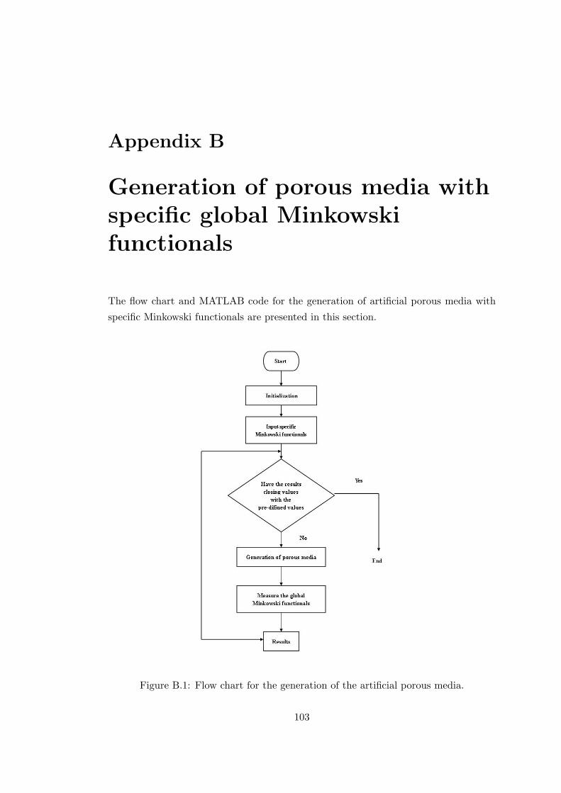
Appendix B

Generation of porous media withspecific global Minkowskifunctionals

The flow chart and MATLAB code for the generation of artificial porous media with

specific Minkowski functionals are presented in this section.

Figure B.1: Flow chart for the generation of the artificial porous media.

103

tic

clear

edge=0; % initial value of contour length

fraction=0; % initial value of solid fraction

solid clusters=0; % initial value of solid cluster

while abs(solid clusters-343)>3 % specify the solid clusters for the artificial porous media

edge=0;

fraction=0;

while abs(edge-0.0236)>0.00005 ∥ abs(fraction-0.324)>0.0002 % specify the contour length and

solid fraction for the artificial porous media

lambda=0.0018; % the value of intensity of germs

sizeW=800; % domain size

noEvents=lambda*sizeW*sizeW;

noEvents=round(noEvents);

coords=rand(noEvents,2).*sizeW;

coords=round(coords);

obst=zeros(sizeW,sizeW);

[lx,ly]=size(obst);

[x,y] = meshgrid(1:lx,1:ly);

random angle=rand(noEvents).*180;

random angle=round(random angle);

a=14; % length of long axis of ellipse

b=5; % length of short axis of ellipse

grain number=size(coords,1);

for i=1:grain number

center x=coords(i,1);

center y=coords(i,2);

Liquid=((x-center x).*cos(random angle(i))+(y-center y).*sin(random angle(i))).

∧2/a∧2+((y-center y).*cos(random angle(i))-(x-center x).*sin(random angle(i))).∧2/b∧2<=1;

bbRegion Liquid=find(Liquid);

obst(bbRegion Liquid)=1;

end

surface area=0;

for i=1:lx

for j=1:ly

if obst(i,j)==1

surface area=surface area+1;

end

end

104

end

fraction=surface area/sizeW/sizeW;

obst fluid=zeros(lx,ly);

for i=1:lx

for j=1:ly

if obst(i,j)==0

obst fluid(i,j)=1;

end

end

end

bbRegion solid=find(obst);

size solid=length(bbRegion solid);

nearest boundary=zeros(lx,ly);

obst2=circshift(obst fluid,[1,0]);


obst4=circshift(obst fluid,[-1,0]);

obst5=circshift(obst fluid,[0,-1]);


obst7=circshift(obst fluid,[-1,1]);

obst8=circshift(obst fluid,[-1,-1]);

obst9=circshift(obst fluid,[1,-1]);

for i=1:size solid

if

obst2(bbRegion solid(i))==1∥obst3(bbRegion solid(i))==1∥obst4(bbRegion solid(i))==1∥obst5(bbRegion solid(i))==1∥obst6(bbRegion solid(i))==1∥obst7(bbRegion solid(i))==1∥obst8(bbRegion solid(i))==1∥obst9(bbRegion solid(i))==1

nearest boundary(bbRegion solid(i))=1;

end

end

bbRegion nearest=find(nearest boundary);

size nearest boundary=length(bbRegion nearest);

side number=zeros(lx,ly);

side number(bbRegion nearest)=4;

obst2=circshift(obst,[-1,0]);

obst3=circshift(obst,[0,1]);


obst5=circshift(obst,[0,-1]);

for i=1:size nearest boundary

if obst2(bbRegion nearest(i))==1

105

side number(bbRegion nearest(i))=side number(bbRegion nearest(i))-1;

end



end



end



end

end

sum=0;

for i=1:size nearest boundary

sum=sum+side number(bbRegion nearest(i));

end

edge=sum/sizeW/sizeW/4;

end

save(’800 0.32 0.0235 343.mat’,’obst’);

mark index=1;

while size solid =0

mark index=mark index+1;

obst(bbRegion solid(1))=mark index;

bbRegion solid(1)=0;

bbRegion solid(find(bbRegion solid==0))=[];


k=0;

k1=1;

while k1-k>0







obst8=circshift(obst,[-1,-1]);


k=k1;

for i=1:size solid

106

if obst2(bbRegion solid(i))==mark index ∥ obst3(bbRegion solid(i))==mark index ∥obst4(bbRegion solid(i))==mark index

∥ obst5(bbRegion solid(i))==mark index ∥ obst6(bbRegion solid(i))==mark index ∥obst7(bbRegion solid(i))==mark index ∥ obst8(bbRegion solid(i))==mark index ∥obst9(bbRegion solid(i))==mark index∥obst(bbRegion solid(i))=mark index;

bbRegion solid(i)=0;

k1=k1+1;

end

end

bbRegion solid(find(bbRegion solid==0))=[];


end

end

solid clusters=mark index-1;

end

toc

107

Appendix C

Measure of pore size distributionin artificial porous media

The flow chart and MATLAB code for the measure of the pore size distribution in the

artificial porous media are presented in this section.

Figure C.1: Flow chart for determining the pore size distribution in the artificial porousmedia.

108

clear

load(’obst.mat’);

lx=2400;

ly=2400;

lx1=800;

ly1=800;


number=0;

index x same porous=zeros(1,lx1*ly1);

index y same porous=zeros(1,lx1*ly1);

for i=1:lx1

for j=1:ly1

if obst(i,j) =1

number=number+1;

index x same porous(1,number)=i;

index y same porous(1,number)=j;

end

end

end

distance=zeros(1,number);

str1=’/home/duo/duo/revision paper4/group 2/800 0.3260 0.0247 456/pore distance/mat’;

for index=1:number

str2=[str1 num2str(index) ’.mat’];

center x=index x same porous(1,index)+lx1;

center y=index y same porous(1,index)+ly1;

small domain=zeros(lx1,ly1);

for radius=1:100

sphere=(x-center y).∧2+(y-center x).∧2<=radius.∧2;[index x bigdomain,index y bigdomain]=find(sphere);

number sphere=size(index x bigdomain,1);

index x smalldomain=zeros(1,number sphere);

index y smalldomain=zeros(1,number sphere);

for i=1:number sphere

if index x bigdomain(i)>=(lx1+1) && index x bigdomain(i)<=(2*lx1)

index x smalldomain(i)=index x bigdomain(i)-lx1;

end

if index y bigdomain(i)>=(ly1+1) && index y bigdomain(i)¡=(2*ly1)

index y smalldomain(i)=index y bigdomain(i)-ly1;

end

109

if index x bigdomain(i)>(2*lx1)

index x smalldomain(i)=index x bigdomain(i)-2*lx1;

end

if index y bigdomain(i)>(2*ly1)

index y smalldomain(i)=index y bigdomain(i)-2*ly1;

end

if index x bigdomain(i)<(lx1+1)

index x smalldomain(i)=index x bigdomain(i);

end

if index y bigdomain(i)<(ly1+1)

index y smalldomain(i)=index y bigdomain(i);

end

end

k=0;

for i=1:number sphere

if obst(index x smalldomain(i),index y smalldomain(i))==1

k=1;

break

end

end

if k==1

distance(1,index)=radius;

bbRegion sphere=sub2ind(size(small domain),index x smalldomain,index y smalldomain);

break

end

end

save(str2,’bbRegion sphere’,’radius’);

end

str3=’/home/duo/duo/revision paper4/group 2/800 0.3260 0.0247 456/distance’;

save(str3,’distance’);

maximum=max(distance);

minimum=min(distance);

lx=800;

ly=800;


number=0;

for i=1:lx

for j=1:ly

if obst(i,j) =1

110

number=number+1;

obst(i,j)=1;

else

obst(i,j)=0;

end

end

end

bbRegion pore space=find(obst);

for index=1:number

str2=[str1 num2str(index) ’.mat’];

load(str2);

str4=[’bbRegion radius’,num2str(radius)];

k=exist(eval(’str4’),’var’);

if k==0

eval([’bbRegion radius’,num2str(radius),’=’,’bbRegion sphere’,’;’])

else

eval([’bbRegion radius’,num2str(radius),’=’,’[’,’bbRegion radius’,num2str(radius),’;’,’bbRegion sphere’,’]’,’;’])

end

end

bbRegion pore space=find(obst);

pore volume fraction=zeros(1,maximum);

for i=1:number

k=0;

for j=maximum:-1:minimum

k=any(eval([’any’,’(’,’bbRegion radius’,num2str(j),’==’,’bbRegion pore space(i)’,’)’]));

if k==1

pore volume fraction(j)=pore volume fraction(j)+1; break

end

end

end

pore volume fraction=pore volume fraction/number;

pore size=(minimum:1:maximum);

plot(pore size,pore volume fraction,’-s’);

pore size cumulative distribution=zeros(1,maximum-minimum+1);

for i=1:1:maximum-minimum+1

pore size cumulative distribution(i)=sum(pore volume fraction(i:maximum-minimum+1));

end

plot(pore size,pore size cumulative distribution,’-s’);

111

List of Publications

1. D. Zhang and K. Papadikis and S. Gu. 2 Dimensional simulation of the hy-

drodeoxygenation of bio-oil in a trickle bed reactor. World Academy of Science,

Engineering and Technology, 71:1617-1624, 2012.

2. D. Zhang and K. Papadikis and S. Gu. Application of a high density ratio lattice-

Boltzmann model for the droplet impingement on flat and spherical surfaces. Int.

J. Therm. Sci, 84:75-85, 2014.

3. D. Zhang and K. Papadikis and S. Gu. Investigations on the droplet impact

onto a spherical surface with a high density ratio multi-relaxation time lattice-

Boltzmann model. Commun. Comput. Phys, 16:892-912, 2014.

4. D. Zhang and K. Papadikis and S. Gu. Three-dimensional multi-relaxation time

lattice-Boltzmann model for the drop impact on a dry surface at large density

ratio. Int. J. Multiphase. Flow, 64:11-18, 2014.

5. D. Zhang and K. Papadikis and S. Gu. A lattice Boltzmann study on the im-

pact of the geometrical properties of porous media on the steady state relative

permeabilities on two-phase immiscible flows. Adv. Water Resour. (Submitted).

112

Bibliography

[1] A. L. Yarin. Drop impact dynamics: splashing, spreading, receding, bouncing...,.

Annu. Rev. Fluid Mech, 38:159–192, 2006.

[2] R. Rioboo and C. Tropea. Outcomes from a drop impact on solid surfaces.

Atomization and Sprays, 11:155–165, 2001.

[3] H. Darcy. Les Fontaines Publiques da la Ville de Dijon. Dalmont, Paris, 1856.

[4] M. Muskat and M. H. Meres. The flow of heterogeneous fluids through porous

media. Physics, 7:346–363, 1936.

[5] J. F. Zhang. Lattice boltzmann method for microfluidics: models and applica-

tions. Microfluid. Nanofluid, 10:1–28, 2011.

[6] A. A. Mohamad. Lattice Boltzmann Method. Springer, 2011.

[7] E. D. Sloan A. K. Sum M. R. Walsh, C. A. Koh and D. T. Wu. Microsecond

simuations of spontaneous methane hydrate nucleation and growth. Science,

326(5956):1095–1098, 2009.

[8] Y. Kobayashi S. Kiyoshima J. Shimizu, E. Ohmura and H. Eda. Molecular dy-

namics simulation of flattening process of a high-temperature, high-speed droplet-

influence of impact parameters. JTTEE5, 16:722–728, 2007.

[9] G. Besold, I. Vattulainen, M. Kartunen, and J. M. Polson. Towards betterr

integrators for dissipative particle dynamics simulations. Phys Rev E, 62:R7611–

R7614, 2000.

[10] E. Monaco. Multiphase lattice Boltzmann simulation of microfluidics. PhD thesis,

University of Southampton, School of Engineering Sciences, 2009.

[11] S. Wolfram. Theory and applications of cellular automata. World Scientific Pub-

lication, 1986.

[12] S. Succi. The lattice Boltzmann equation. Oxford University Press, Oxford, 2001.

[13] G. R. McNamara and G. Zanetti. Use of the boltzmann equation to simulate

lattice-gas automata. Phys. Rev. Lett, 61(20):2332–2335, 1988.

113

[14] F. Higuera and J. Jimenez. Boltzmann approach to lattice gas simulations. Eu-

rophys. Lett., 9(7):663–668, 1989.

[15] F. Higuera, S. Succi, and R. Benzi. Lattice gas dynamics with enhanced collison.

Europhys. Lett., 9(4):345–349, 1989.

[16] Y. H. Qian, D. d’Humieres, and P. Lallemand. Lattice-bgk models for navier-

stokes equation. Europhys. Lett., 17(6):479–484, 1992.

[17] P. Yuan and L. Schaefer. Equations of state in a lattice boltzmann model. Phys.

Fluids, 18:042101, 2006.

[18] D. A. Drew and S. L. Passman. Theory of multicomponent fluids. Springer, New

York, 1999.

[19] M. Ishii and T. Hibiki. Thermo-fluid dynamics of two-phase flow. Springer, New

York, 2006.

[20] C. T. Crowe, M. Sommerfeld, and Y. Tsuji. Multiphase flows with droplets and

particles. CRC Press, Boca Raton, 1998.

[21] S. Unverdi and G. Tryggvason. A front-tracking method for viscous, incompress-

ible, multi-fluid flows. J. Comput. Phys, 100:25–37, 1992.

[22] M. Sussman, P. Smereka, and S. Osher. A level set approach for computing

solutions to incompressible wwo-phase flow. J. Comput. Phys, 114:146–159, 1994.

[23] D. M. Anderson, G. B. McFadden, and A. A. Wheeler. Diffuse-interface methods

in fluid mechanics. Annu. Rev. Fluid Mech, 30:139–165, 1998.

[24] D. Jacqmin. Calculation of two-phase navier-stokes flows using phase-field mod-

eling. J. Comput. Phys, 155(1):96–127, 1999.

[25] S. W. J. Welch. Local simulation of two-phase flows including interface tracking

with mass transfer. J. Comput. Phys, 121(1):142–154, 1995.

[26] H. H. Hu, N. A. Patankar, and M. Y. Zhu. Direct numerical simulations of fluid-

solid systems using the arbitrary lagrangian-eulerian technique. J. Comput. Phys,

169(2):427–462, 2001.

[27] S. Quan and D. P. Schmidt. A moving mesh interface tracking method for 3d

incompressible two-phase flows. J. Comput. Phys, 221(2):761–780, 2007.

[28] S. Ganesan and L. Tobiska. An accurate finite element scheme with moving

meshes for computing 3d-axisymmetric interface flows. Int. J. Numer. Methods.

Fluids, 57(2):119–138, 2008.

114

[29] S. Quan, J. Lou, and D. P. Schmidt. Modeling merging and breakup in the moving

mesh interface tracking method for multiphase flow simulations. J. Comput. Phys,

228(7):2660–2675, 2009.

[30] R. Scardovelli and S. Zaleski. Direct numerical simulation of free-surface and

interfacial flow. Ann. Rev. Fluid Mech, 31:67–603, 1999.

[31] S. Osher and R. P. Fedkiw. Level set methods: an overview and some recent

results. J. Comput. Phy, 169:463–502, 2001.

[32] J. A. Sethian and P. Smereka. Level set methods for fluid interfaces. Ann. Rev.

Fluid Mech, 35:341–372, 2003.

[33] G. Tryggvason, B. Bunner, A. Esmaeeli, D. Juric, N. Al-Rawahi, W. Tauber,

J. Han, S. Nas, and Y. J. Jan. A front-tracking method for the computations of

multiphase flow. J. Comput. Phys, 169:708–759, 2001.

[34] C. W. Hirt and B. D. Nichols. Volume of fluid (vof) methods for the dynamics

of free boundaries. J. Comput. Phys, 39:201–225, 1981.

[35] M. Rudman. Volume-tracking methods for interfacial flow calculations. Int. J.

Numer. Methods. Fluids, 24(7):671–691, 1997.

[36] S. T. Zalesak. Fully multidimensional flux-corrected transport algorthms for flu-

ids. J. Comput. Phys, 31(3):335–362, 1979.

[37] T. Bonometti and J. Magnaudet. An interface-capturing method for imcom-

pressible two-phase flows. validation and application to bubble dynamics. Int. J.

Multiph. Flow, 33(2):109–133, 2007.

[38] E. Olsson and G. Kreiss. A conservative level set method for two phase flow. J.

Comput. Phys, 210(1):225–246, 2005.

[39] E. Olsson, G. Kreiss, and S. Zahedi. A conservative level set method for two

phase flow ii. J. Comput. Phys, 225:785–807, 2007.

[40] V. E. Badalassi, H. D. Ceniceros, and S. Banerjee. Computation of multiphase

systems with phase field models. J. Comput. Phys, 190:371–397, 2003.

[41] S. Chen and G. Doolen. Lattice boltzmann method for fluid flows. Annu. Rev.

Fluid Mech, 30:329–364, 1998.

[42] S. Hou, X. Shan, Q. Zou, G. D. Doolen, and W. Soll. Evaluation of two lattice

boltzmann models for multiphase flows. J. Comput. Phys, 138:695–713, 1997.

[43] D. H. Rothman and J. M. Keller. Immiscible cellular-automation fluids. J. Stat.

Phys, 52:1119–1129, 1988.

115

[44] A. K. Gunstensen, D. H. Rothman, S. Zaleski, and G. L. G. Zanetti. Lattice

boltzmann model of immiscible fluids. Phys. Rev. A, 43:4320–4327, 1991.

[45] X. Shan and H. Chen. Simulation of nonideal gases and liquid-gas phase transi-

tions by the lattice boltzmann equation. Phys. Rev. E, 49:2941–2948, 1994.

[46] M. R. Swift, E. Orlandini, W. R. Osborn, and J. M. Yeomans. Lattice boltzmann

simulations of liquid-gas and binary fluid systems. Phys. Rev. E, 54:5041–5052,

1996.

[47] X. He, S. Chen, and R. Zhang. A lattice boltzmann scheme for incopressible

multiphase flow and its application in simulation of rayleigh-taylor instbility. J.

Comput. Phys, 152:642–663, 1999.

[48] L. O. E. Santos, P. C. Facin, and P. C. Philippi. Lattice-boltzmann model based

on field mediators for immiscible fluids. Phys. Rev. E, 68:056302, 2003.

[49] D. Grunau, S. Chen, and K. Eggert. A lattice boltzmann model for multiphase

fluid flows. Physics of Fluids A: Fluid Dynamics, 5(10):2557–2562, 1993.

[50] S. V. Lishchuk, C. M. Care, and I. Halliday. Lattice boltzmann algorithm for

surface tension with greatly reduced microcurrents. Physical review E, 67:036701,

2003.

[51] M. Latva-Kokko and D. H. Rothman. Diffusion properties of gradient-based

lattice boltzmann models of immiscible fluids. Physical review E, 71:056702,

2005.

[52] T. Reis and T. N. Phillips. Lattice boltzmann model for simulating immiscible

two-phase flows. J. Phys. A. Math. Theor, 40:4033–4053, 2007.

[53] H. Liu and A. J. Valocchi. Three-dimensional lattice boltzmann model for im-

miscible two-phase flow simulations. Phys. Rev. E, 85:046309, 2012.

[54] S. Leclaire, M. Reggio, and J. Y. Trepanier. Numerical evaluation of two recol-

oring operators for an immiscible two-phase flow lattice boltzmann model. Appl.

Math. Model, 36:2237–2252, 2012.

[55] S. Leclaire, N. Pellerin, M. Reggio, and J-Y. Trepanier. Unsteady immiscible mul-

tiphase flow validation of a multiple-relaxation-time lattice boltzmann method.

J. Phys. A: Math. Theor., 47:105501, 2014.

[56] X. Shan. Analysis and reduction of the spurious current in a class of multiphase

lattice boltzmann models. Phys. Rev. E, 73:047701, 2006.

116

[57] M. Sbragaglia, R. Benzi, L. Biferale, S. Succi, K. Sugiyama, and F. Toschi. Gen-

eralized lattice boltzmann method with multirange pseudopotential. Phys. Rev.

E, 75:026702, 2007.

[58] Z. L. Guo, C. G. Zheng, and B. C. Shi. Discrete lattice effects on the forcing

term in the lattice boltzmann method. Phys. Rev. E, 65:046308, 2002.

[59] A. L. Kupershtokh, D. A. Medvedev, and D. I. Karpov. On equations of state in

a lattice boltzmann method. Comput. Math. Appl, 58:965–974, 2009.

[60] Q. Li, K. H. Luo, and X. J. Li. Forcing scheme in pseudopotential lattice boltz-

mann model multiphase flows. Phys. Rev. E, 86:016709, 2012.

[61] S. Mukherjee and J. Abraham. A pressure-evolution-based multi-relaxation-time

high-density-ratio two-phase lattice-boltzmann model. Comput. Fluids, 36:1149–

1158, 2007.

[62] A. Fakhari and T. Lee. Multiple-relaxation-time lattice boltzmann method for

immiscible fluids at high reynolds numbers. Phys. Rev. E, 87:023304, 2013.

[63] Q. Li, K. H. Luo, and X. J. Li. Lattice boltzmann modeling of multiphase flows

at large density ratio with an improved pseudopotential model. Phys. Rev. E,

87:053301, 2013.

[64] A. N. kalarakis, V. N. Burganos, and A. C. Payatakes. Galilean-invariant

lattice-boltzmann simulation of liquid-vapor interface dyanmics. Phys. Rev. E,

65:056702, 2002.

[65] A. N. kalarakis, V. N. Burganos, and A. C. Payatakes. Three-dimensional lattice-

boltzmann model of van der waals fluids. Phys. Rev. E, 67:016702, 2003.

[66] T. Inamuro, T. Ogata, S. Tajima, and N. Konishi. A lattice boltzmann method

for incompressible two-phase flows with large density differences. J. Comput.

Phys, 198:628–644, 2004.

[67] Y. Y. Yan and Y. Q. Zu. A lattice boltzmann method for incompressible two-

phase flows on partial wetting surface with large density ratio. J. Comput. Phys,

227:763–775, 2007.

[68] A. J. Briant, P. Papatzacos, and J. M. Yeomans. Lattice boltzmann simulations

of contact line motion in a liquid-gas system. Philos. Trans. R. Soc. Lond. A,

360:485–495, 2002.

[69] X. Y. He, X. W. Shan, and G. D. Doolen. Discrete boltzmann equation model

for nonideal gases. Phys. Rev. E, 57:R13(R), 1998.

117

[70] T. Lee and L. Lin. Lattice boltzmann simulations of micron-scale drop impact

on dry surfaces. J. Comput. Phys, 229:8045–8063, 2010.

[71] T. Lee and C. L. Lin. A stable discretization of the lattice boltzmann equation

for simulaton of incompressible two-phase flows at high density ratio. J. Comput.

Phys, 206:16–47, 2005.

[72] H. W. Zheng, C. Shu, and Y. T. Chew. Lattice boltzmann interface capturing

method for incompressible flows. Phys. Rev. E, 72:056705, 2005.

[73] H. W. Zheng, C. Shu, and Y. T. Chew. A lattice boltzmann model for multiphase

flows with large density ratio. J. Comput. Phys, 218:353–371, 2006.

[74] A. Fakhari and M. H. Rahimian. Phase-field modeling by the method of lattice

boltzmann equations. Phys. Rev. E, 81:036707, 2010.

[75] J. Y. Shao, C. Shu, H. B. Huang, and Y. T. Chew. Free-energy-based lattice

boltzmann model for the simulation of multiphase flows with density contrast.

Phys. Rev. E, 89:033309, 2014.

[76] Y. Q. Zu and S. He. Phase-field-based lattice boltzmann model for incompressible

binary fluid systems with density and viscosity contrasts. Phys. Rev. E, 87:043301,

2013.

[77] H. Liang, B. C .Shi, Z. L. Guo, and Z. H. Chai. Phase-field-based multiple-

relaxation-time lattice boltzmann model for incompressible multiphase flows.

Phys. Rev. E, 89:053320, 2014.

[78] M. Rein. Phenomena of liquid drop impact on solid and liquid surface. Fluid.

Dyn. Res, 12:61–93, 1993.

[79] R. Rioboo, M. Marengo, and C. Tropea. Time evolution of liquid drop impact

onto solid, dry surfaces. Exp. Fluids, 33:112–124, 2002.

[80] A. Asai, M. Shioya, S. Hirasawa, and T. Okazaki. Impact of an ink drop on paper.

J. Imaging Sci. Technol, 37:205–207, 1993.

[81] B. L. Scheller and D. W. Bousfield. Newtonian drop impact with a solid surface.

AIChE J, 41:1357–1367, 1995.

[82] S. Chandra and C. T. Avedesian. On the collision of a droplet with a solid surface.

Proc. R. Soc. Lond. Ser. A, 432:13, 1991.

[83] M. Pasandideh-Fard, Y. M. Qiao, S. Chandra, and J. Mostaghimi. Capillary

effects during droplet impact on a solid surface. Phys. Fluids, 8:650–660, 1996.

118

[84] T. Mao, D. C. S. Kuhn, and H. Tran. Spread and rebound of liquid droplets upon

impact on flat surfaces. AIChE J, 43:2169–2179, 1997.

[85] I. V. Roisman, R. Rioboo, and C. Tropea. Normal impact of a liquid drop on

a dry surface: model for spreading and receding. Proc. R. Soc. Lond. Ser. A,

458:1411–1430, 2002.

[86] H. Dong, W. W. Carr, D. G. Bucknall, and J. F. Morris. Temporally-resolved

inkjet drop impaction on surfaces. AIChE J, 53:2606–2617, 2007.

[87] L. S. Hung and S. C. Yao. Experimental investigation of the impaction of water

droplets on cylindrical objects. Int. J. Multiphase Flow, 25:1545–1559, 1999.

[88] Y. Hardalupas, A. M. K. P. Taylor, and J. H. Wilkins. Experimental investigation

of submillimeter droplet impingement onto spherical surfaces. Int. J. Heat Fluid

Flow, 20:477–485, 1999.

[89] S. Bakshi, L. V. Roisman, and C. Tropea. Investigations on the impact of a drop

onto a small spherical target. Phys. Fluids, 19:032102, 2007.

[90] S. Mukherjee. Simulation of Wall Impinging Drops. PhD thesis, School of Me-

chanical Engineering, Purdue University, 2006.

[91] G. Trapaga and J. Szekely. Mathematical modeling of the isothermal impingement

of liquid droplets in spraying processes. Metall. Trans. B, 22:901–914, 1991.

[92] M. Bussmann and S. Afkhami. Drop impact simualtion with a velocity-dependent

contact angle. Chem. Eng. Sci, 62:7214, 2007.

[93] M. Pasandideh-Fard, M. Bussmann, S. Chandra, and J. Mostaghimi. Simulating

droplet impact on a substrate of arbitrary shape. Atomization Spray, 11:397–414,

2001.

[94] H. Liu, S. Krishnan, S. Marella, and H. S. Udaykumar. Sharp interface cartesian

grid method ii: A technique for simulating droplet interactions with surfaces of

arbitrary shape. J. Comput. Phys, 210:32–54, 2005.

[95] Y. Ge and L. S. Fan. Droplet-particle collison mechanics with film-boiling evap-

oration. J. Fluid Mech, 573:331–337, 2007.

[96] A. Gupta and R. Kumar. Droplet impingement and breakup on a dry surface.

Comput. Fluids, 39:1696–1703, 2010.

[97] A. Gupta and R. Kumar. Two-dimensional lattice boltzmann model for droplet

impingement and breakup in low density ratio liquids. Comm. Comp. Phys,

10:767–784, 2011.

119

[98] S. Q. Shen, F. F. Bi, and Y. L. Guo. Simulation of droplets impact on curved

surfaces with lattice boltzmann method. Int. J. Heat Mass Trans, 55:6938–6943,

2012.

[99] Y. Bachmat and J. Bear. Macroscopic modelling of transport phenomena in

porous media. 1: The continuum approach. Transp. Porous Media, 1(3):213–240,

1986.

[100] S. Whitaker. Flow in porous media i: A theoretical derivation of darcy’s law.

Transp. Porous Media, 1:3–25, 1986.

[101] W. G. Gray. Thermodynamics and constitutive theory for multiphase porous-

media flow considering internal geometric constraints. Adv. Water Resour,

22(5):521–547, 1999.

[102] C. M. Marle. On macroscopic equations governing multiphase flow with diffusion

and chemical reactions in porous media. Int. J. Eng. Sci, 20(5):643–662, 1982.

[103] F. Kalaydjian. A macroscopic description of multiphase flow in porous media

involving spacetime evolution of fluid/fluid interface. Transp. Porous Media,

2:537–552, 1987.

[104] F. Kalaydjian. Origin and quantification of coupling between relative permeabil-

ities for two-phase flows in porous media. Transp. Porous Media, 5(3):215–229,

1990.

[105] W. G. Gray and C. T. Miller. Thermodynamically constrained averaging theory

approach for modeling of flow in porous media: 1. motivation and overview. Adv.

Water Resour, 28(2):161–180, 2005.

[106] C. T. Miller and W. G. Gray. Thermodynamically constrained averaging theory

approach for modeling flow and transport phenomena in porous medium systems:

2. foundation. Adv. Water Resour, 28:181–202, 2005.

[107] A. Jackson, C. Miller, and W. Gray. Thermodynamically constrained averaging

theory approach for modeling flow and transport phenomena in porous medium

systerms: 6. two-fluid-phase flow. Adv. Water Resour, 32(6):779–795, 2009.

[108] S. M. Hassanizadeh and W. G. Gray. Mechanics and thermodynamics of multi-

phase flow in porous media including interphase boundaries. Adv. Water Resour,

13(4):169–186, 1990.

[109] R. Bowen. Compressible porous media models by use of the theory of mixtures.

Int. J. Eng. Sci, 20(6):697–735, 1982.

120

[110] D. G. Avraam and A. C. Payatakes. Flow regimes and relative permeabilities

during steady-state two-phase flow in porous media. J. Fluid Mech, 293:207–236,

1995a.

[111] D. G. Avraam and A. C. Payatakes. Generalized relative permeability coefficients

during steady-state two-phase flow in porous media, and correlation with the flow

mechanisms. Trans. Porous Media, 20:135–168, 1995b.

[112] D. G. Avraam and A. C. Payatakes. Flow mechanics, relative permeabilities, and

coupling effects in steady-state two-phase flow through porous media, the case of

strong wettability. Ind. Eng. Chem. Res, 38:778–786, 1999.

[113] C. D. Tsakiroglou, D. G. Avraam, and A. C. Payatakes. Transient and steady-

state relative permeabilities from two-phase flow experiments in planar pore net-

works. Adv. Water Resour, 30:1981–1992, 2007.

[114] C. D. Tsakiroglou, M. Theodoropoulou, and V. Karoutsos. Non-equilibrium

capillary pressure and relative permeability curves of porous media. AIChE J,

49:2472–2486, 2003.

[115] C. D. Tsakiroglou, M. Theodoropoulou, and V. Karoutsos. Determination of the

effective transport coefficients of pore networks from transient immiscible and

miscible displacement experiments. Water Resour. Res, 41(2):W02014, 2005.

[116] C. A. Aggelopoulos and C. D. Tsakiroglou. The effect of micro-heterogeneity and

capillary number on capillary pressure and relative permeability curves of soils.

Geoderma, 148:25–34, 2008.

[117] B. Ataie-Ashtiani, S. M. Hassanizadeh, M. Oostrom, M. A. Celia, and M. D.

White. Effective parameters for two-phase flow in a porous medium with peridic

heterogeneities. J. Contam. Hydrol, 49:87–109, 2001.

[118] B. Ataie-Ashtiani, S. M. Hassanizadeh, and M. A. Celia. Effects of heterogeneities

on capillary pressure-saturation-relative permeability relationships. J. Contam.

Hydrol, 56:175–192, 2002.

[119] B. Ataie-Ashtiani, S. M. Hassanizadeh, O. Oung, F. A. Weststrate, and A. Bezui-

jen. Numerical modelling of two-phase flow in a geocentrifuge. Environ. Modell.

Softw, 18:231–241, 2003.

[120] D. B. Das, S. M. Hassanizadeh, B. E. Rotter, and B. Ataie-ashtiani. A numerical

study of micro-heterogeneity effects on upscaled properties of two-phase flow in

porous media. Trans. Porous. Media, 56:329–350, 2004.

121

[121] D. B. Das, M. Mirzaei, and N. Widdows. Non-uniqueness in capillary pressure-

saturation-relative permeability relationships for two-phase flow in porous medi-

a: interplay between intensity and distribution of random micro-heterogeneities.

Chem. Eng. Sci, 61:6786–6803, 2006.

[122] A. Q. Raeini, M. J. Blunt, and B. Bijeljic. Modelling two-phase flow in porous

media at the pore scale using volume-of-fluid method. J. Comput. Phys, 231:5653–

5668, 2012.

[123] M. Ahmadlouydarab, Z. S. Liu, and J. J. Feng. Relative permeability for two-

phase flow through corrugated tubes as model porous media. Int. J. Multiph.

Flow, 47:85–93, 2012.

[124] H. A. Amiri and A. Hamouda. Evaluation of level set and phase field methods

in modeling two phase flow with viscosity contrast through dual-permeability

porous medium. Int. J. Multiph. Flow, 52:22–34, 2013.

[125] M. J. Blunt, M. D. Jackson, M. Piri, and P. H. Valvatne. Detailed physics,

predictive capabilities and macroscopic consequences for pore-network models of

multiphase flow. Adv. Water Resour, 25:1069–1089, 2002.

[126] D. B. Slin and T. W. Patzek. Pore space morphology analysis using maximal

inscribed spheres. Physica A: Statistical and Theoretical Physics, 371(2):336–

360, 2006.

[127] Z. Jiang, K. Wu, G. Couples, M. I. J. vanDijke, K. S. Sorbie, and J .Ma. Efficient

extraction of networks from three-dimensional porous media. Water Resour. Res,

43:W12S03, 2007.

[128] V. Joekar-Niasar, S. M. Hassanizadeh, and A. Leijnse. Insights into the rela-

tionships among capillary pressure, saturation, interfacial area and relative per-

meability using pore-network modeling. Transp. Porous Media, 74(2):201–219,

2008.

[129] V. Joekar-Niasar, S. M. Hassanizadeh, and H. K. Dahle. Non-equilibrium ef-

fects in capillarity and interfacial area in two-phase flow: dynamic pore-network

modelling. J. Fluid Mech, 655:38–71, 2010.

[130] V. Joekar-Niasar and S. M. Hassanizadeh. Effect of fluids properties on non-

equilibrium capillarity effects: dynamic pore-network modeling. Int. J. Multi-

phase Flow, 37:198–214, 2011.

[131] V. Joekar-Niasar and S. M. Hassanizadeh. Uniqueness of specific interfacial area-

caplillary pressure-saturation relationship under non-equilibrium conditions in

two-phase porous media flow. Transp. Porous Media, 94:465–486, 2012.

122

[132] C. K. Aidun and J. R. Clausen. Lattice-boltzmann method for complex flows.

Annu. Rev. Fluid Mech, 42(1):439–472, 2010.

[133] A. K. Gunstensen and D. H. Rothman. Lattice-boltzmann studies of immis-

cible two-phase flow through porous media. J. Geophys. Res. & Solid Earth,

98(B4):6431–6441, 1993.

[134] H. Li, C. Pan, and C. T. Miller. Pore-scale investigation of viscous coupling

effects for two-phase flow in porous media. Phys. Rev. E, 72:026705, 2005.

[135] A. G. Yiotis, J. Psihogios, M. E. Kainourgiakis, A. Papaioannou, and A. K.

Stubos. A lattice boltzmann study of viscous coupling effects in immiscible two-

phase flow in porous media. Colloid Surface A, 300:35–49, 2007.

[136] H. B. Huang, H. W. Zheng, X. Y. Lu, and C. Shu. An evaluation of a 3d free-

energy-based lattice boltzmann model for multiphase flows with large density

ratio. Int. J. Numer. Meth. Fluids, 63:1193–1207, 2009.

[137] Z. Dou and Z. F. Zhou. Numerical study of non-uniqueness of the factors influ-

encing relative permeability in heterogeneous porous media by lattice boltzmann

method. Int. J. Heat Fluid Flow, 42:23–32, 2013.

[138] A. G. Yiotis, L. Talon, and D. Salin. Blob population dynamics during immiscible

two-phase flows in reconstructed porous media. Phys. Rev. E, 87:033001, 2013.

[139] D. A. Perumal and A. K. Dass. Application of lattice boltzmann method for

incompressible viscous flows. Appl. Math. Model, 37:4075–4092, 2013.

[140] Z. Yu and L. S. Fan. Multirelaxation-time interaction-potential-based lattice

boltzmann model for two-phase flow. Phys. Rev. E, 82:046708, 2010.

[141] K. N. Premnath and J. Abraham. Three-dimensional multi-relaxation time (mrt)

lattice-boltzmann models for multiphase flow. J. Comput. Phys, 224:539–559,

2007.

[142] M. E. McCracken and J. Abraham. Multiple-relaxation-time lattice-boltzmann

model for multiphase flow. Phys. Rev. E, 71:036701, 2005.

[143] C. H. Arns, M. A. Knackstedt, and K. R. Meche. Reconstructing complex mate-

rials via effective grain shapes. Phys. Rev. Lett, 91:215506, 2003.

[144] C. H. Arns, M. A. Knackstedt, W. V. Pinczewski, and K. R. Mecke. Euler-

poincare characteristics of classes of disordered media. Phys. Rev. E, 63:031112,

2001.

123

[145] H. J. Vogel. Morphological determination of pore connectivity as a function of

pore size using serial sections. Eur J Soil Sci, 48:365–377, 1997.

[146] K. R. Mecke. Morphology of spatial patterns: porous media, spinodal decompo-

sition, and dissipative structures. Acta Physica Polonica B, 28:1747–1782, 1997.

[147] K. R. Mecke. Additivity, convexity and beyond: applications of minkowski func-

tionals in statistical physics. Lect Notes Phys, 554:111–184, 2000.

[148] A. L. Herring, E. J. Harper, E. A. Andersson, A. Sheppard, B. K. Bay, and

D. Wildenschild. Effect of fluid topology on residual nonwetting phase trapping:

Implications for geologic co2 sequestration. Adv. Water Resour, 62:47–58, 2013.

[149] D. Stoyan, W. S. Kendall, and J. Mecke. Stochastic geometry and its application.

John Wiley and Sones, 1992.

[150] G. D. Prisco, J. Toelke, and M. R. Dernaika. Computation of relative permeabil-

ity functions in 3d digital rocks by a fractional flow approach using the lattice

boltzmann method. International Symposium of the Society of Core Analysts,

Aberdeen, Scotland, UK, August 27th-30th, SCA:36, 2012.

[151] S. Berg, A. W. Cense, J. P. Hofman, and R. M. M. Smits. Two-phase flow in

porous media with slip boundary condition. Transp Porous Med, 74:275–292,

2008.

[152] C. Scholz, F. Wirner, J. Gotz, Ulrich Rude, G. E. Schroder-Turk, K. Mecke,

and C. Bechinger. Permeability of porous materials determined from the euler

characteristic. Phys. Rev. Lett, 109:264504, 2012.

[153] X. He and L. S. Luo. Lattice boltzmann model for the incompressible navier-

stokes equation. J. Stat. Phys, 88:927–944, 1997.

124

school of engineering - core.ac.uk · abstract the scope of the current thesis is the comprehensive...

Documents