THE PENNSYLVANIA STATE UNIVERSITY SCHREYER HONORS COLLEGE

DEPARTMENT OF MECHANICAL AND NUCLEAR ENGINEERING

A STUDY OF ENGINEERING DESIGNERS COLLABORATING IN A VISUAL DESIGN ENVIRONMENT

MATTHEW J. MALONE

Spring 2008

A thesis submitted in partial fulfillment

of the requirements for a baccalaureate degree in Mechanical Engineering

with honors in Mechanical Engineering

Reviewed and approved* by the following:

Timothy W. Simpson Professor of Mechanical and Industrial Engineering Thesis Supervisor

Mary Frecker Professor of Mechanical Engineering Honors Adviser

* Signatures are on file in the Schreyer Honors College.

We approve the thesis of Matthew J. Malone:

Date of Signature

____________________________________ ______________ Timothy W. Simpson Professor of Mechanical and Industrial Engineering Thesis Supervisor ____________________________________ ______________ Mary Frecker Professor of Mechanical Engineering Honors Adviser

9-4668-2397

i

Abstract

Trade space exploration, which often involves multiple users working in a collaborative

environment, is a promising new decision-making paradigm that provides a visual and

more intuitive means for formulating, adjusting, and ultimately solving design

optimization problems. This is achieved by combining multi-dimensional data

visualization techniques, specific user motives, and various levels of design expertise

with visual steering commands to allow designers to “steer” the optimization process

while searching for the best, or Pareto optimal design(s). In this thesis, the goal is to

investigate (1) how designers form local preferences to satisfy subsystem design

objectives and constraints, (2) why subsystem-level designers make sacrifices to the

system-level design during the design process, and (3) how the subsystem designers’

preferences are combined to obtain system-level Pareto optimal design solutions. The

results indicate that subsystem designers formulate design preferences to support

complex, large-scale system design problems most effectively when all system

constraints are accurately accounted for and integrated into the collaborative design

process. At the subsystem-level, designers are inclined to “overshoot” the feasible design

region when the system-level constraint boundaries are not effectively communicated

amongst the design team, which infers that automatic constraint handling would

significantly improve the collaborative design effort. When subsystem designers make

sacrifices to the system-level design early in the optimization process, system-level

designers are challenged to realign team exploration with the principal design objective,

stressing the importance of effective communication between the system designer and the

subsystem designers early and often. The outcome of the collaborative optimization

ii

process is directly proportional to the system designer’s ability to merge the subsystem

mental models and to maintain a level of communication that encourages the subsystem

designers to explore system optimal design regions. By effectively integrating system-

level optimization strategies in the concurrent engineering process, it is possible to

improve the efficiency and quality of the overall design process.

iii

Table of Contents

Table of Contents ............................................................................................................... iii 

List of Figures .................................................................................................................... iv 

List of Tables ..................................................................................................................... vi 

Acknowledgements ........................................................................................................... vii 

Chapter 1. Introduction ....................................................................................................... 1 

Chapter 2. Review of Related Work ................................................................................... 5 

Chapter 3. Test Problem Overview and Experimental Set-Up ......................................... 17 

3.1 Test Problem Overview ....................................................................................... 17 

3.1.1 Model Nomenclature .................................................................................... 18 

3.1.2 Model Description ........................................................................................ 18 

3.2 Experimental Set-Up ............................................................................................ 19 

Chapter 4. User Decision-Making Process and Results.................................................... 23 

4.1 Trial 1 Results ....................................................................................................... 23 

4.2 Trial 2 Results ....................................................................................................... 34 

Chapter 5. Conclusions and Suggestions for Future Work ............................................... 46 

References ......................................................................................................................... 49 

iv

List of Figures

Figure 1. Three Displays of Data in ATSV ........................................................................ 6 

Figure 2. Example of Design Space Sampler .................................................................... 7 

Figure 3. Example of Point Sampler using an Attractor .................................................... 8 

Figure 4. Example of Preference-based Sampler ............................................................... 9 

Figure 5. Example of Pareto Sampler .............................................................................. 10 

Figure 6. Exploration Engine ............................................................................................ 11 

Figure 7. ATSV in Collaborative Environment ................................................................ 12 

Figure 8. Space Transportation System External Fuel Tank Configuration ..................... 17 

Figure 9. EFT Model......................................................................................................... 19 

Figure 10. Distributed ATSV User Action Form.............................................................. 21 

Figure 11. Collaborative Design Environment ................................................................. 22 

Figure 12. Infeasible and Feasible Pareto fronts ............................................................... 26 

Figure 13. Optimal Structures Subsystem Design and Region for Trial 1 ....................... 27 

Figure 14. Optimal Cost Subsystem Design and Region for Trial 1 ................................ 29 

Figure 15. Optimal Cost Design with All Constraints Brushed........................................ 29 

Figure 16. Optimal Payload Subsystem Design and Region for Trial 1 ........................... 31 

Figure 17. Optimal Payload Design with All Constraints Brushed .................................. 31 

Figure 18. Optimal System Design (Weight) for Trial 1 .................................................. 33 

v

Figure 19. Optimal System Design (Cost) for Trial 1 ...................................................... 33 

Figure 20. Optimal System Design (Payload) for Trial 1 ................................................. 34 

Figure 21. Design Details for Point 2333 ......................................................................... 34 

Figure 22. Infeasible and Feasible Pareto Fronts .............................................................. 36 

Figure 23. Optimal Structures Subsystem Design and Region for Trial 2 ....................... 37 

Figure 24. Optimal Cost Subsystem Design and Region for Trial 2 ................................ 39 

Figure 25. Optimal Cost Design with All Constraints Brushed........................................ 40 

Figure 26. Optimal Payload Subsystem Design and Region for Trial 2 ........................... 41 

Figure 27. Optimal Payload Design with All Constraints Brushed .................................. 42 

Figure 28. Optimal System Design (Weight) for Trial 2 .................................................. 43 

Figure 29. Optimal System Design (Cost) for Trial 2 ...................................................... 43 

Figure 30. Optimal System Design (Payload) for Trial 2 ................................................. 44 

Figure 31. Design Details for Point 3267 ......................................................................... 44 

vi

List of Tables

Table 1. Subsystem and System Objectives, Constraints, Inputs, and Outputs ................ 20 

Table 2. Designer Decision-Making Process for Trial 1 .................................................. 24 

Table 3. Designer Decision-Making Process for Trial 2 .................................................. 35 

Table 4. Comparison of Group ATSV Trials and Schuman’s Study ................................ 45 

Table 5. Total # of Function Evaluations for Each User .................................................. 45 

vii

Acknowledgements

I would like to thank my thesis advisor, Dr. Timothy W. Simpson, for the direction and

help he provided in all aspects of this work. Likewise, I would like to thank my honors

advisor, Dr. Mary Frecker, for guiding my academic career, and aligning my interests

with research opportunities. I would also like to thank Dan Carlsen, Gary Stump, and

Chris Congdon, graduate students at The Pennsylvania State University, for their

assistance in running user-guided trials and developing the group-ATSV software

interface. Finally, I would like to thank my parents for their encouragement in pursuing

my academic goals.

This work has been supported by the National Science Foundation under NSF Grant No.

CMMI-0620948. Any opinions, findings, and conclusions or recommendations presented

in this thesis are those of the author and do not necessarily reflect the views of the

National Science Foundation.

1

Chapter 1

Introduction

Many engineering designers employ optimization-based tools and approaches to help

them make decisions, particularly during the design of complex systems such as

automobiles, aircraft, and spacecraft, which require tradeoffs between multiple

conflicting and competing objectives. Trade space exploration is a promising alternative

decision-making paradigm that provides a visual and more intuitive means for

formulating, adjusting, and ultimately solving design optimization problems. It is often a

challenge to integrate human expertise in large-scale analysis and optimization processes

due to the inherent complexity of existing relationships. However, recent experimentation

has shown that human insight can be effectively incorporated into optimization processes

while reducing cycle time and/or expended resources [1].

One strategy to increase human involvement in complex system design is through

collaborative optimization. In this approach, a design problem is divided into a user-

defined number of subsystem design problems that are motivated toward interdisciplinary

compatibility and the appropriate solution by a system-level coordination process, which

decreases the overall complexity of the problem [2]. This group collaboration method has

numerous advantages that include decreasing responsibility for one designer, increasing

the level of insight about the specific problem, and increasing user justification of

preference selection [3]. Moreover, individual user-guided designs for multidisciplinary

problems require the lone designer to simultaneously form and manage both the

subsystem and overall system-level objectives, which is extremely difficult, if not

2

impossible, due to the system complexity. For instance, Wilson and Schooler [4] have

shown that people do worse at some decision tasks when asked to analyze the reasons for

their preferences or evaluate all the attributes of their choices. Likewise, Shanteau [5]

observed that when people are dissatisfied with the results of a rational decision making

process, they often change their ratings to achieve their desired result. These scenarios

demonstrate that having an individual user manage the complete design of large-scale

may not be reliable. Introducing collaboration and reducing design responsibility for

users within the design environment creates a “checks and balances” structure that

ensures reliability and consistency, while eliminating user manipulation from the overall

design solution.

Collaborative Optimization (CO) [6] can effectively be applied to solving both simple

and complex design problems. When designing a basic market product, the complete

team is divided into subgroups whose goal is to satisfy user-defined objectives and

constraints in an attempt to obtain optimal designs. In addition, the project leader is

responsible for continually integrating the subsystem level ideas into the overall system

design. This concurrent methodology eliminates the design hierarchy and ensures group

collaboration [7]. For instance, when IDEO, a design consultancy, developed a state-of-

the-art shopping cart, the overall design group was divided into subgroups that included

child safety, ergonomics, materials, new technology integration, and cost [8]. The

subgroups brainstormed ideas specifically to meet customer needs, surrounding their

defined subsystem, and in some cases, completely neglected the system-level needs. At

the subsystem level, designers form preferences based on the user-defined objectives and

3

constraints, which becomes the foundation for their local “mental model”. Young [9]

defines a mental model as representations of people's behavior, philosophies, and

emotion about how they will accomplish something, regardless of which tools they use.

For example, the child safety subgroup for the IDEO problem developed a working

shopping cart prototype with minimal space allotted for groceries, but a bulky protective

holding mechanism for children to ensure safety. This demonstrates that the designer’s

local mental model was formed primarily to satisfy subsystem-level needs, while

sacrifices were made at the system-level in regards to overall market feasibility.

Meanwhile, the group design leader was collaborating with the subgroups to form the

final product design through the integration of the five subsystems. At the system-level,

the subgroups’ mental models are merged, and the system team effectively combines,

through consensus, the important aspects of the subgroups’ local mental models to form

the team’s mental model.

Regardless of the different objectives, constraints, expertise, and motives within each

subgroup, they all play a unique and influential role in the development of the final

product. Moreover, if the subgroups, consisting of individuals with various expertise and

motives, were altered, a significantly different final product would likely be obtained.

Similarly, in a multidisciplinary complex system design environment, different design

solutions are obtained depending on the user’s defined objectives, formed preferences,

motives, and level of subsystem expertise.

4

In order to study these relationships, this research investigates (1) how subsystem-level

designers form preferences to satisfy specific subsystem objectives and constraints, (2)

the sacrifices that subsystem-level designers make to the system-level design during the

design process, and (3) how the multiple sub-users’ preferences are merged to obtain

system-level Pareto optimal design solutions. Related research in collaborative and group

multidisciplinary design optimization is discussed next in Chapter 2. Chapter 3 describes

the test problem used in this work and the experimental set-up for this study. The results

and findings are discussed in Chapter 4, and conclusions and suggested future work is

outlined in Chapter 5.

5

Chapter 2

Review of Related Work

In the visualization community, interactive optimization-based methods fall primarily

into the area of computational steering whereby the user (e.g., a designer) interacts with a

simulation during the optimization process to help “steer” the search process toward an

optimal solution. The designer observes a visual representation of the optimization

process, and then uses intuition, heuristics, and/or other methods to adjust the design

space to move in a direction that may not have been intuitive at the beginning of the

simulation.

To support trade space exploration, researchers at the Applied Research Laboratory

(ARL) and Penn State have developed the ARL Trade Space Visualizer (ATSV) [10,11],

a Java-based application that is capable of visualizing multi-dimensional trade spaces

using glyph, 1-D and 2-D histogram, 2-D scatter, scatter matrix, and parallel coordinate

plots, linked views [12], and brushing [13]. Figure 1 shows several examples of its data

visualization capability. The glyph plot (left) can display up to seven dimensions by

assigning variables to the x-axis, y-axis, z-axis, position, size, color, orientation, and

transparency of the glyph icons. The scatter matrix (top right), a grid of all 2-D scatter

plots, is useful for visualizing trends and two-way interactions in the data. Histograms

(bottom right) show the distribution of samples in each dimension.

6

Figure 1. Three Displays of Data in ATSV

The design variable (input) and performance (output) data for different design

alternatives can either be generated off-line and then input into ATSV for visualization

and manipulation or it can be generated dynamically “on-the-fly” by linking a simulation

model directly with ATSV using its Exploration Engine capability [14]. If the simulation

model is too computationally expensive to be executed in real-time, then low-fidelity

metamodels can be constructed and used as approximations for quickly searching the

trade space. Once this link is in place, ATSV provides a suite of controls to help

designers navigate and explore the trade space, including visual steering commands to (1)

randomly sample the design space, (2) search near a point of interest, (3) search in a

direction of preference, or (4) search for the Pareto frontier [14]. A brief summary of

each follows.

1) Design space samplers are used to populate the trade space and are typically invoked

if there is no initial data available. The user can sample the design space manually using

7

slider bar controls for each input dimension or randomly. When sampling randomly, the

user specifies the number of samples to be generated and the bounds of the multi-

dimensional hypercube of X. The bounds of the design variables can be reduced at any

point to bias the samples in a given region if desired. An example is shown in Figure 2.

(a) 100 initial samples (b) 100 new samplers in reduced region of interest

Figure 2. Example of Design Space Sampler

2) Point samplers, also referred to as attractors, are used to generate new sample points

near a user-specified location in the trade space. The attractor is specified in the ATSV

interface with a graphical icon that identifies an n-dimensional point in the trade space,

and then new sample points are generated near the attractor – or as close as they can get

to it. Unbeknownst to the user, the attractor generates new points using the Differential

Evolution (DE) algorithm [15], which assess the fitness of each new sample based on the

normalized Euclidean distance to the attractor. As the population evolves in DE, the

samples get closer and closer to the attractor. An example is shown in Figure 3 where the

user specifies an attractor to fill in a “gap” in the trade space (see Figure 3a). The new

samples cluster tightly around Attractor_1 as seen in Figure 3b.

8

(a) 100 initial samples (b) New samples generated near attractor

Figure 3. Example of Point Sampler using an Attractor

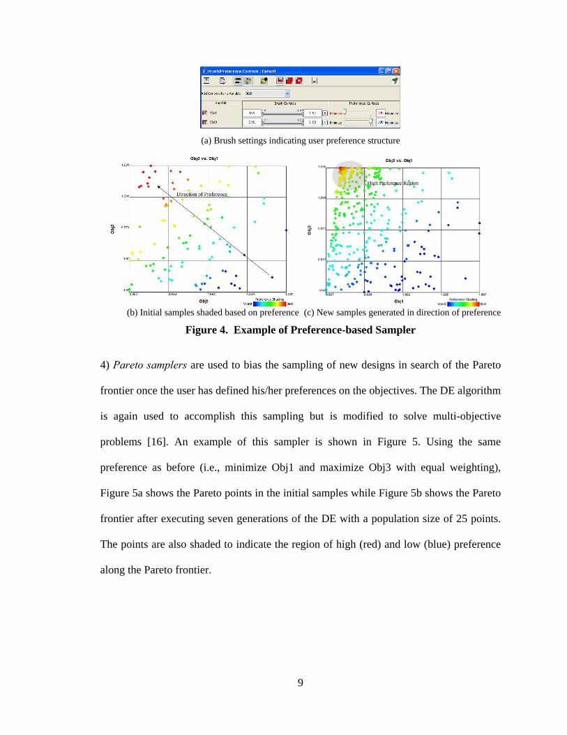
3) Preference-based samplers allow users to populate the trade space in regions that

perform well with respect to a user-defined preference function. New sample points are

also generated by the DE algorithm, but the fitness of each sample is defined by the

user’s preference structure instead of the Euclidean distance. An example of the

preference-based sampler is shown in Figure 4. Using ATSV’s brushing and preference

controls, the user specifies a desire to minimize Obj1 and maximize Obj3 with equal

weighting (see Figure 4a). Figure 4b shows the initial samples shaded based on this

preference, and Figure 4c shows the new samples, where the concentration of points

increases in the direction of preference, namely, the upper left hand corner of the plot.

9

(a) Brush settings indicating user preference structure

(b) Initial samples shaded based on preference (c) New samples generated in direction of preference

Figure 4. Example of Preference-based Sampler

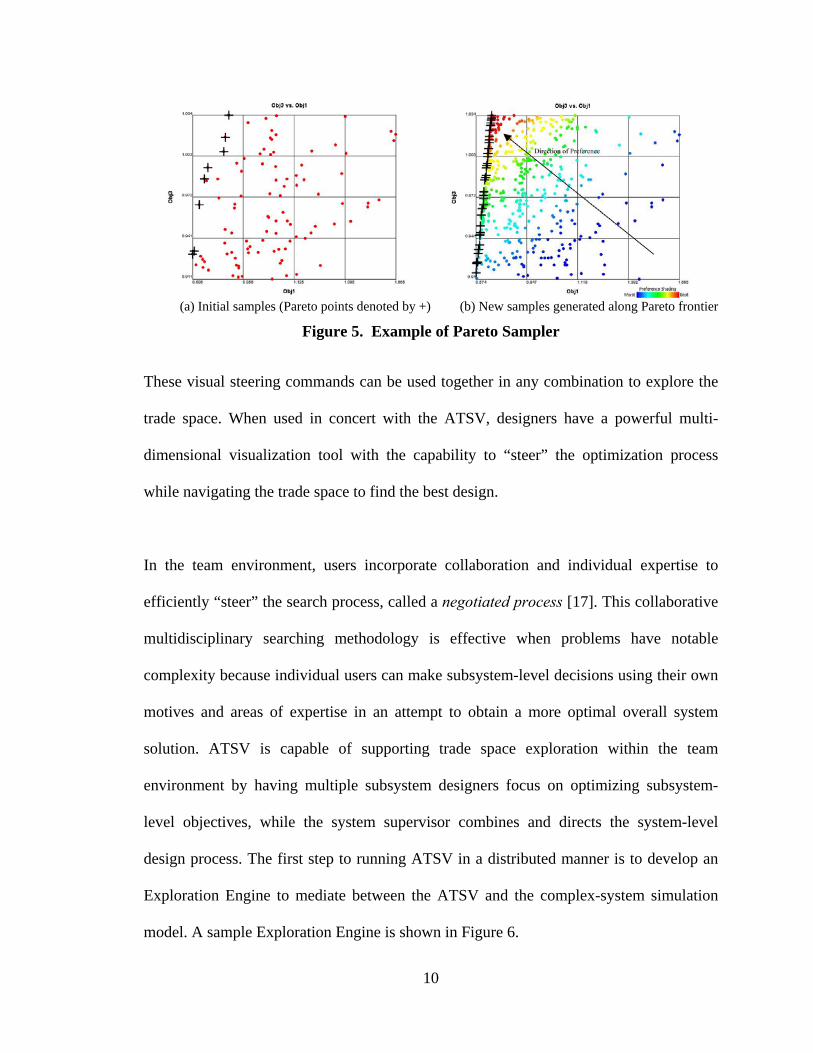
4) Pareto samplers are used to bias the sampling of new designs in search of the Pareto

frontier once the user has defined his/her preferences on the objectives. The DE algorithm

is again used to accomplish this sampling but is modified to solve multi-objective

problems [16]. An example of this sampler is shown in Figure 5. Using the same

preference as before (i.e., minimize Obj1 and maximize Obj3 with equal weighting),

Figure 5a shows the Pareto points in the initial samples while Figure 5b shows the Pareto

frontier after executing seven generations of the DE with a population size of 25 points.

The points are also shaded to indicate the region of high (red) and low (blue) preference

along the Pareto frontier.

10

(a) Initial samples (Pareto points denoted by +) (b) New samples generated along Pareto frontier

Figure 5. Example of Pareto Sampler

These visual steering commands can be used together in any combination to explore the

trade space. When used in concert with the ATSV, designers have a powerful multi-

dimensional visualization tool with the capability to “steer” the optimization process

while navigating the trade space to find the best design.

In the team environment, users incorporate collaboration and individual expertise to

efficiently “steer” the search process, called a negotiated process [17]. This collaborative

multidisciplinary searching methodology is effective when problems have notable

complexity because individual users can make subsystem-level decisions using their own

motives and areas of expertise in an attempt to obtain a more optimal overall system

solution. ATSV is capable of supporting trade space exploration within the team

environment by having multiple subsystem designers focus on optimizing subsystem-

level objectives, while the system supervisor combines and directs the system-level

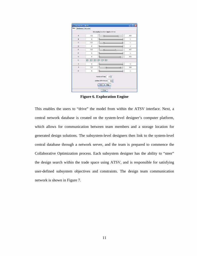
design process. The first step to running ATSV in a distributed manner is to develop an

Exploration Engine to mediate between the ATSV and the complex-system simulation

model. A sample Exploration Engine is shown in Figure 6.

11

Figure 6. Exploration Engine

This enables the users to “drive” the model from within the ATSV interface. Next, a

central network database is created on the system-level designer’s computer platform,

which allows for communication between team members and a storage location for

generated design solutions. The subsystem-level designers then link to the system-level

central database through a network server, and the team is prepared to commence the

Collaborative Optimization process. Each subsystem designer has the ability to “steer”

the design search within the trade space using ATSV, and is responsible for satisfying

user-defined subsystem objectives and constraints. The design team communication

network is shown in Figure 7.

12

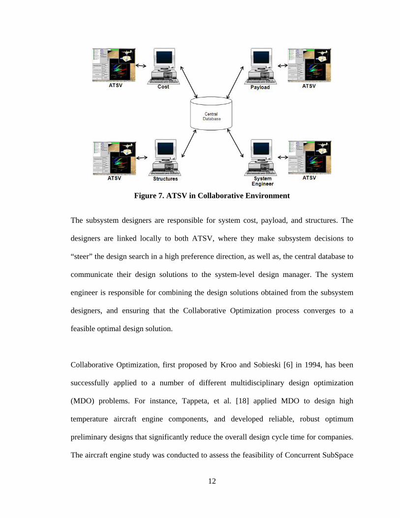
Figure 7. ATSV in Collaborative Environment

The subsystem designers are responsible for system cost, payload, and structures. The

designers are linked locally to both ATSV, where they make subsystem decisions to

“steer” the design search in a high preference direction, as well as, the central database to

communicate their design solutions to the system-level design manager. The system

engineer is responsible for combining the design solutions obtained from the subsystem

designers, and ensuring that the Collaborative Optimization process converges to a

feasible optimal design solution.

Collaborative Optimization, first proposed by Kroo and Sobieski [6] in 1994, has been

successfully applied to a number of different multidisciplinary design optimization

(MDO) problems. For instance, Tappeta, et al. [18] applied MDO to design high

temperature aircraft engine components, and developed reliable, robust optimum

preliminary designs that significantly reduce the overall design cycle time for companies.

The aircraft engine study was conducted to assess the feasibility of Concurrent SubSpace

13

Optimization (CSSO) for the design and optimization of large-scale complex systems.

Likewise, Kroo and Braun [19] investigated the impact of group collaboration for a

single-stage-to-orbit launch vehicle. The problem was divided into three user-defined

subsystems: vehicle design, cost, and trajectory. Like many complex design problems,

the launch vehicle was characterized by 95 design variables and 16 constraints, which is

an intractable task for one designer. The Collaborative Optimization utilizes the

designer’s knowledge in order to reduce time and cost of both the subsets and entire

system-level optimal design processes. Also, the study demonstrates the impact of a

priori criterion on vehicle design and the difference between minimum weight and

minimum cost concepts. Sobieski, et al. [20] used Collaborative Optimization to illustrate

the solution process for aircraft wing and aircraft sizing design problems. For each

example, Collaborative Optimization converged to the optimal solution, whereas, the

direct single-level optimization strategy yielded suboptimal results. Renaud and Tappeta

[21] further investigated collaborative optimization and developed a comprehensive

overview of mathematically rigorous optimization strategies for Multi-Objective

Collaborative Optimization (MOCO). When applied to problems in a multidisciplinary

design environment, this scheme has several advantages over traditional solution

strategies, including reducing the amount of information transferred between disciplines,

the removal of large iteration-loops, and the ability to explore new solution regions in the

trade space.

Throughout the Collaborative Optimization process, mental models are formed by

subsystem and system-level designers to provide a clear road map for increased system

14

organization, a better understanding of user experiences/needs, and to get users on the

same page. During trade space exploration, users are continuously learning, and thus

changing and adapting their mental models to efficiently solve the design optimization

problem. According to Norman, “memory through explanation by using and making

mental models is the more powerful form of internal memory” [22]. This demonstrates

that incorporating human motives and expertise with visual steering commands in the

design paradigm may be more effective than allowing a Multi-Objective Genetic

Algorithm (MOGA) to run “blindly”. Simpson, et al. [1] compares the performance of

different combinations of visual steering commands implemented by two users to a

MOGA that is executed “blindly” on the same problem with no human intervention.

Similar to Norman’s conclusion, Simpson, et al. found a 4x -7x increase in the number of

Pareto solutions that are obtained when the human is “in-the-loop” during the

optimization process. Allowing human interaction in conjunction with a genetic

algorithm may provide the best design scenario because it incorporates the designer’s

mental model shaped by advanced discipline expertise and motives. Likewise, group

interaction during trade space exploration requires team consensus to control the

formation of mental models for making interdisciplinary system-level decisions, thus

eliminating the “apt to be deficient in a number of different ways” [22].

On the subsystem-level, mental models are formulated based on user-defined objectives

and expertise, often making sacrifices to the system-level design. For instance, Cao and

MacKenzie [23] performed task and motion analysis during endoscopic surgery. They

determined that the system-level design was dominated by the subsystem-level designer’s

15

need to minimize both cost and unique surgeon movements. During Collaborative

Optimization, discipline experts make design decisions to satisfy their objectives without

considering the impact of their decisions on the system design. The goal of the system-

level designer is to integrate the multiple subsystem-level designer preferences and input

effectively to guide the system-level exploration process towards feasible, Pareto optimal

designs.

Research indicates that optimal design solutions are attained through effective

communication and group formation of preferences within a collaborative environment.

Orasanu [24] investigated the decision making process of pilots in an aircraft cockpit to

understand how aircraft pilots simultaneously formed individual preferences, to control

their aircraft, and group preferences, to coherently fly multiple aircrafts in a fleet. Such

teams are comprised of individuals who have a high degree of expertise in their specific

discipline areas, making it difficult, yet essential, to effectively converge as a team when

making critical decisions. Furthermore, the decision environments in which these experts

must function are constrained by deadlines, multidisciplinary decision responsibilities,

rapidly changing information, and high information ambiguity. Therefore, designers must

effectively interact in a collaborative environment to form and amalgamate subsystem-

level preferences to obtain optimal system-level decisions. Likewise, concurrent

engineering require the subsystem designers to form local preferences, using personal

expertise and motives, to meet their objectives, while continually merging their optimal

subsystem-level design solutions and preferences with the system-level process. This

16

collaborative technique and the process for forming subsystem and system preferences is

demonstrated in Chapter 3 using a NASA space shuttle external fuel tank model.

17

Chapter 3

Test Problem Overview and Experimental Set-Up

3.1 Test Problem Overview

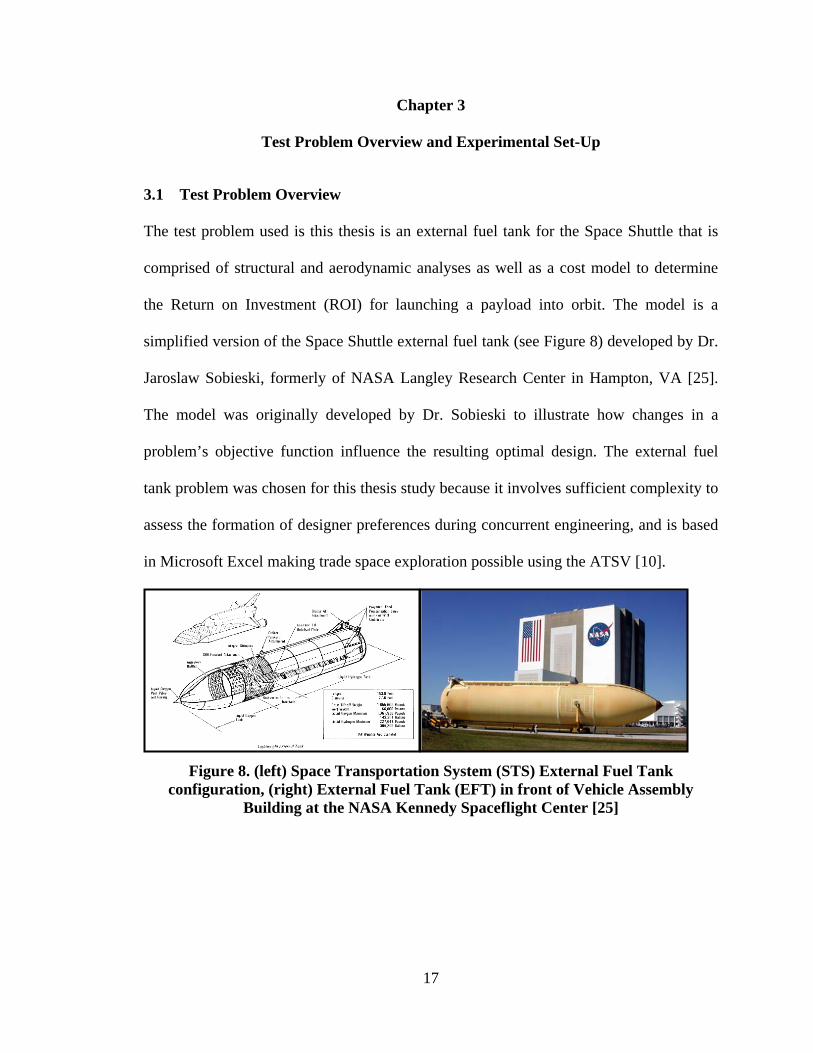
The test problem used is this thesis is an external fuel tank for the Space Shuttle that is

comprised of structural and aerodynamic analyses as well as a cost model to determine

the Return on Investment (ROI) for launching a payload into orbit. The model is a

simplified version of the Space Shuttle external fuel tank (see Figure 8) developed by Dr.

Jaroslaw Sobieski, formerly of NASA Langley Research Center in Hampton, VA [25].

The model was originally developed by Dr. Sobieski to illustrate how changes in a

problem’s objective function influence the resulting optimal design. The external fuel

tank problem was chosen for this thesis study because it involves sufficient complexity to

assess the formation of designer preferences during concurrent engineering, and is based

in Microsoft Excel making trade space exploration possible using the ATSV [10].

Figure 8. (left) Space Transportation System (STS) External Fuel Tank

configuration, (right) External Fuel Tank (EFT) in front of Vehicle Assembly Building at the NASA Kennedy Spaceflight Center [25]

18

3.1.1 Model Nomenclature

C = Cost ($) h/R = Cone height : radius ratio L = Cylinder length R = Tank radius (m) σ = Component stress (N/m2) t1 = Cylinder thickness (m) t2 = Sphere thickness (m) t3 = Cone thickness (m)

3.1.2 Model Description

The model divides the external fuel tank into three hollow geometric segments: (1) a

cylinder (length L, radius R), (2) a hemispherical end cap (radius R), and (3) a conical

nose (height h, radius R), as shown in Figure 9. These segments have thicknesses t1, t2,

and t3, respectively. Surface areas and volumes are determined using geometric relations,

and first principles are used to calculate stresses, vibration modes, aerodynamic drag, and

cost. There are five continuous inputs to the system including radius (R), cylinder

thickness (t1), sphere thickness (t2), cone thickness (t3), and cone height to radius ratio

(h/R). Differing from the model developed by Sobieski, cylinder length is no longer an

input variable in order to achieve a volume equality constraint. This modification

significantly increased the overall number of feasible design solutions because it

eliminates an equality constraint from the problem. There are numerous outputs from the

model including surface areas (Ai), masses (Mt), stresses (σ), first vibration mode

frequency (ζ), payload (pn), seam and material costs (λ and κ), and return on investment

(ROI).

19

Figure 9. EFT Model [25]

3.2 Experimental Set-Up

In this study, the external fuel tank model was divided into the three design subsystems:

(1) structures, (2) cost, and (3) payload to support collaborative engineering techniques.

The overall system objective is to maximize ROI, while the subsystem objectives are to

maximize actual payload, minimize tank material weight, and minimize total cost. Table

1 summarizes the inputs, outputs, objectives, and constraints of the subsystems and

overall system used in the Collaborative Optimization case study.

R

h

L

t1

t2

t3

σ1

σ2

σ1

σ2

σ1

σ2

seam

20

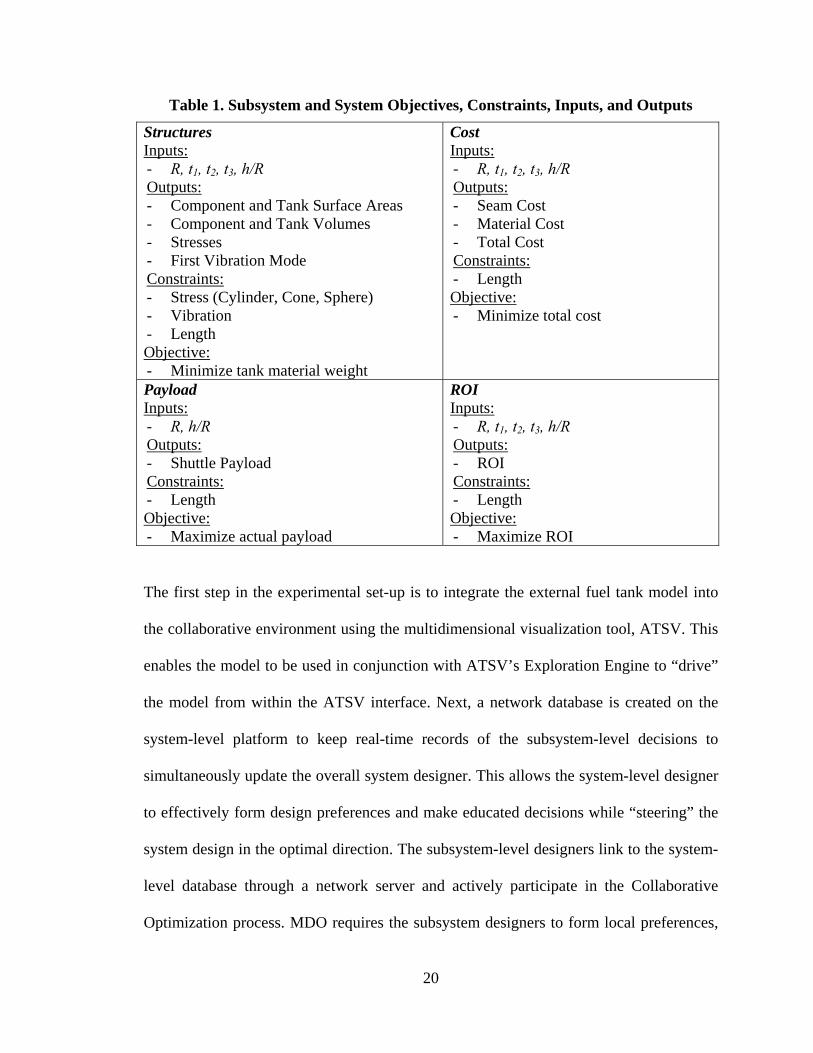
Table 1. Subsystem and System Objectives, Constraints, Inputs, and Outputs

Structures Inputs: - R, t1, t2, t3, h/R Outputs: - Component and Tank Surface Areas - Component and Tank Volumes - Stresses - First Vibration Mode Constraints: - Stress (Cylinder, Cone, Sphere) - Vibration - Length Objective: - Minimize tank material weight

Cost Inputs: - R, t1, t2, t3, h/R Outputs: - Seam Cost - Material Cost - Total Cost Constraints: - Length Objective: - Minimize total cost

Payload Inputs: - R, h/R Outputs: - Shuttle Payload Constraints: - Length Objective: - Maximize actual payload

ROI Inputs: - R, t1, t2, t3, h/R Outputs: - ROI Constraints: - Length Objective: - Maximize ROI

The first step in the experimental set-up is to integrate the external fuel tank model into

the collaborative environment using the multidimensional visualization tool, ATSV. This

enables the model to be used in conjunction with ATSV’s Exploration Engine to “drive”

the model from within the ATSV interface. Next, a network database is created on the

system-level platform to keep real-time records of the subsystem-level decisions to

simultaneously update the overall system designer. This allows the system-level designer

to effectively form design preferences and make educated decisions while “steering” the

system design in the optimal direction. The subsystem-level designers link to the system-

level database through a network server and actively participate in the Collaborative

Optimization process. MDO requires the subsystem designers to form local preferences,

21

using personal expertise and motives, to meet their defined objectives, while continually

merging their optimal subsystem-level design solutions and preferences with the system-

level process. To accurately understand the user’s formation of preferences, each

subsystem designer was required to fill out a form (shown in Figure 10), which indicates

the samplers used by the designer during the exploration process, the parameter settings

for each sampler used, and the users’ motivations for using each sampler.

Figure 10. Distributed ATSV User Action Form

22

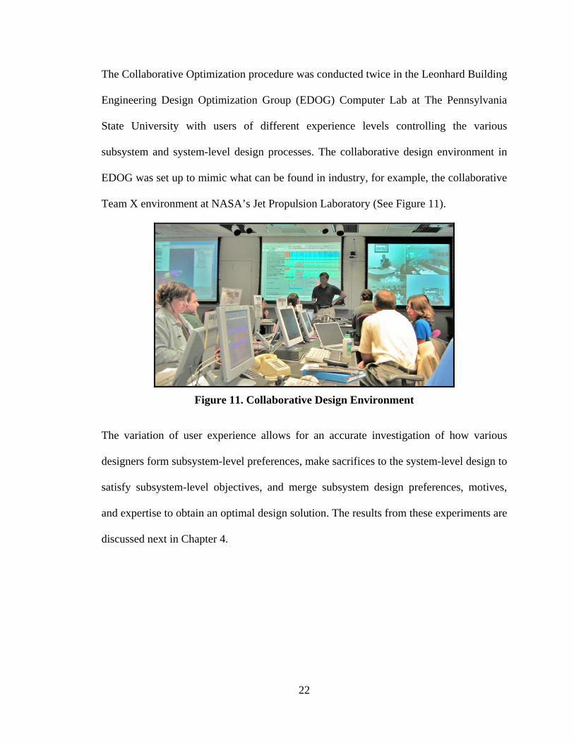
The Collaborative Optimization procedure was conducted twice in the Leonhard Building

Engineering Design Optimization Group (EDOG) Computer Lab at The Pennsylvania

State University with users of different experience levels controlling the various

subsystem and system-level design processes. The collaborative design environment in

EDOG was set up to mimic what can be found in industry, for example, the collaborative

Team X environment at NASA’s Jet Propulsion Laboratory (See Figure 11).

Figure 11. Collaborative Design Environment

The variation of user experience allows for an accurate investigation of how various

designers form subsystem-level preferences, make sacrifices to the system-level design to

satisfy subsystem-level objectives, and merge subsystem design preferences, motives,

and expertise to obtain an optimal design solution. The results from these experiments are

discussed next in Chapter 4.

23

Chapter 4

User Decision-Making Process and Results

The Collaborative Optimization study was conducted by two different groups of users,

each making significantly different design decisions based on individual user expertise,

motives, and preference formation. Understanding user motives when making design

decisions and the development of user preferences is important because each subsystem

plays an integral role in the development of the system design. This chapter discusses

how subsystem-level designers form and evolve design preferences, and make sacrifices

to the system-level design to satisfy their subsystem objectives using external fuel tank

case studies.

4.1 Trial 1 Results

Trial 1 was executed by novice, single time, ATSV users managing the structures and

cost subsystems, an advanced, extended use, user managing the payload subsystem, and

an intermediate, multiple time, user managing the system-level design. The subsystem

users were asked to use an unrestricted number of function evaluations to generate design

solutions to satisfy their objectives and constraints, and then decide upon a region, or

design, of high preference to communicate to the system-level user. Meanwhile, the

system-level designer was responsible for effectively integrating the subsystem-level

preferences to make informed design decisions and develop an optimal overall system

design using ATSV’s visual steering commands [14]. While there are nearly an infinite

number of combinations of brushing, preference controls, and visual steering commands

that could be implemented in ATSV, we allowed the users to form individual design

preferences using their discipline expertise and motives to efficiently “steer” the design

24

search in a direction that they felt was “natural”. During the exploration and collaboration

process, the designers record their motivation for making decisions as well as comment

on their mental model. This gives the ability to accurately understand how designers

initially form preferences, and how these preferences evolve throughout the exploration

process. Table 2 describes the specific combination of visual steering commands and

brush/preference controls used by subsystem-level and system-level designers in Trial 1.

Unless specified, the Exploration Engine options were left at default settings of

generation size = 25, population limit = 500, and the Best1Bin selection strategy.

Table 2. Designer Decision-Making Process for Trial 1 Structures (Total Points: 1375) Cost (Total Points: 2225)

- Basic Sampler: 100 runs - Brush weight: Minimize weight (-100) - Pareto Sampler: Minimize weight - Line Attractor: Set at the current minimum limit of the

weight scatter plot window - Pareto Sampler: Minimize weight - Line Attractor: Set at the current minimum limit of the

weight scatter plot window - Point Attractor: Set to edge of feasible points (Weight

vs. R) - Point Attractor: Set to edge of feasible points (Weight

vs. R) - Point Attractor: Set at the current minimum limit of the

weight and t1 scatter plot window (Weight vs. t1) Picked Best Region

- Basic Sampler: 100 runs - Brush cost: Minimize cost (-100) - Pareto Sampler: Minimize cost - Line Attractor: Set at the current minimum limit of the

cost scatter plot window - Point Attractor: Set Cost = 0, L = 9000 (Cost vs. L) - Line Attractor: Set at the current minimum limit of the

cost scatter plot window - Point Attractor: Set Cost = 0, SphereConstraint = 1

(Cost vs. SphereConstraint) - Picked Best Region

Payload (Total Points: 876) System ROI (Total Points: 2200) - Basic Sampler: 100 runs - Brush payload: Maximize payload (+100) - Pareto Sampler: Maximize payload - Line Attractor: Set at the current maximum limit of the

payload scatter plot window - Brushed Out: R (.5 – 1.2), h/R (.17 – 4.06), Payload

(40700 – 57100) - Pareto Sampler: Maximize payload - Point Attractor: R = .705, Pareto optimal region - Picked Best Region

- Basic Sampler: 100 runs - Brush ROI: Maximize ROI (+100) - Pareto Sampler: Maximize ROI - Line Attractor: Set at the current maximum limit of the

ROI scatter plot window - Line Attractor: Set at the current maximum limit of the

ROI scatter plot window - Pareto Sampler: Maximize ROI - Point Attractor: Pareto optimal region - Picked Best Design

The structures subsystem designer had minimal experience using ATSV prior to the study

and was responsible for minimizing the external fuel tank material weight. With a minor

understanding of the test problem, the structures designer generated 100 design solutions

using the basic sampler to “get an initial sample of data, to locate the range of weight

25

values in the multi-dimensional trade space.” The basic sampler is most efficient and

effective when the designer wants to explore the trade space without the hindrance of

design constraints because it samples uniformly across the entire trade space. Using

intuition, the structures designer formed his initial preferences, and decided to use the

Pareto sampler to search for the optimal solutions along the Pareto frontier. The designer

knows that this decision will begin to move the design search in the desired direction but

will have to use other visual steering commands to further “push” and “fill in” the Pareto

frontier. This was accomplished through the use of several point and line attractors.

When placing the point attractor, the designer decided upon a region that minimized

weight and ROI with the intention to increase diversity along the Pareto frontier. While

this decision benefited the structures subsystem-level design, sacrifices were made to the

overall system-level design, where the objective was to maximize ROI. Next, the

designer located the region of highest preference within the trade space, and brushed the

stresses, vibration, and length constraints to eliminate infeasible design solutions. Before

these controls were set to reveal the feasible region, the user was inclined to place

attractors along the infeasible region’s Pareto frontier since it dominated the resultant

feasible region. The Pareto samplers and line attractors used previously explored only

infeasible regions of the trade space because the designs “overshot” the feasible region

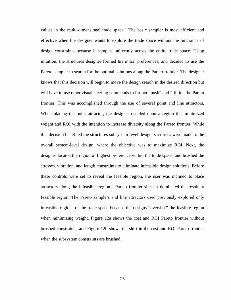
when minimizing weight. Figure 12a shows the cost and ROI Pareto frontier without

brushed constraints, and Figure 12b shows the shift in the cost and ROI Pareto frontier

when the subsystem constraints are brushed.

26

(a) Pareto Frontier without Brushed Constraints (b) Feasible Pareto Frontier

Figure 12. Infeasible (a) and Feasible (b) Pareto fronts (+ denotes Pareto points)

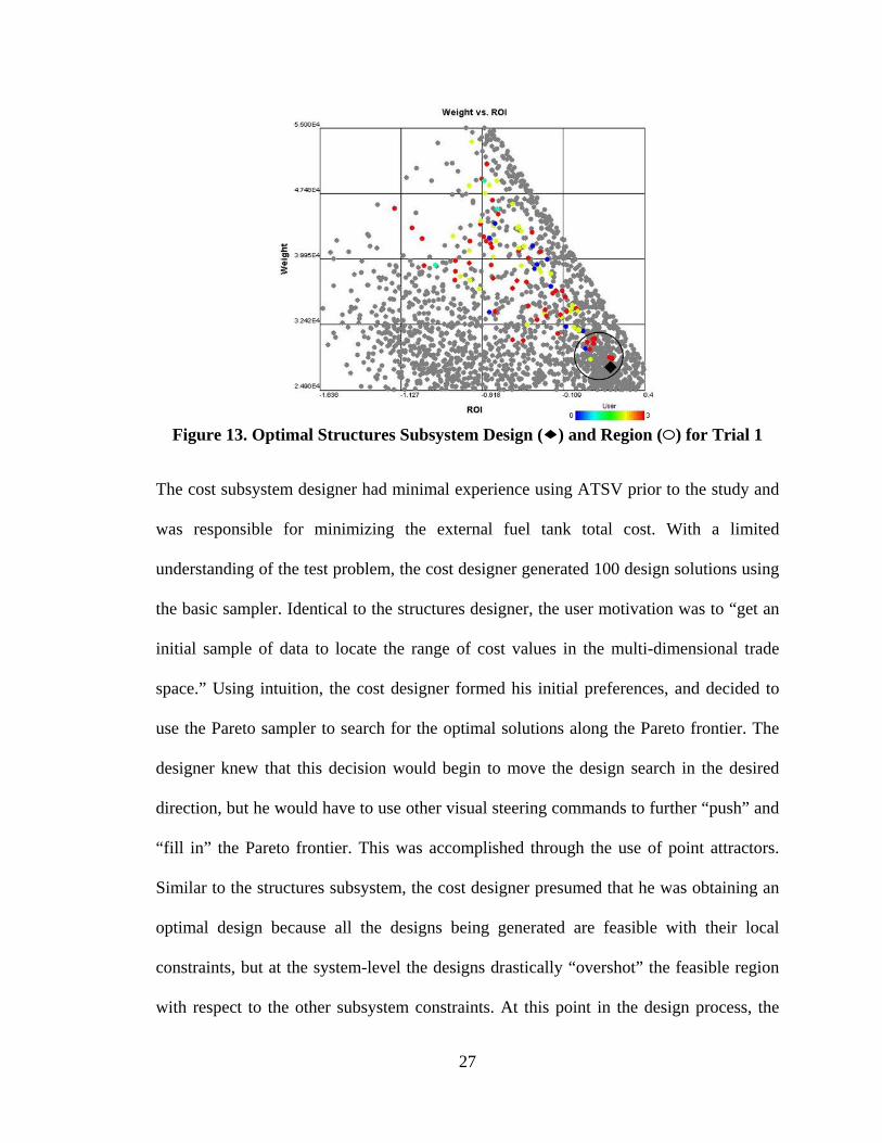
The designer was forced to evolve his mental model and subsystem-level preferences

because brushing the infeasible designs significantly shifted the Pareto frontier. With the

evolved preferences and user motives in mind, he placed a line and point attractor at the

minimum weight value within the constrained feasible region, a method referred to as

manual constraint handling [26]. The structures designer decided that the design search

had “stalled”, and selected the optimal structures design point and region developed

within the subsystem that satisfied all the subsystem constraints. Figure 13 shows the

optimal structures design point by the black diamond ( ), the optimal design region by

the black ellipse ( ), and the infeasible design solutions by the gray dots ( ). The red

dots ( ) represent the designs generated by the structures subsystem designer. The

structures subsystem was highly constrained, thereby, significantly reducing the number

of feasible design solutions. Lastly, the structures designer communicated his preference

model to the system-level designer to ensure that the overall system design could be

collaboratively optimized.

27

Figure 13. Optimal Structures Subsystem Design ( ) and Region ( ) for Trial 1

The cost subsystem designer had minimal experience using ATSV prior to the study and

was responsible for minimizing the external fuel tank total cost. With a limited

understanding of the test problem, the cost designer generated 100 design solutions using

the basic sampler. Identical to the structures designer, the user motivation was to “get an

initial sample of data to locate the range of cost values in the multi-dimensional trade

space.” Using intuition, the cost designer formed his initial preferences, and decided to

use the Pareto sampler to search for the optimal solutions along the Pareto frontier. The

designer knew that this decision would begin to move the design search in the desired

direction, but he would have to use other visual steering commands to further “push” and

“fill in” the Pareto frontier. This was accomplished through the use of point attractors.

Similar to the structures subsystem, the cost designer presumed that he was obtaining an

optimal design because all the designs being generated are feasible with their local

constraints, but at the system-level the designs drastically “overshot” the feasible region

with respect to the other subsystem constraints. At this point in the design process, the

28

user commented that “the Pareto frontier continues to shift towards a more desirable

region, but there are regions with clusters of designs, and others with empty space”. To

resolve this issue, the designer formed a preference to “fill in” the Pareto frontier in the

minimum cost and ROI region, similar to the structures subsystem. Once again, this

decision benefited the structures subsystem-level design, but sacrificed the overall

system-level design, where the objective was to maximize ROI. Next, the designer

located the region of highest preference within the trade space, and brushed the length

constraints to eliminate design solutions that are infeasible. Unlike the structures

subsystem, the cost designer did not need to change his mental model or initial

preferences because brushing had negligible effect on the feasible design Pareto frontier.

The cost designer placed one more attractor to try and further shift the Pareto frontier

towards minimized cost, but realized that the design search had “stalled”, and selected the

optimal cost design point and region within the subsystem that satisfied all the subsystem

constraints. Figure 14 shows the optimal cost subsystem design represented by the black

diamond ( ), the optimal system design represented by a green diamond ( ), the optimal

design region represented by the black ellipse ( ), and the infeasible design solutions for

the subsystem represented by gray dots ( ). Note that there are no infeasible points

visible in gray because the cost subsystem was only constrained by length and not by

strict structures constraints. Therefore, the high preference design region shown in Figure

14 is optimal at the cost subsystem-level, but not for the overall system, which shows that

subsystem designers often neglect the overall system objectives in the exploration

process. The optimal feasible system-level design generated by the subsystem designer

would cost approximately $300,000 more than the optimal subsystem design and increase

29

the ROI slightly (shown by the magenta diamond ( ) in Figure 15). Lastly, the designer

communicated his preference model to the system-level designer to ensure that the

overall system design was optimized. Unlike the structures subsystem, the cost designer

was never informed that his designs are infeasible to structure constraints, and therefore

the optimal design region communicated to the system-level designer was erroneous.

Figure 14. Optimal Cost Subsystem Design ( ) and Region ( ) for Trial 1

Figure 15. Optimal Cost Design ( ) with All Constraints Brushed

30

The payload subsystem designer had expert-level experience using ATSV prior to the

study and was responsible for maximizing the external fuel tank actual payload. With a

concrete understanding of the test problem from previous work, the payload designer

began the trade space exploration process with a Pareto sampler. The user motivation was

to “try to obtain designs which maximize payload in a space that already had several

hundred points populated”. Unlike the other subsystem-level designers, who began the

search with a basic sampler, the payload user had a visual representation of the Pareto

frontier and immediately began to “push” the frontier towards a more desired payload

region. This design decision was ineffective because the initial Pareto frontier, generated

by the Pareto sampler, immediately “overshot” the system-level feasible design region.

This decision resulted in the payload designer generating two feasible system solutions

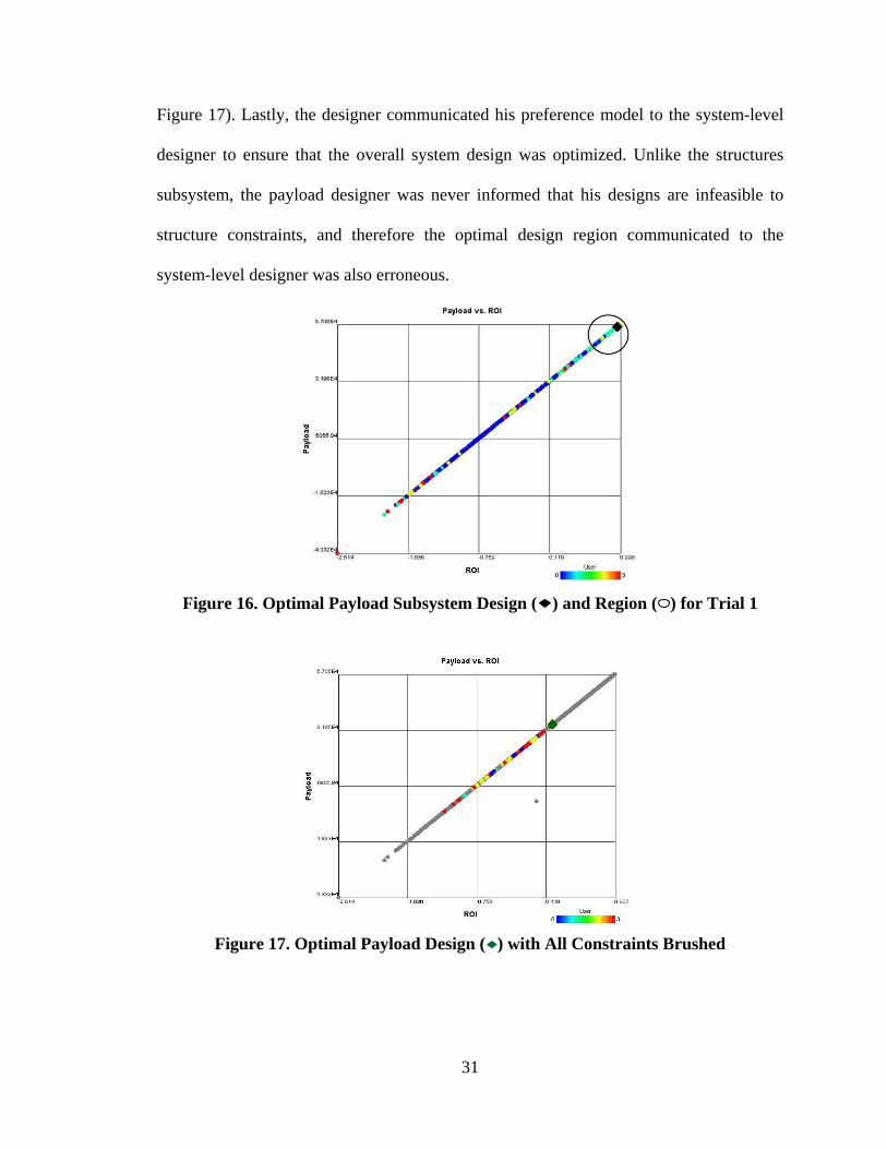
and 874 infeasible solutions. Nevertheless, the designer selected the optimal cost design

point and region developed within the subsystem that satisfied all the subsystem

constraints. Figure 16 shows the optimal cost subsystem design represented by the black

diamond ( ), the optimal design region by the black ellipse ( ), and the infeasible design

solutions for the subsystem represented by gray dots ( ). Note that there are no infeasible

points visible in gray because the payload subsystem was only constrained by length, but

not by the strict structures constraints. Therefore, the high preference design region

shown in Figure 16 is optimal at the cost subsystem-level, but not for the overall system,

which shows that subsystem designers often neglect the overall system objectives in the

exploration process. The optimal feasible system-level design generated by the subsystem

designer would have a payload of approximately 15,000 kg less than the optimal

subsystem design and decrease the ROI significantly (shown by the green diamond ( ) in

31

Figure 17). Lastly, the designer communicated his preference model to the system-level

designer to ensure that the overall system design was optimized. Unlike the structures

subsystem, the payload designer was never informed that his designs are infeasible to

structure constraints, and therefore the optimal design region communicated to the

system-level designer was also erroneous.

Figure 16. Optimal Payload Subsystem Design ( ) and Region ( ) for Trial 1

Figure 17. Optimal Payload Design ( ) with All Constraints Brushed

32

The subsystem designers effectively selected optimal design points and regions for each

of the subsystem objectives, and they communicated their preferences with the system-

level designer in a collaborative environment. The system designer merged the different

decisions and mental models of the subsystem designers, while he searched the trade

space for a feasible design that maximized ROI. This process can be difficult because

optimal designs at the subsystem-level may satisfy local constraints, but they may not

satisfy all system-level constraints. To work around this issue, designers selected a region

of high preference points in a specific range defined within the subsystem trade space.

This allowed the system-level designer to have greater flexibility when selecting the

optimal design in the trade space. Collaboration occurred between subsystems using

differentiation annotations (i.e., with user comments) to further search and refine the

optimal system design. In the study, Trial 1 yielded successful results when combining

the subsystem-level optimal design regions because one design was in the high

preference region for all the subsystems and was the optimal system-level design. The

system design selected was less optimal with respect to individual subsystem-level

optimal designs because the constraints for this test problem significantly reduced the

number of feasible system-level designs (red dots in Figure 18). Without automatic

constraint handling [26] or an accurate knowledge of all system constraints, the

subsystem designs “overshot” the feasible region when using the Pareto and attractor

samplers. The optimum, Point 2333, is shown in Figure 18, Figure 19, and Figure 20 for

weight, cost, and payload versus ROI with infeasible points brushed out (constraints),

respectively. Point 2333 minimizes weight, minimizes cost, maximizes payload, while

maximizing the system ROI. Thus, Point 2333 is deemed the optimal system design

33

within the collaborative environment for Trial 1, and the design details are shown in

Figure 21.

Figure 18. Optimal System Design (Weight) for Trial 1

Figure 19. Optimal System Design (Cost) for Trial 1

34

Figure 20. Optimal System Design (Payload) for Trial 1

Figure 21. Design Details for Point 2333

4.2 Trial 2 Results

Trial 2 was executed by advanced ATSV users managing the structures, cost, and

payload subsystems as well as the system-level design. Identical to the Trial 1 process,

the subsystem users could use an unrestricted number of function evaluations to generate

design solutions to satisfy their objectives and constraints, and then decide upon a region,

or design, of highest preference to communicate to the system-level user. Meanwhile, the

system-level designer was responsible for effectively integrating the subsystem-level

preferences to make educated design decisions and develop an optimal overall system

35

design using ATSV’s visual steering commands [14]. Table 3 describes the specific

combination of visual steering commands and brush/preference controls used by

subsystem-level and system-level designers in Trial 2. Unless specified, the Exploration

Engine options were left at default settings of generation size = 25, population limit =

500, and the Best1Bin selection strategy.

Table 3. Designer Decision-Making Process for Trial 2 Structures (Total Points: 2150) Cost (Total Points: 1375)

- Basic Sampler: 100 runs - Brush weight: Minimize weight (-100) - Pareto Sampler: Minimize weight - Line Attractor: Set at the current minimum limit of the

weight scatter plot window - Line Attractor: Set at the current minimum limit of the

weight scatter plot window - Line Attractor: Set at the limit of the feasible region

(with constraints applied) - Point Attractor: Set to edge of feasible points (Weight

vs. Cost) - Brush constraints: Cone stress (<0), Sphere stress

(<0), Cylinder stress (<0), Vibration Mode (<0), L (>0) - Point Attractor: Set to edge of feasible points (Weight

vs. Cost) - Picked Best Region

- Basic Sampler: 200 runs - Line Attractor: Set at the current minimum limit of the

cost scatter plot window (Cost = 396,068) - Line Attractor: Set at the current minimum limit of the

cost scatter plot window (Cost = 396,068) - Brush cost: Minimize cost (-100) - Pareto Sampler: Minimize cost - Brush cost and ROI: Minimize cost (-100) and

maximize ROI (+100) - Pareto Sampler: Minimize cost and maximum ROI - Picked Best Region

Payload (Total Points: 1400) System ROI (Total Points: 3345) - Basic Sampler: 100 runs - Brush payload: Maximize payload (+100) - Pareto Sampler: Maximize payload - Line Attractor: Set at the current maximum limit of the

payload scatter plot window - Brush L: L (>0) - Line Attractor: Set at the current maximum limit of the

payload scatter plot window - Point Attractor: Set to edge of feasible points

(Payload vs. Cost) - Picked Best Region

- Basic Sampler: 1000 runs - Brush ROI: Maximize ROI (+100) - Point Attractor: Window maximum (ROI = 1.001, L =

17,857) - Pareto Sampler: Maximize ROI - Point Attractor: Window maximum (ROI = 1.001,

Weight = 10,585) - Point Attractor: Window maximum (ROI = 1.001, Cost

= 471,726) - Pareto Sampler: Maximize ROI, minimize cost,

minimize vibration constraint, maximize payload - Point Attractor: Pareto optimal region (ROI = 1.001,

Cost = 677,155, Payload = 57,701) - Picked Best Design

The structures subsystem designer was an advanced ATSV user and was responsible for

minimizing the external fuel tank material weight. With a concrete understanding of the

test problem, the structures designer generated 100 design solutions using the basic

sampler to “get a sense of the multi-dimensional trade space”. Prior to fully investigating

the subsystem design requirements, the structures designer proceeded to use various

36

combinations of Pareto samplers and line attractors to search for the optimal solutions

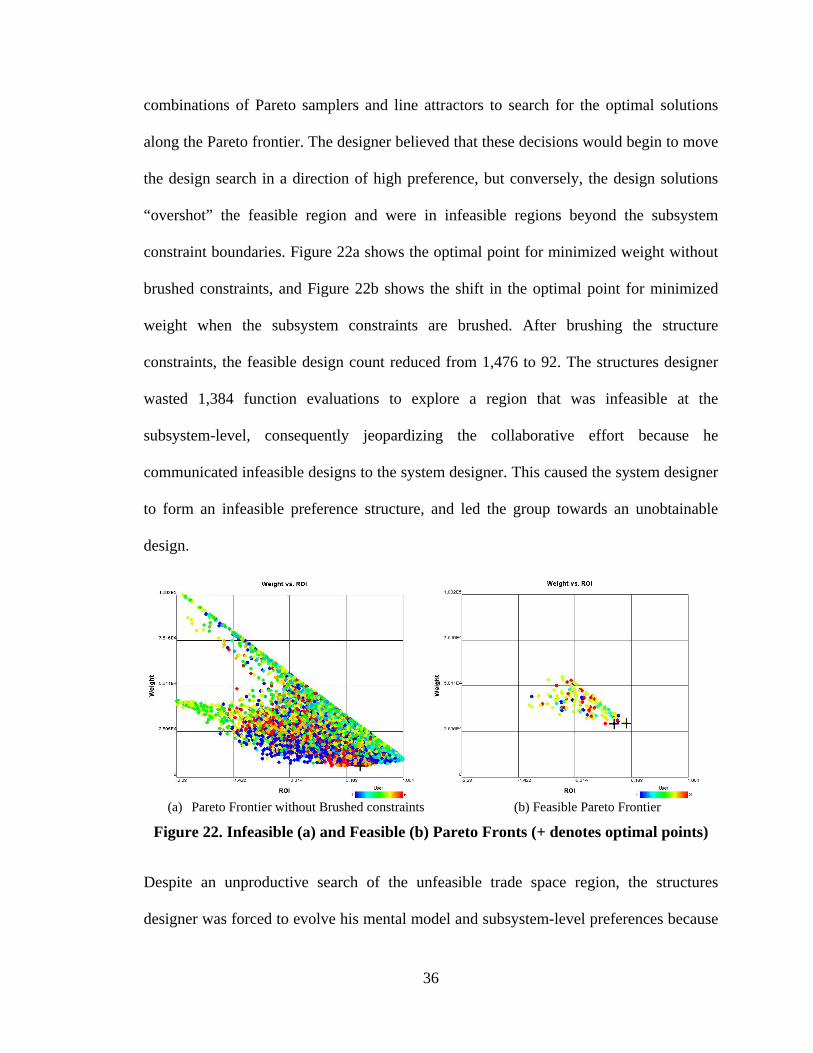
along the Pareto frontier. The designer believed that these decisions would begin to move

the design search in a direction of high preference, but conversely, the design solutions

“overshot” the feasible region and were in infeasible regions beyond the subsystem

constraint boundaries. Figure 22a shows the optimal point for minimized weight without

brushed constraints, and Figure 22b shows the shift in the optimal point for minimized

weight when the subsystem constraints are brushed. After brushing the structure

constraints, the feasible design count reduced from 1,476 to 92. The structures designer

wasted 1,384 function evaluations to explore a region that was infeasible at the

subsystem-level, consequently jeopardizing the collaborative effort because he

communicated infeasible designs to the system designer. This caused the system designer

to form an infeasible preference structure, and led the group towards an unobtainable

design.

(a) Pareto Frontier without Brushed constraints (b) Feasible Pareto Frontier

Figure 22. Infeasible (a) and Feasible (b) Pareto Fronts (+ denotes optimal points)

Despite an unproductive search of the unfeasible trade space region, the structures

designer was forced to evolve his mental model and subsystem-level preferences because

37

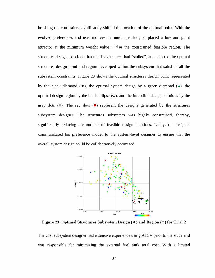
brushing the constraints significantly shifted the location of the optimal point. With the

evolved preferences and user motives in mind, the designer placed a line and point

attractor at the minimum weight value within the constrained feasible region. The

structures designer decided that the design search had “stalled”, and selected the optimal

structures design point and region developed within the subsystem that satisfied all the

subsystem constraints. Figure 23 shows the optimal structures design point represented

by the black diamond ( ), the optimal system design by a green diamond ( ), the

optimal design region by the black ellipse ( ), and the infeasible design solutions by the

gray dots ( ). The red dots ( ) represent the designs generated by the structures

subsystem designer. The structures subsystem was highly constrained, thereby,

significantly reducing the number of feasible design solutions. Lastly, the designer

communicated his preference model to the system-level designer to ensure that the

overall system design could be collaboratively optimized.

Figure 23. Optimal Structures Subsystem Design ( ) and Region ( ) for Trial 2

The cost subsystem designer had extensive experience using ATSV prior to the study and

was responsible for minimizing the external fuel tank total cost. With a limited

38

understanding of the test problem, the cost designer generated 200 design solutions using

the basic sampler. Using intuition, the designer knew that this decision would uniformly

search the entire trade space, but he would have to use other visual steering commands to

further “push” and “fill in” the Pareto frontier. He accomplished this through the use of

point and line attractors. Similar to the structures subsystem from Trial 1, the cost

designer presumed that he was obtaining an optimal design because all the designs being

generated were feasible with their local constraints, but at the system-level the designs

drastically “overshot” the feasible region with respect to the other subsystem constraints.

At this point in the design process, the user commented that “the Pareto frontier continues

to shift towards a more desirable region, but there are regions with clusters of designs and

others with empty space”. To resolve this issue the designer formed a preference to “fill

in” the Pareto frontier in the minimum cost and ROI region, similar to the structures

subsystem. Once again, this decision benefited the structures subsystem-level design, but

sacrificed the overall system-level design, where the objective was to maximize ROI.

Next, the designer located the region of highest preference within the trade space, and

brushed the length constraints to eliminate design solutions that were infeasible. Unlike

the structures subsystem, the cost designer did not need to change his mental model or

initial preferences because brushing had negligible effect on the feasible design Pareto

frontier. The cost designer placed one more attractor to try and further shift the Pareto

frontier towards minimized cost, but he realized that the design search had “stalled”, and

selected the optimal cost design point and region developed within the subsystem that

satisfied all the subsystem constraints. Figure 24 shows the optimal cost subsystem

design represented by the black diamond ( ), the optimal system design represented by a

39

green diamond ( ), the optimal design region by the black ellipse ( ), and the infeasible

design solutions for the subsystem represented by gray dots ( ). Note that there are no

infeasible points visible in gray because the cost subsystem was only constrained by

length, but not by the strict structures constraints. Therefore, the high preference design

region shown in Figure 24 is optimal at the cost subsystem-level, but not for the overall

system, which shows that subsystem designers often neglect the overall system objectives

in the exploration process. The optimal feasible system-level design generated by the

subsystem designer would cost approximately $200,000 more than the optimal subsystem

design and increase the ROI slightly (shown by the magenta diamond ( ) in Figure 25).

Lastly, the designer communicated his preference model to the system-level designer to

ensure that the overall system design was optimized. Unlike the structures subsystem, the

cost designer was never informed that his designs were infeasible to structure constraints,

and therefore the optimal design region communicated to the system-level designer was

erroneous.

Figure 24. Optimal Cost Subsystem Design ( ) and Region ( ) for Trial 2

40

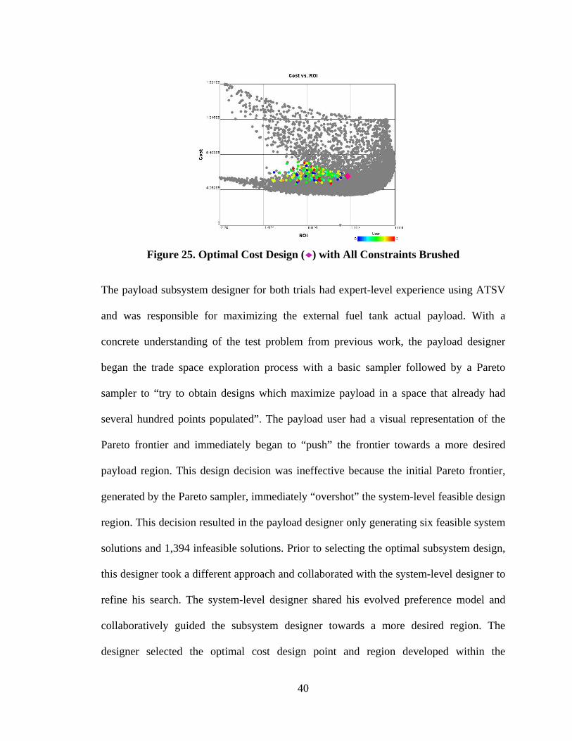
Figure 25. Optimal Cost Design ( ) with All Constraints Brushed

The payload subsystem designer for both trials had expert-level experience using ATSV

and was responsible for maximizing the external fuel tank actual payload. With a

concrete understanding of the test problem from previous work, the payload designer

began the trade space exploration process with a basic sampler followed by a Pareto

sampler to “try to obtain designs which maximize payload in a space that already had

several hundred points populated”. The payload user had a visual representation of the

Pareto frontier and immediately began to “push” the frontier towards a more desired

payload region. This design decision was ineffective because the initial Pareto frontier,

generated by the Pareto sampler, immediately “overshot” the system-level feasible design

region. This decision resulted in the payload designer only generating six feasible system

solutions and 1,394 infeasible solutions. Prior to selecting the optimal subsystem design,

this designer took a different approach and collaborated with the system-level designer to

refine his search. The system-level designer shared his evolved preference model and

collaboratively guided the subsystem designer towards a more desired region. The

designer selected the optimal cost design point and region developed within the

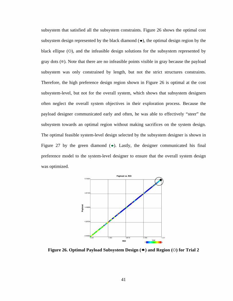
41

subsystem that satisfied all the subsystem constraints. Figure 26 shows the optimal cost

subsystem design represented by the black diamond ( ), the optimal design region by the

black ellipse ( ), and the infeasible design solutions for the subsystem represented by

gray dots ( ). Note that there are no infeasible points visible in gray because the payload

subsystem was only constrained by length, but not the strict structures constraints.

Therefore, the high preference design region shown in Figure 26 is optimal at the cost

subsystem-level, but not for the overall system, which shows that subsystem designers

often neglect the overall system objectives in their exploration process. Because the

payload designer communicated early and often, he was able to effectively “steer” the

subsystem towards an optimal region without making sacrifices on the system design.

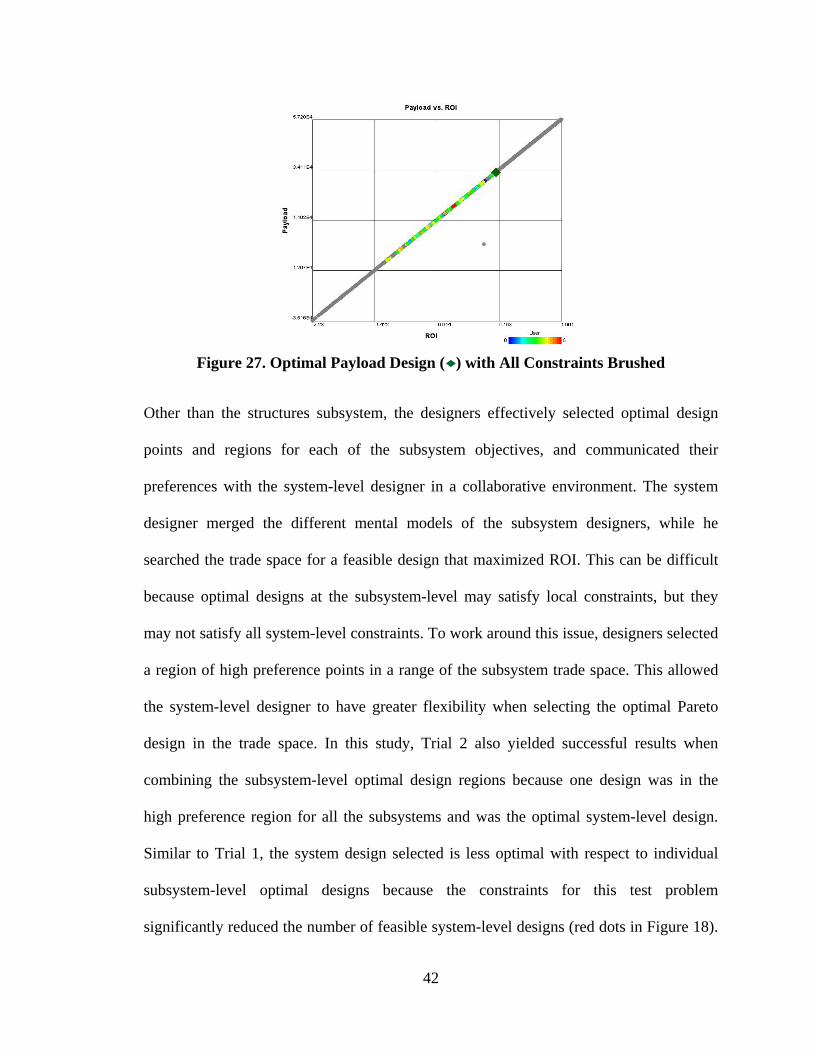
The optimal feasible system-level design selected by the subsystem designer is shown in

Figure 27 by the green diamond ( ). Lastly, the designer communicated his final

preference model to the system-level designer to ensure that the overall system design

was optimized.

Figure 26. Optimal Payload Subsystem Design ( ) and Region ( ) for Trial 2

42

Figure 27. Optimal Payload Design ( ) with All Constraints Brushed

Other than the structures subsystem, the designers effectively selected optimal design

points and regions for each of the subsystem objectives, and communicated their

preferences with the system-level designer in a collaborative environment. The system

designer merged the different mental models of the subsystem designers, while he

searched the trade space for a feasible design that maximized ROI. This can be difficult

because optimal designs at the subsystem-level may satisfy local constraints, but they

may not satisfy all system-level constraints. To work around this issue, designers selected

a region of high preference points in a range of the subsystem trade space. This allowed

the system-level designer to have greater flexibility when selecting the optimal Pareto

design in the trade space. In this study, Trial 2 also yielded successful results when

combining the subsystem-level optimal design regions because one design was in the

high preference region for all the subsystems and was the optimal system-level design.

Similar to Trial 1, the system design selected is less optimal with respect to individual

subsystem-level optimal designs because the constraints for this test problem

significantly reduced the number of feasible system-level designs (red dots in Figure 18).

43

Without automatic constraint handling [26] or an accurate knowledge of all system

constraints, the subsystem designs “overshot” the feasible region when using the Pareto

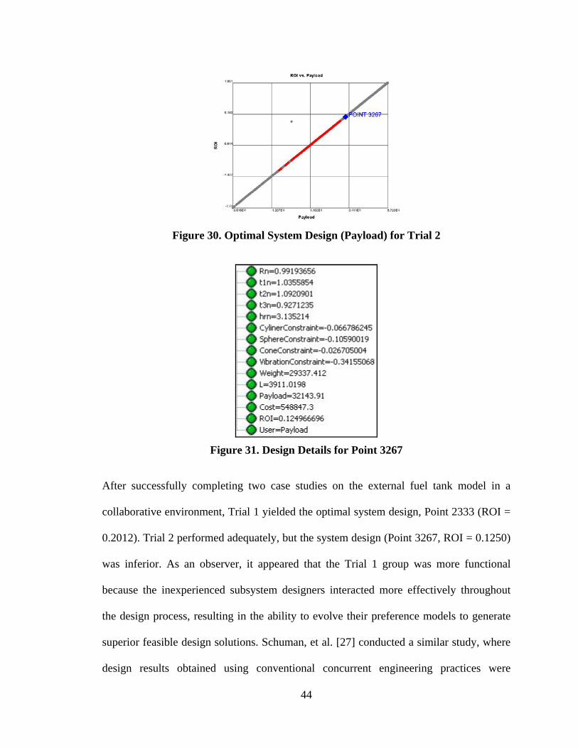
and attractor samplers. The optimum, Point 3267, is shown in Figure 28, Figure 29, and

Figure 30, for weight, cost, and payload versus ROI with infeasible points brushed out

(constraints), respectively. Point 3267 minimizes weight, minimizes cost, maximizes

payload, while maximizing the system ROI. Thus, Point 3267 is deemed the optimal

system design within the collaborative environment for Trial 2 and the design details are

shown in Figure 31.

Figure 28. Optimal System Design (Weight) for Trial 2

Figure 29. Optimal System Design (Cost) for Trial 2

44

Figure 30. Optimal System Design (Payload) for Trial 2

Figure 31. Design Details for Point 3267

After successfully completing two case studies on the external fuel tank model in a

collaborative environment, Trial 1 yielded the optimal system design, Point 2333 (ROI =

0.2012). Trial 2 performed adequately, but the system design (Point 3267, ROI = 0.1250)

was inferior. As an observer, it appeared that the Trial 1 group was more functional

because the inexperienced subsystem designers interacted more effectively throughout

the design process, resulting in the ability to evolve their preference models to generate

superior feasible design solutions. Schuman, et al. [27] conducted a similar study, where

design results obtained using conventional concurrent engineering practices were

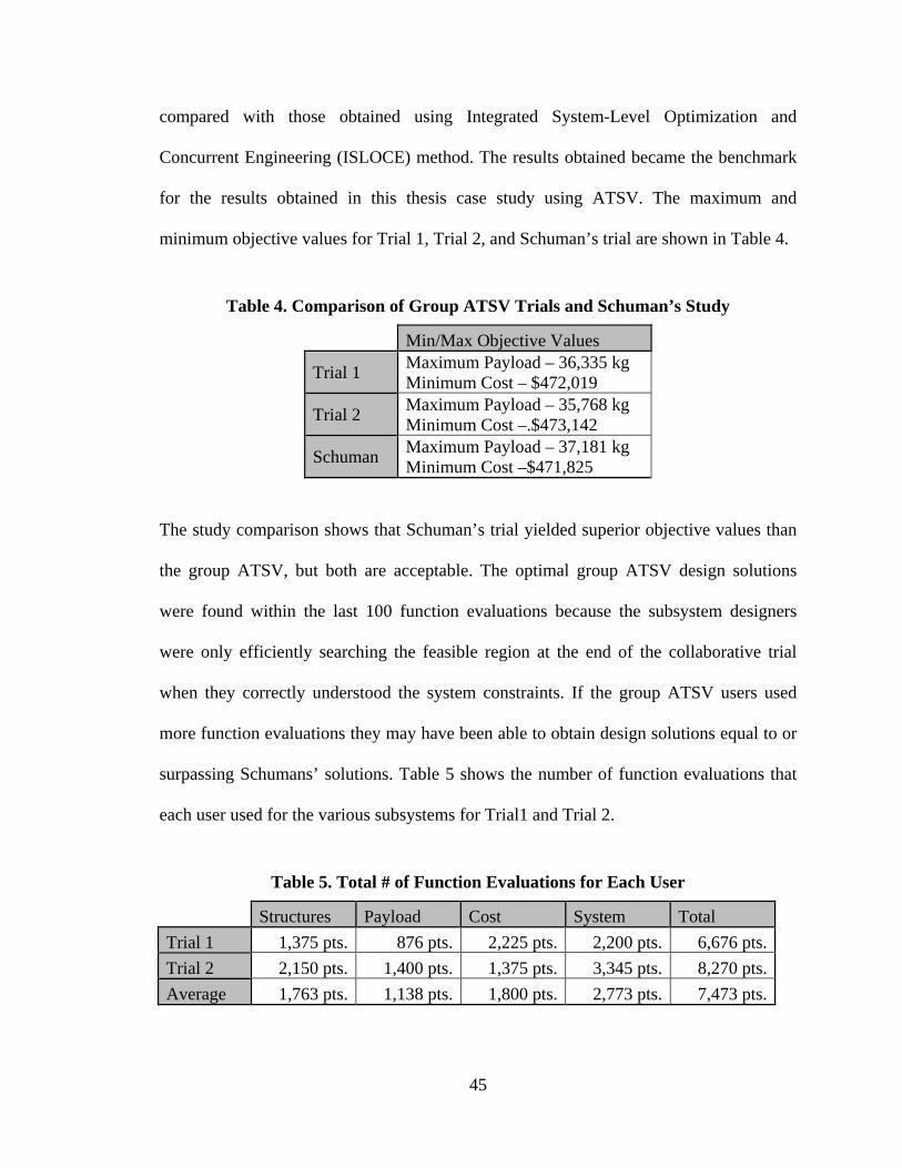
45

compared with those obtained using Integrated System-Level Optimization and

Concurrent Engineering (ISLOCE) method. The results obtained became the benchmark

for the results obtained in this thesis case study using ATSV. The maximum and

minimum objective values for Trial 1, Trial 2, and Schuman’s trial are shown in Table 4.

Table 4. Comparison of Group ATSV Trials and Schuman’s Study

Min/Max Objective Values

Trial 1 Maximum Payload – 36,335 kg Minimum Cost – $472,019

Trial 2 Maximum Payload – 35,768 kg Minimum Cost –.$473,142

Schuman Maximum Payload – 37,181 kg Minimum Cost –$471,825

The study comparison shows that Schuman’s trial yielded superior objective values than

the group ATSV, but both are acceptable. The optimal group ATSV design solutions

were found within the last 100 function evaluations because the subsystem designers

were only efficiently searching the feasible region at the end of the collaborative trial

when they correctly understood the system constraints. If the group ATSV users used

more function evaluations they may have been able to obtain design solutions equal to or

surpassing Schumans’ solutions. Table 5 shows the number of function evaluations that

each user used for the various subsystems for Trial1 and Trial 2.

Table 5. Total # of Function Evaluations for Each User

Structures Payload Cost System Total Trial 1 1,375 pts. 876 pts. 2,225 pts. 2,200 pts. 6,676 pts.Trial 2 2,150 pts. 1,400 pts. 1,375 pts. 3,345 pts. 8,270 pts.Average 1,763 pts. 1,138 pts. 1,800 pts. 2,773 pts. 7,473 pts.

46

Chapter 5

Conclusions and Suggestions for Future Work

As stated earlier, trade space exploration is a promising multi-user decision-making

paradigm that provides a visual and more intuitive means for formulating, adjusting, and

ultimately solving design optimization problems within a collaborative environment. The

results of this thesis indicate that collaborative engineering is an efficient method for

solving complex, multidisciplinary design problems because subsystem designers have

reduced responsibility, thus promoting maximum concentration on a subsystem task

where discipline expertise and motives can be effectively utilized. This allows the

system-level designer to mediate and guide the team decisions, rather than spending

unnecessary time and resources exploring the entire trade space.

The two trials each yielded similar findings in regards to how the designers formed

subsystem preferences, why designers sacrifice the system design to satisfy subsystem

objectives, and how subsystem preferences merge to obtain an optimal system design.

The results indicate that subsystem designers formulate design preferences too early in

the design process before accurately understanding the group objectives relative to their

subsystem objectives causing high preference subsystem regions to “overshoot” the

feasible system design region. Also, through observation, subsystem designers

communicate to the system designer, but the reverse collaboration is sparse in the present

setup. Although subsystem designers need to focus their resources on satisfying the

defined subsystem objectives and constraints, it is counterproductive to neglect the

system objectives during early exploration. To extend this work in the future, the trials

47

should be repeated using automatic constraint handling of system-level constraints. This

will help to prevent the subsystem designers from exploring infeasible regions by

restricting the sampling to only regions within the constraint boundaries.

When subsystem designers make sacrifices to the system design early in the optimization

process, the system-level designer is challenged to realign the team exploration with the

principal design objective. This stresses the importance of effective communication

between the system designer and the subsystem designers early and often. Specifically,

the structures subsystem designer for Trial 2 was completely misaligned early in his

search process, and the system level designer neglected to notify him. If an alarm was set

early, the team would be alleviated the pain of having to re-group at the end of the

collaborative process.

As discussed previously, the outcome of the collaborative engineering process is directly

proportional to the system designer’s ability to merge the subsystem mental models and

to maintain a level of communication that encourages the subsystem designers to explore

system optimal design regions. By effectively integrating system-level optimization

strategies in the concurrent engineering process, it is possible to improve the efficiency

and results of the overall design process. To verify these finding, the study should also be

repeated with test problems of different sizes and complexity as well as with users of

different experience levels to demonstrate how widely applicable – and beneficial – the

trade space exploration process is.

48

There are several possible extensions of this work. The external fuel tank model should

be executed with a single designer focusing on maximizing the system ROI, and then

Pareto performance metrics should be used to quantitatively compare the collaboratively

generated Pareto frontier with the single “human in the loop” design. This will measure

the speed-up in the number of Pareto solutions that are obtained when multidisciplinary

designs are optimized in a team environment.

49

References

[1] Simpson, T.W., Malone, M., Carlsen, D. and Kollat, J., 2008, "Evaluating the Performance of Visual Steering Commands for User-Guided Pareto Frontier Sampling during Trade Space Exploration", 2008 Design Engineering Technical Conferences & Computers and Information in Engineering Conference, New York City, NY, ASME IDETC 2008-49681.

[2] Sobieszczanski-Sobieski, J. and Haftka, R.T., 1997, "Multidisciplinary Aerospace Design Optimization: Survey of Recent Developments", Structural and Multidisciplinary Optimization, 14(1), 1-23.

[3] Braun, R.D. and Kroo, I.M., 1995, "Development and Application of the Collaborative Optimization Architecture in a Multidisciplinary Design Environment", ICASE/NASA Langley Workshop, Hampton, VA, 1-3.

[4] Wilson, T. D. and Schooler, J.W., 1991, "Thinking Too Much: Introspection can Reduce the Quality of Preferences and Decisions", Journal of Personality and Social Psychology, 60(2), 181-192.

[5] Shanteau, J., 1992, "Competence in Experts: The Role of Task Characteristics", Organizational Behavior and Human Decisions, 53(2), 252-266.

[6] Kroo, I., Altus, S., Braun, R., Gage, P. and Sobieski, I., 1994, Multidisciplinary Optimization Methods for Aircraft Preliminary Designs, AAIA Paper 94-4325.

[7] Kusiak, A., 1993, Concurrent Engineering: Automation, Tools, and Techniques, New York, Wiley.

[8] 1999, Nightline: Deep Dive. Palo Alto, CA, ABC News. [9] Young, I., 2008, Mental Models: Aligning Design Strategy with Human Behavior,

Rosenfeld Media, pp. 155-167. [10] Stump, G., Yukish, M. and Simpson, T. W., 2004, “The Advanced Trade Space

Visualizer: An Engineering Decision-Making Tool", 10th AIAA/ISSMO Multidisciplinary Analysis and Optimization Conference, AIAA, AIAA-2004-4568.

[11] Stump, G., Yukish, M., Simpson, T. W., Harris, E. N. and O'Hara, J. J., 2004, "Trade Space Exploration of Satellite Datasets Using a Design by Shopping Paradigm", IEEE Aerospace Conference, Big Sky, MT, March 6-13, Paper No. 1039.

[12] Buja, A., McDonald, J. A., Michalak, J., and Stuetzle, W., 1991, "Interactive Data Visualization Using Focusing and Linking", Proceedings of the IEEE Conference on Visualization '91, San Diego, CA, IEEE Computer Society Press, October, pp. 156-163.

[13] Becker, R.A. and Cleveland, W.S., 1987, "Brushing Scatterplots", Technometrics, 29(1), 127-142.

[14] Simpson, T. W., Donndelinger, J.A., Yukish, M., and Stump, G., 2007, "Visual Steering Commands for Trade Space Exploration: User-Guided Sampling with Example", Proceedings of the ASME 2007 International Design Engineering Technical Conferences & Computers and Information in Engineering Conference, Las Vegas, NV, DECC2007/DAC-34684.

[15] Price, K., Storn, R. and Lampinen, J., 2005, Differential Evolution - A Practical Approach to Global Optimization, Berlin, Springer, pp. 28-32.

50

[16] Robic, T. and Filipic, B., 2005, DEMO: Differential Evolution for Multi-Objective Optimization. In Evolutionary Multi-Criterion Optimization (EMO 2005), 520-533.

[17] Monostori, L., Vancza, J., Markus, A., Kadar, B. and Viharos, Z., 2003, "Towards the Realisation of Digital Enterprises", 36th CIRP International Seminar on Manufacturing Systems, Progress on Virtual Manufacturing Systems, Saarbrucken, Germany, 99-106.

[18] Tappeta, R. V., Nagendra, S. and Renaud, J.E., 1995, "A Mulitdisciplinary Design Optimization Approach for High Temperature Aircraft Engine Components", Springerlink, 18(2-3), 134-145.

[19] Braun, R. D., Moore, A.A. and Kroo, I.M., 1997, "Collaborative Approach to Launch Vehicle Design", Spacecraft and Rockets, 34(4), 478-486.

[20] Sobieski, I., and Kroo, I., 1996, "Aircraft Design Using Collaborative Optimization", Aerospace Sciences Meeting and Exhibit, Reno, NV, AIAA-1996-715.

[21] Tappeta, R.V. and Renaud, J.E., 1997, "Multiobjective Collaborative Optimization", Journal of Mechanical Design, 119(3), 403-411.

[22] Gentner, D., 1983, Mental Models, Lawrence Erlbaum Associates, Mahwah, NJ. [23] Cao, C. G. L., MacKenzie, C. L. and Payandeh, S., 1996, "Task and Motion

Analyses in Endoscopic Surgery", Proceedings of the ASME Dynamic Systems and Control Division, 58, 583-590.

[24] Freeman, J., Cohen, M.S. and Thompson, B.T., 1998, "Time-Stressed Decision-Making in the Cockpit", Proceedings of the Association for Information Systems 1998 Americas Conference, Baltimore, MD. Contract No. NAS2-14075.

[25] Sobieszczanski-Sobieski, J., 2002, "Different Objectives Result in Different Designs", AIAA MDO Short Course. Atlanta, GA.

[26] Simpson, T. W., Carlsen, D. E., Congdon, C. D., Stump, G. and Yukish, M. A., 2008, "Trade Space Exploration of a Wing Design Problem Using Visual Steering and Multi-Dimensional Data Visualization", 4th AIAA Multidisciplinary Design Optimization Specialist Conference, Schaumburg, IL, April 7-10, Paper No. AIAA-2008-2139.

[27] Schuman, T., de Weck, O.L. and Sobieski, J., 2005, "Integrated System-Level Optimization for Concurrent Engineering with Parametric Subsystem Modeling", 1st Multidisciplinary Design Optimization Specialist Conference, Austin, TX, AIAA, AIAA-2005-2199.

51

Academic Vita of Matthew John Malone

Permanent Address 58 Burkedale Crescent Rochester, NY 14625 Phone Contact (585)506-5678 Email Contact mjm5002@psu.edu Education The Pennsylvania State University, Schreyer Honors College, University Park, PA

• Bachelor Degree in Mechanical Engineering • Minor in Engineering Entrepreneurship • Honors in Mechanical Engineering with emphasis on trade space exploration • Graduation: May 2008

Thesis Title A study of engineering designers collaborating in a visual design environment Thesis Supervisor Dr. Timothy Simpson Professor of Mechanical and Industrial Engineering Director of the Learning Factory Work Experience General Electric Transportation, Erie, PA 5/2007-8/2007 Mechanical Engineer, Manufacturing and Methods Intern

• Conducted two lean manufacturing action workouts for consumable and chemical materials to eliminate overflow, reduce walking time, and ensure material availability

• Worked with Process Technical Advisors to develop lean line metrics such as takt time

• Improved with overhead and inside lighting in Main Cab production work centers by leading an action workout with engineers and hourly operators

• Implemented new labeling system on a centralized hardware rack to improve material stocking

• Actively participated in physical inventory by preparing necessary material locations and reconciling database discrepancies

• Assisted with production tasks on the manufacturing floor during weekend efforts intended to overcome scheduling deficiencies and eliminate unusable materials in adjacent yard.

52

General Electric Transportation, Erie, PA 6/2006-8/2006 Mechanical Engineer, Electronic Packaging and Productivity Intern

• Solved design flaws by performing detailed tests for large locomotive customers such as Burlington Northern Santa Fe, Union Pacific, and Canadian National

• Conducted Highly Accelerated Life Testing on equipment for the locomotive such as satellite antennas

• Collaborated with senior engineers to make significant design changes on high voltage cabinets

• Proposed new methods to package traction motor electronics with noteworthy cost savings

• Improved manufacturing processes for electronic packaging weldments in time for scheduled testing

• Assisted with production tasks on the manufacturing floor during weekend efforts intended to overcome scheduling deficiencies

Honors and Awards

• Dean’s List seven semesters at Penn State University • Passed Fundamentals of Engineering Examination • Penn State All-Discipline Honor Society, Phi Kappa Phi • Penn State College of Engineering Honor Society, Tau Beta Pi • Mechanical Engineering Honor Society, Pi Tau Sigma • Allegheny Conference Top 5, Penn State Ski Team, 2004-2008

Affiliations

• Professional Development Committee Chair at GE Transportation in 2007 for over 200 interns

• Penn State Ski Team: Competed in two USCSA National Championships and received 2nd Team All-American recognition

• Tour Guide for Mechanical/Nuclear Engineering Department at Penn State University

• Active member of the Society of Automotive Engineers and ASME Publications

• Simpson, T.W., Malone, M., Carlsen, D., Kollat, J., 2008, Evaluating the Performance of Visual Steering Commands for User-Guided Pareto Frontier Sampling during Trade Space Exploration, ASME IDETC.

Community Service Involvement

• Ronald McDonald House • Coaches Vs. Cancer • THON