SCIENTIFIC COMMITTEE FIFTH REGULAR SESSION

10-21 August 2009 Port Vila, Vanuatu

Yellowfin CPUE Standardization for Taiwanese Distant Water Longline Fishery in the

WCPO – with Emphasis on Target Change

WCPFC-SC5-2005/SA-WP-02

Shui-Kai Chang 1, Simon Hoyle

2 and Hung-I Liu

3

1 College of Marine Science, National Sun Yat-sen University, Kaohsiung, Taiwan 2 Secretariat of the Pacific Community, Noumea, New Caledonia 3 Fisheries Information Department, the Overseas Fisheries Development Council, Taipei, Taiwan

1  

(DO NOT CITE THIS PAPER)

Yellowfin CPUE Standardization for Taiwanese Distant Water Longline Fishery in the WCPO – with Emphasis on Target Change

Shui-Kai Chang1, Simon Hoyle2 and Hung-I Liu3

1 College of Marine Science, National Sun Yat-sen University, Kaohsiung, Taiwan 2 Secretariat of the Pacific Community, Noumea, New Caledonia

3 Fisheries Information Department, the Overseas Fisheries Development Council, Taipei, Taiwan

Introduction

Taiwanese tuna fisheries have a long history of fishing in the Western and Central

Pacific Ocean (WCPO). Currently they employ two main gear types to fish for tuna

and tuna-like species in the region, the longline and the purse seine. Records of

longline fisheries are available as far back as the 1960s. As the longline fisheries

developed, some vessels began to fish in the waters of coastal states of the WCPO in

accordance with fishing access agreements. These vessels were termed the ‘offshore

longline fishery’ and the rest, which constituted the majority of the effort, was termed

the ‘distant-water longline fishery’ (DWLL). The DWLL provides about 45 years of

fishing records since 1964.

Albacore, yellowfin and bigeye tunas have been the main species caught, but the

approach to targeting has varied through time, as well as spatially. Each species has its

main fishing ground: temperate waters in the north and the south Pacific were the

major fishing ground for albacore; and tropical waters in the central Pacific have been

the major fishing ground for bigeye and yellowfin tunas. In the course of target

change, the geographical distribution of efforts and catches of the DWLL changed

(Fig. 1).

Historically, DWLL vessels have continuously fishing for southern albacore (Fig. 1),

but this is not the case for northern albacore. The southern albacore-targeting vessels

(the ALB vessels) also fished for yellowfin in the early stage of the history, and so are

more relevant than are the northern albacore vessels to the stock assessment of the

WCPO yellowfin resource. Albacore has consistently been the major target species of

the DWLL; the annual catch has fluctuated between 15,000 – 25,000 tons (Fig. 2).

However, recently targeting of albacore has declined, with a reduction in the number

of ALB vessels and shifting of target species to tropical tunas, which currently have

higher commercial value.

2  

Yellowfin tuna was a target of the longline fishery in the mid-1960s to mid-1970s for

canning. However this targeting decreased because of the canneries’ preference for

white-meat species such as albacore. Following the development of the bigeye fishery

in the tropical areas of the WCPO since 2002, the catch of yellowfin has increased

again. However, this increase was mainly due to the increase of fishing activities by

bigeye-targeting vessels (BET vessels), not necessary the increase of yellowfin fishing

activities. On the other hand, bigeye tuna was mainly a bycatch when yellowfin was a

target in the early stage of the longline history. The catch was low until the

development of bigeye fishery in WCPO around 2002.

This target change was accompanied by many adaptations in the fishery, such as

changes of fishing ground/season and fishing gear (e.g., number of hooks per basket).

As may be expected, these changes affected the CPUE (catch per unit effort), and

must be taken into account when using CPUE to develop an abundance index. A

simple example is that the increase of targeting activities on bigeye increased the

bigeye CPUE after 2002, but it should not be inferred that the bigeye stock became

abundant.

The effects of target changes on CPUE need to be properly addressed in the CPUE

standardization procedure, but it can be difficult to deal with. In the case of WCPO

bigeye, many models and assumptions have been applied to standardize the CPUE

(such as Su et al. 2008), but it has been difficult to fully remove the effects of

targeting changes. In the aforementioned example, most of the effect of the targeting

change was removed from the index, however the resulted CPUE still increased

significantly after 2002, in contrast with the CPUE from the Japanese fleet fishing in

the same areas but with more consistent targeting behavior (Langley et al. 2008;

Hoyle 2009).

In this paper we standardize the WCPO yellowfin tuna CPUE, with emphasis on the

treatment of targeting factors. Discussions on inclusion of some other factors are also

provided.

Material and methods

The data

Set by set logbook data of Taiwanese DWLL of 1964-2008 were obtained from the

Overseas Fisheries Development Council of the ROC, which since 1996 has been

commissioned by the Fisheries Agency of Taiwan to process and compile tuna

fisheries statistics. These logbook data include vessel identity, fishing position (noon

3  

time position at 55 longitudelatitude square level), fishing date, total hooks

deployed, catches (in number) of major tunas and billfishes, and information of

number of hooks per basket (starting from 1995 when it becomes available). The

catch data has undergone a crosscheck process with commercial trading data on a

trip-by-trip basis, since the detail commercial trading data became available in 1997.

The fishing location information has undergone a similar verification process with

VMS data, since 2005 when VMS data became reasonably complete. CPUE was

calculated as catch in number per 1,000 hooks. The data of 2007-08 are still

preliminary.

This study also references the observer data, which have been collected on DWLL in

the Pacific Ocean since 2002, when the program was implemented by the Taiwan

Fisheries Agency. Accumulated and average catch composition for ALB vessels and

BET vessels were calculated from 49 observation trips from 2002-2008.

The covariates and standardization cases design

Covariates were defined according to the factors that might affect yellowfin CPUE.

Catch rate fluctuates in different spatiotemporal strata and so covariates relating to

fishing time/area are fundamental to the standardization procedure. Basic covariates

defined for this study include year, quarter (Jan.-Mar., Apr.-Jun., Jul.-Sep., and

Oct.-Dec.) and statistical region stratification. The ‘region stratification’ was referred

as ‘Region’ in this study (Fig. 3) and matches the configuration used in the WCPO

yellowfin stock assessment (Langley et al 2007, 2009). In principle, R1 and R2 are

the north Pacific albacore fishing ground, R3 and R4 are the tropical tuna (bigeye and

yellowfin tunas) fishing ground, and R5 and R6 are the south Pacific albacore fishing

ground.

This study also performed many exploratory examinations on effects of additional

covariates. Altogether the study performed 8 cases of CPUE standardization runs; the

covariates included in the models are listed in Table 1. The following remarks

describe the additional covariates and relative case runs.

Considering the complexity of the Taiwanese DWLL fleet, target species is the most

important factor to be addressed. This factor was addressed from two perspectives:

separating the data at the vessel-year level by presumed target, and including a target

indicator in the model. For the first aspect, the study used ad hoc criteria developed

from observer data to separate the data on a vessel*year basis into three ‘fleet types’.

These fleet types were either included in the model as a covariate (Case-2 to -6, a pair

4  

of comparison tests in Case-1 against Case-2), or different types of data were

standardized separately (Case-7 and -8).

For the second aspect, four types of target indicators were defined and tested

individually within a standardization run (Case-3). The four indicator types were (1)

ALB & BET - albacore catch and bigeye catch were included in the model as two

categorical variables, after transforming the continuous catch values by comparing

them to quantile of the catch of the same year; (2) ALB% & BET% - same as (1) but

using of the proportion of the species in the catch, rather than the catch itself; (3) as

for (1), but using catch composition of yellowfin tuna; (4) NHPB - treating number of

hooks per basket as a covariate in the model. These indictor types have been applied

or discussed in the CPUE standardization works for other stocks in the past (Ortiz et

al., 2000; Takeuchi and Yokawa, 2000; Mejuto et al., 2001; Hoey et al., 2003; Chang

and Wang, 2004; Wang et al., 2005; Wang et al., 2006; Chang et al., 2007; Liu et al.,

2007; Chang et al., 2008; Hsu, 2008; Mejuto et al., 2008; Su et al., 2008)

It is common in the scientific meetings of tuna RFMOs of the Atlantic and Indian

Oceans (i.e., ICCAT and IOTC) and many other research works (Yokawa et al., 2001;

Chang, 2003; Chang and Wang, 2004; Ortiz and Arocha, 2004; Wang et al., 2006;

Chang et al., 2007; Liu et al., 2007; Chang et al., 2008; Mejuto et al., 2008; Okamoto,

2008) that, although the distribution of a fish stock could be separated into different

regions (subareas, such as Fig. 3) according to CPUE or fish size distribution patterns,

the ‘region’ factor was included in the model and performed a single standardization

analysis. However, in the tuna RFMOs of the Pacific Ocean (i.e., IATTC and

WCPFC), standardizations are usually performed separately for each region (therefore

no ‘region’ factor in the model) (e.g. Langley et al 2005, Hoyle and Maunder 2005,

Hoyle 2009). The effect of single analysis and separate analyses was tested in the

study in Case-3 vs. Case-5 and Case-4 vs. Case-6.

It is also common that when regions are defined (a region composed of many 55 longitudelatitude squares, or 5-degree squares), the ‘region’ is treated as a factor in

the model, without considering the effect from 5-degree grid position in terms of

longitude and latitude (termed as grid effect). However, this grid effect is considered

in most of the CPUE standardizations of the Pacific tuna species (e.g. Langley et al,

2005; Hoyle and Maunder, 2005; Hoyle, 2009). This effect was tested in the study in

Case-2 vs. Case-4 and Case-5 vs. Case-6.

The basic analytical model used was a generalized linear model (GLM, Kimura, 1981;

Maunder and Punt, 2004; Venables and Dichmont, 2004) with a lognormal error

assumption which is commonly used to standardize catch and effort data (Maunder

5  

and Punt, 2004). Zero catches are usually adjusted by adding a positive constant,

while maintaining or achieving normality of the transformed data (Berry, 1987). In

this study, 10% of the mean catch rate was added to all nominal CPUEs (Ortiz et al.,

2000; Ortiz and Arocha, 2004). However, when dealing with data for bycatch species

in which many sets have zero catch, a GLM approach assuming a delta-lognormal

model distribution will fit the data better. With this two-step approach, the proportion

of positive sets is modeled assuming a binomial error distribution, and the catch rate

of the non-zero catch sets is modeled assuming a lognormal error distribution (Lo et

al., 1992; Stefánsson, 1996; Rodríguez-Marín et al., 2003; Maunder and Punt, 2004;

Ortiz and Arocha, 2004). The standardized index is the product of these

model-estimated components. The results from common lognormal assumption and

delta-lognormal assumption were examined in Case-7 vs. Case-8.

In the model runs, two-way interactions among the main factors were examined.

Normally a step-wise regression procedure is used to determine the set of main factors

and interactions that significantly explain the observed variability and then define the

final model. This procedure was not performed however, because the study has

purposely conducted case comparisons by including specific factor(s) into the model.

Therefore, the study determine the factors and interactions based primarily on whether

they could explain the variability significantly (p<0.001).

Results and Discussion

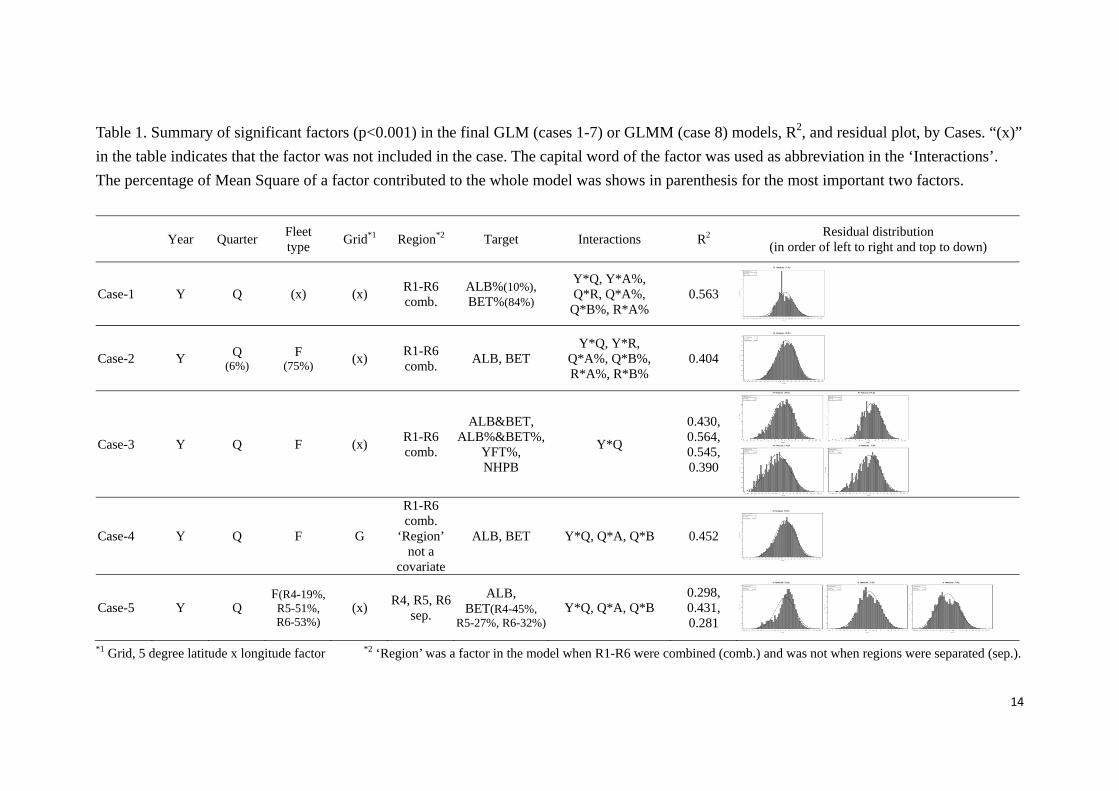
The significant factors (p<0.001) in the final model are shown in Table 1 for the 8

case runs, together with their R2 and residual distributions. The table also provides

percentage of Mean Square (MS) of a factor to overall MS in model for the first two

factors. Explanations of the results, comparisons and discussions follow for each case.

Case-1

This is a simple GLM run that forms a basis for later comparisons. The factors

included in this model (i.e., year, quarter, region, target and interaction terms) were

those commonly used for standardizing Taiwanese distant water CPUE in the other

Oceans (Chang et al., 2007; Liu et al., 2007; Chang et al., 2008). Target indicator was

catch ratios of bigeye (BET%) and albacore (ALB%), assuming that fishing vessels

will make all necessary adjustments to increase the catch composition of their target

species. So, for example, for an albacore targeting vessel the albacore catch would

normally be higher against the vessel’s overall catch. The continuous catch ratios

were grouped into four categories based on quantile of the annual catch ratios by

6  

species. From Table 1, the two target factors have explained over 90% of the mean

squares, emphasizing the importance of target factor in the model.

The GLM assumes a log-normal error distribution. However, the diagnostic residual

plot in Table 1 shows the error distribution did not conform to log-normal assumption

and the residuals could be split into two groups. Fig. 4 shows species compositions of

the source data that resulted in the two groups of residuals, indicating that the features

of the two groups’ data are different in species composition. The group-B data has

higher albacore composition (95% in average) in the catch, indicating that it comes

from the ALB fleet; and the group-A might come from the BET fleet. This suggests

that the different features of the two groups’ data need to be properly addressed in the

model.

Case-2

This case includes fleet type information to address the above concern. The Fisheries

Agency has been implementing an observer program in the Pacific Ocean since 2002.

From the 49 trips of observer data during 2002-08, it was noted that ALB-targeting

vessels fished mainly in the ALB fishing ground (Regions 5 and 6), but sometimes

fished in BET fishing ground (Regions 3 and 4) and the proportion of albacore in the

catch (ALB%) was different in the two fishing grounds. The observer data showed

that the average ALB% of an albacore vessel was 94% in southern albacore fishing

ground and 63% in bigeye fishing ground (Fig. 5). On the other hand, for a

BET-targeting vessel, the ALB% was less than 20% in the bigeye fishing ground.

Based on this information, ad hoc criteria were set to assign each vessel*year a fleet

type: fleet type A – annual ALB% of that vessel >95% in albacore fishing ground;

fleet type B – annual ALB%>70% in bigeye fishing ground; and, fleet type C – the

rest.

The target indicator normally used (ALB%&BET%) has a statistical defect that will

be discussed in the following case. For the convenience of comparisons with the

remaining cases, the target indicator used in this case was catches of ALB and BET

(ALB&BET).

The residual distribution of the Case-2 run, which adds fleet type factor to the Case-1

model, is significantly better than that of Case-1. Fleet type factor has explained 75%

of the overall MS.

Case-3

This case is a test of the effect of different target indicators. Albacore and bigeye

7  

occupy different depths of the sea. If NHPB can be assumed to represent the depth of

the hooks, e.g., larger NHPB indicating hooks set deeper to target bigeye, then NHPB

would be a good indicator for target factor. Although this assumption is not always

valid, since the depth of hooks is affected by strength of current, weight of line

material and many other environmental or technical factors, NHPB has been used for

many CPUE standardizations as a target indicator.

The NHPB information of the Taiwanese DWLL is available only since 1995 and the

coverage was low in the beginning. For comparing the effects of different target

indicators, only the data with NHPB information were used in this case. Table 1

shows that when using catches of ALB and BET (ALB&BET) as an indicator, the

residual distribution was more in conformity with the assumed log-normal distribution.

However the resulting relative CPUEs did not show differ much among the four

indicators (Fig. 6). Although it seems ALB&BET produced flatter trend than that

using ALB%&BET% in Fig. 6, the long term trend (using full set of data) shown a

different image (Fig. 7).

The response variable in the GLM is natural logarithm transformed CPUE of

yellowfin. From a statistical point of view, if the explanatory variable also utilized the

information of yellowfin, then the model violates the requirement that the explanatory

and response variables should be independent. In this case, ALB%&BET% and

YFT% are not appropriate to be target indicators although the results are obviously

similar to that of using NHPB in the short time of 1995-2008.

Case-4

This case, comparing to Case-2, includes 5-degree grid factor in the model. In this

case, the region factor could not be included, or no standardized year effect could be

obtained. The grid factor is confounded with the region factor (region is made up of

many grid squares). From Table 1, there was not much improvement by including grid

factor in terms of residual distribution and R2. The standardized relative CPUEs also

appeared similar between the two series, except for the early two years (Fig. 8).

The consideration for including this grid factor was that, it is very likely that there is a

lot of local (i.e. within region) spatial variation in catch rate, so including this factor

helps to account for catch rate changes when fishing effort moves within the region.

For example, this factor may be important when hyperstability or hyperdepletion are

possible. The underlying concept is that locations have relatively permanent features

(bathymetry, oceanography) that affect the local numbers or catch rates of tuna.

Interacting the grid effect with time is generally not feasible, since there is rarely

8  

enough data to estimate each grid*time parameter. In any case, the stock assessment

model assumes a uniform biomass trend within each region, so a single temporal

abundance index for each region is an appropriate output from the CPUE

standardization.

Including grid factor did not make much difference to the results in this case, in

comparison with Case-2, but similar comparisons were also conducted in Case-5 and

-6 (discussed later) and the results did show improvements. Therefore, this study

recommended including grid factor in the CPUE standardization for wide-range

distributed species.

Case-5

All 6 regions were combined as a single run with region factor in previous cases.

Starting from this case, the GLM run was performed separately for each region. To

make the study concise, only regions 4-6 where most fishing effort is concentrated

were considered in this and the following cases.

This case basically is the same as Case-2 except of separate GLM runs for each region.

The residual distributions in Table 1 demonstrated that the apparent normal

distribution pattern in Case-2 (all regions combined) was not maintained when the

regions were separated, particularly for Regions 4 and 6. This result suggested that the

combined model may have disguised a mixture of distributions. Comparisons of the

CPUE series by region derived from the combined model in Case-2 and from the

separate model in this case (not shown here) also shown improvements in that all the

outliers in Regions 4-6 (large increases in several years) in Case-2 disappeared in this

case. It is very likely that the relationship between response variable (transformed

catch rate) and explanatory variables (covariates) are not constant over the entire

study regions, which may bias the year effects. Therefore, conducting separate model

runs for each region is recommended.

Case-6

This case examines the effect of including the grid factor in separate model runs for

each region. Apart from including the grid factor, it is the same as Case-5. Including

the grid factor improved the residual distributions and R2. As expected for region 6

where spatial variation of yellowfin CPUE is high, grid factor has explained 38% of

the total variance (13% of the overall MS in Table 1). It further demonstrated that if

effort shifts from low catch rate areas to high catch rate areas, then a model without

grid factor included will be biased.

9  

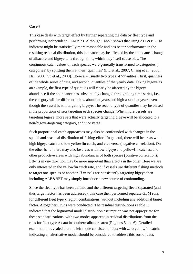
Case-7

This case deals with target effect by further separating the data by fleet type and

performing independent GLM runs. Although Case-3 shows that using ALB&BET as

indicator might be statistically more reasonable and has better performance in the

resulting residual distribution, this indicator may be affected by the abundance change

of albacore and bigeye tuna through time, which may itself cause bias. The

continuous catch values of each species were generally transformed to categories (4

categories) by splitting them at their ‘quantiles’ (Liu et al., 2007; Chang et al., 2008;

Hsu, 2008; Su et al., 2008). There are usually two types of ‘quantiles’: first, quantiles

of the whole series of data, and second, quantiles of the yearly data. Taking bigeye as

an example, the first type of quantiles will clearly be affected by the bigeye

abundance if the abundance has substantially changed through long time series, i.e.,

the category will be different in low abundant years and high abundant years even

though the vessel is still targeting bigeye. The second type of quantiles may be biased

if the proportions of sets targeting each species change. When more vessels are

targeting bigeye, more sets that were actually targeting bigeye will be allocated to a

non-bigeye-targeting category, and vice versa.

Such proportional catch approaches may also be confounded with changes in the

spatial and seasonal distribution of fishing effort. In general, there will be areas with

high bigeye catch and low yellowfin catch, and vice versa (negative correlation). On

the other hand, there may also be areas with low bigeye and yellowfin catches, and

other productive areas with high abundances of both species (positive correlation).

Effects in one direction may be more important than effects in the other. Here we are

only interested in the yellowfin catch rate, and if vessels use different fishing methods

to target one species or another. If vessels are consistently targeting bigeye then

including ALB&BET may simply introduce a new source of confounding.

Since the fleet type has been defined and the different targeting fleets separated (and

thus target factor has been addressed), this case then performed separate GLM runs

for different fleet type x region combinations, without including any additional target

factor. Altogether 6 runs were conducted. The residual distributions (Table 1)

indicated that the lognormal model distribution assumption was not appropriate for

these standardizations, with two modes apparent in residual distributions from the

runs for fleet type A data in southern albacore area (Regions 5 and 6). Detailed

examination revealed that the left mode consisted of data with zero yellowfin catch,

indicating an alternative model should be considered to address this sort of data.

10  

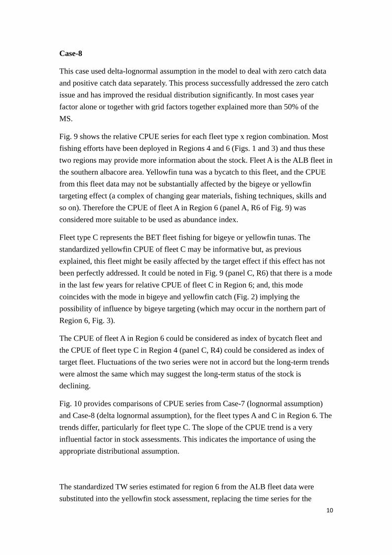
Case-8

This case used delta-lognormal assumption in the model to deal with zero catch data

and positive catch data separately. This process successfully addressed the zero catch

issue and has improved the residual distribution significantly. In most cases year

factor alone or together with grid factors together explained more than 50% of the

MS.

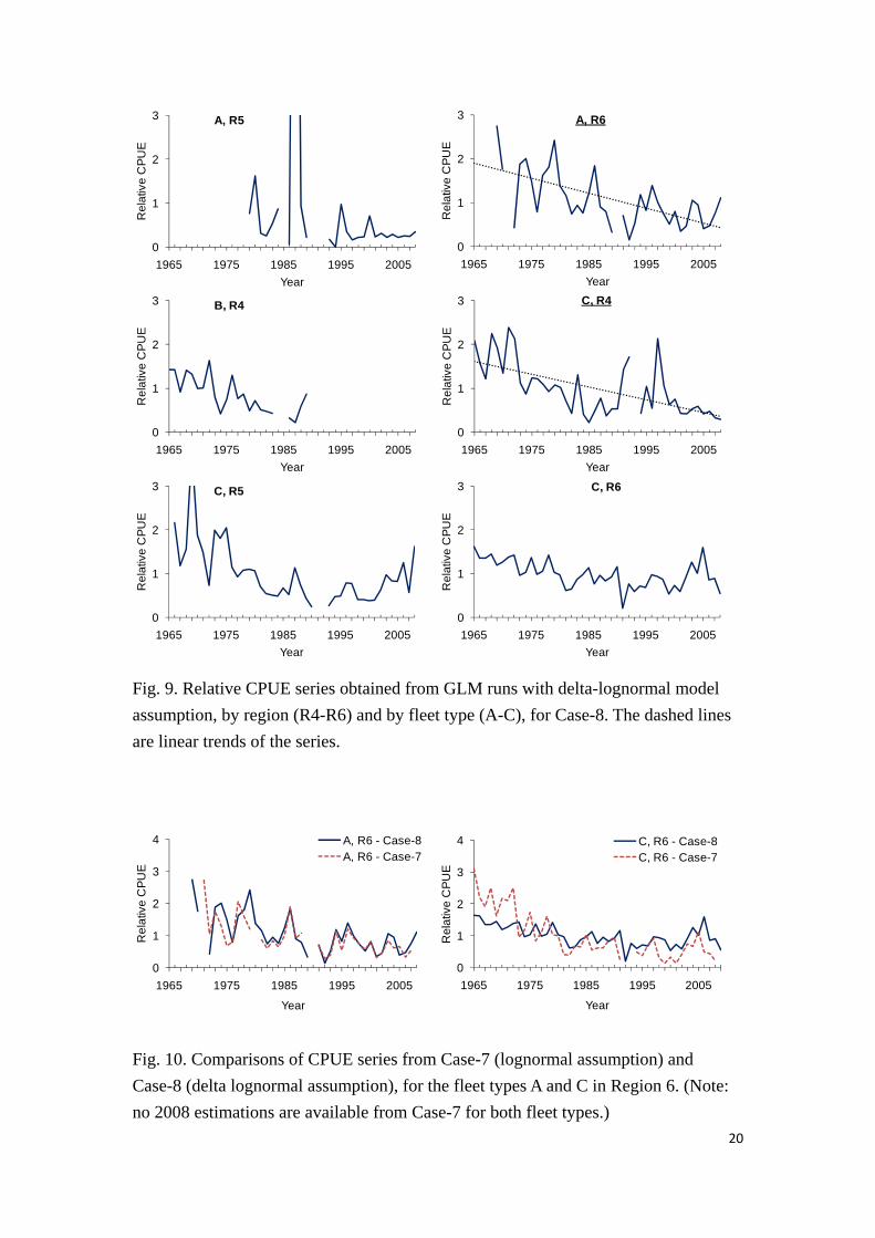
Fig. 9 shows the relative CPUE series for each fleet type x region combination. Most

fishing efforts have been deployed in Regions 4 and 6 (Figs. 1 and 3) and thus these

two regions may provide more information about the stock. Fleet A is the ALB fleet in

the southern albacore area. Yellowfin tuna was a bycatch to this fleet, and the CPUE

from this fleet data may not be substantially affected by the bigeye or yellowfin

targeting effect (a complex of changing gear materials, fishing techniques, skills and

so on). Therefore the CPUE of fleet A in Region 6 (panel A, R6 of Fig. 9) was

considered more suitable to be used as abundance index.

Fleet type C represents the BET fleet fishing for bigeye or yellowfin tunas. The

standardized yellowfin CPUE of fleet C may be informative but, as previous

explained, this fleet might be easily affected by the target effect if this effect has not

been perfectly addressed. It could be noted in Fig. 9 (panel C, R6) that there is a mode

in the last few years for relative CPUE of fleet C in Region 6; and, this mode

coincides with the mode in bigeye and yellowfin catch (Fig. 2) implying the

possibility of influence by bigeye targeting (which may occur in the northern part of

Region 6, Fig. 3).

The CPUE of fleet A in Region 6 could be considered as index of bycatch fleet and

the CPUE of fleet type C in Region 4 (panel C, R4) could be considered as index of

target fleet. Fluctuations of the two series were not in accord but the long-term trends

were almost the same which may suggest the long-term status of the stock is

declining.

Fig. 10 provides comparisons of CPUE series from Case-7 (lognormal assumption)

and Case-8 (delta lognormal assumption), for the fleet types A and C in Region 6. The

trends differ, particularly for fleet type C. The slope of the CPUE trend is a very

influential factor in stock assessments. This indicates the importance of using the

appropriate distributional assumption.

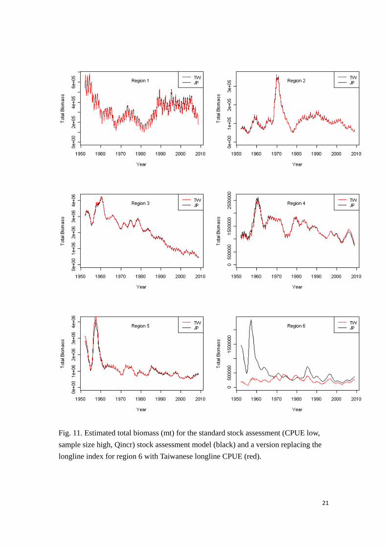
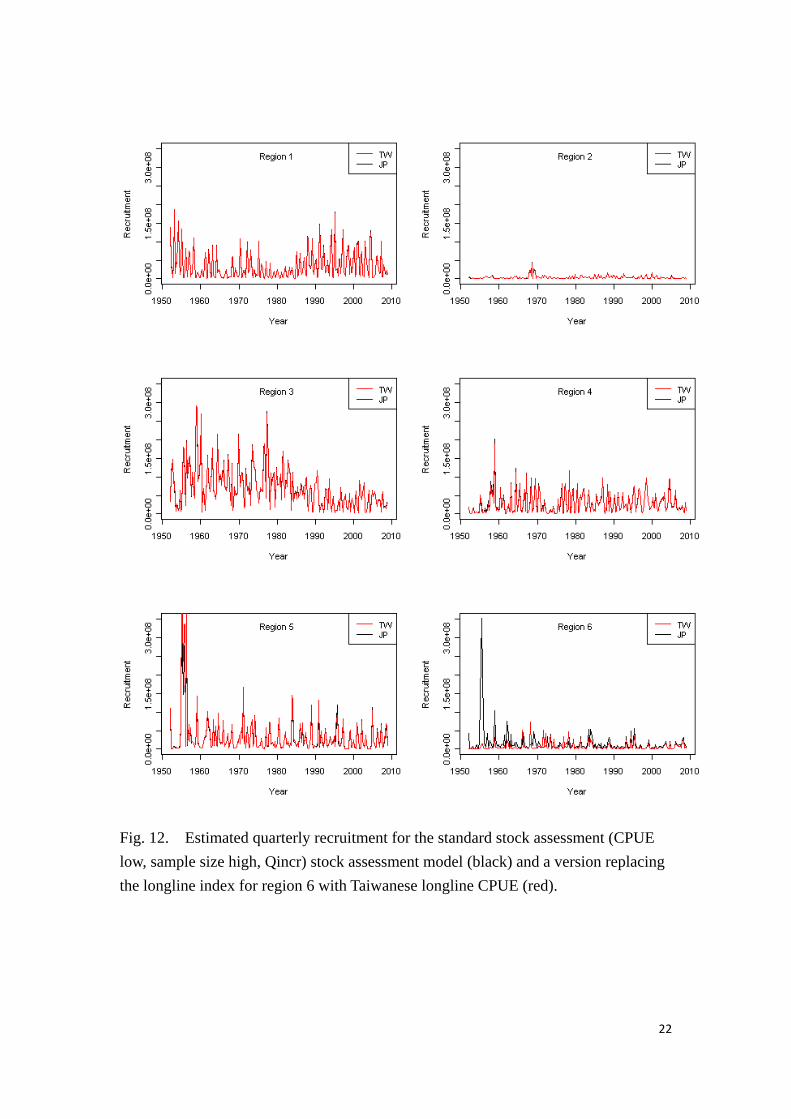
The standardized TW series estimated for region 6 from the ALB fleet data were

substituted into the yellowfin stock assessment, replacing the time series for the

11  

Japanese fleet in region 6. The recruitment and biomass trends (figures 11 and 12) in

region 6 are particularly affected, which indicates the significance of the CPUE trends

for model results. Trends in other regions are not affected substantially. Movement

rates into region 6 drop, and movement rate out of region 6 increase. It is not possible

to draw many strong conclusions about the results since the CPUE series was applied

to a fishery which tends to select slightly smaller fish than the Taiwanese fishery.

Further work should be carried out to separate the Japanese and Taiwanese fleets in

the model.

This report provided several examinations and discussions of inclusions of additional

covariates. The results indicated that 5-degree grid effect should be considered, and

that GLM runs should preferably be conducted separately by region, rather than in a

combined model. The most important factor to take into account was targeting,

especially for a fishery with complex target species. The study demonstrated the

effects of considering different sorts of target indicators but suggested that the best

approach is to separate the data by different targeting fleet. The separation approach

applied here was based on aggregated information from 49 observer trips data (to

avoid influence from singe vessel) from which simple “catch ratio x region” criteria

were developed. This approach provided a simple base for separation. However, the

separation could be done in a more precise manner in future by using statistical

clustering techniques, taking advantage of detailed information from logbook and

observer data.

The 6 regions defined here were adopted from WCPFC, based on spatial analyses of

yellowfin catch size distributions and catch rate trends (Langley 2006a, 2006b). This

regional definition is used in WCPFC stock assessment models, and indices of

abundance used in these models must use matching regions. However, this definition

was not entirely suitable for standardization of Taiwanese DWLL since it did not split

the catch distribution of different species correctly, i.e., the Region 4 should extended

at least 5 south to cover all bigeye targeting efforts (Fig. 3). Further examination of

the regional definitions may be useful, based on (for example) catches, catch

composition, and fish sizes. The effect on standardizations and the stock assessment

of different regional definitions may also be examined.

References

Berry, D.A., 1987. Logarithmic transformations in ANOVA. Biometrics 43, 439–456

Chang, S.K., 2003. Analysis of Taiwanese white marlin catch data and standardization of catch rates. Col. Vol. Sci. Pap. ICCAT 55(2), 453-466.

12  

Chang, S.K., Lee, H.H., Liu, H.I, 2007. Standardization of south Atlantic swordfish by-catch rate for Taiwanese longline fleet. Col. Vol. Sci. Pap. ICCAT 60(6), 1974-1985.

Chang, S.K., Liu, H.I, Chang, S.T., 2008. CPUE standardizations for yellowfin tuna caught by Taiwanese deep sea longline fishery in the tropical Indian Ocean using generalized linear model and generalized linear mixed model. The 2008 Working Party on Tropical Tunas, Indian Ocean Tuna Commission, IOTC-2008-WPTT-31. 11 pp. http://www.iotc.org/files/proceedings/2008/wptt/IOTC-2008-WPTT-31.pdf

Chang, S.K., Wang, S.J., 2004. CPUE standardization of Indian Ocean swordfish from Taiwanese longline fishery for data up to 2002. The 2004 Working Party on Billfish, Indian Ocean Tuna Commission, IOTC-2004-WPB-09. 18 pp. http://www.iotc.org/files/proceedings/2004/wpb/IOTC-2004-WPB-09.pdf

Hoey, J.J., Mejuto, J., Porter, J., Paul, S., Yokawa, K., 2003. An updated biomass index of abundance for north Atlantic swordfish, 1963-2001. Col. Vol. Sci. Pap. ICCAT 55(4), 1562-1575.

Hoyle, S.D., Bigelow, K.A., Langley, A.D., Maunder, M.N., 2007. Proceedings of the pelagic longline catch rate standardization meeting. The 3rd Meeting of the Scientific Committee (2007), Western and Central Pacific Fisheries Commission, ME-IP-1. 71 pp. http://www.wcpfc.int/node/1393

Hoyle, S.D., Maunder, M.N., 2006. Standardisation of yellowfin and bigeye CPUE data from Japanese longliners, 1975-2004. The 6th Stock Assessment Review Meeting, Inter-American Tropical Tuna Commission, SAR-7-07.http://www.iattc.org/PDFFiles2/SAR-7-07-LL-CPUE-standardization.pdf .

Hsu, C.C., 2008. Standardized catch per unit effort of bigeye tuna (Thunnus obesus) for the Taiwanese longline fishery in the Atlantic Ocean by general additive model. Col. Vol. Sci. Pap. ICCAT 62(2), 372-396.

Kimura, D.K., 1981. Standardized measures of relative abundance based on modelling log(c.p.u.e.), and the application to Pacific ocean perch (Sebastes alutus). J. Cons. Int. Explor. Mer. 39, 211–218.

Langley, A., 2006a. Spatial and temporal trends in yellowfin and bigeye longline CPUE for the Japanese fleet in the WCPO. The 2nd Meeting of the Scientific Committee (2006), Western and Central Pacific Fisheries Commission, ME-IP-1. 20 pp. http://www.wcpfc.int/node/1486

Langley, A., 2006b. Spatial and temporal variation in the size composition of the yellowfin and bigeye longline catch in the WCPO. The 2nd Meeting of the Scientific Committee (2006), Western and Central Pacific Fisheries Commission, ME-IP-2. 42 pp. http://www.wcpfc.int/node/1487

Langley, A., Bigelow, K., Maunder, M., Miyabe, N., 2005. Longline CPUE indices for bigeye and yellowfin in the Pacific Ocean using GLM and statistical habitat standardisation methods. The 1st Meeting of the Scientific Committee (2005), Western and Central Pacific Fisheries Commission, SA-WP-8. 40 pp. http://www.wcpfc.int/node/1678

Langley, A.D., Hampton, J., Kleiber, P.M., Hoyle, S.D., 2007. Stock assessment of yellowfin tuna in the western and central Pacific Ocean, including an analysis of management options. The 3rd Meeting of the Scientific Committee (2007), Western and Central Pacific Fisheries Commission. SA-WP-1. http://www.wcpfc.int/node/1409

Liu, H.I, Chang, S.T., Chang, S.K., 2007. Catch rate standardization runs for yellowfin tuna caught by Taiwanese deep sea longline fishery in the Indian Ocean using generalized linear model and generalized linear mixed model. The 2007 Working Party on Tropical Tunas, Indian Ocean Tuna Commission, IOTC-2007-WPTT-19. 13 pp. http://www.iotc.org/files/proceedings/2007/wptt/IOTC-2007-WPTT-19.pdf

Lo, N.C., Jacobson, L.D., Squire, J.L., 1992. Indices of relative abundance from fish spotter data based on delta-lognormal models. Can. J. Fish. Aquat. Sci. 49, 2515–2526.

Maunder, M.N., Punt, A.E., 2004. Standardizing catch and effort data: a review of recent approaches. Fish Res 70: 141-159.

13  

Mejuto, J., García-Cortés, B., De la Serna, J.M., 2001. Standardized catch rates for the north and south Atlantic swordfish (Xiphias gladius) from the Spanish longline fleet for the period 1983-1999. Col. Vol. Sci. Pap. ICCAT 52(4), 1264-1274.

Mejuto, J., García-Cortés, B., Ramos-Cartelle, A., De la Serna, J.M., 2008. Standardized catch rates for the blue shark (Prionace glauca) and shortfin mako (Isurus Oxyrinchus) caught by the Spanish longline fleet in the Atlantic ocean during the period 1990-2007. The 2008 Shark Species Group Meeting, International Commission for the Conservation of Atlantic Tunas, SCRS/2008/129. 14 pp. http://www.iccat.int/Documents/Meetings/Docs/SCRS/SCRS-08-129_Mejuto_et_al_final.pdf#search="standardization GLM target"

Okamoto, H., 2008. Japanese longline CPUE for bigeye tuna standardized for two area definitions in the Atlantic Ocean from 1961-2005. Col. Vol. Sci. Pap. ICCAT 62(2), 419-439.

Ortiz, M., Arocha, F., 2004. Alternative error distribution models for standardization of catch rates of non-target species from a pelagic longline fishery: billfish species in the Venezuelan tuna longline fishery. Fish Res 90, 275-297.

Ortiz, M., Legault, C.M., Ehrhardt, N.M., 2000. An alternative method for estimating bycatch from the U.S. shrimp trawl fishery in the Gulf of Mexico, 1972–1995. Fish. Bull. U.S. 98, 583–599.

Rodríguez-Marín, E., Arrizabalaga, H., Ortiz, M., Rodríguez-Cabello, C., Moreno, G., Kell, L. T., 2003. Standardization of bluefin tuna, Thunnus thynnus, catch per unit effort in the baitboat fishery of the Bay of Biscay (Eastern Atlantic). – ICES J. Mar. Sci. 60, 1216–1231

Stefánsson, G., 1996. Analysis of groundfish survey abundance data: combining the GLM and delta approaches. ICES J. Mar. Sci. 53, 577–588.

Su, N.J., Yeh, S.Z., Sun, C.L., Punt, A.E., Chen, Y., Wang, S.P., 2008. Standardizing catch and effort data of the Taiwanese distant-water longline fishery in the western and central Pacific Ocean for bigeye tuna, Thunnus obesus. Fish Res 90, 235-246.

Takeuchi, Y., Yokawa, K., 2000. A note on methods to account targeting in CPUE standardization. Col. Vol. Sci. Pap. ICCAT 51(1), 2280-2286.

Venables, W.N., Dichmont, C.M., 2004. GLMs, GAMs and GLMMs: an overview of theory for applications in fisheries research. Fish. Res. 70, 319–337.

Wang, S.P., Chang, S.K., Nishida, T., Lin, S.L., 2006. CPUE standardization of Indian Ocean swordfish from Taiwanese longline fishery for Data up to 2003. The 2006 Working Party on Billfish, Indian Ocean Tuna Commission, IOTC-2006-WPB-09. 13 pp. http://www.iotc.org/files/proceedings/2006/wpb/IOTC-2006-WPB-09.pdf

Wang, S.P., Chang, S.K., Shono, H., 2005. Standardization of CPUE for yellowfin tuna caught by Taiwanese longline fishery in the Indian Ocean using generalized linear model. The 2005 Working Party on Tropical Tunas, Indian Ocean Tuna Commission, IOTC-2005-WPTT-16. 13 pp. http://www.iotc.org/files/proceedings/2005/wptt/IOTC-2005-WPTT-16.pdf

Yokawa, K., Takeuchi, Y., Okazaki, M., Uozumi, Y., 2001. Standardizations of CPUE of blue marlin and white marlin caught by Japanese longliners in the Atlantic Ocean. Col. Vol. Sci. Pap. ICCAT 53, 345-355.

14  

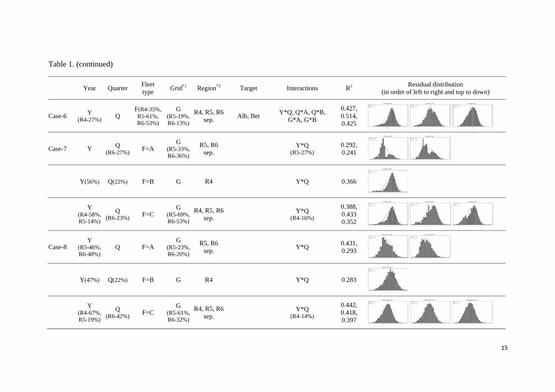
Table 1. Summary of significant factors (p<0.001) in the final GLM (cases 1-7) or GLMM (case 8) models, R2, and residual plot, by Cases. “(x)”

in the table indicates that the factor was not included in the case. The capital word of the factor was used as abbreviation in the ‘Interactions’.

The percentage of Mean Square of a factor contributed to the whole model was shows in parenthesis for the most important two factors.

Year Quarter

Fleet type

Grid*1 Region*2 Target Interactions R2 Residual distribution

(in order of left to right and top to down)

Case-1 Y Q (x) (x) R1-R6 comb.

ALB%(10%), BET%(84%)

Y*Q, Y*A%, Q*R, Q*A%,

Q*B%, R*A% 0.563

Case-2 Y Q (6%)

F (75%) (x)

R1-R6 comb.

ALB, BET Y*Q, Y*R,

Q*A%, Q*B%, R*A%, R*B%

0.404

Case-3 Y Q F (x) R1-R6 comb.

ALB&BET, ALB%&BET%,

YFT%, NHPB

Y*Q

0.430, 0.564, 0.545, 0.390

Case-4 Y Q F G

R1-R6 comb.

‘Region’ not a

covariate

ALB, BET Y*Q, Q*A, Q*B 0.452

Case-5 Y Q F(R4-19%, R5-51%, R6-53%)

(x) R4, R5, R6

sep.

ALB, BET(R4-45%,

R5-27%, R6-32%)Y*Q, Q*A, Q*B

0.298, 0.431, 0.281

*1 Grid, 5 degree latitude x longitude factor *2 ‘Region’ was a factor in the model when R1-R6 were combined (comb.) and was not when regions were separated (sep.).

15  

Table 1. (continued)

Year Quarter

Fleet type

Grid*1 Region*2 Target Interactions R2 Residual distribution

(in order of left to right and top to down)

Case-6 Y (R4-27%)

Q F(R4-35%, R5-61%, R6-53%)

G (R5-19%, R6-13%)

R4, R5, R6sep.

Alb, Bet Y*Q, Q*A, Q*B,

G*A, G*B

0.427, 0.514, 0.425

Case-7 Y Q (R6-27%) F=A

G (R5-33%, R6-36%)

R5, R6 sep.

Y*Q (R5-27%)

0.292, 0.241

Y(56%) Q(22%) F=B G R4 Y*Q 0.366

Y

(R4-58%, R5-14%)

Q (R6-23%) F=C

G (R5-69%, R6-53%)

R4, R5, R6sep.

Y*Q (R4-16%)

0.388, 0.433 0.352

Case-8 Y

(R5-46%, R6-48%)

Q F=A G

(R5-23%, R6-20%)

R5, R6 sep.

Y*Q 0.431, 0.293

Y(47%) Q(22%) F=B G R4 Y*Q 0.283

Y

(R4-67%, R5-19%)

Q (R6-42%) F=C

G (R5-61%, R6-32%)

R4, R5, R6sep.

Y*Q (R4-14%)

0.442, 0.418, 0.397

16  

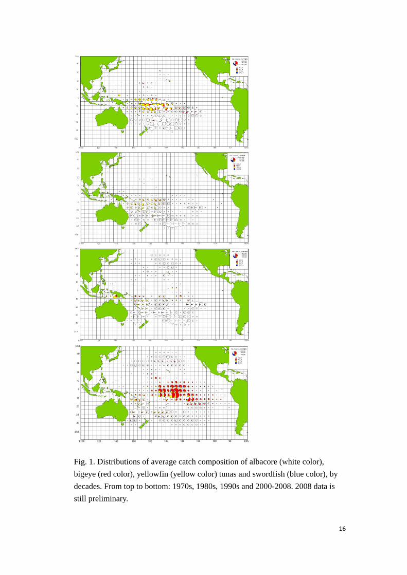
Fig. 1. Distributions of average catch composition of albacore (white color),

bigeye (red color), yellowfin (yellow color) tunas and swordfish (blue color), by

decades. From top to bottom: 1970s, 1980s, 1990s and 2000-2008. 2008 data is

still preliminary.

17  

‐

5 

10 

15 

20 

25 

30 

1964 1969 1974 1979 1984 1989 1994 1999 2004

Catches (K

mt)

Year

ALB‐SPO

BET‐WCPO

YFT‐WCPO

2002

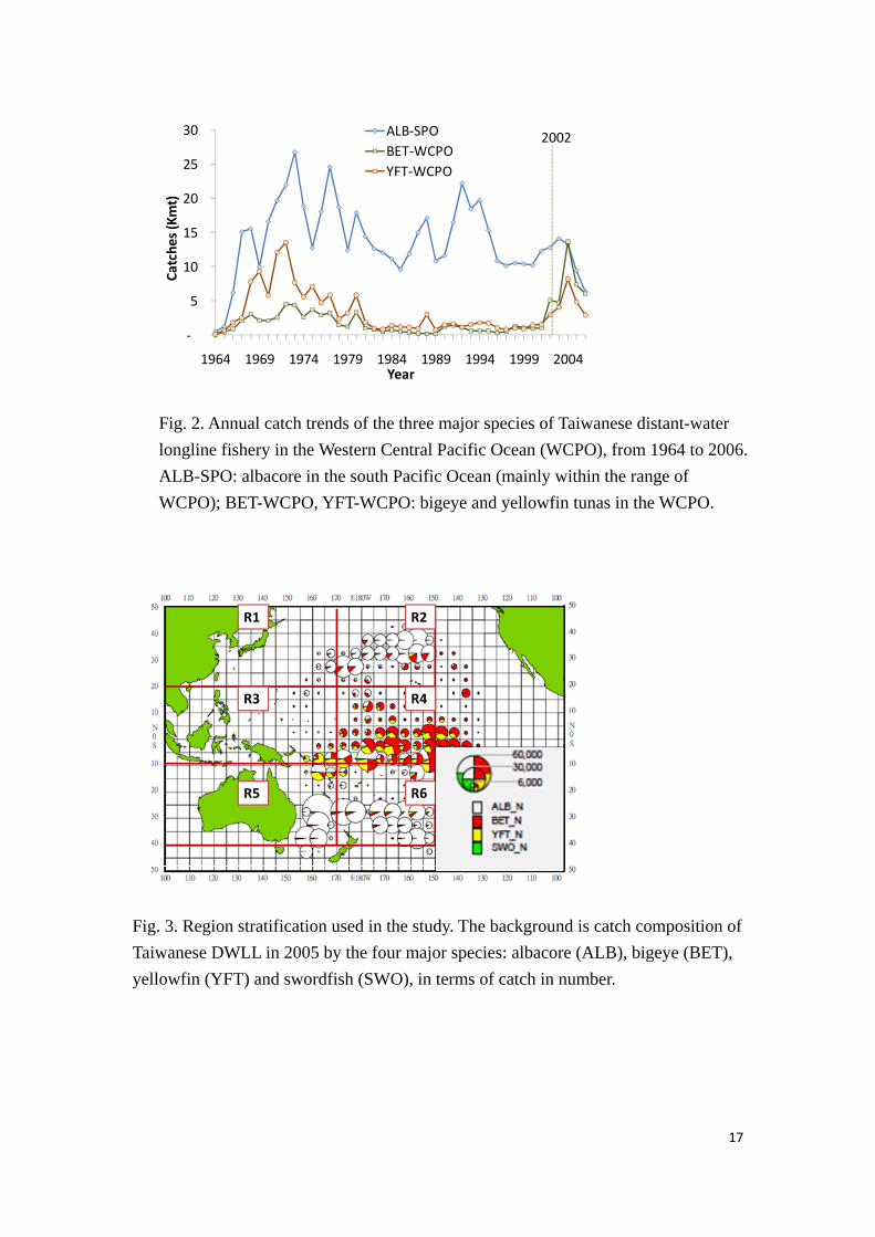
Fig. 2. Annual catch trends of the three major species of Taiwanese distant-water

longline fishery in the Western Central Pacific Ocean (WCPO), from 1964 to 2006.

ALB-SPO: albacore in the south Pacific Ocean (mainly within the range of

WCPO); BET-WCPO, YFT-WCPO: bigeye and yellowfin tunas in the WCPO.

R1 R2

R3 R4

R5 R6

Fig. 3. Region stratification used in the study. The background is catch composition of

Taiwanese DWLL in 2005 by the four major species: albacore (ALB), bigeye (BET),

yellowfin (YFT) and swordfish (SWO), in terms of catch in number.

18  

ALB76%

BET12%

YFT12%

Group A

ALB95%

BET4%

YFT1%

Group B

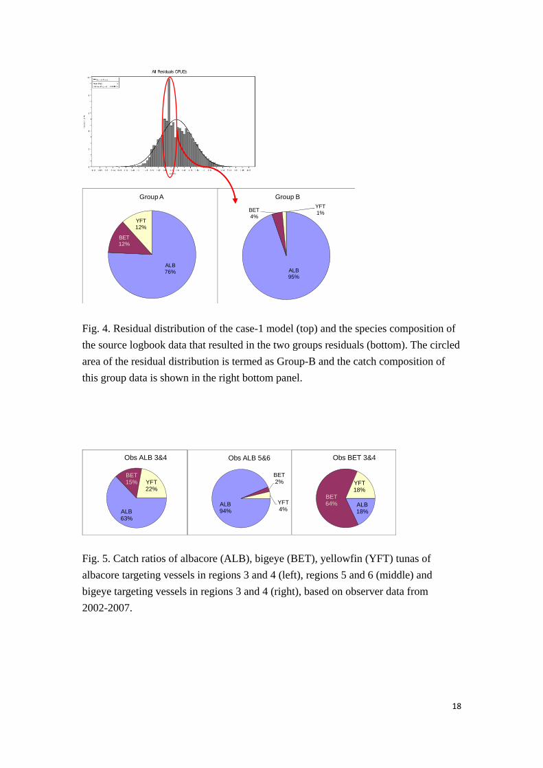
Fig. 4. Residual distribution of the case-1 model (top) and the species composition of

the source logbook data that resulted in the two groups residuals (bottom). The circled

area of the residual distribution is termed as Group-B and the catch composition of

this group data is shown in the right bottom panel.

ALB63%

BET15% YFT

22%

Obs ALB 3&4

ALB94%

BET2%

YFT4%

Obs ALB 5&6

ALB18%

BET64%

YFT18%

Obs BET 3&4

Fig. 5. Catch ratios of albacore (ALB), bigeye (BET), yellowfin (YFT) tunas of

albacore targeting vessels in regions 3 and 4 (left), regions 5 and 6 (middle) and

bigeye targeting vessels in regions 3 and 4 (right), based on observer data from

2002-2007.

19  

0.0

0.5

1.0

1.5

2.0

1995 1998 2001 2004 2007

Rel

ativ

e C

PU

E

Year

NHPB ALB% & BET%YFT% ALB & BET

Fig. 6. Relative CPUE series for using different target indicators in the Case-3 run, for

period of 1995-2008.

0

1

2

3

4

5

6

1965 1975 1985 1995 2005

Rel

ativ

e C

PU

E

Year

ALB% & BET%

ALB & BET

Fig. 7. Relative CPUE series for using catch compositions (ALB%&BET%) and

catches (ALB&BET) of albacore and bigeye tuna as indicators, for period of

1968-2008.

0

1

2

3

4

5

6

7

1968 1978 1988 1998 2008

Re

lativ

e C

PU

E

Year

with 5-deg grid effect

95% CI for with grid effect

without 5-deg grid effect

Fig. 8. Relative CPUE series for comparison of the standardization results with and

without 5-degree grid factor included for Case-2 and -4.

20  

0

1

2

3

1965 1975 1985 1995 2005

Re

lativ

e C

PU

E

Year

A, R5

0

1

2

3

1965 1975 1985 1995 2005

Re

lativ

e C

PU

E

Year

A, R6

0

1

2

3

1965 1975 1985 1995 2005

Rel

ativ

e C

PU

E

Year

B, R4

0

1

2

3

1965 1975 1985 1995 2005R

ela

tive

CP

UE

Year

C, R4

0

1

2

3

1965 1975 1985 1995 2005

Re

lativ

e C

PU

E

Year

C, R5

0

1

2

3

1965 1975 1985 1995 2005

Re

lativ

e C

PU

E

Year

C, R6

Fig. 9. Relative CPUE series obtained from GLM runs with delta-lognormal model

assumption, by region (R4-R6) and by fleet type (A-C), for Case-8. The dashed lines

are linear trends of the series.

0

1

2

3

4

1965 1975 1985 1995 2005

Re

lativ

e C

PU

E

Year

A, R6 - Case-8A, R6 - Case-7

0

1

2

3

4

1965 1975 1985 1995 2005

Re

lativ

e C

PU

E

Year

C, R6 - Case-8C, R6 - Case-7

Fig. 10. Comparisons of CPUE series from Case-7 (lognormal assumption) and

Case-8 (delta lognormal assumption), for the fleet types A and C in Region 6. (Note:

no 2008 estimations are available from Case-7 for both fleet types.)

21  

Fig. 11. Estimated total biomass (mt) for the standard stock assessment (CPUE low,

sample size high, Qincr) stock assessment model (black) and a version replacing the

longline index for region 6 with Taiwanese longline CPUE (red).

22  

Fig. 12. Estimated quarterly recruitment for the standard stock assessment (CPUE

low, sample size high, Qincr) stock assessment model (black) and a version replacing

the longline index for region 6 with Taiwanese longline CPUE (red).