scientific computing in python – numpy, scipy, matplotlib · numpy and scipy numpy provides...
TRANSCRIPT
Workshop on Advanced Techniquesin Scientific Computing
Dr. Axel Kohlmeyer
Associate Dean for Scientific ComputingCollege of Science and Technology
Temple University, Philadelphia
Based on Lecture Material byShawn Brown, PSC
David Grellscheid, Durham
Scientific Computing in Python– NumPy, SciPy, Matplotlib
2Workshop on Advanced Techniquesin Scientific Computing
Python for Scientific Computing?
● Pro:● Programming in Python is convenient● Development is fast (no compilation, no linking)
● Con:● Interpreted language is slower than compiled code● Lists are wasteful and inefficient for large data sets
=> NumPy to the rescue● NumPy is also a great example for using OO-
programming to hide implementation details
3Workshop on Advanced Techniquesin Scientific Computing
NumPy and SciPy
● NumPy provides functionality to create, delete, manage and operate on large arrays of typed “raw” data (like Fortran and C/C++ arrays)
● SciPy extends NumPy with a collection of useful algorithms like minimization, Fourier transform, regression and many other applied mathematical techniques
● Both packages are add-on packages (not part of the Python standard library) containing Python code and compiled code (fftpack, BLAS)
4Workshop on Advanced Techniquesin Scientific Computing
Installation of NumPy / SciPy
● Package manager of your Linux distribution● Listed on PyPi
→ Installation via “pip install numpy scipy”● See http://www.scipy.org/install.html for other
alternatives, suitable for your platform● After successful installation, “numpy” and
“scipy” can be imported like other packages:
import numpy as npimport scipy as sp
5Workshop on Advanced Techniquesin Scientific Computing
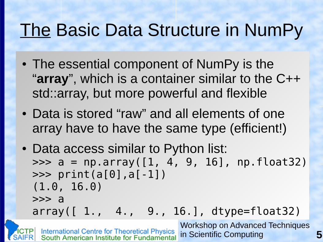
The Basic Data Structure in NumPy
● The essential component of NumPy is the “array”, which is a container similar to the C++ std::array, but more powerful and flexible
● Data is stored “raw” and all elements of one array have to have the same type (efficient!)
● Data access similar to Python list:>>> a = np.array([1, 4, 9, 16], np.float32)>>> print(a[0],a[-1])(1.0, 16.0)>>> aarray([ 1., 4., 9., 16.], dtype=float32)
6Workshop on Advanced Techniquesin Scientific Computing
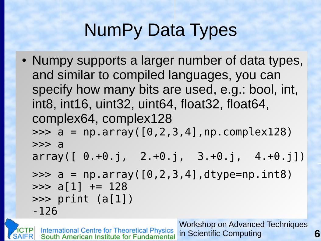
NumPy Data Types
● Numpy supports a larger number of data types, and similar to compiled languages, you can specify how many bits are used, e.g.: bool, int, int8, int16, uint32, uint64, float32, float64, complex64, complex128>>> a = np.array([0,2,3,4],np.complex128)>>> aarray([ 0.+0.j, 2.+0.j, 3.+0.j, 4.+0.j])
>>> a = np.array([0,2,3,4],dtype=np.int8)>>> a[1] += 128>>> print (a[1])-126
7Workshop on Advanced Techniquesin Scientific Computing
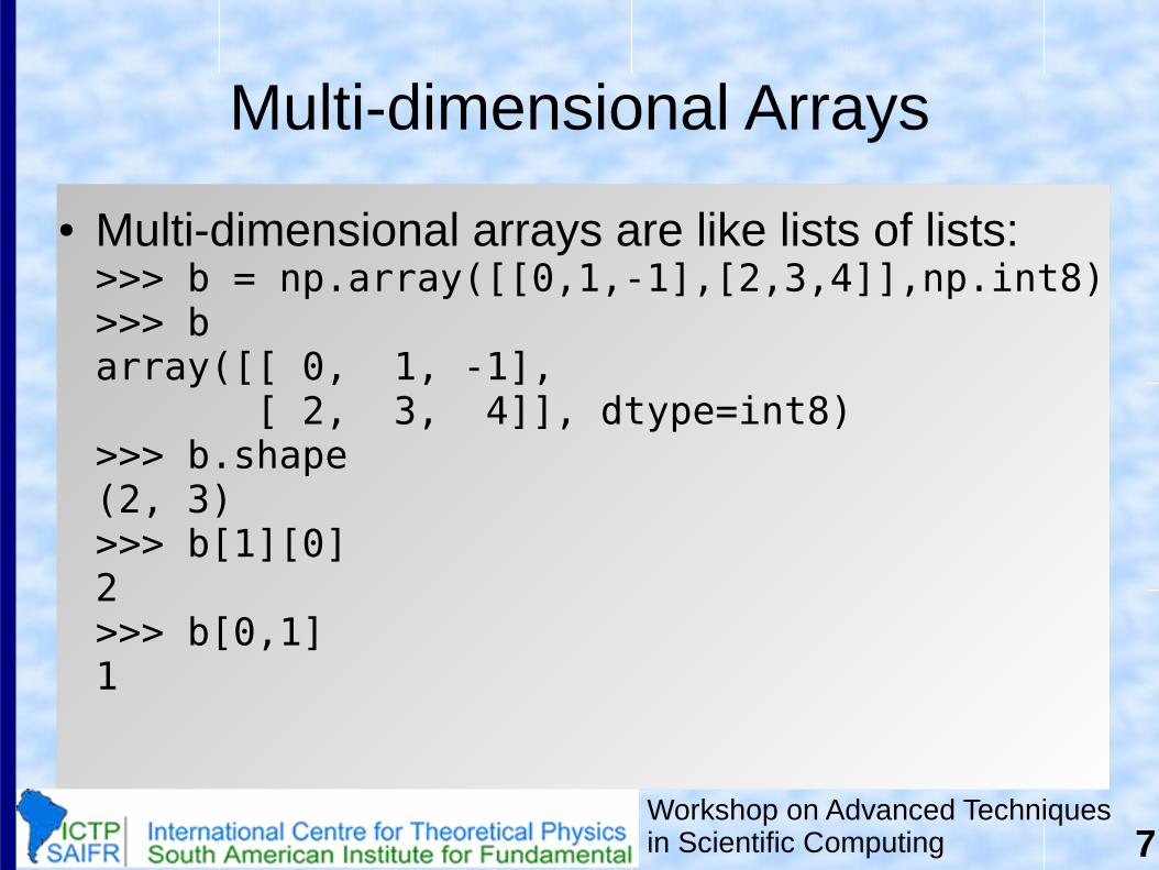
Multi-dimensional Arrays
● Multi-dimensional arrays are like lists of lists:>>> b = np.array([[0,1,-1],[2,3,4]],np.int8)>>> barray([[ 0, 1, -1], [ 2, 3, 4]], dtype=int8)>>> b.shape(2, 3)>>> b[1][0]2>>> b[0,1]1
8Workshop on Advanced Techniquesin Scientific Computing
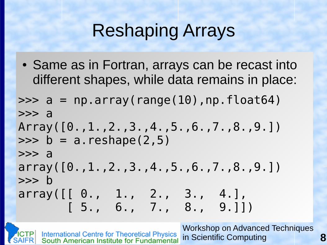
Reshaping Arrays
● Same as in Fortran, arrays can be recast into different shapes, while data remains in place:
>>> a = np.array(range(10),np.float64)>>> aArray([0.,1.,2.,3.,4.,5.,6.,7.,8.,9.])>>> b = a.reshape(2,5)>>> aarray([0.,1.,2.,3.,4.,5.,6.,7.,8.,9.])>>> barray([[ 0., 1., 2., 3., 4.], [ 5., 6., 7., 8., 9.]])
9Workshop on Advanced Techniquesin Scientific Computing
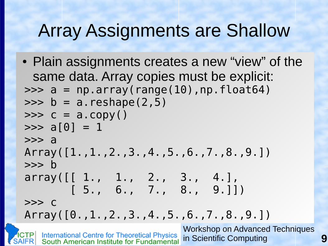
Array Assignments are Shallow
● Plain assignments creates a new “view” of the same data. Array copies must be explicit:
>>> a = np.array(range(10),np.float64)>>> b = a.reshape(2,5)>>> c = a.copy() >>> a[0] = 1>>> aArray([1.,1.,2.,3.,4.,5.,6.,7.,8.,9.])>>> barray([[ 1., 1., 2., 3., 4.], [ 5., 6., 7., 8., 9.]])>>> cArray([0.,1.,2.,3.,4.,5.,6.,7.,8.,9.])
10Workshop on Advanced Techniquesin Scientific Computing
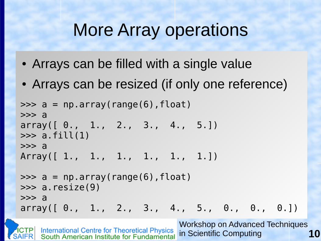
More Array operations
● Arrays can be filled with a single value● Arrays can be resized (if only one reference)
>>> a = np.array(range(6),float)>>> aarray([ 0., 1., 2., 3., 4., 5.])>>> a.fill(1)>>> aArray([ 1., 1., 1., 1., 1., 1.])
>>> a = np.array(range(6),float)>>> a.resize(9)>>> aarray([ 0., 1., 2., 3., 4., 5., 0., 0., 0.])
11Workshop on Advanced Techniquesin Scientific Computing
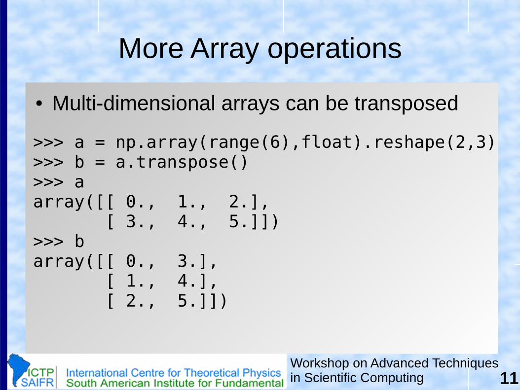
More Array operations
● Multi-dimensional arrays can be transposed
>>> a = np.array(range(6),float).reshape(2,3)>>> b = a.transpose()>>> aarray([[ 0., 1., 2.], [ 3., 4., 5.]])>>> barray([[ 0., 3.], [ 1., 4.], [ 2., 5.]])
12Workshop on Advanced Techniquesin Scientific Computing
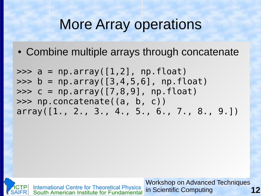
More Array operations
● Combine multiple arrays through concatenate
>>> a = np.array([1,2], np.float)>>> b = np.array([3,4,5,6], np.float)>>> c = np.array([7,8,9], np.float)>>> np.concatenate((a, b, c))array([1., 2., 3., 4., 5., 6., 7., 8., 9.])
13Workshop on Advanced Techniquesin Scientific Computing
More Array operations
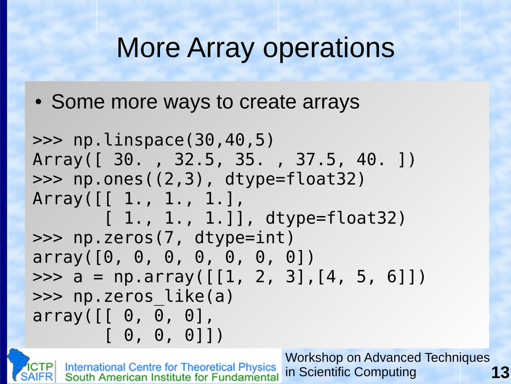
● Some more ways to create arrays
>>> np.linspace(30,40,5)Array([ 30. , 32.5, 35. , 37.5, 40. ])>>> np.ones((2,3), dtype=float32)Array([[ 1., 1., 1.], [ 1., 1., 1.]], dtype=float32)>>> np.zeros(7, dtype=int)array([0, 0, 0, 0, 0, 0, 0])>>> a = np.array([[1, 2, 3],[4, 5, 6]])>>> np.zeros_like(a)array([[ 0, 0, 0], [ 0, 0, 0]])
14Workshop on Advanced Techniquesin Scientific Computing
Element-by-Element Operations
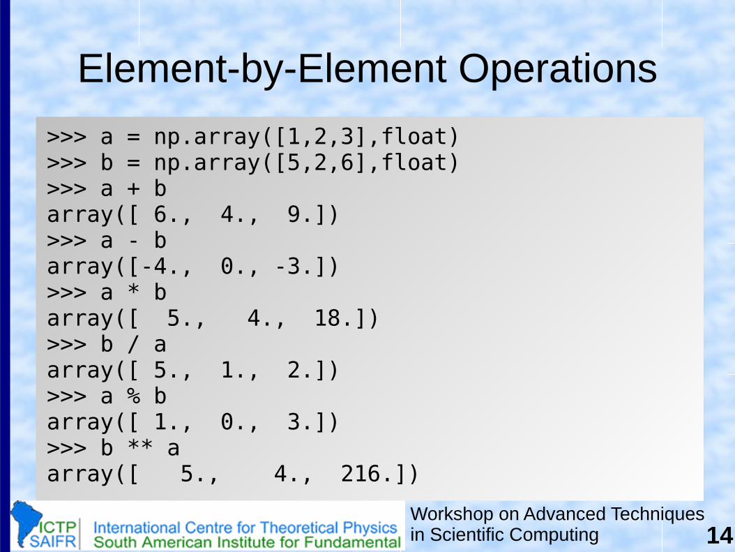
>>> a = np.array([1,2,3],float)>>> b = np.array([5,2,6],float)>>> a + barray([ 6., 4., 9.])>>> a - barray([-4., 0., -3.])>>> a * barray([ 5., 4., 18.])>>> b / aarray([ 5., 1., 2.])>>> a % barray([ 1., 0., 3.])>>> b ** aarray([ 5., 4., 216.])
15Workshop on Advanced Techniquesin Scientific Computing
Mathematical Operations
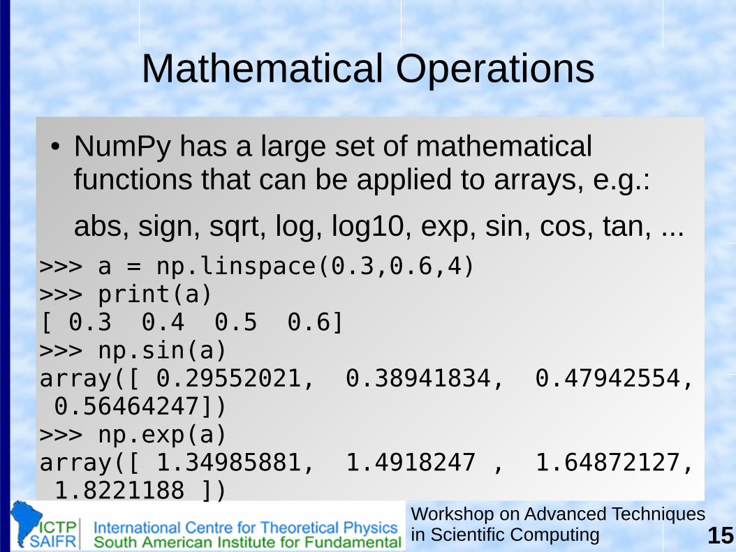
● NumPy has a large set of mathematical functions that can be applied to arrays, e.g.:
abs, sign, sqrt, log, log10, exp, sin, cos, tan, ... >>> a = np.linspace(0.3,0.6,4)>>> print(a)[ 0.3 0.4 0.5 0.6]>>> np.sin(a)array([ 0.29552021, 0.38941834, 0.47942554, 0.56464247])>>> np.exp(a)array([ 1.34985881, 1.4918247 , 1.64872127, 1.8221188 ])
16Workshop on Advanced Techniquesin Scientific Computing
Reduction Operations
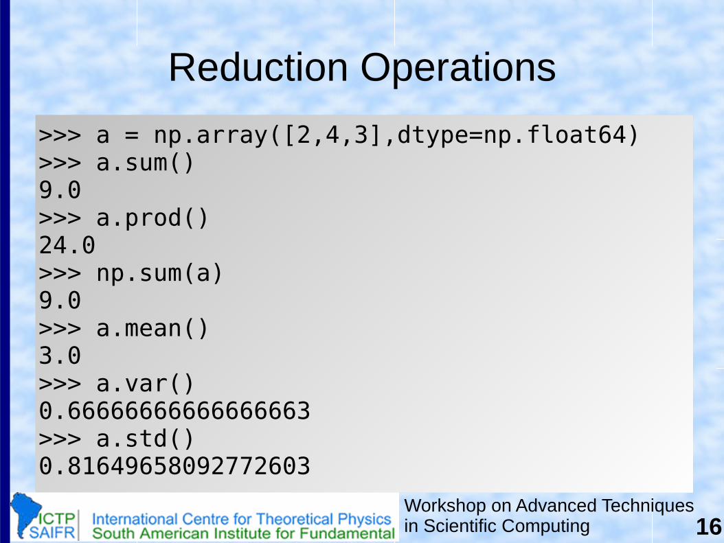
>>> a = np.array([2,4,3],dtype=np.float64)>>> a.sum()9.0>>> a.prod()24.0>>> np.sum(a)9.0>>> a.mean()3.0>>> a.var()0.66666666666666663>>> a.std()0.81649658092772603
17Workshop on Advanced Techniquesin Scientific Computing
Boolean Operations
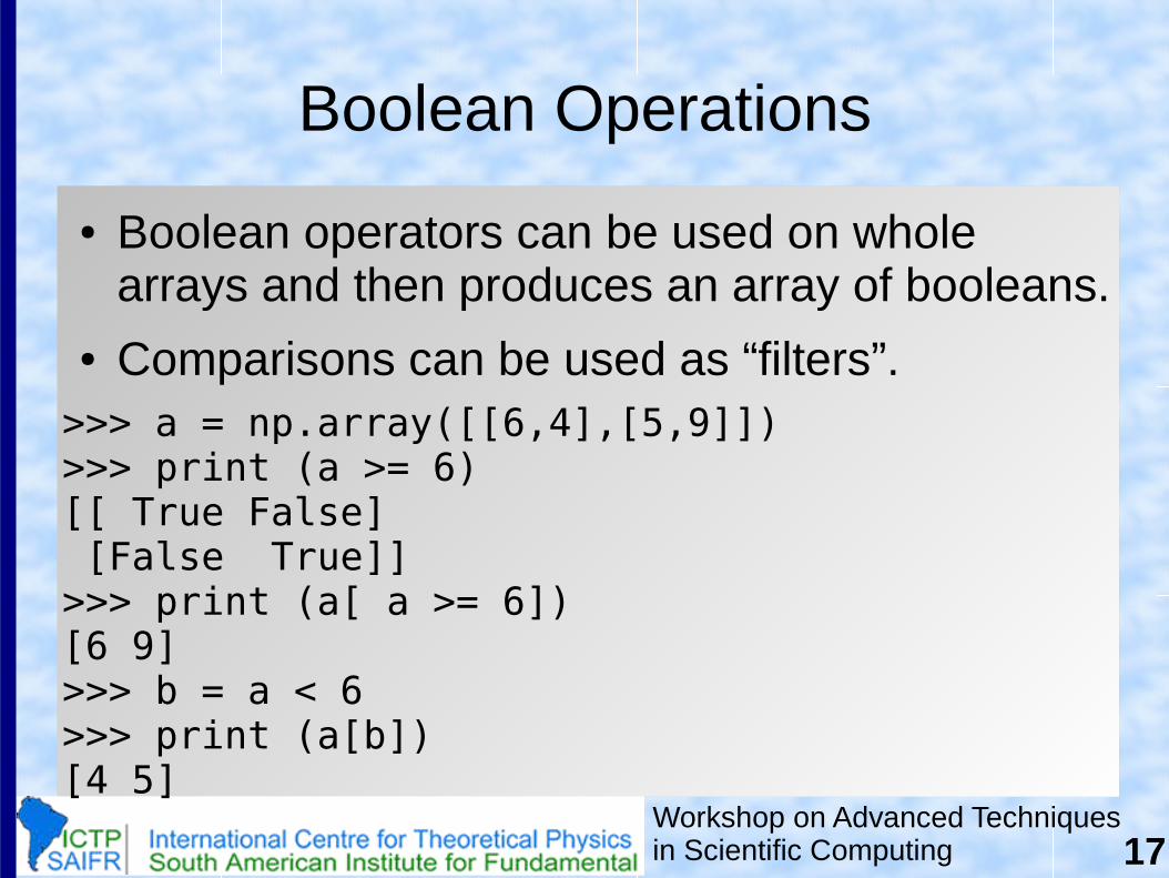
● Boolean operators can be used on whole arrays and then produces an array of booleans.
● Comparisons can be used as “filters”.>>> a = np.array([[6,4],[5,9]])>>> print (a >= 6)[[ True False] [False True]]>>> print (a[ a >= 6])[6 9]>>> b = a < 6>>> print (a[b])[4 5]
18Workshop on Advanced Techniquesin Scientific Computing
Linear Algebra Operations
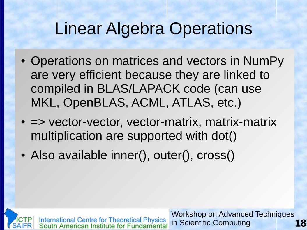
● Operations on matrices and vectors in NumPy are very efficient because they are linked to compiled in BLAS/LAPACK code (can use MKL, OpenBLAS, ACML, ATLAS, etc.)
● => vector-vector, vector-matrix, matrix-matrix multiplication are supported with dot()
● Also available inner(), outer(), cross()
19Workshop on Advanced Techniquesin Scientific Computing
Linear Algebra Operations
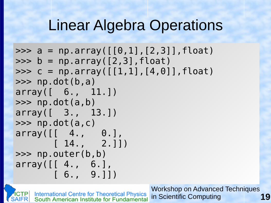
>>> a = np.array([[0,1],[2,3]],float)>>> b = np.array([2,3],float)>>> c = np.array([[1,1],[4,0]],float)>>> np.dot(b,a)array([ 6., 11.])>>> np.dot(a,b)array([ 3., 13.])>>> np.dot(a,c)array([[ 4., 0.], [ 14., 2.]])>>> np.outer(b,b)array([[ 4., 6.], [ 6., 9.]])
20Workshop on Advanced Techniquesin Scientific Computing
Linear Algebra Operations
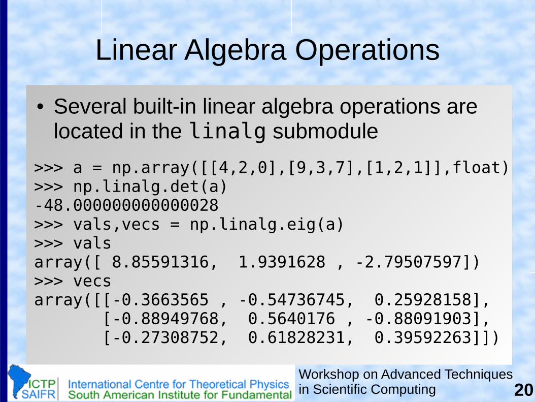
● Several built-in linear algebra operations are located in the linalg submodule
>>> a = np.array([[4,2,0],[9,3,7],[1,2,1]],float)>>> np.linalg.det(a)-48.000000000000028>>> vals,vecs = np.linalg.eig(a)>>> valsarray([ 8.85591316, 1.9391628 , -2.79507597])>>> vecsarray([[-0.3663565 , -0.54736745, 0.25928158], [-0.88949768, 0.5640176 , -0.88091903], [-0.27308752, 0.61828231, 0.39592263]])
21Workshop on Advanced Techniquesin Scientific Computing
This is Only the Beginning
● NumPy has much more functionality:● Polynomial mathematics● Statistical computations● Pseudo random number generators● Discrete Fourier transforms● Size / shape / type testing of arrays
● To learn more, check out the NumPy docs at:http://docs.scipy.org/doc/
22Workshop on Advanced Techniquesin Scientific Computing
SciPy
● SciPy is built on top of NumPy and implements many specialized scientific computation tools:● Clustering, Fourier transforms, numerical
integration, interpolations, data I/O, LAPACK, sparse matrices, linear solvers, optimization, signal processing, statistical functions, sparse eigenvalue solvers, ...
23Workshop on Advanced Techniquesin Scientific Computing
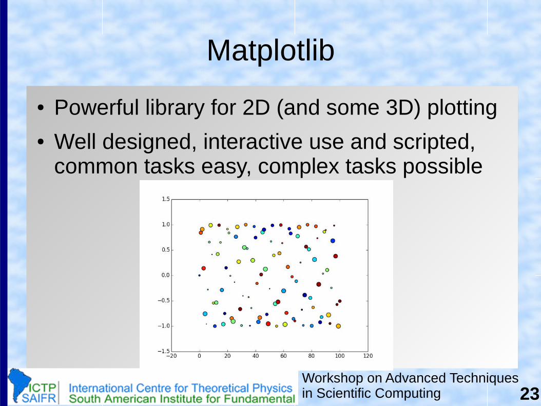
Matplotlib
● Powerful library for 2D (and some 3D) plotting● Well designed, interactive use and scripted,
common tasks easy, complex tasks possible
24Workshop on Advanced Techniquesin Scientific Computing
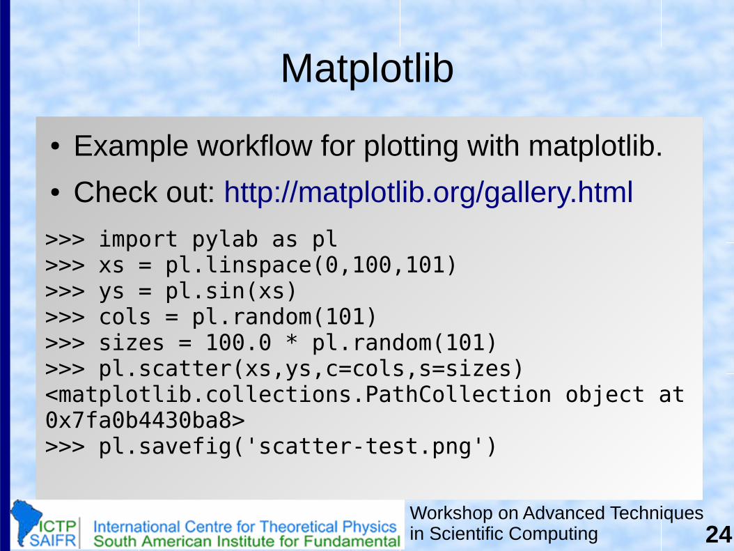
Matplotlib
● Example workflow for plotting with matplotlib. ● Check out: http://matplotlib.org/gallery.html
>>> import pylab as pl>>> xs = pl.linspace(0,100,101)>>> ys = pl.sin(xs)>>> cols = pl.random(101)>>> sizes = 100.0 * pl.random(101)>>> pl.scatter(xs,ys,c=cols,s=sizes)<matplotlib.collections.PathCollection object at 0x7fa0b4430ba8>>>> pl.savefig('scatter-test.png')
25Workshop on Advanced Techniquesin Scientific Computing
Workshop on Advanced Techniquesin Scientific Computing
Dr. Axel Kohlmeyer
Associate Dean for Scientific ComputingCollege of Science and Technology
Temple University, Philadelphia
http://sites.google.com/site/akohlmey/
Scientific Computing in Python– NumPy, SciPy, Matplotlib