SCIENTIFIC VISUALIZATION

Dissertation

Submitted in partial fulfillment of the requirements

for the Dual Degree Program

by

J. Bharath Kumar

97D01010

Under the guidance of

Prof. G. R. Shevare

&

Mr. Chetan Kumar ( C-DAC Pune )

DEPARTMENT OF AEROSPACE ENGINEERING

INDIAN INSTITUTE OF TECHNOLOGY, BOMBAY

June, 2002

Dissertation Approval Sheet

This is to certify that the Dissertation titled Scientific Visualization by J. Bharath Kumar

is approved for the degree of Bachelor of Technology and Master of Technology.

Guide

Co-Guide

Chairman

Internal Examiner

External Examiner

Date:

ii

Acknowledgments

I would like to express my sincere gratitude to Prof. G.R.Shevare for his valuable guid-

ance. His guidance has been a good learning experience, and for his constant inspiration

and motivation.

I would like to thank Centre for Development of Advanced Computing, Pune for spon-

soring this dual degree project, and for entrusting me with this project. I would like to

thank Mr. Chetan Kumar for his valuable guidance.

I would like to thank Mr. Raghavendra Pai for helping me with CGNS implementation,

Irshad Khan for GUI, Sasi Krishna Reddy, Sandip Jadhav, Amitay Issac and Prajakta for

helping me with IITZeus and debugging.

I would like to express my thanks to Vishwadeep, Devendra Ghate and Raghavendra Pai

for providing me with CFD solutions. And to my batch mates Praveen Gill, Amit Batra,

Devendra Ghate, Gaurav Jain, Tuhin Sahai, Jai Mirpuri and colleagues of CFD-Lab for

their company.

J. Bharath Kumar

June, 2002.

iii

Abstract

Numerical methods, such as Computational Fluid Dynamics ( CFD ) need visualization

to make sense of the huge amount of data they produce. This project aims to develop a

visualization tool. Though attempting to develop a generic one, it is primarily meant to

visualise CFD simulations. The tool accepts data in standard file formats such as CGNS,

for both multiblock structured and unstructured grids. The Visualization of scalar fields is

achieved with iso-value curves and surfaces, commonly called contour plots and shaded

plots. Particle tracers and vector plots were developed for flow visualization. Topology

graphs: an advanced method for interpretation of data fields has been implemented. An

extensive framework succesfully integrates all the visualization techniques.

Contents

1 Introduction 1

1.1 What is Scientific Visualization ? . . . . . . . . . . . . . . . . . . . . . . . 1

1.2 Impact of Visualization . . . . . . . . . . . . . . . . . . . . . . . . . . . . 2

1.2.1 Role of Visualization in Computational Fluid Dynamics . . . . . . 2

1.3 Project ’Scientific Visualization’ . . . . . . . . . . . . . . . . . . . . . . . 3

1.4 Layout of The Report . . . . . . . . . . . . . . . . . . . . . . . . . . . . . 4

2 Visualization System 5

2.1 Introduction . . . . . . . . . . . . . . . . . . . . . . . . . . . . . . . . . . 5

2.1.1 Application builders . . . . . . . . . . . . . . . . . . . . . . . . . 5

2.1.2 Turnkey systems . . . . . . . . . . . . . . . . . . . . . . . . . . . 6

2.2 Why another visualization tool ? . . . . . . . . . . . . . . . . . . . . . . . 6

2.2.1 Project Aim . . . . . . . . . . . . . . . . . . . . . . . . . . . . . . 7

2.3 File Input . . . . . . . . . . . . . . . . . . . . . . . . . . . . . . . . . . . 8

2.4 CGNS format . . . . . . . . . . . . . . . . . . . . . . . . . . . . . . . . . 9

2.5 CGNS Implementation: Higher Level APIs . . . . . . . . . . . . . . . . . 10

3 Vector Visualization 11

3.1 Particle Tracers . . . . . . . . . . . . . . . . . . . . . . . . . . . . . . . . 11

3.2 2D Particle Tracer . . . . . . . . . . . . . . . . . . . . . . . . . . . . . . . 12

3.2.1 Governing Equations . . . . . . . . . . . . . . . . . . . . . . . . . 12

3.2.2 Point location . . . . . . . . . . . . . . . . . . . . . . . . . . . . . 12

3.2.3 Generating continuum data . . . . . . . . . . . . . . . . . . . . . . 13

3.2.4 Numerical Integration Schemes . . . . . . . . . . . . . . . . . . . 13

3.2.5 Step size . . . . . . . . . . . . . . . . . . . . . . . . . . . . . . . 14

3.3 Error Analysis . . . . . . . . . . . . . . . . . . . . . . . . . . . . . . . . . 14

3.4 Vector Plots . . . . . . . . . . . . . . . . . . . . . . . . . . . . . . . . . . 14

i

3.5 3D Particle Tracers . . . . . . . . . . . . . . . . . . . . . . . . . . . . . . 16

3.5.1 Point Location . . . . . . . . . . . . . . . . . . . . . . . . . . . . 16

3.5.2 Generating continuum data . . . . . . . . . . . . . . . . . . . . . . 16

3.5.3 Step size . . . . . . . . . . . . . . . . . . . . . . . . . . . . . . . 17

3.6 Vector Field Interpretation . . . . . . . . . . . . . . . . . . . . . . . . . . 17

3.6.1 Introduction . . . . . . . . . . . . . . . . . . . . . . . . . . . . . . 17

3.6.2 Topology Method . . . . . . . . . . . . . . . . . . . . . . . . . . . 18

4 Scalar Visualization 22

4.1 Introduction . . . . . . . . . . . . . . . . . . . . . . . . . . . . . . . . . . 22

4.2 Marching Cube Algorithm . . . . . . . . . . . . . . . . . . . . . . . . . . 22

4.3 2D Isocontour Implementation . . . . . . . . . . . . . . . . . . . . . . . . 23

4.4 2D Shaded/Color Plots . . . . . . . . . . . . . . . . . . . . . . . . . . . . 24

4.5 3D Contours Implementation . . . . . . . . . . . . . . . . . . . . . . . . . 24

4.6 3D Surface Shade Plots . . . . . . . . . . . . . . . . . . . . . . . . . . . . 25

4.6.1 Extraction of Surface . . . . . . . . . . . . . . . . . . . . . . . . . 25

4.7 Scalar Field Interpretation . . . . . . . . . . . . . . . . . . . . . . . . . . 26

4.7.1 Implementation . . . . . . . . . . . . . . . . . . . . . . . . . . . . 26

5 Results 28

5.1 Flow Visualization of 2D structured Grid Simulation . . . . . . . . . . . . 28

5.1.1 Vector Plots 2D . . . . . . . . . . . . . . . . . . . . . . . . . . . . 28

5.1.2 Stream Lines 2D Structured multiblock grid . . . . . . . . . . . . . 28

5.1.3 Vector Field Topology . . . . . . . . . . . . . . . . . . . . . . . . 30

5.2 Scalar Visualization of 2D structured Grid Simulation . . . . . . . . . . . . 30

5.2.1 Shaded Plots 2D MultiBlock . . . . . . . . . . . . . . . . . . . . . 30

5.2.2 Contour Plots 2D Structured . . . . . . . . . . . . . . . . . . . . . 32

5.2.3 Scalar Field Topology . . . . . . . . . . . . . . . . . . . . . . . . 32

5.3 Visualization of 3D structured Grid Simulation . . . . . . . . . . . . . . . 34

5.3.1 Flow Visualization Through Surface Sections . . . . . . . . . . . . 34

5.3.2 Scalar Visualization Through Surface Sections . . . . . . . . . . . 34

5.3.3 Scalar Visualization Through Contour Plots . . . . . . . . . . . . . 34

5.4 Visualization of Surface Structured Grids . . . . . . . . . . . . . . . . . . 36

5.5 Visualization of 2D Unstructured Grids . . . . . . . . . . . . . . . . . . . 36

ii

6 Closure 39

References 40

Appendix A 42

iii

List of Figures

1.1 Visualization for Insight . . . . . . . . . . . . . . . . . . . . . . . . . . . 1

1.2 CFD Engineering Cycle . . . . . . . . . . . . . . . . . . . . . . . . . . . . 3

2.1 SIDS File Mapping . . . . . . . . . . . . . . . . . . . . . . . . . . . . . . 9

3.1 Point location . . . . . . . . . . . . . . . . . . . . . . . . . . . . . . . . . 12

3.2 Error Comparison . . . . . . . . . . . . . . . . . . . . . . . . . . . . . . . 15

3.3 Computational expense . . . . . . . . . . . . . . . . . . . . . . . . . . . . 15

3.4 Comparison of First and Fourth Order Scheme . . . . . . . . . . . . . . . . 16

3.5 Point in Tetrahedron . . . . . . . . . . . . . . . . . . . . . . . . . . . . . 17

3.6 Potential Critical Cells . . . . . . . . . . . . . . . . . . . . . . . . . . . . 18

3.7 Cell Designation . . . . . . . . . . . . . . . . . . . . . . . . . . . . . . . 19

3.8 Classification of Critical points ((R)Real,(I)Imaginary of eigen values) . . . 21

4.1 Quadrilateral Decomposition . . . . . . . . . . . . . . . . . . . . . . . . . 23

4.2 Isocontours . . . . . . . . . . . . . . . . . . . . . . . . . . . . . . . . . . 24

4.3 Hexahedron Decomposition . . . . . . . . . . . . . . . . . . . . . . . . . 24

4.4 Some of scalar critical points . . . . . . . . . . . . . . . . . . . . . . . . . 26

5.1 Vector Plots for 2D Structured Multiblock . . . . . . . . . . . . . . . . . . 28

5.2 Stream Lines for 2D Structured Multiblock . . . . . . . . . . . . . . . . . 29

5.3 Stream Lines with Shaded Plot of Velocity magnitude . . . . . . . . . . . . 29

5.4 2D Vector Field Topology . . . . . . . . . . . . . . . . . . . . . . . . . . . 30

5.5 Shaded Plots for 2D Multiblock . . . . . . . . . . . . . . . . . . . . . . . 31

5.6 Pressure Contours for 2D Structured Multiblock . . . . . . . . . . . . . . . 31

5.7 Contours and Shaded Plots for 2D Structured Multiblock . . . . . . . . . . 32

5.8 2D Scalar Field Topology . . . . . . . . . . . . . . . . . . . . . . . . . . . 33

5.9 Vector Plots on surfaces for 3D . . . . . . . . . . . . . . . . . . . . . . . . 33

iv

5.10 Surface Scalar Plots for 3D . . . . . . . . . . . . . . . . . . . . . . . . . . 34

5.11 Shaded Surface for 3D Structured . . . . . . . . . . . . . . . . . . . . . . 35

5.12 Contour Plots for 3D . . . . . . . . . . . . . . . . . . . . . . . . . . . . . 35

5.13 Combination of Contours and Shaded Plots for 3D . . . . . . . . . . . . . 36

5.14 Contours and Shaded Plots on Surface Grids . . . . . . . . . . . . . . . . . 37

5.15 Vector Plots on Surface Grids . . . . . . . . . . . . . . . . . . . . . . . . . 37

5.16 Shaded Plots on 2D Unstructured Grids . . . . . . . . . . . . . . . . . . . 38

5.17 Vector Plots on 2D Unstructured Grids . . . . . . . . . . . . . . . . . . . . 38

v

Chapter 1

Introduction

Scientific Visualization is defined as generation of computer images from large numerical

data sets for visual perception. It is a tool for gaining insight into numerical data using

graphics.

1.1 What is Scientific Visualization ?

The modern day analysis methods are based upon numerical solution from equations gov-

erning the physics of the problem. Which produce huge chunks of data for various fields.

The size of data is so large, that it is difficult to understand and interpret the variation of the

field and its impact on the design. Visualization helps in understanding these large fields.

Scientific Visualization started in 1960’s with attempts to use computers for visualiza-

tion purpose. The advances in scientific computation and decrease in cost of computational

power and memory have paved the way for the researchers to go for much more complex

and detailed mathematical models and simulations.

INSIGHT

VISUALIZATION

( POST PROCESSING )

DATA User

Figure 1.1: Visualization for Insight

1

The development of computer graphics has greatly helped the usage of computers for

visualization. As the facilities provided by computer graphics cannot be matched by any

other means, visualization has become unthinkable without computer graphics.

Scientific Visualization finds its applications in the fields like molecular modeling, ge-

netics, medical imaging, mathematics, Geo- science, space exploration, Astro physics,

computational electro magnetics, structural analysis and of course computational fluid dy-

namics.

1.2 Impact of Visualization

The use of visualization for design process helps in better understanding of the simula-

tion model, which directly affects the cost, productivity and accuracy of the product being

designed. The use of visualization has resulted in [1].

� Decreased Physical Testing

� Greater integration of Design and Analysis

� Address increase in complexity and sophistication of Analysis

� Design Optimization

� Productivity and Accuracy

1.2.1 Role of Visualization in Computational Fluid Dynamics

To understand role of visualization in CFD, one must understand what constitutes CFD.

Present day CFD essentially consists of (i) geometric modeling, (ii) grid generation, (iii)

numerical simulation of fluid flows, and (iv) visualization (popularly called post-processing).

Geometric Modeling mainly deals with creation or acquisition of the mathematical defini-

tion of the domain of the problem.

Invariably, mathematical definition of the domain needs repair of computational geom-

etry. Grid generation produces discrete definition of the domain. Two major classifications

of the discretizations are (i) Structured and (ii) Un-structured. Solving the Partial Differ-

ential Equations or integral equations cast in finite difference form or finite volume form

constitutes numerical simulation. The last step, namely visualization (Post-Processing)

2

Analysis ( Solving ) Visualisation

Yes

Finished Design

No

Modelling (+grid generation)

OK

Figure 1.2: CFD Engineering Cycle

consists of displaying the data generated in the simulation. Thus it may be seen that visual-

ization is the fourth step of CFD. But it must be realized that this is not the last step of the

design process. Though the visualization provides understanding of the simulation model

and its associated engineering phenomena, this understanding would be needed for modi-

fications in the model. Hence post processing is not just documentation and validation of

CFD results. It is also needed to produce prompt feed back to previous stages of the design

process.

1.3 Project ’Scientific Visualization’

The current project titled ’Scientific Visualization’ is aimed at developing a post-processor

for visualizing CFD data, aimed at visualizing multiblock structured and unstructured grids,

with dimensions of 2D, surface and 3D, for both scalar and vector data fields. An advanced

method for interpretation of fields, called ’Topology graphs’ has also been implemented.

3

1.4 Layout of The Report

Chapter 2 first discusses the available visualization tools in the market. It brings out their

merits and demerits and then stresses motivation for the work. In the same chapter, re-

cently introduced file format for CFD, is explained in brief with its pros and cons, as this

file format is central to the dissertation. Chapter 3 gives describes implementation issues

of Vector visualization techniques. While Chapter 4 deals with scalar visualization tech-

niques. Chapter 5 presents the results of all the implementations.

4

Chapter 2

Visualization System

2.1 Introduction

Currently, there are many Visualization applications available, some of them are even avail-

able for free use, few of them are very elaborate in their formulation, layout, GUI design

and use, while others are basically x-y plot generators.

In this chapter some visualization systems, commonly used in universities and industry

are discussed. Their merits and demerits are brought out. The scope and overall structure

of the proposed visualization is brought out by giving reasons.

CFD visualizers can be classified as (i) Application Builders and (ii) Turnkey Systems.

What is required in CFD post-processor is neither of these applications. Instead the re-

quirement is for an integrated environment, wherein scalars and vector fields are visualized

and interpreted as per the users need.

2.1.1 Application builders

Visualization application builders like IBM Data Explorer, IRIS Explorer, and Application

Visualization System (AVS) are extremely elaborate softwares for visualizing complex 3D

environment. They need efforts in the form of scripting or graphical linking. These are

very generic in nature, less rich in visualization and many of them fail to cater to the needs

of specific fields like CFD. These are developed to cater to a broad range of fields from

astronomy to molecular science. The common functions provided are parameter extrac-

tion, color plots for scalar visualization and Iso-parametric surfaces, with various options,

powerful graphics and capability for distributed computing.

5

2.1.2 Turnkey systems

Turnkey systems like plot3D, pv3, Visual3, GMV, UFAT, FAST, gnuplot etc. are much

more friendlier in comparison with application builders as these are ready to use and are

specifically designed for CFD. These applications provide functions like contour plots,

particle tracer based flow visualization, Line Integral Convolution based flow visualization,

shock detection, topology methods, vortex core identification etc, while some of the appli-

cations support distributed computing. The present project aims at emulating these systems

and integrating it with the complete CFD cycle.

X-Y plot generators like Gnuplot are also popular among CFD researchers, especially in

universities. These packages mostly cater to 1D and 2D data. Support for 3D visualization

is next to nil. Extraction of contours is normally satisfactory, but topology is normally

missing. The environment is invariably limited to 2D plane (x-y) with zoom-in, zoom-

out,etc, capabilities missing. Examples for these packages are gnuplot, grapher, etc.

2.2 Why another visualization tool ?

As explained earlier, visualization in CFD is not the end of CFD cycle. It forms an impor-

tant link in the complete CFD cycle. A user can take multiple actions after visualizing CFD

data, depending on the results. In fact, the human in CFD cycle is most important in this

stage. It is at this stage that the expertise of the designer is required for CFD engineering.

And it is in this stage that the CFD expert decides the worth of CFD simulation. He may

choose to (i) execute CFD code with a different scheme or execute the same code with

higher number of iterations, (ii) adapt the grids to produce better solution to the problem,

(iii) modify the domain (this may mean changing the geometry of the product) or accept

the simulation as it is and document it. Note that this activity requires visualization as a

module in CFD software, interacting with the geometry modeling and solvers, and not as a

stand alone software.

The aim of the project was to develop this expertise and integrate them with IITZeus,

a CFD software being developed within the department. The following paragraph gives

limitations of some of the existing packages. It brings out reasons for the need to develop

visualization tools.

� Limitations with available visualizers : There are a number of visualization sys-

tems [4], many of them come with basic limitation in degree of accuracy. If the

6

algorithms are inaccurate, a closed streamline may get displayed as open, for exam-

ple, with a consequence that a steady flow may get labeled as unsteady flow. Most

available applications bargain accuracy for faster processing.

� Need for customized solutions or flexibility : Many packages do not give values

for forces and moments on objects such as aerospace bodies. Many do not include

calculation of flux across a curve/face, rendering their application useless for specific

needs. There should be scope to produce these kinds of results as required by the

users.

� Tailor-able post processor : In Research and Development, a search for parame-

ters hitherto not stored or calculated is always a need. For example, velocity may

have been made available, but scalar plot of dilation or vector plot of vorticity plots

may be required. Most of the packages, cannot generate this data as a considerable

processing on the stored data is required, which the commercial packages do not

carryout. In post-processing an expression evaluator for generating a new data field

from available data sets is an essential requirement.

� Automation : In a massive and iterative problem like Multi-Disciplinary Optimiza-

tion (MDO), post processing could become a bottle neck, if simulation results are

left for users to perceive and make sense, instead of being directly channeled as feed

back. At the same time, it should be available as and when desired by the user for

monitoring. Future design processes look for automation, replacing human skills

with algorithms. Such a framework would need advanced post processor with abili-

ties of generating insight, interpretation and detection, instead of mere images.

� Self-Reliance : Aerospace industry solves a big crunch of defense needs. Depen-

dence on applications of foreign origin is not generally sought after in India. For

reasons like security, foreign exchange and thrust for indigenzation, this is true of

CFD in general and post-processing in particular.

2.2.1 Project Aim

The current project titled ’Scientific Visualization’ aims at developing a visualization mod-

ule for CFD. It aims at developing post processing with following capabilities

� Scalar visualization : It is achieved using shaded plots, iso-parametric surface extrac-

tion, new data field generation.

7

� Flow visualization : Is Achieved using particle tracers, vector plots.

� Interpretation and detection : For detection of singularities like vortices, separations,

etc, and generating topology graph for scalar and vector data.

� Data Types : For structured and unstructured multiblock datasets, with cell-centered

and cell vertex data fields.

OpenGL has been used for graphical display. It offers a powerful graphics engine and

a huge collection of functionalities. X-Motif have been used for graphic user interface.

The tool is very generic and robust, can be further extended into a powerful visualization

application.

2.3 File Input

The size of CFD data is normally very huge. The data can be better interpreted if and only

if all the parameters relevant to the simulations are available. A typical multibock CFD data

would comprise of data components like Grid, Solution Fields, Block Boundaries, Block

Connectivity etc. These components need to address all types of grids and cells. This

makes file format for CFD data fairly complex and non-trivial. The present work accepts

CFD data in CGNS format, as it addresses almost all the issues related to CFD data in the

most generic form.

CGNS [5], which stands for CFD General Notation System, an ISO standard format.

It is being extensively used in CFD packages for file I/O of CFD data. CGNS has been

developed over the last several years as a joint effort between Boeing, MDC, NASA, and

several other organizations. It comprises of a collection of conventions, and softwares for

implementing the laid conventions, for the storage and retrieval of CFD data.

CGNS is designed and developed to facilitate exchange of data between sites and ap-

plications, and to help stabilize the archiving of aerodynamic data. The data is stored in a

compact, binary format and is accessible through a complete and extensive library of func-

tions. These APIs (Application Program Interface) are platform independent and can be

easily implemented in C, C++, Fortran and Fortran90 languages.

8

CGNSBase1(CGNSBase_t)

ReferenceState(ReferenceState_t)

Zone1Zone_t

Zone1 Zone1Zone_t Zone_t

GridCoordinates(GridCoordinates_t)

FlowSolution(flowSolution_t) ZoneBC

(ZoneBC_t)

CoordinateX(DataArray_t)

(DataArray_t)

(DataArray_t)

CoordinateY

CoordinateZ

MomentumX

(DataArray_t)

(DataArray_t)

(GridLoation_t)GridLocation

MomentumX

MomentumX

(DataArray_t)

(DataArray_t)

Density

(BC_t)

BC2

BC1(BC_t)

GridConnecitivty

(GridConnectivity_t)

OverSetHole_t

OverSetHoles

(ZoneGridConnectivity_t)

ZoneGridConnectivity

CGNS File Mapping Figure.

*_t - Data Structure

Figure 2.1: SIDS File Mapping

2.4 CGNS format

A CGNS file is an organization of entities into a set of nodes in a tree like structure, much

the same as the directory and files arrangement in UNIX systems. The top is referred as

root node or Base of the data-set. Each node is defined by both a name and a numeric id.

And each node can be the parent of its child nodes. CGNS allows flexibility of linking the

child nodes to other CGNS files.

To avoid the storage and performance penalties arising by storing in ASCII format,

CGNS stores data in binary format. And for portability across various platforms. The com-

ponents of CGNS are listed in Appendix A, the Standard Interface data Structure (SIDS)

file mapping (refer Fig 2.1) offers an insight for developing data structures for CFD appli-

cations.

The CGNS files are stored in binary format to avoid the storage and performance penal-

ties arising out of storing the data in ASCII format. To make the files portable across various

platforms, CGNS takes care of the differences in various hardware and Operating system

in the lower level libraries.

9

2.5 CGNS Implementation: Higher Level APIs

The CGNS consortium has provided Mid-level libraries, which are a bit complex to follow.

With the intent of simplifying the CGNS file format operations, higher level APIs were de-

veloped to mask the complexities involved with CGNS mid-level libraries, thus simplifying

the whole process of file format operations and avoid rewriting the CGNS file IO functions.

These APIs make a copy of the CGNS data in computer RAM from the CGNS input

file. The required data fields are then linked to the post processor with pointers. The data

hierarchy used in the post processor is similar to that of Standard Interface Data Structures

(SIDS) file mapping defined in CGNS. The higher lever APIs successfully read/write all

types of multi-block grids of 2D, Surface and 3D, for structured and unstructured with

solutions, boundary conditions and grid connectivity.

10

Chapter 3

Vector Visualization

Vector Visualization involves visualization of vector data, with graphical representation of

the vector magnitude and its direction. Fluid velocity is a vector having both direction and

magnitude, and flow visualization is prime focus in CFD.

Some of the techniques used for vector/flow visualization are Vector Plots, Particle

Tracers and Texture Visualization. Of these Particle tracers, commonly known as stream-

lines are an efficient and common technique for flow visualization.

3.1 Particle Tracers

Particle tracing offers an effective means for visualizing fluid flow. Particle tracers are tra-

jectories traversed by fluid elements over time. A streamline comprises of a set of curves

tangent to the velocity field at an instant in time. Hence streamlines are also called tangent

curves. In case of streaklines, particles need to be traced through all the time steps. Streak-

lines reveal, more and different information about the flow than instantaneous streamlines

[10].

Based on particle tracing algorithm stream ribbons, stream surfaces, stream polygons,

stream tubes, etc can be built. These are based on the same particle tracing algorithm, but

convey more information like vorticity. Streamlines can be used to convey more informa-

tion than mere flow direction by associating the color or brightness to the flow magnitude

or any scalar variable.

11

Right

Right

Right

Rightφ

φ

if > 0 then point is to the right of the side

else the point lies to the left.

φ

Figure 3.1: Point location

3.2 2D Particle Tracer

Particle tracers like stream lines in post processing are analogous to tracing the path of a

seed dropped in a flow.

Particle tracers are computed by releasing a particle or seed point, and tracing its path.

In the case of streaklines, particles are released continuously from the same seed point.

Seed points are released in the domain with user clicking the mouse.

3.2.1 Governing Equations

The particle path is governed by the equation

drdt� v

�r�t ��� t �

r�t ��� t � � r

�t ��� t � � t

t v�r�t ��� t � dt

where r(t) is position, v(r,t) is vector/velocity at point r(t) at time instant t.

3.2.2 Point location

A considerable fraction of the computation is spent in finding out whether a particular point

lies in a cell or not. The point in polygon algorithm by Eric Haines [11], is considered to

be a very efficient one, but is found to be unreliable in certain circumstances.

In the method being used in the algorithm, if the point lies to the left of all the edges

of a polygon, as one traverses it in anti clock wise direction, then the point lies inside the

polygon, else it lies out side the polygon (Fig 3.1).

Finding the block or cell in which a point lies, involves a thorough search of all the

cells. Effective search algorithms use grid connectivity data and other techniques like hash

tables/functions.

12

3.2.3 Generating continuum data

Visualization applications generate continuum data from the discrete data by interpolation.

Depending on the needed accuracy, either linear, bi-linear or tri-linear interpolation are

used.

Linear equation : A method similar to interpolation for obtaining continuum data is

finding the equation of field in each cell. Equations are obtained by solving the discrete

data available at the cell edges. The quadrilateral is decomposed into triangles. Linear

equation of the data values is calculated for each triangle,

Let Field Variable V � f�x � y � � a � bx � cy

The unknown variables a,b,c for the particular triangle are found by solving the equation

using the three known function values v1 � v2 � v3 at the three vertices.

v1� f

�x1 � y1 � ; v2

� f�x2 � y2 � ; v3

� f�x3 � y3 � ;

The Linear Equation method has been used for generating continuum data of velocity

components Vx, and Vy. This method has also been used in other algorithms for generating

continuum data for scalar field variables.

3.2.4 Numerical Integration Schemes

The integrations are evaluated numerically by using multi-stage schemes like Runga-Kutta.

The integration order is chosen by the required accuracy and computational expenditure.

The following are some of the numerical methods being used for particle tracking,

� Euler P�t ��� t ��� P

�t � ��� t �V

�P�t � �

� Ranga-Kutta 2nd Order

P�t ��� t ��� P

�t ��� 1

2

�P1 � P2 �

P1� � t �V

�P�t � �

P2� � t �V

�P�t � � P1 �

P�t ��� t � � P

�t ��� 1

2

�P1 � � t �V

�P�t � � P1 � �

� Ranga-Kutta 4th Order P�t � � t ��� P

�t � � 1

6

�P1 � 2P2 � 2P3 � P4 �

P1� � t �V

�P�t � �

P2� � t �V

�P�t � � P1 �

P3� � t �V

�P�t � � P2 �

P4� � t �V

�P�t � � P3 �

13

where P is the initial position, Pi are intermediate positions, and V(P) is velocity

vector at position P.

3.2.5 Step size

The step size is calculated using the formula [10] dt � sqrt�2A � �

V , where A is Cell Area,

and V is the magnitude of velocity at that point. Various formulas are used for the calcula-

tion of the step size.

Step size becomes crucial in case, tracing through discrete points like critical points is

required.

3.3 Error Analysis

Streamlines are used for visualization of flow or vector data field. These lines are not the

exact path of flow, but collection of tangential curves. As the tracer proceeds the difference

in the path of tangent curves and actual flow increases. This difference or error can be

minimized by decreasing the time step, which comes with increase in computational cost.

For a circular flow, the lines starting from a point ideally are expected to reach the

same point after circumscribing, but the error due to tangential curves would accumulate

resulting in a spiral flow, this error has been calculated.

Opting for the fourth order scheme decreases the error by 40%. But this decrease in

error comes at increased cost of computation by 35%. The Error between the first and

fourth order can be visible compared as shown in Fig 3.2 and Fig 3.3, which is pretty

nominal.

3.4 Vector Plots

Vector Plotting is a simpler and the most commonly used technique for visualization of

vector data fields. It consists of vectors represented by arrows. Arrows indicate the flow

direction, while the magnitude of the flow is indicated by its color mapped with the velocity

magnitude.

14

Figure 3.2: Error Comparison

Figure 3.3: Computational expense

15

Figure 3.4: Comparison of First and Fourth Order Scheme

3.5 3D Particle Tracers

The level of difficulty with regard to flow visualization in 3D volume data is much more

than that of scalar field visualization. The complexity of dealing with hexahedron grid cell

is reduced by decomposing it into 5 tetrahedrons retaining the original vertices. This also

helps in reusing components of algorithms for unstructured implementation.

3.5.1 Point Location

As the tracer proceeds its new cell location needs to be found. This requires checking for

the presence of a point in the tetrahedron. Any point in a tetrahedron divide it into four

smaller tetrahedrons. If the net volume of the newly decomposed tetrahedrons is equal to

the original tetrahedron then the point lies inside the tetrahedron [13].

3.5.2 Generating continuum data

Continuum data of the velocity components or scalar fields need to be generated for calcu-

lating the field value at any point in the cells. A linear equation is assumed for the field in

the cell. The equation is solved for its coefficients with the values of the field at the vertices

of the tetrahedron.

Field Variable V � f�x � y � � a � bx � cy � dz

The unknown variables a,b,c,d for the particular tetrahedron are found by solving the

equation using the four known function values v1 � v2 � v3 � v4 at the four vertices.

16

P1

P2

P3

P4

P

P4

P1

P

P3

P

P3

P4

P2 P

P1

P2

P3

Volume V

Volume V1

P

P4

P1

P2

Volume V4

Volume V2

Volume V3

If (V=(V1+V2+V3+V4)) Then Point ’P’ is Inside Tetrahedron

Figure 3.5: Point in Tetrahedron

v1� f

�x1 � y1 � z1 � ; v2

� f�x2 � y2 � z2 � ; v3

� f�x3 � y3 � z3 � ; v4

� f�x4 � y4 � z4 � ;

The Linear Equation method has been used for generating continuum data of velocity

components Vx, Vy. Vz. This method has been used in other algorithms for generating

continuum data for scalar field variables.

3.5.3 Step size

The step size is calculated using the formula [10] dt � 3� �

2A � �V , Where A is Cell vol-

ume, and V is the magnitude of velocity at that point. Various formulas are used for the

calculation of the step size.

3.6 Vector Field Interpretation

3.6.1 Introduction

Topology Methods introduced by Helman and Hesselink provide an uncluttered means of

visualizing flow at a relatively low computational cost. Topology graphs provide interpre-

tation of the vector field or features. This method can be used for generating feed-back

data for input to previous stages. The non-interpretative visualization techniques display

the information and leave the interpretation to the user, while the topology graphs display

the structure of the fields, and interpret the data fields. Apart from pin pointing location of

features like separations, vortices, etc.

Critical points are defined as point where the vector field is zero or vanishes. A topology

graph consists of a set of critical points and tangent curves i.e stream lines connecting

17

iii

Figure 3.6: Potential Critical Cells

certain critical points, thus dividing the flow into a set of regions [12].

3.6.2 Topology Method

Extraction of topology graphs consists of two steps [2]. The first step involves computation

of critical points and classification of these critical points based on the flow around the

region. In the second step, particle tracers are initiated at these critical points, till they are

linked with other critical points or leave the domain.

Computation of Critical Points

For 2D structured grid, the quadrilaterals are decomposed to triangles, and each triangle

is checked for presence of a critical point in it. The vector field of the potential cells

containing critical points would undergo change in sign for all its physical dimensions.

Once the potential cells containing critical points are identified, a linear vector field

equation is assumed and the equation coefficients are calculated by using the known vector

field components at the cell vertices.

For Vector Field

V � �u � v � � Ax � By � C

u � a1 � a2x � a3y

v � b1 � b2x � b3y

Vector components at the three vertices�u1 � v1 ���

�u2 � v2 ���

�u3 � v3 � are known. Thus solv-

ing for the coefficients of the linear equations for the vectors, we get the values of a1 � a2 � a3,

b1 � b2 � b3.

18

(u1,v1)

(u2,v2)(u3,v3)

A

B C

Figure 3.7: Cell Designation

We know the vector quantity vanishes at the critical point V�xc � yc � � 0. therefore,

u � a1 � a2x � a3y � 0

v = b1 � b2x � b3y � 0

( xc � yc � �� a1b3 � a3b1

a3b2 � a2b3� a2b1 � a1b2

a3b2 � a2b3�

The critical points could be replicated, if the point lies on the edges or vertices of the

cells. Care should be taken to avoid duplication.

Classification of Critical Points

The critical points are classified based on the vector field around the point. The Jacobian

of the vector quantity is [2]

J ��

∂u∂x

∂u∂y

∂v∂x

∂v∂y �

��

a2 a3

b2 b3 �For a two dimensional system, the critical points are classified based on the eigen values

for the Jacobian of the field at the critical point.

JX � λX

[J-λI ��� X � � 0

det � J � I � � 0

=> �����a2 � λ a3

b2 b3 � ���� � 0

19

the eigen values are

λ1��� a � d � ��� � a � d � 2 � 4 � ad � bc �

2

λ2� � a � d � � � � a � d � 2 � 4 � ad � bc �

2

the slopes of the eigen vectors are

m1� � a � λ

b � m2� � c

d � λ

Classification of critical points based on the Jacobian. The criteria for segregation is as

follows,

1. Saddle Point the Jacobian (J) has two real, nonzero eigenvalues which differ in sign.

2. Attracting Node the Jacobian (J) has two negative eigenvalues.

3. Repelling Node the Jacobian (J) has two positive eigenvalues.

4. Attracting Focus the Jacobian (J) has complex eigenvalues with negative real parts

µ � λi � µ � λi � λ �� 0 � µ � 0.

5. Repelling Focus the Jacobian (J) has complex eigenvalues with positive real parts

µ � λi � µ � λi � λ �� 0 � λ � 0.

6. Center a Non-Hyperbolic Critical Point with pure imaginary eigenvalues � λi and �λi � λ �� 0.

Graph Plotting

Tangential curves are started from the critical points till they end up with other critical

points or leave the domain. The curves are either forward tracking or backward tracking

based on the value of the eigenvalues. All the curves starting from the saddle points end up

with the other critical points like focus and nodes, or leave the domain.

The streamlines starting from the critical points are either forward tracking or backward

tracking based on whether the point is an attachment or detachment point [2].

20

Figure 3.8: Classification of Critical points ((R)Real,(I)Imaginary of eigen values)

21

Chapter 4

Scalar Visualization

4.1 Introduction

Scalar field visualization is the graphical expression of relationships between scalar values

distributed in space.

σ � f�x � y � z � t �

Iso-parametric plotting is an efficient technique for visualizing scalar fields. They con-

sist of isoclines or isosurfaces representing the curves/surfaces of same field value. The

magnitude or value of the variable σ is represented by color or brightness. Multiple iso-

contours divide the domain into regions/layers with varying field values.

4.2 Marching Cube Algorithm

The Marching cube algorithm by Lorensen and Cline is the powerful algorithm for extract-

ing or generation of curves and surfaces. The philosophy of this algorithm is to extract

small elements constituting the curves/surfaces from the discretized cells, and form the

required line/surface. This algorithm is an highly effective algorithm and variants of this

method have been used for extracting surfaces, isoclines and iso-value surfaces.

The steps involved in the marching cube are

� Create a regular geometry like cells of a grid.

� Classify the vertex with value lesser or greater.

� Look-up promising edges and interpolate for points of required value.

22

Quadrilaterl decomposition

0 1

23

0 1

3

1

23

Figure 4.1: Quadrilateral Decomposition

� Form the segments/patches for the curves/surfaces.

4.3 2D Isocontour Implementation

The 2D Contour plots implementation is based on marching cube algorithm, the implemen-

tation is for Multiblock grids.

� Cell decomposition : The Quadrilateral is decomposed into two triangles (Fig 4.1),

and each triangle is individually dealt for contour line segments of the field value.

The idea behind the decomposition of quadrilaterals into triangle elements is to reuse

the components with minor modifications for unstructured grids.

� Vertex Classification : The Vertices are classified according to the value of the scalar

field at the vertex. If the value if greater than the field value then it is classified as ’+’

else it is classified as ’-’ (Fig 4.2).

� Promising Edges : Any edge of the triangle consisting of a ’+’ and a ’-’ classified

vertex would consist of one point of the contour segment. Interpolation is used to

find the contour point. The Isocline passes through the Edge formed by the vertices

P1(x1,y1,z1) and P2 (x2,y2,z2) at point P�x � y � z � � �

x2 � � x2 � x1 ��� � σ ��� y2 � � y2 �y1 ��� � σ ��� z2 � � z2 � z1 ��� � σ � � where σ � � F2 � F �

� F2 � F1 � , F1 and F2 are field values at the

vertices of the edge, and F is the field value of the Isovalue line/surface.

� Contour Segments : The contour line passing through a cell will result in two promis-

ing edges, whose interpolation results in two points which form the contour line seg-

ment.

� Contour Line : The display of all the contour segments form the isocontours for that

particular field value.

23

+

- +

Vertex Classification.

if Si >= S then +else -

+

Interpolation

Contour segment

--

S1

S2 S3

S

Vertex ClassificationS2

S3

S1

Contour Plotting for 2D.

for Field value of ’S’

Figure 4.2: Isocontours

0 1

2

5

67

0

4

7

5

0

7

32

4

3

Hexahedral decomposition to Tetrahedrals

10

5

2

5

27

0

6

5

7

2

Figure 4.3: Hexahedron Decomposition

4.4 2D Shaded/Color Plots

Color coding by shading the discretized cells according to the value of the data field is one

of the effective scalar visualization technique. For better appreciation of continuum data

the color allocation is linearly graduated.

4.5 3D Contours Implementation

Iso-parametric surfaces for 3D multiblock has been implemented. The following is the

procedure used in the algorithm, which is similar to the implementation of 2D contour

plots.

24

� Cell decomposition : The hexahedron is decomposed into five tetrahedrons (Fig 4.3).

unlike in the marching cube algorithm the tetrahedrons are searched for contour sur-

face segments instead of the whole Hexahedron. This helps in reducing the com-

plexity of dealing with Hexahedron to tetrahedrons and reuse of the codes for 3D

unstructured data.

� Vertex Classification : The Vertices are classified according to the value of the scalar

field at the vertex. If the value if greater than the value then it is classified as ’+’ else

it is classified as ’-’.

� Promising Edges : Any edge of the tetrahedron consisting of a ’+’ and a ’-’ classified

vertices would consist of one point of the contour surface segment. Interpolation is

used to find the contour point.

� Surface Segments : The iso surface passing through a tetrahedron will result in

three promising edges. The Isocline passes through the Edge formed by the ver-

tices P1(x1,y1,z1), P2(x2,y2,z2) and P3(x3,y3,z3) at point P�x � y � z � � �

x2 � �x2 �

x1 � � � σ ��� y2 � �y2 � y1 � � � σ ��� z2 � �

z2 � z1 � � � σ � � , where σ � � F2 � F �� F2 � F1 � , F1 and F2

are field values at the vertices of the edge, and F is the field value of the Isovalue

line/surface.

� Isosurfaces : The display of all the individual surface will result in the isosurfaces

for that particular field value.

4.6 3D Surface Shade Plots

Visualization of 3D volume data becomes challenging owing to Two dimensional graph-

ical display of the monitors, and tremendous increase in the amount of data. Immersive

Visualization equipment overcomes the problem of Two dimensional displays to a great

extent. The commonly used method for visualizing 3D scalar data fields is through series

of shaded surfaces for insight into the data.

4.6.1 Extraction of Surface

The Surface for an equation f�x � y � z � � 0 can be easily extracted from a volume using

marching cube algorithm. The quality of the surface depends on the size of the geometry

discretization, with a smooth surface resulting from a refined grid.

25

Figure 4.4: Some of scalar critical points

4.7 Scalar Field Interpretation

Introduction to Topology Graphs has been provided in the section 6 "Vector Field Interpre-

tation" of chapter 3,

The Scalar Field topology graph provides a global structure for the scalar field, this

method is claimed to be useful for correct visualization, image processing applications like

image co-registration, isocontouring, mesh compression, data correlation, Adaptive grid

generation etc [14].

Unlike other scalar visualization methods like isocontouring, which leave the interpre-

tation of the field structure to the user. Topology method does the interpretation of the field.

The critical points for a scalar field denote maxima, minima and saddle features.

4.7.1 Implementation

Scalar field topology has been implemented by constructing a vector field from the scalar

field and the using the vector field topology algorithm for constructing the topology graphs.

Vector Field (V(x,y)) is the gradients of the scalar field (S=S(x,y)).

S�x � y � � a � bx � cy �

for each cell. ∂S∂x� b � ∂S

∂y� c

V�x � y � � � ∂S

∂x � ∂S∂y �

26

Gradient Vector field V(x,y) for the scalar field is calculated for the field. The procedure

of extracting scalar topology of a field is the same as extracting the vector topology from

its gradients.

27

Chapter 5

Results

5.1 Flow Visualization of 2D structured Grid Simulation

5.1.1 Vector Plots 2D

Fig 5.1 is vector plot of a 2D structured multiblock, the eight blocks form the profile of a

car. The color of the arrows represents the magnitude of the velocity.

5.1.2 Stream Lines 2D Structured multiblock grid

Fig 5.2 shows flow visualization of a 2D structured multi block grid of an airfoil section,

while fig 5.3 shows stream line plots coupled with shaded plots of velocity magnitude gen-

erated from the velocity components. The stream lines could be seen successfully travers-

ing through the blocks.

Figure 5.1: Vector Plots for 2D Structured Multiblock

28

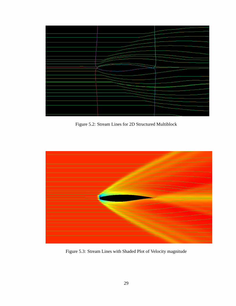
Figure 5.2: Stream Lines for 2D Structured Multiblock

Figure 5.3: Stream Lines with Shaded Plot of Velocity magnitude

29

Figure 5.4: 2D Vector Field Topology

5.1.3 Vector Field Topology

Fig 5.4 is vector field topology graph for the standard field [2] used for comparing topology

graphs. This field is used for comparing topology results.

u � � 0 � 103209 � 0 � 051511x � 0 � 302699y � 0 � 037546xy � 0 � 232875x � 0 � 611528x2 �v � 0 � 143656 � 0 � 687847x � 0 � 144779y � 0 � 21301xy � 1 � 02976x2 � 0 � 2462778y2, The al-

gorithm detects four critical points:

Two Saddle points at (1.03,-0.51) and (-0.23,0.77).

Two Attracting Focii at (-0.20,-0.26) and (0.74,0.83). The algorithm has successfully

plotted the topology graph, with streamlines interconnecting the critical points.

5.2 Scalar Visualization of 2D structured Grid Simulation

5.2.1 Shaded Plots 2D MultiBlock

Fig 5.5 is shaded plot visualization for the Pressure field for a 2D structured eight block

CFD data.

30

Figure 5.5: Shaded Plots for 2D Multiblock

Figure 5.6: Pressure Contours for 2D Structured Multiblock

31

Figure 5.7: Contours and Shaded Plots for 2D Structured Multiblock

5.2.2 Contour Plots 2D Structured

Fig 5.6 is contour plot visualization for Pressure field of 2D structured multiblock CFD

data. The geometry consists of an airfoil and a flap formed by 10 blocks. Data Continuity

across the blocks can be observed by the continuous contour plots.

Fig 5.6 shows Pressure contours and shaded plots for the pressure data field. The combina-

tion of more than one visualization techniques can be seen yielding better data visualiza-

tion.

5.2.3 Scalar Field Topology

Fig 5.8 is scalar field for the function S�x � y � � �

x2 � y � 11 � � x � y2 � 11 � , its topology

contains four Saddle points at (-3.85,-3.85), (3.70,-2.70),(2.85,2.85), (-2.70,3.70). and an

Attracting Focus at (-0.49,-0.49). The contour plots have also been plotted for better visu-

alization.

32

Figure 5.8: 2D Scalar Field Topology

Figure 5.9: Vector Plots on surfaces for 3D

33

Figure 5.10: Surface Scalar Plots for 3D

5.3 Visualization of 3D structured Grid Simulation

5.3.1 Flow Visualization Through Surface Sections

Fig 5.9 shows velocity visualization of a 3D grid data, the data has been synthetically

generated. The clarity of visualization depends heavily on the surfaces selected and view

point of the observer.

5.3.2 Scalar Visualization Through Surface Sections

Fig 5.10 show scalar visualization of 3D Computational Electro Magnetism (CEM) Data.

Scalar visualization comprises of shaded plots on selected surfaces for the field magnetic

field potential.

Fig 5.11 is shaded plot of scalar data field on the surface 2x2 � y2 � 2Z2 � 1.

5.3.3 Scalar Visualization Through Contour Plots

Fig 5.12 is contour plots for CEM Scalar Field potential. The Contours form a tessellated

surface. With color mapped to the value of the field.

34

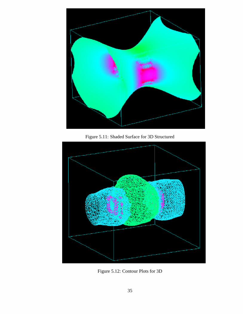
Figure 5.11: Shaded Surface for 3D Structured

Figure 5.12: Contour Plots for 3D

35

Figure 5.13: Combination of Contours and Shaded Plots for 3D

Fig 5.13 is visualization of 3D scalar field using combination of Contours and shaded plots

on surfaces for better visual appreciation of the data.

5.4 Visualization of Surface Structured Grids

Fig 5.14 is visualization of scalar field for Surface Grid CFD data, using iso value contours

and shaded plots. The surface grid data has been synthetically generated.

Fig 5.15 is velocity visualization of Surface Grid CFD data, with vector plots. The data has

been synthetically generated.

5.5 Visualization of 2D Unstructured Grids

Fig. 5.16 is visualization of 2D unstructured CFD data. it consists of shaded plots for

pressure data field.

Fig. 5.17 is velocity visualization of 2D unstructured CFD data.

36

Figure 5.14: Contours and Shaded Plots on Surface Grids

Figure 5.15: Vector Plots on Surface Grids

37

Figure 5.16: Shaded Plots on 2D Unstructured Grids

Figure 5.17: Vector Plots on 2D Unstructured Grids

38

Chapter 6

Closure

A Scientific Visualization tool has been successfully developed for CFD data. This applica-

tion accepts data input in CGNS format and successfully delivers multiblock visualization

of the scalar and vector fields.

Scalar visualization is accomplished using shaded and color plots, while vector visual-

ization is achieved using vector plots and stream lines. An advanced method of interpret-

ing data fields: topology graphs has been implemented. Visualization using one or more

techniques is very much possible and is more effective.

All the techniques have been successfully integrated as a post processing module in

IITZeus.

39

References

[1] Richard S. Gallagher, Computer Visualization: Graphics Techniques for Engineering

and Scientific, Solomon Press, 1995.

[2] Gregory M. Nielson, Hans Hagen, Heinrich Nuller, "Scientific Visualization", IEEE

Computer Society, 1997.

[3] Al Globus, Sam Uselton, "Evaluations of Visualization Software", NASA Advanced

Supercomputing, Report NAS-95-005, 1995.

[4] Advisory Group on Computer Graphics Technical Report, "Review of Visualization

Systems", AGOCG Technical Report 9, 1991.

[5] CFD General Notation System, www.cgns.org.

[6] Helwig Loffelmann, "Visualising local Properties and Characteristic Structures of Dy-

namical System, PhD Thesis, Vienna University of Technology, 1998.

[7] Michael J. Gerald, "Recent Advances in Visualization for Fluid Dynamics", AIAA

Paper Number: AIAA-97-2086, 1997.

[8] David Kenwright, "Visualizing Algorithms for Gigabyte Datasets",MRJ Technology

Solutions, Nasa Ames Research Center.

[9] A. Globus, C. Levit, T. Lasiniki,"A Tool for Visualizing the Topology of 3D Vector

Fields", Report RNR-91-017, NAS, 1991.

[10] Davis N. Kenwright, David A. Lane, "Interactive Time-Dependent Particle Tracing

Using Tetrahedral Decomposition", IEEE Transactions on Visualization and Com-

puter Graphics, 1996.

[11] Dirk Stuker, http://condor.informatik.Uni-Oldenburg.DE/ stueker/graphic/index.html.

40

[12] Daniel Asimov, "Notes on the Topology of Vector Fields and Flows", Visualization

1993. NASA Advanced Supercomputing, Report RNR-93-003.

[13] Doug Obrecht, "Point in a Tetrahedral", http://research.microsoft.com/holasch/cgindex/

geometry/ptintet.html.

[14] Chandrajit L. Bajaj, Daniel R. Schikore, V.Pascucci, "Visualization of Scalar Topol-

ogy for Structural Enhancement", IEEE Visualization 1999.

41

APPENDIX A : Components of CGNS

Advance Data Format (ADF) and the ADF Core : ADF core is the software im-

plementation of ADF database manager. This is very generic in nature, ADF core

consists of a set of routines that perform standard Input-Output (IO) operations on

ADF Files.

ADF Mid-level Library : The ADF Mid-level library is a repository for routines

written in C or FORTRAN for accessing the ADF files on a level higher than that of

ADF Core. The purpose of these routines is to encapsulate frequently used sequences

of operations into a single procedure. Like the ADF core, these routines are not spe-

cific to CFD.

The Standard Interface Data Structures (SIDS) : To guarantee a consistent in-

terpretation of the data by the users, the content and meaning of the data should be

specified in detail. As the ADF tree structure is too generic, the SIDS describes the

intellectual content of CFD related data in detail

CGNS/ADF File Mapping : Also known as "SIDS-to-ADF File mapping" specifies

the exact location where the CFD data defined by the SIDS is to be stored within the

ADF file.

CGNS Mid-level Library, or API : This consists of a set of routines that allow the

application developers to access the CGNS files. CGNS APIs allow developers to

implement CGNS I/O operations with out having a detailed knowledge of ADF or

File Mapping. example : int cg_open(char *filename, int mode, int *fn);

ADF editor : CGNS files being in binary format cannot be opened in ASCII editors.

ADF_Edit is an interactive browser cum editor, provided for displaying the tree struc-

ture and content of the ADF files. The editor is under the process of implementation.

42