scilab manual for power system simulation by prof jain b
TRANSCRIPT

Scilab Manual forPower System Simulationby Prof Jain B. MarshelElectrical Engineering
St. Xavier’s Catholic College of Engineering1
Solutions provided byProf Jain B.MarshelElectrical Engineering
St.Xavier’s Catholic College of Engineering
January 19, 2022
1Funded by a grant from the National Mission on Education through ICT,http://spoken-tutorial.org/NMEICT-Intro. This Scilab Manual and Scilab codeswritten in it can be downloaded from the ”Migrated Labs” section at the websitehttp://scilab.in

1

Contents
List of Scilab Solutions 4
1 Computation of Transmission line Parameters 7
2 Modelling of Transmission Lines 14
3 Formation of Bus Admittance matrix 20
4 Formation of Bus Impedance matrix 23
5 Load flow solution using Gauss-Seidal method 27
6 Load flow solution using Newton-Raphson method 33
7 Symmetrical Fault Analysis 40
8 Unsymmetrical Fault Analysis 45
9 Small Signal and transient Stability Analysis of Single-machineInfinite bus system 51
10 Small Signal and transient Stability Analysis of Multi ma-chine Power Systems 55
11 Electromagnetic Transients in Power Systems 60
12 Load frequency dynamics of single Area Power Systems 62
13 Load frequency dynamics of two Area Power Systems 64
2

14 Economic dispatch in power systems neglecting losses 66
15 Economic dispatch in power systems Including losses 69
3

List of Experiments
Solution 1.1 Inductance of Single Phase line . . . . . . . . . . 7Solution 1.2 Inductance of Three Phase line . . . . . . . . . . 8Solution 1.3 Capacitance of Single Phase line . . . . . . . . . . 10Solution 1.4 Capacitance of Three Phase line . . . . . . . . . . 11Solution 2.1 Nominal T method . . . . . . . . . . . . . . . . . 14Solution 2.2 Nominal pi Method . . . . . . . . . . . . . . . . . 16Solution 3.1 Bus Admittance Matrix . . . . . . . . . . . . . . 20Solution 4.1 Bus Impedance Matrix . . . . . . . . . . . . . . . 23Solution 5.1 Gauss Seidal Load Flow . . . . . . . . . . . . . . 27Solution 6.1 Newton Raphson load Flow . . . . . . . . . . . . 33Solution 7.1 Symmetrical Fault Analysis . . . . . . . . . . . . 40Solution 8.1 Unsymmetrical Fault Analysis . . . . . . . . . . . 45Solution 9.1 SMIB Stability Analysis . . . . . . . . . . . . . . 51Solution 10.1 Multimachine Stability Analysis . . . . . . . . . . 55Solution 14.1 Economic Load Dispatch Excluding Losses . . . . 66Solution 15.1 Economic Load Dispatch Including Losses . . . . 69
4

List of Figures
1.1 Inductance of Single Phase line . . . . . . . . . . . . . . . . 81.2 Inductance of Three Phase line . . . . . . . . . . . . . . . . 101.3 Capacitance of Single Phase line . . . . . . . . . . . . . . . . 121.4 Capacitance of Three Phase line . . . . . . . . . . . . . . . . 13
2.1 Nominal T method . . . . . . . . . . . . . . . . . . . . . . . 162.2 Nominal pi Method . . . . . . . . . . . . . . . . . . . . . . . 19
3.1 Bus Admittance Matrix . . . . . . . . . . . . . . . . . . . . 22
4.1 Bus Impedance Matrix . . . . . . . . . . . . . . . . . . . . . 26
5.1 Gauss Seidal Load Flow . . . . . . . . . . . . . . . . . . . . 275.2 Gauss Seidal Load Flow . . . . . . . . . . . . . . . . . . . . 28
6.1 Newton Raphson load Flow . . . . . . . . . . . . . . . . . . 346.2 Newton Raphson load Flow . . . . . . . . . . . . . . . . . . 34
7.1 Symmetrical Fault Analysis . . . . . . . . . . . . . . . . . . 417.2 Symmetrical Fault Analysis . . . . . . . . . . . . . . . . . . 41
8.1 Unsymmetrical Fault Analysis . . . . . . . . . . . . . . . . . 498.2 Unsymmetrical Fault Analysis . . . . . . . . . . . . . . . . . 50
9.1 SMIB Stability Analysis . . . . . . . . . . . . . . . . . . . . 529.2 SMIB Stability Analysis . . . . . . . . . . . . . . . . . . . . 53
10.1 Multimachine Stability Analysis . . . . . . . . . . . . . . . . 59
11.1 Transient in RLC series circuit with DC source . . . . . . . 61
12.1 Single Area Control . . . . . . . . . . . . . . . . . . . . . . . 63
5
13.1 Two Area Control . . . . . . . . . . . . . . . . . . . . . . . . 65
14.1 Economic Load Dispatch Excluding Losses . . . . . . . . . . 67
15.1 Economic Load Dispatch Including Losses . . . . . . . . . . 70
6

Experiment: 1
Computation of Transmissionline Parameters
Scilab code Solution 1.1 Inductance of Single Phase line
1 //Program to f i n d l oop i nduc t an c e o f a s i n g l e phaset r a n sm i s s i o n l i n e //
2 // This program r e q u i r e s u s e r i nput . Sample Problemand u s e r i nput with output a r e a v a i l a b l e i n ther e s u l t f i l e //
3 // S c i l a b Ve r s i on 5 . 5 . 2 ; OS : Windows4 clc;
5 clear;
6 d=input( ’ Enter the s pa c i n g between conduc t o r s i nmeter : ’ )
7 dia=input( ’ Enter the d i amete r o f the conduc to r i nmeter : ’ )
8 r=dia/2
9 l=input( ’ Enter the l e n g t h o f the l i n e i n km : ’ )10 li=10^( -7) *(1+4*( log(d/r)))*l*1000
11 disp(li, ’ The l oop i nduc t an c e f o r g i v en t r a n sm i s s i o nl i n e i n Henry i s : ’ )
12
13
7
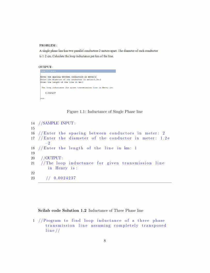
Figure 1.1: Inductance of Single Phase line
14 //SAMPLE INPUT :15
16 // Enter the s pa c i n g between conduc t o r s i n meter : 217 // Enter the d i amete r o f the conduc to r i n meter : 1 . 2 e
−218 // Enter the l e n g t h o f the l i n e i n km : 119
20 //OUTPUT:21 //The l oop i nduc t an c e f o r g i v en t r a n sm i s s i o n l i n e
i n Henry i s :22
23 // 0 . 0024237
Scilab code Solution 1.2 Inductance of Three Phase line
1 //Program to f i n d l oop i nduc t an c e o f a t h r e e phaset r a n sm i s s i o n l i n e assuming c omp l e t e l y t r an spo s edl i n e //
8
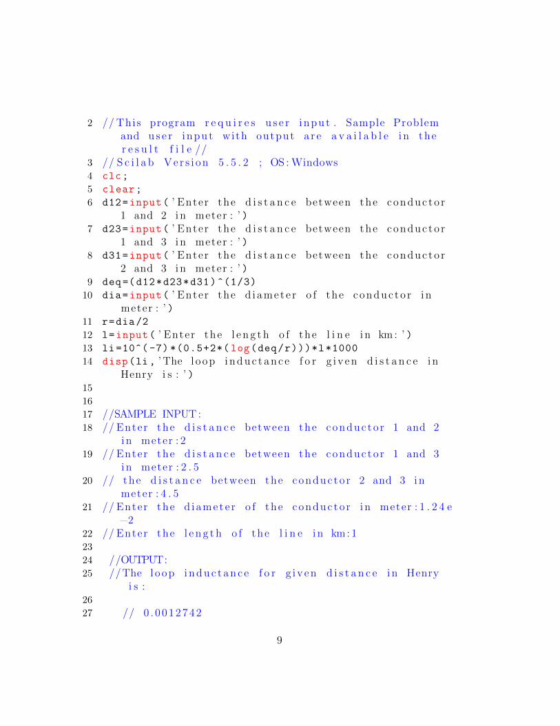
2 // This program r e q u i r e s u s e r i nput . Sample Problemand u s e r i nput with output a r e a v a i l a b l e i n ther e s u l t f i l e //
3 // S c i l a b Ve r s i on 5 . 5 . 2 ; OS : Windows4 clc;
5 clear;
6 d12=input( ’ Enter the d i s t a n c e between the conduc to r1 and 2 in meter : ’ )
7 d23=input( ’ Enter the d i s t a n c e between the conduc to r1 and 3 in meter : ’ )
8 d31=input( ’ Enter the d i s t a n c e between the conduc to r2 and 3 in meter : ’ )
9 deq=(d12*d23*d31)^(1/3)
10 dia=input( ’ Enter the d i amete r o f the conduc to r i nmeter : ’ )
11 r=dia/2
12 l=input( ’ Enter the l e n g t h o f the l i n e i n km : ’ )13 li=10^( -7) *(0.5+2*( log(deq/r)))*l*1000
14 disp(li, ’ The l oop i nduc t an c e f o r g i v en d i s t a n c e i nHenry i s : ’ )
15
16
17 //SAMPLE INPUT :18 // Enter the d i s t a n c e between the conduc to r 1 and 2
in meter : 219 // Enter the d i s t a n c e between the conduc to r 1 and 3
in meter : 2 . 520 // the d i s t a n c e between the conduc to r 2 and 3 in
meter : 4 . 521 // Enter the d i amete r o f the conduc to r i n meter : 1 . 2 4 e
−222 // Enter the l e n g t h o f the l i n e i n km: 123
24 //OUTPUT:25 //The l oop i nduc t an c e f o r g i v en d i s t a n c e i n Henry
i s :26
27 // 0 . 0012742
9

Figure 1.2: Inductance of Three Phase line
Scilab code Solution 1.3 Capacitance of Single Phase line
1 //Program to f i n d the c a p a c i t a n c e o f a s i n g l e phaset r a n sm i s s i o n l i n e //
2 // This program r e q u i r e s u s e r i nput . Sample Problemand u s e r i nput with output a r e a v a i l a b l e i n ther e s u l t f i l e //
3 // S c i l a b Ve r s i on 5 . 5 . 2 ; OS : Windows4 clc;
5 clear;
6 dia=input( ’ Enter the d i amete r o f the conduc to r i nmeter : ’ )
7 r=dia/2
8 d=input( ’ Enter the s pa c i n g between the conduc t o r s i n
10

meter : ’ )9 l=input( ’ Enter the l e n g t h o f the l i n e i n km : ’ )10 c=((%pi *8.854*10^( -12)*l*1000)/log(d/r))
11 disp(c, ’ the c a p a c i t a n c e o f the l i n e f o r g i v end i s t a n c e i s : ’ )
12
13
14
15 //SAMPLE INPUT :16 // Enter the d i amete r o f the conduc to r i n meter : 2 e−217 // Enter the s pa c i n g between the conduc t o r s i n meter
: 318 // Enter the l e n g t h o f the l i n e i n km: 119
20 //OUTPUT:21 // the c a p a c i t a n c e o f the l i n e f o r g i v en d i s t a n c e i s
:22
23 // 4 . 8 7 7D−09
Scilab code Solution 1.4 Capacitance of Three Phase line
1 //Program to f i n d l i n e to n e u t r a l c a p a c i t a n c e o f at h r e e phase t r a n sm i s s i o n l i n e assuming comp l e t e l yt r an spo s ed l i n e //
2 // This program r e q u i r e s u s e r i nput . Sample Problemand u s e r i nput with output a r e a v a i l a b l e i n ther e s u l t f i l e //
3 // S c i l a b Ve r s i on 5 . 5 . 2 ; OS : Windows4 clc;
5 clear;
6 d12=input( ’ Enter the d i s t a n c e between the conduc to r1 and 2 in meter : ’ )
11

Figure 1.3: Capacitance of Single Phase line
7 d23=input( ’ Enter the d i s t a n c e between the conduc to r1 and 3 in meter : ’ )
8 d31=input( ’ Enter the d i s t a n c e between the conduc to r2 and 3 in meter : ’ )
9 deq=(d12*d23*d31)^(1/3)
10 dia=input( ’ Enter the d i amete r o f the conduc to r i nmeter : ’ )
11 r=dia/2
12 l=input( ’ Enter the l e n g t h o f the l i n e i n km : ’ )13 Cn=((2* %pi *8.85*10^ -12) /(log(deq/r)))*l*1000
14 disp(Cn, ’ The l i n e to n e u t r a l c a p a c i t a n c e f o r g i v end i s t a n c e i n Farad i s : ’ )
15
16
17 //SAMPLE INPUT :18
19 // Enter the d i s t a n c e between the conduc to r 1 and 2in meter : 4
20 // Enter the d i s t a n c e between the conduc to r 1 and 3in meter : 4
21 // Enter the d i s t a n c e between the conduc to r 2 and 3
12

Figure 1.4: Capacitance of Three Phase line
i n meter : 822 // Enter the d i amete r o f the conduc to r i n meter : 2 e−223 // Enter the l e n g t h o f the l i n e i n km: 1 0 024
25 //OUTPUT:26 //The l i n e to n e u t r a l c a p a c i t a n c e f o r g i v en
d i s t a n c e i n Farad i s :27
28 // 0 . 0000009
13

Experiment: 2
Modelling of TransmissionLines
Scilab code Solution 2.1 Nominal T method
1 // Ca l c u l a t i o n o f Transmi s s i on Line paramete r s u s i n gNominal−T method //
2 // This program r e q u i r e s u s e r i nput . Sample problemwith u s e r i nput and r e s u l t a r e a v a i l a b l e i n ther e s u l t f i l e //
3 // S c i l a b Ve r s i on 5 . 5 . 2 ; OS : Windows4 clc;
5 clear;
6 pl=input( ’ Enter the power s u pp l i e d to the l oad : ’ );7 vr=input( ’ Enter the r e c e i v i n g end v o l t a g e : ’ );8 pf=input( ’ Enter the power f a c t o r : ’ );9 spf=sin(acos(pf));
10 z=input( ’ Enter the s e r i e s impedance va lu e o f s i n g l econduc to r : ’ );
11 y=input( ’ Enter the shunt admit tance va lu e : ’ );12 e=(z*y)/2;
13 a=(1+e); // c a l c u l a t i o n o f t r a n sm i s s i o nl i n e pa ramete r s
14 b=z*(1+e/2);
14
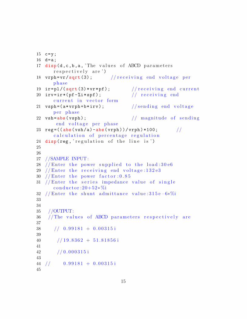
15 c=y;
16 d=a;
17 disp(d,c,b,a, ’ The v a l u e s o f ABCD paramete r sr e s p e c t i v e l y a r e ’ )
18 vrph=vr/sqrt (3); // r e c e i v i n g end v o l t a g e perphase
19 ir=pl/(sqrt (3)*vr*pf); // r e c e i v i n g end cu r r e n t20 irv=ir*(pf-%i*spf); // r e c e i v i n g end
cu r r e n t i n v e c t o r form21 vsph=(a*vrph+b*irv); // s end ing end v o l t a g e
per phase22 vsh=abs(vsph); // magnitude o f s end ing
end v o l t a g e per phase23 reg =((abs(vsh/a)-abs(vrph))/vrph)*100; //
c a l c u l a t i o n o f p e r c en t a g e r e g u l a t i o n24 disp(reg , ’ r e g u l a t i o n o f the l i n e i s ’ )25
26
27 //SAMPLE INPUT :28 // Enter the power s u pp l i e d to the l oad : 3 0 e629 // Enter the r e c e i v i n g end v o l t a g e : 1 3 2 e330 // Enter the power f a c t o r : 0 . 8 531 // Enter the s e r i e s impedance va l u e o f s i n g l e
conduc to r :20+52∗%i32 // Enter the shunt admit tance va lu e : 3 1 5 e−6∗%i33
34
35 //OUTPUT:36 //The v a l u e s o f ABCD paramete r s r e s p e c t i v e l y a r e37
38 // 0 . 9 9181 + 0 . 00315 i39
40 // 19 . 8 362 + 51 . 81856 i41
42 // 0 . 000315 i43
44 // 0 . 9 9181 + 0 . 00315 i45
15

Figure 2.1: Nominal T method
46 // r e g u l a t i o n o f the l i n e i s47
48 // 9 . 2540724
Scilab code Solution 2.2 Nominal pi Method
1 // Ca l c u l a t i o n o f Transmi s s i on Line paramete r s u s i n gNominal−p i method //
2 // This Program r e q u i r e s u s e r i nput . Sample Problemwith u s e r i nput and r e s u l t a r e a v a i l a b l e i n the
16
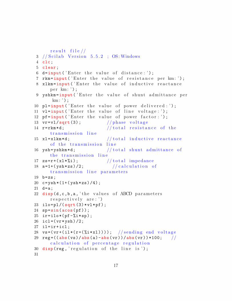
r e s u l t f i l e //3 // S c i l a b Ve r s i on 5 . 5 . 2 ; OS : Windows4 clc;
5 clear;
6 d=input( ’ Enter the va lu e o f d i s t a n c e : ’ );7 rkm=input( ’ Enter the va lu e o f r e s i s t a n c e per km : ’ );8 xlkm=input( ’ Enter the va l u e o f i n d u c t i v e r e a c t a n c e
per km : ’ );9 yshkm=input( ’ Enter the va lu e o f shunt admit tance per
km : ’ );10 pl=input( ’ Enter the va lu e o f power d e l i v e r e d : ’ );11 vl=input( ’ Enter the va lu e o f l i n e v o l t a g e : ’ );12 pf=input( ’ Enter the va lu e o f power f a c t o r : ’ );13 vr=vl/sqrt (3); // phase v o l t a g e14 r=rkm*d; // t o t a l r e s i s t a n c e o f the
t r a n sm i s s i o n l i n e15 xl=xlkm*d; // t o t a l i n d u c t i v e r e a c t a n c e
o f the t r a n sm i s s i o n l i n e16 ysh=yshkm*d; // t o t a l shunt admit tance o f
the t r a n sm i s s i o n l i n e17 zs=r+(xl*%i); // t o t a l impedance18 a=1+( ysh*zs)/2; // c a l c u l a t i o n o f
t r a n sm i s s i o n l i n e pa ramete r s19 b=zs;
20 c=ysh *(1+( ysh*zs)/4);
21 d=a;
22 disp(d,c,b,a, ’ the v a l u e s o f ABCD paramete r sr e s p e c t i v e l y a r e : ’ )
23 ilo=pl/(sqrt (3)*vl*pf);
24 sp=sin(acos(pf));
25 ir=ilo*(pf-%i*sp);
26 icl=(vr*ysh)/2;
27 il=ir+icl;
28 vs=(vr+(il*(r+(%i*xl)))); // s end ing end v o l t a g e29 reg =((abs(vs)/abs(a)-abs(vr))/abs(vr))*100; //
c a l c u l a t i o n o f p e r c en t a g e r e g u l a t i o n30 disp(reg , ’ r e g u l a t i o n o f the l i n e i s ’ );31
17

32 //SAMPLE INPUT :33 // Enter the va lu e o f d i s t a n c e : 1 0 034 // Enter the va lu e o f r e s i s t a n c e per km : 0 . 135 // Enter the va lu e o f i n d u c t i v e r e a c t a n c e per km : 0 . 236 // Enter the va lu e o f shunt admit tance per km: 4 e−6∗%i37 // Enter the va lu e o f power d e l i v e r e d : 1 0 e638 // Enter the va lu e o f l i n e v o l t a g e : 6 6 e339 // Enter the va lu e o f power f a c t o r : 0 . 840
41 //OUTPUT:42 // the v a l u e s o f ABCD paramete r s r e s p e c t i v e l y a r e :43
44 // 0 . 9 9 6 + 0 . 0 02 i45
46 // 1 0 . + 20 . i47
48 // − 0 . 0000004 + 0 . 0003992 i49
50 // 0 . 9 9 6 + 0 . 0 02 i51
52 // r e g u l a t i o n o f the l i n e i s53
54 // 5 . 8069405
18
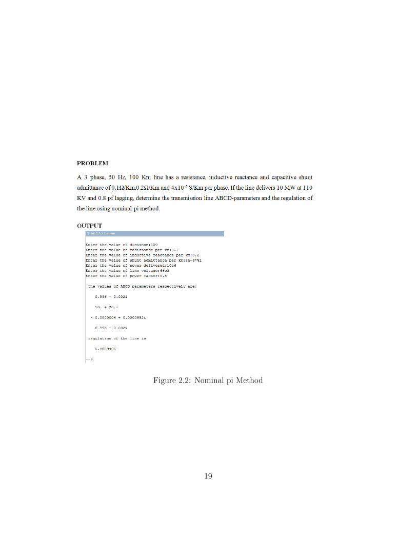
Figure 2.2: Nominal pi Method
19

Experiment: 3
Formation of Bus Admittancematrix
Scilab code Solution 3.1 Bus Admittance Matrix
1
2 //Program to f i n d out bus admit tance matr ix o f apower system o f any s i z e //
3 // This program r e q u i r e s u s e r i nput . A sample problemwith u s e r i nput and output i s a v a i l a b l e i n the
r e s u l t f i l e //4 // S c i l a b Ve r s i on 5 . 5 . 2 ; OS : Windows5 clc;
6 clear;
7 linedata=input( ’ Enter l i n e data i n o rd e r o f s t r t bus, end bus , s e r i e s r e s i s t a n c e , s e r i e s r e a c t an c e , shunts u s c e p t an c e : ’ )
8 sb=linedata (:,1) // S t a r t i n g bus number o f a l l thel i n e s s t o r e d i n v a r i a b l e sb
9 eb=linedata (:,2) // Ending bus number o f a l l thel i n e s s t o r e d i n v a r i a b l e eb
10 lz=linedata (:,3)+linedata (:,4)*%i; // l i n e impedanc e=R+jX
11 sa=-linedata (:,5)*%i; // shunt admit tance=−jB
20

12 nb=max(max(sb ,eb));
13 ybus=zeros(nb ,nb);
14 for i=1: length(sb)
15 m=sb(i);
16 n=eb(i);
17 ybus(m,m)=ybus(m,m)+1/lz(i)+sa(i);
18 ybus(n,n)=ybus(n,n)+1/lz(i)+sa(i);
19 ybus(m,n)=-1/lz(i);
20 ybus(n,m)=ybus(m,n);
21 end
22 disp(ybus , ’ The Bus Admittance matr ix i s : ’ )23
24 //SAMPLE INPUT :25
26 // Enter l i n e data i n o rd e r o f s t r t bus , end bus ,s e r i e s r e s i s t a n c e , s e r i e s r e a c t anc e , shunts u s c e p t an c e : [ 1 2 0 . 0 2 0 . 0 4 0 ; 1 3 0 . 0 1 0 . 0 3 0 ; 2 30 . 0 125 0 . 0 2 5 0 ]
27
28 //OUTPUT:29 //The Bus Admittance matr ix i s :30
31 // 2 0 . − 5 0 . i − 1 0 . + 20 . i − 1 0 . + 30 . i32 // − 1 0 . + 20 . i 2 6 . − 5 2 . i − 1 6 . + 32 . i33 // − 1 0 . + 30 . i − 1 6 . + 32 . i 2 6 . − 6 2 . i
21
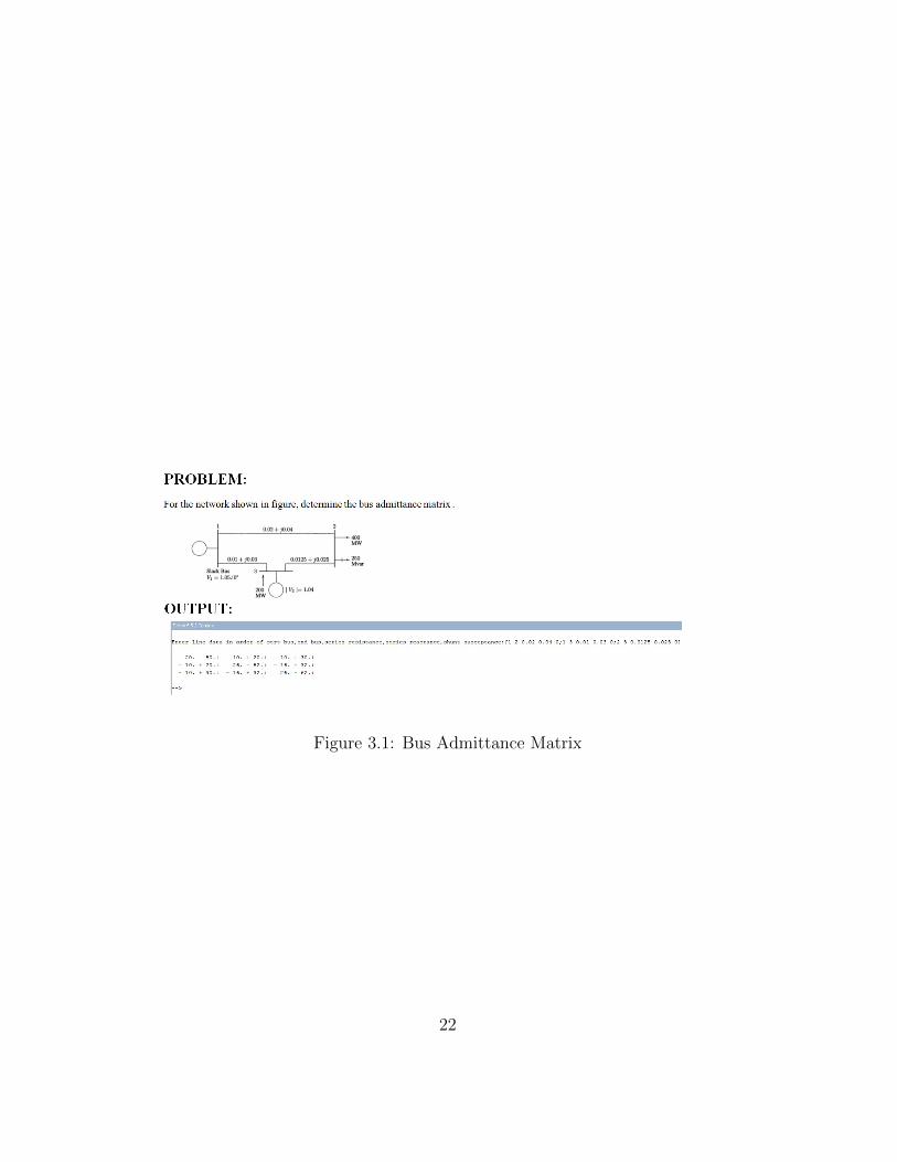
Figure 3.1: Bus Admittance Matrix
22
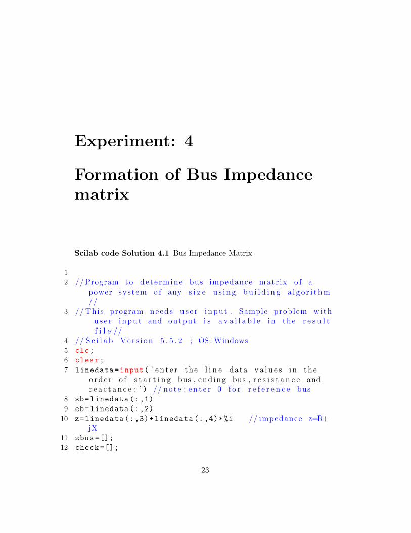
Experiment: 4
Formation of Bus Impedancematrix
Scilab code Solution 4.1 Bus Impedance Matrix
1
2 //Program to de t e rmine bus impedance matr ix o f apower system o f any s i z e u s i n g b u i l d i n g a l g o r i t hm//
3 // This program needs u s e r i nput . Sample problem withu s e r i nput and output i s a v a i l a b l e i n the r e s u l tf i l e //
4 // S c i l a b Ve r s i on 5 . 5 . 2 ; OS : Windows5 clc;
6 clear;
7 linedata=input( ’ e n t e r the l i n e data v a l u e s i n theo rd e r o f s t a r t i n g bus , end ing bus , r e s i s t a n c e andr e a c t a n c e : ’ ) // note : e n t e r 0 f o r r e f e r e n c e bus
8 sb=linedata (:,1)
9 eb=linedata (:,2)
10 z=linedata (:,3)+linedata (:,4)*%i // impedance z=R+jX
11 zbus =[];
12 check =[];
23

13 for i=1: length(sb)
14 m=sb(i);
15 n=eb(i);
16 mn=min(m,n);
17 nm=max(m,n);
18 ncheck=length(find(check==nm)); // Va r i a b l eused f o r ch e ck i ng whether bus nm i s a l r e a dye x i s t i n g
19 mcheck=length(find(check==mn)); // Va r i a b l eused f o r ch e ck i ng whether bus mn i s a l r e a dye x i s t i n g
20 [rows columns ]=size(zbus);
21 // Cond i t i on f o r c onn e c t i o n o f l i n e between r e f e r e n c ebus and new bus
22 if mn==0 & ncheck ==0
23 zbus=[zbus zeros(rows ,1);zeros(1,rows) z(i)
];
24 check=[check nm];
25 // Cond i t i on f o r c onn e c t i o n o f l i n e between e x i s t i n gbus and new bus
26 else if mcheck >0 & ncheck ==0
27 zbus=[zbus zbus(:,mn);zbus(mn ,:) zbus(mn
,mn)+z(i)];
28 check=[check nm];
29 // Cond i t i on f o r c onn e c t i o n o f l i n e between r e f e r e n c ebus and e x i s t i n g bus
30 elseif mn==0 & ncheck >0
31 zbus=[zbus zbus(:,nm);zbus(nm ,:) zbus(nm
,nm)+z(i)];
32 // Modi fy ing Z bus s i z e u s i n g Kron ’ sr e d u c t i o n t ehn i qu e
33 zbusn=zeros(rows ,rows);
34 for r=1: rows
35 for t=1: columns
36 zbusn(r,t)=zbus(r,t)-(zbus(r,
rows +1)*zbus(rows+1,t))/(zbus
(rows+1,rows +1));
37 end
24
38 end
39 zbus=zbusn
40 // Cond i t i on f o r c onn e c t i o n o f l i n e between twoe x i s t i n g buse s
41 elseif mcheck >0 & ncheck >0
42 zbus=[zbus zbus(:,nm)-zbus(:,mn);zbus(nm
,:)-zbus(mn ,:),z(i)+zbus(mn ,nm)+zbus(
nm ,nm) -2*zbus(nm ,mn)];
43 // Modi fy ing Z bus s i z e u s i n g Kron ’ sr e d u c t i o n t ehn i qu e
44 zbusn=zeros(rows ,rows);
45 for r=1: rows
46 for t=1: columns
47 zbusn(r,t)=zbus(r,t)-(zbus(r,rows
+1)*zbus(rows+1,t))/(zbus(rows
+1,rows +1));
48 end
49 end
50 zbus=zbusn;
51 end
52 end
53 end
54 disp(zbus , ’ The bus impedance matr ix i s : ’ );55
56
57 //SAMPLE INPUT :58
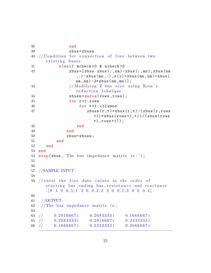
59 // e n t e r the l i n e data v a l u e s i n the o rd e r o fs t a r t i n g bus , end ing bus , r e s i s t a n c e and r e a c t a n c e: [ 0 1 0 0 . 5 ; 1 2 0 0 . 2 ; 2 3 0 0 . 1 ; 3 0 0 0 . 4 ]
60
61 //OUTPUT:62 //The bus impedance matr ix i s :63
64 // 0 . 2916667 i 0 . 2 083333 i 0 . 1 666667 i65 // 0 . 2083333 i 0 . 2 916667 i 0 . 2 333333 i66 // 0 . 1666667 i 0 . 2 333333 i 0 . 2 666667 i
25
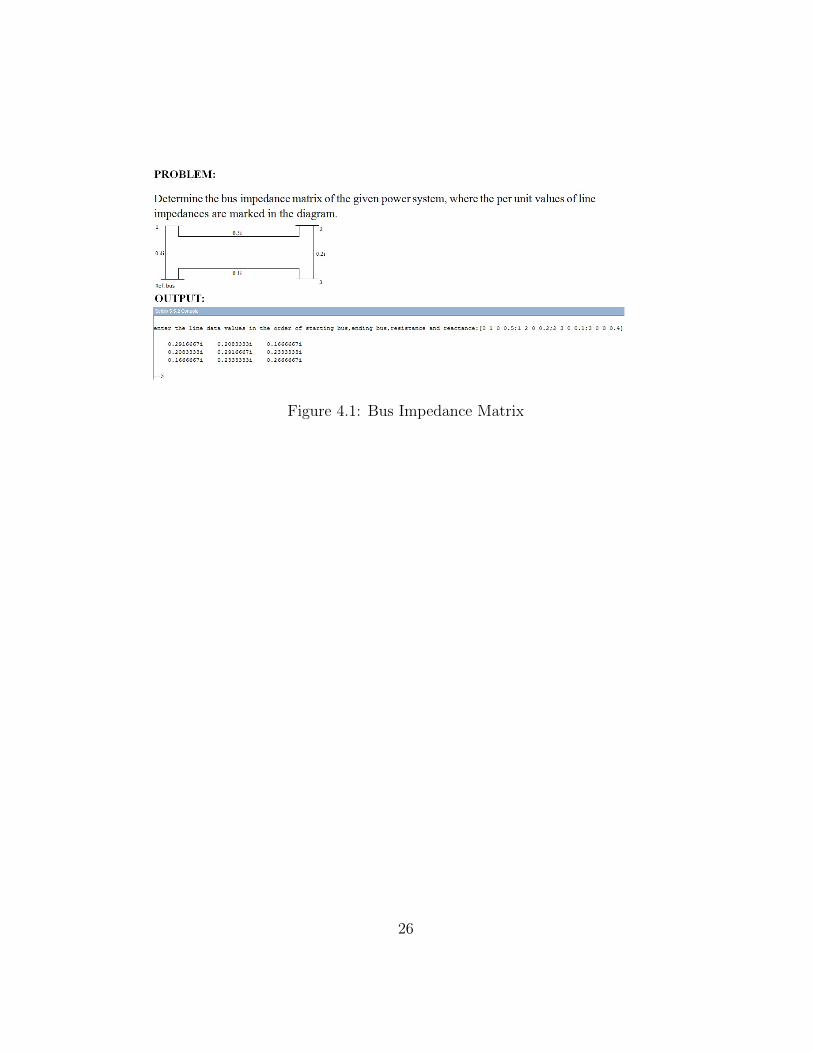
Figure 4.1: Bus Impedance Matrix
26
Experiment: 5
Load flow solution usingGauss-Seidal method
Scilab code Solution 5.1 Gauss Seidal Load Flow
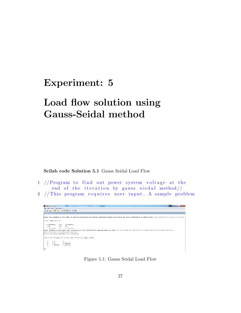
1 //Program to f i n d out power system vo l t a g e at theend o f the i t e r a t i o n by gaus s s i e d a l method //
2 // This program r e q u i r e s u s e r i nput . A sample problem
Figure 5.1: Gauss Seidal Load Flow
27
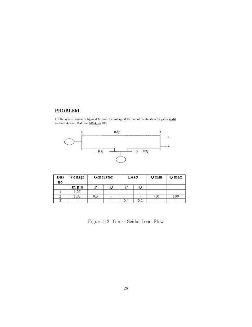
Figure 5.2: Gauss Seidal Load Flow
28
with u s e r i nput and output i s a v a i l a b l e i n ther e s u l t f i l e //
3 // Ques t i on o f example problem i s a v a i l a b l e i n f i l e ”Gau s s s S e i d a lQu e s t i o nF i l e . j pg ” and r e s u l t i sa v a i l a b l e i n the f i l e ” Gaus sS e i da lOutpu tF i l e . j pg ”
4 // S c i l a b Ve r s i on 5 . 5 . 2 ; OS : Windows5 clc;
6 clear;
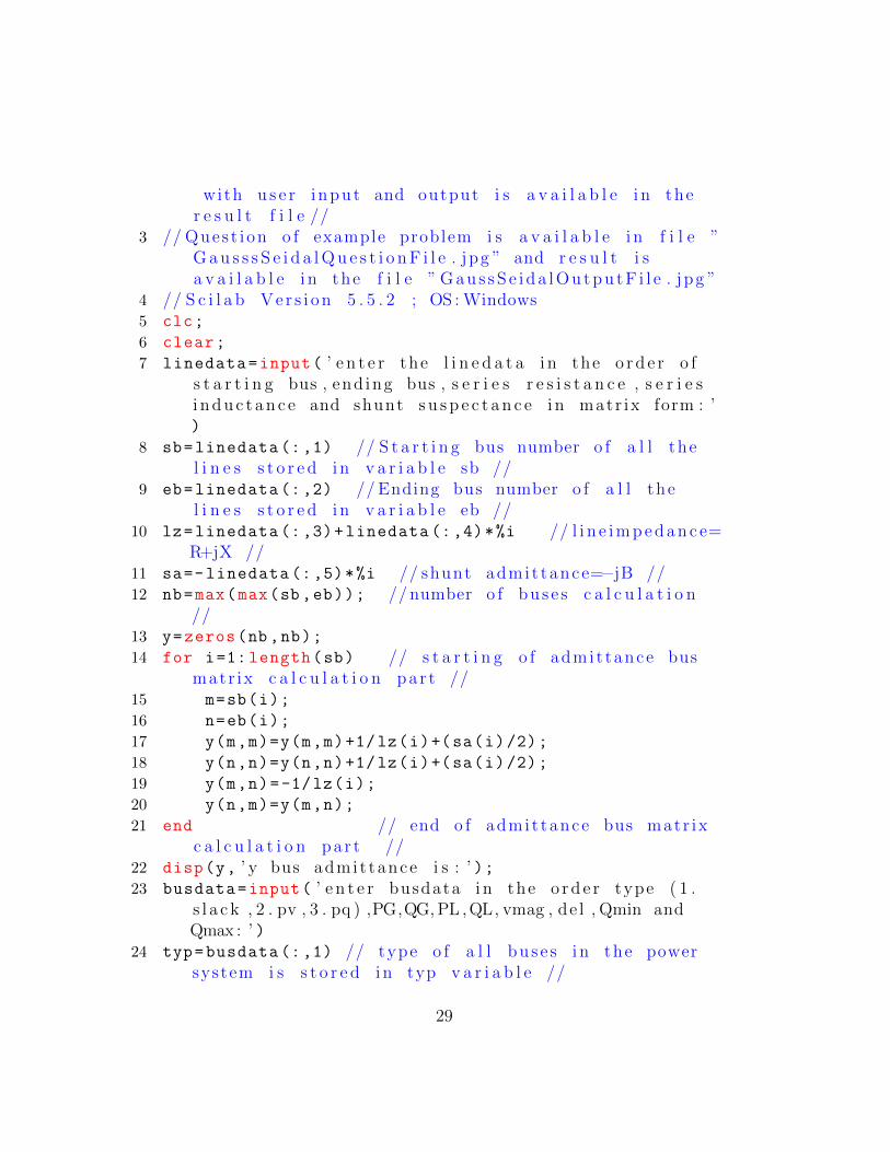
7 linedata=input( ’ e n t e r the l i n e d a t a i n the o rd e r o fs t a r t i n g bus , end ing bus , s e r i e s r e s i s t a n c e , s e r i e si nduc t an c e and shunt s u s p e c t an c e i n matr ix form : ’)
8 sb=linedata (:,1) // S t a r t i n g bus number o f a l l thel i n e s s t o r e d i n v a r i a b l e sb //
9 eb=linedata (:,2) // Ending bus number o f a l l thel i n e s s t o r e d i n v a r i a b l e eb //
10 lz=linedata (:,3)+linedata (:,4)*%i // l i n e impedanc e=R+jX //
11 sa=-linedata (:,5)*%i // shunt admit tance=−jB //12 nb=max(max(sb ,eb)); //number o f buse s c a l c u l a t i o n
//13 y=zeros(nb,nb);
14 for i=1: length(sb) // s t a r t i n g o f admit tance busmatr ix c a l c u l a t i o n pa r t //
15 m=sb(i);
16 n=eb(i);
17 y(m,m)=y(m,m)+1/lz(i)+(sa(i)/2);
18 y(n,n)=y(n,n)+1/lz(i)+(sa(i)/2);
19 y(m,n)=-1/lz(i);
20 y(n,m)=y(m,n);
21 end // end o f admit tance bus matr ixc a l c u l a t i o n pa r t //
22 disp(y, ’ y bus admit tance i s : ’ );23 busdata=input( ’ e n t e r busdata i n the o rd e r type ( 1 .
s l a c k , 2 . pv , 3 . pq ) ,PG,QG,PL ,QL, vmag , de l , Qmin andQmax : ’ )
24 typ=busdata (:,1) // type o f a l l bu s e s i n the powersystem i s s t o r e d i n typ v a r i a b l e //
29

25 qmin=busdata (:,8) // minmum l im i t o f Q f o r a l l thebuse s i s s t o r e d i n the v a r i a b l e qmin //
26 qmax=busdata (:,9) // maximum l im i t o f Q f o r a l l thebuse s i s s t o r e d i n the v a r i a b l e qmax//
27 p=busdata (:,2)-busdata (:,4) // r e a l power o f a l l thebuse s a r e c a l c u l a t e d and i s s t o r e d i n the
v a r i a b l e p //28 q=busdata (:,3)-busdata (:,5) // r e a c t i v e power o f
a l l the buss a r e c a l c u l a t e d and i s s t o r e d i n thev a r i a b l e q //
29 v=busdata (:,6).*( cosd(busdata (:,7))+%i*sind(busdata
(:,7)));
30 alpha=input( ’ e n t e r the va lu e o f a c c e l a r a t i o n f a c t o r :’ );
31 iter =1;
32 err =1;
33 vn(1)=v(1);
34 vold=v(1);
35 while abs(err) >5*10^( -5) // s t a r t i n g o f c a l c u l a t i o npa r t o f bus v o l t a g e f o r f i r s t i t e r a t i o n //
36 for i=2:nb
37 sumyv =0;
38 for j=1:nb
39 sumyv=sumyv+y(i,j)*v(j);
40 end
41 if typ(i)==2
42 q(i)=-imag(conj(v(i)*sumyv));
43 if q(i)<qmin(i) |q(n)>qmax(i)
44 vn(i)=(1/y(i,i))*(((p(i)-%i*q(i))/(
conj(v(i))))-(sumyv -y(i,i)*v(i)))
;
45 vold(i)=v(i);
46 v(i)=vn(i);
47 typ(i)=3
48 if q(i)<qmin(i)
49 q(i)=qmin(i);
50 else
51 q(i)=qmax(i);
30
52 end
53 else
54 vn(i)=(1/y(i,i))*(((p(i)-%i*q(i))/(conj(
v(i)))) -(sumyv -y(i,i)*v(i)));
55 ang=atan(imag(vn(i)),real(vn(i)));
56 vn(i)=abs(v(i))*(cos(ang)+%i*sin(ang));
57 vold(i)=v(i);
58 v(i)=vn(i);
59 end
60 elseif typ(i)==3
61 vn(i)=(1/y(i,i))*(((p(i)-%i*q(i))/(conj(
v(i)))) -(sumyv -y(i,i)*v(i)));
62 vold(i)=v(i);
63 v(i)=vn(i);
64 end
65 end
66 err=max(abs(abs(v)-abs(vold)));
67
68 iter=iter +1;
69 for i=2:nb
70 if err >5*10^( -6) &typ(i)==3
71 v(i)=vold(i)+alpha*(v(i)-vold(i));
72 end
73 end
74 end
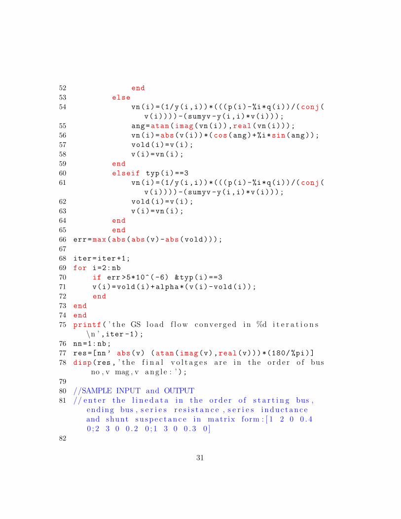
75 printf( ’ the GS load f l ow converged in %d i t e r a t i o n s\n ’ ,iter -1);
76 nn=1:nb;
77 res=[nn ’ abs(v) (atan(imag(v),real(v)))*(180/ %pi)]
78 disp(res , ’ the f i n a l v o l t a g e s a r e i n the o rd e r o f busno , v mag , v ang l e : ’ );
79
80 //SAMPLE INPUT and OUTPUT81 // e n t e r the l i n e d a t a i n the o rd e r o f s t a r t i n g bus ,
end ing bus , s e r i e s r e s i s t a n c e , s e r i e s i nduc t an c eand shunt s u s p e c t an c e i n matr ix form : [ 1 2 0 0 . 40 ; 2 3 0 0 . 2 0 ; 1 3 0 0 . 3 0 ]
82
31

83 //y bus admit tance i s :84
85 // − 5 . 8333333 i 2 . 5 i 3 . 3 333333 i86 // 2 . 5 i − 7 . 5 i 5 . i87 // 3 . 3333333 i 5 . i − 8 . 3333333 i88 // e n t e r busdata i n the o rd e r type ( 1 . s l a c k , 2 . pv , 3 . pq
) ,PG,QG,PL ,QL, vmag , de l , Qmin and Qmax : [ 1 0 0 0 01 . 0 5 0 0 0 ; 2 0 . 3 0 0 0 1 . 0 2 0 −0.1 1 ; 3 0 0 0 . 40 . 2 1 0 0 0 ]
89 // e n t e r the va lu e o f a c c e l a r a t i o n f a c t o r : 190 // the GS load f l ow conve rged i n 5 i t e r a t i o n s91
92 // the f i n a l v o l t a g e s a r e i n the o rd e r o f bus no , vmag , v ang l e :
93
94 // 1 . 1 . 0 5 0 .95 // 2 . 1 . 0 2 0 . 784063396 // 3 . 1 . 0070672 − 2 . 1827934
32
Experiment: 6
Load flow solution usingNewton-Raphson method
Scilab code Solution 6.1 Newton Raphson load Flow
1
2 //Program to f i n d out l oad f l ow s o l u t i o n u s i n gNewton Raphson method //
3 // This program r e q u i r e s u s e r i nput . A sample problemwith u s e r i nput and output i s a v a i l a b l e i n the
r e s u l t f i l e //4 //Example problem i s a v a i l a b l e i n the f i l e ”
NRQuest ionFi l e . j pg ” and u s e r i nput and output i sa v a i l a b l e i n the f i l e ” NRResu l tF i l e ”
5 // S c i l a b Ve r s i on 5 . 5 . 2 ; OS : Windows6
7 clear;
8 clc;
9 linedata=input( ’ E n t e r l i n e d a t a i n the o rd e r l i n e no . ,Frombus , Tobus , s e r i e s r e s i s t a n c e , s e r i e s r e a c t an c e ,
33
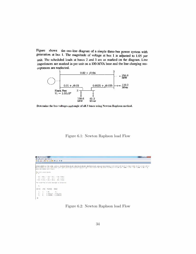
Figure 6.1: Newton Raphson load Flow
Figure 6.2: Newton Raphson load Flow
34
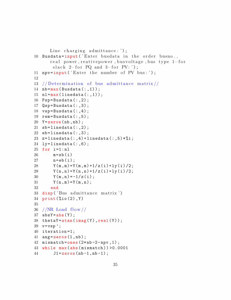
Line cha r g i n g admit tance : ’ );10 Busdata=input( ’ Enter busdata i n the o rd e r busno . ,
r e a l power , r e a t i v epowe r , bu svo l t ag e , bus type 1− f o rs l a c k 2− f o r PQ and 3− f o r PV: ’ );
11 npv=input( ’ Enter the number o f PV bus : ’ );12
13 // Dete rmina t i on o f bus admit tance matr ix //14 nb=max(Busdata (:,1));
15 nl=max(linedata (:,1));
16 Psp=Busdata (:,2);
17 Qsp=Busdata (:,3);
18 vsp=Busdata (:,4);
19 rem=Busdata (:,5);
20 Y=zeros(nb,nb);
21 sb=linedata (:,2);
22 eb=linedata (:,3);
23 z=linedata (:,4)+linedata (:,5)*%i;
24 ly=linedata (:,6);
25 for i=1:nl
26 m=sb(i)
27 n=eb(i);
28 Y(m,m)=Y(m,m)+1/z(i)+ly(i)/2;
29 Y(n,n)=Y(n,n)+1/z(i)+ly(i)/2;
30 Y(m,n)=-1/z(i);
31 Y(n,m)=Y(m,n);
32 end
33 disp( ’ Bus admit tance matr ix ’ )34 print(%io (2),Y)
35
36 //NR Load f l ow //37 absY=abs(Y);
38 thetaY=atan(imag(Y),real(Y));
39 v=vsp ’;
40 iteration =1;
41 ang=zeros(1,nb);
42 mismatch=ones (2*nb -2-npv ,1);
43 while max(abs(mismatch)) >0.0001
44 J1=zeros(nb -1,nb -1);
35

45 J2=zeros(nb -1,nb-npv -1);
46 J3=zeros(nb -npv -1,nb -1);
47 J4=zeros(nb -npv -1,nb-npv -1);
48 P=zeros(nb ,1);
49 Q=P;
50 del_P=Q;
51 del_Q=Q;
52 del_del=zeros(nb -1,1);
53 del_v=zeros(nb -1-npv ,1);
54 ang;
55 mag=abs(v);
56 for i=2:nb
57 for j=1:nb
58 P(i)=P(i)+mag(i)*mag(j)*absY(i,j)*cos(
thetaY(i,j)-ang(i)+ang(j));
59 if rem(i)~=3
60 Q(i)=Q(i)+mag(i)*mag(j)*absY(i,j)*
sin(thetaY(i,j)-ang(i)+ang(j));
61 end
62 end
63 end
64 Q=-1*Q;
65 del_P=Psp -P;
66 del_Q=Qsp -Q;
67 for i=2:nb
68 for j=2:nb
69 if j~=i
70 J1(i-1,j-1)=-mag(i)*mag(j)*absY(i,j)*sin
(thetaY(i,j)-ang(i)+ang(j));
71 J2(i-1,j-1)=mag(i)*absY(i,j)*cos(thetaY(
i,j)-ang(i)+ang(j));
72 J3(i-1,j-1)=-mag(i)*mag(j)*absY(i,j)*cos
(thetaY(i,j)-ang(i)+ang(j));
73 J4(i-1,j-1)=-mag(i)*absY(i,j)*sin(thetaY
(i,j)-ang(i)+ang(j));
74 end
75 end
76 end
36

77 for i=2:nb
78 for j=1:nb
79 if j~=i
80 J1(i-1,i-1)=J1(i-1,i-1)+mag(i)*mag(j)*
absY(i,j)*sin(thetaY(i,j)-ang(i)+ang(
j));
81 J2(i-1,i-1)=J2(i-1,i-1)+mag(j)*absY(i,j)
*cos(thetaY(i,j)-ang(i)+ang(j));
82 J3(i-1,i-1)=J3(i-1,i-1)+mag(i)*mag(j)*
absY(i,j)*cos(thetaY(i,j)-ang(i)+ang(
j));
83 J4(i-1,i-1)=J4(i-1,i-1)+mag(j)*absY(i,j)
*sin(thetaY(i,j)-ang(i)+ang(j));
84 end
85 end
86 J2(i-1,i-1) =2*mag(i)*absY(i,i)*cos(thetaY(i,i))+
J2(i-1,i-1);
87 J4(i-1,i-1)=-2*mag(i)*absY(i,i)*sin(thetaY(i,i))
-J4(i-1,i-1);
88 end
89 J=[J1 J2;J3 J4]
90 lenJ=length(J1);
91 i=2;
92 j=1;
93 while j<=lenJ
94 if rem(i)==2
95 j=j+1;
96 else
97 J(:,length(J1)+j)=[];
98 lenJ=lenJ -1;
99 end
100 end
101 i=i+1;
102 lenJ=length(J1);
103 i=1;
104 j=2;
105 while i<=lenJ
106 if rem(j)==2
37
107 i=i+1;
108 else
109 J(length(J1)+i,:) =[];
110 lenJ=lenJ -1;
111 Q(i+1)=[]
112 del_Q(i+1,:)=[]
113 end
114 // j=j +1;115 end
116 P(1,:)=[]
117 Q(1,:)=[]
118 del_P (1,:) =[];
119 del_Q (1,:) =[];
120 mismatch =[del_P;del_Q];
121 del=J\mismatch;
122 del_del=del(1:nb -1);
123 del_v=del(nb:length(del));
124 ang=ang(2:nb)+del_del ’;
125 j=1;
126 for i=2:nb
127 if rem(i)==2
128 v(i)=v(i)+del_v(j);
129 j=j+1;
130 end
131 end
132 mag=abs(v);
133 ang =[0 ang];
134 nbr =1:nb;
135 iteration=iteration +1;
136 end
137 disp(iteration -1, ’ The l oad f l ow s o l u t i o n cnve rged ati t e r a t i o n ’ )
138 disp( ’ bus no Type v o l t a g e ang l e ’ )139 disp([nbr ’ rem mag ’ ang ’])
140
141
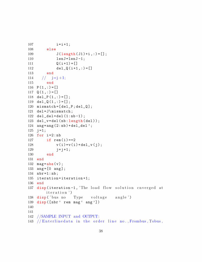
142 //SAMPLE INPUT and OUTPUT:143 // En t e r l i n e d a t a i n the o rd e r l i n e no . , Frombus , Tobus ,
38
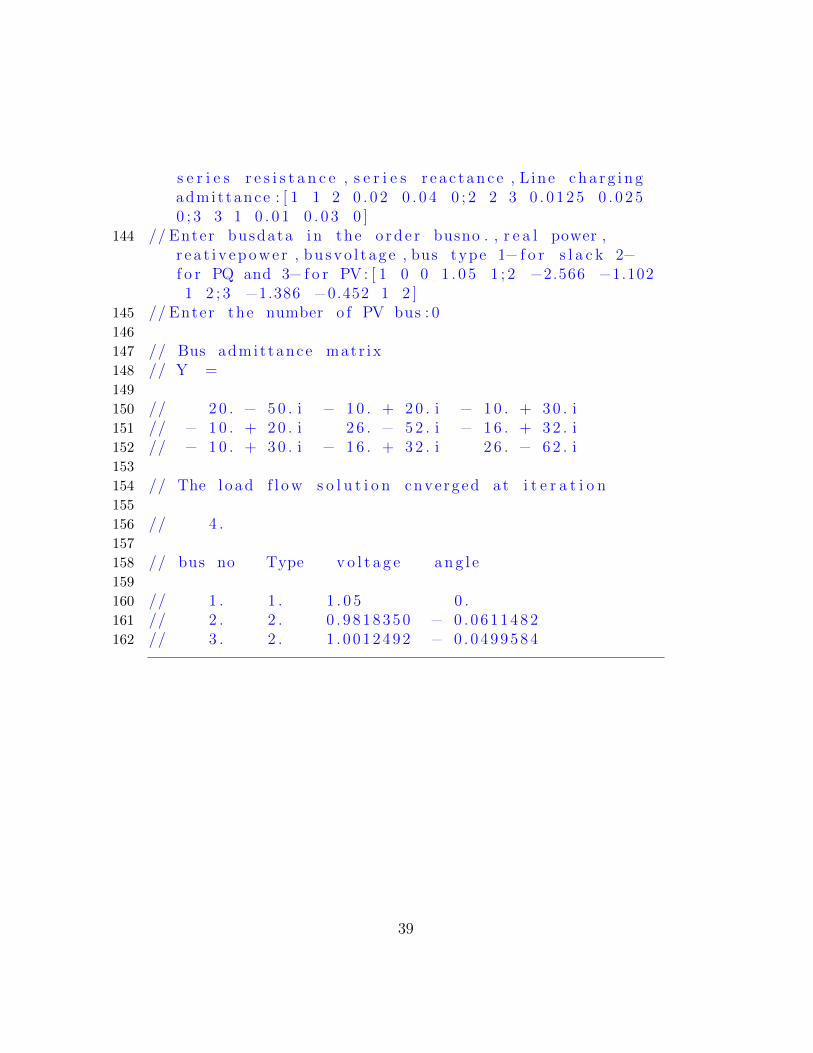
s e r i e s r e s i s t a n c e , s e r i e s r e a c t anc e , L ine cha r g i n gadmit tance : [ 1 1 2 0 . 0 2 0 . 0 4 0 ; 2 2 3 0 . 0 125 0 . 0 2 50 ; 3 3 1 0 . 0 1 0 . 0 3 0 ]
144 // Enter busdata i n the o rd e r busno . , r e a l power ,r e a t i v epowe r , bu svo l t ag e , bus type 1− f o r s l a c k 2−f o r PQ and 3− f o r PV : [ 1 0 0 1 . 0 5 1 ; 2 −2.566 −1.1021 2 ; 3 −1.386 −0.452 1 2 ]
145 // Enter the number o f PV bus : 0146
147 // Bus admit tance matr ix148 // Y =149
150 // 2 0 . − 5 0 . i − 1 0 . + 20 . i − 1 0 . + 30 . i151 // − 1 0 . + 20 . i 2 6 . − 5 2 . i − 1 6 . + 32 . i152 // − 1 0 . + 30 . i − 1 6 . + 32 . i 2 6 . − 6 2 . i153
154 // The l oad f l ow s o l u t i o n cnve rged at i t e r a t i o n155
156 // 4 .157
158 // bus no Type v o l t a g e ang l e159
160 // 1 . 1 . 1 . 0 5 0 .161 // 2 . 2 . 0 . 9 818350 − 0 . 0611482162 // 3 . 2 . 1 . 0 012492 − 0 . 0499584
39

Experiment: 7
Symmetrical Fault Analysis
Scilab code Solution 7.1 Symmetrical Fault Analysis
1 //Program to f i n d out f a u l t cu r r en t , post− f a u l tv o l t a g e s and l i n e f l ow o f a g i v en network //
2 // This program r e q u i r e s u s e r i nput . A sample problemwith u s e r i nput and output i s a v a i l a b l e i n the
r e s u l t f i l e s . Ques t i on i s a v a i l a b l e i n the f i l e ”Symmet r i c a lFau l tQue s t i o nF i l e . j pg ” and r e s u l t i sa v a i l a b l e i n the f i l e ” Symme t r i c a lF au l tRe s u l tF i l e. j pg ”//
3 // S c i l a b Ve r s i on 5 . 5 . 2 ; OS : Windows4 clc;
5 clear;
6 linedata=input( ’ e n t e r the l i n e data v a l u e s i n theo rd e r o f s t a r t i n g bus , nd ing bus , r e s i s t a n c e andr e a c t a n c e : ’ )
7 f=input( ’ e n t e r the bus at wich f a u l t o c c u r s : ’ )8 bv=input( ’ e n t e r the pre− f a u l t bus v o l t a g e : ’ )9 sb=linedata (:,1) // S t a r t i n g bus number o f a l l the
40
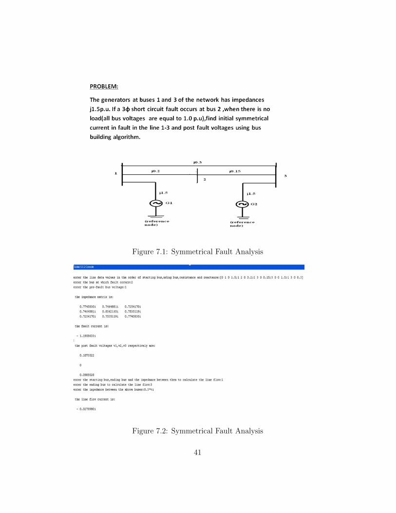
Figure 7.1: Symmetrical Fault Analysis
Figure 7.2: Symmetrical Fault Analysis
41

l i n e s s t o r e d i n v a r i a b l e sb //10 eb=linedata (:,2) // Ending bus number o f a l l the
l i n e s s t o r e d i n v a r i a b l e eb //11 z=linedata (:,3)+linedata (:,4)*%i // l i n e impedanc e=R+
jX //12 zbus =[];
13 check =[];
14 for i=1: length(sb) // s t a r t i n g o f impedance matr ixc a l c u l a t i o n pa r t //
15 m=sb(i);
16 n=eb(i);
17 mn=min(m,n);
18 nm=max(m,n);
19 ncheck=length(find(check==nm));
20 mcheck=length(find(check==mn));
21 [rows columns ]=size(zbus);
22 if mn==0 & ncheck ==0
23 zbus=[zbus zeros(rows ,1);zeros(1,rows) z(i)
];
24 check=[check nm];
25 else if mcheck >0 & ncheck ==0
26 zbus=[zbus zbus(:,mn);zbus(mn ,:) zbus(mn
,mn)+z(i)];
27 check=[check nm];
28 elseif mn==0 & ncheck >0
29 zbus=[zbus zbus(:,nm);zbus(nm ,:) zbus(nm
,nm)+z(i)];
30 zbusn=zeros(rows ,rows);
31 for r=1: rows
32 for t=1: columns
33 zbusn(r,t)=zbus(r,t)-(zbus(r,
rows +1)*zbus(rows+1,t))/(zbus
(rows+1,rows +1));
34 end
35 end
36 zbus=zbusn
37 elseif mcheck >0 & ncheck >0
38 zbus=[zbus zbus(:,nm)-zbus(:,mn);zbus(nm
42

,:)-zbus(mn ,:),z(i)+zbus(mn ,nm)+zbus(
nm ,nm) -2*zbus(nm ,mn)];
39 zbusn=zeros(rows ,rows);
40 for r=1: rows
41 for t=1: columns
42 zbusn(r,t)=zbus(r,t)-(zbus(r,rows
+1)*zbus(rows+1,t))/(zbus(rows
+1,rows +1));
43 end
44 end
45 zbus=zbusn;
46 end
47 end
48 end // end ing o f impedance bus matr ix c a l c u l a t i o npa r t //
49 disp(zbus , ’ the impedance matr ix i s : ’ );50 ifa=bv/zbus(f,f) // c a l c u l a t i o n o f f a u l t c u r r e n t //51 disp(ifa , ’ the f a u l t c u r r e n t i s : ’ )52 disp( ’ the po s t f a u l t v o l t a g e s v1 , v2 , v3 r e s p e c t i v e l y
a r e : ’ );53 for i=1:n
54 v(i)=bv -(ifa*zbus(i,f)); // c a l c u l a t i o n o f p o s t f a u l tbus v o l t a g e s //
55 disp(v(i));
56 end
57 a=input( ’ e n t e r the s t a r t i n g bus to c a l c u l a t e thel i n e f l ow : ’ );
58 b=input( ’ e n t e r the end ing bus to c a l c u l a t e the l i n ef l ow : ’ );
59 zs=input( ’ e n t e r the impedance between the abovebuse s : ’ );
60 i13=(v(a)-v(b))/zs; // c a l c u l a t i o n o f l i n e f l o w s //61 disp(i13 , ’ the l i n e f l ow cu r r e n t i s : ’ )62
63 //SAMPLE INPUT and OUTPUT:64 // e n t e r the l i n e data v a l u e s i n the o rd e r o f
s t a r t i n g bus , nd ing bus , r e s i s t a n c e and r e a c t a n c e: [ 0 1 0 1 . 5 ; 1 2 0 0 . 2 ; 2 3 0 0 . 1 5 ; 3 0 0 1 . 5 ; 1 3 0
43

0 . 3 ]65 // e n t e r the bus at wich f a u l t o c c u r s : 266 // e n t e r the pre− f a u l t bus v o l t a g e : 167
68 // the impedance matr ix i s :69
70 // 0 . 7745830 i 0 . 7 464881 i 0 . 7 254170 i71 // 0 . 7464881 i 0 . 8 362160 i 0 . 7 535119 i72 // 0 . 7254170 i 0 . 7 535119 i 0 . 7 745830 i73
74 // the f a u l t c u r r e n t i s :75
76 // − 1 . 1958633 i77
78 // the po s t f a u l t v o l t a g e s v1 , v2 , v3 r e s p e c t i v e l y a r e:
79
80 // 0 . 107302281
82 // 083
84 // 0 . 098902885 // e n t e r the s t a r t i n g bus to c a l c u l a t e the l i n e f l ow
: 186 // e n t e r the end ing bus to c a l c u l a t e the l i n e f l ow : 387 // e n t e r the impedance between the above buse s : 0 . 3 ∗ %i88
89 // the l i n e f l ow cu r r e n t i s :90
91 // − 0 . 0279980 i
44
Experiment: 8
Unsymmetrical Fault Analysis
Scilab code Solution 8.1 Unsymmetrical Fault Analysis
1
2 //Program to f i n d out unsymmetr i ca l f a u l t c u r r e n t //3 // This program r e q u i r e s u s e r i nput . A sample problem
with u s e r i nput and output i s a v a i l a b l e i n ther e s u l t f i l e . Ques t i on i s a v a i l a b l e i n the f i l e ”Unsymmet r i c a lFau l tQue s t i onF i l e . j pg ” and r e s u l t i sa v a i l a b l e i n the f i l e ”
Un symmet r i c a lFau l tRe su l tF i l e . j pg ”//4 // S c i l a b Ve r s i on 5 . 5 . 2 ; OS : Windows5 clc ;
6 clear;
7 a=input( ’ Enter the p o s i t v e sequence , n e g a t i v es equence and z e r o s equence o f f i r s t g e n e r a t o r i nmatr ix form : ’ )
8 PG1=a(:,1);// p o s i t i v e s equence o f g e n e r a t o r 1 i ss t o r e d i n the v a r i a b l e PG1
9 NG1=a(:,2);// n e g a t i v e s equence o f g e n e r a t o r 1 i ss t o r e d i n the v a r i a b l e NG1
10 ZG1=a(:,3);// n e g a t i v e s equence o f g e n e r a t o r 1 i ss t o r e d i n the v a r i a b l e ZG1
11 b=input( ’ Enter the p o s i t v e sequence , n e g a t i v e
45

s equence and z e r o s equence o f f i r s t t r a n s f o rme ri n matr ix form : ’ )
12 PT1=b(:,1);// p o s i t i v e s equence o f t r a n s f o rme r 1 i ss t o r e d i n the v a r i a b l e PT1
13 NT1=b(:,2);// p o s i t i v e s equence o f t r a n s f o rme r 1 i ss t o r e d i n the v a r i a b l e NT1
14 ZT1=b(:,3);// p o s i t i v e s equence o f t r a n s f o rme r 1 i ss t o r e d i n the v a r i a b l e ZT1
15 c=input( ’ Enter the p o s i t v e sequence , n e g a t i v es equence and z e r o s equence o f f i r s t t r a n sm i s s i o nl i n e i n matr ix form : ’ )
16 PTL=c(:,1);// p o s i t i v e s equence o f t r a n sm i s s i o n l i n e1 i s s t o r e d i n the v a r i a b l e PTL
17 NTL=c(:,2);// p o s i t i v e s equence o f t r a n sm i s s i o n l i n e1 i s s t o r e d i n the v a r i a b l e NTL
18 ZTL=c(:,3);// p o s i t i v e s equence o f t r a n sm i s s i o n l i n e1 i s s t o r e d i n the v a r i a b l e ZTL
19 d=input( ’ Enter the p o s i t v e sequence , n e g a t i v es equence and z e r o s equence o f s econd t r a n s f o rme ri n matr ix form : ’ )
20 PT2=d(:,1);// p o s i t i v e s equence o f t r a n s f o rme r i ss t o r e d i n the v a r i a b l e PT2
21 NT2=d(:,2);// p o s i t i v e s equence o f t r a n s f o rme r 1 i ss t o r e d i n the v a r i a b l e NT2
22 ZT2=d(:,3);// p o s i t i v e s equence o f t r a n s f o rme r 1 i ss t o r e d i n the v a r i a b l e ZT2
23 e=input( ’ Enter the p o s i t i v e sequence , n e g a t i v es equence and z e r o s equence o f s econd g e n e r a t o r i nmatr ix form : ’ )
24 PG2=e(:,1);// p o s i t i v e s equence o f t r a n s f o rme r 1 i ss t o r e d i n the v a r i a b l e PG2
25 NG2=e(:,2);// p o s i t i v e s equence o f t r a n s f o rme r 1 i ss t o r e d i n the v a r i a b l e NG2
26 ZG2=e(:,3);// p o s i t i v e s equence o f t r a n s f o rme r 1 i ss t o r e d i n the v a r i a b l e ZG2
27 MVAB=input( ’ Enter the va l u e o f base MVA: ’ );28 KVB=input( ’ Enter the va lu e o f base KV: ’ );29 z1=((PG1*%i+PT1*%i)*(PTL*%i+PT2*%i+PG2*%i))/((PG1*%i
46
+PT1*%i)+(PTL*%i+PT2*%i+PG2*%i));// c a l c u l a t i o n o fp o s i t i v e impedence
30 z2=((NG1*%i+NT1*%i)*(NTL*%i+NT2*%i+NG2*%i))/((NG1*%i
+NT1*%i)+(NTL*%i+NT2*%i+NG2*%i));// c a l c u l a t i o n o fn e g a t i v e impedence
31 z0=((ZG1*%i+ZT1*%i)*(ZTL*%i+ZT2*%i+ZG2*%i))/((ZG1*%i
+ZT1*%i)+(ZTL*%i+ZT2*%i+ZG2*%i));// c a l c u l a t i o n o fz e r o impedence
32 Ib=(MVAB *(10^6))/((1.732* KVB *(10^3)))// c a l c u l a t i n gbase c u r r e n t
33 disp(z0,z2,z1 , ’ the v a l u e s o f p o s i t i v e ( z1 ) n e g a t i v e (z2 ) , z e r o ( z0 ) s equence impedance r e s p e c t i v e l y a r e’ );
34 disp( ’OPTION ’ , ’LG FAULT=1 ’ , ’LL FAULT=2 ’ , ’LLG FAULT=3’ );
35 MENU=input( ’ Enter the c h o i c e o f f a u l t : ’ )36 if MENU ==1 // c a l c u l a t i n g Line to Ground f a u l t37 If =(3*(1))/(z0+z1+z2)
38 FAULTCURRENT=If*Ib;
39 disp(FAULTCURRENT , ’ The f a u l t c u r r e n t i s : ’ );40 end
41 if MENU ==2 // Ca l c u l a t i n g Line to L ine Fau l t42 If=(( -1.732j)*(1))/(z1+z2)
43 FAULTCURRENT=If*Ib;
44 disp(FAULTCURRENT , ’ The f a u l t c u r r e n t i s : ’ );45 end
46 if MENU ==3 // c a l c u l a t i n g Line−Line−Ground f a u l t47 z=(z0*z2)/(z0+z2);
48 Ia1 =(1)/(z1+z);
49 Ia0 =(( -1+( Ia1*z1))/z0);
50 If=3*Ia0;
51 FAULTCURRENT=If*Ib;
52 disp(FAULTCURRENT , ’ The f a u l t c u r r e n t i s : ’ );53 end
54
55 //SAMPLE INPUT and OUTPUT56
57 // Enter the p o s i t v e sequence , n e g a t i v e s equence and
47

z e r o s equence o f f i r s t g e n e r a t o r i n matr ix form: [ 0 . 3 2 0 . 2 6 0 . 0 9 ]
58 // Enter the p o s i t v e sequence , n e g a t i v e s equence andz e r o s equence o f f i r s t t r a n s f o rme r i n matr ix form: [ 0 . 2 3 0 . 2 3 0 . 2 3 ]
59 // Enter the p o s i t v e sequence , n e g a t i v e s equence andz e r o s equence o f f i r s t t r a n sm i s s i o n l i n e i nmatr ix form : [ 0 . 5 6 0 . 5 6 0 . 0 9 ]
60 // Enter the p o s i t v e sequence , n e g a t i v e s equence andz e r o s equence o f s econd t r a n s f o rme r i n matr ixform : [ 0 . 1 6 0 . 1 6 0 . 1 6 ]
61 // Enter the p o s i t i v e sequence , n e g a t i v e s equence andz e r o s equence o f s econd g e n e r a t o r i n matr ix form: [ 0 . 3 8 0 . 2 4 0 . 1 5 ]
62 // Enter the va lu e o f base MVA:10063 // Enter the va lu e o f base KV: 1 1064
65 // the v a l u e s o f p o s i t i v e ( z1 ) n e g a t i v e ( z2 ) , z e r o ( z0 )s equence impedance r e s p e c t i v e l
66 // y a r e67
68 // 0 . 3666667 i69
70 // 0 . 3244138 i71
72 // 0 . 1777778 i73
74 // LLG FAULT=375
76 // LL FAULT=277
78 // LG FAULT=179
80 // OPTION81 // Enter the c h o i c e o f f a u l t : 382
83 // The f a u l t c u r r e n t i s :84
48

Figure 8.1: Unsymmetrical Fault Analysis
85 // 2112 . 5397 i
49
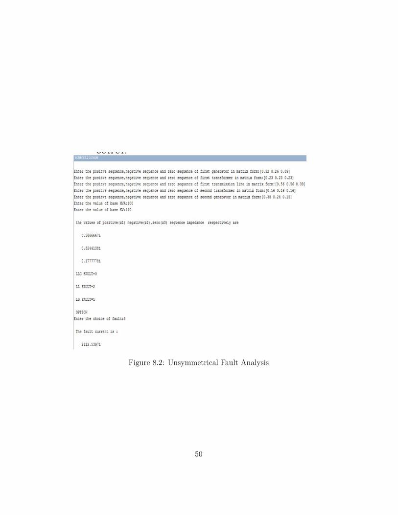
Figure 8.2: Unsymmetrical Fault Analysis
50
Experiment: 9
Small Signal and transientStability Analysis ofSingle-machine Infinite bussystem
Scilab code Solution 9.1 SMIB Stability Analysis
1 //Program to f i n d out t r a n s i e n t s t a b i l i t y a n a l y s i so f s i n g l e machine − i n f i n i t e bus system //
2 //An example problem and output s a r e a v a i l a b l e i nf i l e s ’ r e s u l t 1 ’ and ’ r e s u l t 2 ’
3 // S c i l a b Ve r s i on 5 . 5 . 2 ; OS : Windows4
5 clc;
6 clear;
7
8 xd=0.3;
9
51

Figure 9.1: SMIB Stability Analysis
52

Figure 9.2: SMIB Stability Analysis
53

10 theta=acos (0.8); //Power f a c t o r ang l e
11
12 S=(0.5/0.8)*cos(theta)+%i*sin(theta); //Apparant Power
13 V=1; //P r e f a u l t v l t a g e i s assumed to be 1 pu
14 Ia=(conj(S)/V); //P e f a u l t s t e ady s t a t e c u r r e n t
15
16 E=V+(%i*xd)*(Ia); //Vo l tage beh ind t r a n s i e n t r e a c t a n c e
17
18 disp(E, ’ The v o l t a g e beh ind t r a n s i e n t r e a c t a n c e i n pui s ’ )
19
20 //To f i n d the power ang l e curve21
22 delta =0:0.001: %pi;
23 P=((E*V)/xd)*(sin(delta));
24
25 plot(delta ,P)
26 xlabel( ’ d e l t a i n r a d i a n s ’ )27 ylabel( ’ Power i n pu ’ )28 title( ’ Power ang l e cu rve ’ )
54

Experiment: 10
Small Signal and transientStability Analysis of Multimachine Power Systems
Scilab code Solution 10.1 Multimachine Stability Analysis
1 //Program to f i n d out t r a n s i e n t s t a b i l i t y a n a l y s i so f mu l t i machine at the end o f the i t e r a t i o n //
2 // This program r e q u i r e s u s e r i nput . A sample problemwith u s e r i nput and output i s a v a i l a b l e i n the
r e s u l t f i l e //3 // S c i l a b Ve r s i on 5 . 5 . 2 ; OS : Windows4 // program f o r t r a n s i e n t s t a b i l i t y a n a l y s i s o f mu l t i
machine //5 clc;
6 clc;
7 clear;
8 f=input( ’ e n t e r the f r e qu en cy : ’ );9 bv=input( ’ e n t e r the base va lu e i n MVA: ’ );10 v=input( ’ e n t e r the va l u e o f bus v o l t a g e i n p . u : ’ );11 e=input( ’ e n t e r the va l u e o f t r a n s i e n t r e a c t a n c e
v o l t a g e i n pu : ’ );12 ld=input( ’ e n t e r the t o t a l l o ad : ’ );
55

13 x1=input( ’ e n t e r the p r e f a u l t r e a c t a n c e i n p . u : ’ );14 x2=input( ’ e n t e r the po s t f a u l t r e a c t a n c e va lu e : ’ );15 x3=input( ’ e n t e r dur ing the f a u l t r e a c t a n c e va lu e : ’ );16 delt=input( ’ e n t e r the t ime i n t e r v a l i n s e c ond s : ’ );17 H=input( ’ e n t e r the i n e r t i a c on s t an t : ’ );18 pe1=ld/bv;
19
20 pe2 =0;
21 delnot=asin((pe1*x1)/(e*v));
22
23 omeganot =2*3.14*f;
24
25
26 ddel=omeganot -(2*3.14*f);
27
28 ddelomega =(((3.14*f)*(pe1 -pe2))/H);
29
30 // end o f f i r s t s t e p at t =0.05 s e c31 del1=( delnot +(ddel*delt));// p r e d i c t e d v a l u e s32
33 delomega1=ddel+( ddelomega*delt);
34
35 // d e r i v a t i o n at the end o f t =0.05 s e c36 ddel1=ddel+( ddelomega*delt);
37
38 ddelomega =(((3.14*f)*(pe1 -pe2))/H);
39
40 delc1=delnot +(( delt /2)*(ddel+ddel1));
41
42 delomegac1=ddel +(( delt /2)*( ddelomega+ddelomega));
43
44 ddelc1=ddel +(( delt /2)*( ddelomega+ddelomega));
45
46 ddelomegac =(((3.14*f)*(pe1 -pe2))/H);
47
48 delp2=delc1+ddelc1*delt;
49
50 delomegap2 =( delomegac1 +( ddelomega*delt));
56
51
52 ddelomegap =(((3.14*f)*(pe1 -pe2))/H);
53
54
55 delc2=delc1 +(delt /2*( ddelc1+delomegap2));
56
57 delomegac =( delomegac1 +( ddelomega*delt));
58
59 ddelc2 =( delomegac1 +( ddelomega*delt));
60
61 ddelomegac2 =(((3.14*f)*(pe1 -pe2))/H);
62
63 delp3=delc2+delomegac*delt;
64
65 delomega3=delomegac+ddelomegac2*delt;
66
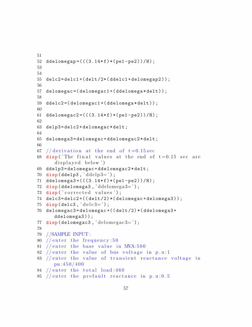
67 // d e r i v a t i o n at the end o f t =0.15 s e c68 disp( ’ The f i n a l v a l u e s at the end o f t =0.15 s e c a r e
d i s p l a y e d below ’ )69 ddelp3=delomegac+ddelomegac2*delt;
70 disp(ddelp3 , ’ dde lp3= ’ );71 ddelomega3 =(((3.14*f)*(pe1 -pe2))/H);
72 disp(ddelomega3 , ’ ddelomega3= ’ );73 disp( ’ c o r r e c t e d v a l u e s ’ );74 delc3=delc2 +(( delt /2)*( delomegac+delomega3));
75 disp(delc3 , ’ d e l c 3= ’ );76 delomegac3=delomegac +(( delt /2)*( ddelomega3+
ddelomega3));
77 disp(delomegac3 , ’ de lomegac3= ’ );78
79 //SAMPLE INPUT :80 // e n t e r the f r e qu en cy : 5 081 // e n t e r the base va lu e i n MVA:50082 // e n t e r the va lu e o f bus v o l t a g e i n p . u : 183 // e n t e r the va lu e o f t r a n s i e n t r e a c t a n c e v o l t a g e i n
pu : 450/40084 // e n t e r the t o t a l l o ad : 4 6 085 // e n t e r the p r e f a u l t r e a c t a n c e i n p . u : 0 . 5
57

86 // e n t e r the po s t f a u l t r e a c t a n c e va l u e : 0 . 7 587 // e n t e r dur ing the f a u l t r e a c t a n c e va lu e : 188 // e n t e r the t ime i n t e r v a l i n s e c ond s : 0 . 0 589 // e n t e r the i n e r t i a c on s t an t : 2 . 590
91
92 //OUTPUT93 // The f i n a l v a l u e s at the end o f t =0.15 s e c a r e
d i s p l a y e d below94
95 // dde lp3=96
97 // 8 . 6 66498
99 // ddelomega3=100
101 // 57 . 7 76102
103 // c o r r e c t e d v a l u e s104
105 // d e l c 3=106
107 // 1 . 0712162108
109 // de lomegac3=110
111 // 8 . 6 664
58
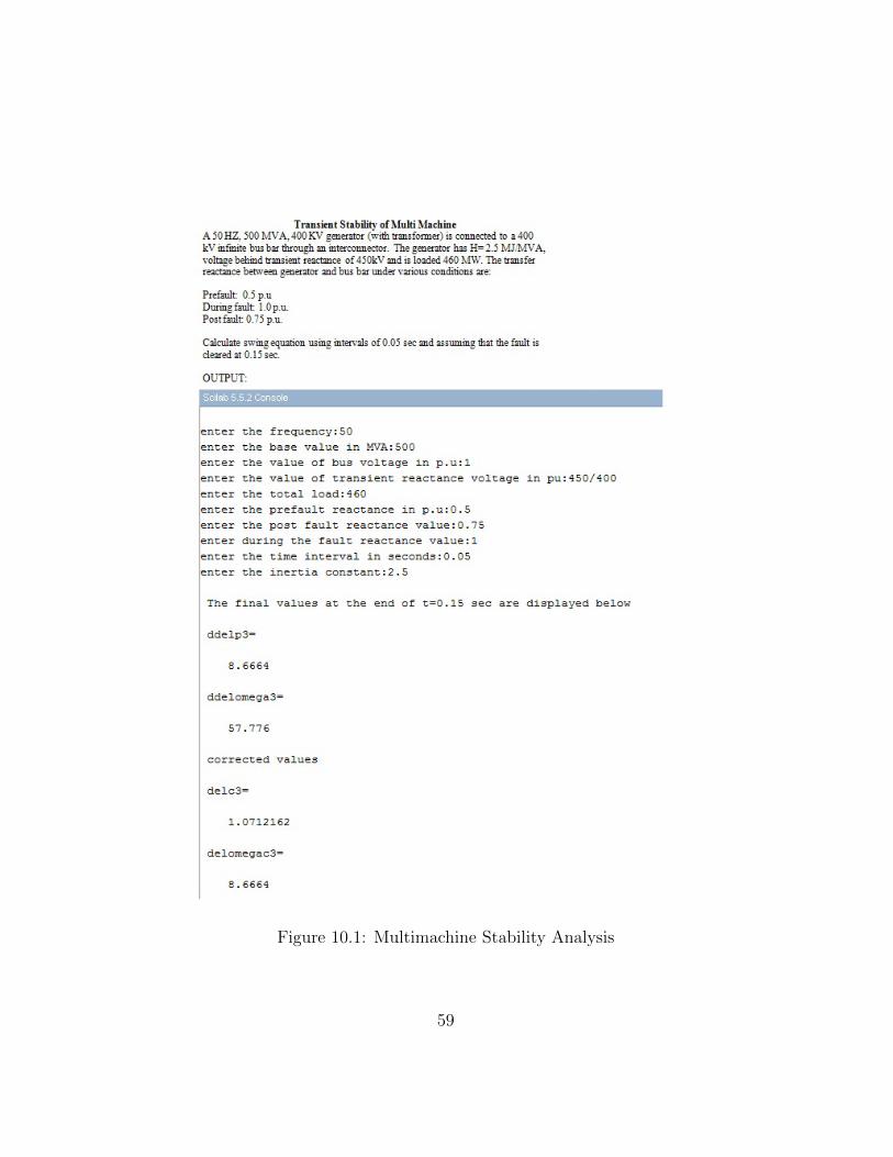
Figure 10.1: Multimachine Stability Analysis
59

Experiment: 11
Electromagnetic Transients inPower Systems
This code can be downloaded from the website wwww.scilab.in
60
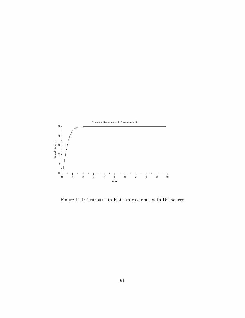
Figure 11.1: Transient in RLC series circuit with DC source
61

Experiment: 12
Load frequency dynamics ofsingle Area Power Systems
This code can be downloaded from the website wwww.scilab.in
62

Figure 12.1: Single Area Control
63

Experiment: 13
Load frequency dynamics oftwo Area Power Systems
This code can be downloaded from the website wwww.scilab.in
64

Figure 13.1: Two Area Control
65

Experiment: 14
Economic dispatch in powersystems neglecting losses
Scilab code Solution 14.1 Economic Load Dispatch Excluding Losses
1 //Program to f i n d out Economic l oad d i s p a t c hn e g l e c t i n g l o s s e s //
2 // This program r e q u i r e s u s e r i nput . A sample problemwith u s e r i nput and output i s a v a i l a b l e i n the
r e s u l t f i l e //3 // Ques t i on and r e s u l t o f example problem i s
a v a i l a b l e i n f i l e ” EDwithoutLoss . j pg ”4 // S c i l a b Ve r s i on 5 . 5 . 2 ; OS : Windows5
6 clear;
7 clc;
8 n=input( ’ Enter no . o f u n i t s : ’ );9 F=input( ’ Enter the c o s t c o e f f i c i e n t i n matr ix form :
’ );10 constraint=input( ’ Enter min and max va l u e s o f P f o r
a l l u n i t s : ’ );11 pd=input( ’ Enter t o t a l demand : ’ );
66

Figure 14.1: Economic Load Dispatch Excluding Losses
12 a=F(:,1);b=F(:,2);c=F(:,3);
13 Pmin=constraint (:,1);
14 Pmax=constraint (:,2);
15 chk=zeros(n,1);
16 rem =1;
17 while rem==1
18 sx=0;sy=0;
19 for i=1:n
20 if i~=chk(i)
21 sx=sx+b(i)/(2*a(i));
22 sy=sy +1/(2*a(i));
23 end
24 end
25 lamda=(pd+sx)/sy;
26 sch =0;
27 for i=1:n
28 if i~=chk(i)
29 P(i)=(lamda -b(i))/(2*a(i));
30 if P(i)<Pmin(i)|P(i)>Pmax(i)
31 if P(i)< Pmin(i)
32 P(i)=Pmin(i);
67
33 else
34 P(i)=Pmax(i);
35 end
36 pd=pd-P(i);
37 chk(i)=i;
38 sch=sch+1;
39 end
40 end
41 if sch ==0
42 rem =0;
43 else
44 rem =1;
45 end
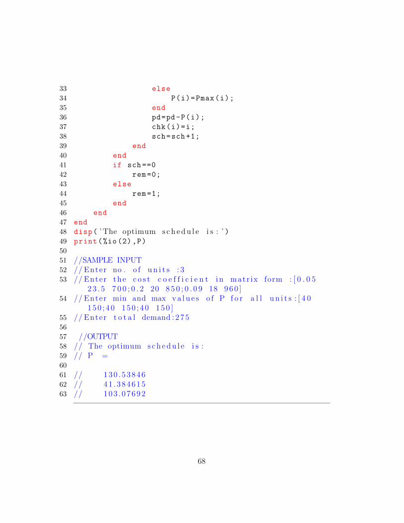
46 end
47 end
48 disp( ’ The optimum s ch edu l e i s : ’ )49 print(%io (2),P)
50
51 //SAMPLE INPUT52 // Enter no . o f u n i t s : 353 // Enter the c o s t c o e f f i c i e n t i n matr ix form : [ 0 . 0 5
2 3 . 5 7 0 0 ; 0 . 2 20 8 5 0 ; 0 . 0 9 18 960 ]54 // Enter min and max va l u e s o f P f o r a l l u n i t s : [ 4 0
150 ; 4 0 150 ; 4 0 1 5 0 ]55 // Enter t o t a l demand : 2 7 556
57 //OUTPUT58 // The optimum s ch edu l e i s :59 // P =60
61 // 130 . 5384662 // 41 . 38461563 // 103 . 07692
68
Experiment: 15
Economic dispatch in powersystems Including losses
Scilab code Solution 15.1 Economic Load Dispatch Including Losses
1 //Program f o r Economic Load Di spatch problemi n c l u d i n g l o s s c o e f f i c i e n t s //
2 // This program r e q u i r e s u s e r i nput . A sample problemwith u s e r i nput and output i s a v a i l a b l e i n the
r e s u l t f i l e named ”EDwithLoss . j pg ”//3 // S c i l a b Ve r s i on 5 . 5 . 2 ; OS : Windows4 clear;
5 clc;
6 n=input( ’ Enter no . o f u n i t s : ’ );7 B=input( ’ Enter the l o s s c o e f f i c i e n t i n matr ix form :
’ );8 a=B(:,1);// l o s s c o e f f i c i e n t s s t o r e d i n v a r i a b l e a9 b=B(:,2);// l o s s c o e f f i c i e n t s s t o r e d i n v a r i a b l e b
10 c=B(:,3);// l o s s c o e f f i c i e n t s s t o r e d i n v a r i a b l e c11 pg=input( ’ Enter the power o f the u n i t s i n matr ix
form in p . u : ’ );12 bv=input( ’ Enter the base va lu e ’ );
69

Figure 15.1: Economic Load Dispatch Including Losses
70

13 pl=0;
14 for i=1:n// c a l c u l a t i o n o f power l o s s15 for j=1:n
16 pl=pl+pg(j)*B(i,j)*pg(i);
17 end
18 end
19 disp(pl, ’ The t r a n sm i s s i o n power l o s s i n pu i s ’ ,);20 ITL=zeros(n,1);// Ca l c u l a t i o n o f i n c r emen t a l
t r a n sm i s s i o n l o s s21 for i=1:n
22 for j=1:n
23 ITL(i)=ITL(i)+2*B(i,j)*pg(j);
24
25 end
26 end
27 disp(ITL , ’ The i n c r emen t a l l o s s e s i n pu a r e ’ );28
29 //SAMPLE INPUT :30
31 // Enter no . o f u n i t s : 332 // Enter the l o s s c o e f f i c i e n t i n matr ix form : [ 0 . 0 1
−0.0003 −0.0002; −0.0003 0 . 0 025 −0.0005; −0.0002−0.0005 0 . 0 0 3 1 ]
33 // Enter the power o f the u n i t s i n matr ix form in p . u: [ 5 0 / 2 0 0 100/200 200/200 ]
34 // Enter the base va lu e20035
36 //OUTPUT37 //The t r a n sm i s s i o n power l o s s i n pu i s38
39 // 0 . 00367540
41 // The i n c r emen t a l l o s s e s i n pu a r e42
43 // 0 . 0 04344 // 0 . 0 013545 // 0 . 0 056
71