scilab textbook companion for mechanical vibration by g. k
TRANSCRIPT
Scilab Textbook Companion forMechanical Vibrationby G. K. Grover1
Created byVishwas Anand
B.EMechanical Engineering
B.M.S.COLLEGE OF ENGINEERINGCollege Teacher
NoneCross-Checked by
Reshma
July 30, 2019
1Funded by a grant from the National Mission on Education through ICT,http://spoken-tutorial.org/NMEICT-Intro. This Textbook Companion and Scilabcodes written in it can be downloaded from the ”Textbook Companion Project”section at the website http://scilab.in
Book Description
Title: Mechanical Vibration
Author: G. K. Grover
Publisher: Nem Chand And Bross, Roorkee .
Edition: 8
Year: 2009
ISBN: 9788185240565
1

Scilab numbering policy used in this document and the relation to theabove book.
Exa Example (Solved example)
Eqn Equation (Particular equation of the above book)
AP Appendix to Example(Scilab Code that is an Appednix to a particularExample of the above book)
For example, Exa 3.51 means solved example 3.51 of this book. Sec 2.3 meansa scilab code whose theory is explained in Section 2.3 of the book.
2
Contents
List of Scilab Codes 4
1 Fundamental of vibration 5
2 Undamped free vibrations of single degree of freedom sys-tem 13
3 Damped free vibrations of single degree of freedom system 17
4 Forced vibrations of single degree of freedom system 24
5 Two degrees of freedom systems 39
6 Multi degree of freedom systems exact analysis 45
7 Multi degree of freedom systems numerical methods 47
8 Critical speeds of shafts 52
3

List of Scilab Codes
Exa 1.4.2 sum of two harmonic motion . . . . . . . . . 5Exa 1.5.1 max and min amplitude of combined motion 6Exa 1.6.1 complex number in exponential form . . . . 7Exa 1.6.2 complex number in rectangular form . . . . 8Exa 1.7.1 work done by a force on displacement . . . . 9Exa 1.8.2 fourier components of periodic motion . . . 9Exa 2.3.4 moment of inertia of flywheel . . . . . . . . 13Exa 2.4.1 natural frequency of torsional pendulum . . 14Exa 2.5.1 mass in a spring mass system . . . . . . . . 15Exa 2.5.2 natural frequency of torsional oscillation . . 15Exa 3.3.2 undamped and damped natural frequencies of
system . . . . . . . . . . . . . . . . . . . . . 17Exa 3.3.3 gun barrel recoilling . . . . . . . . . . . . . 18Exa 3.4.1 disc of torsional pendulum . . . . . . . . . . 19Exa 3.6.1 spring mass system with coulomb damping . 20Exa 3.6.2 vertical spring mass system . . . . . . . . . 21Exa 3.7.1 time taken for complete damping . . . . . . 22Exa 4.2.1 periodic torque on suspended flywheel . . . 24Exa 4.2.2 damping factor and natural frequency of sys-
tem . . . . . . . . . . . . . . . . . . . . . . 25Exa 4.3.1 system of beams supporting a motor . . . . 26Exa 4.3.2 single cylinder vertical petrol engine . . . . 27Exa 4.4.1 mass hung from end of vertical spring . . . . 27Exa 4.4.2 support of spring mass system . . . . . . . . 28Exa 4.4.3 spring of automobile trailer . . . . . . . . . 29Exa 4.5.1 power required to vibrate spring mass dashpot 30Exa 4.6.1 horizontal spring mass system in dry friction 31Exa 4.10.1 machine mounted on 4 identical springs . . . 31
4
Exa 4.10.2 machine mounted on springs . . . . . . . . . 33Exa 4.10.3 radio set isolated from machine . . . . . . . 34Exa 4.11.1 vibrotometer . . . . . . . . . . . . . . . . . 35Exa 4.11.2 commercial type vibration pick up . . . . . 35Exa 4.11.3 device used to measure torsional accerelartion 37Exa 4.11.4 Frahm tachometer . . . . . . . . . . . . . . 37Exa 5.3.2 uniform rods pivoted at their upper ends . . 39Exa 5.3.3 shaft with 2 circular discs at the end . . . . 40Exa 5.7.1 torque applied to a torsional system . . . . . 41Exa 5.7.2 section of pipe in a machine . . . . . . . . . 42Exa 6.8.2 system with rolling masses . . . . . . . . . . 45Exa 7.2.1 fundamental frequency by rayleigh method . 47Exa 7.3.1 Dunkerly method . . . . . . . . . . . . . . . 48Exa 7.4.1 Stodola method . . . . . . . . . . . . . . . . 49Exa 7.7.2 four rotor system . . . . . . . . . . . . . . . 50Exa 8.2.1 rotor mounted midway on shaft . . . . . . . 52Exa 8.3.1 disc mounted midway between bearings . . . 53Exa 8.4.1 two critical speeds . . . . . . . . . . . . . . 54Exa 8.6.1 right cantilever steel shaft with rotor at the
end . . . . . . . . . . . . . . . . . . . . . . . 55
5

Chapter 1
Fundamental of vibration
Scilab code Exa 1.4.2 sum of two harmonic motion
1 clc
2 clear
3 mprintf( ’ Mechan ica l v i b r a t i o n s by G.K. Grover \nExample 1 . 4 . 2 \ n ’ )
4 // g i v e n data5 // c a s e 16 // x1 =(1/2) ∗ co s ( ( %pi /2) ∗ t ) . . . x1=a∗ co s (W1∗ t )7 // x2=s i n ( %pi∗ t ) . . . x2=b∗ s i n (W2∗ t )8 // c a l c u l a t i o n s9 W1=(%pi/2)
10 W2=%pi
11 t1=2*%pi/(W1)
12 t2=2*%pi/(W2)
13 p1=[t1 t2]
14 T1=lcm(p1)
15 // c a s e 216 // x1=2∗ co s ( ( %pi∗ t ) . . . x1=a∗ co s (W3∗ t )17 // x2=2∗ co s (2∗ t ) . . . x2=a∗ co s (W4∗ t )18 W3=%pi
19 W4=2
20 t3=2*%pi/(W3)
6

21 t4=2*%pi/(W4)
22 p2=[t3 t4]
23 T2=lcm(p2)
24 // output25 mprintf( ’ Case ( i ) \nTime p e r i o d o f f i r s t wave i s %f
s e c \nTime p e r i o d o f f i r s t wave i s %f s e c \nThet ime p e r i o d o f combined wave i s %f s e c \nCase ( i i ) \nTime p e r i o d o f f i r s t wave i s %f s e c \nTime p e r i o d
o f f i r s t wave i s %f s e c \nThe t ime p e r i o d o fcombined wave i s %f s e c ’ ,t1 ,t2,T1,t3 ,t4,T2)
26 mprintf( ’ \nNOTE: The t ime p e r i o d o f combined motioni n c a s e ( i i ) cannot be c a l c u l a t e d \n s i n c e p i i s anon−t e r m i n a t i n g and non r e c u r r i n g number . \ n But
SCILAB t a k e s the v a l u e o f p i to be 3 . 1 4 1 5 9 3 andt h e r e f o r e \n c a l c u l a t e s the LCM o f p i and the t ime
p e r i o d o f f i r s t wave i n c a s e ( i i . ’ )
Scilab code Exa 1.5.1 max and min amplitude of combined motion
1 clc
2 clear
3 mprintf( ’ Mechan ica l v i b r a t i o n s by G.K. Grover \nExample 1 . 5 . 1 \ n ’ )
4 // g i v e n data5 // x1=a∗ s i n (W1∗ t )6 // x2=b∗ s i n (W2∗ t )7 // c a l c u l a t i o n s8 a=1.90 // ampl i tude o f f i r s t wave i n cm9 b=2.00 // ampl i tude o f s econd wave i n cm10 W1=9.5 // f r e q u e n c y o f f i r s t wave i n rad / s e c11 W2=10.0 // f r e q u e n c y o f s econd wave i n rad / s e c12 xmax=b+a//maximum ampl i tude o f motion i n cms13 xmin=abs(a-b)//minimum ampl i tude o f motion i n cms14 f=abs(W1-W2)/(2* %pi)// beat f r e q u e n c y i n Hz15 t=1/f// t ime p e r i o d o f beat i n s e c
7

16 // output17 mprintf( ’ The maximum ampl i tude o f motion i s %4 . 4 f
cms\nThe minimum ampl i tude o f motion i s %4 . 4 f cms\n The beat f r e q u e n c y i s %4 . 4 f Hz\n the t imep e r i o d i s %4 . 4 f s e c ’ ,xmax ,xmin ,f,t)
Scilab code Exa 1.6.1 complex number in exponential form
1 clc
2 clear
3 mprintf( ’ Mechan ica l v i b r a t i o n s by G.K. Grover \nExample 1 . 6 . 1 \ n ’ )
4 // g i v e n data5 // c a s e 16 // a complex number i s r e p r e s e n t e d as Z=X+j ∗Y where j
i s imag ina ry7 //V=3 +j ∗78 x1=3
9 y1=7
10 // c a l c u l a t i o n s11 r1=sqrt(x1^2+y1^2)
12 if (y1/x1)>0 then theta1=atan(y1/x1)
13 else theta1=%pi -atan(abs(y1/x1))
14 end
15 theta1=atan(y1/x1)
16 // c a s e 217 //V=−5 +j ∗418 x2=-5
19 y2=4
20 // c a l c u l a t i o n s21 r2=sqrt(x2^2+y2^2)
22 if (y2/x2)>0 then theta1=atan(y2/x2)
23 else theta2=%pi -atan(abs(y2/x2))
24 end
25 // output
8
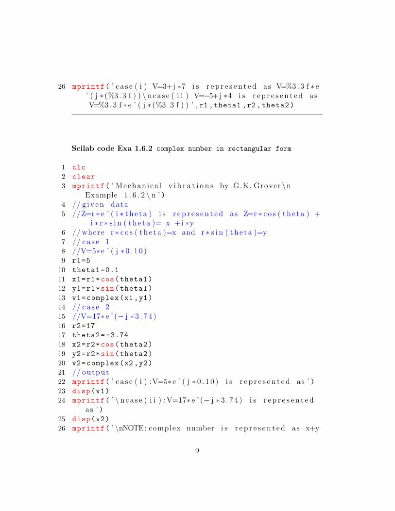
26 mprintf( ’ c a s e ( i ) V=3+j ∗7 i s r e p r e s e n t e d as V=%3 . 3 f ∗ eˆ( j ∗ (%3 . 3 f ) ) \ nca s e ( i i ) V=−5+j ∗4 i s r e p r e s e n t e d asV=%3 . 3 f ∗ e ˆ( j ∗ (%3 . 3 f ) ) ’ ,r1 ,theta1 ,r2 ,theta2)
Scilab code Exa 1.6.2 complex number in rectangular form
1 clc
2 clear
3 mprintf( ’ Mechan ica l v i b r a t i o n s by G.K. Grover \nExample 1 . 6 . 2 \ n ’ )
4 // g i v e n data5 //Z=r ∗ e ˆ( i ∗ t h e t a ) i s r e p r e s e n t e d as Z=r ∗ co s ( t h e t a ) +
i ∗ r ∗ s i n ( t h e t a )= x +i ∗y6 // where r ∗ co s ( t h e t a )=x and r ∗ s i n ( t h e t a )=y7 // c a s e 18 //V=5∗e ˆ( j ∗ 0 . 1 0 )9 r1=5
10 theta1 =0.1
11 x1=r1*cos(theta1)
12 y1=r1*sin(theta1)
13 v1=complex(x1 ,y1)
14 // c a s e 215 //V=17∗ eˆ(− j ∗ 3 . 7 4 )16 r2=17
17 theta2 = -3.74
18 x2=r2*cos(theta2)
19 y2=r2*sin(theta2)
20 v2=complex(x2 ,y2)
21 // output22 mprintf( ’ c a s e ( i ) :V=5∗e ˆ( j ∗ 0 . 1 0 ) i s r e p r e s e n t e d as ’ )23 disp(v1)
24 mprintf( ’ \ nca s e ( i i ) :V=17∗ eˆ(− j ∗ 3 . 7 4 ) i s r e p r e s e n t e das ’ )
25 disp(v2)
26 mprintf( ’ \nNOTE: complex number i s r e p r e s e n t e d as x+y
9
∗ i i n SCILAB ’ )
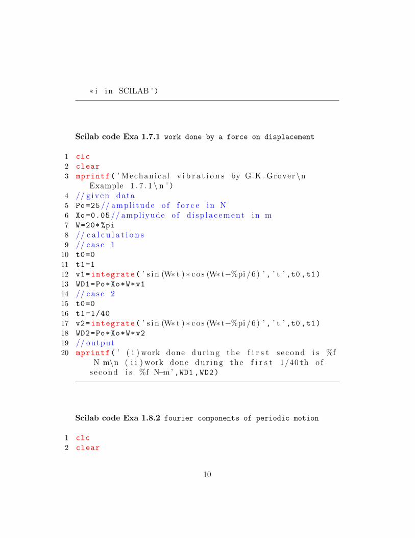
Scilab code Exa 1.7.1 work done by a force on displacement
1 clc
2 clear
3 mprintf( ’ Mechan ica l v i b r a t i o n s by G.K. Grover \nExample 1 . 7 . 1 \ n ’ )
4 // g i v e n data5 Po=25 // ampl i tude o f f o r c e i n N6 Xo=0.05 // ampl iyude o f d i s p l a c e m e n t i n m7 W=20* %pi
8 // c a l c u l a t i o n s9 // c a s e 110 t0=0
11 t1=1
12 v1=integrate( ’ s i n (W∗ t ) ∗ co s (W∗ t−%pi /6) ’ , ’ t ’ ,t0 ,t1)13 WD1=Po*Xo*W*v1
14 // c a s e 215 t0=0
16 t1=1/40
17 v2=integrate( ’ s i n (W∗ t ) ∗ co s (W∗ t−%pi /6) ’ , ’ t ’ ,t0 ,t1)18 WD2=Po*Xo*W*v2
19 // output20 mprintf( ’ ( i ) work done dur ing the f i r s t s econd i s %f
N−m\n ( i i ) work done dur ing the f i r s t 1/40 th o fs econd i s %f N−m’ ,WD1 ,WD2)
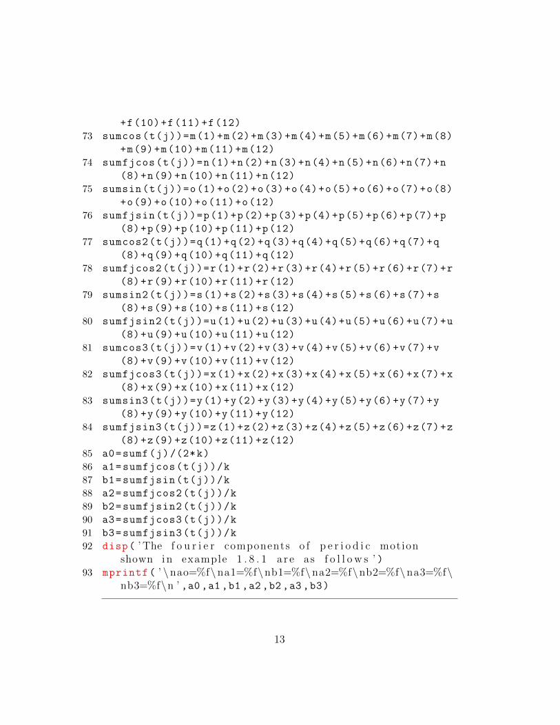
Scilab code Exa 1.8.2 fourier components of periodic motion
1 clc
2 clear
10
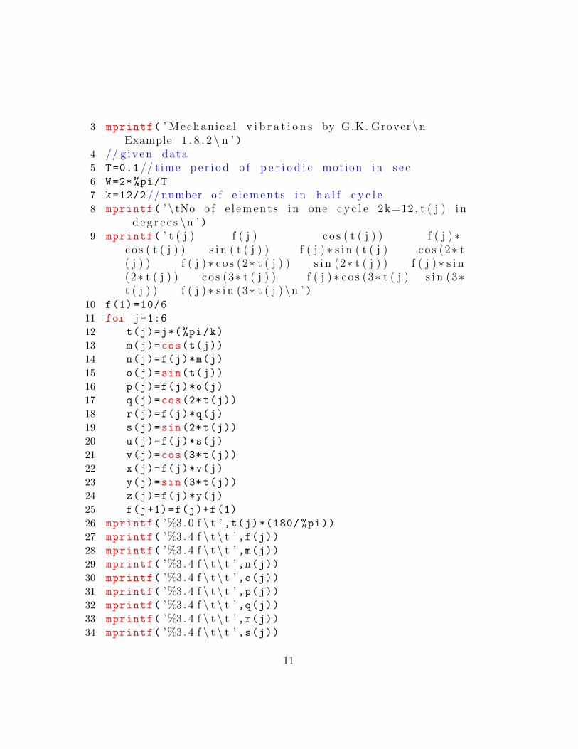
3 mprintf( ’ Mechan ica l v i b r a t i o n s by G.K. Grover \nExample 1 . 8 . 2 \ n ’ )
4 // g i v e n data5 T=0.1 // t ime p e r i o d o f p e r i o d i c motion i n s e c6 W=2*%pi/T
7 k=12/2 // number o f e l e m e n t s i n h a l f c y c l e8 mprintf( ’ \ tNo o f e l e m e n t s i n one c y c l e 2k=12 , t ( j ) i n
d e g r e e s \n ’ )9 mprintf( ’ t ( j ) f ( j ) c o s ( t ( j ) ) f ( j ) ∗
co s ( t ( j ) ) s i n ( t ( j ) ) f ( j ) ∗ s i n ( t ( j ) c o s (2∗ t( j ) ) f ( j ) ∗ co s (2∗ t ( j ) ) s i n (2∗ t ( j ) ) f ( j ) ∗ s i n(2∗ t ( j ) ) c o s (3∗ t ( j ) ) f ( j ) ∗ co s (3∗ t ( j ) s i n (3∗t ( j ) ) f ( j ) ∗ s i n (3∗ t ( j ) \n ’ )
10 f(1) =10/6
11 for j=1:6
12 t(j)=j*(%pi/k)
13 m(j)=cos(t(j))
14 n(j)=f(j)*m(j)
15 o(j)=sin(t(j))
16 p(j)=f(j)*o(j)
17 q(j)=cos(2*t(j))
18 r(j)=f(j)*q(j)
19 s(j)=sin(2*t(j))
20 u(j)=f(j)*s(j)
21 v(j)=cos(3*t(j))
22 x(j)=f(j)*v(j)
23 y(j)=sin(3*t(j))
24 z(j)=f(j)*y(j)
25 f(j+1)=f(j)+f(1)
26 mprintf( ’%3 . 0 f \ t ’ ,t(j)*(180/ %pi))27 mprintf( ’%3 . 4 f \ t \ t ’ ,f(j))28 mprintf( ’%3 . 4 f \ t \ t ’ ,m(j))29 mprintf( ’%3 . 4 f \ t \ t ’ ,n(j))30 mprintf( ’%3 . 4 f \ t \ t ’ ,o(j))31 mprintf( ’%3 . 4 f \ t \ t ’ ,p(j))32 mprintf( ’%3 . 4 f \ t \ t ’ ,q(j))33 mprintf( ’%3 . 4 f \ t \ t ’ ,r(j))34 mprintf( ’%3 . 4 f \ t \ t ’ ,s(j))
11

35 mprintf( ’%3 . 4 f \ t \ t ’ ,u(j))36 mprintf( ’%3 . 4 f \ t \ t ’ ,v(j))37 mprintf( ’%3 . 4 f \ t \ t ’ ,x(j))38 mprintf( ’%3 . 4 f \ t \ t ’ ,y(j))39 mprintf( ’%3 . 4 f \n ’ ,z(j))40 end
41 f(7)=f(j)-f(1)
42 for j=7:12
43 t(j)=j*(%pi/k)
44 m(j)=cos(t(j))
45 n(j)=f(j)*m(j)
46 o(j)=sin(t(j))
47 p(j)=f(j)*o(j)
48 q(j)=cos(2*t(j))
49 r(j)=f(j)*q(j)
50 s(j)=sin(2*t(j))
51 u(j)=f(j)*s(j)
52 v(j)=cos(3*t(j))
53 x(j)=f(j)*v(j)
54 y(j)=sin(3*t(j))
55 z(j)=f(j)*y(j)
56 f(j+1)=f(j)-f(1)
57 mprintf( ’%3 . 0 f \ t ’ ,t(j)*(180/ %pi))58 mprintf( ’%3 . 4 f \ t \ t ’ ,f(j))59 mprintf( ’%3 . 4 f \ t \ t ’ ,m(j))60 mprintf( ’%3 . 4 f \ t \ t ’ ,n(j))61 mprintf( ’%3 . 4 f \ t \ t ’ ,o(j))62 mprintf( ’%3 . 4 f \ t \ t ’ ,p(j))63 mprintf( ’%3 . 4 f \ t \ t ’ ,q(j))64 mprintf( ’%3 . 4 f \ t \ t ’ ,r(j))65 mprintf( ’%3 . 4 f \ t \ t ’ ,s(j))66 mprintf( ’%3 . 4 f \ t \ t ’ ,u(j))67 mprintf( ’%3 . 4 f \ t \ t ’ ,v(j))68 mprintf( ’%3 . 4 f \ t \ t ’ ,x(j))69 mprintf( ’%3 . 4 f \ t \ t ’ ,y(j))70 mprintf( ’%3 . 4 f \n ’ ,z(j))71 end
72 sumf(j)=f(1)+f(2)+f(3)+f(4)+f(5)+f(6)+f(7)+f(8)+f(9)
12
+f(10)+f(11)+f(12)
73 sumcos(t(j))=m(1)+m(2)+m(3)+m(4)+m(5)+m(6)+m(7)+m(8)
+m(9)+m(10)+m(11)+m(12)
74 sumfjcos(t(j))=n(1)+n(2)+n(3)+n(4)+n(5)+n(6)+n(7)+n
(8)+n(9)+n(10)+n(11)+n(12)
75 sumsin(t(j))=o(1)+o(2)+o(3)+o(4)+o(5)+o(6)+o(7)+o(8)
+o(9)+o(10)+o(11)+o(12)
76 sumfjsin(t(j))=p(1)+p(2)+p(3)+p(4)+p(5)+p(6)+p(7)+p
(8)+p(9)+p(10)+p(11)+p(12)
77 sumcos2(t(j))=q(1)+q(2)+q(3)+q(4)+q(5)+q(6)+q(7)+q
(8)+q(9)+q(10)+q(11)+q(12)
78 sumfjcos2(t(j))=r(1)+r(2)+r(3)+r(4)+r(5)+r(6)+r(7)+r
(8)+r(9)+r(10)+r(11)+r(12)
79 sumsin2(t(j))=s(1)+s(2)+s(3)+s(4)+s(5)+s(6)+s(7)+s
(8)+s(9)+s(10)+s(11)+s(12)
80 sumfjsin2(t(j))=u(1)+u(2)+u(3)+u(4)+u(5)+u(6)+u(7)+u
(8)+u(9)+u(10)+u(11)+u(12)
81 sumcos3(t(j))=v(1)+v(2)+v(3)+v(4)+v(5)+v(6)+v(7)+v
(8)+v(9)+v(10)+v(11)+v(12)
82 sumfjcos3(t(j))=x(1)+x(2)+x(3)+x(4)+x(5)+x(6)+x(7)+x
(8)+x(9)+x(10)+x(11)+x(12)
83 sumsin3(t(j))=y(1)+y(2)+y(3)+y(4)+y(5)+y(6)+y(7)+y
(8)+y(9)+y(10)+y(11)+y(12)
84 sumfjsin3(t(j))=z(1)+z(2)+z(3)+z(4)+z(5)+z(6)+z(7)+z
(8)+z(9)+z(10)+z(11)+z(12)
85 a0=sumf(j)/(2*k)
86 a1=sumfjcos(t(j))/k
87 b1=sumfjsin(t(j))/k
88 a2=sumfjcos2(t(j))/k
89 b2=sumfjsin2(t(j))/k
90 a3=sumfjcos3(t(j))/k
91 b3=sumfjsin3(t(j))/k
92 disp( ’ The f o u r i e r components o f p e r i o d i c motionshown i n example 1 . 8 . 1 a r e as f o l l o w s ’ )
93 mprintf( ’ \nao=%f\na1=%f\nb1=%f\na2=%f\nb2=%f\na3=%f\nb3=%f\n ’ ,a0 ,a1,b1,a2 ,b2,a3,b3)
13
Chapter 2
Undamped free vibrations ofsingle degree of freedom system
Scilab code Exa 2.3.4 moment of inertia of flywheel
1 clc
2 clear
3 mprintf( ’ Mechan ica l v i b r a t i o n s by G.K. Grover \nExample 2 . 3 . 4 \ n ’ )
4 // g i v e n data5 M=35 // mass o f f l y w h e e l i n Kgs6 r=0.3/2 // d i s t a n c e o f c e n t r e o f mass from p i v o t i n m7 T=1.22 // t ime p e r i o d o f o s c i l l a t i o n i n s e c8 g=9.81 // a c c e l a r a t i o n due to g r a v i t y i n m/( s e c ˆ2)9 // concep t i s as f o l l o w s
10 // Jo=mass moment o f i n e r t i a about p ivot , Wn=n a t u r a lf r e q e n c y
11 // thetadd=t h e t a doub le dot ( doub le d i f f e r e n t i a t i o n )12 // Jo∗ the tadd=−M∗g∗ r ∗ t h e t a . . . . sum o f moments i s = to
z e r o13 // Jo∗ the tadd +(M∗g∗ r ∗ t h e t a )=014 //Wn=s q r t ( (M∗g∗ r ∗ ) / Jo ) =2∗ p i /T15 // c a l c u l a t i o n s16 Jo=M*g*r/((2* %pi/T)^2)
14
17 Jg=Jo-M*r^2 // mass moment o f i n e r t i a about g e o m e t r i ca x i s
18 // output19 mprintf( ’ Mass moment o f i n e r t i a about p i v o t i s %4 . 4 f
Kg−mˆ2\n Mass moment o f i n e r t i a about g e o m e t r i ca x i s i s %4 . 4 f Kg−mˆ2 ’ ,Jo ,Jg)
Scilab code Exa 2.4.1 natural frequency of torsional pendulum
1 clc
2 clear
3 mprintf( ’ Mechan ica l v i b r a t i o n s by G.K. Grover \nExample 2 . 4 . 1 \ n ’ )
4 // g i v e n data5 l=1 // l e n g h t i n m6 d=0.005 // d i a o f rod im m7 D=0.2 // d i a o f do to r i n m8 M=2 // mass o f motor i n Kg9 G=0.83 *10^11 // modulus o f r i g i d i t y i n N/mˆ2
10 // c a l c u l a t i o n s11 J=M*((D/2) ^2)/2 // mass moment o f i n e r t i a i n Kg−mˆ212 Ip=(%pi /32)*d^4 // s e c t i o n modulus i n mˆ413 Kt=G*Ip/l // s t i f f n e s s i n N−m/ rad14 Wn=sqrt(Kt/J) // n a t u r a l f r e q e n c y i n rad / s e c15 fn=Wn/(2* %pi) // n a t u r a l f r e q i n Hz16 // output17 mprintf( ’ The n a t u r a l f r e q e n c y o f v i b r a t i o n o f
t o r s i o n a l pendulum i s %4 . 4 f rad / s e c \n or %4 . 4 f Hz’ ,Wn ,fn)
18 mprintf( ’ \nNOTE: In book the n a t u r a l f r e q e n c y o fv i b r a t i o n o f t o r s i o n a l pendulum\ n i s g i v e n as 36Hz which i s wrong . ’ )
15
Scilab code Exa 2.5.1 mass in a spring mass system
1 clc
2 clear
3 mprintf( ’ Mechan ica l v i b r a t i o n s by G.K. Grover \nExample 2 . 5 . 1 \ n ’ )
4 // g i v e n data5 k1=2000 // s t i f f n e s s o f s p r i n g 1 i n N/m6 k2=1500 // s t i f f n e s s o f s p r i n g 2 i n N/m7 k3=3000 // s t i f f n e s s o f s p r i n g 3 i n N/m8 k4=500 // s t i f f n e s s o f s p r i n g 4 i n N/m9 k5=500 // s t i f f n e s s o f s p r i n g 5 i n N/m10 fn =10 // n a t u r a l f r e q u e n c y o f system i n Hz11 // c a l c u l a t i o n s12 Ke1 =1/((1/ k1)+(1/k2)+(1/k3)) // e f f e c t i v e s t i f f n e s s
o f top 3 s p r i n g s i n s e r i e s i n N/m13 Ke2=k4+k5 // e f f e c t i v e s t i f f n e s s o f l owe r 2 s p r i n g s
i n p a r a l l e l i n N/m14 Ke=Ke1+Ke2 // t o t a l e f f e c t i v e s t i f f n e s s o f s r i n g
system15 M=Ke/(2* %pi*fn)^2 // r e q i r e d mass such tha t the
n a t u r a l f r e q u e n c y o f system i s 10 Hz ( i n Kg)16 // output17 mprintf( ’ The mass r e q u i r e d such tha t the n a t u r a l
f r e q u e n c y o f system i s 10 Hz\n i s %4 . 4 f Kg ’ ,M)
Scilab code Exa 2.5.2 natural frequency of torsional oscillation
1 clc
2 clear
3 mprintf( ’ Mechan ica l v i b r a t i o n s by G.K. Grover \nExample 2 . 5 . 2 \ n ’ )
4 // g i v e n data5 G=0.83*10^11 // r i g i d i t y modulus i n N/mˆ26 J=14.7 // mass moment o f i n e r t i a i n kg−mˆ2
16
7 l1=0.6 // l e n g h t o f s e c t i o n 1 i n m8 l2=1.8 // l e n g h t o f s e c t i o n 2 i n m9 l3=0.25 // l e n g h t o f s e c t i o n 3 i n m10 d1=0.05 // d i a o f s e c t i o n 1 i n m11 d2=0.08 // d i a o f s e c t i o n 2 i n m12 d3=0.03 // d i a o f s e c t i o n 3 i n m13 // c a l c u l a t i o n s14 Kt1=(G/l1)*(%pi /32)*d1^4 // ( %pi /32) ∗dˆ4 i s the
s e c t i o n modulus15 Kt2=(G/l2)*(%pi /32)*d2^4
16 Kt3=(G/l3)*(%pi /32)*d3^4
17 Kt =1/((1/ Kt1)+(1/ Kt2)+(1/ Kt3)) // t o t a l e f f e c t i v es t i f f n e s s o f the t o r s i o n a l system
18 Wn=sqrt(Kt/J)// n a t u r a l f r e q i n rad / s e c19 fn=Wn/(2* %pi) // n a t u r a l f r e q i n Hz20 // output21 mprintf( ’ The n a t u r a l f r e q u e n c y o f t o r s i o n a l
o s c i l l a t i o n f o r the g i v e n system i s \n %4 . 4 f rad /s e c or %4 . 4 f Hz . ’ ,Wn ,fn)
22 mprintf( ’ \nNOTE: S i n c e the v a l u e o f Kt i n thet ex tbook has been rounded o f \n to 3 dec ima lp l a c e s , the f i n a l answer v a r i e s s l i g h t l y . ’ )
17

Chapter 3
Damped free vibrations ofsingle degree of freedom system
Scilab code Exa 3.3.2 undamped and damped natural frequencies of system
1 clc
2 clear
3 mprintf( ’ Mechan ica l v i b r a t i o n s by G.K. Grover \nExample 3 . 3 . 2 \ n ’ )
4 // g i v e n data5 m=10 // mass o f s o l i d i n Kg6 Kr=3000 // s t i f f n e s s o f n a t u r a l rubber i n N/m7 Kf =12000 // s t i f f n e s s o f f e l t i n N/m8 Cr=100 // damping c o e f f i c i e n t o f n a t u r a l rubber i n N
−s e c /m9 Cf=330 // damping c o e f f i c i e n t o f f e l t i n N−s e c /m
10 // c a l c u l a t i o n s11 Ke =1/((1/ Kf)+(1/Kr)) // e q u i v a l e n t s t i f f n e s s i n N/m12 Ce =1/((1/ Cf)+(1/Cr)) // e q u i v a l e n t damping
c o e f f i c i e n t N−s e c /m13 Wn=sqrt(Ke/m) // undamped n a t u r a l f r e q i n rad / s e c14 fn=Wn/(2* %pi) // undamped n a t u r a l f r e q i n Hz15 zeta=Ce/(2* sqrt(Ke*m)) // damping f a c t o r16 Wd=sqrt(1-zeta ^2)*Wn //damped n a t u r a l f r e u e n c y i n
18
rad / s e c ( eqn 3 . 3 . 1 6 )17 fd=Wd/(2* %pi) // damped n a t u r a l f r e q u e n c y i n Hz18 // output19 mprintf( ’ The undamped n a t u r a l f r e q u e n c y i s %4 . 4 f
rad / s e c or %4 . 4 f Hz\n The damped n a t u r a l f r e u e n c yi s %4 . 4 f rad / s e c or %4 . 4 f Hz ’ ,Wn ,fn,Wd,fd)
Scilab code Exa 3.3.3 gun barrel recoilling
1 clc
2 clear
3 mprintf( ’ Mechan ica l v i b r a t i o n s by G.K. Grover \nExample 3 . 3 . 3 \ n ’ )
4 // g i v e n data5 m=600 // mass o f gun b a r r e l i n Kgs6 k=294000 // s t i f f n e s s i n N/m7 x=1.3 // r e c o i l o f gun i n mete r s8 // c a l c u l a t i o n s9 E=0.5*k*x^2 // ene rgy s t o r e d at the end o f r e c o i l
10 Vo=sqrt (2*E/m)// v e l o c i t y o f r e c o i l11 Cc=2* sqrt(k*m)// c r i t i c a l damping i n N−s e c /m12 Wn=sqrt(k/m)// n a t u r a l f r e q u e n c y o f undamped
v i b r a t i o n i n rad / s e c13 T=2*%pi/Wn // t ime p e r i o d o f undamped v i b r a t i o n i n s e c14 Trecoil =(1/4)*T// t ime p e r i o d f o r r e c o i l o r outward
s t r o k e i n s e c15 //x =(1 .3+28.8∗ t ) ∗ e ˆ(−22.1∗ t ) from eqn 3 . 3 . 2 416 mprintf( ’ a ) the i n i t i a l r e c o i l v e l o c i t y o f b a r r e l i s
%f m/ s \nb ) c r i t i c a l damping co− e f f i c i e n t o f thedashpot which i s engaged at \ nthe end o f r e c o i ls t r o k e i s %f N−s e c /m\n\ n s u b s t i t u t i n g the v a l u ef o r t i n eqn 3 . 3 . 2 4 , s t a r t i n g from t =0.1 s e c \ nwithan inc r ement o f 0 . 0 1 s e c we ge t the f o l l o w i n g
o b s e r v a t i o n s \n ’ ,Vo ,Cc)17 t=0.1
19

18 for i=1:20
19 x=(1.3 +28.8*t)*exp ( -22.1*t)
20 mprintf( ’ x=%f at t=%f\n ’ ,x,t)21 t=t+0.01
22 end
23 mprintf( ’ As x approache s the v a l u e o f 0 . 0 5m, thev a l u e o f t =0.22 s e c ’ )
24 Trec =0.22
25 Tret=Trecoil+Trec
26 mprintf( ’ \nc ) T h e r e f o r e t ime r e q u i r e d f o r b a r r e l tor e t u r n to p o s i t i o n 5cm from \n the i n i t i a lp o s i t i o n i s %f s e c ’ ,Tret)
Scilab code Exa 3.4.1 disc of torsional pendulum
1 clc
2 clear
3 mprintf( ’ Mechan ica l v i b r a t i o n s by G.K. Grover \nExample 3 . 4 . 1 \ n ’ )
4 // g i v e n data5 J=0.06 //moment o f i n e r t i a o f d i s c o f pendulum i n Kg
−mˆ26 G=4.4*10^10 // r i g i d i t y modulus i n N/mˆ27 l=0.4 // l e n g h t o f s h a f t i n m8 d=0.1 // d iamet r e o f s h a f t i n m9 a1=9 // ampl i tude o f f i r s t o s c i l l a t i o n i n d e g r e e s
10 a2=6 // ampl i tude o f s econd o s c i l l a t i o n i n d e g r e e s11 a3=4 // ampl i tude o f t h i r d o s c i l l a t i o n i n d e g r e e s12 // c a l c u l a t i o n s13 delta=log(a1/a2) // l o g a r i t h m i c decrement eqn 3 . 4 . 1
e x p l a i n e d i n s e c 3 . 414 zeta=delta/sqrt (4*%pi ^2+ delta ^2) // r e p r e s e n t i n g z e t a
from eqn 3 . 4 . 1 i n s e c 3 . 415 Kt=(G/l)*(%pi /32)*d^4 // ( %pi /32) ∗dˆ4 i s the s e c t i o n
modulus
20

16 C=zeta *2* sqrt(Kt*J) // t o r s i o n a l damping c o e f f i c i e n twhich i s the damping t o r qu e at u n i t v e l o c i t y (
s i m i l a r to eqn 3 . 3 . 6 i n s e c 3 . 3 )17 Wn=sqrt(Kt/J) // undamped n a t u r a l f r e q i n rad / s e c18 T=2*%pi/(sqrt(1-zeta ^2)*Wn) // p e r i o d i c t ime o f
v i b r a t i o n19 fn=Wn/(2* %pi) // n a t u r a l f r e q o f undamped v i b r a t i o n20 // output21 mprintf( ’ a ) l o g a r i t h m i c decrement i s %4 . 4 f \n b )
damping t o r q u e at u n i t v e l o c i t y i s %4 . 4 f N−m/ rad \n c ) p e r i o d i c t ime o f v i b r a t i o n i s %4 . 5 f s e c \nf r e q u e n c y o f v i b r a t i o n i f the d i s c i s removedfrom v i s c o u s f l u i d i s %4 . 4 f Hz ’ ,delta ,C,T,fn)
Scilab code Exa 3.6.1 spring mass system with coulomb damping
1 clc
2 clear
3 mprintf( ’ Mechan ica l v i b r a t i o n s by G.K. Grover \nExample 3 . 6 . 1 \ n ’ )
4 // g i v e n data5 m=5 // mass i n s p r i n g mass system ) i n kg )6 k=980 // s t i f f n e s o f s p r i n g i n N/m7 u=0.025 // c o e f f i c i e n t o f f r i c t i o n8 g=9.81 // a c c e l e r a t i o n due to g r a v i t y9 // c a l c u l a t i o n s
10 F=u*m*g// f r i c t i o n a l f o r c e i n N11 Wn=sqrt(k/m)// f r e q o f f r e e o s c i l l a t i o n s i n rad / s e c12 fn=Wn/(2* %pi)// f r e q o f f r e e o s c i l l a t i o n s i n Hz13 Ai=0.05 // i n i t i a l ampl i tude i n m14 Ar=0.5*Ai // reduced ampl i tude i n m15 totAreduc=Ai -Ar // t o t a l r e d u c t i o n i n amp i n m16 Areducpercycl =4*F/k // r e d u c t i o n i n ampl i tude / c y c l e
e x p l a i n e d i n s e c t i o n 3 . 6 . 2 i n eqn 3 . 6 . 617 n=round(totAreduc/Areducpercycl) // number o f c y c l e s
21
f o r 50% r e d u c t i o n i n ampl i tude18 Treduc=n*(2* %pi/Wn)// t ime taken to a c h i e v e 50
%reduct ion19 // output20 mprintf( ’ a ) The f r e q u e n c y o f f r e e o s c i l l a t i o n s i s %4
. 4 f rad / s e c or %4 . 4 f Hz\n b ) number o f c y c l e staken f o r 50 p e r c e n t r e d u c t i o n i n ampl i tude i s %1. 0 f c y c l e s \n c ) t ime taken to a c h i e v e 50 p e r c e n tr e d u c t i o n i n ampl i tude i s %4 . 4 f s e c ’ ,Wn ,fn,n,Treduc)
Scilab code Exa 3.6.2 vertical spring mass system
1 clc
2 clear
3 mprintf( ’ Mechan ica l v i b r a t i o n s by G.K. Grover \nExample 3 . 6 . 2 \ n ’ )
4 // g i v e n data5 k=9800 // s t i f f n e s o f s p r i n g i n N/m6 m=40 // mass i n s p r i n g mass system ) i n kg )7 g=9.81 // a c c e l e r a t i o n due to g r a v i t y8 F=49 // f r i c t i o n a l f o r c e i n N9 x=0.126 // t o t a l e x t e n s i o n o f s p r i n g i n m
10 xeq=m*g/k// e x t e n s i o n o f s p r i n g at e q u i l l i b r i u m i n m11 xi=x-xeq // i n i t i a l e x t e n s i o n o f s p r i n g from
e q u i l l i b r i u m i n m12 Alosspercycl =4*F/k// r e d u c t i o n i n ampl i tude / c y c l e
e x p l a i n e d i n s e c t i o n 3 . 6 . 2 i n eqn 3 . 6 . 613 n=int(xi/Alosspercycl)// number o f comple te c y c l e s
tha t system undergoe s14 Af=xi-n*Alosspercycl // ampl i tude at the end o f n
c y c l e s15 SF=k*Af // s p r i n g f o r c e a c t i n g on the upward d i r e c t i o n
f o r an e x t e n s i o n o f Af16 if F<SF then
22
17 disp( ’ The s p r i n g w i l l move up s i n c e s p r i n g f o r c ei s g r e a t e r than f r i c t i o n a l f o r c e ’ )
18 Xa=Af // a s s i g n i n g Af to a new v a r i a b l e Xa19 Xb=0 // assume Xb=0 at f i r s t20 // s o l v i n g the q u a d r a t i c e q u a t i o n i n Xb whose
r o o t s a r e Xb1 and Xb221 Xb1=(F+sqrt((-F)^2 -(4*(0.5*k)*(( -(1/2)*k*Xa^2)+F
*Xa))))/k
22 Xb2=(F-sqrt((-F)^2 -(4*(0.5*k)*(( -(1/2)*k*Xa^2)+F
*Xa))))/k
23 if int(Xb1 -Xa)==0 then
24 Xb=Xb2
25 else
26 Xb=Xb1
27 end
28 finalext=xeq+Xb
29 mprintf( ’ The f i n a l e x t e n t i o n o f s p r i n g i s %fm’ ,finalext)
30 else disp( ’ The s p r i n g w i l l not move up s i n c es p r i n g f o r c e i s not g r e a t e r than f r i c t i o n a lf o r c e ’ )
31 end
Scilab code Exa 3.7.1 time taken for complete damping
1 clc
2 clear
3 mprintf( ’ Mechan ica l v i b r a t i o n s by G.K. Grover \nExample 3 . 7 . 1 \ n ’ )
4 // g i v e n data5 fnA =12 // f r e q u e n c y o f f r e e v i b r a t i o n s o f system A i n
Hz6 fnB =15 // f r e q u e n c y o f f r e e v i b r a t i o n s o f system B i n
Hz7 TdA =4.5 // t ime taken by system A to damp out
23

c o m p l e t e l y i n s e c8 // c a l c u l a t i o n s9 TdB=fnA*TdA/fnB // t ime taken by system B to damp out
c o m p l e t e l y i n s e c10 // output11 mprintf( ’ The t ime taken by system B to damp out
c o m p l e t e l y i s %4 . 4 f s e c ’ ,TdB)
24

Chapter 4
Forced vibrations of singledegree of freedom system
Scilab code Exa 4.2.1 periodic torque on suspended flywheel
1 clc
2 clear
3 mprintf( ’ Mechan ica l v i b r a t i o n s by G.K. Grover \nExample 4 . 2 . 1 \ n ’ )
4 // g i v e n data5 //T=To∗ s i n (W∗ t )6 To =0.588 //maximum v a l u e o f p e r i o d i c t o rq u e i n N−m7 W=4 // f r e q e n c y o f a p p l i e d f o r c e i n rad / s e c8 J=0.12 //moment o f i n e r t i a o f whee l i n kg−mˆ29 Kt =1.176 // s t i f f n e s s o f w i r e i n N−m/ rad
10 Ct =0.392/1 // damping c o e f f i c i e n t i n N−m sec / rad11 // c a l c u l a t i o n s12 theta=To/sqrt((Kt-J*W^2) ^2+(Ct*W)^2) // Equat ion f o r
t o r s i o n a l v i b r a t i o n ampl i tude from Fig ( 4 . 2 . 2 )and Eqn ( 4 . 2 . 5 )
13 MaxDcoup=Ct*W*theta //maximum damping c o u p l e i n N−m14 if atan((Ct*W)/(Kt -J*W^2))>0 then
15 phiD =(180/ %pi)*atan((Ct*W)/(Kt-J*W^2));// fromeqn 4 . 2 . 6 ( i n d e g r e e s )
25

16 else
17 phiD =180+(180/ %pi)*atan((Ct*W)/(Kt-J*W^2));
18
19 end
20 // output21 mprintf( ’ a ) The maximum a n g u l a r d i s p l a c e m e n t from
r e s t p o s i t i o n i s %4 . 4 f r a d i a n s \n b ) The maximumc o u p l e a p p l i e d to dashpot i s %4 . 4 f N−m\n c ) a n g l eby which the a n g u l a r d i s p l a c e m e n t l a g s the t o r qu e
i s %4 . 4 f d e g r e e s ’ ,theta ,MaxDcoup ,phiD)
Scilab code Exa 4.2.2 damping factor and natural frequency of system
1 clc
2 clear
3 mprintf( ’ Mechan ica l v i b r a t i o n s by G.K. Grover \nExample 4 . 2 . 2 \ n ’ )
4 // g i v e n data5 Wd =9.8*2* %pi // damped n a t u r a l f r e q e n c y i n rad / s e c6 Wp =9.6*2* %pi // f r e q e n c y from f o r c e d v i b r a t i o n t e s t i n
rad / s e c7 // c a l c u l a t i o n s8 // (Wp/Wn)=s q r t (1−2∗ z e t a ˆ2) . . . ( 1 ) from Eqn 4 . 2 . 1 8
from Sec 4 . 2 . 19 // (Wd/Wn)=s q r t (1− z e t a ˆ2) . . . ( 2 ) from Eqn 4 . 2 . 1 9 from
Sec 4 . 2 . 110 // d i v i d i n g ( 1 ) by ( 2 )11 x=(Wp/Wd)
12 //x=[ s q r t (1−2∗ z e t a ˆ2) ] / [ s q r t (1− z e t a ˆ2) ]13 zeta=sqrt((1-x)/(2-x))// damping f a c t o r o b t a i n e d on
s i m p l i f y i n g the above eqn14 // s u b s t i t u t i n g f o r z e t a i n eqn 2 above15 Wn=Wd/sqrt(1-zeta ^2) // n a t u r a l f r e q u e n c y o f system i n
rad / s e c16 fn=Wn/(2* %pi)// n a t u r a l f r e q u e n c y o f system i n Hz
26
17 // output18 mprintf( ’ The damping f a c t o r f o r the system i s %f and
\n the n a t u r a l f r e q u e n c y i s %4 . 4 f rad / s e c or %4 . 2f Hz ’ ,zeta ,Wn,fn)
19 mprintf( ’ \nNOTE: The damping f a c t o r z e t a g i v e n i nt ex tbook i s 0 . 1 9 6 , which i s wrong . ’ )
Scilab code Exa 4.3.1 system of beams supporting a motor
1 clc
2 clear
3 mprintf( ’ Mechan ica l v i b r a t i o n s b G.K. Grover \nExample 4 . 3 . 1 \ n ’ )
4 // g i v e n data5 m=1200 // mass o f motor i n kg6 mo=1 // unba lanced mass on motor i n kg7 e=0.06 // l o c a t i o n o f unba lanced mass from motor i n m8 Wn =2210*(2* %pi /60) // r e s o n a n t f r e q i n rad / s e c9 W=1440*(2* %pi /60) // o p e r a t i n g f r e q
10 // c a l c u l a t i o n s11 // c a s e 112 zeta =0.1
13 bet=(W/Wn)
14 y=(mo/m)// from eqn 4 . 3 . 215 X1=(y*e)*(bet)^2/ sqrt((1-bet^2) ^2+(2* zeta*bet)^2) //
from eqn 4 . 3 . 216 // c a s e 217 zeta=0
18 X2=(y*e)*(bet)^2/ sqrt((1-bet^2) ^2+(2* zeta*bet)^2) //from eqn 4 . 3 . 2
19 // output20 mprintf( ’ I f the damping i s l e s s than 0 . 1 then the
ampl i tude o f \n v i b r a t i o n w i l l be between %f mand %f m’ ,X1 ,X2)
27
Scilab code Exa 4.3.2 single cylinder vertical petrol engine
1 clc
2 clear
3 mprintf( ’ Mechan ica l v i b r a t i o n s by G.K. Grover \nExample 4 . 3 . 2 \ n ’ )
4 // g i v e n data5 m=320 // mass o f e n g i n e i n kg6 mo=24 // r e c i p r o c a t i n g mass on motor i n kg7 r=0.15 // v e r t i c a l s t r o k e i n m8 e=r/2
9 delst =0.002 // s t a t i d e f l n i n m10 C=490/(0.3) // damping r e c i s t a n c e i n N−s e c /m11 g=9.81 // g r a v i t y i n m/ s e c ˆ212 N=480 // speed i n rpm i n c a s e b )13 // c a l c u l a t i o n14 Wn=sqrt(g/delst) // n a t u r a l f r e q e n c y i n rad / s e c15 Nr=Wn/(2* %pi)*60 // r e s o n a n t speed i n rpm16 W=(2* %pi*N/60)
17 bet=(W/Wn)
18 zeta=(C/(2*m*Wn)) // damping f a c t o r19 y=(mo/m)// from eqn 4 . 3 . 220 X=(y*e)*(bet)^2/ sqrt((1-bet^2) ^2+(2* zeta*bet)^2) //
from eqn 4 . 3 . 221 // output22 mprintf( ’ a ) speed o f d r i v i n g s h a f t at which e sonance
o c c u r s i s %4 . 4 f RPM\n b ) The ampl i tude o f s t e a dys t a t e f o r c e d v i b r a t i o n s when the d r i v i n g s h a f t \n
o f the e n g i n e r o t a t e s at 480 RPM i s %f m’ ,Nr ,X)
Scilab code Exa 4.4.1 mass hung from end of vertical spring
28
1 clc
2 clear
3 mprintf( ’ Mechan ica l v i b r a t i o n s by G.K. Grover \nExample 4 . 4 . 1 \ n ’ )
4 // g i v e n data5 T=0.8 // t ime p e r i o d o f f r e e v i b r a t i o n i n s e c6 t=0.3 // t ime f o r which the v e r t i c a l d i s t a n c e has to
be c a l c u l a t e d7 //y=18∗ s i n (2∗ p i ∗ t )8 Y=18 //max ampl i tude i n mm9 // c a l c u l a t i o n s
10 W=2*%pi
11 Wn=(2* %pi/T)
12 bet=(W/Wn)
13 x=(Y/(1-bet ^2))*(sin(W*t)-bet*sin(Wn*t))// from eqn4 . 4 . 1 7 e x p l a i n e d i n the same problem
14 // output15 mprintf( ’ The v e r t i c a l d i s t a n c e moved by mass i n the
f i r s t 0 . 3 s e c i s %4 . 4 f mm’ ,x)
Scilab code Exa 4.4.2 support of spring mass system
1 clc
2 clear
3 mprintf( ’ Mechan ica l v i b r a t i o n s by G.K. Grover \nExample 4 . 4 . 2 \ n ’ )
4 // g i v e n data5 m=0.9 // mass i n kg6 K=1960 // s t i f f n e s s i n N/m7 Y=5 //amp o f v i b r a t i o n o f suppor t i n m8 N=1150 // f r e q u e n c y i n c y c l e s per min9 // c a l c u l a t i o n s
10 Wn=sqrt(K/m)
11 W=N*2*%pi/60 // f r e q u e n c y o f v i b r a t i o n o f suppor t12 bet=(W/Wn)
29

13 // c a s e 114 zeta=0
15 X1=Y*(sqrt (1+(2* zeta*bet)^2)/sqrt((1-bet ^2) ^2+(2*
zeta*bet)^2))//Eqn ( 4 . 4 . 6 )16 // c a s e 217 zeta =0.2
18 X2=Y*(sqrt (1+(2* zeta*bet)^2)/sqrt((1-bet ^2) ^2+(2*
zeta*bet)^2))//Eqn ( 4 . 4 . 6 )19 // output20 mprintf( ’ The ampl i tude o f v i b r a t i o n when damping
f a c t o r =0 i s %4 . 4 f mm \n I f damping f a c t o r =0.2 ,then ampl i tude o f v i b r a t i o n i s %4 . 4 f mm’ ,X1 ,X2)
Scilab code Exa 4.4.3 spring of automobile trailer
1 clc
2 clear
3 mprintf( ’ Mechan ica l v i b r a t i o n s by G.K. Grover \nExample 4 . 4 . 3 \ n ’ )
4 // g i v e n data5 delst =0.1 // s t eady s t a t e d e f l n i n m6 g=9.81 // a c c e l e r a t i o n due to g r a v i t y7 Y=0.08 //amp o f v i b r a t i o n o f au tomob i l e i n m8 lambda =14 // wave l enght o f p r o f i l e i n m9 // c a l c u l a t i o n s
10 Wn=sqrt(g/delst)
11 fn=Wn/(2* %pi)// f r e q u e n c y o f v i b r a t i o n o f au tomob i l ei n Hz
12 Vc =(3600/1000)*lambda*fn // c r i t i c a l speed i n km/ hr13 V=60 // speed i n km/ hr14 W=V*(1000/3600) *(2* %pi/lambda)
15 bet=(W/Wn)
16 zeta=0
17 X=Y*(sqrt (1+(2* zeta*bet)^2)/sqrt((1-bet^2) ^2+(2* zeta
*bet)^2))//Eqn ( 4 . 4 . 6 )
30
18 // output19 mprintf( ’ The c r i t i c a l speed o f automob i l e %4 . 4 f km/
hr \n The ampl i tude o f v i b r a t i o n at 60 Km/Hr i s %4. 4 f m ’ ,Vc ,X)
Scilab code Exa 4.5.1 power required to vibrate spring mass dashpot
1 clc
2 clear
3 mprintf( ’ Mechan ica l v i b r a t i o n s by G.K. Grover \nExample 4 . 5 . 1 \ n ’ )
4 // g i v e n data5 X=0.015 // ampl i tude o f v i b r a t i o n o f s p r i n g mass
dashpot system i n m6 f=100 // f r q u e n c y o f v i b r a t i o n o f s p r i n g mass dashpot
system i n Hz7 zeta =0.05
8 fnD =22 //damped n a t u r a l f r e q u e n c y i n Hz9 m=0.5 // mass i n kg
10 // c a l c u l a t i o n s11 W=2*%pi*fnD
12 c=2*m*W*zeta // from Eqn 3 . 3 . 6 and Eqn 3 . 3 . 713 Epercycl=%pi*c*(2* %pi*f)*X^2 //Eqn 4 . 5 . 1 . . . ene rgy
d i s s i p a t e d per c y c l e14 Epersec=Epercycl*f// ene rgy d i s s i p a t e d per s e c15 // output16 mprintf( ’ The power r e q u i r e d to v i b r a t e s p r i n g mass
dashpot system with \n an ampl i tude o f 1 . 5 cm andat f r e q u e n c y o f 100 Hz i s %4 . 4 f Watts ’ ,Epersec)
17 mprintf( ’ \nNOTE: s l i g h t d i f f e r n c e i n answer comparedto t ex tbook \n i s due approx imat ion o f v a l u e o f
p i ’ )
31

Scilab code Exa 4.6.1 horizontal spring mass system in dry friction
1 clc
2 clear
3 mprintf( ’ Mechan ica l v i b r a t i o n s by G.K. Grover \nExample 4 . 6 . 1 \ n ’ )
4 // g i v e n data5 mprintf( ’NOTE: The mass g i v e n i n t ex tbook shou ld be
e q u a l \n to 3 . 7 kgs and not 8 . 7 Kgs ’ )6 m=3.7 // mass i n kg7 g=9.81 // g r a v i t y8 K=7550 // // s t i f f n e s s o f i n N/m9 u=0.22 // c o e f f i c i e n t o f f r i c t i o n
10 Fo=19.6 //amp o f f o r c e i n N11 f=5 // f r e q u e n c y o f f o r c e12 // c a l c u l a t i o n s13 F=u*m*g// f r i c t i o n a l f o r c e14 W=2*%pi*f
15 Wn=sqrt(K/m)
16 bet=(W/Wn)
17 X=(Fo/K)*sqrt (1-(4*F/(%pi*Fo))^2)/(1-bet^2) //Eqn4 . 6 . 2 i n Sec 4 . 6
18 Ceq =4*F/(%pi*W*X)// e q u i v a l e n t v i s c o u s damping Eqn4 . 6 . 1 i n Sec 4 . 6
19 // output20 mprintf( ’ \nThe ampl i tude o f v i b r a t i o n o f mass i s %f
m\n The e q u i v a l e n t v i s c o u s damping i s %f N−s e c /m’,X,Ceq)
21 mprintf( ’ \nNOTE: s l i g h t d i f f e r n c e i n answer comparedto t ex tbook \n i s due approx imat ion o f v a l u e o f
p i i n the taxtbook ’ )
Scilab code Exa 4.10.1 machine mounted on 4 identical springs
1 clc
32
2 clear
3 mprintf( ’ Mechan ica l v i b r a t i o n s by G.K. Grover \nExample 4 . 1 0 . 1 \ n ’ )
4 // g i v e n data5 m=1000 // mass o f machine i n kg6 Fo=490 //amp o f f o r c e i n N7 f=180 // f r e q inRPM8 // c a l c u l a t i o n s9 // c a s e a )10 K=1.96*10^6 // t o t a l s t i f f n e s s o f s p r i n g s i n N/m11 Wn=sqrt(K/m)
12 W=2*%pi*f/60
13 bet=(W/Wn)
14 zeta=0
15 Xst1=Fo/K// ampl i tude o f s t e ady s t a t e16 X1=Xst1 *(1/( sqrt((1-bet^2) ^2+(2* zeta*bet)^2)))//amp
o f v i b r a t i o n Eqn 4 . 2 . 1 5 i n Sec 4 . 2 . 117 Ftr1=Fo*sqrt (1+(2* zeta*bet)^2)/sqrt((1-bet ^2) ^2+(2*
zeta*bet)^2) // f o r c e t r a n s m i t t e d , Eqn 4 . 1 0 . 2 i n Sec4 . 1 0 . 1
18 // c a s e b )19 K=9.8*10^4 // t o t a l s t i f f n e s s o f s p r i n g s i n N/m20 Wn=sqrt(K/m)
21 W=2*%pi*f/60
22 bet=(W/Wn)
23 zeta=0
24 Xst2=Fo/K// ampl i tude o f s t e ady s t a t e25 X2=Xst2 *(1/( sqrt((1-bet^2) ^2+(2* zeta*bet)^2)))//amp
o f v i b r a t i o n Eqn 4 . 2 . 1 5 i n Sec 4 . 2 . 126 Ftr2=Fo*sqrt (1+(2* zeta*bet)^2)/sqrt((1-bet ^2) ^2+(2*
zeta*bet)^2) // f o r c e t r a n s m i t t e d , Eqn 4 . 1 0 . 2 i n Sec4 . 1 0 . 1
27 // output28 mprintf( ’ a ) The ampl i tude o f motion o f machine i s %f
m and the maximum f o r c e t r a n s m i t t e d \n to thef o u n d a t i o n because o f the unba lanced f o r c e when\nK=1.96∗10ˆ6 N/m i s %4 . 4 f N\n b ) f o r same c a s e as
i n a ) i f K=9.8∗10ˆ4 N/m then \n the ampl i tude o f
33
motion o f machine i s %f m\n and the maximum f o r c et r a n s m i t t e d to the f o u n d a t i o n because o f \n the
unba lanced f o r c e %4 . 4 f N ’ ,X1 ,Ftr1 ,X2 ,Ftr2)
Scilab code Exa 4.10.2 machine mounted on springs
1 clc
2 clear
3 mprintf( ’ Mechan ica l v i b r a t i o n s by G.K. Grover \nExample 4 . 1 0 . 2 \ n ’ )
4 // g i v e n data5 m=75 // mass o f machine i n kg6 K=11.76*10^5 // s t i f f n e s s o f s p r i n g s i n N/m7 zeta =0.2
8 mo=2 // mass o f p i s t o n i n kg9 stroke =0.08 // i n m
10 e=stroke /2 // i n m11 N=3000 // spee i n c . p .m12 // c a l c u l a t i o n s13 Wn=sqrt(K/m)
14 W=2*%pi*N/60
15 bet=(W/Wn)
16 y=(mo/m)
17 Fo=mo*W^2*e//max f o r c e e x e r t e d18 X=y*e*bet ^2/( sqrt((1-bet^2) ^2+(2* zeta*bet)^2))//Eqn
4 . 3 . 219 Ftr=Fo*sqrt (1+(2* zeta*bet)^2)/sqrt((1-bet^2) ^2+(2*
zeta*bet)^2) // f o r c e t r a n s m i t t e d , Eqn 4 . 1 0 . 2 i n Sec4 . 1 0 . 1
20 mprintf( ’ a ) The ampl i tude o f v i b r a t i o n o f machine i s%f m and the \n the v i b r a t o r y f o r c e Ftr
t r a n s m i t t e d to the f o u n d a t i o n i s %5 . 4 f N ’ ,X,Ftr)21 mprintf( ’ \nNOTE: s l i g h t d i f f e r n c e i n answer compared
to t ex tbook \n i s due approx imat ion o f v a l u e s i nt ex tbook ’ )
34

Scilab code Exa 4.10.3 radio set isolated from machine
1 clc
2 clear
3 mprintf( ’ Mechan ica l v i b r a t i o n s by G.K. Grover \nExample 4 . 1 0 . 3 \ n ’ )
4 // g i v e n data5 m=20 // mass i n kgs6 k=125600 // o v e r a l l e q i v a l e n t s t i f f n e s s i . e 4∗31400
i n N/m7 c=1568 // o v e r a l l damping c o e f f i c i e n t i . e 4∗392 i n N−
s e c /m8 n=500 // v i b r a t i n g speed o f machine i n cpm9 //y=Ysin (w∗ t )
10 Y=0.00005 // v i b r a t i n g ampl i tude o f machine i n m11 W=2*%pi*n/60 // v i b r a t i n g f r e q u e n c y i n rad / s e c12 Wn=sqrt(k/m) // n a t u r a l f r e q u e n c y i n rad / s e c13 bet=(W/Wn) // speed r a t i o14 zeta=c/(2* sqrt(k*m)) // damping f a c t o r15 // c a l c u l a t i o n s16 X=Y*sqrt ((1+(2* zeta*bet)^2)/((1-bet^2) ^2+(2* zeta*bet
)^2)) // a b s o l u t e ampl i tude o f v i b r a t i o n o f r a d i ofrom eqn ( 4 . 4 . 6 )
17 Z=Y*((bet^2)/sqrt (((1-bet^2) ^2+(2* zeta*bet)^2)))//from eqn 4 . 4 . 1 1
18 FdynT=Z*sqrt((c*W)^2+k^2) // dynamic l oad t o t a l19 Fdyn=FdynT/4 // dynamic l oad on each i s o l a t o r20 FdynTmax=m*W^2*X //max dynamic l oad on the i s o l a t o r s21 Fdynmax=FdynTmax /4 //max dynamic l oad on each
i s o l a t o r22 // output23 mprintf( ’ a ) The ampl i tude o f v i b r a t i o n o f r a d i o i s
%f metre s \n b ) the dynamic l oad on each i s o l a t o rdue to v i b r a t i o n i s %3 . 3 f N ’ ,X,Fdyn)
35
Scilab code Exa 4.11.1 vibrotometer
1 clc
2 clear
3 mprintf( ’ Mechan ica l v i b r a t i o n s by G.K. Grover \nExample 4 . 1 1 . 1 \ n ’ )
4 // g i v e n data5 T=2 // p e r i o d o f f r e e v i b r a t i o n i n s e c6 f=1 // v e r t i c a l harmonic f r e q u e n c y o f machine i n i n Hz7 Z=2.5 // ampl i tude o f v i b r o t o m e t e r mass r e l a t i v e to
v i b r o t o m e t e r f rame i n mm8 // c a l c u l a t i o n s9 Wn=2*%pi/T
10 W=2*%pi*f
11 bet=(W/Wn)
12 zeta=0 // f o r v i b r o t o m e t e r s13 Y=Z*(sqrt((1-bet^2) ^2+(2* zeta*bet)^2))/bet^2 //
ampl i tude o f v i b r a t i o n o f machine Eqn 4 . 4 . 1 1 i nSec 4 . 4 . 2
14 // output15 mprintf( ’ The ampl i tude o f v i b r a t i o n o f suppor t o f
machine i s %4 . 4 f mm’ ,Y)
Scilab code Exa 4.11.2 commercial type vibration pick up
1 clc
2 clear
3 mprintf( ’ Mechan ica l v i b r a t i o n s by G.K. Grover \nExample 4 . 1 1 . 2 \ n ’ )
4 // g i v e n data5 fn=5.75 // n a t u r a l f r e q u e n c y i n Hz
36

6 zeta =0.65
7 ZbyY =1.01
8 // c a s e 19 // s u b s t i t u t i n g f o r (Z/Y) =1.01 and (W/Wn)=r ˆ2 i n Eqn
4 . 4 . 1 1 we g e t the q u a d r a t i c eqn as f o l l o w s10 // 0 . 0 2∗ r ˆ4−0.31∗ r ˆ2+1=011 // s o l v i n g f o r r i n above eqn whose r o o t e s a r e r1 and
r212 r1=sqrt (((0.31)+sqrt ((( -0.31) ^2) -4*0.02*1))/(2*0.02)
)
13 r2=sqrt (((0.31) -sqrt ((( -0.31) ^2) -4*0.02*1))/(2*0.02)
)
14 if r1>r2 then
15 r=r1
16 else r=r2
17 end
18 bet=r// bet =(W/Wn)19 f1=bet*fn
20 // c a s e 221 ZbyY =0.98
22 // s u b s t i t u t i n g f o r (Z/Y) =0.98 and (W/Wn)=r ˆ2 i n Eqn4 . 4 . 1 1 we g e t the q u a d r a t i c eqn as f o l l o w s
23 // 0 . 0 4∗ r ˆ4+0.31∗ r ˆ2−1=024 // s o l v i n g f o r r i n above eqn whose r o o t e s a r e r3 and
r425 r3=sqrt (( -0.31+ sqrt (((0.31) ^2) -4*0.04* -1))/(2*0.04))
26 r4=sqrt ((-0.31- sqrt (((0.31) ^2) -4*0.04* -1))/(2*0.04))
27 t1=real(r3)
28 t2=real(r4)
29 if t1>t2 then
30 r=r3
31 else r=r4
32 end
33 bet=r// bet =(W/Wn)34 f2=bet*fn
35 mprintf( ’ The l o w e s t f r e q u e n c y beyond which theampl i tude can be measured w i t h i n \n ( i ) onep e r c e n t e r r o r i s %4 . 4 f Hz\n ( i i ) two p e r c e n t e r r o r
37
i s %4 . 4 f Hz ’ ,f1 ,f2)
Scilab code Exa 4.11.3 device used to measure torsional accerelartion
1 clc
2 clear
3 mprintf( ’ Mechan ica l v i b r a t i o n s by G.K. Grover \nExample 4 . 1 1 . 3 \ n ’ )
4 // g i v e n data5 J=0.049 //moment o f i n e r t i a i n kg−mˆ26 Kt=0.98 // s t i f f n e s s i n N−m/ rad7 Ct=0.11 // damping c o e f f i c i e n t i n N−m sec / rad8 N=15 //R. P .M9 thetaRD =2 // r e l a t i v e ampl i tude between r i n g and s h a f t
i n d e g r e e s10 // c a l c u l a t i o n s11 W=N*2*%pi /60 // f r e q u e n c y o f v i b r a t i n g s h a f t i n rad /
s e c12 Wn=sqrt(Kt/J) // n a t u r a l f r e q e n c y i n rad / s e c13 zeta=(Ct/(2* sqrt(Kt*J))) // damping f a c t o r14 thetaRR =( thetaRD /(57.3)) // r e l a t i v e ampl i tude i n
r a d i a n s15 bet=(W/Wn)
16 thetamax=thetaRR *(( sqrt((1-bet ^2) ^2+(2* zeta*bet)^2)/
bet ^2))
17 maxacc =(W^2)*thetamax
18 // output19 mprintf( ’ The maximum a c c e l e r a t i o n o f the s h a f t i s %4
. 4 f rad /( s e c ˆ2) ’ ,maxacc)
Scilab code Exa 4.11.4 Frahm tachometer
1 clc
38

2 clear
3 mprintf( ’ Mechan ica l v i b r a t i o n s by G.K. Grover \nExample 4 . 1 1 . 4 \ n ’ )
4 // g i v e n data5 RF=1800 // r e s o n a n t f r e q u e n c y i n rpm6 L=0.050 // l e n g h t o f s t e e l r e ed i n metre s7 B=0.006 // width o f s t e e l r e ed i n metre s8 t=0.00075 // t h i c k n e s s o f s t e e l r e ed i n metre s9 E=19.6*10^10 // young ’ s modulus i n N/(mˆ2)10 // c a l c u l a t i o n s11 Wn=2*%pi*RF/60 // n a t u r a l f r e q u e n c y i n r a d i a n s12 I=(B*t^3) /12 //moment o f i n e r t i a i n (mˆ4)13 m=3*E*I/((Wn^2)*L^3) // r e q u i r e d mass14 // output15 mprintf( ’ The r e q u i r e d mass M to be p l a c e d at the end
o f the r e e d s o f Frahm tachomete r i s %f Kgs ’ ,m)
39

Chapter 5
Two degrees of freedomsystems
Scilab code Exa 5.3.2 uniform rods pivoted at their upper ends
1 clc
2 clear
3 mprintf( ’ Mechan ica l v i b r a t i o n s by G.K. Grover \nExample 5 . 3 . 2 \ n ’ )
4 // g i v e n data5 m1 =5*0.75 // mass o f rod 1 i n kgs6 m2 =5*1.00 // mass o f rod 2 i n kgs7 l1=0.75 // l e n g h t o f rod 1 i n m8 l2=1.00 // l e n g h t o f rod 2 i n m9 K=2940 // s t i f f n e s s o f s p r i n g i n N/m
10 // c a l c u l a t i o n s11 Wn=sqrt (3*(m1+m2)*K/(m1*m2))// n a t u r a l f r e q u e n c y i n
rad / s e c12 fn=Wn/(2* %pi)// n a t u r a l f r e q u e n c y i n Hz as s o l v e d i n
the t ex tbook i t s e l f13 b1=(K*l2)
14 b2=(K*l1-m1*l1*Wn ^2/3)
15 x=(b2/b1)
16 Fmax=K*(l1*1-l2*x)/57.3 // to c o n v e r t i n t o r a d i a n s
40

17 // output18 mprintf( ’ The f r e q u e n c y o f the r e s u l t i n g v i b r a t i o n s
i f the e f e c t o f g r a v i t y \n i s n e g l e c t e d i s %4 . 4 frad / s e c or %4 . 4 f Hz . \ n The a n g u l a r movement o f CD
i s %3 . 3 f d e g r e e s ( out o f phase ) \n with themovement o f AB. \ n The maximum f o r c e i n the s p r i n g
i s %4 . 4 f N ’ ,Wn ,fn,x,Fmax)
Scilab code Exa 5.3.3 shaft with 2 circular discs at the end
1 clc
2 clear
3 mprintf( ’ Mechan ica l v i b r a t i o n s by G.K. Grover \nExample 5 . 3 . 3 \ n ’ )
4 // g i v e n data5 m1=500 // mass o f d i s c 1 i n Kgs6 m2=1000 // mass o f d i s c 2 i n Kgs7 D1=1.25 // o u t e r d i a o f d i s c 1 i n m8 D2=1.9 // o u t e r d i a o f d i s c 2 i n m9 l=3.0 // l e n g h t o f s h a f t i n m
10 d=0.10 // d i a o f s h a f t i n m11 G=0.83*10^11 // r i g i d i t y modulus i n N/mˆ212 // c a l c u l a t i o n s13 J1=m1*(D1/2) ^2/2 // mass moment o f i n e r t i a i n kg−mˆ214 J2=m2*(D2/2) ^2/2 // mass moment o f i n e r t i a i n kg−mˆ215 Ip=(%pi /32)*d^4 // s e c t i o n modulus o f s h a f t i n mˆ416 Kt=G*Ip/l// s t i f f n e s s i n N−m/ rad17 Wn=sqrt(Kt*(J1+J2)/(J1*J2))// from Eqn 5 . 3 . 2 8 , Sec
5 . 3 . 318 fn=Wn/(2* %pi)
19 Kt1 =2*Kt
20 Kt2 =2*Kt*2^4
21 Kte =1/((1/ Kt1)+(1/ Kt2))
22 x=sqrt(Kte/Kt)// r a t i o o f m o d i f i e d n a t u r a l f r e q too r i g i n a l n a t u r a l f r e q u e n c y
41

23 // output24 mprintf( ’ The n a t u r a l f r e q u e n c y o f the t o r s i o n a l
v i b r a t i o n i s \n %4 . 4 f rad / s e c or %3 . 3 f Hz . \ n Ther a t i o o f m o d i f i e d n a t u r a l f r e q u e n c y to o r i g i n a ln a t u r a l f r e q u e n c y \n i s %3 . 3 f . Which meanss t i f f e n i n g a system i n c r e a s e s i t s n a t u r a lf r e q u e n c y ’ ,Wn ,fn,x)
Scilab code Exa 5.7.1 torque applied to a torsional system
1 clc
2 clear
3 mprintf( ’ Mechan ica l v i b r a t i o n s by G.K. Grover \nExample 5 . 7 . 1 \ n ’ )
4 // g i v e n data5 J1 =0.735 //moment o f i n e r t i a o f main system i n Kg−mˆ26 Kt1 =7.35*10^5 // t o r s i o n a l s t i f f n e s s7 To=294 // ampl i tude o f a p p l i e d t o r q u e8 W=10^3 // f r e q u e n c y o f a p p l i e d t o r qu e9 //u=r a t i o o f a b s o r b e r mass to main mass i . e M2/M1
10 //Wn i s e x i t a t i o n f r e q u e n c y11 // c a l c u l a t i o n s12 W1=sqrt(Kt1/J1)
13 // c a s e 114 x1=0.8 // where x=(W/W2)15 u1=[x1^2 -1]^2/x1^2 // from Eqn 5 . 7 . 9 , Sec 5 . 7 . 1 .16 // c a s e 217 x2=1.2 // where x=(W/W2)18 u2=[x2^2 -1]^2/x2^2 // from Eqn 5 . 7 . 9 , Sec 5 . 7 . 1 .19 if u1>u2 then
20 u=u1
21 else
22 u=u2
23 end
24 J2=u*J1 //moment o f i n e r t i a o f a b s o r b e r i n Kg−mˆ2
42
25 Kt2=u*Kt1 // t o t a l t o r s i o n a l s t i f f n e s s o f a b s o r b e r26 K=Kt2 /(4*0.1^2) // s t i f f n e s s o f each s p r i n g i n N/m27 b2=-(To/Kt2)// ampl i tude o f v i b r a t i o n i n rad28 // output29 mprintf( ’ The maximum moment o f i n e r t i a o f a b s o r b e r (
J2 ) i s %4 . 4 f Kg−mˆ2 and\n %f i s the s t i f f n e s s o feach o f the f o u r a b s o r b e r s p r i n g s such tha t \n the
r e s o n a n t f r e q u e n c i e s a r e at l e a s t 20 p e r c e n tfrom e x i t a t i o n f r e q u e n c y . \ n The ampl i tude o fv i b r a t i o n o f t h i s a b s o r b e r ( b2 ) at e x i t a t i o nf r e q u e n c y \n i s %f r a d i a n s ’ ,J2 ,K,b2)
Scilab code Exa 5.7.2 section of pipe in a machine
1 clc
2 clear
3 mprintf( ’ Mechan ica l v i b r a t i o n s by G.K. Grover \nExample 5 . 7 . 2 \ n ’ )
4 // g i v e n data5 W1 =220*2* %pi/60 // v i b r a t i n g f r e q u e n c y at 220 RPM ( i n
rad / s e c )6 W2=W1 // f r e q u e n c y to which the s p r i n g mass system i s
tuned to .7 M2=1 // mass i n s p r i n g mass system i n kgs8 N1=188 // f i r s t r e s o n a n t f r e q o f s p r i n g mass system i n
cpm9 N2=258 // second r e s o n a n t f r e q o f s p r i n g mass system
i n cpm10 //u=r a t i o o f a b s o r b e r mass to main mass i . e M2/M111 // c a l c u l a t i o n s12 K2=M2*W2^2
13 Wn1=N1*2*%pi /60 // f i r s t r e s o n a n t f r e q o f s p r i n g masssystem i n rad / s e c
14 Wn2=N2*2*%pi /60 // second r e s o n a n t f r e q o f s p r i n g masssystem i n rad / s e c
43

15 // c a s e 116 W=Wn1
17 x1=(W/W2)
18 u1=[x1^2 -1]^2/x1^2 // from Eqn 5 . 7 . 9 , Sec 5 . 7 . 1 .19 // c a s e 220 W=Wn2
21 x2=(W/W2)
22 u2=[x2^2 -1]^2/x2^2 // from Eqn 5 . 7 . 9 , Sec 5 . 7 . 1 .23 // t h e r e f o r e24 u=(u1+u2)/2 // which i s e q u a l to M2/M125 M1=M2/u// mass o f main system i n kgs26 K1=K2/u// s t i f f n e s s o f main system i n N/m27 //now28 Wn21 =150*2* %pi /60 //new f i r s t r e s o n a n t f r e q u e n c y i n
rad / s e c29 Wn22 =310*2* %pi /60 //new second r e s o n a n t f r e q u e n c y i n
rad / s e c30 W=Wn21
31 x1=(W/W2)
32 u1=[x1^2 -1]^2/x1^2 // from Eqn 5 . 7 . 9 , Sec 5 . 7 . 1 .33 // c a s e 234 W=Wn22
35 x2=(W/W2)
36 u2=[x2^2 -1]^2/x2^2 // from Eqn 5 . 7 . 9 , Sec 5 . 7 . 1 .37 // c h o o s i n g the h i g h e r v a l u e38 if u1>u2 then
39 u=u1
40 else
41 u=u2
42 end
43 M3=M1*u// mass o f main system i n kgs44 K3=K1*u// s t i f f n e s s o f main system i n N/m45 // output46 mprintf( ’ The mass o f main system r e q u i r e d i s %4 . 4 f
kgs \n s t i f f n e s s o f main system r e q i r e d i s %5 . 5 f N/m\n I f the r e s o n a n t f r e q u e n c i e s l i e o u t s i d e therange o f 150 to 310 rpm then \n mass o f mainsystem i s %4 . 4 f kgs \n s t i f f n e s s o f main system i s
44

%5. 5 f N/m’ ,M1 ,K1,M3,K3)
45
Chapter 6
Multi degree of freedomsystems exact analysis
Scilab code Exa 6.8.2 system with rolling masses
1 clc
2 clear
3 mprintf( ’ Mechan ica l v i b r a t i o n s by G.K. Grover \nExample 6 . 8 . 2 \ n ’ )
4 // g i v e n data5 m1=250;m2=100 // mass o f two b l o c k s i n Kgs6 c1=80;c2=60,c=20 // damping c o e f f i c i e n t s i n N−s e c /m7 F1 =1000; F2=1500 // ampl i tude o f f o r c e a c t i n g on b l o c k
1 and 2 r s p t l y8 k=250000 // s t i f f n e s s o f s p r i n g i n N/m9 W=60 // f r e q u e n c y o f a p p l i e d f o r c e i n rad / s e c
10 // c a l c u l a t i o n s11 M=[m1 ,0;0,m2];
12 K=[k,-k;-k,k];
13 C=[c+c1,-c;-c,c+c2];
14 R=[F1;F2 ;0;0];
15 X=K-(W^2)*M
16 Y=W*C
17 G=[X,-Y;Y,X]
46

18 AB=inv(G) *R// from Eqn6 . 8 . 4 i n Sec 6 . 819 X1=sqrt(AB(1,1)^2 +AB(3,1)^2)
20 X2=sqrt(AB(2,1)^2 +AB(4,1)^2)
21 // output22 mprintf( ’ The ampl i tude o f v i b r a t i o n s a r e %fm f o r
mass 1 and %fm f o r mass 2 ’ ,X1 ,X2)
47

Chapter 7
Multi degree of freedomsystems numerical methods
Scilab code Exa 7.2.1 fundamental frequency by rayleigh method
1 clc
2 clear
3 mprintf( ’ Mechan ica l v i b r a t i o n s by G.K. Grover \nExample 7 . 2 . 1 \ n ’ )
4 // g i v e n data5 E=1.96*10^11 // youngs modulus i n N/mˆ26 I=4*10^ -7 //moment o f a r ea i n mˆ47 M1=100;M2=50 // mass o f d i s c s 1 and 2 i n Kgs8 c=0.18 // d i s t a n c e o f d i s c 1 from suppor t i n m9 l=0.3 // d i s t a n c e o f d i s c 2 from suppor t i n m
10 g=9.81 // a c e l e r a t i o n due to g r a v i t y i n m/ s e c ˆ211 // c a l c u l a t i o n s12 a=[(c^3/(3*E*I)),(c^2/(6*E*I)*(3*l-c));(c^2/(6*E*I)
*(3*l-c)) ,(l^3/(3*E*I))]// from SOM13 y1=g*(M1*a(1,1)+M2*a(1,2))
14 y2=g*(M1*a(2,1)+M2*a(2,2))
15 Wn=sqrt(g*(M1*y1+M2*y2)/(M1*y1^2+M2*y2^2))
16 //now to f i n d out l owe r n a t u r a l f r e q u e n c y17 F1=M1*y1*Wn^2
48

18 F2=M2*y2*Wn^2
19 y1new=F1*a(1,1)+F2*a(1,2)
20 y2new=F1*a(2,1)+F2*a(2,2)
21 Wnnew=sqrt((F1*y1new+F2*y2new)/(M1*y1new ^2+M2*y2new
^2))// a c t u a l n a t u r a l f r e q u e n c y i n rad / s e c22 // output23 mprintf( ’ The p r a c t i c a l n a t u r a l f r e q u e n c y Wn i s %4 . 4
f rad / sec , but the l owe r \n n a t u r a l f r e q u e n c y Wn‘i s %4 . 4 f rad / s e c which i s c l o s e r to the a c t u a l \nn a t u r a l f r e q u e n c y ’ ,Wn ,Wnnew)
Scilab code Exa 7.3.1 Dunkerly method
1 clc
2 clear
3 mprintf( ’ Mechan ica l v i b r a t i o n s by G.K. Grover \nExample 7 . 3 . 1 \ n ’ )
4 // g i v e n data5 E=1.96*10^11 // youngs modulus i n N/mˆ26 I=4*10^ -7 //moment o f a r ea i n mˆ47 M1=100;M2=50 // mass o f d i s c s 1 and 2 i n Kgs8 c=0.18 // d i s t a n c e o f d i s c 1 from suppor t i n m9 l=0.3 // d i s t a n c e o f d i s c 2 from suppor t i n m
10 g=9.81 // a c e l e r a t i o n due to g r a v i t y i n m/ s e c ˆ211 // c a l c u l a t i o n s12 a=[(c^3/(3*E*I)),(c^2/(6*E*I)*(3*l-c));(c^2/(6*E*I)
*(3*l-c)) ,(l^3/(3*E*I))]// from SOM13 y1=g*M1*a(1,1) // c o n s i d e r i n g on ly M1 to be a c t i n g14 y2=g*M2*a(2,2) // c o n s i d e r i n g on ly M2 to be a c t i n g15 W1=sqrt(g/y1)
16 W2=sqrt(g/y2)
17 Wn=sqrt (1/((1/ W1^2) +(1/W2^2)))// a p p l y i n g Eqn 7 . 3 . 7 ,Sec7 . 3
18 // output19 mprintf( ’ The n a t u r a l f r e q u e n c y o f t r a n s v e r s e
49
v i b r a t i o n o b t a i n e d from \n Dunker ly method i s %4. 4 f rad / s e c which i s s l i g h t l y l owe r \n than thec o r r e c t v a l u e ’ ,Wn)
Scilab code Exa 7.4.1 Stodola method
1 clc
2 clear
3 mprintf( ’ Mechan ica l v i b r a t i o n s by G.K. Grover \nExample 7 . 4 . 1 \ n ’ )
4 // g i v e n data5 E=1.96*10^11 // youngs modulus i n N/mˆ26 I=4*10^ -7 //moment o f a r ea i n mˆ47 M1=100;M2=50 // mass o f d i s c s 1 and 2 i n Kgs8 c=0.18 // d i s t a n c e o f d i s c 1 from suppor t i n m9 l=0.3 // d i s t a n c e o f d i s c 2 from suppor t i n m
10 g=9.81 // a c e l e r a t i o n due to g r a v i t y i n m/ s e c ˆ211 // c a l c u l a t i o n s12 a=[(c^3/(3*E*I)),(c^2/(6*E*I)*(3*l-c));(c^2/(6*E*I)
*(3*l-c)) ,(l^3/(3*E*I))]// from SOM13 x1(1)=1;x2(1)=1
14 for i=1:10 // upto 10 th i t e r a t i o n f o r more p e r f e c tanswer
15 F1(i)=100*x1(i)// ’ i ’ r e p r e s e n t s the dash ( ’ )16 F2(i)=50*x2(i)
17 x1(i)=F1(i)*a(1,1)+F2(i)*a(1,2)
18 x2(i)=F1(i)*a(2,1)+F2(i)*a(2,2)
19 r=(x2(i)/x1(i))
20 x2(i+1)=r
21 x1(i+1)=1
22 end
23 x1dd=1
24 W1=(x1dd/x1(10))
25 W2=(r/x2(10))
26 Wn=sqrt((W1+W2)/2) // n a t u r a l f r e q u e n c y i n rad / s e c
50
27 mprintf( ’ The n a t u r a l f r e q u e n c y o f system i ni i l u s t r a t i v e example 7 . 2 . 1 o b t a i n e d by\ nStoda l amethod i s Wn=%f rad / s e c ’ ,Wn)
28 mprintf( ’ \nNOTE: The o b t a i n e d answer i s more near tothe p e r f e c t answer \ s i n c e 10 i t e r a t i o n s / t r i a l s \nhas been c a r r i e d out . In t ex tbook on ly upto 3 rdi t e r a t i o n has been c a r r i e d out ’ )
Scilab code Exa 7.7.2 four rotor system
1 clc
2 clear
3 mprintf( ’ Mechan ica l v i b r a t i o n s by G.K. Grover \nExample 7 . 7 . 2 \ n ’ )
4 // g i v e n data5 J(1) =100 //moment o f i n e r t i a o f f i r s t r o t o r i n Kg−mˆ26 J(2)=50 //moment o f i n e r t i a o f s econd r o t o r i n Kg−mˆ27 J(3)=10 //moment o f i n e r t i a o f t h i r d r o t o r i n Kg−mˆ28 J(4)=50 //moment o f i n e r t i a o f f o u r t h r o t o r i n Kg−mˆ29 Kt(1) =10^4 // s t i f f n e s s o f s h a f t between 1 and 2 i n N−
m/ rad10 Kt(2) =10^4 // s t i f f n e s s o f s h a f t between 2 and 3 i n N−
m/ rad11 Kt(3) =2*10^4 // s t i f f n e s s o f s h a f t between 3 and 4 i n
N−m/ rad12 To =10000 // ampl i tude o f a p p l i e d t o r q u e i n N−m13 W=5 // f r e q u e n c y o f a p p l i e d t o r qu e i n rad / s e c14 // c a l c u l a t i o n s15 b(1) = -(0.789*To)/3825 // t w i s t o f s h a f t 1 i n rad16 P(1)=J(1)*W^2
17 Q(1)=P(1)*b(1) // t w i s t i n g moment o f s h a f t 1 i n N−m18 R(1)=Q(1)
19 S(1)=R(1)/Kt(1) // t w i s t o f s h a f t 1 i n r a d i a n s20 b(2)=b(1)-S(1) // t w i s t o f s h a f t 2 i n rad21 P(2)=J(2)*W^2
51
22 Q(2)=P(2)*b(2)
23 R(2)=Q(1)+Q(2)+To // t w i s t i n g moment o f s h a f t 2 i n N−m24 S(2)=R(2)/Kt(2) // t w i s t o f s h a f t 2 i n r a d i a n s25 b(3)=b(2)-S(2) // t w i s t o f s h a f t 3 i n rad26 P(3)=J(3)*W^2
27 Q(3)=P(3)*b(3)
28 R(3)=Q(2)+Q(3) // t w i s t i n g moment o f s h a f t 3 i n N−m29 S(3)=R(3)/Kt(3) // t w i s t o f s h a f t 3 i n r a d i a n s30 b(4)=b(3)-S(3) // t w i s t o f s h a f t 4 i n rad31 P(4)=J(4)*W^2
32 Q(4)=P(4)*b(4)
33 R(4)=Q(3)+Q(4) // t w i s t i n g moment o f s h a f t 4 i n N−m34 mprintf( ’ The amp l i tude s o f d i s c s a r e as f o l l o w s \n
d i s c 1=%4 . 4 f rad \n d i s c 2=%4 . 4 f rad \n d i s c 3=%4 . 4 frad \n d i s c 4=%4 . 4 f rad ’ ,b(1),b(2),b(3),b(4))
35 mprintf( ’ \nThe t w i s t s o f s h a f t a r e as f o l l o w s \ n f i r s ts h a f t=%5 . 5 f rad \ nsecond s h a f t=%5 . 5 f rad \ n t h i r d
s h a f t=%5 . 5 f rad ’ ,S(1),S(2),S(3))36 mprintf( ’ \nThe t w i s t i n g moments o f s h a f t s a r e as
f o l l o w s \ n f i r s t s h a f t=%5 . 5 f N−m\ nsecond s h a f t=%5 . 5f N−m\ n t h i r d s h a f t=%5 . 5 f N−m’ ,R(1),R(2),R(3))
37 mprintf( ’ \nNOTE: The s l i g h t d i f f e r e n c e i n v a l u e s a r edue to the more a c c u r a t e v a l u e s \ n c a l c u l a t e d bySCILAB ’ )
52

Chapter 8
Critical speeds of shafts
Scilab code Exa 8.2.1 rotor mounted midway on shaft
1 clc
2 clear
3 mprintf( ’ Mechan ica l v i b r a t i o n s by G.K. Grover \nExample 8 . 2 . 1 \ n ’ )
4 // g i v e n data5 E=1.96*10^11 // youngs modulus i n N/mˆ26 m=5 // mass o f r o t o r i n kg7 d=0.01 // d i a o f s h a f t i n m8 I=(%pi /64)*d^4 // /moment o f a r ea i n mˆ49 l=0.4 // b e a r i n g span i n m
10 e=0.02 // d i s t a n c e o f CG away from g e o m e t r i c c e n t r e o fr o t o r i n mm
11 N=3000 // speed o f s h a f t i n RPM12 // c a l c u l a t i o n s13 k=48*E*I/l^3 // s t i f f n e s s o f s h a f t i n N/m14 Wn=sqrt(k/m)
15 W=2*%pi*N/60
16 bet=(W/Wn)
17 r=(bet^2*e/(1-bet^2))// from Eqn 8 . 2 . 2 i n Sec 8 . 218 rabs=abs(r)// a b s o l u t e v a l u e o f d i s p l a c e m e n t19 Rd=k*rabs /1000 // t o t a l dynamic l oad i n b e a r i n g s i n N(
53

d i v i d e by 1000 s i n c e r i s i n mm)20 F=Rd/2 // dynamic l oad on each b e a r i n g s i n N21 // output22 mprintf( ’ The ampl i tude o f s t e ady s t a t e v i b r a t i o n o f
s h a f t i s %f mm\nNOTE: n e g e t i v e s i g n shows tha td i s p l a c e m e n t i s out o f phase with c e n t r i f u g a lf o r c e \nThe dynamic f o r c e t ransmtted to theb e a r i n g s i s %4 . 4 f N\n The dynamic l oad on eachb e a r i n g i s %4 . 4 f N ’ ,r,Rd,F)
Scilab code Exa 8.3.1 disc mounted midway between bearings
1 clc
2 clear
3 mprintf( ’ Mechan ica l v i b r a t i o n s by G.K. Grover \nExample 8 . 3 . 1 \ n ’ )
4 // g i v e n data5 E=1.96*10^11 // youngs modulus i n N/mˆ26 m=4 // mass o f r o t o r i n kg7 g=9.81 // acc due to g r a v i t y i n m/ s e c ˆ28 d=0.009 // d i a o f s h a f t i n m9 I=(%pi /64)*d^4 // /moment o f a r ea i n mˆ4
10 l=0.48 // b e a r i n g span i n m11 e=0.003 // d i s t a n c e o f CG away from g e o m e t r i c c e n t r e
o f r o t o r i n mm12 N=760 // speed o f s h a f t i n RPM13 c=49 // e q u i v a l e n t v i s c o u s damping i n N−s e c /m14 // c a l c u l a t i o n s15 K=48*E*I/l^3 // s t i f f n e s s o f s h a f t i n N/m16 Wn=sqrt(K/m)
17 W=2*%pi*N/60
18 bet=(W/Wn)
19 zeta=c/(2* sqrt(K*m))
20 r=e*(bet^2/ sqrt (((1-bet ^2) ^2+(2* zeta*bet)^2)))// fromEqn 8 . 3 . 4 , Sec 8 . 3
54

21 Fd=sqrt((K*r)^2+(c*W*r)^2) // dynamic l oad on b e a r i n gi n N
22 Fs=m*g// s t a t i c l o ad i n N23 Fmax=Fd+Fs //maximum s t a t i c l oad on the s h a f t under
dynamic c o n d i t i o n i n N24 smax=(Fmax*l/4)*(d/2)/I//maximum s t r e s s under
dynamic c o n d i t i o n i n N/mˆ225 ss=(Fs*l/4)*(d/2)/I//maximum s t r e s s under dead l oad
c o n d i t i o n i n N/mˆ226 Fdamp=(c*W*r)// damping f o r c e i n N27 Tdamp=Fdamp*r// damping t o r q ue i n N−m28 P=2*%pi*N*Tdamp /60 // power i n Watts29 // output30 mprintf( ’ The mamximum s t r e s s i n the s h a f t under
dynamic c o n d i t i o n i s %. 3 f N/(mˆ2) \n The dead l oads t r e s s i s %. 3 f N/(mˆ2) \n The power r e q u i r e d to
d r i v e the s h a f t at 760 RPM i s %4 . 4 f Watts ’ ,smax ,ss ,P)
Scilab code Exa 8.4.1 two critical speeds
1 clc
2 clear
3 mprintf( ’ Mechan ica l v i b r a t i o n s by G.K. Grover \nExample 8 . 4 . 1 \ n ’ )
4 // g i v e n data5 E=1.96*10^11 // youngs modulus i n N/mˆ26 I=4*10^ -7 //moment o f a r ea i n mˆ47 M1=100;M2=50 // mass o f d i s c s 1 and 2 i n Kgs8 c=0.18 // d i s t a n c e o f d i s c 1 from suppor t i n m9 l=0.3 // d i s t a n c e o f d i s c 2 from suppor t i n m
10 g=9.81 // a c e l e r a t i o n due to g r a v i t y i n m/ s e c ˆ211 // c a l c u l a t i o n s12 a=[(c^3/(3*E*I)),(c^2/(6*E*I)*(3*l-c));(c^2/(6*E*I)
*(3*l-c)) ,(l^3/(3*E*I))]// from SOM
55
13 p=M1*a(1,1)+M2*a(2,2) // from Eqn 8 . 4 . 6 , Sec 8 . 414 q=M1*M2*(a(1,1)*a(2,2) -(a(1,2)^2))// from Eqn 8 . 4 . 6 ,
Sec 8 . 415 Wn1=sqrt((p-sqrt(p^2-4*q))/(2*q))// from Eqn 8 . 4 . 6 ,
Sec 8 . 416 Wn2=sqrt((p+sqrt(p^2-4*q))/(2*q))// from Eqn 8 . 4 . 6 ,
Sec 8 . 417 Nc1=Wn1 *60/(2* %pi)// c r i t i c a l speed i n RPM18 Nc2=Wn2 *60/(2* %pi)// c r i t i c a l speed i n RPM19 // output20 mprintf( ’ The c r i t i c a l s p e e d s f o r the system shown
i n f i g 7 . 2 . 1 a r e %4 . 4 f RPM and %4 . 4 f RPM’ ,Nc1 ,Nc2)
Scilab code Exa 8.6.1 right cantilever steel shaft with rotor at the end
1 clc
2 clear
3 mprintf( ’ Mechan ica l v i b r a t i o n s by G.K. Grover \nExample 8 . 6 . 1 \ n ’ )
4 // g i v e n data5 E=1.96*10^11 // youngs modulus i n N/mˆ26 M=10 // mass o f r o t o r i n kg7 g=9.81 // acc due to g r a v i t y i n m/ s e c ˆ28 ra=0.12 // r a d i u s o f g y r a t i o n i n m9 l=0.3 // l e n g h t o f s t e e l s h a f t i n m
10 b=0.06 // t h i c k n e s s o f r o t o r i n m11 I=10*10^ -8 //moment o f i n e r t i a o f s e c t i o n i n mˆ412 // c a l c u l a t i o n s13 r=sqrt((ra^2/2) +(b^2/12))
14 h=3*(r^2)/l^2 // from Eqn 8 . 6 . 4 , Sec 8 . 615 g1=sqrt ((2/h)*((h+1)-sqrt((h+1)^2-h)))// n a t u r a l
f r equency , from Eqn 8 . 6 . 4 , Sec 8 . 616 g2=sqrt ((2/h)*((h+1)+sqrt((h+1)^2-h)))// n a t u r a l
f r equency , from Eqn 8 . 6 . 4 , Sec 8 . 6
56

17 W1=g1*sqrt (3*E*I/(M*l^3))// from Eqn 8 . 6 . 4 , Sec 8 . 618 W2=g2*sqrt (3*E*I/(M*l^3))// from Eqn 8 . 6 . 4 , Sec 8 . 619 Nc1=W1 *60/(2* %pi)// c r i t i c a l speed i n RPM20 Nc2=W2 *60/(2* %pi)// c r i t i c a l speed i n RPM21 // output22 mprintf( ’ The o p e r a t i n g speed o f 10000 RPM i s not
near to e i t h e r o f \n the c r i t i c a l s p e e d s i . e %4 . 4f RPM or %4 . 4 f RPM. \ n T h e r e f o r e the o p e r a t i n gspeed i s s a f e . ’ ,Nc1 ,Nc2)
57