Screening and Adverse Selection in Frictional Markets⇤

Benjamin LesterFRB of Philadelphia

Ali ShouridehUniversity of Pennsylvania – Wharton

Venky VenkateswaranNYU – Stern

Ariel Zetlin-JonesCarnegie Mellon University

April 20, 2015

Abstract

We develop a tractable framework for analyzing adverse selection economies with imper-fect competition. In our environment, uninformed buyers offer a general menu of screeningcontracts to privately informed sellers. Some sellers receive offers from multiple buyerswhile others receive offers from only one buyer, as in Burdett and Judd (1983). This spec-ification allows us to smoothly vary the degree of competition, nesting monopsony andperfect competition à la Rothschild and Stiglitz (1976) as special cases. We show that theunique symmetric mixed-strategy equilibrium exhibits a strict rank-preserving property, inthat different types of sellers have an identical ranking over the various menus offered inequilibrium. These menus can be all separating, all pooling, or a mixture of both, depend-ing on the distribution of types and the degree of competition in the market. This calls intoquestion the practice of using the incidence of separating contracts as evidence of adverseselection without controlling for market structure. We examine the relationship between ex-ante welfare and the degree of competition, and show that in some cases an interior level offrictions maximizes welfare, while in other cases competition is unambiguously bad for wel-fare. Finally, we study the effects of various policy interventions — such as disclosure andnon-discrimination requirements — and show that our model generates new, and perhapscounter-intuitive insights.

Preliminary and Incomplete

⇤We thank Guido Menzio and Alessandro Lizzeri for useful discussions and comments. The views expressedhere are those of the authors and do not necessarily reflect the views of the Federal Reserve Bank of Philadelphiaor the Federal Reserve System.

1

1 Introduction

Many important markets suffer from adverse selection, including markets for insurance, loans,

and even certain financial securities. In these markets, a common way to ameliorate the effects

of asymmetric information is by designing nonlinear contracts that screen (or separate) different

types. As a result, a large literature — both theoretical and empirical — has developed in order

to study prices, allocations, and welfare in adverse selection markets with nonlinear pricing

schedules.

However, perhaps surprisingly, this literature has focused primarily on the two extreme

cases of either perfectly competitive or monopolistic market structures.1 This focus has certainly

not been motivated by empirical considerations, as many insurance, credit, and even financial

markets are characterized by some degree of imperfect competition. Instead, it seems that an

important reason for focusing on these two special cases has been a shortage of tractable models

that can accommodate the analysis of the more general case.2

As a result, in contrast to the extreme cases of perfect competition and monopoly, much

less is known about the continuum of cases in between. Does an equilibrium always exist? Is

it unique? What is the nature of the menu of contracts that are offered in equilibrium? Do

they pool or screen different types? Do some buyers end up predominantly trading with one

type of seller, or do buyers typically trade equally often with different types? Finally, and

perhaps most importantly, how does welfare respond to an increase in competition? Should

policymakers necessarily be promoting competition and transparency in markets with adverse

selection?

In this paper, we construct a simple, parsimonious framework that incorporates adverse

selection, screening, and imperfect competition, and then we use this framework to answer all

of the questions posed above. The basic building blocks of our model are completely standard:

sellers are endowed with a perfectly divisible good, which is either of low or high quality, and

this is the seller’s private information; buyers offer a seller a menu of contracts, using price-

quantity pairs to potentially screen high- and low-quality sellers; and sellers can accept at most

1We discuss several notable exceptions in the literature review below.2As Einav et al. (2010b) remark in a recent survey, relative to the progress made along other dimensions in the

insurance literature, “there has been much less progress on empirical models of insurance market competition, orempirical models of insurance contracting that incorporate realistic market frictions. One challenge is to developan appropriate conceptual framework.”

2

one contract, i.e., contracts are exclusive. Given these assumptions, if all sellers received offers

from multiple buyers, our environment is equivalent to the perfectly competitive case studied

in, e.g., Rothschild and Stiglitz (1976), Rosenthal and Weiss (1984), and Dasgupta and Maskin

(1986). Alternatively, if all sellers receive only a single offer, our environment is equivalent to

the monopsonist case studied in, e.g., Mirrlees (1971), Stiglitz (1977), and Maskin and Riley

(1984).

However, we depart from the existing literature by assuming that there is uncertainty over

the number of offers each seller receives. In particular, in the tradition of Burdett and Judd

(1983), each seller receives two offers with probability ⇡ and only a single offer with probability

1 - ⇡. Thus, when buyers are designing contracts, they are unsure whether they will be a

monopsonist or they will be engaged in Bertrand competition. In this way, we can smoothly

vary the degree of competition in the market between the two extremes discussed above by

simply varying ⇡ 2 [0, 1].

Now, even though the environment is fairly simple, the characterization of equilibrium is

potentially very complicated. This is because, in almost all regions of the parameter space, buy-

ers optimally choose to mix across menus according to a non-generate distribution function.3

Since each menu is comprised of two price-quantity pairs (one for each type), this implies that

the key equilibrium object is a probability distribution over four-dimensional offers. A priori,

there is no obvious reason to believe that these offers take any particular form; equilibria at the

limits of ⇡ = 0 and ⇡ = 1, alone, can be separating or pooling, and can involve trade with only

one type or full trade with both types.

Despite these complications, we develop techniques that enable us to provide a complete

characterization of the equilibrium set. We first show that any contract can be summarized by

the indirect utility it offers the type of seller it is intended for; this reduces the dimensionality

of each menu from four to two. Then, we establish a key property of every equilibria: we show

that any two menus that are offered in equilibrium are ranked in exactly the same way by both

low and high type sellers. In other words, a buyer’s offer will be accepted by exactly the same

fraction of high- and low-quality sellers. This property of equilibria, which we call “strictly rank

preserving,” simplifies the characterization even more, as the marginal distribution of offers3Mixing is to be expected for at least two reasons. First, this is a robust feature of nearly all models in which

buyers are both monopsonists and Bertrand competitors with some probability, even without adverse selection ornon-linear contracts. Second, even in perfectly competitive markets, it is well known that pure strategy equilibriamay not exist in an environment with both adverse selection and non-linear contracts.

3

for high type sellers can be expressed as a strictly monotonic transformation of the marginal

distribution of offers for low type sellers. In section 6, we show that this insight is can be

extended to the more general formulation with many types. As we illustrate, the key force

behind this result is the complementarity between the surplus provided to different types.

Using these results, we characterize the unique equilibrium for any value of ⇡ and any

fraction of high- and low-quality sellers. We then exploit this characterization to explore

the implications—both positive and normative—of imperfect competition in markets suffering

from adverse selection.

We show that, in contrast with many papers in the literature, whether buyers offer sellers

separating or pooling menus depends on the underlying distribution of types in the market.

However, the nature of equilibrium contracts does not depend on this distribution alone, but

also on the market structure. In particular, separating menus are more prevalent when the frac-

tion of high-quality sellers is small or when markets are relatively competitive, while pooling

menus emerge when the fraction of high-quality sellers is sufficiently large and market frictions

are relatively severe. Interestingly, in some region of the parameter space, for a fixed fraction

of high-quality sellers, equilibria can involve all buyers offering pooling contracts, all buyers

offering separating contracts, or buyers mixing between the two; it all depends on the degree

of competition, captured by ⇡. Hence, using the incidence of separating contracts to identify

the severity of adverse selection requires knowledge of the prevailing trading frictions in the

market.

Turning to the model’s normative implications, we first study the relationship between ex

ante welfare and the degree of competition. We show that, when adverse selection is severe

— that is, when the fraction of high-quality sellers is sufficiently small — ex ante welfare is

inverse U-shaped in ⇡. Therefore, in this region of the parameter space, there is an interior

level of market frictions that maximizes surplus from trade. When adverse selection is mild,

on the other hand, ex ante welfare is monotonic and decreasing in ⇡, so that competition

unambiguously hinders the process of realizing gains from trade.

Finally, we demonstrate that, by explicitly modeling adverse selection and imperfect com-

petition in an environment with general contracts, our analysis also yields novel and interest-

ing policy implications. Specifically, we analyze the welfare effects of providing buyers with

additional information about sellers’ types, or making markets more transparent. This is an

4

important, topical question in a number of insurance and financial markets, given a number of

recent policy proposals and/or technological changes. Our main finding is that the desirability

of additional transparency also depends on both the distribution of types and the degree of

competition. In particular, when adverse selection is relatively mild or the market is relatively

competitive, providing buyers with additional information is detrimental to welfare. However,

the opposite is true when adverse selection and trading frictions are relatively severe. Thus,

again, evaluating the implications of policies aimed at promoting transparency requires knowl-

edge about both the distribution of types in the population and the extent of market frictions.

Literature Review Our paper contributes to a long literature on adverse selection.4Our focus

on contracts as screening devices puts us in the tradition of Rothschild and Stiglitz (1976),

in contrast to the branch of the literature which restricts attention to single price contracts,

following Akerlof (1970). Both approaches have been used extensively in empirical work on

markets for financial assets, loans and insurance, ranging from tests of adverse selection to

effects of policy interventions.5

The main novelty of our analysis — and our primary contribution — is a tractable and

flexible specification of imperfect competition without restrictions on contracts. The literature,

on the other hand, has generally stayed within the perfectly competitive paradigm.6 There

are a few notable exceptions. For example, Guerrieri et al. (2010) study an environment with

search frictions, where principals post contracts and match bilaterally with agents who direct

their search efforts towards specific contracts.7 They depart from the perfectly competitive

benchmark by specifying a bilateral matching technology that determines the probability that

each agent trades (or is rationed) in equilibrium. As is customary in the search literature,

this probability depends on the ratio of the measure of principals who offer a specific and the

measure of agents that select it. Under a plausible restriction on off-equilibrium beliefs, the

4This body of work is too vast to cite every worthy paper. Recent contributions include Kurlat (2013), Guerrieriand Shimer (2014b), Guerrieri and Shimer (2014a), Guerrieri et al. (2010), Fuchs et al. (2012), Fuchs and Skrzypacz(2013), Azevedo and Gottlieb (2014), Chari et al. (2014), Mahoney and Weyl (2014), Veiga and Weyl (2012), Chang(2012), Benabou and Tirole (2014), Bigio (2014) and Camargo and Lester (2014).

5For example, Ivashina (2009) and Chiappori and Salanie (2000) test for adverse selection, while Einav et al.(2012) and Einav et al. (2010a) examine effects of policy interventions

6This is true, for example, of Chari et al. (2014), Rosenthal and Weiss (1984) and Azevedo and Gottlieb (2014)who allow for general contracts as well as of papers like Kurlat (2013), Fuchs and Skrzypacz (2013) and Bigio(2014) who analyze single-price contracts.

7Chang (2012), Guerrieri and Shimer (2014b) and Guerrieri and Shimer (2014a) also study adverse selectionunder competitive search.

5

resulting equilibrium is unique.

Our approach to modeling competition is distinct but complementary to the competitive

search paradigm. Both approaches present explicit models of trading and allow principals to

offer general contracts. There are, however, a few important differences. First, we obtain a

unique equilibrium without additional assumptions or refinements. Second, we find that, de-

pending on parameters, equilibrium contracts can be full pooling, separation or a combination

of both; in Guerrieri et al. (2010), on the other hand, the equilibrium always features separa-

tion. In this sense, our approach has the potential to speak to a richer set of observed outcomes.

Finally, our specification allows us to vary the degree of competition in a simple and intuitive

way, nesting the well-known limit cases of monopsony and perfect competition as special cases.

The other approach to modeling imperfect competition with selection effects is product

differentiation. Two recent examples are Benabou and Tirole (2014) and Mahoney and Weyl

(2014). Identical contracts offered by various principals are valued differently by agents due

to an orthogonal attribute — “distance” in a Hotelling interpretation or “taste” in a random

utility, discrete choice framework. This additional dimension of heterogeneity is the source

of market power, and changes in competition are induced by varying the importance of this

alternative attribute, i.e. by altering preferences. We take a different approach to modeling

(and varying) competition, which holds constant preferences and therefore, the potential social

surplus. It is also worth noting that we arrive at very different conclusions about the desirability

of competition than the aforementioned papers. In Benabou and Tirole (2014), a trade-off

from increased competition arises not due to adverse selection per se, but from the need to

provide incentives to allocate effort between multiple, imperfectly observable or contractible

tasks. Without the issues raised by multi-tasking, competition improves welfare even in the

presence of asymmetric information. In Mahoney and Weyl (2014), where attention is restricted

to single-price contracts, welfare always increases with competition under adverse selection.

Our formalization of imperfect competition draws from the literature on search frictions and

in particular, from the seminal work of Burdett and Judd (1983). In a paper contemporaneous to

this one, Garrett et al. (2014) also introduce similar frictions into an environment with private

information and screening contracts. Importantly, however, they restrict attention to private

values. In other words, the private information of the agents is about their own payoffs and not

that of the principals. Under these conditions, screening only serves as a tool for monopsony

6

rent extraction by the principals. Competition reduces (and ultimately, eliminates) these rents

and, along with them, incentives to screen. Thus, when the asymmetric information is about

private values, screening disappears under perfect competition. In contrast, with common

values, screening plays a central role in mitigating adverse selection problem. As a result,

it disappears only when that problem is sufficiently mild - increased competition serves to

strengthen incentives to separate.

2 Model

Environment. We consider a market populated by a measure of sellers and a measure of

buyers. Each seller is endowed with a single unit of a perfectly divisible good. A fraction

µl 2 (0, 1) of sellers posses a low (l) quality good, while the remaining fraction µh = 1 - µl

possess a high (h) quality good. Buyers and sellers derive utility vi and ci, respectively, from

consuming each unit of a quality i 2 {l,h} good. We assume that

vi > ci for i 2 {l,h}, (1)

so that there are gains from trading both high and low quality goods.

There are two types of frictions in the market. First, there is asymmetric information: sellers

observe the quality of the good they possess while buyers do not, though the probability µi

that a randomly selected good is quality i 2 {l,h} is common knowledge. In order to generate

the standard “lemons problem,” we focus on the case in which

vl < ch. (2)

The second type of friction is a search friction: the buyers in our model post offers, but

sellers only sample a finite number of these offers. In particular, we assume that each seller

samples one offer with probability 1 - ⇡ and two offers with probability ⇡. Throughout the

paper, we refer to sellers with one offer as “captive,” while we refer to those with two offers as

“non-captive” sellers.8

We allow buyers to post menus that specify different price-quantity pairs. By the revelation

8This way of modeling search frictions follows from a long tradition, starting with Butters (1977), Varian (1980),and Burdett and Judd (1983).

7

principle, we can restrict attention to menus with two pairs, {(xl, tl), (xh, th)} 2⇣[0, 1]⇥ R+

⌘2,

that specify a quantity xi 6 1 of the good to be sold in exchange for a transfer ti from the

buyer to the seller, given that the seller reports owning a quality i 2 {l,h} good. Importantly,

we assume that contracts are exclusive: if a seller samples two buyers’ offers, he can only accept

the offer of one buyer. Throughout the paper, we refer to a quantity-transfer pair (x, t) as a

“contract,” while we refer to a pair of contracts {(xl, tl), (xh, th)} as a “menu.”

Payoffs. A seller who owns a quality i good and accepts a contract (xi0 , ti0) receives a payoff

ti0 + (1 - xi0)ci,

while a buyer who acquires a quality i good at terms (xi0 , ti0) receives a payoff

-ti0 + xi0vi.

Meanwhile, a seller with a quality i good who does not trade receives a payoff ci, while a buyer

who does not trade receives zero payoff.

Strategies and Definition of Equilibrium. Let zi = (xi, ti) denote the contract that is intended

for a seller of type i 2 {l,h}, and let z = (zl, zh). A buyer’s strategy, then, is a distribution across

menus, � 2 ��([0, 1]⇥ R+)2�.

A seller’s strategy is much simpler: given the available menus, a seller should choose the

menu with the contract that maximizes her payoffs, or mix between menus if she is indifferent.

Of course, conditional on a menu, the seller chooses the contract which maximizes her payoffs.

In what follows, we will take the seller’s optimal behavior as given.

A symmetric equilibrium is thus a distribution �?(z) such that:

1. Incentive compatibility: for almost all z = {(xl, tl), (xh, th)} in the support of �?(z),

tl + cl(1 - xl) > th + cl(1 - xh) (3)

th + ch(1 - xh) > tl + ch(1 - xl). (4)

8

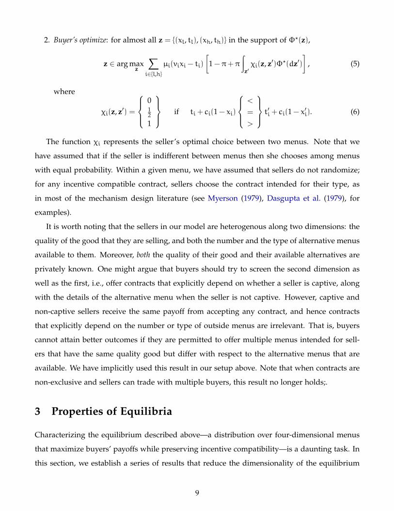
2. Buyer’s optimize: for almost all z = {(xl, tl), (xh, th)} in the support of �?(z),

z 2 arg maxz

X

i2{l,h}µi(vixi - ti)

1 - ⇡+ ⇡

Z

z0�i(z, z0)�?(dz0)

�, (5)

where

�i(z, z0) =

8><

>:

0121

9>=

>;if ti + ci(1 - xi)

8><

>:

<

=

>

9>=

>;t0i + ci(1 - x0i). (6)

The function �i represents the seller’s optimal choice between two menus. Note that we

have assumed that if the seller is indifferent between menus then she chooses among menus

with equal probability. Within a given menu, we have assumed that sellers do not randomize;

for any incentive compatible contract, sellers choose the contract intended for their type, as

in most of the mechanism design literature (see Myerson (1979), Dasgupta et al. (1979), for

examples).

It is worth noting that the sellers in our model are heterogenous along two dimensions: the

quality of the good that they are selling, and both the number and the type of alternative menus

available to them. Moreover, both the quality of their good and their available alternatives are

privately known. One might argue that buyers should try to screen the second dimension as

well as the first, i.e., offer contracts that explicitly depend on whether a seller is captive, along

with the details of the alternative menu when the seller is not captive. However, captive and

non-captive sellers receive the same payoff from accepting any contract, and hence contracts

that explicitly depend on the number or type of outside menus are irrelevant. That is, buyers

cannot attain better outcomes if they are permitted to offer multiple menus intended for sell-

ers that have the same quality good but differ with respect to the alternative menus that are

available. We have implicitly used this result in our setup above. Note that when contracts are

non-exclusive and sellers can trade with multiple buyers, this result no longer holds;.

3 Properties of Equilibria

Characterizing the equilibrium described above—a distribution over four-dimensional menus

that maximize buyers’ payoffs while preserving incentive compatibility—is a daunting task. In

this section, we establish a series of results that reduce the dimensionality of the equilibrium

9

characterization.

First, we show that each menu offered by a buyer can be summarized by the indirect util-

ities that it delivers to each type of seller, so that equilibrium strategies can in fact be defined

by a joint distribution over two-dimensional menus. Then, we establish that the marginal dis-

tributions of offers intended for each type of seller are well-behaved, i.e., that they have fully

connected support and no mass points.

Finally, we establish that there is a very precise link between the two contracts offered by

any buyer, which imposes even more structure on the joint distribution of offers. In particular,

we show that any two menus that are offered in equilibrium are ranked in exactly the same way

by both low and high type sellers; that is, one menu is strictly preferred by a low type seller

if and only if it is also preferred by a high type seller. This property of equilibria, which we

call “strictly rank preserving,” simplifies the characterization even more, as the marginal dis-

tribution of offers for high type sellers can be expressed as a strictly monotonic transformation

of the marginal distribution of offers for low type sellers. This property of equilibria also has

important implications regarding the correlation of offers and terms of trade across different

types of sellers; we explore these predictions in more detail in Section 5, when we explore the

positive implications that emerge from our model in greater detail.

3.1 Utility Representation

As a first step, we establish two results that imply any menu can be summarized by two

numbers, (ul,uh), where

ui = ti + ci(1 - xi) (7)

denotes the utility received by a type i 2 {l,h} seller from accepting a contract zi.

Lemma 1. In any equilibrium, for almost all z in the support of �?, it must be that xl = 1 and

tl = th + cl(1 - xh).

In words, Lemma 1 states that all equilibrium menus require that low quality sellers trade

their entire endowment, and that the incentive compatibility constraint always binds for low

quality sellers. This is reminiscent of the “no-distortion-at-the-top” result in the taxation litera-

ture, or that of full-insurance for the high-risk agents in Rothschild and Stiglitz (1976).

10

Corollary 2. In equilibrium, any menu of contracts {(xl, tl), (xh, th)} 2⇣[0, 1]⇥R+

⌘2can be summa-

rized by a pair (ul,uh) with xl = 1, tl = ul,

xh = 1 -uh - ul

ch - cl, and (8)

th =ulch - uhcl

ch - cl. (9)

Since 0 6 xh 6 1, note that the pair (ul,uh) must satisfy

ch - cl > uh - ul > 0 (10)

in order to satisfy feasibility. Note that when uh = ul, Corollary 2 implies that xh = 1 and

th = tl.

3.2 Recasting the Buyer’s Problem and Equilibrium

Buyer’s Problem. Given the results above, we can recast the problem of a representative buyer

as choosing a menu of indirect utilities, (ul,uh), taking as given the distribution of indirect

utilities offered by other buyers. For any menu (ul,uh), buyers must infer the probability that

the menu will be accepted by a type i 2 {l,h} seller. In order to calculate these probabilities, let

us define the marginal distributions

Fl (ul) =

Z

z0l1⇥t0l + cl

�1 - x0l

�6 ul

⇤��dz0l�

Fh (uh) =

Z

z0h1⇥t0h + ch

�1 - x0h

�6 u

⇤��dz0h

�.

Fl(ul) and Fh(uh) are the probability distributions of indirect utilities arising from each buyer’s

mixed strategy. When these distributions are continuous and have no mass points, the proba-

bility that a contract intended for a type i seller is accepted is simply 1 - ⇡+ ⇡Fi(ui), i.e., the

probability that the seller is captive plus the probability that he is non-captive but receives an

offer less than ui. However, if Fi(·) has a mass point at ui, then the fraction of non-captive

sellers of type i attracted to a contract with value ui is given by Fi(ui) = 12F

-i (ui) +

12Fi(ui),

11

where F-i (ui) = limu%uiFi(u) is the left limit of Fi at ui.9 Given Fi(·), each buyer solves

maxul>cl, uh>ch

µl

�1 - ⇡+ ⇡Fl (ul)

�⇧l (uh,ul) + µh

�1 - ⇡+ ⇡Fh (uh)

�⇧h (uh,ul) (11)

s. t. ch - cl > uh - ul > 0, (12)

with

⇧l (uh,ul) ⌘ vlxl - tl = vl - ul (13)

⇧h (uh,ul) ⌘ vhxh - th = vh - uhvh - clch - cl

+ ulvh - chch - cl

. (14)

In words, ⇧i(uh,ul) is the buyer’s payoff conditional on the offer ui being accepted by a type i

seller. We refer to the objective in (11) as ⇧(uh,ul).

Equilibrium. Using the optimization problem described above, we can redefine the equilib-

rium in terms of the distributions of indirect utilities. In particular, for each ul, let

Uh (ul) = arg maxu0h>ch

⇧�u0h,ul

�

s. t.ch - cl > u0h - ul > 0.

The equilibrium can then be described by the marginal distributions {Fi(ui)}i2{l,h} together with

the requirement that a joint distribution function must exist. In other words, a probability

measure µ over the set of feasible (ul,uh)’s must exist such that, for each ul > u0l and uh > u0

h

1 = µ ({(ul, uh) ; uh 2 Uh (ul)} , ul 2 [cl, vh])

F-l (ul)- Fl�u0l

�= µ

��(ul, uh) ; uh 2 Uh (ul) , ul 2

�u0l,ul

� �, (15)

F-h (uh)- Fh�u0h

�= µ

��(ul, uh) ; uh 2 Uh (ul) , uh 2

�u0h,uh

� �. (16)

Note that this definition of equilibrium imposes two different requirements. The first is that

buyers behave optimally: for each ul, the joint probability measure puts a positive weight only

on uh 2 Uh (ul). The second is aggregate consistency: the fact that Fl and Fh are marginal

distributions associated with a joint measure of menus.

9Since Fi is a distribution function it is right continuous and its left limits exists everywhere (it is cádlág) andit has countable points of discontinuity . We make use of these properties repeatedly throughout the paper.

12

3.3 Basic Properties of Equilibrium Distributions

In this section, we establish that, in equilibrium, the distributions Fl(ul) and Fh(uh) are con-

tinuous and have connected support, i.e., there are neither mass points nor gaps in either

distribution.

Proposition 3. The marginal distributions Fl and Fh have connected support. They are also continuous,

with the possible exception of a mass point at the lower bound of their support.

Much like Burdett and Judd (1983), the basic idea behind the proof of Proposition 3 is to

come up with deviations that rule out having gaps and mass points in the distribution. The

difficulty in our model is that payoffs are interdependent, e.g., a change in the utility offered to

low type sellers changes the contract—and hence the profits—that a buyer receives from high

type sellers. It is possible, however, to prove these claims sequentially, first for the distribution

Fh and then for the distribution Fl. We sketch the proofs here, and present the formal arguments

in the Appendix.

To see that Fh has connected support, suppose towards a contradiction that Fh is constant

on some interval, and consider an equilibrium menu (ul,uh) with uh equal to the upper bound

of this interval. We show that offering a menu (ul,uh), with uh < uh and Fh(uh) = Fh(uh),

is a profitable deviation because the offer uh attracts the same fraction of high quality sellers

but makes more profit per trade. Such a deviation is feasible, however, only if uh > ul. If

instead uh = ul, we show that a deviation to a menu (ul,uh), with ul < ul, must be a profitable

deviation.

To see that Fh has no mass points, suppose towards a contradiction that it does. If ⇧h (uh,ul)

is strictly positive for such a value of uh, then a small increase in uh will increase profits by

attracting a mass of high quality sellers. If, instead, Pih(uh,ul) is not positive, then we can

establish several facts. First, since overall profits must be strictly positive for any ⇡ 2 (0, 1),

then ⇧l(ul,uh) > 0 when ⇧h(ul,uh) 6 0. Second, it must be that uh = ch, as otherwise it

would be profitable to decrease uh by a small amount and shed a positive mass of high type

sellers. Finally, if uh = ch and ⇧h(ul,uh) 6 0, it must be that xh = 0—that is, the buyer will not

actually trade with high type sellers—in which case it must be that ul = cl. Therefore, if there

is a mass point at uh = ch, there must also be a mass point at ul = cl. However, if this is true,

then a small increase in ul is a profitable deviation, which completes the contradiction.

13

Having shown that Fh is continuous and strictly increasing, we then apply an inductive

argument to prove that Fl has connected support and is continuous, with a possible exception

at the lower bound of the support. An important step in the induction argument, which we use

more generally, is to show that the objective function ⇧ (uh,ul) is strictly supermodular. We

state this here as a lemma.

Lemma 4. Suppose Fh has connected support and is continuous over its support. Then the profit

function is strictly supermodular so that

⇧ (uh1,ul1) +⇧ (uh2,ul2) > ⇧ (uh1,ul2) +⇧ (uh2,ul1) , 8ui1 > ui2, i 2 {l,h}

with strict inequality when ui1 > ui2.

The supermodularity of the buyer’s profit function reflects a basic complementarity between

the indirect utilities offered to low and high quality sellers. In particular, an increase in the

indirect utility offered to low quality sellers relaxes their incentive constraint and allows the

buyer to make higher profits from trading high quality sellers. This, in turn, raises the value of

attracting more high types by increasing uh.

An important implication of Lemma 4 is that the correspondence Uh (ul) is weakly increas-

ing. We use this property to construct deviations similar to those described above in order to

rule out gaps and mass points in the distribution Fl at everywhere except possibly at the lower

bound of the support. However, in Section 4, we show that mass points at the lower bound

only occur in a knife-edge case; generically, the marginal distribution Fl has connected support

and no mass points everywhere in its support. We defer the details of the proof to Appendix

A.

3.4 Strict Rank Preserving

In this section, we establish that the mapping between a buyer’s optimal offer to low and high

quality sellers, Uh(ul), is a well-defined, strictly increasing function. As a result, every equilib-

ria has the property that menus are strictly rank preserving—that is, low and high types share the

same ranking over the set of contracts offered in equilibrium—with the possible exception of

the knife-edge case discussed above. To formalize this result, the following definition is helpful.

Definition 5. For any subset Ul of Supp (Fl), an equilibrium is strictly rank-preserving over Ul if

14

the correspondence Uh (ul) is a strictly increasing function of ul for all ul 2 Ul. An equilibrium is

strictly rank-preserving if it is strictly rank-preserving over Supp (Fl).

Equivalently, an equilibrium is strictly rank-preserving when, for any two points in the equi-

librium support (ul,uh) and�u0l,u

0h

�, ul > u0

l if and only if uh > u0h. Given this terminology,

we can now establish one of our key results.

Theorem 6. Let ul = minSupp (Fl). Then all equilibria are strictly rank-preserving over the set

Supp (Fl) \ {ul}.

The proof of Theorem 6, which can be found in the Appendix, makes use of the key facts

established above; namely, that the distributions Fl (·) and Fh (·) are strictly increasing and con-

tinuous, and that ⇧(ul,uh) is supermodular, which implies that Uh (ul) is a weakly increasing

correspondence. In words, if there exists a ul > ul and u0h > uh such that uh,u0

h 2 Uh(ul),

then the supermodularity of ⇧(ul,uh) implies that [uh,u0h] ⇢ Uh(ul). Since Fh(·) has connected

support, this implies that Fl(·) must have a mass point at ul, which contradicts Proposition 3.

A similar argument rules out the possibility that there exist uh and u0l > ul that are offered in

equilibrium with Uh(u0l) = Uh(ul) = uh. Hence, Uh(ul) must be a strictly increasing function

for all ul > ul.

Moreover, when Fl(·) is continuous everywhere—that is, when there is no mass point at the

lower bound of the support—then every menu offered in equilibrium is accepted by exactly the

same fraction of low and high quality non-captive sellers. We state this result in the following

Corollary to Theorem 6.

Corollary 7. If Fl and Fh are continuous, then Fh(Uh(ul)) = Fl(ul).

Taken together, theorem 6 and Corollary 7 simplify the search for equilibrium, which we

undertake in the next Section. Specifically, if an equilibrium exists in which the marginal

distributions Fl and Fh are continuous, then the equilibrium can be described compactly by the

marginal Fl along with the policy function Uh(ul).

4 Construction of Equilibrium

In this section, we use the properties established above to help construct equilibria. Then we

show that the equilibrium we construct is unique. In this sense, we characterize the entire set

of equilibrium outcomes in our model.

15

To fix ideas, it is useful to discuss the well-known extreme cases of ⇡ = 0 and ⇡ = 1,

i.e., when sellers face a monopsonist and when markets are perfectly competitive, respectively.

Using these two extreme cases, we identify a key parameter that governs the structure of the

equilibrium set for the general case of ⇡ 2 (0, 1).

4.1 Monopsony and Perfect Competition

We start by describing the equilibrium outcome when sellers face a monopsonist and perfectly

competitive markets.

Monopsony. When each seller meets with at most one buyer, i.e., ⇡ = 0, the buyers choose a

pair (ul,uh) to maximize

µl(vl - ul) + µh

vh - uh

vh - clch - cl

+ ulvh - chch - cl

�,

subject to the constraint described in (12). The solution to this problem, summarized in Lemma

8 below, is standard and hence we omit the proof.

Lemma 8. Let

� = 1 -µh

µl

✓vh - chch - cl

◆. (17)

When ⇡ = 0, the equilibrium is as follows:

(i) if � > 0, then ul = cl with xl = 1 and uh = ch with xh = 0;

(ii) if � < 0, then ul = uh = ch with xl = xh = 1.

(iii) if � = 0, then ul 2 [cl, ch] with xl = 1 and uh = ch with xh = 0.

Intuitively, the buyer optimally chooses not to trade with the type h seller when � > 0, or

µl > µh

✓vh - chch - cl

◆. (18)

The left hand side of (18) is the marginal benefit of lowering ul = tl: with probability µl, the

buyer pays a marginal unit less in exchange for the low quality good. The right hand side of

(18) is the cost of a small decrease in ul: since reducing ul tightens the incentive compatibility

constraint, the buyer must trade a smaller amount with high quality sellers. Since the objective

is linear, xh = 0 when (18) is satisfied. On the other hand, when (18) is violated, the buyer pools

high and low quality sellers, offering ch in exchange for one unit of either good.

16

Given this interpretation, the parameter � can be thought of as capturing the buyer’s net

loss from a marginal increase in the utility offered to the low quality seller, taking into account

the fact that such an increase relaxes the incentive constraint and leads to higher profits from

trading with the high quality seller. This loss is positive when the fraction of high quality

sellers, µh, is small and/or the gains from trading with high quality sellers, vh- ch, is relatively

small.

Note that an important feature of the monopsony allocations is that the buyer makes non-

negative profits on each type when � > 0. However, when � < 0, the monopolist subsidizes the

low quality sellers in order to be able to trade with high quality sellers, i.e., allocations involve

cross-subsidization. As we will show, this pattern extends to the set of equilibria in our general

model with ⇡ 2 (0, 1).

Bertrand Competition. When markets are perfectly competitive, i.e., when ⇡ = 1, our setup

becomes the same as that in Riley (1975), Riley (1979) and Rosenthal and Weiss (1984), and

similar to that of Rothschild and Stiglitz (1976). As is typical in adverse selection economies,

a pure strategy equilibrium in our model must satisfy separation (uh > ul) and buyers must

earn zero profits on each type of seller (ul = vl and ⇧h(uh, vl) = 0). Indeed, when µh is

sufficiently small, so that � > 0, the unique equilibrium is the least-cost separating contract:

low type sellers earn ul = vl and high type sellers receive vh per unit sold on a fraction of their

endowment, which is sufficiently small to ensure that incentive compatibility holds.

However, when µh is larger, so that � < 0, one can construct a pooling menu which yields

buyers strictly positive payoffs, and hence dominates the pure strategy equilibrium described

above. In this case, no pure strategy equilibrium exists, and thus we turn our attention to

equilibria in mixed strategies, as in Dasgupta and Maskin (1986) and Rosenthal and Weiss

(1984).

In the equilibrium that emerges, buyers mix across menus (ul,uh) in which the payoff from

trading with low types is negative, the payoff from trading with high types is positive, but

the two payoffs offset each other exactly, so that buyers ultimately break even. This is true

across each contract, independent of the marginal distributions. In order to ensure that this

is an equilibrium, however, the marginal distribution Fl(·) must be constructed to ensure that

pure strategy deviations (either pooling or cream-skimming) attract disproportionately many

17

low quality sellers and therefore are not profitable. The following lemma summarizes this

equilibrium in the Bertrand game; the proof is in the Appendix.

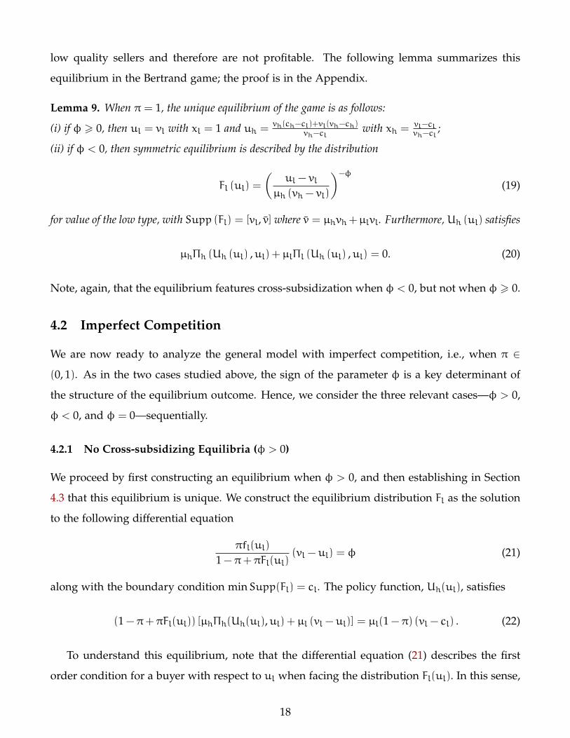
Lemma 9. When ⇡ = 1, the unique equilibrium of the game is as follows:

(i) if � > 0, then ul = vl with xl = 1 and uh = vh(ch-cl)+vl(vh-ch)vh-cl

with xh = vl-clvh-cl

;

(ii) if � < 0, then symmetric equilibrium is described by the distribution

Fl (ul) =

✓ul - vl

µh (vh - vl)

◆-�

(19)

for value of the low type, with Supp (Fl) = [vl, v] where v = µhvh+µlvl. Furthermore, Uh (ul) satisfies

µh⇧h (Uh (ul) ,ul) + µl⇧l (Uh (ul) ,ul) = 0. (20)

Note, again, that the equilibrium features cross-subsidization when � < 0, but not when � > 0.

4.2 Imperfect Competition

We are now ready to analyze the general model with imperfect competition, i.e., when ⇡ 2

(0, 1). As in the two cases studied above, the sign of the parameter � is a key determinant of

the structure of the equilibrium outcome. Hence, we consider the three relevant cases—� > 0,

� < 0, and � = 0—sequentially.

4.2.1 No Cross-subsidizing Equilibria (� > 0)

We proceed by first constructing an equilibrium when � > 0, and then establishing in Section

4.3 that this equilibrium is unique. We construct the equilibrium distribution Fl as the solution

to the following differential equation

⇡fl(ul)

1 - ⇡+ ⇡Fl(ul)(vl - ul) = � (21)

along with the boundary condition minSupp(Fl) = cl. The policy function, Uh(ul), satisfies

(1 - ⇡+ ⇡Fl(ul)) [µh⇧h(Uh(ul),ul) + µl (vl - ul)] = µl(1 - ⇡) (vl - cl) . (22)

To understand this equilibrium, note that the differential equation (21) describes the first

order condition for a buyer with respect to ul when facing the distribution Fl(ul). In this sense,

18

(21) describes necessary conditions for an equilibrium because it ensures local deviations away

from equilibrium menus are not profitable. Implicitly, this first order condition requires three

assumptions. First, that there is not a mass point at the lower bound of the support of Fl(ul).

Second, that for each menu (ul,uh), the utility for the high quality seller is strictly greater

than that for the low quality seller; we call such an equilibrium a separating equilibrium. Lastly,

that the implied quantity traded by the high quality seller is interior in all trades, i.e., 0 <

xh = (uh - ul) /(ch - cl) < 1, except possibly at the boundary of the support of Fl. We call an

equilibrium that satisfies this latter property an interior equilibrium.

Equation (21) is familiar from basic production theory and resembles optimality condition

of a monopolist facing a demand function. For example, in equation (21), the first term on

the left-hand side can be interpreted as the elasticity of demand—it represents the percentage

change in the fraction of low quality sellers attracted to the contract from a one percent change

in the utility offered to the low type seller. Since the second term is profits per trade with low

quality sellers, the left-hand side captures the marginal benefit to the buyer of increasing ul.

On the right-hand side of (21), � represents the marginal cost of increasing the utility of the

low quality seller, taking into account the fact that increasing ul relaxes the incentive constraint.

The fact that � incorporates this additional benefit of increasing ul implies that � < 1, i.e., an

increase in the utility of the low quality seller decreases profits by less than 1.

The boundary condition requires that the lowest utility offered to the low quality seller is

equal to cl. From (22), and using the fact that Fl(cl) = 0, we find Uh(cl) = ch. That is, the

worst menu offered in such an equilibrium coincides with the monopsony outcome. Loosely

speaking, if the worst equilibrium menu offers more utility to high quality sellers than ch,

then a buyer offering this worst menu could increase profit by decreasing uh—his payoff from

trading with high type sellers would increase without changing the payoffs from trading with

low types. On the other hand, if the worst menu offers more utility to low quality sellers than

cl, the buyer could profit by decreasing ul and uh—the gains associated with trading from low

types would exceed the losses associated from trading with high types precisely because � > 0.

The final step in our construction of the equilibrium is to determine the policy function,

Uh(ul). Since the worst menu offered in equilibrium is the monopsony contract and all menus

offered must earn equal profits, Uh(ul) is determined by the equal profit condition, equation

(22). The right-hand side of (22) define monopsony profits. The left-hand side of (22) defines

19

profits earned from the menu (ul,Uh(ul)) given the distribution Fl. The following proposition

asserts that our construction of Fl and Uh(ul) from (21) and (22) constitutes an equilibrium.

Proposition 10. If � > 0, there exists an interior, separating equilibrium with continuous distributions

(Fl, Fh). The equilibrium distribution Fl is characterized by the differential equation (21); the distribution

Fh satisfies Fh(Uh(ul)) = Fl(ul) with Uh(ul) determined by (22).

As discussed above, the differential equation (21) ensures that all local deviations by a buyer

from an equilibrium menu are unprofitable. To complete the proof that Fl and Uh(ul) are an

equilibrium, we need only ensure that no global deviations are profitable; we establish that this

is true in Appendix A. Notice also from (21) that since � > 0, our equilibrium satisfies vl > ul

for all menus in equilibrium. That is, buyers earn strictly positive profits from trading with low

quality sellers. It is straightforward to show that buyers also earn strictly positive profits from

trading with high quality sellers. Therefore, the equilibrium we have constructed features no

cross-subsidization.

4.2.2 Cross-subsidizing Equilibria (� < 0)

We now turn our attention to the case of � < 0. As with monopsony and perfect competition,

cross-subsidization occurs in the region with � < 0. Notice that under Bertrand competition

cross-subsidization is achieved with separating menus. In contrast, under monopsony cross-

subsidization is achieved through a pooling menu. It is then natural to expect equilibrium

menus to feature pooling when � < 0 and markets are imperfectly competitive. We show

that in fact this is the case when the number of high quality sellers is high enough. We pro-

ceed by constructing an equilibrium when � < 0,and then establishing in Section 4.3 that this

equilibrium is unique.

Our equilibrium construction relies on finding a threshold, ul, in the support of the dis-

tribution Fl. For utility levels in the support of Fl, equilibrium menus feature pooling with

Uh(ul) = ul; above the threshold ul, equilibrium menus feature separation with Uh(ul) > ul.

We find the threshold ul as follows. Let ⇧ (ul) be defined as

⇧ (ul) = (1 - ⇡) (µh (vh - ch) + µl (vl - min {ch, ul})) . (23)

20

and let H (ul) satisfy

(1 - ⇡+ ⇡H (ul)) (µhvh + µlvl - ul) = ⇧ (ul) . (24)

Finally, define ul(ul) as

ul(ul) = vl + (ul - vl) [1 - ⇡+ ⇡H (ul)]1� . (25)

Then, the threshold, ul is the value satisfying

µhvh + µlvl - ul(ul) = ⇧ (ul) . (26)

If the solution satisfies ul 2 (ch, ul(ul)), then, we let the equilibrium distribution Fl be given

by

(1 - ⇡+ ⇡Fl (ul)) (µhvh + µlvl - ul) = ⇧ (ul) (27)

for ul 6 ul. For such values of ul, we set Uh(ul) = ul so that menus in this region feature

pooling. For values of ul > ul, Fl satisfies (21) together with the boundary condition

1 - ⇡+ ⇡Fl (ul) =⇧ (ul)

(µhvh + µlvl - ul)

and with Uh(ul) determined by the equal profit condition

(1 - ⇡+ ⇡Fl(ul)) [µh⇧h(Uh(ul),ul) + µl (vl - ul)] = ⇧ (ul) . (28)

In this region of the support of Fl, Uh (ul) > ul so the menus are separating. The support of

the distribution Fl is given by [ch, ul (ul)].

If the solution to (26) satisfies ul 6 ch, then Fl satisfies (21) with the boundary condition

minSupp(Fl) = ul and Uh(ul) is determined by (28). If the solution to (26) satisfies ul > ul(ul),

then Fl satisfies (27), Supp(Fl) = [ch, ul],and Uh(ul) = ul for all ul 2 Supp(Fl).

Relative to our construction when � > 0, it is immediate that our construction when � < 0

is more complicated. Ultimately, this computation relies on finding a solution to the non-

linear equation (26). Note that it is possible for the threshold that solves (26) may be interior

to the support of Fl or at either end of the support. Thus, the constructed equilibrium may

be separating for almost all menus, pooling for all menus, or pooling for some menus and

21

separating for others. We discuss below parameter values such that each of these cases are

possible. Importantly, our equilibrium provides a straightforward partition of the support of

Fl into pooling and separating region which simplifies the characterization greatly. Note also

that the equation (26) may have multiple solutions; in this case, we characterize the equilibrium

using the lowest solution ul.

To understand the equilibria we have constructed, assume that the threshold ul satisfies

ul 2 (ch, ul(ul)), and consider first the pooling region ul 2 [ul, bul). Since buyers must be

indifferent between offering any menu in the pooling region, each of these menus must earn

the same profits in spite of the fact that better utility levels attract a greater number of sellers.

Hence, equation (27) determines the distribution Fl(ul) in this interval. In addition, profits

must satisfy (23) since the worst contract is a pooling menu with a utility offer of ul = ch. The

object, H (ul), determined in (24) specifies the distribution Fl at the upper bound of the pooling

region.

Next consider the separating region. As in Section 4.2.1, local deviations must be unprof-

itable which requires Fl to satisfy (21) and that buyers earn equal profits at all equilibrium

menus determines Uh(ul) in this region according to (28) as a function of Fl(ul). To solve the

differential equation (21) we must specify a boundary condition. Continuity of the distribution

Fl at the threshold, ul, yields the necessary condition given by equation (24). The solution to

the differential equation is given by

1 - ⇡+ ⇡Fl(ul) = (1 - ⇡+ ⇡Fl(bul))

✓bul - vlul - vl

◆�

. (29)

Having solved the differential equation exactly, we then determine the upper bound of the

support of Fl by solving for Fl(ul) = 1 using equation (29). In a slight abuse of notation, we

denote this upper bound ul(bul), which is given by equation (25).

The last step in the construction is to ensure that at the upper bound of the support of Fl,

the pooling menu (ul(bul),ul(bul)) yields profits exactly equal to the profits at the lower bound

⇧ (ul) according to (28). By construction, then, we have imposed that the best menu offered in

equilibrium is a pooling menu. When � < 0, it is straightforward to show that any equilibrium

features this property. If the best menu offered in equilibrium were a separating menu, then a

buyer offering this menu purchases strictly fewer than 1 unit of goods from each high quality

seller; an increase in the utility offered to low quality sellers necessarily improves the buyer’s

22

profits by increasing the amount purchased from high quality sellers with no impact on the

number of sellers the buyer attracts. These results lead us to the non-linear equation (26) which

we solve to determine the threshold, ul.

To prove that our constructed distribution Fl along with the policy function Uh(ul) constitute

an equilibrium we must prove that there are no profitable local deviations in the pooling region

and that there are no global deviations. The following proposition asserts that our construction

of Fl and Uh(ul) using the threshold ul yield an equilibrium and provides a full characterization

of the threshold ul with respect to the support of Fl.

Proposition 11. If � < 0, there exists a threshold equilibrium with continuous distributions (Fl, Fh)

with Fl defined by (26) for ul < ul and (28) for ul > ul, Uh(ul) = ul for ul < ul, Uh(ul) given by

(28) for ul > ul and Fh(Uh(ul)) = Fl(ul). There exists two cutoffs �2 < �1 < 0 such that:

1. When �2 < � < �1, the threshold ul is interior to the support of Fl,

2. When �1 6 �, the threshold ul satisfies ul = minSupp (Fl),

3. When � 6 �2, the threshold ul satisfies ul = maxSupp (Fl).

Proposition 11 describes three types of equilibria: semi-separating equilibria when �2 <

� < �1, separating when �1 6 �, and pooling when � 6 �2. The cutoffs, �1 and �2 represent

necessary conditions for existence of an equilibrium with only separating menus (� > �1) or

with only pooling menus (� 6 �2).

Consider first the cutoff �1. An equilibrium with only separating menus has Uh (ul) > ul

for almost all ul in the support of Fl. In particular, at the lower bound of the support of Fl, in

this case given by the threshold ul, the equilibrium must satisfy ul 6 ch. In the Appendix, we

show that this condition is satisfied for the constructed ul if and only if

ch > vl +⇡(1 - µl) (vh - vl)

(1 - ⇡)h(1 - ⇡)

1-�� - 1

i . (30)

The condition (30) yields an lower bound on �, which we refer to as �1, such that a separating

equilibrium exists. Note also that a lower bound on � is equivalent to an upper bound on µh.

Next consider the cutoff �2. An equilibrium with only pooling menus has ⇧ (ul) = (1 -

⇡) (µhvh + µlvl - ch) and Fl determined by (27). To verify this distribution Fl yields an equi-

librium, we must ensure that the standard cream-skimming deviation is not profitable relative

23

to any pooling menu (ul,ul) with ul in the support of Fl. Such a cream-skimming deviation,

locally, is of the form (ul - ",ul). The decrease in ul can be attractive for two reasons: first, it

decreases the loss in a trade with a low quality seller; and second, it decreases the number of

non-captive low quality sellers that the buyer attracts, inducing a more favorable mix of non-

captive high and low quality sellers. Since the best pooling menu offers the largest subsidy to

low quality sellers, one can that show a buyer’s incentive to cream-skim are strongest at the

most generous menu offered in equilibrium, which occurs at the threshold ul. Thus, if cream-

skimming is not profitable at the pooling menu offering utility bul, then it is not profitable at

any pooling menu offering utility less than bul. As we show in the Appendix, cream-skimming

is not profitable at the pooling menu offering utility bul if, and only if,

1 - ⇡ > µhvh + µlvl - vl(1 -�)(µhvh + µlvl - ch)

. (31)

The condition (31) yields an upper bound on �, which we refer to as �2, such that a pooling

equilibrium exists. One can prove that �2 < �1 so that if a pooling equilibrium exists, then a

separating equilibrium does not and vice versa.

When � lies between these cutoffs, �2 < � < �1, one can prove that the threshold ul is inte-

rior to the support of the constructed Fl. To confirm that the candidate threshold equilibrium is

indeed an equilibrium, we must prove that buyers have no profitable deviations. By construc-

tion, buyers have no incentive to deviate locally to alternative menus in the separating region.

Hence, we need only check deviations in the pooling interval. As in the pooling equilibrium, it

suffices to check that cream-skimming is not profitable at the pooling menu offering utility ul.

In the Appendix, we show that when �2 < � < �1, such cream-skimming deviations are not

profitable at ul.

4.2.3 Equilibria with Mass Points (� = 0)

When � 6= 0, we have described the construction of equilibria assuming that the distributions

Fl and Fh do not feature mass points. Here, we construct an equilibrium � = 0 that does feature

mass points. In particular, we construct an equilibrium in which the distribution Fl assigns full

mass to ul = vl. The distribution Fh is determined by the equation

(1 - ⇡+ ⇡Fh (uh))µh⇧h (uh, vl) = (1 - ⇡)µl (vl - cl) (32)

24

with Supp(Fh) =hch, ch + ⇡

(vl-cl)(vh-ch)vh-cl

i.

To understand this equilibrium, note that (32) is determined to ensure that buyers have no

incentive to deviate by changing only uh. Next, consider the incentives of a buyer to deviate by

perturbing ul away from vl. An marginal increase in ul leads to a marginal increase in profits

earned per high quality seller attracted. However, the number of non-captive low quality sellers

increases discretely. A marginal decrease in ul is also unprofitable. Such a deviation increases

profits earned per captive low-quality seller but decrease profits earned per high-quality seller.

It is straightforward to show that when � = 0, the losses from this deviation are larger than

the gains. The next proposition asserts that the equilibrium we have constructed is indeed an

equilibrium.

Proposition 12. When � = 0, the pair of distribution functions - Fl degenerate at vl and Fh satisfying

(32) - constitute an equilibrium.

4.3 Uniqueness

In this section, we establish uniqueness of the equilibrium we have constructed. We proceed by

discussing the key results needed to ensure uniqueness for each �.

Consider first the separating equilibrium we construct when � > 0. We demonstrate unique-

ness of the separating equilibrium by ruling out the two relevant alternatives. To be more

precise, we first show that there are no equilibria with mass points when � > 0. Then we

establish that there are no equilibria that feature pooling, i.e., there are no equilibria in which

Uh(ul) = ul for some ul 2 Supp(Fl).

Next, consider the threshold equilibrium we construct when � < 0. We demonstrate unique-

ness of the threshold equilibrium as follows: first, we show that any equilibrium features pool-

ing at the upper bound of the support of Fl; second, we prove that any equilibrium features at

most one interval of pooling followed by at most one interval of separation; third, we prove that

the equilibria characterized in Proposition 11 are mutually exclusive so that equilibria without

mass points are unique; fourth, we prove no equilibrium features mass points demonstrating

uniqueness of the equilibrium characterized in Proposition 11.

Finally, when � = 0, it is straightforward to prove that in any equilibrium, Fl must be

degenerate at ul = vl. We summarize these results in the following Theorem.

25

Theorem 13. For any (⇡,�), the applicable equilibrium constructed in Section 4.2.1, 4.2.2, or 4.2.3 is

unique.

5 Discussion

In this section, we explore the implications of the equilibrium characterization provided above.

We begin with positive implications, paying particular attention to how the nature of the con-

tracts that are offered in equilibrium are affected by both the severity of the adverse selection

problem and the degree of competition. We show that, in contrast with many papers in the

literature, whether buyers offer sellers separating or pooling menus depends on the underly-

ing distribution of types in the market. Moreover, this decision depends systematically on the

underlying market structure: separating menus are more prevalent when markets are more

competitive, while pooling menus emerge when markets are more frictional. Hence, observing

separating contracts in a market is not necessarily a sign of severe adverse selection; identifying

the severity of information frictions requires knowledge of the prevailing trading frictions.

We then explore some of the normative implications, fleshing out the affect of competition

on ex ante welfare in different regions of the parameter space. We show that, when adverse

selection is severe, ex ante welfare is inverse U-shaped in ⇡, so that there is an interior level of

frictions that maximizes surplus from trade. When adverse selection is mild, on the other hand,

ex ante welfare is monotonic and decreasing in ⇡, so that competition unambiguously hinders

the process of realizing gains from trade.

Finally, we demonstrate that explicitly modeling competition and allowing for general con-

tracts yields novel and interesting policy implications. Specifically, we analyze the effect of

making additional information about sellers’ types available to buyers on ex-ante welfare. This

is a very topical question in the context of recent developments, both due to policy and/or

technological changes, in a number of insurance and financial markets. Our main finding is

that the desirability of additional information depends both on the distribution of types and

the degree of competition. In particular, when adverse selection is relatively mild to begin with

or when the market is very competitive, additional information is detrimental to welfare. The

opposite is true when adverse selection and trading frictions are relatively severe. Thus, eval-

uating the implications of these policies requires knowledge of the distribution of types in the

26

0 1

1

π

µh

µ0

µ1

µ2

Region CRegion D

Region B

Region A

Figure 1: Equilibrium thresholds. Region A: no cross-subsidization, separating. Region B:cross-subsidization, separating. Region C: cross-subsidization, pooling at low ul, separating athigh ul. Region D: cross-subsidization, pooling.

population as well as the extent of frictions.

5.1 Equilibrium Contracts, Adverse Selection, and Competition

Figure 1 depicts the various types of equilibria that arise for different values of µh and ⇡, which

represent the fraction of high quality sellers and the degree of competition in the market,

respectively. The figure shows that for each value of ⇡ 2 (0, 1), there are three critical cutoffs:

µ0, µ1, and µ2. When the adverse selection problem is relatively severe — that is, when µh < µ0

— buyers optimally choose to offer separating contracts (region A). Moreover, these contracts

do not feature cross subsidization; all contracts offered in equilibrium yield a positive expected

payoff from both low and high type sellers. As µh increases, however, the incentive to trade

larger quantities with high type sellers increases, as such sellers are more abundant. Indeed,

for all µh > µ0 (regions B,C and D), all equilibrium contracts feature cross-subsidization, as

low quality sellers earn information rents that relax incentive constraints and enable buyers to

trade larger quantities with high quality sellers.

In region B, i.e. when µh 2 (µ0,µ1), all equilibrium menus are composed of separating

contracts. In this region, even though a monopsonist would like to pool low and high quality

sellers, such an offer cannot be sustained. The reason, as we discussed above, is that cream-

27

skimming is still optimal in this region: a buyer could profitably deviate by offering less utility

to low types, while offering the same utility to high types by trading a smaller quantity at a

higher price. Since µh is still relatively small in this region, the benefits of trading with fewer

low types (and hence suffering fewer losses) outweigh the cost of extracting less rents from

high types.

As µh continues to increase, however, the benefits of cream-skimming deviations subside

while the costs grow. As a result, in region C, when µh > µ1, at least some pooling menus can

be sustained in equilibrium. In particular, whenever some pooling menus are offered, they will

be the menus that deliver low levels of utility to sellers. Intuitively, those buyers whose offers

fall in the lower portion of the distribution of indirect utilities earn most of their profits from

captive sellers; the benefits of altering the mix of low and high quality non-captive sellers they

attract by deviating to a cream-skimming menu are small relative to the costs of extracting fewer

rents from the mass of captive, high quality sellers. Conversely, those buyers offering indirect

utilities at the top of the distribution trade with a large fraction of non-captive sellers, and

hence the cream skimming deviation may still be profitable. Thus, when µh 2 (µ1,µ2), menus

that offer high indirect utilities remain separating menus. However, when µh > µ2 (region

D), cream-skimming is not profitable anywhere in the distribution of equilibrium offers, and

all buyers offer pooling menus. Overall, comparative statics with respect to µh reveal that the

underlying distribution of asset quality affects whether menus feature cross-subsidization and

whether they feature pooling or separating contracts. Interestingly, this is not the case in related

models like Guerrieri et al. (2010).

Figure 1 also shows that pooling is more prevalent when markets are less competitive. In

particular, when µh is sufficiently high, the equilibrium features at least some (if not all) pooling

menus. However, for similar reasons to those discussed above, the incentive to deviate to a

cream-skimming menu grows as ⇡ increases and a larger fraction of profits are generated from

trades with non-captive sellers. When ⇡ gets sufficiently close to 1, in fact, no pooling menus

can be sustained. Note that these last results imply that the relationship between the contracts

that are traded in a market and the severity of the adverse selection problem can ultimately

depend heavily on the degree of competition in that market. In particular, the observation that

separating contracts are observed in market A and not in market B does not necessarily imply

that adverse selection is more severe in market A than B.

28

5.2 Ex-ante Welfare and Competition with Adverse Selection

We now turn our attention to the relationship between ex ante welfare and competition, as

captured by ⇡, for varying degrees of adverse selection, as captured by µh. To start, note that

ex ante welfare is given by

µlvl +(1 - ⇡)

Zµh (vhxh (ul) + ch (1 - xh (ul)))dFl (ul) (33)

+⇡

Zµh (vhxh (ul) + ch (1 - xh (ul)))d

⇣Fl (ul)

2⌘

where

xh (ul) = 1 -Uh (ul)- ul

ch - cl. (34)

The first term represents the total surplus from trade between low quality sellers and buyers;

since xl = 1 with probability 1, all low quality trades generate a surplus of vl, the buyers’

valuation. The second term in (33) captures the total surplus created from trades between

buyers and captive high-quality sellers; a captive high-quality seller trades a quantity xh (ul),

where ul is drawn from Fl (ul). Likewise, the last term in (33) captures the total surplus

created from trades between buyers and non-captive high-quality sellers; since non-captive

sellers choose the maximum indirect utility among the two offers they receive, they trade xh (ul)

with ul drawn from Fl (ul)2.

Using this definition of ex ante welfare, we show that ex ante welfare is inverse U-shaped

in ⇡ when adverse selection is severe; that is, there is an interior level of frictions that maximize

the surplus generated from trade. On the other hand, when adverse selection is mild, ex ante

welfare is strictly decreasing in ⇡; that is, more competition is unambiguously bad for welfare.

The following proposition summarizes.

Proposition 14. When µh < µ0, there exists a ⇡ 2 (0, 1) that maximizes ex ante welfare. On the other

hand, when µh > µ0, ex ante welfare is maximized at ⇡ = 0.

Two key features of our equilibrium can account for the first result. First, when ⇡ is suffi-

ciently large, xh(ul) is inverse U-shaped in ul. Second, as ⇡ increases, Fl (ul) increases in the

sense of first order stochastic dominance; that is, Fl shifts to the right, putting more weight on

offers with lower values of xh. This drives down the total quantity traded with high quality

sellers, and thus ex ante welfare.

29

But why is xh(ul) decreasing for high values of ul when ⇡ is sufficiently close to 1? Intu-

itively, when � > 0, buyers compete for low quality sellers more intensely than they compete

for high quality sellers, since the former are relatively more abundant. Thus, offers to low qual-

ity sellers are clustered very tightly at the top of Fl; demand in this region is very elastic and,

in order to satisfy the equal profits condition, prices offered to low quality sellers have to rise

relatively slowly.10 Competition for high quality sellers, on the other hand, is less fierce. As a

result, offers to high quality sellers are more dispersed at the top of Fh; demand in this region

is more inelastic, and hence prices offered to high quality sellers have to rise very quickly. In

order to achieve this increase, the quantity traded with high quality sellers has to fall.

To see the mathematics behind this result, note that (8) implies that xh (ul) = xh(Uh(ul)) is

decreasing if and only if U0h (ul) > 1. Moreover, from (22), one can derive

U0h (ul) =

� (ch - cl)

vh - cl

�⇥ ⇧h(Uh(ul),ul)

vl - ul. (35)

Therefore, as ⇡ ! 1, U0h (ul) > 1 if ul converges to vl faster than ⇧h(ul,Uh(ul)) converges to

zero. This is exactly the case when � > 0, and the incentive to outbid other buyers to trade

with non-captive, low quality sellers is strong relative to the incentive to outbid other buyers

for non-captive, high quality sellers.

The second result — that ex ante welfare is maximized at ⇡ = 0 when � < 0 — is more

straightforward. Since a monopsonist offers a pooling contract in this region of the parameter

space, all gains from trade are exhausted. By introducing competition, one simply increases

a buyer’s incentive to deviate to a cream-skimming menu. In order to make such a deviation

unprofitable, equilibrium contracts offer high quality sellers a higher price but a lower quantity

to trade, and this causes a decline in ex ante welfare.

5.3 Information, Disclosure, Discrimination, and Welfare

In this section, we show that explicitly modeling imperfect competition in an environment with

both adverse selection and general contracts reveals new and interesting implications regarding

the impact of certain policy choices and technological innovations. In other words, several

normative insights that have been derived under a particular market structure (e.g., perfect

competition) or with ad-hoc restrictions on contracts may not be particularly robust.

10Indeed, from (21), one can see that as ⇡ tends to 1, limul!vl fl(ul) = 1.

30

We demonstrate this insight by analyzing what happens when buyers have better informa-

tion about sellers. Consider an environment in which the probability that a particular seller

is high quality, µ0h, is a random variable drawn from G(µ0

h). In the baseline case, i.e. without

additional information, buyer behavior and therefore, the equilibrium outcome is determined

by the unconditional average, µh =Rµ0hdG(µ0

h). and ⇡. If buyers have additional information

about the seller’s type, denoted I, it induces a set of conditional distributions, G(µ0h, I). For

each such I, the equilibrium is determined by the conditional mean µh(I) =Rµ0hdG(µ0

h, I). Ob-

viously, µh = E[µh(I)], where the expectation is taken over the realizations of I. In this sense,

more information induces a mean-preserving spread of the distribution of the average asset

quality, µh. Below, we discuss how this is a natural way to model additional information -

whether due to policies or other changes - in insurance and financial markets and examine its

effects on welfare.

1. Non-discrimination in insurance markets. Under the Affordable Care Act, insurance

providers are not allowed to discriminate based on certain observable characteristics (e.g.

health factors). In other words, participants with known differences in risk must be of-

fered the same menus (of benefits, premiums etc.). In the context of our model, we can

interpret these differences in risk as differences in µh across subgroups of the population.

The distribution of group-specific µh is a mean-preserving spread of the unconditional

distribution. Then, under the non-discrimination policy, insurance companies would offer

contracts based on the pooled (or population) µh. In the absence of such a policy, i.e. if

companies were free to offer different terms to different subgroups, the set of contracts

offered in equilibrium to each subgroup would be based on their µh.

2. Credit scores in consumer loan markets. The development of standardized scoring sys-

tems to assess borrower creditworthiness is widely believed to have played an important

role in the expansion of US consumer credit markets over the last three decades11. Again,

interpreting these credit scores as signals about borrower types, it is easy to see that they

induce a mean-preserving spread of the distribution of the average asset quality.

3. Transparency in financial markets. An important debate in financial regulation relates

to disclosure of trades conducted in decentralized or over-the-counter settings. Many

11See Chatterjee et al. (2011) and Einav et al. (2013)

31

securities in the US are now subject to rules requiring public dissemination of trade in-

formation. For example, all transactions in corporate bonds and asset-backed securities

are now required to be reported within 15 minutes through a centralized reporting sys-

tem called Trade Reporting and Compliance Engine (TRACE). This is intended to induce

"price discovery and improved bargaining power of previously uninformed participants",

and in turn " a decrease in bond price dispersion and an increase in trading activity"

(Levitt (1999)). To map this into our mean-preserving spread experiment, suppose that

the fraction of high quality assets is state-dependent. Disclosure of past trades essen-

tially generates a signal about the state of the world (i.e. about µh) and thus, induces a

mean-preserving spread of the unconditional distribution.

To start, let us define welfare explicitly in terms of µh, so that

W (µh) = (1 - µh) vl + µhvhXh (µh) + µhch (1 -Xh (µh))

where Xh (µh) ⌘Zxh (u)dR (u,µh)

and R (u,µh) = (1 - ⇡) Fl (u,µh) + ⇡F2l (u,µh) .

Note that, for expositional simplicity, we have retained the dependence of allocations and the

distribution on µh, while suppressing the dependence on ⇡. The effect of a mean-preserving

thus depends on the curvature of W (µh). If W is convex (concave) in µh over the relevant

region, a mean-preserving spread increases (reduces) welfare.

It is important to mention that we are interested in local mean-preserving spreads. Addi-

tional information of sufficiently high quality always improves welfare. To see this, consider the

extreme case of a perfectly informative signal. This eliminates the adverse selection problem

and achieves first-best welfare, irrespective of the degree of competition - clearly, not a very

interesting (or realistic) experiment. Therefore, in what follows, we restrict attention to ‘small’

spreads.

Before considering the general case, it is worthwhile to examine the limiting cases of monop-

sony and Bertrand competition. Recall from Lemma 8, that under monopsony, xh = 0 when

µh < µ0, so W (µh) = (1 - µh) vl + µhch = vl + µh (ch - vl). When µh > µ0, the monopsonist

pools so xh = 1, so we have W (µh) = vl + µh (vh - vl). In other words, under monopsony,

W consists of two piece-wise linear segments, with a discontinuity at µh = µ0. Directly, a

32

µh

Wel

fare

Cross−subsidizing, µh > µ0

µ0 1

Low πHigh π

0µh

Wel

fare

No cross−subsidizing, µh < µ0

µ0

Low πHigh π

Figure 2: Welfare as a function of µh

mean-preserving spread is welfare-neutral unless such spreading spans the discontinuity. At

the other extreme, when ⇡ = 1, W is also linear in the region where a pure strategy equilibrium

exists (i.e. which µh < µ0). This is because xh is pinned down entirely by the incentive con-

straint and independent of µh. Again, within this region, the policy experiments have no effect

on welfare. The analysis of the case with mixed strategies is more involved and closely related

to the general case of ⇡ 2 (0, 1) to which we turn next.

Our results for ⇡ 2 (0, 1) are depicted in Figure 2, which shows the effect of mean preserving

spreads for the two cases of cross-subsidizing and no-cross subsidizing equilibria. Each panel

plots the W over an interval of µh, for two different values of ⇡. The first panel considers an

interval entirely in the cross-subsidizing region, i.e. when µh > µ0. In this region, W is concave,

both for high and low ⇡, implying that mean-preserving spreads are detrimental. To see why,

first note that higher µh shifts the distributions of ul and uh to the right. This is intuitive -

as the probability of high quality assets increases, the adverse selection becomes less severe,

so both seller types receive higher utilities. This also results in higher xh, increasing overall

welfare. However, this change in the distribution becomes more gradual as µh rises closer to

the pooling region. In other words, a reduction in µh has a bigger effect on the distribution -

and consequently on expected trade Xh and welfare - than an increase of similar magnitude.

The opposite happens in the no-cross subsidization region, provided ⇡ is sufficiently low. In

this region, W is convex, so mean-preserving spreads increase welfare. With ⇡ is high, however,

there is an additional effect. Recall from Section 5.2 that xh is decreasing in ul when ⇡ is high.

33

This moderates the direct gains from a rightward shift in the distribution of utilities induced

by higher µh. The combined effect of these two forces results in a region where W is concave,

making mean-preserving spreads undesirable. Thus, in the no cross subsidization region, the

curvature of W varies with ⇡ so mean-preserving spreads can be good or bad for welfare12.

Thus, the concavity of W depends in a rich way both on the type of equilibrium (cross-

subsidizing vs no cross subsidization) as well as on ⇡. Broadly speaking, our results suggest

that providing additional information to buyers is less likely to be desirable when the adverse

selection problem is relatively mild to begin with (in the sense that µh is high) or when the

market is very competitive (i.e. when ⇡ is high). Therefore, in order to assess even the qualita-

tive effect of policies like the ones described at the beginning of the section, one needs to first

accurately measure both the degree of competition and the severity of adverse selection.

6 General Model with Many Types

In this section, we modify our environment to allow for more than two types and show that

the key insight about equilibria in the two type case - strict rank-preserving menus - extends to

this more general case.

Formally, there is one seller endowed with a single unit of a perfectly divisible good of

type i 2 {1, 2, · · · ,N}. The probability of type i is given by µi. As before, buyers and sellers

derive utility vi and ci with vi > ci 8 i. Without loss of generality, we order the types so that

c1 < c2 < ..... < cN, i.e. type-1 is the lowest seller type. We maintain the ‘lemons assumption’,

which in this setting amounts to ci+1 > vi i = 1, 2...N- 1.

Strategies and definition of equilibrium: Let zi = (xi, ti) denote the contract intended for

type i. It specifies the quantity that changes hands and the transfer. Correspondingly, we let

z = (z1, z2.....zN) denote a menu of contracts offered by each buyer. A buyer’s strategy is a

distribution � over such menus, while the seller simply chooses the contract with the highest

payoff from the menus available to her.

A symmetric equilibrium is given by a distribution �⇤ such that, for almost all z in the

support of �⇤ the following properties are satisfied

12Numerical calculations, however, suggest that the concavity of W is relatively mild and occurs only over anarrow region of the parameter space - in other words, W appears to be mostly convex in the no cross subsidizationregion.

34

1. Incentive compatibility

ti + ci (1 - xi) > tj + ci�1 - xj

�

2. Buyers optimize

z 2 arg maxz

X

i2{l,h}µi(vixi - ti)

1 - ⇡+ ⇡

Z

z0�i(z, z0)�?(dz0)

�

where

�i(z, z0) =

8><

>:

0121

9>=

>;if ti + ci(1 - xi)

8><

>:

<

=

>

9>=

>;t0i + ci(1 - x0i).

As in the two type, we first show that a menu can be summarized by a vector of indirect

utilities it offers to each type: u = (u1, .....uN), where ui = ti + ci (1 - xi). The next result

follows from the same logic as that underlying Lemma 1.

Lemma 15. In almost all equilibrium menus, x1 = 1 and the local downward IC’s are binding, i.e.

ti + ci (1 - xi) = ti+1 + ci (1 - xi+1) i = 1, 2.....N- 1

This result allows us to recast the buyer’s problem in terms of the utility vector u. Formally,

define a family of distribution functions

Fi (ui) =

Z

z0i1⇥t0i + ci

�1 - x0i

�6 ui

⇤��dz0i�

i = 1, 2, .....N

Given {Fi}, the buyer solves

maxui>ci

NX

i=1

µi (1 - ⇡+ ⇡Fi (ui))⇧i (u1,u2....uN)

subject to ci+1 - ci > ui+1 - ui > 0

with ⇧i (u1,u2....uN) = vi - ui

✓vi - ci-1ci - ci-1

◆+ ui-1

✓vi - cici - ci-1

◆

Note that the profit function ⇧i is increasing the ui-1 ,reflecting the value of relaxing the in-

centive constraint of type i- 1. Let ⇧ (u1,u2....uN) denote the objective in the above problem.

Define

U (u1) =

8<

:(u2, ....uN) : (u2, ....uN) 2 arg max{uj}

N

j=2

⇧ (u1, u2..ui, ..uN)

9=

;

35

Definition 16. An equilibrium is strictly rank-preserving if, for all ul 2 Supp (Fl), U (u1) is single-

valued and strictly increasing, element by element, i.e. if u1 > u01, then every element of U (u1) is

strictly larger than its counterpart in U�u0

1�

.

We are now ready to state the main result of this section. It shows that, except in a knife-

edge case where the cost of providing utility to the lowest type is exactly zero, the equilibrium

is strictly rank-preserving.

Theorem 17. If �1 = 1 - µ2µ1

⇣v2-c2c2-c1

⌘6= 0, the equilibrium is strictly rank-preserving.

The strategy for the proof, laid out in the Appendix, closely follows the one we used for

Theorem 6 in the two-type case. The key step is to show that the distribution functions, {Fi}Ni=1

are continuous and have connected support. We proceed by induction - we start by proving

this for FN, the highest quality type. We then use this result and the supermodularity of the

profit function to inductively rule out flat spots in the distribution functions Fi.

The next step in the proof is show that if the equilibrium exhibits masspoints in any Fi,

they must be comprised of menus which make zero profits from the lowest type13, i.e. where

u1 = v1. For such a masspoint to be sustainable when ⇡ 2 (0, 1), the net marginal cost of

providing utility to the lowest type, the coefficient �1 in the statement of the theorem, must be

exactly zero. If this condition is violated, i.e. if �1 6= 0, deviations from u1 = v1 yield strictly

higher profits. In other words, if �1 6= 0, masspoints cannot occur in any equilibrium Fi. Finally,

the fact that all the Fi’s are continuous and strictly increasing can be used to rule out regions

where U (u1) is weakly-increasing or is a correspondence, completing the proof.

13This is analogous to our finding in the two type case that masspoints in Fl can only occur at ul = vl.

36

References

Akerlof, G. A. (1970): “The market for" lemons": Quality uncertainty and the market mecha-

nism,” The quarterly journal of economics, 488–500. 5

Azevedo, E. M. and D. Gottlieb (2014): “Perfect Competition in Markets with Adverse Selec-

tion,” The Wharton School Research Paper. 5

Benabou, R. and J. Tirole (2014): “Bonus Culture: Competitive Pay, Screening, and Multitask-

ing,” Journal of Political Economy, forthcoming. 5, 6

Bigio, S. (2014): “Endogenous Liquidity and the Business Cycle,” Tech. rep. 5

Burdett, K. and K. L. Judd (1983): “Equilibrium Price Dispersion,” Econometrica, 51, 955–69. 3,

6, 7, 13

Butters, G. R. (1977): “Equilibrium Distributions of Sales and Advertising Prices.” Review of

Economic Studies, 44. 7

Camargo, B. and B. Lester (2014): “Trading dynamics in decentralized markets with adverse

selection,” Journal of Economic Theory, 153, 534–568. 5

Chang, B. (2012): “Adverse selection and liquidity distortion,” Available at SSRN 1701997. 5

Chari, V., A. Shourideh, and A. Zetlin-Jones (2014): “Reputation and persistence of adverse

selection in secondary loan markets,” American Economic Review, 104, 4027–70. 5

Chatterjee, S., D. Corbae, and J.-V. Rios-Rull (2011): “A theory of credit scoring and com-

petitive pricing of default risk,” Unpublished paper, University of Minnesota.[672]. 31

Chiappori, P.-A. and B. Salanie (2000): “Testing for asymmetric information in insurance

markets,” Journal of Political Economy, 108, 56–78. 5

Dasgupta, P., P. Hammond, and E. Maskin (1979): “The Implementation of Social Choice

Rules: Some General Results on Incentive Compatibility,” The Review of Economic Studies,

185–216. 9

Dasgupta, P. and E. Maskin (1986): “The Existence of Equilibrium in Discontinuous Economic

Games, I: Theory,” The Review of Economic Studies, 53, 1–26. 3, 17, 40

37

Einav, L., A. Finkelstein, and M. R. Cullen (2010a): “Estimating welfare in insurance markets

using variation in prices,” Quarterly Journal of Economics, 125. 5

Einav, L., A. Finkelstein, and J. Levin (2010b): “Beyond Testing: Empirical Models of Insur-

ance Markets,” Annu. Rev. Econ, 2, 311–36. 2

Einav, L., M. Jenkins, and J. Levin (2012): “Contract pricing in consumer credit markets,”

Econometrica, 80, 1387–1432. 5

——— (2013): “The impact of credit scoring on consumer lending,” The RAND Journal of Eco-

nomics, 44, 249–274. 31

Fuchs, W., A. Ory, and A. Skrzypacz (2012): “Transparency and distressed sales under asym-

metric information,” Unpublished manuscript. 5

Fuchs, W. and A. Skrzypacz (2013): “Costs and benefits of dynamic trading in a lemons

market,” . 5

Garrett, D. F., R. D. Gomes, and L. Maestri (2014): “Competitive Screening Under Hetero-

geneous Information,” . 6

Guerrieri, V. and R. Shimer (2014a): “Dynamic Adverse Selection: A Theory of Illiquidity,

Fire Sales, and Flight to Quality,” The American Economic Review, 104. 5

——— (2014b): “Markets with multidimensional private information,” Tech. rep., National

Bureau of Economic Research. 5

Guerrieri, V., R. Shimer, and R. Wright (2010): “Adverse selection in competitive search

equilibrium,” Econometrica, 78, 1823–1862. 5, 6, 28

Ivashina, V. (2009): “Asymmetric information effects on loan spreads,” Journal of Financial

Economics, 92, 300–319. 5

Kurlat, P. (2013): “Lemons markets and the transmission of aggregate shocks,” The American

Economic Review, 103, 1463–1489. 5

Levitt, A. (1999): “Testimony to the U.S. Congress House of Representa-

tives House Subcommittee on Finance and Hazardous Materials,” Available at:

http://www.sec.gov/news/testimony/testarchive/1999/tsty0499.htm. 32

38

Mahoney, N. and E. G. Weyl (2014): “Imperfect Competition in Selection Markets,” Tech. rep.,

National Bureau of Economic Research. 5, 6

Maskin, E. and J. Riley (1984): “Monopoly with incomplete information,” The RAND Journal

of Economics, 15, 171–196. 3

Mirrlees, J. (1971): “An Exploration in the Theory of Optimum Income Taxation,” The Review

of Economic Studies, 38, 175–208. 3

Myerson, R. B. (1979): “Incentive Compatibility and the Bargaining Problem,” Econometrica, 47,

61–74. 9

Riley, J. G. (1975): “Competitive Signalling,” Journal of Economic Theory, 10, 174–186. 17

——— (1979): “Informational Equilibrium,” Econometrica, 47, 331–59. 17

Rosenthal, R. W. and A. M. Weiss (1984): “Mixed Strategy Equilibrium in a Market with

Asymmetric Information,” Review of Economic Studies, 51, 333–342. 3, 5, 17

Rothschild, M. and J. Stiglitz (1976): “Equilibrium in Competitive Insurance Markets: An

Essay on the Economics of Imperfect Information,” Quarterly Journal of Economics, 90, 629–649.

3, 5, 10, 17

Stiglitz, J. E. (1977): “Monopoly, non-linear pricing and imperfect information: the insurance

market,” The Review of Economic Studies, 407–430. 3

Varian, H. R. (1980): “A Model of Sales,” American Economic Review, 70, 651–59. 7

Veiga, A. and E. G. Weyl (2012): “Multidimensional product design,” University of Chicago

mimeo. 5

39

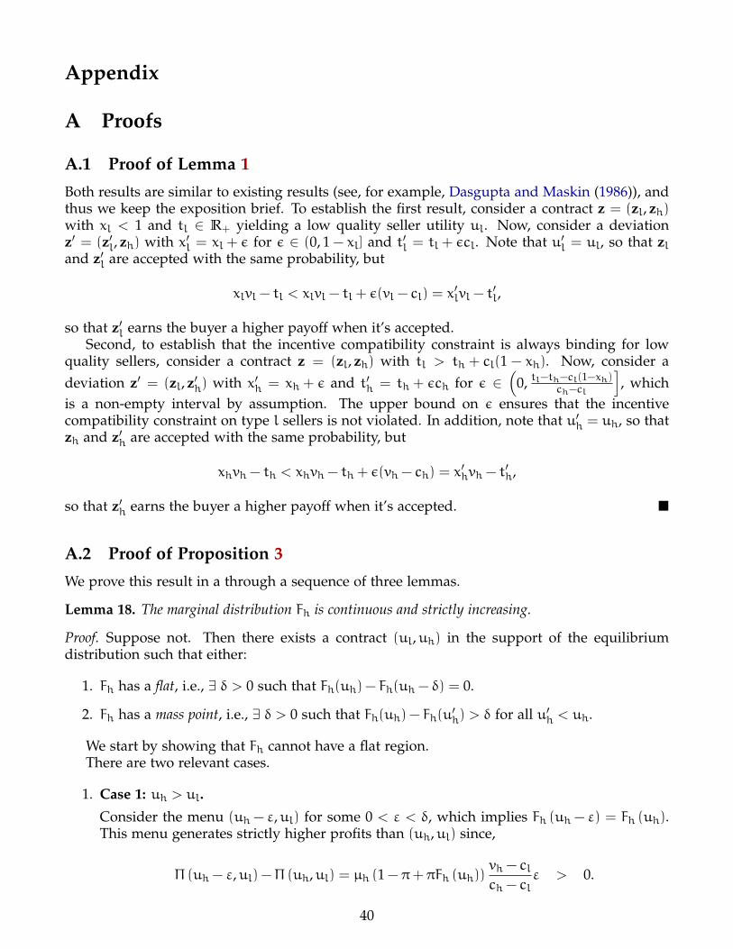
Appendix

A Proofs

A.1 Proof of Lemma 1

Both results are similar to existing results (see, for example, Dasgupta and Maskin (1986)), andthus we keep the exposition brief. To establish the first result, consider a contract z = (zl, zh)with xl < 1 and tl 2 R+ yielding a low quality seller utility ul. Now, consider a deviationz0 = (z0l, zh) with x0l = xl + ✏ for ✏ 2 (0, 1 - xl] and t0l = tl + ✏cl. Note that u0

l = ul, so that zland z0l are accepted with the same probability, but

xlvl - tl < xlvl - tl + ✏(vl - cl) = x0lvl - t0l,

so that z0l earns the buyer a higher payoff when it’s accepted.Second, to establish that the incentive compatibility constraint is always binding for low

quality sellers, consider a contract z = (zl, zh) with tl > th + cl(1 - xh). Now, consider adeviation z0 = (zl, z0h) with x0h = xh + ✏ and t0h = th + ✏ch for ✏ 2

⇣0, tl-th-cl(1-xh)

ch-cl

i, which

is a non-empty interval by assumption. The upper bound on ✏ ensures that the incentivecompatibility constraint on type l sellers is not violated. In addition, note that u0

h = uh, so thatzh and z0h are accepted with the same probability, but

xhvh - th < xhvh - th + ✏(vh - ch) = x0hvh - t0h,

so that z0h earns the buyer a higher payoff when it’s accepted. ⌅

A.2 Proof of Proposition 3

We prove this result in a through a sequence of three lemmas.

Lemma 18. The marginal distribution Fh is continuous and strictly increasing.

Proof. Suppose not. Then there exists a contract (ul,uh) in the support of the equilibriumdistribution such that either:

1. Fh has a flat, i.e., 9 � > 0 such that Fh(uh)- Fh(uh - �) = 0.

2. Fh has a mass point, i.e., 9 � > 0 such that Fh(uh)- Fh(u0h) > � for all u0

h < uh.

We start by showing that Fh cannot have a flat region.There are two relevant cases.

1. Case 1: uh > ul.

Consider the menu (uh - ",ul) for some 0 < " < �, which implies Fh (uh - ") = Fh (uh).This menu generates strictly higher profits than (uh,ul) since,

⇧ (uh - ",ul)-⇧ (uh,ul) = µh (1 - ⇡+ ⇡Fh (uh))vh - clch - cl

" > 0.

40

which is a contradiction.

2. Case 2: uh = ul = u.Suppose that Fh has a flat. We prove a contradiction by working with three differentdeviations. Note first that if Fl has a flat in an interval of the form (u- ✏ 0,u), then a smallequal reduction in both values of ul and uh increases profits. Therefore, it must be thatFl does not have a flat in a neighborhood below u. Furthermore, since (u,u) is offered inequilibrium a small reduction in both uh and ul should not raise profits. In other words,we must have

µh(1 - ⇡+ ⇡Fh(u))-D-⇧l(u)µl 6 0 (36)

where ⇧l (ul) = (1 - ⇡+ ⇡F (ul)) (ql - ul) and D- is a notion of derivative defined as

D-⇧l(u) = limx%u

inf⇧l(x)- ⇧l(u)

x- u

Similarly, a small reduction in ul should not raise the profits either and therefore, we musthave

- µh(1 - ⇡+ ⇡Fh(u))vh - chch - cl

-D-⇧l(u)µl 6 0 (37)

Since the left hand side of (37) is strictly lower than that of (36), we must have that

- µh(1 - ⇡+ ⇡Fh(u))vh - chch - cl

-D-⇧l(u)µl < 0 (38)

or

0 < µh(1 - ⇡+ ⇡Fh(u))vh - chch - cl

+D-⇧l(u)µl (39)

Note that since Fl does not have a flat in a neighborhood below u, there must exists asequence

�ukl

1k=0 where uk

l < u and

ukl 2 Supp(Fl), lim

k!1ukl = u

Since ukl is in the support of Fl, there must exist uk

h’s such that profits evaluated at (ukl ,uk

h)is equal to the equilibrium profits, ⇧. Note that we must have uk

l 6 ukh. Furthermore, since

Fh is flat in the interval [u- �,u], it must be that for k large enough ukh > u. Therefore, for

k large enough, ukl < u 6 uk

h. We can use the definition of the derivative D-, (39) impliesthat

0 < µh(1 - ⇡+ ⇡Fh(u))vh - chch - cl

+⇧l(u)- ⇧l(u

kl )

u- ukl

µl

41

which implies that

0 < µh(1 - ⇡+ ⇡Fh(u))vh - chch - cl

⇣u- uk

l

⌘+⇣⇧l(u)- ⇧l(u

kl )⌘µl

6 µh(1 - ⇡+ ⇡Fh(ukh))

vh - chch - cl

⇣u- uk

l

⌘+⇣⇧l(u)- ⇧l(u

kl )⌘µl

Using the fact that µl⇧l(ukl ) + µh(1 - ⇡+ ⇡Fh(u

kh))⇧h(u

kl ,uk

h) = ⇧, and adding ⇧ to theabove inequality, we have

⇧ < ⇧+ µh(1 - ⇡+ ⇡Fh(ukh))

vh - chch - cl

⇣u- uk

l

⌘+⇣⇧l(u)- ⇧l(u

kl )⌘µl

= µh(1 - ⇡+ ⇡Fh(ukh))

vh - chch - cl

⇣u- uk

l

⌘+⇧h(u

kl ,uk

h)

�+ ⇧l(u)µl

= µh(1 - ⇡+ ⇡Fh(ukh))⇧h(u,uk

h) + ⇧l(u)µl

This implies that the menu represented by (u,ukh) is a profitable deviation which is a

contradiction. Therefore, in this case, Fl cannot have a flat.

Next, we show that Fh cannot have a mass point. Suppose that uh exists such that Fh(uh) >limu%uh

Fh(u). Note that ul 6 uh must exists so that profits from the menu (ul,uh) is equal toequilibrium profits ⇧. There are two possibilities:

1. ⇧h(ul,uh) > 0: In this case a small increase in uh leads to a discontinuous increase inthe probability of trading with high quality sellers while the profits per trade with highquality sellers change continuously. Thus a small enough increase in uh is a profitabledeviation.

2. ⇧h(ul,uh) 6 0: In this case, it must be that profits from the low quality sellers are non-negative (since equilibrium profits must be non-negative) and therefore, ul 6 vl < ch >uh. Therefore, if uh > ch, a downward deviation in uh is profitable since it is feasible andit leads to higher profits from trading with high quality sellers. Therefore, we must haveuh = ch. In this case, non-positivity of the profits from high quality sellers imply that

⇧(ul, ch) = vh - chvh - clch - cl

+vh - chch - cl

ul =vh - chch - cl

(ul - cl) 6 0

Thus, we must have that ul = cl. This implies that ch 2 Uh(cl). Using the consistencyrequirement for the equilibrium, we must have that

Fh(ch)- F-h (ch) = µ ({(cl, ch)}) > 0Fl(cl)- F-l (cl) = µ ({(cl,uh),uh 2 Uh(cl)}) > µ ({(cl, ch)}) > 0

Thus Fl also has a mass point at cl. Now, consider the equilibrium menu (cl, ch) andconsider the deviation to (cl + ", ch) for small and positive ". This deviation leads to adiscontinuous increase in the probability of trade with low quality sellers and thus in-creases the profits for low quality sellers. Furthermore, since the function ⇧h is increasingin ul, this deviation also raises profits from the high quality sellers and thus is a profitabledeviation. This establishes the contradiction.

42

Therefore, Fh cannot have a mass point.⌅

Lemma 19. The profit function ⇧(ul,uh) is strictly super-modular.

Proof. Suppose ul2 > ul1 and uh2 > uh1. Then, letting ⇠1 ⌘ vh-chch-cl

> 0 and ⇠2 ⌘ vh-clch-cl

> 0,

⇧ (ul1,uh2)-⇧ (ul1,uh1)

= µh {[1 - ⇡+ ⇡Fh(uh2)]⇧h(ul1,uh2)- [1 - ⇡+ ⇡Fh(uh1)]⇧h(ul1,uh1)}

= µh {[1 - ⇡+ ⇡Fh(uh2)] [vh + ⇠1ul1 - ⇠2uh2]- [1 - ⇡+ ⇡Fh(uh1)] [vh + ⇠1ul1 - ⇠2uh1]}

< µh {[1 - ⇡+ ⇡Fh(uh2)] [vh + ⇠1ul2 - ⇠2uh2]- [1 - ⇡+ ⇡Fh(uh1)] [vh + ⇠1ul2 - ⇠2uh1]}

= ⇧ (ul2,uh2)-⇧ (ul2,uh1) ,

where the inequality follows from the fact that Fh is strictly increasing, and hence

⇡⇠1(ul2 - ul1)[Fh(uh2)- Fh(uh1)] > 0.

⌅Lemma 20. The correspondence Uh(ul) is weakly increasing. That is, if ul2 > ul1 then uh2 > uh1 forall uh1 2 Uh (ul1) and uh2 2 Uh (ul2).

Proof. Suppose by way of contradiction that ul2 > ul1 but uh2 < uh1 for some uh1 2 Uh(ul1)and uh2 2 Uh(ul2). Since ul1 < ul2 6 uh2 < uh1 6 ul1 + vh - vl < ul2 + vh - vl, all pairs��

uli,uhj

� i,j2{1,2} satisfy the constraint set. Then, since uhi 2 Uh(uli) for i 2 {1, 2}, it must be

that ⇧ (ul1,uh1) > ⇧ (ul1,uh2) and ⇧ (ul2,uh2) > ⇧ (ul2,uh1), so that

⇧ (ul1,uh1) +⇧ (ul2,uh2) > ⇧ (ul1,uh2) +⇧ (ul2,uh1) . (40)

However, since ul1 < ul2 and uh2 < uh1, the strict supermodularity of the profit functionimplies

⇧ (ul1,uh1) +⇧ (ul2,uh2) < ⇧ (ul1,uh2) +⇧ (ul2,uh1) ,

which contradicts (40). ⌅Lemma 21. The marginal distribution Fl is strictly increasing and continuous (except possibly at itslower bound.)

Proof. To show that Fl is strictly increasing, we suppose that it has a flat region, i.e. thereexists ul1 < ul2 such that Fl (ul1) = Fl (ul2) = F for some F and all ul 2 (ul1,ul2), Fl (ul) = F.Let uh1 = supUh (ul1) and uh2 = infUh (ul2). Since ul2 > ul1, Lemma 20 implies uh2 > uh1.

Next, we argue that uh2 = uh1. To see this, suppose instead that uh2 > uh1. By Lemma18, since Fh has connected support, for any sub-interval [u,u0] ⇢ [uh1,uh2], Fh (u0)- Fh (u) > 0.This means that there exists a positive measure of uh 2 (uh1,uh2), such that for each uh thereexists ul with uh 2 Uh (ul). By our initial contradiction assumption, we must have ul < ul1 orul > ul2. If ul < ul1 then the fact that uh > uh1 contradicts the weak rank preserving property.Similarly, if ul > ul2, then the fact that uh < uh2 contradicts Lemma 20. Hence, it must be thatuh2 = uh1 = uh.

Since Fh has connected support and no mass, ⇧ (ul,uh) is continuous in uh and therefore,uh = maxUh (ul1) and uh = minUh (ul2). That is ⇧ (ul1, uh) = ⇧ (ul2, uh) = ⇧ where ⇧ isequilibrium profits.

43

Note that

8ul 2 [ul1,ul2] , ⇧ (ul,uh) = (1 - ⇡+ ⇡F)µl (ql - ul) + µh (1 - ⇡+ ⇡Fh (uh))⇧h (ul,uh) (41)

which is a linear function in ul. Hence, if @@ul

⇧ (ul, uh) 6= 0, we would be able to constructprofitable deviations (either ⇧ (ul1 + ", uh) > ⇧ or ⇧ (ul2 - ", uh) > ⇧). This means for all ul 2[ul1,ul2], @

@ul⇧ (ul, uh) = 0; that is, profits must be constant in this interval so that ⇧ (ul, uh) = ⇧

8ul 2 [ul1,ul2].Furthermore, note that the profit function in (41) is differentiable with respect to uh. Since

this derivative is linear with respect to ul, there must exist a value of ul 2 (ul1,ul2) so that@

@uh⇧(ul, uh) 6= 0. Therefore when @

@uh⇧(ul, uh) > 0, a deviation of the form (ul, uh + ") with

" > 0 small is profitable and vice versa. This establishes the contradiction and hence Fl mustnot have a flat.

Next, we show that Fl is continuous except possibly at its lower bound. That is, suppose thatul 2 Supp(Fl) exists such that ul > minSupp(Fl) and Fl(ul) > F-l (ul). There are two possiblecases:

1. ul 6= vl: Since Fh has no mass point, it must be that Uh (ul) is an interval when Fl puts amass point on ul. This implies that there are uh’s in Uh (ul) that are interior in the sensethat uh > ul. Now consider a deviation to ul + " for a small and positive ". This increasesthe number of low types by a large amount. This more than offsets the decline in profitsper low type (which vary in a continuous fashion) for small enough " and is therefore aprofitable deviation. Note that this is a feasible deviation since uh is interior. A similardeviation in the opposite direction rules out ul > vl.

2. ul = vl: In this case, we show that F-l (vl) = 0 which implies that the masspoint is at thelower bound of the support.Suppose that F-l (vl) > 0 and that � > 0. First, since Fh is continuous and strictly in-creasing, if Fl has a masspoint at vl, it must be that Uh(vl) is a non-degenerate interval.Let uh = minUh(vl). Note that Fl is continuous and strictly increasing for all ul 6= vl,which implies that Uh(ul) is a strictly increasing function in that region. This impliesthat Fh (uh) > Fl (vl), 8uh 2 Uh (ul) with equality only for uh = uh. Furthermore, forall ul < vl, Fl (ul) = Fh (Uh (ul)). Now, consider the change in profits from offering(ul + ",Uh (ul)) for a value of ul close to vl and a small but positive value of ". Sincech > vl, for values of ul close enough to vl, the allocations must be separating and there-fore a small increase in ul is feasible. Furthermore, since Fl cannot have a mass point andflat below vl, the profit function must be differentiable and its derivative with respect to" should be given by

µh(1 - ⇡+ ⇡Fl(ul))vh - chch - cl

- µl(1 - ⇡+ ⇡Fl(ul)) + µl⇡fl (ul) (vl - ul)

Optimality of Uh (ul) implies that the above must be zero. This implies that in a neigh-borhood of vl, Fl must satisfy

1 - ⇡+ ⇡Fl (ul) = (vl - ul)-�

for some positive value of which implies that Fl (vl) = 1 which is a contradiction.

44

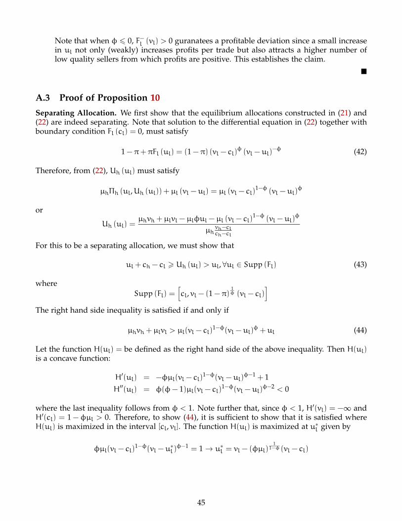
Note that when � 6 0, F-l (vl) > 0 guranatees a profitable deviation since a small increasein ul not only (weakly) increases profits per trade but also attracts a higher number oflow quality sellers from which profits are positive. This establishes the claim.

⌅

A.3 Proof of Proposition 10

Separating Allocation. We first show that the equilibrium allocations constructed in (21) and(22) are indeed separating. Note that solution to the differential equation in (22) together withboundary condition Fl (cl) = 0, must satisfy

1 - ⇡+ ⇡Fl (ul) = (1 - ⇡) (vl - cl)� (vl - ul)

-� (42)

Therefore, from (22), Uh (ul) must satisfy

µh⇧h (ul,Uh (ul)) + µl (vl - ul) = µl (vl - cl)1-� (vl - ul)

�

or

Uh (ul) =µhvh + µlvl - µl�ul - µl (vl - cl)

1-� (vl - ul)�

µhvh-clch-cl

For this to be a separating allocation, we must show that

ul + ch - cl > Uh (ul) > ul, 8ul 2 Supp (Fl) (43)

whereSupp (Fl) =

hcl, vl - (1 - ⇡)

1� (vl - cl)

i

The right hand side inequality is satisfied if and only if

µhvh + µlvl > µl(vl - cl)1-�(vl - ul)

� + ul (44)

Let the function H(ul) = be defined as the right hand side of the above inequality. Then H(ul)is a concave function:

H0(ul) = -�µl(vl - cl)1-�(vl - ul)

�-1 + 1H00(ul) = �(�- 1)µl(vl - cl)

1-�(vl - ul)�-2 < 0

where the last inequality follows from � < 1. Note further that, since � < 1, H0(vl) = -1 andH0(cl) = 1 -�µl > 0. Therefore, to show (44), it is sufficient to show that it is satisfied whereH(ul) is maximized in the interval [cl, vl]. The function H(ul) is maximized at u⇤

l given by

�µl(vl - cl)1-�(vl - u⇤

l )�-1 = 1 ! u⇤

l = vl - (�µl)1

1-� (vl - cl)

45

Therefore

H(u⇤l ) =

1�(vl - u⇤

l ) + u⇤l

=(�µl)

11-� (vl - cl)

�+ vl - (�µl)

11-� (vl - cl)

= vl + (vl - cl)µ1

1-�

l ��

1-� [1 -�]

Note that since ch > vl, we must have the following

(�µl)�

1-� < 1 6 (ch - cl) (vh - vl)

(vl - cl) (vh - ch)

The above inequality implies that

(vl - cl) (�µl)�

1-�vh - chch - cl

< (vh - vl) ! (vl - cl)µl (�µl)�

1-�µh

µl

vh - chch - cl

< µh (vh - vl)

Hence,(vl - cl)µl (�µl)

�1-� (1 -�) < µh (vh - vl)

andvl + (vl - cl)µl (�µl)

�1-� (1 -�) < µh (vh - vl) + vl

ormax

ule[cl,vl]H (ul) < µhvh + µlvl

which in turn implies that Uh (ul) > ul for all ul 2 Supp (Fl).Next, we show the left inequality in (43). For this to hold, we must have

µhvh + µlvl - µl�ul - µl (vl - cl)1-� (vl - ul)

�

µhvh-clch-cl

6 ul + ch - cl

or equivalently

µhcl + µlvl 6 ul + µl (vl - cl)1-� (vl - ul)

� , 8ul 2 Supp (Fl) ⇢ [cl, vl] (45)

Since, the right hand side of (45) is a concave function, it takes its minimum values at theextremes of the interval [vl, cl]. These values are given by vl and µlvl + µhcl both of which areat least as large the left side of (45). Hence, (45) must be satisfied for all ul 2 [vl, cl].

Global Deviations. Note that our conditions (21) and (22) imply that local deviations withrespect to uh and ul are not profitable. It, thus, remains to show that for all

�u0h,u0

l

�

⇧�u0h,u0

l

�= µl

�1 - ⇡+ ⇡Fl

�u0l

�� �vl - u0

l

�+µh

�1 - ⇡+ ⇡Fh

�u0h

��⇧h

�u0h,u0

l

�6 µl (1 - ⇡) (vl - cl)

We consider two cases:

46

1. u0h > maxSupp (Fh) = uh: In this case, 1 - ⇡+ ⇡Fh

�u0h

�= 1. If u0

l > maxSupp (Fl) = ul,then the profits from this menu are given by

µl

�vl - u0

l

�+ µh⇧h

�u0h,u0

l

�

Since � > 0, the above function is decreasing in�u0h,u0

l

�and therefore

µl

�vl - u0

l

�+ µh⇧h

�u0h,u0

l

�< µl (vl - ul) + µh⇧h (uh, ul) = µl (1 - ⇡) (vl - cl)

When u0l 6 maxSupp (Fl), the partial derivative of the above profit function with respect

to u0l is given by

- µl

�1 - ⇡+ ⇡Fl

�u0l

��+ µl⇡fl

�u0l

� �vl - u0

l

�+ µh

vh - chch - cl

>

-µl

�1 - ⇡+ ⇡Fl

�u0l

��+ µl⇡fl

�u0l

� �vl - u0

l

�+ µh

�1 - ⇡+ ⇡Fl

�u0l

�� vh - chch - cl

= 0

Thus for a given value of u0h, we must have

⇧�u0h,u0

l

�6 ⇧

�u0h, ul

�< ⇧ (uh, ul) = µl (1 - ⇡) (vl - cl)

This proves the claim.

2. u0h 2 [ch, uh]. In this case, we must have there exists ul such that u0

h = Uh (ul) and thusFh�u0h

�= Fl (ul). We can thus write the profit function as

µl

�1 - ⇡+ ⇡Fl

�u0l

�� �vl - u0

l

�+ µh (1 - ⇡+ ⇡Fl (ul))⇧h

�u0h,u0

l

�(46)

We show that the above function is maximized at u0l = ul. This proves our claim.

To show this, we show that the function is strictly concave for values of u0l 2 Supp (Fl)

and decreasing for values of u0l > ul. When u0

l 2 Supp (Fl), since ⇧h is linear in u0l, the

second derivative of (46) with respect to u0l is given by

@2

@�u0l

�2µl

�1 - ⇡+ ⇡Fl

�u0l

�� �vl - u0

l

�

Using (42), we can rewrite the above as

@2

@�u0l

�2µl

�1 - ⇡+ ⇡Fl

�u0l

�� �vl - u0

l

�=

@2

@�u0l

�2µl (1 - ⇡) (vl - cl)� �vl - u0

l

�1-�

= (�- 1)�µl (1 - ⇡) (vl - cl)� �vl - u0

l

�-1-�< 0

This implies that (46) is strictly concave in u0l for values of u0

l 2 Supp (Fl). When u0l > ul,

1 - ⇡+ ⇡Fl�u0l

�= 1 and thus the value in (46) is given by

µl

�vl - u0

l

�+ µh (1 - ⇡+ ⇡Fl (ul))⇧h

�u0h,u0

l

�

47

The derivative of this function with respect to u0l is given by

-µl + µh (1 - ⇡+ ⇡Fl (ul))vh - chch - cl

< -µl + µhvh - chch - cl

= -µl� < 0

Therefore, (46) is maximized at a value of u0l which equates the partial derivative of (46)

with zero. This value must satisfy

-µl

�1 - ⇡+ ⇡Fl

�u0l

��+ µl⇡fl

�u0l

� �vl - u0

l

�+ µh (1 - ⇡+ ⇡Fl (ul))

vh - chch - cl

= 0

Note that since (46) is strictly concave, at most one u0l exists that satisfies the above. The

differential equation (21) implies that u0l = ul is a solution to the above equation. This

implies that (46) must be maximized at u0l = ul. This concludes the proof.

⌅

A.4 Proof of Proposition 11

We first show that the thresholds, �1 and �2 defined as the values of � that satisfy (30) and(31) represent lower and upper bounds on � respectively and that �2 < �1 < 0. We state theseresults as Lemma 22. Next, we show for each case described in the proposition, that there existno profitable local or global deviations.

Lemma 22. Let �1 and �2 satisfy (30) and (31) respectively. Then (30) is satisfied for all �1 6 � 6 0and (31) is satisfied for all � 6 �2. Moreover, �2 < �1 < 0.

Proof. First, note that equation (30) which determines the threshold �1 can be re-written as

(1 - ⇡)1-�� > ⇡

1 - ⇡

vh - vlch - vl

µh + 1, (47)

or, after taking logs and substituting for �,

µh (vh - ch)

ch - cl - µh (vh - cl)log (1 - ⇡)- log(µh⇡ (vh - vl) + (1 - ⇡) (ch - vl))- log [(1 - ⇡) (ch - vl)] > 0.

(48)We show that the left-hand side of (48) is a decreasing function of µh which is strictly satisfiedwhen µh is such that � = 0 and is weakly violated when µh = 1. Hence, there is a uniquethreshold µ1 (and implied threshold �1) such that for all µh 6 µ1 and � < 0, the separatingcondition (30) is satisfied. Differentiating the left-hand side of (48) with respect to µh we obtain

log (1 - ⇡)(vh - ch) (ch - cl)

[ch - cl - µh (vh - cl)]2 -

⇡ (vh - vl)

µh⇡ (vh - vl) + (1 - ⇡) (ch - vl)

which is negative for all ⇡ 6 1. Next, as � ! 0 from below, it is immediate that (47) is satisfiedsince the left-hand side tends to infinity. As µh ! 1, the term (1 -�) /� ! -1 and so (47)tends to the requirement that

1 > ⇡vh - vlch - vl

+ (1 - ⇡)

48

which is violated since ch < vh.Next, consider equation (31) which determines the threshold �2. Substituting for � and

straightforward algebra shows this equation is equivalent to

µh (vh - vl)

1 + (1 - ⇡)

vh - chch - cl

�> vh - vl + (ch - vl) (1 - ⇡)

vh - chch - cl

. (49)

Clearly, (49) represents a lower bound on µh, or, equivalently, an upper bound on �. Note thatthis equation is necessarily satisfied at µh = 1. It is immediate that when µh is such that � = 0,equation (31) is violated since ch > vl.

We now prove that if � 6 �2, then � < �1 to establish that �2 < �1. Suppose � 6 �2 andlet v = µhvh + µlvl so that

1 - ⇡ > v- vl(1 -�) (v- ch)

. (50)

Note that (50) implies

1 -� > v- vl(v- ch) (1 - ⇡)

>v- vlv- ch

and so-� >

ch - vlv- ch

.

We will show that (30) is violated. First, we re-arrange (30) as

(1 - ⇡)h(1 - ⇡)

1-�� - 1

i(ch - vl)- ⇡µh (vh - vl) > 0

or, using straightforward algebra, as

(1 - ⇡) (v- ch) + (1 - ⇡)1� (ch - vl) > v- vl.

We show that if (50) holds, then

(1 - ⇡) (v- ch) + (1 - ⇡)1� (ch - vl) < v- vl.

Towards this end, define a function

H(⇡) = (1 - ⇡) (v- ch) + (1 - ⇡)1� (ch - vl) .

We argue that

H

✓1 -

v- vl(1 -�) (v- ch)

◆< v- vl (51)

and that this result implies H(⇡) < v- vl. Note that using the expression for H(⇡), we have

H

✓1 -

v- vl(1 -�) (v- ch)

◆=

v- vl(1 -�) (v- ch)

(v- ch) +

✓v- vl

(1 -�) (v- ch)

◆ 1�

(ch - vl) . (52)

49

Straightforward algebra can be applied to (52) to show that (51) holds if and only if

✓v- vl

(1 -�) (v- ch)

◆ 1-��

< -�v- chch - vl

.

Raising both sides of the last inequality by �, we obtain (51) holds if and only if

✓v- vl

(1 -�) (v- ch)

◆1-�

>

✓-�

v- chch - vl

◆�

or ✓ch - vlv- ch

◆�✓v- vlv- ch

◆1-�

> (-�)� (1 -�)1-�. (53)

Let B(x) = x�(1+ x)1-� and since (v- vl) / (v- ch) = 1+(ch - vl) / (v- ch), (53) can be writtenas

B

✓ch - vlv- ch

◆> B (-�) .

Observe thatB0(x) = B(x)

✓�

x+

1 -�

1 + x

◆= B(x)

�+ x

x (1 + x))

so that for 0 < x < -�, B0(x) < 0. Since -� > (ch - vl) / (v- ch) and B (x) is strictly decreasing,we have proved (53) and, therefore, (51) are satisfied.

Finally, note that the function H(x) is convex since

H0 (⇡) = - (v- ch)-1�(1 - ⇡)

1�-1 (ch - vl)

H00(⇡) =1�

✓1�

- 1◆(1 - ⇡)

1�-2 (ch - vl) > 0.

Additionally, H(0) = v- vl, H0(0) 6 0 when -� > (ch - vl) / (v- ch) and lim⇡!1 H(⇡) = 1.Thus, there is a unique value ⇡s > 0 such that for all ⇡ < ⇡s, H(⇡) 6 v- vl. Since (51) holds,and since ⇡ 6 1 - (v- vl) / ((1 -�)(v- ch)), we must have H(⇡) < v- vl. This proves � < �1as desired. ⌅

We now prove that in each region (� 6 �2,�2 < � < �1,�1 6 � < 0), there are no local orglobal deviations for buyers which earn strictly positive profits.

Case 1: Only Separating Menus. Here, it suffices to rule out global deviations since thedistribution Fl(ul) is chosen to ensure no local deviations are profitable. To rule out globaldeviations a proof similar to that of Proposition 10 can be used. Here, we show that for a givenvalue of u0

h, the profit function is strictly concave in u0l and therefore it must be maximized at

u0l = U-1

h

�u0h

�– since at this value its derivative is set to zero.

The profits are given by

µl

�1 - ⇡+ ⇡Fl

�u0l

�� �vl - u0

l

�+ µh

�1 - ⇡+ ⇡Fh

�u0h

��⇧h

�u0h,u0

l

�

50

Since ⇧h is linear in u0l, the second derivative of the above function is equal to the second

derivative of the profits for the low quality sellers. Using differential equation (21), we knowthat

�1 - ⇡+ ⇡Fl

�u0l

��=

�u0l - vl

�-� for some constant . Therefore, we have

@2

@�u0l

�2µl

�1 - ⇡+ ⇡Fl

�u0l

�� �vl - u0

l

�= -µl

@2

@�u0l

�2

�u0l - vl

�1-�

= -µl (1 -�) (-�)�u0l - vl

�-1-�< 0

This completes the proof.

Case 2: Only Pooling Menus. We first prove that no local deviations in the pooling equilib-rium yield strictly positive profits. Below we demonstrate global deviations are also unprof-itable. Recall that in a pooling equilibrium, the distributions Fl (ul) satisfies

(1 - ⇡+ ⇡Fl(ul)) [v- ul] = (1 - ⇡) (v- ch) (54)

where v = µhvh + µlvl, Uh(ul) = ul, Fh(ul) = Fl(ul), and Supp(Fl) = [ch, v- (1 - ⇡) (v- ch)] .Fix any utility, ul, interior to the support of Fl and consider a perturbation that increases uh by" (uh = ul + ") holding ul fixed. Profits from such a deviation satisfy

µl (1 - ⇡+ ⇡Fl(ul)) (vl - ul) + µh (1 - ⇡+ ⇡Fl (ul + "))⇧h (ul + ",ul)

= µl (1 - ⇡+ ⇡Fl(ul)) (vl - ul) + µh (1 - ⇡+ ⇡Fl (ul + "))

vh - ul - "

vh - clch - cl

�.

If local deviations are unprofitable, this function must be maximized at " = 0, so that Fl mustsatisfy

µh⇡fl (ul) [vh - ul]- µh (1 - ⇡+ ⇡Fl (ul))vh - clch - cl

6 0.

Totally differentiating (54) yields the following relationship between Fl and fl,

⇡fl(ul) (v- ul) = (1 - ⇡+ ⇡Fl(ul)) (55)

so that for local deviations to be unprofitable, we require

µh⇡fl (ul) [vh - ul]- µh⇡fl(ul) (v- ul)vh - clch - cl

6 0.

Since Fl is continuous in our constructed equilibrium, we may simplify this condition usingstraightforward algebra as

ul (vh - ch) 6 v (vh - cl)- vh (ch - cl) .

Consequently, we see that it suffices to check that this deviation is unprofitable at maxSupp(Fl).Using ul = v- (1 - ⇡) (v- ch) , simple algebraic manipulations show that this local deviation

51

is unprofitable as long asv- vl

(1 -�) (v- ch)6 1 - ⇡. (56)

In order to rule out global deviations, we show that for any value of u0h 2 Supp (Fl), when

u0l 6 u0

h, the profit function is increasing in u0l. This implies that profits are maximized at

u0l = u0

h and therefore there are no profitable deviation. To see this, note that profits are givenby

µl

�1 - ⇡+ ⇡Fl(u

0l)� �

vl - u0l

�+ µh

�1 - ⇡+ ⇡Fl

�u0h

��⇧h

�u0h,u0

l

�

The derivative of this function with respect to u0l is given by

µl⇡fl�u0l

� �vl - u0

l

�- µl

�1 - ⇡+ ⇡Fl(u

0l)�+ µh

�1 - ⇡+ ⇡Fl

�u0h

�� vh - chch - cl

>

µl⇡fl�u0l

� �vl - u0

l

�- µl

�1 - ⇡+ ⇡Fl(u

0l)�+ µh

�1 - ⇡+ ⇡Fl

�u0l

�� vh - chch - cl

=

µl⇡fl�u0l

� �vl - u0

l

�- µl�

�1 - ⇡+ ⇡Fl(u

0l)�

(57)

Using (55), we can write the above as

µlvl - u0

l

v- u0l

(1 - ⇡+ ⇡Fl(ul))- µl��1 - ⇡+ ⇡Fl(u

0l)�=

µl(1 - ⇡+ ⇡Fl(u0l))

vl - u0

l

v- u0l

-�

�= µl(1 - ⇡+ ⇡Fl(u

0l))

1 +

vl - v

v- u0l

-�

�

Since u0l 6 u0

h 6 maxSupp (Fl), the expression in the bracket takes its minimum value atu0l = maxSupp (Fl) and we have

1 +vl - v

v- u0l

-� > 1 +vl - v

(1 - ⇡) (v- ch)-� > 0

where the second inequality follows from (56). This implies that the expression in (57) ispositive and concludes the proof.

Case 3: Equilibrium Features Pooling and Separating Menus. As in Case 1 with only sep-aration, the distribution Fl for ul 2 [ul, maxSupp(Fl)] is chosen to ensure local deviations arenot profitable. Thus, we need only prove that local deviations are not profitable in the poolingregion and that no global deviations are profitable. As in Case 2 with only pooling menus,it suffices to ensure that at the upper bound of the pooling region, ul, no local deviations areprofitable, or

ul (vh - ch) 6 v (vh - cl)- vh (ch - cl) . (58)

To prove that (58) holds, first note that since �2 < � < �1, we have ch < ul < u (ul). To seethis, guess that ul > ch (we will verify it later), in which case ul satisfies

v-

�

vl + (ul - vl)

(1 - ⇡)

v- chv- ul

� 1�

✏

- (1 - ⇡) (v- ch) = 0. (59)

52

Let H(u) denote the left-hand side of (59). Observe that one solution to H (u) = 0 is given by

u = v- (1 - ⇡) (v- ch) .

This solution occurs when u (ul) = ul. For ul < u, we have ul (ul) > ul. We now show thatwhen �2 < � < �1, then there is another solution with ul 2 (ch, u). We show this by provingthat H0(u) > 0, H(u) = 0 H (ch) > 0 and H00 (u) > 0. Then, there exists a unique threshold, ul

such that H(u) = 0. Note that

H0 (u) = -

(1 - ⇡)

v- chv- u

� 1�

- (u- vl)1�

(1 - ⇡)

v- chv- u

� 1�-1

(1 - ⇡) (v- ch) (v- u)-2 .

Algebraic computations, available on request, then demonstrate that H00 (u) > 0. Next, observethat by construction, H(u) = 0 and

H0 (u) = -1 -1�

u- vlv- u

.

Substituting for u and re-arranging terms, we find that

H0 (u) =1 -�

�

1 -

v- vl(1 - ⇡) (1 -�) (v- ch)

�.

When � > �2, the term in brackets is negative so that H0 (u) > 0.Finally, note that H(ch) satisfies

H (ch) = v- vl - (ch - vl) (1 - ⇡)1� - (1 - ⇡) (v- ch)

= ⇡ (v- vl)- (ch - vl) (1 - ⇡)1� + (1 - ⇡) (ch - vl)

= ⇡ (v- vl)- (ch - vl)h(1 - ⇡)

1� - (1 - ⇡)

i

=1

(1 - ⇡)1� - (1 - ⇡)

"

vl +⇡ (v- vl)

(1 - ⇡)1� - (1 - ⇡)

- ch

#

.

The fact that � < �1 < 0 implies that the term in brackets is strictly positive and the leadingfraction is also positive so that H(ch) > 0.

We now prove that (58) is satisfied at ul. Algebra, available upon request shows that (58)may be written as

ul 6-�

1 -�v+

11 -�

vl.

We demonstrate that this condition is verified by proving that H⇣

-�1-� v+

11-�vl

⌘6 0. To see

53

this, note that

H

✓-�

1 -�v+

11 -�

vl

◆

= v- vl -

✓-�

1 -�v+

11 -�

vl - vl

◆"(1 - ⇡)

v- ch

v- -�1-� v-

11-�vl

# 1�

-(1 - ⇡) (v- ch)

= v- vl +�

1 -�(v- vl)

(1 - ⇡) (1 -�) (v- ch)

v- vl

� 1�

- (1 - ⇡) (v- ch)

= (v- vl)

"v- vl - (1 - ⇡) (v- ch)

v- vl+�

(1 -�)1�-1 (1 - ⇡)

1� (v- ch)

1�

(v- vl)1�

#

. (60)

We now show that the term in brackets on the right side of (60) is negative. To simplify notation,define ⇠ = (1 - ⇡) (v- ch) / (v- vl). Since � > �2, we have that ⇠ < 1/(1 -�). As well, theterm in brackets can be written compactly as

1 - ⇠+� (1 -�)1�-1 ⇠

1� .

Let G(⇠) = 1 - ⇠+� (1 -�)1�-1 ⇠

1� and observe that for ⇠ 6 1/(1 -�), we have

G0(⇠) = -1 + [(1 -�) ⇠]1�-1 > 0

so that for low values of ⇠, G(⇠) is an increasing function. Finally, we see that G(1/(1-�)) = 0so that G(⇠) 6 G(1/(1 -�)) 6 0 which ensures the term in brackets in (60) is indeed negativeas desired.

To rule out global deviations, one can use the arguments provided in the two cases above(when equilibrium is fully separating or pooling) in each region of the Supp (Fh). The argumentis the exact replication of the above arguments and is thus omitted. ⌅

A.5 Proof of Proposition 12

We show that there are no profitable deviations. In other words,

8�u0h,u0

l

�: µh

�1 - ⇡+ ⇡Fl

�u0l

��⇧h

�u0h,u0

l

�+µl

�1 - ⇡+ ⇡Fl

�u0l

�� �vl - u0

l

�6 (1 - ⇡)µl (vl - cl)

We consider two cases:

1. u0h > maxSupp (Fh) = uh: In this case, when u0

l > vl, the profit function is given by

µh⇧h

�u0h,u0

l

�+ µl

�vl - u0

l

�

Since � = 0, the above function is invariant to changes in u0l and is strictly decreasing

in u0l. Therefore, its value must be less than its value evaluated at (uh, vl) which gives

the equilibrium profits. When, u0l 6 vl, the profits are given by µh⇧h

�u0h,u0

l

�which is

54

decreasing in u0h and therefore

µh⇧h

�u0h,u0

l

�+ µl (1 - ⇡)

�vl - u0

l

�< µh⇧h

�uh,u0

l

�+ µl (1 - ⇡)

�vl - u0

l

�

Note that the right hand side of the above inequality is a linear function of u0l whose

derivative is given by

µhvh - chvl - cl

- µl (1 - ⇡) = µhvh - chch - cl

- µl + µl⇡

= -µl�+ µl⇡ = µl⇡ > 0.

Therefore, we must have that

µh⇧h

�uh,u0

l

�+ µl (1 - ⇡)

�vl - u0

l

�6 µh⇧h (uh, vl) = (1 - ⇡)µl (vl - cl)

where the last equality follows from (32).

2. u0h 2 [ch, uh]. In this case, when u0

l > vl, profits are given by

µh

�1 - ⇡+ ⇡Fl

�u0h

��⇧h

�u0h,u0

l

�+ µl

�vl - u0

l

�6 µh

�1 - ⇡+ ⇡Fl

�u0h

��⇧h

�u0h, vl

�

= (1 - ⇡)µl (vl - cl)

where the inequality is satisfied since u0l > vl and the last equality follows from (32).

When u0l 6 vl, profits are given by

µh

�1 - ⇡+ ⇡Fl

�u0h

��⇧h

�u0h,u0

l

�+ µl (1 - ⇡)

�vl - u0

l

�

The above function is linear in u0l and its derivative is given by

µh

�1 - ⇡+ ⇡Fl

�u0h

�� vh - chch - cl

- µl (1 - ⇡) = (1 - ⇡)

✓µh

vh - chch - cl

- µl

◆+ ⇡Fl

�u0h

� vh - chch - cl

= ⇡Fl�u0h

� vh - chch - cl

> 0

Therefore it is maximized at u0l = vl. This completes the proof.

⌅

A.6 Proof of Theorem 13

We prove uniqueness of the equilibrium first for � > 0 and then for � < 0. Finally, we showuniqueness for � = 0.

Case 1: � > 0. As discussed in the text, we need to prove that no equilibrium features a masspoint in Fl and that no equilibrium features pooling (Uh(ul) = ul) on any interval in the supportof Fl. We state these results and proofs as independent lemmas below. These results implythat any equilibrium is separating and has continuous distribution Fl; since there is a unique

55

solution to the differential equation (21) with the boundary condition minSupp(Fl) = cl, wehave then shown that the equilibrium described in Proposition 10 is unique.Lemma 23. If � > 0, then Fl has no mass points.

Proof. We have already shown that if Fl has a mass point, then it must occur at the lower boundof the support of Fl which satisfies minSupp(Fl) = cl. Suppose by way of contradiction that Flhas a mass point at cl. Since Fh has no mass point, Uh(ul) must be a correspondence at ul = cl.Hence, there exists a uh 2 Uh(ul) such that uh > ul = cl. Consider a deviation by a buyerto the menu (cl + ",uh). Such a deviation induces a jump in the number of non-captive lowquality sellers attracted while decreasing the profits earned per low quality seller marginally.Hence, this deviation yields strictly positive profits, implying a contradiction. ⌅Lemma 24. If � > 0, in any equilibrium, there is no interval [u1,u2] 2 Supp Fl such that Uh(ul) = ul

for ul 2 [u1,u2]. That is, there is no interval which features pooling menus.

Proof. Suppose by way of contradiction that a pooling interval exists. We will show that thisnecessarily implies that the separating equilibrium we construct in Proposition 10 must notexist.

Towards this end, we first prove that there can be at most one interval of pooling and thatthe pooling thresholds u1 and u2 are uniquely determined. First, note that since the worstequilibrium menu is the menu (cl, ch) which satisfies Uh(cl) > cl, the equilibrium near thelower bound of the support must be separating. Let [u1,u2] denote the lowest interval ofpooling and assume u2 < maxSupp(Fl). We show that for all ul > u2, Uh(ul) > ul. Sincethe equilibrium is locally pooling below u2, limul%u2 U

0h(ul) = 1. IF u2 < maxSupp(Fl), the

equilibrium must be locally separating above u2 so that Uh(ul) satisfies

(1 - ⇡+ ⇡Fl(ul)) [µl (vl - ul) + µh⇧h(ul,Uh(ul)] = (1 - ⇡) (vl - cl)

with Fl(ul) satisfying the differential equation

⇡fl(ul)

1 - ⇡+ ⇡Fl(ul)=

�

vl - ul. (61)

Twice differentiating the equal profit condition with respect to ul, we obtain

U00h (ul) = �(1 -�)

(1 - ⇡) (vl - cl) (vh - vl)

(1 - ⇡+ ⇡Fl(ul)) (vl - ul)2 µh (vh - cl)

> 0

where the inequality holds when � > 0 (recall � 6 1) so that Uh is convex. This means that forall ul > u2, Uh(ul) > ul. We conclude that there can be at most one region of pooling menus.

For the pooling region to exist, cream-skimming deviations must be unprofitable at theupper threshold of the pooling interval, u2 so that

u2 6 v+ (v- vh)ch - clvh - ch

⌘ vpool.

The lower threshold is determined by imposing the boundary condition Uh(u1) = u1 on thedifferential equation (61). Solving the differential equation, we find u1 satisfies

v = u1 + µl (vl - cl)1-� (vl - u1)

� . (62)

56

We now analyze solutions to the non-linear equation (62). Let

H (u) = u+ µl (vl - cl)1-� (vl - u)�

so thatH0 (u) = 1 -�µl (vl - cl)

1-� (vl - u)�-1

Straightforward calculations show that H (u) is a concave function when � > 0 and u 6 vl.Since H0 (vl) < 0, we have that arg maxu H (u) < vl. Since the pooling region exists, by assump-tion, we must have maxu H(u) > v. Since Uh(ul) ! ul as ul ! u1, we must have U0

h(ul) 6 1 asul ! u1. Or, using the equal profit condition again

- µl�- µhvh - clch - cl

U0h(ul) = H0(u)- 1. (63)

Using (63), one can show that requiring U0h(u1) 6 1 is equivalent to requiring H0(u) > 0.

Hence, u1 is uniquely determined as the lowest solution to H(u) = v. Extensive algebraicmanipulations, available upon request, can be used to show that H0 �vpool

�< 0 so that by

concavity of H (u), we know that u1 6 vpool. A similar argument, applied to the upper boundimplies that the upper threshold is also uniquely determined if u2 < Supp(Fl).

Now, note that the equilibrium we describe in Proposition 10 satisfies maxSupp(Fl) = vl -

(1 - ⇡)1/� (vl - cl). If the pooling interval exists, it is immediate that u1 6 vl- (1 - ⇡)1/� (vl - cl).(If u1 > vl - (1 - ⇡)1/� (vl - cl), then F (u1) > 1). If the threshold u1 satisfies

u1 < vl - (1 - ⇡)1/� (vl - cl) , (64)

then the equilibrium with only separating menus described in Proposition 10 does not exist,which is a contradiction. If such an equilibrium exists when u1 satisfies the inequality (64), thenfor some values ul 2

hu1, vl - (1 - ⇡)1/� (vl - cl)

i, we have Uh(ul) = ul violating the separating

feature of the equilibrium. ⌅

Case 2: � < 0. To prove the equilibrium characterized in Proposition 11 is unique, we firstprove that in any equilibrium with � < 0, if u = maxSupp(Fl), then Uh(u) = u so that thebest menu in equilibrium is a pooling menu. We then demonstrate that Fl has no mass pointswhen � < 0. Next, We then prove that if the equilibrium has a pooling region, the regionbegins at the lower bound of the support of Fl or ends at the upper bound of Fl. Additionally,if the equilibrium features a separating region, this region must end at the upper bound ofthe support of Fl. These results imply that any equilibrium must take one of the three formsdescribed in Proposition 11: only separating, only pooling, or semi-separating. Finally, weshow that the necessary conditions for each type of equilibrium to exist are mutually exclusiveso that at most one type of equilibrium exists for each region of the parameter space, ensuringour equilibrium is unique for all � < 0. We prove these results in the sequence of followinglemmas.

Lemma 25. If � < 0, then Fl has no mass points.

Proof. Suppose by way of contradiction that Fl has a mass point at the lower bound of thesupport of Fl. Then it must be that minSupp(Fl) = vl. Exactly as in Lemma 23, if Fl has a

57

mass point at some ul < vl, then a deviation to a menu (ul ± ",uh) must be feasible for someuh 2 Uh(ul) and earn strictly positive profits.

Next note that if Fl has a mass point at vl, then we must have F+l (vl) = 1. If insteadF+l (vl) = m < 1, then, since Uh(vl) is an interval, there must be an interval of ul such that forul 2 (vl, vl + ") for " > 0 the equilibrium menus are separating, or Uh(ul) > ul. In this intervalof Supp(Fl), since local deviations must be unprofitable, Fl must satisfy

1 - ⇡+ ⇡Fl(ul) = C (ul - vl)-�

for some positive constant C. But then,

limul&vl

1 - ⇡+ ⇡Fl(ul) = limul&vl

C(ul - vl)-� = 0

which contradicts the fact that

limul&vl

1 - ⇡+ ⇡Fl(ul) = 1 - ⇡+ ⇡Fl (vl) = 1 - ⇡(1 -m) > 0.

Hence, F+l (vl) = 1.As a consequence, we have that Supp(Fl) = {vl} while maxSupp(Fh) > uh > vl = maxSupp(Fl)

(this last fact follows since Fh is continuous). Let uh = maxSupp(Fh) and consider the profitsa buyer would obtain by following a deviation to a menu (vl + ✏, uh). Profits at the originalcontract satisfy

µh

✓vh - uh

vh - clch - cl

+ vlvh - chch - cl

◆

while the deviation contract yields profits equal to

µh

✓vh - uh

vh - clch - cl

+ (vl + ✏)vh - chch - cl

◆+ µl (vl - (vl + ✏))

= µh

✓vh - uh

vh - clch - cl

+ vlvh - chch - cl

◆- µl✏+ µh

vh - chch - cl

✏.

Since the increment to profits earned from this deviation is given by

-µl✏+ µhvh - chch - cl

✏ = -µl�✏

and since � < 0, this deviation earns strictly greater profits than the equilibrium menu (vl, uh),which yields the necessary contradiction. ⌅

Lemma 26. If � < 0, then the best equilibrium menu is a pooling menu.

Proof. Let u = maxSupp(Fl) and suppose for contradiction that Uh(u) > u. Consider a devia-tion menu with (ul,uh) = (u+ ",Uh(u)). Since Uh (u) > u, this menu is incentive compatibleand has Fl(ul) = Fl (uh) = 1. This menu increases the buyer’s profits relative to the menu(u,Uh(u)) by the amount

-µl"+ µhvh - chch - cl

= -µl�" > 0

58

where the inequality follows from � < 0. This profitable deviation yields the necessary contra-diction so that we must have Uh(u) = u. ⌅

Lemma 27. If � < 0 and an equilibrium features [u1,u2] ✓ Supp(Fl) such that Uh(ul) = ul forul 2 [u1,u2], then either u1 = minSupp(Fl) or u2 = maxSupp(Fl).

Proof. Suppose for contradiction that an interval of pooling exists and u1 > minSupp(Fl) andu2 < maxSupp(Fl). Then there must exist intervals sufficiently close to and below u1 andabove u2 respectively in which the equilibrium menus feature separation. Consequently, wemust have limul%u1 U

0h(ul) 6 1 and limul&u2 U

0h(ul) > 1. In any region with Uh(ul) > ul, the

distribution Fl must also satisfy

⇡fl(ul)

1 - ⇡+ ⇡Fl (ul)=

-�

ul - vl

to rule out profitable local deviations and Uh must satisfy

v- µl�ul - µhvh - clch - cl

Uh(ul) = ⇧ (1 - ⇡+ ⇡Fl (ul))-1

to ensure all menus earn the equilibrium level of profits which we denote with ⇧.Using these features of the conjectured equilibrium, we have that in the separating regions,

U0h(ul) satisfies

-µl�- (1 - µl�)U0h (ul) =

⇧

1 - ⇡+ ⇡Fl(ul)

�

ul - vl.

Moreover, the second derivative of Uh satisfies

- (1 - µl�)U00h(ul) =

⇧⇡fl (ul)

[1 - ⇡+ ⇡Fl(ul)]2

�

ul - vl+

⇧

1 - ⇡+ ⇡Fl(ul)

-�

[ul - vl]2

which implies U00h(ul) 6 0 since � < 0. However, the pooling region requires U0+

h (u2) >1 > U0-

h (u1) which contradicts the concavity of Uh given that u1 < u2. Hence, either u1 =minSupp(Fl) or u2 = maxSupp(Fl). ⌅

Lemma 28. If � < 0 and an equilibrium features [u1,u2] ✓ Supp(Fl) such that Uh (ul) > ul forul 2 (u1,u2), then u2 = maxSupp(Fl).

Proof. Suppose such a separating interval exists with min Supp(Fl) < u2 < maxSupp(Fl). Thenthere exists a pooling interval [u2, u] for some u. Since u2 > minSupp(Fl), Lemma 27 impliesthat u = maxSupp (Fl). Since the conjectured equilibrium features separation in [u1,u2] withUh (ul) ! ul as ul ! u2, we must have U0-

h (u2) 6 1 or

11 - µl�

-µl�+

⇧

1 - ⇡+ ⇡Fl (u2)

-�

u2 - vl

�6 1

which can be re-written as

-�⇧ 6 [1 - ⇡+ ⇡Fl (u2)] (u2 - vl) .

59

Since u2 < u, F (u2) < 1 so that-�⇧ < u2 - vl. (65)

Moreover, since the best menu is pooling with utility u, equilibrium profits satisfy

⇧ = v- u

equation (65) impliesvl -� (v- u) < u2 < u

orvl -�v < (1 -�)u (66)

Since the equilibrium features pooling in the interval [u2, u], we must have cream-skimming isnot a profitable deviation, in particular from the pooling menu (u, u), or

u < vvh - clvh - ch

- vhch - clvh - ch

. (67)

Conditions (66) and (67) then require

vl -�v

1 -�< v

vh - clvh - ch

- vhch - clvh - ch

.

By substituting for � and using straightforward algebraic manipulations we show that

vl -�v

1 -�= v

vh - clvh - ch

- vhch - clvh - ch

which yields the needed contradiction. ⌅

Since the only possible equilibria when � < 0, then, are fully separating (except at theupper bound of the support of Fl), fully pooling, or semi-separating, we need only provethat only one of these equilibria may exist for any value of �. We have already shown inthe proof of Proposition 11 that �2 < �1 < 0. Recall that a necessary condition for a fullypooling equilibrium is that � 6 �2. Hence, there is no fully pooling equilibrium when � > �2.Similarly, a necessary condition for a fully separating equilibrium is that � > �1 so that when� < �1, no fully separating equilibrium exists. This means that in the interval �2 < � < �1,the only possible equilibrium is a semi-separating equilibrium. Moreover, the threshold in thesemi-separating equilibrium is interior to the support of Fl only if � lies between �2 and �1.Hence, at most one of these types of equilibria may exist for any value of � < 0, proving thatthe equilibrium described in Proposition 13 is unique.

A.7 Proof of Proposition 14

When � < 0, it is immediate that welfare is (weakly) maximized when ⇡ = 0. To prove thatwelfare is maximized for ⇡ 2 (0, 1) when � > 0 we prove that our measure of welfare isdecreasing in ⇡ at ⇡ = 1. Since welfare associated with the endpoint ⇡ = 1 is strictly larger thanat the other extreme, when ⇡ = 0, this finding necessarily implies that welfare is maximized atan interior ⇡.

60

To show that welfare is decreasing at ⇡ = 1, we first demonstrate that the volume of loanssold by high-quality sellers is decreasing in the level of indirect utility offered to low-qualitysellers when this level is sufficiently close to vl. We state this result as the following Lemma.Below, we use this finding to prove that welfare is decreasing in ⇡ at ⇡ = 1.

Lemma 29. As ul tends to vl, the volume of loans sold by high-quality sellers at the associated uh isdecreasing.

Proof. First, note that for any equilibrium menu, (ul,Uh(ul)), the associated volume of loanssold by high quality sellers satisfies

x(ul) = 1 -Uh(ul)- ul

ch - cl.

Thus, x (ul) is decreasing if and only if U0h(ul) > 1. We determine U0

h(ul) using propertiesof the equilibrium, namely equations (21) and (22). Specifically, if we differentiate (22) withrespect to ul, we find

µhvh - clch - cl

U0h (ul) = -µl�+

µl (1 - ⇡) (vl - cl)

1 - ⇡+ ⇡Fl(ul)

⇡fl(ul)

1 - ⇡+ ⇡Fl(ul).

Using (21), we can simplify this expression as

µhvh - clch - cl

U0h (ul) = -µl�+

µl (1 - ⇡) (vl - cl)

1 - ⇡+ ⇡Fl(ul)

�

vl - ul.

Using (22) again to replace µl(1 - ⇡) (vl - cl) / [1 - ⇡+ ⇡Fl(ul)] yields equation (35) in the text,which we replicate here.

µhvh - clch - cl

U0h (ul) = -µl�+

� [µh⇧h(Uh(ul),ul) + µl (vl - ul)]

vl - ul

) U0h(ul) =

� (ch - cl)

vh - cl

�⇥ ⇧h(Uh(ul),ul)

vl - ul.

We show that as ul ! vl, U0h(ul) ! 1. To see this, note that

⇧h(Uh(ul),ul)

vl - ul=

µl

µh

(1 - ⇡) (vl - cl)

vl - ul

11 - ⇡+ ⇡Fl(ul)

- 1�

.

When � > 0, the equilibrium distribution (that is, the solution to the differential equation)satisfies

1 - ⇡+ ⇡Fl(ul) = (1 - ⇡)

✓vl - clvl - ul

◆�

and hence⇧h(Uh(ul),ul)

vl - ul=

µl

µh

"✓vl - clvl - ul

◆1-�

- 1

#

.

Since � > 0, as ul ! vl, we see that this term tends to infinity. ⌅

61

Next, we show that welfare is a decreasing function of ⇡ at ⇡ = 1.Note ex-ante welfare is given by µl (vl - cl) + (vh - ch) times the expected trade by the high

quality sellers which is given by

(1 - ⇡)µh

Z ul

cl

xh (ul) f (ul)dul + ⇡µh

Z ul

cl

2xh (ul) f (ul) F (ul)dul

= µh

Z ul

cl

xh (ul) f (ul) [1 - ⇡+ 2⇡F (ul)]dul

= µh

Z ul

cl

µl (vl - cl)

1-� (vl - ul)� + ul - µhcl - µlvl

µh (vh - cl)

!✓1 - ⇡

⇡� (vl - cl)

� (vl - ul)-1-�

◆

"(1 - ⇡) + 2 (1 - ⇡)

✓vl - clvl - ul

◆�

- 2 (1 - ⇡)

#

dul

= �µh(1 - ⇡)2

⇡

Z ul

cl

µl (vl - cl)1-� (vl - ul)

� + ul - µhcl - µlvlµh (vh - cl)

(vl - cl)� (vl - ul)

-1-�

"

2✓vl - clvl - ul

◆�

- 1

#

dul

= �(vl - cl)

�

vh - cl

(1 - ⇡)2

⇡

Z ul

cl

⇣µl (vl - cl)

1-� (vl - ul)� + ul - µhcl - µlvl

⌘(vl - ul)

-1-�

"

2✓vl - clvl - ul

◆�

- 1

#

dul

Expected trade by the high type is �(vl-cl)

�

vh-cltimes

(1 - ⇡)2

⇡

Z ul

cl

⇣µl (vl - cl)

1-� (vl - ul)-1 + (ul - µhcl - µlvl) (vl - ul)

-1-�⌘

"

2✓vl - clvl - ul

◆�

- 1

#

dul

=(1 - ⇡)2

⇡2 (vl - cl)

✓Z ul

cl

µl (vl - ul)-1-� + (ul - µhcl - µlvl) (vl - ul)

-1-2� (vl - cl)�-1 dul

◆

-(1 - ⇡)2

⇡

✓Z ul

cl

⇣µl (vl - cl)

1-� (vl - ul)-1 + (ul - µhcl - µlvl) (vl - ul)

-1-�⌘dul

◆

=(1 - ⇡)2

⇡2 (vl - cl)

✓Z ul

cl

µl (vl - ul)-1-� + (ul - vl + µh (vl - cl)) (vl - ul)

-1-2� (vl - cl)�-1 dul

◆

-(1 - ⇡)2

⇡

✓Z ul

cl

⇣µl (vl - cl)

1-� (vl - ul)-1 + (ul - vl + µh (vl - cl)) (vl - ul)

-1-�⌘dul

◆

62

The indefinite integral in the first term:Z h

µl (vl - ul)-1-� + (ul - vl + µh (vl - cl)) (vl - ul)

-1-2� (vl - cl)�-1idul

= -

Z hµlz

-1-� + (-z+ µh (vl - cl)) z-1-2� (vl - cl)

�-1idz

= -

-µl

z-�

�- (vl - cl)

�-1 z1-2�

1 - 2�- µh (vl - cl) (vl - cl)

�-1 z-2�

2�

�

= µlz-�

�+ (vl - cl)

�-1 z1-2�

1 - 2�+ µh (vl - cl)

� z-2�

2�

= µl(vl - ul)

-�

�+ (vl - cl)

�-1 (vl - ul)1-2�

1 - 2�+ µh (vl - cl)

� (vl - ul)-2�

2�

and in the second term

=

Z ⇣µl (vl - cl)

1-� (vl - ul)-1 + (ul - vl + µh (vl - cl)) (vl - ul)

-1-�⌘dul

= -

Z ⇣µl (vl - cl)

1-� z-1 + (-z+ µh (vl - cl)) z-1-�

⌘dz

= -

µl (vl - cl)

1-� ln z-z1-�

1 -�- µh (vl - cl)

z-�

�

�

= -µl (vl - cl)1-� ln z+

z1-�

1 -�+ µh (vl - cl)

z-�

�

= -µl (vl - cl)1-� ln (vl - ul) +

(vl - ul)1-�

1 -�+ µh (vl - cl)

(vl - ul)-�

�

Using the above two integrals and extensive algebra implies that expected value of trade isgiven by

=1⇡(vl - cl)

1-� 2

"

µl(1 - ⇡)⇡

�+

(1 - ⇡)1� - (1 - ⇡)2

1 - 2�+ µh

1 - (1 - ⇡)2

2�

#

-1⇡(vl - cl)

1-�

"

-µl(1 - ⇡)2

�ln (1 - ⇡) +

(1 - ⇡)1+�� - (1 - ⇡)2

1 -�+ µh

(1 - ⇡)⇡

�

#

Using the above formula, the derivative of expected value of trade by the high quality seller

63

w.r.t ⇡ is given by

-1⇡2 (vl - cl)

1-� 2

"

µl(1 - ⇡)⇡

�+

(1 - ⇡)1� - (1 - ⇡)2

1 - 2�+ µh

1 - (1 - ⇡)2

2�

#

+1⇡(vl - cl)

1-� 2

2

4µl1 - 2⇡

�+

- 1� (1 - ⇡)

1�-1 + 2 (1 - ⇡)

1 - 2�+ µh

2 (1 - ⇡)

2�

3

5

+1⇡2 (vl - cl)

1-�

"

-µl(1 - ⇡)2

�ln (1 - ⇡) +

(1 - ⇡)1+�� - (1 - ⇡)2

1 -�+ µh

(1 - ⇡)⇡

�

#

-1⇡(vl - cl)

1-�

2

4µl2 (1 - ⇡)

�ln (1 - ⇡) + µl

(1 - ⇡)

�-

1+�� (1 - ⇡)

1� - 2 (1 - ⇡)

1 -�+ µh

1 - 2⇡�

3

5

Evaluated at ⇡ = 1, this becomes

- (vl - cl)1-� µh

�+ (vl - cl)

1-�

-2µl

�

�- (vl - cl)

1-�

-µh

�

�

=(vl - cl)

1-�

�[-µh - 2µl + µh] = -2µl

(vl - cl)1-�

�

< 0

A.8 Proof of Theorem 17

Lemma 30. In almost all equilibrium menus, x1 = 1 and the local downward IC’s are binding.

Proof. Suppose not. Then adding Ci,i+1 +Ci+1,i > 0 and hence (ci+1 - ci) (xi - xi+1) > 0 orxi+1 < xi. Consider the deviation (x1, · · · , xi+1, xi+2, · · · , xN) and (t1, · · · , ti, ti+1, ti+2, · · · , tN)where ti+1 = ti+1 + vi+1" and xi+1 = xi+1 + " for small " > 0. Since the utility of none of thetypes change, this deviation can only affect Ci,i+1 and Ci+2,i+1. These are given by

Ci,i+1 = ui - ui+1 - (ci - ci+1) (1 - xi+1) = ui - ui+1 - (ci - ci+1) (1 - xi+1)- " (ci+1 - ci)

Ci+2,i+1 = ui+2 - ui+1 - (ci+2 - ci+1) (1 - xi+1) = ui+2 - ui+1 - (ci+2 - ci+1) (1 - xi+1) + " (ci+2 - ci+1)

Since the original allocation satisfies Ci,i+1 > 0. If " is small enough, the above value of Ci,i+1 >0 is satisfied. Furthermore, for " > 0, Ci+2,i+1 > Ci+2,i+1 > 0. The difference between theprofits from these two allocations is given by (vi+1 - ci+1) " > 0. Hence there exists a profitabledeviation.

Q.E.D.

Claim 31. 8u 2 U,⇧N (uN,uN-1) > 0.

1. Proof: Suppose not. Then there is a profitable deviation which involves lowering uN. Tobe more precise, there are two cases:

(a) uN > cN: In this case, take the value of i such that uN = · · · = ui > ui-1; when theallocation has pooling for all types set i = 1 . Then since ⇧N (uN,uN-1) < 0, then for

64

all j > i+ 1, ⇧j

�uj,uj-1

�< 0 and decreasing the value of uj for j = i, i+ 1, · · · ,N

by a small amount increases profits – either some customers are lost or profits areincreases which makes the deviation profitable.

(b) uN = cN: If uN = cN, then since uN-1 > cN-1, we have

⇧N (uN,uN-1) = vN -vN - cNcN - cN-1

cN +vN - cN-1cN - cN-1

uN-1

> vN -vN - cN-1cN - cN-1

cN +vN - cNcN - cN-1

cN-1

= vN -vN (cN - cN-1)

cN - cN-1= 0

which confirms the claim.(c) Discussion: Can we rule out ⇧N = 0. Note that if this is the case, it must be that

uN = cN and uN-1 = cN. Why is this? because if uN > cN then a decline in uN

increases profits. But then if uN = cN and ⇧N = 0 it must be that uN-1 = cN-1.

Claim 32. If FN has a mass point at uN, then it must be that for all u 2 U with uN = uN must satisfy⇧N (uN, uN-1) = 0.

1. Proof: Suppose that ⇧N (uN, uN-1) > 0 (From Claim 1 we cannot have ⇧N < 0) andthat F+N (uN) > F-N (uN). Then there must be a positive measure of allocations wheretype–N cutomers are shared equally. Hence an infinitesimal increase in uN attracts all ofthese type–N sellers and since ⇧N > 0 the decline in the profits from increasing uN isinfinitesimal compared to the increase in profits from attracting a mass of type– N’s.

(a) Corollary. If FN has a mass point at uN, then it must be that uN = cN and that for allu 2 U with uN = cN, we must have uN-1 = cN-1.

Claim 33. FN does not have a mass point.

1. Proof. The line of argument following the above Corollary can be extended inductively.Following the corollary, the consistency condition (??) implies that FN-1 must also putmass at cN-1. The situation is then similar for type N- 1. In particular, we can showthat at any u with uN-1 = cN-1, we must have that ⇧N-1 = 0 and uN-2 = cN-2. Con-tinuing in this way, we must have that the underlying measure, µ, must put a mass onu =(c1, · · · , cN). Then an upward deviation in u1 yields strictly positive profits, yieldingthe contradiction.

Claim 34. FN has a connected support.

1. Proof: Suppose that it does not. That is there exists uN and uN such that FN (uN) =FN (uN) = F < 1 with uN < uN 2 UN14. Then we show that it is possible to construct aprofitable deviation. Note that when FN is flat in the interval (uN, uN), so is FN. Note,futher, that since uN > cN it must be that uN > cN. To show this, we consider a fewoptions for deviations:

14I think this is an important assumption but we can probably show that it is without loss of generality. At thispoint I am fucking tired of thinking about it!

65

(a) Suppose that u 2 U exists such that uN = uN with uN-1 < uN. Then for a small ", thevector u-(0, · · · , 0| {z }

N-1

, ") is incentive compatible and individually rational. Moreover,

since this deviation does not change profits from types 1 to N- 1 and it increasesprofits from type N seller without changing the measure of non-captive N–types thatare attracted (recall that FN (uN - ") = FN (uN) = F for " > 0 small enough).

(b) Suppose that for all u 2 U with uN = uN satisfy uN-1 = uN. More specifically,consider the highest value of i for which u 2 U exists such that uN = uN anduN = · · · = ui > ui-1. There are two possibilities:

i. There exists a " > 0 small enough such that

[uN - ", uN)N-i \U (i, · · · ,N- 1) = ;.

In this case, consider the vector u- (0, · · · , 0| {z }i-1–times

, "/2, · · · , "/2| {z }) which is incentive

compatible and individually rational. As before the profits from types 1 to i-1 do not change since [uN - ", uN)

N-i+1 \ U (i, · · · ,N) = ;, Fj (u) is flat, 8j =i, · · · ,N in the interval [uN - ", uN) and hence this deviation increases profits.

ii. There exists a sequence�

uk 1k=1 2 U whose projection onto the elements i, · · · ,N-

1 belongs to the set (-1, uN)N-i and converges to u. Since FN is flat close to uN

for k high enough, it must be that ukN > uN. Optimality of u implies that a fea-

sible dowanward deviation of the form u-("1 · · · · · · , "N) with "N-1 = "N shouldnot increase profits. This implies that we must have the following condition:

µN

�1 - ⇡+ ⇡FN (uN)

�-D-⇧1,··· ,N-1 (u) 6 0 (68)

where ⇧1,··· ,N-1 (·) is the total profit from types 1 to N-1 and D- is the derivativeas defined below

D-⇧1,··· ,N-1 (u) = lim inft&0

supu2V(t) ⇧1,··· ,N-1 (u)- ⇧1,··· ,N-1 (u)

t

with

V (t) = {u =(u1, · · · , uN-1) : u satisfies (??), (??), uN-1 < uN; |uN - uN-1| = t}

Note that deviation of the form u- (0, · · · , 0| {z }i-1–times

, "i, · · · , "N-1, 0) for "j’s small enough

leads to the following inequality:

- µN

�1 - ⇡+ ⇡FN (uN)

� vN - cNcN - cN-1

-D-⇧1,··· ,N-1 (u) 6 0 (69)

The left side of (69) is less than that of (68) and therefore it must be negative.

66

Since uk converges to u, it must be that for some value of k high enough,

-µN

�1 - ⇡+ ⇡FN (uN)

� vN - cNcN - cN-1

-⇧1,··· ,N-1 (u)- ⇧1,··· ,N-1

�uk�

uN - ukN-1

< 0

Hence, we have

0 < µN

�1 - ⇡+ ⇡FN (uN)

� vN - cNcN - cN-1

⇣uN - uk

N-1

⌘+ ⇧1,··· ,N-1 (u)- ⇧1,··· ,N-1

⇣uk⌘

Since ukN > uN, we must have that

0 < µN

⇣1 - ⇡+ ⇡FN

⇣ukN

⌘⌘ vN - cNcN - cN-1

⇣uN - uk

N-1

⌘+ ⇧1,··· ,N-1 (u)- ⇧1,··· ,N-1

⇣uk⌘

Adding µN

�1 - ⇡+ ⇡FN

�ukN

��⇧N

�ukN, uk

N-1�

to both sides of the above inequal-ity, we can write

µN

⇣1 - ⇡+ ⇡FN

⇣ukN

⌘⌘⇧N

⇣ukN, uk

N-1

⌘+ ⇧1,··· ,N-1

⇣uk⌘

< µN

⇣1 - ⇡+ ⇡FN

⇣ukN

⌘⌘ vN - cNcN - cN-1

⇣uN - uk

N-1

⌘+⇧N

⇣ukN, uk

N-1

⌘�+ ⇧1,··· ,N-1 (u)

or⇧ < µN

⇣1 - ⇡+ ⇡FN

⇣ukN

⌘⌘+ ⇧1,··· ,N-1 (u)

Hence the vector�u1, · · · , uN-1, uk

N

�is a profitable deviation. This proves the

claim.

Lemma 35. Lemma: If {Fs}Ns=i+1 has connected support and no mass points, then Fi has connected

support.

Proof: TO BE COMPLETED.

Lemma 36. : If {Fs}Ns=i+1 has connected support and contain no mass points, then Fi has no masspointsunless

�j = µj

✓vj - cj-1

cj - cj-1

◆- µj+1

✓vj+1 - cj+1

cj+1 - cj

◆= 0 8 1 6 j 6 i

Strategy for proof: We first show that if Fi has a masspoint, it must be the case the equi-librium distribution puts full mass on menus with utilities u1,u2....ui equal to the least costseparating (LCS) utilities, i.e.

uLCS1 = v1

uLCSj = uLCS

j-1 +⇣

1 - xLCSj

⌘ �cj - cj-1

�where xLCSj =

uLCSj-1 - cj-1

vj - cj-1

We then show that, if �j 6= 0 for some j 6 i, we can construct a profitable deviation.

67

We proceed in steps. The following two claims show that if there is a mass at ui, then⇧1 = ⇧2 = ...⇧i = 0 for every menu that offers ui to type-i. This pins down the unique setof indirect utilities to the first i types that can be part of a masspoint in Fi. Then, we usesupermodularity and the resulting rank preserving (weak) property to show that, if �j > 0 forsome j 6 i, increasing uj-1 raises profits. If �j < 0, we decrease uj-1.

Claim 37. If Fi has a mass point at ui, then for all u 2 U with ui = ui must satisfy ⇧i (ui-1, ui) = 0.

Proof. Suppose otherwise. If ⇧i (ui-1, ui) > 0, then increasing ui leads to a discrete jumpin the probability of winning, but the reduction in profits conditional on trade can be madearbitrarily small. Thus, ⇧i (ui-1, ui) 6 0. Now, to rule out ⇧i (ui-1, ui) < 0, find the lowest k >0 such that ui-k-1 < ui. Applying the above argument, we can show that ⇧i-s (ui-s-1, ui-s) 6 0for s 6 k. Now, decrease all the utilities i.e. (ui-k, ui-k+1, ....ui) by " > 0. As " ! 0, the resultingchange in profits converges to.

⇡

kX

s=0

µi-s

⇥F-i-s (ui-s)- Fi-s (ui-s)

⇤⇧i-s (ui-s-1,ui-s) > 0

For example, if ui-1 < ui, consider a deviation which reduces ui by ". As " ! 0, the resultingchange in profits converges to

⇡µi

⇥F-i (ui)- Fi (ui)

⇤⇧i (ui-1,ui) > 0

QED.

Claim 38. If Fi has a masspoint at ui, then it must be that all u 2 U with ui = ui must satisfyui-k = uLCS

i-k , k = 0, 1, 2...i- 1 where uLCSj are defined by15

uLCS1 = v1

uLCSj = uLCS

j-1 +⇣

1 - xLCSj

⌘ �cj - cj-1

�where xLCSj =

uLCSj-1 - cj-1

vj - cj-1

Proof: By the previous claim, all u 2 U with ui = ui satisfy ⇧i (ui-1, ui) = 0, which meansthere must be a masspoint at in Fi-1 at ui-1, with ⇧i (ui-1,ui) = 0. Then, all u 2 U withui = ui and ui-1 = ui-1, we must have ⇧i-1 (ui-2, ui-1) = 0. To see why, suppose otherwise. If⇧i-1 (ui-2, ui-1) > 0, then an arbitrarily small increase in ui-1 yields strictly higher profits. If⇧i-1 (ui-2, ui-1) < 0, we decrease ui-1 by " > 0. This deviation reduces (in a discrete fashion)the probability of (loss-making) trades with type-i - 1, but leads to continuous losses fromtype-i. Therefore, as " ! 0, it delivers strictly higher profits16. By induction, this argumentleads to mass at some u1 with ⇧1 (u1) = 0, implying u1 = v1 = uLCS

1 . But, since ⇧2 (u1, u2) = 0,u2 = uLCS

2 and so on.QED.

15These are the utilities associated with the least-cost separating outcome.16Note: If ui-1 = ui-2 = .... = ui-1-k, then we reduce all these utilities in a symmetric fashion.

68

Claim 39. If Fi has a masspoint at ui, then �j = 0 for all j 6 i.

Proof. Suppose otherwise. First, suppose �i < 0. Note that since Fi+1 has no masspoints,Ui+1 (ui) must be an interval. Now, we increase ui by " > 0 for some menu with ui+1 = ui+1 >minUi+1 (ui). (CANT WE JUST USE THE MINIMUM OF Ui HERE ?). As " ! 0, the changein profits from this deviation (per ") goes to

- (1 - ⇡+ ⇡Fi (ui))

✓vi - ci-1ci - ci-1

◆µi + (1 - ⇡+ ⇡Fi+1 (ui+1))

✓vi+1 - ci+1ci+1 - ci

◆µi+1

where we use the fact that Fi is right-continuous. The strict supermodularity of the profitfunction implies

Fi (ui) 6 Fi+1 (ui+1)

Also, since �i < 0 by assumption, we have✓vi - ci-1ci - ci-1

◆µi <

✓vi+1 - ci+1ci+1 - ci

◆µi+1

Together, these two inequalities imply that the change in profits is strictly positive. TO BECOMPLETED.

Claim 40. If all the Fi are continuous and strictly increasing, then U (u1) is a strictly increasingfunction.

Proof: Suppose otherwise. If U (u1) is only weakly increasing in some element uj over someregion, that implies a masspoint at uj, contradicting the previous claims. If it is a correspon-dence for some u1, it implies a masspoint in F1, again contradicting the previous results. TOBE COMPLETED.

69