scripting brainvoyager qx from matlab · chapter 1 introduction the component object model (com)...
TRANSCRIPT

Scripting BrainVoyager QX from Matlab
August 30, 2012

2

Contents
1 Introduction 51.1 History . . . . . . . . . . . . . . . . . . . . . . . . . . . . . . . . . . . 6
1.1.1 Changes in scripting . . . . . . . . . . . . . . . . . . . . . . . 61.1.2 Changes in documentation . . . . . . . . . . . . . . . . . . . 8
1.2 Getting started . . . . . . . . . . . . . . . . . . . . . . . . . . . . . . 91.2.1 Starting BrainVoyager QX from Matlab . . . . . . . . . . . . . 91.2.2 Syntax differences . . . . . . . . . . . . . . . . . . . . . . . . 121.2.3 List of functions . . . . . . . . . . . . . . . . . . . . . . . . . . 13
2 Creating projects 152.1 Renaming DICOM files . . . . . . . . . . . . . . . . . . . . . . . . . 152.2 Creating a functional project (*.fmr) . . . . . . . . . . . . . . . . . . . 15
2.2.1 List of functions . . . . . . . . . . . . . . . . . . . . . . . . . . 172.2.2 Scripts . . . . . . . . . . . . . . . . . . . . . . . . . . . . . . . 18
2.3 Creating an anatomical project (*.vmr) . . . . . . . . . . . . . . . . . 192.3.1 List of functions . . . . . . . . . . . . . . . . . . . . . . . . . . 202.3.2 Scripts . . . . . . . . . . . . . . . . . . . . . . . . . . . . . . . 21
2.4 Creating AMR projects . . . . . . . . . . . . . . . . . . . . . . . . . . 282.4.1 List of functions . . . . . . . . . . . . . . . . . . . . . . . . . . 28
2.5 Creating a diffusion weighted project (*.dmr) . . . . . . . . . . . . . . 292.5.1 List of functions . . . . . . . . . . . . . . . . . . . . . . . . . . 292.5.2 Scripts . . . . . . . . . . . . . . . . . . . . . . . . . . . . . . . 30
3 Preprocessing functional data 313.1 Preprocessing functional data (*.fmr) . . . . . . . . . . . . . . . . . . 31
3.1.1 Slice scan time correction . . . . . . . . . . . . . . . . . . . . 313.1.2 Motion correction . . . . . . . . . . . . . . . . . . . . . . . . . 323.1.3 Motion correction and intrasession alignment . . . . . . . . . 323.1.4 Interpolation differences . . . . . . . . . . . . . . . . . . . . . 333.1.5 Temporal filtering . . . . . . . . . . . . . . . . . . . . . . . . . 333.1.6 List of functions . . . . . . . . . . . . . . . . . . . . . . . . . . 35
3.2 Preprocessing of functional normalized data (*.vtc) . . . . . . . . . . 363.2.1 List of functions . . . . . . . . . . . . . . . . . . . . . . . . . . 36
3.3 Scripts . . . . . . . . . . . . . . . . . . . . . . . . . . . . . . . . . . . 373.3.1 Preprocessing a functional data file (*.fmr) . . . . . . . . . . . 373.3.2 Intra-session alignment . . . . . . . . . . . . . . . . . . . . . 383.3.3 Preprocessing a normalized functional data file (*.vtc) . . . . 38
4 Transformations 394.1 Introduction . . . . . . . . . . . . . . . . . . . . . . . . . . . . . . . . 394.2 Isovoxelation of anatomical data (*.vmr) . . . . . . . . . . . . . . . . 394.3 Scripts . . . . . . . . . . . . . . . . . . . . . . . . . . . . . . . . . . . 40
3

4 CONTENTS
4.4 Transform anatomical data (*.vmr) to sagittal orientation . . . . . . . 404.5 Transform functional data to a standard space (*.vtc) . . . . . . . . . 42
4.5.1 Script to create multiple VTC files . . . . . . . . . . . . . . . 454.5.2 List of functions . . . . . . . . . . . . . . . . . . . . . . . . . . 49
4.6 Transform diffusion weighted data to a standard space (*.vdw) . . . 504.6.1 List of functions . . . . . . . . . . . . . . . . . . . . . . . . . . 514.6.2 More on BrainVoyager transformation (*.trf) files . . . . . . . 524.6.3 Function to write a transformation file . . . . . . . . . . . . . 54
5 Experimental design 575.1 Creating stimulation protocols (*.prt) . . . . . . . . . . . . . . . . . . 575.2 Scripts . . . . . . . . . . . . . . . . . . . . . . . . . . . . . . . . . . . 58
5.2.1 Script to create stimulation protocol from Presentation Log file 585.2.2 Script to create stimulation protocol for BrainVoyager exam-
ple dataset . . . . . . . . . . . . . . . . . . . . . . . . . . . . 605.3 Creating design matrices (*.sdm, *.mdm) . . . . . . . . . . . . . . . 61
5.3.1 List of functions . . . . . . . . . . . . . . . . . . . . . . . . . . 625.3.2 Script to create a single-subject design matrix . . . . . . . . . 635.3.3 Script to create a multi-study design matrix . . . . . . . . . . 63
6 Statistical analysis 656.1 Computing General Linear Models (*.glm) . . . . . . . . . . . . . . . 65
6.1.1 Computing a single study GLM . . . . . . . . . . . . . . . . . 656.1.2 Computing a multi study GLM . . . . . . . . . . . . . . . . . . 676.1.3 List of functions . . . . . . . . . . . . . . . . . . . . . . . . . . 68
6.2 Scripts . . . . . . . . . . . . . . . . . . . . . . . . . . . . . . . . . . . 696.3 Manipulating contrasts (*.ctr) . . . . . . . . . . . . . . . . . . . . . . 71
6.3.1 List of functions . . . . . . . . . . . . . . . . . . . . . . . . . . 726.4 Data-driven analysis . . . . . . . . . . . . . . . . . . . . . . . . . . . 73
6.4.1 Plotting IC parameter values in Matlab . . . . . . . . . . . . . 736.4.2 Validating the IC components . . . . . . . . . . . . . . . . . . 76
7 Surface meshes 777.1 Loading meshes and capture the screen step-by-step . . . . . . . . 77
7.1.1 List of functions . . . . . . . . . . . . . . . . . . . . . . . . . . 787.2 Scripts . . . . . . . . . . . . . . . . . . . . . . . . . . . . . . . . . . . 79
7.2.1 Script to create MTC files . . . . . . . . . . . . . . . . . . . . 797.2.2 Script to read surface file . . . . . . . . . . . . . . . . . . . . 80
8 Using BVQXtools 83
Chapter 1
Introduction
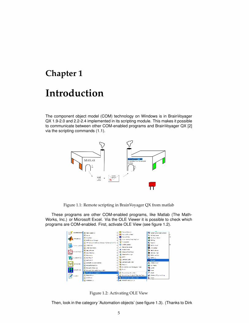
The component object model (COM) technology on Windows is in BrainVoyagerQX 1.9-2.0 and 2.2-2.4 implemented in its scripting module. This makes it possibleto communicate between other COM-enabled programs and BrainVoyager QX [2]via the scripting commands (1.1).
Figure 1.1: Remote scripting in BrainVoyager QX from matlab
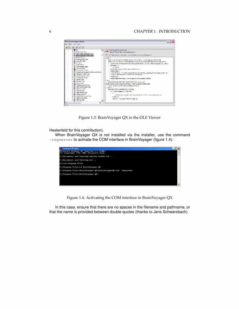
These programs are other COM-enabled programs, like Matlab (The Math-Works, Inc.) or Microsoft Excel. Via the OLE Viewer it is possible to check whichprograms are COM-enabled. First, activate OLE View (see figure 1.2).
Figure 1.2: Activating OLE View
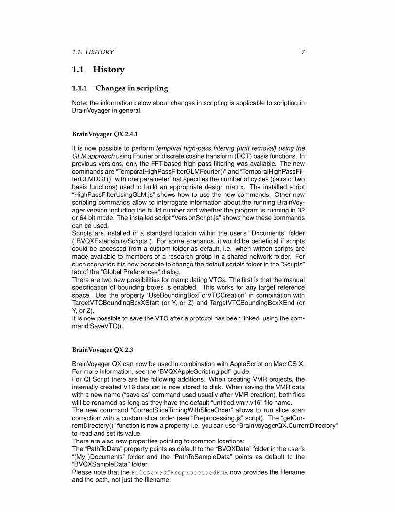
Then, look in the category ’Automation objects’ (see figure 1.3). (Thanks to Dirk
5
6 CHAPTER 1. INTRODUCTION
Figure 1.3: BrainVoyager QX in the OLE Viewer
Heslenfeld for this contribution).When BrainVoyager QX is not installed via the installer, use the command
-regserver to activate the COM interface in BrainVoyager (figure 1.4):
Figure 1.4: Activating the COM interface in BrainVoyager QX
In this case, ensure that there are no spaces in the filename and pathname, orthat the name is provided between double quotes (thanks to Jens Schwarzbach).
1.1. HISTORY 7
1.1 History
1.1.1 Changes in scripting
Note: the information below about changes in scripting is applicable to scripting inBrainVoyager in general.
BrainVoyager QX 2.4.1
It is now possible to perform temporal high-pass filtering (drift removal) using theGLM approach using Fourier or discrete cosine transform (DCT) basis functions. Inprevious versions, only the FFT-based high-pass filtering was available. The newcommands are “TemporalHighPassFilterGLMFourier()” and “TemporalHighPassFil-terGLMDCT()” with one parameter that specifies the number of cycles (pairs of twobasis functions) used to build an appropriate design matrix. The installed script“HighPassFilterUsingGLM.js” shows how to use the new commands. Other newscripting commands allow to interrogate information about the running BrainVoy-ager version including the build number and whether the program is running in 32or 64 bit mode. The installed script “VersionScript.js” shows how these commandscan be used.Scripts are installed in a standard location within the user’s ”Documents” folder(”BVQXExtensions/Scripts”). For some scenarios, it would be beneficial if scriptscould be accessed from a custom folder as default, i.e. when written scripts aremade available to members of a research group in a shared network folder. Forsuch scenarios it is now possible to change the default scripts folder in the ”Scripts”tab of the ”Global Preferences” dialog.There are two new possibilities for manipulating VTCs. The first is that the manualspecification of bounding boxes is enabled. This works for any target referencespace. Use the property ‘UseBoundingBoxForVTCCreation’ in combination withTargetVTCBoundingBoxXStart (or Y, or Z) and TargetVTCBoundingBoxXEnd (orY, or Z).It is now possible to save the VTC after a protocol has been linked, using the com-mand SaveVTC().
BrainVoyager QX 2.3
BrainVoyager QX can now be used in combination with AppleScript on Mac OS X.For more information, see the ‘BVQXAppleScripting.pdf’ guide.For Qt Script there are the following additions. When creating VMR projects, theinternally created V16 data set is now stored to disk. When saving the VMR datawith a new name (“save as” command used usually after VMR creation), both fileswill be renamed as long as they have the default “untitled.vmr/.v16” file name.The new command “CorrectSliceTimingWithSliceOrder” allows to run slice scancorrection with a custom slice order (see “Preprocessing.js” script). The “getCur-rentDirectory()” function is now a property, i.e. you can use “BrainVoyagerQX.CurrentDirectory”to read and set its value.There are also new properties pointing to common locations:The “PathToData” property points as default to the “BVQXData” folder in the user’s“(My )Documents” folder and the “PathToSampleData” points as default to the“BVQXSampleData” folder.Please note that the FileNameOfPreprocessedFMR now provides the filenameand the path, not just the filename.

8 CHAPTER 1. INTRODUCTION
BrainVoyager QX 2.2
There are now reading and writing (File I/O) possibilities. Also, the COM (compo-nent object model) functionality has been implemented, which means that commu-nication between COM-enabled applications on Windows is possible, for examplescripting BrainVoyager from Matlab.New BrainVoyager script functions are available for preprocessing VTC files, cre-ation of MTC from VTC and create function handles.
BrainVoyager QX 2.1
The language is now fully ECMA-script compliant, which means it is basicallyJavaScript. Most of the language features are the same; the graphical user in-terface (GUI) widgets can be made using external user interface files (*.ui).The parameter dataType has been added for creating VTC and VDW files. Twoproperties for changing the confound in SDM files have been added.COM not available.
BrainVoyager QX 2.0
No changes.
BrainVoyager QX 1.10
In BrainVoyager QX 1.10.4, it is also possible to create VDW files via scripting.In BrainVoyager QX 1.10.3, the types of interpolation that can be selected havebeen extended. For more information, please consult the Interpolation in motioncorrection page.
BrainVoyager QX 1.9
This version is updated for BrainVoyager QX 1.9. Two important new changesin BrainVoyager QX 1.9 are the DTI analysis functionality and scripting via thecomponent object model (COM)(this works on Windows platforms).
Also, there are 5 new scripting functions:RenameDicomFilesInDirectory(), BrowseFile(), BrowseDirectory(), CreateProject-DMR() and CreateProjectMosaicDMR().
For details on creating diffusion weighted projects (DMR), see the topic Creat-ing DMR projects.
For the function to rename DICOM files and the use of BrowseDirectory(),please see the new rename DICOM files page.
The new BrainVoyager QX Getting Scripted Guide can be consulted for a step-by-step approach into scripting.
In 1.9.10, the number of interpolation options has increased for slice scan timecorrection* and VTC creation. For details, see the BrainVoyager QX 1.9.10 Re-lease Notes.Changes in the programming language itself concern, for example, the undefinedwhich is in BrainVoyager QX 1.9 an object (so no double quotes are needed). Also,the arguments for the getOpenFileName(s) functions have changed. The languagespecification for Qt Script 1.2.2 by Trolltech can be found also in this guide.

1.1. HISTORY 9
1.1.2 Changes in documentation
29-08-2012: Added information about new functions and properties

10 CHAPTER 1. INTRODUCTION
1.2 Getting started
1.2.1 Starting BrainVoyager QX from Matlab
The BrainVoyager QX can be started from Matlab via the simple command
bvqx = actxserver(’BrainVoyagerQX.BrainVoyagerQXInterface.1’)(QX 1.9 and 2.0)bvqx = actxserver(’BrainVoyagerQX.BrainVoyagerQXScriptAccess.1’)(QX 2.2 and higher)
. BrainVoyager QX will fullfil the role of COM-server, where the COM-client Matlabwill request its methods via the COM-interface (see figure 1.5).
Figure 1.5: Matlab requesting the COM-interface to the BrainVoyager scriptingmethods
The items that are accessible via COM are shown as yellow cubes (objects) inthe Matlab Workspace (see figure 1.6).
We can literally send messages from Matlab to BrainVoyager QX via the PrintToLogfunction of BrainVoyager. The figure 1.7 below shows how easy this is. First, theBrainVoyager QX COM server object is invoked viabvqx = actxserver(’BrainVoyagerQX.BrainVoyagerQXInterface.1’);(QX 1.9 and 2.0) orbvqx = actxserver(’BrainVoyagerQX.BrainVoyagerQXScriptAccess.1’);(QX 2.2) Then, the log tab is sent to the front via bvqx.ShowLogTab;. Now themessage can be sent via the argument for the function PrintToLog():bvqx.PrintToLog(’Message from Matlab...’).
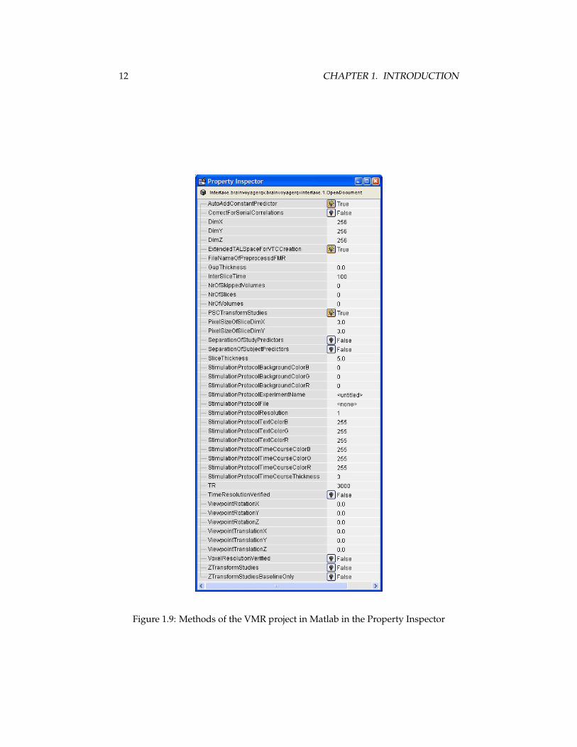
The methods and properties of an object can be found via the Property Inspec-tor in Matlab (see figures 1.8 and 1.9). To open the Property Inspector, right-clickon the bvqx object.
They can also be obtained in a Workspace object list via the method bvqxfuncs = get(bvqx).If necessary, the BrainVoyager QX window can be resized so that Matlab
and BrainVoyager fit on one screen viabvqx.ResizeWindow(600,700);.

1.2. GETTING STARTED 11
Figure 1.6: COM and other objects in the Matlab Workspace
Figure 1.7: Sending a message from Matlab to the BrainVoyager QX log tab
Figure 1.8: Methods of the BrainVoyager QX object in Matlab in the Property In-spector
12 CHAPTER 1. INTRODUCTION
Figure 1.9: Methods of the VMR project in Matlab in the Property Inspector
1.2. GETTING STARTED 13
1.2.2 Syntax differences
The same principles as in Qt Script should be used when scripting BrainVoyagerQX from Matlab. When using a scripting function, first the name of the object ismentioned, then a ’.’ and then the function of that object:nameObject.functionObject();. So when the BrainVoyager server just is
started, only the methods of the BrainVoyager QX application object (here ’bvqx’)can be used, for examplebvqx.OpenDocument(’C:/Data/CG_QX_DCM.vmr’);.Once a BrainVoyager FMR, VMR or AMR project is opened, the functions of projectscan be used as well, for example vmrproject.AddCondition(’LVF’);. How-ever, there is one difference between scripting via the BrainVoyager QX ScriptingEditor and BrainVoyager scripting via Matlab, which is that the () are not usedwhen there are no arguments for a function, for examplevmrproject.ClearStimulationProtocol;.
In BrainVoyager QX, several scripting functions return a boolean value trueor false to indicate whether the operation succeeded, for example when creatingprojects or preprocessing FMR files. In Matlab, these values are simply repre-sented by 0 for false and 1 for true.
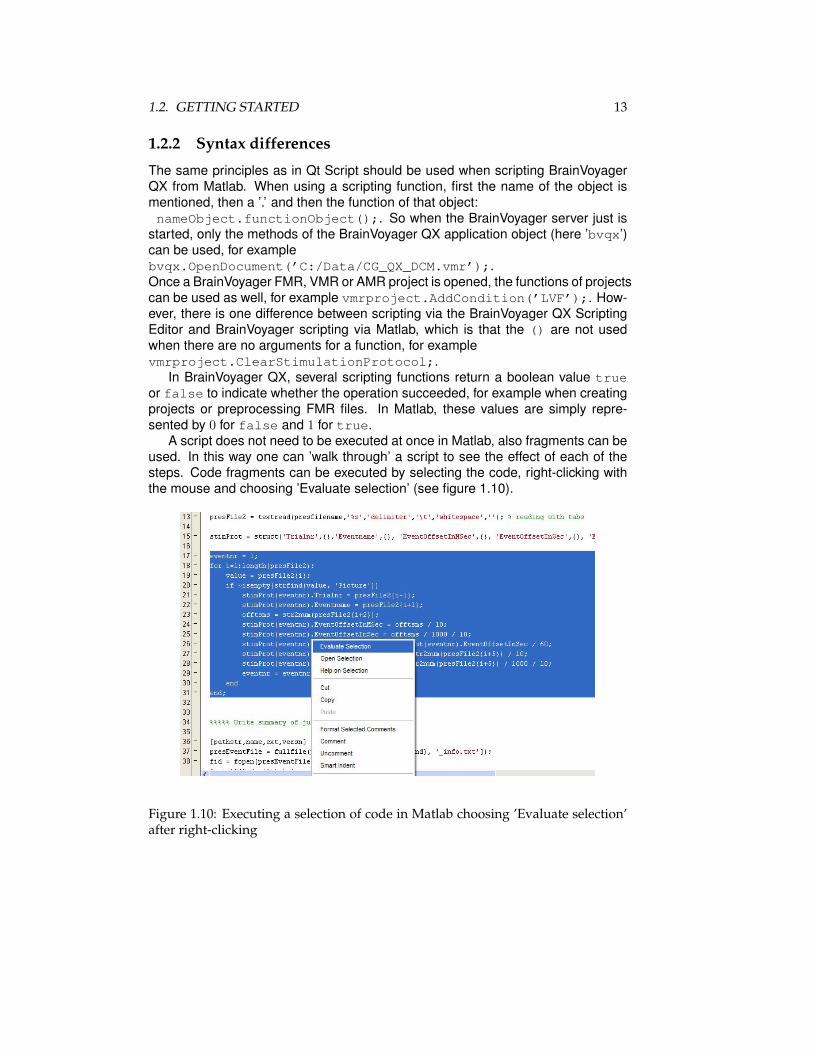
A script does not need to be executed at once in Matlab, also fragments can beused. In this way one can ’walk through’ a script to see the effect of each of thesteps. Code fragments can be executed by selecting the code, right-clicking withthe mouse and choosing ’Evaluate selection’ (see figure 1.10).
Figure 1.10: Executing a selection of code in Matlab choosing ’Evaluate selection’after right-clicking
14 CHAPTER 1. INTRODUCTION
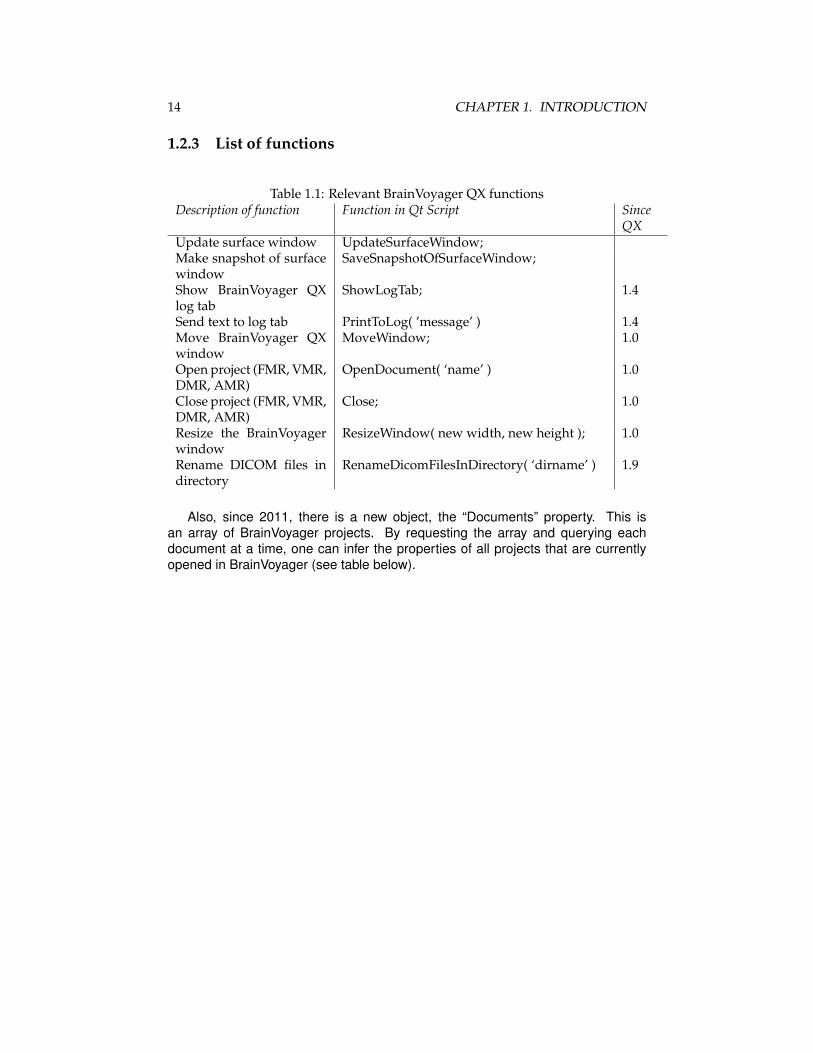
1.2.3 List of functions
Table 1.1: Relevant BrainVoyager QX functionsDescription of function Function in Qt Script Since
QXUpdate surface window UpdateSurfaceWindow;Make snapshot of surfacewindow
SaveSnapshotOfSurfaceWindow;
Show BrainVoyager QXlog tab
ShowLogTab; 1.4
Send text to log tab PrintToLog( ’message’ ) 1.4Move BrainVoyager QXwindow
MoveWindow; 1.0
Open project (FMR, VMR,DMR, AMR)
OpenDocument( ‘name’ ) 1.0
Close project (FMR, VMR,DMR, AMR)
Close; 1.0
Resize the BrainVoyagerwindow
ResizeWindow( new width, new height ); 1.0
Rename DICOM files indirectory
RenameDicomFilesInDirectory( ‘dirname’ ) 1.9
Also, since 2011, there is a new object, the “Documents” property. This isan array of BrainVoyager projects. By requesting the array and querying eachdocument at a time, one can infer the properties of all projects that are currentlyopened in BrainVoyager (see table below).

1.2. GETTING STARTED 15
Table 1.2: BrainVoyager QX object propertiesDescription of property Function in Qt Script Since
QXGet or set current direc-tory
CurrentDirectory 2.3(changefromfunc-tion toprop-erty)
Points to “BVQXData”folder in the users “(My)Documents” folder
PathToData 2.3
Points to “BVQXSample-Data” folder
PathToSampleData 2.3
Get version number ofBrainVoyager QX
VersionMajor 2.3
Get subversion number ofBrainVoyager QX
VersionMinor 2.3
Get build number ofBrainVoyager QX
BuildNumber 2.3
Check whether currentBrainVoyager QX versionis 64-bits (otherwise 32-bits)
Is64Bits 2.3
Position on screen of leftcorner of BrainVoyagerwindow on x-axis
x (property) 1.0
Position on screen of up-per corner of BrainVoy-ager window on y-axis
y (property) 1.0
Get array of currentlyopened projects
Documents (property) 2011
Table 1.3: Documents object propertiesDescription of property Function in Qt Script Since
QXGet number of currentlyopen projects
Count 2011
Get project i of array Item(i) 2011

16 CHAPTER 1. INTRODUCTION

Chapter 2
Creating projects
In this chapter is shown via examples how to create BrainVoyager QX functional(FMR), anatomical 3D (VMR), anatomical 2D (AMR) and diffusion weighted (DMR)projects.
2.1 Renaming DICOM files
But first it might be necessary to rename the files, in case they are DICOM. Thiscan be performed with the commandRenameDicomFilesInDirectory( ’dirname’ ). Example use is first to startBrainVoyager QX via:bvqx = actxserver(’BrainVoyagerQX.BrainVoyagerQX.BrainVoyagerQXScriptAccess.1’);then to rename the files in a certain directory:bvqx.RenameDicomFilesInDirectory(’C:\Data\Experiment\’);
2.2 Creating a functional project (*.fmr)
For a mosaic functional data project (*.fmr), the following parameters need to beprovided:
1. Filetype Define the file type. fileType = ’DICOM’; or use one of’SIEMENS’, ’GE_I’, ’GE_MR’, ’PHILIPS_REC’, ’ANALYZE’.
2. Name of first file Create a variable with the first file name including the filepath. firstFile = ’C:/Data/0001.dcm’;
3. Number of volumes Specify the number of volumes nrOfVols = 252;
4. Number of volumes to skip Specify the number of volumes that should beskipped var skipVols = 2;
5. Create pseudo AMR Indicate whether a pseudo AMR project should be cre-ated from the first functional volume via true or false.createAMR = true;
6. Number of slices Specify the number of slices. nrSlices = 25;
7. STC prefix Provide an prefix name that will be used for the *.stc slice(s).stcprefix = ’run1-’;
17

18 CHAPTER 2. CREATING PROJECTS
8. Swap In case the raw data are Big Endian, set the ’swapBytes’ parameter totrue. byteswap = false;
9. Width of mosaic image Indicate the x-resolution of the mosaic image, this isthe size of the concatenated slices (for example 25 slices will be in a squaregrid of 5 x 5. When the x-resolution of a single file is 64, the x-resolution forthe mosaic image is 5 x 64 = 320. The size is also visible in the ’Rows’ and’Columns’ of the Info tab when creating a project via the user interface.
10. Height of mosaic image Indicate the y-resolution of the mosaic image.
11. Number of bytes per pixel Insert the number of bytes per pixel of the data.For functional data, the number of bytes is usually 2 (short integer, 16 bits).bytesperpixel = 2;
12. Directory to save the data Provide the name of the path where the files shouldbe saved. savingDir = "C:/Data/";
13. Number of volumes in mosaic image Enter the number of volumes in a mo-saic image.
14. Image width The x-resolution parameter should describe the width of theimage. sizeX = 64;
15. Image height The y-resolution parameter should describe the height of theimage. sizeY = 64;
Please note that the order of the parameters is different when the data arenon-mosaic (see the examples below).
Non-mosaicfmr = BrainVoyagerQX.CreateProjectFMR(fileType, fmrname, nrOfVols,...
skipVols, createAMR, nrSlices,...stcprefix,byteswap, sizeX, sizeY, bytesperpixel);
Mosaicfmr = BrainVoyagerQX.CreateProjectMosaicFMR(fileType, fmrname,...nrOfVols, skipVols, createAMR, nrSlices,...
stcprefix, byteswap, mosaicSizeX, mosaicSizeY, bytesperpixel,...targetfolder, nrVolsInImg, sizeX, sizeY);,...
For the BrainVoyager QX sample data used for the Getting Started Guide 2.5,the command would be:
fmr = bvqx.CreateProjectMosaicFMR( ’DICOM’,...’C:/Data/BetSog_20040312_Goebel_C2 -0003-0036-00876.dcm’,...252, 2, true, 25, ’ObjectsExperiment-’, false, 320, 320, 2,...
’C:/Data/Experiment’, 1, 64, 64 );
Save the project via fmr.SaveAs(’ObjectsExperiment.fmr’);.
2.2. CREATING A FUNCTIONAL PROJECT (*.FMR) 19
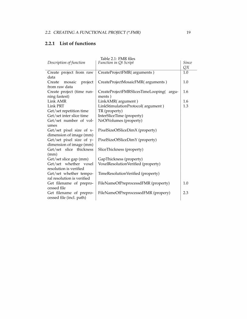
2.2.1 List of functions
Table 2.1: FMR filesDescription of function Function in Qt Script Since
QXCreate project from rawdata
CreateProjectFMR( arguments ) 1.0
Create mosaic projectfrom raw data
CreateProjectMosaicFMR( arguments ) 1.0
Create project (time run-ning fastest)
CreateProjectFMRSlicesTimeLooping( argu-ments )
1.6
Link AMR LinkAMR( argument ) 1.6Link PRT LinkStimulationProtocol( argument ) 1.3Get/set repetition time TR (property)Get/set inter slice time InterSliceTime (property)Get/set number of vol-umes
NrOfVolumes (property)
Get/set pixel size of x-dimension of image (mm)
PixelSizeOfSliceDimX (property)
Get/set pixel size of y-dimension of image (mm)
PixelSizeOfSliceDimY (property)
Get/set slice thickness(mm)
SliceThickness (property)
Get/set slice gap (mm) GapThickness (property)Get/set whether voxelresolution is verified
VoxelResolutionVerified (property)
Get/set whether tempo-ral resolution is verified
TimeResolutionVerified (property)
Get filename of prepro-cessed file
FileNameOfPreprocessdFMR (property) 1.0
Get filename of prepro-cessed file (incl. path)
FileNameOfPreprocessedFMR (propery) 2.3

20 CHAPTER 2. CREATING PROJECTS
2.2.2 Scripts
Script to create multiple mosaic FMR projects in MatlabBelow a script to use the CreateProjectMosaicFMR() function.
%%%%%%%%%%%%%%%%%%%%%%%%%%%%%%%%%%%%%%%%%%%%%%%%%%%%%%%%%%%%%%%%%%%%%%%% create_multiple_fmr_projects.m; script to create multiple functional projects (*.fmr) in Matlab% Works with BrainVoyager QX 2.2%%%%%%%%%%%%%%%%%%%%%%%%%%%%%%%%%%%%%%%%%%%%%%%%%%%%%%%%%%%%%%%%%%%%%%%
% declare and initialize variables (change for own use)filetype = ’DICOM’maindir = ’C:/Data/bvqxdata/AurRou_METFAC_raw_data/AurRou_METFAC_raw_data/functional/’projects = {[maindir ’FFA_localizer_1/BetSor_050730_FACIM_AurRou-0002-0001-0001.dcm’], ...[maindir ’FFA_localizer_2/BetSor_050730_FACIM_AurRou-0003-0001-0001.dcm’]};nrofvols = 268;nrofvolsskip = 4;createamr = 1;nrslices = 24;stcprefix = ’untitled’;swapbytes = 0;mosaicx = 320;mosaicy = 320;bytesperpixel = 2;nrofvolsinimg = 1;imgx = 64;imgy = 64;nrproj = size(projects)
% start (does not require change)bvqx = actxserver(’BrainVoyagerQX.BrainVoyagerQXScriptAccess.1’)for i=1:nrproj(2)
[pathstr, name, ext, versn] = fileparts(projects{i})fmr = bvqx.CreateProjectMosaicFMR(filetype, projects{i}, nrofvols, nrofvolsskip, createamr, nrslices, ...stcprefix, swapbytes, mosaicx, mosaicy, bytesperpixel, pathstr, nrofvolsinimg, imgx, imgy);fmr.SaveAs([pathstr ’/’ name ’.fmr’]);fmr.Close;
end

2.3. CREATING AN ANATOMICAL PROJECT (*.VMR) 21
2.3 Creating an anatomical project (*.vmr)
Scripting a VMR project is relatively straightforward, if the parameters are known.The function CreateProjectVMR() only requires 7 parameters:
1. The filetype, which is one of ’DICOM’, ’SIEMENS’, ’GE_I’, ’GE_MR’,’PHILIPS_REC’ or ’ANALYZE’.2. The first file name, including path.3. A boolean value true or false indicating whether the data need to be swapped.4. The number of slices.5. The size of the image on the x-axis.6. The size of the image on the y-axis.7. The number of bytes per pixel. For anatomical data, this likely to be 1 or 2 bytes.
The function returns a VMR project object (see figure 2.1).
Figure 2.1: The VMR project object
22 CHAPTER 2. CREATING PROJECTS
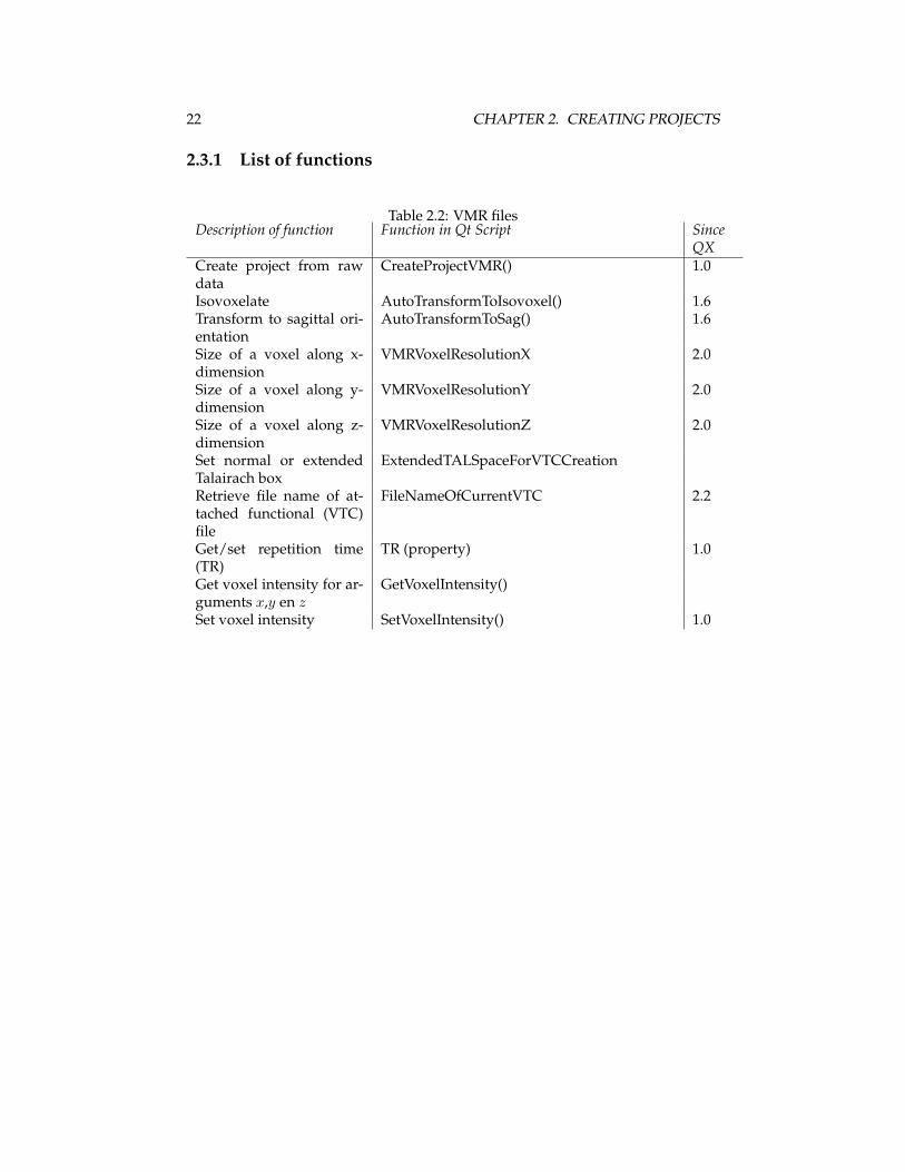
2.3.1 List of functions
Table 2.2: VMR filesDescription of function Function in Qt Script Since
QXCreate project from rawdata
CreateProjectVMR() 1.0
Isovoxelate AutoTransformToIsovoxel() 1.6Transform to sagittal ori-entation
AutoTransformToSag() 1.6
Size of a voxel along x-dimension
VMRVoxelResolutionX 2.0
Size of a voxel along y-dimension
VMRVoxelResolutionY 2.0
Size of a voxel along z-dimension
VMRVoxelResolutionZ 2.0
Set normal or extendedTalairach box
ExtendedTALSpaceForVTCCreation
Retrieve file name of at-tached functional (VTC)file
FileNameOfCurrentVTC 2.2
Get/set repetition time(TR)
TR (property) 1.0
Get voxel intensity for ar-guments x,y en z
GetVoxelIntensity()
Set voxel intensity SetVoxelIntensity() 1.0

2.3. CREATING AN ANATOMICAL PROJECT (*.VMR) 23
2.3.2 Scripts
Script to create a VMR project via Matlab dialogs%%%%%%%%%%%%%%%%%%%%%%%%%%%%%%%%%%%%%%%%%%%%%%%%%%%%%%%%%%%%%%%%%%%%%
% create_vmrproject_via_interface.m% Script to create a BrainVoyager VMR project in Matlab% Works with BrainVoyager QX 2.2%%%%%%%%%%%%%%%%%%%%%%%%%%%%%%%%%%%%%%%%%%%%%%%%%%%%%%%%%%%%%%%%%%%%%%
bvqx = actxserver(’BrainVoyagerQX.BrainVoyagerQXScriptAccess.1’)h = msgbox(’Please select the first file of the raw data set’, ’Create VMR project’);% Seefigure 2.2uiwait(h);cancel = 0;
Figure 2.2: Announcement at beginning of script
% get first file % See figure 2.3[filename, pathname] = uigetfile( ...
{’*.dcm; *.IMA; *.I; *.MR; *.REC;*.hdr’,’Raw data files (*.dcm,*.IMA,*.I, *.MR, *.REC,*.hdr)’;’*.dcm’, ’DICOM files (*.dcm)’; ...
’*.IMA’,’Siemens DICOM files (*.IMA)’; ...’*.I’,’GE I files (*.I)’; ...’*.MR’,’GE MR (*.MR)’; ...’*.REC’,’Philips files (*.REC)’; ...’*.hdr’,’Analyze (*.hdr)’}, ...
’Please select the first file’);
Figure 2.3: Select the first file
firstfilename = strcat(pathname, filename);[pathstr,name,ext,versn] = fileparts(firstfilename);switch ext
case ’.dcm’, filetype = ’DICOM’case ’.IMA’, filetype = ’SIEMENS’case ’.I’, filetype = ’GE_I’case ’.MR’, filetype = ’GE_MR’case ’.REC’, filetype = ’PHILIPS_REC’case ’.hdr’, filetype = ’ANALYZE’otherwise cancel = 1
end
if ˜cancel% get parameters
if (strcmp(ext, ’.dcm’) == 1) && (exist(’dicominfo.m’) > 0)dcminfo = dicominfo(firstfilename);bytesperpixel = (dcminfo.BitsAllocated/8);xres = dcminfo.Columns;yres = dcminfo.Rows;
24 CHAPTER 2. CREATING PROJECTS
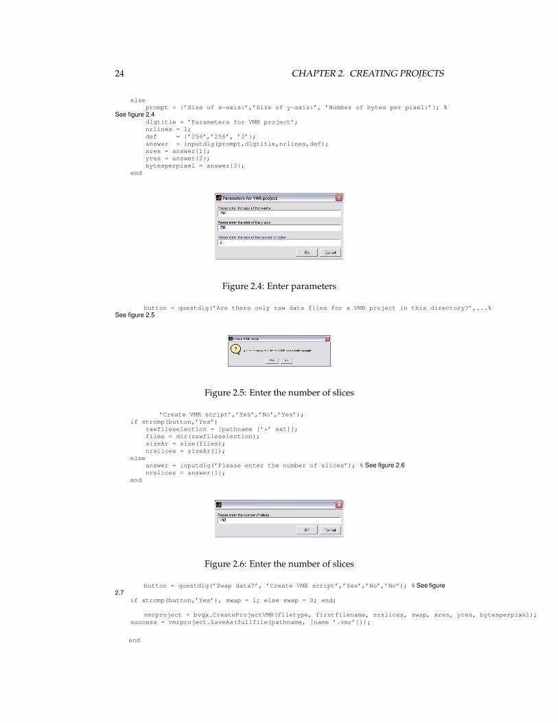
elseprompt = {’Size of x-axis:’,’Size of y-axis:’, ’Number of bytes per pixel:’}; %
See figure 2.4dlgtitle = ’Parameters for VMR project’;nrlines = 1;def = {’256’,’256’, ’2’};answer = inputdlg(prompt,dlgtitle,nrlines,def);xres = answer{1};yres = answer{2};bytesperpixel = answer{3};
end
Figure 2.4: Enter parameters
button = questdlg(’Are there only raw data files for a VMR project in this directory?’,...%See figure 2.5
Figure 2.5: Enter the number of slices
’Create VMR script’,’Yes’,’No’,’Yes’);if strcmp(button,’Yes’)
rawfileselection = [pathname [’*’ ext]];files = dir(rawfileselection);sizeAr = size(files);nrslices = sizeAr(1);
elseanswer = inputdlg(’Please enter the number of slices’); % See figure 2.6nrslices = answer{1};
end
Figure 2.6: Enter the number of slices
button = questdlg(’Swap data?’, ’Create VMR script’,’Yes’,’No’,’No’); % See figure2.7
if strcmp(button,’Yes’), swap = 1; else swap = 0; end;
vmrproject = bvqx.CreateProjectVMR(filetype, firstfilename, nrslices, swap, xres, yres, bytesperpixel);success = vmrproject.SaveAs(fullfile(pathname, [name ’.vmr’]));
end

2.3. CREATING AN ANATOMICAL PROJECT (*.VMR) 25
Figure 2.7: Question whether swapping is necessary
26 CHAPTER 2. CREATING PROJECTS
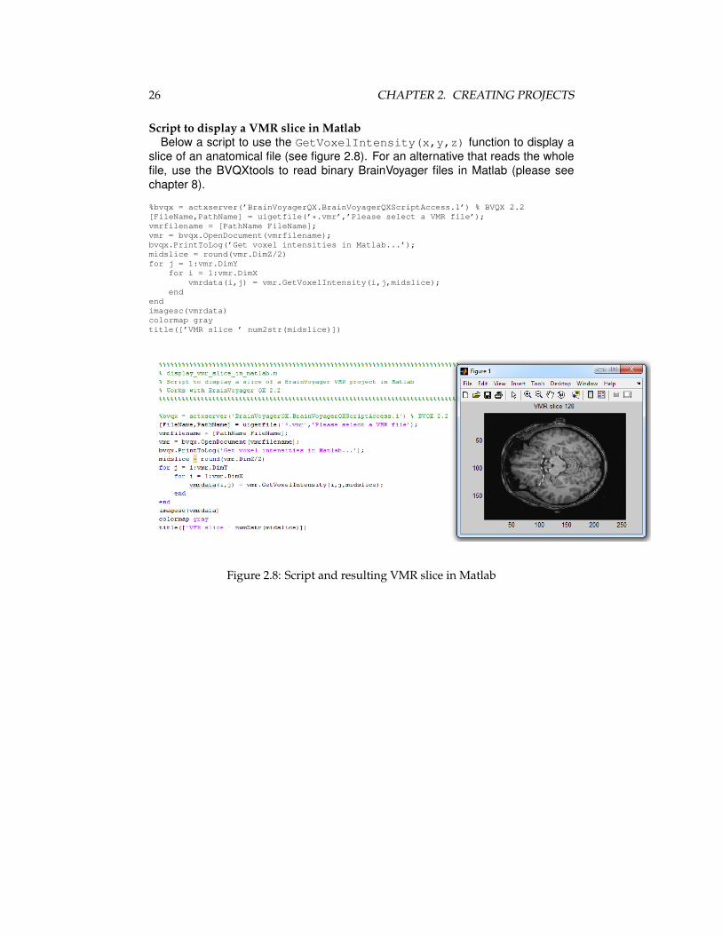
Script to display a VMR slice in MatlabBelow a script to use the GetVoxelIntensity(x,y,z) function to display a
slice of an anatomical file (see figure 2.8). For an alternative that reads the wholefile, use the BVQXtools to read binary BrainVoyager files in Matlab (please seechapter 8).
%bvqx = actxserver(’BrainVoyagerQX.BrainVoyagerQXScriptAccess.1’) % BVQX 2.2[FileName,PathName] = uigetfile(’*.vmr’,’Please select a VMR file’);vmrfilename = [PathName FileName];vmr = bvqx.OpenDocument(vmrfilename);bvqx.PrintToLog(’Get voxel intensities in Matlab...’);midslice = round(vmr.DimZ/2)for j = 1:vmr.DimY
for i = 1:vmr.DimXvmrdata(i,j) = vmr.GetVoxelIntensity(i,j,midslice);
endendimagesc(vmrdata)colormap graytitle([’VMR slice ’ num2str(midslice)])
Figure 2.8: Script and resulting VMR slice in Matlab
2.3. CREATING AN ANATOMICAL PROJECT (*.VMR) 27
Script to filter a VMR in MatlabThis script applies a Laplacian of a Gaussian, a Sobel (approximating a gradient)
or a Canny filter on a VMR project and displays it in BrainVoyager QX.%%%%%%%%%%%%%%%%%%%%%%%%%%%%%%%%%%%%%%%%%%%%%%%%%%%%%%%%%%%%%%%%%%%%%
% filter_vmr_in_matlab.m% Script to filter a BrainVoyager VMR project in Matlab%% Works with BrainVoyager QX 1.9 and VMR versions higher than 1.%%%%%%%%%%%%%%%%%%%%%%%%%%%%%%%%%%%%%%%%%%%%%%%%%%%%%%%%%%%%%%%%%%%%%%
[FileName,PathName] = uigetfile(’*.vmr’,’Please select a VMR file’);vmrfilename = [PathName FileName];fid = fopen(vmrfilename, ’rb’);version = fread(fid, [1 1], ’uint16’);dimx = fread(fid, [1 1], ’uint16’);dimy = fread(fid, [1 1], ’uint16’);dimz = fread(fid, [1 1], ’uint16’);data = fread(fid, [1 dimx*dimy*dimz], ’uchar’);rest = fread(fid);fclose(fid);vmrdata = reshape(data, dimx, dimy, dimz);
% H = FSPECIAL(’log’,HSIZE,SIGMA) returns a rotationally symmetric% Laplacian of Gaussian filter of size HSIZE with standard deviation% SIGMA (positive). HSIZE can be a vector specifying the number of rows% and columns in H or a scalar, in which case H is a square matrix.% The default HSIZE is [5 5], the default SIGMA is 0.5.
% show filters %(see figure 2.9)figure;img = vmrdata(:,:,floor(dimx/2));img = rot90(img, 3);subplot(2,2,1);imagesc(img);title(’Original Image’);H = fspecial(’log’,[5 5],.5);Laplacian = imfilter(img,H);subplot(2,2,2);imagesc(Laplacian);title(’Laplacian of Gaussian filter’);cannyimg = edge(img,’canny’,.15);subplot(2,2,3);imagesc(cannyimg);title(’Canny filter (0.15)’);H = fspecial(’sobel’);sobelimg = imfilter(img,H);subplot(2,2,4);imagesc(sobelimg);title(’Sobel filter’);colormap gray;
filterlist = {’Laplacian’, ’Canny’, ’Sobel’}; %(see figure 2.10)[filter,ok] = listdlg(’PromptString’,’Select a filter:’,...’SelectionMode’,’single’,...’Name’, ’Filter VMR’,...’ListString’,filterlist);
H_log = fspecial(’log’,[5 5],.5);H_sobel = fspecial(’sobel’);
if filter == 2 %(see figure 2.11)prompt = {’Enter canny filter value:’};
dlg_title = ’Filter VMR’;num_lines= 1;def = {’0.15’};answer = inputdlg(prompt,dlg_title,num_lines,def);filterval = answer{1};
end
% apply filter and write image[pathstr,name,ext,versn] = fileparts(vmrfilename);filteredimgname = fullfile(pathstr, [name ’_filtered’ ext]);if ok == 1
% write VMR headerfid = fopen(filteredimgname,’w’);fwrite(fid,version,’ushort’);fwrite(fid,dimx,’ushort’);fwrite(fid,dimy,’ushort’);fwrite(fid,dimz,’ushort’);% write VMR image volumefor slicenr=1:len(3)
img = vmrdata(:,:,slicenr);if filter==1
filteredimg = imfilter(img,H_log);elseif filter ==3
filteredimg = imfilter(img, H_sobel);elseif filter == 2

28 CHAPTER 2. CREATING PROJECTS
filteredimg = edge(img,’canny’,filterval);else
break;endfwrite(fid,filteredimg,’uchar’);
end% write rest of VMR headerfwrite(fid,rest);fclose(fid);
end
% show in BrainVoyager QX
bvqx = actxserver(’BrainVoyagerQX.BrainVoyagerQXInterface’);
filteredvmr = bvqx.OpenDocument(filteredimgname);
bvqx.ShowLogTab;
bvqx.PrintToLog([’Filter: ’ filterlist{filter}]);
Figure 2.9: Show filters
Figure 2.10: Select filter dialog

2.3. CREATING AN ANATOMICAL PROJECT (*.VMR) 29
Figure 2.11: Enter canny filter value

30 CHAPTER 2. CREATING PROJECTS
2.4 Creating AMR projects
The parameters for CreateProjectAMR() are:Parameter: Filetype (string): file type of original data. One of "DICOM", "SIEMENS","GE_I" (no parameters for +20 logic like in GUI),"GE_MR", "PHILIPS_REC" or"ANALYZE".Parameter: firstFile (string): the filename and path of the first file of the data.Parameter: nrOfSlices (integer): the number of slices in a volume.Parameter: isLittleEndian (boolean): Is ’true’ when the byte order is little endian;otherwise ’false’.Parameter: xSize (integer): Size of image along x-axis. Example value: 256.Parameter: ySize (integer): Size of image along y-axis. Example value: 256.Parameter: nrOfBytes (integer): Number of bytes for each pixel. 1 byte is 8 bits.Example value: 2.Returns: AMR project object
2.4.1 List of functions
Table 2.3: AMR filesDescription of function Function in Qt Script Since
QXCreate project from rawdata
CreateProjectAMR() 1.0

2.5. CREATING A DIFFUSION WEIGHTED PROJECT (*.DMR) 31
2.5 Creating a diffusion weighted project (*.dmr)
Diffusion weighted data can be treated in the same fashion as anatomical andfunctional data, via the creation of a BrainVoyager QX project.
2.5.1 List of functions
Table 2.4: DMR filesDescription of function Function in Qt Script Since
QXCreate project from rawdata
CreateProjectDMR() 1.9
Create mosaic projectfrom raw data
CreateProjectMosaicDMR() 1.9
Link AMR LinkAMR() 1.6Get data TR (property)
InterSliceTime (property)NrOfVolumes (property)PixelSizeOfSliceDimX (property)PixelSizeOfSliceDimY (property)SliceThickness (property)GapThickness (property)VoxelResolutionVerified (property)TimeResolutionVerified (property)

32 CHAPTER 2. CREATING PROJECTS
2.5.2 Scripts
Script to create diffusion weighted projects (*.dmr) and normalized files (*.vdw)
%%%%%%%%%%%%%%%%%%%%%%%%%%%%%%%%%%%%%%%%%%%%%%%%%%%%%%%%%%%%%%%%%%%%%%%% diffusion_data.m% Assumes: a) all data are in same folder b) data are aligned and% anatomical volume is transformed to all spaces (please comment lines out% if not the case)%% Works with BrainVoyager QX 2.2%%%%%%%%%%%%%%%%%%%%%%%%%%%%%%%%%%%%%%%%%%%%%%%%%%%%%%%%%%%%%%%%%%%%%%%
bvqx = actxserver(’BrainVoyagerQX.BrainVoyagerQXScriptAccess.1’)bvqx.PrintToLog(’Start processing diffusion weighted data...’);
% ˜˜˜ this part will require modifications, if used for own purposes ˜˜˜dmrname = ’C:/Data/bvqxdata/Human31dir/human31dir_from_script.dmr’; % this variable is also used in 2nd partanswer = questdlg(’Create diffusion project?’, ’Create DMR’);if answer == ’Yes’
dmr = bvqx.CreateProjectDMR( ’DICOM’, ...’C:/Data/bvqxdata/Human31dir/pimpul_070907_dti -0007-0001-00001.dcm’, ...31, 0, true, 75, ’human31dir’, false, 128, 128, 2, ’C:/Data/bvqxdata/Human31dir’);dmr.SaveAs(dmrname);
end
% ˜˜˜ this part does not require modifications, is all user-interface based ˜˜˜% if alignment files happen to be available, one could as well create% normalized diffusion weighted data files:answer = questdlg(’Create normalized diffusion data? (requires *.trf files)’, ’Create VDW’);if answer == ’Yes’
[pathstr, name, ext, versn] = fileparts(dmrname)[FileName, PathName] = uigetfile(’*.vmr’,’Please select the anatomical file...’);vmr = bvqx.OpenDocument([PathName FileName]);% assumes a single initial alignment file in the directory of the VMRiafilename = dir([PathName ’*_IA.trf’])% assumes a single fine alignment file in the directory of the VMRfafilename = dir([PathName ’*_FA.trf’])% assumes a single AC-PC transformation file in the directory of the VMRacpcfilename = dir([PathName ’*_ACPC.trf’])% assumes a single Talairach landmark file in the directory of the VMRtalfilename = dir([PathName ’*.tal’])answer = questdlg(’Would you like a high-precision data format (float)?’, ’Datatype’);if answer == ’Yes’
datatype = 2;else
datatype = 1;endresolutionlist = {’1mmˆ3’, ’2mmˆ3’, ’3mmˆ3’};[resolution, ok] = listdlg(’PromptString’,’Select the target resolution:’,...
’SelectionMode’,’single’,...’Name’, ’VDW resolution’,...’ListString’, resolutionlist);
interpolationlist = {’nearest neighbor’, ’trilinear’, ’sinc’};[interpolation, ok] = listdlg(’PromptString’,’Select the interpolation type:’,...
’SelectionMode’,’single’,...’Name’, ’Interpolation’,...’ListString’, interpolationlist)
interpolation = interpolation - 1; % 0: nearest neighbour, 1: trilinear interpolation, 2: interpolation.
prompt = {’Enter intensity threshold:’};%,’Enter colormap name:’};dlg_title = ’Intensity threshold’;num_lines = 1;def = {’100’};%,’hsv’};threshold = inputdlg(prompt,dlg_title,num_lines,def);ia = [PathName iafilename(1).name] % takes first initial alignment file it finds in folderfa = [PathName fafilename(1).name] % takes first fine alignment file it finds in folderacpc = [PathName acpcfilename(1).name] % takes first AC-PC alignment file it finds in foldertal = [PathName talfilename(1).name] % takes first Talairach landmarks file it finds in folderthresh = str2num(threshold{1})vmr.ExtendedTALSpaceForVTCCreation = 0; % no extended bounding box for cerebellumvdw = fullfile(pathstr, [name ’_native.vdw’])success = vmr.CreateVDWInVMRSpace(dmrname,ia,fa,vdw,datatype,resolution, interpolation, thresh);vdw = fullfile(pathstr, [name ’_acpc.vdw’])success = vmr.CreateVDWInACPCSpace(dmrname,ia,fa,acpc,vdw,datatype,resolution, interpolation, thresh);vdw = fullfile(pathstr, [name ’_tal.vdw’])success = vmr.CreateVDWInTALSpace(dmrname,ia,fa,acpc,tal,vdw,datatype,resolution, interpolation, thresh);
endbvqx.PrintToLog(’Finished processing diffusion data.’);

Chapter 3
Preprocessing functional data
In this section will be described how to preprocess functional data in BrainVoyagerfrom Matlab.
3.1 Preprocessing functional data (*.fmr)
3.1.1 Slice scan time correction
There are two slice scan time correction functions. The first slice scan time correc-tion method, CorrectSliceTiming(), accepts two parameters, which are theslice order and the type of interpolation. The second
Slice scan time correction with slice order and interpolation arguments
The slice order parameter can have the following values:
Table 3.1: Slice order optionsSlice order ValueAscending 0Ascending interleaved 1Ascending interleaved 2 2Descending 10Descending interleaved 11Descending interleaved 2 12
The interpolation can have the following values:
Table 3.2: Interpolation optionsInterpolation type ValueTrilinear 0Cubic spline 1Sinc 2
33
34 CHAPTER 3. PREPROCESSING FUNCTIONAL DATA
Perform the slice scan time correction from Matlab viasuccess = fmr.CorrectSliceTiming(1, 0);
Obtain the name of the slice scan time corrected project vianewfmrname = fmr.FileNameOfPreprocessedFMR;.
Close the non-preprocessed FMR viafmr.Close;.
Open the slice scan time corrected project vianewfmr = fmr.OpenDocument(newfmrname);
Slice scan time correction with specified slice order and interpolation
In the first argument of the function CorrectSliceTimingWithSliceOrder theorder of the slices is provided via a text string:
fmr = BrainVoyagerQX.ActiveDocument;fmr.CorrectSliceTimingWithSliceOrder("1 14 2 15 3 16 4 17 5 18 6 19 7 20 8 21 9 22 10 23 11 24 12 25 13", 1);
3.1.2 Motion correction
In BrainVoyager QX, there are two methods to perform motion correction withinone run. These areCorrectMotion() and CorrectMotionEx(). In the latter method, the numberof parameters that can be used for the motion correction is extended.
If multiple runs are performed in one session, the run closest to the 3D scanwould be corrected by using the single-run version: CorrectMotion(int TargetVolume),i.e. with a value of 1 for the parameter TargetVolume. All subsequent runs wouldthen be corrected by specifying the name of the first run as target as well as thesame volume as specified for the first run. This ensures that all volumes of all runsare aligned to the same target volume.
If CorrectMotion( <target volume nr> ) is used, the applied methodis trilinear detection and sinc interpolation. This can be inspected in the *_3DMC.logfile. This can also be seen from the resulting filename, containing ’3DMCTS’,where the ’T’ stands for trilinear detection and the ’S’ for sinc interpolation.The full data set will be used, and the default number of iterations is set (100). Noextended log file is created.
In the version with extended parameters, the parameters are the following:CorrectMotionEx(Target volume (number), ...Interpolation method (0 or 1),...Full data set (true or false), ...
Max nr of iterations (number),...movies (true or false),...log (true or false));(Replace the names by real parameters and remove spaces in the names).
3.1.3 Motion correction and intrasession alignment
To combine motion correction with intra-session alignment, the methodsCorrectMotionTargetVolumeInOtherRun() andCorrectMotionTargetVolumeInOtherRunEx() are available.
The CorrectMotionTargetVolumeInOtherRun(filename, volume) ac-cepts the following 2 parameters:
1. target fmr file name
3.1. PREPROCESSING FUNCTIONAL DATA (*.FMR) 35
2. target volume number
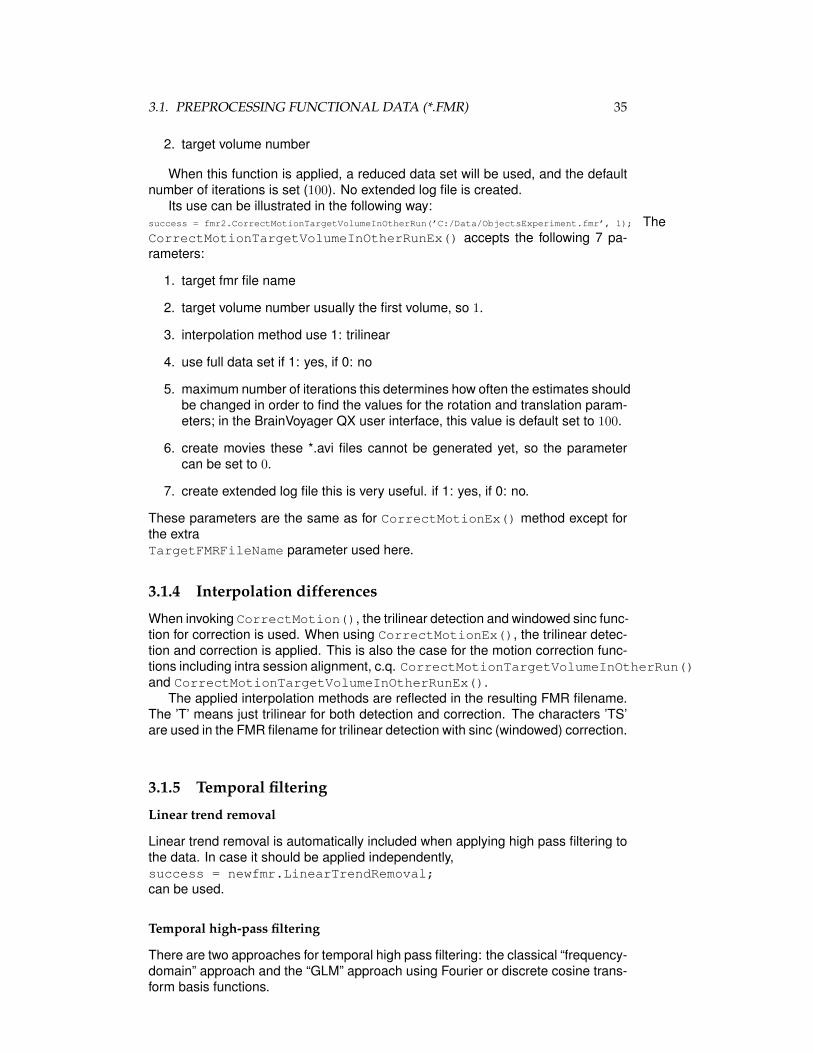
When this function is applied, a reduced data set will be used, and the defaultnumber of iterations is set (100). No extended log file is created.
Its use can be illustrated in the following way:success = fmr2.CorrectMotionTargetVolumeInOtherRun(’C:/Data/ObjectsExperiment.fmr’, 1); TheCorrectMotionTargetVolumeInOtherRunEx() accepts the following 7 pa-rameters:
1. target fmr file name
2. target volume number usually the first volume, so 1.
3. interpolation method use 1: trilinear
4. use full data set if 1: yes, if 0: no
5. maximum number of iterations this determines how often the estimates shouldbe changed in order to find the values for the rotation and translation param-eters; in the BrainVoyager QX user interface, this value is default set to 100.
6. create movies these *.avi files cannot be generated yet, so the parametercan be set to 0.
7. create extended log file this is very useful. if 1: yes, if 0: no.
These parameters are the same as for CorrectMotionEx() method except forthe extraTargetFMRFileName parameter used here.
3.1.4 Interpolation differences
When invoking CorrectMotion(), the trilinear detection and windowed sinc func-tion for correction is used. When using CorrectMotionEx(), the trilinear detec-tion and correction is applied. This is also the case for the motion correction func-tions including intra session alignment, c.q. CorrectMotionTargetVolumeInOtherRun()and CorrectMotionTargetVolumeInOtherRunEx().
The applied interpolation methods are reflected in the resulting FMR filename.The ’T’ means just trilinear for both detection and correction. The characters ’TS’are used in the FMR filename for trilinear detection with sinc (windowed) correction.
3.1.5 Temporal filtering
Linear trend removal
Linear trend removal is automatically included when applying high pass filtering tothe data. In case it should be applied independently,success = newfmr.LinearTrendRemoval;can be used.
Temporal high-pass filtering
There are two approaches for temporal high pass filtering: the classical “frequency-domain” approach and the “GLM” approach using Fourier or discrete cosine trans-form basis functions.

36 CHAPTER 3. PREPROCESSING FUNCTIONAL DATA
High-pass filtering: “Frequency-domain” approachThe high pass filter is applied in the frequency domain. The temporal high-pass
filter can be specified in cycles or in Hz.When it is specified in cycles, is this relative to the number of time points specifiedin the functional data, i.e. length of the time series. When the units are specified inHz, it is in signal intensity changes per Hz, for example:
success = newfmr.TemporalHighPassFilter(0.115385, ’Hz’);
The units in Hertz can be computed from the cycles per time course via: num-ber of cycles / number of data points.
High-pass filtering: GLM with Fourier or DCT basis functionsWith Fourier basis functions: TemporalHighPassFilterGLMFourier().
With discrete cosine transform basis functions: TemporalHighPassFilterGLMDCT().The functions take one parameter that specifies the number of cycles (pairs of twobasis functions) used to build an appropriate design matrix.
Temporal Gaussian smoothing
Temporal Gaussian smoothing in FMR projects can be applied by specifying thewidth of the smoothing kernel in seconds (’s’) or in TR (’TR’), for example:
newfmr.TemporalGaussianSmoothing(20, ’s’);
Spatial smoothing
Specification of the smoothing kernel for the FMR project is possible up to twodecimals. When more values are specified, they will be rounded (1.06667 pixelsround to 1.07). The units can be specified in pixels, ’px’ or millimeters, ’mm’:
newfmr.SpatialGaussianSmoothing(4, ’mm’);andnewfmr.SpatialGaussianSmoothing(1.06667, ’px’);
The resulting files will be placed in the same folder as the source files. Thefilenames will contain the _SD3DSS appendix.
3.1. PREPROCESSING FUNCTIONAL DATA (*.FMR) 37
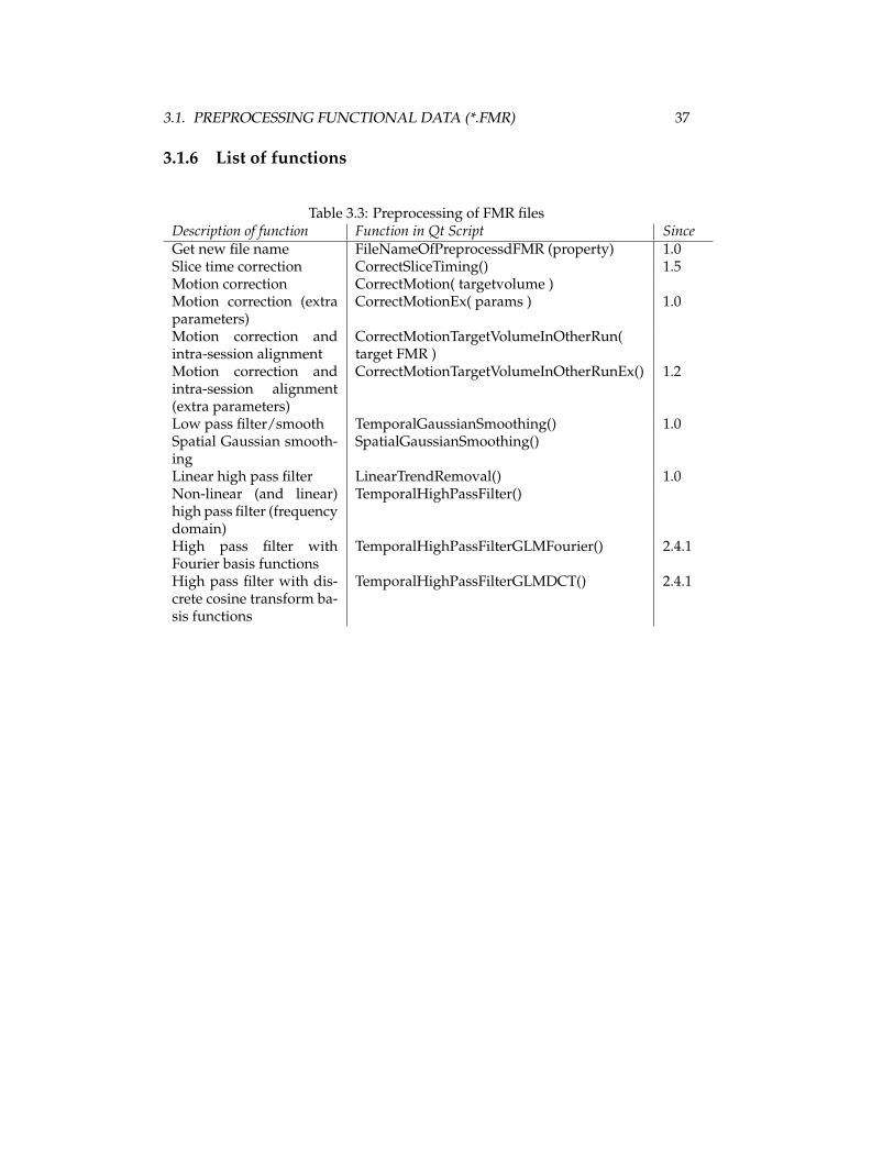
3.1.6 List of functions
Table 3.3: Preprocessing of FMR filesDescription of function Function in Qt Script SinceGet new file name FileNameOfPreprocessdFMR (property) 1.0Slice time correction CorrectSliceTiming() 1.5Motion correction CorrectMotion( targetvolume )Motion correction (extraparameters)
CorrectMotionEx( params ) 1.0
Motion correction andintra-session alignment
CorrectMotionTargetVolumeInOtherRun(target FMR )
Motion correction andintra-session alignment(extra parameters)
CorrectMotionTargetVolumeInOtherRunEx() 1.2
Low pass filter/smooth TemporalGaussianSmoothing() 1.0Spatial Gaussian smooth-ing
SpatialGaussianSmoothing()
Linear high pass filter LinearTrendRemoval() 1.0Non-linear (and linear)high pass filter (frequencydomain)
TemporalHighPassFilter()
High pass filter withFourier basis functions
TemporalHighPassFilterGLMFourier() 2.4.1
High pass filter with dis-crete cosine transform ba-sis functions
TemporalHighPassFilterGLMDCT() 2.4.1

38 CHAPTER 3. PREPROCESSING FUNCTIONAL DATA
3.2 Preprocessing of functional normalized data (*.vtc)
Since BrainVoyager QX 2.2. it is possible to apply temporal and spatial filtering tofunctional normalized data (*.vtc).
3.2.1 List of functions
Table 3.4: Preprocessing of VTC filesDescription of function Function in Qt Script SinceSpatial low-pass filter SpatialGaussianSmoothing 2.2Temporal low pass fil-ter/smooth
TemporalGaussianSmoothing() 2.2
Non-linear (and linear)temporal high-pass filter
TemporalHighPassFilter() 2.2
Linear temporal high-pass filter
LinearTrendRemoval() 2.2

3.3. SCRIPTS 39
3.3 Scripts
3.3.1 Preprocessing a functional data file (*.fmr)
This script applies preprocessing to a functional data (*.fmr) file.
%%%%%%%%%%%%%%%%%%%%%%%%%%%%%%%%%%%%%%%%%%%%%%%%%%%%% preprocess_fmr.m% Preprocess a previously created functional data file (*.fmr).% Here we open the "CG_OBJECTS_SCRIPT.fmr" file.% Works with BrainVoyager QX 2.2%%%%%%%%%%%%%%%%%%%%%%%%%%%%%%%%%%%%%%%%%%%%%%%%%%%%
bvqx = actxserver(’BrainVoyagerQX.BrainVoyagerQXScriptAccess.1’)[FileName PathName] = uigetfile(’*.fmr’) % select the CG_OBJECTS filedocFMR = bvqx.OpenDocument([PathName FileName]);
% Set spatial and temporal parameters relevant for preprocessing% You can skip this, if you have checked that these values are set when reading the data% To check whether these values have been set already (i.e. from header),% use the "VoxelResolutionVerified" and "TimeResolutionVerified" propertiesif ˜docFMR.TimeResolutionVerified
docFMR.TR = 2000;docFMR.InterSliceTime = 80;docFMR.TimeResolutionVerified = 1;
endif ˜docFMR.VoxelResolutionVerified
docFMR.PixelSizeOfSliceDimX = 3.5;docFMR.PixelSizeOfSliceDimY = 3.5;docFMR.SliceThickness = 3;docFMR.GapThickness = 0.99;docFMR.VoxelResolutionVerified = 1;
end
% We save the new settings into the FMR filedocFMR.Save;
% Preprocessing step 1: Slice time correctiondocFMR.CorrectSliceTiming( 1, 0 );% First param: Scan order 0 -> Ascending, 1 -> Asc-Interleaved, 2 -> Asc-Int2,% 10 -> Descending, 11 -> Desc-Int, 12 -> Desc-Int2% Second param: Interpolation method: 0 -> trilinear, 1 -> cubic spline, 2 -> sincResultFileName = docFMR.FileNameOfPreprocessdFMR;docFMR.Close;docFMR = bvqx.OpenDocument( ResultFileName );
% Preprocessing step 2: 3D motion correctiondocFMR.CorrectMotion(1);% the current doc (input FMR) knows the name of the automatically saved output FMRResultFileName = docFMR.FileNameOfPreprocessdFMR;docFMR.Remove; % close or remove input FMRbvqx.PrintToLog(’Removed slice scan time corrected files instead of just closing...’)% docFMR.Close(); // close input FMR% Open motion corrected file (output FMR) and assign to our doc vardocFMR = bvqx.OpenDocument( ResultFileName );
% Preprocessing step 3: Spatial Gaussian Smoothing (not recommended% for individual analysis with a 64x64 matrix)docFMR.SpatialGaussianSmoothing( 4, ’mm’); % FWHM value and unitResultFileName = docFMR.FileNameOfPreprocessdFMR;docFMR.Close; % docFMR.Remove(); % close or remove input FMRdocFMR = bvqx.OpenDocument( ResultFileName );
% Preprocessing step 4: Temporal High Pass Filter, includes Linear Trend% RemovaldocFMR.TemporalHighPassFilter( 3, ’cycles’);ResultFileName = docFMR.FileNameOfPreprocessdFMR;docFMR.Close; % docFMR.Remove(); // close or remove input FMRdocFMR = bvqx.OpenDocument( ResultFileName );
% Preprocessing step 5: Temporal Gaussian Smoothing (not recommended for% event-related data)docFMR.TemporalGaussianSmoothing( 10, ’s’);ResultFileName = docFMR.FileNameOfPreprocessdFMR;docFMR.Close; % docFMR.Remove(); % close or remove input FMRdocFMR = bvqx.OpenDocument( ResultFileName );
40 CHAPTER 3. PREPROCESSING FUNCTIONAL DATA
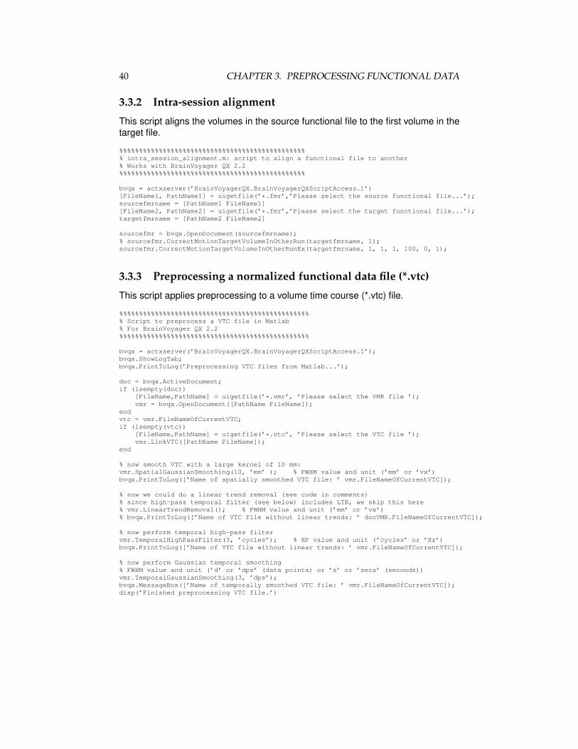
3.3.2 Intra-session alignment
This script aligns the volumes in the source functional file to the first volume in thetarget file.
%%%%%%%%%%%%%%%%%%%%%%%%%%%%%%%%%%%%%%%%%%%%%%%% intra_session_alignment.m: script to align a functional file to another% Works with BrainVoyager QX 2.2%%%%%%%%%%%%%%%%%%%%%%%%%%%%%%%%%%%%%%%%%%%%%%%
bvqx = actxserver(’BrainVoyagerQX.BrainVoyagerQXScriptAccess.1’)[FileName1, PathName1] = uigetfile(’*.fmr’,’Please select the source functional file...’);sourcefmrname = [PathName1 FileName1][FileName2, PathName2] = uigetfile(’*.fmr’,’Please select the target functional file...’);targetfmrname = [PathName2 FileName2]
sourcefmr = bvqx.OpenDocument(sourcefmrname);% sourcefmr.CorrectMotionTargetVolumeInOtherRun(targetfmrname, 1);sourcefmr.CorrectMotionTargetVolumeInOtherRunEx(targetfmrname, 1, 1, 1, 100, 0, 1);
3.3.3 Preprocessing a normalized functional data file (*.vtc)
This script applies preprocessing to a volume time course (*.vtc) file.
%%%%%%%%%%%%%%%%%%%%%%%%%%%%%%%%%%%%%%%%%%%%%%%%% Script to preprocess a VTC file in Matlab% For BrainVoyager QX 2.2%%%%%%%%%%%%%%%%%%%%%%%%%%%%%%%%%%%%%%%%%%%%%%%%
bvqx = actxserver(’BrainVoyagerQX.BrainVoyagerQXScriptAccess.1’);bvqx.ShowLogTab;bvqx.PrintToLog(’Preprocessing VTC files from Matlab...’);
doc = bvqx.ActiveDocument;if (isempty(doc))
[FileName,PathName] = uigetfile(’*.vmr’, ’Please select the VMR file ’);vmr = bvqx.OpenDocument([PathName FileName]);
endvtc = vmr.FileNameOfCurrentVTC;if (isempty(vtc))
[FileName,PathName] = uigetfile(’*.vtc’, ’Please select the VTC file ’);vmr.LinkVTC([PathName FileName]);
end
% now smooth VTC with a large kernel of 10 mm:vmr.SpatialGaussianSmoothing(10, ’mm’ ); % FWHM value and unit (’mm’ or ’vx’)bvqx.PrintToLog([’Name of spatially smoothed VTC file: ’ vmr.FileNameOfCurrentVTC]);
% now we could do a linear trend removal (see code in comments)% since high-pass temporal filter (see below) includes LTR, we skip this here% vmr.LinearTrendRemoval(); % FWHM value and unit (’mm’ or ’vx’)% bvqx.PrintToLog([’Name of VTC file without linear trends: ’ docVMR.FileNameOfCurrentVTC]);
% now perform temporal high-pass filtervmr.TemporalHighPassFilter(3, ’cycles’); % HP value and unit (’cycles’ or ’Hz’)bvqx.PrintToLog([’Name of VTC file without linear trends: ’ vmr.FileNameOfCurrentVTC]);
% now perform Gaussian temporal smoothing% FWHM value and unit (’d’ or ’dps’ (data points) or ’s’ or ’secs’ (seconds))vmr.TemporalGaussianSmoothing(3, ’dps’);bvqx.MessageBox([’Name of temporally smoothed VTC file: ’ vmr.FileNameOfCurrentVTC]);disp(’Finished preprocessing VTC file.’)
Chapter 4
Transformations
4.1 Introduction
Several transformations in BrainVoyager QX can be scripted. For anatomical data,these are the transformation to isotropic voxels and the reorientation to sagittal.For functional data, these are the transformation to normalized functional (*.vtc)and normalized diffusion (*.vdw) file scripting functions; this is discussed in section4.5.
It is also possible to write a transformation file in Matlab and apply the transfor-mation in BrainVoyager QX. This will be shown in section 4.6.2.
4.2 Isovoxelation of anatomical data (*.vmr)
VMR files can be automatically transformed to isovoxel size of 1×1×1 mm via thefunctionAutoTransformToIsoVoxel(<interpolation method>, <new vmr name>).The resulting VMR is written to disk. The function returns a boolean value (true orfalse) to indicate whether the transformation succeeded. The transformation matrixis also displayed in the BrainVoyager QX Log tab.
41

42 CHAPTER 4. TRANSFORMATIONS
4.3 Scripts
The function below presents a file dialog to select a VMR file, opens this VMR filein the BrainVoyager QX main window, transforms the VMR file and saves it on diskin the same directory as the original VMR file with the name “isovoxel.vmr”.
%%%%%%%%%%%%%%%%%%%%%%%%%%%%%%%%%%%%%%%%%%%%%%%%%%%%%%%%%%%%%%%%%%%%% isovoxel_vmr.m% Script to make a VMR isovoxel%% Works with BrainVoyager QX 2.2%%%%%%%%%%%%%%%%%%%%%%%%%%%%%%%%%%%%%%%%%%%%%%%%%%%%%%%%%%%%%%%%%%%%
bvqx = actxserver(’BrainVoyagerQX.BrainVoyagerQXScriptAccess.1’);
bvqx.ShowLogTab;
[FileName,PathName] = uigetfile(’*.vmr’,’Please select the anatomical data file...’);
vmrfilename = strcat(PathName, FileName);
vmrproject = bvqx.OpenDocument(vmrfilename);
bvqx.PrintToLog(’Start isovoxelating VMR...’);
[pathstr,name,ext,versn] = fileparts(vmrfilename);
isovmrfilename = fullfile(pathstr, [name ’_ISO’ ext]);
success = vmrproject.AutoTransformToIsoVoxel(1, isovmrfilename);
bvqx.PrintToLog([’Saving ’ isovmrfilename ’...’]);
isoproject = bvqx.OpenDocument(isovmrfilename); %see figure 4.1
h = msgbox([’The isovoxel file can be found at ’ isovmrfilename]);
uiwait(h);
Figure 4.1: Isovoxel VMR
4.4 Transform anatomical data (*.vmr) to sagittal ori-entation
To transform the anatomical image (*.vmr) to BrainVoyager’s default sagittal orien-tation, the function AutoTransformToSAG() can be applied. The result is saved

4.4. TRANSFORM ANATOMICAL DATA (*.VMR) TO SAGITTAL ORIENTATION43
to disk with the new name. Note: this function might not work if the voxel sizes ofthe VMR are not equal.The function takes one parameter: the new name (string) for the transformed VMR.The function returns a boolean to indicate whether the transformation succeeded.

44 CHAPTER 4. TRANSFORMATIONS
4.5 Transform functional data to a standard space (*.vtc)
The functions CreateVTCInVMRSpace(), CreateVTCInACPCSpace() andCreateVTCInTALSpace() will transform the time series in slices (*.stc) to timeseries in volumes so that the functional data are aligned to the anatomical data inone of the native (VMR), AC-PC aligned (ACPC) or Talairach space (TAL) coordi-nate spaces.To invoke these functions, BrainVoyager QX needs to be provided with the same in-formation as it would have when creating VTCs via the user interface. The creationof VTC files can be performed from Matlab in the following steps:
1. Start the BrainVoyager QX server
2. Open an anatomical file (*.vmr)
3. Set bounding box flags. It is advised to set the ExtendedTALSpaceForVTCCreationand the UseBoundingBoxForVTCCreation properties to true or false,otherwise VTCs of arbitrary size might be the result. If UseBoundingBoxForVTCCreationis set, the coordinates for the VTC w.r.t. the VMR can be set via TargetVTCBoundingBoxXStartand TargetVTCBoundingBoxXEnd (replace X with Y or Z, when appropri-ate). The coordinates that are not specified will get the default Talairachbounding box size.
4. Collect the parameters to provide to the CreateVTC...() function Theseare the parameters:
• Name of FMR project This is the name of the functional data (*.fmr) thatshould be transformed to a VTC file.
• Name of initial alignment file This is the name of the initial alignment file(*IA.trf); the matrix in this file represents the largest part of the mappingfrom the anatomical to the functional data.
• Name of fine alignment file This is the name of the fine alignment file(*FA.trf); the matrix in this file represents additional small changes forthe mapping of the anatomical to the functional data.
• Name of AC-PC alignment file This is the name of the file that trans-forms the data from native space to a space where data are aligned tothe plane of the anterior commissure (AC) and the posterior commissure(PC). This argument only needs to be provided in case the functionsCreateVTCInACPCSpace() and CreateVTCInTALSpace() are in-voked.
• Name of Talairach landmarks file This file contains the coordinates ofthe 12 landmarks that are used to transform the data from AC-PC spaceto Talairach space. This argument only needs to be provided in case thefunction CreateVTCInTALSpace() is invoked.
• Resolution The value of this parameter defines whether the VTC file willhave a resolution of 3mm3, 2mm3 or 1mm3.
• Interpolation This numeric value indicates the interpolation method. Cur-rently the value should be set to 1, which means ’trilinear interpolation’.In future, more interpolation methods will be available for this function.
• Bounding box threshold This value is only relevant in case the VTC isnot created in Talairach space; however, the value should always be pro-vided. The default is 100. The value represents the intensity thresholdon basis of which the size of the VTC box is determined.
4.5. TRANSFORM FUNCTIONAL DATA TO A STANDARD SPACE (*.VTC) 45
5. Set the extended Talairach parameter This is a property of the VMR project,and should also be set in case the VTC will not be in Talairach space.
6. Invoke the CreateVTC...() function
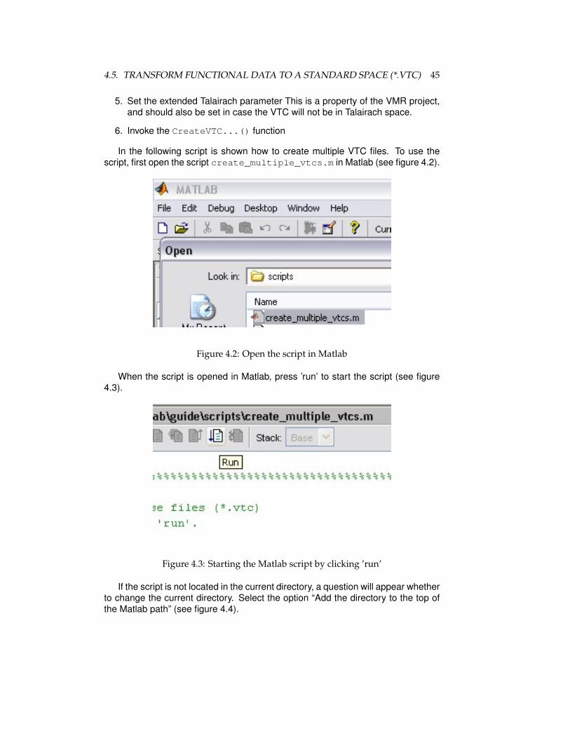
In the following script is shown how to create multiple VTC files. To use thescript, first open the script create_multiple_vtcs.m in Matlab (see figure 4.2).
Figure 4.2: Open the script in Matlab
When the script is opened in Matlab, press ’run’ to start the script (see figure4.3).
Figure 4.3: Starting the Matlab script by clicking ’run’
If the script is not located in the current directory, a question will appear whetherto change the current directory. Select the option “Add the directory to the top ofthe Matlab path” (see figure 4.4).
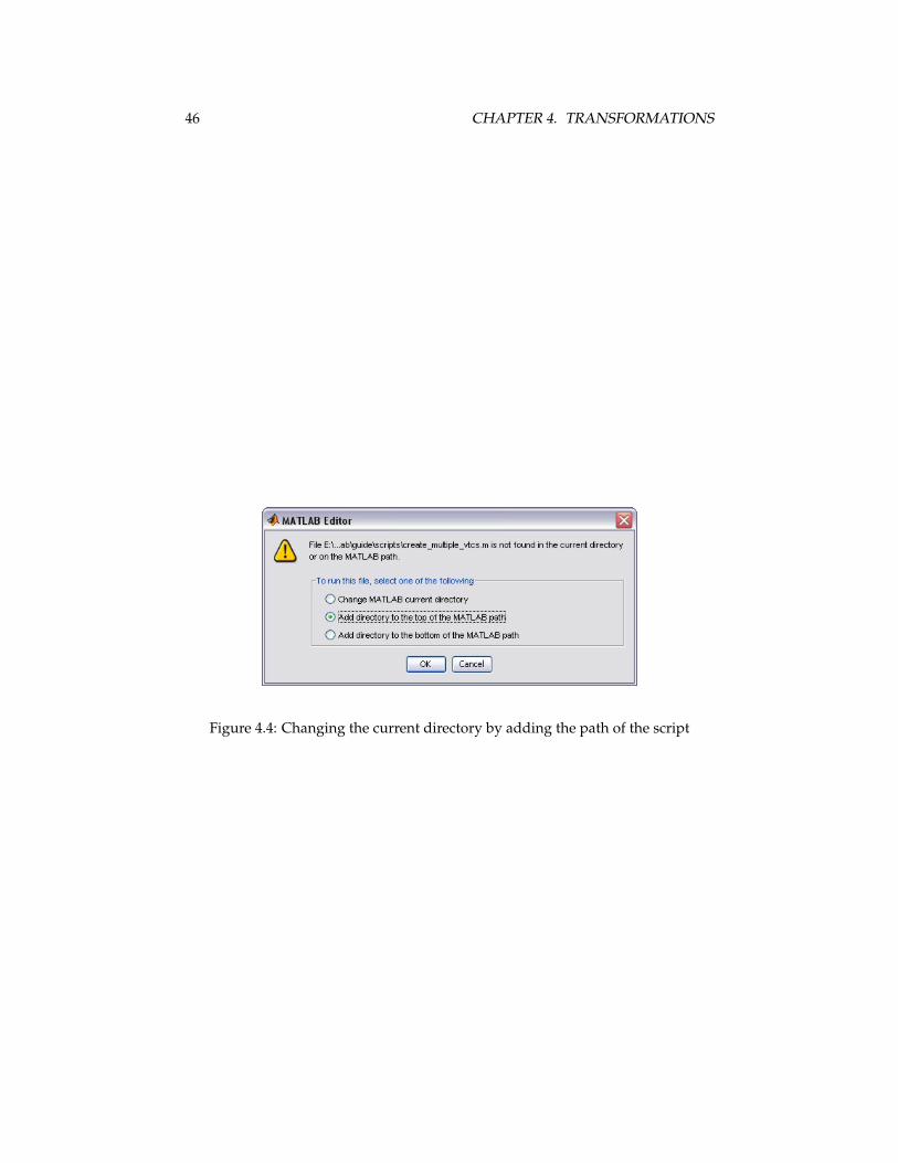
46 CHAPTER 4. TRANSFORMATIONS
Figure 4.4: Changing the current directory by adding the path of the script

4.5. TRANSFORM FUNCTIONAL DATA TO A STANDARD SPACE (*.VTC) 47
4.5.1 Script to create multiple VTC files
%%%%%%%%%%%%%%%%%%%%%%%%%%%%%%%%%%%%%%%%%%%%%%%%%%%%%%%%%%% create_multiple_vtcs.m% Script to create volume time course files (*.vtc)% For use: load in Matlab and press ’run’.%% Works with BrainVoyager QX 2.2%%%%%%%%%%%%%%%%%%%%%%%%%%%%%%%%%%%%%%%%%%%%%%%%%%%%%%%%%%
h = msgbox([’Via this script will be multiple VTCs created. Please first define all parameters...’])uiwait(h);bvqx = actxserver(’BrainVoyagerQX.BrainVoyagerQXScriptAccess.1’);bvqx.ShowLogTab;bvqx.PrintToLog(’Creating VTC files from Matlab...’);loadparams = questdlg(’Would you like to load VTC parameters (from earlier use of this script)?’,...’Create multiple VTCs’);if strcmp(loadparams, ’Yes’) == 1
[FileName,PathName] = uigetfile(’*.mat’, ’Please select the VTC parameters file ’);load([PathName FileName]);
elseanswer = inputdlg(’Please enter the number of projects...’,’Create multiple VTCs’,1);if isnumeric(str2num(answer{1})) && str2num(answer{1}) > 0
nrofprojects = str2num(answer{1});end
% create cell arrays to store the vtc parametersfmr_names = cell(nrofprojects, 1);ia_names = cell(nrofprojects, 1);fa_names = cell(nrofprojects, 1);acpc_names = cell(nrofprojects, 1);tal_names = cell(nrofprojects, 1);vtc_names = cell(nrofprojects, 1);
vtcspaces = {’native’, ’acpc’, ’talairach’};[space,v] = listdlg(’PromptString’,’select the target space:’,...
’SelectionMode’,’single’,...’Name’, ’Create multiple VTCs’,...’ListSize’, [200 160],...’ListString’, vtcspaces)
for i=1:nrofprojects
[FileName,PathName] = uigetfile(’*.fmr’, ...[’Please select FMR file ’ num2str(i) ’ of ’ num2str(nrofprojects) ’...’]);fmr_names{i,1} = strcat(PathName, FileName);[FileName,PathName] = uigetfile(’*_IA.trf’, ...[’Please select initial alignment file ’ num2str(i) ’ of ’ num2str(nrofprojects) ’...’]);ia_names{i,1} = strcat(PathName, FileName);[FileName,PathName] = uigetfile(’*_FA.trf’, ...[’Please select fine alignment file ’ num2str(i) ’ of ’ num2str(nrofprojects) ’...’]);fa_names{i,1} = strcat(PathName, FileName);
if space > 1[FileName,PathName] = uigetfile(’*_ACPC.trf’, ...[’Please select AC-PC alignment file ’ num2str(i) ’ of ’ num2str(nrofprojects) ’...’]);acpc_names{i,1} = strcat(PathName, FileName);if space > 2
[FileName,PathName] = uigetfile(’*.tal’, ...[’Please select Talairach landmarks file ’ num2str(i) ’ of ’ num2str(nrofprojects) ’...’]);tal_names{i,1} = strcat(PathName, FileName);
endend[pathstr,name,ext,versn] = fileparts(fmr_names{i,1});vtc_names{i,1} = fullfile(pathstr, [name ’_’ vtcspaces{space} ’.vtc’]);
end
resolution = 3;answer = inputdlg(’Please enter the voxel resolution...’,’Create multiple VTCs’,1,{num2str(resolution)});if isnumeric(str2num(answer{1})) && str2num(answer{1}) > 0
resolution = str2num(answer{1});endinterpolation = 1; % trilinearbbithresh = 100;cerebellum = 0;if space < 3
answer = inputdlg(’Please enter an intensity threshold...’,’Create multiple VTCs’,1,{num2str(bbithresh)});if isnumeric(str2num(answer{1})) && str2num(answer{1}) > 0
bbithreshold = str2num(answer{1});end
48 CHAPTER 4. TRANSFORMATIONS
elsebutton = questdlg(’Would you like an extended Talairach space (incl. cerebellum)?’,’Create multiple VTCs’);if strcmp(button, ’Yes’) == 1, cerebellum = 1; end
endbutton = questdlg(’Would you like high-precision data (float format)?’,’float or integer format’);if strcmp(button, ’Yes’) == 1
datatype = 2; // float 32else
datatype = 1; // integer 16-bitend[FileName,PathName] = uigetfile(’*.vmr’,’Please select the anatomical data file...’);vmrfilename = [PathName FileName];
end
vmrproject = bvqx.OpenDocument(vmrfilename);vmrproject.ExtendedTALSpaceForVTCCreation = cerebellum;for i=1:nrofprojects
if space == 1success = vmrproject.CreateVTCInVMRSpace(fmr_names{i,1}, ia_names{i,1}, fa_names{i,1},...
vtc_names{i,1}, datatype, resolution, interpolation, bbithresh);elseif space == 2
success = vmrproject.CreateVTCInACPCSpace(fmr_names{i,1}, ia_names{i,1}, fa_names{i,1},...acpc_names{i,1}, vtc_names{i,1}, datatype, ...resolution, interpolation, bbithresh);
elseif space == 3success = vmrproject.CreateVTCInTALSpace(fmr_names{i,1}, ia_names{i,1}, fa_names{i,1},...
acpc_names{i,1}, tal_names{i,1}, vtc_names{i,1}, datatype, ...resolution, interpolation, bbithresh);
elsedisp(’An error occurred. Our apologies’);
endif (success == 1)
bvqx.PrintToLog([’Created ’ vtc_names{i,1}]);else
disp([’An error occurred while creating the VTC file’ vtc_names{i,1}]);end
end
button = questdlg(’Would you like to save the VTC parameters (for later use of this script)?’,’Create multiple VTCs’);if strcmp(button, ’Yes’) == 1
vtcparamsfilename = fullfile(pathstr, ’vtcparams.mat’)save(vtcparamsfilename);
end
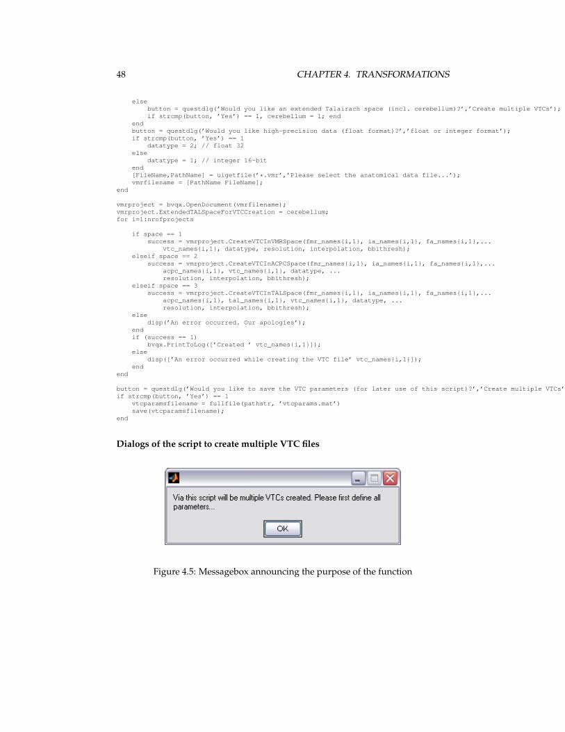
Dialogs of the script to create multiple VTC files
Figure 4.5: Messagebox announcing the purpose of the function

4.5. TRANSFORM FUNCTIONAL DATA TO A STANDARD SPACE (*.VTC) 49
Figure 4.6: Dialog for entering the number of projects
Figure 4.7: Dialog for selecting the VTC space
Figure 4.8: Selecting the FMR file
50 CHAPTER 4. TRANSFORMATIONS
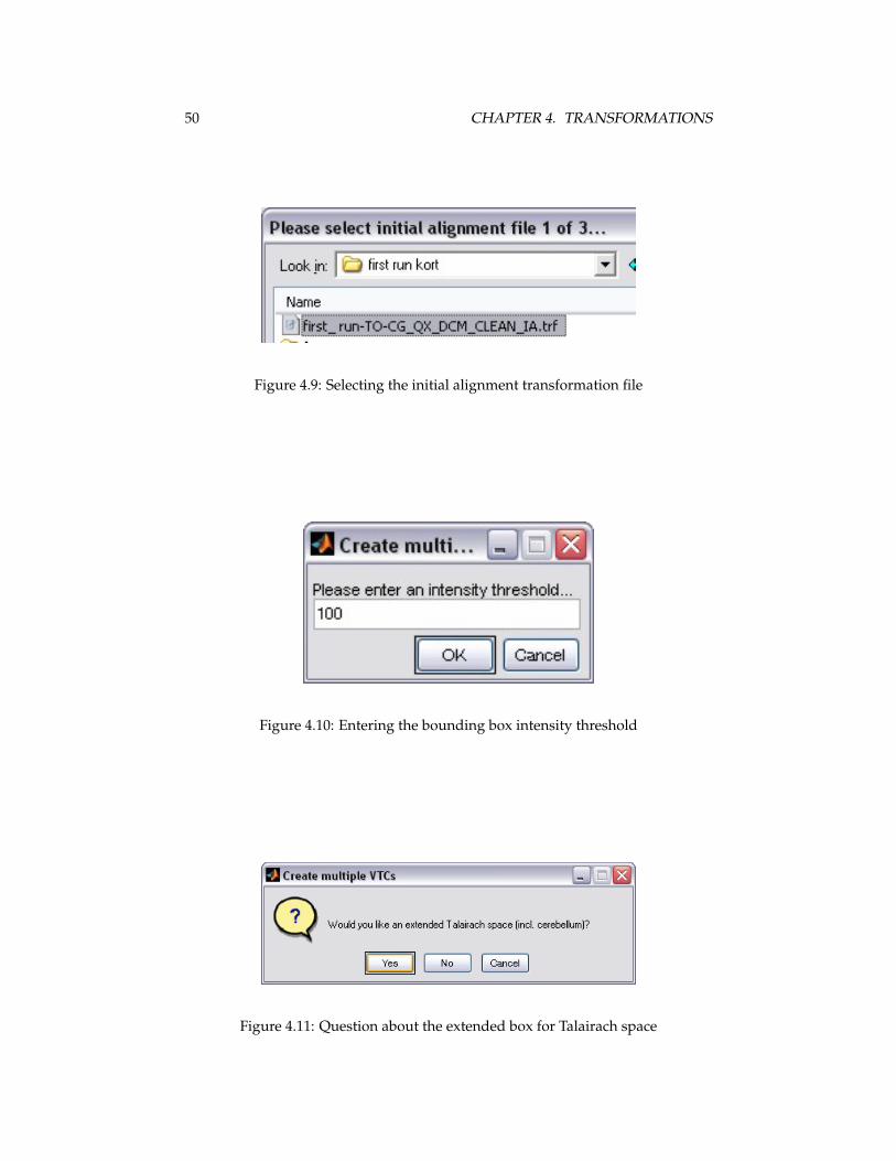
Figure 4.9: Selecting the initial alignment transformation file
Figure 4.10: Entering the bounding box intensity threshold
Figure 4.11: Question about the extended box for Talairach space
4.5. TRANSFORM FUNCTIONAL DATA TO A STANDARD SPACE (*.VTC) 51
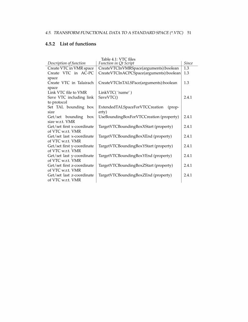
4.5.2 List of functions
Table 4.1: VTC filesDescription of function Function in Qt Script SinceCreate VTC in VMR space CreateVTCInVMRSpace(arguments):boolean 1.3Create VTC in AC-PCspace
CreateVTCInACPCSpace(arguments):boolean 1.3
Create VTC in Talairachspace
CreateVTCInTALSPace(arguments):boolean 1.3
Link VTC file to VMR LinkVTC( ’name’ )Save VTC including linkto protocol
SaveVTC() 2.4.1
Set TAL bounding boxsize
ExtendedTALSpaceForVTCCreation (prop-erty)
Get/set bounding boxsize w.r.t. VMR
UseBoundingBoxForVTCCreation (property) 2.4.1
Get/set first x-coordinateof VTC w.r.t. VMR
TargetVTCBoundingBoxXStart (property) 2.4.1
Get/set last x-coordinateof VTC w.r.t. VMR
TargetVTCBoundingBoxXEnd (property) 2.4.1
Get/set first y-coordinateof VTC w.r.t. VMR
TargetVTCBoundingBoxYStart (property) 2.4.1
Get/set last y-coordinateof VTC w.r.t. VMR
TargetVTCBoundingBoxYEnd (property) 2.4.1
Get/set first z-coordinateof VTC w.r.t. VMR
TargetVTCBoundingBoxZStart (property) 2.4.1
Get/set last z-coordinateof VTC w.r.t. VMR
TargetVTCBoundingBoxZEnd (property) 2.4.1

52 CHAPTER 4. TRANSFORMATIONS
4.6 Transform diffusion weighted data to a standardspace (*.vdw)
The BrainVoyager script functions to create normalized diffusion weighted data(*.vdw) are quite similar to the functions to create normalized functional MRI data(*.vtc). Therefore, in case the bounding box sizes are not consistent, one couldset the property ExtendedTALSpaceForVTCCreation to true or false like withVTC files; see also the information on the UseBoundingBoxForVTCCreationproperty (since BrainVoyager QX 2.4.1). The commands are listed in table 4.6.1.The arguments are:Parameter: Name DMR: Name of the diffusion-weighted data file (*.dmr) whichshould be transformed to Talairach space.Parameter: Name IA file: Name of the initial alignment transformation file (*_IA.trf).Parameter: Name FA file: Name of the fine alignment transformation file (*_FA.trf).Parameter (optional): Name ACPC file: Name of the transformation file of the VMRto AC-PC space (*_ACPC.trf).Parameter (optional): Name TAL file: Name of the file containing 12 landmarksused to transform the VMR to Talairach space (*.tal).Parameter: Name VDW: Name for the new VDW file.Parameter: Datatype: Create the VDW in integer 2-byte format: 1 or in float format:2.Parameter: Resolution: Target resolution, either ‘1’ (1x1x1mm), ‘2’ or ‘3’.Parameter: Interpolation: ‘0’ for nearest neighbor interpolation, ‘1’ for trilinear in-terpolation, ‘2’ for sinc interpolation.Parameter: Threshold: intensity threshold for bounding box (is not relevant for Ta-lairach space, but should be provided). Default value: ‘100’.Returns: True (success) or false.
For an example script, please see section 2.5.2.

4.6. TRANSFORM DIFFUSION WEIGHTED DATA TO A STANDARD SPACE (*.VDW)53
4.6.1 List of functions
Table 4.2: VDW filesDescription of function Function in Qt Script SinceCreate VDW in VMRspace
CreateVDWInVMRSpace(arguments):boolean 1.x
Create VDW in AC-PCspace
CreateVDWInACPCSpace(arguments):boolean 1.x
Create VDW in Talairachspace
CreateVDWInTALSpace(arguments):boolean 1.x
54 CHAPTER 4. TRANSFORMATIONS
4.6.2 More on BrainVoyager transformation (*.trf) files
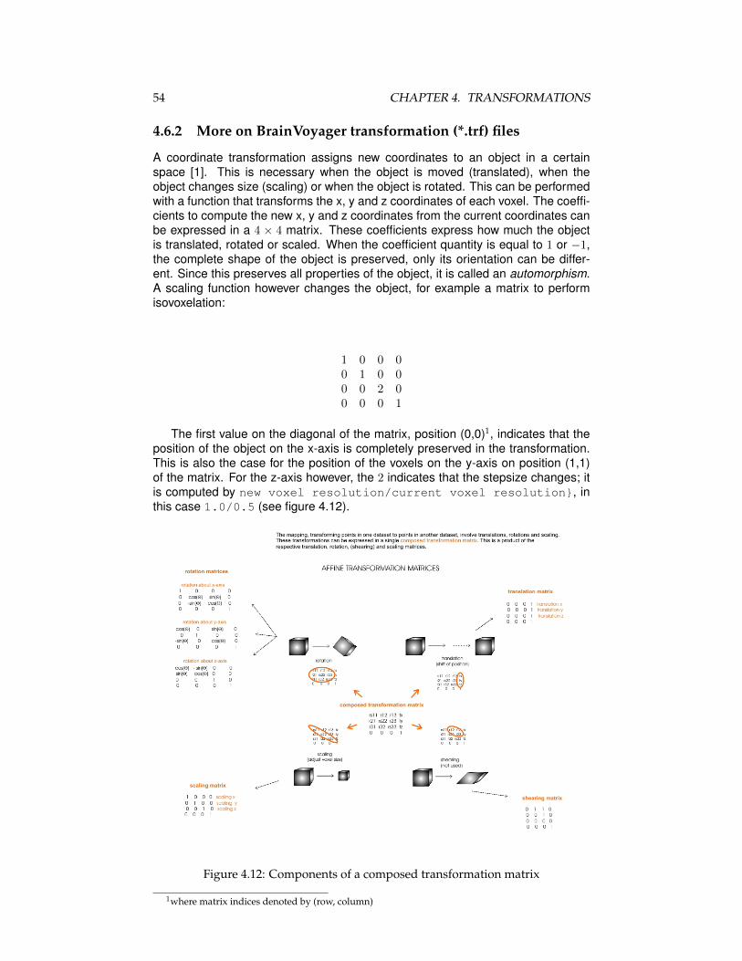
A coordinate transformation assigns new coordinates to an object in a certainspace [1]. This is necessary when the object is moved (translated), when theobject changes size (scaling) or when the object is rotated. This can be performedwith a function that transforms the x, y and z coordinates of each voxel. The coeffi-cients to compute the new x, y and z coordinates from the current coordinates canbe expressed in a 4 × 4 matrix. These coefficients express how much the objectis translated, rotated or scaled. When the coefficient quantity is equal to 1 or −1,the complete shape of the object is preserved, only its orientation can be differ-ent. Since this preserves all properties of the object, it is called an automorphism.A scaling function however changes the object, for example a matrix to performisovoxelation:
1 0 0 00 1 0 00 0 2 00 0 0 1
The first value on the diagonal of the matrix, position (0,0)1, indicates that theposition of the object on the x-axis is completely preserved in the transformation.This is also the case for the position of the voxels on the y-axis on position (1,1)of the matrix. For the z-axis however, the 2 indicates that the stepsize changes; itis computed by new voxel resolution/current voxel resolution}, inthis case 1.0/0.5 (see figure 4.12).
Figure 4.12: Components of a composed transformation matrix
1where matrix indices denoted by (row, column)
4.6. TRANSFORM DIFFUSION WEIGHTED DATA TO A STANDARD SPACE (*.VDW)55
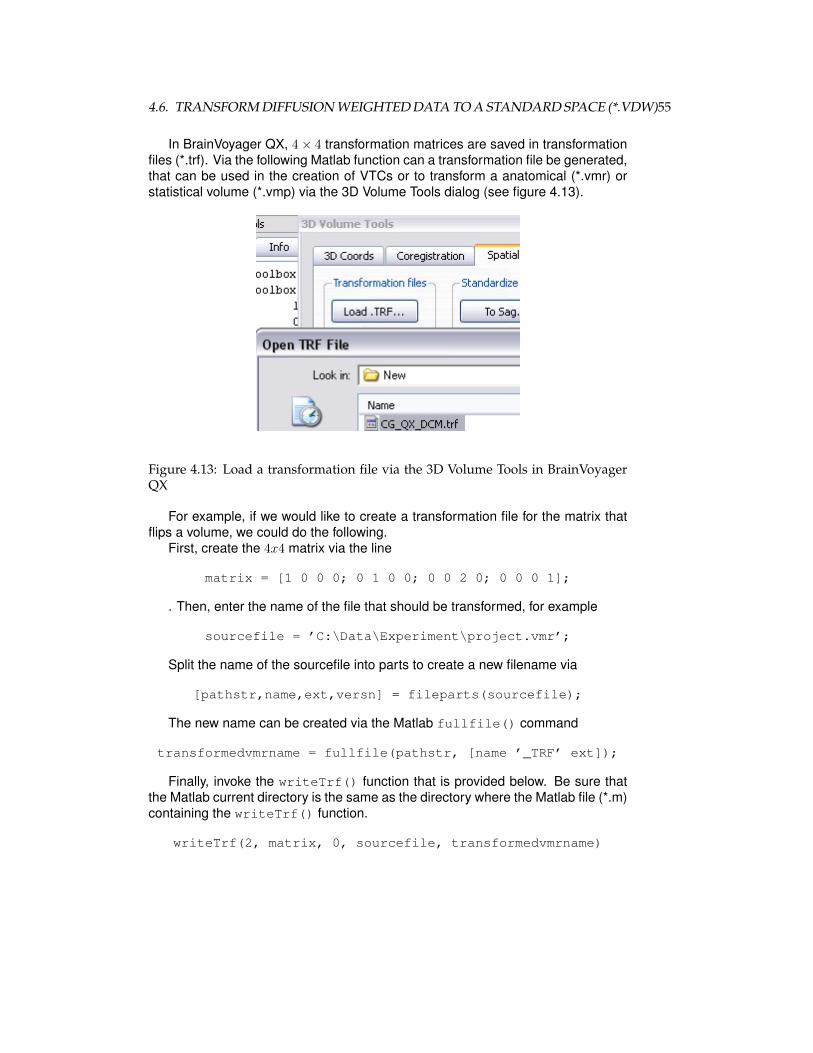
In BrainVoyager QX, 4× 4 transformation matrices are saved in transformationfiles (*.trf). Via the following Matlab function can a transformation file be generated,that can be used in the creation of VTCs or to transform a anatomical (*.vmr) orstatistical volume (*.vmp) via the 3D Volume Tools dialog (see figure 4.13).
Figure 4.13: Load a transformation file via the 3D Volume Tools in BrainVoyagerQX
For example, if we would like to create a transformation file for the matrix thatflips a volume, we could do the following.
First, create the 4x4 matrix via the line
matrix = [1 0 0 0; 0 1 0 0; 0 0 2 0; 0 0 0 1];
. Then, enter the name of the file that should be transformed, for example
sourcefile = ’C:\Data\Experiment\project.vmr’;
Split the name of the sourcefile into parts to create a new filename via
[pathstr,name,ext,versn] = fileparts(sourcefile);
The new name can be created via the Matlab fullfile() command
transformedvmrname = fullfile(pathstr, [name ’_TRF’ ext]);
Finally, invoke the writeTrf() function that is provided below. Be sure thatthe Matlab current directory is the same as the directory where the Matlab file (*.m)containing the writeTrf() function.
writeTrf(2, matrix, 0, sourcefile, transformedvmrname)
56 CHAPTER 4. TRANSFORMATIONS
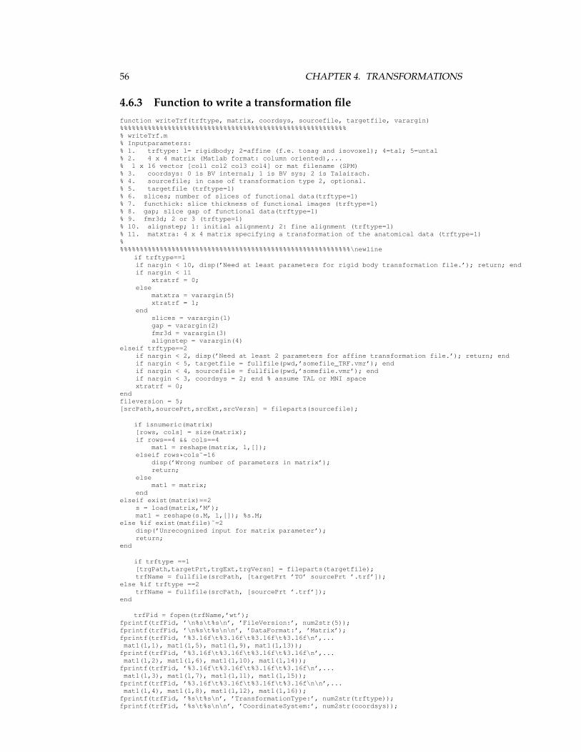
4.6.3 Function to write a transformation filefunction writeTrf(trftype, matrix, coordsys, sourcefile, targetfile, varargin)%%%%%%%%%%%%%%%%%%%%%%%%%%%%%%%%%%%%%%%%%%%%%%%%%%%%%%%%%% writeTrf.m% Inputparameters:% 1. trftype: 1= rigidbody; 2=affine (f.e. tosag and isovoxel); 4=tal; 5=untal% 2. 4 x 4 matrix (Matlab format: column oriented),...% 1 x 16 vector [col1 col2 col3 col4] or mat filename (SPM)% 3. coordsys: 0 is BV internal; 1 is BV sys; 2 is Talairach.% 4. sourcefile; in case of transformation type 2, optional.% 5. targetfile (trftype=1)% 6. slices; number of slices of functional data(trftype=1)% 7. functhick: slice thickness of functional images (trftype=1)% 8. gap; slice gap of functional data(trftype=1)% 9. fmr3d; 2 or 3 (trftype=1)% 10. alignstep; 1: initial alignment; 2: fine alignment (trftype=1)% 11. matxtra: 4 x 4 matrix specifying a transformation of the anatomical data (trftype=1)%%%%%%%%%%%%%%%%%%%%%%%%%%%%%%%%%%%%%%%%%%%%%%%%%%%%%%%%%%%\newline
if trftype==1if nargin < 10, disp(’Need at least parameters for rigid body transformation file.’); return; endif nargin < 11
xtratrf = 0;else
matxtra = varargin(5)xtratrf = 1;
endslices = varargin(1)gap = varargin(2)fmr3d = varargin(3)alignstep = varargin(4)
elseif trftype==2if nargin < 2, disp(’Need at least 2 parameters for affine transformation file.’); return; endif nargin < 5, targetfile = fullfile(pwd,’somefile_TRF.vmr’); endif nargin < 4, sourcefile = fullfile(pwd,’somefile.vmr’); endif nargin < 3, coordsys = 2; end % assume TAL or MNI spacextratrf = 0;
endfileversion = 5;[srcPath,sourcePrt,srcExt,srcVersn] = fileparts(sourcefile);
if isnumeric(matrix)[rows, cols] = size(matrix);if rows==4 && cols==4
mat1 = reshape(matrix, 1,[]);elseif rows*cols˜=16
disp(’Wrong number of parameters in matrix’);return;
elsemat1 = matrix;
endelseif exist(matrix)==2
s = load(matrix,’M’);mat1 = reshape(s.M, 1,[]); %s.M;
else %if exist(matfile)˜=2disp(’Unrecognized input for matrix parameter’);return;
end
if trftype ==1[trgPath,targetPrt,trgExt,trgVersn] = fileparts(targetfile);trfName = fullfile(srcPath, [targetPrt ’TO’ sourcePrt ’.trf’]);
else %if trftype ==2trfName = fullfile(srcPath, [sourcePrt ’.trf’]);
end
trfFid = fopen(trfName,’wt’);fprintf(trfFid, ’\n%s\t%s\n’, ’FileVersion:’, num2str(5));fprintf(trfFid, ’\n%s\t%s\n\n’, ’DataFormat:’, ’Matrix’);fprintf(trfFid, ’%3.16f\t%3.16f\t%3.16f\t%3.16f\n’,...mat1(1,1), mat1(1,5), mat1(1,9), mat1(1,13));fprintf(trfFid, ’%3.16f\t%3.16f\t%3.16f\t%3.16f\n’,...mat1(1,2), mat1(1,6), mat1(1,10), mat1(1,14));fprintf(trfFid, ’%3.16f\t%3.16f\t%3.16f\t%3.16f\n’,...mat1(1,3), mat1(1,7), mat1(1,11), mat1(1,15));fprintf(trfFid, ’%3.16f\t%3.16f\t%3.16f\t%3.16f\n\n’,...mat1(1,4), mat1(1,8), mat1(1,12), mat1(1,16));fprintf(trfFid, ’%s\t%s\n’, ’TransformationType:’, num2str(trftype));fprintf(trfFid, ’%s\t%s\n\n’, ’CoordinateSystem:’, num2str(coordsys));
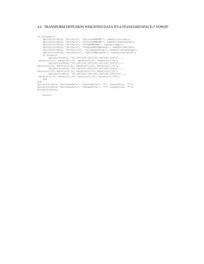
4.6. TRANSFORM DIFFUSION WEIGHTED DATA TO A STANDARD SPACE (*.VDW)57
if trftype==1fprintf(trfFid, ’%s\t%s\n’, ’NSlicesFMRVMR:’, num2str(slices));fprintf(trfFid, ’%s\t%s\n’, ’SlThickFMRVMR:’, num2str(functhick));fprintf(trfFid, ’%s\t%s\n’, ’SlGapFMRVMR:’, num2str(gap));fprintf(trfFid, ’%s\t%s\n’, ’CreateFMR3DMethod:’, num2str(fmr3d));fprintf(trfFid, ’%s\t%s\n\n’, ’AlignmentStep:’, num2str(alignstep));fprintf(trfFid, ’%s\t%s\n\n’, ’ExtraVMRTransf:’, num2str(xtratrf));if xtratrf
fprintf(trfFid, ’%3.16f\t%3.16f\t%3.16f\t%3.16f\n’,...matxtra(1,1), matxtra(1,5), matxtra(1,9), matxtra(1,13));
fprintf(trfFid, ’%3.16f\t%3.16f\t%3.16f\t%3.16f\n’,...matxtra(1,2), matxtra(1,6), matxtra(1,10), matxtra(1,14));
fprintf(trfFid, ’%3.16f\t%3.16f\t%3.16f\t%3.16f\n’,...matxtra(1,3), matxtra(1,7), matxtra(1,11), matxtra(1,15));
fprintf(trfFid, ’%3.16f\t%3.16f\t%3.16f\t%3.16f\n\n’,...matxtra(1,4), matxtra(1,8), matxtra(1,12), matxtra(1,16));
endendfprintf(trfFid, ’%s\t%s%s%s\n’, ’SourceFile:’, ’"’, sourcefile, ’"’);fprintf(trfFid, ’%s\t%s%s%s\n’, ’TargetFile:’, ’"’, targetfile, ’"’);fclose(trfFid);
return;

58 CHAPTER 4. TRANSFORMATIONS

Chapter 5
Experimental design
In this chapter is described how to create stimulation protocols (*.prt) and designmatrices (*.sdm, *.mdm).
5.1 Creating stimulation protocols (*.prt)
The colors for each condition can be set via the functionfmrproject.SetConditionColor(’conditionname’, red, green, blue);.To discriminate the different conditions, different colors can be used. The colors inBrainVoyager are specified as a combination of red, green and blue components,in this order. To lowest value for each component is 0 and the highest value is 255.When one of the components is set to 255 and the other two to 0, a primary color isobtained. When each of the components red, green and blue is set to 0, the resultwill be black in absence of all colors. A list with red, green and blue componentvalues for the most common colors can be found in figure 5.1.
Figure 5.1: RGB colors
59
60 CHAPTER 5. EXPERIMENTAL DESIGN
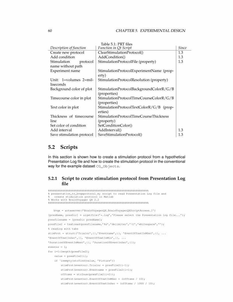
Table 5.1: PRT filesDescription of function Function in Qt Script SinceCreate new protocol ClearStimulationProtocol() 1.3Add condition AddCondition() 1.3Stimulation protocolname without path
StimulationProtocolFile (property) 1.3
Experiment name StimulationProtocolExperimentName (prop-erty)
Unit: 1=volumes 2=mil-liseconds
StimulationProtocolResolution (property)
Background color of plot StimulationProtocolBackgroundColorR/G/B(properties)
Timecourse color in plot StimulationProtocolTimeCourseColorR/G/B(properties)
Text color in plot StimulationProtocolTextColorR/G/B (prop-erties)
Thickness of timecourseline
StimulationProtocolTimeCourseThickness(property)
Set color of condition SetConditionColor()Add interval AddInterval() 1.3Save stimulation protocol SaveStimulationProtocol() 1.3
5.2 Scripts
In this section is shown how to create a stimulation protocol from a hypotheticalPresentation Log file and how to create the stimulation protocol in the conventionalway for the example dataset CG_Objects.
5.2.1 Script to create stimulation protocol from Presentation Logfile
%%%%%%%%%%%%%%%%%%%%%%%%%%%%%%%%%%%%%%%%%%%%%%%%%%%%%%%%%%%%%%%% presentation_to_bvqxprotocol.m; script to read Presentation Log file and% create stimulation protocol in Matlab% Works with BrainVoyager QX 2.2%%%%%%%%%%%%%%%%%%%%%%%%%%%%%%%%%%%%%%%%%%%%%%%%%%%%%%%%%%%%%%%
bvqx = actxserver(’BrainVoyagerQX.BrainVoyagerQXScriptAccess.1’)
[presName, presDir] = uigetfile(’*.log’,’Please select the Presentation log file...’);
presfilename = [presDir presName];
presFile2 = textread(presfilename,’%s’,’delimiter’,’\t’,’whitespace’,’’);
% reading with tabs
stimProt = struct(’Trialnr’,{},’Eventname’,{}, ’EventOffsetInMSec’,{}, ...
’EventOffsetInSec’,{}, ’EventOffsetInMin’,{}, ...
’DurationOfEventInMsec’,{}, ’DurationOfEventInSec’,{});
eventnr = 1;
for i=1:length(presFile2);
value = presFile2{i};
if ˜isempty(strfind(value, ’Picture’))
stimProt(eventnr).Trialnr = presFile2{i-1};
stimProt(eventnr).Eventname = presFile2{i+1};
offtsms = str2num(presFile2{i+2});
stimProt(eventnr).EventOffsetInMSec = (offtsms / 10);
stimProt(eventnr).EventOffsetInSec = (offtsms / 1000 / 10);

5.2. SCRIPTS 61
stimProt(eventnr).EventOffsetInMin = (stimProt(eventnr).EventOffsetInSec / 60);
stimProt(eventnr).DurationOfEventInMsec = (str2num(presFile2{i+5}) / 10);
stimProt(eventnr).DurationOfEventInSec = (str2num(presFile2{i+5}) / 1000 / 10);
eventnr = eventnr + 1;
end
end;
[vmrName, vmrDir] = uigetfile(’*.vmr’,’Please select the VMR file...’);
vmrfilename = [vmrDir vmrName];
vmrproject = bvqx.OpenDocument(vmrfilename);
bvqx.ResizeWindow(600,400);
[vtcName, vtcDir] = uigetfile(’*.vtc’,’Please select the VTC file...’);
vtcfilename = [vtcDir vtcName];
vmrproject.LinkVTC(vtcName); % only filename, not pathname
vmrproject.ClearStimulationProtocol;
vmrproject.StimulationProtocolExperimentName = ’Objects_in_VF’;
vmrproject.AddCondition(’LVF’);
vmrproject.SetConditionColor(’Objects in LVF’, 255,0,0); % red
vmrproject.AddCondition(’RVF’);
vmrproject.SetConditionColor(’Objects in RVF’, 0,255,0); % green
vmrproject.AddCondition(’BVF’);
vmrproject.SetConditionColor(’Objects in BVF’, 0,0,255); % blue
vmrproject.AddCondition(’Fixation’);
vmrproject.SetConditionColor(’Fixation’, 192,192,192); % gray
% go through all the ’Picture’ objects in the ’stimProt’ structure
% to assign them as intervals to the different conditions
Picture_LVF = ’LVF’;
Picture_RVF = ’RVF’;
Picture_BVF = ’BVF’;
for i=1:length(stimProt)
if (strfind(stimProt(i).Eventname, Picture_LVF) > 0)
vmrproject.AddInterval(’LVF’, stimProt(i).EventOffsetInMSec,...
(stimProt(i).EventOffsetInMSec+stimProt(i).DurationOfEventInMsec));
elseif (strfind(stimProt(i).Eventname, Picture_RVF) > 0)
vmrproject.AddInterval(’RVF’, stimProt(i).EventOffsetInMSec,...
(stimProt(i).EventOffsetInMSec+stimProt(i).DurationOfEventInMsec));
elseif (strfind(stimProt(i).Eventname, Picture_BVF) > 0)
vmrproject.AddInterval(’BVF’, stimProt(i).EventOffsetInMSec,...
(stimProt(i).EventOffsetInMSec+stimProt(i).DurationOfEventInMsec));
end;
end
vmrproject.SaveStimulationProtocol(’cgobjects_frommatlab.prt’);
%vmrproject.LoadStimulationProtocol(’cgobjects_frommatlab.prt’);
%vmrproject.Close;

62 CHAPTER 5. EXPERIMENTAL DESIGN
5.2.2 Script to create stimulation protocol for BrainVoyager exam-ple dataset
%%%%%%%%%%%%%%%%%%%%%%%%%%%%%%%%%%%%%%%%%%%%%%%%%%%%%%%%%%%%%%%%%%%%%%%% create_cgobjects_protocol.m; script to create stimulation protocol in% Matlab%% Works with BrainVoyager QX 2.2%%%%%%%%%%%%%%%%%%%%%%%%%%%%%%%%%%%%%%%%%%%%%%%%%%%%%%%%%%%%%%%%%%%%%%%
bvqx = actxserver(’BrainVoyagerQX.BrainVoyagerQXScriptAccess.1’);bvqx.ShowLogTab;bvqx.PrintToLog(’Creating a BrainVoyager stimulation protocol from Matlab...’);[FileName,PathName] = uigetfile(’*.vmr’, ’Please select the anatomical file ’);doc = bvqx.OpenDocument([PathName FileName]);[FileName,PathName] = uigetfile(’*.vtc’, ’Please select the functional file ’);doc.LinkVTC([PathName FileName]);doc.ClearStimulationProtocol();doc.StimulationProtocolExperimentName = ’Objects Experiment’;doc.StimulationProtocolResolution = 1;doc.AddCondition(’Fixation’);doc.AddCondition(’Objects in LVF’);doc.AddCondition(’Objects in RVF’);doc.AddCondition(’Objects in BVF’);for interval = 0:9
intervalstart = interval*27 -1;intervalend = intervalstart + 8;if (interval == 0)
intervalstart = 1;intervalend = 7;
enddoc.AddInterval(’Fixation’, intervalstart, intervalend);
endfor interval = 0:2
intervalstart = 35+interval*81;intervalend = intervalstart + 17;doc.AddInterval(’Objects in LVF’, intervalstart, intervalend);
endfor interval = 0:2
intervalstart = 8+interval*81;intervalend = intervalstart + 17;doc.AddInterval(’Objects in RVF’, intervalstart, intervalend);
endfor interval = 0:2
intervalstart = 62+interval*81;intervalend = intervalstart + 17;doc.AddInterval(’Objects in BVF’, intervalstart, intervalend);
enddoc.SetConditionColor(’Fixation’, 100, 100, 100);doc.SetConditionColor(’Objects in LVF’, 255, 0, 0);doc.SetConditionColor(’Objects in RVF’, 0, 255, 0);doc.SetConditionColor(’Objects in BVF’, 0, 0, 255);doc.StimulationProtocolBackgroundColorR = 0;doc.StimulationProtocolBackgroundColorG = 0;doc.StimulationProtocolBackgroundColorB = 0;doc.StimulationProtocolTimeCourseColorR = 255;doc.StimulationProtocolTimeCourseColorG = 255;doc.StimulationProtocolTimeCourseColorB = 255;doc.StimulationProtocolTimeCourseThickness = 4;doc.SaveStimulationProtocol(’CG_OBJECTS_FROMMATLABSCRIPT.prt’);doc.Save(); % to save link to protocol permanently
5.3. CREATING DESIGN MATRICES (*.SDM, *.MDM) 63
5.3 Creating design matrices (*.sdm, *.mdm)
Creating a single-subject design matrix (*.sdm) consists of the following steps.First, a project needs to be opened via the OpenDocument(name) method. Thisreturns a BrainVoyager AMR, FMR, VMR or DMR project object. All following func-tions belong to this project. Then, a VTC file and a stimulation protocol are linkedvia the functions LinkVTC(name) and LinkStimulationProtocol(name).Save the name of the stimulation protocol file in the VTC file via the SaveVTCfunction. Make space for the new matrix via the function ClearDesignMatrix;.Then, the predictors can be added via AddPredictor(’name’). Set the predic-tor values via SetPredictorValuesFromCondition 1. .Then, apply the delay of the HRF in the model viaApplyHemodynamicResponseFunctionToPredictor();2. Finally, the de-sign matrix (*.sdm) can be saved with the functionSaveSingleStudyGLMDesignMatrix(’name.sdm’);. For an example script,please see below.
1arguments: ‘name’, ‘name in protocol’ and ‘value’ in decimals. The default value is 1.0.2argument: name (string)

64 CHAPTER 5. EXPERIMENTAL DESIGN
5.3.1 List of functions
Table 5.2: Design matrices (SDM and MDM files)Description of function Function in Qt Script SinceCreate new design matrix ClearDesignMatrix() 1.3Add predictor AddPredictor()
AutoAddConstantPredictor() 1.3-1.9(obso-lete)
Set predictor values SetPredictorValues()Set predictor values froma condition in existingprotocol
SetPredictorValuesFromCondition(‘predictor’,‘protocolcondition’, value)
Scale predictor values fora condition
ScalePredictorValues() 1.3
Apply (Boynton) HRF tocondition
ApplyHemodynamicResponseFunctionToPredictor()1.3
Get predictor valuesGet/set first confoundpredictor column
FirstConfoundPredictorOfSDM (property) 2.1
Get/set whether constantpredictor is available(boolean)
SDMContainsConstantPredictor (property) 2.1
Load design matrix LoadSingleStudyGLMDesignMatrix() 1.3Save design matrix SaveSingleStudyGLMDesignMatrix() 1.3Create new multi-studydesign matrix
ClearMultiStudyGLMDefinition() 1.3
Add FMR/VTC and SDMto multi-study design ma-trix
AddStudyAndDesignMatrix() 1.3
Load MDM LoadMultiStudyGLMDefinitionFile() 1.3Save MDM SaveMultiStudyGLMDefinitionFile() 1.3

5.3. CREATING DESIGN MATRICES (*.SDM, *.MDM) 65
5.3.2 Script to create a single-subject design matrix%%%%%%%%%%%%%%%%%%%%%%%%%%%%%%%%%%%%%%%%%%%%%%%%%%%%%%%%%%%%%%%%%%%%%%%%%%%%%%%% bvqxprotocol_to_bvqxdesignmatrix.m% Script to create a design matrix from a stimulation protocol in Matlab% Works with BrainVoyager QX 2.2%%%%%%%%%%%%%%%%%%%%%%%%%%%%%%%%%%%%%%%%%%%%%%%%%%%%%%%%%%%%%%%%%%%%%%%%%%%%%%%
bvqx = actxserver(’BrainVoyagerQX.BrainVoyagerQXScriptAccess.1’)bvqx.PrintToLog(’Create design matrix in Matlab...’);[vmrName, vmrDir] = uigetfile(’*.vmr’,’Please select the VMR file...’);vmrfilename = [vmrDir vmrName];vmrproject = bvqx.OpenDocument(vmrfilename);bvqx.ResizeWindow(600,400);[vtcName, vtcDir] = uigetfile(’*.vtc’,’Please select the VTC file...’);vtcfilename = [vtcDir vtcName];bvqx.PrintToLog([’Link vtc file: ’ vtcfilename]);vmrproject.LinkVTC(vtcfilename);[prtName, prtDir] = uigetfile(’*.prt’,’Please select the protocol file...’);vmrproject.LinkStimulationProtocol(prtName); % only filename, not pathnamebvqx.PrintToLog([’Link stimulation protocol: ’ prtName]);vmrproject.ClearDesignMatrix;vmrproject.AddPredictor(’LVF’);vmrproject.AddPredictor(’RVF’);vmrproject.AddPredictor(’BVF’);vmrproject.SetPredictorValuesFromCondition(’LVF’, ’Objects in LVF’, 1.0);vmrproject.SetPredictorValuesFromCondition(’RVF’, ’Objects in RVF’, 1.0);vmrproject.SetPredictorValuesFromCondition(’BVF’, ’Objects in BVF’, 1.0);vmrproject.ApplyHemodynamicResponseFunctionToPredictor(’LVF’);vmrproject.ApplyHemodynamicResponseFunctionToPredictor(’RVF’);vmrproject.ApplyHemodynamicResponseFunctionToPredictor(’BVF’);% vmrproject.FirstConfoundPredictorOfSDMvmrproject.SDMContainsConstantPredictor = 0;vmrproject.SaveSingleStudyGLMDesignMatrix(’CG_Objects_fromMatlabScript.sdm’);vmrproject.CorrectForSerialCorrelations = true;vmrproject.ComputeSingleStudyGLM;vmrproject.ShowGLM;vmrproject.SaveGLM(’CG_Objects_fromMatlabScript.glm’);
5.3.3 Script to create a multi-study design matrix%%%%%%%%%%%%%%%%%%%%%%%%%%%%%%%%%%%%%%%%%%%%%%%%%%%%%%%%%%%%%% create_multistudy_designmatrix.m; script to create BrainVoyager multi-study design matrix% and compute GLM in Matlab.% Script assumes that functional data (*.vtc) are in same folder as% single-subject design matrix files (*.sdm).% Works with BrainVoyager QX 2.2%%%%%%%%%%%%%%%%%%%%%%%%%%%%%%%%%%%%%%%%%%%%%%%%%%%%%%%%%%%%%
% create COM server, ask for the anatomy (*.vmr) and single-subject design matrix (*.sdm) filesbvqx = actxserver(’BrainVoyagerQX.BrainVoyagerQXScriptAccess.1’)[FileName PathName] = uigetfile(’*.vmr’)doc = bvqx.OpenDocument([PathName FileName]);doc.ClearMultiStudyGLMDefinition;[FileName PathName] = uigetfile(’*.sdm’, ’Select the design matrix file for run 1’)sdm1 = [PathName FileName][FileName PathName] = uigetfile(’*.sdm’, ’Select the design matrix file for run 2’)sdm2 = [PathName FileName]
% create the multi-study design matrixvtcstruct = dir([PathName ’*.vtc’]) % assumes all files are in same foldersubjset = size(vtcstruct)for i = 1:subjset(1)isrun1 = strfind(vtcstruct(i).name, ’run1’)
if ˜isempty(isrun1)doc.AddStudyAndDesignMatrix(vtcstruct(i).name, sdm1);
elsedoc.AddStudyAndDesignMatrix(vtcstruct(i).name, sdm2);
endenddoc.SaveMultiStudyGLMDefinitionFile([PathName ’MultiStudy_fromBVQXMatlabScript.mdm’])doc.LoadMultiStudyGLMDefinitionFile([PathName ’MultiStudy_fromBVQXMatlabScript.mdm’])doc.ComputeMultiStudyGLM

66 CHAPTER 5. EXPERIMENTAL DESIGN
Chapter 6
Statistical analysis
6.1 Computing General Linear Models (*.glm)
Via the ComputeSingleStudyGLM(), ComputeMultiStudyGLM() en ComputeRFXGLM()scripting functions, the beta weights for the model defined in the design matrix arecomputed (see figure 6.1). This expresses to what extent the actual values can beexplained from the model formulated in the design matrix.
6.1.1 Computing a single study GLM
Since the model is saved in a design matrix file (*.sdm), this should be loadedfirst. The logical sequence of steps to compute a single study general linear model(GLM) is then the following.
1. Start BrainVoyager QX Start BrainVoyager QX from Matlab viabvqx = actxserver(’BrainVoyagerQX.BrainVoyagerQXScriptAccess.1’)
2. Open a project An FMR project or VMR project needs to be opened viavmrproject = bvqx.OpenDocument( <name> ).
3. Link VTC In case of a VMR file, link the corresponding VTC file to the VMRwith the methodvmrproject.LinkVTC( <name> ). Provide the function with the name ofthe VTC file that should be linked to the VMR file.
4. Link stimulation protocol Link the stimulation protocol defined in the *.prt fileviavmrproject.LinkStimulationProtocol( <name without path> );. This file should be in the same folder as the project.
5. Load design matrix Load the model in the reference time course file (*.sdm)viavmrproject.LoadSingleStudyGLMDesignMatrix( <name without path> );. The file should also reside in the same folder as the project.
6. Set appropriate flags
• Autocorrelation removal Set the flag for removal of the autocorrelationof the noise. This can be performed setting the BrainVoyager projectproperty vmrproject.CorrectForSerialCorrelations to true.
67

68 CHAPTER 6. STATISTICAL ANALYSIS
• Normalize time courses Also can be chosen to normalize the time courses.This can be done by setting one of the project properties PSCTransformStudies,to transform to percent signal change, or ZTransformStudies orZTransformStudiesBaselineOnly, to z-transform, to true.
• Indicate whether a confound is present If a confound has been used inthe design matrix, set the propertySDMContainsConstantPredictor to true.
• Start of confounds in model To indicate from which column in the designmatrix the predictors are confounds, use the propertyFirstConfoundPredictorOfSDM.
7. Compute the GLM The necessary preparations are entered now and theGeneral Linear Model can be computed via ComputeSingleStudyGLM().This method does not require additional arguments.
8. Save GLM results The results of the computation of the GLM can be savedvia the SaveGLM( <name> ) method. The argument that should be pro-vided is the name for the *.glm file.
Figure 6.1: Analysis of variance

6.1. COMPUTING GENERAL LINEAR MODELS (*.GLM) 69
6.1.2 Computing a multi study GLM
1. Start BrainVoyager QX Start BrainVoyager QX from Matlab viabvqx = actxserver(’BrainVoyagerQX.BrainVoyagerQXInterface.1’)
2. Open a VMR project A VMR project needs to be opened viavmrproject = bvqx.OpenDocument( <name> ).
3. Load design matrix Load the models (*.sdm) and functional data (*.fmr/*.vtc)listed in the multi-study GLM definition file (*.mdm) viavmrproject.LoadMultiStudyGLMDefinitionFile( <name without path> );. The file should also reside in the same folder as the project.
4. Set appropriate flags
• Autocorrelation removal Set the flag for removal of the autocorrelationof the noise. This can be performed setting the BrainVoyager projectproperty vmrproject.CorrectForSerialCorrelations to true.
• Normalize time courses Also can be chosen to normalize the time courses.This can be done by setting one of the project properties PSCTransformStudies,to transform to percent signal change, or ZTransformStudies orZTransformStudiesBaselineOnly, to z-transform, to true.
5. Compute the GLM The necessary preparations are entered now and theGeneral Linear Model can be computed via ComputeMultiStudyGLM. Thismethod does not require additional arguments.
6. Save GLM results The results of the computation of the GLM can be savedvia the SaveGLM( <name> ) method. The argument that should be pro-vided is the name for the *.glm file.
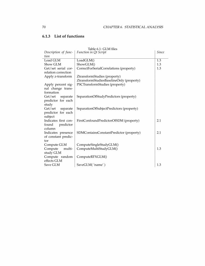
70 CHAPTER 6. STATISTICAL ANALYSIS
6.1.3 List of functions
Table 6.1: GLM filesDescription of func-tion
Function in Qt Script Since
Load GLM LoadGLM() 1.3Show GLM ShowGLM() 1.3Get/set serial cor-relation correction
CorrectForSerialCorrelations (property) 1.3
Apply z-transform ZtransformStudies (property)ZtransformStudiesBaselineOnly (property)
Apply percent sig-nal change trans-formation
PSCTransformStudies (property)
Get/set separatepredictor for eachstudy
SeparationOfStudyPredictors (property)
Get/set separatepredictor for eachsubject
SeparationOfSubjectPredictors (property)
Indicates first con-found predictorcolumn
FirstConfoundPredictorOfSDM (property) 2.1
Indicates presenceof constant predic-tor
SDMContainsConstantPredictor (property) 2.1
Compute GLM ComputeSingleStudyGLM()Compute multi-study GLM
ComputeMultiStudyGLM() 1.3
Compute randomeffects GLM
ComputeRFXGLM()
Save GLM SaveGLM( ’name’ ) 1.3
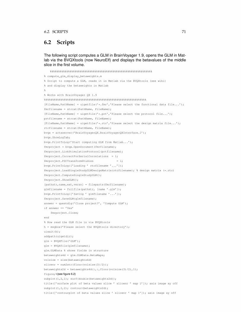
6.2. SCRIPTS 71
6.2 Scripts
The following script computes a GLM in BrainVoyager 1.9, opens the GLM in Mat-lab via the BVQXtools (now NeuroElf) and displays the betavalues of the middleslice in the first volume.
%%%%%%%%%%%%%%%%%%%%%%%%%%%%%%%%%%%%%%%%%%%%%%%%%%%%%%%%%%%%%%
% compute_glm_display_betaweights.m
% Script to compute a GLM, reads it in Matlab via the BVQXtools (see wiki)
% and display the betaweights in Matlab
%
% Works with BrainVoyager QX 1.9
%%%%%%%%%%%%%%%%%%%%%%%%%%%%%%%%%%%%%%%%%%%%%%%%%%%%%%%%%%%%%%
[FileName,PathName] = uigetfile(’*.fmr’,’Please select the functional data file...’);
fmrfilename = strcat(PathName, FileName);
[FileName,PathName] = uigetfile(’*.prt’,’Please select the protocol file...’);
prtfilename = strcat(PathName, FileName);
[FileName,PathName] = uigetfile(’*.rtc’,’Please select the design matrix file...’);
rtcfilename = strcat(PathName, FileName);
bvqx = actxserver(’BrainVoyagerQX.BrainVoyagerQXInterface.1’);
bvqx.ShowLogTab;
bvqx.PrintToLog(’Start computing GLM from Matlab...’);
fmrproject = bvqx.OpenDocument(fmrfilename);
fmrproject.LinkStimulationProtocol(prtfilename);
fmrproject.CorrectForSerialCorrelations = 1;
fmrproject.PSCTransformStudies = 1;
bvqx.PrintToLog([’Loading ’ rtcfilename ’...’]);
fmrproject.LoadSingleStudyGLMDesignMatrix(rtcfilename); % design matrix (*.rtc)
fmrproject.ComputeSingleStudyGLM();
fmrproject.ShowGLM();
[pathstr,name,ext,versn] = fileparts(fmrfilename);
glmfilename = fullfile(pathstr, [name ’.glm’]);
bvqx.PrintToLog([’Saving ’ glmfilename ’...’]);
fmrproject.SaveGLM(glmfilename);
answer = questdlg(’Close project?’, ’Compute GLM’);
if answer == ’Yes’
fmrproject.Close;
end
% Now read the GLM file in via BVQXtools
h = msgbox(’Please select the BVQXtools directory’);
uiwait(h);
addpath(uigetdir);
glm = BVQXFile(’GLM’);
glm = BVQXfile(glmfilename);
glm.GLMData % shows fields in structure
betaweights4d = glm.GLMData.BetaMaps;
volsize = size(betaweights4d)
slicenr = num2str(floor(volsize(3)/2));
betaweights2d = betaweights4d(:,:,floor(volsize(3)/2),1);
figure;%(see figure 6.2)
subplot(1,2,1); surf(double(betaweights2d));
title([’surface plot of beta values slice ’ slicenr ’ map 1’]); axis image xy off
subplot(1,2,2); contour(betaweights2d);
title([’contourplot of beta values slice ’ slicenr ’ map 1’]); axis image xy off

72 CHAPTER 6. STATISTICAL ANALYSIS
Figure 6.2: Plot of beta values
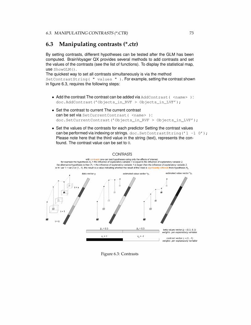
6.3. MANIPULATING CONTRASTS (*.CTR) 73
6.3 Manipulating contrasts (*.ctr)
By setting contrasts, different hypotheses can be tested after the GLM has beencomputed. BrainVoyager QX provides several methods to add contrasts and setthe values of the contrasts (see the list of functions). To display the statistical map,use ShowGLM().The quickest way to set all contrasts simultaneously is via the methodSetContrastString( " values " ). For example, setting the contrast shownin figure 6.3, requires the following steps:
• Add the contrast The contrast can be added via AddContrast( <name> ):doc.AddContrast(’Objects_in_RVF > Objects_in_LVF’);
• Set the contrast to current The current contrastcan be set via SetCurrentContrast( <name> ):doc.SetCurrentContrast(’Objects_in_RVF > Objects_in_LVF’);
• Set the values of the contrasts for each predictor Setting the contrast valuescan be performed via indexing or strings. doc.SetContrastString(’1 -1 0’);Please note here that the third value in the string (text), represents the con-found. The contrast value can be set to 0.
Figure 6.3: Contrasts

74 CHAPTER 6. STATISTICAL ANALYSIS
6.3.1 List of functions
Table 6.2: CTR filesDescription of function Function in Qt Script SinceClear contrasts ClearContrasts() 1.3Add contrast AddContrast( ’name’ ) 1.3Select contrast to change SetCurrentContrast()
SetCurrentContrastIndex() 1.3Set contrast(s) SetContrastString( ’text’ )
SetContrastValue( number )SetContrastValueAtIndex( index, value ) 1.3
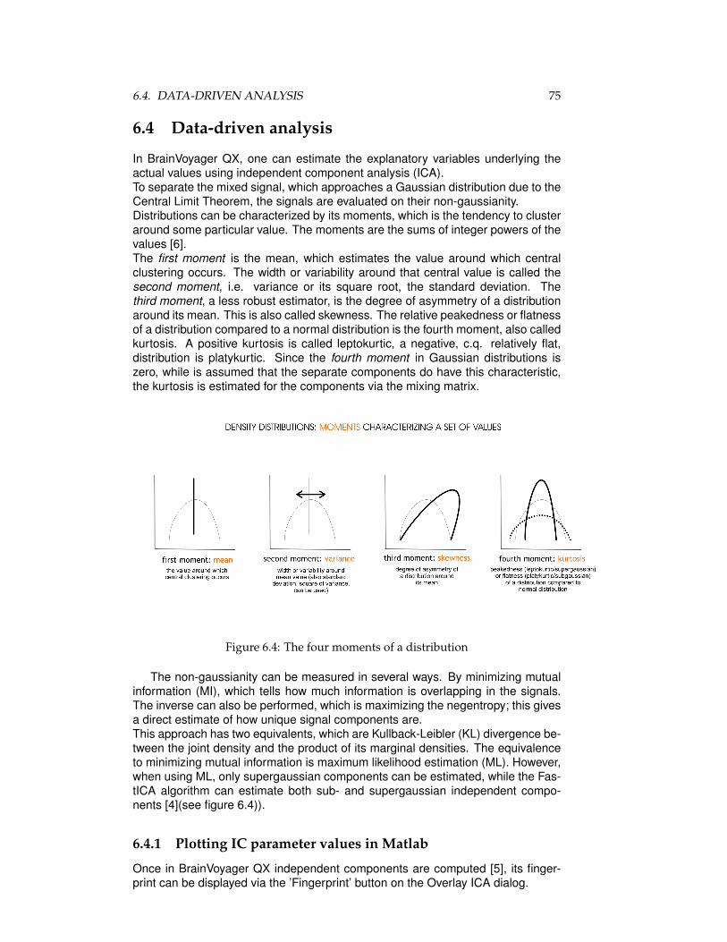
6.4. DATA-DRIVEN ANALYSIS 75
6.4 Data-driven analysis
In BrainVoyager QX, one can estimate the explanatory variables underlying theactual values using independent component analysis (ICA).To separate the mixed signal, which approaches a Gaussian distribution due to theCentral Limit Theorem, the signals are evaluated on their non-gaussianity.Distributions can be characterized by its moments, which is the tendency to clusteraround some particular value. The moments are the sums of integer powers of thevalues [6].The first moment is the mean, which estimates the value around which centralclustering occurs. The width or variability around that central value is called thesecond moment, i.e. variance or its square root, the standard deviation. Thethird moment, a less robust estimator, is the degree of asymmetry of a distributionaround its mean. This is also called skewness. The relative peakedness or flatnessof a distribution compared to a normal distribution is the fourth moment, also calledkurtosis. A positive kurtosis is called leptokurtic, a negative, c.q. relatively flat,distribution is platykurtic. Since the fourth moment in Gaussian distributions iszero, while is assumed that the separate components do have this characteristic,the kurtosis is estimated for the components via the mixing matrix.
Figure 6.4: The four moments of a distribution
The non-gaussianity can be measured in several ways. By minimizing mutualinformation (MI), which tells how much information is overlapping in the signals.The inverse can also be performed, which is maximizing the negentropy; this givesa direct estimate of how unique signal components are.This approach has two equivalents, which are Kullback-Leibler (KL) divergence be-tween the joint density and the product of its marginal densities. The equivalenceto minimizing mutual information is maximum likelihood estimation (ML). However,when using ML, only supergaussian components can be estimated, while the Fas-tICA algorithm can estimate both sub- and supergaussian independent compo-nents [4](see figure 6.4)).
6.4.1 Plotting IC parameter values in Matlab
Once in BrainVoyager QX independent components are computed [5], its finger-print can be displayed via the ’Fingerprint’ button on the Overlay ICA dialog.
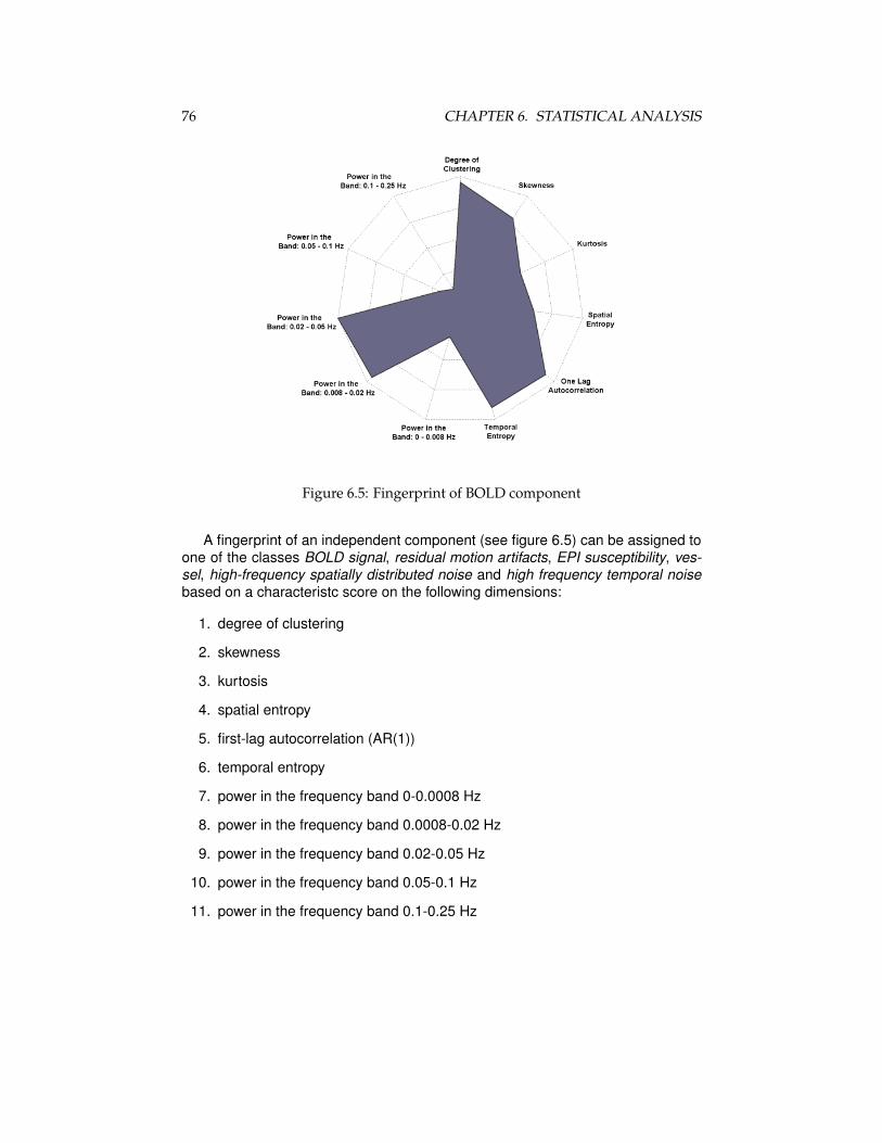
76 CHAPTER 6. STATISTICAL ANALYSIS
Figure 6.5: Fingerprint of BOLD component
A fingerprint of an independent component (see figure 6.5) can be assigned toone of the classes BOLD signal, residual motion artifacts, EPI susceptibility, ves-sel, high-frequency spatially distributed noise and high frequency temporal noisebased on a characteristc score on the following dimensions:
1. degree of clustering
2. skewness
3. kurtosis
4. spatial entropy
5. first-lag autocorrelation (AR(1))
6. temporal entropy
7. power in the frequency band 0-0.0008 Hz
8. power in the frequency band 0.0008-0.02 Hz
9. power in the frequency band 0.02-0.05 Hz
10. power in the frequency band 0.05-0.1 Hz
11. power in the frequency band 0.1-0.25 Hz
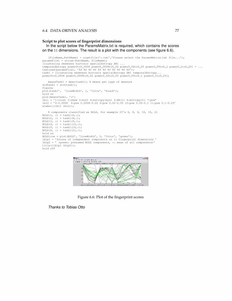
6.4. DATA-DRIVEN ANALYSIS 77
Script to plot scores of fingerprint dimensionsIn the script below the ParamsMatrix.txt is required, which contains the scores
on the 11 dimensions. The result is a plot with the components (see figure 6.6).
[FileName,PathName] = uigetfile(’*.txt’,’Please select the ParamsMatrix.txt file...’);paramsFile1 = strcat(PathName, FileName);[clustering skewness kurtosis spatialEntropy AR1 ...temporalEntropy power0to0_0008 power0_0008to0_02 power0_02to0_05 power0_05to0_1 power0_1to0_25] = ...textread(paramsFile1, ’%f %f %f %f %f %f %f %f %f %f %f’);task1 = [clustering skewness kurtosis spatialEntropy AR1 temporalEntropy...power0to0_0008 power0_0008to0_02 power0_02to0_05 power0_05to0_1 power0_1to0_25];
meansTask1 = mean(task1); % means per type of measurestdTask1 = std(task1);figure;plot(task1’, ’LineWidth’, 1, ’Color’, ’black’);hold onplot(meansTask1, ’*’)lbl1 = ’1:clust 2:skew 3:kurt 4:entropy(xyz) 5:AR(1) 6:entropy(t) 7:pow’lbl2 = ’0-0.0008 8:pow 0.0008-0.02 9:pow 0.02-0.05 10:pow 0.05-0.1 11:pow 0.1-0.25’xlabel([lbl1 lbl2]);
% components classified as BOLD, for example IC’s 6, 8, 9, 10, 16, 21BOLD(1, :) = task1(6,:);BOLD(2, :) = task1(8,:);BOLD(3, :) = task1(9,:);BOLD(4, :) = task1(10,:);BOLD(5, :) = task1(16,:);BOLD(6, :) = task1(21,:);hold onBOLDline = plot(BOLD’, ’LineWidth’, 2, ’Color’, ’green’);lblp1 = ’Scores of independent components on 11 fingerprint dimensions ’lblp2 = ’ (green: presumed BOLD components, *: mean of all components)’title([lblp1 lblp2]);hold off
Figure 6.6: Plot of the fingerprint scores
Thanks to Tobias Otto

78 CHAPTER 6. STATISTICAL ANALYSIS
6.4.2 Validating the IC components
Script to perform first validation steps of ICsBelow is a script to get started with the ICASSO toolbox [3], using the default
BrainVoyager QX ICA settings with deflation approach, tanh non-gaussianity mea-sure and 30 eigenvalues. After the VTC is created using the COM functionality de-scribed in chapter 4, the BVQXtoolbox is used to read the VTC value in the Matlabworkspace. Then, the clusters are estimated and plotted, showing the consistencyof the component (see figure 6.7).
h = msgbox(’Please select the ICASSO directory...’)uiwait(h);dirname = uigetdiraddpath(dirname)h = msgbox(’Please select the FastICA-25 directory...’)uiwait(h);dirname = uigetdiraddpath(dirname)h = msgbox(’Please select the BVQXTools directory...’)uiwait(h);bvqxtoolsdir = uigetdiraddpath(bvqxtoolsdir)[FileName,PathName] = uigetfile(’*.vtc’,’Please select the VTC file...’);vtcfilename = [PathName FileName];vtc = BVQXfile(vtcfilename);size(vtc.VTCData)vtcdata = permute(vtc.VTCData,[2 3 4 1]);vtcdims = size(vtcdata);vtc2d = double(reshape(vtcdata,[],vtcdims(4)));sR=icassoEst(’both’, vtc2d’, 25, ’lastEig’, 30,...’g’, ’tanh’, ’approach’, ’defl’);sR=icassoExp(sR);disp(’Launch Icasso visualization supposing 30 estimate-clusters.’);disp(’Show demixing matrix rows...’);icassoShow(sR,’L’,30,’estimate’,’demixing’);disp(’Launch Icasso visualization supposing 30 estimate-clusters...’);disp(’Show IC source estimates (default), reduce number of lines...’);[iq,A,W,S]=icassoShow(sR,’L’,30,’colorlimit’,[.8 .9]);
Figure 6.7: Similarity graph of the estimates

Chapter 7
Surface meshes
Currently, the scripting methods available for meshes are for display purposes.This can be used for example for automation of the display of several meshes se-quentially, and taking screenshots.
7.1 Loading meshes and capture the screen step-by-step
Start BrainVoyager from Matlab:bvqx = actxserver(’BrainVoyagerQX.BrainVoyagerQXScriptAccess.1’)Get the name of the VMR file:[FileName,PathName] = uigetfile(’*.vmr’,...’Please select the VMR file...’);Create the VMR name:vmrname = [PathName FileName]Open a VMR project:vmr = bvqx.OpenDocument(vmrname). Get the name of the mesh:[FileName,PathName] = uigetfile(’*.srf’,...’Please select the surface file...’);Create the SRF name:srfname = [PathName FileName]Load the mesh:vmr.LoadMesh(srfname);Make a screenshot by providing an image name:vmr.SaveSnapshotOfSurfaceWindow(’C:\Data\srfsnapshot.png’);
79

80 CHAPTER 7. SURFACE MESHES
7.1.1 List of functions
Table 7.1: Surface (*.srf), mesh time course (*.mtc) and viewpoint settings (*.vwp)files
Description of function Function in Qt Script SinceSave SRF file SaveMesh() 1.2Load SRF file LoadMesh() 1.2Add SRF file AddMesh() 1.2Create mesh time course CreateMTCFromVTC() 2.2Link MTC file LinkMTC() 2.2Screen capture SaveSnapshotOfSurfaceWindow() 1.xChange viewpoint set-tings
ViewpointTranslationX (property) 1.2
ViewpointTranslationY (property) 1.2ViewpointTranslationZ (property) 1.2ViewpointRotationX (property) 1.2ViewpointRotationY (property) 1.2ViewpointRotationZ (property) 1.2
Update surface window UpdateSurfaceWindow() 1.x

7.2. SCRIPTS 81
7.2 Scripts
7.2.1 Script to create MTC files
Below an example how a mesh time course (*.mtc) on a surface mesh (*.srf) couldbe created from functional data in a volume time course (*.vtc).The first parameter for the CreateMTCFromVTC() function indicates the samplingdepth in the white matter, the second in the gray matter, the third the name for themesh time course.
bvqx = actxserver(’BrainVoyagerQX.BrainVoyagerQXScriptAccess.1’);[FileName,PathName] = uigetfile(’*.vmr’,’Please select the anatomical data file...’);vmrfilename = strcat(PathName, FileName);docVMR = bvqx.OpenDocument(vmrfilename);docVMR.CreateMTCFromVTC(-1.0, 3.0, ’test.mtc’ );
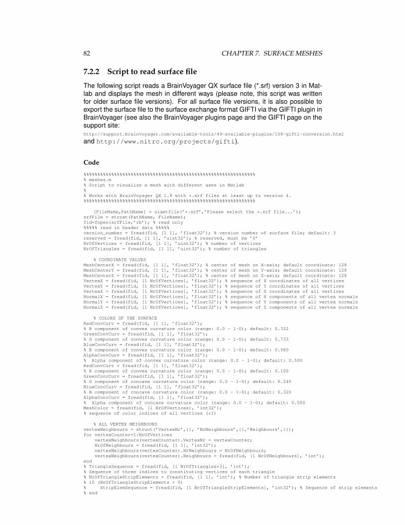
82 CHAPTER 7. SURFACE MESHES
7.2.2 Script to read surface file
The following script reads a BrainVoyager QX surface file (*.srf) version 3 in Mat-lab and displays the mesh in different ways (please note, this script was writtenfor older surface file versions). For all surface file versions, it is also possible toexport the surface file to the surface exchange format GIFTI via the GIFTI plugin inBrainVoyager (see also the BrainVoyager plugins page and the GIFTI page on thesupport site:http://support.brainvoyager.com/available-tools/49-available-plugins/158-gifti-conversion.html
and http://www.nitrc.org/projects/gifti).
Code
%%%%%%%%%%%%%%%%%%%%%%%%%%%%%%%%%%%%%%%%%%%%%%%%%%%%%%%%%%%%%%% meshes.m% Script to visualize a mesh with different axes in Matlab%% Works with BrainVoyager QX 1.9 with *.srf files at least up to version 4.%%%%%%%%%%%%%%%%%%%%%%%%%%%%%%%%%%%%%%%%%%%%%%%%%%%%%%%%%%%%%%
[FileName,PathName] = uigetfile(’*.srf’,’Please select the *.srf file...’);srfFile = strcat(PathName, FileName);fid=fopen(srfFile,’rb’); % read only%%%%% read in header data %%%%%version_number = fread(fid, [1 1], ’float32’); % version number of surface file; default: 3reserved = fread(fid, [1 1], ’uint32’); % reserved, must be ’0’NrOfVertices = fread(fid, [1 1], ’uint32’); % number of verticesNrOfTriangles = fread(fid, [1 1], ’uint32’); % number of triangles
% COORDINATE VALUESMeshCenterX = fread(fid, [1 1], ’float32’); % center of mesh on X-axis; default coordinate: 128MeshCenterY = fread(fid, [1 1], ’float32’); % center of mesh on Y-axis; default coordinate: 128MeshCenterZ = fread(fid, [1 1], ’float32’); % center of mesh on Z-axis; default coordinate: 128VertexX = fread(fid, [1 NrOfVertices], ’float32’); % sequence of X coordinates of all verticesVertexY = fread(fid, [1 NrOfVertices], ’float32’); % sequence of Y coordinates of all verticesVertexZ = fread(fid, [1 NrOfVertices], ’float32’); % sequence of Z coordinates of all verticesNormalX = fread(fid, [1 NrOfVertices], ’float32’); % sequence of X components of all vertex normalsNormalY = fread(fid, [1 NrOfVertices], ’float32’); % sequence of Y components of all vertex normalsNormalZ = fread(fid, [1 NrOfVertices], ’float32’); % sequence of Z components of all vertex normals
% COLORS OF THE SURFACERedConvCurv = fread(fid, [1 1], ’float32’);% R component of convex curvature color (range: 0.0 - 1-0); default: 0.322GreenConvCurv = fread(fid, [1 1], ’float32’);% G component of convex curvature color (range: 0.0 - 1-0); default: 0.733BlueConvCurv = fread(fid, [1 1], ’float32’);% B component of convex curvature color (range: 0.0 - 1-0); default: 0.980AlphaConvCurv = fread(fid, [1 1], ’float32’);% Alpha component of convex curvature color (range: 0.0 - 1-0); default: 0.500RedConvCurv = fread(fid, [1 1], ’float32’);% R component of convex curvature color (range: 0.0 - 1-0); default: 0.100GreenConcCurv = fread(fid, [1 1], ’float32’);% G component of concave curvature color (range: 0.0 - 1-0); default: 0.240BlueConcCurv = fread(fid, [1 1], ’float32’);% B component of concave curvature color (range: 0.0 - 1-0); default: 0.320AlphaConcCurv = fread(fid, [1 1], ’float32’);% Alpha component of concave curvature color (range: 0.0 - 1-0); default: 0.500MeshColor = fread(fid, [1 NrOfVertices], ’int32’);% sequence of color indices of all vertices (*1)
% ALL VERTEX NEIGHBOURSvertexNeighbours = struct(’VertexNr’,{}, ’NrNeighbours’,{},’Neighbours’,{});for vertexCounter=1:NrOfVertices
vertexNeighbours(vertexCounter).VertexNr = vertexCounter;NrOfNeighbours = fread(fid, [1 1], ’int32’);vertexNeighbours(vertexCounter).NrNeighbours = NrOfNeighbours;vertexNeighbours(vertexCounter).Neighbours = fread(fid, [1 NrOfNeighbours], ’int’);
end% TriangleSequence = fread(fid, [1 NrOfTriangles*3], ’int’);% Sequence of three indices to constituting vertices of each triangle% NrOfTriangleStripElements = fread(fid, [1 1], ’int’); % Number of triangle strip elements% if (NrOfTriangleStripElements > 0)% StripElemSequence = fread(fid, [1 NrOfTriangleStripElements], ’int32’); % Sequence of strip elements% end

7.2. SCRIPTS 83
fclose(fid);% (*1) Each vertex has one color index. An index value of 0 references the convex curvature color,% a value of 1 references the concave curvature color. Functional colors, RGB colors can be also represented.
% From example from Matlab Help documentation on multiple axes
tris = reshape(TriangleSequence,3,[])’+1;
figure; %(see figure 7.1)
h(1) = axes(’Position’,[0 0 1 1]);
trimesh(tris, VertexX’,VertexY’,VertexZ’);
h(2) = axes(’Position’,[0 0 .4 .6]); % closer, on the left lower corner
trimesh(tris, VertexX’,VertexY’,VertexZ’);
h(3) = axes(’Position’,[0 .5 .5 .5]); % closer, on the left upper corner, stretched
trimesh(tris, VertexX’,VertexY’,VertexZ’);
h(4) = axes(’Position’,[.5 0 .4 .4]); % closer, on the right lower corner, stretched
trimesh(tris, VertexX’,VertexY’,VertexZ’);
h(5) = axes(’Position’,[.5 .5 .5 .3]); % closer, on the right upper corner, very stretched
trimesh(tris, VertexX’,VertexY’,VertexZ’);
set(h,’Visible’,’off’)
Figure 7.1: Display meshes with different axes

84 CHAPTER 7. SURFACE MESHES

Chapter 8
Using BVQXtools
The BVQXtools is a toolbox created by Jochen Weber to read and manipulateBrainVoyager data in Matlab. The functionality in BrainVoyager QX and the BVQX-tools can be nicely combined now COM is available.For example, once a COM connection is established between Matlab and Brain-Voyager QX, one can first instruct BrainVoyager QX to create and preprocess func-tional data, and even create VTC files. Then, the files can be read quickly into theMatlab workspace by the BVQXtools1.
To obtain the BVQXtools, download the toolbox fromthe BrainVoyager support site (see figure 8.1). To make the BVQXTools available inMatlab, add the path of the BVQXtools to Matlab. This can for example be realizedvia the instruction addpath(uigetdir);.
Figure 8.1: BVQXtools on the BrainVoyager QX support site
1The most recent version of BVQXtools is called NeuroElf
85

86 CHAPTER 8. USING BVQXTOOLS

Bibliography
[1] J.D. Foley, A. van Dam, S.K. Feiner, and J.F. Hughes. Computer Graphics;Principles and Practice. Boston: Addison-Wesley Publishing Company, Inc.,1997.
[2] R. Goebel, F. Esposito, and E. Formisano. Analysis of fiac data with brain-voyager qx: From single-subject to cortically aligned group glm analysis andself-organizing group ica. Human Brain Mapping, 27(5):392–401, 2006.
[3] J. Himberg, A. Hyvrinen, and F. Esposito. Validating the independent compo-nents of neuroimaging time-series via clustering and visualization. NeuroIm-age, 22(3):1214–1222, 2004.
[4] A. Hyvrinen and E. Oja. Independent component analysis: Algorithms andapplications. Neural Networks, 13(4-5):411–430, 2000.
[5] F. de Martino, F. Gentile, F. Esposito, M. Balsi, F. Di Salle, R. Goebel,and E. Formisano. Classification of fmri independent components using ic-fingerprints and support vector machine classifiers. NeuroImage, 34(1):177–194, 2007.
[6] W.A. Press, S.A. Teukolsky, W.T. Vettering, and B.P. Flannery. NumericalRecipes in C; The Art of Scientific Computing. Cambridge: Cambridge Uni-versity Press, 2002.
87