scripting manual - software for chemistry & materials · scripting manual, release 2017-c: core...

Scripting ManualADF Modeling Suite 2018

www.scm.com

Sep 10, 2018

CONTENTS

1 Command Line Tools 11.1 ADFprep: generate (multiple) ADF jobs . . . . . . . . . . . . . . . . . . . . . . . . . . . . . . . . 1

1.1.1 Additional Notes . . . . . . . . . . . . . . . . . . . . . . . . . . . . . . . . . . . . . . . . 51.2 Tutorial: Generate structures for substituent effects screening . . . . . . . . . . . . . . . . . . . . . 51.3 ADFreport: generate reports . . . . . . . . . . . . . . . . . . . . . . . . . . . . . . . . . . . . . . . 9

1.3.1 Additional notes . . . . . . . . . . . . . . . . . . . . . . . . . . . . . . . . . . . . . . . . . 161.4 KF command line utilities . . . . . . . . . . . . . . . . . . . . . . . . . . . . . . . . . . . . . . . . 16

2 Python Stack in ADF Modeling Suite 192.1 Using other modules with the ADF Python Stack . . . . . . . . . . . . . . . . . . . . . . . . . . . . 20

3 ASE 213.1 General Concepts . . . . . . . . . . . . . . . . . . . . . . . . . . . . . . . . . . . . . . . . . . . . . 21

3.1.1 Components of ASE . . . . . . . . . . . . . . . . . . . . . . . . . . . . . . . . . . . . . . 21Quantum Chemical Model . . . . . . . . . . . . . . . . . . . . . . . . . . . . . . . . . . . . 21Quantum Chemical Calculation . . . . . . . . . . . . . . . . . . . . . . . . . . . . . . . . . 22Simulation Definitions . . . . . . . . . . . . . . . . . . . . . . . . . . . . . . . . . . . . . . 22

3.1.2 A Typical ASE Run . . . . . . . . . . . . . . . . . . . . . . . . . . . . . . . . . . . . . . . 223.2 SCM Calculators in ASE . . . . . . . . . . . . . . . . . . . . . . . . . . . . . . . . . . . . . . . . . 23

3.2.1 Technical Notes . . . . . . . . . . . . . . . . . . . . . . . . . . . . . . . . . . . . . . . . . 23New Interface Design in ADF2017 . . . . . . . . . . . . . . . . . . . . . . . . . . . . . . . 23Interfaces to Individual Programs . . . . . . . . . . . . . . . . . . . . . . . . . . . . . . . . 23

3.2.2 Usage and Examples . . . . . . . . . . . . . . . . . . . . . . . . . . . . . . . . . . . . . . 24Import . . . . . . . . . . . . . . . . . . . . . . . . . . . . . . . . . . . . . . . . . . . . . . . 24Interface Keywords . . . . . . . . . . . . . . . . . . . . . . . . . . . . . . . . . . . . . . . . 24Examples . . . . . . . . . . . . . . . . . . . . . . . . . . . . . . . . . . . . . . . . . . . . . 24

4 FlexMD 254.1 Basic philosophy and intended usage . . . . . . . . . . . . . . . . . . . . . . . . . . . . . . . . . . 254.2 FlexMD functionality summary . . . . . . . . . . . . . . . . . . . . . . . . . . . . . . . . . . . . . 254.3 Introduction . . . . . . . . . . . . . . . . . . . . . . . . . . . . . . . . . . . . . . . . . . . . . . . 274.4 Molecular Dynamics . . . . . . . . . . . . . . . . . . . . . . . . . . . . . . . . . . . . . . . . . . . 274.5 Multi-scale Molecular Dynamics . . . . . . . . . . . . . . . . . . . . . . . . . . . . . . . . . . . . 284.6 Biased Molecular Dynamics . . . . . . . . . . . . . . . . . . . . . . . . . . . . . . . . . . . . . . . 294.7 Working with FlexMD . . . . . . . . . . . . . . . . . . . . . . . . . . . . . . . . . . . . . . . . . . 29

4.7.1 Creating a molecule object . . . . . . . . . . . . . . . . . . . . . . . . . . . . . . . . . . . 294.7.2 Creating a ForceJob . . . . . . . . . . . . . . . . . . . . . . . . . . . . . . . . . . . . . . . 304.7.3 Creating and running the MD job . . . . . . . . . . . . . . . . . . . . . . . . . . . . . . . . 31

4.8 Required Citations . . . . . . . . . . . . . . . . . . . . . . . . . . . . . . . . . . . . . . . . . . . . 324.8.1 External programs and Libraries . . . . . . . . . . . . . . . . . . . . . . . . . . . . . . . . 32

i

4.9 References . . . . . . . . . . . . . . . . . . . . . . . . . . . . . . . . . . . . . . . . . . . . . . . . 32

5 PLAMS 355.1 Required Citations . . . . . . . . . . . . . . . . . . . . . . . . . . . . . . . . . . . . . . . . . . . . 35

5.1.1 External programs and Libraries . . . . . . . . . . . . . . . . . . . . . . . . . . . . . . . . 35

6 AuToGraFS 376.1 General AuToGraFS Scripting concepts . . . . . . . . . . . . . . . . . . . . . . . . . . . . . . . . . 37

6.1.1 Components of AuToGraFS . . . . . . . . . . . . . . . . . . . . . . . . . . . . . . . . . . 37The Fragment class . . . . . . . . . . . . . . . . . . . . . . . . . . . . . . . . . . . . . . . . 37The Model class . . . . . . . . . . . . . . . . . . . . . . . . . . . . . . . . . . . . . . . . . 38The Autografs class . . . . . . . . . . . . . . . . . . . . . . . . . . . . . . . . . . . . . . . . 39

6.1.2 About the databases of building units . . . . . . . . . . . . . . . . . . . . . . . . . . . . . . 396.1.3 Using the overhauled Atom Typer . . . . . . . . . . . . . . . . . . . . . . . . . . . . . . . 40

6.2 AuToGraFS Examples . . . . . . . . . . . . . . . . . . . . . . . . . . . . . . . . . . . . . . . . . . 406.2.1 Generation of all available pillared SURMOF . . . . . . . . . . . . . . . . . . . . . . . . . 406.2.2 Generation of a defectuous UIO-66 MOF from custom files . . . . . . . . . . . . . . . . . . 416.2.3 Generation of conformers in the IRMOF-5 . . . . . . . . . . . . . . . . . . . . . . . . . . . 42

Index 43

ii

CHAPTER

ONE

COMMAND LINE TOOLS

• adfprep: prepare an ADF job from a script (or command line).

• adfreport: get information (including images) from an ADF result file (for use in your script, or to generate anHTML or tab-separated report).

• pkf, cpkf, dmpkf, udmpkf: the KF utilities, which are command-line utilities to process KF files.

1.1 ADFprep: generate (multiple) ADF jobs

ADFprep allows one to generate input files for the different programs of the ADF modeling suite by means of consolecommands. As such ADFprep can be used to run the same type of calculation on a series of different chemical systems.Another important example are automatic checks of the convergence of the results with respect to the computationalparameters e.g. by varying input settings such as basis set choice or numerical integration accuracy while recomputingthe same system.

ADFprepare ($ADFBIN/adfprep) generates a job script from a template .adf file. Such a template file can either beproduced by ADFinput or simply be found among the default templates included. These default templates are identicalto those present in ADFinput.

Two examples are presented here to demonstrate the capabilities of ADFprep:

• In BakersetSP you will see how to use adfprep to run a particular job for a test set of molecules. The individualmolecular structures are provided as xyz-files which contain no ADF specific information. ADFreport is usedto collect the values of the bonding energies resulting from these calculations.

• In ConvergenceTestCH4 you will see how to use ADFprep to test convergence of the bonding energy withrespect to the basis set and the numerical integration grid.

The options of ADFprep are listed when running the module without further command line arguments, or with the -hflag:

% adfprep -hADFprepare (adfprep) generates a job script from a .adf file (the template),with user specified changes to input options / method / system.

Usage: adfprep -t template.adf [-m molecule.(adf|xyz|mol|t21)] [-z charge] [-s spin][-runtype SinglePoint|GeometryOptimization|Frequencies][-gradientsonly][-q quality] [-zlmfit quality] [-kspace quality][-lattice v1.x v1.y v1.z ...][-i integration] [-b basis] [-c core] [-r relativity][-basiscacheid id][-x xcpotential] [-e xcenergy] [-bondsonly][-dftbmodel DFTB|SCC-DFTB|DFTB3] [-dftbparameters dir]

1

Scripting Manual, ADF Modeling Suite 2018

[-dftbdispersion None|Default|D3-BJ|D2|ULG|UFF][-logfile logfile] [-j jobname] [-a adffile][-dist "atom1 atom2 distance ..."][-angle "atom1 atom2 atom3 angle ..."][-dihed "atom1 atom2 atom3 atom4 angle ..."][-atomtype "atom type ..."][-structure "atom structure ..."][-pointcharges file][-efield "Ex Ey Ez"][-rxforcefield fname] [-rxniter n] [-rxnrstep n] [-

→˓rxtstep T][-rxmethod method] [-rxmdtemp T] [-rxmdpres p][-region "name at1 at2... "][-fragments prefix] [-onejob][-g "key value"]

Start with a job template, adjust it for this particular job, and write the resulting→˓jobto standard output. Values specified should match exactly the values as you would→˓specifyusing ADFinput, also for menu choices.

TEMPLATE-t: the .adf file (saved by ADFinput) to be used as template, defining the whole job

All other options override values from this job

Instead of a .adf file, you may also specify the name of one of the standard→˓templates

as defined in ADFinput: "Single Point", Frequencies, "Geometry Optimization", etcA special option for energy and gradientsfor the current geometry: EG (see also -gradientsonly)

Some shortcuts: SP, EG, GO, FREQ, optionally prefixed by→˓(ADF|BAND|DFTB|UFF|MOPAC)-

For example: ADF-FREQ, BAND-SP, DFTB-GO, MOPAC-EG

Some ReaxFF shortcuts: REAXFF-EG for a single ReaxFF iteration

CHANGES TO TEMPLATE-m: the molecule to use, element types and coordinates

This can be taken from anything that ADFinput can import,for example .adf, .mol, xyz or .t21 files

The -m flag may be repeated, each molecule added will be in its own regionThis may be used for fragment calculations, but it does not work with .adf files

If you specify an .sdf file, you can select which frames to import:conformers.sdf#1-10 loop over the first 10 framesconformers.sdf#e2.0 loop over all frames with energy below 2.0

(units as in the file, wrt the lowest energy of all frames in the file,energies from comment lines)

conformers.sdf#1-10e2.0 loop over the first 10 frames,and use only those with energy below 2.0

conformers.sdf use the first frame of the sdf file

If you specify a .t21 file, you can select which frames or range of frames to→˓import:

2 Chapter 1. Command Line Tools


ajob.t21#ircf3 3rd frame in the IRC forward pathajob.t21#ircb2 2nd frame in the IRC backward pathajob.t21#h7 7th frame in the historyajob.t21#lt8 8th frame in the LT pathajob.t21#ircf3-10 IRCForward frame 3, 4, ... 10ajob.t21#ircf IRCForward all frames, starting at 1ajob.t21#ircf0- IRCForward all frames, starting at 0

(original geometry, before first step)

If you specify a .cry file, the compound to import may be specified:$ADFHOME/atomicdata/Molecules/Crystals/Cubic/CsCl.cry#MgTl

When looping, all resulting jobs will be joined together, the jobname and adf→˓files

get the frame sequence number appended after an _When looping only one -m flag may be specified

-xyz: use xyz coordinates from specified file, not touching anything elseit is applied after -t and -mthe elements and number of atoms should matchcurrently works with KF and xyz files

-smiles: use smiles to describe the molecule

-irc: when using IRC frames in the -m flag, revert the backwards order

-dist: change the distance between atom1 and atom2 to the specified distancethe arguments must be enclosed in quotes, and may be repeated for multiple

→˓distances-angle: change the angle (atom1, atom2, atom3) to the specified angle

the arguments must be enclosed in quotes, and may be repeated for multiple→˓angles-dihed: change the dihedral (atom1, atom2, atom3, atom4) to the specified angle

the arguments must be enclosed in quotes, and may be repeated for multiple→˓angles-atomtype: set the type (element) of atom to type

the arguments must be enclosed in quotes, and may be repeated for multiple→˓types-structure: add a structure just as if using the structure tool in ADFinput

atom is the selected atom, structure is the name of the structure filethe arguments must be enclosed in quotes, and may be repeated for multiple

→˓changes-liststructures: list available structure files for use with -structure, and exit

-runtype: run type (SinglePoint,GeometryOptimization,Frequencies)-gradientsonly: after calculating the gradients, stop

works also for excited state gradients if requested in your template-z: charge (real number)-s: spin (integer), if not zero this implies an unrestricted calculation-q: quality (Basic, Normal, Good, VeryGood or Excellent), default for Becke/ZlmFit-i: integration (integer)-i: Becke integration (Basic, Normal, Good, VeryGood or Excellent)-i: teVelde integration (integer)-zlmfit: ZlmFit quality (Basic, Normal, Good, VeryGood or Excellent)-kspace: KSpace quality (GammaOnly, Basic, Normal, Good, VeryGood or Excellent)-lattice: lattice vectors first three numbers for the first vector, next for the→˓second etc

The dimension follows from the number of vectors-b: basis type (SZ, DZ, DZP, TZ, TCP, TZ2P, QZ4P)

1.1. ADFprep: generate (multiple) ADF jobs 3


-c: core type (None, Small, Medium, Large)-basiscacheid id: refer to t21 files from previous runs prefixed with this id-r: relativistic level (None, Scalar, Spin-Orbit), using ZORA-x: XC potential during SCF, one from the options available in ADFinput:

LDA,GGA:BP, GGA:BLYP, GGA:PW91, GGA:mPW, GGA:PBE, GGA:RPBE, GGA:revPBE, GGA:mPBE,GGA:OLYP, GGA:OPBE,Model:SAOP, Model:LB94,Hartree-Fock,Hybrid:B3LYP, Hybrid:B3LYP*, Hybrid:B1LYP, Hybrid:KMLYP, Hybrid:O3LYP,

→˓Hybrid:X3LYP,Hybrid:BHandH, Hybrid:BHandHLYP, Hybrid:B1PW91, Hybrid:MPW1PW, Hybrid:MPW1K,Hybrid:PBE0, Hybrid:OPBE0

-e: XC energy after SCF (Default, LDA+GGA_METAGGA, LDA+GGA+METAGGA+HYBRIDS)-pointcharges: file, file with point charges, one point charge per line (ADF only)

x y z charge, xyz in Angstrom, charge in elementary units (+1 for a→˓proton)-efield: Ex Ey Ez the electric field vector (in Hartree/(e Bohr))-k: replace any key, the single argument will be broken into:

the key, the replacement value, and END for a block keyall separated by spaces. To insert a return, add a |When the key is not found, it is added just before the ATOMS keyThe -k key may be repeated, and is applied at the end, replacing even earlier

→˓changes

-dftbmodel DFTB|SCC-DFTB|DFTB3: select the DFTB model-dftbparameters dir: select the directory with DFTB parameters-dftbdispersion [None|Default|D3-BJ|D2|ULG|UFF]: dispersion option to use, default is→˓None

-rxforcefield fname: the ReaxFF force field file-rxniter n: number of ReaxFF iterations-rxnrstep n: number of non-reactive iterations (out of the total number of iterations)-rxtstep T: the time step used in the MD simulation-rxmethod string: the simulation type: Velocity Verlet + Berendsen|NPT|NVE-rxmdtemp T: the thermostat temperature-rxmdpres p: the required pressure

-region name at1 at2 ...: make a region with specified name and atoms, may be repeatedThe atom numbers at1 at2 refer to input order, after geometry modifications,

→˓start at 1Use at1-at2 to refer to all atoms between at1 and including at2If the region key is present all regions already present are deleted

-fragments prefix: set up a fragment calculation, prefix fragment run/job scripts→˓with prefix

if this key is present fragment run/job scripts will be saved→˓(unless -onejob)

if a job script is requested, the fragment job names will be→˓prefix.fragname.job-onejob: for fragment jobs, concatenate the fragment jobs and final job into one on→˓stdout-g "key value": set any key to the specified value (note key value within quotes)

key: internal name in ADFinput for some option, see bin/adfinput.tcl/tpl/→˓Defaults.tpl

value: set gin(key) to the specified value-nochain: unset chain option (used internally by chain jobs)

OUTPUT



-bondsonly: only the bonds as generated by the GUI will be exported (the GUIBONDS→˓block)-logfile: force the specified logfile to be used in the run script-j: produce a fully runnable job (as the .job files from ADFjobs),

using the specified jobname.The job script produces files like jobname.out, jobname.t21 etc. Several job

→˓scripts can simplybe concatenated, the results will be stored in different files using th jobname

→˓parameterthe default is a simple run script (the .run file from ADFinput, files are left

→˓as they are)-a: save a .adf file that matches the run script, except for the -k arguments

(they are listed in the user input field)adffile is the name of the adffile, including the .adf extension (required)

Example: calculate gradients for a molecule in file mymol.xyzadfprep -t GO -m mymol.xyz -k "stopafter ggrads"

Example: calculate gradients for a molecule in file mymol.xyz, using good quality→˓integration and fit:

adfprep -t GO -q Good -m mymol.xyz -k "stopafter ggrads"

Example: calculate DFTB frequencies for a molecule in file mymol.xyzadfprep -t DFTB-FREQ -m mymol.xyz

1.1.1 Additional Notes

CRSprep represents a scripting solution which is exclusively oriented towards generating input files for the COSMO-RS program.

1.2 Tutorial: Generate structures for substituent effects screening

Overview

Screening substituent patterns of a base compound is a common task in computer aided materials design. In thefollowing short tutorial we demonstrate how you can use adfprep to automatize the replacement of substituents withjust a few lines of simple shell scripting.

1.2. Tutorial: Generate structures for substituent effects screening 5


Contents:

• The library of substituents in ADFinput

• Exchanging substituents with ADFprep

• Combining ADFprep and ADFreport in shell script

The substituent library in ADFinput

ADFinput comes with a customizable library of common substituents that we can use for our screening purposes rightaway. It can be accessed via the structure builder tool in ADFinput:

Note how the entries are organized. For example the isocyanide functional group (“NC”) can be found in “Ligands”.

Its also possible to add your own compounds: Simply draw the structure of interest and select the atom which will



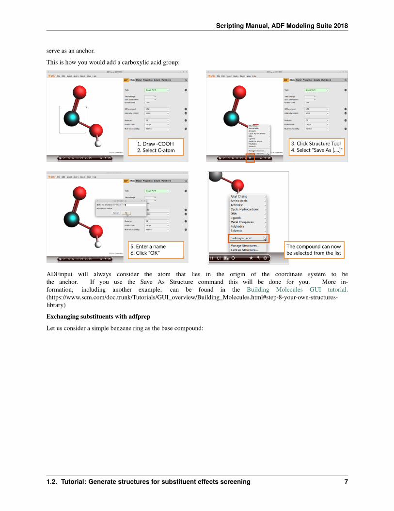
serve as an anchor.

This is how you would add a carboxylic acid group:

ADFinput will always consider the atom that lies in the origin of the coordinate system to bethe anchor. If you use the Save As Structure command this will be done for you. More in-formation, including another example, can be found in the Building Molecules GUI tutorial.(https://www.scm.com/doc.trunk/Tutorials/GUI_overview/Building_Molecules.html#step-8-your-own-structures-library)

Exchanging substituents with adfprep

Let us consider a simple benzene ring as the base compound:

1.2. Tutorial: Generate structures for substituent effects screening 7

https://www.scm.com/doc.trunk/Tutorials/GUI_overview/Building_Molecules.html#step-8-your-own-structures-library


The adfprep command to exchange Hydrogen atom #12 with an isocyanide group (“NC”) and create a runfile for aUFF geometry optimization is:

"$ADFBIN/adfprep" -t UFF-GO -m benzene.xyz -structure "12 Ligands/NC.adf" > "benzene_→˓NC.run"

Remember that the “CN” group was located in the “Ligands” menu hence “Ligands/NC.adf”. In case the path containswhitespace, you need to escape the whitespace as in this example

"$ADFBIN/adfprep" -t UFF-GO -m benzene.xyz -structure "12 Alkyl\ Chains/Ethyl.adf" >→˓"ethyl_benzene.run"

When using custom substituents, e.g. the hydroxylic_acid in the above example, a full path need to be providedto adfprep. The path is displayed when clicking on the Structure Tool in ADFinput and selecting “Manage yourstructures”. On an ubuntu linux system the path is “/home/[your_username]/.scm_gui/Structures” and the commandto use your own structures becomes:

"$ADFBIN/adfprep" -t UFF-GO -m benzene.xyz -structure "12 /home/[your_username]/.scm_→˓gui/Structures/carboxylic_acid.adf" > "benzoic_acid.run"

Bringing it all together

The following few lines of shell script demonstrate how to automatically exchange the substituents on a benzene ring,run a UFF optimization on the new structure and extract the optimized geometry with adfreport.

#! /bin/sh## copy the file benzene.xyz from the ADF compounds database#cp "$ADFHOME/atomicdata/Molecules/ADF/Benzene.xyz" .## loop through different substituents#for ligand in CN CO CO3 NC NH2 NH2CH3 NH3 OC OCH3 OH PH3 Pyridine; do



## prepare the coordinates and the UFF calculation#"$ADFBIN/adfprep" -t UFF-GO -m Benzene.xyz -structure "12 Ligands/$ligand.adf" >

→˓"benzene_$ligand.run"## run UFF GeoOpt#sh "./benzene_$ligand.run"## extract the optimized geometry via adfreport#"$ADFBIN/adfreport" uff.rkf SDF > "benzene_$ligand.mol"## rename the generic UFF output file#mv uff.rkf "benzene_$ligand.rkf"

done

Running the script

Linux and Mac: Copy and paste the above into a file called substituents_script and execute it in the commandline

sh substituents_script

Windows: Just use the pre-configured shell, adf_command_line.bat (https://www.scm.com/doc/Scripting/) ,shippedwith ADF to run the same command as the Linux and Mac users.

1.3 ADFreport: generate reports

The utility ADFreport ($ADFBIN/adfreport) allows to retrieve the results (including images) computed from the bi-nary output files of either ADF, BAND, ReaxFF, DFTB, UFF, or MOPAC. For ADF this is the .t21 file (TAPE21). Itcan also be the .runkf file from BAND, the .rxkf file from ReaxFF or the .rkf file from DFTB, MOPAC or UFF.

The selected results are printed out via standard output or, alternatively, either written to a tab separated file or anHTML file. When creating a new output file ADFreport will also generate a line with headers identifying the informa-tion. Images are generated using the ADF-GUI.

Also individual KF variables can be retrieved from the file as shown by the following example, which illustrates howto obtain the bonding energy from a .t21 file.

adfreport job.t21 BondingEnergy

Also high-quality pictures of orbitals can be obtained as shown below.

adfreport job.t21 HOMO LUMO+1 -v "-grid Fine" -v "-antialias" -v "-bgcolor #ffffff"

The options of ADFreport are listed when running the module without further command line arguments. At presentthe following command line options are available

-h prints the help screen.

Hint: If used with the name of a valid KF file in the command line the -h option lists the names of all data blockspresent in that file. It is strongly encouraged to use this option to retrieve the names of the options available in a given

1.3. ADFreport: generate reports 9

https://www.scm.com/doc/Scripting/


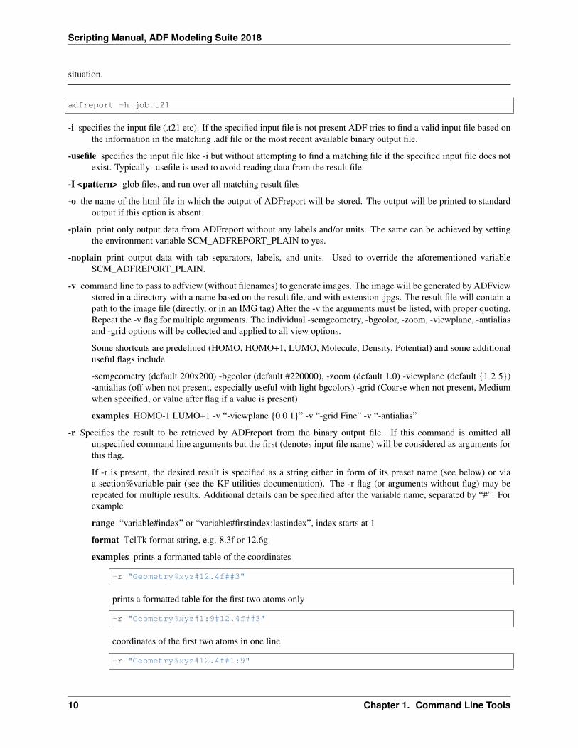
situation.

adfreport -h job.t21

-i specifies the input file (.t21 etc). If the specified input file is not present ADF tries to find a valid input file based onthe information in the matching .adf file or the most recent available binary output file.

-usefile specifies the input file like -i but without attempting to find a matching file if the specified input file does notexist. Typically -usefile is used to avoid reading data from the result file.

-I <pattern> glob files, and run over all matching result files

-o the name of the html file in which the output of ADFreport will be stored. The output will be printed to standardoutput if this option is absent.

-plain print only output data from ADFreport without any labels and/or units. The same can be achieved by settingthe environment variable SCM_ADFREPORT_PLAIN to yes.

-noplain print output data with tab separators, labels, and units. Used to override the aforementioned variableSCM_ADFREPORT_PLAIN.

-v command line to pass to adfview (without filenames) to generate images. The image will be generated by ADFviewstored in a directory with a name based on the result file, and with extension .jpgs. The result file will contain apath to the image file (directly, or in an IMG tag) After the -v the arguments must be listed, with proper quoting.Repeat the -v flag for multiple arguments. The individual -scmgeometry, -bgcolor, -zoom, -viewplane, -antialiasand -grid options will be collected and applied to all view options.

Some shortcuts are predefined (HOMO, HOMO+1, LUMO, Molecule, Density, Potential) and some additionaluseful flags include

-scmgeometry (default 200x200) -bgcolor (default #220000), -zoom (default 1.0) -viewplane (default {1 2 5})-antialias (off when not present, especially useful with light bgcolors) -grid (Coarse when not present, Mediumwhen specified, or value after flag if a value is present)

examples HOMO-1 LUMO+1 -v “-viewplane {0 0 1}” -v “-grid Fine” -v “-antialias”

-r Specifies the result to be retrieved by ADFreport from the binary output file. If this command is omitted allunspecified command line arguments but the first (denotes input file name) will be considered as arguments forthis flag.

If -r is present, the desired result is specified as a string either in form of its preset name (see below) or viaa section%variable pair (see the KF utilities documentation). The -r flag (or arguments without flag) may berepeated for multiple results. Additional details can be specified after the variable name, separated by “#”. Forexample

range “variable#index” or “variable#firstindex:lastindex”, index starts at 1

format TclTk format string, e.g. 8.3f or 12.6g

examples prints a formatted table of the coordinates

-r "Geometry%xyz#12.4f##3"

prints a formatted table for the first two atoms only

-r "Geometry%xyz#1:9#12.4f##3"

coordinates of the first two atoms in one line

-r "Geometry%xyz#12.4f#1:9"



print just the first coordinate

-r "Geometry%xyz#1"

print the bond energy

-r "Energys%Bond Energy"

While any proper KF variable can be accessed via a “section%variable” construct, the following predefined keysare available for the KF files resulting from the various programs of the ADF modeling suite.

ADF-specific ‘‘-r‘‘ presets for .t21 files

orient* affine transform (3x4) from input to internal ADF orientation, format after #

iorient* affine transform (3x4) from internal ADF to input orientation, format after #

title title of the calculation

type calculation type (single point, geometry optimization, ...)

weight molecular weight

symmetry molecular symmetry

natoms number of atoms

integration integration accuracy

integration-min minimum integration accuracy

integration-max maximum integration accuracy

scfstatus SCF convergence status

charge the requested charge

charges shorthand for Voronoi, Hirshfeld and Mulliken charges

voronoi Voronoi deformation charges

hirshfeld Hirshfeld fragment charges, atomic fragment definition required

mdc All available MDC atom charges

mdc-m MDC-M charges

mdc-d MDC-D charges

mdc-q MDC-Q charges

mulliken Mulliken charges

bondorders Mayer bond orders

nmr NMR shieldings

nmr-shieldings NMR shieldings

nmr-shielding-tensor NMR shielding tensor

nmr-j-coupling-tensor NMR j coupling tensor

nmr-k-coupling-tensor NMR k coupling tensor

nmr-j-coupling-constant NMR j coupling constant

nmr-k-coupling-constant NMR k coupling constant



dipolev* dipole vector

dipole dipole moment (length of dipole vector)

quadrupole quadrupole tensor

orbital-info orbital info (energy, occupation and label), format for energy after #, range after # with HOMO orLUMO for example:

orbital-info#HOMO, orbital-info#HOMO-1,orbital-info#HOMO-2:LUMO+2, orbital-info#HOMO#12.8f

orbital-e* orbital energies, format and range after # as in orbital-info

orbital-o* orbital occupations, format and range after # as in orbital-info

orbital-l* orbital labels, format and range after # as in orbital-info

homo-lumo-gap* HOMO-LUMO gap, format after #

atomlabels name of atoms with sequence number, starting at 0

atomlabels-from0 name of atoms with sequence number, starting at 0

atomlabels-from1 name of atoms with sequence number, starting at 1

nstep number of steps in history / LT / IRC data, type (h,lt,ircf,ircb) after #

spin the requested spin polarization

step use coordinates from history / LT / IRC data, step number after # with h for history, lt for LT, ircf/ircb forforward/backward IRC if no letter after #, history data will be used (if not, last step will be used) for example:

step#23 (or step#h23), step#lt4, step#ircf3

geometry, geometry-a*, geometry-b* geometry (element type and coordinates), in input order, inangstrom or bohr (default)

sdf geometry in SDF format

bgf geometry in BGF format

distance distance between two atoms, in angstrom. Input separated by #

labels (optional): include atom labels in output

format (optional): format field

atom numbers, starting at 1, in input order

examples

distance#2#3, distance#labels#2#3, distance#-8.3f#5#8,distance#labels#8.4f#1#2, distance#2#3#4#5, distance#labels#1#2#3#4

angle angle between three atoms, in degrees. Input see distance, but with three atoms per angle

dihedral dihedral between four atoms, in degrees. Input see distance, but with our atoms per dihedral

hessian* Hessian matrix (from GeoOpt%Hessian_CART), fmt and nperline options after #

gradients* gradients with respect to nuclear displacements (from GeoOpt%Gradients), fmt and nperline optionsafter #

energies* all avaliable energies (bonding up to xc, with labels), fmt option after #

bonding total bonding energy



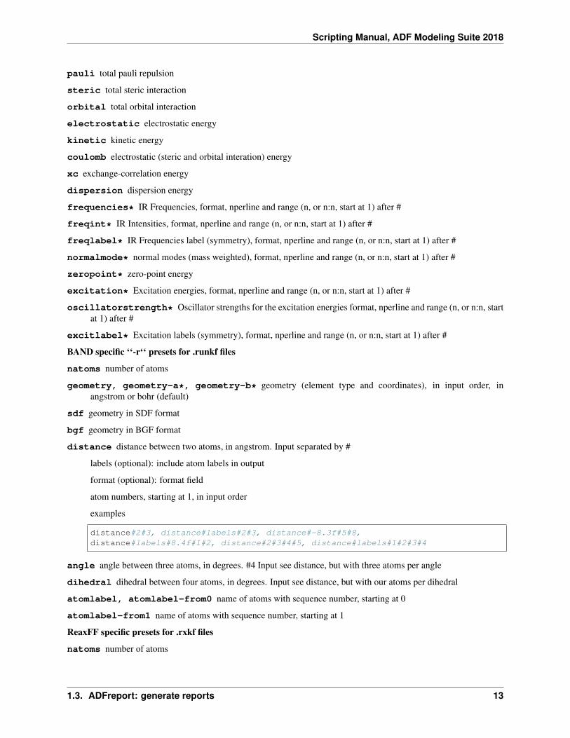
pauli total pauli repulsion

steric total steric interaction

orbital total orbital interaction

electrostatic electrostatic energy

kinetic kinetic energy

coulomb electrostatic (steric and orbital interation) energy

xc exchange-correlation energy

dispersion dispersion energy

frequencies* IR Frequencies, format, nperline and range (n, or n:n, start at 1) after #

freqint* IR Intensities, format, nperline and range (n, or n:n, start at 1) after #

freqlabel* IR Frequencies label (symmetry), format, nperline and range (n, or n:n, start at 1) after #

normalmode* normal modes (mass weighted), format, nperline and range (n, or n:n, start at 1) after #

zeropoint* zero-point energy

excitation* Excitation energies, format, nperline and range (n, or n:n, start at 1) after #

oscillatorstrength* Oscillator strengths for the excitation energies format, nperline and range (n, or n:n, startat 1) after #

excitlabel* Excitation labels (symmetry), format, nperline and range (n, or n:n, start at 1) after #

BAND specific ‘‘-r‘‘ presets for .runkf files









examples


angle angle between three atoms, in degrees. #4 Input see distance, but with three atoms per angle


atomlabel, atomlabel-from0 name of atoms with sequence number, starting at 0

atomlabel-from1 name of atoms with sequence number, starting at 1

ReaxFF specific presets for .rxkf files









examples




atomlabel, atomlabel-from0 name of atoms with sequence number, starting at 0

atomlabel-from1 name of atoms with sequence number, starting at 1

rx-frame n options information for a particular reaxff frame. Note the spaces, you will need to quote this key.

n: frame number 0, 1, 2, ... (is not the ReaxFF step number)

options: combination of the following (if omitted, all will be reported)

nframes: total number of frames

step: the ReaxFF step number for the specified frame

nats: number of atoms

xyz: the xyz coordinates

names: element names (C, H etc) for each atom in the same order as the→˓coordinates

neighbors: bond information

cell: cell information

example

adfreport water.rxkf "rx-frame 20 step xyz cell"

pdbtrajectory the trajectory information (including molecule details) as a sequence of PDB models due to limi-tations of the PDB format to less than 100000 atoms and it will not be a standard conforming PDB file

pdbtrajectory-(nobonds|usepdbinfo)

nobonds: as pdbtrajectory, but no bond info (CONECT records)

usepdbinfo: as pdbtrajectory, but use pdb residue info from first step instead of→˓reaxff mol info

xmol: the trajectory information (only element, xyz) in xmol format

gro: trajectory as .gro file (xyz and velocities) options after a - sign:



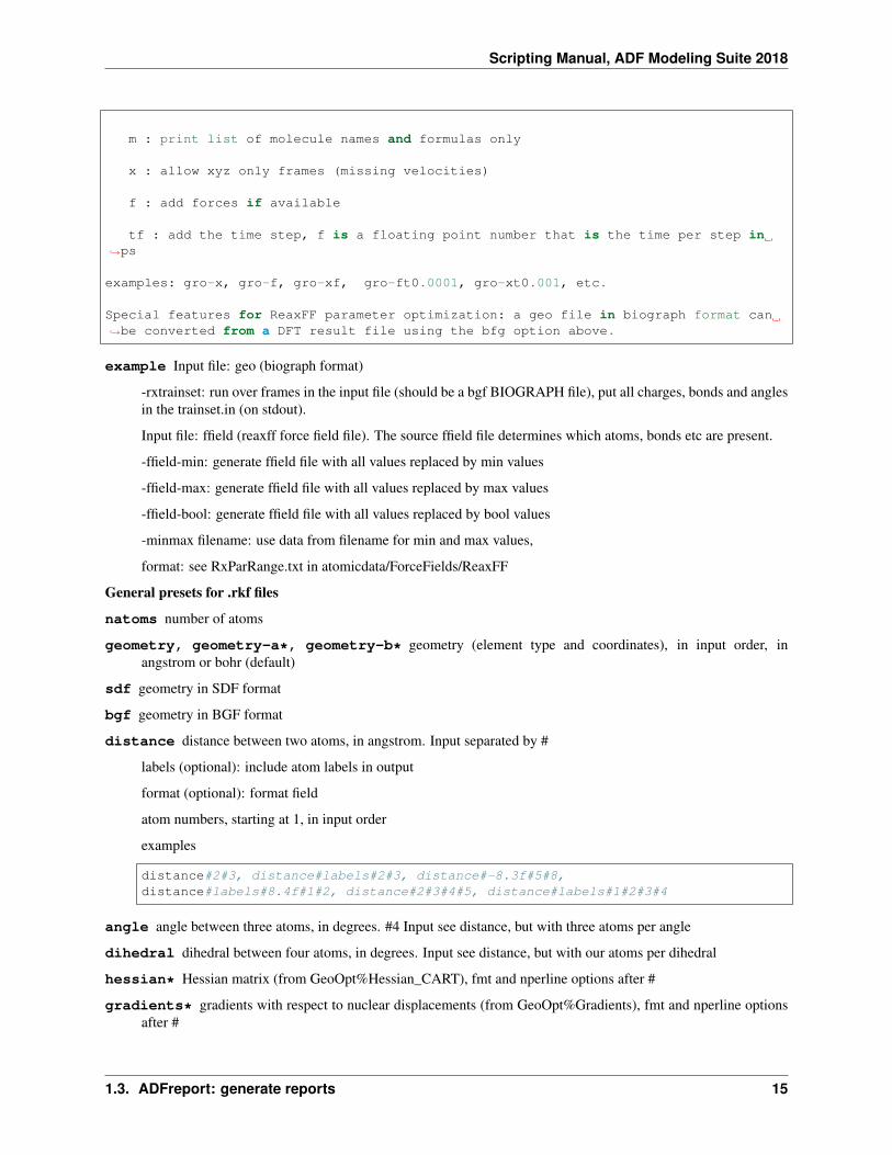
m : print list of molecule names and formulas only

x : allow xyz only frames (missing velocities)

f : add forces if available

tf : add the time step, f is a floating point number that is the time per step in→˓ps

examples: gro-x, gro-f, gro-xf, gro-ft0.0001, gro-xt0.001, etc.

Special features for ReaxFF parameter optimization: a geo file in biograph format can→˓be converted from a DFT result file using the bfg option above.

example Input file: geo (biograph format)

-rxtrainset: run over frames in the input file (should be a bgf BIOGRAPH file), put all charges, bonds and anglesin the trainset.in (on stdout).

Input file: ffield (reaxff force field file). The source ffield file determines which atoms, bonds etc are present.

-ffield-min: generate ffield file with all values replaced by min values

-ffield-max: generate ffield file with all values replaced by max values

-ffield-bool: generate ffield file with all values replaced by bool values

-minmax filename: use data from filename for min and max values,

format: see RxParRange.txt in atomicdata/ForceFields/ReaxFF

General presets for .rkf files









examples




hessian* Hessian matrix (from GeoOpt%Hessian_CART), fmt and nperline options after #

gradients* gradients with respect to nuclear displacements (from GeoOpt%Gradients), fmt and nperline optionsafter #



energies all avaliable energies (bonding up to xc, with labels), fmt option after #

1.3.1 Additional notes

• SDF and BGF records can be produced from from ANY file that can be read by ADFinput.

• KFreader is a free (LGPL) alternative to ADFreport. The C sources are available in our download section(http://www.scm.com/Downloads/KFReader-20140106.zip) and can be modified for more specific needs.

1.4 KF command line utilities

There are four utility programs for manipulating files in the so-called Keyed File (KF) format from the command shell.Two of them convert KF files from binary to ASCII and vice versa. See the pkf and dmpkf utilities for a descriptionof the ASCII format of a kf file. Such a readable version of a KF file can be useful to inspect its contents in detail.

All programs from the package will convert a KF file to the binary format native to this platform if necessary. In sucha case, the original file will be renamed to a file with tilde “~” appended to its name and a message will printed on thestandard output.

The KF software was developed at the Vrije Universiteit Amsterdam as a general-purpose package for storing dataand re-accessing it via keyword-driven procedures.

pkf

pkf file1 { file2 ... filen }

pkf prints a summary of the contents of the kf files file1... filen.

All variables are listed by name, type (integer, real, character, logical), and size (number of array elements) andbundled into named sections.

To put the results in an ASCII file for later inspection:

pkf file > ascii_result

Each section on the file contains an index of its variables and their associated values. All data are organized in blocks.Each section may have any number of index blocks and any number of data blocks (this depends simply on the amountof data to be stored in such a block). In addition there is one special section, the SuperIndex, which is an index of allsections on the file.

The output of pkf consists of:

• General information about the file (name of the file, internally used unit numbers during processing the file...)

• A summary of the SuperIndex, hence an index of blocks in the file and the associated sections.

• A summary: total numbers of blocks associated with the different types of blocks.

• For each section a list of its variables. For each variable in the list the following is displayed

– The variable name.

– Its length, i.e. the storage requirements of the variable within the file.

– Its ‘used’ size, hence the file storage associated with the variable (in units off 8 Bytes for double precisionreal numbers, 4 for integers, etc.).

– The number of actual elements within the variable (for real, integer, and logical data types) or the numberof characters in a string.


http://www.scm.com/Downloads/KFReader-20140106.zip


– The (logical) index of the data block it is stored in.

– The off-set of the data within its data block.

– Its value or the first element of an array variable, respectively.

cpkf

cpkf file1 file2 {key1 .. keyn}

cpkf copies the sections and/or variables key1 .. keyn from file1 to file2.

If a referenced section or variable already exists on file2 it is overwritten, else it is created. Sections and variableswhich are already present on file2 but which are not referenced in the command are not affected.

If no sections and/or variables are explicitly mentioned at all the copying is carried out for all sections and variableson file1.

As a side effect of this operation any ‘holes’ eventually present in the original due to the formal deletion of obsoletesections and variables are not copied. Note that the KF file is not rearranged upon deletion of data. Rather only thecorresponding entries in the index tables are removed in this case. During the copying process the data is howeverrearranged for optimum storage efficiency and the resulting file copy may therefore be smaller than the correspondingoriginal.

Skipping specific sections during the copying process can be manually controlled as follows:

cpkf file1 file2 -rm section1 ...

In this form, all sections will be copied except for the ones specified on the command line, thus effectively removingthem from the file.

To copy and rename a section:

cpkf file1 file2 "section_name --rename new_section_name"

dmpkf

A utility to extract information from a KF file and make it available in ASCII format:

dmpkf file {key1 .. keyn}

dmpkf prints the sections and/or variables from the file file indicated by key1 .. keyn on standard output. The completefile is printed if no sections or variables are specified.

The format to be used for the individual keys:

Sec%Var

where Var the variable of interest present in section Sec. The complete section is dumped if no variable name isspecified.

By redirecting the result to another file a human readable output is obtained:

dmpkf file > ascii_result

The output contains for each printed variable:

• One line with the name of the section it belongs to;

• One line with the name of the variable itself;

• One line with three integers:

1.4. KF command line utilities 17


– The amount of space reserved for the variable on the file which is, however, relevant for programs operatingwith KF files only;

– The amount of data associated with the variable: for reals, integers, logicals: the number of such elements;for strings: the number of characters;

– An integer code for the data type of the variable: 1=integer, 2=real, 3=character, 4=logical;

• The values of the variable (on as many lines as necessary): for scalar variables only one value, for arrays asmany values as the array contains.

udmpkf

A utility to put information read from standard input into a KF file:

udmpkf file

udmpkf reads an ASCII file in the format created by dmpkf from standard input and creates the binary KF file there-from. If such a KF file is already present the sections and variables in the input file are appended to the existing KFfile. Whenever a section or variable already exists in target file it will be overwritten. Other data on the target file arenot affected.

The combination of dmpkf and udmpkf makes it easy to modify KF files with a normal text editor:

dmpkf TAPE21 > t21_ASCII

After the desired modifications within t21_ASCII this file may be reconverted into a binary KF file:

udmpkf < t21_ASCII TAPE21_new

Also note that dmpkf and udmpkf only require a single argument here, respectively, as “< t21_ASCII” passes thecontent of the edited file via the standard input.


CHAPTER

TWO

PYTHON STACK IN ADF MODELING SUITE

The ADF Modeling Suite includes a python stack based on the Enthought Python Distribution(https://www.enthought.com/products/epd/). Some of the included modules are:

• numpy (1.11.3) and scipy (0.18.1): Big modules with a lot of functionality for math and science, more informa-tion on the SciPy website (https://www.scipy.org/).

• ipython4 (5.1.0): An improved interactive python shell, more information can be found on the iPython website(https://ipython.org/). Can be started with:

$ADFBIN/startipython

• ase (3.13.0): ASE (Atomistic Simulation Environment) is a python module for atomistic simulations, moreinformation in the ASE documentation (page 21).

• matplotlib (1.5.1): A library for plotting data in 2D, more information on the Matplotlib web-site (https://matplotlib.org/). We do not ship an interactive backend for matplotlib, so make sure toset a non-interactive backend (https://matplotlib.org/faq/howto_faq.html#generate-images-without-having-a-window-appear) when using it. For example the Agg backend for PNGs:

import matplotlibmatplotlib.use('Agg')

• pip (9.0.1): The recommended tool for installing packages from the Python Package Index (PyPI). The pipdocumentation (https://pip.pypa.io/en/stable/) explains in detail how to use this tool, but for the Python stackshipped with the ADF Modelling Suite all pip commands need to be prefixed with $ADFBIN/startpython -m:

$ADFBIN/startpython -m pip list$ADFBIN/startpython -m pip show scipy$ADFBIN/startpython -m pip search rotate-backups$ADFBIN/startpython -m pip install rotate-backups

• flexmd: A module for running MD simulations with adaptive QM/MM regions. Details can be found in theFlexMD documentation (page 25).

• plams: PLAMS (Python Library for Automating Molecular Simulation) is a collection of tools that aim atproviding powerful, flexible and easily extendable Python interface to molecular modeling programs. It takescare of input preparation, job execution, file management and output processing as well as helps with buildingmore advanced data workflows. See the PLAMS tutorials and PLAMS documentation for more information.

• autografs: AuToGraFS stands for Automatic Topological Generator for Framework Structures. Information andexamples can be found in the AuToGraFS documentation (page 37).

19

https://www.enthought.com/products/epd/

https://www.scipy.org/

https://ipython.org/

https://matplotlib.org/

https://matplotlib.org/

https://matplotlib.org/faq/howto_faq.html#generate-images-without-having-a-window-appear

https://pip.pypa.io/en/stable/

https://pip.pypa.io/en/stable/


2.1 Using other modules with the ADF Python Stack

You can extend the the ADF Python Stack with other modules. You can use pip (see above) to install additionalmodules if they are available on the Python Package Index (PyPI (https://pypi.python.org/pypi)).

If the module is your own code or you just have a copy of the source code, you can add the location of the sourceto the SCM_PYTHONPATH variable to make the module available in the ADF Python Stack. To avoid collisionswith other python installations on the system, we unload PYTHONPATH and PYTHONHOME from the environmentwhen launching the ADF Python Stack and put the content of SCM_PYTHONPATH into PYTHONPATH.

Hint: If you for some reason have to use the PYTHONPATH variable and are unable to use SCM_PYTHONPATH,you can modify $ADFBIN/startpython and $ADFBIN/startipython to not have it cleared when starting python.

20 Chapter 2. Python Stack in ADF Modeling Suite

https://pypi.python.org/pypi

CHAPTER

THREE

ASE

The Atomic Simulation Environment (ASE) (https://wiki.fysik.dtu.dk/ase/) tool collection suite was designed as aflexible, easy-to-use, and customizable approach for the manipulation of quantum chemical models as well as forsetting up and running the calculations required and for the analysis of the final results.

The development of ASE was originally started at the Technical University of Denmark but received also significantcontributions from a large, international community. While ASE is available (https://gitlab.com/ase/ase/tree/3.13.0/)under a GNU LGPL license, a modified version of this library is shipped together with the ADF modeling suite.

This latter version of ASE provides the interfaces to ADF, BAND, DFTB, ReaxFF, and UFF. In addition, the shippedversion was extended by several command line scripts that allow one to perform tasks such as geometry and transitionstate searches in terms of single-line commands.

The interfaces of ASE to the ADF modeling suite were written by Damien Coupry and Thomas M. Soini.

While the reader is encouraged to consult the very detailed ASE manual (https://wiki.fysik.dtu.dk/ase/ase/ase.html) forthe clarification of technical details, an overview about the general concepts and mechanisms behind ASE is provided.The rest of this section is then dedicated to a documentation and a demonstration of the usage of the extensions toASE provided in the ADF modeling suite.

Note: On Windows machines the developers of the ASE library provide only a partial support, see the ASE website(https://wiki.fysik.dtu.dk/ase/download.html#installation-on-windows) for further details.

3.1 General Concepts

The ASE library makes extensive use of the object oriented programming features included inPython. Objects (https://en.wikipedia.org/wiki/Object_(computer_science)) and their corresponding classes(https://en.wikipedia.org/wiki/Class_(computer_programming)) are therefore the most relevant entities in ASE-basedscripts. While the ASE library consists of very many different classes, they can be subdivided into the following threemain groups described in the following section.

3.1.1 Components of ASE

Quantum Chemical Model

Objects like those defined by the Atoms class (https://wiki.fysik.dtu.dk/ase/ase/atoms.html#module-ase.atoms) rep-resent the core part of ASE. Different ways to construct Atoms objects are provided by the ASE library, includ-ing constructors for specific types of quantum chemical systems such as bulk materials and surfaces, clusters, nan-otubes etc. During runtime an Atoms object always comprises all available information about the quantum chemical

21

https://wiki.fysik.dtu.dk/ase/

https://gitlab.com/ase/ase/tree/3.13.0/

https://wiki.fysik.dtu.dk/ase/ase/ase.html

https://wiki.fysik.dtu.dk/ase/download.html#installation-on-windows

https://en.wikipedia.org/wiki/Object_(computer_science)

https://en.wikipedia.org/wiki/Class_(computer_programming)

https://wiki.fysik.dtu.dk/ase/ase/atoms.html#module-ase.atoms


model it describes. Furthermore, the Atoms class includes the essential methods for manipulating the atomic model(https://wiki.fysik.dtu.dk/ase/ase/atoms.html#working-with-the-array-methods-of-atoms-objects) under study.

While Atoms (https://wiki.fysik.dtu.dk/ase/ase/atoms.html#module-ase.atoms) is by far most frequently encounteredclass in ASE scripts, several other objects have similar purposes in more specialized respective contexts. The Con-straints and Filter classes (https://wiki.fysik.dtu.dk/ase/ase/constraints.html#module-ase.constraints) are important ex-amples for such cases and serve e.g. to enforce user defined constraints on the system upon geometry relaxation.

Quantum Chemical Calculation

Calculator classes (https://wiki.fysik.dtu.dk/ase/ase/calculators/calculators.html#module-ase.calculators) provide thedefinition of the quantum chemical computation required to obtain the desired physical property of models definedby the Atoms objects. Such classes essentially interface ASE to a specific quantum chemistry program and containmethods necessary to transfer input information to this program as well as to retrieve the corresponding results afterthe completion of the program run.

Calculators are essential for the aforementioned Atoms object to be fully applicable. As an example, most physicalproperties of a system represented by an Atoms object require a prescription about how to actually compute the result,which is in turn mediated by the assigned Calculator class. Due to that, Calculator objects usually become part of theAtoms object during an ASE run (see also the next section).

The ASE variant within the ADF modeling suite includes five additional Calculator classes which enable computationswith ADF, BAND, DFTB, ReaxFF, and UFF from within ASE, respectively.

Simulation Definitions

Finally, a third type of class (denoted as Simulation object in the following) represents the actual simulationwhich is conducted for a given combination of Atoms and Calculator objects. Such a Simulation object can forexample either represent a simple geometry relaxation (https://wiki.fysik.dtu.dk/ase/ase/optimize.html#module-ase.optimize), a (numerical) frequency (https://wiki.fysik.dtu.dk/ase/ase/vibrations/vibrations.html)or phonon calculation (https://wiki.fysik.dtu.dk/ase/ase/phonons.html#module-ase.phonons), a tran-sition state search (https://wiki.fysik.dtu.dk/ase/ase/neb.html), or an entire gobal optimiza-tion (https://wiki.fysik.dtu.dk/ase/ase/ga.html#module-ase.ga) or molecular dynamics simulation(https://wiki.fysik.dtu.dk/ase/ase/md.html#module-ase.md).

3.1.2 A Typical ASE Run

In a standard ASE run objects of the three kinds presented above interact in order to perform the intended calculations.A typical ASE run is organized as follows

Definition and Initialization of Objects Mind that there are alternative, usually more convenient ways to define achemical system from file inputs or system specific presets

MySystem = Atoms( <initializing variables> )MyCalculator = <CalculatorClass>( <options> )

Calculator → Atoms The Calculator object is assigned to the Atoms object and becomes part of it.

MySystem.set_calculator( MyCalculator )

The methods of the Atoms object that refer to calculated results can then directly call methods from the Calcu-lator.

Atoms → Simulation The Atoms object is used as one of the initialization variables for the constructor of the Simu-lation object.

22 Chapter 3. ASE

https://wiki.fysik.dtu.dk/ase/ase/atoms.html#working-with-the-array-methods-of-atoms-objects

https://wiki.fysik.dtu.dk/ase/ase/atoms.html#module-ase.atoms

https://wiki.fysik.dtu.dk/ase/ase/constraints.html#module-ase.constraints

https://wiki.fysik.dtu.dk/ase/ase/constraints.html#module-ase.constraints

https://wiki.fysik.dtu.dk/ase/ase/calculators/calculators.html#module-ase.calculators

https://wiki.fysik.dtu.dk/ase/ase/optimize.html#module-ase.optimize

https://wiki.fysik.dtu.dk/ase/ase/vibrations/vibrations.html

https://wiki.fysik.dtu.dk/ase/ase/phonons.html#module-ase.phonons

https://wiki.fysik.dtu.dk/ase/ase/neb.html

https://wiki.fysik.dtu.dk/ase/ase/neb.html

https://wiki.fysik.dtu.dk/ase/ase/ga.html#module-ase.ga

https://wiki.fysik.dtu.dk/ase/ase/ga.html#module-ase.ga

https://wiki.fysik.dtu.dk/ase/ase/md.html#module-ase.md


MySimulation = <SimulatorClass>( MySystem, <options> )

The Simulation object is now able to automatically alter the System object (e.g. by setting new atomic coordi-nates during a geometry relaxation) as well as to request the calculation of the required physical properties forthe current status of the system. The simulation can be started as follows.

MySimulation.run( <options> )

Evaluation It is sometimes convenient to print or further evaluate the result e.g. by calculating the reaction energiesbetween two different Systems

MyReactands = Atoms(..., calculator = MyCalculator(), ...)MyProducts = ...

# Relax both, MyReactands and MyProducts...

E_R = MyReactands.get_potential_energy()E_P = MyProducts.get_potential_energy()

print 'ReactionEnergy (eV) = ', E_P - E_R

Mind that ASE exclusively uses eV and Å as units of energy and length, respectively.

3.2 SCM Calculators in ASE

ASE calculators are implemented for ADF, BAND, DFTB, ReaxFF, and UFF.

The options for the programs in the ADF modeling suite are controlled by a single string containing all the informationrequired to set up the respective calculations with ADFprep (page 1).

3.2.1 Technical Notes

New Interface Design in ADF2017

ADF2017 ships new, simplified versions of all calculator interfaces to ASE. The interfaces for setting up these newclasses are not compatible to those in earlier versions of the ADF modeling suite, but support now all calculationoptions accepted by ADFprep (page 1). Examples on the usage of the new classes are shown below.

Interfaces to Individual Programs

The ASE calculators for the programs of the ADF modeling suite derive from a common parent class (basically aninterface to ADFprep (page 1) and ADFreport (page 9)) and differ from each other only in some program-specificfilename internals. All of SCM’s ASE interfaces can therefore be constructed in the following fashion

myCalculator = CalculatorName(label, adfprep_options, ...)

where CalculatorName can be any of the following:

ADF ADFCalculator

BAND BANDCalculator

DFTB DFTBCalculator

3.2. SCM Calculators in ASE 23


ReaxFF ReaxFFCalculator

UFF UFFCalculator

3.2.2 Usage and Examples

Import

Within the ASE repository, the SCM calculator classes are all implemented in calculators/scm.py and can be importedvia

from ase.calculators.scm import ADFCalculator

Interface Keywords

The constructors of the SCM’s calculator classes include the following keywords

label (default: label=None) calculation tag used for calculation directory and prefix for calculationfiles: label='dir1/abc' will create a directory dir1 and name the calculation files therein asabc.XXX while label=abc will use the current directory and create calculation files as abc.XXXin it during runtime.

adfprep_options (default: adfprep_options=None) string containing a sequence of optionsaccepted by ADFprep (page 1). Please consult the ADFprep manual (page 1) for further details. Alsonote that the calculator will explicitly add the options -j calculationFile, -sym NOSYM,-importangstrom, and -gradientsonly to the option list before invoking the adfprep com-mand.

Examples

Single point energy and gradients calculation with ADF

from ase.io.scmio import *from ase.calculators.scm import *

myAtoms = read_scmxyz('myAtoms.xyz')

myCalculator = ADFCalculator(label='myCalculation', adfprep_options='-t ADF-EG')

myAtoms.set_calculator(myCalculator)print(myAtoms.get_potential_energy())

24 Chapter 3. ASE

CHAPTER

FOUR

FLEXMD

FlexMD is a python library for Flexible multi-scale Molecular Dynamics simulation, developed by Rosa E. Bulo,Christoph Jacob, Stefano Borini, Tao Jiang, Jelle Boereboom, Stanislav Simko and Hans van Schoot.

4.1 Basic philosophy and intended usage

We present a flexible python library for molecular dynamics, specialized in multi-scale simulations in a broad sense. Atits core, the library interfaces the Atomistic Simulation Environment (ASE) (page 21) [1 (page 32)] molecular dynamicsmodules with a wide range of molecular mechanics and electronic structure codes. As such, it allows simple dynamicsusing forces computed with any energy/gradient evaluator provided by the ADF package.

Additionally, FlexMD allows the partitioning of a system into regions described at different resolution, with the aimof running multi-scale (hybrid) force calculations. Besides the traditional, rigid, multi-scale partitioning, FlexMDincludes different schemes for Adaptive Multi-scale Molecular Dynamics. Such simulations allow the resolution of aparticle to change according to its distance from a predefined active site, which is a necessity for successful multi-scaledescription of diffusive systems such as chemical reactions in solution.

Finally, the library couples the dynamics to rare events techniques, either implemented in FlexMD itself, or accessiblethrough an interface with the PLUMED library for free energy calculations [7 (page 33)], opening the possibility forevaluation on time-scales beyond the reach of standard molecular dynamics simulations.

The FlexMD package is designed to make simulation options possible that are not available natively in the ADFpackage. Its flexible nature makes it very versatile, but comes at a cost. This cost might be completely negligiblein most simulations, but it can be very high in some cases (usually when combining only cheap methods such asforcefields).

The intended users for the FlexMD package are those with some Unix/Linux experience and a basic understandingof the Python Programming Language (http://python.org/). The user is also supposed to have a basic understandingof the various methods he wishes to combine. For example, if metadynamics is supposed to be combined with ADF,FlexMD expects the user to have knowledge about DFT calculations and the usage of Collective Variables. Finally, aswith every computational method, the user should monitor the FlexMD performance, both in accuracy and speed.

4.2 FlexMD functionality summary

Molecule

Input/output

• Reads and writes PDB and XYZ files

• Reads and writes topology data (in CHARMM format)

• Reads and writes force field data (on CHARMM format)

25

http://python.org/


Analysis

• Extracts geometry data

Drawing functionality

• Adds atoms and bonds

• Changes bond-lengths, angles and torsions

• Cuts fragments

• Cuts solvent boxes and droplets

• Performs rotations and translations, to fit bonds to axes and planes

Periodic functionality

• Adds periodic images

• Wraps molecules into periodic box

Water specific

• Finds hydrogen bonds

• Finds shortest water bridge connecting H-donor and acceptor

Energy and force calculations

Standard

• ADF

• DFTB

• REAXFF

• UFF

• MOPAC

• NAMD

• Lennard-Jones force fields

Multi-scale

• QM/MM, mechanical embedding: Combines all the codes above

• Hybrid: More flexible than QM/MM. Combines different force calculations by summing or subtracting theenergies and forces. The standard calculations (above) can therefore be combined with:

– Metadynamics

– Plumed (external code that computes free energy data)

– Constraints

• Adaptive QM/MM (for chemistry in solution)

– Difference-based Adaptive Solvation (DAS)

– Sorted Adaptive Partitioning (SAP)

– Buffered-Core (BC)

– Flexible Inner Region Ensemble Separator (FIRES)

Molecular Dynamics

26 Chapter 4. FlexMD


• Uses ASE as the molecular dynamics driver for all above methods

• Analyses trajectories

4.3 Introduction

FlexMD is a python package providing molecular dynamics (MD) simulations using the energy evaluation methodsmade available by the ADF suite. A set of example scripts can be found in the examples/scmlib directory of a standardADF installation.

FlexMD can be accessed interactively by running startpython, followed by a standard python import command forthe package scm.flexmd. The python help function can be used to obtain detailed documentation about all FlexMDclasses. In the following example, an inquiry of one class (the MDMolecule class) can be performed.

$ startpythonfrom scm import flexmdhelp(flexmd.MDMolecule)

To leave the interactive help, press q. The help function can also be used to list the contents of the FlexMD package:

$ startpythonfrom scm import flexmdhelp(flexmd)

Python can also give the help documentation as plain text:

$ startpythonfrom scm import flexmdimport pydocprint pydoc.render_doc(flexmd.ForceJob, "Help on %s")

4.4 Molecular Dynamics

FlexMD defines the molecular system under study through the MDMolecule class: an instantiation of this class holdsall information about the molecular system to be simulated, such as coordinates, topology, and force field parameters(if needed). An MDMolecule object can be initialized from a PDB or XYZ file, by specifying its path at objectcreation.

An interface to energy evaluators is provided by specialized ForceJob classes, acting as wrappers around the ADF suiteof programs. A ForceJob requires an MDMolecule object to be specified at creation. The resulting ForceJob objectcan either be used directly by the Atomistic Simulation Environment (ASE) [1 (page 32)] library as a calculator object(see examples/scmlib/ASE_emt_h2o) or with the ASEMDPropagator class, which provides methods for running anMD time step using ASE classes. Internally, the propagator sets up the required ASE objects, passes the ForceJobobject to them, and retrieves the new positions and velocities. An additional protagonist, an MDManager classinstance, coordinates the MD simulation by running the MD steps with the ASEMDPropagator object and writingtrajectory information to file.

During creation of an MDManager object, a directory ‘QMMD’ is created, which contains a file TRAJEC00.DCDholding the geometries along the trajectory, a file FTRAJEC00.DCD holding the forces along the trajectory, and finallya file ENERGY00.dat holding the potential and kinetic energy, as well as the temperature throughout the evaluation.To extract the geometries from the trajectory file, the DCDFile class is available, providing methods to read and writegeometries to and from a trajectory file in DCD format. The MDManager is also responsible for handling restart ofa previous MD evaluation: if a ‘QMMD’ directory is already present at script invocation, the new output files will be

4.3. Introduction 27


assigned the number subsequent to the highest numbered files in that directory. In addition, provided the previous runterminated normally, the restart will continue from the final geometry and velocity of the previous run.

The ADF package contains different electronic structure methods of varying degrees of accuracy and speed. Thebest-known methods are the ADF Density Functional Theory (DFT) code itself, and the BAND DFT code for periodicsystems. FlexMD provides an interface toward both programs. For the interface with ADF, FlexMD makes use ofclasses from PyADF [2 (page 32)], a scripting framework for efficient quantum chemistry calculations. In addition toADF and BAND, several semi-empirical methods are included in the ADF suite, such as DFTB and the NDDO typeschemes available in the MOPAC package [3 (page 32)]. The ADF suite also provides classical mechanics methods,such as the reactive force field ReaxFF and the simple force field UFF. Interfaces to all of these methods are availablein FlexMD. A simple example of a python script for MD using the UFFForceJob class for UFF calculations can befound in the examples directory, under examples/scmlib/flexmd_uff_h2o.

To increase the flexibility of FlexMD, an interface towards force calculations using the NAMD2.8 classical moleculardynamics package is provided (examples/scmlib/namd_h2o). NAMD2.8 is not distributed with the ADF suite, butit is available from a third party to be downloaded and installed ( http://www.ks.uiuc.edu/Development/Download/download.cgi).

4.5 Multi-scale Molecular Dynamics

The design of the ForceJob class allows for flexible extension of its behavior, while at the same time keeping theclient code unaware of its nature: it can either act as a simple wrapper for ADF programs, or it can be a more complexorchestrating class, combining simpler ForceJob classes to implement multi-scale strategies. One application ofthis extensible design can be found in the QMMMForceJob object, which combines a QM and an MM methodin an IMOMM-type scheme (mechanical embedding). The QMMMForceJob object is assigned two other ForceJobobjects, the first representing the high-resolution calculation (QM), while the other represents the low resolution (MM).Both ForceJob objects contain an MDMolecule object for the full molecular system. The selection of the QM-regionis handled by the QMMMForceJob, which contains the information about the part of the molecule that constitutesthe QM region. When forces are requested from the QMMMForceJob, the following behavior is orchestrated: first, aMM force calculation is performed on the full system; then, the QM-region is selected, a QM calculation is executedsolely for that region, and energy and forces are added to those from the full system MM calculation. Finally, an MMcalculation is computed for the small QM-region, and the energy and forces are subtracted, yielding the final result,returned to the invoker. In symbols:

EQM/MM(Full) = EMM(Full) + EQM(QMRegion) – EMM(QMRegion)

The QMMMForceJob handles periodic boundary conditions if the low-level (MM) method supports this feature(i.e. NAMD). Whether the periodic interaction of the QM region with itself is handled at high or low resolution de-pends on the method used for the QM calculation. An example of QM/MM MD calculations can be found in theexamples directory examples/scmlib/qmmm_dftbUFF_2h2o. The QMMMForceJob allows the use of link atomswhen the QM boundary cuts through covalent bonds. However, this feature comes at the price of an increased scriptcomplexity. An example of a QMMM link-atom MD simulation is provided in the examples directory, under exam-ples/scmlib/qmmm_linkatom_dftbNAMD_glutamate.

For more complex multi-scale calculations the HybridForceJob class can be used. This class allows the combinationof a large set of different ForceJobs, each of them describing either the same, or different molecular systems. EachForceJob can either involve a calculation on the full MDMolecule object it contains, or restricted to a specified regionof the corresponding molecule. The forces from each contributing ForceJob can either be added or subtracted fromthe total force according to user preference, as specified at construction of the HybridForceJob object.

In order to perform QM/MM simulations on chemical reactivity in solution, it is important that the description of thesolvent molecules can change on the fly, as the molecules move towards or away from the reactive region. To facilitatethis, an AdaptiveQMMMForceJob class is available to provide adaptive QM/MM simulations using several availableschemes, as described by Bulo et al.[4 (page 32)] and P. Fleurat-Lessard et al.[8 (page 33)] In these schemes, thedescription of the diffusing molecules changes gradually from QM to MM and vice versa, based on the distance of


http://www.ks.uiuc.edu/Development/Download/download.cgi

http://www.ks.uiuc.edu/Development/Download/download.cgi


those molecules to a predefined reactive site. Various schemes are available for assigning the QM and MM characterof the molecules. The class contains a QMMMForceJob object, as well as a partitioning object that assigns the partialQM and MM character to the molecules. An examples python script for such an adaptive QM/MM simulation, usingthe DAS [4 (page 32)] method, is provided in the examples directory, examples/scmlib/adqmmm_mopacscmUFF_h2o.

4.6 Biased Molecular Dynamics

Constraints can be added to a simulation using the derived ForceJob class WallJob. The constraint is in the formof a large one-dimensional Gaussian on the potential energy surface, along a predefined Collective Variable (CV).Examples of CV’s are the distance between two atoms, the coordination number of two atoms, but also more complexquantities such as the minimum distance between two sets of atoms, or the distance of an atom to a hydroxide ion.The Collective Variables can be specified through the CollectiveVariable class. Derived CollectiveVariable classesare available to specify sums or multiples of other CollectiveVariable objects.

Regular MD calculations are limited in the time-scales achievable with current hardware. The order of such time-scalesis much smaller than what is required for chemical reactions. To overcome this problem, two rare-events methods havebeen implemented directly into the library: metadynamics [5 (page 32)] and umbrella sampling [6 (page 33)]. Boththese methods involve biasing the simulations along a CV. An example of a metadynamics input can be found in theexamples directory in examples/scmlib/metadynamics_emt_h2o.

For a wider range of rare-events methods, FlexMD also offers an interface with the PLUMED library for free en-ergy calculations [7 (page 33)].To use this, a PLUMED input file is required, and for this we refer to the PLUMEDmanual. An example of a FlexMD input script using PLUMED can be found in the examples directory in exam-ples/scmlib/plumed_emt_h2o.

4.7 Working with FlexMD

It is recomended to read the sections Introduction (page 27) and Molecular Dynamics (page 27) before working withFlexMD. Basic understanding of the Python Programming Language (http://python.org/) is also required. The Pythonwebsite hosts documentation and a tutorial (http://docs.python.org/2/tutorial/) that can be used to learn Python.

The performance of the FlexMD package is difficult to predict because it depends on system size, the type of ForceJobsused and how these ForceJobs are combined. It is advised to first test the overhead of the FlexMD package for yoursystem before running large simulations. When ab initio forces are involved, the overhead should not give a significantperformance penalty. However, it may become a bottleneck when your system only uses cheap forcefields.

4.7.1 Creating a molecule object

FlexMD can be run trough the interactive python interpreter in the ADF package. To start it, run: $ADF-BIN/startpython in a terminal, followed by:

from scm import flexmd

Note that it is also possible, and usually more convenient, to write your FlexMD code in a file and then to executethis file. To do this, type all the commands you would use in the interactive interpreter in a file, and then enter$ADFBIN/startpython myFlexMDjob.py in a terminal (after changing to the directory where the file was stored ofcourse).

Most FlexMD jobs will start with importing FlexMD and creating an MDMolecule object. This can be done by startingfrom a geometry in xyz or pdb format, or by manually adding the atoms in the FlexMDjob.py file. Geometries canbe generated in the ADF GUI, and then be exported to xyz file. For more details on the MDMolecule object, run$ADFBIN/startpython, import flexmd and call help(flexmd.mdmolecule).

4.6. Biased Molecular Dynamics 29

http://python.org/

http://docs.python.org/2/tutorial/


from scm import flexmdmyMol = flexmd.MDMolecule('myGeometryFile.xyz')

Some ForceJobs require the system to be periodic. If we create an MDMolecule object from a pdb file that includesperiodic information, the periodic boundary conditions are automaticly imported. If the information is not there, wecan add it to the MDMolecule object:

myMol = flexmd.pdb.set_box([50.0,25.0,100.0])

Info on set_box (and other functions, such as set_cellvectors, and write_pdb) can be found usinghelp(flexmd.pdbmolecule).

It is also possible to write the info in the MDMolecule object to a pdb file. to do so, callpdb.write_pdb(‘mypdbfile.pdb’) on the myMol object:

myMol.pdb.write_pdb('mypdbfile.pdb', box=True)

4.7.2 Creating a ForceJob

To specify what type of forces we want to use in the MD simulation, a ForceJob must be created. FlexMDhas a number of ForceJobs (see PACKAGE CONTENTS in help(flexmd)), most of them with examples in$ADFHOME/examples/scmlib. The ForceJobs can be combined into a single ForceJob using flexmd.hybrid_ForceJob.As an example, we combine a reaxff_ForceJob with a metadynamicsjob and a walljob:

from scm import flexmdmyMol = flexmd.MDMolecule('myGeometryFile.xyz')myMol = flexmd.pdb.set_box([50.0,25.0,100.0])

# setup our reaxff ForceJob and attach the forcefield file# (place the ff file in the same dir as the script and the xyz!)

myReaxffForceJob = flexmd.ReaxffForceJob(molecule=myMol)myReaxffForceJob.settings.set_ff_filename('reax_forcefield_file.ff')

# next we define the collective variable: the distance between atom 1 and 2myCvs = [flexmd.DistCV([1,2])]

# create a set of metadynamics properties, using the CVmtdSettings = flexmd.MetadynamicsSettings(cvs=myCvs, widths=[0.30], height=0.25 )

# create the metadynamics job by combining the molecule, settings (with CV)# and the number of md steps between depositing metadynamics hills.

myMetadynamicsjob = flexmd.MetadynamicsJob( myMol, settings=mtdSettings, nstep=150 )

# add a wall to prevent the two atoms from drifting more than 10 Angstrom away.myWalljob = flexmd.WallJob(molecule=myMol, cvs=myCvs, cntrs=[10.0], widths=[1.0],→˓heights=[500.0])

# combine the forces into a hybrid job that will be used for the MDmyForceJob = flexmd.HybridForceJob( [[myReaxffForceJob,'+'], [theMetadynamicsjob,'+'],→˓ [theWalljob,'+']], myMol )

Note that all the ForceJobs require some special input and settings, and that these settings can be applied bothbefore and after defining the ForceJob. For the reaxffForceJob, we first define the ForceJob, and add the force-field parameters file afterwards. For the metadynamics job we reverse this, and first create a metadynamic-sJobSettings object, which is then used in the creation of the metadynamics job. For more detailed info onthe different ForceJobs and their inputs, see the help function by calling help on a ForceJob, for example:help(flexmd.ReaxffForceJob) or help(flexmd.WallJob). Also remember that other examples of ForceJobs can be foundin $ADFHOME/examples/scmlib.



4.7.3 Creating and running the MD job

Before the simulation can be set in motion, a propagator is needed. The propagatorJob controls simulation settingssuch as temperature and timestep size. FlexMD uses the Atomistic Simulation Environment (ASE) [1 (page 32)] forthis. The MDPropagatorJob object is created just like the other objects in FlexMD:

# do this after importing flexmd and creating a ForceJob.# it creates the MDPropagator job, with some settings

myMDJob = flexmd.ASEMDPropagatorJob( ForceJob=myForceJob )myMDJob.settings.set_tempcontrol( True, nhfreq=2, maxdef=50.0 )myMDJob.settings.set_temperature(300.0)myMDJob.settings.set_timestep( 0.02 )

For more details on the ASEMDPropagatorJob, view it’s help page: help(flexmd.ASEMDPropagatorJob), or take alook at the MDSettings object: help(flexmd.MDSettings).

The propagatorJob can be used to create an MDManager object:

# create an MD managermyManager = flexmd.MDManager( mdjob=myMDJob)

The manager object is now in control of the MD simulation, and we can use it to run the simulation for a number ofsteps:

# tell the MD manager to run the simulationmyManager.run( ncycles = 2500 )

Note that the number of steps here should be increased a lot if metadynamics effects are to be observed, but it isalways wise to first run a small number of steps to check if everything works. Some information will be printed duringthe simulation, depending on the settings of the components used. The manager will also create some folders in theworking directory, and store the data produced by the simulation in there.

The full flexmd jobfile should now look something like this:

from scm import flexmdmyMol = flexmd.MDMolecule('myGeometryFile.xyz')myMol = flexmd.pdb.set_box([50.0,25.0,100.0])

# setup our reaxff ForceJob and attach the forcefield file# (place the ff file in the same dir as the script and the xyz!)

myReaxffForceJob = flexmd.ReaxffForceJob(molecule=myMol)myReaxffForceJob.settings.set_ff_filename('reax_forcefield_file.ff')

# next we define the collective variable: the distance between atom 1 and 2myCvs = [flexmd.DistCV([1,2])]

# create a set of metadynamics properties, using the CVmtdSettings = flexmd.MetadynamicsSettings(cvs=myCvs, widths=[0.30], height=0.25 )

# create the metadynamics job by combining the molecule, settings (with CV)# and the number of md steps between depositing metadynamics hills.

myMetadynamicsjob = flexmd.MetadynamicsJob( myMol, settings=mtdSettings, nstep=150 )

# add a wall to prevent the two atoms from drifting more than 10 Angstrom away.myWalljob = flexmd.WallJob(molecule=myMol, cvs=myCvs, cntrs=[10.0], widths=[1.0],→˓heights=[500.0])

# combine the forces into a hybrid job that will be used for the MDmyForceJob = flexmd.HybridForceJob( [[myReaxffForceJob,'+'], [theMetadynamicsjob,'+'],→˓ [theWalljob,'+']], myMol )

4.7. Working with FlexMD 31


# do this after importing flexmd and creating a ForceJob.# it creates the MDPropagator job, with some settings

myMDJob = flexmd.ASEMDPropagatorJob( ForceJob=myForceJob )myMDJob.settings.set_tempcontrol( True, nhfreq=2, maxdef=50.0 )myMDJob.settings.set_temperature(300.0)myMDJob.settings.set_timestep( 0.02 )

# create an MD managermyManager = flexmd.MDManager( mdjob=myMDJob)

# tell the MD manager to run the simulationmyManager.run( ncycles = 2500 )

This job can be resumed by just running the script again, FlexMD should pick up on the coordinates and velocities fromthe QMMD folder. To do this, simply run the job again, and a new set of trajectory and energy files should appear inthe QMMD folder. If you wish to specify which files FlexMD restarts from, you can use the set_restartnum() functionon myMDJob.settings:

# add this below the "myMDJob.settings.set_timestep( 0.02 )" line# FlexMD will restart from the files with index numbers 1 lower than you pass to

→˓set_restartnum# This will cause FlexMD to restart from QMMD/TRAJEC00.dcd and QMMD/TRAJEC00.dcd

myMDJob.settings.set_restartnum(1)

4.8 Required Citations

When you publish results in the scientific literature that were obtained with programs of the ADF package, you arerequired to include references to the program package with the appropriate release number, and a few key publications.

For calculations with FlexMD: 1. FlexMD 2017, SCM, T. Jiang, H. van Schoot, S. Simko, C. R. Jacob, S. Borini,R. E. Bulo, A python library for flexible multi-scale molecular dynamics simulations. http://www.scm.com

4.8.1 External programs and Libraries

Click here for the list of programs and/or libraries used in the ADF package. On some platforms optimized librarieshave been used and/or vendor specific MPI implementations.

4.9 References

1. S.R. Bahn, K.W. Jacobsen, An object-oriented scripting interface to a legacy electronic structure code. Comput.Sci. Engin. 4, 56-66 (2002) (https://doi.org/10.1109/5992.998641). The Atomistic Simulation Enviromentwebsite and documentation (https://wiki.fysik.dtu.dk/ase/)

2. C.R. Jacob, S.M. Beyhan, R.E. Bulo, A. Severo Pereira Gomes, A.W. Gotz, K. Kiewisch, J. Sikkema, L. Viss-cher, PyADF - A scripting framework for multiscale quantum chemistry. J. Comput. Chem. 32, 2328-2338(2011) (https://doi.org/10.1002/jcc.21810)

3. J.J.P. Stewart, Optimization of parameters for semiempirical methods IV: extension of MNDO, AM1, and PM3to more main group elements., J. Mol. Model. 10, 155-164 (2004) (https://doi.org/10.1007/s00894-004-0183-z)

4. R.E. Bulo, B. Ensing, J. Sikkema, L. Visscher, Toward a Practical Method for Adaptive QM/MM Simulations.J. Chem. Theory Comput. 5, 2212-2221 (2009) (https://doi.org/10.1021/ct900148e)


http://www.scm.com

https://doi.org/10.1109/5992.998641

https://doi.org/10.1109/5992.998641



https://doi.org/10.1002/jcc.21810

https://doi.org/10.1002/jcc.21810

https://doi.org/10.1007/s00894-004-0183-z

https://doi.org/10.1021/ct900148e


5. A. Laio, M. Parrinello, Escaping free-energy minima. Proc. Natl. Acad. Sci. USA., 99, 12562-12566 (2002)(https://doi.org/10.1073/pnas.202427399)

6. B. Roux, The calculation of the potential of mean force using computer simulations. Comput. Phys. Commun.91, 275-282 (1995) (https://doi.org/10.1016/0010-4655(95)00053-I)

7. M. Bonomi, D. Branduardi, G. Bussi, C. Camilloni, D. Provasi, P. Raiteri, D. Donadio, F. Marinelli, F. Pietrucci,R.A. Broglia, M. Parrinello, PLUMED: A portable plugin for free-energy calculations with molecular dynamics.Comp. Phys. Comm. 180, 1961-1972 (2009) (https://doi.org/10.1016/j.cpc.2009.05.011). PLUMED websiteand documentation (http://www.plumed-code.org/)

8. (a) Fleurat-Lessard, C. Michel, R. E. Bulo, Energy extrapolation schemes for adaptive multi-scale moleculardynamics simulations. J. Chem. Phys. 137, 174111 (2012) (https://doi.org/10.1063/1.4739743)

4.9. References 33

https://doi.org/10.1073/pnas.202427399

https://doi.org/10.1016/0010-4655(95)00053-I

https://doi.org/10.1016/0010-4655(95)00053-I

https://doi.org/10.1016/j.cpc.2009.05.011

http://www.plumed-code.org/

http://www.plumed-code.org/

https://doi.org/10.1063/1.4739743

CHAPTER

FIVE

PLAMS

PLAMS (Python Library for Automating Molecular Simulation) is a collection of tools that aim at providing powerful,flexible and easily extendable Python interface to molecular modeling programs. It takes care of input preparation, jobexecution, file management and output processing as well as helps with building more advanced data workflows.

• PLAMS tutorials

• PLAMS documentation

5.1 Required Citations

When you publish results in the scientific literature that were obtained with programs of the ADF package, you arerequired to include references to the program package with the appropriate release number, and a few key publications.

For calculations with PLAMS: PLAMS, written by Michał Handzlik, http://www.scm.com

5.1.1 External programs and Libraries

Click here for the list of programs and/or libraries used in the ADF package. On some platforms optimized librarieshave been used and/or vendor specific MPI implementations.

35

http://www.scm.com


36 Chapter 5. PLAMS

CHAPTER

SIX

AUTOGRAFS

The Automatic Topological Generator for Framework Structures (http://pubs.acs.org/doi/abs/10.1021/jp507643v) is asoftware for the design ang high throughput generation of framework structures such as Metal-Organic Frameworks(MOFs), Zeolites, Covalent-Organic Frameworks (COFs), or any product of reticular chemistry. The underlyinglibrary for chemical objects makes extensive use of the ASE (page 21) environment shipped with the ADF modellingsuite.

AuToGraFS was developped in the group of Prof. Dr. Heine at Jacobs University Bremen by Dr. M. Addicoat andD. Coupry. While a console application is available (https://github.com/maddicoat/AuToGraFS) under a GNU LGPLlicense, the version shipped together with the ADF modeling suite was heavily modified into a fully importable pythonlibrary for easy scripting capabilities. The software was also fully integrated into the GUI, and some native functionswere developped for added functionality in this particular environment. A database of building units often used inexisting MOFs is also provided, to cover basic needs.

The rest of this section is dedicated to a documentation and a demonstration of the usage of both the scripting capabil-ities and GUI tools from the Automatic Topological Generator for Framework Structures.

6.1 General AuToGraFS Scripting concepts

AuToGraFS relies on the concept of underlying nets common to many structures. These nets, or topologies can befound in the RCSR (http://rcsr.anu.edu.au/) and EPINET (http://epinet.anu.edu.au/) databases. Once implemented,AuToGraFS will follow these blueprints to generate a framework from building units of compatible geometries. Sincethese geometries are ideal objects, and most chemical structures are distorted, an optimization step using UFF isnecessary for the building units to “snap into place”. Correct handling of bonding information and UFF atom typesare crucial to the generation of correct structures.

6.1.1 Components of AuToGraFS

The Fragment class

This is a slightly modified version of the native ASE Atoms object, designed to hold essential data for UFF postpro-cessing. This englobes the uff atom types, and the bonding information.

from scm.autografs.fragment import Fragmentfrom ase import Atoms

line = Fragment(ase.Atoms("X2", positions=...),mmtypes=["H_", "H_"],bonds = [[0,0,1],[0,0,1],[1,1,0]],shape="linear",

37

http://pubs.acs.org/doi/abs/10.1021/jp507643v

https://github.com/maddicoat/AuToGraFS

http://rcsr.anu.edu.au/

http://epinet.anu.edu.au/


unit=None,name="a_line_has_no_name")

Where mmtypes is a list of the UFF atom types symbols, ordered as the corresponding atoms in the structure, andbonds is a symmetric numpy array (https://docs.scipy.org/doc/numpy-1.10.0/reference/generated/numpy.array.html)of size equal to the number of atoms. The i,j elements in the bonds array are the bond order between atom i and atomj of the structure. These bond orders should follow the UFF conventions (1.5 for aromatic, 0.5 for coordination bonds,0.001 for hydrogen bonds...). The shape holds information for AuToGraFS about the connectivity of the fragment.Each dummy atom, with symbol “X” in ASE, represents a point of connection between two fragments. In the aboveexample, the shape is clearly “linear”. This is used to check compatibility between a fragment and a given topology.The unit of a fragment is set internally by AuToGraFS and is of no interest here. The name of a fragment is used onlyfor logging purposes. Individual building blocks of a framework are manipulated through the Fragment class. It ispossible to export a fragment from the GUI using edit -> framework -> export fragment. If the UFF atom types arenot specified, an automatic typing script will take care of it.

The Model class

This is a container class that holds in one place the topology of a framework and the correctly positioned fragments.Most of the postprocessing methods found in AuToGraFS are Model methods.

from scm.autografs import *

model = autografs.Model(...)

# view the framework in adfinput. set clean to False to keep dummy atoms.model.view(clean=True, verbose=True)

# write the name.adf and name.run filesmodel.write(name="framework", clean=True, verbose=True)

# returns a Fragment, with correct bonding information and mmtypes# if indices is True, it also returns the index of the corresponding fragment in the→˓model for each atomatoms = model.get_atoms(self, clean=False, indices=False)

# returns a supercell of the framework as a Fragmentsupercell = model * (2,2,2)

# deletes a fragment in the framework. if no index is given, the fragment will be→˓chosen at random.# the defects will cap with hydrogen the empty spaces. returns a Fragment# here, a linker at random will be deletedmodel.insert_defect(indices=None, centers=0, linkers=1)

# flip a linear objectmodel.flip_fragment(index=the_fragment_index)

# rottates a linear object around its axis by angle in degreesmodel.rotate_fragment(index=the_fragment_index, angle=85.0)

# Will add a functional group to the selected fragment on a random hydrogen# if and only if the hydogen is connected to a carbon.# for more precise handling, use the GUI for now.model.functionalize_fragment(functional_group="NH2", index=the_fragment_index)

38 Chapter 6. AuToGraFS

https://docs.scipy.org/doc/numpy-1.10.0/reference/generated/numpy.array.html


The Autografs class

This class is the builder in itself. Given a path to a database of building units in .inp format (exportable via the GUI), itwill generate any valid framework from a topology name, a center and linker name or objects, and optionally a pillarname or object. The linkers, centers and pillars objects have to be passed as Fragment .

from scm.autografs import *from random import choice

# create the generator and update the database of building unitsmofgen = autografs.Autografs(refresh_database=True, verbose=True, path="path/to/my/→˓fragments/")

# choose a topology from the available one given no center or linkerstopologies = mofgen.get_available_topologies(center=None, linker=None)topology = choice(topologies)

# choose a center in the list of available centers for the topologycenters = mofgen.get_available_centers(topology=topology, linker=None)center = choice(centers)

# choose a linker in the list of available linkers for the topology and centerlinkers = mofgen.get_available_linkers(topology=topology, center=center)linker = choice(linkers)

# modify the linker by changing all hydrogens to fluorinelinker_structure = mofgen.database[linker]linker_symbols = linker_structure.get_chemical_symbols()linker_structure.set_chemical_symbols(["F" if l=="H" else l for l in linker_symbols])

# generate the framework using multiprocessing tools and automatic scaling of unit→˓cellframework = mofgen.make(lable="my_framework", topology=topology, center=center,→˓linker=linker, pillar=None, form_factor=None, parallel=True)

# visualize in adfinputframework.view()

do not forget to run a quick UFF optimization after genertion to optimize lattice and fragment into an optimal config-uration.

6.1.2 About the databases of building units

AuToGraFS uses both a binary database format, and structures in the DemonNano file format from which the binaryis compiled. To ask AuToGraFS to use a custom directory containing .inp files, symply pass the directory to the pathargument when initializing the constructor. The ”.inp” file format should be formatted like the following example.

Data: SBUtype = linkerData: shape = linearData: name = benzeneGEOMETRY CARTESIANC 0.00000000 -1.39103633 0.00000000 MMTYPE=C_R QMMM=MM BOND=2/1.→˓5:6/1.5:12/1.0C -1.20606758 -0.69440959 0.00000000 MMTYPE=C_R QMMM=MM BOND=1/1.→˓5:3/1.5:8/1.0C -1.20606758 0.69440959 -0.00000000 MMTYPE=C_R QMMM=MM BOND=2/1.→˓5:4/1.5:10/1.0

6.1. General AuToGraFS Scripting concepts 39


C -0.00000000 1.39103633 0.00000000 MMTYPE=C_R QMMM=MM BOND=3/1.→˓5:5/1.5:11/1.0C 1.20606758 0.69440959 0.00000000 MMTYPE=C_R QMMM=MM BOND=4/1.→˓5:6/1.5:7/1.0C 1.20606758 -0.69440959 -0.00000000 MMTYPE=C_R QMMM=MM BOND=1/1.→˓5:5/1.5:9/1.0H 2.02806392 1.16933783 0.00000000 MMTYPE=H_ QMMM=MM BOND=5/1.0H -2.02806392 -1.16933783 0.00000000 MMTYPE=H_ QMMM=MM BOND=2/1.0H 2.02806392 -1.16933783 0.00000000 MMTYPE=H_ QMMM=MM BOND=6/1.0H -2.02806392 1.16933783 0.00000000 MMTYPE=H_ QMMM=MM BOND=3/1.0X 0.00000000 2.09099413 0.00000000 MMTYPE=H_ QMMM=MM BOND=4/1.0X 0.00000000 -2.09099413 0.00000000 MMTYPE=H_ QMMM=MM BOND=1/1.0END

6.1.3 Using the overhauled Atom Typer

Both AuToGraFS and the GUI now use a new python library for the assignment of UFF types to atoms and generationof the bonding matrix. The process goes as follows:

from scm.autografs import atomtyper

# instantiate the typer on a readable molecule file (e.g: "mol.cif")typer = atomtyper.MolTyper("path/of/fileToType")

# choose the UFF library. options are uff and uff4moflibrary = read_db("uff4mof")

# actual typing is done heretyper.type_mol(library)

# prints the bond matrix as a numpy array# item i, j of matrix is the bond order between atoms i and jprint typer.get_guibonds()

# print a list of UFF types in orderprint typer.get_mmtypes()

# write a SCM-UFF intput file with correct infotyper.structure.write(name="mytypedmol")

6.2 AuToGraFS Examples

the following examples work with all calculators of the ADF modeling suite. Any python script using these librariesshould be launched using the “$ADFBIN/startpython” binary.

6.2.1 Generation of all available pillared SURMOF

# Required importsfrom scm.autografs import *

from itertools import combinations_with_replacement

# create the generator object



mofgen = autografs.Autografs(path="./my_database/")

# the SURMOF family of frameworks istopology = "pcu"

# get all available linkers, center, pillars for the pcu topologycenters = mofgen.get_available_centers(topology=topology)for center in centers:

# the pcu topology accepts up to three different linkers.# here, we'll use two and a pillar

linkers = mofgen.get_available_linkers(topology=topology, center=center)for linker in combination_with_replacement(linkers, 2):

pillars = mofgen.get_available_pillars(topology=topology, center=center)for pillar in pillars:

label = "{0}-{1}-{2}".format(center, linker,pillar)# generate this particulat frameworkframework = mofgen.make(label=label,

topology=topology,center=center,linker=linker,pillar=pillar)

# write the UFF inpufile under "label.run" and "label.adf"framework.write()

6.2.2 Generation of a defectuous UIO-66 MOF from custom files

# Required importsfrom scm.autografs import *from random import gauss

# get the building units as Fragment objectscenter = utils.read_inp("UIO66_center.inp")linker = utils.read_inp("UIO66_linker.inp")

# instantiate the generatormofgen = autografs.Autografs()

# generate the MOFmof = mofgen.make(label="UIO66", topology="bcu", center=center, linker=linker)

# get the 3*3*3 supercellsupercell = mof * (3,3,3)

# introduce 10 defects in a gaussian distribution around the center of the→˓supercell

# the connections are capped with hydrogen.indices = []mu = len(supercell)/2sigma = len(supercell)/4number_of_defects = 10while len(indices) < number_of defects:

index = int(abs(gauss(mu, sigma)))if (index not in indices) and index < len(supercell):

indices.append(index)supercell.insert_defect(indices = indices))

6.2. AuToGraFS Examples 41


# view resulting framework in adfinputsupercell.view()

6.2.3 Generation of conformers in the IRMOF-5

# Required importsfrom scm.autografs import *from itertools import combinations_with_replacement

# instantiate the generatormofgen = autografs.Autografs()

# generate the MOFmof = mofgen.make(label="IRMOF-5", topology="pcu", center="mof5", linker="benzene")

# get the indices of the benzenes in the mofbenzenes = mof.get_linkers()choice_angles = [0.0,45.0,90.0]

# generate all possible combinationsiteration = 0for angles in combinations_with_replacement(choice_angles, 3):

conformer = mof.copy()for benzene, angle in zip(benzenes, angles):

conformer.rotate_fragment(index=benzene, angle=angle)conformer.write(name="conformer-{0}".format(iteration))iteration += 1


INDEX

Aadfprep module, 1adfreport module, 9

Ccpkf module, 16

Ddmpkf module, 16

KKF command line utilities, 16

Ppkf module, 16

Uudmpkf module, 16

43

scripting manual - software for chemistry & materials · scripting manual, release 2017-c: core...

Documents