``scrna-seq workflow conclus: from consensus clusters to a

“ScRNA-seq workflow CONCLUS: fromCONsensus CLUSters to a meaningfulCONCLUSion”

"Ilyess Rachedi, Polina Pavlovich, Nicolas Descostes, andChristophe Lancrin"

26 October 2021

Contents

1 Introduction . . . . . . . . . . . . . . . . . . . . . . . . . . . . . . 3

2 Getting help . . . . . . . . . . . . . . . . . . . . . . . . . . . . . . 3

3 Important note . . . . . . . . . . . . . . . . . . . . . . . . . . . . 3

4 Standard workflow . . . . . . . . . . . . . . . . . . . . . . . . . . 3

4.1 Quick start . . . . . . . . . . . . . . . . . . . . . . . . . . . . 3

4.2 Data . . . . . . . . . . . . . . . . . . . . . . . . . . . . . . . 4

4.3 Test clustering . . . . . . . . . . . . . . . . . . . . . . . . . . 7

5 CONCLUS step by step . . . . . . . . . . . . . . . . . . . . . . . 10

5.1 Normalization of the counts matrix . . . . . . . . . . . . . . . . 10

5.2 Generation of t-SNE coordinates . . . . . . . . . . . . . . . . . 12

5.3 Clustering with DB-SCAN . . . . . . . . . . . . . . . . . . . . . 13

5.4 Cell and cluster similarity matrix calculation . . . . . . . . . . . . 14

5.5 Plotting. . . . . . . . . . . . . . . . . . . . . . . . . . . . . . 15

5.6 Marker genes identification . . . . . . . . . . . . . . . . . . . . 19

6 Plot a heatmap with positive marker genes . . . . . . . . . . . . 23

7 Plot t-SNE colored by expression of a selected gene . . . . . . 24

8 Collect publicly available info about marker genes . . . . . . . . 27

8.1 Collect information for the top 10 markers for each cluster . . . . . 27

9 Supervised clustering . . . . . . . . . . . . . . . . . . . . . . . . 29

10 Conclusion . . . . . . . . . . . . . . . . . . . . . . . . . . . . . . 34

“ScRNA-seq workflow CONCLUS: from CONsensus CLUSters to a meaningful CONCLUSion”

11 Session info . . . . . . . . . . . . . . . . . . . . . . . . . . . . . . 34

2


1 IntroductionCONCLUS is a tool for robust clustering and positive marker features selection of single-cellRNA-seq (sc-RNA-seq) datasets. It is designed to identify rare cells populations by consensusclustering. Of note, CONCLUS does not cover the preprocessing steps of sequencing filesobtained following next-generation sequencing. You can find a good resource to start withhere.CONCLUS is organized into the following steps:

• Generation of multiple t-SNE plots with a range of parameters including differentselection of genes extracted from PCA.

• Use the Density-based spatial clustering of applications with noise (DBSCAN) algorithmfor idenfication of clusters in each generated t-SNE plot.

• All DBSCAN results are combined into a cell similarity matrix.• The cell similarity matrix is used to define “CONSENSUS” clusters conserved accross

the previously defined clustering solutions.• Identify marker genes for each concensus cluster.

2 Getting helpIssues can be submitted directly to the Bioconductor forum using the keyword ‘conclus’ inthe post title. To contact us directly write to [email protected] or [email protected] principles of this package were originally developed by Polina Pavlovich who is now doingher Ph.D at the Max Planck Institute of Immunobiology and Epigenetics.

3 Important noteDue to the stochastic aspect of tSNE, everything was generated with a random seed of42 (default parameter of generateTSNECoordinates) to ensure reproducibility of the results.Because of the evolution of biomaRt, you might get slightly different figures. However, themarker genes for each cluster should be the same.The package is currently limited to mouse and human. Other organisms can be added ondemand. Write to [email protected] or [email protected]. Priority will be given tomodel organisms.

4 Standard workflow

4.1 Quick startCONCLUS requires to start with a raw-count matrix with reads or unique molecular identifiers(UMIs). The columns of the count matrix must contain cells and the rows – genes. CONCLUSneeds a large number of cells to collect statistics, we recommend using CONCLUS if you haveat least 100 cells.In the example below, a small toy example is used to illustrate the runCONCLUS method.Real data are used later in this vignette.

3

https://scrnaseq-course.cog.sanger.ac.uk/website/index.html

mailto:[email protected]





library(conclus)

outputDirectory <- tempdir()

experimentName <- "Test"

species <- "mouse"

countmatrixPath <- system.file("extdata/countMatrix.tsv", package="conclus")

countMatrix <- loadDataOrMatrix(file=countmatrixPath, type="countMatrix",

ignoreCellNumber=TRUE)

coldataPath <- system.file("extdata/colData.tsv", package="conclus")

columnsMetaData <- loadDataOrMatrix(file=coldataPath, type="coldata",

columnID="cell_ID")

sceObjectCONCLUS <- runCONCLUS(outputDirectory, experimentName, countMatrix,

species, columnsMetaData=columnsMetaData,

perplexities=c(2,3), tSNENb=1,

PCs=c(4,5,6,7,8,9,10), epsilon=c(380, 390, 400),

minPoints=c(2,3), clusterNumber=4)

In your “outputDirectory”, the sub-folder pictures contains all tSNE with dbscan coloration(sub-folder tSNE_pictures), the cell similarity matrix ( Test_cells_correlation_X_clusters.pdf),the cell heatmap (Test_clustersX_meanCenteredTRUE_orderClustersFALSE_orderGenesFALSEmarkersPerCluster.pdf), and the cluster similarity matrix (Test_clusters_similarity_10_clusters.pdf).You will also find in the sub-folder Results:

• 1_MatrixInfo: The normalized count matrix and its meta-data for both rows andcolumns.

• 2_TSNECoordinates: The tSNE coordinates for each parameter of principal components(PCs) and perplexities.

• 3_dbScan: The different clusters given by DBscan according to different parameters.Each file gives a cluster number for each cell.

• 4_CellSimilarityMatrix: The matrix underlying the cells similarity heatmap.• 5_ClusterSimilarityMatrix: The matrix underlying the clusters similarity heatmap.• 6_ConclusResult: A table containing the result of the consensus clustering. This table

contains two columns: clusters-cells.• 7_fullMarkers: Files containing markers for each cluster, defined by the consensus

clustering.• 8_TopMarkers: Files containing the top 10 markers for each cluster.• 9_genesInfos: Files containing gene information for the top markers defined in the

previous folder.Further details about how all these results are generated can be found below.

4.2 DataIn this vignette, we demonstrate how to use CONCLUS on a sc-RNA-seq dataset fromShvartsman et al . The Yolk Sac (YS) and Aorta-Gonad-Mesonephros (AGM) are two majorhaematopoietic regions during embryonic development. Interestingly, AGM is the only onegenerating haematopoietic stem cells (HSCs). To identify the difference between AGM andYS, Shvartsman et al compared them using single cell RNA sequencing between 9.5 and 11.5days of mouse embryonic development. This vignette aims at reproducing the identification

4

https://www.biorxiv.org/content/10.1101/774547v1


of a rare population corresponding to liver like cells in the YS at day 11.5. The number ofclusters used in this vignette is lower than in the original article for sake of simplification. Thisvignette neither provides a description of the differences between the AGM and YS. Pleaserefer to Shvartsman et al for a complete description.Since endothelial cells represent a small population in these tissues, cells expressing theendothelial marker VE-Cadherin (VE-Cad, also called Cdh5) were enriched and sorted, VE-CadNegative cells constituting the microenvironment. Therefore, four cell states are defined bythe cell barcodes: YS VE-Cad minus, AGM VE-Cad minus, YS VE-Cad minus, and AGMVE-Cad minus. The E11.5 data are constituted of 1482 cells. After filtering and normalization,1303 cells were retained.This sc-RNA-seq experiment was performed using the SMARTer ICELL8 Single-Cell System(Click here for more info). The protocol was based on 3’ end RNA sequencing where eachmRNA molecule is labeled with a unique molecular identifier (UMI) during reverse transcriptionin every single cell.Shvartsman et al deleted highly abundant haemoglobins having names starting with ‘Hba’or ‘Hbb’ because they seemed to be the primary source of contamination. Additionally, theyexcluded poorly annotated genes that did not have gene symbols to improve the clustersannotation process. Finally, the human cell controls were removed.

4.2.1 Retrieving data from GEO

The code below format the count matrix and the columns meta-data. The source data aredownloaded from the GEO page GSE161933. The URL of the count matrix and the cellsmeta-data were retrieved by right-click and ‘copy link adress’ on the http hyperlink of thesupplementary file at the bottom of the page. If the columns metadata are not available inthe supplementary file section, the name of the series matrix, containing columns meta-datacan be retrieved by clicking the ‘Series Matrix File(s)’ link just above the count matrix. Thefunction retrieveFromGEO used with the parameter seriesMatrixName will download all seriesmatrices present in the GEO record however only the one of interest will be kept.

library(conclus)

## Setting options('download.file.method.GEOquery'='auto')

## Setting options('GEOquery.inmemory.gpl'=FALSE)

##

outputDirectory <- tempdir()

dir.create(outputDirectory, showWarnings=FALSE)

species <- "mouse"

countMatrixPath <- file.path(outputDirectory, "countmatrix.txt")

metaDataPath <- file.path(outputDirectory, "metaData.txt")

matrixURL <- paste0("https://www.ncbi.nlm.nih.gov/geo/download/?acc=GSM492",

"3493&format=file&file=GSM4923493%5FE11%5F5%5Frawcounts%5Fmatrix%2Etsv%2Egz")

metaDataURL <- paste0("https://www.ncbi.nlm.nih.gov/geo/download/?acc=",

"GSM4923493&format=file&file=GSM4923493%5FMetadata%5FE11%5F5%2Etxt%2Egz")

result <- retrieveFromGEO(matrixURL, countMatrixPath, species,

metaDataPath=metaDataPath, colMetaDataURL=metaDataURL)

## Warning in .retrieveColMetaDataFromURL(bfc, colMetaDataURL, metaDataPath): The

## columns of the cells meta-data should be: cellName, state, and cellBarcode.

5

https://www.takarabio.com/learning-centers/automation-systems/icell8-introduction/icell8-technology-overview

https://www.ncbi.nlm.nih.gov/geo/query/acc.cgi?acc=GSM4923493


## Please correct the dataframe.

## Formating data.

## Warning in .filteringAndOrdering(countMatrix, columnsMetaData): The cell

## barcodes were not found in the matrix. The columns of the count matrix and the

## rows of the meta-data will not be re-ordered. Are you sure that the count matrix

## and the meta-data correspond?

## Converting ENSEMBL IDs to symbols.

## Loading required package: org.Mm.eg.db

## Loading required package: AnnotationDbi

## Loading required package: stats4

## Loading required package: BiocGenerics

##

## Attaching package: 'BiocGenerics'

## The following objects are masked from 'package:stats':

##

## IQR, mad, sd, var, xtabs

## The following objects are masked from 'package:base':

##

## Filter, Find, Map, Position, Reduce, anyDuplicated, append,

## as.data.frame, basename, cbind, colnames, dirname, do.call,

## duplicated, eval, evalq, get, grep, grepl, intersect, is.unsorted,

## lapply, mapply, match, mget, order, paste, pmax, pmax.int, pmin,

## pmin.int, rank, rbind, rownames, sapply, setdiff, sort, table,

## tapply, union, unique, unsplit, which.max, which.min

## Loading required package: Biobase

## Welcome to Bioconductor

##

## Vignettes contain introductory material; view with

## 'browseVignettes()'. To cite Bioconductor, see

## 'citation("Biobase")', and for packages 'citation("pkgname")'.

## Loading required package: IRanges

## Loading required package: S4Vectors

##

## Attaching package: 'S4Vectors'

## The following objects are masked from 'package:base':

##

## I, expand.grid, unname

##

## 'select()' returned 1:many mapping between keys and columns

## Warning in clusterProfiler::bitr(matrixSym, fromType = annoType, toType =

## c("SYMBOL"), : 95.54% of input gene IDs are fail to map...

## Warning in retrieveFromGEO(matrixURL, countMatrixPath, species, metaDataPath =

## metaDataPath, : Nb of lines removed due to duplication of row names: 1

countMatrix <- result[[1]]

columnsMetaData <- result[[2]]

## Correct the columns names to fit conclus input requirement

## The columns should be: cellName, state, and cellBarcode

columnsMetaData <- columnsMetaData[,c(1,3,2)]

colnames(columnsMetaData) <- c("cellName", "state", "cellBarcode")

## Removing embryonic hemoglobins with names starting with "Hba" or "Hbb"

6


idxHba <- grep("Hba", rownames(countMatrix))

idxHbb <- grep("Hbb", rownames(countMatrix))

countMatrix <- countMatrix[-c(idxHba, idxHbb),]

## Removing control human cells

idxHumanPos <- which(columnsMetaData$state == "Pos Ctrl")

idxHumanNeg <- which(columnsMetaData$state == "Neg Ctrl")

columnsMetaData <- columnsMetaData[-c(idxHumanPos, idxHumanNeg),]

countMatrix <- countMatrix[,-c(idxHumanPos, idxHumanNeg)]

## Removing genes not having an official symbol

idxENS <- grep("ENSMUSG", rownames(countMatrix))

countMatrix <- countMatrix[-idxENS,]

4.2.2 Using local data

If you executed the code above, a matrix path is stored in countMatrixPath and a file pathto the meta-data is stored in metaDataPath. Just indicate the paths to your files in thesetwo variables. Please also note that to load the metadata, you need to fill in the columnID

argument with the name of the column containing the names of the cells. These names mustbe the same as those in the count matrix.

## countMatrixPath <- ""

## metaDataPath <- ""

countMatrix <- loadDataOrMatrix(countMatrixPath, type="countMatrix")

columnsMetaData <- loadDataOrMatrix(file=metaDataPath, type="coldata",

columnID="")

## Filtering steps to add here as performed above

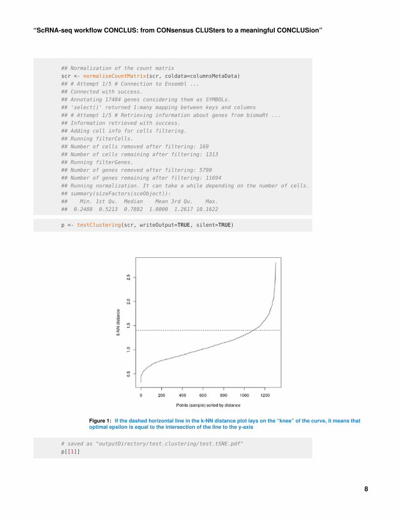
4.3 Test clusteringThe TestClustering function runs one clustering round out of the 84 (default) rounds thatCONCLUS normally performs. This step can be useful to determine if the default DBSCANparameters are suitable for your dataset. By default, they are dbscanEpsilon = c(1.3, 1.4,1.5) and minPts = c(3,4). If the dashed horizontal line in the k-NN distance plot lays on the“knee” of the curve (as shown below), it means that optimal epsilon is equal to the intersectionof the line to the y-axis. In our example, optimal epsilon is 1.4 for 5-NN distance where 5corresponds to MinPts.In the “test_clustering” folder under outputDirectory, the three plots below will be savedwhere one corresponds to the “distance_graph.pdf”, another one to “test_tSNE.pdf” (p[[1]]),and the last one will be saved as “test_clustering.pdf” (p[[2]]).

## Creation of the single-cell RNA-Seq object

scr <- singlecellRNAseq(experimentName = "E11_5",

countMatrix = countMatrix,

species = "mouse",

outputDirectory = outputDirectory)

7


## Normalization of the count matrix

scr <- normaliseCountMatrix(scr, coldata=columnsMetaData)

## # Attempt 1/5 # Connection to Ensembl ...

## Connected with success.

## Annotating 17484 genes considering them as SYMBOLs.

## 'select()' returned 1:many mapping between keys and columns

## # Attempt 1/5 # Retrieving information about genes from biomaRt ...

## Information retrieved with success.

## Adding cell info for cells filtering.

## Running filterCells.

## Number of cells removed after filtering: 169

## Number of cells remaining after filtering: 1313

## Running filterGenes.

## Number of genes removed after filtering: 5790

## Number of genes remaining after filtering: 11694

## Running normalization. It can take a while depending on the number of cells.

## summary(sizeFactors(sceObject)):

## Min. 1st Qu. Median Mean 3rd Qu. Max.

## 0.2488 0.5213 0.7882 1.0000 1.2617 10.1622

p <- testClustering(scr, writeOutput=TRUE, silent=TRUE)

Figure 1: If the dashed horizontal line in the k-NN distance plot lays on the “knee” of the curve, it means thatoptimal epsilon is equal to the intersection of the line to the y-axis

# saved as "outputDirectory/test_clustering/test_tSNE.pdf"

p[[1]]

8


Figure 2: One of the 14 tSNE (by default) generated by conclus

# saved as "outputDirectory/test_clustering/test_clustering.pdf"

p[[2]]

9


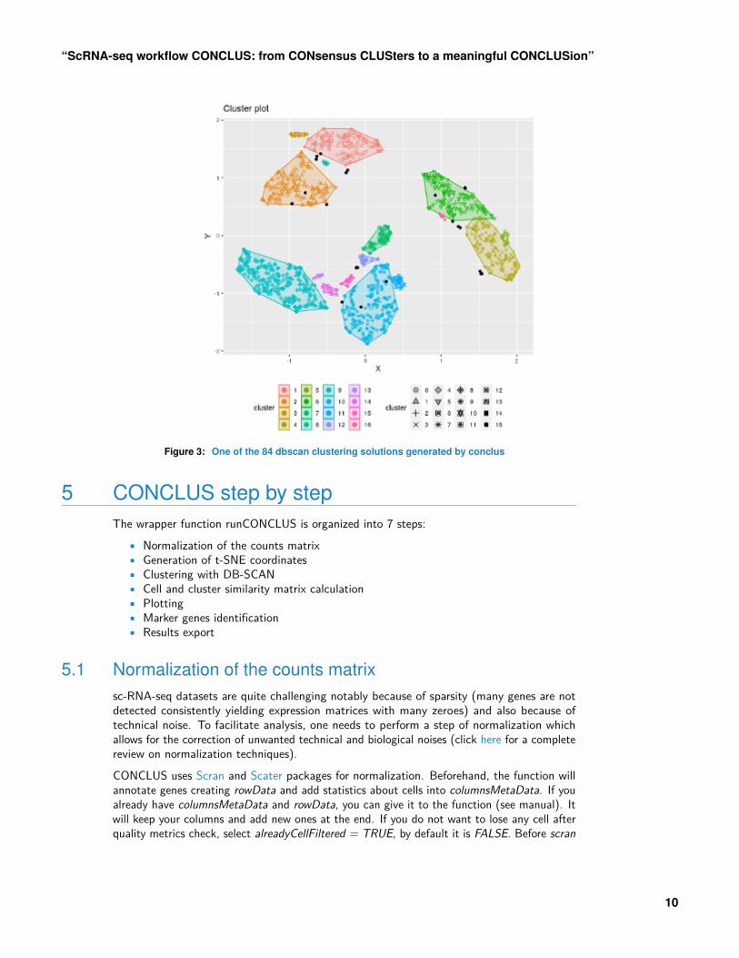
Figure 3: One of the 84 dbscan clustering solutions generated by conclus

5 CONCLUS step by stepThe wrapper function runCONCLUS is organized into 7 steps:

• Normalization of the counts matrix• Generation of t-SNE coordinates• Clustering with DB-SCAN• Cell and cluster similarity matrix calculation• Plotting• Marker genes identification• Results export

5.1 Normalization of the counts matrixsc-RNA-seq datasets are quite challenging notably because of sparsity (many genes are notdetected consistently yielding expression matrices with many zeroes) and also because oftechnical noise. To facilitate analysis, one needs to perform a step of normalization whichallows for the correction of unwanted technical and biological noises (click here for a completereview on normalization techniques).CONCLUS uses Scran and Scater packages for normalization. Beforehand, the function willannotate genes creating rowData and add statistics about cells into columnsMetaData. If youalready have columnsMetaData and rowData, you can give it to the function (see manual). Itwill keep your columns and add new ones at the end. If you do not want to lose any cell afterquality metrics check, select alreadyCellFiltered = TRUE, by default it is FALSE. Before scran

10

https://www.ncbi.nlm.nih.gov/pmc/articles/PMC5549838/

https://bioconductor.org/packages/release/bioc/html/scran.html

http://www.bioconductor.org/packages/release/bioc/html/scater.html


and scater normalization, the function will call scran::quickCluster (see manual for details). Ifyou want to skip this step, set runQuickCluster = FALSE, by default it is TRUE. We advice tofirst try the analysis with this option and to set it to FALSE if no rare populations are found.scr <- normaliseCountMatrix(scr, coldata=columnsMetaData)

The method normaliseCountMatrix returns a scRNASeq object with its sceNorm slot updated.This slot contains a SingleCellExperiment object having the normalized count matrix, thecolData (table with cells informations), and the rowData (table with the genes informations).See ?SingleCellExperiment for more details.The rowdata can help to study cross-talk between cell types or find surface protein-codingmarker genes suitable for flow cytometry. The columns with the GO terms are go_id andname_1006 (see manual).The slots can be accessed as indicated below:## Accessing slots

originalMat <- getCountMatrix(scr)

SCEobject <- getSceNorm(scr)

normMat <- SingleCellExperiment::logcounts(SCEobject)

# checking what changed after the normalisation

dim(originalMat)

## [1] 17484 1482

dim(normMat)

## [1] 11694 1313

# show first columns and rows of the count matrix

originalMat[1:5,1:5]

## c1 c2 c3 c4 c5

## Gnai3 0 0 0 0 0

## Cdc45 0 0 0 0 0

## H19 13 10 17 9 7

## Scml2 0 0 0 0 0

## Apoh 0 0 0 0 0

# show first columns and rows of the normalized count matrix

normMat[1:5,1:5]

## c1 c2 c3 c4 c5

## Gnai3 0.000000 0.000000 0.000000 0.000000 0.000000

## Cdc45 0.000000 0.000000 0.000000 0.000000 0.000000

## H19 3.223584 3.540887 4.705018 4.315128 3.505963

## Scml2 0.000000 0.000000 0.000000 0.000000 0.000000

## Narf 0.000000 0.000000 1.307690 0.000000 0.000000

# visualize first rows of metadata (coldata)

coldataSCE <- as.data.frame(SummarizedExperiment::colData(SCEobject))

head(coldataSCE)

## cellName state cellBarcode genesNum genesSum oneUMI oneUMIper mtGenes

## c1 c1 YS_VECad_min AACCAACCTGC 1621 2795 1168 72.05429 6

## c2 c2 YS_VECad_min AACCAAGACGA 984 1552 738 75.00000 6

## c3 c3 YS_VECad_min AACCAAGCCTG 912 1373 696 76.31579 7

11


## c4 c4 YS_VECad_min AACCAAGCTAA 653 904 527 80.70444 1

## c5 c5 YS_VECad_min AACCAAGGCCT 846 1333 656 77.54137 6

## c6 c6 YS_VECad_min AACCAAGTTGG 474 626 391 82.48945 3

## mtSum codGenes codSum mtPer codPer sumMtPer sumCodPer filterPassed

## c1 42 1525 2472 0.3701419 94.07773 1.5026834 88.44365 1

## c2 39 932 1393 0.6097561 94.71545 2.5128866 89.75515 1

## c3 21 867 1235 0.7675439 95.06579 1.5294975 89.94902 1

## c4 1 616 816 0.1531394 94.33384 0.1106195 90.26549 1

## c5 41 807 1224 0.7092199 95.39007 3.0757689 91.82296 1

## c6 10 447 590 0.6329114 94.30380 1.5974441 94.24920 1

## sizeFactor

## c1 1.5585578

## c2 0.9399435

## c3 0.6777597

## c4 0.4760406

## c5 0.6756387

## c6 0.2952552

# visualize beginning of the rowdata containing gene information

rowdataSCE <- as.data.frame(SummarizedExperiment:::rowData(SCEobject))

head(rowdataSCE)

## nameInCountMatrix ENSEMBL SYMBOL

## Gnai3 Gnai3 ENSMUSG00000000001 Gnai3

## Cdc45 Cdc45 ENSMUSG00000000028 Cdc45

## H19 H19 ENSMUSG00000000031 H19

## Scml2 Scml2 ENSMUSG00000000037 Scml2

## Narf Narf ENSMUSG00000000056 Narf

## Cav2 Cav2 ENSMUSG00000000058 Cav2

## GENENAME

## Gnai3 guanine nucleotide binding protein (G protein), alpha inhibiting 3

## Cdc45 cell division cycle 45

## H19 H19, imprinted maternally expressed transcript

## Scml2 Scm polycomb group protein like 2

## Narf nuclear prelamin A recognition factor

## Cav2 caveolin 2

## chromosome_name gene_biotype go_id name_1006

## Gnai3 3 protein_coding <NA> <NA>

## Cdc45 16 protein_coding <NA> <NA>

## H19 7 lncRNA <NA> <NA>

## Scml2 X protein_coding <NA> <NA>

## Narf 11 protein_coding <NA> <NA>

## Cav2 6 protein_coding GO:0009986 cell surface

5.2 Generation of t-SNE coordinatesrunCONCLUS generates an object of fourteen (by default) tables with tSNE coordinates.Fourteen because it will vary seven values of principal components PCs=c(4, 6, 8, 10, 20, 40,50) and two values of perplexity perplexities=c(30, 40) in all possible combinations.

12


The chosen values of PCs and perplexities can be changed if necessary. We found that thiscombination works well for sc-RNA-seq datasets with 400-2000 cells. If you have 4000-9000cells and expect more than 15 clusters, we recommend to use more first PCs and higherperplexity, for example, PCs=c(8, 10, 20, 40, 50, 80, 100) and perplexities=c(200, 240). Fordetails about perplexities parameter see ‘?Rtsne’.scr <- generateTSNECoordinates(scr, cores=2)

## Running TSNEs using 2 cores.

## Calculated 14 2D-tSNE plots.

## Building TSNEs objects.

Results can be explored as follows:tsneList <- getTSNEList(scr)

head(getCoordinates(tsneList[[1]]))

## X Y

## c1 -12.69446 -18.9154725

## c2 -11.93449 -19.5735135

## c3 -19.99432 -2.0386814

## c4 -22.36769 -2.2171536

## c5 -20.10163 0.5100164

## c6 -20.56566 0.3563303

5.3 Clustering with DB-SCANFollowing the calculation of t-SNE coordinates, DBSCAN is run with a range of epsilonand MinPoints values which will yield a total of 84 clustering solutions (PCs x perplexitiesx MinPoints x epsilon). minPoints is the minimum cluster size which you assume to bemeaningful for your experiment and epsilon is the radius around the cell where the algorithmwill try to find minPoints dots. Optimal epsilon must lay on the knee of the k-NN function asshown in the “test_clustering/distance_graph.pdf” (See Test clustering section above).scr <- runDBSCAN(scr, cores=2)

## The following matrix shows how many times a number of clusters 'k' has been found among the dbscan solutions :

## 1 2 3 4 5 6 7 8 9 10 11 12 13

## Number of clusters k : 6 8 5 10 7 9 11 12 4 13 14 16 17

## Count : 11 11 10 10 9 7 7 5 4 4 4 1 1

##

## Statistics about number of clusters 'k' among dbscan solutions:

## Min. 1st Qu. Median Mean 3rd Qu. Max.

## 4.000 6.000 8.000 8.619 11.000 17.000

##

## Suggested clusters number to use in clusterCellsInternal() : clusterNumber=8.

Results can be explored as follows:dbscanList <- getDbscanList(scr)

clusteringList <- lapply(dbscanList, getClustering)

clusteringList[[1]][, 1:10]

## c1 c2 c3 c4 c5 c6 c7 c8 c9 c10

## 1 1 2 2 2 2 1 2 2 3

13


5.4 Cell and cluster similarity matrix calculationThe above calculated results are combined together in a matrix called “cell similarity matrix”.runDBSCAN function returns an object of class scRNASeq with its dbscanList slot updated.The list represents 84 clustering solutions (which is equal to number of PCs x perplexitiesx MinPoints x epsilon). Since the range of cluster varies from result to result, there is noexact match between numbers in different elements of the list. Cells having the same numberwithin an element are guaranteed to be in one cluster. We can calculate how many timesout of 84 clustering solutions, every two cells were in one cluster and that is how we cometo the similarity matrix of cells. We want to underline that a zero in the dbscan resultsmeans that a cell was not assigned to any cluster. Hence, cluster numbers start from one.clusterCellsInternal is a general method that returns an object of class scRNASeq with itscellsSimilarityMatrix slot updated.Note that the number of clusters is set to 10 (it was set to 11 in the original study, seedata section). Considering that clusters can be merged afterwards (see Supervised clusteringsection), we advise to keep this number. One might want to increase it if the cell similaritymatrix or the tSNE strongly suggest more clusters but this number is suitable for mostexperiments in our hands.scr <- clusterCellsInternal(scr, clusterNumber=10)

## Calculating cells similarity matrix.

## Assigning cells to 10 clusters.

## Cells distribution by clusters:

## 1 2 3 4 5 6 7 8 9 10

## 190 186 340 45 135 37 111 8 128 133

cci <- getCellsSimilarityMatrix(scr)

cci[1:10, 1:10]

## c1 c2 c3 c4 c5 c6 c7

## c1 1.0000000 1.0000000 0.7023810 0.7023810 0.7023810 0.6785714 0.9523810

## c2 1.0000000 1.0000000 0.7023810 0.7023810 0.7023810 0.6785714 0.9523810

## c3 0.7023810 0.7023810 1.0000000 1.0000000 1.0000000 0.9761905 0.6547619

## c4 0.7023810 0.7023810 1.0000000 1.0000000 1.0000000 0.9761905 0.6547619

## c5 0.7023810 0.7023810 1.0000000 1.0000000 1.0000000 0.9761905 0.6547619

## c6 0.6785714 0.6785714 0.9761905 0.9761905 0.9761905 1.0000000 0.6547619

## c7 0.9523810 0.9523810 0.6547619 0.6547619 0.6547619 0.6547619 0.9761905

## c8 0.7023810 0.7023810 1.0000000 1.0000000 1.0000000 0.9761905 0.6547619

## c9 0.6904762 0.6904762 0.9285714 0.9285714 0.9285714 0.9047619 0.6428571

## c10 0.6547619 0.6547619 0.7380952 0.7380952 0.7380952 0.7142857 0.6071429

## c8 c9 c10

## c1 0.7023810 0.6904762 0.6547619

## c2 0.7023810 0.6904762 0.6547619

## c3 1.0000000 0.9285714 0.7380952

## c4 1.0000000 0.9285714 0.7380952

## c5 1.0000000 0.9285714 0.7380952

## c6 0.9761905 0.9047619 0.7142857

## c7 0.6547619 0.6428571 0.6071429

## c8 1.0000000 0.9285714 0.7380952

## c9 0.9285714 0.9642857 0.6666667

## c10 0.7380952 0.6666667 0.8095238

14


After looking at the similarity between elements on the single-cell level, which is useful if wewant to understand if there is any substructure which we did not highlight with our clustering,a “bulk” level where we pool all cells from a cluster into a representative “pseudo cell” canalso be generated. This gives a clusterSimilarityMatrix :scr <- calculateClustersSimilarity(scr)

csm <- getClustersSimilarityMatrix(scr)

csm[1:10, 1:10]

## 1 2 3 4 5 6 7

## 1 1.000000 0.702381 0.0000000 0.00000000 0.00000000 0.00000000 0.00000000

## 2 0.702381 1.000000 0.0000000 0.00000000 0.00000000 0.00000000 0.00000000

## 3 0.000000 0.000000 0.9761905 0.00000000 0.00000000 0.00000000 0.00000000

## 4 0.000000 0.000000 0.0000000 1.00000000 0.04761905 0.66666667 0.32142857

## 5 0.000000 0.000000 0.0000000 0.04761905 1.00000000 0.04761905 0.11904762

## 6 0.000000 0.000000 0.0000000 0.66666667 0.04761905 0.98809524 0.44047619

## 7 0.000000 0.000000 0.0000000 0.32142857 0.11904762 0.44047619 1.00000000

## 8 0.000000 0.000000 0.0000000 0.16666667 0.00000000 0.16666667 0.16666667

## 9 0.000000 0.000000 0.0000000 0.04761905 0.47619048 0.04761905 0.07142857

## 10 0.000000 0.000000 0.0000000 0.19047619 0.33333333 0.19047619 0.21428571

## 8 9 10

## 1 0.0000000 0.00000000 0.0000000

## 2 0.0000000 0.00000000 0.0000000

## 3 0.0000000 0.00000000 0.0000000

## 4 0.1666667 0.04761905 0.1904762

## 5 0.0000000 0.47619048 0.3333333

## 6 0.1666667 0.04761905 0.1904762

## 7 0.1666667 0.07142857 0.2142857

## 8 1.0000000 0.00000000 0.1428571

## 9 0.0000000 1.00000000 0.7142857

## 10 0.1428571 0.71428571 1.0000000

5.5 Plotting

5.5.1 t-SNE colored by clusters or conditions

CONCLUS generated 14 tSNE combining different values of PCs and perplexities. Each tSNEcan be visualized either using coloring reflecting the results of DBScan clustering, the conditions(if the metadata contain a ‘state’ column) or without colors. Here plotClusteredTSNE is usedto generate all these possibilities of visualization.tSNEclusters <- plotClusteredTSNE(scr, columnName="clusters",

returnPlot=TRUE, silentPlot=TRUE)

tSNEnoColor <- plotClusteredTSNE(scr, columnName="noColor",


tSNEstate <- plotClusteredTSNE(scr, columnName="state",


For visualizing the 5th (out of 14) tSNE cluster:

15


tSNEclusters[[5]]

Figure 4: DBscan results on the 5th tSNE

This tSNE suggests that the cluster 8 corresponds to a rare population of cells. We can alsoappreciate that clusters 1 and 2, as clusters 9 and 10 could be considered as single clustersrespectively.For visualizing the 5th (out of 14) tSNE cluster without colors:tSNEnoColor[[5]]

For visualizing the 5th (out of 14) tSNE cluster colored by state:tSNEstate[[5]]

One can see that the cluster 8 contains only cells of the YS.

16


Figure 5: The 5th tSNE solution without coloring

Figure 6: The 5th tSNE solution colored by cell condition

17


5.5.2 Cell similarity heatmap

The cellsSimilarityMatrix is then used to generate a heatmap summarizing the results of theclustering and to show how stable the cell clusters are across the 84 solutions.plotCellSimilarity(scr)

Figure 7: Cell similarity matrix showing the conservation of clustering across the 84 solutions

CellsSimilarityMatrix is symmetrical and its size proportional to the “number of cells x numberof cells”. Each vertical or horizontal tiny strip is a cell. Intersection shows the proportionof clustering iterations in which a pair of cells was in one cluster (score between 0 and 1,between blue and red). We will call this combination “consensus clusters” and use themeverywhere later. We can appreciate that cellsSimilarityMatrix is the first evidence showingthat CONCLUS managed not only to distinguish VE-Cad plus cells from the VE-Cad minusbut also find sub-populations within these groups.

5.5.3 Cluster similarity heatmap

plotClustersSimilarity(scr)

18


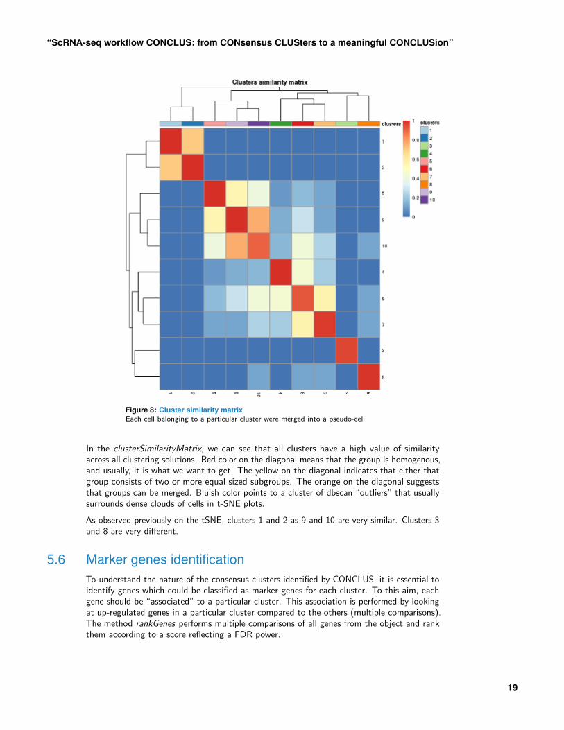
Figure 8: Cluster similarity matrixEach cell belonging to a particular cluster were merged into a pseudo-cell.

In the clusterSimilarityMatrix, we can see that all clusters have a high value of similarityacross all clustering solutions. Red color on the diagonal means that the group is homogenous,and usually, it is what we want to get. The yellow on the diagonal indicates that either thatgroup consists of two or more equal sized subgroups. The orange on the diagonal suggeststhat groups can be merged. Bluish color points to a cluster of dbscan “outliers” that usuallysurrounds dense clouds of cells in t-SNE plots.As observed previously on the tSNE, clusters 1 and 2 as 9 and 10 are very similar. Clusters 3and 8 are very different.

5.6 Marker genes identificationTo understand the nature of the consensus clusters identified by CONCLUS, it is essential toidentify genes which could be classified as marker genes for each cluster. To this aim, eachgene should be “associated” to a particular cluster. This association is performed by lookingat up-regulated genes in a particular cluster compared to the others (multiple comparisons).The method rankGenes performs multiple comparisons of all genes from the object and rankthem according to a score reflecting a FDR power.

19


In summary, the method conclus::rankGenes() gives a list of marker genes for each cluster,ordered by their significance. See ?rankGenes for more details.scr <- rankGenes(scr)

## Ranking marker genes for each cluster.

## Working on cluster 1










markers <- getMarkerGenesList(scr)

head(markers[[1]])

## Gene vs_2 vs_3 vs_4 vs_5 vs_6

## 1 Meg3 1.739620e-15 4.553883e-20 4.603199e-20 9.507688e-39 8.405951e-18

## 2 Lum 5.565749e-07 1.515679e-57 1.767243e-20 6.281449e-38 3.220902e-16

## 3 Smarca1 7.521807e-12 1.656410e-36 1.052507e-14 5.275938e-29 2.532553e-12

## 4 Col1a2 7.086632e-03 1.580798e-62 1.843967e-26 4.171211e-45 1.838659e-19

## 5 Colec10 7.595290e-10 9.772120e-50 7.115534e-15 4.471748e-29 5.116283e-13

## 6 Pdzrn3 3.010753e-14 5.172901e-09 5.282962e-12 1.809078e-21 4.724952e-10

## vs_7 vs_8 vs_9 vs_10 mean_log10_fdr n_05

## 1 4.818401e-18 0.7494232248 8.868140e-36 4.057796e-37 -21.93574 8

## 2 3.826736e-36 0.0009837544 3.003934e-37 8.007236e-41 -27.84041 9

## 3 1.121875e-24 0.7494232248 2.879664e-28 9.729950e-29 -20.04270 8

## 4 2.898643e-42 0.0008157513 1.541016e-48 2.228903e-51 -32.87672 9

## 5 1.406019e-22 0.0736917453 5.123149e-31 1.707433e-31 -21.88450 8

## 6 5.103183e-21 0.7494232248 6.089826e-21 1.512921e-20 -13.73399 8

## score

## 1 2.248656

## 2 1.880134

## 3 1.870253

## 4 1.811593

## 5 1.805929

## 6 1.741935

The top 10 markers by cluster (default) can be selected with:scr <- retrieveTopClustersMarkers(scr, removeDuplicates=TRUE)

topMarkers <- getClustersMarkers(scr)

topMarkers

## geneName clusters

## 1 Meg3 1

## 2 Lum 1

## 3 Smarca1 1

## 4 Col1a2 1

## 5 Colec10 1

## 6 Pdzrn3 1

20


## 7 Klhl29 1

## 8 Sox5 1

## 9 Col5a1 1

## 10 Col3a1 1

## 11 Prdx2 2

## 12 Col1a1 2

## 13 Gpx1 2

## 14 Rpl41 2

## 15 Fth1 2

## 16 Car2 2

## 17 Rplp0 2

## 18 Alas2 2

## 19 Slc4a1 2

## 20 Acta2 2

## 21 Gpc6 3

## 22 Ptn 3

## 23 Tenm3 3

## 24 Mdk 3

## 25 Aff3 3

## 26 Peg3 3

## 27 Zfhx4 3

## 28 Igfbp5 3

## 29 Foxp2 3

## 30 Auts2 3

## 31 Fcer1g 4

## 32 Tyrobp 4

## 33 Ctss 4

## 34 Lst1 4

## 35 Aif1 4

## 36 Ccl3 4

## 37 Laptm5 4

## 38 C1qb 4

## 39 C1qc 4

## 40 Fcgr3 4

## 41 Afp 5

## 42 Apoa2 5

## 43 Ttr 5

## 44 Apoa1 5

## 45 St6galnac3 5

## 46 Mt1 5

## 47 Apob 5

## 48 S100g 5

## 49 Nudt4 5

## 50 Hsd3b6 5

## 51 Mctp1 6

## 52 P2ry12 6

## 53 F13a1 6

## 54 Mitf 6

## 55 Ms4a4a 6

## 56 Fyb 6

## 57 Slc9a9 6

21


## 58 Tbxas1 6

## 59 Cd180 6

## 60 Hdac9 6

## 61 Stab2 7

## 62 Lyve1 7

## 63 Calcrl 7

## 64 Flt1 7

## 65 Ralgapa2 7

## 66 Ldb2 7

## 67 Col13a1 7

## 68 Tek 7

## 69 Gpr182 7

## 71 Cldn1 8

## 72 A2m 8

## 73 Maob 8

## 74 Serpind1 8

## 75 Krt20 8

## 76 Pcbd1 8

## 77 Klb 8

## 78 F2 8

## 79 Serpinf2 8

## 80 Lrp2 8

## 81 Cdk8 9

## 83 Camk1d 9

## 84 Epb41 9

## 86 Mir6236 9

## 88 Slc25a21 9

## 89 Kel 9

## 90 Ank1 9

## 91 Ptprg 10

## 92 Pde8a 10

## 93 Ptprm 10

## 94 Col18a1 10

## 95 Cdh5 10

## 96 Tspan18 10

## 97 Mecom 10

## 98 Mast4 10

## 99 Col4a1 10

## 100 Pecam1 10

Cluster 8 contains the marker genes A2m, Cldn1, Maob, Pcbd1, Pdzk1, Krt20, Klb, Serpind1,and F2. Alpha-2-Macroglobulin (A2m) is a large (720 KDa) plasma protein found in the bloodand is mainly produced by the liver; Claudins (CLDNs) are a family of integral membraneproteins, Cldn1 being expressed by epithelial liver cells; The monoamine oxidase (Maob) isfound in abundance in the liver. All these markers play a role in the liver. This sub-populationis hence called liver-like hereafter.

22


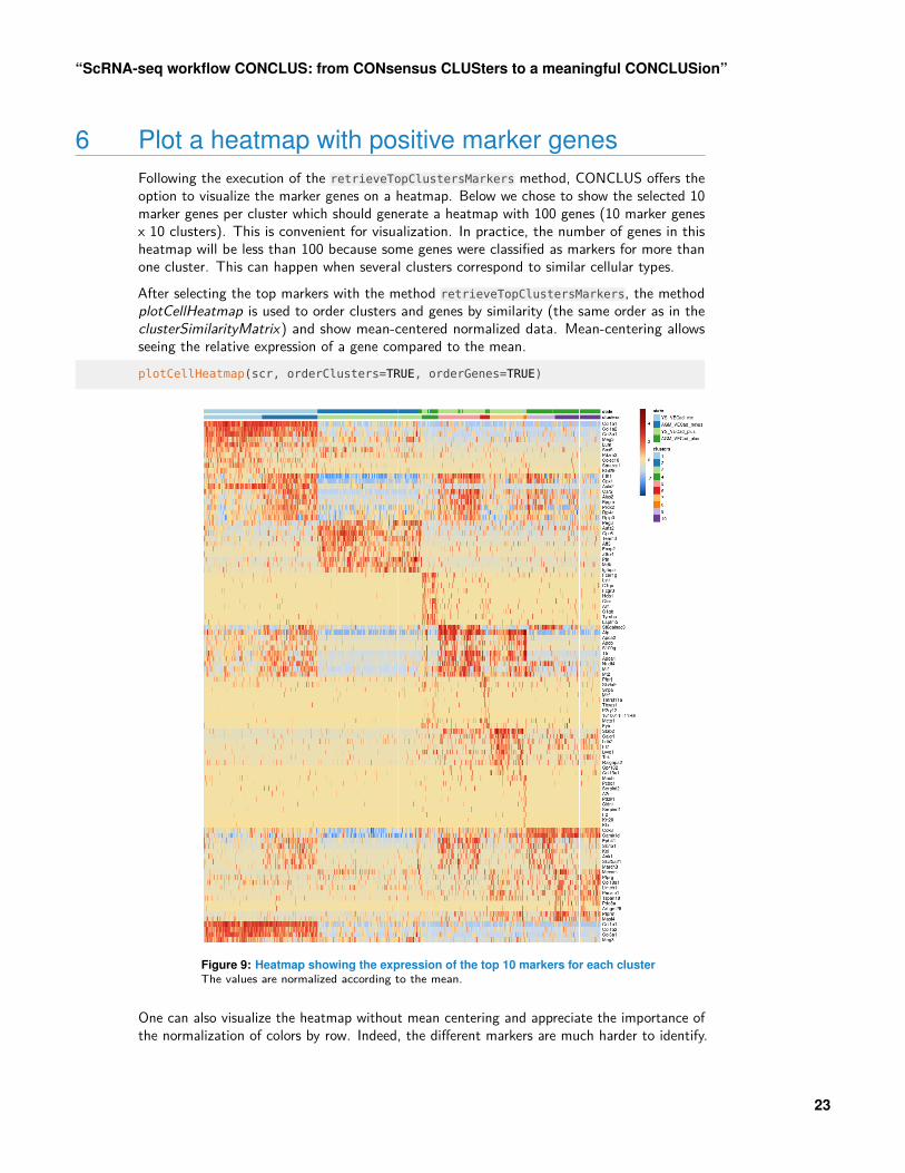
6 Plot a heatmap with positive marker genesFollowing the execution of the retrieveTopClustersMarkers method, CONCLUS offers theoption to visualize the marker genes on a heatmap. Below we chose to show the selected 10marker genes per cluster which should generate a heatmap with 100 genes (10 marker genesx 10 clusters). This is convenient for visualization. In practice, the number of genes in thisheatmap will be less than 100 because some genes were classified as markers for more thanone cluster. This can happen when several clusters correspond to similar cellular types.After selecting the top markers with the method retrieveTopClustersMarkers, the methodplotCellHeatmap is used to order clusters and genes by similarity (the same order as in theclusterSimilarityMatrix) and show mean-centered normalized data. Mean-centering allowsseeing the relative expression of a gene compared to the mean.plotCellHeatmap(scr, orderClusters=TRUE, orderGenes=TRUE)

Figure 9: Heatmap showing the expression of the top 10 markers for each clusterThe values are normalized according to the mean.

One can also visualize the heatmap without mean centering and appreciate the importance ofthe normalization of colors by row. Indeed, the different markers are much harder to identify.

23


plotCellHeatmap(scr, orderClusters=TRUE, orderGenes=TRUE, meanCentered=FALSE)

Figure 10: Same heatmap as before without normalizing by the mean

Alternative order of clusters is by name or by hierarchical clustering as in the default pheatmapfunction.

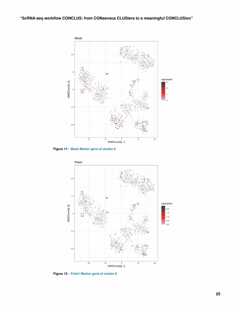
7 Plot t-SNE colored by expression of a selectedgenePlotGeneExpression allows visualizing the normalized expression of one gene in a t-SNE plot.It can be useful to inspect the specificity of top markers.Cluster 8 was identified as being a liver-like rare population. Below are examples of theexpression of its marker genes:plotGeneExpression(scr, "Maob", tSNEpicture=5)

plotGeneExpression(scr, "Pcbd1", tSNEpicture=5)

24


Figure 11: Maob Marker gene of cluster 8

Figure 12: Pcbd1 Marker gene of cluster 8

25


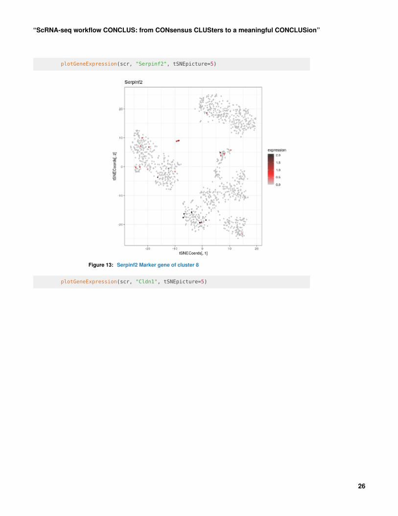
plotGeneExpression(scr, "Serpinf2", tSNEpicture=5)

Figure 13: Serpinf2 Marker gene of cluster 8

plotGeneExpression(scr, "Cldn1", tSNEpicture=5)

26


Figure 14: Cldn1 Marker gene of cluster 8

8 Collect publicly available info about marker genes

8.1 Collect information for the top 10 markers for each clusterretrieveGenesInfo retrieves gene information from NCBI, MGI, and UniProt. It requires theretrieveTopMarkers method to have been run on the object.scr <- retrieveGenesInfo(scr)

## # Attempt 1/5 # Connection to Ensembl ...

## Connected with success.





result <- getGenesInfos(scr)

head(result)

## uniprot_gn_symbol clusters external_gene_name

## 1 Lum 1 Lum

## 2 Smarca1 1 Smarca1

## 3 Col1a2 1 Col1a2

## 4 Colec10 1 Colec10

## 5 Pdzrn3 1 Pdzrn3

## 6 Klhl29 1 Klhl29

## go_id

## 1 GO:0005515, GO:0062023, GO:0007601, GO:0030199, GO:0005615, GO:0005576, GO:0045944, GO:0031012, GO:0005518, GO:0030021, GO:0014070, GO:0032914, GO:0051216, GO:0070848, GO:0005583

27


## 2 GO:0005634, GO:0003677, GO:0003676, GO:0005524, GO:0006338, GO:0031491, GO:0043044, GO:0016818, GO:0016787, GO:0000166, GO:0070615, GO:0005654, GO:0043231, GO:0045944, GO:0003682, GO:0004386, GO:0006325, GO:0045893, GO:0007420, GO:0000733, GO:0008094, GO:0008134, GO:0000785, GO:0016589, GO:0006355, GO:0090537, GO:0030182, GO:0036310, GO:2000177,

## 3 , GO:0005201, GO:0005615, GO:0046872, GO:0005515, GO:0005576, GO:0005783, GO:0005581, GO:0042802, GO:0030674, GO:0030198, GO:0031012, GO:0007266, GO:0030282, GO:0030199, GO:0032963, GO:0001568, GO:0007179, GO:0046332, GO:0043589, GO:0001501, GO:0030020, GO:0062023, GO:0002020, GO:0071230, GO:0008217, GO:0048407, GO:0085029, GO:0005584, GO:0070208

## 4 GO:0005634, GO:0005737, GO:0005794, GO:0005615, GO:0005576, GO:0005581, GO:0005829, GO:0030246, GO:0050918, GO:0006952, GO:0009792, GO:0007157, GO:0005537, GO:0042056, GO:1904888

## 5 GO:0005515, GO:0008270, GO:0005737, GO:0016740, GO:0046872, GO:0030054, GO:0045202, GO:0016567, GO:0004842, GO:0061630, GO:0007528, GO:0031594,

## 6 GO:0005515

## mgi_description

## 1 lumican

## 2 SWI/SNF related, matrix associated, actin dependent regulator of chromatin, subfamily a, member 1

## 3 collagen, type I, alpha 2

## 4 collectin sub-family member 10

## 5 PDZ domain containing RING finger 3

## 6 kelch-like 29

## entrezgene_description

## 1 lumican

## 2 SWI/SNF related, matrix associated, actin dependent regulator of chromatin, subfamily a, member 1

## 3 collagen, type I, alpha 2

## 4 collectin sub-family member 10

## 5 PDZ domain containing RING finger 3

## 6 kelch-like 29

## gene_biotype chromosome_name Symbol ensembl_gene_id mgi_id

## 1 protein_coding 10 Lum ENSMUSG00000036446 MGI:109347

## 2 protein_coding X Smarca1 ENSMUSG00000031099 MGI:1935127

## 3 protein_coding 6 Col1a2 ENSMUSG00000029661 MGI:88468

## 4 protein_coding 15 Colec10 ENSMUSG00000038591 MGI:3606482

## 5 protein_coding 6 Pdzrn3 ENSMUSG00000035357 MGI:1933157

## 6 protein_coding 12 Klhl29 ENSMUSG00000020627 MGI:2683857

## entrezgene_id uniprot_gn_id

## 1 17022 P51885

## 2 93761 Q6PGB8, Q8BS67, F6QS43, F6Z6F4

## 3 12843 Q01149, Q3TX57, E0CXI2

## 4 239447 Q8CF98

## 5 55983 Q69ZS0, A0A5F8MPS6

## 6 208439 Q80T74, A0A1W2P6N5

result contains the following columns:• uniprot_gn_symbol: Uniprot gene symbol.• clusters: The cluster to which the gene is associated.• external_gene_name: The complete gene name.• go_id: Gene Ontology (GO) identification number.• mgi_description: If the species is mouse, description of the gene on MGI.• entrezgene_description: Description of the gene by the Entrez database.• gene_biotype: protein coding gene, lincRNA gene, miRNA gene, unclassified non-coding

RNA gene, or pseudogene.• chromosome_name: The chromosome on which the gene is located.• Symbol: Official gene symbol.• ensembl_gene_id: ID of the gene in the ensembl database.• mgi_id: If the species is mouse, ID of the gene on the MGI database.• entrezgene_id: ID of the gene on the entrez database.• uniprot_gn_id: ID of the gene on the uniprot database.

28


9 Supervised clusteringUntil now, we have been using CONCLUS in an unsupervised fashion. This is a good way tostart the analysis of a sc-RNA-seq dataset. However, the knowledge of the biologist remainsa crucial asset to get the maximum of the data. This is why we have included in CONCLUS,additional options to do supervised analysis (or “manual” clustering) to allow the researcherto use her/his biological knowledge in the CONCLUS workflow. Going back to the exampleof the Shvartsman et al. dataset above (cluster similarity heatmap), one can see that someclusters clearly belong to the same family of cells after examining the clusters_similarity matrixgenerated by CONCLUS.As previously mentioned, clusters 1 and 2 as 9 and 10 are very similar. In order to figureout what marker genes are defining these families of clusters, one can use manual clusteringin CONCLUS to fuse clusters of similar nature: i.e. combine clusters 1 and 2 (9 and 10)together.## Retrieving the table indicating to which cluster each cell belongs

clustCellsDf <- retrieveTableClustersCells(scr)

## Replace "2/10" by "1/9" to merge 1/2 and 9/10

clustCellsDf$clusters[which(clustCellsDf$clusters == 2)] <- 1

clustCellsDf$clusters[which(clustCellsDf$clusters == 10)] <- 9

## Modifying the object to take into account the new classification

scrUpdated <- addClustering(scr, clusToAdd=clustCellsDf)

Now we can visualize the new results taking into account the new classification:plotCellSimilarity(scrUpdated)

plotCellHeatmap(scrUpdated, orderClusters=TRUE, orderGenes=TRUE)

tSNEclusters <- plotClusteredTSNE(scrUpdated, columnName="clusters",


tSNEclusters[[5]]

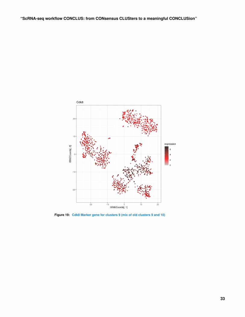
The cell heatmap above shows that Col1a1 is a good marker of cluster 1 and that Cdk8 is agood marker of cluster 9 (at the bottom). One can visualize them in the t-SNE plots below.plotGeneExpression(scrUpdated, "Col1a1", tSNEpicture=5)

plotGeneExpression(scrUpdated, "Cdk8", tSNEpicture=5)

29


Figure 15: Updated cells similarity matrix with merged 1/2 and 9/10

30


Figure 16: Updated cells heatmap with merged 1/2 and 9/10

31


Figure 17: 5th tSNE solution colored by dbscan result showing the merged clusters

Figure 18: Col1a1 Marker gene for cluster 1 (mix of old clusters 1 and 2)

32


Figure 19: Cdk8 Marker gene for clusters 9 (mix of old clusters 9 and 10)

33


10 ConclusionHere we demonstrated how to use CONCLUS and combine multiple parameters testing forsc-RNA-seq analysis. It allowed us to identify a rare population in the data of Shvartsman etal and will help gaining deeper insights into others.

11 Session info

sessionInfo()

## R version 4.1.1 (2021-08-10)

## Platform: x86_64-pc-linux-gnu (64-bit)

## Running under: Ubuntu 20.04.3 LTS

##

## Matrix products: default

## BLAS: /home/biocbuild/bbs-3.14-bioc/R/lib/libRblas.so

## LAPACK: /home/biocbuild/bbs-3.14-bioc/R/lib/libRlapack.so

##

## locale:

## [1] LC_CTYPE=en_US.UTF-8 LC_NUMERIC=C

## [3] LC_TIME=en_GB LC_COLLATE=C

## [5] LC_MONETARY=en_US.UTF-8 LC_MESSAGES=en_US.UTF-8

## [7] LC_PAPER=en_US.UTF-8 LC_NAME=C

## [9] LC_ADDRESS=C LC_TELEPHONE=C

## [11] LC_MEASUREMENT=en_US.UTF-8 LC_IDENTIFICATION=C

##

## attached base packages:

## [1] stats4 stats graphics grDevices utils datasets methods

## [8] base

##

## other attached packages:

## [1] org.Mm.eg.db_3.14.0 AnnotationDbi_1.56.0 IRanges_2.28.0

## [4] S4Vectors_0.32.0 Biobase_2.54.0 BiocGenerics_0.40.0

## [7] conclus_1.2.0 BiocStyle_2.22.0

##

## loaded via a namespace (and not attached):

## [1] utf8_1.2.2 tidyselect_1.1.1

## [3] RSQLite_2.2.8 grid_4.1.1

## [5] BiocParallel_1.28.0 Rtsne_0.15

## [7] scatterpie_0.1.7 munsell_0.5.0

## [9] ScaledMatrix_1.2.0 codetools_0.2-18

## [11] statmod_1.4.36 scran_1.22.0

## [13] withr_2.4.2 colorspace_2.0-2

## [15] GOSemSim_2.20.0 filelock_1.0.2

## [17] knitr_1.36 SingleCellExperiment_1.16.0

## [19] robustbase_0.93-9 DOSE_3.20.0

## [21] MatrixGenerics_1.6.0 GenomeInfoDbData_1.2.7

## [23] polyclip_1.10-0 bit64_4.0.5

## [25] farver_2.1.0 pheatmap_1.0.12

## [27] downloader_0.4 vctrs_0.3.8

34


## [29] treeio_1.18.0 generics_0.1.1

## [31] xfun_0.27 BiocFileCache_2.2.0

## [33] diptest_0.76-0 R6_2.5.1

## [35] doParallel_1.0.16 GenomeInfoDb_1.30.0

## [37] ggbeeswarm_0.6.0 graphlayouts_0.7.1

## [39] rsvd_1.0.5 locfit_1.5-9.4

## [41] flexmix_2.3-17 bitops_1.0-7

## [43] cachem_1.0.6 fgsea_1.20.0

## [45] gridGraphics_0.5-1 DelayedArray_0.20.0

## [47] assertthat_0.2.1 scales_1.1.1

## [49] ggraph_2.0.5 nnet_7.3-16

## [51] enrichplot_1.14.0 beeswarm_0.4.0

## [53] gtable_0.3.0 beachmat_2.10.0

## [55] tidygraph_1.2.0 rlang_0.4.12

## [57] splines_4.1.1 lazyeval_0.2.2

## [59] GEOquery_2.62.0 BiocManager_1.30.16

## [61] yaml_2.2.1 reshape2_1.4.4

## [63] qvalue_2.26.0 clusterProfiler_4.2.0

## [65] tools_4.1.1 bookdown_0.24

## [67] ggplotify_0.1.0 ggplot2_3.3.5

## [69] ellipsis_0.3.2 RColorBrewer_1.1-2

## [71] Rcpp_1.0.7 plyr_1.8.6

## [73] sparseMatrixStats_1.6.0 progress_1.2.2

## [75] zlibbioc_1.40.0 purrr_0.3.4

## [77] RCurl_1.98-1.5 prettyunits_1.1.1

## [79] dbscan_1.1-8 viridis_0.6.2

## [81] SummarizedExperiment_1.24.0 ggrepel_0.9.1

## [83] cluster_2.1.2 factoextra_1.0.7

## [85] magrittr_2.0.1 data.table_1.14.2

## [87] DO.db_2.9 matrixStats_0.61.0

## [89] hms_1.1.1 patchwork_1.1.1

## [91] evaluate_0.14 XML_3.99-0.8

## [93] mclust_5.4.7 gridExtra_2.3

## [95] compiler_4.1.1 biomaRt_2.50.0

## [97] scater_1.22.0 tibble_3.1.5

## [99] crayon_1.4.1 shadowtext_0.0.9

## [101] htmltools_0.5.2 ggfun_0.0.4

## [103] tzdb_0.1.2 tidyr_1.1.4

## [105] aplot_0.1.1 DBI_1.1.1

## [107] tweenr_1.0.2 dbplyr_2.1.1

## [109] MASS_7.3-54 fpc_2.2-9

## [111] rappdirs_0.3.3 Matrix_1.3-4

## [113] readr_2.0.2 metapod_1.2.0

## [115] parallel_4.1.1 igraph_1.2.7

## [117] GenomicRanges_1.46.0 pkgconfig_2.0.3

## [119] scuttle_1.4.0 xml2_1.3.2

## [121] foreach_1.5.1 ggtree_3.2.0

## [123] vipor_0.4.5 dqrng_0.3.0

## [125] XVector_0.34.0 yulab.utils_0.0.4

## [127] stringr_1.4.0 digest_0.6.28

## [129] Biostrings_2.62.0 rmarkdown_2.11

35


## [131] fastmatch_1.1-3 tidytree_0.3.5

## [133] edgeR_3.36.0 DelayedMatrixStats_1.16.0

## [135] curl_4.3.2 kernlab_0.9-29

## [137] modeltools_0.2-23 lifecycle_1.0.1

## [139] nlme_3.1-153 jsonlite_1.7.2

## [141] BiocNeighbors_1.12.0 viridisLite_0.4.0

## [143] limma_3.50.0 fansi_0.5.0

## [145] pillar_1.6.4 lattice_0.20-45

## [147] KEGGREST_1.34.0 fastmap_1.1.0

## [149] httr_1.4.2 DEoptimR_1.0-9

## [151] GO.db_3.14.0 glue_1.4.2

## [153] png_0.1-7 prabclus_2.3-2

## [155] iterators_1.0.13 bluster_1.4.0

## [157] bit_4.0.4 ggforce_0.3.3

## [159] class_7.3-19 stringi_1.7.5

## [161] blob_1.2.2 BiocSingular_1.10.0

## [163] memoise_2.0.0 dplyr_1.0.7

## [165] irlba_2.3.3 ape_5.5

36

``scrna-seq workflow conclus: from consensus clusters to a

Documents