The Cryosphere, 10, 2027–2041, 2016www.the-cryosphere.net/10/2027/2016/doi:10.5194/tc-10-2027-2016© Author(s) 2016. CC Attribution 3.0 License.

Sea-ice indicators of polar bear habitatHarry L. Stern1 and Kristin L. Laidre1,2

1Polar Science Center, Applied Physics Laboratory, University of Washington, 1013 NE 40th Street,Seattle, WA 98105, USA2Greenland Institute of Natural Resources, Box 570, 3900 Nuuk, Greenland

Correspondence to: Harry L. Stern (harry@apl.washington.edu)

Received: 5 May 2016 – Published in The Cryosphere Discuss.: 24 May 2016Revised: 18 August 2016 – Accepted: 24 August 2016 – Published: 14 September 2016

Abstract. Nineteen subpopulations of polar bears (Ursusmaritimus) are found throughout the circumpolar Arctic, andin all regions they depend on sea ice as a platform for travel-ing, hunting, and breeding. Therefore polar bear phenology– the cycle of biological events – is linked to the timing ofsea-ice retreat in spring and advance in fall. We analyzed thedates of sea-ice retreat and advance in all 19 polar bear sub-population regions from 1979 to 2014, using daily sea-iceconcentration data from satellite passive microwave instru-ments. We define the dates of sea-ice retreat and advance ina region as the dates when the area of sea ice drops belowa certain threshold (retreat) on its way to the summer mini-mum or rises above the threshold (advance) on its way to thewinter maximum. The threshold is chosen to be halfway be-tween the historical (1979–2014) mean September and meanMarch sea-ice areas. In all 19 regions there is a trend to-ward earlier sea-ice retreat and later sea-ice advance. Trendsgenerally range from −3 to −9 days decade−1 in spring andfrom +3 to +9 days decade−1 in fall, with larger trends inthe Barents Sea and central Arctic Basin. The trends are notsensitive to the threshold. We also calculated the number ofdays per year that the sea-ice area exceeded the threshold(termed ice-covered days) and the average sea-ice concen-tration from 1 June through 31 October. The number of ice-covered days is declining in all regions at the rate of −7 to−19 days decade−1, with larger trends in the Barents Sea andcentral Arctic Basin. The June–October sea-ice concentra-tion is declining in all regions at rates ranging from −1 to−9 percent decade−1. These sea-ice metrics (or indicators ofhabitat change) were designed to be useful for managementagencies and for comparative purposes among subpopula-tions. We recommend that the National Climate Assessment

include the timing of sea-ice retreat and advance in futurereports.

1 Introduction

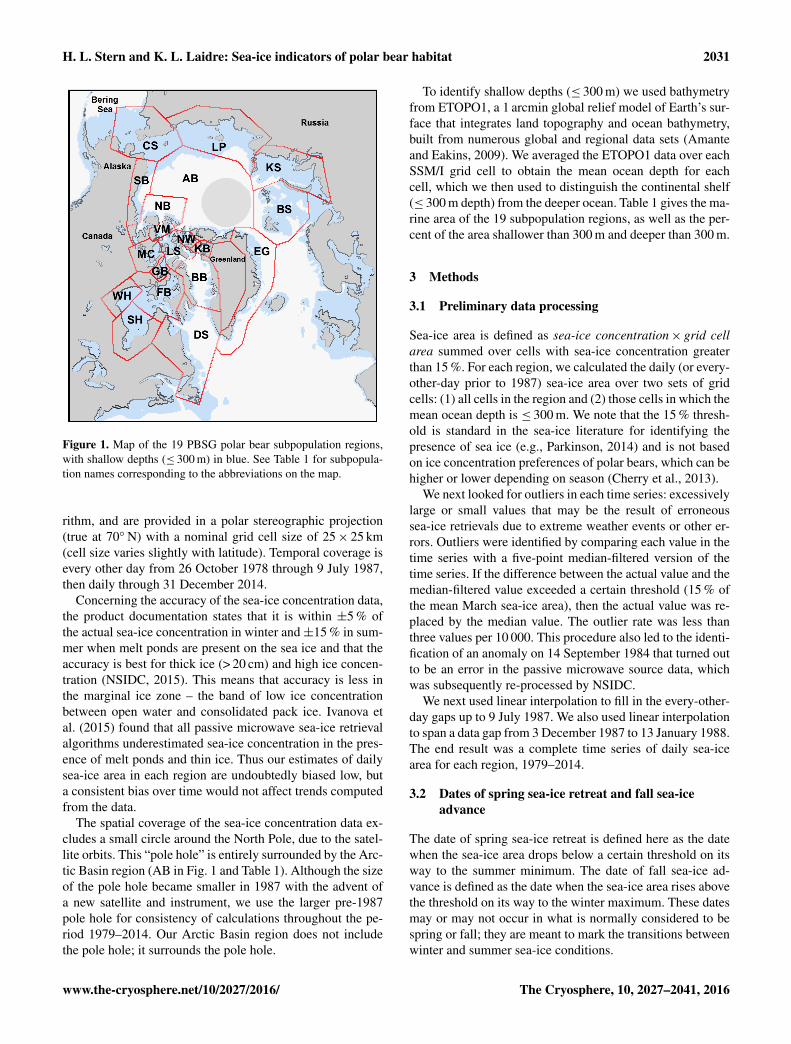
The International Union for Conservation of Nature (IUCN)Polar Bear Specialist Group (PBSG) recognizes 19 subpopu-lations of polar bears (Ursus maritimus; Obbard et al., 2010;Fig. 1 and Table 1). They are found throughout the sea-ice-covered areas of the circumpolar Arctic, especially over thecontinental shelf and inter-island channels. Polar bears de-pend on sea ice as a platform for hunting ice seals, theirprimary prey. Sea ice also facilitates their seasonal move-ments, mating, and, in some areas, maternal denning (Wiiget al., 2015). Some polar bears remain on sea ice year-round,but in more southerly areas where the ice melts completely,all bears are forced to spend up to several months on land,largely fasting until freeze-up allows them to return to theice again (e.g., Stirling et al., 1999; Stirling and Parkinson,2006). The global population size of polar bears is roughlyestimated to be about 25 000 (Obbard et al., 2010). Ge-netic analysis shows that gene flow occurs among the vari-ous subpopulations, which are considered to be semi-discrete(Paetkau et al., 1999; Peacock et al., 2015; Wiig et al., 2015).

Multiple approaches have been taken to construct sea-icemetrics for studies of survival and body condition in specificpolar bear subpopulations (Table 2). These have generally fo-cused on subpopulation-specific metrics such as the numberof ice-free or ice-covered days per year (Obbard et al., 2007;Regehr et al., 2010, 2015; Hamilton et al., 2014), the datesof spring sea-ice breakup and/or fall sea-ice freeze-up (Stir-ling and Parkinson, 2006; Regehr et al., 2007; Lunn et al.,

Published by Copernicus Publications on behalf of the European Geosciences Union.

2028 H. L. Stern and K. L. Laidre: Sea-ice indicators of polar bear habitat

Table 1. Polar bear subpopulation region names, abbreviations, and areas. See Fig. 1 for a map of the regions. The area of each regionincludes the marine portion only, not land. The number of cells is the number of SSM/I grid cells. The percent of total area is with respectto all regions (last row). The percent of area shallower than 300 m and deeper than 300 m are given in the last two columns. The pole hole(second to last row) is the circular area around the North Pole excluded from analysis due to the satellite orbits. The Arctic Basin region (AB)surrounds the pole hole but does not include it. All regions includes all 19 subpopulation regions plus the pole hole.

Abbreviation Subpopulation Number of Area % of total % %cells (103 km2) area ≤ 300 m > 300 m

KB Kane Basin 81 53 0.3 68 32BB Baffin Bay 1042 656 4.3 28 72LS Lancaster Sound 380 243 1.6 73 27NW Norwegian Bay 108 70 0.5 84 16VM Viscount Melville 157 101 0.7 64 36NB Northern Beaufort 1055 677 4.4 23 77SB Southern Beaufort 529 333 2.2 59 41MC M’Clintock Channel 224 140 0.9 100 0GB Gulf of Boothia 100 62 0.4 99 1FB Foxe Basin 883 528 3.4 97 3WH Western Hudson Bay 326 188 1.2 100 0SH Southern Hudson Bay 744 417 2.7 100 0DS Davis Strait 2416 1367 8.9 40 60EG East Greenland 2237 1387 9.0 27 73BS Barents Sea 2379 1540 10.0 63 37KS Kara Sea 1645 1054 6.9 87 13LP Laptev Sea 2169 1393 9.1 84 16CS Chukchi Sea 1840 1117 7.3 98 2AB Arctic Basin 4307 2813 18.3 15 85

Pole hole 1799 1193 7.8 0 100All regions 24 421 15 332 100.0 50 50

2014; Laidre et al., 2015a; Obbard et al., 2016), or the sea-ice concentration (Rode et al., 2012; Peacock et al., 2012,2013). Sea-ice metrics have mainly been selected based onthe specific region under study or developed for single stud-ies or data sets. There is a need to develop standardized cir-cumpolar metrics of polar bear habitat based on the satelliterecord of sea ice that allow for regional comparisons of habi-tat change and for tracking changes into the future, e.g., asin Vongraven et al. (2012). Thus the objective of this study isto propose and produce metrics of polar bear sea-ice habitatthat are also relevant to other Arctic marine mammal (AMM)species.

In this study we used daily sea-ice concentration data tocalculate several sea-ice metrics for each of the 19 polar bearsubpopulation regions for the period 1979–2014. The metricsare date of spring sea-ice retreat, date of fall sea-ice advance,average sea-ice concentration from 1 June to 31 October, andthe number of ice-covered days per year. We calculated eachmetric for the total marine area of each region and for theshallow depths only (≤ 300 m). Shallow depths are more bi-ologically productive and are considered to be better polarbear habitat (Durner et al., 2009).

Several previous studies have divided the Arctic into dis-tinct regions and calculated the sea-ice area trend in eachregion (e.g., Stroeve et al., 2012; Perovich and Richter-

Menge, 2009; Parkinson and Cavalieri, 2008). While this isa straightforward and useful way to document changes in seaice, other metrics of sea-ice habitat are more relevant to ma-rine mammals whose life history events, such as hunting andbreeding, depend on the annual retreat of sea ice in the springand advance in the fall. Many ecologically important regionsof the Arctic are ice covered in winter and ice free in summerand will probably remain so for a long time into the future.Therefore the dates of sea-ice retreat in spring and advancein fall, and the interval of time between them, are key indi-cators of climate change for ice-dependent marine mammals(Stirling et al., 1999; Stirling and Parkinson, 2006).

2 Data

As in Laidre et al. (2015a) we used the Sea Ice Concentra-tions from Nimbus-7 SMMR and DMSP SSM/I-SSMIS Pas-sive Microwave Data (Cavalieri et al., 1996) data set avail-able from the National Snow and Ice Data Center (NSIDC)in Boulder, CO. This product is designed to provide a con-sistent time series of sea-ice concentrations (the fraction, orpercentage, of ocean area covered by sea ice) spanning thecoverage of several passive microwave instruments. The sea-ice concentrations are produced using the NASA Team algo-

The Cryosphere, 10, 2027–2041, 2016 www.the-cryosphere.net/10/2027/2016/

H. L. Stern and K. L. Laidre: Sea-ice indicators of polar bear habitat 2029

Table 2. Recent literature where sea-ice metrics were used for analysis of polar bear habitat. Note that these studies examined habitat for asingle polar bear subpopulation (or geographically close set of subpopulations). Bold text gives names of sea-ice metrics. Abbreviations: PM(passive microwave), SIC (sea-ice concentration), CIS (Canadian Ice Service).

Subpopulation Data Years Methods for sea-ice metric Reference

WesternHudson Bay

DailyPM SIC

1979–2004 Calculated daily percent sea-ice cover in the re-gion. Date of spring sea-ice breakup is thedate when the ice cover fell below 50 %.

Stirling and Parkinson (2006)

WesternHudson Bay

DailyPM SIC

1984–2004 Date of spring sea-ice breakup is the datewhen the ice cover fell below 50 %(same as Stirling and Parkinson, 2006).

Regehr et al. (2007)

SouthernHudson Bay

DailyPM SIC

1984–2003 Date of spring sea-ice breakup is the datewhen the ice cover fell below 50 % (same asStirling and Parkinson, 2006).Date of fall sea-ice freeze-up is the date whenthe ice cover rose above 50 %.Ice-free period is the number of days betweenbreakup and freeze-up.

Obbard et al. (2007)

SouthernBeaufortSea

DailyPM SIC

2001–2005 Calculated the daily percent sea-ice cover forthe continental shelf only (depth < 300 m).Number of ice-free days is the number of daysper calendar year with ice cover < 50 %.

Regehr et al. (2010)

NorthernBeaufortSea

DailyPM SIC

1979–2006 Mean annual number of grid cells with sea-ice concentration > 50 %, calculated for conti-nental shelf only (depth < 300 m) and excludinga buffer of one ocean grid cell along all coast-lines. Second sea-ice covariate is derived fromthe resource selection functions of Durner etal. (2009).

Stirling et al. (2011)

Baffin Bay,Davis Strait

MeanweeklySIC(CIS)

1977–2010 Mean weekly sea-ice concentration from 15May to 15 October.

Rode et al. (2012)

ChukchiSea, South-ern BeaufortSea

DailyPM SIC

1985–1993,2007–2010

Reduced-ice days per year is the number ofdays with sea-ice area < 6250 km2 (continentalshelf of each region only, depth < 300 m).Distance to ice edge is the daily minimum dis-tance from continental shelf to pack ice, aver-aged over all days in September. When pack iceis over the continental shelf the distance is setto zero.

Rode et al. (2014)

Baffin Bay DailyPM SIC

1979–2009 Sea-ice concentration in April, May,and June for the continental shelf only(depth < 300 m). (Note that the continentalshelf consists of two parts: Baffin Island in thewest and Greenland in the east.)

Peacock et al. (2012)

Davis Strait MeanweeklySIC(CIS)

1974–2007 Mean weekly sea-ice concentration from 14May to 15 October.

Peacock et al. (2013)

www.the-cryosphere.net/10/2027/2016/ The Cryosphere, 10, 2027–2041, 2016

2030 H. L. Stern and K. L. Laidre: Sea-ice indicators of polar bear habitat

Table 2. Continued.

Subpopulation Data Years Methods for sea-ice metric Reference

CanadianArcticArchipelago

MITgeneralcirculationmodel(GCM)

2006–2100 Future projections of sea ice were made using theMIT GCM with 18 km grid size and monthly output,forced by “business as usual” RCP8.5 emission sce-nario.Month of spring sea-ice breakup is the first monthin a given year with sea-ice concentration < 50 %.Month of fall sea-ice freeze-up is the first month af-ter breakup with sea-ice concentration ≥ 10 %.Ice-free season is the time from breakup to freeze-up. If all months of the year have sea-ice concentra-tion < 10 % then the ice-free season is 12 months.

Hamilton et al. (2014)

WesternHudson Bay

Daily PMSIC

1979–2012 Calculated daily percent sea-ice cover in the region.Date of spring sea-ice breakup is the date whenthe ice cover fell below 50 % (same as Stirling andParkinson, 2006) and stayed below 50 % for at least3 consecutive days.Date of fall sea-ice freeze-up is the date when theice cover rose above 50 % and stayed above 50 % forat least 3 consecutive days.Ice decay is the rate of sea-ice loss from 1 May untilthe date of complete disappearance of sea ice, calcu-lated as the absolute value of the slope of the ordinaryleast squares regression line of ice concentration vs.time.

Lunn et al. (2014)

East Green-land

Daily PMSIC

1979–2012 Calculated the daily sea-ice area in the region. De-fined threshold area A as halfway between meanMarch ice area and mean September ice area, wherethe means are calculated over the baseline period1979–1988.Date of spring sea-ice breakup is the date when icearea fell below threshold area A.Date of fall sea-ice freeze-up is the date when icearea rose above threshold area A.

Laidre et al. (2015a)

ChukchiSea, South-ern BeaufortSea

Daily PMSIC

1979–2013 Calculated the daily sea-ice area in each region. De-fined threshold area A as halfway between meanMarch ice area and zero area, where the mean Marcharea is calculated over the baseline period 1979–2013.Ice-covered days is the number of days each yearwith ice area > threshold area A.Calculated the mean number of ice-covered days for1994–2013 and then projected the number of ice-covered days forward in time.

Regehr et al. (2015)

SouthernBeaufortSea

2001–2010 Summer habitat is the sum of monthly indices ofthe area of optimal polar bear habitat over the conti-nental shelf for July through October each year (fromDurner et al., 2009).Melt season is the time between melt onset andfreeze onset (“inner melt length” from Stroeve et al.,2014).

Bromaghin et al. (2015)

SouthernHudson Bay

Daily PMSIC

1980–2012 Date of spring sea-ice breakup is the date whenmean ice concentration falls below 5 %.Date of fall sea-ice freeze-up is the date when meanice concentration rises above 5 %.

Obbard et al. (2016)

The Cryosphere, 10, 2027–2041, 2016 www.the-cryosphere.net/10/2027/2016/

H. L. Stern and K. L. Laidre: Sea-ice indicators of polar bear habitat 2031

Figure 1. Map of the 19 PBSG polar bear subpopulation regions,with shallow depths (≤ 300 m) in blue. See Table 1 for subpopula-tion names corresponding to the abbreviations on the map.

rithm, and are provided in a polar stereographic projection(true at 70◦ N) with a nominal grid cell size of 25× 25 km(cell size varies slightly with latitude). Temporal coverage isevery other day from 26 October 1978 through 9 July 1987,then daily through 31 December 2014.

Concerning the accuracy of the sea-ice concentration data,the product documentation states that it is within ±5 % ofthe actual sea-ice concentration in winter and±15 % in sum-mer when melt ponds are present on the sea ice and that theaccuracy is best for thick ice (> 20 cm) and high ice concen-tration (NSIDC, 2015). This means that accuracy is less inthe marginal ice zone – the band of low ice concentrationbetween open water and consolidated pack ice. Ivanova etal. (2015) found that all passive microwave sea-ice retrievalalgorithms underestimated sea-ice concentration in the pres-ence of melt ponds and thin ice. Thus our estimates of dailysea-ice area in each region are undoubtedly biased low, buta consistent bias over time would not affect trends computedfrom the data.

The spatial coverage of the sea-ice concentration data ex-cludes a small circle around the North Pole, due to the satel-lite orbits. This “pole hole” is entirely surrounded by the Arc-tic Basin region (AB in Fig. 1 and Table 1). Although the sizeof the pole hole became smaller in 1987 with the advent ofa new satellite and instrument, we use the larger pre-1987pole hole for consistency of calculations throughout the pe-riod 1979–2014. Our Arctic Basin region does not includethe pole hole; it surrounds the pole hole.

To identify shallow depths (≤ 300 m) we used bathymetryfrom ETOPO1, a 1 arcmin global relief model of Earth’s sur-face that integrates land topography and ocean bathymetry,built from numerous global and regional data sets (Amanteand Eakins, 2009). We averaged the ETOPO1 data over eachSSM/I grid cell to obtain the mean ocean depth for eachcell, which we then used to distinguish the continental shelf(≤ 300 m depth) from the deeper ocean. Table 1 gives the ma-rine area of the 19 subpopulation regions, as well as the per-cent of the area shallower than 300 m and deeper than 300 m.

3 Methods

3.1 Preliminary data processing

Sea-ice area is defined as sea-ice concentration× grid cellarea summed over cells with sea-ice concentration greaterthan 15 %. For each region, we calculated the daily (or every-other-day prior to 1987) sea-ice area over two sets of gridcells: (1) all cells in the region and (2) those cells in which themean ocean depth is ≤ 300 m. We note that the 15 % thresh-old is standard in the sea-ice literature for identifying thepresence of sea ice (e.g., Parkinson, 2014) and is not basedon ice concentration preferences of polar bears, which can behigher or lower depending on season (Cherry et al., 2013).

We next looked for outliers in each time series: excessivelylarge or small values that may be the result of erroneoussea-ice retrievals due to extreme weather events or other er-rors. Outliers were identified by comparing each value in thetime series with a five-point median-filtered version of thetime series. If the difference between the actual value and themedian-filtered value exceeded a certain threshold (15 % ofthe mean March sea-ice area), then the actual value was re-placed by the median value. The outlier rate was less thanthree values per 10 000. This procedure also led to the identi-fication of an anomaly on 14 September 1984 that turned outto be an error in the passive microwave source data, whichwas subsequently re-processed by NSIDC.

We next used linear interpolation to fill in the every-other-day gaps up to 9 July 1987. We also used linear interpolationto span a data gap from 3 December 1987 to 13 January 1988.The end result was a complete time series of daily sea-icearea for each region, 1979–2014.

3.2 Dates of spring sea-ice retreat and fall sea-iceadvance

The date of spring sea-ice retreat is defined here as the datewhen the sea-ice area drops below a certain threshold on itsway to the summer minimum. The date of fall sea-ice ad-vance is defined as the date when the sea-ice area rises abovethe threshold on its way to the winter maximum. These datesmay or may not occur in what is normally considered to bespring or fall; they are meant to mark the transitions betweenwinter and summer sea-ice conditions.

www.the-cryosphere.net/10/2027/2016/ The Cryosphere, 10, 2027–2041, 2016

2032 H. L. Stern and K. L. Laidre: Sea-ice indicators of polar bear habitat

Figure 2. Daily sea-ice area in Baffin Bay (all depths), January–December, 1979–2014 (gray curves). The colored curves aredecadal averages, as indicated in the legend. The upper horizontaldotted line (at 613× 103 km2) is the average sea-ice area in March(1979–2014); the lower horizontal dotted line (at 9× 103 km2) isthe average sea-ice area in September. The middle horizontal dottedline, halfway between the upper and lower lines, is the threshold fordetermining the spring and fall transition dates in Baffin Bay. SeeFig. S1 for similar plots for other subpopulation regions.

Arctic sea ice typically reaches its maximum area inMarch and its minimum area in September. Accordingly,we chose the transition threshold for each region as follows.We calculated the mean March sea-ice area over the period1979–2014, and the mean September sea-ice area over thesame period, and then chose the transition threshold to behalfway between these means. This is illustrated for the Baf-fin Bay region in Fig. 2 and for the other regions in Supple-ment Fig. S1. (Figs. 2–9 use Baffin Bay as a sample regionfor purposes of illustration).

Figure 3 illustrates the method for finding the dates ofspring retreat and fall advance in Baffin Bay in one particularyear. The daily sea-ice area (gray curve) exhibits small dailyfluctuations that can be attributed to the uncertainty in theunderlying sea-ice concentration data. We smooth the dailyvalues with a low-pass Gaussian-shaped filter in which 87 %of the weight is within ±1 week of the central value (blackcurve). Then, starting from the minimum sea-ice area in sum-mer, we search forward and backward in time for the firstintersections of the smoothed time series with the threshold.The backward search gives the spring date (red vertical line)and the forward search gives the fall date (blue vertical line).

Occasionally the smoothed sea-ice area time series maycross the threshold more than once in spring and/or fall. Ourmethod always chooses the crossing date that is closest intime to the summer minimum. In practice, out of 2736 cross-ing dates (36 years× 2 seasons× 19 regions× 2 time seriesper region), only 131 dates (4.8 %) had any potential for am-biguity. In more than 95 % of the cases there was clearly onlya single crossing date.

Figure 3. Determination of the spring and fall transition dates forthe year 2005 in Baffin Bay. The gray curve is the daily sea-ice area;the black curve is a smoothed version. The horizontal dotted line (at311× 103 km2) is the threshold. The intersection of the thresholdwith the smoothed (black) curve determines the spring (red) andfall (blue) transition dates.

3.3 Summer sea-ice concentration

For each region we calculated the mean sea-ice concentra-tion for 1 June–31 October for each year, from 1979 to 2014.While it has already been established that the sea-ice concen-tration in every region of the Arctic except the Bering Seais declining in every month of the year (e.g., Perovich andRichter-Menge, 2009), the winter sea-ice cover will likelycontinue to provide suitable polar bear habitat for at leastseveral more decades (especially in the Canadian high Arc-tic; Amstrup et al., 2008; Hamilton et al., 2014), whereas thesummer sea-ice cover may not. A summer sea-ice metric,therefore, measures the change in polar bear habitat duringthe season when that habitat is most vulnerable to change.

3.4 Number of ice-covered days per year

We calculated the number of days per year that the sea-icearea in each subpopulation region exceeded the threshold de-fined in Sect. 3.2 (i.e., 50 % of the way from mean Septemberto mean March sea-ice area). For example, in Fig. 3, the sea-ice area in Baffin Bay was greater than the 50 % threshold for220 days in the year 2005. This sea-ice metric was used as ameasure of polar bear habitat in the IUCN Red List assess-ment of polar bears (Wiig et al., 2015).

4 Results

4.1 Sea-ice metrics

In all 19 regions, the date of spring sea-ice retreat is trendingearlier and the date of fall sea-ice advance is trending later.Along with this, the length of the summer season is increas-ing, the summer sea-ice concentration is decreasing, and the

The Cryosphere, 10, 2027–2041, 2016 www.the-cryosphere.net/10/2027/2016/

H. L. Stern and K. L. Laidre: Sea-ice indicators of polar bear habitat 2033

Figure 4. Dates of sea-ice retreat (red) and sea-ice advance (blue)in Baffin Bay (all depths) for 1979–2014. The red and blue lines areleast-squares fits. The vertical green lines indicate the time intervalbetween retreat and advance (i.e., length of summer season). SeeTable 3 for trends. See Fig. S2 for similar plots for other regions.

number of ice-covered days per year is decreasing, for the pe-riod 1979–2014 (Table 3). Nearly all the trends (88 of 95) arestatistically significant. Trends in the date of spring sea-iceretreat are on the order of −3 to −9 days decade−1 (negativebeing earlier), with the largest trend (−16 days decade−1) inthe Barents Sea. Trends in the date of fall sea-ice advanceare on the order of +3 to +9 days decade−1 (positive beinglater), with the largest trend (+18 days decade−1) again inthe Barents Sea. This means that over the 3.5 decades of thisstudy, the time interval from the date of spring retreat to thedate of fall advance has lengthened by 3 to 9 weeks in mostregions and by 17 weeks in the Barents Sea. The summer(June–October) sea-ice concentration is declining at a rate of−1 to −9 percent decade−1, depending on region. The num-ber of ice-covered days is declining in all regions at the rateof −7 to −19 days decade−1, with larger trends in the Bar-ents Sea and central Arctic Basin. Results for the shallow(≤ 300 m) portions of each region are similar (Table 4). Notethat some regions consist almost entirely of shallow depths(see Fig. 1 and Table 1).

Figure 4 illustrates results for the Baffin Bay region (seeFig. S2 for similar plots for other regions). Sea-ice re-treat in spring is changing by −7.3 days decade−1 (red) andsea-ice advance in fall is changing by +5.4 days decade−1

(blue), both statistically significant. The time interval be-tween the spring and fall transition dates is changing by+12.7 days decade−1 (Fig. 5; see Fig. S3 for similar plots forother regions). The summer sea-ice concentration is chang-ing by −4.1 percent decade−1 (Fig. 6; see Fig. S4 for similarplots for other regions). The number of ice-covered days ischanging by −12.7 days decade−1, which is the negative ofthe fall-minus-spring trend: the loss of every ice-covered dayoccurs between the time of spring sea-ice retreat and fall sea-ice advance.

Figure 5. Length of the summer season (from spring sea-ice retreatto fall sea-ice advance) vs. year for Baffin Bay (all depths), withleast-squares line in red (slope: +12.7 days decade−1). See Fig. S3for similar plots for other regions.

Figure 6. Summer (June through October) sea-ice concentration vs.year for Baffin Bay (all depths), with least-squares line in red (slope:−4.1 percent decade−1). See Fig. S4 for similar plots for other re-gions.

We also calculated the number of ice-covered days basedon a 15 % threshold of sea-ice area, as illustrated in Figs. 7and 8 (see Fig. S5 for similar plots for other regions). The 15and 50 % thresholds intersect the annual cycle of sea-ice areaat different levels and therefore contain information aboutthe shape of the annual cycle. In Baffin Bay, the rate of de-cline in the number of ice-covered days is about the same forboth thresholds (Fig. 8). However, in the Chukchi Sea region(Fig. S5) the rate of decline is faster for the 15 % threshold,meaning that the rise and fall of the annual cycle of sea-icearea is steepening, leading to faster transitions between sum-mer and winter sea-ice coverage. In the Barents Sea (Fig. S5)the opposite is occurring. Further analysis of changes in theshape of the annual cycle of sea-ice area is possible but isbeyond the scope of the present study.

www.the-cryosphere.net/10/2027/2016/ The Cryosphere, 10, 2027–2041, 2016

2034 H. L. Stern and K. L. Laidre: Sea-ice indicators of polar bear habitat

Table 3. Trend in date of spring sea-ice retreat (days decade−1), trend in date of fall sea-ice advance (days decade−1), trend in length ofsummer season (days decade−1), trend in June–October sea-ice concentration (percent concentration decade−1), trend in number of ice-covered days (days decade−1), and correlation of de-trended dates of spring retreat and fall advance (dimensionless). All quantities arecomputed from the total marine area of each region, regardless of depth (compare Table 4), for the period 1979–2014. The trend in the lengthof the summer season (fall–spring trend) is equal to the fall trend minus the spring trend. Statistical significance is indicated by * (95 % level)or ** (99 % level) according to a two-sided F test (for trends) or a two-sided t test (for correlations).

Subpopulation Spring Fall Fall−spring Jun–Oct Ice-covered Correlation oftrend trend trend ice concentration days dates

Kane Basin −6.8 * 5.6 ** 12.4 ** −5.4 ** −14.1 ** −0.55 **Baffin Bay −7.3 ** 5.4 ** 12.7 ** −4.1 ** −12.7 ** −0.64 **Lancaster Sound −5.4 * 4.7 ** 10.1 ** −4.4 ** −10.6 ** −0.11Norwegian Bay −1.2 4.3 5.5 −1.6 −7.1 * −0.21Viscount Melville −4.0 7.9 11.8 * −4.7 ** −12.3 ** 0.36 *Northern Beaufort −6.0 * 3.1 9.0 * −4.3 ** −9.3 * −0.40 *Southern Beaufort −9.0 ** 8.8 ** 17.8 ** −9.3 ** −17.5 ** −0.50 **M’Clintock Channel −4.1 ** 5.9 ** 10.0 ** −5.1 ** −11.1 ** −0.74 **Gulf of Boothia −8.6 ** 7.6 ** 16.2 ** −8.9 ** −18.6 ** −0.57 **Foxe Basin −5.3 ** 5.7 ** 11.0 ** −3.3 ** −11.4 ** −0.58 **Western Hudson Bay −5.1 ** 3.5 ** 8.7 ** −2.9 ** −8.6 ** −0.25Southern Hudson Bay −3.0 * 3.6 * 6.6 ** −1.8 * −6.8 ** −0.35 *Davis Strait −7.4 ** 9.2 ** 16.6 ** −1.0 ** −17.1 ** −0.35 *East Greenland −5.7 ** 4.8 * 10.5 ** −1.4 * −10.4 ** −0.34 *Barents Sea −16.4 ** 18.2 ** 34.6 ** −3.8 ** −41.0 ** −0.46 **Kara Sea −9.2 ** 7.3 ** 16.5 ** −7.9 ** −16.9 ** −0.49 **Laptev Sea −6.9 ** 7.0 ** 13.9 ** −9.4 ** −13.5 ** −0.78 **Chukchi Sea −4.0 ** 5.3 ** 9.3 ** −4.0 ** −8.9 ** −0.39 *Arctic Basin −11.9 ** 15.2 ** 27.1 ** −6.0 ** −24.6 ** 0.35 *

Figure 7. Sea-ice area in Baffin Bay (all depths), 1979–2014. Top green line is mean March sea-ice area; bottom green line is mean Septembersea-ice area. Two thresholds are shown: 15 and 50 % of the way from the mean September area to the mean March area.

4.2 Correlation of de-trended dates

Figure 4 shows that there is year-to-year variability about thetrend lines in the dates of spring sea-ice retreat and fall sea-ice advance. Subtracting out the trend lines leaves residuals.We calculated the correlation of the spring residuals with thefall residuals (Table 3, last column). The correlation is neg-ative in most regions, often significantly so. This means thatan early spring sea-ice retreat (relative to the trend line) tendsto be followed by a late fall sea-ice advance (relative to the

trend line), and vice versa. The de-trended spring and falldates for Baffin Bay are shown in Fig. 9. The negative corre-lations are likely the result of the ice–albedo feedback, dis-cussed in Sect. 5.4.

In regions with a strong negative correlation, this suggestsa method for predicting the date of fall sea-ice advance, oncethe date of spring sea-ice retreat has been observed. (1) Findthe slope (S) of the least-squares fit of the de-trended falldates vs. the de-trended spring dates (as in Fig. 9, red line).(2) Calculate the projected date of retreat (Dr) and date of

The Cryosphere, 10, 2027–2041, 2016 www.the-cryosphere.net/10/2027/2016/

H. L. Stern and K. L. Laidre: Sea-ice indicators of polar bear habitat 2035

Figure 8. Number of ice-covered days in Baffin Bay (all depths),1979–2014, based on two thresholds: 15 % (blue) and 50 % (red)(see also Fig. 7). Least-squares lines are also shown. See Fig. S5 forsimilar plots for other regions.

advance (Da) for the current year by extrapolating the his-torical trends (Table 3). (3) In the current year, once the dateof spring sea-ice retreat has been observed (Dobs

r ), predictthe date of fall sea-ice advance as Da+ S × (Dobs

r −Dr).This is the date projected by the trend line plus the anomalypredicted by the historical correlation of the spring and falldates. This method should give several months of lead timefor the predicted date of fall sea-ice advance, with a higherdegree of skill than simply predicting a continuation of thefall linear trend, in those regions where the spring and falldates are significantly correlated.

4.3 Spatial patterns

The spatial pattern of trends in the date of spring sea-ice re-treat (Fig. 10) shows that all trends over shallow depths arestatistically significant except in the Northern Beaufort, Vis-count Melville, and Norwegian Bay regions. Otherwise, thecontinental shelves around the Arctic show significantly ear-lier spring retreat, generally −3 to −9 days decade−1, withfaster retreat in the northern Chukchi and East Siberian seas,Kane Basin, and especially the Barents Sea. For the date offall sea-ice advance (Fig. 11), all regions have positive trends,but the trends are not statistically significant in some parts ofthe Canadian Arctic Archipelago. The rest of the continentalshelf regions around the Arctic show significantly later falladvance, generally 3 to 9 days decade−1, with larger rates inthe northern Chukchi and East Siberian seas and in the Bar-ents Sea, similar to the spring pattern. The increase in thelength of the summer season (Fig. 12) shows the same pat-tern, with roughly double the rate (since it equals the fall rateminus the spring rate).

Note that in this analysis, the Chukchi Sea region extendssouth of Bering Strait into the northern Bering Sea. We knowfrom other analyses (e.g., Laidre et al., 2015a; Parkinson,2014) that there has been a slight increase in sea ice in the

Bering Sea. Therefore the negative trends for the ChukchiSea reported here, while still statistically significant, are rel-atively small because of the inclusion of the northern BeringSea within the Chukchi Sea region. Similarly, the trends forthe Arctic Basin region are relatively large because that re-gion includes the northern Chukchi Sea, where summer seaice has been rapidly disappearing (e.g., Frey et al., 2015;Parkinson, 2014).

4.4 Sensitivity to threshold

The calculation of the spring and fall transition dates is basedon a sea-ice area threshold that is halfway between the meanSeptember sea-ice area and the mean March sea-ice area foreach region. Different thresholds would lead to different tran-sition dates. How sensitive are the transition dates to the ac-tual choice of threshold? The answer can be seen in Fig. 2(and Fig. S1). The rate of change of sea-ice area (i.e., itsslope) is relatively steep at the times of threshold crossing,indicating that sea ice diminishes quickly in spring and growsback quickly in fall compared to the rate of change in winterand summer. Therefore the transition dates are relatively in-sensitive to the threshold, in the sense that a small change inthe threshold would lead to a small change in the transitiondates.

5 Discussion

5.1 Previous studies of the timing of Arctic sea-iceadvance and retreat

Many studies in the last 10 years have considered changesin the timing of sea-ice advance and retreat in the con-text of polar bear ecology. Stirling and Parkinson (2006)used daily sea-ice concentration from satellite passive mi-crowave data to calculate the date of sea-ice breakup (50 %concentration) in spring in Baffin Bay for each year from1979 through 2004, finding a statistically significant trendtoward earlier breakup (−6.6± 2.0 days decade−1). The tim-ing of polar bear onshore arrival in western Hudson Baywas previously shown to be significantly related to the 50 %sea-ice concentration threshold (Stirling et al., 1999). Otherstudies of sea-ice timing and polar bears include Regehr etal. (2007), Obbard et al. (2007), Hamilton et al. (2014), Lunnet al. (2014), Laidre et al. (2015a), and Obbard et al. (2016).These studies are summarized in Table 2, along with eightother studies where sea-ice metrics were used for analysis ofpolar bear habitat.

Other researchers have considered changes in the timingof sea-ice advance and retreat without specific emphasis onpolar bears. Stammerjohn et al. (2012) used daily sea-iceconcentration from satellite passive microwave data (1979–2007) to calculate trends in the dates of sea-ice retreat andadvance at every 25× 25 km grid cell. Then they identifiedtwo regions where the trends were particularly large, encom-

www.the-cryosphere.net/10/2027/2016/ The Cryosphere, 10, 2027–2041, 2016

2036 H. L. Stern and K. L. Laidre: Sea-ice indicators of polar bear habitat

Figure 9. Date of fall sea-ice advance (de-trended) vs. date of springsea-ice retreat (de-trended) for Baffin Bay (all depths). The de-trended dates have correlation −0.64. This suggests that the dateof fall sea-ice advance can be predicted from the date of spring sea-ice retreat with more skill than simply extrapolating the fall trend.See Table 3 for correlations in all regions. The red line is the least-squares fit.

passing parts of the East Siberian/Chukchi/Beaufort seas andthe Kara/Barents seas. Dates of sea-ice retreat in these re-gions trended earlier by 15–18 days decade−1, and dates ofsea-ice advance trended later by 10–13 days decade−1, withcorrelations of de-trended dates on the order of −0.8. Theirresults are slightly more extreme than ours (Table 3) becausetheir regions were specifically tailored to include the largesttrends, but our results are nevertheless generally consistentwith theirs.

Parkinson (2014) used daily passive microwave data(1979–2013) to calculate and map the number of days peryear with sea-ice concentration ≥ 15 %, finding that mostof the Arctic seasonal ice zone (roughly all regions inFig. 1 except the Arctic Basin) is experiencing a loss of 10–20 days decade−1, with the most rapid loss in the BarentsSea. They also found that the trends are not sensitive to the15 % threshold, with similar trends obtained using 50 %. Theresults are consistent with ours (Table 3) that show a decreasein the number of ice-covered days.

Frey et al. (2015) used daily passive microwave data(1979–2012) to study the timing of sea-ice breakup, freeze-up, and persistence in the Beaufort, Chukchi, and Beringseas, finding trends toward earlier breakup and later freeze-up in the Beaufort and Chukchi seas, with steeper trendssince 2000. They also used wind and air temperature datato determine that for the localized areas that are experienc-ing the most rapid shifts in sea ice, those in the Beaufort Seaare primarily wind driven, while those offshore in the CanadaBasin are primarily thermally driven.

Figure 10. Trend map of the date of spring sea-ice retreat for theshallow parts of each PBSG region. Trends are also given in Table 4.

Steele et al. (2015) looked at the timing of sea-ice retreat inthe southeastern and southwestern Beaufort Sea using dailysea-ice concentration data (1979–2012). They found no trendin the date of retreat in the southeastern Beaufort Sea but didfind a trend toward earlier retreat in the southwestern Beau-fort Sea. Furthermore, an increase in monthly mean easterlywinds of∼ 1 m s−1 during spring was associated with an ear-lier summer sea-ice retreat of 6–15 days, offering predictivecapability of sea-ice retreat with 2 to 4 months of lead time.

Our methods in the present study are based on our pre-vious work. Laidre et al. (2015a) calculated the timing ofsea-ice advance and retreat in 12 Arctic regions (1979–2013)for the Conservation of Arctic Flora and Fauna (CAFF) Arc-tic Biodiversity Assessment (ABA). Laidre et al. (2015b)focused on polar bear habitat in East Greenland, includingchanges in the timing of sea-ice advance and retreat. Laidreet al. (2012) examined narwhal sea-ice entrapments and thetiming of fall sea-ice advance in six narwhal summering ar-eas of Baffin Bay. Heide-Jørgensen et al. (2013) consideredchanges in the timing of spring sea-ice retreat in the NorthWater Polynya. All these studies found trends toward earlierspring sea-ice retreat and later fall sea-ice advance from the1980s to present.

Our sea-ice metrics are currently being used in theIUCN PBSG Status Table (http://pbsg.npolar.no/en/status/status-table.html), the primary source of scientific informa-tion for managers, nongovernmental organizations, and thepublic on the status of the world’s polar bears. The Status Ta-ble includes trends in the dates of spring sea-ice retreat, fall

The Cryosphere, 10, 2027–2041, 2016 www.the-cryosphere.net/10/2027/2016/

H. L. Stern and K. L. Laidre: Sea-ice indicators of polar bear habitat 2037

Figure 11. Trend map of the date of fall sea-ice advance for theshallow parts of each PBSG region. Trends are also given in Table 4.

sea-ice advance, and summer (June–October) sea-ice con-centration for each of the 19 polar bear subpopulations, asreported here, and will be updated accordingly. The IUCNRed List assessment of polar bears (Wiig et al., 2015) usedthe number of ice-covered days per year as its sea-ice metric,as presented here in Sect. 3.4.

5.2 Relevance to other Arctic marine mammal species

While the metrics reported here were tailored specifically topolar bears and polar bear ecology, they can be consideredrelevant for a range of other AMM species. Besides the polarbear, AMMs are typically considered to be three cetaceanspecies (the narwhal, Monodon monoceros; beluga, Del-phinapterus leucas; and bowhead whale, Balaena mystice-tus) and seven pinniped species (the ringed seal, Pusa hisp-ida; bearded seal, Erignathus barbatus; spotted seal, Phocalargha; ribbon seal, Phoca fasciata; harp seal, Pagophilusgroenlandicus; hooded seal, Cystophora cristata; and wal-rus, Odobenus rosmarus) (Laidre et al., 2008; Laidre et al.,2015a). These species all occur north of the Arctic Circle formost of the year and depend on the Arctic marine ecosystemfor all aspects of life. In a few cases some may live outsidethe Arctic for part of the year. All depend on the timing ofsea-ice advance and retreat for different aspects of their lifehistory, and thus the metrics in this study may be relevantto understanding changes in the regions where these AMMsoccur.

Figure 12. Trend map of the length of the summer season for theshallow parts of each PBSG region. Trends are also given in Table 4.

5.3 Variability in the timing of sea-ice advance andretreat

The dates of sea-ice advance and retreat, as shown in Figs. 4and S2, vary about the trend lines. Some regions such as EastGreenland have high year-to-year variability, while other re-gions such as Foxe Basin have low year-to-year variability(as measured, for example, by the standard deviation of theresiduals about the trend line). The high variability is likelydue to advection of sea ice through the region due to windand currents, while the low variability indicates a lack of suchadvection, as noted by Laidre et al. (2012), who found thatthree sheltered sites on the western side of Baffin Bay hadlow variability in fall freeze-up dates, while sites near theNorth Water Polynya in northern Baffin Bay, and in the EastGreenland Current, had high variability. In regions wheresea-ice advance and retreat are primarily driven by thermo-dynamics, the year-to-year variability will be lower than inregions where wind and currents are strong.

5.4 Correlation of dates of sea-ice retreat and advance

The negative correlations between the de-trended dates ofsea-ice retreat and advance (Tables 3 and 4) are likely the re-sult of the ice–albedo feedback, noted also by Stammerjohnet al. (2012). When sea ice retreats earlier than average inspring, the ocean has more time to absorb heat from the sun.The extra heat is stored in the upper ocean through the sum-mer, and must be released to the atmosphere in the fall before

www.the-cryosphere.net/10/2027/2016/ The Cryosphere, 10, 2027–2041, 2016

2038 H. L. Stern and K. L. Laidre: Sea-ice indicators of polar bear habitat

Table 4. Same as Table 3 but for the shallow (≤ 300 m) portions of each region.

Subpopulation Spring Fall Fall–spring Jun–Oct Ice-covered Correlation oftrend trend trend ice concentration days dates

Kane Basin −9.7 ** 5.5 ** 15.2 ** −6.9 ** −15.1 ** −0.36 *Baffin Bay −8.4 ** 9.7 ** 18.1 ** −3.3 ** −19.8 ** −0.54 **Lancaster Sound −7.6 ** 4.6 ** 12.2 ** −4.3 ** −11.2 ** −0.35 *Norwegian Bay −1.3 4.2 5.5 −1.6 −7.0 ** −0.21Viscount Melville −4.3 6.9 11.2 * −4.3 ** −11.7 ** 0.31Northern Beaufort −5.6 3.5 ** 9.1 * −3.6 * −8.5 * −0.62 **Southern Beaufort −7.3 ** 8.6 ** 15.9 ** −7.9 ** −15.5 ** −0.53 **M’Clintock Channel −4.1 ** 5.8 ** 10.0 ** −5.2 ** −11.0 ** −0.74 **Gulf of Boothia −8.6 ** 7.6 ** 16.2 ** −9.0 ** −18.8 ** −0.57 **Foxe Basin −5.2 ** 5.6 ** 10.9 ** −3.2 ** −11.3 ** −0.57 **Western Hudson Bay −5.1 ** 3.5 ** 8.7 ** −2.9 ** −8.6 ** −0.25Southern Hudson Bay −3.0 * 3.6 * 6.6 ** −1.8 * −6.8 ** −0.35Davis Strait −6.9 ** 8.0 ** 14.9 ** −1.9 ** −14.7 ** −0.26East Greenland −4.5 ** 4.6 ** 9.0 ** −3.0 * −9.4 ** −0.30Barents Sea −17.0 ** 21.0 ** 37.9 ** −4.2 ** −44.6 ** −0.46 **Kara Sea −8.8 ** 7.0 ** 15.8 ** −7.3 ** −16.2 ** −0.47 **Laptev Sea −6.8 ** 6.5 ** 13.3 ** −9.1 ** −13.2 ** −0.77 **Chukchi Sea −4.1 ** 5.4 ** 9.5 ** −4.1 ** −9.1 ** −0.39 *Arctic Basin −9.4 ** 16.8 ** 26.1 ** −9.0 ** −29.3 ** −0.18

sea ice can begin to form, thus delaying fall freeze-up. Con-versely, a late spring sea-ice retreat prevents the ocean fromabsorbing as much heat, allowing sea ice to form earlier inthe fall (e.g., Perovich et al., 2007). The negative correlationsare not perfect because other factors contribute to the timingof sea-ice retreat and advance, such as short-term weatherevents and long-term climate patterns. This is also discussedin more detail by Blanchard et al. (2011), who attributed the“re-emergence of memory” in the fall to the several-monthpersistence of sea surface temperatures (SSTs) over the sum-mer, enhanced by the ice–albedo feedback. We calculated thecorrelation of the date of fall sea-ice advance in year n withthe date of spring sea-ice retreat in year n+ 1, but the corre-lation was not significant in any region, suggesting that SSTanomalies do not persist through the winter.

5.5 Sea-ice area vs. extent

Some sea-ice studies use sea-ice extent, rather than sea-icearea, to characterize sea-ice coverage. Sea-ice extent is thetotal area of all grid cells with sea-ice concentration greaterthan 15 %, i.e., not weighted by the sea-ice concentration.If the sea-ice concentration in a grid cell exceeds 15 %, theentire area of the grid cell counts toward the sea-ice extent.This is useful in some contexts, but we believe that sea-icearea is a better measure of how much usable sea ice is actu-ally present for polar bears. Also, sea-ice extent is a highlynonlinear function of sea-ice concentration, which leads tomore abrupt jumps in its time series than sea-ice area.

5.6 Melt onset and freeze-up

Some investigators have approached the idea of seasonaltransitions in the Arctic by examining the dates of melt onsetin the spring and freeze-up in the fall, based on the presenceof liquid water in the surface layer of the ice or snow (Wine-brenner et al., 1994, 1996; Smith, 1998; Belchansky et al.,2004; Markus et al., 2009; Stroeve et al., 2014). In these stud-ies, melt onset and freeze-up are closely tied to the surfaceair temperature, but they are not indicators of sea-ice cover-age or condition. For example, at the SHEBA station in theBeaufort Sea in 1997–1998 (Perovich et al., 1999), melt on-set occurred on 29 May when rain fell, but the sea ice did notactually break up until the end of July when a storm passedthrough. Similarly in fall, melt ponds on the surface of the icebegan to freeze in mid-August but the sea ice did not actu-ally consolidate into winter-like pack ice until early October(Stern and Moritz, 2002). Melt onset and freeze-up dates areuseful as climate metrics, but for ice-dependent marine mam-mals, transition dates between seasons are best measured bythe sea-ice coverage itself, rather than proxies tied to air tem-perature.

5.7 National Climate Assessment (NCA)

The NCA summarizes the impacts of climate change acrossthe United States, now and into the future, with the goalof better informing public and private decision-making atall levels. The third NCA report was released in May 2014(Melillo et al., 2014). It documents the decline of Arctic sea-ice extent, thickness, and volume, but not changes in the tim-ing of sea-ice advance and retreat. One of the motivations of

The Cryosphere, 10, 2027–2041, 2016 www.the-cryosphere.net/10/2027/2016/

H. L. Stern and K. L. Laidre: Sea-ice indicators of polar bear habitat 2039

the present study was to develop a sea-ice climate metric (orindicator) with relevance to marine mammals that could beused in future NCA reports. The timing of sea-ice advanceand retreat satisfies all the qualifications for climate indica-tors put forward by the NCA (NCA, 2011).

6 Conclusions

It is well established that the area of Arctic sea ice is declin-ing in all months of the year, based on satellite passive mi-crowave data from 1979 to the present (Fetterer et al., 2016;IPCC, 2013). In this study we looked instead at the timing ofsea-ice retreat in spring and advance in fall, because the dura-tion of the sea-ice season (or equivalently the ice-free season)is important for polar bears. We found that there has been aconsistent and large loss of habitat for polar bears across theArctic. In 17 of the 19 subpopulation regions there are sig-nificant trends toward earlier spring sea-ice retreat, mostlyranging from −3 to −9 days decade−1. In 16 of the regionsthere are significant trends toward later fall sea-ice advance,mostly ranging from +3 to +9 days decade−1. Over the 3.5decades of this study, the time interval from the date of springretreat to the date of fall advance has lengthened by 3 to 9weeks in most regions.

General circulation models (GCMs) predict ice-free Arc-tic summers by mid-century or sooner (IPCC, 2013; Over-land and Wang, 2013). Spring sea-ice retreat will continueto arrive earlier and fall sea-ice advance will continue to ar-rive later, with no reversal in sight. Barnhart et al. (2015)used daily sea-ice output from a 30-member GCM ensem-ble, driven by the business-as-usual emissions scenario (RCP8.5), to map the annual duration of open water in the Arc-tic through 2100. They found that by 2050 the entire Arcticcoastline and most of the Arctic Ocean will experience anadditional 1 to 2 months of open water per year, relative topresent conditions, which is consistent with extrapolation ofthe trends in Table 3.

What are the implications of these physical changes forthe global population of polar bears? Their dependence onsea-ice means that climate warming poses the single mostimportant threat to their persistence (Stirling and Derocher,2012; USFWS, 2013). Changes in sea ice have been shown toimpact polar bear abundance, productivity, body condition,and distribution (Stirling et al., 1999; Durner et al., 2009;Regehr et al., 2010; Rode et al., 2012, 2014; Bromaghin etal., 2015; Obbard et al., 2016). Furthermore, population andhabitat models predict substantial declines in the distributionand abundance of polar bears in the future (Durner et al.,2009; Amstrup et al., 2008; Castro de la Guardia et al., 2013;Hamilton et al., 2014). This study offers standardized metricswith which to compare polar bear habitat change across the19 subpopulations and provides a starting point for includingsea-ice habitat change in circumpolar polar bear managementand conservation plans.

The Supplement related to this article is available onlineat doi:10.5194/tc-10-2027-2016-supplement.

Author contributions. Harry L. Stern carried out the sea-ice calcu-lations in consultation with Kristin L. Laidre; Harry L. Stern andKristin L. Laidre prepared the manuscript.

Acknowledgements. This work was supported by NASA underthe programs Development and Testing of Potential Indicatorsfor the National Climate Assessment, grant NNX13AN28G (PI:Harry L. Stern), and Climate and Biological Response, grantNNX11A063G (PI: Kristin L. Laidre). We also acknowledgesupport from the Greenland Institute of Natural Resources. Wethank the National Snow and Ice Data Center in Boulder for sea-iceconcentration data, and NOAA for bathymetry data (ETOPO1).We thank Eric Regehr, Steve Amstrup, and Cecilia Bitz forconversations about sea-ice metrics. We thank the PBSG for inputduring the development of the metrics. We thank Andy Derocherand one anonymous reviewer for comments that helped to improvethe paper.

Edited by: C. HaasReviewed by: two anonymous referees

References

Amante, C. and Eakins, B. W.: ETOPO1 1 Arc-Minute GlobalRelief Model: Procedures, Data Sources and Analysis, NOAATechnical Memorandum NESDIS NGDC-24, National Geophys-ical Data Center, NOAA, doi:10.7289/V5C8276M, 2009.

Amstrup, S. C., Marcot, B. G., and Douglas, D. C.: A Bayesian net-work modeling approach to forecasting the 21st century world-wide status of polar bears, in: Arctic Sea Ice Decline: Obser-vations, Projections, Mechanisms and Implications, edited by:DeWeaver, E. T., Bitz, C. M., and Tremblay, L. B., GeophysicalMonograph Series 180, American Geophysical Union, Washing-ton, DC, USA, 213–268, 2008.

Barnhart, K. R., Miller, C. R., Overeem, I., and Kay, J. E.: Map-ping the future expansion of Arctic open water, Nature ClimateChange, 6, 280–285, doi:10.1038/NCLIMATE2848, 2015.

Belchansky, G. I., Douglas, D. C., and Platonov, N. G.: Duration ofthe Arctic Sea Ice Melt Season: Regional and Interannual Vari-ability, 1979–2001, J. Climate, 17, 67–80, 2004.

Blanchard, E., Armour, K. C., and Bitz, C. M.: Persis-tence and Inherent Predictability of Arctic Sea Ice in aGCM Ensemble and Observations, J. Climate, 24, 231–250,doi:10.1175/2010JCLI3775.1, 2011.

Bromaghin, J. F., McDonald, T. L., Stirling, I., Derocher, A. E.,Richardson, E. S., Regehr, E. V., Douglas, D. C., Durner, G. M.,Atwood, T., and Amstrup, S. C.: Polar bear population dynamicsin the southern Beaufort Sea during a period of sea ice decline,Ecol. Appl., 25, 634–651, doi:10.1890/14-1129.1, 2015.

www.the-cryosphere.net/10/2027/2016/ The Cryosphere, 10, 2027–2041, 2016

2040 H. L. Stern and K. L. Laidre: Sea-ice indicators of polar bear habitat

Castro de la Guardia, L., Derocher, A. E., Myers, P. G., Terwisschavan Scheltinga, A. D., and Lunn, N. J.: Future sea ice conditionsin Western Hudson Bay and consequences for polar bears in the21st century, Glob. Change Biol., 19, 2675–2687, 2013.

Cavalieri, D. J., Parkinson, C. L., Gloersen, P., and Zwally, H. J.: SeaIce Concentrations from Nimbus-7 SMMR and DMSP SSM/I-SSMIS Passive Microwave Data, Version 1, Boulder, ColoradoUSA, NASA National Snow and Ice Data Center DistributedActive Archive Center, doi:10.5067/8GQ8LZQVL0VL, updatedyearly, 1996.

Cherry, S. G., Derocher, A. E., Thiemann, G. W., and Lunn, N. J.:Migration phenology and seasonal fidelity of an Arctic marinepredator in relation to sea ice dynamics, J. Animal Ecology, 82,912–921, doi:10.1111/1365-2656.12050, 2013.

Durner, G. M., Douglas, D. C., Nielson, R. M., Amstrup, S. C.,McDonald, T. L., Stirling, I., Mauritzen, Born, E. W., Wiig, Ø.,DeWeaver, E. T., Serreze, M. C., Belikov, S. E., Holland, M. M.,Maslanik, J., Aars, J., Bailey, D. A., and Derocher, A. E.: Predict-ing 21st-century polar bear habitat distribution from global cli-mate models, Ecol. Monogr., 79, 25–58, doi:10.1890/07-2089.1,2009.

Fetterer, F., Knowles, K., Meier, W., and Savoie, M.: Sea Ice Index,updated daily, Boulder, Colorado USA: National Snow and IceData Center, doi:10.7265/N5QJ7F7W, 2016.

Frey, K. E., Moore, G. W. K., Cooper, L. W., and Grebmeier, J.M.: Divergent patterns of recent sea ice cover across the Bering,Chukchi, and Beaufort seas of the Pacific Arctic Region, Prog.Oceanogr., 136, 32–49, 2015.

Hamilton, S. G., Castro de la Guardia, L., Derocher, A. E., Saha-natien, V., and Tremblay, B.: Projected Polar Bear Sea Ice Habi-tat in the Canadian Arctic Archipelago, PLoS ONE, 9, e113746,doi:10.1371/journal.pone.0113746, 2014.

Heide-Jørgensen, M. P., Burt, M. L., Hansen, R. G., Nielsen, N. H.,Rasmussen, M., Fossette, S., and Stern, H.: The Significance ofthe North Water Polynya to Arctic Top Predators, AMBIO, 42,596–610, doi:10.1007/s13280-012-0357-3, 2013.

IPCC: Climate Change 2013: The Physical Science Basis, in: Con-tribution of Working Group I to the Fifth Assessment Reportof the Intergovernmental Panel on Climate Change, edited by:Stocker, T. F., Qin, D., Plattner, G.-K., Tignor, M., Allen, S. K.,Boschung, J., Nauels, A., Xia, Y., Bex, V., and Midgley, P. M.,Cambridge University Press, Cambridge, United Kingdom andNew York, NY, USA, 1535 pp., 2013.

Ivanova, N., Pedersen, L. T., Tonboe, R. T., Kern, S., Heyg-ster, G., Lavergne, T., Sørensen, A., Saldo, R., Dybkjær, G.,Brucker, L., and Shokr, M.: Inter-comparison and evaluationof sea ice algorithms: towards further identification of chal-lenges and optimal approach using passive microwave obser-vations, The Cryosphere, 9, 1797–1817, doi:10.5194/tc-9-1797-2015, 2015.

Laidre, K. L., Stern, H., Kovacs, K. M., Lowry, L., Moore, S.,Regehr, E. V., Ferguson, S., Wiig, Ø., Boveng, P., Angliss, R.P., Born, E. W., Litovka, D., Quakenbush, L., Lydersen, C.,Vongraven, D., and Ugarte, F.: Arctic marine mammal pop-ulation status, sea ice habitat loss, and conservation recom-mendations for the 21st century, Conserv. Biol., 29, 724–737,doi:10.1111/cobi.12474, 2015a.

Laidre, K. L., Born, E. W., Heagerty, P., Wiig, Ø., Stern, H., Dietz,R., Aars, J., and Andersen, M.: Shifts in female polar bear (Ursus

maritimus) habitat use in East Greenland, Polar Biol., 38, 879–893, doi:10.1007/s00300-015-1648-5, 2015b.

Laidre, K., Heide-Jørgensen, M. P., Stern, H., and Richard, P.: Un-usual narwhal sea ice entrapments and delayed autumn freeze-uptrends, Polar Biol., 35, 149–154, doi:10.1007/s00300-011-1036-8, 2012.

Laidre, K. L., Stirling, I., Lowry, L., Wiig, Ø., Heide-Jørgensen,M. P., and Ferguson, S.: Quantifying the sensitivity of arctic ma-rine mammals to climate-induced habitat change, Ecol. Appl.,18, S97–S125, 2008.

Lunn, N., Servanty, S., Regehr, E., Converse, S., Richardson, E.,and Stirling, I.: Demography and population status of polar bearsin Western Hudson Bay, Environment Canada research report,2014.

Markus, T., Stroeve, J. C., and Miller, J.: Recent changes in Arcticsea ice melt onset, freezeup, and melt season length, J. Geophys.Res., 114, C12024, doi:10.1029/2009JC005436, 2009.

Melillo, J. M., Terese, T. C. R., and Gary, W. Y. (Eds.): ClimateChange Impacts in the United States: The Third National Cli-mate Assessment, US Global Change Research Program, 841 pp.doi:10.7930/J0Z31WJ2, 2014.

NCA: The United States National Climate Assessment, NCA Re-port Series, Volume 5b, Monitoring Climate Change and its Im-pacts: Physical Climate Indicators, 32 pp., 2011.

NSIDC: Documentation at: http://nsidc.org/data/docs/daac/nsidc0051_gsfc_seaice.gd.html, 2015.

Obbard, M., McDonald, T. L., Howe, E. J., Regehr, E. V., andRichardson, E. S.: Polar Bear Population Status in Southern Hud-son Bay, Canada, USGS Administrative report, 2007.

Obbard, M. E., Thiemann, G. W., Peacock, E., and DeBruyn, T.D. (Eds.): Polar Bears: Proceedings of the 15th Working Meet-ing of the IUCN/SSC Polar Bear Specialist Group, Copenhagen,Denmark, 29 June–3 July 2009, IUCN, Gland, Switzerland andCambridge, UK, 235 pp., 2010.

Obbard, M. E., Cattet, M. R. L., Howe, E. J., Middel, K. R., Newton,E. J., Kolenosky, G. B., Abraham, K. F., and Greenwood, C. J.:Trends in body condition in polar bears (Ursus maritimus) fromthe Southern Hudson Bay subpopulation in relation to changesin sea ice, Arct. Sci., 2, 15–32, doi:10.1139/as-2015-0027, 2016.

Overland, J. E. and Wang, M.: When will the summer Arcticbe nearly sea ice free?, Geophys. Res. Lett., 40, 2097–2101,doi:10.1002/grl.50316, 2013.

Paetkau, D., Amstrup, S. C., Born, E .W., Calvert, W., Derocher, A.E., Garner, G. W., Messier, F., Stirling, I., Taylor, M. K., Wiig,Ø., and Strobeck, C.: Genetic structure of the world’s polar bearpopulations, Molecular Ecol., 8, 1571–1584, 1999.

Parkinson, C. L.: Spatially mapped reductions in the length ofthe Arctic sea ice season, Geophys. Res. Lett., 41, 4316–4322,doi:10.1002/2014GL060434, 2014.

Parkinson, C. L. and Cavalieri, D. J.: Arctic sea ice variabil-ity and trends, 1979–2006, J. Geophys. Res., 113, C07003,doi:10.1029/2007JC004558, 2008.

Peacock, E., Laake, J., Laidre, K. L., Born, E., and Atkinson, S.: Theutility of harvest recoveries of marked individuals to assess polarbear (Ursus maritimus) survival, Arctic, 65, 391–400, 2012.

Peacock, E., Taylor, M. K., Laake, J., and Stirling, I.: Populationecology of polar bears in Davis Strait, Canada and Greenland, J.Wildlife Manage., 77, 463–476, 2013.

The Cryosphere, 10, 2027–2041, 2016 www.the-cryosphere.net/10/2027/2016/

H. L. Stern and K. L. Laidre: Sea-ice indicators of polar bear habitat 2041

Peacock, E., Sonsthagen, S. A., Obbard, M. E., Boltunov, A.,Regehr, E. V., Ovsyanikov, N., Aars, J., Atkinson, S. N., Sage,G. ., Hope, A. G., Zeyl, E., Bachmann, L., Ehrich, D., Scribner,K. T., Amstrup, S. C., Belikov, S., Born, E. W., Derocher, A.E., Stirling, I., Taylor, M. K., Wiig, Ø., Paetkau, D., and Talbot,S. L.: Implications of the circumpolar genetic structure of polarbears for their conservation in a rapidly warming Arctic, PLoSONE, 10, e11202, doi:10.1371/journal.pone.0112021, 2015.

Perovich, D. K. and Richter-Menge, J. A.: Loss of Sea Ice in theArctic, Annu. Rev. Mar. Sci., 1, 417–441, 2009.

Perovich, D. K., Light, B., Eicken, H., Jones, K. F., Runciman,K., and Nghiem, S. V.: Increasing solar heating of the Arc-tic Ocean and adjacent seas, 1979–2005: Attribution and rolein the ice-albedo feedback, Geophys. Res. Lett., 34, L19505,doi:10.1029/2007GL031480, 2007.

Perovich, D. K., Andreas, E. L., Curry, J. A., Eiken, H., Fairall, C.W., Grenfell, T. C., Guest, P. S., Intrieri, J., Kadko, D., Lindsay,R. W., McPhee, M. G., Morison, J., Moritz, R. E., Paulson, C. A.,Pegau, W. S., Persson, P. O. G., Pinkel, R., Richter-Menge, J. A.,Stanton, T., Stern, H., Sturm, M., Tucker III, W. B., and Uttal, T.:Year on Ice Gives Climate Insights, Eos, Transactions, AmericanGeophysical Union, 80, 41, 485–486, 1999.

Regehr, E. V., Lunn, N. J., Amstrup, S. C., and Stirling, I.: Effects ofearlier sea ice breakup on survival and population size of polarbears in western Hudson Bay, J. Wildlife Manage., 71, 2673–2683, doi:10.2193/2006-180, 2007.

Regehr, E. V., Hunter, C. M., Caswell, H., Amstrup, S. C., andStirling, I.: Survival and breeding of polar bears in the southernBeaufort Sea in relation to sea-ice, J. Animal Ecol., 79, 117–127,2010.

Regehr, E. V., Wilson, R. R., Rode, K. D., and Runge, M. C.: Re-silience and risk – A demographic model to inform conservationplanning for polar bears, US Geological Survey Open-File Re-port 2015–1029, 56 pp., doi:10.3133/ofr20151029, 2015.

Rode, K. D., Peacock, E., Taylor, M., Stirling, I., Born, E. W.,Laidre, K. L., and Wiig, Ø.: A tale of two polar bear populations:Ice habitat, harvest, and body condition, Population Ecology, 54,3–18, doi:10.1007/s10144-011-0299-9, 2012.

Rode, K. D., Regehr, E. V., Douglas, D. C., Durner, G., Derocher,A. E., Thiemann, G. W., and Budge, S. M.: Variation in theresponse of an Arctic top predator experiencing habitat loss:feeding and reproductive ecology of two polar bear populations,Glob. Change Biol., 20, 76–88, 2014.

Smith, D. M.: Recent increase in the length of the melt season ofperennial Arctic sea ice, Geophys. Res. Lett., 25, 655–658, 1998.

Stammerjohn, S., Massom, R., Rind, D., and Martinson, D.:Regions of rapid sea ice change: An inter-hemisphericseasonal comparison, Geophys. Res. Lett., 39, L06501,doi:10.1029/2012GL050874, 2012.

Steele, M., Dickinson, S., Zhang, J., and Lindsay, R.: Sea-sonal ice loss in the Beaufort Sea: Toward synchronyand prediction, J. Geophys. Res.-Oceans, 120, 1118–1132,doi:10.1002/2014JC010247, 2015.

Stern, H. L. and Moritz, R. E.: Sea ice kinematics and sur-face properties from RADARSAT synthetic aperture radarduring the SHEBA drift, J. Geophys. Res., 107, 8028,doi:10.1029/2000JC000472, 2002.

Stirling, I. and Derocher, A. E.: Effects of climate warming on polarbears: a review of the evidence, Glob. Change Biol., 18, 2694–2706, doi:10.1111/j.1365-2486.2012.02753.x, 2012.

Stirling, I. and Parkinson, C. L.: Possible Effects of Climate Warm-ing on Selected Populations of Polar Bears (Ursus maritimus) inthe Canadian Arctic, Arctic, 59, 261–275, 2006.

Stirling, I., Lunn, N. J., and Iacozza, J.: Long-term trends in the pop-ulation ecology of polar bears in western Hudson Bay in relationto climatic change, Arctic, 52, 294–306, 1999.

Stirling, I., McDonald, T., Richardson, E. S., Regehr, E. V., and Am-strup, S.: Polar bear population status in the northern BeaufortSea, Canada, 1971–2006, Ecol. Appl., 21, 859–876, 2011.

Stroeve, J. C., Serreze, M. C., Holland, M. M., Kay, J. E., Malanik,J., and Barrett, A. P.: The Arctic’s rapidly shrinking sea ice cover:a research synthesis, Climatic Change, 110, 1005–1027, 2012.

Stroeve, J. C., Markus, T., Boisvert, M., and Barrett, A.: Changesin Arctic melt season and implications for sea ice loss, Geophys.Res. Lett., 41, 1216–1225, doi:10.1002/2013GL058951, 2014.

US Fish and Wildlife Service (USFWS): Endangered and Threat-ened Wildlife and Plants; Special Rule for the Polar Bear UnderSection 4(d) of the Endangered Species Act, Federal Register 78,34, 11766–11788, Washington, D.C., USA, 2013.

Vongraven, D., Aars, J., Amstrup, S., Atkinson, S. N., Belikov, S.,Born, E. W., DeBruyn, T. D., Derocher, A. E., Durner, G., Gill,M., Lunn, N., Obbard, M. E., Omelak, J., Ovsyanikov, N., Pea-cock, E., Richardson, E., Sahanatien, V., Stirling, I., and Wiig,Ø.: A circumpolar monitoring framework for polar bears, Ursus,Vol. 23, Special Issue: Monograph Series Number 5, 1–66, 2012.

Wiig, Ø., Amstrup, S., Atwood, T., Laidre, K., Lunn, N., Ob-bard, M., Regehr, E., and Thiemann, G.: Polar Bear (Ursusmaritimus), The IUCN Red List of Threatened Species 2015,doi:10.2305/IUCN.UK.2015-4.RLTS.T22823A14871490.en,2015.

Winebrenner, D. P., Holt, B., and Nelson, E. D.: Observation of au-tumn freeze-up in the Beaufort and Chukchi Seas using the ERS1 synthetic aperture radar, J. Geophys. Res., 101, 16401–16419,1996.

Winebrenner, D. P., Nelson, E. D., Colony, R., and West, R. S.: Ob-servation of melt onset on multiyear Arctic sea ice using the ERS1 synthetic aperture radar, J. Geophys. Res., 99, 22425–22441,1994.

www.the-cryosphere.net/10/2027/2016/ The Cryosphere, 10, 2027–2041, 2016