seagrass patch dynamics in areas of historical loss in
TRANSCRIPT

University of South Florida University of South Florida
Scholar Commons Scholar Commons
Graduate Theses and Dissertations Graduate School
2011
Seagrass Patch Dynamics in Areas of Historical Loss in Tampa Seagrass Patch Dynamics in Areas of Historical Loss in Tampa
Bay, FL, USA Bay, FL, USA
Kristen A. Kaufman University of South Florida, [email protected]
Follow this and additional works at: https://scholarcommons.usf.edu/etd
Part of the American Studies Commons, and the Biology Commons
Scholar Commons Citation Scholar Commons Citation Kaufman, Kristen A., "Seagrass Patch Dynamics in Areas of Historical Loss in Tampa Bay, FL, USA" (2011). Graduate Theses and Dissertations. https://scholarcommons.usf.edu/etd/3178
This Thesis is brought to you for free and open access by the Graduate School at Scholar Commons. It has been accepted for inclusion in Graduate Theses and Dissertations by an authorized administrator of Scholar Commons. For more information, please contact [email protected].
Seagrass Patch Dynamics in Areas of Historical Loss in Tampa Bay, FL, USA
by
Kristen Kaufman
A thesis submitted in partial fulfillment of the requirements for the degree of
Master of Science Department of Integrative Biology
College of Arts and Sciences University of South Florida
Major Professor: Susan S. Bell, Ph.D. David B. Lewis, Ph.D.
David A. Tomasko, Ph.D.
Date of Approval: October 28, 2011
Keywords: landscape, mapping, fine scale, spatial heterogeneity, fragmentation
Copyright © 2011, Kristen Kaufman

ACKNOWLEDGMENTS
This research was made possible by the Southwest Florida Water
Management District’s commitment to monitor, conserve, and restore natural
systems such as estuarine seagrass habitats. High quality historical seagrass
mapping data made available by the Southwest Florida Water Management
District and created by Photo Science, Inc., was invaluable to the design and
analysis of this research. I greatly appreciate the support of professional
staff and friends from the Southwest Florida Water Management District:
Mike Heyl and Stephanie Powers. I would also like to acknowledge my
committee, Dr. Susan Bell, Dr. David Lewis, and Dr. David Tomasko for their
support and guidance.

i
TABLE OF CONTENTS
LIST OF TABLES .................................................................................. iii
LIST OF FIGURES .................................................................................. v
ABSTRACT .......................................................................................... vii
INTRODUCTION .................................................................................... 1
Study Objectives ......................................................................... 4
MATERIALS AND METHODS .................................................................... 7
General Approach ........................................................................ 7
Background Information ............................................................... 8
Study Location .......................................................................... 10
Sampling Site Selection .............................................................. 16
Data Collection: Source Imagery ................................................. 18
Data Extraction: Imagery Interpretation ....................................... 19
Analysis .................................................................................... 23
GIS-based workflow .......................................................... 23
Data compilation and metric calculations ............................. 24
RESULTS ........................................................................................... 28
Patterns in Area-based Metrics for All Map Data ............................. 28
Influence of External Patches on Evaluation of Seagrass Dynamics... 39
Patch-based Landscape Analysis .................................................. 42
Patch Change, Loss, and Fragmentation ....................................... 50
Comparison of Different Map Resolutions ...................................... 63
DISCUSSION ...................................................................................... 71
Examining Seagrass Dynamics from Patch Datasets 1 and 2 ........... 73
Area-based Metrics for All Data (Patch Dataset 1) ................. 73
Comparison of Results Including and Excluding External Patches ...................................................................................... 74

ii
Analysis of Patch-based Patterns (Patch Dataset 2) ........................ 78
Potential Causes for Seagrass Change Patterns .............................. 82
Comparison of Mapping Resolutions ............................................. 86
CONCLUSION ..................................................................................... 92
REFERENCES ...................................................................................... 94
APPENDIX A: Seagrass Mapping Approach Utilized by the Southwest Florida Water Management District ................................................................ 100

iii
LIST OF TABLES
Table 1. Scenarios of change detected between two subsequent seagrass maps that result in a loss of seagrass in the final map. ............... 16
Table 2. Summary characteristics of 30 focal landscape windows. ............ 31
Table 3. Summary of Patch Dataset 1 by landscape window (LW). ........... 32
Table 4. Direction of change counts based on percent change of seagrass area for all landscape windows. ............................................... 35
Table 5. Directionality of change counts for Patch Dataset 1 tested using Chi2 Goodness of Fit. .................................................................... 37
Table 6. Fine scale mapping total seagrass area (m2). ............................ 41
Table 7. Patch Dataset 2 composition and configuration broken out by the landscape window size categories large and small. .................... 42
Table 8. Descriptive statistics for the large landscape window size category from Patch Dataset 2. ............................................................ 44
Table 9. Descriptive statistics for the small landscape window size category from Patch Dataset 2 ............................................................. 44
Table 10. Direction of detectable change for all landscape windows by time interval using Patch Dataset 2. .............................................. 52
Table 11. Calculations of the PARA_AM, shape complexity metric for determination of fragmentation by landscape window. .............. 60
Table 12. Patch Dataset 2 metrics. ....................................................... 64
Table 13. Landscape windows above and below a 60% cover threshold in 2004 and the corresponding count of positive (gain), negative (loss), or no change in percent seagrass cover from 2004-2008. 65
Table 14. Total area (m2) of seagrass mapped by date for 30 landscape windows calculated from Patch Dataset 1. ............................... 67
Table 15. Counts of direction of change for District maps. ....................... 70

iv
Table A1. Environmental and atmospheric conditions required for acquisition of aerial imagery by the District. ........................................... 102

v
LIST OF FIGURES
Figure 1. Conceptual Framework of Seagrass Loss ................................... 6
Figure 2. Location map of Tampa Bay, Florida with 5 segments identified.. 11
Figure 3. Relative positions of landscape windows in Old Tampa Bay ........ 12
Figure 4. Relative positions of landscape windows in Middle Tampa Bay .... 13
Figure 5. Relative positions of landscape windows in Lower Tampa Bay and Manatee River ..................................................................... 14
Figure 6. Relative positions of landscape windows in Boca Ciega Bay ........ 15
Figure 7. Example of original classification for internal (blackened features) and external patches (black outline only) ................................ 23
Figure 8. Histogram of the size distribution of extents of landscape windows.............................................................................. 29
Figure 9. Change in seagrass total area over for each small landscape window ............................................................................... 33
Figure 10. Change in seagrass total area over for each small landscape window .............................................................................. 34
Figure 11. Change in total seagrass percent cover for all time intervals .... 38
Figure 12. Box plots of patch area for Patch Dataset 1 ............................ 40
Figure 13. Frequency distribution curves for sizes of seagrass patches in large and small landscape windows ....................................... 46
Figure 14. Cumulative distribution curves of patch sizes for Patch Dataset 2 by landscape window size category and by year ...................... 47
Figure 15. Patch count by landscape window total area for 2004, 2006, and 2008 ................................................................................. 48
Figure 16. Patch Dataset 2, absolute values of percent change in seagrass area by landscape window over time ..................................... 49

vi
Figure 17. Patterns of seagrass in all landscape windows that were assessed to have net area loss from 2004-2008 ................................... 54
Figure 18. Net difference in number of patches vs. net difference in seagrass area (m2) by landscape window as indicators of fragmentation . 59
Figure 19. Measures of PARA_AM shape complexity for landscape windows by date .............................................................................. 61
Figure 20. Fine scale map representations of patterns of seagrass changing over time that are not explained by the PARA_AM fragmentation index ................................................................................. 62
Figure 21. All landscape windows plotted by their 2004 initial percent cover vs. the change in seagrass percent cover between 2004 and 2008 ................................................................................. 65
Figure 22. Relationship between landscape windows with net loss from 2004-2008 and initial percent seagrass cover ......................... 66
Figure 23. Location map of LW4 in 2008 ............................................... 69
Figure 24. Map representation of LW4 experiencing gap formation over time .................................................................................. 69
Figure 25. Spatial heterogeneity of LW20 in 2008 .................................. 89
vii
ABSTRACT
The study documents seagrass patch dynamics over large spatial
extents in Tampa Bay, Florida. Using GIS techniques a set of fine scale
seagrass maps was created within locations previously identified as “patchy”
seagrass or areas of seagrass loss. Thirty randomly selected landscape
windows of various extents were mapped for the years 2004, 2006, and
2008 by visualizing 0.3 m resolution color imagery on-screen at a digitizing
scale of 1:500 using a minimum mapping unit of 1 m2. Characteristics of
seagrass patches and patterns of seagrass change were quantified using
area-based and time interval metrics including total seagrass area, percent
change in seagrass area, seagrass percent cover, and number of patches.
Patterns of change were then reviewed at multiple levels of spatial
organization and multiple temporal scales. Results from seagrass mapping
generated from the fine scale (1 m2 resolution) and previously-reported
broad scale (2.02 ha resolution) mapping approaches were also compared.
The study documented seagrass patches ranging in size from 1 m2 to
greater than 10,000 m2. The fine scale mapping data reported a net increase
in seagrass cover from 2004-2008. However, only 19 landscape windows
were either stable in cover or contributed to the gains in seagrass
documented during the study. The remaining 11 landscape windows

viii
exhibited various temporal patterns in seagrass loss where patch contraction,
complete patch mortality, seagrass fragmentation, and seagrass gap
formation were all documented. Results from fine scale mapping indicate
that the amount of total seagrass patch area represented by locations
categorized as “patchy” in broad scale mapping was 44% less than estimated
by the broad scale maps. Together these findings provide new information
on how different mapping techniques may produce variable views of seagrass
dynamic
1
INTRODUCTION
Seagrasses often represent prominent vegetative structure in
nearshore marine waters. Seagrass structure creates essential marine
habitat, providing nursery and feeding grounds for various fish and
invertebrates as well as shelter and protection from predators. Additionally,
individual seagrass blades create microhabitats utilized by a host of mobile
and attached epibenthic organisms (Borowitzka et al. 2006). The role of
seagrass structure in supporting biodiversity has increasingly been reported
across broad geographic areas (Irlandi 1995, Turner et al. 1999, Bostrom et
al. 2006, Warry et al. 2009).
Structure and arrangement of seagrass habitats are known to be
under constant transition and change (Bell et al. 1999). Distribution and
spatial patterning of landscape structure is the result of relationships among
biotic and abiotic processes (Turner 2005) with multiple change mechanisms
operating simultaneously within seagrass habitats (Duarte et al. 2006).
Changes in seagrass habitat are observable at multiple scales from 0.01 m2 –
100 km2 and these observations are often made for seagrass “patches”.
Interest in patch formation and change has received some current attention
(Turner et al. 1999, Robbins and Bell 2000, Jensen and Bell 2001, Fonseca et
al. 2004, Cunha et al. 2005, Hernandez-Cruz et al. 2006). Determining

2
underlying patterns in seagrass patch dynamics and understanding how
patch structure changes through time may provide insight into the drivers
controlling change, such as disturbance (Turner 2005).
As clonal plants, seagrass growth occurs as a production of basic units
(modules of roots and shoots) (Duarte et al. 2006) and the reiteration of
units produce horizontal and vertical biomass structure. The radiative growth
and the frequency and angle of branching create seagrass arranged as
discrete patches of variable size. Thus, changes in seagrass communities at
the sub-meter scale include expansion of horizontal rhizomes, generation of
new ramets, turnover of shoots, and mortality of plants. At larger spatial
scales seagrass demography becomes observable as expansion or
contraction of patch size or when entire patches are gained or lost (Bostrom
et al. 2006, Duarte et al. 2006). Large event driven losses and chronic
degradation of seagrass beds can contribute to observable seagrass
dynamics at this level as well. The balances, or lack thereof, among the
mechanisms driving change across the range of spatial scales helps define
the spatial arrangement and shape of seagrass habitats within a given
landscape (sensu Robbins and Bell 1994).
In general, growth and recruitment dynamics, in combination with
natural and anthropogenic disturbance, determine seagrass cover over broad
spatial scales (Bostrom et al. 2006). Natural disturbances such as climatic
events (e.g. Carlson et al. 2010), and anthropogenic impacts, such as
excessive nutrient inputs and dredge and fill activities (e.g. Waycott et al.
2009), threaten seagrass habitats along coastal communities. In some cases

3
these disturbances have led to reduced seagrass coverage and habitat
destruction. Acute and chronic instances of disturbance, both natural and
anthropogenic, create the need for conservation efforts by management
agencies and provide insight into resilience of these underwater landscapes.
When disturbance occurs and recovery strategies are initiated,
monitoring programs can collect baseline seagrass survey data and, if
collected regularly, can assess the effectiveness of recovery strategies over
the long-term. Monitoring efforts developed to measure seagrass change
often utilize broad scale aerial mapping and geographic information system
(GIS) analysis as data collection approaches to document seagrass
distribution for bay-wide extents (e.g. USA: Morris and Virnstein 2004,
Ferguson et al. 1993, Tomasko et al. 2005, Denmark: Fredericksen et al.
2004, Australia: Kendrick et al. 1999, Kendrick et al. 2002, Campbell and
McKenzie 2004). In contrast, our current understanding of seagrass
dynamics and their causes are generated by studies conducted in situ over
smaller spatial extents and at finer resolutions than typical resource
monitoring efforts (e.g. Jensen and Bell 2001, Robbins and Bell 2000,
Rasheed 2004, Sintes et al. 2005, Rollon et al. 1998, Hackney and Durako
2004, Bell et al. 1995). Given that distribution and abundance of seagrass
can be measured at a hierarchy of spatial scales, from individual shoots to
large beds, the resolutions selected for seagrass monitoring efforts have
spanned large ranges, from less than 1 m2 to 100s km2) (Kirkman 1996).
For accurate observations of seagrass dynamics at patch and
landscape scales, some researchers recommend mapping and monitoring

4
seagrass distribution at both coarse and fine scales (McKenzie et al. 2001,
Kirkman 1996). Integrating data on landscape distribution with
measurements at finer scales has proven problematic, however, with
difficulties including transfer of information between and across scales and
synthesis of data across multiple scales (Duarte 1999, Turner 2005, Kendrick
et al. 2005, Bostrom et al. 2006). Yet, incorporation of fine scale resolution
mapping into a large landscape level study can be critical for interpreting
seagrass landscape dynamics (Bell et al. 1999). Thus, developing
methodologies to address the challenges of working across different spatial
scales would be beneficial to both studies of landscape dynamics and the
design of seagrass monitoring programs.
Study Objectives
With the introduction of landscape approaches for analysis of structural
features in the marine environment (Robbins and Bell 1994), researchers
have begun to examine links among seagrass patterns with the processes
that mold them by applying landscape ecology concepts and metrics. As
marine landscape ecology research progresses and the utility of landscape
metrics become better understood (Wu 2004), the problem of scientific
inferences being constrained by the resolution and extent of ecological
studies (Wiens 1989) and difficulties related to spatial heterogeneity being
scale dependant (Wu 2004), have been identified but not yet resolved
(Stafford and Bell 2006). The number of studies investigating seagrass
patterns by measuring and comparing data of multiple resolutions and

5
extents are limited and few move beyond comparisons to evaluate the
significance of ecological patterns, their related processes, and resulting
ecological consequences (Bell et al. 2006).
The primary objective of this research is to quantify patterns of
seagrass change in a coastal shallow water landscape by applying fine
resolution mapping techniques across a large extent. While fine resolution
mapping has been done in a limited number of settings and seagrass change
has been evaluated over large extents, often logistical considerations prevent
combining both approaches. This is unfortunate as changes in seagrass
coverage may not be directly or immediately visible at landscape and larger
extents due to the amount of time and magnitude of change needed to be
detected when reviewing the seagrass at coarse scales (Bostrom et al.
2006). For example, seagrass maps often assembled by government
agencies over 10s or 100s of km2 along coastlines or within estuaries
document the distribution and extent of broad seagrass landscapes but these
representations may not display all identifiable and ecologically relevant
spatial heterogeneity present at scales of less than 1 m2 to 10s of m2.
Therefore studies which address the need for combining approaches are
warranted.
Here, the study examined the heterogeneity of seagrass within broadly
defined areas of patchy seagrass or areas of seagrass loss from previously
mapped sampling areas (landscape windows), distributed throughout a
subtropical estuary. Based upon observations from existing seagrass maps
from 2006 and 2008, areas of loss have been operationally characterized in

6
two ways, as a change in seagrass coverage resulting in a shift in the map’s
qualitative description of the area (from continuous seagrass to patchy or
from patchy seagrass to an unvegetated classification) or as a quantitative
reduction in seagrass areal extent (Figure 1). The objectives of the research
were to: 1) quantify seagrass patterns of change (loss) at two different
spatial extents while maintaining a constant, patch (discrete extents of
seagrass greater than 1 m2) and landscape (aggregation of patches within a
specified boundary) and; 2) compare changes in seagrass patterns for
seagrass maps generated at two different resolutions.
Figure 1. Conceptual framework of seagrass loss. Depictions:a) reduction in seagrass area, b) reduction in area with multiple patches, c) shift in seagrass from continuous seagrass (solid black) to patchy (striped black) d) seagrass consistently
qualified as patchy (striped black) (with loss of patch area going undetected).
a)
b)
c)
d)

7
MATERIALS AND METHODS
General Approach
The ability to detect pattern in the landscape is a function of resolution
(grain) and extent (Wiens 1989) and the study is seeking to determine
whether current aerial mapping technologies can provide the means for
expanding fine grained data collection over larger extents and to broader
geographic ranges. Documentation of seagrass loss through time was
investigated here by examining seagrass spatial arrangement and patch
dynamics via quantification of changes in a number of landscape composition
and configuration metrics: areal cover, percent cover, shape complexity, and
number of patches. In addition, temporal patterns in seagrass spatial
heterogeneity were investigated by describing directionality of changes in
seagrass (losses and gains) as well as the frequency of different expressions
of change (chronic or acute declines, fragmentation, complete mortality, and
recovery). These measures were made across various seagrass landscapes
within the Tampa Bay estuary encompassing 1,036 km2 and therefore
provide a basis for comparing seagrass dynamics over a large spatial scale.
Data collected from fine scale mapping landscapes across Tampa Bay
were also used to examine variation in seagrass change across spatial scales.
Quantification of differences in landscape metrics for sampling areas of

8
different sizes were investigated to determine if sampling extent constrained
observations of seagrass change. Patch data was aggregated up for review
at coarser levels of spatial organization. The aggregation of fine scale
mapping patch data was summarized by individual landscape windows, by
landscape window size categories, and by the broader overall mapping effort
for determination of patterns in seagrass distribution and arrangement. In
addition, aggregation of the data allows for comparisons of different
landscape metrics and comparisons of the study’s data with previously
conducted seagrass mapping and other studies of coarse extents.
Background Information
The decline and recovery of seagrass in Tampa Bay is documented in
historical and contemporary aerial photography and seagrass mapping
products provided by the efforts of the Southwest Florida Water Management
District (referred to as the District) and its long-term seagrass mapping
program (1988-2011). Broad scale GIS-based seagrass maps, produced by
the District, document the areal extent and distribution of seagrass in Tampa
Bay. Current methods employed by the District create thematic seagrass
polygon maps through on-screen manual interpretation of medium, 1:24,000
scale, natural color aerial photography products acquired over a two-year
cycle.
The distribution of seagrass structure depicted by District polygon
maps is the result of implementing consistent mapping decisions and
protocols to create the products (see Appendix A). The District’s

9
classification scheme uses modified Florida Land Use Land Cover
Classification System (FLUCCS) level four hierarchical classes, applying
patchy (9113) and continuous (9116) codes to polygons identified as
seagrass (FDOT 1999). Associated with the FLUCCS codes are descriptive
classification conventions (Southwest Florida Water Management District
2009). At the map resolution used by the District, seagrass patches are
often too small to be mapped individually and are aggregated to create larger
landscape polygon features. Polygons are delineated and classified as patchy
when internal seagrass cover consists of discontinuous patches having
variable densities and appearances. More specifically, patchy polygons are
described as having multiple isolated clumps or circular patches close to one
another or extensive patches mixed with open bottom (Southwest Florida
Water Management District 2009a). Continuous seagrass polygons are
defined as having a uniform signature with less than 25 percent of any area
within the polygon showing as unvegetated bottom (Southwest Florida Water
Management District 2009a).
Importantly, the District’s categorical maps do not quantify seagrass
spatial heterogeneity inside the boundaries of their map polygons. In this
study, by conducting fine scale mapping beyond the scope of existing agency
maps, the delineation of individual seagrass patches within District map
polygons may reveal previously undocumented patterns of seagrass
dynamics. The District’s mapping protocols related to resolution and extent
were modified such that fine scale mapping could be accomplished using

10
aerial imagery for selected seagrass landscapes. Reported here, are fine
scale mapping of seagrasses to the patch level.
Study Location
The study focused on the marine landscape of Tampa Bay situated
along the west central coast of Florida. Tampa Bay is a 1,036 km2 open
water estuary with an average water depth of 4 m (Greening et al. 2011).
As of 2008, the entire Tampa Bay estuary contained an estimated 11,998 ha
of seagrass habitat (Southwest Florida Water Management District 2009b).
Tampa Bay has three dominant seagrass species, Thalassia testudinum,
Halodule wrightti, and Syringodium filiforme with varying dominance
depending upon location within the bay (Robbins and Bell 2000, Bell et al.
1995). The Tampa Bay complex is made up of 7 distinctly different
segments (Lewis and Whitman 1985). The areas of interest for this study
are distributed throughout 5 of them: Old Tampa Bay, Middle Tampa Bay,
Lower Tampa Bay, Boca Ciega Bay, and the Manatee River segment, within
which the landscape windows were, established (Figure 2). The landscape
positions of sampling locations were qualified as behind longshore bars,
partially protected (by longshore bars, proximity to land, or adjacency to
surrounding seagrass meadows), or exposed (Figures 3-6).

11
Figure 2. Location map of Tampa Bay, Florida with 5 segments identified.

12
Figure 3. Relative positions of landscape windows in Old Tampa Bay. Landscape windows 13, 15, 16, 17, 19, 20, 23, 24, and 30.

13
Figure 4. Relative positions of landscape windows in Middle Tampa Bay. Landscape windows 1, 8, 9, 18, 21, 22, 25, 28, and 29.
14
Figure 5. Relative positions of landscape windows in Lower Tampa Bay and Manatee River. Landscape windows 2, 3, 4, 10, 11, 12, 14, and 26 in Lower Tampa Bay and
LW5 in the Manatee River bay segment.

15
Figure 6. Relative positions of landscape windows in Boca Ciega Bay. Landscape windows 6, 7, and 27.
16
Sampling Site Selection
Within the greater Tampa Bay marine landscape, a total of 30
randomly-selected focal areas (referred to as landscape windows) were
selected as the study population (Figures 3-6). Candidate areas for fine
scale mapping were selected using map polygons designated by the District
as areas of short-term seagrass loss. A set of criteria was pre-determined
to identify the habitats of interest for the study (Table 1). Figure 1 depicts a
conceptual framework of the possible change scenarios that would result in
seagrass loss between two years of maps and served as the basis for the
setting of criteria for the study. Polygon data from the District’s 2008
seagrass map provided a priori information used to identify 2008 polygons
matching the criteria set for inclusion in the study (Table 1).
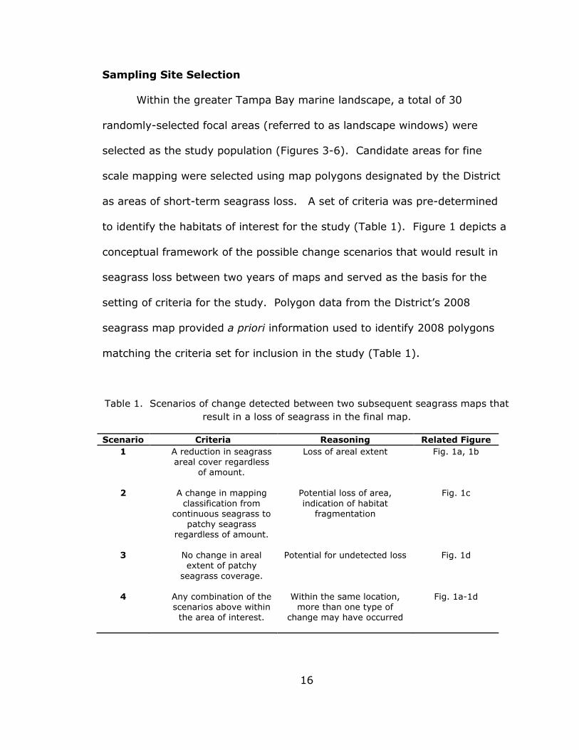
Table 1. Scenarios of change detected between two subsequent seagrass maps that result in a loss of seagrass in the final map.
Scenario Criteria Reasoning Related Figure 1 A reduction in seagrass
areal cover regardless of amount.
Loss of areal extent Fig. 1a, 1b
2 A change in mapping classification from
continuous seagrass to patchy seagrass
regardless of amount.
Potential loss of area, indication of habitat
fragmentation
Fig. 1c
3 No change in areal extent of patchy
seagrass coverage.
Potential for undetected loss Fig. 1d
4 Any combination of the scenarios above within the area of interest.
Within the same location, more than one type of
change may have occurred
Fig. 1a-1d

17
Two additional restrictions to the site selection process were applied.
The population of 2008 District polygons, reflecting interannual seagrass
loss, was restricted to polygons with maximum extents of 20,234.28 m2
(2.02 ha) and located at depths no greater than 1 m. Additional criteria were
applied that addressed setting practical limitations on the level of effort
required for mapping focal landscape windows and logistical constraints
related to the consistency of photo quality and clarity.
A total of 2,089 polygons were identified that matched all of the
criteria. In GIS, a Jenks natural break algorithm was applied to a frequency
distribution of the polygon sizes and was used to categorize the polygons into
two size categories: large and small. Polygons less than 7,130.56 m2 (0.713
ha) were categorized as small, and polygons greater than 7,130.56 m2
(0.713 ha) but less than 20,234.28 m2 (2.02 ha) were categorized as large.
A random set of 15 small and 15 large polygons was then generated. The
imagery for each of the 30 large and small polygons was reviewed for quality
and polygons were randomly selected repeatedly until 30 sampling locations
with suitable imagery were identified. The 30 District map polygons selected
as sampling locations for the fine scale mapping are now referred to as
landscape windows.
Patch data were collected within 30 focal landscape windows randomly
selected from the two, predetermined large and small size categories. The
extent for each of the 15 small landscape windows ranged from 170 m2 to
5,594 m2 with a median size of 1,150 m2. Interesting to note, eleven of the
small landscape windows were below the District’s contractually mandated

18
minimum mapping unit (MMU) of 2,023 m2. Extent for each of the 15 large
landscape windows ranged from 7,241 m2 to 19,470 m2 with a median area
of 10,964 m2. Landscape windows were designated LW1 to LW30 in ranked
order from smallest to largest. The spatial extent of each of the 30 selected
landscape windows, based on District 2008 map polygons, became fixed
study locations and were then analyzed for seagrass changes for the time
intervals 2004–2006, 2006–2008, and 2004–2008. Overall, the study
investigated a total area of 201,665 m2 (20.17 ha) within the 30 locations.
Data Collection: Source Imagery
The fixed landscape windows were assessed using three years of
imagery 2004, 2006, and 2008 previously collected for District seagrass
mapping purposes. The study’s 2004 traditional film aerial photography was
scanned at 13 µ providing a 0.3 m pixel resolution creating digital imagery
source data. The 2006 and 2008 digital aerial imagery were acquired using a
Z/I Digital Mapping Camera, an airborne imaging sensor. Imagery was
collected at a flight altitude of 3,048 m, equivalent to a photographic scale of
1:24,000 with a pixel resolution of 0.3 m. Additional information related to
the source imagery can be found in Appendix A. Source imagery was loaded
into ArcGIS 10.0 (Environmental Research Systems Institute, Redlands, CA)
as individual geotiff files and displayed on a Dell 24” Full HD widescreen
monitor with 1920 x 1080 resolutions for on-screen interpretation and
digitizing.
19
Data Extraction: Imagery Interpretation
The 30 landscape windows acted as the boundary extents of each
study area. Within the extent of each landscape window, imagery was
analyzed for visual signatures of seagrass and patches were outlined creating
high resolution seagrass maps. Fine scale mapping was conducted by a
single analyst using the ArcGIS 10.0 software sketch and trace editing tools.
All polygon data generated for the fine scale mapping were stored as feature
classes in an ArcGIS 10.0 geodatabase.
Interpretation rules for imagery followed logic similar to that of the
District’s seagrass mapping protocols but were modified to accommodate
mapping at a finer resolution. Mapping to the patch level resulted in a binary
map, without hierarchical structure, and documented only one class type,
“seagrass”. Interpretation of seagrass relied upon evaluating the
fundamental characteristics of color images: color, contrast, texture, and
shadow. Combinations of these traits and the generally round shape of
seagrass patches created the identifiable signature of seagrass in the
reviewed images. The signatures of seagrass patch edges are dark colored
and often distinct in imagery when compared to surrounding lighter colored
sediments. Based on these visual representations of patch boundaries in
images, the perimeters for all individual seagrass patches were outlined. The
primary interpretation rule was to map all seagrass patches with distinct
boundaries meeting the MMU of 1 m2 when the imagery was zoomed into,
on-screen, to a mapping and digitizing scale of 1:500.

20
Data extraction protocols were tested on five landscapes prior to
starting the fine scale mapping with the main objective to confirm the use of
a 1 m2 MMU within the limitations of the source imagery and digitizing tools.
While viewing imagery at a 1:500 scale on-screen, seagrass patches smaller
than 1 m2 were visible, however delineation of patch boundaries was difficult
to map consistently. Mapping patches smaller than an MMU of 1 m2 had the
potential to create suspect data with unacceptable levels of inaccuracy and
uncertainty. The test confirmed 1 m2 seagrass patches could be successfully
digitized using ArcGIS 10.0 Editor tools. Any seagrass patches mapped for
the fine scale study found to be less than 1m2 were removed from the
dataset.
Prior to placing line work along patch boundaries, various zoom scales
were employed to assist in visualizing seagrass patches within each
landscape window and to garner the best understanding of patch boundaries.
Consistency in interpretation and delineation was maintained by drawing all
line work at a 1:500 digitizing scale. Instances were encountered where
discrete features or a patch’s edge detail was visible at the 1:500 digitizing
scale but logistically could not be drawn to demarcate all details effectively.
The difficulties were due to tolerance constraints or functionality of the
editing tool, in these cases after a patch was delineated at a digitizing scale
of 1:500, the detailing of line-work was enhanced by zooming into the image
and editing the outline of patches at a 1:100 scale. The smaller scale
allowed for more accurate observation of patch details allowing the

21
placement of additional vertices or movement of vertices to the desired,
correct position along the patch boundary.
The positional accuracy of District’s map line work is reduced when
examined at a finer mapping scale of 1:500. Boundaries drawn (digitized) to
delineate the outlines of seagrass habitats within District maps were placed
to differentiate continuous seagrass from areas with multiple patches of
seagrass more widely dispersed throughout areas of unvegetated sediment
and often too small to be mapped independently in the District maps as
seagrass features. District polygon boundaries for continuous or patchy
seagrass habitats were drawn when imagery was viewed at mapping scale of
no less than 1:2,500. When viewed at a more detailed, 1:500 mapping
scale, for the purposes of fine resolution mapping, sometimes seagrass
signatures were visible within the landscape windows that were not intended
to be included inside of the original District landscape window linework. Such
signatures currently included inside landscape window boundaries that
crossed into the study area were the result of “spillover” from external
patches or larger meadows originating outside of and adjacent to, the
landscape window boundaries of interest to the study. To capture this
distinction, all polygons delineated for the fine scale map were labeled with
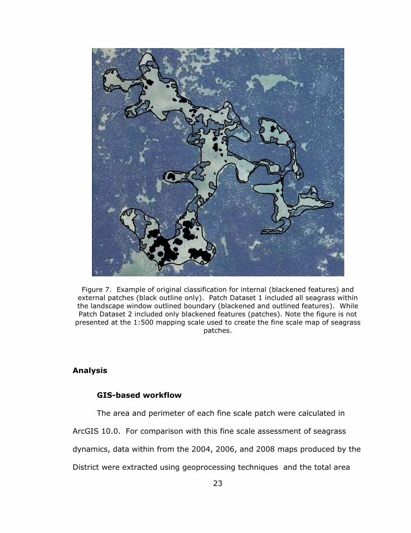
an origination attribute feature of “internal” or “external”.
The fine scale mapping protocols allow for the mapping of all seagrass
signatures within the study’s extent and therefore the leading edges of any
external patches contained within the landscape window were delineated only
to the extent of the landscape window boundary (Figure 7). At landscape

22
window boundaries where fine scale mapping ends, the trace editing tool was
utilized to follow and capture the exact existing landscape window boundary.
Each identifiable intrusion of the landscape window boundary by portions of
external seagrass patches was outlined and labeled in the map attributes as
originating from outside of the landscape window. In general, patches
contained completely within the landscape window, even if adjacent to and
touching a landscape window boundary, were labeled as an interior patches.
Seagrass patches were also labeled as interior patches if origination could not
be determined because a patch was sufficiently large that it extended beyond
the boundaries of the landscape window and origination was unclear. The
identification of a patch’s origination attribute allowed for data related to the
external patches to be both included and excluded from datasets for analysis
purposes. Data related to all seagrass patches delineated in the fine scale
mapping is referred to as Patch Dataset 1; Patch Dataset 1 with external
patches removed, is now referred to as Patch Dataset 2.
23
Figure 7. Example of original classification for internal (blackened features) and external patches (black outline only). Patch Dataset 1 included all seagrass within the landscape window outlined boundary (blackened and outlined features). While Patch Dataset 2 included only blackened features (patches). Note the figure is not
presented at the 1:500 mapping scale used to create the fine scale map of seagrass patches.
Analysis
GIS-based workflow
The area and perimeter of each fine scale patch were calculated in
ArcGIS 10.0. For comparison with this fine scale assessment of seagrass
dynamics, data within from the 2004, 2006, and 2008 maps produced by the
District were extracted using geoprocessing techniques and the total area

24
(m2) of each FLUCCS code (patchy seagrass, continuous seagrass, tidal flats,
land, or water) were collected. Data derived from both fine scale and District
maps were exported as tabulated data for calculation of landscape metrics
and data interpretation.
Data compilation and metric calculations
The fine scale individual polygon areas and perimeters were summed
to calculate patch counts, total seagrass area, total seagrass perimeter, and
percent seagrass cover (proportion of seagrass within the total landscape
area) for each landscape window in Patch Dataset 1 and Patch Dataset 2.
This was done by year for each landscape window thereby creating area-
based metrics that could be compared over time intervals. Time interval
metrics, i.e., year-to-year changes in a specified area-based metric, were
calculated for 2004 to 2006 (time interval 1), 2006 to 2008 (time interval 2),
and the overall time period, 2004 to 2008 (time interval 3= net change).
The time periods depict two consecutive intervals of interannual change,
interval 1 and 2, and the overall time interval 2004 to 2008 (interval 3)
depicted net change. A total of n=30 landscape windows were examined and
used to evaluate time interval metrics, those that calculate the change in an
area-based metric for the years specified in an interval (e.g. 2004-2006),
with n= 90 potential instances of change for area-based metrics by
landscape windows over all time intervals. Specific area-based metrics were
compared over time and the following outcomes assessed: change in patch
count, change in total seagrass area, change in percent cover, and area
percent change (Equation 1). Instances occurred when it was not possible to

25
calculate percent change for an interval because seagrass was absent within
the landscape windows at the start of the interval. To compare outcomes of
areal change from fine scale maps, with that of District maps, data by
FLUCCS code was aggregated into two classes “seagrass present” and
“seagrass absent”. These data were then used to calculate change in
seagrass area and change in seagrass percent cover for District maps.
Equation 1. Percent Change= [(New Observation- Old Observation) ]*100 Old Observation
The level of detectable percent change in seagrass area for this study
was set at ≥5% in either the positive or negative direction; any change ≤5%
was considered stable seagrass with no change. Direction of change
analyses were conducted for the all time periods, interval 1 (n= 26), interval
2 (n= 28), and interval 3 (n= 26). The percent change value for each
observation was converted to categorical data (positive, negative, and no
change).
Nonparametric statistics were conducted using SYSTAT 13 (Copyright
SYSTAT Software, Inc. 2009) to compare types of changes recorded in small
and large landscape windows and patterns of change and patterns of change
in fine scale mapping compared to District broad scale mapping. Specifically
the Chi Square Test of Independence was used on Patch Dataset 2 to
determine if there was any association between direction of change for large
and small landscape window categories. The null hypothesis of association
could not be rejected so the landscape window categories were pooled for

26
further analysis. Chi Square Goodness of Fit Tests were conducted to
determine if the observed frequencies of positive and negative change in fine
scale mapping: a) differed from equal proportions of observations, or b)
differed from proportions of negative and positive change previously
documented in District seagrass maps. In this case a 0.60 positive change
and 0.40 negative change was reported from change analyses of the District
seagrass maps.
Descriptive statistics for area and perimeter of seagrass patches were
calculated for the Patch Dataset by landscape window size categories (large
versus small) to examine differences in central tendencies and dispersion.
Paired comparison tests were run on the absolute value of change in total
seagrass area for each landscape window over each time interval. Wilcoxon
Sign Ranked Tests were run to compare Patch Dataset 1 change in total
seagrass area and Patch Dataset 2 change in total seagrass area for each
year of data. The patch size cumulative distribution curves were created for
the large and small landscape window size categories by year to examine
temporal differences as well as differences in landscape window size
categories. Mann-Whitney Tests were used to determine if there were
significant differences between percent change in small versus large
landscape windows during time intervals 1, 2, and 3.
To measure seagrass fragmentation as a mechanism of loss, Sleeman
et al. (2005) suggested area-weighted mean perimeter to area ratio, a
measure of shape complexity, as one of the most appropriate indices. The

27
area-weighted mean perimeter to area ratio equation, as presented in Feagin
and Wu (2006) was calculated using Equation 2;
Equation 2. PARA_AM= Σnj=1 [ [ pij ] * [ aij ] ]
aij Σnj=1 aij
where n is the number of patches in the landscape class i (landscape
window), pij is the perimeter of patch ij, and aij is the area of patch ij.
The statistical methods and landscape indices specified will be used to
characterize and compare different levels of spatial and temporal
heterogeneity.

28
RESULTS
Patterns in Area-based Metrics for All Map Data
Data were compiled from a time series of fine scale seagrass maps
conducted within the 30 landscape windows of various sizes and locations.
Summary characteristics of each landscape window are presented in Table 2.
The study’s comprehensive dataset (Patch Dataset 1) documented a total of
1,617 individual seagrass patches with a cumulative area represented by
patches totaling 182,887 m2 (18.29 ha) of seagrass. Number of seagrass
patches, total area, and percent cover are presented for each landscape
window by year (Table 3). The range in seagrass area within patches per
landscape window was large (0 m2 -1,000’s m2) among the mapped
locations. When all 30 landscape windows are combined, the fine resolution
maps recorded a decrease in total seagrass area of -16% from 2004-2006
and a subsequent increase in seagrass of 54% from 2006-2008. The net
change in seagrass total area from 2004-2008 was a gain in seagrass of
17,065 m2, or a 29% increase.
Changes in total seagrass area over time for individual landscape
windows revealed that not all landscape windows contributed to the overall
increase in seagrass for the fine scale mapping effort. Landscape windows
were examined by landscape window size categories large and small (see

29
methods, Figure 8) for change in total seagrass area during the three time
intervals.
Figure 8. Histogram of the size distribution of extents of landscape windows. The landscape windows are organized by the small landscape window size category
(LW1-15) and large landscape window size category (LW16-30). The dashed line separates the two size categories.
When seagrass area loss was documented, for small landscape
windows recording loss during a 2-year time interval, 5 of the 8 (62.5%)
ended with a net loss when viewed over the entire 4-year period (Figures 9).
In contrast, only 2 of the 9 (22.22%) large landscape windows recording
instances of loss during a 2-year time interval displayed a net loss over 4
years (Figure 10). In addition, temporal change in seagrass patterns among
0
2,000
4,000
6,000
8,000
10,000
12,000
14,000
16,000
18,000
20,000
To
tal
Are
a (
m2)
Landscape Window Name (Ordered by Size)

30
the size categories was not similar; the majority of instances of loss occurred
in time interval 1 (2004-2006) for small landscape windows, while loss
occurred more often in time interval 2 (2006-2008) for large landscape
windows. The temporal patterns of loss were not consistent across large
landscape windows and varied in the amount of seagrass lost per time
interval (interval 1 mean= -2,614.38 m2 versus interval 2 mean= -50.76
m2). The time interval metric percent change in seagrass area, was used to
determine whether the areal losses incurred by the 7 landscape windows
experiencing net loss of seagrass during the study period were large enough
to warrant detectable change.

31
Table 2. Summary characteristics of 30 focal landscape windows.
Landscape Window
2008 District Map Classification
Landscape Position Geographic Region
1 Patchy Seagrass Partial Protection Middle Tampa Bay
2 Tidal Flat Partial Protection Lower Tampa Bay
3 Patchy Seagrass Exposed Lower Tampa Bay
4 Tidal Flat Partial Protection Lower Tampa Bay
5 Patchy Seagrass Behind Bar Manatee River
6 Tidal Flat Protected Boca Ciega Bay
7 Patchy Seagrass Exposed Boca Ciega Bay
8 Patchy Seagrass Partial Protection Middle Tampa Bay
9 Patchy Seagrass Exposed Middle Tampa Bay
10 Patchy Seagrass Exposed Lower Tampa Bay
11 Tidal Flat Protected Lower Tampa Bay
12 Patchy Seagrass Exposed Lower Tampa Bay
13 Patchy Seagrass Exposed Old Tampa Bay
14 Patchy Seagrass Exposed Lower Tampa Bay
15 Patchy Seagrass Behind Bar Old Tampa Bay
16 Patchy Seagrass Protected Old Tampa Bay
17 Patchy Seagrass Exposed Old Tampa Bay
18 Patchy Seagrass Behind Bar Middle Tampa Bay
19 Tidal Flat Behind Bar Old Tampa Bay
20 Patchy Seagrass Partial Protection Old Tampa Bay
21 Patchy Seagrass Protected Middle Tampa Bay
22 Patchy Seagrass Behind Bar Middle Tampa Bay
23 Patchy Seagrass Partial Protection Old Tampa Bay
24 Patchy Seagrass Behind Bar Old Tampa Bay
25 Patchy Seagrass Behind Bar Middle Tampa Bay
26 Tidal Flat Partial Protection Lower Tampa Bay
27 Patchy Seagrass Protected Boca Ciega Bay
28 Patchy Seagrass Partial Protection Middle Tampa Bay
29 Patchy Seagrass Partial Protection Middle Tampa Bay
30 Patchy Seagrass Exposed Old Tampa Bay

32
Table 3. Summary of Patch Dataset 1 by landscape window (LW). Small LW category = LW1-15. Large LW Category = LW16-30. Solid line delimits size
categories.
2004 2006 2008
LW N
ame
LW A
rea
(m2)
No.
of
Patc
hes
Tota
l Are
a (m
2)
Perc
ent
Cove
r
No.
of
Patc
hes
Tota
l Are
a (m
2)
Perc
ent
Cove
r
No.
of
Patc
hes
Tota
l Are
a (m
2)
Perc
ent
Cove
r
1 170 2 122.08 71.66 2 141.84 83.26 2 150.09 88.10
2 553 1 553.00 100.00 1 553.00 100.00 7 99.25 17.95
3 599 1 500.76 83.59 1 571.30 95.37 1 563.58 94.08
4 641 1 610.75 95.23 1 541.91 84.49 3 171.28 26.71
5 684 1 614.18 89.76 11 164.71 24.07 4 315.87 46.16
6 1,025 0 0.00 0.00 5 651.62 63.57 2 27.33 2.67
7 1,137 4 198.30 17.44 6 318.93 28.05 5 450.35 39.61
8 1,150 4 78.58 6.83 8 123.49 10.73 7 349.55 30.38
9 1,260 1 793.45 62.99 1 779.39 61.87 1 916.21 72.73
10 1,505 0 0.00 0.00 4 676.06 44.93 5 482.22 32.05
11 1,783 4 27.00 1.51 7 95.89 5.38 19 218.78 12.27
12 2,322 1 550.99 23.73 8 1,978.16 85.19 17 1,523.63 65.61
13 2,610 3 1,375.34 52.69 3 1,303.00 49.92 12 262.00 10.04
14 2,625 3 2,262.60 86.19 9 870.23 33.15 7 1,324.74 50.46
15 5,594 10 593.25 10.61 20 753.98 13.48 26 1,601.56 28.63
16 7,241 4 1,079.58 14.91 47 355.47 4.91 39 3,284.80 45.36
17 7,365 14 4,425.68 60.09 37 654.52 8.89 39 1,553.46 21.09
18 8,508 12 247.35 2.91 50 571.01 6.71 43 1,336.27 15.71
19 9,173 2 11.55 0.13 5 19.81 0.22 20 1,909.81 20.82
20 9,686 20 1,200.15 12.39 29 1,937.36 20.00 1 9,686.09 100.00
21 9,784 1 8,383.19 85.69 1 8,823.37 90.19 1 8,463.98 86.51
22 9,815 9 9,173.84 93.47 28 4,648.54 47.36 2 9,594.04 97.75
23 10,964 14 547.20 4.99 49 1,219.03 11.12 38 2,631.72 24.00
24 11,623 39 3,322.57 28.59 68 428.72 3.69 62 6,406.47 55.12
25 11,787 3 146.70 1.24 4 269.62 2.29 53 3,446.70 29.24
26 13,501 39 673.58 4.99 60 1,857.81 13.76 23 956.66 7.09
27 14,727 9 568.50 3.86 25 1,174.53 7.98 66 2,769.45 18.81
28 16,355 24 939.19 5.74 11 629.33 3.85 19 4,552.02 27.83
29 18,008 8 16,579.47 92.07 104 13,117.43 72.84 112 7,035.98 39.07
30 19,470 37 2,841.98 14.60 48 3,750.74 19.26 57 3,401.94 17.47

33
Figure 9. Change in seagrass total area over for each small landscape window. a) Change in seagrass area for small landscape windows during time intervals 1 (filled diamonds) and 2 (hollow squares). b) Change in seagrass for entire study period
interval 3 (filled squares).
-2,000
-1,600
-1,200
-800
-400
0
400
800
1,200
1,600
2,000
0 1 2 3 4 5 6 7 8 9 10 11 12 13 14 15
Ch
an
ge i
n T
ota
l S
eag
rass
Are
a (
m2) a)
-2,000
-1,600
-1,200
-800
-400
0
400
800
1,200
1,600
2,000
0 1 2 3 4 5 6 7 8 9 10 11 12 13 14 15
Ch
an
ge i
n T
ota
l S
eag
rass
Are
a (
m2)
Landscape Windows (Ordered by Size)
b)

34
Figure 10. Change in seagrass total area over for each small landscape window. a) Change in seagrass area for large landscape windows during time intervals 1 (filled diamonds) and 2 (hollow squares). b) Change in seagrass for entire study period
interval 3 (filled squares).
-10,000
-8,000
-6,000
-4,000
-2,000
0
2,000
4,000
6,000
8,000
10,000
15 16 17 18 19 20 21 22 23 24 25 26 27 28 29 30
Ch
an
ge i
n T
ota
l S
eag
rass
Are
a (
m2) a)
-10,000
-8,000
-6,000
-4,000
-2,000
0
2,000
4,000
6,000
8,000
10,000
15 16 17 18 19 20 21 22 23 24 25 26 27 28 29 30
Ch
an
ge
in T
ota
l S
eag
rass
Are
a (
m2)
Landscape Windows (Ordered by Size)
b)

35
Detectable change of greater than or equal to ±5% of percent change
in seagrass area (see methods) was documented for 93% of all instances
where percent change was measured. Only two landscape windows
positioned within protected (along a mangrove island and behind a nearshore
bar) locations in Middle Tampa Bay (i.e. LW21 and LW22) maintained stable
cover levels of seagrass from 2004 to 2008. Review of the directionality of
change in seagrass across all landscape windows (Table 4) indicated that
seagrass within all 7 landscape windows recording net loss in total seagrass
area experienced detectable percent change in seagrass area. Detectable
net loss occurred in 2 large (LW 17 and 29) and 5 small landscape windows
(LW 2, 4, 5, 13, and 14). The landscape windows with seagrass loss were
located within all 4 regions of Tampa Bay (Figure 2).
Table 4. Direction of change counts based on percent change of seagrass area for all landscape windows. Detectable change reflects a percent change ≥5%.
Interval 1 Interval 2 Interval 3
(2004-2006) (2006-2008) (2004-2008) Increase (Positive) 16 19 19 Decrease (Negative) 10 9 7 Stable (No Change) 2 2 2 Count 28 30 28 Total Detectable Change 26 28 26
Analyses of the percent change counts for gains and losses (Table 4)
indicated that when testing all instances of detectable change, the direction
of change that occurred was not related to landscape window size.
Observations of change for small versus large landscape windows were not
independent (χ2 = 1.605, df= 1, p-value= 0.205). Therefore, counts of

36
direction of positive and negative change from small and large landscape
windows were pooled by year to examine further patterns of seagrass change
versus expected frequencies of gains and losses. During time intervals 1 and
2, the counts of positive and negative changes in seagrass did not
significantly deviate from the hypothesis that an equal proportion of positive
and negative changes would be observed for the fine scale mapping could
not be rejected (Table 5a). Only during Interval 3 (2004-2008) was direction
of change significantly different than the equal proportions expected, with a
disproportionately higher number of gains recorded versus that expected.
Using the same observations, versus expected values generated from District
data (0.40 losses and 0.60 gains) no significant differences between
expected and observed counts were recorded for any time interval. This
indicates that the proportions of positive and negative change recorded with
fine scale mapping did not significantly differ from 60% positive changes and
40% negative changes (Table 5b).
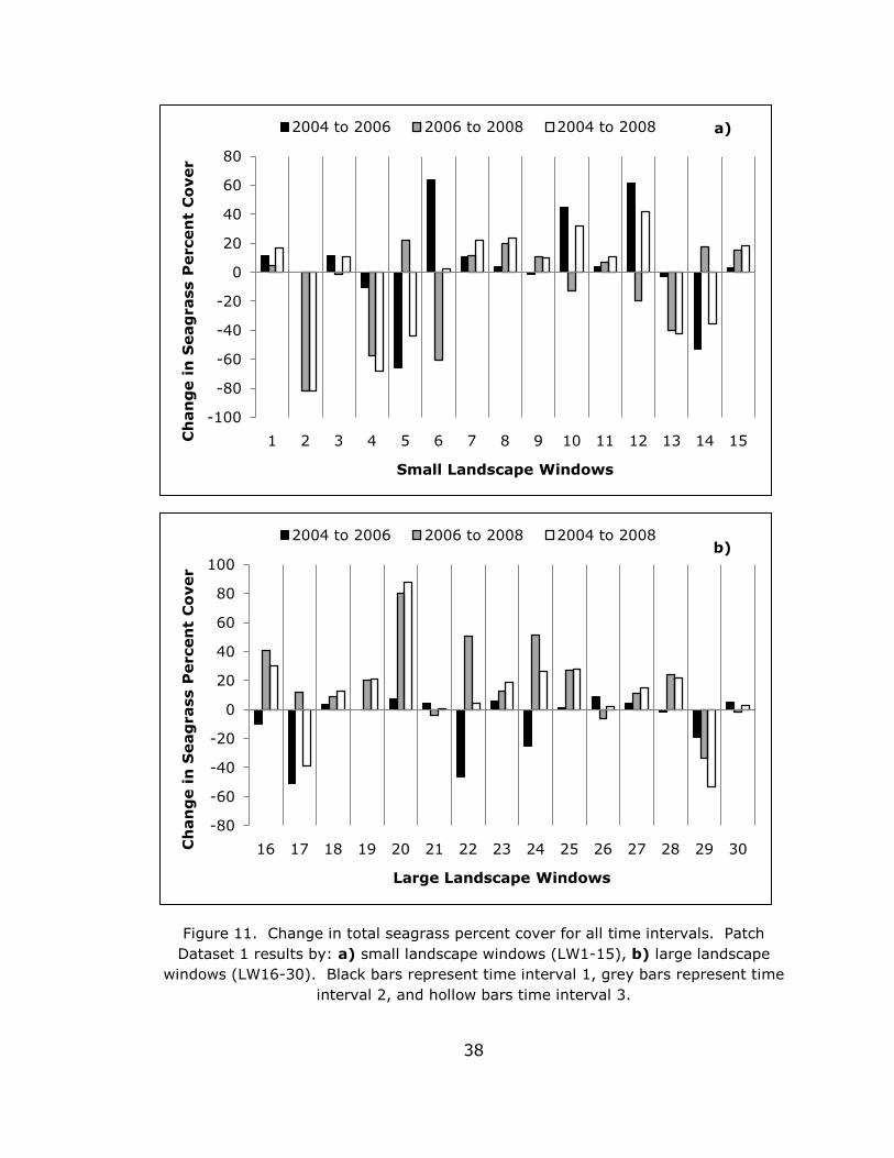
Patterns of change in seagrass percent cover (total seagrass area/total
landscape window extent) were examined for each of the 30 landscape
windows for each time interval (Figure 11). The most obvious patterns of
change in percent seagrass cover (percent cover time b – percent cover time a)
were noted for large landscape windows as moderate to large increases in
percent seagrass cover occurred in time interval 2 (2006-2008). Patterns of
change in percent seagrass cover for small landscape windows were more
variable over time with moderate and large percent change in both positive
and negative directions. The small landscape window category had a higher

37
frequency of percent cover net loss and displayed a larger range of loss
(35.72% - 82.05%) than that for large landscape windows. Although small
landscape windows contain less seagrass per m2, the losses incurred reflect a
larger proportion of total seagrass cover for these areas.
Table 5. Directionality of change counts for Patch Dataset 1 tested using Chi2 Goodness of Fit. All count data analyzed for each time period. Results for null hypothesis: a) expecting equal proportions of positive and negative change, b)
expecting 60% positive change and 40% negative change.
a.) Equal Proportions of Positive and Negative Change
χ2 df p-value
Interval 1 (2004-2006) 1.385 1 0.240
Interval 2 (2006-2008) 3.571 1 0.059
Interval 3 (2004-2008) 5.538 1 0.019
b.) Positive Change (60%) and Negative Change (40%)
χ2 df p-value
Interval 1 (2004-2006) 0.256 1 0.873
Interval 2 (2006-2008) 0.72 1 0.396
Interval 3 (2004-2008) 1.852 1 0.173
38
Figure 11. Change in total seagrass percent cover for all time intervals. Patch Dataset 1 results by: a) small landscape windows (LW1-15), b) large landscape
windows (LW16-30). Black bars represent time interval 1, grey bars represent time interval 2, and hollow bars time interval 3.
-100
-80
-60
-40
-20
0
20
40
60
80
1 2 3 4 5 6 7 8 9 10 11 12 13 14 15Ch
an
ge i
n S
eag
rass
Perc
en
t C
over
Small Landscape Windows
2004 to 2006 2006 to 2008 2004 to 2008 a)
-80
-60
-40
-20
0
20
40
60
80
100
16 17 18 19 20 21 22 23 24 25 26 27 28 29 30Ch
an
ge i
n S
eag
rass
Perc
en
t C
over
Large Landscape Windows
2004 to 2006 2006 to 2008 2004 to 2008b)

39
Influence of External Patches on Evaluation of Seagrass Dynamics
External patches (see Figure 7) represented 42.7% of all patches
mapped at the fine scale. A total of 690 external patches were delineated for
the entire study and were documented in increasing numbers over time as
well as increasing in their geographical extent from 17 landscape windows in
2004, to 21 and 22 in 2006 and 2008 respectively. One landscape window,
LW4, contained external patches exclusively with no seagrass patches
unattached to seagrass coverage extending outside of the specified
landscape window. The relative influences of seagrass contributions from
margins of bordering seagrass patches or meadows outside of the landscape
windows may affect the patterns of change detectable for patches completely
contained within the landscape windows.
The internal and external patches from Patch Dataset 1 were reviewed
by plotting the patches separately in box plots for each year (Figure 12)
which provided information on the influence of external patches as major
contributors to seagrass dynamics. The central tendencies of seagrass patch
total area (m2) for the internal patches compared to external patches
differed, with the total area of external patches similar to or less than that
for internal patches. Patch size differences for internal patches compared to
external patches were apparent when plotted (Figure 12). Distribution of
patch area had positive skewness for internal and external patch types with a
shift to smaller patch sizes over time. Outliers of patch size were not
consistent for the two patch types and were recorded for larger patch sizes
when only internal patches were considered. Across years, differences in
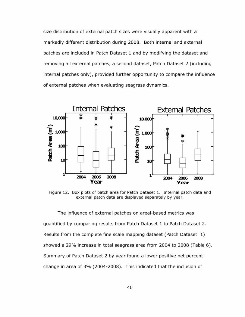
40
size distribution of external patch sizes were visually apparent with a
markedly different distribution during 2008. Both internal and external
patches are included in Patch Dataset 1 and by modifying the dataset and
removing all external patches, a second dataset, Patch Dataset 2 (including
internal patches only), provided further opportunity to compare the influence
of external patches when evaluating seagrass dynamics.
Figure 12. Box plots of patch area for Patch Dataset 1. Internal patch data and external patch data are displayed separately by year.
The influence of external patches on areal-based metrics was
quantified by comparing results from Patch Dataset 1 to Patch Dataset 2.
Results from the complete fine scale mapping dataset (Patch Dataset 1)
showed a 29% increase in total seagrass area from 2004 to 2008 (Table 6).
Summary of Patch Dataset 2 by year found a lower positive net percent
change in area of 3% (2004-2008). This indicated that the inclusion of
2004 2006 2008Year
1
10
100
1,000
10,000
Patc
h Are
a (m
2 )
Internal Patches
2004 2006 2008Year
1
10
100
1,000
10,000
Patc
h Are
a (m
2 )
External Patches

41
external patches in Patch Dataset 1 resulted in higher magnitudes of positive
change (gains) in seagrass by the end of the study period (Table 6).
Table 6. Fine scale mapping total seagrass area (m2). Patch Dataset 1 includes internal and external patches. Patch Dataset 2 includes internal patches only.
2004 2006 2008
External Patch Area 6,520 5,581 21,976 Internal Patch Area (Patch Dataset 2) 51,901 43,400 53,310
Total Seagrass Area, All Patches (Patch Dataset 1) 58,421 48,981 75,286
A paired comparison of the absolute values of change in total seagrass
area (|total area time b – total area time a|) for landscape windows using Patch
Dataset 1 and Patch Dataset 2 for each time interval was examined using the
Wilcoxon Signed-Rank Test. Results indicated significant differences in
absolute values of total seagrass area change in landscape windows across
all time intervals (Interval 1: z-score= 2.381, p-value= 0.017; Interval 2: z-
score= 2.386, p-value= 0.017; Interval 3: z-score= 2.678, p-value= 0.007).
Specifically, inclusion of the seagrass organized as patches originating from
areas outside of the landscape windows altered the outcomes of patterns of
change for seagrass in the landscape windows examined here. Since
inclusion of external patches in Patch Dataset 1 was found to affect seagrass
change results in landscape windows, only Patch Dataset 2 was subsequently
used for calculations of patch level metrics. Patch level metrics were used to
investigate ecologically relevant patterns in seagrass cover and arrangement.

42
Patch-based Landscape Analysis
The modified dataset including only internal patches, Patch Dataset 2,
displays a decrease in total seagrass between 2004-2006 and an increase in
seagrass from 2006-2008 similar to that found for the comprehensive fine
scale mapping dataset (Table 7). Individual seagrass patch data from Patch
Dataset 2 was summarized by landscape window and aggregated into the
small and large landscape window size categories to examine patterns in
seagrass composition and configuration. The composition of the landscape
window size categories in 2006 revealed the losses documented that year
occurred in the large landscape window size category (Table 7). Patch
configuration for landscape window size categories documented a doubling or
more of the number of patches in both the large and small categories from
2004-2006. The increase in number of patches for large landscape windows
coincided with a decrease in total seagrass area while the increase in patches
for small landscape windows coincided with an increase in total seagrass
area. Findings suggested there was a difference in seagrass dynamics for
large and small landscape windows.
Table 7. Patch Dataset 2 composition and configuration broken out by the landscape window size categories large and small.
2004 2006 2008
No. of
Patches Total Area
(m2) No. of
Patches Total Area
(m2) No. of
Patches Total Area
(m2)
Large LWs 146 44,307.61 352 35,414.93 281 46,422.55
Small LWs 29 7,593.38 59 7,985.44 60 6,887.40
Patch Dataset 2 175 51,900.99 411 43,400.37 341 53,309.95

43
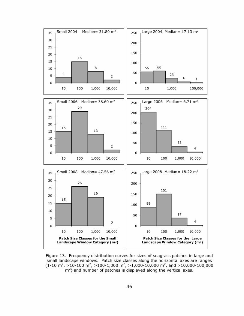
Patch Dataset 2 was used to quantify the size range of seagrass
patches within 30 locations within Tampa Bay. Patches over all years within
the large landscape window size category ranged in size from 1.02 m2 –
14,132.67 m2. Patches over all years within the small landscape window size
category ranged in size from 1.04 m2 – 1,964.27 m2. The maximum patch
size in the large landscape window size category was 7 times larger than the
maximum size of patches as recorded in the small landscape windows and
was larger in size than any of the small landscape window extents. Median
patch sizes for the small and large landscape window categories were 39.12
m2 and 12.52 m2 respectively. Variation and spread in patch size distribution
were also lower for the small landscape window size category (Tables 8 and
9).
The seagrass dynamics of large and small landscape windows are
further explained by the patch size distributions for the landscape window
size categories by year. Focusing on the 2006 frequency distributions
(Figure 13), the increase that occurred from 2004-2006 in number of patches
for both the small and large landscape window size categories showed a shift
to smaller patch sizes. The large landscape window size category had a
greater increase in the smallest patch size class of 1 m2 – 10 m2 compared to
the small landscape window size category.

44
Table 8. Descriptive statistics for the large landscape window size category from Patch Dataset 2.
Area (m2) Perimeter (m) N of Cases 779 779 Minimum 1.02 4.02 Maximum 14,132.67 1,295.02 Sum 126,145.09 29,370.85 Median 12.52 14.85 Arithmetic Mean 161.93 37.70 Standard Deviation 985.00 98.62 Coefficient of Variation 6.08 2.62
Table 9. Descriptive statistics for the small landscape window size category from Patch Dataset 2.
Area (m2) Perimeter (m) N of Cases 148 148 Minimum 1.04 4.07 Maximum 1,964.27 246.75 Sum 22,466.21 6,839.09 Median 39.12 28.38 Arithmetic Mean 151.80 46.21 Standard Deviation 284.38 49.17 Coefficient of Variation 1.87 1.06
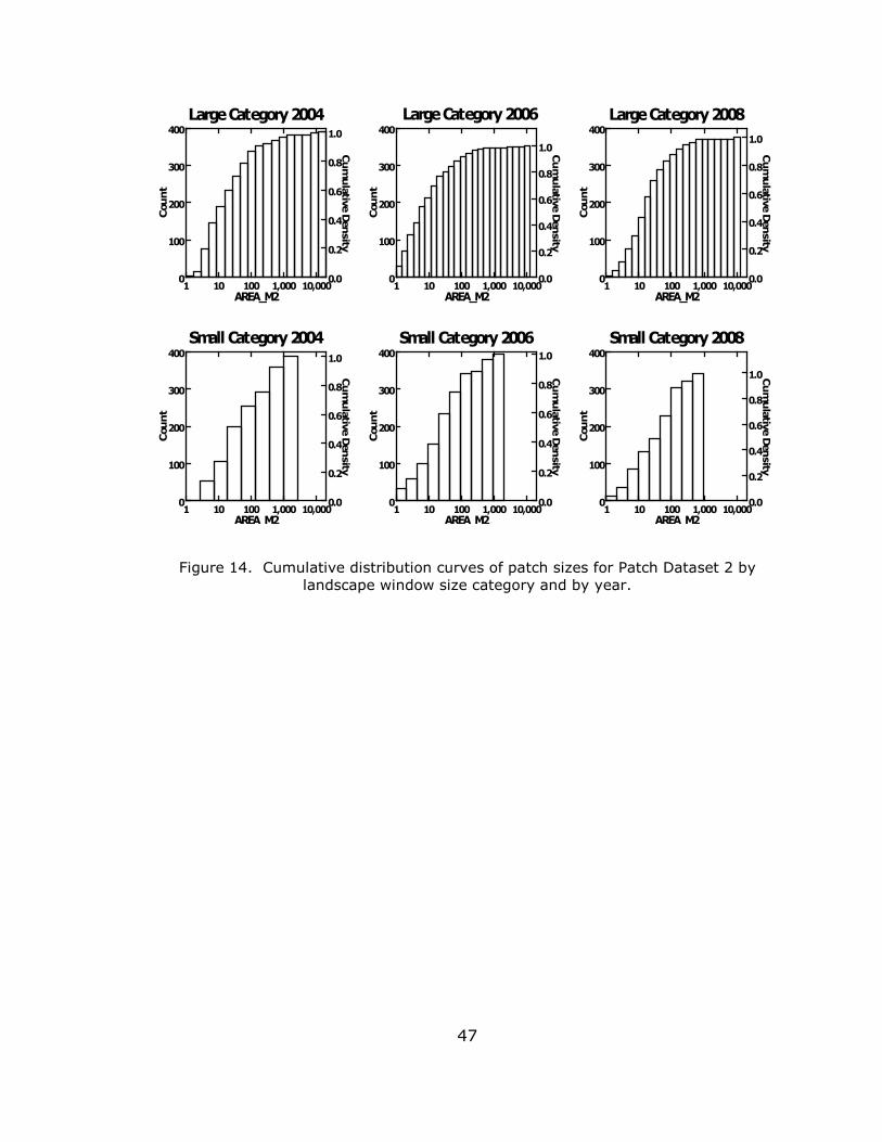
From a different perspective, patch size cumulative distribution curves
for Patch Dataset 2, organized by the large and small landscape window
categories (Figure 14), changed over time and differed between size
categories. The difference in medians is partially explained by a higher
percentage of patches being ≤10 m2 each year in large landscape compared
to small landscape windows. Nearly 80% or more of patches from large
landscape windows were smaller than 100 m2 each year and this exceeded
the percent of patches less than 100 m2 in small landscape windows.

45
Regardless, the majority of patches in either large or small landscape
windows were less than 100 m2.
The variation in total number of patches also changed over the study
period (Figure 15). Both landscape window categories had the lowest
number of patches per landscape in 2004, with the maximum patch counts
occurring in 2006. Patch counts varied by landscape window size category
with the larger landscape windows having a greater variation in number of
patches. Fourteen of the 15 small landscape windows acted similarly and
maintained patch counts under 10 for the 4 year study period. One
landscape window, LW15, maintained a slightly higher number of patches
within its boundaries, with counts similar to some larger landscape windows.
Percent change in total seagrass area, where the difference in area
between the new and old observations is divided by the total area of the old
observation (Equation 1), is a time interval metric indicating the magnitude
of change occurring over time. The absolute values of percent change in
seagrass area for landscape windows during time interval 1 (n= 27) and time
interval 2 (n= 28) were plotted against the total area (m2) of landscape
windows (Figure 16). Change greater than 200% during time interval 1 only
occurred in 1 small and 1 large landscape window. While during time interval
2, 5 large landscape windows changed more than 200%. The majority of
percent change in seagrass area for the 30 landscape windows was less than
200% during either time interval (Figure 16), regardless of landscape window
size.
46
Figure 13. Frequency distribution curves for sizes of seagrass patches in large and small landscape windows. Patch size classes along the horizontal axes are ranges (1-10 m2, >10-100 m2, >100-1,000 m2, >1,000-10,000 m2, and >10,000-100,000
m2) and number of patches is displayed along the vertical axes.
4
15
8
2
0
5
10
15
20
25
30
35
10 100 1,000 10,000
Small 2004 Median= 31.80 m2
56 60
236 1
0
50
100
150
200
250
10 1,000 100,000
Large 2004 Median= 17.13 m2
15
29
13
2
0
5
10
15
20
25
30
35
10 100 1,000 10,000
Small 2006 Median= 38.60 m2
204
111
33
40
50
100
150
200
250
10 100 1,000 10,000
Large 2006 Median= 6.71 m2
15
26
19
00
5
10
15
20
25
30
35
10 100 1,000 10,000
Patch Size Classes for the Small Landscape Window Category (m2)
Small 2008 Median= 47.56 m2
89
151
37
40
50
100
150
200
250
10 100 1,000 10,000
Patch Size Classes for the Large Landscape Window Category (m2)
Large 2008 Median= 18.22 m2
47
Figure 14. Cumulative distribution curves of patch sizes for Patch Dataset 2 by landscape window size category and by year.
1 10 100 1,000 10,000AREA_M2
0.0
0.2
0.4
0.6
0.8
1.0
Cum
ulative D
ensity
0
100
200
300
400
Cou
nt
Large Category 2004
1 10 100 1,000 10,000AREA_M2
0.0
0.2
0.4
0.6
0.8
1.0Cum
ulative D
ensity
0
100
200
300
400
Cou
nt
Large Category 2006
1 10 100 1,000 10,000AREA_M2
0.0
0.2
0.4
0.6
0.8
1.0
Cum
ulative D
ensity
0
100
200
300
400
Cou
nt
Large Category 2008
1 10 100 1,000 10,000AREA M2
0.0
0.2
0.4
0.6
0.8
1.0
Cum
ulative D
ensity
0
100
200
300
400
Cou
nt
Small Category 2004
1 10 100 1,000 10,000AREA M2
0.0
0.2
0.4
0.6
0.8
1.0
Cum
ulative D
ensity
0
100
200
300
400
Cou
nt
Small Category 2006
1 10 100 1,000 10,000AREA M2
0.0
0.2
0.4
0.6
0.8
1.0Cum
ulative D
ensity
0
100
200
300
400
Cou
nt
Small Category 2008

48
Figure 15. Patch count by landscape window total area for 2004, 2006, and 2008. Data presented by year: 2004 (diamonds), 2006 (squares), 2008 (triangles).
0
5
10
15
20
25
30
35
40
0 2,000 4,000 6,000 8,000 10,000 12,000 14,000 16,000 18,000 20,000
No
. o
f P
atc
hes
Landscape Window Total Area (m2)
0
10
20
30
40
50
60
70
80
0 2,000 4,000 6,000 8,000 10,000 12,000 14,000 16,000 18,000 20,000
No
. o
f P
atc
hes
Landscape Window Total Area (m2)
0
10
20
30
40
50
60
70
80
0 2,000 4,000 6,000 8,000 10,000 12,000 14,000 16,000 18,000 20,000
No
. o
f P
atc
hes
Landscape Window Total Area (m2)

49
Figure 16. Patch Dataset 2, absolute values of percent change in seagrass area by landscape window over time. Data is shown for: a) small landscape windows, and
b) large landscape windows during Interval 1 (filled diamonds) and Interval 2 (hollow squares).
-200
-100
0
100
200
300
400
500
600
700
800
900
1,000
0 1 2 3 4 5 6 7 8 9 10 11 12 13 14 15Perc
en
t C
han
ge i
n S
eag
rass
Are
a (
%)
Landscape Windows (Ordered by Size)
Small 2004-2006 Small 2006-2008 a)
-200
-100
0
100
200
300
400
500
600
700
800
900
1,000
15 16 17 18 19 20 21 22 23 24 25 26 27 28 29 30Perc
en
t C
han
ge i
n S
eag
rass
Are
a (
%)
Landscape Windows (Ordered by Size)
Large 2004-2006 Large 2006-2008 b)

50
When seagrass percent change was compared in large versus small
landscape windows over each of the three time intervals, no significant
difference in the median values of percent change values were found for time
intervals 1 and 3 (Interval 1: Mann-Whitney Test Statistic= 84.00, p-value=
0.770, df= 1; Interval 3: Mann-Whitney Test Statistic= 109.00, p-value=
0.860, df= 1). However, a significant difference in central tendencies
between large and small landscape windows for time interval 2 was recorded
(Mann-Whitney Test Statistic= 150.00, p-value= 0.017, df= 1). A few large
landscape windows during time interval 2 (2004-2006) displayed greater
percent change than that found in most of the landscape windows. The
findings indicate that both the size of patches and the percentages of change
in total seagrass area varied over time and in dissimilar ways in small versus
large sized landscape windows. Review of composition, configuration, and
changes in seagrass over time suggested that the extent of landscape
windows can influence observations of seagrass patterns and dynamics.
Patch Change, Loss, and Fragmentation
In order to investigate the fate of patches, Patch Dataset 2 (no
external patches) was examined. Using the available data on percent change
in seagrass area for time intervals 1, 2, and 3, the direction of change in
seagrass was qualified as increasing, decreasing, or the absence thereof
(stable seagrass). Detectable change (≥5%) in seagrass area was
documented for 77 of the 82 or 94% of combined percent change
observations for time interval 1 (2004-2006), interval 2 (2006-2008), and

51
interval 3 (2004-2008). Landscape window, LW21, did not exhibit detectable
change and therefore maintained stable cover from 2004 to 2008. Because
LW4, LW6, and LW10 started the study with no internal seagrass patches
present, percent change was not calculated for them in time intervals 1 and
3. This led to the inability to determine whether change in the landscape
windows resulted in net seagrass loss for the study time period (2004-2008).
Landscape window LW4 was the only location where no seagrass patches
originated from within the boundaries of the area during all three years.
Therefore, internal seagrass loss was not possible and no further evaluation
of seagrass change for LW4 was necessary. For the other two landscape
windows that began the study lacking seagrass, LW 10 gained seagrass area
in 2006 then lost some but not all seagrass by 2008, and LW6 gained
seagrass area in 2006 then lost the full extent by 2008. The determinations
of overall loss for LW6 and LW10 were made based on total seagrass area
lost as well as the available percent change measures for time interval 2.
These instances of change qualified LW6 and LW10 as having undergone net
seagrass loss.
Review of the directionality of change in seagrass for small and large
landscape windows, found the most common type of change was positive
(increasing) in seagrass cover (Table 10). Most landscape windows had
gains over all intervals (n=18). Net seagrass loss from 2004 to 2008
occurred in 6 small landscape windows (LW 2, 5, 6, 10, 13, and 14) and 5
large landscape windows (LW 17, 19, 24, 26, and 29), with three of the
landscape windows (LW 2, 5, and 6) experiencing complete mortality in

52
2008. Landscape windows with a net loss of seagrass were located within 5
regions of Tampa Bay (Figure 2) and are presented (Figure 17) as time series
of maps for each landscape window from 2004 to 2008.
Table 10. Direction of detectable change for all landscape windows by time interval using Patch Dataset 2. () represents adjusted counts when net loss determined via
alternative methods are considered.
Interval 1 Interval 2 Interval 3 (2004-2006) (2006-2008) (2004-2008)
Increase (Positive) 15 17 17 Decrease (Negative) 10 9 9 (11)* Stable (No Change) 2 2 1 Count 27 28 27
Total Detectable Change 25 26 26 *Note: The adjusted count for “net loss in seagrass” is based on results from interval 2 for
LWs 6 and 10. This does not affect the total detectable change for interval 3.
Landscape windows with a net decline in seagrass exhibited distinct
change patterns over time during either a singular time interval or
consistently across both 2-year time intervals. Four landscape windows with
a net loss exhibited acute declines during interval 1 (2004-2006). These
declines were characterized as acute because subsequent seagrass gains
(recolonization) during interval 2 were not sufficient to meet levels of
seagrass area seen in initial 2004 coverages (LW 14, 17, 19, and 24). The
second pattern of loss detected was interannual loss during only time interval
2 (2006-2008) where net loss reflected the change that occurred during the
2-year time interval directly preceding the completion of the study in 2008
(LW 2, 6, 10, and 26). The final pattern was chronic decline where landscape
windows underwent loss that persisted through consecutive time intervals 1

53
and 2 (LW 5, 13, and 29). The change patterns clearly reflect different
magnitudes of spatial and temporal dynamics that resulted in loss.
The composition and configuration of landscape windows with net
seagrass loss revealed patterns of negative change and have provided insight
into a major underlying process of negative change, fragmentation.
Fragmentation, as indicated by a loss of seagrass area with a concurrent
increase in the number of seagrass patches present, affected a majority of
the landscape windows with net seagrass loss. Seven of the 11 landscape
windows with net seagrass loss exhibited the stated indications of
fragmentation during either time interval 1 (LW 5, 14, 17, 24, and 29) or
time interval 2 (LW 10 and 13) (Figure 18). However, temporal trends in the
fragmentation show this process occurred most often during time interval 1
(71% of landscape windows). All landscape windows with chronic loss and
acute loss patterns exhibited fragmentation and LW5 fragmentation resulted
in complete mortality of all patches in LW5 (Figure 17b). Four landscape
windows recognized as having undergone fragmentation during either
interval 1 or 2, experienced net fragmentation from 2004 to 2008: LW 13,
14, 17, and 29 (Figure 18).

54
a) Landscape window 2
b) Landscape window 5
c) Landscape window 6
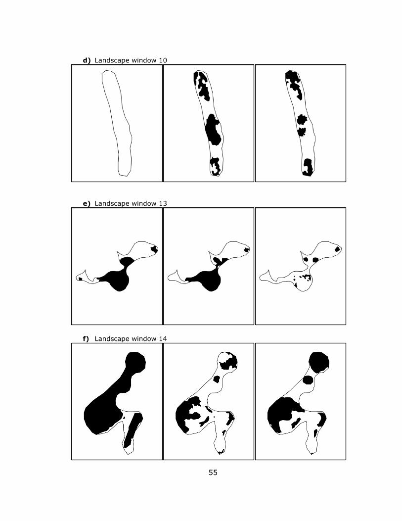
55
d) Landscape window 10
e) Landscape window 13
f) Landscape window 14

56
g) Landscape window 17
h) Landscape window 24
i) Landscape window 26
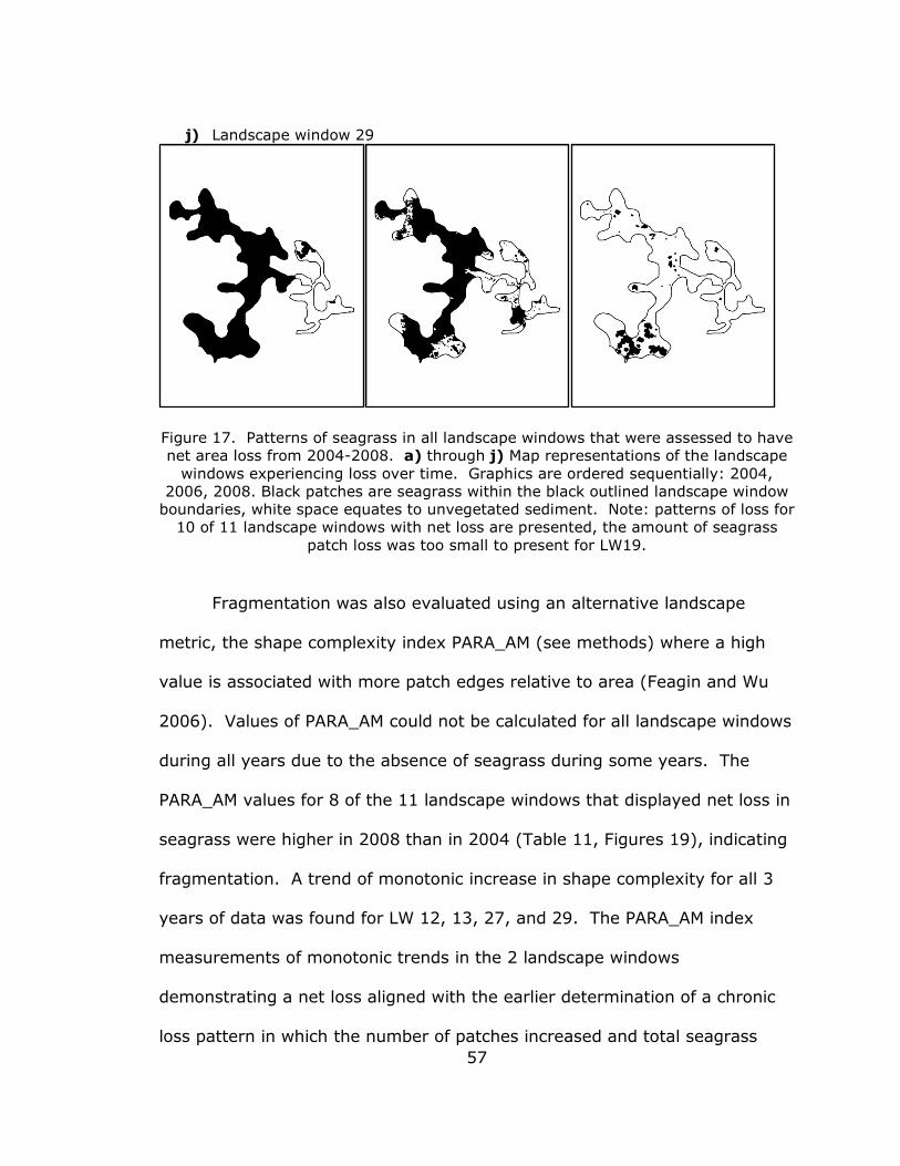
57
j) Landscape window 29
Figure 17. Patterns of seagrass in all landscape windows that were assessed to have net area loss from 2004-2008. a) through j) Map representations of the landscape
windows experiencing loss over time. Graphics are ordered sequentially: 2004, 2006, 2008. Black patches are seagrass within the black outlined landscape window
boundaries, white space equates to unvegetated sediment. Note: patterns of loss for 10 of 11 landscape windows with net loss are presented, the amount of seagrass
patch loss was too small to present for LW19.
Fragmentation was also evaluated using an alternative landscape
metric, the shape complexity index PARA_AM (see methods) where a high
value is associated with more patch edges relative to area (Feagin and Wu
2006). Values of PARA_AM could not be calculated for all landscape windows
during all years due to the absence of seagrass during some years. The
PARA_AM values for 8 of the 11 landscape windows that displayed net loss in
seagrass were higher in 2008 than in 2004 (Table 11, Figures 19), indicating
fragmentation. A trend of monotonic increase in shape complexity for all 3
years of data was found for LW 12, 13, 27, and 29. The PARA_AM index
measurements of monotonic trends in the 2 landscape windows
demonstrating a net loss aligned with the earlier determination of a chronic
loss pattern in which the number of patches increased and total seagrass

58
area decreased at these sites. Landscape window, LW27, however, deviated
from this pattern. This landscape window displayed a net gain over the
study period, and experienced an increase in seagrass area with a concurrent
large increase in the number of patches (Figure 20). Reviewing PARA_AM for
all landscape windows found 5 of the 18 landscape windows that experienced
net gains also had higher PARA_AM values in 2008 compared to 2004.
The metric based on increases in number of patches and decreases in
total seagrass area agreed with PARA_AM in the identification of 7 of the 8
landscape windows designated as experiencing loss via fragmentation by the
PARA_AM metric. When evaluating Patch Dataset 2 data by landscape
window, the fate of individual patches were detectable via expressions of loss
such as complete patch mortality and the process of fragmentation. The
landscape metrics utilized in this study were able to detect mechanisms of
loss; however, the PARA_AM metric did not detect fragmentation exclusively.

59
Figure 18. Net difference in number of patches vs. net difference in seagrass area (m2) by landscape window as indicators of fragmentation. Patch Dataset 2 is
presented by: a) intervals 1 and 2 and, b) interval 3.
-40.00
-20.00
0.00
20.00
40.00
60.00
80.00
-10,000 -7,500 -5,000 -2,500 0 2,500 5,000 7,500 10,000
No
. o
f P
atc
hes
Seagrass Area (m2)
Large 04-06
Large 06-08
Small 04-06
Small 06-08
a)
-30
-20
-10
0
10
20
30
40
50
60
-15,000 -12,000 -9,000 -6,000 -3,000 0 3,000 6,000 9,000
No
. o
f P
atc
hes
Seagrass Area (m2)
Large LWs 04-08
Small LWs 04-08Fig. 23b

60
Table 11. Calculations of the PARA_AM, shape complexity metric for determination of fragmentation by landscape window. Metric values are greater than zero and the higher the value, the more complex the average patch within a landscape. Blanks
represent instances where the metric could not be calculated.
LW Name 2004 2006 2008
1 0.51 0.45 0.42
2 0.16 0.16 3 0.21 0.17 0.18
5 0.22 2.98 6
1.34
7 0.67 0.74 0.55
8 0.88 0.71 0.44
9 0.17 0.18 0.15
10
0.45 0.51
11 1.30 1.45 1.21
12 0.18 0.26 0.38
13 0.19 0.21 0.77
14 0.15 0.46 0.26
15 0.50 0.60 0.43
16 0.27 1.52 0.42
17 0.37 0.99 0.67
18 0.67 0.86 0.72
19 1.52
1.97
20 0.54 0.55 0.07
21 0.09 0.08 0.08
22 0.11 0.27 0.11
23 0.55 0.70 0.42
24 0.30 1.21 0.40
25 0.43 0.31 0.65
26 1.56 0.54 1.18
27 0.43 0.49 0.51
28 0.68 0.64 0.24
29 0.10 0.22 0.54
30 0.46 0.38 0.44
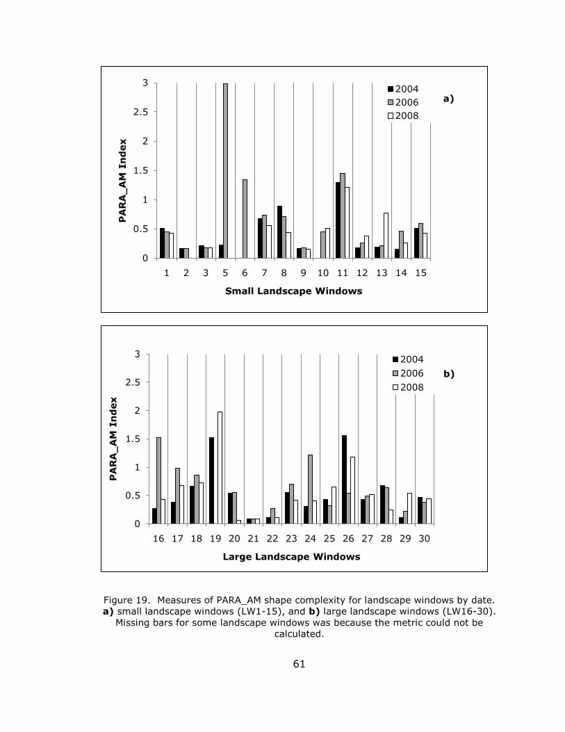
61
Figure 19. Measures of PARA_AM shape complexity for landscape windows by date. a) small landscape windows (LW1-15), and b) large landscape windows (LW16-30).
Missing bars for some landscape windows was because the metric could not be calculated.
0
0.5
1
1.5
2
2.5
3
1 2 3 5 6 7 8 9 10 11 12 13 14 15
PA
RA
_A
M I
nd
ex
Small Landscape Windows
200420062008
a)
0
0.5
1
1.5
2
2.5
3
16 17 18 19 20 21 22 23 24 25 26 27 28 29 30
PA
RA
_A
M I
nd
ex
Large Landscape Windows
2004
2006
2008b)

62
Figure 20. Fine scale map representations of patterns of seagrass changing over time that are not explained by the PARA_AM fragmentation index. Instance of high shape complexity for LW27 coincident with increases in seagrass. Note increases of
many small patches by 2008.
Seagrass percent cover of each landscape window was examined to
determine if a relationship existed between initial cover levels in 2004 and
the change in seagrass percent cover from 2004 to 2008 (percent cover of
seagrass 2008 – percent cover of seagrass 2004). The percent cover of
landscape windows from Patch Dataset 2 in 2004 (Table 12) was plotted
against the change in seagrass percent cover that occurred during the overall
interval (2004-2008) (Figure 21). A linear relationship was found between
initial seagrass percent cover and the net change in seagrass percent cover
(y= -0.574x + 16.72; r2= 0.327). Both large and small landscape windows
displayed greater losses in percent seagrass cover over time for landscape
windows with higher initial percent seagrass cover. An obvious break occurs
in the initial percent cover between 30-60% dividing landscape windows in
their response to change over time. A 60% coverage threshold is described
as being the distinguishing percent cover at which point landscapes can be

63
considered continuous (Fonseca and Bell 1998) and potentially above a
threshold such that seagrasses are resilient to physical disturbance and
ultimately loss. A count of landscape windows above and below the cover
threshold (Table 13) indicate that more than 50% of all landscape windows,
regardless of their initial percent cover, experienced gains during time
interval 3. Of these, 70% were landscape windows with seagrass percent
cover less than the 60% cover threshold. When the landscape windows
identified as experiencing net seagrass loss were plotted alone, a strong
positive relationship (y= 0.8202x + 0.5246; r2= 0.8432) between the
percent of seagrass cover lost from 2004 to 2008 and beginning cover in
2004 was recorded (Figure 22).
Comparison of Different Map Resolutions
Because the 2008 District map was used as the baseline for the fine
scale study, area-based metrics as well as the 2008 map polygons were
candidates for comparison to the fine scale mapping data. The area-based
metrics for landscape level analyses were conducted using Patch Dataset 1
that included all of the study’s mapped patch data. The study’s sampling
locations were determined by selecting 30 of the District’s 2008 broad scale
map polygons for investigation. In comparison, for the same year, within the
boundaries of these 30 broad scale thematic map polygons, the fine scale
map documented 693 patches of seagrass.

64
Table 12. Patch Dataset 2 metrics. Organized by ascending order of initial 2004 percent cover. The solid line delimits LWs with percent cover <60% in 2004.
2004 2006 2008
LW N
ame
LW A
rea
(m2)
No.
of
Patc
hes
Perc
ent
Cove
r
Tota
l Are
a (m
2)
No.
of
Patc
hes
Perc
ent
Cove
r
Tota
l Are
a (m
2)
No.
of
Patc
hes
Perc
ent
Cove
r
Tota
l Are
a (m
2)
10 1,505 0 0.00 0.00 4 44.93 676.06 5 32.05 482.22
6 1,025 0 0.00 0.00 3 3.65 37.43 0 0.00 0.00
4 641 0 0.00 0.00 0 0.00 0.00 0 0.00 0.00
19 9,173 2 0.13 11.55 0 0.00 0.00 2 0.08 7.68
26 13,501 6 0.44 59.60 11 4.65 628.18 4 0.39 52.42
11 1,783 2 1.03 18.32 3 1.26 22.40 3 1.74 30.98
18 8,508 3 1.12 94.89 8 1.24 105.09 10 3.52 299.88
25 11,787 1 1.13 133.46 2 2.12 250.24 21 6.67 786.09
27 14,727 8 3.82 562.59 22 6.76 995.69 62 17.98 2,647.39
8 1,150 3 4.79 55.13 3 6.84 78.67 3 18.54 213.32
28 16,355 17 4.95 809.03 9 3.50 572.93 10 19.25 3,148.32
23 10,964 13 4.97 544.73 42 10.81 1,184.82 24 19.84 2,175.26
15 5,594 7 9.82 549.24 16 12.11 677.16 16 20.98 1,173.56
20 9,686 20 12.39 1,200.15 29 20.00 1,937.36 1 100.00 9,686.09
30 19,470 34 14.44 2,811.04 47 18.94 3,688.26 55 17.30 3,367.69
16 7,241 3 14.77 1,069.71 35 3.25 235.55 19 28.14 2,037.64
7 1,137 4 17.44 198.30 6 28.05 318.93 5 39.61 450.35
12 2,322 1 23.73 550.99 6 84.78 1,968.74 8 57.62 1,338.13
24 11,623 21 23.89 2,776.77 28 2.27 264.40 12 13.58 1,577.86
17 7,365 7 27.06 1,992.88 21 7.10 522.86 19 9.55 703.16
13 2,610 3 52.69 1,375.34 2 49.28 1,286.54 9 9.36 244.22
9 1,260 1 62.99 793.45 1 61.87 779.39 1 72.73 916.21
1 170 2 71.66 122.08 2 83.26 141.84 2 88.10 150.09
29 18,008 5 81.79 14,728.55 71 67.56 12,166.81 39 10.41 1,875.04
3 599 1 83.59 500.76 1 95.37 571.30 1 94.08 563.58
21 9,784 1 85.69 8,383.19 1 90.19 8,823.37 1 86.51 8,463.98
14 2,625 3 86.19 2,262.60 9 33.15 870.23 7 50.46 1,324.74
5 684 1 89.76 614.18 2 0.55 3.76 0 0.00 0.00
22 9,815 5 93.02 9,129.47 26 41.16 4,039.38 2 97.75 9,594.04
2 553 1 100.00 553.00 1 100.00 553.00 0 0.00 0.00

65
Figure 21. All landscape windows plotted by their 2004 initial percent cover vs. the change in seagrass percent cover between 2004 and 2008.
Table 13. Landscape windows above and below a 60% cover threshold in 2004 and the corresponding count of positive (gain), negative (loss), or no change in percent
seagrass cover from 2004-2008.
Gains
Loss
No Change
LWs > 60% Cover (n= 9) 5
4
0
LWs < 60% Cover (n= 21) 14 5 2
y = -0.5742x + 16.727R² = 0.3278
-100
-80
-60
-40
-20
0
20
40
60
80
100
0 20 40 60 80 100
Ch
an
ge i
n P
erc
en
t S
eag
rass
Co
ver
(20
04
-20
08
)
Percent Seagrass Cover in 2004
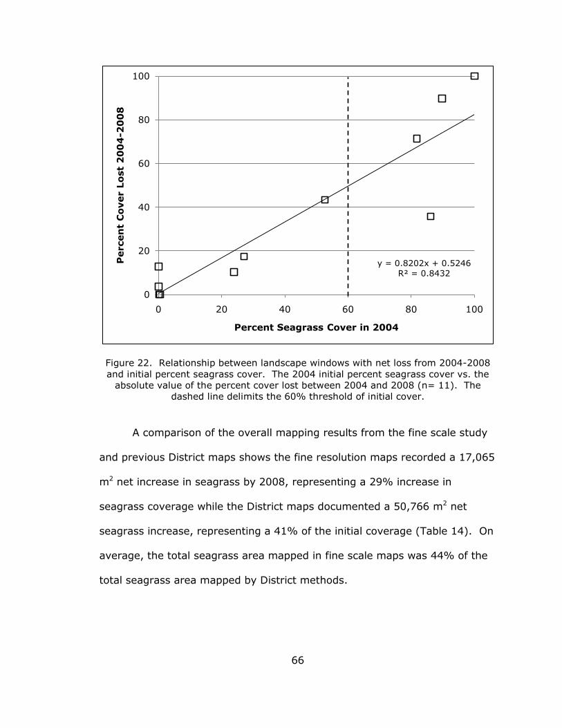
66
Figure 22. Relationship between landscape windows with net loss from 2004-2008 and initial percent seagrass cover. The 2004 initial percent seagrass cover vs. the
absolute value of the percent cover lost between 2004 and 2008 (n= 11). The dashed line delimits the 60% threshold of initial cover.
A comparison of the overall mapping results from the fine scale study
and previous District maps shows the fine resolution maps recorded a 17,065
m2 net increase in seagrass by 2008, representing a 29% increase in
seagrass coverage while the District maps documented a 50,766 m2 net
seagrass increase, representing a 41% of the initial coverage (Table 14). On
average, the total seagrass area mapped in fine scale maps was 44% of the
total seagrass area mapped by District methods.
y = 0.8202x + 0.5246R² = 0.8432
0
20
40
60
80
100
0 20 40 60 80 100
Perc
en
t C
over
Lo
st 2
00
4-2
00
8
Percent Seagrass Cover in 2004

67
Table 14. Total area (m2) of seagrass mapped by date for 30 landscape windows calculated from Patch Dataset 1. The percent cover of the total study area mapped
of 201,665 m2 presented in ().
The 2008 District seagrass map, originally utilized as the a priori data
for selecting this study’s landscape windows, characterized 24 of the
landscape windows as the thematic classification of “patchy seagrass”
(FLUCCS code 9113) and the remaining 6 as “tidal flats” (FLUCCS code
6510). Both polygon classification types were considered potential locations
of seagrass loss as described by Figure 1 and Table 1. The District’s patchy
seagrass polygons examined as landscape windows in this study were found
to range in percent seagrass cover from 10.04% to 100%. Notably, mean
percent cover within “patchy seagrass” landscape windows, in 2008, was
48.02%. This demonstrates there is a substantial amount of internal spatial
heterogeneity for “patchy seagrass” polygons when mapping the FLUCCS
thematic classification. Based on mapping rules this FLUCCS thematic
classification allows for the inclusion of the unvegetated sediment matrix
within the mapping of “patchy seagrass” and can result in an overestimation
of actual seagrass patch areal cover. The study areas classified as
unvegetated “tidal flats” by the District had a mean seagrass cover of
14.58% and a range of 2.6% to 26.71% seagrass cover. This quantifies
2004 2006 2008
Fine Scale Mapping 58,421 (29%) 48,981 (24%) 75,486 (37%) District Mapping 124,223 (62%) 119,680 (59%) 174,989 (87%)
68
errors of omission in the District seagrass map where seagrass cover was
underestimated.
The District-classified tidal flat landscape windows were reviewed using
the fine scale study results to evaluate the time course over which seagrass
was lost by 2008. Of the 6 tidal flat landscape windows (LW 2, 4, 6, 11, 19,
and 26) only one, LW6, did not have seagrass present at the initiation of the
study. In 2004, the remaining five landscape windows were documented as
having 5.78 m2 to 553 m2 of seagrass present (0.13% to 100% cover).
Tidal flat landscape windows that started with greater than 95% cover
(LW2 and LW4) in 2004 fine scale maps, by the end of the study, had lost
82.05% and 71.96% respectively. Both of these landscape windows were
documented in the 2004 and 2006 District seagrass maps as being portions
of continuous seagrass polygons. As an example, landscape window, LW4, is
shown in Figure 23 and is within portion of a continuous seagrass bed with a
small gap within its boundaries. Figure 24 shows the progression of loss that
occurred over the next few years and as shown in Figure 23; gaps in the bed
are also visible to the north and south of the study region. Landscape
windows, LW2 and LW4, were located within a larger seagrass matrix
undergoing change and both mapping approaches (fine scale and District)
were able to detect and document the formation of the gap in the seagrass
coverage.

69
Figure 23. Location map of LW4 in 2008. The landscape window is shown to be within a larger seagrass meadow. Gaps beyond the extent of the study area are
visible.
Figure 24. Map representation of LW4 experiencing gap formation over time. Graphics are ordered sequentially: 2004, 2006, and 2008. Black patches are
seagrass within the black outlined landscape window boundaries, white space within the landscape window boundary space equates to unvegetated sediment. The area
surrounding the landscape window was continuous seagrass in this instance.

70
Paired comparisons of directionality (increasing, stable, or decreasing)
of change for each landscape window indicated that both fine scale and
District mapping agreed on the direction of change for 39 of the 86 change
observations (43%). During intervals 1 and 2 combined, the District
documented 24 instances of no change, of which 20 were documented as
detectable change in seagrass area in the fine scale maps (Table 15). In
addition, detectable seagrass declines were documented more often in the
fine scale maps than in District maps and often had larger ranges of loss in
seagrass area percent change (Table 15). Although the District and fine
scale mapping approaches agreed on the overall map trend of increasing
seagrass cover, the methods qualified change within the individual landscape
windows differently due to the ability of fine scale maps to detect spatial
heterogeneity within the extents of landscape windows.
Table 15. Counts of direction of change for District maps. Values in () are the corresponding counts from fine scale mapping.
Interval 1 Interval 2 Interval 3 (2004-2006) (2006-2008) (2004-2008)
Increase (Positive) 10 (15) 9 (17) 11 (17)
Decrease (Negative) 7 (10) 6 (9) 6 (9)*
Stable (No Change) 12 (2) 15 (2) 12 (1)
Count 29 (27) 30 (28) 29 (27)
Total Detectable Change 17 (25) 15 (26) 17 (26) * Note: The count presented in () for fine scale mapping is the original count and has not been modified for alternative measures of net loss.

71
DISCUSSION
Change in seagrass patch distribution and arrangement were
quantified only for locations broadly defined as patchy seagrass or tidal flats
by previous surveys. Long-term aerial seagrass mapping data in Tampa Bay
provided a useful framework for identifying broad extents of patchy seagrass
or areas of seagrass loss, prompting further investigation into quantifying the
spatial heterogeneity and patterning of mapped marine landscapes. The
study demonstrated that discrete seagrass patches as small as 1 m2 were
detectable in high resolution aerial imagery and that 3 mapping events over
a 4-year time period provided adequate data to quantify landscape patterns
and mechanisms of loss, such as fragmentation.
Mapping of individual seagrass patches within variably-sized landscape
windows provided unique data for evaluating spatial and temporal dynamics
at multiple levels of spatial heterogeneity (patch and landscape) and at
multiple temporal scales (2-year and 4-year time intervals). The results of
this fine scale mapping study offer new information about seagrass dynamics
and spatial heterogeneity in a subtropical setting. The large extent and fine
resolution of the seagrass data reported here has been previously
unavailable for Tampa Bay and subtropical systems in general. However,
comparisons to previous work are problematic given differences in data

72
collection methods, areal extent of sampling, duration of sampling, and focal
seagrass species. Some studies (Robbins and Bell 2000, Fonseca and Bell
1998, Bell et al. 199), Jensen and Bell 2001), while suitable for providing
context and comparison because they measured seagrass at similar
resolutions (1 m2), utilized different collection methods (in situ versus aerial
mapping). In Kendall and Miller (2008), while comparable in methodological
approach where two independent seagrass mapping efforts of one location
were conducted, scaling elements differed (e.g. mapping scales). The
seemingly small number of studies reflects a general lack of available
information on seagrass patterns collected at multiple spatial and temporal
resolutions using methods similar to the approach of the current study.
The a priori assumptions made by the study, that investigating
locations currently (2006-2008) thought to have undergone seagrass loss or
that were loss-prone areas would reveal 1) seagrass loss going undetected in
broadly defined areas of stable patchy seagrass and 2) locations mapped as
unvegetated tidal flats were the result of seagrass loss, were not fully
supported by the findings of this study. Thirty individual locations
investigated for seagrass loss when combined for analysis of the entire
landscape complex from 2004 to 2008, revealed general trends of a positive
change on both Patch Dataset 1 and Patch Dataset 2. This supported the
trends of increasing seagrass areal extent previously reported by the
District’s broad scale maps. However, the magnitude of change was not
similar for the data collected with of resolutions. The fine scale mapping
dataset provided an opportunity examine these general trends in greater

73
detail by comparing the patterns of change detected with different
approaches (large versus small landscape windows; fine scale patch mapping
versus broad scale polygon mapping). The overall increasing trends in
seagrass for all map data quantified by either fine scale or broad scale
approaches did not hold when individual landscape windows were examined
for trends over time. During the time period being studied, seagrass areal
cover was dynamic at fine scales with detectable levels of seagrass change
recorded for greater than 90% of all observations within fine scale datasets
(i.e. Patch Dataset 1 and Patch Dataset 2) with 37% of landscape windows
experiencing a net loss of seagrass. Below the major findings of this study
are explored in more detail.
Examining Seagrass Dynamics from Patch Datasets 1 and 2
Area-based metrics for all data (Patch Dataset 1)
Findings from the study suggest that seagrass gains or losses do not
appear to be limited by size of area reviewed, or restricted to certain
locations. With all landscape windows combined and reviewed by time
interval, positive and negative changes occurred over 2-year time intervals in
similar or equal frequencies across the range of landscape window sizes in
the Tampa Bay system and did not deviate from the expected proportions of
gains and losses as set by previous District data. Large and small landscape
windows exhibited different temporal patterns of seagrass loss for the 2-year
time intervals (2004-2006 or 2006-2008) with a disproportionately high

74
number of small landscape windows experiencing net seagrass loss (2004-
2008). In addition, each landscape window lost various amounts of total
seagrass area and thus different proportional cover.
Comparison of results including and excluding external patches
The locations of landscape window boundaries were predetermined
based on a previous District mapping effort that delimited unique patchy
seagrass and tidal flat habitats as indicated by obvious breaks in their
photographic signatures in imagery. Many of the 30 mapping locations were
embedded within expansive seagrass habitat mosaics creating a complex
landscape to map at broad scales. Visual review of patches within the
landscape windows at a fine resolution identified a set of external patches
from the fine scale mapping, and these were most often continuations of
large seagrass beds or meadow edges that abutted the periphery of the
landscape window boundaries. As mapping is a passive form of data
collection, there is no ability to manipulate sampling locations or exclude
elements of the contiguous environment from the area of interest.
Therefore, in this study a new mapping protocol was included for identifying
partial patches in maps by classifying the origin of each patch as internal or
external (see methods).
The inclusion of external patches in Patch Dataset 1 resulted in higher
magnitude of positive change (gains) in seagrass by the end of the study
period compared to Patch Dataset 2. The contribution of external patches to

75
Patch Dataset 1 documented an overall positive change of 29% in seagrass
from 2004 to 2008 while overall change for patches completely contained
within the landscape windows (Patch Dataset 2) documented only a 3%
increase in seagrass area. Comparison of Patch Dataset 1 (with external
patches) and Patch Dataset 2 (no external patches) revealed median patch
sizes, ranges of patch sizes, and the percent change in seagrass were all
influenced by the presence of external patches.
Interestingly, patterns of seagrass loss for individual landscape
windows were similar for Patch Dataset 1 and 2 when percent change of
seagrass area was analyzed for net loss (2004-2008). Landscape windows
with net seagrass loss between 2004 and 2008 totaled 7 for Patch Dataset 1
and 9 for Patch Dataset 2 (when not including alternative determinations of
net loss). Both datasets agreed on the directional change for 6 of the
landscape windows. Disagreement on directional change for 3 of landscape
windows (LW 19, 24, and 26) were due to external patches (margins of
external seagrass meadows encroaching into the area) contributing the
majority of the seagrass present within the landscape windows (greater than
90%). When these 3 landscape windows were analyzed for Patch Dataset 1,
external patches offset or mitigated for trends in seagrass loss by discrete
patches completely contained within the landscape windows. In this case
then, loss by internal patches was only detected by analysis of Patch Dataset
2. Another disagreement was attributed to features of seagrass patches in
LW4 in which no seagrass originated from inside the landscape window.
Therefore negative changes in seagrass cover from external patches were

76
only detected by analysis of Patch Dataset 1. The influence of external
patches mitigating for loss may also partially explain why, when analyzing
landscape windows in Patch Dataset 1 for net loss; there was more loss
prevalent in small landscape windows. Interestingly, small landscape
windows were more often found in exposed and isolated locations with less
potential to be positively influence by external seagrass (see Figure 3 and
Table 2).
Bell et al. (2006) identified the complexities of mixed and overlapping
seagrass patch boundaries and this too could be encountered within
landscape windows abutting external seagrass, where coalescence of discrete
interior patches could be mixing or growing into the margins of seagrass
patches outside of landscape window boundaries and vice versa. Such
“external” patches with connection to seagrass patches or meadows outside
of the landscape window contributed to areal cover within landscape windows
of interest, but were problematic when patch metrics were being collected.
Given that seagrass is clonal and physiologically integrated (Tomasko and
Dawes 1989), change in external patches may not only reflect conditions
within the window boundaries but possibly also conditions outside the
window boundary. Beyond the identification of problems when sampling
seagrass patch boundaries that overlap (Bell et al. 2006); the concept of
patch origination is not often addressed in the marine ecology literature (but
see wetland paper by Browning et al. 2008). The ability to identify external
patch information within fine scale mapping data afforded multiple

77
opportunities for analyses of patch dynamics and has not been considered in
earlier seagrass work.
Data on external patches and the temporal differences in their
contribution to the overall dataset may reflect possible patch and meadow
expansion and other change mechanisms occurring at broader spatial scales.
That external patches contributed to positive change in seagrass coverage in
this study through expansion of seagrass meadow edges is supported by
investigations into recolonization strategies of seagrasses. After
disturbances, reports of a “border effect” with asexual growth dominating or
contributing to the infilling of bare sediments from the periphery of an area
are available for a number of different types of seagrass assemblages (Rollon
et al. 1998, Rasheed 2004, Chiarello and Barrat-Segretain 1997). Thus in
some areas within Tampa Bay contributions by external patches need to be
carefully considered.
Use of Patch Dataset 1 appears to be necessary for evaluation of
dynamics of total seagrass area, for baseline information and surveys of
seagrass status and for use when comparing independent mapping efforts
conducted at different mapping resolutions for an area. However, Patch
Dataset 2 may be more appropriate for analysis of landscape change and is
more appropriate for investigation of patch dynamics, especially if a large
number of external patches are present within a study area.

78
Analysis of Patch-based Patterns (Patch Dataset 2)
Patch Dataset 2 provided information about each landscape window’s
structural composition and configuration revealing ecologically relevant
patterns in seagrass cover and arrangement such as fragmentation of
seagrass landscapes. Some seagrass populations have been described as
existing under a constant state of loss and replacement creating a mosaic of
variably size patches of different ages (Duarte et al. 2006). Fine scale
mapping showed seagrass patches varied in size, number, and changed in
area over both 2-year and 4-year time intervals fitting the description of
dynamic seagrass landscapes.
A previous study conducted in Tampa Bay found within their 50,000
m2 (5 ha) study location, that although a series of gains and losses occurred
periodically during the 2-year study, an overall increase in coverage of 14%
was reported (Robbins and Bell 2000). The general findings of the fine scale
mapping reported here found cover decreased in 2006, and then increased in
2008, but an overall increase in cover of only 3% was revealed using Patch
Dataset 2. However, not all individual landscape windows contributed to the
increase in seagrass cover, only 18 of the 30 landscape windows experienced
overall gains in seagrass.
Trends in the number of seagrass patches present within a landscape
window over time revealed, that increases in number of patches coincided
with both increases and decreases in total seagrass area for landscape
windows. Temporally, most landscape windows increased in the number of
seagrass patches present over both 2-year and 4-year intervals. However,

79
some landscape windows deviated from the pattern, incurring loss that
resulted in complete mortality of patches while others reported decreases in
patches with increases in total seagrass area, suggesting coalescence of
patches could have occurred.
Fine scale mapping quantified a wide range of patch sizes for small
and large landscape windows in Tampa Bay, however; the range was
constrained by the detection limit of mapping, 1 m2, and the largest extent of
a landscape window examined (19,470 m2). By sampling at a variety of
spatial locations over different extents this study had the advantage of being
able to place patch size distributions into a larger context than most studies
by comparing among landscape size categories, or among individual
landscape windows. The patch composition for both landscape window size
categories were characterized as having a majority of patches (greater than
50%) smaller than 100 m2 in size. Descriptive statistics for the large and
small landscape windows showed differences in the categories’ central
tendencies with large landscape windows exhibiting a higher proportion of
small patches (<10 m2).
The distribution of seagrass patch sizes as elements of composition are
often of interest in landscape studies but are difficult to compare with
previous research of seagrass. Limitations arise due to the variability in the
spatial resolution (grain size) of previous studies as well as the use of
alternative methods for collecting patch size measurements in situ, which are
often reported as patch diameter (m) or shoots per patch (e.g. Vidondo et al.
1997, Marba and Duarte 1995, Sintes et al. 2005) . In addition, the studies
80
and their designs could bias sampling towards a certain patch size class
based on site selection or the methodological limitations of working within
large patches. One study with data available for comparison was conducted
10 years earlier in a portion of Lower Tampa Bay and reported a prevalence
of smaller seagrass patches, 5 m2 in size (Robbins and Bell 2000). There
seems to be a high propensity for studies on seagrass dynamics to report
patchy seagrass landscapes as having high proportions of “small” patches
whether they are defined as: < 1 m diameter (Vidondo et al. 1997), <5 m2
(Robbins and Bell 2000), up to 10 m2 (this study), or <100 m2 (Frederiksen
et al. 2004, Hernandez-Cruz et al. 2006). Moreover, in some cases it has
been suggested that large proportions of small patches are found to be
indicative of fast growing patches with high mortality rates (Frederiksen et al.
2004). Additional analysis of Patch Dataset 2 which followed the fate of
individual patches would be needed in order to make such conclusions for
this study.
The 11 landscape windows that experienced net seagrass loss did not
lose seagrass consistently but, instead, exhibited a variety of temporal
patterns. The net loss landscape windows exhibited 3 distinct patterns of
negative change that included: losing acute amounts of seagrass during
interval 1 from which it could not recover, having a singular instance of loss
during interval 2 that reflected the most recent interannual conditions, or
having chronic loss during both intervals 1 and 2. Complete mortality for
patches within 3 landscape windows are examples of declines in seagrass
during a single 2-year interval that resulted in net seagrass loss. Between 1
81
and 3 patches per landscape window with total area between 3.76 m2 and
553 m2 were all lost within a 2 year period. These examples of patch
mortality are not the only instances of complete patch loss in the available
data but further GIS analysis would be needed to track the fate of other
individual seagrass patches.
One mechanism of habitat loss that has both structural and functional
consequences in marine habitats and often evaluated in seagrass-related
studies is fragmentation (Fonseca and Bell 1998, Jaeger 2000, Bostrom et al.
2006, Sleeman et al. 2005). Fragmentation is a process of seagrass cover
loss coincident with patch size reduction and an increase in the proportions of
patch edges (Bostrom et al. 2006). The term “fragmentation” is often used
to describe the static spatial arrangement of seagrasses (similar to the use of
the descriptor patchy) but only a small number of studies measure patterns
of fragmentation as a trend through time (Jaegar 2000, Bostrom et al.
2006). Numbers of patches and mean patch size have also been used to
identify fragmentation (Sleeman et al. 2005). Building upon these past
investigations, this study utilized time interval metrics (i.e. change in total
patch number and change in total patch area) for each landscape window as
well as a shape complexity index to evaluate fragmentation. The overall
important finding was that the process of fragmentation, as indicated by
patterns in 1 m2 resolution landscape composition, was detectable after 2
years; finer temporal resolution may reveal that the process could occur over
even shorter time periods.

82
Other landscape metrics, suitable for investigating fragmentation in
seagrass landscapes, such as landscape division (Sleeman et al. 2005) as
well as GIS change analysis could be applied in order to provide insight into
the fate of individual patches experiencing fragmentation overtime. It has
been suggested that map patterns displayed visually and analyzed within the
GIS environment may provide a higher level of information not detectable by
summaries of the extracted data (Turner 2005 and references within). In
any case, in order to determine the relationship between spatial patterns
found for seagrass loss and ecological processes that drive them, more
extensive monitoring of site characteristics including measurements of
hydrodynamics, light availability, and nutrients must be examined (Sleeman
et al. 2005).
Potential Causes for Seagrass Change Patterns
While information available to describe patterns of seagrass change is
limited in scope and often lacks comparable collection technologies,
processes responsible for producing patterns are even less well known. Gap
formation quantified as a net loss in seagrass for two landscape windows,
LW2 and LW4, was most likely due to the environmental settings of the
landscape windows. Gap formation occurred within landscape windows
situated inside larger continuous seagrass meadows and the formation was
shown to be an easily identifiable mechanism of loss for both the fine scale
and District mapping approaches. In a previous study of seagrass gaps in
Tampa Bay seagrass landscapes, a positive relationship was found between

83
gaps and sedimentation events and the area and persistence of seagrass
gaps were not related to water depth (Bell et al. 1999). The previous study
also found seagrass gaps ranged in size from 10 m2 to 305 m2 and persisted
most frequently for 6 months or 1.5 years (Bell et al. 1999). In the current
study, gaps in LW2 and LW4 were 553 m2 and 641 m2 in size respectively,
larger than those documented in Bell et al. (1999). Additionally, contrary to
Bell et al. (1999) gaps grew larger over time, suggesting that the expected
lifespan of these gaps could be longer than 1.5 years. Future studies could
examine these events in more detail by documenting the fine scale features
within the Tampa Bay seagrass complex over a larger geographic range and
linking change dynamics in physical processes such as sedimentation events
building upon the findings by Bell et al. (1999).
Increased exposure to disturbances or stress created by the
directionality of waves, currents, and tides make landscape position an
important consideration in seagrass loss. Physical processes as mechanisms
of change, specifically loss, have been investigated extensively (Marba and
Duarte 1995, Fonseca and Bell 1998, Bell et al. 1999, Fredericksen et al.
2004, Campbell and McKenzie 2004, Cunha et al. 2005) and have been found
to structure seagrass landscapes and influence seagrass spatial dynamics.
During a high energy disturbance, a seagrass patch or meadow with high
percent cover, greater than 59.28% as suggested by percolation theory
(With and Christ 1995) and 50% as documented by Fonseca and Bell (1998)
represent the percent cover at which loss of seagrass patch structure was
less likely to occur. Contrary to these previous findings, the current study

84
found that landscape windows both above and below a 60% cover threshold,
at the initiation of the study in 2004, had a higher propensity to gain than
lose seagrass coverage by 2008 (55% of landscape windows above the
threshold gained seagrass cover and 66% of landscape windows below the
threshold gained seagrass percent cover; Table 13). Moreover in this study,
the structural integrity of the variable numbers of discrete seagrass patches
in landscape windows was most often maintained when initial total coverage
was below 30% (Figure 21). While the fine scale mapping results do not
support the 60% threshold, the landscape windows examined in our study
may not be located in sufficiently high energy regimes such that physical
disturbances have a strong role in directing change. This conclusion may
support the idea that physical disturbances within these locations could be
better described as chronic low energy stressors and that percent cover
thresholds for chronic or average disturbance regimes need to be
investigated over multiple time periods, possibly greater than 4 years.
The differences in intensity and duration of disturbances caused by
wave energy and currents may call for a partitioning of disturbances into two
levels, chronic and acute (Tewfik et al. 2007). In a 0.8 ha subtropical
shallow water site, Tewfik et al. (2007) demonstrated that zones of various
benthic habitats experienced chronic low level hydrodynamic forces and
supported persistent mixed seagrass and macroalgae beds, with gaps in
seagrass distributed throughout. One critical aspect of this study was that
submerged aquatic vegetation behind a nearshore bar experienced average
wave energy that influenced the distribution of submerged aquatic

85
vegetation, but was protected from acute disturbances. In our study, nearly
equal numbers of the 11 landscape windows with a net loss of seagrass were
positioned inside of a longshore bar or within a protected area versus being
at “more exposed” positions; thus this does not appear to provide strong
evidence for physical disturbance driving patterns of seagrass loss. To
further investigate possible physical processes as mechanisms of loss in
these areas it may be necessary to better characterize the physical
disturbance regimes as described in Tewfik et al. (2007).
While physical factors do not appear to adequately explain the
patterns of seagrass loss, another factor that might be linked with declining
seagrass coverage is abundance of macroalgae (e.g. Hauxwell et al. 2001).
The accumulation of large amounts of macroalgae can add additional stress
to a seagrass system by reducing the amount of light available to the
seagrasses for photosynthesis (e.g. Hauxwell et al. 2001). The location of
macroalgae within the environment is often due to hydrodynamic forces
moving the vegetation around the system as most macroalgae do not require
attachment to sediments and are transient structural elements of the marine
benthic environment. Bell et al. (1995) found significantly more drift
macroalgae accumulated within large natural and artificially constructed
seagrass patches when compared to small patches. This indicated that total
seagrass area may not be the factor influencing accumulation of macroalgae
and suggested it was due to greater amounts of attenuated flow in larger
seagrass areas. In our study, 21 of the 30 landscape windows are located
behind nearshore bars or within partially protected areas, indicative of lower

86
energy environments where drift macroalgae could accumulate. Of the 11
landscape windows that experienced net losses in seagrass, 7 of them were
either behind a nearshore bar or partially protected, of those locations within
Tampa Bay, anecdotal evidence and personal observation suggest LW29
(Wheedon Island area), LW 19 (between the Howard Franklin and Gandy
Bridges in Old Tampa Bay), and LW 6 (near Ft. Desoto) may be susceptible
to stress from accumulation of macroalgae.
Comparison of Mapping Resolutions
Unique to this study, 2 separate mapping approaches were compared
that created a time series of maps with differing levels of thematic and
spatial resolution for 30 of the same locations created from the same source
imagery. Questions from the field of landscape ecology regarding the
collection of scientific data at different scales have led to researching
comparisons of landscape mapping at different scales. Published
comparisons of mapping efforts conducted at different resolutions have been
done for terrestrial and marine environments through the use of simulated
map landscapes and neutral models (Saura 2002, Wu 2004) or resampling of
a single map by aggregating data to a larger scale (Rutchey and Godin 2009)
and very rarely by producing independent maps of varying resolutions
(Kendall and Miller 2008). Comparisons of data from the two mapping
approaches were used to characterize and quantify differences in levels of
heterogeneity. Patterns of change in the mapping results were examined to
distinguish the effects of changes in spatial resolution (MMU).
87
Direct comparison was made between the two mapping approaches for
2008. In 2008, the fine scale mapping (1 m2 MMU) documented 693
seagrass patch polygons within the same extent of the 30 broad scale (0.202
ha MMU) District map polygons. In general, fine scale mapping created a
finer level of detail where seagrass was increasingly differentiated from bare
sediment; this reduced the amount of seagrass quantified within the study’s
extents compared to the District maps. Extraction of seagrass data at a
more detailed level meant the total amount of seagrass documented in the
fine scale map was, on average, 44% less than that mapped in the broad
scale maps. Coincident with this finding is the example from the fine scale
mapping for 2008, where the average percent cover of seagrass within a
landscape window was 40.78%. In previous work, a comparison of marine
benthic maps of low thematic resolution at two spatial scales (100 m2 and
2.02 ha) also found a shift in the total area of the unconsolidated sand class
between the two maps. The amount of unconsolidated sand present as a
mapped feature was found to be 15 times higher in maps with the smaller
100 m2 MMU compared to the larger 2.02 ha MMU map (Kendall and Miller
2008). These data show that the unvegetated sand matrix within mapped
polygons at broad spatial scales can have an influence on the quantification
of seagrass. Specifically, patches of seagrass aggregated into the patchy
seagrass classification (FLUCCS code 9113) can overestimate total seagrass
patch area within a given polygon extent. It must be noted however that the
generalization of environmental features at broad scale resolutions is

88
recognized and the allowance of unvegetated areas within patchy seagrass
classifications is an accepted broad scale mapping methodology.
The fine scale mapping clearly distinguished between seagrass and
unvegetated sediments and quantified percent cover of seagrass within each
location versus the District’s method of applying a thematic classification to
describe an area’s seagrass features. Stated mapping logic and
recommendations made by guidance documents for seagrass mapping
(Finkbeiner et al. 2001, Kendall and Miller 2008) identify 10% seagrass cover
as the minimum percent cover required for classifying a map polygon as
“patchy seagrass.” However, no information was available regarding
whether these recommendations or definitions of coverage for patchy
seagrass were tested to confirm patch cover within the boundaries of patchy
polygons equaled at least 10% cover for various mapping efforts. This fine
scale study is the first found to investigate and test the quantification of
percent seagrass cover of a broad scale map thematic seagrass classification.
The District’s use of a patchy seagrass classification was quantified by
fine scale mapping as 10%-100% seagrass cover. The fine scale mapping
results demonstrated consistency with the standard 10% cover
characterizing the minimum coverage of patchy seagrass map polygons. The
quantification of 100% cover for patchy polygons is somewhat contradictory
as the District can map these polygons as continuous seagrass. Landscape
window LW20 was documented having 100% seagrass cover in the 2008 fine
scale map and was classified as a patchy seagrass polygon in the District
2008 map. Based on the percent cover quantified by the fine scale mapping,
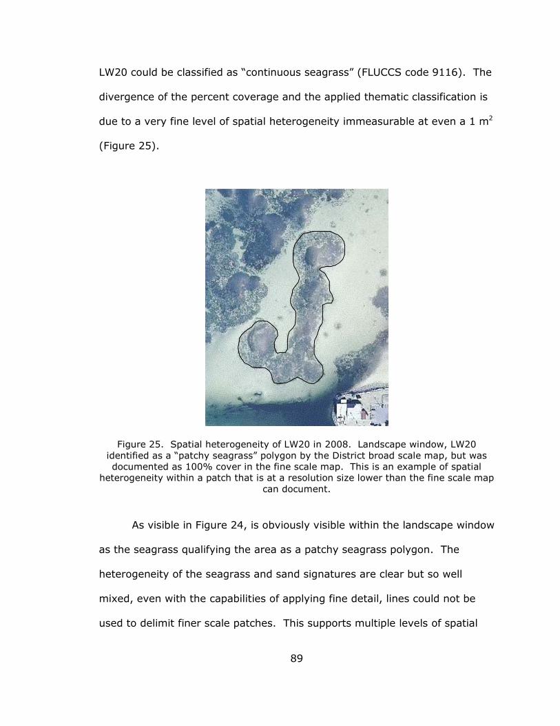
89
LW20 could be classified as “continuous seagrass” (FLUCCS code 9116). The
divergence of the percent coverage and the applied thematic classification is
due to a very fine level of spatial heterogeneity immeasurable at even a 1 m2
(Figure 25).
Figure 25. Spatial heterogeneity of LW20 in 2008. Landscape window, LW20 identified as a “patchy seagrass” polygon by the District broad scale map, but was documented as 100% cover in the fine scale map. This is an example of spatial
heterogeneity within a patch that is at a resolution size lower than the fine scale map can document.
As visible in Figure 24, is obviously visible within the landscape window
as the seagrass qualifying the area as a patchy seagrass polygon. The
heterogeneity of the seagrass and sand signatures are clear but so well
mixed, even with the capabilities of applying fine detail, lines could not be
used to delimit finer scale patches. This supports multiple levels of spatial

90
heterogeneity within the environment where even within fine scale patches;
they are never completely homogeneous (Gustafason 1998).
Another explanation for landscape windows with high percent cover
above the 50% being given a patchy seagrass mapping classification in some
instances could be due to a mapping decision utilized in the District seagrass
mapping approach. A small backwater embayment along a natural shoreline,
where seagrass was located within the protected vicinity of mangrove islands
(e.g. LW21 in Cockroach Bay) can accumulate dark organic sediments and
substantial amounts of drift macroalgae. The seagrass signatures in these
areas are often characterized as patchy so as not to overestimate their
coverage. This study has identified use of the patchy seagrass thematic
descriptor in District maps in multiple ways, in order to characterize different
spatial compositions, environmental conditions, and varying levels of
heterogeneity.
The study also quantified seagrass percent cover of landscape windows
classified in 2008 as tidal flat (FLUCCS code 6510). The tidal flat
classification was defined by the fine scale mapping as mean percent cover of
14.58%. The quantification of seagrass within landscape windows
characterized in the District map as unvegetated tidal flats, demonstrates the
potential for errors of omission when reviewed at a finer scale, resulting in
underestimations of seagrass coverage to occur in broad scale maps. This is
due to the limitations of larger MMUs and less detailed digitizing scales used
by broad scale mapping such that significant areas of light colored sand can
obscure faint and diffuse signatures of the short sparse seagrass

91
characteristic of tidal flats. As expected prior to this study, investigation into
the interior spatial heterogeneity of 2008 District mapped polygons found
varying levels of heterogeneity within their boundaries.
Although the spatial heterogeneity differed for the two mapping
methods as commonly understood by landscape ecologists when comparing
maps of two different resolutions (Wu 2004, Kendall and Miller 2008), the
directionality of change in vegetation overtime was similar. Overall, total
seagrass area increased for both mapping methods during the study period.
The fine scale maps’ frequencies of positive and negative changes for all time
intervals were not significantly different from the expected proportions of
change documented by the a priori District data (60% positive change and
40% negative change). The broad scale maps exhibited a high level of
stability or lack of change, in their results for some landscape windows and
when compared to the fine scale data, it revealed this tendency meant
change in either direction may have gone undetected depending upon the
landscape window.

92
CONCLUSION
The study presented here investigated the spatial and temporal
dynamics of seagrass at multiple scales using fine scale aerial mapping
techniques. The implications of understanding short and long term seagrass
dynamics are significant as seagrass contribute structurally and functionally
to the benthic marine environment. The study produced unique datasets
that identified fine scale patterns of seagrass change. Through application of
landscape ecology concepts and indices, patterns of seagrass loss were
identified and processes of fragmentation and gap formation were quantified
for individual landscape windows. This study is one of the first reported
quantifications of seagrass fragmentation at this scale over multiple years.
In contrast to predictions of seagrass global decline (Waycott et al.
2009) the evidence presented in the current study suggests this is not case
for patchy seagrass habitats in portions of Tampa Bay. Although areas of
short–term historical seagrass loss were targeted for this study, the total
combined changes occurring in the study areas resulted in overall increases
in seagrass cover. Variability in seagrass dynamics reported in the study
suggest that patterns of change are sensitive to the duration of observations
and should be carefully considered during interpretation of data.

93
Comparison of fine scale mapping to previously generated broad scale
maps provided a detailed assessment of landscape features categorized as
“patchy” by the ongoing District’s mapping program. Overall the broad scale
maps correctly identify estuarine wide trends in seagrass and provide
valuable data products that can be utilized for extensive investigations of the
mapped marine environment. Although a fine scale mapping effort may not
be practical for an entire estuary the size of Tampa Bay, the data were
proven useful and appears to be a reasonable method for implementation of
local studies.

94
REFERENCES
Bell SS, Fonseca MS, Stafford NB. 2006. Seagrass ecology: new contributions from a landscape perspective. In: Larkum AWD, Orth RJ, Duarte CM, editors. Seagrasses: biology, ecology, and conservation. Dordrecht, Netherlands: Springer. p. 625-645.
Bell SS, Hall MO, Robbins BD. 1995. Toward a landscape approach in
seagrass beds: using macroaglal accumulation to address questions of scale. Oecolgia 104:163-168.
Bell SS, Robbins BD, Jensen SL. 1999. Gap dynamics in a seagrass landscape. Ecosystems 2:493-504.
Borowitzka MA, Lavery PS, van Keulen M. 2006. Epiphytes of seagrasses. In:
Larkum AWD, Orth RJ, Duarte CM, editors. Seagrasses: biology, ecology, and conservation. Dordrecht, Netherlands: Springer. p.441 -461.
Bostrom C, Jackson EL, Simenstad CA. 2006. Seagrass landscapes and their
effects on associated fauna: a review. Estuarine Coastal and Shelf Science 68:383-403.
Browning DM, Archer SR, Asner GP, McClaran MP, Wessman CA. 2008. Woody plants in grasslands: post-encroachment to stand dynamics. Ecological Applications 18:928-944.
Caloz R, Collet C. 1997. Geographic information systems (GIS) and remote sensing in aquatic botany: methodological aspects. Aquatic Botany 58:209-228.
Campbell SJ, McKenzie LJ. 2004. Flood related loss and recovery of intertidal seagrass meadows in southern Queensland, Australia. Estuarine Coastal and Shelf Science 60:477-490.
Carlson PR Jr., Yarboro LA, Kaufman KA, Mattson RA. 2010. Vulnerability and resilience of seagrasses to hurricane runoff impacts along Florida’s west coast. Hydrobiologia 649:39-53.

95
Chiarello E, Barrat-Segretain MH. 1997. Recolonization of cleared patches by macrophytes: modeling with point processes and random mosaics. Ecological Modeling 96:61-73.
Cunha AH, Santos RP, Gaspar AP, Bairros MF. 2005. Seagrass landscape-
scale changes in response to disturbance created by the dynamics of barrier-islands: a case study from Rio Formosa (Southern Portugal). Estuarine, Coastal and Shelf Science 64:636-644.
Duarte CM. 1999. Seagrass ecology at the turn of the millennium:
challenges for the new century. Aquatic Botany 65:7-20. Duarte CM. 2002. The future of seagrass meadows. Environmental
Conservation 29:192-202. Duarte CM, Fourqurean JW, Krause-Jensen D, Olesen B. 2006. Dynamics of
seagrass stability and change. In: Larkum AWD, Orth RJ, Duarte CM, editors. Seagrasses: biology, ecology, and conservation. Dordrecht, Netherlands: Springer. p. 271-294.
Feagin RA, Wu XB. 2006. Spatial patterns and edges characteristics in
restored terrace versus reference salt marshes in Galveston Bay. Wetlands 26:1004-1011.
Ferguson RL, Wood LL. 1993. Monitoring spatial change in seagrass habitat
with aerial photography. Photogrammetric Engineering and Remote Sensing 59:1033-1038.
Finkbeiner M, Stevenson B, Seaman R. 2001. Guidance for benthic habitat
mapping: an aerial photographic approach. URL: http://www.csc.noaa.gov/benthic/mapping/pdf/bhmguide.pdf. Charleston, South Carolina: U.S. NOAA Coastal Service Center.
Florida Department of Transportation (FDOT). 1999. Florida land use, cover
and forms classification system: handbook. Third Edition. URL: http://www.dot.state.fl.us/surveyingandmapping/regulations.shtm.
Fonseca MS, Bell SS. 1998. Influence of physical setting on seagrass
landscapes near Beaufort, North Carolina, USA. Marine Ecology Progress Series 171:109-121.
Frederiksen M, Krause-Jensen D, Holmer M, Laursen JS. 2004. Spatial and
temporal variation in eelgrass (Zostera marina) landscapes: influence of physical setting. Aquatic Botany 78:147-165.

96
Greening HS, Cross LM, Sherwood ET. 2011. A multiscale approach to seagrass recovery in Tampa Bay, Florida. Ecological Restoration 29:83-92.
Gustafson EJ. 1998. Quantifying landscape spatial pattern: what is the state
of the art? Ecosystems 1:143-156. Hauxwell J, Cebrian J, Furlong C, Valiela I. 2001. Macroalgal canopies
contribute to eelgrass (Zostera marina) decline in temperate estuarine ecosystems. Ecology 82:1007-1022.
Hackney JW, Durako MJ. 2004. Size-frequency patterns in morphometric
characteristics of the seagrass Thalassia testudinum reflect environmental variability. Ecological Indicators 4:55-71.
Hernandez-Cruz LR, Purkis SJ, Riegl BM. 2006. Documenting decadal spatial changes in seagrass and Acropora Palmata cover by aerial photography analysis in Vieques, Puerto Rico: 1937-2000.
Jaeger JA. 2000. Landscape division, splitting index, and effective mesh size:
new measures of landscape fragmentation. Landscape Ecology 15:115-130.
Jensen S, Bell S. 2001. Seagrass growth and patch dynamics: cross-scale
morphological plasticity. Plant Ecology 155:201-217. Kendall MS, Miller T. 2008. The influence of thematic and spatial resolution
on maps of coral reef ecosystems. Marine Geodesy 31:75-102. Kendrick GA, Eckersley J, Walker DI. 1999. Landscape-scale changes in
seagrass distribution over time: a case study from Success Bank, Western Australia. Aquatic Botany 65:293-309.
Kendrick GA, Duarte CM, Marba N. 2005. Clonality in seagrasses, emergent properties and seagrass landscapes. Marine Ecology Progress Series 290:291-296.
Kirkman H. 1996. Baseline and monitoring methods for seagrass meadows.
Journal of Environmental Management 47:191-201. Lewis RR III, Whitman JJ. 1985. A new geographic description of the
boundaries and subdivisions of Tampa Bay. In: Treat SF, Simon JL, Lewis III RR, Whitman RL. Proceedings, Tampa Bay Area Scientific Information Symposium. Florida Sea Grant, St. Petersburg, FL., p. 10-17.

97
Marba N, Duarte CM. 1995. Coupling of seagrass (Cymodocea nodosa) patch dynamics to subaqueous dune migration. Journal of Ecology 83:381-389.
McGarigal K, Marks BJ. 1995. FRAGSTATS: Spatial pattern analysis program
for quantifying landscape structure. USDA Forest Service Technical Report PNW-351.
Olesen B, Sand-Jensen K. 1994. Patch dynamics of eelgrass Zostera marina.
Marine Ecology Progress Series 106:147-156. Irlandi EA, Ambrose WG Jr., Orlando BA. 1995. Landscape ecology and the
marine environment: how spatial configuration of seagrass habitat influences growth and survival of the bay scallop. Oikos 72:307-313.
Rasheed MA. 2004. Recovery and succession in a multi-species tropical seagrass meadow following experimental disturbance: the role of sexual and asexual reproduction. Journal of Experimental Marine Biology and Ecology 310:13-45.
Robbins BD, Bell SS. 2000. Seagrass landscapes: a terrestrial approach to the marine subtidal environment. Tree 9:301-304.
Robbins BD, Bell SS. 2000. Dynamics of subtidal seagrass landscape:
seasonal and annual change in relation to water depth. Ecology 81:1193-1205.
Rollon RN, De Ruyter Van Steveninck ED, Van Vierssen W, Fortes MD. 1998. Contrasting recolonization strategies in multi-species seagrass meadows. Marine Pollution Bulletin 37:450-459.
Rutchey K, Godin J. 2009. Determining an appropriate minimum mapping
unit in vegetation mapping for ecosystem restoration: a case study from the Everglades, USA. Landscape Ecology 24:1351-1362.
Saunders DA, Hobbs RJ, Margules CR. 1991. Biological consequences of
ecosystem fragmentation: a review. Conservation Biology 5:18-32.
Sintes T, Marba N, Duarte CM, Kendrick GA. 2005. Nonlinear processes in
seagrass colonization explained by simple clonal growth rules. Oikos 108: 165-175.
Sleeman JC, Kendrick GA, Boggs GS, Hegge BJ. 2005. Measuring
fragmentation of seagrass landscapes: which indices are most appropriate for detecting change? Marine and Freshwater Research 56:851-864.

98
Stafford NB, Bell SS. 2006. Space competition between seagrass and Caulerpa prolifera (Forsskaal) Lamouroux following simulated disturbances in Lassing Park, FL.
Southwest Florida Water Management District (District). 2009a. Final report
for the Southwest Florida Water Management District: seagrass 2008, seagrass distribution from Tarpon Springs to Boca Grande. Prepared by: Photo Science Inc., St. Petersburg, Florida. p.1-48.
Southwest Florida Water Management District (District). 2009b. Recent
seagrass coverages in the District from 2004 to 2009. URL: www.swfwmd.state.fl.us/data/gis/layer_library/category/swim
Tewfik A, Guichard F, McCann KS. 2007. Influence of acute and chronic
disturbance on macrophyte landscape zonation. Marine Ecology Progress Series 335:111-121.
Tomasko DA, Corbett CA, Greening HS, Raulerson GE. 2005. Spatial and
temporal variation in seagrass coverage in Southwest Florida: assessing the relative effects of anthropogenic nutrient load reductions and rainfall in four contiguous estuaries. Marine Pollution Bulletin 50:797-805.
Turner MG. 2005. Landscape ecology in North America: past, present, and future. Ecology 86:1967-1974.
Turner SJ, Hewitt JE, Wilkinson MR, Morrisey DJ, Thrush SF, Cummings VJ,
Funnell G. 1999. Seagrass patches and landscapes: the influence of wind-wave dynamics and hierarchical arrangements of spatial structure on macrofaunal seagrass communities. Estuaries 22:1016-1032.
Vidondo B, Duarte CM, Middelboe AL, Stefansen K, Lutzen T, Nielsen SL. 1997. Dynamics of a landscape mosaic: size and age distributions, growth and demography of seagrass Cymodocea nodosa patches. Marine Ecology Progress Series 158:131-138.
Waycott M, Duarte CM, Carruthers TJB, Orth RJ, Dennison WC, Olyarnik S,
Calladin A, Fourqurean JW, Heck KL Jr., Hughes AR, Kendrick GA, Kenworthy WJ, Short FT, Williams SL. Accelerating loss of seagrass across the globe threatens coastal ecosystems. PNAS 106:12377-12381.
Warry FY, Hindell JS, Macreadie PI, Jenkins GP, Connolly RM. 2009.
Integrating edge effects into studies of habitat fragmentation: a test using meiofauna in seagrass. Oecologia 159:883-892.

99
With KA, Crist TO. 1995. Critical thresholds in species’ responses to landscape structure. Ecology 76:2446-2459.
Wiens JA. 1989. Spatial scaling in ecology. Functional Ecology 3:385-397. Wu J. 2004. Effects of changing scale on landscape pattern analysis: scaling
relations. Landscape Ecology 19:125-138.

100
APPENDIX A: Seagrass Mapping Approach Utilized by the Southwest
Florida Water Management District
Background
In the 1980s, deterioration of water quality along Florida’s Gulf Coast
and dramatic seagrass losses drove involvement by state and local
governments to protect and restore Florida estuaries. Tampa Bay, Florida, is
a well-documented case study where poor water quality contributed to
seagrass losses in the system. Subsequent changes in seagrass distribution
and recovery of seagrass habitat are credited, in part, to management efforts
that reduce nutrient pollution entering the estuary (Tomasko et al. 2005,
Greening and Janicki 2006).
Introduction
The selection of mapping resolution and extent is driven by the
intended use for map-derived data and the constraints placed on mapping by
available source data. Mapping components related to scaling and
resolutions include: the minimum mapping unit (MMU), digitizing scale, and
thematic classification of the benthic features. These determine the level of
detail reflected in the data extracted from source imagery and may create
limitations on the levels of detectable change, and landscape patterns

101
evident in the resulting seagrass map. The majority of these criteria will be
unique for every mapping project and are defined by the map creator.
Imagery Resolution
Working within the limitations of the source imagery resolution is an
important consideration when setting map criteria. Spatial resolution refers
to the ability to record spatial detail (Lo and Yeung 2007) and describes the
level of detail that can be seen in an image. The District mapping program
acquires project specific source data from within the same time frame every
two years. Acquisition is conducted under a set of specific environmental
conditions in order to collect high quality imagery where benthic features are
visible. Aerial photography is a passive remote sensing collection technique.
Although not a defined resolution, characteristics of spatial scale for
traditional film photography are described by photographic scale.
Photographic scale denotes a cartographic representation of the world using
a ratio between the distance on the map and the distance it represents in the
real world (Dungan et al. 2002). A photographic scale of 1:24,000 is
considered medium to large scale photography that captures a smaller area
per frame with higher resolution than photography at smaller scales like
1:100,000 (Clinton et al. 2007). Source imagery data is then simplified
based on a predetermined set of interpretation rules and extracted as map
data. Regardless of a sensor’s detection ability, there is a geographic scale
which best defines the areal extent of a distinct biological community (SAIC
2003).

102
The District mapping program acquires imagery under a specific set of
atmospheric and environmental conditions (Table A1) for the explicit purpose
of seagrass mapping. Every two years acquisition is scheduled for the same
time period (November – February) when atmospheric and water clarity
conditions are most suitable. District programmatic mapping protocols have
consistently captured the same extent of Tampa Bay utilizing 1:24,000 scale
natural color aerial photography or digital aerial imagery.
Table A1. Environmental and atmospheric conditions required for acquisition of aerial imagery by the District.
Environmental Consideration Allowable Limits
Atmospheric: Cloud Cover 0% Atmospheric: Wind ≤ 10 knots Sun Angle 30⁰ - 45⁰ Water Transparency 2 m Sea Surface: Wave Height ≤ 61 cm (2 ft) Tidal Stage ≤ Mean tide level Tidal Cycle (phase) Ebb tide cycle
Imagery Interpretation
Interpretation rules state the logic for what features are delineated in
the thematic map, determines how lines are placed, and how thematic
attributes will be applied to those features. Rule sets are designed and
followed to ensure consistency during map creation. The District’s GIS based
mapping is conducted by manual interpretation using vector models,
delineating the location and extent of benthic features using polygons. This
is a subjective method of data collection where the analyst must use their
working knowledge of the particular environment and remote sensing to

103
decide how features will be delineated in a map. Image interpretation
approximates the perimeter of map features (seagrass) based on their visual
representation in an image, thereby creating the habitat polygon.
Polygons are irregular, varying in size and shape, and represent areal
features in maps as fixed discrete objects (Caloz and Collet 1997). Polygon
boundaries separate different habitat types but are artificial breakpoints
drawn in the benthic habitat mosaic. In general, mapping protocols used by
the District rely on observing the consistency of seagrass signatures in the
images at a macro scale over a large extent. The proximity of these
signatures to one another over large extents dictates the size of the
demarcated polygons. In general, the District’s mapping guidelines state: 1)
the outer polygon boundaries of seagrass habitats are more important than
internal structure (patchiness, shapes of sand patches within) of stands, 2)
the MMU of 0.2 ha will be followed with consideration that small and isolated
detectable patches of seagrass will be mapped whenever visible in
photography, 3) within patchy seagrass habitat each patch is not mapped
individually because the entire matrix of patches is the mapped object, 4)
seagrass patches meeting the MMU criterion may be aggregated into a single
classified polygon if part of the same habitat complex (District 2009).
The program identifies seagrass using manual photo interpretation
techniques and classifies the thematic maps by applying modified special
classification codes from the Florida Land Use Land Cover Classification
System (FLUCCS). The Florida Department of Transportation developed
FLUCCS as a remote sensing based hierarchical classification system with
104
increasing specificity in the descriptors at higher levels (FDOT 1999). An
understanding of the District’s logic behind application of the modified codes
is found in District final mapping project reports (District 2009).
The District’s classification scheme uses modified FLUCCS’s level four
hierarchical classes, applying patchy (9113) and continuous (9116) codes to
polygons identified as seagrass. Associated with the FLUCCS codes are
descriptive classification conventions (District 2009). At the map resolution
utilized by the District, seagrass patches are often too small to be mapped
individually and are aggregated to create larger landscape polygon features.
A patchy seagrass FLUCC’s code classification narrative describes an area of
the marine landscape with distinct and obvious spatial heterogeneity visible
at a macro scale. Polygons are delineated and classified as patchy when
internal seagrass cover consists of discontinuous patches having variable
densities and appearances. More specifically, patchy polygons are described
as having multiple isolated clumps or circular patches close to one another or
extensive patches mixed with open bottom (District 2009).
Minimum mapping unit
The spatially characterized features in a thematic map are created by
imagery interpretation and feature classification. The ability to interpret and
delineate map features such as seagrass is determined by specification of an
MMU, a standard that states only features equal to or larger than the unit will
be present on the map. Minimum mapping units are essential components of
mapping; they define the extent of detail in a map (Saura 2002). The
105
District’s MMU is 0.2 ha; a commonly used mapping criterion amongst
seagrass mapping efforts.
Digitizing scale
Visual perception gives an overall view of an object's form and
arrangement (Caloz and Collect 1997). In order to visualize and interpret
seagrass photographic signatures from the digital aerial imagery in a
consistent manner, the District set digitizing scale guidelines. A digitizing
scale is expressed as cartographic ratio at which imagery will appear for
interpretation and creation of the map line work. The smaller the ratio, the
more “zoomed in” and the more detail provided on screen during
interpretation and creation of line work. Depending on the equality of the
photography and the signatures present, the District’s digitizing scale for the
broad level seagrass mapping is between 1:4,000 and 1:6,000, with areas
requiring more detail interpreted at 1:2,500 (District 2009). The guidelines
are in agreement with FDOT’s logic for application of level four FLUCCS
codes, where it is suggested that low altitude photography producing
1:24,000 photography be reviewed and digitized at 1:6,000 (FDOT 1999).
106
REFERENCES
Caloz R, Collet C. 1997. Geographic information systems (GIS) and remote
sensing in aquatic botany: methodological aspects. Aquatic Botany 58:209-228.
Clinton PJ, Young DR, Specht DT, Lee H. 2007. A guide to mapping intertidal
eelgrass and non-vegetated habitats in estuaries of the Pacific Northwest USA. United States Environmental Protection Agency. EPA/600/R-07/062. Newport, Oregon.
Dungan JL, Perry JN, Dale MRT, Legendre P, Citron-Pousty S, Fortin MJ,
Jakomulska A, Miriti M, Rosenberg MS. 2002. A balanced view of scale in spatial statistical analysis. Ecography 25:626-640.
Finkbeiner M, Stevenson B, Seaman R. 2001. Guidance for Benthic Habitat Mapping: An aerial photographic approach. URL: http://www.csc.noaa.gov/benthic/mapping/pdf/bhmguide.pdf. Charleston, South Carolina: U.S. NOAA Coastal Services Center.
Greening HS, Cross LM, Sherwood ET. 2011. A multiscale approach to
seagrass recovery in Tampa Bay, Florida. Ecological Restoration 29:83-92.
Lo CP, Yeung AKW. 2007. Concepts and Techniques of Geographic
Information systems: 2nd Edition. New Jersey: Pearson Prentice Hall Upper Saddle River.
Saura S. 2002. Effects of minimum mapping unit on land cover data spatial
configuration and composition. International Journal of Remote Sensing 23:4853-4880.
Science Applications International Corporation (SAIC). 2003. Techniques for
spatial analysis and visualization of benthic mapping data. Prepared for National Oceanic and Atmospheric Administration (NOAA) Coastal Services Center. SAIC Report No. 623.
Southwest Florida Water Management District (District). 2009a. Final report
for the Southwest Florida Water Management District: seagrass 2008,

107
seagrass distribution from Tarpon Springs to Boca Grande. Prepared by: Photo Science Inc., St. Petersburg, Florida. p.1-48.
Tomasko DA, Corbett CA, Greening HS, Raulerson GE. 2005. Spatial and
temporal variation in seagrass coverage in Southwest Florida: assessing the relative effects of anthropogenic nutrient load reductions and rainfall in four contiguous estuaries. Marine Pollution Bulletin 50:797-805.