search for seesaw type iii signals in 2011 lhc cms...
TRANSCRIPT

Search for Seesaw type III
Signals in 2011 LHC CMS Data
Sara Vaniniborn in Bergamo, Italy
Physics Department Galielo Galieli
University of Padua, Italy
A thesis submitted for the degree of
PhilosophiæDoctor - Field of Physics
Padua, Italy - January 2012

1. Reviewer: prof. Paolo Checchia
2. Reviewer: prof. Gianni Zumerle
Day of the defense: March 2012
Signature from head of PhD committee: Andrea Vitturi
ii

Abstract
In 2010 the Compact Muon Solenoid (CMS) detector at the CERN Large
Hadron Collider (LHC) started collecting proton collision data at a center
of mass energy√s = 7TeV with a target integrated luminosity for the first
run of 1 fb−1. Collisions continued during 2011 and on 30th October 2011
the LHC dumped the last proton beams for the year. During 2011 the LHC
delivered 5.74 fb−1 of proton collisions and CMS experiment has recorded
5.21 fb−1.
The analysis expounded in this thesis performs a search for new physics sig-
nals in CMS detector 2011 data in multileptons channels. The analysis uses
the data sample corresponding to the overall certified integrated luminosity
of 2011, i.e. 4.6 fb−1.
Among several models of Physics Beyond the Standard Model the Seesaw
type-III was probed. Seesaw models predict the addition of massive parti-
cles in Standard Model; type-III seesaw model specify these particles to be
fermion triplets. According to this model, the p-p collisons produce Seesaw
triplet which decay in standard model bosons and leptons. Final states
contain SM leptons, jets and missing energy. The 3-leptons final states pro-
vide the cleanest signature. The signal from this signature, with muons and
electrons, was searched, for five values of Seesaw triplet mass.
Detailed Monte Carlo simulation of the physics interactions and detector
performance is been compared with 2011 data. A simple and robust event
selection, was developed to discriminate Seesaw signature from instrumen-
tal and Standard Model backgrounds, as well as methods to control back-
grounds estimates from data.
Event yields for tri-leptons channels were computed for predicted Seesaw
signal and backgrounds, and were compared to observed data.

No significant excess of events with respect to the standard model expec-
tations was found. The 95% confidence level limits on Seesaw cross section
was computed.
Results show that Seesaw mass is excluded below 180 GeV (185 GeV at
NLO) for equal lepton mixings. If the Seesaw triplet couples with one
leptonic flavor only, the limit on the mass is 200 GeV. The limit on Seesaw
cross section is 20 fb for the equal mixings scenario.

To Andrea
...and Niccolo, Pietro, Tommaso, Clara.

Contents
List of Figures ix
List of Tables xiii
1 Introduction 1
1.1 Motivations . . . . . . . . . . . . . . . . . . . . . . . . . . . . . . . . . . 1
1.2 Analysis Strategy . . . . . . . . . . . . . . . . . . . . . . . . . . . . . . . 2
1.2.1 Blind Analysis . . . . . . . . . . . . . . . . . . . . . . . . . . . . 2
1.2.2 Outline . . . . . . . . . . . . . . . . . . . . . . . . . . . . . . . . 2
1.3 Definitions . . . . . . . . . . . . . . . . . . . . . . . . . . . . . . . . . . . 3
1.3.1 Coordinate system . . . . . . . . . . . . . . . . . . . . . . . . . . 3
1.3.2 Units . . . . . . . . . . . . . . . . . . . . . . . . . . . . . . . . . 4
1.3.3 Other Definitions . . . . . . . . . . . . . . . . . . . . . . . . . . . 4
1.4 Machine Energy . . . . . . . . . . . . . . . . . . . . . . . . . . . . . . . 5
1.4.1 LHC Delivered Luminosity and 2011 Run Summary . . . . . . . 5
2 Seesaw theory Beyond the Standard Model 7
2.1 Standard Model . . . . . . . . . . . . . . . . . . . . . . . . . . . . . . . . 7
2.2 Beyond the Standard Model . . . . . . . . . . . . . . . . . . . . . . . . . 7
2.2.1 Direct evidence . . . . . . . . . . . . . . . . . . . . . . . . . . . . 8
2.2.1.1 Neutrinos . . . . . . . . . . . . . . . . . . . . . . . . . . 8
2.2.1.2 Gravity . . . . . . . . . . . . . . . . . . . . . . . . . . . 13
2.2.1.3 Astrophysics and Cosmology . . . . . . . . . . . . . . . 13
2.2.2 Indirect evidence . . . . . . . . . . . . . . . . . . . . . . . . . . . 14
2.2.2.1 Masses and mixing angles . . . . . . . . . . . . . . . . . 14
2.2.2.2 Dimensional Analysis of the Lagrangian . . . . . . . . . 15
2.2.2.3 Grand Unification . . . . . . . . . . . . . . . . . . . . . 16
2.2.2.4 Hierarchy problems . . . . . . . . . . . . . . . . . . . . 16
2.3 The Seesaw Model for Mass Generation Mechanisms . . . . . . . . . . . 17
2.3.1 Seesaw Models . . . . . . . . . . . . . . . . . . . . . . . . . . . . 17
2.3.2 Seesaw I . . . . . . . . . . . . . . . . . . . . . . . . . . . . . . . . 18
2.3.3 Seesaw II . . . . . . . . . . . . . . . . . . . . . . . . . . . . . . . 19
2.3.4 Seesaw III . . . . . . . . . . . . . . . . . . . . . . . . . . . . . . . 21
iii
CONTENTS
2.3.5 Seesaw type-III simplified model . . . . . . . . . . . . . . . . . . 23
3 Experimental Apparatus 27
3.1 Accelerators in Particle Physics . . . . . . . . . . . . . . . . . . . . . . . 27
3.1.1 Colliders main Features . . . . . . . . . . . . . . . . . . . . . . . 27
3.1.2 Particle Physics Discoveries . . . . . . . . . . . . . . . . . . . . . 29
3.2 The Large Hadron Collider . . . . . . . . . . . . . . . . . . . . . . . . . 30
3.2.1 Introduction . . . . . . . . . . . . . . . . . . . . . . . . . . . . . 30
3.2.2 Energy and Luminosity Design . . . . . . . . . . . . . . . . . . . 31
3.2.3 The Global Design . . . . . . . . . . . . . . . . . . . . . . . . . . 32
3.2.4 Technical details . . . . . . . . . . . . . . . . . . . . . . . . . . . 34
3.2.5 LHC Operation History . . . . . . . . . . . . . . . . . . . . . . . 35
3.3 The Compact Muon Solenoid Detector . . . . . . . . . . . . . . . . . . . 37
3.3.1 Physics Benchmarks . . . . . . . . . . . . . . . . . . . . . . . . . 37
3.3.2 Detector Requirements . . . . . . . . . . . . . . . . . . . . . . . . 40
3.3.3 CMS Layout . . . . . . . . . . . . . . . . . . . . . . . . . . . . . 41
4 Seesaw @ LHC 51
4.1 Introduction . . . . . . . . . . . . . . . . . . . . . . . . . . . . . . . . . . 51
4.2 Σ Production . . . . . . . . . . . . . . . . . . . . . . . . . . . . . . . . . 53
4.3 Production Cross Section . . . . . . . . . . . . . . . . . . . . . . . . . . 53
4.4 Triplet Decays . . . . . . . . . . . . . . . . . . . . . . . . . . . . . . . . 55
4.5 Bounds on the Mixing Angles . . . . . . . . . . . . . . . . . . . . . . . . 57
4.5.1 Mixing Angle Scenarios . . . . . . . . . . . . . . . . . . . . . . . 63
4.5.2 Mixing Angle and Decay Length . . . . . . . . . . . . . . . . . . 66
4.6 Branching Ratios . . . . . . . . . . . . . . . . . . . . . . . . . . . . . . . 66
4.7 Final States . . . . . . . . . . . . . . . . . . . . . . . . . . . . . . . . . . 67
4.7.1 Detector Response . . . . . . . . . . . . . . . . . . . . . . . . . . 73
5 Simulation 77
5.1 Introduction . . . . . . . . . . . . . . . . . . . . . . . . . . . . . . . . . . 77
5.2 Particle Collision Physics . . . . . . . . . . . . . . . . . . . . . . . . . . 77
5.3 Event Simulation Chain . . . . . . . . . . . . . . . . . . . . . . . . . . . 80
5.3.1 FeynRules . . . . . . . . . . . . . . . . . . . . . . . . . . . . . . . 81
iv

CONTENTS
5.3.1.1 Seesaw Model Implementation . . . . . . . . . . . . . . 81
5.3.2 Madgraph Generation . . . . . . . . . . . . . . . . . . . . . . . . 81
5.3.2.1 Generators Introduction . . . . . . . . . . . . . . . . . . 81
5.3.2.2 Madgraph . . . . . . . . . . . . . . . . . . . . . . . . . 82
5.3.2.3 Seesaw Event Generation . . . . . . . . . . . . . . . . . 83
5.3.2.4 Validation . . . . . . . . . . . . . . . . . . . . . . . . . 83
5.3.3 Pythia-CMSSW . . . . . . . . . . . . . . . . . . . . . . . . . . . 84
5.3.3.1 Pythia . . . . . . . . . . . . . . . . . . . . . . . . . . . 85
5.3.3.2 Madgraph-CMSSW interface . . . . . . . . . . . . . . . 85
5.3.4 CMSSW: Detector Response . . . . . . . . . . . . . . . . . . . . 87
6 Reconstruction of Physics Objects 89
6.1 Introduction . . . . . . . . . . . . . . . . . . . . . . . . . . . . . . . . . . 89
6.2 The Particle Flow Algorithm . . . . . . . . . . . . . . . . . . . . . . . . 90
6.2.1 Track . . . . . . . . . . . . . . . . . . . . . . . . . . . . . . . . . 90
6.2.2 Vertex . . . . . . . . . . . . . . . . . . . . . . . . . . . . . . . . . 91
6.2.3 Calorimeter Energy . . . . . . . . . . . . . . . . . . . . . . . . . 91
6.2.4 Link Algorithm . . . . . . . . . . . . . . . . . . . . . . . . . . . . 92
6.3 Particle Flow Electrons . . . . . . . . . . . . . . . . . . . . . . . . . . . 92
6.4 Particle Flow Muons . . . . . . . . . . . . . . . . . . . . . . . . . . . . . 93
6.5 Particle Flow Taus . . . . . . . . . . . . . . . . . . . . . . . . . . . . . . 93
6.6 Particle Flow Missing Energy . . . . . . . . . . . . . . . . . . . . . . . . 94
6.7 Particle Flow Jets . . . . . . . . . . . . . . . . . . . . . . . . . . . . . . 95
7 CMS 2011 data 97
7.1 Introduction . . . . . . . . . . . . . . . . . . . . . . . . . . . . . . . . . . 97
7.2 Data Flow . . . . . . . . . . . . . . . . . . . . . . . . . . . . . . . . . . . 97
7.3 Trigger Paths . . . . . . . . . . . . . . . . . . . . . . . . . . . . . . . . . 99
7.3.1 Trigger Efficiency . . . . . . . . . . . . . . . . . . . . . . . . . . . 101
7.3.2 Duplicated Events . . . . . . . . . . . . . . . . . . . . . . . . . . 104
7.4 Reconstructed Data Samples . . . . . . . . . . . . . . . . . . . . . . . . 105
7.5 Event Skimming . . . . . . . . . . . . . . . . . . . . . . . . . . . . . . . 106
7.6 2011 2-Opposite-Sign Leptons . . . . . . . . . . . . . . . . . . . . . . . . 107
v

CONTENTS
8 Backgrounds Analysis 121
8.1 Introduction . . . . . . . . . . . . . . . . . . . . . . . . . . . . . . . . . . 121
8.2 Backgrounds for Multi-Lepton Final State . . . . . . . . . . . . . . . . . 122
8.3 Real Three-Lepton Backgrounds . . . . . . . . . . . . . . . . . . . . . . 122
8.3.1 Di-bosons . . . . . . . . . . . . . . . . . . . . . . . . . . . . . . . 122
8.3.2 Tri-bosons . . . . . . . . . . . . . . . . . . . . . . . . . . . . . . . 124
8.3.3 V γ . . . . . . . . . . . . . . . . . . . . . . . . . . . . . . . . . . . 124
8.3.4 Backgrounds From Asymmetric Photon Conversions (Dalitz Back-
ground) . . . . . . . . . . . . . . . . . . . . . . . . . . . . . . . . 125
8.3.5 Opposite sign prompt-prompt Leptons . . . . . . . . . . . . . . . 132
8.4 Non-Physical Backgrounds . . . . . . . . . . . . . . . . . . . . . . . . . . 133
8.4.1 Real Plus Mis-identified Leptons Events . . . . . . . . . . . . . . 133
8.4.1.1 Drell-Yan (γ∗ and Z) + Jets . . . . . . . . . . . . . . . 134
8.4.1.2 WW + Jets . . . . . . . . . . . . . . . . . . . . . . . . 136
8.4.2 tt . . . . . . . . . . . . . . . . . . . . . . . . . . . . . . . . . . . . 136
8.4.3 bb . . . . . . . . . . . . . . . . . . . . . . . . . . . . . . . . . . . 137
8.4.4 QCD . . . . . . . . . . . . . . . . . . . . . . . . . . . . . . . . . . 138
8.4.5 Data-driven Estimation . . . . . . . . . . . . . . . . . . . . . . . 139
8.5 Background Simulation . . . . . . . . . . . . . . . . . . . . . . . . . . . 144
8.5.0.1 Trigger Efficiencies . . . . . . . . . . . . . . . . . . . . . 144
8.5.0.2 Lepton Identification Efficiencies . . . . . . . . . . . . . 145
8.5.0.3 Isolation Efficiencies . . . . . . . . . . . . . . . . . . . . 146
9 Signal-Background Discrimination 149
9.1 Introduction . . . . . . . . . . . . . . . . . . . . . . . . . . . . . . . . . . 149
9.2 Search Strategy . . . . . . . . . . . . . . . . . . . . . . . . . . . . . . . . 154
9.3 Event pre-selection . . . . . . . . . . . . . . . . . . . . . . . . . . . . . . 156
9.3.1 Event Cleanup and Vertex Selection . . . . . . . . . . . . . . . . 156
9.3.2 Electron selection . . . . . . . . . . . . . . . . . . . . . . . . . . . 156
9.3.3 Muon Selection . . . . . . . . . . . . . . . . . . . . . . . . . . . . 157
9.3.4 Jets . . . . . . . . . . . . . . . . . . . . . . . . . . . . . . . . . . 158
9.3.5 Preselection Yield . . . . . . . . . . . . . . . . . . . . . . . . . . 158
9.4 Selections . . . . . . . . . . . . . . . . . . . . . . . . . . . . . . . . . . . 158
vi

CONTENTS
9.4.1 Momentum Requirements . . . . . . . . . . . . . . . . . . . . . . 161
9.4.2 Missing Transverse Energy . . . . . . . . . . . . . . . . . . . . . 161
9.4.3 Hadron Activity . . . . . . . . . . . . . . . . . . . . . . . . . . . 161
9.4.4 Z veto . . . . . . . . . . . . . . . . . . . . . . . . . . . . . . . . . 161
9.5 Event Yields . . . . . . . . . . . . . . . . . . . . . . . . . . . . . . . . . 163
10 Systematic Uncertainties 177
10.1 Uncertainties Description . . . . . . . . . . . . . . . . . . . . . . . . . . 177
10.1.1 Simulation Uncertainties . . . . . . . . . . . . . . . . . . . . . . . 178
10.1.2 Simulation versus Data Efficiency Differences . . . . . . . . . . . 179
10.1.3 Background . . . . . . . . . . . . . . . . . . . . . . . . . . . . . . 180
10.2 Summary . . . . . . . . . . . . . . . . . . . . . . . . . . . . . . . . . . . 181
11 Exclusion Limits 183
11.1 Event Yield Interpretation . . . . . . . . . . . . . . . . . . . . . . . . . . 183
11.2 Statistical Procedure . . . . . . . . . . . . . . . . . . . . . . . . . . . . . 184
11.3 Results . . . . . . . . . . . . . . . . . . . . . . . . . . . . . . . . . . . . 186
12 Conclusions 191
12.1 2011 Data Analysis Conclusions . . . . . . . . . . . . . . . . . . . . . . . 191
12.2 Further Development with 2012 Data . . . . . . . . . . . . . . . . . . . . 192
References 195
A Standard Model Review 201
A.1 Particle Content . . . . . . . . . . . . . . . . . . . . . . . . . . . . . . . 201
A.2 Symmetry . . . . . . . . . . . . . . . . . . . . . . . . . . . . . . . . . . . 202
A.3 The Lagrangian . . . . . . . . . . . . . . . . . . . . . . . . . . . . . . . . 203
A.4 Electroweak Symmetry Breaking . . . . . . . . . . . . . . . . . . . . . . 204
A.5 Fermion masses and mixing . . . . . . . . . . . . . . . . . . . . . . . . . 205
A.6 The Standard Model Assessment . . . . . . . . . . . . . . . . . . . . . . 207
A.7 Experimental Properties of SM Particles . . . . . . . . . . . . . . . . . . 208
A.7.1 Electro-Weak Bosons . . . . . . . . . . . . . . . . . . . . . . . . . 208
A.7.2 Leptons . . . . . . . . . . . . . . . . . . . . . . . . . . . . . . . . 209
A.7.3 Quarks and gluons . . . . . . . . . . . . . . . . . . . . . . . . . . 210
vii
CONTENTS
B The Seesaw Type-III Lagrangian 213
B.1 The Lagrangian in the mass basis . . . . . . . . . . . . . . . . . . . . . . 213
B.2 The explicit Lagrangian in the minimal model . . . . . . . . . . . . . . . 215
C Simulation Programs Details 219
C.1 Madgraph . . . . . . . . . . . . . . . . . . . . . . . . . . . . . . . . . . . 219
C.1.1 Model Assumptions . . . . . . . . . . . . . . . . . . . . . . . . . 219
C.1.2 Run Card . . . . . . . . . . . . . . . . . . . . . . . . . . . . . . . 219
C.1.3 Run Card Parameters Notes . . . . . . . . . . . . . . . . . . . . . 226
C.2 Pythia6-CMSSW Interface . . . . . . . . . . . . . . . . . . . . . . . . . . 226
C.2.1 Configuration Setting . . . . . . . . . . . . . . . . . . . . . . . . 226
C.2.2 Fast Simulation . . . . . . . . . . . . . . . . . . . . . . . . . . . . 228
D Backgrounds Samples 231
D.1 Datasets . . . . . . . . . . . . . . . . . . . . . . . . . . . . . . . . . . . . 231
viii

List of Figures
1.1 LHC delivered luminosity . . . . . . . . . . . . . . . . . . . . . . . . . . 6
2.1 Neutrino mixing summary. . . . . . . . . . . . . . . . . . . . . . . . . . . 11
2.2 The Seesaw realizations . . . . . . . . . . . . . . . . . . . . . . . . . . . 18
2.3 Type I seesaw diagram . . . . . . . . . . . . . . . . . . . . . . . . . . . . 20
2.4 Type II seesaw diagram . . . . . . . . . . . . . . . . . . . . . . . . . . . 21
3.1 Particle Physics Discoveries . . . . . . . . . . . . . . . . . . . . . . . . . 29
3.2 LHC parameters . . . . . . . . . . . . . . . . . . . . . . . . . . . . . . . 31
3.3 LHC beam collision . . . . . . . . . . . . . . . . . . . . . . . . . . . . . . 32
3.4 LHC hard scattering cross-sections . . . . . . . . . . . . . . . . . . . . . 33
3.5 LHC layout . . . . . . . . . . . . . . . . . . . . . . . . . . . . . . . . . . 36
3.6 CMS layout . . . . . . . . . . . . . . . . . . . . . . . . . . . . . . . . . . 41
3.7 CMS muon detector installation . . . . . . . . . . . . . . . . . . . . . . . 42
3.8 CMS longitudinal view . . . . . . . . . . . . . . . . . . . . . . . . . . . . 43
3.9 CMS muon system . . . . . . . . . . . . . . . . . . . . . . . . . . . . . . 44
3.10 CMS ZZ event display . . . . . . . . . . . . . . . . . . . . . . . . . . . . 44
3.11 CMS multi-jet event display . . . . . . . . . . . . . . . . . . . . . . . . . 45
4.1 Σ0 distributions at 7 TeV . . . . . . . . . . . . . . . . . . . . . . . . . . 53
4.2 Σ production cross section at 14 TeV - Reference (24) . . . . . . . . . . 54
4.3 Σ production cross section at 14 TeV . . . . . . . . . . . . . . . . . . . . 56
4.4 Seesaw model mixing allowed parameter space . . . . . . . . . . . . . . 58
4.5 Σ branching ratios for Ve = Vτ = 0 , Vµ = 0.063 . . . . . . . . . . . . . . 61
4.6 Σ branching ratios for Vτ = 0 , Ve = Vµ = 4.1 · 10−4 . . . . . . . . . . . . 62
4.7 Σ decay length - small mixings . . . . . . . . . . . . . . . . . . . . . . . 65
4.8 Σ decay length - large mixings . . . . . . . . . . . . . . . . . . . . . . . 65
4.9 Invariant mass of the two µ+ for a luminosity of 30fb−1 and MΣ = 100 GeV 72
4.10 Diagram of the Seesaw dominant process . . . . . . . . . . . . . . . . . . 72
4.11 Lepton from Σ decays pT distributions . . . . . . . . . . . . . . . . . . . 74
4.12 Muon and electron from Σ decays pT distributions . . . . . . . . . . . . 75
4.13 Reconstructed mass of the charged Seesaw triplet . . . . . . . . . . . . . 76
5.1 Event collision sketch . . . . . . . . . . . . . . . . . . . . . . . . . . . . . 78
ix

LIST OF FIGURES
5.2 Event simulation chain . . . . . . . . . . . . . . . . . . . . . . . . . . . . 80
5.3 Lepton from Σ decay multiplicity . . . . . . . . . . . . . . . . . . . . . . 83
5.4 Muon and electron from Σ decay distributions . . . . . . . . . . . . . . . 84
5.5 CMS computing model . . . . . . . . . . . . . . . . . . . . . . . . . . . . 87
7.1 CMS computing model: real event data flow . . . . . . . . . . . . . . . . 98
7.2 Di-muon trigger efficiency versus primary vertexes . . . . . . . . . . . . 102
7.3 Di-muon trigger efficiency versus pTand η . . . . . . . . . . . . . . . . . 103
7.4 HT600 trigger efficiency versus pT . . . . . . . . . . . . . . . . . . . . . 103
7.5 2011 two opposite-sign muon events: PV, EmissT , MT . . . . . . . . . . . 109
7.6 2011 two opposite-sign muon events: LT, HT, ST . . . . . . . . . . . . . 110
7.7 2011 two opposite-sign muon events: lepton multiplicity, Mll, pT, η . . . 111
7.8 2011 two opposite-sign muon events: jet pTand η . . . . . . . . . . . . . 112
7.9 2011 two opposite-sign electron events: PV, EmissT , MT . . . . . . . . . . 113
7.10 2011 two opposite-sign electron events: LT, HT, ST . . . . . . . . . . . . 114
7.11 2011 two opposite-sign electron events: lepton multiplicity, Mll, pT, η . 115
7.12 2011 two opposite-sign electron events: jet pTand η . . . . . . . . . . . . 116
7.13 2011 two opposite-sign electron plus muon events: PV, EmissT , MT . . . 117
7.14 2011 two opposite-sign electron plus muon events: LT, HT, ST . . . . . 118
7.15 2011 two opposite-sign electron plus muon events: lepton multiplicity,
Mll, pT, η . . . . . . . . . . . . . . . . . . . . . . . . . . . . . . . . . . . 119
7.16 2011 two opposite-sign electron plus muon events: jet pTand η . . . . . 120
8.1 Di-boson Feynman diagrams . . . . . . . . . . . . . . . . . . . . . . . . . 123
8.2 Dalitz Feynman diagrams . . . . . . . . . . . . . . . . . . . . . . . . . . 125
8.3 Dalitz background: Mµ+µ−γ versus Mµ+µ− distribution . . . . . . . . . . 126
8.4 Dalitz background: Me+e−γ versus Me+e− . . . . . . . . . . . . . . . . . 127
8.5 Three-lepton invariant mass distribution in µ+µ−e+ channel . . . . . . . 128
8.6 M(l+l−γ) (top) and Ml+l−e± from Reference (97) . . . . . . . . . . . . . 129
8.7 M(e+e−γ) and M(µ+µ−γ) after our analysis selections . . . . . . . . . 130
8.8 Mµ+µ−e+ after our analysis selections . . . . . . . . . . . . . . . . . . . . 131
8.9 Charge mis-identification rate versus pT . . . . . . . . . . . . . . . . . . 132
8.10 Di-lepton invariant mass spectrum in data for same sign and opposite
sign lepton events . . . . . . . . . . . . . . . . . . . . . . . . . . . . . . . 134
x

LIST OF FIGURES
8.11 Drell-Yan Feynman diagrams . . . . . . . . . . . . . . . . . . . . . . . . 135
8.12 tt Feynman diagrams . . . . . . . . . . . . . . . . . . . . . . . . . . . . . 136
8.13 bb Feynman diagrams . . . . . . . . . . . . . . . . . . . . . . . . . . . . 138
8.14 Channel µ−eµ+ kinematics distribution of 2011 data with fakes . . . . . 142
8.15 Muon identification efficiency . . . . . . . . . . . . . . . . . . . . . . . . 145
8.16 Electron identification efficiency . . . . . . . . . . . . . . . . . . . . . . . 146
8.17 Muon isolation efficiency . . . . . . . . . . . . . . . . . . . . . . . . . . . 146
8.18 Electron isolation efficiency . . . . . . . . . . . . . . . . . . . . . . . . . 147
9.1 Background and data EmissT and HTdistribution for ``−µ and ``−e channel159
9.2 pTdistribution of leptons from Σ and W . . . . . . . . . . . . . . . . . . 160
9.3 Invariant mass for µ−e+µ+ and µ−µ+µ+ . . . . . . . . . . . . . . . . . . 162
9.4 e−e+µ+ lepton kinematics distributions at pre-selection . . . . . . . . . 164
9.5 e−e+µ+ lepton kinematics distributions after lepton selections . . . . . . 165
9.6 e−e+µ+ lepton kinematics distributions after leptons and jet selections . 166
9.7 e−e+µ+ lepton kinematics distributions after all selections . . . . . . . . 167
9.8 µ−e+e+ kinematics distribution before all selections . . . . . . . . . . . 168
9.9 µ−e+e+ kinematics distribution after all selections . . . . . . . . . . . . 169
11.1 Limit versus Seesaw mass for Vµ = Ve = Vτ . . . . . . . . . . . . . . . . 187
11.2 Limit versus Seesaw mass for Vµ 6= 0 and Ve 6= 0 . . . . . . . . . . . . . 188
11.3 Limit on Seesaw σ versus mass for Vµ = Ve = Vτ . . . . . . . . . . . . . 189
12.1 2012 LHC schedule . . . . . . . . . . . . . . . . . . . . . . . . . . . . . . 193
A.1 Particle content of the Standard Model . . . . . . . . . . . . . . . . . . . 201
A.2 Tau decay . . . . . . . . . . . . . . . . . . . . . . . . . . . . . . . . . . . 210
xi


List of Tables
2.1 Neutrino data: best-fit values, 2σ, 3σ, and 4σ intervals. . . . . . . . . . 11
3.1 Precision testing of the SM. . . . . . . . . . . . . . . . . . . . . . . . . . 30
3.2 LHC physics processes at√s = 14 TeV . . . . . . . . . . . . . . . . . . 34
4.1 Σ production cross section versus mass at 7 TeV . . . . . . . . . . . . . 56
4.2 Σ+, Σ− and Σ0 decay branching ratios . . . . . . . . . . . . . . . . . . . 66
4.3 Two-muons final state cross sections . . . . . . . . . . . . . . . . . . . . 68
4.4 Three muons (+ + -) intermediate and final state cross sections . . . . . 69
4.5 Three muons (+ - -) intermediate and final state cross sections . . . . . 70
7.1 Primary data-sets and trigger paths . . . . . . . . . . . . . . . . . . . . 99
7.2 Di-muon HLT Mu13 Mu18 Dataset information . . . . . . . . . . . . . . 102
7.3 Event yield for two same-sign lepton events in different trigger path
combination . . . . . . . . . . . . . . . . . . . . . . . . . . . . . . . . . . 105
7.4 Data samples . . . . . . . . . . . . . . . . . . . . . . . . . . . . . . . . . 106
7.5 HWW skim selections . . . . . . . . . . . . . . . . . . . . . . . . . . . . 107
8.1 Dalitz Events . . . . . . . . . . . . . . . . . . . . . . . . . . . . . . . . . 130
8.2 Event yields in Z invariant mass window for two same-sign lepton events 133
8.3 Estimated charge mis-identification probability . . . . . . . . . . . . . . 133
8.4 Primary datasets used for estimation of fake events . . . . . . . . . . . . 140
8.5 Fake events yield . . . . . . . . . . . . . . . . . . . . . . . . . . . . . . . 141
9.1 Seesaw cross sections for relevant processes from Madgraph output . . 151
9.2 Seesaw cross sections for relevant processes from CMS simulation output 152
9.3 Number of Events of MonteCarlo signal . . . . . . . . . . . . . . . . . . 153
9.4 Final yield for the different backgrounds . . . . . . . . . . . . . . . . . . 170
9.5 Final yield for backgrounds and data . . . . . . . . . . . . . . . . . . . . 170
9.6 Yield for signal after each selection step - 1 . . . . . . . . . . . . . . . . 171
9.7 Yield for signal after each selection step - 2 . . . . . . . . . . . . . . . . 172
9.8 Final yield for signal for different processes - 1 . . . . . . . . . . . . . . 173
9.9 Final yield for signal for different processes - 2 . . . . . . . . . . . . . . 174
9.10 Yield for backgrounds after each selection step - 1 . . . . . . . . . . . . 175
xiii

LIST OF TABLES
9.11 Yield for backgrounds after each selection step - 2 . . . . . . . . . . . . 176
10.1 Systematic uncertainties for backgrounds . . . . . . . . . . . . . . . . . 180
10.2 Systematic uncertainties on yield . . . . . . . . . . . . . . . . . . . . . . 181
10.3 Systematic uncertainties summary . . . . . . . . . . . . . . . . . . . . . 182
A.1 The fields of the standard model and their gauge quantum numbers. . . 202
A.2 List of important W− decays . . . . . . . . . . . . . . . . . . . . . . . . 208
A.3 Z0 decays. . . . . . . . . . . . . . . . . . . . . . . . . . . . . . . . . . . . 209
A.4 List of important tau decay modes. . . . . . . . . . . . . . . . . . . . . . 211
C.1 Typical Madgraph qcut values . . . . . . . . . . . . . . . . . . . . . . . 226
D.1 MonteCarlo background samples list - 1 . . . . . . . . . . . . . . . . . . 232
D.2 MonteCarlo background samples list - 2 . . . . . . . . . . . . . . . . . . 233
D.3 Monte Carlo background samples: generator and number of events . . . 234
xiv

1Introduction
1.1 Motivations
The Standard Model of particle physics (extended to include right-handed neutrinos)
continues to successfully describe all existing data with good approximation. Neverthe-
less there are both theoretical and experimental reasons to believe that there is physics
beyond the Standard Model.
From a theoretical point of view: in the Standard Model the masses and mixings
of all the fermions are simply parameters (the Yukawa couplings) that need to be
measured, but are not theoretically founded. When going beyond the Standard Model
those fermion masses and mixings can arise through underlying mechanisms such as the
seesaw mechanism, that generate fermion masses through higher dimension operators
involving heavier particles.
From an experimental point of view the data from neutrino oscillations compounds
the puzzle of the fermion masses and mixings. The data indicates that the leptonic
mixing angles are large - in stark contrast with the small mixing angles of the quark
sector. Moreover, the data indicates that neutrinos do have mass, in contrast with
Standard Model assumptions.
Therefore several particle physics theories Beyond the Standard Model have been
developed in the last decades and their predictions are going to be probed with early
LHC data. Among these, we Analise a promising signature from Seesaw type-III mech-
anism hypothesis and we infer discovery potential and exclusion limits with the CMS
detector data.
1

1. INTRODUCTION
1.2 Analysis Strategy
The profusion of new physics scenarios to be tested at the LHC will require inclusive
searches and model-independent analysis, in order to be sensitive to different types of
new physics contributing to a given channel. Therefore in our analysis we will not set
fine-tuned kinematic cuts on many variables to enhance the signals, but our criteria
for variable selection and background suppression will be rather general, and in most
cases valid for seesaw I, II and III signals. In this way, our results and procedures will
be adequate for model-independent searches in the multi-lepton final states. Of course,
if some hint of new physics is found the analysis can be refined and adapted to some
particular scenario, in order to reconstruct the resonance masses and/or enhance the
sensitivity. In conclusion, we will focus on the final state signature without fine-tuned
cuts to select particular seesaw model, to be as much inclusive as possible.
1.2.1 Blind Analysis
The method used in this analysis is the so-called blind analysis method. Its main
objective is to avoid biased decisions involving the data selection. This goal is achieved
by avoiding looking at the data sample until the signal signature and the total Standard
Model backgrounds are evaluated.
1.2.2 Outline
Chapter 1 is the present introduction. The Chapter 2 is dedicated to a brief introduc-
tion to the theoretical framework: I give a short summary of the Standard Model and
I briefly review the current status of fermion masses and mixings knowledge, and of
neutrino oscillations observation results. I present and briefly discuss the recent model
of the seesaw mechanism.
The experimental apparatus: the LHC collider and the CMS detector is described
in Chapter 3.
The Chapter 4 is dedicated to the feasibility to study the signals from Seesaw models
in LHC data.
Furthermore, the complete analysis procedure is sorted out in the next Chapters.
The complete procedure is described as follows:
2

1.3 Definitions
• Use Monte Carlo to generate the Seesaw signal events, Analise the generated
signal, then pass through the CMS detector simulation (Chapter 5).
• Identify physics objects in the CMS detector, and reconstruction criteria (Chapter
6).
• Select data sample containing two same-sign leptons passing certain criteria (Chap-
ter 7).
• Identify the Standard Model backgrounds that can yield a similar signature to the
Seesaw signal, and generate and pass through the CMS detector simulation and
reconstruction the Standard Model backgrounds not present in official production
(Chapter 8).
• Study the reconstructed events and develop selection criteria to enhance the See-
saw signal through suppressing the Standard Model backgrounds. The event
selection criteria are chosen according to the kinematic distribution of decay
products to reject background with a minimal loss of signal acceptance, and
optimization process is carried out for the final cuts to improve the results. We
then apply the selection criteria to the data sample (Chapter 9).
• Estimate the systematic, statistical and theoretical uncertainties on the number
of expected signal and background events (Chapter 10).
• Obtain a 95% confidence level upper limit on the Seesaw cross section from the
number of observed data events, then translate it into an upper limit of Seesaw
triplet mass. (Chapter 11).
Finally an overview of the full work is presented in the conclusions, Chapter 12.
1.3 Definitions
1.3.1 Coordinate system
When discussing the physical dimensions of the detector, Cartesian coordinates are
used, where x points inwards to the center of the accelerator, y is positive in the
upwards vertical direction and z is aligned along the beampipe (pointing towards the
3

1. INTRODUCTION
Jura mountains). The kinematics of physical events and certain aspects of the detector
are discussed in terms of the coordinate system (η; φ; z). In this system, z is defined
as in the Cartesian system and the azimuthal angle, φ, is given by:
φ = arctany
x.
The pseudorapidity, η, is defined as
η = −ln(tanθ
2),
where the polar angle, θ, is given by
θ = artan
√x2 + y2
z
The quantity ∆R is often used, which describes a separation in η and φ
∆R(~v1;~v2) =√
∆η2(~v1;~v2) + ∆φ2(~v1;~v2),
where ~v1,2 are vectors in the (η; φ; z) basis.
1.3.2 Units
All calculations are expressed in terms of natural units, where energy is measured in
eV, and it is defined that
~ =h
2π= c = 1
In this system, the units of mass, momentum and time are eV, eV and eV −1 re-
spectively. When discussing units of data, powers of 2 are indicated as kiB (1024B),
whereas powers of 10 are indicated as kB (1000B).
1.3.3 Other Definitions
Matrices are indicated by bold face (T), and three-vectors by an over-arrow (~x). Four
vectors are indicated by Greek indices (xµ), with summation over repeated indices
assumed. The Minkowski metric gµν = gµν = diag(+,−,−,−) is used throughout.
Missing energy is denoted by EmissT .
4

1.4 Machine Energy
1.4 Machine Energy
During the time this thesis was written, the LHC beam energy was√s = 7 TeV and
therefore the analysis contained within assume√s = 7 TeV.
1.4.1 LHC Delivered Luminosity and 2011 Run Summary
2011 proton-proton collisions at√s =7 TeV beam energy started in March. At 17:00
on Sunday 30th October the LHC dumped the last proton beams for the year to start
the machine development period and to prepare for heavy ion running. Thus the proton
operation for 2011 ended. In 2011 the LHC delivered 5.74 fb-1 of proton collisions and
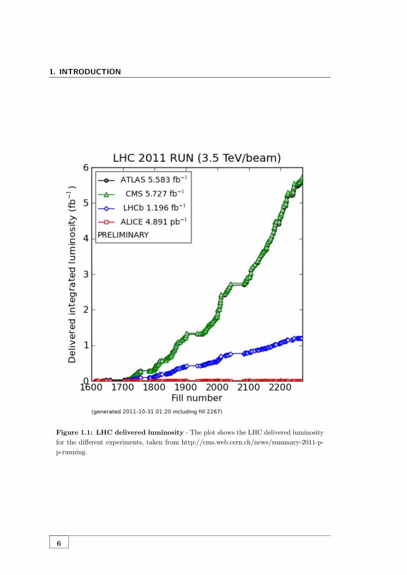
CMS has recorded 5.21 fb-1, as shown in Figure 1.1. The overall data taking efficiency
is 91%, and the average fraction of operational channels per subsystem is > 98.5%.
Results shown in this thesis use a large fraction of the full data-set. Certied data for
physics: Golden 4745pb−1 (91.2%), Muon 4965pb−1 ( 96%). The Uncertainty on the
luminosity determination is 4.5%.
A few highlights from the 2011 run summary (cfr: (1)) follows.
Peak Instantaneous Luminosity: 3.55 · 1033 Hz/cm 2 in fill 2256 2011.10.26.
Delivered luminosity in one Fill: 123 pb −1 in fill 2219 2011.10.16
Maximum Luminosity in one Day: 136 pb−1 on 2011.10.13
Maximum Luminosity Delivered in one Week: 538 pb−1 in week 41
Maximum Luminosity Delivered in one Month: 1614 pb−1 in October 2011.
LHC declared stable beams for 1364 hours in this year.
5
1. INTRODUCTION
Figure 1.1: LHC delivered luminosity - The plot shows the LHC delivered luminosityfor the different experiments, taken from http://cms.web.cern.ch/news/summary-2011-p-p-running.
6
2Seesaw theory Beyond the Standard Model
2.1 Standard Model
The Standard Model is regarded as one of the biggest achievements in physics of the
last century because it is the current best description of the physics of fundamental
particles and their interactions: electromagnetic, weak, and strong interactions. It
describes them with high accuracy and stands numerous experimental tests. It has
been tested to high precision by the Large Electron Positron (LEP) collider at CERN,
the Tevatron at Fermi National Laboratory, and by the Stanford Linear Collider (SLC)
at Stanford National Laboratory.(i.e. LEP electroweak measurements).
The Standard Model is a particular quantum field theory. Quantum field theory
combines the two great achievements of 20th-century physics, quantum mechanics and
relativity.
We’ll review in Appendix A the most important features of the Standard Model,
stressing the aspects relevant for the theory underling this thesis. For a complete
description see References (3) and (2). The evidences for physics beyond the Standard
Model are descried in Section 2.2, and a closer examination of the Seesaw model,
analyzed in this thesis, is given in Section 2.3.
2.2 Beyond the Standard Model
The Standard Model is a simple, elegant, and successful theory. It successfully describes
the majority of current experimental data. Nevertheless, there are anomalies and both
direct and indirect evidence for it physics beyond the standard model. We’ll summarize
them in this section.
7
2. SEESAW THEORY BEYOND THE STANDARD MODEL
2.2.1 Direct evidence
2.2.1.1 Neutrinos
The existence of neutrino particle was first postulated in 1930 by Wolfgang Pauli
to preserve the conservation of energy, conservation of momentum, and conservation of
angular momentum in beta decay: n→ p+e+νe. This undetected particle should carry
away the observed difference between the energy, momentum, and angular momentum
of the initial and final particles.
The experiment for direct detection, the so called β-capture, was proposed in 1942
by Kan-Chang Wang. In 1956 Clyde Cowan, Frederick Reines, F. B. Harrison, H.
W. Kruse, and A. D. McGuire detected the neutrino through this process, and were
rewarded with the 1995 Nobel Prize. In this experiment neutrinos created in a nuclear
reactor by beta decay were shot into protons producing neutrons and positrons both
of which could be detected.
In 1962 Leon M. Lederman, Melvin Schwartz and Jack Steinberger showed that
more than one type of neutrino exists by detecting interactions of the muon neutrino.
When the third type of lepton, the tauon, was discovered in 1975 at the Stanford
Linear Accelerator Center, it too was expected to have an associated neutrino, and the
evidence for this third neutrino type came from the observation of missing energy and
momentum in tauon decays analogous to the beta decay leading to the discovery of the
neutrino. The first detection of tauon neutrino interactions was announced in summer
of 2000 at the Fermi National Laboratory, making it the latest particle of the Standard
Model to have been directly observed. The current best measurement of the number
of neutrino types comes from observing the decay of the Z boson. This particle can
decay into any light neutrino and its antineutrino, and the more types of light neutrinos
available, the shorter the lifetime of the Z boson. Measurements of the Z lifetime have
shown that the number of light neutrino types is 3. The Standard Model of particle
physics (SM) assumes that neutrinos are 3, they are massless and cannot change flavor.
The neutrino flavor oscillations. Starting in the late 1960s, several experiments
found that the number of electron neutrinos arriving from the sun was between one third
and one half the number predicted by the Standard Solar Model (SSM), a discrepancy
which became known as the solar neutrino problem and remained unresolved for some
8

2.2 Beyond the Standard Model
thirty years. The idea of neutrino flavor oscillations was first suggested by Bruno
Pontecorvo in 1957, and developed in 1967. According to this theory neutrinos are able
to oscillate between the three available flavors while they propagate through space.
The observation of neutrino flavor oscillations indicates that neutrinos have mass,
which is not explained by the Standard Model. Moreover, the existence of neutrino
masses leads to leptonic mixing. The observation of neutrino oscillations is thus unam-
biguous evidence of physics beyond the standard model.
Neutrino oscillations arise from a straightforward quantum mechanical phenomenon
that occurs during the propagation of the neutrinos, causing them to change flavor.
This is possible due to the existence of lepton mixing, which is entirely analogous to
quark mixing (although the values of the mixing angles are quite different). Instead
of the Cabibbo-Kobayashi-Maskawa (CKM) matrix of the quark sector, the respective
mixing matrix is sometimes denoted as the Pontecorvo-Maki-Nakagawa-Sakata (PMNS,
or often only MNS) matrix. In the basis where the charged lepton mass matrix is
diagonal:
νi =∑α
Uαiνα
�� ��2.1
νi are the mass eigenstates, να the flavor eigenstates. The unitary matrix U expressing
the linear combination in eq.(2.1) is the PMNS matrix (here we use Greek letters to
clearly distinguish the flavor indices α, β from the mass indices i, j). With this in
mind it is easy to understand how a specific flavor eigenstate can oscillate to a different
one as it propagates: it is composed of a linear combination of mass eigenstates with
masses mi.
The neutrino mass eigenstates propagation could be described by plane wave solu-
tions of the form:
|νi(t = L)〉 = e−i(Eit−~pi·~x)|νi(0)〉 ≈ e−im2i L/2E |νi(0)〉
�� ��2.2
with t is the time from the start of the propagation, ~x is the current position of
the particle, ~pi is the 3-dimensional momentum. The neutrinos are very light, with
mi � pi, so one can take t ' L (natural units), so c = 1 t = L = traveled distance.
The proportion of mass eigenstates will change during the propagation due to the phase
factors e−imiτ in the νi rest frame. In the laboratory frame, the phase factor becomes
9

2. SEESAW THEORY BEYOND THE STANDARD MODEL
e−i(Eit−piL) (Ei and pi being the energy and momentum of νi, t and L the time and
position, all quantities in the laboratory frame). Since neutrino masses are less than 1
eV and their energies are at least 1 MeV, we could consider the ultra-relativistic limit,
therefore the energy could be approximated as: Ei =√p2
i +m2i ' pi + m2
i2pi
.
Eigenstates with different masses propagate at different speeds. Since the mass
eigenstates are combinations of flavor eigenstates, this difference in speed causes inter-
ference between the corresponding flavor components of each mass eigenstate.
The phase factor becomes (approximately) e−i(m2i /2p)L, and considering the average
energy of the various mass eigenstates E ' p, we can obtain the formula for probability
of flavor change from flavor state α into flavor state β after propagation for a distance
L in the vacuum:
Pα→β =
∣∣∣∣∣∑i
U∗αiUβie
−im2
i L
2E
∣∣∣∣∣2 �� ��2.3
Eq.(2.3) may be conveniently expressed as Pα→β = δαβ +Qα→β, with Qα→β being:
Qα→β = −4∑i>j
Re(U∗
αiUβiUαjU∗βj
)sin2
(∆m2
ijL
4E
)+2Im
(U∗
αiUβiUαjU∗βj
)sin
(∆m2
ijL
2E
)�� ��2.4
The terms in eq.(2.4) clearly show that the squared mass differences ∆m2ij ≡ m2
i −m2
j are measurable from oscillation (although the overall mass scale isn’t).
The phase that is responsible for oscillation is often written as:
∆m2 c3 L
4~E=
GeV fm4~c
× ∆m2
eV2
L
kmGeVE
≈ 1.267× ∆m2
eV2
L
kmGeVE
�� ��2.5
All neutrino experiments observing oscillations measure the squared mass difference
and not absolute mass, therefore it could be hypothesized that the lightest neutrino
mass is exactly zero, but it is regarded as unlikely by theorists.
A convenient summary of the neutrino oscillation data is given in (16). For reference,
we reproduce in Table 2.2.1.1 the relevant table with the values (updated in June 2006
(16)).
It is important to note that the large angles of table 2.2.1.1 contrast with the small
angles of the CKM matrix (the largest of which, the Cabibbo angle, has sin(θC) < 0.23).
10

2.2 Beyond the Standard Model
parameter best fit 2σ 3σ 4σ
∆m221[10−5eV] 7.9 7.3–8.5 7.1–8.9 6.8–9.3
∆m231[10−3eV] 2.6 2.2–3.0 2.0–3.2 1.8–3.5sin2 θ12 0.30 0.26–0.36 0.24–0.40 0.22–0.44sin2 θ23 0.50 0.38–0.63 0.34–0.68 0.31–0.71sin2 θ13 0.000 ≤ 0.025 ≤ 0.040 ≤ 0.058
Table 2.1: Neutrino data: best-fit values, 2σ, 3σ, and 4σ intervals (from (16)).
The experimental data is conveniently displayed in a graphical manner by use of
colored or shaded bars, taken from (17). Figure 2.1 features the two possible mass hier-
archies (due to the ambiguity in the sign of the atmospheric squared mass difference),
and shows the peculiar situation described by tri-bi-maximal mixing quite clearly: one
neutrino mass eigenstate (ν3) is approximately comprised of equal parts νµ and ντ , and
another (ν2) is approximately equal parts of all three flavor eigenstates.
Figure 2.1: Neutrino mixing summary from (27).
Neutrino masses and mixings in the Standard Model could be explained with
a conservative hypothesis, i.e.: the Standard Model restricts to the simplest possible
interactions, additional interactions are present, but they are suppressed. To add these
11

2. SEESAW THEORY BEYOND THE STANDARD MODEL
additional interactions, we need to add more terms to the Lagrangian in Eq. A.1, with
coefficients with dimensions of an inverse power of mass (3):
L = LSM +1M
L5 +1M2
L6 + · · ·�� ��2.6
where M is a mass scale greater than the Higgs-field vacuum-expectation value, v. At
energies much less than M , the least-suppressed interactions come from the Lagrangian
labeled L5. There is only one possible term in this Lagrangian (assuming the standard-
model particle content and gauge symmetries) (3, 6),
L5 = cij(LiTL εφ)C(φT εLj
L) + h.c. .�� ��2.7
where LL and φ are the lepton and Higgs-doublet fields (see Table A.1) and C is the
charge-conjugation matrix. When the Higgs field acquires a vacuum-expectation value,
this term gives rise to a Majorana 1
1For the Dirac particle we have to put in the Feynmann rule: γµ(1 − γ5). If the neutrino is a
Majorana particle The Lagrangian looks the same but in the Feynamann rule we have to include
instead the term: γµγ5. To understand it we need to go back to the field expression:
ΦDirac =
Z(fe−ip + f†eip)
ΦMajorana =
Z(fe−ip + f†eip)
where f is the fermion annihilation operator, and f is the anti-fermion annihilation operator. So the
creation in the Dirac case is:
< νν|(f† + f)γµ(1− γ5)(f + f†)|Z >
=< 0|ff [(f† + f)γµ(1− γ5)(f + f†)]|Z >
where < νν =< 0|ff and the contractions in the Dirac case are f f† and ff†.
In the Majorana case we have:
< 0|ff [(f† + f)γµ(−1− γ5)(f + f†)]|Z >�� ��2.8
in this case we have two contractions: ff† for each field f , so we obtain: γµ(1− γ5)− γµ(1− γ5).
Therefore we could write:
νγµ(1− γ5)ν
=1
2νγµ(1− γ5)ν +
1
2(νγµ(1− γ5)ν)
t
=1
2νγµ(1− γ5)ν +
1
2(−νt(1− γ5)γ
tµν
t)
=1
2νγµ(1− γ5)ν +
1
2(−νcγµ(1 + γ5)νc
12

2.2 Beyond the Standard Model
mass matrix for the neutrinos,
M ijν = cij
v2
M.
�� ��2.10
Given this addition lagrangian term, we expect neutrino masses and mixing, with
masses much less than v (for M � v). We will describe neutrino masses and mixings
in the following paragraph. For a exhaustive derivation the most indicated reference
is the original treatment in (13). It is useful the neutrino mixing review in (15) too,
which includes extensive references. The following clear brief summary is taken mostly
from (14).
2.2.1.2 Gravity
Gravity is not explained by the Standard Model, thus is another direct evidence of
physics beyond the standard model. If a graviton field is added to the theory, gµν , the
least-suppressed additional interactions (using dimensional analysis) are
Lgravity =M2
P
16π√−g(−2Λ +R+ · · · )
�� ��2.11
where MP is the Planck scale, g ≡ det gµν , R is the Ricci scalar, and Λ is the cos-
mological constant. The Ricci-scalar term accounts for all of classical gravity. The
cosmological constant, long thought to be exactly zero, is able to account for the mys-
terious dark energy needed to accommodate cosmological observations.
2.2.1.3 Astrophysics and Cosmology
Along with the dark energy mentioned above there is also dark matter, whose nature is
unknown, which accounts for about 35% of the mass-energy. Observations of fluctua-
tions in the spectrum of the microwave background, remnant from the Big Bang, have
established the existence of cold dark matter. In particular, recent measurements from
the Wilkinson Microwave Anisotropy Probe (WMAP) satellite show that dark matter
composes 23.3% of the Universe, while ordinary baryonic matter makes up only 4.6%
Since in the Majorana case: νc = ν we obtain:
νγµ(1− γ5)ν =1
2νγµ(1− γ5)ν −
1
2(νγµ(1 + γ5)ν = νγµγ5ν
�� ��2.9
13

2. SEESAW THEORY BEYOND THE STANDARD MODEL
of it. Moreover, observation of large red shifts in the spectrum of the oldest Type Ia su-
pernovas confirms the theory that 70% of the Universe is made up of dark energy. This
measurement has also been supported by the WMAP satellite measurements, which
established the dark matter content at 72.1%. Whatever this matter is, it is certainly
beyond the standard model.
The observed baryon asymmetry of the universe also cannot be explained by the
standard model, because it requires a source of CP violation beyond that contained in
the CKM matrix. The inflationary model of the universe, so successful in explaining
many of the features of our universe, also requires physics beyond the standard model.
2.2.2 Indirect evidence
2.2.2.1 Masses and mixing angles
The standard model accommodates generic masses and mixing angles, but the observed
values are far from generic. The fermion masses and mixing angles strongly suggest
that there is a deeper structure underlying the Yukawa sector of the standard model.
Since the standard model can accommodate any masses and mixing angles, we must
seek an explanation from physics beyond the standard model.
The introduction of the scalar field to explain the breaking of the electroweak sym-
metry is done ”by hand” and the Higgs particle has to be still confirmed by the exper-
iments. 1
Moreover, the natural scale of charged fermion masses is of order v, but all charged
fermions (except the top quark) are much lighter than this, and display a hierarchical
pattern. The CKM mixing angles are also not generic; they are small, and are also
hierarchical. These facts suggest that there is physics beyond the standard model
1Discovering and studying the Higgs boson (or bosons) is central to understanding physics beyond
the standard model because almost all of these anomalies and hints of physics beyond the standard
model involve the Higgs field in one way or another. Neutrino masses involve the Higgs field, via
Eq. (2.7); the vacuum-expectation value of the Higgs field contributes to the cosmological constant; the
axion (a type of Higgs field) is a dark-matter candidate; there could be additional CP violation in the
Higgs sector that generates the baryon asymmetry; the inflaton (a scalar field) could drive inflation;
precision electroweak data constrain the Higgs sector; fermion masses and mixing angles result from
the coupling of the Higgs field to fermions, Eq. (A.8); SUSY SU(5) grand unification requires two Higgs
doublets; and the hierarchy problems involve the Higgs-field vacuum-expectation value.
14

2.2 Beyond the Standard Model
that explains the pattern of charged fermion masses and mixing. Unfortunately, the
standard model does not indicate at what energy scale this new physics resides (8).
2.2.2.2 Dimensional Analysis of the Lagrangian
The Standard Model lagrangian written in Eq. A.1 includes only the simplest terms
because these are the renormalizable terms. Renormalizability or dimensional analysis
is a stronger constraint than is really necessary (7).
The action has units of ~ = 1:
S =∫d4x L .
�� ��2.12
so the Lagrangian must have units of mass4. From the kinetic energy terms in the
Lagrangian for a generic scalar (φ), fermion (ψ), and gauge boson (Aµ),
LKE = ∂µφ∗∂µφ+ iψ 6∂ψ − 12(∂µAν∂µAν + ∂µAν∂νAµ)
�� ��2.13
we can deduce the dimensionality of the various fields:
dim φ = mass
dim ψ = mass3/2
dim Aµ = mass
All operators (products of fields) in the Lagrangian of the Standard Model are of
dimension four, except the operator φ†φ in the Higgs potential, which is of dimension
two. The coefficient of this term, µ2, is the only dimensionful parameter in the standard
model; it (or, equivalently, v ≡ µ/√λ) sets the scale of all particle masses.
Imagine that the Lagrangian at the weak scale is an expansion in some large mass
scale M ,
L = LSM +1M
dim 5 +1M2
dim 6 + · · · ,�� ��2.14
where dim n represents all operators of dimension n. By dimensional analysis, the
coefficient of an operator of dimension n has dimension mass4−n, since the Lagrangian
has dimension mass4. At energies much less than M , the dominant terms in this
Lagrangian will be those of LSM ; the other terms are suppressed by an inverse power
of M . This is the modern reason why we believe the “simplest” terms in the Lagrangian
15

2. SEESAW THEORY BEYOND THE STANDARD MODEL
are the dominant ones. When searching for deviations from the standard model, we
need to look for the effects of higher-dimension operators. The least suppressed terms in
the Lagrangian beyond the standard model are of dimension five. We should therefore
expect our first observation of physics beyond the standard model to come from these
terms. Although there is only one operator of dimension five, there are dozens of
operators of dimension six.
Thus far, none of the effects of any of these operators have been observed. The
best we can do is set lower bounds on M (assuming some dimensionless coefficient).
These lower bounds range from 1 TeV to 1016 GeV, depending on the operator. As we
explore nature at higher energy and with higher accuracy, we hope to begin to see the
effects of some of these dimension-six operators.
The mass scale M corresponds to the mass of a particle that is too heavy to observe
directly. At energies greater than M , the expansion of Eq. (2.14) is no longer useful,
as each successive term is larger than the previous. Instead, one must explicitly add
the new field of mass M to the model. For example, if nature is supersymmetric at the
weak scale, one must add the superpartners of the standard-model fields to the theory
and include their interactions in the Lagrangian. If we raise the mass scale of the
superpartners to be much greater than the weak scale, then we can no longer directly
observe the superpartners, and we return to a description in terms of standard-model
fields, with an expansion of the Lagrangian in inverse powers of the mass scale of the
superpartners, M .
2.2.2.3 Grand Unification
SU(5) grand unification it has been a smart idea (9), but now the gauge couplings it
is known with good accuracy, and they do not unify at high energies. It is remarkable
that by imposing weak-scale supersymmetry on the theory, the relative evolution of
the couplings is nudged just enough to successfully unify the couplings at the scale
MGUT ≈ 1016 GeV. This suggests that the supersymmetric partners of the known
particles await us as we probe the weak scale.
2.2.2.4 Hierarchy problems
The standard model has only one energy scale, i.e. the Higgs-field vacuum-expectation
value, v. The questions why there is a strong hierarchy is still unresolved. In other
16

2.3 The Seesaw Model for Mass Generation Mechanisms
words, it appears that physics beyond the standard model is associated with scales
wildly different from v, but the questions is unanswered. Perhaps the explanation for
this requires yet more physics beyond the standard model, such as supersymmetry or
large extra dimensions.
2.3 The Seesaw Model for Mass Generation Mechanisms
An appealing possibility to include the neutrino masses and accounting for their small-
ness is the seesaw mechanism. With this model new heavy particles having a Yukawa
interaction with the lepton and the Higgs doublets generate a small Majorana mass
for the neutrinos, generically suppressed, with respect to charged fermion masses, by a
factor v/M , where M the mass of the heavy particle. If one requires O(1) Yukawa cou-
plings, M should be of the order of the grand unification scale in order to account for
neutrino masses smaller than the eV. However, in principle nothing prevents the scale
to be as low as hundreds of GeV. In this case the heavy field responsible for neutrino
masses could be discovered at the LHC.
Detailed description of seesaw mechanism theory is contained in references: (18),
(19), (20) and (24). Here we will give only a brief summary.
2.3.1 Seesaw Models
Depending on the nature of the heavy state, seesaw models are called type I (18),
type II (19) or type III (20), corresponding to heavy fermionic singlet, scalar triplet or
fermionic triplet, respectively.
The three types of seesaw mechanism generate new lagrangian terms with dimension
greater then four. They generate dimension five operator which gives light neutrino
masses, but also additional lepton number conserving (LNC) dimension six operators,
which are different in each seesaw scenario(References (70),(24)). Therefore, seesaw
models may in principle be discriminated, albeit indirectly, with precise low-energy
measurements sensitive to these dimension six operators.
The only five-dimensional operator allowed by the SU(3)× SU(2)L × U(1)Y gauge
symmetry is the lepton number violating (LNV) dimension five operator (5):
(O5)ij = LciLφ
∗φ†LjL
�� ��2.15
17

2. SEESAW THEORY BEYOND THE STANDARD MODEL
where
LiL =(νiL
liL
), i = 1, 2, 3
�� ��2.16
are the SM left-handed lepton doublets, φ the SM Higgs and φ = iτ2φ∗, with τi the Pauli
matrices. This operator yields Majorana masses for the neutrinos after spontaneous
symmetry breaking.
Figure 2.2: The three generic realizations of the Seesaw mechanism, depending on thenature of the heavy fields exchanged: SM singlet fermions (type I Seesaw) on the left, SMtriplet scalars (type II Seesaw) and SM triplet fermions (type III Seesaw) on the right.
2.3.2 Seesaw I
Type-I seesaw is usually implemented by adding three right-handed current eigenstates
N ′iR, i = 1, 2, 3, transforming as singlets under the SM gauge group. This allows to
write a Yukawa interaction for neutrinos analogous to the one for charged leptons,
LY = −Yij L′iLN′jR φ+ H.c. ,
�� ��2.17
where Y is a 3 × 3 matrix of couplings and L′iL the SM lepton doublets (in the weak
eigenstate basis). This interaction generates a mass term upon spontaneous symmetry
breaking
φ =(φ+
φ0
)→ 1√
2
(0v
), φ ≡ iτ2φ
∗ → 1√2
(v0
),
�� ��2.18
with v = 246 GeV. Since N ′iR are SM singlets, gauge symmetry allows a Majorana mass
term
LM = −12MijN ′
iLN′jR + H.c. ,
�� ��2.19
18

2.3 The Seesaw Model for Mass Generation Mechanisms
with M a 3× 3 symmetric matrix and N ′iL ≡ N
′ciR.1 Defining ν ′iR ≡ ν
′ciL, where ν ′iL are
the SM neutrino eigenstates, the full neutrino mass term reads
Lmass = −12(ν ′L N
′L
)( 0 v√2Y
v√2Y T M
) (ν ′RN ′
R
)+ H.c. .
�� ��2.20
The neutrino gauge interactions are the same as in the SM. Then, the relevant inter-
action terms for the heavy neutrino mass eigenstates Ni ' N ′iR can be obtained by
diagonalizing the mass matrix in Eq. (2.20) and rewriting the interactions in the mass
eigenstate basis.
In the absence of any particular symmetry in the Yukawa couplings, light neutrino
masses mν are of the order Y 2v2/2mN , and the heavy neutrino mixings are VlN ∼√mν/mN . Hence, for a heavy neutrino within LHC reach, say with a mass mN ∼ 100
GeV, its seesaw-type contribution to light neutrino masses is of the order of 300Y 2 GeV,
requiring very small Yukawas Y ∼ 10−6 to reproduce light neutrino masses mν ∼ 0.1
eV. Moreover, the natural order of magnitude of the mixings is O(10−6), too small to
give observable signals.
Even if we put aside the connection between heavy neutrino mixing and light neu-
trino masses, the former must be small due to present experimental constraints. Elec-
troweak precision data set limits on mixings involving a single charged lepton, and using
the latest experimental data, the constraints at 90% confidence level (CL) are (25)
3∑i=1
|VeNi |2 ≤ 0.0030 ,3∑
i=1
|VµNi |2 ≤ 0.0032 ,3∑
i=1
|VτNi |2 ≤ 0.0062 ,�� ��2.21
which in particular imply constraints on the individual mixings VlN of a heavy
neutrino N . These constraints are particularly important since they determine the
heavy neutrino production cross sections at LHC. Figure 2.3 is a typical type I seesaw
diagram (with the “×” in the νc propagator denoting the Majorana mass insertion).
2.3.3 Seesaw II
In type II seesaw light neutrinos acquire masses from a gauge-invariant Yukawa inter-
action of the left-handed lepton doublets with a scalar triplet ∆ of hypercharge Y = 11We avoid writing parentheses in charge conjugate fields to simplify the notation, and write ψc
L ≡(ψL)c, ψc
R ≡ (ψR)c.
19

2. SEESAW THEORY BEYOND THE STANDARD MODEL
Figure 2.3: Type I seesaw diagram.
(with Q = T3 + Y ). Writing the triplet in Cartesian components ~∆ = (∆1, ∆2, ∆3),
the Yukawa interaction reads
LY =1√2Yij LiL (~τ · ~∆)LjL + H.c. ,
�� ��2.22
with
LjL = iτ2
(νc
jL
lcjL
) �� ��2.23
and Y a symmetric matrix of Yukawa couplings. We assume without loss of generality
that the charged lepton mass matrix is diagonal, and drop primes on the neutrino fields,
which are taken in the flavor basis νe, νµ, ντ . The triplet charge eigenstates are related
to the Cartesian components by
∆++ =1√2(∆1 − i∆2) , ∆+ = ∆3 , ∆0 =
1√2(∆1 + i∆2) .
�� ��2.24
When the neutral triplet component acquires a vacuum expectation value (vev) 〈∆0〉 =
v∆, the Yukawa interaction in Eq. (2.22) induces a neutrino mass term
Lmass = −Y ∗ijv∆ νiL νjR + H.c.
≡ −12Mij νiL νjR + H.c. ,
�� ��2.25
where we have again introduced the notation νiR ≡ νciL, and
Mij = 2Y ∗ijv∆
�� ��2.26
are the matrix elements of the light neutrino Majorana mass matrix.
20

2.3 The Seesaw Model for Mass Generation Mechanisms
The triplet Yukawa interaction in Eq. (2.22) also generates triplet couplings to the
charged leptons.
The gauge interactions of the triplet components are obtained from the kinetic term
LK = (Dµ~∆)† · (Dµ~∆) ,
�� ��2.27
For a detailed derivation of gauge interactions mediating scalar triplet pair produc-
tion processes see ref. (24).
Constraints on the triplet parameters are much less important than for heavy neu-
trino singlets, because the new scalars can be produced at LHC by unsuppressed gauge
interactions. Electroweak precision data set an upper limit on the triplet vev v∆. The
most recent bound obtained from a global fit is (26)
v∆ < 2 GeV ,�� ��2.28
which is much less stringent than the one derived from neutrino masses, Eq. (2.26),
if Yij are of the order of the charged lepton Yukawa couplings. The type II seesaw
mechanism typical diagram is shown in figure 2.4.
Figure 2.4: Type II seesaw diagram.
2.3.4 Seesaw III
In type III seesaw the SM is usually enlarged with three leptonic triplets Σj , each
composed by three Weyl spinors of zero hypercharge. Writing the triplets in Cartesian
components ~Σj = (Σ1j , Σ2
j , Σ3j ) and using standard four-component notation, the triplet
Yukawa interaction with the lepton doublets takes the form
LY = −Yij L′iL(~Σj · ~τ) φ+ H.c. ,
�� ��2.29
21

2. SEESAW THEORY BEYOND THE STANDARD MODEL
with Y a 3×3 matrix of Yukawa couplings. The triplet Majorana mass term mediating
the seesaw is
LM = −12Mij
~Σci · ~Σj + H.c. ,
�� ��2.30
with M a 3×3 symmetric matrix. Notice that all the members Σ1j , Σ2
j , Σ3j of the triplet
Σj have the same mass term. For each triplet Σj , the charge eigenstates are related to
the Cartesian components by
Σ+j =
1√2(Σ1
j − iΣ2j ) , Σ0
j = Σ3j , Σ−
j =1√2(Σ1
j + iΣ2j ) .
�� ��2.31
The physical particles are charged Dirac fermions E′j and neutral Majorana fermions
N ′j (as before, we use primes for the weak interaction eigenstates),
E′j = Σ−
j + Σ+cj , N ′
j = Σ0j + Σ0c
j .�� ��2.32
Then, for our choice of right-handed chirality for the triplets we have
E′jL = Σ+c
j , E′jR = Σ−
j , N ′jL = Σ0c
j , N ′jR = Σ0
j .�� ��2.33
After spontaneous symmetry breaking the terms in Eqs. (2.29), (2.30) lead to the
neutrino mass matrix
Lν,mass = −12(ν ′L N
′L
)( 0 v√2Y
v√2Y T M
) (ν ′RN ′
R
)+ H.c. ,
�� ��2.34
similar to the one for type-I seesaw in Eq. (2.20). The mass matrix for charged leptons,
also including the 3× 3 SM Yukawa matrix Y l, reads
Ll,mass = −(l′L E
′L
)( v√2Y l vY
0 M
) (l′RE′
R
)+ H.c.
�� ��2.35
The gauge interactions of the new triplets can be obtained from the kinetic term
LK = i ~Σj · γµDµ~Σj ,
�� ��2.36
where a sum over j = 1, 2, 3 is understood. The covariant derivative is
Dµ = ∂µ + ig ~T · ~Wµ ,�� ��2.37
The Bµ term is absent because the triplets have zero hypercharge. With the definitions
in Eqs. (2.31) and (2.32), the gauge interactions in the weak eigenstate basis could be
derived.
22

2.3 The Seesaw Model for Mass Generation Mechanisms
As in the case of heavy neutrino singlets, limits on the mixing of new fermion triplets
arise from electroweak precision data. The most recent constraints are (25)
3∑i=1
|VeNi |2 ≤ 0.00036 ,3∑
i=1
|VµNi |2 ≤ 0.00029 ,3∑
i=1
|VτNi |2 ≤ 0.00073�� ��2.38
at 90% CL.
2.3.5 Seesaw type-III simplified model
The model considered in this thesis is the seesaw type III simplified model derived in
Ref. (30), which is based on the full model presented in Ref. (28).
The Complete Lagrangian is written with the addition to the standard model of
SU(2) triplets of fermions with zero hypercharge, Σ. In this model at least two such
triplets are necessary in order to have two non-vanishing neutrino masses. The beyond
the standard model interactions are described by the following lagrangian (with implicit
flavor summation):
L = Tr[Σi/DΣ]− 12Tr[ΣMΣΣc + ΣcM∗
ΣΣ]− φ†Σ√
2YΣL− L√
2YΣ†Σφ ,
�� ��2.39
with L ≡ (ν, l)T , φ ≡ (φ+, φ0)T ≡ (φ+, (v +H + iη)/√
2)T , φ = iτ2φ∗, Σc ≡ CΣT and
with, for each fermionic triplet,
Σ =(
Σ0/√
2 Σ+
Σ− −Σ0/√
2
), Σc =
(Σ0c/
√2 Σ−c
Σ+c −Σ0c/√
2
),
Dµ = ∂/µ − i√
2g(W 3
µ/√
2 W+µ
W−µ −W 3
µ/√
2
).
�� ��2.40
Without loss of generality, we can assume that we start from the basis where MΣ is
real and diagonal, as well as the charged lepton Yukawa coupling, not explicitly written
above. In order to consider the mixing of the triplets with the charged leptons, it is
convenient to express the four degrees of freedom of each charged triplet in terms of a
single Dirac spinor:
Ψ ≡ Σ+cR + Σ−
R .�� ��2.41
The neutral fermionic triplet components on the other hand can be left in two-component
notation, since they have only two degrees of freedom and mix with neutrinos, which
23

2. SEESAW THEORY BEYOND THE STANDARD MODEL
are also described by two-component fields. This leads to the Lagrangian
L = Ψi∂/Ψ + Σ0Ri∂/Σ
0R −ΨMΣΨ−
(Σ0
R
MΣ
2Σ0c
R + h.c.)
+ g(W+
µ Σ0RγµPRΨ +W+
µ Σ0cR γµPLΨ + h.c.
)− gW 3
µΨγµΨ
−(φ0Σ0
RYΣνL +√
2φ0ΨYΣlL + φ+Σ0RYΣlL −
√2φ+νL
cY TΣ Ψ + h.c.
).�� ��2.42
The mass matrices of the charged and the neutral sectors need to be diagonalized
as they possess off-diagonal terms. Following the diagonalization procedure described
in Ref. (28), we obtain the Lagrangian in the mass basis written in Appendix B.1, see
ref. (30) from the detailed derivation of the lagrangian terms.
First assumption: one Triplet Restriction: the lagrangian derived is written for
a generic number of triplets. Nevertheless, in the presence of more triplets, it will be the
lightest the one that will be more easily discovered. Therefore, since we are interested
in LHC physics, we can safely restrict the model to the case of only one triplet.
Under this assumption, the new Yukawa couplings matrix reduces to a
1× 3 vector:
YΣ =(YΣe YΣµ YΣτ
),
�� ��2.43
and the mass matrix MΣ is now a scalar.
Second assumption: real parameters will be taken, i.e. we do not take into
account the phases of the Yukawa couplings nor the ones of the PMNS matrix. Barring
cancellations, they should not play a role in the discovery process.
As a consequence ε is a 3× 3 matrix whose elements are
εαβ =v2
2M−2
Σ YΣαYΣβ,
�� ��2.44
and ε′ is now a scalar:
ε′ =v2
2M−2
Σ
(Y 2
Σe+ Y 2
Σµ+ Y 2
Στ
).
�� ��2.45
24

2.3 The Seesaw Model for Mass Generation Mechanisms
Finally, we express all the couplings in terms of the mixing parameters, Vα =v√2M−1
Σ YΣα , since they are the parameters which are truly constrained by the elec-
troweak precision tests and the lepton flavor violating processes. Then ε′ = V · V T
while ε = V T ∧ V .
By applying these simplifications and redefinitions, the couplings of Eqs. (B.10)-
(B.24) in terms of MΣ and Vα are obtained; they are shown in Appendix B.2.
25


3Experimental Apparatus
3.1 Accelerators in Particle Physics
The high energy particle accelerators are like microscopes which have allowed physicist
to peer at the ’heart of matter’. A particle accelerator uses electromagnetic fields to
propel charged particles to high speeds and to contain them in well-defined beams.
Machines make particle beams to collide, either to fixed target or between each others.
Main features about colliders are given in Section 3.1.1. A description of LHC collider
is given in 3.2, and CMS experiment is presented in Section 3.3.
3.1.1 Colliders main Features
From the point of view of energetics the collider mode is superior for new particle
production than the fixed target mode because the energy available is higher1.
The higher the available energy in the center-of-mass (√s), the higher the energy of
new particles produced in collisions. Therefore√s is one of the most important aspect
of the collider.
The next important aspect of the collider is the rate, and therefore the total number
of collisions. Even if√s is high, the production of new particles may never take place if
1 High energy particle beams are used to collide in two different ways:
• Fixed Target Machines: beams are incident on a stationary target which consists of light or
heavy nuclei. In this case for a beam of energy Eb incident on a target of mass MT , total energy
available for new particle production is Ecm =√MTEbc.
• Colliders: beams of accelerated particles collide against each other. In the collider environment,
specializing to the case where both the beams have particles with same mass and energy, the
energy available for particle production is 2Eb.
27

3. EXPERIMENTAL APPARATUS
the production cross section of the signal process is considerably small at the design√s
with low collision rate. Maximizing the number of collisions per beam fill it is necessary
to take data efficiently too, as preparation of beams take time O(1 hour) and beam
intensities decrease as the time goes by. The expected event rate depends on the cross
section and the luminosity delivered by the accelerator:
Nevents
t= Lσ
�� ��3.1
where L is the luminosity expressed in units of inverse barn, and σ is the cross
section expressed in units of barn. The number and types of possible interactions for
a given combination of two partons i and j determine the partonic cross section σij .
The sum of these partonic cross sections, weighted by the probability to find each
combination, is the total cross section. This probability can be described by Parton
Density Functions (PDFs) which are equal to the probability to find a given parton i
with momentum fraction xi at an energy scale Q.
Particle beams in colliders could be made of protons or electrons. Hadronic and
leptonic colliders have played very complementary roles in particle physics fundamental
research. Their main characteristics are listed briefly below, for a complete review see
(33).
• Leptonic Colliders (e+e−) are precision measurement machines, since the initial
beam energy is very accurately known as the colliding particles are the same ones
which are being accelerated.
• Hadronic Colliders (pp or pp machines) are ’discovery’ machines. The colliding
particles are composites and at high energies the colliding fundamental particles
are partons (quarks, anti-quarks, gluons). It is known that, on the average, only
1/6 of the energy of the proton is available to the colliding partons. Thus for the
same energy of the beams, Ecm(e+e−) ∼ 6Ecm(pp). Nevertheless, it is easier to
accelerate the p/p to much higher energies, and the hadronic machines can provide
a broad range of energies at which collisions between partons can happen, so a
broad sweep of different energies processes can be analyzed.
28

3.1 Accelerators in Particle Physics
Figure 3.1: A summary of particle physics discoveries made with different machines.
3.1.2 Particle Physics Discoveries
The physics flow and the experimental evidence of the main physics discoveries made
at different colliders have been summarized in Fig. 3.1 from (33). Missing from this
figure is the fixed target experiment at SLAC, with electron beams of energy up to
50 GeV which made the discovery of light quarks (u,d) inside proton in 1968 and the
fixed target machines which followed it at Fermilab and CERN, with µ, ν beams up to
energy 800 GeV, which helped confirm the existence of the strange quark (s).
29
3. EXPERIMENTAL APPARATUS
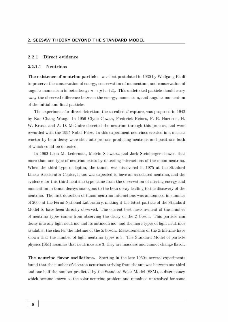
Experimental measurements from the accelerators and colliders have confirmed with
a very high level of precision the Standard Model theoretical predictions. In Table 3.1
(Reference (15)), details of some of the most crucial parameters of the unified theory of
electromagnetic and weak (EW) interactions is presented. The level of precision of the
EW theory predictions as well as the experimental measurements and the agreement
between the two is impressive. Theoretical predictions for various EW observables
depend on the mass of the Higgs Boson, MH . The Higgs is expected from the theory
but it is still undiscovered. The range of MH allowed in the SM by the experiments up
to now, at 95% CL, is 115 < MHc2 < 150 GeV (34). Physicist are currently analyzing
LHC - the Large Hadron Collider - data for discovering Higgs signals. At the moment,
the most updated combined Higgs limit, from LHC CMS and ATLAS experiments, is:
MHc2 < 141 GeV.
Observable Experimentally measured value SM fit
Width of the Z boson: ΓZ 2.4952± 0.0023 GeV 2.4959 GeV
Mass of the W boson: MW 80.404± 0.030 GeV/c2 80.376 GeV/c2
Mass of the t quark Mt 172.5± 2.3 GeV/c2 172.9 GeV/c2
Table 3.1: Precision testing of the SM.
3.2 The Large Hadron Collider
3.2.1 Introduction
The Large Hadron Collider (LHC), located at CERN, the European Laboratory for
Particle Physics, outside Geneva, Switzerland, is a unprecedented tool for fundamental
physics research for many years to come. LHC provides two proton beams, circulating
in opposite directions, at their design energy of 7 TeV each, corresponding to a center-
of-mass energy of√s = 14 TeV, and at a design luminosity of 1034 cm−2s−1.
Among the particle accelerators LHC is going to be a watershed for the subject
of fundamental particle physics. The main purpose of LHC project is to find the last
missing piece of the standard model, the Higgs boson. Also, to point the way ahead
and help understanding new physics beyond the Standard Model. Important LHC
parameters are listed in Figure 3.2.
30

3.2 The Large Hadron Collider
Figure 3.2: Main parameters of LHC machine.
3.2.2 Energy and Luminosity Design
The LHC collides proton on protons 1. The theoretical knowledge about the SM, has set
the bar for the new machine energy and intensity. (33). The choice of the design energy
of 7 TeV each proton beam could be easily understood with the following argument.
Keeping in mind the Higgs discovery benchmark, consider the scattering process in
Figure 3.3 with a Higgs production. For the two W’s to have a total energy of 1
TeV, each of them must have energy of 0.5 TeV and hence each of the parent quark in
1The physics potential of the machine would be independent of whether one has a pp machine or a
pp machine. The decision to make pp machine was taken because cheaper and simpler respect to a pp
machine, with the same physics potential
31
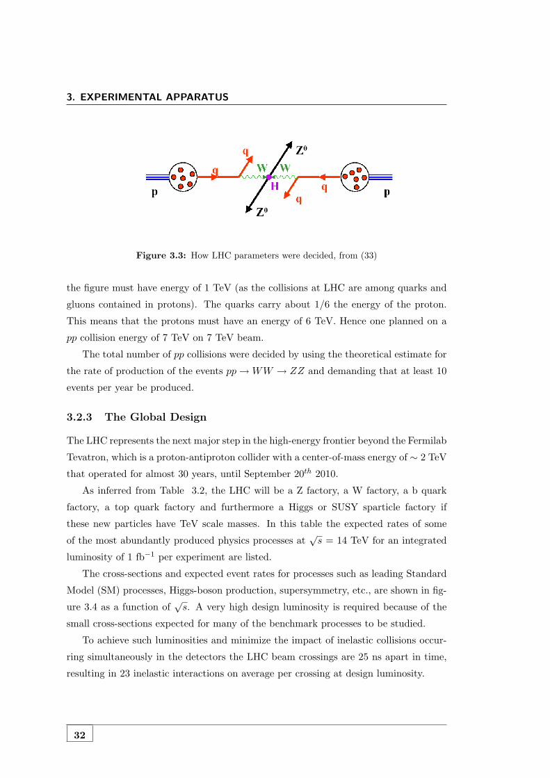
3. EXPERIMENTAL APPARATUS
Figure 3.3: How LHC parameters were decided, from (33)
the figure must have energy of 1 TeV (as the collisions at LHC are among quarks and
gluons contained in protons). The quarks carry about 1/6 the energy of the proton.
This means that the protons must have an energy of 6 TeV. Hence one planned on a
pp collision energy of 7 TeV on 7 TeV beam.
The total number of pp collisions were decided by using the theoretical estimate for
the rate of production of the events pp→WW → ZZ and demanding that at least 10
events per year be produced.
3.2.3 The Global Design
The LHC represents the next major step in the high-energy frontier beyond the Fermilab
Tevatron, which is a proton-antiproton collider with a center-of-mass energy of ∼ 2 TeV
that operated for almost 30 years, until September 20th 2010.
As inferred from Table 3.2, the LHC will be a Z factory, a W factory, a b quark
factory, a top quark factory and furthermore a Higgs or SUSY sparticle factory if
these new particles have TeV scale masses. In this table the expected rates of some
of the most abundantly produced physics processes at√s = 14 TeV for an integrated
luminosity of 1 fb−1 per experiment are listed.
The cross-sections and expected event rates for processes such as leading Standard
Model (SM) processes, Higgs-boson production, supersymmetry, etc., are shown in fig-
ure 3.4 as a function of√s. A very high design luminosity is required because of the
small cross-sections expected for many of the benchmark processes to be studied.
To achieve such luminosities and minimize the impact of inelastic collisions occur-
ring simultaneously in the detectors the LHC beam crossings are 25 ns apart in time,
resulting in 23 inelastic interactions on average per crossing at design luminosity.
32

3.2 The Large Hadron Collider
Figure 3.4: Cross sections and event rates at design LHC luminosity for hard scatteringprocesses as a function of the center-of-mass energy
√s (32).
In order to cope with the potentially overwhelming SM processes, high rejection
power is needed with optimal efficiency for rare channels such as many of the Higgs-
boson decays. In the most extreme case, a selection power of 10−14− 10−15 is required
for Higgs-boson discovery when small signal rates are compared to the total interaction
rate. This represents an increase of many orders of magnitude over the selection rates
33

3. EXPERIMENTAL APPARATUS
Table 3.2: Some of the most abundantly produced physics processes at the LHC at designluminosity. Expected numbers of events recorded by ATLAS and CMS for an integratedluminosity of 1 fb−1 per experiment are listed. From Reference (32).
Physics processes Number of events per fb−1
QCD jets with ET > 150 GeV 106 (for 10% of trigger bandwidth)W → µν 7× 10⁶
Z → µµ 1.1× 10⁶
tt → e/µ+X 1.6× 10⁵
gg production (mg ≈ 1 TeV) 102 to 103
achieved at the Tevatron.
The QCD jet production cross-section is overwhelmingly dominant over all elec-
troweak processes: this means that lepton signatures are most often essential in ex-
tracting rare processes from the background at the LHC. It is for this very reason that
both excellent measurements and superb identification capabilities of both electrons
and muons have been among the primordial requirements of detectors. Additional
signatures have also driven the global design to a large extent, e.g. missing transverse
energy, EmissT , typically indicating the presence of high-pT non-interacting particles such
as neutrinos, or secondary vertexes, typically indicating the presence of heavy-flavor
hadrons usually embedded in high-pT b/c-jets. As already mentioned, excellent lepton
identification should be achieved with high efficiency to extract rare signals from the
huge QCD backgrounds. For instance, the electron-to-jet ratio at the LHC is ∼ 10−5
at pT ∼ 20 GeV, a factor ∼ 100 times worse than at the Tevatron. The online rejection
to be achieved in real time is ∼ 107 and huge data volumes have to be recorded to
permanent storage, typically ∼ 109 events of 1 Mbyte size per year. For further details
see References (32) and (33).
3.2.4 Technical details
LHC (Fig. 3.5) is located at the French-Swiss border west of Lac Leman and in the
former LEP tunnel. The tunnel has a circumstance of 27 km and lies between 45 and
170 m below the surface. The energetic beams circulate in vacuum pipes there and are
kept on track by a magnetic field provided by dipole magnets. Superconducting Radio
34

3.2 The Large Hadron Collider
Frequency (RF, usually referred as resonator) cavities are used to accelerate beams to
the desired energy. The LHC is capable of operating with either proton or heavy ion
beams. At design conditions, it will run at a luminosity of 1034cm2s−1 for pp beams
at√s = 14TeV , supplying the high luminosity experiments CMS and ATLAS with
collisions every 25 ns corresponding to the nominal bunch spacing. During 2010 and
2011 runs, the center-of-mass energy was set to 7 TeV and the highest instantaneous
luminosity achieved was about 2 · 1032cm2s1 in 2010 and 3.55 · 1033cm2s1. In order to
reach the design luminosity 2808 proton bunches are filled in the LHC, separated by 25
ns. These luminosities are high enough to provide a sufficient rate of hard interactions
in which the physics processes interesting for most of experiments take place. At
the same time the probability for soft interactions is orders of magnitude higher than
for hard interactions, thus around 20 significant soft interactions are expected per
bunch crossing. As these soft interactions are considered unwanted background by the
experiments, the detectors must be able to separate these pile-up events from hard
interactions. The number of protons per bunch is limited by the non-linear beam-beam
interactions that each proton experiences each bunch crossing. In combination with
the constraints from the mechanical aperture the nominal peak beam size is 1.2mm
the maximum bunch intensity is thus NB = 1.15 × 10¹¹. At a pp collider both beams
need different magnetic field polarities in the dipoles. Thus the beams run in separated
vacuum pipes with separated dipole fields. 1232 dipoles are used to hold beams on track.
Only in the ≈ 130m long sections at the interaction regions do both beams share one
beam pipe. Sustained fields of this strength can only be generated by superconducting
magnets, and thus all dipoles are cooled down to 1.9K using superfluid helium. Using
state-of-the-art technologies a maximum magnetic field strength of 8.4 Tesla is obtained,
providing the possibility of operating with 7 TeV beams.
3.2.5 LHC Operation History
A brief review of LHC operatin history was presented in (31). A brief summary follows.
After the formal construction approval of the Large Hadron Collider (LHC) by the
CERN Council on December 16 (1994) it took more than 13 years to build the LHC
and the four large experiments ALICE, ATLAS, CMS, LHCb as well as the smaller
experiments LHCf and TOTEM.
35

3. EXPERIMENTAL APPARATUS
Figure 3.5: The LHC. The injector chain and the CMS experiment are shown with otherexperiments.
3.5
The injection of the first proton beams into the LHC was scheduled on September
10, 2008. The LHC staff managed to inject and circulate single proton beams in both
directions within a few hours. A few days later, on September 19, in an attempt to
test super conducting LHC magnets at high currents, a quench occurred in sector 3-4,
most likely due to a faulty electrical contact between two magnets. As a consequence,
an electrical arc developed and punctured the helium enclosure, leading to release of
helium into the insulation vacuum of the cryostat causing substantial damage to the
magnets and to the beam pipe.
A subsequent investigation of the possible cause of this accident identified several
critical areas, which needed repair and improvements before another attempt for proton-
proton collisions could be started. The CERN management decided to replace some
of the magnets and to repair only the electrical contacts with the highest resistivity
(leaving the others for the first technical stop in 2012), and to operate the LHC for two
years at a reduced beam energy of 3.5 TeV for the first two years.
36

3.3 The Compact Muon Solenoid Detector
On November 20, 2009, a new attempt to inject proton beams started. Single beams
circulated in both directions within a few hours and the first collisions at injection
energy (450 GeV) were recorded by the LHC experiments already after four days.
Before the Christmas break, collision data sets were recorded at center-of-mass (cms)
energies of 900 GeV and 2.36 TeV. The main data taking period in 2010 started with
the first collisions at a c.m.-energy of 7 TeV on March 30. The aim of the machine
operators in 2010 was to increase the number of protons per bunch, and successively
throughout the year the number of bunches and the total stored energy. Each increase
of the stored energy was taken with great care to protect the experiments and machine
components from beam loss. The specific luminosity increased from 1028cm−2s−1 in
April to 2× 1032cm−2s−1 at the end of the proton run on November 4, exceeding the
goal by a factor of two. The experiments recorded data during all 2011, with a total
integrated luminosity of about 5fb1 up to now. These data, collected till November
2011 have been used for the analysis presented in this thesis.
3.3 The Compact Muon Solenoid Detector
The Compact Muon Solenoid (CMS) Experiment is a general purpose particle detector
experiment located at the LHC. The detector goal is to explore physics at an un-
precedented physics energy scale. As already mentioned, it is expected that the data
produced at the LHC will elucidate the electroweak symmetry breaking mechanism
(EWSB) and provide evidence of physics beyond the standard model. CMS will also
be an instrument to perform precision measurements of parameters of the Standard
Model.
3.3.1 Physics Benchmarks
Detector requirements result from specific physics benchmarks. We will list the most
important in this section.
Search for the Higgs Boson. In the design phase of CMS the detection of the SM
Higgs boson was an important benchmark. The signatures and the detector require-
ments depend on the hypothesized range of the mass of the Higgs boson, as described
in the following paragraph.
37

3. EXPERIMENTAL APPARATUS
• In the vicinity of 114.4 GeV/c2 limit (the current lower limit on the mass of the
Higgs boson from LEP), the branching fractions of the Higgs boson are domi-
nated by hadronic decays, which are difficult to use to discover the Higgs boson
at the LHC due to the large QCD backgrounds and the relatively poor mass res-
olution that is obtainable with jets. Hence, the search is preferentially conducted
using final states that contain isolated leptons and photons, despite the smaller
branching ratios.
• In the mass interval 114-130 GeV/c2, the two-photon decay is one of the principal
channels likely to yield a significant signal.
• The Higgs boson should be detectable via its decay into 2 Z bosons if its mass is
larger than about 130 GeV/c2.
• For 2mZ < mH < 600 GeV/c2 the ZZ decay, with its four-lepton final states, is
the mode of choice.
• In the region 600 < mH < 1000 GeV/c2, the cross section decreases so that higher
branching fraction modes involving jets or EmissT from W or Z decays have to be
used.
• The dominant Higgs-boson production mechanism, for masses up to about 700
GeV/c2, is gluon-gluon fusion via a t-quark loop.
• The WW or ZZ fusion mechanism becomes important for the production of
higher-mass Higgs bosons.
Search for Supersymmetric Particles. The decays of supersymmetric particles,
such as squarks and gluinos, involve cascades that, if R-parity is conserved, always
contain the lightest SUSY particle (LSP). The latter is expected to interact very weakly,
thus leading to significant EmissT in the final state. The rest of the cascade results in
an abundance of leptons and jets. In GMSB schemes with the LSP decaying into a
photon and gravitino, an increased number of hard isolated photons is expected.
38
3.3 The Compact Muon Solenoid Detector
Search for new massive Vector Bosons. The detector requirements for high mo-
menta can be determined by considering decays of high-mass objects such as Z ′ → e+e−
and µ+µ. Ways of distinguishing between different models involve the measurement of
the natural width and the forward-backward asymmetry, both of which require suffi-
ciently good momentum resolution at high pT to determine the sign of the leptons and
a pseudorapidity coverage up to η = 2.4.
Extra dimensions. The existence of extra dimensions can lead to a characteristic
energy scale of quantum gravity, MD, which is the analogue of the Planck mass in a
D-dimensional theory, and which could lie just beyond the electroweak scale.
Standard Model. The LHC will also allow studies of QCD, electroweak, and flavor
physics. Precision studies can give indications for physics beyond the SM, providing
complementary information with respect to direct searches. As an example, extensive
tests of QCD will be possible through the measurement of the production of jets and
direct photons with transverse energies up to 3-4 TeV and from cross-section measure-
ments which fall by 11 orders of magnitude. Top quarks will be produced at the LHC
with a rate measured in Hz, thus the opportunity to test the SM couplings and spin of
the top quark is available provided good identification of b-jets in the decays is possible.
Searches for flavor changing neutral currents, lepton flavor violation, measurements of
B0s decays, measurements of triple and quartic gauge couplings, etc. can open a window
onto new physics. Finally, in association with TOTEM, CMS will be able to cover the
full range of diffractive physics as well.
Heavy-ion physics. The recent results from RHIC indicate that very strongly in-
teracting nuclear matter is produced in high energy heavy-ion collisions. The most
striking experimental signatures of the produced matter are the suppression of high pT
particles (jet quenching) and the strong elliptical flow approaching the hydrodynamic
limit. The increase in collision energy at LHC will allow the extension of studies of jet
quenching to much higher pT and the identification of fully formed jets. The measure-
ments of energy flow at LHC will stringently test the liquid-like behavior of the hot
nuclear matter. The studies of jet quenching, energy flow, and quarkonium production
39

3. EXPERIMENTAL APPARATUS
will require large-acceptance, high-resolution calorimeters and tracking devices, as well
as a flexible trigger.
3.3.2 Detector Requirements
The design of CMS meets the requirements to achieve the goals of the LHC physics
program. These requirements can be summarized as follows:
• Good radiation-hard detectors and front-end electronics, to be able to stand the
high radiation levels due to the large flux of particles coming from the interaction
region.
• High granularity detectors with good time resolution (and thus low occupancy):
large number of detector channels with very good synchronization. This require-
ment is necessary to reduce the effect of pile-up. At the design luminosity, a mean
of about 20 inelastic (hard-core scattering) collisions will be superimposed on the
event of interest, and so ≈ 1000 charged particles will emerge from the interac-
tion region every 25 ns, and may be confused with the products of an interaction
under study in the same bunch crossing.
• High efficiency trigger system. Since the total proton-proton cross-section at√s = 14 TeV is roughly 100 mb, the online event selection process must reduce
the approximately 109 inelastic events/s to no more than about 100 events/s for
storage and subsequent analysis.
• Good muon identification and momentum resolution over a wide range of mo-
menta in the region |η| < 2.5, good dimuon mass resolution (1% at 100 GeV/c2),
and the ability to determine unambiguously the charge of muons with pT <
1TeV/c.
• Good charged particle momentum resolution and reconstruction efficiency in the
inner tracker. Efficient triggering and offline tagging of τs and b-jets, requiring
pixel detectors close to the interaction region.
• Good electromagnetic energy resolution, good diphoton and dielectron mass res-
olution (1% at 100 GeV/c2), wide geometric coverage (|η| < 2.5), measurement
40

3.3 The Compact Muon Solenoid Detector
C ompac t Muon S olenoid
Pixel Detector
Silicon Tracker
Very-forwardCalorimeter
Electromagnetic�Calorimeter
HadronCalorimeter
Preshower
Muon�Detectors
Superconducting Solenoid
Figure 3.6: Sketch of the Compact Muon Solenoid detector.
of the direction of photons and/or correct localization of the primary interaction
vertex, π0 rejection and efficient photon and lepton isolation at high luminosities.
• Good EmissT and dijet mass resolution, requiring hadron calorimeters with a large
hermetic geometric coverage (|η| < 5) and with fine lateral segmentation.
3.3.3 CMS Layout
Figure 3.6 shows the overall layout of the CMS Detector. The overall dimensions of
the CMS detector are a length of 21.6 m, a diameter of 14.6 m and a total weight of
12500 tons. The thickness of the detector in radiation lengths is greater than 25 ·X0
for the ECAL, and the thickness in interaction lengths varies from 7-11 λI for HCAL
depending on |η|.
A modular detector design was chosen to allow for construction, installation, and
41

3. EXPERIMENTAL APPARATUS
Figure 3.7: The CMS detector during installation of the muon wheels.
testing before lowering underground. Figure 3.7 shows a photo of the CMS detector
during installation of the muons detector. The construction phase of the CMS detector
is now complete, and the detector has been fully installed and commissioned in the
underground cavern at LHC Point 5. Since May 2007, CMS has undergone frequent
“global runs” devoted to global commissioning, exercising all of the installed detector
subsystems together. In addition, to test the global readout, global runs have also
helped exercise event selection and reconstruction, data analysis, alignment and cali-
bration, data quality monitoring, computing operations and data transfer. The global
runs culminated in data taking for over a week with first LHC beam in September
2008, and a two week Cosmic Run at Full Tesla (CRAFT) in October-November 2008.
See Reference (35) for details about first run performances. From September 2009 to
November 2011 CMS has taken data from LHC collisions. See Section 3.2.5 for a brief
LHC run-history.
CMS structure and subdetectors are graphically sketched in Figure 3.8. A brief
description will be given in the next sections. Main material is taken from CMS
TDRs (36), where many other details could be found.
42

3.3 The Compact Muon Solenoid Detector
Figure 3.8: Layout of the longitudinal view of CMS experiment.
Magnet. The 4 T iron-core superconducting solenoid is 13-m-long, with a 5.9 m inner
diameter. In order to achieve good momentum resolution within a compact spectrom-
eter without making stringent demands on muon-chamber resolution and alignment,
a high magnetic field was chosen, as the bending starts at the primary vertex. The
return field is large enough to saturate 1.5 m of iron.
Muon system. The iron yoke of the magnet system is instrumented with a muon
spectrometer, composed of three types of gaseous detectors used to identify and mea-
sure muons: drift tubes (DT) in the central region and cathode strip chambers (CSC)
in the endcaps, both complemented by resistive plate chambers (RPC). The choice of
the detector technologies has been driven by the very large surface to be covered and by
the different radiation environments. In the barrel region (|η| < 1.2), where the neutron
induced background is small, the muon rate is low and the residual magnetic field in
the chambers is low, drift tube (DT) chambers are used. In the 2 endcaps, where the
muon rate as well as the neutron induced background rate is high, and the magnetic
field is also high, cathode strip chambers (CSC) are deployed and cover the region up
to |η| < 2.4. In addition to this, resistive plate chambers (RPC) are used in both the
barrel and the endcap regions. These RPCs are operated in avalanche mode to ensure
43

3. EXPERIMENTAL APPARATUS
0
100
200
300
400
500
600
700
800
0 200 400 600 800 1000 1200Z (c m)
R
(cm
)
RPC
CSC
DT 1.04
2.4
�
�
�� � �
2.1
1.2 eta = 0.8
1.6
ME 1
ME 2 ME 3 ME 4
MB 4
MB 3
MB 2
MB 1
Figure 3.9: Layout of one quarter of the CMS muon system for initial low luminosityrunning. The RPC system is limited to |η| < 1.6 in the endcap, and for the CSC systemonly the inner ring of the ME4 chambers have been deployed.
Figure 3.10: Event display of a candidate ZZ event, in which one Z decays to two electrons(red towers) the other to two muons (red lines).
good operation at high rates (up to 10 kHz/cm2) and have double gaps with a gas gap
of 2mm. RPCs provide a fast response with good time resolution but with a coarser
44

3.3 The Compact Muon Solenoid Detector
Figure 3.11: CMS collision events: multi-jet event at 7 TeV.
position resolution than the DTs or CSCs. RPCs can therefore identify unambiguously
the correct bunch crossing. The DTs or CSCs and the RPCs operate within the first
level trigger system, providing 2 independent and complementary sources of informa-
tion. The complete system results in a robust, precise and flexible trigger device. The
layout of one quarter of the CMS muon system is shown in Figure 3.9.
In the Muon Barrel (MB) region, 4 stations of detectors are arranged in cylinders
interleaved with the iron yoke. The segmentation along the beam direction follows
the 5 wheels of the yoke (labeled YB2 for the farthest wheel in z, and YB+2 for the
farthest is +z). In each of the endcaps, the CSCs and RPCs are arranged in 4 disks
perpendicular to the beam, and in concentric rings, 3 rings in the innermost station,
and 2 in the others. In total, the muon system contains of order 25000 m2 of active
detection planes, and nearly 1 million electronic channels.
The required performance of the muon system, and hence the bending power, is
defined by the narrow states decaying into muons and by the unambiguous determina-
tion of the sign for muons with a momentum of ≈ 1 TeV/c. This requires a momentum
resolution of ∆p/p ≈ 10% at p = 1 TeV/c.
45

3. EXPERIMENTAL APPARATUS
Picture 3.10 shows a real CMS collision event detected in calorimeters and muon
chambers.
Electromagnetic calorimeter. Calorimetry is performed by a high-resolution, high-
granularity electromagnetic calorimeter (ECAL), comprised of more than 70k lead-
tungstate crystals, and a brass-scintillator hadronic calorimeter (HCAL). The EM
calorimeter (ECAL) uses lead tungstate (PbWO4) crystals with coverage in pseudo-
rapidity up to |η| < 3.0. 61200 lead tungstate (PbWO4) crystals are mounted in the
central barrel part, closed by 7324 crystals in each of the 2 endcaps. The use of PbWO4
crystals has thus allowed the design of a compact calorimeter inside the solenoid that is
fast, has fine granularity, and is radiation resistant. These crystals have short radiation
(X0 = 0.89 cm) and Moliere (2.2 cm) lengths, are fast (80% of the light is emitted
within 25 ns) and radiation hard (up to 10 Mrad). However, the relatively low light
yield (30γ/MeV) requires use of photodetectors with intrinsic gain that can operate
in a magnetic field. Silicon avalanche photodiodes (APDs) are used as photodetectors
in the barrel and vacuum phototriodes (VPTs) in the endcaps. In addition, the sen-
sitivity of both the crystals and the APD response to temperature changes requires a
temperature stability (the goal is 0.10C). A preshower system is installed in front of
the endcap ECAL for π0 rejection.
Picture 3.10 shows a real CMS collision event detected in calorimeters and muon
chambers.
Hadron calorimeter. The ECAL is surrounded by a brass/scintillator sampling
hadron calorimeter with coverage up to |η| < 3.0. The design of the hadron calorimeter
(HCAL) is strongly influenced by the choice of magnet parameters since most of the
CMS calorimetry is located inside the magnet coil and surrounds the ECAL system.
An important requirement of HCAL is to minimize the non-Gaussian tails in the energy
resolution and to provide good containment and hermeticity for the EmissT measure-
ment. Hence, the HCAL design maximizes material inside the magnet coil in terms
of interaction lengths. This is complemented by an additional layer of scintillators,
referred to as the hadron outer (HO) detector, lining the outside of the coil. Brass has
been chosen as absorber material as it has a reasonably short interaction length, is easy
46

3.3 The Compact Muon Solenoid Detector
to machine and is non-magnetic. Maximizing the amount of absorber before the mag-
net requires keeping to a minimum the amount of space devoted to the active medium.
The tile/fiber technology makes for an ideal choice. It consists of plastic scintillator
tiles read out with embedded wavelength-shifting (WLS) fibers. The photodetection
readout is based on multi-channel hybrid photodiodes (HPDs). The overall assembly
enables the HCAL to be built with essentially no uninstrumented cracks or dead areas
in φ. The gap between the barrel and the endcap HCAL, through which the services of
the ECAL and the inner tracker pass, is inclined at 530 and points away from the center
of the detector. Just outside the solenoid is a scintillator-based tail-catching hadronic
outer calorimeter (HO). In addition, a steel and quartz fiber forward hadronic calorime-
ter system (HF) is placed on both sides of the detector endcaps to ensure hermiticity.
See Picture 3.11 for a real CMS collision multi-jet event.
Inner tracking system The bore of the magnet coil is large enough to accommodate
the inner tracker and the calorimetry inside. The tracking volume is given by a cylinder
of length 5.8 m and diameter 2.6 m. By considering the charged particle flux at various
radii at high luminosity 3 regions can be delineated:
• Closest to the interaction vertex where the particle flux is the highest (≈ 107/s
at r ≈ 10 cm), pixel detectors are placed. The size of a pixel is ≈ 100× 150µ m2,
giving an occupancy of about 104 per pixel per LHC crossing. Pixel detectors are
placed close to the interaction region to improve the measurement of the impact
parameter of charged-particle tracks, as well as the position of secondary vertexes.
• In the intermediate region (20 < r < 55 cm), the particle flux is low enough
to enable use of silicon microstrip detectors with a minimum cell size of 10 cm
×80µm, leading to an occupancy of ≈ 2-3%/LHC crossing. Overall the silicon
tracker consist of 66M pixel.
• In the outermost region (r > 55 cm) of the inner tracker, the particle flux has
dropped sufficiently to allow use of larger-pitch silicon microstrips with a maxi-
mum cell size of 25 cm ×180µm, whilst keeping the occupancy to ≈ 1%. There
are 10M strip detectors.
47

3. EXPERIMENTAL APPARATUS
Even in heavy-ion (Pb-Pb) running, the occupancy is expected to be at the level
of 1% in the pixel detectors and less than 20% in the outer silicon strip detectors,
permitting track reconstruction in the high density environment. The outer radius of
the CMS tracker extends to nearly 110 cm, and its total length is approximately 540
cm.
Trigger and data acquisition The LHC bunch crossing rate of 40 MHz leads to
≈ 109 interactions/sec at design luminosity. Data from only about 102 crossings/sec
can be written to archival media; hence, the trigger system has to achieve a rejection
factor of nearly 106. The CMS trigger and data acquisition system consists of 4 parts:
• The detector electronics.
• The Level-1 trigger processors (calorimeter, muon, and global). Custom hardware
processors form the Level-1 decision. The Level-1 triggers involve the calorimetry
and muon systems, as well as some correlation of information between these
systems. The Level-1 decision is based on the presence of trigger primitive objects
such as photons, electrons, muons, and jets above set ET or pT thresholds. It
also employs global sums of ET and EmissT . The total time allocated for the
transit and for reaching a decision to keep or discard data from a particular beam
crossing is 3.2µs. During this time, the detector data must be held in buffers while
trigger data is collected from the front-end electronics and decisions reached that
discard a large fraction of events while retaining the small fraction of interactions
of interest (nearly 1 crossing in 1000). Of the total latency, the time allocated
to Level-1 trigger calculations is less than 1µ s. The Level-1 rate is estimated
16 kHz. The design value of 100 kHz is set by the average time to transfer full
detector information through the readout system.
• The readout network.
• The online event filter system (processor farm) that executes the software for the
High-Level Triggers (HLT). Upon receipt of a Level-1 trigger the data from the
pipelines are transferred to front-end readout buffers, and placed in dual-port
memories for access by the DAQ system. Through the event building switch,
data from a given event are transferred to a processor. Each processor runs the
48

3.3 The Compact Muon Solenoid Detector
same high-level trigger (HLT) software code to reduce the Level-1 output rate of
100 kHz to 100 Hz for mass storage. Various strategies guide the development of
the HLT code: whenever possible only those objects and regions of the detector
that are actually needed are reconstructed. Moreover, events are to be discarded
as soon as possible.
49


4Seesaw @ LHC
4.1 Introduction
Even with the first year of data-taking at LHC (few fb−1 of luminosity of collected data),
a remarkable opportunity to explore physics beyond the electroweak scale is offered.
In particular, physics at higher scales can be explored in the lepton sector, where the
only evidence of physics beyond the Standard Model (SM) has been found up to now,
namely massive neutrinos (see Section 2.2.1.1). Many theories have been proposed to
enlarge the SM incorporating tiny neutrino masses, as required by experimental data
(4).
Among them, seesaw models explain their smallness by introducing extra matter at
a high scale, as pointed out in section 2.3. LHC gives a unique chance to uncover the
mechanism of neutrino mass generation if these heavy states are directly observed, cfr.
Reference (24). In the seesaw models, the introduction of five-dimensional operator
allowed by gauge symmetry yields light Majorana masses for the neutrinos after spon-
taneous symmetry breaking. Moreover, the three types of seesaw mechanism generate
additional lepton number conserving (LNC) dimension six operators, which are differ-
ent in each seesaw scenario (Ref. (23), (70)). Therefore, seesaw models may in principle
be probed and discriminated with LHC precise low-energy measurements sensitive to
these dimension six operators. The seesaw typeI production is drastically suppressed if
the Yukawa couplings are small; on the other hand the seesaws of type II and III can
be produced via gauge interactions and can be observed at the LHC if their mass is
sufficiently small, independently of the size of the Yukawa couplings or mixing angles.
Previous studies have been performed on the possibility of discovering seesaw signals
at LHC. In particular, in the literature papers (24, 29, 68) discussing the possibility of
51

4. SEESAW @ LHC
discovering the type III seesaw at the LHC at 14 TeV are present. According to (28) for
scalar triplets of 100 GeV mass, 5σ discovery would be possible with only 3.6 fb−1 of
luminosity for normal neutrino mass hierarchy and 0.9 fb−1 for inverted hierarchy. For
fermionic triplets the luminosity needed is 2.5 fb−1, while for heavy neutrino singlets
it is much larger, around 180 fb−1. A clean model discrimination would be possible
within the first LHC year with 10 fb−1.
The purpose of this thesis is to investigate the LHC potential to discover heavy
fermion triplet predicted by the seesaw type III simplified model, and to analyze 2011
LHC data to find hints of seesaw signal or put a limit on the production cross section1.
In this Chapter the Seesaw type III signal characteristics at LHC are investigated.
The Seesaw type III simplified model presented in Chapter 2, was implemented and
published in Reference (30). In collaboration with the authors, and cross-checking
results with them, we have computed the Seesaw triplet production and final state cross-
sections. Many validations and cross checks have been performed, we will present the
relevant results in this Chapter. Results about production cross section are presented
in Section 4.3. Decays are described in Section 4.4. Mixing angles values and bounds
issues are discussed in Section 4.5. Intermediate and final state cross sections of the
relevant channels at the LHC running at 7 TeV center-of-mass collision energy results
are presented in Section 4.7. Details about the signal simulation will be described in
Chapter 5.
The main conclusion of this preliminary signal analysis is that several events are
expected for a luminosity of few fb−1 in many final states; therefore a discovery is
already possible if the mass of the triplet is low enough and the background rejection
is good. Otherwise, in case of non-discovery, an upgrade of the bounds on the triplet
mass can be set.
1The Lagrangian we are considering is a phenomenological one. On the other hand, the parameters
are build in a realistic model in which heavy Majorana neutrinos appear with non-negligible mixings
52

4.2 Σ Production
4.2 Σ Production
At the LHC Seesaw triplets are mainly produced in pair. The production of Σ±Σ0 and
Σ+Σ− is given by the process:
qq → Z∗ / γ∗ → Σ+Σ−
qq′ →W ∗ → Σ±Σ0.�� ��4.1
The neutral lepton pairs are not produced because Σ0 has quantum numbers T3 = 0,
Y = 0 and thus they do not couple to the Z boson.
Some kinematics distribution of Σ, produced at 7 TeV pp collision energy, are given
in Figure 4.1.
Figure 4.1: Σ0 kinematics distributions at 7 TeV
4.3 Production Cross Section
The production cross section only depends on the Σ±, Σ0 masses, i.e. do not depend
on the mixing parameters, since the triplet are produced via gauge interactions (i.e.
fixed by the gauge symmetry).
53

4. SEESAW @ LHC
Σ Mass. Since our main interest is focused in early discoveries, we have concentrated
our study on seesaw messengers with masses close to the electroweak scale, since this
is the condition for quick discovery at LHC. To be as optimistic as possible in order to
have the highest possible cross sections, we decided to take the first mass point of the
neutral component of the triplet at the lower bound MΣ0 = 100.8GeV (from Reference
(15)) and the mass of the charged one MΣ± = 101GeV . See ref.(29) for details on this
mass splitting.
It is possible that having such a small mass for the triplet enhances the cross sections
but reduces the efficiency of the cuts, since the produced particle would be softer and
much difficult to detect, making more difficult the discovery. Therefore for further
analysis we have considered four other mass-points, namely: 120, 130, 140 and 180
GeV, as will be explained in Chapter 9
Figure 4.2: Cross section for production of heavy lepton pairs Σ±Σ0, Σ+Σ− at LHC at14 TeV Reference (24).
54

4.4 Triplet Decays
The production cross section of heavy lepton pairs at 14 TeV. It was es-
timated in previous studies, and have been published in Reference (24), from which
Fig. 4.2 is taken. The expected cross sections for production of heavy lepton pairs of
mass 100 GeV, are approximately: σΣ±Σ0 = 2 · 104 fb and σΣ+Σ− = 104 fb.
In order to test our implementation of the model, we decided to generate signals
for a center of mass energy of 14 TeV, to be able to compare the values with previous
studies. We have computed the production cross section at 14 TeV for two values of
triplet mass, and we have compared our output with the one reported in Reference (24)
The values we obtained are the following (cfr. Figure 4.3)
mΣ0 = 100.8 : pp→ Σ+Σ0 11.18pb
pp→ Σ+Σ− 9.19pb
pp→ Σ−Σ0 6.95pb
mΣ0 = 400 : pp→ Σ+Σ0 70.5fb
pp→ Σ+Σ− 49.5fb
pp→ Σ−Σ0 30.8fb
which agree with the values from Fig. 4.2 if Σ+Σ0 and Σ−Σ0 cross sections are
summed.
The production cross section at 7 TeV. As mentioned before, LHC data we
analyze in the thesis were produced with a center-of-mass energy of collisions of 7 TeV.
Therefore, we started the generation of Seesaw signals at this collider energy. The
results are collected in Table 4.1, were production cross section is listed for different Σ
masses. A first important observation from the results shown in the Table, is that the
cross sections of Σ+Σ0 production have higher values. Therefore, we will concentrate
the analysis on this Seesaw production.
4.4 Triplet Decays
To study the feasibility of discover the signal in LHC 2011 data, the decays of Seesaw
fermions inside the detector must be studied.
55

4. SEESAW @ LHC
Figure 4.3: Production of a pair of triplets at 14 TeV at the LHC. The mixing parametersas been set to Vµ = 0.063 and Ve = Vτ = 0.
MΣ σ(pp→ Σ+Σ0)(fb) σ(pp→ Σ+Σ−)(fb) σ(pp→ Σ−Σ0)(fb)
100 4.329×10³ 3.339×10³ 2.325×10³
120 2.157×10³ 1.629×10³ 1.106×10³
140 1.200×10³ 8.882×10² 5.894×10²
160 7.215×10² 5.229e+3 3.387×10²
180 4.555×10² 3.249×10² 2.059×10²
200 3.006×10² 2.109×10² 1.311×10²
300 5.488×101 3.580×101 2.027×101
400 1.434×101 8.777 4.632
600 1.527 8.576×10⁻¹ 4.118×10⁻¹
800 2.097×10⁻¹ 1.132×10⁻¹ 5.139×10⁻²
1000 3.133×10⁻² 1.774×10⁻² 7.401×10⁻²
Table 4.1: Production cross sections at 7 TeV.
It is shown in Reference (24) that except for very tiny mixings VlΣ ∼ 10−8, the new
heavy leptons decay almost exclusively to SM leptons plus a gauge or Higgs boson.
56

4.5 Bounds on the Mixing Angles
The decay width analytic expressions are displayed in Eqs. (4.2)-(4.8) (29). It is worth
to notice from the equations that the width depend quadratically on the mixing angle
values.
As a cross check of the implementation of the model, the width was computed
numerically by a MonteCarlo program and the results were found correctly match the
theoretical prediction listed in Eqs. (4.2)-(4.8).
Γ(Σ0 → l−αW+) =
g2
64π|Vα|2
M3Σ
M2W
(1−
M2W
M2Σ
)2(1 + 2
M2W
M2Σ
),
�� ��4.2
Γ(Σ0 → l+αW−) = Γ(Σ0 → l−αW
+),�� ��4.3∑
l
Γ(Σ0 → νlZ) =g2
64πc2W
∑α
|Vα|2M3
Σ
M2Z
(1−
M2Z
M2Σ
)2(1 + 2
M2Z
M2Σ
),
�� ��4.4
∑l
Γ(Σ0 → νlH) =g2
64π
∑α
|Vα|2M3
Σ
M2W
(1−
M2H
M2Σ
)2
,�� ��4.5
∑l
Γ(Σ+ → νlW+) =
g2
32π
∑α
|Vα|2M3
Σ
M2W
(1−
M2W
M2Σ
)2(1 + 2
M2W
M2Σ
),
�� ��4.6
Γ(Σ+ → l+αZ) =g2
64πc2W|Vα|2
M3Σ
M2Z
(1−
M2Z
M2Σ
)2(1 + 2
M2Z
M2Σ
),
�� ��4.7
Γ(Σ+ → l+αH) =g2
64π|Vα|2
M3Σ
M2W
(1−
M2H
M2Σ
)2
.�� ��4.8
4.5 Bounds on the Mixing Angles
Since the widths depend on the mixing angle values, care must be taken in the choice
of a mixing scenario to be studied. In particular, the bounds on the mixing values, and
the repercussion of mixing scenario on experimental observables (e.g. Σ decay length),
have to be studied with care.
The mixing angles of the seesaw triplet with light leptons is defined by the following
quantity:
Vα =v√2Yα
M,
�� ��4.9
57

4. SEESAW @ LHC
Figure 4.4: Contour plot of the parameter space allowed by equations 4.11-4.16. Mathe-matica package has been used.
where α is the particular flavor, Yα is the Yukawa couplings (see 2.3.5) M the triplet
mass and v the Higgs vev.
The bounds on the mixing angles are derived from electroweak processes (like W
and Z decays) and lepton flavor violating processes. The former set a constrain on the
single mixing angle Vα, while the latter on combinations of two of them. The latter are
stronger, but can be evaded if we assume that only one mixing angle is different from
zero.
Stronger constraint would be set if we consider neutrino masses. In general, when a
seesaw mechanism is at work, neutrino mass are given by the expression: v2Y tM−1Y/2 =
mν . Since mν ≈ 1 eV and we are searching for signals in LHC data, we require M ≈TeV scale (200 GeV < M <1 TeV = 1012 eV) This in turn implies V < 10−6, which
is a stronger bound with respect to the ones discussed above. This goes under the
58

4.5 Bounds on the Mixing Angles
”naturalness” criteria. Notice however that the combination of parameters which char-
acterizes all the other electroweak processes, such the decays in which we are interested
at the LHC, is given by v2Y †M−2Y/2 = V †V . This means that in principle neutrino
masses could be small while this combination is large. This happens if cancellation in
the expression of neutrino masses occur or if we are in presence of some extension of
the seesaw. For example, in the so-called ”Inverse Seesaw”, a small parameter η in the
neutrino mass formula appears: v2Y tM−2Y η/2, which permits to the Yukawas to be
large even with low mass M . In this case only the constraints derived from electroweak
processes have to be respected.
In particular, electroweak precision data set limits on mixings involving a single
charged lepton, and using the latest experimental data, the constraints at 90% confi-
dence level (CL) are found in Reference (25, 28, 70) and reported in Equations 4.11-4.16.
The bounds apply to the following combination of parameters:
v2
2
∣∣∣Y †M−2Y∣∣∣αβ
= |VαVβ| .�� ��4.10
And the constraints are:
|Ve| < 5.5 · 10−2�� ��4.11
|Vµ| < 6.3 · 10−2�� ��4.12
|Vτ | < 6.3 · 10−2�� ��4.13
|VeVµ| < 1.7 · 10−7�� ��4.14
|VeVτ | < 4.2 · 10−4�� ��4.15
|VµVτ | < 4.9 · 10−4.�� ��4.16
A contour plot of the parameter space allowed by equations 4.11-4.16 is shown in
Figure 4.4.
Notice that if only Ve or Vµ is present the stronger constrain of Eq. (4.14) does not
apply and O(10−2) mixings are allowed. On the other side, if both are different from
zero, then either one of the two is much smaller than the other, effectively reducing
this case to the one with only one non-zero Vα, or they are both O(10−3), in order to
satisfy the strong bound of Eq. (4.14).
59
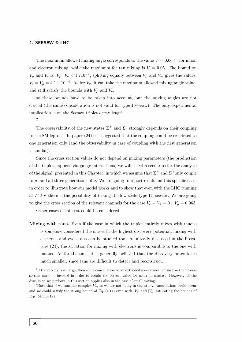
4. SEESAW @ LHC
The maximum allowed mixing angle corresponds to the value V = 0.063 1 for muon
and electron mixing, while the maximum for tau mixing is V = 0.05. The bound on
Vµ and Ve is: Vµ · Ve < 1.710−7; splitting equally between Vµ and Ve, gives the values:
Ve = Vµ = 4.1× 10⁻⁴. As for Vτ , it can take the maximum allowed mixing angle value,
and still satisfy the bounds with Vµ and Ve.
so these bounds have to be taken into account, but the mixing angles are not
crucial (the same consideration is not valid for type I seesaw). The only experimental
implication is on the Seesaw triplet decay length.2
The observability of the new states Σ± and Σ0 strongly depends on their coupling
to the SM leptons. In paper (24) it is suggested that the coupling could be restricted to
one generation only (and the observability in case of coupling with the first generation
is similar).
Since the cross section values do not depend on mixing parameters (the production
of the triplet happens via gauge interactions) we will select a scenarios for the analysis
of the signal, presented in this Chapter, in which we assume that Σ± and Σ0 only couple
to µ, and all three generations of ν. We are going to report results on this specific case,
in order to illustrate how our model works and to show that even with the LHC running
at 7 TeV there is the possibility of testing the low scale type III seesaw. We are going
to give the cross section of the relevant channels for the case Ve = Vτ = 0 , Vµ = 0.063.
Other cases of interest could be considered:
Mixing with taus. Even if the case in which the triplet entirely mixes with muons
is somehow considered the one with the highest discovery potential, mixing with
electrons and even taus can be studied too. As already discussed in the litera-
ture (24), the situation for mixing with electrons is comparable to the one with
muons. As for the taus, it is generally believed that the discovery potential is
much smaller, since taus are difficult to detect and reconstruct.
1If the mixing is so large, then some cancellation or an extended seesaw mechanism like the inverse
seesaw must be invoked in order to obtain the correct value for neutrino masses. However, all the
discussion we perform in this section applies also in the case of small mixing.2Note that if we consider complex Vα, as we are not doing in this study, cancellations could occur
and we could satisfy the strong bound of Eq. (4.14) even with |Ve| and |Vµ| saturating the bounds of
Eqs. (4.11,4.12).
60

4.5 Bounds on the Mixing Angles
Figure 4.5: Branching ratios of the neutral component (up) and charged component(down) of the fermionic triplet in the case Ve = Vτ = 0 , Vµ = 0.063. The dots correspondto numerically evaluated values while the lines correspond to the theoretical predictions.Notice that, as expected from Eqs. (4.2)-(4.8) in the case of one non-zero mixing angle, theresult is the same for charged and neutral triplet decay.
Mixing with 2 or 3 charged leptons. In such a case the triplet can couple to more
than one family. The mixing angles are thus more constrained. As we have
already shown (see Figs. 4.5-4.6), the simultaneous presence of two (or three) non
61

4. SEESAW @ LHC
Figure 4.6: Branching ratios of the neutral component (up) and charged component(down) of the fermionic triplet in the case Vτ = 0 , Ve = Vµ = 4.1 · 10−4. The dotscorrespond to numerically evaluated values while the lines correspond to the theoreticalpredictions while the lines correspond to the theoretical predictions. When both channelwith e and µ are open, only one is displayed, since, for this particular choice of the mixingangles, they are overlapped.
zero Vα would reduce the corresponding branching ratio by a small factor: if, for
instance, two of them are taken to be equal, then the corresponding branching
ratio will be decreased by a factor 2 with respect to the case with only one non-
62

4.5 Bounds on the Mixing Angles
zero mixing angle (see Figs. 4.5-4.6). However the pair production cross section
of triplets is not affected by the mixing values and thus only the branching ratios
and the mass of the triplet drive the relevant processes studied here.
Small mixing angles, O(10−6). This case is the “most natural” one, since here
small neutrino masses can be accommodated without any cancellation or fur-
ther source of suppression 1. Such small mixing angles drastically reduce the
value of the triplet decay width, so that displaced vertexes up to few millimeters
can be present (see also (29), and the results presented in Section 4.5.2). In case
of finding an excess of events in some of the considered channels, the measurement
of these displaced vertexes could be a clear signal that we are in presence of this
kind of physics. A part from this, in general the cross sections are not affected
and the analysis can proceed as in the case of large mixing.
Given these considerations, we performed analysis on LHC data, considering dif-
ferent mixing scenario as the one choose here for cross sections analysis. A discussion
about different mixing values scenario will be presented in Chapter 9, the implication
on deriving the correct cross sections from the Ve = Vτ = 0 , Vµ = 0.063 case is briefly
discussed in the following Section.
4.5.1 Mixing Angle Scenarios
In the case we consider the mixing angle with all the lepton flavors different from
zero, care must be taken in computing the cross section contributions from different
processes giving the same final state, from the cross sections we have quoted in this
Chapter, namely of the case of coupling with muons alone, and decay in final state with
the muon flavor only. A description of the issue is given in this paragraph, were an
example for two processes is given. If more other processes are considered, the derived
formulas need to take into account all the contributions.
Given
bα =|Vα|2
Σi|Vi|2�� ��4.17
1Notice that in this case the approximation of taking zero neutrino masses is no longer consistent
and they should be turned on in the numerical simulations; for consistency also non-zero electron and
muon masses should be considered, even if the effect of all these masses turns out to be negligible.
63

4. SEESAW @ LHC
with α =e, µ , τ , and considering the two processes of Σ0, Σ+ decay
Pααα1 : Σ0 → α−W+, Σ+ →W+ν, W+ → α+ν
�� ��4.18
and the process
Pααα11 : Σ0 → α+W−, Σ+ →W+ν, W± → α±ν
�� ��4.19
we consider the cross section for the process Pααα1 , Pααα
11 : σP1 = P1=σP11 = P11 = σ1.
Neglecting the contributions from leptonic τ decays, the cross sections for the positive
final states can be expressed in terms of bα:
σµ−e+e+ = bµP1 + beP11 = (bµ + be)σ1
�� ��4.20
σµ−e+µ+ = 2bµP1 + bµP11 + beP11 = (3bµ + be)σ1
�� ��4.21
σµ−µ+µ+ = bµP1 + bµP11 = 2bµσ1
�� ��4.22
σe−µ+µ+ = beP1 + bµP11 = (bµ + be)σ1
�� ��4.23
σe−e+µ+ = 2beP1 + beP11 + bµP11 = (3be + bµ)σ1
�� ��4.24
σe−e+e+ = beP1 + beP11 = 2beσ1.�� ��4.25
Including τ decay contributions, we have to rewrite eq.(4.20-4.25) as e.g.
σµ−µ+µ+ = bµ(P1+P11)(1+2εWτµ+ε2Wτµ)+bτ εΣτµ(P1+P11)(1+2εWτµ+ε2Wτµ)�� ��4.26
where εWτ` (εΣτ`) corresponds to the efficiency (including τ leptonic branching
ratio) to select events from W → τ → ` (Σ → τ → `) decay chain. Since εXτ` are all
expected to be < 10%, second order terms in ε can be neglected and then the cross
sections (4.20-4.25) have to be multiplied by a factor ∼ (1 + 2εWτ` + εΣτ`).
64
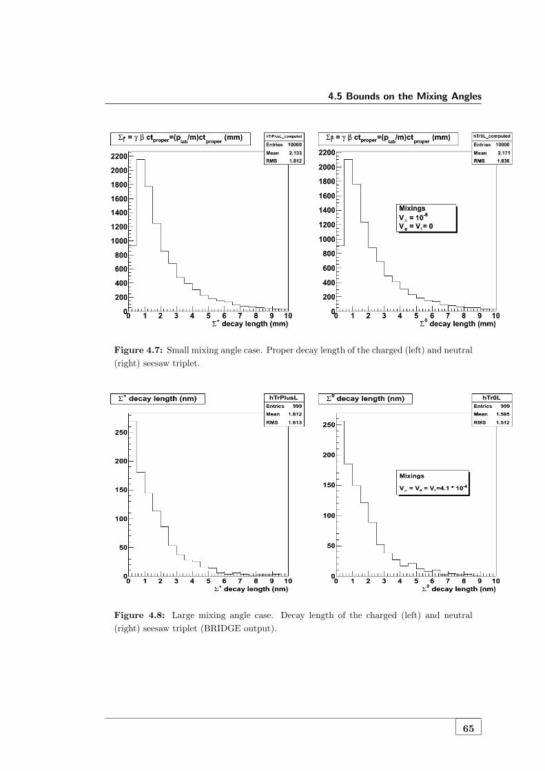
4.5 Bounds on the Mixing Angles
Figure 4.7: Small mixing angle case. Proper decay length of the charged (left) and neutral(right) seesaw triplet.
Figure 4.8: Large mixing angle case. Decay length of the charged (left) and neutral(right) seesaw triplet (BRIDGE output).
65
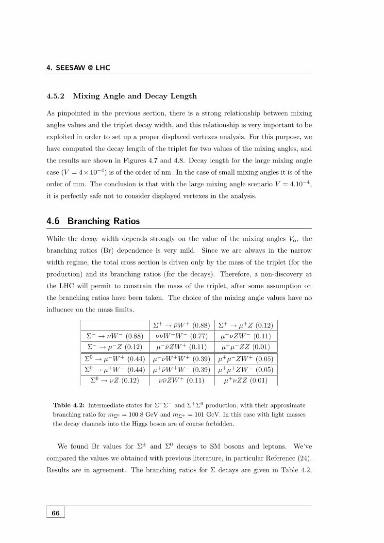
4. SEESAW @ LHC
4.5.2 Mixing Angle and Decay Length
As pinpointed in the previous section, there is a strong relationship between mixing
angles values and the triplet decay width, and this relationship is very important to be
exploited in order to set up a proper displaced vertexes analysis. For this purpose, we
have computed the decay length of the triplet for two values of the mixing angles, and
the results are shown in Figures 4.7 and 4.8. Decay length for the large mixing angle
case (V = 4×10⁻⁴) is of the order of nm. In the case of small mixing angles it is of the
order of mm. The conclusion is that with the large mixing angle scenario V = 4.10−4,
it is perfectly safe not to consider displayed vertexes in the analysis.
4.6 Branching Ratios
While the decay width depends strongly on the value of the mixing angles Vα, the
branching ratios (Br) dependence is very mild. Since we are always in the narrow
width regime, the total cross section is driven only by the mass of the triplet (for the
production) and its branching ratios (for the decays). Therefore, a non-discovery at
the LHC will permit to constrain the mass of the triplet, after some assumption on
the branching ratios have been taken. The choice of the mixing angle values have no
influence on the mass limits.
Σ+ → νW+ (0.88) Σ+ → µ+Z (0.12)
Σ− → νW− (0.88) ννW+W− (0.77) µ+νZW− (0.11)
Σ− → µ−Z (0.12) µ−νZW+ (0.11) µ+µ−ZZ (0.01)
Σ0 → µ−W+ (0.44) µ−νW+W+ (0.39) µ+µ−ZW+ (0.05)
Σ0 → µ+W− (0.44) µ+νW+W− (0.39) µ+µ+ZW− (0.05)
Σ0 → νZ (0.12) ννZW+ (0.11) µ+νZZ (0.01)
Table 4.2: Intermediate states for Σ+Σ− and Σ+Σ0 production, with their approximatebranching ratio for mΣ0 = 100.8 GeV and mΣ+ = 101 GeV. In this case with light massesthe decay channels into the Higgs boson are of course forbidden.
We found Br values for Σ± and Σ0 decays to SM bosons and leptons. We’ve
compared the values we obtained with previous literature, in particular Reference (24).
Results are in agreement. The branching ratios for Σ decays are given in Table 4.2,
66

4.7 Final States
where the mixing angles have been taken, as stressed in previous section, Ve = Vτ = 0
and Vµ = 0.063.
4.7 Final States
Once the triplets have decayed into leptons and gauge bosons (we call it the intermediate
state), further decays take place. In the final state the observable particles will be:
charged leptons, quarks1, and neutrinos, which will manifest themselves as missing
energy.
There is a plethora of possible final states resulting from Σ± and Σ0 production
and decay possibilities of each heavy lepton. All decays of Σ±, Σ0 to light leptons and
gauge or Higgs bosons could be in principle calculated. This is a cumbersome task since
it involves 289 different final states with 128 different matrix elements for Σ+Σ− and
748 final states with 72 matrix elements for Σ±Σ0, which have to be generated with
their corresponding weights.
Therefore, we classify signals by the signatures actually seen at the experiment.
As the number of jets in the final state is not a good discriminant due to radiation
and pile-up, signals are classified in terms of the charged lepton multiplicity, and the
number of hard jets is considered only in few special cases as an extra information
for the kinematic reconstruction. The possible signals from Seesaw triplet decays are
classified in terms of the following charged lepton multiplicity, ranging from one to six
charged leptons:
• six leptons: Σ+Σ− → l+Zl−Z and Z → l+l−;
• five leptons: Σ+Σ0 → l+Zl±W∓ and Z → l+l−; negligible cross section;
• four leptons:
l±l±l±l∓X : negligible cross section (only seesaw III);
l±l±l∓l∓X : negligible cross section (common to scalar i.e. seesaw II);
• three leptons:
l±l±l±X;
l±l±l∓X : good channel with small background and high cross section;1quarks will show up as either as jets, or leptons, when heavy quarks decay semileptonically
67

4. SEESAW @ LHC
• two leptons:
l±l±X
l±l∓jjjjX : very large background;
• l±jjjjX
Process Production Cross Sections (fb) Final State Final Cross Section (fb)
100 GeV 120 140 100 GeV 120 140
Final State ++
W−µ+Zµ+ 2.36e + 2 2.02e + 2 1.16e + 2 µ+µ+jets 108 92.7 53.4
µ+µ+ννjets 32.4 27.8 15.9
W−µ+hµ+ 1.22e− 3 1.39e− 1 1.40e + 1 µ+µ+jets - - 8.9
µ+µ+ννjets - - -
Final State −−W+µ−Zµ− 1.27e + 2 1.04e + 2 5.67e + 1 µ−µ−jets 58.3 47.7 26.1
µ−µ−ννjets 17.4 14.3 7.8
W+µ−hµ− 5.87e− 6 7.13e− 2 6.86 µ−µ−jets - - 4.4
µ−µ−ννjets - - -
Table 4.3: Final states with two muons of the same sign for Ve = Vτ = 0, Vµ = 0.063.The final cross sections have been computed using the measured branching ratios, exceptfor the Higgs, whose branching ratios have been calculated assuming a mass of 120 GeV.Only channels with a final cross section higher than 0.1 have been reported.
Using a fast detector simulation (see Chapter 5 for details about simulation) of
signals and backgrounds, it has been found that the tri-lepton channel l±l±l∓X is by
far the best one for fermion triplets, as good as the like-sign di-lepton channel l±l±,
balancing large signal branching ratios and small backgrounds. Reference (22), (23),
(24), (25), (26). It is a good signature even if the cross section is not very high,
because for the discovery channel we don’t need a very large cross-section. In addition
to evaluating the discovery potential, if a positive signal is observed we could make
special emphasis on the discrimination among seesaw models since this channel is the
same in seesaw model II and III. This could be accomplished, for example, by searching
for signals in different final states, and also by reconstructing the mass and determining
68

4.7 Final States
Process Production Cross Sections (fb) Final State Final Cross Section (fb)
100 GeV 120 140 100 GeV 120 140
Final State + +−W+µ−W+ν 1.66e + 3 6.08e + 2 2.82e + 2 µ+µ+µ−ννν 20.9 7.7 3.5
W−µ+W+ν 1.66e + 3 6.06e + 2 2.82e + 2 µ+µ+µ−ννν 20.9 7.7 3.5
W+µ−Zµ+ 2.36e + 2 2.03e + 2 1.16e + 2 µ+µ+µ−νjets 18.2 15.7 8.9
µ+µ+µ−ννν 5.5 4.7 2.7
W−µ+Zµ+ 2.36e + 2 2.02e + 2 1.16e + 2 µ+µ+µ−νjets 18.3 15.6 8.9
µ+µ+µ−ννν 5.5 4.6 2.6
W+νZν 4.62e + 2 4.02e + 2 2.32e + 2 µ+µ+µ−ννν 1.8 1.6 0.9
Zµ+Zν 6.55e + 1 1.35e + 2 9.48e + 1 µ+µ+µ−νjets 1.6 3.2 2.28
µ+µ+µ−ννν 0.47 0.98 0.68
Zµ+hν 6.80e− 4 1.54e− 1 2.28e + 1 µ+µ+µ−νjets - - 0.76
W−νZµ+ 3.61e + 2 3.08e + 2 1.71e + 2 µ+µ+µ−νjets 8.4 7.2 4.0
W+µ−hµ+ 1.22e− 3 1.39e− 1 1.40e + 1 µ+µ+µ−νjets - - 1.5
W−µ+hµ+ 1.22e− 3 1.39e− 1 1.40e + 1 µ+µ+µ−νjets - - 1.5
Total Cross Sections µ+µ+µ− + jets + missing ET 46.5 41.7 27.8
Total Cross Sections µ+µ+µ− + jets + missing ET (only via W) 36.5 31.3 20.8
Total Cross Sections µ+µ+µ− + missing ET 55.1 27.0 13.9
Total Cross Sections µ+µ+µ− + missing ET (only via W) 52.8 24.7 12.3
Table 4.4: Intermediate and final states with three muons µ+µ+µ− for Ve = Vτ = 0,Vµ = 0.063 cross sections. The final cross sections have been computed using the mea-sured branching ratios, except for the Higgs, whose branching ratios have been calculatedassuming a mass of 120 GeV. Only channels with a final cross section higher than 0.1 havebeen reported.
the charge of the new resonances (seen as a peak in the invariant mass1 distribution of
two opposite charge leptons plus the missing momentum) 2
1m(l1, l2) =p
(El1 + El2)2 − | ~pl1 + ~pl2 |2.
2A first straightforward discrimination of seesaw models results from considering a systematic
analysis of all possible final states in which the signals can be seen and their statistical significance,
which are not the same for seesaw I, II and III. Moreover, if a positive signal is found in a given channel,
the mass reconstruction of the heavy resonance can be often performed and its charge measured, giving
clear direct evidence for the production of the new particle, if the peak is present. For high integrated
luminosities, the opening angle distribution can also be tested in the cleanest channels, giving evidence
69

4. SEESAW @ LHC
Process Production Cross Sections (fb) Final State Final Cross Section (fb)
100 GeV 120 140 100 GeV 120 140
Final State +−−W−µ+W−ν 8.94e + 2 3.13e + 2 1.39e + 2 µ−µ−µ+ννν 11.1 3.9 1.7
W−µ+W−ν 8.96e + 2 3.11e + 2 1.39e + 2 µ−µ−µ+ννν 11.2 3.9 1.7
W−µ+Zµ− 1.27e + 2 1.04e + 2 5.67e + 1 µ−µ−µ+νjets 9.8 8.0 4.4
µ−µ−µ+ννν 2.9 2.4 1.3
W+µ−Zµ− 1.27e + 2 1.04e + 2 5.67e + 1 µ−µ−µ+νjets 9.8 8.0 4.4
µ−µ−µ+ννν 2.9 2.4 1.3
W−νZν 2.49e + 2 2.07e + 2 1.13e + 2 µ−µ−µ+ννν 1.0 0.8 0.4
Zµ−Zν 3.53e + 1 6.93e + 1 4.65e + 1 µ−µ−µ+νjets 0.85 1.7 1.1
µ−µ−µ+ννν 0.25 0.5 0.3
Zµ−hν 3.27e− 4 7.87e− 1 1.12e + 1 µ−µ−µ+νjets - - 0.37
W+νZµ− 3.62e + 2 3.07e + 2 1.72e + 2 µ−µ−µ+νjets - - 0.37
W−µ+hµ− 5.87e− 6 7.13e− 5 6.86 µ−µ−µ+νjets 8.4 7.2 4.0
W+µ−hµ− µ−µ−µ+νjets - - 0.7
Total Cross Sections µ+µ−µ− + jets + missing ET 28.9 24.9 15.7
Total Cross Sections µ+µ−µ− + jets + missing ET (only via W) 19.6 16.0 8.8
Total Cross Sections µ+µ−µ− + missing ET 29.4 13.9 6.7
Total Cross Sections µ+µ−µ− + missing ET (only via W) 28.1 12.6 6.0
Table 4.5: Intermediate and final states with three muons µ+µ−µ− for Ve = Vτ = 0,Vµ = 0.063 cross sections. The final cross sections have been computed using the mea-sured branching ratios, except for the Higgs, whose branching ratios have been calculatedassuming a mass of 120 GeV. Only channels with a final cross section higher than 0.1 havebeen reported.
Given these results, we choose the signature l±l±l∓X to be studied in this thesis,
and we computed cross sections of the tri-leptons final states. 1
for the scalar or fermionic nature of the heavy states produced. For high luminosities, further evidence
is provided by the analysis of the production angular distributions in the cleanest channels with three
or four leptons. Nothing could be said, on the other hand, from the shape of the kinematic distribution.
Should be noted that for discriminating among different seesaw models we need a big cross-section,
because of high statistic study needs.1However, since the probability of missing a lepton is relatively high for multi-lepton channels,
when studying signal in the tri and di-leptons channels, events with 4 leptons should be generated too.
The inclusive 4-leptons final state cross section varies between 5-10 fb for triplet masses in the range
70

4.7 Final States
Since the l±l±l∓ final state receives contributions from many processes, we have
computed the cross sections of the intermediate and final state for Σ+Σ0 decay processes
(similar channels are for Σ−Σ0), and we reported in the Table only the relevant ones.
While the intermediate ones are calculated with MadGraph, the final ones are obtained
by multiplication with the branching ratios from Reference (15)
The branching ratios for the Higgs have been calculated assuming a mass of 120 GeV.
Tables 4.3 and 4.4 and 4.5 display the cross sections for the intermediate and final
states with 2 and 3 leptons at different mass energies. 1 Only channels with a final
cross section higher than 0.1 have been reported.
Important comments and conclusions could be drawn from these results.
• Even with LHC running at 7 TeV, with the few fb−1 of luminosity several events
are expected, for low triplet mass.
• In some channels involving a Z boson the cross section increases moving from
100 GeV to 120 GeV. This is simply due to the faster growing of the branching
ratio of the triplet decay into Z with respect to the decreasing of the production
cross section.
• In the 3-leptons table, in the total cross section we have isolated the channels with
leptons not-coming from Z decay. Indeed, the channels with muons generated via
Z decay have a very large background and are difficult to analyze. If a Z-veto
cut on the invariant mass of the leptons will be applied in order to reduce the
background events coming from Z decay, these events will mostly disappear. Then
the numbers we quote in blue in Table 4.4 can be considered the effective cross
section after the application of this cut.
By looking at these table we see that there are 4 possible final states with 2 and 3
leptons:
100-140 GeV. We didn’t generate 4-leptons final states, since we considered negligible the fraction of
three-lepton events from four-lepton samples with one missed lepton.1We give numbers for the case of mixing with muons exclusively, however similar results apply when
the final states contains electrons as well. On the other hand, they do not apply completely to taus.
Indeed, taus are not detected as such, because of their fast decay. Moreover, in a detector like CMS,
leptons coming from taus decay are not distinguished from prompt leptons and therefore identified taus
are only hadronic taus.
71

4. SEESAW @ LHC
2l1lm
0 50 100 150 200 250 300 350 4000
50
100
150
200
250
300
350
Figure 4.9: Invariant mass of the two µ+ for a luminosity of 30fb−1 and MΣ = 100 GeV.Pre-selection cuts selected only the events with 3 charged leptons among which 2 positivemuons.
A) 3 leptons + missing transverse energy (MET);
B) 3 leptons + 2 jets + MET;
C) 2 same-sign leptons + 4 jets;
D) 2 same-sign leptons + 2 jets + MET.
Figure 4.10: Dominant process for the discovery channel for the fermionic triplet at theLHC.
72

4.7 Final States
4.7.1 Detector Response
We are going to summarize the main features of the signals described in the previous
Section, from the treatment given in Reference (30), were results about CMS simulation
via the PGS software (71) are given. (after MadGraph/MadEvents event generation and
hadronization with PYTHIA (47) package).
pp→ Σ+Σ0 → µ+µ+µ− + νs(+jets) with . The CMS detector has been simulated
3 leptons + MET. This is the best discovery channel. One of the two dominant
processes generating it is depicted in Fig. 4.10, the other dominant process is
the analogues with Σ0 → l+W−. Indeed, not only it possesses the highest cross
section, but the background is more easily reduced due to the absence of jets in
the final state. In an ideal detector where jets are not misidentified with leptons,
the only physical irreducible background sources would be WWW , WZ and ZZ
when a lepton is missed. The backgrounds will be discussed in detail in Chapter
8.
In this channel, the invariant mass mµ+µ+ of the two same-sign muons presents
a long tail in the high energy region that is characteristic of the presence of new
physics, see Fig. 4.9, and can be exploited to reduce the background. Moreover,
this is typical of this kind of seesaw, permitting thus to distinguish among type I,
II and III (24). Other characteristics of the final leptons can be used to reduce the
different SM backgrounds. In Fig. 4.11, the three leptons pT are plot. However,
the pT emitted by the triplet has a softer transverse momentum as shown in Figure
4.12 where the mixing values are Vµ = Ve = Vτ = 4.10−4 and the simulated mass
point is 100 GeV.
3 leptons + 2 jets + MET. This channel is the best one in order to reconstruct
the mass of the triplet. Moreover it can be used also to discriminate between
type II and type III seesaw (24). It also appears in the type I seesaw with a
gauged U(1)B−L (72). In this case the reduction of the background can be more
complicated, due to the impossibility of applying a jet veto. A precise estimation
of the sensitivity to this new physics would require the complete simulation of
the background and a detailed analysis.
73

4. SEESAW @ LHC
Tp
0 20 40 60 80 100 120 1400
0.02
0.04
0.06
0.08
0.1
0.12
Figure 4.11: pT distribution of the different leptons for MΣ = 100 GeV. The black,red and blue curves represent the lepton with the highest, intermediate and smallest pT
respectively. Pre-selection cuts selected only the events with 3 charged leptons amongwhich 2 positive muons.
Once the triplet has been observed, its mass needs to be measured. To this aim,
this channel, emerging from the process pp → (Σ± → `±Z/H)(Σ0 → `±W∓)
with Z/H decaying into jets, is the best one. Indeed the momentum of the Z/H
boson is reconstructed from the jets momenta, while its combination with the
momentum of one of the two same-sign leptons gives the mass of the charged
triplet. Since there are two possibilities for this combination, the chosen one will
be that giving closest invariant mass for the reconstructed charged and neutral
triplets, where the latter is given by the combination of the momenta of the two
remaining leptons plus MET 1.
1The neutrino longitudinal momenta should be added as well (24).
74

4.7 Final States
hTrMuonEntries 33656Mean 22.16RMS 15.24
0 20 40 60 80 100 120 140 160 180 2000
200
400
600
800
1000
1200
1400
hTrMuonEntries 33656Mean 22.16RMS 15.24
Generated Seesaw type-III signal-4=4.1 * 10τ = Ve = VµV
+ MET+ l+ l-
P1: l100 GeV mass point
(GeV)T PΣMuon hTrEleEntries 33016Mean 22.06RMS 15.25
0 20 40 60 80 100 120 140 160 180 2000
200
400
600
800
1000
1200
1400
hTrEleEntries 33016Mean 22.06RMS 15.25
(GeV)T PΣEle
hWMuonEntries 66632Mean 41.92RMS 26.3
0 20 40 60 80 100 120 140 160 180 2000
200
400
600
800
1000
1200
1400
hWMuonEntries 66632Mean 41.92RMS 26.3
(GeV)T PWMuon hWEleEntries 66711Mean 41.68RMS 26.38
0 20 40 60 80 100 120 140 160 180 2000
200
400
600
800
1000
1200
1400
hWEleEntries 66711Mean 41.68RMS 26.38
(GeV)T PWEle
Figure 4.12: pT distribution of the muons and electrons, for MΣ = 100 GeV and mixingvalues Vµ = Ve = Vτ = 4.10−4. The muons and electrons are coming from Σ decay (top)and W decays (bottom)
The reconstructed mass of the charged and neutral triplet are shown in Fig. 4.13
where no cuts has been applied. Note that a selection cut on the invariant mass
mjj of the jets
|mjj −MZ/H | < 10 GeV�� ��4.27
will improve the mass reconstruction. Even if the background is added, a clear
peak in the reconstructed mass will still be visible, which should also permit to
distinguish from type II seesaw (24).
2 same-sign leptons + jets (+MET) As it is clear from Table 4.3, the cross
section for these final states is comparable to the one of the previous channels.
In this case the backgrounds are essentially the same as in the previous channel
and it has been shown (24) that the discovery and the discriminatory potentials
are similar too. A realistic study, especially a study on real data, should consider
this channel as well.
75

4. SEESAW @ LHC
rec+ΣM
0 50 100 150 200 250 300 3500
0.02
0.04
0.06
0.08
0.1 Σ M100 GeV140 GeV
rec^0ΣM
0 50 100 150 200 250 300 3500
0.02
0.04
0.06
0.08
0.1
0.12
Σ M100 GeV140 GeV
Figure 4.13: Reconstructed mass of the charged triplet (left) and neutral triplet (right),for a luminosity of 30fb−1, in the case MΣ = 100 GeV (black curve) and MΣ = 140 GeV(red curve). Pre-selection cuts selected only the events with 3 charged leptons and at least2 jets.
76

5Simulation
5.1 Introduction
High energy physics analysis results depends on very accurate comparisons of theo-
retical expectations with experimental output from the detector. Based on current
theoretical models, theoretical expectations are computed with computer simulations.
The simulation uses Monte Carlo techniques (named after the city widely known for its
gambling casino) to perform simulated experiments using random number generators
for evaluating the integrals typically involved in the computation. We have implemented
the minimal seesaw type III model described in Chapter 2 in high energy physics sim-
ulation applications, and we have tested the implementation. In the present Chapter
we’ll present a brief review of the simulation tools, and we’ll discuss the model imple-
mentation and validation. Section 5.2 reviews the fundamentals of high energy physics
collisions, in Section 5.3 the simulation of the collision is described, with a particular
emphasis on the software tools we used for simulation in this work.
5.2 Particle Collision Physics
In the following section I’ll give some information about the simulation of the physics
of high energy particle collision, with particular focus on proton-proton collisions at
LHC energy scale. A sketch of two protons collision process is shown in Figure 5.1.
Basic Information. Simulated events in high energy physics collisions are consti-
tuted by a sets of outgoing particles produced in the interactions between two incom-
ing particles. All the information about the collision itself must be provided to the
77

5. SIMULATION
Figure 5.1: Sketch showing the event collision stages.
simulation program: the particles to be collided and the center-of-mass energy of the
collision. We consider LHC colliding protons with a center-of-mass energy of 7 TeV.
Colliding Protons Structure. The structure of the colliding protons is modeled
with the use of parton distribution functions (PDFs), which define the probability den-
sity for finding a parton (a quark or gluon) with a given longitudinal momentum fraction
x at a particular value of momentum transfer Q2 of the collision. PDFs containing this
information cannot be calculated perturbatively, and are instead determined by fits to
data from processes such as deep inelastic scattering (DIS) and Drell-Yan (DY).
The Hard Process. The collision occurs between individual partons within each
proton, and is referred to as the hard process, in which the particles of interest for
the event are produced (e.g. heavy quarks, vector bosons, hypothetical new particles,
etc.). The production of these particles, and their subsequent decays, are described by
matrix elements corresponding to each interaction. These are calculated from Feynman
78
5.2 Particle Collision Physics
diagrams in quantum field theory, where the square of the matrix element gives the
probability density for the process, so that the production cross section can be derived
from this matrix element. The programs used to generate the events are tree level (i.e.
leading order) generators, and separate programs could be used to calculate the cross
sections in order to include higher-order effects.
Hadronization. In addition to the hard scattering process the interaction produces
parton showers, hadronizing into collections of hadrons seen as jets. The primary
collision includes QCD radiation from both the incoming (ISR initial state radiation)
and outgoing partons (FSR final state radiation). This radiation depends primarily
on the momentum transfer scale Q2, rather than the details of the particular process
being simulated. This QCD radiation depends on color confinement: partons produced
in the hard scatter cannot exist on their own. Their kinetic energy is transferred to the
color field, where it produces additional partons from the vacuum. The partons in this
shower then hadronize, forming color-neutral combinations. The resulting collinear
spray of particles is called a jet. The process of hadronization is not well described
theoretically, it is modeled phenomenologically with the Lund string model instead
((60)). In this model, the gluons binding two quarks are treated as field lines. Gluons
are self-interacting, and hence the color field they produce is compressed into a narrow
tube (or string). By contrast, the electromagnetic field tends to spread much more,
because the photon has no self-interaction terms. When sufficient energy is stored in
the color field to produce new quark-antiquark pairs, the string snaps, and the newly
produced particles form bound-state mesons with the original quarks. In hadronization
this process happens repeatedly, and the produced bound states model the kinematics
of the original parton. Moreover, the remaining partons from the protons cannot be
ignored, and represent the underlying event. The proton remnants are left behind after
the hard scatter, but due to their strong interactions with the hard process, they must
be included when considering hadronization. These interactions are typically soft and
the description of the underlying event relies on non-perturbative or semi-perturbative
phenomenological models.
Pileup. Additionally, the effect of pileup must also be considered, where multiple
protons in a single bunch crossing interact. Pileup is simulated in generated events by
79

5. SIMULATION
superimposing minimum bias events on the events in the nominal samples, according
to the distribution of number of pileup collisions observed in the data for 2011.
5.3 Event Simulation Chain
Monte Carlo event generation is used to simulate high-energy-physics events (Ref. (39),
(44)), therefore it must “mimic” the physical processes described in Section 5.2. HEP
Monte Carlo event generation is typically modular and proceeds in stages. It is usually
split into the following steps: Matrix Element calculation, Parton Shower, Underlying
Event and Hadronisation. Last stage in event processing is the simulation of the de-
tector response, which reproduces the experimental output. Usually the physics event
of interest, as well as the cross-section information is done with the computation of the
Matrix Element (PDF evaluation, phase space, amplitudes, spin correlations, etc...)
and the remaining steps are used to evolve the parton-level event to its final state, and
to simulate the detector response.
Different programs could be used to perform each step of the simulation chain.
Figure 5.2 includes a sketch of the programs used to perform the different stages for
the signal simulation of the present thesis. Each simulation step, the software used and
a reference are listed here and described in the following sections:
1. Feynman rules and couplings computation: FeynRules (63);
2. Matrix Element (ME) calculation, event generation and decay: Madgraph5 (58);
3. Parton showering and hadronization: Pythia6 (47), (46);
4. CMS detector simulation, digitization and reconstruction: CMSSW 4 2 5 (64).
Figure 5.2: Sketch showing the software chain for event simulation.
80

5.3 Event Simulation Chain
5.3.1 FeynRules
FeynRules is a Mathematica package that allows the calculation of Feynman rules in
momentum space for any QFT physics model. The user needs to provide FeynRules
with the minimal information required to describe the new model, contained in the
so-called model-file. This information is then used to calculate the set of Feynman
rules associated with the Lagrangian. The Feynman rules calculated by the code can
then be used to implement the new physics model into other existing tools, such as
MC generators. This is done via a set of interfaces which are developed together
and maintained by the corresponding MC authors. The seesaw type III model was
implemented in FeynRules for the subsequent event generation and analysis for this
thesis; the implementation of the model has been published in: (65).
5.3.1.1 Seesaw Model Implementation
In the literature few papers (24, 29, 68) discussing the possibility of discovering the
type III seesaw at the LHC are present. However so far no code was publicly available
to perform calculations and simulations in this model. Very recently, the minimal
Seesaw type-III model was implemented and published (119), (30). In this references,
implementation details are given. With the help of the authors we have generated and
simulated the seesaw signal to be compared with real data.
5.3.2 Madgraph Generation
5.3.2.1 Generators Introduction
The generators used in High Energy Physics could be classified in:
• Matrix Element (ME) calculators, such as Alpgen, MadGraph, MCatNLO, etc.
They deliver an event at the parton level.
• general-purpose generators, such as Herwig, Pythia or Sherpa. They can further
be used to develop a fully hadronized event. The objective of general-purpose
event generators is to provide as accurate as possible a description of what hap-
pens in a particle collision. They contain theory and models for a number of
physics aspects, such as hard and soft interactions, parton distributions, initial
and final state parton showers, multiple interactions, fragmentation and decay.
81

5. SIMULATION
Most ME generators output is a standardized text file: the Les Houches Events
(LHE) file format is an agreement between Monte Carlo event generators and theorists
to define Matrix Element level event listings in a common language. This LHE text files
contains some arbitrary headers and comments, information about the run (processes,
cross-sections, PDFs, beam type, beam energy) and a per-event parton listing with
incoming particles, outgoing particles and optionally decays of those particles (like e.g.
top quark and W boson decay including spin correlations).
Matrix Element calculations are to be combined with Parton Showers of any multi-
purpose event generator, so a matching procedure has to be performed in order to
avoid double-counting of emissions between the ME and the PS. Generators like Mad-
Graph/MadEvent come with their own preferred matching prescription (MLM-style
jet matching), which should be used preferably. Also more recent Parton Showers
come with an alternative matching procedure called CKKW re weighting which ex-
ploits knowledge of the Sukadov form factors during the Parton Shower evolution to re
weight the events. 1
5.3.2.2 Madgraph
MadGraph/MadEvent (MG/ME) is a event generator software that allows to generate
amplitudes and events for any process (with up to 9 external particles) in any model.
MadEvent is a multi-purpose, tree-level event generator which is powered by the matrix
element generator MadGraph. A process-dependent, self-consistent code for a specific
1The matching procedure involves jet matching, see for Reference(38). Multi-jet events generation
need to be able to simulate physics down to QCD scale (around the GeV) in order to have a simulated
interaction between stable particles and a detector. This means that a parton-shower (PS) generator
(PYTHIA, HERWIG,...) is mandatory for this work. On the other hand, an issue in the PS method is
the algorithm of showering itself, working on a cascade-decay basis, and therefore being very sensitive
to the shower parameters/definition. In fact the best way to simulate the kinematics is by using a true
matrix-element calculation. This means that if the matrix-element calculation is used, the physical
result is less sensitive to the parametrization of the showers.
The main problem comes up when both kind of generation are used together because of the over-
lapping of the respective phase-spaces of the two regimes. To avoid this, the solution is the jet-parton
matching of which the general aims are: avoid overlapping between phase-space descriptions given
by matrix-element generators and showering/hadronization software in multi-jets process simulation,
avoid dead zones: the region of the phase space between PS and ME cover has to be filled correctly,
and obtain a result invariant from the choice of showering parametrization: the matching parameters
are not physical observable.
82

5.3 Event Simulation Chain
SM process is generated upon the user’s request on a web form or using the standalone
program see References (58).
Given the process, MadGraph automatically generates the amplitudes for all the
relevant subprocesses and produces the mappings for the integration over the phase
space. This process-dependent information is packaged into MadEvent, and a stand-
alone code is produced that can be downloaded from the web site and allows the user
to calculate cross sections and to obtain unweighted events automatically.
Once the events have been generated - event information (e.g. particle id’s, mo-
menta, spin, color connections) is stored in the Les Houches format, and the events
may be passed directly to a shower Monte Carlo program.
5.3.2.3 Seesaw Event Generation
To provide seesaw type-III signal data-sets to be analyzed for the study presented in
this thesis, we performed event generation as described in this section. We imported
the seesaw model computed with FeynRules package and described in Section 5.3.1
into Madgraph application. We generated 100k events for each sample (for each mass
point and each process contributing to the final state `±`±`∓ (described in Chapter 9).
Decays of standard model bosons were included in the Madgraph processing.
Madgraph run details are listed in Appendix C.
hMuonMultEntries 100000
Mean 1.003
RMS 0.8156
0 1 2 3 4 5 6 7 8 9 100
5000
10000
15000
20000
25000
30000
35000
40000
45000
hMuonMultEntries 100000
Mean 1.003
RMS 0.8156
Muon mult hEleMultEntries 100000
Mean 0.9973
RMS 0.8147
0 1 2 3 4 5 6 7 8 9 100
5000
10000
15000
20000
25000
30000
35000
40000
45000
hEleMultEntries 100000
Mean 0.9973
RMS 0.8147
Ele mult hTauMultEntries 100000
Mean 0.9999
RMS 0.8157
0 1 2 3 4 5 6 7 8 9 100
5000
10000
15000
20000
25000
30000
35000
40000
45000
hTauMultEntries 100000
Mean 0.9999
RMS 0.8157
Tau mult
Figure 5.3: Lepton multiplicity in the final state from process: pp → Σ+Σ0 →l−W+W+νl , W+ → l+νl
5.3.2.4 Validation
Some sanity checks were performed on Madgraph output, to check implementation of
the model. The LHE files were dumped on a rootuple and analyzed with a ROOT
83
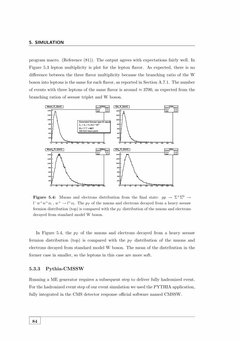
5. SIMULATION
program macro. (Reference (81)). The output agrees with expectations fairly well. In
Figure 5.3 lepton multiplicity is plot for the lepton flavor. As expected, there is no
difference between the three flavor multiplicity because the branching ratio of the W
boson into leptons is the same for each flavor, as reported in Section A.7.1. The number
of events with three leptons of the same flavor is around ≈ 3700, as expected from the
branching ration of seesaw triplet and W boson.
hTrMuonEntries 33656Mean 22.16RMS 15.24
0 20 40 60 80 100 120 140 160 180 2000
200
400
600
800
1000
1200
1400
hTrMuonEntries 33656Mean 22.16RMS 15.24
Generated Seesaw type-III signal-4=4.1 * 10τ = Ve = VµV
+ MET+ l+ l-
P1: l100 GeV mass point
(GeV)T PΣMuon hTrEleEntries 33016Mean 22.06RMS 15.25
0 20 40 60 80 100 120 140 160 180 2000
200
400
600
800
1000
1200
1400
hTrEleEntries 33016Mean 22.06RMS 15.25
(GeV)T PΣEle
hWMuonEntries 66632Mean 41.92RMS 26.3
0 20 40 60 80 100 120 140 160 180 2000
200
400
600
800
1000
1200
1400
hWMuonEntries 66632Mean 41.92RMS 26.3
(GeV)T PWMuon hWEleEntries 66711Mean 41.68RMS 26.38
0 20 40 60 80 100 120 140 160 180 2000
200
400
600
800
1000
1200
1400
hWEleEntries 66711Mean 41.68RMS 26.38
(GeV)T PWEle
Figure 5.4: Muons and electrons distribution from the final state: pp → Σ+Σ0 →l−w+w+νl , w+ → l+νl. The pT of the muons and electrons decayed from a heavy seesawfermion distribution (top) is compared with the pT distribution of the muons and electronsdecayed from standard model W boson.
In Figure 5.4, the pT of the muons and electrons decayed from a heavy seesaw
fermion distribution (top) is compared with the pT distribution of the muons and
electrons decayed from standard model W boson. The mean of the distribution in the
former case in smaller, so the leptons in this case are more soft.
5.3.3 Pythia-CMSSW
Running a ME generator requires a subsequent step to deliver fully hadronized event.
For the hadronized event step of our event simulation we used the PYTHIA application,
fully integrated in the CMS detector response official software named CMSSW.
84

5.3 Event Simulation Chain
5.3.3.1 Pythia
PYTHIA is a program for the generation and/or hadronization of high-energy physics
events, i.e. for the description of collisions at high energies between elementary particles
such as e+, e-, p and p in various combinations. It contains theory and models for a
number of physics aspects, including hard and soft interactions, parton distributions,
initial- and final-state parton showers, multiple interactions, fragmentation and decay.
It is largely based on original research, but also borrows many formulas and other
knowledge from the literature. Development of JETSET, the first member of the ”Lund
Monte Carlo” family, was begun by members of the Lund theory group in 1978, and
has continued since then, on and off (47). A number of people have contributed to this
and other programs based on it. The most extensive of these is PYTHIA. Over the
years, these two programs have more and more come to be maintained in common. In
1997 they were therefore merged to one, under the PYTHIA label. Up until recently
the current version was PYTHIA 6.4. Many examples of Pythia6 configuration cards
can be found in (40).
5.3.3.2 Madgraph-CMSSW interface
MadGraph cannot be directly integrated in parton shower and hadronization programs.
To pass the events to Pythia and interface MadGraph to CMSSW, the MadGraphIn-
terface package has been written (45). MadGraphInterface is a CMSSW package in
the GeneratorInterface subsystem that allows to read in events in the Les Houches for-
mat, perform parton shower and hadronization using Pythia and write CMSSW objects
(edm::HepMCProduct) in the event (edm::Event).
As for many other recent parton level generators, events are passed to CMSSW
as parton level files in the standard format called Les Houches format. These parton
level files are passed to CMSSW through interfaces. PYTHIA, integrated in CMSSW,
takes care about the parton showering and the fragmentation part before passing the
event to simulation. The matching procedure of matrix elements to parton shower
(ME-PS) also happens in the interface . So, producing GEN level events is a two-step
procedure which factories the physics contents of the matrix element calculation from
the parameters of the parton showering/fragmentation/UE. It is for this reason that
the physics content of a process are in the MG cards and not in the CMSSW cfg files.
85

5. SIMULATION
The only process dependent parameter entering the cfg files for a MG production is the
threshold for the matching, which needs to be known by the interface: this significantly
simplifies the production of CMSSW cfg files for MG. The generator group of CMS, in
collaboration with the MadGraph authors and developers, has set in place a (as much
as possible) complete partition of the SM (+BSM) phase space, covering every portion
with proper generations. Cuts and input parameter settings have been agreed with the
CMS PAGs (Physics Analysis Groups).
In the particular case in which a LHE source is used as input source in CMSSW, it
needs to be converted into EDM-compatible form, and become an LHEEventProduct
branch (C++ implementation of the Les Houches Accord format) in the edm::Event (via
Source). The branch is always kept in the event. Run-specific information for the ME
generators is recorded in a form of LHERunInfoProduct. The LHEInterface focuses on
integrating the LHE file standard in a general way into CMSSW. The software resides
in GeneratorInterface subsystem in CMSSW repository. The data formats are defined
in SimDataFormats/GeneratorProducts package. The CMSSW modules to be run in
order to read an LHE file and process it through a shower generator are:
• reading the LHE file → LHESource: is a EDM source and behaves similarly as
PoolSource in that it provides a stream of events to the EDM main loop. In con-
trast to other generators it does, however, not provide an edm::HepMCProduct
but rather an LHEEventProduct per event that carries such event characteristics
as weight(s), scale, PDF, etc and a LHERunInfoProduct for the run.
• processing the ME information through a shower generator→ ”HadronizerFilter”:
provides an interface to the shower generators and in turn reads already existing
LHE products (as provided by the LHESource) and produces the edm::HepMCProduct
in the end. In case ME/PS matching is done, this module also acts as an EDM
filter which can veto the event.
• The LHEWriter module: merges different LHE files;
• LHEAnalyzer can do a jet matching analysis.
Details about the Madgraph-Pythia-CMSSW interface configuration used for this
thesis are described in Appendix C.2.
86

5.3 Event Simulation Chain
Figure 5.5: Framework diagram illustrating how an Event changes as data processingoccurs in CMSSW processing chain.
5.3.4 CMSSW: Detector Response
Physics event generation is the earliest steps in the event processing chain that leads
to producing data-sets suitable for physics analysis.
The following steps are:
• Simulation: the newly generated particles are run through a detailed, Geant4-
based (62) simulation of the CMS detector, a toolkit used to model: the inter-
actions of particles in the detector, and the detector electronics response. The
algorithm incorporates information on the materials, magnetic fields and spe-
cific geometry of the CMS detector. In alternative to the full GEANT4-based-
Simulation is the Fast Simulation approach. It uses parametric approach to sim-
ulate and reconstruct events with the CMS detector; the concept of FastSim is
to reduce the CPU time overhead, while still benefiting from an accurate simu-
87

5. SIMULATION
lation of the detector effects, in view of doing physics analysis, develop and tune
reconstruction algorithms, design detector upgrades, etc.
• Digitization: the detector response to the simulated particles is determined.
• Reconstruction: from detector response, physical objects are reconstructed for
the analysis. A description of objects reconstruction in for CMS experiment are
given in the following Chapter.
The event processing chain is illustrated in Figure 5.5
88

6Reconstruction of Physics Objects
6.1 Introduction
The data from an event is collected by the CMS detector in a very low-level form
(e.g. hits in the tracker, energy deposits in the calorimeters). The output of the Data
Acquisition (DAQ) system consists of signal pulse heights, the time when the signal
occurred, and the address of the detector element where it occurred.
This raw data from the detector contains all the information relevant to analyzing
interesting physics. Nevertheless, the information must be correlated with the infor-
mation about the geometry of the detector, the current values of all detector alignment
and calibration constants, the beam parameters and other relevant experimental condi-
tions. Furthermore, the DAQ information must be synthesized into the actual objects
that are used in the analysis, employing knowledge about the Standard Model and the
interactions of particles and with the material of the detector.
This process is called offline reconstruction. In reconstruction all detector informa-
tion is used and all possibilities of particle trajectories are checked and compared to
each another. The resulting physics objects are the particles which were produced in
the collision (muons, electrons, taus, jets and missing energy), their energies, momenta,
masses, and the coordinates of their origin.
The same reconstruction software is applied to MonteCarlo simulated events.
In this chapter we will describe the general particle flow approach and the particle
flow algorithms for the different physical objects.
89
6. RECONSTRUCTION OF PHYSICS OBJECTS
6.2 The Particle Flow Algorithm
In this analysis we use the particle flow framework to reconstruct the physical objects
used, i.e. leptons, jets and missing transverse energy.
The Particle-flow algorithms aim to individually reconstruct and identify all sta-
ble particles in the event, (electrons, muons, photons, charged hadrons and neutral
hadrons) by comprehensively using all sub-detectors in an optimal way to determine
each particle’s direction, energy and type. The list of individual reconstructed particles
in the event can then be used to reconstruct higher level observables, such as jets, miss-
ing transverse energy, isolated electrons and muons, identification of tau and b jets,
etc.
The particle flow algorithm consists in the following steps:
• Fundamental ingredients:
calorimeter clustering
tracking (with the tracking POG), and extrapolation to the calorimeters
muon identification (from the muon POG)
electron pre-identification (with the e/gamma POG)
• Linking topologically connected elements;
• Particle identification and reconstruction.
The key elements of Particle Flow approach are described in the following sections.
6.2.1 Track
One of the most fundamental components of many physics objects is the reconstruction
of tracks of charged particles. In CMS experiment, the large magnetic field and high
resolution of the tracker make it possible to measure the momentum of charged particles
extremely accurately.
Tracks in the CMS detector are reconstructed via the combinatorial track finder
(CTF). Initial estimates (or seeds) of tracks are constructed either from triplets of hits
or from pairs of hits with additional constraints from the beam spot or a vertex. This
seed is then propagated outwards, and as new hits are found in the tracker, they are
90

6.2 The Particle Flow Algorithm
added to the seed trajectory and the entire track is updated with the new information.
This collection of hits is then fit to obtain the best estimate of the track parameters,
including the pT, η and φ of the reconstructed track. Multiple iterations of this process
are performed, with hits removed from the collection as they become unambiguously
assigned to tracks. After each iteration, filtering is applied to remove potential fake
tracks. The initial seeding criteria are very tight, to ensure the initial fake rate is
negligibly low. The criteria are progressively loosened for subsequent iterations in
order to increase the efficiency to match charged hadrons and to find tracks far from
the interaction vertex, such as electrons from photon conversion and tracks from b-
jets. The successive removal of matched hits ensures that rates of fake tracks are kept
low, and tracks with high efficiency and small fake rate can be constructed down to
transverse momenta on the order of 100 MeV.
6.2.2 Vertex
In CMS experiment is possible to determine the production vertex of the event with
high precision. The primary interaction vertex is reconstructed from the collection of
tracks. Prompt tracks, coming directly from the primary interaction, are defined based
on multiple variables, including the transverse impact parameter d0, the number of hits
in the track, and its normalized χ2. These tracks are then clustered along the z axis,
and this cluster is fit using an adaptive vertex fit (84). The location of the primary
interaction vertex is then determined from this fit.
6.2.3 Calorimeter Energy
The calorimeters first aim is determining the energy of a number of different parti-
cles, including electrons and photons (which deposit all their energy in the ECAL) and
hadrons (which deposit energy in both the ECAL and the HCAL). Combining infor-
mation from the two calorimeters to obtain a single energy estimate gives an energy
resolution of order 10% for a typically energetic hadron of 100 GeV. This makes it
possible to separate neutral hadrons from charged hadrons by identifying an excess of
energy beyond that deposited by the charged hadrons. The PF algorithm employs a
clustering method in the calorimeters to measure the energy from neutral particles,
separate them from charged particles, and reconstruct the energy of electrons, which
can undergo significant energy loss on their way to the calorimeter due to the process
91
6. RECONSTRUCTION OF PHYSICS OBJECTS
of Bremsstrahlung. First, the cluster is seeded by a single calorimeter cell with a local
energy maximum above some threshold, defined as a two standard deviation excess
above the electronics noise in the calorimeter (80 MeV in the barrel and 300MeV in
the endcaps). Next, the algorithm grows the cluster by aggregating cells that share a
side with a cell already in the cluster and have an energy greater than the threshold.
Each separate seed eventually becomes a particle flow cluster.
6.2.4 Link Algorithm
Particle Flow approach employs a link algorithm whose purpose is to combine informa-
tion from each detector element in a way that ensures that it is not double-counted, in
order to construct final state object. A link is established between two elements, with
the distance between them determining the link quality, and blocks are formed from
these linked elements. A link between a charged particle track and a calorimeter cluster
is established by extrapolating the track from the last measured hit in the tracker to
the ECAL and HCAL. If this extrapolated track lies within a cluster boundary defined
in the calorimeter, that cluster is then linked to the track. The link distance here is
defined as the difference in η − φ space between the position of the extrapolated track
and the position of the cluster. Other clusters are linked by taking positions tangent
to the track, in order to include the energy lost due to Bremsstrahlung. Links between
deposits in the ECAL and HCAL are performed similarly. Here, the cluster position is
defined in the ECAL, which has greater granularity, and extrapolated into the HCAL.
If the cluster position lies within the envelope defined by the HCAL cluster, then the
two are linked.For muons, it is also necessary to link tracks in the tracker to tracks in
the muon chambers. This link depends on matching the hits in each detector element
to a global fit, and requiring that this fit return an acceptable χ2. In the case where
a given track in the muon chambers is compatible with multiple tracks in the tracker,
the fit that returns the smallest χ2 is used to define the muon.
6.3 Particle Flow Electrons
The electron identication and reconstruction within the particle-ow algorithm is de-
scribed in detail in References (83) and (85). A short description is given here.
92

6.4 Particle Flow Muons
Particle Flow Electrons algorithm consists in two main parts: a tracker-driven
seeding for GSF tracks focused on low pT or non-isolated electrons, complementing
the ECAL-driven seeding; and an electron recon- struction and identication included
in the core of the particle ow algorithm. The key step of the reconstruction is the
Bremsstrahlung recovery. The super-cluster thus obtained allows calorimeter-track
matching variables to be easily built. The resulting observables are combined with the
electron track properties in a multivariate analysis.
6.4 Particle Flow Muons
The muon reconstruction is done prior to the particle-flow event reconstruction. The re-
constructed muons contain in general a significant amount of misidentified (un-decayed)
charged hadrons. In order to have a pure sample of muon can- didates, identification
requirements must be applied to the original reco muon collection. A standard choice
of possible selections is presented in Ref. (54).
The particle-flow algorithm makes use of some of these identification tools and
together with the use of the measurement of energy released in the calorimeter, defines
an alternative set of selections which are appropriate for and needed by the particle-
flow algorithm. These selections have been optimized to identify muons in jets with
high efficiency and low fake rate, as missed or fake muons can seriously bias jet and
missing ET measurements. As a consequence, this selection is able to retain non-
isolated muons, including hadron decays in flight, usually considered as a background
in typical analysis. Additional muon selections can be performed after particle-flow
reconstruction without any residual bias.
6.5 Particle Flow Taus
As described in References (88) and (89), tau reconstruction and identification using
particle flow with the CMS detector has three major components: a general particle
flow reconstruction, a common tau reconstruction using reconstructed particles, and a
higher level identication.
The optimization of the tau identification performance in terms of efficiency and
the fakerate is achieved by analyzing the constituents of jets in order to identify specific
individual tau hadronic decay modes. The majority of tau decays proceeds through
93
6. RECONSTRUCTION OF PHYSICS OBJECTS
intermediate resonances, therefore the hadronic tau identification can be re framed from
a search for collimated hadron jets satisfying the tau mass constraint into an ensemble
of searches for production of the differ- ent hadronic tau decay resonances.
CMS developed two main tau reconstruction algorithms : Tau Neural Classifier
(TaNC) and Hadron plus Strips (HPS). Both algorithms use Particle Flow (PF) ob-
jects. The resulting list of particles computed from PF algorithm is used to construct
taus. One of the major tasks in reconstructing the decay mode of the tau is determining
the number of π0 mesons produced in the decay. The TaNC attempts to reconstruct
the best π0 candidate based on the existing PF photon candidates, whereas the HPS
combines PF electromagnetic particles in strips, to take into account possible broaden-
ing of calorimeter depositions from photon conversions. The neutral objects are then
combined with existing charged hadrons to recon- struct the hadronic tau decay prod-
ucts. After the decay mode of the tau candidate has been reconstructed, the TaNC
algorithm feeds the tau candidate to an ensemble of neural networks, each correspond-
ing to one of the five dominant hadronic decay modes. By adjusting the thresholds
of cuts on the neural network output three working points: loose,medium and tight
were defined. In the case of HPS if more than one hypothesis for possible tau decay
signatures exists the hypothesis leading to the lowest ET sum of jet constituents not
associated to tau decay products is given preference. Finally, reconstructed candidates
are required to satisfy isolation criteria which are based on counting the number of
charged hadrons and photons above a certain ET threshold, not associated to the tau
decay signature within an isolation cone of size ∆R = 0.5. Three sets of ET thresholds
dene loose, medium and tight working points. It has been shown in Reference (89) that
the performance of the tau algorithm in data is well reproduced by predictions of the
MC simulation.
6.6 Particle Flow Missing Energy
The signature we study for the thesis contains neutrinos in the final state. Neutrinos
do not register by the detector but create an energy imbalance which can be measured.
The energy imbalance is computed in the transverse view only, since the longitudinal
momentum of the individual colliding partons is not known (just the longitudinal mo-
mentum of the whole proton can be measured) and only the transverse momentum of
94

6.7 Particle Flow Jets
the colliding partons can be assumed with a large precision to be zero. Thus we only
measure the transverse part of the energy imbalance, which we call the missing trans-
verse energy ETmiss. This is the sum of the transverse momenta of all particles. The
particle flow algorithm reconstructs the missing transverse energy along with all the
other particle reconstruction. Care must be taken in the evaluation of the calorimeter
noise. The noise in calorimeter towers and crystals can be reconstructed as neutral
hadrons and photons and included into the calculation of the missing transverse en-
ergy. Therefore a simple cleaning algorithm was developed and tuned by the CMS
collaboration to identify the noise patterns even if they are in the neighborhood of the
real signal, to mask noisy channels so that they are not used in the particle flow re-
construction while insuring that none of the real signal was suppressed. Together with
cleaning applied the particle flow missing transverse energy exhibited better resolu-
tion when compared to the missing transverse energy calculated using only calorimeter
information. Thus it was used in our analysis.
6.7 Particle Flow Jets
For this analysis, Jets are reconstructed following a particle-flow (PF) technique (86,
87). Particle found by the PF algorithm are clustered to jets using the anti-kT algorithm
with the distance parameter of 0.5. Jet energies are corrected for non-uniformity in
calorimeter response and for differences found between jets in simulation and data (99).
The process of the hadronization usually results in a number of hadrons in tight
cone around the original quark or gluon direction. Hadrons originating from heavy-
favor quarks can decay emitting a lepton, that is sometimes isolated from the jet of
hadrons in a jet. In other cases, the hadron itself can be confused with an electron
by depositing all of its energy in the electromagnetic calorimeter or with a muon by
punching through the calorimeter and the magnet and leaving a track segment in the
muon chambers. Leptons originating from hadrons are called fake leptons as they are
not part of the signal.
For this analysis, it is important to understand their rate and how it depends on
the properties of the jets in the event. For that reason we need to reconstruct the
parameters of the jets.
95

6. RECONSTRUCTION OF PHYSICS OBJECTS
In particle flow framework, jets are defined as groups of any reconstructed parti-
cles that have been clustered (their four-momentum combined to yield the jet’s four-
momentum) according to some clustering algorithm. In this analysis we used jets
clustered by the anti-kT algorithm [7], which is a fast, infrared safe and collinear safe
jet clustering algorithm. The criteria for clustering particles into a jet are the following:
dij = min(k2pti , k
2pti )
∆2ij
R2
di = k2pti
where ∆2ij = (ηi−ηj)2+(φi−φj)2, with kti, ηi and φi are the transverse momentum,
pseudo-rapidity , and azimuthal angle of the particle i, respectively and R is the radius
that defines the jet. The algorithm loops over all entities (particles, clusters of particles)
and compares dij and di. If dij < di, then i and j entities are clustered, if dij > di is
smaller, then it is called a jet and removed from the list. The traditional kt algorithm
has p = 1, thus the anti-kt algorithm has p = −1. It is easy to demonstrate that
with anti-kt condition the clustering algorithm prefers to cluster around hard particles,
thus forming nice conical jets with a hard particle center, while the jets of the soft
particles in the neighborhood of the hard particles will have deformed cones. The anti-
kt jet clustering algorithm with the jet cone size R = 0.5 is the default jet clustering
algorithm in CMS. Thus it was used in this analysis within a particle flow framework.
Except for applying threshold on jet transverse momentum and assuring that a jet was
not coinciding with one of the selected leptons no additional jet identification variables
were used in this analysis.
96

7CMS 2011 data
7.1 Introduction
The data used for this analysis were taken with the CMS Detector at LHC in the
year 2011 (RunA and RunB). In 2011 the LHC delivered 5.74fb−1 of proton collisions
and CMS has recorded 5.21fb−1. From recorded data, runs with technical hitches or
other kind of issues are removed, and only the so-called ’certified’ data are available
for analysis. CMS certified data amount to a luminosity of 4745pb−1, and this is the
total luminosity we used for the data analysis in the thesis. In this Chapter, a brief
introduction regarding CMS data flow is given in Section 7.2, the choice of the trigger
path is discussed in Section 7.3, the skimming selection is specified in Section 7.5.
Finally, a first look at 2011 data with 2 opposite-sign leptons is reported in Section 7.6.
7.2 Data Flow
A brief summary of the data flow is given in this section. Figure 7.1 from Reference
(90) shows the schematic flow of the real event data through CMS Computing Centers.
Online System. The CMS online, named High Level Trigger (HLT) farm, processes
events from the Data Acquisition System (DAQ) which have successfully passed the
L1 trigger criteria. An entire event is distributed to an HLT node which either rejects
it forever, or accepts it based on its passing one or more of the HLT selection criteria
(according to the HLT trigger table). The raw event data constitutes the output of
the HLT farm. The first attribute of an event is its trigger path. Thus events will
be clustered into a number of Primary Datasets, as a function of their trigger history.
Datasets greatly facilitate prioritization of first-pass reconstruction, the scheduling of
97

7. CMS 2011 DATA
Figure 7.1: Schematic flow of bulk (real) event data in the CMS Computing Model.Not all connections are shown - for example flow of MC data from Tier-2s to Tier-1s orpeer-to-peer connections between Tier-1s. Reference (90).
re-calibration and re-reconstruction passes, and the organization of physics analysis.
The CMS online system classify RAW events into O(50) Primary Datasets based solely
on the trigger path (L1+HLT). Duplication of events between Primary Datasets is up
to ≈ 10%).
For performance reasons, sets of the O(50) Primary Datasets are grouped into O(10)
Online Streams with roughly similar rates. The online streams are data management
artifacts, they are not visible as such to end users. The subdivision of events into online
streams allows: to prioritize processing of a calibration stream; to delay processing of
certain lower-priority online Streams; to simplify handling of production job output.
The online system will write one or possibly several Express-Line streams, at a rate
of a few % of the total event rate, containing (by definition) any events which require
very high priority for the subsequent processing. The express-line is not intended for
final physics analysis but rather to allow for very rapid feedback to the online running
and for hot and rapidly changing offline analysis. As well as being written to a normal
online stream, an event may also be written into an express line stream (maybe one or
several).
98
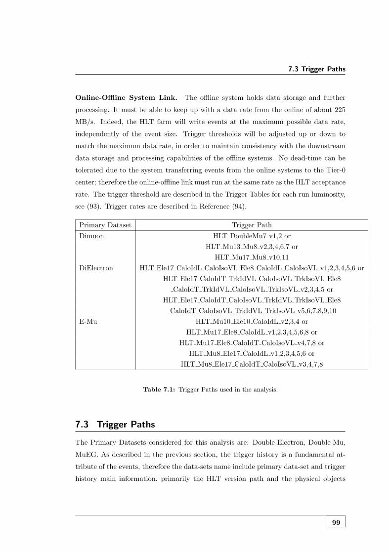
7.3 Trigger Paths
Online-Offline System Link. The offline system holds data storage and further
processing. It must be able to keep up with a data rate from the online of about 225
MB/s. Indeed, the HLT farm will write events at the maximum possible data rate,
independently of the event size. Trigger thresholds will be adjusted up or down to
match the maximum data rate, in order to maintain consistency with the downstream
data storage and processing capabilities of the offline systems. No dead-time can be
tolerated due to the system transferring events from the online systems to the Tier-0
center; therefore the online-offline link must run at the same rate as the HLT acceptance
rate. The trigger threshold are described in the Trigger Tables for each run luminosity,
see (93). Trigger rates are described in Reference (94).
Primary Dataset Trigger Path
Dimuon HLT DoubleMu7 v1,2 orHLT Mu13 Mu8 v2,3,4,6,7 or
HLT Mu17 Mu8 v10,11DiElectron HLT Ele17 CaloIdL CaloIsoVL Ele8 CaloIdL CaloIsoVL v1,2,3,4,5,6 or
HLT Ele17 CaloIdT TrkIdVL CaloIsoVL TrkIsoVL Ele8CaloIdT TrkIdVL CaloIsoVL TrkIsoVL v2,3,4,5 or
HLT Ele17 CaloIdT CaloIsoVL TrkIdVL TrkIsoVL Ele8CaloIdT CaloIsoVL TrkIdVL TrkIsoVL v5,6,7,8,9,10
E-Mu HLT Mu10 Ele10 CaloIdL v2,3,4 orHLT Mu17 Ele8 CaloIdL v1,2,3,4,5,6,8 or
HLT Mu17 Ele8 CaloIdT CaloIsoVL v4,7,8 orHLT Mu8 Ele17 CaloIdL v1,2,3,4,5,6 or
HLT Mu8 Ele17 CaloIdT CaloIsoVL v3,4,7,8
Table 7.1: Trigger Paths used in the analysis.
7.3 Trigger Paths
The Primary Datasets considered for this analysis are: Double-Electron, Double-Mu,
MuEG. As described in the previous section, the trigger history is a fundamental at-
tribute of the events, therefore the data-sets name include primary data-set and trigger
history main information, primarily the HLT version path and the physical objects
99

7. CMS 2011 DATA
pTthresholds set in HLT path. Primary Datasets and Trigger Paths used in this anal-
ysis are listed in Table 7.1.
To clarify the meaning of trigger path nomenclature, we will describe the features
of few of them, e.g.:
• Di-electron primary data-set:
– HLT_Ele17_CaloIdT_CaloIsoVL_TrkIdVL_TrkIsoVL_Ele8_
CaloIdT_CaloIsoVL_TrkIdVL_TrkIsoVL_v*
This is a double electron trigger which requires one HLT electron with ET >
17 GeV and a second HLT electron with ET > 8 GeV together with some
identification and isolation requirements on both legs. At Level-1 this HLT
path is seeded by the trigger L1_SingleEG12 i.e. a trigger which requires
one electromagnetic object with ET > 12 GeV.
• Di-muon primary dataset:
– HLT_Double_Mu7_v*
This is a double muon trigger which is based on L3 (combined muon system
and tracker information) muon reconstruction and requires two L3 muons
at HLT with pT > 7 GeV. At Level-1 this HLT path is seeded by the trigger
L1_DoubleMu3 i.e. a double muon trigger which requires pT > 3 GeV.
– HLT_Mu13_Mu8_v*
This is a double muon trigger which is based on L3 (combined muon system
and tracker information) muon reconstruction and requires two L3 muons
at HLT with pT > 8 and 13 GeV. At Level-1 this HLT path is seeded by the
trigger L1_DoubleMu3 i.e. a double muon trigger which requires pT > 3 GeV.
– HLT_Mu17_Mu8_v*
This is a double muon trigger which is based on L3 (combined muon system
and tracker information) muon reconstruction and requires two L3 muons
at HLT with pT > 8 and 17 GeV. At Level-1 this HLT path is seeded by the
trigger L1_DoubleMu3 i.e. a double muon trigger which requires pT > 3 GeV.
The choice of Di-lepton primary datasets and trigger path, instead of single-lepton
ones, is motivated by the following argument. Clearly, single lepton (muon or electron)
100

7.3 Trigger Paths
trigger is more efficient (about 10% larger) than di-lepton trigger. Efficiency wise, it
would be convenient to use single lepton trigger. Nevertheless, for full dataset in 2011,
single lepton trigger is not an option because it is pre-scaled too tight. Moreover, single
lepton triggers have usually high pT thresholds, whereas we want to keep lepton pT
thresholds as low as possible because the leptons coming from Seesaw triplet are soft
(especially for light mass points), as shown in Chapter 4. Therefore, we choose di-lepton
triggers for 2011 full dataset, to retain all the available events without cancellations. 1
Trigger efficiency and event overlapping will be discussed in the following subsec-
tions.
7.3.1 Trigger Efficiency
The trigger efficiency estimation is an important issue in order to apply the same
efficiency to the MonteCarlo background simulated sample, because the simulation by
definition has a 100% efficiency.
We will refer to trigger efficiency estimation performed by CMS Muon HLT analysis
group (with the Tag and Probe method), reporting the results from Reference (92).
The trigger path probed in this work is HLT Mu13 Mu18, one of the path we
used in our analysis. The measurements were done on 4 different data taking periods,
written in Table 7.2. The Json file (i.e. the certified collection of runs) was:
Cert 160404-177515 7TeV PromptReco Collisions11 JSON.txt
The efficiency results for full path HLT Mu13 Mu18 trigger are shown in Fig-
ures 7.3 and7.2, were the trigger efficiency versus pT, η and primary vertex number is
shown.
Taking the reported results, we could draw the following conclusion. Di-muon
trigger efficiency is greater then 95% in most of the phase space. We could suppose
1 In particular for our di-muon analysis, we are going to use HLT Mu13 Mu8 for the data up to
2011A prompt-v4 and HLT Mu17 Mu8 as a main trigger for the data above 2011A prompt v4 to get
the most of data without the prescale. This ensures we loose only about 3% of the data. We can use
these triggers only after run 165970 since they are not available before that run. For this initial period
(covering ≈ 0.3fb−1) DoubleMu7 is available without any prescale, and trigger efficiency should not
be different than Mu13 Mu8 trigger efficiency when we are using pT>20 GeV. From run 160410 to
163261, we can use HLT DoubleMu6 v1 and HLT DoubleMu7 v1 and from run 163270 to 163869 we
can use HLT DoubleMu7 v2 (Mu6 is prescaled in this second range). And there are no good runs in
between 163869 to 165088. Using Mu13 Mu8 or Mu17 Mu8 in the range after 170249, we loose less
then 1% of the events in the di muon sample that pass our selections.
101

7. CMS 2011 DATA
Period Menus (·1033) Run Range L (pb−1) Comments
1 1.-1.4 165088-167913 930 L2 Quality cuts applied2 2. 170249-173198 744 Double Muon L1 seeds (Mu3-Mu3p5)3 3. 173236-173692 216 Technical Stop4 3. 175971-177515 659
Table 7.2: Information about the run period, ran range, luminosity, of the datasets usedto compute di-muon HLT Mu13 Mu18 trigger efficiency. Reference (92).
Figure 7.2: Full path HLT Mu13 Mu18 trigger efficiency versus the number of primaryvertexes in the event (pT < 20 and |η| < 2.1. Reference (92).
pessimistically to loose around 10% of the di-muons events when using di-muon triggers.
Since we are looking for 3-leptons events, it is realistic to suppose that the third lepton
in our selection could fire the di-lepton trigger with one of the first two leptons. The
efficiency would be 90% of 10% equal to 9%. Summing the initial 90% efficiency with
the latter 9% a very high efficiency of 99% is reached. For di-electrons and muon-
electrons triggers similar reasoning could be follow. The conclusion is that for the
analysis of the seesaw signature with three leptons final state the trigger efficiency is
reasonable to be around 99%. Thus, we could neglect to apply trigger efficiency to the
MonteCarlo samples.
102

7.3 Trigger Paths
Figure 7.3: Full path HLT Mu13 Mu18 trigger efficiency versus pT(left) and η (right).Reference (92).
Figure 7.4: Using trigger HLT HT600 v8 , Muon OR Efficiency (left) and Electron ORefficiency (right) by the method described in Reference (97).
103

7. CMS 2011 DATA
To cross check the above conclusion, we studied the reported results in several anal-
ysis, which have performed in detail the di-leptons trigger efficiency. We will refer in
this section to Reference (97). Double leptons trigger efficiencies are measured directly
in Data using an independent triggered data sample (e.g. EmissT or HTtriggered), assum-
ing no correlations between these and the signal triggers. In such samples one searches
for events containing the number of tight leptons respecting the trigger threshold and
determines for which fraction the signal trigger fired. This fraction represents the trig-
ger efficiency. In order to estimate the trigger efficiencies, Reference (97) analysis use
the HT primary data set and select events that have a single isolated lepton that passes
selection criteria and that fires a HT600 trigger. The trigger efficiency is estimated by
taking the ratio of the number of events that satisfied both the HT and lepton trig-
ger to the number of events that satisfied the HT trigger. This ratio will be equal to
εij/εi = εj if the HT and lepton triggers are uncorrelated 1.
The single-lepton trigger efficiency is determined for the OR of all selected single
electron and single muon triggers in the run range 162803 to 180252 for the pTrange 30
GeV/c to 140 GeV/c, for different triggers path. In Figure 7.4 from Reference (97) the
efficiency versus lepton pT is shown for the HLT HT600 v8 trigger. Overall, in this
note the isolated electron trigger efficiency is quoted to be 94.5%, and the muon trigger
efficiency to be 87%. Result for di-electron efficiency is 99% and for di-muons is 92.6%.
Using HLT HT500 v8, as tag single non-lepton trigger, the electron trigger efficiency is
93%± 2.8% and the muon trigger efficiency is 89.6%± 2.3%. For electron-muon cross
trigger they found 96.9%± 2% efficiency 2.
7.3.2 Duplicated Events
In principle, different trigger paths could contain duplicated events, therefore we an-
alyzed the number of duplicated event in our datasets. Priory we select events with
1Additionally they require pfMET ¿ 180 or HT ¿ 550 or HT ¿ 300 and pfMET ¿ 70 to try and
remove trigger correlations or biases between HT and lepton triggers, especially electron triggers.2 The cuts on the leptons for to fire the dilepton triggers are looser than the ones for single
lepton triggers, including the L1seeds for the dilepton and single lepton triggers. This is one of the
primary reasons why the dilepton trigger efficiencies are larger than, or comparable to single lepton
trigger efficiencies . This true especially for electrons. The single electron triggers rely on either L1
SingleEG15 and L1 SingleEG20 where as the dielectron triggers rely on L1 SingleEG12.
104
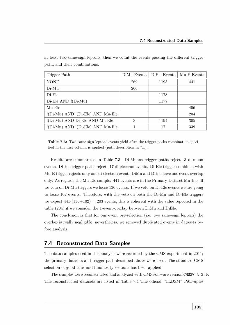
7.4 Reconstructed Data Samples
at least two-same-sign leptons, then we count the events passing the different trigger
path, and their combinations.
Trigger Path DiMu Events DiEle Events Mu-E Events
NONE 269 1195 441
Di-Mu 266
Di-Ele 1178
Di-Ele AND !(Di-Mu) 1177
Mu-Ele 406
!(Di-Mu) AND !(Di-Ele) AND Mu-Ele 204
!(Di-Mu) AND Di-Ele AND Mu-Ele 3 1194 305
!(Di-Mu) AND !(Di-Ele) AND Mu-Ele 1 17 339
Table 7.3: Two-same-sign leptons events yield after the trigger paths combination speci-fied in the first column is applied (path description in 7.1).
Results are summarized in Table 7.3. Di-Muons trigger paths rejects 3 di-muon
events. Di-Ele trigger paths rejects 17 di-electron events. Di-Ele trigger combined with
Mu-E trigger rejects only one di-electron event. DiMu and DiEle have one event overlap
only. As regards the Mu-Ele sample: 441 events are in the Primary Dataset Mu-Ele. If
we veto on Di-Mu triggers we loose 136 events. If we veto on Di-Ele events we are going
to loose 102 events. Therefore, with the veto on both the Di-Mu and Di-Ele triggers
we expect 441-(136+102) = 203 events, this is coherent with the value reported in the
table (204) if we consider the 1-event-overlap between DiMu and DiEle.
The conclusion is that for our event pre-selection (i.e. two same-sign leptons) the
overlap is really negligible, nevertheless, we removed duplicated events in datasets be-
fore analysis.
7.4 Reconstructed Data Samples
The data samples used in this analysis were recorded by the CMS experiment in 2011;
the primary datasets and trigger path described above were used. The standard CMS
selection of good runs and luminosity sections has been applied.
The samples were reconstructed and analyzed with CMS software version CMSSW_4_2_5.
The reconstructed datasets are listed in Table 7.4 The official “TLBSM” PAT-uples
105

7. CMS 2011 DATA
(version 9) have been used for the analysis.
Dataset Run range
/DoubleMuon/Run2011A-May10ReReco-v1/AOD 160329-163869/DoubleMuon/Run2011A-PromptReco-v4/AOD 165071-168437/DoubleMuon/Run2011A-05AugReReco-v1/AOD 170053-172619/DoubleMuon/Run2011A-PromptReco-v6/AOD 172620-175770/DoubleMuon/Run2011B-PromptReco-v1/AOD 175832-180296/DoubleElectron/Run2011A-May10ReReco-v1/AOD 160329-163869/DoubleElectron/Run2011A-PromptReco-v4/AOD 165071-168437/DoubleElectron/Run2011A-05AugReReco-v1/AOD 170053-172619/DoubleElectron/Run2011A-PromptReco-v6/AOD 172620-175770/DoubleElectron/Run2011B-PromptReco-v1/AOD 175832-180296/MuEG/Run2011A-May10ReReco-v1/AOD 160329-163869/MuEG/Run2011A-PromptReco-v4/AOD 165071-168437/MuEG/Run2011A-05AugReReco-v1/AOD 170053-172619/MuEG/Run2011A-PromptReco-v6/AOD 172620-175770/MuEG/Run2011B-PromptReco-v1/AOD 175832-180296
Table 7.4: Data samples used for the analysis
7.5 Event Skimming
The immutability of Primary Datasets in no way precludes the possibility to form
subsets of these Primary datasets for some specific analysis purposes. For example it is
expected that subsets of events that further satisfy some more complex offline selection
can be made. These are called Skims. Central skims for physics have been run during
data processing. The aim of a central skim is to provide a small sized release validation
data sample, saving a lot a processing time.
We decided to use the following central skim for our analysis: HWW prompt skim.
It was requested by CMS analysis group for Higgs → WW analysis. The Primary
Datasets used in this skim are: SingleMu, DoubleMu, SingleElectron, DoubleElectron,
MuEG. The rate at a luminosity of 1. ·1033 is: 0.9% (1.8Hz) of SingleMu, 2% (0.7Hz) of
DoubleMu, 2% (1Hz) DoubleEle 5% (1.3Hz) MuEG. See Reference (91) for details. As
regards Muon selection and isolation, this skim requires the use of global reconstructed
106

7.6 2011 2-Opposite-Sign Leptons
muons (see Chapter 6), adding some additional requirements; the isolation is a combi-
nation of several variables in order to be able to go down in pT. The Electron selection
and isolation foreseen a re-optimization of electron Id, with the use of new techniques,
and the isolation is combination of several variables in order to be able to go down in
pTfor electrons too.
The HWW request are summarized in Table 7.5.
Particle Cut
Muon pt > 10 GeVrelative isolation < 1.0
GlobalMuon and TrackerMuon
Electron GsfElectronRefSelectorpt > 10GeV
fully instrumented η coverage
Di-Muons invariant mass > 5 GeV
Di-Electron invariant mass > 5 GeV
E-Mu invariant mass > 1 GeV
Table 7.5: HWW skim selections.
7.6 2011 2-Opposite-Sign Leptons
A very preliminary look at 2011 data has been performed and most important plots
are presented in this sections. Data were selected with the trigger path and skimming
described in this chapter, plus the physical objects selections described in Chapter 9.
Two-opposite-sign leptons were requested in each of the datasets: MuMu, EE, Mu-
E. Plots of the most important kinematic variables are shown for the three datasets,
lepton and jets distribution, together with standard model backgrounds and signifi-
cance plot (i.e. data-MC/MC plot). The relevance of these plots the following. In
the opposite-sign leptons control region data and Standard Model background agrees
with a considerable precision. At this level of selection no hints of new physics is of
course present. This is a important cross check and validation for the algorithms and
all data processing we developed for the thesis analysis. Moreover, the plots shows
that opposite sign same flavor leptons events are largely dominated by Z backgrounds,
107

7. CMS 2011 DATA
whereas opposite sign different flavor events are dominated by tt events. A detailed
discussion about standard model backgrounds involved in this analysis will be given in
the following Chapter.
108

7.6 2011 2-Opposite-Sign Leptons
Number of PV0 5 10 15 20 25
Cou
nts
0
20
40
60
80
100
120
140
310×
Number of PV0 5 10 15 20 25
Cou
nts
0
20
40
60
80
100
120
140
310×
0 5 10 15 20 250
20
40
60
80
100
120
140
310×
DataWW (ss) + WWW
tt + W,Z
Di Bosons
W + jets
Z + jets
top (pair+single)
+ jetsγV
0 5 10 15 20 25
(dat
a-M
C)/
MC
-2
-1.5
-1
-0.5
0
0.5
1
1.5
2
MET (GeV)0 20 40 60 80 100 120 140 160 180 200
Cou
nts/
6 G
eV
0
50
100
150
200
250
3003
10×
MET (GeV)0 20 40 60 80 100 120 140 160 180 200
Cou
nts/
6 G
eV
0
50
100
150
200
250
3003
10×
0 20 40 60 80 100 120 140 160 180 2000
50
100
150
200
250
3003
10×
Data
WW (ss) + WWW
tt + W,Z
Di Bosons
W + jets
Z + jets
top (pair+single)
+ jetsγV
0 20 40 60 80 100 120 140 160 180 200
(dat
a-M
C)/
MC
-2
-1.5
-1
-0.5
0
0.5
1
1.5
2
(1)TM0 50 100 150 200 250 300
Cou
nts/
4 G
eV
0
20
40
60
80
100
120
140
160
310×
(1)TM0 50 100 150 200 250 300
Cou
nts/
4 G
eV
0
20
40
60
80
100
120
140
160
310×
0 50 100 150 200 250 3000
20
40
60
80
100
120
140
160
310×
Data
WW (ss) + WWW
tt + W,Z
Di Bosons
W + jets
Z + jets
top (pair+single)
+ jetsγV
0 50 100 150 200 250 300
(dat
a-M
C)/
MC
-2
-1.5
-1
-0.5
0
0.5
1
1.5
2
(2)TM0 50 100 150 200 250 300
Cou
nts/
4 G
eV
0
20
40
60
80
100
120
140
160
180
310×
(2)TM0 50 100 150 200 250 300
Cou
nts/
4 G
eV
0
20
40
60
80
100
120
140
160
180
310×
0 50 100 150 200 250 3000
20
40
60
80
100
120
140
160
180
310×
Data
WW (ss) + WWW
tt + W,Z
Di Bosons
W + jets
Z + jets
top (pair+single)
+ jetsγV
0 50 100 150 200 250 300
(dat
a-M
C)/
MC
-2
-1.5
-1
-0.5
0
0.5
1
1.5
2
Figure 7.5: Di-muon datasets. Event plots for 2011 two opposite-sign muon events: PV,Emiss
T , MT distributions.
109

7. CMS 2011 DATA
LT (GeV)0 100 200 300 400 500 600 700
Cou
nts/
20 G
eV
310
410
510
610
LT (GeV)0 100 200 300 400 500 600 700
Cou
nts/
20 G
eV
310
410
510
610
0 100 200 300 400 500 600 700
310
410
510
610
Data
WW (ss) + WWW
tt + W,Z
Di Bosons
W + jets
Z + jets
+ jetsγV
0 100 200 300 400 500 600 700
(dat
a-M
C)/
MC
-2
-1.5
-1
-0.5
0
0.5
1
1.5
2
HT (GeV)0 200 400 600 800 1000 1200 1400 1600 1800 2000
Cou
nts/
20 G
eV
210
310
410
HT (GeV)0 200 400 600 800 1000 1200 1400 1600 1800 2000
Cou
nts/
20 G
eV
210
310
410
0 200 400 600 800 1000 1200 1400 1600 1800 2000
210
310
410
Data
WW (ss) + WWW
tt + W,Z
Di Bosons
W + jets
Z + jets
+ jetsγV
0 200 400 600 800 1000 1200 1400 1600 1800 2000
(dat
a-M
C)/
MC
-2
-1.5
-1
-0.5
0
0.5
1
1.5
2
ST (GeV)0 200 400 600 800 1000 1200 1400 1600 1800 2000
Cou
nts/
20 G
eV
310
410
510
ST (GeV)0 200 400 600 800 1000 1200 1400 1600 1800 2000
Cou
nts/
20 G
eV
310
410
510
0 200 400 600 800 1000 1200 1400 1600 1800 2000
310
410
510
Data
WW (ss) + WWW
tt + W,Z
Di Bosons
W + jets
Z + jets
+ jetsγV
0 200 400 600 800 1000 1200 1400 1600 1800 2000
(dat
a-M
C)/
MC
-2
-1.5
-1
-0.5
0
0.5
1
1.5
2
ST with MET (GeV)0 200 400 600 800 1000 1200 1400 1600 1800 2000
Cou
nts/
20 G
eV
310
410
510
610
ST with MET (GeV)0 200 400 600 800 1000 1200 1400 1600 1800 2000
Cou
nts/
20 G
eV
310
410
510
610
0 200 400 600 800 1000 1200 1400 1600 1800 2000
310
410
510
610
Data
WW (ss) + WWW
tt + W,Z
Di Bosons
W + jets
Z + jets
+ jetsγV
0 200 400 600 800 1000 1200 1400 1600 1800 2000
(dat
a-M
C)/
MC
-2
-1.5
-1
-0.5
0
0.5
1
1.5
2
Figure 7.6: Di-muon datasets. Event plots for 2011 two opposite-sign muon events: LT,HT, ST distributions.
110

7.6 2011 2-Opposite-Sign Leptons
mult.0 1 2 3 4 5 6 7 8 9
Cou
nts
310
410
510
610
mult.0 1 2 3 4 5 6 7 8 9
Cou
nts
310
410
510
610
0 1 2 3 4 5 6 7 8 9
310
410
510
610 Data
WW (ss) + WWWtt + W,ZDi BosonsW + jetsZ + jets
+ jetsγV
0 1 2 3 4 5 6 7 8 9
(dat
a-M
C)/
MC
-2
-1.5
-1
-0.5
0
0.5
1
1.5
2
(GeV)llM0 50 100 150 200 250 300 350 400
Cou
nts/
4 G
eV
0
100
200
300
400
500
310×
(GeV)llM0 50 100 150 200 250 300 350 400
Cou
nts/
4 G
eV
0
100
200
300
400
500
310×
m/GeV0 50 100 150 200 250 300 350 400
coun
ts
0
100
200
300
400
500
310×
Data
WW (ss) + WWW
tt + W,Z
Di Bosons
W + jets
Z + jets
+ jetsγV
0 50 100 150 200 250 300 350 400
(dat
a-M
C)/
MC
-2
-1.5
-1
-0.5
0
0.5
1
1.5
2
(GeV)T
p0 50 100 150 200 250 300 350 400
Cou
nts/
5 G
eV
310
410
510
610
(GeV)T
p0 50 100 150 200 250 300 350 400
Cou
nts/
5 G
eV
310
410
510
610
0 50 100 150 200 250 300 350 400
310
410
510
610 Data
WW (ss) + WWW
tt + W,Z
Di Bosons
W + jets
Z + jets
+ jetsγV
0 50 100 150 200 250 300 350 400
(dat
a-M
C)/
MC
-2
-1.5
-1
-0.5
0
0.5
1
1.5
2
η0 0.5 1 1.5 2 2.5 3 3.5 4 4.5
Cou
nts
210
310
410
η0 0.5 1 1.5 2 2.5 3 3.5 4 4.5
Cou
nts
210
310
410
η0 0.5 1 1.5 2 2.5 3 3.5 4 4.5
coun
ts
210
310
410
Data
WW (ss) + WWW
tt + W,Z
Di Bosons
W + jets
Z + jets
+ jetsγV
0 0.5 1 1.5 2 2.5 3 3.5 4 4.5
(dat
a-M
C)/
MC
-2
-1.5
-1
-0.5
0
0.5
1
1.5
2
Figure 7.7: Di-muon datasets. Event plots for 2011 two opposite-sign muon events:multiplicity, Mll, pT, η distributions.
111

7. CMS 2011 DATA
[GeV]t
p0 100 200 300 400 500
coun
ts
210
310
410
[GeV]t
p0 100 200 300 400 500
coun
ts
210
310
410
[GeV]t
p0 100 200 300 400 500
coun
ts
210
310
410
Data
WW (ss) + WWW
tt + W,Z
Di Bosons
W + jets
Z + jets
+ jetsγV
0 100 200 300 400 500
(dat
a-M
C)/
MC
-2
-1.5
-1
-0.5
0
0.5
1
1.5
2
[GeV]t
p0 100 200 300 400 500
coun
ts
10
210
310
410
[GeV]t
p0 100 200 300 400 500
coun
ts
10
210
310
410
[GeV]t
p0 100 200 300 400 500
coun
ts
10
210
310
410 Data
WW (ss) + WWW
tt + W,Z
Di Bosons
W + jets
Z + jets
+ jetsγV
0 100 200 300 400 500
(dat
a-M
C)/
MC
-2
-1.5
-1
-0.5
0
0.5
1
1.5
2
[GeV]t
p0 100 200 300 400 500
coun
ts
10
210
310
[GeV]t
p0 100 200 300 400 500
coun
ts
10
210
310
[GeV]t
p0 100 200 300 400 500
coun
ts
10
210
310
Data
WW (ss) + WWW
tt + W,Z
Di Bosons
W + jets
Z + jets
+ jetsγV
0 100 200 300 400 500(d
ata-
MC
)/M
C-2
-1.5
-1
-0.5
0
0.5
1
1.5
2
η0 0.5 1 1.5 2 2.5 3 3.5 4 4.5 5
coun
ts
10
210
310
410
η0 0.5 1 1.5 2 2.5 3 3.5 4 4.5 5
coun
ts
10
210
310
410
η0 0.5 1 1.5 2 2.5 3 3.5 4 4.5 5
coun
ts
10
210
310
410Data
WW (ss) + WWW
tt + W,Z
Di Bosons
W + jets
Z + jets
+ jetsγV
0 0.5 1 1.5 2 2.5 3 3.5 4 4.5 5
(dat
a-M
C)/
MC
-2
-1.5
-1
-0.5
0
0.5
1
1.5
2
η0 0.5 1 1.5 2 2.5 3 3.5 4 4.5 5
coun
ts
1
10
210
310
η0 0.5 1 1.5 2 2.5 3 3.5 4 4.5 5
coun
ts
1
10
210
310
η0 0.5 1 1.5 2 2.5 3 3.5 4 4.5 5
coun
ts
1
10
210
310
Data
WW (ss) + WWW
tt + W,Z
Di Bosons
W + jets
Z + jets
+ jetsγV
0 0.5 1 1.5 2 2.5 3 3.5 4 4.5 5
(dat
a-M
C)/
MC
-2
-1.5
-1
-0.5
0
0.5
1
1.5
2
η0 0.5 1 1.5 2 2.5 3 3.5 4 4.5 5
coun
ts
1
10
210
η0 0.5 1 1.5 2 2.5 3 3.5 4 4.5 5
coun
ts
1
10
210
η0 0.5 1 1.5 2 2.5 3 3.5 4 4.5 5
coun
ts
1
10
210
Data
WW (ss) + WWW
tt + W,Z
Di Bosons
W + jets
Z + jets
+ jetsγV
0 0.5 1 1.5 2 2.5 3 3.5 4 4.5 5
(dat
a-M
C)/
MC
-2
-1.5
-1
-0.5
0
0.5
1
1.5
2
Figure 7.8: Di-muon datasets. Event plots for 2011 two opposite-sign muon events: jetpTand η distributions, from the first (left) to the third (right) jet, in pTdescending order.
112

7.6 2011 2-Opposite-Sign Leptons
Number of PV0 5 10 15 20 25
Cou
nts
0
20
40
60
80
100
310×
Number of PV0 5 10 15 20 25
Cou
nts
0
20
40
60
80
100
310×
0 5 10 15 20 250
20
40
60
80
100
310×
DataWW (ss) + WWW
tt + W,ZDi BosonsW + jetsZ + jetstop (pair+single)
+ jetsγV
0 5 10 15 20 25
(dat
a-M
C)/
MC
-2
-1.5
-1
-0.5
0
0.5
1
1.5
2
MET (GeV)0 20 40 60 80 100 120 140 160 180 200
Cou
nts/
6 G
eV
0
20
40
6080
100
120
140
160
180
200
220
310×
MET (GeV)0 20 40 60 80 100 120 140 160 180 200
Cou
nts/
6 G
eV
0
20
40
6080
100
120
140
160
180
200
220
310×
0 20 40 60 80 100 120 140 160 180 2000
20
40
6080
100
120
140
160
180
200
220
310×
Data
WW (ss) + WWW
tt + W,Z
Di Bosons
W + jets
Z + jets
top (pair+single)
+ jetsγV
0 20 40 60 80 100 120 140 160 180 200
(dat
a-M
C)/
MC
-2
-1.5
-1
-0.5
0
0.5
1
1.5
2
(1)TM0 50 100 150 200 250 300
Cou
nts/
4 G
eV
0
20
40
60
80
100
120
310×
(1)TM0 50 100 150 200 250 300
Cou
nts/
4 G
eV
0
20
40
60
80
100
120
310×
0 50 100 150 200 250 3000
20
40
60
80
100
120
310×
Data
WW (ss) + WWW
tt + W,Z
Di Bosons
W + jets
Z + jets
top (pair+single)
+ jetsγV
0 50 100 150 200 250 300
(dat
a-M
C)/
MC
-2
-1.5
-1
-0.5
0
0.5
1
1.5
2
(2)TM0 50 100 150 200 250 300
Cou
nts/
4 G
eV
0
20
40
60
80
100
120
140
310×
(2)TM0 50 100 150 200 250 300
Cou
nts/
4 G
eV
0
20
40
60
80
100
120
140
310×
0 50 100 150 200 250 3000
20
40
60
80
100
120
140
310×
Data
WW (ss) + WWW
tt + W,Z
Di Bosons
W + jets
Z + jets
top (pair+single)
+ jetsγV
0 50 100 150 200 250 300
(dat
a-M
C)/
MC
-2
-1.5
-1
-0.5
0
0.5
1
1.5
2
Figure 7.9: Di-electron datasets. Event plots for 2011 two opposite-sign electron events:PV, Emiss
T , MT distributions.
113

7. CMS 2011 DATA
LT (GeV)0 100 200 300 400 500 600 700
Cou
nts/
20 G
eV
310
410
510
LT (GeV)0 100 200 300 400 500 600 700
Cou
nts/
20 G
eV
310
410
510
0 100 200 300 400 500 600 700
310
410
510
DataWW (ss) + WWW
tt + W,Z
Di BosonsW + jets
Z + jets
+ jetsγV
0 100 200 300 400 500 600 700
(dat
a-M
C)/
MC
-2
-1.5
-1
-0.5
0
0.5
1
1.5
2
HT (GeV)0 200 400 600 800 1000 1200 1400 1600 1800 2000
Cou
nts/
20 G
eV
210
310
410
HT (GeV)0 200 400 600 800 1000 1200 1400 1600 1800 2000
Cou
nts/
20 G
eV
210
310
410
0 200 400 600 800 1000 1200 1400 1600 1800 2000
210
310
410
Data
WW (ss) + WWW
tt + W,Z
Di Bosons
W + jets
Z + jets
+ jetsγV
0 200 400 600 800 1000 1200 1400 1600 1800 2000
(dat
a-M
C)/
MC
-2
-1.5
-1
-0.5
0
0.5
1
1.5
2
ST (GeV)0 200 400 600 800 1000 1200 1400 1600 1800 2000
Cou
nts/
20 G
eV
310
410
510
ST (GeV)0 200 400 600 800 1000 1200 1400 1600 1800 2000
Cou
nts/
20 G
eV
310
410
510
0 200 400 600 800 1000 1200 1400 1600 1800 2000
310
410
510
Data
WW (ss) + WWW
tt + W,Z
Di Bosons
W + jets
Z + jets
+ jetsγV
0 200 400 600 800 1000 1200 1400 1600 1800 2000
(dat
a-M
C)/
MC
-2
-1.5
-1
-0.5
0
0.5
1
1.5
2
ST with MET (GeV)0 200 400 600 800 1000 1200 1400 1600 1800 2000
Cou
nts/
20 G
eV
310
410
510
ST with MET (GeV)0 200 400 600 800 1000 1200 1400 1600 1800 2000
Cou
nts/
20 G
eV
310
410
510
0 200 400 600 800 1000 1200 1400 1600 1800 2000
310
410
510
Data
WW (ss) + WWW
tt + W,Z
Di Bosons
W + jets
Z + jets
+ jetsγV
0 200 400 600 800 1000 1200 1400 1600 1800 2000
(dat
a-M
C)/
MC
-2
-1.5
-1
-0.5
0
0.5
1
1.5
2
Figure 7.10: Di-electron datasets. Event plots for 2011 two opposite-sign electron events:LT, HT, ST distributions.
114

7.6 2011 2-Opposite-Sign Leptons
mult.0 1 2 3 4 5 6 7 8 9
Cou
nts
310
410
510
610
mult.0 1 2 3 4 5 6 7 8 9
Cou
nts
310
410
510
610
0 1 2 3 4 5 6 7 8 9
310
410
510
610
Data
WW (ss) + WWW
tt + W,Z
Di Bosons
W + jets
Z + jets
+ jetsγV
0 1 2 3 4 5 6 7 8 9
(dat
a-M
C)/
MC
-2
-1.5
-1
-0.5
0
0.5
1
1.5
2
(GeV)llM0 50 100 150 200 250 300 350 400
Cou
nts/
4 G
eV
0
50
100
150
200
250
300
350
310×
(GeV)llM0 50 100 150 200 250 300 350 400
Cou
nts/
4 G
eV
0
50
100
150
200
250
300
350
310×
m/GeV0 50 100 150 200 250 300 350 400
coun
ts
0
50
100
150
200
250
300
350
310×
Data
WW (ss) + WWW
tt + W,Z
Di Bosons
W + jets
Z + jets
+ jetsγV
0 50 100 150 200 250 300 350 400
(dat
a-M
C)/
MC
-2
-1.5
-1
-0.5
0
0.5
1
1.5
2
(GeV)T
p0 50 100 150 200 250 300 350 400
Cou
nts/
5 G
eV
310
410
510
610
(GeV)T
p0 50 100 150 200 250 300 350 400
Cou
nts/
5 G
eV
310
410
510
610
0 50 100 150 200 250 300 350 400
310
410
510
610
Data
WW (ss) + WWW
tt + W,Z
Di Bosons
W + jets
Z + jets
+ jetsγV
0 50 100 150 200 250 300 350 400
(dat
a-M
C)/
MC
-2
-1.5
-1
-0.5
0
0.5
1
1.5
2
η0 0.5 1 1.5 2 2.5 3 3.5 4 4.5
Cou
nts
210
310
410
η0 0.5 1 1.5 2 2.5 3 3.5 4 4.5
Cou
nts
210
310
410
η0 0.5 1 1.5 2 2.5 3 3.5 4 4.5
coun
ts
210
310
410
Data
WW (ss) + WWW
tt + W,Z
Di Bosons
W + jets
Z + jets
+ jetsγV
0 0.5 1 1.5 2 2.5 3 3.5 4 4.5
(dat
a-M
C)/
MC
-2
-1.5
-1
-0.5
0
0.5
1
1.5
2
Figure 7.11: Di-electron datasets. Event plots for 2011 two opposite-sign electron events:multiplicity, Mll, pT, η distributions.
115

7. CMS 2011 DATA
[GeV]t
p0 100 200 300 400 500
coun
ts
210
310
410
[GeV]t
p0 100 200 300 400 500
coun
ts
210
310
410
[GeV]t
p0 100 200 300 400 500
coun
ts
210
310
410
Data
WW (ss) + WWW
tt + W,Z
Di Bosons
W + jets
Z + jets
+ jetsγV
0 100 200 300 400 500
(dat
a-M
C)/
MC
-2
-1.5
-1
-0.5
0
0.5
1
1.5
2
[GeV]t
p0 100 200 300 400 500
coun
ts
10
210
310
410
[GeV]t
p0 100 200 300 400 500
coun
ts
10
210
310
410
[GeV]t
p0 100 200 300 400 500
coun
ts
10
210
310
410Data
WW (ss) + WWW
tt + W,Z
Di Bosons
W + jets
Z + jets
+ jetsγV
0 100 200 300 400 500
(dat
a-M
C)/
MC
-2
-1.5
-1
-0.5
0
0.5
1
1.5
2
[GeV]t
p0 100 200 300 400 500
coun
ts
10
210
310
[GeV]t
p0 100 200 300 400 500
coun
ts
10
210
310
[GeV]t
p0 100 200 300 400 500
coun
ts
10
210
310
Data
WW (ss) + WWW
tt + W,Z
Di Bosons
W + jets
Z + jets
+ jetsγV
0 100 200 300 400 500(d
ata-
MC
)/M
C-2
-1.5
-1
-0.5
0
0.5
1
1.5
2
η0 0.5 1 1.5 2 2.5 3 3.5 4 4.5 5
coun
ts
10
210
310
410
η0 0.5 1 1.5 2 2.5 3 3.5 4 4.5 5
coun
ts
10
210
310
410
η0 0.5 1 1.5 2 2.5 3 3.5 4 4.5 5
coun
ts
10
210
310
410Data
WW (ss) + WWW
tt + W,Z
Di Bosons
W + jets
Z + jets
+ jetsγV
0 0.5 1 1.5 2 2.5 3 3.5 4 4.5 5
(dat
a-M
C)/
MC
-2
-1.5
-1
-0.5
0
0.5
1
1.5
2
η0 0.5 1 1.5 2 2.5 3 3.5 4 4.5 5
coun
ts
1
10
210
310
η0 0.5 1 1.5 2 2.5 3 3.5 4 4.5 5
coun
ts
1
10
210
310
η0 0.5 1 1.5 2 2.5 3 3.5 4 4.5 5
coun
ts
1
10
210
310 Data
WW (ss) + WWW
tt + W,Z
Di Bosons
W + jets
Z + jets
+ jetsγV
0 0.5 1 1.5 2 2.5 3 3.5 4 4.5 5
(dat
a-M
C)/
MC
-2
-1.5
-1
-0.5
0
0.5
1
1.5
2
η0 0.5 1 1.5 2 2.5 3 3.5 4 4.5 5
coun
ts
1
10
210
η0 0.5 1 1.5 2 2.5 3 3.5 4 4.5 5
coun
ts
1
10
210
η0 0.5 1 1.5 2 2.5 3 3.5 4 4.5 5
coun
ts
1
10
210
Data
WW (ss) + WWW
tt + W,Z
Di Bosons
W + jets
Z + jets
+ jetsγV
0 0.5 1 1.5 2 2.5 3 3.5 4 4.5 5
(dat
a-M
C)/
MC
-2
-1.5
-1
-0.5
0
0.5
1
1.5
2
Figure 7.12: Di-electron datasets. Event plots for 2011 two opposite-sign electron events:jet pTand η distributions, from the first (left) to the third (right) jet, in pTdescending order.
116
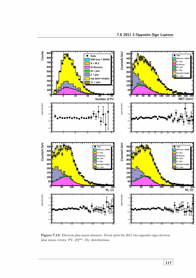
7.6 2011 2-Opposite-Sign Leptons
Number of PV0 5 10 15 20 25
Cou
nts
0
100
200
300
400
500
600
700
800
900
Number of PV0 5 10 15 20 25
Cou
nts
0
100
200
300
400
500
600
700
800
900
0 5 10 15 20 250
100
200
300
400
500
600
700
800
900DataWW (ss) + WWW
tt + W,Z
Di Bosons
W + jets
Z + jets
top (pair+single)
+ jetsγV
0 5 10 15 20 25
(dat
a-M
C)/
MC
-2
-1.5
-1
-0.5
0
0.5
1
1.5
2
MET (GeV)0 20 40 60 80 100 120 140 160 180 200
Cou
nts/
6 G
eV
0
50
100
150
200
250
300
350
400
450
MET (GeV)0 20 40 60 80 100 120 140 160 180 200
Cou
nts/
6 G
eV
0
50
100
150
200
250
300
350
400
450
0 20 40 60 80 100 120 140 160 180 2000
50
100
150
200
250
300
350
400
450Data
WW (ss) + WWW
tt + W,Z
Di Bosons
W + jets
Z + jets
top (pair+single)
+ jetsγV
0 20 40 60 80 100 120 140 160 180 200
(dat
a-M
C)/
MC
-2
-1.5
-1
-0.5
0
0.5
1
1.5
2
(1)TM0 50 100 150 200 250 300
Cou
nts/
4 G
eV
0
50
100
150
200
250
300
350
400
450
(1)TM0 50 100 150 200 250 300
Cou
nts/
4 G
eV
0
50
100
150
200
250
300
350
400
450
0 50 100 150 200 250 3000
50
100
150
200
250
300
350
400
450 Data
WW (ss) + WWW
tt + W,Z
Di Bosons
W + jets
Z + jets
top (pair+single)
+ jetsγV
0 50 100 150 200 250 300
(dat
a-M
C)/
MC
-2
-1.5
-1
-0.5
0
0.5
1
1.5
2
(2)TM0 50 100 150 200 250 300
Cou
nts/
4 G
eV
0
50
100
150
200
250
300
350
400
450
(2)TM0 50 100 150 200 250 300
Cou
nts/
4 G
eV
0
50
100
150
200
250
300
350
400
450
0 50 100 150 200 250 3000
50
100
150
200
250
300
350
400
450 Data
WW (ss) + WWW
tt + W,Z
Di Bosons
W + jets
Z + jets
top (pair+single)
+ jetsγV
0 50 100 150 200 250 300
(dat
a-M
C)/
MC
-2
-1.5
-1
-0.5
0
0.5
1
1.5
2
Figure 7.13: Electron plus muon datasets. Event plots for 2011 two opposite-sign electronplus muon events: PV, Emiss
T , MT distributions.
117

7. CMS 2011 DATA
LT (GeV)0 100 200 300 400 500 600 700
Cou
nts/
20 G
eV
1
10
210
310
LT (GeV)0 100 200 300 400 500 600 700
Cou
nts/
20 G
eV
1
10
210
310
0 100 200 300 400 500 600 700
1
10
210
310 Data
WW (ss) + WWWtt + W,ZDi BosonsW + jetsZ + jetstop (pair+single)
+ jetsγV
0 100 200 300 400 500 600 700
(dat
a-M
C)/
MC
-2
-1.5
-1
-0.5
0
0.5
1
1.5
2
HT (GeV)0 200 400 600 800 1000 1200 1400 1600 1800 2000
Cou
nts/
20 G
eV
1
10
210
HT (GeV)0 200 400 600 800 1000 1200 1400 1600 1800 2000
Cou
nts/
20 G
eV
1
10
210
0 200 400 600 800 1000 1200 1400 1600 1800 2000
1
10
210
Data
WW (ss) + WWW
tt + W,Z
Di Bosons
W + jets
Z + jets
top (pair+single)
+ jetsγV
0 200 400 600 800 1000 1200 1400 1600 1800 2000
(dat
a-M
C)/
MC
-2
-1.5
-1
-0.5
0
0.5
1
1.5
2
ST (GeV)0 200 400 600 800 1000 1200 1400 1600 1800 2000
Cou
nts/
20 G
eV
1
10
210
ST (GeV)0 200 400 600 800 1000 1200 1400 1600 1800 2000
Cou
nts/
20 G
eV
1
10
210
0 200 400 600 800 1000 1200 1400 1600 1800 2000
1
10
210
Data
WW (ss) + WWW
tt + W,Z
Di Bosons
W + jets
Z + jets
top (pair+single)
+ jetsγV
0 200 400 600 800 1000 1200 1400 1600 1800 2000
(dat
a-M
C)/
MC
-2
-1.5
-1
-0.5
0
0.5
1
1.5
2
ST with MET (GeV)0 200 400 600 800 1000 1200 1400 1600 1800 2000
Cou
nts/
20 G
eV
1
10
210
310
ST with MET (GeV)0 200 400 600 800 1000 1200 1400 1600 1800 2000
Cou
nts/
20 G
eV
1
10
210
310
0 200 400 600 800 1000 1200 1400 1600 1800 2000
1
10
210
310
Data
WW (ss) + WWW
tt + W,Z
Di Bosons
W + jets
Z + jets
top (pair+single)
+ jetsγV
0 200 400 600 800 1000 1200 1400 1600 1800 2000
(dat
a-M
C)/
MC
-2
-1.5
-1
-0.5
0
0.5
1
1.5
2
Figure 7.14: Electron plus muon datasets. Event plots for 2011 two opposite-sign electronplus muon events: LT, HT, ST distributions.
118

7.6 2011 2-Opposite-Sign Leptons
mult.0 1 2 3 4 5 6 7 8 9
Cou
nts
10
210
310
410
mult.0 1 2 3 4 5 6 7 8 9
Cou
nts
10
210
310
410
0 1 2 3 4 5 6 7 8 9
10
210
310
410Data
WW (ss) + WWW
tt + W,Z
Di Bosons
W + jets
Z + jets
top (pair+single)
+ jetsγV
0 1 2 3 4 5 6 7 8 9
(dat
a-M
C)/
MC
-2
-1.5
-1
-0.5
0
0.5
1
1.5
2
(GeV)llM0 50 100 150 200 250 300 350 400
Cou
nts/
4 G
eV
0
50
100
150
200
250
300
(GeV)llM0 50 100 150 200 250 300 350 400
Cou
nts/
4 G
eV
0
50
100
150
200
250
300
m/GeV0 50 100 150 200 250 300 350 400
coun
ts
0
50
100
150
200
250
300 Data
WW (ss) + WWW
tt + W,Z
Di Bosons
W + jets
Z + jets
top (pair+single)
+ jetsγV
0 50 100 150 200 250 300 350 400
(dat
a-M
C)/
MC
-2
-1.5
-1
-0.5
0
0.5
1
1.5
2
(GeV)T
p0 50 100 150 200 250 300 350 400
Cou
nts/
5 G
eV
10
210
310
(GeV)T
p0 50 100 150 200 250 300 350 400
Cou
nts/
5 G
eV
10
210
310
0 50 100 150 200 250 300 350 400
10
210
310
Data
WW (ss) + WWW
tt + W,Z
Di Bosons
W + jets
Z + jets
top (pair+single)
+ jetsγV
0 50 100 150 200 250 300 350 400
(dat
a-M
C)/
MC
-2
-1.5
-1
-0.5
0
0.5
1
1.5
2
η0 0.5 1 1.5 2 2.5 3 3.5 4 4.5
Cou
nts
1
10
210
η0 0.5 1 1.5 2 2.5 3 3.5 4 4.5
Cou
nts
1
10
210
η0 0.5 1 1.5 2 2.5 3 3.5 4 4.5
coun
ts
1
10
210
Data
WW (ss) + WWW
tt + W,Z
Di Bosons
W + jets
Z + jets
top (pair+single)
+ jetsγV
0 0.5 1 1.5 2 2.5 3 3.5 4 4.5
(dat
a-M
C)/
MC
-2
-1.5
-1
-0.5
0
0.5
1
1.5
2
Figure 7.15: Electron plus muon datasets. Event plots for 2011 two opposite-sign electronplus muon events: multiplicity, Mll, pT, η distributions.
119

7. CMS 2011 DATA
[GeV]t
p0 100 200 300 400 500
coun
ts
1
10
210
[GeV]t
p0 100 200 300 400 500
coun
ts
1
10
210
[GeV]t
p0 100 200 300 400 500
coun
ts
1
10
210
Data
WW (ss) + WWW
tt + W,Z
Di Bosons
W + jets
Z + jets
top (pair+single)
+ jetsγV
0 100 200 300 400 500
(dat
a-M
C)/
MC
-2
-1.5
-1
-0.5
0
0.5
1
1.5
2
[GeV]t
p0 100 200 300 400 500
coun
ts
1
10
210
310
[GeV]t
p0 100 200 300 400 500
coun
ts
1
10
210
310
[GeV]t
p0 100 200 300 400 500
coun
ts
1
10
210
310
Data
WW (ss) + WWW
tt + W,Z
Di Bosons
W + jets
Z + jets
top (pair+single)
+ jetsγV
0 100 200 300 400 500
(dat
a-M
C)/
MC
-2
-1.5
-1
-0.5
0
0.5
1
1.5
2
[GeV]t
p0 100 200 300 400 500
coun
ts
1
10
210
[GeV]t
p0 100 200 300 400 500
coun
ts
1
10
210
[GeV]t
p0 100 200 300 400 500
coun
ts
1
10
210
Data
WW (ss) + WWW
tt + W,Z
Di Bosons
W + jets
Z + jets
top (pair+single)
+ jetsγV
0 100 200 300 400 500(d
ata-
MC
)/M
C-2
-1.5
-1
-0.5
0
0.5
1
1.5
2
η0 0.5 1 1.5 2 2.5 3 3.5 4 4.5 5
coun
ts
1
10
210
η0 0.5 1 1.5 2 2.5 3 3.5 4 4.5 5
coun
ts
1
10
210
η0 0.5 1 1.5 2 2.5 3 3.5 4 4.5 5
coun
ts
1
10
210
Data
WW (ss) + WWW
tt + W,Z
Di Bosons
W + jets
Z + jets
top (pair+single)
+ jetsγV
0 0.5 1 1.5 2 2.5 3 3.5 4 4.5 5
(dat
a-M
C)/
MC
-2
-1.5
-1
-0.5
0
0.5
1
1.5
2
η0 0.5 1 1.5 2 2.5 3 3.5 4 4.5 5
coun
ts
1
10
210
η0 0.5 1 1.5 2 2.5 3 3.5 4 4.5 5
coun
ts
1
10
210
η0 0.5 1 1.5 2 2.5 3 3.5 4 4.5 5
coun
ts
1
10
210
Data
WW (ss) + WWW
tt + W,Z
Di Bosons
W + jets
Z + jets
top (pair+single)
+ jetsγV
0 0.5 1 1.5 2 2.5 3 3.5 4 4.5 5
(dat
a-M
C)/
MC
-2
-1.5
-1
-0.5
0
0.5
1
1.5
2
η0 0.5 1 1.5 2 2.5 3 3.5 4 4.5 5
coun
ts
-110
1
10
210
η0 0.5 1 1.5 2 2.5 3 3.5 4 4.5 5
coun
ts
-110
1
10
210
η0 0.5 1 1.5 2 2.5 3 3.5 4 4.5 5
coun
ts
-110
1
10
210Data
WW (ss) + WWW
tt + W,Z
Di Bosons
W + jets
Z + jets
top (pair+single)
+ jetsγV
0 0.5 1 1.5 2 2.5 3 3.5 4 4.5 5
(dat
a-M
C)/
MC
-2
-1.5
-1
-0.5
0
0.5
1
1.5
2
Figure 7.16: Electron plus muon datasets. Event plots for 2011 two opposite-sign electronplus muon events: jet pTand η distributions, from the first (left) to the third (right) jet, inpTdescending order.
120

8Backgrounds Analysis
8.1 Introduction
The background is defined as a process that can mimic the signature of the signal.
Background evaluation is crucial for a correct estimation of the discovery potential of a
signal. In evaluating the background sources for a particular analysis, we need to focus
carefully on the physical processes which could give the same final state we are looking
for, and, in addition, on all other instrumental effects which could mimic the signature
as well.
With this in mind, the background contributions are often classified into two cate-
gories:
1. Physical: i.e. physical processes ending in the same final states, both at gener-
ator level and at showering level.
2. Instrumental or non-physical: pile-up, mis-calibration of jets, charge mis-
identification, mis-identified leptons or fakes1; charged leptons missed by the de-
tector2.
In the following sections we will list all possible background sources for the signal
channels we are analyzing. In case the background source is relevant, we will describe
in detail the contribution and the strategy for removing it.
1Fake events are defined as real leptons from the unrelated parts of the event (underlying event), or
a hadronic track misidentified as a lepton, or non-prompt leptons coming from decays of heavy particles
as t and b quarks and τ2A charged lepton could be missed by the detector, for example if it is located inside a hadronic
jet and thus it is not isolated
121

8. BACKGROUNDS ANALYSIS
8.2 Backgrounds for Multi-Lepton Final State
As a preliminary consideration it is important to notice that the request of two hard
same-sign leptons (the two coming from the boson decays) nearly removes all SM
backgrounds at particle-antiparticle level.
Still, there are standard model processes which can produce a three-lepton final
state; following the classification given before, those backgrounds are:
• physical backgrounds: events with three or more real leptons (some of them could
be missed by the detector) can be produced by di-boson and tri-boson decays, as
explained in Section 8.3;
• non-physical backgrounds: events with one or two real leptons plus fake leptons
could be produced by tt and bb, WWj, cc and Drell-Yan (γ∗ and Z). These will
be discussed in Section 8.4.1.
8.3 Real Three-Lepton Backgrounds
The physics backgrounds that can produce three or more real leptons are dominated
by SM WZ production, but also include ZZ and tri-bosons production where one of
the leptons is either outside the detector acceptance or mis-reconstructed.
8.3.1 Di-bosons
The Standard Model processes can produce 3 or more real, prompt leptons with EmissT or
HT via diboson+jets production where both bosons decay leptonically. The production
of dibosons: ZZ and W±Z are illustrated in Figure 8.1. ZZ is a source of background
when the Z bosons both decay in l+l−, but one of the four leptons is missed by the
detector.
The measured cross section by the CMS collaboration (79) for these backgrounds
are:
• σ(pp→ WZ +X) = 17.0± 2.4(stat.)± 1.1(syst.)± 1.0(lumi.) pb. This will give
∼ 60 fb for the final state cross section.
• σ(pp→ ZZ +X) = 3.8+1.5−1.2(stat.)± 0.2(syst.)± 0.2(lumi.) pb.
122

8.3 Real Three-Lepton Backgrounds
Figure 8.1: The Feynman diagrams of tree-level di-boson production.
Both the production cross section of ZZ and WZ times the branching ratio to
three lepton final states are small. However this class of processes is the most important
source of background because the characteristics are too similar to the search signature.
We will refer to it as irreducible background.
Di-boson backgrounds cannot be predicted directly from the data without invok-
ing specific models, therefore they must be obtained from theory and Monte Carlo
simulations. Several analysis have checked the simulation against control samples, by
comparing it with data samples enriched in WZ-production (the dominant contribution
to trilepton signatures from diboson+jets). WZ samples can be selected by requiring
three leptons, EmissT , and an on-shell Z. These analysis show that the simulation de-
scribes such a pure sample of WZ events well within the statistical uncertainty of 15%.
In this analysis we will use MonteCarlo WZ sample with the cross section measured
from data fro normalization.
To reduce the di-boson backgrounds we can use a Z veto to remove them, since A Z
is contained in both ZZ and W±Z productions. As discussed in Chapter 9, we applied
a cut on the invariant mass of two leptons with opposite sign, |MZ −mll| > 10 GeV
to eliminate leptons coming from Z decay. Moreover, it is important to notice that
channels without two same-sign-same-flavor leptons, as: e−W+W+ν → e−µ+νµ+νν
123

8. BACKGROUNDS ANALYSIS
and µ−W+W+ν → µ−e+νe+νν µ−e+e+, are free from such a background. This will
be clarified in Chapter 9 were cuts for the different analysis channels are discussed.
8.3.2 Tri-bosons
Among the 3 gauge bosons backgrounds 3V (where V is the generic vector boson), we
have considered WWW as the most relevant background source, since it is the one that
cannot be removed by Z veto, and it has the highest production cross section1.
According to Reference (52) the cross section for the background W+W+W− is
around 65fb, and for the opposite sign dataset W−W−W+ is around 29fb.
Anyway, when considering the branching ratio into the final state with leptons, even
WWW background is negligible. As a cross check we added this source of background
to our analysis and the results are in agreement with the prediction. Since there was
no official WWW produced sample, we generated it with Madgraph, and then run
the simulation-reconstruction chain. We obtained the computed cross section from
Madgraph value to be around σWWW = 71 fb for the positive charged sample, which
is in agreement with the published values within statical errors.
8.3.3 V γ
Photon conversions, in presence of W or Z bosons, give rise to isolated leptons forming
a source of a background for three-leptons signature searches, very similar to WZ and
ZZ.
There are two different types of photon conversions that can give rise to backgrounds
in multi-lepton analysis. The first type is an external conversion where a photon in-
teracts with the material in the detector and generates an l+l− pair. Such conversions
primarily produce e+e− pairs. The ratio of the rate of external conversions to e+e− and
the rate of external conversions µ+µ− is between 6.0 ·104 and 2.0 ·105 (Reference (96)).
This is not a dangerous source of background since it could be largely reduced by a
requirement on the two opposite-sign-same-flavor leptons invariant mass; as explained
in Chapter 9 we put a cut M(l+l−) > 4GeV/c2.
The second type is asymmetric (internal) photon conversions, and will be discussed
in detail in Section 8.3.4.1 Considering that Z has a cross section approximately 1/10 respect to the W , then WWZ, WZZ
and ZZZ have very small cross sections in comparison
124

8.3 Real Three-Lepton Backgrounds
Figure 8.2: A Feynman diagram showing a Z decay to electrons, and an asymmetric FSRdecay to muons (indicated by length of the muon legs).
8.3.4 Backgrounds From Asymmetric Photon Conversions (Dalitz Back-
ground)
Internal or asymmetric photon conversions involve a virtual photon and one lepton
that takes most of the photon energy, and a second lepton very soft and not measured.
The internal conversion can produce muons almost as often as electrons.
The most important source of background from internal photon conversion for this
analysis involves Z bosons decaying to leptons, and one of the leptons radiating an
off-shell photon, γ∗ (FSR), and γ∗ undergo an asymmetric conversion. The FSR would
cause the invariant mass of the leptons from the Z decay to not reconstruct at the Z-
pole, and the asymmetric internal conversion would add one more lepton to the event.
Figure 8.2 shows a diagram of this process. The Z is shown decaying to electrons, and
the e+ emitting an FSR γ∗ which produces a µ+µ−. If one of the muons carries most of
the γ∗ momentum, this could appear as a 3-lepton event. In such events, the invariant
mass of the l+l−l shows a peak in correspondence to the Z boson mass.
Both Z+γ (ISR) and Z → l+l−γ (FSR) can clearly be seen in the data by plotting
the M(l+l−γ) mass versus M(l+l−). The FSR band is seen spread along at the x-axis
at 90 GeV on the y-axis. The ISR band is seen spread along the y-axis at 90 GeV on
the x-axis. The 3-body z-peak is a clear indication that the photon (or third lepton)
involved is produced by FSR. If on-resonance Z → l+l− has FSR on one of the legs, the
dilepton mass will be pushed off the Z peak. However, the 3-body mass of the l+l−γ∗
will still be on the Z peak. We find clean FSR events in CMS 2011 data by searching
for a 3-body Z peak as shown in Figure 8.3 for muons and 8.4 for electrons.
125

8. BACKGROUNDS ANALYSIS
Figure 8.3: Mµ+µ−γ versus Mµ+µ− .
Internal conversions are an important background to any analysis with leptons and
may be underestimated by various MC generators. While MC generators do simulate
internal conversion of emitted photons, by necessity they have a cutoff on the conversion
lepton momentum. Therefore highly asymmetric conversions, with one of the leptons
at pT ≤ 1GeV/c and the other one carrying all the momentum of emission, is not
properly accounted for. This is shown in Figure 8.5, were the invariant mass of the
three leptons measured in data is compared to those obtained in simulation in events
where no OSSF dilepton pair forms an invariant mass of Z boson, after all analysis
selections. The disagreements seen in the figure confirms that MC samples do not
properly account the internal conversion process, and it motivates the need for a data-
based determination of photon conversion factors.
126

8.3 Real Three-Lepton Backgrounds
Figure 8.4: Me+e−γ versus Me+e− .
For these reasons, we used a data driven method to estimate the background due to
asymmetric photon conversions. In this method, we assume that the rate for standard
model to produce on-shell photons is proportional to the rate for producing virtual
photons that yield asymmetric conversions. The conversion factor is a ratio of the
probability for a photon to produce a valid lepton candidate via asymmetric conversion
divided by the probability for the photon to be on-shell and pass all photon selection
criteria.
Several analysis have computed the conversion factors from final state radiation
(FSR) of the Z for both muons and electrons. See References (96) and (97), were
the conversion factors is measured in a control region devoid of new physics (e.g. low
EmissT and high HT) . To get the conversion factor the number of l+l−l± on the Z peak
127

8. BACKGROUNDS ANALYSIS
Figure 8.5: Three-lepton invariant mass distributions after Z veto (on OSSF dileptonpairs) and all our analysis selections, in µ+µ−e+ channel. The disagreement shows thatthe MC fails to get the conversion background correctly, thus motivating the data-basedmeasurement of photon conversion factors as described in the text.
is divided by the number of l+l−γ∗ on the Z peak. Figure 8.6 on the left from Reference
(97) shows the 3-body mass l+l−γ∗ in data where the l+l− is not on the Z peak (< 75
GeV and > 105 GeV). Figure 8.6 on the right shows the 3-body l+l−e± peak where no
opposite sign same flavor (OSSF) pair makes a Z candidate. Reference (97) reports the
following values for conversion factors: Cµ = 0.35%±0.10% for muons and for electrons
Ce = 1.1%±0.2% where uncertainties are statistical only, and systematic uncertainties
have been determined to be again 100%.
Reference (96) reports a measured conversion factor for muons Cµ = 0.5%± 0.15%
and for electrons Ce = 1.5%±0.2% where uncertainties are statistical only. Theoretical
systematic uncertainties have been determined to be 100% to these conversion factors
128
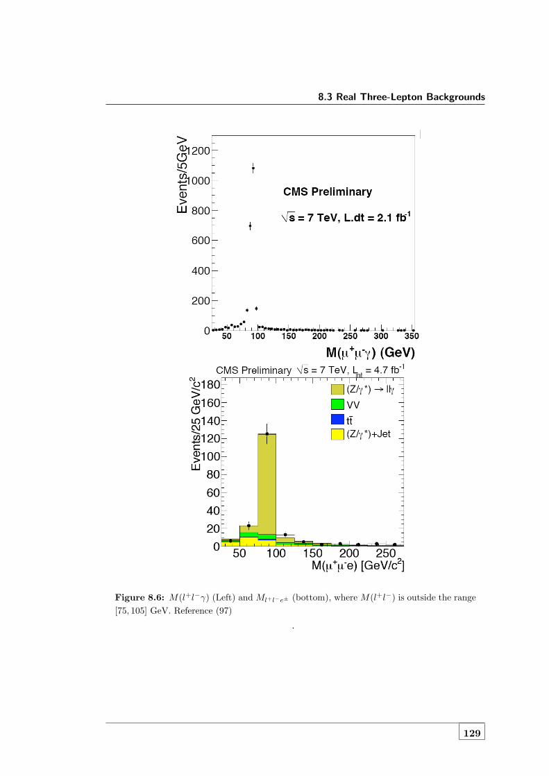
8.3 Real Three-Lepton Backgrounds
Figure 8.6: M(l+l−γ) (Left) and Ml+l−e± (bottom), where M(l+l−) is outside the range[75, 105] GeV. Reference (97)
.
129

8. BACKGROUNDS ANALYSIS
from the underlying assumption that the number of isolated photons is proportional to
the number of leptons from asymmetric internal and external conversions.
Figure 8.7: On the left: M(e+e−γ) whereM(e+e−) is outside the range [82, 102] GeV andall our analysis selections have been applied. On the right: M(µ+µ−γ) where M(µ+µ−)is outside the range [82, 102] GeV and all our analysis selections have been applied.
Channel Number of Dalitz Events
µ−e+e+ -µ−µ+e+ 9.27 ± 1.69µ−µ+µ+ 2.95 ± 0.84e−µ+µ+ -e−µ+e+ 1.69 ± 0.48e−e+e+ 5.31 ± 0.97
Table 8.1: Dalitz Events - Estimation of the number of events from asymmetric gammainternal conversion. Conversion factor values are: Cµ = 0.35% ± 0.10% and for electronsCe = 1.1%± 0.2%. Statistical errors are reported. A systematic error of 100% is assumedin the analysis.
We used the values of Cµ and Ce computed in (97) analysis to estimate the back-
ground due to FSR in our signal regions. We found clean FSR events by searching for
a 3-body Z peak in the signal region, as is evident from Figures 8.7 for electrons (Left)
and for muons (Right). Rescaling the plots with the conversion factors above gives
the number of events and distribution of asymmetric photon conversion backgrounds.
130

8.3 Real Three-Lepton Backgrounds
Figure 8.8: Mµ+µ−e+ where Mµ+µ− is outside the range [82, 102] GeV and al otheranalysis selections are applied.
The error on this background determination is the sum of statistical error plus 100%
of systematical error. The results are summarized in Table 8.1.
We compared the data with the data-driven background just described, plus the
other source of backgrounds for our signal region, and we find a very nice agreement
between data and backgrounds as shown in Figure 8.8 for channel µ+µ−e+. As will be
described in Chapter 9, we decided to remove events within the 3-body Z peak in the
range [82, 102] GeV for channels µ+µ−e+ and e+e−e+, since the Dalitz contribution
is remarkable. For the other channels we used the data-driven prediction as a source
of background since the predicted Dalitz number of events is small and a cut on the
3-body Z peak would reduce the efficiency of the signal.
131

8. BACKGROUNDS ANALYSIS
8.3.5 Opposite sign prompt-prompt Leptons
Prompt leptons could be mis-reconstructed with the wrong charge leading to a same-
sign di-lepton final state. Therefore processes with two prompt leptons that have
opposite sign can contribute to the Seesaw background if the charge of the negative
charged lepton is incorrectly identified, and another negative charged lepton is present
in the event.
Figure 8.9: Projection of the charge mis-identification rate onto pT (Left) and η. Refer-ence (103).
The magnitude of this contribution can be derived from the Monte-Carlo back-
grounds and for data by using the Z-boson resonance. We have checked the contribution
for 2 same-sign events, passing all cleaning, trigger, and lepton quality cut requirements.
The fraction of misidentified leptons is obtained by considering events with two leptons
of the same flavor in which the invariant mass of the leptons falls inside the Z-mass
window: 76 GeV < M(ll) < 106 GeV. As can be seen in the Table 8.2, this sample is
expected to be dominated by Z+Jets. For electrons, Z+Jets dominates both the overall
sample and the same sign sub-sample whereas for muons, the simulation predicts the
rate of charge mis-identification to be negligible.
The results of applying the same method to data are shown in Table 8.3. They
are consistent with the prediction taken from Reference (103) and shown in Figure 8.9.
The probability of misidentifying the charge of each lepton is computed by assuming
that the entirety of the same sign contribution is due to misidentified Z+Jets events.
132

8.4 Non-Physical Backgrounds
Electrons
Total Bckd tt ZJets W+Jets W±W± WWW ttW ttZ
In Z-Window 8.69e+05 600 8.68e+05 32.4 0.0929 0.536 0.456 1.48Same Sign 992 1.01 981 9.38 0.0929 0.343 0.264 0.0717
Muons
Total Bckd tt Z+Jets W+Jets W±W± WWW ttW ttZ
In Z-Window 1.08e+06 723 1.08e+06 0 0.130 0.600 0.500 1.68Same Sign 2.19 1.37 0 0 0.130 0.332 0.308 0.0474
Table 8.2: Expected events yields within the Z invariant mass window (76 GeV <
M(ll) < 106 GeV) for backgrounds.
In Z-Window Same Sign Mis-ID Probability
Electrons 857241 1010 5.89E-4Muons 1107821 27 1.22E-5
Table 8.3: Events yields within the Z invariant mass window (76 GeV< M(ll) < 106 GeV)for electrons and muons in data and the estimated charge mis-identification probabilitybased on these events.
To confirm that this upper limit is close to the true probability, we consider the di-
lepton invariant mass spectrum shown in Figure 8.10. In the case of electrons, both
the simulation and the mass spectrum suggest that the upper limit is close to the true
probability (within approximately 1% according to the simulation). For muons, the
charge misidentification probability is so small that we use the upper limit in its place.
The number of expected same sign events due to charge mis-identification can be es-
timated from the mis-ID probability in Table 8.3. The contribution for the seesaw final
state selections, requiring three leptons with charge ++- can be considered negligible
for both electrons and muons.
8.4 Non-Physical Backgrounds
8.4.1 Real Plus Mis-identified Leptons Events
One or two true prompt leptons resulting from SM processes together with isolated
tracks or leptons that are mis-identified as prompt leptons gives rise to a multi-lepton
background. Isolated tracks can be mis-identified as an electron or muon because of
133

8. BACKGROUNDS ANALYSIS
]2 [GeV/ceeM80 85 90 95 100 1050
0.02
0.04
0.06
0.08
0.1
0.12
]2 [GeV/cµµM80 85 90 95 100 1050
0.02
0.04
0.06
0.08
0.1
0.12
0.14
0.16
Figure 8.10: Di-lepton invariant mass spectrum in data for electrons (left) and muons(right). The opposite sign distributions are shown in black and the same sign ones are inred. All distributions are normalized to unit area.
the overlap of a hadron with an electromagnetic or an hadronic shower (with a large
electromagnetic component) or from a punch through of a hadronic shower. Moreover,
leptons that are misidentified as prompt can be real leptons from the decay of mesons
which satisfy the isolation and vertex criteria of the prompt leptons, but are not from
the physical process of interest, thus the name fake.
Throughout this thesis, we refer to as fake lepton any lepton that is not a prompt
isolated lepton from a W, Z, γ or some beyond the standard model source. In particular,
muons from K/π in flight decay, electrons or muons from heavy flavor decay, etc. are
all referred to as fake leptons.
Processes which can produce two real leptons plus a fake lepton, relevant for our
analysis, include Drell-Yan (γ∗ and Z) plus jets, and WWj production. Processes
which can produce one real leptons plus two fake leptons, as for example W jets, are
less relevant because the probability to have two fake leptons that pass the standard
isolation requirements is very low.
8.4.1.1 Drell-Yan (γ∗ and Z) + Jets
The largest background remaining after the basic three-lepton reconstruction originates
from the Z+jets process (including Drell-Yan production), in which the Z boson decays
134

8.4 Non-Physical Backgrounds
Figure 8.11: The Feynman diagrams for leading and some higher order Drell-Yan pro-duction.
leptonically and a third fake lepton is produced from a jet in the event. The Feynman
diagrams for leading and some higher order Drell-Yan productions are shown in Figure
8.11.
The Drell-Yan background can be split up into three categories, depending on the
energy scale. The list of the processes and the strategy for removing each category of
events is the following:
• qq → γ∗ → l+l−; events could be removed with an opening angle cut since the
virtual photon momentum is low;
• low-pT Z production: qq → Z → l+l−: leptons are back-to-back on the transverse
plain, so they can be removed with an opening angle cut (Z veto would result in
efficiency decrease);
• high-pT Z production: qq → Z → l+l−; leptons will not be back to back so they
will be removed with a Z veto.
The Drell-Yan MonteCarlo sample background has been validated by other analysis,
in particular: (96).
The conclusion of this analysis is that the MC simulation describes the data well.
Nevertheless, fake rates are very depend upon the particular selections of each anal-
ysis, therefore the Drell-Yan process simulation validation performed for a particular
analysis cannot be trusted for another analysis. We decided therefore not to consider
Drell-Yan process simulation MC datasets, but to estimate it with a data-driven method
instead, as described in Section 8.4.5.
135

8. BACKGROUNDS ANALYSIS
8.4.1.2 WW + Jets
Each W can decay semi-leptonically so the WW decay will produce only two real
leptons; thus a fake lepton must be present in the event to be accepted by three-lepton
selection.
WW process has a large production cross section: at 7 TeV, it has been measured by
CMS (77) and ATLAS (78) to be : σWW = 41.1±15.3(stat.)±5.8(syst.)±4.5lumi.) pb
and σWW = 41+20−16(stat.) ± 5(syst.) ± 1lumi.) pb, with an integrated luminosity of 36
and 34 pb−1, respectively. CMS collaboration also found (79) : σ(pp → WW +X) =
55.3± 3.3(stat.)± 6.9(syst.)± 3.3(lumi.) pb.
In spite of a big cross section, our pre-selection cuts (3 charged leptons out of which
2 have the same sign, 2 hard leptons) reduce this background to a negligible level, as
will be shown in Chapter 9.
Figure 8.12: The Feynman diagrams of tree-level tt production.
8.4.2 tt
The tt production is illustrated in Figure 8.12. A top quark decays via t→W±b (with a
branching ratio of 100%). We can get up to two leptons from theW± decays 1. At 7 TeV
1One from the t and the other from the t, and at least a third lepton from the semi-leptonic decay
of a b quark.
136

8.4 Non-Physical Backgrounds
the production of a top quarks pair has been measured by CMS (75) and ATLAS (76)
to be σtt = (173+39−32) pb and (171± 20± 14+8
−6) pb, with an integrated luminosity of 36
and 35 pb−1, respectively. Combining the branching ratio BR(W → lν) = 30% with
the 10% of branching ratio for the semileptonic decay of the b, the final cross section
for such background should be around 0.15− 1.5 pb depending on how many different
lepton flavors one expect in the final state.
The simulation of tt process has been carefully validated as reported for example
in Reference (96).
We have studied the contribution of tt background in our signal region and we have
found that our isolation criteria nearly kills all this background. From tt, b and c
quarks could decay semi-leptonically and give true leptons indeed, but they should be
non-isolated and so are rejected by our isolation requirements discussed in Chapter 6.
We have further studied a cut on the number of jets or hadron activity (HT) to reduce
this background to negligible levels, and b-tagging have also been considered, as will be
discussed in Chapter 9.
Other tt background alterations could be considered. For example: ttW±j, ttWW ,
ttZ, etc. The presence of one or two bosons in addition to tt ensures the presence of
three leptons in the final state, if the top decays semi-leptonically. To have an idea of
the approximate cross section of these backgrounds, we have computed the production
cross section with Madgraph5 package and we have found that the only backgrounds
among these that could be relevant are tt W, and tt Z. We generate 30k events of these
processes with Madgraph5, and request the standard simulation and reconstruction
processing for Summer 11 CMS production. Anyway, cross section is so low that even
these two processes turned out to be irrelevant for our analysis.
8.4.3 bb
The bb production is illustrated in Figure 8.13. A b quark can decay via b → Wc →W (Wd). Each W has equal chance of decaying to an electron and a muon, about 11%,
thus the probability of both Ws to decay leptonically is about 4%. If either of the W
from the b also decays leptonically, we will have three real leptons in the event. Charged
leptons from b quark decays typically have small transverse momentum, but the cross
section for bb production at LHC is high, as reported in Appendix D, so the bb can be
a substantial background. Nevertheless, in our analysis, the same consideration on tt
137

8. BACKGROUNDS ANALYSIS
Figure 8.13: The Feynman diagrams for leading and some higher order production of bb.The production of c is obtained by replacing b with c.
isolation could be applied. Moreover, since the invariant mass of the two leptons coming
from the same b hadron is typically below 4 GeV/c2, we have added this requirement
to our selection criteria1
8.4.4 QCD
QCD multi-jet events produce all non-isolated fake leptons. The probability for select-
ing three fake lepton events with the selection requirements of our analysis is deep-low,
therefore we neglected this background contribution. We made a quick cross check with
QCD simulation 2 and found that at pre-selection level nearly all the QCD events are
removed. We decided not to estimate QCD background with a data-driven method
because of the considerations above.
1Strictly speaking, the two closest leptons between any two of the three lepton candidates (regardless
of flavor) must be considered to calculate the invariant mass, i.e. the two that form the smallest spatial
angle, because they are most likely to be from the same b quark.2QCD processes are very difficult to simulate, nevertheless several analysis have cross-checked
MonteCarlo versus data-driven QCD estimation and no relevant discrepancies have been found.
138
8.4 Non-Physical Backgrounds
8.4.5 Data-driven Estimation
As remarked in the previous sections, processes with fake leptons are not properly sim-
ulated by the MC, and the samples validations are very sensitive to analysis selections.
Therefore, we performed data-driven estimation of all non-physical backgrounds, and
add the results to our total background estimation.
The background becomes very small in events with more than one fake lepton: for
this reason we have computed the fake contribution both for: one fake lepton plus two
real leptons, and two fake leptons plus one real lepton; we have neglected the case
with three fake leptons. From now on we will name true-fakes contribution the former,
fake-fake contribution the second mentioned.
In general the largest source of the true-fakes contribution is semi-leptonic top or
W/Z plus jets events where the second or third lepton comes from a heavy flavor decay.
The fake-fake contribution is dominated by pure multi-jet QCD events.
The data driven calculation of the fake contribution is done with the Tight-Loose
method described in Ref. (103) and (102).
The following assumptions are made:
• the probability of a lepton to be fake is independent from the presence of another
lepton;
• for final states with both µ and electron we consider electron and muon fakes
separately, and add them up;
• no correlation is included for the fake-fake lepton case;
• the fake rate as measured in an inclusive QCD sample as described in Ref.(102)
is applicable to the case of a QCD object in a lepton plus jet event;
• we assigned a systematic uncertainty of 50% as in Reference (102) to this proce-
dure.
The procedure is in two steps: first the average fake rate is determined using control
samples. Secondly the fake rate is applied to the events selected by the analysis. The
fake rate is defined as follows: it is the probability for a Loose lepton to pass the Tight
identification selection in samples where the presence of prompt isolation leptons is
suppressed, and therefore all leptons are candidate fakes. In formula: FR = NTL/NL
139
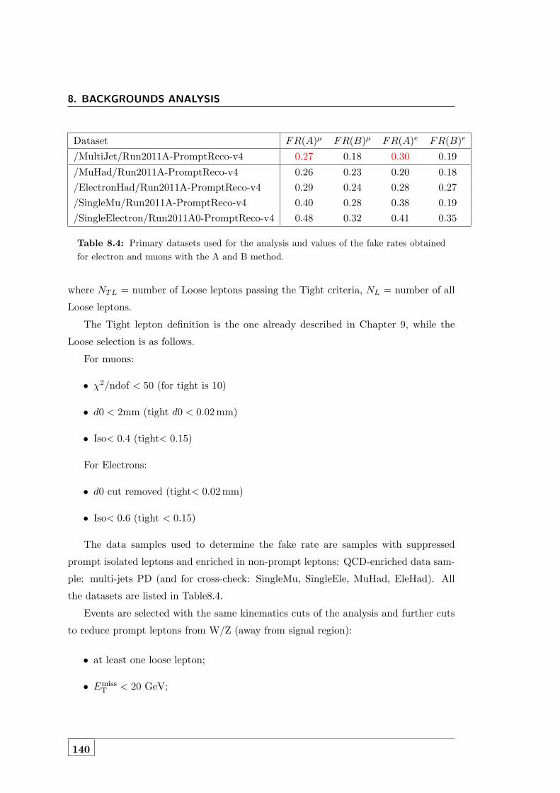
8. BACKGROUNDS ANALYSIS
Dataset FR(A)µ FR(B)µ FR(A)e FR(B)e
/MultiJet/Run2011A-PromptReco-v4 0.27 0.18 0.30 0.19
/MuHad/Run2011A-PromptReco-v4 0.26 0.23 0.20 0.18/ElectronHad/Run2011A-PromptReco-v4 0.29 0.24 0.28 0.27/SingleMu/Run2011A-PromptReco-v4 0.40 0.28 0.38 0.19/SingleElectron/Run2011A0-PromptReco-v4 0.48 0.32 0.41 0.35
Table 8.4: Primary datasets used for the analysis and values of the fake rates obtainedfor electron and muons with the A and B method.
where NTL = number of Loose leptons passing the Tight criteria, NL = number of all
Loose leptons.
The Tight lepton definition is the one already described in Chapter 9, while the
Loose selection is as follows.
For muons:
• χ2/ndof < 50 (for tight is 10)
• d0 < 2mm (tight d0 < 0.02 mm)
• Iso< 0.4 (tight< 0.15)
For Electrons:
• d0 cut removed (tight< 0.02 mm)
• Iso< 0.6 (tight < 0.15)
The data samples used to determine the fake rate are samples with suppressed
prompt isolated leptons and enriched in non-prompt leptons: QCD-enriched data sam-
ple: multi-jets PD (and for cross-check: SingleMu, SingleEle, MuHad, EleHad). All
the datasets are listed in Table8.4.
Events are selected with the same kinematics cuts of the analysis and further cuts
to reduce prompt leptons from W/Z (away from signal region):
• at least one loose lepton;
• EmissT < 20 GeV;
140

8.4 Non-Physical Backgrounds
Selection: SS leptons + 3 leptons +HT <100 GeV +Zll vetoEmiss
T > 20 GeV ≥ 2 leptons pT >15 GeV b-veto Zlll veto
µ−e+e+ channel
Nnn 11 1 1 1Nnn 57 3 1 1Nnn fakes 20.04 ±3.71 0.99±0.68 0.24± 0.41 0.24 ± 0.41
µ−µ+e+ channel
Nnn 759 34 25 6Nnn 1610 114 91 15Nnn fakes 501.49 ±51.64 38.35±5.89 30.92±5.03 4.83±1.59
µ−µ+µ+ channel
Nnn 1111 22 17 5Nnn 758 76 52 17Nnn fakes 124.97±16.50 27.08±5.83 18.21±4.24 6.05±1.99
e−µ+µ+ channel
Nnn 33 2 0 0Nnn 62 15 2 2Nnn fakes 18.77 ±3.56 5.4±1.61 0.76±0.54 0.76±0.54
e−µ+e+ channel
Nnn 759 13 7 4Nnn 1610 52 34 14Nnn fakes 501.49 ±51.64 17.85±3.43 11.89 ±2.63 4.73± 1.54
e−e+e+ channel
Nnn 584 13 10 0Nnn 3972 59 44 7Nnn fakes 1339.78±69.19 19.35±2.92 14.39 ±2.49 2.49±0.95
Table 8.5: Estimation of the number of fake events in the various channels, for the subse-quent steps of our analysis selections: from left to right the cuts are applied subsequently.The errors on the fake event values are purely statistic. For a comparison with selectedevents in the analysis, see Chapter 9.
141

8. BACKGROUNDS ANALYSIS
Figure 8.14: Some kinematics distribution of 2011 data, physical background, and fakeestimated backgrounds, for the channel µ−eµ+, after all the analysis selections.
• MT < 25 GeV;
• Z veto: reject events if 71 GeV < M(``) <111 GeV;
This we called method A. We used a second approach, with the further requirement
of one additional jet with pT > 40 GeV and ∆R(`, jet) > 1.0 (method B). The results
of the two approaches are used to evaluate the systematic uncertainty on FR value.
The values used for the final calculation are those obtained with the method A in the
Multi-Jet sample. The other values are used to determine the systematic uncertainty
on the FR itself. The estimated statistical uncertainty is 4% for muons and 1% for
142

8.4 Non-Physical Backgrounds
electrons. The systematic uncertainty has been included in the systematic uncertainty
on fake event number estimation.
In order to predict the final contribution to the background we use the technique
described in Ref. (103) and (102). The procedure is the following:
• select events that pass the full kinematics selections of the analysis, in the signal
region, but relax lepton isolation criteria;
• count the events that contain: 1 Tight lepton and 1 lepton passing a looser set of
requirements but not tight Nnn;
• count the events that contain: both leptons satisfying the Loose-no-Tight condi-
tions Nnn;
• apply the Formulas 8.1-8.4 to find the number of fake events prediction.
Assuming Nnn is dominated by QCD (both leptons are fake), a relatively simple
calculation leads to the following, neglecting much smaller terms. The contribution to
the signal sample Nffnn is given by (were ff=fake-fake, fp=fake-prompt):
Nffnn =
∑i,j
FRiFRj
(1− FRi)(1− FRj)N ij
nn
�� ��8.1
where the indices i, j correspond to the binning and flavor of corresponding non-
numerator lepton objects. The contribution from one true and one fake lepton (e.g. tt,
single top, Wjets) contribution in the signal sample NW,rawnn is given by:
Nfp,rawnn =
∑i
FRi
(1− FRi)N i
nn
�� ��8.2
Nfpnn = Nfp,raw
nn − 2Nffnn .
�� ��8.3
To account for both single and double fakes, we take as total prediction the quantity:
N totalnn = Nfp,raw
nn −Nffnn
�� ��8.4
The result about FR estimation are summarized in Table 8.4. The number of
predicted fake events for our analysis selection are listed in Table 8.5 1.1We have neglected the dependency of FR and fake event number on pT and η.
143

8. BACKGROUNDS ANALYSIS
Furthermore, we made an estimation of fake events distributions from data samples,
requiring one anti-isolated and one isolated lepton, and applying the analysis selection.
Figure 8.14 shows the distribution of physical backgrounds, fake events, and data for
the channel µ−eµ+, after all the analysis selections. Data and backgrounds are in good
agreement and no hint of new physics is present.
8.5 Background Simulation
In order to determine the contribution of the physical SM processes to the signal we
used MonteCarlo samples. We considered WZ and ZZ backgrounds, WWW, Vγ. They
are listed in Appendix D, together with all other backgrounds we have studied and
examined for the present study.
Pile-up was modeled by re weighting the Monte Carlo simulation to match the num-
ber of reconstructed vertexes found in data, using the 3D re weighting method (108),
the input data distribution reflects the 73.5 mb minimum bias cross section. The indi-
vidual event weight is calculated using 3D histograms which take as input the in-time
and out-of-time bunch crossing number of interactions. These weight histograms are
created using, as the input, the Monte Carlo distribution used in the sample genera-
tion process, and the data distribution. MC events were re-scaled to match the data
effective luminosity before comparison with data.
Since the detector simulation program does not model trigger efficiencies or isola-
tion efficiencies, and tends to be over-efficient in lepton identification, an evaluation
of the efficiencies and corrections to apply to MC samples is important for a correct
background evaluation. We will discuss this issue in the following sections. Further
details about the efficiency values used in our analysis are contained in Chapter 10
about the analysis systematics.
8.5.0.1 Trigger Efficiencies
The data need to pass various triggers to enter the final data set. In order to compare
MC events with data, we need to check each lepton candidate of the MC event to
determine which triggers it would have most likely activated. More detailed study
could be done on an event-by-event basis, and for each event a weighting factor could
be applied in order to take into account the overall trigger efficiency. Trigger efficiency
144

8.5 Background Simulation
considerations are described in Section 7.3.1. The conclusion is that we decided to
assign a trigger efficiency correction of the order of 1%.
8.5.0.2 Lepton Identification Efficiencies
The MonteCarlo production tends to overestimate the lepton identification efficiency
due to not including subtle detector efforts. An overall lepton identification efficiency
correction factor must be obtained. We decided to pursue a most conservative ap-
proach: review similar analysis were the efficiency have been computed, and combine
the correction factors that will give us the largest correction, and apply to both the
background and signal MC calculation.
In Reference (97) there is a computation of the lepton identification efficiency for
CMS, and we will refer to these results, summarized below. In this analysis, a tag and
probe method on Z → e+e and Z → µ+µ events is used to measure the efficiency of
the identification and isolation requirements for electrons and muons.
For both the electron and muon cases, selection request for tag and probes are
described in (97).
Figure 8.15: Muon identification efficiency (over probe) as a function of probe pt (left)and ratio of data and MC (right). Reference (97)
The Monte Carlo models the identification efficiencies to within a few percent
throughout the whole pt range. Figures 8.15 and 8.16 show the identification efficiency
and corresponding data to Monte Carlo ratio as a function of probe pt for muons and
electrons, respectively.
145

8. BACKGROUNDS ANALYSIS
Figure 8.16: Electron identification efficiency as a function of probe pt (left) and ratioof data and MC (right). Reference (97)
Figure 8.17: Muon isolation efficiency as a function of probe pt (left) and ratio of dataand MC (right). Reference (97)
8.5.0.3 Isolation Efficiencies
During LHC run multiple interactions occur at high instantaneous luminosity, which
can affect the lepton isolation but are not considered by CMS simulation. Therefore a
correction factor (the ratio of MC and data isolation efficiency) must be applied to all
MC events.
In Reference (97) there is a computation of the lepton isolation efficiency for CMS,
and we will refer to these results, summarized below.
For the isolation efficiency, the measured efficiency in the range of pT < 25 GeV/c
146

8.5 Background Simulation
Figure 8.18: Electron isolation efficiency as a function of probe pt (left) and ratio of dataand MC (right). Reference (97)
is significantly smaller than in Monte Carlo. Figures 8.17 and 8.18 show the isolation
efficiency and corresponding data to Monte Carlo ratio as a function of probe pTfor
muons and electrons, respectively. This was modeled in Reference (97), with a fit of
the ratio of data and MC isolation efficiencies to the equation which was proposed in
the same sign di-lepton analysis for lepton efficiencies,
Although the isolation efficiency may depend on the number of jets(vertexes) in the
event, they find that variations in the parameters with the number of jets (vertexes) is
consistent with the statistical uncertainties. In this analysis the average ratio of data
and MC muon isolation efficiencies is found to be 0.9974 for muons and 1.0053 for
electrons, at plateau at high momenta. Systematic errors are around 7%.
One more possible concern with the ever growing luminosity is pileup. For lepton
pt > 25GeV/c we need not worry about ID or Isolation efficiencies as the MC agrees
well with data. This can be seen from the plots provided in the Reference (97). For
softer leptons care must be taken, and further studies would be needed to have the
efficiency behavior under control. They will be investigated in further works.
147

9Signal-Background Discrimination
9.1 Introduction
In this Chapter we will present the analysis strategy adopted to discriminate Seesaw sig-
nal from background. The event preselection requirements are discussed in Section 9.3,
the selections are discussed and motivated in Section 9.4, and finally the results about
event yields are given for 2011 luminosity in Section 9.5.
In this introduction the highlights of the analysis are summarized. They were
described in deep detail in the previous chapters, but pinpoint them now is important
to understand the subsequent analysis selections.
Seesaw type-III Model. Electroweak scale heavy neutrino fermion triplets (Seesaw
type-III) signals are investigated in this analysis. We restrict ourselves to heavy Majo-
rana fermion triplets decaying to light leptons plus gauge or Higgs bosons, which are
dominant except for unnaturally small mixings. As described in Chapter 2, the seesaw
mechanism could provide an explanation that accounts for neutrino mass.
The seesaws of type II and III can be produced at LHC via gauge interactions and
can be observed if their mass is sufficiently small, regardless of the size of Youkawa
couplings. The possibility of type III Seesaw discovering at LHC for a center-of-mass√s = 14 TeV is discussed in (24, 29). Recently a complete evaluation of the signal at
√s = 7 TeV and a code allowing calculations and simulations with the model has been
provided, see Reference (30).
Mixing Scenarios. The heavy lepton production cross section is independent from
the mixing angle values, while the decay branching ratios depend on the mixing Vα
149

9. SIGNAL-BACKGROUND DISCRIMINATION
where α = e, µ or τ . Constraints on the mixing parameters and their products exists
as reported in (30) and described in Chapter 4. Given the results reported in that
Chapter, we choose the following scenarios as benchmarks to set limits on the seesaw
mass:
1. Ve = Vτ = Vµ = 4.1× 10⁻⁴;
2. Vµ = 0.063, and Ve = Vτ = 0;
3. Ve = 0.05 and Vµ = Vτ = 0;
Signature. Given the triplet charge status Σ+, Σ0 and Σ−, the most promising signal
chain are:
pp→ Σ0Σ+, Σ0 → `∓W±,Σ+ →W+ν�� ��9.1
pp→ Σ0Σ+, Σ0 → `±W∓,Σ+ →W+ν�� ��9.2
These processes have the higher cross sections. Other processes with a smaller cross
section, but potentially ending in the same final state, are:
pp→ Σ0Σ+, Σ0 → `∓W±,Σ+ → `+Z�� ��9.3
pp→ Σ0Σ+, Σ0 → `±W∓,Σ+ → `+Z�� ��9.4
By requiring W± decay to `±ν (here ` is an electron or muon), and Z decay to
neutrinos or jets, the final state shows a very clean signature with a positive charged
triplet of leptons. We focus the search on tree positive charged leptons final state.
Signal. The model was implemented in FeynRules package and the signal samples
have been generated with the MadGraph (58) event generator. The hadronization and
fragmentation of quarks and gluons is then performed by pythia (47). Detector simu-
lation and reconstruction was performed using Fast Simulation CMSSW 4 2 8 patch4
release with true pile up distribution. The signal samples are listed with the cross sec-
tion from Madgraph output in Table 9.1, with the cross section from CMS simulation
150

9.1 Introduction
in Table 9.2 and with the number of events in Table 9.3, versus Σ mass point spanning
from the lower limit (set by L3 at LEP (98)) to 180 GeV mass point1.
ID Process Cross Sections (fb) for Σ mass (GeV)
100 120 130 140 180
P1 `−W+W+ν,W+ → `+ 182.7 65.11 43.66 30.25 9.17P11 `+W−W+ν,W± → `± 183.0 65.15 43.64 30.24 18.09P2 `−`+ZW+,W+ → `+, Z → νν 18.35 13.53 10.28 7.68 2.63P3 `+`+ZW−,W− → `−, Z → νν 18.34 13.54 10.26 7.66 2.63P4 (*) `+`+ZW−,W− → `−, Z → jj 44.75 33.39 25.41 18.98 6.54P5 (*) `−`+ZW+,W+ → `+, Z → jj 44.80 33.43 25.47 18.97 6.55PAllJets(*) Σ+Σ0j → P∗ 296.7 - - - -P1Jets(*) `−W+W+νj,W+ → `+ 85.93 32.70 - - -P11Jets(*) `+W−W+νj,W± → `± 86.12 32.71 - - -P2Jets(*) `−`+ZW+j,W+ → `+, Z → νν 18.42 14.58 - - -P3Jets(*) `+`+ZW−j,W− → `−, Z → νν 18.38 14.57 - - -P4Jets(*) `+`+ZW−j,W− → `−, Z → jj 43.80 - - - -P5Jets(*) `−`+ZW+j,W+ → `+, Z → jj 44.10 - - - -P1pSmallV100(#) µ−W+W+ν 1173. - - - -P1pVtau100 `−W+W+ν,W+ → `+ 182.6 - - - -
Table 9.1: Cross sections of the signal Monte Carlo samples in output from Madgraph5.Cross section is relative to the final state, before Pythia hadronization and jet-matching,CMS simulation and reconstruction. The process PAllJets includes P1, P11, P2, P3;P4 and P5 with with a hard jet at parton-level generation added. Processes with (*)have a different jet-matching parameters: xqcut=10, QCUT=15, while the other processessettings are: xqcut=20, QCUT=30. Process with (#) has no jet-matching.
Definition of Analysis Categories. The signature for this search is three leptons
of charge ++- plus missing energy and jets. Leptons in this search can be either
electrons or muons. Selected events are subdivided into the six categories here listed:
1. µ−e+e+,
1The mass dependence of the expected cross section is very steep and other signatures could be
more relevant at higher mass values. Their study is not included here.
151

9. SIGNAL-BACKGROUND DISCRIMINATION
ID Process Cross Sections (fb) for Σ mass (GeV)
100 120 130 140 180
P1 `−W+W+ν,W+ → `+ 130.7 44.78 29.60 20.12 5.84P11 `+W−W+ν,W± → `± 130.8 44.88 29.68 20.19 5.85P2 `−`+ZW+,W+ → `+, Z → νν 13.12 9.34 6.97 5.13 1.67P3 `+`+ZW−,W− → `−, Z → νν 13.12 9.35 6.95 5.13 1.67P4 (*) `+`+ZW−,W− → `−, Z → jj 21.79 15.31 11.37 8.37 2.67P5 (*) `−`+ZW+,W+ → `+, Z → jj 21.82 15.48 11.52 8.33 2.69
Total `−`+`+ + EmissT + jets 331.35 139.14 96.09 67.27 20.39
PAllJets(*) Σ+Σ0j → P∗ 92.07 - - - -P1Jets(*) `−W+W+νj,W+ → `+ 26.88 - - - -P11Jets(*) `+W−W+νj,W± → `± 26.60 - - - -P2Jets(*) `−`+ZW+j,W+ → `+, Z → νν 5.65 - - - -P3Jets(*) `+`+ZW−j,W− → `−, Z → νν 5.68 - - - -P4Jets(*) `+`+ZW−j,W− → `−, Z → jj 13.59 - - - -P5Jets(*) `−`+ZW+j,W+ → `+, Z → jj 13.68 - - - -P1pSmallV100(#) µ−W+W+ν 1174 - - - -P1pVtau100 `−W+W+ν,W+ → `+ 131 - - - -
Table 9.2: Cross sections of the signal Monte Carlo samples used for the analysis. Crosssection is relative to the final state, after CMS simulation and reconstruction. The finalstate is `−`+`+Emiss
T for P1, P11, P2, P3; P4 and P5 give `−`+`+EmissT jets final state. The
process PAllJets includes P1, P11, P2, P3; P4 and P5 with with a hard jet at parton-levelgeneration added. Processes with (*) have a different jet-matching parameters: xqcut=10,QCUT=15, while the other processes settings are: xqcut=20, QCUT=30. Process with(#) has no jet-matching.
2. µ−e+µ+,
3. µ−µ+µ+,
4. e−µ+µ+,
5. e−e+µ+,
6. e−e+e+.
152

9.1 Introduction
ID Process Number of Events for Σ mass (GeV)
100 120 130 140 180
P1 `−W+W+ν,W+ → `+ 71502 68778 67794 66794 63682P11 `+W−W+ν,W± → `± 71508 68890 68010 66791 63559P2 `−`+ZW+,W+ → `+, Z → νν 71501 69023 67857 66816 63432P3 `+`+ZW−,W− → `−, Z → νν 71547 69017 67786 66955 63565P4 (*) `+`+ZW−,W− → `−, Z → jj 48693 45864 44756 44090 40887P5 (*) `−`+ZW+,W+ → `+, Z → jj 48717 46304 45228 43890 41181PAllJets(*) Σ+Σ0j → P∗ 31025 - - - -P1Jets(*) `−W+W+νj,W+ → `+ 8988 - - - -P11Jets(*) `+W−W+νj,W± → `± 8952 - - - -P2Jets(*) `−`+ZW+j,W+ → `+, Z → νν 1925 - - - -P3Jets(*) `+`+ZW−j,W− → `−, Z → νν 1904 - - - -P4Jets(*) `+`+ZW−j,W− → `−, Z → jj 4629 - - - -P5Jets(*) `−`+ZW+j,W+ → `+, Z → jj 4627 - - - -P1pSmallV100 (#) µ−W+W+ν 10000 - - - -P1pVtau100 `−W+W+ν,W+ → `+ 71718 - - - -
Table 9.3: Number of events of the signal Monte Carlo samples used for the analysis. Theprocess PAllJets includes P1, P11, P2, P3; P4 and P5 with with a hard jet at parton-levelgeneration added. Processes with (*) have a different jet-matching parameters: xqcut=10,QCUT=15, while the other processes settings are: xqcut=20, QCUT=30. Process with(#) has no jet-matching.
To avoid double counting events that are found in multiple datasets, a check was
performed on selected events and double counted events rejected.
Backgrounds. All standard model sources of three isolated leptons (two same sign)
at CMS are vanishingly small. Nevertheless, several background sources have been
analyzed, divided into physics and instrumental. As described in Chapter 8, the most
relevant of the former is the irreducible background WZ, with both bosons decaying
into leptons. The physics background includes also the ZZ production with one of the
leptons either out of the detector acceptance or mis-reconstructed.
We analyzed physical backgrounds using the official CMS Standard Model datasets
of Summer 11 production, listed in Appendix D. The details about simulation are given
153
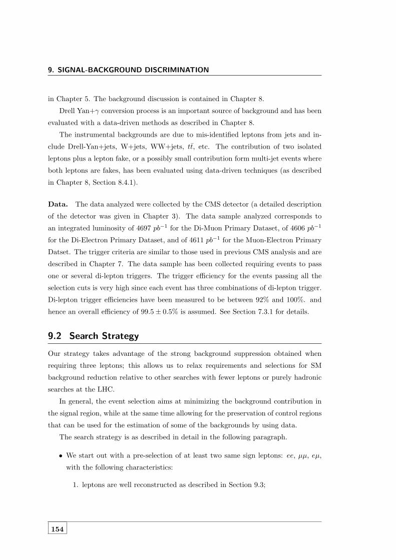
9. SIGNAL-BACKGROUND DISCRIMINATION
in Chapter 5. The background discussion is contained in Chapter 8.
Drell Yan+γ conversion process is an important source of background and has been
evaluated with a data-driven methods as described in Chapter 8.
The instrumental backgrounds are due to mis-identified leptons from jets and in-
clude Drell-Yan+jets, W+jets, WW+jets, tt, etc. The contribution of two isolated
leptons plus a lepton fake, or a possibly small contribution form multi-jet events where
both leptons are fakes, has been evaluated using data-driven techniques (as described
in Chapter 8, Section 8.4.1).
Data. The data analyzed were collected by the CMS detector (a detailed description
of the detector was given in Chapter 3). The data sample analyzed corresponds to
an integrated luminosity of 4697 pb−1 for the Di-Muon Primary Dataset, of 4606 pb−1
for the Di-Electron Primary Dataset, and of 4611 pb−1 for the Muon-Electron Primary
Datset. The trigger criteria are similar to those used in previous CMS analysis and are
described in Chapter 7. The data sample has been collected requiring events to pass
one or several di-lepton triggers. The trigger efficiency for the events passing all the
selection cuts is very high since each event has three combinations of di-lepton trigger.
Di-lepton trigger efficiencies have been measured to be between 92% and 100%. and
hence an overall efficiency of 99.5± 0.5% is assumed. See Section 7.3.1 for details.
9.2 Search Strategy
Our strategy takes advantage of the strong background suppression obtained when
requiring three leptons; this allows us to relax requirements and selections for SM
background reduction relative to other searches with fewer leptons or purely hadronic
searches at the LHC.
In general, the event selection aims at minimizing the background contribution in
the signal region, while at the same time allowing for the preservation of control regions
that can be used for the estimation of some of the backgrounds by using data.
The search strategy is as described in detail in the following paragraph.
• We start out with a pre-selection of at least two same sign leptons: ee, µµ, eµ,
with the following characteristics:
1. leptons are well reconstructed as described in Section 9.3;
154

9.2 Search Strategy
2. lepton pT > 10 GeV; such a low pT limit is necessary to maintain sensitivity
to possible signals with relatively low pT leptons generated in the cascade
decays of heavy objects;
• We perform a counting experiment in this region and predict the expected yield
for the standard model background contribution of true isolated tri-leptons (i.e.
physical irreducible backgrounds) by Monte Carlo simulation.
• We then tighten the selection further as follows:
1. we require the presence of a third lepton and no other leptons in the event,
in addition we require at least two leptons of pT > 15 GeV;
2. we measure the yield for with an additional requirement of EmissT > 20 GeV
(this cut was chosen a priori to reduce the total standard model expected
yield in Monte Carlo);
3. we measure the yield for an additional HT < 100GeV cut and b-tag veto.
• We perform a counting experiment in the regions after each of the selection steps
and predict:
1. the expected yield for non-physical backgrounds using data driven techniques
for the sum of single and double fake events,
2. we consider a contribution from conversions of isolated photons from Wγ
and Zγ. These contributions are computed using data driven technique. We
find the Zγ contribution to be not negligible, as discussed in Section 8.3.4.
The Wγ is negligible.
• We compute the event yield after all the cuts above;
• We compare observations with background expectations;
• We compare signal expectations;
• Finally, if no excess yield is observed we place an upper limit on cross section.
155

9. SIGNAL-BACKGROUND DISCRIMINATION
9.3 Event pre-selection
The pre-selected events must have a well reconstructed primary interaction vertex and
at least two positive-charged well-reconstructed lepton candidates, as described in the
following subsections. The analysis relies on the reconstruction of three types of objects:
electrons, muons and jets. The events are reconstructed using a full Particle Flow
approach (PF2PAT) (85, 86, 87) as described in Chapter 6 and the details of the
object selection are provided below.
9.3.1 Event Cleanup and Vertex Selection
The events are cleaned up by requiring:
• Event cleaning (i.e. Scraping cut): if there are ≥ 10 tracks, require at least 25%
of them to be high purity.
• Require at least one good vertex:
1. not fake;
2. ndof > 4;
3. |ρ| < 2 cm;
4. |z| < 24 cm.
• HBHE event-level noise filtering
9.3.2 Electron selection
Electron candidates are reconstructed from a collection of electromagnetic clusters with
matched pixel tracks. The momentum of the electron track is fitted using a Gaussian-
Sum Filter (GSF) algorithm along its trajectory with the algorithm taking into account
the possible emission of Bremsstrahlung photons in the silicon tracker. Requirements
on electrons are:
• pT > 10GeV
• |η| < 2.5; we also exclude the barrel and endcap transition region (1.4442 <
|ηsc| < 1.566).
156

9.3 Event pre-selection
• electron identification using the Cut in Categories (CiC) approach (see Chap-
ter 6)1. Electrons are required to pass the eidMediumMC CiC selection.
• Particle Flow based relative isolation is required to be less than 0.202.
• Conversion rejection cuts: we reject an electron if the number of missing expected
inner hits is equal to zero and the electron is flagged as conversion using the
partner track conversion veto (0.02, 0.02).
• Transverse impact parameter of the electron with respect to the beamspot <
0.02 cm.
• Require that all three charge measurements for an electron agree (Gsf-Ctf-ScPix
charge consistency (cfr. Chapter 6).3.
• Conversion rejection4.
9.3.3 Muon Selection
• pT > 10 GeV;
• |η| < 2.1;
• Classified as GlobalMuon and TrackerMuon;
• Number of valid Silicon hits ≥11;
• Transverse impact parameter of the electron with respect to the beamspot< 0.02 ;
• χ2/ndof < 10;
• Number of Muon hits > 0;
1This method classifies an electron in a number of categories (barrel versus endcap, fbrem versus
E/p, and transverse energy) which are optimized to select electrons from W or Z decays and reject
fakes from jets or conversions.2relative combined particle flow isolation calculated using tracks, Ecal and HCal energy deposit
within a cone ∆R < 0.3.3One from the charge of the GSF track, one from the charge of the CTF track associated to the
GSF track and one, the so-called supercluster charge, determined from the relative position of the
supercluster with respect to the projected track from the pixel seed.4nLostHits == 0 and (|convDCot| > 0.02 or |convDist > 0.02).
157

9. SIGNAL-BACKGROUND DISCRIMINATION
• Number of Pixel Hits > 0;
• Number of chambers with matched segments > 1;
• Particle Flow based relative isolation is required to be less than 0.15.
9.3.4 Jets
• Jets are reconstructed using the Anti-kT algorithm (cfr. Chapter 6);
• Jet energy corrections: charged hadron subtraction, L1FastJet corrections and
L2L3Jet-EnergyScale corrections;
• PT > 30 GeV;
• |η| < 2.4;
• Loose jet Id (see (110) for more info) ;
9.3.5 Preselection Yield
The number of events after preselection for the simulated background are listed in
Tables 9.11 and 9.10, in the 2SS column. The dominant contribution is from Z0 →e+e− with one of the two electrons with the charge misidentified.
Signal samples yields are shown in Tables 9.7 and 9.6 in the same column. The
signal is computed for five mass points ranging from 100 to 180 GeV.
9.4 Selections
By comparing the kinematics of signal and background events, we can use a series of
cuts to reject background with minimal effect on signal acceptance.
For multi-lepton searches, the SM background (once the total number and charge
of leptons is imposed) is small and can be further reduced by minimal requirements on
either hadronic activity or missing energy above the typical SM values1
Moreover, both hadronic activity and EmissT are good discriminating observables for
physics beyond the SM.1 These variables are well described by the simulation, as shown in Fig. 9.1 from Reference (96)
for events with two isolated and one lepton with isolation selection removed.
158

9.4 Selections
[GeV]missTE
0 20 40 60 80 100 120 140 160 180 200
Eve
nts/
5 G
eV
-110
1
10
210
310
410DATA
VV+Jets
+Jetstt
DY+Jets
CMS preliminary-1=2.1fb
int=7TeV, Ls
[GeV]TH0 50 100 150 200 250 300 350 400 450 500
Eve
nts/
5 G
eV
-110
1
10
210
310
410DATA
VV+Jets
+Jetstt
DY+Jets
CMS preliminary-1=2.1fb
int=7TeV, Ls
[GeV]missTE
0 20 40 60 80 100 120 140 160 180 200
Eve
nts/
5 G
eV
-110
1
10
210
310
410DATA
VV+Jets
+Jetstt
DY+Jets
CMS preliminary-1=2.1fb
int=7TeV, Ls
[GeV]TH0 50 100 150 200 250 300 350 400 450 500
Eve
nts/
5 G
eV
-110
1
10
210
310
410 DATA
VV+Jets
+Jetstt
DY+Jets
CMS preliminary-1=2.1fb
int=7TeV, Ls
Figure 9.1: EmissT (left)and HT(right) distributions for ``−µ (top), ``−e (bottom), where
two leptons `` are isolated but the third lepton is required to be non-isolated. VV, TT andDY refers to the diboson, top-quark and Drell-Yan SM production, respectively. Reference(96).
159

9. SIGNAL-BACKGROUND DISCRIMINATION
In order to retain search sensitivity for our signal region both EmissT and HT selec-
tions have been used.
The distribution of various kinematic variables form the signal sample (for one
specific mass point) have been compared to the distribution of the overall predicted
backgrounds after each of the cuts, in order to optimize the event selection and obtain
the best sensitivity for signal extraction or for setting a limits.
The selections applied in this analysis are summarized here, and discussed and
motivated in the following sections. The selection requires:
• Exactly three isolated leptons as defined above, with charges ++-, at least two
leptons with pT > 15 GeV/c.
• EmissT >20 GeV.
• HT< 100 GeV, where HTis summed over the selected jets only.
• reject events with a b-tag;
• M(``) > 4GeV .
• Z Veto: M(``) <82 GeV or M(``) >102 GeV.
• Z asymmetric conversion veto: M(```) <82 GeV or M(```) >102 GeV for cate-
gories: e−e+e+ and µ−e+µ+.
hTrMuonEntries 33656Mean 22.16RMS 15.24
Σ (GeV) of Muons from T
p0 20 40 60 80 100 120 140 160 180 2000
200
400
600
800
1000
1200
1400
hTrMuonEntries 33656Mean 22.16RMS 15.24
Generated Seesaw type-III signal
-4=4.1 * 10τ = Ve = VµV
+ MET+ l+ l-P1: l
100 GeV mass point
(GeV)T PΣMuon hWMuonEntries 66632Mean 41.92RMS 26.3
(GeV) of Muons from WT
p0 20 40 60 80 100 120 140 160 180 2000
200
400
600
800
1000
1200
1400
hWMuonEntries 66632Mean 41.92RMS 26.3
(GeV)T PWMuon
Figure 9.2: Transverse momentum distribution for muons from Σ0 (left) and W (right)µ−µ+µ+ events for different background and signal samples.
160

9.4 Selections
9.4.1 Momentum Requirements
As it can be seen on Fig. 9.2 the lepton pT distribution depends on the parent particle.
In particular leptons coming from Σ0 decay have a softer spectrum with respect to the
W-generated one, especially for mass points close to 100 GeV. Consequently, to ensure
a reasonable selection efficiency, the selected candidate events are required to have:
• at least two isolated muons (electrons) with pT > 15 GeV/c;
• a third isolated lepton with pT > 10 GeV/c;
• no other leptons in the event, to reject background from ZZ leptonic decays;
9.4.2 Missing Transverse Energy
The missing transverse energy (EmissT ) is defined as the magnitude of the vectorial sum
of the transverse energy of all Particle Flow(PF) candidates. The low backgrounds in
the multilepton selections allows us to selectively impose the ETmiss requirement. We
exploit the background reduction ability of ETmiss plotting Emiss
T distribution after the
selection cuts.
Events with EmissT > 20 GeV are said to satisfy the requirement.
9.4.3 Hadron Activity
The presence of hadronic activity in an event is characterized by the variable HT,
defined as the scalar sum of the transverse jet energies for all jets with kinematic
cuts of the analysis (pT > 30 GeV). Jets used for the HTdetermination must be well
separated from any identified leptons, hence jets are required to have no lepton in a
cone ∆R < 0.3 around the jet axis. To remove residual backgrounds from events with
leptonic W decay and an additional lepton, we state the HTrequirement: HT<100
GeV/c.
9.4.4 Z veto
Another criterion for background reduction is the requirement of Z veto, as discussed
in Chapter 8. The first and the fourth categories in Section 9.1 have no contributions
from Z decay, while the others can be produced by WZ events and they have one or
161

9. SIGNAL-BACKGROUND DISCRIMINATION
(GeV)llM0 50 100 150 200 250 300 350 400
Cou
nts/
4 G
eV
0
24
6
8
10
1214
16
18
20
2224
DataWWp_CastorWWWp_CastorTTWWp_CastorttWp_CastorttZm_CastorttZp_CastorZZWZZJetsMadGrttbarJetsMadGrGVJetsSeesaw100p
Total background: 45.97WWp_Castor: 0.00WWWp_Castor: 0.18TTWWp_Castor: 0.00ttWp_Castor: 0.11ttZm_Castor: 0.02ttZp_Castor: 0.02ZZ: 1.65WZ: 31.27ZJetsMadGr: 2.61ttbarJetsMadGr: 0.00GVJets: 10.12Seesaw100p: 6.11Data: 61.00
(GeV)llM0 50 100 150 200 250 300 350 400
Cou
nts/
4 G
eV
0
5
10
15
20
25
DataWWp_CastorWWWp_CastorTTWWp_CastorttWp_CastorttZm_CastorttZp_CastorZZWZZJetsMadGrttbarJetsMadGrGVJetsSeesaw100p
Total background: 79.52WWp_Castor: 0.00WWWp_Castor: 0.24TTWWp_Castor: 0.00ttWp_Castor: 0.12ttZm_Castor: 0.04ttZp_Castor: 0.03ZZ: 4.75WZ: 73.60ZJetsMadGr: 0.00ttbarJetsMadGr: 0.75GVJets: 0.00Seesaw100p: 6.35Data: 95.00
Figure 9.3: Invariant mass for µ−e+µ+ (top) and µ−µ+µ+ (bottom) events for differentbackground and signal samples.
162

9.5 Event Yields
two possible combinatorial contributions to the Z→ `+`− invariant mass. As shown
in Fig. 9.3 a clear Z peak is evident in the simulated events. To reduce the WZ
background an Z veto has been added to the selection requirements for categories
2,3,5,6 (as described in 9.1).
We veto events for which a third lepton is found that passes all the lepton require-
ments and makes an opposite sign same flavor Z candidate with one of the two same
sign leptons we require. Events with at least one µ+µ− (e−e+) mass combination in
the range 82 > mµ+µ− > 102 (82 > me−e+ > 102) are rejected.
To reject low mass Drell–Yan production and the J/Ψ(1S) we required opposite
sign same flavor lepton pairs to have M(2`) > 4 GeV/c2 for all combinations.
As described in detail in Chapter 8, Section 8.3.4, a possible source of background
is from the final state radiation in Z → 2l(l = e, µ) events undergoing a γ → 2l
conversion. Therefore, the Z veto requirement is also applied to the invariant mass
M(3l) of three leptons for category e−e+e+ and µ−e+µ+: in these cases the asymmetric
gamma conversion background is significant. For categories: µ−µ+µ+ and e−e+µ+ the
background is much more smaller and thus we estimated the background with data-
driven techniques to ensure minimal loss of signal efficiency. The remaining categories,
µ−e+e+ and e−µ+µ+ have no contribution from this kind of background.
9.5 Event Yields
After all the selections, we are able to discriminate signal from background. As an
example, we show some kinematics distributions at pre-selection (2 same sign leptons)
in Figure 9.8 and after all selections in Figure 9.9 for channel µ−e+e+. Signal sample
at 100 GeV point mass is plot. Clearly, this channel is almost free from standard model
background, and the signal is evident after selections.
To see the step-by-step background rejection capabilities of our selections, we show
some plots of lepton distributions for channel e−e+µ+, at preselection (Figure 9.4), after
the requirements on lepton multiplicity and pT(Figure 9.4.4), after the requirement on
HT and the b-tag veto (Figure 9.6), and adding the Z-veto after all the selections
(Figure 9.7).
The expected event yields for the signal in each category as function of the cuts and
for each Σ mass point are shown in Table 9.6 for µ−`+`+ categories, and in Table 9.7
163

9. SIGNAL-BACKGROUND DISCRIMINATION
Figure 9.4: e−e+µ+ lepton kinematics distributions at pre-selection.
164

9.5 Event Yields
Figure 9.5: e−e+µ+ lepton kinematics distributions after lepton selections.
165

9. SIGNAL-BACKGROUND DISCRIMINATION
Figure 9.6: e−e+µ+ lepton kinematics distributions after leptons and jet selections.
166

9.5 Event Yields
Figure 9.7: e−e+µ+ lepton kinematics distributions after all selections.
167

9. SIGNAL-BACKGROUND DISCRIMINATION
Figure 9.8: µ−e+e+ kinematics distribution before all selections
168

9.5 Event Yields
Figure 9.9: µ−e+e+ kinematics distribution after all selections
169

9. SIGNAL-BACKGROUND DISCRIMINATION
for e−`+`+ categories. The contribution to the signal yield of each relevant process
fort he final state we analyzed is reported in Table 9.8 and Table 9.9. Similar expected
events yields for backgrounds (exclusively from Monte-Carlo) are shown in Table 9.10
for µ−`+`+ channels, Table 9.11 for e−`+`+ channels.
As mentioned before, we used Monte-Carlo samples for estimating backgrounds
with three prompt, same sign leptons. Data driven methods were used to estimate
asymmetric gamma conversions as described in Chapter 8, Section 8.3.4 (Dalitz in the
Tables). For non-prompt fake lepton backgrounds, we used the data driven methods
described in Chapter 8, Section 8.4.1. The background yields divided for each of these
sources are listed in Table 9.4. The final estimates of observed and expected event
yields are shown in Table 9.5.
VV VVV Vγ Fakes Dalitz
µ−e+e+ 0.36 ± 0.04 0.08 ±0.04 - 0.24±0.41 -µ−e+µ+ 4.49±0.63 0.16±0.08 6.90±2.63 4.83 ±1.59 -µ−µ+µ+ 5.51±0.77 0.08 ±0.04 - 6.05±1.99 2.95± 0.84e−µ+µ+ 0.35±0.05 0.06±0.03 - 0.76±0.54 -e−e+µ+ 5.42±0.78 0.18±0.09 - 4.73±1.54 -e−e+e+ 2.97±0.44 0.05±0.03 3.45±1.86 2.49±0.95 5.31±0.97
Table 9.4: Summary table of expected and observed events for all channels, after all theSeesaw selections. The expected yield is composed of the physical backgrounds from MC(di and tri-bosons, were V is the bosons Z or W in the table, and Vγ), the contributiondue to Dalitz estimation, an the contribution due to fake leptons.
MC Backgrounds Data-Driven Backgrounds Total Data
µ−e+e+ 0.44 ± 0.06 (13.6%) 0.24 ±0.41 (170.8%) 0.68±0.41 1µ−e+µ+ 11.55±2.70 (23.4%5) 4.83±1.59 (32.9%) 16.38±3.14 21µ−µ+µ+ 5.59±0.77 (13.8%) 9 ±2.16 (24.%) 14.59±2.29 14e−µ+µ+ 0.41±0.06 (14.6%) 0.76±0.54 (71.1%) 1.17±0.54 0e−e+µ+ 5.60±0.78 (13.9%) 6.42±1.61 (25.1%) 12.02±1.79 11e−e+e+ 6.47±1.91 (29.5%) 2.49±0.95 (38.2%) 8.96±2.13 6
Table 9.5: Summary table of expected events for all channels, for backgrounds fromMonteCarlo and data-driven, after all the Seesaw selections. Percentage errors are reportedin parenthesis.
170

9.5 Event Yields
µ−e+e+
MΣ 2SS EmissT >20 GeV 3 leptons HT≤ 100 Z veto
(GeV) b-veto
100 59.10 52.85 13.36 13.24 13.24±3.64120 33.12 29.79 8.63 8.24 8.24±2.87130 24.77 22.44 6.68 6.24 6.24±2.50140 18.48 16.92 4.10 4.59 4.59±2.14180 6.73 6.32 1.93 1.72 1.72±1.31
µ−e+µ+
MΣ 2SS EmissT >20 GeV 3 leptons HT≤ 100 Z veto
(GeV) b-veto
100 150.56 132.43 33.34 32.98 24.76±4.98120 79.84 71.75 20.22 19.25 14.03±3.75130 60.18 54.43 15.60 14.55 10.08±3.18140 44.86 40.98 11.87 11.01 7.75±2.78180 15.79 14.81 4.47 3.97 3.19±1.79
µ−µ+µ+
MΣ 2SS EmissT >20 GeV 3 leptons HT≤ 100 Z veto
(GeV) b-veto
100 95.03 83.05 20.40 20.20 17.59±4.19120 48.90 43.86 12.21 11.61 9.56±3.09130 35.99 32.59 9.27 8.66 6.16±2.48140 26.72 24.47 6.95 6.40 4.21±2.05180 9.26 8.71 2.60 2.31 1.61±1.27
Table 9.6: Summary table of expected events from signal in the µ−`+`+ channel, for thefive mass points and after each selection step. are also given. Reported errors are statistical
171

9. SIGNAL-BACKGROUND DISCRIMINATION
e−µ+µ+
MΣ 2SS EmissT >20 GeV 3 leptons HT≤ 100 Z veto
(GeV) b-veto
100 93.28 81.52 16.10 15.93 15.93±3.99120 48.00 43.05 9.91 9.43 9.43±3.07130 35.33 31.99 7.57 7.09 7.09±2.66140 26.23 24.02 5.76 5.33 5.33±2.31180 9.09 8.55 2.16 1.92 1.92±1.39
e−e+µ+
MΣ 2SS EmissT >20 GeV 3 leptons HT≤ 100 Z veto
(GeV) b-veto
100 150.56 132.43 26.36 26.13 24.55±4.95120 79.84 71.75 16.84 16.01 14.39±3.79130 60.18 54.43 13.13 12.32 10.31±3.21140 44.86 40.98 10.02 9.22 7.33±2.71180 15.79 14.81 3.82 3.40 2.84±1.68
e−e+e+
MΣ 2SS EmissT >20 GeV 3 leptons HT≤ 100 Z veto
(GeV) b-veto
100 59.94 52.80 10.33 10.22 7.14±2.67120 33.09 29.76 6.92 6.60 4.18±2.05130 24.74 22.42 5.40 5.07 2.93±1.71140 18.47 16.91 4.10 3.80 2.09±1.45180 6.72 6.32 1.62 1.43 0.96±0.98
Table 9.7: Summary table of expected events from signal in the e−`+`+ channels, for thefive mass points and after each selection step. Reported errors are statistical.
172

9.5 Event Yields
µ−e+e+
MΣ P1 P11 P2 P3 P4 P5 Total(GeV)
100 6.25 6.05 0.33 0.25 0.17 0.20 13.24±3.64120 3.16 3.13 0.54 0.51 0.44 0.47 8.24±2.87130 2.25 2.16 0.51 0.46 0.42 0.45 6.24±2.50140 1.62 1.53 0.41 0.40 0.32 0.31 4.59±2.14180 0.57 0.57 0.17 0.17 0.11 0.12 1.72±1.31
µ−e+µ+
MΣ P1 P11 P2 P3 P4 P5 Total(GeV)
100 11.54 11.52 0.57 0.47 0.33 0.33 24.76±4.98120 5.48 5.18 0.95 0.90 0.70 0.81 14.03±3.75130 3.72 3.53 0.81 0.79 0.61 0.61 10.08±3.18140 2.66 2.64 0.69 0.65 0.53 0.58 7.75±2.78180 1.03 1.04 0.32 0.31 0.24 0.25 3.19±1.79
µ−µ+µ+
MΣ P1 P11 P2 P3 P4 P5 Total(GeV)
100 8.63 7.62 0.39 0.40 0.25 0.29 17.59±4.19120 3.69 3.42 0.68 0.61 0.52 0.62 9.56±3.09130 2.19 2.13 0.49 0.50 0.44 0.41 6.16±2.48140 1.46 1.40 0.37 0.37 0.28 0.32 4.21±2.05180 0.54 0.51 0.17 0.16 0.11 0.12 1.61±1.27
Table 9.8: Summary table of expected events from signal in the µ−`+`+ channel, forthe five mass points and after all selections. Contribution from the different channels isreported.
173

9. SIGNAL-BACKGROUND DISCRIMINATION
e−µ+µ+
MΣ P1 P11 P2 P3 P4 P5 Total(GeV)
100 7.56 7.24 0.35 0.33 0.24 0.20 15.93±3.99120 3.63 3.42 0.66 0.63 0.55 0.55 9.43±3.07130 2.55 2.39 0.57 0.56 0.49 0.53 7.09±2.66140 1.98 1.70 0.47 0.45 0.35 0.38 5.33±2.31180 0.64 0.61 0.20 0.20 0.13 0.14 1.92±1.39
e−e+µ+
MΣ P1 P11 P2 P3 P4 P5 Total(GeV)
100 11.54 11.25 0.54 0.53 0.34 0.34 24.55±4.95120 5.45 5.31 0.99 0.94 0.81 0.88 14.39±3.79130 3.65 3.62 0.87 0.77 0.68 0.72 10.31±3.21140 2.53 2.48 0.66 0.62 0.52 0.53 7.33±2.71180 0.99 0.89 0.28 0.27 0.19 0.22 2.84±1.68
e−e+e+
MΣ P1 P11 P2 P3 P4 P5 Total(GeV)
100 3.64 2.97 0.17 0.13 0.11 0.12 7.14±2.67120 1.56 1.60 0.29 0.28 0.22 0.24 4.18±2.05130 1.07 1.06 0.23 0.22 0.17 0.18 2.93±1.71140 0.75 0.69 0.19 0.18 0.13 0.14 2.09±1.45180 0.32 0.31 0.10 0.10 0.07 0.07 0.96±0.98
Table 9.9: Summary table of expected events from signal in the e−`+`+ channels, forthe five mass points and after all selections. Contribution from the different channels isreported.
174
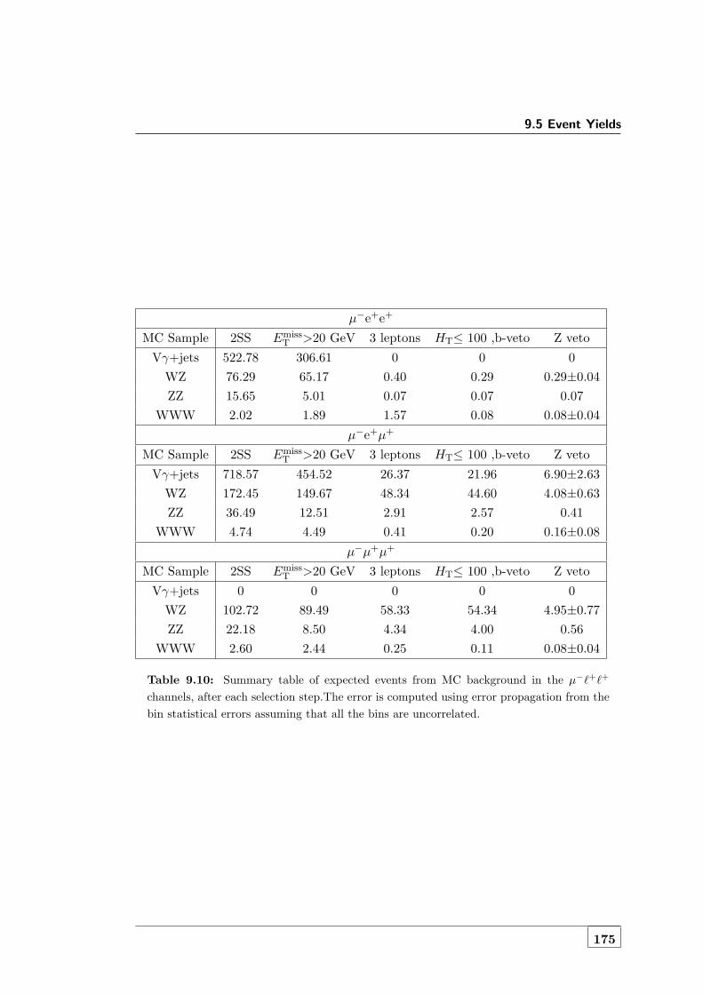
9.5 Event Yields
µ−e+e+
MC Sample 2SS EmissT >20 GeV 3 leptons HT≤ 100 ,b-veto Z veto
Vγ+jets 522.78 306.61 0 0 0WZ 76.29 65.17 0.40 0.29 0.29±0.04ZZ 15.65 5.01 0.07 0.07 0.07
WWW 2.02 1.89 1.57 0.08 0.08±0.04
µ−e+µ+
MC Sample 2SS EmissT >20 GeV 3 leptons HT≤ 100 ,b-veto Z veto
Vγ+jets 718.57 454.52 26.37 21.96 6.90±2.63WZ 172.45 149.67 48.34 44.60 4.08±0.63ZZ 36.49 12.51 2.91 2.57 0.41
WWW 4.74 4.49 0.41 0.20 0.16±0.08
µ−µ+µ+
MC Sample 2SS EmissT >20 GeV 3 leptons HT≤ 100 ,b-veto Z veto
Vγ+jets 0 0 0 0 0WZ 102.72 89.49 58.33 54.34 4.95±0.77ZZ 22.18 8.50 4.34 4.00 0.56
WWW 2.60 2.44 0.25 0.11 0.08±0.04
Table 9.10: Summary table of expected events from MC background in the µ−`+`+
channels, after each selection step.The error is computed using error propagation from thebin statistical errors assuming that all the bins are uncorrelated.
175

9. SIGNAL-BACKGROUND DISCRIMINATION
e−µ+µ+
MC Sample 2SS EmissT >20 GeV 3 leptons HT≤ 100 ,b-veto Z veto
Vγ+jets 0 0 0 0 0WZ 100.83 87.85 0.39 0.32 0.32±0.05ZZ 21.77 8.34 0.03 0.03 0.03
WWW 2.55 2.39 0.18 0.06 0.06±0.03
e−e+µ+
MC Sample 2SS EmissT >20 GeV 3 leptons HT≤ 100 ,b-veto Z veto
Vγ+jets 718.57 454.52 0 0 0WZ 172.45 149.67 46.51 43.21 5.00±0.78ZZ 36.49 12.51 3.03 2.74 0.42
WWW 4.74 4.49 0.43 0.20 0.18±0.09
e−e+e+
MC Sample 2SS EmissT >20 GeV 3 leptons HT≤ 100 ,b-veto Z veto
Vγ+jets 532.58 312.36 17.85 15.78 3.45±1.86WZ 76.21 65.11 38.68 35.70 2.81±0.44ZZ 15.95 5.11 2.12 1.84 0.16
WWW 2.06 1.92 0.17 0.07 0.05±0.03
Table 9.11: Summary table of expected events from MC background in the e−`+`+
channels, after each selection step. The error is computed using error propagation fromthe bin statistical errors assuming that all the bins are uncorrelated.
176

10Systematic Uncertainties
10.1 Uncertainties Description
Systematic uncertainties affect expected events passing all selections calculated from
simulation. Systematic uncertainties can be due to imperfect knowledge of either de-
tector effects (energy scales and resolution, pile-up,etc.) or uncertainties on process
production at generator level. Moreover, uncertainties arise from the absolute normal-
ization of the total number of expected events.
Systematic uncertainties can be grouped into three categories. In the first group,
we combine the theoretical uncertainties in the parton distribution functions (PDFs)
and from NLO effects, together with uncertainties that affect the product energy scales
and resolution of final-state objects, as determined from simulation.
The second group includes the systematic uncertainties affecting the data versus
simulation correction factors for the efficiencies of the trigger, reconstruction, and iden-
tification requirements. In particular for our analysis these include lepton trigger,
reconstruction and identification efficiencies1.
The third category comprises uncertainties on the background yield, either simu-
lated and data-driven, and uncertainty on the total integrated luminosity.
We will describe all those sources of uncertainty in the following sections.
1The lepton efficiencies could be determined by the tag-and-probe method (111) in the same way for
data and simulation, and the uncertainty on the ratio of efficiencies is taken as a systematic uncertainty.
177
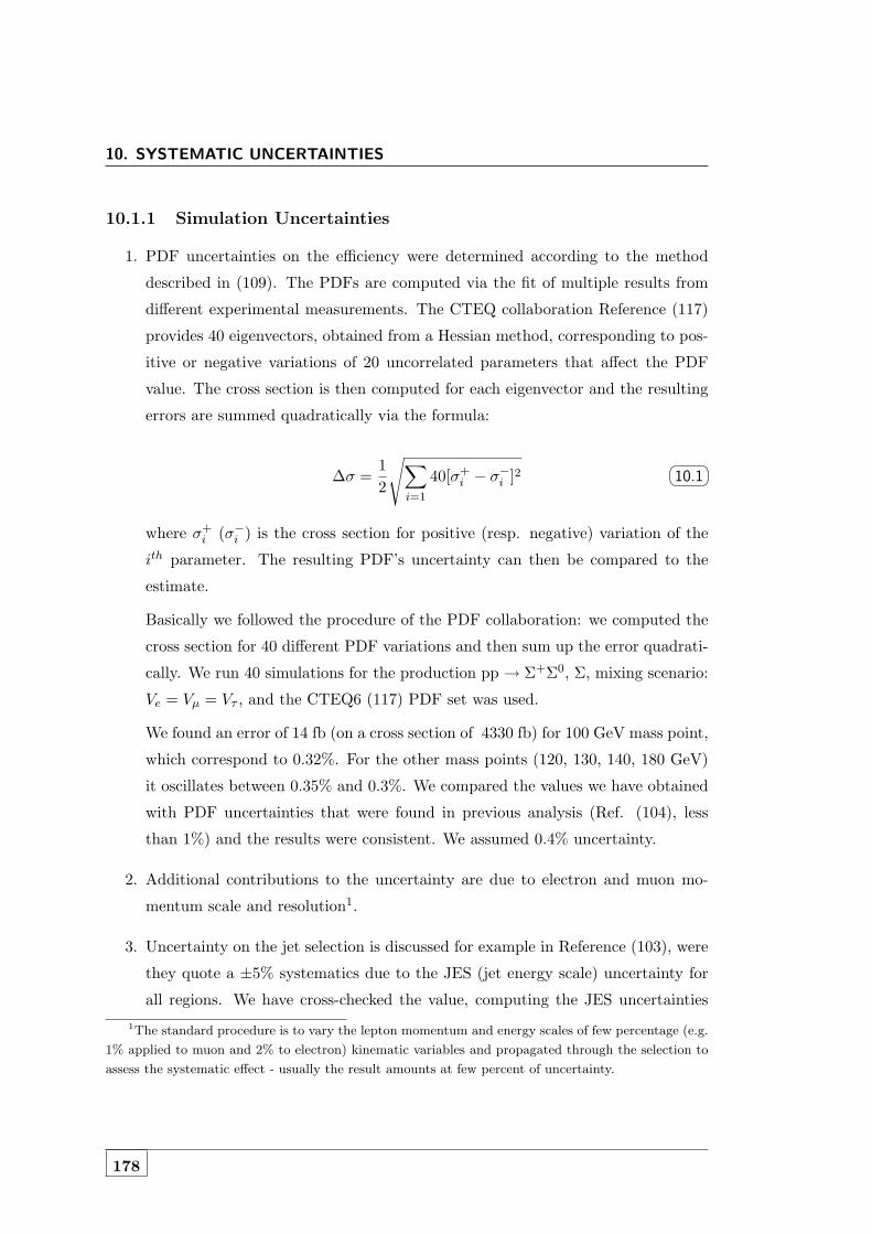
10. SYSTEMATIC UNCERTAINTIES
10.1.1 Simulation Uncertainties
1. PDF uncertainties on the efficiency were determined according to the method
described in (109). The PDFs are computed via the fit of multiple results from
different experimental measurements. The CTEQ collaboration Reference (117)
provides 40 eigenvectors, obtained from a Hessian method, corresponding to pos-
itive or negative variations of 20 uncorrelated parameters that affect the PDF
value. The cross section is then computed for each eigenvector and the resulting
errors are summed quadratically via the formula:
∆σ =12
√∑i=1
40[σ+i − σ−i ]2
�� ��10.1
where σ+i (σ−i ) is the cross section for positive (resp. negative) variation of the
ith parameter. The resulting PDF’s uncertainty can then be compared to the
estimate.
Basically we followed the procedure of the PDF collaboration: we computed the
cross section for 40 different PDF variations and then sum up the error quadrati-
cally. We run 40 simulations for the production pp → Σ+Σ0, Σ, mixing scenario:
Ve = Vµ = Vτ , and the CTEQ6 (117) PDF set was used.
We found an error of 14 fb (on a cross section of 4330 fb) for 100 GeV mass point,
which correspond to 0.32%. For the other mass points (120, 130, 140, 180 GeV)
it oscillates between 0.35% and 0.3%. We compared the values we have obtained
with PDF uncertainties that were found in previous analysis (Ref. (104), less
than 1%) and the results were consistent. We assumed 0.4% uncertainty.
2. Additional contributions to the uncertainty are due to electron and muon mo-
mentum scale and resolution1.
3. Uncertainty on the jet selection is discussed for example in Reference (103), were
they quote a ±5% systematics due to the JES (jet energy scale) uncertainty for
all regions. We have cross-checked the value, computing the JES uncertainties1The standard procedure is to vary the lepton momentum and energy scales of few percentage (e.g.
1% applied to muon and 2% to electron) kinematic variables and propagated through the selection to
assess the systematic effect - usually the result amounts at few percent of uncertainty.
178

10.1 Uncertainties Description
by varying the JES according to the recommended recipes in the Monte-Carlo
samples we have considered. The JES uncertainties are summarized in Table 10.1
for the backgrounds. We have taken the overall value of 5%. They are considered
negligible for the signal, since jet energy is not relevant for the final state.
4. From Reference (106) EmissT resolution and scale systematics have been evaluated.
We will assume an Uncertainty of 0.6% for the overall EmissT uncertainties. The
effect of this uncertainty on the event yield could be considered negligible.
5. Uncertainty due to pile-up is discussed for example in Reference (103), were sys-
tematics on the efficiency due to pile-up has been considered negligible. We have
cross checked this analysis results, estimating the systematic effect of pileup uncer-
tainty (the recommended ±8% minimum bias uncertainty as in Reference (107)),
on the final selection yield. Estimated pile-up effect are reported in Table 10.1.
We will consider these effects negligible on final yields.
10.1.2 Simulation versus Data Efficiency Differences
The uncertainty on event selection efficiency differences in simulation compared to data
includes the following:
1. The uncertainties on trigger efficiencies are low since each event category has a
trigger efficiency which is almost saturated to values near 100%. A conservative
overall value of 1% for muons ans electrons has been assumed.
2. The systematics uncertainty due to charge mis-ID has been evaluated in (106),
and checked for our same-sign di-lepton preselected sample in Chapter 8, both
for electrons and for muons. We found very small effect, so it can be negligible.
3. Uncertainty on the lepton selection efficiency (which depends on the lepton flavor
and pT ). We will take the take this systematics values from Reference (100),
where the integral value of the corrections is reported1. We list the uncertainties
in Table 10.2. Further details about lepton identification and isolation criteria
are discussed in Section 8.5.0.2 and 8.5.0.3 of Chapter 8.
1In this analysis, the single lepton efficiency evaluated with simulation has been cross checked with
data by means of tag and probe methods on Z0 → e+e− and Z0→ µ+µ− events.
179

10. SYSTEMATIC UNCERTAINTIES
Sample Pileup Normalization
WZ 1.9% 17%ZZ 1.2% 7.5%V γ 1.5% 13%WWW 0.5% 50%
Table 10.1: Systematic uncertainties for backgrounds that are taken from Monte-Carlo.
4. The uncertainties on the remaining selections (primary vertex, event cleaning,
etc.) are negligible compared to the ones mentioned above as the corresponding
efficiencies are essentially 100%.
10.1.3 Background
1. Uncertainties on the background estimates contribute to the overall systematic
uncertainty. As discussed in Chapter 9 the main physical backgrounds relevant
for our analysis are the di-bosons backgrounds and Vγ. We will pinpoint here
their uncertainties.
Usually the uncertainties on the background estimates are dominated by the
uncertainties on the NLO k-factor corrections for the simulated background com-
ponents, in the case the cross section is the one computed by the Monte Carlo
Ref. (112). In our analysis, we will use the measured cross section for the domi-
nant irreducible background (WZ), so no uncertainties on NLO k-factors need to
be quoted.
Uncertainties on the ZZ and Vγ have been computed, and the values have been
reported in previous studies: 7.5% for ZZ in Reference (113), 13% for (114).
Same values are reported in Reference (107). For the rare backgrounds, we assume
a normalization uncertainty of 50%. Table 10.1 contains the overall normalization
uncertainty for each background sample considered in the analysis. It should be
remarked that the effect of these uncertainties on the final event yield is very
small, in particular for background like WW and Vγ that are non influential
respect to WZ background. The backgrounds and the systematics on final event
yields are reported in Table 9.5 of Chapter 9.
180
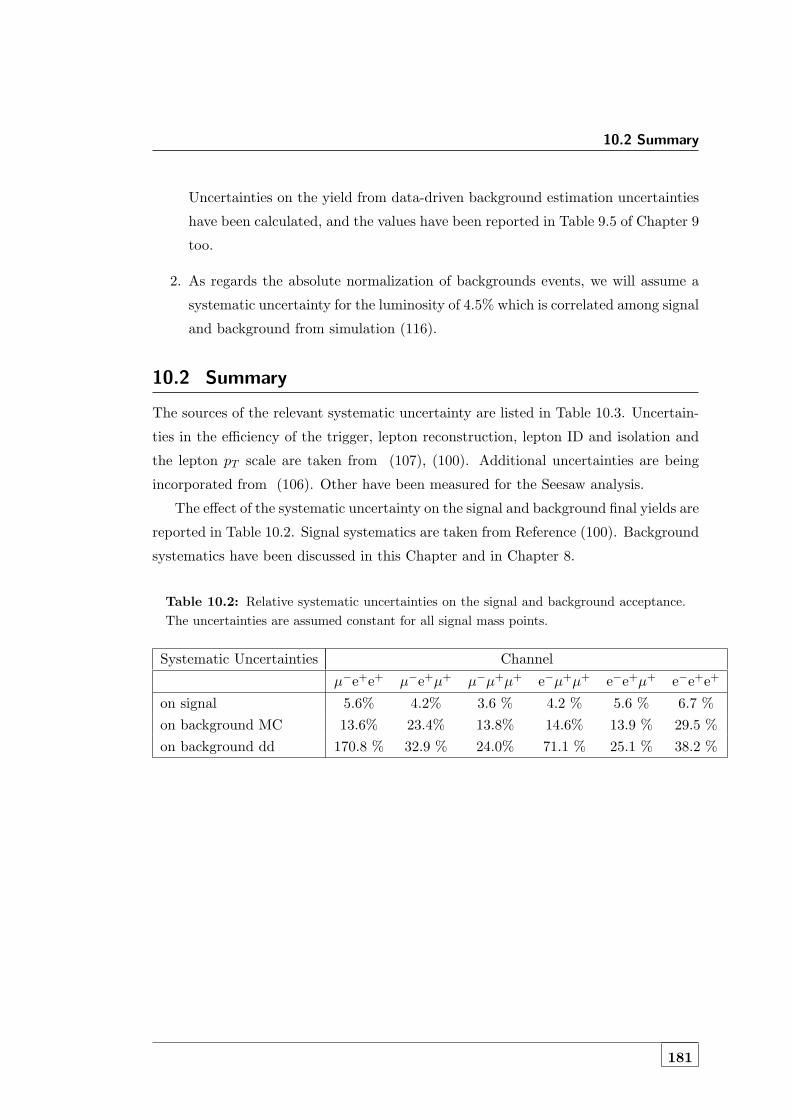
10.2 Summary
Uncertainties on the yield from data-driven background estimation uncertainties
have been calculated, and the values have been reported in Table 9.5 of Chapter 9
too.
2. As regards the absolute normalization of backgrounds events, we will assume a
systematic uncertainty for the luminosity of 4.5% which is correlated among signal
and background from simulation (116).
10.2 Summary
The sources of the relevant systematic uncertainty are listed in Table 10.3. Uncertain-
ties in the efficiency of the trigger, lepton reconstruction, lepton ID and isolation and
the lepton pT scale are taken from (107), (100). Additional uncertainties are being
incorporated from (106). Other have been measured for the Seesaw analysis.
The effect of the systematic uncertainty on the signal and background final yields are
reported in Table 10.2. Signal systematics are taken from Reference (100). Background
systematics have been discussed in this Chapter and in Chapter 8.
Table 10.2: Relative systematic uncertainties on the signal and background acceptance.The uncertainties are assumed constant for all signal mass points.
Systematic Uncertainties Channel
µ−e+e+ µ−e+µ+ µ−µ+µ+ e−µ+µ+ e−e+µ+ e−e+e+
on signal 5.6% 4.2% 3.6 % 4.2 % 5.6 % 6.7 %on background MC 13.6% 23.4% 13.8% 14.6% 13.9 % 29.5 %on background dd 170.8 % 32.9 % 24.0% 71.1 % 25.1 % 38.2 %
181

10. SYSTEMATIC UNCERTAINTIES
Table 10.3: Summary of the input systematic uncertainties for the Seesaw analysis.Reference (107) and (106). Only those background which contributed to the final yieldare listed.
Simulation Systematic uncertainty
Electron energy scale 2%Muon pT scale 1%Emiss
T Resolution and scale 0.6%JES 5%PileupPDFDrell-Yan EW corrections 7 %Drell-Yan QCD correction 5 %NLO effect 2.5%
Simulation versus Data Systematic uncertainty
Di-lepton trigger 1%Electron reconstruction 0.9%Electron ID and isolation 1.%Muon reconstruction 0.7%Muon ID and isolation 0.7%
Background Estimation Systematic uncertainty
ZZ 7.5%Zγ 13%Fakes 50%Dalitz 100%WZ cross section 17%Luminosity 4.5%
182
11Exclusion Limits
11.1 Event Yield Interpretation
As discussed in Chapter 9, all of the data events that pass the selections are sorted
into the six exclusive channels as described in Section 9.1, and results about event yield
are summarized in Table 9.5.
In each channel we can compare data with the number of expected Standard Model
background events, either from MonteCarlo and from data-driven prediction. Several
observation can be made here.
• The number of events observed in all the categories is consistent with the number
of predicted background events. Therefore: no hints of new physics from
Seesaw model is present in 2011 LHC data.
• There are no events observed in category e−µ+µ+ and only 1 event in category
µ−e+e+, consistent with the background expectation. Since no excess is found
in these categories an upper limit to the an upper limit to the Seesaw cross
section could be set. This is a remarkable result since no limit have been
computed on Seesaw type-III cross section by know.
• In channels µ−e+µ+ and e−e+e+ there is a small excess of events in the back-
ground prediction over data, but it is within statistical and systematic errors on
background prediction.
Given the event yields and the systematic uncertainties described in Chapter 10,
we calculated exclusion limits on the production cross section of the Seesaw fermionic
triplet σ(pp→ Σ+Σ0 → `−`+`+ + EmissT + jets).
183

11. EXCLUSION LIMITS
Exclusion limits between combined channels are calculated at the 95% C.L. by
employing the CL95 technique in the RooStats implementation (81), using Bayesian
statistics and a flat prior for the signal production cross section. A brief description of
the statistical method is contained in Section 11.2.
Conclusions are drawn in Section 11.3.
11.2 Statistical Procedure
This section describes the method we used for setting statistical limits with multiple
channels1.
For Seesaw analysis we used the CMS Higgs Combined Limit Analysis Toolkit to set
limits (References (118), (97), (105)). We will briefly describe it in the following. We
used the MarkovChainMC tool of the Higgs Combined Limit Analysis Toolkit, which
is a RooStats based package put out by the Higgs PAG in CMS collaboration. This
tool calculates the Bayesian limit using Monte Carlo integration (moreover, we used
CLs approach as well for a cross-check of results). For the observed limit, we run 100
chains, with a burn-in of 100 steps 2. For the expected limit and uncertainty band, we
run 50 toy Monte Carlos. Log-normal nuisance parameters were used for the systematic
uncertainties on both signal and background. We cross-checked the results using a CLs
approach tool, results of both methods are reported in the plots.
We will a brief review of the RooStats statistical algorithm. This framework is used
to compute likelihoods. The key inputs to the fitter for channel i are:
• The irreducible background events from Monte Carlo in channel i: bB−Irri =
σB−Irri × L for a L luminosity
• The number of expected background events in the i-th channel predicted by the
data-driven method, bDDi
3.
1It is important to note that channels that do not expect any signal do not have an effect on the
limit setting. The reason for this is that terms associated with signal free channels analytically factor
out of the likelihood when calculating a Bayesian upper limit. Effectively, the signal model in question
tells which channels are important, and weighs them according to which channels expect the most
signal.2Depending on the mass point, this value was decreased for convergence issues.3 The reason for splitting the background prediction into irreducible Monte Carlo and data driven
184
11.2 Statistical Procedure
• σS , which represents the specific signal process cross section, and depends on the
decay chain and on the combinatorial contribution to the final state.
• εSi combined efficiency for the signal
• εB−Irri combined efficiency for the background
The statistical model for the number of events in channel i is a Poisson distribu-
tion with expected value λi and truncated Gaussian constraints for all of the nuisance
parameters.
λi is the sum of the signal and the expected backgrounds given by:
λi = L× (σSi × εSi + σB−Irr
i × εBi ) + bDDi
�� ��11.1
where the first term corresponds to the expected signal, the second term corresponds
to the expected background from Monte-Carlo simulations, and the third term is the
expected background from the data-driven method.
Given the number of observed events Ni on the ith category a Poisson likelihood
function (i.e. the probability of observing the Ni events) can be written as:
L (Ni) =λNi
i
Ni!· e−λi ,
�� ��11.2
We then combine the Poissonian distributions Eq.11.1 for each channel into a like-
lihood function:
L(N1, N2...|NS) =∏
i
f(Ni, λi(NS))�� ��11.3
which is the joint conditional probability of observing N1, N2, N3, ... events in chan-
nel 1, channel 2, etc.
The posterior distribution for σS is given by the integral over the nuisance pa-
rameters, with proper prior functions. The fit is performed in order to maximize the
likelihood function. The nuisance parameters are allowed to vary during the fit accord-
ing to their log-normal distributions.
components is because in the background numbers predicted using the data-driven method the lumi-
nosity, lepton identification efficiencies, lepton isolation efficiencies, and lepton trigger efficiencies are
included. While, in the background numbers derived from simulation all the above parameters have to
be accounted for.
185

11. EXCLUSION LIMITS
We set our exclusion upper limit on cross section (σ) times branching fraction times
acceptance at 95% C.L.
To determine the number of signal events required to exclude the model at 95% con-
fidence, we use the Bayesian 95% upper limit using the Nsignal prior [0,∞]. Therefore,
we solve the following integral equation for N95:
0.95 =
∫ N95
− inf π(NS)L(NS)dNS∫ + inf− inf π(NS)L(NS)dNS
�� ��11.4
where π(NS) is a flat prior probability, equal to 1 for NS ≥ 0 and equal to 0 when
NS ≤ 0. (Reference (105)).
11.3 Results
As pointed out in the introduction of this Chapter, no significant excess of events
with respect to the SM expectations have been found in the channels analyzed in this
study, described in Chapter 9. The 95% confidence level limits on cross section for the
combination of all the six analyzed channels was computed.
The limits on cross section versus Seesaw fermion mass are shown in Figures 11.1,
11.2 The red horizontal line correspond to exactly the 95% CL. Therefore, we can
conclude that Seesaw mass are excluded below 180-185(at NLO) GeV for
equal mixing scenario. If the Seesaw triplet couples with one leptonic flavor
only, the limit on the mass is 200 GeV.
The limit on Seesaw cross section is shown in in Figures 11.3: were the theoretical
cross section is reported in blue line. The limit on cross section is 20 fb for the
equal mixings scenario.
186
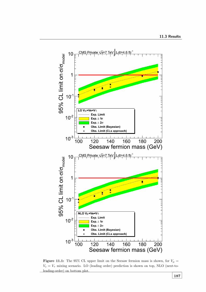
11.3 Results
Figure 11.1: The 95% CL upper limit on the Seesaw fermion mass is shown, for Vµ =Ve = Vτ mixing scenario. LO (leading order) prediction is shown on top, NLO (next-to-leading-order) on bottom plot.
187

11. EXCLUSION LIMITS
Figure 11.2: The 95% CL upper limit on the Seesaw fermion mass is shown, for Vµ 6=0,Ve = Vτ = 0 mixing scenario(top), and for Vµ = Vτ = 0, and Ve 6= 0 mixing scenario(bottom).
188

11.3 Results
Figure 11.3: The 95% CL upper limit on the Seesaw σ is shown, for Vµ = Ve = Vτ mixingscenario.
189


12Conclusions
12.1 2011 Data Analysis Conclusions
We have searched for evidence of Seesaw type III signal from pp collisions at 7 TeV using
the CMS detector data at LHC. In the Minimal Seesaw type III, the lightest fermion
triplet would be produced in pp collision and decay into Standard Model gauge bosons
and leptons, plus neutrinos which are stable and will escape the detector resulting in a
missing energy signature.
In this thesis we searched for three lepton production from Seesaw decays. This
channel have the largest production cross section among all states at LHC. The signa-
ture in the detector would be three standard leptons (electrons and muons), jets, and
missing energy. We neglected the analysis of signatures with tau lepton production.
The Standard Model background for the Seesaw signature is dominated by WZ
irreducible background (taken from MonteCarlo Summer11 official CMS production)
while other backgrounds dominated by fake lepton events have been computed with
data-driven techniques.
The Seesaw signal Monte Carlo samples were generated with madgraph5 and passed
through CMS detector simulation and objects reconstruction. Event pre-selection cri-
teria were chosen according to the Physical Analysis Group recommendation and ac-
cording to the kinematic distribution of decay products determined from Monte Carlo
studies. Event selection requirement were optimized in order to reject background with
a minimal loss of signal acceptance.
We searched for Seesaw signature in 4.6fb−1 of integrated luminosity data collected
during CMS 2011 RunA and RunB period. We found no evidence for Seesaw fermion
triplet pair production.
191

12. CONCLUSIONS
We set a lower limit at 95% confidence level on the Seesaw-type III fermion mass
of 180-200 GeV, depending on the Seesaw mixing with leptons scenarios.
12.2 Further Development with 2012 Data
The LHC will continue to operate at 3.5TeV per beam, half of its planned capability,
until the end of 2012 (draft schedule is in Figure 12.1). It will then be shut down for
a year for upgrades to allow full energy operation (7TeV per beam), with reopening
planned for 2014. The key 2012 expectations are:
• possibly move to higher beam energy: 3.5TeV → 4TeV (will be decided at the
beginning of 2012);
• possible peak performance with 50ns beams:
- 3.5 TeV: higher bunch intensity, smaller β∗ (0.8-0.9 m);
- peak luminosity increase: 20 to 30 %;
- 4 TeV: higher bunch intensity, smaller β∗ (0.7 0.8 m);
- peak luminosity increase: 60 to 75 %;
• luminosity of about 10fb−1 should be within in reach.
Therefore, more data will be collected in CMS run from April 2012 to the end
of the year, and a further development of this analysis can be done using the same
technique and increased statistics. Assuming the limit on ΣΣ pair production cross
section depends primarily on statistics, we can expect an improvement in the cross
section limit.
192

12.2 Further Development with 2012 Data
Figure 12.1: 2012 LHC schedule.
193

References
[1] http://cms.web.cern.ch/news/summary-2011-p-p-running.
5
[2] S. Willenbrock, Hadron Colliders, the Standard
Model, and Beyond, arXiv:hep-ph/0212032v1, 2002. 7
[3] S. Willenbrock, Proceedings of the Advanced Study
Institute on Techniques and Concepts of High
Energy Physics, St. Croix, U. S. Virgin Islands,
arXiv:hep-ph/0211067, 2006. 7, 12
[4] C. Amsler et al. [Particle Data Group], Review of par-
ticle physics, Phys. Lett. B 667 (2008) 1, 2008. 51
[5] S. Weinberg, Baryon And Lepton Nonconserving
Processes, Phys. Rev. Lett. 43 (1979) 1566, 1979. 17
[6] S. Weinberg, Baryon And Lepton Nonconserving
Processes, Phys. Rev. Lett. 43, 1566, 1979. 12
[7] S. Weinberg, Conceptual Foundations Of The Uni-
fied Theory Of Weak And Electromagnetic Inter-
actions, Rev. Mod. Phys. 52, 515,(1980), Science 210,
1212, (1980). 15
[8] F. Maltoni, J. M. Niczyporuk and S. Willenbrock, The
scale of fermion mass generation, Phys. Rev. D 65,
033004 (2002) [arXiv:hep-ph/0106281], 2002. 15
[9] H. Georgi and S. L. Glashow, Unity Of All Elementary
Particle Forces, Phys. Rev. Lett. 32, 438, (1974). 16
[10] K. Hagiwara et al. [Particle Data Group Collaboration],
Review Of Particle Physics, Phys. Rev. D 66, 010001,
(2002). 207
[11] A. F. Falk The CKM matrix and the heavy quark
expansion, in Flavor Physics for the Millennium, TASI 2000,
ed. J. Rosner (World Scientific,Singapore, 2001), p. 379
[arXiv:hep-ph/0007339], 2001.
[12] W. Buchmuller and D. Wyler, Effective Lagrangian
Analysis Of New Interactions And Flavor Conser-
vation, Nucl. Phys. B 268, 621 (1986), 1986.
[13] B. Kayser, On the Quantum Mechanics of Neutrino
Oscillation, Phys. Rev. D24, 110 (1981), 1981. 13
[14] I. d. M. Varzielas, Family symmetries and the ori-
gin of fermion masses and mixings, arXiv:0801.2775
[hep-ph], 2008. 13
[15] W.-M. e. a. Yao, Review of Particle Physics, Journal
of Physics G 33, 1+ (2011), 2001. 13, 30, 54, 71
[16] M. Maltoni, T. Schwetz, M. A. Tortola and J. W. F. Valle,
Status of global fits to neutrino oscillations, New J.
Phys. 6, 122 (2004), hep-ph/0405172, 2004. 10, 11
[17] A. Y. Smirnov, Neutrino masses and oscillations,
(0700), hep-ph/9611465, 2007. 11
[18] P. Minkowski, Phys. Lett. B 67 421, (1977); M. Gell-
Mann, P. Ramond and R. Slansky, Supergravity, edited by
P. van Nieuwenhuizen and D. Freedman, (North-Holland,
1979), p. 315, 1979; T. Yanagida, Proceedings of the
Workshop on the Unified Theory and the Baryon
Number in the Universe, edited by O. Sawada and A.
Sugamoto (KEK Report No. 79-18, Tsukuba, 1979), p. 95,
1979; R.N. Mohapatra and G. Senjanovic, Phys. Rev. Lett.
44 (1980) 912, 1980. 17
[19] M. Magg and C. Wetterich, Phys. Lett. B94 (1980) 61,
1980; J. Schechter and J. W. F. Valle, Phys. Rev. D 22
(1980) 2227, 1980; C. Wetterich, Nucl. Phys. B187 (1981)
343, 1981; G. Lazarides, Q. Shafi and C. Wetterich, Nucl
Phys. B181 (1981) 287, 1981; R.N. Mohapatra and G. Sen-
janovic, Phys.Rev. D23 (1981) 165, 1981. 17
[20] R. Foot, H. Lew, X.-G. He and G.C. Joshi, Z. Phys. C44
(1989) 441, 1989. 17
[21] J. Kersten and A. Y. Smirnov, Right-Handed Neu-
trinos at LHC and the Mechanism of Neutrino
Mass Generation, Phys. Rev. D 76 (2007) 073005
[arXiv:0705.3221 [hep-ph]], 2007.
[22] F. del Aguila, J. A. Aguilar-Saavedra and R. Pittau, Neu-
trino physics at large colliders, J. Phys. Conf. Ser. 53,
506 (2006) [arXiv:hep-ph/0606198], 2006 68
[23] F. del Aguila, J. A. Aguilar-Saavedra and R. Pittau,
Heavy neutrino signals at large hadron colliders,
JHEP 0710 (2007) 047 [hep-ph/0703261], 2007. 51, 68
[24] F. del Aguila and J. A. Aguilar-Saavedra, Distinguish-
ing seesaw models at LHC with multi-lepton sig-
nals, Nucl. Phys. B 813, 22 (2009)[arXiv:0808.2468 [hep-
ph]], 2009. ix, 17, 21, 51, 54, 55, 56, 60, 66, 68, 73, 74,
75, 81, 149
[25] F. del Aguila, J. de Blas and M. Perez-Victoria, Effects
of new leptons in Electroweak Precision Data, Phys.
Rev. D 78 (2008) 013010,[arXiv:0803.4008 [hep-ph]], 2008.
19, 23, 59, 68
[26] F. del Aguila, J. A. Aguilar-Saavedra, J. de Blas and
M. Perez-Victoria, Electroweak constraints on see-
saw messengers and their implications for LHC,
arXiv:0806.1023 [hep-ph], 2008. 21, 68
[27] A. Y. Smirnov, Recent developments in neutrino
phenomenology, (0200), hep-ph/0702061, 2002. 11
[28] A. Abada, C. Biggio, F. Bonnet, M. B. Gavela and T. Ham-
bye, µ → eγ and τ → lγ decays in the fermion
triplet seesaw model, Phys. Rev. D 78 (2008) 033007
[arXiv:0803.0481 [hep-ph]], 2008. 23, 24, 52, 59, 213
[29] R. Franceschini, T. Hambye and A. Strumia, Type-
III see-saw at LHC, Phys. Rev. D 78 (2008) 033002
[arXiv:0805.1613 [hep-ph]], 2008 51, 54, 57, 63, 81, 149
[30] C. Biggio and F. Bonnet, Implementation of the
type III seesaw model in FeynRules/MadGraph
and prospects for discovery with early LHC data,
arXiv:1107.3463 [hep-ph], 2011. 23, 24, 52, 73, 81, 149,
150
[31] Gregor Herten, The First Year of the Large Hadron
Collider: A Brief Review. arXiv:1104.4205v1, 2011. 35
195

REFERENCES
[32] D. Froidevaux and V. A. Mitsou, Experimental
prospects at the Large Hadron Collider, J. Phys.
Conf. Ser. 171, 012021 (2009) [arXiv:0905.0258 [hep-ex]],
2009. 33, 34
[33] Godbole, Rohini M., Story of a journey: Ruther-
ford to the Large Hadron Collider and onwards,
[arXiv:1007.0946[hep-ex]], 2010. 28, 29, 31, 32, 34
[34] K. Moenig, View point: First bounds on the Higgs
boson from hadron colliders, Physics 3, 14 (2010);
http://physics.aps.org/, 2010. 30
[35] T. J. Orimoto [CMS Collaboration], First CMS Results
with LHC Beam, arXiv:0905.4814 [hep-ex], 2009. 42
[36] G. L. Bayatian et al. [CMS Collaboration], CMS
Technical Design Report, CERN-LHCC-2006-001,
CERN-LHCC-2006-021, CMS-TDR-008-2, J. Phys.
G 34, 995 (2007), 2007. 42
[37] http://lhc.web.cern.ch/lhc/LHC-DesignReport.html
[38] https://twiki.cern.ch/twiki/bin/view/CMS/MadgraphGrid-
packPreparation 82
[39] https://twiki.cern.ch/twiki/bin/view/CMS/WorkBookGene-
ration. 80, 226
[40] https://twiki.cern.ch/twiki/bin/view/CMS/SWGuidePythi-
a6Interface. 85
[41] https://twiki.cern.ch/twiki/bin/view/CMS/MadGraphCMS-
Page.
[42] http://cp3wks05.fynu.ucl.ac.be/twiki/bin/view/Libra-
ry/MadGraphSamples 219
[43] https://twiki.cern.ch/twiki/bin/view/CMS/SWGuideEve-
ntGeneration.
[44] https://twiki.cern.ch/twiki/bin/view/CMS/SWGuideLHE-
Interface. 80
[45] https://twiki.cern.ch/twiki/bin/view/CMS/SWGuideMad-
GraphInterface. 85
[46] https://twiki.cern.ch/twiki/bin/view/CMS/SWGuidePyt-
hia6Interface. 80
[47] T. Sjostrand, S. Mrenna and P. Skands, PYTHIA
6.4 physics and manual, JHEP 0605 (2006) 026
[hep-ph/0603175], 2006. 73, 80, 85, 150, 231
[48] The CMS Collaboration, Search for Pair Produc-
tion of Second Generation Scalar Leptoquarks in
pp Collisions at ps = 7 TeV, CMS PAS EXO-10-007,
2007.
[49] G. Brooijmans et al., New Physics at the LHC: A Les
Houches Report. Physics at Tev Colliders 2007 –
New Physics Working Group, Part 8 ”A search for top
partners at the LHC using same-sign dilepton final states;
arXiv:0802.3715v1 [hep-ph], 2008.
[50] R. Contino and G. Servant, arXiv:0801.1679 [hep-
ph],2008.
[51] http://ceballos.web.cern.ch/ceballos/hwwlnln/samples cms-
sw35x.txt
[52] The CMS Collaboration, Search for a Heavy Bottom-
like quark in pp Collisions at ps = 7 TeV, CMS PAS
EXO-10-018, 2010. 124
[53] The CMS Collaboration, Measurements of Inclu-
siveW and Z Cross Sections in pp Collisions at ps
= 7 TeV, CMS PAS EWK-10-002, 2010.
[54] The CMS Collaboration, Performance of CMS muon
identification in pp collisions at ps = 7 TeV,
CMS PAS MUO-2010-002 (2010), 2010. Performance of
muon reconstruction, identification, and trigger in
2010 data, CMS PAS MUO-2010-004 (2010), 2010. 93
[55] The CMS Collaboration, Performance of tau recon-
struction algorithms in 2010 data collected with
CMS, CMS PAS TAU-11-001 (2011), 2011.
[56] https://twiki.cern.ch/twiki/bin/view/CMSPublic/SWGui-
dePFTauID.
[57] Murayama et al., HELAS libraries, KEK-91-11, 1992.
[58] J. Alwall et al., JHEP 0709 (2007) 028,
[arXiv:0706.2334 [hep-ph]], 2007; J. Alwall, M. Her-
quet, F. Maltoni, O. Mattelaer, T. Stelzer,
JHEP 1106 (2011) 128, [arXiv:1106.0522
[hep-ph]], 2011. http://madgraph.hep.uiuc.edu/,
http://madgraph.roma2.infn.it/,
http://madgraph.phys.ucl.ac.be/. 80, 83, 150, 231
[59] http://lepp.cornell.edu/public/theory/BRIDGE/index.html.
[60] Torbjorn Sjostrand, A model for initial state parton
showers, Physics Letters B, 157(4):321325, 1985. 79
[61] https://twiki.cern.ch/twiki/bin/view/Main/PowhegBOX.
231
[62] http://geant4.cern.ch/. 87
[63] http://feynrules.irmp.ucl.ac.be/. 80
[64] https://cms-cpt-software.web.cern.ch/cmscpt-
software/General/ 80
[65] http://feynrules.irmp.ucl.ac.be/wiki/TypeIIISeeSaw 81
[66] N. D. Christensen and C. Duhr, FeynRules - Feynman
rules made easy, Comput. Phys. Commun. 180 (2009)
1614 [arXiv:0806.4194 [hep-ph]], 2009.
[67] R. N. Mohapatra, Phys. Rev. Lett. 56 (1986) 561-563,
1986; R. N. Mohapatra, J. W. F. Valle, Phys. Rev. D34
(1986) 1642, 1986.
[68] B. Bajc, G. Senjanovic, JHEP 0708 (2007) 014, [hep-
ph/0612029], 2007; B. Bajc, M. Nemevsek, G. Senjanovic,
Phys. Rev. D76 (2007) 055011, [hep-ph/0703080], 2007;
A. Arhrib, B. Bajc, D. K. Ghosh, T. Han, G. -Y. Huang,
I. Puljak, G. Senjanovic, Phys. Rev. D82 (2010) 053004,
[arXiv:0904.2390 [hep-ph]], 2010. 51, 81
196

REFERENCES
[69] P. Meade and M. Reece, BRIDGE: Branching ra-
tio inquiry / decay generated events, arXiv:hep-
ph/0703031, 2007.
[70] A. Abada, C. Biggio, F. Bonnet, M. B. Gavela and T. Ham-
bye, Low energy effects of neutrino masses, JHEP
0712 (2007) 061 [arXiv:0707.4058 [hep-ph]], 2007. 17, 51,
59
[71] J. Conway et al., PGS4: Pretty Good
Simulation of high energy collisions,
http://www.physics.ucdavis.edu/ conway/research/software/-
pgs/pgs4-general.htm, 2006. 73
[72] L. Basso, A. Belyaev, S. Moretti and C. H. Shepherd-
Themistocleous, Phenomenology of the minimal B-L
extension of the Standard model: Z’ and neutrinos,
Phys. Rev. D 80 (2009) 055030 [arXiv:0812.4313 [hep-ph]],
2009; L. Basso, Phenomenology of the minimal B-
L extension of the Standard Model at the LHC,
arXiv:1106.4462 [hep-ph], 2011. 73
[73] S. Chatrchyan et al. [ CMS Collaboration ], Search for a
Heavy Bottom-like Quark in pp Collisions at√
s = 7
TeV, [arXiv:1102.4746 [hep-ex]], 2011. 231
[74] N. D. Christensen, P. de Aquino, C. Degrande, C. Duhr,
B. Fuks, M. Herquet, F. Maltoni, S. Schumann, A Com-
prehensive approach to new physics simulations,
Eur. Phys. J. C71 (2011) 1541 [arXiv:0906.2474 [hep-
ph]], 2011.
[75] S. Chatrchyan et al. [ CMS Collaboration ], Measure-
ment of the Top-antitop Production Cross Section
in pp Collisions at sqrt(s)=7 TeV using the Kine-
matic Properties of Events with Leptons and Jets,
[arXiv:1106.0902 [hep-ex]], 2011. 137
[76] G. Aad et al. [ ATLAS Collaboration ], Measurement
of the top quark pair production cross section in
pp collisions at sqrt(s) = 7 TeV in dilepton final
states with ATLAS, [arXiv:1108.3699 [hep-ex]], 2011.
137
[77] S. Chatrchyan et al. [ CMS Collaboration ], Measure-
ment of W+W- Production and Search for the
Higgs Boson in pp Collisions at sqrt(s) = 7 TeV,
Phys. Lett. B699 (2011) 25-47 [arXiv:1102.5429 [hep-ex]],
2011. 136
[78] G. Aad et al. [ ATLAS Collaboration ], Measurement
of the WW cross section in sqrt(s) = 7 TeV pp col-
lisions with ATLAS, [arXiv:1104.5225 [hep-ex]], 2011.
136
[79] [ CMS Collaboration ], Measurement of the WW,
WZ and ZZ cross sections at CMS, CMS-EWK-11-
010-PAS, 2011. 122, 136
[80] https://twiki.cern.ch/twiki/bin/view/CMSPublic/SWGuide-
FastSimPileUp#Arbitrary distribution,
https://indico.cern.ch/getFile.py/access?contribId=1&ses-
sionId=5&resId=0&materialId=slides&confId=126180,
https://twiki.cern.ch/twiki/bin/view/CMSPublic/SWGuide-
FastSimulation?redirectedfrom=CMS.SWGuideFast-
Simulation#Recipe for CMSSW 3 8 X cmsDriver,
https://twiki.cern.ch/twiki/bin/view/CMSPublic/SWGuide-
FastSimTags,
https://twiki.cern.ch/twiki/bin/view/CMS/FastSimTag42X.
229
[81] http://root.cern.ch/drupal/. 84, 184
[82] [ CMS Collaboration ], EXO-10-015,2011.
[83] [ CMS Collaboration ], CMS AN -2010/034,2010. 92
[84] R Fruhwirth, Wolfgang Waltenberger, and Pascal Van-
laer, Adaptive Vertex Fitting, Technical Re-
port CMS-NOTE-2007-008. CERN-CMS-NOTE-2007-008,
CERN, Geneva, Mar 2007. 91
[85] [ CMS Collaboration ], CMS PAS PFT-10-003, 2010. 92,
156
[86] [ CMS Collaboration ], Commissioning of the
Particle-flow Event Reconstruction with the first
LHC collisions recorded in the CMS detector, CMS
PAS PFT-10-001, 2010. 95, 156
[87] [ CMS Collaboration ], Particle–Flow Event Recon-
struction in CMS and Performance for Jets, Taus,
and EmissT , CMS PAS PFT-09-001, 2010. 95, 156
[88] [ CMS Collaboration ], CMS PAS PFT-08-001, 2008. 93
[89] [ CMS Collaboration ], CMS PAS TAU-11-001, 2011. 93,
94
[90] [ CMS Collaboration ], CERN-LHCC-2004-035/G-083,
CMS NOTE / 2004-031, December 2004. CMS Com-
puting TDR, CERN-LHCC-2005-023, CMS TDR 7, 20
June 2005. 97, 98
[91] https://twiki.cern.ch/twiki/bin/viewauth/CMS/RecoSki-
mming;
http://cmssw.cvs.cern.ch/cgi-
bin/cmssw.cgi/CMSSW/Configuration/Skimming/python/-
PDWG HWWSkim cff.py. 106
[92] https://indico.cern.ch/conferenceDisplay.py?confId=156711,
https://espace.cern.ch/cms-quarkonia/tnp/default.aspx.
101, 102, 103
[93] https://twiki.cern.ch/twiki/bin/view/CMS/TriggerTables
99
[94] https://cmswbm.web.cern.ch/cmswbm/cmsdb/servlet/-
L1Summary,
https://cmswbm.web.cern.ch/cmswbm/cmsdb/servlet/-
TriggerMode,
https://cmswbm.web.cern.ch/cmswbm/cmsdb/servlet/-
HLTSummary,
https://cmswbm.web.cern.ch/cmswbm/cmsdb/servlet/-
RunSummary.
99
[95] https://twiki.cern.ch/twiki/bin/viewauth/CMS/Standard-
ModelCrossSections. 231
[96] CMS Collaboration, Multileptonic SUSY searches
with Jets and EmissT pp Collisions at 7 TeV, CMS
PAS SUS-11-013, 2011. 124, 127, 128, 135, 137, 158, 159
197

REFERENCES
[97] S. Arora, K. Chan, J.P. Chou, E. Contreras-Campana,
R.C. Gray, A. Lath, K. Mei, S. Panwalkar, S. Somalwar,
S. Thomas, M. Walker, E. Williams, Background and
efficiency determination methods for multilepton
analyses, CMS AN -2011/281, 2011. x, 103, 104, 127,
128, 129, 130, 145, 146, 147, 184
[98] L3 Collaboration, Search for heavy neutral and
charged leptons in e+e- annihilation at LEP, Phys.
Lett., B517 pag.75,doi=10.1016/j.physletb.2003.10.071 ,
2001. 151
[99] CMS Collaboration, Determination of Jet Energy
Calibration and Transverse Momentum Resolution
in CMS, Submitted to JINST, arXiv 1107.4277 , 2011. 95
[100] CMS Collaboration, Measurement of the WW,
WZ and ZZ cross sections at CMS, CMS
Physics Analysis Summary, CMS-PAS-EWK-11-010,
http://cdsweb.cern.ch/record/1279362, 2011. 179, 181
[101] CMS Collaboration, Measurement of the Inclusive
W and Z Production Cross Sections in pp Colli-
sions at√
s = 7 TeV, arXiv 1107.4789 hep-ex, 2011 .
[102] D. Barge, C. Campagnari, P. Kalavase, D. Kovalskyi, V.
Krutelyov, J. Ribnik W. Andrews, D. Evans, F. Golf, J.
Mulmenstadt, S. Padhi, Y. Tu, F. Wurthwein, A. Yagil, J.
Yoo, L. Bauerdick, I. Bloch, K. Burkett, I. Fisk, Y. Gao,
O. Gutsche, B. Hooberman, Fake Rates for dilepton
Analyses, CMS AN -2010/257, 2010. 139, 143
[103] D. Barge, C. Campagnari, P. Kalavase, D. Kovalskyi, V.
Krutelyov, J. Ribnik W. Andrews, D. Evans, F. Golf, J.
Mulmenstadt, S. Padhi, Y. Tu, F. Wurthwein, A. Yagil, J.
Yoo, L. Bauerdick, I. Bloch, K. Burkett, I. Fisk, Y. Gao,
O. Gutsche, B. Hooberman Inclusive search for New
Physics with Same-Sign Dileptons using early LHC
data, CMS AN -2010/247, 2010. 132, 139, 143, 178, 179
[104] D. Barge et al., AN-CMS2010/258
http://arxiv.org/abs/1010.5994, 2010. 178
[105] J. Conway, http://www-
cdf.fnal.gov/physics/statistics/code/bayes.f , 2010. 184,
186
[106] Aytul Adiguzel, Vuko Brigljevic, Tulika Bose, Claude
Charlot, Cory Fantasia, Nicola De Filippis, Senka Duric,
Jeff Klukas, Jelena Luetic, Yurii Maravin, Arabella
Martelli, Srecko Morovic, and Salvatore A. Tupputi,
Measurement of the WZ cross section at the CMS
Experiment, AN-11-259, 2011. 179, 181, 182, 233
[107] Aytul Adiguzel, Vuko Brigljevic, Tulika Bose, Cory
Fantasia, Matthew Herndon, Jeff Klukas, Christos
Leonidopoulos, Yurii Maravin, and Srecko Morovic,
Search for exotic WZ resonances at CMS, CMS AN
AN-11-333, 2011. 179, 180, 181, 182
[108] CMS Collaboration, Pileup Reweighting Utili-
ties, ”CMS TWiki (PileupMCReweightingUtilities)”, url =
https://twiki.cern.ch/twiki/bin/view/CMS/PileupMCRe-
weightingUtilities, 2011. 144
[109] Campbell, John M. and Huston, J.W. and Stir-
ling, W.J., Hard Interactions of Quarks and Glu-
ons: A Primer for LHC Physics, Rept.Prog.Phys,
vol 70, doi: 10.1088/0034-4885/70/1/R02, arXiv:hep-
ph/0611148, 2006. 178
[110] https://twiki.cern.ch/twiki/bin/viewauth/CMS/TopLike-
BSMSpring2011, 2011. 158
[111] Measuring Electron Efficiencies at CMS with
Early Data, CMS Physics Analysis Summary, EGM-07
-001 ,2007 . 177
[112] Campbell, John M. and Ellis, R. K., MCFM for the
Tevatron and the LHC, Nucl. Phys. Proc. Suppl.,205-
206,10-15, arXiv:1007.3492, 2010. 180
[113] John Campbell, Keith Ellis, Ciaran Williams, Vector
boson pair production at the LHC, JHEP, 07, 018,
arXiv: hep-ph/1105.0020v1, 2011. 180
[114] Chatrchyan, Serguei and others, Measurement of W-
gamma and Z-gamma production in pp collisions at
sqrt(s) = 7 TeV, Physics Letters B, vol.701, n.5, pag.535
- 555, doi:10.1016/j.physletb.2011.06.034, 2011. 180
[115] CMS Collaboration, Measurement of the WW,
WZ, and ZZ cross sections at CMS, CMS Physics
Analysis Summary, EWK-11-010, 2011.
[116] CMS Collaboration, Luminosity Estimation for
2010 Data - Update, CMS Physics Analysis Summary,
CMS-PAS-EWK-11-001, 2011. 181
[117] J. Pumplin, D. R. Stump, J. Huston, H. L. Lai, P. M. Nadol-
sky and W. K. Tung, New generation of parton distri-
butions with uncertainties from global QCD analy-
sis, JHEP 0207 (2002) 012 [arXiv:hep-ph/0201195], 2002.
178
[118] CMS Higgs Combined Limit Analysis Toolkit,
https://twiki.cern.ch/twiki/bin/view/CMS/SWGuideHiggs-
AnalysisCombinedLimit, . 184
[119] http://feynrules.phys.ucl.ac.be/wiki/TypeIIISeeSaw,
2011.
81
198

Declaration
I herewith declare that I have produced this paper without the prohibited
assistance of third parties and without making use of aids other than those
specified; notions taken over directly or indirectly from other sources have
been identified as such. This paper has not previously been presented in
identical or similar form to any other Italian or foreign examination board.
The thesis work was conducted from 2009 to 2011 under the supervision of
Paolo Checchia and Gianni Zumerle.
Padua, January 31th 2012


AStandard Model Review
A.1 Particle Content
Figure A.1: Particle content of the Standard Model - Particle content of theStandard Model, with associated mass, charge and spin.
The Standard Model particle content arises by construction from:
• observed evidences from which the fields are postulated;
• the particular choice of the underlying gauge theory: the gauge symmetries.
Once the fields and the gauge symmetries (SU(3)C×SU(2)L×U(1)Y ) are specified
the rest follows automatically, and the Standard Model is the most general theory that
can be constructed.
201

A. STANDARD MODEL REVIEW
Table A.1: The fields of the standard model and their gauge quantum numbers: the indexi = 1, 2, 3 on each field refers to the generation, and the subscript L,R refers to the chiralityof the field (ψL,R ≡ 1
2 (1 ∓ γ5)ψ). The left-chiral and right-chiral fields corresponding toa given particle have different SU(2) × U(1) quantum numbers, which leads to parityviolation in the weak interaction.
fields SU(3) SU(2) U(1)Y
QiL =
(uL
dL
) (cL
sL
) (tL
bL
)3 2 1
6
uiR = uR cR tR 3 1 2
3
diR = dR sR bR 3 1 −1
3
LiL =
(νeL
eL
) (νµL
µL
) (ντL
τL
)1 2 −1
2
eiR = eR µR τR 1 1 −1
φ =
(φ+
φ0
)1 2 1
2
Particle content is shown in graphically in Figure A.1, and is described in detail
in Table A.1 where particles are listed along with their SU(3)C × SU(2)L × U(1)Y
quantum numbers. There are three generations of quarks and leptons and one Higgs
field, φ.
A.2 Symmetry
The symmetry that describes all Standard Model interactions is: SU(3)C × SU(2)L ×U(1)Y .
• SU(3)C is a non-Abelian symmetry that describes the strong interactions between
particles that carry a property called color (”C” in the subscript). The symmetry
generator is a color triplet. The carriers of the strong interaction are the massless
fields called gluons. There are eight different color combinations of gluons gen-
erated by the SU(3)C symmetry. The only other particles that carry color are
quarks.
• SU(2)L is another non-Abelian symmetry that describes the weak interaction,
202

A.3 The Lagrangian
which acts on particles having weak isospin, t, which is a quantum number asso-
ciated with an SU(2) doublet. The subscript ”L” indicates that this symmetry
only acts on the left-handed doublets, or the doublets whose eigenvalue is −1
when acted by chirality operator γ5.
• U(1)Y is an Abelian symmetry, which is similar to the U(1) symmetry of electro-
magnetism, but instead of electric charge it is acting on particles carrying a
quantum number called hyper-charge, Y.
A.3 The Lagrangian
To describe the particles and their interactions, the Standard Model uses the Lagrangian
density which is a classical mechanics invention. By using local gauge symmetries, one
can construct a theory of interactions between particles and describe the properties of
these interactions. With the Lagrangian density the equations of motion are derived,
and the Lagrangian density and the resulting equation of motion are required to be
invariant under the transformations of the symmetry.
The complete Lagrangian of the standard model is the sum of the gauge, matter,
Higgs, and Yukawa interactions, and so it could be written in the following pieces:
LSM = LGauge + LMatter + LY ukawa + LHiggs .�� ��A.1
This is the simplest and most general Lagrangian, given the field content and gauge
symmetries of the standard model. Given this Lagrangian, one can proceed to calculate
any physical process of interest.
The pure gauge Lagrangian is the first piece, given by
LGauge =1
2g2S
Tr GµνGµν +1
2g2Tr WµνWµν −
14BµνBµν ,
�� ��A.2
where Gµν , Wµν , and Bµν are the gluon, weak, and hypercharge field-strength tensors.
These terms contain the kinetic energy of the gauge fields and their self interactions.
203

A. STANDARD MODEL REVIEW
The matter Lagrangian is the next piece, and is given by
LMatter = iQiL 6DQi
L + iuiR 6Dui
R + idiR 6Ddi
R + iLiL 6DLi
L + ieiR 6DeiR .�� ��A.3
This piece contains the kinetic energy of the fermions and their interactions with the
gauge fields, which are contained in the covariant derivatives (D). These two pieces
of the Lagrangian depend only on the gauge couplings gS , g, g′. Mass terms for the
gauge bosons and the fermions are forbidden by the gauge symmetries, i.e., similar to
electro-magnetic case, the mass terms are not invariant under the transformations of
these symmetries.
In the case of the fermions, for example, masses are forbidden by the fact that the
left-chiral and right-chiral components of a given fermion field have different SU(2)×U(1)Y quantum numbers. 1
Because all fermions are massless there is no difference between the three generations
- they are physically indistinguishable. This manifests itself as a global flavor symmetry
of the matter Lagrangian, Eq. (A.3).
The next pieces of the Lagrangian: LHiggs and LY ukawa, are introduced for arrang-
ing in the simplest and most general way consistent with the gauge symmetry the Higgs
field, responsible for generating the masses of the gauge bosons and fermions, as briefly
described in the following sections.
A.4 Electroweak Symmetry Breaking
Electroweak symmetry breaking is the mechanism that has been introduced in the Stan-
dard Model for generating the masses of the gauge bosons and fermions. Electroweak
symmetry breaking is achieved by introducing another field into the model, the Higgs
field φ, with the quantum numbers shown in Table A.1. The simplest and most general
Lagrangian for the Higgs field, consistent with the gauge symmetry, is given by
LHiggs = (Dµφ)†Dµφ+ µ2φ†φ− λ(φ†φ)2 .�� ��A.5
1For example, a mass term for the up quark,
L = −muLuR + h.c. ,�� ��A.4
is forbidden by the fact that uL is part of the SU(2) doublet QL, so such a term violates the SU(2)
gauge symmetry (it also violates U(1)Y ).
204

A.5 Fermion masses and mixing
This piece contains the kinetic energy of the Higgs field, its gauge interactions, and
the Higgs potential. The coefficient of the quadratic term, µ2, is the only dimensionful
parameter in the standard model. The sign of this term is chosen such that the Higgs
field has a nonzero vacuum-expectation value on the circle of minima in Higgs-field
space given by 〈φ0〉 = µ/√
2λ ≡ v/√
2. The dimensionful parameter µ is replaced by
the dimensionful parameter v ≈ 246 GeV.
When the SU(2)L doublet of the scalar field obtains vacuum expectation value, it
spontaneously breaks the SU(2)L × U(1)Y symmetry to U(1)em, which is electromag-
netic gauge symmetry. The breaking of the symmetry mixes the electro-weak gauge
fields and as a result gives masses to the gauge fields that carry weak interaction, the
W± and Z0 bosons, and leaves massless the electro-magnetic gauge field, γ or the
photon.
MW =12gv
MZ =12
√g2 + g′2 v ,
�� ��A.6
and the fermions,
Regarding the fermions, diagonalizing the fermion mass matrices generates the
Cabibbo-Kobayashi-Maskawa (CKM) matrix, including the CP-violating phase, and
the mass expression is:
M = Γv√2.
�� ��A.7
For a more detailed description see Section A.5.
A.5 Fermion masses and mixing
The simplest and most general Lagrangian, consistent with the gauge symmetry, that
describes the interaction between the Higgs field and the fermions is:
LY ukawa = −Γiju Q
iLεφ
∗ujR − Γij
d QiLφd
jR − Γij
e LiLφe
jR + h.c.
�� ��A.8
where Γu,Γd,Γe are 3× 3 complex matrices in generation space (in general they need
not be diagonal, so there is mixing between different generations). These matrices
contain most of the parameters of the standard model. A sum on the index i, which
205

A. STANDARD MODEL REVIEW
represents the generation, is implied in the Lagrangian. We have therefore apparently
introduced 3 × 3 × 3 × 2 = 54 new parameters into the theory, but only a subset of
these parameters are physically relevant because these so-called Yukawa interactions of
the Higgs field with fermions violate almost all of the [U(3)]5 global symmetry of the
fermion gauge interactions, Eq. (A.3). The only remaining global symmetries are the
subset corresponding to baryon number
QiL → eiθ/3Qi
L
uiR → eiθ/3ui
R
diR → eiθ/3di
R
�� ��A.9
and lepton number
LiL → eiφLi
L
eiR → eiφeiR .�� ��A.10
1
Replacing the Higgs field with its vacuum-expectation value, φ = (0, v/√
2), in
Eq. (A.8) yields
LM = −M iju u
iLu
jR −M ij
d diLd
jR −M ij
e eiLe
jR + h.c. ,
�� ��A.11
where
M ij = Γij v√2
�� ��A.12
are fermion mass matrices. The Yukawa interactions are therefore responsible for pro-
viding the charged fermions with mass; the neutrinos, however, remain massless. To
make the masses of the fermions manifest, a unitary field redefinitions on the fields is
performed in order to diagonalize the mass matrices in Eq. (A.11). 2
1The conservation of baryon number and lepton number in the standard model is a consequence of
these symmetries, which are not put in by hand, but follow automatically from the field content and
gauge symmetries of the theory.2The field redefinition is the following:
uiL = Aij
uLu′jL ui
R = AijuRu′jR
diL = Aij
dLd′jL di
R = AijdRd′jR
eiL = Aij
eLe′jL ei
R = AijeRe′jR
νiL = Aij
νLν′jL
�� ��A.13
206

A.6 The Standard Model Assessment
After the field redefinitions are performed, the physically-relevant parameters of the
Standard Model that remain could be calculated. 1
A.6 The Standard Model Assessment
The gauge-boson self interactions and the gauge interactions of the fermions (with the
exception of the top quark) have been tested to very good accuracy, so we are sure
that they are described by the standard model. The top-quark’s gauge interactions
have been tested less accurately, but thus far they agree with the standard model.
Quark mixing agrees with the CKM picture to very good accuracy in the first two
generations, but with less accuracy in the third generation. The relation between the
W - and Z-boson masses that follows from Eq. (A.6),
M2W = M2
Z cos2 θW (1 + ∆ρ) ,�� ��A.14
where ∆ρ contains the radiative corrections, has been tested to good accuracy. The
pieces of the standard model that we have no direct knowledge of involve the coupling
of the Higgs boson to fermions, gauge bosons, and to itself.
The Fermilab Tevatron have contributed to our knowledge of the pieces of the
standard model. The CERN Large Hadron Collider (LHC) will luckly discover the
Higgs boson, as well as measure its coupling to other particles.
Once the mass matrices are diagonalized, the masses of the fermions are manifest. These trans-
formations also diagonalize the Yukawa matrices Γ, since they are proportional to the mass matrices
[see Eq. (A.12)]. The impact of these field redefinitions on the rest of the Lagrangian is the following.
They have no effect on the pure gauge or Higgs parts of the Lagrangian, Eqs. (A.2) and (A.5), which
are independent of the fermion fields. They do impact the matter part of the Lagrangian, Eq. (A.3).
However, a subset of these field redefinitions is the global [U(3)]5 symmetry of the matter Lagrangian;
this subset therefore has no impact.1 For example for the quark sector: the ten remaining parameters correspond to the six quark masses
and the four parameters of the Cabibbo-Kobayashi-Maskawa (CKM) matrix (three mixing angles and
one CP -violating phase). One expects the field redefinitions that diagonalize the mass matrices to yield
a CKM matrix with large mixing angles. Nevertheless the measured angles are (10)
θ12 ≈ 13◦
θ23 ≈ 2.3◦
θ13 ≈ 0.23◦
δ ≈ 60◦
which, with the exception of the CP -violating phase δ, are small.
207

A. STANDARD MODEL REVIEW
A.7 Experimental Properties of SM Particles
After having reviewed the theoretical properties of the Standard Model fields, in this
section I will briefly describe the experimental properties of the Standard Model parti-
cles. Experimental properties define the characteristic of the physical objects that are
going to be reconstructed from the detector signals, and are particularly important for
the object definition and selection for the analysis, as will be described in chapter 9.
A.7.1 Electro-Weak Bosons
Photon is the carrier of the electro-magnetic interaction. It has zero rest mass, zero
charge, and infinite lifetime. In this analysis we do not search for photons, however,
if a photon converts into an electron-positron pair while interacting with material, it
may interfere with our signal. See section 8.3.4.
The charged W± bosons are the carriers of weak interactions. They have the same
mass mW ≈ 80.4GeV and the same inclusive production cross-section in proton-proton
collision at 7 TeV: σ ≈ 92nb. W bosons are responsible for flavor-changing-charged-
currents, interactions where the incoming particle has the charge and the flavor different
from that of an outgoing particle. In fact, most of the decays of the Standard Model
particles occur with inter mediation of the W boson. Thus the decay of the W boson
determines the decays of most particles.
Decay mode fraction of all decays (%)
e−νe 10.75± 0.13µ−νµ 10.57 ± 0.15τ−ντ 11.25 ± 0.20
Hadronic decays 67.60 ± 0.27
Table A.2: List of important W− decays, W+ decays are analogous.
Z0 is the neutral vector boson, it is the carrier of weak interactions. It has mass
mZ ≈ 91GeV , and its inclusive production cross-section in proton-proton collisions at
7 TeV is about σ ≈ 28nb. The invariant mass of Z0 decay products sharply peaks
at mZ owning to a narrow width of Z0 decay. The decays of the off-shell Z0 boson,
208

A.7 Experimental Properties of SM Particles
whose decay products have invariant mass lower than mZ , are indistinguishable from
the decays of the virtual photon, γ∗. The decay processes of the Z0 and γ∗ into lepton-
antilepton pairs are collectively called Drell-Yan processes and the decay products are
called Drell-Yan pairs or Drell-Yan leptons. In Table A.3 Z0 important decay modes,
with their branching ratio, are listed for reference.
Decay mode fraction of all decays (%)
e−e+ 3.36 ± 0.004µ−µ+ 3.37 ± 0.006τ−τ+ 3.37 ± 0.008
Invisible decays 20.00 ± 0.06
Hadronic decays 69.9 1 ± 0.06
Table A.3: List of important Z0 decays.
A.7.2 Leptons
The Neutrinos are neutral leptons which interact weakly and escape the detector
leaving energy imbalance in the detector. This energy imbalance is called missing
energy and is indicated with symbol EmissT .
The Electron is the lightest charged lepton; the mass is ≈ 0.5MeV ; it is a stable
particle and it leaves charge trace in the tracker and quite all its energy deposit in the
electro-magnetic calorimeter.
The Muon is a charged lepton heavier than electron, with mass 106MeV , mean
life time τ ≈ 2µs, and mean decay length cτ ≈ 600m. Thus most of the time muon
decays outside of the detector. It interacts with matter weakly and electro-magnetically,
although since it is 2000 times heavier than electron it leaves a lot less energy in the
detector and only leaves a charge trace in the tracker and in the muon system.
The Tau is the heaviest of all known leptons, with mass 172.9± 0.6± 0.9 GeV and
a very short lifetime, τ ≈ 3 · 10−13sec, and a mean decay length cτ ≈ 90µm. This
means that tau decays almost immediately after its production and before it is able
to be registered by the detector. The detector registers only tau decay products. The
209

A. STANDARD MODEL REVIEW
tau decay proceeds via W± see Figure A.2. However, since the tau is lighter than the
W±, the W± in the tau decay is virtual. Therefore some of the decay modes are not
accessible, while the branching fractions of the remaining decay modes increase.
Figure A.2: Tau decay - The W± in tau decay is virtual, thus (f′,f) can only be
(e−, νe),(µ−, νµ), (d,u), and their charge conjugates. The decay to (s,u) occurs rarely anddoes not affect the branching fraction of other decays.
The most important decay modes are listed in table A.4. They are usually catego-
rized into:
• Leptonic decay modes, which include the decay modes with a charged lepton,
either electron or muon in the final state.
• Hadronic single-prong decay modes, which include the decay modes with a single
charged hadron, usually π0, in the final state.
• Hadronic three-prong decay modes, which include the decay modes with three
charged hadrons in the final state.
A.7.3 Quarks and gluons
There are six quarks in the Standard Model, forming three generations, each generation
includes an up-like quark and a down-like quark. The three lightest quarks are u, d,
and s named up, down, and strange. They have masses ranging from few MeV for
’up’ and ’down’ quarks to 100 MeV for ’strange’ quark. The light quarks have a long
lifetime, but due to color confinement cannot be seen individually in the detector, and
instead form hadrons, which are particles consisting of two or more quarks.
210
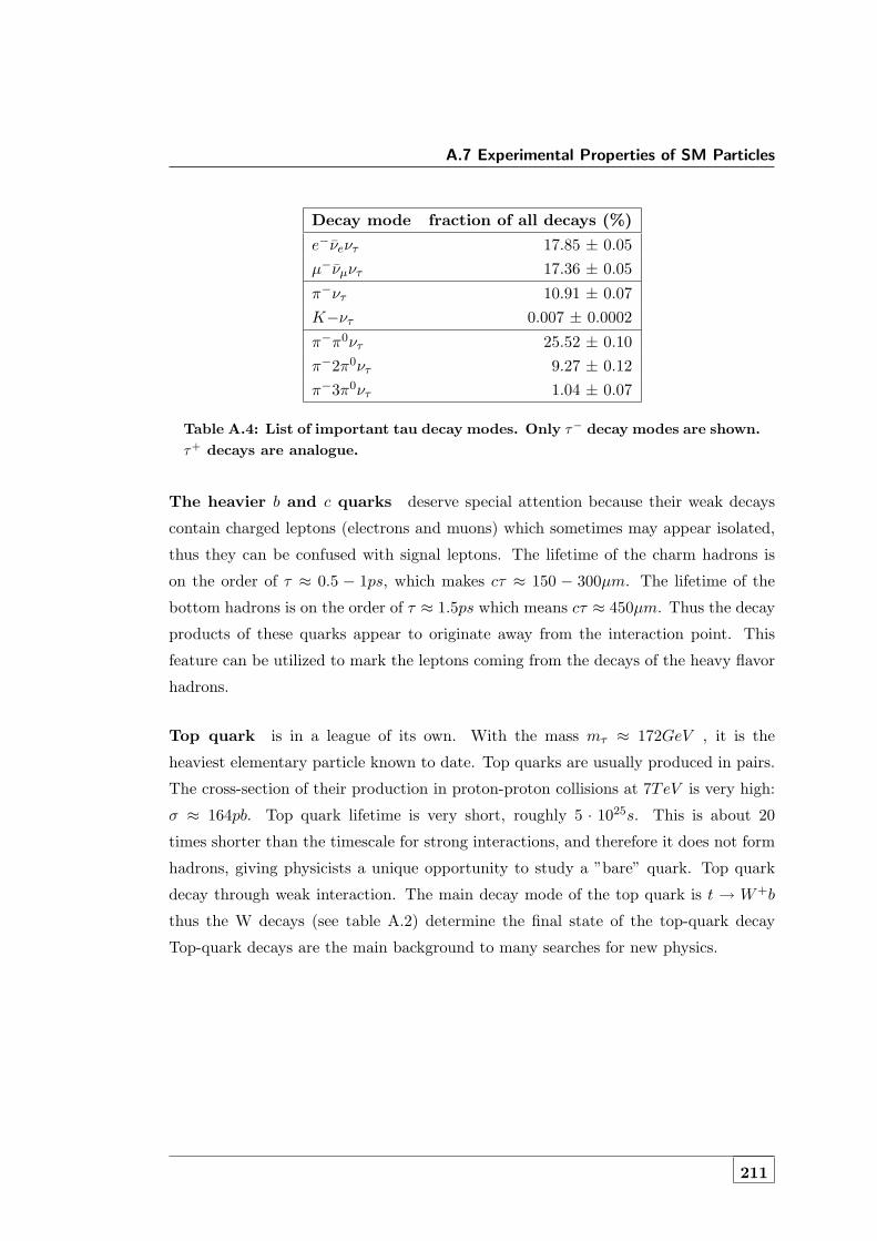
A.7 Experimental Properties of SM Particles
Decay mode fraction of all decays (%)
e−νeντ 17.85 ± 0.05µ−νµντ 17.36 ± 0.05
π−ντ 10.91 ± 0.07K−ντ 0.007 ± 0.0002
π−π0ντ 25.52 ± 0.10π−2π0ντ 9.27 ± 0.12π−3π0ντ 1.04 ± 0.07
Table A.4: List of important tau decay modes. Only τ− decay modes are shown.τ+ decays are analogue.
The heavier b and c quarks deserve special attention because their weak decays
contain charged leptons (electrons and muons) which sometimes may appear isolated,
thus they can be confused with signal leptons. The lifetime of the charm hadrons is
on the order of τ ≈ 0.5 − 1ps, which makes cτ ≈ 150 − 300µm. The lifetime of the
bottom hadrons is on the order of τ ≈ 1.5ps which means cτ ≈ 450µm. Thus the decay
products of these quarks appear to originate away from the interaction point. This
feature can be utilized to mark the leptons coming from the decays of the heavy flavor
hadrons.
Top quark is in a league of its own. With the mass mτ ≈ 172GeV , it is the
heaviest elementary particle known to date. Top quarks are usually produced in pairs.
The cross-section of their production in proton-proton collisions at 7TeV is very high:
σ ≈ 164pb. Top quark lifetime is very short, roughly 5 · 1025s. This is about 20
times shorter than the timescale for strong interactions, and therefore it does not form
hadrons, giving physicists a unique opportunity to study a ”bare” quark. Top quark
decay through weak interaction. The main decay mode of the top quark is t → W+b
thus the W decays (see table A.2) determine the final state of the top-quark decay
Top-quark decays are the main background to many searches for new physics.
211


BThe Seesaw Type-III Lagrangian
B.1 The Lagrangian in the mass basis
The Lagrangian in the mass basis after the diagonalization of the mass matrices of
the charged and the neutral sectors ( the diagonalization procedure is described in
Ref. (28)), is the following:
L = LKin + LCC + L`NC + Lν
NC + L`H + Lν
H + L`η + Lν
η + Lφ− ,�� ��B.1
where
LCC =g√2
(l Ψ
)γµW−
µ
(PLg
CCL + PRg
CCR
√2)( ν
Σ
)+ h.c.
�� ��B.2
L`NC =
g
cosθW
(l Ψ
)γµZµ
(PLg
NCL + PRg
NCR
)( lΨ
) �� ��B.3
LνNC =
g
2cosθW
(ν Σ0c
)γµZµ
(PLg
NCν
)( νL
Σ0c
) �� ��B.4
L`H = −
(l Ψ
)H(PLg
H`L + PRg
H`R
)( lΨ
) �� ��B.5
LνH = −
(ν Σ0
) H√2
(PLg
HνL + PRg
HνR
)( νΣ0
) �� ��B.6
L`η = −
(l Ψ
)iη(PLg
η`L + PRg
η`R
)( lΨ
) �� ��B.7
Lνη = −
(ν Σ0
) iη√2
(PLg
ηνL + PRg
ηνR
)( νΣ0
) �� ��B.8
Lφ− = −(l ψ
)φ−(PLg
φ−
L + PRgφ−
R )(
νΣ0
)+ h.c.
�� ��B.9
we have indicated UPMNS simply with U. The couplings are:
213

B. THE SEESAW TYPE-III LAGRANGIAN
gCCL =
(1 + ε
2
)U −Y †
ΣM−1Σ
v√2
0√
2(1− ε′
2
) �� ��B.10
gCCR =
(0 −mlY
†ΣM
−2Σ v
−M−1Σ Y ∗
ΣU∗ v√2
1− ε′∗
2
) �� ��B.11
gNCL =
(12 − cos2θW − ε 1
2Y†ΣM
−1Σ v
12M
−1Σ YΣv ε′ − cos2θW
) �� ��B.12
gNCR =
(1− cos2θW mlY
†ΣM
−2Σ v
M−2Σ YΣmlv −cos2θW
) �� ��B.13
gNCν =
(1− U† εU U†Y †
ΣM−1Σ
v√2
v√2M−1
Σ YΣ U ε′
) �� ��B.14
gH`L =
(mlv (1− 3ε) mlY
†ΣM
−1Σ
YΣ (1− ε) +M−2Σ YΣm
2l YΣY
†ΣM
−1Σ v
) �� ��B.15
gH`R =
(gH`L
)† �� ��B.16
gHνL =
(−√
2v UT mν U UT mνY
†ΣM
−1Σ
(YΣ − YΣε2 −
ε′T
2 YΣ)U YΣY†ΣM
−1Σ
v√2
) �� ��B.17
=
(−√
2v md
ν mdν U†Y †
ΣM−1Σ
(YΣ − YΣε2 −
ε′T
2 YΣ)U YΣY†ΣM
−1Σ
v√2
)gHνR =
(gHνL
)† �� ��B.18
gη`L =
(−ml
v (1 + ε) −mlY†ΣM
−1Σ
YΣ(1− ε)−M−2Σ YΣm
2l vYΣY
†ΣM
−1Σ
) �� ��B.19
gη`R = −
(gη`L
)† �� ��B.20
gηνL = gHν
L
�� ��B.21
gηνR = −
(gηνL
)† �� ��B.22
gφ−
L =( √
2mlv (1− ε
2)U mlY†ΣM
−1Σ√
2m2lM
−2Σ YΣU 0
) �� ��B.23
gφ−
R =
(−√
2Umd∗
νv
[(Y †
Σ − εY †Σ − Y †
Σε′∗
2 )− 2m∗νY
†ΣM
−1Σ
]−√
2Y ∗Σ(1− ε∗
2 )U∗ 2[−MΣv ε′T + ε′MΣ
v ]
).
�� ��B.24
Here U is the lowest order leptonic mixing matrix which is unitary, ml is a diagonal
matrix whose elements are the masses of the charged leptons, v ≡√
2〈φ0〉 = 246 GeV,
214

B.2 The explicit Lagrangian in the minimal model
ε = v2
2 Y†ΣM
−2Σ YΣ, ε′ = v2
2 M−1Σ YΣY
†ΣM
−1Σ and δ = m2
l
M2Σ. The above expressions are all
valid at O(ε, ε′, δ,
√εδ,√ε′δ).
B.2 The explicit Lagrangian in the minimal model
gCCL =
(1 + V T∧V
2
)U −V T
0√
2(1− V ·V T
2
) =
=
Ue1 + VeVα
2 Uα1 Ue2 + VeVα2 Uα2 Ue3 + VeVα
2 Uα3
Uµ1 + VµVα
2 Uα1 Uµ2 + VµVα
2 Uα2 Uµ3 + VµVα
2 Uα3
Uτ1 + Vτ Vα2 Uα1 Uτ2 + Vτ Vα
2 Uα2 Uτ3 + Vτ Vα2 Uα3
0 0 0
∣∣∣∣∣∣∣∣∣∣∣∣∣∣∣∣∣−Ve
−Vµ
−Vτ√2(1− V 2
e +V 2µ +V 2
τ
2 )
gCCR =
(0 −
√2mlV
TM−1Σ
−V U 1− V ·V T
2
)=
=
0 0 0 −
√2M−1
Σ meVe
0 0 0 −√
2M−1Σ mµVµ
0 0 0 −√
2M−1Σ mτVτ
−VαUα1 −VαUα2 −VαUα3 1− V 2e +V 2
µ +V 2τ
2
gNCL =
(12 − cos2θW − V T ∧ V 1√
2V T
1√2V V · V T − cos2θW
)=
=
12 − cos2θW − V 2
e VeVµ VeVτVe√
2
VeVµ12 − cos2θW − V 2
µ VµVτVµ√
2
VeVτ VµVτ12 − cos2θW − V 2
τVτ√
2Ve√
2
Vµ√2
Vτ√2
V 2e + V 2
µ + V 2τ − cos2θW
gNCR =
(1− cos2θW
√2mlV
TM−1Σ√
2M−1Σ V ml −cos2θW
)=
215

B. THE SEESAW TYPE-III LAGRANGIAN
=
1− cos2θW 0 0
√2M−1
Σ meVe
0 1− cos2θW 0√
2M−1Σ mµVµ
0 0 1− cos2θW
√2M−1
Σ mτVτ√2M−1
Σ meVe
√2M−1
Σ mµVµ
√2M−1
Σ mτVτ −cos2θW
gNCν =
(1− UT V T ∧ V U UTV T
V U V · V T
)=
=
1− Uα1VαVβUβ1 −Uα1VαVβUβ2
−Uα2VαVβUβ1 1− Uα2VαVβUβ2
−Uα3VαVβUβ1 −Uα3VαVβUβ2
VαUα1 VαUα2
∣∣∣∣∣∣∣∣∣∣∣∣∣∣∣∣−Uα1VαVβUβ3 VαUα1
−Uα2VαVβUβ3 VαUα2
1− Uα3VαVβUβ3 VαUα3
VαUα3 V 2e + V 2
µ + V 2τ
gH`L =
(mlv
(1− 3V T ∧ V
) √2ml
v VT
√2MΣ
v V · (1− V T ∧ V ) +√
2M−1Σ V
m2l
v 2MΣv V · V T
)=
=
mev (1− 3V 2
e ) −3mev VeVµ
−3mµ
v VµVemµ
v (1− 3V 2µ )
−3mτv VτVe −3mτ
v VτVµ√2MΣ
v Ve(1− V 2e − V 2
µ − V 2τ ) +
√2M−1
Σm2
ev Ve
√2MΣ
v Vµ(1− V 2e − V 2
µ − V 2τ ) +
√2M−1
Σ
m2µ
v Vµ
∣∣∣∣∣∣∣∣∣∣∣∣∣∣∣∣∣∣−3me
v VeVτ
√2me
v Ve
−3mµ
v VµVτ
√2mµ
v Vµmτv (1− 3V 2
τ )√
2mτv Vτ√
2MΣv Vτ (1− V 2
e − V 2µ − V 2
τ ) +√
2M−1Σ
m2τ
v Vτ 2MΣv (V 2
e + V 2µ + V 2
τ )
gHνL =
( √2
v mdν
√2
v mdνU
TV T√
2v (1− ε′)MΣV U
√2
v MΣε′
)=
=√
2v
mν1 0 0 mν1Uα1Vα
0 mν2 0 mν2Uα2Vα
0 0 mν3 mν3Uα3Vα
(1− ε′)MΣVαUα1 (1− ε′)MΣVαUα2 (1− ε′)MΣVαUα3 MΣε′
gη`L =
(−ml
v (1 + V T ∧ V ) −mlv
√2V T
MΣv
√2V (1− V T ∧ V − m2
l
M2Σ) 2MΣ
v V · V T
)=
216

B.2 The explicit Lagrangian in the minimal model
=
−me
v (1 + V 2e ) −me
v VeVµ
−mµ
v VµVe −mµ
v (1 + V 2µ )
−mτv VτVe −mτ
v VτVµ√2MΣ
v Ve(1− V 2e − V 2
µ − V 2τ )−
√2M−1
Σm2
ev Ve
√2MΣ
v Vµ(1− V 2e − V 2
µ − V 2τ )−
√2M−1
Σ
m2µ
v Vµ
∣∣∣∣∣∣∣∣∣∣∣∣∣∣∣∣∣∣−me
v VeVτ −√
2mev Ve
−mµ
v VµVτ −√
2mµ
v Vµ
−mτv (1 + V 2
τ ) −√
2mτv Vτ√
2MΣv Vτ (1− V 2
e − V 2µ − V 2
τ )−√
2M−1Σ
m2τ
v Vτ 2MΣv (V 2
e + V 2µ + V 2
τ )
gφL =
( √2ml
v (1− V T∧V2 )U
√2
v mlVT
2M−1Σ V
m2l
v U 0
)=
=
√
2v (me(δeα − VeVα
2 )Uα1)√
2v (me(δeα − VeVα
2 )Uα2)√
2v (me(δeα − VeVα
2 )Uα3)√
2v meVe√
2v (mµ(δµα − VµVα
2 )Uα1)√
2v (mµ(δµα − VµVα
2 )Uα2)√
2v (mµ(δµα − VµVα
2 )Uα3)√
2v mµVµ√
2v (mτ (δτα − Vτ Vα
2 )Uα1)√
2v (mτ (δτα − Vτ Vα
2 )Uα2)√
2v (mτ (δτα − Vτ Vα
2 )Uα3)√
2v mτVτ
2M−1Σ Vα
m2α
v Uα1 2M−1Σ Vα
m2α
v Uα2 2M−1Σ Vα
m2α
v Uα3 0
gφR =
(−√
2Umd
νv (V T − (V T ∧ V ) · V T − V T · V.V T
2 )√
2MΣv − 2
√2U
mdν
v UTV T
−2MΣv V (1− (V T∧V )
2 )U 0
)=
=
−√
2v mν1Ue1 −
√2
v mν2Ue2 −√
2v mν3Ue3
−√
2v mν1Uµ1 −
√2
v mν2Uµ2 −√
2v mν3Uµ3
−√
2v mν1Uτ1 −
√2
v mν2Uτ2 −√
2v mν3Uτ3
MΣv Vα(V 2
e + V 2µ + V 2
τ − 2)Uα1MΣv Vα(V 2
e + V 2µ + V 2
τ − 2)Uα2MΣv Vα(V 2
e + V 2µ + V 2
τ − 2)Uα3
∣∣∣∣∣∣∣∣∣∣∣∣∣∣∣∣∣√
2MΣv Ve(1− 3
2(V 2e + V 2
µ + V 2τ ))− 2
√2mνi
v UeiUαiVα√2MΣ
v Vµ(1− 32(V 2
e + V 2µ + V 2
τ ))− 2√
2mνiv UµiUαiVα√
2MΣv Vτ (1− 3
2(V 2e + V 2
µ + V 2τ ))− 2
√2mνi
v UτiUαiVα
0
In the above expressions repeated flavor indexes are summed. As we will discuss
later, we will take neutrino masses equal to zero, except in the case of small mixing
angles 1.
1In this case, indeed, for consistency we will turn neutrino masses, as well as electron and muon
masses, on. However, this will not basically affect the result.
217


CSimulation Programs Details
C.1 Madgraph
C.1.1 Model Assumptions
• In seesaw type III model we add 3 fermion triplets. Since only the lightest one
could be detected in LHC, we build a model including the lightest triplet only.
It is easier to develop, and it doesn’t have drawbacks. The Yukawa coupling (Y )
will reduce to be a vector, instead of a matrix.
• We are not interested in the phase, so Y t = Y .
• As input parameter we will use the quantity U = YMv instead of the Yukawa
coupling.
• Neutrino masses are zero.
C.1.2 Run Card
Examples of Madgraph configuration cards could be taken from (42). The run card
used for the signal generation is the following:#*********************************************************************
# MadGraph/MadEvent *
# http://madgraph.hep.uiuc.edu *
# *
# run card.dat *
# *
# This file is used to set the parameters of the run. *
# *
219

C. SIMULATION PROGRAMS DETAILS
# Some notation/conventions: *
# *
# Lines starting with a ’# ’ are info or comments *
# *
# mind the format: value = variable ! comment *
#*********************************************************************
#
#*******************
# Running parameters
#*******************
#
#*********************************************************************
# Tag name for the run (one word) *
#*********************************************************************
’seesaw’ = run tag ! name of the run
#*********************************************************************
# Run to generate the grid pack *
#*********************************************************************
.false. = gridpack !True = setting up the grid pack
#*********************************************************************
# Number of events and rnd seed *
# Warning: Do not generate more than 100K event in a single run *
#*********************************************************************
100000 = nevents ! Number of unweighted events requested
0 = iseed ! rnd seed (0=assigned automatically=default))
#*********************************************************************
# Collider type and energy *
#*********************************************************************
1 = lpp1 ! beam 1 type (0=NO PDF)
1 = lpp2 ! beam 2 type (0=NO PDF)
3500 = ebeam1 ! beam 1 energy in GeV
3500 = ebeam2 ! beam 2 energy in GeV
#*********************************************************************
# Beam polarization from -100 (left-handed) to 100 (right-handed) *
#*********************************************************************
0 = polbeam1 ! beam polarization for beam 1
220

C.1 Madgraph
0 = polbeam2 ! beam polarization for beam 2
#*********************************************************************
# PDF CHOICE: this automatically fixes also alpha s and its evol. *
#*********************************************************************
’cteq6l1’ = pdlabel ! PDF set
#*********************************************************************
# Renormalization and factorization scales *
#*********************************************************************
F = fixed ren scale ! if .true. use fixed ren scale
F = fixed fac scale ! if .true. use fixed fac scale
91.1880 = scale ! fixed ren scale
91.1880 = dsqrt q2fact1 ! fixed fact scale for pdf1
91.1880 = dsqrt q2fact2 ! fixed fact scale for pdf2
1 = scalefact ! scale factor for event-by-event scales
#*********************************************************************
# Matching - Warning! ickkw > 1 is still beta
#*********************************************************************
1 = ickkw ! 0 no matching, 1 MLM, 2 CKKW matching
1 = highestmult ! for ickkw=2, highest mult group
1 = ktscheme ! for ickkw=1, 1 Durham kT, 2 Pythia pTE
1 = alpsfact ! scale factor for QCD emission vx
F = chcluster ! cluster only according to channel diag
T = pdfwgt ! for ickkw=1, perform pdf reweighting
#*********************************************************************
# Automatic ptj and mjj cuts if xqcut > 0
# (turn off for VBF and single top processes)
#**********************************************************
T = auto ptj mjj
#**********************************************************
#
#**********************************
# BW cutoff (M+/-bwcutoff*Gamma)
#**********************************
10000 = bwcutoff
#**********************************************************
# Apply pt/E/eta/dr/mij cuts on decay products or not
221

C. SIMULATION PROGRAMS DETAILS
# (note that etmiss/ptll/ptheavy/sorted cuts always apply)
#**********************************************************
T = cut decays
#*************************************************************
# Number of helicities to sum per event (0 = all helicities)
# 0 gives more stable result, but longer run time (needed for
# long decay chains e.g.).
# Use >=2 if most helicities contribute, e.g. pure QCD.
#*************************************************************
0 = nhel
#*******************
# Standard Cuts
#*******************
# #*********************************************************************
# Minimum and maximum pt’s *
#*********************************************************************
20 = ptj ! minimum pt for the jets
20 = ptb ! minimum pt for the b
0 = pta ! minimum pt for the photons
0 = ptl ! minimum pt for the charged leptons
0 = misset ! minimum missing Et (sum of neutrino’s momenta)
0 = ptheavy ! minimum pt for one heavy final state
1.0 = ptonium ! minimum pt for the quarkonium states
1d5 = ptjmax ! maximum pt for the jets
1d5 = ptbmax ! maximum pt for the b
1d5 = ptamax ! maximum pt for the photons
1d5 = ptlmax ! maximum pt for the charged leptons
1d5 = missetmax ! maximum missing Et (sum of neutrino’s momenta)
#*********************************************************************
# Minimum and maximum E’s (in the lab frame) *
#*********************************************************************
0 = ej ! minimum E for the jets
0 = eb ! minimum E for the b
0 = ea ! minimum E for the photons
0 = el ! minimum E for the charged leptons
1d5 = ejmax ! maximum E for the jets
222
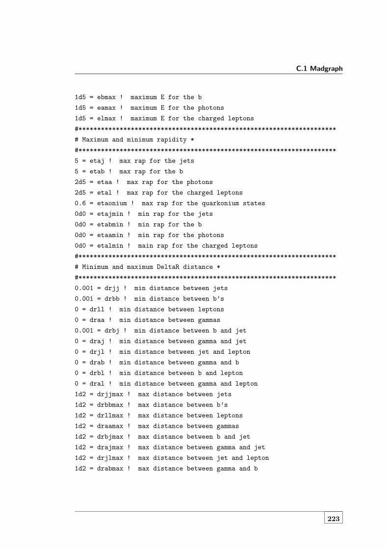
C.1 Madgraph
1d5 = ebmax ! maximum E for the b
1d5 = eamax ! maximum E for the photons
1d5 = elmax ! maximum E for the charged leptons
#*********************************************************************
# Maximum and minimum rapidity *
#*********************************************************************
5 = etaj ! max rap for the jets
5 = etab ! max rap for the b
2d5 = etaa ! max rap for the photons
2d5 = etal ! max rap for the charged leptons
0.6 = etaonium ! max rap for the quarkonium states
0d0 = etajmin ! min rap for the jets
0d0 = etabmin ! min rap for the b
0d0 = etaamin ! min rap for the photons
0d0 = etalmin ! main rap for the charged leptons
#*********************************************************************
# Minimum and maximum DeltaR distance *
#*********************************************************************
0.001 = drjj ! min distance between jets
0.001 = drbb ! min distance between b’s
0 = drll ! min distance between leptons
0 = draa ! min distance between gammas
0.001 = drbj ! min distance between b and jet
0 = draj ! min distance between gamma and jet
0 = drjl ! min distance between jet and lepton
0 = drab ! min distance between gamma and b
0 = drbl ! min distance between b and lepton
0 = dral ! min distance between gamma and lepton
1d2 = drjjmax ! max distance between jets
1d2 = drbbmax ! max distance between b’s
1d2 = drllmax ! max distance between leptons
1d2 = draamax ! max distance between gammas
1d2 = drbjmax ! max distance between b and jet
1d2 = drajmax ! max distance between gamma and jet
1d2 = drjlmax ! max distance between jet and lepton
1d2 = drabmax ! max distance between gamma and b
223

C. SIMULATION PROGRAMS DETAILS
1d2 = drblmax ! max distance between b and lepton
1d2 = dralmax ! maxdistance between gamma and lepton
#*********************************************************************
# Minimum and maximum invariant mass for pairs *
#*********************************************************************
0 = mmjj ! min invariant mass of a jet pair
0 = mmbb ! min invariant mass of a b pair
0 = mmaa ! min invariant mass of gamma gamma pair
0 = mmll ! min invariant mass of l+l- (same flavour) lepton pair
1d5 = mmjjmax ! max invariant mass of a jet pair
1d5 = mmbbmax ! max invariant mass of a b pair
1d5 = mmaamax ! max invariant mass of gamma gamma pair
1d5 = mmllmax ! max invariant mass of l+l- (same flavour) lepton pair
#*********************************************************************
# Minimum and maximum invariant mass for all letpons *
#*********************************************************************
0 = mmnl ! min invariant mass for all letpons (l+- and vl)
1d5 = mmnlmax ! max invariant mass for all letpons (l+- and vl)
#*********************************************************************
# Minimum and maximum pt for 4-momenta sum of leptons *
#*********************************************************************
0 = ptllmin ! Minimum pt for 4-momenta sum of leptons(l and vl)
1d5 = ptllmax ! Maximum pt for 4-momenta sum of leptons(l and vl)
#*********************************************************************
# Inclusive cuts *
#*********************************************************************
0 = xptj ! minimum pt for at least one jet
0 = xptb ! minimum pt for at least one b
0 = xpta ! minimum pt for at least one photon
0 = xptl ! minimum pt for at least one charged lepton
#*********************************************************************
# Control the pt’s of the jets sorted by pt *
#*********************************************************************
0 = ptj1min ! minimum pt for the leading jet in pt
0 = ptj2min ! minimum pt for the second jet in pt
0 = ptj3min ! minimum pt for the third jet in pt
224

C.1 Madgraph
0 = ptj4min ! minimum pt for the fourth jet in pt
1d5 = ptj1max ! maximum pt for the leading jet in pt
1d5 = ptj2max ! maximum pt for the second jet in pt
1d5 = ptj3max ! maximum pt for the third jet in pt
1d5 = ptj4max ! maximum pt for the fourth jet in pt
0 = cutuse ! reject event if fails any (0) / all (1) jet pt cuts
#*********************************************************************
# Control the Ht(k)=Sum of k leading jets *
#*********************************************************************
0 = htjmin ! minimum jet HT=Sum(jet pt)
1d5 = htjmax ! maximum jet HT=Sum(jet pt)
0 = ihtmin !inclusive Ht for all partons (including b)
1d5 = ihtmax !inclusive Ht for all partons (including b)
0 = ht2min ! minimum Ht for the two leading jets
0 = ht3min ! minimum Ht for the three leading jets
0 = ht4min ! minimum Ht for the four leading jets
1d5 = ht2max ! maximum Ht for the two leading jets
1d5 = ht3max ! maximum Ht for the three leading jets
1d5 = ht4max ! maximum Ht for the four leading jets
#*********************************************************************
# WBF cuts *
#*********************************************************************
0 = xetamin ! minimum rapidity for two jets in the WBF case
0 = deltaeta ! minimum rapidity for two jets in the WBF case
#*********************************************************************
# maximal pdg code for quark to be considered as a light jet *
# (otherwise b cuts are applied) *
#*********************************************************************
5 = maxjetflavor
#*********************************************************************
# Jet measure cuts *
#*********************************************************************
20 = xqcut ! minimum kt jet measure between partons
#*********************************************************************
225

C. SIMULATION PROGRAMS DETAILS
C.1.3 Run Card Parameters Notes
Notes about crucial run card parameters are given below.
maxjetflavor defines which cuts to apply on jet types. For example if maxjetflavor=5
this means that the b quarks will be constrained by the cuts for jets, (ptj, etaj). On
the contrary the usual cuts for b’s are applied (ptb, etab, etc).
xqcut is the minimal distance between the ISR in the matrix-element calculation. It
is typically closed to the cutoff used for the matching. The good value for xqcut is
always a compromise between the fact that we want a reasonable matching efficiency,
and in the same time not too high cause in this case there could be dead zones in the
PS region of the phase-space.
Some typical choices of xqcut/qcut for processes with massive particles are in Table
C.1.
Process xqcut Qcut
V, VV, VVV +jets 10 15ttbar 20 30
Table C.1: Typical qcut values
.
C.2 Pythia6-CMSSW Interface
C.2.1 Configuration Setting
Configuration file example for processing a MadGraph sample with Pythia6 in CMSSW
could be seen for example in CMSSW directory:
Configuration/Generator/python/MadGraph matching cfi.py. Reference: (39).
Here I’ll give some details of interest about the configuration file I’ve used to run
Madgraph signal LHE files in Pythia-CMSSW.
1. LHESource (rather than EmptySource) feed with parton-level MadGraph sample
(.lhe file);
226

C.2 Pythia6-CMSSW Interface
2. generator = cms.EDFilter("Pythia6HadronizerFilter"): it means that we
use Pythia6-based module that is dedicated to processing externally generated
partons;
3. The module configured specifically for processing MadGraph events is:
processParameters = cms.vstring(’MSEL=0 ! User defined processes’,
’PMAS(5,1)=4.4 ! b quark mass’,
’PMAS(6,1)=172.4 ! t quark mass’,
’MSTJ(1)=1 ! Fragmentation/hadronization on or off’,
’MSTP(61)=1 ! Parton showering on or off’),
4. Dedicated Madgraph parton-shower matching algorithm, to decide on the event
internal validity, or to veto events of incorrect topology:
jetMatching = cms.untracked.PSet(
scheme = cms.string("Madgraph"),
mode = cms.string("auto"), # soup, or "inclusive" / "exclusive"
MEMAIN etaclmax = cms.double(5.0),
MEMAIN qcut = cms.double(30.0),
MEMAIN minjets = cms.int32(0),
MEMAIN maxjets = cms.int32(15),
MEMAIN showerkt = cms.double(0),
MEMAIN nqmatch = cms.int32(5),
MEMAIN excres = cms.string(""),
outTree flag = cms.int32(0)
)
Note: the use of matching procedure is optional; Pythia6HadronizerFilter may
operate without it. However, if parton-shower matching is used, in case an event
is vetoed the EDFilter will return a false code, and the HepMCProduct will be
empty.
5. Those event will be filtered out of the output, because event generation step isincluded in the ”production filtering sequence”:
227

C. SIMULATION PROGRAMS DETAILS
ProductionFilterSequence = cms.Sequence(generator)
Configuration fragment could be processed through cmsDriver.py, for example for
Summer 11 datasets production I’ve used the following: cmsDriver.py
Configuration/GenProduction/python/SeesawToLeptons M 120 7TeV pythia6 cff.py
-s GEN --conditions START311 V2::All --beamspot Realistic7TeV2011Collision
--datatier GEN-SIM --eventcontent RAWSIM --filein file:...lhe -n 10000 --no exec
and cmsDriver.py
Configuration/GenProduction/python/SeesawToLeptons M 120 7TeV pythia6 cff.py
-s GEN,SIM,DIGI,L1,DIGI2RAW,HLT --conditions START311 V2::All --beamspot
Realistic7TeV2011Collision --datatier GEN-SIM-RAW --eventcontent RAWSIM --filein
file:...lhe -n 30 --no exec
The even loop is driven by a special purpose LHESource (rather than EmptySource)
source = cms.Source("LHESource",
fileNames = cms.untracked.vstring(
’file:....lhe’)
)
which is feed with the parton-level MadGraph sample.
C.2.2 Fast Simulation
We used Fast Simulation to run simulation-reconstruction chain of the signal datasets
analyzed in the thesis.
The code used is:
228

C.2 Pythia6-CMSSW Interface
CMSSW 4 2 8 patch4
FastSimulation/PileUpProducer tag: V04-05-12
The cmsDriver command used is:
cmsDriver.py SeesawTo3lept 30qcut 7TeV pythia6 cff.py --filein=file:....lhe
--filetype=LHE -s GEN,FASTSIM,HLT:GRun --pileup=E7TeV Fall2011 Reprocess inTimeOnly
--geometry DB --conditions=auto:startup --eventcontent=AODSIM --datatier
GEN-SIM-DIGI-RECO -n 100000 --no exec
The pileup distribution superimposed to events have been taken from real 2011 data
pileup distributions.
References about CMSSW Fast Simulation could be see in Reference (80).
229

DBackgrounds Samples
Reference: (95)
D.1 Datasets
The signal and background samples used in this analysis have been obtained using
detailed Monte Carlo simulations. In most cases, the samples are taken from the
official CMS Summer 11 production cycle with digitization and reconstruction done with
CMSSW_4_2_X. Background processes for Summer 11 production have been generated
using Madgraph (58), Pythia (47), and powheg (61) generators.
The 2011 Monte Carlo samples used in this analysis for the backgrounds include
all the luminosity-dependent trigger configurations as used in the data. Therefore,
implementation of the trigger matching was introduced. We require the HLT objects
to match the leptons selected for our analysis, and reproduce the HLT requirements by
applying the corresponding pT thresholds.
Private Madgraph5 generations have been performed for the samples not present
in the official production (i.e. ttW , ttWW , ttZ, WW same sign), and the request for
official simulation and reconstruction processing was submit to the CMS generators
team. They have been approved, processed and included in Summer 11 dataset.
Whenever the cross section for the different background under study has not been
measured, we have used MadGraph/MadEvent to obtain the cross-sections for LHC run-
ning at 7 TeV and compared our results with previous results obtained by the CMS
collaboration (73).
The full list of background samples we considered or studied, including their dataset
231

D. BACKGROUNDS SAMPLES
names and cross sections, are presented in Table D.1 and D.2. Detail about the gener-
ator and the number of events of the main backgrounds are listed in Table D.3.
Table D.1: Samples, Dataset names, leading order (LO) and next-to-leading order (NLO)cross sections for the physical background samples considered in this analysis. Datasetsmarked with ∗ are taken from the Spring11 production, while all others are from Summer11.Cross sections marked with † are next-to-next-to-leading order.
Sample Dataset Name σLO σNLO
(pb) (pb)
TTbarJetMadGr TTJets_TuneZ2_7TeV-madgraph-tauola 157.5
V γ+ jets GVJets_7TeV-madgraph 173
WZ WZ_TuneZ2_7TeV_pythia6_tauola 18.3 (#)
WZ3L WZTo3LNu_7TeV-pythia6 0.34 0.594
ZZ ZZ_TuneZ2_7TeV_pythia6_tauola 4.3 5.9
ZZTo4mu ZZTo4mu_7TeV-powheg-pythia6 0.0154
ZZTo2e2mu ZZTo2e2mu_7TeV-powheg-pythia6 0.0308
ZZTo4e ZZTo4e_7TeV-powheg-pythia6 0.0154
ZZTo4L ZZTo4L_TuneZ2_7TeV-pythia6-tauola∗ 0.065 0.082
WWWm Castor WWWTo2Lminus2Nu_Qcut-20_Castor_7TeV-madgraph 0.003402
WWWp Castor WWWTo2Lplus2Nu_Qcut-20_Castor_7TeV-madgraph 0.007903
TTWWm Castor TTWWTo2Lminus2Nu_Qcut-20_Castor_7TeV-madgraph 0.00004719
TTWWp Castor TTWWTo2Lplus2Nu_Qcut-20_Castor_7TeV-madgraph 0.0000476
WWm Castor WWminusTo2L2Nu_Castor_7TeV-madgraph 0.001559
WWp Castor WWplusTo2L2Nu_Castor_7TeV-madgraph 0.004216
TTZm Castor TTZTo2Lminus2Nu_Castor_7TeV-madgraph 0.001946
TTZp Castor TTZTo2Lplus2Nu_Castor_7TeV-madgraph 0.002024
TTWm Castor TTWTo2Lminus2Nu_Castor_7TeV-madgraph 0.002705
TTWp Castor TTWTo2Lplus2Nu_Castor_7TeV-madgraph 0.006841
232

D.1 Datasets
Table D.2: Samples, Dataset names, leading order (LO) and next-to-leading order (NLO)cross sections for the non-physical background samples considered in this analysis. Datasetsmarked with ∗ are taken from the Spring11 production, while all others are from Summer11.Cross sections marked with † are next-to-next-to-leading order. (#)For WZ sample we usedthe measured cross section instead of the MC one. The value is taken from Reference (106),and is equal to: 17.0± 2.4(stat.)±1.1(syst.)±1.0(lumi).
Sample Dataset Name σLO σNLO
(pb) (pb)
QCD −MuEnrichedPt15 QCD_Pt-20_MuEnrichedPt-15_TuneZ2_7TeV-pythia6 84679.3
QCD − EMEnriched QCD_Pt-20to30_EMEnriched_TuneZ2_7TeV-pythia6 2502.66
Zee DYToEE_M-20_TuneZ2_7TeV-pythia6 1667
Zmumu DYToMuMu_M-20_TuneZ2_7TeV-pythia6 1667
Ztautau DYToTauTau_M-20_TuneZ2_7TeV-pythia6-tauola 1667
Wenu WtoENu_TuneD6T_7TeV-pythia6 10438
Wmunu WtoMuNu_TuneD6T_7TeV-pythia6 10438
Wtaunu WtoTauNu_TuneD6T_7TeV-pythia6-tauola 10438
WW WW_TuneZ2_7TeV_pythia6_tauola 42.9
WW2L WWTo2L2Nu_TuneZ2_7TeV_pythia6_tauola
SingleTop t T_TuneZ2_t-channel_7TeV-powheg-tauola 41.92
SingleAntiTop t Tbar_TuneZ2_t-channel_7TeV-powheg-tauola 22.65
SingleTop tW T_TuneZ2_tW-channel-DR_7TeV-powheg-tauola 7.87
SingleAntiTop tW Tbar_TuneZ2_tW-channel-DR_7TeV-powheg-tauola 7.87
SingleTop s T_TuneZ2_s-channel_7TeV-powheg-tauola 3.19
SingleAntiTop s Tbar_TuneZ2_s-channel_7TeV-powheg-tauola 1.44
ZJetsMadGr DYJetsToLL_TuneD6T_M-50_7TeV-madgraph-tauola 2289 3048
ZJetsMadgr 10− 50 DYJetsToLL_TuneD6T_M-10To50_7TeV-madgraph-tauola ∗ 310
WJetsMadGr jets WJetsToLNu_TuneZ2_7TeV-madgraph-tauola 24640*3 31314*3†
DY ToCC DYToCC_M_50_TuneZ2_7TeV_pythia6 1809.6
DY ToBB DYToBB_M_50_TuneZ2_7TeV_pythia6 2272.65
Zbb + 0 jets ZBB0JetsToLNu_TuneZ2_7TeV-alpgen-tauola∗ 1.7 2.9
Zbb + 1 jets ZBB1JetsToLNu_TuneZ2_7TeV-alpgen-tauola∗ 0.962 1.645
Zbb + 2 jets ZBB2JetsToLNu_TuneZ2_7TeV-alpgen-tauola∗ 0.364 0.622
Zbb + 3 jets ZBB3JetsToLNu_TuneZ2_7TeV-alpgen-tauola∗ 0.16 0.273
Zcc + 0 jets ZCC0JetsToLNu_TuneZ2_7TeV-alpgen-tauola∗ 1.71 2.92
Zcc + 1 jets ZCC1JetsToLNu_TuneZ2_7TeV-alpgen-tauola∗ 0.953 1.629
Zcc + 2 jets ZCC2JetsToLNu_TuneZ2_7TeV-alpgen-tauola∗ 0.366 0.626
Zcc + 3 jets ZCC3JetsToLNu_TuneZ2_7TeV-alpgen-tauola∗ 0.164 0.28
233

D. BACKGROUNDS SAMPLES
Process MC Generator σ (pb) Number of events
Background Samples:
tt MADGRAPH 164.4 (NNLO) 3,701,947W (→)`ν+jets MADGRAPH 31314 (NNLO) 77,105,816Drell Yan - Z/γ∗(→ ``)+jets MADGRAPH 3048 (NNLO) 36,277,961WW MADGRAPH 3.78 1,197,558WZ MADGRAPH 0.72 1,221,134ZZ MADGRAPH 0.04 1,185,188Wγ → eνγ MADGRAPH 114.7 524,503Wγ → µνγ MADGRAPH 114.6 521,774W±W± MADGRAPH 0.006 99,307WWW MADGRAPH 0.01 60,469ttW MADGRAPH 0.01 99,199ttZ MADGRAPH 0.004 73,521
Table D.3: Details of the background Monte Carlo samples used for the analysis.
234