searching and learning in internet auctions: the ebay example · searching and learning in internet...
TRANSCRIPT
Searching and Learning in Internet Auctions:
The eBay Example
Inaugural-Dissertation
zur Erlangung des Grades
Doctor oeconomiae publicae (Dr. oec. publ.)
an der Ludwig-Maximilians-Universitat Munchen
2005
vorgelegt von
Katharina Sailer
Referent: Prof. Sven Rady, PhD
Korreferent: Prof. Dr. Joachim Winter
Promotionsabschlussberatung: 08. Februar 2006

Acknowledgements
This work benefited from the input of many people during my stays at the Kiel Institute for
World Economics - where it was started off -, the London School of Economics - where I learnt
more about empirical industrial organization and the econometrics of auctions -, and last but
not least the University of Munich - where the dissertation finally gained shape and was finished.
First of all I want to thank my supervisors at the University of Munich - Sven Rady, Joachim
Winter, and Stefan Mittnik - as well as Toker Doganoglu for their advice and encouragement.
Sven Rady provided very detailed and helpful comments on all chapters of this dissertation.
At the IfW, Henning Klodt was always ready to discuss my (changing) ideas, gave advice, and
encouraged and helped me to pursue my projects. Finally, I want to thank Martin Pesendorfer
for supporting this work at a very preliminary stage and for giving advice with the modelling
as well as with the relevant literature.
The data collection could not have been done without the collaboration of Albrecht Mengel
and Sandrine Pierloz. I owe special thanks to them for their very dedicated help.
Administrative support and backing by Almut Hahn-Mieth, Rita Halbfas, Helga Winter-
mantel, and Manuela Beckstein is greatfully acknowledged.
Many helpful suggestions were given at the internal seminars in Kiel, at the LSE, and at
the University of Munich. Chapter 2 was changed various times due to questions and comments
following conference presentations. Here, I especially want to thank Emmanuel Guerre.
I also thank my collegues - among them Albrecht Blasi, Stefan Brandauer, Thomas Buttner,
Antonio Butta, Lukasz Grzybowski, Rossitsa Kotseva, Christian Pigorsch, Christoph Hartz, Flo-
rian Herold, Hannah Horisch, Simone Kohnz, Katrin and Daniel Piazolo, Jorn Kleinert, Martin
Reichhuber, Richard Schmidtke, Julius Spatz, and Farid Toubal. A cheerful environment, ’open
ears’ to smaller or bigger problems and doubts, and (extensive) discussions helped tremendously
in completing this work.
Financial support from the Volkswagen Foundation, the Nixdorf Foundation, and the Deutsche
Forschungsgemeinschaft (DFG) is gratefully acknowledged. I also want to thank the Economics
of Industry Group at the LSE for their hospitality during my research stay.
Dank geht schliesslich an meine Familie.
Contents
List of Tables . . . . . . . . . . . . . . . . . . . . . . . . . . . . . . . . . . . . . . . . . iii
List of Figures . . . . . . . . . . . . . . . . . . . . . . . . . . . . . . . . . . . . . . . . iv
1 Introduction 1
2 Searching the eBay Marketplace 7
2.1 Introduction . . . . . . . . . . . . . . . . . . . . . . . . . . . . . . . . . . . . . . . 7
2.2 The Rules of the eBay Game: Facts and Simplifications . . . . . . . . . . . . . . 11
2.3 The Model . . . . . . . . . . . . . . . . . . . . . . . . . . . . . . . . . . . . . . . 16
2.3.1 Primitives, Information Structure, and Timing . . . . . . . . . . . . . . . 16
2.3.2 The Bidders’ Problem in a Static Environment . . . . . . . . . . . . . . . 18
2.3.3 The General Problem . . . . . . . . . . . . . . . . . . . . . . . . . . . . . 20
2.4 Data and Preliminary Evidence . . . . . . . . . . . . . . . . . . . . . . . . . . . . 23
2.4.1 The Data Set . . . . . . . . . . . . . . . . . . . . . . . . . . . . . . . . . . 23
2.4.2 Evidence from Reduced Form Estimations . . . . . . . . . . . . . . . . . . 29
2.5 Identification . . . . . . . . . . . . . . . . . . . . . . . . . . . . . . . . . . . . . . 32
2.6 Estimation . . . . . . . . . . . . . . . . . . . . . . . . . . . . . . . . . . . . . . . 35
2.6.1 Preliminaries: Bidder’s Valuations . . . . . . . . . . . . . . . . . . . . . . 35
2.6.2 Estimation of Parent Distributions and of Missing Winning Bids . . . . . 36
2.6.3 Computation of Bidding Costs . . . . . . . . . . . . . . . . . . . . . . . . 37
2.6.4 Alternative Approaches . . . . . . . . . . . . . . . . . . . . . . . . . . . . 38
2.7 Results . . . . . . . . . . . . . . . . . . . . . . . . . . . . . . . . . . . . . . . . . . 40
2.7.1 Bidders’ Valuations for Product Characteristics . . . . . . . . . . . . . . . 40
2.7.2 Bidding Costs . . . . . . . . . . . . . . . . . . . . . . . . . . . . . . . . . . 42
i
CONTENTS ii
2.8 Conclusion . . . . . . . . . . . . . . . . . . . . . . . . . . . . . . . . . . . . . . . 45
2.A Proofs . . . . . . . . . . . . . . . . . . . . . . . . . . . . . . . . . . . . . . . . . . 46
2.B Data . . . . . . . . . . . . . . . . . . . . . . . . . . . . . . . . . . . . . . . . . . . 51
2.B.1 Description of Variables Used in Regression . . . . . . . . . . . . . . . . . 51
2.B.2 Frequency of Trials . . . . . . . . . . . . . . . . . . . . . . . . . . . . . . . 53
2.B.3 OLS Estimation . . . . . . . . . . . . . . . . . . . . . . . . . . . . . . . . 54
2.B.4 Participation Decision . . . . . . . . . . . . . . . . . . . . . . . . . . . . . 55
3 Bayesian Learning at eBay?
Updating From Related Data and Empirical Evidence. 58
3.1 Introduction . . . . . . . . . . . . . . . . . . . . . . . . . . . . . . . . . . . . . . . 58
3.2 Benchmark Model . . . . . . . . . . . . . . . . . . . . . . . . . . . . . . . . . . . 61
3.3 Impact of Learning on Optimal Bidding Strategies . . . . . . . . . . . . . . . . . 69
3.4 Detecting Learning in eBay Data . . . . . . . . . . . . . . . . . . . . . . . . . . . 72
3.5 Conclusion . . . . . . . . . . . . . . . . . . . . . . . . . . . . . . . . . . . . . . . 77
3.A Proofs . . . . . . . . . . . . . . . . . . . . . . . . . . . . . . . . . . . . . . . . . . 78
Bibliography . . . . . . . . . . . . . . . . . . . . . . . . . . . . . . . . . . . . . . . . . . 85
List of Tables
2.1 Summary Statistics of Auctions . . . . . . . . . . . . . . . . . . . . . . . . . . . . 24
2.2 Summary Statistics of Bidders . . . . . . . . . . . . . . . . . . . . . . . . . . . . 26
2.3 OLS Estimation . . . . . . . . . . . . . . . . . . . . . . . . . . . . . . . . . . . . 29
2.4 Conditional Logit Estimation . . . . . . . . . . . . . . . . . . . . . . . . . . . . . 31
2.5 Bid Distribution . . . . . . . . . . . . . . . . . . . . . . . . . . . . . . . . . . . . 41
2.6 Frequency of Trials . . . . . . . . . . . . . . . . . . . . . . . . . . . . . . . . . . . 53
2.7 OLS Estimation (Full Specification) . . . . . . . . . . . . . . . . . . . . . . . . . 54
2.8 Conditional Logit Estimation (Full Specification) . . . . . . . . . . . . . . . . . . 56
3.1 Estimates of the Learning Model Using a Linear Specification for the Bids . . . . 75
iii
List of Figures
2.1 Density of All Bids and Bids Submitted in Last 10% of an Auction . . . . . . . . 27
2.2 Evolution of Transaction Prices over the Course of the Sample . . . . . . . . . . 28
2.3 Transaction Prices for New Products . . . . . . . . . . . . . . . . . . . . . . . . . 28
2.4 Frequency of Bidding Costs . . . . . . . . . . . . . . . . . . . . . . . . . . . . . . 43
2.5 Distribution of Bidding Costs for Different Specifications . . . . . . . . . . . . . . 44
3.1 Simulation Results for αe and Expected Bids. . . . . . . . . . . . . . . . . . . . . 71
iv
Chapter 1
Introduction
Internet auction platforms were among the early players in the commercial Internet. And they
were successful! Many of them survived the hype, and its best known representatives, eBay,
Yahoo!, hood.de in Germany,..., are now established, sizeable companies. Their business concept
bases on a well accredited old selling mechanism, the auction, which is offered in one or the other
standardized form.1 While for most but some very specific transactions the obstacles of using
auctions hitherto had far outweighed its merits, with the Internet the transaction costs dropped
tremendously. Buyers and sellers now could convene “asynchronously”, that is, by staying at
home and taking part at their preferred time without loosing the “feel” of an auction. This
made it feasible to use the mechanism also for small person-to-person bargains.
While person-to-person online auctions started out as sort of “e-garage sales” for midget
to small-scale transactions among individuals, and foremost for collectibles, today virtually
everybody, individuals, companies, even the government,2 uses it to sell any kind of product. At
eBay, the major auction platform in most countries, the bulk of the sale is now in standardized
new products such as consumer electronics, computers, domestic appliances, DVDs, etc.3 An
1While all of the 4 standard auction formats can be found in online auctions, most of them use a variant of
an open ascending second price auction (see Lucking-Reiley (2000)).
2see, e.g., “Council sells abandoned cars on eBay” on Tuesday April 19, 2005 at
http://www.guardian.co.uk/online/news/0,12597,1463316,00.html
3The following categories at eBay had $1 billion or more in worldwide annualized gross merchandize value
(GMV)- value of all successfully closed listings on eBay’s trading platforms: eBay Motors ($14.3 billion),
Clothing & Accessories ($3.3B), Consumer Electronics ($ 3.2B), Computers ($2.9B), Home & Garden ($2.5B),
INTRODUCTION 2
immediate consequence of the success of these platforms and the fact that many products are
available en masse is that a specific product is offered many times in different auctions on the
same platform.4 A bidder, who carries out a search for her desired product, most likely finds
many auctions open at the same time and has to decide in which one to bid. This does not
match the standard decision problem considered in the auction literature.
While Internet auctions received considerable attention in the economic literature, this as-
pect has been neglected. The aim of the work at hand is to explore this idiosyncrasy of Internet
auctions in more detail: First, what are the consequences for bidders’ optimal behavior, and sec-
ond, which kind of inference does data generated from such behavior allow the econometrician?
Since eBay is in most countries by far the market leader, the following analysis uses the eBay
specific setting to exemplify the main points. The proposed model is, however, flexible enough
to allow for different rules in the static auction game and could thus be adapted to Internet
auction platforms with other rules. The empirical analysis bases on data from eBay Germany.
With its 16 million registered users, $1.8 billion gross merchandise value (GMV, Q3-2004), and
total listings of over 80 million (Q4-2004), eBay.de is one of the major contributors in the eBay
group5 and by far the biggest online auction platform in Germany.6
The economic literature first focused on eBay’s new reputation mechanism (e.g. Lucking-
Reiley et al. (2000) and Houser and Wooders (forthcoming)). The rich and readily accessible
data, however, also seemed ideal to test other microeconomic theories, first of all auction models
Books/Movies/Music ($2.4B), Sports ($2.1B), Collectibles ($2.0B), Toys ($1.6B), Jewelry & Watches ($1.5B),
Business & Industrial ($1.5B), and Cameras & Photo ($1.3B). [If not otherwise stated this and all following
figures on eBay base on the second quarter 2005 (Q2-2005) and stem from either http://presse.ebay.de/ or the
eBay annual statements which are available at http://investor.ebay.com/.]
4In 2005 eBay.de reports that via its platform are sold: each 2 minutes a vehicle, each 11 minutes a fridge,
each 4 seconds a book, each 2 minutes a notebook, and 13 diggers per day.
5Corresponding figures in Q2-2005 for a) all eBay platforms: Registered users: 157.3 million (active users -
users who bid, bought, or listed an item within the previous 12-month : 64.6M), GMV: $10.9 billion (8.3B $ in
Q3-2004), total new listings: 440 million (405M in Q4-2004). b) ebay.com: registered users: 75 million, GMV:
$5.25 billion.
6alleauktionen.de regularly computes all listing which are open at a certain time for the major German auction
platforms. The average figures for August, 2005 are: 6.3 million (ebay.de), 1 million (hood.de), and 0.6 million
(echtwahr.de).

INTRODUCTION 3
(e.g. Roth and Ockenfels (2002)), and to infer characteristics of demand (e.g. Bajari and
Hortacsu (2003) and Song (2004)). All of the authors though apply static auction models.
There are two reasons why this practice of modelling individual eBay auctions as unrelated
events presents an unsatisfactory stylization. The first concerns bidders’ strategies and market
outcomes: While a loosing bidder in a static auction model forgoes the product forever, those
who do not win an eBay auction, especially when looking for off-the-shelf products, can just
try again in the next upcoming one which is only a few hours ahead. It is likely that the eBay
bidder is aware of her future options and adjusts her strategy accordingly. When using a static
auction model for empirical analysis, the influence of a bidder’s valuation for the product on her
strategy is thus overestimated, whereas the influence of the competitive environment cannot be
assessed.
The second reason, why looking at a dynamic rather than a static setting makes sense, is
due to data availability. eBay’s individual auction sites offer much more information than most
other auction data sets. Not only is it possible to extract very detailed information on auction
and seller covariates. Besides the transaction price, eBay’s bidding histories allow to recover
all of the non-winning bids as well. The pseudonyms, that is, the bidders’ identities, are also
available. When observing the market for a specific product over time, it is thus possible to trace
a bidder’s behavior in this market. Her decision whether to participate in a specific auction or
not and, in case of participation, her bid can be observed and used for inference about additional
individual specific parameters. The next two chapters provide examples for how to exploit this
information in different ways: While Chapter 2 looks at participation behavior and uncovers
bidding costs, Chapter 3 investigates bidders reactions towards uncertainty in model primitives.
Part of the reason, why the dynamic aspect in Internet auctions has been left aside so far,
might be because it does not fit easily into the existing literature. From Riley and Samuelson
we know that “The auction model is a useful description of ”thin markets” characterized by a
fundamental asymmetry of market position. While the standard model of perfect competition
posits buyers and sellers sufficiently numerous that no economic agent has any degree of market
power, the bare bones of the auction model involves competition on only one side of the market.”
(Riley and Samuelson (1981), p. 381) This is exactly not true for many of eBay’s product
categories. At eBay both sellers and buyers are numerous.
INTRODUCTION 4
The literature on sequential auctions relaxes the “thin markets” assumption by considering
bidders’ strategies when a number of identical objects are offered to bidders in a series of con-
secutive auctions. It is shown that, as opposed to static auctions, a bidder now is not willing to
bid her valuation in the early auctions but takes account of what other bidders would have to
pay in the following ones. A bidder’s optimal bidding strategy in a sequential sealed bid second
price auction consists in shading her valuation exactly by her option value, that is, by the added
value which she receives from the possibility to participate in future upcoming events (Weber
(2000)). Since there are only a limited number of objects available, this option value decreases
over time. While the optimal bid of a non-winning bidder hence increases, the expected prices
that are paid in case of winning are the same and correspond to the highest valuation among
the bidders who do not receive a product. Thus, the law of one price for identical objects holds
in expectation.
This framework does not apply to eBay because a bidder’s “search” for low prices is restricted
by the limited availability of products, since there are more bidders than products on offer. The
“fundamental asymmetry of market position” is thus not really given up. Assuming a fixed
number of auctions for a specific product does not fit the eBay market very well. However,
when extending the horizon, that is, the number of products available, towards infinity, optimal
bids in Weber (2000) would tend towards zero. This is where Chapter 2 takes its starting point.
Assume, it is costly for a bidder to take part in an eBay auction. While there is no formal cost
involved in bidding, bidders bear opportunity costs and have to pay for the Internet connection
while bidding. Since both of these presumably differ across individuals, bidding costs will differ.
Together with her valuation, the cost remains a bidder’s private information. Further assume, a
bidder does not update her beliefs about a specific competitor after participating in an auction.
Under these two conditions an infinite horizon model leads to similar results as a sequential
auction model: A bidder shades her valuation by her option value due to future opportunities.
Given the infinite horizon, now the future relation between supply and demand stays constant,
and a bidder’s continuation value, and thus her bid, do not change over time – as long as the
exogenous shocks remain the same.
In the approach ventured here, the asymmetry of market position is maintained in the single
auction. Over time sellers and bidders are considered so numerous, though, that none of them
INTRODUCTION 5
believes to affect future markets outcomes by her current actions. The consequence is that a
bidder essentially faces a dynamic decision problem under uncertainty similar to a search model.
What have search models and eBay auctions in common? Optimal search behavior follows a
stopping (or reservation price) rule: Accept offers which exceed your reservation value and
reject all others. The reservation value when searching auctions for low prices corresponds to
a “reservation bid” which has to be placed in every new auction. If the transaction price, that
is, the second highest bid, is above the bidder’s reserve bid, she loses and has to try in a new
auction, if it is below it, she wins and pays the second highest bid. While the reservation value
of a worker in the labor market helps him to find an employer offering a reasonably high wage,
the eBay bidder searches for a favorable draw of competitors’ valuations since in a second price
auction a bidder pays less when her competitors have low valuations.
The similarity to the search setting is also matched by the data. Even after correcting for
product heterogeneity, the transaction prices that are observed at eBay show considerable price
dispersion. The IO literature makes search frictions responsible for why the law of one price
often cannot be observed in reality despite of seemingly identical products. The model for eBay
shows, in the auction setting it is also the differing costs of bidders which cause price dispersion:
Bidders with higher search cost have a lower option value of bidding in future auctions and
therefore shade their bids less. If bidders bid differently and have a chance of winning the
product if they try long enough, observed prices will differ in equilibrium.
The ultimate aim of Chapter 2 is to show how to recover characteristics of demand from
the observed auction data. Assuming bidders’ behavior follows the proposed “search model”, it
can be shown that a two stage procedure allows to nonparametrically identify the parameters
of interest, namely bidders’ valuations and bidding costs, from information on bids, bidders’
identities, and auction covariates such as product characteristics and the minimum bid. Unlike
in a static auction model, valuations are only identified up to location, though. The first step of
the estimation algorithm recovers bidders’ valuations. After replacing the missing winning bids
by estimates, the cost can then be computed from an optimality condition of the model.
The estimation strategy joins two strands of literature. On the one hand, there is an active
and theoretically very well developed literature on estimating structural auction models. One
of the main insights from this literature is that observed bids stem from an ordered sample;
INTRODUCTION 6
the information on the order of observed and unobserved bids helps to identify the underlying
distributions of interest. In the first step I build on this literature. It is shown that by estimat-
ing from conditional order statistics distributions it is possible to deal at the same time with
unobserved winning bids, correlation across bids of the same bidder, and endogenous selection,
induced by a participation decision. Insights from the recent literature on estimating dynamic
games help to overcome the problem that the continuation value, which is part of the bidding
strategy, is not given in closed form. Instead of solving a dynamic optimization problem at each
estimation stage, implications of the dynamic game can be used to infer static and dynamic
parameters consecutively.
An application to a data set of auctions for a handheld device, a Compaq PDA, concludes
this chapter and shows that the proposed estimation procedure works well and leads to realistic
results.
Observed bid data shows, bidders at eBay increase their bid with each trial in a new auction
for the same object. This cannot be explained by the previous model. Chapter 3 uses a simplified
version of the model and analyzes how bidders react to uncertainty over model primitives. An
important primitive for the bidder is the distribution of competitors’ bids which might only be
vaguely known when the bidder starts his search. Maintaining the assumptions that no bidder
updates his beliefs about a specific competitor, the observed bids can though be used to learn
about the underlying distribution. Chapter 3 shows that increasing bids of individual bidders
are optimal if bidders engage in Bayesian learning.
Learning from observed data in second price auctions is complicated by the fact that the
bidder cannot directly observe the statistic of interest, namely the highest bid of his competitors,
but only the transaction price, which is the second highest bid. Using results from the asymptotic
distribution of extreme order statistics, it is shown that the transaction price can also be used
to update the beliefs over a parameter of the distribution of the highest bid. It results that the
bidder not only increases his bid over time but also with each observation of a transaction price.
Applying the model to the Compaq data set shows that learning is a possible explanation
for the observed bidding patterns at eBay.
Chapter 2
Searching the eBay Marketplace
2.1 Introduction
The internet greatly reduced the transaction costs of selling objects via auctions and of partici-
pating in auctions. Entrepreneurs soon exploited this fact and developed platforms that offered
standardized selling mechanisms on the basis of auctions which can be used by any interested
individual at low costs. The story of eBay is probably the most stunning one: Every day sellers
now offer millions of items over individual eBay auctions. The auction house claims to be the
most popular shopping address for online buyers. What once started off as an e-garage sale by
now has become a fully developed marketplace for private and professional resale of new and
used goods.
eBay’s success story did not go unnoticed. eBay’s reputation mechanism as well as aspects
of its specific auction rules have received considerable attention in the scholarly literature. One
of the primary internet auction idiosyncracies, though, has been left aside: Whenever a bidder
comes to eBay, she faces not one but a multitude of similar products which are offered to her
in independent auction, closing one after the other. When bidding in one auction, the bidder
is probably aware of the future availability of products and thus behaves differently than in
the static auction models which have been applied so far. Further, by focusing on very specific
products within the group of collectibles,1 authors have lost sight of eBay’s most important
1See e.g. Lucking-Reiley, Bryan, Prasad and Reeves (2000) and Bajari and Hortacsu (2003) for coins, Song
(2004) for university yearbooks, and Jin and Kato (2005) for baseball cards.
SEARCHING THE EBAY MARKETPLACE 8
segment, that for standardized new products such as consumer electronics, computers, domestic
appliances, DVDs, etc.
This chapter aims at closing this gap and presents a simple dynamic bidding model which
emphasizes the aspect that bidders optimally try in several auctions and choose at the beginning
of each new auction on the basis of their valuation for the product on offer whether to participate
in this specific one. The following estimation procedure provides a workable structure for demand
estimation for eBay’s off-the-shelf product categories where bidders’ behavior is believed to come
close to this model. Under the assumptions of this model, the rich data which is available at
eBay does not only allow to identify valuations but also bidder specific costs.
When coming to eBay, a bidder effectively faces an infinite sequence of second price auction
which offer comparable products. Assume, the bidder’s problem is to acquire one of these
products for a reasonably cheap price. In principle she can try as often as she wishes. However,
bidding is costly. These costs reflect, for example, connection charges and the time spent in
front of the computer when placing a bid.2 When thinking about an optimal strategy the bidder
weights the cost of participation against the expected return from participating. The expected
return depends not only on her own bid but also on the competitors’ behavior. Assume, bidders
believe that competitors’ bids always represent a random draw from the same distribution.
The bidder then basically faces an optimal stopping problem. Consequently, if participation
is optimal, she searches with a “reservation bid” for low-price auctions. The reservation bid
consists of shading her valuation by her continuation value.3
A basic assumption underlying the model is that the bidder does not update her beliefs
about a specific competitor after participating in an auction. While this assumption is rather
restrictive, it provides a good approximation to the eBay setting. If there is a lot of entry and
exit and stochastic components to valuations,4 updating the beliefs about a specific competitor
provides little payoff since the bidder is neither sure that this competitor will also bid in the
2See also Bajari and Hortacsu (2003).
3This is a well known result from the sequential auction literature. Standard sequential auction models,
however, do not provide a good approximation to the eBay market since they assume a fix pool of products for
which a much larger number of predetermined bidders compete until none is left.
4For stochastic valuations in sequential auctions see e.g. Engelbrecht Wiggans (1994).
SEARCHING THE EBAY MARKETPLACE 9
next auction nor what his valuation will be. The assumption also implies, an individual bidder
can influence neither the number nor the future distribution of competitor’s characteristics by
his current bid or participation decision. It thus reflects the marketplace characteristic of eBay,
which means, the competition among a multitude of anonymous strangers.
In the following, I allow for consumer heterogeneity and let bidding costs differ between
bidders. While some people enjoy bargain hunting, others find they could spent their time
better elsewhere; while some bidders have access to a fast internet connection or might even
be allowed to use their computer at work for this purpose, others rely on a slow modem and
bear the connection charges themselves. Bidders’ continuation values therefore differ. Since this
difference translates into the bidding strategies, observed bids and hence transaction prices vary,
not only because of differing valuations but also due to different costs. This reflects insights from
the search literature: Price dispersion is caused by search frictions.
Estimation of the parameters of interest, namely the distribution of valuations and the
individual bidding costs, is complicated by unobserved winning bids, endogenous selection, and
correlation across bids of the same bidder. Further, there is no closed from solution for the value
function as a function of the unobserved costs. Full information Maximum Likelihood inference
is thus computationally intensive and would have to rely on several parametric assumptions. I
suggest a stepwise procedure instead which allows me to show, both the distribution of valuations
and the costs are nonparametrically identified from the data.
First, valuations are inferred by exploiting information on the ordering of the observed and
unobserved bids as is done in the empirical auction literature (for overviews see Hendricks and
Porter (forthcoming) or Athey and Haile (2002)). For this purpose an identification result by
Song (2004) is extended to the case of asymmetric bidders: Information on the second and
third highest bid and on the identities of the winner and the second highest bidder identifies the
individual parent bid distributions. From the bid distributions the distribution of valuations is
identified up to location. Next, the parent bid distributions are used to provide estimates of the
unobserved winning bids, the highest bid of the competitors, and bidders’ winning odds. With
this information it is finally possible to compute a bidders’ costs from an optimality condition
of the model.
The approach to first estimate the winning odds and then use these estimates to infer the
SEARCHING THE EBAY MARKETPLACE 10
model parameters, here the costs, from observed optimal strategies is similar in spirit to Guerre,
Perrigne and Vuong (2000). The stepwise procedure resembles the approach used in the literature
on estimating dynamic games (see Bajari, Benkard and Levin (2005) and Pakes, Ostrovsky and
Berry (2005)): Computation of the value function can be circumvented by first estimating those
structural parameters which determine per period optimal policies and then estimating the
parameters which affect behavior only via dynamic considerations from equilibrium conditions.
The procedure is tried on a data set of 788 auctions for a Compaq PDA (personal digital
assistant or palm pilot) with a mean transaction price of 470e . First, the distribution of bidders’
valuations is recovered. Unlike in a static setting, inference is though only possible up to location.
The standard deviation of valuations for the Compaq PDA is estimated at 25.41e . Secondly,
individual specific bidding costs are computed. This additional information derives from the
bidders’ participation decision and from the fact that at eBay bidders are observed with their
identities over a sequence of auctions. The resulting distribution of costs is highly skewed with
a median of around 1% of the average transaction price.
While the estimation procedures differ, it is interesting to compare the results to those
obtained in the search literature. Estimating search models has a long history in the labor
market literature (e.g. van den Berg and Ridder (1998)). Recent contributions in IO are
Sorensen (2001), Hong and Shum (2003), and Hortacsu and Syverson (2004). The search costs
which are needed to justify the observed price dispersion are often very high. The advantage
of the data from eBay is that the “reserve bid” is observed in every auction, even when a
bidder is not winning, and that very detailed information on the covariates is available. This
allows us to distinguish price dispersion caused by search frictions from that induced by product
differentiation. The costs which are estimated here are lower than in both Sorensen (2001) and
Hong and Shum (2003).
The next section explicates the rules of the eBay game. Section 2.3 introduces the model.
The data is described in section 2.4. Section 2.5 discusses identification while section 2.6 goes
into the details of the estimation procedure. The results are provided in Section 2.7. Section
2.8 concludes.
SEARCHING THE EBAY MARKETPLACE 11
2.2 The Rules of the eBay Game: Facts and Simplifications
A growing empirical literature uses auction data for demand estimation.5 Besides being a rich
source for observing strategic interaction between individuals, the advantage of auction data as
compared to other micro data is that the rules of the game are explicitly stated and common
knowledge to all participants at the outset of the game. Additionally, many of the auctions for
which data is available, e.g. procurement auctions, have been explicitly designed by economists
and therefore come close to what is taught in theory. Models for a structural empirical analysis
are therefore readily available. Most of this does not hold true for data from eBay. eBay’s rules
are much less clear cut and many details are left to the discretion of the competing parties.
Further, the combination of rules that is used or could potentially be used does not fit any of
the textbook examples. A few clarifications and simplifications are therefore in order before
starting to develop the model.
Different auction models make different assumptions about the valuations of bidders. Pure
private (PV) and common values (CV) as well as more general models, containing both private
and common components, have been considered in the theoretical literature. Further, valuations
can be independent or affiliated. While the general affiliated values model would be the most
desirable, it does not lend itself easily to empirical analysis. In general, the parameters of this
model are not identified in an ascending or second price auction (see Laffont and Vuong (1996)
and Theorem 4 in Athey and Haile (2002)). To ease identification, I first of all restrict myself to
independent valuations. Whether authors of empirical papers decide for PVs or CVs normally
depends on the characteristics of the goods. The focus of this paper is on eBay’s market segment
for off-the-shelf products that are frequently sold outside eBay. They are presumably mainly
acquired for personal usage. The PV assumption therefore seems to be more applicable and is
taken as a good approximation to the true bidding model.6
Assumption 2.1. IPV. Conditional on product characteristics, bidders’ valuations for products
are independent and private information.
5Good overviews are provided in Laffont and Vuong (1996) and Hendricks and Porter (forthcoming). For
nonparametric approaches see Athey and Haile (forthcoming).
6See Bajari and Hortacsu (2003) for a common values model and the role of the winners curse in the market
for coins at eBay.

SEARCHING THE EBAY MARKETPLACE 12
Bidders have to register at eBay before being able to place a bid. eBay does not charge them
any fee, though. Instead, it charges a fixed listing fee to the sellers which varies with the auction
details a seller chooses and a variable sales commission, depending on the final transaction price.
eBay forbids sellers to role this fee over to the bidders. So there is no cost in money terms for
a bidder to participate in an auction nor for buying the product. However, bidders presumably
differ in the value they attach to their time, in their connection speeds and connection costs. I
therefore assume, bidders incur a bidding cost when participating in an auction and let these
costs differ between bidders. While valuations might differ across auctions, the bidder’s bidding
cost can be thought of as representing her type. It is drawn once at the beginning and stays
constant over time. It remains private information.
Assumption 2.2. Private Bidding Costs. Bidding is costly. Individual bidding costs are
private information and constant over time.
What about eBay’s bidding rules? eBay allows a bidder to either bid incrementally as in an
English auction or to submit her maximum willingness to pay to a proxy bidding software at
eBay that will then bid for her. Secondly, the rules do not specify when a bidder has to enter an
auction. Bidder’s are free to abstain from bidding for a while or to only enter in the last seconds
of the auction. Thus, a bidder never knows for sure how many other bidders are currently
competing for the product nor can she be sure, the observed bid is the final bid of a competitor.
Finally, there is a so called ”hard close”, that is, an auction ends at a fixed pre-defined point in
time and not when bidding activity ceases.
To my knowledge, the literature on eBay so far does not provide any theoretical evidence how
early bidding could benefit a bidder. There are however reasons why a bidder might be reluctant
to reveal any private information before the end of an auction. Roth and Ockenfels (2002) show
that “sniping”, that is, bidding in the very last second, is a dominant strategy for a bidder
when she faces other bidders who bid incrementally. The argument is, by bidding late, bidders
avoid price wars. The advantage of this strategy, however, disappears when the competitors
decide to tell their maximum willingness to pay to eBay’s proxy bidding service. Bajari and
Hortacsu (2003) look at a common value setting. Bidding early can not be advantageous since
it reveals valuable information on the signal that a bidder received. Wang (2003) shows that
a common value component is introduced into the private value setting when there is a series
SEARCHING THE EBAY MARKETPLACE 13
of auctions featuring the same product. As was pointed out before, sequential auctions lead to
bid shading. The amount of shading depends on expectations about future competitors’ bids.
Different bidders’ expectations though contain a common component.
Actual bidder’s at eBay seem to find it in their best interest to bid late. Most data sets on
eBay, including my own, show a pronounced increase in bidding activity towards the very end of
an auction. Following the literature and the data, I thus assume, it is not optimal for a bidder
to bid early in an auction and therefore the bidding rules can be approximated by a sealed bid
Vickrey auction. The choice set of a bidder comprises an infinite series of such Vickrey auctions.
Assumption 2.3. Vickrey Auction. The bidding rules in each auction can be approximated
by a Vickrey auction.
When a bidder decides to buy a product at eBay and runs a search at eBay’s homepage, she
will find a number of auctions that offer more or less equivalent products. And new auctions
open every instant featuring again the same product. Given Assumption 2.3, only the end of
an auction matters, and so auctions can be sorted by their ending dates into a non-overlapping
infinite sequence. There are different possibilities how a bidder decides in which of the auctions
listed in the search results she will participate. Here, it will be assumed, she considers the
auctions one after the other, first looking at the one that closes next. Further, the characteristics
of products and the auction details of the next auction are only realized after the entry and
bidding strategy in the current auction is decided upon. Future auctions are thus perceived as
“average”.
This is a very strong assumption. First of all, it does not allow a bidder to jump directly
to auctions in the search list that attract her attention most. Secondly, bidders act presumably
more forward looking and have a number of auctions in their choice set when starting to bid
in one of them. Zeithammer (2004) discusses how forward looking behavior of bidders with
respect to future product characteristics can be included into a bidding model and presents
reduced form estimation results that give evidence in favor of such a behavior. While in principle
forward looking behavior could be included into the model via additional state variables, it would
increase the computational burden in the empirical analysis in a non trivial way.7 Secondly, it
7Searching for all products that include the words “Compaq” and “3850” in the category “PDA’s and Orga-
nizers” returns a list with usually more than 50 items. Including all details of these auctions would considerably
SEARCHING THE EBAY MARKETPLACE 14
is hard to judge for the econometrician which other auctions the bidder actually investigated
more closely before placing her bid since there is no click data available. I therefore opt for
ignoring this aspect of a bidders’ search. Given the specific market segment I have in mind,
where new auctions on more or less the same product open every few hours, I though believe,
this simplification does not present a major restriction.
Assumption 2.4. IID Shocks. Auctions can be sorted by their ending dates into an infinite
sequence. Bidders evaluate one auction in the sequence after the other. Details of future auctions
are only realized after the preceding auction ended.
Finally, assumptions have to be made on how bidders enter and exit the market and how this
behavior influences the distribution of valuations and costs of participants in an auction. In my
data, only very few bidders continue bidding after winning an auction (see also section 2.4). I will
therefore assume, bidders are only interested in one product and exit after winning. While the
number of actual bidders in a specific auction will be derived by individual rationality conditions
and could therefore be affected by auction covariates, the number of potential bidders is assumed
to stay constant. Further, the distribution of personal characteristics of potential bidders is not
affected by entry and exit. Lastly, I assume, there is no difference in the beliefs between active
bidders and newcomers, that is, not only the newcomers but also those who already bid before
do believe, the current potential bidders represent a random draw from a commonly known
distribution. This is probably the most critical assumption of all. It does not allow a bidder to
learn about the characteristics of her future competitors from past participation. It is justified
by randomness in the entry and exit process which make it hard to forecast who will potentially
participate in the next auction and by shocks to a bidder’s valuations which make it hard to
forecast who will actually bid and what the personal characteristics of these bidders will be.
Due to the data, bidders rarely interact twice with the same person. This could be interpreted
in favor of the hypothesis that from participating in one auction it is hard to forecast who would
participate in subsequent auctions. The fact that bidders in the data do not interact with each
other more than once, however, could also be the outcome of strategic behavior. To see why, go
back to the original sequential auction model by Weber (2000). There it was optimal to bid the
valuation minus the continuation value. The first auction thus provided a complete ranking of
augment the state space.
SEARCHING THE EBAY MARKETPLACE 15
competitors’ valuations. If there are two auctions and bidding is costly, only the second highest
bidder in the first auction will find it profitable to enter the second auction. All the others
know, they have no chance of winning and are therefore reluctant to incur the bidding costs.
The winner in the second auction then pays a price of zero. Since everybody foresees that,
bidders will not find it optimal to follow the aforementioned strategies.
von der Fehr (1994) shows, in a two-objects-many-bidders model there is room for predation.
While the bids in the first auction still provide a complete ranking of bidders’ valuations, bids are
higher than in Weber (2000). Bidder’s might even bid more than their valuation for obtaining
the chance of being the only bidder in the highly profitable second auction. The optimality
of this predatory strategy hinges on the assumption that there is a limited number of objects
available, that is, not every bidder will receive one. The proof does not necessarily carry over
to the case where an infinite number of objects are on offer. To see why, note that predation is
costly since it includes the danger of winning the object for a price higher than one’s valuation.
Incurring these costs might not be optimal if bidders could obtain the object at a later instant
when the high value bidders exited.
Instead of trying to predate entry into future auctions by their bidding strategies, bidders
might also just decide to stay out of some of the auctions but to reveal truthfully when entering
(strategic non-participation). If bidders know, they have no chance of winning since they expe-
rienced in past auctions that there are many high value bidders currently in the market they
might want to stay out until they believe, the high value bidders left.8 As argued before, infer-
ring which of her competitors will enter the next auction and with which valuation is, however,
rather difficult for a bidder at eBay.
At this stage it seems impossible to model the full fledged dynamic game with entry and exit
where the distribution of the participants’ valuations is derived endogenously. I will therefore
assume, bidders’ fully dynamic strategies would not influence the optimality of their bidding
strategies given entry, that is, predation and strategic non-participation do not exist or are
negligible.9
8Caillaud and Mezzetti (2003) and Bremzen (2003) consider two-period models where bidders engage in strate-
gic non-participation since they are reluctant to convey information to the seller respectively to a new entrant.
9The data gives evidence in favor of this assumption. E.g. there is no correlation between a bidder’s rank in
an auction which she looses and the number of auctions she passes before trying again.
SEARCHING THE EBAY MARKETPLACE 16
Assumption 2.5. No Updating of Beliefs. The number of potential bidders is constant. All
bidders believe, the draw of their potential competitors’ valuations conditional on product specific
covariates comes from the same distribution in every new auction.
Given these assumptions, it is now possible to model the eBay market. Besides some notation
it is necessary to make more precise assumptions on the bidders’ valuations. The next section
deals with these issues and presents bidders’ optimal strategies.
2.3 The Model
2.3.1 Primitives, Information Structure, and Timing
Consider a mass of possibly differentiated products which are auctioned off in an infinite sequence
of Vickery auctions, one in each period t = 1, ...,∞. While there is scope for strategic behavior
on the seller side, for the time being it will be assumed, the characteristics of products in these
auctions, xt, the amount of advertising and any auction details, at, such as a minimum bid
(reserve price, rt)10, the duration of an auction, or the availability of a buy-it-now option (bynt),
can be represented by a stochastic process. The supply side shocks st = (xt,at) are drawn at
the beginning of each period independently from a distribution Fs with compact support S.
Each bidder is interested in one product only. As soon as she wins, she exits the market
for good. The valuation of an active bidder i for the product on offer in t is denoted by vit.
The valuation depends on the product characteristics and bidder i’s preferences. Conditional
on product characteristics, valuations are independent. They are drawn in each period after the
realization of s from a continuous density fv(·|xt) defined on [v(xt), v(xt)].11 The bidder may
participate in as many auctions as she wishes. Participation, however, is costly. A bidder’s costs
10At eBay.de there exists no secret reserve price.
11At this point I do not allow for any difference in the valuations for product characteristics across agents nor for
any private information about valuations that is carried over from period to period. See also Engelbrecht Wiggans
(1994) and Jofre-Bonet and Pesendorfer (2003). While this assumption is stronger than necessary for the theo-
retical model, relaxing it would cause considerable complications in the empirical part. An extension to bidder
specific valuations for product characteristics though seems interesting and is deferred to future research. At this
stage all individual heterogeneity that is carried over to the next period and therefore could introduce correlation
between the bids of a bidder is captured in the bidding costs.
SEARCHING THE EBAY MARKETPLACE 17
ci are drawn independently once upon entry from a common and continuous density fc(·) defined
on [c, c] and can be thought of as representing a bidder’s type.12 Both v and c remain private
information of a bidder. The personal characteristics of bidder i in auction t are summarized by
the vector νit = (vit, ci) with density fν(νit|xt) = fv(vit|xt)fc(ci). The vector ν−i,t collects the
personal characteristics of all potential competitors in auction t. Entry and exit by bidders to
and from the market happen in a way so that the distribution of ν and the number of potential
bidders m stay constant. The dimension of ν−i,t, m− 1, is thus constant over time.
In the following, I restrict attention to Markov perfect equilibria in pure and symmetric
strategies. Given such strategies exist, they will only depend on a bidder’s private information
and the state variables. In the current setting each bidder has two strategic variables: δit
denotes a bidder’s participation decision in auction t; it takes the value 1 when a bidder finds it
profitable to participate in this auction and 0 otherwise. Let Dit denote the set of vit for which
participation of bidder i with cost ci is profitable in t:
Dit = D (ci, st) = {vit : δ∗it = δ (vit, ci, st) = 1} . (2.1)
When participation is optimal, the bidder places her optimal bid:
b∗it = b(νit, st) = bit(νit, st).13 (2.2)
To evaluate the profitability of her strategies, a bidder has to build expectations about the
realizations of the shocks. Besides the supply side shocks and her own future realizations of vit,
the bidder does not know what her competitors will do. Not only the bidding strategies of her
opponents matter but also who will participate since the bidder’s winning odds and the price
she pays are determined by the highest bid of those competitors who decided to participate in
the auction, b∗ht ≡ maxj 6=i{b∗jt|δ∗jt = 1} = maxj 6=i{b(νjt, st)|δ(νjt, st) = 1}.Computation of the distribution of the maximum as a function of the underlying distribution
of competitors’ characteristics is complicated by the two-dimensional uncertainty - about vj
12One could also think of an additional one time cost which is incurred the first time a bidder enters the eBay
market. Since this cost is sunk at the moment of entering the first auction, it would not influence the bidder’s
strategy, though, and is therefore omitted for notational ease.
13I assume, a bidder can choose any bid on the real line, that is, I ignore the minimum increment of 1e that
eBay’s rules require since it is very small compared to the average transaction price. I further assume, bidding
strategies are differentiable and monotone in vit and ci.

SEARCHING THE EBAY MARKETPLACE 18
and cj - and by the two-stage decision process - first compute the optimal bid, then decide
whether to participate with this bid or not. Following Gal, Landsberger and Nemirovski (2004),
I will collapse the two-stage decision on the side of the competitors into one by assuming, a
nonparticipating bidder places a bid blow14 which is too low to have any winning chances. For
this purpose the new random variable:
b∗ =
blow if δ∗ = 0
b∗ if δ∗ = 1
is introduced. The highest bid out of the m − 1 competitors’ bids in auction t is now denoted
by b∗ht ≡ maxj 6=i{b∗jt}. Since b∗ht = b∗ht for all ν and s, building the expectation with respect
to the random variable b∗ is equivalent to using b∗δ∗ conditional on δ∗ = 1. The advantage of
the former is that it allows one to express the distribution of the maximum in each period as
a function of the potential number of competitors; only its shape and the support potentially
change with changes in the expected participation decisions.
To summarize, the timing of the events and the information structure is as follows: First,
new entrants receive their cost draw from the common density fc. Then, the auction specifics s
are realized and observed by everybody. The potential bidders draw their private valuation for
the product on offer from the common density fv|x and compute their optimal bid. Each bidder
next considers whether participation is profitable for her or not. Given participation, the bidder
places her bid. In case she wins, she leaves the auction market. Otherwise, she continues and
starts evaluating the auction that closes next.
2.3.2 The Bidders’ Problem in a Static Environment
It remains to be shown that the optimal strategies stated in the last paragraph do exist as the
outcome of a bidder’s optimization problem and see whether they can be characterized more
closely. Let’s first look at a simple example where a bidder’s valuation is independently drawn
from a common density fv and remains constant over time: vit = vi. This characterizes a
situation with fully homogenous products. It is further assumed that there is no variation in the
auction details. While being highly stylized and therefore not useful for the purpose of empirical
14Since in the next subsection, by definition, the lowest bid has to be strictly higher than the reserve, I can let
blow = r.
SEARCHING THE EBAY MARKETPLACE 19
analysis, this setting best illustrates the search aspect in the bidder’s behavior.
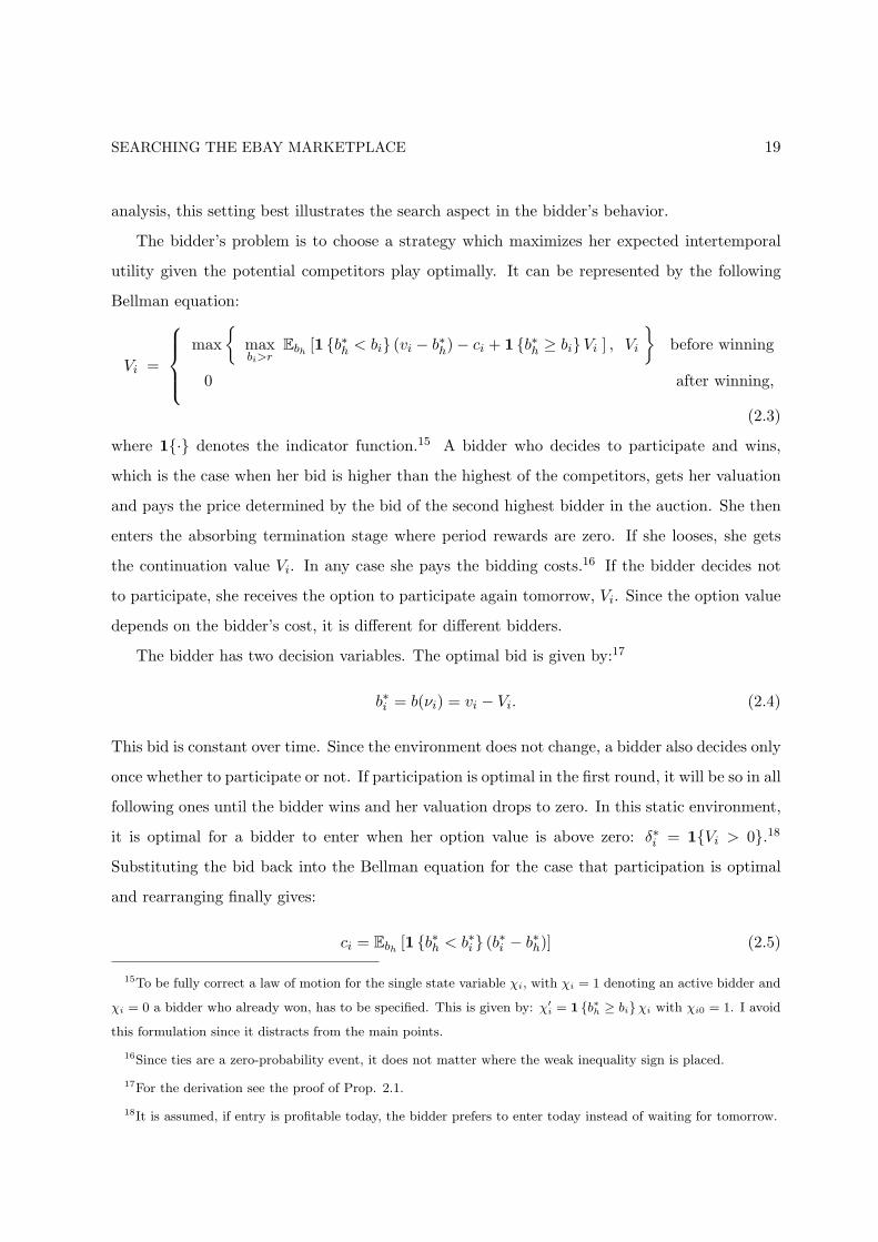
The bidder’s problem is to choose a strategy which maximizes her expected intertemporal
utility given the potential competitors play optimally. It can be represented by the following
Bellman equation:
Vi =
max{
maxbi>r
Ebh[1 {b∗h < bi} (vi − b∗h)− ci + 1 {b∗h ≥ bi}Vi ] , Vi
}before winning
0 after winning,
(2.3)
where 1{·} denotes the indicator function.15 A bidder who decides to participate and wins,
which is the case when her bid is higher than the highest of the competitors, gets her valuation
and pays the price determined by the bid of the second highest bidder in the auction. She then
enters the absorbing termination stage where period rewards are zero. If she looses, she gets
the continuation value Vi. In any case she pays the bidding costs.16 If the bidder decides not
to participate, she receives the option to participate again tomorrow, Vi. Since the option value
depends on the bidder’s cost, it is different for different bidders.
The bidder has two decision variables. The optimal bid is given by:17
b∗i = b(νi) = vi − Vi. (2.4)
This bid is constant over time. Since the environment does not change, a bidder also decides only
once whether to participate or not. If participation is optimal in the first round, it will be so in all
following ones until the bidder wins and her valuation drops to zero. In this static environment,
it is optimal for a bidder to enter when her option value is above zero: δ∗i = 1{Vi > 0}.18
Substituting the bid back into the Bellman equation for the case that participation is optimal
and rearranging finally gives:
ci = Ebh[1 {b∗h < b∗i } (b∗i − b∗h)] (2.5)
15To be fully correct a law of motion for the single state variable χi, with χi = 1 denoting an active bidder and
χi = 0 a bidder who already won, has to be specified. This is given by: χ′i = 1 {b∗h ≥ bi}χi with χi0 = 1. I avoid
this formulation since it distracts from the main points.
16Since ties are a zero-probability event, it does not matter where the weak inequality sign is placed.
17For the derivation see the proof of Prop. 2.1.
18It is assumed, if entry is profitable today, the bidder prefers to enter today instead of waiting for tomorrow.
SEARCHING THE EBAY MARKETPLACE 20
An optimal bidding policy thus equalizes the cost of bidding with the expected gain from winning
in a new trial.
The bidder’s decision rule here appears as myopic as that of the decision maker in an optimal
stopping problem which is at the basis of search models, known for example from the labor
market literature (see e.g. Albrecht and Axell (1984) and Burdett and Mortensen (1998)) or the
IO literature where a seller faces uncertain demand (see the seminal work by Diamond (1971)
and Rob (1985) for a model with heterogenous costs.). There the decision maker decides on
a reservation value which serves as a cutoff value for accepting a price or a wage offer. This
reservation value is found by equating the cost from one further search with the expected gain
from this search. As long as the environment is constant, that is the state variables do not
change over time, there is no added value in deciding sequentially. This holds true for both the
auction and the standard search setting. In both cases the state variable only changes once,
namely when the decision maker succeeds. The distribution of other bidders’ bids and the wage
or price offer curve stay constant.
By this model it is also possible to explain the buy-it-now (byn) option, offered from time
to time by sellers. If the seller offers a byn price, the item can be bought for this price without
engaging in bidding. This option can only be exercised as long as no other bid has been sub-
mitted. Exercising byn leads to a premature end of the auction. Assuming that it is less costly,
since less time consuming, for a bidder to buy by byn than by bidding, the problem changes as
follows:
Vi = max{
maxbi>r
Ebh[1 {b∗h < bi} (vi − Vi − b∗h)]− ci + Vi, vi − pbyn − cbyn
i , Vi
}.
Comparing the different options, it is easily found that a bidder exercises byn instead of bidding
if:
pbyn < Ebh[1 {b∗h < bi} bh] + Ebh
[1 {b∗h ≥ bi} (vi − Vi)] + ci − cbyni
Since I do not have enough information on the byn option in the data, I will ignore this option
in the following.
2.3.3 The General Problem
The model described so far assumed an infinite sequence of identical products. At eBay there
are hardly any two products that are exactly the same. It is therefore necessary to allow for

SEARCHING THE EBAY MARKETPLACE 21
valuations that take account of product heterogeneity. Additionally, details in the auction rules
can change. I therefore turn to the case of exogenous variation in the bidding environment as
described in subsection 2.3.1. The bidder’s problem including a minimum bid now is:
Vi(vi, s) =
max{
maxbi>r
Ebh[1 {b∗h < bi} (vi − b∗h)− ci + 1 {b∗h ≥ bi}V e
i |s] , V ei
}before winning
0 after winning,
(2.6)
where V ei denotes the expected future payoff when the bidder stays active defined by:
V ei =
∫
S
∫ v(x′)
v(x′)Vi(v′, s′)dFv
(v′|x′) dFs
(s′
). (2.7)
The main difference to before is that the continuation value now includes an expectation over
the unknown own future valuations for the products and the future realizations of the supply
side details.
The following proposition summarizes the bidder’s optimal bidding strategy and the corre-
sponding distribution of the maximum bid of the competitors, given these behave optimally as
well. All details of the computation are provided in the appendix.
Proposition 2.1. Under Assumptions 2.1-2.5, the following holds for a risk neutral bidder i
with cost ci who faces an infinite sequence of Vickrey auctions:
(a) Optimal Bidding Strategies. The bidder computes her optimal bid as:
b∗i = b(νi) = vi − V ei (2.8)
This bid is placed when b∗i > r and δ∗it = 1.
(b) Distribution of the Maximum. From the optimal behavior of all participants it follows that:
fhb(b∗h|s) = (m− 1)
∫ c
cfv(b∗h + V e|x)1{b∗h + V e ∈ D(c, s)}dFc(c)·
·
∫ c
c
∫
z∈D(c,s),
z<b∗h+V e
dFv(z|x)dFc(c)
m−2
(2.9)
and F hb(x|s) =
∫ x−∞ fh
b(b∗h|s)db∗h which is non-degenerate.
SEARCHING THE EBAY MARKETPLACE 22
Proof. See appendix.
Note that a bidder still shades her valuation by her option value. As before, the option value
is individual specific because of the differing costs. As in any second price auction, the optimal
bid does not respond to changes in current auction details such as the reserve price; different
product characteristics, however, now make it optimal to adapt it over time.
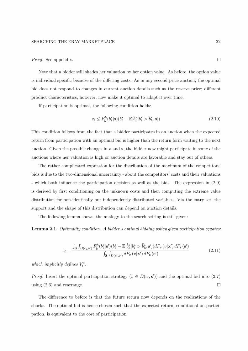
If participation is optimal, the following condition holds:
ci ≤ F hb(b∗i |s)(b∗i − E[b∗h|b∗i > b∗h, s]) (2.10)
This condition follows from the fact that a bidder participates in an auction when the expected
return from participation with an optimal bid is higher than the return form waiting to the next
auction. Given the possible changes in v and s, the bidder now might participate in some of the
auctions where her valuation is high or auction details are favorable and stay out of others.
The rather complicated expression for the distribution of the maximum of the competitors’
bids is due to the two-dimensional uncertainty - about the competitors’ costs and their valuations
- which both influence the participation decision as well as the bids. The expression in (2.9)
is derived by first conditioning on the unknown costs and then computing the extreme value
distribution for non-identically but independently distributed variables. Via the entry set, the
support and the shape of this distribution can depend on auction details.
The following lemma shows, the analogy to the search setting is still given:
Lemma 2.1. Optimality condition. A bidder’s optimal bidding policy given participation equates:
ci =
∫S
∫D(ci,s′) F h
b(b∗i |s′)(b∗i − E[b∗h|b∗i > b∗h, s′])dFv (v|x′) dFs (s′)∫
S
∫D(ci,s′) dFv (v|x′) dFs (s′)
(2.11)
which implicitly defines V ei .
Proof. Insert the optimal participation strategy (v ∈ D(ci, s′)) and the optimal bid into (2.7)
using (2.6) and rearrange.
The difference to before is that the future return now depends on the realizations of the
shocks. The optimal bid is hence chosen such that the expected return, conditional on partici-
pation, is equivalent to the cost of participation.
SEARCHING THE EBAY MARKETPLACE 23
Lemma 2.2 finally summarizes some results about the strategies which will prove useful in
the empirical part:
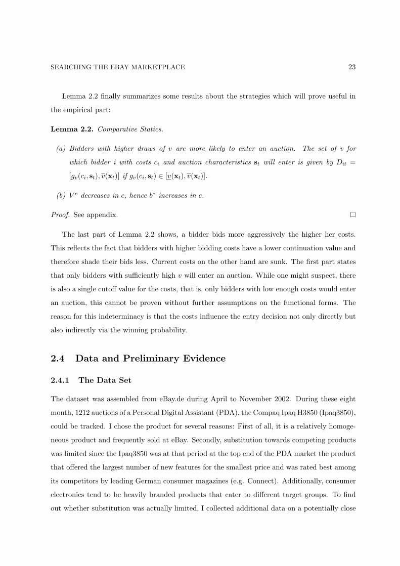
Lemma 2.2. Comparative Statics.
(a) Bidders with higher draws of v are more likely to enter an auction. The set of v for
which bidder i with costs ci and auction characteristics st will enter is given by Dit =
[gv(ci, st), v(xt)] if gv(ci, st) ∈ [v(xt), v(xt)].
(b) V e decreases in c, hence b∗ increases in c.
Proof. See appendix.
The last part of Lemma 2.2 shows, a bidder bids more aggressively the higher her costs.
This reflects the fact that bidders with higher bidding costs have a lower continuation value and
therefore shade their bids less. Current costs on the other hand are sunk. The first part states
that only bidders with sufficiently high v will enter an auction. While one might suspect, there
is also a single cutoff value for the costs, that is, only bidders with low enough costs would enter
an auction, this cannot be proven without further assumptions on the functional forms. The
reason for this indeterminacy is that the costs influence the entry decision not only directly but
also indirectly via the winning probability.
2.4 Data and Preliminary Evidence
2.4.1 The Data Set
The dataset was assembled from eBay.de during April to November 2002. During these eight
month, 1212 auctions of a Personal Digital Assistant (PDA), the Compaq Ipaq H3850 (Ipaq3850),
could be tracked. I chose the product for several reasons: First of all, it is a relatively homoge-
neous product and frequently sold at eBay. Secondly, substitution towards competing products
was limited since the Ipaq3850 was at that period at the top end of the PDA market the product
that offered the largest number of new features for the smallest price and was rated best among
its competitors by leading German consumer magazines (e.g. Connect). Additionally, consumer
electronics tend to be heavily branded products that cater to different target groups. To find
out whether substitution was actually limited, I collected additional data on a potentially close
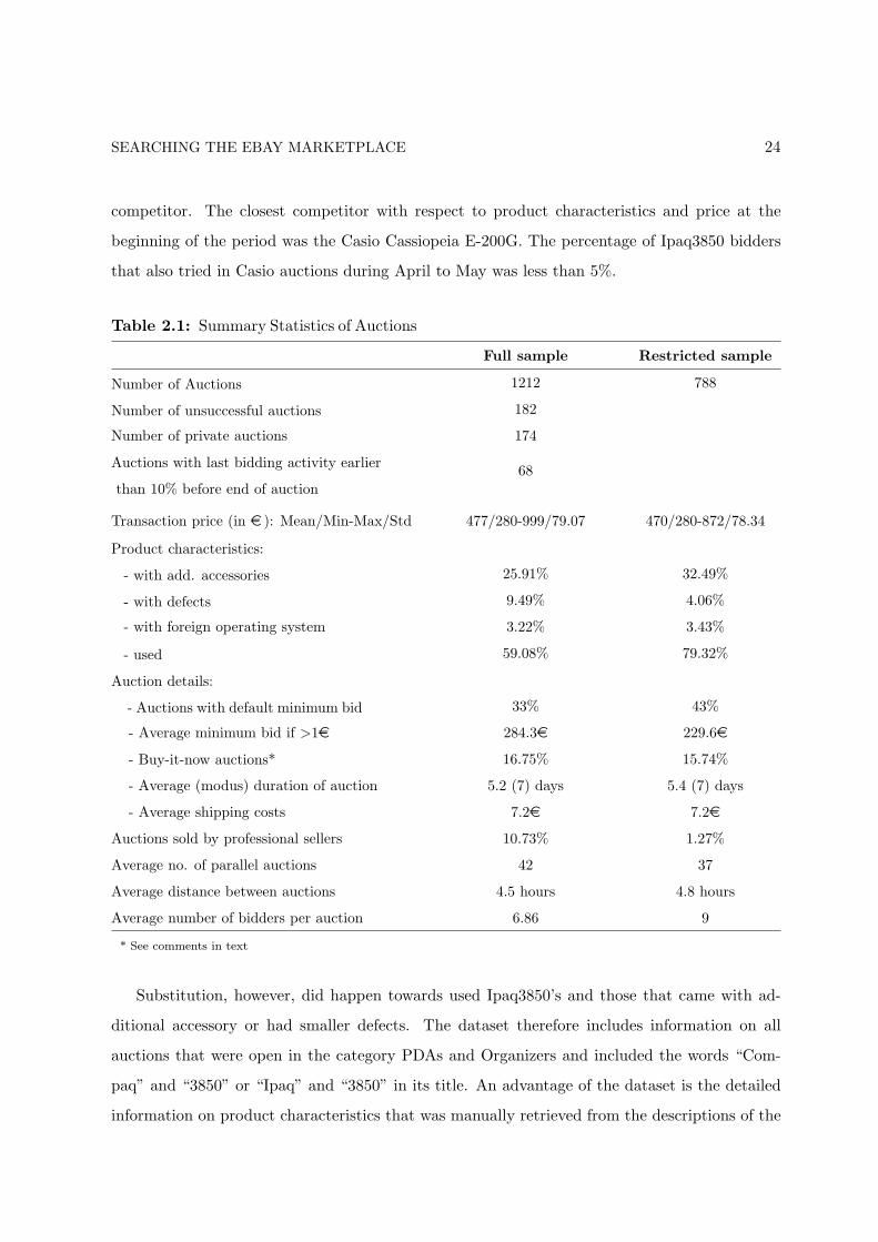
SEARCHING THE EBAY MARKETPLACE 24
competitor. The closest competitor with respect to product characteristics and price at the
beginning of the period was the Casio Cassiopeia E-200G. The percentage of Ipaq3850 bidders
that also tried in Casio auctions during April to May was less than 5%.
Table 2.1: Summary Statistics of Auctions
Full sample Restricted sample
Number of Auctions 1212 788
Number of unsuccessful auctions 182
Number of private auctions 174
Auctions with last bidding activity earlier
than 10% before end of auction68
Transaction price (in e ): Mean/Min-Max/Std 477/280-999/79.07 470/280-872/78.34
Product characteristics:
- with add. accessories 25.91% 32.49%
- with defects 9.49% 4.06%
- with foreign operating system 3.22% 3.43%
- used 59.08% 79.32%
Auction details:
- Auctions with default minimum bid 33% 43%
- Average minimum bid if >1e 284.3e 229.6e
- Buy-it-now auctions* 16.75% 15.74%
- Average (modus) duration of auction 5.2 (7) days 5.4 (7) days
- Average shipping costs 7.2e 7.2e
Auctions sold by professional sellers 10.73% 1.27%
Average no. of parallel auctions 42 37
Average distance between auctions 4.5 hours 4.8 hours
Average number of bidders per auction 6.86 9
* See comments in text
Substitution, however, did happen towards used Ipaq3850’s and those that came with ad-
ditional accessory or had smaller defects. The dataset therefore includes information on all
auctions that were open in the category PDAs and Organizers and included the words “Com-
paq” and “3850” or “Ipaq” and “3850” in its title. An advantage of the dataset is the detailed
information on product characteristics that was manually retrieved from the descriptions of the
SEARCHING THE EBAY MARKETPLACE 25
sellers. Appendix B.1 lists the variables and provides detailed descriptions. A product’s quality
is, first of all, assessed by the age and the condition of the product as stated by the seller. This
category, further, includes dummies for non German operating systems and different kinds of
defects, such as scratches and missing standard accessory. Next, there is a number of additional
accessories that are frequently bundled with the Ipaq3850. The most typical extras are covers,
memory cards, charge and synchronization cables, and expansion packs (jackets), plastic casings
that enhance the functionality of Ipaqs by for example providing extra slots for memory cards.
Most common among the expensive extras are navigation systems and microdrives. Finally, the
seller’s quality might have an influence on the valuation, a buyer ascribes to the product. This
is captured by the seller’s eBay reputation and the variable PROFI that takes the value 1 if the
seller gives reference to an own shop outside eBay.
While eBay’s selling mechanism is mostly standardized, the seller can choose among a number
of smaller details to customize his auction. eBay auctions have a fixed duration (hard close)
that varies in between 3, 5, 7 and 10 days. Most often sellers choose a duration of 7 days. By
paying a small additional fee, the seller can raise the default minimum bid above 1e . 67% of
sellers choose this option by asking on average for minimum bids in excess of 284e . Around 1/6
of the auctions were bought by buy-it-now. Since this information is only available in the data
when it was actually exercised or the auction did not receive any bids, the actual percentage of
auctions that carried this option is higher.19 Finally, the seller can choose the option private in
which case the pseudonyms of the bidders are not revealed. Sellers choose this option in 14.4%
of the observed auctions.
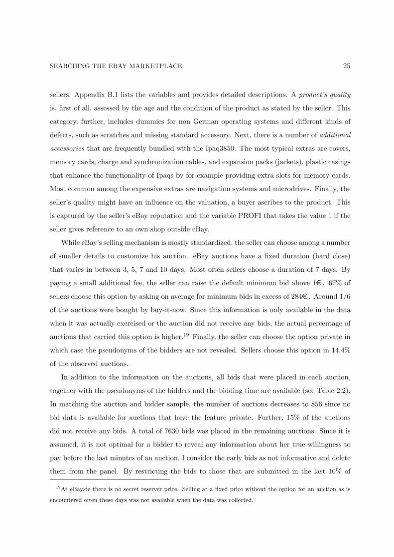
In addition to the information on the auctions, all bids that were placed in each auction,
together with the pseudonyms of the bidders and the bidding time are available (see Table 2.2).
In matching the auction and bidder sample, the number of auctions decreases to 856 since no
bid data is available for auctions that have the feature private. Further, 15% of the auctions
did not receive any bids. A total of 7630 bids was placed in the remaining auctions. Since it is
assumed, it is not optimal for a bidder to reveal any information about her true willingness to
pay before the last minutes of an auction, I consider the early bids as not informative and delete
them from the panel. By restricting the bids to those that are submitted in the last 10% of
19At eBay.de there is no secret reserver price. Selling at a fixed price without the option for an auction as is
encountered often these days was not available when the data was collected.
SEARCHING THE EBAY MARKETPLACE 26
Table 2.2: Summary Statistics of Bidders
Full sample Restricted sample
Number of bids 7630 3202
Number of individual bidders 3829 1869
Av. number of trials 2 1.7
Importance of “switching back”.* 9.72 % 3.1 %
Importance of “simultaneous bidding”.** 10.13 % 3.6 %
Bidder is observed in sample for:
Mean 5.65 days 7.15 days
Quantiles (25 50 75) 0min 5.6min 1.89 days 0min 2.44hrs 3.98 days
Bids (in e ):
Mean/Min-Max/Std. dev 334/1-827/155.39 438/203 - 872/78.73
Av. std. dev. per bidder 52.21 27.13
* Percentage of bids, placed by a bidder in an auction t after she was outbid in auction t+1.
* Percentage of bids, placed by a bidder while she still had a standing bid in another auction.
the time, the number of bids reduces to 3202 observations. The 10% mark is found by striking
a balance between the informativeness of the bids and the number of remaining observations
per bidder.20 Figure 2.1 displays the bid distribution in the full (left) and the restricted sample
(right). The full distribution displays a second peak at very low prices. This is due to a number
of bids between 1e and 20e . Bidders will hardly believe, they will win with these bids. One
explanation why bidders engage in these bids is that it is an easy way to track an auction.21 By
excluding early bids the two peakedness of the distribution disappears.
Table 2.1 reports summary statistics of the remaining 788 auctions. Every day around 5
Ipaq3850 auctions closed. 20% of these auctions offered new products, 33% were bundled with
20Whenever possible, the estimation procedure will rely on the highest observed bids only since these are the
ones that are most likely to reflect bidders’ optimal bids in an ascending price auction (see Haile and Tamer
(2003) and Song (2004)). They are also least affected by the 10% cutoff rule.
21As opposed to eBay.com at eBay.de auctions that are closed cannot be searched for anymore. Alternative
ways for obtaining information on the price at which an auction closed are to use eBays tracking service (”observe
auctions”), to remember the ID of an auction and construct the URL afterwards manually, or to just participate,
since participants receive an email with all the necessary information at the end of the auction.

SEARCHING THE EBAY MARKETPLACE 270
.001
.002
.003
.004
Den
sity
0 200 400 600 800 1000Bid
0.0
02.0
04.0
06D
ensi
ty
200 400 600 800 1000Bid
Figure 2.1: Density of All Bids and Bids Submitted in Last 10% of an Auction.
additional accessories, 3.5% came with a non-German operating system, and 4% had some
other kind of defect such as scratches or missing standard accessory. Winners paid on aver-
age 469.93e for their products (Std: 78.34e , min: 280e , max: 872 Euro) plus an additional
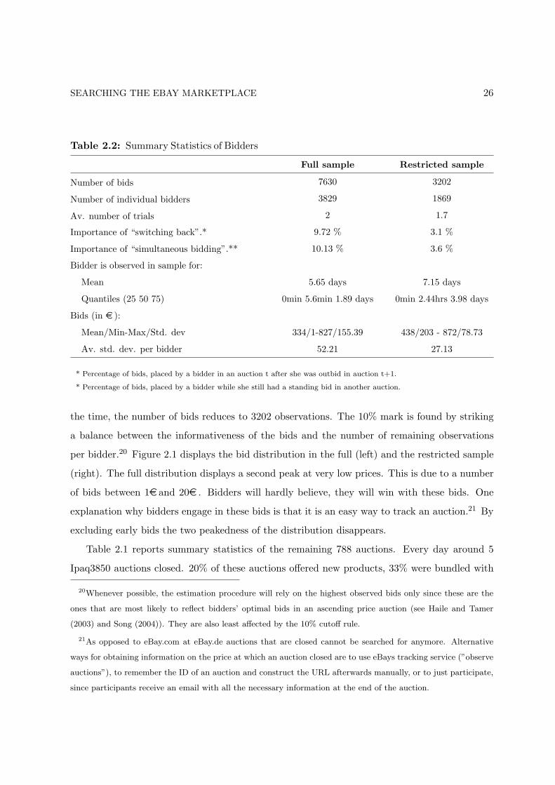
7.2e for shipping and handling. Figure 2.2 displays the evolution of prices over time. There
is a pronounced decrease in the average transaction price during the sample period. This is
probably due to the high tech characteristic of the product. After correcting for this, apply-
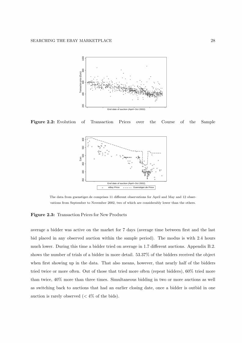
ing a simple linear time trend, the average standard deviation reduces to 52.83e . Figure 2.3
compares transactions prices at eBay for standard products as sold in the shop, that is, new
products without any extras, with the corresponding prices from guenstiger.de, a German price
comparison machine. From the graphic it appears as if the guenstiger.de prices built an upper
bound to the prices at eBay.22
The 788 auctions are won by 744 different bidders. Only around 6 % of the winners thus
buy more than 1 item. Bidders that buy more than one item are in the following regarded
as different bidders, that is, for the purpose of the regression they receive a new identity after
winning. Table 2.2 reports summary statistics of the bids for the full and the restricted sample.
The bids that were placed in the last 10% of the time stem from 1869 different bidders. On
22Since I have only a few price observations from the beginning and the end of the period, I can not exclude
that heavy price drops as they can be observed in the guenstiger.de data towards the end of the sample period
are not an exception but the rule.
SEARCHING THE EBAY MARKETPLACE 28
200
400
600
800
1000
Tran
sact
ion
pric
e (E
uro)
End date of auction (April−Oct 2002)
Figure 2.2: Evolution of Transaction Prices over the Course of the Sample
350
400
450
500
550
600
Euro
End date of auction (April−Oct 2002)
eBay Price Guenstiger.de Price
The data from guenstiger.de comprises 11 different observations for April and May and 12 obser-
vations from September to November 2002, two of which are considerably lower than the others.
Figure 2.3: Transaction Prices for New Products
average a bidder was active on the market for 7 days (average time between first and the last
bid placed in any observed auction within the sample period). The modus is with 2.4 hours
much lower. During this time a bidder tried on average in 1.7 different auctions. Appendix B.2.
shows the number of trials of a bidder in more detail. 53.37% of the bidders received the object
when first showing up in the data. That also means, however, that nearly half of the bidders
tried twice or more often. Out of those that tried more often (repeat bidders), 60% tried more
than twice, 40% more than three times. Simultaneous bidding in two or more auctions as well
as switching back to auctions that had an earlier closing date, once a bidder is outbid in one
auction is rarely observed (< 4% of the bids).
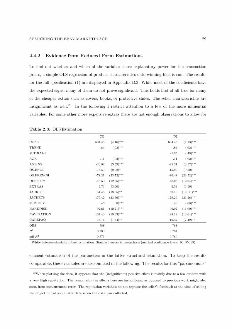
SEARCHING THE EBAY MARKETPLACE 29
2.4.2 Evidence from Reduced Form Estimations
To find out whether and which of the variables have explanatory power for the transaction
prices, a simple OLS regression of product characteristics onto winning bids is run. The results
for the full specification (1) are displayed in Appendix B.3. While most of the coefficients have
the expected signs, many of them do not prove significant. This holds first of all true for many
of the cheaper extras such as covers, books, or protective slides. The seller characteristics are
insignificant as well.23 In the following I restrict attention to a few of the more influential
variables. For some other more expensive extras there are not enough observations to allow for
Table 2.3: OLS Estimation
(2) (3)
CONS 601.45 (4.16)∗∗∗ 604.45 (4.13)∗∗∗
TREND -.84 (.02)∗∗∗ -.84 (.02)∗∗∗
# TRIALS -1.95 (.49)∗∗∗
AGE -.11 (.02)∗∗∗ -.11 (.02)∗∗∗
AGE NS -26.82 (3.59)∗∗∗ -25.31 (3.57)∗∗∗
OS ENGL -18.53 (9.92)∗ -15.90 (9.50)∗
OS FRENCH -78.21 (23.72)∗∗∗ -80.48 (23.52)∗∗∗
DEFECT2 -46.50 (12.55)∗∗∗ -48.08 (12.64)∗∗∗
EXTRAS 5.73 (3.60) 5.53 (3.56)
JACKET1 54.46 (18.65)∗∗ 58.16 (19..11)∗∗∗
JACKET5 179.42 (23.56)∗∗∗ 179.29 (23.26)∗∗∗
MEMORY .46 (.08)∗∗∗ .46 (.08)∗∗∗
HARDDISK 92.61 (10.71)∗∗∗ 96.07 (11.00)∗∗∗
NAVIGATION 131.40 (19.33)∗∗∗ 128.19 (18.64)∗∗∗
CAREPAQ 16.74 (7.64)∗∗ 16.42 (7.49)∗∗
OBS 788 788
R2 0.780 0.784
adj R2 0.776 0.780
White heteroscedasticity robust estimation. Standard errors in parenthesis (marked confidence levels: 90, 95, 99).
efficient estimation of the parameters in the latter structural estimation. To keep the results
comparable, these variables are also omitted in the following. The results for this “parsimonious”
23When plotting the data, it appears that the (insignificant) positive effect is mainly due to a few outliers with
a very high reputation. The reason why the effects here are insignificant as opposed to previous work might also
stem from measurement error. The reputation variables do not capture the seller’s feedback at the time of selling
the object but at some later date when the data was collected.
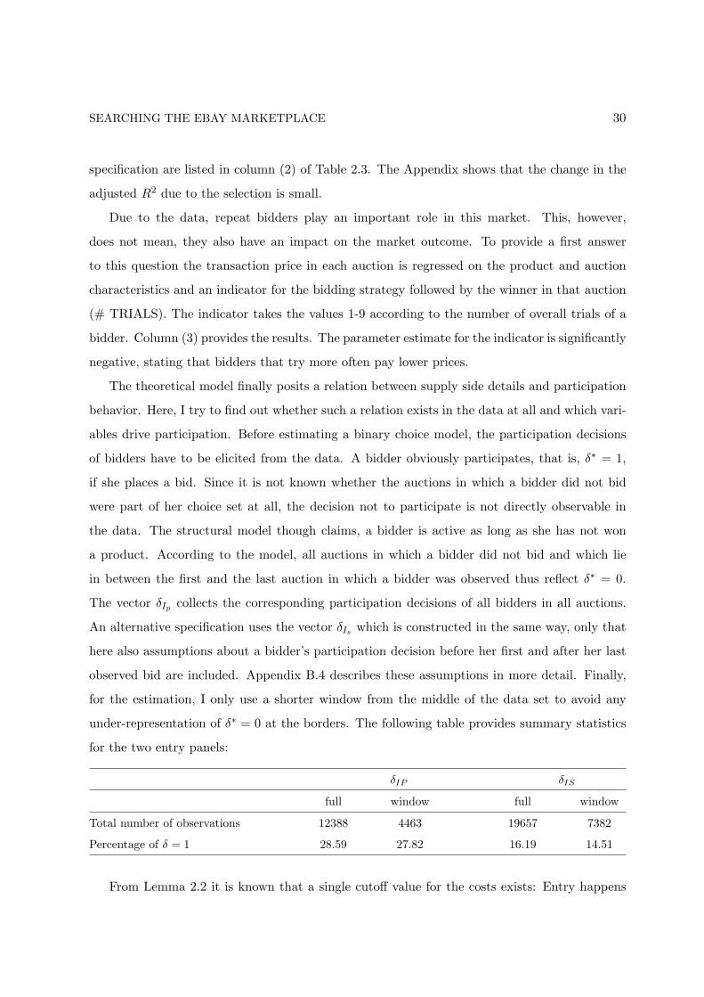
SEARCHING THE EBAY MARKETPLACE 30
specification are listed in column (2) of Table 2.3. The Appendix shows that the change in the
adjusted R2 due to the selection is small.
Due to the data, repeat bidders play an important role in this market. This, however,
does not mean, they also have an impact on the market outcome. To provide a first answer
to this question the transaction price in each auction is regressed on the product and auction
characteristics and an indicator for the bidding strategy followed by the winner in that auction
(# TRIALS). The indicator takes the values 1-9 according to the number of overall trials of a
bidder. Column (3) provides the results. The parameter estimate for the indicator is significantly
negative, stating that bidders that try more often pay lower prices.
The theoretical model finally posits a relation between supply side details and participation
behavior. Here, I try to find out whether such a relation exists in the data at all and which vari-
ables drive participation. Before estimating a binary choice model, the participation decisions
of bidders have to be elicited from the data. A bidder obviously participates, that is, δ∗ = 1,
if she places a bid. Since it is not known whether the auctions in which a bidder did not bid
were part of her choice set at all, the decision not to participate is not directly observable in
the data. The structural model though claims, a bidder is active as long as she has not won
a product. According to the model, all auctions in which a bidder did not bid and which lie
in between the first and the last auction in which a bidder was observed thus reflect δ∗ = 0.
The vector δIp collects the corresponding participation decisions of all bidders in all auctions.
An alternative specification uses the vector δIs which is constructed in the same way, only that
here also assumptions about a bidder’s participation decision before her first and after her last
observed bid are included. Appendix B.4 describes these assumptions in more detail. Finally,
for the estimation, I only use a shorter window from the middle of the data set to avoid any
under-representation of δ∗ = 0 at the borders. The following table provides summary statistics
for the two entry panels:
δIP δIS
full window full window
Total number of observations 12388 4463 19657 7382
Percentage of δ = 1 28.59 27.82 16.19 14.51
From Lemma 2.2 it is known that a single cutoff value for the costs exists: Entry happens
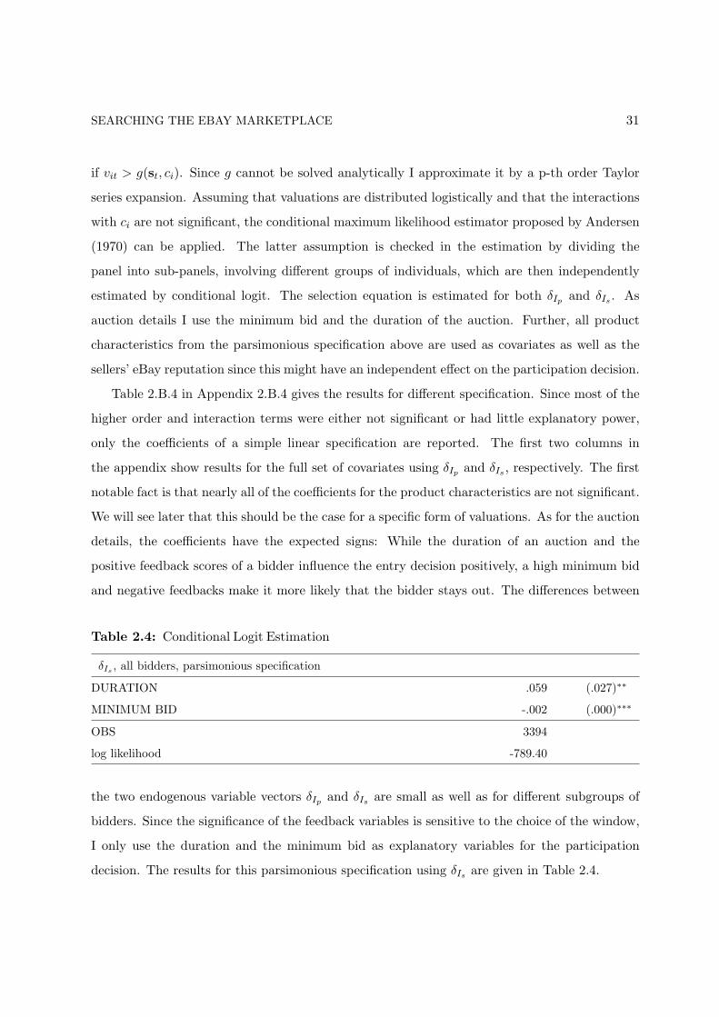
SEARCHING THE EBAY MARKETPLACE 31
if vit > g(st, ci). Since g cannot be solved analytically I approximate it by a p-th order Taylor
series expansion. Assuming that valuations are distributed logistically and that the interactions
with ci are not significant, the conditional maximum likelihood estimator proposed by Andersen
(1970) can be applied. The latter assumption is checked in the estimation by dividing the
panel into sub-panels, involving different groups of individuals, which are then independently
estimated by conditional logit. The selection equation is estimated for both δIp and δIs . As
auction details I use the minimum bid and the duration of the auction. Further, all product
characteristics from the parsimonious specification above are used as covariates as well as the
sellers’ eBay reputation since this might have an independent effect on the participation decision.
Table 2.B.4 in Appendix 2.B.4 gives the results for different specification. Since most of the
higher order and interaction terms were either not significant or had little explanatory power,
only the coefficients of a simple linear specification are reported. The first two columns in
the appendix show results for the full set of covariates using δIp and δIs , respectively. The first
notable fact is that nearly all of the coefficients for the product characteristics are not significant.
We will see later that this should be the case for a specific form of valuations. As for the auction
details, the coefficients have the expected signs: While the duration of an auction and the
positive feedback scores of a bidder influence the entry decision positively, a high minimum bid
and negative feedbacks make it more likely that the bidder stays out. The differences between
Table 2.4: Conditional Logit Estimation
δIs , all bidders, parsimonious specification
DURATION .059 (.027)∗∗
MINIMUM BID -.002 (.000)∗∗∗
OBS 3394
log likelihood -789.40
the two endogenous variable vectors δIp and δIs are small as well as for different subgroups of
bidders. Since the significance of the feedback variables is sensitive to the choice of the window,
I only use the duration and the minimum bid as explanatory variables for the participation
decision. The results for this parsimonious specification using δIs are given in Table 2.4.
SEARCHING THE EBAY MARKETPLACE 32
2.5 Identification
The structural parameters of interest in the general model considered in Subsection 2.3.3 are
bidders’ valuations for the product conditional on its characteristics and the individual bidding
costs. The focus in the existing empirical work on auctions has been on the distribution of
bidders’ valuations. The main aim of this work is to see whether individual specific demand
parameters which affect strategies when dynamic considerations are taken into account, can be
identified as well when data with a panel structure is available.
In principle, all information is summarized in the distribution of the observed bids. Full
information Maximum Likelihood inference, if feasible at all, would though be computationally
very expensive in the current setting. Difficulties arise due to unobserved winning bids, endoge-
nous selection, and correlation among bids of the same bidder. Further, no closed form solution
exists for the value function as a function of the unobserved costs. By extending results known
from the literature on estimating demand from auction data, the first set of issues can be dealt
with. The problem with the unknown value function is solved when as in the literature on
estimating dynamic games the full information approach is swapped for a less efficient stepwise
procedure (see e.g. Bajari et al. (2005) and Pakes et al. (2005)). The following discussion on
identification focuses on the identifying restrictions in such a stepwise approach.
Rewriting the optimality condition given in (2.11) for bidder i as a function of optimal bids
and the optimal participation decision of bidder i and using the expectations operator gives:
ci = Es, b∗i [Fhb(b∗i |s)(b∗i − E[b∗h|b∗i > b∗h, s])|δ∗i = 1]
The expectation is still build over the auxiliary random variable bj whose maximum over all
j is distributed according to fhb|s depicted in Prop. 2.1. As was pointed out before, the two
viewpoints, either attach zero winning probability to bids which fall below the participation
threshold but still include the corresponding bidders when building the expectation or only
include bids of participants and build expectations over different participation patterns, lead to
the same result. While the former viewpoint proved more practical when trying to express the
distribution of the bids as a function of the underlying distributions of costs and valuations, the
latter viewpoint will be entertained in the empirical part since what we observe in the data is
a draw from the distribution of b∗j conditional on δ∗j = 1. The expected return from winning is
then built over different b∗h and different participation vectors δ∗−i.
SEARCHING THE EBAY MARKETPLACE 33
Lemma 2.3. Given observations on supply side characteristics s, on all bids of participants, and
hence on participation decisions in case they are affirmative, bidder i’s costs can be computed
from:
ci = Es, b∗i [Fhb (b∗i |s)(b∗i − E[b∗h|b∗i > b∗h, s])|δ∗i = 1]), (2.12)
where F hb|s denotes the expected distribution of the highest bid over different participation vectors.
Proof. See Appendix.
In principle, the behavior of all bidders as well as the product characteristics and the auction
details can be observed at eBay. However, in a second price auction winning bids are not
observable but only a lower bound to them, the transaction prices which correspond to the
second highest bids. Using the observed bids would therefore bias the cost estimates. Estimates
of the parent distribution(s) from which all bids ultimately are drawn can, however, be obtained
from the observed bids by exploiting information contained in the ordering of the bids following
methodologies developed in the empirical auctions literature. The parent distribution(s) can
then be used to construct estimates of the unobserved winning bids which will be used to
complete the bid data set.
Since bids of the same bidder are correlated across auctions, it has to be taken into account
that the parent distributions from which bidders draw their bids conditional on a certain draw
of c are not identical. Identification results for likelihood inference in second price auctions with
asymmetric bidders are available when the data consists of transaction prices and the identity
of the winner (see Athey and Haile (forthcoming) and Brendstrup and Paarsch (2004)). These
identification results can be traced back to the literature on competing risks. An insight from
this literature, which becomes valuable in the asymmetric bidders’ case, is that knowledge of
bidders’ identities eases identification (see Berman (1963) and Prakasa Rao (1992)). In the eBay
setting identities and bids of all of the loosing bidders are available as well. Song (2004) points
to the fact that, if lower ordered bids are observable, estimating from the distribution of the
second highest bid conditional on the third highest bid allows inference without having to know
the total number of bidders. Combining these two results, the following lemma can be stated:
SEARCHING THE EBAY MARKETPLACE 34
Lemma 2.4. Let X1, ..., Xn be independent random variables with continuous distribution func-
tions Fi, i = 1, . . . , n.
(a) The probability distribution of the highest observed bid Xn−1:n with realization b2 con-
ditional on the third highest bid being Xn−2:n = b3 when the identities of the winner,
respectively the second and third highest bidder, are In:n = m, In−1:n = l, and In−2:n = k
is given by:
gn−1:n( b2, m, l| b3 ) =(1− Fm( b2 )) fl( b2 )
(1− Fm( b3 )) (1− Fl( b3 ))= (1− Fm( b2 | b3 )) fl( b2 | b3 ) (2.13)
(b) The Fi(·) are nonparametrically identified from observation of the second and third highest
bids when the identities of the winner and the second highest bidder are observed as well.
Proof. See Appendix.
In the asymmetric setting conditioning thus makes the distribution to estimate not only
independent of the number of lower ordered bids but also of the distribution functions of these
bidders. The distribution of the conditioning variable y is irrelevant as well, what matters is its
value.
Letting Fi be the bid distribution for bidder i we have from Lemma 2.4 that these are
identified from eBay data. Since the common distribution of valuations only differs by an
individual specific constant V ei from the individual bid distributions, they can easily be related.
However, identification is, as opposed to the static setting, only possible up to location since
the common parts in v and V e cannot be separated. Given the bid distributions, estimates of
the unobserved winning bids can be built and thus the costs can be computed from 2.12. The
following proposition summarizes the preceding discussion and presents the main identification
results:
Proposition 2.2. Under the assumptions of the theoretical model proposed in 2.3.3, the follow-
ing holds given eBay data:
(a) The distribution of valuations is nonparametrically identified up to location.
(b) Bidding cost are nonparametrically identified.
Proof. See Appendix.
SEARCHING THE EBAY MARKETPLACE 35
2.6 Estimation
After having established identification, I can now come to the procedure for estimating the
parameters of interest. The algorithm proceeds in steps:
1. Estimation of the observed bid distribution using information on the second and third
highest bid as well as the identities of the winner and the second highest bidder.
2. Estimation of the expected highest bids and replacement of the observed bids of the winners
by these estimates.
3. Computation of the bidding costs.
Since the first step requires the unknown costs as an input, the steps have to be iterated until
convergence.
2.6.1 Preliminaries: Bidder’s Valuations
While nonparametric identification is possible, the data requirements for nonparametric estima-
tion are huge. A characterizing feature of eBay data though is that the products are normally
rather heterogenous and the time dimension of the panel, that is, the number of observations
per bidder, is small. Finding an expected value for each bidder and all combinations of s in
equation (2.12) therefore is a limiting factor which should be considered when devising an esti-
mation procedure. An alternative is to first homogenize the data so that the bids present bids
for identical products and use the corrected data to build an expected value for c as described
above. This approach relies on some mild parametric assumptions.
The influence of product heterogeneity is via bidders’ valuations; homogenization of the
data thus starts from assumptions about the form of this dependency. To ease identification a
common index assumption with additive errors is maintained:
Assumption 2.6. Additive Separability. Bidders’ private information is composed of a
common object specific component and an additive idiosyncratic part: vit = v(xt)+ εit. The εit’s
are iid draws from fε(ε; 0, σε) and are independent of ci.
From the additive form of the bidders’ valuations it follows that product characteristics do
not determine winning odds and expected returns.

SEARCHING THE EBAY MARKETPLACE 36
Lemma 2.5. Under Assumption 2.6, the optimal entry strategy δ∗it and hence the entry set Dit
as well as the optimality condition given by (2.11) are independent of product characteristics.
Proof. Optimal bids are now given by: b∗it = v(xt) + εit − V ei . Using these in entry condition
(2.10) gives: E[1maxj 6=i{v(xt)+εjt−V ej } < v(xt)+εit−V e
i }(v(xt)+εit−V ei −maxj 6=i{v(xt)+εjt−
V ej })] ≥ ci which readily simplifies to E[1{maxj 6=i{εjt−V e
j } < εit−V ei }(εit−V e
i −maxj 6=i{εjt−V e
j })] ≥ ci. The proof for the optimality condition (2.11) follows along the same lines.
Firstly, the product characteristics in the selection equation can thus be ignored, that is,
all bidders with draws of εit > gε(ci,at) participate. The findings from the conditional logit in
section 2.4 corroborate this result. Secondly, for the purpose of estimation of the costs, the data
can first be homogenized and then only estimates of b∗i − v(xt) and maxj 6=i{b∗i − v(xt)|δ∗j = 1}for each a ∈ A and all bidders are needed. This is advantageous since it reduces the data
requirements for consistent estimation since dim(a) < dim(s).
In principle estimation could now start from here. Given the large number of equally impor-
tant covariates as compared to the total number of observations in my specific data set, I will
simplify further and use an hedonic approach for v(x) which stipulates a simple linear relation
between product characteristics (1,x) = (1, x1, . . . , xK) and bidders’ valuations. Combining this
with Assumption 2.6 it follows for the bids:
b∗it = CONS + xtβ1 + b0it with CONS = β0 − V
e (2.14)
and b0it = −V 0
i + εit.
(β0, β1) = (β0, β11, β12, . . . , β1Kx) collects the common parameters and V 0i = V e
i − Ve is the
individual specific influence of the continuation value. In other data sets for eBay one could
think of using a nonparametric approximation for the function v(x) instead.
2.6.2 Estimation of Parent Distributions and of Missing Winning Bids
From the proof of Proposition 2.2 it follows that the likelihood contribution per auction is given
by:fbl
(b2|x)(1− Fbm(b2|x))(1− Fbm(b3|x))(1− Fbl
(b3|x))(2.15)
where b2 and b3 denote the observed second, respectively third highest bid and m and l the
identities of the winner and the second highest bidder. Since auctions are independent of each
SEARCHING THE EBAY MARKETPLACE 37
other, the log likelihood just sums the individual contributions:
l =T∑
t=1
ln
[fblt
( b2t |xt) (1− Fbmt( b2t |xt))
(1− Fbmt( b3t |xt)) (1− Fblt
( b3t |xt)
](2.16)
Song (2004) proposes a semi-nonparametric procedure for estimation. As opposed to her
case, here the parent bid distributions are bidder specific. Given the small time dimension
of the panel it does not make sense to attempt a nonparametric approach. Instead, I use a
normal form for the parent bid distributions.24 The individual parameters as well as product
characteristics then only affect the mean: fbi(bi|x) = N [µbi , σ] with µbi = CONS + xβ1 − V 0i .
Given the huge amount of bidders as compared to the number of auctions, is it not feasible
to estimate the V ei as parameters. Instead, I exploit the fact that option values are functions
of the individual costs. The V 0i thus can be approximated by a polynomial in ci. The ci are,
however, only known at the next step. I thus start with an initial guess for these costs given
by the observed number of trials of a bidder and then iterate this and the following steps until
convergence. The choice of the starting value is motivated by the fact that bidders with lower
costs will in expectation try more often until they win a product than those with higher costs,
so the two variables are correlated.
Once estimates of the parent bid distributions, Fbi|x, are obtained, the expected winning bid
of bidder i in auction t, given it is higher than the bid of the second highest bidder, is computed
from:
bn:nit ≡ E[bit|bit > b2t,xt; Fbi|x] =
11− Fbi(b2t|xt)
∫ ∞
b2t
bitdFbi(bit|xt) (2.17)
Due to the conditioning, the participation decision again becomes irrelevant. These estimates
replace in the following the truncated winning bids.
2.6.3 Computation of Bidding Costs
From Lemma 2.5 we know that the optimality condition is independent of product characteris-
tics. What matters, however, are the auction details. The conditional logit estimation identified
the duration d of an auction and the minimum bid r as the major factors influencing participa-
tion. The possible combinations of these details are collected in the set A = {a1, · · · ,aK}. Let
24Trials with log normal and gamma distributions gave similar, though, slightly worse results.
SEARCHING THE EBAY MARKETPLACE 38
b0i = {b0
i1, . . . , b0iK} be the set of estimated residuals for bidder i from the prior step, where
b0ik = {b0
ik1, . . . , b0iaTik
} collects the residuals for bidder i from those auctions that have auction
details ak. Equivalently b0hk = {b0
hk1, . . . , b0ikThk
} collect the highest bids in all auctions with
details ak. Expressing the expectations in terms of their sample means then gives:
ci =K∑
k=1
αk
∑
b0i∈b0ik
1Tik
∑
b0h∈b0hk
1Thk
1{b0h < b0
i }(b0i − b0
h) (2.18)
where αk presents the empirical share of auction details ak.25
My eBay data is not rich enough to offer enough observations for each bidder so that the
individual beliefs for the error term conditional on all combinations of auction details can be
elicited from the data to build this expectation correctly. Even when only major groups of auc-
tion details are distinguished, for example, A = {(d < 7 days, low r), (d ≥ 7 days, low r), (d <
7 days, high r), (d ≥ 7 days, high r)}, correct computation is only possible for a few bidders. I
thus have to ignore the weighting by auction details. The error due to this simplification is alle-
viated by the fact, that the highest bid of the competitors will be affected by this simplification
in a similar way.26 A Monte Carlo study could help to assess how big the remaining mistake is.
This is deferred to future research.
2.6.4 Alternative Approaches
Due to data limitations, distributional assumptions were made in the prior estimation procedure
for the bid distribution (Specification 1). Further, the likelihood estimation depends on the
incidental parameter ci and could for that reason provide inconsistent estimates. In this section,
I will introduce some other specifications which should be seen as a robustness check on the
results.
Since at eBay all lower bids are observed as well, the winning bids usually only present a
small share. It would thus be interesting to check whether ignoring the problem of the truncated
25To be fully correct, the expectation should be independently done for different participation vectors as well.
For notational ease and since the data restrictions anyways do not allow to do this summation, I ignore this aspect
here.
26“Linear effects” would just be differenced away, following the same logic as, when arguing, in the proof to
Lemma 2.5, that product characteristics are irrelevant.
SEARCHING THE EBAY MARKETPLACE 39
winning bids would have a major impact on the results (Specification 3). Another approach is to
use additional price data (Specification 2). In the data description it could be seen that the prices
from guenstiger.de built an upper bound to the prices at eBay. Assuming that a bidder always
prefers to buy at guenstiger.de when the prices are equal, any value in between the guenstiger.de
prices and the transaction prices (e.g. half the difference) can be used as an estimate for the
unobserved winning bids. The drawback of this approach is that normally one will not have price
data for all additional extras that are bundled with the eBay products and certainly will not have
external information on the discount attached to used products or products with defects. If one
is willing to assume that the relative prices between additional features and the basic product
are the same for eBay and guenstiger.de, fictional prices for guenstiger.de-prices for extras can
be computed though by multiplying the eBay.de average price for extras - represented e.g. by
the OLS regression coefficients times the value of the variable - with the ratio of the average
observed guenstiger.de price and the average eBay transaction price for standard new products.
As opposed to Specification 1, both approaches do not provide estimates of bidders’ val-
uations. To be able to homogenize the data, thus, an additional step is required. Given the
completed data and using the prior assumptions on the form of the valuations, standard panel
methods, such as first differencing, can be applied in principle. A difficulty arises through the
participation decision which causes that only selected bids of a bidder can be observed. It is
therefore necessary to distinguish the latent data, in the following denoted by an asterisk, from
the observed data (without asterisk). The bid equation (2.14) in its difference form now writes
as:
bit − bi,t−1 = δitb∗it − δi,t−1b
∗i,t−1 = (δit − δi,t−1)CONS + (δitxt − δi,t−1xt−1)β1−
−(δit − δi,t−1)V 0∗i + δitε
∗it − δi,t−1ε
∗i,t−1. (2.19)
Since δ is always one when observed and since the product characteristics are not affected by
the participation decision, the equation simplifies to:
bit − bi,t−1 = (xt − xt−1)β1 + δitε∗it − δi,t−1ε
∗i,t−1. (2.20)
Lets first look at the case when only the product characteristics but not the auction details
change over time (Specification a). While E[ε∗it|δit = 1, δi,t−1 = 1] is not zero, it is equal to
E[ε∗i,t−1|δi,t−1 = 1, δit = 1] for all differences of bids of the same bidder and thus falls out. The
parameter vector β1 therefore can be consistently estimated by OLS from (2.20).
SEARCHING THE EBAY MARKETPLACE 40
The more general case is when the participation decision responds to auction covariates. Now,
the parameters γ from the participation equation which has been estimated before (coefficients
of the conditional logit estimation in Section 2.4 ) are used as described in Kyriazidou (1997)
to construct weights (Specification b). These weights are used in the OLS estimation of the
first differenced bid data to over-represent differences that are based on the same underlying
explanatory variables for participation and to under-represent the others. The idea is that when
the exogenous variables explaining selection are the same, the selection bias is the same and can
be differenced out. The parameter vector β1 is now estimated by OLS from:
∆bit
√K
(∆atγ
h
)= ∆xt
√K
(∆atγ
h
)β1 + ∆εit, (2.21)
where K(·) denotes a kernel density and h the bandwidth of data to be included.
After homogenizing the data, the bidding costs can be computed as described before.
2.7 Results
2.7.1 Bidders’ Valuations for Product Characteristics
Table 2.5 (1) reports the results from the estimation of the bid distribution by conditional order
statistics distributions. Since only those auctions where at least three bidders placed bids can
be used for the estimation, the number of auctions in the sample reduces to 537.
As an approximation to the value function I use a second order Taylor approximation in the
costs. I1 and I2 report the estimated coefficients. As expected V e decreases in the costs, but
does so at a decreasing rate.
Due to the normal form of the parent bid distribution the remaining estimates directly
describe bidders’ valuations. Not much can be said about the mean of the distribution of
valuations, only that it is above 520.38e , since the estimated constant subsumes the constant
part of the valuations and of the continuation values. The standard deviation of the distribution
is estimated at 25.41e .
The negative time trend indicates that over time the valuations for the product decrease.
As already mentioned, this is due to the high tech characteristic of the product. Age, defects,
and a foreign operating system have a negative effect on the valuation, while additional extras
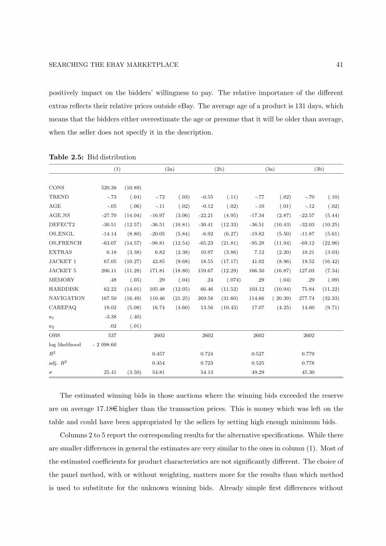
SEARCHING THE EBAY MARKETPLACE 41
positively impact on the bidders’ willingness to pay. The relative importance of the different
extras reflects their relative prices outside eBay. The average age of a product is 131 days, which
means that the bidders either overestimate the age or presume that it will be older than average,
when the seller does not specify it in the description.
Table 2.5: Bid distribution
(1) (2a) (2b) (3a) (3b)
CONS 520.38 (10.89)
TREND -.73 (.04) -.72 (.03) -0.55 (.11) -.77 (.02) -.70 (.10)
AGE -.05 (.06) -.11 (.02) -0.12 (.02) -.10 (.01) -.12 (.02)
AGE NS -27.70 (14.04) -16.97 (3.06) -22.21 (4.95) -17.34 (2.87) -22.57 (5.44)
DEFECT2 -30.51 (12.57) -36.51 (10.81) -30.41 (12.33) -36.51 (10.43) -32.03 (10.25)
OS ENGL -14.14 (8.80) -20.05 (5.84) -6.92 (6.27) -19.82 (5.50) -11.87 (5.61)
OS FRENCH -63.07 (14.57) -98.81 (12.54) -65.23 (21.81) -95.28 (11.94) -69.12 (22.96)
EXTRAS 6.18 (3.38) 6.82 (2.38) 10.97 (3.86) 7.12 (2.20) 10.21 (3.03)
JACKET 1 67.05 (10.27) 42.85 (9.68) 18.55 (17.17) 41.02 (8.96) 19.52 (16.42)
JACKET 5 206.11 (11.28) 171.81 (18.80) 159.67 (12.29) 166.50 (16.87) 127.03 (7.34)
MEMORY .48 (.05) .29 (.04) .24 (.074) .29 (.04) .29 (.09)
HARDDISK 62.22 (14.01) 105.48 (12.05) 66.46 (11.52) 103.12 (10.94) 75.84 (11.22)
NAVIGATION 167.50 (16.49) 110.46 (21.25) 269.58 (31.60) 114.66 ( 20.39) 277.74 (32.33)
CAREPAQ 18.02 (5.08) 16.74 (4.60) 13.56 (10.43) 17.07 (4.25) 14.60 (9.71)
a1 -3.38 (.40)
a2 .02 (.01)
OBS 537 2602 2602 2602 2602
log likelihood - 2 098.60
R2 0.457 0.724 0.527 0.779
adj. R2 0.454 0.723 0.525 0.778
σ 25.41 (3.50) 54.81 54.13 49.29 45.30
The estimated winning bids in those auctions where the winning bids exceeded the reserve
are on average 17.18ehigher than the transaction prices. This is money which was left on the
table and could have been appropriated by the sellers by setting high enough minimum bids.
Columns 2 to 5 report the corresponding results for the alternative specifications. While there
are smaller differences in general the estimates are very similar to the ones in column (1). Most of
the estimated coefficients for product characteristics are not significantly different. The choice of
the panel method, with or without weighting, matters more for the results than which method
is used to substitute for the unknown winning bids. Already simple first differences without
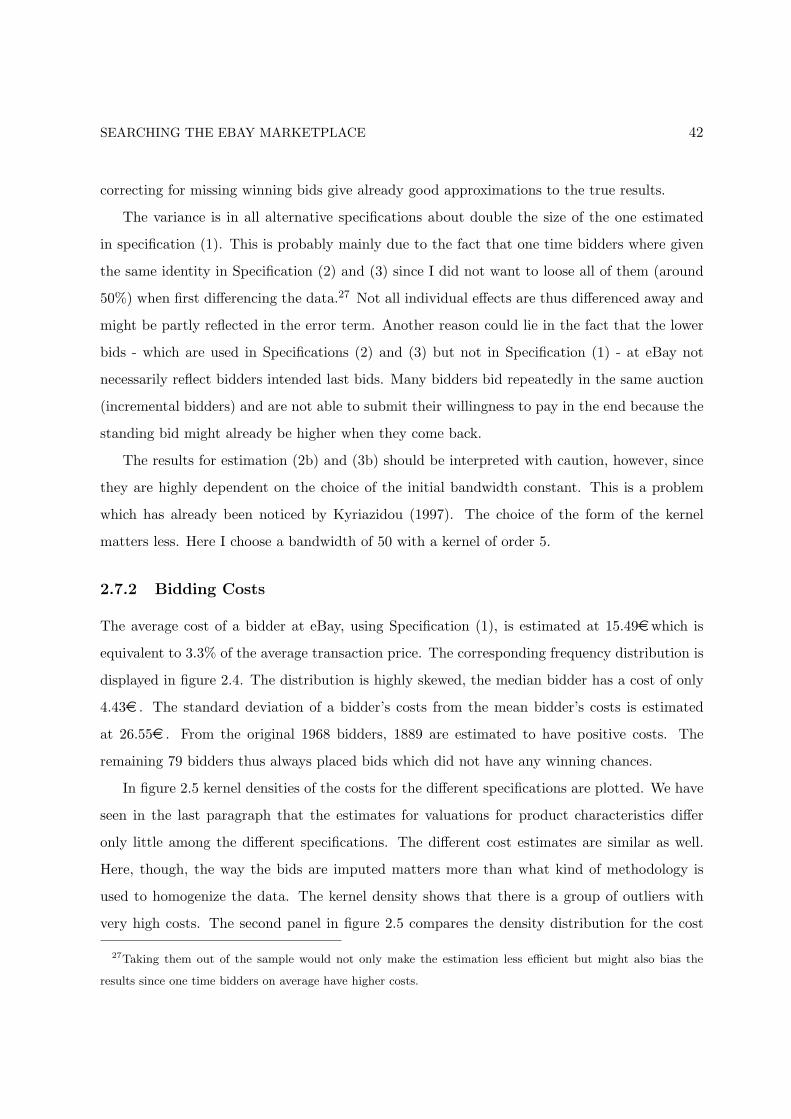
SEARCHING THE EBAY MARKETPLACE 42
correcting for missing winning bids give already good approximations to the true results.
The variance is in all alternative specifications about double the size of the one estimated
in specification (1). This is probably mainly due to the fact that one time bidders where given
the same identity in Specification (2) and (3) since I did not want to loose all of them (around
50%) when first differencing the data.27 Not all individual effects are thus differenced away and
might be partly reflected in the error term. Another reason could lie in the fact that the lower
bids - which are used in Specifications (2) and (3) but not in Specification (1) - at eBay not
necessarily reflect bidders intended last bids. Many bidders bid repeatedly in the same auction
(incremental bidders) and are not able to submit their willingness to pay in the end because the
standing bid might already be higher when they come back.
The results for estimation (2b) and (3b) should be interpreted with caution, however, since
they are highly dependent on the choice of the initial bandwidth constant. This is a problem
which has already been noticed by Kyriazidou (1997). The choice of the form of the kernel
matters less. Here I choose a bandwidth of 50 with a kernel of order 5.
2.7.2 Bidding Costs
The average cost of a bidder at eBay, using Specification (1), is estimated at 15.49ewhich is
equivalent to 3.3% of the average transaction price. The corresponding frequency distribution is
displayed in figure 2.4. The distribution is highly skewed, the median bidder has a cost of only
4.43e . The standard deviation of a bidder’s costs from the mean bidder’s costs is estimated
at 26.55e . From the original 1968 bidders, 1889 are estimated to have positive costs. The
remaining 79 bidders thus always placed bids which did not have any winning chances.
In figure 2.5 kernel densities of the costs for the different specifications are plotted. We have
seen in the last paragraph that the estimates for valuations for product characteristics differ
only little among the different specifications. The different cost estimates are similar as well.
Here, though, the way the bids are imputed matters more than what kind of methodology is
used to homogenize the data. The kernel density shows that there is a group of outliers with
very high costs. The second panel in figure 2.5 compares the density distribution for the cost
27Taking them out of the sample would not only make the estimation less efficient but might also bias the
results since one time bidders on average have higher costs.
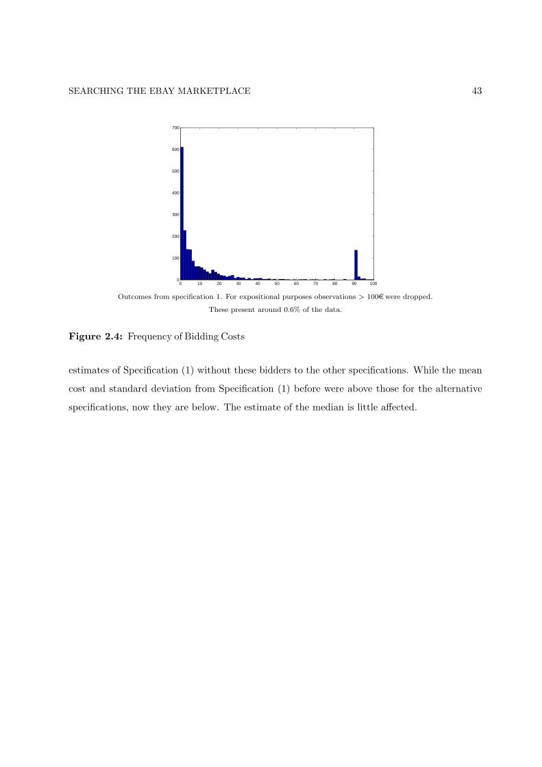
SEARCHING THE EBAY MARKETPLACE 43
0 10 20 30 40 50 60 70 80 90 1000
100
200
300
400
500
600
700
Outcomes from specification 1. For expositional purposes observations > 100ewere dropped.
These present around 0.6% of the data.
Figure 2.4: Frequency of Bidding Costs
estimates of Specification (1) without these bidders to the other specifications. While the mean
cost and standard deviation from Specification (1) before were above those for the alternative
specifications, now they are below. The estimate of the median is little affected.
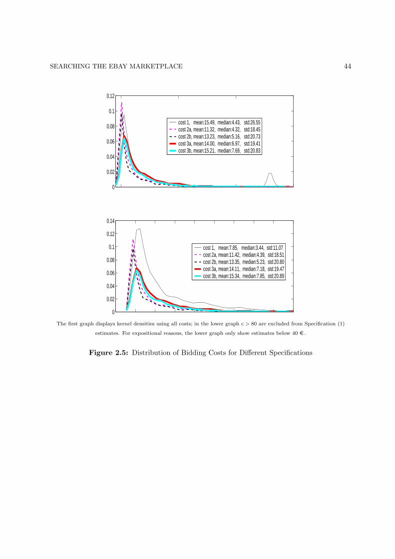
SEARCHING THE EBAY MARKETPLACE 44
0
0.02
0.04
0.06
0.08
0.1
0.12
0
0.02
0.04
0.06
0.08
0.1
0.12
0.14
cost 1, mean:15.49, median:4.43, std:26.55cost 2a, mean:11.32, median:4.32, std:18.45cost 2b, mean:13.23, median:5.16, std:20.73cost 3a, mean:14.00, median:6.97, std:19.41cost 3b, mean:15.21, median:7.69, std:20.83
cost 1, mean:7.85, median:3.44, std:11.07cost 2a, mean:11.42, median:4.39, std:18.51cost 2b, mean:13.35, median:5.23, std:20.80cost 3a, mean:14.11, median:7.18, std:19.47cost 3b, mean:15.34, median:7.85, std:20.89
The first graph displays kernel densities using all costs; in the lower graph c > 80 are excluded from Specification (1)
estimates. For expositional reasons, the lower graph only show estimates below 40 e .
Figure 2.5: Distribution of Bidding Costs for Different Specifications
SEARCHING THE EBAY MARKETPLACE 45
2.8 Conclusion
The paper presented a dynamic framework for the eBay marketplace, similar to a search model.
It was shown that a stepwise estimation approach can be used to consistently estimate demand
parameters from eBay bidding data. While costs and valuations are nonparametrically identified,
the huge amount of covariates asks for parametric assumptions in the estimation process. The
small time dimension of the panel requires further simplifications.
A number of issues remains for future research. First of all, the seller side so far is modelled
rather crudely. Further, the theoretical model assumed that in every instant a new auction
opens and bidders do not care whether the time difference between the auctions is small or
big. Including parameters for the degree of competition from other auctions into the theoretical
model would be desirable.
Secondly, when deriving the theoretic model it was assumed, the characteristics of poten-
tial bidders are given exogenously and stay constant over time. Relaxing this assumption
could lead to more sophisticated dynamic strategies which include predation and strategic non-
participation. While I do not believe that this would add much explanation to the data gener-
ation process in markets for standardized products, it might play a role in thin markets and is
interesting from a theoretical perspective.
Finally, assuming, bidders exactly know the distribution of their competitor’s bids, is asking
a lot of a bidder. While here it was assumed that bidders exactly know the distribution, the
next chapter allows for the possibility of learning about a parameter of the distribution of second
highest bid.
SEARCHING THE EBAY MARKETPLACE 46
Appendix
2.A Proofs
Proof of Proposition 2.1.
(a) Optimal Bid:
Exploiting the fact that loosing is complementary to winning the decision problem of a
participating bidder given in equation (2.6) can be rewritten as:
Vi = maxbi>r
Ebh[1 {b∗h < bi} (vi − V e
i − b∗h) |s]− ci + V ei .
The proof of optimality of the bid is then a simple application of the proof for a standard second
price auction with valuation y = v − V e. (The additional constant −ci + V ei influences neither
the price nor the winning probability and is thus irrelevant for the bidding strategy.)
(b) Distribution of the Maximum:
Given participation is optimal we know from equation (2.6) that the following holds for
bidder i:
Vi (·) = maxbi>r
E[1{max
j 6=i{b(νj , s)|δ(νj , s) = 1} < bi}
(vi − V e
i −maxj 6=i
{b(νj , s)|δ(νj , s) = 1})|s]−
−ci + V ei .
Now build the expectation with respect to the unknown variables ν−i:
Vi (·) = maxbi>r
∫ c
c
. . .
∫ c
c
∫ v(x)
v(x)
. . .
∫ v(x)
v(x)
1{maxj 6=i
{b(νj , s)|δ(νj , s) = 1} < bi}·
·(vi − V ei −max
j 6=i{b(νj , s)|δ(νj , s) = 1})dFν−i(ν−i|x)− ci + V e
i .
While the competitors’ bids are functions of both the costs and the valuations, the entry set Dj ,
which gives all v for which a bidder with costs cj enters, is a function of the costs alone. To apply
a change of variables it is therefore necessary to first condition on the unknown costs and then
to change the variable of integration to b∗j . The conditioning brings about that the variables
of interest, namely the bids of the competitors, are now drawn from different distributions.
The distribution of the maximum of m − 1 non-identically but independently drawn variables
distributed according to fj with cdf Fj is given by fm−1:m−1(b) =[Πm−1
j=1 Fj(b)]∑m−1
j=1
( fj(b)Fj(b)
)
SEARCHING THE EBAY MARKETPLACE 47
(see David and Nagaraja (2003, p 96)) or f (m−1)(b) =∑m−1
i=1 fi(b)Πm−1j=1j 6=i
Fj(b). Finally, from
transformation techniques we know that the distribution of a variable y = g(x) where x is a
continuous variable with pdf fx which is non-zero for x ∈ X and y a one-to-one transformation
of X onto Z is given by fy(y) =∣∣∣ ddyg−1(y)
∣∣∣ fx(g−1(y))1(y ∈ Z). For v ∈ Dj and V ej a known
constant the function bj = v − V ej is continuous and one-to-one; hence fb(b∗j |cj ,x) = fv(b∗j +
V ej |x)1{b∗h +V e
j ∈ Dj}. The rest of the probability mass, that is when v /∈ Dj , is concentrated at
blow. Since blow by assumption does not influence neither the price nor the winning probability
it is irrelevant for the computation of the distribution of the maximum. It then follows for the
bidders’ problem:
Vi (·) = maxbi≥r
∫
b∗h<bi
(vi − V e
i − b∗h) ∫ c
c. . .
∫ c
cfh
b(b∗h, c−i|s)dc−idb∗h − ci + V e
i
with
fhb(b∗h, c−i|s) =
m−1∑
j=1
fv(b∗h + V ej |x)1{b∗h + V e
j ∈ Dj}fc(cj)m−1∏
k=1k 6=j
∫
z∈Dk,
z<b∗h+V ek
dFv(z|x)fc(ck).
Since∫ cc fv(b∗h + V e
j |x)1{b∗h + V ej ∈ Dj}dFc(cj) =
∫ cc fv(b∗h + V e
k |x)1{b∗h + V ek ∈ Dk}dFc(ck) we
can also write
fhb(b∗h|s) =
∫ c
c. . .
∫ c
cfh
b(b∗h, c−i|s)dc−i
= (m− 1)∫ c
cfv(b∗h + V e|x)1{b∗h + V e ∈ D(c, s)}dFc(c)·
·
∫ c
c
∫
z∈D(c,s),
z<b∗h+V e
dFv(z|x)dFc(c)
m−2
SEARCHING THE EBAY MARKETPLACE 48
Proof of Lemma 2.2. Let
F hb(b∗|s) ≡
∫ c
c. . .
∫ c
c
∫
b∗h<bi
fhb(b∗h, c−i|s)db∗hdc−i
and E[b∗h|b∗h < b∗, s] ≡∫ c
c. . .
∫ c
c
∫
b∗h<bi
b∗hfhb (b∗h, c−i|s)db∗hdc−i/F h
b (b∗|s).
(a) Entry Set:
Start by defining:
F (v, c) : = (b∗ − E[b∗h|b∗h < b∗, s])F hb(b∗|s)− c, (2.22)
From the optimal participation strategy we know that F (v, c) < 0 ⇒ δ∗ = 0 and F (v, c) > 0 ⇒δ∗ = 1 (see equation (2.10) ). This function monotonically increases in v: ∂F (v,c)
∂v = F hb (b∗|s) > 0.
It is further negative for very low v and positive for high v (assuming that both are within the
range of v). Thus there is a single v0 = gv(V e, c, s) above which entry is profitable and below
which it is not. The set Dit is thus defined as [v0it, v(xt)].
What about the derivative of F with respect to c? From (2.22) we have:
dF
dc=
∂b∗
∂cF h
b(b∗|s)− 1
Using the result on the derivative of b∗ with respect to c proved in the next paragraph, it can
be shown that:dF
dc=
∫S
∫ v(x′)gv(V e,c,s′) F h
b(b∗|s)dFv(v′|x′)dFs(s′)
∫S
∫ v(x′)gv(V e,c,s′) F h
b(b∗′|s′)dFv(v′|x′)dFs(s′)
− 1
Whether this term is positive or negative depends on the size of today’s winning probability
compared to tomorrow’s expected winning probability.
(b) Derivative of b∗ with respect to c:
From the optimality condition (2.11) it follows that:∫
S
∫ v(x′)
gv(V e,c,s′)
(Ebh
[1 {b∗h < bi}
(v′ − V e
i − b∗h) |s′]− c
)dFv(v′|x′)dFs(s′) = 0.
Using the implicit function theorem, Leibniz’s rule and the condition that F (v0, c) = 0 we get:
dV e
dc= −
∫S
∫ v(x′)gv(V e,c,s′) dFv(v′|x′)dFs(s′)
∫S
∫ v(x′)gv(V e,c,s′) F h
b(v′ − V e|s′)dFv(v′|x′)dFs(s′)
.
Given that F hb|s is always smaller one the numerator is bigger than the denominator which leads
to the derivative being smaller than -1, hence ∂b∗∂c = −∂V e
∂c > 1.
SEARCHING THE EBAY MARKETPLACE 49
Proof of Lemma 2.3.
Writing the expected return from winning conditional on a certain b∗i and s in terms of observ-
ables gives Ebh,δ−i [1{maxj 6=i{b∗j |δ∗j = 1} < b∗i }(b∗i −maxj 6=i{b∗j |δ∗j = 1})|b∗i , s]. Just counting the
cases where b∗i would have been higher than all other bids given the same supply side details
and the same number of bidders and relating this to all auctions with these details and num-
ber of bidders provides an estimate for the winning odds for a specific number of competitors,
averaging these over different numbers of participants finally provides an estimate of F hb (b∗i |s);
multiplying the winning odds with the average realization of b∗h build in the same way gives an
estimate for F hb (b∗i |s)E[b∗h|b∗i > b∗h, s]. Averaging over different bids of the same bidder given a
certain s and then averaging over all possible supply vectors finally gives ci. From the economic
restriction that agents have perfect expectations, it follows that the corresponding sample means
provide consistent estimators for the expectations in (2.12) and thus identification obtains.
Proof of Lemma 2.4.
(a) Conditional Order Statistics Distribution:
The probability of the event {Xm ≥ Xl, Xk ≤ Xl ≤ b2, Xj ≤ Xk ≤ b3 ∀j 6= m, l, k} is given by
Fn−1,n−2:n(b2, b3,m, l, k) = P{Xn−1:n ≤ b2, Xn−2:n ≤ b3, In:n = m, In−1:n = l, In−2:n = k}
=∫ b3
−∞
∫ b2
z(1− Fm(u))
∏
j 6=m,l,k
Fj(z)
dFl(u)dFk(z).
The probability of the event {Xm, Xl ≥ Xk, Xj ≤ Xk ≤ b3 ∀j 6= m, l, k} is given by
Fn−2:n(b3, {m, l}, k) = P{Xn−2:n ≤ b3, In:n ∈ {m, l}, In−1:n ∈ {m, l}, In−2:n = k}
=∫ b3
−∞
∏
j 6=m,l,k
Fj(u)
(1− Fm(u))(1− Fl(u))dFk(u).
Taking derivatives with respect to b2 and b3, respectively b3 gives the corresponding densities.
Equation (2.13) now follows from applying Bayes’ theorem.
(b) Identification:
Since gn−1:n(b2, In:n = m, In−1:n = l|b3) = (1−Fm(b2 |b3 ))fl(b2 |b3 ) = f1:2(b2, I2:2 = m|b3) and
limb3→−∞ f1:2(b2, I2:2 = m|b3) = f1:2(b2, I2:2 = m) the proof now directly follows from Athey
and Haile (forthcoming), Theorem 2.
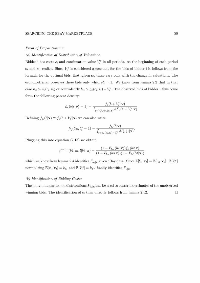
SEARCHING THE EBAY MARKETPLACE 50
Proof of Proposition 2.2.
(a) Identification of Distribution of Valuations:
Bidder i has costs ci and continuation value V ei in all periods. At the beginning of each period
st and vit realize. Since V ei is considered a constant for the bids of bidder i it follows from the
formula for the optimal bids, that, given st, these vary only with the change in valuations. The
econometrician observes these bids only when δ∗it = 1. We know from lemma 2.2 that in that
case vit > gv(ci, st) or equivalently bit > gv(ci, st)−V ei . The observed bids of bidder i thus come
form the following parent density:
fbi(b|s, δ∗i = 1) =fv(b + V e
i |x)∫z+V e
i >gv(ci,s)dFv(z + V e
i |x).
Defining fbi(b|x) ≡ fv(b + V ei |x) we can also write
fbi(b|s, δ∗i = 1) =fbi(b|x)∫
z>gv(ci,st)−V ei
dFbi(z|x).
Plugging this into equation (2.13) we obtain
gn−1:n(b2,m, l|b3,x) =(1− Fbm(b2|x))fbl
(b2|x)(1− Fbm(b3|x))(1− Fbl
(b3|x))
which we know from lemma 2.4 identifies Fbj |x given eBay data. Since E[bit|xt] = E[vit|xt]−E[V ei ]
normalizing E[vit|xt] = kvt and E[V ei ] = kV e finally identifies Fv|x.
(b) Identification of Bidding Costs:
The individual parent bid distributions Fbj |x can be used to construct estimates of the unobserved
winning bids. The identification of ci then directly follows from lemma 2.12.

SEARCHING THE EBAY MARKETPLACE 51
2.B Data
2.B.1 Description of Variables Used in Regression
Category Variable Description
Product Quality
OVP 1 if in original packing (unopened) .
AGE/AGE NSAge in days as stated by the seller/1 if age
is not mentioned in description.
COND NEW/
COND USED
Condition is said to be new/used (as op-
posed to average condition)
OS ENGL/OS FRENCH 1 if english/french operating system.
DEFECT1-4
1 if product comes without bill (1), lacks
standard accessory (2), has scratches on
the display (3) or other defects (4).
Additional Accessories
EXTRAS1 if the product comes with any additional
extra.
JACKET1-5
1 if with PC Card Jacket (1), CF Card
Jacket (2), Dual Slot Jacket (3), Bluetooth
Jacket (4), GSM/GPRS Jacket (5).
HARDDISK1 if with external memory in form of
Toshiba 1GB harddisk.
NAVIGATION0, 1, or 2 depending on the scope of the
included navigation system.
MEMORYAmount in MB of external memory in form
of CF, SD, or MMC card(s).
CAREPAQ0, 1, 2, or 3 depending on the scope of the
additional producer warranty.
Other extras: Dummies for book, cover, earplugs, keyboard, modem,
protective slides, software, synchronization and charge cable.
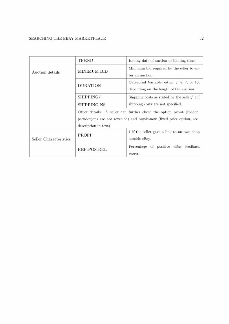
SEARCHING THE EBAY MARKETPLACE 52
Auction details
TREND Ending date of auction or bidding time.
MINIMUM BIDMinimum bid required by the seller to en-
ter an auction.
DURATIONCategorial Variable, either 3, 5, 7, or 10,
depending on the length of the auction.
SHIPPING/
SHIPPING NS
Shipping costs as stated by the seller/ 1 if
shipping costs are not specified.
Other details: A seller can further chose the option privat (bidder
pseudonyms are not revealed) and buy-it-now (fixed price option, see
description in text).
Seller CharacteristicsPROFI
1 if the seller gave a link to an own shop
outside eBay.
REP POS RELPercentage of positive eBay feedback
scores.
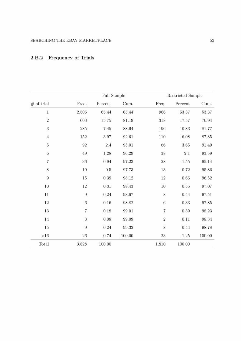
SEARCHING THE EBAY MARKETPLACE 53
2.B.2 Frequency of Trials
Full Sample Restricted Sample
# of trial Freq. Percent Cum. Freq. Percent Cum.
1 2,505 65.44 65.44 966 53.37 53.37
2 603 15.75 81.19 318 17.57 70.94
3 285 7.45 88.64 196 10.83 81.77
4 152 3.97 92.61 110 6.08 87.85
5 92 2.4 95.01 66 3.65 91.49
6 49 1.28 96.29 38 2.1 93.59
7 36 0.94 97.23 28 1.55 95.14
8 19 0.5 97.73 13 0.72 95.86
9 15 0.39 98.12 12 0.66 96.52
10 12 0.31 98.43 10 0.55 97.07
11 9 0.24 98.67 8 0.44 97.51
12 6 0.16 98.82 6 0.33 97.85
13 7 0.18 99.01 7 0.39 98.23
14 3 0.08 99.09 2 0.11 98.34
15 9 0.24 99.32 8 0.44 98.78
>16 26 0.74 100.00 23 1.25 100.00
Total 3,828 100.00 1,810 100.00

SEARCHING THE EBAY MARKETPLACE 54
2.B.3 OLS Estimation
(1) (2) (3)
CONS 612.10 (24.20)∗∗∗ 601.45 (4.16)∗∗∗ 604.45 (4.13)∗∗∗
TREND -.85 (.02)∗∗∗ -.84 (.02)∗∗∗ -.84 (.02)∗∗∗
# TRIALS -1.95 (.49)∗∗∗
OVP 8.71∗∗ (2.95)
AGE -.09 (.02)∗∗∗ -.11 (.02)∗∗∗ -.11 (.02)∗∗∗
AGE NS -24.30 (3.59)∗∗∗ -26.82 (3.59)∗∗∗ -25.31 (3.57)∗∗∗
COND NEW 1.19 (3.26)
COND USED -7.43 (3.42)∗
OS ENGL -13.21 (9.44) -18.53 (9.92)∗ -15.90 (9.50)∗
OS FRENCH -74.63 (23.34)∗∗∗ -78.21 (23.72)∗∗∗ -80.48 (23.52)∗∗∗
DEFECT1 -16.10 (7.21)∗
DEFECT2 -44.442 (11.00)∗∗∗ -46.50 (12.55)∗∗∗ -48.08 (12.64)∗∗∗
DEFECT3 -18.97 (10.15)∗
DEFECT4 -38.86 (7.72)∗∗∗
SHIPPING -1.23 (.66)∗
SHIPPING NS -10.51 (5.58)∗
EXTRAS 1.73 (4.48) 5.73 (3.60) 5.53 (3.56)
JACKET1 46.38 (16.05)∗∗ 54.46 (18.65)∗∗ 58.16 (19..11)∗∗∗
JACKET2 -6.13 (9.88)
JACKET3 95.14 (23.50)∗∗∗
JACKET4 11.70 (12.32)
JACKET5 177.28 (25.03)∗∗∗ 179.42 (23.56)∗∗∗ 179.29 (23.26)∗∗∗
MEMORY .50 (.08)∗∗∗ .46 (.08)∗∗∗ .46 (.08)∗∗∗
HARDDISK 94.40 (11.21)∗∗∗ 92.61 (10.71)∗∗∗ 96.07 (11.00)∗∗∗
NAVIGATION 141.29 (19.13)∗∗∗ 131.40 (19.33)∗∗∗ 128.19 (18.64)∗∗∗
CAREPAQ 13.18 (4.60)∗∗ 16.74 (7.64)∗∗ 16.42 (7.49)∗∗
MODEM 50.59 (40.60)
KEYBOARD 23.17 (13.99)∗
EARPLUGS 5.71 (12.71)
PROTECT 1.21 (1.43)
COVER 0.56 (1.78)
BOOK -24.74 (16.27)
SOFTWARE 12.04 (5.50)∗
REP POS REL -6.54 (24.52)
URL 25.65 (16.14)
OBS 788 788 788
R2 0.798 0.780 0.784
adj R2 0.789 0.776 0.780
White heteroscedasticity robust estimation. Standard errors in parenthesis (marked confidence levels: 90, 95, 99).
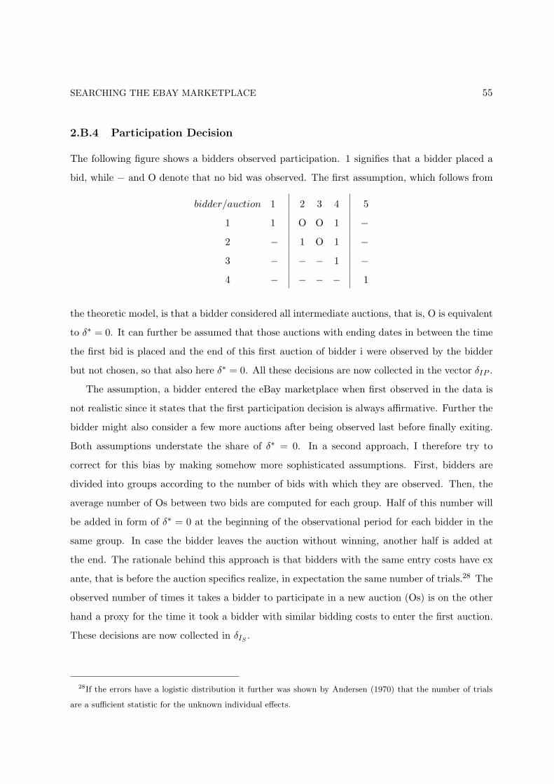
SEARCHING THE EBAY MARKETPLACE 55
2.B.4 Participation Decision
The following figure shows a bidders observed participation. 1 signifies that a bidder placed a
bid, while − and O denote that no bid was observed. The first assumption, which follows from
bidder/auction 1 2 3 4 5
1 1 O O 1 −2 − 1 O 1 −3 − − − 1 −4 − − − − 1
the theoretic model, is that a bidder considered all intermediate auctions, that is, O is equivalent
to δ∗ = 0. It can further be assumed that those auctions with ending dates in between the time
the first bid is placed and the end of this first auction of bidder i were observed by the bidder
but not chosen, so that also here δ∗ = 0. All these decisions are now collected in the vector δIP .
The assumption, a bidder entered the eBay marketplace when first observed in the data is
not realistic since it states that the first participation decision is always affirmative. Further the
bidder might also consider a few more auctions after being observed last before finally exiting.
Both assumptions understate the share of δ∗ = 0. In a second approach, I therefore try to
correct for this bias by making somehow more sophisticated assumptions. First, bidders are
divided into groups according to the number of bids with which they are observed. Then, the
average number of Os between two bids are computed for each group. Half of this number will
be added in form of δ∗ = 0 at the beginning of the observational period for each bidder in the
same group. In case the bidder leaves the auction without winning, another half is added at
the end. The rationale behind this approach is that bidders with the same entry costs have ex
ante, that is before the auction specifics realize, in expectation the same number of trials.28 The
observed number of times it takes a bidder to participate in a new auction (Os) is on the other
hand a proxy for the time it took a bidder with similar bidding costs to enter the first auction.
These decisions are now collected in δIS.
28If the errors have a logistic distribution it further was shown by Andersen (1970) that the number of trials
are a sufficient statistic for the unknown individual effects.
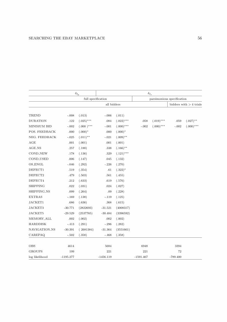
SEARCHING THE EBAY MARKETPLACE 56
δIp δIs
full specification parsimonious specification
all bidders bidders with > 4 trials
TREND -.008 (.013) -.006 (.011)
DURATION .122 (.025)∗∗∗ .084 (.022)∗∗∗ .058 (.019)∗∗∗ .059 (.027)∗∗
MINIMUM BID -.002 (.000 )∗∗∗ -.001 (.000)∗∗∗ -.002 (.000)∗∗∗ -.002 (.000)∗∗∗
POS. FEEDBACK .000 (.000)∗ .000 (.000)∗
NEG. FEEDBACK -.025 (.011)∗∗ -.021 (.009)∗∗
AGE .001 (.001) .001 (.001)
AGE NS .257 (.188) .338 (.166)∗∗
COND NEW .178 (.136) .329 (.121)∗∗∗
COND USED .006 (.147) .045 (.132)
OS ENGL -.046 (.292) -.226 (.270)
DEFECT1 .519 (.354) .61 (.322)∗
DEFECT2 .479 (.503) .561 (.455)
DEFECT4 .212 (.633) .619 (.576)
SHIPPING .022 (.031) .024 (.027)
SHIPPING NS .099 (.264) .09 (.228)
EXTRAS -.169 (.138) -.119 (.125)
JACKET1 .686 (.636) .368 (.615)
JACKET3 -30.771 (2822693) -31.521 (4008317)
JACKET5 -29.529 (2537765) -30.484 (3396592)
MEMORY ALL .002 (.002) .002 (.002)
HARDDISK -.413 (.291) -.296 (.282)
NAVIGATION NS -30.391 ( 2681384) -31.364 (3551661)
CAREPAQ -.502 (.358) -.468 (.358)
OBS 4614 5684 6948 3394
GROUPS 199 221 221 72
log likelihood -1195.277 -1456.119 -1591.467 -789.400
SEARCHING THE EBAY MARKETPLACE 57
The fact that the panel arbitrarily begins at auction 1 and ends at some auction T leads to
an under-representation of δ∗ = 0. To circumvent this problem in the later estimation, I will
only use a shorter window from the middle which in the figure is equivalent to auctions 2 to 4.
This does not create any bias as long as the auction details do not change in a systematic way
over time. In the above example this restriction causes that bidder 4 will not be relevant for
the estimation; bidder 3 is denoted as a one time participant, while 2 and 3 both evaluated all
three auctions 2-4.29
While I consider the non-successful auctions in the construction of both panels, the private
auctions are dropped since no information on bidders’ pseudonyms are available. Private auc-
tions which did not receive any bids are kept. Also those bids that were placed before the last
10% of the auction are left aside. That is, if a bidder only places a bid early on in the auction I
denote that she did not participate in the auction.
29Using for each bidder only a random sample of x % of the observations would do the same trick and would
also overcome some of the problems mentioned in the last paragraph. The drawback of this method is, however,
that many of the bidders that are observed only a few times would be lost in this way which again would bias
the results.
Chapter 3
Bayesian Learning at eBay?
Updating From Related Data and
Empirical Evidence.
3.1 Introduction
Empirical evidence shows that bidders at eBay increase their bid with each trial in a new
auction for the same object. Static auction models are not able to explain this behavior. While
the sequential auction literature (see e.g. Weber (2000)) can rationalize increasing individual
bids, the assumptions which make these models applicable provide no good description for the
eBay market. All of these models have a finite horizon, determined by the ex ante known total
number of products to be sold, and the number of bidders is always larger than the available
products. The reason why a bidder increases his bid over time is intimately related to this
scarcity of supply: Each time he looses, his remaining winning chances decrease, and, thus, he
bids more aggressively.
Starting from a predetermined group of people who compete for a fixed amount of products
until none is left seems ill-founded for the eBay market. There rather is a permanent inflow of new
products and new bidders while others leave. This is especially true for the segment of off-the-
shelf products like computers, consumer electronics, domestic appliances, or DVDs. Chapter
2 introduced a model of search which captures this characteristic better. While the model
BAYESIAN LEARNING AT EBAY 59
follows the sequential auction literature in that it explicitly incorporates the future availability
of products, it departs from it by allowing for an infinite horizon. The bidder is not restricted
anymore by the limited availability of products. What stops him from participating in each
auction with a bid close to zero is, instead, assumed to be his bidding cost. As in a sequential
auction game, it is still optimal for the bidder to bid his valuation minus his continuation value.
Given that the relation between supply and demand remains constant, the continuation value
though does not change over time, and the bidder places the same bid in each auction.
I will show in the following that learning is a possible explanation for bidders’ increasing
bids in this environment. When first coming to eBay, bidders probably believe, they would
get the product cheaper than elsewhere. Many, however, will not know by exactly how much
cheaper they realistically can obtain the product. The price a bidder pays in a second price
auction like eBay is determined by the highest bid of the competitors. Following the framework
of the previous chapter, I assume, bidders believe that this bid is drawn in each period anew
from the same distribution. This assumption is based on the observation that entry of new
bidders, individual participation decisions, and stochastic components in valuations introduce
so much noise that updating the beliefs about the characteristics of any specific competitor
provides relatively little payoff and is thus not undertaken at all. Under the assumption that
none of the bidders reacts to any specific competitor, the bids in each auction are, however,
very informative about the underlying distribution of competitors’ bids. It is thus assumed,
the bidder uses the observed bids to update his prior beliefs about this distribution after each
auction he participated in. The way the uncertainty is resolved over the course of a bidders’
participation in the eBay game and how exactly bidders’ can incorporate new information into
their bidding strategy is the subject of this paper.
Burdett and Vishwanath (1988) show how to introduce learning in a search model. In their
model the job seeker in the labor market is uncertain about the (location parameter of the)
job offer distribution. With each offer he receives, he updates his prior in a Bayesian way;
consecutive decisions are based on the posterior distribution. The corresponding distribution in
a second price auction is the distribution of the highest bid of the competitors which determines
a bidder’s winning odds and the price he pays. The main technical challenge is that bidders
in these auctions normally do not observe the highest bid of their competitors and thus cannot
BAYESIAN LEARNING AT EBAY 60
use this information to update their beliefs. They only observe the transaction price, which is
equal to the second highest bid of the competitors (+ 1 increment), and maybe some or all lower
ordered bids. I will show in the following that a function of the transaction price provides a
sufficient statistic for updating the distribution of the highest bid when relying on asymptotic
distributions of order statistics. Moreover, starting from a prior knowledge of the distribution
of the highest bid of the competitors, the bidder can update his beliefs each time he participates
in an auction in a simple way, that is, using conjugate priors.
The statistical literature on asymptotic distributions of order statistics, also referred to as
extreme value distributions, dates back to the beginnings of the last century. A seminal work is
Gumbel (1958). It has been applied in so diverse fields as survival analysis in biology, reliability
studies in engineering, or to measure any kind of extremal event, such as floods or wind speeds.
The only application to economics, to my knowledge, is in finance where it is used to model the
tails of the distribution of stock returns. The paper shows how to make use of the framework
in the auction environment. In standard auctions the number of bidders is normally not big
enough to justify the application of asymptotic distributions. This is different for eBay; here
the potential number of bidders, that is, those that consider bidding in any given auction, is for
many product categories rather large.
As opposed to eBay.com, at eBay.de auctions cannot be searched for anymore as soon as
they are closed. By this policy eBay makes it more difficult for a bidder to inform himself about
his competitors’ bids before participating in an auction. It can therefore be expected that part
of the learning process a bidder undergoes can actually be observed in the bidding data. I will
use a data set of all auctions and the corresponding bids for a specific palm pilot, which was
collected from eBay.de during a seven month period, to see whether bidders combine their prior
knowledge with the new information, obtained in those auctions where they participated in, in
the way predicted by the model.
The model builds on the classic theoretical decision making literature which gives clear advice
on how people should behave under uncertainty. Researchers have questioned whether people
actually follow this advice. There is some evidence in the experimental literature that people
are applying Bayesian rules to resolve uncertainty (see e.g. El-Gamal and Grether (1995)). The
paper adds to this literature, using field data, by showing that bidders at eBay incorporate new
BAYESIAN LEARNING AT EBAY 61
information into their strategies in a Bayesian way.
The next section states a model of updating in second price auctions where a large number
of potential bidders are present and bidders are unable to follow a specific bidder or a specific
sample of bidders over time. This model reflects a situation which is typical for internet auctions.
Section 3.3 discusses the impact of learning on the optimal bidding strategies. The application
to eBay and the econometric specification are given in section 3.4. The last section concludes.
3.2 Benchmark Model
Setup. Assume an infinite number of homogenous products which are offered to buyers in
sequence, one in each period t. The selling format in each period is a Vickrey auction. Bidder i
is interested in one product only which he values at vit = vi+εit. vit is private information. While
vi remains constant over time and can be considered a bidder’s type, εit is drawn anew before
the start of each auction from a common density function fε with mean zero and variance σε.1
The bidder can bid in as many auction as he wishes. Bidding though comes at a cost c which is
common to all bidders. In each period the bidder has to decide about participation, δit ∈ {0, 1},and about a bidding policy, bit. Policies are chosen such as to maximize the intertemporal utility
given by the sum of the expected period returns.
Beliefs. To simplify the analysis and to focus the view on the learning aspect, I assume, the
bidder believes, he can influence neither the number nor the type of his potential competitors
over time by his actions. He reckons that entry and exit to the marketplace happen in a way
which keeps the potential number of competitors constant at n − 1. He further believes, the
personal characteristics of these bidders always represent an independent random draw from
the same distribution. Concentrating on Markov equilibria, the only variable which affects
bidding strategies is then the private valuation of the bidder, or more formally bjt = b(vjt). The
bid of each potential competitor is therefore distributed according to some density fb which is
composed of the densities of vi and εit and is thus believed not to change across auctions. In
1εit is introduced in view of the empirical part. There it reflects the time-varying part in the individual
valuations which cannot be attributed to observables such as product characteristics. In the theoretical part it
could be left aside. See also Chapter 2, Subsection 2.3.2.
BAYESIAN LEARNING AT EBAY 62
the following I will take fb with corresponding distribution Fb as given without relating it back
to the underlying distribution of valuations.2
What really matters for the bidder is the highest bid of the actual participants in an auction
since this determines his winning odds and the price he pays. The optimal Markovian partic-
ipation decision of each potential competitor is given by δjt = δ(vjt) = δ(b−1(bjt)). Since c is
the same for all bidders, there exists a common thresholds b for the bids: While bidders with
optimal bids above b participate, all the others wait for one of the next auctions where their
draw of ε is higher.3 Bidder i can thus compute his winning odds either as the probability of
being higher than the highest bid out of the actual competitors, who draw their bids from the
parent bid distribution truncated at the participation threshold, or as the probability of being
higher than the highest out of all potential competitors, who draw their bids from the full parent
bid distribution Fb. The latter viewpoint will be maintained in the following. Let bh ≡ bn−1:n−1
denote the highest bid out of a sample of n − 1 from the parent Fb. The distribution of this
order statistic is then given by (Fb)n−1 ≡ F hb .
Learning. While the model stipulates, the bidder cannot trace a specific competitor or
a specific sample of competitors by observing bids and participation decisions, it allows for
the possibility that the bidder is uncertain about the underlying primitives, namely the bid
distribution from which the bids of his competitors are randomly drawn in each auction and
that he can learn about it by observing realizations of this distribution. By assumption, only
participants in an auction can observe these realizations.4 Learning is assumed to happen in a
Bayesian way, that is, the bidder incorporates new relevant information into his prior beliefs and
future decisions rely on the posterior distribution (see e.g. DeGroot (1970)). More specifically,
the distribution of the unknown variable bh is known up to a parameter θ; the bidder does not
know the value of this parameter but can specify a prior probability distribution over it. With
each observation, that is, after each auction he participated in, he can update this prior with all
2Here it is assumed that a non-degenerate distribution exists as the outcome of competitors’ optimal behavior.
Chapter 2 shows that this holds true for the eBay setting without learning.
3For a formal proof see Chapter 2, Lemma 2.2.
4Letting also non-participants to an auction learn as soon as they have entered the marketplace would not
make too big a difference. Then the continuation value without participating would also be a function of the
updated parameters. See also argumentation in the empirical part.
BAYESIAN LEARNING AT EBAY 63
relevant information he obtained. The result is a posterior distribution of the parameter θ and
a new predictive distribution for bh.
The Bidders’ Problem. Taking account of the auction environment and incorporating the
learning aspect yields the following expected per period profit function for a participating bidder
in period t:
Et−1 [1{bit > bht}(vi + εit − bht)− c] (3.1)
The decision to participate, first of all, involves paying the bidding cost c. If the bidder wins,
which is the case when his bid is higher than the highest of his competitors, he gets his valuation
and pays the price determined by the highest bid of his competitors.5 The time subscript on the
expectation operator indicates that the bidder can incorporate all information that has realized
up to period t− 1 in his expectation over the unknown variable bht. A non-participating bidder
obtains zero in that period.
Since there is an infinite number of consecutive auctions, the bidder can try again in the next
auction whenever he looses. In recursive form, bidder i’s intertemporal optimization problem is
thus given by:
Wi(εi, θi) =
max{
maxbi≥0
E [1{bi > bh} (vi + εi − bh)− c + 1{bi ≤ bh}W ei (θ′i) ] , W e
i (θi)}
before winning
0 after winning
(3.2)
where W ei (θi) ≡
∫Wi(εi, θi)fε(ε)dε denotes the expected continuation value. Equation (3.2)
states, whenever the bidder participates and does not win, his return is the updated continuation
value W ei (θ′i) minus the bidding costs. When the bidder decides not to participate in that auction,
he gets the continuation value W ei (θi) which does not include any updating of the parameter.
In case the bidder wins, his continuation value becomes zero and he leaves the market. I will
drop the case Wi(·) = 0 as well as the subscript i in the following for notational ease .
Updating in Second Price Auctions. So far nothing has been said about what information
the bidder could use for updating. Even if learning is directly over the distribution of the highest
5In the following I will ignore the minimal increment since it is usually very small in comparison with the price
to be paid.
BAYESIAN LEARNING AT EBAY 64
bid, it is not straightforward since the information the bidder is primarily interested in, bht, is
not observable in a second price auction. Is there alternative information which the bidder could
use instead to improve his prior over the parameter of the distribution of bh? What the bidder
can observe is the full bidding history below the transaction price. He therefore could use some
or all of the lower ordered bids. Since these are drawn from the same parent as bh, there exists
a relation between these bids. In the following, I explore whether and how this relation can be
exploited for Bayesian updating in the above dynamic optimization problem.
Given the bid information, the bidder has in principle two options. First, he can use all
or part of the available lower bids to update the parent distribution. From the parent he then
derives the distribution of the order statistic he is interested in. Updating a distribution from
the sort of incomplete data encountered here, that is, data that lacks the highest bid and those
that fall below the participation thresholds, is though far from easy; incorporating this into
a recursive dynamic programming problem seems to be doomed to failure. Directly learning
about a parameter of the relevant order statistic distribution appears more straightforward at
first glance; given that in general distributions of order statistics are merely functions of the
underlying parents, the same parameters would, though, have to be updated unless specific
functional forms for the distributions are assumed. The problem of the latter approach is that
a convenient form for the distribution of any order statistic, e.g. the normal (see Burdett and
Vishwanath (1988)), might lead to an implausible parent. Further, the related distribution of any
other order statistic that is used for updating would not necessarily have the same or any other
convenient functional form. The computational problems would thus not change. I will show in
the following that if one is willing to rely on asymptotic distributions, analytical results can be
obtained in a dynamic programming problem without making ad hoc distributional assumptions
for the parent. Before continuing, a digression on the asymptotics of order statistics distributions
is in order.
Asymptotic Order Statistics Distributions. Since Gumbel (1958), if not before, it is known
that if the highest order statistic bh = bn:n of any parent has, upon suitable standardization, a
limiting distribution as n →∞, this will be one of either Gumbel (double exponential), Weibull,
or Frechet type. Gumbel, often also referred to as the extreme value distribution, is by far the
BAYESIAN LEARNING AT EBAY 65
most common type. Its density is given by:
g(zh) = e−e−zh e−zh with zh = (bh − θ)τ. (3.3)
θ and τ denote the location and scale parameters which are used for standardization.6 While
for normal distributions convergence has been found to be excessively slow (n > 100), for most
other distributions already much smaller sample sizes lead to good approximations.
It has further been shown that not only the highest but also all lower order statistics (k-th
extremes, b(k) ≡ bn−k+1:n and b(1) = bh) have asymptotic densities given by:7
g(k)(z(k)) = kk([k − 1]!)−1e−ke−z(k)
e−kz(k) with z(k) = (b(k) − θ)τ (3.4)
It should be noted that all limiting densities have the same normalizing constants.
Another result, which will prove helpful, is that the joint density of the top k extremes
asymptotically converges to:
g1,...,k(z(1), ..., z(k)) = G(z(k))Πki=1
g(z(k))G(z(k))
, (3.5)
where g(·) is defined as in (3.3) and G(·) denotes the corresponding cdf. (These and the preceding
results as well as further discussion can be found in David and Nagaraja (2003, Ch. 10) and Kotz
and Nadarajah (2002).) In the following, a tilde depicts the density of the bid corresponding to
g: g(b; θ, τ) = τg((b− θ)τ). The joint density of bh and b(2) is thus given by:
g1,2(bh, b(2); θ, τ) = τ2 g((bh − θ)τ)g((b(2) − θ)τ)G((bh − θ)τ)
= τ2e−(bh−θ)τg((b(2) − θ)τ)). (3.6)
As mentioned above, uncertainty will be defined as uncertainty about a parameter of the
distribution of bh. Let this be the location parameter θ. The bidder has a subjective prior over
this parameter which is distributed according to ξprior(θ). With each participation the bidder
incorporates new information in a Bayesian way. If the information he uses is the k-th order
statistic, the posterior distribution, that is, the distribution of the parameter conditional on the
6The variable z = (bh − θ)τ has mode 0, median ln(ln(2)), mean γ, and variance π2/6. The optimal choice of
the standardizing parameters θ and τ depends on the sample size, n.
7I only report the Gumbel form. Also here three limiting types are possible where the other two are similar
to Weibull and Frechet distributions.
BAYESIAN LEARNING AT EBAY 66
observation b(k), is computed from:8
ξpost (θ|b(k)) =g(k)(b(k)|θ)ξprior(θ)∫g(k)(b(k)|θ)ξprior(θ)dθ
If the prior and the posterior distribution belong to the same family, that is, they differ only
by the value of a finite parameter vector, we say that ξ and g(k) constitute a conjugate family.
Using conjugate priors facilitates the updating procedure since at each step only the parameters
of ξ change as a function of the observed information but not the distribution itself.
When the scale parameter τ is known, all of the asymptotic extreme value distributions
belong to the exponential family. For members of the exponential family there always exists a
sufficient statistic of fixed dimension (see e.g. DeGroot (1970, Ch.9)). This statistic is given
by t(b(k), N) =∑N
i=1 e−τb(k),i ,9 where N denotes the number of independent observations of
the same k-th order statistic which are used for updating, and the vector b(k) collects all the
observations. On the other hand, if such a statistic exists then there also exists a conjugate
family for this distribution:
Lemma 3.1. A conjugate family for the Gumbel distribution is given by:
ξ(k)(θ; r, C) =τ
(kreθτ
)kCe−kreθτ
Γ (kC), (3.7)
where x = eθτ is distributed according to a gamma distribution with shape parameter kC (C ≥1)10 and scale parameter 1/(kr).11 C and r are the parameters of this distribution which are
updated with each new observation as follows:
r′k = rk + t(bn−k+1, 1) and C ′ = C + 1. (3.8)
τ , the scale parameter of the Gumbel distribution, is known and thus not part of the updating
process. k is the order of the statistic that is used for updating.
8So far I used the notation f(x; θ) to denote the density of x for each θ ∈ Θ. To highlight that θ now is the
value of a random variable I will in the following denote f(x|θ) as the density conditional on a specific realization
of θ.
9A consistent estimator for θ given τ is given by bθ = −τ−1ln`
1N
PNi=1 e−bhτ
´(see Kotz and Nadarajah (2002)).
10This assumption guarantees that the predictive distribution has finite mean and variance for whatever statistic
is used for updating, including k = 1.
11The expected value of the gamma distribution is E(x) = Cr, the expected value of θ is given by E(θ) =
Ψ(2C)−ln(2r)τ
, where Ψ denotes the digamma function.
BAYESIAN LEARNING AT EBAY 67
Proof. See Appendix.
To build the expectation in (3.2) over bh we first have to integrate out the unknown parameter
θ. The resulting density of bh is parameterized by the parameters of the posterior distribution
ξ and is called the predictive distribution. The following lemma shows that under the Gumbel
assumption this density has a well known form as well:
Lemma 3.2. The predictive distribution of bh when bh is known to have a Gumbel distribution
with scale parameter τ is given by:
h(bh; r, C) =1r
(r
r + (kC)−1e−τbh
)kC+1
τe−τbh (3.9)
where x = e−τbh is distributed according to a Generalized Pareto distribution (GPD) with scaling
parameter r = r/C and shape parameter 1/kC.12
Proof. See appendix.
The Bidder’s Problem Continued. The observation most commonly available in auction data
sets is the transaction price which corresponds to the second highest bid. The following analysis
thus concentrates on the case when this statistic is used for updating. The preceding results can
then be combined to restate the bidder’s problem as follows:
Proposition 3.1. Assuming the number of potential participants in an auction is large enough
to apply the asymptotic results discussed in the previous paragraphs, the bidder’s problem when
the transaction price is used for updating is given by:
W (ε, r, C) = max{
maxb≥0
∫ b
−∞(v + ε− bh)h(bh; r, C)dbh − c
)+
∫ ∞
b
∫ bh
−∞W e(r′, C ′)·
· h(b(2); r, C)i(bh, b(2); r, C)db(2)h(bh; r, C)dbh,W ei (r, C)
}
s.t. C ′ = C + 1, r′ = r2C
2C + 1+
12C + 1
e−τb(2) and r0, C0 given,
where
i(bh, b(2); r, C) =2C + 1
2C
r
r + (2C)−1e−τb(2)
(r + (2C)−1e−τbh
r
)2C+1
and h(·) as defined in Lemma 3.2.
12The GPD is the limiting distribution for extreme exceedances. The threshold for x here is 0, that is this GPD
gives the exceedances of x above 0. For 1/2C = 0 the distribution is equivalent to the Gumbel distribution, for
1/2C > 0 the tails are heavier. For r = 1 the distribution is also called Generalized Standard Pareto Distribution.
BAYESIAN LEARNING AT EBAY 68
Proof. See Appendix.
The advantage of this formulation as opposed to the problem stated in (3.2) is that it
uses analytic solutions for the distributions which are used for expectation building without
significantly restricting the parent distributions from which the bids are drawn. Further, it gives
the bidder clear advice how to incorporate new information in form of transaction prices into
his beliefs.
To be able to provide analytical results for the optimal strategies, the impact of the unknown
variable b(2) on the value function has to be disentangled from the impact of the other variables.
A first step forward is to separate the unknown bh into a function of the stochastically evolving
scaling parameter r and a random variable whose realization is independent of r. From this
“standardized” version of the problem (see Appendix) the following guess for the value function
emanates which isolates the influence of the stochastic variable b(2):
W (ε, r, C) =ln(r)
τ+ α(ε, C). (3.10)
α(ε, C) ≡ W (ε, 1, C) denotes the part of the value function which evolves deterministically with
C.
Under this guess, it is possible to derive analytic forms for the optimal strategies. These are
given in Proposition 3.2. The proposition also states that the guess for the value function is
correct. All details of the computation are provided in the Appendix.
Proposition 3.2.
(a) The value function can be written in the form:
W (ε, r, C) =ln(r)
τ+ α(ε, C) (3.11)
with α(ε, C) ≡ W (ε, 1, C), W e(r, C) = ln(r)τ + αe(C), and αe(C) ≡ ∫
α(ε, C)dFε(ε).
(b) The bidder’s optimal bid is given by:
b∗ = b(ε, r, C) = v + ε− ln(r)τ
− αe(C + 1)− l(ε, C). (3.12)
with
l(ε, C) ≡ 1τ
(1
2C + 1+ ln
[2C
2C + 1− e1
2C+1+τ(αe(C+1)−v−ε)
]).
BAYESIAN LEARNING AT EBAY 69
Proof. See Appendix.
The optimal bid, thus, also separates into a part which changes with the new prior for r and
another part which deterministically evolves with C. This part consists of αe(C + 1) and an
additional component l(ε, C) which vanishes with C →∞.13
The first term of l(ε, C) clearly is positive. The sign of the second term is less obvious. If
αe(C + 1) > v + ε14 then the numerator is bigger than the denominator and the logarithmic
term in l(·) is positive. Due to the learning possibilities, the bidder would hence shade his bid.
When no learning happens anymore (C = ∞), the optimal bidding strategy collapses into
one where the bidder shades his valuation by his continuation value:
b∗C→∞ = v + ε− ln (r)τ
− αe (∞) = v + ε−W ei (r,∞). (3.13)
This is exactly the same solution as in the case where the bidder knows the competitors’ bid
distribution from the beginning and learning is thus not necessary (see Chapter 2).
3.3 Impact of Learning on Optimal Bidding Strategies
Learning influences the bidder’s optimal bidding behavior in two ways: First, the prior over the
distribution of the location parameter changes with each new observation.
Proposition 3.3. The optimal bid increases with the observed transaction price; the bid in-
creases less the higher C.
Proof. ∂b∗∂b(2)
= ∂b∗∂r
∂r∂b(2)
= 1rC e−τb(2) and 1
r(C+1)e−τb(2) − 1
rC e−τb(2) < 0.
In a second price auction any influence of the competitive environment can work only via
the continuation value. The higher the last observed transaction price was, the lower the prior
of r and, thus, the lower the winning chances in the future. Lower future expected returns
decrease the continuation value. Since the bidding strategy involves shading the valuation by
the continuation value, the bidder will now shade less and the bid is thus higher. The effect
13This is true as long as αe(C + 1) does not increase “too quickly” with C. In the next section I show by
numerical simulation that αe(C + 1) actually decreases in C for reasonable values of the parameters.
14The simulation exercise shows that this is true for reasonable values of the parameters.
BAYESIAN LEARNING AT EBAY 70
becomes less pronounced with each participation since the more observations the bidder has
already sampled the less influential is any new information.
The influence of the number of observations works via the same channel. The results are,
however, less clear cut. Differencing the optimal bid with respect to C gives:
b(ε, r, C + 1)− b(ε, r, C) = αe(C + 2)− αe(C + 1) +1τ
2(2C + 1)(2C + 3)
+
+1τ
ln
[2C2 + 3C − Ce
12C+3
+τ(αe(C+2)−v−ε)
2C2 + 3C − (C + 1)e1
2C+1+τ(αe(C+1)−v−ε) + 1
](3.14)
A sufficient condition for this difference to be positive is α (C + 2)−α (C + 1) < 1τ
2(2C+1)(2C+3) .
To be able to say more about the evolution of bids during the course of learning α thus has
to be characterized more closely. Combining the standardized form of the value function with
the value function guess provides a form for α (see proof of Prop. 3.2). Solving the integrals
as far as possible and rearranging gives a functional form which separates the total value into a
value from winning the object, which is similar to the one in the problem without learning, and
a value from learning:
α(ε, C) = max{∫ ∞
b0∗
(v + ε +
ln(x)τ
)h0(x;C)dx
︸ ︷︷ ︸Ex. value of winning (ERw(ε,C))
− c +∫ b0∗
0αe(C + 1)h0(x; , C)dx
+4C+1
(2C+1)2C − ln(
2C+12C
)
(2C)2C−
ln(
2C+b0∗2C+1
)+ 4C+1
(2C+1)2C
(2C + b0∗)2C
︸ ︷︷ ︸Ex. value from learning (ERl(ε,C))
, αe(C)}
(3.15)
with h0(x; C) =(
2C2C+x
)2C+1
and b0∗ = b0(ε, C) = 1re−τb∗ = 2C
(e−τ(αe(C+1)−v−ε)− 1
(2C+1) (2C + 1)− 1)−1
.
There are thus two influences of an increase in C on the bidder’s value: Clearly, ERl(ε, C)
decreases in C and eventually vanishes. Diminishing returns from learning are also consistent
with intuition. The second influence comes via the predictive distribution h0(x; C) which the
bidder uses for determining his expected value of winning. With each new observation this
distribution becomes less dispersed. Differencing the expected value of winning with respect to

BAYESIAN LEARNING AT EBAY 71
C and using integration by parts gives:
ERw(ε, C))− ERw(ε, C + 1)) =−∫ b0(ε,C)
b0(ε,C+1)
(v + ε +
ln(x)τ
)h(x; C + 1)dx+
+(
v + ε +ln(b0(ε, C))
τ
)(H0(b0(ε, C);C + 1)−H0(b0(ε, C);C)
)
+∫ ∞
b0(ε,C)
(v + ε +
ln(x)τ
)(H0(x;C + 1)−H0(x; C)) dx (3.16)
The last two lines are positive since H0(x;C) < H0(x; C +1) for all x. This result shows that the
bidder prefers to play against a more dispersed distribution of competitors’ bids. On the other
hand, the bidder is free to choose the cutoff values b0∗ in each period (first line). By choosing a
lower bid in C + 1 than in C the bidder can counteract the negative effect. The overall effect is
ambiguous.
Given this uncertainty over how ERw(C) changes with C, it is not possible to determine
analytically how αe and thus the bids change with each new trial. I therefore compute the value
function numerically for values of the parameters which match the latter empirical analysis. The
following figure shows the results for αe and E[b∗ + ln(r)/τ ]. 15
0 50 100 150 200439
440
441
442
443
444
445
446
447
448
449alphae(C)
C0 50 100 150 200
−100
−90
−80
−70
−60
−50
−40
−30b*(C) +ln(r)/tau
C
Figure 3.1: Simulation results for αe and E[b∗ + ln(r)/τ ](v = 400, c = 8, fε(ε) = N (0, 10), τ = 0.016, and C0 = 2. C is assumed to be close to infinity at C = 200)
For the given parameter values αe thus decreases and the optimal bid given any value of r
increases in C. The increases however quickly become smaller and eventually vanish.
15Since I do not want to pick out an arbitrary realization of ε, I here report the mean. Bids also increase for
all possible realization of ε.
BAYESIAN LEARNING AT EBAY 72
Proposition 3.4. If αe(C) decreases in C the optimal bid increases in C. This is for example
true for v = 400, c = 8, fε(ε) = N (0, 10), τ = 0.016, and C0 = 2.
Proof. Follows from the preceding discussion and the simulation exercise.
3.4 Detecting Learning in eBay Data
A characterizing feature or Internet auctions is that in many product categories there are a
large number of buyers and sellers present, much like in a marketplace, which makes a search
framework applicable. eBay is in most countries the major auction platform. I collected data on
a Personal Digital Assistant (PDA or palm pilot), the Compaq Ipaq H3850, from eBay Germany
over a 7 month period in 2002. This data is in the following used to test the implications of
the learning model. Section 2.4 in the last chapter provides a detailed description of the data
set; the variables used in the latter estimation are listed in Appendix B of the same chapter.
Every 4 1/2 hours an auction for this product closed. The average price bidders paid for it was
477e . 3829 distinct bidders are observed in the sample who on average placed bids in 2 different
auctions. Many, however, bid many more times (see frequency distribution in Appendix B to
Chapter 2).16
Does the eBay setting conform with the main assumptions of the benchmark model? First of
all, the auction rules at eBay are a mixture of an open ascending and a sealed bid second price
auction. The literature on eBay, though, argues that the Vickery assumption presents a good
approximation to the true rules since it is not optimal for a bidder to reveal private information
early on. The data confirms this; bidding activity is concentrated at the end of an auction (see
also Section 2.2).
An estimate of the potential number of bidders is obtained when adding to the actual bidders
in an auction those that bid in any previous auction without winning and show up later again in
another auction.17 The data reveals, on average 68 people are looking for the Compaq 3850 in
16Here, I use the full bidding data, if not otherwise mentioned, as opposed to Chapter 2 where only those bids
submitted in the last 10% of the auction time entered the estimation. The reason is that low bids now might
actually represent optimal strategies. In the latter estimation I will present results for both, the full data set and
the data which only includes bids submitted in the last 10% of the time.
17See also the description of the participation vector IPS in the Appendix to Chapter 2.
BAYESIAN LEARNING AT EBAY 73
any given auction. And this is still a conservative estimate since it only includes bidders who took
part in the last 10% of an auction. When including the early bids the number doubles. Further,
there are probably bidders who never show up in my sample at all but are still considering to
bid for the product. Using asymptotic results, thus, is justified for this product category.
As opposed to eBay.com, at eBay.de it was not possible to search for past, closed auctions
at the time the data was collected. While the potential bidder can also use eBay’s function
“observe auctions” to learn about his competitors’ bids before starting to bid himself, he would
have to spend considerable time to figure out what the average transaction price is, given that
an average eBay auction lasts 5 days. This is costly. An alternative is to participate right away
with a low bid using an initial guess for the competitors’ bid distribution. As opposed to merely
observing, this strategy involves not only a cost but also a winning chance. If the bidder actually
learns from past observations in the way described by the model, there is thus a good chance
that this shows up in the data.
Bidding in the model is assumed to be costly. eBay does not charge the bidder any fee;
however, there is a cost in terms of the time spent in front of the computer and the connection
charges. Given this cost, the bidder has to take a participation decision in each auction. The
bidder participates if his draw of ε is so high that it leads to an optimal bid above b. The
question is whether, once the bidder has started bidding for a product, he would also observe
the transaction prices in those auctions that he decided not to participate in? While in principal
he could, it is hard to judge which of the auctions he actually observed since there is no click
data available. In the following I will therefore restrict attention to those auctions in which the
bidder is observed with a bid.
Finally, the model assumed an infinite sequence of identical products. At eBay there are
hardly any two products that are exactly the same. This is also true for the Compaq 3850.
Many of them come with extras or are used, some have defects or a foreign operating system.
To account for the heterogeneity in the estimation, bidders’ valuations for products have to be
adjusted. I assume that bidder i’s valuation for a product is made up out of an individual part
vi, the weighted sum of its k=1,...,K product characteristics, x = (x1, . . . , xK), with weights
common to all bidders, and an individual and auction specific error term εit:
vit = vi + xtβ + εit.
BAYESIAN LEARNING AT EBAY 74
From the model and the simulation exercise we know how bidders should react to new
information in from of past observed transaction prices and with each new trial. This behavior
will be captured by the following reduced from for the bid:
bit∼= vi + xtβ + εit −W red
i (bo,it(2) , Cit) (3.17)
where the vector bo,it(2) collects all observations of transaction prices which bidder i has made up
to auction t, starting with the first one, and Cit is equivalent to the number of previous trials.
Since the influence of the number of trials and the past observations of transaction prices is
via the continuation value, which is used to shade the valuation, the learning component W redi
enters the bid equation negatively. It is specified as follows:
W redi (bo,it
(2) , Cit) = ai0 + a1Cit + a2C2it + bo,it
(2) γit, (3.18)
with γit = (γ1, . . . γti , . . . γCit). From the model we know that a1 and a2 should be negative
and positive, respectively, that is, the continuation value decreases with each new trial but in
a decreasing way over time. All the γ-coefficients should be negative since the future winning
chances decrease the higher the transaction price observations. Since the influence vanishes over
time, the coefficients should be smaller the higher the index.
Data from eBay auctions does not represent a random sample from the parent bid distribution
due to missing winning bids and the participation decision. (See Chapter 2 for a detailed
discussion.) The estimation results in Chapter 2.6 have shown that estimates obtained by
simple first differences, however, provide good approximations to the true coefficients. I therefore
estimate the coefficients by OLS from:
bit − bi,t−1 = (xt − xt−1)β + a1 + a2
((Cit)2 − (Ci,t−1)2
)+
(bo,it
(2) − bo,it−1(2)
)γit + εit − εi,t−1.
(3.19)
Note that due to the differencing only the last observed transaction price actually enters this
equation.
The transaction prices also reflect the product features. The bidder has to account for this
heterogeneity. Given the bidder knows xtβ, the news in each observation of a transaction price
is the amount the second highest bid is above this common component. In Specification (1) I
ignore this fact and use the bids as observed. In Specification (2) the observed transaction prices
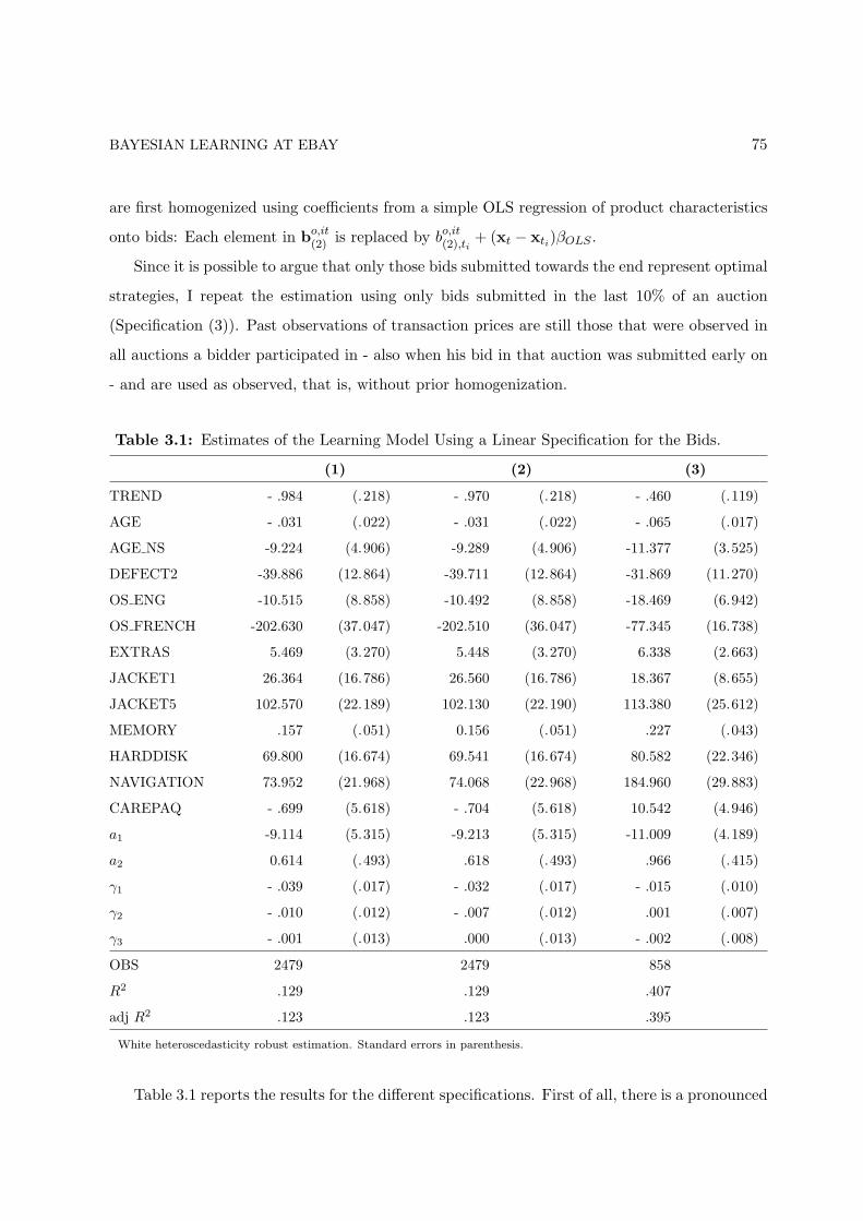
BAYESIAN LEARNING AT EBAY 75
are first homogenized using coefficients from a simple OLS regression of product characteristics
onto bids: Each element in bo,it(2) is replaced by bo,it
(2),ti+ (xt − xti)βOLS .
Since it is possible to argue that only those bids submitted towards the end represent optimal
strategies, I repeat the estimation using only bids submitted in the last 10% of an auction
(Specification (3)). Past observations of transaction prices are still those that were observed in
all auctions a bidder participated in - also when his bid in that auction was submitted early on
- and are used as observed, that is, without prior homogenization.
Table 3.1: Estimates of the Learning Model Using a Linear Specification for the Bids.
(1) (2) (3)
TREND - .984 (.218) - .970 (.218) - .460 (.119)
AGE - .031 (.022) - .031 (.022) - .065 (.017)
AGE NS -9.224 (4.906) -9.289 (4.906) -11.377 (3.525)
DEFECT2 -39.886 (12.864) -39.711 (12.864) -31.869 (11.270)
OS ENG -10.515 (8.858) -10.492 (8.858) -18.469 (6.942)
OS FRENCH -202.630 (37.047) -202.510 (36.047) -77.345 (16.738)
EXTRAS 5.469 (3.270) 5.448 (3.270) 6.338 (2.663)
JACKET1 26.364 (16.786) 26.560 (16.786) 18.367 (8.655)
JACKET5 102.570 (22.189) 102.130 (22.190) 113.380 (25.612)
MEMORY .157 (.051) 0.156 (.051) .227 (.043)
HARDDISK 69.800 (16.674) 69.541 (16.674) 80.582 (22.346)
NAVIGATION 73.952 (21.968) 74.068 (22.968) 184.960 (29.883)
CAREPAQ - .699 (5.618) - .704 (5.618) 10.542 (4.946)
a1 -9.114 (5.315) -9.213 (5.315) -11.009 (4.189)
a2 0.614 (.493) .618 (.493) .966 (.415)
γ1 - .039 (.017) - .032 (.017) - .015 (.010)
γ2 - .010 (.012) - .007 (.012) .001 (.007)
γ3 - .001 (.013) .000 (.013) - .002 (.008)
OBS 2479 2479 858
R2 .129 .129 .407
adj R2 .123 .123 .395
White heteroscedasticity robust estimation. Standard errors in parenthesis.
Table 3.1 reports the results for the different specifications. First of all, there is a pronounced
BAYESIAN LEARNING AT EBAY 76
negative time trend in the data. This is attributed to the high tech characteristic of the product
and also observed in shops outside eBay. The signs of the coefficients for product characteristics
are, besides the variable CAREPAQ, all significant and have the expected signs: The age, a
foreign operating system, and a defect have a negative impact on the bids while additional
extras lead to higher bids. The relative importance of the different extras matches their relative
prices outside eBay.
The coefficients which measure the influence of the past number of trials, a1 and a2, are
negative and positive, respectively, that is, they conform to the predictions of the model. Both
coefficients are significant at the 10% level in all specifications. As for the influence of the past
observations, reflected in the γ coefficients, the results are less pronounced. The maximum
number of observations of transaction prices taken by an individual, that is, the maximum
number of auctions he already participated in, is larger than 16. Since I do not have enough
observations, I cannot estimate all of these coefficients. Instead, I restrict attention to the first
3 observations a bidder took and see whether they fulfil the predictions of the theoretical model.
The coefficient for the first observation, γ1, is significantly negative in all specifications and,
thus, in line with the model. While mostly the influence of the second and third observation is
negative as well and smaller, the effects are insignificant. A reason for this insignificance might
be that part of the learning is not reflected in the data, that is, the bidder also learns when he
does not participate.
There is nearly no difference in the results between Specification (1) and (2). This is not
too astonishing since on average the influence of high and low value products cancels. There are
some small differences when using Specification (3). These could, however, also be attributed
to the considerably smaller sample size. The problem with first differences in the eBay setting
is that half of the bidders are lost since they only participate once. This is reflected in the
relatively low R2. This effect is even more pronounced when only using bids submitted in the
last 10% of the time. If the one time bidders are different from the other bidders (see Chapter
2) this would bias the results.
BAYESIAN LEARNING AT EBAY 77
3.5 Conclusion
Standard sequential auction models cannot rationalize increasing individual bids which are en-
countered at eBay. The paper showed that uncertainty over the competitors’ primitives can
provoke such bidding patterns. By augmenting the search model proposed in Chapter 2 by a
Bayesian learning procedure it was not only shown that the bidder optimally increases his bids
over time but also how he will incorporate new information in form of past observations of trans-
action prices into his bidding strategy. Results from reduced form estimations gave evidence
that learning is a possible explanation for the observed bidding patterns.
Besides showing that there is evidence of Bayesian updating in the eBay data, a main con-
tribution of this work is to show how to make use of asymptotic order statistic distributions in
an auction environment. Learning in second price auctions is complicated by the fact that the
bidder cannot directly observe the statistic of interest, namely the highest bid of his competi-
tors, but only the transaction price, which is the second highest bid. Using results from the
asymptotic distribution of extreme order statistics, it was shown that the transaction price can
also be used to update the beliefs over a parameter of the distribution of the highest bid.
While the empirical part allowed for bidder heterogeneity in form of different valuations,
all bidders started with the same priors. It would be interesting to see whether the results
are robust to heterogenous priors. Since such a specification would require a more structural
approach, this has to be deferred to future research. A structural approach would also be
desirable to see whether the results are robust to possible non-linearities.
Finally, the results hinge on the premise that the proposed model is the true model. While
increasing bids over time and with new observations of transaction prices intuitively make sense,
derivation of the optimal bidding strategy is far from easy. It would be interesting to see whether
other bidding strategies, including e.g. reasonable heuristics or behavioral strategies, would
explain the data better.
BAYESIAN LEARNING AT EBAY 78
Appendix
3.A Proofs
Proof of Lemma 3.1. The posterior distribution of the parameter, given that only one observa-
tion is included at a time which is distributed Gumbel, is given by:
ξpost(θ|bn−k+1) =g(k)(bn−k+1|θ)ξ(k)(θ; r, C)∫∞
−∞ g(k)(bn−k+1|θ)ξ(k)(θ; r, C)dθ
=e−ke
−(b(k)−θ)τ
e−k(b(k)−θ)τeθτkCe−kreθk
∫∞−∞ e−ke
−(b(k)−θ)τ
e−k(b(k)−θ)τeθτkCe−kreθkdθ
=eθτk(C+1)e
−eθτ k“r+e
−b(k)τ”
∫∞−∞ eθτk(C+1)e
−eθτ k“r+e
−b(k)τ”dθ
.
It is easily shown that the denominator integrates to Γ (k(C + 1)) /(τ
(k
(r + e−b(k)τ
))k(C+1))
(Use equation 3.7 and the fact that distributions integrate to 1) and thus:
ξpost(θ|bn−k+1) =τ
(k(rk + t(bn−k+1, 1))eθτ
)k(C+1)e−k(rk+t(bn−k+1,1))eθτ
Γ (k(C + 1)). (3.20)
Letting r′k = rk + t(bn−k+1, 1) and C ′ = C + 1 we have ξpost(θ|bn−k+1) = ξ(k)(θ; r′, C ′).
Proof of Lemma 3.2. The predictive distribution is given by∫Θ g(bh|θ)ξ(2)(θ; r, C)dθ. Using the
Gumbel density of the bid and (3.7) gives:
h(bh; r, C) =∫ ∞
−∞
τ2e−e−(bh−θ)τ−(bh−θ)τ(rk eθ τ
)k Ce−rk eθ τ
Γ (k C)dθ.
Now take the constants as far as possible out of the integral, change the variable of integration
from θ to x = eθτ , and use the fact that∫∞0 e−xa1xa2dx = Γ(a2)a2
a1a2a1for any positive constants a1
and a2. It then follows that:
h(bh; r, C) = τ(rk)kC
Γ(Ck)e−τbh
Γ (kC) kC
(e−τbh + rk)kC+1
Rearranging finally gives:
h(bh; r, C) =τ (rk)kC kCe−τbh(e−τbh + rk)−(kC+1),
which is equivalent to a Generalized Pareto Distribution (GPD).
BAYESIAN LEARNING AT EBAY 79
Proof of Prop. 3.1. Using the transaction price for updating in (3.2) we obtain:
W (ε, θ) = max{
maxb≥0
∫
Bh
1{b > bh}(v + ε− bh)∫
Θl(bh, θ)dθdbh − c+
+∫
Bh
1{b > bh}∫
B(2)
1{b(2) < bh}W e(θ(b(2)))·
·∫
Θl(bh, b(2), θ)dθdbhdb(2),W
e(θ)}
where Bh and B(2) are the set of all possible values of the highest respectively second highest
bid and l(·, . . . , ·) denotes the relevant joint distribution of its arguments. Combining this with
Lemma 3.2 for the predictive distribution and using (3.6) for the joint distribution gives:
W (ε, r, C) = max{
maxb≥0
∫ b
−∞(v + ε− bh)h(bh; r, C)dbh − c+
+∫ ∞
b
∫ bh
−∞W e(r′, C ′)
∫
Θτ2e−(bh−θ)τg((b(2) − θ)τ))·
· ξ(θ; r, C)dθdbhdb(2),We(r, C)
}.
Integrating τ2e−(bh−θ)τg((b(2) − θ)τ))ξ(θ; r, C) over θ finally gives
h(b(2); r, C)2C+12C
r
r+(2C)−1e−τb(2)
(r+(2C)−1e−τbh
r
)2C+1h(bh; r, C).
Proof of Prop. 3.2.
I. Standardization.
Upon changing the variables of integration from bh to b0h = e−τbh r−1 and from b(2) to b0
(2) =
e−τb(2) r−1 and rearranging we obtain:
W (ε, r, C) = max
{maxb≥0
(v + ε +
ln(r)τ
)(1−H0(b0; C)) +
1τ
∫ ∞
b0ln (x) h0(x; C)dx− c+
+∫ b0
0
∫ ∞
xW e
(2C + y
2C + 1r, C + 1
)h0(y; C)i0(x, y; C)dyh0(x;C)dx,W e(r, C)
}. (3.21)
with b0 = e−τbr−1, h0(x; C) =(
2C2C+x
)2C+1with H0(x; C) = 1 −
(2C
2C+x
)2C, and i0(x, y; C) =
2C+12C+y
(2C+x
2C
)2C+1. In the following the expression h0(y; C)i0(x, y;C)h0(x; C) will be used in its
more concise form 2C+12C
(2C
2C+y
)2C+2.
The functions which are used for expectation building are now independent of the stochastic
updating parameter r. Analytical results for the optimal strategies can still not be obtained
BAYESIAN LEARNING AT EBAY 80
unless we know the form of the value function as separate functions of the stochastically changing
r and the deterministically evolving C.
II. Value Function Guess.
Start with the following guess:
W (ε, r, C) =ln(r)
τ+ α(ε, C)
where α(ε, C) ≡ Wi(ε, 1, C) denotes the mean corrected form of the value function which only
depends on C.
Replacing W e(r′, C ′) in (3.21) by this guess and solving the integrals as far as possible gives:
W (ε, r, C) =max{
maxb≥0
ln (r)τ
+ (v + ε) (1−H0
(b0; C
)) +
1τ
∫ ∞
b0ln (x) h0(x; C)dx− c+
+(
αe(C + 1) +4C + 1
2C(2C + 1)τ− 1
τln
(2C + 1
2C
))H0
(b0; C
)−
− 1τ
ln(
2C + b0
2C
)(1−H0
(b0; C
)),W e(r, C)
}.
Under the guess the value function thus separates additively into ln(r)τ and some other part which
only depends on C and b0 and which has the form:
α(ε, C) = max{
maxb≥0
∫ ∞
b0
(v + ε +
ln(x)τ
)h0(x; C)dx− c +
∫ b0
0αe(C + 1)h0(x; C)dx
+∫ b0
0
∫ ∞
x
1τ
ln(
2C + y
2C + 1
)2C + 1
2C
(2C
2C + y
)2C+2
dydx, αe(C)}
= max{
maxb≥0
∫ ∞
b0
(v + ε +
ln(x)τ
)h0(x; C)dx− c +
∫ b0
0αe(C + 1)h0(x; C)dx
+∫ b0
0
1τ
(ln
(2C + x
2C + 1
)+
12C + 1
)h0(x;C)dx, αe(C)
}
where αe(C) =∫
α(ε, C)dFε(ε). It thus remains to be shown that b0 is independent of r.
III. Optimal Bidding Strategy.
Taking derivatives with respect to b0 leads to the following FOC:
v + ε +ln
(b0∗)
τ− 1
τ (2C + 1)+ ln
(2C + 1
2C + b0∗
)τ−1 − αe (C + 1) = 0.
From here it can already be seen that b0∗ is independent of r. This completes the proof that
the guess for the value function was correct.
BAYESIAN LEARNING AT EBAY 81
Evaluating the FOC at b0 = e−τbr−1 and solving for b gives:
b∗ =1τ
ln((2C + 1)e−
12C+1 eτ(v+ε−αe(C+1)) − 1
)− ln(2Cr)
τ.
Rearranging leads to equation (3.12).

Bibliography
Albrecht, James W. and Bo Axell, “An Equilibrium Model of Search Unemployment,”
Journal of Political Economy, October 1984, 92 (5), 824–40.
Andersen, Erling Bernhard, “Asymptotic Properties of Conditional Maximum-likelihood
Estimators.,” Journal of the Royal Statistical Society, Series B, 1970, 32 (2), 283–301.
Athey, Susan and Philip A. Haile, “Identification of Standard Auction Models,” Economet-
rica, November 2002, 70 (6), 2107–40.
and , “Nonparametric Approaches to Auctions,” in “Handbook of Econometrics”
forthcoming.
Bajari, Patrick and Ali Hortacsu, “The Winner’s Curse, Reserve Prices, and Endogenous
Entry: Empirical Insights from eBay Auctions,” RAND Journal of Economics, Summer
2003, 34 (2), 329–55.
, Lanier Benkard, and Jonathan Levin, “Estimating Dynamic Models of Imperfect
Competition,” mimeo, 2005, (July).
Berman, Simeon M., “Note on extreme values, competing risks and semi-Markov processes,”
Ann. Math. Statist., 1963, 34 (3), 1104–1106.
Bremzen, Andrei, “Sequential Auctions with Entry Deterrence,” mimeo, 2003, (November).
Brendstrup, Bjarne and Harry J. Paarsch, “Identification and Estimation in Sequential,
Asymmetric, English Auctions,” Typescript. Iowa City, Iowa: Department of Economics,
University of Iowa, 2004.
BIBLIOGRAPHY 83
Burdett, Kenneth and Dale T. Mortensen, “Wage Differentials, Employer Size, and Un-
employment,” International Economic Review, May 1998, 39 (2), 257–73.
and Tara Vishwanath, “Declining Reservation Wages and Learning,” Review of Eco-
nomic Studies, 1988, 55, 655–666.
Caillaud, Bernard and Claudio Mezzetti, “Equilibrium Reserve Prices in Sequential As-
cending Auctions,” mimeo, 2003, (May).
David, H. A. and H. N. Nagaraja, Order Statistics, Wiley-Interscience, 2003.
DeGroot, Morris H., Optimal Statistical Decisions, McGraw-Hill, 1970.
Diamond, Peter, “A Model of Price Adjustment,” Journal of Economic Theory, 1971, 3,
156–168.
El-Gamal, Mahmoud A. and David M. Grether, “Are People Bayesian? Uncovering
Behavioral Strategies,” Journal of the American Statistical Association, September 1995,
90 (432), 1137–45.
Gal, Shmuel, Michael Landsberger, and Arkadi Nemirovski, “Participation in Auc-
tions,” mimeo, 2004, (November).
Guerre, Emmanuel, Isabelle Perrigne, and Quang Vuong, “Optimal Nonparametric
Estimation of First-Price Auctions,” Econometrica, May 2000, 68 (3), 525–74.
Gumbel, Emil Julius, Statistics of Extremes, Columbia Univ. Press, 1958.
Haile, Philip and Elie Tamer, “Inference with an Incomplete Model of English Auctions,”
Journal of Political Economy, 2003, 111 (1), 1–50.
Hendricks, K. and R.H. Porter, “Lectures on Auctions: An Empirical Perspective,” in
“Handbook of Industrial Organization” forthcoming.
Hong, Han and Matthew Shum, “Can Search Costs Rationalize Equilibrium Price Disper-
sion in Online Markets?,” mimeo, 2003, (May).
BIBLIOGRAPHY 84
Hortacsu, Ali and Chad Syverson, “Product Differentiation, Search Costs, and Competition
in the Mutual Fund Industry: A Case Study of S&P 500 Index Funds,” Quarterly Journal
of Economics, May 2004, 119 (2), 403–56.
Houser, Dan and John Wooders, “Reputation in Auctions: Theory, and Evidence from
eBay,” Journal of Economics and Management Strategy, forthcoming.
Jin, Ginger Z. and Andrew Kato, “Price, Quality and Reputation: Evidence From An
Online Field Experiment,” March 2005.
Jofre-Bonet, Mireia and Martin Pesendorfer, “Estimation of a Dynamic Auction Game,”
Econometrica, September 2003, 71 (5), 1443–89.
Kotz, Samuel and Saralees Nadarajah, Extreme value distributions. Theory and applica-
tions, London: Imperial College Press, 2002.
Kyriazidou, Ekaterini, “Estimation of a Panel Data Sample Selection Model,” Econometrica,
November 1997, 65 (6), 1335–64.
Laffont, Jean Jacques and Quang Vuong, “Structural Analysis of Auction Data,” American
Economic Review, May 1996, 86 (2), 414–20.
Lucking-Reiley, David, “Auctions on the Internet: What’s Being Auctioned, and How?,”
Journal of Industrial Economics, September 2000, 48 (3), 227–252.
, Doug Bryan, Naghi Prasad, and Daniel Reeves, “Pennies from eBay: the Deter-
minants of Price in Online Auctions,” mimeo, 2000, (January).
Pakes, Ariel, Michael Ostrovsky, and Steve Berry, “Simple Estimators for the Parameters
of Discrete Dynamic Games (with Entry / Exit Examples),” mimeo, June 2005.
Rao, B.L.S. Prakasa, “Identifiability in Stochastic Models. Characterization of Probability
Distributions.,” in “in” Probability and Mathematical Statistics, Boston et al.: Harcourt
Brace Jovanovich Publishers, 1992.
Riley, John G. and William F. Samuelson, “Optimal Auctions,” American Economic
Review, June 1981, 71 (3), 381–92.
BIBLIOGRAPHY 85
Rob, Rafael, “Equilibrium Price Distributions,” Review of Economic Studies, July 1985, 52
(3), 487–504.
Roth, Alvin E. and Axel Ockenfels, “Last-Minute Bidding and the Rules for Ending Second-
Price Auctions: Evidence from eBay and Amazon Auctions on the Internet,” American
Economic Review, September 2002, 92 (4), 1093–1103.
Song, Unjy, “Nonparametric Estiamtion of an eBay Auction Model with an Unknown Number
of Bidders,” mimeo, 2004, (January).
Sorensen, Alan T., “An Empirical Model of Heterogeneous Consumer Search for Retail Pre-
scription Drugs,” NBER Working Paper, October 2001, 8548.
van den Berg, Gerard J. and Geert Ridder, “An Empirical Equilibrium Search Model of
the Labor Market,” Econometrica, September 1998, 66 (5), 1183–1221.
von der Fehr, Nils Henrik Morch, “Predatory Bidding in Sequential Auctions,” Oxford
Economic Papers, July 1994, 46 (3), 345–56.
Weber, Robert J., “Multiple-Object Auctions,” in Paul Klemperer, ed., The economic theory
of auctions, VOL 2, Cheltenham, UK and Northampton, MA: Elgar, 2000, pp. 240–66.
Wiggans, Richard Engelbrecht, “Sequential Auctions of Stochastically Equivalent Objects,”
Economics Letters, 1994, 44 (1-2), 87–90.
yi Wang, Joseph Tao, “Is Last Minute Bidding Bad?,” mimeo, 2003, (September).
Zeithammer, Robert, “Forward-looking Bidding in Online Auctions,” Working paper, Uni-
versity of Chicago, 2004.
Curriculum Vitae
12 Juni 1974 Geboren in Lich, Hessen.
1993 Abitur, Modellschule Obersberg, Bad Hersfeld.
1993-1994 Spanischstudium, Universidad Complutense de Madrid/private Sprach-
schulen, Madrid, Spanien.
1994 - 2000 Diplomstudium Volkswirtschaftslehre, Universitat zu Koln.
1997 Auslandssemester, Universite Paris II, Frankreich.
2000 - 2003 Economist, Institut fur Weltwirtschaft, Kiel.
2002/2003 Forschungsaufenthalt, London School of Economics and Political Sci-
ence, UK.
2003 - 2006 Promotion, Munich Graduate School of Economics und Center for
Information and Network Economics, Institut fur Statistik, Ludwig-
Maximilians-Universitat Munchen.