Searching for an Ultra High-EnergyDiffuse Flux of Extraterrestrial

Neutrinos with IceCube 40

Henrik Johansson

Doctoral dissertationFysikumStockholm UniversityRoslagstullsbacken 21106 91 Stockholm

Cover page illustration:A view of the first and most convincingly neutrino-likeevent surviving all filter levels of the analysis.

c© Henrik Johansson, Stockholm 2011

ISBN 978-91-7447-290-5

Printed in Sweden by Universitetsservice AB, Stockholm 2011

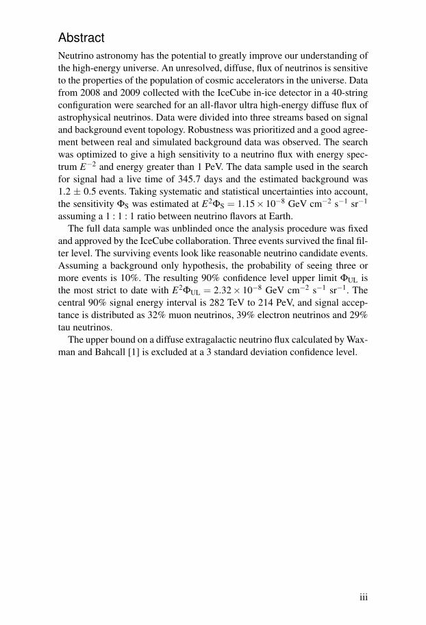
AbstractNeutrino astronomy has the potential to greatly improve our understanding ofthe high-energy universe. An unresolved, diffuse, flux of neutrinos is sensitiveto the properties of the population of cosmic accelerators in the universe. Datafrom 2008 and 2009 collected with the IceCube in-ice detector in a 40-stringconfiguration were searched for an all-flavor ultra high-energy diffuse flux ofastrophysical neutrinos. Data were divided into three streams based on signaland background event topology. Robustness was prioritized and a good agree-ment between real and simulated background data was observed. The searchwas optimized to give a high sensitivity to a neutrino flux with energy spec-trum E−2 and energy greater than 1 PeV. The data sample used in the searchfor signal had a live time of 345.7 days and the estimated background was1.2 ± 0.5 events. Taking systematic and statistical uncertainties into account,the sensitivity ΦS was estimated at E2ΦS = 1.15× 10−8 GeV cm−2 s−1 sr−1

assuming a 1 : 1 : 1 ratio between neutrino flavors at Earth.The full data sample was unblinded once the analysis procedure was fixed

and approved by the IceCube collaboration. Three events survived the final fil-ter level. The surviving events look like reasonable neutrino candidate events.Assuming a background only hypothesis, the probability of seeing three ormore events is 10%. The resulting 90% confidence level upper limit ΦUL isthe most strict to date with E2ΦUL = 2.32× 10−8 GeV cm−2 s−1 sr−1. Thecentral 90% signal energy interval is 282 TeV to 214 PeV, and signal accep-tance is distributed as 32% muon neutrinos, 39% electron neutrinos and 29%tau neutrinos.

The upper bound on a diffuse extragalactic neutrino flux calculated by Wax-man and Bahcall [1] is excluded at a 3 standard deviation confidence level.

iii

Till mina föräldrar, Inger och Roine

Contents

Abstract . . . . . . . . . . . . . . . . . . . . . . . . . . . . . . . . . . . . . . . . . . . . . . . . iiiAbout this thesis . . . . . . . . . . . . . . . . . . . . . . . . . . . . . . . . . . . . . . . . . viiiAcknowledgements . . . . . . . . . . . . . . . . . . . . . . . . . . . . . . . . . . . . . . . x

Part I: Neutrino production and detection1 Introduction . . . . . . . . . . . . . . . . . . . . . . . . . . . . . . . . . . . . . . . . . . 32 High-energy neutrino astrophysics . . . . . . . . . . . . . . . . . . . . . . . . . 7

2.1 Cosmic rays . . . . . . . . . . . . . . . . . . . . . . . . . . . . . . . . . . . . . . . . . . . . 72.2 Astrophysical neutrino production . . . . . . . . . . . . . . . . . . . . . . . . . . . . . . 102.3 Astrophysical neutrino sources . . . . . . . . . . . . . . . . . . . . . . . . . . . . . . . 12

3 Atmospheric muons and neutrinos . . . . . . . . . . . . . . . . . . . . . . . . . 173.1 Extensive air showers . . . . . . . . . . . . . . . . . . . . . . . . . . . . . . . . . . . . . . 173.2 Atmospheric muons . . . . . . . . . . . . . . . . . . . . . . . . . . . . . . . . . . . . . . . 173.3 Atmospheric neutrinos . . . . . . . . . . . . . . . . . . . . . . . . . . . . . . . . . . . . . 20

4 Neutrino detection . . . . . . . . . . . . . . . . . . . . . . . . . . . . . . . . . . . . . . 234.1 Neutrino interactions . . . . . . . . . . . . . . . . . . . . . . . . . . . . . . . . . . . . . . 234.2 Cherenkov radiation . . . . . . . . . . . . . . . . . . . . . . . . . . . . . . . . . . . . . . . 244.3 Lepton energy loss . . . . . . . . . . . . . . . . . . . . . . . . . . . . . . . . . . . . . . . . 254.4 Electromagnetic cascades . . . . . . . . . . . . . . . . . . . . . . . . . . . . . . . . . . . 284.5 Hadronic cascades . . . . . . . . . . . . . . . . . . . . . . . . . . . . . . . . . . . . . . . . 294.6 The Antarctic ice . . . . . . . . . . . . . . . . . . . . . . . . . . . . . . . . . . . . . . . . . 30

5 The IceCube detector . . . . . . . . . . . . . . . . . . . . . . . . . . . . . . . . . . . 335.1 Hole ice . . . . . . . . . . . . . . . . . . . . . . . . . . . . . . . . . . . . . . . . . . . . . . . 355.2 Digital optical module . . . . . . . . . . . . . . . . . . . . . . . . . . . . . . . . . . . . . . 365.3 Data acquisition system . . . . . . . . . . . . . . . . . . . . . . . . . . . . . . . . . . . . 395.4 Triggering and online filtering . . . . . . . . . . . . . . . . . . . . . . . . . . . . . . . . . 39

Part II: Simulation and reconstruction methods6 Simulation . . . . . . . . . . . . . . . . . . . . . . . . . . . . . . . . . . . . . . . . . . . . 43

6.1 Event generation . . . . . . . . . . . . . . . . . . . . . . . . . . . . . . . . . . . . . . . . . 436.2 Propagation . . . . . . . . . . . . . . . . . . . . . . . . . . . . . . . . . . . . . . . . . . . . 466.3 Detector simulation . . . . . . . . . . . . . . . . . . . . . . . . . . . . . . . . . . . . . . . 466.4 Simulation production . . . . . . . . . . . . . . . . . . . . . . . . . . . . . . . . . . . . . . 476.5 Simulated data sample . . . . . . . . . . . . . . . . . . . . . . . . . . . . . . . . . . . . . 47

7 Event reconstruction . . . . . . . . . . . . . . . . . . . . . . . . . . . . . . . . . . . . 537.1 Waveform calibration and feature extraction . . . . . . . . . . . . . . . . . . . . . . . 53

7.2 First guess algorithms . . . . . . . . . . . . . . . . . . . . . . . . . . . . . . . . . . . . . 547.3 Likelihood description . . . . . . . . . . . . . . . . . . . . . . . . . . . . . . . . . . . . . . 567.4 Track reconstructions . . . . . . . . . . . . . . . . . . . . . . . . . . . . . . . . . . . . . . 587.5 Cascade reconstructions . . . . . . . . . . . . . . . . . . . . . . . . . . . . . . . . . . . . 60

Part III: Searching for an Ultra-High Energy Diffuse Fluxof Extraterrestrial Neutrinos with IceCube 408 Analysis overview . . . . . . . . . . . . . . . . . . . . . . . . . . . . . . . . . . . . . . 63

8.1 Signal . . . . . . . . . . . . . . . . . . . . . . . . . . . . . . . . . . . . . . . . . . . . . . . . . 638.2 Background . . . . . . . . . . . . . . . . . . . . . . . . . . . . . . . . . . . . . . . . . . . . . 638.3 Structure . . . . . . . . . . . . . . . . . . . . . . . . . . . . . . . . . . . . . . . . . . . . . . 638.4 Blindness . . . . . . . . . . . . . . . . . . . . . . . . . . . . . . . . . . . . . . . . . . . . . . 638.5 Experimental data sample . . . . . . . . . . . . . . . . . . . . . . . . . . . . . . . . . . . 648.6 The IceCube frame of reference . . . . . . . . . . . . . . . . . . . . . . . . . . . . . . . 64

9 Filter level 1 . . . . . . . . . . . . . . . . . . . . . . . . . . . . . . . . . . . . . . . . . . 659.1 Muon filter . . . . . . . . . . . . . . . . . . . . . . . . . . . . . . . . . . . . . . . . . . . . . . 659.2 Cascade filter . . . . . . . . . . . . . . . . . . . . . . . . . . . . . . . . . . . . . . . . . . . 669.3 EHE filter . . . . . . . . . . . . . . . . . . . . . . . . . . . . . . . . . . . . . . . . . . . . . . 66

10 Filter level 2 . . . . . . . . . . . . . . . . . . . . . . . . . . . . . . . . . . . . . . . . . . 6710.1 fADC information . . . . . . . . . . . . . . . . . . . . . . . . . . . . . . . . . . . . . . . . . 6710.2 Pre-cut . . . . . . . . . . . . . . . . . . . . . . . . . . . . . . . . . . . . . . . . . . . . . . . . 7210.3 Reprocessing . . . . . . . . . . . . . . . . . . . . . . . . . . . . . . . . . . . . . . . . . . . 74

11 Filter level 3 . . . . . . . . . . . . . . . . . . . . . . . . . . . . . . . . . . . . . . . . . . 7711.1 Event topology . . . . . . . . . . . . . . . . . . . . . . . . . . . . . . . . . . . . . . . . . . . 7711.2 Cut variables . . . . . . . . . . . . . . . . . . . . . . . . . . . . . . . . . . . . . . . . . . . . 8211.3 Structure . . . . . . . . . . . . . . . . . . . . . . . . . . . . . . . . . . . . . . . . . . . . . . 8411.4 Passing rates . . . . . . . . . . . . . . . . . . . . . . . . . . . . . . . . . . . . . . . . . . . 108

12 Final cut . . . . . . . . . . . . . . . . . . . . . . . . . . . . . . . . . . . . . . . . . . . . . 11112.1 Unbiased optimization . . . . . . . . . . . . . . . . . . . . . . . . . . . . . . . . . . . . . 11112.2 Passing rates . . . . . . . . . . . . . . . . . . . . . . . . . . . . . . . . . . . . . . . . . . . 11212.3 Sensitivity and effective area . . . . . . . . . . . . . . . . . . . . . . . . . . . . . . . . . 114

13 Non-signal events . . . . . . . . . . . . . . . . . . . . . . . . . . . . . . . . . . . . . . 11713.1 Tagging of flasher-type events . . . . . . . . . . . . . . . . . . . . . . . . . . . . . . . . 11713.2 IceTop coincidences . . . . . . . . . . . . . . . . . . . . . . . . . . . . . . . . . . . . . . . 120

14 Systematic uncertainties . . . . . . . . . . . . . . . . . . . . . . . . . . . . . . . . . 12114.1 DOM efficiency . . . . . . . . . . . . . . . . . . . . . . . . . . . . . . . . . . . . . . . . . . 12214.2 Ice model . . . . . . . . . . . . . . . . . . . . . . . . . . . . . . . . . . . . . . . . . . . . . . 12314.3 Absolute energy scale . . . . . . . . . . . . . . . . . . . . . . . . . . . . . . . . . . . . . 12314.4 Neutrino-nucleon interaction cross sections . . . . . . . . . . . . . . . . . . . . . . . 12414.5 Atmospheric neutrino flux normalization . . . . . . . . . . . . . . . . . . . . . . . . . 12614.6 Cosmic ray flux normalization . . . . . . . . . . . . . . . . . . . . . . . . . . . . . . . . 12814.7 Cosmic ray composition . . . . . . . . . . . . . . . . . . . . . . . . . . . . . . . . . . . . 12914.8 Seasonal variation . . . . . . . . . . . . . . . . . . . . . . . . . . . . . . . . . . . . . . . . 12914.9 Neutrino coincidences . . . . . . . . . . . . . . . . . . . . . . . . . . . . . . . . . . . . . 130

vi

14.10 Summary . . . . . . . . . . . . . . . . . . . . . . . . . . . . . . . . . . . . . . . . . . . . . . 13115 Results . . . . . . . . . . . . . . . . . . . . . . . . . . . . . . . . . . . . . . . . . . . . . . 133

15.1 Upper limits on astrophysical neutrino fluxes . . . . . . . . . . . . . . . . . . . . . . 13315.2 Characterizing surviving events . . . . . . . . . . . . . . . . . . . . . . . . . . . . . . . 13315.3 Non-signal tags . . . . . . . . . . . . . . . . . . . . . . . . . . . . . . . . . . . . . . . . . . 141

16 Conclusions and outlook . . . . . . . . . . . . . . . . . . . . . . . . . . . . . . . . . 14316.1 Lessons learned . . . . . . . . . . . . . . . . . . . . . . . . . . . . . . . . . . . . . . . . . 144

Summary in Swedish . . . . . . . . . . . . . . . . . . . . . . . . . . . . . . . . . . . . . . 145A Multivariate classifiers . . . . . . . . . . . . . . . . . . . . . . . . . . . . . . . . . . . 147

A.1 Boosted decision trees . . . . . . . . . . . . . . . . . . . . . . . . . . . . . . . . . . . . . 147A.2 Evaluation of BDTs . . . . . . . . . . . . . . . . . . . . . . . . . . . . . . . . . . . . . . . 148A.3 Downgoing track stream . . . . . . . . . . . . . . . . . . . . . . . . . . . . . . . . . . . . 149A.4 Upgoing track stream . . . . . . . . . . . . . . . . . . . . . . . . . . . . . . . . . . . . . . 149A.5 Cascade stream . . . . . . . . . . . . . . . . . . . . . . . . . . . . . . . . . . . . . . . . . 150

List of Abbreviations . . . . . . . . . . . . . . . . . . . . . . . . . . . . . . . . . . . . . . . 153Bibliography . . . . . . . . . . . . . . . . . . . . . . . . . . . . . . . . . . . . . . . . . . . . . 155

vii

About this thesisThis thesis is divided into three parts. Part I describes neutrino production anddetection. Chapter 2 covers astrophysical neutrino production. Atmosphericneutrino and muon production is described in chapter 3. Chapter 4 deals withthe principles behind neutrino detection and chapter 5 gives an overview ofthe IceCube detector.

Part II describes methods used in simulation and event reconstruction.Chapter 6 gives an overview of the simulation chain and details the particularsimulation samples used in this work. Reconstruction algorithms applied inthis work are described in chapter 7.

Part III describes a search for a diffuse flux of astrophysical ultra high-energy neutrinos. A general overview of the analysis is given in chapter 8.Chapters 9 and 10 cover the first two filter levels of the analysis. The mainfilter level is described in chapter 11 and the optimization of a final cut inchapter 12. Chapter 13 deals with a tagging of non-signal events. Systematicuncertainties are investigated in chapter 14. The results of the analysis aredetailed in chapter 15, and an outlook is given in chapter 16.

Appendix A shows the details involved in evaluating multivariate classi-fiers.

Author’s contributionI have developed a search for a diffuse flux of astrophysical ultra high-energyneutrinos using data from 2008 and 2009 acquired with the IceCube detectorin a 40-string configuration. This work is presented in this thesis. It is basedon previous knowledge and efforts within the IceCube collaboration and hasbeen carried out within the diffuse analysis working group.

Work not included in this thesis where I have contributed during my timeas a PhD student at Stockholm University include:

• Geometry and timing calibration of newly deployed detector strings, andvisualization of detector performance for the purpose of verification andmonitoring, at the South Pole, February 2008.• Developing a weighting scheme for biased coincident CORSIKA event

simulation.• Developing a method for calibration of photon detection efficiency [2],

within the calibration working group.• Developing observables describing detector performance and methods for

quantifying and visualizing performance, within the verification and mon-itoring working groups.• Developing the high-energy event reconstruction algorithm Hyperreco [2],

in collaboration with the extremely high-energy working group in Chiba,Japan.

viii

• Characterizing signal-like detector artefact events in AMANDA-II [2].• Developing an interface facilitating general use of IceCube’s software

framework IceTray on SweGrid [3]. This includes management of files onSweGrid storage elements.• Installing and maintaining IceTray specific runtime environments on Swe-

Grid.• Responsibility for production of standardized simulated data on SweGrid.

This includes developing a plugin interfacing IceCube’s central job man-agement system IceProd with SweGrid, maintaining a local job manage-ment server, and continuous cooperation with IceProd developers to im-prove job management.• Configuring, generating and verifying simulated data sets for use in high-

energy analyses and in evaluation of systematic uncertainties. Data setsinclude ultra high-energy neutrino simulation, high-energy biased coinci-dent atmospheric muon simulation, neutrino simulation using state-of-the-art neutrino-nucleon cross sections [4], and neutrino simulation using dif-ferent ice models (see section 14.2).• Configuring the processing of atmospheric muon simulation with a non-

standard cosmic ray composition model, the so-called 2-component model(see section 6.1.1). A comparative study between the 2-component and thestandard composition model was performed, identifying essential differ-ences and focusing on agreement with real data. Some of the conclusionsare discussed in section 11.3.4.• A study of fADC digitizer (see section 5.2) information and how well sim-

ulation agrees with real data, for the purpose of determining if it is reason-able to use in analysis. Part of this study is described in section 10.1.I have participated in collaboration wide work on IceCube research, publi-

cations and talks. I represented the IceCube collaboration at the Lake LouiseWinter Institute 2011, presenting the results of the analysis described in thisthesis. I have given technical talks at nine collaboration meetings. I have rep-resented IceCube and the Stockholm group by giving overview talks at Par-tikeldagarna 2007 and AlbaNova open house 2007. I have represented Ice-Cube and the Stockholm group at Fysik i Kungsträdgården 2009 and with aposter for Fysikumdagen 2006.

ix

AcknowledgementsThis work is based on previous knowledge and efforts within the IceCubecollaboration, and I owe a great deal of thanks to a great deal of people. Iwish to thank my working group, in particular Gary Hill and Sean Grullon,with whom I had many fruitful and energizing discussions during two visits toMadison. Olga Botner and Allan Hallgren have provided invaluable feedback,insightful reasoning and encouraging support during the development of myanalysis, for which I am very grateful. I also wish to thank Chris Wendt andKurt Woschnagg for being sources of all kinds of inspiration. I want to thankHenrike Wissing, Paolo Desiati and Juan Carlos Díaz-Vélez for tireless helpwith simulation and for great company. I am grateful to Shigeru Yoshida andAya Ishihara, for the warmest hospitality imaginable during a visit to Chiba,and for many helpful discussions concerning this work.

I want to thank all friends and colleagues at Stockholm University, in andoutside the elementary particle physics group, for creating an environmentthat’s exciting and enjoyable when working and when not.

I’d like to thank my supervisors, Christian Walck, Per Olof Hulth and KlasHultqvist. I am very grateful for the opportunity to contribute to the work atthe South Pole, to travel and work with collaborators in Chiba and Madison,and for the flexiblity that allowed me to at times work remotely. I want tothank Christian for heartfelt support and for always giving good advice onissues of any size. I want to thank Per Olof for relating everyday work to thebig picture, driving and energizing our efforts. And I want to thank Klas, forinvaluable help on this thesis and throughout my time as a PhD student.

I most feel like a physicist in relaxed, exploratory conversation with col-leagues, and I would particularly like to thank Chad Finley and Seon-Hee Seofor enlightening and inspiring discussions.

Joakim Edsjö and Per Erik Tegnér provided valuable feedback on this the-sis, for which I am very thankful.

I also want to thank my office mates and fellow PhD students, old and new.I’ve grown as a physicist and enjoyed memorable travels with fellow PhD stu-dents Gustav Wikström, Thomas Burgess, Christin Wiedemann, Johan Lund-berg, Marianne Johansen, Olle Engdegård and Daan Hubert. My office matesMaja Tylmad, Matthias Danninger and Marcel Zoll have created a friendly,open-minded atmosphere which I am fortunate to share.

I am very thankful for my friends outside of physics, who keep me anchoredto a world with far more forces and interactions.

I am forever grateful to my parents and my brother and his family, who havealways provided encouragement and the sense that anything is possible.

Most of all, I want to thank Angela, for the unfailing support that made thiswork possible, and for providing a perspective where everything makes sense.

x

Part I:Neutrino production and detection

1. Introduction

Observations of photons from the universe have shed light on mysteries of thenight sky for centuries, and continue to do so. Traditionally in the form of visi-ble light, now photons are observed in a range from low frequency radio wavesto very high-energy gamma rays. Photons are good carriers of information inthe sense that they are stable, emitted in large numbers, easy to detect andpoint back to the source. Furthermore, the photon spectrum contains detailedinformation about the chemical and physical properties of the source.

Photons are, however, attenuated by interstellar dust and gas and cosmicbackground radiation. Gamma ray astronomy has made remarkable discov-eries of sources with extreme physical conditions, but the range for furtherexploration is limited by the attenuation due to pair production in interactionswith the cosmic background radiation. Above 100 TeV gamma rays are notexpected to survive from extragalactic distances, as shown in figure 1.1.

Due to the optical thickness of astrophysical sources, photons reveal infor-mation about the surface of objects. Charged cosmic rays provide informationabout the inner processes which lead to their acceleration but directional infor-mation is degraded in galactic magnetic fields. For the highest energy cosmicrays the magnetic deflection is expected to be small and there are indicationsof possible correlations with nearby extragalactic matter distributions [6–8].

Neutrinos are uncharged, interact weakly and travel unimpeded over vastdistances. Neutrinos escape unaffected from the inner regions of the most en-ergetic objects seen in the universe and therefore carry crucial informationabout the nature of the energy-release processes. Observations of gamma raysare often equally well described by electromagnetic and hadronic accelerationmodels, which makes the correlation between gamma rays and cosmic raysunclear. High-energy neutrinos provide a direct link between gamma rays andcosmic rays. Observations of all messengers are necessary to deepen our un-derstanding of the processes driving non-thermal astrophysical sources, illus-trated in figure 1.2.

What makes neutrinos excellent messengers also makes them difficult todetect. Since interactions are rare, a very large detection volume is requiredto observe high-energy neutrinos. The IceCube Neutrino Observatory was re-cently completed, resulting in a detector volume of one cubic kilometer deepin the Antarctic ice.

Neutrino astronomy is a young field, so far the only confirmed sources ofextraterrestrial neutrinos are the sun and supernova SN 1987a. The detection

3

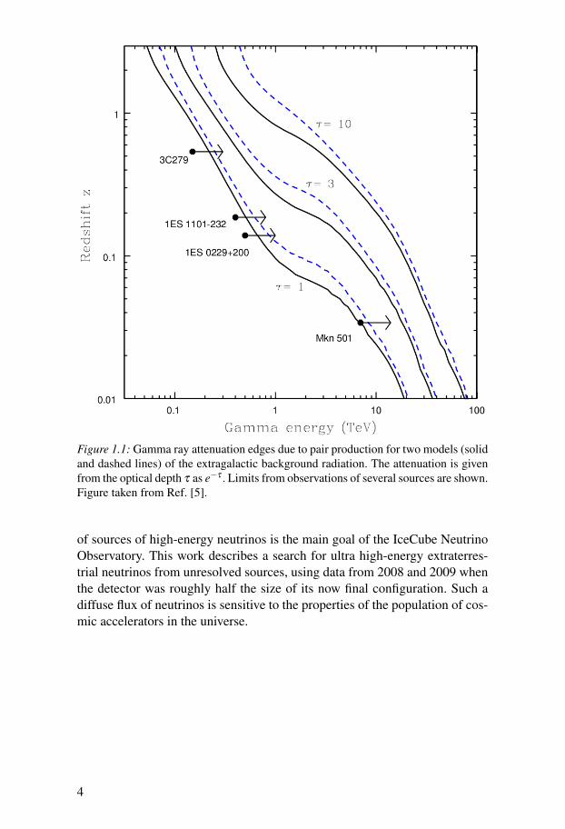
Figure 1.1: Gamma ray attenuation edges due to pair production for two models (solidand dashed lines) of the extragalactic background radiation. The attenuation is givenfrom the optical depth τ as e−τ . Limits from observations of several sources are shown.Figure taken from Ref. [5].

of sources of high-energy neutrinos is the main goal of the IceCube NeutrinoObservatory. This work describes a search for ultra high-energy extraterres-trial neutrinos from unresolved sources, using data from 2008 and 2009 whenthe detector was roughly half the size of its now final configuration. Such adiffuse flux of neutrinos is sensitive to the properties of the population of cos-mic accelerators in the universe.

4

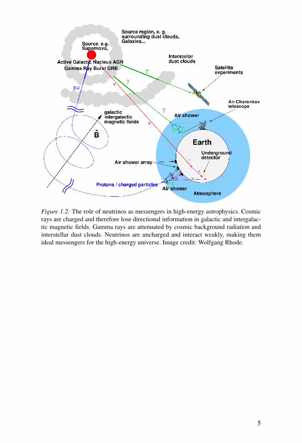
Figure 1.2: The role of neutrinos as messengers in high-energy astrophysics. Cosmicrays are charged and therefore lose directional information in galactic and intergalac-tic magnetic fields. Gamma rays are attenuated by cosmic background radiation andinterstellar dust clouds. Neutrinos are uncharged and interact weakly, making themideal messengers for the high-energy universe. Image credit: Wolfgang Rhode.

5

2. High-energy neutrino astrophysics

Neutrino astronomy is a young field with the potential to greatly improveour understanding of the high-energy universe. There is a close link betweenthe production of high-energy astrophysical neutrinos and the acceleration ofhigh-energy cosmic rays. Neutrino observations can elucidate the mystery ofthe origin of the highest energy cosmic rays. Neutrinos escape virtually unim-peded from the inner regions of extreme astrophysical objects such as activegalactic nuclei (AGNs) and gamma ray bursts (GRBs) and therefore probe theunderlying energy-release processes. Astrophysical neutrinos provide a directlink between gamma rays and cosmic rays.

2.1 Cosmic raysCosmic rays are stable charged particles and nuclei traversing the universeat nearly the speed of light. When such a particle reaches the Earth’s atmo-sphere, interactions with air nuclei produce a shower of particles propagatingthrough the atmosphere. For high-energy cosmic rays this cascade can reachthe surface of the Earth. Observations of cosmic rays can be made directly orindirectly, with detectors carried by satellites or balloons or at the surface ofthe Earth. The composition of cosmic rays range from protons and electrons tothe heaviest nuclei produced in stellar and supernova nucleosynthesis. About79% of primary cosmic rays are protons and about 70% of the rest are heliumnuclei [9].

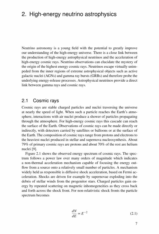
Figure 2.1 shows the observed energy spectrum of cosmic rays. The spec-trum follows a power law over many orders of magnitude which indicatesa non-thermal acceleration mechanism capable of focusing the energy out-flow from a source onto a relatively small number of particles. A mechanismwidely held as responsible is diffusive shock acceleration, based on Fermi ac-celeration. Shocks are driven for example by supernovae exploding into thedebris of stellar winds from the progenitor stars. Charged particles gain en-ergy by repeated scattering on magnetic inhomogeneities as they cross backand forth across the shock front. For non-relativistic shock fronts the particlespectrum becomes

dNdE

∝ E−2 (2.1)

7

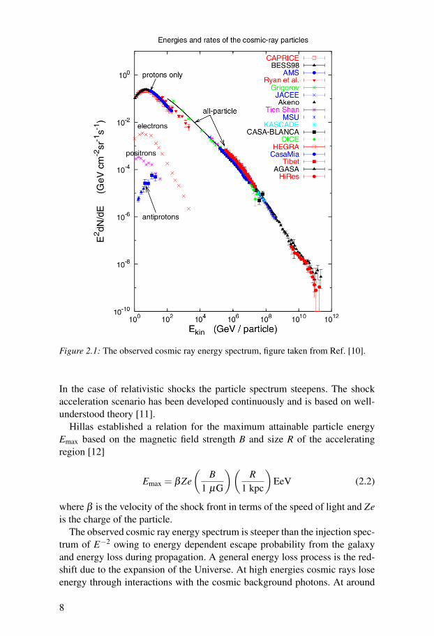
Figure 2.1: The observed cosmic ray energy spectrum, figure taken from Ref. [10].

In the case of relativistic shocks the particle spectrum steepens. The shockacceleration scenario has been developed continuously and is based on well-understood theory [11].

Hillas established a relation for the maximum attainable particle energyEmax based on the magnetic field strength B and size R of the acceleratingregion [12]

Emax = βZe(

B1 µG

)(R

1 kpc

)EeV (2.2)

where β is the velocity of the shock front in terms of the speed of light and Zeis the charge of the particle.

The observed cosmic ray energy spectrum is steeper than the injection spec-trum of E−2 owing to energy dependent escape probability from the galaxyand energy loss during propagation. A general energy loss process is the red-shift due to the expansion of the Universe. At high energies cosmic rays loseenergy through interactions with the cosmic background photons. At around

8

Figure 2.2: All-particle cosmic ray energy spectrum measured by air shower experi-ments. The shaded area shows the energy range of direct measurements. The spectrumhas been multiplied by E−2.7 to enhance spectral features. Figure taken from Ref. [9].

1 EeV, e+e− pair production becomes relevant for protons and is the dominantenergy loss process up to around 70 EeV where pion production takes over.Heavier nuclei also lose energy through photo-disintegration [13].

The low cosmic ray flux at energies above around 100 TeV makes measure-ments with small detectors carried by satellites or balloons difficult. Groundbased air shower detectors operated for a long time are well-suited for study-ing higher energy cosmic rays. There are three main types of air shower de-tectors [9]: arrays of detectors that study the shower size and the lateral dis-tribution, Cherenkov detectors that detect the Cherenkov radiation emitted bythe charged shower particles, and fluorescence detectors that study the nitro-gen fluorescence excited by the charged shower particles. Cross-calibrationsbetween different types of detectors and detailed simulations are required todetermine the primary cosmic ray energy spectrum from air shower experi-ments. Figure 2.2 shows the all-particle cosmic ray energy spectrum measuredby air shower experiments.

The change in spectral slope at around 3 PeV is commonly called the“knee”. Shock acceleration in galactic supernova remnants (SNRs) canexplain observations up to PeV energies [10]. It is suspected that the

9

steepening of the spectrum at the knee has to do with the upper reach inenergy of galactic sources. Acceleration and propagation both depend onmagnetic fields and therefore on magnetic rigidity. A rigidity dependentcutoff around the knee has been suggested [14], as first lighter and thenheavier nuclei reach an upper limit on energy per particle. Figure 2.2 showsthat measurements in the knee region differ by as much as a factor of two,which indicates experimental systematic uncertainties.

To reach higher energies, larger acceleration sites and stronger magneticfields are necessary. It is generally believed that the flattening of the spectralslope at around 5 EeV, commonly called the “ankle”, is caused by the onset ofan extragalactic component. Natural extragalactic source candidates includeAGNs and GRBs. The power required to generate the observed spectrum ofcosmic rays above the ankle seems consistent with the observed output inelectromagnetic energy of these sources [15].

Composition measurements at the highest energies differ. HiRes data isconsistent with a composition of mainly protons and light nuclei [16], whileAuger sees a more mixed composition intermediate between proton andiron [17].

There is a suppression in the cosmic ray energy spectrum above around50 EeV [18, 19]. At these energies cosmic ray protons are above the energythreshold for pion production through the ∆+ resonance in interaction withthe cosmic microwave background radiation, the so-called Greisen-Zatsepin-Kuzmin (GZK) mechanism. Protons lose most of their energy over a propaga-tion length of less than around 50 Mpc. In the case of heavier nuclei a suppres-sion because of photo-disintegration would have a similar effect [13, 20, 21].

2.2 Astrophysical neutrino productionCosmic ray acceleration sites are surrounded by matter and radiation fieldsof varying density. Neutrinos are produced through pion decay in cosmic rayinteractions with radiation or matter. The main pion production channels are

p+ γ → ∆+→

{p+π0

n+π+(2.3)

n+ γ → ∆0→

{n+π0

p+π−(2.4)

p+ p→

{p+ p+π0

p+n+π+(2.5)

10

p+n→

{p+n+π0

p+ p+π−(2.6)

Neutrinos are produced through decay of charged pions. Neutral pion decaygives rise to gamma rays

π+→µ

+ +νµ (2.7)

µ+→ e+ +νe + νµ

π−→µ

−+ νµ (2.8)

µ−→ e−+ νe +νµ

π0→ γ + γ (2.9)

Neutrinos can also be produced similarly through decay of kaons producedin cosmic ray interactions, which may contribute significantly at very highenergies [22].

On average, the fraction of energy going to the pion in pγ interactions is∼0.2 [15]. Assuming the four leptons resulting from the charged pion decaycarry an equal amount of energy, the energy transferred from the proton tothe neutrino becomes Eν ∼ Ep/20. Sophisticated approximations based onsimulations give a similar value, for both pγ [23] and pp interactions [24].

The decay channels 2.7 and 2.8 show that neutrinos are produced in a flavorratio of

νe : νµ : ντ = 1 : 2 : 0 (2.10)

Experiments have provided compelling evidence for the existence of neutrinooscillations between flavors during propagation, caused by nonzero neutrinomasses and neutrino mixing [25]. For astrophysical neutrinos, this implies anexpected flavor ratio at Earth of [26]

νe : νµ : ντ = 1 : 1 : 1 (2.11)

which is assumed in the work presented in this thesis.A differing neutrino production flavor ratio at the source, for example due

to muon energy loss in strong magnetic fields, may result in different flavorratios at Earth [27,28]. Effects of quantum decoherence would alter the flavorratio towards 1 : 1 : 1 regardless of initial flavor content [29].

11

Channel 2.9 shows the decay of neutral pions to gamma rays, which impliesthat gamma production occurs in astrophysical neutrino sources. The photonsare produced at > TeV energies, which means that optically thin sources emitTeV gamma rays in coincidence with neutrinos. If the source is optically thick,the photons will avalanche to lower energies until they can escape the sourceregion.

The opposite is not true, observations of gamma rays do not necessarily im-ply neutrino production. Gamma rays can be produced through electromag-netic acceleration of electrons that lose energy through synchrotron radiation.The accelerated electrons can further boost photons from the synchrotron fieldor external photon fields through inverse Compton scattering. Gamma ray pro-duction models based on electromagnetic or hadronic acceleration can be dif-ficult to distinguish. Neutrino production implies hadronic acceleration andtherefore provides a direct link between gamma rays and cosmic rays.

2.3 Astrophysical neutrino sourcesThe particle physics responsible for neutrino production is well established.However, the astrophysics underlying hadronic acceleration of cosmic raysis not as well known. There is a large range of models predicting neutrinosfrom different astrophysical source classes. Common for these models is tonormalize the neutrino flux based on correlations to observations of photonsor cosmic rays. A good review of astrophysical neutrino source models isgiven in Ref. [30].

The power required to generate the observed spectrum of extragalactic cos-mic rays seems consistent with the observed output in electromagnetic energyof AGNs and GRBs, which is why they have emerged as natural candidatesources of ultra high-energy cosmic rays [15].

The analysis presented in this thesis is a search for an unresolved (“diffuse”)flux of ultra high-energy neutrinos. A diffuse flux of neutrinos is sensitive tothe properties of the population of cosmic accelerators in the universe. Themodels considered in the analysis are shown in figure 2.3. They describe thediffuse flux from extragalactic source classes and are described further in thissection.

2.3.1 Neutrinos from active galactic nucleiAGNs are the most luminous persistent sources of electromagnetic radiationin the universe. An AGN radiates more power than our entire galaxy from aregion smaller than the size of our planetary system. Roughly 1% of all brightgalaxies are believed to have an active nucleus. The only known mechanismthat could sustain this luminosity is the gravitational energy release associatedwith accreting supermassive black holes [37]. Assuming hadronic acceleration

12

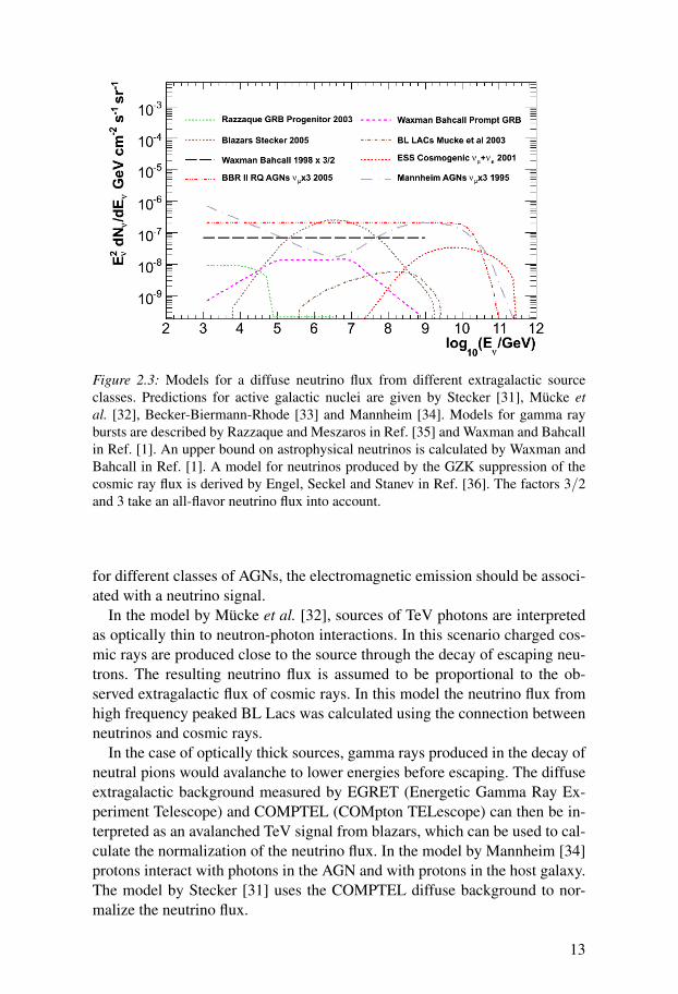
Figure 2.3: Models for a diffuse neutrino flux from different extragalactic sourceclasses. Predictions for active galactic nuclei are given by Stecker [31], Mücke etal. [32], Becker-Biermann-Rhode [33] and Mannheim [34]. Models for gamma raybursts are described by Razzaque and Meszaros in Ref. [35] and Waxman and Bahcallin Ref. [1]. An upper bound on astrophysical neutrinos is calculated by Waxman andBahcall in Ref. [1]. A model for neutrinos produced by the GZK suppression of thecosmic ray flux is derived by Engel, Seckel and Stanev in Ref. [36]. The factors 3/2and 3 take an all-flavor neutrino flux into account.

for different classes of AGNs, the electromagnetic emission should be associ-ated with a neutrino signal.

In the model by Mücke et al. [32], sources of TeV photons are interpretedas optically thin to neutron-photon interactions. In this scenario charged cos-mic rays are produced close to the source through the decay of escaping neu-trons. The resulting neutrino flux is assumed to be proportional to the ob-served extragalactic flux of cosmic rays. In this model the neutrino flux fromhigh frequency peaked BL Lacs was calculated using the connection betweenneutrinos and cosmic rays.

In the case of optically thick sources, gamma rays produced in the decay ofneutral pions would avalanche to lower energies before escaping. The diffuseextragalactic background measured by EGRET (Energetic Gamma Ray Ex-periment Telescope) and COMPTEL (COMpton TELescope) can then be in-terpreted as an avalanched TeV signal from blazars, which can be used to cal-culate the normalization of the neutrino flux. In the model by Mannheim [34]protons interact with photons in the AGN and with protons in the host galaxy.The model by Stecker [31] uses the COMPTEL diffuse background to nor-malize the neutrino flux.

13

In the model by Becker, Biermann and Rhode [33], the diffuse neutrinoflux from radio galaxies of class FR-II was calculated. It was assumed thatthe neutrino flux is proportional to the total power of the jet, which can berelated to disk luminosity, which in turn can be related to the radio output.The prediction is highly sensitive to the energy spectrum resulting from theacceleration mechanism. The neutrino spectrum was assumed to follow theproton spectrum. Effects on the neutrino spectrum from multi-pion productionwere considered small in comparison to other uncertainties. For the modelconsidered here the assumed spectrum is E−2. Changing the spectral index to-2.6 would reduce the total flux by two orders of magnitude.

2.3.2 Neutrinos from gamma-ray burstsGRBs are the most luminous outbursts of gamma radiation known, where oneGRB can outshine an entire galaxy by a hundred times. On average aroundone GRB per day is detected. They appear isotropically over the sky and ob-servations suggest that they lie at cosmological distances.

The appearance of observed GRBs is diverse, with durations from afew ms to several minutes. A distinction is commonly made between shortand long GRBs, where short GRBs last on average around 0.3 s and longaround 30 s [38]. Long GRBs are often accompanied by massive stellarexplosions [39] while a viable model for short GRBs is the merger ofcompact binary systems [40].

There are three phases of non-thermal emission connected with GRBs: theless bright precursor phase 10–100 s before the bright gamma ray burst, thebright prompt phase, and an afterglow phase. A precursor model was devel-oped by Razzaque and Meszaros in Ref. [35], based on a general class of mas-sive stellar collapses. Neutrino spectra were calculated from shock acceleratedprotons in jets just below the outer stellar envelope, before their emergence.The precursor in this model is thus not observable in photons. The observa-tion of neutrinos provides the possiblity to alert photon experiments beforethe GRB prompt phase occurs.

A model for average neutrino emission in the prompt phase, normalized tothe observation of ultra high-energy cosmic rays, was developed by Waxmanand Bahcall in Ref. [1]. In the region where electrons are accelerated, protonsare also expected to be accelerated, and neutrinos are produced in interactionswith the gamma ray burst photons. In this model, the neutrino spectrum isdetermined by the observed gamma ray spectrum.

2.3.3 The Waxman-Bahcall upper boundThe upper bound calculated by Waxman and Bahcall [1] refers to a diffuse ex-tragalactic flux of neutrinos and is valid for optically thin sources. The bound

14

is often used as a measuring rod in high-energy neutrino searches and is there-fore described here in somewhat more detail.

It is assumed that protons are accelerated in the source region and the dom-inating interaction process is with photons, producing charged and neutralpions along with neutrons and protons. Neutrinos are produced through thedecay of charged pions, and neutrons decay producing protons.

Assuming a cosmic ray generation spectrum of E−2 and taking into ac-count energy loss during propagation, the energy production rate for pro-tons was calculated based on the observed cosmic ray energy spectrum above∼ 1019 eV, giving

E2CR

dNCR

dECR≈ 1044 erg Mpc−3yr−1 (2.12)

It is assumed that the energy going to pions is roughly equal to the en-ergy ending up in protons. Neutral pions, which do not contribute to neutrinoproduction, are produced with approximately the same probability as chargedpions, and in the decay of charged pions, muon neutrinos carry approximatelyhalf the charged pion energy. Over Hubble time tH ≈ 1010 yr, the present daymuon neutrino energy density then becomes

E2ν

dNν

dEν

≈ 0.25× tHE2CR

dNCR

dECR(2.13)

The upper bound on the muon neutrino flux Φmax can then be calculatedthrough the relation flux = velocity × density, which results in

E2νΦmax =

c4π

E2ν

dNν

dEν

≈ 1.5×10−8 GeV cm−2s−1sr−1 (2.14)

Taking into account neutrino energy loss due to redshift, and evolution ofcosmic ray sources with redshift, the upper bound becomes 3×Φmax. Consid-ering neutrino oscillations the muon neutrino flux at Earth becomes E2

νΦWB =2.25×10−8 GeV cm−2s−1sr−1.

Note that even if protons are trapped by magnetic fields in the source region,escaping neutrons decay into observable cosmic ray protons. The calculationis referred to as an upper bound in part because in reality more energy is trans-ferred to the neutron than to the charged pion in the source. Halzen shows [15]that the bound should rather be interpreted as a flux estimate based on the re-lation between neutrinos and cosmic rays.

2.3.4 Cosmogenic neutrinosUltra high-energy cosmic ray protons above around 50 EeV can interact withthe cosmic microwave background radiation via the ∆+ resonance. Protonslose most of their energy over a propagation length of 50 Mpc causing theso-called GZK suppression of cosmic rays. Neutrinos are produced through

15

the decay of the ∆+ resonance via production of charged pions. The resultingdiffuse neutrino flux is commonly referred to as cosmogenic or GZK neutri-nos.

The model by Engel, Seckel and Stanev [36] is normalized to the observedspectrum of ultra high-energy cosmic rays. The model assumes an extragalac-tic cosmic ray energy spectrum of E−2 with a maximum energy of 1021 eV.Cosmological evolution of sources is taken into account.

The predictions from cosmogenic neutrino models are sensitive to the frac-tion of ultra high-energy cosmic rays composed of heavy nuclei, which isuncertain. Heavy nuclei lose energy via photo-disintegration which results infar less efficient neutrino production [41].

The primary source candidates are AGNs and GRBs but it is not clear towhat extent each source class contributes. GRBs follow a stronger cosmolog-ical evolution than AGNs, which affects the resulting neutrino flux [42].

2.3.5 Other sourcesOther sources of astrophysical neutrinos have not been considered in thiswork. They are for example neutrinos resulting from annihilation of neutralinodark matter and top-down scenarios such as decay of superheavy particles.

16

3. Atmospheric muons and neutrinos

Muons and neutrinos created in the atmosphere in cosmic ray induced airshowers constitute the main background in searches for astrophysical neutri-nos.

3.1 Extensive air showersAn air shower is created by a single cosmic ray colliding with Earth’s atmo-sphere. Interactions with air nuclei create a chain of secondary particle pro-duction and decay, resulting in a cascade of particles. Extensive air showersare induced by high energy cosmic rays and produce particles that reach theEarth’s surface. Air showers typically have a hadronic core which acts as acollimated source of electromagnetic subshowers, mainly through decay ofneutral mesons [9]. Figure 3.1 shows a schematic view of particle productionin an air shower.

Figure 3.2 shows the vertical flux of air shower particles with energy greaterthan 1 GeV as a function of atmospheric depth. At the surface of the Earthmuons and neutrinos are most abundant, and they are the only particles toreach depths relevant for the IceCube in-ice detector.

3.2 Atmospheric muonsMuons are produced in the air shower through decay of charged pions andkaons and charmed hadrons. The muon flux resulting from decay of chargedpions and kaons is called the conventional component and dominates at ener-gies up to around 10 TeV. The decay of pions (see section 2.2) dominates upto TeV energies, where the contribution from kaons becomes significant [44].The cricital energy, which is defined as the energy where decay length and in-teraction length are equal, is 115 GeV for pions and 855 GeV for kaons. Thismeans that for energies above 115 GeV pions are more likely to interact withair than to decay. This causes an energy dependent reduction in muon produc-tion and for energies greater than 1 TeV the muon energy spectrum approachesone power steeper than the primary spectrum [9]. At zenith angles closer tohorizontal the effect is smaller, because pions will travel further through thelow density upper atmosphere where the probability to decay is enhanced inrelation to interaction.

17

Figure 3.1: Schematic view of an air shower, showing the production of conventionalatmospheric muons and neutrinos. Figure taken from Ref. [43].

18

Figure 3.2: Vertical flux of air shower particles with energy greater than 1 GeV as afunction of atmospheric depth, estimated from a model of the intensity of primary nu-cleons. The points show measurements of negative muons. Figure taken from Ref. [9].

The semi-leptonic decay of charmed hadrons, mainly D-mesons and Λ+c -

hyperons, gives rise to muons through the decay modes

D→ K + µ +ν (3.1)

Λc→ Λ0 + µ +ν (3.2)

Charmed hadrons are very short-lived and decay before they have a chanceto interact, which means that the resulting muon energy spectrum is flatterthan for the conventional component. The muon flux resulting from decay ofcharmed hadrons is called the prompt component. The energy threshold forcharmed hadron production is higher than for pions and kaons, and the cross-over between the conventional and prompt component may occur between10 TeV to 1 PeV [45].

19

3.3 Atmospheric neutrinosNeutrinos are also produced in the decay of charged pions and kaons (see sec-tion 2.2). Muon decays contribute substantially to the neutrino flux only upto a few GeVs, which means that a very small fraction will decay at the ener-gies relevant for this work. The conventional atmospheric neutrino componentwill therefore be dominated by muon neutrinos. Following the same line of ar-gument as for muons, the energy spectrum for the conventional component isclose to one power steeper than the primary spectrum for energies greater than1 TeV.

Since cosmic ray primaries are positively charged, more positive than neg-ative pions and kaons will be produced in the air shower [44]. This results inan asymmetry between neutrinos and anti-neutrinos [46].

The model used in this work to describe the conventional atmospheric neu-trino component is derived by Honda et al [47].

Charmed hadrons decay equally likely into muons or electrons which re-sults in equal flux of muon and electron neutrinos for the prompt component.The flux of tau neutrinos is much smaller than for the other flavors, more thanan order of magnitude [48] since only the Ds meson decays into ντ . For thisreason the atmospheric tau neutrino flux was not considered in this work.

The cross-over between the conventional and prompt component may bearound 300 TeV for muon neutrinos. Because of the small electron neutrinoflux in the conventional component, the cross-over for electron neutrinos maybe already at around 10 TeV [48].

The model used in this work to describe the prompt component is due toEnberg et al [48].

Figure 3.3 shows the Honda and Enberg models for the conventional andprompt atmospheric neutrino flux along with the astrophysical models consid-ered in this work.

Oscillation effects for baselines equal to the diameter of the Earth are notpresent for neutrino energies greater than 50 GeV, and are therefore not im-portant for this work.

20

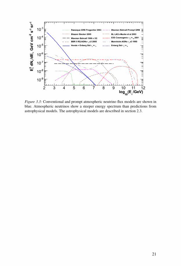
Figure 3.3: Conventional and prompt atmospheric neutrino flux models are shown inblue. Atmospheric neutrinos show a steeper energy spectrum than predictions fromastrophysical models. The astrophysical models are described in section 2.3.

21

4. Neutrino detection

What makes neutrinos excellent cosmic messengers also makes them difficultto detect. Because of the low interaction cross sections, the detection of high-energy neutrinos requires very large detector volumes. The IceCube NeutrinoObservatory detects neutrinos via Cherenkov light resulting from neutrino-nucleon interactions in the Antarctic ice. IceCube is sensitive to neutrinos inan energy range from 10 GeV to above 100 EeV.

For energies above ∼100 PeV, other detection techniques are possible.Cherenkov radiation also has a strong effect in radio, the so-called Askaryaneffect [49], which is utilized by the RICE (Radio Ice Cherenkov Experi-ment) [50] and ANITA (ANtarctic Impulsive Transient Antenna) [51, 52]experiments. SPATS (South Pole Acoustic Test Setup) [53] utilizes thefact that an acoustic signal can be produced by neutrino-induced cascadeswith high energy density. Air showers induced in the outer mantle of theEarth by Earth-skimming neutrinos have been studied by the Pierre AugerObservatory [54–56].

4.1 Neutrino interactionsAt energies relevant for ultra high-energy astrophysical neutrino searches,neutrino-nucleon interactions are in the deep inelastic scattering regime. Neu-trinos interact weakly, through charged-current (CC) via the exchange of a Wboson or through neutral-current (NC) via the exchange of a Z boson

νl(νl)+N→ l−(l+)+X (CC) (4.1)

νl(νl)+N→ νl(νl)+X (NC) (4.2)

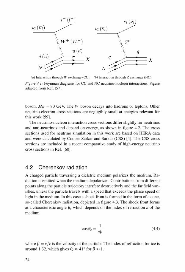
where l denotes lepton flavor, e, µ or τ , N a nucleon, and X the hadronicproduct of the interaction. The neutrino transfers enough energy to a partonto dissociate the parent nucleon which results in a hadronic shower. Feynmandiagrams depicting the interactions are shown in figure 4.1.

For νe neutrinos, resonant W− production is possible through

νe + e−→W− (4.3)

the so-called Glashow resonance [58]. It occurs at neutrino energy around6.3 PeV where the center of mass energy is close to the rest mass of the W

23

(a) Interaction through W exchange (CC). (b) Interaction through Z exchange (NC).

Figure 4.1: Feynman diagrams for CC and NC neutrino-nucleon interactions. Figureadapted from Ref. [57].

boson, MW = 80 GeV. The W boson decays into hadrons or leptons. Otherneutrino-electron cross sections are negligibly small at energies relevant forthis work [59].

The neutrino-nucleon interaction cross sections differ slightly for neutrinosand anti-neutrinos and depend on energy, as shown in figure 4.2. The crosssections used for neutrino simulation in this work are based on HERA dataand were calculated by Cooper-Sarkar and Sarkar (CSS) [4]. The CSS crosssections are included in a recent comparative study of high-energy neutrinocross sections in Ref. [60].

4.2 Cherenkov radiationA charged particle traversing a dieletric medium polarizes the medium. Ra-diation is emitted when the medium depolarizes. Contributions from differentpoints along the particle trajectory interfere destructively and the far field van-ishes, unless the particle travels with a speed that exceeds the phase speed oflight in the medium. In this case a shock front is formed in the form of a cone,so-called Cherenkov radiation, depicted in figure 4.3. The shock front formsat a characteristic angle θc which depends on the index of refraction n of themedium

cosθc =1

nβ(4.4)

where β = v/c is the velocity of the particle. The index of refraction for ice isaround 1.32, which gives θc ≈ 41◦ for β ≈ 1.

24

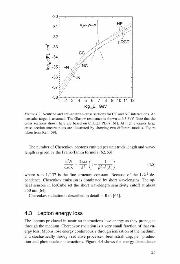
Figure 4.2: Neutrino and anti-neutrino cross sections for CC and NC interactions. Anisoscalar target is assumed. The Glasow resonance is shown at 6.3 PeV. Note that thecross sections shown here are based on CTEQ5 PDFs [61]. At high energies largecross section uncertainties are illustrated by showing two different models. Figuretaken from Ref. [59].

The number of Cherenkov photons emitted per unit track length and wave-length is given by the Frank-Tamm formula [62, 63]

d2Ndxdλ

=2πα

λ 2

(1− 1

β 2n2(λ )

)(4.5)

where α ∼ 1/137 is the fine structure constant. Because of the 1/λ 2 de-pendence, Cherenkov emission is dominated by short wavelengths. The op-tical sensors in IceCube set the short wavelength sensitivity cutoff at about350 nm [64].

Cherenkov radiation is described in detail in Ref. [65].

4.3 Lepton energy lossThe leptons produced in neutrino interactions lose energy as they propagatethrough the medium. Cherenkov radiation is a very small fraction of that en-ergy loss. Muons lose energy continuously through ionization of the medium,and stochastically through radiative processes: bremsstrahlung, pair produc-tion and photonuclear interactions. Figure 4.4 shows the energy dependence

25

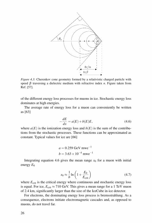
Figure 4.3: Cherenkov cone geometry formed by a relativistic charged particle withspeed β traversing a dielectric medium with refractive index n. Figure taken fromRef. [57].

of the different energy loss processes for muons in ice. Stochastic energy lossdominates at high energies.

The average rate of energy loss for a muon can conveniently be writtenas [63]

−dEdx

= a(E)+b(E)E, (4.6)

where a(E) is the ionization energy loss and b(E) is the sum of the contribu-tions from the stochastic processes. These functions can be approximated asconstant. Typical values for ice are [66]

a = 0.259 GeV mwe−1

b = 3.63×10−4 mwe−1

Integrating equation 4.6 gives the mean range x0 for a muon with initialenergy E0

x0 ≈1b

ln(

1+E0

Ecrit

)(4.7)

where Ecrit is the critical energy where continuous and stochastic energy lossis equal. For ice, Ecrit ≈ 710 GeV. This gives a mean range for a 1 TeV muonof 2.4 km, significantly larger than the size of the IceCube in-ice detector.

For electrons, the dominating energy loss process is bremsstrahlung. As aconsequence, electrons initiate electromagnetic cascades and, as opposed tomuons, do not travel far.

26

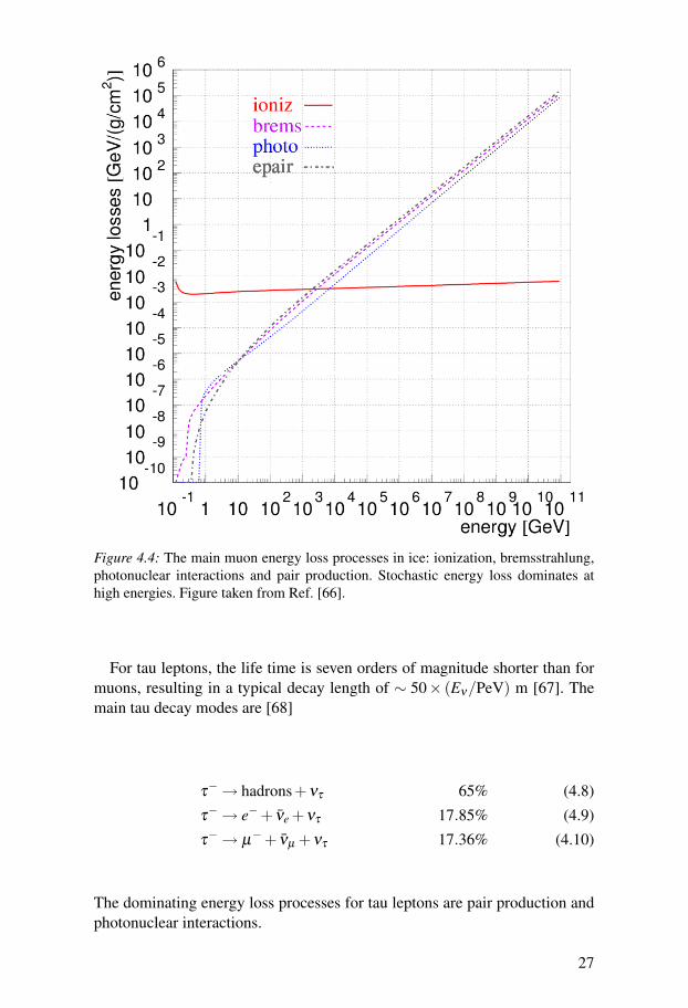
Figure 4.4: The main muon energy loss processes in ice: ionization, bremsstrahlung,photonuclear interactions and pair production. Stochastic energy loss dominates athigh energies. Figure taken from Ref. [66].

For tau leptons, the life time is seven orders of magnitude shorter than formuons, resulting in a typical decay length of ∼ 50× (Eν/PeV) m [67]. Themain tau decay modes are [68]

τ−→ hadrons+ντ 65% (4.8)

τ−→ e−+ νe +ντ 17.85% (4.9)

τ−→ µ

−+ νµ +ντ 17.36% (4.10)

The dominating energy loss processes for tau leptons are pair production andphotonuclear interactions.

27

4.4 Electromagnetic cascadesThe secondaries produced as a charged particle loses energy throughbremsstrahlung or pair production also suffer radiative energy loss andgenerate new secondaries. This results in an electromagnetic cascade.

To get an idea of how the main features of an electromagnetic cascade scale,a simplistic model can be considered [69]. An initial electron with energy E0loses 1/2 of its energy to a bremsstrahlung photon in one radiation length X0.The photon produces an electron-positron pair in the next radiation length,each with energy E0/4. During this radiation length another bremsstrahlungphoton is radiated from the original electron, with energy E0/4. This processis repeated until the energy of the electrons fall below the critical energy Ec,where energy loss through ionization becomes dominant and the developmentof the cascade ceases.

After t radiation lengths, each particle has energy E(t) = E0/2t . The maxi-mum number of particles is reached when each particle is down to the criticalenergy, after tmax radiation lengths

Ec =E0

2tmax=⇒ tmax =

1ln2

ln(

E0

Ec

)(4.11)

Nmax = 2tmax = etmax ln2 =E0

Ec(4.12)

The depth of shower maximum, reached after tmax radiation lengths, scaleswith the logarithm of E0, while the number of particles scales linearly withE0.

The total track length for all charged particles is then given by

L =(

23

)X0

∫ tmax

02tdt ∼

(2X0

3ln2E0

Ec

)(4.13)

where the factor of 2/3 roughly accounts for the fraction of charged particlesin this simplified model. The total track length is proportional to the initalenergy E0. The amount of Cherenkov photons emitted is roughly proportionalto the total track length, and this relation is used in simulation to estimate thetotal light output from cascades.

Detailed simulations have been performed where the behavior of cascadeswas parameterized [70]. An effective track length was defined to take into ac-count that the number of emitted Cherenkov photons depends on the velocityof the particle. For an electromagnetic cascade it was parameterized as

Leff = 0.894× E0

1 GeV×4.889 m (4.14)

28

where the first factor accounts for the velocity dependence. The amount ofCherenkov photons emitted is then calculated as

NC = Leff(E0)nC (4.15)

where nC is given by integrating the Frank-Tamm formula, equation 4.5, tak-ing the sensitivity profile of the optical sensor into account.

The longitudinal extension of an electromagnetic cascade is typically con-tained within ∼ 10 m. The lateral spread is small, typically less than ∼ 1 m.Because of the angular distribution of the direction of cascade particles, theshape of the Cherenkov cone from a cascade becomes slightly smeared.

At energies above ∼ 100 PeV energy loss through bremsstrahlung andpair production is suppressed by the so-called Landau-Pomeranchuk-Migdal(LPM) effect [71–73]. This can result in elongated electromagnetic cascadeson the order of 100 m [74].

4.5 Hadronic cascadesHadronic interactions such as neutrino-nucleon interactions, photonuclear in-teractions, and hadronic decay of the tau lepton, result in secondary hadronswhich in turn interact with nucleons producing new secondaries, yielding ahadronic cascade. Hadronic cascades have a slightly lower Cherenkov photonyield than electromagnetic cascades. This has several reasons. Part of the cas-cade energy goes into neutrons, which do not produce Cherenkov radiation.Energy is lost in hadronic processes because of the large nuclear binding ener-gies involved. Furthermore, charged hadrons have a higher Cherenkov photonemission threshold than electrons.

Hadronic cascades have an electromagnetic component, mainly from decayof neutral pions. This component becomes larger with energy and thereforethe difference in light yield between hadronic and electromagnetic cascadesbecomes smaller with energy. The electromagnetic component does not fur-ther contribute to the development of the hadronic cascade. Muons can beproduced in the decay of charged pions or other hadrons. The muons escapethe cascade and do not contribute further either. If these processes occur earlyit affects the development strongly. The behavior of hadronic cascades there-fore fluctuates more than for electromagnetic cascades.

For a hadronic cascade the effective track length was parameterized throughdetailed simulations as [70]

Leff = 0.860× E0

1 GeV×4.076 m (4.16)

29

4.6 The Antarctic iceFor the faint Cherenkov light to be detectable, the medium must be highlytransparent and the surroundings as dark as possible. IceCube uses the Antarc-tic glacial ice at the South Pole as a detector medium. The IceCube opticalsensors are sensitive to photons with wavelengths in a range from 350 nm to650 nm [64], with a peak sensitivity around 400 nm. The Antarctic glacialice is the most transparent solid known for wavelengths between 200 nm and400 nm [75].

The glacial ice at the South Pole was created over a period of 165,000years [76] and has a thickness of 2820 m [75]. The ice has a structure ofroughly horizontal ice sheets with varying concentrations of dust impuritiesthat can be correlated to climatological changes. The IceCube in-ice detectoris situated at depths between 1450 m and 2450 m.

The propagation of photons is governed by the scattering and absorptionproperties of the medium. The absorption length λa is defined as the distanceof travel at which the photon survival probability drops to 1/e. The scatteringlength λs is the average distance a photon travels before scattering. The aver-age scattering angle is described by 〈cosθ〉 which is strongly forward peakedwith a value of 0.94 typical for South Pole ice conditions. An effective scat-tering length can be defined as the average distance after which the photondirection is randomized [75]

λe =λs

1−〈cosθ〉(4.17)

At depths down to∼1350 m scattering is dominated by residual air bubblesin the ice. Below 1400 m air bubbles have gone through a phase transition intosolid nonscattering air hydrates [77]. Scattering and absorption below 1400 mis therefore determined by the concentration of dust impurities.

The effective scattering length and the absorption length were parameter-ized in a six parameter model based on Mie scattering [75]. The effectivescattering coefficient be and absorption coefficient a are defined as

be =1λe

(4.18)

a =1λa

(4.19)

The model fits be and a at a wavelength of 400 nm, close to where thephoton detection sensitivity is maximum, taking the optical sensor sensitivityand wavelength dependence of Cherenkov radiation into account. The modeldepends on the temperature of the ice ∆T and the six parameters α , κ , A, B,D and E

30

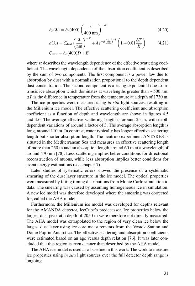
be(λ ) = be(400)(

λ

400 nm

)−α

(4.20)

a(λ ) = Cdust

(λ

nm

)−κ

+Ae−B( λ

nm)−1(

1+0.01∆TK

)(4.21)

Cdust = be(400)D+E

where α describes the wavelength dependence of the effective scattering coef-ficient. The wavelength dependence of the absorption coefficient is describedby the sum of two components. The first component is a power law due toabsorption by dust with a normalization proportional to the depth dependentdust concentration. The second component is a rising exponential due to in-trinsic ice absorption which dominates at wavelengths greater than ∼500 nm.∆T is the difference in temperature from the temperature at a depth of 1730 m.

The ice properties were measured using in situ light sources, resulting inthe Millenium ice model. The effective scattering coefficient and absorptioncoefficient as a function of depth and wavelength are shown in figures 4.5and 4.6. The average effective scattering length is around 25 m, with depthdependent variations of around a factor of 3. The average absorption length islong, around 110 m. In contrast, water typically has longer effective scatteringlength but shorter absorption length. The neutrino experiment ANTARES issituated in the Mediterranean Sea and measures an effective scattering lengthof more than 250 m and an absorption length around 60 m at a wavelength ofaround 470 nm [78]. Less scattering implies better conditions for directionalreconstruction of muons, while less absorption implies better conditions forevent energy estimations (see chapter 7).

Later studies of systematic errors showed the presence of a systematicsmearing of the dust layer structure in the ice model. The optical propertieswere measured by fitting timing distributions from Monte Carlo simulation todata. The smearing was caused by assuming homogeneous ice in simulation.A new ice model was therefore developed where the smearing was correctedfor, called the AHA model.

Furthermore, the Millenium ice model was developed for depths relevantfor the AMANDA detector, IceCube’s predecessor. Ice properties below thelargest dust peak at a depth of 2050 m were therefore not directly measured.The AHA model was extrapolated to the region of very clean ice below thelargest dust layer using ice core measurements from the Vostok Station andDome Fuji in Antarctica. The effective scattering and absorption coefficientswere estimated based on an age versus depth relation [76]. It was later con-cluded that this region is even cleaner than described by the AHA model.

The AHA ice model is used as a baseline in this work. The work to measureice properties using in situ light sources over the full detector depth range isongoing.

31

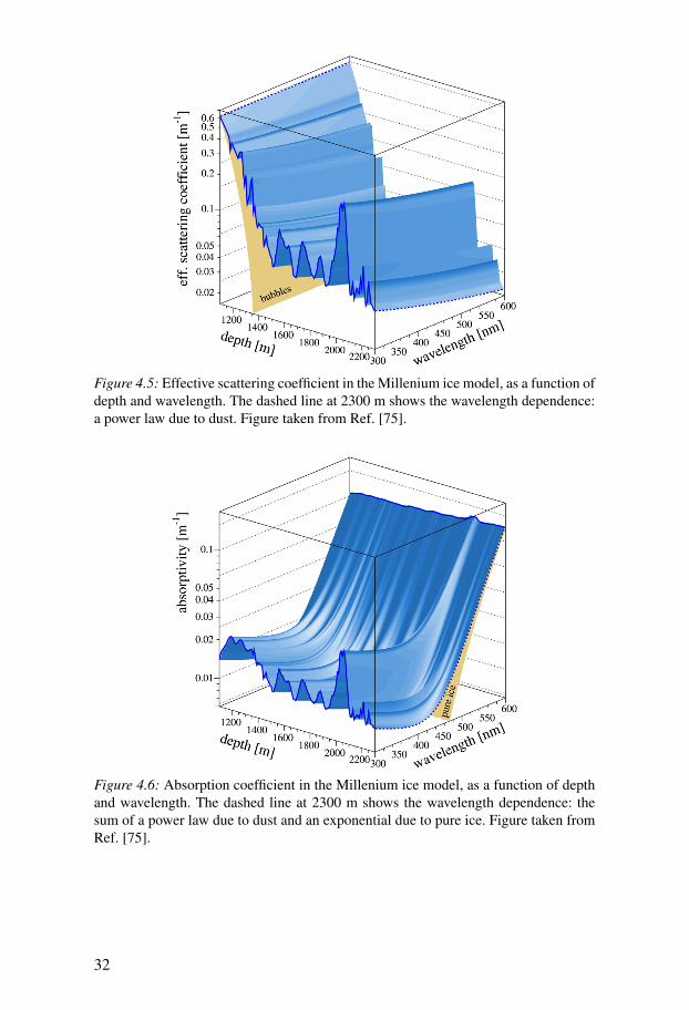
Figure 4.5: Effective scattering coefficient in the Millenium ice model, as a function ofdepth and wavelength. The dashed line at 2300 m shows the wavelength dependence:a power law due to dust. Figure taken from Ref. [75].

Figure 4.6: Absorption coefficient in the Millenium ice model, as a function of depthand wavelength. The dashed line at 2300 m shows the wavelength dependence: thesum of a power law due to dust and an exponential due to pure ice. Figure taken fromRef. [75].

32

5. The IceCube detector

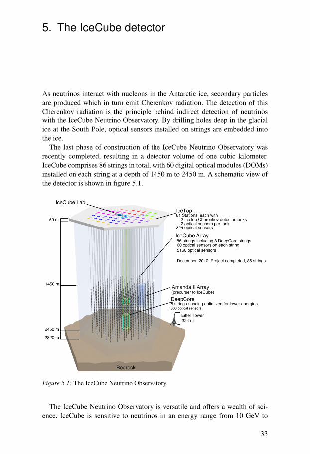
As neutrinos interact with nucleons in the Antarctic ice, secondary particlesare produced which in turn emit Cherenkov radiation. The detection of thisCherenkov radiation is the principle behind indirect detection of neutrinoswith the IceCube Neutrino Observatory. By drilling holes deep in the glacialice at the South Pole, optical sensors installed on strings are embedded intothe ice.

The last phase of construction of the IceCube Neutrino Observatory wasrecently completed, resulting in a detector volume of one cubic kilometer.IceCube comprises 86 strings in total, with 60 digital optical modules (DOMs)installed on each string at a depth of 1450 m to 2450 m. A schematic view ofthe detector is shown in figure 5.1.

Figure 5.1: The IceCube Neutrino Observatory.

The IceCube Neutrino Observatory is versatile and offers a wealth of sci-ence. IceCube is sensitive to neutrinos in an energy range from 10 GeV to

33

above 100 EeV. By studying overall counting rate, the reach of IceCube ex-tends to supernovae neutrinos at tens of MeV. IceCube’s main science goal isto discover new sources of high-energy neutrinos. The science goals includerevealing sources of the highest energy cosmic rays, providing informationabout the nature of the energy release processes behind extreme objects suchas AGNs and GRBs, determining the properties of the population of cosmicaccelerators in the universe, exploring the nature of dark matter, and constrain-ing neutrino oscillation parameters.

IceCube’s predecessor AMANDA was decommissioned at the end of thedata taking season of 2008 to 2009, after 13 years of successful operation.Between the years 2005 and 2009 data were collected using both IceCube andAMANDA strings. The size and dense instrumentation of AMANDA made itwell-suited for detection of lower energy neutrinos.

The IceCube Neutrino Observatory includes IceTop, an air shower array atthe glacier surface above the in-ice detector. There is one IceTop station above81 out of 86 IceCube strings. IceTop stations are composed of two tanks of ice,with two DOMs frozen into the ice in each tank. IceTop detects atmosphericmuons through the Cherenkov radiation emitted as they pass through the iceas well as electromagnetic cascades induced by the electromagnetic part of theair shower. Correlating events between IceTop and the in-ice detector expandsthe range of possible exploration of astroparticle physics.

The in-ice detector includes Deep Core, a low energy extension of IceCube.A large fraction of the Deep Core DOMs are extra photo-sensitive. The DeepCore DOMs are installed on 8 strings in regions of clean ice at the center ofthe in-ice detector. The dense instrumentation of Deep Core renders it optimalfor lower energy neutrino detection.

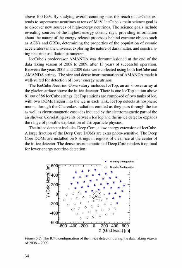
Figure 5.2: The IC40 configuration of the in-ice detector during the data taking seasonof 2008 – 2009.

34

In this work, data acquired with the in-ice detector from April 2008 to May2009 are analyzed in the search for a diffuse flux of ultra high-energy neutri-nos. During this data taking season, the detector was in a configuration with40 strings, shown in figure 5.2.

5.1 Hole iceThe holes in the ice, typically around 60 cm in diameter and 2500 m deep, aredrilled using a hot water drill. A hole is first drilled through the firn, which isabout 50 m of compacted snow on top of the ice, using a firn drill that meltsthe snow. Water is pressurized and heated to around 88 ◦C using high pressurepumps and a heating plant with generators capable of generating 5 MW. Thehot water is pumped through a hose into the hole, melting the ice. The hoseis slowly lowered using a hose reel capable of storing more than 2.9 km ofhose. Water is continuously pumped back using a submersible pump, and isreheated and recycled into the system. The drill and drilling process has beencontinuously improved upon, making it possible to drill a 2500 m deep holein less than 30 hours.

Typically it takes around two weeks for a hole to freeze in. The upper partof the hole freezes first. Also after freeze-in there is a temperature gradientfrom around −30 ◦C at the uppermost DOM to around −10 ◦C at the bottomof the string because of the temperature difference between the atmosphereand the bedrock. The freeze-in is monitored by studying noise rates. Duringfreeze-in, noise rates can increase by more than a factor of 40 owing to tribo-luminescence.

The hole ice is the refrozen column of ice in which the DOMs are embed-ded. It is believed that the hole ice contains residual air bubbles. The air bub-bles increase scattering near the DOMs, which has the effect of isotropizingthe angular sensitivity of the DOMs, in the sense that downgoing photons thatwould otherwise pass by have a larger probability of scattering into the DOM.In simulation this effect is taken into account by modifying the angular DOMsensitivity measured in the lab. Early measurements indicated a geometricalscattering length of around 0.5 m in the hole ice.

During the last season of deplyoment two video cameras housed in glassspheres were installed at the bottom of one of the detector strings. Observa-tions of the freeze-in process indicate that bubbles might be restricted to anarrow column at the center of the hole, while the rest of hole ice appearsvery clear.

35

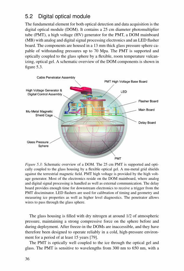
5.2 Digital optical moduleThe fundamental element for both optical detection and data acquisition is thedigital optical module (DOM). It contains a 25 cm diameter photomultipliertube (PMT), a high voltage (HV) generator for the PMT, a DOM mainboard(MB) with analog and digital signal processing electronics and an LED flasherboard. The components are housed in a 13 mm thick glass pressure sphere ca-pable of withstanding pressures up to 70 Mpa. The PMT is supported andoptically coupled to the glass sphere by a flexible, room temperature vulcan-izing, optical gel. A schematic overview of the DOM components is shown infigure 5.3.

Figure 5.3: Schematic overview of a DOM. The 25 cm PMT is supported and opti-cally coupled to the glass housing by a flexible optical gel. A mu-metal grid shieldsagainst the terrestrial magnetic field. PMT high voltage is provided by the high volt-age generator. Most of the electronics reside on the DOM mainboard, where analogand digital signal processing is handled as well as external communication. The delayboard provides enough time for downstream electronics to receive a trigger from thePMT disciminator. LED flashers are used for calibration of timing and geometry andmeasuring ice properties as well as higher level diagnostics. The penetrator allowswires to pass through the glass sphere.

The glass housing is filled with dry nitrogen at around 1/2 of atmosphericpressure, maintaining a strong compressive force on the sphere before andduring deployment. After freeze-in the DOMs are inaccessible, and they havetherefore been designed to operate reliably in a cold, high-pressure environ-ment for a period of at least 15 years [79].

The PMT is optically well coupled to the ice through the optical gel andglass. The PMT is sensitive to wavelengths from 300 nm to 650 nm, with a

36

peak sensitivity at around 400 nm [64]. The optical gel and glass set the lowersensitivity cutoff at 350 nm.

The nominal gain for the in-ice PMTs was chosen at 107 to give single pho-toelectron (SPE) pulses around 8 mV, well above electronics noise [64]. ThePMT response is linear to within 10% for currents up to 31 photoelectrons/ns(PE/ns), and saturates completely at 93 PE/ns. Simulations show that at a60 m distance, a 600 TeV cascade would cause a peak intensity of 30 PE/ns.Above ∼10 PeV many nearby PMTs would saturate and energy reconstruc-tions would have to rely more on information from DOMs further away.

The Hamamatsu R7081-02 PMT was chosen based on low dark noise andgood time and charge resolution for single photons [64]. At temperatures rel-evant to the detector environment, between −40 ◦C and −10 ◦C, a dark noiserate of around 300 Hz was measured. The low temperature noise rate is be-lieved to be dominated by radioactive decay in the PMT glass. A similar darknoise contribution comes from decays in the glass housing, resulting in a to-tal dark noise rate of around 650 Hz. Typically, a high-energy muon neutrinoevent has a duration of less than 3 µs, with most information contained withina time window of 300 ns for each DOM. This implies that only 1% of muonswould have a relevant noise count among the 100 DOMs closest to the track.The degradation of reconstructions due to dark noise is expected to be small.

The charge resolution for SPEs was measured to be approximately30% [64]. Including on-board digitization delay, the time resolution wasmeasured to be 2.7 ns. Because of the strong photon scattering in the icethe timing resolution is not the limiting factor for reconstruction of eventproperties.

The mainboard contains the analog front-end and two digitizer systems. Atrigger is issued when the PMT signal exceeds a programmable discriminatorthreshold, set to 0.25 PE for in-ice DOMs in IC40. In order for the digitizersto capture the entire waveform, the PMT signal is delayed by 75 ns using an11.2 m long strip line on a dedicated delay board [79]. The MB also containsa 20 MHz quartz oscillator, which is doubled to 40 MHz and controls localtiming [80]. The local clock is regularly calibrated relative to a master clockat the surface. The trigger is given a time stamp by the local clock.

The first digitizer is an application specific integrated circuit, the AnalogTransient Waveform Digitizer (ATWD) [80]. The ATWD has four channels,where three are used for waveform capture. The three channels amplify theinput signal by 16×, 2× and 0.25×. This way the full dynamic range of thePMT is well resolved. 128 samples of 10-bit data are collected per channel ata sampling frequency of 300 mega-samples per second (MSPS). The samplingfrequency is variable, the current setting results in a bin width of 3.3 ns anda total waveform length of 422 ns. The fourth channel measures signals fromsources on the DOM MB and is used for calibration and monitoring. TheATWD takes 29 µs to digitize a waveform after capture. To minimize dead

37

time, each DOM has two ATWDs which allows one to be available for signalcapture while the other is processing input signals.

For very high-energy events the PMT signal can be longer than the ATWDcapture window. The second digitizer is a fast ADC (fADC) which continu-ously samples the PMT signal at 40 MSPS [80]. The fADC collects 256 sam-ples of 10-bit data, resulting in a waveform with a sample spacing of 25 ns anda length of 6.4 µs. The waveform length more than covers the maximum timeinterval over which the most energetic events are expected to yield detectablelight to any one DOM. The fADC is operated at relative low gain to give areasonable dynamic range. An SPE pulse produces approximately a 13-countvalue above the baseline.

Communication between a DOM and surface electronics occurs over acopper-wire twisted-pair, including power distribution, data transmission andtiming calibration signals. Signal and communications processing, data trans-port, system testing and monitoring is performed by a field programmable gatearray (FPGA) containing a 32-bit ARM CPU, 8 MB flash storage and 32 MBRAM [80]. The FPGA code, ARM software and DOM operating parametersare remotely configurable.

To reduce noise, DOMs can operate in different local coincidence (LC)modes. Each DOM is connected to its nearest neighbor via copper-wiretwisted-pairs. When a DOM triggers it sends an LC signal to its nearestneighbours. DOMs receiving an LC signal can send it along to the nextneighboring DOM, depending on the LC mode. Upon triggering, or uponreceiving an LC signal, the DOM opens a time window that is typicallyat most 1 µs long. The LC condition is met if a trigger occurs and an LCsignal is received within the time window, indicating that at least one of itsneighbors also triggered. Noise hits are uncorrelated and typically isolatedwhich makes LC unlikely.

During data taking with IC40, all DOMs were required to fulfill the LC con-dition to contribute event information, referred to as hard local coincidence(HLC) operating mode. The HLC condition reduces the single DOM noisetrigger rate to less than 1 Hz. During more recent data taking, the detectorhas been operated in soft local coincidence (SLC) mode. In this mode, DOMswith isolated triggers that do not fulfill the LC condition contribute limited in-formation. A coarse charge stamp is created from the fADC waveform, basedon the highest sample within 400 ns. By including isolated triggers, morefine-grained event information is provided. However, a large fraction of iso-lated triggers are caused by noise, and a sophisticated cleaning procedure isperformed at a later stage to reduce the noise contribution.

The flasher board contains 12 gallium nitride LED flashers, directed radiallyoutwards [79]. 6 flashers point horizontally and 6 upwards at a 48◦ angle.The LEDs are capable of emitting 107 to 1010 photons per pulse at a flashingrate up to 610 Hz. The peak wavelength is in the range 400 nm to 420 nm.The flashers are used for calibration of timing, geometry and PMT response

38

linearity, measurement of optical properties of the ice, calibration of cascadeevent reconstructions, etc.

A number of DOMs are equipped with multi-wavelength flashers, so-calledcolor DOMs (CDOMs). Each CDOM has LEDs of 4 different wavelengths:340 nm, 370 nm, 450 nm, and 505 nm. The multi-wavelength flashers will beused to measure ice properties and the wavelength range was chosen to matchthe Cherenkov light seen by the DOMs.

5.3 Data acquisition systemThe general purpose of the data acquisition (DAQ) system is to capture andtimestamp all detected optical signals [80]. The digitization is performed in-side the DOMs. The digital output record sent from a DOM is often referredto as a DOM launch (in Ref. [80] it is referred to as a Hit, which is not usedhere because of a different connotation from the perspective of physics analy-sis). A DOM launch contains a timestamp generated locally within the DOM,a coarse charge stamp, and in the case of a fulfilled LC condition, severalwaveforms from the digitizers.

The data are collected in the counting house in the IceCube laboratory (ICL)on the surface of the ice [80]. Each string is connected to a DOMHub, whichis a computer in the ICL that communicates with all DOMs on the string. EachDOMHub contains eight DOM readout (DOR) cards, each of which is capableof communicating with eight DOMs. The DOR cards control the power, boot-up, software, firmware, calibration and data transfer of the DOMs. There isa master clock which distributes time calibration signals to the DOMHubs.The master clock is based on timing from a GPS receiver and is accurate towithin ±10 ns averaged over 24 h. A software element called the StringHubconverts the DOM launch timestamp from local DOM time to ICL clock timeand time-orders the stream of launches from a string.

5.4 Triggering and online filteringEvents are transferred to the northern hemisphere via a satellite link with lim-ited bandwidth. The DAQ data rate, around 1.5 kHz for IC40, is far abovethe available bandwidth, which was 35 GB/day for IC40. The DAQ data arerequired to pass one or more higher level triggers. The relevant trigger for thiswork is called simple majority trigger 8 (SMT8), which requires 8 triggeredDOMs within 5 µs.

Events which fulfill the higher level trigger condition are passed on to theprocessing and filtering (PnF) system. The PnF runs on a cluster of comput-ers in the ICL. A number of online filters are developed by different workinggroups searching for different types of signal events. The PnF runs fast event

39

reconstruction algorithms (see chapter 7) which are utilized by the online fil-ters.

Events that pass one or more online filters are scheduled for transmissionto the northern hemisphere via satellite through the South Pole Archival andData Exchange (SPADE) system.

40

Part II:Simulation and reconstruction methods

6. Simulation

Reliable Monte Carlo (MC) simulation is essential in order to make mean-ingful statements about an unknown signal flux. With a good description ofbackground components the claim to understand the detector is substantiatedand there can be confidence in the predicted expression of signal components.

Simulation in IceCube takes place within the software framework IceSim.The simulation starts with generation of particles with physical properties likeenergy, direction, distance from the detector and type. Particles are then prop-agated through matter, taking energy loss and secondary particle productioninto account. This includes the propagation of photons in the Antarctic ice. Fi-nally, the detector response is simulated. The simulation chain is summarizedin figure 6.1.

6.1 Event generation6.1.1 Atmospheric muonsThe largest background component for most IceCube analyses is downgo-ing muons produced in extensive air showers initiated by high-energy cosmicrays. Extensive air showers are simulated using the Monte Carlo event gener-ator CORSIKA (COsmic Ray SImulations for KAscade) [81]. Nuclei in therange from protons to iron can be treated as cosmic ray primaries. Particlesare tracked through the atmosphere until they interact with air nuclei or decay.High-energy hadronic interactions are described by the SIBYLL model [82].The CORSIKA simulation used in this analysis assumes atmospheric condi-tions typical for the South Pole in October.

The poly-gonato model by Hörandel [14] is used in the default IceCubesimulation to describe the primary cosmic ray spectrum. In this model, thecosmic ray flux is a superposition of individual primary fluxes from protonsto uranium nuclei. Here, the “knee” in the cosmic ray energy spectrum is theresult of a rigidity-dependent cutoff in the individual primary spectra.

For technical reasons, only primaries up to iron can be simulated with COR-SIKA. Furthermore, the poly-gonato model does not describe the observedcosmic ray flux at ultra high energies, where it omits what is generally as-sumed to be an extragalactic contribution. In this analysis, the cosmic rayspectrum at ultra high energies is approximated by extending the iron compo-nent with a power law with index -3, following that of the observed overall

43

Figure 6.1: Summary of the simulation chain.

cosmic ray spectrum. This implicitly assumes that the cosmic ray spectrumcontinues indefinitely as E−3 and that the ultra high-energy cosmic ray fluxconsists mainly of heavy nuclei. This approximation does not mitigate thelimited statistics at the highest energies due to the inherent rigidity-dependentcutoffs in generation spectra.

The live time for simulated data should ideally be substantially larger thanfor experimental data to minimize the impact of statistical uncertainties. Thecosmic ray energy spectrum falls steeply with energy and this analysis is opti-mized for ultra high energies. If simulated data were generated according to aphysical spectrum, an unfeasibly large amount of data would be required to getsatisfying statistics in the relevant energy range. Instead, simulation is biasedto oversample events at high energies and can then be weighted to a physicalspectrum. For poly-gonato CORSIKA, events are generated according to anenergy spectrum one power flatter than the model spectrum.

There is a significant probability of two or more atmospheric muon eventstriggering the detector within the DAQ readout window. Double and triple co-incident events are simulated separately from single events. Previously it wasnot possible to oversample coincident events at high energies, which severelylimited statistics at high energies. The work on simulation within the contextof this analysis included implementing a weighting scheme for coincidentevents, which allowed the use of high-energy biased simulation. Coincidentevents were generated according to an energy spectrum one half power flatterthan the model spectrum.

44

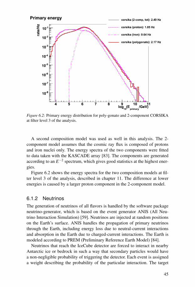
Figure 6.2: Primary energy distribution for poly-gonato and 2-component CORSIKAat filter level 3 of the analysis.

A second composition model was used as well in this analysis. The 2-component model assumes that the cosmic ray flux is composed of protonsand iron nuclei only. The energy spectra of the two components were fittedto data taken with the KASCADE array [83]. The components are generatedaccording to an E−2 spectrum, which gives good statistics at the highest ener-gies.

Figure 6.2 shows the energy spectra for the two composition models at fil-ter level 3 of the analysis, described in chapter 11. The difference at lowerenergies is caused by a larger proton component in the 2-component model.

6.1.2 NeutrinosThe generation of neutrinos of all flavors is handled by the software packageneutrino-generator, which is based on the event generator ANIS (All Neu-trino Interaction Simulation) [59]. Neutrinos are injected at random positionson the Earth’s surface. ANIS handles the propagation of primary neutrinosthrough the Earth, including energy loss due to neutral-current interactionsand absorption in the Earth due to charged-current interactions. The Earth ismodeled according to PREM (Preliminary Reference Earth Model) [84].

Neutrinos that reach the IceCube detector are forced to interact in nearbyAntarctic ice or bedrock in such a way that secondary particles would havea non-negligible probability of triggering the detector. Each event is assigneda weight describing the probability of the particular interaction. The target

45

medium is assumed to be isoscalar, which is a valid assumption for rock, butnot for ice, which has more protons than neutrons. In the low energy deepinelastic scattering regime the error due to non-isoscalarity is on the order of4% [85]. At higher energies the error is smaller, and at energies relevant forthis work the error is expected to be negligible.

For simulation used in this analysis neutrinos are generated according toan E−1 spectrum. A number of atmospheric and astrophysical neutrino fluxmodels are available within IceSim and can be used to weight the neutrinosimulation accordingly.

Assumptions of atmospheric conditions are included in the atmosphericneutrino flux models. The baseline model for the conventional flux componentin this analysis is derived by Honda et al [47] and assumes an atmosphere thatis a climatological average (the U.S. Standard Atmosphere 1976). The modelused to describe the prompt flux component is due to Enberg et al [48] andassumes an isothermal atmosphere where the density decreases exponentiallywith height.

6.2 PropagationAtmospheric muons and neutrino induced leptons are propagated through iceand rock using the software package MMC (Muon Monte Carlo) [66]. MMCtakes continuos and stochastic energy losses into account and handles propa-gation of secondary leptons.

The propagation of Cherenkov photons is handled separately. Real-timephoton propagation is computationally intensive. Given a model for the prop-agation medium, the software package Photonics [86] determines photon fluxand time distributions throughout a volume containing a light source throughMonte Carlo simulation. Photons are propagated and time distributions arerecorded throughout a cellular grid constituting the simulation volume. Tablesare generated with the photon distribution results for light sources with vary-ing properties. In the simulation chain, predicted light distributions are drawnfrom the tables. This is a computationally efficient approach which also allowsusage of the full ice model information in event reconstructions, described inchapter 7.

6.3 Detector simulationThe detector simulation starts with hit construction. Based on lepton propaga-tion information the expected number of photoelectrons produced in a partic-ular DOM is drawn from the Photonics tables, along with the expected photonarrival time distribution. The expected number of photoelectrons is affectedby the DOM efficiency, which is a collective term describing the local hole

46

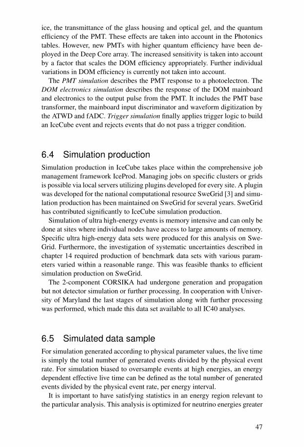
ice, the transmittance of the glass housing and optical gel, and the quantumefficiency of the PMT. These effects are taken into account in the Photonicstables. However, new PMTs with higher quantum efficiency have been de-ployed in the Deep Core array. The increased sensitivity is taken into accountby a factor that scales the DOM efficiency appropriately. Further individualvariations in DOM efficiency is currently not taken into account.

The PMT simulation describes the PMT response to a photoelectron. TheDOM electronics simulation describes the response of the DOM mainboardand electronics to the output pulse from the PMT. It includes the PMT basetransformer, the mainboard input discriminator and waveform digitization bythe ATWD and fADC. Trigger simulation finally applies trigger logic to buildan IceCube event and rejects events that do not pass a trigger condition.

6.4 Simulation productionSimulation production in IceCube takes place within the comprehensive jobmanagement framework IceProd. Managing jobs on specific clusters or gridsis possible via local servers utilizing plugins developed for every site. A pluginwas developed for the national computational resource SweGrid [3] and simu-lation production has been maintained on SweGrid for several years. SweGridhas contributed significantly to IceCube simulation production.

Simulation of ultra high-energy events is memory intensive and can only bedone at sites where individual nodes have access to large amounts of memory.Specific ultra high-energy data sets were produced for this analysis on Swe-Grid. Furthermore, the investigation of systematic uncertainties described inchapter 14 required production of benchmark data sets with various param-eters varied within a reasonable range. This was feasible thanks to efficientsimulation production on SweGrid.

The 2-component CORSIKA had undergone generation and propagationbut not detector simulation or further processing. In cooperation with Univer-sity of Maryland the last stages of simulation along with further processingwas performed, which made this data set available to all IC40 analyses.

6.5 Simulated data sampleFor simulation generated according to physical parameter values, the live timeis simply the total number of generated events divided by the physical eventrate. For simulation biased to oversample events at high energies, an energydependent effective live time can be defined as the total number of generatedevents divided by the physical event rate, per energy interval.

It is important to have satisfying statistics in an energy region relevant tothe particular analysis. This analysis is optimized for neutrino energies greater

47

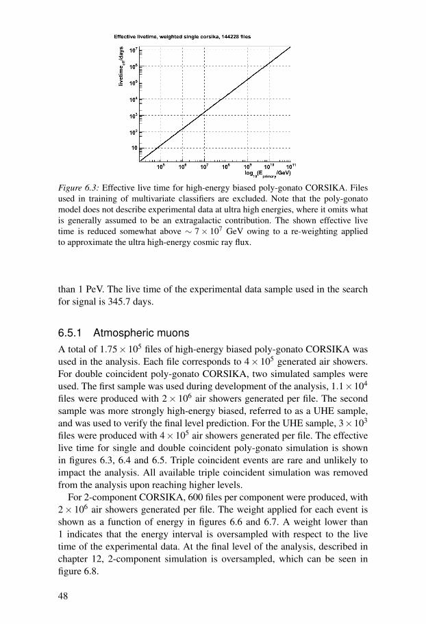
Figure 6.3: Effective live time for high-energy biased poly-gonato CORSIKA. Filesused in training of multivariate classifiers are excluded. Note that the poly-gonatomodel does not describe experimental data at ultra high energies, where it omits whatis generally assumed to be an extragalactic contribution. The shown effective livetime is reduced somewhat above ∼ 7× 107 GeV owing to a re-weighting appliedto approximate the ultra high-energy cosmic ray flux.

than 1 PeV. The live time of the experimental data sample used in the searchfor signal is 345.7 days.

6.5.1 Atmospheric muonsA total of 1.75×105 files of high-energy biased poly-gonato CORSIKA wasused in the analysis. Each file corresponds to 4× 105 generated air showers.For double coincident poly-gonato CORSIKA, two simulated samples wereused. The first sample was used during development of the analysis, 1.1×104

files were produced with 2× 106 air showers generated per file. The secondsample was more strongly high-energy biased, referred to as a UHE sample,and was used to verify the final level prediction. For the UHE sample, 3×103

files were produced with 4×105 air showers generated per file. The effectivelive time for single and double coincident poly-gonato simulation is shownin figures 6.3, 6.4 and 6.5. Triple coincident events are rare and unlikely toimpact the analysis. All available triple coincident simulation was removedfrom the analysis upon reaching higher levels.

For 2-component CORSIKA, 600 files per component were produced, with2× 106 air showers generated per file. The weight applied for each event isshown as a function of energy in figures 6.6 and 6.7. A weight lower than1 indicates that the energy interval is oversampled with respect to the livetime of the experimental data. At the final level of the analysis, described inchapter 12, 2-component simulation is oversampled, which can be seen infigure 6.8.

48

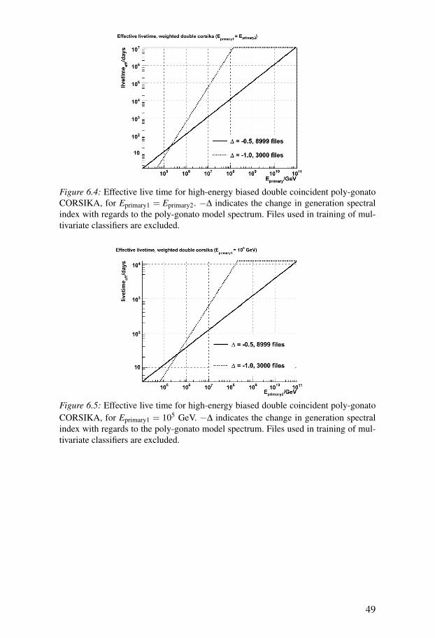
Figure 6.4: Effective live time for high-energy biased double coincident poly-gonatoCORSIKA, for Eprimary1 = Eprimary2. −∆ indicates the change in generation spectralindex with regards to the poly-gonato model spectrum. Files used in training of mul-tivariate classifiers are excluded.

Figure 6.5: Effective live time for high-energy biased double coincident poly-gonatoCORSIKA, for Eprimary1 = 105 GeV. −∆ indicates the change in generation spectralindex with regards to the poly-gonato model spectrum. Files used in training of mul-tivariate classifiers are excluded.

49

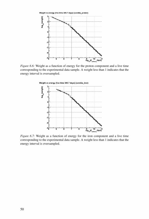
Figure 6.6: Weight as a function of energy for the proton component and a live timecorresponding to the experimental data sample. A weight less than 1 indicates that theenergy interval is oversampled.

Figure 6.7: Weight as a function of energy for the iron component and a live timecorresponding to the experimental data sample. A weight less than 1 indicates that theenergy interval is oversampled.

50

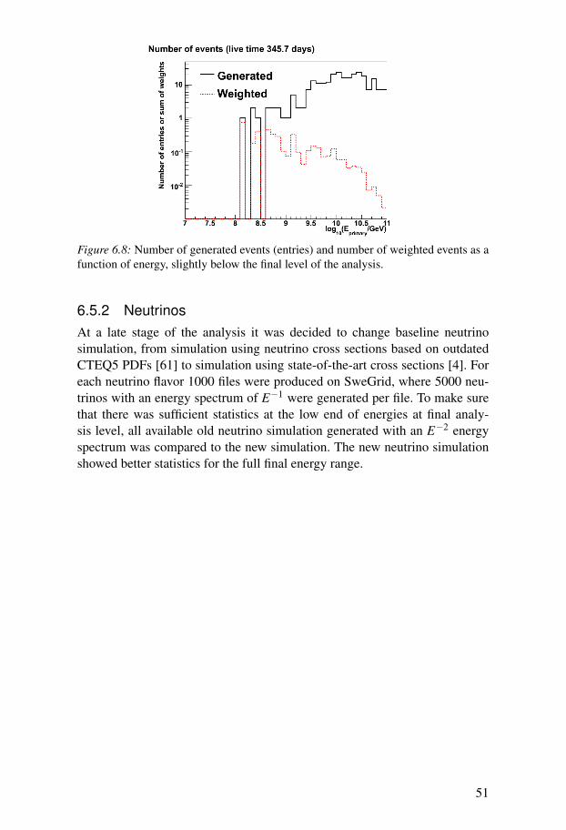
Figure 6.8: Number of generated events (entries) and number of weighted events as afunction of energy, slightly below the final level of the analysis.

6.5.2 NeutrinosAt a late stage of the analysis it was decided to change baseline neutrinosimulation, from simulation using neutrino cross sections based on outdatedCTEQ5 PDFs [61] to simulation using state-of-the-art cross sections [4]. Foreach neutrino flavor 1000 files were produced on SweGrid, where 5000 neu-trinos with an energy spectrum of E−1 were generated per file. To make surethat there was sufficient statistics at the low end of energies at final analy-sis level, all available old neutrino simulation generated with an E−2 energyspectrum was compared to the new simulation. The new neutrino simulationshowed better statistics for the full final energy range.

51

7. Event reconstruction

The main purpose of reconstruction is to estimate physical quantities of anevent, such as type, direction, location and energy. Depending on the con-text, event type can refer to lepton or neutrino flavor, or interaction type, andis commonly characterized as track-like or cascade-like (see section 11.1).Estimates of physical quantities of events are essential since signal and back-ground typically differ in for example direction and energy. The estimation isbased on the waveforms registered by the two types of digitizers in the DOMs,the ATWD and fADC (see section 5.2). The reconstruction algorithms appliedin this analysis are based on pulses extracted from the waveforms.

7.1 Waveform calibration and feature extractionThe software module DOMcalibrator calibrates the waveforms digitized bythe ATWD and fADC. Between the PMT and the high voltage board thereis a transformer that causes tails of waveforms to “droop”. In DOMcalibrator,baseline subtraction is performed, individual gain is accounted for and a trans-former droop correction is applied. The ATWD has three channels with differ-ent gain which results in three different waveforms. DOMcalibrator combinesthe three waveforms to maximize the dynamic range. The digitizer clock speedis determined and PMT transit time and relative start time offsets are correctedfor.

Feature extraction is the method by which pulses are extracted from wave-forms. A pulse is characterized by a leading edge time, an amplitude and awidth. The amplitude of a pulse is measured in photoelectrons (PEs), the typ-ical charge a single photoelectron (SPE) pulse would yield. Feature extractionis performed by the software module FeatureExtractor [87].

Feature extraction is done differently for ATWD and fADC waveforms. AnfADC waveform is composed of 256 bins with a bin width of 25 ns. For fADCwaveforms, a threshold charge value is defined and the first bin with chargeabove the threshold is located. Advancing through the waveform, the pair ofbins between which the rate of ascent is locally at maximum is found. A line isfitted to the charge values in these two bins. The point of intersection betweenthe fitted line and the baseline is taken as the leading edge of the found pulse,as illustrated in figure 7.1. The end of the pulse is defined as the lower binedge of the succeeding bin closest to the first bin, that has charge below thethreshold. The sum of the charge for bins belonging to the pulse is used as

53

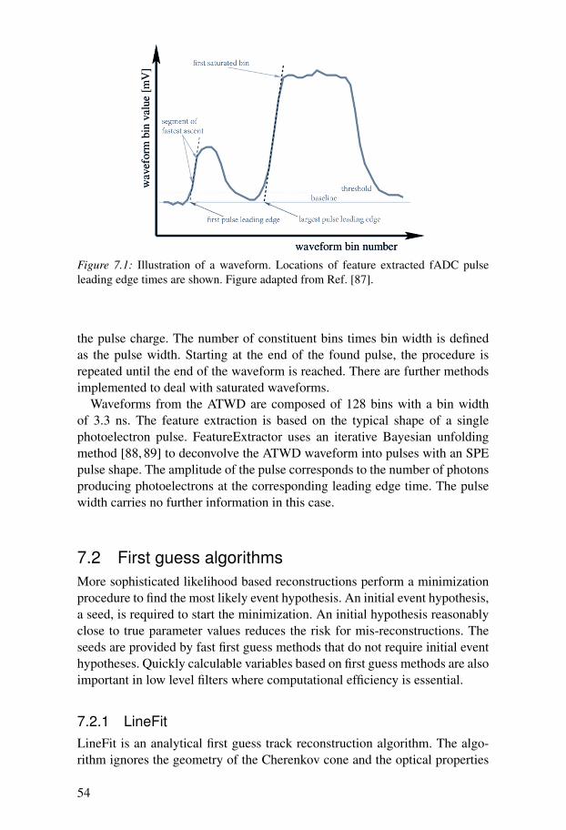
Figure 7.1: Illustration of a waveform. Locations of feature extracted fADC pulseleading edge times are shown. Figure adapted from Ref. [87].

the pulse charge. The number of constituent bins times bin width is definedas the pulse width. Starting at the end of the found pulse, the procedure isrepeated until the end of the waveform is reached. There are further methodsimplemented to deal with saturated waveforms.

Waveforms from the ATWD are composed of 128 bins with a bin widthof 3.3 ns. The feature extraction is based on the typical shape of a singlephotoelectron pulse. FeatureExtractor uses an iterative Bayesian unfoldingmethod [88, 89] to deconvolve the ATWD waveform into pulses with an SPEpulse shape. The amplitude of the pulse corresponds to the number of photonsproducing photoelectrons at the corresponding leading edge time. The pulsewidth carries no further information in this case.

7.2 First guess algorithmsMore sophisticated likelihood based reconstructions perform a minimizationprocedure to find the most likely event hypothesis. An initial event hypothesis,a seed, is required to start the minimization. An initial hypothesis reasonablyclose to true parameter values reduces the risk for mis-reconstructions. Theseeds are provided by fast first guess methods that do not require initial eventhypotheses. Quickly calculable variables based on first guess methods are alsoimportant in low level filters where computational efficiency is essential.

7.2.1 LineFitLineFit is an analytical first guess track reconstruction algorithm. The algo-rithm ignores the geometry of the Cherenkov cone and the optical properties

54

of the ice, and assumes that photons are travelling along a 1-dimensional linewith a certain velocity~vLF. A vertex point~r and the velocity~vLF is attained byminimizing

χ2 =

Npulse

∑i=1

(~ri−~r−~vLFti)2 (7.1)

where ~ri is the position of a DOM, ti is the leading edge time of a pulse de-tected in the corresponding DOM, and the sum goes over all pulses in an event.The minimization has an analytic solution

~r = 〈~ri〉−~vLF〈ti〉 (7.2)

~vLF =〈~riti〉−〈~ri〉〈ti〉〈t2

i 〉−〈ti〉2(7.3)

where 〈x〉 denotes the mean of parameter x with respect to all pulses. Thedirection is given by~vLF/|~vLF|.

For track-like events vLF is typically close to the speed of light, whereasfor cascade-like events where there is little commonality to the direction ofphotons vLF is typically small, approaching 0.

7.2.2 Tensor of inertiaThe tensor of inertia algorithm assigns a virtual mass (ai)w to a DOM at posi-tion~ri. The virtual mass corresponds to the number of detected photoelectronsin the DOM and w is a weight chosen according to how one wants to weighphotoelectrons. For applications in this work, w is set to 1. The origin of thetensor of inertia is the center of gravity (COG) of the mass distribution

~rCOG =∑

Nchi=1(ai)w~ri

∑Nchi=1(ai)w

(7.4)

where Nch denotes the number of DOMs with non-zero virtual mass. The ten-sor of inertia~I for the virtual mass distribution is

Ik,l =Nch

∑i=1

(ai)w[δ k,l(~ri)2− rki rl

i ] (7.5)

~I has three eigenvalues corresponding to three main axes, with the smallesteigenvalue corresponding to the longest axis. For track-like events, the direc-tion of the longest axis can be used as a first guess seed. Cascade-like eventsare typically fairly spherical which means that the main axes will be similarin magnitude. The ratio between the smallest eigenvalue and the sum of alleigenvalues is called the eval ratio and is an indicator of the sphericity of anevent. The COG can be used as a first guess for the interaction vertex positionin cascade reconstructions.

55

7.2.3 CFirstCFirst is a cascade first guess algorithm that uses the COG as estimated vertexposition.

For the purpose of estimating a vertex time, the geometrical time is definedas the time when unscattered Cherenkov photons reach a DOM. The shiftedresidual time is defined as the first registered pulse time in a DOM minus thegeometrical time from the COG to the DOM. This is calculated for all DOMswithin a radius of 1000 m around the COG. For each DOM, with correspond-ing shifted residual time tshift, the number of DOMs with shifted residual timewithin 200 ns following tshift is counted. The earliest tshift for which there areat least 3 such DOMs is used as the vertex time [90].

7.3 Likelihood descriptionThe general problem is estimating a set of unknown parameters ~a given aset of measured values~x. The parameters~a are determined by maximizing thelikelihood function L(~a|~x) which for independent measured values xi becomes

L(~a|~x) =N

∏i

p(xi|~a) (7.6)

where p(xi|~a) is the probability density function (PDF) of observing the mea-sured value xi given the parameter values ~a. The reconstruction is performedby minimizing − log(L) with respect to ~a. An event is generally described bythe parameters

~a = (~r0, t0, p,E0) (7.7)

where~r0 in the case of a track hypothesis is an arbitrary point along the track,and in the case of a cascade hypothesis is the interaction vertex position, t0 isthe time of the event at ~r0, p is the direction of the event and E0 the energyof the event at ~r0. For cascades there are seven degrees of freedom, the ver-tex time and position, and the direction and energy of the event. For tracksthere are six degrees of freedom, since the point along the track can be chosenarbitrarily. All parameters can be reconstructed simultaneously or the geomet-rical parameters and the energy can be reconstructed separately. The measuredvalues~x correspond to the feature extracted pulses.

If the observed number of photoelectrons and the expected number of pho-toelectrons are binned in time into K bins, the probability of observing ni

photoelectrons in the ith bin given an expectation of µi, is given by Poissonianstatistics. The likelihood for a single DOM is given by

L(~a|~x) =K

∏i=1

e−µi

ni!(µi)ni (7.8)

56

The full log-likelihood is then given by the sum of log(L) for all DOMs, whichis maximized with respect to the parameters describing the event hypothesis.

µi is given by a PDF which describes the photon arrival time distributiongiven a certain event hypothesis. A commonly used PDF is the Pandel func-tion, which parameterizes the arrival time distribution of Cherenkov photonsas a gamma distribution. It assumes bulk ice without dust layers and is moti-vated by an analysis of laser light signals in the BAIKAL experiment [91,92].The Pandel function is normalized, can be integrated over time analyticallyand is computationally efficient.

The main drawback with the Pandel function is that it assumes bulk ice,with scattering and absorption coefficients constant over depth. The propertiesof the Antarctic ice have been measured using in situ light sources, resultingin a model of the depth dependence of scattering and absorption. The softwarepackage Photonics [86] (see section 6.2) simulates photon propagation takingthe ice model into account and stores the result in tables. An interface for thepurpose of reconstruction called Photorec provides a numerical PDF describ-ing the arrival time of Cherenkov photons based on the full ice description.

Both PDFs depend on whether the light source hypothesis is an electromag-netic cascade or a muon track. The shape of the PDF is mainly determined bythe scattering of photons in the ice. The final PDF is modified to also accountfor PMT jitter and dark noise.

As mentioned previously, all event parameters can be reconstructed simul-taneously, or the geometrical parameters and the energy can be reconstructedseparately. Looking at the components separately simplifies the likelihood ex-pression. When reconstructing location and direction, the arrival times of thephotoelectrons carry the most crucial information and the total charge infor-mation can be ignored. Given a geometrical hypothesis, the energy can bereconstructed by modeling the expected total charge as a function of event en-ergy. In the simplest case, where total charge scales linearly with energy, theproblem has an analytical solution. For electromagnetic cascades the depen-dence of the amount of Cherenkov light on the cascade energy can be modeledas linear [93].

The minimization procedure can sometimes find local instead of globalminima of− log(L). A way of dealing with this undesired behavior is to repeatthe reconstruction for several seeds, which is here referred to as performingiterations of the reconstruction. One seed is provided to the reconstruction andthe other seeds are chosen with directions according to a pseudo-random uni-form distribution on the unit sphere. Ultimately the event hypothesis with thebest likelihood is used.

57

7.4 Track reconstructionsFor the track reconstructions used in this analysis the geometry of the trackis reconstructed separately from the energy. The geometry reconstructions arebased on the Pandel PDF describing photon arrival times.

7.4.1 SPE track reconstructionThe single photoelectron (SPE) PDF describes photon arrival times at a spe-cific location. Only information about the first photoelectron detected by aDOM contributes to the likelihood function in the SPE track reconstruction.This has been seen to give a more robust reconstruction than when using in-formation from all detected photoelectrons. The SPE track reconstruction isseeded by LineFit, and the result is used as a seed for a 32-iteration SPE re-construction (SPE-32).

7.4.2 MPE track reconstructionThe multi-photoelectron (MPE) PDF describes the arrival time of the first ofN photons, where N corresponds to the detected number of photoelectronsper DOM. The result of the SPE-32 reconstruction is used as a seed for theMPE reconstruction. The MPE PDF works very well for high energy muontracks. The first of many photons is likely to have suffered little scatteringand therefore carry most information about the geometry of the track. In thecase of many photons the PDF becomes narrow. In the likelihood calculationemphasis is therefore placed on the information from DOMs that detect alarge amount of light. The MPE reconstruction is relatively sensitive to localminima, compared to SPE, and a good seed is required.

7.4.3 Bayesian track reconstructionThe likelihood function can be extended to incorporate prior informationabout the atmospheric muon flux. Bayes’ theorem for an event withparameters ~a and measured values~x states

P(~a|~x) =P(~x|~a)P(~a)

P(~x). (7.9)

P(~a) is the prior probability distribution for the event hypothesis. The atmo-spheric muon flux has a well characterized zenith dependence, shown in fig-ure 7.2, which serves as a prior in the likelihood function of the Bayesian trackreconstruction. Close to the horizon, the atmospheric muon flux becomes zero,which enforces downgoing track hypotheses. P(~x) does not depend on theevent parameters and is therefore constant and can be ignored. The Bayesiantrack reconstruction is based on the SPE PDF, is seeded by the SPE-32 track

58

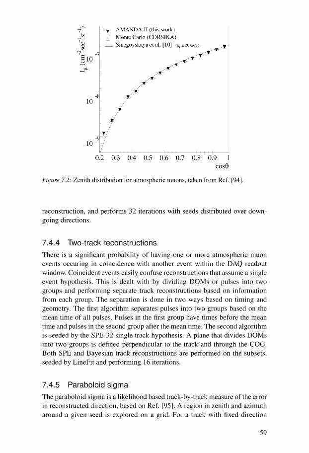
Figure 7.2: Zenith distribution for atmospheric muons, taken from Ref. [94].

reconstruction, and performs 32 iterations with seeds distributed over down-going directions.

7.4.4 Two-track reconstructionsThere is a significant probability of having one or more atmospheric muonevents occuring in coincidence with another event within the DAQ readoutwindow. Coincident events easily confuse reconstructions that assume a singleevent hypothesis. This is dealt with by dividing DOMs or pulses into twogroups and performing separate track reconstructions based on informationfrom each group. The separation is done in two ways based on timing andgeometry. The first algorithm separates pulses into two groups based on themean time of all pulses. Pulses in the first group have times before the meantime and pulses in the second group after the mean time. The second algorithmis seeded by the SPE-32 single track hypothesis. A plane that divides DOMsinto two groups is defined perpendicular to the track and through the COG.Both SPE and Bayesian track reconstructions are performed on the subsets,seeded by LineFit and performing 16 iterations.

7.4.5 Paraboloid sigmaThe paraboloid sigma is a likelihood based track-by-track measure of the errorin reconstructed direction, based on Ref. [95]. A region in zenith and azimutharound a given seed is explored on a grid. For a track with fixed direction

59

at one of the grid points, the vertex position is reoptimized to give a newlikelihood. An error ellipse is defined as the curve in parameter space on which− log(L) is 0.5 times higher than − log(Lbest), where − log(Lbest) is the bestlikelihood in the explored region. The paraboloid sigma is formed as

σ =

√σ2

1 +σ22

2, (7.10)

where σ1 and σ2 are the minor and major axes of the error ellipse.The paraboloid sigma is evaluated for the SPE-32 and MPE track recon-

structions.

7.4.6 MuE energy reconstructionThe muon track energy reconstruction used in this analysis is called MuE.MuE assumes bulk ice but nevertheless performs as well as an alternativeenergy reconstruction utilizing Photorec PDFs. Based on observed signal ef-ficiency, MuE was chosen as the main track energy reconstruction for thisanalysis. The MPE track hypothesis is used as a seed and MuE performs alikelihood based reconstruction of energy only. The energy is reconstructedbased on an estimation of the number of emitted photons per unit track length.

7.5 Cascade reconstructions7.5.1 CLLH vertex reconstructionThe CLLH vertex reconstruction uses the Pandel PDF for describing photonarrival times. It is seeded by the CFirst first guess method.

7.5.2 ACER energy reconstructionThe ACER (Atmospheric Cascade Energy Reconstruction) energy reconstruc-tion models the expected total charge detected by a DOM as linearly depen-dent on cascade energy. The problem can therefore be solved analyticallywhich results in a fast reconstruction. The expected total charge is given bythe Photorec PDF which takes the full ice description into account. For thisanalysis ACER uses the vertex position from CLLH.

7.5.3 Credo vertex and energy reconstructionCredo reconstructs all event parameters simultaneously and uses the PhotorecPDF to describe photon arrival times and total expected charge. It is seeded bythe CLLH vertex, the direction of the longest main axis from tensor of inertia,and the energy from ACER.

60

Part III:Searching for an Ultra-High Energy Diffuse Fluxof Extraterrestrial Neutrinos with IceCube 40

8. Analysis overview

8.1 SignalSignal for this analysis is defined as an all-flavor, extraterrestrial, diffuse fluxof neutrinos with an energy spectrum of E−2. The upper bound calculated byWaxman and Bahcall, described in section 2.3.3, is used as a test signal flux.The analysis is optimized for neutrinos with energy greater than 1 PeV.

8.2 BackgroundThe largest background component is muons produced in cosmic ray inducedextensive air showers, described in section 3.2.

The second largest background component is neutrinos produced in thesame air showers, described in section 3.3. This component is smaller by aboutfive orders of magnitude but constitutes an irreducible background.

8.3 StructureThe analysis consists of three filter levels followed by a final cut that definesa final level.

In general, level is correlated to the signal to background ratio at a cer-tain point in the analysis. When different points in the analysis are compared,“higher level” implies a higher signal to background ratio. Higher level alsoimplies more signal-like events where underlying physical quantities are moreeasily discernible.

8.4 BlindnessIn a blind analysis some aspect of the data or the result is kept hidden toprevent experimenter’s bias [96]. Experimenter’s bias can be defined as theunintended influence on a measurement in a particular direction, typically to-wards prior results or theoretical predictions. Minimizing experimenter’s biasis especially important in the search for a small signal, where one event canimpact the statistical significance of an excess or strictness of an upper limit.

63

Here, blindness is achieved by using a sub-sample of experimental data dur-ing the development of the analysis, a so-called “burn sample”. The burn sam-ple is used to verify that simulated data describe the experiment well. Since thesignal region for this analysis is not well known or localized, the final back-ground estimate cannot be based on experimental data and is instead basedon the prediction from simulation. The burn sample is also used to search fordetector artefacts or any previously unforeseen problems. It is not used in thesearch for a signal, instead it is discarded (“burned”).

The full experimental data sample is kept hidden until the analysis method,selection cuts and background estimate is fixed. Once the analysis has passedthe scrutiny of the working group and internal referees, the full data sample isunblinded and an observation is made or an upper limit is set.

8.5 Experimental data sampleWith the detector in the 40-string configuration, experimental data were ac-quired from April 6 2008 to May 20 2009. Detector uptime was ∼92%, re-sulting in a total live time of 375.5 days. The burn sample was chosen as datafrom the month of August 2008, giving a live time of 29.8 days. This choicewas made by the analysis working group, to allow the development of analy-ses to start before the end of the data taking season.

8.6 The IceCube frame of referenceThe coordinate system used by IceCube has the same orientation as the globalcoordinate system used by the South Pole surveyors. The y axis is Grid North,aligned with the Prime Meridian, pointing towards Greenwich, UK. The xaxis is Grid East, pointing 90 degrees clock-wise from Grid North. The zaxis is normal to the Earth’s surface, pointing up, completing a right-handedcoordinate system. The y axis unit is called Northings (N) and the x axis unitEastings (E).

The origin of the IceCube coordinate system is defined in the global co-ordinate system and is located close to the center of the full IceCube in-icedetector. The precise location of the origin is 46500 ft E, 52200 ft N, at anelevation of 2900 ft.

The official meaning of “depth” in IceCube is the vertical distance from thefloor of the tower used for deployment of string 21, the first IceCube string, atan elevation of 9291.31 ft.

Zenith and azimuth angles refer to the direction which is opposite to theparticle’s direction, that is they refer to the direction the particle came from.

64

9. Filter level 1

This analysis searches for an ultra high-energy all-flavor neutrino flux. Neu-trinos of different flavors show different characteristic event topologies in thedetector. Two main topologies are track-like and cascade-like, described fur-ther in section 11.1. Filter level 1 is defined by selecting which online filtersevents are required to pass. Because signal includes all neutrino flavors, sev-eral online filters are included in the analysis. Filter level 1 requires that eventspass one or more of the muon filter, cascade filter or EHE filter. These onlinefilters are described in the following sections. The muon and cascade filterhave the highest passing rate of all online filters.

9.1 Muon filterThe muon filter aims at rejecting down-going atmospheric muons and retain-ing neutrino induced muons from near or below the horizon. The filter consistsof two branches, summarized in table 9.1.

The branches are complementary to one another, with branch 2 aiming atevents with higher energy. The variables are described below:

• Number of channels, Nch: The number of DOMs that detected photonsper event. Channel is commonly used to indicate a DOM. The number ofchannels can serve as a crude energy estimator.• Number of photoelectrons, Npe: The total number of photoelectrons de-

tected per event. It can be calculated by summing the charge of all pulsesper event. The number of photoelectrons can serve as a crude energy esti-mator.• Zenith angle of the SPE reconstruction, θSPE-X: X signifies how the SPE

reconstruction was seeded. I indicates that the first guess reconstruction

Table 9.1: Summary of the level 1 muon filter.

Branch Selection criteria

1 (θSPE-I AND θSPE-II ≥ 80◦ AND Nch ≥ 10) OR(θSPE-I AND θSPE-II ≥ 70◦ AND Nch ≥ 16)

2 Npe/Nch ≥ 5 AND ((θSPE-I OR θSPE-II ≥ 50◦ AND Nch ≥ 20) OR(θSPE-I OR θSPE-II ≥ 70◦ AND Nch ≥ 10))

65

LineFit was used as a seed. II indicates that both the LineFit direction andits reciprocal were used as seeds. The SPE reconstruction that gives thebest likelihood would then be used. This is a technique used to reduce mis-reconstructions.

9.2 Cascade filterThe cascade filter aims at selecting cascade-like events while rejecting track-like events. Cascade-like events are characterized by a roughly spherical lightemission. The selection criterion is vLF < 0.13 AND Reval > 0.12. The vari-ables are described below:• LineFit velocity, vLF: The LineFit first guess algorithm is described in sec-

tion 7.2. For track-like events, the LineFit velocity is usually close to thespeed of light, ∼ 0.3 m/ns, the speed with which a muon traverses the de-tector. For cascade-like events, where the expansion of light typically doesnot have a common directionality, the velocity is usually small, approach-ing 0. For coincident events, the velocity can be significantly larger thanthe speed of light.• Eval ratio, Reval: The eval ratio is based on the calculation of the tensor

of inertia for an event, using the total number of detected photoelectronsper DOM as the mass at the corresponding DOM position. The eval ratio isdefined as the ratio between the smallest eigenvalue of the tensor of inertiaand the sum of all three eigenvalues. For events that are highly sphericalthe eval ratio is close to 1/3 and for track-like events the eval ratio ap-proaches 0.

9.3 EHE filterThe EHE filter is optimized to keep signal events with in-ice energies above1 PeV. The selection criterion, log10(Npe) > 3, selects very bright events.

66

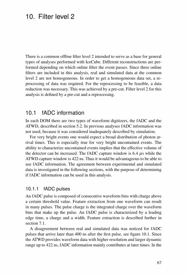
10. Filter level 2

There is a common offline filter level 2 intended to serve as a base for generaltypes of analyses performed with IceCube. Different reconstructions are per-formed depending on which online filter the event passes. Since three onlinefilters are included in this analysis, real and simulated data at the commonlevel 2 are not homogeneous. In order to get a homogeneous data set, a re-processing of data was required. For the reprocessing to be feasible, a datareduction was necessary. This was achieved by a pre-cut. Filter level 2 for thisanalysis is defined by a pre-cut and a reprocessing.

10.1 fADC informationIn each DOM there are two types of waveform digitizers, the fADC and theATWD, described in section 5.2. In previous analyses fADC information wasnot used, because it was considered inadequately described by simulation.

For very bright events one would expect a broad distribution of photon ar-rival times. This is especially true for very bright uncontained events. Theability to characterize uncontained events implies that the effective volume ofthe detector can be increased. The fADC capture window is 6.4 µs while theATWD capture window is 422 ns. Thus it would be advantageous to be able touse fADC information. The agreement between experimental and simulateddata is investigated in the following sections, with the purpose of determiningif fADC information can be used in this analysis.

10.1.1 fADC pulsesAn fADC pulse is composed of consecutive waveform bins with charge abovea certain threshold value. Feature extraction from one waveform can resultin many pulses. The pulse charge is the integrated charge over the waveformbins that make up the pulse. An fADC pulse is characterized by a leadingedge time, a charge and a width. Feature extraction is described further insection 7.1.

A disagreement between real and simulated data was noticed for fADCpulses that arrive later than 400 ns after the first pulse, see figure 10.1. Sincethe ATWD provides waveform data with higher resolution and larger dynamicrange up to 422 ns, fADC information mainly contributes at later times. In the

67

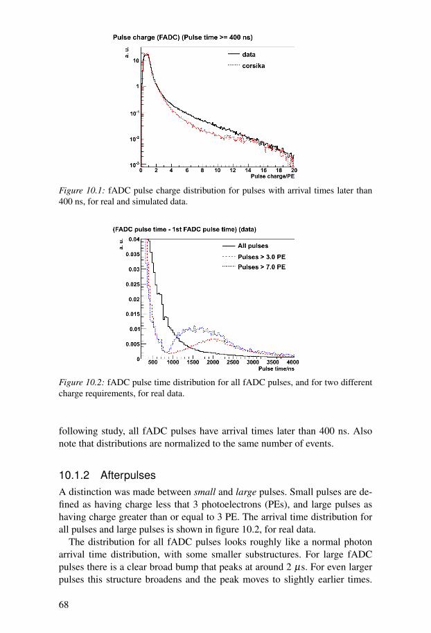
Figure 10.1: fADC pulse charge distribution for pulses with arrival times later than400 ns, for real and simulated data.

Figure 10.2: fADC pulse time distribution for all fADC pulses, and for two differentcharge requirements, for real data.

following study, all fADC pulses have arrival times later than 400 ns. Alsonote that distributions are normalized to the same number of events.

10.1.2 AfterpulsesA distinction was made between small and large pulses. Small pulses are de-fined as having charge less that 3 photoelectrons (PEs), and large pulses ashaving charge greater than or equal to 3 PE. The arrival time distribution forall pulses and large pulses is shown in figure 10.2, for real data.

The distribution for all fADC pulses looks roughly like a normal photonarrival time distribution, with some smaller substructures. For large fADCpulses there is a clear broad bump that peaks at around 2 µs. For even largerpulses this structure broadens and the peak moves to slightly earlier times.

68

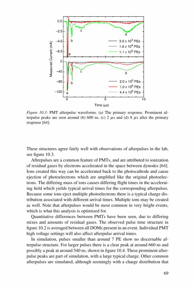
Figure 10.3: PMT afterpulse waveforms. (a) The primary response. Prominent af-terpulse peaks are seen around (b) 600 ns, (c) 2 µs and (d) 8 µs after the primaryresponse [64].

These structures agree fairly well with observations of afterpulses in the lab,see figure 10.3.

Afterpulses are a common feature of PMTs, and are attributed to ionizationof residual gases by electrons accelerated in the space between dynodes [64].Ions created this way can be accelerated back to the photocathode and causeejection of photoelectrons which are amplified like the original photoelec-trons. The differing mass of ions causes differing flight times in the accelerat-ing field which yields typical arrival times for the corresponding afterpulses.Because some ions eject multiple photoelectrons there is a typical charge dis-tribution associated with different arrival times. Multiple ions may be createdas well. Note that afterpulses would be most common in very bright events,which is what this analysis is optimized for.

Quantitative differences between PMTs have been seen, due to differingmixes and amounts of residual gases. The observed pulse time structure infigure 10.2 is averaged between all DOMs present in an event. Individual PMThigh voltage settings will also affect afterpulse arrival times.

In simulation, pulses smaller than around 7 PE show no discernable af-terpulse structure. For larger pulses there is a clear peak at around 660 ns andpossibly a peak at around 540 ns, shown in figure 10.4. These prominent after-pulse peaks are part of simulation, with a large typical charge. Other commonafterpulses are simulated, although seemingly with a charge distribution that

69

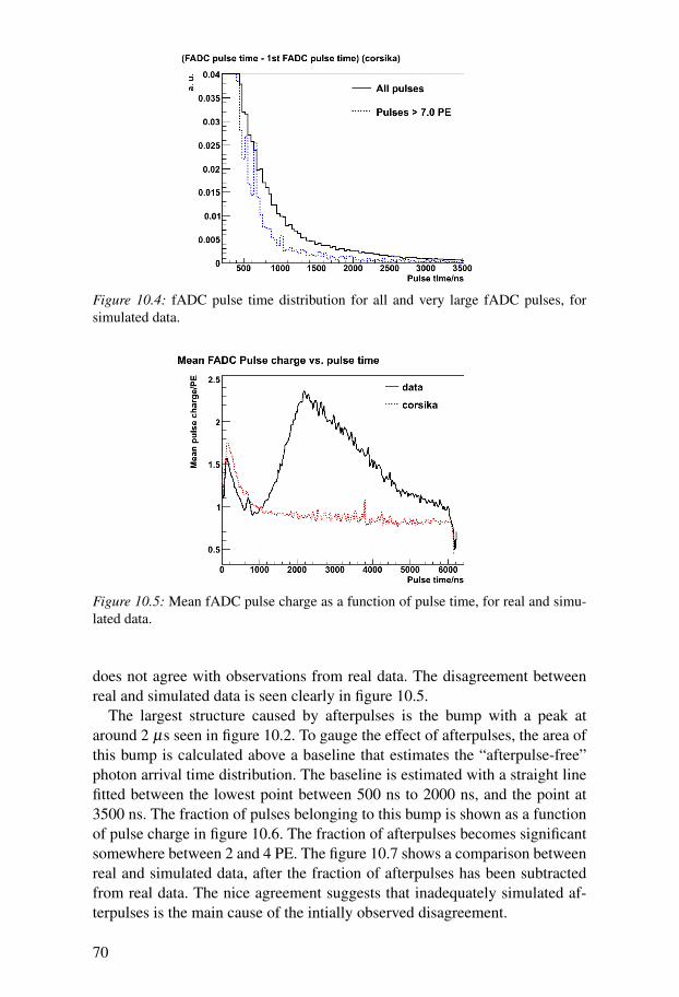
Figure 10.4: fADC pulse time distribution for all and very large fADC pulses, forsimulated data.

Figure 10.5: Mean fADC pulse charge as a function of pulse time, for real and simu-lated data.

does not agree with observations from real data. The disagreement betweenreal and simulated data is seen clearly in figure 10.5.

The largest structure caused by afterpulses is the bump with a peak ataround 2 µs seen in figure 10.2. To gauge the effect of afterpulses, the area ofthis bump is calculated above a baseline that estimates the “afterpulse-free”photon arrival time distribution. The baseline is estimated with a straight linefitted between the lowest point between 500 ns to 2000 ns, and the point at3500 ns. The fraction of pulses belonging to this bump is shown as a functionof pulse charge in figure 10.6. The fraction of afterpulses becomes significantsomewhere between 2 and 4 PE. The figure 10.7 shows a comparison betweenreal and simulated data, after the fraction of afterpulses has been subtractedfrom real data. The nice agreement suggests that inadequately simulated af-terpulses is the main cause of the intially observed disagreement.

70

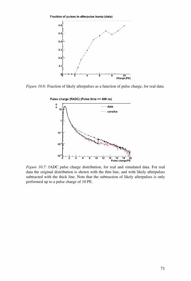
Figure 10.6: Fraction of likely afterpulses as a function of pulse charge, for real data.

Figure 10.7: fADC pulse charge distribution, for real and simulated data. For realdata the original distribution is shown with the thin line, and with likely afterpulsessubtracted with the thick line. Note that the subtraction of likely afterpulses is onlyperformed up to a pulse charge of 10 PE.

71

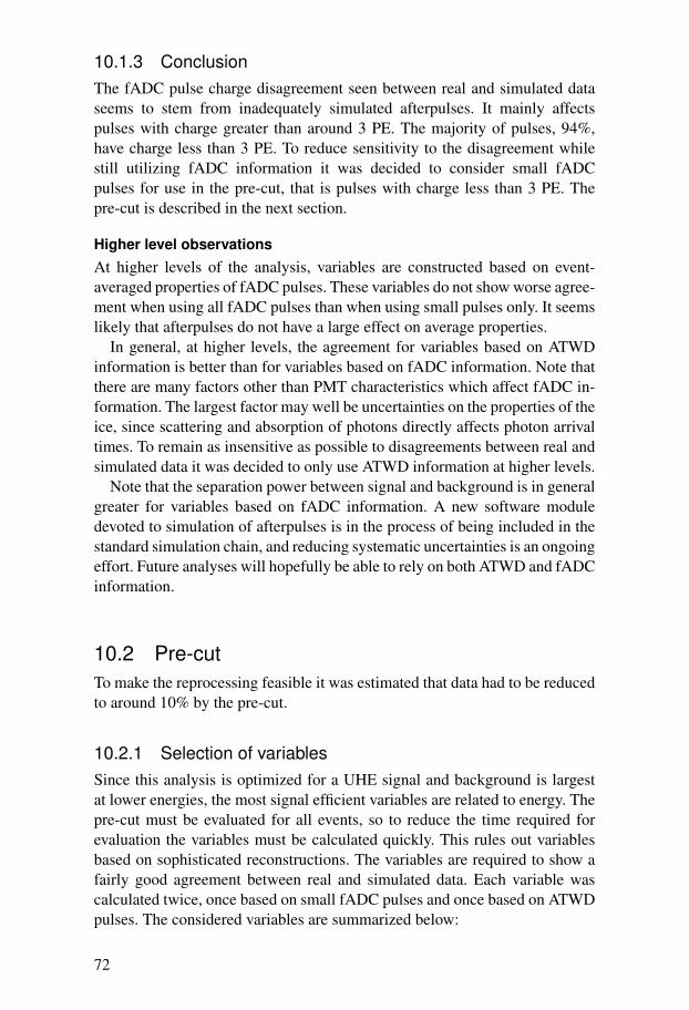
10.1.3 ConclusionThe fADC pulse charge disagreement seen between real and simulated dataseems to stem from inadequately simulated afterpulses. It mainly affectspulses with charge greater than around 3 PE. The majority of pulses, 94%,have charge less than 3 PE. To reduce sensitivity to the disagreement whilestill utilizing fADC information it was decided to consider small fADCpulses for use in the pre-cut, that is pulses with charge less than 3 PE. Thepre-cut is described in the next section.

Higher level observationsAt higher levels of the analysis, variables are constructed based on event-averaged properties of fADC pulses. These variables do not show worse agree-ment when using all fADC pulses than when using small pulses only. It seemslikely that afterpulses do not have a large effect on average properties.

In general, at higher levels, the agreement for variables based on ATWDinformation is better than for variables based on fADC information. Note thatthere are many factors other than PMT characteristics which affect fADC in-formation. The largest factor may well be uncertainties on the properties of theice, since scattering and absorption of photons directly affects photon arrivaltimes. To remain as insensitive as possible to disagreements between real andsimulated data it was decided to only use ATWD information at higher levels.

Note that the separation power between signal and background is in generalgreater for variables based on fADC information. A new software moduledevoted to simulation of afterpulses is in the process of being included in thestandard simulation chain, and reducing systematic uncertainties is an ongoingeffort. Future analyses will hopefully be able to rely on both ATWD and fADCinformation.

10.2 Pre-cutTo make the reprocessing feasible it was estimated that data had to be reducedto around 10% by the pre-cut.

10.2.1 Selection of variablesSince this analysis is optimized for a UHE signal and background is largestat lower energies, the most signal efficient variables are related to energy. Thepre-cut must be evaluated for all events, so to reduce the time required forevaluation the variables must be calculated quickly. This rules out variablesbased on sophisticated reconstructions. The variables are required to show afairly good agreement between real and simulated data. Each variable wascalculated twice, once based on small fADC pulses and once based on ATWDpulses. The considered variables are summarized below:

72

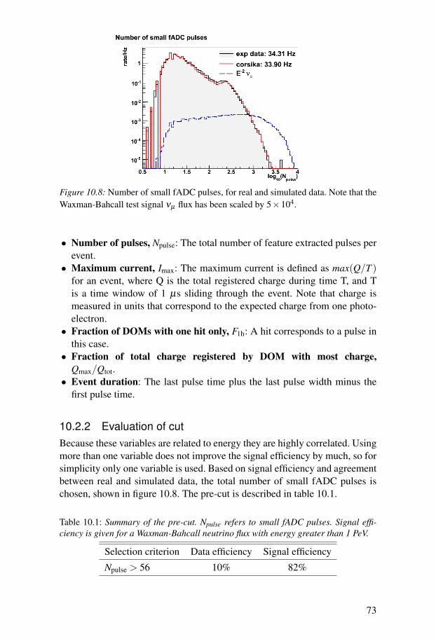
Figure 10.8: Number of small fADC pulses, for real and simulated data. Note that theWaxman-Bahcall test signal νµ flux has been scaled by 5×104.

• Number of pulses, Npulse: The total number of feature extracted pulses perevent.• Maximum current, Imax: The maximum current is defined as max(Q/T )

for an event, where Q is the total registered charge during time T, and Tis a time window of 1 µs sliding through the event. Note that charge ismeasured in units that correspond to the expected charge from one photo-electron.• Fraction of DOMs with one hit only, F1h: A hit corresponds to a pulse in

this case.• Fraction of total charge registered by DOM with most charge,

Qmax/Qtot.• Event duration: The last pulse time plus the last pulse width minus the

first pulse time.

10.2.2 Evaluation of cutBecause these variables are related to energy they are highly correlated. Usingmore than one variable does not improve the signal efficiency by much, so forsimplicity only one variable is used. Based on signal efficiency and agreementbetween real and simulated data, the total number of small fADC pulses ischosen, shown in figure 10.8. The pre-cut is described in table 10.1.

Table 10.1: Summary of the pre-cut. Npulse refers to small fADC pulses. Signal effi-ciency is given for a Waxman-Bahcall neutrino flux with energy greater than 1 PeV.

Selection criterion Data efficiency Signal efficiency

Npulse > 56 10% 82%

73

Figure 10.9: The ratio between simulated and real data rate is shown on the left axisand efficiency is shown on the right axis, as a function of cut on the number of smallfADC pulses.

Table 10.2: Passing rates before and after the pre-cut, for real and simulated data.The last column shows pre-cut efficiency.

Online filter Before: exp/sim After: exp/sim Eff: exp/sim

Total 34.8 Hz / 33.9 Hz 3.36 Hz / 2.74 Hz 9.7% / 8.1%

Muon 19.9 Hz / 22.0 Hz 1.81 Hz / 1.65 Hz 9.1% / 7.5%

Cascade 16.2 Hz / 13.1 Hz 0.91 Hz / 0.54 Hz 5.6% / 4.1%

EHE 1.12 Hz / 0.90 Hz 1.05 Hz / 0.87 Hz 93% / 96%

10.2.3 Effect of cutThe effect of the pre-cut follows expectation, events far from the detector andlow energy events are removed. The agreement between real and simulateddata is adequate in a region around the pre-cut, as shown in figure 10.9. Thepre-cut reduces data by one order of magnitude only and is not likely to havea large impact on the final level of the analysis. The passing rates before andafter the pre-cut is shown in table 10.2.

The signal efficiency of the precut for different classes of events is shownin table 10.3. Rejected events are rather evenly distributed between classes.

10.3 ReprocessingThe common filter level 2 processing includes almost all of the most sophis-ticated track and cascade reconstructions available within the IceCube soft-ware framework. The reprocessing performed for the analysis discussed hereclosely follows the common filter level 2 processing, with the addition of two

74

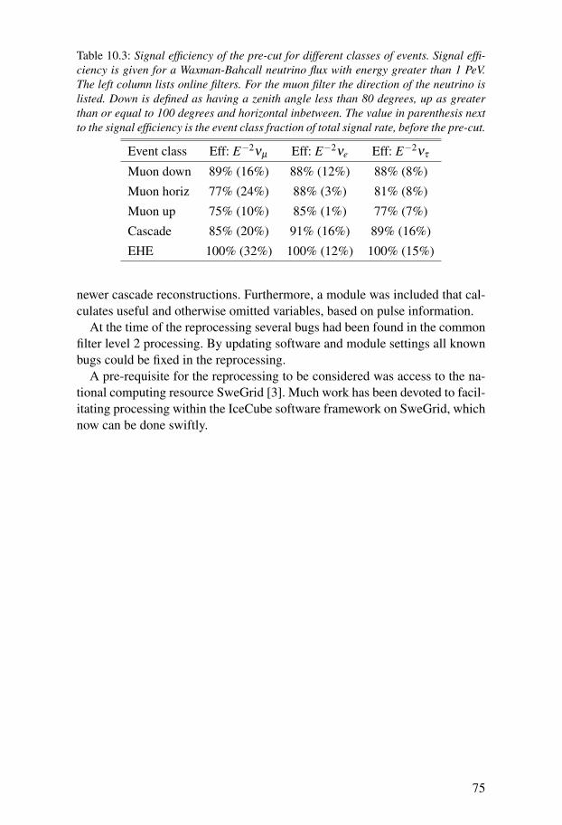
Table 10.3: Signal efficiency of the pre-cut for different classes of events. Signal effi-ciency is given for a Waxman-Bahcall neutrino flux with energy greater than 1 PeV.The left column lists online filters. For the muon filter the direction of the neutrino islisted. Down is defined as having a zenith angle less than 80 degrees, up as greaterthan or equal to 100 degrees and horizontal inbetween. The value in parenthesis nextto the signal efficiency is the event class fraction of total signal rate, before the pre-cut.

Event class Eff: E−2νµ Eff: E−2νe Eff: E−2ντ

Muon down 89% (16%) 88% (12%) 88% (8%)

Muon horiz 77% (24%) 88% (3%) 81% (8%)

Muon up 75% (10%) 85% (1%) 77% (7%)

Cascade 85% (20%) 91% (16%) 89% (16%)

EHE 100% (32%) 100% (12%) 100% (15%)

newer cascade reconstructions. Furthermore, a module was included that cal-culates useful and otherwise omitted variables, based on pulse information.

At the time of the reprocessing several bugs had been found in the commonfilter level 2 processing. By updating software and module settings all knownbugs could be fixed in the reprocessing.

A pre-requisite for the reprocessing to be considered was access to the na-tional computing resource SweGrid [3]. Much work has been devoted to facil-itating processing within the IceCube software framework on SweGrid, whichnow can be done swiftly.

75

11. Filter level 3

Filter level 3 is the main filter level. Variables from the most sophisticated re-constructions are available for all events, owing to the reprocessing. Emphasisis placed on developing a robust analysis, well described by simulation. Forthis reason, agreement between real and simulated data is often prioritizedbefore signal efficiency when selecting cut variables.

11.1 Event topologyDifferent types of events have different topology in the detector. The mainevent signatures are listed below:

• Track-like: A track topology is simple and fairly insensitive to many sys-tematic uncertainties, for example ice properties.• Cascade-like: Roughly spherical light emission. The sphericity of an event

describes the three dimensional shape of the photon distribution and ishighly sensitive to for example ice properties.• Composite: A combination of track-like and cascade-like.

11.1.1 NeutrinosNeutrino-nucleon interactions result in a hadronic shower. Neutral-current in-teractions therefore yield cascade-like events. The remainder of this sectiondiscusses charged-current interactions.

νµ

Muons traversing the detector produce track-like signatures. In IceCube, anal-yses searching for muon neutrinos are the most mature. The atmosphericmuon neutrino energy spectrum has been measured [97] and point source anal-yses are possible owing to the good pointing resolution.

Muon neutrinos interacting inside the detector volume produce “startingtrack” events. The combination of the hadronic shower at the interaction pointand the outgoing muon constitutes a composite event.

νe

Electromagnetic showers are produced in electron neutrino charged-currentinteractions resulting in cascade-like events. The atmospheric electron neu-

77

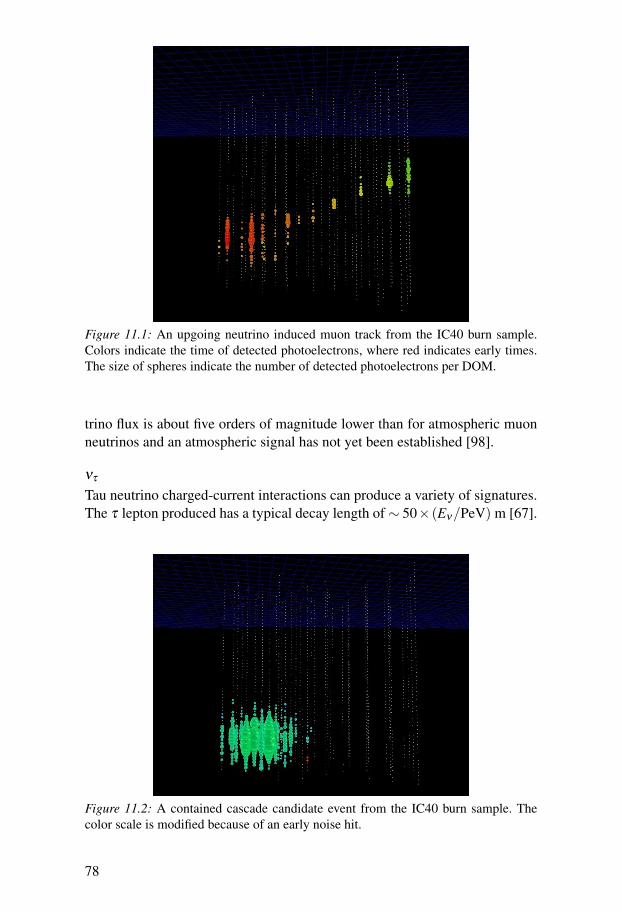
Figure 11.1: An upgoing neutrino induced muon track from the IC40 burn sample.Colors indicate the time of detected photoelectrons, where red indicates early times.The size of spheres indicate the number of detected photoelectrons per DOM.

trino flux is about five orders of magnitude lower than for atmospheric muonneutrinos and an atmospheric signal has not yet been established [98].

ντ

Tau neutrino charged-current interactions can produce a variety of signatures.The τ lepton produced has a typical decay length of∼ 50× (Eν/PeV) m [67].

Figure 11.2: A contained cascade candidate event from the IC40 burn sample. Thecolor scale is modified because of an early noise hit.

78

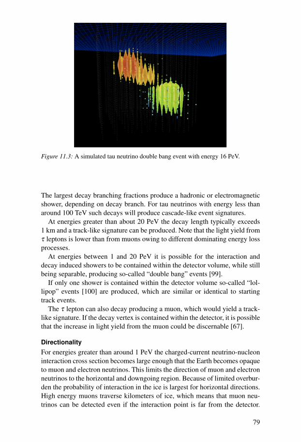
Figure 11.3: A simulated tau neutrino double bang event with energy 16 PeV.

The largest decay branching fractions produce a hadronic or electromagneticshower, depending on decay branch. For tau neutrinos with energy less thanaround 100 TeV such decays will produce cascade-like event signatures.

At energies greater than about 20 PeV the decay length typically exceeds1 km and a track-like signature can be produced. Note that the light yield fromτ leptons is lower than from muons owing to different dominating energy lossprocesses.

At energies between 1 and 20 PeV it is possible for the interaction anddecay induced showers to be contained within the detector volume, while stillbeing separable, producing so-called “double bang” events [99].

If only one shower is contained within the detector volume so-called “lol-lipop” events [100] are produced, which are similar or identical to startingtrack events.

The τ lepton can also decay producing a muon, which would yield a track-like signature. If the decay vertex is contained within the detector, it is possiblethat the increase in light yield from the muon could be discernable [67].

DirectionalityFor energies greater than around 1 PeV the charged-current neutrino-nucleoninteraction cross section becomes large enough that the Earth becomes opaqueto muon and electron neutrinos. This limits the direction of muon and electronneutrinos to the horizontal and downgoing region. Because of limited overbur-den the probability of interaction in the ice is largest for horizontal directions.High energy muons traverse kilometers of ice, which means that muon neu-trinos can be detected even if the interaction point is far from the detector.

79

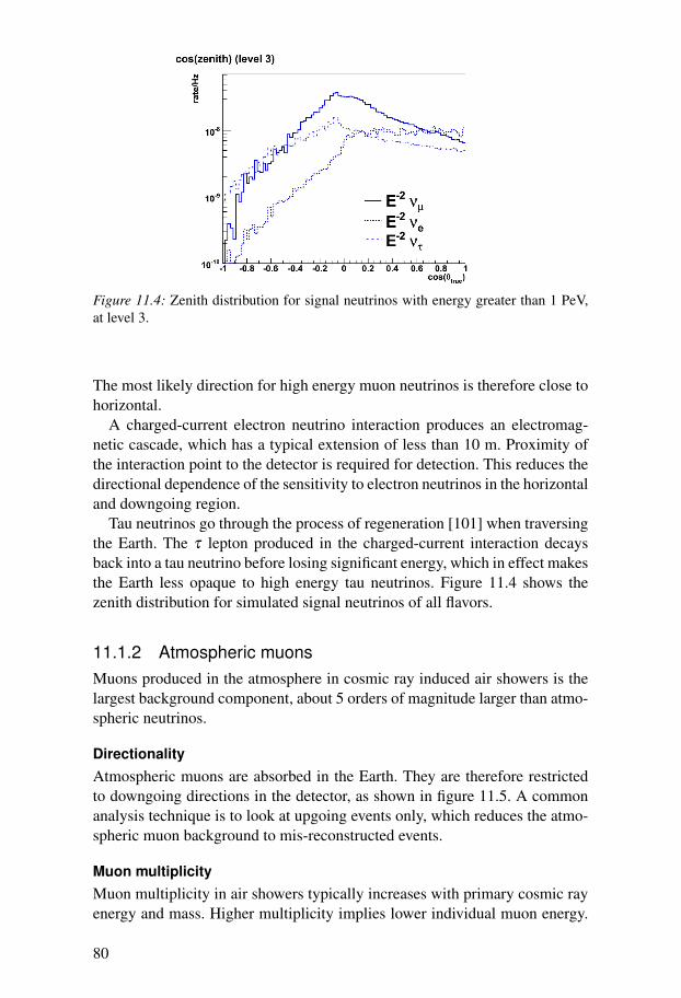
Figure 11.4: Zenith distribution for signal neutrinos with energy greater than 1 PeV,at level 3.

The most likely direction for high energy muon neutrinos is therefore close tohorizontal.

A charged-current electron neutrino interaction produces an electromag-netic cascade, which has a typical extension of less than 10 m. Proximity ofthe interaction point to the detector is required for detection. This reduces thedirectional dependence of the sensitivity to electron neutrinos in the horizontaland downgoing region.

Tau neutrinos go through the process of regeneration [101] when traversingthe Earth. The τ lepton produced in the charged-current interaction decaysback into a tau neutrino before losing significant energy, which in effect makesthe Earth less opaque to high energy tau neutrinos. Figure 11.4 shows thezenith distribution for simulated signal neutrinos of all flavors.

11.1.2 Atmospheric muonsMuons produced in the atmosphere in cosmic ray induced air showers is thelargest background component, about 5 orders of magnitude larger than atmo-spheric neutrinos.

DirectionalityAtmospheric muons are absorbed in the Earth. They are therefore restrictedto downgoing directions in the detector, as shown in figure 11.5. A commonanalysis technique is to look at upgoing events only, which reduces the atmo-spheric muon background to mis-reconstructed events.

Muon multiplicityMuon multiplicity in air showers typically increases with primary cosmic rayenergy and mass. Higher multiplicity implies lower individual muon energy.

80

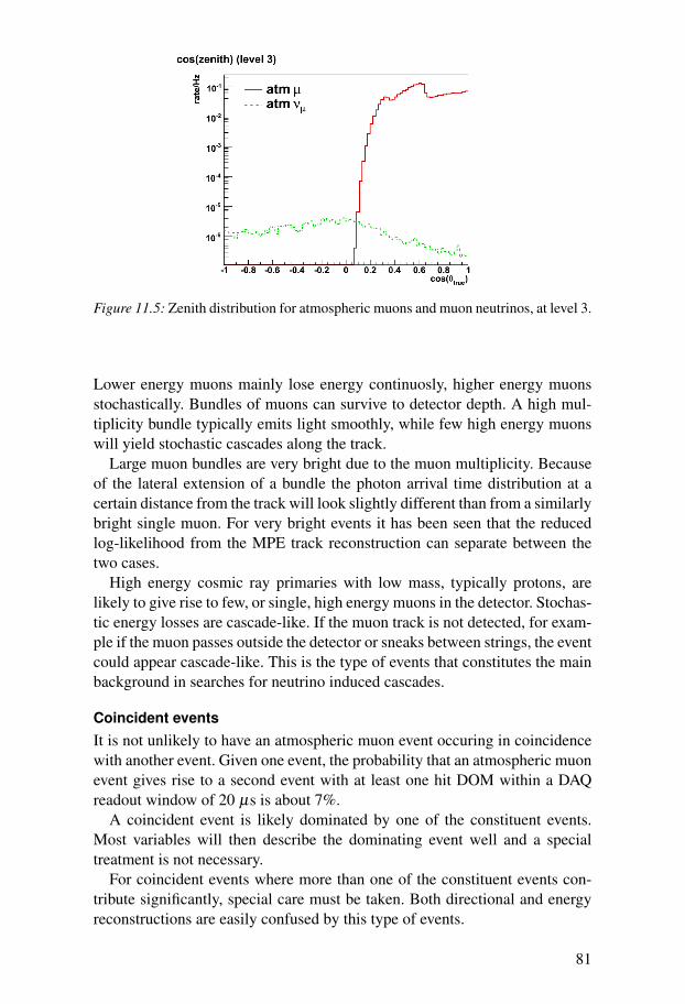
Figure 11.5: Zenith distribution for atmospheric muons and muon neutrinos, at level 3.

Lower energy muons mainly lose energy continuosly, higher energy muonsstochastically. Bundles of muons can survive to detector depth. A high mul-tiplicity bundle typically emits light smoothly, while few high energy muonswill yield stochastic cascades along the track.

Large muon bundles are very bright due to the muon multiplicity. Becauseof the lateral extension of a bundle the photon arrival time distribution at acertain distance from the track will look slightly different than from a similarlybright single muon. For very bright events it has been seen that the reducedlog-likelihood from the MPE track reconstruction can separate between thetwo cases.

High energy cosmic ray primaries with low mass, typically protons, arelikely to give rise to few, or single, high energy muons in the detector. Stochas-tic energy losses are cascade-like. If the muon track is not detected, for exam-ple if the muon passes outside the detector or sneaks between strings, the eventcould appear cascade-like. This is the type of events that constitutes the mainbackground in searches for neutrino induced cascades.

Coincident eventsIt is not unlikely to have an atmospheric muon event occuring in coincidencewith another event. Given one event, the probability that an atmospheric muonevent gives rise to a second event with at least one hit DOM within a DAQreadout window of 20 µs is about 7%.

A coincident event is likely dominated by one of the constituent events.Most variables will then describe the dominating event well and a specialtreatment is not necessary.

For coincident events where more than one of the constituent events con-tribute significantly, special care must be taken. Both directional and energyreconstructions are easily confused by this type of events.

81

11.2 Cut variablesReconstruction algorithms are described in chapter 7. The variables used infilter level 3 are summarized below:

• Zenith from MPE track reconstruction, θMPE: Powerful observable sinceatmospheric muons, atmospheric neutrinos and predicted signal neutrinoshave differing zenith distributions.• Total number of photoelectrons, Npe: Can serve as a crude energy estima-

tor. Especially powerful in conjunction with an energy reconstruction, toreject mis-reconstructed events.• Energy from MuE track reconstruction, EMuE: Sophisticated energy es-

timator based on a track hypothesis and observed average energy loss.• Reduced log-likelihood from MPE and SPE-32 track reconstructions,

ρMPE and ρSPE32: A low value indicates a well reconstructed track.• Sigma from paraboloid based on MPE and SPE-32 track reconstruc-

tions, σMPE and σSPE32: An indication of the error on the reconstructedtrack direction.• Direct length based on MPE track reconstruction, LDirC: The geometri-

cal time is defined as the time when unscattered Cherenkov photons reacha DOM. Direct pulses are defined and categorized depending on the pulsetime in relation to the geometrical time. Pulse times between −15 ns and+75 ns around the geometrical time fall in category C. The positions ofDOMs with direct pulses can be projected onto the track. The maximumdistance between projected DOM positions is called the direct length.• Smoothness based on MPE track reconstruction, SMPE: Smoothness is a

measure of how uniformly the detected photons are distributed along thetrack. The value of smoothness lies in a range between -1 and 1. Positivevalues indicate that photons cluster at the beginning of the track and theopposite is true for negative values. A value close to 0 indicates uniformlydistributed photons.• The Bayesian likelihood ratio, log(`SPE32)− log(`Bayes): The Bayesian re-

construction uses the observed atmospheric muon zenith distribution asa prior. The Bayesian likelihood ratio thus compares the hypothesis of adowngoing track to that given by SPE-32. For the upgoing track stream thisis a powerful observable to reject mis-reconstructed atmospheric muons. Ithas also been found to be useful for the downgoing track stream, likelybecause the zenith distribution for atmospheric muons and neutrinos differ.Low values of the likelihood ratio support the hypothesis of a downgoingtrack, high values support the track hypothesis from SPE-32.• LineFit velocity, vLF: See section 9.2.• Minimum zenith angle of a time split two-track reconstruction, θmin:

Two tracks are reconstructed using information from two non-overlappingsubsets of pulses. The subsets are formed using pulse time information.θmin is the zenith angle for the track with the smallest zenith angle.

82

For the upgoing track stream this is a powerful observable to rejectmis-reconstructed coincident events.• The time split Bayesian likelihood ratio, log(`SPE32)− (log(`BayesT1) +

log(`BayesT2)): The time split Bayesian likelihood ratio compares the hy-pothesis of a single track with the hypothesis of two downgoing tracks. Thetwo-track reconstruction is performed using information from two non-overlapping subsets of pulses formed based on timing information. Notethat the likelihood for the two-track hypothesis depends on how well thesplitting algorithm works. For the upgoing track stream this is a powerfulobservable to reject mis-reconstructed coincident events.• The geometry split likelihood ratio, log(`SPE32)− (log(`G1)+ log(`G2)):

The geometry split Bayesian likelihood ratio compares the hypothesis of asingle track with the hypothesis of two tracks. The two-track reconstruc-tion is performed using information from two non-overlapping subsets ofDOMs formed based on geometry information. Note that the likelihoodfor the two-track hypothesis depends on how well the splitting algorithmworks. For the downgoing track stream this is a useful observable to rejectcoincident events.• Average pulse charge, Qavg: The average pulse charge per event is a good

indicator of dim events, which are either low energy or far away from thedetector.• Fraction of DOMs with one hit only, F1h: One hit corresponds to one

pulse in this case. F1h is a good indicator of dim events. Signal typicallyhas lower values than background events.• Fill ratio, Rfill: The algorithm looks at the distribution of distances from

a given cascade vertex hypothesis to the the hits in the event. A sphere isdefined based on a radius proportional to the RMS of the distance distri-bution. The fill ratio is calculated as the ratio between the number of hitDOMs and active DOMs within the sphere. Cascade-like events are typi-cally highly spherical and would therefore get a large fill ratio, approach-ing 1. Track-like events on the other hand typically has a small fill ratio,approaching 0. Coincident events also cluster close to 0.• Reduced log-likelihood from CLLH cascade vertex reconstruction,

ρcllh: Low values indicates a well reconstructed cascade.• Fraction of total charge registered by the DOM with most charge,

Qmax/Qtot: Events where one DOM detects the majority of photonsare called “balloon events”. It has been shown that they are caused bystochastic energy loss in immediate proximity of a DOM. Balloon eventscan confuse energy reconstructions. Qmax/Qtot is a good indicator ofballoon events.• Energy from ACER cascade reconstruction, Eacer: Sophisticated analyt-

ical cascade energy reconstruction.• Maximum current, Imax: See section 10.2.1.

83

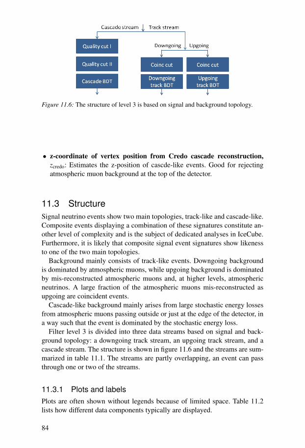
Figure 11.6: The structure of level 3 is based on signal and background topology.

• z-coordinate of vertex position from Credo cascade reconstruction,zcredo: Estimates the z-position of cascde-like events. Good for rejectingatmospheric muon background at the top of the detector.

11.3 StructureSignal neutrino events show two main topologies, track-like and cascade-like.Composite events displaying a combination of these signatures constitute an-other level of complexity and is the subject of dedicated analyses in IceCube.Furthermore, it is likely that composite signal event signatures show likenessto one of the two main topologies.

Background mainly consists of track-like events. Downgoing backgroundis dominated by atmospheric muons, while upgoing background is dominatedby mis-reconstructed atmospheric muons and, at higher levels, atmosphericneutrinos. A large fraction of the atmospheric muons mis-reconstructed asupgoing are coincident events.

Cascade-like background mainly arises from large stochastic energy lossesfrom atmospheric muons passing outside or just at the edge of the detector, ina way such that the event is dominated by the stochastic energy loss.

Filter level 3 is divided into three data streams based on signal and back-ground topology: a downgoing track stream, an upgoing track stream, and acascade stream. The structure is shown in figure 11.6 and the streams are sum-marized in table 11.1. The streams are partly overlapping, an event can passthrough one or two of the streams.

11.3.1 Plots and labelsPlots are often shown without legends because of limited space. Table 11.2lists how different data components typically are displayed.

84

Table 11.1: Summary of level 3 data streams.

Data stream Selection criteria

Downgoing track (Muon OR EHE filter) AND θMPE < 90◦

Upgoing track (Muon OR EHE filter) AND θMPE ≥ 90◦

Cascade (Cascade OR EHE filter)

Table 11.2: Display style for different data components. Exp is short for experimental(real) data. CORSIKA is atmospheric muon simulation, poly-gonato and 2-componentsignify different cosmic ray composition models, and coinc indicates coincident eventsimulation. Atmospheric muon neutrino simulation is shown on plots where this com-ponent clearly stands out. Signal neutrino simulation is usually shown.

Data component Line style Line color

Exp Solid (filled area) Black (gray)

Poly-gonato CORSIKA Solid Red

2-comp CORSIKA Solid Magenta

Coinc poly-gonato CORSIKA Dashed Red

Atm νµ Dashed-dotted Green

Signal ν Long dashed Blue

11.3.2 Downgoing track streamThis stream has by far the largest background rate from atmospheric muons.In particular, background reaches very high energies, which means a hard cuton energy is required to select the signal region. Also among the most pow-erful observables is direction, where signal typically has close to horizontaldirections. Track quality is another important property, although in this veryhigh energy signal region less important than energy and direction.

This stream is optimized for UHE track-like neutrino events with an E−2

energy spectrum. To ensure that simulated signal is track-like, the error onthe reconstructed direction is required to be smaller than 5 degrees. For allfigures in this section, signal is shown for muon neutrinos with energy greaterthan 1 PeV and reconstructed directional error less than 5 degrees. Signalefficiencies are also quoted for this type of signal. Note that the Waxman-Bahcall test signal flux is scaled by a factor 5× 104 to make plots easier toread.

The downgoing track stream consists of a “coincidence cut” and the evalu-ation of a multivariate classifier, a boosted decision tree (BDT).

Coincidence cutThe purpose of the coincidence cut is to remove coincident events. This typeof events can confuse reconstructions that assume a single event hypothesis.

85

For the downgoing track stream this cut can be viewed as a cleaning cut, wheretails that are dominated by coincident events are removed. The coincidence cutis described in table 11.3 and variable distributions are shown in figure 11.7.Note that data components and display styles in the figures are explained intable 11.2.

Evaluation of BDTTo efficiently separate signal from background, a multivariate classifier wasused. Based on previous experience the boosted decision tree classifier im-plemented in the toolkit TMVA [102] within the data analysis frameworkROOT [103] was chosen.

The variables used to characterize signal and background are shown in fig-ure 11.8. The variables describe the energy, direction and track quality of anevent. Note that these distributions are shown with the coincidence cut ap-plied. Three variables used in the coincidence cut are also included in theBDT: the geometry split likelihood ratio, the Bayesian likelihood ratio andLineFit velocity.

Atmospheric muon simulation was used as background when training theBDT. UHE track-like muon neutrino simulation with an E−2 energy spec-trum was used as signal. A further restriction was imposed on signal, a directlength greater than 300 m was required. This improved background rejectionwithout loss of signal efficiency. The BDT score is shown in figure 11.9. Seeappendix A for detailed information about the BDT evaluation.

86

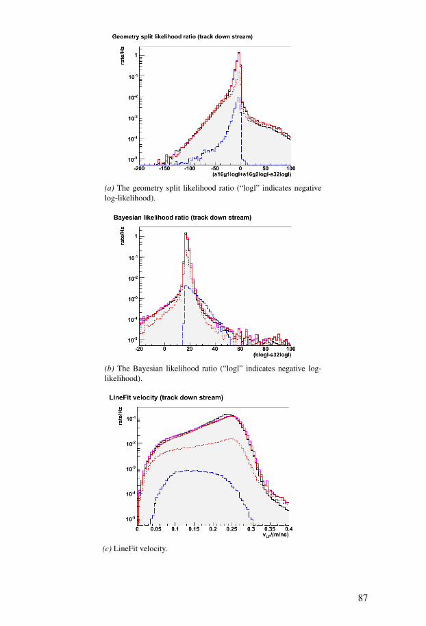
(a) The geometry split likelihood ratio (“logl” indicates negativelog-likelihood).

(b) The Bayesian likelihood ratio (“logl” indicates negative log-likelihood).

(c) LineFit velocity.

87

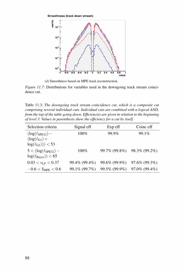
(d) Smoothness based on MPE track reconstruction.

Figure 11.7: Distributions for variables used in the downgoing track stream coinci-dence cut.

Table 11.3: The downgoing track stream coincidence cut, which is a composite cutcomprising several individual cuts. Individual cuts are combined with a logical AND,from the top of the table going down. Efficiencies are given in relation to the beginningof level 3. Values in parenthesis show the efficiency for a cut by itself.

Selection criteria Signal eff Exp eff Coinc eff

(log(`SPE32)−(log(`G1)+log(`G2))) < 53

100% 99.9% 99.1%

5 < (log(`SPE32)−log(`Bayes)) < 65

100% 99.7% (99.8%) 98.3% (99.2%)

0.03 < vLF < 0.37 99.4% (99.4%) 99.6% (99.9%) 97.6% (99.3%)

−0.6 < SMPE < 0.6 99.1% (99.7%) 99.5% (99.9%) 97.0% (99.4%)

88

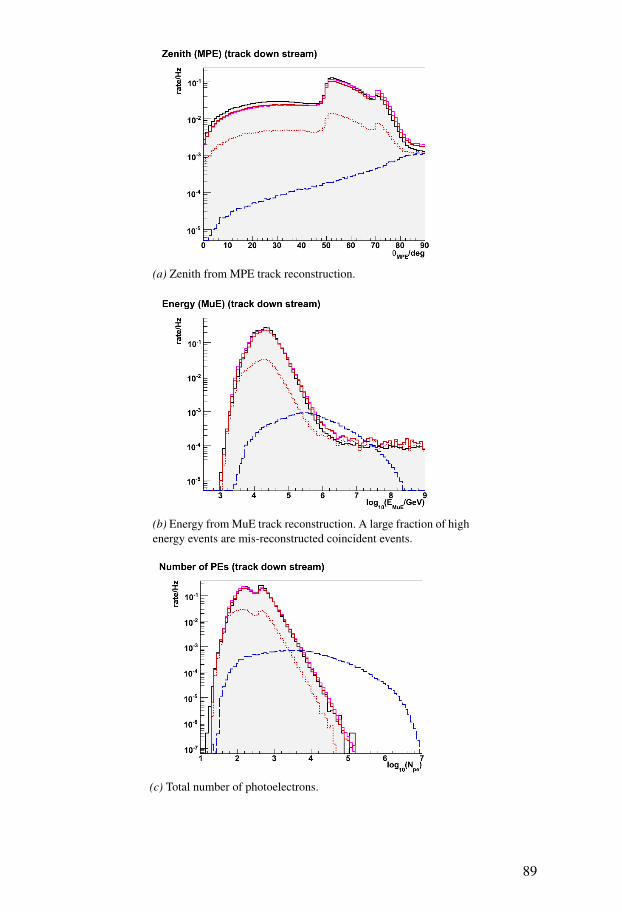
(a) Zenith from MPE track reconstruction.

(b) Energy from MuE track reconstruction. A large fraction of highenergy events are mis-reconstructed coincident events.

(c) Total number of photoelectrons.

89

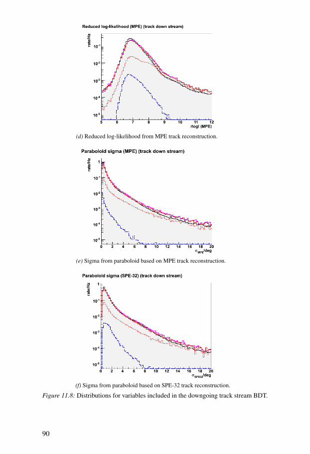
(d) Reduced log-likelihood from MPE track reconstruction.

(e) Sigma from paraboloid based on MPE track reconstruction.

(f) Sigma from paraboloid based on SPE-32 track reconstruction.

Figure 11.8: Distributions for variables included in the downgoing track stream BDT.

90

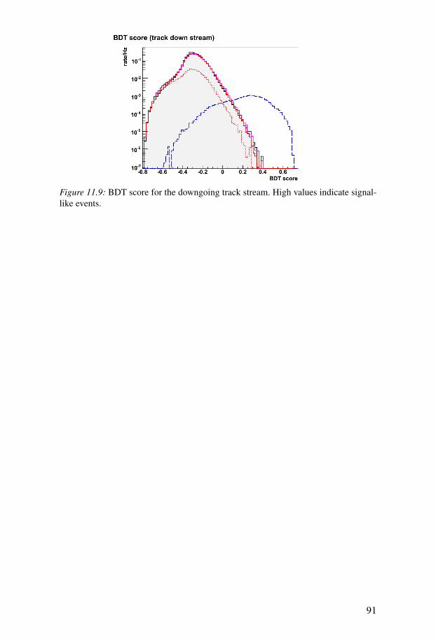
Figure 11.9: BDT score for the downgoing track stream. High values indicate signal-like events.

91

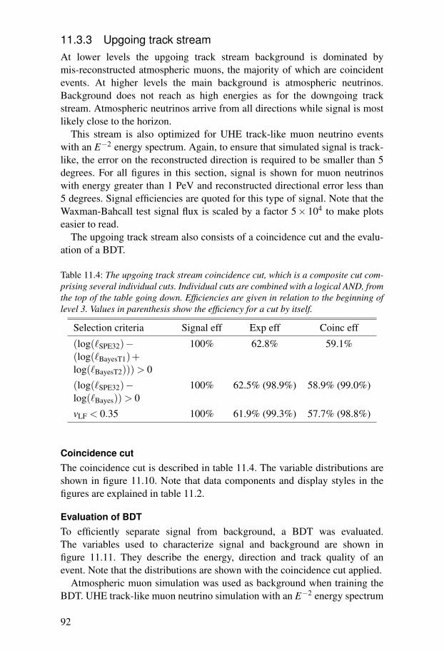
11.3.3 Upgoing track streamAt lower levels the upgoing track stream background is dominated bymis-reconstructed atmospheric muons, the majority of which are coincidentevents. At higher levels the main background is atmospheric neutrinos.Background does not reach as high energies as for the downgoing trackstream. Atmospheric neutrinos arrive from all directions while signal is mostlikely close to the horizon.

This stream is also optimized for UHE track-like muon neutrino eventswith an E−2 energy spectrum. Again, to ensure that simulated signal is track-like, the error on the reconstructed direction is required to be smaller than 5degrees. For all figures in this section, signal is shown for muon neutrinoswith energy greater than 1 PeV and reconstructed directional error less than5 degrees. Signal efficiencies are quoted for this type of signal. Note that theWaxman-Bahcall test signal flux is scaled by a factor 5× 104 to make plotseasier to read.

The upgoing track stream also consists of a coincidence cut and the evalu-ation of a BDT.

Table 11.4: The upgoing track stream coincidence cut, which is a composite cut com-prising several individual cuts. Individual cuts are combined with a logical AND, fromthe top of the table going down. Efficiencies are given in relation to the beginning oflevel 3. Values in parenthesis show the efficiency for a cut by itself.

Selection criteria Signal eff Exp eff Coinc eff

(log(`SPE32)−(log(`BayesT1)+log(`BayesT2))) > 0

100% 62.8% 59.1%

(log(`SPE32)−log(`Bayes)) > 0

100% 62.5% (98.9%) 58.9% (99.0%)

vLF < 0.35 100% 61.9% (99.3%) 57.7% (98.8%)

Coincidence cutThe coincidence cut is described in table 11.4. The variable distributions areshown in figure 11.10. Note that data components and display styles in thefigures are explained in table 11.2.

Evaluation of BDTTo efficiently separate signal from background, a BDT was evaluated.The variables used to characterize signal and background are shown infigure 11.11. They describe the energy, direction and track quality of anevent. Note that the distributions are shown with the coincidence cut applied.

Atmospheric muon simulation was used as background when training theBDT. UHE track-like muon neutrino simulation with an E−2 energy spectrum

92

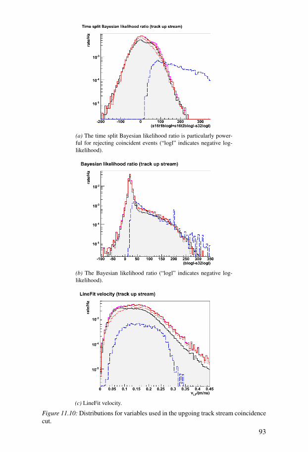
(a) The time split Bayesian likelihood ratio is particularly power-ful for rejecting coincident events (“logl” indicates negative log-likelihood).

(b) The Bayesian likelihood ratio (“logl” indicates negative log-likelihood).

(c) LineFit velocity.

Figure 11.10: Distributions for variables used in the upgoing track stream coincidencecut.

93

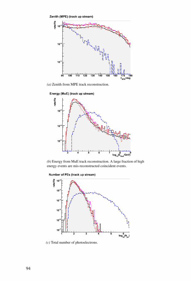
(a) Zenith from MPE track reconstruction.

(b) Energy from MuE track reconstruction. A large fraction of highenergy events are mis-reconstructed coincident events.

(c) Total number of photoelectrons.

94

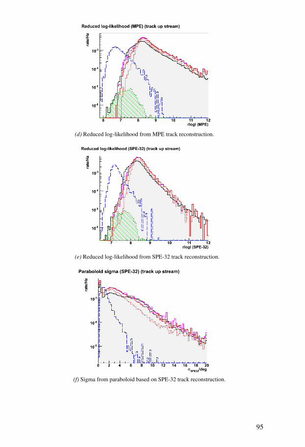
(d) Reduced log-likelihood from MPE track reconstruction.

(e) Reduced log-likelihood from SPE-32 track reconstruction.

(f) Sigma from paraboloid based on SPE-32 track reconstruction.

95

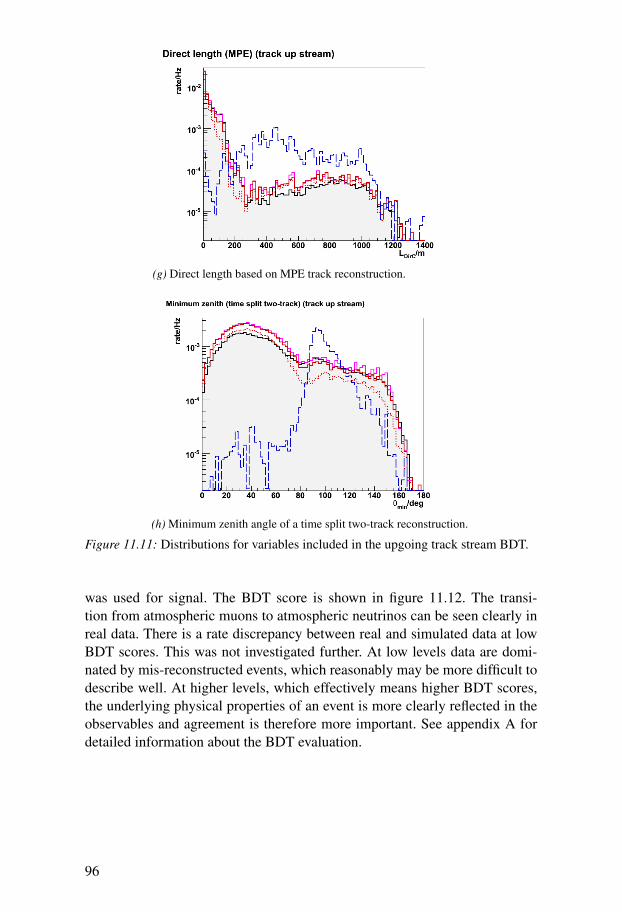
(g) Direct length based on MPE track reconstruction.

(h) Minimum zenith angle of a time split two-track reconstruction.

Figure 11.11: Distributions for variables included in the upgoing track stream BDT.

was used for signal. The BDT score is shown in figure 11.12. The transi-tion from atmospheric muons to atmospheric neutrinos can be seen clearly inreal data. There is a rate discrepancy between real and simulated data at lowBDT scores. This was not investigated further. At low levels data are domi-nated by mis-reconstructed events, which reasonably may be more difficult todescribe well. At higher levels, which effectively means higher BDT scores,the underlying physical properties of an event is more clearly reflected in theobservables and agreement is therefore more important. See appendix A fordetailed information about the BDT evaluation.

96

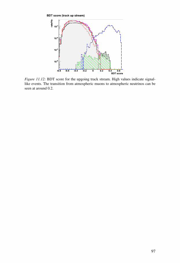
Figure 11.12: BDT score for the upgoing track stream. High values indicate signal-like events. The transition from atmospheric muons to atmospheric neutrinos can beseen at around 0.2.

97

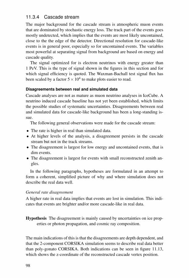
11.3.4 Cascade streamThe major background for the cascade stream is atmospheric muon eventsthat are dominated by stochastic energy loss. The track part of the events goesmostly undetected, which implies that the events are most likely uncontained,close to the the edge of the detector. Directional resolution for cascade-likeevents is in general poor, especially so for uncontained events. The variablesmost powerful at separating signal from background are based on energy andcascade quality.

The signal optimized for is electron neutrinos with energy greater than1 PeV. This is the type of signal shown in the figures in this section and forwhich signal efficiency is quoted. The Waxman-Bachall test signal flux hasbeen scaled by a factor 5×104 to make plots easier to read.

Disagreements between real and simulated dataCascade analyses are not as mature as muon neutrino analyses in IceCube. Aneutrino induced cascade baseline has not yet been established, which limitsthe possible studies of systematic uncertainties. Disagreements between realand simulated data for cascade-like background has been a long-standing is-sue.

The following general observations were made for the cascade stream:

• The rate is higher in real than simulated data.• At higher levels of the analysis, a disagreement persists in the cascade

stream but not in the track streams.• The disagreement is largest for low energy and uncontained events, that is

dim events.• The disagreement is largest for events with small reconstructed zenith an-

gles.

In the following paragraphs, hypotheses are formulated in an attempt toform a coherent, simplified picture of why and where simulation does notdescribe the real data well.

General rate disagreementA higher rate in real data implies that events are lost in simulation. This indi-cates that events are brighter and/or more cascade-like in real data.

Hypothesis The disagreement is mainly caused by uncertainties on ice prop-erties or photon propagation, and cosmic ray composition.

The main indications of this is that the disagreements are depth dependent, andthat the 2-component CORSIKA simulation seems to describe real data betterthan poly-gonato CORSIKA. Both indications can be seen in figure 11.13,which shows the z-coordinate of the reconstructed cascade vertex position.

98

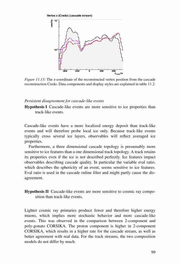
Figure 11.13: The z-coordinate of the reconstructed vertex position from the cascadereconstruction Credo. Data components and display styles are explained in table 11.2.

Persistent disagreement for cascade-like eventsHypothesis I Cascade-like events are more sensitive to ice properties than

track-like events.

Cascade-like events have a more localized energy deposit than track-likeevents and will therefore probe local ice only. Because track-like eventstypically cross several ice layers, observables will reflect averaged iceproperties.

Furthermore, a three dimensional cascade topology is presumably moresensitive to ice features than a one dimensional track topology. A track retainsits properties even if the ice is not described perfectly. Ice features impactobservables describing cascade quality. In particular the variable eval ratio,which describes the sphericity of an event, seems sensitive to ice features.Eval ratio is used in the cascade online filter and might partly cause the dis-agreement.

Hypothesis II Cascade-like events are more sensitive to cosmic ray compo-sition than track-like events.

Lighter cosmic ray primaries produce fewer and therefore higher energymuons, which implies more stochastic behavior and more cascade-likeevents. This was observed in the comparison between 2-component andpoly-gonato CORSIKA. The proton component is higher in 2-componentCORSIKA, which results in a higher rate for the cascade stream, as well asbetter agreement with real data. For the track streams, the two compositionmodels do not differ by much.

99

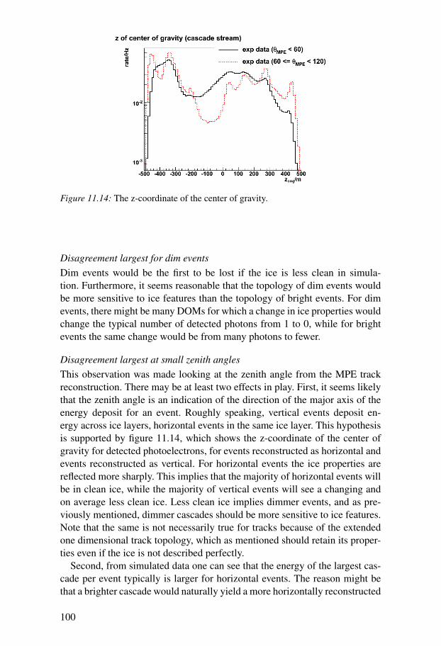
Figure 11.14: The z-coordinate of the center of gravity.

Disagreement largest for dim eventsDim events would be the first to be lost if the ice is less clean in simula-tion. Furthermore, it seems reasonable that the topology of dim events wouldbe more sensitive to ice features than the topology of bright events. For dimevents, there might be many DOMs for which a change in ice properties wouldchange the typical number of detected photons from 1 to 0, while for brightevents the same change would be from many photons to fewer.

Disagreement largest at small zenith anglesThis observation was made looking at the zenith angle from the MPE trackreconstruction. There may be at least two effects in play. First, it seems likelythat the zenith angle is an indication of the direction of the major axis of theenergy deposit for an event. Roughly speaking, vertical events deposit en-ergy across ice layers, horizontal events in the same ice layer. This hypothesisis supported by figure 11.14, which shows the z-coordinate of the center ofgravity for detected photoelectrons, for events reconstructed as horizontal andevents reconstructed as vertical. For horizontal events the ice properties arereflected more sharply. This implies that the majority of horizontal events willbe in clean ice, while the majority of vertical events will see a changing andon average less clean ice. Less clean ice implies dimmer events, and as pre-viously mentioned, dimmer cascades should be more sensitive to ice features.Note that the same is not necessarily true for tracks because of the extendedone dimensional track topology, which as mentioned should retain its proper-ties even if the ice is not described perfectly.

Second, from simulated data one can see that the energy of the largest cas-cade per event typically is larger for horizontal events. The reason might bethat a brighter cascade would naturally yield a more horizontally reconstructed

100

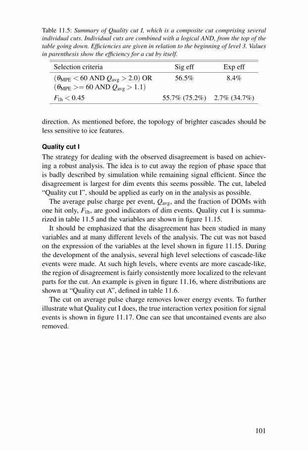
Table 11.5: Summary of Quality cut I, which is a composite cut comprising severalindividual cuts. Individual cuts are combined with a logical AND, from the top of thetable going down. Efficiencies are given in relation to the beginning of level 3. Valuesin parenthesis show the efficiency for a cut by itself.

Selection criteria Sig eff Exp eff

(θMPE < 60 AND Qavg > 2.0) OR(θMPE >= 60 AND Qavg > 1.1)

56.5% 8.4%

F1h < 0.45 55.7% (75.2%) 2.7% (34.7%)

direction. As mentioned before, the topology of brighter cascades should beless sensitive to ice features.

Quality cut IThe strategy for dealing with the observed disagreement is based on achiev-ing a robust analysis. The idea is to cut away the region of phase space thatis badly described by simulation while remaining signal efficient. Since thedisagreement is largest for dim events this seems possible. The cut, labeled“Quality cut I”, should be applied as early on in the analysis as possible.

The average pulse charge per event, Qavg, and the fraction of DOMs withone hit only, F1h, are good indicators of dim events. Quality cut I is summa-rized in table 11.5 and the variables are shown in figure 11.15.

It should be emphasized that the disagreement has been studied in manyvariables and at many different levels of the analysis. The cut was not basedon the expression of the variables at the level shown in figure 11.15. Duringthe development of the analysis, several high level selections of cascade-likeevents were made. At such high levels, where events are more cascade-like,the region of disagreement is fairly consistently more localized to the relevantparts for the cut. An example is given in figure 11.16, where distributions areshown at “Quality cut A”, defined in table 11.6.

The cut on average pulse charge removes lower energy events. To furtherillustrate what Quality cut I does, the true interaction vertex position for signalevents is shown in figure 11.17. One can see that uncontained events are alsoremoved.

101

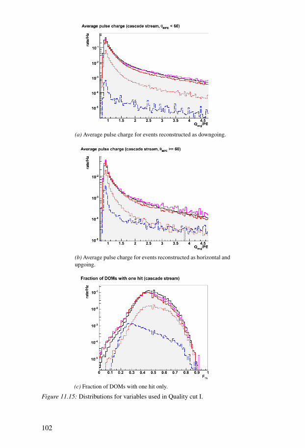
(a) Average pulse charge for events reconstructed as downgoing.

(b) Average pulse charge for events reconstructed as horizontal andupgoing.

(c) Fraction of DOMs with one hit only.

Figure 11.15: Distributions for variables used in Quality cut I.

102

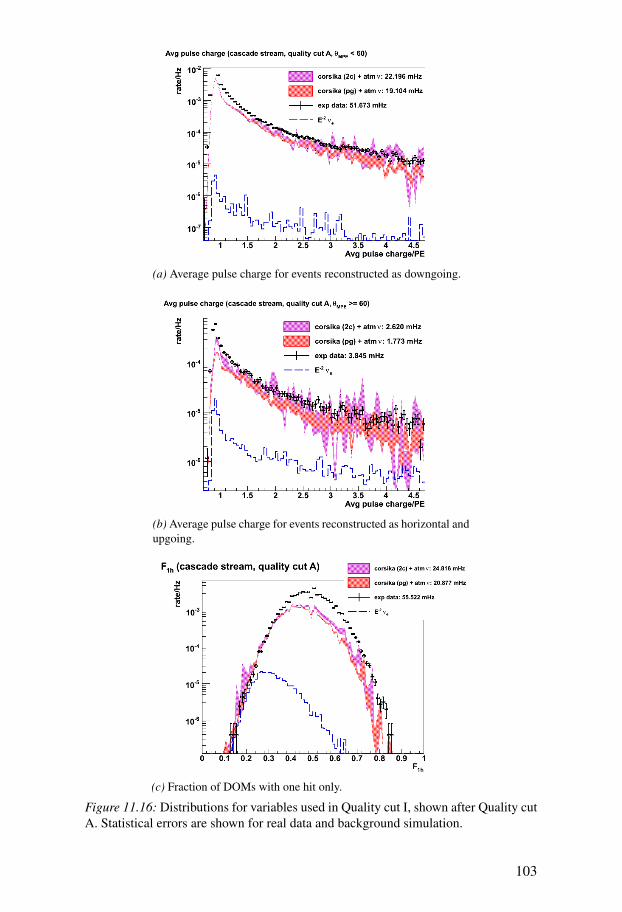
(a) Average pulse charge for events reconstructed as downgoing.

(b) Average pulse charge for events reconstructed as horizontal andupgoing.

(c) Fraction of DOMs with one hit only.

Figure 11.16: Distributions for variables used in Quality cut I, shown after Quality cutA. Statistical errors are shown for real data and background simulation.

103

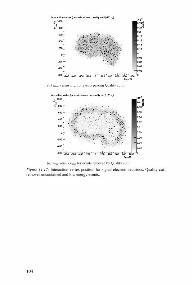
(a) ytrue versus xtrue for events passing Quality cut I.

(b) ytrue versus xtrue for events removed by Quality cut I.

Figure 11.17: Interaction vertex position for signal electron neutrinos. Quality cut Iremoves uncontained and low energy events.

104

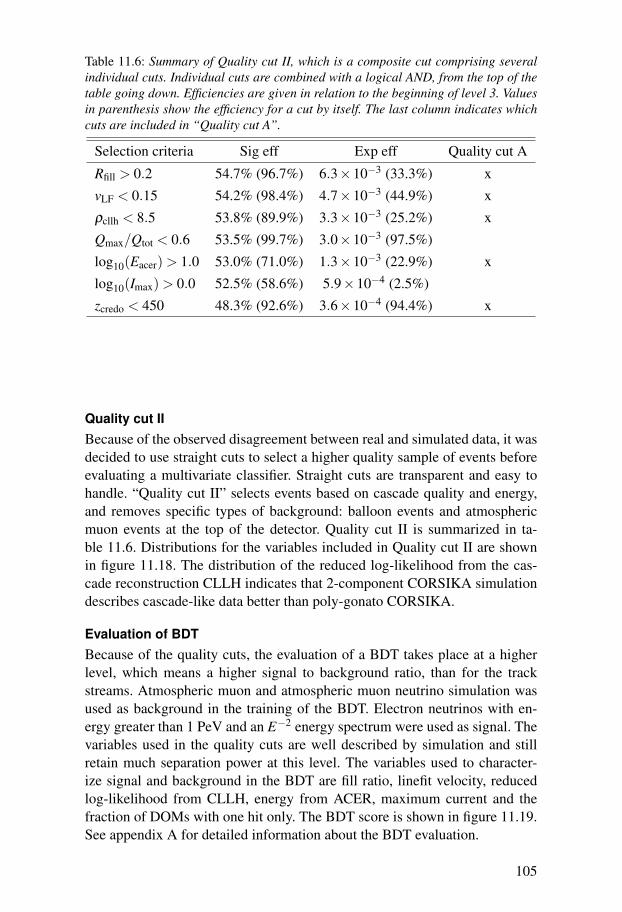
Table 11.6: Summary of Quality cut II, which is a composite cut comprising severalindividual cuts. Individual cuts are combined with a logical AND, from the top of thetable going down. Efficiencies are given in relation to the beginning of level 3. Valuesin parenthesis show the efficiency for a cut by itself. The last column indicates whichcuts are included in “Quality cut A”.

Selection criteria Sig eff Exp eff Quality cut A

Rfill > 0.2 54.7% (96.7%) 6.3×10−3 (33.3%) x

vLF < 0.15 54.2% (98.4%) 4.7×10−3 (44.9%) x

ρcllh < 8.5 53.8% (89.9%) 3.3×10−3 (25.2%) x

Qmax/Qtot < 0.6 53.5% (99.7%) 3.0×10−3 (97.5%)

log10(Eacer) > 1.0 53.0% (71.0%) 1.3×10−3 (22.9%) x

log10(Imax) > 0.0 52.5% (58.6%) 5.9×10−4 (2.5%)

zcredo < 450 48.3% (92.6%) 3.6×10−4 (94.4%) x

Quality cut IIBecause of the observed disagreement between real and simulated data, it wasdecided to use straight cuts to select a higher quality sample of events beforeevaluating a multivariate classifier. Straight cuts are transparent and easy tohandle. “Quality cut II” selects events based on cascade quality and energy,and removes specific types of background: balloon events and atmosphericmuon events at the top of the detector. Quality cut II is summarized in ta-ble 11.6. Distributions for the variables included in Quality cut II are shownin figure 11.18. The distribution of the reduced log-likelihood from the cas-cade reconstruction CLLH indicates that 2-component CORSIKA simulationdescribes cascade-like data better than poly-gonato CORSIKA.

Evaluation of BDTBecause of the quality cuts, the evaluation of a BDT takes place at a higherlevel, which means a higher signal to background ratio, than for the trackstreams. Atmospheric muon and atmospheric muon neutrino simulation wasused as background in the training of the BDT. Electron neutrinos with en-ergy greater than 1 PeV and an E−2 energy spectrum were used as signal. Thevariables used in the quality cuts are well described by simulation and stillretain much separation power at this level. The variables used to character-ize signal and background in the BDT are fill ratio, linefit velocity, reducedlog-likelihood from CLLH, energy from ACER, maximum current and thefraction of DOMs with one hit only. The BDT score is shown in figure 11.19.See appendix A for detailed information about the BDT evaluation.

105

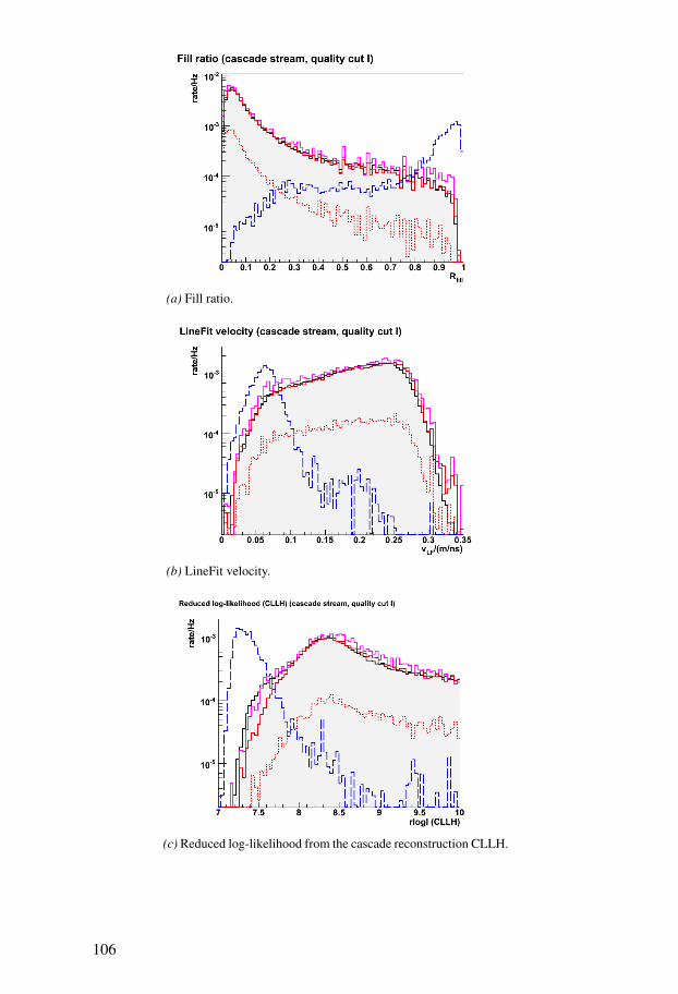
(a) Fill ratio.

(b) LineFit velocity.

(c) Reduced log-likelihood from the cascade reconstruction CLLH.

106

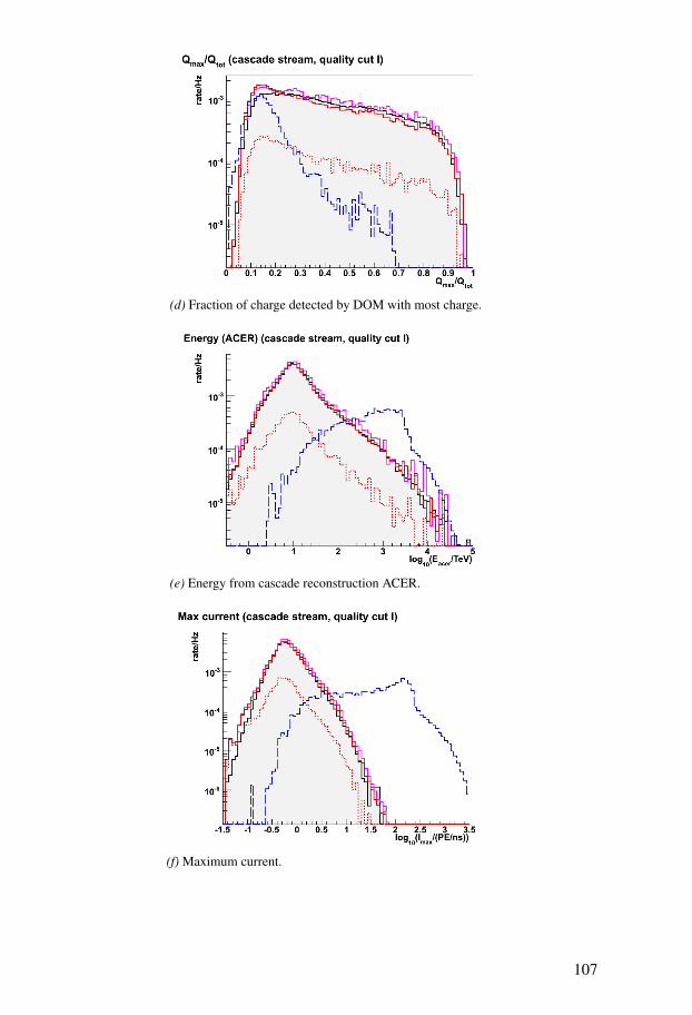
(d) Fraction of charge detected by DOM with most charge.

(e) Energy from cascade reconstruction ACER.

(f) Maximum current.

107

(g) Z-coordinate of vertex position from cascade reconstructionCredo.

Figure 11.18: Distributions for variables included in Quality cut II. Note that Qualitycut I has been applied.

ContainmentThere is sensitivity to UHE cascades located well outside the detector. Onlyin the context of discovery might a containment cut be required, dependingon the degree of confidence in simulation. Uncontained events are more dif-ficult to conclusively characterize as neutrino induced or not. In the case of aless than significant excess, an upper limit is set and characterizing survivingevents is not strictly required. This seems like a possible scenario based onresults from previous IceCube high energy diffuse cascade analyses [98].

A containment cut would significantly reduce the UHE signal efficiency.Selecting the region immediately above the last burn sample data event whencutting on the cascade stream BDT score, 47% of signal is inside the detectorand 90% is inside 1.5 × the detector size.

After thorough investigation of the cascade stream and after devising qual-ity cuts, the degree of confidence in the simulation was deemed adequate.

In light of this a containment cut was not included.

11.4 Passing ratesPassing rates at different cut levels are shown in table 11.7. The cut levels aredescribed in table 11.8, and were chosen for the purpose of evaluating passingrates at different points in the analysis. They were not chosen arbitrarily butcould have been. Level 3-II was chosen to remove almost pure backgroundand keep most signal. Level 3-III defines the region where the final cut wasdeveloped.

108

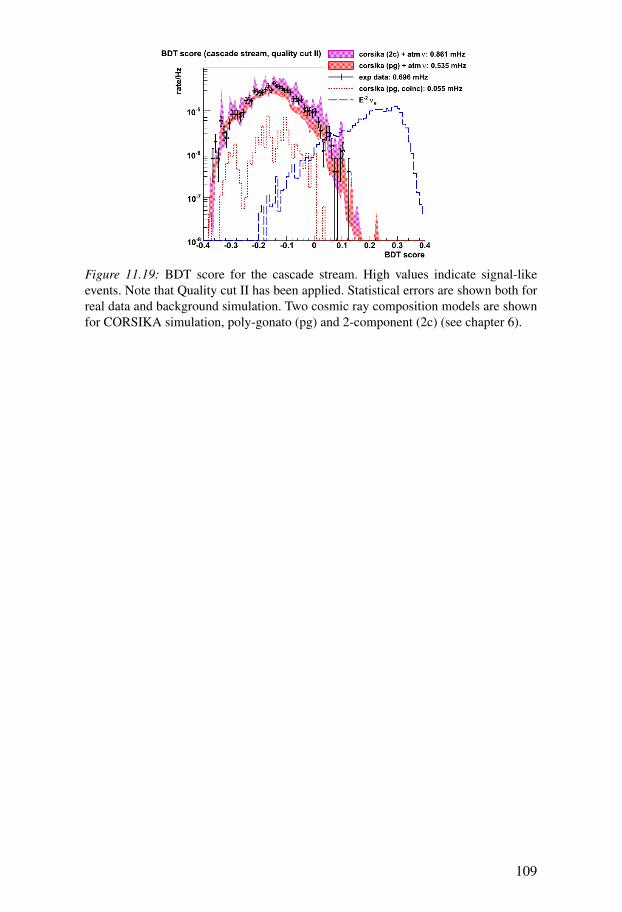
Figure 11.19: BDT score for the cascade stream. High values indicate signal-likeevents. Note that Quality cut II has been applied. Statistical errors are shown both forreal data and background simulation. Two cosmic ray composition models are shownfor CORSIKA simulation, poly-gonato (pg) and 2-component (2c) (see chapter 6).

109

Tabl

e11

.7:P

assi

ngra

tes

atdi

ffer

entc

utle

vels

.

Cut

leve

lE

xpTo

tbg

(pol

y-go

nato

)To

tbg

(2-c

omp)

Coi

ncA

tmν

µA

tmν

e

Lev

el3

3.37

Hz

2.80

Hz

3.16

Hz

0.67

Hz

119.

75µ

Hz

6.41

µH

z

Lev

el3-

I2.

68H

z2.

32H

z2.

58H

z0.

47H

z11

2.97

µH

z5.

73µ

Hz

Lev

el3-

II89

5m

Hz

813

mH

z89

0m

Hz

117

mH

z99

.35

µH

z4.

21µ

Hz

Lev

el3-

III

1.03

mH

z0.

74m

Hz

1.17

mH

z0.

19m

Hz

54.0

5µ

Hz

0.49

µH

z

Tabl

e11

.8:D

escr

iptio

nof

cutl

evel

s.E

ach

cutl

evel

isde

fined

asan

OR

betw

een

cuts

fore

ach

stre

am.E

ach

cutl

evel

build

son

the

prev

ious

leve

l.

Cut

leve

lTr

ack

dow

nTr

ack

upC

asca

de

Lev

el3

Star

tofL

evel

3

Lev

el3-

IC

oinc

cut

Coi

nccu

tQ

ualit

ycu

tI

Lev

el3-

IIB

DT t

rack

dow

n>−

0.25

BD

T tra

ckup

>−

0.25

Qua

lity

cutI

IAN

DB

DT c

asca

de>−

0.15

Lev

el3-

III

BD

T tra

ckdo

wn>

0.15

2B

DT t

rack

up>−

0.00

8B

DT c

asca

de>−

0.12

4

110

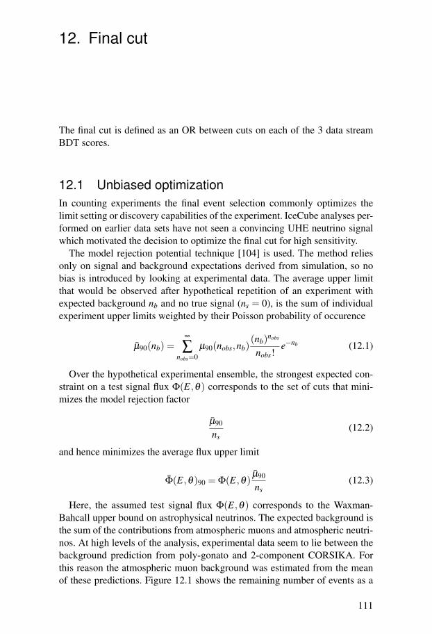
12. Final cut

The final cut is defined as an OR between cuts on each of the 3 data streamBDT scores.

12.1 Unbiased optimizationIn counting experiments the final event selection commonly optimizes thelimit setting or discovery capabilities of the experiment. IceCube analyses per-formed on earlier data sets have not seen a convincing UHE neutrino signalwhich motivated the decision to optimize the final cut for high sensitivity.

The model rejection potential technique [104] is used. The method reliesonly on signal and background expectations derived from simulation, so nobias is introduced by looking at experimental data. The average upper limitthat would be observed after hypothetical repetition of an experiment withexpected background nb and no true signal (ns = 0), is the sum of individualexperiment upper limits weighted by their Poisson probability of occurence

µ90(nb) =∞

∑nobs=0

µ90(nobs,nb)(nb)nobs

nobs!e−nb (12.1)

Over the hypothetical experimental ensemble, the strongest expected con-straint on a test signal flux Φ(E,θ) corresponds to the set of cuts that mini-mizes the model rejection factor

µ90

ns(12.2)

and hence minimizes the average flux upper limit

Φ(E,θ)90 = Φ(E,θ)µ90

ns(12.3)

Here, the assumed test signal flux Φ(E,θ) corresponds to the Waxman-Bahcall upper bound on astrophysical neutrinos. The expected background isthe sum of the contributions from atmospheric muons and atmospheric neutri-nos. At high levels of the analysis, experimental data seem to lie between thebackground prediction from poly-gonato and 2-component CORSIKA. Forthis reason the atmospheric muon background was estimated from the meanof these predictions. Figure 12.1 shows the remaining number of events as a

111

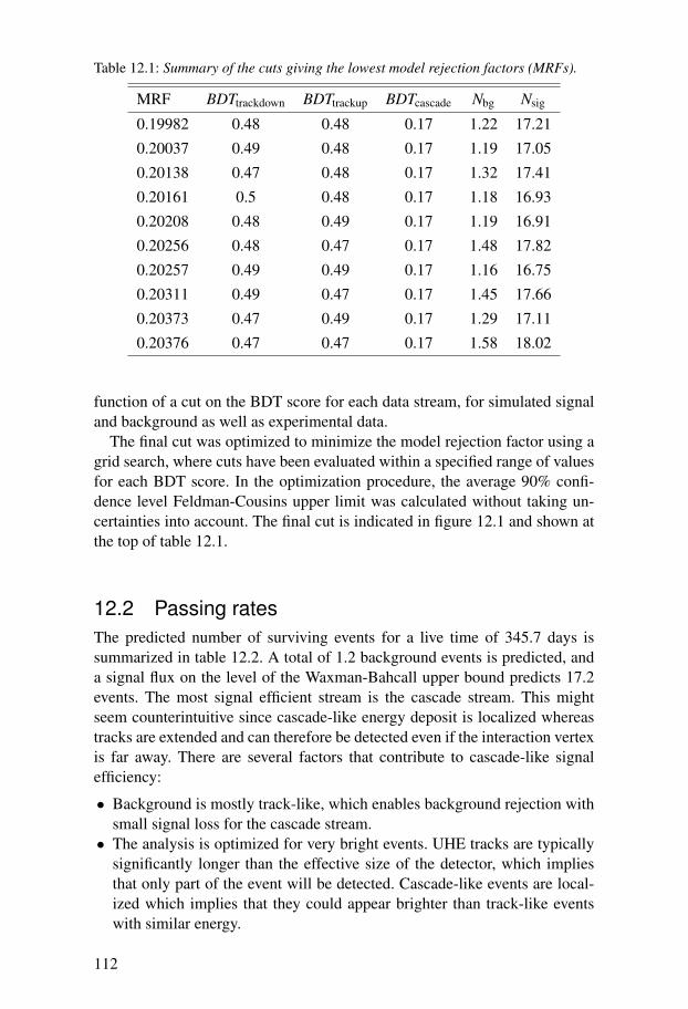
Table 12.1: Summary of the cuts giving the lowest model rejection factors (MRFs).

MRF BDTtrackdown BDTtrackup BDTcascade Nbg Nsig

0.19982 0.48 0.48 0.17 1.22 17.21

0.20037 0.49 0.48 0.17 1.19 17.05

0.20138 0.47 0.48 0.17 1.32 17.41

0.20161 0.5 0.48 0.17 1.18 16.93

0.20208 0.48 0.49 0.17 1.19 16.91

0.20256 0.48 0.47 0.17 1.48 17.82

0.20257 0.49 0.49 0.17 1.16 16.75

0.20311 0.49 0.47 0.17 1.45 17.66

0.20373 0.47 0.49 0.17 1.29 17.11

0.20376 0.47 0.47 0.17 1.58 18.02

function of a cut on the BDT score for each data stream, for simulated signaland background as well as experimental data.

The final cut was optimized to minimize the model rejection factor using agrid search, where cuts have been evaluated within a specified range of valuesfor each BDT score. In the optimization procedure, the average 90% confi-dence level Feldman-Cousins upper limit was calculated without taking un-certainties into account. The final cut is indicated in figure 12.1 and shown atthe top of table 12.1.

12.2 Passing ratesThe predicted number of surviving events for a live time of 345.7 days issummarized in table 12.2. A total of 1.2 background events is predicted, anda signal flux on the level of the Waxman-Bahcall upper bound predicts 17.2events. The most signal efficient stream is the cascade stream. This mightseem counterintuitive since cascade-like energy deposit is localized whereastracks are extended and can therefore be detected even if the interaction vertexis far away. There are several factors that contribute to cascade-like signalefficiency:

• Background is mostly track-like, which enables background rejection withsmall signal loss for the cascade stream.• The analysis is optimized for very bright events. UHE tracks are typically

significantly longer than the effective size of the detector, which impliesthat only part of the event will be detected. Cascade-like events are local-ized which implies that they could appear brighter than track-like eventswith similar energy.

112

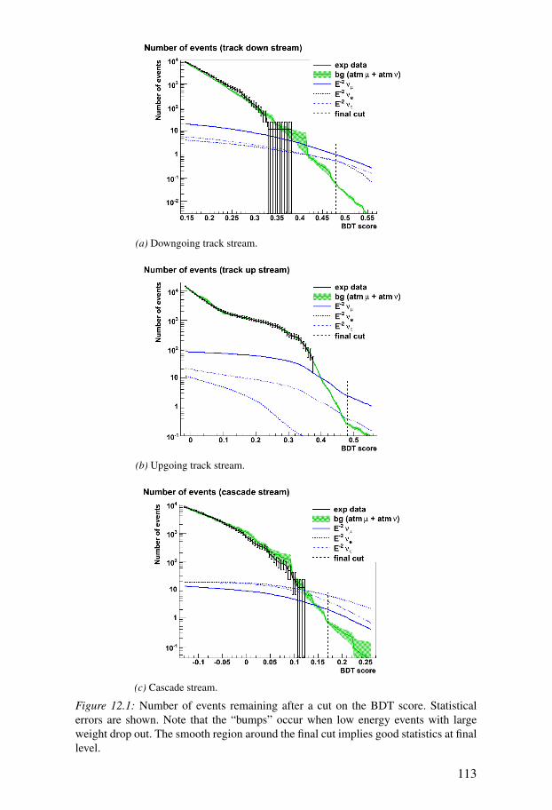
(a) Downgoing track stream.

(b) Upgoing track stream.

(c) Cascade stream.

Figure 12.1: Number of events remaining after a cut on the BDT score. Statisticalerrors are shown. Note that the “bumps” occur when low energy events with largeweight drop out. The smooth region around the final cut implies good statistics at finallevel.

113

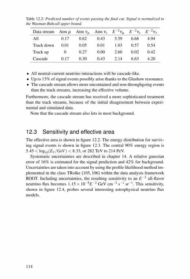
Table 12.2: Predicted number of events passing the final cut. Signal is normalized tothe Waxman-Bahcall upper bound.

Data stream Atm µ Atm νµ Atm νe E−2νµ E−2νe E−2ντ

All 0.17 0.62 0.43 5.59 6.68 4.94

Track down 0.01 0.05 0.01 1.03 0.57 0.54

Track up 0 0.27 0.00 2.60 0.02 0.42

Cascade 0.17 0.30 0.43 2.14 6.63 4.20

• All neutral-current neutrino interactions will be cascade-like.• Up to 13% of signal events possibly arise thanks to the Glashow resonance.• The cascade stream allows more uncontained and non-throughgoing events

than the track streams, increasing the effective volume.Furthermore, the cascade stream has received a more sophisticated treatmentthan the track streams, because of the initial disagreement between experi-mental and simulated data.

Note that the cascade stream also lets in most background.

12.3 Sensitivity and effective areaThe effective area is shown in figure 12.2. The energy distribution for surviv-ing signal events is shown in figure 12.3. The central 90% energy region is5.45 < log10(Eν/GeV ) < 8.33, or 282 TeV to 214 PeV.

Systematic uncertainties are described in chapter 14. A relative gaussianerror of 16% is estimated for the signal prediction and 42% for background.Uncertainties are taken into account by using the profile likelihood method im-plemented in the class TRolke [105, 106] within the data analysis frameworkROOT. Including uncertainties, the resulting sensitivity to an E−2 all-flavorneutrino flux becomes 1.15× 10−8E−2 GeV cm−2 s−1 sr−1. This sensitivity,shown in figure 12.4, probes several interesting astrophysical neutrino fluxmodels.

114

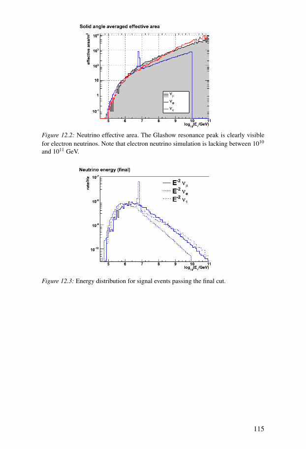
Figure 12.2: Neutrino effective area. The Glashow resonance peak is clearly visiblefor electron neutrinos. Note that electron neutrino simulation is lacking between 1010

and 1011 GeV.

Figure 12.3: Energy distribution for signal events passing the final cut.

115

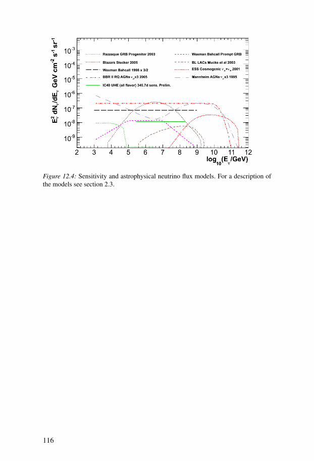
Figure 12.4: Sensitivity and astrophysical neutrino flux models. For a description ofthe models see section 2.3.

116

13. Non-signal events

13.1 Tagging of flasher-type eventsIn three high energy analyses performed with AMANDA-II using data from2000–2003, at least twelve very similar events were found. The events allexhibit spherical light emission that seems to originate from the region arounda particular optical module (OM). For this reason it seems likely that theseevents spring from some sort of detector artefact.

These events are in many ways similar to high energy cascade-like signalevents which makes it important to characterize and if possible exclude themfrom the signal search. Here, a selection is devised with the purpose of taggingevents for further investigation. Any event tagged is not included in the searchfor signal.

13.1.1 Light originates from the same regionThe light seems to originate from the region around OM 531.OM 531, number 19 on AMANDA string 16, has position (x, y, z) =(296.5 m, 30.5 m, 187.1 m). Table 13.1 shows the reconstructed vertexposition for as many events of this type that could be found, along with thedistance from OM 531. The mean reconstructed vertex position is (x, y, z)= (296.5 m, 29.9 m, 184.4 m) with standard deviations (∆x, ∆y, ∆z) =(2.4 m, 4.2 m, 4.1 m). The largest distance from OM 531 is 13.1 m.

One further event of this type was found in a high energy analysis per-formed with IceCube in the 22-string configuration, using data from 2007.Owing to differing geometry and DOM sensitivity this type of event will ap-pear slightly different in IceCube than in AMANDA. The reconstructed z-position for the icecube event is 12 m above the mean, at 196.6 m. The DOMthat detected most light is the DOM closest to and above OM 531, at z-position201 m.

13.1.2 Stationary sourceIf the light originates from OM 531 and the light emission is spherical thisshould be reflected in a low value of the LineFit velocity. The IceCube eventyields vLF = 0.02, in agreement with this expectation.

117

Table 13.1: Reconstructed vertex position for flasher type events, along with distanced from OM 531. Note that only distances were available for data sample Wiedemann.The events in data sample Ackermann and Wiedemann may be overlapping.

Data sample x/m y/m z/m d/m

Gerhardt (AMANDA-II 2001) 295.4 32.3 184.3 3.5

295.5 30.1 183.8 3.5

295.5 31.4 183.5 3.9

295.1 27.9 182.1 5.8

293.7 28.8 183.5 4.8

297.2 31.0 182.4 4.8

Ackermann (AMANDA-II 2003) 301.1 32.8 183.7 6.1

294.5 18.5 182.2 13.1

300.7 32.4 182.3 6.7

Wiedemann (AMANDA-II 2003) - - - 7

- - - 8

- - - 12

- - - 11

- - - 6

Seo (IceCube-22 2007) 296.2 34.1 196.6 10.2

118

13.1.3 Bright eventsAll of the events for which there is information about brightness are brightevents. The AMANDA events have more than 2000 hits, where one hit cancorrespond to many photoelectrons. The IceCube event has an estimated num-ber of photoelectrons of around 5 ·104.

The events were all found in high energy analyses, which might be the rea-son they are all very bright. That is, there might be dimmer events of this typethat were removed from these analyses at a lower level. However, the similar-ity among the events seems to indicate a general regularity to their expression.Furthermore, this type of events has not been found in lower energy analyses.Stricter quality cuts are generally used in lower energy analyses though, andsince these events appear artificial they may have been removed by qualitycuts.

13.1.4 TimingFor the AMANDA events the hit time distribution was investigated. A possibleconclusion was that light was produced over a longer time scale than for eventsof particle origin. The event duration for each of the AMANDA events ismore than 10 µs. The icecube event has a duration of more than 27 µs. Atypical event of particle origin has a duration of less than 6 µs, bounded bythe geometry of the detector and absorption of photons in the ice.

13.1.5 Event hypothesesOne hypothesis for the production of light in these events is a discharge inthe PMT or from the PMT base board in OM 531. However, the brightnessof these events might not be compatible with a discharge. Furthermore, onemight expect a damaged PMT to stop functioning, which has not been ob-served.

OM 531 is equipped with a UV flasher board and given the brightness ofthe events another hypothesis is that the flasher was triggered. The designerof the flasher board deems this hypothesis unlikely though. This investigationremains unconclusive.

13.1.6 Event selectionSince AMANDA was still powered and active for the data sample used in thisanalysis, an event selection was devised to tag this type of events.

A study of the performance of cascade reconstruction methods shows thatthere is often a systematic shift in reconstructed vertex position of flasherevents. For this reason events were selected in relation to the reconstructedvertex for the 2007 IceCube event rather than OM 531. The resulting selec-tion is showed in table 13.2.

119

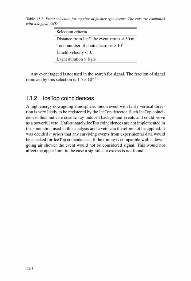
Table 13.2: Event selection for tagging of flasher type events. The cuts are combinedwith a logical AND.

Selection criteria

Distance from IceCube event vertex < 30 m

Total number of photoelectrons > 103

Linefit velocity < 0.1

Event duration > 8 µs

Any event tagged is not used in the search for signal. The fraction of signalremoved by this selection is 1.5×10−5.

13.2 IceTop coincidencesA high energy downgoing atmospheric muon event with fairly vertical direc-tion is very likely to be registered by the IceTop detector. Such IceTop coinci-dences thus indicate cosmic-ray induced background events and could serveas a powerful veto. Unfortunately IceTop coincidences are not implemented inthe simulation used in this analysis and a veto can therefore not be applied. Itwas decided a priori that any surviving events from experimental data wouldbe checked for IceTop coincidences. If the timing is compatible with a down-going air shower the event would not be considered signal. This would notaffect the upper limit in the case a siginificant excess is not found.

120

14. Systematic uncertainties

Two main types of analyses performed within IceCube are point source anddiffuse analyses. Point source analyses look for a resolved flux, signal is local-ized and background can be estimated from experimental data. Diffuse anal-yses look for an unresolved flux, signal is not well localized and backgroundmust be estimated based on simulated data. Systematic errors arise from im-perfect description of the detector, the environment and the physical processesbehind event generation, propagation and energy loss. Many systematic un-certainties can be avoided in point source analyses, while a comprehensiveinvestigation of uncertainties is required for diffuse analyses.

A common technique for estimating the impact of systematic uncertaintiesis to vary relevant parameters in simulation within a reasonable range andpropagate the effects through the analysis. Here, this technique was used ex-tensively. This approach is computationally intensive and was possible largelythanks to the national computational resource SweGrid. Much work was spentincorporating SweGrid in the standard IceCube simulation production frame-work.

For this approach to be feasible, benchmark data sets used to investigatesystematics were generated with less statistics than for data sets serving as thebaseline for most analyses. Where statistics is severely limited at final level,the impact on the analysis was estimated at a slightly lower level. Further-more, the effect on all-flavor neutrino data was estimated using νµ neutrinosimulation only. This was considered reasonable since νµ neutrino simulationprobes all data streams of the analysis and the final passing rate is similarbetween neutrino flavors.

Note that the neutrino cross sections used in the benchmark data sets arebased on CTEQ5 PDFs [59, 61], except in the absolute energy scale and neu-trino cross section uncertainty investigations. Also note that in the followingsections the signal neutrino component is often indicated by the energy spec-trum, E−2, and is normalized to the Waxman-Bachall upper bound. Numberof events are listed assuming a livetime corresponding to the blinded experi-mental data set, 345.7 days, unless otherwise noted.

The systematic uncertainties are summarized in the last section.

121

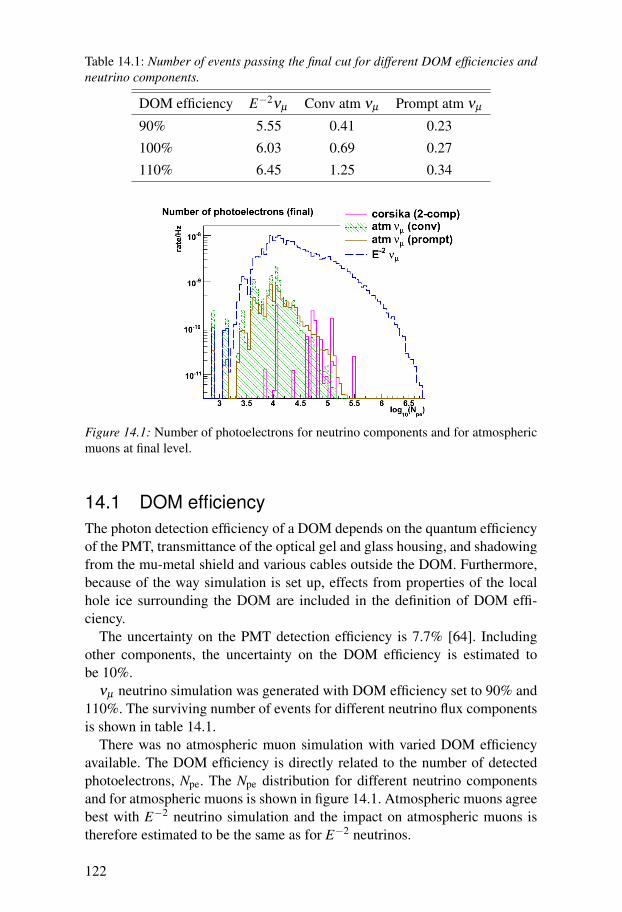
Table 14.1: Number of events passing the final cut for different DOM efficiencies andneutrino components.

DOM efficiency E−2νµ Conv atm νµ Prompt atm νµ

90% 5.55 0.41 0.23

100% 6.03 0.69 0.27

110% 6.45 1.25 0.34

Figure 14.1: Number of photoelectrons for neutrino components and for atmosphericmuons at final level.

14.1 DOM efficiencyThe photon detection efficiency of a DOM depends on the quantum efficiencyof the PMT, transmittance of the optical gel and glass housing, and shadowingfrom the mu-metal shield and various cables outside the DOM. Furthermore,because of the way simulation is set up, effects from properties of the localhole ice surrounding the DOM are included in the definition of DOM effi-ciency.

The uncertainty on the PMT detection efficiency is 7.7% [64]. Includingother components, the uncertainty on the DOM efficiency is estimated tobe 10%.

νµ neutrino simulation was generated with DOM efficiency set to 90% and110%. The surviving number of events for different neutrino flux componentsis shown in table 14.1.

There was no atmospheric muon simulation with varied DOM efficiencyavailable. The DOM efficiency is directly related to the number of detectedphotoelectrons, Npe. The Npe distribution for different neutrino componentsand for atmospheric muons is shown in figure 14.1. Atmospheric muons agreebest with E−2 neutrino simulation and the impact on atmospheric muons istherefore estimated to be the same as for E−2 neutrinos.

122

Table 14.2: Number of events passing the final cut for different ice models.

Ice model E−2νµ Conv atm νµ Prompt atm νµ Atm µ

AHA 6.03 0.693 0.275 0.0316 ± 0.0127

SPICE1 5.30 0.484 0.246 0.0313 ± 0.0227

Table 14.3: A signal efficient cut giving at least 10 times the final level statistics foratmospheric muon simulation.

Selection criteria

(BDTtrackdown > 0.386) OR (BDTtrackup > 0.414) OR (BDTcascade > 0.108)

14.2 Ice modelThe AHA ice model (see section 4.6) is used as baseline in this analysis. Adifferent ice model, SPICE1 [107], derived in an independent fashion, is usedas an estimate of a reasonable variation of ice properties in one direction.νµ neutrino simulation and 2-component CORSIKA was generated using theSPICE1 ice model. The surviving number of events for different data compo-nents and ice models is shown in table 14.2.

2-component CORSIKA predicts almost the same number of events forAHA and SPICE1 after the final cut. The statistics for the SPICE1 data set is10% of that of the AHA data set and the statistical error on the prediction at fi-nal level is large. For this reason, the effect on atmospheric muon backgroundis estimated at a slighty lower level. A looser, signal efficient, cut was evalu-ated with the intention of increasing statistics by at least 10 times. The cut isdescribed in table 14.3. The number of events surviving this cut is shown intable 14.4. If the cut is tightened or loosened slightly the resulting systematicuncertainty becomes similar or smaller.

14.3 Absolute energy scaleFor variables based on the number of detected photoelectrons, backgroundand signal extend to higher values than the burn sample experimental data.This means that experimental data cannot be used to constrain the uncertainty

Table 14.4: Number of events passing a looser-than-final cut for different ice models.

Ice model Atm µ

AHA 3.94 ± 1.00

SPICE1 2.52 ± 1.10

123

Table 14.5: Number of events passing the final cut for different shifts of detected num-ber of photoelectrons.

Shift E−2ν Conv atm ν Prompt atm ν Atm µ

0% 17.21 0.398 0.654 0.0316

-11.6% 16.54 0.336 0.599 0.0224

on the number of detected photoelectrons, or the absolute energy scale, inthis region. This uncertainty is investigated by manually shifting the detectednumber of photoelectrons by an appropriate amount, then re-evaluating theBDT scores and final cut passing rates.

The estimation of a reasonable shift is based on an analysis of standard can-dle (SC) data. A standard candle is a laser module with absolutely calibratedlight output. There are two standard candles installed inside the in-ice detectorvolume. A disagreement in number of detected photoelectrons between exper-imental and simulated data was seen for the standard candles. The disagree-ment is mainly attributed to uncertainties on the ice model, DOM efficiency,DOM saturation behavior and possibly a miscalibration of ATWD channel 2gain. In the SC analysis, DOMs are divided into saturated and unsaturated,and the two categories are studied separately.

In this analysis, systematic uncertainties on the ice model and DOM effi-ciency are taken into account by other means. The error on detected numberof photoelectrons is therefore estimated based on the SC analysis results us-ing saturated DOMs. The burn sample data extends to about log10(Npe) = 5.2.The SC light output setting corresponding to the number of detected photo-electrons closest above this value shows a shift of -11.6% for simulation inrelation to experimental data.

The impact of shifting the number of detected photoelectrons by -11.6%is shown in table 14.5, for all-flavor neutrino components and 2-componentCORSIKA.

14.4 Neutrino-nucleon interaction cross sectionsThe baseline neutrino simulation within IceCube uses neutrino-nucleon in-teraction cross sections based on CTEQ5 PDFs [59, 61]. At a late stage ofthe analysis it was pointed out that these PDFs do not fit modern data, andthat there were state-of-the-art calculations available based on HERA dataperformed by A. Cooper-Sarkar and S. Sarkar (CSS) [4]. The CSS calcula-tions account for PDF uncertainties deriving from both model uncertaintiesand from the experimental uncertainties of the input data sets. The new CSScross sections are lower than the ones based on CTEQ5 PDFs, as shown infigure 14.2.

124

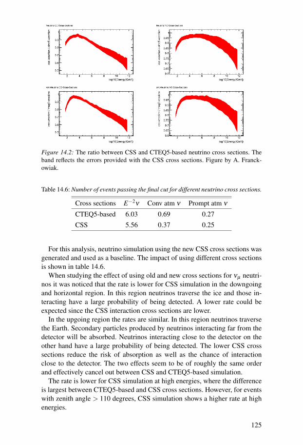
Figure 14.2: The ratio between CSS and CTEQ5-based neutrino cross sections. Theband reflects the errors provided with the CSS cross sections. Figure by A. Franck-owiak.

Table 14.6: Number of events passing the final cut for different neutrino cross sections.

Cross sections E−2ν Conv atm ν Prompt atm ν

CTEQ5-based 6.03 0.69 0.27

CSS 5.56 0.37 0.25

For this analysis, neutrino simulation using the new CSS cross sections wasgenerated and used as a baseline. The impact of using different cross sectionsis shown in table 14.6.

When studying the effect of using old and new cross sections for νµ neutri-nos it was noticed that the rate is lower for CSS simulation in the downgoingand horizontal region. In this region neutrinos traverse the ice and those in-teracting have a large probability of being detected. A lower rate could beexpected since the CSS interaction cross sections are lower.

In the upgoing region the rates are similar. In this region neutrinos traversethe Earth. Secondary particles produced by neutrinos interacting far from thedetector will be absorbed. Neutrinos interacting close to the detector on theother hand have a large probability of being detected. The lower CSS crosssections reduce the risk of absorption as well as the chance of interactionclose to the detector. The two effects seem to be of roughly the same orderand effectively cancel out between CSS and CTEQ5-based simulation.

The rate is lower for CSS simulation at high energies, where the differenceis largest between CTEQ5-based and CSS cross sections. However, for eventswith zenith angle > 110 degrees, CSS simulation shows a higher rate at highenergies.

125

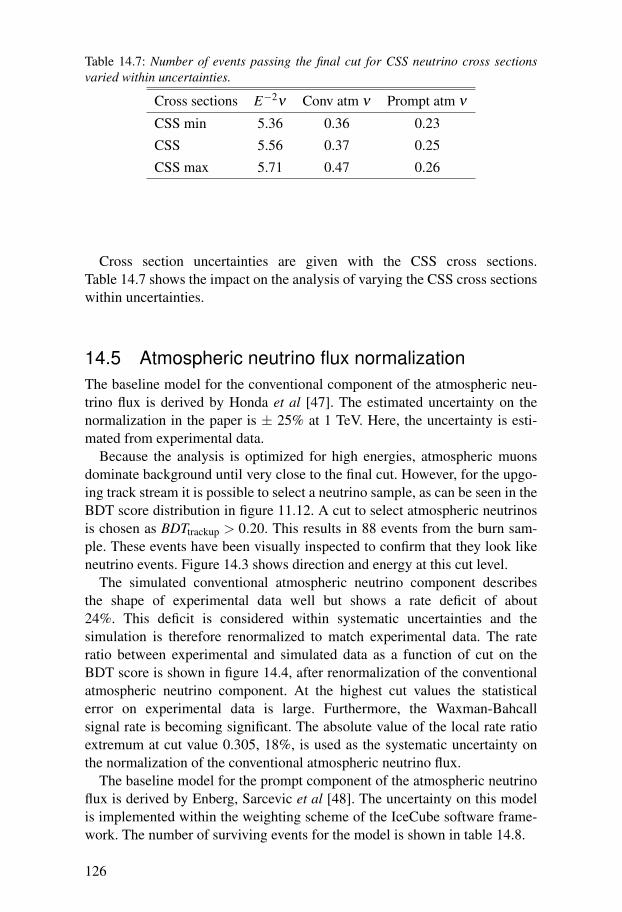
Table 14.7: Number of events passing the final cut for CSS neutrino cross sectionsvaried within uncertainties.

Cross sections E−2ν Conv atm ν Prompt atm ν

CSS min 5.36 0.36 0.23

CSS 5.56 0.37 0.25

CSS max 5.71 0.47 0.26

Cross section uncertainties are given with the CSS cross sections.Table 14.7 shows the impact on the analysis of varying the CSS cross sectionswithin uncertainties.

14.5 Atmospheric neutrino flux normalizationThe baseline model for the conventional component of the atmospheric neu-trino flux is derived by Honda et al [47]. The estimated uncertainty on thenormalization in the paper is ± 25% at 1 TeV. Here, the uncertainty is esti-mated from experimental data.

Because the analysis is optimized for high energies, atmospheric muonsdominate background until very close to the final cut. However, for the upgo-ing track stream it is possible to select a neutrino sample, as can be seen in theBDT score distribution in figure 11.12. A cut to select atmospheric neutrinosis chosen as BDTtrackup > 0.20. This results in 88 events from the burn sam-ple. These events have been visually inspected to confirm that they look likeneutrino events. Figure 14.3 shows direction and energy at this cut level.

The simulated conventional atmospheric neutrino component describesthe shape of experimental data well but shows a rate deficit of about24%. This deficit is considered within systematic uncertainties and thesimulation is therefore renormalized to match experimental data. The rateratio between experimental and simulated data as a function of cut on theBDT score is shown in figure 14.4, after renormalization of the conventionalatmospheric neutrino component. At the highest cut values the statisticalerror on experimental data is large. Furthermore, the Waxman-Bahcallsignal rate is becoming significant. The absolute value of the local rate ratioextremum at cut value 0.305, 18%, is used as the systematic uncertainty onthe normalization of the conventional atmospheric neutrino flux.

The baseline model for the prompt component of the atmospheric neutrinoflux is derived by Enberg, Sarcevic et al [48]. The uncertainty on this modelis implemented within the weighting scheme of the IceCube software frame-work. The number of surviving events for the model is shown in table 14.8.

126

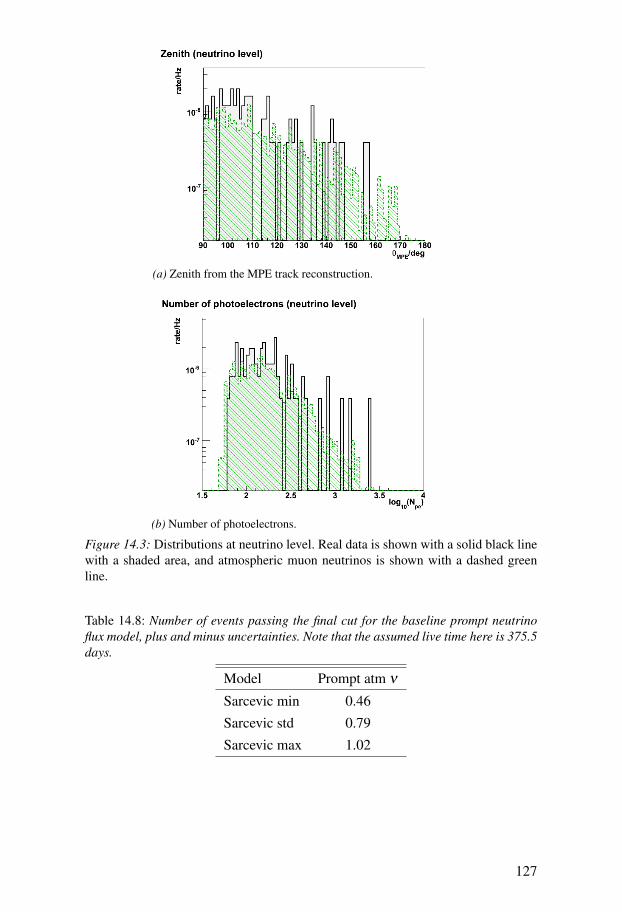
(a) Zenith from the MPE track reconstruction.

(b) Number of photoelectrons.

Figure 14.3: Distributions at neutrino level. Real data is shown with a solid black linewith a shaded area, and atmospheric muon neutrinos is shown with a dashed greenline.

Table 14.8: Number of events passing the final cut for the baseline prompt neutrinoflux model, plus and minus uncertainties. Note that the assumed live time here is 375.5days.

Model Prompt atm ν

Sarcevic min 0.46

Sarcevic std 0.79

Sarcevic max 1.02

127

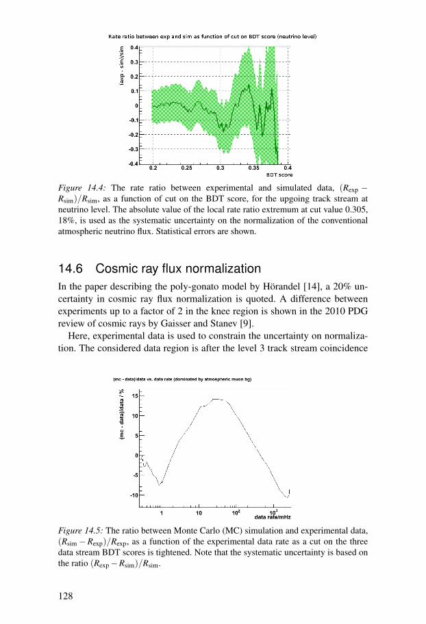
Figure 14.4: The rate ratio between experimental and simulated data, (Rexp −Rsim)/Rsim, as a function of cut on the BDT score, for the upgoing track stream atneutrino level. The absolute value of the local rate ratio extremum at cut value 0.305,18%, is used as the systematic uncertainty on the normalization of the conventionalatmospheric neutrino flux. Statistical errors are shown.

14.6 Cosmic ray flux normalizationIn the paper describing the poly-gonato model by Hörandel [14], a 20% un-certainty in cosmic ray flux normalization is quoted. A difference betweenexperiments up to a factor of 2 in the knee region is shown in the 2010 PDGreview of cosmic rays by Gaisser and Stanev [9].

Here, experimental data is used to constrain the uncertainty on normaliza-tion. The considered data region is after the level 3 track stream coincidence

Figure 14.5: The ratio between Monte Carlo (MC) simulation and experimental data,(Rsim−Rexp)/Rexp, as a function of the experimental data rate as a cut on the threedata stream BDT scores is tightened. Note that the systematic uncertainty is based onthe ratio (Rexp−Rsim)/Rsim.

128

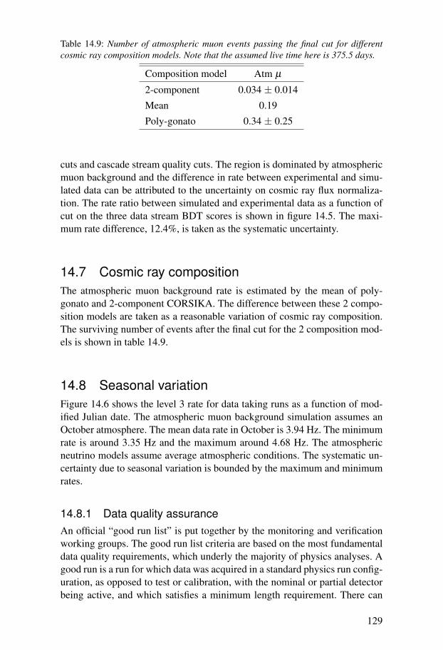
Table 14.9: Number of atmospheric muon events passing the final cut for differentcosmic ray composition models. Note that the assumed live time here is 375.5 days.

Composition model Atm µ

2-component 0.034 ± 0.014

Mean 0.19

Poly-gonato 0.34 ± 0.25

cuts and cascade stream quality cuts. The region is dominated by atmosphericmuon background and the difference in rate between experimental and simu-lated data can be attributed to the uncertainty on cosmic ray flux normaliza-tion. The rate ratio between simulated and experimental data as a function ofcut on the three data stream BDT scores is shown in figure 14.5. The maxi-mum rate difference, 12.4%, is taken as the systematic uncertainty.

14.7 Cosmic ray compositionThe atmospheric muon background rate is estimated by the mean of poly-gonato and 2-component CORSIKA. The difference between these 2 compo-sition models are taken as a reasonable variation of cosmic ray composition.The surviving number of events after the final cut for the 2 composition mod-els is shown in table 14.9.

14.8 Seasonal variationFigure 14.6 shows the level 3 rate for data taking runs as a function of mod-ified Julian date. The atmospheric muon background simulation assumes anOctober atmosphere. The mean data rate in October is 3.94 Hz. The minimumrate is around 3.35 Hz and the maximum around 4.68 Hz. The atmosphericneutrino models assume average atmospheric conditions. The systematic un-certainty due to seasonal variation is bounded by the maximum and minimumrates.

14.8.1 Data quality assuranceAn official “good run list” is put together by the monitoring and verificationworking groups. The good run list criteria are based on the most fundamentaldata quality requirements, which underly the majority of physics analyses. Agood run is a run for which data was acquired in a standard physics run config-uration, as opposed to test or calibration, with the nominal or partial detectorbeing active, and which satisfies a minimum length requirement. There can

129

Figure 14.6: The level 3 rate per run as a function of modified Julian date. The burnsample period is shown in red (light).

be no external light sources active in the detector during data taking. The rateshould be stable over the run and no severe problems should be observed bythe run coordinator or in further offline checks by monitoring and verification.Furthermore, no general problem should be be reported by standard offlineprocessing.

It is the responsibility of each analyzer to further assure data quality. A fewruns in the good run list were excluded from this analysis because a previouspoint source analysis found anomalous zenith distributions. Here, the rate ofeach run was compared with the mean of the surrounding 10 runs. All runswith a rate that differed more than 3 standard deviations from the mean wereinvestigated. The majority of these runs either had a partial detector configu-ration or were less than an hour long. A partial detector configuration meansthat fewer than the nominal number of strings were active, which naturallyaffects the data rate. There is a short period at the beginning and possibly atthe end of each run where data rate deviates from the nominal value. If theruns are short it will affect the rate of the run.

Three runs differed more than 3 standard deviations, had a long run lengthand a nominal detector configuration. In one of these runs a significant numberof DOMs dropped out. For the other two runs, no problems were found. Sinceno problems were found for the runs with deviating rates, none were excluded.

14.9 Neutrino coincidencesCoincidences between atmospheric muon and neutrino events were not sim-ulated. Given a neutrino event, the most likely coincidence is with a low en-ergy atmospheric muon event. Since the analysis is optimized for high energyneutrino events, this implies that the majority of this type of events will be

130

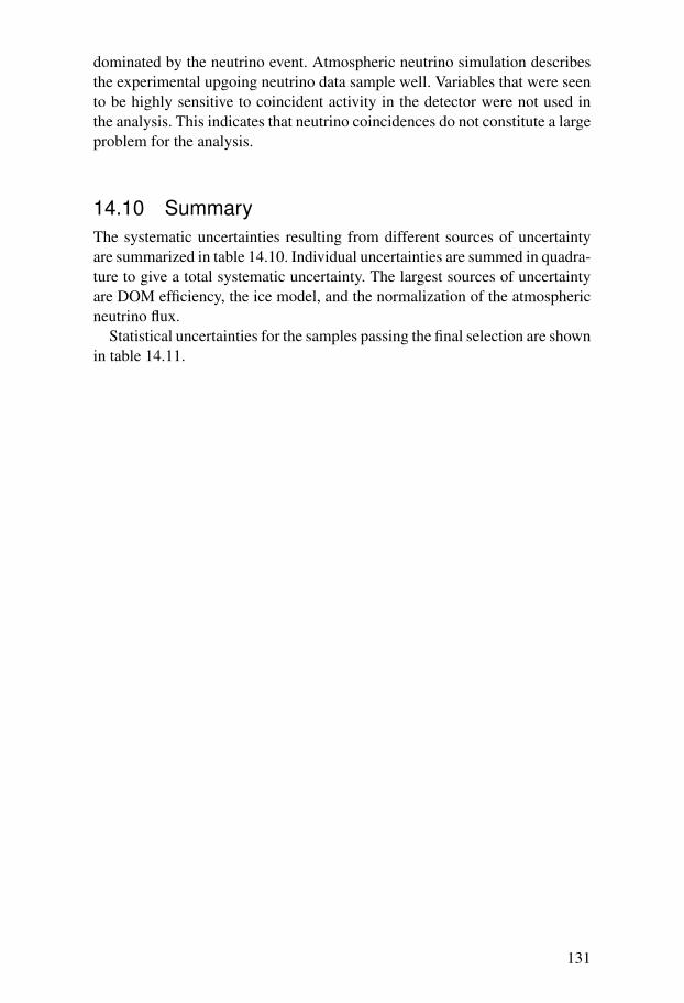
dominated by the neutrino event. Atmospheric neutrino simulation describesthe experimental upgoing neutrino data sample well. Variables that were seento be highly sensitive to coincident activity in the detector were not used inthe analysis. This indicates that neutrino coincidences do not constitute a largeproblem for the analysis.

14.10 SummaryThe systematic uncertainties resulting from different sources of uncertaintyare summarized in table 14.10. Individual uncertainties are summed in quadra-ture to give a total systematic uncertainty. The largest sources of uncertaintyare DOM efficiency, the ice model, and the normalization of the atmosphericneutrino flux.

Statistical uncertainties for the samples passing the final selection are shownin table 14.11.

131

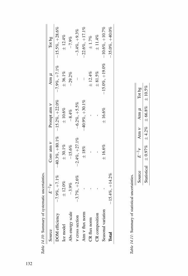
Tabl

e14

.10:

Sum

mar

yof

syst

emat

icun

cert

aint

ies.

Sour

ceE−

2 νC

onv

atm

νPr

ompt

atm

νA

tmµ

Totb

g

DO

Mef

ficie

ncy

−7.

9%,+

7.1%

−40

.3%

,+80

.1%−

15.2

%,+

22.0

%−

7.9%

,+7.

1%−

15.5

%,+

28.6

%

Ice

mod

el±

12.0

%±

30.1

%±

10.6

%±

36.1

%±

12.4

%

Abs

ener

gysc

ale

−3.

9%−

15.6

%−

8.4%

−29

.2%

−7.

9%

νcr

oss

sect

ion

−3.

7%,+

2.6%

−2.

4%,+

27.1

%−

6.2%

,+5.

5%−

−3.

4%,+

9.3%

Atm

νflu

xno

rm-

±18

%−

40.9

%,+

30.1

%−

−22

.6%

,+17

.1%

CR

flux

norm

--

-±

12.4

%±

1.7%

CR

com

posi

tion

--

-±

81.5

%±

11.4

%

Seas

onal

vari

atio

n-

±16

.6%

±16

.6%

−15

.0%

,+19

.0%−

10.6

%,+

10.7

%

Tota

l−

15.4

%,+

14.2

%−

35.0

%,+

40.0

%

Tabl

e14

.11:

Sum

mar

yof

stat

istic

alun

cert

aint

ies.

Sour

ceE−

2 νA

tmν

Atm

µTo

tbg

Stat

istic

al±

0.97

%±

4.2%

±66

.8%±

10.5

%

132

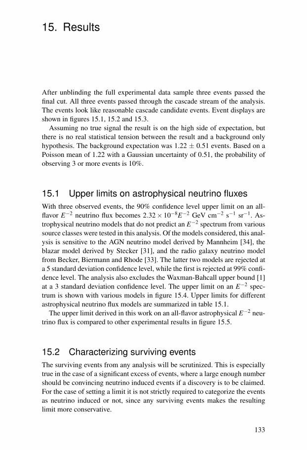
15. Results

After unblinding the full experimental data sample three events passed thefinal cut. All three events passed through the cascade stream of the analysis.The events look like reasonable cascade candidate events. Event displays areshown in figures 15.1, 15.2 and 15.3.

Assuming no true signal the result is on the high side of expectation, butthere is no real statistical tension between the result and a background onlyhypothesis. The background expectation was 1.22 ± 0.51 events. Based on aPoisson mean of 1.22 with a Gaussian uncertainty of 0.51, the probability ofobserving 3 or more events is 10%.

15.1 Upper limits on astrophysical neutrino fluxesWith three observed events, the 90% confidence level upper limit on an all-flavor E−2 neutrino flux becomes 2.32× 10−8E−2 GeV cm−2 s−1 sr−1. As-trophysical neutrino models that do not predict an E−2 spectrum from varioussource classes were tested in this analysis. Of the models considered, this anal-ysis is sensitive to the AGN neutrino model derived by Mannheim [34], theblazar model derived by Stecker [31], and the radio galaxy neutrino modelfrom Becker, Biermann and Rhode [33]. The latter two models are rejected ata 5 standard deviation confidence level, while the first is rejected at 99% confi-dence level. The analysis also excludes the Waxman-Bahcall upper bound [1]at a 3 standard deviation confidence level. The upper limit on an E−2 spec-trum is shown with various models in figure 15.4. Upper limits for differentastrophysical neutrino flux models are summarized in table 15.1.

The upper limit derived in this work on an all-flavor astrophysical E−2 neu-trino flux is compared to other experimental results in figure 15.5.

15.2 Characterizing surviving eventsThe surviving events from any analysis will be scrutinized. This is especiallytrue in the case of a significant excess of events, where a large enough numbershould be convincing neutrino induced events if a discovery is to be claimed.For the case of setting a limit it is not strictly required to categorize the eventsas neutrino induced or not, since any surviving events makes the resultinglimit more conservative.

133

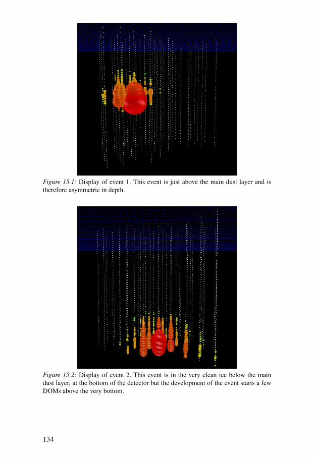
Figure 15.1: Display of event 1. This event is just above the main dust layer and istherefore asymmetric in depth.

Figure 15.2: Display of event 2. This event is in the very clean ice below the maindust layer, at the bottom of the detector but the development of the event starts a fewDOMs above the very bottom.

134

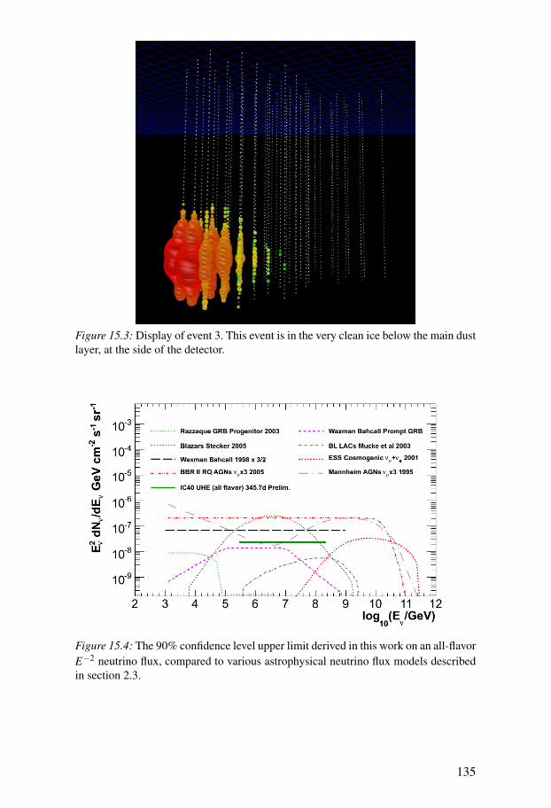
Figure 15.3: Display of event 3. This event is in the very clean ice below the main dustlayer, at the side of the detector.

Figure 15.4: The 90% confidence level upper limit derived in this work on an all-flavorE−2 neutrino flux, compared to various astrophysical neutrino flux models describedin section 2.3.

135

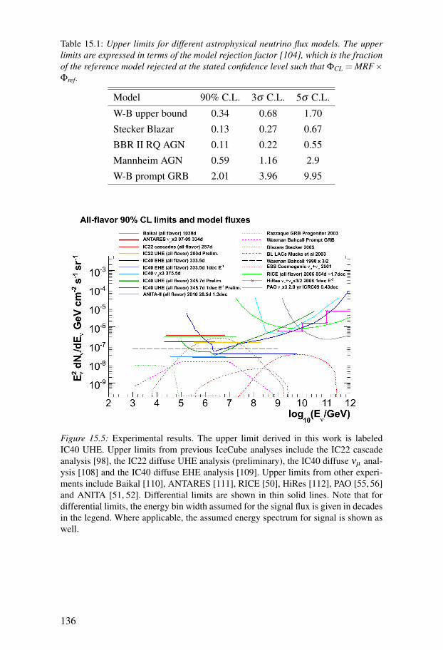
Table 15.1: Upper limits for different astrophysical neutrino flux models. The upperlimits are expressed in terms of the model rejection factor [104], which is the fractionof the reference model rejected at the stated confidence level such that ΦCL = MRF×Φref.

Model 90% C.L. 3σ C.L. 5σ C.L.

W-B upper bound 0.34 0.68 1.70

Stecker Blazar 0.13 0.27 0.67

BBR II RQ AGN 0.11 0.22 0.55

Mannheim AGN 0.59 1.16 2.9

W-B prompt GRB 2.01 3.96 9.95

Figure 15.5: Experimental results. The upper limit derived in this work is labeledIC40 UHE. Upper limits from previous IceCube analyses include the IC22 cascadeanalysis [98], the IC22 diffuse UHE analysis (preliminary), the IC40 diffuse νµ anal-ysis [108] and the IC40 diffuse EHE analysis [109]. Upper limits from other experi-ments include Baikal [110], ANTARES [111], RICE [50], HiRes [112], PAO [55, 56]and ANITA [51, 52]. Differential limits are shown in thin solid lines. Note that fordifferential limits, the energy bin width assumed for the signal flux is given in decadesin the legend. Where applicable, the assumed energy spectrum for signal is shown aswell.

136

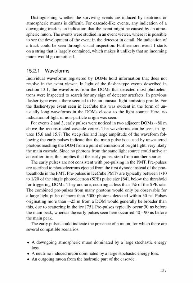
Distinguishing whether the surviving events are induced by neutrinos oratmospheric muons is difficult. For cascade-like events, any indication of adowngoing track is an indication that the event might be caused by an atmo-spheric muon. The events were studied in an event viewer, where it is possibleto see the development of the event in the detector in detail. No indication ofa track could be seen through visual inspection. Furthermore, event 1 startson a string that is largely contained, which makes it unlikely that an incomingmuon would go unnoticed.

15.2.1 WaveformsIndividual waveforms registered by DOMs hold information that does notresolve in the event viewer. In light of the flasher-type events described insection 13.1, the waveforms from the DOMs that detected most photoelec-trons were inspected to search for any sign of detector artefacts. In previousflasher-type events there seemed to be an unusual light emission profile. Forthe flasher-type event seen in IceCube this was evident in the form of un-usually long waveforms in the DOMs closest to the light source. Here, noindication of light of non-particle origin was seen.

For events 2 and 3, early pulses were noticed in two adjacent DOMs∼80 mabove the reconstructed cascade vertex. The waveforms can be seen in fig-ures 15.6 and 15.7. The steep rise and large amplitude of the waveform fol-lowing the early pulses indicate that the main pulse is caused by unscatteredphotons reaching the DOM from a point of emission of bright light, very likelythe main cascade. Since no photons from the same light source could arrive atan earlier time, this implies that the early pulses stem from another source.

The early pulses are not consistent with pre-pulsing in the PMT. Pre-pulsesare ascribed to photoelectrons ejected from the first dynode instead of the pho-tocathode in the PMT. Pre-pulses in IceCube PMTs are typically between 1/10to 1/20 of the single photoelectron (SPE) pulse size [64], below the thresholdfor triggering DOMs. They are rare, ocurring at less than 1% of the SPE rate.The combined pre-pulses from many photons would only be observable fora large light pulse of more than 5000 photons detected within 30 ns. Pulsesoriginating more than ∼25 m from a DOM would generally be broader thanthis, due to scattering in the ice [75]. Pre-pulses typically occur 30 ns beforethe main peak, whereas the early pulses seen here occurred 40 - 90 ns beforethe main peak.

The early pulses could indicate the presence of a muon, for which there areseveral compatible scenarios:

• A downgoing atmospheric muon dominated by a large stochastic energyloss.• A neutrino induced muon dominated by a large stochastic energy loss.• An outgoing muon from the hadronic part of the cascade.

137

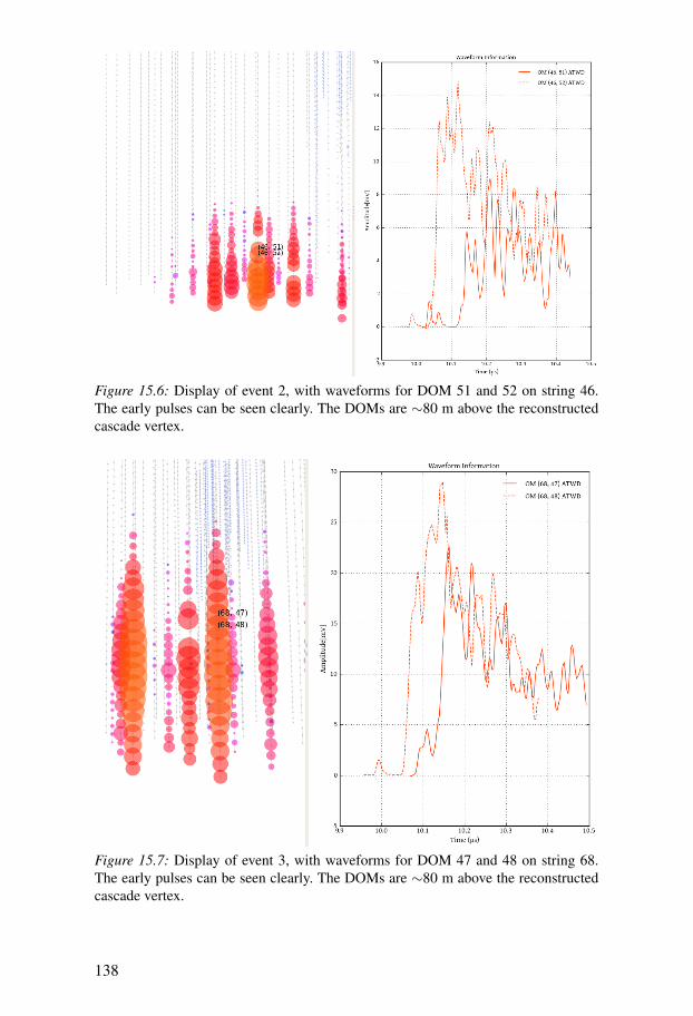
Figure 15.6: Display of event 2, with waveforms for DOM 51 and 52 on string 46.The early pulses can be seen clearly. The DOMs are ∼80 m above the reconstructedcascade vertex.

Figure 15.7: Display of event 3, with waveforms for DOM 47 and 48 on string 68.The early pulses can be seen clearly. The DOMs are ∼80 m above the reconstructedcascade vertex.

138

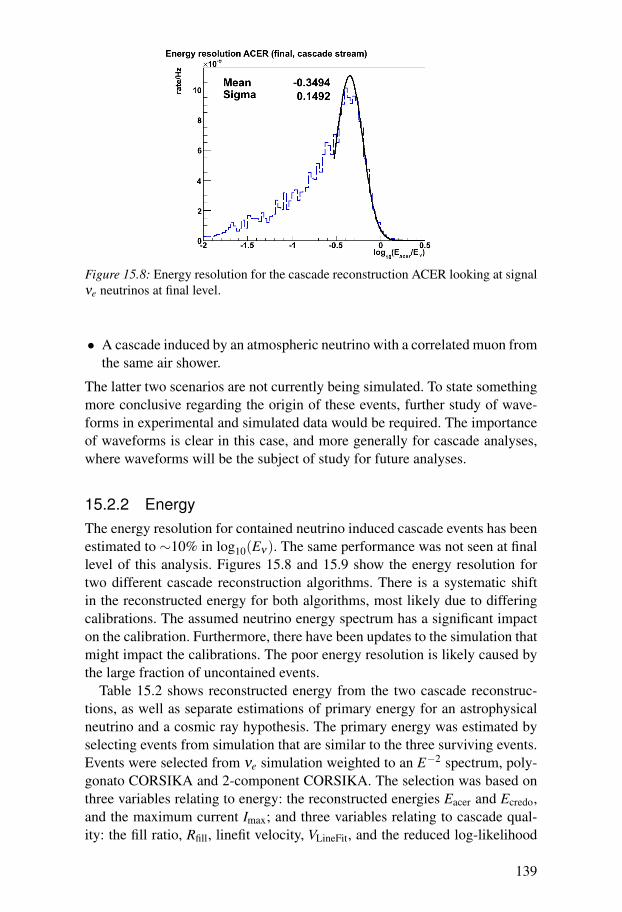
Figure 15.8: Energy resolution for the cascade reconstruction ACER looking at signalνe neutrinos at final level.

• A cascade induced by an atmospheric neutrino with a correlated muon fromthe same air shower.

The latter two scenarios are not currently being simulated. To state somethingmore conclusive regarding the origin of these events, further study of wave-forms in experimental and simulated data would be required. The importanceof waveforms is clear in this case, and more generally for cascade analyses,where waveforms will be the subject of study for future analyses.

15.2.2 EnergyThe energy resolution for contained neutrino induced cascade events has beenestimated to ∼10% in log10(Eν). The same performance was not seen at finallevel of this analysis. Figures 15.8 and 15.9 show the energy resolution fortwo different cascade reconstruction algorithms. There is a systematic shiftin the reconstructed energy for both algorithms, most likely due to differingcalibrations. The assumed neutrino energy spectrum has a significant impacton the calibration. Furthermore, there have been updates to the simulation thatmight impact the calibrations. The poor energy resolution is likely caused bythe large fraction of uncontained events.

Table 15.2 shows reconstructed energy from the two cascade reconstruc-tions, as well as separate estimations of primary energy for an astrophysicalneutrino and a cosmic ray hypothesis. The primary energy was estimated byselecting events from simulation that are similar to the three surviving events.Events were selected from νe simulation weighted to an E−2 spectrum, poly-gonato CORSIKA and 2-component CORSIKA. The selection was based onthree variables relating to energy: the reconstructed energies Eacer and Ecredo,and the maximum current Imax; and three variables relating to cascade qual-ity: the fill ratio, Rfill, linefit velocity, VLineFit, and the reduced log-likelihood

139

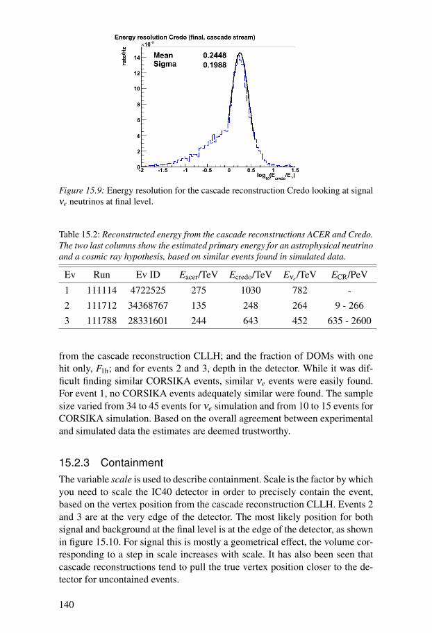
Figure 15.9: Energy resolution for the cascade reconstruction Credo looking at signalνe neutrinos at final level.

Table 15.2: Reconstructed energy from the cascade reconstructions ACER and Credo.The two last columns show the estimated primary energy for an astrophysical neutrinoand a cosmic ray hypothesis, based on similar events found in simulated data.

Ev Run Ev ID Eacer/TeV Ecredo/TeV Eνe /TeV ECR/PeV

1 111114 4722525 275 1030 782 -

2 111712 34368767 135 248 264 9 - 266

3 111788 28331601 244 643 452 635 - 2600

from the cascade reconstruction CLLH; and the fraction of DOMs with onehit only, F1h; and for events 2 and 3, depth in the detector. While it was dif-ficult finding similar CORSIKA events, similar νe events were easily found.For event 1, no CORSIKA events adequately similar were found. The samplesize varied from 34 to 45 events for νe simulation and from 10 to 15 events forCORSIKA simulation. Based on the overall agreement between experimentaland simulated data the estimates are deemed trustworthy.

15.2.3 ContainmentThe variable scale is used to describe containment. Scale is the factor by whichyou need to scale the IC40 detector in order to precisely contain the event,based on the vertex position from the cascade reconstruction CLLH. Events 2and 3 are at the very edge of the detector. The most likely position for bothsignal and background at the final level is at the edge of the detector, as shownin figure 15.10. For signal this is mostly a geometrical effect, the volume cor-responding to a step in scale increases with scale. It has also been seen thatcascade reconstructions tend to pull the true vertex position closer to the de-tector for uncontained events.

140

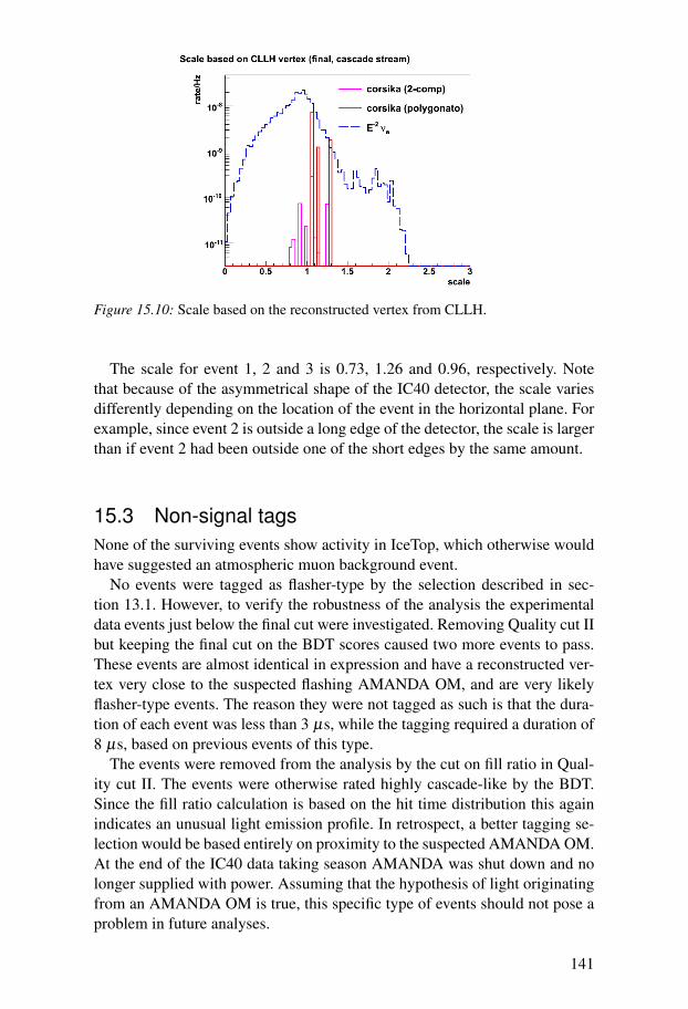
Figure 15.10: Scale based on the reconstructed vertex from CLLH.

The scale for event 1, 2 and 3 is 0.73, 1.26 and 0.96, respectively. Notethat because of the asymmetrical shape of the IC40 detector, the scale variesdifferently depending on the location of the event in the horizontal plane. Forexample, since event 2 is outside a long edge of the detector, the scale is largerthan if event 2 had been outside one of the short edges by the same amount.

15.3 Non-signal tagsNone of the surviving events show activity in IceTop, which otherwise wouldhave suggested an atmospheric muon background event.

No events were tagged as flasher-type by the selection described in sec-tion 13.1. However, to verify the robustness of the analysis the experimentaldata events just below the final cut were investigated. Removing Quality cut IIbut keeping the final cut on the BDT scores caused two more events to pass.These events are almost identical in expression and have a reconstructed ver-tex very close to the suspected flashing AMANDA OM, and are very likelyflasher-type events. The reason they were not tagged as such is that the dura-tion of each event was less than 3 µs, while the tagging required a duration of8 µs, based on previous events of this type.

The events were removed from the analysis by the cut on fill ratio in Qual-ity cut II. The events were otherwise rated highly cascade-like by the BDT.Since the fill ratio calculation is based on the hit time distribution this againindicates an unusual light emission profile. In retrospect, a better tagging se-lection would be based entirely on proximity to the suspected AMANDA OM.At the end of the IC40 data taking season AMANDA was shut down and nolonger supplied with power. Assuming that the hypothesis of light originatingfrom an AMANDA OM is true, this specific type of events should not pose aproblem in future analyses.

141

16. Conclusions and outlook

An analysis structure with three streams based on signal and backgroundtopology was a novel approach within IceCube. This posed several challenges,the first of which was processing an analysis-specific filter level 2 in orderto get a homogeneous data set. Secondly, by looking at both track-like andcascade-like events, a coherent picture describing the agreement between ex-perimental and simulated data was required, to achieve a satisfactory degreeof confidence in the predictions from simulation. Robustness was prioritizedbefore signal efficiency.

Three events survived after unblinding. The events passed through the cas-cade stream of the analysis and look like reasonable cascade candidate events.There is no real statistical tension between the result and a background onlyhypothesis. The analysis structure proved efficient and the resulting upperlimit on an astrophysical all-flavor neutrino flux with an E−2 energy spectrumis the most strict to date.

For future analyses this type of approach could be made easier by includinga “UHE filter” in the standard IceCube offline processing.

Sources of systematic uncertainty are continuously being investigated andthe simulation being improved upon. More specifically, improvements are ex-pected from better modeling and simulation of:

• The detector• Ice properties• Cosmic ray composition and flux normalization• Atmospheric neutrino flux normalization and spectrum• Neutrino-nucleon interaction cross sections

In this analysis a final cut was optimized for high sensitivity using themodel rejection technique [104]. An alternate approach is to test the com-patibility of a distribution from experimental data with simulated backgroundand signal components. An suitable distribution could for example be a BDTscore or an energy related variable. A frequentist approach suggested by Feld-man [113, 114] was followed in a recent IceCube diffuse analysis, using theprofile likelihood construction method to incorporate systematic uncertaintiesas nuisance parameters. This gave a better sensitivity than optimizing a finalcut, especially for astrophysical neutrino flux models with distinctive energyspectra.

The final phase of construction of the 86-string IceCube detector was re-cently successfully completed, resulting in a detector volume of one cubic

143

kilometer. With increased exposure, an improvement in sensitivity to an as-trophysical UHE diffuse neutrino flux of more than an order of magnitude isanticipated.

16.1 Lessons learnedInitially an additional filter level was planned for the analysis. Early investi-gations indicated that an extra filter level would not improve signal efficiencysignificantly. Because of time constraints it was decided to simplify the struc-ture of the analysis by evaluating a final cut at filter level 3. In hindsight, apossibly more efficient approach would have been to apply the cascade streamstructure to the track streams as well. Applying harder quality cuts provides alimited phase space, relevant for signal, within which a multivariate classifiershould perform efficiently.

144

Summary in Swedish

Vår kunskap om universum kommer till stor del från observationer av fotoner,det vill säga elektromagnetisk strålning i olika våglängder. De mest ljusstarkaoch våldsamma objekten i universum, aktiva galaxkärnor och gammablix-tar, har studerats noggrannt genom observationer av gammastrålning. Flödetav fotoner dämpas dock av gas och stoft i det interstellära mediet, och vidhöga energier av kosmisk bakgrundsstrålning, vilket begränsar sikten. Astro-fysikaliska källor med omgärdande regioner har ofta betydande optisk täthet,vilket gör att fotoner ger information om egenskaper på ytan av objekt.

Neutriner är oladdade och växelverkar genom den svaga kärnkraften, vilketgör att de färdas enorma avstånd utan påverkan. Neutriner undkommer dessu-tom opåverkade från de inre regionerna av våldsamma astrofysikaliska ob-jekt, och bär därigenom med sig viktig information om de processer somfrigör energi. I denna mening är neutrinon en utmärkt budbärare. Produk-tion av hög-energetiska neutriner förutsätter acceleration av elektriskt laddadehadroner, som också medför produktion av gammastrålning. Gammastrålningkan dock också uppstå genom acceleration av elektroner, vilket gör det svårtatt bestämma accelerationsmekanismen bakom gammakällor.

Acceleration av hadroner ger upphov till stabila laddade kosmiska partiklarsom färdas genom universum med hög energi. Dessa kosmiska partiklar kanockså observeras. På grund av den elektriska laddningen böjs kosmiska partik-lar av i inter- och extragalaktiska magnetiska fält, vilket gör att de inte pekartillbaka till källan. Observationer av neutriner kan avslöja källor till kosmiskapartiklar, och tillhandahålla en länk mellan observationer av gammastrålningoch kosmiska partiklar.

Neutrinoastronomi är ett ungt forskningsområde, de hittills enda bekräftadeutomjordiska neutrinokällorna är solen och supernova SN1987a. Att neutri-non växelverkar så sällan gör den till en utmärkt budbärare men också svår attdetektera. En mycket stor detektorvolym krävs för att fånga neutriner. Neutri-noobservatoriet IceCube är beläget på Sydpolen och använder den Antarktiskaglaciärisen som detektormedium. Neutriner som växelverkar i isen producerarsekundära partiklar som avger Cherenkov-strålning, som kan detekteras medhjälp av optiska sensorer. Sådana sensorer har installerats på strängar som bor-rats ner i isen. Detektorn färdigställdes nyligen och består av 86 strängar med60 optiska sensorer per sträng, installerade på ett djup av 1450 m till 2450 m.Detta medför en detektorvolym på en kubikkilometer. Neutrinons färdriktningoch energi kan sedan återskapas från den detekterade Cherenkov-strålningen.

145

Analysen som beskrivs i denna avhandling eftersöker ett diffust flödeav utomjordiska neutriner med ett energispektrum som är typiskt föracceleration av hadroner i chockvågor, E−2. Analysen är optimerad förultra-högenergetiska neutriner, det vill säga neutriner med energi över1 PeV. Data som samlats in med IceCube under 2008 och 2009 harundersökts. Under denna tidsperiod bestod detektorn av 40 strängar, ochvar ungefär hälften så stor som den nu färdigställda detektorn. Ett diffustflöde av neutriner är känsligt för egenskaper hos populationen av kosmiskaacceleratorer i universum.

Neutrinosignalen är mycket svag i förhållande till bakgrundsnivån i detek-torn. Bakgrunden består av myoner och neutriner som produceras i atmosfäreni skurar av partiklar som uppstår när kosmiska partiklar kolliderar med jordensatmosfär. Signal skiljer sig från bakgrund i framförallt två avseenden, signalenhar högre energi och en annan typisk riktning.

Hela experimentet simuleras för att försäkra sig om att man förstår de-tektorn och insamlade data. En god överensstämmelse mellan simulering avbakgrund och insamlade data bekräftar god förståelse av detektorn och gerförtroende för beskrivningen av signalhypotesen. Analysen går ut på att filtr-era bort bakgrunden och behålla så god acceptans för signalen som möjligt. Idenna analys har förståelse för insamlade data prioriterats i störst möjliga mån.Under utvecklandet av analysen har ett mindre urval av insamlade data använtsför att bekräfta simuleringens validitet. Detta urval används inte i sökandetefter signal. Analysen är optimerad för att ge god känslighet för signal, baserathelt på simulerade data. Denna procedur skyddar forskaren mot omedvetenpåverkan i någon riktning, till exempel mot en teoretisk förutsägelse.

Denna analys letar efter neutrinoinducerade händelser som kan ta sig olikatyp av uttryck i detektorn. En struktur med tre olika dataströmmar baseradepå dessa uttryck har utvecklats. Det är första gången en sådan struktur haranvänts inom IceCube, detta medförde flera utmaningar men gav också godkänslighet för signal.

Efter att analysen färdigställdes och godkändes av IceCube-kollaborationenapplicerades den på data med en livstid på 345,7 dagar. Tre händelser över-levde analysens samtliga filternivåer. De överlevande händelserna ser ut somrimliga neutrinokandidater men åtminstone två kan möjligtvis vara orsakadeav atmosfäriska myoner. Resultatet är i rimlig överensstämmelse med bak-grund, och en gräns kan sättas för det maximala flödet av signalneutriner somär statistiskt förenligt med resultatet. Denna gräns är den mest strikta till dagsdato och utesluter flera teoretiska modeller för flödet av utomjordiska neu-triner.

146

A. Multivariate classifiers

In high energy physics a common problem is extracting a small signal froma very large data set. Multivariate classification algorithms based on machinelearning techniques are able to utilize available information efficiently. Com-mon for machine learning techniques is a training phase, where the algorithmlearns how to classify events as signal-like or background-like based on datadescribing signal and background.

A.1 Boosted decision treesA decision tree is a classifier that uses a binary tree structure. For an event,repeated left/right decisions are made based on a single variable at a timeuntil a stop criterion is fulfilled, placing the event in a leaf node. In the phasespace spanned by the variables used to characterize events, each leaf nodecorresponds to a hypercube defined by a series of straight cuts. Each leaf nodeis categorized as signal-like or background-like depending on the number ofsignal and background training events ending up in that node.

Boosting refers to an extension of the single decision tree. Several trees, aforest, are derived from the same training sample by reweighting events. Theboosted decision tree (BDT) classifies events based on a weighted majorityvote from the individual trees of the forest. Boosting stabilizes the response ofthe decision trees with respect to statistical fluctuations in the training sample.The weighted majority vote is referred to as the BDT score and lies in therange from -1 to 1, where low values indicate background-like events andhigh values signal-like events.

A classifier is said to be overtrained if statistical fluctuations in the trainingsample affect the classification of events. BDTs are pruned in order to reduceovertraining. The number of events in a leaf node decides the statistical sig-nificance of the classification as signal-like or background-like. The pruningremoves leaf nodes with statistical significance lower than a specified value.

The BDT algorithm implemented in the TMVA toolkit [102] within theanalysis framework ROOT [103] was used in this analysis. The TMVA toolkitprovides several tools for evaluating the performance of BDTs. Overtrainingis tested by comparing the BDT response between two independent data sam-ples. Correlations between variables used to characterize events are providedto inform the variable selection process.

147

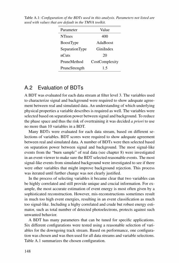
Table A.1: Configuration of the BDTs used in this analysis. Parameters not listed areused with values that are default in the TMVA toolkit.

Parameter Value

NTrees 400

BoostType AdaBoost

SeparationType GiniIndex

nCuts 20

PruneMethod CostComplexity

PruneStrength 1.5

A.2 Evaluation of BDTsA BDT was evaluated for each data stream at filter level 3. The variables usedto characterize signal and background were required to show adequate agree-ment between real and simulated data. An understanding of which underlyingphysical properties a variable describes is required as well. The variables wereselected based on separation power between signal and background. To reducethe phase space and thus the risk of overtraining it was decided a priori to useno more than 10 variables in a BDT.

Many BDTs were evaluated for each data stream, based on different se-lections of variables. BDT scores were required to show adequate agreementbetween real and simulated data. A number of BDTs were then selected basedon separation power between signal and background. The most signal-likeevents from the “burn sample” of real data (see chapter 8) were investigatedin an event-viewer to make sure the BDT selected reasonable events. The mostsignal-like events from simulated background were investigated to see if therewere other variables that might improve background rejection. This processwas iterated until further change was not clearly justified.

In the process of selecting variables it became clear that two variables canbe highly correlated and still provide unique and crucial information. For ex-ample, the most accurate estimation of event energy is most often given by asophisticated reconstruction. However, mis-reconstructions sometimes resultin much too high event energies, resulting in an event classification as muchtoo signal-like. Including a highy correlated and crude but robust energy esti-mator, such as total number of detected photoelectrons, protects against suchunwanted behavior.

A BDT has many parameters that can be tuned for specific applications.Six different configurations were tested using a reasonable selection of vari-ables for the downgoing track stream. Based on performance, one configura-tion was chosen and was then used for all data streams and variable selections.Table A.1 summarizes the chosen configuration.

148

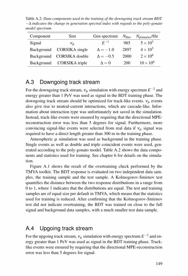
Table A.2: Data components used in the training of the downgoing track stream BDT.−∆ indicates the change in generation spectral index with regards to the poly-gonatomodel spectrum.

Component Sim Gen spectrum Nfiles Nprimaries/file

Signal νµ E−1 985 5×103

Background CORSIKA single ∆ =−1.0 2897 4×105

Background CORSIKA double ∆ =−0.5 2000 2×106

Background CORSIKA triple ∆ = 0 200 10×106

A.3 Downgoing track streamFor the downgoing track stream, νµ simulation with energy spectrum E−2 andenergy greater than 1 PeV was used as signal in the BDT training phase. Thedowngoing track stream should be optimized for track-like events. νµ eventsalso give rise to neutral-current interactions, which are cascade-like. Infor-mation about interaction type was unfortunately not saved in the simulation.Instead, track-like events were ensured by requiring that the directional MPE-reconstruction error was less than 5 degrees for signal. Furthermore, moreconvincing signal-like events were selected from real data if νµ signal wasrequired to have a direct length greater than 300 m in the training phase.

Atmospheric µ simulation was used as background in the training phase.Single events as well as double and triple coincident events were used, gen-erated according to the poly-gonato model. Table A.2 shows the data compo-nents and statistics used for training. See chapter 6 for details on the simula-tion.

Figure A.1 shows the result of the overtraining check performed by theTMVA toolkit. The BDT response is evaluated on two independent data sam-ples, the training sample and the test sample. A Kolmogorov-Smirnov testquantifies the distance between the two response distributions in a range from0 to 1, where 1 indicates that the distributions are equal. The test and trainingsamples are of equal size per default in TMVA, which means that the statisticsused for training is reduced. After confirming that the Kolmogorov-Smirnovtest did not indicate overtraining, the BDT was trained on close to the fullsignal and background data samples, with a much smaller test data sample.

A.4 Upgoing track streamFor the upgoing track stream, νµ simulation with energy spectrum E−2 and en-ergy greater than 1 PeV was used as signal in the BDT training phase. Track-like events were ensured by requiring that the directional MPE-reconstructionerror was less than 5 degrees for signal.

149

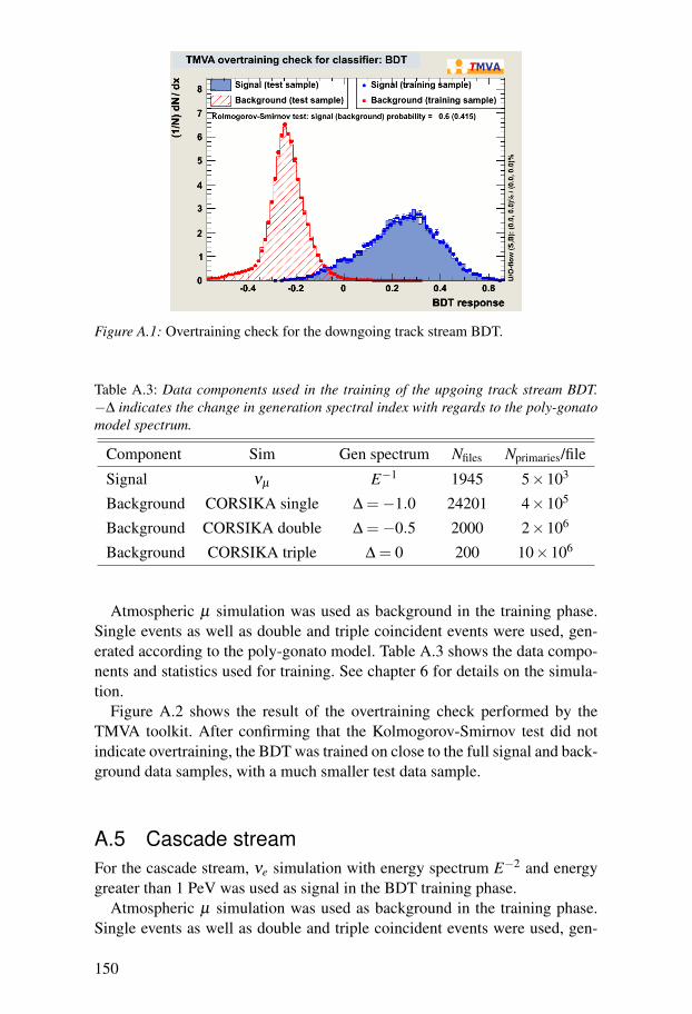
Figure A.1: Overtraining check for the downgoing track stream BDT.

Table A.3: Data components used in the training of the upgoing track stream BDT.−∆ indicates the change in generation spectral index with regards to the poly-gonatomodel spectrum.

Component Sim Gen spectrum Nfiles Nprimaries/file

Signal νµ E−1 1945 5×103

Background CORSIKA single ∆ =−1.0 24201 4×105

Background CORSIKA double ∆ =−0.5 2000 2×106

Background CORSIKA triple ∆ = 0 200 10×106

Atmospheric µ simulation was used as background in the training phase.Single events as well as double and triple coincident events were used, gen-erated according to the poly-gonato model. Table A.3 shows the data compo-nents and statistics used for training. See chapter 6 for details on the simula-tion.

Figure A.2 shows the result of the overtraining check performed by theTMVA toolkit. After confirming that the Kolmogorov-Smirnov test did notindicate overtraining, the BDT was trained on close to the full signal and back-ground data samples, with a much smaller test data sample.

A.5 Cascade streamFor the cascade stream, νe simulation with energy spectrum E−2 and energygreater than 1 PeV was used as signal in the BDT training phase.

Atmospheric µ simulation was used as background in the training phase.Single events as well as double and triple coincident events were used, gen-

150

Figure A.2: Overtraining check for the upgoing track stream BDT.

Table A.4: Data components used in the training of the cascade stream BDT. −∆ in-dicates the change in generation spectral index with regards to the poly-gonato modelspectrum.

Component Sim Gen spectrum Nfiles Nprimaries/file

Signal νe E−1 999 5×103

Background νµ E−1 1945 5×103

Background CORSIKA single ∆ =−1.0 24201 4×105

Background CORSIKA double ∆ =−0.5 2000 2×106

Background CORSIKA triple ∆ = 0 200 10×106

erated according to the poly-gonato model. Because the cascade stream BDTwas evaluated at a higher level than the track stream BDTs, atmospheric νµ

simulation was included in the background as well. Table A.4 shows the datacomponents and statistics used for training. See chapter 6 for details on thesimulation.

Figure A.3 shows the result of the overtraining check performed by theTMVA toolkit. After confirming that the Kolmogorov-Smirnov test did notindicate overtraining, the BDT was trained on close to the full signal and back-ground data samples, with a much smaller test data sample.

151

Figure A.3: Overtraining check for the cascade stream BDT.

152

List of Abbreviations

ACER Atmospheric cascade energy reconstruction

AGN Active galactic nucleus

AMANDA Antarctic muon and neutrino detector array

ANIS All neutrino interaction simulation

ATWD Analog transient waveform digitizer

BDT Boosted decision tree

CC Charged-current

CDOM Color DOM

COG Center of gravity

CORSIKA Cosmic ray simulations for Kascade

CSS Cooper-Sarkar and Sarkar

DAQ Data acquisition

DOM Digital optical module

DOR DOM readout

EHE Extremely high-energy

fADC Fast analog-to-digital converter

FPGA Field programmable gate array

GRB Gamma ray burst

GZK Greisen-Zatsepin-Kuzmin

HLC Hard local coincidence

HV High voltage

ICL IceCube laboratory

153

LC Local coincidence

LPM Landau-Pomeranchuk-Migdal

MB Mainboard

MC Monte Carlo

MMC Muon monte carlo

MPE Multi-photoelectron

MRF Model rejection factor

MSPS Mega-samples per second

NC Neutral current

OM Optical module

PDF Probability density function

PE Photoelectron

PMT Photomultiplier tube

PnF Processing and filtering

PREM Preliminary reference Earth model

SC Standard candle

SLC Soft local coincidence

SMT8 Simple majority trigger 8

SNR Supernova remnant

SPADE South Pole Archival and Data Exchange

SPE Single photoelectron

SPE-32 SPE track reconstruction, 32 iterations

UHE Ultra high-energy

154

Bibliography

[1] Eli Waxman and John N. Bahcall. High energy neutrinos from astrophysicalsources: An upper bound. Phys. Rev., D59:023002, 1999, hep-ph/9807282.

[2] H. Johansson. Methods for High Energy Neutrino Searches and Calibra-tion of Photon Detection Efficiency in IceCube. http://www.physto.

se/~henjoh/lic/lic_henrik_final.pdf, 2008. Licentiate thesis,Stockholm U.

[3] SweGrid — The Swedish GRID initiative. http://www.snic.vr.se/

projects/swegrid.

[4] Amanda Cooper-Sarkar and Subir Sarkar. Predictions for high energy neutrinocross-sections from the ZEUS global PDF fits. JHEP, 0801:075, 2008.

[5] Joel R. Primack, Rudy C. Gilmore, and Rachel S. Somerville. Diffuse Extra-galactic Background Radiation. AIP Conf. Proc., 1085:71, 2009, 0811.3230.

[6] J. Abraham et al. Correlation of the highest energy cosmic rays with nearbyextragalactic objects. Science, 318:938, 2007, 0711.2256.

[7] J. Abraham et al. Correlation of the highest-energy cosmic rays with thepositions of nearby active galactic nuclei. Astropart. Phys., 29:188, 2008,0712.2843.

[8] P. Abreu et al. Update on the correlation of the highest energy cosmic rays withnearby extragalactic matter. Astropart. Phys., 34:314, 2010, 1009.1855.

[9] K Nakamura et al. Review of particle physics, chapter 24, Cosmic rays. J.Phys. G, G37:075021, 2010.

[10] T.K. Gaisser. The cosmic-ray spectrum: From the knee to the ankle. J. Phys.Conf. Ser., 47:15, 2006.

[11] R. Blandford and D. Eichler. Particle Acceleration at Astrophysical Shocks: ATheory of Cosmic Ray Origin. Phys. Rept., 154:1, 1987.

[12] A.M. Hillas. The Origin of Ultrahigh-Energy Cosmic Rays. Ann. Rev. Astron.Astrophys., 22:425, 1984.

[13] J. L. Puget, F. W. Stecker, and J. H. Bredekamp. Photonuclear Interactions ofUltrahigh-Energy Cosmic Rays and their Astrophysical Consequences. Astro-phys. J., 205:638, 1976.

155

[14] Joerg R. Hoerandel. On the knee in the energy spectrum of cosmic rays. As-tropart. Phys., 19:193, 2003, astro-ph/0210453.

[15] Francis Halzen. Cosmic neutrinos from the sources of galactic and extragalac-tic cosmic rays. Astrophys. Space Sci., 309:407, 2007, astro-ph/0611915.

[16] R. U. Abbasi et al. A Study of the Composition of Ultra High Energy CosmicRays Using the High Resolution Fly’s Eye. Astrophys. J., 622:910, 2005,astro-ph/0407622.

[17] J. Abraham et al. Studies of Cosmic Ray Composition and Air Shower Struc-ture with the Pierre Auger Observatory. 2009, 0906.2319. Submissions to the31st International Cosmic Ray Conference, Lodz, Poland.

[18] R.U. Abbasi et al. First observation of the Greisen-Zatsepin-Kuzmin suppres-sion. Phys. Rev. Lett., 100:101101, 2008, astro-ph/0703099.

[19] J. Abraham et al. Observation of the suppression of the flux of cosmic raysabove 4×1019 eV. Phys. Rev. Lett., 101:061101, 2008, 0806.4302.

[20] V.S. Berezinsky and S.I. Grigor’eva. A Bump in the ultrahigh-energy cosmicray spectrum. Astron.Astrophys., 199:1, 1988.

[21] L.N. Epele and E. Roulet. Comment on ’on the origin of the highest energycosmic rays’. Phys.Rev.Lett., 81:3295, 1998, astro-ph/9806251.

[22] Katsuaki Asano and S. Nagataki. Very high energy neutrinos originating fromkaons in gamma-ray bursts. Astrophys. J., 640:L9, 2006, astro-ph/0603107.

[23] S.R. Kelner and F.A. Aharonian. Energy spectra of gamma-rays, electronsand neutrinos produced at interactions of relativistic protons with low energyradiation. Phys.Rev., D78:034013, 2008, 0803.0688.

[24] S.R. Kelner, Felex A. Aharonian, and V.V. Bugayov. Energy spectra of gamma-rays, electrons and neutrinos produced at proton-proton interactions in the veryhigh energy regime. Phys. Rev., D74:034018, 2006, astro-ph/0606058.

[25] K Nakamura et al. Review of particle physics, chapter 13, Neutrino mass,mixing and oscillations. J. Phys. G, G37:075021, 2010.

[26] H. Athar, M. Jezabek, and O. Yasuda. Effects of neutrino mixing on high-energy cosmic neutrino flux. Phys. Rev., D62:103007, 2000, hep-ph/0005104.

[27] Tamar Kashti and Eli Waxman. Flavoring astrophysical neutrinos: Flavor ratiosdepend on energy. Phys. Rev. Lett., 95:181101, 2005, astro-ph/0507599.

[28] S. Hummer, M. Maltoni, W. Winter, and C. Yaguna. Energy dependent neutrinoflavor ratios from cosmic accelerators on the Hillas plot. Astropart. Phys.,34:205, 2010, 1007.0006.

156

[29] Dan Hooper, Dean Morgan, and Elizabeth Winstanley. Probing quantum de-coherence with high-energy neutrinos. Phys. Lett., B609:206, 2005, hep-ph/0410094.

[30] Julia K. Becker. Neutrinos on the rocks: On the phenomenology of poten-tial astrophysical neutrino sources. PhD thesis, Dortmund U., 2007.

[31] Floyd W. Stecker. A Note on High Energy Neutrinos from AGN Cores. Phys.Rev., D72:107301, 2005, astro-ph/0510537.

[32] A. Muecke, R. J. Protheroe, R. Engel, J. P. Rachen, and T. Stanev. BL Lacobjects in the synchrotron proton blazar model. Astropart. Phys., 18:593,2003, astro-ph/0206164.

[33] Julia K. Becker, Peter L. Biermann, and Wolfgang Rhode. The diffuse neutrinoflux from FR-II radio galaxies and blazars: A source property based estimate.Astropart. Phys., 23:355, 2005, astro-ph/0502089.

[34] K. Mannheim. High-energy neutrinos from extragalactic jets. Astropart.Phys., 3:295, 1995.

[35] Soebur Razzaque, Peter Meszaros, and Eli Waxman. Neutrino tomographyof gamma ray bursts and massive stellar collapses. Phys. Rev., D68:083001,2003, astro-ph/0303505.

[36] Ralph Engel, David Seckel, and Todor Stanev. Neutrinos from propagation ofultra-high energy protons. Phys. Rev., D64:093010, 2001, astro-ph/0101216.

[37] J.G. Learned and K. Mannheim. High-energy neutrino astrophysics. Ann. Rev.Nucl. Part. Sci., 50:679, 2000.

[38] Chryssa Kouveliotou et al. Identification of two classes of gamma-ray bursts.Astrophys. J., 413:L101, 1993.

[39] S.E. Woosley and J.S. Bloom. The Supernova Gamma-Ray Burst Connection.Ann. Rev. Astron. Astrophys., 44:507, 2006, astro-ph/0609142.

[40] Ehud Nakar. Short-Hard Gamma-Ray Bursts. Phys. Rept., 442:166, 2007,astro-ph/0701748.

[41] Dan Hooper, Andrew Taylor, and Subir Sarkar. The Impact of heavy nu-clei on the cosmogenic neutrino flux. Astropart. Phys., 23:11, 2005, astro-ph/0407618.

[42] Hasan Yuksel and Matthew D. Kistler. Enhanced cosmological GRB rates andimplications for cosmogenic neutrinos. Phys. Rev., D75:083004, 2007, astro-ph/0610481.

157

[43] B. Louis, V. Sandberg, G. Garvey, H. White, G. Mills, et al. The evidence foroscillations. Los Alamos Sci., 25:116, 1997.

[44] P. Adamson et al. Measurement of the atmospheric muon charge ratio at TeVenergies with MINOS. Phys. Rev., D76:052003, 2007, 0705.3815.

[45] C.G.S. Costa. The Prompt lepton cookbook. Astropart. Phys., 16:193, 2001,hep-ph/0010306.

[46] G.D. Barr, T.K. Gaisser, P. Lipari, Simon Robbins, and T. Stanev. A Three-dimensional calculation of atmospheric neutrinos. Phys. Rev., D70:023006,2004, astro-ph/0403630.

[47] Morihiro Honda, T. Kajita, K. Kasahara, S. Midorikawa, and T. Sanuki. Calcu-lation of atmospheric neutrino flux using the interaction model calibrated withatmospheric muon data. Phys. Rev., D75:043006, 2007, astro-ph/0611418.

[48] Rikard Enberg, Mary Hall Reno, and Ina Sarcevic. Prompt neutrino fluxesfrom atmospheric charm. Phys. Rev., D78:043005, 2008, 0806.0418.

[49] G.A. Askaryan. Excess negative charge of an electron-photon shower and itscoherent radio emission. JETP, 14:441, 1962.

[50] I. Kravchenko, C. Cooley, S. Hussain, D. Seckel, P. Wahrlich, et al. Rice limitson the diffuse ultrahigh energy neutrino flux. Phys. Rev., D73:082002, 2006,astro-ph/0601148.

[51] P.W. Gorham et al. Observational Constraints on the Ultra-high Energy CosmicNeutrino Flux from the Second Flight of the ANITA Experiment. Phys. Rev.,D82:022004, 2010, 1003.2961.

[52] P.W. Gorham, P. Allison, B.M. Baughman, J.J. Beatty, K. Belov, et al. Er-ratum: Observational Constraints on the Ultra-high Energy Cosmic NeutrinoFlux from the Second Flight of the ANITA Experiment. 2010, 1011.5004.

[53] R. Abbasi et al. Measurement of Acoustic Attenuation in South Pole Ice. As-tropart.Phys., 34:382–393, 2011, 1004.1694.

[54] Xavier Bertou, Pierre Billoir, O. Deligny, C. Lachaud, and A. Letessier-Selvon.Tau neutrinos in the Auger Observatory: A New window to UHECR sources.Astropart. Phys., 17:183, 2002, astro-ph/0104452.

[55] J. Abraham et al. Limit on the diffuse flux of ultra-high energy tau neutri-nos with the surface detector of the Pierre Auger Observatory. Phys.Rev.,D79:102001, 2009, 0903.3385.

[56] Pierre Billoir. Limit on the diffuse flux of ultra high energy neutrinos using thePierre Auger Observatory. J. Phys. Conf. Ser., 203:012125, 2010.

158

[57] Johan Lundberg. On the search for high-energy neutrinos: Analysis ofdata from AMANDA-II. PhD thesis, Uppsala U., 2008.

[58] Sheldon L. Glashow. Resonant Scattering of Antineutrinos. Phys. Rev.,118:316, 1960.

[59] Askhat Gazizov and Marek P. Kowalski. ANIS: High energy neutrino genera-tor for neutrino telescopes. Comput. Phys. Commun., 172:203, 2005, astro-ph/0406439.

[60] V.P. Goncalves and P. Hepp. A comparative study of the neutrino-nucleon crosssection at ultra high energies. Phys. Rev., D83:014014, 2011, 1011.2718.

[61] H.L. Lai et al. Global QCD analysis of parton structure of the nucleon: CTEQ5parton distributions. Eur. Phys. J., C12:375, 2000, hep-ph/9903282.

[62] I.M. Frank and I. Tamm. Coherent visible radiation of fast electrons passingthrough matter. C. R. Acad. Sci. URSS, 14:109, 1937.

[63] K Nakamura et al. Review of particle physics, chapter 27, Passage of particlesthrough matter. J. Phys. G, G37:075021, 2010.

[64] R. Abbasi et al. Calibration and Characterization of the IceCube Photomulti-plier Tube. Nucl. Instrum. Meth., A618:139, 2010, 1002.2442.

[65] John D. Jackson. Classical Electrodynamics. Wiley, 3 edition, 1998.

[66] Dmitry Chirkin and Wolfgang Rhode. Muon Monte Carlo: A high-precisiontool for muon propagation through matter. 2004, hep-ph/0407075.

[67] T. DeYoung, S. Razzaque, and D. F. Cowen. A novel tau signature in neutrinotelescopes. J. Phys. Conf. Ser., 60:231, 2007.

[68] K Nakamura et al. Review of particle physics, τ branching fractions. J. Phys.G, G37:075021, 2010.

[69] W. Heitler. The Quantum Theory of Radiation. Oxford University Press, 3edition, 1954.

[70] Christopher Henrik V. Wiebusch. The Detection of faint light in deep un-derwater neutrino telescopes. PhD thesis, DESY, Zeuthen, 1995.

[71] L.D. Landau and I. Pomeranchuk. Limits of applicability of the theory ofbremsstrahlung electrons and pair production at high-energies. Dokl. Akad.Nauk Ser. Fiz., 92:535, 1953.

[72] L.D. Landau and I. Pomeranchuk. Electron cascade process at very high-energies. Dokl. Akad. Nauk Ser. Fiz., 92:735, 1953.

159

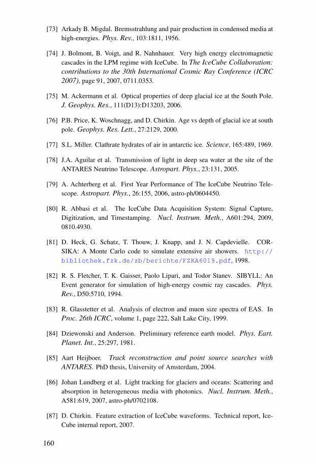
[73] Arkady B. Migdal. Bremsstrahlung and pair production in condensed media athigh-energies. Phys. Rev., 103:1811, 1956.

[74] J. Bolmont, B. Voigt, and R. Nahnhauer. Very high energy electromagneticcascades in the LPM regime with IceCube. In The IceCube Collaboration:contributions to the 30th International Cosmic Ray Conference (ICRC2007), page 91, 2007, 0711.0353.

[75] M. Ackermann et al. Optical properties of deep glacial ice at the South Pole.J. Geophys. Res., 111(D13):D13203, 2006.

[76] P.B. Price, K. Woschnagg, and D. Chirkin. Age vs depth of glacial ice at southpole. Geophys. Res. Lett., 27:2129, 2000.

[77] S.L. Miller. Clathrate hydrates of air in antarctic ice. Science, 165:489, 1969.

[78] J.A. Aguilar et al. Transmission of light in deep sea water at the site of theANTARES Neutrino Telescope. Astropart. Phys., 23:131, 2005.

[79] A. Achterberg et al. First Year Performance of The IceCube Neutrino Tele-scope. Astropart. Phys., 26:155, 2006, astro-ph/0604450.

[80] R. Abbasi et al. The IceCube Data Acquisition System: Signal Capture,Digitization, and Timestamping. Nucl. Instrum. Meth., A601:294, 2009,0810.4930.

[81] D. Heck, G. Schatz, T. Thouw, J. Knapp, and J. N. Capdevielle. COR-SIKA: A Monte Carlo code to simulate extensive air showers. http://

bibliothek.fzk.de/zb/berichte/FZKA6019.pdf, 1998.

[82] R. S. Fletcher, T. K. Gaisser, Paolo Lipari, and Todor Stanev. SIBYLL: AnEvent generator for simulation of high-energy cosmic ray cascades. Phys.Rev., D50:5710, 1994.

[83] R. Glasstetter et al. Analysis of electron and muon size spectra of EAS. InProc. 26th ICRC, volume 1, page 222, Salt Lake City, 1999.

[84] Dziewonski and Anderson. Preliminary reference earth model. Phys. Eart.Planet. Int., 25:297, 1981.

[85] Aart Heijboer. Track reconstruction and point source searches withANTARES. PhD thesis, University of Amsterdam, 2004.

[86] Johan Lundberg et al. Light tracking for glaciers and oceans: Scattering andabsorption in heterogeneous media with photonics. Nucl. Instrum. Meth.,A581:619, 2007, astro-ph/0702108.

[87] D. Chirkin. Feature extraction of IceCube waveforms. Technical report, Ice-Cube internal report, 2007.

160

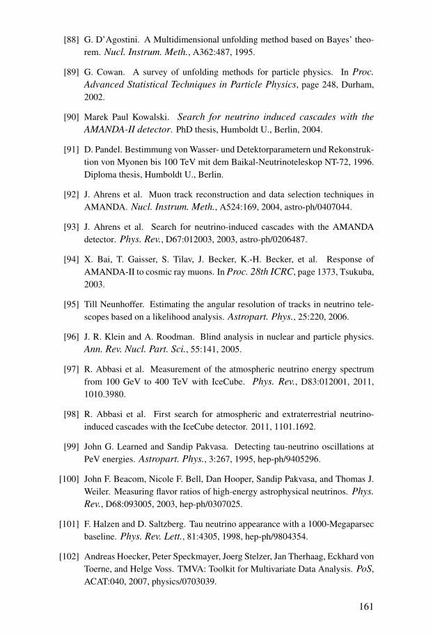
[88] G. D’Agostini. A Multidimensional unfolding method based on Bayes’ theo-rem. Nucl. Instrum. Meth., A362:487, 1995.

[89] G. Cowan. A survey of unfolding methods for particle physics. In Proc.Advanced Statistical Techniques in Particle Physics, page 248, Durham,2002.

[90] Marek Paul Kowalski. Search for neutrino induced cascades with theAMANDA-II detector. PhD thesis, Humboldt U., Berlin, 2004.

[91] D. Pandel. Bestimmung von Wasser- und Detektorparametern und Rekonstruk-tion von Myonen bis 100 TeV mit dem Baikal-Neutrinoteleskop NT-72, 1996.Diploma thesis, Humboldt U., Berlin.

[92] J. Ahrens et al. Muon track reconstruction and data selection techniques inAMANDA. Nucl. Instrum. Meth., A524:169, 2004, astro-ph/0407044.

[93] J. Ahrens et al. Search for neutrino-induced cascades with the AMANDAdetector. Phys. Rev., D67:012003, 2003, astro-ph/0206487.

[94] X. Bai, T. Gaisser, S. Tilav, J. Becker, K.-H. Becker, et al. Response ofAMANDA-II to cosmic ray muons. In Proc. 28th ICRC, page 1373, Tsukuba,2003.

[95] Till Neunhoffer. Estimating the angular resolution of tracks in neutrino tele-scopes based on a likelihood analysis. Astropart. Phys., 25:220, 2006.

[96] J. R. Klein and A. Roodman. Blind analysis in nuclear and particle physics.Ann. Rev. Nucl. Part. Sci., 55:141, 2005.

[97] R. Abbasi et al. Measurement of the atmospheric neutrino energy spectrumfrom 100 GeV to 400 TeV with IceCube. Phys. Rev., D83:012001, 2011,1010.3980.

[98] R. Abbasi et al. First search for atmospheric and extraterrestrial neutrino-induced cascades with the IceCube detector. 2011, 1101.1692.

[99] John G. Learned and Sandip Pakvasa. Detecting tau-neutrino oscillations atPeV energies. Astropart. Phys., 3:267, 1995, hep-ph/9405296.

[100] John F. Beacom, Nicole F. Bell, Dan Hooper, Sandip Pakvasa, and Thomas J.Weiler. Measuring flavor ratios of high-energy astrophysical neutrinos. Phys.Rev., D68:093005, 2003, hep-ph/0307025.

[101] F. Halzen and D. Saltzberg. Tau neutrino appearance with a 1000-Megaparsecbaseline. Phys. Rev. Lett., 81:4305, 1998, hep-ph/9804354.

[102] Andreas Hoecker, Peter Speckmayer, Joerg Stelzer, Jan Therhaag, Eckhard vonToerne, and Helge Voss. TMVA: Toolkit for Multivariate Data Analysis. PoS,ACAT:040, 2007, physics/0703039.

161

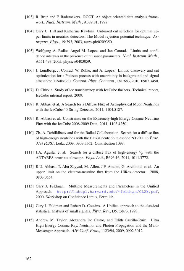
[103] R. Brun and F. Rademakers. ROOT: An object oriented data analysis frame-work. Nucl. Instrum. Meth., A389:81, 1997.

[104] Gary C. Hill and Katherine Rawlins. Unbiased cut selection for optimal up-per limits in neutrino detectors: The Model rejection potential technique. As-tropart. Phys., 19:393, 2003, astro-ph/0209350.

[105] Wolfgang A. Rolke, Angel M. Lopez, and Jan Conrad. Limits and confi-dence intervals in the presence of nuisance parameters. Nucl. Instrum. Meth.,A551:493, 2005, physics/0403059.

[106] J. Lundberg, J. Conrad, W. Rolke, and A. Lopez. Limits, discovery and cutoptimization for a Poisson process with uncertainty in background and signalefficiency: TRolke 2.0. Comput. Phys. Commun., 181:683, 2010, 0907.3450.

[107] D. Chirkin. Study of ice transparency with IceCube flashers. Technical report,IceCube internal report, 2009.

[108] R. Abbasi et al. A Search for a Diffuse Flux of Astrophysical Muon Neutrinoswith the IceCube 40-String Detector. 2011, 1104.5187.

[109] R. Abbasi et al. Constraints on the Extremely-high Energy Cosmic NeutrinoFlux with the IceCube 2008-2009 Data. 2011, 1103.4250.

[110] Zh.-A. Dzhilkibaev and for the Baikal Collaboration. Search for a diffuse fluxof high-energy neutrinos with the Baikal neutrino telescope NT200. In Proc.31st ICRC, Lodz, 2009. 0909.5562. Contribution 1093.

[111] J.A. Aguilar et al. Search for a diffuse flux of high-energy νµ with theANTARES neutrino telescope. Phys. Lett., B696:16, 2011, 1011.3772.

[112] R.U. Abbasi, T. Abu-Zayyad, M. Allen, J.F. Amann, G. Archbold, et al. Anupper limit on the electron-neutrino flux from the HiRes detector. 2008,0803.0554.

[113] Gary J. Feldman. Multiple Measurements and Parameters in the UnifiedApproach. http://huhepl.harvard.edu/~feldman/CL2k.pdf,2000. Workshop on Confidence Limits, Fermilab.

[114] Gary J. Feldman and Robert D. Cousins. A Unified approach to the classicalstatistical analysis of small signals. Phys. Rev., D57:3873, 1998.

[115] Andrew M. Taylor, Alexandra De Castro, and Edith Castillo-Ruiz. UltraHigh Energy Cosmic Ray, Neutrino, and Photon Propagation and the Multi-Messenger Approach. AIP Conf. Proc., 1123:94, 2009, 0902.3012.

162