searching for the past: archaeological research using a ......figure 21: roman emperors of britain...
TRANSCRIPT

Searching for the Past:
Archaeological Research using a Multi-Method Geomatics Approach
By
Robert Oikle
A thesis submitted to the Faculty of Graduate and Postdoctoral Affairs in partial
fulfillment of the requirements for the degree of
Master of Science
in
MSc. Geography
Carleton University
Ottawa, Ontario
© 2016, Robert Oikle

i
Abstract
Adopting a multi-method geomatics approach using cybercartography, a geographic
information system (GIS) with fuzzy set theory, and remote sensing software, can overcome
limitations encountered with isolated geomatics tools. Using Roman building practices as a test
case, the strengths of each geomatics method were utilized to identify ideal locations for Roman
fortifications. Cybercartography offered a flexible environment for collecting historical data,
presenting research, and developing custom tools and educational aids for users. The combination
of GIS with fuzzy set theory provided an improved analysis approach for developing a model of
Roman building practices, and supported the successful identification of 36 known Roman fortified
sites. Lastly the use of remote sensing software offered an extensive library for analysing
multispectral satellite imagery, and was able to identify numerous crop and soil marks.

ii
Acknowledgements
This research would not be possible without the continuous support from my supervisors,
Dr. Fraser Taylor and Dr. Scott Mitchell. Your encouragement and guidance have made this thesis
possible and I‟ll be forever grateful for the chance you took by accepting me as a student.
Thank you to Amos Hayes and Jean-Pierre Fiset for your unending patience in answering
my many questions and by assisting in the development of the cybercartographic atlas. The use of
Nunaliit is only possible due to your unending devotion to the development and support of this
great software.
To the staff, faculty and fellow students of the Department of Geography and Environmental
Studies, thank you for your continuous support over the years. Reaching this point would not be
possible without the help, guidance and friendship provided by the many members of this
department.
To Suman, Mom, and close family members, thank you for the unwavering support you‟ve
provide over the years. Each of you has made reaching this point in my life possible, and I‟m
eternally grateful for the wonderful family I‟ve been blessed with.

iii
Table of Contents
Abstract ........................................................................................................................................... i
Acknowledgements ......................................................................................................................... ii
Table of Contents ........................................................................................................................... iii
List of Tables ................................................................................................................................. vi
List of Figures ............................................................................................................................... vii
List of Appendices ......................................................................................................................... ix
Chapter 1.0: Introduction ................................................................................................................ 1
1.1 Why this research matters ...................................................................................................... 3
1.2 Research questions ................................................................................................................ 4
1.3 Thesis structure ...................................................................................................................... 4
Chapter 2.0: Background ................................................................................................................. 6
2.1 Roman fortification building practices ................................................................................... 6
2.1.1 Topography ..................................................................................................................... 7
2.1.2 Water .............................................................................................................................. 8
2.1.3 Food ................................................................................................................................ 8
2.1.4 Wood .............................................................................................................................. 9
2.1.5 Connectivity .................................................................................................................... 9
2.2 Cybercartography a tool for historical scholarship................................................................ 10
2.2.2.1 Application of cybercartography ............................................................................ 12
2.2.4.1 Challenges with historical data ............................................................................... 19
2.2.4.2 The value of providing a spatial context ................................................................. 21
2.2.4.2.1 Organizing historical records ............................................................................... 22
2.2.4.2.2 Visualizing the past ............................................................................................. 22
2.2.4.2.3 Spatial analysis ................................................................................................... 23
2.3 Fuzzy Set Theory ................................................................................................................. 26
2.3.1 Membership functions ................................................................................................... 27
2.3.2 The use of fuzzy set theory in spatial research ............................................................... 32
2.3.3 Advantages and criticisms of fuzzy set theory ............................................................... 33
2.4 Archaeological applications of remote sensing ..................................................................... 34
2.4.1 Remotely sensed imagery and the Electromagnetic Spectrum ........................................ 34
2.4.2 The influence of subsurface features on surface conditions ............................................ 36
2.4.3 Techniques to identify surface patterns .......................................................................... 38
2.4.4 Possible challenges of using remote sensing .................................................................. 39
Chapter 3.0: Study area ................................................................................................................. 41

iv
3.1 Site selection analysis study area ......................................................................................... 42
3.2 Image analysis study area .................................................................................................... 42
3.3 Temporal and spatial scales of data ...................................................................................... 42
Chapter 4.0: Methodology ............................................................................................................. 43
4.1 Spatial data collection .......................................................................................................... 43
4.1.1 Sampling scheme for archaeological data ...................................................................... 43
4.1.2 Sampling method for archaeological features ................................................................ 44
4.2 Visualizing data ................................................................................................................... 45
4.2.1 Displaying data through a dynamic atlas ........................................................................ 46
4.2.1.1 Schemas ................................................................................................................. 46
4.2.1.2 Modules ................................................................................................................. 47
4.2.2 Aiding visual analysis through custom widgets .............................................................. 48
4.2.3 Enhancing atlas content with education aids and research tools ..................................... 51
4.3 Site Selection Analysis ........................................................................................................ 54
4.3.1 Data preparation ............................................................................................................ 55
4.3.1.1 Preparing elevation data ......................................................................................... 55
4.3.1.2 Preparing Roman feature data ................................................................................ 56
4.3.1.3 Preparing river data ................................................................................................ 56 4.3.2 Representing Roman fort placement factors with raster layers ....................................... 56
4.3.2.1 General factors for Roman fort placement .............................................................. 57
4.3.2.2 Raster layer creation representing Roman building pattern factors .......................... 57
4.3.2.3 Fuzzy Set Theory membership functions ................................................................ 61
4.3.2.4 Develop SUM, MIN and MAX fuzzy membership raster layers ............................. 65 4.5 Mulitispectral imagery analysis of chosen sites .................................................................... 66
4.5.1 Image analysis script ..................................................................................................... 66
4.5.1.1 Pre-processing imagery .......................................................................................... 67
4.5.1.1.1 Converting Raw-DN to Radiance values ......................................................... 68
4.5.1.1.2 Radiance to Surface Reflectance...................................................................... 68
4.5.1.1 Imagery preparation ............................................................................................... 71
4.5.1.2 Pan-sharpening the imagery with the Brovey method ............................................. 72 4.5.1.3 Preliminary image analysis investigation .................................................................... 72
4.5.1.4 Image analysis methods. ............................................................................................. 73
4.5.1.4.1 Vegetation Indices ............................................................................................... 73
4.5.1.4.2 Unsupervised classification ................................................................................. 74
4.5.1.4.3 Principal component analysis .............................................................................. 74
4.5.1.4.4 Edge enhancement .............................................................................................. 75 Chapter 5.0: Results ...................................................................................................................... 76
5.1 Visual analysis of the cybercartographic atlas map interface ................................................ 76
5.2 Site selection analysis .......................................................................................................... 79
5.2.1 An overview of the site selection raster layers ............................................................... 79
5.2.2 Investigation of 41 suitable regions ............................................................................... 79

v
5.2.3 Selection of the image analysis site................................................................................ 81
5.3 Image analysis of selected sites ............................................................................................ 83
5.3.1 Crop marks of the Ellerton Pumping Station .................................................................. 84
5.3.2 Other surface patterns .................................................................................................... 85
Chapter 6.0: Discussion................................................................................................................. 92
6.1 Successes provided by a multi-method approach .................................................................. 92
6.2 Discussion of findings ......................................................................................................... 92
6.3 Potential data errors ............................................................................................................. 93
6.4 Challenges encountered during the analysis ......................................................................... 93
6.4.1 Challenges with the use of the Topographic Position Index ........................................... 94
6.4.2 Challenges with the site selection analysis results .......................................................... 94
6.4.3 Challenges of acquiring adequate imagery in Britain ..................................................... 94
6.4.4 Image analysis difficulties caused by human activities ................................................... 95
6.5 Future research recommendations ........................................................................................ 95
6.5.1 Recommendations for collecting data with Nunaliit ....................................................... 95
6.5.2 Recommendations for the site selection analysis ............................................................ 96
6.5.3 Recommendations for the image analysis ...................................................................... 97
Chapter 7.0: Conclusion ................................................................................................................ 98
Appendices ................................................................................................................................. 100
References .................................................................................................................................. 130

vi
List of Tables
Table 1: Temporal and spatial scales of project data....................................................................... 42
Table 2: Membership Functions for each factor or constraint raster ............................................... 65 Table 3: Spectral ranges for each spectral band .............................................................................. 66
Table 4: K and λ values for each spectral band .............................................................................. 68 Table 5: Spectral irradiance values of each spectral band, (Note. From 'Radiometric Use of
WorldView-2 Imagery' (Updike & Comp 2010, p.6)). ................................................................... 70 Table 6: Min radiance values for each spectral band ...................................................................... 71
Table 7: Vegetation Indices Listing ................................................................................................ 73 Table 8: Site selection analysis search results ................................................................................ 80
vii
List of Figures
Figure 1: GraphoMap illustrating how complex information can be distributed in an interactive
manner (http://atlas.gcrc.carleton.ca/homelessness/graphomap/Grapho_homelessness.xml.html). . 15 Figure 2: Clustering of points in the Kitikmeot Place Name Atlas ................................................. 25
Figure 3: Degree of tallness example showing the different between a crisp and fuzzy membership
functions design. ........................................................................................................................... 27
Figure 4: Linear, left open trapezoidal and right open trapezoidal membership functions (Robinson,
2003, p.9). Reproduced with permission from the publisher. ......................................................... 29
Figure 5: S membership functions (Robinson, 2003, p.10). Reproduced with permission from the
publisher. ...................................................................................................................................... 30
Figure 6: Right and left shoulder sigmoidal membership functions (Robinson, 2003, p.11).
Reproduced with permission from the publisher. ........................................................................... 30
Figure 7: Two generalized bell membership functions (Robinson, 2003, p.11). Reproduced with
permission from the publisher. ...................................................................................................... 31
Figure 8: Triangular membership function defined by μ(x) = max(min(x- α/ β- α, y-x/y- β),0)
(Robinson, 2003, p.12). Reproduced with permission from the publisher....................................... 31
Figure 9: Closed trapezoidal membership function, defined as μ(x) = max(min(1,x- α/ β- α, δ-x/ δ-
y) ,0) (Robinson, 2003, p.13). Reproduced with permission from the publisher. ........................... 32
Figure 10: Diagram showing the electromagnetic spectrum (Public Domain, produced by NASA) 35 Figure 11: Crop mark and soil mark surface patterns produced by subsurface structures ................ 36
Figure 12: Typical spectral reflectance curves for different surface conditions (Aggarwal, 2004,
p.33). Reproduced with permission from the publisher. ................................................................. 37
Figure 13: Map showing the study areas investigated for the larger site selection analysis and the
smaller image analysis .................................................................................................................. 41
Figure 14: Flow chart illustrating how each method is integrated .................................................. 43 Figure 15: A portion of the Form View for the Fort schema, illustrating the customizable data
gathering approach used by the atlas. ............................................................................................ 47 Figure 16: Histogram Widget ........................................................................................................ 49
Figure 17: Dataset summary widget .............................................................................................. 50 Figure 18: Temporal slider widget ................................................................................................. 51
Figure 19: OS Grid Reference Search Tool .................................................................................... 52 Figure 20: Custom SVG canvas illustrating the interior of a Roman fort ....................................... 53
Figure 21: Roman Emperors of Britain interactive timeline (using custom SVG canvas) ............... 54 Figure 22: Site selection analysis flowchart ................................................................................... 55
Figure 23: Diagram explaining TPI equation, Figure adapted by author from figure 3.a in Position
and Landforms Analysis (Weiss, 2001). ......................................................................................... 58
Figure 24: TPI Landform Classification Grid (Weiss, 2001). Reproduced with permission from the
publisher. ...................................................................................................................................... 60
Figure 25: Small radius vs. large radius TPI scatter plot results ..................................................... 61 Figure 26: Histogram and descriptive statistics for distance from a fort to a known river ............... 62
Figure 27: Histogram and descriptive statistics for distance from a fort to a Roman road ............... 62 Figure 28: Histogram and descriptive statistics for the slope at fort locations ................................ 63
Figure 29: The six fuzzy membership functions used in the analysis of Roman fort building
practices ........................................................................................................................................ 64
Figure 30: Image analysis script flowchart .................................................................................... 67 Figure 31: Solar zenith angle equation with an explanation figure (Note. From 'Radiometric Use of
WorldView-2 Imagery' (Updike & Comp, 2010, p.14)) ................................................................. 69 Figure 32: Roman forts along the coast line ................................................................................... 77
Figure 33: Collected Roman fort and settlement (including villas) data in the atlas ........................ 78 Figure 34: Zoomed in view of the image analysis study area with neighbouring Roman sites for

viii
context .......................................................................................................................................... 82
Figure 35: Image analysis study area with the site selection results overlaid and the expected
location for a fortified site marked on the map .............................................................................. 83
Figure 36: Rectangle negative crop marks at a known pumping station at Ellerton ........................ 85 Figure 37: Image analysis result - rectangular negative crop mark(s) in a field .............................. 86
Figure 38: Image analysis result - line and square shaped crop marks crossing multiple fields ....... 87 Figure 39: Image analysis result –crop mark showing a rectangular shape next to a brook ............. 88
Figure 40: Image analysis result – negative crop mark showing multiple lines/corners .................. 89 Figure 41: Image analysis result - square rectangular crop mark in the middle of a field ................ 90
Figure 42: Image analysis result - positive crop marks showing a rectangular outline with rounded
corners .......................................................................................................................................... 91
Figure 43: Site selection analysis results for 41 regions ............................................................... 107

ix
List of Appendices
Appendix A Metadata for datasets used in this research ............................................................... 100
Appendix B Site selection results of the 41 regions investigated .................................................. 104 Appendix C generateTPI.py script ............................................................................................... 108
Appendix D generateTPI.ini (used by the generateTPI.py script) ................................................. 110 Appendix E euclideanDistanceProcessing.py script ......................................................................111
Appendix F membershipFunctions.py script ................................................................................ 112 Appendix G siteSelection.py ....................................................................................................... 114
Appendix H AtmosphericCorrect_WorldView2.eas script (Multispectral bands).......................... 115 Appendix I AtmosphericCorrect_WorldView2_Pan.eas script ..................................................... 118
Appendix J PansharpenData_WorldView2.eas script ................................................................... 120 Appendix K ImageAnalysis_WorldView2_NoPANSHARPENING..eas script ............................. 122
Appendix L ImageAnalysis_WorldView2.eas script ................................................................... 126

1
Chapter 1.0: Introduction
Britain is an archaeologically rich region which has benefited from the use of geomatics
technologies to uncover its past. Common approaches, including geographic information systems
(GIS), ground surveys, aerial photography, and ground penetrating radar, have successfully been
applied in Britain, contributing greatly to the archaeological record of the region. This research
attempts to add to this list of enquiry methods, by performing archaeological research using a multi-
method geomatics approach. Combining a cybercartographic atlas framework, spatial analysis using
GIS with fuzzy set theory, and image analysis of multispectral satellite imagery, this research will
investigate the Roman archaeological landscape of Britain by adopting the strengths of multiple
geomatics technologies.
The basis for using a multi-method approach is rooted in the idea that different spatial tools
can provide benefits which other tools lack. By combing the strengths of each tool, limitations can
be overcome by using a more appropriate method for a specific task, and therefore multiple research
goals are more likely to be accomplished. By combining these different geomatics tools, this study
will visualize and share historical data, analyse Roman building practices, and search for unknown
archaeological Roman sites through the combination of different spatial tools.
The nature of historical records is often rich in historical details, but also spatially vague due
to the loss of specific location information over time. For example, a historian may know that an
area was occupied by an army and the history behind why a battle was fought, but at the same time
be unaware of the exact location an army set camp or the location of nearby natural resources used
by that army. This contradiction of a rich historical dataset being poor in spatial detail creates
numerous challenges when attempting to tell a story with a spatial framework that requires specific
spatial information. To address this challenge, a cybercartographic atlas framework is used in this
research to ensure any type of historical document can be collected (regardless if spatial details are
available or not), while also providing a suitable means of telling the story of Roman Britain.

2
This flexibility of customizing how and what types of data can be stored in an atlas, provides
greater opportunity for multiple types of historical records to be incorporated, including text, maps,
and pictures. As a dynamic atlas it also provides the flexibility to include custom geovisualizations
and education aids to improve the atlas‟ ability in telling a historical story, which may not be
possible with traditional frameworks. Since Roman building practices are a focus of this research,
particular attention was given to known archaeological site locations; however, these spatial data
were often enhanced by including historical documents, such as site sketches or pictures. The result
of utilizing a flexible spatial framework for data collection and visualization provides more
opportunities for different sources to be incorporated and greater potential for the historical dataset
to grow and become spatially refined as new sources of information are included. This process of
gradual refinement is often referred to as being organic, and is an important component of
cybercartographic atlases.
Selecting sites for the image analysis was performed using the power of GIS with fuzzy set
theory. Through this combination, spatial datasets can be processed by applying degrees of
membership to the dataset values, which accounts for spatial vagueness in the original records. The
result of this combination is the identification of the most suitable locations for future investigation
in Britain, while still recognizing that historical records can be spatially fuzzy.
Lastly this research tests the success of the site selection analysis and data collection
process, by examining potential Roman archaeological sites using a variety of image analysis
techniques on multi-spectral satellite imagery. The analysis of multispectral satellite imagery is a
common method in archaeological research, but the use of this technology has not been common in
Britain (Mr. Simon Crutchley, Development & Strategy Manager Remote Sensing, Heritage
Protection Department, English Heritage, pers. comm., 10 January 2014). Multispectral imagery
can be an effective tool in identifying subtle surface patterns caused by subsurface archaeological
features, often visible as differences in soil colour/texture, changes in vegetation health, and
variations in topography (Masini & Lasaponara, 2006, p.230). The absence of multispectral imagery

3
use in Britain provides an opportunity to investigate the utility of multispectral imagery in
archaeological research, exploring whether Britain's environment is appropriate for the use of this
imagery and testing the effectiveness of the image analysis contributing to archaeological research.
1.1 Why this research matters
The use of a multi-method geomatics approach in archaeology has merit beyond the
implementation of a new research methodology or the potential discoveries that may result from the
process. Additional benefits include: the preservation of sites, improved understanding of the past,
remote access to inaccessible locations, and a reduction in research costs.
Archaeological sites are at risk of being destroyed or concealed due to the expansion of
human created landscapes. Mechanized farming (Masini & Lasaponara, 2006, p.234), and urban
development (Parcak, 2007, p.67) are two examples of this expansion which have resulted in the
loss of archaeological sites around the world. By studying archaeological remains before they are
destroyed, new cultural knowledge can be derived. Evidence of this was seen in the expanded
understanding of Maya settlement/agricultural practices with the identification and study of 70 bajo
sites (large seasonal swamps) using a combination of remote sensing techniques. Through the
investigation of these bajo sites, cultural remains were discovered, demonstrating the significance of
this approach in helping to understand the Maya civilization (Sever & Irwin, 2003, p.118).
The availability of high resolution satellite imagery is comparable in expense to aerial
photographs (Fowler, 2002, p.55) and the spatial extents of high resolution satellite imagery is now
similar to traditional aerial photographs with the added benefit of superior spectral data for
archaeological analysis (Kumar, 2012, p.2). By utilizing satellite imagery in this research the
financial and time costs of performing archaeological research can be reduced significantly. Parcak
(2007, pp.74-75) supports this position, where the use of remote sensing for investigating an
archaeological landscape allowed for the equivalent of an estimated 3.5 year ground survey to be
performed in only 14 days, reducing both the time and financial costs associated with the research.
Furthermore, in the context of this project, performing ground surveys in Britain was not

4
within the scope of this study, but through the use of geomatics methods, it becomes possible to
research the past from a remote location. By combining the strengths of multiple geomatics
technologies in this research, new approaches to archaeology may become possible, leading to more
cost effective research and greater opportunities for discovering/preserving cultural heritage.
1.2 Research questions
Main Research Question: Can a multi-method geomatics approach aid in the understanding
of Roman building practices in Britain, and provide a new methodology for studying the
past?
Sub Research Question 1: Will a cybercartographic framework provide the flexibility
needed for historical data collection and visualization?
Sub Research Question 2: Can spatial patterns for Roman building practices in Britain be
identified using a combination of visual and statistical assessments, allowing for accurate
prediction of potential Roman archaeological sites?
Sub Research Question 3: Will fuzzy set theory be an effective approach in classifying
degrees of association between spatial characteristics and Roman building practices?
Sub Research Question 4: Can the use of fine resolution multispectral satellite imagery
identify subsurface Roman archaeological features in Britain?
Sub Research Question 5: What multispectral image analysis techniques are the most
effective in detecting Roman subsurface archaeological features in Britain?
1.3 Thesis structure
This thesis consists of seven chapters, beginning with this introduction outlining the goals and
context behind the research. The second chapter provides the background on key topics covered in
this research, including an overview of Roman building practices in Britain; an introduction to the
cybercartographic framework Nunaliit and how spatial technology can be utilized in historical
research; fuzzy set theory; and the use of multispectral satellite imagery in archaeological research.

5
The third chapter offers a short overview of the study area and the data incorporated in this
research. The fourth chapter provides the methodology used in this project. The results of this
research are shared in the fifth chapter, and lastly a discussion of the results and conclusion are
provided in the final two chapters of this thesis.

6
Chapter 2.0: Background
This multi-method spatial research represents a fusion of cybercartography, spatial analysis
using fuzzy set theory, and remote sensing, to study Roman military building practices in Britain.
This background chapter is divided into four sub-chapters, providing fundamentals on; 1) the spatial
building practices of Romans in Britain, 2) cybercartography and how spatial technology can be
used as a tool for historical scholarship, 3) fuzzy set theory, and 4) the use of remote sensing
technologies for archaeological applications.
2.1 Roman fortification building practices
Numerous factors influenced the placement of Roman forts in Britain, including military
strategy, topography, resource supply to Roman soldiers, and connectivity with neighbouring
Roman sites. This sub-chapter provides the general conditions that Romans considered vital when
selecting sites, which will play a key role in the spatial analysis of this research.
The purpose of a Roman fort was a base for soldiers who maintained control of an occupied
region (Johnson, 1983, p.36). The control provided by each fortified location was also
interconnected with other areas under Roman influence through the Roman transportation networks
(Wilson, 2011, p.5). Selecting a location for a permanent Roman military base required
consideration of numerous factors, which is evident in the 4th
century Roman writer, Vegetius, who
stated the following on how Romans selected suitable sites;
“A camp, especially in the neighbourhood of an enemy, must be chosen with great care.
Its situation should be strong by nature, and there should be plenty of wood, forage and
water. If the army is to continue in it for a considerable time, attention must be paid to
the salubrity of the place. The camp must not be commanded by any higher grounds
from whence it might be insulted or annoyed by the enemy, nor must the location be
liable to floods which would expose the army to greater danger” (Johnson, 1983, p.36).
Vegetius provides an excellent overview of how Roman military sites were selected and the
factors of topography, water, food, wood, and interconnectivity will be considered in this research.
It is worth noting that temporal and local considerations also influenced the placement of forts such
as the need to protect strategic locations. Examples of this include the Mendips lead mine protected

7
by the Charterhouse fort in Somerset (Johnson, 1983, p.3), the protection of river crossings
(Johnson, 1983, p.36), or controlling the approach of a mountain pass in the Scottish Highlands
(Johnson, 1983, p.36). However the scope of this research will only consider broad factors which
influenced Roman fortification placement, since the inclusion of time and local considerations
would be too complex to accurately account for in the site selection analysis.
2.1.1 Topography
Topography played an important role in the site selection of Roman forts. Romans
commonly placed forts on “a low flat-topped hill or elevated platform” (Breeze, 1983, p.47) which
had gentle surrounding slopes and were not typically at inaccessible locations that were highly
defensible (Johnson, 1983, p.36), such as a steep mountain peak. Numerous factors influence this
reasoning. Elevated land provides a defensive advantage to the troops, as well as affording a greater
view of the landscape (Breeze, 1983, p.47). Since many forts were placed near water, the elevated
placement of a fort was also chosen for protection from flooding (Johnson, 1983, p.37). The
requirement of gently sloping ground, relates to the nature of the Roman army and how it
commonly engaged enemy troops. The Roman army was an offensive army (Breeze, 1983, p.59),
with its legions engaging the enemy in the field (Johnson, 1983, p.2).This preference for engaging
the enemy, rather than fighting from behind walls is seen with the redesign of Hadrian‟s Wall to
include forts which each contained “the equivalent of six milecastle gateways” (Breeze & Dobson,
1978, p.45) providing greater ease to engage the enemy. Including additional forts with multiple
gates, eliminated the hindrance of auxiliary troops needing to “march a mile or two up to the wall
and then pass through a relatively narrow milecastle gateway before they could come to grips with
the enemy” (Breeze & Dobson, 1978, p.45). It should be noted that although the Roman army was
offensive in its tactics, towards the end of the third century, a series of Roman Saxon Shore forts
were departing from the traditional fort design having “high, thick walls, wide, deep ditches and
small, heavily defended gates” (Breeze, 1983, p.21).
Clearly military strategy required careful consideration of local topography, when selecting

8
suitable sites for Roman forts/camps. Forts not only needed to be placed in areas where military
control was required, but also locations needed to be selected which aided strategic success of the
military when engaging or spotting an enemy.
2.1.2 Water
Water is an obvious requirement for all inhabited locations, especially for military structures
housing a large number of soldiers. It has been estimated that 2.5 litres of water per day were
required for each Roman solider and water was also needed for livestock and for supplying
buildings such as bathhouses and latrines (Johnson, 1983, p.202). Consequently a number of
solutions were developed to meet this need at Roman sites. Most forts were placed beside a water
supply, such as a river or stream (Breeze, 1983, p.47). When possible a fort would protect a spring
within its walls, or place wells when the water table was close to the surface (Johnson, 1983, p.202).
Additionally water tanks have been found at some fort locations for the collection/storage of water
(Johnson, 1983, p.204), and forts like Greatchesters, even routed water from distant sources via
aqueduct (Johnson, 1983, p.206).
Although a number of different methods were used to secure water for a fort, placement near
rivers/streams was a common approach to solve this fort requirement, and consequently will be
incorporated in the site selection analysis.
2.1.3 Food
Food was vital in maintaining an occupying army in Britain. A variety of food sources were
provided to soldiers, with forts often containing a granary “with a raised floor designed to provide
maximum ventilation for the grain and other foodstuffs stored inside” (Johnson, 1983, p.142). The
safe storage of grain was vital to a fort, providing each Roman legion or auxiliary troop solider with
approximately 1 kg/day of grain (Johnson, 1983, p.195). The importance of fort food storage is also
evident in writings by Tacitus, in which each fort was required to store a year‟s worth of food
supplies for its soldiers in case their fort was under siege (Breeze, 1983, p.31). Although grain was
important, soldiers also had access to food from other sources. Soldiers could grow/raise food on

9
the land provided to the fort (known as territorium or prata) (Johnson, 1983, p.195). Food could
also be acquired by outside providers such as the requisition of grain from civilian supplies
(Johnson, 1983, p.195), and food could be requested from distant sources (Johnson, 1983, p.196).
An example of this diverse diet is seen in the Chesterholm store list, which included mutton, pork,
beef, goat, young pig, ham, venison, fish sauce, pork fat, spices, salt, vintage wine, sour wine, and
Celtic beer (Johnson, 1983, p.196).
2.1.4 Wood
During the construction of many forts, wood was a vital resource for both construction and
firewood (Johnson, 1983, p.36). It‟s estimated that 6.5 to 12.1 ha of woodland would be needed for
a 1.6 ha fort (Breeze, 1983, p.48), with early Roman forts in Britain having ramparts made from turf
or timber and internal buildings made from timber as well (Wilson, 2011, p.1). It should be noted
that as turf and timber fort locations became permanent, they were often rebuilt in stone (Wilson,
2011, p.2).
2.1.5 Connectivity
Maintaining control over a region also played an important part in the decision of where to
place a military camp or fort. Roads provided a vital means of communication with neighbouring
Roman sites, and gave access to supplies (Johnson, 1983, p.37). Not surprisingly, roads are often
found near fort locations, illustrating the connection between these two features.
Forts were also placed with consideration to neighbouring military locations. Commonly forts
were spaced a day‟s march away, approximately 22 km to 32 km apart (Breeze, 1983, p.17),
although Roman frontiers such as Hadrian‟s Wall had smaller distances between forts.
This need for close proximity to the lines of communication and common spacing between
forts illustrate the planning involved by Romans to maintain a tight net of control over conquered
areas. This careful planning by Romans in matters of connectivity throughout the empire, both in
terms of distance from the road network and proximity to other forts will be considered in the site
selection analysis performed in this research.

10
2.2 Cybercartography a tool for historical scholarship
Cybercartography is defined as “the organization, presentation, analysis and communication
of spatially referenced information on a wide variety of topics of interest and use to society in a
interactive, dynamic, multimedia, multisensory and multidisciplinary format” (Taylor, 2003, p.
406), and more recently described as “the application of geographic information processing to the
analysis of topics of interest to society and the display of the results in ways that people can readily
understand” (Taylor, 2014, p.4). As a research field, it consists of seven major elements:
[Cybercartography] is multisensory using vision, hearing, touch and eventually,
smell and taste;
[Cybercartography] uses multimedia formats and new telecommunications
technologies, such as the World Wide Web;
[Cybercartography] is highly interactive and engages the users in new ways;
[Cybercartography] is applied to a wide range of topics of interest to the society,
not only to location finding and the physical environment;
[Cybercartography] is not a stand-alone product like the traditional map, but part
of an information/analytical package;
[Cybercartography] is compiled by teams of individuals from different
disciplines; and
[Cybercartography] involves new research partnerships among academia,
government, civil society, and the private sector. (Taylor, 2003, p. 407)
These elements of cybercartography are the basis behind the creation of the
cybercartographic framework, Nunaliit, which is one of the spatial tools used in this research. To
better understand the role of cybercartography and why it was selected as one of the geomatics tools
in this research, background information will be provided on; the evolution of mapping, what
cybercartography is and how it has been applied to research, what makes up the Nunaliit atlas
framework, the role of spatial technology in historical research, and how a cybercartographic atlas
can be used to study the past.
2.2.1 Evolution of maps
Traditional static maps have played an important role in the study of the world, and this
importance has continued with the emergence of increasingly dynamic digital map products. To
better understand how digital maps can aid historical scholarship, it is important to discuss the
gradual evolution from static paper maps to dynamic digital formats, in order to appreciate how

11
cartographic products have changed and the potential research areas dynamic maps can support.
This evolution in mapping often coincides with the development of information technology,
and pre-dates web-based mapping. Early examples of interactive digital maps include the creation
of Hypermaps and Multimedia maps, which were delivered by compact disks (CD) or on a
computer's hard-disk (Cartwright, 2003, p.36). Hypermaps were created using links between
different levels of a map's hierarchy (Cartwright, 2003, p.37), while Multimedia maps became
increasing popular with the emergence of CD technology, by providing users a 'rich media'
interactive spatial product (Cartwright, 2003, p.37). Both examples illustrate the adoption of new
digital technology for providing increasingly interactive and richer experiences with maps.
With the creation of the Internet, maps emerged on the web, gradually improving in quality
and functionality as web technology advanced. This improvement of web mapping can be divided
into three stages. “In the first stage, paper maps were simply scanned and distributed like pictures.
In the second stage, beginning in about 1997, the Web emerged as a major form of delivery for
interactive maps. In the current third stage, the continued development of this form of map delivery
is dependent on solving specific problems related to map delivery, map design and use” (Peterson,
2003, p.1).
The use of the Internet to distribute maps has proven to be successful, and continues to grow
in popularity. This is evident with paper map distribution beginning to be exceeded by digital map
distribution in the late 1990's (Peterson, 2003, p.2), and over 200 million digital maps were being
distributed over the internet each day compared to every printed map (Peterson, 2003, p.1). This
increase in growth is likely linked to the many advantages which the internet provides map
distribution. Using the Internet, maps can be interactive, updated more frequently, and map data can
be displayed in increasingly new ways (Peterson, 2003, p.1). Additionally, maps provided in a
digital format are much cheaper to produce compared to their printed counter parts (Peterson, 2003,
p.6).
Map creation and delivery has seen amazing changes in recent decades, and continues to be

12
developed and adapted as digital technology advances. It has been stated that “Traditional maps
were key to the age of exploration. Cybermaps may equally be a key to navigation in the
information era both as a framework to integrate information and a process by which that
information can be organized, understood and used” (Talyor, 2003, p.405). This research adopts this
view of modern mapping and hopes to present yet another example of how modern dynamic maps
can be adapted to a specific task.
2.2.2 The beginning of cybercartography
Cybercartography was first introduced during the keynote address at the 18th International
Cartographic Conference in Stockholm, Sweden, in June 1997 (Taylor, cited in Taylor, 2005, p.2).
Following the initial conception of cybercartography, a multidisciplinary research team collaborated
on the New Economy Project, to develop the foundation for a cybercartographic paradigm in 2002
(Taylor, 2005, p.7). The initial goal of the New Economy Project was to make data more accessible
and understandable to the public, researchers, and decision makers in multiple disciplines (Taylor,
2005, p.7). The result was two cybercartographic atlases: the “Cybercartographic Atlas of
Antarctica and a Cybercartographic Atlas of Canada‟s Trade with the World” (Taylor, 2005, p.7).
It should be noted that, in a cybercartographic context, the term „atlas‟ extends beyond the
traditional meaning of a collection of related maps, and is a metaphor for structuring related spatial
data for the organization, presentation and analysis of the data (Taylor, & Caquard, 2006, p.2). Each
atlas is designed in an iterative manner, in which the requirements of interactivity, technology
limitations and the type of content being added by the author, all play an important role in an atlas‟
development (Taylor, & Caquard, 2006, p.2).
Since the creation of the first two cybercartographic atlases for the New Economy Project, the
framework has continued to mature through the development of numerous cybercartographic atlas
projects.
2.2.2.1 Application of cybercartography
Cybercartography has seen success as a research framework for numerous projects,

13
providing new ways of exploring data and deriving new insights on topics. Three advantages
offered by a cybercartographic atlas which were of importance to this research, are the
incorporation of multimedia, interactivity, and collaboration. The following section will provide
examples on how cybercartography has been applied to a variety of spatial topics, and will give
context for why Nunaliit was selected as a tool in this research.
2.2.2.1.1 Multi-media integration
A distinguishing aspect of cybercartography is conveying spatial information with multiple
senses while traditionally cartography is often limited to the visual sense. Numerous
cybercartographic atlases have incorporated this benefit by including different forms of multi-
media, such as sound to enhance an atlas' story.
In a cybercartographic project focusing on the use of sound for sharing additional electoral
information, Glenn Brauen of the GCRC incorporated sound clips to explore riding contention on a
choropleth election results map. By including sound clips of party leader speeches, users can hear
the level of contest experienced in Ottawa electoral ridings during the 2004 Canadian federal
election. Selected ridings that were won by a clear majority had that party‟s leader speaking clearly,
while ridings of heavy competition had multiple party leader speeches overlapping (fighting to be
heard), conveying the degree of struggle between parties to win that riding (Brauen, 2006, p.64).
The use of sound shows the importance that hearing can play in learning details about a topic, and
how a multi-sense approach to cartography can extend a product‟s utility. It also provides an
excellent example of how maps can archive information which would normally be lost in a
traditional choropleth map format. By including the speeches of party leaders who lost ridings, we
are reintroducing “voices, silenced in the original map” (Brauen, 2006, p.65), which are often
ignored in the final map product.
The “Views of the North Atlas” (http://viewsfromthenorth.ca/index.html), also incorporates
a variety of multimedia to study Canada‟s Northern history. By allowing anyone with an Internet
connection to contribute to the atlas, information on the North can “be input in various forms

14
(digital files with photographs or videos, text, etc.) and languages. Such flexibility and accessibility
are crucial to Views from the North, which seeks to reach out to communities across Nunavut”
(Payne, Hayes, & Ellison, 2014, p.197).
With the advancement of technology, cartographic projects can expand beyond a static map
and include non-traditional data formats. Conveying information through multimedia is a major
element of cybercartography. In fact the incorporation of different data formats is so important in
cybercartographic atlases that the framework was organized around the concept that the map is the
interface “designed to facilitate information retrieval in any format the user desires” (Taylor, 2003,
p.409). By including multimedia into an atlas, the possible types of messages which can be
conveyed are increased and knowledge not able to be shown on a traditional map, is now included.
2.2.2.1.2 Interactivity
One of the major strengths of cybercartography is its ability to reach a larger audience by
interacting with users through different media (for example as text, pictures, sound, video, etc.).
This inclusive approach to atlas design, supports the multiple intelligence and interactive learning
theories of Howard Gartner (Taylor, 2014, p.12), and enables users to engage with material in
formats which best suit their needs (Taylor, Cowan, Ljubicic, & Sullivan, 2014, p.298).
The importance of interactivity is evident in the use of sound incorporated in the Kitikmeot
Place Name Atlas (http://kitikmeot.gcrc.carleton.ca/index.html). By utilizing audio and visual
elements on a map, each location is marked and accompanied with an audio clip from a local
Inuktitut elder providing the proper pronunciation of the site (Engler, Scassa & Taylor, 2013, p.
192). This interactive approach allows atlas information (toponyms) to be simultaneously presented
visually and audibly, allowing greater opportunity for traditional knowledge to be passed down
through generations. The atlas also provides cultural preservation of interview transcripts by
including video interviews with Elders (Keith, Crockatt, & Hayes, 2014, p.225). This example
illustrates the important role of multimedia in the transference of traditional knowledge between
generations (Caquard, et al., 2009, p.87), as well as the role interactivity can play in an atlases‟

15
design.
The Canadian Atlas of Risk of Homelessness provides another example of the use of
interactivity in cybercartography. Through a series of interactive maps, atlas users observe the
changing levels of risk in homelessness in different major cities in Canada. One notable map in this
series is the unique GraphoMap developed by Dr. Sebastien Caquard which visualizes multiple
factors relating to homelessness, and the level of risk in each major city at three different time
intervals (Lauriault, 2014, p.185). By designing a graph with a 180 degree semi-circle, each city is
represented by a circle marker which adjusts in size proportionally to real number values of the
selected category and which moves towards or away from the center of the semi-circle graph
depending on the level of risk associated with the city and that selected category (Lauriault, 2014,
p.185). By presenting dense social data in this manner “interactivity and a well-designed
visualization can make accessible great complexity relatively easily when compared to data tables
on multiple pages in a PDF report” (Lauriault, 2014, p.185).
Figure 1: GraphoMap illustrating how complex information can be distributed in an interactive
manner (http://atlas.gcrc.carleton.ca/homelessness/graphomap/Grapho_homelessness.xml.html).
16
By presenting different types of data in multi ways, a greater audience is reached and in turn
the impact of the atlas is increased through the use of interactive techniques.
2.2.2.1.3 Collaboration
The team structure of a cybercartographic product is different from traditional cartographic
teams due to the required input from a wide variety of specialists in different fields (Taylor, 2003,
p.412). For example the research teams of the Cybercartographic Atlas of Antarctica consisted of
members from nine different disciplines (Taylor, 2003, p.412), and cooperated with “eight national
mapping agencies, Antarctic Treaty managers, the Geomatics Industry Association of Canada and a
number of non-government and private sector organizations” (Taylor, 2003, p.414).
Participation of communities in cybercartographic atlases allows the atlas to become an
evolving document. With access to the Internet, community members are able to continually
contribute to an atlas in a data format of their choice, including video, audio and photographs
(Caquard, et al., 2009, p.87). A clear example of this is the “Views from the North Atlas”, which
included community contributions in a variety of formats including: historic and contemporary
photographs, audio interviews, and video clips (Views from the North Atlas, 2015). The Inuit Sea
Ice Atlas also provides a wonderful model for collaboration with community members providing:
oral history/interview details about sea ice, community based monitoring programs, and also
participatory mapping using global positioning system (GPS) receivers to map travel routes over
sea ice (Inuit Siku (sea ice) Atlas, 2013).
Partnerships are a key component of any project. Access to spatial data can present a
challenge and “the creation of new partnerships among research centres, national mapping agencies,
the private sector, civil sector, and educational institutions helps respond to these challenges”
(Taylor, 2003, p.414).
2.2.3 The Nunaliit framework
The cybercartographic atlas framework, Nunaliit (http://nunaliit.org), “is an interactive data
management platform for collecting, relating, presenting, and preserving information and its

17
context, with a particular focus on using maps as a unifying framework” (Hayes, Pulsifer, & Fiset,
2014, p.129). Its name originated from the Inuktitut word for community or settlement (Taylor &
Pyne, 2010, p. 8), and was selected to emphasize the community-based approach of the
development of the cybercartographic software (Caquard, et al., 2009, p.85).
Nunaliit has a flexible open design, capable of working with different data formats. Many
existing tools and frameworks are not adequate for atlas research projects and often don‟t meet a
developer‟s project requirements or has an inability to use a specific data type (Hayes, Pulsifer, &
Fiset, 2014, p.130). Nunaliit is designed with open standards in mind, and avoids “depending on
rigid proprietary data structures and encouraging interactions with other systems” (Hayes, Pulsifer,
& Fiset, 2014, p.130). By not subscribing to rigid rules in its framework, Nunaliit “is designed to
work with data stored in different locations while still allowing new connections to be made and
new stories to be told” (Hayes, Pulsifer, & Fiset, 2014, p.130). The end result of this open approach
is a framework that integrates geographic information with other forms of data, including: video,
audio, text and photographs (Caquard, et al., 2009, p.85), which offers more to atlas developers and
greater opportunities to “facilitate new knowledge-construction networks” (Caquard, et al., 2009,
p.85).
The cybercartographic atlas framework can be simplified as interactions between three main
components; 1) a web browser, 2) a database, and 3) the Nunallit software development kit (SDK)
which provides the means of communication between these two components (Developer
Documentation, 2015). Most user interaction with an atlas is performed through a web browser,
allowing requests of dynamic maps, viewing images, reading spatial records, and other interactions
with an atlas dataset.
Atlas documents are stored within a schema-less document-oriented database called
CouchDB. Unlike relational databases (common to GIS software), document-oriented databases
don‟t use tables, rows and columns to organize and store data (Hayes, Pulsifer, & Fiset, 2014,
p.134). Each document in CouchDB is unique, with its attributes stored in JavaScript Object

18
Notation (JSON) format, which allows values in the form of strings, numbers, arrays and objects to
be associated with a unique id and a revision id used for accounting for document changes (Hayes,
Pulsifer, & Fiset, 2014, p.134). CouchDB document data can also be extended by including
attachments which are stored in a reserved attribute in the document (Hayes, Pulsifer, & Fiset, 2014,
p.134). By using CouchDB for an atlas‟ storage, a wide variety of digital data can be included,
which provides greater flexibility in the type of story being told by a cybercartographic atlas.
Although CouchDB provides flexibility for atlas design, some standardized structure is
provided to each atlas using schema documents and modules, through which information is
organized for presentation to the viewer. Schema documents “define a class of documents and
indicate what attributes one might expect to find in documents declaring themselves to be of that
class, and how to display those attributes in various circumstances” (Hayes, Pulsifer, & Fiset, 2014,
p.134). Although schema documents are used for aiding the structure of a Nunaliit atlas, it is
important to note that schema documents are more reminiscent of guidelines for documents, rather
than a rigid set of rules. Documents can still be edited to include attributes not described in the
schema document, but the structure provided by schemas does aid the development of an atlas and
how information can be retrieved. Atlas modules are used for organizing atlas content and contain
information on how data used by a module should be displayed to a user. For example, a module
could be designed to show data in the form of a map, an interactive graphic, or simply as a page of
text. By incorporating different modules in an atlas, related content can be structured in a variety of
methods which aids the user‟s absorption of the material.
Nunaliit offers a flexible framework for spatial research. It can adapt as new technologies
are developed/adopted by its structure, is able to display data in variety of formats, and utilizes a
schema-less CouchDB document-based database for its data storage which allows users to
incorporate a wide variety of digital content. This flexibility provides the ideal means of handling
historical data.

19
2.2.4 Researching history with spatial technology
Historical research has benefited from spatial technology although the suitability of such
tools is often imperfect. Although a map may provide new insights about the past or aid with
explanation, the qualitative nature of historical data often creates challenges in modern spatial
frameworks. GIS analyses often use large volumes of quantitative data, while historical analyses are
often limited in the quantity of data available and that which is available is often qualitative in
nature (Gregory & Ell, 2007, p.1). However, though historical data may not be ideally suited for
typical GIS tools, spatial technology can still provide a benefit to historical scholarship.
Spatial tools can provide researchers a means of organizing historical records, can aid in
visualizing the past, and offer numerous options for spatial analysis (Gregory & Ell, 2007, p.10).
The following section will provide a short overview of the benefits offered and challenges faced by
spatial technology when focusing on historical topics.
2.2.4.1 Challenges with historical data
Although errors can exist in any spatial dataset, historical data can be even more sensitive to
this problem due to the lack of available records/resources to replace any discovered errors, and the
often subjective nature in which historic records are interpreted. It becomes increasingly important
that possible errors are accounted for in the atlases‟ development.
The collection of data is often the most time consuming and expensive portion of any project
(Gregory & Ell, 2007, p.41) and can add additional challenges when dealing with historical data.
Historic records are often prone to error when added to a geographic framework. One source of
error is inaccuracies in the original data, as was seen with the Digital Archaeological Atlas of Crete,
in which a number of recorded site positions needed to be recollected due to errors in the original
survey records (Sarris, et al., 2007, p.2). Another example of inaccuracies was shown with the GIS
Professional Browser view of Boston, where the Charles River was recorded as a lake by the
geographic system (Wallace & van den Heuvel, 2005, p.174). Extracting data from historic maps
can also pose multiple issues including errors introduced during the digitizing process or
20
inaccuracies caused by damage to the maps (e.g. folded crease marks or warping of the map)
(Gregory, & Ell, 2007, p.46). Georeferencing historical maps can also produce new errors which are
not apparent at first sight, and are often the result of comparing maps of different formats and
scales, or different historical measurement systems (Wallace & van den Heuvel, 2005, p.179).
Lastly, the reliability of historical maps can be affected by the original function and context of the
map (Wallace & van den Heuvel, 2005, p.179).
Since ambiguity and errors can often occur in historical records, the cartographer needs to
acknowledge those potential inaccuracies in historical maps. Developing a map which conveys
absolute truth in either a geographic or historic sense may not be possible, but absolute
accountability should be strived for (Wallace & van den Heuvel, 2005, p.179). A possible approach
for being accountable in map development is by providing adequate metadata, in order that “„errors‟
in the visualization can be accounted for and explained” (Wallace & van den Heuvel, 2005, p.175).
Another possible challenge of using historical data, especially for existing archaeological
sites, is recognizing both legal and cultural preservation issues. Careful planning needs to occur
about what level of access to the public should be provided in an atlas concerning mapped
archaeological sites. This challenge was addressed in the Digital Archaeological Atlas of Crete by
limiting external access to unpublished data on archaeological sites, and by recognizing Greek
Archaeological Law by protecting archaeological photographic material with a watermark on each
image (Sarris, et al., 2007, p.2).
The ability to show time has always been at conflict with the static nature of maps. Maps are
designed to show space and often lack the functionality to show more than one moment in time.
Three methods to represent time are: 1) time-slice snapshots, 2) a base map with overlays, and 3)
the space-time composite method (Gregory & Ell, 2007, pp.127-128). Each method presents valid
ways to illustrate temporal change with maps. The base map with overlays approach uses an initial
base map to represent a surface, and the overlay layers represents moments of change, allowing for

21
time to be queried and selected by merging all overlays to a set time frame with the initial base map
(Gregory & Ell, 2007, pp.127-128). The space-time composite method is very similar to the base
map and overlays approach with the exception that the base map now contains a composite of
spatial objects which can be identified temporally by their attribute data (Gregory & Ell, 2007,
p.128). The final method for showing time on maps uses time-slice snapshots. This approach is
probably the easiest to understand since it is simply a set of static maps defined at different time
intervals (Gregory & Ell, 2007, p.127).
A more dynamic approach in dealing with time is the use of a chronological slider, which is
used in many cybercartographic atlases. This is similar to the space-time composite approach
mentioned above, with the appearance of features being determined by a chronology attribute. For
example the Lake Huron Treaty Atlas uses this techniques to illustrate the movement of survey
teams based on historic journal entries, which are temporally queried using a slider bar (Lake Huron
Treaty Atlas, 2015). Another method that is well suited for cybercartography is the use of animation
to display temporal change. This approach is not a new idea, as is evident in the introduction of the
1932, Atlas of the Historical Geography of the United States. In the introduction it states that
“History is a record of movement and change” (Paullin, 1932, p. xiv) and that “the ideal historical
atlas might well be a collection of motion picture maps” (Paullin, 1932, p. xiv). Although it‟s
disappointing that these suggestions were not more readily explored by cartography, we do see
some successful attempts at animating temporal change such as modern weather maps. Although
this approach is not often used in historical mapping applications, it should be recognized that
through animation we are able to more effectively capture the fluid nature of time, which is not as
easily shown in a static product.
2.2.4.2 The value of providing a spatial context
Understanding the relation of one historical location with another can provide numerous
benefits to research which are not apparent when sites are examined independently. A wider spatial
context can aid in the organization of historical records, provide a means of visualizing the past, and

22
new information can be derived through the use of spatial analysis.
2.2.4.2.1 Organizing historical records
Spatial organization of data can provide numerous benefits. Having data associated with a
coordinate system allows for relations between datasets to be recognized more easily, and the
retrieval of data can be done in a less ambiguous manner. For example, retrieving data contained in
a specified coordinate extent is more precise than performing a search of a name/term which may
occur in multiple places or be called something else in the dataset (Gregory & Ell, 2007, p.10).
Organizing data in a geographic framework can also provide benefits in how the data are
distributed/used by the public. A notable example of this is the Digital Archaeological Atlas of
Crete, which was designed with the goal of providing valuable historical information about
archaeological sites, but also includes spatial data about potential risks to those sites from either
human activities (e.g. tourism) or environmental factors (e.g. seismic activity) (Sarris, et al., 2007,
p.1). By including both archaeological and environmental data in the organizing structure of the
database, the atlas provides numerous benefits, including the raising of awareness about cultural
heritage on Crete, and also providing an organized reference for managing conservation efforts and
performing analysis on the area (Sarris, et al., 2007, p.6).
2.2.4.2.2 Visualizing the past
The second benefit for providing a spatial context to historic/archaeological data is the
ability to visualize the past. Two clear uses of visualizing historical records are the enhanced ability
to present/engage audiences with historical information, and the ability that visualization provides
valuable information about historical landscapes that are no longer present. One historic
visualization project which demonstrated the role of engagement with users is the Palenque project,
a virtual archaeological site providing cultural learning about the Mayan city at Palenque, in
Chiapas, Mexico (Champion, Bishop, & Dave, 2012, p.122). Interactions through the virtual
archaeological site occurred in three different ways: user activities, observations, and instructions
(Champion, Bishop, & Dave, 2012, p.124), all of which engaged the user to learn new details about

23
Mayan culture. Examples include participation in a sacrificial offering ritual, or partaking in a
Mayan ball game (Champion, Bishop, & Dave, 2012, p.123). Through the use of avatars to engage
users, cultural information was able to be shared between the website and the user.
Another common method of visualizing past landscapes is to utilize historic maps in
determining feature locations. This was demonstrated through the creation of multiple 3D bird‟s-
eye views which utilized historic maps and a DEM to represent how the city of Tokyo (previously
known as Edo) looked during different stages in its development (Fuse, & Shimizu, 2004, p.5). This
visualization project also used historic Japanese wood block prints as records for recreating 3D
landscapes and discovered in the process that many of the historic prints were created inaccurately
by including famous views/features of the time which from a landscape perspective would have
been impossible (Fuse, & Shimizu, 2004, p.6). Visualization of historic records not only aids in
providing a more engaging way to observe past landscapes, but can play a key role in the initial
analysis by observing patterns not apparent in traditional sources.
2.2.4.2.3 Spatial analysis
The final benefit of mapping history is the ability to perform analysis on the data collected.
Although spatial analysis is possible without a geographic framework, it becomes much easier with
one due to the organizational benefits provided. One benefit is that new information about historical
sites can be derived, as was seen in the visualization project of the historic landscape of Tokyo.
Using a combination of a land use/ownership data with elevation data, it was discovered that social
rank of individuals played little role in the placement of land ownership, dispelling the researcher‟s
belief that higher ranked people were given more elevated land over lower ranked members of
society (Fuse, & Shimizu, 2004, p.5).
Another example of how organizing historic data into a spatial framework can aid in
analysis was shown in a study concerning the Salem witch trials. By associating spatial locations
with legal records for accused, accusers, defenders and witches, a spatial pattern emerged in the
analysis. With the creation of a map of accusations, it was shown that more accusers came from the

24
west side of the village and more accused lived in the eastern side (Ray, 2002, p.26). Upon further
analysis, it was also discovered that although not acknowledged during the witch trials, socio-
economic status appears to have been a major factor, since most of the accusers came from
wealthy/prominent families in the village while the accused were often from the mid-lower brackets
of society (Ray, 2002, p.26).
2.2.5 Studying the past with cybercartography
The cybercartographic framework Nunaliit has great potential as a tool to aid historical
research. The flexible design of the atlas allows for dynamic maps to be produced without many of
the limitations found in static maps, and allows the visualization of a wide variety of historical data
which may provide insights about the past that traditional geographic systems would be incapable
of incorporating.
The creation of an “accurate” 2D representation of a 3D environment continues to challenge
cartographers. Map makers are required to make decisions about what map projection to use, which
data to include on the map, how features should be symbolized, and what scale to represent
information, all of which play a role in distorting reality (Monmonier, 1996, p.1). A resulting
cartographic paradox exists in which “to present a useful and truthful picture, an accurate map must
tell white lies” (Monmonier, 1996, p.1).
Through the use of dynamic map design, many of these issues can be minimized. A common
problem faced by cartographers is choosing appropriate symbols. Although symbols often provide
additional information not apparent on a map, features beneath them are often obscured. In order to
address this issue, the GCRC has developed a clustering ability for symbols (i.e. point data) on the
map, which not only keeps the map clean in appearance, but also groups closely positioned data
until the user zooms closer, allowing cluster points to be visually separated.

25
Figure 2: Clustering of points in the Kitikmeot Place Name Atlas
Another benefit for dynamic web maps over traditional maps is the ability to adjust the scale
in the current map view. This is a common feature of many online map products that have built-in
zoom functionality (e.g. Google Maps). By allowing the user to change the scale of the data
dynamically, many cartographic challenges are overcome while traditional cartographic products
are still limited by the original quality/scale of the data being displayed.
Cartography has traditionally focused on physical and human environments, and only since
the 19th century have thematic maps emerged (Taylor, 2003, p. 412). Cybercartography recognizes
this limitation in scope and attempts to expand the range of geographic topics covered by atlases. A
notable example of this is the inclusion of spatial information generated by indigenous communities
which are not typically recorded in a map format, such as the Inuit Sea Ice Atlas. The ISIUOP –Inuit
Sea Ice Use Atlas represents the spatial recording of traditional knowledge about sea ice, with a
goal of the atlas to help pass this valuable environmental information onto Inuit youth, who are
often not gaining the experience/knowledge needed to safely use sea ice for transportation needs
(Inuit Siku (sea ice) Atlas, 2013).
Cybercartography provides a valuable framework for historical scholarship. The information
architecture of cybercartographic atlases is flexible in allowing the inclusion of multiple data types,
and the focus on collaboration with other experts is well suited for historical investigation. The
Lake Huron Treaty Atlas provides an excellent example of incorporating historical details about the

26
Lake Huron Treaty negotiation, signing, and survey process (Caquard, et al., 2009, p.87). Of
particular note, the atlas captures the journey taken by the original survey team of the area, by
extracting spatial information found in the survey journal (Caquard, et al., 2009, p.89). This
example illustrates both the challenge of visualizing historical spatial data which is limited to a
written record, but also shows the power of cybercartography in incorporating those journal entries
in the atlas‟ design, allowing for contributors to upload different forms of media with each survey
stop recorded in the journal (Pyne & Taylor, 2012, p.94). This visualization of the past also includes
other historical data sources, such as the pre-treaty, 1849 Alexander Vidal map, which illustrates
numerous spatial features, including: locations designated as “Indian Territories”, and a series of
mining lots marked in those “Indian Territories” (Pyne & Taylor, 2012, p.94). Historically this is of
interest because it brings to light that mining lots were applied for by prospectors prior to a treaty
being signed in 1850 (Pyne & Taylor, 2012, p.94). By including the Vidal map in this atlas, it
emphasizes “cartographically the relationship between colonial pressure for resource development
and the treaty and reserve-making process” (Pyne & Taylor, 2012, p.94)
The organic process in which cybercartographic atlases are developed is also shown with the
Lake Huron Treaty Atlas. New linkages between maps are developed as new information emerges
about a topic. Cybercartography provides this important benefit to historical research and is clearly
shown with the historic research on the lead surveyor, J.S. Dennis. By researching J.S. Dennis, new
details about his home (which is located in present day Toronto and was later converted into a
sanatorium) were included in the atlas, allowing for both map links and temporal linkages to be
developed (Pyne & Taylor, 2012, p.97).
2.3 Fuzzy Set Theory
Fuzzy set theory was first proposed in 1965 by Zadeh, who recognized the inherent fuzziness
of the real world and the possible inadequateness of applying crisp classifications to topics. For
example, “the „class of all real numbers which are much greater than 1,‟ or . . . „the class of tall
men,‟ do not constitute classes or sets in the usual mathematical sense of these terms” (Zadeh, 1965,

27
p.338). To address this issue, Zadeh provides a possible solution by replacing crisp values (e.g. 1 or
0) with a grade of membership in a fuzzy set represented by values from 1 (full membership) to 0
(no membership) (Zadeh, 1965, p.339).
Figure 3: Degree of tallness example showing the different between a crisp and fuzzy membership
functions design.
Using the example (Figure 3) of who is considered tall, the crisp classification defines people
as tall who are at least 6‟ in height. In comparison, the fuzzy set uses a range of membership grades
to represent how tall a person is between 6‟ and 5‟6”. Comparing both sets, a person who is 5‟ 10”
in height is considered short (a value of 0) in the crisp set, while the fuzzy set expressed the same
height as a value of (~0.667) which may represent the degree of tallness of the individual better,
especially when taking into account the cultural context in which the assessment was made.
2.3.1 Membership functions
When comparing classical set theory with fuzzy set theory, membership functions represent a
primary difference between the two theories (Woodcock, & Gopal, 2000, p.154). Membership
functions define the degree to which an element is part of a fuzzy set, and is commonly expressed

28
with the notation of µA : X →[0, 1] or A : X →[0, 1] (Robinson, 2003, p.6), which simply describes
that an element of the universal set X is a member of fuzzy set A which has a membership value in
the range of 0 to 1. Based on the nature of the parameters of the function, different degrees of
membership can be assigned to an element.
Numerous approaches exist for developing membership functions. One approach is the use of a
standard membership function that has had its parameters adjusted for a specific problem (Kandel
1986, cited in Robinson, 2003, p.8). Since this is the method adopted by this research, it will be the
focus of this background sub-chapter.
Standard membership functions include: linear/triangle, trapezoidal, S-shaped, sigmoidal, and
Gaussian, (Robinson, 2003, pp.8-14) and are provided in either an open or closed form. The open
form is “characterized as being non-decreasing and having values inside 0 and 1 only within a
bounded interval” (Bohlin et al. 2000, cited in Robinson, 2003, p.8), while closed form function
“allows non-zero membership values only in a bounded interval” (Robinson, 2003, p.10 & 12).

29
Figure 4: Linear, left open trapezoidal and right open trapezoidal membership functions (Robinson,
2003, p.9). Reproduced with permission from the publisher.

30
Figure 5: S membership functions (Robinson, 2003, p.10). Reproduced with permission from the
publisher.
Figure 6: Right and left shoulder sigmoidal membership functions (Robinson, 2003, p.11).
Reproduced with permission from the publisher.

31
Figure 7: Two generalized bell membership functions (Robinson, 2003, p.11). Reproduced with
permission from the publisher.
Figure 8: Triangular membership function defined by μ(x) = max(min(x- α/ β- α, y-x/y- β),0)
(Robinson, 2003, p.12). Reproduced with permission from the publisher.

32
Figure 9: Closed trapezoidal membership function, defined as μ(x) = max(min(1,x- α/ β- α, δ-x/ δ-
y) ,0) (Robinson, 2003, p.13). Reproduced with permission from the publisher.
2.3.2 The use of fuzzy set theory in spatial research
Fuzzy set theory has been applied to numerous spatial research projects and is often considered
more realistic in how natural characteristics are represented compared to a limited Boolean
approach. Natural features often change gradually, however they are frequently represented
spatially as either existing or not existing; for example a forest may be classified coniferous when in
fact deciduous trees also exist there.
One example of fuzzy set theory being used in spatial research was shown in the analysis of
soil pollution at Sao Paulo, Brazil. An issue with identifying areas with soil pollution is the risk of
over simplification errors when dealing with continuous spatial features (Lourenҫo, et al., 2010,
pp.495-496). Instead of simply stating an area is polluted or not, fuzzy logic provided a means for
soil pollution by heavy metals to be given a membership value for four classes representing degrees
of pollution (Lourenҫo, et al., 2010, p.499). By adopting this approach, the transitional zones
between polluted and unpolluted soil were represented and allowed researchers to generate a more
realistic view of the degree of membership in each class (Lourenҫo, et al, 2010, p.496).
Another example is the successful use of fuzzy logic to model land suitability for hybrid poplar
in the Canadian Prairies. Suitability for this species was determined accounting for multiple factors,

33
including precipitation, the moisture index, growing degree days, Canada Land Inventory
agriculture capability, and elevation (Joss, et al., 2008, p.79). By adopting a fuzzy approach over a
Boolean method, land suitability results were shown to be more descriptive (Joss, et al., 2008,
p.79), and compared well with other published studies while also providing the added benefit of
presenting afforestation suitability as a continuous trend (Joss, et al., 2008, p.92).
2.3.3 Advantages and criticisms of fuzzy set theory
The use of fuzzy set theory for processing spatial data provides numerous advantages over the
commonly adopted Boolean logic approach. Boolean systems are popular for their simplicity,
flexibility and use of quantitative data, but are criticised for simplifying data which is more variable
(Joss, et al., 2008, p.80). In contrast, fuzzy set theory offers a more representative approach for data
which is variable or continuous in nature (Joss, et al., 2008, p.81).
Furthermore, the use of uncertain data is better suited using a fuzzy approach. This view is
reflected in the archaeological GIS research on estimating the presence of Roman streets. Due to the
varying level of confidence in archaeological data and the variety of sources used, the data is both
multi-modal and uncertain (Runz, Desjardin, Piantoni, & Herbin, 2007, p.2), and the use of fuzzy
logic provided the benefit of managing these sources of uncertainty (Runz, Desjardin, Piantoni, &
Herbin, 2007, p.4).
In contrast, the main criticism of fuzzy set theory is placing confidence in a level of
membership to a class, while simultaneously not being capable of providing a definitive
classification to a location (Goodchild, 2000, p.5). An example of this contradiction would be a
census stating that it is unsure if a household has two children living in a home, while also given the
same house a membership value of 0.8 for the possibility of 2 children living in a house based on
household size trends. In this situation, the membership value may not accurately represent the true
census for that household, and could be a source of error in future analysis.
Although fuzzy set theory is not perfect in its representation of spatial features, its use provides
potential for more accurate depictions of complex spatial features. This is especially true when

34
compared to a more traditional Boolean approach, which frequently classifies features as black or
white when shades of grey would be more reflective of reality.
2.4 Archaeological applications of remote sensing
The use of remote sensing in archaeological research is extensive, and has existed for over a
century (Kumar, 2012, p.1). Initially this technology provided a synoptic view of a study area,
shedding new details about a landscape which are not apparent at the ground level, including
variations in texture, pattern, shape, shadow and context (Abrams & Comer, 2013, pp.65-66).
A notable example of this is the 1920's discovery of the Nazca Lines of Peru (Lillesand, Kiefer, &
Chipman, 2007, p 281). Beyond the benefit of a synoptic view, remote sensing technologies also
provide methods of identifying archaeological sites by using imagery sensors that have greater
spectral sensitivity than human vision (e.g. multispectral satellite imagery). This portion of the
chapter will provided a background on: remote sensing and the electromagnetic spectrum, how
subsurface archaeological features can influence surface conditions and corresponding spectral
reflectance values, a discussion of some of the benefits of using remote sensing in archaeological
research, common techniques used to identify surface patterns in remotely sensed imagery, and
what challenges exist with using remote sensing techniques in archaeological applications.
2.4.1 Remotely sensed imagery and the Electromagnetic Spectrum
The multispectral satellite imagery used in this research is acquired by passive sensors,
recording reflected solar energy (electromagnetic radiation) off the earth's surface, which is
measured in ranges of wavelengths specific from the electromagnetic spectrum (Abrams & Comer,
2013, p.57). The Sun, the source of this energy, “produces a continuous spectrum of
electromagnetic radiation ranging from very short, extremely high-frequency gamma and cosmic
waves to long, very-low-frequency radio waves” (Jensen, 2007, p.43).

35
Figure 10: Diagram showing the electromagnetic spectrum (Public Domain, produced by NASA)
The satellite sensors commonly record this data as sub-divisions of wavelength intervals that
are given a description (e.g. red light) (Jensen, 2007, p.43), which are found in the visual spectrum
and non-visual portion of the spectrum (e.g. infrared). The visual spectrum represents the portion of
the electromagnetic spectrum which humans can see and are typically represented as the colours
Red, Green and Blue, with the corresponding wavelengths roughly between ~0.4 nanometres and
~0.7 nanometres in size (Abrams & Comer, 2013, pp. 58). Infrared is outside of what we can see,
and is often further divided into the Near Infrared (NIR), and various ranges in the Short
Wavelength Infrared (SWIR) (Abrams & Corner, 2013, pp 57-58). By recording portions of the
electromagnetic spectrum such as in the NIR, SWIR, or even thermal ranges (TIR), hidden
characteristics about the surface can become apparent through imagery analysis, allowing patterns
in the surface to be identified.

36
2.4.2 The influence of subsurface features on surface conditions
With the use of remotely sensed imagery, archaeologists can detect subsurface
archaeological sites, due to changes in vegetation health, differences in moisture levels, and minor
elevation changes, which result in distinctive surface patterns. These surface patterns are commonly
referred to as crop marks, soil marks and shadow marks.
Figure 11: Crop mark and soil mark surface patterns produced by subsurface structures
Crop marks appear as variations in vegetation growth caused by subsurface structures,
which influence the health of vegetation by altering the availability of soil nutrients and/or water to
plants (Masini & Lasaponara, 2006, p. 230). Vegetation which benefits from subsurface structures
are called positive crop marks, while subsurface structures that hinder the growth of vegetation are
called negative crop marks (Masini & Lasaponara, 2006, p.230). Identification of either type can be
performed using vegetation indices (Masini & Lasaponara, 2006, p.231).
Soil marks, like crop marks, are the result of subsurface structures influencing the
appearance of soil on the surface. They are seen as surface variations in texture or colour and are
often apparent when the soil is damp (Masini & Lasaponara, 2006, p.230). Soil marks are
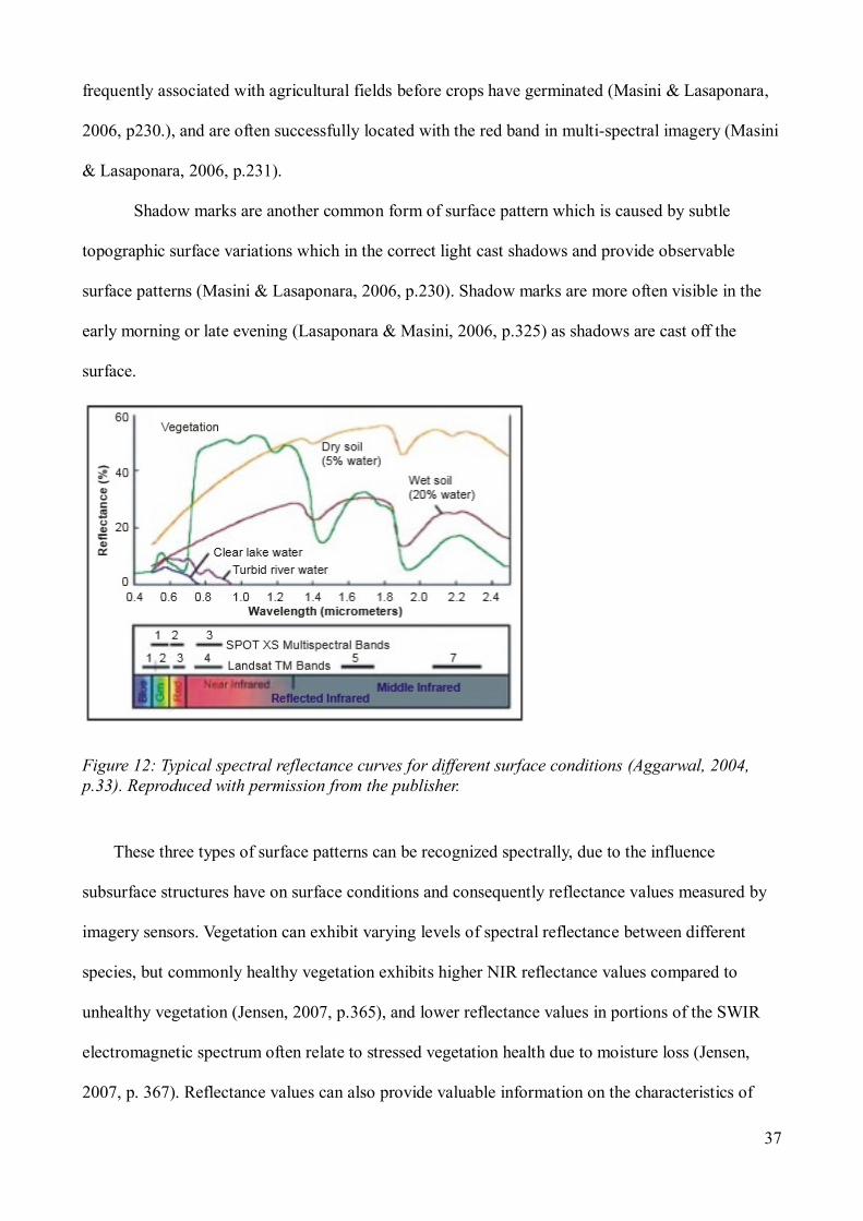
37
frequently associated with agricultural fields before crops have germinated (Masini & Lasaponara,
2006, p230.), and are often successfully located with the red band in multi-spectral imagery (Masini
& Lasaponara, 2006, p.231).
Shadow marks are another common form of surface pattern which is caused by subtle
topographic surface variations which in the correct light cast shadows and provide observable
surface patterns (Masini & Lasaponara, 2006, p.230). Shadow marks are more often visible in the
early morning or late evening (Lasaponara & Masini, 2006, p.325) as shadows are cast off the
surface.
Figure 12: Typical spectral reflectance curves for different surface conditions (Aggarwal, 2004,
p.33). Reproduced with permission from the publisher.
These three types of surface patterns can be recognized spectrally, due to the influence
subsurface structures have on surface conditions and consequently reflectance values measured by
imagery sensors. Vegetation can exhibit varying levels of spectral reflectance between different
species, but commonly healthy vegetation exhibits higher NIR reflectance values compared to
unhealthy vegetation (Jensen, 2007, p.365), and lower reflectance values in portions of the SWIR
electromagnetic spectrum often relate to stressed vegetation health due to moisture loss (Jensen,
2007, p. 367). Reflectance values can also provide valuable information on the characteristics of

38
soil, with wet soil commonly exhibiting lower reflectance in the Red and NIR electromagnetic
spectrum ranges compared to dry soil which typically has higher reflectance in those ranges
(Jensen, 2007, p.366). This relation between reflectance values and corresponding surface
conditions is useful in the context of archaeological site selection, since surface patterns caused by
subsurface archaeological features can be identified using common imagery analysis techniques and
provide a marker for potential archaeological sites.
2.4.3 Techniques to identify surface patterns
Surface patterns caused by subsurface structures are often identified through imagery
analysis. These patterns are noticeable to observers due to the geometric nature in which humans
often construct structures (Lasaponara, Masini & Scardozzi, 2008, p.88), which in comparison to
the natural environment are not typically exhibited. Due to this distinction, subtle surface patterns
can be enhanced using imagery analysis techniques commonly applied in remote sensing. These
techniques include: the use of vegetation indices, principal component analysis (PCA), image
classification, contrast stretching, and image filters. Since each of these techniques will be applied
during the analysis of the selected site, a short description of each will be provided here.
Vegetation indices are a common method of image analysis in archaeological research,
because of their ability to illustrate degrees of vegetation health/biomass. Common examples
include: NDII, NDVI, EVI, DVI and MSI, and have been useful in identifying crop and soil marks.
A more statistical approach in image analysis is the use of principal components analysis
(PCA). PCA address the issue of interband correlation, frequently encountered with multispectral
imagery (Lillesand, Kiefer, & Chipman, 2007, p.527). Simply speaking “PCA reduces the amount
of spectral redundancy in remotely-sensed data” (Parcak, 2007, p.71) and produces uncorrelated
components, with the first component representing most of the scene‟s variance with subsequent
bands representing less of the variance (Lillesand, Kiefer, & Chipman, 2007, p.529).
Image classification, as the term suggests, classifies an image into separate spectral classes,
which can be performed in a supervised (i.e. training data guides the classification) or unsupervised
39
manner (i.e. the scene is broken down into spectral classes by the computer). An example of this
approach is the successful use of an unsupervised classification to locate 70 archaeological sites,
shown to be 98% accurate when ground surveyed (Parcak, 2007, p.73).
Contrast stretching allows for a narrow range of brightness values to be stretched over a
wider range of displayed values (Lillesand, Kiefer, & Chipman, 2007, p.501). The result of this
method is an improvement of feature contrast, and aids in the identification of possible
archaeological features.
Image filters provide another method for image analysis by enhancing or restraining spatial
details or frequencies (Showalter, 1993, p.81), such as the enhancement of edge/line features or the
reduction of noise in an image.
Although numerous image analysis/enhancement techniques are available for archaeological
research, the effectiveness of each technique can vary between locations. Therefore multiple
techniques may need to be applied, in order to discover hidden archaeological structures.
2.4.4 Possible challenges of using remote sensing
The presence of surface patterns is not guaranteed in imagery and is often dependent on
external physical factors. Elements which can contribute to mark prominence in imagery include:
the time of year the image is taken, the study area location, the type of vegetation above the surface,
climatic events prior to the imagery date, and moisture level in the soil. An example of the
variability in crop mark prominence in high resolution satellite imagery was recently studied in
Greece. By examining the same areas at multiple time frames while also ranking the visibility of
known crop marks, the results showed notable differences depending on the time of year in which
the imagery was collected (Kaimaris, Patias, & Tsakiri, 2012, p.17). The study of the Hohokam
Canal System near Phoenix, Arizona, provides another example of surface pattern variability.
Recently irrigated fields exhibited more prominent surface marks for segments of the canal
compared to drier locations (Showalter, 1993, p.88). Consequently it was concluded that the most
ideal conditions for locating soil marks of the Hohokam canal system would be three to four days

40
after a significant rain event, which would allow puddles to evaporate and shallow soils to drain,
while moisture would be retained in ditches and canals (Showalter, 1993, p.88).
Regional differences can also challenge researchers in locating patterns in imagery. In a
study concerning the East Delta and Middle Egypt, noticeable differences in responses occurred due
to varying soil compositions, requiring different imagery analysis techniques to be incorporated to
locate patterns in both regions (Parcak, 2007, p.73). Each of these examples emphasises that
optimal times and landscape conditions can play a significant role in how obvious surface patterns
appear to a researcher and presents a notable challenge for archaeological research.
The data itself can also present a number of challenges, which need to be considered before
performing analysis. Image quality can suffer from various errors, including how archived imagery
has aged, inconsistencies in the archival treatment of data, deterioration of film negatives, and the
concealment of features in photographs due to annotations (Ottean & Hanson, 2013, p.323).
Furthermore the time frame when imagery is collected is often out of control of the researcher since
the original purpose of the data may not be intended for archaeological investigation (Ottean &
Hanson, 2013, p.323). Selecting imagery for archaeological research requires extra attention to
ensure the quality of data meets the project‟s needs.

41
Chapter 3.0: Study area
The spatial scale of this research is broken into two sites. The initial site selection analysis and
data collection using the cybercartographic atlas were performed throughout mainland Britain. The
image analysis for the selected site was spatially refined to an area straddling the English counties
of Shropshire and Staffordshire, (see Figure 13).
Figure 13: Map showing the study areas investigated for the larger site selection analysis and the
smaller image analysis

42
3.1 Site selection analysis study area
With evidence of Roman occupation being found throughout much of Britain‟s mainland,
the study area for the initial data collection and following site selection analysis was vast. It
extended from the south coast of England to the northern regions of Scotland, including almost all
of Britain, with a total area of ~234353 km² and a bounding box of [8.650007°W, 49.864636°N,
1.768912°E, 60.860766°N].
The characteristics of this terrain varied with an approximate elevation range between -76 m
and 1346 m, containing an abundance of water sources, arable soil, and woodlands, making it a
resource rich region during Roman times.
3.2 Image analysis study area
The selected area for the image analysis included a stretch of land along a known Roman
road in the western mainland of England. The study area was ~28.2 km² and had a bounding box of
[2.484513°W, 52.784724°N, 2.314826°W, 52.856125°N]. Elevation in the region ranged from 64
m to 139 m, and the landscape is currently dominated by agricultural lands with ample sources of
water.
3.3 Temporal and spatial scales of data
Table 1: Temporal and spatial scales of project data
Dataset Spatial Scale Temporal Scale
SRTM Digital Elevation Model 1 arc second (~25.2 m² after
mosaic process).
Acquisition Date : Feb 11, 2000
Publication Date: Sept 23, 2014
Rivers Dataset (OS Open
Rivers)
1:15000 to 1:30000 2015
Polygon of Britain (produced
from the OS Open Data –
Boundary Line™)
1:10000 2014
WorldView-2 imagery 2 m (0.5m pan-sharpened) 2015-07-14
Roman historical sites Variable 50 C.E. to 400 C.E.

43
Chapter 4.0: Methodology
A multi-method geomatics approach was adopted for this research, incorporating a
cybercartographic atlas for data collection, GIS software and fuzzy set theory for the site selection
analysis, and remote sensing software for the imagery analysis. This chapter describes the role each
method played in this research approach.
Figure 14: Flow chart illustrating how each method is integrated
4.1 Spatial data collection
A variety of data sources were collected for this research, including elevation data provided
by the Shuttle Radar Topographic Mission (SRTM), river location data provided by OS Open Data
(called OS Open Rivers), WorldView-2 multispectral satellite imagery provided by Digital Globe,
and archaeological Roman site locations in Britain provided by a variety of sources, such as books,
journals, maps and aerial photographs (see Appendix A for a full metadata listing).
4.1.1 Sampling scheme for archaeological data
Archaeological data was collected by the author and were limited to large Roman structures in
Britain, to limit the scope of the research data collection. Features including: roads, forts,

44
settlements (cities, town, settlements and villas), military camps, spiritual structures (e.g. temples),
military towers, and theatres were all collected in the dataset, with particular attention given to road
and fort locations. Sampling was limited to large structures because of increased visibility in
satellite imagery, greater likelihood of being previously surveyed, and consequently, greater
availability of historical information. By limiting sampling to large archaeological structures, a
valuable overview of Roman occupation becomes available providing a starting place for the spatial
analysis of Roman building patterns while also providing opportunity for future growth.
4.1.2 Sampling method for archaeological features
Archaeological data were derived from secondary sources that provided spatial details used
to digitize a location in the cybercartographic atlas framework. Sources for identifying Roman
Britain structures included: aerial photos, survey records, journals, books, survey sketches,
Ordnance Survey Grid References, websites, general site descriptions, and other sources which
were considered reputable.
Identification of feature locations was performed using a variety of free spatial tools,
including Google Earth, Google Maps, Open Street Maps, Ordnance Survey Street View WMS
(accessed via: Old Maps UK (https://www.old-maps.co.uk)), and OS Grid Reference search tools.
By incorporating different sources of information during data sampling there was a greater
opportunity for site locations to be correctly identified and therefore included in the atlas dataset.
The selection of tools for identifying a feature location was dependent on the provided
source information. Locations which were only described in text would commonly require a
thorough investigation and a variety of tools were often used to narrow down a spatial location
being described. Through the use of different Web Mapping Services (WMS), including Google
Maps, Open Street Maps, and Ordnance Survey Street View, different spatial details could be
identified relating to a feature location. Ordnance Survey Street View would often have historical
names/features not available in other sources, Open Street Maps frequently provided local details

45
not available elsewhere due to the participatory mapping nature of the service, while Google Maps
often provided information that was absent from the other two services.
Historical records which were visual, such as an aerial photograph, or a survey sketch, were
spatially identified using Google Earth. Google Earth is an ideal research tool for identifying
locations provided in visual sources due to access of free and high resolution imagery, available
archived historical imagery, and conveniently the cybercartographic atlas also incorporated the
same imagery as one of its base maps making it easier to find the same location in the atlas.
In some cases archaeological records had specific OS Grid References associated with a site
which could be used to locate a feature. Using common OS Grid Reference search tools, including
one which was incorporated in the cybercartographic atlas, OS Grid References were converted into
lat/long coordinates and those specific locations were identified. Using Google Earth, locations
were examined and in some cases a finer location was determined from the provided rough OS Grid
Reference locations.
Once locations were identified, they would be digitized as point or line features in the atlas.
During the feature creation process, schemas specific to the type of feature being created were used
to guide the user in what data should be submitted about the new feature, including information
about the name of the feature (Roman and English), feature type, lat/long coordinates, construction
date, garrison details, excavation details, additional notes, as well as other attributes. When
possible, imagery under public domain or Creative Commons licences was also associated with the
vector data, in order to improve the historical and spatial context of the data in the atlas.
4.2 Visualizing data
Although the cybercartographic atlas was used for collecting data, it also serves as the
primary means of visualizing and exploring this research on Roman building practices in Britain
through its dynamic mapping interface. The atlas framework provides a number of visualization
benefits including: the sharing of data with a wider audience through the Internet, development of
46
custom widgets to aid visualization and the collection of data; and educational resources were also
included to provide added context to the atlas content.
4.2.1 Displaying data through a dynamic atlas
With building patterns being the emphasis of this research, attention was given to the types
and distribution of Roman structures. Utilizing the flexibility of the Nunaliit atlas framework,
feature data were collected and styled in unique ways, allowing archaeological features to be easily
identified on a map. By focusing on different types of structures, it was hoped that spatial patterns
would emerge during the initial visual analysis of Roman building practices in the atlas.
4.2.1.1 Schemas
How spatial data are collected and stored was defined using atlas schemas for each type of
Roman structure, including; forts, camps, towers, settlements, theatres, roads, and walls. Note that
schemas were also created for the collection of specific internal buildings in forts, Roman emperors,
Celtic tribe locations, and various results schemas. Schemas aid the atlases design by defining how
data were collected and stored in the atlas, what information appeared in the atlas, and which types
of documents could reference other document types.
By defining schemas for Roman structures, an organized and consistent dataset was created
allowing for easy data retrieval tasks.

47
Figure 15: A portion of the Form View for the Fort schema, illustrating the customizable data
gathering approach used by the atlas.
4.2.1.2 Modules
With the data collected and stored using schemas, the atlas organizes its content through
modules. Modules provide the required grouping of data into specific topics within the atlas,
accessible through the navigation bar. Many of the modules developed for this atlas provided text or
visual aids to the user, but four map modules were also provided to display spatial content to the
user.
The map modules created for the atlas divide the content collected by the schemas into four
collections. The first module provides the user with the entire dataset, allowing the user to select
and view any spatial atlas data of interest. Since Roman Britain was a province with multiple man-
made frontiers, the two most notable, Hadrian's Wall and the Antonine Wall, were selected to be the
focus of individual map modules. The diversity of Celtic tribes in Britain was also represented by
its own module, showing the approximate territory each tribe encompassed. By dividing the atlas

48
content into different modules, users are able to explore sub-topics which only contain relevant
information to that specific topic.
The use of different modules also provides numerous benefits for telling stories in a
cybercartographic atlas. All spatial data can be displayed as overlay layers on the atlas, with unique
style rules applied to each layer. In this atlas style choices were made to improve user interaction
and understanding of the content being presented. Custom graphics were created to represent the
general shape of the features being shown on the map. For example, Roman camps were given a
graphic which appeared as a tent, and Roman forts were provided a fort shaped graphic. Style rules
were also used to aid user interaction with each map, such as unique colours for each type of
overlay and utilizing consistent colours and sizes with user interaction events. One example is when
a feature is selected on the map it would appear larger and change colour from their unique default
colour to a universal selection colour of light blue or a universal orange colour when the user hovers
over a feature.
In addition to styling overlay layers in the atlas, numerous background layers can also be
included in a module to aid the story being told on the map. The atlas included background imagery
from Google Earth, Google Maps, Open Street Maps, site selection results maps and also a
historical map. By including different background sources, an improved understanding of the
research topic can occur because each background source provides unique information.
4.2.2 Aiding visual analysis through custom widgets
Custom tools (widgets) were developed for the atlas, to improve the visual data analysis.
This included the creation of a histogram tool to display descriptive statistics on selected fort data, a
dataset summary widget, and a time-line widget. Each widget was developed in partnership with the
Nunaliit architects, which involved extending the framework to meet the needs of this research.
The histogram visualization widget was designed to aid users in understanding Roman forts
in Britain based on their area. Statistical data visualization was achieved using the Nunaliit

49
framework, and incorporating the open source data driven documents library, d3.js. When a user
selects a fort location on the map, a histogram illustrating the frequency of Roman forts based on
area is presented to the user in the information side panel. Users are then able to further explore the
fort data by moving the cursor over corresponding bars in the histogram which will highlight
associated features on the map. By providing this interaction, users are able to explore the spatial
distribution of forts based on fort area.
Figure 16: Histogram Widget

50
Figure 17: Dataset summary widget
The data summary widget provides information on the data currently contained in the atlas‟
database. All map data are counted by type and the tally results are provided in a convenient ring
chart format. Users are able to explore the summary chart by moving the cursor over the ring
sections to see more details about each feature type.
Lastly the modified time slider widget was created to aid the display of spatio-temporal data
in the atlas (see Figure 18). Using the Nunaliit time filter functionality, a scroll bar representing the
timeline was provided at the bottom of the map window; users then have the ability to move the
scroll bar to hide or show features based on their construction date. Inclusion of the scroll bar
provides a more dynamic approach to handling time on a map.
51
Figure 18: Temporal slider widget
4.2.3 Enhancing atlas content with education aids and research tools
Two education aids and a research tool were created for the atlas. The research tool provided a
search tool to convert an OS Grid Reference into a lat/long coordinate using an open source library
created by Paul Dixon (available from: http://www.nearby.org.uk/tests/GeoTools.html). Once
converted into lat/long, the map‟s focus would zoom to the searched location, and a temporary
marker was placed at that position. This tool was created to aid in the digitizing process of atlas
data, and to ensure a tool was available for future use (see Figure 19).

52
Figure 19: OS Grid Reference Search Tool
The educational aids developed for the atlas were used to help the user explore and
understand the content provided through the atlas. Using the custom scalable vector graphics (SVG)
canvas functionality provided by the Nunaliit framework, an interactive diagram was created to aid
users in exploring the interior layout of a Roman fort. This was developed by first creating a SVG
copy of a public domain image of the Housesteads fort plan, and documents describing internal
buildings were linked to their respective structures in the layout. Although relatively simple in
design, this educational aid allows users to click on different buildings commonly found in the fort‟s
layout and provided basic information about each. The result provides an educational tool for users
to better understand forts identified in the atlas, as well as a reference for future users who may add
data to the atlas and need help identifying Roman structures (see Figure 20).

53
Figure 20: Custom SVG canvas illustrating the interior of a Roman fort
An interactive time-line representing the reigns of Roman Emperors during the occupation of
Roman Britain, was also provided as an educational aid in the atlas. A SVG diagram of a time-line
of Roman Emperors was created, and documents for Emperors were added and linked to the SVG.
This allowed non-spatial records such as emperor biographies and historical images of Roman
emperor busts/coins to be included as documents, and the opportunity for users to click on a
specific emperor on the timeline and retrieve these historical records. By including this time-line,
users are able to have a greater understanding of the historical context of when emperors reigned
and the level of stability available during in the Roman Empire (see Figure 21).

54
Figure 21: Roman Emperors of Britain interactive timeline (using custom SVG canvas)
4.3 Site Selection Analysis
The analysis of multispectral imagery for the entire British landscape would exceed the
scope of this research and therefore potential sites for investigation were filtered based on the
likeliness of positive results in the multispectral imagery analysis. This site selection process
required multiple stages of data preparation, the use of fuzzy set theory to determine the degree of
membership in which locations were ideal for further analysis, and finally narrowing down
selection results based on background knowledge of the topic.

55
Figure 22: Site selection analysis flowchart
4.3.1 Data preparation
Prior to the site selection analysis, collected data were prepared to maintain consistency
between the different layers used in the analysis. All data were provided the same projection of
British National Grid, the same extent, and the same cell size for the raster layers used in the spatial
analysis.
4.3.1.1 Preparing elevation data
The elevation dataset used in this site selection analysis was generated from NASA‟s Shuttle
Radar Topographic Mission (SRTM) data. The resolution of the imagery is 1 arc second, and 95
raster tiles were downloaded to represent the entire mainland of Britain.
Using ArcGIS a 16 bit signed raster with a WGS84 coordinate system was created, which
matched the original SRTM raster data. The mosaic tool was than executed to mosaic each of the
elevation raster layers into a single elevation dataset for the entire mainland of Britain. Note some
small islands in the north were excluded from the final dataset, because this research analysis was
limited to only the mainland of Britain. Following the creation of the mosaic, a polygon mask

56
representing the areas of interest in Britain was created from dissolved regional OS Opendata
“Boundary Line™” polygon data. This mask was used to clip the elevation data needed for the
study area, and then the DEM mosaic was projected from its original WGS84 into the British
National Grid, using the transformation OSGB_1936_To_WGS_1984_Petroleum. This resulted in a
dataset with a square cell size of ~25.2m x 25.2m, which is sufficient for the initial site analysis for
forts much greater in area.
4.3.1.2 Preparing Roman feature data
Feature data for both Roman roads and forts were collected using the cybercartographic
atlas, and stored as a JavaScript Object Notation (JSON) documents in CouchDB with spatial data
using the WGS84 coordinate system. Applying the data modification tool provided with Nunaliit,
the atlas data were queried for all documents created with the Roman forts schema and the Roman
roads schema, and both query results were exported as a geojson file. Quantum GIS (QGIS)
software was then used to translate the geojson files into a shapefile format for further analysis in
ArcGIS. Since the data were collected and saved with the WGS84 coordinate system, both shape
files needed to be projected into British National Grid format, using the transformation
OSGB_1936_To_WGS_1984_Petroleum provided by ArcGIS.
4.3.1.3 Preparing river data
The river data were provided by the OS Open Data – OS Rivers dataset. These data had a
comparable resolution to the elevation data of 1:15000 – 1:30000 scale, and covered the entire study
area. The data were also provided with the British National Grid projection, and therefore required
no additional preparation.
4.3.2 Representing Roman fort placement factors with raster layers
Following the preparation of input datasets, each factor which influenced the placement of a
Roman fort needed to be transformed into raster representations before fuzzy set theory could be
used in the analysis.

57
4.3.2.1 General factors for Roman fort placement
As mentioned in the background chapter many factors influenced where Romans placed a
fortification. These factors include; 1) availability of food, 2) an abundance of wood, 3) near a
water source (commonly a river or stream), 4) being located on elevated terrain, 5) having gentle
slopes around the fort, 6) close proximity to a road network, and 7) forts were commonly spaced a
day‟s march apart (unless placed on a frontier).
The first two factors are unfortunately too difficult to represent due to limited data
availability and were excluded from the analysis. Food sources were potentially very diverse and
consequently difficult to map, and ancient woodland data is also too difficult to map for the scope
of this research. The remaining factors can be represented as raster layers, which were assessed
using fuzzy membership functions.
4.3.2.2 Raster layer creation representing Roman building pattern factors
The creation of the raster layers was performed using multiple Python scripts (see Appendix
C - E), by utilizing the ArcGIS Python library, Arcpy. Although this process could be performed
using the ArcGIS interface, the use of Python scripts has the advantage of faster data processing,
and consistency between each raster dataset by including the same environmental parameters in
each Python script, which ensures every raster has the same extent, projection, and cell size.
The first series of raster layers addressed the factor of how near forts were to rivers, roads,
and to other forts. Using the ArcGIS Spatial Analyst extension, Euclidean distances were created for
the first three raster layers, representing distance from Roman roads, from Roman forts and from
known river locations. Each raster was output in a geotiff format.
The next raster addressed the factor of slope. Using the Spatial Analyst surface function
Slope, a slope raster was created representing the slope values in Britain as percent rise.
Lastly, raster layers were produced to represent the landscape characteristic of isolated
elevated location, but at the same time identifying whether a high point in the elevation was a steep
peak. Thankfully this specific description for local hill tops and ridges can be classified using the

58
Topographic Position Index (TPI), (Weiss, 2001). This process performs a number of steps to
identify terrain locations suitable for a Roman camp or fort.
Figure 23: Diagram explaining TPI equation, Figure adapted by author from figure 3.a in Position
and Landforms Analysis (Weiss, 2001).
The basic premise behind TPI analysis is the examination of a landscape using large and
small scale neighbourhoods, to characterize topographic features (Weiss, 2001). Using the arcpy
library, circle shaped neighbourhoods were defined and applied in the focal statistics to calculate the
mean elevation based on the neighbourhood size. The results of this analysis were then exported as
a mean elevation raster layer and then map algebra was used to determine the difference between
each cell's elevation (Elev) to the mean neighbourhood elevation (MNE), using the TPI formula (1)
(Weiss, 2001).
(1)
The next step in the TPI analysis is to standardize the TPI raster with the Mean and Standard
Deviation values for the TPI raster. Using the zonal statistics to table function, descriptive statistics
were generated for the TPI raster and that statistical information was applied in the standardization
formula (2) (Weiss, 2001). Once again map algebra functions were used to process the provided
formula and a standardized raster was output.
(2)
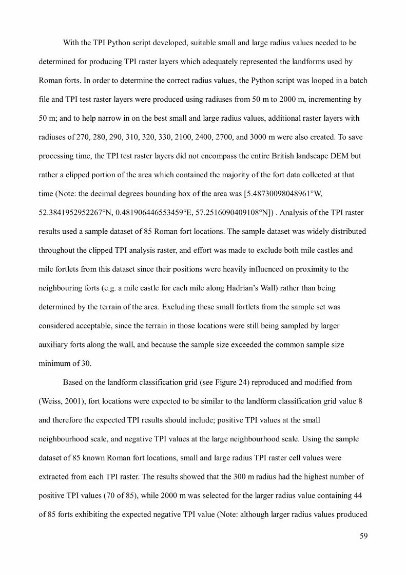
59
With the TPI Python script developed, suitable small and large radius values needed to be
determined for producing TPI raster layers which adequately represented the landforms used by
Roman forts. In order to determine the correct radius values, the Python script was looped in a batch
file and TPI test raster layers were produced using radiuses from 50 m to 2000 m, incrementing by
50 m; and to help narrow in on the best small and large radius values, additional raster layers with
radiuses of 270, 280, 290, 310, 320, 330, 2100, 2400, 2700, and 3000 m were also created. To save
processing time, the TPI test raster layers did not encompass the entire British landscape DEM but
rather a clipped portion of the area which contained the majority of the fort data collected at that
time (Note: the decimal degrees bounding box of the area was [5.48730098048961°W,
52.3841952952267°N, 0.481906446553459°E, 57.2516090409108°N]) . Analysis of the TPI raster
results used a sample dataset of 85 Roman fort locations. The sample dataset was widely distributed
throughout the clipped TPI analysis raster, and effort was made to exclude both mile castles and
mile fortlets from this dataset since their positions were heavily influenced on proximity to the
neighbouring forts (e.g. a mile castle for each mile along Hadrian‟s Wall) rather than being
determined by the terrain of the area. Excluding these small fortlets from the sample set was
considered acceptable, since the terrain in those locations were still being sampled by larger
auxiliary forts along the wall, and because the sample size exceeded the common sample size
minimum of 30.
Based on the landform classification grid (see Figure 24) reproduced and modified from
(Weiss, 2001), fort locations were expected to be similar to the landform classification grid value 8
and therefore the expected TPI results should include; positive TPI values at the small
neighbourhood scale, and negative TPI values at the large neighbourhood scale. Using the sample
dataset of 85 known Roman fort locations, small and large radius TPI raster cell values were
extracted from each TPI raster. The results showed that the 300 m radius had the highest number of
positive TPI values (70 of 85), while 2000 m was selected for the larger radius value containing 44
of 85 forts exhibiting the expected negative TPI value (Note: although larger radius values produced

60
slightly more negative TPI values such as 3000 m having 48 of 85 forts exhibiting negative TPI, the
change was very subtle between 3000 and 2000 m, therefore 2000 m was selected for the upper
radius).
Figure 24: TPI Landform Classification Grid (Weiss, 2001). Reproduced with permission from the
publisher.
The results of the TPI test based on 85 known fort locations (especially the larger TPI radius
values) were not found exclusively in the expected landform classification grid 8 or neighbouring
grids 4, 5, & 9 (see Figure 25 for a scatter plot of the small and large radius TPI results with
horizontal and vertical lines for the TPI landform classification ranges overlaid). However the
results do show an expected pattern in which most Roman forts were placed on high ground locally,
and the variation in the larger radius TPI values could be the result of locations in Britain which did
not change drastically on a larger scale (e.g. wide relatively flat valleys surrounding the hill top or
ridge in which a fort was placed). As a result, TPI radius values of 300 m and 2000 m were

61
considered reflective of the general landscape conditions chosen by Romans, and illustrate the
importance with which Romans placed forts on higher ground.
Figure 25: Small radius vs. large radius TPI scatter plot results
4.3.2.3 Fuzzy Set Theory membership functions
The use of fuzzy set theory to categorize Roman building practices began with the development
of membership functions. Using the six raster layers that represent the Roman building factors,
membership rules were developed to identify value ranges which best represent known Roman fort
locations.
The process of creating fuzzy membership functions began with the extraction of raster cell
values at known Roman fort location (137 fort locations were used in the creation of the
histograms) from each of the factors, and histograms with descriptive statistics were produced using
R to assist in the design of membership functions that reflect the data. Note: Due to the on-going
nature of the atlas, additional forts and roads have been added to the dataset since the creation of the
histograms.
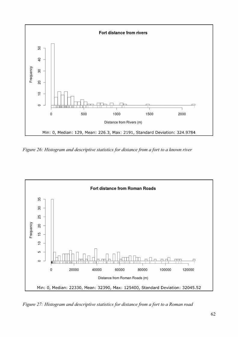
62
Figure 26: Histogram and descriptive statistics for distance from a fort to a known river
Figure 27: Histogram and descriptive statistics for distance from a fort to a Roman road

63
Figure 28: Histogram and descriptive statistics for the slope at fort locations
Based on the data distribution the following patterns were observed. Most forts were located
near rivers, and where road data were available most forts were located near Roman roads. It also
appears that as distance increases fewer forts are associated with either feature. As a result, the
range 0-200 m were given a membership value of 1 for the Roman roads raster and the range 0-300
m were represented by a membership value of 1 for the rivers raster. All values outside these ranges
were given a membership value derived from a modified inverse distance equation, since
membership appears related to distance.
Slope values appear to be more gradual in change, with most forts exhibiting a low percent rise
and gradual decrease in the number of forts having larger slope values. Consequently, a membership
function was developed which uses the narrow range of slope values between 0% – 2% being given
a membership value of 1, values between 2% and 20% will be given decreasing values of
membership, and all slope values greater than 20% will be given a value of 0.
For the two TPI Landform raster layers, membership functions were generated which accounts

64
for both small and large scale radius values. Based on the scatter plot results shown in Figure 25,
TPI values greater than -20 and less than 60 at the small scale will be given a membership value 1,
values between -20 to -100 and between 60 and 400 will have decreasing membership values, and
the remaining will be given a value of 0. Large radius TPI values which were between -20 and 10
will be given a membership value of 1, values between 10 and 160 and between -20 and -200 will
be given a gradually reduced membership values, and all other values will be given a value of 0.
Figure 29: The six fuzzy membership functions used in the analysis of Roman fort building practices

65
Lastly a membership function was used to produce a constraint raster based on distance
from forts. All raster cells which were between 22 km and 32 km away from any known fort were
given a value of 1, while all others were given a value of 0.
Table 2: Membership Functions for each factor or constraint raster
Name Membership Function
Rivers (m) A(x) = 1
300/x
for x <= 300
for x > 300
Roman Roads
(m)
A(x) = 1
200/x
for x <= 200
for x > 200
Slope (% rise) A(x) = 1
((20 - x)/(20 - 2))
0
for x <= 2
for x > 2 & x <=20
for x > 20
Proximity to
Forts (m)
A(x) = 0
1
0
for x < 22000
for x >= 22000 & x <= 32000
for x > 32000
TPI - 300m
Radius
A(x) = 0
((x + 100)/(-20 + 100))
1
((400 – x)/(400 - 60))
0
for x < -100
for x < -20 & x >= -100
for x >= -20 & x <= 60
for x > 60 & x <= 400
for x > 400
TPI - 2000m
Radius
A(x) = 0
((-200 - x)/(-200 + 20))
1
((160 – x)/(160 - 10))
0
for x <= -200
for x < -20 & x > -200
for x >= -20 & x <= 10
for x > 10 & x <= 160
for x > 160
4.3.2.4 Develop SUM, MIN and MAX fuzzy membership raster layers
Following the creation of the membership function layers, three raster datasets were produced
by examining the collective of each Roman building factor. The resulting raster layers included the
sum of each factor with each membership factor being given an equal weight, a min raster which
represents the minimum value of the five raster factors, and the max raster which represents the
maximum value of each of the five factors. After which the constraint layer was applied producing
results which were a suitable distance from known fortified locations.
4.4 Imagery site selection
WorldView-2 satellite imagery, provided by Digital Globe, offers both a high spatial and

66
spectral resolution product. It consists of eight multispectral bands (2 m cell resolution) and a
panchromatic band (0.5 m cell resolution). Due to its high resolution, it provides greater potential
for identifying subtle changes in the landscape which may not be evident in imagery with fewer
bands or larger cell sizes.
Table 3: Spectral ranges for each spectral band
Spectral Band Spectral Range
Panchromatic 450 – 800 nm
Coastal 400 – 450 nm
Blue 450 – 510 nm
Green 510 – 580 nm
Yellow 585 – 625 nm
Red 630 – 690 nm
Red-Edge 705 – 745 nm
NIR 1 770 – 895 nm
NIR 2 860 – 1040 nm
The imagery requirements for this project focused on four main considerations. The imagery
needed to be in a location with an absence of known Roman Archaeological sites (i.e. I wouldn‟t be
discovering a site which was already known), be of fine spatial resolution, be relatively free of
cloud cover, and the acquisition time had to be during the growing season (preferably during a time
of drought/dry conditions to aid in the creation of crop and soil marks).
Keeping these concerns in mind a recent WorldView-2 scene was selected, which had limited
cloud cover, an acquisition date in mid-summer, and an excellent spatial resolution.
4.5 Mulitispectral imagery analysis of chosen sites
Following the acquisition of multispectral satellite imagery, analysis for surface patterns
occurred to test the idea that the site selection analysis could be used to locate potential
archaeological sites. Multiple methods were employed to analyse the imagery, including: vegetation
indices, edge enhancements, principal component analysis, and unsupervised classification.
4.5.1 Image analysis script
The imagery analysis was performed using the PCI Geomatica remote sensing software

67
package and included the use of EASI scripts and the graphical user interface (GUI) called Focus
(Figure 30). (see Appendices for a copy of the EASI Scripts).
Figure 30: Image analysis script flowchart
4.5.1.1 Pre-processing imagery
The Worldview-2 imagery purchased for analysis was delivered as radiometrically corrected
image pixels (Updike & Comp, 2010, p.8) in the form of Raw Digital Numbers (DN), and
consequently required pre-processing before performing the image analysis. The pre-processing
was performed with EASI scripts, resulting in one pix file consisting of a composite of the lower

68
spatial resolution multispectral bands, and one for the panchromatic band. The Raw-DN values
were then converted into top of atmosphere radiance values, and finally a pre-processing step of
converting the radiance values into approximate surface reflectance values was performed using the
Dark Object Subtraction (DOS) method.
4.5.1.1.1 Converting Raw-DN to Radiance values
Conversion to top of atmosphere radiance follows a simple equation (3) (Updike & Comp,
2010, p.9). K represents the band‟s absolute radiometric calibration factor, q is the radiometrically
corrected image pixels (i.e. the Raw-DN value) and Λλ is equal to the effective bandwidth in
micrometres for a given band.
(3)
K and Λλ values were provided for each band in the imagery metadata (see Table 4), and
were used to convert raw-DN values into Radiance (see Appendices for the full EASI scripts).
Table 4: K and λ values for each spectral band
Spectral Bands K Λ λ
Panchromatic 0.05678345 0.2846000
Coastal 0.009295654 0.04730000
Blue 0.01783568 0.05430000
Green 0.01364197 0.06300000
Yellow 0.005829815 0.03740000
Red 0.01103623 0.05740000
Red Edge 0.005188136 0.03930000
NIR 1 0.01224380 0.09890000
NIR 2 0.009042234 0.09960000
4.5.1.1.2 Radiance to Surface Reflectance
In order to perform the image analysis used in this research, the Top of Atmosphere (TOA)
radiance values needed to be converted into surface reflectance values, using formula (4) (Moran et
al, cited in Chavez, 1996, p.1027).

69
(4)
Figure 31: Solar zenith angle equation with an explanation figure (Note. From 'Radiometric Use of
WorldView-2 Imagery' (Updike & Comp, 2010, p.14))
Using the metadata provided with the imagery, many of the parameters in this equation can
be solved. The solar zenith angle (TZ) can be derived by subtracting the mean sun elevation angle
of 57.7 degrees (provided by imagery metadata) from 90 (see Figure 31).
The band-averaged spectral irradiance at a given Earth Sun distance value (Eo) can be
derived once the Band-Average Solar Spectral Irradiance and the Earth-Sun Distance is determined.
The Spectral Irradiance values were obtained from documentation provided by Digital Globe
(Updike & Comp, 2010, p.6) (see Table 5).
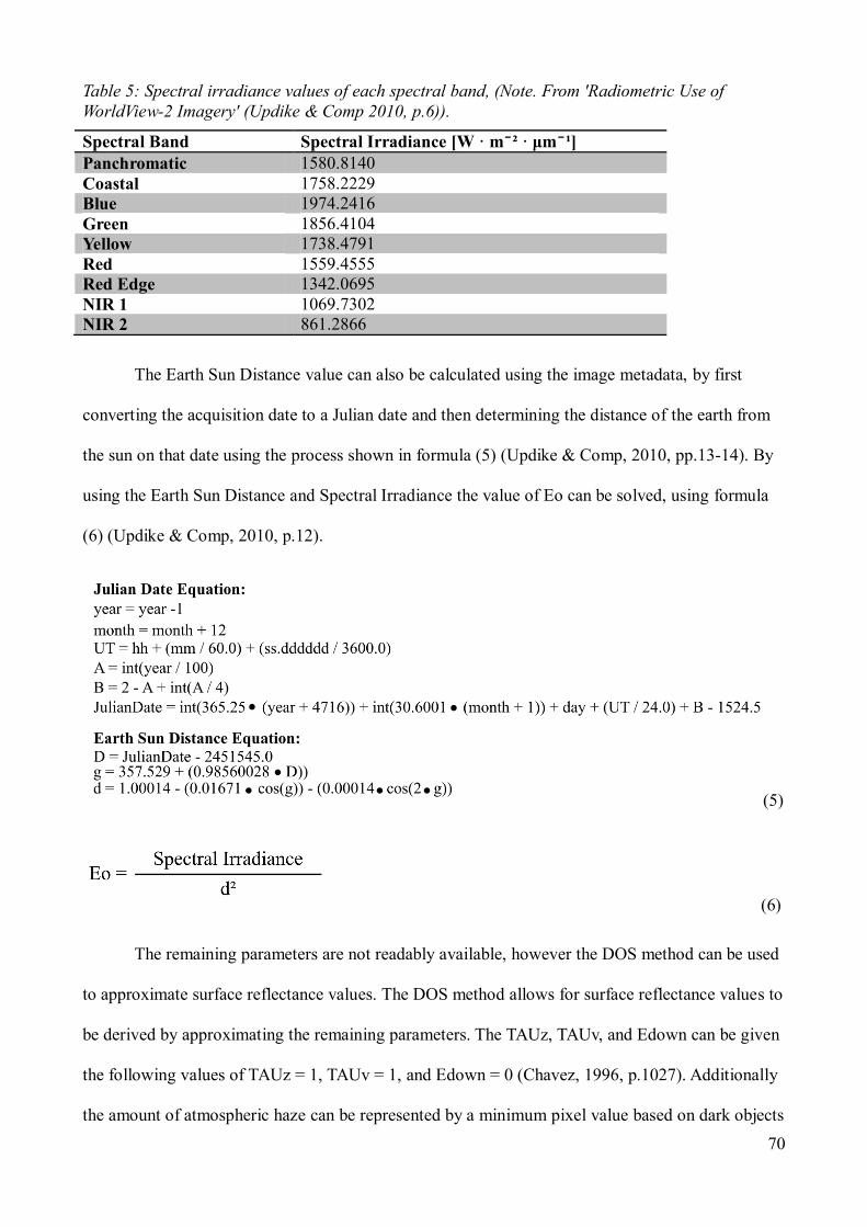
70
Table 5: Spectral irradiance values of each spectral band, (Note. From 'Radiometric Use of
WorldView-2 Imagery' (Updike & Comp 2010, p.6)).
Spectral Band Spectral Irradiance [W · m ̄ ² · μm ̄ ¹]
Panchromatic 1580.8140
Coastal 1758.2229
Blue 1974.2416
Green 1856.4104
Yellow 1738.4791
Red 1559.4555
Red Edge 1342.0695
NIR 1 1069.7302
NIR 2 861.2866
The Earth Sun Distance value can also be calculated using the image metadata, by first
converting the acquisition date to a Julian date and then determining the distance of the earth from
the sun on that date using the process shown in formula (5) (Updike & Comp, 2010, pp.13-14). By
using the Earth Sun Distance and Spectral Irradiance the value of Eo can be solved, using formula
(6) (Updike & Comp, 2010, p.12).
(5)
(6)
The remaining parameters are not readably available, however the DOS method can be used
to approximate surface reflectance values. The DOS method allows for surface reflectance values to
be derived by approximating the remaining parameters. The TAUz, TAUv, and Edown can be given
the following values of TAUz = 1, TAUv = 1, and Edown = 0 (Chavez, 1996, p.1027). Additionally
the amount of atmospheric haze can be represented by a minimum pixel value based on dark objects

71
in the imagery. The logic behind this approach is that pixels for objects in shadow will have
radiance values due to atmospheric scattering, and therefore these values can approximate the
minimum radiance values which can be subtracted from each pixel (Chavez, 1996, p.1027). Using
the histogram method (Chavez, 1988, pp.461-466), dark object minimum values were derived for
each band (see Table 6) and were substituted into the equation for the haze value.
Table 6: Min radiance values for each spectral band
Spectral Band Min Radiance Value (derived from histogram)
Panchromatic 22
Coastal 50
Blue 45
Green 25
Yellow 17
Red 11
Red Edge 9
NIR 1 4
NIR 2 2
By using the DOS method to derive the surface reflectance values, the formula shown in
Equation 4 can be simplified to the formula (7) (Chavez, 1996, p.1027).
(7)
With each of the parameters determined, surface reflectance values were calculated. (See
Appendices for a full copy of the EASI scripts used in this conversion process).
4.5.1.1 Imagery preparation
Following the conversion from Raw-DN values to surface reflectance values, two image
composites were produced for the image analysis, one pan-sharpened and the other remaining in its
original spatial resolution. By including both composites a sacrifice between spectral resolution vs.
spatial resolution was not required, providing greater opportunity to identify surface patterns.
The first image composite included all eight multispectral bands at the 2 m spatial
resolution. The second composite included four multispectral bands (Blue, Green, Red and NIR1)

72
each of which was resampled to 0.5 m in cell size to match the panchromatic band and used in
producing a pan-sharpened version of the imagery. Pan-sharpening is a technique in which higher
spatial resolution imagery is fused with higher spectral resolution imagery bands, producing higher
spatial resolution imagery containing spectral information provided by the lower spatial resolution
imagery bands.
4.5.1.2 Pan-sharpening the imagery with the Brovey method
Pan-sharpening of the Blue, Green, Red and NIR1 bands was performed using the Brovey
method (see Formula (8)) (Davidson, 2014). The Brovey method is performed by dividing each
band‟s reflectance values by the sum of the reflectance values of each band and then multiplying
this product by the panchromatic band. The final result produces four pan-sharpened bands.
(8)
4.5.1.3 Preliminary image analysis investigation
Prior to the final image analysis, a preliminary study was performed on two known
archaeological sites in Britain, the Roman forts Vindolanda and Carrawburgh. Using image analysis
methods similar to those applied in the final analysis, the preliminary investigation was intended to
guide which techniques were the most suitable for investigating Roman archaeological sites in a
British landscape.
The results of this study provided multiple considerations for the methodology of the final
image analysis. The preliminary-image analysis demonstrated greater success in identifying known
archaeological sub-surface features using vegetation indices; however it was also noted that method
success varied between the two sites. Since each site had varying method results, the continued use
of multiple image analysis techniques was considered important for the final image analysis, in
order to increase the potential identification of surface patterns.
Additionally this preliminary study showed potential surface patterns being caused by
variations in vegetation levels at known locations containing sub-surface Roman structures.

73
Although this is not definitive proof that these surface patterns were caused by Roman structures,
consideration should be given for vegetated locations in Britain when performing future image
analysis site selections.
4.5.1.4 Image analysis methods.
Various image analysis methods were used in this research, including vegetation indices, PCA,
unsupervised classifications, and edge enhancements. Although each method is performed in this
project, vegetation indices proved the most successful for enhancing surface patterns and will be the
focus of the results.
4.5.1.4.1 Vegetation Indices
Vegetation indices are one of the most common methods used to capture information about
variations in vegetation health, and base on the preliminary image analysis was the most successful
method at two known Roman fort locations. However, without knowing which vegetation indices
are the most informative for archaeological applications in Britain, 18 were performed on the 8
band composite and 9 were used on the pansharpened imagery (see Table 7).
Of the 18 vegetation indices selected for this project, many were developed specifically to
take advantage of the additional bands provided by World-View 2 satellite imagery data, including
numerous variations of the common NDVI. By applying a wide range of indices, greater
opportunity existed for identifying surface patterns caused by subtle vegetation changes.
Table 7: Vegetation Indices Listing
Vegetation
Indices
Equation Source
NDVI 1 NDVI 1 = (NIR1 - RED) / (NIR1 + RED) (Rouse, et al, 1973, p.43)
NDVI 2
(WV-WI)
NDVI 2 = (NIR2 - RED) / (NIR2 + RED) (Harris Geospatial Solutions,
2016).
NDVI 3
(FCI)
NDVI 3 = (NIR1 - RED EDGE) / (NIR1 + RED EDGE) (Xiaocheng, et al, 2012, p.5)
NDVI 4 NDVI 4 = (NIR2 - RED EDGE) / (NIR2 + RED EDGE) (Nouri, et al, 2014, p.585)
NDVI 5 NDVI 5 = (NIR2 - YELLOW) / (NIR2 + YELLOW) (Nouri, et al, 2014, p.585)

74
NDVI 6 NDVI 6 = (RED EDGE - COASTAL) / (RED EDGE + COASTAL) (Nouri, et al, 2014, p.585)
NDVI 7 NDVI 7 = (RED EDGE - RED) / (RED EDGE + RED) (Nouri, et al, 2014, p.585)
DVI DVI = NIR1 – RED (Tucker, 1979, p.134)
IPVI IPVI = NIR1 / (NIR1 + RED) (Crippen, 1990, p.72)
SAVI SAVI = ((NIR1 - RED) * (1 + 0.5)) / (NIR1 + RED + 0.5) (Huete, 1988, p.299)
MVI MVI = (NIR1 - (1.2 * RED)) / (NIR1 + RED) (Paltridge & Barber, 1988,
p.384)
SIPI SIPI = (NIR1 - BLUE) / (NIR1 + RED) (Peñuelas, & Inoue, 1999,
p.356)
GRVI GRVI = NIR1 / GREEN (Sripada, et al, cited in Harris
Geospatial Solutions, 2016).
NNIR NNIR = NIR1 / (NIR1 + RED + GREEN) (Ojala, et al, 2004, p.915)
GNDVI GNDVI = (NIR1 - GREEN) / (NIR1 + GREEN) (Gitelson & Merzlyak, 1998,
p.692)
WV-BI WV-BI = (COASTAL – RED EDGE) / (COASTAL + RED EDGE) (Harris Geospatial Solutions,
2016a).
WV-NHFD
(NHFD)
WV-NHFD = (RED EDGE – COASTAL ) / (RED EDGE +
COASTAL)
(Wolf, 2010, p.5)
NDWI NDWI = (COASTAL – NIR2) / (COASTAL + NIR2) (Wolf, 2010, p.4)
4.5.1.4.2 Unsupervised classification
Unsupervised classification is another common method used in imagery analysis for
archaeological applications. Due to subtle differences between classification methods, three
approaches were used in the analysis; ISO Clusters, Fuzzy K-Means, and K-Means. Each method
resulted in classes representing spectrally similar surface features (Lillesand, Kiefer, & Chipman,
2007, p.568), which has the potential to identify subtle patterns on the surface. Due to a speckling
effect in the results, a 3x3 averaging filter was applied to each classification result to produce a
cleaner final result.
4.5.1.4.3 Principal component analysis
Principal Component Analysis (PCA) was performed on both the original 8 band composite
and the pansharpened composite, using the original bands supplied as the eigen channels for each.
The output of the process included 7 PCA results for the first composite and 4 PCA results for the
pansharpened composite. The resulting PCA raster layers provide reducing levels of spectral
75
redundancy, with the first component representing the greatest level of scene variance in the
imagery data, and subsequent bands representing less of the variance (Lillesand, Kiefer, &
Chipman, 2007, p.529). The result of this process provides the potential for subtle features to be
visible once the redundant data is removed from the layers.
4.5.1.4.4 Edge enhancement
Roman structures were frequently linear in shape, including straight lines for many roads
and often straight walls for forts (typically in the shape of a playing card). The final imagery
analysis technique attempts to identify these linear features by applying an edge enhancement filter.
This filter was applied using the PCI Geomatica EDGE function on each of the original
multispectral bands with a filter radius value of 1 pixel, which produced a result containing
enhanced edge features in the scene.

76
Chapter 5.0: Results
This chapter is divided into three main sections, representing the results from the key stages
in the multi-method approach adopted by this project. The first stage focuses on what Roman
building practices were evident through a preliminary visual analysis of the cybercartographic atlas
map interface. The second stage covers the results from the site selection analysis. The final stage
provides details on surface patterns identified during the image analysis.
5.1 Visual analysis of the cybercartographic atlas map interface
The cybercartographic framework offers an ideal environment for a preliminary visual
examination of the collected data and for performing analysis on feature characteristics through the
use of custom widgets. Attempts to determine spatial patterns for Roman building practices were
initially performed by examining whether relations existed between feature locations of different
Roman structure types, as well as examining the characteristics of the structure (primarily the fort
size in relation to location).
Although the atlas does not contain a complete dataset of all known Roman structures in
Britain, details about the Roman occupation can still be gleaned from the atlas‟ map view. The most
striking is the clustering of forts around Wales, along the Stanegate, Hadrian‟s Wall and the
Antonine Wall. These clusters appear to correspond with the ebb and flow of Roman limits in the
province during different periods of Roman campaigns and changing patterns of occupation
(Salway, 2001, pp.100-101). Although the occupation of these forts varied over time, the clustering
of forts does indicate where significant military operations were occurring in Britain.

77
Figure 32: Roman forts along the coast line
Changing patterns in the Roman occupation are also evident in the presence of various
Roman forts along the south-eastern coast line. This coastal perimeter of forts illustrates the
growing need for a coastal defence from Saxon raiders during the later Roman occupation of Britain
(Rodgers, 2014, pp.178-179).
The atlas is also effective in showing Roman patterns of expansion in Britain. Not only are
many of the Roman towns/cities tribal capitals for various Celtic groups, but numerous fort
locations became established Roman towns/cities.

78
Figure 33: Collected Roman fort and settlement (including villas) data in the atlas
A spatial pattern emerged in which many Roman forts, camps and settlements were placed
near collected Roman road data, and equally important the spacing between forts/major settlements
along these roads was often regular. Both examples support the idea that Romans were not only
successful in developing extensive networks in their empire, but the network was also well planned.
These observations also support the decision to include proximity to roads as a factor and
fortification proximity as a constraint in the site selection analysis used in this research.
Fort locations also followed practices related to topography requirements and resource
availability. Upon examining known fort locations on the Google Physical map background, many
forts were placed on slightly higher elevated ground locally and also near flowing water (e.g. a river
or stream). This illustrates the importance Romans gave to the careful selection of topography when
constructing forts.

79
Lastly, no obvious visual pattern was seen when using the bar graph widget to examine
characteristic of fort area in relation to spatial location. Forts of various sizes were positioned
throughout Britain, which may suggest a need for a variety of fort sizes for effective governance,
but such speculation is not answerable with only visual analysis of the map.
5.2 Site selection analysis
The site selection analysis provides an overview of the specific locations identified as suitable
for a Roman fortification, as well as the post analysis investigation results. The analysis identified
41 regions of varying size as being suitable for a Roman fortification, and each region was
researched to confirm if Roman sites had previously been discovered in these locations. From this
process a final site was selected for the image analysis.
5.2.1 An overview of the site selection raster layers
The site selection analysis generated three raster layers representing the results of the Min,
Max and Sum analyses, with each raster categorizing the suitability of the landscape for Roman
fortification construction. The Min result highlighted the most ideal locations for Roman
fortifications but was heavily dependent on the presence of data being available for all factors.
Consequently if data for a single factor such as Roman roads were not available in a location the
result would be given an unsuitable site selection value. In contrast the Max reported most locations
as being suitable and was more useful in high-lighting those locations which were the least suitable.
Lastly the Sum result provided a middle of the road evaluation since each factor used in the analysis
was given an equal weight, allowing for the final suitability result to be an average of the various
factors that influence Roman building practices.
5.2.2 Investigation of 41 suitable regions
The results of each site selection raster (Min, Max and Sum) were examined and a high
threshold value was identified for selecting potential investigation sites on the map. In attempting to
select a suitable threshold value, comparisons between 0.5 (low) and 0.9 (high) were tested, which
resulted in 45 potential investigation sites being identified with a 0.5 threshold value and 38 being

80
identified with the high value of 0.9. Since the number of areas to investigate were very similar
regardless of how high the threshold was, an intermediate value of 0.75 was selected which
included 41 of the potential areas while also excluding a few of the less likely regions identified
with the 0.5 threshold. The final 41 identified regions to investigate were considered the most likely
spots to find Roman fortifications and contained a total area of ~71 km² (see Appendix B).
Using the antiquity archaeological atlas (http://www.vici.org) and an online repository of the
National Record of the Historic Environment (NRHE) for England (http://www.pastscape.org.uk),
the 41 regions were investigated to confirm if known Roman fortifications in the form of forts,
camps or defended towns/cities, existed near (within ~2 km) of the identified sites in the analysis
results. Of the 41 potential regions selected, 22 were noted as having known forts, camps or
defended cities/towns in close proximity to the areas considered likely of having Roman
fortifications. It should also be noted that various non-fortified structures such as villas, non-walled
settlements and numerous sites which were considered „possibly‟ Roman in origin were noted
during this investigation however these sites were excluded from the results.
Table 8: Site selection analysis search results
Region ID Number of Forts Number of Camps Number of defended towns/cities 0 1
1 1
2
3 1
4 1
5
6 1
7 1
8 1
9 1
10
11
12 2 1
13
14
15
16 1
17
18 1
19 1
20 1
21 1
22
23
24

81
25 3 5 1
26
27
28 1 1
29 1
30
31
32
33 1
34 1 1
35
36
37
38 2
39 1 1
40 1
Total 10 11 15
The final result of this process proved very positive with over half of the potential regions
identified as having some form of Roman fortification, which included 10 known Roman forts, 11
Roman camps and 15 defended Roman towns/cities (which were often previously the sites of
Roman forts as well). Although not every identified site resulted in a known Roman fort location,
the results do appear to indicate some level of success in modelling the human reasoning behind
Roman building practices.
5.2.3 Selection of the image analysis site
During the investigation of suitable sites for Roman fortifications, two potential locations were
noted in this process and both were identified as being defended Roman sites in the post-analysis
investigation. Each site, (the defended town of Mediolanum, and the forts/camps near Stretton, UK)
were located on either end of a small Roman road 19, and were ~48 km apart. Upon further
examination of this region, no known fortified sties have been identified between these two
locations, which provided a suitable location for further investigation with the image analysis.

82
Figure 34: Zoomed in view of the image analysis study area with neighbouring Roman sites for
context
Justification for this location stems from multiple reasons, including the travel distance of ~48
km between known Roman sites exceeding the traditional marching distance of 22 km to 32 km,
and access to water and arable land appears available in the region. Furthermore when examining
the site selection analysis results for this region without the fort proximity constraint, suitable site
locations appeared along Roman road 19, with one location being identified near higher elevated
land at a confluence of rivers and also a suitable marching distance between the two known sites
which is marked in red stripes on Figure 35.

83
Figure 35: Image analysis study area with the site selection results overlaid and the expected
location for a fortified site marked on the map
In addition to these reasons for selecting this site for the image analysis, external factors
were also considered. Performing the image analysis required availability of cloud free imagery in
the area that also had sufficient spatial resolution to distinguish patterns on the surface, and the
imagery acquisition date needed to be during the summer growing season for greater opportunity
for crop marks to be present.
5.3 Image analysis of selected sites
The results of the image analysis identified numerous patterns located in the imagery.
Although none of the results can be proven as Roman in origin without ground excavations, surface
patterns were still clearly evident, and consequently support the argument that multispectral satellite
imagery could be a valuable tool for archaeologists of the region.

84
The results collected from the image analysis were primarily provided by the vegetation
indices performed in the analysis. Image classifications, PCA, and edge enhancements all provided
less obvious patterns or no patterns at all, and consequently the results shown in this chapter will
only focus on those produced by various vegetation indices.
5.3.1 Crop marks of the Ellerton Pumping Station
During this analysis one known historic site was identified in the imagery results. A rectangular
crop mark can be seen in the NDVI 1 imagery results at a documented location of the former
Ellerton Pumping Station. The rectangular shape suggesting the existence of a former building
footprint (see Figure 36) and based on the available historical records through pastscape.org.uk
(Historic England, 2000), this location matches the grid reference position where the former
pumping station was located. Although the pumping station is more recent in origin than the Roman
sites being investigated in this research, this result does provide evidence of the value of
multispectral imagery in locating former building locations.

85
Figure 36: Rectangle negative crop marks at a known pumping station at Ellerton
5.3.2 Other surface patterns
Due to the nature of the heavily used agricultural landscape, it becomes increasing difficult to
identify crop/soil marks as Roman in origin. A geometric pattern in a field is as likely, if not more
likely the result of past farming practices, than ancient sub-surface remains. Furthermore, with the
soil being well worked, past remains may have been covered/destroyed by human efforts. Keeping
this in mind a number of surface patterns which seemed out of place were identified and may
represent various Roman or non-Roman sub-surface structures.

86
Figure 37: Image analysis result - rectangular negative crop mark(s) in a field
The first site of interest, shown in Figure 37, is located in a field which illustrates clear
variations in the level of vegetation. Patches of green can be seen next to linear stretches of varying
levels of bare soil, which become more prominent in the SAVI image results as negative crop marks
(shown as red).
This site was selected as having potential because of the linear patterns evident in the SAVI
imagery and because the field contrasts with its neighbouring fields which do not exhibit the same
level of variation in vegetation.
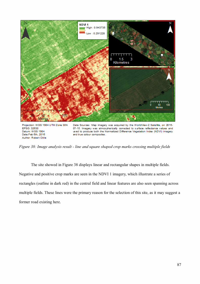
87
Figure 38: Image analysis result - line and square shaped crop marks crossing multiple fields
The site showed in Figure 38 displays linear and rectangular shapes in multiple fields.
Negative and positive crop marks are seen in the NDVI 1 imagery, which illustrate a series of
rectangles (outline in dark red) in the central field and linear features are also seen spanning across
multiple fields. These lines were the primary reason for the selection of this site, as it may suggest a
former road existing here.

88
Figure 39: Image analysis result –crop mark showing a rectangular shape next to a brook
The site shown in Figure 39 was selected for its rectangular shape and proximity to a water
source. Although many of the lines are likely caused by farming practices (especially the north west
field boundary), a double ring of green vegetation is clearly seen in the true colour imagery
suggesting greater resources being available for the plants (possibly provided by former ditches).

89
Figure 40: Image analysis result – negative crop mark showing multiple lines/corners
The next two figures were selected for the unusual geometric shapes seen in both fields. In
Figure 40, negative crop marks in the form of linear shapes are evident in the NDVI 1 imagery, and
in contrast the DVI imagery in Figure 41 shows a positive crop mark seen as a large square in the
middle of a field.
Both sites, much like the previous three, were selected for their geometric patterns in fields,
which contrast with their surroundings. Although these positive and negative crop marks are likely
the result of farming practices, they have been included to present a complete picture of all sites of
interest.

90
Figure 41: Image analysis result - square rectangular crop mark in the middle of a field
The final and arguably most interesting surface pattern seen in the image analysis results is
the positive crop mark seen in the Figure 42. In the middle of a field a distinct rounded corner
rectangle is seen, which appears out of place next to the modern agricultural landscape/field
boundaries.
This green rectangular feature may represent a ditch, and the inner yellow ring could
represent the remains of rampart/wall. Unfortunately, definitive proof of this feature‟s
origin/purpose can only come from a ground survey, which exceeds the scope of this research, but
the crop marks do suggest some form of non-farming human activity.
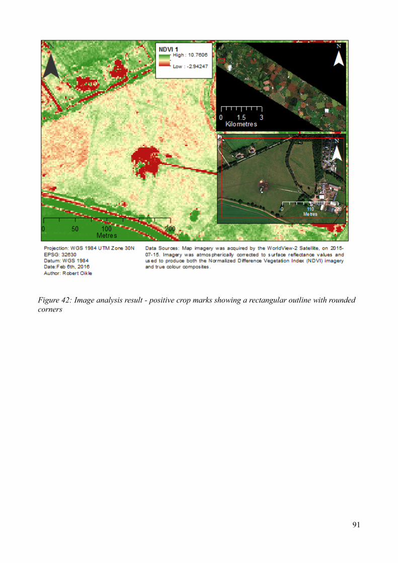
91
Figure 42: Image analysis result - positive crop marks showing a rectangular outline with rounded
corners

92
Chapter 6.0: Discussion
The use of a multi-method geomatics approach provides numerous benefits to the research
process, but a number of issues were encountered and future research considerations are needed.
The following chapter will discuss both the successes of this approach, as well as what should be
changed if adopted in the future.
6.1 Successes provided by a multi-method approach
By combining the strengths of cybercartography, GIS, fuzzy set theory, and remote sensing,
limitations of each component in this research were minimized. The cybercartographic framework
Nunaliit is an ideal platform for sharing research, collecting data, and organizing that data to fit the
needs of the project. Nunaliit, due to the nature of its design/purpose, lacks the extensive spatial
analysis library common to many GIS platforms, and is why ArcGIS was used for the site selection
analysis. Although ArcGIS provides an extensive library for analysis, it is also limited in the types
of functions available. To address this limitation, custom algorithms were developed for both the
TPI and fuzzy membership functions. Lastly, the image analysis was performed using PCI‟s
Geomatica. This software provided many of the analysis tools needed for image analysis, and
limitations in ArcGIS were side-stepped by adopting a more appropriate tool for the job.
Although the use of multiple tools can require more work on the part of the researcher, the final
analysis product is more robust, and provides greater details often excluded if research was limited
to a single tool.
6.2 Discussion of findings
The use of cybercartography, GIS with fuzzy set theory, and remote sensing, demonstrated the
value of a multi-method approach when studying the past. Through the inclusion of a wider array of
tools, greater functionality becomes available and is essential in answering the questions posed in
this research.
By using the flexible Nunaliit framework, historical data from various sources of different
degrees of spatial detail were incorporated into the atlas, including historical sketches, maps,

93
photographs, and text. Without the use of Nunaliit, many of these data sources would be difficult or
impossible to include, resulting in a smaller dataset, and prevention of various educational aids
being developed.
The merger of fuzzy set theory with the analytical power of GIS resulted in an improved
understanding of Roman building practices. With core building factors identified, the combination
of these two approaches effectively modeled the core requirements for selecting sites possibly
occupied by Roman fortifications. Although the analysis was limited to a small number of the
Roman building considerations, the results did identify 36 known Roman fortification sites. These
results suggest not only can Roman building practices be modeled but with further refinement this
suitability analysis could be an effective tool for discovering unknown archaeological sites.
Lastly, the analysis of multispectral satellite imagery provides greater detail on its
applicability in Britain. Although other remote sensing sources may be better suited to a British
landscape, the results from this study do show that vegetation indices were effective in identifying
crop and soil marks, and former building sites such as the Ellerton Pumping Station were identified.
Since this approach is possible in this region, greater attention should be given to the use of
multispectral satellite imagery for archaeological research in Britain.
6.3 Potential data errors
Although every attempt is made to minimize errors during data collection, a number of
potential sources exist. Notably these data are provided by different authors, from different time
frames and digitized using different tools. This reliance on secondary sources, although great for
spatial data collection, can introduce errors caused by incorrect assumptions generated by the
source, misinterpretations by the data recorder, errors being introduced during the digitizing
process, historical/spatial vagueness in the original record (or loss of spatial details since the
creation of the record), or even bias contained in the original source.
6.4 Challenges encountered during the analysis
Numerous challenges were encountered during this project, including issues with generating

94
membership functions, identifying appropriate sites for image analysis, purchasing suitable
imagery, and lastly imagery assessment challenges.
6.4.1 Challenges with the use of the Topographic Position Index
During the initial formulation of membership functions, the use of the Topographic Position
Index (TPI) to classify terrain types proved challenging. Roman forts are commonly placed on flat
elevated positions near water, and as a result it was expected that a TPI classification value of 8
(ridges/hills found in valleys) would represent this terrain type. Upon review of the data for known
Roman fort locations and their corresponding TPI values, it was clear that most of the forts did not
reflect this expected classification value. Although most forts had the characteristic of being placed
on high ground on a smaller local scale, and at a broader scale variation in elevation were often
minimal, resulting in much fewer TPI classification values of 8 than initially expected.
Consequently the use of a single TPI classification value was replaced by including both TPI
index values for each scale (larger regional and smaller local extents), with membership functions
being customized to reflect the data collected, instead of forcing an inaccurate classification on the
analysis.
6.4.2 Challenges with the site selection analysis results
The results from the site selection analysis were proven valid through the identification of
numerous known Roman sites which were not included in the site selection analysis. However the
success of the analysis may have been improved if the initial dataset also included defended
settlements, forts and camps. By incorporating all forms of fortified features, the results may have
included new sites not identified in this study.
6.4.3 Challenges of acquiring adequate imagery in Britain
Attempts were made to purchase imagery which were acquired during the summer, possessed
little cloud-cover, from a sensor that provides high resolution imagery, and preferably during a time
of low precipitation (e.g. during drought conditions). Due to the specific nature of the imagery
95
requirements, there were limited sources of imagery in the selected study area.
Although the final scene selected for this research was acquired in the summer, had low cloud-
cover, and was very high in spatial resolution, few imagery scenes were available to select from,
and consequently a more expensive source of imagery was purchased for this research. Additionally
it was hoped that imagery during a period of drought experienced in parts of the UK between 2010-
2012 (Met Office, 2013), would be a possible acquisition date for the imagery, but this proved
impossible and a more recent acquisition date in the summer of 2015 was selected.
6.4.4 Image analysis difficulties caused by human activities
Numerous geometric shapes were identified in the image analysis results, but the landscape of
the study area presented numerous challenges for accurately identifying archaeological remains.
Human activities in the form of urbanization and modern agriculture practices may have destroyed
or covered Roman remains in the selected study area. This was unfortunately true at the location
considered the most likely spot to find a Roman fortification (identified in Figure 35). This location
was currently occupied by fields and numerous buildings in the hamlet of Ellerton, in Shopshire,
England, which significantly hindered the use of multispectral imagery at this location.
6.5 Future research recommendations
Following the completion of this research a number of recommendations can be offered about
the methods used in the three main stages of this project. Specifically, changes to how the initial
data was collected, factors which could have improved the site selection analysis, and how imagery
analysis could yield improved results, were all discussed.
6.5.1 Recommendations for collecting data with Nunaliit
The data concerning Roman sites were collected by the author, and although this was acceptable
for the scope of this project, results could have been improved by increasing the number of
participants. By limiting the data collected to a single user, the time needed for the project was
extended and the volume of data was potentially reduced. A possible solution to this problem would

96
be utilising Nunaliit‟s strength of being a multi-user framework.
The Nunaliit framework provides a built-in and an easy approach for users around the world to
contribute to an atlas. By creating a free account, users can add data to an existing atlas, with
limited technical requirements. If the scope of this project were to increase, a more effective
approach would be to enlist the help of others interested in Roman history to improve the atlas‟
dataset. The potentially larger dataset would allow a more effective site selection analysis, and
provide new Roman building patterns to be derived as the picture of the past becomes clearer.
6.5.2 Recommendations for the site selection analysis
The site selection analysis which modeled the building patterns of Roman forts, only addressed
core factors which influenced this decision process. Other factors could be added and refined in the
analysis, which may improve the final accuracy of the identifying locations.
The analysis was limited by the data available, however if forest locations, farmlands and the
positions of all fresh water in Britain during Roman times were available, these datasets could have
been utilized in the analysis and consequently improve the accuracy of the final result.
The analysis also does not take into account temporal considerations regarding the factors
influencing the Roman fortification patterns. This is especially relevant regarding when Romans
occupied known sites, which may have influenced proximity values in the analysis. For example,
multiple forts in an area may not have been occupied at the same time, which would affect how far
away a day‟s march and consequently where a search for unknown Roman fortifications would
occur, depending on which fort was occupied, and when. To address this issue, an added dimension
for time could be added to the spatial analysis results, which would provide time intervals in order
to present a more accurate picture of Roman occupation in Britain and where fortifications may be
found both spatially and temporally.
Another possible modification to the site selection analysis is that the proximity to other Roman
fortifications constraint was derived from a Euclidean distance calculation in which areas that were
between 22 km and 32 km were considered valid places to expect Roman fortifications. This

97
process could be improved by factoring in Roman travel difficulties based on terrain considerations.
Ease of marching could be factored in using a cost-distance analysis where shorter marching
distances could be adopted in more difficult terrain, while easier travel routes (i.e. where roads or
flat ground existed) would be given longer marching distances. Furthermore travel distances could
be enhanced by measuring distances along common travel routes, instead of a straight Euclidean
distance.
Lastly the results of the site selection analysis could be improved by consulting modern experts
to determine which factors were of the greatest consideration to Roman builders. By identifying the
most important factors, appropriate weights could be assigned to each factor, providing a greater
level of accuracy in the results.
6.5.3 Recommendations for the image analysis
The image analysis was limited in the type of imagery used. By including additional sources
of imagery greater opportunity exists for locating sub-surface structures. The World-View 2
imagery provided eight fine resolution spectral bands, however by included additional sources of
imagery at different acquisition dates or with different imagery characteristics, greater potential for
new discoveries could be found. For example the use of active sensor products such as LiDAR or
RADAR would likely provide valuable information that is absent in the World-View 2 imagery and
as a result it is recommended that additional sources of imagery be incorporated for future work.
98
Chapter 7.0: Conclusion
Studying the past using a multi-method geomatics approach offers numerous advantages
which are not available when a single tool or process are adopted. This collective approach provides
a more robust result with fewer limitations and demonstrates a new approach for studying the past.
The cybercartographic framework Nunaliit provided the flexibility needed for collecting
spatial data, and was capable of visualizing this data in multiple ways. This included traditional
content in the form of text and maps, but also the development of custom widgets for finding and
analysing data, as well as interactive education aids for improving the understanding of the atlas‟
material.
The site selection analysis benefited from the combination of GIS and fuzzy set theory,
allowing for the accurate prediction of numerous Roman fortified sites. By combining the analysis
power of GIS libraries with the use of fuzzy set theory to aid in the design of new algorithms, the
site selection analysis was able to accurately model Roman building practices. The results
successfully predicted 36 fortified locations, using factors consider core to Roman building
requirements to guide where investigations should occur. Common GIS software libraries and fuzzy
set theory would find performing this analysis difficult independently, but when used
collaboratively new and increasingly accurate results are possible.
The use of the PCI Geomatica remote sensing software package was the last geomatics tool
used in this multi-method research. It provided the requirements to perform the image analysis of
the multispectral satellite imagery, in an effort to show that this form of imagery could provide
useful information in identifying potential sub-surface structures. To date the use of this technology
has been limited in Britain, however through this research many surface patterns were identified,
and a footprint of a previously known historical building was located with this process. Although
the use of this technology cannot prove the existence of archaeological remains, it does provide
another cost effective and useful source of information for planning ground investigations.
Beyond the success of employing a multi-method geomatics approach, this research has the

99
potential to influence future historical and archaeological scholarship, as well as other fields which
present spatial questions. This research provides examples of how spatial tools can be applied
outside the field of geomatics, and offers new insights on well studied topics. For example
background research on Roman fortification placements, indicated that Romans typically placed
forts on flat surfaces. However specific details on what was considered “flat” in a Roman context
are often excluded from these descriptions. By using a multi-method approach, the vagueness of the
term “flat” is replaced with a more specific definition of forts often being placed on surfaces of “0%
to 2% rise in slope, and gradually becoming less common on surfaces as the slope increased from
2% to 20%”. Although both provide a description of Romans preferring flat surfaces for building
forts, the later provides greater details on the specifics.
The study of Roman fortification building practices not only provides new insights on
Roman spatial decisions, but also offers a work flow for studying the construction of other Roman
features (e.g. roads, towns, etc) and could even be extended to the study of other cultures. By
adopting a flexible multi-method geomatics approach, spatial practices can be modeled and offer
insights on topics through the use of a new methodology.
This multi-method approach attempted to show the value of combining multiple tools and
processes in order to produce more robust results that would not be possible if these tools were used
independently. By expanding methodology to include a wide range of techniques, limitations in the
technology designs can be overcome and provides greater opportunities for new discoveries even in
well studied fields.

100
Appendices
Appendix A Metadata for datasets used in this research
Dataset Metadata
Shuttle
Radar
Topography
Mission 1
(SRTM) -
Digital
Elevation
Model (1
Arc
Second)
Originators: U.S. Geological Survey (USGS), National Geospatial-Intelligence Agency
(NGA), and National Aeronautics and Space Administration (NASA)
Format: GeoTiff
Acquistion Date: February 11, 2000
Publication Date: September 23, 2014
Publication Place: Sioux Falls, South Dakota
Publisher: USGS Earth Resources Observations and Science (EROS) Center
SRTM data acquired from http://earthexplorer.usgs.gov/:
n49_w002_1arc_v3.tif, n49_w003_1arc_v3.tif, n49_w006_1arc_v3.tif,
n49_w007_1arc_v3.tif, n50_e000_1arc_v3.tif, n50_e001_1arc_v3.tif,
n50_w001_1arc_v3.tif, n50_w002_1arc_v3.tif, n50_w003_1arc_v3.tif,
n50_w004_1arc_v3.tif, n50_w005_1arc_v3.tif, n50_w006_1arc_v3.tif, n51_e000_1arc_v3.tif, n51_e001_1arc_v3.tif, n51_e002_1arc_v3.tif,
n51_w001_1arc_v3.tif, n51_w002_1arc_v3.tif, n51_w003_1arc_v3.tif,
n51_w004_1arc_v3.tif, n51_w005_1arc_v3.tif, n51_w006_1arc_v3.tif,
n51_w008_1arc_v3.tif, n51_w009_1arc_v3.tif, n51_w010_1arc_v3.tif,
n51_w011_1arc_v3.tif, n52_e000_1arc_v3.tif, n52_e001_1arc_v3.tif,
n52_w001_1arc_v3.tif, n52_w002_1arc_v3.tif, n52_w003_1arc_v3.tif,
n52_w004_1arc_v3.tif, n52_w005_1arc_v3.tif, n52_w006_1arc_v3.tif,
n52_w007_1arc_v3.tif, n52_w008_1arc_v3.tif, n52_w009_1arc_v3.tif,
n52_w010_1arc_v3.tif, n52_w011_1arc_v3.tif, n53_e000_1arc_v3.tif,
n53_w001_1arc_v3.tif, n53_w002_1arc_v3.tif, n53_w003_1arc_v3.tif,
n53_w004_1arc_v3.tif, n53_w005_1arc_v3.tif, n53_w006_1arc_v3.tif, n53_w007_1arc_v3.tif, n53_w008_1arc_v3.tif, n53_w009_1arc_v3.tif,
n53_w010_1arc_v3.tif, n53_w011_1arc_v3.tif, n54_w001_1arc_v3.tif,
n54_w002_1arc_v3.tif, n54_w003_1arc_v3.tif, n54_w004_1arc_v3.tif,
n54_w005_1arc_v3.tif, n54_w006_1arc_v3.tif, n54_w007_1arc_v3.tif,
n54_w008_1arc_v3.tif, n54_w009_1arc_v3.tif, n54_w010_1arc_v3.tif,
n54_w011_1arc_v3.tif, n55_w002_1arc_v3.tif, n55_w003_1arc_v3.tif,
n55_w004_1arc_v3.tif, n55_w005_1arc_v3.tif, n55_w006_1arc_v3.tif,
n55_w007_1arc_v3.tif, n55_w008_1arc_v3.tif, n55_w009_1arc_v3.tif,
n56_w003_1arc_v3.tif, n56_w004_1arc_v3.tif, n56_w005_1arc_v3.tif,
n56_w006_1arc_v3.tif, n56_w007_1arc_v3.tif, n56_w008_1arc_v3.tif,
n57_w002_1arc_v3.tif, n57_w003_1arc_v3.tif, n57_w004_1arc_v3.tif,
n57_w005_1arc_v3.tif, n57_w006_1arc_v3.tif, n57_w007_1arc_v3.tif, n57_w008_1arc_v3.tif, n57_w009_1arc_v3.tif, n58_w003_1arc_v3.tif,
n58_w004_1arc_v3.tif, n58_w005_1arc_v3.tif, n58_w006_1arc_v3.tif,
n58_w007_1arc_v3.tif, n58_w008_1arc_v3.tif, n59_w002_1arc_v3.tif,
n59_w003_1arc_v3.tif, n59_w004_1arc_v3.tif, n59_w005_1arc_v3.tif,
n59_w006_1arc_v3.tif, n59_w007_1arc_v3.tif
Rivers
Dataset (OS
Open
Rivers)
Publisher: Ordnance Survey
Product: OS Open Rivers
Format: Shape file
Data structure: Vector points and lines
Scale: 1:15 000 to 1:30 000
Update frequency: Twice a year – April and October
Coverage: Great Britain
Licence: http://os.uk/opendata/licence

101
URL: https://www.ordnancesurvey.co.uk/business-and-government/products/os-open-
rivers.html
WorldView-
2 imagery
Publisher: Copyright 2015 DigitalGlobe Incorporated, Longmont CO USA 80503-6493
Format: GeoTIFF
Satellite ID: WV02
Mode: FullSwath
scanDirection: Forward
Acquistion Date: 2015-07-15
imageDescriptor: ORStandard2A
cloudCover: 0.005
productLevel : LV2A
productType: Standard
radiometricLevel: Corrected
radiometricEnhancement: Off
bitsPerPixel: 16
Roman
historical
sites
Various sources, including;
Bidwell, P.T, Bridgewater, R, & Silvester, R.J. 1979, 'The Roman Fort at Okehampton,
Devon', Britannia, vol.10, pp. 255-258, Available from: http://www.jstor.org/stable/526061
[25 August 2014]
Brading Roman Villa, 2015. Available from: <http://www.bradingromanvilla.org.uk>. [Sept
8th, 2015].
Breeze, D. 2006, Hadrian's Wall, English Heritage, London, England.
Breeze, D.J. & Dobson, B. 2000, Hadrian's Wall, 4th Ed, Penguin Books, London, England.
Bruce, Rev. John Collingwood, M.A. 1851, The Roman Wall: A Historical, Topographical
and Descriptive Account of the Barrier of the Lower Isthmus, Extending from the Tyne to the
Solway, Deduced from Numerous Personal Surveys, John Russell Smith, London.
Burnham, B.C, Hunter, F, Booth, P, Worrell, S, Tomlin, R.S.O, & Hassall, M.W.C. 2007,
'Roman Britain in 2006, Britannia, vol.38, pp.241-366, Available from:
http://www.jstor.org/stable/30030578 [7 August 2014]
Burnham, B.C, Hunter, F, Fitzpatrick, A.P, Hassall, M.W.C, & Tomlin, R.S.O. 2003, 'Roman
Britain in 2002', Britannia, vol. 34, pp. 293-359+361-382, Available from:
http://www.jstor.org/stable/3558552 [14 August 2014]
Burnham, B.C, Hunter, F, Fitzpatrick, A.P, Worrell, S, Hassall, M.W. C, & Tomlin, R.S.O.
2004, 'Roman Britain in 2003', Britannia, vol. 35, pp. 253-349, Available from:
http://www.jstor.org/stable/4128635 [14 August 2014]
Chapman, E.M, Hunter, F, Booth, P, Wilson, P, Pearce, J, Worrell, S, & Tomlin, R.S.O. 2012, 'Roman Britain in 2011: I. Sites Explored, II. Finds Reported Under The Portable Antiquities
Scheme, III. Inscriptions', Britannia, vol. 43, pp. 271-354, doi:10.1017/S0068113X12000451,
Available from: http://journals.cambridge.org/article_S0068113X12000451 [14 Aug 2014]
Chapman, E.M, Hunter, F, Booth, P, Wilson, P, Worrell, S, & Tomlin, R.S.O. 2009, 'Roman
Britain in 2008', Britannia, vol. 40, pp. 219-364, Available from:
http://www.jstor.org/stable/27793241 [14 August 2014]
Chapman, E.M, Hunter, F, Booth, P, Wilson, P, Worrell, S, & Tomlin, R.S.O. 2010, 'Roman
Britain in 2009', Britannia, vol. 41, pp. 341-469, Available from:
http://www.jstor.org/stable/41725172 [14 August 2014]

102
Clayton, P.A. (ed.), 1980, A Companion to Roman Britain, Phaidon Press Limited, Oxford
Cunliffe, B, Reece, R, Henig, M, Hawkes, S.C, Care, V, & Young, C.J. 1980, 'Excavation at
the Roman Fort at Lympne, Kent 1976-78', Britannia, vol. 11, pp.227-288, Available from:
http://www.jstor.org/stable/525682 [24 August 2014]
Derwent Riverside Project 2008, Malton Castle Garden - Welcome. Available from:
http://www.maltoncastlegarden.org.uk. [15 October 2015]
Durham County Council 2009, Conservation Area Appraisal Ebchester, Available from:
http://www.durham.gov.uk/media/3556/Ebchester-Conservation-Area-
Appraisal/pdf/EbchesterConservationAreaCharacterAppraisal.pdf. [12 October 2015].
Frere, S.S, Hassall, M.W.C, & Tomlin, R.S.O. 1977, 'Roman Britain in 1976', Britannia, vol.
8, pp. 355-449, Available from: http://www.jstor.org/stable/525911 [7 August 2014]
Frere, S.S, Hassall, M.W.C, & Tomlin, R.S.O. 1986, 'Roman Britain in 1985', Britannia,
vol.17, pp.363-454, Available from: http://www.jstor.org/stable/526562 [7 August 2014]
Frere, S.S and St Joseph, J.K.S, 1983, Roman Britain From the Air, Cambridge University
Press, Cambridge, Great Britain.
Goodburn, R, Hassall, M.W.C, & Tomlin, R.S.O. 1979, 'Roman Britain in 1978', Britannia,
vol.10, pp.267-356, Available from: http://www.jstor.org/stable/526068 [7 August 2014]
Goodburn, R, Wright, R.P, Hassall, M.W.C, & Tomlin, R.S.O. 1976, 'Roman Britain in 1975',
Britannia, vol. 7, pp. 290-392, Available from: http://www.jstor.org/stable/525786 [7 August
2014]
Grew, F. O, Hassall, M. W. C, & Tomlin, R. S. O. 1981, 'Roman Britain in 1980', Britannia, vol. 12, pp. 313-396, Available from: http://www.jstor.org/stable/526267 [7 August 2014]
Holder, P. A. 1982, The Roman Army in Britain, B T Batsford Ltd, London
Johnson, A. 1983, Roman Forts of the 1st and 2nd centuries AD in Britain and the German Provinces, Adam & Charles Black (Publishers) Ltd, London.
Laing, L. 1979, Celtic Britain, Routledge & Kegan Paul Ltd, London
Manley, J, Rudkin, D, Sykes, N, Lyne, M, Dannell, G, Scaife, R, Somerville, L, Barber, L,
Allen, D, Williams, D, Pelling, R, & Clegg, S. 2005, 'A Pre-A.D. 43 Ditch at Fishbourne Roman Palace, Chichester', Britannia, vol. 36, pp. 55-99, Available from:
http://www.jstor.org/stable/30030480 [24 August 2014]
Margary, I. D. 1967, Roman Roads In Britain, Humanities Press Inc., New York
Maxwll, G.S & Wilson, D.R. 1987, 'Air Reconnaissance in Roman Britain 1977-84', Britannia, vol. 18, pp. 1-48, Available from: http://www.jstor.org/stable/526438 [16 August
2014]
Moore, H & Wilmot, T. 2001, 'Centre for Archaeology Report 102/2001: Hadrian's Wall
Milecastle 14 (March Burn), Northumberland: Interim Report on Archaeological Evaluation,
September 2000', English Heritage, 2001, available from: http://research.english-
heritage.org.uk/report/?8175 accessed July 15, 2014.
'Roman Britain in 1944: I. Sites Explored: II'. Inscriptions, 1945, The Journal of Roman
Studies, vol. 35, parts 1 and 2, pp.79-92, Available from: http://www.jstor.org/stable/297281
[7 August 2014]
St Joseph, J.K. 1955, 'Air Reconnaissance in Britain, 1951-5', The Journal of Roman Studies,
Vol. 45, Parts 1 and 2, pp.82-91, Available from: http://www.jstor.org/stable/298747 [16 August 2014]

103
St Joseph, J.K. 1958, 'Air Reconnaissance in Britain, 1955-7', The Journal of Roman Studies,
Vol. 48, no.1/2, pp.86-101, Available from: http://www.jstor.org/stable/298217 [16 August
2014]
St Joseph, J.K. 1973, 'Air Reconnaissance in Britain, 1969-72', The Journal of Roman Studies,
vol. 63, pp. 214-246, Available from: http://www.jstor.org/stable/299178 [16 August 2014]
St Joseph, J.K. 1977, 'Air Reconnaissance in Roman Britain, 1973-76', The Journal of Roman
Studies, vol. 67, pp.125-161, Available from: http://www.jstor.org/stable/299924 [16 August
2014]
Symonds, M.F.A & Mason, D.J.P (eds). 2009. Frontiers of Knowledge. A Research Framework for Hadrian's Wall, Part of the Frontiers of the Roman Empire World Heritage
Site. Volume 1 Resource Assessment. Durham University/English Heritage/Durham County
Council, Durham, Available From
https://www.dur.ac.uk/resources/archaeology/pdfs/research/Vol_1_Resource_Assessment.pdf.
Todd, M. 1985, 'The Roman Fort at Bury Barton, Devonshire', Britannia, vol.16. pp.49-55,
Available from: http://www.jstor.org/stable/526394 [25 August 2014]
Wilmot, T. 2001. 'Centre for Archaeology Report 100/2001: Hadrian's Wall Milecastle 9
(Chapel House), Tyne and Wear: Interim Report on Archaeological Evaluation, September
2000', English Heritage, 2001, available from: http://research.english-
heritage.org.uk/report/?8173 accessed July 14, 2014.
Wilmot, T. 2001a. 'Centre for Archaeology Report 103/2001: Hadrian's Wall Milecastle 63
(Walby, West), Cumbria: Interim Report on Archaeological Evaluation, September 2000', English Heritage, 2001, available from: http://research.english-heritage.org.uk/report/?8176
accessed July 15, 2014.
Wilmot, T (ed). 2009, Hadrian's Wall: Archaeological Research by English Heritage 1976-
2000, English Heritage, Swindon, England.
Wilson, D. R, Wright, R. P, & Hassall, M. W. C. 1971, 'Roman Britain in 1970', Britannia, vol. 2, pp. 242-304, Available from: http://www.jstor.org/stable/525817 [14 August 2014]
Wilson, R.J.A. 1975, A guide to the Roman Remains in Britain, Constable, London
Wright, R.P. 1941, 'Roman Britain in 1940: I. Sites Explored: II. Inscriptions', The Journal of Roman Studies, Vol. 31, pp. 128-148, Available from:
http://http://www.jstor.org/stable/297109 [8 August 2014]
Wright, R.P, 1950, 'Roman Britain in 1949: I. Sites Explored: II. Inscriptions', The Journal of
Roman Studies, vol. 40, Parts 1 and 2, pp. 92-118, Available from:
http://www.jstor.org/stable/298508 [8 August 2014]
Polygon of
Britain
(produced
from the
OS Open
Data –
Boundary
Line™)
Publisher: Ordnance Survey
Product: Boundary-Line
Format: Shape file
Data structure: Vector
Scale: 1:10 000
Update frequency: Twice a year – May and October
Coverage: Great Britain
Licence: www.ordnancesurvey.co.uk/opendata/licence
URL: https://www.ordnancesurvey.co.uk/business-and-government/products/boundary-
line.html

104
Appendix B Site selection results of the 41 regions investigated

105

106

107
Figure 43: Site selection analysis results for 41 regions

108
Appendix C generateTPI.py script
# Program Name: generateTPI.py
# Description: Script for producing TPI Rasters with a defined radius
# Parameter: <DEM file name> <Radius in meters for defining neighbourhood size in TPI analysis>
# Usage Example: generateTPI.py DEM.tif 500
# Author: Robert Oikle
# Version: 1.0
# import modules
import arcpy, sys, os, time
from arcpy import env
from arcpy.sa import *
# Enable Spatial-Analyst Extension
arcpy.CheckOutExtension("Spatial")
# Initialize Global Variables
RADIUS = ""
TPIFileName = ""
TPI = ""
TPIMean = ""
TPISTD = ""
MeanElev = ""
DEM = ""
TPIZonalStatsTable = 'tpiZonalStats.dbf'
clip = "C:/siteselection/BNGData/testanalysis/miniclip.shp"
# ####################################################################################
# TPI Functions
# ####################################################################################
# Function: parameterSummary
# Description: Provides a short summary of the the parameters used by
# the arcpy environment and by this script
def parameterSummary():
# Print summary of environmental parameters
print "------------------------------------------------------------------"
print "Workspace: " + str(arcpy.env.workspace)
print "Scratch Workspace: " + str(arcpy.env.scratchWorkspace)
print "Over Write Files: " + str(arcpy.env.overwriteOutput)
print "EPSG: " + str(arcpy.env.outputCoordinateSystem)
print "Bounding Box: " + str(arcpy.env.extent)
print "Mask: " + str(arcpy.env.mask)
print "Cell Size: " + str(arcpy.env.cellSize)
print "Digital Elevation Model (DEM): " + str(DEM)
print "Neighbourhood Radius (m): " + str(RADIUS)
print "------------------------------------------------------------------\n"
# Function: setEnvironmentalParameters()
def setEnvironmentalParameters():
# Open TPISettings File
TPISettings = open('generateTPI.ini', 'r')
EXTENT = [0,0,0,0]
for line in TPISettings:
if line.find('workspace', 0) > -1:
arcpy.env.workspace = line.lstrip('workspace=').rstrip('\n')
elif line.find('scratchWorkspace', 0) > -1:
arcpy.env.scratchWorkspace = line.lstrip('scratchWorkspace=').rstrip('\n')
elif line.find('overwriteOutput', 0) > -1:
arcpy.env.overwriteOutput = line.lstrip('overwriteOutput=').rstrip('\n')
elif line.find('EPSG', 0) > -1:
arcpy.env.outputCoordinateSystem =
arcpy.SpatialReference(int(line.lstrip('EPSG=').rstrip('\n')))
elif line.find('bboxLeft', 0) > -1:
EXTENT[0] = float(line.lstrip('bboxLeft=').rstrip('\n'))
elif line.find('bboxBottom', 0) > -1:
EXTENT[1] = float(line.lstrip('bboxBottom=').rstrip('\n'))
elif line.find('bboxRight', 0) > -1:
EXTENT[2] = float(line.lstrip('bboxRight=').rstrip('\n'))
elif line.find('bboxTop', 0) > -1:
EXTENT[3] = float(line.lstrip('bboxTop=').rstrip('\n'))
elif line.find('cellSize', 0) > -1:
arcpy.env.cellSize = line.lstrip('cellSize=').rstrip('\n')
elif line.find('mask', 0) > -1:
arcpy.env.mask = line.lstrip('mask=').rstrip('\n')
#Define extent based on Extent values
arcpy.env.extent = arcpy.Extent(EXTENT[0], EXTENT[1], EXTENT[2], EXTENT[3])

109
# Close TPISettings File
TPISettings.close()
# Function: meanElevation
# Parameters: DEMinput (string of DEM file name), zonalRadius (radius value in metres).
# Description: Function which creates a mean elevation raster based on a defined window size
def meanElevation(DEMinput, zonalRadius):
print "Creating Mean Elevation Raster ..."
# define name of output Mean Elevation File.
MeanDEMName = str(DEMinput).rstrip('.tif') + "_MD.tif"
# define neighbourhood
neighbourhoodDef = "Circle " + str(zonalRadius) + " MAP"
# Calculate focal statistics
arcpy.gp.FocalStatistics_sa(DEMinput,MeanDEMName,neighbourhoodDef,"MEAN","DATA")
print "Finished Mean Elevation Raster"
return MeanDEMName;
# Function: createTPI
# Parameters: DEMinput (string of DEM file name), MeanDEMinput (string of MeanDEM file name),
# TPIOutput (output location of TPI Raster)
# Description: Function which creates a TPI raster
def createTPI(DEMinput, MeanDEMinput, TPIOutput):
print "Creating TPI Raster ..."
global DEM, MeanElev
DEM = arcpy.Raster(DEMinput)
MeanElev = arcpy.Raster(MeanDEMinput)
result = arcpy.sa.Int(Plus(Minus(DEM, MeanElev),0.5))
result.save(TPIOutput)
print "Finished TPI Raster"
# Function: getMean
# Parameter: zonalStatsTable
# Description: Function which returns mean found in first row of zonal statistics table
def getMean(zonalStatsTable):
# Create search cursor and iterate through fields to retrieve mean value
cursor = arcpy.SearchCursor(zonalStatsTable)
row = cursor.next()
mean = row.getValue('MEAN')
return float(mean);
# Function: getSTD
# Parameter: zonalStatsTable
# Description: Function which returns standard deviation found in first row of
# zonal statistics table
def getSTD(zonalStatsTable):
# Create search cursor and iterate through fields to retrieve standard deviation value
cursor = arcpy.SearchCursor(zonalStatsTable)
row = cursor.next()
std = row.getValue('STD')
return float(std);
# Function: standardizeTPI
# Parameters: TPIRaster (string of TPI raster file name),
# stdTPIOutput (string of the standardized tpi raster file being created)
# Description: Function which standardizes TPI raster
def standardizeTPI(TPIRaster, stdTPIOutput):
global TPIMean, TPISTD, TPI
#Set TPI Value
TPI = arcpy.Raster(TPIRaster)
# Produce zonal statistics for TPI Raster
print "Calculating Zonal Statistics for TPI Rasters ..."
arcpy.gp.ZonalStatisticsAsTable_sa(clip,"FID",TPI,TPIZonalStatsTable,"DATA","ALL")
# Set TPIMean and TPISTD values
TPIMean = getMean(TPIZonalStatsTable)
print " - Mean: " + str(TPIMean)
TPISTD = getSTD(TPIZonalStatsTable)
print " - Standard Deviation: " + str(TPISTD)
print "Finished Calculating Zonal Statistics for TPI Rasters"
print "Standardize TPI raster ..."
# Produce Standardized TPI Raster
results = arcpy.sa.Int(Plus(Times(Divide(Minus(TPI, TPIMean), TPISTD), 100), 0.5))
results.save(stdTPIOutput)
print "Finished standardizing TPI raster"
# ####################################################################################
if len(sys.argv) <= 2:

110
print "Please provide a dem file and radius (m) value as parameters – e.g. generateTPI.py
DEM.tif 500"
else:
DEM = str(sys.argv[1])
RADIUS = sys.argv[2]
TPIFileName = "tpi" + str(RADIUS) + ".tif"
print " ___________________________________________________________ "
print "| _____________ _________ _____________ |"
print "| /____________/| /________/\ /____________/| |"
print "| |_____ _____|/ | _____ \ \ |____ ____|/ |"
print "| | | | | | | \ \ | | | | |"
print "| | | | | | |___| | | | | | |"
print "| | | | | |/___/ |/ | | | |"
print "| | | | | _______/ | | | |"
print "| | | | | | | ___| | |____ |"
print "| | | | | | | /___| |/____/| |"
print "| |__|/ |__|/ |____________|/ |"
print "| |"
print "| -= Topographic Position Index Raster Generator - v.1.0 =- |"
print "|___________________________________________________________|\n"
# Define environmental parameters
try:
print "Defining environmental parameters ..."
# Set Environmental Parameters
setEnvironmentalParameters()
# Print summary of environmental parameters
parameterSummary()
print "--------------------------------------------------------------\n"
print "Starting TPI script @ " + time.strftime("%b %d, %Y %H:%M:%S",
time.localtime(time.time())) + "..."
print "--------------------------------------------------------------"
try:
createTPI(DEM, meanElevation(DEM, RADIUS), TPIFileName)
except:
print "Error while creating TPI raster: ", sys.exc_info()[0]
try:
standardizeTPI(TPIFileName, str(TPIFileName).rstrip('.tif') + "_s.tif")
except:
print "Error encountered while standardizing TPI Raster: ", sys.exc_info()[0]
except:
print "Error while defining environmental parameters: ", sys.exc_info()[0]
print "\n--------------------------------------------------------------"
print "Finished TPI script " + time.strftime("%b %d, %Y %H:%M:%S", time.localtime(time.time()))
print "--------------------------------------------------------------\n"
Appendix D generateTPI.ini (used by the generateTPI.py script)
workspace=C:/siteselection/analysis
scratchWorkspace=C:/siteselection/analysis/temp
overwriteOutput=True
EPSG=27700
bboxLeft=34415.719961468
bboxBottom=-100110.890701867
bboxRight=692664.68166540
bboxTop=1023309.41095295
cellSize=25.21253875
mask=C:/siteselection/analysis/mask.shp

111
Appendix E euclideanDistanceProcessing.py script
# Program Name: euclideanDistanceProcessing.py
# Description: Script for preparing site selection data for slope and Euclidean distance rasters.
# Author: Robert Oikle
# Version: 1.0
# import modules
import arcpy, sys, os, time, math
from arcpy import env
from arcpy.sa import *
print "--------------------------------------------------------------"
print "Starting Euclidean distance processing script - " + time.strftime("%b %d, %Y %H:%M:%S",
time.localtime(time.time()))
print "--------------------------------------------------------------\n"
# Enable Spatial-Analyst Extension
arcpy.CheckOutExtension("Spatial")
# Define environmental parameters
print "Defining environmental parameters - " + time.strftime("%b %d, %Y %H:%M:%S",
time.localtime(time.time()))
arcpy.env.workspace = "C:/siteselection/analysis/"
arcpy.env.scratchWorkspace = "C:/siteselection/analysis/temp/"
arcpy.env.compression = 'LZW'
arcpy.env.overwriteOutput = True
arcpy.env.outputCoordinateSystem = arcpy.SpatialReference(27700)
arcpy.env.extent = arcpy.Extent(34415.7199614685, -100110.890701866, 692664.681665404,
1023309.41095295)
arcpy.env.cellSize = 25.21253875
arcpy.env.mask = "C:/siteselection/analysis/mask.shp"
# Create directory string variables
dataDir = "C:/siteselection/data/"
DEM = "C:/siteselection/analysis/DEM.tif"
romanForts = "C:/siteselection/analysis/RomanForts_Oct25_2015_BNG.shp"
romanRoads = "C:/siteselection/analysis/RomanRoads_Nov21_BNG.shp"
rivers = "C:/siteselection/analysis/Rivers.shp"
romanFortsEucDist = "C:/siteselection/analysis/romanFortsEucDist.tif"
romanRoadsEucDist = "C:/siteselection/analysis/romanRoadsEucDist.tif"
riversEucDist = "C:/siteselection/analysis/riversEucDist.tif"
# Produce slope raster
print "Creating Slope (%) Raster - " + time.strftime("%b %d, %Y %H:%M:%S",
time.localtime(time.time()))
ElevationRaster = arcpy.Raster(DEM)
outputSlope = arcpy.sa.Int(arcpy.sa.Slope(ElevationRaster, "PERCENT_RISE"))
outputSlope.save("slopePercent.tif")
arcpy.CopyRaster_management("C:/siteselection/analysis/slopePercent.tif",
"C:/siteselection/analysis/slopePercent_LZW.tif")
arcpy.Delete_management("C:/siteselection/analysis/slopePercent.tif")
print "Finished Slope (%) Raster - " + time.strftime("%b %d, %Y %H:%M:%S",
time.localtime(time.time()))
# Produce euclidean distance raster for Roman Forts
print "Creating Euclidean Distance raster for Roman forts - " + time.strftime("%b %d, %Y %H:%M:%S",
time.localtime(time.time()))
RomanFortsEucDistance = arcpy.sa.EucDistance(romanForts,"#",arcpy.env.cellSize,"#")
RomanFortsEucDistance.save(romanFortsEucDist)
arcpy.CopyRaster_management("C:/siteselection/analysis/romanFortsEucDist.tif",
"C:/siteselection/analysis/romanFortsEucDist_LZW.tif")
arcpy.Delete_management("C:/siteselection/analysis/romanFortsEucDist.tif")
print "Finished generating euclidean distance Roman forts raster - " + time.strftime("%b %d, %Y
%H:%M:%S", time.localtime(time.time()))
# Produce euclidean distance raster for Roman Roads
print "Creating Euclidean Distance raster for Roman roads - " + time.strftime("%b %d, %Y %H:%M:%S",
time.localtime(time.time()))
RomanRoadsEucDistance = arcpy.sa.EucDistance(romanRoads,"#",arcpy.env.cellSize,"#")
RomanRoadsEucDistance.save(romanRoadsEucDist)

112
arcpy.CopyRaster_management("C:/siteselection/analysis/romanRoadsEucDist.tif",
"C:/siteselection/analysis/romanRoadsEucDist_LZW.tif")
arcpy.Delete_management("C:/siteselection/analysis/romanRoadsEucDist.tif")
print "Finished generating euclidean distance Roman roads raster - " + time.strftime("%b %d, %Y
%H:%M:%S", time.localtime(time.time()))
# Produce euclidean distance raster for Rivers
print "Creating Euclidean Distance raster for rivers - " + time.strftime("%b %d, %Y %H:%M:%S",
time.localtime(time.time()))
riversEucDistance = arcpy.sa.EucDistance(rivers,"#",arcpy.env.cellSize,"#")
riversEucDistance.save(riversEucDist)
arcpy.CopyRaster_management("C:/siteselection/analysis/riversEucDist.tif",
"C:/siteselection/analysis/riversEucDist_LZW.tif")
arcpy.Delete_management("C:/siteselection/analysis/riversEucDist.tif")
print "Finished generating euclidean distance rivers raster - " + time.strftime("%b %d, %Y
%H:%M:%S", time.localtime(time.time()))
print "\n--------------------------------------------------------------"
print "Finishing euclidean distance processing script - " + time.strftime("%b %d, %Y %H:%M:%S",
time.localtime(time.time()))
print "--------------------------------------------------------------"
Appendix F membershipFunctions.py script
# Program Name: membershipFunctions.py
# Description: Script for producing membership function raster layers
# Author: Robert Oikle
# Version: 1
# import modules
import arcpy, sys, os, time, math
from arcpy import env
from arcpy.sa import *
print "--------------------------------------------------------------"
print "Starting Membership Function Rasters script - " + time.strftime("%b %d, %Y %H:%M:%S",
time.localtime(time.time()))
print "--------------------------------------------------------------\n"
# Enable Spatial-Analyst Extension
arcpy.CheckOutExtension("Spatial")
# Define environmental parameters
print "Defining environmental parameters - " + time.strftime("%b %d, %Y %H:%M:%S",
time.localtime(time.time()))
arcpy.env.workspace = "C:/siteselection/analysis/"
arcpy.env.scratchWorkspace = "C:/siteselection/analysis/temp/"
arcpy.env.compression = 'LZW'
arcpy.env.overwriteOutput = True
arcpy.env.outputCoordinateSystem = arcpy.SpatialReference(27700)
arcpy.env.extent = arcpy.Extent(34415.7199614685, -100110.890701866, 692664.681665404,
1023309.41095295)
arcpy.env.cellSize = 25.21253875
arcpy.env.mask = "C:/siteselection/analysis/mask.shp"
# Define rasters
ROADS = arcpy.Raster("C:/siteselection/analysis/romanRoadsEucDist_LZW.tif")
FORTS = arcpy.Raster("C:/siteselection/analysis/romanFortsEucDist_LZW.tif")
RIVERS = arcpy.Raster("C:/siteselection/analysis/riversEucDist_LZW.tif")
SLOPE = arcpy.Raster("C:/siteselection/analysis/slopePercent_LZW.tif")
TPI300 = arcpy.Raster("C:/siteselection/analysis/tpi300_s.tif")
TPI2000 = arcpy.Raster("C:/siteselection/analysis/tpi2000_s.tif")
# ##################################################################################################
# Membership Functions
# ##################################################################################################
# Roads membership function
# for distance <= 200 = 1, else distance > 200 = 200/distance
print "Calculating Roads Membership Raster - " + time.strftime("%b %d, %Y %H:%M:%S",
time.localtime(time.time()))
roadsMembership = Con((ROADS <= 200), 1, (200/(ROADS)))
roadsMembership.save("C:/siteselection/analysis/roadsMembership.tif")
arcpy.CopyRaster_management("C:/siteselection/analysis/roadsMembership.tif",
"C:/siteselection/analysis/roadsMembership_LZW.tif")

113
arcpy.Delete_management("C:/siteselection/analysis/roadsMembership.tif")
print "Finished Roads Membership Raster - " + time.strftime("%b %d, %Y %H:%M:%S",
time.localtime(time.time()))
# Forts proximity membership function
# for distance >= 22000 & distance <= 32000, membership = 1 When forts are less than a days march
away ~32km
# else the raster is given a value of 0
print "Calculating Forts Membership Raster - " + time.strftime("%b %d, %Y %H:%M:%S",
time.localtime(time.time()))
fortsMembership = Con(( FORTS >= 22000 ) & ( FORTS <= 32000 ), 1, 0)
fortsMembership.save("C:/siteselection/analysis/fortsMembership.tif")
arcpy.CopyRaster_management("C:/siteselection/analysis/fortsMembership.tif",
"C:/siteselection/analysis/fortsMembership_LZW.tif")
arcpy.Delete_management("C:/siteselection/analysis/fortsMembership.tif")
print "Finished Forts Membership Raster - " + time.strftime("%b %d, %Y %H:%M:%S",
time.localtime(time.time()))
# Slope membership function
# for SLOPE <= 2 = 1, else if SLOPE >2 & <= 20 = ((20 - x)/(20 - 2)), else 0
print "Calculating Slope Membership Raster - " + time.strftime("%b %d, %Y %H:%M:%S",
time.localtime(time.time()))
slopeMembership = Con((SLOPE <= 2.0), 1, Con(((SLOPE > 2.0) & (SLOPE <= 20.0)), ((20.0 -
SLOPE)/(20.0 - 2.0)), 0))
slopeMembership.save("C:/siteselection/analysis/slopeMembership.tif")
arcpy.CopyRaster_management("C:/siteselection/analysis/slopeMembership.tif",
"C:/siteselection/analysis/slopeMembership_LZW.tif")
arcpy.Delete_management("C:/siteselection/analysis/slopeMembership.tif")
print "Finished Slope Membership Raster - " + time.strftime("%b %d, %Y %H:%M:%S",
time.localtime(time.time()))
# Rivers membership function
# for distance <= 300 = 1, else distance > 300 = 300/distance
print "Calculating Rivers Membership Raster - " + time.strftime("%b %d, %Y %H:%M:%S",
time.localtime(time.time()))
riversMembership = Con((RIVERS <= 300), 1, (300/(RIVERS)))
riversMembership.save("C:/siteselection/analysis/riversMembership.tif")
arcpy.CopyRaster_management("C:/siteselection/analysis/riversMembership.tif",
"C:/siteselection/analysis/riversMembership_LZW.tif")
arcpy.Delete_management("C:/siteselection/analysis/riversMembership.tif")
print "Finished Rivers Membership Raster - " + time.strftime("%b %d, %Y %H:%M:%S",
time.localtime(time.time()))
# TPI300 membership function
# for TPI300 >= -20 & TPI300 <= 60 = 1, else if TPI300 < -20 & TPI300 >= -100 = (TPI300 + 100)/(-20
+ 100),
# else if TPI300 > 60 & TPI300 <= 400 = (400 + TPI300)/(400 - 60), else 0
print "Calculating TPI300 Membership Raster - " + time.strftime("%b %d, %Y %H:%M:%S",
time.localtime(time.time()))
tpi300Membership = Con(((TPI300 >= -20.0) & (TPI300 <= 60.0)), 1, \
Con(((TPI300 < -20.0) & (TPI300 >= -100.0)), ((TPI300 + 100.0)/(-20.0 +
100.0)), \
Con(((TPI300 > 60.0) & (TPI300 <= 400.0)), ((400.0 - TPI300)/(400.0 -
60.0)), 0)))
tpi300Membership.save("C:/siteselection/analysis/tpi300Membership.tif")
arcpy.CopyRaster_management("C:/siteselection/analysis/tpi300Membership.tif",
"C:/siteselection/analysis/tpi300Membership_LZW.tif")
arcpy.Delete_management("C:/siteselection/analysis/tpi300Membership.tif")
print "Finished TPI300 Membership Raster - " + time.strftime("%b %d, %Y %H:%M:%S",
time.localtime(time.time()))
# TPI2000 membership function
# for TPI2000 <= 10 & TPI2000 >= -20 = 1, else if TPI2000 > 10 & TPI2000 <= 160 = (160.0 -
TPI2000)/(160 - 10),
# else if TPI2000 < -20 & TPI2000 > -200 = (-200 - TPI2000)/(-200 + 20), else 0
print "Calculating TPI2000 Membership Raster - " + time.strftime("%b %d, %Y %H:%M:%S",
time.localtime(time.time()))
tpi2000Membership = Con(((TPI2000 <= 10.0) & (TPI2000 >= -20.0)), 1, \
Con(((TPI2000 > 10.0) & (TPI2000 <= 160.0)), ((160.0 - TPI2000)/(160.0 -
10.0)), \
Con(((TPI2000 < -20.0) & (TPI2000 > -200.0)),((-200.0 - TPI2000)/(-200.0
+ 20)),0)))
tpi2000Membership.save("C:/siteselection/analysis/tpi2000Membership.tif")
arcpy.CopyRaster_management("C:/siteselection/analysis/tpi2000Membership.tif",
"C:/siteselection/analysis/tpi2000Membership_LZW.tif")
arcpy.Delete_management("C:/siteselection/analysis/tpi2000Membership.tif")
print "Finished TPI2000 Membership Raster - " + time.strftime("%b %d, %Y %H:%M:%S",
time.localtime(time.time()))

114
print "\n--------------------------------------------------------------"
print "Membership Function Rasters script finished - " + time.strftime("%b %d, %Y %H:%M:%S",
time.localtime(time.time()))
print "--------------------------------------------------------------"
Appendix G siteSelection.py
# Program Name: siteSelection.py
# Description: Script for performing site selection analysis
# Author: Robert Oikle
# Version: 1
# import modules
import arcpy, sys, os, time, math
from arcpy import env
from arcpy.sa import *
print "--------------------------------------------------------------"
print "Starting site selection script - " + time.strftime("%b %d, %Y %H:%M:%S",
time.localtime(time.time()))
print "--------------------------------------------------------------\n"
# Enable Sppatial-Analyst Extension
arcpy.CheckOutExtension("Spatial")
# Define environmental parameters
print "Defining environmental parameters - " + time.strftime("%b %d, %Y %H:%M:%S",
time.localtime(time.time()))
arcpy.env.workspace = "C:/siteselection/analysis/"
arcpy.env.compression = 'LZW'
arcpy.env.scratchWorkspace = "C:/siteselection/analysis/temp/"
arcpy.env.overwriteOutput = True
arcpy.env.outputCoordinateSystem = arcpy.SpatialReference(27700)
arcpy.env.extent = arcpy.Extent(34415.7199614685, -100110.890701866, 692664.681665404,
1023309.41095295)
arcpy.env.cellSize = 25.21253875
arcpy.env.mask = "C:/siteselection/analysis/mask.shp"
# Define membership rasters
ROADSMEMBERSHIP = arcpy.Raster("C:/siteselection/analysis/roadsMembership_LZW.tif")
FORTSMEMBERSHIP = arcpy.Raster("C:/siteselection/analysis/fortsMembership_LZW.tif")
RIVERSMEMBERSHIP = arcpy.Raster("C:/siteselection/analysis/riversMembership_LZW.tif")
SLOPEMEMBERSHIP = arcpy.Raster("C:/siteselection/analysis/slopeMembership_LZW.tif")
TPI300MEMBERSHIP = arcpy.Raster("C:/siteselection/analysis/tpi300Membership_LZW.tif")
TPI2000MEMBERSHIP = arcpy.Raster("C:/siteselection/analysis/tpi2000Membership_LZW.tif")
# #########################################################################################
# SUM, MIN and MAX site selection without fort proximity constraint
# #########################################################################################
# Produce site selection analysis summing membership rasters
print "Calculate SUM site selection - " + time.strftime("%b %d, %Y %H:%M:%S",
time.localtime(time.time()))
results = Divide(Plus(ROADSMEMBERSHIP, Plus(RIVERSMEMBERSHIP, Plus(SLOPEMEMBERSHIP,
Plus(TPI300MEMBERSHIP, TPI2000MEMBERSHIP)))), 5.0)
results.save("C:/siteselection/analysis/selection_SUM.tif")
arcpy.CopyRaster_management("C:/siteselection/analysis/selection_SUM.tif",
"C:/siteselection/analysis/selection_SUM_LZW.tif")
arcpy.Delete_management("C:/siteselection/analysis/selection_SUM.tif")
print "Finished SUM site selection raster - " + time.strftime("%b %d, %Y %H:%M:%S",
time.localtime(time.time()))
# Produce site selection analysis MIN membership rasters value
print "Calculate MIN site selection - " + time.strftime("%b %d, %Y %H:%M:%S",
time.localtime(time.time()))
results = CellStatistics([ROADSMEMBERSHIP, RIVERSMEMBERSHIP, SLOPEMEMBERSHIP, TPI300MEMBERSHIP,
TPI2000MEMBERSHIP], "MINIMUM", "DATA")
results.save("C:/siteselection/analysis/selection_MIN.tif")
arcpy.CopyRaster_management("C:/siteselection/analysis/selection_MIN.tif",
"C:/siteselection/analysis/selection_MIN_LZW.tif")
arcpy.Delete_management("C:/siteselection/analysis/selection_MIN.tif")
print "Finished MIN site selection raster - " + time.strftime("%b %d, %Y %H:%M:%S",
time.localtime(time.time()))

115
# Produce site selection analysis MIN membership rasters value
print "Calculate Max site selection - " + time.strftime("%b %d, %Y %H:%M:%S",
time.localtime(time.time()))
results = CellStatistics([ROADSMEMBERSHIP, RIVERSMEMBERSHIP, SLOPEMEMBERSHIP, TPI300MEMBERSHIP,
TPI2000MEMBERSHIP], "MAXIMUM", "DATA")
results.save("C:/siteselection/analysis/selection_MAX.tif")
arcpy.CopyRaster_management("C:/siteselection/analysis/selection_MAX.tif",
"C:/siteselection/analysis/selection_MAX_LZW.tif")
arcpy.Delete_management("C:/siteselection/analysis/selection_MAX.tif")
print "Finished Max site selection raster - " + time.strftime("%b %d, %Y %H:%M:%S",
time.localtime(time.time()))
# #########################################################################################
# Apply fort proximity constraints to SUM, MIN and MAX site selection results
# #########################################################################################
SELECTIONMAX = arcpy.Raster("C:/siteselection/analysis/selection_MAX_LZW.tif")
SELECTIONMIN = arcpy.Raster("C:/siteselection/analysis/selection_MIN_LZW.tif")
SELECTIONSUM = arcpy.Raster("C:/siteselection/analysis/selection_SUM_LZW.tif")
# Apply Fort Proximity Constraint to Site Selections
print "Applying fort proximity constraint to MAX site selection results - " + time.strftime("%b %d,
%Y %H:%M:%S", time.localtime(time.time()))
results = Times(SELECTIONMAX, FORTSMEMBERSHIP)
results.save("C:/siteselection/analysis/selection_MAX_wConstraint.tif")
arcpy.CopyRaster_management("C:/siteselection/analysis/selection_MAX_wConstraint.tif",
"C:/siteselection/analysis/selection_MAX_wConstraint_LZW.tif")
arcpy.Delete_management("C:/siteselection/analysis/selection_MAX_wConstraint.tif")
print "Finished applying constraint - " + time.strftime("%b %d, %Y %H:%M:%S",
time.localtime(time.time()))
# Apply Fort Proximity Constraint to Site Selections
print "Applying fort proximity constraint to MIN site selection results - " + time.strftime("%b %d,
%Y %H:%M:%S", time.localtime(time.time()))
results = Times(SELECTIONMIN, FORTSMEMBERSHIP)
results.save("C:/siteselection/analysis/selection_MIN_wConstraint.tif")
arcpy.CopyRaster_management("C:/siteselection/analysis/selection_MIN_wConstraint.tif",
"C:/siteselection/analysis/selection_MIN_wConstraint_LZW.tif")
arcpy.Delete_management("C:/siteselection/analysis/selection_MIN_wConstraint.tif")
print "Finished applying constraint - " + time.strftime("%b %d, %Y %H:%M:%S",
time.localtime(time.time()))
# Apply Fort Proximity Constraint to Site Selections
print "Applying fort proximity constraint to SUM site selection results - " + time.strftime("%b %d,
%Y %H:%M:%S", time.localtime(time.time()))
results = Times(SELECTIONSUM, FORTSMEMBERSHIP)
results.save("C:/siteselection/analysis/selection_SUM_wConstraint.tif")
arcpy.CopyRaster_management("C:/siteselection/analysis/selection_SUM_wConstraint.tif",
"C:/siteselection/analysis/selection_SUM_wConstraint_LZW.tif")
arcpy.Delete_management("C:/siteselection/analysis/selection_SUM_wConstraint.tif")
print "Finished applying constraint - " + time.strftime("%b %d, %Y %H:%M:%S",
time.localtime(time.time()))
print "\n--------------------------------------------------------------"
print "Site selection script finished - " + time.strftime("%b %d, %Y %H:%M:%S",
time.localtime(time.time()))
Appendix H AtmosphericCorrect_WorldView2.eas script (Multispectral bands)
!Script Name: AtmosphericCorrect_WorldView2.eas
!Description: Perform atmospheric correction on WorldView 2 imagery
!Author: Robert Oikle
!Version: 1.0
!initialize variables
local string data_dir,pixFile
local int bandnum, A, B
local double PI, MEAN_SUN_ELEVATION_ANGLE, SOLAR_ZENITH_ANGLE, YEAR, MONTH, DAY, UT, JULIANDATE
local double D, G, ESDISTANCE
local double COASTAL_absCalFactor, COASTAL_effectiveBandwidth, COASTAL_ESUN, COASTAL_MIN_RADIANCE
local double BLUE_absCalFactor, BLUE_effectiveBandwidth, BLUE_ESUN, BLUE_MIN_RADIANCE
local double GREEN_absCalFactor, GREEN_effectiveBandwidth, GREEN_ESUN, GREEN_MIN_RADIANCE
local double YELLOW_absCalFactor, YELLOW_effectiveBandwidth, YELLOW_ESUN, YELLOW_MIN_RADIANCE
local double RED_absCalFactor, RED_effectiveBandwidth, RED_ESUN, RED_MIN_RADIANCE
local double REDEDGE_absCalFactor, REDEDGE_effectiveBandwidth, REDEDGE_ESUN, REDEDGE_MIN_RADIANCE

116
local double NIR1_absCalFactor, NIR1_effectiveBandwidth, NIR1_ESUN, NIR1_MIN_RADIANCE
local double NIR2_absCalFactor, NIR2_effectiveBandwidth, NIR2_ESUN, NIR2_MIN_RADIANCE
!--------------------------------------------------------------------------
!Define variables used for atmospheric correction
!--------------------------------------------------------------------------
PI = 3.14159265358
MEAN_SUN_ELEVATION_ANGLE = 57.7
SOLAR_ZENITH_ANGLE = 90.0 - MEAN_SUN_ELEVATION_ANGLE
print "Solar Zenith Angle: ",SOLAR_ZENITH_ANGLE
! Acquisition Date/Time: 2015-07-15T11:30:00.816785Z
YEAR = 2015
MONTH = 7
DAY = 15
UT = 11 + (30.0/60.0) + (00.816785/3600.0)
! Calculating Julian Date
A = INT(2015/100)
B = 2 - A + (A/4)
JULIANDATE = INT(365.25 * (YEAR + 4716)) + INT(30.6001 * (MONTH + 1)) + DAY + (UT/24.0) + B - 1524.5
print "Julian Date: ",JULIANDATE
! Calculating Earth-Sun Distance based on Julian Date
D = JULIANDATE - 2451545.0
G = 357.529 + (0.98560028 * D)
ESDISTANCE = 1.00014 - (0.01671 * Cos(G)) - (0.00014 * Cos(2 * G))
print "Earth Sun Distance: ",ESDISTANCE
!--------------------------------------------------------------------------
!Define Band specific variables
!--------------------------------------------------------------------------
! Coastal Band Constants
COASTAL_absCalFactor = 0.009295654
COASTAL_effectiveBandwidth = 0.04730000
COASTAL_ESUN = 1758.2229
COASTAL_MIN_RADIANCE = 50
! Blue Band Constants
BLUE_absCalFactor = 0.01783568
BLUE_effectiveBandwidth = 0.05430000
BLUE_ESUN = 1974.2416
BLUE_MIN_RADIANCE = 45
! Green Band Constants
GREEN_absCalFactor = 0.01364197
GREEN_effectiveBandwidth = 0.06300000
GREEN_ESUN = 1856.4104
GREEN_MIN_RADIANCE = 25
! Yellow Band Constants
YELLOW_absCalFactor = 0.005829815
YELLOW_effectiveBandwidth = 0.03740000
YELLOW_ESUN = 1738.4791
YELLOW_MIN_RADIANCE = 17
! Red Band Constants
RED_absCalFactor = 0.01103623
RED_effectiveBandwidth = 0.05740000
RED_ESUN = 1559.4555
RED_MIN_RADIANCE = 11
! Red-Edge Band Constants
REDEDGE_absCalFactor = 0.005188136
REDEDGE_effectiveBandwidth = 0.03930000
REDEDGE_ESUN = 1342.0695
REDEDGE_MIN_RADIANCE = 9
! NIR1 Band Constants
NIR1_absCalFactor = 0.01224380
NIR1_effectiveBandwidth = 0.09890000
NIR1_ESUN = 1069.7302
NIR1_MIN_RADIANCE = 4

117
! NIR2 Band Constants
NIR2_absCalFactor = 0.009042234
NIR2_effectiveBandwidth = 0.09960000
NIR2_ESUN = 861.2866
NIR2_MIN_RADIANCE = 2
!set the data directory
data_dir = "D:\WorldView2\data\
!--------------------------------------------------------------------------
!Add sixteen 32-Bit Unsigned bands to .pix file
!--------------------------------------------------------------------------
!set the pixFile value
pixFile = "D:\WorldView2\data\worldview2_ms_raw.pix
print "-------------------------------------------------------------------"
print "Set PCIMOD function settings to add sixteen 32-bit bands to .pix file"
!Settings for PCIMOD
FILE = pixFile
PCIOP = "ADD"
PCIVAL = 0,0,0,16
!Execute pcimod command
print "Running PCIMOD ..."
run PCIMOD
printf "Finished PCIMOD \n\n"
!--------------------------------------------------------------------------
!Perform Top of Atmosphere Radiance MODEL calculations
!--------------------------------------------------------------------------
print "-------------------------------------------------------------------"
print "Calculating Top of Atmosphere Radiance values ..."
MODEL ON pixFile
%9 = (COASTAL_absCalFactor*%1)/COASTAL_effectiveBandwidth
%10 = (BLUE_absCalFactor*%2)/BLUE_effectiveBandwidth
%11 = (GREEN_absCalFactor*%3)/GREEN_effectiveBandwidth
%12 = (YELLOW_absCalFactor*%4)/YELLOW_effectiveBandwidth
%13 = (RED_absCalFactor*%5)/RED_effectiveBandwidth
%14 = (REDEDGE_absCalFactor*%6)/REDEDGE_effectiveBandwidth
%15 = (NIR1_absCalFactor*%7)/NIR1_effectiveBandwidth
%16 = (NIR2_absCalFactor*%1)/NIR2_effectiveBandwidth
ENDMODEL
printf "Finished Calculating Top of Atmosphere Radiance Values \n\n"
!--------------------------------------------------------------------------
!Perform Ground Reflectance MODEL calculations
!--------------------------------------------------------------------------
print "-------------------------------------------------------------------"
print "Calculating Ground Reflectance values ..."
MODEL ON pixFile
%17 = ((%9-COASTAL_MIN_RADIANCE)*PI) /
((COASTAL_ESUN/(ESDISTANCE*ESDISTANCE))*Cos(SOLAR_ZENITH_ANGLE))
%18 = ((%10-
BLUE_MIN_RADIANCE)*PI)/((BLUE_ESUN/(ESDISTANCE*ESDISTANCE))*Cos(SOLAR_ZENITH_ANGLE))
%19 = ((%11-
GREEN_MIN_RADIANCE)*PI)/((GREEN_ESUN/(ESDISTANCE*ESDISTANCE))*Cos(SOLAR_ZENITH_ANGLE))
%20 = ((%12-
YELLOW_MIN_RADIANCE)*PI)/((YELLOW_ESUN/(ESDISTANCE*ESDISTANCE))*Cos(SOLAR_ZENITH_ANGLE))
%21 = ((%13-
RED_MIN_RADIANCE)*PI)/((RED_ESUN/(ESDISTANCE*ESDISTANCE))*Cos(SOLAR_ZENITH_ANGLE))
%22 = ((%14-
REDEDGE_MIN_RADIANCE)*PI)/((REDEDGE_ESUN/(ESDISTANCE*ESDISTANCE))*Cos(SOLAR_ZENITH_ANGLE))
%23 = ((%15-
NIR1_MIN_RADIANCE)*PI)/((NIR1_ESUN/(ESDISTANCE*ESDISTANCE))*Cos(SOLAR_ZENITH_ANGLE))
%24 = ((%16-
NIR2_MIN_RADIANCE)*PI)/((NIR2_ESUN/(ESDISTANCE*ESDISTANCE))*Cos(SOLAR_ZENITH_ANGLE))
ENDMODEL
printf "Finished Calculating Ground Reflectance Values \n\n"
!--------------------------------------------------------------------------
!Update Channel Descriptors
!--------------------------------------------------------------------------
print "-------------------------------------------------------------------"
print "Renaming Channel Descriptors ..."
FILE = pixFile

118
for bandnum = 1 to 24 by 1
!Update Band Labels
DBOC = bandnum
if (bandnum = 1) then
CM01 = "Coastal Band - RAW DN"
elseif (bandnum = 2) then
CM01 = "Blue Band - RAW DN"
elseif (bandnum = 3) then
CM01 = "Green Band - RAW DN"
elseif (bandnum = 4) then
CM01 = "Yellow Band - RAW DN"
elseif (bandnum = 5) then
CM01 = "Red Band - RAW DN"
elseif (bandnum = 6) then
CM01 = "Red Edge Band - RAW DN"
elseif (bandnum = 7) then
CM01 = "NIR 1 Band - RAW DN"
elseif (bandnum = 8) then
CM01 = "NIR 2 Band - RAW DN"
elseif (bandnum = 9) then
CM01 = "Coastal Band - Radiance"
elseif (bandnum = 10) then
CM01 = "Blue Band - Radiance"
elseif (bandnum = 11) then
CM01 = "Green Band - Radiance"
elseif (bandnum = 12) then
CM01 = "Yellow Band - Radiance"
elseif (bandnum = 13) then
CM01 = "Red Band - Radiance"
elseif (bandnum = 14) then
CM01 = "Red Edge Band - Radiance"
elseif (bandnum = 15) then
CM01 = "NIR 1 Band - Radiance"
elseif (bandnum = 16) then
CM01 = "NIR 2 Band - Radiance"
elseif (bandnum = 17) then
CM01 = "Coastal Band - Reflectance"
elseif (bandnum = 18) then
CM01 = "Blue Band - Reflectance"
elseif (bandnum = 19) then
CM01 = "Green Band - Reflectance"
elseif (bandnum = 20) then
CM01 = "Yellow Band - Reflectance"
elseif (bandnum = 21) then
CM01 = "Red Band - Reflectance"
elseif (bandnum = 22) then
CM01 = "Red Edge Band - Reflectance"
elseif (bandnum = 23) then
CM01 = "NIR 1 Band - Reflectance"
else
CM01 = "NIR 2 Band - Reflectance"
endif
!Execute MCD
RUN MCD
endfor
print "Finished Renaming Channel Descriptors"
Appendix I AtmosphericCorrect_WorldView2_Pan.eas script
!Script Name: AtmosphericCorrect_WorldView2_Pan.eas
!Description: Perform atmospheric correction on WorldView 2 imagery
!Author: Robert Oikle
!Version: 1.0
!initialize variables
local string data_dir,pixFile
local int bandnum, A, B
local double PI, MEAN_SUN_ELEVATION_ANGLE, SOLAR_ZENITH_ANGLE, YEAR, MONTH, DAY, UT, JULIANDATE
local double D, G, ESDISTANCE
local double PAN_absCalFactor, PAN_effectiveBandwidth, PAN_ESUN, PAN_MIN_RADIANCE

119
!--------------------------------------------------------------------------
!Define variables used for atmospheric correction
!--------------------------------------------------------------------------
PI = 3.14159265358
MEAN_SUN_ELEVATION_ANGLE = 57.7
SOLAR_ZENITH_ANGLE = 90.0 - MEAN_SUN_ELEVATION_ANGLE
print "Solar Zenith Angle: ",SOLAR_ZENITH_ANGLE
! Acquisition Date/Time: 2015-07-15T11:30:00.816785Z
YEAR = 2015
MONTH = 7
DAY = 15
UT = 11 + (30.0/60.0) + (00.816785/3600.0)
! Calculating Julian Date
A = INT(2015/100)
B = 2 - A + (A/4)
JULIANDATE = INT(365.25 * (YEAR + 4716)) + INT(30.6001 * (MONTH + 1)) + DAY + (UT/24.0) + B - 1524.5
print "Julian Date: ",JULIANDATE
! Calculating Earth-Sun Distance based on Julian Date
D = JULIANDATE - 2451545.0
G = 357.529 + (0.98560028 * D)
ESDISTANCE = 1.00014 - (0.01671 * Cos(G)) - (0.00014 * Cos(2 * G))
print "Earth Sun Distance: ",ESDISTANCE
!--------------------------------------------------------------------------
!Define Band specific variables
!--------------------------------------------------------------------------
! PAN Band Constants
PAN_absCalFactor = 0.05678345
PAN_effectiveBandwidth = 0.2846000
PAN_ESUN = 1580.8140
PAN_MIN_RADIANCE = 22
!set the data directory
data_dir = "D:\WorldView2\data\
!--------------------------------------------------------------------------
!Add two 32-Bit Unsigned bands to .pix file
!--------------------------------------------------------------------------
!set the pixFile value
pixFile = "D:\WorldView2\data\worldview2_pan_raw.pix
print "-------------------------------------------------------------------"
print "Set PCIMOD function settings to add two 32-bit bands to .pix file"
!Settings for PCIMOD
FILE = pixFile
PCIOP = "ADD"
PCIVAL = 0,0,0,2
!Execute pcimod command
print "Running PCIMOD ..."
run PCIMOD
printf "Finished PCIMOD \n\n"
!--------------------------------------------------------------------------
!Perform Top of Atmosphere Radiance MODEL calculations - PAN
!--------------------------------------------------------------------------
print "-------------------------------------------------------------------"
print "Calculating Top of Atmosphere Radiance values (PAN) ..."
MODEL ON pixFile
%2 = (PAN_absCalFactor*%1)/PAN_effectiveBandwidth
ENDMODEL
printf "Finished Calculating Top of Atmosphere Radiance Values \n\n"
!--------------------------------------------------------------------------
!Perform Ground Reflectance MODEL calculations - PAN
!--------------------------------------------------------------------------
print "-------------------------------------------------------------------"
print "Calculating Ground Reflectance values (PAN) ..."
MODEL ON pixFile
%3 = ((%2-PAN_MIN_RADIANCE)*PI)/((PAN_ESUN/(ESDISTANCE*ESDISTANCE))*Cos(SOLAR_ZENITH_ANGLE))

120
ENDMODEL
printf "Finished Calculating Ground Reflectance Values \n\n"
!--------------------------------------------------------------------------
!Update Channel Descriptors
!--------------------------------------------------------------------------
print "-------------------------------------------------------------------"
print "Renaming Channel Descriptors ..."
FILE = pixFile
for bandnum = 1 to 3 by 1
!Update Band Labels
DBOC = bandnum
if (bandnum = 1) then
CM01 = "PAN Band - RAW DN"
elseif (bandnum = 2) then
CM01 = "PAN Band - Radiance"
else
CM01 = "PAN Band - Reflectance"
endif
!Execute MCD
RUN MCD
endfor
print "Finished Renaming Channel Descriptors"
Appendix J PansharpenData_WorldView2.eas script
!Script Name: PansharpenData_WorldView2.eas
!Description: Perform pansharpening on Worldview 2 imagery
!Author: Robert Oikle
!Version: 1.0
!initialize variables
local string data_dir
local string pixFile
local int bandnum
!set the data directory
data_dir = "D:\WorldView2\data\
!--------------------------------------------------------------------------
!Delete past worldview2_reproject.pix file
!--------------------------------------------------------------------------
print "-------------------------------------------------------------------"
!If worldview2_reproject.pix file exists, delete file
SYSTEM "IF EXIST " + data_dir + "worldview2_reproject.pix" + " DEL " + data_dir +
"worldview2_reproject.pix"
printf "Old reprojection file removed\n\n"
!--------------------------------------------------------------------------
!Reproject 2m WorldView-2 Multispectral Imagery to 0.5m cell size
!--------------------------------------------------------------------------
print "-------------------------------------------------------------------"
print "Set REPROJ function settings"
!Settings for Reprojection
FILI = data_dir + "worldview2_ms.pix"
DBIC = 2,3,5,7
FILO = data_dir + "worldview2_reproject.pix"
REPMETH = "BR"
PXSZ = 0.5,0.5
MAXBNDS = "YES"
MAPUNITS = "UTM 30 U D000"
RESAMPLE = "NEAR"
!Run Reprojection
print "Running REPROJ2 ..."
RUN REPROJ2
printf "Finished REPROJ2 \n\n"
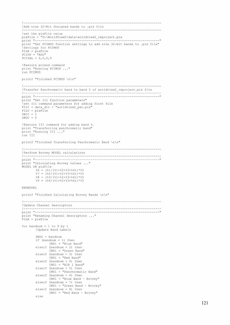
121
!--------------------------------------------------------------------------
!Add nine 32-Bit Unsigned bands to .pix file
!--------------------------------------------------------------------------
!set the pixFile value
pixFile = "D:\WorldView2\data\worldview2_reproject.pix
print "-------------------------------------------------------------------"
print "Set PCIMOD function settings to add nine 32-bit bands to .pix file"
!Settings for PCIMOD
FILE = pixFile
PCIOP = "ADD"
PCIVAL = 0,0,0,9
!Execute pcimod command
print "Running PCIMOD ..."
run PCIMOD
printf "Finished PCIMOD \n\n"
!--------------------------------------------------------------------------
!Transfer Panchromatic band to band 5 of worldview2_reproject.pix file
!--------------------------------------------------------------------------
print "-------------------------------------------------------------------"
print "Set III function parameters"
!set III command parameters for adding first file
FILI = data_dir + "worldview2_pan.pix"
FILO = pixFile
DBIC = 1
DBOC = 5
!Execute III command for adding band 5.
print "Transferring panchromatic band"
print "Running III ..."
run III
printf "Finished Transferring Panchromatic Band \n\n"
!--------------------------------------------------------------------------
!Perform Brovey MODEL calculations
!--------------------------------------------------------------------------
print "-------------------------------------------------------------------"
print "Calculating Brovey values ..."
MODEL ON pixFile
%6 = (%1/(%1+%2+%3+%4))*%5
%7 = (%2/(%1+%2+%3+%4))*%5
%8 = (%3/(%1+%2+%3+%4))*%5
%9 = (%4/(%1+%2+%3+%4))*%5
ENDMODEL
printf "Finished Calculating Brovey Bands \n\n"
!--------------------------------------------------------------------------
!Update Channel Descriptors
!--------------------------------------------------------------------------
print "-------------------------------------------------------------------"
print "Renaming Channel Descriptors ..."
FILE = pixFile
for bandnum = 1 to 9 by 1
!Update Band Labels
DBOC = bandnum
if (bandnum = 1) then
CM01 = "Blue Band"
elseif (bandnum = 2) then
CM01 = "Green Band"
elseif (bandnum = 3) then
CM01 = "Red Band"
elseif (bandnum = 4) then
CM01 = "NIR 1 Band"
elseif (bandnum = 5) then
CM01 = "Panchromatic Band"
elseif (bandnum = 6) then
CM01 = "Blue Band - Brovey"
elseif (bandnum = 7) then
CM01 = "Green Band - Brovey"
elseif (bandnum = 8) then
CM01 = "Red Band - Brovey"
else

122
CM01 = "NIR 1 Band - Brovey"
endif
!Execute MCD
RUN MCD
endfor
print "Finished Renaming Channel Descriptors"
Appendix K ImageAnalysis_WorldView2_NoPANSHARPENING..eas script
!Script Name: ImageAnalysis_WorldView2_NoPANSHARPENING.eas
!Description: Perform image analysis on non-pansharpened imagery
!Author: Robert Oikle
!Version: 1.0
!initialize variables
local string data_dir
local string pixFile
local int bandnum
!set the data directory
data_dir = "D:\WorldView2\data\
!--------------------------------------------------------------------------
!Add 28, 32-Bit Unsigned bands to .pix file
!--------------------------------------------------------------------------
!set the pixFile value
pixFile = "D:\WorldView2\data\worldview2_ms_noPan.pix
print "-------------------------------------------------------------------"
print "Set PCIMOD function settings to add 28, 32-bit bands to .pix file"
!Settings for PCIMOD
FILE = pixFile
PCIOP = "ADD"
PCIVAL = 0,0,0,28
!Execute pcimod command
print "Running PCIMOD ..."
run PCIMOD
printf "Finished PCIMOD \n\n"
!--------------------------------------------------------------------------
!****************************VEGETATION INDICES****************************
!--------------------------------------------------------------------------
!Perform NDVI1 calculations
!--------------------------------------------------------------------------
print "-------------------------------------------------------------------"
print "Calculate NDVI1"
MODEL ON pixFile
%9 = (%7-%5)/(%7+%5)
ENDMODEL
printf "Finished Calculating NDVI1 \n\n"
!--------------------------------------------------------------------------
!Perform NDVI2 calculations
!--------------------------------------------------------------------------
print "-------------------------------------------------------------------"
print "Calculate NDVI2"
MODEL ON pixFile
%10 = (%8-%5)/(%8+%5)
ENDMODEL
printf "Finished Calculating NDVI2 \n\n"
!--------------------------------------------------------------------------
!Perform NDVI3 calculations
!--------------------------------------------------------------------------
print "-------------------------------------------------------------------"
print "Calculate NDVI3"
MODEL ON pixFile
%11 = (%7-%6)/(%7+%6)
ENDMODEL
printf "Finished Calculating NDVI3 \n\n"
!--------------------------------------------------------------------------
!Perform NDVI4 calculations
!--------------------------------------------------------------------------
print "-------------------------------------------------------------------"
print "Calculate NDVI4"
MODEL ON pixFile

123
%12 = (%8-%6)/(%8+%6)
ENDMODEL
printf "Finished Calculating NDVI4 \n\n"
!--------------------------------------------------------------------------
!Perform NDVI5 calculations
!--------------------------------------------------------------------------
print "-------------------------------------------------------------------"
print "Calculate NDVI5"
MODEL ON pixFile
%13 = (%8-%4)/(%8+%4)
ENDMODEL
printf "Finished Calculating NDVI5 \n\n"
!--------------------------------------------------------------------------
!Perform NDVI6 calculations
!--------------------------------------------------------------------------
print "-------------------------------------------------------------------"
print "Calculate NDVI6"
MODEL ON pixFile
%14 = (%6-%1)/(%6+%1)
ENDMODEL
printf "Finished Calculating NDVI6 \n\n"
!--------------------------------------------------------------------------
!Perform NDVI7 calculations
!--------------------------------------------------------------------------
print "-------------------------------------------------------------------"
print "Calculate NDVI7"
MODEL ON pixFile
%15 = (%6-%5)/(%6+%5)
ENDMODEL
printf "Finished Calculating NDVI7 \n\n"
!--------------------------------------------------------------------------
!Perform DVI MODEL calculations
!--------------------------------------------------------------------------
print "-------------------------------------------------------------------"
print "Calculate DVI"
MODEL ON pixFile
%16 = %7-%5
ENDMODEL
printf "Finished Calculating DVI \n\n"
!--------------------------------------------------------------------------
!Perform IPVI MODEL calculations
!--------------------------------------------------------------------------
print "-------------------------------------------------------------------"
print "Calculate IPVI"
MODEL ON pixFile
%17 = %7/(%7+%5)
ENDMODEL
printf "Finished Calculating IPVI \n\n"
!--------------------------------------------------------------------------
!Perform SAVI MODEL calculations
!--------------------------------------------------------------------------
print "-------------------------------------------------------------------"
print "Calculate SAVI"
MODEL ON pixFile
%18 = ((%7-%5)*(1+0.5))/(%7+%5+0.5)
ENDMODEL
printf "Finished Calculating SAVI \n\n"
!--------------------------------------------------------------------------
!Perform MVI MODEL calculations
!--------------------------------------------------------------------------
print "-------------------------------------------------------------------"
print "Calculate MVI"
MODEL ON pixFile
%19 = (%7-(1.2*%5))/(%7+%5)
ENDMODEL
printf "Finished Calculating MVI \n\n"
!--------------------------------------------------------------------------
!Perform SIPI MODEL calculations
!--------------------------------------------------------------------------
print "-------------------------------------------------------------------"
print "Calculate SIPI"
MODEL ON pixFile
%20 = (%7-%2)/(%7+%5)
ENDMODEL
printf "Finished Calculating SIPI \n\n"
!--------------------------------------------------------------------------
!Perform GRVI MODEL calculations
!--------------------------------------------------------------------------
print "-------------------------------------------------------------------"

124
print "Calculate GRVI"
MODEL ON pixFile
%21 = %7/%3
ENDMODEL
printf "Finished Calculating GRVI \n\n"
!--------------------------------------------------------------------------
!Perform NNIR MODEL calculations
!--------------------------------------------------------------------------
print "-------------------------------------------------------------------"
print "Calculate NNIR"
MODEL ON pixFile
%22 = %7/(%7+%5+%3)
ENDMODEL
printf "Finished Calculating NNIR \n\n"
!--------------------------------------------------------------------------
!Perform GNDVI MODEL calculations
!--------------------------------------------------------------------------
print "-------------------------------------------------------------------"
print "Calculate GNDVI"
MODEL ON pixFile
%23 = (%7-%3)/(%7+%3)
ENDMODEL
printf "Finished Calculating GNDVI \n\n"
!--------------------------------------------------------------------------
!Perform WorldView Built-Up Index (WV-BI) calculations
!--------------------------------------------------------------------------
print "-------------------------------------------------------------------"
print "Calculate WV-BI"
MODEL ON pixFile
%24 = (%1-%6)/(%1+%6)
ENDMODEL
printf "Finished Calculating WV-BI \n\n"
!--------------------------------------------------------------------------
!Perform WorldView Non-Homogeneous Feature Difference (WV-NHFD) calculations
!--------------------------------------------------------------------------
print "-------------------------------------------------------------------"
print "Calculate WV-NHFD"
MODEL ON pixFile
%25 = (%6-%1)/(%6+%1)
ENDMODEL
printf "Finished Calculating WV-NHFD \n\n"
!--------------------------------------------------------------------------
!Perform Normalized Difference Water Index (NDWI) calculations
!--------------------------------------------------------------------------
print "-------------------------------------------------------------------"
print "Calculate NDWI"
MODEL ON pixFile
%26 = (%1-%8)/(%1+%8)
ENDMODEL
printf "Finished Calculating NDWI \n\n"
!--------------------------------------------------------------------------
!**********************Unsupervised Classifications************************
!--------------------------------------------------------------------------
!Perform 3 unsupervised classifications
! - K-Means
! - Fuzzy K-Means
! - ISO Cluster
!--------------------------------------------------------------------------
print "-------------------------------------------------------------------"
print "Beginning Unsupervised Classifications"
!Define Classification Settings
FILE = pixFile
!--------------------------------------------------------------------------
!KMeans Classification
!--------------------------------------------------------------------------
print "Starting K-Means Classification"
DBIC = 1,2,3,4,5,6,7,8
DBOC = 27
RUN KCLUS
print "Applying 3x3 averaging filter to classification results"
DBIC = 27
DBOC = 27
FLSZ = 3,3
RUN FAV
printf "Finished K-Means Classification \n\n"
!--------------------------------------------------------------------------
!Fuzzy KMeans Classification
!--------------------------------------------------------------------------

125
print "Starting Fuzzy K-Means Classification"
DBIC = 1,2,3,4,5,6,7,8
DBOC = 28
RUN FUZCLUS
print "Applying 3x3 averaging filter to classification results"
DBIC = 28
DBOC = 28
FLSZ = 3,3
RUN FAV
printf "Finished Fuzzy K-Means Classification \n\n"
!--------------------------------------------------------------------------
!ISO Cluster Classification
!--------------------------------------------------------------------------
print "Starting ISO Cluster Classification"
DBIC = 1,2,3,4,5,6,7,8
DBOC = 29
MINCLUS = 5
NUMCLUS = 10
MAXCLUS = 16
RUN ISOCLUS
print "Applying 3x3 averaging filter to classification results"
DBIC = 29
DBOC = 29
FLSZ = 3,3
RUN FAV
printf "Finished ISO Cluster Classification \n\n"
!--------------------------------------------------------------------------
!**********************Principal Components Analysis***********************
!--------------------------------------------------------------------------
print "-------------------------------------------------------------------"
print "Begin Prinicipal Components Analysis"
FILE = pixFile
DBIC = 1,2,3,4,5,6,7,8
EIGN = 1,2,3,4,5,6,7
DBOC = 30,31,32,33,34,35,36
RUN PCA
printf "Finished Principal Components Analysis \n\n"
!--------------------------------------------------------------------------
!Update Band Labels for Image Analysis bands 9-36
!--------------------------------------------------------------------------
print "-------------------------------------------------------------------"
print "Renaming Image Analysis Channel Descriptors 9-36 ..."
FILE = pixFile
for bandnum = 9 to 36 by 1
!Update Band Labels
DBOC = bandnum
if (bandnum = 9) then
CM01 = "NDVI 1"
elseif (bandnum = 10) then
CM01 = "NDVI 2"
elseif (bandnum = 11) then
CM01 = "NDVI 3"
elseif (bandnum = 12) then
CM01 = "NDVI 4"
elseif (bandnum = 13) then
CM01 = "NDVI 5"
elseif (bandnum = 14) then
CM01 = "NDVI 6"
elseif (bandnum = 15) then
CM01 = "NDVI 7"
elseif (bandnum = 16) then
CM01 = "DVI"
elseif (bandnum = 17) then
CM01 = "IPVI"
elseif (bandnum = 18) then
CM01 = "SAVI"
elseif (bandnum = 19) then
CM01 = "MVI"
elseif (bandnum = 20) then
CM01 = "SIPI"
elseif (bandnum = 21) then
CM01 = "GRVI"
elseif (bandnum = 22) then
CM01 = "NNIR"
elseif (bandnum = 23) then
CM01 = "GNDVI"
elseif (bandnum = 24) then

126
CM01 = "WVBI"
elseif (bandnum = 25) then
CM01 = "WVNHFD"
elseif (bandnum = 26) then
CM01 = "WVWI"
elseif (bandnum = 27) then
CM01 = "K-Means Classification"
elseif (bandnum = 28) then
CM01 = "Fuzzy K-Means Classification"
elseif (bandnum = 29) then
CM01 = "ISO Cluster Classification"
elseif (bandnum = 30) then
CM01 = "PC 1"
elseif (bandnum = 31) then
CM01 = "PC 2"
elseif (bandnum = 32) then
CM01 = "PC 3"
elseif (bandnum = 33) then
CM01 = "PC 4"
elseif (bandnum = 34) then
CM01 = "PC 5"
elseif (bandnum = 35) then
CM01 = "PC 6"
else
CM01 = "PC 7"
endif
!Execute MCD
RUN MCD
endfor
print "Finished Renaming Image Analysis Bands"
Appendix L ImageAnalysis_WorldView2.eas script
!Script Name: ImageAnalysis_WorldView2.eas
!Description: Perform image analysis on pansharpened imagery
!Author: Robert Oikle
!Version: 1.0
!initialize variables
local string data_dir
local string pixFile
local int bandnum
!set the data directory
data_dir = "D:\WorldView2\data\
!--------------------------------------------------------------------------
!Add 16, 32-Bit Unsigned bands to .pix file
!--------------------------------------------------------------------------
!set the pixFile value
pixFile = "D:\WorldView2\data\worldview2_reproject.pix
print "-------------------------------------------------------------------"
print "Set PCIMOD function settings to add 16, 32-bit bands to .pix file"
!Settings for PCIMOD
FILE = pixFile
PCIOP = "ADD"
PCIVAL = 0,0,0,16
!Execute pcimod command
print "Running PCIMOD ..."
run PCIMOD
printf "Finished PCIMOD \n\n"
!--------------------------------------------------------------------------
!****************************VEGETATION INDICES****************************
!--------------------------------------------------------------------------
!Perform NDVI1 calculations
!--------------------------------------------------------------------------
print "-------------------------------------------------------------------"
print "Calculate NDVI1"
MODEL ON pixFile
%10 = (%9-%8)/(%9+%8)
ENDMODEL
printf "Finished Calculating NDVI1 \n\n"
!--------------------------------------------------------------------------
!Perform DVI MODEL calculations
!--------------------------------------------------------------------------
print "-------------------------------------------------------------------"
print "Calculate DVI"
127
MODEL ON pixFile
%11 = %9-%8
ENDMODEL
printf "Finished Calculating DVI \n\n"
!--------------------------------------------------------------------------
!Perform IPVI MODEL calculations
!--------------------------------------------------------------------------
print "-------------------------------------------------------------------"
print "Calculate IPVI"
MODEL ON pixFile
%12 = %9/(%9+%8)
ENDMODEL
printf "Finished Calculating IPVI \n\n"
!--------------------------------------------------------------------------
!Perform SAVI MODEL calculations
!--------------------------------------------------------------------------
print "-------------------------------------------------------------------"
print "Calculate SAVI"
MODEL ON pixFile
%13 = ((%9-%8)*(1+0.5))/(%9+%8+0.5)
ENDMODEL
printf "Finished Calculating SAVI \n\n"
!--------------------------------------------------------------------------
!Perform MVI MODEL calculations
!--------------------------------------------------------------------------
print "-------------------------------------------------------------------"
print "Calculate MVI"
MODEL ON pixFile
%14 = (%9-(1.2*%8))/(%9+%8)
ENDMODEL
printf "Finished Calculating MVI \n\n"
!--------------------------------------------------------------------------
!Perform SIPI MODEL calculations
!--------------------------------------------------------------------------
print "-------------------------------------------------------------------"
print "Calculate SIPI"
MODEL ON pixFile
%15 = (%9-%6)/(%9+%8)
ENDMODEL
printf "Finished Calculating SIPI \n\n"
!--------------------------------------------------------------------------
!Perform GRVI MODEL calculations
!--------------------------------------------------------------------------
print "-------------------------------------------------------------------"
print "Calculate GRVI"
MODEL ON pixFile
%16 = %9/%7
ENDMODEL
printf "Finished Calculating GRVI \n\n"
!--------------------------------------------------------------------------
!Perform NNIR MODEL calculations
!--------------------------------------------------------------------------
print "-------------------------------------------------------------------"
print "Calculate NNIR"
MODEL ON pixFile
%17 = %9/(%9+%8+%7)
ENDMODEL
printf "Finished Calculating NNIR \n\n"
!--------------------------------------------------------------------------
!Perform GNDVI MODEL calculations
!--------------------------------------------------------------------------
print "-------------------------------------------------------------------"
print "Calculate GNDVI"
MODEL ON pixFile
%18 = (%9-%7)/(%9+%7)
ENDMODEL
printf "Finished Calculating GNDVI \n\n"
!--------------------------------------------------------------------------
!**********************Unsupervised Classifications************************
!--------------------------------------------------------------------------
!Perform 3 unsupervised classifications
! - K-Means
! - Fuzzy K-Means
! - ISO Cluster
!--------------------------------------------------------------------------
print "-------------------------------------------------------------------"
print "Beginning Unsupervised Classifications"
!Define Classification Settings

128
FILE = pixFile
!--------------------------------------------------------------------------
!KMeans Classification
!--------------------------------------------------------------------------
print "Starting K-Means Classification"
DBIC = 6,7,8,9
DBOC = 19
RUN KCLUS
print "Applying 3x3 averaging filter to classification results"
DBIC = 19
DBOC = 19
FLSZ = 3,3
RUN FAV
printf "Finished K-Means Classification \n\n"
!--------------------------------------------------------------------------
!Fuzzy KMeans Classification
!--------------------------------------------------------------------------
print "Starting Fuzzy K-Means Classification"
DBIC = 6,7,8,9
DBOC = 20
RUN FUZCLUS
print "Applying 3x3 averaging filter to classification results"
DBIC = 20
DBOC = 20
FLSZ = 3,3
RUN FAV
printf "Finished Fuzzy K-Means Classification \n\n"
!--------------------------------------------------------------------------
!ISO Cluster Classification
!--------------------------------------------------------------------------
print "Starting ISO Cluster Classification"
DBIC = 6,7,8,9
DBOC = 21
MINCLUS = 5
NUMCLUS = 10
MAXCLUS = 16
RUN ISOCLUS
print "Applying 3x3 averaging filter to classification results"
DBIC = 21
DBOC = 21
FLSZ = 3,3
RUN FAV
printf "Finished ISO Cluster Classification \n\n"
!--------------------------------------------------------------------------
!**********************Principal Components Analysis***********************
!--------------------------------------------------------------------------
print "-------------------------------------------------------------------"
print "Begin Prinicipal Components Analysis"
FILE = pixFile
DBIC = 6,7,8,9
EIGN = 1,2,3,4
DBOC = 22,23,24,25
RUN PCA
printf "Finished Principal Components Analysis \n\n"
!--------------------------------------------------------------------------
!Update Band Labels for Image Analysis bands 10-25
!--------------------------------------------------------------------------
print "-------------------------------------------------------------------"
print "Renaming Image Analysis Channel Descriptors 10-25 ..."
FILE = pixFile
for bandnum = 10 to 25 by 1
!Update Band Labels
DBOC = bandnum
if (bandnum = 10) then
CM01 = "NDVI 1"
elseif (bandnum = 11) then
CM01 = "DVI"
elseif (bandnum = 12) then
CM01 = "IPVI"
elseif (bandnum = 13) then
CM01 = "SAVI"
elseif (bandnum = 14) then
CM01 = "MVI"
elseif (bandnum = 15) then
CM01 = "SIPI"
elseif (bandnum = 16) then
CM01 = "GRVI"
elseif (bandnum = 17) then

129
CM01 = "NNIR"
elseif (bandnum = 18) then
CM01 = "GNDVI"
elseif (bandnum = 19) then
CM01 = "K-Means Classification"
elseif (bandnum = 20) then
CM01 = "Fuzzy K-Means Classification"
elseif (bandnum = 21) then
CM01 = "ISO Cluster Classification"
elseif (bandnum = 22) then
CM01 = "PC 1"
elseif (bandnum = 23) then
CM01 = "PC 2"
elseif (bandnum = 24) then
CM01 = "PC 3"
else
CM01 = "PC 4"
endif
!Execute MCD
RUN MCD
endfor
print "Finished Renaming Image Analysis Bands"

130
References
Abrams, M. J. & Comer, D. C. 2013, 'Chapter 6 Multispectral and Hyperspectral Technology and
Archaeological Applications' in Mapping Archaeological Landscapes from Space, Springer, New
York, pp. 57-71. Available from: Springer Link E-Book.
Aggarwal, S. 2004, „Principles of Remote Sensing‟, in Sivakumar, M.V.K., Roy, P.S.,
Harmsen, K., and Saha, S.K. (eds.), Satellite Remote Sensing and GIS Applications
Agricultural Meteorology, World Meteorological Organization, Geneva, Switzerland, pp. 23-38.
Available from < http://www.wamis.org/agm/pubs/agm8/Paper-2.pdf> [March 10th
, 2016].
Brauen, G. 2006, „Designing Interactive Sound Maps Using Scalable Vector Graphics‟,
Cartographica, vol. 41, issue 1, pp. 59-71.
Breeze, D. J. 1983, Roman Forts in Britain, Shire Publications LTD, Cromwell House, Church
Street, Princes Risborough, Aylesbury, Bucks, UK.
Breeze, D. J. & Dobson, B. 1978, Hadrian’s Wall, Penguin Books Ltd, Harmondsworth, Middlesex,
England.
Caquard, S., Pyne, S., Igloliorte, H., Mierins, K., Hayes, A. & Taylor, D.R. F. 2009, „A “Living”
Atlas for Geospatial Storytelling: The Cybercartographic Atlas of Indigenous Perspectives and
Knowledge of the Great Lakes Region”, Cartographica, vol. 44, issue 2, pp. 83-100.
Cartwright, W. 2003, „Maps on the Web‟, in Maps and the Internet, ed M.P Peterson, Elsevier,
Amsterdam, pp. 35- 56.
Champion, E., Bishop, I. & Dave, B. 2012, „The Palenque project: evaluating interaction in an
online virtual archaeology site‟, Virtual Reality, vol. 16, Issue 2, pp. 121-139.
Chaves, P. 1988, 'An Improved Dark-Object Subtraction Technique for Atmospheric Scattering
Correction of Multispectral Data', Remote Sensing of Environment, Vol. 24, pp. 459-479.
Chavez, P. 1996, 'Image-Based Atmospheric Corrections - Revisited and Improved',
Photogrammetric Engineering & Remote Sensing, Vol. 62, No. 9, pp. 1025-1036.
Crippen, R.E. 1990,'Calculating the Vegetation Index Faster', Remote Sensing of Environment, Vol.
34, pp.71-73.
Davidson, A.M. 2014, “Lesson 12 – Image Enhancement”, lecture notes distributed in GEOM
4003: Remote Sensing of the Environment, at Carleton University, p.53.
De Runz, C., Desjardin, E., Piantoni, E. & Herbin, M. 2007, „Using fuzzy logic to manage uncertain
multi-modal data in an archaeological GIS‟, 5th International Symposium on Spatial Data Quality,
pp.1-4, Available from <http://www.isprs.org/proceedings/XXXVI/2-
C43/Postersession/runz_et_al.pdf > [March 6th, 2015]
Developer Documentation, 2015, Available from:
<https://github.com/GCRC/nunaliit/wiki/Developer-Documentation> [Sept 19th, 2015]

131
Engler, N.J., Scassa, T. & Taylor, D.R.F. 2013, „Mapping Traditional Knowledge: Digital
Cartography in the Canadian North‟, Cartographica, vol. 48, issue 3, pp. 189-199.
Fowler, M.J.F. 2002, 'Satellite Remote Sensing and Archaeology: a Comparative Study of Satellite
Imagery of the Environs of Figsbury Ring, Wiltshire', Archaeological Prospection, vol. 9, pp. 55-
69, Published online in Wiley InterScience (www.interscience.wiley.com), doi: 10.1002/arp.181.
Fuse, T. & Shimizu, E. 2004, Visualizing the Landscape of Old-Time Tokyo (Edo City), ISPRS
Archives – Volume XXXVI-5/W1, WG V/6, pp.1-8, Available from
<http://www.isprs.org/proceedings/XXXVI/5-W1/papers/21.pdf>
Gitelson, A. A. & Merzlyak, M. N. 1998, 'Remote Sensing of Chlorophyll Concentration in Higher
Plant Leaves', Advances in Space Research, Vol.22, No.5, pp.689-692.
Goodchild, M. 2000, "Introduction: special issue on 'Uncertainty in geographic information
systems'", Fuzzy Sets and Systems, Vol.113, pp. 3-5.
Gregory, I. N. & Ell, P. S. 2007, Historical GIS: Technologies, Methodologies and
Scholarship, Cambridge University Press, Cambridge, UK.
Harris Geospatial Solutions 2016, Broadband Greenness (Using ENVI)|Exelis VIS Docs Center,
Available from: <https://www.harrisgeospatial.com/docs/broadbandgreenness.html> [Apr 24th,
2016]
Harris Geospatial Solutions 2016a, Miscellaneous Indicies Background (Using ENVI)|Exelis VIS
Docs Center, Available from:
<https://www.harrisgeospatial.com/docs/BackgroundOtherIndices.html> [Apr 24th, 2016]
Hayes, A., Pulsifer, P. L. & Fiset, J. P. 2014, „The Nunaliit Cybercartographic Atlas Framework‟, in
Taylor, D. F. & Lauriault, T. P. (Eds.), Developments In The Theory And Practice Of
Cybercartography: Applications and Indigenous Mapping, vol. 5, Elsevier, Amasterdam, The
Netherlands.
Historic England 2000, PUMPING STATION, ELLERTON, Available from:
<http://www.pastscape.org.uk/hob.aspx?hob_id=1319841> [Jan 22nd
, 2016]
Huete, A. R. 1988, 'A Soil-Adjusted Vegetation Index', Remote Sensing of Environment, vol.25,
pp.295-309.
Inuit Siku (sea ice) Atlas, Available from: <http://sikuatlas.ca/> [Dec 12th, 2013]
Jensen, J. 2007, Remote Sensing of the Environment: An Earth Resourse Perspective, 2nd ed,
Pearson Education Inc, Indian Subcontinent Version.
Johnson, A. 1983, Roman Forts of the 1st and 2
nd centuries AD in Britain and the German
Provinces, Adam & Charles Black (Publishers) Ltd, London.
Joss, B. N., Hall, R. J., Sidders, D. M., & Keddy, T. J. 2008, „Fuzzy-logic modeling of land
suitability for hybrid poplar across the Prairie Provinces of Canada‟, Environmental Monitoring
Assessment, vol. 141, issue.1-3, pp.79-96.

132
Kaimaris, D., Patias, P. & Tsakiri, M. 2012, 'Best period for high spatial resolution satellite images
for detection of marks of buried structures', The Egyptian Journal of Remote Sensing and Space
Sciences, vol. 15, pp. 9-18.
Keith, D., Crockatt, K. & Hayes, A. 2014, „The Kitikmeot Place Name Atlas‟, in Taylor, D. F. &
Lauriault, T. P. (Eds.), Developments In The Theory And Practice Of Cybercartography:
Applications and Indigenous Mapping, vol. 5, Elsevier, Amasterdam, The Netherlands.
Kumar, P. N. 2012, 'Advances in Applications of Remote Sensing in Archaeology', International
Journal of Social Sciences and Humanities, vol. 1, pp. 1-7.
Lake Huron Treaty Atlas, Available from: <http://lhta.ca/> [Sept 18th, 2015]
Lasaponara, R. & Masini, N. 2006, 'Identification of Archaeological Burial Remains Based on the
Normalized Difference Vegetation Index (NDVI) from Quickbird Satellite Data', IEEE Geoscience
and Remote Sensing Letters, vol. 3, no. 3, pp.325-328.
Lasaponara, R., Masini, N. & Scardozzi, G. 2008, 'New perspectives for satellite-based
archaeological research in the ancient territory of Hierapolis (Turkey)', Advances in Geosciences,
vol. 19, pp. 87-96.
Lauriault, T. P. 2014, „Pilot Cybercartographic Atlas of the Risk of Homelessness‟, in Taylor, D. F.
& Lauriault, T. P. (Eds.), Developments In The Theory And Practice Of Cybercartography:
Applications and Indigenous Mapping, vol. 5, Elsevier, Amasterdam, The Netherlands.
Lillesand, T. M., Kiefer, R. W. & Chipman, J.W. 2007, Remote Sensing and Image Interpretation,
6th ed, John Wiley & Sons, Inc, United States of America.
Lourenҫo, R.W, Landim, P.M.B, Rosa, A.H., Roveda, J.A.F, Martins, A.C.G, & Fraceto, L.F. 2010,
„Mapping soil pollution by spatial analysis and fuzzy classification‟, Environmental Earth Sciences,
vol. 60, pp.495-504.
Masini, N., & Lasaponara, R. 2006, 'Satellite-based recognition of landscape archaeological
features related to ancient human transformation', Journal of Geophysics and Engineering, vol 3,
pp. 230-235
Met Office, 2013, England and Wales drought 2010 to 2012, Available from:
<http://www.metoffice.gov.uk/climate/uk/interesting/2012-drought> [Mar 10th, 2016]
Monmonier, M. 1996, How to Lie with Maps, 2nd ed, The University of Chicago Press, Chicago.
Nouri, H., Beecham, S., Anderson, S. & Nagler, P. 2014, 'High Spatial Resolution WorldView-2
Imagery for Mapping NDVI and Its Relationship to Temporal Urban Landscape Evapotranspiration
Factors‟, Remote Sensing, vol.6, pp.580-602.
Ojala, J., DeTar, W., Chesson, J., Penner, V. & Funk, H. 2004. 'Leaf Indices to Quantify Nitrogen in
Cotton', pp.913-920, Beltwide Cotton Conferences, San Antonio, TX. January 5-9, Available from:
<http://naldc.nal.usda.gov/naldc/download.xhtml?id=11994&content=PDF>

133
Ottean, I. A. & Hanson, W. S. 2013, 'Chapter 18 Integrating Aerial and Satellite Imagery:
Discovering Roman Imperial Landscapes in Southern Dobrogea (Romania)', in Archaeology from
Historical Aerial and Satellite Archives, Springer, New York, pp. 315-336. Available from: Springer
Link E-Book.
Paltridge, G.W. & Barber, J. 1988, 'Monitoring Grassland Dryness and Fire Potential in Australia
with NOAA/AVHRR Data', Remote Sensing of Environment, vol.25, pp.381-394.
Parcak, S. 2007, 'Satellite Remote Sensing Methods for Monitoring Archaeological Tells in the
Middle East', Journal of Field Archaeology, vol. 32, no. 1, pp. 65-81.
Paullin, C.O. 1932, Atlas of the Historical Geography of the United States, ed. by Wright, J.K.,
The Carnegie Institution, Washington, DC, and the American Geographic Society of New York
Available from: <http://name.umdl.umich.edu/abl7462.0001.001>
Payne, C., Hayes, A. & Ellison, S. 2014, „Mapping Views from the North: Cybercartographic
Technology and Inuit Photographic Encounters‟, in Taylor, D. F. & Lauriault, T. P. (Eds.),
Developments In The Theory And Practice Of Cybercartography: Applications and Indigenous
Mapping, vol. 5, Elsevier, Amasterdam, The Netherlands.
Peñuelas, J. & Inoue, Y. 1999, 'Reflectance indices indicative of changes in water and pigment
contents of peanut and wheat leaves', Photosynthetica, vol.36, issue.3, pp.355-360.
Peterson, M. 2003, „Maps and the Internet: An Introduction‟ in Maps and the Internet, ed M.P
Peterson, Elsevier, Amsterdam, pp.1-16.
Pyne, S. & Taylor, D.R. F. 2012, „Mapping Indigenous Perspectives in the Making of the
Cybercartographic Atlas of the Lake Huron Treaty Relationship Process: A Performative Approach
in a Reconciliation Context‟, Cartographica, vol. 47, issue 2, pp. 92-104.
Ray, B.C. 2002, „Teaching the Salem Witch Trials‟ in Past Time, Past Place: GIS for History, ed.
Knowles, A.K., ESRI Press, Redlands, California, pp.19-33.
Rodgers, N. 2014, Roman Empire, Anness Publishing Ltd, Leicestershire, England.
Robinson, V.B. 2003, 'A Perspective on the Fundamentals of Fuzzy Sets and their Use in
Geographic Information Systems', Transactions In GIS, vol.7, issue.1, pp.3-30.
Rouse, J.W., Hass, R.H., Deering, D.W., & Schell, J.A. 1973, 'Monitoring the vernal advancement
and retrogradation (green wave effect) of natural vegetation‟, Progress Report RSC 1978-2, E74-
10113, Remote Sensing Center, Texas A&M University., College Station.
Salway, P. 2001, A History of Roman Britain, Oxford University Press, Great Britain.
Sarris, A., Trigkas, V., Papadakis, G., Papazoglou, M., Peraki, E., Chetzoyiannaki, N., Elvanidou,
M., Karimali, E., Kouriati, K., Katifori, M., Kakoulaki, G., Kappa, E., Athanasaki, K., &
Papadopoulos, N. 2007, „A Web-GIS Approach to Cultural Resources Management in Crete: the
Digital Archaeological Atlas of Crete‟, Layers of Perception. Proceedings of the 35th International
Conference on Computer Applications and Quantitative Methods in Archaeology (CAA), Berlin, 2.-
6. April, 2007, pp.1-6. Available from:
<http://archiv.ub.uni-heidelberg.de/propylaeumdok/volltexte/2010/541>

134
Sever, T. L. & Irwin, D. E. 2003, 'Landscape Archaeology: Remote-sensing investigation of the
ancient Maya in the Peten rainforest of northern Guatemala', Ancient Mesoamerica, vol. 14, pp.113-
122.
Showalter, P. S. 1993, 'A Thematic Mapper Analysis of the Prehistoric Hohokam Canal
System, Phoenix, Arizona', Journal of Field Archaeology, vol. 20, no. 1, pp. 77-90, Available from:
JSTOR [6 July 2006].
Taylor, D.R.F. 2003, „The Concept of Cybercartography‟, in Maps and the Internet, ed M.P
Peterson, Elsevier, Amsterdam, pp. 405-420.
Taylor, D.R.F. 2005, Cybercartography: Theory and Practice, Elsevier, Amsterdam.
Taylor, D.R.F. & Caquard, S. 2006, „Cybercartography: Maps and Mapping in the Information Era‟,
Cartographic, vol. 41, issue 1, pp. 1-5.
Taylor, D.R.F. & Pyne, S. 2010, „The history and development of the theory and practice of
cybercartography‟, International Journal of Digital Earth, vol. 3, no. 1, pp. 2-15
Taylor, D. F. 2014, „Some Recent Developments in the Theory and Practice of Cybercartography:
Applications in Indigenous Mapping: An Introduction‟, in Taylor, D. F. & Lauriault, T. P. (Eds.),
Developments In The Theory And Practice Of Cybercartography: Applications and Indigenous
Mapping, vol. 5, Elsevier, Amasterdam, The Netherlands.
Taylor, D. F, Cowan, C., Ljubicic, G. J. & Sullivan, C. 2014, „Cybercartography for Education: The
Application of Cybercartography to Teaching and Learning in Nunavut, Canada‟, in Taylor, D. F. &
Lauriault, T. P. (Eds.), Developments In The Theory And Practice Of Cybercartography:
Applications and Indigenous Mapping, vol. 5, Elsevier, Amasterdam, The Netherlands.
Tucker, C. J. 1979,'Red and photographic infrared linear combinations for monitoring vegetation',
Remote Sensing of Environment, vol.8, p.127–150
Updike, T. & Comp, C. 2010, Radiometric Use of WorldView-2 Imagery, Digital Globe Inc., pp.1-
17, Available from
<http://global.digitalglobe.com/sites/default/files/Radiometric_Use_of_WorldView-
2_Imagery%20%281%29.pdf>
Views from the North Atlas, Available from: <http://viewsfromthenorth.ca/index.html> [Sept 18th,
2015]
Wallace, T.R & van den Heuvel, C. 2005, „Truth and Accountability in Geographic and Historical
Visualizations‟, The Cartographic Journal, vol. 42, no. 2, pp.173-181.
Weiss, A. 2001, Topographic Position and Landforms Analysis, Poster presentation, ESRI User
Conference, San Diego, CA, viewed 17 September 2015, Available from:
<http://www.jennessent.com/downloads/TPI-poster-TNC_18x22.pdf >
Wilson, P. 2011, 'Introductions to Heritage Assets Roman Forts and Fortresses',
English Heritage, pp. 1-5.
135
Wolf, A. 2010, „Using WorldView 2 Vis-NIR MSI Imagery to Support Land Mapping and Feature
Extraction Using Normalized Difference Index Ratios‟, Longmont, CO: DigitalGlobe, Available
from: <http://www.harrisgeospatial.com/portals/0/pdfs/envi/8_bands_Antonio_Wolf.pdf>
Woodcock, C.E., & Gopal, S. 2000, „Fuzzy set theory and thematic maps: accuracy assessment and
area estimation‟, International Journal of Geographic Information System, vol. 14, no. 2, pp.153-
172.
Xiaocheng, Z., Tamás, J., Chongcheng, C. & Malgorzata, W.V. 2012, 'Urban Land Cover Mapping
Based on Object Oriented Classification Using WorldView 2 Satellite Remote Sensing Images',
Internation Scientific Conference on Sustainable Development & Ecological Footprint, Sopron,
Hungary, Available from:
<https://bismarck.nyme.hu/fileadmin/dokumentumok/palyazat/tamop421b/IntConference/Papers/Ar
ticles/PDF/Xiaocheng_UrbanLandCoverMappingBasedOnObjectOrientedClassificationUsingWorld
View2SatelliteRemoteSensingImages.pdf>
Zadeh, L.A. 1965, „Fuzzy Sets‟, Information and Control, vol. 8, pp 338-353.