Searching Massive Databases Using Locality Sensitive Hashing

Ting Li Haiying Shen∗

Wal-mart Stores Inc. Department of Electrical and Computer Engineering702 SW 8th St Clemson University

Bentonville, AR 72716 Clemson, SC, 29634dragonflyting@hotmail.com shenh@clemson.edu

Abstract

Locality Sensitive Hashing (LSH) is a method ofperforming probabilitic dimension reduction of high-dimensional data. It can be used for approxi-mate nearest neighbor search on a high-dimensionaldataset. We first present a LSH-based similaritysearching method. However, it needs large memoryspace and long processing time in a massive dataset.In addition, it is not effective on locating similar datain a very high-dimensional dataset. Further, it can-not easily adapt to data insertion and deletion. Toaddress the problems, we then propose a new LSH-based similarity searching scheme that intelligentlycombines SHA-1 consistent hash function and Min-wise independent permutation into LSH (SMLSH).SMLSH effectively classifies information according tothe similarity with reduced memory space require-ment and in a very efficient manner. It can quicklylocate similar data in a massive dataset. Experimen-tal results show that SMLSH is both time and spaceefficient in comparison with LSH. It yields significantimprovements on the effectiveness of similar search-ing over LSH in a massive dataset.Keywords: Locality sensitive hashing, High-

dimensional dataset, Similarity searching, Min-Wisepermutations, Consistent hashing

1 Introduction

Driven by the tremendous growth of information ina massive dataset, there is an increasing need foran efficient similarity searching method that can lo-

q p

Figure 1: An example of finding nearest neighbor ofa query point.

cate desired information rapidly with low cost. Anideal similarity searching scheme should work well ina high-dimensional database. Specifically, it shouldlocate nearly all the similar records of a query with ashort query time and small memory requirement. Inaddition, it should also deal with data insertion anddeletion. Many approaches have been proposed forsimilarity searching in high-dimensional databases.The approaches treat the records in a database aspoints in a high-dimensional space and each record isrepresented by a high-dimensional vector. Figure 1gives an example of finding the nearest neighbor ofa query point. There is a set of points in a two-dimensional space. Point q is a query point. Fromthe figure, we can see point p is the closest point toq.

Distance measurement (i.e., Euclidean distance)can be used to decide the closeness of two records.Figure 2 shows an example of three records and theirrepresentation in Euclidean space. We see that record1 and record 3 have three common keywords, whilerecord 1 and record 2 have two common keywords.

1

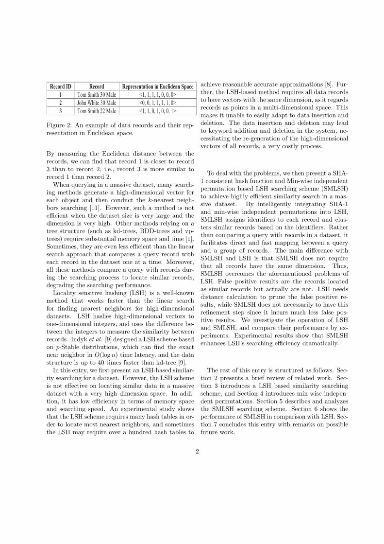
Record ID Record Representation in Euclidean Space

1 Tom Smith 30 Male <1, 1, 1, 1, 0, 0, 0>

2 John White 30 Male <0, 0, 1, 1, 1, 1, 0>

3 Tom Smith 22 Male <1, 1, 0, 1, 0, 0, 1>

Figure 2: An example of data records and their rep-resentation in Euclidean space.

By measuring the Euclidean distance between therecords, we can find that record 1 is closer to record3 than to record 2, i.e., record 3 is more similar torecord 1 than record 2.When querying in a massive dataset, many search-

ing methods generate a high-dimensional vector foreach object and then conduct the k-nearest neigh-bors searching [11]. However, such a method is notefficient when the dataset size is very large and thedimension is very high. Other methods relying on atree structure (such as kd-trees, BDD-trees and vp-trees) require substantial memory space and time [1].Sometimes, they are even less efficient than the linearsearch approach that compares a query record witheach record in the dataset one at a time. Moreover,all these methods compare a query with records dur-ing the searching process to locate similar records,degrading the searching performance.Locality sensitive hashing (LSH) is a well-known

method that works faster than the linear searchfor finding nearest neighbors for high-dimensionaldatasets. LSH hashes high-dimensional vectors toone-dimensional integers, and uses the difference be-tween the integers to measure the similarity betweenrecords. Indyk et al. [9] designed a LSH scheme basedon p-Stable distributions, which can find the exactnear neighbor in O(log n) time latency, and the datastructure is up to 40 times faster than kd-tree [9].In this entry, we first present an LSH-based similar-

ity searching for a dataset. However, the LSH schemeis not effective on locating similar data in a massivedataset with a very high dimension space. In addi-tion, it has low efficiency in terms of memory spaceand searching speed. An experimental study showsthat the LSH scheme requires many hash tables in or-der to locate most nearest neighbors, and sometimesthe LSH may require over a hundred hash tables to

achieve reasonable accurate approximations [8]. Fur-ther, the LSH-based method requires all data recordsto have vectors with the same dimension, as it regardsrecords as points in a multi-dimensional space. Thismakes it unable to easily adapt to data insertion anddeletion. The data insertion and deletion may leadto keyword addition and deletion in the system, ne-cessitating the re-generation of the high-dimensionalvectors of all records, a very costly process.

To deal with the problems, we then present a SHA-1 consistent hash function and Min-wise independentpermutation based LSH searching scheme (SMLSH)to achieve highly efficient similarity search in a mas-sive dataset. By intelligently integrating SHA-1and min-wise independent permutations into LSH,SMLSH assigns identifiers to each record and clus-ters similar records based on the identifiers. Ratherthan comparing a query with records in a dataset, itfacilitates direct and fast mapping between a queryand a group of records. The main difference withSMLSH and LSH is that SMLSH does not requirethat all records have the same dimension. Thus,SMLSH overcomes the aforementioned problems ofLSH. False positive results are the records locatedas similar records but actually are not. LSH needsdistance calculation to prune the false positive re-sults, while SMLSH does not necessarily to have thisrefinement step since it incurs much less false pos-itive results. We investigate the operation of LSHand SMLSH, and compare their performance by ex-periments. Experimental results show that SMLSHenhances LSH’s searching efficiency dramatically.

The rest of this entry is structured as follows. Sec-tion 2 presents a brief review of related work. Sec-tion 3 introduces a LSH based similarity searchingscheme, and Section 4 introduces min-wise indepen-dent permutations. Section 5 describes and analyzesthe SMLSH searching scheme. Section 6 shows theperformance of SMLSH in comparison with LSH. Sec-tion 7 concludes this entry with remarks on possiblefuture work.

2

2 Approaches for similaritysearching

The similarity searching problem is closely related tothe nearest neighbor search problem, which has beenstudied by many researchers. Various indexing datastructures have been proposed for nearest neighborsearching.

2.1 Tree structures

Some of the similarity searching methods rely ontree structures, such as R-tree, SS-tree and SR-tree. These data structures partition the data ob-jects based on their similarity. Therefore, during aquery, only a part of the data records have to be com-pared with the query record, which is more efficientthan the linear search that compares a query with ev-ery data record in the database. Though these datastructures can support nearest neighbor searching,they are not efficient in a large and high-dimensionaldatabase (i.e., the dimensionality is more than 20).The M-tree [4] was proposed to organize and searchlarge datasets from a generic metric space, i.e., whereobject proximity is only defined by a distance func-tion satisfying the positivity, symmetry, and trian-gle inequality postulates. The M-tree partitions ob-jects on the basis of their relative distances measuredby a specific distance function, and stores these ob-jects into nodes that correspond to constrained re-gions of the metric space [4]. All data objects arestored in the leaf nodes of M-tree. The non-leafnodes contain “routing objects” which describe theobjects contained in the branches. For each routingobject, there is a so-called covering radius of all its en-closing objects, and the distances to each child nodeare pre-computed. When a range querying is com-pleted, sub-trees are pruned if the distance betweenthe query object and the routing object is larger thanthe routing object’s covering radius plus the query ra-dius. Because a lot of the distances are pre-computed,the query speed is dramatically increased. The mainproblem is the overlap between different routing ob-jects in the same level.

2.2 Vector approximation file

Another kind of similarity searching method is thevector approximation file (VA-file) [17], which canreduce the amount of data that must be read dur-ing similarity searches. It divides the data space intogrids and creates an approximation for each data ob-ject that fall into a grid. When searching for the nearneighbors, the VA-file sequentially scans the file con-taining these approximations, which is smaller thanthe size of the original data file. This allows mostof the VA-file’s disk accesses to be sequential, whichare much less costly than random disk accesses [6].One drawback of this approach is that the VA-file re-quires a refinement step, where the original data fileis accessed using random disk accesses [6].

2.3 Approximation tree

Approximation tree (A-tree) [11] has better perfor-mance than VA-file and SR-tree for high dimensionaldata searching. The A-tree is an index structure forsimilarity search of high-dimensional data. A-treestores virtual bounding rectangles (VBRs), whichcontain and approximate minimum bounding rect-angles (MBR) and data objects, respectively. MBRis a bounding box to bind data object. iDistance [19]partitions the data into different regions and definesa reference point for each partition. The data in eachregion is transformed into a single dimensional spacebased on their similarity with the reference point inthe region. Finally, these points are indexed using aB+-tree structure and similarity search is performedin the one-dimensional space. As reported in [19],iDistance outperforms the M-tree and linear search.

2.4 Hashing

Hashing is a common approach to facilitate similar-ity search in high dimension databases, and spectralhashing [18] is one state-of-the-art work for data-aware hashing. Spectral hashing applies the machinelearning techniques to minimize the semantic loss ofhashed data resulting from embedding. However, thedrawback of Spectral hashing lies in its limited ap-plicability. As spectral hashing relies on Euclidean

3

distance to measure the similarity between two datarecords, and it requires that data points are from aEuclidean space and are uniformly distributed.Most recently, much research also has been con-

ducted on locality-sensitive hashing. Dasgupta etal. [5] proposed a new and simple method to speedup the widely-used Euclidean realization of LSH. Atthe heart of the method is a fast way to estimatethe Euclidean distance between two d-dimensionalvectors; this is achieved by the use of randomizedHadamard transforms in a non-linear setting. Tra-ditionally, several LSH functions are concatenated toform a “static” compound hash function for buildinga hash table. Gan et al. [7] proposed to use a base ofm single LSH functions to construct “dynamic” com-pound hash functions, and defined a new LSH schemecalled Collision Counting LSH (C2LSH). In C2LSH,if the number of LSH functions under which a dataobject o collides with a query object q is greater thana pre-specified collision threshold, then o can be re-garded as a good candidate of c-approximate nearestneighbors of q. Slaney and Casey [16] described anLSH technique that allows one to quickly find simi-lar entries in large databases. This approach belongsto a novel and interesting class of algorithms thatare known as randomized algorithms, which do notguarantee an exact answer but instead provide a highprobability guarantee of returning correct answer orone close to it.Recent work has also explored ways to embed high-

dimensional features or complex distance functionsinto a low-dimensional Hamming space where itemscan be efficiently searched. However, existing meth-ods do not apply for high-dimensional kernelized datawhen the underlying feature embedding for the kernelis unknown. Kulis and Grauman [10] showed how togeneralize locality-sensitive hashing to accommodatearbitrary kernel functions, making it possible to pre-serve the algorithm’s sub-linear time similarity searchguarantees for a wide class of useful similarity func-tions. Semantic hashing [12] seeks compact binarycodes of data-points so that the Hamming distancebetween codewords correlates with semantic similar-ity. Weiss et al. [18] showed that the problem of find-ing a best code for a given dataset is closely related tothe problem of graph partitioning and can be shown

to be NP hard. By relaxing the original problem,they obtained a spectral method whose solutions aresimply a subset of thresholded eigenvectors of thegraph Laplacian. Satuluri and Parthasarathy [13]proposed BayesLSH, a principled Bayesian algorithmfor performing candidate pruning and similarity es-timation using LSH. They also presented a simplervariant, BayesLSH-Lite, which calculates similaritiesexactly. BayesLSH can quickly prune away a largemajority of the false positive candidate pairs. Thequality of BayesLSH’s output can be easily tuned anddoes not require any manual setting of the number ofhashes to use for similarity estimation.

3 Locality Sensitive Hashing

In this section, we introduce LSH, LSH-based simi-larity searching method, and min-wise independentpermutations.LSH is an algorithm used for solving the approxi-

mate and exact near neighbor search in high dimen-sional spaces [9]. The main idea of the LSH is touse a special family of hash functions, called LSHfunctions, to hash points into buckets, such that theprobability of collision is much higher for the ob-jects which are close to each other in their high-dimensional space than for those which are far apart.A collision occurs when two points are in the samebucket. Then, query points can identify their nearneighbors by using the hashed query points to re-trieve the elements stored in the same buckets.For a domain S of a set of points and distance mea-

sure D, the LSH family is defined as:DEFINITION 1. A family H = {h : S → U} is

called (r1, r2, p1, p2) sensitive for D if for any point v,q belongs to S

• If v ∈ B(q, r1), then PrH[h(q) = h(v)] ≥ p1,

• If v /∈ B(q, r2), then PrH[h(q) = h(v)] ≤ p2,

where r1, r2, p1, p2 satisfy p1 < p2 and r1 < r2.LSH is a dimension reduction technique that

projects objects in a high-dimensional space to alower-dimensional space while still preserving the rel-ative distances among objects. Different LSH familiescan be used for different distance functions.

4

g1: (h1,…,hk)

g2: (h1,…,hk)

…

gL: (h1,…,hk)

V(h1)

…

V(h1)

V(h1)

V(h2)

…

V(h2)

V(h2)

…

…

…

…

V(hk)

…

V(hk)

V(hk)

Id1

Id2

.

.

.

Idn

.

.

.

Hv1 Hvn

k

L

H2

H1

Hash familyFinal hash table

Bucket

Figure 3: The process of LSH.

Based on LSH on p-stable distribution [9], we de-velop a similarity searching method. Figure 3 showsthe process of LSH. The hash function family of LSHhas L groups of function functions, and each grouphas k hash functions. Given a data record, LSH ap-plies the hash functions to the record to generate Lbuckets, and each bucket has k hash values. LSHuses hash function H1 on the k hash values of eachbucket to generate the location index of the recordin the final hash table, and uses hash function H2

on the k hash values of each bucket to generate thevalue of the record to store in the location. Finally,the record has L values stored in the final hash table.Given a query, LSH uses the same process to producethe L indices and values of the query, and finds sim-ilar records based on the indices, and identifies finalsimilar records based on the stored values. Let ustake an example to explain how the LSH-based simi-larity searching works. Assume that the records in adataset are as follows:

Ann Johnson 16 Female 248 Dickson Street

Ann Johnson 20 Female 168 Garland

Mike Smith 16 Male 1301 Hwy

John White 24 Male Fayetteville 72701

First, LSH constructs a keyword list which consistsof all unique keywords in all records, with each key-word functioning as a dimension. The scheme thentransforms these records into binary data based onthe keyword list. Specifically, if a record contains thekeyword, the dimension representing the keyword hasthe value 1, otherwise, it has the value 0. Figure 4shows the process to determine the vector of each

AnnMikeJohn

JohnsonSmithWhite162024

FemaleMaleAnn2481681301DicksonStreetGarlandHwy

Fayetteville72701

V1 V2 V3 V4 q10010010010100110000

10010001010010001000

01001010001001000100

00100100101000000011

10010001010010001000

Figure 4: Multi-dimensional keyword space.

record. The number of dimensions of a record is thetotal length of the keyword list. Finally, the recordsare transformed to multi-dimensional vector:

v1: 1 0 0 1 0 0 1 0 0 1 0 1 0 0 1 1 0 0 0 0

v2: 1 0 0 1 0 0 0 1 0 1 0 0 1 0 0 0 1 0 0 0

v3: 0 1 0 0 1 0 1 0 0 0 1 0 0 1 0 0 0 1 0 0

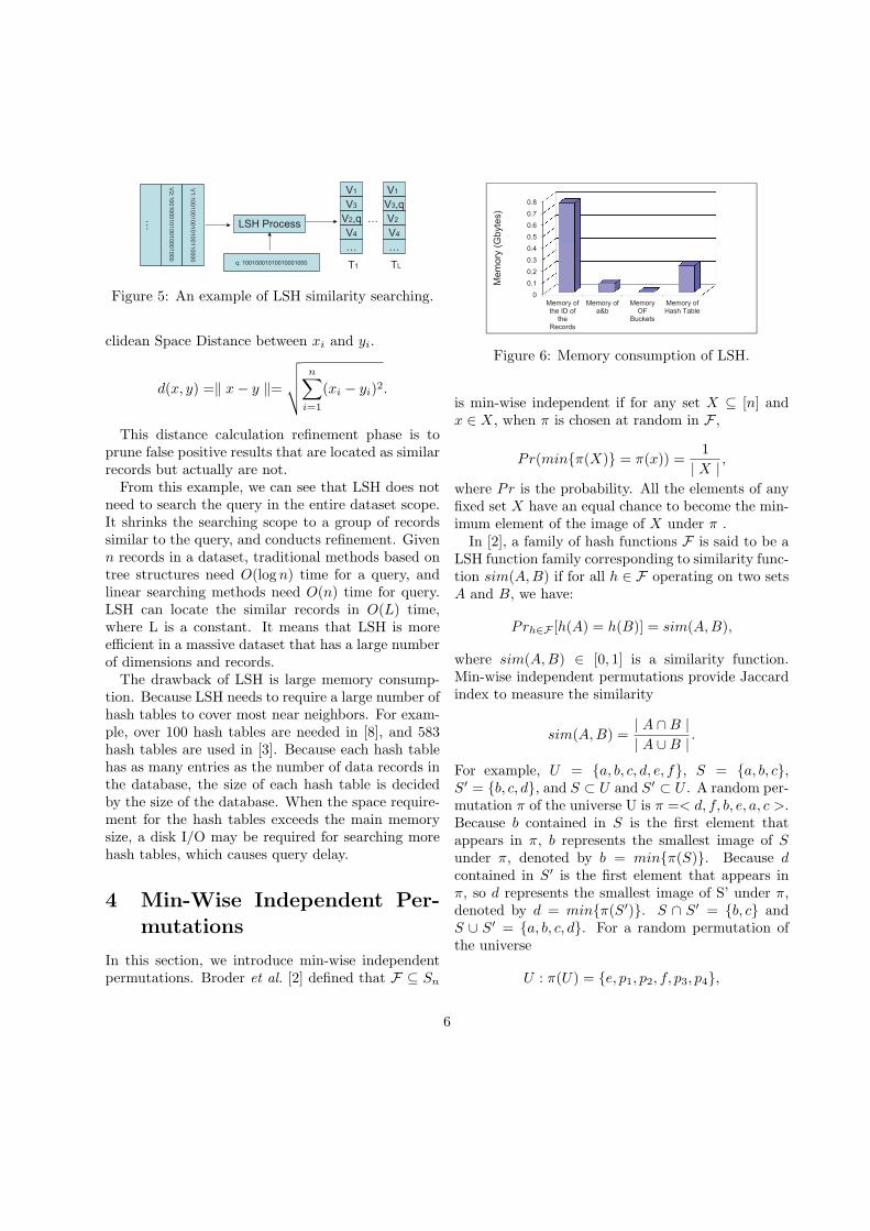
v4: 0 0 1 0 0 1 0 0 1 0 1 0 0 0 0 0 0 0 1 1As shown in Figure 3, LSH then produces the hashbuckets gi(v) (1 ≤ i ≤ L) for every record. There-after, LSH computes the hash value for every bucket.Finally, record v’s hashed value by H2 hash func-tion, Hv, is stored in final hash tables pointed by thehashed value by H1. Figure 5 shows the process ofsearching similar records of a query. If a query recordq is:

Ann Johnson | 20 | Female | 168 Garland

Using the same procedure, q will be transformedto

q: 1 0 0 1 0 0 0 1 0 1 0 0 1 0 0 0 1 0 0 0Then, the index of q will be stored in the final hashtables through the same procedure. Consequently,the records that are in the same rows with q in hashtable 1 to hash table L are similar records. In theexample, v2 and v3 are in the similar record set. Fi-nally, the Euclidean Space Distance between each lo-cated record and the query is computed to prune theresults. A record will be removed from the locatedrecord set if its distance to the query is larger thanR, which is a pre-defined threshold of distance.

The following formular is used to compute the Eu-

5

…

V2

:10010001010010001000

V1

:10010010010100110000

LSH Process

q: 10010001010010001000

V1

V3

V2,q

V4

…

V1

V3,q

V2

V4

…

…

T1 TL

Figure 5: An example of LSH similarity searching.

clidean Space Distance between xi and yi.

d(x, y) =∥ x− y ∥=

√√√√ n∑i=1

(xi − yi)2.

This distance calculation refinement phase is toprune false positive results that are located as similarrecords but actually are not.From this example, we can see that LSH does not

need to search the query in the entire dataset scope.It shrinks the searching scope to a group of recordssimilar to the query, and conducts refinement. Givenn records in a dataset, traditional methods based ontree structures need O(log n) time for a query, andlinear searching methods need O(n) time for query.LSH can locate the similar records in O(L) time,where L is a constant. It means that LSH is moreefficient in a massive dataset that has a large numberof dimensions and records.The drawback of LSH is large memory consump-

tion. Because LSH needs to require a large number ofhash tables to cover most near neighbors. For exam-ple, over 100 hash tables are needed in [8], and 583hash tables are used in [3]. Because each hash tablehas as many entries as the number of data records inthe database, the size of each hash table is decidedby the size of the database. When the space require-ment for the hash tables exceeds the main memorysize, a disk I/O may be required for searching morehash tables, which causes query delay.

4 Min-Wise Independent Per-mutations

In this section, we introduce min-wise independentpermutations. Broder et al. [2] defined that F ⊆ Sn

0

0.1

0.2

0.3

0.4

0.5

0.6

0.7

0.8

Memory ofthe ID of

theRecords

Memory ofa&b

MemoryOF

Buckets

Memory ofHash Table

Me

mo

ry (

Gb

yte

s)

Figure 6: Memory consumption of LSH.

is min-wise independent if for any set X ⊆ [n] andx ∈ X, when π is chosen at random in F ,

Pr(min{π(X)} = π(x)) =1

| X |,

where Pr is the probability. All the elements of anyfixed set X have an equal chance to become the min-imum element of the image of X under π .In [2], a family of hash functions F is said to be a

LSH function family corresponding to similarity func-tion sim(A,B) if for all h ∈ F operating on two setsA and B, we have:

Prh∈F [h(A) = h(B)] = sim(A,B),

where sim(A,B) ∈ [0, 1] is a similarity function.Min-wise independent permutations provide Jaccardindex to measure the similarity

sim(A,B) =| A ∩B || A ∪B |

.

For example, U = {a, b, c, d, e, f}, S = {a, b, c},S′ = {b, c, d}, and S ⊂ U and S′ ⊂ U . A random per-mutation π of the universe U is π =< d, f, b, e, a, c >.Because b contained in S is the first element thatappears in π, b represents the smallest image of Sunder π, denoted by b = min{π(S)}. Because dcontained in S′ is the first element that appears inπ, so d represents the smallest image of S’ under π,denoted by d = min{π(S′)}. S ∩ S′ = {b, c} andS ∪ S′ = {a, b, c, d}. For a random permutation ofthe universe

U : π(U) = {e, p1, p2, f, p3, p4},

6

where p1, p2, p3 and p4 can be a, b, c and d inany order, if p1 is from {b, c}, then min{π(S)} =min{π(S′)}, and S and S’ are similar. From

Pr(min{π(S)} = min{π(S′)}) = | S ∩ S′ || S ∪ S′ |

,

=| {b, c} |

| {a, b, c, d} |,

we can compute the similarity between S and S′.

5 SMLSH Searching Scheme

A massive dataset has a tremendous number of key-words, and a record may contain only a few keywords.As a result, in LSH, the identifier of a record mayhave a lot of 0s, and only a few 1s. This identifiersparsity leads to low effectiveness of Euclidean SpaceDistance measurement to quantify the closeness oftwo records. This is confirmed by our simulations re-sults that the LSH returns many records that are notsimilar to the query even though all expected recordsare returned. We also observe that the memory re-quired for the LSH scheme is mainly used to store theidentifiers of records and the hash tables. Figure 6shows the memory used for different objects in LSH.

5.1 Record Vector Construction

SMLSH reduces the false positive results and mean-while reduces the memory for records and hash ta-bles. It does not require all records have the samedimension. That is, it does not need to derive a vec-tor for each record from a unified multi-dimensionalspace consisting of keywords.The records in databases are usually described in

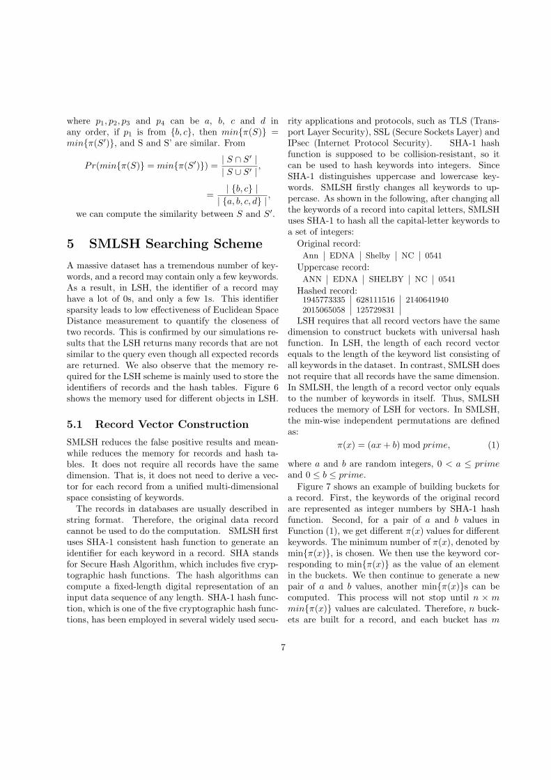
string format. Therefore, the original data recordcannot be used to do the computation. SMLSH firstuses SHA-1 consistent hash function to generate anidentifier for each keyword in a record. SHA standsfor Secure Hash Algorithm, which includes five cryp-tographic hash functions. The hash algorithms cancompute a fixed-length digital representation of aninput data sequence of any length. SHA-1 hash func-tion, which is one of the five cryptographic hash func-tions, has been employed in several widely used secu-

rity applications and protocols, such as TLS (Trans-port Layer Security), SSL (Secure Sockets Layer) andIPsec (Internet Protocol Security). SHA-1 hashfunction is supposed to be collision-resistant, so itcan be used to hash keywords into integers. SinceSHA-1 distinguishes uppercase and lowercase key-words. SMLSH firstly changes all keywords to up-percase. As shown in the following, after changing allthe keywords of a record into capital letters, SMLSHuses SHA-1 to hash all the capital-letter keywords toa set of integers:

Original record:

Ann EDNA Shelby NC 0541

Uppercase record:

ANN EDNA SHELBY NC 0541

Hashed record:1945773335 628111516 21406419402015065058 125729831

LSH requires that all record vectors have the samedimension to construct buckets with universal hashfunction. In LSH, the length of each record vectorequals to the length of the keyword list consisting ofall keywords in the dataset. In contrast, SMLSH doesnot require that all records have the same dimension.In SMLSH, the length of a record vector only equalsto the number of keywords in itself. Thus, SMLSHreduces the memory of LSH for vectors. In SMLSH,the min-wise independent permutations are definedas:

π(x) = (ax+ b) mod prime, (1)

where a and b are random integers, 0 < a ≤ primeand 0 ≤ b ≤ prime.

Figure 7 shows an example of building buckets fora record. First, the keywords of the original recordare represented as integer numbers by SHA-1 hashfunction. Second, for a pair of a and b values inFunction (1), we get different π(x) values for differentkeywords. The minimum number of π(x), denoted bymin{π(x)}, is chosen. We then use the keyword cor-responding to min{π(x)} as the value of an elementin the buckets. We then continue to generate a newpair of a and b values, another min{π(x)}s can becomputed. This process will not stop until n × mmin{π(x)} values are calculated. Therefore, n buck-ets are built for a record, and each bucket has m

7

oriKey hashKey

ANN 1945773335

EDNA 628111516

SHELBY 2140641940

NC 2015065058

0541 125729831

hashKey1 hashKey2 … hashKey1

hashKey3 hashKey5 … hashKey2

… … … …

hashKey4 hashKey1 … hashKey2

ANN EDNA SHELBY NC 0541

Original Record

Hashed Record

min{ (hashKey1), (hashKey2), (hashKey3), (hashKey4), (hashKey5)}

Buckets

n

m

Figure 7: An example of building buckets for arecord.

values. Algorithm 1 shows the procedure of bucketconstruction in SMLSH.

———————————————————————-Algorithm 1. Bucket construction in SMLSH.———————————————————————-(1) determine n×m values of a and b(2) for each k[i] do //k[i] is one of the keywords of

//a record(3) Use SHA-1 to hash k[i] into hashK[i](4) for each pair of a[p][q] and b[p][q] do(5) g[p][q] = (a[p][q] ∗ hashK[i] + b[p][q])

mod prime(6) if i == 0 then(7) min[p][q]=g[p][q](8) else if g[p][q] < min[p][q] then(9) min[p][q] = g[p][q](10) endif(11) endif(12) endfor(13) endfor—————————————————————–

5.2 Record Clustering

SMLSH makes n groups of m min-wise independentpermutations. Applying the m × n hash values toa record, SMLSH constructs n buckets with eachbucket having m hashed values. SMLSH then hasheseach bucket to a hash value with similarity preser-vation and clusters the data records based on their

hashKeyi hashKeyj … hashKeyk

hashKeyi hashKeyj … hashKeyk

… … … …

hashKeyi hashKeyj … hashKeyk

Buckets of a Record

hashID1 Hash Table 1

hashID2 Hash Table 2

… … …

hashIDn Hash Table n

Hash Tables

Figure 8: The process of finding locations for arecord.

similarity. Specifically, SMLSH uses XOR operationon the elements of each bucket to get a final hashvalue. Consequently, each record has n final hashedvalues, denoted by hashIDi.

hashIDi = (min{π1(S′)} XOR min{πm(S′)}) mod tableSize,

(2)

where S′ is a SHA-1 hased integer set, 1 ≤ i ≤ n.Algorithm 2 shows the pseudo-code for the procedureof records clustering in SMLSH.

——————————————————————Algorithm 2. Record clustering in SMLSH.——————————————————————(1) for each hashID[j] do(2) hashID[j]=0(3) for each min[j][t] do(4) hashID[j]ˆ=min[j][t](5) endfor(6) hashID[j]=hashID[j]mod tableSize(7) Insert the index of the record into the hash

table(8) endfor——————————————————————

Figure 8 presents the process of finding locations ofa record. There are n buckets for each record. Eachrow of hashKeys in a bucket is used to calculate afinal hash value for the bucket. Therefore, n buckethash values are produced (i.e., hashID1, , hashIDn).n hash tables are needed for saving all the buckets ofthe records in a database. Each hashID of a recordrepresenting the location of the record is stored in thecorresponding hash table.

8

5.3 SMLSH Searching Process

When searching a record’s similar records, SMLSHuses SHA-1 to hash the query record to integer rep-resentation. Then, SMLSH builds buckets for thequery record. Base on the clustering algorithm men-tioned above, SMLSH gets the n hashIDs for thequery record. It then searches every location basedon hashID in every hash table, exports all the recordswith the same hashID as the candidates of similarrecords of the query record. In order not to missother similar records (i.e., reduce false negatives),at the same time, SMLSH continues to build newn buckets from each located record for further sim-ilar record search. Specifically, SMLSH generates nbuckets from a located record using the method intro-duced previously. To generate the ith bucket, it ran-domly chooses elements in the ith bucket of the queryrecord and in the ith bucket of the located record. Itthen calculates the hashID of each newly constructedbucket and searches similar records using the aboveintroduced method. As the new buckets are gener-ated from the buckets of the query record and itssimilar record, the located records based on the newbuckets may have a certain similarity with the queryrecord.

Figure 9 shows the SMLSH similarity searchingprocess. Let us say after computing the buckets ofthe query record, we get the first hashID equals 1.Therefore, SMLSH checks the records which hashIDequals to 1 in the first hash table (i.e., HashTable1).As the figure shows, the hashID of record v equalsto 1 in HashTable1. We generate n buckets from v.Then, we use the ith bucket of records q and v togenerate the ith new bucket in the new group of nbuckets. The elements in the ith new bucket are ran-domly picked from the ith bucket of record q and fromthe ith bucket of record v. XOR operation is used tocompute the hashIDs of the new buckets. Accordingto the hashIDs of the new buckets, SMLSH searchesthe HashTable1 again to collect all the records havingthe same hashIDs and considers them as the candi-dates of the similar records of query record q. Afterfinishing searching the first hash table for hashID1,SMLSH continues searching the hash tables for otherhashIDs until finishing searching the nth hash table

QhashKeyi … QhashKeyj

… … …

QhashKeyi … QhashKeyj

Buckets of Query Record: q

Buckets of Query Record: v

VhashKeyi VhashKeyj… VhashKeyi VhashKeyj…

… ……

VhashKeyj VhashKeyi…

New Buckets

HashTable1

hashID = 1: v

…

hashID1=1

hashIDs

Figure 9: The process of similarity search.

for hashIDn.

——————————————————————Algorithm 3. Searching process in SMLSH.——————————————————————(1) Calculate n hashIDs of the query record(2) for each hashID[j] of the query record do(3) Get the records v with hashID[j] in the j-th

hash table(4) for each record v[k] do(5) Insert record v[k] into the similar record list(6) Collect all the elements in j-th bucket of

query record and record v[k](7) Randomly pick elements from the collection

to build n new buckets(8) Compute new hashIDs for the new buckets(9) Retrieve the records with new hashIDs in

the j-th hash table(10) Insert the retrieved records into the similar

record list(11) endfor(12) endfor(13) Compute the similarity of the records in the

similar record list(14) Output the similar records with similarity

greater than a threshold r——————————————————————

Algorithm 3 shows the pseudo-code of the search-ing process in SMLSH. For a record searching,SMLSH gets the hashIDs for the query record basedon the algorithm. It then searches the hash table,exports all the records with the same hashID as thesimilar records of the query record. A range also can

9

…

…

…

…

m

hashID

Source records Final hash tableBuckets

Ann

Johnso

n 1

6 F

em

ale

248

Dickso

n S

tree

t

Ann

Johnso

n | 2

0 | F

em

ale

| 168 G

arla

nd

…

K1

K2

K3

K4

K5

min{ (v)}

…

min{ (v)}

min{ (v)}

min{ (v)}

…

min{ (v)}

min{ (v)}

n

Id1

Id2

.

.

.

Idn

.

.

.

v1 vn

v1

SHA-1

Ann Johnson | 20 | Female | 168 Garland Query record:

qrangeSimilar

Records

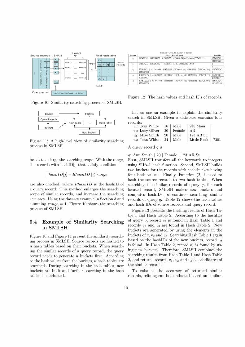
Figure 10: Similarity searching process of SMLSH.

Source Buckets

Hash Table Hash Table …

Query Records

Buckets

New Buckets

Figure 11: A high-level view of similarity searchingprocess in SMLSH.

be set to enlarge the searching scope. With the range,the records with hashID[j] that satisfy condition:

| hashID[j]−RhashID |≤ range

are also checked, where RhashID is the hashID ofa query record. This method enlarges the searchingscope of similar records, and increase the searchingaccuracy. Using the dataset example in Section 3 andassuming range = 1, Figure 10 shows the searchingprocess of SMLSH.

5.4 Example of Similarity Searchingin SMLSH

Figure 10 and Figure 11 present the similarity search-ing process in SMLSH. Source records are hashed ton hash tables based on their buckets. When search-ing the similar records of a query record, the queryrecord needs to generate n buckets first. Accordingto the hash values from the buckets, n hash tables aresearched. During searching in the hash tables, newbuckets are built and further searching in the hashtables is conducted.

THE HASH VALUES AND HASH IDS OF RECORDS

Record SHA-1 Hash Values hashID

v1 895479561 | 1630694977 | 612003623 | 1870446154 | 669783043 | 537429199 132419788

1416462664

v2 786139273 | 1186247512 | 114561690 | 1658656342 | 288242920 0

0

v3 370869835 | 1937983344 | 114561690 | 1870446154 | 323411961 | 2010266570 |

1226489228

1687479347

0

v4 1002692496 | 1630694977 | 586341023 | 1870446154 | 847272969 | 458697817 |

300130902

179605007

275941014

q 1945773335 | 1937983344 | 114561690 | 1658656342 | 323411961 | 537429199 |

1226489228

1687479347

1906035119

Figure 12: The hash values and hash IDs of records.

Let us use an example to explain the similaritysearch in SMLSH. Given a database contains fourrecords:

v1: Tom White 16 Male 248 Mainv2: Lucy Oliver 20 Female ARv3: Mike Smith 20 Male 123 AR St.v4: John White 24 Male Little Rock 7201

A query record q is:

q: Ann Smith | 20 | Female | 123 AR St.First, SMLSH transfers all the keywords to integersusing SHA-1 hash function. Second, SMLSH buildstwo buckets for the records with each bucket havingfour hash values. Finally, Function (2) is used tohash the source records to two hash tables. Whensearching the similar records of query q, for eachlocated record, SMLSH makes new buckets andcomputes hashIDs to continue searching similarrecords of query q. Table 12 shows the hash valuesand hash IDs of source records and query record.

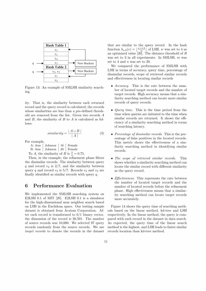
Figure 13 presents the hashing results of Hash Ta-ble 1 and Hash Table 2. According to the hashIDsof query q, record v3 is found in Hash Table 1 andrecords v2 and v3 are found in Hash Table 2. Newbuckets are generated by using the elements in thebuckets of q, v2 and v3. Searching Hash Table 1 againbased on the hashIDs of the new buckets, record v2is found. In Hash Table 2, record v1 is found by us-ing new buckets. Therefore, SMLSH combines thesearching results from Hash Table 1 and Hash Table2, and returns records v1, v2 and v3 as candidates ofthe similar records.

To enhance the accuracy of returned similarrecords, refining can be conducted based on similar-

10

Hash Table 1

v2

v1

v4

v3

Hash Table 2

v2, v3

v1

v4

q New Buckets

New Buckets q

Figure 13: An example of SMLSH similarity search-ing.

ity. That is, the similarity between each returnedrecord and the query record is calculated, the recordswhose similarities are less than a pre-defined thresh-old are removed from the list. Given two records Aand B, the similarity of B to A is calculated as fol-lows:

similarity =| A ∪B || A |

(3)

For example,A: Ann Johnson 16 FemaleB: Ann Johnson 20 Female

To A, the similarity of B is 34 = 0.75.

Then, in the example, the refinement phase filtersthe dissimilar records. The similarity between queryq and record v2 is 2/7, and the similarity betweenquery q and record v3 is 5/7. Records v2 and v3 arefinally identified as similar records with query q.

6 Performance Evaluation

We implemented the SMLSH searching system onE2LSH 0.1 of MIT [20]. E2LSH 0.1 is a simulatorfor the high-dimensional near neighbor search basedon LSH in the Euclidean space. Our testing sampledataset is obtained from Acxiom Corporation. Af-ter each record is transformed to 0/1 binary vector,the dimension of the record is 20,591. The numberof source records was 10,000. We selected 97 queryrecords randomly from the source records. We usetarget records to denote the records in the dataset

that are similar to the query record. In the hashfunction ha,b(v) = ⌊a·v+b

w ⌋ of LSH, w was set to 4 asan optimized value [20]. The distance threshold of Rwas set to 3 in all experiments. In SMLSH, m wasset to 4 and n was set to 20.

We compared the performance of SMLSH withLSH in terms of accuracy, query time, percentage ofdissimilar records, scope of retrieved similar recordsand effectiveness in locating similar records

• Accuracy. This is the rate between the num-ber of located target records and the number oftarget records. High accuracy means that a sim-ilarity searching method can locate more similarrecords of query records.

• Query time. This is the time period from thetime when queries are initiated to the time whensimilar records are returned. It shows the effi-ciency of a similarity searching method in termsof searching latency.

• Percentage of dissimilar records. This is the per-centage of false positives in the located records.This metric shows the effectiveness of a sim-ilarity searching method in identifying similarrecords.

• The scope of retrieved similar records. Thisshows whether a similarity searching method canlocate the similar record with different similarityas the query record.

• Effectiveness. This represents the rate betweenthe number of located target records and thenumber of located records before the refinementphase. High effectiveness means that a similar-ity searching method can locate target recordsmore accurately.

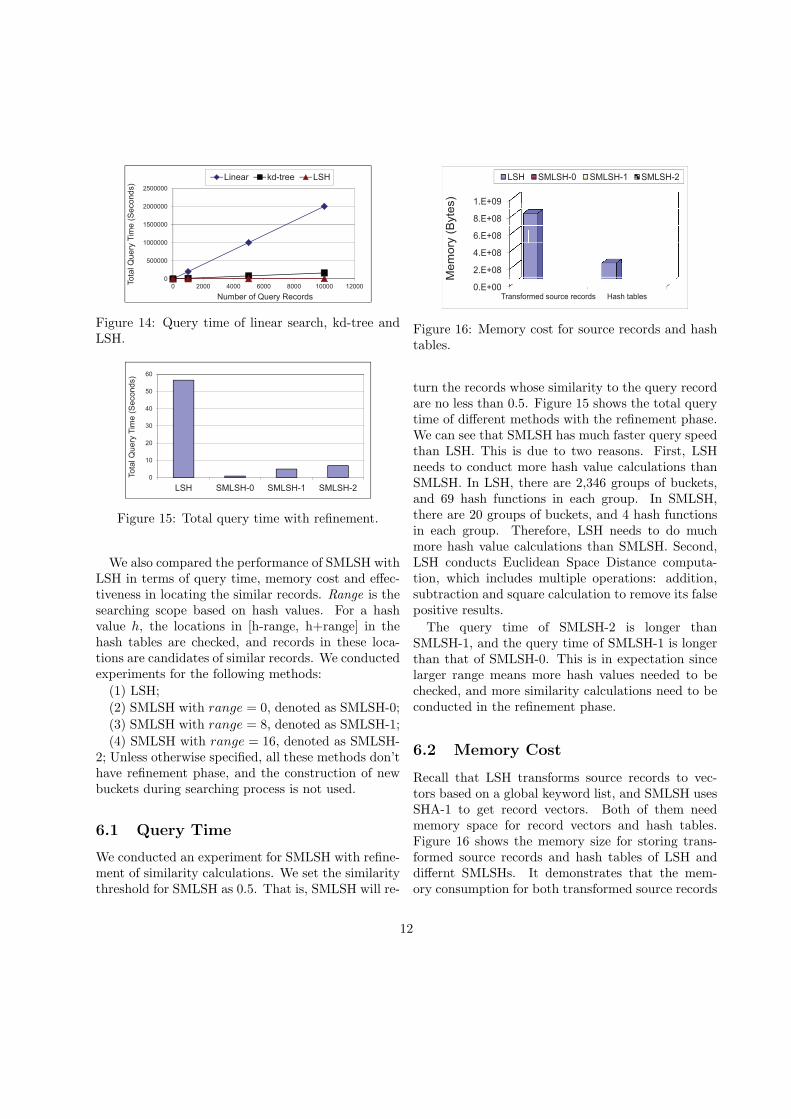
Figure 14 shows the query time of searching meth-ods based on the linear method, kd-tree and LSHrespectively. In the linear method, the query is com-pared with each record in the dataset in data search.As expected, the query time of the linear searchmethod is the highest, and LSH leads to faster similarrecords location than kd-tree method.

11

0

500000

1000000

1500000

2000000

2500000

0 2000 4000 6000 8000 10000 12000

Tota

l Q

ue

ry T

ime

(S

eco

nd

s)

Number of Query Records

Linear kd-tree LSH

Figure 14: Query time of linear search, kd-tree andLSH.

0

10

20

30

40

50

60

LSH SMLSH-0 SMLSH-1 SMLSH-2

Tota

l Q

ue

ry T

ime

(S

eco

nd

s)

Figure 15: Total query time with refinement.

We also compared the performance of SMLSH withLSH in terms of query time, memory cost and effec-tiveness in locating the similar records. Range is thesearching scope based on hash values. For a hashvalue h, the locations in [h-range, h+range] in thehash tables are checked, and records in these loca-tions are candidates of similar records. We conductedexperiments for the following methods:

(1) LSH;

(2) SMLSH with range = 0, denoted as SMLSH-0;

(3) SMLSH with range = 8, denoted as SMLSH-1;

(4) SMLSH with range = 16, denoted as SMLSH-2; Unless otherwise specified, all these methods don’thave refinement phase, and the construction of newbuckets during searching process is not used.

6.1 Query Time

We conducted an experiment for SMLSH with refine-ment of similarity calculations. We set the similaritythreshold for SMLSH as 0.5. That is, SMLSH will re-

LSH SMLSH 0 SMLSH 1 SMLSH 2

1 E+09s)

LSH SMLSH-0 SMLSH-1 SMLSH-2

8.E+08

1.E+09

Byte

s

4.E+08

6.E+08

mory

(

0 E 00

2.E+08

Me

m

0.E+00Transformed source records Hash tables

Figure 16: Memory cost for source records and hashtables.

turn the records whose similarity to the query recordare no less than 0.5. Figure 15 shows the total querytime of different methods with the refinement phase.We can see that SMLSH has much faster query speedthan LSH. This is due to two reasons. First, LSHneeds to conduct more hash value calculations thanSMLSH. In LSH, there are 2,346 groups of buckets,and 69 hash functions in each group. In SMLSH,there are 20 groups of buckets, and 4 hash functionsin each group. Therefore, LSH needs to do muchmore hash value calculations than SMLSH. Second,LSH conducts Euclidean Space Distance computa-tion, which includes multiple operations: addition,subtraction and square calculation to remove its falsepositive results.

The query time of SMLSH-2 is longer thanSMLSH-1, and the query time of SMLSH-1 is longerthan that of SMLSH-0. This is in expectation sincelarger range means more hash values needed to bechecked, and more similarity calculations need to beconducted in the refinement phase.

6.2 Memory Cost

Recall that LSH transforms source records to vec-tors based on a global keyword list, and SMLSH usesSHA-1 to get record vectors. Both of them needmemory space for record vectors and hash tables.Figure 16 shows the memory size for storing trans-formed source records and hash tables of LSH anddiffernt SMLSHs. It demonstrates that the mem-ory consumption for both transformed source records

12

0

500

1000

1500

2000

2500

Nu

mb

er o

f H

ash

Tab

les

SMLSH with Refinement LSH

Figure 17: The number of hash tables.

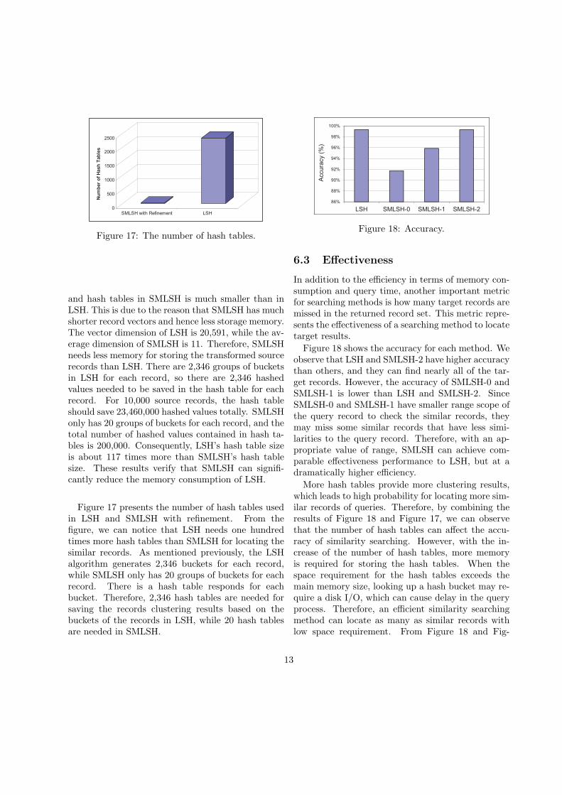
and hash tables in SMLSH is much smaller than inLSH. This is due to the reason that SMLSH has muchshorter record vectors and hence less storage memory.The vector dimension of LSH is 20,591, while the av-erage dimension of SMLSH is 11. Therefore, SMLSHneeds less memory for storing the transformed sourcerecords than LSH. There are 2,346 groups of bucketsin LSH for each record, so there are 2,346 hashedvalues needed to be saved in the hash table for eachrecord. For 10,000 source records, the hash tableshould save 23,460,000 hashed values totally. SMLSHonly has 20 groups of buckets for each record, and thetotal number of hashed values contained in hash ta-bles is 200,000. Consequently, LSH’s hash table sizeis about 117 times more than SMLSH’s hash tablesize. These results verify that SMLSH can signifi-cantly reduce the memory consumption of LSH.

Figure 17 presents the number of hash tables usedin LSH and SMLSH with refinement. From thefigure, we can notice that LSH needs one hundredtimes more hash tables than SMLSH for locating thesimilar records. As mentioned previously, the LSHalgorithm generates 2,346 buckets for each record,while SMLSH only has 20 groups of buckets for eachrecord. There is a hash table responds for eachbucket. Therefore, 2,346 hash tables are needed forsaving the records clustering results based on thebuckets of the records in LSH, while 20 hash tablesare needed in SMLSH.

86%

88%

90%

92%

94%

96%

98%

100%

LSH SMLSH-0 SMLSH-1 SMLSH-2

Accu

racy (

%)

Figure 18: Accuracy.

6.3 Effectiveness

In addition to the efficiency in terms of memory con-sumption and query time, another important metricfor searching methods is how many target records aremissed in the returned record set. This metric repre-sents the effectiveness of a searching method to locatetarget results.

Figure 18 shows the accuracy for each method. Weobserve that LSH and SMLSH-2 have higher accuracythan others, and they can find nearly all of the tar-get records. However, the accuracy of SMLSH-0 andSMLSH-1 is lower than LSH and SMLSH-2. SinceSMLSH-0 and SMLSH-1 have smaller range scope ofthe query record to check the similar records, theymay miss some similar records that have less simi-larities to the query record. Therefore, with an ap-propriate value of range, SMLSH can achieve com-parable effectiveness performance to LSH, but at adramatically higher efficiency.

More hash tables provide more clustering results,which leads to high probability for locating more sim-ilar records of queries. Therefore, by combining theresults of Figure 18 and Figure 17, we can observethat the number of hash tables can affect the accu-racy of similarity searching. However, with the in-crease of the number of hash tables, more memoryis required for storing the hash tables. When thespace requirement for the hash tables exceeds themain memory size, looking up a hash bucket may re-quire a disk I/O, which can cause delay in the queryprocess. Therefore, an efficient similarity searchingmethod can locate as many as similar records withlow space requirement. From Figure 18 and Fig-

13

Table 1: Whether the original record can be found.

Similarity SMLSH-0 SMLSH-1 SMLSH-21.0 Y Y Y0.9 Y Y Y0.8 Y Y Y0.7 Y Y Y0.6 N N Y0.5 N N Y0.4 N N Y0.3 N N Y0.2 N N Y0.1 N Y Y

ure 17, we can see that SMLSH can locate more than90% of target records with small numbers of hashtables.

In order to see the similarity degree of locatedrecords to the query record of SMLSH, we conductedexperiments on SMLSH-0, SMLSH-1 and SMLSH-2. We randomly chose one record, and changed onekeyword to make a new record as query record everytime. Our purpose is to see if SMLSH can find theoriginal record with the decreasing degree of similar-ity to the query record. Table 1 shows whether themethod can find the original record when it has dif-ferent similarities to the query record. “Y” meansthe method can find the original record and “N”means it cannot. The figure illustrates that SMLSH-2 can locate the original record in all similarity levels,and SMLSH-0 and SMLSH-1 can return the recordswhose similarity are greater than 0.6 to the queryrecord. The reason that SMLSH-2 can locate recordswith small similarity is because it has a larger scope ofrecords to check. The results imply that in SMLSH,records having higher similarity to the query recordhave higher probability to be located than recordshaving lower similarity.

Figure 19 depicts the percentage of similar recordsreturned in different similarity in SMLSH. From thefigure, we can observe that 100% of the similarrecords with similarity to the query records greaterthan 70% can be located in SMLSH. The percent-age of returned similar records decreases as the sim-ilarity between source records and query records de-creases. However, SMLSH still can locate more than90% of similar records when the similarity of source

0.00% 20.00% 40.00% 60.00% 80.00% 100.00%

Percentage of Returned Similar Records (%)

0%-10%

10%-20%

20%-30%

30%-40%

40%-50%

50%-60%

60%-70%

70%-80%

80%-90%

90%-100%

Sim

ilari

ty

Figure 19: Percentage of similar records returned indifferent similarity.

records and query records are between 60% and 70%.Few similar records can be located with low similarity(less than 60%). Therefore, the source records withhigh similarity have higher probability to be foundthan the source records with low similarity.

7 Conclusions

Traditional information searching methods rely onlinear searching or a tree structure. Both approachessearch similar records to a query in the entire scopeof a dataset, and compare a query with the recordsin the dataset in the searching process, leading tolow efficiency. This entry first presents a LocalitySensitive Hashing (LSH) based similarity searching,which is more efficient than linear searching and treestructure based searching in a massive dataset. How-ever, LSH still needs a large memory space for storingsource record vectors and hash tables, and leads tolong searching latency. In addition, it is not effec-tive in a very high-dimensional dataset and is notadaptive to data insertion and deletion. This en-try then presents an improved LSH based searchingscheme (SMLSH) that can efficiently and successfullyconduct similarity searching in a massive dataset.SMLSH integrates SHA-1 consistent hashing functionand min-wise independent permutations into LSH.It avoids sequential comparison by clustering similarrecords and mapping a query to a group of records di-rectly. Moreover, compared to LSH, it cuts down thespace requirement for storing source record vectors

14

and hash tables, and accelerates the query processdramatically. Further, it is not affected by data in-sertion and deletion. Simulation results demonstratethe efficiency and effectiveness of SMLSH in similar-ity searching in comparison with LSH. SMLSH dra-matically improves the efficiency over LSH in termsof memory consumption and searching time. In addi-tion, it can successfully locate queried records. Ourfuture work will be focused on further improving theaccuracy of SMLSH.

Acknowledgements

This research was supported in part by U.S. NSFgrants IIS-1354123, CNS-1254006, CNS-1249603,CNS-1049947, CNS-0917056 and CNS-1025652, Mi-crosoft Research Faculty Fellowship 8300751. Anearly version of this work was presented in the Pro-ceedings of ICDT’08 [15].

References

[1] C. Bohm, S. Berchtold, and D. A. Keim. Search-ing in high-dimensional spaces: Index structuresfor improving the performance of multimediadatabases. ACM Comput. Surv. 2001, 33(3),322–373.

[2] A. Z. Broder, M. Charikar, A. M. Frieze, andM. Mitzenmacher. Min-wise independent per-mutations. Journal of Computer and SystemSciences 2002, 1(3), 630–659.

[3] J. Buhler. Efficient large-scale sequence compar-ison by locality-sensitive hashing. Bioinformat-ics 2001, 5(17), 419–428.

[4] P. Ciaccia, M. Patella, and P. Zezula. M-trees:an efficient access method for similarity search inmetric space. In Proc. of the 23rd InternationalConference on Very Large Data Bases, Athens,Greece, August 25-29, 1997.

[5] A. Dasgupta, R. Kumar, and T. Sarlos. Fastlocality-sensitive hashing. In Proc. of the17th ACM SIGKDD international conference on

Knowledge discovery and data mining (KDD),San Diego, USA, August 21-24, 2011.

[6] C. Digout and M. A. Nascimento. High-dimensional similarity searches using a met-ric pseudo-grid. In Proc. of the 21st Interna-tional Conference on Data Engineering Work-shops, Tokyo, Japan, April 5-8, 2005.

[7] J. Gan, J. Feng, Q. Fang, and W. Ng. Locality-sensitive hashing scheme based on dynamic col-lision counting. In Proceedings of the ACMSIGMOD International Conference, Scottsdale,USA, May 20-24, 2012.

[8] A. Gionis, P. Indyk, and R. Motwani. SimilaritySearch in High Dimensions via Hashing. TheVLDB Journal 1999, 2(1), 518–529.

[9] P. Indyk and R. Motwani. Approximate near-est neighbors: Towards removing the curse ofdimensionality. In Proc. of the 30th AnnualACM Symposium on Theory of Computing, Dal-las, USA, May 24-26, 1998.

[10] B. Kulis and K. Grauman. Kernelized locality-sensitive hashing for scalable image search. InProc. 12th International Conference on Com-puter Vision, Kyoto, Japan, September 27-October 4, 2009.

[11] Q. Lv, W. Josephson, Z. Wang, M. Charikar,and K. Li. Integrating semantics-based accessmechanisums with P2P file systems. In Proc. ofthe the Third International Conference on Peer-to-Peer Computing (P2P), Linkping, Sweden,September 1-3,2003.

[12] R. R. Salakhutdinov and G. E. Hinton. Learninga nonlinear embedding by preserving class neigh-bourhood structure. Proceedings of the EleventhInternational Conference on Artificial Intelli-gence and Statistics, San Juan, Puerto Rico,March 21-24, 2007.

[13] V. Satuluri and S. Parthasarathy. Bayesian lo-cality sensitive hashing for fast similarity search.PVLDB 2012, 5(5), 430-441.

15

[14] T. Sellis, N. Roussopoulos, and C. Faloutsos.Multidimensional access methods: Trees havegrown everywhere. In Proc. of the 23rd Inter-national Conference on Very Large Data Bases,Athens, Greece, August 25-29, 1997.

[15] H. Shen, T. Li, and T. Schweiger. An ef-ficient similarity searching scheme in massivedatabases. In Proc. of the Third Interna-tional Conference on Digital Telecommunica-tions, Bucharest, Romania, June 29-July 5,2008.

[16] M. Slaney and M. Casey. Locality-sensitivehashing for finding nearest neighbors. IEEE Sig-nal Process. Mag. 2008, 1(2):128–131.

[17] H.-J. S. R. Weber and S. Blott. A quantitativeanalysis and performance study for similarity-search methods in high-dimensional spaces. InProc. of the 24th International Conference onVery Large Data Bases, New York, USA, August24-27, 1998.

[18] Y. Weiss, A. Torralba, and R. Fergus. Spectralhashing. In Proc. of Neural Information Pro-cessing Systems, Vancouver, Canada, December8-13, 2008.

[19] C. Yu, B. C. Ooi, K. L. Tan, and H. V. Jagadish.Indexing the distance: an efficient method toknn processing. In Proc. of the of 26th Inter-national Conference on Very Large Data Bases,Seoul, Korea, September 12-15, 2001.

[20] A. Andoni and P. Indyk.E2LSH 0.1 User Manual, 2005.http://web.mit.edu/andoni/www/LSH/index.html[Accessed in May 2012].

16