Search, Matching and Training

Christopher Flinn

New York University

Collegio Carlo Alberto

Ahu Gemici

Royal Holloway, U. of London

Steven Laufer

Board of Governors/FRB

February 21, 2016

1

Search, Matching and Training

Abstract

We estimate a partial and general equilibrium search model in which firms and workerschoose how much time to invest in both general and match-specific human capital. Tohelp identify the model parameters, we use NLSY data on worker training and wematch moments that relate the incidence and timing of observed training episodes tooutcomes such as wage growth and job-to-job transitions. We use our model to offera novel interpretation of standard Mincer wage regressions in terms of search frictionsand returns to training. Finally, we show how a minimum wage can reduce trainingopportunities and decrease the amount of human capital in the economy.

1 Introduction

There is a long history of interest in human capital investment, both before and afterentry into the labor market. In the latter case, it is common to speak of general andspecific human capital, which are differentiated in terms of their productivity-enhancingeffects across jobs (which may be defined by occupations, industries, or firms). Theclassic analysis of Becker (1964) considered these types of investments in competitivemarkets and concluded that workers should pay the full costs of general training, withthe costs of specific training (that increases productivity only at the current employer)being shared in some way. Analysis of these investments in a noncompetitive setting ismore recent. Acemoglu and Pischke (1999) consider how the predictions of the amountand type of human capital investment in a competitive labor market are altered whenthere exist market imperfections in the form of search frictions. Frictions create animperfect “lock in” between a worker and the firm, so that increases in general orspecific human capital are generally borne by both the worker and the firm.

We utilize training data in the estimation of what otherwise is a reasonably standardsearch model with general and specific human capital. These data, described brieflybelow, indicate that formal training is reported by a not insignificant share of workers,and that the likelihood of receiving training is a function of worker characteristics, inparticular, education. Workers do not receive training only at the beginning of jobspells, although the likelihood of receiving training is typically a declining function oftenure. Since training influences the likelihood of termination of the job and wages, it isimportant to examine training decisions in a relatively complete model of worker-firmemployment relationships.

One motivation for this research is related to recent observations regarding shifts inthe Beveridge curve, which is the relationship between job vacancies and job searchers.While the unemployment rate in the U.S. has been markedly higher from 2008 andbeyond,1 reported vacancies remain high. This mismatch phenomenon has been inves-tigated through a variety of modeling frameworks (see, e.g., Cairo (2013), Lindenlaub(2013)), typically by allowing some shift in the demand for workers’ skills. In our mod-eling framework, such a shift could be viewed as a shift downward in the distribution ofinitial match productivities. Given the absence of individuals with the desired skill sets,the obvious question is why workers and firms do not engage in on-the-job investmentso as to mitigate the mismatch in endowments. Using our model, we can theoreti-cally and empirically investigate the degree to which a decentralized labor market withsearch frictions is able to offset deterioration in the initial match productivity distri-bution. This will lead us to consider policies that could promote increased investmentactivities, some of which are described below.

Another motivation for our research is to provide a richer model of the path of wages

1While the unemployment rate has declined recently, the employment rate in the population is at ahistoric low. Many of those counted as out of the labor force are in fact willing to take a reasonable joboffer, and hence should be considered to be “untemployed” in the true sense of the term.

3

on the job and a more complete view of the relationship between workers and firms.In this model, firms offer workers the opportunity to make mutually advantageousinvestments in the worker’s skills, both of the general and specific (to the job) type.While investing, the worker devotes less time to productive activities, which is the onlycost of investment that we include in the model.2 Wage changes over the course of theemployment spell are produced by changes in general skill levels, changes in specificskill levels, and changes in investment time. In model specifications that include on-the-job search possibilities, which is the case for ours, wages during an employmentspell may also increase due to the presence of another firm bidding for the employee’sservices, as in Postel-Vinay and Robin (2002), Dey and Flinn (2005), and Cahuc et al.(2006). When there exists the potential for other firms to “poach” the worker fromher current firm, investments in match-specific skills will be particularly attractive tothe current employer, since high levels of match-specific skills will make it less likelythat the worker will exit the firm for one in which her initial match-specific skill levelis higher. Other things equal, these differences in the retention value component ofspecific-skill investment implies that firms will reduce the employee’s wage less for agiven level of specific-skill investment than for general skill investment.

Why would firms ever partially finance improvements in general ability? In ourmodeling framework the flow productivity of a match is given by y(a, θ) = aθ − ζ,where a is the general ability of the worker, θ is match productivity, and ζ is a flowcost of employment, which may be thought of as the rental rate on capital equipmentrequired for the job. The gain in flow productivity from a small change in a is simply θand the gain in flow productivity from a small change in θ is simply a. Jobs for whicha is relatively high in comparison to θ will experience bigger productivity gains frominvestment in θ and conversely for job matches in which a is relatively low in comparisonwith θ. Thus, strictly from the productivity standpoint, there will an incentive to moreevenly balance a and θ in the investment process. This, coupled with the fact thatthere exist search frictions, will lead firms to be willing to finance part of the investmentin general human capital, even if this does not change the expected duration of thematch.

We believe that our modeling framework may be useful in understanding the linkbetween initial labor market endowments and earnings inequality over the labor marketcareer. Flinn and Mullins (2015) estimated a model with an identical specificationfor flow productivity as the one employed here and examined the pre-market entryschooling decision.3 In their model, initial ability endowments were altered by schooling

2That is, the only costs of investing in either of the skills is the lost output associated with the investmenttime. Moreover, these costs are the same for either type of investment. There are no direct costs of investmentas in Wasmer (2006), for example. In his case, all investment in skills occurs instantaneously at the beginningof a job spell. Lentz and Roys (2015), instead, assume that general and match-specific skills are binary, andthat for a low type worker on either dimension the cost of training is a flow cost that is increasing in therate at which the transition to the high skill type occurs. They do not allow for depreciation in skills, whichwe find to be an empirically important phenomenon.

3They did not consider flow costs of employment, so in that paper ζ = 0.

4

decisions, and these decisions were a function of all of the primitive labor marketparameters. In their setting, a was fixed over the labor market career and a matchdraw at a firm was also fixed over the duration of the job spell. In the case of ourmodel, both a and θ are subject to (endogenous) change, although it may well be thata is more difficult and costly to change after labor market entry. This is due to thefact that employers are not equipped to offer general learning experiences as efficientlyas are schools that specialize in increasing the cognitive abilities of their students.To the extent that a is essentially fixed over the labor market careers, individualswith large a endowments will be more attractive candidates for investment in match-specific skills than will individuals with low values of a. Even if initial values of θ aredrawn from the same distribution for all a types, which is the assumption made inour model, higher values of a at the time of labor market entry would be expected tolead to more investments and a more rapidly increasing wage profile over the course ofan employment spell. This offers a mechanism to amplify the differences in earningsgenerated by the initial variability in a.

Using estimates from the model, we can determine the impact of various types oflabor market policies on investment in the two types of human capital. For example,Flinn and Mullins (2015) investigated the impact of minimum wage laws on pre-marketinvestment. They found that for relatively low (yet binding for some low generalability workers) minimum wage levels, the minimum wage could be a disincentivefor pre-market investment, since similar wage rates could be obtained without costlyeducation. At high levels of the minimum wage, however, most individuals investedin a to increase their chance of finding a job. For firms to earn nonnegative profitflows in that model, productivity has to be at least aθ ≥ m, where m is the minimumwage. For high values of m, workers will invest in general ability to increase theirlevel of a so as to increase the likelihood of generating a flow productivity level thatsatisfies the firm’s nonnegative flow profit condition. In our framework of post-entryinvestment, the impact of minimum wages is also ambiguous. As in the standardBecker story, a high minimum wage will discourage investment activity if the firm isto achieve nonnegative flow profits. On the other hand, through investment activitythat raises the individual’s productivity (through a and/or θ), the firm and worker canact to remove the constraint and push the individual’s productivity into a region forwhich w > m. These possibilities may mitigate the need to increase pre-market entryinvestment in a.

Another policy that we will investigate is government subsidization of OTJ trainingby firms.4 In our model, there exists only an opportunity cost to training, which is theoutput lost from the worker investing in skill acquisition during a portion of the workday. In this case, a government subsidy amounts to a transfer to the worker-firm pairthat compensates them for a portion of the lost productivity associated with training.We will have these subsidies financed through taxes on labor earnings and firm profits,and will look for constant marginal rate taxes on both that will pay for an efficient

4Investment ubsidies are not considered in the current draft..

5

subsidy program.In terms of related research, the closest paper to ours is probably Wasmer (2006).

He presents a formal analysis of the problem in a framework with search frictions andfiring costs. His model is stylized, as is the one we develop below, and is not takento data. He assumes that human capital investments, be it of the general or specifickind, are made as soon as the employment relationship between a worker and a firmbegins. Investment does not explicitly involve time or learning by doing, which webelieve to be an important part of learning on the job. However, due to the simplicityof the investment technology, Wasmer is able to characterize worker and firm behaviorin a general equilibrium setting, and he provides elegant characterizations of the statesof the economy in which workers and firms will choose only general, only specific, orboth kinds of human capital investment. The goal of our paper is to estimate a partialequilibrium version of this type of model with what we think may be a slightly morerealistic form of the human capital production technology, one in which time plays thecentral role.

Another related paper is Bagger et al. (2014). This paper examines wage andemployment dynamics in a discrete-time model with deterministic growth in generalhuman capital in the number of years of labor market experience. There is no match-specific heterogeneity in productivity, but the authors do allow for the existence offirm and worker time invariant heterogeneity. There is complementarity between theworker’s skill level and the productivity level of the firm, so that it would be opti-mal to reallocate more experienced workers to better firms. The authors allow forrenegotiation of wage contracts between workers and firms when an employed workermeets an alternative employer, and due to the generality of human capital, the moreproductive firm always wins this competition. The model is estimated using Danishemployer-employee matched data. Key distinctions between our approach and the onetaken in that paper are the lack of firm heterogeneity but the presence of worker-firmmatch heterogeneity, the value of which can be changed by the investment decisionsof the worker-firm pair. This paper also allows for worker heterogeneity that is anendogenous stochastic process partially determined through the investment decisionsof workers and firms.

Lentz and Roys (2015) also examine general and specific human capital accumula-tion in a model that features worker-firm renegotation and the ability of firms to makelifetime welfare promises to workers in the bargaining stage. There is firm heterogene-ity in productivity, and the authors find that better firms provide more training. Thenature of the contracts offered to workers is more sophisticated than the ones consid-ered here, and the authors explicitly address the issue of inefficiencies in the trainingand mobility process. They assume that there are only four training states in theeconomy (an individual can be high or low skill in general and specific productivity),which greatly aids in the theoretical analysis at the cost of not being able to generatewage and employment sample paths that can fit patterns observed at the individuallevel. They also assume that there is no skill depreciation, which aids in the theoreticalanalysis of the model.

6

The plan of the paper is as follows. In Section 2, we analyze a partial equilibriumsearch model with general and specific human capital and subsequently extend it to ageneral equilibrium framework. Section 3 discusses the data used in the estimation ofthe model, and presents descriptive statistics. Section 4 discusses econometric issuessuch as the model specification used in our estimation, the estimator we use, andidentification. In Section 5, we present the estimation results and discuss the detailsof the estimated model, such as parameter values, within-sample fit and policy rules.Section 5 also presents a discussion regarding the implications of our estimated modelfor sources of wage growth and provides a unique perspective on the interpretationof the standard Mincer wage regression. In Section 6, we conduct a minimum wageexperiment to determine the impact of minimum wages on general and specific humancapital investment decisions, in a partial as well as general equilibrium framework.Section 7 concludes.

2 Modeling Framework

Individuals are characterized in terms of a (general) ability level a, with which theyenter the labor market.5 There are M values of ability, given by

0 < a1 < ... < aM <∞.

When an individual of type ai encounters a firm, she draws a value of θ from thediscrete distribution G over the K values of match productivity θ, which are given by

0 < θ1 < ... < θK <∞.

The flow productivity value of the match is given by

y(i, j) = aiθj − ζ,

where ζ is a flow cost of the job, which we think of as the rental rate on capital equip-ment that must be used in the production process in addition to the labor input. In thegeneral equilibrium version of the model, to be discussed below, firms are assumed topay flow posting fees while holding a vacancy open. One rationale for such a cost couldbe that firms rent a piece of capital equipment on which an individual’s skills at the jobcan be assessed when they apply. In this case, it also seems reasonable to assume thata piece of capital equipment is required in the case in which the individual is hired.Under our assumptions on the distributions of a and θ, we obtain an estimate of ζ that

5Flinn and Mullins (2015) examine pre-market entry education decisions in a search environment inwhich a hold-up problem exists. We will not explicitly model the pre-market entry schooling decision, butwill merely assume that the distribution of an individual’s initial value of a at the time of market entry isa stochastic function of their completed schooling level. In estimation, we will distinguish three schoolinglevels.

7

is large and positive, and that significantly improves the fit of the model. It also servesto produce what we consider to be more reasonable human capital investment policyfunctions than when ζ = 0.

We consider the case in which both general ability and match productivity can bechanged through investment on the job. The investment level, along with the wage, aredetermined cooperatively in a model with a surplus division rule. At every moment oftime, the individual and firm can devote a proportion τa of time to training in generalability, in the hope of increasing a. Similarly, they can invest a proportion of time τθin job-specific training, in the hope of increasing θ.

We will assume that the two stochastic production technologies for a and θ areindependent, in the sense that the likelihood of an improvement in a depends only onτa and not on τθ, and that the likelihood of an improvement in θ depends only on τθand not τa. Given that the level of a is currently ai, the rate of improvement in a isgiven by

ϕa(i, τa),

with ϕa(i, τa) ≥ 0, and ϕa(i, 0) = 0 for all i. We restrict the improvement process toincrease the value of i to i+1 in the case of a successful investment. We will also allowfor reductions in the value of a. This depreciation rate is assumed to be constant andequal to δa for all i > 1. In the case of one of these Poisson shocks, the level of a willdecrease from i to i−1, except when i = 1, when the individual is already at the lowestability level. Since the rate of decreases in a are independent of investment time, theimplication is that at the highest level of a, aM , no investment in a will occur.

For purposes of estimation, we further restrict the function ϕa to have the form

ϕa(i, τa) = ϕ0a(i)ϕ

1a(τa),

where ϕ1a is strictly concave in τa, with ϕ

1a(0) = 0. The term ϕ0

a(i) can be thought of astotal factor productivity (TFP) in a way, and we place no restriction on whether ϕ0

a(i)is increasing or decreasing in i, although the functional form we utilize in estimationwill restrict this function to be monotone.6

There is an exactly analogous production technology for increasing match-specificproductivity, with the rate of increase from match value j to match value j + 1 givenby

ϕθ(j, τθ) = ϕ0θ(j)ϕ

1θ(τθ),

with ϕ1θ strictly concave in τθ, and ϕ

1θ(0) = 0. There is no necessary restriction on the

TFP terms, as above. As is true for the a process, there is an exogenous depreciation

6By this we mean that eitherϕ0

a(1) ≤ ϕ0

a(2) ≤ ... ≤ ϕ0

a(M)

orϕ0

a(1) ≥ ϕ0

a(2) ≥ ... ≥ ϕ0

a(M).

8

rate associated with all θj , j > 1, which is equal to δθ. If one of these shocks arrive,then match productivity is reduced from θj to θj−1. As was true in the case of a, ifmatch productivity is at its highest level, θK , then τθ = 0.

The only costs of either type of training are foregone productivity, since total pro-ductivity is given by (1−τa−τθ)y(i, j). The gain from an improvement in either accruesto both the worker and firm, although obviously, gains in general human capital in-crease the future value of labor market participation (outside of the current job spell)to the individual only. As noted by Wasmer (2006), this means that the individual’sbargaining position in the current match is impacted by a change in a to a greaterextent than it is due to a change in θ. Motives for investment in the two different typesof human capital depend importantly on the worker’s surplus share α, but also on allother primitive parameters characterizing the labor market environment.

2.1 No On-the-Job Search

We first consider the case of no on-the-job search in order to fix ideas. In definingsurplus, we use as the outside option of the worker the value of continued search in theunemployment state, given by VU (a), and for the firm, we will assume that the valueof an unfilled vacancy is 0, produced through the standard free entry condition (FEC).We can write the problem as

maxw,τ

(

VE(i, j;w, τa, τθ)− VU (i))α

VF (i, j;w, τa, τθ)1−α,

where VE and VF functions are the value of employment to the worker and to the firm,respectively, given the wage and investment times.

We first consider the unemployment state. We will assume that the flow value ofunemployment to an individual of type ai is proportional to ai, or bai, i = 1, ...,M.Then we can write

VU (i) =bai + λU

∑

j=r∗(i)+1 pjVE(i, j)

ρ+λU G(θr∗(i))

(1)

where the critical (index) value r∗(i) is defined by

VU (i) ≥ VE(i, θr∗(i))

VU (i) < VE(i, θr∗(i)+1).

An agent of general ability ai will reject any match values of θr∗(i) or less, and acceptany match values greater than this.7

Given a wage of w and a training level of τa and τθ, the value of employment of

7Note that we assume that there are no shocks to the individuals’ ability level during unemployment.

9

type ai at a match of θj is

VE(i, j;w, τa, τθ) = (ρ+ ϕa(i, τa) + ϕθ(j, τθ) + δa(i) + δθ(j) + η)−1×

[w + ϕa(i, τa)Q(i+ 1, j) + ϕθ(j, τθ)VE(i, j + 1) + δa(i)Q(i− 1, j)

+δθ(j)Q(i, j − 1) + ηVU (ai)],

where δk(i) = 0 if i = 1 and δk(i) = δk if i > 1, for k = a, θ. The term

Q(i, j) ≡ max[VE(i, j), VU (i)],

allows for the possibility that a reduction in the value of a or θ could lead to anendogenous termination of the employment contract, with the employee returning tothe unemployment state. It also allows for the possibility that an increase in a from aito ai+1 could lead to an endogenous separation. This could occur if the reservation θ,r∗(i), is increasing in i. In this case, an individual employed at the minimally acceptablematch r∗(i) + 1, may quit if a improves and r∗(i+ 1) ≥ r∗(i) + 1.

The corresponding value to the firm is

VF (i, j;w, τa, τθ) = (ρ+ ϕa(i, τa) + ϕθ(j, τθ) + δa(i) + δθ(j) + η)−1×

[(1− τa − τθ)y(i, j) − w + ϕa(i, τa)QF (i+ 1, j) + ϕθ(j, τθ)VF (i, j + 1)

+δaQF (i− 1, j) + δθQF (i, j − 1)]

where QF (i, j) = 0 if Q(i, j) = VU (i) and QF (i, j) = VF (i, j) if Q(i, j) = VE(i, j). Thenthe solution to the surplus division problem is given by

w∗(i, j), τ∗a (i, j), τ∗

θ (i, j) = arg maxw,τa,τθ

(

VE(i, j;w, τa, τθ)− VU (i))α

×VF (i, j;w, τa, τθ)1−α;

VE(i, j) = VE(i, j;w∗(i, j), τ∗a (i, j), τ

∗

θ (i, j)),

VF (i, j) = VF (i, j;w∗(i, j), τ∗(i, j), τ∗θ (i, j)).

More specifically, the surplus division problem is given by

maxw,τa,τθ

(ρ+ ϕa(i, τa) + ϕθ(j, τθ) + δa(i) + δθ(j) + η)−1

×

[

w + ϕa(i, τa)[QE(i+ 1, j) − VU (i)] + ϕθ(j, τθ)[VE(i, j + 1)− VU (i)]

+δa(i)[Q(i − 1, j) − VU (i)] + δθ(j)[Q(i, j − 1)− VU (i)]− ρVU (ai)

]α

×

[

(1− τ)y(i, j) − w + ϕa(i, τα)QF (i+ 1, j) + ϕθ(j, τθ)VF (i, j + 1)

+δa(i)QF (i− 1, j) + δθ(j)QF (i, j − 1)

]1−α

.

The first order conditions for this problem can be manipulated to get the reasonably

10

standard wage-setting equation,

w∗(i, j) = α(1 − τ∗a − τ∗θ )y(i, j) + ϕa(i, τ∗

a )QF (i+ 1, j) + ϕθ(j, τ∗

θ )VF (i, j + 1)

+δa(i)QF (i− 1, j) + δθ(j)QF (i, j − 1)

+(1− α)ρVU (i) − ϕa(i, τ∗

a )(VE(i+ 1, j) − VU (i))

−ϕθ(j, τ∗

θ )(VE(i, j + 1)− VU (i))] − δa(i)Q(i − 1, j) − δθ(j)Q(i, j − 1).

The first order conditions for the investment times τa and τθ are also easily derived,but are slightly more complex than the wage condition. The assumptions regardingthe investment technologies ϕa and ϕθ have important implications for the investmentrules, obviously. The time flow constraint is

1 ≥ τa + τθ,

τa ≥ 0

τθ ≥ 0.

Depending on the parameterization of the production technology, it is possible thatoptimal flow investment of either type is 0, that one type of investment is 0 whilethe other is strictly positive, and even that all time is spent in investment activity,whether it be in one kind of training or both. In such a case, it is possible to producethe implication of negative flow wages, and we shall not explicitly assume these awayby imposing a minimum wage requirement in estimation. In the case of internships, forexample, which are supposed to be mainly investment activities, wage payments arelow or zero. Including the worker’s direct costs of employment, the effective wage ratemay be negative. What is true is that no worker-firm pair will be willing to engage insuch activity without the future expected payoffs being positive, which means that theworker would generate positive flow profits to the firm at some point during the jobmatch.

2.2 On-the-Job Search

In the case of on-the-job search, individuals who are employed are assumed to receiveoffers from alternative employers at a rate λE , and it is usually the case that λE < λU .If the employee meets a new employer, the match value at the alternative employer, θj′ ,is immediately revealed. Whether or not the employee leaves for the new job and whatthe new wage of the employee is after the encounter depends on assumptions maderegarding how the two employers compete for the individual’s labor services. In Flinnand Mabli (2009), two cases were considered. In the first, in which employers are notable to commit to wage offers, the outside option in the wage determination problemalways remains the value of unemployed search, since this is the action available tothe employee at any moment in time. This model produces an implication of efficientmobility, in that individuals will only leave a current employer if the match produc-

11

tivity at the new employer is at least as great as current match productivity (generalproductivity has the same value at all potential employers). An alternative assump-tion, utilized in Postel-Vinay and Robin (2002), Dey and Flinn (2005), and Cahuc etal. (2006), is to allow competing employers to engage in Bertrand competition for theemployee’s services (this model assumes the possibility of commitment to the offeredcontract on the part of the firm). In this case, efficient mobility will also result, butthe wage distribution will differ in the two cases, with employees able to capture moreof the surplus (at the same value of the primitive parameters) in the case of Bertrandcompetition. We begin our discussion with the Bertrand competition case in this sec-tion, although we estimate the model under both scenarios. For reasons explained atthe end of this section, the empirical work will emphasize the no-renegotiation case.

Under either scenario, ai has no impact on mobility decisions, since it assumes thesame value across all employers. In the Bertrand competition case (as in Dey andFlinn (2005), for example), the losing firm in the competition for the services of theworker is willing to offer all of the match surplus in its attempt to retain the worker.For example, let the match value at the current employer be θj, and the match valueat the potential employer be θj′. We will denote the maximum value to an employee oftype ai of working at a firm where her match value is θj by V (i, j), which is the casein which the employee captures all of the match surplus (since the value of holding anunfilled vacancy is assumed to be equal to 0, by transferring all of its surplus to theemployee, the firm is no worse of than it would be holding an unfilled vacancy). In theBertrand competition case then, and assuming that j′ ≤ j, the losing firm offers V (i, j′)for the individual’s labor services. The winning firm then divides the surplus with theemployee, where the employee’s outside option becomes V (i, j′). Note that in the casethat j′ = j, the individual would be indifferent between the two firms, the two firmswould be indifferent with respect to hiring her or not, and whichever offer it accepted,the employee would capture the entire match value, that is, VE(i, j) = V (i, j). Becauseof the investment possibilities, it is not generally the case that the wage at the winningfirm will be equal to aiθj − ζ, which would be true when there are no investmentpossibilies.

In the case of on-the-job search with Bertrand competition between employers, wedenote the value of the employment match to the worker and the firm by V (i, j, j′)and VF (i, j, j

′), respectively. The first argument denotes the individual’s general abilitytype, ai, and the second denotes the value of the match at the employer. The thirdargument in the function is the highest match value encountered during the current em-ployment spell (which is a sequence of job spells not interrupted by an unemploymentspell) at any other employer. Since mobility decisions are efficient, we know that j′ ≤ j.When the individual has encountered no other match values during the current em-ployment spell that exceeded the value r∗(i)+1, then we will write V (i, j, j∗(i)). Whenan individual encounters a new firm with a new match draw j′′, then the individual’s

12

new value of being employed is given by

V (i, j′′, j) if j′′ > jV (i, j, j′′) if j ≥ j′′ > j′

V (i, j, j′) if j′ ≥ j′′(2)

In the first row, the individual changes employer, and now the match value at thecurrent employer becomes the next best match value during the current employmentspell. In the second row, the employee stays with her current employer, but gains moreof the total surplus associated with the match, which implies an increase in her wageat the employer. In the third row, the individual does not report the encounter to hercurrent employer, since it doesn’t increase her outside option.

To see these effects more formally, we first consider the case in which a worker witha current match value of θj who has previously worked at a job with a match value ofθk, k ≤ j, and where there was no intervening unemployment spell. In this case, wewrite the worker’s value given wage w and training time τ as

VE(i, j, k;w, τa, τθ) =NE(w, τa, τθ; i, j, k)

D(τa, τθ; i, j, k),

where

NE(w, τa, τθ; i, j, k) = w + λE [

j∑

s=k+1

psVE(i, j, s) +∑

s=j+1

psVE(i, s, j)]

+ϕa(i, τa)Q(i+ 1, j, k) + ϕθ(j, τθ)VE(i, j + 1, k)

δa(i)Q(i − 1, j, k) + δθ(j)Q(i, j − 1, k) + ηVU (i);

D(τa, τθ; i, j, k) = ρ+ λEG(θk) + ϕa(i, τa) + ϕθ(j, τθ)

δa(i) + δθ(j) + η.

The term Q(i + 1, j, k) = maxV (i + 1, j, k), VU (i + 1), indicating the possibilitythat an increase in a could lead to an endogenous separation depending on the valueof θj . The term Q(i − 1, j, k) = maxV (i − 1, j, k), VU (i − 1), indicating that thevalue of unemployed search has decreased as well. Finally, we have Q(i, j − 1, k) =maxV (i, j − 1,min(j − 1, k)), VU (i). In the case where j = k, this implies that thevalue of the outside option is reduced with the current match value. We impose thisconvention so as to keep the surplus division problem well-defined. Other assumptionscould be made regarding how the negotiations between and employer and employee areimpacted when the match value decreases.

The value to the firm is given by

VF (i, j, k;w, τa, τθ) =NF (w, τa, τθ; i, j, k)

D(τa, τθ; i, j, k),

13

where

NF (w, τa, τθ; i, j, k) = y(i, j)(1 − τa − τθ)− w + ϕa(i, τa)QF (i+ 1, j, k)

+ϕθ(j, τθ)VF (i, j + 1, k) + δa(i)QF (i− 1, j, k)

+δθ(j)QF (i, j − 1,min(j − 1, k)) + λE

j∑

s=k+1

psVF (i, j, s).

Now the surplus division problem is

maxw,τa,τθ

D(τa, τθ; i, j, k)−1[NE(w, τa, τθ; i, j, k) − V (i, k)]α

×NF (w, τa, τθ; i, j, k)1−α,

which is only slightly more involved than the problem without OTJ search, but thegeneralization yields another fairly complex dependency between the current value ofthe match and the training time decisions. It is clear that the value of match-specificinvestment to the employer in the case of OTJ search is even higher than in the noOTJ case, since it also increases (in expected value) the duration of the match, andthis value always exceeds the value of an unfilled vacancy, which is 0. The value ofeither type of training is also enhanced from the point of view of the worker, since inaddition to increasing her value at her current employer, higher values of a or θ enhanceher future bargaining position during the current employment spell, and, in the caseof a, even beyond the current employment spell. Once the employment spell ends,the bargaining advantage from the match history ends, including gains accumulatedthrough investment in match-specific productivity. On the other hand, the value ofprevious investments in general productivity is carried over, in a stochastic sense,which is what makes this type of human capital particularly valuable from the worker’sperspective, and accounts for her disproportionate costs of funding these investments.Finally, the value of unemployed search is given by

VU (i) =bai + λU

∑

j=r∗(i)+1 pjVE(i, j, j∗(i))

ρ+λU G(θr∗(i))

.

As we have seen, in the case of Bertrand competition, there is some arbitrarinessin defining the employment state when the outside option and current match valuesare equal and there is depreciation in the current match value. In this case, we havesimply assumed that the employee continues to receive the entire surplus of the match,although this total surplus has decreased due to the decrease in match-specific produc-tivity from θj to θj−1. The other case of employer-employee interaction we consider iswhen employers do not respond to outside offers. This would be the case when outsideoffers cannot be observed and verified. Moreover, even if they were, employers have anincentive to cheat on the employment contract agreed to once the outside offer is nolonger available. When the outside offer is removed, the employee’s only alternative

14

is to quit into unemployed search, so that this is the outside option considered whendeciding upon wage-setting and the amount of work time devoted to investment.

In this case, decisions are considerably simplified. As in the case of no OTJ search,the employment contract is only a function of the individual’s type and the currentmatch value, (i, j). The property of efficient turnover decisions continues to hold, withthe employee accepting all jobs with a match value j′ > j, and refusing all others. Theformal structure of the problem is modified as follows.

VE(i, j;w, τa, τθ) =NE(w, τa, τθ; i, j)

D(τa, τθ; i, j),

where

NE(w, τa, τθ; i, j) = w + λE∑

s=j+1

psVE(i, s)

+ϕa(i, τa)Q(i+ 1, j) + ϕθ(j, τθ)VE(i, j + 1)

+δa(i)Q(i − 1, j) + δθ(j)Q(i, j − 1) + ηVU (ai);

D(τa, τθ; i, j) = ρ+ λEG(θj) + ϕa(i, τa) + ϕθ(j, τθ)

+δa(i) + δθ(j) + η.

The term Q(i + 1, j) = maxV (i + 1, j), VU (i + 1), indicating the possibility that anincrease in a could lead to an endogenous separation depending on the value θj. Theterm Q(i−1, j) = maxV (i−1, j), VU (i−1), indicating that the value of unemployedsearch has decreased as well. Finally, we have Q(i, j − 1) = maxV (i, j − 1), VU (i).

The value to the firm conditional on the wage and investment decisions is given by

VF (i, j;w, τa, τθ) =NF (w, τa, τθ; i, j)

D(τa, τθ; i, j),

where

NF (w, τa, τθ; i, j) = y(i, j)(1 − τa − τθ)− w + ϕa(i, τa)QF (i+ 1, j)

+ϕθ(j, τθ)VF (i, j + 1) + δa(i)QF (i− 1, j)

+δθ(j)QF (i, j − 1),

and where QF (i+1, j) = VF (i+1, j) if V (i+1, j) > VU (i+1) and equals 0 otherwise,QF (i − 1, j) = VF (i − 1, j) if V (i − 1, j) > VU (i − 1) and equals 0 otherwise, andQF (i, j − 1) = VF (i, j − 1) if j − 1 > r∗(i). Now the surplus division problem becomes:

maxw,τa,τθ

D(τa, τθ; i, j)−1[NE(w, τa, τθ; i, j) − VU (i)]

α

×NF (w, τa, τθ; i, j)1−α.

15

The value of unemployed search in this case is simply

VU (i) =bai + λU

∑

j=r∗(i)+1 pjVE(i, j)

ρ+λU G(θr∗(i))

.

In what follows, we will emphasize the estimates associated with the no renegoti-ation model. This is due to its relative simplicity, and the fact that in other studies(Flinn and Mabli (2009), Flinn and Mullins (2015)) and in this one, we have found thatthe no renegotiation model fits the sample characteristics used to define our Methodof Simulated Moments (MSM) estimator better than does the Bertrand competitionmodel. Of course, in a model without investment options, the model without rene-gotiation implies that wages will be constant over a job spell of an individual and aparticular firm. The Bertrand competition assumption in a stationary search settingimplies that wage gains may be observed over the course of a job spell, but never wagedeclines. Of course, in the data we see a number of wage decreases over a job spell.No doubt, many of these are due solely to measurement error, or the fact that wagesfixed in nominal terms across interview dates will imply real wage declines in the faceof inflation. Our model, with endogenous productivity shocks in both general and spe-cific human capital, is capable of generating both types of wage fluctuations withoutrelying on the use of difficult to verify bargaining protocols.

2.3 Equilibrium Model

The model described to this point is one set in partial equilibrium, with contact ratesbetween unemployed and employed searchers and firms viewed as exogenous. Themodel can be closed most simply by employing the matching function framework ofMortensen and Pissaridies (1994). We let the measure of searchers be given by S =U + ξE, where U is the steady state measure of unemployed and E is the measure ofthe employed (= 1 − U, since we assume that all individuals are participants in thelabor market). The parameter ξ reflects the relative efficiency of search in the employedstate, and it is expected that 0 < ξ < 1. We denote the measure of vacancies postedby firms by v. The flow contact rate between workers and firms is given by

M = Sφv1−φ,

with φ ∈ (0, 1).8 Letting k ≡ v/S be a measure of labor market tightness, we can writethe rate at which searchers contact firms holding vacancies by

M

v= kφ.

The proportion of searchers who are employed is given by ξE/S, so that the mass

8We have fixed TFP = 1 in the Cobb Douglas matching function due to the impossibility of identifyingthis parameter given the data available.

16

of matches that involve an employed worker is simply ξE/S ×M, which means thatthe flow rate of contacts for the employed is

λE =ξE

S

Sφv1−φ

E

= ξkφ−1.

A similar argument is used to find the contact rate for unemployed searchers,

λU = kφ−1.

A fact that will be utilized in the estimation of demand side parameters below is thatξ = λE/λU .

Let the flow cost of holding a vacancy be given by ψ > 0. The steady state distribu-tions of a among the unemployed and (a, θ) among the employed are complex objectsthat have no closed form solution, due to the (endogenous) dynamics of the a and θprocesses in the population. However, these distributions are well-defined objects, thevalues of which can be obtained through simulation. The way we obtain the steadystate distributions through simulation is given in Appendix A.

Let the steady state distribution of a among the unemployed be given by πUi , i =1, ...,M, and the steady state distribution of (a, θ) among the employed by πEi,j,i = 1, ...,M, j = 1, ...,K. Then the expected flow value of a vacancy in the steady stateis given by

−ψ +kφ

S× U

∑

i

∑

j=r∗(i)+1

pjVF (i, j)πUi

+ξE∑

i

∑

j′

∑

j

pj′VF (i, j′)πEi,j.

By imposing a free entry condition on firms that equates this value to zero, the equationcan be solved for equilibrium values of λU and λE given knowledge of the parametersψ, φ, and ξ.

3 Data

We utilize data from the National Longitudinal Survey of Youth 1997 (NLSY97) to con-struct our estimation sample. The NLSY97 consists of a cross-sectional sample of 6, 748respondents designed to be representative of people living in the United States duringthe initial survey round and born between January 1, 1980, and December 31, 1984, anda supplemental sample of 2, 236 respondents designed to oversample Hispanic, Latinoand African-American individuals. At the time of first interview, respondents’ ages

17

range from 12 to 18, and at the time of the interview from the latest survey round,their ages range from 26 to 32.

For our analysis, we use a subsample of 1,994 respondents from the NLSY97. Weobtain this sample through three main selection criteria: (1) The oversample of His-panic, Latino and African-American respondents are excluded so that the final samplecomprises only of the nationally representative cross-sectional sample, (2) The mili-tary sample is excluded, (3) All females and high-school dropouts are excluded. Arespondent who satisfies these criteria enters our sample after completing all schooling.

The estimation sample is constructed this way since our model is not designed toexplain behavior while in school and staying in school or continuing education arenot endogenous choices. These sample selection criteria give us an unbalanced sampleof 1, 994 individuals and 661, 452 person-week observations. The proportion of highschool graduates is 37 percent and the proportion of those with some college and thosewith a college degree are 30 and 33 percent, respectively.

NLSY97 provides detailed retrospective data on the labor market histories andwage profiles of each respondent. This retrospective data is included in the employ-ment roster, which gives the start/end dates of each employment spell experienced bythe respondent since the last interview, wage profiles and other characteristics of theeach employment (or unemployment) episode. We use the employment roster to con-struct weekly data on individual labor market histories. This information provides uswith some of the key moments that identify the parameters of the search environmentfaced by the agents in our model. Some of these moments are transitions between em-ployment states and transitions between jobs, average wages and wage changes duringemployment transitions, and wage growth within jobs.

While we make extensive use of the weekly data constructed retrospectively fromthe NLSY97 employment rosters for obtaining moments related to training, we mostlyuse information collected from respondents on interview dates for our empirical analysison wages and wage transitions. This is mainly because of the potential measurementproblems inherent in the weekly employment data in NLSY97 due to its retrospectivenature. More specifically, in each annual survey round, the NLSY97 respondents answerdetailed questions about current and previously held jobs and this data is collectedabout every employer for whom the respondent worked since her previous interviewso that a complete picture of the respondent’s employment can be constructed. Thatthere is usually approximately a year between each interview date brings into questionthe accuracy of respondents’ answers regarding the detailed questions they are askedabout especially the wages that pertain to each employment episode experienced duringthe course of the year. For these reasons, while we still take advantage of some ofthe retrospective weekly data in the employment roster, we use it in conjunction withinformation collected on interview dates and put more emphasis on the latter especiallyfor moments related to wages and wage transitions.

Some of the implications of restricting our data to interview dates can be seen inTable 1, which displays the percentage of job spells by the number of interview datesthey span. The proportions for each number of interview date are shown separately

18

for each schooling level and they closely mirror the actual duration distribution of jobsobtained from the retrospective data from employment rosters. They are not exactlythe same since the start date of the job and the calendar date of the interview alsomatter in addition to the actual duration of the job spell. However, the maximumdiscrepancy should be one year. We see in Table 1’s second row that for high schoolgraduates, about 61 percent of all observed job spells cover no interview dates at all.This is due to the fact that a large proportion of job spells for this group end in lessthan a year and do not last long enough to coincide with an interview date. For thesame education group, 23 percent of all observed job spells span one interview dateand 7 percent last long enough to span two interview dates. The proportion of jobspells with longer durations increase by education level. Consequently, it can be seenfrom Table 1 that the proportion of higher number of interview dates covered increasesby education level. For example, the proportion of job spells that span two interviewdates is 11 percent for individuals with a college degree. In the context of the model,the duration of a job spell is indicative of the value of the match between workerand the firm. This value is a result of initial match-specific quality, initial individuallevel worker productivity as well as the specific or general training taken on by thefirm-worker pair during the course of the job spell.

In addition to key labor market variables, NLSY97 contains a wealth of informationthat is of central importance to the focus of our analysis, which is human capitalgrowth and factors that govern firm and worker incentives to engage in different typesof human capital investment. In our model, human capital investment on the jobexplicitly involves time and learning by doing. For this aspect of our analysis, we useNLSY97’s training roster, where respondents are asked about what types of trainingthey receive over the survey year and the start/end dates of training periods by sourceof training.9 Combining the information from the employment and training rosters, weconstruct a weekly event history of employment and training for each respondent. Wedo not make assumptions regarding the specificity of human capital acquired duringa training episode. Instead, we use the empirical relationship between the patternsof training and previous/future employment and wage transitions in order to makeinferences about the degree of specificity in the human capital accumulation process.

Tables 2-3 present some descriptive statistics on the training patterns observed inour sample. More specifically, these tables display the incidence of training by schoolingand the timing of training spells by job tenure. The proportion of respondents with atleast one training spell is 18 percent for high school graduates. For higher schoolingcategories, this proportion is 13 percent. Moreover, most respondents experience onlyone training spell during the time they are observed in the sample: It can be seenin Table 3 that proportion with one training spell (conditional on having at least onetraining spell throughout the labor market history) is 72 percent.

9Some examples to sources of training are business colleges, nursing programs, apprenticeships, vocationaland technical institutes, barber and beauty schools, correspondence courses, and company training. Trainingreceived in formal regular schooling programs is included in the schooling variables.

19

We next discuss training in relation to employment and wage transitions in oursample. Table 4 provides detailed information about job-to-job transitions betweeninterview dates and the impact of these transitions on wage levels. In Table 4, thefirst two rows of Panel A focuses on transitions where the worker is employed in bothinterview dates t − 1 and t. These rows distinguish between two types of transitions:(1) employment transitions that involve a chance in employer (job switchers), and (2)employment transitions that do not involve a change in employer (i.e. worker simplystays at her current firm). For example, we see in the first row of Panel A that outof all high school graduates who remain employed at interview dates t− 1 and t, only19 percent had a different employer at t relative to employer at t− 1. The first row ofPanel A also shows that this proportion is lower for the higher schooling categories.

The last two rows of Panel A distinguish between different types of job switchersaccording to whether the workers experience an intervening period of nonemploymentbetween their employment episodes. These are the cases where individuals are observedto be not working for a period of at least 13 weeks between the first employment episodethat covers their interview date t− 1 and second employment episode that covers theirinterview date t. For example, consider an individual who is interviewed in Septem-ber 2002 and also interviewed in November of the following year. Suppose that thisindividual is observed to be currently employed on both of these interview dates. Thenonemployment spell in between these dates is determined according to this individ-ual’s weekly employment status in the periods between these dates. If the individualis observed to leave the first job in May 2003 and not start the second employmentepisode until August 2003, then this person is considered to be a job switcher with anintervening nonemployment spell between the interview dates 2002 and 2003. It canbe seen that a large proportion experience no nonemployment between their consec-utive employment spells. For example, for high school graduates, the proportion ofjob switchers who experience an intervening nonemployment spell is 4 percent and theproportion who do not experience such a spell is 15 percent. Note that the sum is 19percent, which is the overall percentage of job switchers among the employment-to-employment transitions. Unlike the overall decomposition between job switchers andstayers, there is no clear pattern by education level for job switchers with nonemploy-ment spells.

As discussed previously, wage growth within and across job spells are importantindicators of which type of human capital investment behavior workers engage in. PanelB shows the difference between log wages for employment-to-employment transitionsbetween interview dates. These transitions are separated into groups of job switchersand stayers as well as job switchers with or without nonemployment spells in betweenin the same manner described in Panel A. One of the patterns that stand out in Panel Bis the fact that mean log wage difference (logwt− logwt−1) experienced by job switchersincreases by education level. More specifically, average log wage difference is 0.11, 0.15and 0.20 for high school graduates, individuals with some college education and collegegraduates, respectively.

Table 5 shows mean log wage differences (logwt − logwt−1) by training status be-

20

tween consecutive interview dates for transitions between employment spells, where anemployment spell is defined as a sequence of jobs not interrupted by an unemploymentspell. As explained above, we do not use retrospective weekly wage information forthese moments. An individual is considered to be a part of the group with training ifhe/she receives general or match-specific training by the interview date t− 1. We seethat for stayers, the average log wage differences by training status are equal. On theother hand, for job switchers, the average lof wage difference between t and t − 1 forthose individuals who obtained some form of training in the first job spell is smaller.In terms of what these differences mean for whether the training acquired is general ormatch-specific, it is more informative to look at the wage differences for job switchersdistinguishing between whether the individual experienced a period of nonemploymentin between the two job spells. These are displayed in the last two rows of Table 5.We see that for individuals who moved to their next job with no intervening spell ofnonemployment, the average log wage difference is 0.15 if they received no training inthe previous job and it is 0.09 otherwise.

In the context of the model, wage growth for job switchers occurs through fourchannels. The first is human capital accumulation that arises through training thattakes place during the course of the first job spell (the job that is still ongoing atinterview date t − 1). The second is due to the fact that the return to the worker’sgeneral human capital may be different at the new firm compared to the previousfirm. This is because of bargaining, which allows the worker to potentially acquire adifferent share of the total match surplus at the new firm. The third is due to thepossibility that the worker’s initial match quality with the new firm may be higherthan the one he/she had by the end of his/her previous job spell. The fourth channelis the difference in the training time between the two jobs. The fact that wage growthseems to be lower for job changes that follow an employment spell with training (0.15vs. 0.09 as summarized above), might mean that the training that took place prior tothe move is more general rather than match-specific. It is difficult to draw definitiveconclusions based on one moment, but all else equal, the theoretical model shows thatthere should be a positive correlation between the level of match-specific capital in theprevious firm and the wage acquired at the new firm since the wage change requiredfor moving to a new firm will be higher if the match quality at the incumbent firm ishigh.

4 Econometric Issues

4.1 Empirical Implementation of the Model

We make several assumptions in order to solve the model, which does not produceclosed form solutions. We restrict workers and firms to choose training times froma discrete choice set consisting of multiples of five percent of the worker’s total time(τa, τθ ∈ .00, .05, .10, ...1.00). The production functions are assumed to have the

21

following functional forms. Recall that there are M values of a, 0 < a1 < ... < aM .There is no ability to increase ability if an individual is already at the highest level, sothe hazard rate for improvements for aM is equal to 0. For i < M, we have that thehazard rate to level i+ 1 is given by

ϕa(i, τa) = δ0a × aδ1ai × (τa)

δ2a ,

where δ0a, δ1a, and δ

2a are scalar constants. Similarly, there are K values of θ, 0 < θ1 <

... < θK , and no possibility to increase match productivity when θ = θK . For a workerwith i < K who spends a fraction τθ of his time in firm-specific training, the value ofthe match increases at rate

ϕθ(j, τθ) = δ0θ × θδ1θ

j × (τθ)δ2θ ,

where again δ0θ , δ1θ , and δ

2θ are scalar constants.

Because it is difficult to separately identify the level of general ability and matchquality, we attempted to make the support of the distributions of a and θ as symmetricas possible. Therefore, we choose identical grids for for ai and θj. We chose grid pointsto cover the range of likely values of θ including the possibility that workers with highvalues of θ will receive match-specific training that will produce match values abovethe set of values that they would naturally receive from searching. In the end, weuse a grid containing 24 points which are spaced logarithmically from 2.5 standarddeviations below the mean of the theta distribution to 3.5 standard deviations aboveit. At the estimated parameters of our baseline model, moving up by one grid point ineither a or θ corresponds to a roughly 9 percent increase in productivity.

Several model parameters are fixed outside the estimation. We choose α = 0.5,giving the worker and firm equal bargaining weight. All rate parameters are expressedat a weekly frequency and we set the discount factor ρ = 0.0016, corresponding to toa four percent annual discount rate.

Training observed in the data is likely a very rough proxy for the amount of timespent developing workers’ human capital. To relate our observed measures of trainingin the data to the training time chosen in the model simulations, we assume thata worker who spends a fraction of time τ engaged in training is observed to receivetraining is that period with probability

Prob(Training observed | τ) = Φ(β0 + β1τ)

where Φ is the c.d.f. for the normal distribution. In calculating τ from the simulations,we compute the average fraction of time spent training over each six month period, or,for job spells lasting less than six months, over the entire job spell. We estimate theparameters β0 and β1 jointly with the other parameters of the model, giving us a totalof 21 parameters to estimate.

22

4.2 Estimator

4.2.1 Estimation of Supply-Side Parameters

We utilize a method of simulated moments estimator (MSM) in order to estimate all ofthe parameters of the model with the exception of those characterizing firms’ vacancydecisions. Under the data generating process (DGP) of the model, there are a numberof sharp restrictions on the wage and mobility process that are generally not consistentwith the empirical distributions observed. In such a case, measurement error in wageobservations is often added to the model. This is not really a feasible alternativehere given that we are already trying to estimate a convolution, so that the additionof another random variable to the wage and mobility processes can only exacerbatethe difficulty of separately identifying the distributions of a and θ, particularly giventheir endogeneity with respect to investment decisions. We chose to use a moment-based estimator which employs a large amount of information characterizing wagedistributions within and across jobs, often by schooling class, as well as some traininginformation, as was described in the previous section.

The information from the sample that is used to define the estimator is given byMN ,where there are N sample observations. Under the DGP of the model, the analogouscharacteristics are given by M(ω), where ω is the vector of all identified parameters(which are all parameters and decision rules except ρ). Then the estimator is given by

ωN,WN= argmin

ω∈Ω(MN − M(ω))′WN (MN − M(ω)),

where WN is a symmetric, positive-definite weighting matrix and Ω is the parame-ter space. The weighting matrix, WN , is a diagonal matrix with elements equal tothe inverse of the variance of the corresponding element of MN . Under our randomsampling assumption, we have that plimN→∞

MN = M, the population value of thesample characteristics used in estimation. Since WN is a positive-definite matrix byconstruction, our moment-based estimator is consistent since plimN→∞

ωN,Q = ω forany positive-definite matrix Q. We compute bootstrap standard errors using 100 repli-cations.

4.2.2 Demand-Side Parameter Estimator

It is most often the case that the parameters characterizing firms’ vacancy creationdecisions are not identified. Our estimator of an employment cost parameter mayenable identification of a Cobb-Douglas matching function parameter. In this sectionwe explore how this can be accomplished.

Recall that the matching function was defined as

M = νφS1−φ,

with ν ∈ (0, 1), and the measure of searchers was given by S = U + ξE, where U is

23

the measure of unemployed and E is its complement. The parameter ξ is a measureof the search efficiency of employed agents relative to that of the unemployed, and itis expected that ξ ∈ (0, 1]. M is the flow matching rate, and we note that we haveassumed that the TFP parameter is equal to 1 to aid in identification (the number ofmatches is unobserved, so that this essentially amounts to a normalization). The rateat which employers with vacancies contact applicants is

λF =M

ν

= νφ−1S1−φ

= kφ−1,

where k ≡ ν/S is a measure of labor market tightness.The proportion of matches that involve an unemployed worker is given by

U

U + ξEM,

so that the contact rate per unemployed searcher is

λU =U

S

M

U

= kφ.

The contact rate for employed searchers is

λE =ξE

S

M

E

= ξkφ.

Proposition 1 If a consistent estimator of the cost of posting a vacancy, ψ, is avail-

able, then the matching function parameter φ can be consistently estimated.

Proof Our first stage MSM estimator produces consistent estimates of λU and λE .Then a consistent estimator of ξ is given by

ξ = λE/λU .

Using the model estimates, we can compute consistent estimates of the steady statevalues of U and E, which are denoted by U and E. The free entry condition (FEC)implies that

0 = −ψ + λFp(A)E(VF |A),

where the event A denotes job acceptance. From the first stage estimates, we can con-sistently estimate the probability of acceptance, p(A), and the expected value of a new

filled vacancy, E(VF |A), where the estimated values are given by p(A) and E(VF |A),

24

and let B ≡ p(A)E(VF |A). Then B = p(A) × E(VF |A) is a consistent estimator of B.We can write

λF = λUS/ν.

The FEC is rewritten as

ψ =λUS

νB,

and after substituting consistent estimators, we have

ψ =λU S

νB

⇒ ν =λU S

ψB.

If a consistent estimator of ψ is available, ψ, then a consistent estimator of the steadystate vacancy rate is

ν =λU S

ψB.

Given this estimate of ν, we haveλU = kφ,

where k = ν/S. Then a consistent estimator of φ is given by

φ =ln λU

ln k.

In our modeling framework, we assume that costs of employment and vacancies areidentical, with costs in both cases consisting of the flow rental rate of capital requiredto produce output and to evaluate the productivity of applicants arriving at randompoints in time. Under this assumption, we can recover the Cobb-Douglas matchingfunction parameter φ.

Note that the computation of E(VF |A) requires us to solve for the steady statedistribution of general and match-specific levels. In Appendix A we derive this distri-bution. While we have not yet proven that this distribution is unique, simulations ofthe steady state distribution and the steady state distribution derived in the appendixare equivalent.

In practice, we found that our estimate of the employment cost parameter ζ wasinsufficiently large to produce an estimate of the Cobb-Douglas parameter φ that lie inthe unit interval. In this case, it appears that we must reject the assumption that thecost of posting a vacancy is the same as the cost of capital in an employment match.From previous analyses (e.g., Flinn (2006), Flinn and Mullins (2015)), we know thatthe implied value of ψ is typically much larger than our estimate of ζ. In this case, the

25

parameters of the demand side are not identified, and we follow the usual approach forrecovering an estimate of ψ. Under the assumption of a given value of the Cobb-Douglasparameter, φ, we first find an estimator for unobserved vacancies, ν. We have

λU = kφ

= (ν/S)φ

⇒ ν = S(λU )1φ .

Using consistent estimates of the relevant parameters, we have that a consistent esti-mate of ν is

ν = S(λU )1φ .

Of course, consistency of ν is based on the assumption that we have used the truematching function parameter, φ. In practice, we utilize the value of 0.5, which is com-mon in the literature (see Petrongolo and Pissarides (2001)).

Using this estimator of ν, we then find a consistent estimator of λF , which is simply

λF = (v/S)φ−1.

We then find a consistent estimator of φ, which is given by

ψ = λF p(A) E(VF |A).

The estimate of ψ is used in our counterfactual experiments involving the minimumwage.

5 Estimation Results

5.1 Parameter Estimates

The estimated parameter values are shown in Table 6 together with bootstrappedstandard errors. We start with a discussion of the parameters that control employmenttransition rates. First, the flow value of unemployment for a worker of ability a isestimated to be ba = 4.93a, very close to the output of that worker at a firm with themedian match quality, exp(µθ) ·a = 4.37a. For unemployed workers, an offer arrives ata rate of λu = .145 or approximately once every seven weeks. Workers with mediumlevels of general ability accept 32 percent of job offers, implying that the averageunemployment spell lasts 21 weeks. Conversely, matches are exogenously dissolved at arate of η = .0033, or approximately once every six years. Matches may also be dissolvedendogenously, if a shock to general ability or match quality makes unemploymentpreferable to the worker’s current match. To assess the relative importance of thesetwo shocks, we observe that the overall unemployment rate in the model is 14.9 percent,close to the data target of 14.0 percent. However, much of this unemployment occurs

26

along the transition path as the model moves towards steady state and the steady stateunemployment rate in the model is just 8.8 percent. Together with the job finding rateand exogenous job separation rate, this equilibrium unemployment rate implies thatapproximately one quarter of separations are endogenous. For employed workers, newoffers arrive at rate λe = 0.074, or approximately once every three months, about halfas frequently as for unemployed workers.

The parameters µa(e) and σa control the distribution of starting values for generalability, where e denotes the education level of the worker. The estimated values implythat workers with some college education begin their labor force careers with 20 percentmore human capital than high school graduates, on average, and those with at least abachelor’s degree begin with an additional 25 percent. These parameters are identifiedlargely from wages of new workers entering the labor force. We match the startingwages of workers is the two higher education groups almost exactly. For workers withonly a high school degree, starting wages are slightly higher in the model than in thedata but subsequently increase at a slow rate. The variance for the initial distribution ofability σ2a = 0.036, which is approximately one quarter the variance in the distributionof match qualities.

The parameters that govern the technologies for the rate of increase in generalability are δ0a, δ

1a and δ2a. As specified in Section 4.1, for an individual with general

ability ai, the hazard rate of improvement to ability level ai+1 is given by

ϕa(i, τa) = δ0a × aδ1ai × (τa)

δ2a i < M

with the analogous expression specified for the θ process. In the estimated model, δ0aand δ0θ are basically equal to each other, at 0.015. However, the remaining componentsof the general and match-specific skill processes look considerably different. In Table 6,we see that δ1a is −0.050, whereas δ1θ is 0.702. In other words, the parameter estimatesshow that general training becomes less productive as a increases, whereas match-specific training becomes more productive with increases in θ. This is a reasonablefinding since a is likely to be more difficult and costly to change after labor market entrydue to the fact that employers are not equipped to offer general learning experiencesas efficiently as are schools that specialize in increasing students’ cognitive abilities.These parameter estimates also provide a bridge between this model and the Flinnand Mullins (2015) specification, where a is assumed to be fixed over the labor marketcareer. In our model, we allow a to change over the labor market career, but theestimated model shows that it can indeed be thought of as quasi-fixed since it is sodifficult to change after labor market entry anyway.

As we wrote earlier, the training observed in the data is likely a very rough proxy forthe amount of time spent developing workers’ human capital. Despite the predictionsof our model that most workers are generally receiving some kind of training, only fivepercent of workers in the data report training in their current job. The parametersβ0 and βτ control the relationship between training in the model and the probabilitythat we observe a worker to be receiving training in the data. Although the median

27

worker in our model spends 25 percent of her time training, we expect that this workerwill be observed to be involved in training only 0.5 percent of the time. For a workerengaged in full-time training, we would expect to observe this training in the data only25 percent of the time.

To help us identify the separate roles of general and firm-specific training in gen-erating the patterns we see in the data, we estimate alternative versions of the modelwhere we allow only one kind of training. First, we consider a model with only firm-specific training. The parameter estimates for this version of the model are shown inthe second and third columns of Table 7. When all wage growth within a job spell isattributed to improvements in the match between the worker and firm, the quality ofthe match must increase relatively quickly and it becomes less likely that an outsideoffer will dominate her current match. As a result, we estimate a higher arrival rateof offers for on-the-job search (λe) in order to match the rate of job-to-job transitions.However, at higher match values, the expected increase in θ from a new outside offeris smaller and the model generates wage changes for job-to-job transitions that aresmaller than those observed in the data. Our baseline model that includes generaltraining as well does a better job matching the wage gains over these transitions. Weconclude from this exercise that the amount of general training is at least partiallyidentified from the growth in wages across job transitions.

Alternatively, we estimate a version of the model with only general training. Thisversion of the model does a better job matching the average wage growth within andacross job spells. However, without the match-specific training, it is unable to matchthe differences in wage growth and separation rates that we observe between short andlong job spells. In all versions of the model, longer job spells are associated with highermatch qualities. In the baseline model, the productivity of match-specific trainingrises with the quality of the match since δθ2 > 0. This explains why jobs with bettermatches experience more wage growth. In addition, the increase in match quality overtime due to match-specific training explains the decrease in the job-to-job transitionrate with increasing job tenure. The alternative model with only general training isunable to match these features of the data. Therefore, we conclude that the amount offirm-specific training is at least partially identified by the wage growth and job-to-jobtransition rates for workers with different tenures.

5.2 Policy Rules

We next explore the choices of workers and firms implied by these parameter values.First, we consider the worker’s decision to accept a match. A worker of ability awho receives an offer with match value θ will accept the offer if θ > θ∗(a), and willotherwise remain unemployed and continue to search. For our estimated parameters,we plot θ∗(a) in Figure 1. At very low values of a, a high value of θ is required for thematch to cover the firm’s employment cost and also deliver more value to the workerthan the value of unemployment. As a increases, θ∗(a) decreases as matches of lowervalue become feasible. The value of θ∗(a) remains flat and then begins to increase at

28

higher values of a. To understand the reason for this increase, we need to examine thechoice of how much general training the firm provides at each combination of a andθ, which is plotted in Figure 2 (analagous plot for θ in Figure 3). At medium valuesof a, for values of θ just above θ∗(a), workers spend 20 percent of their time engagedin general training. This suggests that these marginal matches become feasible onlybecause of the opportunity they provide for the workers to build their general humancapital. As a increases, general training becomes less productive (because δa1 < 0),these marginal draws no longer deliver positive surplus relative to unemployment, andworkers raise their reservation value of θ.

Next, we consider the choices of how much general and match-specific training firmsand workers choose to provide for different levels of (a, θ). First, to understand howmuch workers value each kind of training relative to simply receiving wages, Figure ??shows combinations of training and wages that solve the bargaining problem betweenthe worker and the firm. Near the actual solution, the wages decrease quickly as thefirm chooses to provides more general training, suggesting that workers regard generaltraining as a good substitute for wages. In contrast, increasing match-specific trainingresults in a much smaller decrease in wages, implying that the worker’s value fromadditional match-speciific training is small, and that most of the value from match-specific training goes to the firm. However, the worker does receive some benefit fromthe match-specific training, which is reflected in his willingness to trade off some wagesfor more match-specific training.

To show the outcome of the bargaining over training, in Figures 2 and 3, we plotthe amount of general and match-specific training that workers receive at differentcombinations of a and θ. For ease of illustration, both states are shown on a log scaleand the lines on the graph show contours along which the amount of training remainsconstant. The bottom of the figures, corresponding to low values of θ, are combinationsfor which workers will not accept the job offer.

Looking first at the policy for firm-specific training plotted in Figure 3, we see thatthe amount of firm-specific training is essentially a function of the current value of θwith very little dependence on the worker’s level of general ability. At values of θ justabove the minimum θ∗(a) threshold, the amount of training is small. Firm-specifictraining increases for higher values of θ, reaching a maximum of 25 percent of theworker’s time at roughly the 85th percentile of the distribution of acceptable θ draws.Two different mechanisms contribute to this pattern. First, in the estimated model,δ1θ > 0 so firm-specific training is more productive at higher values of θ. Second, athigher values of θ, the expected duration of the current match increases as it becomesless likely that the worker will leave to take an outside offer. Because firm-specifictraining increases future output only for as long as the worker remains with her currentemployer, this increase in expected duration raises the value of match-specific training.Offsetting these effects is the incentive for the firm to provide match-specific trainingin order to raise the value of θ and thereby increase the length of the current match.This incentive is stronger at lower values of θ because the density of potential joboffers is higher so that increase in θ yields a greater reduction in the fraction of outside

29

offers that would cause the worker to leave. This mechanism should also give firmsan incentive to provide more match-specific training at higher values of a where thebenefit of the match is higher. However, in practice, firms seem to have little abilityto increase the match duration by providing firm-specific training. Also, as describedabove, workers with higher general ability do not receive noticeably more match-specifictraining. Finally, we find that in a counter-factual experiment with no on-the-jobsearch, the amount of match-specific training actually increases. All of this evidencesuggests that the firm’s ability to retain workers by providing match-specific trainingis quite limited. Instead, the decision to provide firm-specific training seems to dependon the productivity of that training

Next, we look at the amount of general training provided to the workers, which weplot in Figure 2. At values of θ just above the θ∗(a) cutoff, workers spend about 20percent of their time engaged in general training. The amount of training decreasesat higher values of either a or θ. Also, unlike the match-specific training discussedabove, a worker retains her accumulated general human capital even after the currentmatch is dissolved, so general training does not become more valuable as the expectedduration of the match increases. Rather, as in a standard Ben-Porath model, thebenefits of general training flow largely to the worker and the amount of general trainingis determined by worker’s trade off in allocating time between production and theaccumulation of general human capital. In the context of our model, this implies thatnegotiations over the amount of general training should look similar to the negotiationsover wages. In states where the bargaining process yields higher compensation for theworker, she will choose to receive some of this compensation as higher wages and someas general training. Indeed, in Figure 4, we plot the fraction of worker’s output that ispaid in wages and we observe that it follows the same pattern as the general trainingshown in Figure 2.

5.3 Within Sample Fit

In this section, we go through the simulated moments from the estimated model andlook at how they compare to the data. In parts of the discussion, we also includea comparison to the simulated moments from different estimations of the model. Inparticular, in addition to the baseline, we estimate two other versions. One is the samemodel but without the possibility of investment in general human capital and the otheris without the possibility of investment in match-specific human capital. We includethe predictions from these two other estimated models in order to demonstrate howthe training component built into the model is necessary to capture certain aspects ofsome key employment and wage patterns in the data. These comparisons also help tosee which aspects of data on labor market transitions and wage growth patterns helpidentify the degree of ‘specificity’ in training and human capital investment.

Figures 5-7 show that the model simulations for wages provide a good fit to observedwages in the data. More specifically, the model accurately captures the variation byschooling level and job tenure. Figure 5 contains the histogram plots for log wages

30

of workers with job tenure of 0-2 years. There are three panels in this figure andeach panel displays a histogram plot for workers of a different education group. Forexample, in Figure 5, the first panel is for high school graduates, the panel to theright of it is for individuals with some college and the histogram in the lower panelis for the log wage distribution of individuals with a BA or higher degree. All threepanels of Figure 5 show that for workers of this job tenure level (0-2 years), the modelpredictions for log wages of each of the three education groups are consistent with thedata. While all are consistent with the data, the model simulations do a slightly betterjob for the log wages of workers with some college degree and workers with a college incomparison to high school graduates. For example, the average log wage level for highschool graduates is 2.36 in the data and 2.47 in the estimated model so that the modelunderstates the log wages for this education group. On the other hand, for workerswith some college degree, the average log wage is 2.72 in both the estimated model aswell as in the data. Also, for workers with a college degree, the average log wage is3.04 in the data and 3.03 in the model.

Figure 6 shows the histogram plots for log wages of workers with job tenures of3-5 years. Again, the three panels correspond to the three education groups. Theaverage log wage levels can be seen in Table 12 for the same groups of workers. Thefirst aspect of note here is that the model predictions do a very good job in matchingthe distribution of wages for all education groups. This can be seen in Figure 6.For example, the average log wage is 2.67 in data and 2.71 in model for high schoolgraduates, 2.98 in the data and 2.95 in the model for workers with some college degrees,and 3.25 in both the data and model for workers with college degrees. Lastly, Figure7 shows the histogram plots for log wages of workers with job tenures of 6-8 years. Wesee that the wage fit is very good for this job tenure category as well.

Table 8 shows the incidence of training for the data and estimated model. We seethat the model does a good job in this dimension as well. The first column shows theoverall proportion of individuals who are observed to acquire some form of training(general or match-specific) during the total time they are observed in the sample. Wesee that in the data this proportion is 15 percent and in the model simulations it is16 percent. The next three columns display the proportion of training for workers ofdifferent education groups. In the data, 18 percent of workers with a high school degreeacquire training at least once during the sample period and this number is 13 percentfor workers with some college education as well as workers with a college or higherdegree. In the estimated model, we see that these numbers are 20, 15 and 13 percent,respectively. It can be seen that the model does a good job in matching the decreasingproportion of training with education.

Which features of the estimated model allow us to capture the fact that it is theindividuals with lower education levels who are more likely to get training throughouttheir labor market career? The first thing to note here is that in the model, individualsof different educational attainment levels are allowed to differ only in terms of themean of their initial a distributions. Parameter estimates show that there are indeedconsiderable differences between the means: µa is 1.07, 1.28 and 1.52, for workers with

31

high school degree, workers with some college education and workers with a college orhigher degree, respectively. Consequently, on average the initial values of a drawn atthe time of labor market entry are higher for workers with more education.

While it is easy to see which aspect of the estimated model allows us to capturedifferences in training by education, the explanation behind the exact direction of therelationship between training and education is more involved. To find the factors thatgive rise to the negative relationship between training and education, we look at someof the policy rule Figures 2 and 3, which were previously discussed in Section 5.2.These figures display decision rules for training against different pairs of (θ, a) values.It can be seen from Figure 3 that the amount of firm-specific training is mostly anincreasing function of the current value of θ (above a certain θ threshold) with littledependence on a. One could expect some dependence of firm-specific training on a dueto the complementarity between a and θ in the production technology, since highervalues of a imply larger marginal returns to an increase in θ. However, we see fromFigure 3 that this is not the case, which leads us to conclude that the positive effect ofa on match-specific investment that arises due to complementarity in the productiontechnology is clearly being offset by a countervailing force. High a workers are moreattractive to other firms relative to lower a workers and therefore might have higherexit rates and lower expected job duration.10. This decreases the value of any trainingon high a individuals. It seems that these two countervailing factors offset each otherresulting in a match-specific training policy rule that is seemingly independent of a.

In addition, it can be seen from Figure 2 that the amount of general trainingprovided to the workers decrease with θ as well as a (more so for θ). High a doesnot lead to more investment in a because general training becomes less productive athigher values of a. Through Figures 2 and 3 together with an analysis of some ofthe parameter estimates, we have looked at the reasons the estimated model predictsdecreasing training (specific or general) with values of a. We also mentioned how thevalues of the mean of the initial a distribution decrease by education. The combinationof these factors together provide the explanation for how the estimated model givesrise to decreasing training with education.

The plots for the policy rules together with the above explanation of some of themechanisms at work in the estimated model show the complexity of how various as-pects of match-specific heterogeneity and training opportunities manifest themselvesas various wage and employment patterns in equilibrium. In particular, we see thatthe observed policy rules and consequent wage growth patterns through transitions area result of countervailing incentives at play vis-a-vis human capital investment on-the-job. For example, for investment in general ability, important channels at play are thecomplementarity between a and θ as well as the fact that the productivity of general

10This is true regardless of whether there is renegotiation or not. When the outside option is alwaysunemployed search, workers with high a’s are still more likely to exit into unemployment or to another job.They have a higher value of unemployed search overall and the value of their current job is more likely tobe exceeded by an alternative option

32

training decreases with a. On the other hand, parameter estimates show that produc-tivity of specific training increases with values of θ. Then, for high values of θ, thecomplementarity in the production technology gives an incentive to engage in generaltraining to balance the value of θ and a, while the estimated values of δθ1 ≥ 0 andδa1 ≤ 0 mean that there is a large opportunity cost to spending the total available timein general training (since δθ1 ≥ 0, it is more productive to spend that time in specificinvestment). Similar to the description above of the patterns by education, this leadsto two offsetting effects as well: The increased incentive to invest in more a at highvalues of θ due to production complementarities is offset by the high opportunity costof general training. This highlights the importance of taking into account differentparts of the estimated model together in understanding the policy rules generated inequilibrium.

Table 9 compares some moments that pertain to employment transitions betweenthe data and the estimated model. It consists of three panels and each are defined in thesame way as in the corresponding table in the data section, where the first panel displaysthe proportion of job-to-job transitions between interview dates, and the second andthird panels display log wage growth for these transitions. More specifically, these aretransitions that involve individuals who were employed at the time of the interview inboth survey rounds t−1 and t. We see that overall, the estimated model provides a goodfit to the data. For example, the proportion of stayers for high school graduates in thedata is 81 percent and it is 78 percent in the model. While the model simulations getthe decreasing proportion of stayers with education, it does not match the proportionof stayers for the higher education groups as well as it does for high school graduates.This can be seen in the second and third columns of the first row in Table 9. In thedata, the proportion of stayers is 85 and 88 percent for these two education categories,whereas they are 75 and 73 percent in the model.

The last two moments in Panel A of Table 9 distinguish between two different kindsof job switches: (1) Employment spells interrupted by an unemployment spell, and (2)employment spells uninterrupted by an unemployment spell.11 In the data, there arestark differences between these two transitions both in terms of their overall rates aswell as in terms of the wage growth that occurs during these transitions. Moreover,these differences contain a wealth of information about the relative contributions ofgeneral and specific human capital to productivity, output and wages. For example,for high school graduates, the proportion of employment spells with and without anintervening unemployment spell is 8 and 14 percent, respectively, and the correspondingdata moments are close, at 5 and 15 percent.

For the higher education groups, transition rates and the corresponding wage tran-sitions look similar. Therefore, in what follows, we mainly base our discussion on themoments for high school graduates in the first row of Table 9. Panel B shows wagegrowth during these employment spells. In the data, for job switchers with an interven-ing unemployment spell, the average log wage difference is 0.06, and for job switchers

11The precise definition of these transitions can be found in the data section.

33

with no intervening unemployment spell, it is 0.12. In the model, when individualsreceive an alternative job offer while working, they only leave their current employerif the match productivity θ at the new employer is at least as great as their currentmatch productivity. On the other hand, when an unemployment spell is experiencedbetween the job at t − 1 and the job at t, the total density of acceptable jobs at t islarger than the case when there is no unemployment spell in between. This is how themodel is able to match the fact that the average wage growth for job switchers withan intervening unemployment spell is lower than those without an intervening unem-ployment spell. While the estimated model captures the direction of the implicationsof an intervening unemployment spell (i.e. that the wage change is larger for the casewith no intervening unemployment spell), it does not do so well in terms of the exactlevels. In the estimated model, the corresponding simulated moments are -0.17 and0.21. Below, we discuss aspects of the estimated model that may be behind the failureof the model to capture some of these wage growth moments as well as aspects of theestimated model that enable the model simulations to do well for some of the wagegrowth moments.

In the model, values of θ and any investments made in match-specific productivitydo not carry over into future employers, whereas general human capital does. In otherwords, any advantage that a worker has at a particular firm due to high values ofθ (that result from high initial θ and/or investment in θ) ends once an employmentspell ends and the worker becomes unemployed. The wage difference during a jobtransitions with an intervening unemployment spell therefore includes the value of theloss in the match-specific productivity. It can be seen in Panel C that the proportionof job switches that entailed a negative wage change between t− 1 and t is 54 percentwith an intervening unemployment and it is 18 percent without. This explains thenegative wage change observed in Panel B.

As explained above, for employment spells with an intervening unemployment spell,the worker loses the value from his previous match-specific productivity and for thenext job in the sequence, there is a large density of match values that are acceptableto her. On the other hand, for a worker who directly switches to a new job, the onlyacceptable jobs are those that have θ values higher than her current value. Therefore, itmakes sense that the proportion of negative wage transitions is higher for the latter case(the case without an intervening unemployment spell). The model in fact does capturethis pattern so that the model matches the fact that the proportion of negative wagetransitions is lower for the cases with no intervening unemployment spell. Due to thefact that it overstates this proportion for the case with an intervening unemploymentspell, we see in Panel B that the wage change in the model predictions is not a goodfit with the data.

We see more evidence of general and specific types of human capital investmentcontributing differentially to employment and wage transitions in Table 10, which re-ports the same transition moments as in Table 9 for alternative estimations of themodel. We estimate the model under two alternate scenarios. The first is one wherewe only allow for investment in match-specific human capital and the second is when

34

we only alow for investment in general human capital. Panel C shows that the pro-portion of negative wage transitions decrease from 54 in the baseline estimation to 49percent in the estimation with no θ investment. With no possibility of investment inmatch-specific productivity, any loss incurred during a job transition with an unem-ployment spell occurs due to the initial value of θ that the firm-worker pair draw whenthey meet. Hence, the additional loss that occurs due to past investment in θ doesnot happen in this scenario and this is the reason why the proportion of negative wagetransitions is lower. However, the fact that it is not considerably lower shows that alarge part of the variation in θ in the original estimated model (i.e. baseline) comesfrom the variation in the initial distribution of match values. On the other hand, in theestimation with no a investment, the proportion of negative wage transitions actuallyincrease from 54 to 60 percent. With the only possibility of investment being θ, there isno increase in the general skill of the worker during a job spell. Hence, with a decreasein the component of wages that the worker can carry over (decrease in a through lackof investment activity in a), the proportion of negative wage transition increases.

The average log wage differences for job switchers displayed in Panel C of Table10 support these explanations as well. This table shows that the average log wagedifference for the estimations with no θ is lower in absolute value compared to thebaseline (-0.08 in comparison to -0.17). This confirms that the main reason the negativewage difference for these transitions is overstated is the investments made in θ.

The comparison between the estimations with no investment in a and no investmentin θ help us see the importance of transition moments in the identification of θ anda distributions and the degree to which skills and investment activities on-the-job arefirm-specific. Similar to the annual transition dates that only look at changes that oc-cur between interview dates, Table 11 shows the comparison of weekly transition ratesbetween baseline and the two estimations with only θ and only a investments. We seethat job finding probability is 4.04 percent in the baseline, 3.95 percent for the estima-tion with no a investment and 5.09 percent for the estimation with no θ investment.Hence, the first aspect to note is the similarity between the job finding probabilityestimates between the baseline estimation and the estimation with no investment ina. On the other hand, the job finding probability estimate for the estimation withno investment in θ is much higher relative to the baseline estimation. Without anypossibility of investing in θ, workers will, on average, have higher endowments of a andtherefore be more attractive to firms. Therefore, it will take a shorter time to find ajob for any worker.

Lastly, Figures 8-10 show average log wages for the three different estimations of themodel (baseline, no a and no θ). Each figure corresponds to a different education level.We see the same pattern for all three education groups: The initial accepted wages(wages that correspond to Year 0-2 of labor market tenure) are lower in the estimatedmodel with no investment in θ and higher in the estimated model with no investmentin a. The baseline is in between. On the other hand, this order gets reversed over thecourse of the worker’s labor market tenure. In other words, by Year 6-8, the averagelog wages that correspond to the estimated model with no investment in θ overtakes

35

the other two and the average log wages for the case with no investment in a endsup as the smallest average among all three estimated models. In the estimation withno θ investment, there is only the possibility of investing in a worker’s general humancapital, a. Hence, throughout the worker’s labor market career, she carries over thebenefits of any training incurred in her jobs and the resulting wage growth throughoutthe labor market career of a workers is consequently larger (due to higher accumulationof a). On the other hand, for the case with no a investment, the opposite is true. Theonly training that a worker is able to engage in is training in θ, which is somethingthat she cannot carry over to future jobs. Hence, the amount of benefits that she canaccrue and transfer to future periods is smaller in the model with no a investment andconsequently overall wage growth throughout the labor market career is much lower.This is why the average log wages for the case with no a ends up being the lowest atthe end of the Year 6-8 tenure profile.

The comparison between these wage plots shows us that the difference between wagegrowth rates during the course of a worker’s career within a firm and over the courseof a worker’s overall labor market career is an important indication of the occurrenceof either form of training. We exploit these differences by including in the estimationmoments such as the average wages by number of years on a job as well as number ofyears in the labor market and wage growth at different levels of firm-specific or overalllabor market tenure.

5.4 Training and Wage Growth in the Model Simulations

Given these decision rules, how much training do workers actually receive? In Figure 11,we plot the fraction of time that workers spend training as they move through the firstyears of their careers. When workers first enter the labor force, initial match qualitiesare relatively low and therefore most of the training takes the form of general training.In the model simulations, workers in their first year in the labor force spend about15 percent of their time in general training and 10 percent in firm-specific training.Over time, match quality increases as workers sort into jobs of higher match quality.Because the expected duration of these jobs is higher and also because firm-specifictraining becomes more productive at higher values of θ, more of the training becomesfirm-specific and the total amount of training increases, peaking one to two years afterlabor market entry. As match quality increases further over time, the amount of timespent on both general and firm-specific training begins to decline as workers spend lesstime training and more time engaged in production.

We next address the question of what drives wage growth in our model. Themodel contains four possible sources of wage growth. First, workers can increase theirproductivity by building general human capital through on-the job training. Second,workers can increase productivity by improving the quality of the match with theiremployers. Third, as workers spend less time training and more time engaged in

36

production, some of this increased output will flow to them in the form of higher wages.(Alternatively, a shift towards less training and higher wages could be interpreted asa shift in the workers’ compensation towards higher current wages and away fromexpected higher future wages.) Finally, the bargaining between workers and firms canresult in different shares of worker output being paid as wages depend on the value ofthe workers’ outside options. The current section aims to quantify the importance ofeach of these channels.

In the absence of employment costs, output y would equal a · θ · (1 − τa − τθ) andwe could formally write the wage w as the product of the four pieces described above:

w = a · θ · (1− τa − τθ) · (w/y),

or in logs,

log(w) = log(a) + log(θ) + log(1− τa − τθ) + log(w/y)

In Figure 12, we plot the evolution of each of these four components, together withthe total wage, as workers move through the early years of their careers. The figureshows that in the worker’s first few years in the labor force, most of the growth in wagescan be attributed to the development of match-specific human capital. General abilitygrows more slowly, contributing less to wage growth at the beginning of a worker’scareer but accounting for a larger fraction of total wage growth as the rise in match-specific human capital slows over time. As described above, the time spent trainingincreases at the very start of a worker’s career, but thereafter, the reduction in trainingtime begins to contribute noticeably to the worker’s overall output and therefore to herwage. The last component, the fraction of output represented by the worker’s wage, isquite flat and has almost no effect on the evolution of wages over time.

5.5 Interpreting Mincer Regressions

Our structural model allows us to interpret the coefficients of a standard wage regressionin terms of the different source of wage growth discussed above. As an example, weconsider a simple Mincer wage regression of the form

log(wageit) =∑

j

βwj Xjit + εwit

where log(wageit) is the log of the wage for person i at time t. Specifically, we estimate

log(wageit) = βw0 +∑

e

βwe edie + βwy yearsit + βwt tenureit + εwit . (3)

where edie is a dummy variable indicating that person i has education level e (foreach level of education except HS graduate), years denotes the number of years in thelabor force and tenure the length of time with current employer. We first estimate this

37

model on the actual NLSY data and on the simulated data from the model. Resultsare shown in the first two lines of Table 13. As expected, more education, more years inthe labor force and greater job tenure are all associated with higher wages. Comparingthe regressions on the real and simulated data, we find that additional education isassociated with less of an increase in wages in the simulated data cokmpared less ofin increase in wages in than in the data. Also, relative to the data, more of the wagegrowth in the model is attributed to tenure with particular employers and less to overalllabor-market experience.

Focusing on the regression using the simulated data, we next aim to understandhow the increases in wages associated with education, labor market experience and jobtenure reflect the different determinants of wages present in the model. Similar to thedecomposition described in the previous section, we can decompose log wages in themodel as a sum of the logs of i) general ability, ii) match quality, iii) time spent nottraining and iv) wage as a fraction of output. Additionally, it is useful in this contextto decompose θ into two separate components, as θ = θ0 ·θτ where θ0 the match qualityat the start of the match, and θτ is the additional match quality accumulated troughmatch-specific training. Finally, because we are interested in the level of wages ratherthan just the growth rate, we express the worker’s general ability as a combination ofhis initial endowment (a0) and the additional human capital he accumulates throughtraining (aτ ). This defines six components of wages, which we denote Y k

it , k = 1, ..., 6,allowing us to write

log(wit) =∑6

k=1 log(Ykit )

= log(a0,it) + log(aτ,it) + log(θ0,it) + log(θτ,it) + log(1− τa,it − τθ,it) + log(wit

yit)

(4)

In order to measure how education, labor-market experience and job tenure affect eachof these components, we repeat the regression from Equation 3 on each of these sixpieces separately, i.e. we estimate

log(Y kit ) =

∑

j

βkjXjit + εkit, k = 1, ..., 6.

It is straight forward to show that for each covariate (indexed by j), the sum of theregression coefficients from these six regressions must equal the coefficient for regressionusing the total log wage, i.e.

βwj =

6∑

k=1

βkj .

This allows us to interpret each of the coefficients βwj from Equation 3 as reflectingdifferent combinations of the components of wages defined in Equation 4. The resultsof this exercise, which we present in Table 13, are all quite reasonable. The increasein wages with more education is largely picking up differences in initial ability and

38

to a lesser extent the fact that more educated workers are paid a larger share of theoutput, possibly because the constant employment costs consume a smaller fraction oftheir output. The positive coefficient on labor market experience is mostly capturinggeneral ability learned through training and to some extent workers’ ability to findbetter matches over time and their receiving a larger fraction of output. Finally,the increase in wages for workers with more tenure mostly reflects improved matchquality from training. To a lesser extent, wages also appear to increase with tenurebecause workers engage in less training as they remain with a firm longer, and thereis an additional selection effect whereby longer-tenured workers received better initialmatches with their firms. Overall, we feel our model provides a novel and interestingway to interpret the results of standard wage regressions.

6 Policy Analysis: The Minimum Wage and In-

vestment

6.1 Minimum Wage in Partial Equilibrium

To study the effect of a minimum wage in the context of our model, we resolve themodel imposing a minimum wage of $15 per hour (in 2014 dollars, corresponding to$10.17 in the our model and data, where we express wage rates in 1994 dollars).

As is common in the literature (e.g. Flinn and Mullins (2015)), we find that im-posing a minimum wage increases the unemployment rate by rendering low qualitymatches unprofitable for firms. Figure 13 shows the minimal acceptable match qualitydraw in the baseline model and under the minimum wage. Because the minimum wageis more likely to be binding for low ability workers, the policy raises the value of theIn our simulations, imposing the minimum wage raises the equilibrium unemploymentrate from 8.8 to 9.7 percent with most of the increase concentrated among less educatedworkers.

In addition to the effect on employment, our model shows how the minimum wagecan also affect the amount of training provided to employed workers. Because employersmust pay workers a higher wage, they decrease the amount of compensation that isprovided in the form of general training. Figure 14 compares the amount of trainingthat workers receive in the baseline model and with the minimum wage. With aminimum wage in place, employed workers spend 5-10 percent less time on generaltraining than they do in the baseline model. The long-run effect of this decrease intraining is to reduce the average amount of general ability in the population by abouthalf a percent. At the bottom of the distribution, where the impact of a minimumwage is largest, general ability is about three percent lower than in the baseline.12

12As shown in figure 14, the amount of match-spefic training is slightly higher in the presence of a miniu-mum wage. The reason for this effect is that the minimum wage raises the average match quality of acceptedoffers and match-specific training is more productive for workers with higher match qualities.

39

Conditional on employment, workers receive higher wages with a minimum wagein place than they do in the baseline model. Average wages are six percent higher forworkers entering the labor force and remain 1.5 percent higher after several years. Partof this increase is due to selection on both general ability and match quality as thepresence of a minimum wage raises the distribution of acceptable match values and alsodisproportionately keeps low-ability workers unemployed. In addition to the selectioneffects, the lower amount of training discussed above means that workers are spendingmore of their time engaged in production and some of this additional output naturallyflows to the worker in the form of a higher wage. Finally, when the minimum wageis binding, employers must pay workers a higher fraction of their output then theyotherwise would in order to raise their wages to the required level. Quantitatively, thistotal increase in wages can be attributed to the increase in match quality, the decreasein training time and increase in the workers’ wages as a fraction of total output, eachof which contribute an equal amount.

Overall, the welfare effects from the minimum wage are negative. However, thelosses are small as the loss to workers from a higher unemployment rate and loweramounts of general training is largely offset by the higher wages they receive. At thelowest value of general ability, the welfare losses to an unemployed worker from facinga minimum wage is one percent. For high school graduates on average, the welfareloss is just 0.02 percent and it is even smaller for those with more education. Finally,because the minimum wage reduces the value of being unemployed, it has additionaleffect of decreasing the value of the worker’s outside option when she bargains with apotential employer. As a result, low-ability workers receive slightly lower wages evenwhen the minimum wage is not binding, though the difference in wages is small.

6.2 Minimum Wage in General Equilibrium

The results presented above consider a partial equilibrium response to a minimum wage,ignoring the effect of the policy change on vacancy creation and thereby on the job offerrate for workers. Flinn (2006) and Flinn and Mullins (2015), however, find that mini-mum wage impacts on labor market outcomes and welfare tend to be greatly changedafter relaxing the assumption of constant transition rates. To investigate minimumwage impacts more robustly, we study its effects within a simple Mortensen-Pissaridesframework as described in Section 2.3. In order to move to a general equilibriumframework, we need to define the steady-state distribution of workers. We do this byassuming that workers are subject to a retirement shock that causes them to leave thelabor force at a rate calibrated so that the average career last 45 years.13 This additionmakes the workers expected lifetime finite and allows us to simulate the model untila point where the remaining fraction of non-retired workers approaches zero. Underassumptions of stationarity and zero-population growth, these simulations represent anapproximation to the steady-state distribution of workers in an overlapping generations

13In the model solution, this retirement shock increases the worker’s discount factor by υ=1/(45 years).

40

framework.Having identified the baseline steady-state distribution of workers, the next chal-

lenge is to is to identify the firm’s cost for posting a vacancy (ψ) and the value of theCobb-Douglass parameter in the matching function for workers and firms (θ). Follow-ing the discussion in Sections 2.3 and 4.2.2, we attempt to estimate these parametersin several different ways. First, as described in Section 4.2.2, we assume that the va-cancy posting cost is equal to the estimated employment cost ζ and back out the valueof Cobb-Douglas parameter. Unfortunately, this approach fails under our estimatedparameters, yielding an negative estimate of θ. Alternatively, as described in Section4.2.2, we fix the Cobb-Douglas parameter at θ = 0.5 and back out the vacancy cost.This procedure produces an estimate of the vacancy cost ψ = 594.

In general equilibrium, the minimum wage constraint reduces the firm’s incentive topost a vacancy and therefore decreases the number of vacancies and the rate at whichworkers receive job offers. With a minimum wage of $15 (in 2014 dollars), the mini-mum wage binds on a very small fraction of matches in the steady state distribution sothe impact on transition rates is small: the change in job-finding rates is smaller thanour uncertainty in our estimates of these rates. As a result, the general equilibriumresponse of firms to the imposed minimum wage does not noticeably change the par-tial equilibrium results presented above. Alternatively, we consider higher minimumwages equal to $20 and $25.14 With the minimum wage set at $20, the steady stateunemployment rate increases from 11.3% to 13.0%. In addition, because low-abilityworkers are employed less and receive less training, the very bottom of the generalability distribution shifts downward with the first percentile of the distribution movingnine percent lower. As we increase the minimum wage to $25, we get even larger effectswith the steady state unemployment rate climbing to 17.5% and the first percentileof the ability distribution falling to the lowest grid point, a total decline of 27% fromthe baseline. In addition, the higher minimum wage now has effects further up theability distribution so that the tenth percentile of general human capital declines bynine percent relative to the baseline.

7 Conclusion

We have developed an estimable model of investment in both (completely) general and(completely) match-specific human capital while individuals are active members ofthe labor force, which we assume follows the completion of formal full-time schooling.While other researchers have examined investment decisions in a search, matching,and borrowing framework, ours is perhaps the first to attempt to estimate such amodel in a reasonably general framework. Perhaps the greatest challenge we face inestimation is to attain credible identification of such a model when human capital stocksand investments essentially are unobservable. In this we are aided by having access

14These values are again expressed in 2014 dollars. Expressed in the our units of 1994 dollars, the wagerates we actually impose in the model are $13.56 and $16.95 repsectively.

41

to (self-reported) data on whether a worker engaged in formal training during a jobspell. We heavily exploit this information in our moment-based estimation procedure.Furthermore, our assumptions regarding the specificity of human capital imply thatchanges in the stock of general human capital have no impact on the future mobilitydecisions of an individual during the employment spell. This stands is stark contrastto changes in the stock of match-specific human capital, which strictly reduce thelikelihood of accepting a job with another firm during the employment spell. Thus job-to-job mobility along with wage changes during the current job spell can be utilized toinfer whether the wage change was the result of general or match-specific investment.

Our estimates of the human capital production technology exhibit decreasing re-turns to investment in both types of human capital, of approximately the same degree.Our production technology also includes a TFP term that captures how the currentlevel of both types of human capital affect the returns to investment. Here we find thatthe payoffs from time investment in match-specific human capital are increasing in itscurrent level, while there is no impact of the current level of general human capital onthe return to investment in it. These results imply fairly complex dynamic patterns ininvestment and wage growth. They also serve to produce a job acceptance probabilityfrom the unemployment state that is non-monotone in the individual’s level of generalhuman capital.

We use our estimates to examine the impact of minimum wage policy on investmentin human capital and equilibrium outcomes. Our experiments are conducted in bothpartial and general equilibrium frameworks, where the general equilibrium specificationrelies on the topical matching function approach. Unlike previous estimates of theseminimum wage effects, as in Flinn (2006) and Flinn and Mullins (2015), the deleteriouseffects on high minimum wages on job finding rates can partially be alleviated byincreases in the productivity of workers, which is obtained by investment in generaland match-specific human capital on the job. In the general equilibrium setting, wefind that a minimum wage of $15 does little to affect the labor market equilibrium,since the steady state distributions of worker and match quality used to determinethe vacancy creation decisions of firms already produce a vast majority of matchesthat have productive quality levels greater than this amount. A minimum wage of $20dollars an hour also has fairly minor impacts on unemployment and other features ofthe labor market equilibrium. On the other hand, the impact of a minimum wage of$25 dollars an hour does have notable impacts on unemployment and the steady statedistribution of human capital and wages. To some extent, these results parallel thosefound in Flinn and Mullins (2015), which examined minimum wage impacts within amodel of formal schooling decisions that did not allow post-schooling investment inhuman capital of either type.

In our future research, we intend to endogenize the formal schooling decision, asin Flinn and Mullins. This will provide us with a relatively complete model of humancapital investment over the entire life-cycle, and will allow us to examine the relation-ship between the human capital acquired during the formal schooling phase and thatacquired while in the labor market. Our belief is that formal school training is to

42

some extent similar to what we are calling general human capital in this paper, butthat the two are not perfect substitutes in production. We believe that much of whatone acquires during formal schooling is a technology for learning, which impacts theproduction of both general and match-specific human capital during the individual’slabor market career. In this view, skills acquired or not acquired during early peri-ods of development and formal schooling will have long-lasting effects on labor marketoutcomes and lifetime welfare.

43

Appendix

A Deriving the Steady State Distribution in the Labor Market

In order to simplify notation, we first expand the space of match values to include0, which signifies that the agent is unmatched, that is, unemployed. All employedindividuals at an arbitrary point in time are characterized by the labor market state(j, k), which signifies aj and θk. Let the probability of (j, k) be denoted by π(j, k). Thesteady state marginal distributions of a and θ are given by πa(j) and πθ(k), respectively.There are J possible values of a, and K possible values of θ (for employed agents), with

0 < a1 < ... < aJ

0 < θ1 < ... < θK .

From our estimates, we have determined the minimal value of θ that is acceptable whenan agent characterized by aj is in the unemployment state, which we denote by k(j)(that is, θk(j) is the minimal acceptable match value to an individual with ability levelaj). We define the indicator variable

d(j, k) =

1 if k ≥ k(j)0 if k < k(j)

, j = 1, ..., J ; k = 1, ...,K.

Tautologically, π(j, k) = 0 for all (j, k) such that d(j, k) = 0, j = 1, ..., J, k = 1, ...,K.Unemployed agents of type aj occupy the state (j, 0), with the probability of a type

j individual being unemployed given by π(j, 0). Then we have

πa(j) = π(j, 0) +∑

k>0

π(j, k)

is the marginal distribution of a in the population. The conditional probability that atype j individual is unemployed is U(i) = π(j, 0)/πa(j).

We begin by considering movements in the probability of being unemployed for anagent of ability type j. We have

·

π(j, 0) = η∑

k>0

π(j, k)

+δa(j + 1)[∑

k>0

π(j + 1, k)(1 − d(j, k))]

+∑

k>0

δθ(k)π(j, k)(1 − d(j, k − 1))

−λUπ(j, 0)∑

k>0

pθ(k)d(j, k).

44

The right hand side terms correspond to the following events. On the first line is therate at which jobs of any acceptable type (all k for which d(j, k) = 1) are destroyedtimes the probability that type j individuals are employed. The second line representsinflows in to the unemployment state that result from depreciation in general skillsthat are associated with “endogenous” quits into unemployment. In this case, anindividual employed with skills (j + 1, k) will quit into unemployment if they wouldnot accept employment at (j, k). The third line represents inflows into unemploymentfrom individuals with skills (j, k) when their match skill level depreciates to k− 1 and(j, k−1) is not an acceptable match. The last line is the outflow from the unemploymentstate, which is the the product of the rate of receiving job offers in the unemployedstate, the probability of being in the state (j, 0), and the probability of receiving anacceptable job offer. Then, in the steady state,

π∗(j, 0) = [λU∑

k>0

pθ(k)]−1

×η∑

k>0

π∗(j, k)

+δa(j + 1)[∑

k>0

π∗(j + 1, k)(1 − d(j, k))]

+∑

k>0

δθ(k)π(j, k)(1 − d(j, k − 1)), (5)

for j = 1, ..., J.Now consider the determination of the probabities associated with employment,

those for which k > 0. The generic expression for the time derivative of π(j, k) is

·

π(j, k) = π(j − 1, k)ϕa(j − 1, k) + π(j, k − 1)ϕθ(j, k − 1)

+δa(j + 1)π(j + 1, k) + δθ(k + 1)π(j, k + 1)

+λUπ(j, 0)pθ(j) + λE∑

l<k

π(j, l)

−[η + δa(j) + δθ(k) + λE∑

l>k

π(j, l)]π(j, k).

In terms of the expressions on the right hand side of this equation, the first line rep-resents improvements resulting in attaining state (j, k) from the states (j − 1, k) and(j, k − 1). The second line represents inflows from human capital depreciations fromthe states (j+1, k) and (j, k+1). The third lines represent inflows from the unemploy-ment state and from contacts with other employed individuals of ability type j whoare currently working at jobs in which there match value is less than k. The final linerepresents all of the ways in which individuals from (j, k) exit the state. These arethe exogenous dismissals, decreases in j or k, or finding another job for which match

45

productivity is greater than k. Then in the steady state we have

π∗(j, k) = [η + δa(j) + δθ(k) + λE∑

l>k

π∗(j, l)]−1

×ϕa(j − 1, k)π∗(j − 1, k) + ϕθ(j, k − 1)π∗(j, k − 1)

+δa(j + 1)π∗(j + 1, k) + δθ(k + 1)π∗(j, k + 1)

+λUπ∗(j, 0)pθ(k) + λE

∑

l<k

π∗(j, l),

for j = 1, ..., J, k = 1, ...,K.We can vectorize the π matrix, and define the column vector

Π =

π(1, ·)π(2, ·)

...π(J, ·)

,

where π(j, ·) = (π(j, 0) π(j, 1) ... π(j,K))′. Some elements of this vector are identicallyequally to 0, those for which d(j, k) = 0. Let the number of nonzero elements of Π bedenoted N(Π), where N(Π) ≤ J × (K + 1). Denote the entire system of equations byD(Π). Then we seek

Π∗ = D(Π∗).

With no on-the-job search, this mapping is monotone on a compact space, andhence the solution is unique. With on-the-job search, it is clear that an equilibriumalways exists, although we have not yet proven uniqueness. Simulations of the modeland computation of the fixed point have consistently agreed, however, so that we areconfident in the uniqueness property.

46

References

Acemoglu, D. and J. S. Pischke (1999) “The Structure of Wages and Investment inGeneral Training,” Journal of Political Economy 107(3): 539-572.

Acemoglu, D. (1996) “A Microfoundation for Social Increasing Returns in HumanCapital,” Quarterly Journal of Economics 111: 779804.

Acemoglu, D. (1997) “Training and Innovation in an Imperfect Labor Market,” Review

of Economic Studies 64: 44564.

Acemoglu, D. and R. Shimer (1999) “Holdups and Inefficiencies with Search Frictions,”International Economic Review 40: 827-849.

Bagger, J., F. Fontaine, F. Postel-Vinay and J-M Robin (2014), “Tenure, Experience,Human Capital and Wages: A Tractable Equilibrium Search Model of Wage Dynam-ics,” American Economic Review 104(6): 1551-96.

Bartolucci, C. (2013) “Gender Wage Gaps Reconsidered: A Structural Approach UsingMatch Employer-Employee Data,” Journal of Human Resources 48: 998-1034.

Becker G. (1964) Human Capital, 2nd edition, Columbia University Press, New York.

Bound, J., C. Brown, G. Duncan, and W. Rodgers (1994) “Evidence on the Validityof Cross-Sectional and Longitudinal Labor Market Data,” Journal of Labor Economics

12: 345-368.

Brown, J. N. (1989) “Why do Wages Increase with Tenure? On-the-Job Training andLife-Cycle Wage Growth Observed within Firms,” American Economic Review, 79(5):971-991.

Cahuc, P., F. Postel-Vinay, and J.-M. Robin (2006) “Wage Bargaining with On-theJob Search: Theory and Evidence.” Econometrica 74: 323-64.

Card, D. (1992) “Do Minimum Wages Reduce Employment? A Case Study of Califor-nia, 1987-1989,” Industrial and Labor Relations Review 46: 38-54.

Dey, M. and C. Flinn (2005) “An Equilibrium Model of Health Insurance Provisionand Wage Determination,” Econometrica 73: 571-627.

Eckstein, Z., and K. Wolpin (1995) “Duration to First Job and the Return to Schooling:Estimates from a Search-Matching Model,” Review of Economic Studies 62: 263- 286.

Flinn, C. (2006) “Minimum Wage Effects on Labor Market Outcomes under Search,Bargaining, and Endogenous Contact Rates,” Econometrica 74: 1013-1062.

Flinn, C., and J. Heckman (1982) “New Methods for Analyzing Structural Models ofLabor Force Dynamics.” Journal of Econometrics 18: 115-68.

Flinn, C., and J. Mabli (2009) “On-the-Job Search, Minimum Wages, and Labor Mar-ket Outcomes in an Equilibrium Bargaining Framework, Department of Economics,NYU. Downloadable at: http://www.nyu.edu/econ/user/flinnc/papers/flinnmabliberlin.pdf

47

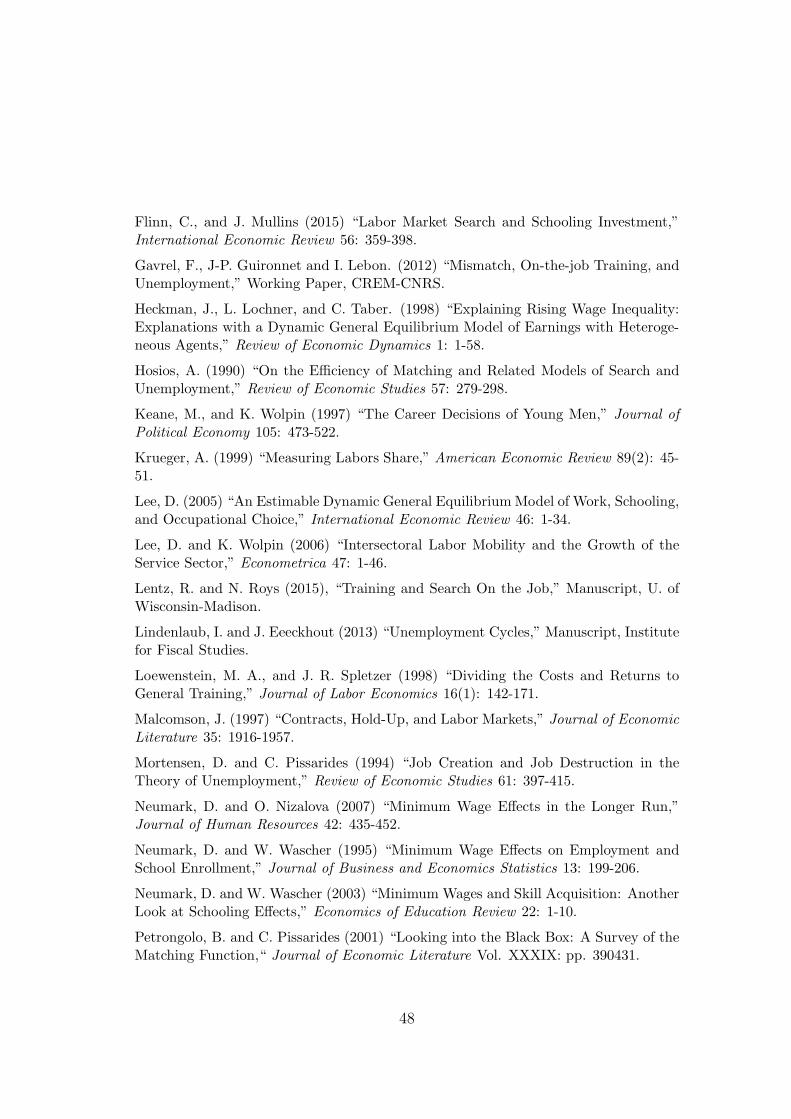
Flinn, C., and J. Mullins (2015) “Labor Market Search and Schooling Investment,”International Economic Review 56: 359-398.

Gavrel, F., J-P. Guironnet and I. Lebon. (2012) “Mismatch, On-the-job Training, andUnemployment,” Working Paper, CREM-CNRS.

Heckman, J., L. Lochner, and C. Taber. (1998) “Explaining Rising Wage Inequality:Explanations with a Dynamic General Equilibrium Model of Earnings with Heteroge-neous Agents,” Review of Economic Dynamics 1: 1-58.

Hosios, A. (1990) “On the Efficiency of Matching and Related Models of Search andUnemployment,” Review of Economic Studies 57: 279-298.

Keane, M., and K. Wolpin (1997) “The Career Decisions of Young Men,” Journal of

Political Economy 105: 473-522.

Krueger, A. (1999) “Measuring Labors Share,” American Economic Review 89(2): 45-51.

Lee, D. (2005) “An Estimable Dynamic General EquilibriumModel of Work, Schooling,and Occupational Choice,” International Economic Review 46: 1-34.

Lee, D. and K. Wolpin (2006) “Intersectoral Labor Mobility and the Growth of theService Sector,” Econometrica 47: 1-46.

Lentz, R. and N. Roys (2015), “Training and Search On the Job,” Manuscript, U. ofWisconsin-Madison.

Lindenlaub, I. and J. Eeeckhout (2013) “Unemployment Cycles,” Manuscript, Institutefor Fiscal Studies.

Loewenstein, M. A., and J. R. Spletzer (1998) “Dividing the Costs and Returns toGeneral Training,” Journal of Labor Economics 16(1): 142-171.

Malcomson, J. (1997) “Contracts, Hold-Up, and Labor Markets,” Journal of Economic

Literature 35: 1916-1957.

Mortensen, D. and C. Pissarides (1994) “Job Creation and Job Destruction in theTheory of Unemployment,” Review of Economic Studies 61: 397-415.

Neumark, D. and O. Nizalova (2007) “Minimum Wage Effects in the Longer Run,”Journal of Human Resources 42: 435-452.

Neumark, D. and W. Wascher (1995) “Minimum Wage Effects on Employment andSchool Enrollment,” Journal of Business and Economics Statistics 13: 199-206.

Neumark, D. and W. Wascher (2003) “Minimum Wages and Skill Acquisition: AnotherLook at Schooling Effects,” Economics of Education Review 22: 1-10.

Petrongolo, B. and C. Pissarides (2001) “Looking into the Black Box: A Survey of theMatching Function,“ Journal of Economic Literature Vol. XXXIX: pp. 390431.

48

Pissarides, C. (2000) Equilibrium Unemployment Theory, 2nd edition. Cambridge,MA: MIT Press.

Postel-Vinay, F., and J-M Robin (2002) “Equilibrium Wage Dispersion with Hetero-geneous Workers and Firms.” Econometrica 70: 2295-1350.

Shimer, R., R. Rogerson and R. Wright (2005) “Search Theoretic Models of the LaborMarket: A Survey,” Journal of Economic Literature, 43: 959-988.

49

Table 1: Proportion of Job Spells by the number of interview dates they span

High School Graduates Some College College Graduates

0 61% 55% 53%1 23% 24% 21%

2 7% 9% 11%3 3% 4% 6%4 2% 3% 3%

5 1% 2% 3%6 3% 3% 3%

50

Table 2: Incidence of Training

Some CollegeAll HS College or More

% who got training at least once 15% 18 % 13 % 13%% who got training at the start of job spell 6% 10 % 5 % 3%

Table 3: Proportion by Number of Training Spells (Conditional on Having Participated

At Least Once)

Percentage over All Workers with at Least One Training Spell

1 72 %2 18 %3 6 %

4 3 %5 1 %

51

Table 4: Annual Labor Turnover Rates and Wage Growth

Some College

HS College or More

Panel A: job-to-job transitions btw interview dates t− 1 and t

% of stayers 81 % 85 % 88%

% of job switchers 19 % 15 % 12%

..... % of job switchers with nonemployment spell btw t− 1 and t 4 % 3% 2%

..... % of job switchers with no nonemployment spell btw t− 1 and t 15% 12% 10%

Panel B: Wage Growth btw Interview Dates t− 1 and t

stayers 0.08 0.08 0.09

job switchers 0.11 0.15 0.20

..... job switchers with nonemployment spell btw t− 1 and t 0.06 0.06 0.23

..... job switchers with no nonemployment spell btw t− 1 and t 0.12 0.17 0.20

Panel C: % of Negative Wage Growth btw Interview Dates t− 1 and t

stayers 17 % 20 % 23%

job switchers 21 % 22 % 15%

..... job switchers with nonemployment spell btw t− 1 and t 30 % 36% 18%

..... job switchers with no nonemployment spell btw t− 1 and t 18% 18% 14%

52

Table 5: Log Wage Difference btw Interview Dates t− 1 and t by Training

logwt − logwt−1

No Training Got Training

stayers 0.08 0.08

job switchers 0.14 0.10

job switchers with nonemployment spell btw t− 1 and t 0.08 0.15

job switchers with no nonemployment spell btw t− 1 and t 0.15 0.09

53

Table 6: Parameter Estimates

PARAMETERS FOR EMPLOYMENT TRANSITIONSflow value of unemployment b 4.93 (0.064)job offer rate - unemployed λu 0.145 (.004)job offer rate - employed λe .074 (.002)exogenous job separation rate η .0033 (.0001)PARAMETERS OF INVESTMENT FUNCTIONSGeneral ability investment TFP δ0a .0150 (.0003)Firm-specific investment TFP δ0

θ.0151 (.0003)

State-dependence of general ability investment δ1a -.050 (.010)State-dependence of firm-specific investment δ1

θ.702 (.006)

Curvature of general ability investment δ2a .354 (.008)Curvature of firm-specific investment δ2

θ.493 (.007)

Rate of decrease in general ability ϕ−

a .0011 (.00004)

Rate of decrease in match quality ϕ−

θ.0144 (.0004)

PARAMETERS OF INITIAL ABILITY DISTRIBUTIONSMean of initial general ability - High School µa(ei = 1) 1.07 (.024)Mean of initial general ability - Some College µa(ei = 2) 1.28 (.020)Mean of initial general ability - BA or higher µa(ei = 3) 1.53 (.051)Variance of initial general ability σa .190 (.005)PARAMETERS OF JOB OFFERSMean of match quality distribution µθ 1.48 (.016)Variance of match quality distribution σθ .362 (.006)Employment cost ζ 4.51 (.120)PARAMETERS GOVERNING TRAINING OBSERVATIONIntercept for training observation β0 -3.19 (.025)Coefficient on τ for training observation βa 2.35 (.019)

54

Table 7: Parameter Estimates: Baseline vs. Estimations with No a/No θ

Baseline No a No θ

PARAMETERS FOR EMPLOYMENT TRANSITIONSflow value of unemployment b 4.93 2.92 5.20job offer rate - unemployed λu 0.145 0.148 0.161job offer rate - employed λe .074 0.104 0.044exogenous job separation rate η .0033 0.0037 .0043PARAMETERS OF INVESTMENT FUNCTIONSGeneral ability investment TFP δ0a .0150 0 0.0164Firm-specific investment TFP δ0

θ.0151 0.0204 0

State-dependence of general ability investment δ1a -.050 - 0.083State-dependence of firm-specific investment δ1

θ.702 0.696 -

Curvature of general ability investment δ2a .354 - 0.261Curvature of firm-specific investment δ2

θ.493 0.610 -

Rate of decrease in general ability ϕ−

a .0011 0 0.0012

Rate of decrease in match quality ϕ−

θ.0144 0.0118 0

PARAMETERS OF INITIAL ABILITY DISTRIBUTIONSMean of initial general ability - High School µa(ei = 1) 1.07 1.05 1.24Mean of initial general ability - Some College µa(ei = 2) 1.28 1.24 1.41Mean of initial general ability - BA or higher µa(ei = 3) 1.53 1.50 1.62Variance of initial general ability σa 0.19 0.29 0.17PARAMETERS OF JOB OFFERSMean of match quality distribution µθ 1.48 1.36 1.44Variance of match quality distribution σθ 0.36 0.36 0.36Employment cost ζ 4.51 3.79 6.15PARAMETERS GOVERNING TRAINING OBSERVATIONIntercept for training observation β0 -3.19 -3.04 -2.99Coefficient on τ for training observation βa 2.35 2.26 2.63

55

Figure 1: Minimum Acceptible Match-Quality

This figure shows the θ∗(a), the lowest match quality that workers with each level of general ability will accept.

0 0.5 1 1.5 2 2.5 31.6

1.65

1.7

1.75

1.8

1.85

Log M

atc

h V

alu

e

Log Worker Ability

Minimum Acceptable Match Value

56

Figure 2: General Training

This figure shows the amount of general training that wokers receive at different combinations on a and θ. Lines on the graph

show contours along which the amount of training remains constant. The blank area below the black line, shows states for

which workers will not accept the job offer.

0.0

5

0.05

0.050.05

0.1

0.1

0.10.1

0.1

0.15

0.15

0.15

0.150.15

0.15

0.2

0.2

0.20.2

0.2

0.2

5

Log M

atc

h V

alu

e

Log Worker Ability

Time Spent on General Training

0.5 1 1.5 2 2.5

0.5

1

1.5

2

2.5

57

Figure 3: Match-Specific Training

This figure shows the amount of match-specific training that wokers receive at different combinations on a and θ. Lines on the

graph show contours along which the amount of training remains constant. The blank area below the black line, shows states

for which workers will not accept the job offer.

0.05 0.05 0.05

0.05

0.05 0.05

0.05

0.1 0.1 0.1

0.10.1

0.1

0.15 0.15 0.15

0.15 0.15 0.15

0.2 0.2 0.2

0.2 0.2 0.2

0.25

0.250.25 0.25 0.25

Log M

atc

h V

alu

e

Log Worker Ability

Time Spend on Match−Specific Training

0.5 1 1.5 2 2.5

0.5

1

1.5

2

2.5

58

Figure 4: Wage as Fraction of OutputThis figure shows the worker’s wage as a fraction of her total output at different combinations on a and θ. Lines on the graph

show contours along which the fraction remains constant. The blank area below the black line, shows states for which workers

will not accept the job offer.

0.6

0.6

0.6 0.6

0.7

0.7

0.7

0.7

0.7 0.7

0.8

0.8

0.8

0.8

0.80.8

0.8

0.9

0.9

0.9

0.9

0.9

1

11

1.1

1.1

Log M

atc

h V

alu

e

Log Worker Ability

Wage as Fraction of Output

0.5 1 1.5 2 2.5

0.5

1

1.5

2

2.5

59

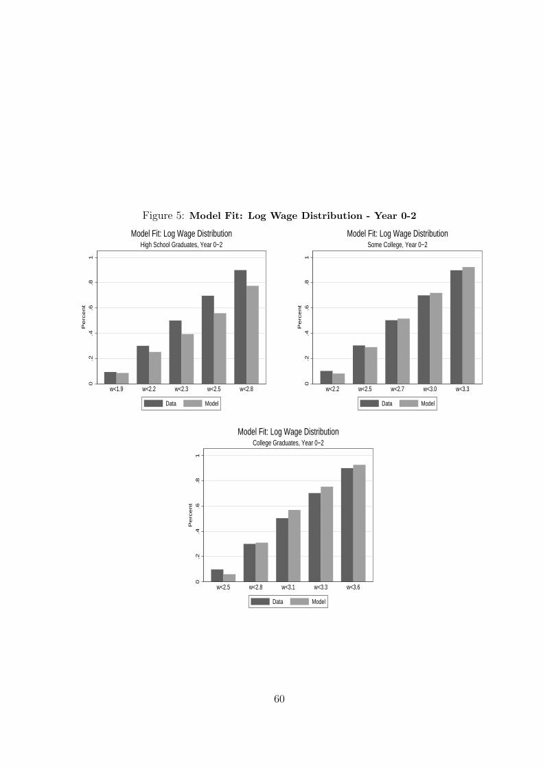
Figure 5: Model Fit: Log Wage Distribution - Year 0-2

0.2

.4.6

.81

Pe

rce

nt

w<1.9 w<2.2 w<2.3 w<2.5 w<2.8

High School Graduates, Year 0−2Model Fit: Log Wage Distribution

Data Model

0.2

.4.6

.81

Pe

rce

nt

w<2.2 w<2.5 w<2.7 w<3.0 w<3.3

Some College, Year 0−2Model Fit: Log Wage Distribution

Data Model

0.2

.4.6

.81

Pe

rce

nt

w<2.5 w<2.8 w<3.1 w<3.3 w<3.6

College Graduates, Year 0−2Model Fit: Log Wage Distribution

Data Model

60

Figure 6: Model Fit: Log Wage Distribution - Year 3-5

0.2

.4.6

.81

Pe

rce

nt

w<2.2 w<2.5 w<2.7 w<2.8 w<3.1

High School Graduates, Year 3−5Model Fit: Log Wage Distribution

Data Model

0.2

.4.6

.81

Pe

rce

nt

w<2.5 w<2.8 w<3.0 w<3.2 w<3.5

Some College, Year 3−5Model Fit: Log Wage Distribution

Data Model

0.2

.4.6

.81

Pe

rce

nt

w<2.7 w<3.0 w<3.3 w<3.5 w<3.8

College Graduates, Year 3−5Model Fit: Log Wage Distribution

Data Model

61

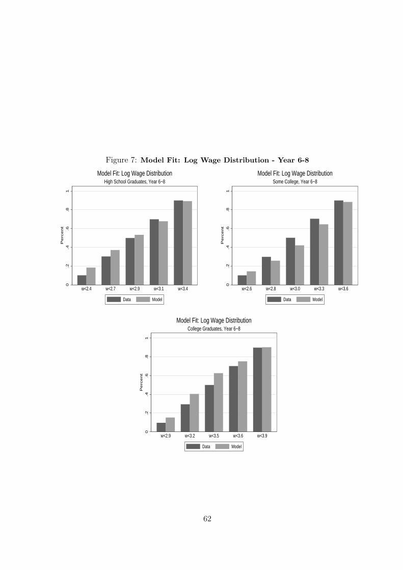
Figure 7: Model Fit: Log Wage Distribution - Year 6-8

0.2

.4.6

.81

Pe

rce

nt

w<2.4 w<2.7 w<2.9 w<3.1 w<3.4

High School Graduates, Year 6−8Model Fit: Log Wage Distribution

Data Model

0.2

.4.6

.81

Pe

rce

nt

w<2.6 w<2.8 w<3.0 w<3.3 w<3.6

Some College, Year 6−8Model Fit: Log Wage Distribution

Data Model

0.2

.4.6

.81

Pe

rce

nt

w<2.9 w<3.2 w<3.5 w<3.6 w<3.9

College Graduates, Year 6−8Model Fit: Log Wage Distribution

Data Model

62

Table 8: Model Fit: Incidence of Training

Some CollegeAll HS College or More

% who got training at least once........ Data 15% 18 % 13 % 13%........ Model 16% 20 % 15 % 13%% who got training at the start of job spell........ Data 6% 10 % 5 % 3%........ Model 4% 5 % 4 % 4%

63

Table 9: Model Fit: Annual Labor Turnover Rates and Wage Growth

Some CollegeHS College or More

Panel A: job-to-job transitions btw interview dates t− 1 and t

% of stayers........ Data 81 % 85 % 88%....... Model 78 % 75 % 73%% of job switchers........ Data 19 % 15 % 12%....... Model 22 % 25 % 27%

% of job switchers with nonemployment spell btw t − 1 and t

....... Data 4 % 3% 2%

....... Model 8 % 8% 9%% of job switchers with no nonemployment spell btw t − 1 and t

....... Data 15% 12% 10%

....... Model 14% 16% 18%

Panel B: Wage Growth btw Interview Dates t− 1 and t

stayers....... Data 0.08 0.08 0.09....... Model 0.08 0.08 0.07job switchers....... Data 0.11 0.15 0.20....... Model 0.07 0.11 0.12

job switchers with nonemployment spell btw t− 1 and t

....... Data 0.06 0.06 0.23

....... Model -0.17 -0.12 -0.08job switchers with no nonemployment spell btw t− 1 and t

....... Data 0.12 0.17 0.20

....... Model 0.21 0.22 0.22

Panel C: % of Negative Wage Growth btw Interview Dates t− 1 and t

stayers....... Data 17 % 20 % 23%....... Model 39 % 39 % 39%job switchers....... Data 21% 22% 15%....... Model 31% 27% 26%

job switchers with nonemployment spell btw t− 1 and t

....... Data 30 % 36% 18%

....... Model 54 % 50% 47%job switchers with no nonemployment spell btw t− 1 and t

....... Data 18% 18% 14%

....... Model 18% 16% 16%

64

Table 10: Simulations: Baseline vs. Estimations with No a/No θ

Annual Labor Turnover Rates and Wage GrowthSome College

HS College or More

Panel A: job-to-job transitions btw interview dates t− 1 and t

% of stayers....... Baseline 78 % 75 % 73%....... No a 78 % 76 % 72%....... No θ 72 % 72 % 71%% of job switchers....... Baseline 22 % 25 % 27%....... No a 22 % 24 % 28%....... No θ 28 % 28 % 29%

% of job switchers with nonemployment spell btw t− 1 and t

....... Baseline 8 % 8% 9%

....... No a 8 % 8 % 9%

....... No θ 10% 10 % 10%% of job switchers with no nonemployment spell btw t− 1 and t

....... Baseline 14% 16% 18%

....... No a 14% 16% 19%

....... No θ 18% 19% 19%

Panel B: Wage Growth btw Interview Dates t − 1 and t

stayers....... Baseline 0.08 0.08 0.07....... No a 0.07 0.08 0.08....... No θ 0.06 0.06 0.06job switchers....... Baseline 0.07 0.11 0.12....... No a -0.008 0.03 0.05....... No θ 0.17 0.19 0.17

job switchers with nonemployment spell btw t− 1 and t

....... Baseline -0.17 -0.12 -0.08

....... No a -0.22 -0.17 -0.14

....... No θ -0.08 -0.05 -0.009job switchers with no nonemployment spell btw t− 1 and t

....... Baseline 0.21 0.22 0.22

....... No a 0.12 0.12 0.13

....... No θ 0.31 0.31 0.27

Panel C: % of Negative Wage Growth btw Interview Dates t− 1 and t

stayers....... Baseline 39 % 39 % 39%....... No a 40% 39% 38%....... No θ 40% 40% 40%job switchers....... Baseline 31% 27% 26%....... No a 38% 34% 31%....... No θ 27% 24% 24%

job switchers with nonemployment spell btw t− 1 and t

....... Baseline 54 % 50% 47%

....... No a 60% 55% 52%

....... No θ 49% 46% 43%job switchers with no nonemployment spell btw t− 1 and t

....... Baseline 18% 16% 16%

....... No a 26% 23% 21%

....... No θ 14% 13% 13%65

Table 11: Simulations: Baseline vs. No a/No θ

Weekly Transition Rates Between t− 1 and t

Baseline No a No θ

EU probability 0.42% 0.42% 0.44%

% not employed - At Interview Date 14.88% 15.25% 12.23%

% not employed - All Periods 13.59% 13.91% 11.27%

tenure x EU probability 41.45% 44.02% 41.35%

EU probability by Tenure... ¡6 mths 0.52% 0.51% 0.45%... 6-12 mths 0.46% 0.46% 0.43%

... 1-2 yrs 0.41% 0.41% 0.44%

... 2-4 yrs 0.36% 0.37% 0.43%

... ¿4 yrs 0.33% 0.37% 0.42%

EE transition probability 0.38% 0.42% 0.39%

tenure x EE probability 21.22% 18.16% 30.19%

job finding probability 4.04% 3.95% 5.09%

Atime not employed x job finding probability 91.29% 90.07% 90.21%

66

Simulations: Baseline vs. No a/No θ

Figure 8: Avg. Log Wages by Tenure2

.42

.52

.62

.72

.82

.9L

og

Wa

ge

Year 0−2 Year 3−5 Year 6−8

baseline no ano theta

Log Wages − High School GraduatesModel Simulations: Baseline vs. No Training in A or Theta

67

Figure 9: Avg. Log Wages by Tenure2

.62

.72

.82

.93

3.1

Lo

g W

ag

e

Year 0−2 Year 3−5 Year 6−8

baseline no ano theta

Log Wages − Some CollegeModel Simulations: Baseline vs. No Training in A or Theta

Figure 10: Avg. Log Wages by Tenure

33

.13

.23

.33

.4L

og

Wa

ge

Year 0−2 Year 3−5 Year 6−8

baseline no ano theta

Log Wages − College GraduatesModel Simulations: Baseline vs. No Training in A or Theta

68

Table 12: Simulations: Baseline vs. No a/No θ

Log Wages by Labor Market Tenure and EducationYears in Labor Mkt. Education Data Baseline No a No θ

0-2 High School 2.36 2.47 2.56 2.363-5 High School 2.67 2.71 2.73 2.656-8 High School 2.90 2.85 2.78 2.86

0-2 Some College 2.72 2.72 2.77 2.653-5 Some College 2.99 2.96 2.94 2.93

6-8 Some College 3.04 3.08 2.99 3.110-2 College or Higher 3.03 3.03 3.06 2.983-5 College or Higher 3.25 3.25 3.22 3.23

6-8 College or Higher 3.43 3.35 3.26 3.39

69

Figure 11: Training by Years in Labor Market

This figure shows the average fraction of their time that workers spend on general and match specfic training in the model

simulation as a fucntion of the number of years in the labor market.

.1.1

5.2

.25

.3Fr

actio

n of

Tim

e

0 2 4 6 8Years

Total Training General TrainingMatch−Specific Training

Training by Years in Labor Force

70

Figure 12: Sources of Wage Growth by Years in Labor Market

This figure shows the average of the log of general human capital, the average amount of matc-specific capital, the log of the

fraction of time they spend not training, and the log of the average wage as a fraction of worker output for simulated workers

as a fucntion of the number of years in the labor market. In the absence of employment costs, these four componets would add

up to the total log wage, which is also shown.

0.1

.2.3

.4

0 2 4 6 8Years

Total Log Wage Log General HCLog Specific HC Log Time Not TrainingLog Wage/Output

Decomposition of Log Wage by Years in Labor Force

71

Table 13: Mincer Regressions

Const Some College BA Years in LF TenureDATAlog wage 2.141 0.316 0.796 0.051 0.045

(0.098) (0.098) (0.098) (0.002) (0.003)MODELlog wage 2.421 0.257 0.563 0.031 0.075starting a 1.067 0.208 0.459 0.001 -0.002a from training 0.016 -0.001 -0.005 0.020 0.002θ from seach 2.011 -0.006 -0.009 0.005 0.017θ from training 0.028 0.001 0.002 -0.001 0.046hours worked -0.345 0.005 0.012 0.001 0.019wage/output -0.356 0.049 0.104 0.005 -0.008

72

Figure 13: Mininimum Acceptable Wage with Minimum Wage

This figure shows the θ∗(a), the lowest match quality that workers with each level of general ability will accept. The solid line

shows θ∗(a) for the baseline model, the dashed line when we impose a minimum wage.

0 0.5 1 1.5 2 2.5 31.6

1.7

1.8

1.9

2

2.1

2.2

2.3

Log M

atc

h V

alu

e

Log Worker Ability

Minimum Acceptable Match Value

Baseline

Minimum Wage

73

Figure 14: Training by Years in Labor Market with Minimum Wage

This figure shows the average fraction of their time that workers spend on general and match specfic training in the model

simulation as a fucntion of the number of years in the labor market. The solid lines show the amount of training in the baseline

model. The corresponding dashed lines show the amount of training when we impose a minimum wage.

.1.1

5.2

.25

.3Fr

actio

n of

Tim

e

0 2 4 6 8Age

Total Training General TrainingMatch−Specific Training With Minimum Wage

Training by Years in Labor Force

74