season-invariant semantic segmentation with a deep … · season-invariant semantic segmentation...

Season-Invariant Semantic Segmentation with ADeep Multimodal Network

Dong-Ki Kim, Daniel Maturana, Masashi Uenoyama, and Sebastian Scherer

Abstract Semantic scene understanding is a useful capability for autonomous ve-hicles operating in off-roads. While cameras are the most common sensor used forsemantic classification, the performance of methods using camera imagery may suf-fer when there is significant variation between the train and testing sets caused byillumination, weather, and seasonal variations. On the other hand, 3D informationfrom active sensors such as LiDAR is comparatively invariant to these factors, whichmotivates us to investigate whether it can be used to improve performance in thisscenario. In this paper, we propose a novel multimodal Convolutional Neural Net-work (CNN) architecture consisting of two streams, 2D and 3D, which are fusedby projecting 3D features to image space to achieve a robust pixelwise semanticsegmentation. We evaluate our proposed method in a novel off-road terrain classifi-cation benchmark, and show a 25% improvement in mean Intersection over Union(IoU) of navigation-related semantic classes, relative to an image-only baseline.

1 Introduction

For autonomous vehicles operating in unstructured off-road environments, under-standing their environment in terms of semantic categories such as “trail”, “grass”or “rock” is useful for safe and deliberate navigation. It is essential to have robustscene understanding as false information can result in collisions or other accidents.

An important step toward scene understanding is semantic image segmenta-tion, which classifies an image at a pixel level. In recent years, deep ConvolutionalNeural Networks (CNNs) have achieved the state-of-the-art in semantic segmenta-tion [5, 6,8,10, 12,17, 19], surpassing traditional computer vision algorithms. How-

Dong-Ki Kim, Daniel Maturana, Sebastian SchererCarnegie Mellon University, USA, e-mail: dkkim,dmaturan,[email protected]

Masashi UenoyamaYamaha Motor Corporation, USA, e-mail: [email protected]

1

2 Dong-Ki Kim, Daniel Maturana, Masashi Uenoyama, and Sebastian Scherer

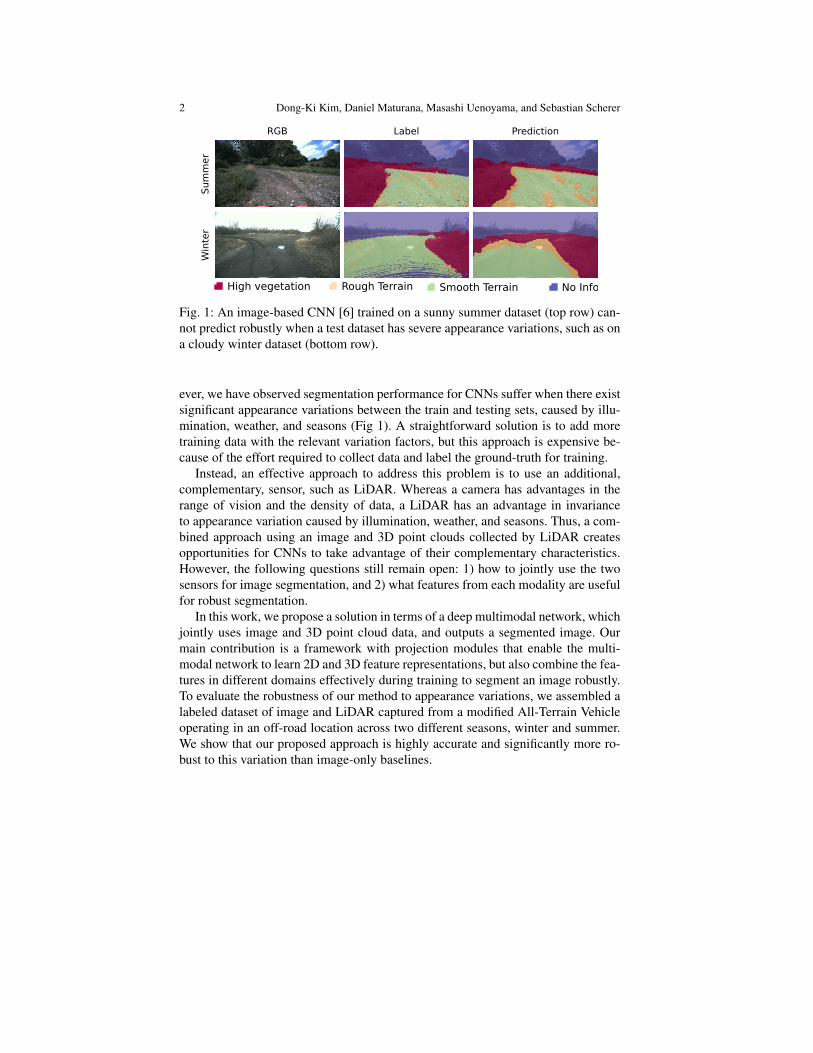
No InfoHigh vegetation Rough Terrain Smooth Terrain

Sum

mer

Win

ter

RGB Label Prediction

Fig. 1: An image-based CNN [6] trained on a sunny summer dataset (top row) can-not predict robustly when a test dataset has severe appearance variations, such as ona cloudy winter dataset (bottom row).

ever, we have observed segmentation performance for CNNs suffer when there existsignificant appearance variations between the train and testing sets, caused by illu-mination, weather, and seasons (Fig 1). A straightforward solution is to add moretraining data with the relevant variation factors, but this approach is expensive be-cause of the effort required to collect data and label the ground-truth for training.

Instead, an effective approach to address this problem is to use an additional,complementary, sensor, such as LiDAR. Whereas a camera has advantages in therange of vision and the density of data, a LiDAR has an advantage in invarianceto appearance variation caused by illumination, weather, and seasons. Thus, a com-bined approach using an image and 3D point clouds collected by LiDAR createsopportunities for CNNs to take advantage of their complementary characteristics.However, the following questions still remain open: 1) how to jointly use the twosensors for image segmentation, and 2) what features from each modality are usefulfor robust segmentation.

In this work, we propose a solution in terms of a deep multimodal network, whichjointly uses image and 3D point cloud data, and outputs a segmented image. Ourmain contribution is a framework with projection modules that enable the multi-modal network to learn 2D and 3D feature representations, but also combine the fea-tures in different domains effectively during training to segment an image robustly.To evaluate the robustness of our method to appearance variations, we assembled alabeled dataset of image and LiDAR captured from a modified All-Terrain Vehicleoperating in an off-road location across two different seasons, winter and summer.We show that our proposed approach is highly accurate and significantly more ro-bust to this variation than image-only baselines.

Season-Invariant Semantic Segmentation with A Deep Multimodal Network 3

2 Related Work

In general, relevant approaches for semantic scene understanding broadly fall intoone of two classes depending on the number of input modalities: unimodal (e.g.,only image input) or multimodal (e.g., image and 3D point cloud).

2.1 Unimodal image-based approaches

Semantic segmentation of RGB images is an active research topic. Many successfulapproaches use graphical models, such as Markov or Conditional Random Fields(MRFs or CRFs) [1–4]. These approaches often start with an over-segmentationof an image into superpixels and extract hand-crafted features from individual andneighboring segments. A graphical model uses the extracted features to ensure theconsistency of the labeling for neighboring regions.

Instead of relying on engineered features, CNN-based approaches have achievedthe state-of-the-art segmentation performance by learning strong feature represen-tations from raw data [5, 6, 8]. The main difference between CNN approaches isthe network architecture. Shelhamer et al. [5] introduce the use of skip layers to re-fine the segmentation produced by so-called deconvolution layers. Badrinarayananet al. [6] propose an encoder-decoder architecture with unpooling layers. These ar-chitectures use the relatively slow VGG [7] architecture. To reduce computationalcosts, an important goal for robotics, Paszke et al. [8] apply a bottleneck structure,motivated by [9], to build an efficient network with a small number of parametersbut similar accuracy to prior models. We base the image-based part of our networkon these architectures.

2.2 Multimodal Approaches

Researchers have used image and 3D point clouds for scene understanding. In oneof the main inspirations for our work, Munoz et al. [13] train two classifier cascades,one for each modality, and hierarchically propagate information across the two clas-sifiers using a stacking approach. Newman el at. [14] describe a framework thatclassifies an individual LiDAR data by the Bayes decision rule and support-vectormachines, and uses the majority consensus to label superpixels in an image. Cadenaand Kosecka [15] propose a CRF framework that enforces spatial consistency be-tween separate feature sets extracted from two sensor’s coverage. Alvis et al. [16]extract appearance features from images for CRF and obtain global constraints forsets of superpixels from 3D point clouds.

There are also several CNN-based approaches using RGB and Depth (RGBD)representations, usually from stereo or structured lighting sensors. Couprie et al. [10]combine feature maps of multiscale CNNs from RGB-D and superpixels obtained


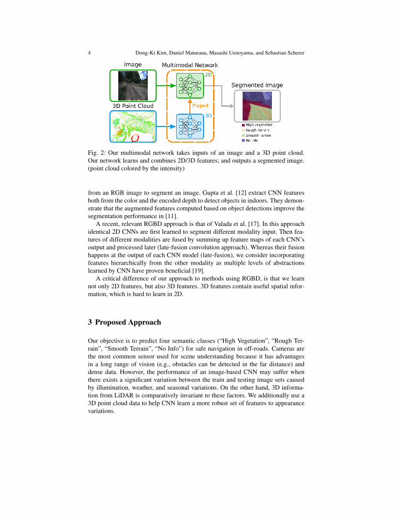
Fig. 2: Our multimodal network takes inputs of an image and a 3D point cloud.Our network learns and combines 2D/3D features; and outputs a segmented image.(point cloud colored by the intensity)

from an RGB image to segment an image. Gupta et al. [12] extract CNN featuresboth from the color and the encoded depth to detect objects in indoors. They demon-strate that the augmented features computed based on object detections improve thesegmentation performance in [11].

A recent, relevant RGBD approach is that of Valada et al. [17]. In this approachidentical 2D CNNs are first learned to segment different modality input. Then fea-tures of different modalities are fused by summing up feature maps of each CNN’soutput and processed later (late-fusion convolution approach). Whereas their fusionhappens at the output of each CNN model (late-fusion), we consider incorporatingfeatures hierarchically from the other modality as multiple levels of abstractionslearned by CNN have proven beneficial [19].

A critical difference of our approach to methods using RGBD, is that we learnnot only 2D features, but also 3D features. 3D features contain useful spatial infor-mation, which is hard to learn in 2D.

3 Proposed Approach

Our objective is to predict four semantic classes (“High Vegetation”, “Rough Ter-rain”, “Smooth Terrain”, “No Info”) for safe navigation in off-roads. Cameras arethe most common sensor used for scene understanding because it has advantagesin a long range of vision (e.g., obstacles can be detected in the far distance) anddense data. However, the performance of an image-based CNN may suffer whenthere exists a significant variation between the train and testing image sets causedby illumination, weather, and seasonal variations. On the other hand, 3D informa-tion from LiDAR is comparatively invariant to these factors. We additionally use a3D point cloud data to help CNN learn a more robust set of features to appearancevariations.


convmax

concat

Initial

bn

bn

bn + regularizer

1x1

deconvup

1x1

1x1

Upsample

bn + relu

bn + relu

bn + regularizer

1x1

conv

relu

max

1x1

1x1

Downsample

bn + relu

bn + relu

bn + regularizer

1x1

conv

relu

1x1

Bottleneck

bn + relu

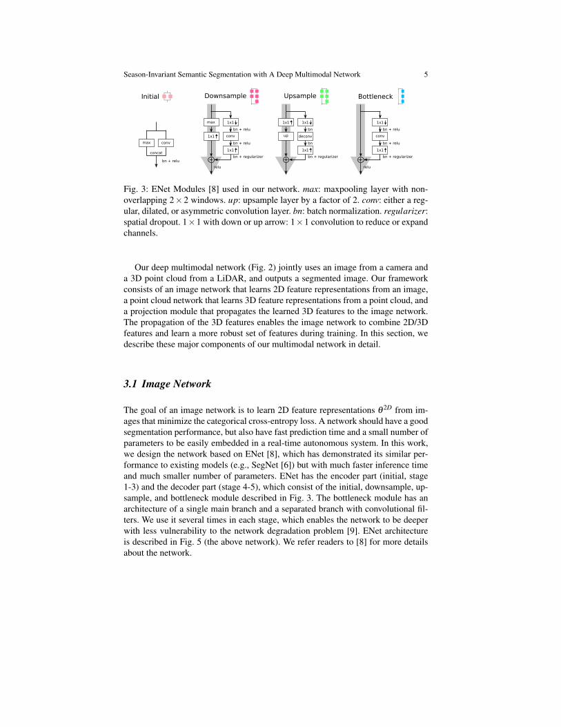
Fig. 3: ENet Modules [8] used in our network. max: maxpooling layer with non-overlapping 2×2 windows. up: upsample layer by a factor of 2. conv: either a reg-ular, dilated, or asymmetric convolution layer. bn: batch normalization. regularizer:spatial dropout. 1×1 with down or up arrow: 1×1 convolution to reduce or expandchannels.

Our deep multimodal network (Fig. 2) jointly uses an image from a camera anda 3D point cloud from a LiDAR, and outputs a segmented image. Our frameworkconsists of an image network that learns 2D feature representations from an image,a point cloud network that learns 3D feature representations from a point cloud, anda projection module that propagates the learned 3D features to the image network.The propagation of the 3D features enables the image network to combine 2D/3Dfeatures and learn a more robust set of features during training. In this section, wedescribe these major components of our multimodal network in detail.

3.1 Image Network

The goal of an image network is to learn 2D feature representations θ 2D from im-ages that minimize the categorical cross-entropy loss. A network should have a goodsegmentation performance, but also have fast prediction time and a small number ofparameters to be easily embedded in a real-time autonomous system. In this work,we design the network based on ENet [8], which has demonstrated its similar per-formance to existing models (e.g., SegNet [6]) but with much faster inference timeand much smaller number of parameters. ENet has the encoder part (initial, stage1-3) and the decoder part (stage 4-5), which consist of the initial, downsample, up-sample, and bottleneck module described in Fig. 3. The bottleneck module has anarchitecture of a single main branch and a separated branch with convolutional fil-ters. We use it several times in each stage, which enables the network to be deeperwith less vulnerability to the network degradation problem [9]. ENet architectureis described in Fig. 5 (the above network). We refer readers to [8] for more detailsabout the network.


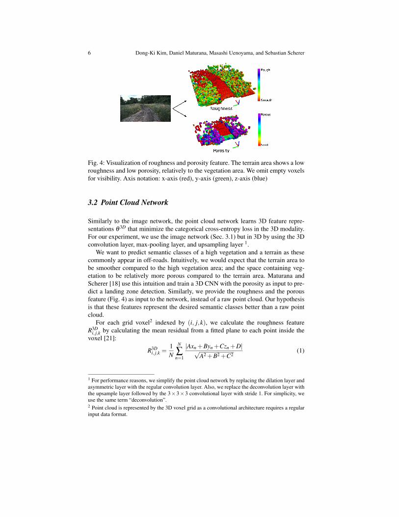
Fig. 4: Visualization of roughness and porosity feature. The terrain area shows a lowroughness and low porosity, relatively to the vegetation area. We omit empty voxelsfor visibility. Axis notation: x-axis (red), y-axis (green), z-axis (blue)

3.2 Point Cloud Network

Similarly to the image network, the point cloud network learns 3D feature repre-sentations θ 3D that minimize the categorical cross-entropy loss in the 3D modality.For our experiment, we use the image network (Sec. 3.1) but in 3D by using the 3Dconvolution layer, max-pooling layer, and upsampling layer 1.

We want to predict semantic classes of a high vegetation and a terrain as thesecommonly appear in off-roads. Intuitively, we would expect that the terrain area tobe smoother compared to the high vegetation area; and the space containing veg-etation to be relatively more porous compared to the terrain area. Maturana andScherer [18] use this intuition and train a 3D CNN with the porosity as input to pre-dict a landing zone detection. Similarly, we provide the roughness and the porousfeature (Fig. 4) as input to the network, instead of a raw point cloud. Our hypothesisis that these features represent the desired semantic classes better than a raw pointcloud.

For each grid voxel2 indexed by (i, j,k), we calculate the roughness featureR3D

i, j,k by calculating the mean residual from a fitted plane to each point inside thevoxel [21]:

R3Di, j,k =

1N

N

∑n=1

|Axn +Byn +Czn +D|√A2 +B2 +C2

(1)

1 For performance reasons, we simplify the point cloud network by replacing the dilation layer andasymmetric layer with the regular convolution layer. Also, we replace the deconvolution layer withthe upsample layer followed by the 3×3×3 convolutional layer with stride 1. For simplicity, weuse the same term “deconvolution”.2 Point cloud is represented by the 3D voxel grid as a convolutional architecture requires a regularinput data format.


where N is the number of points inside each voxel, x, y, z are the position of eachpoint, and A, B, C, D are the fitted plane parameters for N points inside the voxel(i.e., Ax+By+Cy+D = 0). For empty voxels (i.e., no points), we assign a constantnegative roughness value of −0.1.

For the porosity feature P3Di, j,k, we use the 3D ray tracing [20] to obtain the num-

ber of hits and pass-throughs for each grid voxel. Then we model the porosity byupdating Beta parameters α t

i, j,k and β ti, j,k for the sequence of LiDAR measurements

{zt}Tt=1 [18]:

αti, j,k = α

t−1i, j,k + zt (2)

βti, j,k = β

t−1i, j,k +(1− zt) (3)

P3Di, j,k =

α ti, j,k

α ti, j,k +β t

i, j,k(4)

where α0i, j,k = β 0

i, j,k = 1 for all (i, j,k), zt = 1 for the hit, and zt = 0 for the pass.

3.3 Projection Module

The projection module first projects the 3D features learned by the point cloud net-work onto 2D image planes. Then the bottleneck module in Fig. 3 is followed sothat better feature representations can be propagated to the image network.

In terms of the projection, we map each voxel’s centroid position (x,y,z) withrespect to the LiDAR onto the image plane (u,v) by the pinhole camera model:

s

uv1

=

fx 0 cx0 fy cy0 0 1

[R | t]

xyz1

(5)

where fx, fy, cx, cy are the camera intrinsic parameters, R and t are the 3x3 rotationmatrix and the 3x1 translation matrix from a camera to a LiDAR, respectively. Wesample (x,y,z) for every voxel size from the original point cloud dimension (e.g.,16× 48× 40 in Fig. 5). This is to address a problem that the projection becomessparse due to the 3D maxpooling layers that reduce a dimension of a point cloud.We apply the z-buffer technique to account pixels that have multiple LiDAR pointsprojected onto the same pixel location. Then, we use the nearest-neighbor interpo-lation to downsample the projected image planes to match the size of the imagenetwork’s layer that the projection module will be merged to (Sec. 3.4).

We consider a fixed volume of 3D point clouds with regard to a LiDAR (Sec 4.3).Thus, voxel locations and their corresponding projection locations in the image net-work are constant if the dimensions of a point cloud and an image are same (e.g.,projection for stage 1 and 4). In practice, we pre-compute indices of voxel locationsand their corresponding pixel indices, and use them inside the network.


SemanticImage

Roughness& Porous

Initial Stage 1 Stage 2 Stage 3 Stage 4 Stage 5

3x224x22416x112x112

64x56x56

2x16x48x40

16x8x24x2064x4x12x10

128x2x6x5

128x28x28 128x28x2864x56x56

16x112x1124x224x224

deconv

128x2x6x564x4x12x10

16x8x24x20

x8 x8x4 x2

RGBImage

Projection Module

Sum

ENet Modules

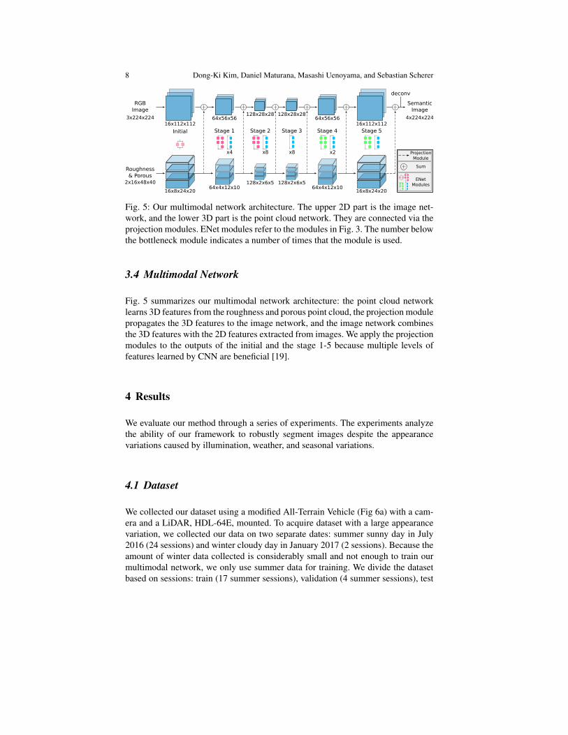
Fig. 5: Our multimodal network architecture. The upper 2D part is the image net-work, and the lower 3D part is the point cloud network. They are connected via theprojection modules. ENet modules refer to the modules in Fig. 3. The number belowthe bottleneck module indicates a number of times that the module is used.

3.4 Multimodal Network

Fig. 5 summarizes our multimodal network architecture: the point cloud networklearns 3D features from the roughness and porous point cloud, the projection modulepropagates the 3D features to the image network, and the image network combinesthe 3D features with the 2D features extracted from images. We apply the projectionmodules to the outputs of the initial and the stage 1-5 because multiple levels offeatures learned by CNN are beneficial [19].

4 Results

We evaluate our method through a series of experiments. The experiments analyzethe ability of our framework to robustly segment images despite the appearancevariations caused by illumination, weather, and seasonal variations.

4.1 Dataset

We collected our dataset using a modified All-Terrain Vehicle (Fig 6a) with a cam-era and a LiDAR, HDL-64E, mounted. To acquire dataset with a large appearancevariation, we collected our data on two separate dates: summer sunny day in July2016 (24 sessions) and winter cloudy day in January 2017 (2 sessions). Because theamount of winter data collected is considerably small and not enough to train ourmultimodal network, we only use summer data for training. We divide the datasetbased on sessions: train (17 summer sessions), validation (4 summer sessions), test


(a) (b)

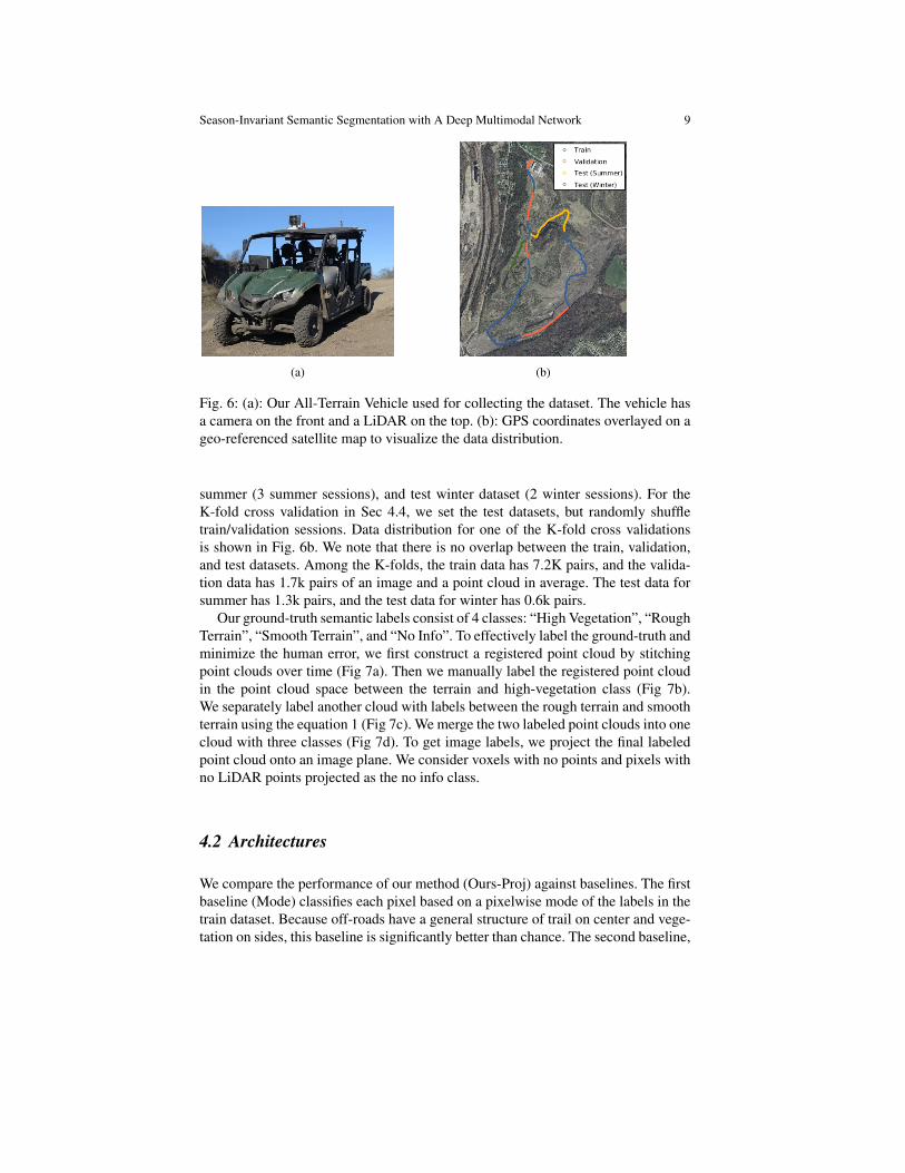
Fig. 6: (a): Our All-Terrain Vehicle used for collecting the dataset. The vehicle hasa camera on the front and a LiDAR on the top. (b): GPS coordinates overlayed on ageo-referenced satellite map to visualize the data distribution.

summer (3 summer sessions), and test winter dataset (2 winter sessions). For theK-fold cross validation in Sec 4.4, we set the test datasets, but randomly shuffletrain/validation sessions. Data distribution for one of the K-fold cross validationsis shown in Fig. 6b. We note that there is no overlap between the train, validation,and test datasets. Among the K-folds, the train data has 7.2K pairs, and the valida-tion data has 1.7k pairs of an image and a point cloud in average. The test data forsummer has 1.3k pairs, and the test data for winter has 0.6k pairs.

Our ground-truth semantic labels consist of 4 classes: “High Vegetation”, “RoughTerrain”, “Smooth Terrain”, and “No Info”. To effectively label the ground-truth andminimize the human error, we first construct a registered point cloud by stitchingpoint clouds over time (Fig 7a). Then we manually label the registered point cloudin the point cloud space between the terrain and high-vegetation class (Fig 7b).We separately label another cloud with labels between the rough terrain and smoothterrain using the equation 1 (Fig 7c). We merge the two labeled point clouds into onecloud with three classes (Fig 7d). To get image labels, we project the final labeledpoint cloud onto an image plane. We consider voxels with no points and pixels withno LiDAR points projected as the no info class.

4.2 Architectures

We compare the performance of our method (Ours-Proj) against baselines. The firstbaseline (Mode) classifies each pixel based on a pixelwise mode of the labels in thetrain dataset. Because off-roads have a general structure of trail on center and vege-tation on sides, this baseline is significantly better than chance. The second baseline,


Registered Point Cloud

(a)

Terrain vs High Vegetation

High vegetationTerrain

(b)

Rough vs Smooth Terrain

Smooth TerrainRough Terrain

(c)

High VegetationRough Terrain

Labeled Registered Cloud

Smooth Terrain

(d)

Fig. 7: The point cloud ground-truth generation procedure. (a): Point clouds are firstregistered. (b): The terrain and high-vegetation class are labeled manually. (c): Therough and smooth terrain class are labeled automatically using equation 1. (d): Finallabeled point cloud is acquired by merging labeled point cloud (b) and (c).

SegNet is a popular encoder-decoder image segmentation network [6]. The thirdbaseline, Ours-Image, is the image network of our multimodal network without thepoint cloud network and the projection modules. The last baseline (Ours-RGBRP)is same as Ours-Image, but its input to the network is 5 channels (RGB, Roughness,Porous) by projecting the point cloud network’s inputs onto the image planes andtreating them as additional channels similarly to the color channels. Ours-RGBRPbaseline compares the effectiveness of the learning and propagation of the 3D fea-tures against learning 2D features.

We also explore options for Ours-Proj with different locations of the projectionmodule. We experiment with a single projection module for each stage, encoderprojections (initial and stage 1-3), and decoder projections (stage 4-5).

4.3 Training Details

All input and label images are resized to 224×224 px. With respect to the LiDAR,we have a fixed volume of point cloud: −3.0m to 0.6m (z-axis), 3.0m to 17.4m (x-axis), and −6.0m to 6.0m (y-axis), where the axis corresponds to the one in Fig 4.The voxel size is 0.3m, so the input and label point clouds have a dimension of 12×48×40 (z, x, y-axis). The intrinsic and extrinsic parameters in the projection moduleare calibrated off-line. To reduce a GPU memory required for training Ours-Proj, wefirst separately train the point cloud network. Then we remove the deconvolutionand softmax layer in the point cloud network, connect with the image network viathe projection modules, and train the image network and projection modules byfixing the point cloud network’s weight. Except for SegNet, all learning methodsare based on Theano. For SegNet [6], we use its publicly available code. We trainall learning methods from scratch. We use the validation data to determine weightsfor the testing.


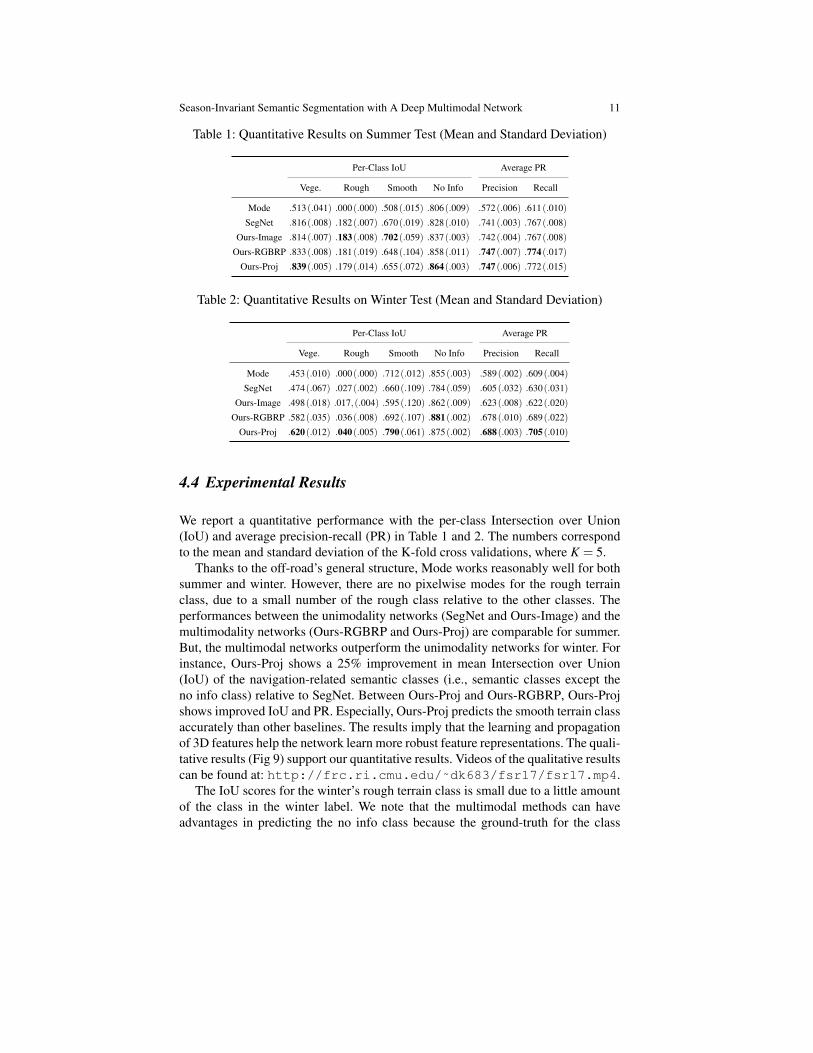
Table 1: Quantitative Results on Summer Test (Mean and Standard Deviation)

Per-Class IoU Average PR

Vege. Rough Smooth No Info Precision Recall

Mode .513(.041) .000(.000) .508(.015) .806(.009) .572(.006) .611(.010)

SegNet .816(.008) .182(.007) .670(.019) .828(.010) .741(.003) .767(.008)

Ours-Image .814(.007) .183(.008) .702(.059) .837(.003) .742(.004) .767(.008)

Ours-RGBRP .833(.008) .181(.019) .648(.104) .858(.011) .747(.007) .774(.017)

Ours-Proj .839(.005) .179(.014) .655(.072) .864(.003) .747(.006) .772(.015)

Table 2: Quantitative Results on Winter Test (Mean and Standard Deviation)

Per-Class IoU Average PR

Vege. Rough Smooth No Info Precision Recall

Mode .453(.010) .000(.000) .712(.012) .855(.003) .589(.002) .609(.004)

SegNet .474(.067) .027(.002) .660(.109) .784(.059) .605(.032) .630(.031)

Ours-Image .498(.018) .017,(.004) .595(.120) .862(.009) .623(.008) .622(.020)

Ours-RGBRP .582(.035) .036(.008) .692(.107) .881(.002) .678(.010) .689(.022)

Ours-Proj .620(.012) .040(.005) .790(.061) .875(.002) .688(.003) .705(.010)

4.4 Experimental Results

We report a quantitative performance with the per-class Intersection over Union(IoU) and average precision-recall (PR) in Table 1 and 2. The numbers correspondto the mean and standard deviation of the K-fold cross validations, where K = 5.

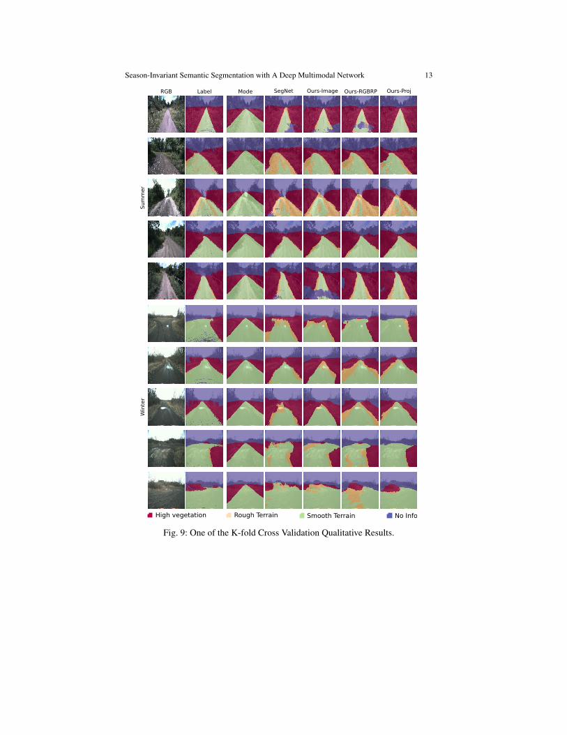
Thanks to the off-road’s general structure, Mode works reasonably well for bothsummer and winter. However, there are no pixelwise modes for the rough terrainclass, due to a small number of the rough class relative to the other classes. Theperformances between the unimodality networks (SegNet and Ours-Image) and themultimodality networks (Ours-RGBRP and Ours-Proj) are comparable for summer.But, the multimodal networks outperform the unimodality networks for winter. Forinstance, Ours-Proj shows a 25% improvement in mean Intersection over Union(IoU) of the navigation-related semantic classes (i.e., semantic classes except theno info class) relative to SegNet. Between Ours-Proj and Ours-RGBRP, Ours-Projshows improved IoU and PR. Especially, Ours-Proj predicts the smooth terrain classaccurately than other baselines. The results imply that the learning and propagationof 3D features help the network learn more robust feature representations. The quali-tative results (Fig 9) support our quantitative results. Videos of the qualitative resultscan be found at: http://frc.ri.cmu.edu/˜dk683/fsr17/fsr17.mp4.

The IoU scores for the winter’s rough terrain class is small due to a little amountof the class in the winter label. We note that the multimodal methods can haveadvantages in predicting the no info class because the ground-truth for the class


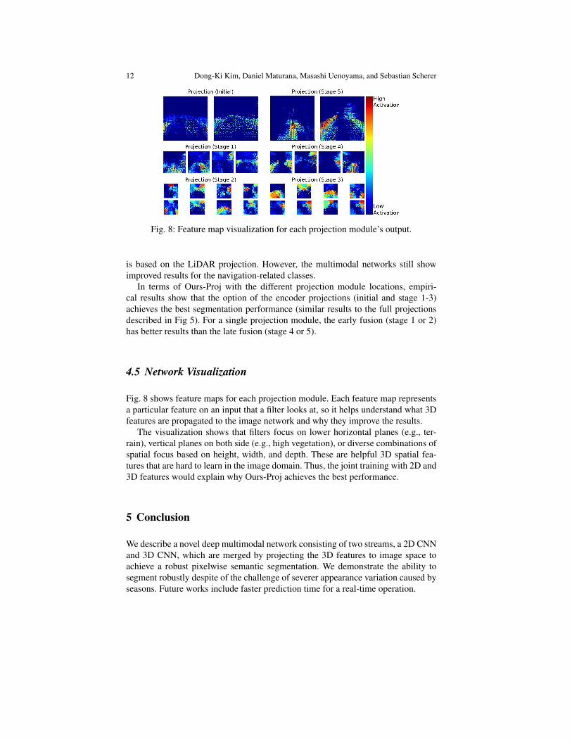
Fig. 8: Feature map visualization for each projection module’s output.

is based on the LiDAR projection. However, the multimodal networks still showimproved results for the navigation-related classes.

In terms of Ours-Proj with the different projection module locations, empiri-cal results show that the option of the encoder projections (initial and stage 1-3)achieves the best segmentation performance (similar results to the full projectionsdescribed in Fig 5). For a single projection module, the early fusion (stage 1 or 2)has better results than the late fusion (stage 4 or 5).

4.5 Network Visualization

Fig. 8 shows feature maps for each projection module. Each feature map representsa particular feature on an input that a filter looks at, so it helps understand what 3Dfeatures are propagated to the image network and why they improve the results.

The visualization shows that filters focus on lower horizontal planes (e.g., ter-rain), vertical planes on both side (e.g., high vegetation), or diverse combinations ofspatial focus based on height, width, and depth. These are helpful 3D spatial fea-tures that are hard to learn in the image domain. Thus, the joint training with 2D and3D features would explain why Ours-Proj achieves the best performance.

5 Conclusion

We describe a novel deep multimodal network consisting of two streams, a 2D CNNand 3D CNN, which are merged by projecting the 3D features to image space toachieve a robust pixelwise semantic segmentation. We demonstrate the ability tosegment robustly despite of the challenge of severer appearance variation caused byseasons. Future works include faster prediction time for a real-time operation.


RGB Label

Sum

mer

Win

ter

No InfoHigh vegetation Rough Terrain Smooth Terrain

Ours-ProjOurs-RGBRPOurs-ImageSegNetMode

Fig. 9: One of the K-fold Cross Validation Qualitative Results.


Acknowledgements We thank the Yamaha Motor corporation for supporting this research.

References

1. C. Farabet, C. Couprie, L. Najman, and Y. LeCun. Learning Hierarchical Features for SceneLabeling. In IEEE Transactions on Pattern Analysis and Machine Intelligence (TPAMI), vol.35, no. 8, pp. 1915-1929, 2013.

2. L. Ladicky, P. Sturgess, K. Alahari, C. Russell, and P. H. S. Torr. What, Where and HowMany? Combining Object Detectors and CRFs. In Proc. European Conf. on Computer Vision(ECCV), 2010.

3. B. Micusik, J. Kosecka, and G. Singh. Semantic Parsing of Street Scenes from Video. In IntlJ. Rob. Res. (IJRR), vol. 31, no. 4, pp. 484-497, 2012.

4. J. Xiao and L. Quan. Multiple View Semantic Segmentation for Street View Images. In Proc.IEEE Intl Conf. on Computer Vision (ICCV), 2009.

5. J. Long, E. Shelhamer, T. Darrell. Fully Convolutional Models for Semantic Segmentation.In Proc. IEEE Conf. on Computer Vision and Pattern Recognition (CVPR), 2015.

6. V. Badrinarayanan, A. Kendall, and R. Cipolla. SegNet: A Deep Convolutional Encoder-Decoder Architecture for Image Segmentation. arXiv:1511.00561 [cs.CV], 2015.

7. K. Simonyan and A. Zisserman. Very Deep Convolutional Networks for Large-Scale ImageRecognition. arXiv:1409.1556 [cs.CV], 2014.

8. A. Paszke, A. Chaurasia, S. Kim, and E. Culurciello. ENet: A Deep Neural Network Archi-tecture for Real-Time Semantic Segmentation. arXiv:1606.02147 [cs.CV], 2016.

9. K. He, X. Zhang, S. Ren, and J. Sun. Deep Residual Learning for Image Recognition.arXiv:1512.03385 [cs.CV], 2015.

10. C. Couprie, C. Farabet, L. Najman, and Y. LeCun. Indoor Semantic Segmentation using depthinformation. arXiv:1301.3572 [cs.CV], 2013.

11. S. Gupta, P. Arbelaez, and J. Malik. Perceptual Organization and Recognition of IndoorScenes from RGB-D Images. In Proc. IEEE Conf. on Computer Vision and Pattern Recogni-tion (CVPR), 2013.

12. S. Gupta, R. Girshick, P. Arbelaez, and J. Malik. Learning Rich Features from RGB-D Im-ages for Object Detection and Segmentation. In Proc. European Conf. on Computer Vision(ECCV), 2014.

13. D. Munoz, J. A. Bagnell, and M. Hebert. Co-inference for Multi-modal Scene Analysis. InProc. European Conf. on Computer Vision (ECCV), 2012.

14. P. Newman et al. Navigating, Recognizing and Describing Urban Spaces With Vision andLasers. In Intl J. Rob. Res. (IJRR), vol. 28, no. 11-12, pp. 1406-1433, 2009.

15. C. Cadena, J. Kosecka. Semantic segmentation with heterogeneous sensor coverages. In Proc.IEEE Intl Conf. on Robotics and Automation (ICRA), 2014.

16. C. D. Alvis, L. Ott, and F. Ramos. Urban scene segmentation with laser-constrained CRFs. InProc. IEEE/RSJ Intl Conf. on Intelligent Robots and Systems (IROS), 2016.

17. A. Valada, G. L. Oliveira, T. Brox, and W. Burgard. Deep Multispectral Semantic SceneUnderstanding of Forested Environments Using Multimodal Fusion. In proc. InternationalSymposium on Experimental Robotics (ISER), 2016.

18. D. Maturana and S. Scherer. 3D Convolutional Neural Networks for Landing Zone Detectionfrom LiDAR. In Proc. IEEE Intl Conf. on Robotics and Automation (ICRA), 2015.

19. B. Hariharan, P. Arbelaez, R. Girshick, and J. Malik. Hypercolumns for Object Segmentationand Fine-grained Localization. In Proc. IEEE Conf. on Computer Vision and Pattern Recog-nition (CVPR), 2015.

20. J. Amanatides and A. Woo. A Fast Voxel Traversal Algorithm for Ray Tracing. In Proc.Eurographics, 1987

21. S. Scherer, L. J. Chamberlain, and S. Singh. Online Assessment of Landing Sites. In Proc.AIAA Infotech@Aerospace, 2010.

season-invariant semantic segmentation with a deep … · season-invariant semantic segmentation...

Documents