seasonal ensemble prediction with a coupled ocean ... · prognostic primitive equation atmospheric...

53

Australian Meteorological and Oceanographic Journal 59 (2010) 53-66

Introduction

Seasonal prediction with dynamical models of El Niño events, and the associated changes in the Southern Oscilla-tion and atmospheric circulation, has been an area of intense

interest and effort for more than two decades. The early ex-perimental forecasts of El Niño-Southern Oscillation (ENSO) events (Cane and Zebiak 1985; Cane et al. 1986; Zebiak and Cane 1987; Battisti and Hirst 1989; Kleeman 1993) used sim-ple dynamical prognostic models of the equatorial ocean coupled to a single-layer linear diagnostic atmospheric mod-el. Schopf and Suarez (1988) studied ENSO vacillations with

Seasonal ensemble prediction with a coupled ocean-atmosphere model

Jorgen S. Frederiksen1, Carsten S. Frederiksen2 and Stacey L. Osbrough3

1Climate Adaptation Flagship, CSIRO Marine and Atmospheric Research, Australia,2Centre for Australian Weather and Climate Research - a partnership between CSIRO and the

Bureau of Meteorology, Australiaand

3Centre for Australian Weather and Climate Research, CSIRO Marine and Atmospheric Research, Australia

Ensemble prediction methods, in which the control initial conditions are per-turbed by coupled ocean-atmosphere non-linear instabilities obtained by a breed-ing method, have been applied within a coupled ocean-atmosphere model with prognostic primitive equation atmospheric and oceanic components. The bred vectors have a distinct annual cycle of growth rates with the maximum occurring during boreal winter and a minimum during boreal summer. Bred vector ampli-tudes peak in boreal spring and have a minimum in boreal autumn. The leading empirical orthogonal functions of the 50 m ocean temperature of bred vectors have maxima in the equatorial Pacific between 120 – 150°W, as well as in the west-ern Pacific, while the associated 500 hPa streamfunction fields have large-scale wave-trains in extratropical regions that are strongly influenced by ENSO. Coupled control and ensemble forecasts for one year have been initiated on the first day of each month during a period in the 1990s to examine the sensitiv-ity of enhanced ensemble mean skill, compared with the control, on the number and type of ensemble perturbations. The focus has been on the skill of predicting the 50 m ocean temperature in the equatorial region. For forecasts longer than about two months the root mean square errors in the ensemble mean forecasts are smaller than for the control based on averages over all the forecasts. There is considerable variability in the skill of both control and ensemble forecasts dur-ing the 1990s. In particular, forecasts through the 1997 El Niño and 1998 La Niña regime transitions tend to be less skilful than in more quiescent periods. Forecast errors tend to increase with time as expected and there are peaks in error ampli-tudes for forecasts verifying in boreal spring. Forecast skill increases with increas-ing numbers of bred vectors but saturates with little additional gain in using 64 members compared with 32. Ensemble forecasts with cyclic mode perturbations, the non-linear generalisations of finite time normal modes, are found to be more skilful than bred vectors, with eight cyclic modes producing similar error reduc-tion in three to nine-month forecasts as 32 to 64 bred vectors. Our results suggest that a contributing cause of the boreal spring predictability barrier is the fact that large-scale atmospheric teleconnection patterns and insta-bilities peak in boreal spring and in turn couple to the ocean.

Corresponding author address: Jorgen S. Frederiksen, CSIRO Marine and Atmospheric Research, PMB#1, Aspendale, Vic. 3195, Australia.Email: [email protected]

54 Australian Meteorological and Oceanographic Journal 59 January 2010

a global two-layer prognostic atmospheric model coupled to a two-layer equatorial Pacific prognostic ocean model. More complex coupled ocean-atmosphere general circula-tion models have subsequently been employed for seasonal dynamical prediction (Latif et al. 1993; Kirtman et al. 1997; Rosati et al. 1997); much of the literature has been reviewed by Latif et al. (1998), Shukla et al. (2000) and Yang et al. (2006). It has also been realised that, as in the case of weather forecasting (Frederiksen et al. (2004) review the literature), ensemble prediction methods offer the prospect of improved seasonal forecasts as well as estimates of the reliability of the forecasts. For seasonal prediction with coupled ocean-atmosphere models perturbations to the initial conditions can be made in the atmospheric fields (e.g. Stockdale et al. 1998), the oceanic fields (e.g. Chen et al. 1997) or, as argued by Cai et al. (2003) and Yang et al. (2006), it may be more appropriate to introduce ensemble perturbations that are coupled modes. Again, as in the case of ensemble weather forecasting, there are a number of ways of specifying en-semble perturbations. They could be chosen to be random fields, but then are unlikely to grow or be effective (Toth and Kalnay 1993). More realistically ensemble perturbations can be represented as leading singular vectors in an appropriate norm, leading Lyapunov vectors or bred vectors, or leading finite-time normal modes; Frederiksen (2000) and Wei and Frederiksen (2004) review the literature and discuss the rela-tions between these dynamical vectors. The singular vector approach to generating ensemble perturbations in simple equatorial basin prognostic mod-els coupled to a diagnostic linear Gill-type atmosphere has been applied by a number of authors including Moore and Kleeman (1996, 1998), Chen et al. (1997), Xue et al. (1997a, b), Fan et al. (2000) and Thompson and Battisti (2000, 2001). This approach has also been employed in slightly more com-plex models by Moore et al. (2003) while Kleeman et al. (2003) developed a filtering method for calculating the climatically relevant singular vectors in the presence of weather noise for a coupled general circulation model. Cai et al. (2003) and Yang et al. (2006) instead seek to generate coupled en-semble perturbations through a breeding method in which fast-growing disturbances are allowed to grow for about a month to filter out some of the uncoupled purely atmo-spheric perturbations. The instabilities are thus non-linearly modified, as in earlier atmospheric studies (Frederiksen and Puri (1985) and references therein). The breeding method is closely related to the method of obtaining the fastest growing mode of a linearised system by simply integrating the equations forward in time from a random initial perturbation (Brown 1969). If the basic state is independent of time then the fastest growing normal mode emerges while if the basic state has time dependence then the fastest growing Lyapunov vector is obtained after suf-ficiently long integration time (Frederiksen (2000) reviews the literature). In the breeding method the non-linear equa-tions are not explicitly linearised. Instead a control simula-tion and perturbed simulation are performed with the non-linear model and the perturbations are periodically rescaled.

For short periods of rescaling, such as six or twelve hours, as used for ensemble weather prediction (Toth and Kalnay 1993, Frederiksen et al. 2004), the equations are effectively linearised for small perturbations, but include a stochastic component due to convection. Many models of climate prediction over the tropical Pa-cific encounter a predictability barrier in boreal spring (e.g. Latif and Graham 1991; Cane 1991; Yang et al. 2006 and ref-erences therein) when lagged correlations of the monthly mean Southern Oscillation index also decrease rapidly (Webster and Yang 1992; Webster 1995). In two recent stud-ies, Frederiksen and Branstator (2001, 2005; hereafter FB1 and FB2) examined the seasonal variability of large-scale barotropic instabilities of the observed 300 hPa global flow field and the seasonal variability of corresponding large-scale teleconnection patterns. They found that the largest amplitudes of both instabilities and the leading telecon-nection patterns based on reanalyses occur in early boreal spring and plummet in late boreal spring and summer with minimum amplitudes in boreal autumn. They suggested that a likely contributing cause of the boreal spring predictability and correlation barrier may be the fact that amplitudes of the large-scale teleconnection patterns and instabilities of the atmospheric circulation have peaks during the first half of the year. Our first aim in this paper is to examine the properties of coupled ocean-atmosphere instabilities within the coupled ocean-atmosphere model of Frederiksen et al. (2010; hereaf-ter FFB) and relate them to the characteristics of the atmo-spheric instabilities and teleconnection patterns of FB1 and FB2. The FFB coupled model has fully dynamic non-linear ocean and atmosphere components and excites the fast-growing weather instabilities and other atmospheric distur-bances as well as oceanic and coupled ocean-atmosphere disturbances. In this respect it behaves like coupled ocean-atmosphere general circulation models, although the physi-cal processes are much simpler and both the atmosphere and ocean have only two active levels. To obtain the coupled instabilities we use the method of breeding which yields the leading non-linearly modified Lyapunov vectors. We note for comparison that the leading finite time normal modes (FT-NMs) of FB1 are the Lyapunov vectors for the cyclic prob-lem of time-dependent basic states with a period of one year and that the leading finite time principal oscillation patterns (FTPOPs) of FB2 are the corresponding Lyapunov vectors of empirical dynamical systems. Here we are particularly in-terested in coupled bred vectors for which the ocean fields have large amplitudes in the equatorial regions. Our second major aim is to examine whether ensemble forecasts (or strictly hindcasts) with bred vectors as ensem-ble perturbations yield improvements over control forecasts with the coupled ocean-atmosphere model of FFB. We ex-amine the extent to which the improvements in prediction with ensemble forecasts depend on the number of ensemble perturbations. As well, we examine the variability in forecast skill during the ENSO cycle of 1997 and 1998 and during the average annual cycle. We also examine ensemble prediction

Frederiksen et al.: Seasonal ensemble prediction with a coupled ocean-atmosphere model 55

using cyclic modes, the non-linear generalisations of leading finite time normal modes, as ensemble perturbations. Cyclic modes that grow fastest over a month are used and their ef-fects on error reduction in ensemble forecasts are compared with those of bred vectors. The plan of this paper is as follows. In the next section we briefly discuss the coupled ocean-atmosphere model that is used in these studies. Details of the model equations and the performance of the model in simulating the ENSO cycle have been presented in the companion paper of FFB. We next present the methodology for calculating the leading bred vectors for the coupled system; we use a rescaling time of one month to filter out some of the faster-growing purely atmospheric instabilities. We also define the local, global and total growth rates of bred vector instabilities and the related relative amplification factors. The method for determining the analyses between 1 January 1992 and 1 December 2000, using a nudging scheme for data assimilation, is then de-scribed. These analyses are used for verifying the control and ensemble forecasts described in a later section. We also study the leading empirical orthogonal functions (EOFs) of the 50 m analysed ocean temperatures and the associated 500 hPa global streamfunction covariance, based on the pro-jection of the time series of analyses onto EOF1 for the 50 m ocean temperature. Next we examine the structures of the bred vectors and their variation of growth rates and relative amplification factors over the annual cycle. Here, we also compare these quantities with growth rates and amplifica-tion factors for atmospheric instabilities and teleconnection patterns from the studies of FB1 and FB2. We then describe control and ensemble forecasts with the coupled ocean-atmosphere model starting every month between 1 January 1992 and 1 December 1999. We focus on the root mean square error growth in the 50 m ocean tem-perature. Separate ensemble forecasts are performed with 2, 8, 32 and 64 paired bred vectors and the sensitivity of the skill of the ensemble forecasts to the number of bred vec-tors is examined. We compare the relative skill of control and ensemble forecasts based on average error growth for annual forecasts initiated monthly between 1 January 1992 and 1 December 1999. As well, we examine the variability in error growth in control and ensemble forecasts during the ENSO cycle of 1997 and 1998 and during the average annual cycle. In the next section we present corresponding ensemble forecast results using cyclic modes and compare the findings with those for bred vectors. We then discuss the sensitivity of our results and present our conclusions.

Coupled model description

The coupled ocean-atmosphere model that we use in this study is described in detail by FFB. The model solves the primitive equations for two levels in the atmosphere (250 and 750 hPa) and for two levels in the ocean (50 and 150 m) and is coupled to a third level, with fixed temperature pro-file, representing the abyss. The model has an atmosphere of global extent, with a circulation flowing over the topogra-

phy shown in Fig. 1(a) of FFB, coupled to Pacific basin ocean as shown in Fig. 1(b) of FFB. The model resolution of both atmosphere and ocean corresponds to a grid of circa 2.3° latitude and 3.75° longitude. As detailed in FFB, atmospheric primitive equations are described in terms of a mean streamfunction y, which is the average between the values at the upper (250 hPa) and lower (750 hPa) levels, a vertical shear streamfunction t, which is half the difference between the upper and lower-level val-ues, the lower-level velocity potential c (equal to minus the upper-level velocity potential), and the mean and vertical shear potential temperatures q and s respectively. In the ocean, the Boussinesq approximation is used and the primi-tive equations are described in terms of a mean streamfunc-tion y0, which is the average between the values at the upper (50 m) and lower (150 m) levels, a vertical shear streamfunc-tion t0, which is half the difference between the upper and

Fig. 1 The first, EOF1, (a) and second, EOF2, (b) empirical orthogonal functions of 50 m analysed ocean tem-peratures (in relative units) between 20°S and 20°N. Also shown is (c) the 500 hPa streamfunction covari-ance (km2s-1) associated with the standardised prin-cipal component time series of EOF1 for 50 m ocean temperatures. Contour intervals as shown on bars.

(a)

(b)

(c)


lower-level values, the lower-level velocity potential c0 (equal to minus the upper-level velocity potential), and the mean and vertical shear temperatures q0 and s0 respectively. Note that q and s are the atmospheric mean and shear potential temperatures, while for convenience we denote by q0 and s0 the ocean mean and shear temperatures. The parameters used in our simulations are as described in FFB and include a Haney (1971) heating parameter of g = 4 Wm-2 K-1.

Theoretical approach

Calculation of bred vectorsThe coupled ocean-atmosphere instabilities analysed and employed in this paper have been obtained using the breeding method described by Toth and Kalnay (1993) and Frederiksen et al. (2004). In the breeding method a small per-turbation is added to the initial conditions for a given fore-cast. The unperturbed control and the perturbed forecasts are then performed. After a period of time the differences between the perturbed and control forecasts are calculated. The perturbation is then scaled to a suitable small amplitude and control and perturbed forecasts are performed from the analysis and perturbed (with the scaled perturbation) analy-sis at the new time. The process is continued forward and generally for several pairs of perturbations with equal and opposite structures at the time of each rescaling. A sche-matic of the scheme is shown in Fig. 1 of Frederiksen et al. (2004). If the perturbation is kept suitably small and the re-start periods sufficiently short then it can be shown that for a deterministic dynamical system the perturbation will even-tually converge to the fastest growing Lyapunov vector (Toth and Kalnay 1997; Frederiksen 2000). In our studies, we shall however be interested in the large-scale slower growing non-linearly coupled modes of the ocean-atmosphere system. For this reason the restart time is taken to be one month, which allows the large-scale coupled modes to be generated (Cai et al. 2003; Yang et al. 2006). In general, the disturbances will consist of a contribu-tion from atmospheric internal perturbations as well as the coupled perturbations with a larger contribution from the coupled disturbances with increasing restart period. We are primarily interested in modes for which there is a signifi-cant equatorial ocean perturbation that is coupled to a large-scale atmospheric perturbation. For this reason we mask the ocean perturbation by cos8 f, where f is latitude, at each monthly restart, but leave the atmospheric perturbations un-changed. The oceanic mask has been chosen, after experi-mentation, to suitably localise the perturbations in the equa-torial region. We note that equatorial ocean anomalies will in general have a global response. Sensitivity to the choice of mask and to the amplitude of bred vector perturbations is discussed later. All the perturbation fields are rescaled pro-portionally so that the 50 m root mean square temperature is 0.1°C in the NINO3+ region at each restart time. Here the NINO3+ region is the same as the NINO3 region (90°W to 150°W) but ranges from 10°S to 10°N latitude. We use the

wider latitudinal region because the ENSO anomalies and bred vectors have significant amplitudes between 10°S to 10°N latitude. The scaling factor has been chosen to optimise the ensemble forecasts.

Growth rates and relative amplification factorsSuppose we denote by x (t, t) a vector of grid-point values of any of the atmospheric or oceanic fields of a bred vector ini-tiated at time t and evolved to time t + t. Further, we denote the root mean square of the vector x (t, t), which is our L2 norm, by ||x (t, t)||. Then, with the initial time t0 = 0, the total amplification factor of a bred vector initiated at t and evolved between t + t0 = t and t + t is

A (τ, t) = || x(τ, t) || / || x(0, t) ||

ωi (t) = T ln A(T , t)

ln R(t)

ln < R(t) >

...1

...2

...3

–1

30

0

j=1

0

30

...4

...5(a)R(t) = exp ∫ ds ωi (s)

~

~ ωi (t) = T ∫ dt ωi (t)

–1

max

–1

max max

maxT

maxY

t

0

t

...5(b)ωi (t) =

~ ωi (t) = ωi (t) – ωi ^

...6< ωi (t) > = Y ∑ ωi (t + (j – 1)Y )^

^

^

^

^

^

...8< ωi (t) > = ~ < ωi (t) > + ωi

...7(a)< R (t) > = exp ∫ ds < ωi (s) >

...7(b)< ωi (t) > =

^ ddt

ddt

We may then define the local total growth rate w~i (t), aver-aged over a time interval T

30 that we take to be 30 days, by

A (τ, t) = || x(τ, t) || / || x(0, t) ||


ln R(t)

ln < R(t) >

...1

...2

...3

–1

30

0

j=1

0

30

...4

...5(a)R(t) = exp ∫ ds ωi (s)

~

~ ωi (t) = T ∫ dt ωi (t)

–1

max

–1

max max

maxT

maxY

t

0

t

...5(b)ωi (t) =

~ ωi (t) = ωi (t) – ωi ^

...6< ωi (t) > = Y ∑ ωi (t + (j – 1)Y )^

^

^

^

^

^

...8< ωi (t) > = ~ < ωi (t) > + ωi

...7(a)< R (t) > = exp ∫ ds < ωi (s) >

...7(b)< ωi (t) > =

^ ddt

ddt

Further, we define the grand average, or global growth rate, wi as the average value of w~i (t) as t ranges between t0 = 0 and Tmax, the last initial condition for the forecasts. Thus,

A (τ, t) = || x(τ, t) || / || x(0, t) ||


ln R(t)

ln < R(t) >

...1

...2

...3

–1

30

0

j=1

0

30

...4

...5(a)R(t) = exp ∫ ds ωi (s)

~

~ ωi (t) = T ∫ dt ωi (t)

–1

max

–1

max max

maxT

maxY

t

0

t

...5(b)ωi (t) =

~ ωi (t) = ωi (t) – ωi ^

...6< ωi (t) > = Y ∑ ωi (t + (j – 1)Y )^

^

^

^

^

^

...8< ωi (t) > = ~ < ωi (t) > + ωi

...7(a)< R (t) > = exp ∫ ds < ωi (s) >

...7(b)< ωi (t) > =

^ ddt

ddt

We also define the local relative growth rate by

A (τ, t) = || x(τ, t) || / || x(0, t) ||


ln R(t)

ln < R(t) >

...1

...2

...3

–1

30

0

j=1

0

30

...4

...5(a)R(t) = exp ∫ ds ωi (s)

~

~ ωi (t) = T ∫ dt ωi (t)

–1

max

–1

max max

maxT

maxY

t

0

t

...5(b)ωi (t) =

~ ωi (t) = ωi (t) – ωi ^

...6< ωi (t) > = Y ∑ ωi (t + (j – 1)Y )^

^

^

^

^

^

...8< ωi (t) > = ~ < ωi (t) > + ωi

...7(a)< R (t) > = exp ∫ ds < ωi (s) >

...7(b)< ωi (t) > =

^ ddt

ddt

The local relative growth rate is related to R(t), the relative amplification factor, through the relationships

A (τ, t) = || x(τ, t) || / || x(0, t) ||


ln R(t)

ln < R(t) >

...1

...2

...3

–1

30

0

j=1

0

30

...4

...5(a)R(t) = exp ∫ ds ωi (s)

~

~ ωi (t) = T ∫ dt ωi (t)

–1

max

–1

max max

maxT

maxY

t

0

t

...5(b)ωi (t) =

~ ωi (t) = ωi (t) – ωi ^

...6< ωi (t) > = Y ∑ ωi (t + (j – 1)Y )^

^

^

^

^

^

...8< ωi (t) > = ~ < ωi (t) > + ωi

...7(a)< R (t) > = exp ∫ ds < ωi (s) >

...7(b)< ωi (t) > =

^ ddt

ddt

where R(0) = 1. We can also form the average local relative growth rate <w^i (t)>, at a given time of the year, by averaging over the total number of years of Ymax:

A (τ, t) = || x(τ, t) || / || x(0, t) ||


ln R(t)

ln < R(t) >

...1

...2

...3

–1

30

0

j=1

0

30

...4

...5(a)R(t) = exp ∫ ds ωi (s)

~

~ ωi (t) = T ∫ dt ωi (t)

–1

max

–1

max max

maxT

maxY

t

0

t

...5(b)ωi (t) =

~ ωi (t) = ωi (t) – ωi ^

...6< ωi (t) > = Y ∑ ωi (t + (j – 1)Y )^

^

^

^

^

^

...8< ωi (t) > = ~ < ωi (t) > + ωi

...7(a)< R (t) > = exp ∫ ds < ωi (s) >

...7(b)< ωi (t) > =

^ ddt

ddt

Thus, the average relative amplification factor <R(t)> is de-termined by

A (τ, t) = || x(τ, t) || / || x(0, t) ||


ln R(t)

ln < R(t) >

...1

...2

...3

–1

30

0

j=1

0

30

...4

...5(a)R(t) = exp ∫ ds ωi (s)

~

~ ωi (t) = T ∫ dt ωi (t)

–1

max

–1

max max

maxT

maxY

t

0

t

...5(b)ωi (t) =

~ ωi (t) = ωi (t) – ωi ^

...6< ωi (t) > = Y ∑ ωi (t + (j – 1)Y )^

^

^

^

^

^

...8< ωi (t) > = ~ < ωi (t) > + ωi

...7(a)< R (t) > = exp ∫ ds < ωi (s) >

...7(b)< ωi (t) > =

^ ddt

ddt

where <R(0)> = 1. Further, the local total growth rate <w~i (t)> averaged over the number of years Ymax is given by:

A (τ, t) = || x(τ, t) || / || x(0, t) ||


ln R(t)

ln < R(t) >

...1

...2

...3

–1

30

0

j=1

0

30

...4

...5(a)R(t) = exp ∫ ds ωi (s)

~

~ ωi (t) = T ∫ dt ωi (t)

–1

max

–1

max max

maxT

maxY

t

0

t

...5(b)ωi (t) =

~ ωi (t) = ωi (t) – ωi ^

...6< ωi (t) > = Y ∑ ωi (t + (j – 1)Y )^

^

^

^

^

^

...8< ωi (t) > = ~ < ωi (t) > + ωi

...7(a)< R (t) > = exp ∫ ds < ωi (s) >

...7(b)< ωi (t) > =

^ ddt

ddt


Analysis period

The forecasts described in this paper start from analyses be-ginning on 1 January 1992 and the last forecast starts from the analysis for 1 December 1999. We also examine the properties of leading bred vectors over one-month integrations start-ing from analyses in the same period. This period of course includes the major El Niño event of 1997 followed by the La Niña of 1998. The analyses are determined using a nudging scheme for data assimilation described in FFB. As noted there, the scheme produces flow fields that are close to obser-vations but that are also consistent with the model; as a con-sequence, there are no shocks when the model is started from these analyses. Throughout the study our source for the ob-served atmospheric fields is the National Centers for Environ-mental Prediction (NCEP)/National Center for Atmospheric Research (NCAR) reanalysis project (Kalnay et al. 1996). Also, as discussed in FFB, we have used the Reynolds (Reynolds and Smith 1994) sea-surface temperature (SST) data-set, the Bureau of Meteorology Ocean Analysis (Meinen and McPh-aden 2000) data-set, and the Florida State University surface wind data-set (Bourassa et al. 2005), as our observed data-sets for the 50 m temperature and 150 m temperature, and to cal-culate the observed surface wind stress anomalies.

Empirical orthogonal functionsFigures 1(a) and 1(b) show the two leading EOFs, EOF1 and EOF2, respectively, of the 50 m analysed ocean temperatures between 20°S and 20°N. The first EOF explains 48.8 per cent of the variance while the second EOF explains 18.3 per cent of the variance. The leading EOF has the typical structure of El Niño variability with maximum on the equator in the east-ern Pacific. The 500 hPa global streamfunction covariance, based on the projection of the time series of analyses onto EOF1 for 50 m ocean temperatures, is shown in Fig. 1(c). Very similar patterns of 50 m ocean temperatures and 500 hPa streamfunction are found by doing a singular value de-composition (SVD, Frederiksen and Zheng (2007a), and ref-erences therein) of the two joint fields and considering the leading coupled mode (not shown). In both the atmospheric covariance and SVD streamfunction field we note the large amplitudes in the tropics as in streamfunction EOF1 for Jan-uary in Fig. 1(a) of Frederiksen and Branstator (2005).

Coupled ocean-atmosphere instabilities

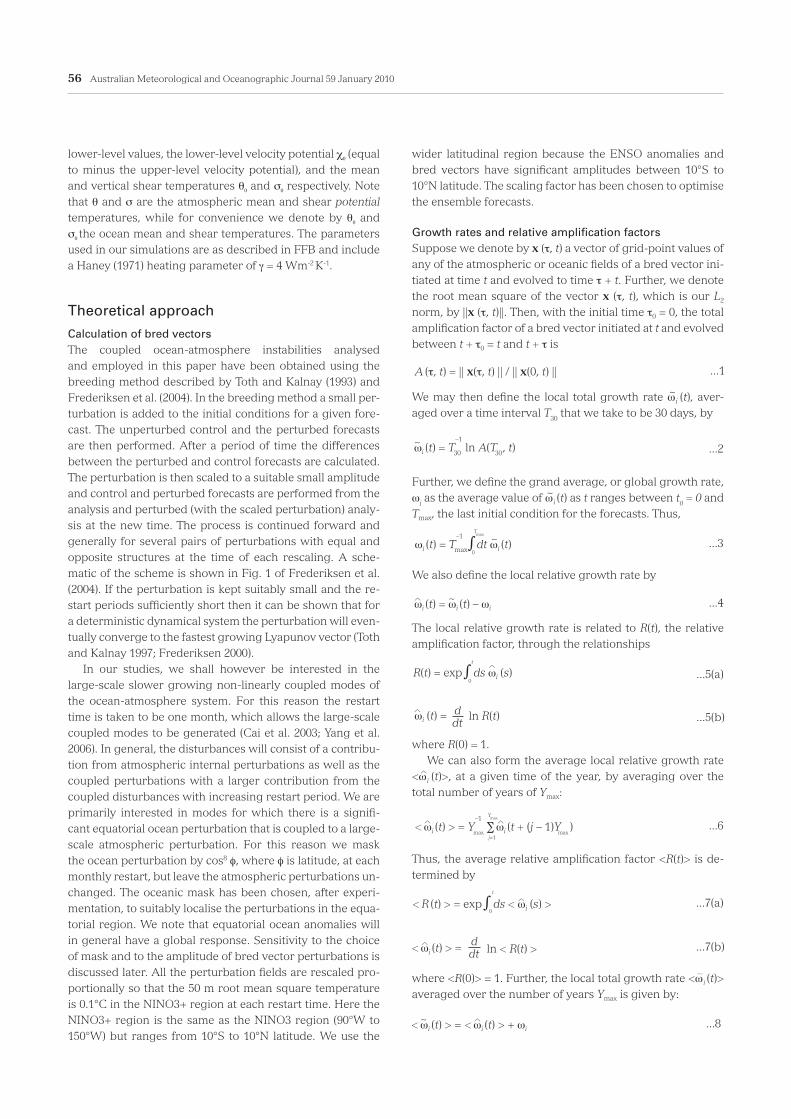
Growth rates and relative amplification factorsThe global growth rate of the bred vectors is wi = 0.02 day-1, corresponding to an e-folding time of 50 days, and this is the case whether 2, 8, 32 or 64 bred vectors are used in the calcu-lation. As discussed earlier, the growth rates of bred vectors, like the growth rates of the FTNMs of FB1, are not uniform but vary with time in the manner detailed below. Figure 2 shows the average local total growth rate,<w~i (t)> (thin solid) and relative amplification factor <R(t)>

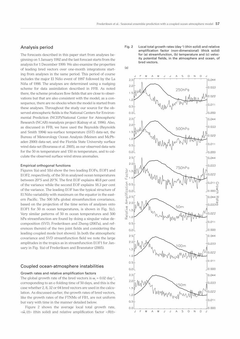
Fig. 2 Local total growth rates (day-1) (thin solid) and relative amplification factor (non-dimensional) (thick solid) for (a) streamfunction, (b) temperature and (c) veloc-ity potential fields, in the atmosphere and ocean, of bred vectors.

(a)


(thick solid), based on the global norm, for the coupled ocean-atmosphere instability fields obtained by breeding; the results are based on an average over eight bred vectors and breeding cycles for a month started every three days between 1 January 1992 and 1 December 1999. Figure 2(a) shows the streamfunction fields at three levels in each of the atmosphere and ocean. Figure 2(b) shows the corre-sponding quantities for the potential temperature fields in the atmosphere and the temperature fields in the ocean. The growth rates and amplification factors for the atmospheric and oceanic velocity potential fields are shown in Fig. 2(c). Comparing these diagrams with the corresponding results in Fig. 4 of FB1 for the 300 hPa atmospheric streamfunction for their FTNM1, the fastest growing FTNM, and for their five leading FTNMs, we note a number of general similari-ties. Firstly the maximum relative amplification factor occurs in early boreal spring and has a magnitude of around twice the value in January. It then decreases in late boreal spring attaining low values in boreal autumn and with generally in-creasing values in winter. We also note that the minimum in <R(t)> for both the bred vector and FTNM1 occurs between October and November. These similarities are also reflect-ed in the local growth rates. For example, for both FTNM1 and the bred vector, the maximum in <R(t)> in early boreal spring is preceded by a local maximum in the growth rate. On the whole, the maximum in <R(t)> for the coupled insta-bility occurs slightly later than for FTNM1 of FB1 and the variability in the growth rates <w~i (t)> are perhaps not as dra-matic as for the finite-time barotropic instability. These dif-ferences are probably partly due to the fact that the growth characteristics of the coupled instabilities are based on

Fig. 2 Continued.

(b) (c)


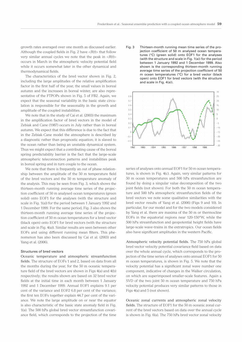
growth rates averaged over one month as discussed earlier. Although the coupled fields in Fig. 2 have <R(t)> that follow very similar annual cycles we note that the peak in <R(t)> occurs in March in the atmospheric velocity potential field while it occurs somewhat later in the other dynamical and thermodynamical fields. The characteristics of the bred vector shown in Fig. 2, including the large amplitudes of the relative amplification factor in the first half of the year, the small values in boreal autumn and the increases in boreal winter, are also repre-sentative of the FTPOPs shown in Fig. 5 of FB2. Again, we expect that the seasonal variability in the basic state circu-lation is responsible for the seasonality in the growth and amplitude of the coupled instabilities. We note that in the study of Cai et al. (2003) the maximum in the amplification factor of bred vectors in the model of Zebiak and Cane (1987) occurs in July rather than in boreal autumn. We expect that this difference is due to the fact that in the Zebiak-Cane model the atmosphere is described by a diagnostic rather than prognostic equation; it is slaved to the ocean rather than being an unstable dynamical system. Thus we might expect that a contributing cause of the boreal spring predictability barrier is the fact that the large-scale atmospheric teleconnection patterns and instabilities peak in boreal spring and in turn couple to the ocean. We note that there is frequently an out of phase relation-ship between the amplitude of the 50 m temperature field of the bred vectors and the 50 m temperature anomaly of the analysis. This may be seen from Fig. 3, which shows the thirteen-month running average time series of the projec-tion coefficient of 50 m analysed ocean temperatures (green solid) onto EOF1 for the analyses (with the structure and scale in Fig. 1(a)) for the period between 1 January 1992 and 1 December 1999. For the same period, Fig. 3 also shows the thirteen-month running average time series of the projec-tion coefficient of 50 m ocean temperatures for a bred vector (black open) onto EOF1 for bred vectors (with the structure and scale in Fig. 4(a)). Similar results are seen between other EOFs and using different running mean filters. This phe-nomenon has also been discussed by Cai et al. (2003) and Yang et al. (2006).

Structures of bred vectorsOceanic temperature and atmospheric streamfunction fields. The structure of EOFs 1 and 2, based on data from all the months during the year, for the 50 m oceanic tempera-ture field of the bred vectors are shown in Figs 4(a) and 4(b) respectively; the results shown are based on 32 bred vector fields at the initial time in each month between 1 January 1992 and 1 December 1999. Annual EOF1 explains 9.1 per cent of the variance and EOF2 6.8 per cent of the variance; the first ten EOFs together explain 44.7 per cent of the vari-ance. We note the large amplitude on or near the equator is also characteristic of the basic state anomaly field in Fig. 1(a). The 500 hPa global bred vector streamfunction covari-ance field, which corresponds to the projection of the time

series of analyses onto annual EOF1 for 50 m ocean tempera-tures, is shown in Fig. 4(c). Again, very similar patterns for 50 m ocean temperatures and 500 hPa streamfunction are found by doing a singular value decomposition of the two joint fields (not shown). For both the 50 m ocean tempera-ture and 500 hPa atmospheric streamfunction fields of the bred vectors we note some qualitative similarities with the bred vector results of Yang et al. (2006) (Figs 9 and 10). In particular, for our model and for the two models considered by Yang et al. there are maxima of the 50 m or thermocline EOFs in the equatorial regions near 120-150°W, while the 500 hPa streamfunction and geopotential height fields have large-scale wave-trains in the extratropics. Our ocean fields also have significant amplitudes in the western Pacific.

Atmospheric velocity potential fields. The 750 hPa global bred vector velocity potential covariance field based on data over the whole annual cycle, which corresponds to the pro-jection of the time series of analyses onto annual EOF1 for 50 m ocean temperatures, is shown in Fig. 5. We note that the velocity potential has a significant zonal wave number one component, indicative of changes in the Walker circulation, on which are superimposed smaller-scale features. Again a SVD of the two joint 50 m ocean temperature and 750 hPa velocity potential produces very similar patterns to those in Figs 4(a) and 5 (not shown).

Oceanic zonal currents and atmospheric zonal velocity fields. The structure of EOF1 for the 50 m oceanic zonal cur-rent of the bred vectors based on data over the annual cycle is shown in Fig. 6(a). The 750 hPa bred vector zonal velocity

Fig. 3 Thirteen-month running mean time series of the pro-jection coefficient of 50 m analysed ocean tempera-tures (°C) (green solid) onto EOF1 for the analyses (with the structure and scale in Fig. 1(a)) for the period between 1 January 1992 and 1 December 1999. Also shown is the corresponding thirteen-month running average time series of the projection coefficient of 50 m ocean temperatures (°C) for a bred vector (black open) onto EOF1 for bred vectors (with the structure and scale in Fig. 4(a)).


covariance field, which corresponds to the projection of the time series of analyses onto annual EOF1 for the 50 m ocean zonal current, is shown in Fig. 6(b). We note the somewhat similar structure between the corresponding oceanic and atmospheric fields with the atmospheric velocities extend-ing downstream of the oceanic zonal currents. These fields have large amplitudes at the longitudes where westerly wind bursts commonly occur (Seiki and Takayabu (2007a, b) review the literature). Seiki and Takayabu (2007a) note that a strong Madden Julian Oscillation (MJO) amplitude is a fa-vourable condition for westerly wind burst formation but is not a sufficient condition.

Seasonal variability of bred vector structures. As well as annual EOFs based on bred vector fields for the whole pe-riod between 1 January 1992 and 1 December 1999, we have calculated EOFs for the four seasons. Figure 7(a) shows, as an example, EOF1 for the 50 m temperature field of the bred vectors for December-January-February (DJF); this EOF ex-

Fig. 4 The first, EOF1 (a) and second, EOF2 (b) empirical or-thogonal functions of 50 m ocean temperatures (in relative units) between 20°S and 20°N for bred vec-tors. Also shown is (c) the 500 hPa streamfunction covariance (km2s-1) associated with the standardised principal component time series of EOF1 for 50 m ocean temperatures of bred vectors. Contour inter-vals as shown on bars.

Fig. 5 Velocity potential covariance field (km2s-1) at 750 hPa associated with EOF1 for 50 m ocean temperatures of bred vectors. Contour intervals as shown on bar.

Fig. 6 (a) The first empirical orthogonal functions, EOF1, of 50 m analysed ocean zonal current (in relative units) be-tween 20°S and 20°N for bred vectors. Also shown is (b) the 750 hPa atmospheric zonal wind covariance (m s-1) associated with EOF1 for 50 m ocean zonal currents of bred vectors. Contour intervals as shown on bars.

(a)

(a)

(b)

(b)

(c)


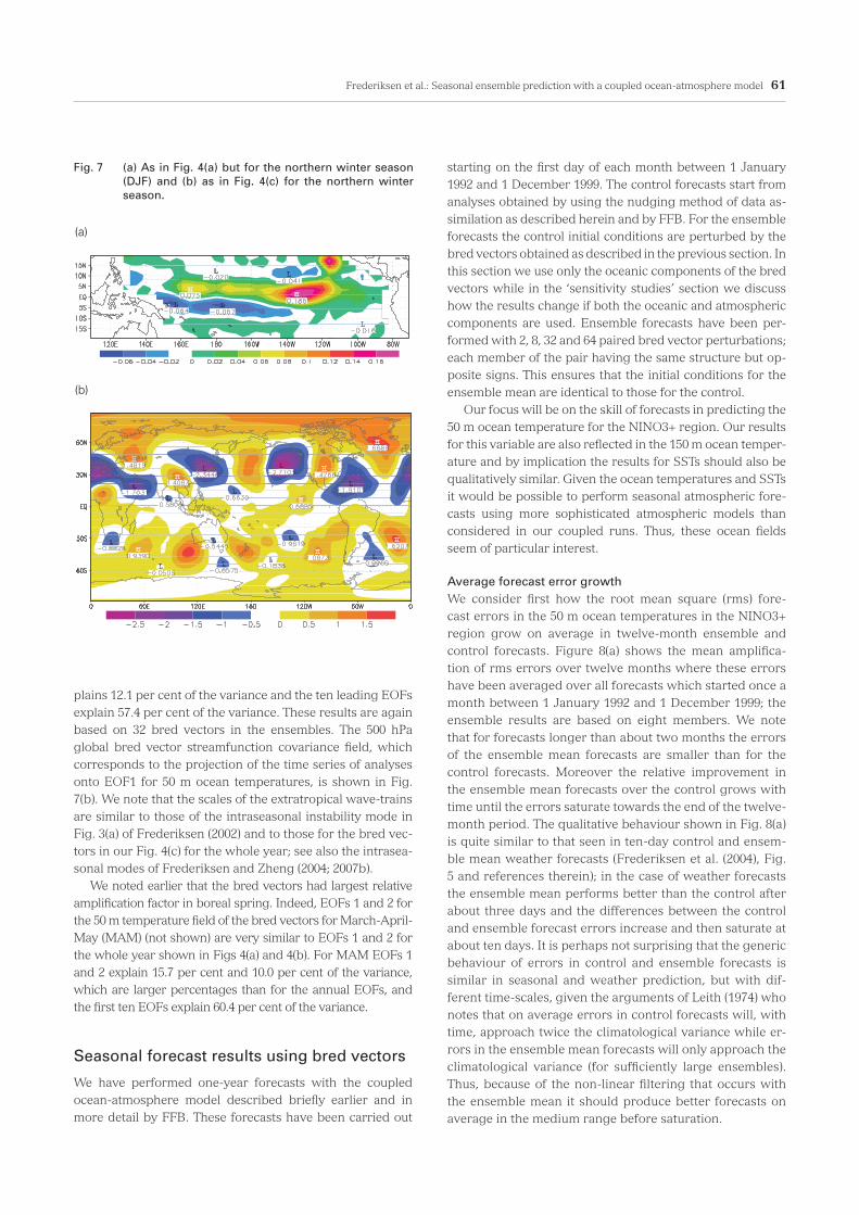
plains 12.1 per cent of the variance and the ten leading EOFs explain 57.4 per cent of the variance. These results are again based on 32 bred vectors in the ensembles. The 500 hPa global bred vector streamfunction covariance field, which corresponds to the projection of the time series of analyses onto EOF1 for 50 m ocean temperatures, is shown in Fig. 7(b). We note that the scales of the extratropical wave-trains are similar to those of the intraseasonal instability mode in Fig. 3(a) of Frederiksen (2002) and to those for the bred vec-tors in our Fig. 4(c) for the whole year; see also the intrasea-sonal modes of Frederiksen and Zheng (2004; 2007b). We noted earlier that the bred vectors had largest relative amplification factor in boreal spring. Indeed, EOFs 1 and 2 for the 50 m temperature field of the bred vectors for March-April-May (MAM) (not shown) are very similar to EOFs 1 and 2 for the whole year shown in Figs 4(a) and 4(b). For MAM EOFs 1 and 2 explain 15.7 per cent and 10.0 per cent of the variance, which are larger percentages than for the annual EOFs, and the first ten EOFs explain 60.4 per cent of the variance.

Seasonal forecast results using bred vectors

We have performed one-year forecasts with the coupled ocean-atmosphere model described briefly earlier and in more detail by FFB. These forecasts have been carried out

starting on the first day of each month between 1 January 1992 and 1 December 1999. The control forecasts start from analyses obtained by using the nudging method of data as-similation as described herein and by FFB. For the ensemble forecasts the control initial conditions are perturbed by the bred vectors obtained as described in the previous section. In this section we use only the oceanic components of the bred vectors while in the ‘sensitivity studies’ section we discuss how the results change if both the oceanic and atmospheric components are used. Ensemble forecasts have been per-formed with 2, 8, 32 and 64 paired bred vector perturbations; each member of the pair having the same structure but op-posite signs. This ensures that the initial conditions for the ensemble mean are identical to those for the control. Our focus will be on the skill of forecasts in predicting the 50 m ocean temperature for the NINO3+ region. Our results for this variable are also reflected in the 150 m ocean temper-ature and by implication the results for SSTs should also be qualitatively similar. Given the ocean temperatures and SSTs it would be possible to perform seasonal atmospheric fore-casts using more sophisticated atmospheric models than considered in our coupled runs. Thus, these ocean fields seem of particular interest.

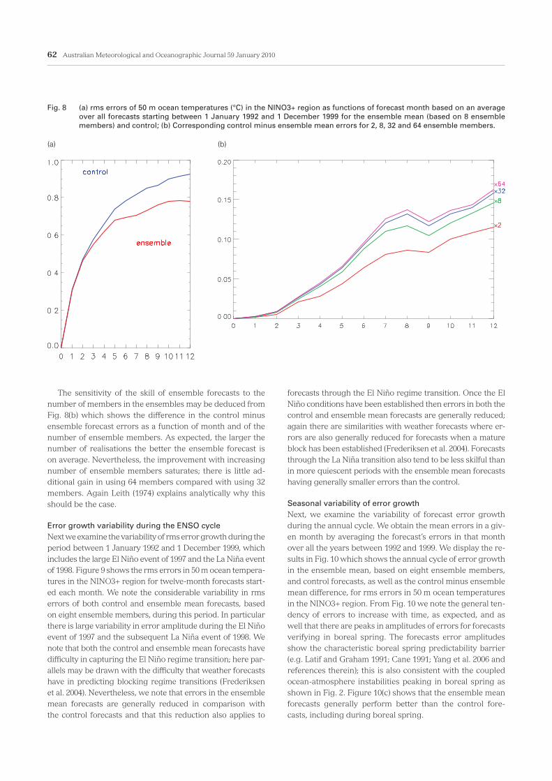
Average forecast error growthWe consider first how the root mean square (rms) fore-cast errors in the 50 m ocean temperatures in the NINO3+ region grow on average in twelve-month ensemble and control forecasts. Figure 8(a) shows the mean amplifica-tion of rms errors over twelve months where these errors have been averaged over all forecasts which started once a month between 1 January 1992 and 1 December 1999; the ensemble results are based on eight members. We note that for forecasts longer than about two months the errors of the ensemble mean forecasts are smaller than for the control forecasts. Moreover the relative improvement in the ensemble mean forecasts over the control grows with time until the errors saturate towards the end of the twelve-month period. The qualitative behaviour shown in Fig. 8(a) is quite similar to that seen in ten-day control and ensem-ble mean weather forecasts (Frederiksen et al. (2004), Fig. 5 and references therein); in the case of weather forecasts the ensemble mean performs better than the control after about three days and the differences between the control and ensemble forecast errors increase and then saturate at about ten days. It is perhaps not surprising that the generic behaviour of errors in control and ensemble forecasts is similar in seasonal and weather prediction, but with dif-ferent time-scales, given the arguments of Leith (1974) who notes that on average errors in control forecasts will, with time, approach twice the climatological variance while er-rors in the ensemble mean forecasts will only approach the climatological variance (for sufficiently large ensembles). Thus, because of the non-linear filtering that occurs with the ensemble mean it should produce better forecasts on average in the medium range before saturation.

(a)

(b)

Fig. 7 (a) As in Fig. 4(a) but for the northern winter season (DJF) and (b) as in Fig. 4(c) for the northern winter season.


The sensitivity of the skill of ensemble forecasts to the number of members in the ensembles may be deduced from Fig. 8(b) which shows the difference in the control minus ensemble forecast errors as a function of month and of the number of ensemble members. As expected, the larger the number of realisations the better the ensemble forecast is on average. Nevertheless, the improvement with increasing number of ensemble members saturates; there is little ad-ditional gain in using 64 members compared with using 32 members. Again Leith (1974) explains analytically why this should be the case.

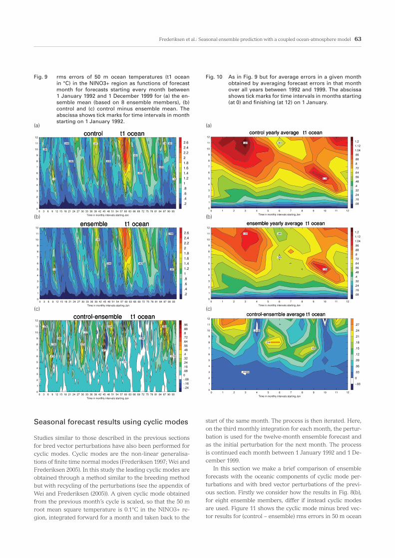
Error growth variability during the ENSO cycleNext we examine the variability of rms error growth during the period between 1 January 1992 and 1 December 1999, which includes the large El Niño event of 1997 and the La Niña event of 1998. Figure 9 shows the rms errors in 50 m ocean tempera-tures in the NINO3+ region for twelve-month forecasts start-ed each month. We note the considerable variability in rms errors of both control and ensemble mean forecasts, based on eight ensemble members, during this period. In particular there is large variability in error amplitude during the El Niño event of 1997 and the subsequent La Niña event of 1998. We note that both the control and ensemble mean forecasts have difficulty in capturing the El Niño regime transition; here par-allels may be drawn with the difficulty that weather forecasts have in predicting blocking regime transitions (Frederiksen et al. 2004). Nevertheless, we note that errors in the ensemble mean forecasts are generally reduced in comparison with the control forecasts and that this reduction also applies to

forecasts through the El Niño regime transition. Once the El Niño conditions have been established then errors in both the control and ensemble mean forecasts are generally reduced; again there are similarities with weather forecasts where er-rors are also generally reduced for forecasts when a mature block has been established (Frederiksen et al. 2004). Forecasts through the La Niña transition also tend to be less skilful than in more quiescent periods with the ensemble mean forecasts having generally smaller errors than the control.

Seasonal variability of error growthNext, we examine the variability of forecast error growth during the annual cycle. We obtain the mean errors in a giv-en month by averaging the forecast’s errors in that month over all the years between 1992 and 1999. We display the re-sults in Fig. 10 which shows the annual cycle of error growth in the ensemble mean, based on eight ensemble members, and control forecasts, as well as the control minus ensemble mean difference, for rms errors in 50 m ocean temperatures in the NINO3+ region. From Fig. 10 we note the general ten-dency of errors to increase with time, as expected, and as well that there are peaks in amplitudes of errors for forecasts verifying in boreal spring. The forecasts error amplitudes show the characteristic boreal spring predictability barrier (e.g. Latif and Graham 1991; Cane 1991; Yang et al. 2006 and references therein); this is also consistent with the coupled ocean-atmosphere instabilities peaking in boreal spring as shown in Fig. 2. Figure 10(c) shows that the ensemble mean forecasts generally perform better than the control fore-casts, including during boreal spring.

Fig. 8 (a) rms errors of 50 m ocean temperatures (°C) in the NINO3+ region as functions of forecast month based on an average over all forecasts starting between 1 January 1992 and 1 December 1999 for the ensemble mean (based on 8 ensemble members) and control; (b) Corresponding control minus ensemble mean errors for 2, 8, 32 and 64 ensemble members.

(a) (b)


Seasonal forecast results using cyclic modes

Studies similar to those described in the previous sections for bred vector perturbations have also been performed for cyclic modes. Cyclic modes are the non-linear generalisa-tions of finite time normal modes (Frederiksen 1997; Wei and Frederiksen 2005). In this study the leading cyclic modes are obtained through a method similar to the breeding method but with recycling of the perturbations (see the appendix of Wei and Frederiksen (2005)). A given cyclic mode obtained from the previous month’s cycle is scaled, so that the 50 m root mean square temperature is 0.1°C in the NINO3+ re-gion, integrated forward for a month and taken back to the

start of the same month. The process is then iterated. Here, on the third monthly integration for each month, the pertur-bation is used for the twelve-month ensemble forecast and as the initial perturbation for the next month. The process is continued each month between 1 January 1992 and 1 De-cember 1999. In this section we make a brief comparison of ensemble forecasts with the oceanic components of cyclic mode per-turbations and with bred vector perturbations of the previ-ous section. Firstly we consider how the results in Fig. 8(b), for eight ensemble members, differ if instead cyclic modes are used. Figure 11 shows the cyclic mode minus bred vec-tor results for (control – ensemble) rms errors in 50 m ocean

Fig. 9 rms errors of 50 m ocean temperatures (t1 ocean in °C) in the NINO3+ region as functions of forecast month for forecasts starting every month between 1 January 1992 and 1 December 1999 for (a) the en-semble mean (based on 8 ensemble members), (b) control and (c) control minus ensemble mean. The abscissa shows tick marks for time intervals in month starting on 1 January 1992.

Fig. 10 As in Fig. 9 but for average errors in a given month obtained by averaging forecast errors in that month over all years between 1992 and 1999. The abscissa shows tick marks for time intervals in months starting (at 0) and finishing (at 12) on 1 January.

(a) (a)

(b) (b)

(c) (c)


temperatures in the NINO3+ region for twelve-month fore-casts started each month. We note from Figs 8(b) and 11 that the error reduction with eight cyclic modes in three to nine-month ensemble forecasts (values in Fig. 11 plus results in Fig. 8(b) for eight bred vectors) is very similar to that with 32 to 64 bred vectors. Secondly, we show in Fig. 12 how this ad-ditional error reduction, in ensemble forecasts over control forecasts for cyclic modes compared with bred vectors, varies with the annual cycle. The differences in error reduction are again for eight ensemble members of each type. We note that the improvements using cyclic modes in ensemble forecasts occur primarily during the second half of the year in three to nine-month ensemble forecasts. Importantly the largest error reductions occur for forecasts verifying in boreal spring.

The findings in this section, comparing the effectiveness of cyclic modes, the non-linear generalisations of finite time normal modes, and bred vectors, the non-linear generalisa-tions of Lyapunov vectors, have relationships with the results of Wei and Frederiksen (2004) that may be significant. Wei and Frederiksen (2004) performed tangent linear barotropic simulations of 100 initially random errors on evolving south-ern hemisphere atmospheric flows. They found that for inte-grations periods between one day and fourteen days mean pattern correlations between the evolved errors and leading FTNMs were generally considerably larger than with leading Lyapunov vectors. FTNMs might therefore be expected to be more efficient in improving ensemble forecasts compared with Lyapunov vectors, as we have found here for their non-linear generalisations in coupled forecasts.

Sensitivity studies

We have examined the sensitivity of our results to the choice of model parameters, as described to some extent in FFB, and to the specification of the coupled instabilities used as ensemble perturbations. In this section we briefly discuss forecast sensitiv-ity to the specification of the bred vectors. As well as the studies described earlier, where the ensemble perturbations used the oceanic components of the bred vectors, we have performed analogous forecasts using the coupled bred vectors with both oceanic and atmospheric components. This change has little ef-fect on the error reduction with ensembles in forecasting the 50 m or 150 m ocean temperatures. However, as might be ex-pected, the atmospheric components of coupled bred vectors that grow fastest over a month are not ideal perturbations for ensemble weather forecasting. In fact, the atmospheric com-ponents of the bred vectors cause a decrease in atmospheric ensemble forecasting skill, particularly for forecasts of about a month. Of course, one could perturb the atmosphere with bred vectors that grow fast over six or twelve hours, and that may be a useful strategy with more complex coupled general circula-tion models, but that is beyond the scope of our present study. We have also performed sensitivity studies to examine the effects of using different specifications of the mask for the ocean components of the bred vectors and of using different rescaling factors. Our choice of the mask and rescaling fac-tor described earlier is based on this experimentation.

Discussion and conclusions

We have applied ensemble prediction methods, in which the control initial conditions are perturbed by coupled ocean-atmosphere disturbances, within the coupled ocean-atmo-sphere model of FFB. The coupled ocean-atmosphere insta-bilities are obtained using a breeding method in which the perturbations are grown over a period of a month before res-caling. The coupled modes are therefore non-linearly modi-fied and the method effectively filters out the faster growing weather instabilities of the dynamical atmospheric model.

Fig. 11 Cyclic mode minus bred vector results for (control – ensemble) rms errors in 50 m ocean temperatures (°C) in the NINO3+ region for 12-month forecasts started each month and based on an average over all forecasts starting between 1 January 1992 and 1 De-cember 1999.

Fig. 12 As in Fig. 11 but for average errors, in a given month, obtained by averaging forecast errors in that month over all years between 1992 and 1999. The abscissa shows tick marks for time intervals in months starting (at 0) and finishing (at 12) on 1 January.


First, we have studied in some detail the properties of the leading coupled ocean-atmosphere non-linear modes. The bred vectors have a global growth rate of 0.02 day-1 corre-sponding to an e-folding time of 50 days. However, the local growth rates of bred vectors are not uniform but vary with time in a way similar to the leading barotropic atmospheric FTNMs of FB1 and atmospheric teleconnection pattern FT-POPs of FB2. The most striking similarity between the bred vectors and the atmospheric FTNMs and FTPOPs is in the seasonality of the growth rates of the leading disturbances. For bred vectors and FTNMs and FTPOPs there is a distinct annual cycle of these growth rates with the maximum oc-curring during the middle of the boreal cold season and a minimum being present during the boreal warm season. The amplitude of this annual cycle for bred vectors is also rather similar to that for the FTPOPs with a difference in average growth rates of about 0.02 day-1 between warm and cold sea-sons (Fig. 2) while the leading FTNMs have a correspond-ing range of roughly twice this amount. The similarity in the seasonality of growth characteristics is even more evident if one considers the time-integrated effects of growth, as given by our relative amplification rate. In this case one finds that the bred vectors and atmospheric FTNMs and FTPOPs have maximum amplitudes in boreal spring and minimum ampli-tudes in boreal autumn. The leading EOFs of the 50 m ocean temperature of bred vectors have maxima in the equatorial Pacific between 120 – 150°W as well as in the western Pacific, while the associated 500 hPa streamfunction fields have large-scale wave-trains in the extratropics, including over the North Pacific, North American and Australian regions that are strongly influ-enced by ENSO. The associated 750 hPa velocity potential has a significant wave number one component centred on the equator indicative of changes in the Walker circulation. The leading EOFs of the 50 m ocean zonal current of bred vectors have maximum amplitudes in the equatorial western Pacific with associated 750 hPa atmospheric zonal winds ex-tending from this region across the central Pacific. In many respects the properties of the bred vectors are similar to those found by Yang et al. (2006) for two coupled general cir-culation models, although our 50 m ocean temperature EOFs have additional centres in the western Pacific. The second part of our study has been to perform one-year control and ensemble forecasts with the coupled ocean-atmosphere model of FFB. The control forecasts have been initiated on the first day of each month between 1 January 1992 and 1 December 1999 from analyses obtained using the nudging method of data assimilation that ensures the anal-yses are consistent with the model and the forecasts start without shocks. For the ensemble forecasts bred vectors perturb the analyses and we have considered 2, 8, 32 and 64 paired bred vectors with each member of the pair having the same structure but opposite sign. This ensures that the ensemble mean forecast starts from the same analysis as the control. We have focused on the skill of predicting the 50 m ocean temperature for the NINO3+ region.

We find that for forecasts longer than about two months the rms errors in the ensemble mean forecasts are smaller than for the control based on averages over all the fore-casts started between 1 January 1992 and 1 December 1999. There is considerable variability in the skill of both control and ensemble forecasts during the period studied. This is particularly the case during the period between the start of the El Niño event of 1997 and the La Niña of 1998. Both the control and ensemble mean forecasts have difficulty in capturing the regime transition into the El Niño event. Once the El Niño conditions have been established predictability improves with rms errors in control and ensemble mean forecasts generally reduced. Similarly, forecasts through the La Niña regime transition also tend to be less skilful than in more quiescent periods. In general the ensemble mean forecasts have smaller rms errors than the control. Again, there is significant variability in forecast error growth dur-ing the annual cycle. As expected errors increase with time and there are peaks in error amplitudes for forecasts verify-ing in boreal spring. This is consistent with the bred vector coupled ocean-atmosphere instabilities peaking in boreal spring (Fig. 2). Ensemble mean forecast skill improves with increasing number of bred vector perturbations but the improvement saturates for larger number of members with little additional gain in using 64 members compared with 32. We have also performed similar ensemble forecasts using cyclic modes, non-linear generalisations of finite time normal modes, for ensemble perturbations. We have found that ensemble mean forecasts based on eight cyclic modes have similar skill in three to nine-month forecasts as those based on 32 to 64 bred vectors. We have argued on the basis of the results of FB1, FB2 and our findings in this paper that we expect that a contrib-uting cause of the boreal spring predictability barrier is the fact that large-scale atmospheric teleconnection patterns and instabilities peak in boreal spring and in turn couple to the ocean. In future studies we plan to examine in more detail the re-lationships between bred vectors and cyclic modes and their relative efficacy in seasonal ensemble prediction.

Acknowledgments

We thank Janice Sisson for assistance during the early stages of this work.

ReferencesBattisti, D.S. and Hirst, A.C. 1989. Interannual variability in a tropical at-

mosphere-ocean model: influence of the basic state, ocean geometry and nonlinearity. J. Atmos. Sci., 46, 1687-712.

Bourassa, M.A., Romero, R., Smith, S.R. and O’Brien, J.J. 2005. A new FSU winds climatology. Jnl Climate., 18, 3,692–704.

Brown, J. 1969. A numerical investigation of hydrodynamic instability and energy conversions in the quasi-geostrophic atmosphere. Part I. J. Atmos. Sci., 26, 352-65.


Cai, M., Kalnay, E. and Toth, Z. 2003. Bred vectors of the Zebiak-Cane model and their potential application to ENSO predictions. Jnl Cli-mate, 16, 40-56.

Cane, M.A. 1991. Forecasting El Niño with a geophysical model. Telecon-nections Connecting World-Wide Climate Anomalies, M. Glantz, R. Katz, and N. Nicholls (Eds), Cambridge University Press, 345-69.

Cane, M.A. and Zebiak, S.E. 1985. A theory of El Niño and the Southern Oscillation. Science, 228, 1085-7.

Cane, M.A., Zebiak, S.E. and Dolan, S.C. 1986. Experimental forecasts of El Niño. Nature, 321, 827-32.

Chen, Y.-Q., Battisti, D.S., Palmer, T.N., Barsugli, J. and Sarachik, E.S. 1997. A study of the predictability of tropical Pacific SST in a coupled atmosphere-ocean model using singular vector analysis: The roles of the annual cycle and the ENSO cycle. Mon. Weath. Rev., 125, 831-45.

Fan, Y., Allen, M.R., Anderson, D.L.T. and Balmaseda, M.A. 2000. How predictability depends on the nature of uncertainty in initial condi-tions in a coupled model of ENSO. Jnl Climate, 13, 3298-313.

Frederiksen, C.S. and Zheng, X. 2004. Variability of seasonal-mean fields arising from intraseasonal variability: Part II, Application to NH win-ter circulations. Clim. Dyn., 23, 193-206.

Frederiksen, C.S. and Zheng, X. 2007a. Coherent patterns of interannual variability of the atmospheric circulation: The role of intraseasonal variability. Frontiers in Turbulence and Coherent Structures, Chapter 4, 87-120. J. Denier and J.S. Frederiksen (Eds), World Scientific Lecture Notes in Complex Systems, 490 pp.

Frederiksen, C.S. and Zheng, X. 2007b. Variability of seasonal-mean fields arising from intraseasonal variability. Part 3: Application to SH winter and summer circulations. Clim. Dyn., 28, 849-66.

Frederiksen, C.S., Frederiksen, J.S. and Balgovind, R.C. 2010. ENSO vari-ability and prediction in a coupled ocean-atmosphere model. Aust. Met. Oceanogr. J.,59, 35-52.

Frederiksen, J.S. 1997. Adjoint sensitivity and finite-time normal mode disturbances during blocking. J. Atmos. Sci., 54, 1144-65.

Frederiksen, J.S. 2000. Singular vectors, finite-time normal modes, and error growth during blocking. J. Atmos. Sci., 57, 312-33.

Frederiksen, J.S. 2002. Genesis of intraseasonal oscillations and equato-rial waves. J. Atmos. Sci., 59, 2761-81.

Frederiksen, J.S. and Puri, K. 1985. Nonlinear instability and error growth in Northern Hemisphere three-dimensional flows: Cyclogenesis, on-set-of-blocking and mature anomalies. J. Atmos. Sci., 42, 1374-97.

Frederiksen, J.S. and Branstator, G. 2001. Seasonal and intraseasonal variability of large-scale barotropic modes. J. Atmos. Sci., 58, 50-69.

Frederiksen, J.S. and Branstator, G. 2005. Seasonal variability of telecon-nection patterns. J. Atmos. Sci., 62, 1346-65.

Frederiksen, J.S., Collier, M.A. and Watkins, A.B. 2004. Ensemble predic-tion of blocking regime transitions. Tellus, 56A, 485-500.

Haney, R.L. 1971. Surface thermal boundary condition for ocean circula-tion model. J. Phys. Oceanogr., 6, 621-31.

Kalnay, E., Kanamitsu, M., Kistler, R., Collins, W., Deaven, D., Gandin, L., Iredell, M., Saha, S., White, G., Woollen, J., Zhu, Y., Leetmaa, A., Reynolds, R., Chelliah, M., Ebisuzaki, W., Higgins, W., Janowiak, J., Mo, K.C., Ropelewski, C., Wang, J., Jenne, R. and Joseph, D. 1996. The NCEP/NCAR 40-year Reanalysis Project. Bull. Am. Met. Soc., 77, 437-71.

Kirtman, B.P., Shukla, J., Huang, B., Zhu, Z. and Schneider, E.K. 1997. Multiseasonal predictions with a coupled Tropical Ocean Global At-mosphere system. Mon. Weath. Rev., 125, 789-808.

Kleeman, R. 1993. On the dependence of hindcast skill on ocean ther-modynamics in a coupled ocean-atmosphere model. Jnl Climate, 6, 2012-33.

Kleeman, R., Tang, Y. and Moore, A.M. 2003. The calculation of climati-cally relevant singular vectors in the presence of weather noise as ap-plied to the ENSO problem. J. Atmos. Sci., 60, 2856-68.

Latif, M. and Graham, N.E. 1991. How much predictive skill is contained in the thermal structure of an OGCM? TOGA Notes, 2, 6-8.

Latif, M., Sterl, A., Maier-Reimer, E., and Junge, M. M. 1993. Climate vari-ability in a coupled GCM. Part I: The tropical Pacific. Jnl Climate, 6, 5-21.

Latif, M., Anderson D., Barnett T., Cane, M., Kleeman, R., Leetmaa, A., O’Brien, J., Rosati, A. and Schneider, E. 1998. A review of the predict-ability and prediction of ENSO. J. Geophys. Res., 103, 14,375-93.

Leith, C.E. 1974. Theoretical skill of Monte Carlo forecasts. Mon. Weath. Rev., 102, 409-18.

Meinen, C.S. and McPhaden, M.J. 2000. Observations of warm water vol-ume changes in the equatorial Pacific and their relationship to El Niño and La Niña. Jnl Climate, 13, 3552-9.

Moore, A.M. and Kleeman, R. 1996. The dynamics of error growth and predictability in a coupled model of ENSO. Q. Jl R. Met. Soc., 122, 1405-46.

Moore, A.M. and Kleeman, R. 1998. Skill assessment for ENSO using en-semble prediction. Q. Jl R. Met. Soc., 124, 557-86.

Moore, A.M., Vialard, J., Weaver, A.T., Anderson, D.L.T, Kleeman, R. and Johnson, J.R. 2003. The role of air-sea interaction in controlling the optimal perturbations of low-frequency tropical coupled ocean-atmo-sphere modes. Jnl Climate, 16, 951-68.

Reynolds, R.W. and Smith, T.M. 1994. Improved Global Sea Surface Tem-perature Analyses Using Optimum Interpolation. J. Climatol., 7, 929-48.

Rosati, A., Miyakoda, K. and Gudgel, R. 1997. The impact of ocean initial conditions on ENSO forecasting with a coupled model. Mon. Weath. Rev., 125, 754-72.

Schopf, P.S. and Suarez, M.J. 1988. Vacillations in a coupled ocean-atmo-sphere model. J. Atmos. Sci., 45, 549-66.

Seiki, A. and Takayabu, Y.N. 2007a. Westerly wind bursts and their re-lationship with intraseasonal variations and ENSO. Part I: Statistics. Mon. Weath. Rev., 135, 3325-45.

Seiki, A. and Takayabu, Y.N. 2007b. Westerly wind bursts and their rela-tionship with intraseasonal variations and ENSO. Part II: Energetics over the Western and Central Pacific. Mon. Weath. Rev., 135, 3346-61.

Shukla, J., Anderson, J., Baumhefner, D., Brankovic, C., Chang, Y., Kalnay, E., Marx, L., Palmer, T., Paolino, D., Ploshay, J., Schubert, S., Straus, D., Suarez, M. and Tribbia, J. 2000. Dynamical seasonal prediction. Bull. Am. Met. Soc., 81, 2593-606.

Stockdale, T.N., Anderson, D.L.T, Alves, J.O.S, and Balmaseda, M.A. 1998. Global seasonal rainfall forecasts using a coupled ocean-atmosphere model. Nature, 392, 370-3.

Thompson, C.J. and Battisti, D.S. 2000. A Linear stochastic dynamical model of ENSO. Part I: Model development. Jnl Climate, 13, 2818-32.

Thompson, C.J. and Battisti, D.S. 2001. A linear stochastic dynamical model of ENSO. Part II: Analysis. Jnl Climate, 14, 445-66.

Toth, Z. and Kalnay, E. 1993. Ensemble forecasting at NMC: The genera-tion of perturbations. Bull. Am. Met. Soc., 74, 2317-30.

Toth, Z. and Kalnay, E. 1997. Ensemble forecast at NCEP and the breeding method. Mon. Weath. Rev., 125, 3297-319.

Webster, P.J. 1995. The annual cycle and the predictability of the tropical coupled ocean-atmosphere system. Met. Atmos. Phys., 56, 33-55.

Webster, P.J. and Yang, S. 1992. Monsoon and ENSO: Selectively interac-tive systems. Q. Jl R. Met. Soc., 118, 877-926.

Wei, M. and Frederiksen, J.S. 2004. Error growth and dynamical vectors during Southern Hemisphere blocking. Nonl. Proc. in Geophys., 11, 99-118.

Wei, M. and Frederiksen, J.S. 2005. Finite-time normal mode disturbanc-es and error growth during Southern Hemisphere blocking. Adv. At-mos. Sci., 22, 69-89.

Xue, Y., Cane, M.A. and Zebiak, S.E. 1997a. Predictability of a coupled model of ENSO using singular vector analysis. Part I: Optimal growth in seasonal background and ENSO cycles. Mon. Weath. Rev., 125, 2043-56.

Xue, Y., Cane, M.A., Zebiak, S.E. and Palmer, T.N. 1997b. Predictability of a coupled model of ENSO using singular vector analysis. Part II: Opti-mal growth and forecast skill. Mon. Weath. Rev., 125, 2057-73.

Yang, S.-C., Kalnay, E., Rienecker, M., Yuan, G., and Toth, Z. 2006. ENSO bred vectors in coupled ocean-atmosphere general circulation mod-els. J. Climatol., 19, 1422-33.

Zebiak, S.E. and Cane, M.A. 1987. A model El Niño-Southern Oscillation. Mon. Weath. Rev., 115, 2262-78.

seasonal ensemble prediction with a coupled ocean ... · prognostic primitive equation atmospheric...

Documents