Second-order model of entrainment in planar turbulent jets at low Reynolds numberS. Paillat and E. Kaminski

Citation: Physics of Fluids (1994-present) 26, 045110 (2014); doi: 10.1063/1.4871521 View online: http://dx.doi.org/10.1063/1.4871521 View Table of Contents: http://scitation.aip.org/content/aip/journal/pof2/26/4?ver=pdfcov Published by the AIP Publishing Articles you may be interested in Similarity analysis of the momentum field of a subsonic, plane air jet with varying jet-exit and local Reynoldsnumbers Phys. Fluids 25, 015115 (2013); 10.1063/1.4776782 Effects of passive control rings positioned in the shear layer and potential core of a turbulent round jet Phys. Fluids 24, 115103 (2012); 10.1063/1.4767535 Investigations on the local entrainment velocity in a turbulent jet Phys. Fluids 24, 105110 (2012); 10.1063/1.4761837 The thermal signature of a low Reynolds number submerged turbulent jet impacting a free surface Phys. Fluids 20, 115102 (2008); 10.1063/1.2981534 An experimental investigation of the near-field flow development in coaxial jets Phys. Fluids 15, 1233 (2003); 10.1063/1.1566755

This article is copyrighted as indicated in the article. Reuse of AIP content is subject to the terms at: http://scitation.aip.org/termsconditions. Downloaded to IP:

81.194.22.198 On: Mon, 28 Apr 2014 23:06:15

PHYSICS OF FLUIDS 26, 045110 (2014)

Second-order model of entrainment in planar turbulent jetsat low Reynolds number

S. Paillata) and E. KaminskiInstitut de Physique du Globe de Paris, Sorbonne Paris Cite, Univ Paris Diderot, CNRS,1 rue Jussieu, F-75252 Paris, France

(Received 5 December 2013; accepted 5 April 2014; published online 24 April 2014)

Turbulent jets and plumes are commonly encountered in natural and industrial envi-ronments, and have been the objects of seminal works on turbulent free shear flows.The dynamics of turbulent jets is most often described as a function of the so-calledentrainment coefficient, α, which quantifies the entrainment of ambient fluid into thejets. This key parameter has been determined in numerous and extensive experimen-tal, numerical, and theoretical studies of axisymmetric jets. However, data remainscarce on turbulent planar jets. Available studies have shown that at low distancefrom the source, α increases with the source Reynolds number, and that α increaseswith distance from the source for large source Reynolds number. But no link has beenmade between these two kinds of observation so far. To study the relative influenceof source Reynolds number, Re0, and distance from source on entrainment in planarturbulent jets, we perform new experiments at low Re0 (between 59 and 424) withthree different aspect ratio (185, 370, and 925) and at small and large distances fromthe source. Our experimental results show no systematic variations of α as a functionof Re0 or as a function of the distance from the source. To interpret these observations,we develop a formalism based on the flow velocity profiles, which yields an expres-sion of α as a function of the evolution of the Reynolds shear stress and of the turbulentfluctuations of the radial and vertical velocities. We obtain that the main contributionto entrainment is related to the turbulent shear stress, and that second-order fluctua-tions of the velocity account for the observed variations of α. The evolution to a fullyself-similar regime in which these fluctuations are fully negligible is too slow at smallRe0 for this regime to be observed in our experiments, even at the largest distancesfrom the source. C© 2014 AIP Publishing LLC. [http://dx.doi.org/10.1063/1.4871521]

I. INTRODUCTION

The dynamics of turbulent jets and plumes depends on their source conditions and on theefficiency of turbulent entrainment of the surrounding fluid into the mean flow. Quantifying turbulententrainment is key in assessing the rate of dilution and the rising height of natural and industrial jetsand plumes. In volcanology, for example, entrainment plays an important role in the evolution of theeruptive column, and controls both the production of pyroclastic flows on the ground and the rateand the height of injection of volcanic gas and ash in the atmosphere.1, 2

A large body of experimental and theoretical works on axisymmetric turbulent jets and plumes isavailable in the literature. In their seminal paper, Morton et al.3 introduced the concept of entrainmentcoefficient, defined as the ratio of the lateral velocity of fluids engulfed in the flow to the verticalmean flow velocity. The values of the so-called “Gaussian” entrainment coefficient, αG, are obtainedby measuring the vertical velocity and fitting it by Gaussian functions. Such measurements inaxisymmetric jets and plumes4 have shown that entrainment is enhanced by positive buoyancy inplumes.5, 6 Recently, Carazzo and co-workers7, 8 proposed a theoretical expression of αG that depends

a)Author to whom correspondence should be addressed. Electronic mail: paillat@ipgp.fr

1070-6631/2014/26(4)/045110/14/$30.00 C©2014 AIP Publishing LLC26, 045110-1

This article is copyrighted as indicated in the article. Reuse of AIP content is subject to the terms at: http://scitation.aip.org/termsconditions. Downloaded to IP:

81.194.22.198 On: Mon, 28 Apr 2014 23:06:15

045110-2 S. Paillat and E. Kaminski Phys. Fluids 26, 045110 (2014)

both on buoyancy (either positive or negative) and on the distance from the source. Their formalismaccounts well for experimental measurements and observations on jets, plumes, and fountains,9, 10

and has been applied successfully to immiscible fluids11 and reactive flows.12

Planar turbulent jets and plumes occurred also often in nature, for example, in the case ofbasaltic fissure eruptions, on Earth13, 14 and on other planets,15 or in the case of the discharge ofrivers into quiescent water.16 However, they have not been the subject of as numerous and compre-hensive studies as axisymmetric jets and plumes. For example, in their review, Fischer et al.17 gaveαG = 0.035 ± 0.001 for pure planar jets and αG = 0.070 ± 0.001 for pure planar plumes, but nomodels have been proposed so far to explain these values. Furthermore, to our knowledge, no exper-iments have been performed on planar negatively buoyant plumes yet. Our general goal is to providea theoretical framework able to account for the effect of buoyancy and of potential self-similaritydrift in planar jets and plumes, and to apply it to the modelling of geological turbulent flows. As afirst step, we focus here on the behaviour of pure jets (i.e., driven only by their initial momentum,and without buoyancy forces).

The majority of experimental constraints on the entrainment coefficient in turbulent planar jetshave been obtained at small and intermediate distances from the source (5 < z/d < 150, wherez is the vertical distance from the source and d the source width). Determinations of αG reliedfirst on the measurement of opening angle of the jets from velocity profiles obtained by hot-wireanemometry.18–21 Kotsovinos22 and Ramaprian and Chandrasekhara23 later obtained complementarydata using Laser Doppler Anemometry. All these studies, performed at source Reynolds number,Re0, larger than 1000 yielded a similar average value of αG ≈ 0.03. However, from a detailed reviewof the literature, Kotsovinos24 rather concluded that αG was a function of distance from the sourceup to z/d ≈ 200, where it reached a constant value αG = 0.042.

More recently, Namer and Otungen,25 Suresh et al.,26 and Deo27 measured the opening angleof jets for various Re0. They found that the value of αG varied from 0.072 for Re0 ≈ 250, to 0.024for Re0 > 6000. Deo27 experimentally studied the influence of the aspect ratio (width/length) of thesource on αG. At Re0= 16 000, he showed that the entrainment coefficient varies between 0.016,for an aspect ratio of 20, to 0.032 for an aspect ratio of 72, which is consistent with the value ofαG given in the literature for higher aspect ratios and states that the entrainment coefficient does notdepend on this parameter for such high aspect ratio.

In order to understand better the relative influence of this jet Reynolds number and distancefrom the source on the rate of entrainment in turbulent planar jets, we performed new experimentsat small and large distances from the source, ranging from z/d = 40 to z/d = 1000, and at smallsource Reynolds numbers, ranging from Re0 = 60 to Re0 = 420. To interpret our experimentalresults as well as those from the literature in a common framework, we developed an expression forthe entrainment coefficient derived from the theory of Priestley and Ball28 and Kaminski et al.7 foraxisymmetric jets and plumes. Our results emphasize the key role played by the turbulent Reynoldsstress on entrainment, and imply that second order refinements are required to explain the values ofαG measured at low Re0 (<500). We propose that these second-order contributions can be calculatedfrom the axial terms of the Reynolds stress which are often negligible in 2D turbulent jets.

II. ENTRAINMENT COEFFICIENTS IN PLANAR TURBULENT JETS

A. Review of literature data

Planar “pure” jets are turbulent free shear flows produced by a linear source of momentuminfinite in one direction. They have no density anomaly relative to the ambient fluid, hence they aredriven by their momentum flux only and no buoyancy forces are at play. The flow is bi-dimensionaland can be described in a (x, z) plan, where z is the vertical direction, and x lies in the horizontalplane and is normal to the direction of the linear source, y.

Entrainment in turbulent planar jets and plumes is measured from the evolution of the verticalvelocity profile in the flow as a function of z the vertical distance from the source. Previous studieshave shown that the velocity w(x, z) at distances from the source z > 5d (with d the source width),

This article is copyrighted as indicated in the article. Reuse of AIP content is subject to the terms at: http://scitation.aip.org/termsconditions. Downloaded to IP:

81.194.22.198 On: Mon, 28 Apr 2014 23:06:15

045110-3 S. Paillat and E. Kaminski Phys. Fluids 26, 045110 (2014)

is well described by a Gaussian function,

w(x, z) = wm(z) exp

(−

[x

bw(z)

]2)

, (1)

where bw is the (1/e)-width of the profile, and wm is the velocity on the jet axis (x = 0). Followingthe approach of Morton et al.,3 the mass and momentum conservation equations in pure planar jetsare written as

d

dz(bwwm) = 2 αG wm, (2)

d

dz

(bww2

m

) = 0, (3)

with αG the “Gaussian” entrainment coefficient. The solutions of these equations are

bw = bw0 + 4 αG z, (4)

wm = wm0/√

1 + 4 αG z/bw0 , (5)

with bw0 and wm0 values at the source (z = 0). From these expressions, the entrainment coefficientis determined locally as

αG = 1

4

dbw

dz. (6)

We report in Table I values of the entrainment coefficient computed from the plot of bw againstz∗. The data show that, for source Reynolds number, Re0, higher that 3000, the entrainment coefficientdisplays a rather well-defined average value of 0.030 ± 0.006. The data are more variable at lowersource Reynolds numbers, and αG tends to increase when Re0 decreases, up to αG = 0.072 ± 0.006for Re0 = 250. This conclusion may seem at odds with the intuitive idea that entrainment shouldincrease with increasing turbulence intensity, and could also be related to an evolution of self-similarity in the flow as a function of both Re0 and distance from the source. To test this hypothesis,we performed experiments at low Re0 (<500) and at small and large distances from the source.

B. Experimental measurements of the entrainment coefficient

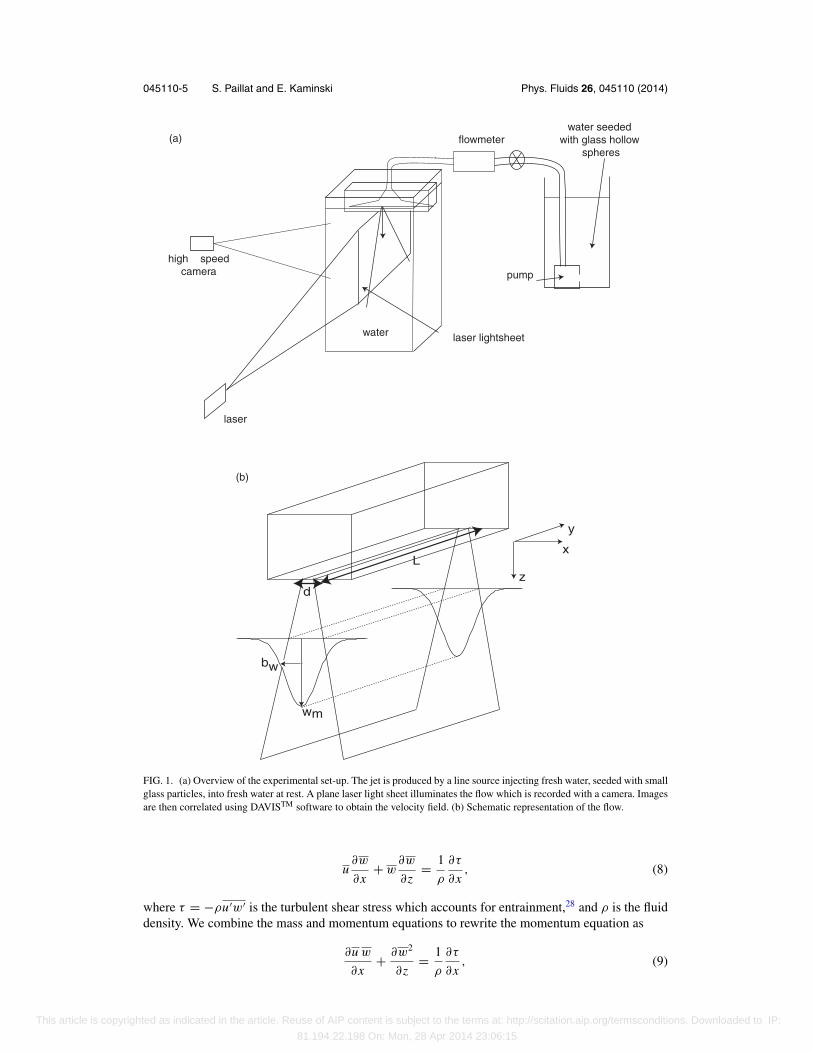
In our experiments, turbulent linear jets are generated by the injection of fresh water througha line source in a 45 × 30 × 30 cm3 glass tank filled with fresh water (Figure 1) through eightsmall pipes to ensure a homogeneous supplying of the slot. To study the flow at large distances fromthe source, we use a slot width d of 0.2 mm (with an aspect ratio of 925) allowing measurementswithin a range of dimensionless distances relative to the source, z∗ = z/d, between 200 and 800. Tocharacterize the flow at smaller dimensionless distances from the source, we use slot widths of 1mm (with an aspect ratio of 185) and 0.5 mm (aspect ratio of 370) and performed measurementsin the range 40 < z∗ < 150 (d = 1 mm) and 80 < z∗ < 250 (d = 0.5 mm). The aspect ratio isalways high enough not to influence the measurement of αG.27 In the three cases, we use flow ratesQ between 0.5 and 5 l min−1, which correspond to source Reynolds numbers between 50 and 450.For PIV measurements, the fluid is seeded with glass hollow sphere particles (LaVision 110P8) witha mean diameter of 11.7 μm and a median of 8 μm. Videos of the jets are recorded with a camera ata frame rate of 40 Hz with 2000 frames (it has been checked from longer recording and ensures theconvergence of the measures), and DavisTM software is used to compute the instantaneous velocity inthe flow by standard PIV methods. We use an interrogation window of 16 × 16 pixel with an ellipticweighting 4:1 and an overlap of 50% for the calculations of the correlations. We then calculate boththe Reynolds-averaged velocities and their turbulent fluctuations using MATLABTM programs.

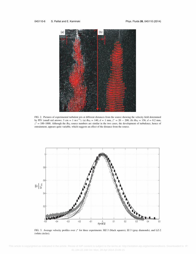
Figure 2 shows pictures of turbulent jets at similar Re0 but for two different slot widths, henceat two different distances from the source. The pictures show two different types of evolution ofturbulence: (a), corresponding to small z∗, shows some meandering, whereas turbulence appearsmore regular in (b). Hence entrainment is likely to be different in the two cases.

This article is copyrighted as indicated in the article. Reuse of AIP content is subject to the terms at: http://scitation.aip.org/termsconditions. Downloaded to IP:

81.194.22.198 On: Mon, 28 Apr 2014 23:06:15

045110-4 S. Paillat and E. Kaminski Phys. Fluids 26, 045110 (2014)

TABLE I. Literature values of the “Gaussian” entrainment coefficient in planar turbulent jets, αG calculated from theevolution of bw with the distance from the source. The uncertainties are given by the standard deviation corresponding to the95% confidence interval. Two different measurement methods were used: Hot-Wire anemometry (HWA), and Laser DopplerAnemometry (LDA). The dimensionless distance from the source is z∗ = z

d , with d the width of the linear source. Re0 is theReynolds number at the source (z∗ = 0).

Method Fluid Re0 z∗ αG Ref.

HWA Air 17 800 5–40 0.029 ± 0.006 18HWA Air 30 000 13.9–68.5 0.033 ± 0.003 19HWA Air 34 000 47–155 0.033 ± 0.003 20LDA Water 1700–1900 20.8–93.8 0.033 ± 0.008 22HWA Air 30 000 65–118 0.033 ± 0.004 21LDA Water 1500 10–60 0.034 ± 0.006 23LDA Water 2635–5197 45–80 0.036 ± 0.005 29HWA/LDA Air 1000 16–95 0.054 ± 0.002 25HWA/LDA Air 2000 16–95 0.037 ± 0.002HWA/LDA Air 6000 16–95 0.030 ± 0.002HWA Air 1500 0–100 0.041 ± 0.002 30HWA Air 3000 0–100 0.038 ± 0.002HWA Air 7000 0–100 0.032 ± 0.002HWA Air 10 000 0–100 0.029 ± 0.002HWA Air 16 500 0–100 0.026 ± 0.002HWA Air 250 20–100 0.072 ± 0.006 26HWA Air 550 20–100 0.064 ± 0.006HWA Air 1100 20–100 0.060 ± 0.006HWA Air 2000 20–100 0.044 ± 0.006HWA Air 4000 20–100 0.032 ± 0.006HWA Air 6250 20–100 0.025 ± 0.006

With the maximum frame rate used in the experiments, we cannot measure the velocity in thenear-source region with a satisfying accuracy. We determine the range of z∗ where the measurementsof velocity is correct by plotting the momentum flux M = bww2

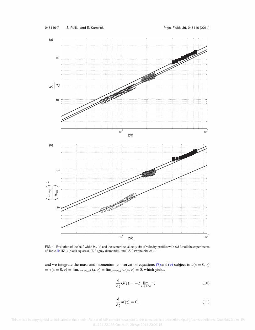
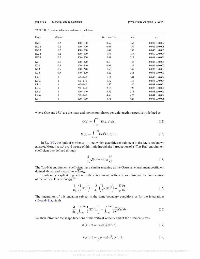
m which should be constant in a purejet against z∗. We then measure bw and wm , the 1/e-width and the centerline velocity of the Gaussianfits (Figure 3) in the range of constant M which are plotted in Figure 4. The entrainment coefficientαG is deduced from these plots and shown in Table II as a function of the source conditions anddistance from source.

Our results are quite variable and do not show any systematic variation of αG as a function ofRe0. Furthermore, the maximal value we found for αG is 0.046, whereas Suresh et al.26 obtained αG

= 0.072 for similar Re0. Our values are more consistent with the ones obtained for Re0 > 1500 inthe literature (αG between 0.029 and 0.045) and tend to be close to the highest values reported inthese studies. To develop a quantitative interpretation of these results, we now follow the approachof Kaminski et al.7 to derive an explicit expression of αG as a function of the velocity and turbulentstress profiles.

III. THEORETICAL MODEL OF ENTRAINMENT IN PLANAR JETS

A. An explicit expression for the Gaussian entrainment coefficient αG

Following Priestley and Ball,28 we introduce u = u + u′ the velocity along the x-direction andw = w + w′ the velocity along the z-direction, with u and w their Reynolds time-averages, and u′

and w′ their turbulent fluctuations. At large Reynolds numbers, the time-averaged local mass andmomentum conservation equations are written as

∂u

∂x+ ∂w

∂z= 0, (7)

This article is copyrighted as indicated in the article. Reuse of AIP content is subject to the terms at: http://scitation.aip.org/termsconditions. Downloaded to IP:

81.194.22.198 On: Mon, 28 Apr 2014 23:06:15

045110-5 S. Paillat and E. Kaminski Phys. Fluids 26, 045110 (2014)

flowmeter

water

water seeded with glass hollow

spheres

high speed camera

laser lightsheet

pump

laser

(a)

(b)

z

x

y

bw

wm

d

L

FIG. 1. (a) Overview of the experimental set-up. The jet is produced by a line source injecting fresh water, seeded with smallglass particles, into fresh water at rest. A plane laser light sheet illuminates the flow which is recorded with a camera. Imagesare then correlated using DAVISTM software to obtain the velocity field. (b) Schematic representation of the flow.

u∂w

∂x+ w

∂w

∂z= 1

ρ

∂τ

∂x, (8)

where τ = −ρu′w′ is the turbulent shear stress which accounts for entrainment,28 and ρ is the fluiddensity. We combine the mass and momentum equations to rewrite the momentum equation as

∂u w

∂x+ ∂w2

∂z= 1

ρ

∂τ

∂x, (9)

This article is copyrighted as indicated in the article. Reuse of AIP content is subject to the terms at: http://scitation.aip.org/termsconditions. Downloaded to IP:

81.194.22.198 On: Mon, 28 Apr 2014 23:06:15

045110-6 S. Paillat and E. Kaminski Phys. Fluids 26, 045110 (2014)

0

zz

2 cm2 cm

FIG. 2. Pictures of experimental turbulent jets at different distances from the source showing the velocity field determinedby PIV (small red arrows: 3 cm = 1 m s−1). (a) Re0 = 140, d = 1 mm, z∗ = 20 − 200; (b) Re0 = 156, d = 0.2 mm,z∗ = 100–1000. Although the Re0 source numbers are similar in the two cases, the development of turbulence, hence ofentrainment, appears quite variable, which suggests an effect of the distance from the source.

−0.5 −0.4 −0.3 −0.2 −0.1 0 0.1 0.2 0.3 0.4 0.50

0.2

0.4

0.6

0.8

1

FIG. 3. Average velocity profiles over z∗ for three experiments: HZ-3 (black squares), IZ-3 (gray diamonds), and LZ-2(white circles).

This article is copyrighted as indicated in the article. Reuse of AIP content is subject to the terms at: http://scitation.aip.org/termsconditions. Downloaded to IP:

81.194.22.198 On: Mon, 28 Apr 2014 23:06:15

045110-7 S. Paillat and E. Kaminski Phys. Fluids 26, 045110 (2014)

102

103

101

102

z/d

102

103

101

102

z/d

(a)

(b)

FIG. 4. Evolution of the half-width bw (a) and the centerline velocity (b) of velocity profiles with z/d for all the experimentsof Table II: HZ-3 (black squares), IZ-3 (gray diamonds), and LZ-2 (white circles).

and we integrate the mass and momentum conservation equations (7) and (9) subject to u(x = 0, z)= τ (x = 0, z) = limx → ∞, zτ (x, z) = limx→∞,z w(x, z) = 0, which yields

d

dzQ(z) = −2 lim

x→+∞ u, (10)

d

dzM(z) = 0, (11)

This article is copyrighted as indicated in the article. Reuse of AIP content is subject to the terms at: http://scitation.aip.org/termsconditions. Downloaded to IP:

81.194.22.198 On: Mon, 28 Apr 2014 23:06:15

045110-8 S. Paillat and E. Kaminski Phys. Fluids 26, 045110 (2014)

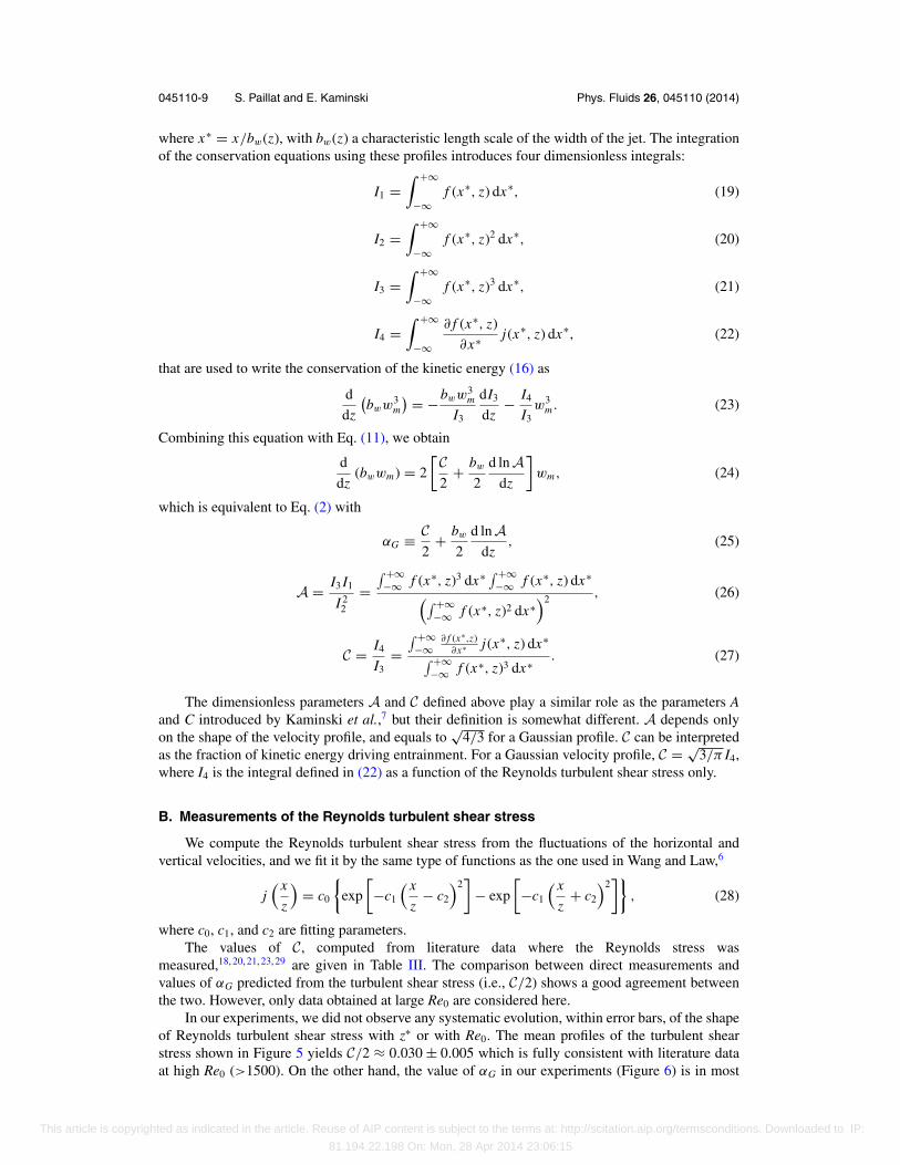
TABLE II. Experimental results and source conditions.

Expt. d (mm) z∗ Q0 (l min−1) Re0 αG

HZ-1 0.2 400−600 0.69 62 0.037 ± 0.002HZ-2 0.2 400−900 0.65 59 0.042 ± 0.008HZ-3 0.2 400−750 1.47 133 0.043 ± 0.005HZ-4 0.2 400−600 1.73 156 0.039 ± 0.004HZ-5 0.2 450−750 2.41 217 0.034 ± 0.001

IZ-1 0.5 100−220 0.5 45 0.045 ± 0.004IZ-2 0.5 170−240 0.97 87 0.037 ± 0.002IZ-3 0.5 180−240 1.65 149 0.032 ± 0.003IZ-4 0.5 140−220 4.22 381 0.031 ± 0.003

LZ-1 1 40−140 1.12 101 0.046 ± 0.004LZ-2 1 60−140 1.52 137 0.036 ± 0.004LZ-3 1 60−140 1.55 140 0.038 ± 0.004LZ-4 1 90−140 2.16 195 0.033 ± 0.004LZ-5 1 100−140 3.52 318 0.038 ± 0.006LZ-6 1 90−140 4.68 422 0.044 ± 0.004LZ-7 1 120−170 4.71 424 0.043 ± 0.005

where Q(z) and M(z) are the mass and momentum fluxes per unit length, respectively, defined as

Q(z) =∫ +∞

−∞w(x, z) dx, (12)

M(z) =∫ +∞

−∞(w)2(x, z) dx . (13)

In Eq. (10), the limit of u when x → +∞, which quantifies entrainment in the jet, is not knowna priori. Morton et al.3 avoid the use of this limit through the introduction of a “Top-Hat” entrainmentcoefficient αTH defined through

d

dzQ(z) = 2αT H

M

Q. (14)

The Top-Hat entrainment coefficient has a similar meaning as the Gaussian entrainment coefficientdefined above, and is equal to

√2παG .

To obtain an explicit expression for the entrainment coefficient, we introduce the conservationof the vertical kinetic energy,28

∂

∂z

(1

2(w)3

)+ ∂

∂x

(1

2u (w)2

)= w

ρ

∂τ

∂x. (15)

The integration of this equation subject to the same boundary conditions as for the integrations(10) and (11), yields

d

dz

[∫ +∞

−∞

1

2(w)3dx

]=

∫ +∞

−∞

∂w

∂xu′w′dx . (16)

We then introduce the shape functions of the vertical velocity and of the turbulent stress,

w(x∗, z) = wm(z) f (x∗, z), (17)

τ (x∗, z) = 1

2ρ wm(z)2 j(x∗, z), (18)

This article is copyrighted as indicated in the article. Reuse of AIP content is subject to the terms at: http://scitation.aip.org/termsconditions. Downloaded to IP:

81.194.22.198 On: Mon, 28 Apr 2014 23:06:15

045110-9 S. Paillat and E. Kaminski Phys. Fluids 26, 045110 (2014)

where x∗ = x/bw(z), with bw(z) a characteristic length scale of the width of the jet. The integrationof the conservation equations using these profiles introduces four dimensionless integrals:

I1 =∫ +∞

−∞f (x∗, z) dx∗, (19)

I2 =∫ +∞

−∞f (x∗, z)2 dx∗, (20)

I3 =∫ +∞

−∞f (x∗, z)3 dx∗, (21)

I4 =∫ +∞

−∞

∂ f (x∗, z)

∂x∗ j(x∗, z) dx∗, (22)

that are used to write the conservation of the kinetic energy (16) as

d

dz

(bww3

m

) = −bww3m

I3

dI3

dz− I4

I3w3

m . (23)

Combining this equation with Eq. (11), we obtain

d

dz(bwwm) = 2

[C2

+ bw

2

d lnAdz

]wm, (24)

which is equivalent to Eq. (2) with

αG ≡ C2

+ bw

2

d lnAdz

, (25)

A = I3 I1

I 22

=∫ +∞−∞ f (x∗, z)3 dx∗ ∫ +∞

−∞ f (x∗, z) dx∗(∫ +∞−∞ f (x∗, z)2 dx∗

)2 , (26)

C = I4

I3=

∫ +∞−∞

∂ f (x∗,z)∂x∗ j(x∗, z) dx∗∫ +∞

−∞ f (x∗, z)3 dx∗ . (27)

The dimensionless parameters A and C defined above play a similar role as the parameters Aand C introduced by Kaminski et al.,7 but their definition is somewhat different. A depends onlyon the shape of the velocity profile, and equals to

√4/3 for a Gaussian profile. C can be interpreted

as the fraction of kinetic energy driving entrainment. For a Gaussian velocity profile, C = √3/π I4,

where I4 is the integral defined in (22) as a function of the Reynolds turbulent shear stress only.

B. Measurements of the Reynolds turbulent shear stress

We compute the Reynolds turbulent shear stress from the fluctuations of the horizontal andvertical velocities, and we fit it by the same type of functions as the one used in Wang and Law,6

j( x

z

)= c0

{exp

[−c1

( x

z− c2

)2]

− exp

[−c1

( x

z+ c2

)2]}

, (28)

where c0, c1, and c2 are fitting parameters.The values of C, computed from literature data where the Reynolds stress was

measured,18, 20, 21, 23, 29 are given in Table III. The comparison between direct measurements andvalues of αG predicted from the turbulent shear stress (i.e., C/2) shows a good agreement betweenthe two. However, only data obtained at large Re0 are considered here.

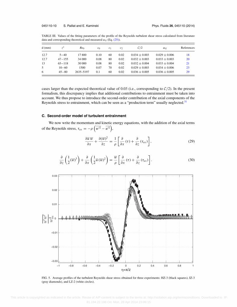
In our experiments, we did not observe any systematic evolution, within error bars, of the shapeof Reynolds turbulent shear stress with z∗ or with Re0. The mean profiles of the turbulent shearstress shown in Figure 5 yields C/2 ≈ 0.030 ± 0.005 which is fully consistent with literature dataat high Re0 (>1500). On the other hand, the value of αG in our experiments (Figure 6) is in most

This article is copyrighted as indicated in the article. Reuse of AIP content is subject to the terms at: http://scitation.aip.org/termsconditions. Downloaded to IP:

81.194.22.198 On: Mon, 28 Apr 2014 23:06:15

045110-10 S. Paillat and E. Kaminski Phys. Fluids 26, 045110 (2014)

TABLE III. Values of the fitting parameters of the profile of the Reynolds turbulent shear stress calculated from literaturedata and corresponding theoretical and measured αG (Eq. (25)).

d (mm) z∗ Re0 c0 c1 c2 C/2 αG References

12.7 5−40 17 800 0.10 60 0.02 0.034 ± 0.003 0.029 ± 0.006 1812.7 47−155 34 000 0.08 80 0.02 0.032 ± 0.003 0.033 ± 0.003 2013 65−118 30 000 0.08 80 0.02 0.032 ± 0.004 0.033 ± 0.004 215 10−60 1500 0.07 70 0.02 0.029 ± 0.003 0.034 ± 0.006 236 45−80 2635–5197 0.1 60 0.02 0.036 ± 0.005 0.036 ± 0.005 29

cases larger than the expected theoretical value of 0.03 (i.e., corresponding to C/2). In the presentformalism, this discrepancy implies that additional contributions to entrainment must be taken intoaccount. We thus propose to introduce the second-order contribution of the axial components of theReynolds stress to entrainment, which can be seen as a “production term” usually neglected.31

C. Second-order model of turbulent entrainment

We now write the momentum and kinetic energy equations, with the addition of the axial terms

of the Reynolds stress, τax = −ρ(w′2 − u′2

),

∂u w

∂x+ ∂(w)2

∂z= 1

ρ

[∂

∂x(τ ) + ∂

∂z(τax )

], (29)

∂

∂z

(1

2(w)3

)+ ∂

∂x

(1

2u (w)2

)= w

ρ

[∂

∂x(τ ) + ∂

∂z(τax )

]. (30)

η=x/z−1 −0.8 −0.6 −0.4 −0.2 0 0.2 0.4 0.6 0.8 1

−0.03

−0.02

−0.01

0

0.01

0.02

0.03

FIG. 5. Average profiles of the turbulent Reynolds shear stress obtained for three experiments: HZ-3 (black squares), IZ-3(gray diamonds), and LZ-2 (white circles).

This article is copyrighted as indicated in the article. Reuse of AIP content is subject to the terms at: http://scitation.aip.org/termsconditions. Downloaded to IP:

81.194.22.198 On: Mon, 28 Apr 2014 23:06:15

045110-11 S. Paillat and E. Kaminski Phys. Fluids 26, 045110 (2014)

0.01 0.02 0.03 0.04 0.05 0.060.01

0.02

0.03

0.04

0.05

0.06

αG

α Gm

odel

FIG. 6. Comparison between model predictions (αGmodel = C2 ) and measured αG at small (white circles), intermediate (gray

diamonds), and large distances from the source (black squares). The thick black line corresponds to model predictions withoutthe second order contribution to entrainment, and the dashed line corresponds to the complete model (Eq. (35)) with theaverage contribution of the axial component of the Reynolds stress, B

2 = 0.013.

The integration of these two equations subject to the same boundary conditions as in Sec. III Ayields

d

dz

(bww2

m

) = bww2m

(I2 + J1)

d(I2 + J1)

dz, (31)

d

dz

(bww3

m

) = −bww3m

I3

dI3

dz− I4

I3w3

m − J2

I3w3

m, (32)

where we have introduced two new integral profiles associated with the axial terms of the Reynoldsstress,

J1 = −1

ρ

1

w2m

∫ +∞

−∞τax dx∗, (33)

J2 = −bw

ρd

1

w3m

∫ +∞

−∞w

∂

∂z∗ (τax ) dx∗. (34)

After some algebra, and combining Eqs. (29) and (30), we obtain a new expression for the massconservation equation, hence for αG,

d

dz(bwwm) = 2 αG wm = 2

[C2

+ bw

2

d lnA∗

dz+ B

2

]wm, (35)

with

A∗ = I3 I1

(I2 + J1)2, (36)

B = J2

I3. (37)

This article is copyrighted as indicated in the article. Reuse of AIP content is subject to the terms at: http://scitation.aip.org/termsconditions. Downloaded to IP:

81.194.22.198 On: Mon, 28 Apr 2014 23:06:15

045110-12 S. Paillat and E. Kaminski Phys. Fluids 26, 045110 (2014)

η=x/z−0.5 −0.4 −0.3 −0.2 −0.1 0 0.1 0.2 0.3 0.4 0.50

0.2

0.4

0.6

0.8

1

1.2x 10

−4

z* = 300

z* = 450

z* = 750

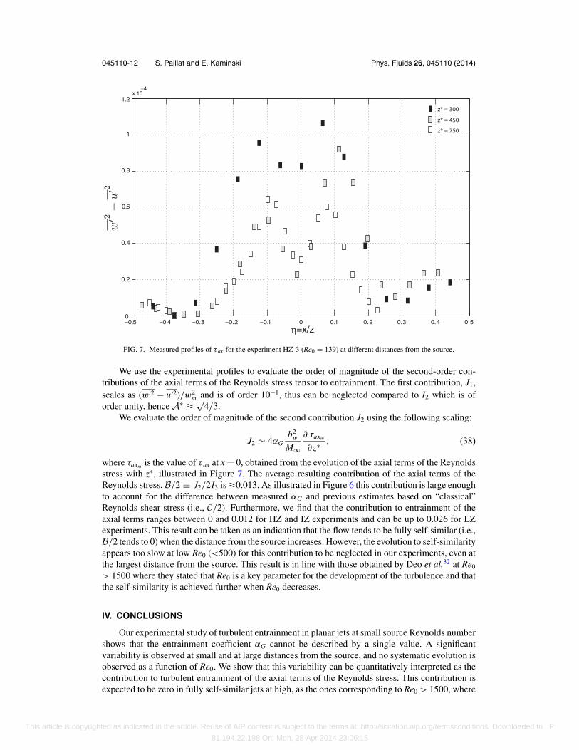
FIG. 7. Measured profiles of τ ax for the experiment HZ-3 (Re0 = 139) at different distances from the source.

We use the experimental profiles to evaluate the order of magnitude of the second-order con-tributions of the axial terms of the Reynolds stress tensor to entrainment. The first contribution, J1,scales as (w′2 − u′2)/w2

m and is of order 10−1, thus can be neglected compared to I2 which is oforder unity, hence A∗ ≈ √

4/3.We evaluate the order of magnitude of the second contribution J2 using the following scaling:

J2 ∼ 4αGb2

w

M∞

∂ τaxm

∂z∗ , (38)

where τaxm is the value of τ ax at x = 0, obtained from the evolution of the axial terms of the Reynoldsstress with z∗, illustrated in Figure 7. The average resulting contribution of the axial terms of theReynolds stress, B/2 ≡ J2/2I3 is ≈0.013. As illustrated in Figure 6 this contribution is large enoughto account for the difference between measured αG and previous estimates based on “classical”Reynolds shear stress (i.e., C/2). Furthermore, we find that the contribution to entrainment of theaxial terms ranges between 0 and 0.012 for HZ and IZ experiments and can be up to 0.026 for LZexperiments. This result can be taken as an indication that the flow tends to be fully self-similar (i.e.,B/2 tends to 0) when the distance from the source increases. However, the evolution to self-similarityappears too slow at low Re0 (<500) for this contribution to be neglected in our experiments, even atthe largest distance from the source. This result is in line with those obtained by Deo et al.32 at Re0

> 1500 where they stated that Re0 is a key parameter for the development of the turbulence and thatthe self-similarity is achieved further when Re0 decreases.

IV. CONCLUSIONS

Our experimental study of turbulent entrainment in planar jets at small source Reynolds numbershows that the entrainment coefficient αG cannot be described by a single value. A significantvariability is observed at small and at large distances from the source, and no systematic evolution isobserved as a function of Re0. We show that this variability can be quantitatively interpreted as thecontribution to turbulent entrainment of the axial terms of the Reynolds stress. This contribution isexpected to be zero in fully self-similar jets at high, as the ones corresponding to Re0 > 1500, where

This article is copyrighted as indicated in the article. Reuse of AIP content is subject to the terms at: http://scitation.aip.org/termsconditions. Downloaded to IP:

81.194.22.198 On: Mon, 28 Apr 2014 23:06:15

045110-13 S. Paillat and E. Kaminski Phys. Fluids 26, 045110 (2014)

the entrainment coefficient can be considered constant with a value αG = C/2 = 0.030 ± 0.005. Atlow Re0 the development of self-similarity is too small for such a regime to be observed, even atlarge distances from the source. The question put forward by George33 about the influence of sourceconditions on the self-similarity of axisymmetric jets seems them to be quite relevant in planarturbulent jets.

ACKNOWLEDGMENTS

The authors thank two anonymous referees for their constructive comments and Prof. John Kimfor his editorial handling of the manuscript. The experimental device was built by Yves Gamblinand Ramon Vazquez-Paseiro at the IPGP workshop. We thank Angela Limare for her constant helpin the experiments.

1 G. Carazzo, E. Kaminski, and S. Tait, “On the dynamics of volcanic columns: A comparison of field data with a new modelof negatively buoyant jets,” J. Volcanol. Geoth. Res. 178(1), 94–103 (2008).

2 A. W. Woods, “Turbulent plumes in nature,” Annu. Rev. Fluid Mech. 42, 391–412 (2010).3 B. R. Morton, G. Taylor, and J. S. Turner, “Turbulent gravitational convection from maintained and instantaneous sources,”

Proc. R. Soc. London, Ser. A 234, 1–23 (1956).4 J. S. Turner, “Turbulent entrainment: The development of the entrainment assumption, and its application to geophysical

flows,” J. Fluid Mech. 173, 431–471 (1986).5 P. N. Papanicolaou and E. J. List, “Investigations of round turbulent buoyant jets,” J. Fluid Mech. 195, 341–391 (1988).6 H. Wang and A. W.-K. Law, “Second-order integral model for a round turbulent buoyant jet,” J. Fluid Mech. 459, 397–428

(2002).7 E. Kaminski, S. Tait, and G. Carazzo, “Turbulent entrainment in jets with arbitrary buoyancy,” J. Fluid Mech. 526, 361–376

(2005).8 G. Carazzo, E. Kaminski, and S. Tait, “The route of self-similarity in turbulent jets and plumes,” J. Fluid Mech. 547,

137–148 (2006).9 G. Carazzo, E. Kaminski, and S. Tait, “On the rise of turbulent plumes: Quantitative effects of variable entrainment

for submarine hydrothermal vents, terrestrial and extra terrestrial explosive volcanism,” J. Geophys. Res. 113, B09201,doi:10.1029/2007JB005458 (2008).

10 G. Carazzo, E. Kaminski, and S. Tait, “The rise and fall of turbulent fountains: a new model for improved quantitativepredictions,” J. Fluid Mech. 657, 265–284 (2010).

11 A. Geyer, J. C. Phillips, and M. Mier-Torrecilla, “Flow behaviour of negatively buoyant jets in immiscible ambient fluid,”Exp. Fluids 52(1), 261–271 (2012).

12 S. S. Cardoso and S. T. McHugh, “Turbulentplumes with heterogeneous chemical reaction on the surface of small buoyantdroplets,” J. Fluid Mech. 642, 49–77 (2010).

13 R. B. Stothers, “Turbulent atmospheric plumes above line sources with an application to volcanic fissure eruption on theterrestrial planets,” J. Atmos. Sci. 46(17), 2662–2670 (1989).

14 A. W. Woods, “A model of the plumes above basaltic fissure eruptions,” Geophys. Res. Lett. 20, 1115–1118,doi:10.1029/93GL01215 (1993).

15 L. S. Glaze, S. M. Baloga, and J. Wimert, “Explosive volcanic eruptions from linear vents on Earth, Venus, and Mars:Comparisons with circular vent eruptions,” J. Geophys. Res. 116, E01011, doi:10.1029/2010JE003577 (2011).

16 J. C. Rowland, M. T. Stacey, and W. E. Dietrich, “Turbulent characteristics of a shallow wall-bounded plane jet: experimentalimplications for river mouth hydrodynamics,” J. Fluid Mech. 627, 423–449 (2009).

17 H. B. Fischer, E. J. List, R. C. Y. Koh, J. Imberger, and N. H. Brooks, “Mixing in inland and coastal waters,” TurbulentJets and Plumes (Academic Press, 1979), pp. 315–389, Chap. 9.

18 D. R. Miller and E. W. Comings, “Static pressure distribution in the free turbulent jet,” J. Fluid Mech. 3(1), 1–16 (1957).19 L. J. S. Bradbury, “The structure of a self-preserving turbulent plane jet,” J. Fluid Mech. 23(1), 31 (1965).20 G. Heskestad, “Hot-wire measurements in a plane turbulent jet,” J. Appl. Mech. 32, 721–734 (1965).21 E. Gutmark and I. Wygnanski, “The planar turbulent jet,” J. Fluid Mech. 73(part 3), 465–495 (1976).22 N. E. Kotsovinos, “A study of the entrainment and turbulence in a plane buoyant jet,” Ph.D. thesis (California Institute of

Technology, 1975).23 B. R. Ramaprian and M. S. Chandrasekhara, “LDA measurements in plane turbulent jets,” J. Fluid. Eng.-Trans. ASME

107, 264–271 (1985).24 N. E. Kotsovinos, “A note on the spreading rate and virtual origin of a plane turbulent jet,” J. Fluid Mech. 77(2), 305–311

(1976).25 I. Namer and M. V. Otungen, “Velocity measurements in a plane turbulent air jet at moderate Reynolds numbers,” Exp.

Fluids 6, 387–399 (1988).26 P. R. Suresh, K. Srinivasan, T. Sundararajan, and S. K. Das, “Reynolds number dependence of plane jet development in

the transitional regime,” Phys. Fluids 20, 044105 (2008).27 R. C. Deo, “Experimental investigations of the influence of Reynolds number and boundary conditions on a plane air jet,”

Ph.D. thesis (School of Mechanical Engineering, The University of Adelaide, 2005).28 C. H. B. Priestley and F. K. Ball, “Continuous convection from an isolated source of heat,” Q. J. R. Meteorol. Soc. 81,

144–157 (1955).

This article is copyrighted as indicated in the article. Reuse of AIP content is subject to the terms at: http://scitation.aip.org/termsconditions. Downloaded to IP:

81.194.22.198 On: Mon, 28 Apr 2014 23:06:15

045110-14 S. Paillat and E. Kaminski Phys. Fluids 26, 045110 (2014)

29 J. Andreopoulos, A. Praturi, and W. Rodi, “Experiments on vertical buoyant jets in shallow water,” J. Fluid Mech. 168,305–336 (1986).

30 R. C. Deo, J. Mi, and G. J. Nathan, “The influence of Reynolds number on a plane jet,” Phys. Fluids 20, 075108 (2008).31 S. B. Pope, Turbulent Flows (Cambridge University Press, 2000).32 R. C. Deo, G. J. Nathan, and J. Mi, “Similarity analysis of the momentum field of a subsonic, plane air jet with varying

jet-exit and local Reynolds similarity analysis of the momentum field of a subsonic, plane air jet with varying jet-exit andlocal Reynolds numbers,” Phys. Fluids 25, 015115 (2013).

33 W. K. George, “The self-preservation of turbulent flows and its relation to initial conditions and coherent structures,”Advances in Turbulence (Springer-Verlag, 1989), pp. 39–72.

This article is copyrighted as indicated in the article. Reuse of AIP content is subject to the terms at: http://scitation.aip.org/termsconditions. Downloaded to IP:

81.194.22.198 On: Mon, 28 Apr 2014 23:06:15