2�1

SECTION 2

TIME SCALES AND TIME DIFFERENCES

Contents

2.1 Introduction .....................................................................................2�3

2.2 Time Scales .......................................................................................2�3

2.2.1 Ephemeris Time (ET) .......................................................2�3

2.2.2 International Atomic Time (TAI) ...................................2�3

2.2.3 Universal Time (UT1 and UT1R)....................................2�4

2.2.4 Coordinated Universal Time (UTC)..............................2�5

2.2.5 GPS or TOPEX Master Time (GPS or TPX)...................2�5

2.2.6 Station Time (ST) ..............................................................2�5

2.3 Time Differences..............................................................................2�6

2.3.1 ET − TAI.............................................................................2�6

2.3.1.1 The Metric Tensor and the Metric...................2�6

2.3.1.2 Solar-System Barycentric Frame ofReference............................................................2�10

2.3.1.2.1 Tracking Station on Earth .................2�13

2.3.1.2.2 Earth Satellite ......................................2�16

2.3.1.2.3 Approximate Expression...................2�17

2.3.1.3 Geocentric Frame of Reference.......................2�18

SECTION 2

2�2

2.3.1.3.1 Tracking Station on Earth .................2�19

2.3.1.3.2 Earth Satellite ......................................2�20

2.3.2 TAI − UTC .........................................................................2�20

2.3.3 TAI − GPS and TAI − TPX ...............................................2�21

2.3.4 TAI − UT1 and TAI − UT1R.............................................2�21

2.3.5 Quadratic Offsets Between Station Time ST andUTC or (GPS or TPX) Master Time................................2�21

2.4 Input Files for Time Differences, Polar Motion, andNutation Angle Corrections..........................................................2�21

2.5 Time Transformation Trees...........................................................2�23

2.5.1 Reception at DSN Tracking Station on Earth...............2�24

2.5.2 Reception at GPS Receiving Station on Earth ..............2�25

2.5.3 Reception at the TOPEX Satellite....................................2�26

2.5.4 Transmission at DSN Tracking Station on Earth.........2�27

2.5.5 Transmission at a GPS Satellite.......................................2�27

Figures

2�1 Time Transformations at a Tracking Station on Earth ..............2�25

2�2 Time Transformations at an Earth Satellite.................................2�26

TIME SCALES

2�3

2.1 INTRODUCTION

This section is presented first because time is discussed in all of the othersections of this report. The various time scales used in programs PV and Regresof the ODP are described in Section 2.2. A time difference is the differencebetween values of an epoch recorded in two different time scales. Section 2.3describes the time differences and gives the equations used for calculating them.Some of the time differences are obtained by interpolation of input files, whichare described in Section 2.4. Section 2.5 presents time transformation trees. Thesefigures indicate how to transform an epoch in one time scale to thecorresponding epoch in any other time scale by adding and/or subtracting theintervening time differences. Time transformation trees are given for receptionor transmission at a tracking station on Earth and at an Earth satellite.

Time in any time scale is represented as seconds past January 1, 2000, 12h

in that time scale. This epoch is J2000.0, which is the start of the Julian year 2000.The Julian Date for this epoch is JD 245,1545.0.

2.2 TIME SCALES

2.2.1 EPHEMERIS TIME (ET)

Ephemeris time (ET) means coordinate time, which is the time coordinateof general relativity. It is either coordinate time of the Solar-System barycentricspace-time frame of reference or coordinate time of the local geocentric space-time frame of reference, depending upon which reference frame the ODP userhas selected. It is the independent variable for the motion of celestial bodies,spacecraft, and light rays. The scale of ET in each of these two reference frames isdefined below in Section 2.3.1.

2.2.2 INTERNATIONAL ATOMIC TIME (TAI)

International Atomic Time (TAI) is based upon the SI second(International System of Units). From p. 40�41 of the Explanatory Supplement to

SECTION 2

2�4

the Astronomical Almanac (1992), it is defined to be the duration of 9,192,631,770periods of the radiation corresponding to the transition between two hyperfinelevels of the ground state of the cesium-133 atom. It is further stated that thisdefinition applies on the geoid (mean sea level). TAI is obtained from aworldwide system of synchronized atomic clocks. It is calculated as a weightedaverage of times obtained from the individual clocks, and corrections are appliedfor known effects.

Time obtained from a clock on board an Earth satellite will be referencedto satellite International Atomic Time. Satellite TAI is an imaginary time scaleobtained from an ideal atomic clock on the satellite. It agrees on average withTAI obtained from atomic clocks on Earth.

2.2.3 UNIVERSAL TIME (UT1 AND UT1R)

Universal Time (UT) is the measure of time that is the basis for all civiltime-keeping. It is an observed time scale, and the specific version used in theODP is UT1. It is used to calculate mean sidereal time, which is the Greenwichhour angle of the mean equinox of date, measured in the true equator of date.Adding the equation of the equinoxes gives true sidereal time, which is used tocalculate the position of the tracking station relative to the true equator andequinox of date. The equation for calculating mean sidereal time from observedUT1 is given in Section 5.3.6. From p. 51 of the Explanatory Supplement to the

Astronomical Almanac (1992), the rate of UT1 is chosen so that a day of 86400 s ofUT1 is close to the duration of the mean solar day. The phase of UT1 is chosen sothat the Sun crosses the Greenwich meridian at approximately 12h UT1.

Observed UT1 contains 41 short-period terms with periods between 5 and35 days which are caused by long-period solid Earth tides. The algorithm forcalculating the sum ∆UT1 of the 41 short-period terms of UT1 is given in Section5.3.3. If ∆UT1 is subtracted from UT1, the result is called UT1R (where R meansregularized). If UT1R is input to the ODP, the sum ∆UT1 must be calculated andadded to UT1R to produce UT1, which is used to calculate mean sidereal time.

TIME SCALES

2�5

2.2.4 COORDINATED UNIVERSAL TIME (UTC)

Coordinated Universal Time (UTC) is standard time for 0° longitude. SinceJanuary 1, 1972, UTC uses the SI second and has been behind InternationalAtomic Time TAI by an integer number of seconds. UTC is maintained within0.90 s of observed UT1 by adding a positive or negative leap second to UTC. Aleap second is usually positive, which has the effect of retarding UTC by onesecond; it is usually added at the end of June or December. After a positive leapsecond was added at the end of December, 1998, TAI − UTC increased from 31 sto 32 s; at the beginning of 1972, it was 10 s. The history of TAI − UTC is given inInternational Earth Rotation Service (1998), Table II-3, p. II-7.

2.2.5 GPS OR TOPEX MASTER TIME (GPS OR TPX)

GPS master time (GPS) is an atomic time scale, which is used instead ofUTC as a reference time scale for GPS receiving stations on Earth and for GPSsatellites. Similarly, TOPEX master time (TPX) is an atomic time scale used as areference time scale on the TOPEX satellite. GPS time and TPX time are each aninteger number of seconds behind TAI or satellite TAI. As opposed to UTC, theseatomic time scales do not contain leap seconds. Therefore, the constant offsetsfrom TAI or satellite TAI do not change.

2.2.6 STATION TIME (ST)

Station time (ST) is atomic time at a Deep Space Network (DSN) trackingstation on Earth, a GPS receiving station on Earth, a GPS satellite, or the TOPEXsatellite. These atomic time scales depart by small amounts from thecorresponding reference time scales. The reference time scale for a DSN trackingstation on Earth is UTC. For a GPS receiving station on Earth or a GPS satellite,the reference time scale is GPS master time (GPS). For the TOPEX satellite, thereference time scale is TOPEX master time (TPX). Note, the TPX and GPS timescales can be used for any Earth-orbiting spacecraft.

SECTION 2

2�6

2.3 TIME DIFFERENCES

2.3.1 ET − TAI

2.3.1.1 The Metric Tensor and the Metric

This section gives the equations for the n-body metric tensor and thecorresponding expression for the interval ds. All of the relativistic equations inprograms PV and Regres of the ODP can be derived from these equations orfrom simplifications of them. The components of the Parameterized Post�Newtonian (PPN) n-body point-mass metric tensor, which contains the PPNparameters β and γ of Will and Nordtvedt (1972), are given by the followingequations, where the subscripts 1 through 4 refer to the four space-timecoordinates. Subscripts 1, 2, and 3 refer to position coordinates, and 4 refers tocoordinate time t multiplied by the speed of light c.

g g gc r

j

i jj i11 22 33 21

2= = = − +

≠∑γ µ

(2�1)

g p q p qpq = = ≠0 1 2 3( , , , ; ) (2�2)

g gc

x

rj j

i jj i14 41 3

2 2= = +

≠∑γ µ ú

(2�3)

g gc

y

rj j

i jj i24 42 3

2 2= = +

≠∑γ µ ú

(2�4)

g gc

z

rj j

i jj i34 43 3

2 2= = +

≠∑γ µ ú

(2�5)

TIME SCALES

2�7

gc r c r c

s

r

c r r c

r

t

j

i jj i

j

i jj i

j j

i jj i

j

i jj i

k

jkk jj

i j

j i

44 2 4

2

4

2

4 4

2

2

12 2 1 2

2 2 1 1

= − +

− +

+ − −

≠ ≠ ≠

≠ ≠ ≠

∑ ∑ ∑

∑ ∑ ∑

µ β µ γ µ

β µ µµ

∂

∂

ú

( )(2�6)

where the indices j and k refer to the n bodies and k includes body i, whosemotion is desired. Also,

µ j = gravitational constant for body j.= Gmj, where G is the universal gravitational constant and

mj is the rest mass of body j.c = speed of light.

Let the position, velocity, and acceleration vectors of body j, with rectangularcomponents referred to a non-rotating frame of reference whose origin islocated at the barycenter of the system of n bodies, be denoted by :

r r rj

j

j

j

j

j

j

j

j

j

j

j

x

y

z

x

y

z

x

y

z

=

=

=

; úúúú

; úúúúúúúú

(2�7)

where the dots denote differentiation with respect to coordinate time t. Then, ri j

and ús j

2 can be obtained from:

ri j j i j i2 = − ⋅ −( ) ( )r r r r (2�8)

ú ú ús j j j

2 = ⋅r r (2�9)

From Eq. (2�8), the first and second partial derivatives of ri j with respect tocoordinate time t (obtained by holding the rectangular components of theposition vector of body i fixed) are given by:

SECTION 2

2�8

∂

∂

r

t ri j j i j

i j=

−( ) ⋅r r rú(2�10)

∂

∂

2

2

22

3

r

t r

s

r r

i j j i j

i j

j

i j

j i j

i j

=−( ) ⋅

+ −−( ) ⋅[ ]r r r r r rúú ú ú

(2�11)

Since this equation is used to evaluate the last term of Eq. (2�6) which is of order

14c , and higher order terms are ignored, the acceleration of body j can be

evaluated from Newtonian theory:

úúrr r

jk k j

jkk jr

=−( )

≠∑

µ3 (2�12)

where k includes body i whose motion is desired.

The invariant interval ds between two events with differences in theirspace and time coordinates of dx1, dx2, dx3, and dx4 is given by

ds g dx dxpqp q2 = (2�13)

where the repeated indices are summed over the integers 1 through 4 and gpq isthe n-body metric tensor given by Eqs. (2�1) to (2�6) and related equations. Thefour space-time coordinates are the three position coordinates of point i (wherethe interval ds is recorded) and the speed of light c multiplied by coordinatetime t:

x x

x y

x z

x ct

i

i

i

1

2

3

4

====

(2�14)

TIME SCALES

2�9

Substituting the components of the metric tensor and the differentials of (2�14)into (2�13) gives

ds g c dt g dx dy dz

g dx cdt g dy cdt g dz cdt

i i i

i i i

244

2 211

2 2 2

14 24 342 2 2

= + + +( )+ + +

(2�15)

All of the terms of this equation are required in order to calculate the n-bodypoint-mass relativistic perturbative acceleration in the Solar-System barycentricframe of reference (Section 4.4.1). However, all other relativistic terms inprograms PV and Regres of the ODP can be derived from Eq. (2�15), where eachcomponent of the metric tensor contains terms to order 1

2c only. Substitutingterms to order 1

2c from Eqs. (2�1) to (2�6) into Eq. (2�15) and scaling the fourspace-time coordinates by the constant scale factor l gives

ds l

U

cc dt

U

cdx dy dz2 2

22 2

22 2 21

21

2= −

− +

+ +( )

γ(2�16)

where the subscript i has been deleted from the position components of point i,and U > 0 is the gravitational potential at point i which is given by

Ur

j

i jj i

=≠∑µ

(2�17)

where the summation includes the bodies of the Solar System in the Solar-System barycentric frame of reference. In the local geocentric frame of reference,U is the gravitational potential due to the Earth only. The scale factor l, whosevalue is very close to unity, will be represented by

l L= +1 (2�18)

The scale factor l does not affect the equations of motion for bodies or light.However, it does affect the rate of an atomic clock, which records the interval ds

divided by the speed of light c. The definitions for L which apply for the Solar-

SECTION 2

2�10

System barycentric frame of reference and for the local geocentric frame ofreference are defined below in Sections 2.3.1.2 and 2.3.1.3. Numerical values for Lin these two frames of reference are not required in this section in order toobtain the various expressions for ET − TAI. However, they are required inSection 4.3 to transform the geocentric space-fixed position vector of the trackingstation from the local geocentric frame of reference to the Solar-Systembarycentric frame of reference. They are also used in that section to transformthe gravitational constant of the Earth from its value in the Solar-Systembarycentric frame of reference to its value in the local geocentric frame ofreference.

An approximate solution to Einstein�s field equations for the case of amassless particle moving in the gravitational field of n massive bodies was firstobtained by Droste (1916). de Sitter (1915�1916 and 1916�1917) extended thework of Droste to account for the mass of the body whose motion is desired.However, he made a theoretical error in the calculation of one of his terms,which was corrected by Eddington and Clark (1938). The Droste/deSitter/Eddington and Clark metric tensor is the same as Eqs. (2�1) to (2�6) andEq. (2�11), if the PPN parameters β and γ are set to their general relativisticvalues of unity. The PPN metric of Will and Nordtvedt (1972) has a differentform. However, Shahid-Saless and Ashby (1988) used a gauge transformation totransform the PPN metric to the Eddington and Clark metric. The resultingmetric tensor given by Eqs. (11) to (13) of Shahid-Saless and Ashby (1988), withthe PPN parameters ζ1 and ζ2 set to their general relativistic values of zero, isequal to (the negative of) the metric tensor given by Eqs. (2�1) to (2�6) and(2�11) above. The corresponding n-body Lagrangian was first derived byEstabrook (1971). The n-body point-mass relativistic perturbative accelerationgiven in Section 4.4.1 can be derived from the n-body metric tensor or thecorresponding Lagrangian.

2.3.1.2 Solar-System Barycentric Frame of Reference

This section presents two expressions for coordinate time ET in the Solar-System barycentric frame of reference minus International Atomic Time TAI. In

TIME SCALES

2�11

the expression given in Subsection 2.3.1.2.1, TAI is obtained from a fixed atomicclock at a tracking station on Earth. In the expression given in Subsection2.3.1.2.2, TAI is obtained from an atomic clock on an Earth satellite. As statedabove in Section 2.2.2, satellite TAI agrees on average with TAI obtained fromfixed atomic clocks on Earth. An approximation for either of these twoexpressions for ET − TAI is given in Subsection 2.3.1.2.3.

In both expressions for ET − TAI, coordinate time ET and InternationalAtomic Time TAI run on average at the same rate. Both of these expressionscontain the same constant offset in seconds plus periodic terms. The specificcoordinate time (ET) used in the ODP is referred to as Barycentric DynamicalTime (TDB) on p. 42 of the Explanatory Supplement (1992). From p. 41 of thisreference, TDB shall differ from TAI + 32.184 seconds (exactly) by periodic termsonly. Hence, the constant offset appearing in the expressions for ET − TAI will be32.184 s. The Explanatory Supplement (1992) also refers (on p. 46) to BarycentricCoordinate Time (TCB) which differs from TDB in rate. This alternate form ofcoordinate time (TCB) is not used in the ODP.

The differential equation relating coordinate time ET in the Solar-Systembarycentric frame of reference and International Atomic Time TAI at a trackingstation on Earth or on an Earth satellite can be obtained from Eq. (2−16). Sincethe differential equation and the resulting expression for ET − TAI will containterms to order 1

2c only, the second factor containing the gravitational potentialU can be deleted. The resulting expression for the interval ds (which is called themetric) is the Newtonian approximation to the n-body metric.

An interval of proper time dτ recorded on an atomic clock is related to theinterval ds along its world line by

d

dsc

τ = (2�19)

Proper time τ will refer specifically to International Atomic Time TAI. InEq. (2�16), t will refer specifically to coordinate time (ET) in the Solar-Systembarycentric frame of reference. In Eq. (2�18), it will be seen that the constant L is

SECTION 2

2�12

of order 12c . Substituting Eqs. (2�19) and (2�18) into (2�16), expanding and

retaining terms to order 12c gives the differential equation relating TAI and ET:

ddt

U

c

v

cL

τ = − − +1122

2

2 (2�20)

where U is the gravitational potential (2�17) at the tracking station on Earth or atthe Earth satellite, and v is the Solar-System barycentric velocity of the trackingstation on Earth or the Earth satellite, given by

v

dxdt

dydt

dzdt

22 2 2

=

+

+

(2�21)

From Eq. (2�20), TAI will run on average at the same rate as ET if the constant Lhas the value

L

cU v= ⟨ + ⟩1 1

222 (2�22)

where the brackets ⟨ ⟩ denote the long-term time average value of the quantitycontained within them. From (2�20) and (2�22), it can be seen that the desiredexpression for ET − TAI at a tracking station on Earth or at an Earth satellite canbe obtained by integrating periodic variations in the gravitational potential U atthis point and periodic variations in the square of the Solar-System barycentricvelocity of this point.

The value of the constant L, which applies in the Solar-System barycentricframe of reference, is obtained in Section 4.3.1.2 by evaluating Eq. (2�22) at meansea level on Earth. If L were evaluated at the location of an Earth satellite, adifferent value would be obtained. This offset value of L is used in Eq. (2�20) inorder to force satellite TAI to run on average at the same rate as coordinate timeET in the Solar-System barycentric frame of reference. Any departure in the rateof atomic time on the Earth satellite from the rate of satellite TAI can beabsorbed into the quadratic time offset described below in Section 2.3.5.

TIME SCALES

2�13

2.3.1.2.1 Tracking Station on Earth

Eq. (2�20) was evaluated in Moyer (1981) for proper time τ equal toInternational Atomic Time TAI obtained from an atomic clock located at a fixedtracking station on Earth. This equation was integrated to give an expression forcoordinate time ET in the Solar-System barycentric frame of reference minus TAIobtained at a fixed tracking station on Earth. The derivation was simplified byusing a first-order expansion of the gravitational potential and integration byparts. This technique was first applied to this problem by Thomas (1975). Moyer(1981) gives two different expressions for calculating ET − TAI at a trackingstation on Earth. Eq. (46) of Part 1 is the �vector form� of the expression. It is afunction of position and velocity vectors of various celestial bodies of the SolarSystem and the geocentric space-fixed position vector of the tracking station onEarth. This equation was converted to a function of time given by Eq. (38) ofPart 2 and related equations. The ODP previously calculated ET − TAI as afunction of time. However, it currently calculates ET − TAI from the vector formof the equation. The vector form is more accurate and easier to calculate.Furthermore, it was easier to modify the derivation of the vector form so thatthe resulting expression for ET − TAI applied for TAI obtained at an Earthsatellite. However, evaluation of ET − TAI from the vector form of the equationsometimes requires the use of an iterative procedure because the requiredvectors are not always available until after the time difference is calculated.

Appendix A of Moyer (1981) describes the calculation of the computedvalues of two-way (same transmitting and receiving station) and three-way(different transmitting and receiving stations) range and doppler observablesand shows how the ET − TAI time differences are used in these calculations. Italso gives equations for the direct and indirect effects of various types of termsof ET − TAI on the computed values of these observables. The indirect effects aredue to the effects of ET − TAI on the reception time at the receiving station, thereflection time at the spacecraft, and the transmission time at the transmittingstation. Changes in these epochs have an indirect effect on the computedobservables. Appendix B of Moyer (1981) develops criteria for the retained termsof ET − TAI. The accuracy of two-way range observables of the DSN is currently

SECTION 2

2�14

about 1�2 m in the one-way range ρ from the tracking station to the spacecraft.It was desired to limit the direct effect of neglected terms of ET − TAI on ρ to anRSS error of 1�2 m at a range ρ of 10 Astronomical Units (AU). The RSS directerror in computed two-way range observables due to neglected terms of ET −TAI, expressed as the equivalent change in the one-way range ρ, is 0.13 m perAU or 1.3 m at 10 AU. The accuracy of two-way doppler observables of the DSNis about 0.4 x 10�5 m/s in the one-way range rate úρ under the very best ofconditions. The RSS direct error in computed two-way doppler observables dueto neglected terms of ET − TAI, expressed as the equivalent change in úρ , is 0.4 x10�6 m/s per AU or 0.4 x 10�5 m/s at 10 AU. The RSS value of neglected terms ofET − TAI is about 4.2 µs. For a range rate of 30 km/s, this produces an indirecterror in ρ of 0.13 m. For a spacecraft in heliocentric cruise, the indirect error in úρis negligible. However, for a spacecraft near Jupiter where the acceleration canbe about 25 m/s2, the indirect error in úρ can be up to 10�4 m/s. For a Jupiterflyby, estimation of the spacecraft state vector relative to Jupiter will eliminate aconstant error in ET − TAI, and consequently, the indirect error in úρ will bereduced to less than 10�6 m/s. For a Jupiter orbiter, the indirect error can bereduced by estimating the spacecraft state and a time-varying clock offset at thetracking station.

The vector form of the expression for coordinate time ET in the Solar-System barycentric frame of reference minus International Atomic Time TAIobtained from an atomic clock at a tracking station on Earth is Eq. (46) of Part 1of Moyer (1981):

ET TAI s BS

BS

BC

EB

EC

AE

J

S JJS

JS Sa

S SaSaS

SaS

SC

BS

− = + ⋅( ) + ⋅( ) + ⋅( )+

+( ) ⋅( ) ++( )

⋅( )

+ ⋅( )

32 1842 1 1

1

2 2 2

2 2

2

. ú ú ú

ú ú

ú

c c c

c c

c

r r r r r r

r r r r

r r

µ

µ µµ

µ µ(2�23)

where

TIME SCALES

2�15

r rij

ijand ú = space-fixed position and velocity vectors of point i

relative to point j, km and km/s. They are a function ofcoordinate time ET, and the time derivative is withrespect to ET.

Superscript or subscript C = Solar-System barycenter, S = Sun, B = Earth-Moon barycenter, E = Earth, M = Moon, J = Jupiter,Sa = Saturn, and A = location of atomic clock on Earthwhich reads TAI.

µ µ µS J Sa, , = gravitational constants of the Sun, Jupiter, and Saturn,km3/s2.

c = speed of light, km/s.

All of the vectors in Eq. (2�23) except the geocentric space-fixed positionvector of the tracking station on Earth can be interpolated from the planetaryephemeris or computed from these quantities as described in Section 3.Calculation of the geocentric space-fixed position vector of the tracking station isdescribed in Section 5. Section 7 gives algorithms for computing ET − TAI at thereception time or transmission time at a tracking station on Earth or an Earthsatellite.

Eq. (2�23) for ET − TAI contains the clock synchronization term (listedbelow in the next paragraph) which depends upon the location of the atomicclock which reads International Atomic Time TAI and five location-independentperiodic terms. The sum of the location-independent terms can also be obtainedby numerical integration as described in Fukushima (1995). There are severalalternate expressions for ET − TAI which have greater accuracies than Eq. (2�23)and more than 100 additional periodic terms. Fairhead and Bretagnon (1990) givean expression containing 127 terms with a quoted accuracy of 100 ns. They alsohave an expression containing 750 terms with an accuracy of 1 ns. Hirayama et al.(1987) present an expression containing 131 periodic terms with a quotedaccuracy of 5 ns. Fukushima (1995) developed an extended version of thisexpression containing 1637 terms. These expressions were fit to the numericallyintegrated periodic terms of Fukushima (1995) for the JPL planetary ephemeris

SECTION 2

2�16

DE245 (obtained from E. M. Standish1). In fitting the more accurate expression ofFairhead and Bretagnon (1990) to the numerical terms, some analytical termswere deleted, and the coefficients of an empirical correction term wereestimated. The numerical minus analytical residuals for this modified expression(containing 515 terms) were less than 3 ns. For the other four unmodifiedexpressions, the residuals varied from �131 ns to +64 ns.

2.3.1.2.2 Earth Satellite

The derivation of Eq. (2�23) is given in Moyer (1981). This derivation hasbeen modified so that it applies for coordinate time ET in the Solar-Systembarycentric frame of reference minus satellite International Atomic Time TAIobtained from an atomic clock on an Earth satellite. The resulting expression forET − TAISAT, where the subscript indicates that TAI is satellite TAI, is Eq. (2�23)with one term changed plus one new periodic term. The term of (2�23), which ischanged, is the third periodic term on the right hand side:

12cúr rE

CAE⋅( )

In this term, the point A no longer refers to the location of the tracking stationon Earth. For this application, it refers to the position of the Earth satellite. Thenew periodic term is PSAT:

P

cSAT SAT

ESATE= ⋅( )2

2úr r (2�24)

where r rSATE

SATE and ú are the geocentric space-fixed position and velocity vectors

of the Earth satellite interpolated from the satellite ephemeris as a function ofcoordinate time ET of the Solar-System barycentric frame of reference. Applyingthese two changes to Eq. (2�23) gives the desired expression for coordinate timeET in the Solar-System barycentric frame of reference minus satellite TAIobtained from an atomic clock on an Earth satellite:

1 Unofficial interim version, never released.

TIME SCALES

2�17

ET TAI ET TAISAT A SAT SAT− = −[ ] += P (2�25)

where the first term on the right hand side means Eq. (2�23) evaluated with rAE

equal to the geocentric space-fixed position vector of the Earth satellite, r SATE ,

and PSAT is given by Eq. (2�24). Interpolation of the planetary ephemeris and thesatellite ephemeris at the ET value of the epoch will give all of the vectorsrequired to evaluate Eq. (2�25).

2.3.1.2.3 Approximate Expression

A number of algorithms require an approximate expression forcoordinate time ET in the Solar-System barycentric frame of reference minusInternational Atomic Time TAI at a tracking station on Earth or an Earth satellite.The approximate expression consists of the first two terms on the right hand sideof Eq. (2�23) converted to a function of time. The second of these two terms isthe 1.6 ms annual term. The remaining periodic terms of (2�23) have amplitudesof 21 µs or less. The second term on the right hand side of Eqs. (37) and (38) ofPart 2 of Moyer (1981) is the 1.6 ms annual term with an analytical expressionand a numerical value for the amplitude, respectively. The amplitude of this termis proportional to the eccentricity e of the heliocentric orbit of the Earth-Moonbarycenter, which is given by the quadratic on p. 98 of the Explanatory

Supplement (1961). Changing the value of e from its J1975 value of 0.01672 to itsJ2000 value of 0.01671 changes the amplitude of the 1.6 ms term from 1.658 ms to1.657 ms. Hence, the approximate expression for ET − TAI in seconds at atracking station on Earth or an Earth satellite in the Solar-System barycentricframe of reference is given by

ET TAI− = + × −32 184 1 657 10 3. . sinE (2�26)

where the eccentric anomaly of the heliocentric orbit of the Earth-Moonbarycenter is given approximately by Eq. (40) of Part 2 of Moyer (1981):

E M M= + 0 01671. sin (2�27)

SECTION 2

2�18

The mean anomaly M of the heliocentric orbit of the Earth-Moon barycenter isgiven by (in radians):

M t= + × −6 239 996 1 990 968 71 10 7. , . , , (2�28)

where t is ET or TAI in seconds past J2000.0. This linear expression is tangent tothe cubic given on p. 98 of the Explanatory Supplement (1961) at J2000.

2.3.1.3 Geocentric Frame of Reference

The expression for the interval ds in the local geocentric frame ofreference is Eq. (2�16) with the gravitational potential U replaced by the term of(2�17) due to the Earth. This is the one-body metric of Schwarzschild expressedin isotropic coordinates and containing all terms in the metric tensor to order

12c .

This section presents two expressions for coordinate time ET in the localgeocentric frame of reference minus International Atomic Time TAI. In theexpression given in Subsection 2.3.1.3.1, TAI is obtained from a fixed atomic clockat a tracking station on Earth. In the expression given in Subsection 2.3.1.3.2, TAIis satellite TAI obtained from an atomic clock on an Earth satellite.

In both expressions for ET − TAI, coordinate time ET in the localgeocentric frame of reference and International Atomic Time TAI or satellite TAIrun on average at the same rate. Both of these expressions contain the sameconstant offset of 32.184 s. The specific coordinate time ET used in theseexpressions is referred to as Terrestrial Dynamical Time (TDT) or TerrestrialTime (TT) on pp. 42 and 47 of the Explanatory Supplement (1992). This referencealso refers (on pp. 46�47) to Geocentric Coordinate Time (TCG), which differsfrom TT in rate. This alternate form of coordinate time (TCG) in the geocentricframe is not used in the ODP.

The differential equation relating International Atomic Time TAI at atracking station on Earth or satellite TAI recorded on an atomic clock on an Earthsatellite (both denoted by τ), and coordinate time ET in the local geocentric frame

TIME SCALES

2�19

of reference (denoted as t) is given by Eq. (2�20), where the constant L (denotedas LGC in the geocentric frame of reference) is given by Eq. (2�22), thegravitational potential U is replaced by the term of (2�17) due to the Earth, and vgiven by (2�21) is the geocentric velocity of the tracking station or the Earthsatellite.

The value of the constant LGC which applies in the local geocentric frameof reference is obtained in Section 4.3 by evaluating Eq. (2�22), as modified in thepreceding paragraph, at mean sea level on Earth. If LGC were evaluated at thelocation of an Earth satellite, a different value would be obtained. This offsetvalue of LGC is used in Eq. (2�20) in order to force satellite TAI to run on averageat the same rate as coordinate time ET in the geocentric frame of reference. Anydeparture in the rate of atomic time on the Earth satellite from the rate ofsatellite TAI can be absorbed into the quadratic time offset described below inSection 2.3.5.

2.3.1.3.1 Tracking Station on Earth

For a fixed atomic clock at a tracking station on Earth, the gravitationalpotential at the clock due to the Earth and the geocentric velocity of the clock arenearly constant, and periodic variations in these quantities will be ignored.Hence, the constant values of U and v in (2�20) cancel the corresponding valuesin (2�22) and (2�20) reduces to

ddtτ = 1 (2�29)

and coordinate time ET in the local geocentric frame of reference minusInternational Atomic Time TAI at a tracking station on Earth is a constant:

ET TAI s− = 32 184. (2�30)

From pp. 42 and 47 of the Explanatory Supplement (1992), Terrestrial DynamicalTime (TDT) or Terrestrial Time (TT), denoted here as coordinate time ET in the

SECTION 2

2�20

local geocentric frame of reference, minus International Atomic Time TAI isequal to 32.184 s.

2.3.1.3.2 Earth Satellite

For satellite International Atomic Time TAI obtained from an atomic clockon an Earth satellite which is moving on a geocentric elliptical orbit, thegravitational potential U at the satellite due to the Earth and the square of thegeocentric velocity v of the satellite in Eq. (2�20) will vary periodically from theiraverage values in (2�22) due to the eccentricity of the elliptical orbit. Using thepoint-mass gravitational potential due to the Earth, Eqs. (2�20) and (2�22) can beintegrated to give the following expression for coordinate time ET in the localgeocentric frame of reference minus satellite TAI:

ET TAI sSAT SAT− = +32 184. P (2�31)

where PSAT is given by Eq. (2�24). The geocentric space-fixed position andvelocity vectors of the Earth satellite in (2�24) are interpolated from the satelliteephemeris at the ET value of the epoch. Note that the form of PSAT, which is dueto the elliptical orbit of the satellite about the Earth, is the same as the firstperiodic term of (2�23), which is due to the elliptical orbit of the Earth-Moonbarycenter about the Sun. In each case, one-half of the term is due to thevariation in the gravitational potential of the central body, and the other half ofthe term is due to the variation in the square of the velocity.

2.3.2 TAI − UTC

From Section 2.2.4, TAI − UTC is an integer number of seconds. Its valueat any given time can be obtained by interpolating either of the input files fortime differences discussed below in Section 2.4 with the UTC value of the epochas the argument.

TIME SCALES

2�21

2.3.3 TAI − GPS AND TAI − TPX

From Section 2.2.5, TAI − GPS and TAI − TPX are constants. The user caninput the values of these constants to the ODP on the General Input Program(GIN) file.

2.3.4 TAI − UT1 AND TAI − UT1R

Universal Time UT1 and its regularized form UT1R were discussed inSection 2.2.3. The value of TAI − UT1 or UT1R can be obtained by interpolatingeither of the input files for time differences as discussed in Section 2.4.

2.3.5 QUADRATIC OFFSETS BETWEEN STATION TIME ST AND UTC

OR (GPS OR TPX) MASTER TIME

Section 2.2.6 discussed station time ST at a DSN tracking station on Earth,a GPS receiving station on Earth, a GPS satellite, and the TOPEX satellite. Each ofthese atomic time scales departs by a small amount from the correspondingreference time scale. The reference time scale is UTC for a DSN tracking stationon Earth, GPS Master Time (GPS) for a GPS receiving station on Earth or a GPSsatellite, and TOPEX Master Time (TPX) for the TOPEX satellite. The timedifferences UTC − ST, GPS − ST at a GPS receiving station on Earth or a GPSsatellite, or TPX − ST are all represented by the following quadratic function oftime:

UTC or GPS or TPX ST( ) − = + −( ) + −( )a b t t c t t0 02 (2�32)

where a, b, and c are quadratic coefficients specified by time block with start timet0 at each station or satellite, and t is the current time. The time scale for t and t0 iseither of the two time scales related by (2�32).

2.4 INPUT FILES FOR TIME DIFFERENCES, POLARMOTION, AND NUTATION ANGLE CORRECTIONS

Some of the time differences used in the ODP are obtained byinterpolation of either of two different input files that the ODP can read. The

SECTION 2

2�22

older of these two files is the so-called STOIC file (named after the programwhich originally created it) which contains the TP (timing and polar motion)array. This array contains the time differences TAI − UTC and TAI − UT1 orUT1R, the X and Y coordinates of the Earth�s true pole of date relative to themean pole of 1903.0 (defined in Section 5.2.5), and the time derivatives of each ofthese four quantities at each time argument, which is specifically UTC. The fixedsize of the TP array limits the timespan of the data to about three years if thedata is spaced a month apart. The newer of these two files is the EarthOrientation Parameter (EOP) file. It contains the four quantities which are in theTP array plus the corrections δψ and δε to the nutations in longitude ∆ψ andobliquity ∆ε, respectively (defined in Section 5.3.5). The nominal values of thetwo nutation angles are obtained from the 1980 IAU (International AstronomicalUnion) Theory of Nutation (Seidelmann, 1982). The EOP file contains the valuesof these six quantities at each time argument, which is UTC. It does not containthe time derivatives of the six quantities. The file is open-ended and the dataspacing is usually about a day.

For each quantity in the TP array, the value and rate at each of twosuccessive time points defines a cubic. The cubic and its time derivative can beevaluated at the interpolation time. The only exception to this is TAI − UTCwhich is constant between two successive time points. Interpolation of eachquantity on the EOP file, except TAI − UTC, requires the value of the quantity ateach of four successive time points. The algorithm and code are due to X XNewhall. The first three points are fit to a quadratic, which is differentiated togive the derivative at the second point. Applying the same procedure to the lastthree points gives the derivative at point three. The values and derivatives atpoints two and three produce a cubic that is valid between these two points. Thecubic and its time derivative can be evaluated at the interpolation time whichmust be between points two and three. Note that interpolation of each of thesetwo files produces a continuous function and its derivative.

Interpolation of the TP array yields TAI − UT1 or UT1R, whichever isinput. If it is the latter, program Regres calculates ∆UT1 (see Section 2.2.3) andsubtracts it from TAI − UT1R to give TAI − UT1. If the EOP file contains

TIME SCALES

2�23

TAI − UT1, the interpolation program converts it internally to TAI − UT1R, whichis the quantity that is always interpolated. The program calculates ∆UT1, which issubtracted from the interpolated quantity to give TAI − UT1, which is always theoutput quantity.

The quantities on the EOP file, Earth-fixed station coordinates (seeSection 5), quasar coordinates (Section 8), and the frame-tie rotation matrix(Section 5) are determined on a real-time basis at the Jet Propulsion Laboratory(JPL) by fitting to Very Long Baseline Interferometry (VLBI) data, Lunar LaserRanging (LLR) data, and data obtained from the International Earth RotationService (IERS). The data in the TP array currently comes from the same solution.Previously, it was obtained from the IERS.

2.5 TIME TRANSFORMATION TREES

This section presents two time transformation trees that show how thereception time in station time ST or the transmission time in coordinate time ETat a fixed tracking station on Earth or an Earth satellite is transformed to all ofthe other time scales. Each time transformation tree shows the route or path thatmust be taken to transform the ST or ET value of the epoch to the correspondingvalues in all of the other time scales. In general, each time transformation tree isnot an algorithm which must be evaluated at a particular place in the code.Instead, each time transformation tree is broken into several parts, which areevaluated in different parts of the code. When the calculation of timetransformations is described in the various sections of this report, thecorresponding parts of the calculations described in the following fivesubsections will be referenced.

In the time transformation trees, ET refers to coordinate time in the Solar-System barycentric frame of reference or to coordinate time in the localgeocentric frame of reference, depending upon which frame of reference hasbeen specified by the ODP user.

The reception time in station time ST is the known data time tag for arange data point. For a doppler data point, it is the time tag for the data point

SECTION 2

2�24

plus or minus one-half of the count interval (see Section 13). For quasar VLBIdata points, the reception time in station time ST at station 1 is the data time tagfor wideband data. For narrowband data, it is the time tag plus or minus one-half of the count interval (see Section 13). The transmission time in coordinatetime ET at a tracking station on Earth or an Earth satellite is obtained from thespacecraft light-time solution. The reception time in coordinate time ET atstation 2 for a quasar VLBI data point is obtained from the quasar light-timesolution.

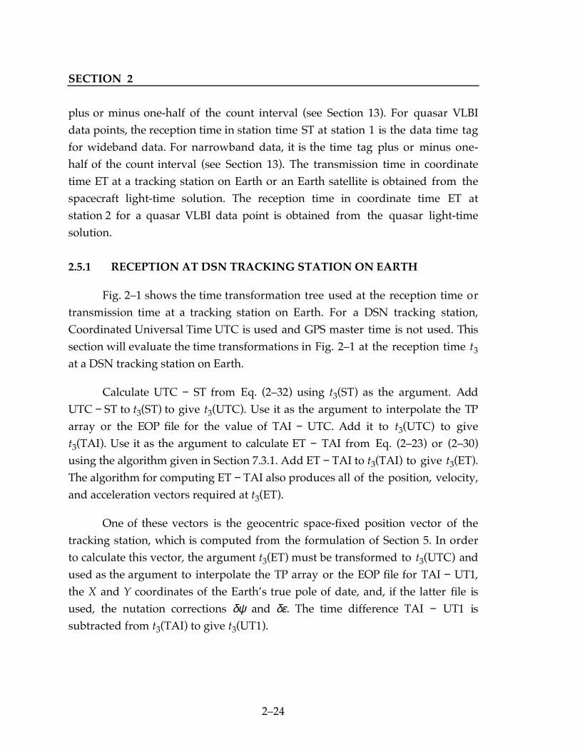
2.5.1 RECEPTION AT DSN TRACKING STATION ON EARTH

Fig. 2�1 shows the time transformation tree used at the reception time ortransmission time at a tracking station on Earth. For a DSN tracking station,Coordinated Universal Time UTC is used and GPS master time is not used. Thissection will evaluate the time transformations in Fig. 2�1 at the reception time t3

at a DSN tracking station on Earth.

Calculate UTC − ST from Eq. (2�32) using t3(ST) as the argument. AddUTC − ST to t3(ST) to give t3(UTC). Use it as the argument to interpolate the TParray or the EOP file for the value of TAI − UTC. Add it to t3(UTC) to givet3(TAI). Use it as the argument to calculate ET − TAI from Eq. (2�23) or (2�30)using the algorithm given in Section 7.3.1. Add ET − TAI to t3(TAI) to give t3(ET).The algorithm for computing ET − TAI also produces all of the position, velocity,and acceleration vectors required at t3(ET).

One of these vectors is the geocentric space-fixed position vector of thetracking station, which is computed from the formulation of Section 5. In orderto calculate this vector, the argument t3(ET) must be transformed to t3(UTC) andused as the argument to interpolate the TP array or the EOP file for TAI − UT1,the X and Y coordinates of the Earth�s true pole of date, and, if the latter file isused, the nutation corrections δψ and δε. The time difference TAI − UT1 issubtracted from t3(TAI) to give t3(UT1).

TIME SCALES

2�25

ET

TAI

UTC or GPS UT1, X, Y, δψ, δε

ST

Figure 2�1 Time Transformations at a Tracking Station on Earth

The transformation of t3(ET) to t3(UTC) is accomplished as follows.Calculate ET − TAI from Eq. (2�23) in the Solar-System barycentric frame ofreference or from (2�30) in the local geocentric frame of reference. In the formercase, the geocentric space-fixed position vector of the tracking station iscomputed as a function of ET from the simplified algorithm given in Section5.3.6.3. Subtract ET − TAI from t3(ET) to give t3(TAI). Use it as the argument tointerpolate the TP array or the EOP file for TAI − UTC, and subtract it fromt3(TAI) to give t3(UTC). Use it as the argument to re-interpolate the TP array orthe EOP file for TAI − UTC and subtract it from t3(TAI) to give the final value oft3(UTC). Near a leap second in UTC, the second value obtained for UTC maydiffer from the first value by exactly one second.

2.5.2 RECEPTION AT GPS RECEIVING STATION ON EARTH

For a GPS receiving station on Earth, ST (see Fig. 2�1) is referred to GPS(GPS master time) and not to UTC. Calculate GPS − ST from Eq. (2�32) usingt3(ST) as the argument. Add GPS − ST to t3(ST) to give t3(GPS). Obtain TAI − GPSfrom the GIN file and add it to t3(GPS) to give t3(TAI). Use it as the argument to

SECTION 2

2�26

calculate ET − TAI from Eq. (2�23) or (2�30) using the algorithm given in Section7.3.1. Add ET − TAI to t3(TAI) to give t3(ET). The algorithm for computingET − TAI also produces all of the position, velocity, and acceleration vectorsrequired at t3(ET). The last two paragraphs of Section 2.5.1 also apply here.

2.5.3 RECEPTION AT THE TOPEX SATELLITE

Fig. 2�2 shows the time transformation tree used at the reception time ortransmission time at an Earth satellite. For the TOPEX satellite, station time ST isreferred to TPX (TOPEX master time). Calculate TPX − ST from Eq. (2�32) usingt3(ST) as the argument. Add TPX − ST to t3(ST) to give t3(TPX). Obtain TAI − TPXfrom the GIN file and add it to t3(TPX) to give t3(TAI). Use it as the argument tocalculate ET − TAI from Eq. (2�25) or (2�31) using the algorithm given in Section7.3.3. Add ET − TAI to t3(TAI) to give t3(ET).

The algorithm for computing ET − TAI also produces all of the position, velocity,and acceleration vectors required at t3(ET).

ET

TAI

GPS or TPX

ST

Figure 2�2 Time Transformations at an Earth Satellite

TIME SCALES

2�27

2.5.4 TRANSMISSION AT DSN TRACKING STATION ON EARTH

The time transformation tree shown in Fig. 2�1 is used at the transmissiontime t1(ET) at a DSN tracking station on Earth. It is also used at the receptiontime t2(ET) at station 2 on Earth for a quasar VLBI data point. This epoch, whichwill be denoted here as t1(ET), and all of the required position, velocity, andacceleration vectors at this epoch are available from the spacecraft light-timesolution (see Section 8.3) or the quasar light-time solution (Section 8.4). Thegeocentric space-fixed position vector of the tracking station is calculated ineither of these two light-time solutions by using the time transformationsdescribed above in the last two paragraphs of Section 2.5.1.

Using t1(ET) as the argument, calculate ET − TAI from Eq. (2�23) or (2�30).In the former equation, all of the required position and velocity vectors areavailable from the light-time solution. Subtract ET − TAI from t1(ET) to givet1(TAI). Using t1(TAI) as the argument, interpolate the TP array or the EOP filefor TAI − UTC and subtract it from t1(TAI) to give t1(UTC). Using it as theargument, re-interpolate the TP array or the EOP file for TAI − UTC and subtractit from t1(TAI) to give the final value of t1(UTC). Use it as the argument tocalculate UTC − ST from Eq. (2�32), and subtract it from t1(UTC) to give t1(ST).

2.5.5 TRANSMISSION AT A GPS SATELLITE

The time transformation tree shown in Fig. 2�2 is used at the transmissiontime t2(ET) at a GPS satellite. This epoch and all of the required position, velocity,and acceleration vectors at this epoch are available from the spacecraft (the GPSsatellite) light-time solution (Section 8.3).

Using t2(ET) as the argument, calculate ET − TAI from Eq. (2�25) or (2�31),where all of the required position and velocity vectors are available from thelight-time solution. Subtract ET − TAI from t2(ET) to give t2(TAI). ObtainTAI − GPS from the GIN file and subtract it from t2(TAI) to give t2(GPS). Use it asthe argument to calculate GPS − ST from Eq. (2�32), and subtract it from t2(GPS)to give t2(ST).