Securitization Networks and Endogenous Financial Norms in U.S.

Mortgage Markets∗

Richard Stanton† Johan Walden‡ Nancy Wallace§

December 8, 2014

PRELIMINARY DRAFT

Abstract

We develop a theoretical model of a network of intermediaries, which we apply to the U.S.mortgage supply chain. In our model, heterogeneous financial norms and systemic vulnerabil-ities arise endogenously. Intuitively, the optimal behavior of each intermediary, in terms of itsattitude toward risk, the quality of the projects that it undertakes, and the intermediaries itchooses to interact with, is influenced by the behavior of its prospective counterparties. Thesenetwork effects, together with intrinsic quality differences between intermediaries, jointly deter-mine financial health and systemic vulnerability at the aggregate level as well as for individualintermediaries. We apply our model to the mortgage-origination and securitization networkof financial intermediaries, using a large data set of more than twelve million mortgages orig-inated and securitized through the private-label supply chain from 2002–2007. We then trackthe ex-post foreclosure performance of each loan in the network and compare the evolutionof credit risk by vintage with the model’s predictions. We find that credit risk evolves in aconcentrated manner among highly linked nodes, defined by the geography of the network andthe interactions between originator and counterparty over time. This confirms that networkeffects are of vital importance for understanding the U.S. mortgage supply chain.

JEL classification: G14.

∗We are grateful for financial support from the Fisher Center for Real Estate and Urban Economics.†Haas School of Business, U.C. Berkeley, stanton@haas.berkeley.edu.‡Haas School of Business, U.C. Berkeley, walden@haas.berkeley.edu.§Haas School of Business, U.C. Berkeley, wallace@haas.berkeley.edu.

1 Introduction

Several recent studies highlight the importance of network linkages between intermediaries

and financial institutions in explaining systemic risk in the financial system (see, for exam-

ple, Allen and Gale, 2000; Allen, Babus, and Carletti, 2012; Cabrales, Gottardi, and Vega-

Redondo, 2014; Glasserman and Young, 2013; Acemoglu, Ozdaglar, and Tahbaz-Salehi, 2013;

Elliott, Golub, and Jackson, 2014). These studies show that financial networks may create

resilience against shocks in a market via diversification and insurance, but also contagion and

systemic vulnerabilities by allowing shocks to propagate and amplify. The network structure

is thus a pivotal determinant of the riskiness of a financial market.

These theoretical studies of networks and risk in financial markets typically focus on how

the network redistributes risk between participants, and on the consequences for the system’s

solvency and liquidity after a shock. This is an ex post effect of the financial network. One

may also expect ex ante effects to be important. Specifically, the presence and structure of a

financial network should affect—and be affected by—the actions of individual intermediaries

and financial institutions, even before shocks are realized. Understanding the equilibrium

interaction between network structure, the actions taken by market participants, and the

market’s riskiness is the focus of our study.

We build upon the approach in Stanton, Walden, and Wallace (2014), who study the

mortgage market from a network perspective, showing that network linkages defined by con-

tractual relationships are an important factor in the U.S. single-family residential-mortgage

market and find that, despite the large total number of firms, the market is highly concen-

trated, with significant inter-firm linkages—even between seemingly independent institutions—

once account is taken of the wholesale lending mechanisms used to fund mortgage origina-

tion.1 They represent the mortgage market as a network of mortgage firms, where links are

represented by loan flows, and show that the performance of an individual node is closely

related to the performance of the node’s neighbors in the network.

We introduce a model with multiple agents representing financial intermediaries, who

are connected in a network. Network structure in our model, in addition to determining the

ex post riskiness of the financial system, also affects—and is affected by—what we call the

financial norms in the network, inspired by the literature on influence and endogenous evolu-

tion of opinions and social norms in networks (see, for example, Friedkin and Johnsen, 1999;

Jackson and Lopez-Pintado, 2013; Lopez-Pintado, 2012). These financial norms represent

the quality and riskiness of the actions agents take.

1The most important of these funding mechanisms are master repurchase agreements, a form of repo,and extendable asset-backed commercial paper programs.

1

Our model is parsimonious, in that the strategic action space of agents as well as the

contract space is quite limited. Links in the network represent risk-sharing agreements, as

in Allen et al. (2012). Agents may add and sever links, in line with the concept of pairwise

stability in games on networks (see Jackson and Wolinsky, 1996), and also have the binary

decision of whether to invest in a costly screening technology that improves the quality of

the projects they undertake.

The equilibrium concept used is subgame-perfect Nash. In an equilibrium network each

agent optimally chooses to accept the network structure, as well as whether to invest in

the screening technology, having correct beliefs about all other agents’ actions and risk.

Shocks are then realized and distributed among market participants according to a clearing

mechanism similar to that introduced in Eisenberg and Noe (2001).

As in Elliott et al. (2014), we assume that there are costs associated with the insolvency

of an intermediary, potentially creating contagion and propagation of shocks through the

clearing mechanism, and thereby making the market systemically vulnerable. The model is

simple enough to allow us to computationally analyze the equilibrium properties of large-

scale networks using approximation methods.

Our model has three general implications. First, network structure influences financial

norms. Given that an agent’s actions influence and are influenced by the actions of those

that the agent interacts with, this result is natural and intuitive. Importantly, an agent’s

actions affect not only others to whom the agent is directly linked but also those who

are indirectly connected through a sequence of links. As a consequence, there is a rich

relationship between equilibrium financial norms and network structure, in turn suggesting

a deeper relationship between the network and the financial health of the market beyond the

mechanical relationship generated by shock propagation.

Second, heterogeneous financial norms may coexist in the network, in equilibrium. Thus,

two intermediaries that are ex ante identical may be very different when their network

position is taken into account, not just in how they are influenced by the rest of the network

but also in their actions. Empirically, this suggests that network structure is an important

determinant not only of the aggregate properties of the economy but also of the actions and

performance of individual intermediaries.

Third, proximity in the network is related to financial norms: nodes that are close tend

to develop similar norms, just like in the literature on social norms in networks. This result

suggests the possibility of decomposing the market’s financial network into “good” and “bad”

parts, and address vulnerabilities generated by the latter.

We analyze the mortgage-origination and securitization network of financial intermedi-

aries, using a large data set of more than twelve million mortgages originated and securitized

2

through the private-label supply chain from 2002–2007. Our approach is to use loan flows to

identify the network structure of this market. We then use ex-post foreclosure rates of these

loans as a measure of performance, and use the model to estimate the evolution of credit risk

by vintage. Our analysis suggests that credit risk evolves in a concentrated manner among

highly linked nodes, defined by the geography of the network and the interactions between

originator and counterparty over time, and more generally that both ex ante and ex post

network effects are of vital importance for understanding the U.S. mortgage supply chain

and its systemic vulnerabilities.

Our supply-chain representation of the private-label mortgage market allows us to high-

light several key characteristics of the organizational structure of this market that impor-

tantly differentiate this paper from prior work. Rather than studying possible relationships

between risk taking and aggregate measures of market concentrations (see Allen and Gale,

2004; Beck, Coyle, Seabright, and Freixas, 2010; Claessens, 2009; Scharfstein and Sunderam,

2013), we focus on the economic and organizational forces that underlie the system of disin-

tegrated exchange that characterizes the supply chain of this industry (see Bresnahan and

Levin, 2012; Jacobides, 2005). We follow Stanton et al. (2014) and represent this system of

disintegrated exchange as a network in which the related activities of origination, funding for

origination, aggregation for securitization, and the sales of the mortgage backed securities

to investors are largely undertaken by independent firms whose actions are coordinated ex-

plicitly through contracts, such as funding commitments, or implicitly through standardized

institutional structures and norms that are difficult to contemporaneously monitor, such as

the underwriting quality choices of originators within the network.

We show in Stanton et al. (2014) that the disintegrated exchange system that charac-

terizes the private-label supply chain considered here shares many characteristics with the

government-sponsored enterprise (GSE) supply chain of the Federal National Mortgage Asso-

ciation (FNMA) and the Federal Home Loan Mortgage Corporation (FHLMC) for residential

prime loans. They share similar data standards for performance reporting and standardized

institutional infrastructure such as the treatment of foreclosures under state laws and the

legal standing of loan sales along the supply chain under U.S. Universal Commercial Code,

Article 9 (see Follain and Zorn, 1990; Jacobides, 2005; Hunt, Stanton, and Wallace, 2014;

Stanton et al., 2014).

There are two important differences, however. First, the GSEs apply ex ante standardized

screening protocols, called LoanProspector (FHLMC) and Desktop Underwriter (FNMA),

to determine which loans meet quality standards for securitization. Secondly, the GSEs

apply long term ex post performance evaluations of originators’ loans to identify poor quality

originators who can be sanctioned either by permanent expulsion from the insured securitized

3

markets or by long-term putback risks. Ex post exercise of putback rights, allowing the

trustees of the loan pools to require that the originator buy back at par any poorly performing

loans within 60 days of origination, are, and were pre-crisis, enforceable through the pooling

and servicing agreements of both GSE and private-label securitized pools. We would indeed

expect such differences to affect the behavior of the individual players in the market, both

ex ante and ex post.

The rest of the paper is organized as follows. Section 2 describes the structure of the U.S.

residential mortgage market and available data. Section 3 introduces the model. Section 4

analyzes the properties of equilibrium, and Section 5 discusses how to estimate equilibrium

from observed data in a large-scale network. Section 6 lays out our approach to identifying

the mortgage-securitization network from loan flows. Section 7 shows some preliminary

results for the 2006 U.S. private-label mortgage market, and Section 8 concludes. The

appendix contains a detailed description of the network game used in the model.

2 Structure of the U.S. residential mortgage market

There is a very small literature that considers the economic factors that lead to disintegrated

exchange systems, in theoretical treatments (see Jacobides, 2005; Chen, 2005; Bresnahan and

Levin, 2012), in empirical studies (see Langlois and Robertson, 1992; Holmes, 1999; Chen,

2005), or even in studies of the sociological and institutional norms, or pre-conditions, needed

to engender disintegrated market structures (see Cooter, 2000; MacKenzie and Millo, 2003;

Fligstein, 2001; Jacobides, 2005). In his famous essay on the nature of the firm, Coase (1937)

describes why and how economic activity divides between firms and markets. He argues that

firms exist to reduce the costs of transacting through markets. Building on Coase’s seminal

ideas, Williamson won a Nobel prize for his development of the transaction cost theory of

integration (see Williamson, 1971, 1975, 1979). A key element of this theory is that market

contracts are inherently incomplete and this limitation of explicit contracts may be especially

severe when complexity or uncertainty make it difficult to specify contractual safeguards, or

when parties cannot walk away without incurring substantial costs. Transaction cost theory

therefore argues that vertical integration can be an effective response when these features

are present. A related rationale for integration is that it might mitigate potential holdups

by suppliers (see Joskow, 2005; Williamson, 2010).

The property rights theories of vertical integration (see Grossman and Hart, 1986; Hart

and Moore, 1990; Hart, 1995) have focused on how integration changes the incentives to

make specific investments and find that ownership strengthens a party’s bargaining position.

Incentive theories (see Holmstrom and Milgrom, 1994; Holmstrom, 1999) have shown that

4

under certain conditions, asset ownership by the agent (e.g., non-integration) can be comple-

mentary to providing high-powered financial incentives. In contrast to the contracting and

transaction cost literatures, theories in organizational economics have focused more directly

on the determination of horizontal market structure, typically based in firm-level costs or

in strategic interaction among firms. Stigler (1951) argued that in the early and innovative

phases of an industry, firms have to be vertically integrated because there are no markets for

the relevant inputs – the costs of organizing those markets, he assumes, are higher than the

costs of coordinating the production of the inputs within the firm. As the industry becomes

larger, what had formerly been internal inputs are supplied by new, vertically disintegrated

industries. In addition to the trade-off between efficient horizontal scale and vertical market

power, Stigler’s theory adds the additional idea that market institutions that are needed to

support disintegrated trade are themselves endogenous and have to be developed over time.

The point made by Stigler (1951) that market institutions need to be invented before a

wide variety of firms can participate in them remains only partially explored in organiza-

tional economics. Jacobides (2005) builds on these ideas based on an extensive case study

of vertical disintegration in the U.S. mortgage banking industry from 1970 through 1998.

He argues that transaction costs theories, decision and incentive theories provide an inad-

equate explanation for how the mortgage banking industry and its value chain structures

evolved. Both Jacobides (2005) and Bresnahan and Levin (2012) argue that transaction costs

depend on existing market institutions — institutions that facilitate search and matching,

and institutions that facilitate contractual and pricing arrangements. As a result, a dis-

integrated market structure, and particularly the creation of a disintegrated industry with

frequent arms-length exchange, often requires the creation of market institutions: standards

for products and contracts, and mechanisms for matching buyers and sellers, determining

prices, and disseminating information (see Jacobides, 2005; Bresnahan and Levin, 2012).

Jacobides (2005) also points out that the creation of market institutions is facilitated by

having a degree of standardization in the underlying products.

According to Jacobides (2005), the disintegration of the highly vertically integrated mort-

gage origination and funding systems that existed prior to 1970 was caused by three institu-

tional changes. First, the federal government introduced standardized securitization systems

through the GSEs and the Government National Mortgage Association (GNMA) and allowed

non-depository mortgage banks to issue and service loans under GSE criteria. To fund loans

temporarily before sales to the GSE securitizers, mortgage banks would use lines of credit ob-

tained from commercial banks (see Fabozzi and Modigliani, 1992). The second major change

occurred as the result of the recession of 1979–81, when banks and S&Ls laid off their loan

origination staff and then re-established long-term relationships, often with the same staff,

5

as independent loan brokers. The loan brokerage vertical disintegration was funded with

lines of credit from mortgage banks, commercial banks or S&Ls or by an alternative model

whereby the brokers merely served as agents that matched borrowers with loan products

without making the underwriting or funding decisions. The third major change was the ver-

tical disintegration of loan servicing from loan origination through the creation of a market

for mortgage servicing rights.

Each of these stages of vertical disintegration in the mortgage market led to the cre-

ation of highly specialized entities: mortgage brokers with highly specialized local market

knowledge; mortgage bankers with specialized knowledge concerning capital market funding

and managing pre-securitization pipeline risk; depository institutions who did some origina-

tion but increasing specialized in funding downstream originators through short-term lines

of credit and repurchase agreements that require the management of liquidity and roll-over

risks; mortgage servicers specialized in the management of interest rate and prepayment risk;

and mortgage securitizers with specialized capital market knowledge associated with access-

ing the mortgage investors needed to purchase the mortgage backed securities. In addition,

the mortgage market became characterized by potential gains from trade, resulting from the

imbalances associated with the specialization of existing participants along the value chain

or gains that could be obtained if new, vertically specialized entrants, such as specialized

technology venders or investment banks, were to enter the market.

As discussed above, the highly co-specialized and coordinated agents within the private-

label mortgage supply chain appear to be well characterized as a network in which the

actions of independent firms are coordinated explicitly through contracts, such as funding

commitments, or implicitly through standardized institutional structures and norms. Exist-

ing theories in the economics of transactions costs, contracting, and industrial organization

provide limited insight into competitive outcomes in vertically disintegrated markets in which

agents can act strategically when entering into contractual agreements among themselves;

are influenced by the actions of others to whom they are only indirectly connected poten-

tially through quality norms within the network; and make unobservable quality choices

that impact outcomes, locally as well as globally in the network. We first characterize the

lender, securitization shelf, and holding company funders of this disintegrated supply chain

in the following sections and then in Section 3 we develop a network model of the strategic

interactions of the disintegrated private-label mortgage market.

6

2.1 The lenders

The residential-mortgage origination market comprises thousands of firms and subsidiaries,

including commercial banks, savings banks, savings and loan institutions (S&Ls), mortgage

companies, real estate investment trusts (REITs), mortgage brokers and credit unions. The

industry operates within the dual (state and federal) supervisory system of the banking in-

dustry established by the National Bank Act (1863). Under this system, there is a federal

system based on national bank charters and a state system based on state charters. There

are three different types of bank charter, corresponding to the three different primary federal

regulators: the Office of the Comptroller of the Currency (OCC), the Federal Deposit Insur-

ance Corporation (FDIC), and the Federal Reserve System (FRS). Federally chartered banks

and their branches are known as National Banks (N.A.), and are primarily chartered and

supervised by the OCC (see Engel and McCoy, 2011). The FDIC regulates state-chartered

banks that are not members of the Federal Reserve System. Prior to October 19, 2010,

and after the passage of the Financial Institutions, Reform, Recovery and Enforcement Act

(1989), S&Ls were regulated by the Office of Thrift Supervision (OTS). Mortgage companies

are the most diverse group of mortgage originators. They include mortgage bankers, large

mortgage brokers that use their own money for origination, and Real Estate Investment

Trusts. Since 2004, mortgage companies, even those affiliated with large regulated bank or

thrift holding companies, tend to be regulated by the Department of Housing and Urban

Development (HUD) (see Engel and McCoy, 2011). Finally, there are also mortgage brokers

who are regulated by the states (see Pahl, 2007).

In the early 1990s, all banks and thrifts had to obey state mortgage and consumer

protection laws, and non-bank mortgage companies had to comply with the same laws. In

1996 the OTS issued two preemption rules, under which federal thrifts and their subsidiaries

were exempted from many state mortgage laws. In 2004, the OCC issued a preemption rule

giving national banks the ability to exercise “incidental powers” for activities such as lending

and deposit taking, thus preempting all state laws that “obstruct, impair or condition” the

business of banking. Again, many of these laws involved consumer protection.2 The mixing

of federal preemption and charter competition among the various regulatory agencies led

to inconsistencies in the implementation of examination rules for mortgage lending (see

Agarwal, Lucca, Seru, and Trebbi, 2012). It also allowed mortgage originators to actively

shop for regulators (see Rosen, 2003, 2005) and to engage in a “race to the bottom” in an

effort to seek out the least restrictive regulatory charter (see Kane, 1989; Calomiris, 2006).

A second distinction among the firms in the industry is between retail and wholesale

2See Ding, Quercia, Reid, and White (2010) and Mortgage Banking: Comptrollers Handbook, Comptrollerof the Currency, Administration of National Banks, March, 1998.

7

originators. For retail originators, the underwriting and funding processes are carried out by

the labor and capital of either a single originator or the consolidated subsidiary of a single

originator. In contrast, the origination and underwriting processes of wholesale originators

are handled in whole or in part by the labor and capital of another party. Wholesale origi-

nators are also distinguished by the degree of autonomy that the originating party exercises

over the underwriting and funding processes. Wholesale broker lending usually involves

a more limited level of autonomy, because brokers generally do not make the final credit

decision and neither do they fund the loan. Correspondent wholesale originators — who

can be subsidiaries of mortgage companies, REITs, or depositories — originate and deliver

loans determined by defined underwriting standards (usually an advance commitment on the

loan structure and price), and they exercise full control over the underwriting and funding

processes of loan origination. They are also legally the creditor of record.

The result of the U.S. system of dueling regulatory charters for pre-crisis mortgage orig-

inators was that it was not uncommon for large bank holding companies, thrift holding

companies, and large mortgage REITs to acquire, or internally develop, subsidiaries that

had different functional roles, such as retail or wholesale origination, and operated under

different regulatory charters. Thus, for example from 2002–2007, the Wells Fargo Bank

holding company was composed of: depository banks (National Associations, or N.A.s) and

their branches that were engaged in retail mortgage origination under OCC charters; Wells

Fargo Home Loan, Inc. an affiliated mortgage company operating under a HUD charter; and

Wells Fargo Funding Inc., a correspondent lender (a lender to originators) operating under

an OCC charter.

Figure 1 shows the organizational structure for the residential mortgage origination mar-

ket for loans securitized by entities other than Freddie Mac or Fannie Mae: the private-label

securitized market. Mortgage origination flows are organized within five strata of influence:

1) the independents, either depositories or non-depository mortgage companies; 2) the de-

positories and subsidiaries; 3) the bank and thrift holding companies; 4) the regulators; and

5) the securitization channels that were owned by investment banks, banks and finance com-

panies. Direct ownership (or partial ownership) channels between these strata are shown

by red dotted lines. Black dotted lines connect the regulators to their respective regulated

entities. Blue dotted lines are the primary securitization channels, and green dotted lines

represent the contractual mortgage-origination funding channels (lines of credit structured

as repo and/or ABCP) from the wholesale lenders, the warehouse lenders, and/or the bank

holding companies to the independent mortgage companies and depositories, who originated

mortgages with borrowed capital. These contractual funding channels introduced important

elements of systemic risk exposures associated with the short-term liquidity risk of the loans

8

and the counterparty exposures among the mortgage originators and their funders.3

Holding Company

Securitization Channel

Regulator

BHCs or THCs

Depositories & Subs

Independents

Regulator: FRS, OTS Regulators: OCC, HUD

Warehouse Lender:Master Repur-chase Agreement

Shelf Securitization

Depository Depository Wholesale Lender MC: Sub

Ind. De-pository

Ind. MC

Ind. MC

Ind. De-pository

Figure 1: Structure of the U.S. private-label mortgage market

2.2 Securitization

As is well known, securitization was a key feature of the pre-crisis structure of the residential-

mortgage origination system. Mortgage originators would sell their newly originated mort-

gages to sponsors, who would pool them into so-called special purpose entities (SPEs). The

SPEs would in turn issue and sell bonds to fund the purchase of the mortgage assets held by

the SPEs, the principal and interest payments of which were used to service the bond debt

of the SPE. Each SPE would be an independent legal entity with its own capital structure.

However, each SPE also belongs to what is called a shelf registration.4 The sponsor first files

3The mortgage companies and independent depositories used revolving credit lines to fund the mortgagesthat they originated. Their warehouse lenders then owned an interest in the newly originated mortgagesthat were subject to a commitment by the originator to repurchase the loan within thirty days. Once themortgage originator sold the loans into the securitized market, the sales proceeds were used to repay thewarehouse lender, releasing the capacity of the facility for future lending.

4The SPEs are organized as a form of business trust called Real Estate Mortgage Investment Conduits(REMIC). The REMIC securities of private-label MBS are subject to the registration requirements of thefederal securities laws. To offer and sell these securities, the sponsor must file a registration statementwith the SEC following the procedural requirements of the Securities Act. When private-label issuers file aregistration statement to register an issuance of a REMIC security, they typically use a “shelf registration”(see Simplification of Registration Procedures for Primary Securities Offerings, Release No. 33-6964, Oct.22, 1992, and SEC Staff Report: Enhancing Disclosure in the Mortgage-Backed Securities Markets, January,2003, http://www.sec.gov/news/studies/mortgagebacked.htm#secii).

9

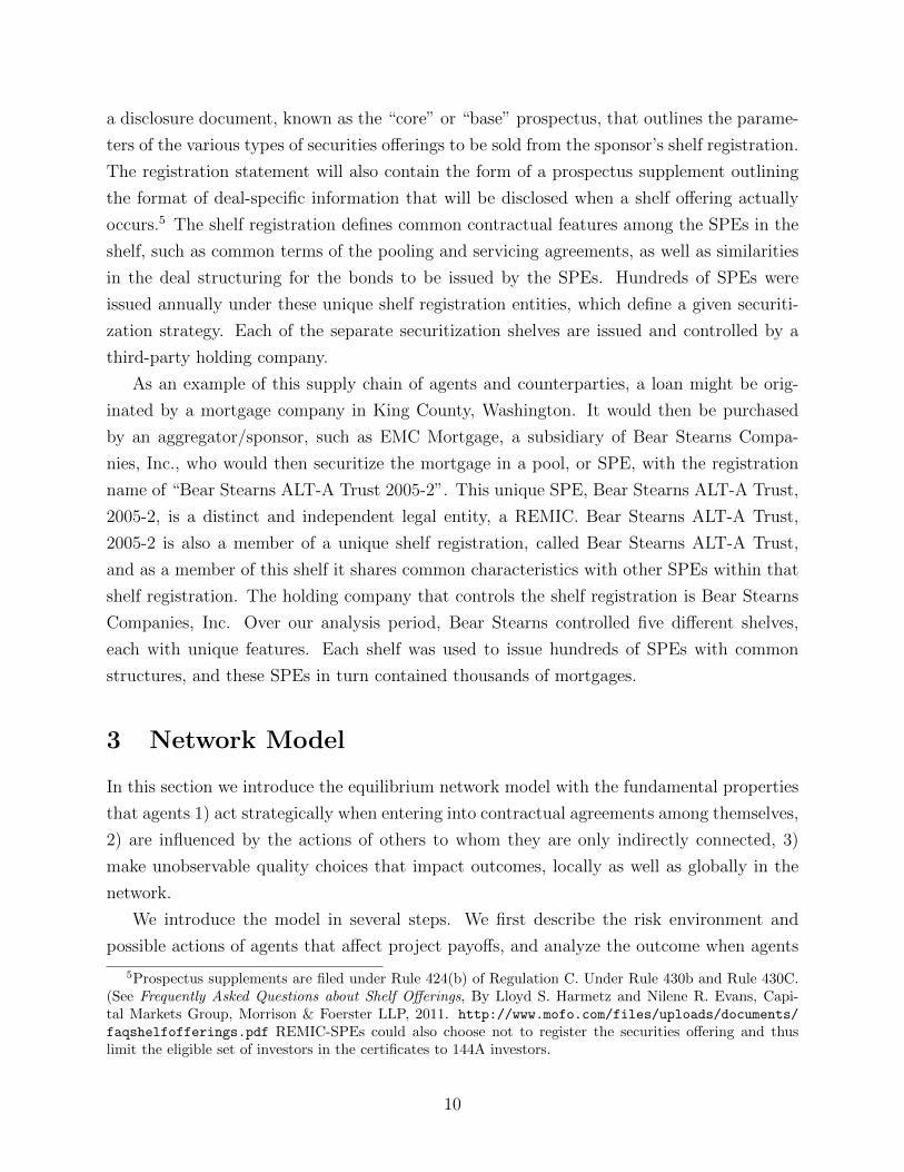
a disclosure document, known as the “core” or “base” prospectus, that outlines the parame-

ters of the various types of securities offerings to be sold from the sponsor’s shelf registration.

The registration statement will also contain the form of a prospectus supplement outlining

the format of deal-specific information that will be disclosed when a shelf offering actually

occurs.5 The shelf registration defines common contractual features among the SPEs in the

shelf, such as common terms of the pooling and servicing agreements, as well as similarities

in the deal structuring for the bonds to be issued by the SPEs. Hundreds of SPEs were

issued annually under these unique shelf registration entities, which define a given securiti-

zation strategy. Each of the separate securitization shelves are issued and controlled by a

third-party holding company.

As an example of this supply chain of agents and counterparties, a loan might be orig-

inated by a mortgage company in King County, Washington. It would then be purchased

by an aggregator/sponsor, such as EMC Mortgage, a subsidiary of Bear Stearns Compa-

nies, Inc., who would then securitize the mortgage in a pool, or SPE, with the registration

name of “Bear Stearns ALT-A Trust 2005-2”. This unique SPE, Bear Stearns ALT-A Trust,

2005-2, is a distinct and independent legal entity, a REMIC. Bear Stearns ALT-A Trust,

2005-2 is also a member of a unique shelf registration, called Bear Stearns ALT-A Trust,

and as a member of this shelf it shares common characteristics with other SPEs within that

shelf registration. The holding company that controls the shelf registration is Bear Stearns

Companies, Inc. Over our analysis period, Bear Stearns controlled five different shelves,

each with unique features. Each shelf was used to issue hundreds of SPEs with common

structures, and these SPEs in turn contained thousands of mortgages.

3 Network Model

In this section we introduce the equilibrium network model with the fundamental properties

that agents 1) act strategically when entering into contractual agreements among themselves,

2) are influenced by the actions of others to whom they are only indirectly connected, 3)

make unobservable quality choices that impact outcomes, locally as well as globally in the

network.

We introduce the model in several steps. We first describe the risk environment and

possible actions of agents that affect project payoffs, and analyze the outcome when agents

5Prospectus supplements are filed under Rule 424(b) of Regulation C. Under Rule 430b and Rule 430C.(See Frequently Asked Questions about Shelf Offerings, By Lloyd S. Harmetz and Nilene R. Evans, Capi-tal Markets Group, Morrison & Foerster LLP, 2011. http://www.mofo.com/files/uploads/documents/

faqshelfofferings.pdf REMIC-SPEs could also choose not to register the securities offering and thuslimit the eligible set of investors in the certificates to 144A investors.

10

act in isolation. We then study in detail the case when two agents interact, before analyzing

equilibrium in the general N -agent model. A detailed description of the strategic game

between agents is provided in the appendix.

3.1 Intermediaries and projects

There are N intermediaries with limited liability, each owned by a different risk-neutral

agent. Each intermediary invests in a project that generates risky cash flows at t = 1, CFn

P ,

and may moreover incur some costs at t = 0. The one-period discount rate is normalized to 0.

Agent n’s objective is to maximize the expectation at t = 0 of the value of the intermediary’s

cash flows at t = 1, CFn

1 , net any costs incurred at time 0.6

V n = E0[CFn

1 ]− Cn0 .

The risky project has scale sn > 0, and there are two possible returns, represented by the

Bernoulli-distributed random variables ξn, so that Rn = RH if ξn = 1, and Rn = RL if

ξn = 0. The probability, p, that ξn = 0 is exogenous, with 0 < p 1. We assume complete

symmetry in that the probability is the same for each project of the N projects.7

Each agent has the option to invest a fixed amount, Cn0 = csn > 0 at t = 0, to increase

the quality of the project. This cost is raised externally at t = 0. If the agent invests, then

in case of the low realization, ξn = 0, the return on the project is increased by ∆R > c, to

RL + ∆R. This investment cost could, for example, represent an investment in a screening

procedure that allows the agent to filter out the parts of the project that are most vulnerable

to aggregate shocks. We represent this investment choice by the variable qn ∈ 0, 1, where

qn = 1 denotes that the intermediary invests in quality improvement. Intermediaries that

choose q = 1 are said to be of high quality, whereas those that choose q = 0 are said to be of

low quality. For the time being, we assume that c is the same for all intermediaries. We will

subsequently allow c to vary across intermediaries, representing exogenous quality variation

(as opposed to the quality differences that arise endogenously because of intermediaries’

investment decisions).8

There is a threshold, d > 0, such that if the return on the investment for an intermediary

6The intermediary’s cash flow CFn

1 may differ from CFn

P because intermediaries may enter risk-sharingagreements with each other.

7Each project may be viewed as a representative project for a portfolio of a large number of small projectswith idiosyncratic risks that cancel out, and an aggregate risk component measured by ξn.

8Several variations of the model are possible, e.g., assuming that screening costs, c, are part of the t = 1cash flows, and fixing the scale of all intermediaries to s ≡ 1, all leading to qualitatively similar results. Theversion presented here was chosen for its tractability in combination with empirical relevance.

11

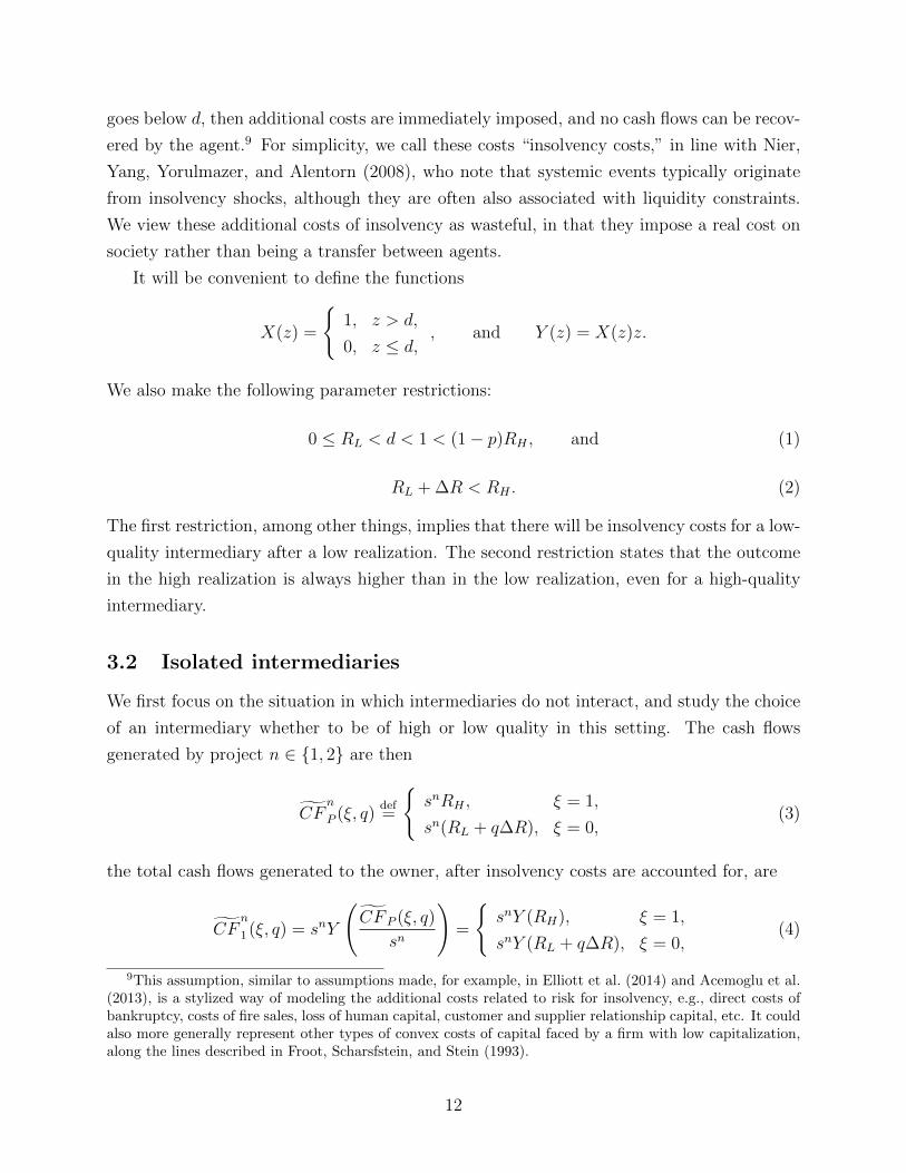
goes below d, then additional costs are immediately imposed, and no cash flows can be recov-

ered by the agent.9 For simplicity, we call these costs “insolvency costs,” in line with Nier,

Yang, Yorulmazer, and Alentorn (2008), who note that systemic events typically originate

from insolvency shocks, although they are often also associated with liquidity constraints.

We view these additional costs of insolvency as wasteful, in that they impose a real cost on

society rather than being a transfer between agents.

It will be convenient to define the functions

X(z) =

1, z > d,

0, z ≤ d,, and Y (z) = X(z)z.

We also make the following parameter restrictions:

0 ≤ RL < d < 1 < (1− p)RH , and (1)

RL + ∆R < RH . (2)

The first restriction, among other things, implies that there will be insolvency costs for a low-

quality intermediary after a low realization. The second restriction states that the outcome

in the high realization is always higher than in the low realization, even for a high-quality

intermediary.

3.2 Isolated intermediaries

We first focus on the situation in which intermediaries do not interact, and study the choice

of an intermediary whether to be of high or low quality in this setting. The cash flows

generated by project n ∈ 1, 2 are then

CFn

P (ξ, q)def=

snRH , ξ = 1,

sn(RL + q∆R), ξ = 0,(3)

the total cash flows generated to the owner, after insolvency costs are accounted for, are

CFn

1 (ξ, q) = snY

(CF P (ξ, q)

sn

)=

snY (RH), ξ = 1,

snY (RL + q∆R), ξ = 0,(4)

9This assumption, similar to assumptions made, for example, in Elliott et al. (2014) and Acemoglu et al.(2013), is a stylized way of modeling the additional costs related to risk for insolvency, e.g., direct costs ofbankruptcy, costs of fire sales, loss of human capital, customer and supplier relationship capital, etc. It couldalso more generally represent other types of convex costs of capital faced by a firm with low capitalization,along the lines described in Froot, Scharsfstein, and Stein (1993).

12

and the t = 0 value of the intermediary is

V n = V n(q) = E0[CFn

1 ]− Cn0 = sn ((1− p)Y (RH) + pY (RL + q∆R)− qc) . (5)

Given the parameter restrictions (1), we have V n(0) = sn(1− p)RH . We assume that if

an intermediary is indifferent between being high and low quality, it chooses to become low

quality. Therefore, q = 1, if and only if V n(1) > sn(1 − p)RH , immediately leading to the

following result:

Proposition 1. An intermediary chooses to be of high quality, q = 1, if and only if

RL + ∆R > max

(d,c

p

). (6)

Qualitatively, the result above is very intuitive, implying that increases in costs of infor-

mation acquisition, the probability of a high outcome, and costs of being insolvent, make it

less attractive for an intermediary to be of high quality. The first argument in the maximum

function on the RHS ensures that a high-quality firm avoids insolvency in the low realiza-

tion. If the condition is not satisfied, there is no benefit to being high quality even in the

low realization. The second argument ensures that the expected increase of cash flows in

the low state outweighs the cost of investing in quality. The value of the intermediary when

acting in isolation and following the rule (6) is then V nI = snVI , where

VI =

pRH , q = 0,

pRH + (1− p)(RL + ∆R)− c, q = 1.

Note that the objective functions of the agents coincide with that of society in this special

case. Specifically, given that society has the social welfare function, V =∑

n Vn, under the

constraint that intermediaries act in isolation, the socially optimal outcome is realized by

the intermediaries’ joint actions. We obviously do not expect this to be the case in general,

when agents interact.

3.3 Two intermediaries

We now explore the case with two interacting intermediaries, allows us to gain intuition in a

fairly simple setting, before introducing the general N -agent network model. Intermediaries

may enter into contracts that transfer risk. These contracts are settled according to a market-

clearing system along the lines of that in Eisenberg and Noe (2001). Because of the high

13

dimensionality of the problem when we allow agents to act strategically, we necessarily have

to assume a very limited contract space between intermediaries. Specifically, we assume that

the contracts available are such that intermediaries swap claims on the aggregate cash flows

generated by their projects in a one-to-one fashion, similar to Allen et al. (2012).

We focus on the case when the two intermediaries have the same scale (s1 = s2 = 1).

The contract is then such that intermediary 1 agrees to deliver π × CF1

P to intermediary 2

at t = 1, and in turn receive π × CF2

P from intermediary 2, for some 0 ≤ π ≤ 1. Our focus

is on the two cases when project risks are shared equally (π = 0.5) and when intermediaries

act in isolation (π = 0). We use the general π notation, since in the general case with N

agents that we will analyze subsequently, π will typically take on other values.

The probabilities for the possible realizations of (ξ1, ξ2) are10

P(ξ1 = 0, ξ2 = 0) = p2, P(ξ1 = 1, ξ2 = 0) = p1,

P(ξ1 = 0, ξ2 = 1) = p1, P(ξ1 = 1, ξ2 = 1) = 1− 2p1 − p2.

Consider a situation in which the intermediaries choose qualities q1 and q2, respectively, and

let fn(ξ1, ξ2) denote the binary variable that takes on value 0 if intermediary n ∈ 1, 2 is

insolvent in state (ξ1, ξ2), and 1 otherwise. Define

z1(ξ1, ξ2|q1, q2, π) = (1− π)f 1(ξ1, ξ2)CF1

P (ξ1, q1) + πf 2(ξ1, ξ2)CF2

P (ξ2, q2), (7)

z2(ξ1, ξ2|q1, q2, π) = πf 1(ξ1, ξ2)CF1

P (ξ1, q1) + (1− π)f 2(ξ1, ξ2)CF2

P (ξ2, q2). (8)

Because of insolvency costs, it follows that

CFn(ξ1, ξ2|q1, q2, π) = fn(ξ1, ξ2)zn(ξ1, ξ2|q1, q2, π), (9)

and

fn(ξ1, ξ2) = X

(zn(ξ1, ξ2|q1, q2)

sn

). (10)

A realization of cash flows and insolvency that satisfies (7-10) in each state is said to be an

outcome of the clearing mechanism. The time-0 value of an intermediary is then

V n(q1, q2|π) =∑

x1,x2∈0,1

CFn(x1, x2|q1, q2, π)P(ξ1 = x1, ξ

2 = x2)− qcsn.

Equations (7-10) provide the adaptation of the clearing system in Eisenberg and Noe

10Note here that the subscripts of p refer to the number of projects that yield low realizations, not towhich investment, n, is considered (which is not needed since we assume symmetric probabilities).

14

(2001) to our setting. This specification is almost identical to theirs (state by state), except

for the important difference that insolvency is costly in our setting, represented by d > 0.

As a consequence of insolvency costs, there may be multiple solutions to the clearing

mechanism (7,9,10) that lead to different net cash flows to intermediaries. This is because

the insolvency of one intermediary can trigger the insolvency of another in a self-generating

circular fashion. Along similar lines to Elliott et al. (2014), who also introduce solvency costs

in their clearing mechanism, we focus on the unique outcome that minimizes the number of

insolvencies. As noted in their study, since insolvencies are complements, all intermediaries,

as well as society, agree that their number should be minimized. Briefly, their method initially

assumes no insolvencies and then calculates which nodes become insolvent iteratively, taking

into account that the insolvency of one node may trigger that of another.

We use an algorithm similar to Elliott et al. (2014) to define the outcome of the clearing

mechanism, which will be the one we focus on henceforth. The algorithm also leads to

a natural shock-propagation mechanism, through which insolvencies spread step-by-step,

triggering others. With two intermediaries, the propagation mechanism is of course simple:

either the insolvency of one intermediary triggers that of the other, or it does not. In the

general case an iterative algorithm is needed, which we define in Appendix A. We stress

that although our clearing mechanism is similar to that in earlier work, what distinguishes or

work is our focus on the endogenous development and coexistence of heterogeneous financial

norms (represented by the q’s), and how these norms are influenced by and influence the

equilibrium network structure.

It is worthwhile discussing why it may be beneficial for agents to interact. Clearly,

the contracts offer a simple form of risk-sharing. Agents are risk neutral, but the cost

of insolvency introduces a motive for avoiding low outcomes that trigger solvency costs,

effectively introducing risk aversion. By sharing risks, the negative effects of a low realization

for the two agents can be limited.

It is also clear that the incentive for an agent to invest in high quality is affected by the

interaction with other agents. One may conjecture several potential effects, depending on the

economic environment. In some circumstances, an agent’s incentive to invest in quality may

decrease compared with the case of no interaction, since the benefits of quality are shared

whereas the costs are not. Under other circumstances, the incentive to invest in quality

may actually increase, because risk sharing allows insolvency to be avoided for high-quality

intermediaries that interact, although it cannot be avoided when they act in isolation. Thus

our stylized contracting environment promises to allow for rich equilibrium behavior..

15

3.3.1 Equilibrium

Intermediaries can either act in isolation (corresponding to π = 0) or share risks (π = 1/2).

For a risk-sharing outcome to be an equilibrium, both agents must have correct beliefs about

the quality decisions made by their counterparties. We make the standard assumptions that

each agent may unilaterally decide to sever a link to the other agent, and that bilaterally the

two agents can decide to add a link between themselves. For an outcome with risk sharing to

be an equilibrium, it follows that neither agent can be made better off by acting in isolation.

For an isolated outcome to be an equilibrium, it cannot be that both agents are better off

by sharing risk.

We model the mechanism by a strategic game with the sequence of events described in

Figure 2, where we have formulated the game in the general N agent case. At t = −2, given

Agents decidewhether to acceptproposed newlinks

Agents choose quality, qn

Outcomes arerealized

Each agent decides whether to- cut a link- propose a new link- isolate

t= -2 t= -1 t=0 t=1

Figure 2: Sequence of events in network formation game with endogenous financial norms.

that π = 1/2, each agent may unilaterally decide to sever the link to the other agent and

switch to π = 0, leading to the isolated outcome. If, on the other hand, π = 0, each agent

can propose to switch to π = 1/2, in which case the other agent has the option to accept

or decline at t = −1. Then, after the resulting network is determined, agents choose quality

and outcomes are realized. Note that we implicitly assume that the actual quality decision

is not contractible.11

11In our stylized model, the quality decision can of course be inferred from the realization of project cashflows. The issue could be avoided by assuming a small positive probability for ∆R = 0 in case of a lowrealization. For simplicity, we assume that contracts are restricted to being linear in realized project cashflows.

16

An equilibrium is now described by (q1, q2), and π, such that neither agent has an incen-

tive to sever the link (in the case π = 1/2), and it is not the case that both agents have an

incentive to form a link (in the case π = 0). Moreover, the agents’ beliefs about the other

agent’s actions, both in the case when π remains the same and in the case when it switches

because of actions at t = −2 and t = −1, need to be correct.

For the action q ∈ 0, 1, we let ¬q denote the complementary action (¬q = 1 − q). It

follows that the three numbers, q1, q2 and π > 0, describe an equilibrium with risk sharing

if:

V 1(q1, q2|π) ≥ V 1(¬q1, q2|π),

V 2(q1, q2|π) ≥ V 2(q1,¬q2|π),

V 1(q1, q2|π) ≥ V 1I ,

V 2(q1, q2|π) ≥ V 2I .

The first two conditions ensure that it is incentive-compatible for both agents to choose the

suggested investment strategies given that they share risks, whereas the latter two state that

risk sharing dominates acting in isolation for both agents.

Interesting dynamics arise already in this network with only two intermediaries, as seen

in the following example. We choose parameter values RH = 1.2, RL = 0.1, ∆R = 0.5,

c = 0.05, p1 = 0.1, p2 = 0.05, π = 0.5, and vary the insolvency threshold, d. Since the

setting is symmetric, it follows that V 1I = V 2

I = VI , and V 1(q,¬q) = V 2(¬q, q), reducing the

number of incentive constraints that need to be checked. The resulting value functions are

shown in Figure 3.

There are five different regions with qualitatively different equilibrium behavior. In the

first region, 0 < d < 0.35, the unique equilibrium is the one where both agents invest in

quality, (q1, q2) = (1, 1), and there is no risk-sharing, leading to values VI for both inter-

mediaries. No intermediary ever becomes insolvent in this case (since RL + ∆R > d). The

outcome where both agents invest and share risk would lead to the same values, but cannot

be an equilibrium because each agent would deviate and choose to avoid investments in this

case, given that the other agent invests. For example, if intermediary 1 does not invest, but

intermediary 2 does, agent 1 reaches V 1(0, 1) > V 1(1, 1) by avoiding the cost of investment

but still capturing the benefits of not becoming insolvent after a low realization. Therefore,

V 1(1, 1) cannot be sustained in equilibrium. Now, V 1(0, 1) can of course not be an equilib-

rium either, since under this arrangement intermediary 2 is on the (blue) V 1(1, 0) line, which

is inferior to VI . So only the isolated outcome survives as an equilibrium.

In the second region, 0.35 ≤ d < 0.6, there are two equilibria, both with investments,

17

0 0.1 0.2 0.3 0.4 0.5 0.6 0.7 0.8 0.9 10.8

0.85

0.9

0.95

1

1.05

1.1

1.15

d

V

V1(0,0)

V1(1,0)

V1(0,1)

V1(1,1)

VI

Figure 3: Value functions in economy with two intermediaries, as a function insolvencythreshold, d. The following value functions are shown: VI (circles, dotted black line), V 1(1, 1)(squares, magenta), V 1(0, 1) (stars, red), V 1(1, 0) (pluses, blue), and V 1(0, 0) (crosses, green).

(q1, q2) = (1, 1), and the same value for both intermediaries, VI . In addition to the isolated

outcome, the outcome with risk-sharing and investments in quality by both agents is now

an equilibrium. The reason is that the solvency threshold has now become so high that

agent 1 has an incentive to invest in the risk-sharing outcome when agent 2 invests, to avoid

insolvency which otherwise occurs if both ξ1 = 0, and ξ2 = 0.

The third region is 0.6 ≤ d < 0.65, in which the unique equilibrium is for intermediaries

to share risk and not invest, (q1, q2) = (0, 0), leading to value V 1(0, 0) for both agents.

Indeed, this strategy dominates the value under isolation, VI , which for d ≥ 0.6 entails the

strategy of not investing in quality since in that region insolvency occurs even when such

investments are made (this is the reason for the discontinuity in VI at d = 0.6). Note that

V 1(0, 0) is dominated by V 1(1, 1) and V 1(0, 1), though neither can constitute an equilibrium.

The outcome V 1(1, 1) is not sustainable, since it is better for either agent to switch to not

investing in quality, as it is for agent 2 under V 1(0, 1). So the only equilibrium is the one

with risk-sharing

When 0.65 ≤ d < 0.9, i.e., in the fourth region, V 1(0, 0) decreases substantially compared

with the third region, because for such high levels of the default threshold, both interme-

diaries become insolvent if there is one low realization, whereas two low realizations were

needed in the third region. This makes V 1(0, 0) inferior to the isolated outcome, VI (in which

18

both agents choose not to invest since d is so high), because of a contagion effect. When

risks are shared, a low realization for one intermediary not only causes that intermediary to

become insolvent but also triggers the insolvency of the other intermediary. Thus, the only

remaining equilibrium is now V 1(1, 1), i.e., for agents to share risk and for both to invest in

quality, (q1, q2) = (1, 1).

Finally, when d ≥ 0.9, the isolated equilibrium without quality investments, (q1, q2) =

(0, 0), is the only remaining equilibrium, since any risk sharing equilibrium will lead to

contagion.

We note that equilibrium quality choice is non-monotone in d, in contrast to the isolated

case in which q is naturally non-increasing in d (see (1)). With interaction between inter-

mediaries, the unique quality choice in the third region, 0.6 ≤ d < 0.65, is (q1, q2) = (0, 0),

whereas in the fourth region, 0.65 ≤ d < 0.9, (q1, q2) = (1, 1) in equilibrium, as the prospects

for high-quality investments increases with d in parts of the domain in this case. Then, for

d > 0.9, investments in quality again become inferior, leading to (q1, q2) = (0, 0).

We also note that all equilibrium outcomes have q1 = q2. This is natural for the isolated

equilibria, but also occurs for the risk-sharing equilibria. It suggests that the “financial

norm”—defined as the quality it chooses—depends on the financial norms of the intermediary

with which it interacts. We wish to explore this effect in more complex financial networks. In

such networks, not only will the actions of the intermediaries matter, but so will the actions

of the neighbors of those intermediaries, their neighbors’ neighbors, etc.

3.4 General networks of intermediaries

We now introduce the general network model with N ≥ 2 intermediaries, represented by the

graph G = (N , E), N = 1, . . . , N. The relation E ⊂ N×N describes which intermediaries

are connected in the network. Specifically, the edge e = (n, n′) ∈ E, if and only if there

is a connection (edge, link) between intermediary n and n′. No intermediary is connected

to itself, (n, n) /∈ E for all n, i.e., E is irreflexive. We define the transpose of the link

(n, n′)T = (n, n′), and assume that connections are bidirectional, i.e., e ∈ E ⇔ eT ∈ E.

The operation E + e = E ∪ e, eT, augments the link e (and its transpose) to the network,

whereas E − e = E\e, eT severs the link if it exists. The number of neighbors of node n

is Zn(E) = |(n, n′) ∈ E|.Intermediaries will in general have different scale and number of neighbors, and therefore

choose to share different amounts of risk amongst themselves. Similar to the case with two

intermediaries, we choose a simple sharing rule, represented by the sharing matrix Π ∈ RN×N+ ,

where 0 ≤ (Π)nn′ ≤ sn is the amount of risk that is swapped between intermediary n and

19

n′, with the summing up constraint that Πs = s, where s = (s1, . . . , sN)′. It will be more

convenient to characterize the fraction of risk that agent n′ shares with agent n, which is

represented by the matrix Π = ΠΛ−1s . Here, we have used the notation that for a general

vector, v ∈ RN , we define the diagonal matrix Λv = diag(v). We also use the notation that δn

represents a vector of zeros, except for the nth element which is 1. In our previous example

with two intermediaries of unit scale, s = (1, 1)′ and the sharing matrix is

Π =

[1− π π

π 1− π

].

The network represents a restriction on which sharing rules are feasible. As we will discuss,

this restriction can be self-imposed by intermediaries in equilibrium, who may chose not to

interact even if they may, or it could arise exogenously. Specifically, for a sharing rule to

be feasible it must be that every off-diagonal element in the sharing matrix that is strictly

positive is associated with a pair of agents who are linked, Πnn′ > 0⇒ (n, n′) ∈ E.

We choose to study a specifically simple class of sharing rules that ensure that all weights

are nonnegative and that each intermediary keeps some of its own project risk, namely

(Π)nn′ = min

sn

1 + Zn(E),

sn′

1 + Zn′(E)

, n 6= n′, (11)

and (Π)nn

= sn −∑n′ 6=n

Πnn′ . (12)

We write Π(E) when stressing the underlying network from which the sharing rules is con-

structed.

The joint quality decision of all agents is represented the vector q = (q1, . . . , qN) ∈0, 1N . In the general case, the cost of investing in quality may vary across intermediaries,

represented by the vector c = (c1, . . . , cN) ∈ RN++. The state realization is represented by the

vector ξ = (ξ1, . . . , ξN) ∈ 0, 1N . We will work with a limited state space, assuming that

ξ ∈ Ω ⊂ 0, 1N where Ω is a strict subset of 0, 1N , and mainly focus on three such sets:

The first set is Ω1 =ξ ∈ 0, 1N : ξ′1 ≥ N − 1

, with P(ξ = 1− δn) = p1, 1 ≤ n ≤ N , and

associated probability space P : Ω1 → [0, 1]. Here, 1 = (1, . . . , 1) is an N -vector of ones. For

this set, either zero or one low realization occurs, and the probability for a low realization is

the same for all intermediaries. The second state space is Ω2 =ξ ∈ 0, 1N : ξ′1 ≥ N −2

,

for which no more than two realizations may be low, with full symmetry across intermediaries,

20

so that

P(ξ = 1− δn) = p1, 1 ≤ n ≤ N,

P(ξ = 1− δn − δn′) = p2, 1 ≤ n < n′ ≤ N,

P(ξ = 1) = 1−Np1 −N(N − 1)

2p2.

Finally, the third state pace is ΩA = 0,1, for which either no or all realizations are low,

the latter case with probability P(ξ = 0) = pA.

Solvency is represented by a vector f ∈ 0, 1N , and realized cash flows to agents by

the random vector CF = (CF1, . . . , CF

N)′ ∈ RN+ . The realized project cash-flows are then

represented by the vector CF P = (CF1

P , . . . , CFN

P )′, where

CFn

P (ξ, q) = RHξn + (RL + qn∆R)(1− ξn), n = 1, . . . , N.

The general network version of the clearing system that calculates a mapping CF 1(ξ, q) =

CM[CF P (ξ, q)], is described by the iterative algorithm described in detail in Appendix A.

The outcome of the algorithm is the solution that minimizes the number of insolvencies, or

equivalently maximizes the total cash-flows to agents. In vector form, this can be written as

CF 1 = CM[CF P ] = maxf

(ΛfΠΛf )× CF P , s.t. (13)

f = X(

Λ−1s × CF 1

). (14)

Here, X operates element-wise in (14), X(v) = (X(v1), X(v2), . . . , X(vN))′. The net cash

flows to the intermediaries are then given by the vector

w(ξ|q, E) = CF 1(ξ)− ΛcΛsq. (15)

This is the general network version of equations (7-10). The t = 0 value vector of interme-

diaries, given quality investments, q, and network E is then given by

V (q|E) =∑ξ∈Ω

w(ξ|q, E)P(ξ). (16)

A variation of the algorithm assumes that insolvencies only propagate up until a fixed

number of steps, m, terminating the algorithm when m reaches m (see the description in

Appendix A). We write CF 1 = CM[CF P |m] in this case, and the standard version of the

clearing mechanism is then CM[CF P ] = CM[CF P |∞].

21

3.4.1 Equilibrium

Let E∗ denote the complete network in which all agents are connected. We assume that there

is a maximum possible network, E ⊂ E∗, such that only links that belong to E may exist

in the sharing network. This restriction on feasible networks could, for example, represent

environments in which it is impossible for some agents to credibly commit to deliver upon

a contract written with some other agents, due to low relationship capital, limited contract

enforcement across jurisdictions, etc. A network, E, is feasible if E ⊂ E. If all agents who

may be linked actually choose to be linked in equilibrium, i.e., if E = E, we say that the

equilibrium network is maximal. It may also be the case that E is a strict subnetwork of E,

just as was the case in the economy with two intermediaries where E = E∗, but E = ∅ for

some parameter values because agents chose the isolated outcome in equilibrium.

To define equilibrium, we build upon the pairwise stability concept of Jackson and Wolin-

sky (1996). We require equilibrium in this multistage game to be subgame perfect. The game

and equilibrium requirements are explained in detail in the appendix. Here we provide a

summary. The sequence of events is as in Figure 2. Consider a candidate equilibrium, repre-

sented by a network E and quality choices q. Each agent, n, has the opportunity to accept

the sharing rule, Π(E), as is, by neither severing nor proposing new links at t = 0. But,

in line with the pairwise stability concept, any agent n can also unilaterally decide to sever

a link with one neighbor, n′, leading to the sharing network E ′ = E − (n, n′), and corre-

sponding sharing rule Π(E ′). Also, any agent can propose an augmentation of another link

(n, n′) ∈ E\E, which if agent n′ accepts leads to the sharing network E ′′ = E + (n, n′) with

sharing rule Π(E ′′). Finally, we assume that each agent can unilaterally choose the isolated

outcome, V nI , by severing its links to all other agents.

The possibility to unilaterally sever all links in a sharing network—although not techni-

cally part of the standard definition of pairwise stability—is natural, in line with there being

a participation constraint that no intermediary can be forced to violate. It provides a slight

extension of the strategy space.

The severance, proposal, and acceptance/rejection of links occur at t = −2 and t = −1.

The agents then decide whether to invest in quality or not at t = 0, each agent choosing

qn ∈ 0, 1. A pair (q, E), where E ⊂ E, is now defined to be an equilibrium, if agents

given network structure E choose investment strategy q, if no agent given beliefs about

other agent’s actions—under the current network structure as well as under all other feasible

network structures in E—has an incentive to either propose new links or sever links, and

if every agent’s beliefs about other agents actions under network E as well as under all

alternative network formations are correct.

22

4 Analysis of equilibrium

We wish to understand how the quality choices—the financial norms—of agents affect and are

affected by equilibrium network structure. To gain some intuition, we first study a specific

example with N = 8 intermediaries, all of which have scale equal to unity, s = 1, with the

shock structure Ω2. The maximal network, E, which is also an equilibrium network is shown

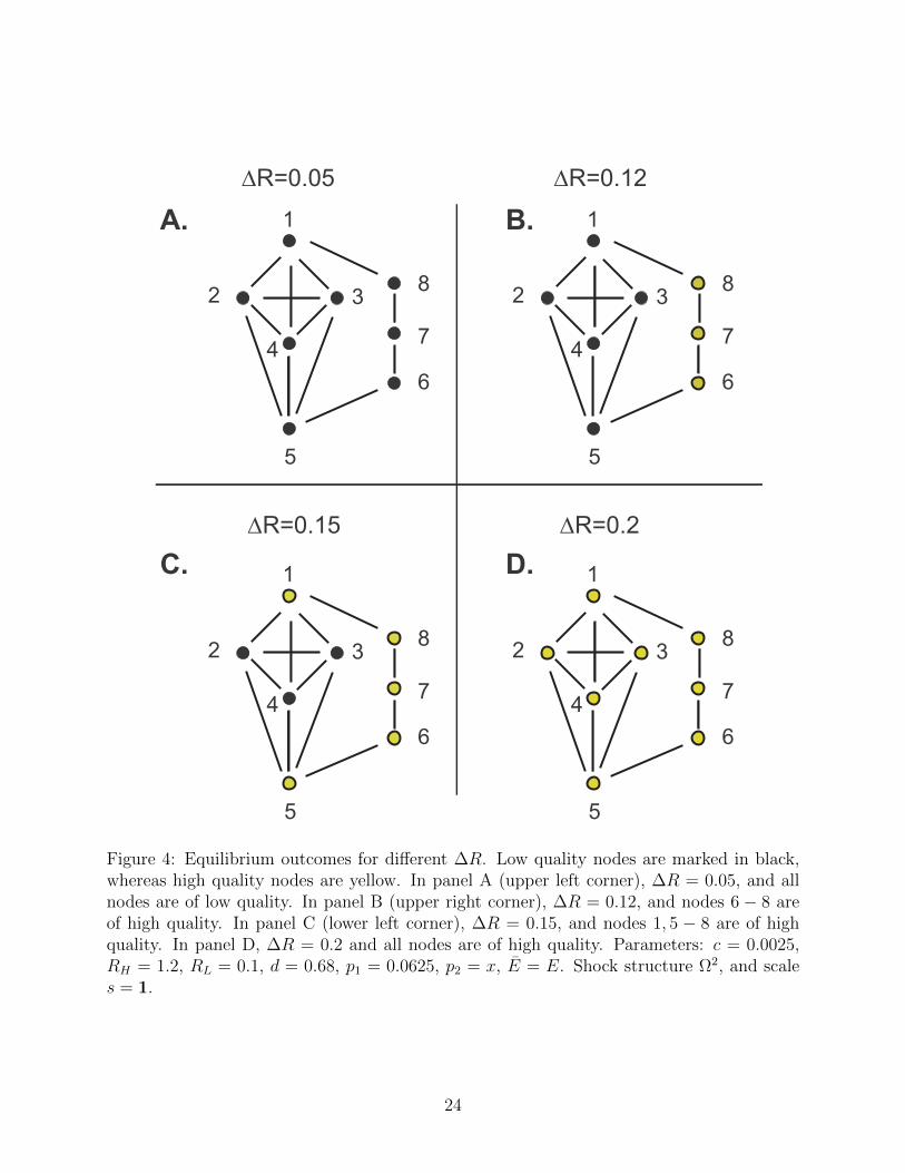
in panel A of Figure 4. We say that the equilibrium network is maximal. As shown in panel

A, for low ∆R the equilibrium outcome is for all intermediaries to be of low quality. This is

simply because investing is quality does not increase the payoff in low states sufficiently to

avoid insolvency for any intermediary for such low ∆R.

For ∆R = 0.12, shown in Panel B, by investing in quality, intermediaries can now avoid

insolvency. This is what intermediaries 6–8 do in equilibrium. However, intermediaries 1-5

cannot sustain an equilibrium in which they also invest in quality, since it is too tempting for

them to free-ride on the investments by others. This is because they have so many neighbors

that their investment decision is not pivotal for avoiding insolvency. For ∆R = 0.15, shown

in Panel C, it is an equilibrium strategy also for 1 and 5 to invest in quality. This is because

they can now avoid insolvency for several cases in which two shocks hit the network, in which

case they are pivotal. This is less of a carrot for agents 2-4 though, who still cannot sustain

quality investments in equilibrium. Finally, when ∆R = 0.2, nodes 2-4 can also be made to

invest in quality in equilibrium, since they are now also pivotal in avoiding insolvency after

two shocks in a sufficient number of states. Thus, as shown in Panel B and C, heterogeneous

financial norms may coexist in equilibrium, and intermediaries with the same quality tend

to be linked (or at least to be close in the network) in these situation.

We wish to explore this relationship between network structure and quality choice for

a larger class of networks. We simulate 1,000 networks for which equilibrium exists, each

with N = 9 nodes. We use the Erdos-Renyi random graph generation model, in which

the probability that there is a link between any two agents is i.i.d., with the probability

0.25 for a link between any two nodes, and we also randomly vary c across intermediaries,

cn ∼ U(0, 0.025). For computational reasons, we focus on networks in which equilibria are

maximal, E = E.

Table 1 shows summary statistics for nodes that are of high quality compared with those

of low quality in equilibrium. We see that there are on average more high-quality nodes in

equilibrium with these parameters. Also, the average cost of investing in quality for high-

quality nodes is lower than for low-quality nodes. More interestingly, the average number of

neighbors of high-quality nodes is higher, and the average quality of neighbors of high-quality

nodes is higher than of low-quality nodes. All these differences are statistically significant.

23

1

5

4

2 3

6

7

8

A. B.

C. D.

1

5

4

2 3

6

7

8

1

5

4

2 3

6

7

8

1

5

4

2 3

6

7

8

R=0.05 R=0.12

R=0.15 R=0.2

Figure 4: Equilibrium outcomes for different ∆R. Low quality nodes are marked in black,whereas high quality nodes are yellow. In panel A (upper left corner), ∆R = 0.05, and allnodes are of low quality. In panel B (upper right corner), ∆R = 0.12, and nodes 6 − 8 areof high quality. In panel C (lower left corner), ∆R = 0.15, and nodes 1, 5 − 8 are of highquality. In panel D, ∆R = 0.2 and all nodes are of high quality. Parameters: c = 0.0025,RH = 1.2, RL = 0.1, d = 0.68, p1 = 0.0625, p2 = x, E = E. Shock structure Ω2, and scales = 1.

24

Average Number in network Iq(neighbors) Number of neighbors costq = H 6.34 0.79 4.32 0.011q = L 2.66 0.4 3.12 0.016

Table 1: Summary statistics of high- and low-quality intermediaries. Number of simulations:1,000. Parameters: RH = 1.1, RL = 0.2, ∆R = 0.3, d = 0.75, p1 = 4/90, p2 = 1/90,c ∼ U(0, 0.025). Shock structure Ω2, an scale s = 1.

The last result is especially important, since it shows that the financial norms that arise

in the network are indeed closely related to network positions, i.e., that different clusters

exist in which nodes have different norms. Another way of measuring whether such clusters

exist is to partition each network into a high-quality and a low-quality component, and

study whether the number of links between these two clusters is lower than what would be if

quality were randomly generated across nodes. Specifically, consider a network with a total

of K = |(n, n′) ∈ E| links, and a partition of the nodes into two clusters: N = NA ∪NB,

of size NA = |NA| and NB = |NB| = N−NA, respectively, and the number of links between

the two components: M = |(n, n′) ∈ E : n ∈ NA, n′ ∈ NB|. In the terminology of graphs,

M is the size of the cut-set, and is lower the more disjoint the two clusters are. The number

of links one would expect between the two clusters, if links were randomly generated, would

be W = 1N(N−1)

NANBK, so if the average M in the simulations is significantly lower than

the average W , this provides further evidence that financial norms are clustered. Indeed,

the average M in our simulations is 12.2, substantially lower than the average W which is

14.2, corroborating the presence of endogenous financial norms.

5 Computation of Equilibrium

Although the equilibrium calculations are straightforward in economies with networks up to

about 15 nodes, they become computationally infeasible for real-world large-scale networks—

potentially with thousands of intermediaries. In addition, in practice some or all of the model

parameters (d, p, RL, and RH) may be unobservable, and therefore have to be estimated from

observed dynamics. We introduce a numerical method that addresses these two issues jointly,

by approximating an equilibrium that optimally matches observed insolvency dynamics, and

that can be applied to large-scale problems.

Specifically, we assume that w, E, and c are observable, whereas the parameter values

RL, RH , d, p, and ∆R, and the quality vector q ∈ 0, 1N def= D are not. We assume that the

shock structure is ΩA, and use the clearing mechanism CM[CF P |2], allowing for two steps

of shock propagation.

25

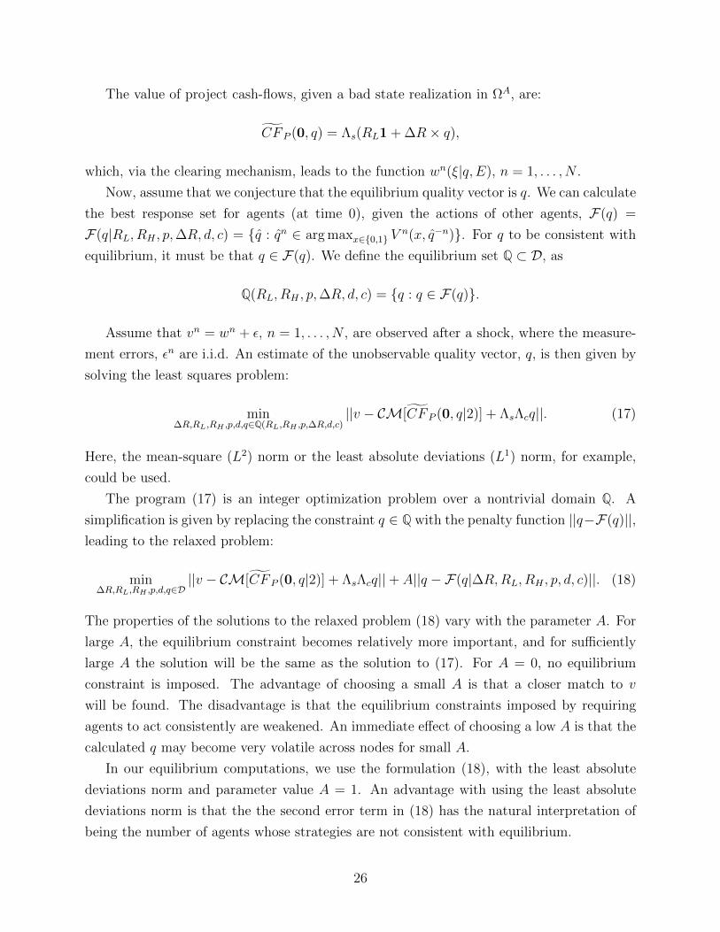
The value of project cash-flows, given a bad state realization in ΩA, are:

CF P (0, q) = Λs(RL1 + ∆R× q),

which, via the clearing mechanism, leads to the function wn(ξ|q, E), n = 1, . . . , N .

Now, assume that we conjecture that the equilibrium quality vector is q. We can calculate

the best response set for agents (at time 0), given the actions of other agents, F(q) =

F(q|RL, RH , p,∆R, d, c) = q : qn ∈ arg maxx∈0,1 Vn(x, q−n). For q to be consistent with

equilibrium, it must be that q ∈ F(q). We define the equilibrium set Q ⊂ D, as

Q(RL, RH , p,∆R, d, c) = q : q ∈ F(q).

Assume that vn = wn + ε, n = 1, . . . , N , are observed after a shock, where the measure-

ment errors, εn are i.i.d. An estimate of the unobservable quality vector, q, is then given by

solving the least squares problem:

min∆R,RL,RH ,p,d,q∈Q(RL,RH ,p,∆R,d,c)

||v − CM[CF P (0, q|2)] + ΛsΛcq||. (17)

Here, the mean-square (L2) norm or the least absolute deviations (L1) norm, for example,

could be used.

The program (17) is an integer optimization problem over a nontrivial domain Q. A

simplification is given by replacing the constraint q ∈ Q with the penalty function ||q−F(q)||,leading to the relaxed problem:

min∆R,RL,RH ,p,d,q∈D

||v − CM[CF P (0, q|2)] + ΛsΛcq||+ A||q −F(q|∆R,RL, RH , p, d, c)||. (18)

The properties of the solutions to the relaxed problem (18) vary with the parameter A. For

large A, the equilibrium constraint becomes relatively more important, and for sufficiently

large A the solution will be the same as the solution to (17). For A = 0, no equilibrium

constraint is imposed. The advantage of choosing a small A is that a closer match to v

will be found. The disadvantage is that the equilibrium constraints imposed by requiring

agents to act consistently are weakened. An immediate effect of choosing a low A is that the

calculated q may become very volatile across nodes for small A.

In our equilibrium computations, we use the formulation (18), with the least absolute

deviations norm and parameter value A = 1. An advantage with using the least absolute

deviations norm is that the the second error term in (18) has the natural interpretation of

being the number of agents whose strategies are not consistent with equilibrium.

26

6 Empirical identification of the mortgage network

A key component of our theoretical model is that links are defined through the passing of

risky “projects” from one node to another. The natural interpretation in mortgage markets

is that these projects represent loans. Along these lines, we identify the market’s network

from the mortgage flows through the private label supply chain.

6.1 Tracking mortgages from originator to securitizer

The available data sources that account for the firm-level composition of the residential-

mortgage origination market define individual mortgage originators either as entities that

underwrite and fund mortgage originations (the definition used by the Home Mortgage Dis-

closure Act (HMDA) surveys) or alternatively through the identification of the legal creditor

of record as shown in the local land recording facilities, the assessor’s (or equivalent) offices.

We use the latter source of data and definition of originator in this paper. Both HMDA and

the assessor data allow originators to be classified by type, such as federal commercial banks,

S&Ls/state banks, finance companies, credit unions, and mortgage companies. This classifi-

cation of individual mortgage originators into lender type makes an analysis of the network

structure of the industry tractable. It also corresponds well to the dueling regulatory and

functional structure of the industry.

A significant challenge in network analysis of the U.S. mortgage market is the fact that

there is no unique mortgage identifier that can be used to track individual mortgages through

the supply chain. Thus, identifying the supply chain network from the address of the houses

that collateralize the loans, the identity of the legally recorded loan originator, the pools

or special purpose entities (SPE) in which the loans are securitized, the holding companies

that exercise the control rights to structure the SPEs, to underwrite the bonds, and often

to retain the equity positions of the SPEs requires complicated merging protocols between

disparate data sets. Another challenge is measuring the life-of-loan performance of individual

loans in the mortgage network. To address these limitations, we create a new data set that

merges together three different data sets. These data sets are: 1) the Dataquick Historical

Transaction data that records the legal originator of record, the recording date and the loan

principal but has no other information about the mortgages such as the performance of the

loan or who it was sold to; 2) the newly updated ABSNet loan- and pool-level origination

and transaction data that includes detailed information about the individual loans in each

pool and their performance over time but less information about the ownership of the shelf

and the initial originator of record; 3) the prospectuses for all the pools in the ABSNet data

that provide the legal names of all the agents involved in the securitization and the legal

27

name of the SPE which we obtained from the Securities and Exchange Commission (SEC)

website.

The Dataquick Transaction data provides extensive coverage of lien records for all of the

U.S. including the name of the legally recorded originator of the mortgage and a taxonomy

of originator types (e.g., bank, finance company, credit union, home builder, mortgage com-

pany, savings and loan institution, Mortgage Electronic Registration System (MERS)12).

The Dataquick assessor’s data also includes information on the loan amount; whether it is

a first, second, or third lien position; the mortgage recording date; and the value of the

house price at purchase (if the mortgage is a purchase-money mortgage). There are 103

million individual first-lien records, including every state in the U.S. from 1996–2013, in the

Dataquick Transaction Data.

An important advantage of the Dataquick originator taxonomy is that it allows us to

separately identify mortgage-company subsidiaries, finance companies, and the regulated

bank or savings-and-loan retail lender within large bank or thrift holding companies such

as Wells Fargo and Countrywide. The taxonomy also allows us to unravel the different

functional entities within large mortgage companies such as New Century (a mortgage REIT

with many subsidiaries). This taxonomy is important because it makes the empirical network

analysis tractable while accurately representing the primary competitive differences among

the firms.

Since our interest is in securitized loan networks, we merge the Dataquick lien data with

loan-level data obtained from ABSNet. The ABSNet data set includes detailed information

about private-label securitized mortgages, including the initial loan balance, loan contract

features, the loan zip code, the origination date, and the identifiers for the special purpose

entity (SPE) in which the loan is securitized. ABSNet records a total of 13,453,796 first-

lien loan originations between 2002 and 2007. We successfully merge 9,099,280 of these loan

records with the Dataquick Historical Transaction data, giving us an originator of record and

a lender type for each merged loan. For the remaining unmerged Dataquick loans, we found

that Dataquick had a lender name for 3,370,730 of these loans and we used the Dataquick

taxonomy to assign a lender-type to each. We were unable to identify a lender name for

1,083,796 loans, so these observations were discarded.

We then downloaded all the prospectuses for all the residential mortgage-backed security

deals from the SEC website to obtain the full deal name for each SPE in the ABSNet data

12As discussed in Hunt, Stanton, and Wallace (2012), the MERS system was widely used to record liens.Interestingly, in our data the assessor lien records indicate whether it was a MERS-recorded lien, but inaddition gives the legal name of the origination lien holder. For a relatively small number of mortgages, thename of the actual lien holder name is missing, so that MERS appears as the lien holder. We chose not todelete these observations if we knew the remaining identities in the supply chain.

28

from each prospectus. We then hand-searched the SEC deal names to obtain the name of

the shelf registration for the SPE and the identity of the holding company that had made the

shelf registration. We successfully linked 12,370,000 loans to their county of origin, lender of

record, lender type, securitization shelf, and the holding company that controlled the shelf

registration. For each loan, we track the month-by-month payment performance from the

origination date until December 2013 (the end of our performance data). We thus identify

all the ex post foreclosure outcomes for each loan over our performance period.

6.2 Loan network performance, 2002–2007

In our model of intermediary networks the functional and geographic location of agents mat-

ters. We therefore first develop a network representation technology that accounts for spatial

competition among lender-types to originate mortgages for borrowers (houses) within proxi-

mate geographic areas.13 As discussed previously, there are seven first-lien originator types in

our taxonomy: banks, credit unions, finance companies, home builders, mortgage companies,

savings and loan institutions, and MERS. Table 2 shows that there was a significant increase

in first-lien private-label securitized lending from 2002 until its peak in 2005, followed by

a decline until 2007.14 Mortgage companies accounted for more than half of the first-lien

originations over the period.15 The next largest lender types were the banks (regulated by

the Office of the Comptroller of the Currency (OCC) and the Federal Deposit Insurance

Corporation (FDIC)) and the savings and loan institutions (regulated by the Office of Thrift

Supervision). Both of these lender types were engaged primarily in retail lending (again

these categories do not include the mortgage company and financial company subsidiaries

of these institutions). The home builders with mortgage subsidiaries, the credit unions, and

the MERS originators accounted for a much smaller market share of overall private-label

securitized first lien mortgage origination.

In our networks, we assign each loan to the lender-type and county pairing for the ob-

served originator of record for the loan and for the location of the house collateralizing the

loan. There are 1,848 counties in our data, and hence the potential for 12,936 pairings of

13Our representation also accounts for competition to purchase originated mortgages across the securi-tization SPEs, and competition among the holding companies that ultimately control the securitizationchannels.

14Private-label securitization accounted for 21.26% of all mortgage origination in the U.S. in 2005 (seeInside Mortgage Finance, January 12, 2007).

15The “mortgage company” lender type includes the mortgage company subsidiaries of large commercialbanks such as Wells Fargo Mortgage Company, Inc., or Countrywide Home Loans, Inc., that may or maynot have been consolidated on the regulated holding-company balance sheets, and whose lending activitieswere regulated separately from the lending activities of the retail entities within the same holding companies(see Engel and McCoy, 2011). These entities also had different cost structures due to their organization aswholesale lenders that usually did not involve the ownership of actual bricks and mortar origination facilities.

29

Table 2: Private-label securitized residential mortgage originations by lender type and yearof origination.

2002 2003 2004 2005 2006 2007 TotalsBanks 106,253 238,703 434,382 613,001 555,028 206,931 2,154,298Credit Unions 9,567 19,999 34,531 44,313 36,928 11,140 156,478Finance Companies 10,987 15,099 11,885 11,032 2,408 148 51,559Home Builders 88,205 154,516 301,570 324,607 222,300 70,925 1,162,123Mortgage Companies 574,680 1,086,534 1,628,435 1,955,751 1,644,587 463,350 7,353,337Savings and Loans 107,799 175,563 322,968 409,257 368,464 101,315 1,485,366MERS 808 657 121 112 1,018 182 2,898Totals 898,299 1,691,071 2,733,892 3,358,073 2,830,733 853,991 12,370,000

lender-type and county. Each of these pairings is then linked with the observed securitization

shelf for each of the loans from the lender-type and county pairing. An important character-

istics of the observed mortgage origination networks is that single county/lender-type nodes

are securitized through more than one shelf (a one to many mapping). There are a total of

190 pool securitization shelves and 77 separate holding companies in our data.

Figure 5 shows the mortgage network for years 2002, 2005, 2006 and 2007, each panel

showing the network of originations for a different year. The upper rim of the network rep-

resents the lender-type and county pairs for mortgages originated in each year. The second

tier of nodes represents the shelves in which the mortgages were securitized, and the lowest

tier of nodes represents the holding companies that control the shelves. As is clear from the

networks presented in Figure 5, the private-label securitized mortgage market was highly

inter-linked, and the volume of origination (the density of the origination linkages in the

upper tier) was significantly higher in 2005 than in 2002, although the number of holding

companies controlling the securitization flow remained quite small and concentrated.16 Per-

formance is measured by the percentage of loans along a given edge that have foreclosed by

December, 2013, and an edge is colored red if more than 30% of the loans tracked by the

edge have foreclosed by 2013.

Comparing panels a) and b), the ex post performance of the 2002 and 2005 vintages of

origination differed in the intensity and the geographic location of the foreclosures. Among

the 2002 vintage loans, only a highly localized set of lender-types and locations experienced

significant levels of foreclosure by 2013. Although not shown, mortgage companies accounted

for more than 60% of mortgage foreclosures for the 2002 vintage loans. In addition, though

16Although not shown in the graph, Stanton et al. (2014) discuss another important mechanism thatis coordinating the actions of the originators. This mechanism is the warehouse funding and the assetbacked commercial paper facilities that provided short-term funding capital to the originators throughoutthe mortgage market. These funding entities were also largely controlled by the same holding companiesthat controlled the securitization shelves.

30

(a) 2002 (b) 2005

(c) 2006 (d) 2007

Figure 5: Networks for lender-type and county pairs for 2002, 2005, 2006 and 2007 vintageoriginations and subsequent foreclosure as of December, 30, 2013.

31

again not shown explicitly in Figure 5, among the ten worst mortgage foreclosure counties

for the 2002 vintage mortgages four were Midwestern counties (Wayne, Cook, Cuyahoga and

Marion); four were Southern and Southwestern counties (Shelby, Harris, Dallas and Tarrant);

and only two were Western counties (Los Angeles and Maricopa). In the top forty worst

2002 vintage counties, only three were in California and six were in Florida. In contrast the

2005 vintage mortgages, as shown in the right-hand panel of Figure 5, began to experience

much more widespread incidence of lender-type and county pairings that generated edges

with more than 30% of foreclosure as the foreclosure incidence expands from the previous

locations and lender-types to include close-by neighbors. Now the top forty worst counties

included fifteen California counties and eight Florida counties, and the scale of foreclosures

in the prior ten worst counties grew substantially. Mortgage companies again accounted for

just less than 60% of all foreclosures among the 2007 vintage of originations. As a result,

the network shows a growing concentration of red and a blush of red throughout about one

half of the edges.

Panels c) and d) of Figure 5 show the network for originations in 2006 and 2007, respec-

tively. The lender volumes look similar to those of 2005. However, the degree of foreclosures

has increased dramatically and has propagated through substantial portions of the overall

private-label first lien mortgage market. The initial lender-type and geographic concentra-

tion areas are still apparent in both networks. However, the scale of the foreclosure volume

associated with these vintages has contaminated large swaths of lender-type and county pair-

ings as well as a large fraction of the shelves and the holding companies. Only an admirable

few originators, holding companies, and shelves appear to have withstood the temptation to

originate mortgages that, ex post, experienced a high incidence of foreclosure either due to

inferior underwriting strategies, reliance on risky contracts, and/or bad luck associated with

the economic performance of the geographic locations.

As further evidence on the abysmal performance of a highly localized set of mortgage

originators within the first lien private-label securitized mortgage market, Figure 6 shows

the percentage of the mortgage origination by vintage for each lender that subsequently

foreclosed by 2013. These originators are the top ten by ranking for the highest overall

number of foreclosures for at least four of the six years of the sample. As shown, Argent

Mortgage Company had a staggering foreclosure rate of more than 80% of all the mortgages

that it originated in 2006. Residential Funding Company had nearly a 20% foreclosure

rate for the loans that it securitized starting with the 2002 vintage and its foreclosure rate

rose to more than 50% for the 2006 and 2007 vintages. Option One Mortgage Corporation

exhibited a similarly elevated foreclosure rate over the entire period. All three of these

originators were mortgage companies. Wells Fargo Bank, N.A., significantly underperformed

32

Wells Fargo Home Loans, Inc., (a mortgage company within the Wells Fargo Bank holding

company) over nearly every vintage of origination. The foreclosure rate for Wells Fargo Bank

originated mortgages in the 2006 vintage had an ex post foreclosure rate of 35%, whereas the

mortgage company foreclosure rate for the same vintage was less than 30%. Loans originated

by Bank of America exhibited foreclosure rates very similar to those of Wells Fargo Bank.

Countrywide Home Loans, Inc. (a mortgage company), and Washington Mutual, FSB (a

savings and loan institution), exhibited nearly identical foreclosure rates for every vintage of

origination, reaching a high of 45% of total origination for the 2006 vintage.

Figure 6: Percentage of mortgages originated that subsequently foreclosed by 2013 for the10 mortgage originators with the highest volume of mortgage foreclosures.

Figure 7 reports the percentage of first lien private-label securitized mortgages that fore-

closed by 2013 for the 10 holding companies with the worst performance record for four of

the seven years of the sample. From 2004 onward, UBS Financial Services, ACC Capital

Holdings, and Lehman Brothers Holdings, Inc had the worst foreclosure record for mortgages

that were acquired and securitized in their shelves. More than 50% of the 2006 vintages loans

that were securitized by UBS and ACC had foreclosed by December of 2013. More than 50%

of the 2007 vintage loans that were securitized by Lehman Brothers had foreclosed by De-

cember of 2013. Among the holding companies, the foreclosure rates for the 2006 and 2007

33

vintage mortgages that they securitized were around 45%. The one exception was Country-

wide Financial Corp that exhibited a decrease from 40% to 35% in the foreclosure rate for

the 2007 vintage mortgages as compared to that of the 2006 vintages. Overall, for these top

worst holding companies, there was a very large fourfold increase in mortgage foreclosure

rates from the 2004 to the 2006 and 2007 vintages of mortgage securitization. These holding

companies all appear in the network representations with substantial amounts of red among

the edges that report to them.

Figure 7: Percentage of first lien private-label securitized mortgages that subsequently fore-closed by 2013 for the 10 shelf holding companies with the worst performance record.

Overall, our network representations of the first lien securitized mortgage market in the

U.S indicate that the market is highly interlinked and very concentrated at the level of the

securitization funding outlets. Ex post foreclosure outcomes were initially highly localized

among a relatively small number of lender-types and counties and then with later vintages

the seeds of future foreclosure outcomes were propagated to the closest competing firms

and localities. Once these propagation mechanisms reached the large California and Florida

counties, that have traditionally represented a large fraction of the U.S. mortgage market, the

negative outcomes for mortgage origination appeared to saturate the entire market. These

trends appear to have been initially instigated by a relatively few, large firms, however,

through the trading mechanisms in this market and due to the nature of competition in such

a network structure, the market appears to have tilted to an outcome with a preponderance

34

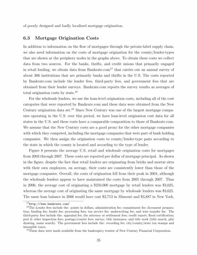
of poorly designed and badly localized mortgage origination.

6.3 Mortgage Origination Costs

In addition to information on the flow of mortgages through the private-label supply chain,

we also need information on the costs of mortgage origination for the county/lender-types

that are shown at the periphery nodes in the graphs above. To obtain these costs we collect

data from two sources. For the banks, thrifts, and credit unions that primarily engaged

in retail lending, we obtain data from Bankrate.com17 that carries out an annual survey of

about 306 institutions that are primarily banks and thrifts in the U.S. The costs reported

by Bankrate.com include the lender fees, third-party fees, and government fees that are

obtained from their lender surveys. Bankrate.com reports the survey results as averages of

total origination costs by state.18

For the wholesale lenders, we use the loan-level origination costs, including all of the cost

categories that were reported by Bankrate.com and these data were obtained from the New

Century origination data set.19 Since New Century was one of the largest mortgage compa-

nies operating in the U.S. over this period, we have loan-level origination cost data for all

states in the U.S. and these costs have a comparable composition to those of Bankrate.com.

We assume that the New Century costs are a good proxy for the other mortgage companies

with which they competed, including the mortgage companies that were part of bank holding

companies. We then assign the origination costs to county/lender-type pairs according to

the state in which the county is located and according to the type of lender.

Figure 8 presents the average U.S. retail and wholesale origination costs for mortgages

from 2003 through 2007. These costs are reported per dollar of mortgage principal. As shown

in the figure, despite the fact that retail lenders are originating from bricks and mortar sites

with their own employees, on average, their costs are consistently lower than those of the

mortgage companies. Overall, the costs of origination fell from their peak in 2004, although

the wholesale lenders appear to have maintained the costs from 2005 through 2007. Thus

in 2006, the average cost of originating a $250,000 mortgage by retail lenders was $3,025,

whereas the average cost of originating the same mortgage by wholesale lenders was $3,625.

The same loan balance in 2006 would have cost $2,713 in Missouri and $3,887 in New York,

17http://www.bankrate.com/18The Lender fees include the: points in dollars, administration fee; commitment fee; document prepara-

tion; funding fee; lender fee; processing fees; tax service fee; underwriting fee; and wire transfer fee. Thethird-party fees include the: appraisal fee; the attorney or settlement fees; credit report; flood certification;pest & other inspection fees; postage/courier fees; survey; title insurance; and title work (title search, platdrawing, name search). The government fees include the: recording fee; city/county/state tax stamps andintangible taxes.

19These data were made available from the bankruptcy trustee of New Century Financial Corporation.

35

Figure 8: Average U.S. retail and wholesale origination costs and reported as the cost perdollar of mortgage principal.

36

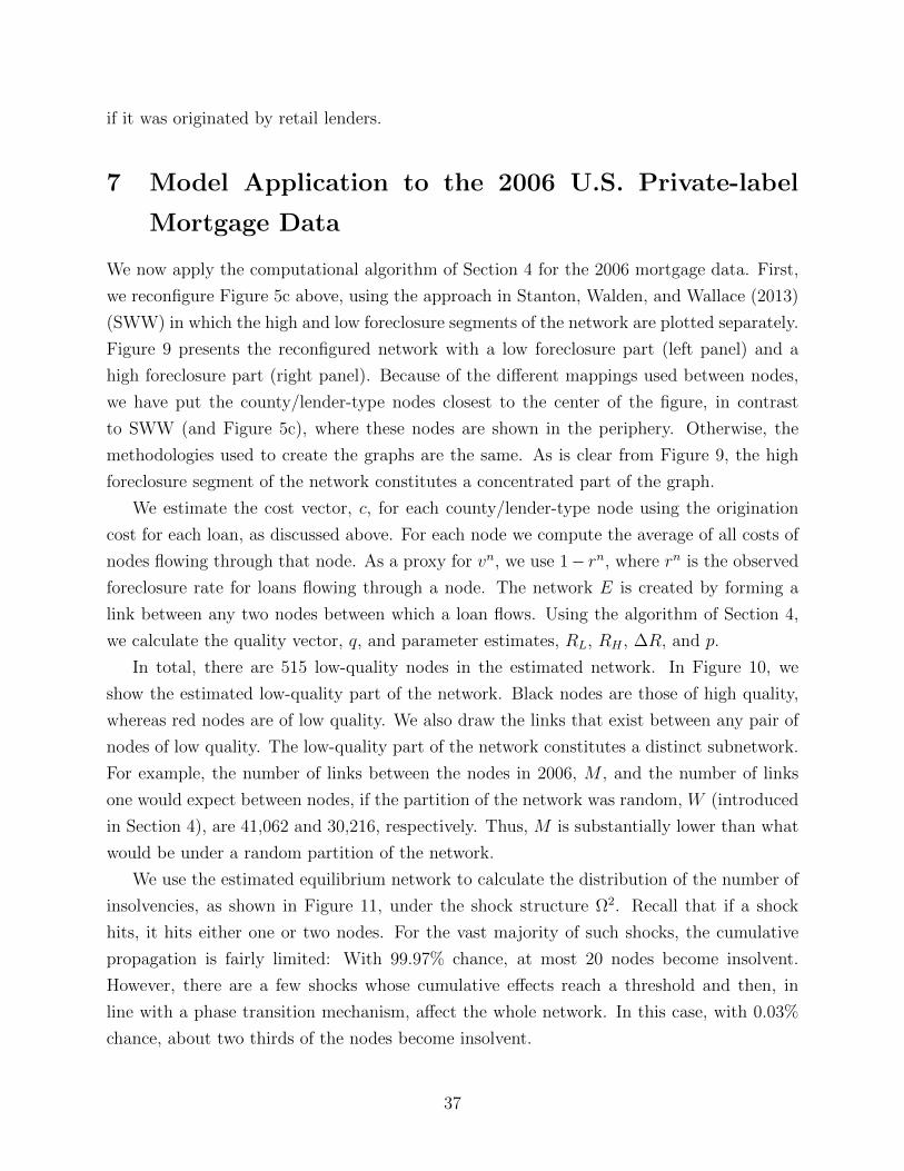
if it was originated by retail lenders.

7 Model Application to the 2006 U.S. Private-label

Mortgage Data

We now apply the computational algorithm of Section 4 for the 2006 mortgage data. First,

we reconfigure Figure 5c above, using the approach in Stanton, Walden, and Wallace (2013)

(SWW) in which the high and low foreclosure segments of the network are plotted separately.

Figure 9 presents the reconfigured network with a low foreclosure part (left panel) and a

high foreclosure part (right panel). Because of the different mappings used between nodes,

we have put the county/lender-type nodes closest to the center of the figure, in contrast

to SWW (and Figure 5c), where these nodes are shown in the periphery. Otherwise, the

methodologies used to create the graphs are the same. As is clear from Figure 9, the high

foreclosure segment of the network constitutes a concentrated part of the graph.

We estimate the cost vector, c, for each county/lender-type node using the origination

cost for each loan, as discussed above. For each node we compute the average of all costs of

nodes flowing through that node. As a proxy for vn, we use 1− rn, where rn is the observed

foreclosure rate for loans flowing through a node. The network E is created by forming a

link between any two nodes between which a loan flows. Using the algorithm of Section 4,

we calculate the quality vector, q, and parameter estimates, RL, RH , ∆R, and p.

In total, there are 515 low-quality nodes in the estimated network. In Figure 10, we

show the estimated low-quality part of the network. Black nodes are those of high quality,

whereas red nodes are of low quality. We also draw the links that exist between any pair of

nodes of low quality. The low-quality part of the network constitutes a distinct subnetwork.

For example, the number of links between the nodes in 2006, M , and the number of links

one would expect between nodes, if the partition of the network was random, W (introduced

in Section 4), are 41,062 and 30,216, respectively. Thus, M is substantially lower than what

would be under a random partition of the network.

We use the estimated equilibrium network to calculate the distribution of the number of

insolvencies, as shown in Figure 11, under the shock structure Ω2. Recall that if a shock

hits, it hits either one or two nodes. For the vast majority of such shocks, the cumulative

propagation is fairly limited: With 99.97% chance, at most 20 nodes become insolvent.

However, there are a few shocks whose cumulative effects reach a threshold and then, in

line with a phase transition mechanism, affect the whole network. In this case, with 0.03%

chance, about two thirds of the nodes become insolvent.

37

−1 −0.5 0 0.5 1−1

−0.8

−0.6

−0.4

−0.2

0

0.2

0.4

0.6

0.8

1Low foreclosure part of network

−1 −0.5 0 0.5 1−1

−0.8

−0.6

−0.4

−0.2

0

0.2

0.4

0.6

0.8

1High foreclosure part of network

Figure 9: High (left) and low (right) foreclosure part of network. The outer circle of nodesrepresents holding companies (63 in total in 2006), sorted clockwise in increasing order ofquality of loans. The middle circle represents shelf companies (142 in total in 2006) withthe same ordering. The inner circle (only present in the right panel) represents county-type nodes (3,681 in total in 2006). The cutoff is made so that links with a higher than80% foreclosure rate are shown in the right panel, whereas links between holding and shelfcompanies with a lower foreclosure rate are shown in the left panel. Year: 2006.

38

−1 −0.5 0 0.5 1−1

−0.8

−0.6

−0.4

−0.2

0

0.2

0.4

0.6

0.8

1Estimated low−quality part of network

Figure 10: Red nodes in the figure represent those that are estimated as being of low quality,using the algorithm described in Section 4. Links between pairs of nodes of low qualityare also shown. Equilibrium parameter estimates: RL = 0.54, d = 0.663, ∆R = 0.1220,p = 0.42. There are 3,371 high-quality and 515 low-quality nodes in the network. Year:2006.

39

2 4 6 8 10 12 14 16 18 200

0.1

0.2

0.3

0.4

0.5

0.6

Distribution of #insolvencies

Figure 11: Distribution of number of insolvent nodes. The probability is 99.97% that atmost 20 nodes become insolvent. There is a 0.03% chance that 2,731-2,733 nodes becomeinsolvent. Year: 2006.

Figure 12 shows an example of a limited shock, initially hitting a holding company, and

ultimately spreading to 17 other nodes. Figure 13, in contrast, shows a shock that propagates

throughout the network. It initially hits one holding company and one shelf company. It

then “spreads” step by step. Each step here represents a new round of insolvencies in the

clearing mechanism, when the amount of capital goes below the insolvency threshold, d, for a

new set of nodes, bringing them down and in turn further affecting their counterparties in the

next step. The shock is still fairly limited after 4 steps, but once step 6 is reached, its effects

are global. It ultimately causes almost all the shelf companies, as well as most county-type

nodes, to become insolvent, whereas the holding companies show higher resilience (according

to the assumptions of the model), as shown in step 8 beyond which no further insolvencies

occur.

Overall, our application of the computational algorithm of Section 4 using the real-

ized network structure and foreclosure outcomes of the 2006 mortgage data, generates pre-

dicted equilibrium quality metrics, q, that appear to be concentrated among an inner core of

county/lender-type nodes, their securitization shelves, and the holding companies for those

shelves. Using this implied equilibrium quality structure, our analysis suggests that in most

states of the world the network is quite resilient to shocks, since the full effect of a shock

is limited to a relatively limited number of nodes. However, the model computations also

suggest that the network is prone, with positive probability, to a cascading outcome in which

almost all the shelf companies, as well as most county/lender-types become insolvent. This

outcome with cascading insolvencies may be used as a definition of systemic vulnerability of

40

−1 −0.5 0 0.5 1−1

−0.8

−0.6

−0.4

−0.2

0

0.2

0.4

0.6

0.8

1

Shock with minor effect

Figure 12: Example of minor shock. In total 18 nodes become insolvent after a shock initiallyhits the holding company in the lower left part of the figure. Year: 2006.

41

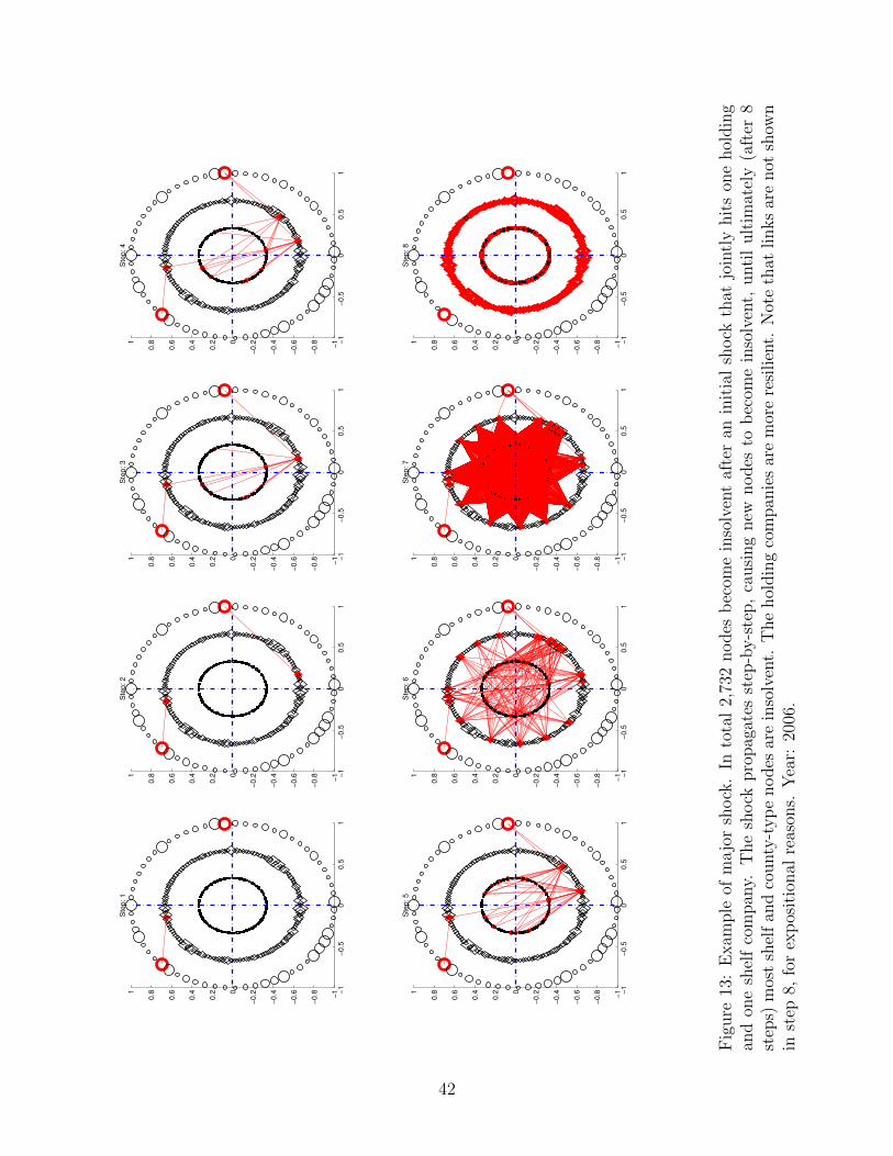
−1

−0.5

00.5

1−

1

−0.8

−0.6

−0.4

−0.20

0.2

0.4

0.6

0.81

Ste

p: 1

−1

−0.5

00.5

1−

1

−0.8

−0.6

−0.4

−0.20

0.2

0.4

0.6

0.81

Ste

p:

2

−1

−0.5

00.5

1−

1

−0.8

−0.6

−0.4

−0.20

0.2

0.4

0.6

0.81

Ste

p:

3

−1

−0

.50

0.5

1−

1

−0

.8

−0

.6

−0

.4

−0

.20

0.2

0.4

0.6

0.81

Ste

p:

4

−1

−0.5

00.5

1−

1

−0.8

−0.6

−0.4

−0.20

0.2

0.4

0.6

0.81

Ste

p: 5

−1

−0.5

00.5

1−

1

−0.8

−0.6

−0.4

−0.20

0.2

0.4

0.6

0.81

Ste

p:

6

−1

−0.5

00.5

1−

1

−0.8

−0.6

−0.4

−0.20

0.2

0.4

0.6

0.81

Ste

p:

7

−1

−0

.50

0.5

1−

1

−0

.8

−0

.6

−0

.4

−0

.20

0.2

0.4

0.6

0.81

Ste

p:

8

Fig

ure

13:

Exam

ple

ofm

ajo

rsh

ock

.In

tota

l2,

732

nodes

bec

ome

inso

lven

taf

ter

anin

itia

lsh

ock

that

join

tly

hit

son

ehol

din

gan

don

esh

elf

com

pan

y.T

he

shock

pro

pag

ates

step

-by-s

tep,

causi

ng

new

nodes

tob

ecom

ein

solv

ent,

unti

lult

imat

ely

(aft

er8

step

s)m

ost

shel

fan

dco

unty

-typ

enodes

are

inso

lven

t.T

he

hol

din

gco

mpan

ies

are

mor

ere

silien

t.N

ote

that

links

are

not

show

nin

step

8,fo

rex

pos

itio

nal

reas

ons.

Yea

r:20

06.

42

the financial market, being caused by an ex ante small shock that propagates and is amplified

within the system, eventually affecting the whole market.

Our estimates of the inherent vulnerability of the 2006 network may thus provide a po-

tentially powerful ex ante indicator of the systemic risks of such networks. Specifically, the

computational algorithm may potentially be applied to an observed network structure to-

gether with ex ante predictions of mortgage foreclosure, solving for the implied unobservable

quality measures of intermediaries, and subsequently stress testing the system with various

shocks.

8 Conclusions

We develop a theoretical model of a network of intermediaries, which we apply to the U.S.

mortgage supply chain. In our model, heterogeneous financial norms and systemic vulner-

abilities arise endogenously. We show that the optimal behavior of each intermediary, in

terms of its attitude toward risk, the quality of the projects that it undertakes, and the

intermediaries it chooses to interact with, is influenced by the behavior of its prospective

counterparties. These network effects, together with the intrinsic differences between in-

termediaries, jointly determine financial health, quality, and systemic vulnerability, at the

aggregate level as well as for individual intermediaries. Our model therefore allows us to

evaluate the relative importance of network effects for intermediary behavior. It also makes

predictions about the conditions under which a network is systemically vulnerable to shocks

and about how such systemic vulnerabilities can be detected empirically.

We apply our model to the mortgage-origination and securitization network of financial

intermediaries, using a large data set of more than twelve million mortgages originated and

securitized through the private-label supply chain from 2002–2007. We show that annual

origination supply chains operate in highly interlinked networks and that the ex post foreclo-

sure rates of loans are quite concentrated in certain parts of the empirical network. We then

apply the model’s computational algorithm to the observed 2006 network of county/lender-

types, securitization shelves, and holding companies., tracking the ex-post foreclosure per-

formance of each loan in the network and compare the evolution of credit risk with the

model’s predictions under different stress scenarios. We find that credit risk evolves in a

concentrated manner among highly linked nodes, defined by the geography of the network

and the interactions between originator and counterparty nodes. This suggests that network

effects are indeed of vital importance for understanding the U.S. mortgage supply chain.

43

A Clearing Algorithm for general network model

Algorithm 1 (Clearing mechanism).

1. Set iteration m = 0 and the initial insolvency vector f1 = 1.

2. Repeat:

• Set m = m+ 1.

• Calculate zm = ΛfmΠΛfmCF P .

• Calculate fnm+1 = X(znMsn

), n = 1, . . . , N .

3. Until fm+1 = fm.

4. Calculate the t = 1 cash flow as CFn

1 = Λfmznm.

The iteration over M can be viewed as showing the gradual propagation of insolvencies,

where fM − fM−1 show the insolvencies that are triggered in step M , by the insolvencies

that occurred in step M − 1.

We can write the algorithm using returns, defining R1 = Λ−1s CF P , and Γ = Λ−1

s Π. The

algorithm then becomes even simpler:

Algorithm 2 (Clearing mechanism on return form).

1. Set iteration m = 0 and the initial insolvency vector f1 = 1.

2. Repeat:

• Set m = m+ 1.

• Calculate zm = ΛfmΓΛfmRm.

• Calculate fm+1 = X(zm).

3. Until fm+1 = fm.

4. Calculate the t = 1 cash flow as CFn

1 = ΛsRm.

It is straightforward to show that the two algorithms are equivalent.

B Network formation game

We describe the network formation game between theN intermediaries/agents. The sequence

of events are as in Figure 2. We use subgame perfect, pairwise stable Nash as the equilibrium

concept. We make one extension of the pairwise stability concept in the definition of agents’

action space. Specifically, agents are allowed to unilaterally decide to become completely

isolated by severing links to all agents they are connected to. In contrast, with the standard

definition of pairwise stability agents are only allowed to sever exactly one link, or propose

44

the addition of one link. The assumption that agents can choose to become isolated can thus

be viewed as a network participation constraint.

The sequence of events is as follows: At t = −2—the proposal/severance stage of the

game—there is a given initial network, E ⊂ E. Recall that E here is the maximal network

in the economy, which arises if all possible links are present. Each agent, n = 1, . . . , N ,

simultaneously chooses from the following mutually exclusive set of actions:

1. Sever links to all other agents and become completely isolated.

2. Sever exactly one existing link to another agent, (n, n′) ∈ E.

3. Propose the formation of a new link to (exactly) one other agent, (n, n′) ∈ E\E.

4. Do nothing.

In contrast to actions 1. and 2., which are unilateral, agent n′ needs to agree for the links

to actually be added to the network under action 3.

The set of networks that can potentially arise from this process is denoted by E . We note

that E ′ ⊂ E for all E ′ ∈ E . The set of actual proposals for addition of links, generated by

actions 3., is denoted by LA. The set of links that are actually severed, generated by actions

1. and 2., is LS. The total set of potential link modifications is L = (LA, LS).At t = −1—the acceptance/decline stage—LA and LS are revealed to all agents, who

then simultaneously choose whether to accept or decline proposed links. Formally, for each

proposed link, ` = (n, n′) ∈ LA, agent n′ chooses an action a` ∈ D,A (representing

the actions of Declining or Accepting the proposed link). The total set of actions is then

A = a` : ` ∈ LA ∈ D,ALA , which for each n′ can be decomposed into An′ ∪ A−n′

,

where An′

= (n, n′) ∈ LA represents the actions taken by agent n′, and A−n′

= A\An′

the actions taken by all other agents. Altogether, E, LA, LD, and A then determines the

resulting network, E ′, after the first two stages of the game, at t = 0.

At t = 0—the quality choice stage—each agent, n = 1, . . . , N , simultaneously chooses

the quality qn ∈ 0, 1. The joint quality actions of all agents are summarized in the action

vector q ∈ 0, 1N .

At t = 1, shocks, ξ, are realized, leading to realized net cash flows wn(ξ|q, E ′) as defined

by equations (13-14). The value of intermediary n at t = 0 is thus

V n(q|E ′) =∑ξ∈Ω

wn(ξ|E ′, q)P(ξ), n = 1, . . . , N. (19)

Equilibrium

An equilibrium to the network formation game is an initial network and quality strategies,

together with a set of beliefs about agent actions for other feasible network structures, such

45

that no agent has an incentive to add or sever links, given that no other agents do so, and

agents’ have consistent beliefs about each others’ behavior on and off the equilibrium path.

Specifically, the action-network pair (q,E), together with t = −1 acceptance strategies:

A : L → D,ALA , and t = 0 quality strategies Q : E → 0, 1N constitute an equilibrium,

if

1. At t = 0, strategies are consistent in that for each E ′ ∈ E , and q = Q(E ′),

qn ∈ arg maxx∈0,1

V n((x, q−n)|E),

for all n = 1, . . . , N , i.e., it is optimal for each agent, n, to choose strategy qn, given

that the other agents choose q−n.

2. At t = −1, strategies are consistent in that for each (LA, LD) ∈ L, An(LA, LD) is

the optimal action for each agent, n, given that the other agents choose A−n(LA, LD).

Optimal here, means that the action maximizes V n at t = 0.

3. At t = −2, the strategy L = ∅ is consistent, i.e., for each agent n, given that no other

agent severs links or proposes additional links, it is optimal for agent n not to do so

either, given the value such actions would lead to at t = −1.

An equilibrium is said to be maximal if E = E.

It follows that the following conditions are necessary and sufficient for there to exists

acceptance and quality strategies such that (q, E) is an equilibrium:

1. For all n, V n(q|E) ≥ V n((¬qn, q−n)|E).

2. For all n, V n(q|E) ≥ V nI .

3. For all (n, n′) ∈ E, ∃q′ ∈ L,HN such that

• V n(q|E) ≥ V n(q′|E − (n, n′)),

• For all n′′, V n′′(q′|E − (n, n′)) ≥ V n′′

((¬(q′)n′′, (q′)−n

′′)|E − (n, n′)),

4. For all (n, n′) ∈ E\E, ∃q′ ∈ L,HN such that

• V n(q|E) ≥ V n(q′|E + (n, n′)) or V n′(q|E) ≥ V n′

(q′|E + (n, n′)),

• For all n′′, V n′′(q′|E + (n, n′)) ≥ V n′′

((¬(q′)n′′, (q′)−n

′′)|E + (n, n′)),

The first condition ensures that each agent makes the optimal quality choice at t = 0, given

that no change to the network is made. The second condition ensures that it is not optimal

for any agent to sever all links and become isolated. The third condition ensures that there

are consistent beliefs about future actions, such that no agent has an incentive to sever a

link at t = −2. The fourth condition ensures that there are consistent beliefs about future

actions, so that no two agents can be made jointly better off by adding a link.

46

References

Acemoglu, Daron, Asuman Ozdaglar, and Alireza Tahbaz-Salehi, 2013, Systemic risk and

stability in financial networks, Working Paper 18727, NBER.

Agarwal, Sumit, David Lucca, Amit Seru, and Francesco Trebbi, 2012, Inconsistent regula-

tors: Evidence from banking, Working paper, University of Chicago.

Allen, Franklin, Ana Babus, and Elena Carletti, 2012, Asset commonality, debt maturity

and systemic risk, Journal of Financial Economics 104, 519–534.

Allen, Franklin, and Douglas Gale, 2000, Financial contagion, Journal of Political Economy

108, 1–33.

Allen, Franklin, and Douglas Gale, 2004, Competition and financial stability, Journal of

Money, Credit and Banking 36, 453–480.

Beck, Thorsten, Diane Coyle, Paul Seabright, and Xavier Freixas, 2010, Bailing out the

banks: Reconciling stability and competition, Working paper, Centre for Economic Policy

Research.

Bresnahan, Timothy F., and Jonathan D. Levin, 2012, Vertical integration and market

structure, NBER Working paper 17889.

Cabrales, Antonio, Piero Gottardi, and Fernando Vega-Redondo, 2014, Risk-sharing and

contagion in networks, Working paper, Universitat Pompeu Fabra.

Calomiris, Charles W., 2006, The regulatory record of the Greenspan Fed, American Eco-

nomic Review, Papers and Proceedings 96, 170–173.

Chen, Yongmin, 2005, Vertical disintegration, Journal of Economics and Management Strat-

egy 14, 209–229.

Claessens, Stijn, 2009, Competition in the financial sector: Overview of competition policies,

Working paper, International Monetary Fund.

Cooter, R. D., 2000, Law from order: Economic development and the jurisprudence of social

norms, in M. Olson, and S. Kahkonen, eds., A Not-So-Dismal Science: A Broader View

of Economics and Societies (Oxford University Press, Oxford).

Ding, Lei, Roberto G. Quercia, Carolina K. Reid, and Alan M. White, 2010, The impact of

federal preemption of state anti-predatory lending laws on the foreclosure crisis, Working

paper, Center for Community Capital, University of North Carolina.

47

Eisenberg, Larry, and Thomas H. Noe, 2001, Systemic risk in financial systems, Management

Science 47, 236–249.

Elliott, Matthew, Benjamin Golub, and Matthew O. Jackson, 2014, Financial networks and

contagion, Working paper, Caltech.

Engel, Kathleen C., and Patricia A. McCoy, 2011, The Subprime Virus: Reckless Credit,

Regulatory Failure, and Next Steps (Oxford University Press, New York).

Fabozzi, F. J., and F. Modigliani, 1992, Mortgage and Mortgage-Backed Securities Markets

(Harvard Business School Press, Boston).

Fligstein, N., 2001, The Architecture of Markets (Princeton University Press, Princeton, NJ).

Follain, J.R., and Peter Zorn, 1990, Unbundling of residential mortgage finance, Journal of

Housing Research 1, 117–137.

Friedkin, Noah E., and Eugene C. Johnsen, 1999, Social influence networks and opinion

change, Advances in Group Processes 16, 1–29.

Froot, Kenneth A., David Scharsfstein, and Jeremy C. Stein, 1993, Risk management: Coor-

dinating corporate investment and financing decisions, Journal of Finance 48, 1629–1658.

Glasserman, Paul, and H. Peyton Young, 2013, How likely is contagion in financial networks?,

Discussion Paper 642, University of Oxford, Department of Economics.

Grossman, Sanford, and Oliver Hart, 1986, The costs and benefits of ownership: A theory

of vertical and lateral integration, Journal of Political Economy 94, 691–719.

Hart, Oliver, 1995, Firms, Contracts, and Financial Structure (Oxford University Press,

Oxford and New York).

Hart, Oliver, and John Moore, 1990, Property rights and the nature of the firm, Journal of

Political Economy 98, 1119–1158.

Holmes, Thomas, 1999, Localization of industry and vertical disintegration, Review of Eco-

nomics and Statistics 81, 314–325.

Holmstrom, Bengt, 1999, The firm as a subeconomy, Journal of Law, Economics, and Or-

ganization 15, 74–102.

Holmstrom, Bengt, and Paul Milgrom, 1994, The firm as an incentive system, American

Economic Review 84, 972–991.

48

Hunt, John Patrick, Richard Stanton, and Nancy Wallace, 2012, All in one basket: The

bankruptcy risk of a national agent-based mortgage recording system, U. C. Davis Law

Review 46, 1–63.

Hunt, John Patrick, Richard Stanton, and Nancy Wallace, 2014, U.S. residential-mortgage

transfer systems: A data-management crisis, in Margarita S. Brose, Mark D. Flood, Dilip

Krishna, and Bill Nichols, eds., Handbook of Financial Data and Risk Information II:

Software and Data, chapter 18 (Cambridge University Press, Cambridge, England).

Jackson, Matthew O., and Dunia Lopez-Pintado, 2013, Diffusion in networks with heteroge-

neous agents and homophily, Network Science 1, 49–67.

Jackson, Matthew O., and Asher Wolinsky, 1996, A strategic model of social and economic

networks, Journal of Economic Theory 71, 44–74.

Jacobides, Michael, 2005, Industry change through vertical disintegration: How and why

markets emerged in mortgage banking, Academy of Management Journal 48, 465–498.

Joskow, Paul L., 2005, Vertical integration, in C. Menard, and M. M. Shirley, eds., Handbook

of New Institutional Economics (Springer, Dordrecht and New York).

Kane, Edward J., 1989, The S&L Insurance Mess: How Did it Happen? (The Urban Institute

Press, Washington, DC).

Langlois, Richard, and Paul L. Robertson, 1992, Networks and innovation in a modular

system: Lessons from the microcomputer and stereo component industries, Research Policy

21, 297–313.

Lopez-Pintado, Dunia, 2012, Influence networks, Games and Economic Networks 75, 776–

787.

MacKenzie, Donald, and Yuval Millo, 2003, Constructing a market, performing theory: The

historical sociology of a financial derivatives exchange, American Journal of Sociology 109,

107–145.

Nier, Erlend W., Jing Yang, Tanju Yorulmazer, and Amadeo Alentorn, 2008, Network models

and financial stability, Working Paper 346, Bank of England.

Pahl, Cynthia, 2007, A compilation of state mortgage broker laws and regulations, 1996–

2006, Community Affairs Report 2007-2, Federal Reserve Bank of Minneapolis.

49

Rosen, Richard J., 2003, Is three a crowd? Competition among regulators in banking,

Journal of Money Credit and Banking 35, 967–998.

Rosen, Richard J., 2005, Switching primary federal regulators: Is it beneficial for U.S. banks?,

Federal Reserve Bank of Chicago Economic Perspectives Q3, 16–33.

Scharfstein, David, and Adi Sunderam, 2013, Concentration in mortgage lending, refinancing

activity, and mortgage rates, Working paper, NBER, forthcoming, American Economic

Review.

Stanton, Richard, Johan Walden, and Nancy Wallace, 2014, The industrial organization of

the U.S. residential mortgage market, Annual Review of Financial Economics 6.

Stigler, George. J., 1951, The division of labor is limited by the extent of the market, Journal

of Political Economy 59, 185–193.

Williamson, Oliver, 1971, The vertical integration of production: Market failure considera-

tions, American Economic Review 61, 112–123.

Williamson, Oliver, 1975, Markets and Hierarchies: Analysis and Antitrust Implications

(Free Press, New York).

Williamson, Oliver, 1979, Transaction-cost economics: The governance of contractual rela-

tions, Journal of Law and Economics 22, 233–261.

Williamson, Oliver, 2010, Transaction cost economics: The natural progression, American

Economic Review 100, 673–690.

50