security of quantum key distribution protocols
TRANSCRIPT

Security of QuantumKey Distribution Protocols
Rotem Liss


Security of QuantumKey Distribution Protocols
Research Thesis
In partial fulfillment of the requirements
for the degree of Doctor of Philosophy
Rotem Liss
Submitted to the Senate
of the Technion — Israel Institute of Technology
Sivan 5781 Haifa May 2021


The research thesis was done under the supervision of Assoc. Prof. Tal Mor in the
Faculty of Computer Science.
Most results in this thesis have been published as articles by the author and research
collaborators in journals and conferences:
1. Michel Boyer, Matty Katz, Rotem Liss, and Tal Mor. Experimentally feasible protocolfor semiquantum key distribution. Physical Review A, 96:062335, Dec 2017. doi:10.1103/
PhysRevA.96.062335. (Chapter 3)
2. Michel Boyer, Rotem Liss, and Tal Mor. Attacks against a simplified experimentallyfeasible semiquantum key distribution protocol. Entropy, 20(7):536, Jul 2018. doi:10.3390/
e20070536. (Chapter 4)
3. Walter O. Krawec, Rotem Liss, and Tal Mor. Security proof against collective attacksfor an experimentally feasible semi-quantum key distribution protocol. arXiv preprintarXiv:2012.02127, Dec 2020. URL: https://arxiv.org/abs/2012.02127. (Chapter 5)
4. Michel Boyer, Rotem Liss, and Tal Mor. Composable security against collective attacks ofa modified BB84 QKD protocol with information only in one basis. Theoretical ComputerScience, 801:96–109, Jan 2020. doi:10.1016/j.tcs.2019.08.014. (Chapter 6)
5. Rotem Liss and Tal Mor. From practice to theory: The “Bright Illumination” attack onquantum key distribution systems. In Carlos Martın-Vide, Miguel A. Vega-Rodrıguez, andMiin-Shen Yang, editors, Theory and Practice of Natural Computing, pages 82–94, Cham, Dec2020. Springer International Publishing. doi:10.1007/978-3-030-63000-3_7. (Chapter 8)
Acknowledgements
I would like to thank my advisor, Assoc. Prof. Tal Mor, for his very helpful guidance,
discussions, ideas, and advice during this research and for his invaluable help and encour-
agement throughout my graduate studies. I would also like to thank Assoc. Prof. Michel
Boyer and Asst. Prof. Walter Krawec for fruitful research collaborations and many
research discussions leading to a variety of results and joint publications.
I would also like to thank Gilles Brassard, Roman Orus, Renato Renner, Rotem
Arnon-Friedman, Andreas Winter, John Smolin, Charles Bennett, David DiVincenzo,
Cica Gustiani, Louis Salvail, Eli Biham, Yossi Weinstein, Roman Shapira, Yair Rezek,
and Itay Fayerverker.
My family deserves special thanks.
The generous financial help of Daniel’s fund, Jacobs’ fund, and the Technion is gratefully
acknowledged.


Contents
List of Figures
Abstract 1
1 Introduction to Quantum Information Processing 3
1.1 Quantum States . . . . . . . . . . . . . . . . . . . . . . . . . . . . . . . 3
1.1.1 Quantum Measurements . . . . . . . . . . . . . . . . . . . . . . . 4
1.1.2 Unitary Operators . . . . . . . . . . . . . . . . . . . . . . . . . . 4
1.2 Bipartite and Multipartite Hilbert Spaces . . . . . . . . . . . . . . . . . 5
1.2.1 Tensor Products of Hilbert Spaces . . . . . . . . . . . . . . . . . 5
1.2.2 Tensor Products of Vectors . . . . . . . . . . . . . . . . . . . . . 5
1.2.3 Tensor Products of Operators . . . . . . . . . . . . . . . . . . . . 6
1.3 Quantum Mixed States . . . . . . . . . . . . . . . . . . . . . . . . . . . 6
1.3.1 Quantum Operations on Mixed States . . . . . . . . . . . . . . . 8
1.3.2 Partial Trace: Removing (Ignoring and Forgetting) a Subsystem 8
1.4 List of Allowed Quantum Operations . . . . . . . . . . . . . . . . . . . . 9
1.5 Trace Distance . . . . . . . . . . . . . . . . . . . . . . . . . . . . . . . . 9
1.5.1 The Information-Theoretical Meaning of the Trace Distance . . . 9
2 Introduction to Quantum Key Distribution 11
2.1 Motivation: Unsolved Encryption Problems in a Non-Quantum World . 11
2.2 Quantum Key Distribution . . . . . . . . . . . . . . . . . . . . . . . . . 12
2.2.1 The QKD Protocol of Bennett and Brassard (BB84) . . . . . . . 13
2.2.2 Types of QKD Protocols . . . . . . . . . . . . . . . . . . . . . . . 13
2.3 Security and Robustness of QKD . . . . . . . . . . . . . . . . . . . . . . 14
2.3.1 Security Definitions and Composable Security . . . . . . . . . . . 14
2.3.2 Collective, “Uniform Collective”, and Joint Attacks . . . . . . . . 16
2.3.3 Different Approaches for Security Proofs . . . . . . . . . . . . . . 17
2.3.4 Robustness Definitions of QKD . . . . . . . . . . . . . . . . . . . 18
2.4 Semiquantum Key Distribution . . . . . . . . . . . . . . . . . . . . . . . 18
2.5 Practical Implementations of QKD Protocols . . . . . . . . . . . . . . . 20
2.5.1 The Fock Space Notations . . . . . . . . . . . . . . . . . . . . . . 20

2.5.2 Experimental Implementations of Polarization-Based QKD . . . 21
2.5.3 Practical Attacks . . . . . . . . . . . . . . . . . . . . . . . . . . . 22
2.6 Hoeffding’s Theorem . . . . . . . . . . . . . . . . . . . . . . . . . . . . . 23
2.7 Notation for Bit Strings . . . . . . . . . . . . . . . . . . . . . . . . . . . 25
2.8 Structure of this Thesis . . . . . . . . . . . . . . . . . . . . . . . . . . . 25
3 The Mirror Protocol and Robustness Proof 27
3.1 Experimental Infeasibility of the SIFT Operation in SQKD Protocols . . 27
3.2 The Mirror Protocol . . . . . . . . . . . . . . . . . . . . . . . . . . . . . 28
3.3 Robustness Analysis . . . . . . . . . . . . . . . . . . . . . . . . . . . . . 32
3.4 Conclusion . . . . . . . . . . . . . . . . . . . . . . . . . . . . . . . . . . 36
4 Attacks Against a Simplified Variant of the Mirror Protocol 37
4.1 The Simplified Mirror Protocol . . . . . . . . . . . . . . . . . . . . . . . 37
4.2 Attacks Against the Simplified Mirror Protocol . . . . . . . . . . . . . . 39
4.2.1 A Full Attack on the Simplified Protocol . . . . . . . . . . . . . . 39
4.2.2 A Weaker Attack on the Simplified Protocol . . . . . . . . . . . . 41
4.3 Conclusion . . . . . . . . . . . . . . . . . . . . . . . . . . . . . . . . . . 44
5 Security of the Mirror Protocol Against Uniform Collective Attacks 45
5.1 Introduction . . . . . . . . . . . . . . . . . . . . . . . . . . . . . . . . . . 45
5.2 The Mirror Protocol: a Concise Description . . . . . . . . . . . . . . . . 46
5.3 Security Proof of the Mirror Protocol Against Uniform Collective Attacks 48
5.3.1 Eve’s Attacks . . . . . . . . . . . . . . . . . . . . . . . . . . . . . 48
5.3.2 Analyzing all Types of Rounds . . . . . . . . . . . . . . . . . . . 49
5.3.3 “Raw Key” Rounds: Alice Chooses the SWAP-x Operation . . . 51
5.3.4 “Test” Rounds: Alice Chooses the CTRL Operation . . . . . . . 53
5.3.5 “SWAP-ALL” Rounds: Alice Chooses the SWAP-ALL Operation,
and Bob Chooses the z Basis . . . . . . . . . . . . . . . . . . . . 55
5.3.6 Deriving the Final Key Rate . . . . . . . . . . . . . . . . . . . . 57
5.3.7 Algorithm for Computing the Key Rate . . . . . . . . . . . . . . 59
5.4 Examples . . . . . . . . . . . . . . . . . . . . . . . . . . . . . . . . . . . 60
5.4.1 First Scenario: Single-Photon Attacks without Losses . . . . . . 60
5.4.2 Second Scenario: Single-Photon Attacks with Losses . . . . . . . 61
5.4.3 Evaluation Results . . . . . . . . . . . . . . . . . . . . . . . . . . 61
5.5 Conclusion . . . . . . . . . . . . . . . . . . . . . . . . . . . . . . . . . . 65
6 Composable Security of the “BB84-INFO-z” Protocol Against Collec-
tive Attacks 67
6.1 Introduction . . . . . . . . . . . . . . . . . . . . . . . . . . . . . . . . . . 67
6.2 Full Definition of the “BB84-INFO-z” Protocol . . . . . . . . . . . . . . 68
6.3 Security Proof for the BB84-INFO-z Protocol Against Collective Attacks 69

6.3.1 The General Collective Attack of Eve . . . . . . . . . . . . . . . 69
6.3.2 Results from [BGM09] . . . . . . . . . . . . . . . . . . . . . . . . 70
6.3.3 Bounding the Differences Between Eve’s States . . . . . . . . . . 71
6.3.4 Proof of Security . . . . . . . . . . . . . . . . . . . . . . . . . . . 74
6.3.5 Reliability . . . . . . . . . . . . . . . . . . . . . . . . . . . . . . . 75
6.3.6 Proof of Fully Composable Security . . . . . . . . . . . . . . . . 75
6.3.7 Security, Reliability, and Error Rate Threshold . . . . . . . . . . 79
6.4 Conclusion . . . . . . . . . . . . . . . . . . . . . . . . . . . . . . . . . . 79
7 Composable Security of Generalized BB84 Protocols Against General
(Joint) Attacks 83
7.1 Full Definition of the Generalized BB84 Protocols . . . . . . . . . . . . . 83
7.2 Bound on the Security Definition for the Generalized BB84 Protocols . 85
7.2.1 The Hypothetical “Inverted-INFO-Basis” Protocol . . . . . . . . 85
7.2.2 The General Joint Attack of Eve . . . . . . . . . . . . . . . . . . 86
7.2.3 The Symmetrized Attack of Eve . . . . . . . . . . . . . . . . . . 87
7.2.4 Results from [BBBMR06] . . . . . . . . . . . . . . . . . . . . . . 89
7.2.5 Bounding the Differences Between Eve’s States . . . . . . . . . . 90
7.2.6 Bound for Fully Composable Security . . . . . . . . . . . . . . . 94
7.3 Full Security Proofs for Specific Protocols . . . . . . . . . . . . . . . . . 100
7.3.1 The BB84-INFO-z Protocol . . . . . . . . . . . . . . . . . . . . . 100
7.3.2 The Standard BB84 Protocol . . . . . . . . . . . . . . . . . . . . 103
7.3.3 The “Efficient BB84” Protocol . . . . . . . . . . . . . . . . . . . 105
7.3.4 The “Modified Efficient BB84” Protocol . . . . . . . . . . . . . . 112
8 From Practice to Theory: the “Bright Illumination” Attack on Quan-
tum Key Distribution Systems 117
8.1 Introduction . . . . . . . . . . . . . . . . . . . . . . . . . . . . . . . . . . 117
8.2 Imperfections in Experimental Implementation of QKD . . . . . . . . . 118
8.3 The “Bright Illumination” Attack . . . . . . . . . . . . . . . . . . . . . . 119
8.4 “Reversed-Space” Attacks . . . . . . . . . . . . . . . . . . . . . . . . . . 120
8.5 Quantum Side-Channel Attacks . . . . . . . . . . . . . . . . . . . . . . . 123
8.6 From Practice to Theory: The Possibility of Predicting the “Bright
Illumination” Attack . . . . . . . . . . . . . . . . . . . . . . . . . . . . . 124
8.7 Conclusion . . . . . . . . . . . . . . . . . . . . . . . . . . . . . . . . . . 126
9 Summary 127
Hebrew Abstract i


List of Figures
3.1 A schematic diagram of the Mirror protocol described in Sec-
tion 3.2. This figure was generated by Walter O. Krawec for [KLM20]
(Chapter 5). . . . . . . . . . . . . . . . . . . . . . . . . . . . . . . . . . . 29
5.1 A graph of the final key rate versus the noise level of the Mirror
protocol in the first scenario (single-photon attacks without losses),
for dependent (QX = QZ) and independent (QX = 2QZ(1−QZ)) noise
models, compared to two copies of BB84. . . . . . . . . . . . . . . . . . 63
5.2 A graph of the final key rate versus the noise level of the Mirror
protocol in the second scenario (single-photon attacks with losses),
compared to two copies of BB84, for two possible lengths of fiber channels
(` = 10km and ` = 50km). . . . . . . . . . . . . . . . . . . . . . . . . . . 64
6.1 The secure asymptotic error rates zone for BB84-INFO-z (below
the curve) . . . . . . . . . . . . . . . . . . . . . . . . . . . . . . . . . . . 80
7.1 The secure asymptotic error rates zone for BB84-INFO-z (below
the curve) . . . . . . . . . . . . . . . . . . . . . . . . . . . . . . . . . . . 103


Abstract
The counter-intuitive features of quantum mechanics make it possible to solve problems
and perform tasks that are beyond the abilities of non-quantum (classical) computers
and communication devices. The field of quantum information processing studies how
we can achieve such improvements by representing information as quantum states.
One of the early achievements of quantum information processing is the development
of quantum key distribution (QKD). QKD protocols allow two participants (Alice and
Bob) to achieve the classically-impossible task of generating a secret shared key even if
their adversary is computationally unlimited.
Unfortunately, the security promises of QKD are true only in theory; practical
implementations of QKD deviate from the theoretical protocols, and many of these
deviations give rise to practical attacks. In this research thesis, we study the security
properties of various QKD protocols in many practical settings:
First, we study practical security of semiquantum key distribution (SQKD) protocols,
where either Alice or Bob is non-quantum (classical). Following practical security
problems in previous SQKD protocols, we suggest a new SQKD protocol (the “Mirror
protocol”) which can be securely implemented, and we prove it robust and secure against
a wide range of attacks (the “uniform collective attacks”).
Then, we study “composable security” of the first QKD protocol created by Bennett
and Brassard (BB84). BB84 has its unconditional security proved against adversaries
performing the most general attacks in a theoretical (idealized) setting; however, some
security approaches do not prove “composable security”, which requires the secret key
to remain secret even when Alice and Bob actually use it for cryptographic purposes.
We generalize an algebraic security approach for BB84, making it prove composable
security of BB84 (and many variants of BB84) against the most general attacks.
Finally, we analyze an important practical attack (named “Bright Illumination”),
showing how it can be modeled as a theoretical “Reversed-Space” attack.
Overall, all results aim to enhance our understanding on how to bridge the gap
between theory and practice in various sub-fields of QKD, and they may help solve a
major open problem in the field of QKD: constructing a realistic QKD implementation
that can be proved truly and unconditionally secure against any possible attack.
1

2

Chapter 1
Introduction to Quantum
Information Processing
The field of quantum information processing (QIP) uses the laws of quantum physics
for performing tasks that are impossible (or hard) in the non-quantum world.
In this chapter, we describe the basic notions of QIP that are used in this thesis.
See [NC00, Gru99, RP00, GMD02] for more background and explanations about QIP.
1.1 Quantum States
In QIP, information is represented by quantum states. A quantum state is the state
of a specific physical system; all possible quantum states of the system belong to a
Hilbert space, which is defined as a vector space over the field C (the field of complex
numbers) that has an inner product and satisfies the “completeness” property (the exact
definition of this property can be found in standard textbooks, and it is satisfied by all
finite-dimensional inner product spaces). A quantum pure state is represented by |ψ〉,which denotes a normalized column vector (namely, a column vector of norm 1) in the
Hilbert space. In other words, the Hilbert space is the set of all possible quantum pure
states of a system (including the non-normalized states).
As an important example, the qubit Hilbert space is H2 , Span{|0〉, |1〉}, where
|0〉 and |1〉 are two orthonormal vectors (namely, they are normalized, and their inner
product is 0). Two other important orthonormal states in H2 are |+〉 , |0〉+|1〉√2
and
|−〉 , |0〉−|1〉√2
. The most general qubit pure state is |ψ〉 = α|0〉+ β|1〉, where α, β ∈ Cand |α|2 + |β|2 = 1 (a normalization condition). The qubit states are sometimes denoted
by their vector representations in the {|0〉, |1〉} basis: |0〉 =
(1
0
), |1〉 =
(0
1
),
|+〉 = 1√2
(1
1
), |−〉 = 1√
2
(1
−1
), and |ψ〉 =
(α
β
). We note that {|0〉, |1〉} is an
orthonormal basis named “the z basis”, “the computational basis”, or “the standard
basis”, and {|+〉, |−〉} is an orthonormal basis named “the x basis” or “the Hadamard
3

basis”. We also note various notations of both bases: the states of the z basis are
sometimes denoted {|00〉, |10〉} or {|0〉0, |1〉0}, and the states of the x basis are sometimes
denoted {|01〉, |11〉} or {|0〉1, |1〉1}.We note that multiplying a pure state |ψ〉 by any global phase eiφ , cos(φ) + i sin(φ)
has no physical significance. In other words, two pure states that differ only by a global
multiplicative phase eiφ are identical for all intents and purposes.
The |ψ〉 notation (the column vector) is named ket. A related notation, 〈ψ|, is named
bra, and it is a row vector defined by 〈ψ| , [|ψ〉]†: namely, the bra is the conjugate
transpose of the ket. For example, if |ψ〉 = α|0〉+ β|1〉, then 〈ψ| = α?〈0|+ β?〈1| (where
α? is the complex conjugate of α); in vector notations, 〈ψ| =(α? β?
).
Given an orthonormal basis {|ψ1〉, |ψ2〉, . . . , |ψm〉}, the inner product of two pure
states |ψ〉 =∑m
j=1 αj |ψj〉 and |φ〉 =∑m
j=1 βj |ψj〉 is 〈ψ|φ〉 ,∑m
j=1 α?jβj . The norm of |ψ〉
is |||ψ〉|| ,√〈ψ|ψ〉 =
√∑mj=1 |αj |2, and |ψ〉 is said to be normalized if
∑mj=1 |αj |2 = 1.
1.1.1 Quantum Measurements
Quantum physics allows us to measure a quantum state |ψ〉 with respect to any
orthonormal basis {|ψ1〉, |ψ2〉, . . . , |ψm〉}. The possible measurement outcomes are all
states “ψj” of this orthonormal basis; each outcome “ψj” (corresponding to the quantum
state |ψj〉) is obtained with probability pj = |〈ψj |ψ〉|2. Note that∑m
j=1 pj = 〈ψ|ψ〉 = 1.
Also note that a measurement result “ψj” is a classical (non-quantum) indicator that can
be read and used; we have not discussed the resulting quantum state after measurement,
but we should note that the original quantum state |ψ〉 may be ruined (or change its
state) following the measurement operation.
For example, if the quantum state |ψ〉 = α|0〉+ β|1〉 is measured with respect to the
orthonormal basis {|0〉, |1〉} (namely, it is “measured in the z basis”), the “0” result is
obtained with probability |〈0|ψ〉|2 = |α|2, and the “1” result is obtained with probability
|〈1|ψ〉|2 = |β|2. Notice that the normalization condition |α|2 + |β|2 = 1 means that
these two probabilities sum to 1.
There are also generalized definitions of quantum measurements (see, e.g., in [NC00]),
but they can all be reduced to the set of quantum operations described in Section 1.4.
1.1.2 Unitary Operators
Quantum physics allows us to apply any unitary operator U : H → H to a quantum state
in the Hilbert space H. Unitary operators are linear operators (namely, U [α|ψ〉+β|φ〉] =
αU |ψ〉+ βU |φ〉) that satisfy U † = U−1. They preserve inner products and norms.
As an important example, the Hadamard operator on the qubit space is defined by
H , 1√2
(1 1
1 −1
): namely, H|0〉 = |+〉 and H|1〉 = |−〉. It also satisfies H|+〉 = |0〉
and H|−〉 = |1〉.
4
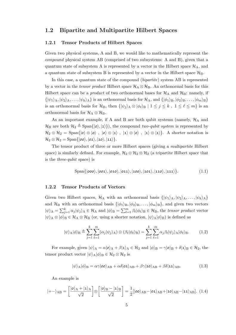
1.2 Bipartite and Multipartite Hilbert Spaces
1.2.1 Tensor Products of Hilbert Spaces
Given two physical systems, A and B, we would like to mathematically represent the
compound physical system AB (comprised of two subsystems: A and B), given that a
quantum state of subsystem A is represented by a vector in the Hilbert space HA, and
a quantum state of subsystem B is represented by a vector in the Hilbert space HB.
In this case, a quantum state of the compound (bipartite) system AB is represented
by a vector in the tensor product Hilbert space HA⊗HB. An orthonormal basis for this
Hilbert space can be a product of two orthonormal bases for HA and HB: namely, if
{|ψ1〉A, |ψ2〉A, . . . , |ψk〉A} is an orthonormal basis for HA, and {|φ1〉B, |φ2〉B, . . . , |φm〉B}is an orthonormal basis for HB, then {|ψj〉A ⊗ |φ`〉B | 1 ≤ j ≤ k , 1 ≤ ` ≤ m} is an
orthonormal basis for HA ⊗HB.
As an important example, if A and B are both qubit systems (namely, HA and
HB are both H2 , Span{|0〉, |1〉}), the compound two-qubit system is represented by
H2 ⊗ H2 = Span{|0〉 ⊗ |0〉 , |0〉 ⊗ |1〉 , |1〉 ⊗ |0〉 , |1〉 ⊗ |1〉}. A shorter notation is
H2 ⊗H2 = Span{|00〉, |01〉, |10〉, |11〉}.The tensor product of three or more Hilbert spaces (giving a multipartite Hilbert
space) is similarly defined. For example, H2 ⊗H2 ⊗H2 (a tripartite Hilbert space that
is the three-qubit space) is
Span{|000〉, |001〉, |010〉, |011〉, |100〉, |101〉, |110〉, |111〉}. (1.1)
1.2.2 Tensor Products of Vectors
Given two Hilbert spaces, HA with an orthonormal basis {|ψ1〉A, |ψ2〉A, . . . , |ψk〉A}and HB with an orthonormal basis {|φ1〉B, |φ2〉B, . . . , |φm〉B}, and given two vectors
|ψ〉A =∑k
j=1 αj |ψj〉A ∈ HA and |φ〉B =∑m
`=1 β`|φ`〉B ∈ HB, the tensor product vector
|ψ〉A ⊗ |φ〉B ∈ HA ⊗HB (or, using a shorter notation, |ψ〉A|φ〉B) is defined as
|ψ〉A|φ〉B ,k∑j=1
m∑`=1
(αj |ψj〉A)⊗ (β`|φ`〉B) =
k∑j=1
m∑`=1
αjβ`|ψj〉A|φ`〉B. (1.2)
For example, given |ψ〉A = α|0〉A + β|1〉A ∈ H2 and |φ〉B = γ|0〉B + δ|1〉B ∈ H2, the
tensor product vector |ψ〉A|φ〉B ∈ H2 ⊗H2 is
|ψ〉A|φ〉B = αγ|00〉AB + αδ|01〉AB + βγ|10〉AB + βδ|11〉AB. (1.3)
An example is
|+−〉AB =
[|0〉A + |1〉A√
2
]⊗[|0〉B − |1〉B√
2
]=
1
2[|00〉AB−|01〉AB+|10〉AB−|11〉AB]. (1.4)
5

We note that most states in HA ⊗HB are not tensor product vectors, and are thus
called entangled. Four important entangled two-qubit states (that form together an
orthonormal basis of H2 ⊗H2, named the Bell basis or the BMR basis) are:
|Φ+〉 ,|00〉+ |11〉√
2, |Φ−〉 ,
|00〉 − |11〉√2
, (1.5)
|Ψ+〉 ,|01〉+ |10〉√
2, |Ψ−〉 ,
|01〉 − |10〉√2
. (1.6)
The definition of the tensor product is easily generalized to tensor products of three
(or more) vectors: for example,
|+0−〉ABC =
[|0〉A + |1〉A√
2
]⊗ |0〉B ⊗
[|0〉C − |1〉C√
2
]=
1
2[|000〉ABC − |001〉ABC + |100〉ABC − |101〉ABC]. (1.7)
1.2.3 Tensor Products of Operators
Given two linear operators, U operating on the Hilbert space HA and V operating on
the Hilbert space HB, the linear operator U ⊗V operates on the Hilbert space HA⊗HB
and is defined as follows:
(U ⊗ V )(|ψ〉A ⊗ |φ〉B) , (U |ψ〉A)⊗ (V |φ〉B). (1.8)
(It extends by linearity to vectors that are not tensor products, such as |00〉AB+|11〉AB√2
.)
For example, the tensor product of the Hadamard operator H with itself, denoted
H ⊗H or H⊗2, operates as follows:
H⊗2|00〉AB = (H|0〉A)⊗ (H|0〉B) = |++〉AB , (1.9)
H⊗2|01〉AB = (H|0〉A)⊗ (H|1〉B) = |+−〉AB , (1.10)
H⊗2|10〉AB = (H|1〉A)⊗ (H|0〉B) = |−+〉AB , (1.11)
H⊗2|11〉AB = (H|1〉A)⊗ (H|1〉B) = |−−〉AB . (1.12)
This definition is generalized to tensor products of three (or more) operators.
1.3 Quantum Mixed States
A quantum mixed state is a probability distribution over several pure states: namely, it
is a set {(|ψj〉, qj)}j consisting of pairs of pure states |ψj〉 and probabilities qj (where
0 < qj ≤ 1 and∑
j qj = 1), meaning that each pure state |ψj〉 has probability qj .
Unlike a pure state, a mixed state is not represented by a vector in Hilbert space. It
is represented by a density matrix: ρ =∑
j qj |ψj〉〈ψj |, where qj is the probability of
the pure state |ψj〉. (This definition of qj should not be confused with the probabilities
6

of measurement results, mentioned in Subsection 1.1.1.) In particular, the pure state
|ψ〉 is represented by the density matrix ρ = |ψ〉〈ψ|.For example, if the system is prepared in state |0〉 with probability 1
3 or in state
|+〉 with probability 23 , the corresponding quantum mixed state has density matrix
ρ = 13 |0〉〈0|+
23 |+〉〈+|. It should be emphasized that these probabilities are of preparation,
not of any measurement. For example, if this state is measured in the z basis {|0〉, |1〉},the probability of measuring “0” is 1
3 · 1 + 23 ·
12 = 2
3 , and the probability of measuring
“1” is 13 · 0 + 2
3 ·12 = 1
3 ; and if the state is measured in the x basis {|+〉, |−〉}, the
probability of measuring “+” is 13 ·
12 + 2
3 · 1 = 56 , and the probability of measuring “−”
is 13 ·
12 + 2
3 · 0 = 16 . Notice that the probability of measuring “0” is not 1
3 , and the
probability of measuring “+” is not 23 .
We note that several different probability distributions may represent the same mixed
state: namely, the states they represent are physically identical (e.g., giving exactly the
same measurement results in all orthonormal bases). This happens if and only if they
are represented by equal density matrices. (A similar observation is that a global phase
eiφ for pure states has no physical significance; and, indeed, the two pure states |ψ〉and eiφ|ψ〉 are represented by identical density matrices, ρ = |ψ〉〈ψ|.) For example, the
completely mixed state ρ = 12 |0〉〈0|+
12 |1〉〈1| is the same as ρ = 1
2 |+〉〈+|+12 |−〉〈−|, and
these two density matrices are equal.
A density matrix must always satisfy three conditions: (a) it is a Hermitian matrix;
(b) it is positive semidefinite; and (c) it is normalized (namely, its trace equals 1).
These three conditions are also sufficient : any matrix ρ satisfying them is a density
matrix. From these conditions it follows that any density matrix ρ can be presented as
ρ =∑
j λj |ψj〉〈ψj | (the spectral decomposition), where λj ≥ 0,∑
j λj = 1, and {|ψj〉}jis an orthonormal set (of eigenvectors); in other words, for any mixed state we can
choose a corresponding probability distribution over a set of orthonormal states. For
example, for ρ = 13 |0〉〈0|+
23 |+〉〈+|, the spectral decomposition is
ρ =3 +√
5
6
[2|0〉+ (
√5− 1)|1〉√
10− 2√
5
][2〈0|+ (
√5− 1)〈1|√
10− 2√
5
]
+3−√
5
6
[2|0〉 − (
√5 + 1)|1〉√
10 + 2√
5
][2〈0| − (
√5 + 1)〈1|√
10 + 2√
5
], (1.13)
and it is the unique decomposition of ρ as a mixture of orthonormal pure states; on
the other hand, the completely mixed state ρ = 12 |0〉〈0|+
12 |1〉〈1| =
12 |+〉〈+|+
12 |−〉〈−|
has an infinite number of decompositions as a mixture of orthonormal pure states,
because its eigenvalue (12) is degenerate—namely, it has two orthonormal eigenvectors
corresponding to the same eigenvalue.
The probability distribution in the definition of mixed states represents the “standard”
(“classical”) notion of uncertainty, and not a quantum phenomenon: it simply represents
a lack of knowledge. Nonetheless, mixed states naturally appear in many areas of QIP. For
7

example, if a joint system AB is in the entangled pure state√
13 |0〉A|0〉B +
√23 |1〉A|+〉B,
the quantum state of subsystem B is the mixed state ρ = 13 |0〉B〈0|B + 2
3 |+〉B〈+|B(see Subsection 1.3.2 for details about this computation) that we have seen before.
Moreover, we note that the state of the joint system AB can also be represented as√56 |+〉A
2|0〉B+|1〉B√5−√
16 |−〉A|1〉B; thus, the state of subsystem B can also be represented
as ρ = 56
[2|0〉B+|1〉B√
5
] [2〈0|B+〈1|B√
5
]+ 1
6 |1〉B〈1|B. This is another example of multiple
probability distributions corresponding to the same mixed state.
We should note an important difference between pure states and mixed states:
for a pure state |ψ〉, there exists an orthonormal basis (consisting of |ψ〉 itself and
states orthonormal to it) such that if we measure |ψ〉 in this basis, we obtain a specific
measurement result (“ψ”) for certain. This claim is never true for a mixed state ρ: if
we measure ρ in any orthonormal basis, the measurement result is always uncertain.
1.3.1 Quantum Operations on Mixed States
Two important results (that can be mathematically proved) are:
• If we measure a mixed state ρ in some orthonormal basis {|ψ1〉, |ψ2〉, . . . , |ψm〉},we get the measurement result “ψj” with probability pj = 〈ψj | ρ |ψj〉.
• If we apply a unitary operator U to a mixed state ρ, the resulting state is the
mixed state UρU †.
1.3.2 Partial Trace: Removing (Ignoring and Forgetting) a Subsystem
Sometimes, we would like to compute the quantum state of a specific subsystem, while
ignoring and forgetting the other subsystems. For example, given a tripartite quantum
state ρABE (shared by three parties named Alice (A), Bob (B), and Eve (E)), we may
want to ignore the two subsystems A,B and look only at the state of Eve’s subsystem E.
In other words, we may want to assume that subsystems A,B will never be accessible
to Eve (maybe they will be measured by Alice and Bob, who will then forget the
measurement results or keep them secret) and find the state ρE of subsystem E.
The mathematical operation corresponding to this scenario is the partial trace. The
partial trace of a bipartite state ρXY over subsystem X is defined as follows:
ρY = trX(ρXY) ,∑|x〉∈X
〈x| ρXY |x〉 , (1.14)
where X is an arbitrary orthonormal basis of the Hilbert space HX corresponding to
subsystem X. The result of this computation is the quantum state ρY of subsystem Y.
In the above example, the partial trace of ρABE over subsystems A,B is:
ρE = trAB(ρABE) ,∑
|a〉∈A,|b〉∈B
〈a| 〈b| ρABE |a〉 |b〉, (1.15)
8

where A,B are some arbitrary orthonormal bases of the Hilbert spaces HA,HB corre-
sponding to subsystems A,B.
For example, the partial trace of the two-qubit pure state |ψ〉XY =√
13 |0〉X|−〉Y +√
23 |1〉X|+〉Y over subsystem X is
ρY = trX(|ψ〉XY〈ψ|XY) =1
3|−〉Y〈−|Y +
2
3|+〉Y〈+|Y, (1.16)
and the partial trace of the same state |ψ〉XY over subsystem Y is
ρX = trY(|ψ〉XY〈ψ|XY) =1
3|0〉X〈0|X +
2
3|1〉X〈1|X. (1.17)
More details about the partial trace are available in standard QIP textbooks (e.g., [NC00]).
1.4 List of Allowed Quantum Operations
1. measuring the state with respect to an orthonormal basis (Subsection 1.1.1);
2. applying a unitary operator (Subsection 1.1.2);
3. adding a new (ancillary) subsystem; and
4. removing (ignoring and forgetting) a subsystem (Subsection 1.3.2).
1.5 Trace Distance
The trace distance between two quantum states is, informally, a measure of their
distinguishability. This measure is very useful for security definitions of quantum key
distribution protocols (see details in Subsection 2.3.1).
The trace distance of two states ρ and σ is defined as follows:
D(ρ, σ) ,1
2tr |ρ− σ| = 1
2
∑j
|λj |, (1.18)
where {λj}j are the eigenvalues of ρ− σ, all of which are real numbers. (We note that
|A| is defined as√A†A.) In other words, the trace distance D(ρ, σ) is one half of the
sum of absolute values of the eigenvalues of ρ− σ.
1.5.1 The Information-Theoretical Meaning of the Trace Distance
It can be proved [FvdG99, BBBGM02] that the trace distance D(ρ, σ) between two
quantum states ρ and σ upper-bounds the Shannon Distinguishability between ρ and σ.
The Shannon Distinguishability is defined as the classical mutual information between
the random variable T ,
0 The quantum state is ρ
1 The quantum state is σand the random variable X (the
9

result of a measurement), maximized over all possible quantum measurements (including
measurements consisting of adding an ancillary state, performing a general unitary
transformation, and then measuring in some orthonormal basis).
In other words, the trace distance upper-bounds the information that some user,
who holds a quantum state and does not know whether it is ρ or σ (it can be either ρ
or σ, with equal probabilities), can find by using a measurement.
Examples:
• D(|0〉〈0|, |1〉〈1|) = 1, because the two quantum states |0〉 and |1〉 can be distin-
guished for certain by measuring in the z basis {|0〉, |1〉}.
• D(|0〉〈0|, |0〉〈0|) = 0, because the two quantum state |0〉 and |0〉 are identical, so
they cannot be distinguished from each other at all.
10

Chapter 2
Introduction to Quantum Key
Distribution
The properties of quantum mechanics permit cryptographic protocols that are more
secure than standard (“classical” or “non-quantum”) protocols. Quantum key distribu-
tion (QKD) protocols allow two users, conventionally named Alice and Bob, to generate
a secret shared key. This thesis is devoted to studying security properties of QKD
protocols.
In this chapter, we describe relevant existing knowledge in the research field of QKD.
In particular, we discuss security definitions of QKD and the notion of semiquantum
key distribution (SQKD) protocols.
2.1 Motivation: Unsolved Encryption Problems in a Non-
Quantum World
Cryptography is the science of protecting security and correctness of data against
adversaries. One of the most important cryptographic problems is encryption—namely,
transmitting a secret message from a sender (Alice) to a receiver (Bob), and ensuring
the adversary (Eve) cannot read it. Two main encryption methods are used today:
• Symmetric-key cryptography, in which the same secret key is used by both Alice
and Bob: Alice uses the secret key for encrypting her message, and Bob uses the
same secret key for decrypting the message. Several examples of symmetric-key
ciphers are the Advanced Encryption Standard (AES) [DR13], the older Data
Encryption Standard (DES), and one-time pad (“Vernam cipher”).
• Public-key cryptography [DH76], in which a public key (known to everyone) and
a secret key (known only to Bob) are used: Alice uses the public key for en-
crypting her message, and Bob uses the secret key for decrypting the message.
Several examples of public-key ciphers include RSA [RSA78] and elliptic curve
cryptography.
11

However:
• Current public-key cryptography is not formally proved secure; moreover, its
security is only computational—namely, it relies on computational hardness of spe-
cific problems, such as integer factorization and discrete logarithm. Furthermore,
factorization and discrete logarithm can both be efficiently solved on a quantum
computer by using Shor’s factorization algorithm [Sho94, Sho99]; therefore, if a
scalable quantum computer is successfully built in the future, it will break security
of many public-key ciphers, including RSA and elliptic curve cryptography.
• Symmetric-key cryptography requires Alice and Bob to share a secret key in
advance: namely, if Alice and Bob want to share a secret message, they must
share a secret key beforehand. Moreover, no computational security proofs are
known for many current symmetric-key ciphers, including AES and DES; and
unconditional security against computationally-unlimited adversaries has been
proved to require many resources: the secret key must be used only once and be
at least as long as the secret message [Sha49].
Nonetheless, there exist ciphers that are fully and unconditionally secure (even against
computationally-unlimited adversaries). For example, the one-time pad (symmetric-
key) cipher is defined as follows: given a message M and a secret key K of the same
length, the encrypted message C is computed as the XOR between M and K—namely,
C = M ⊕K (decryption can then be performed by computing M = C ⊕K). One-time
pad has been proved fully and unconditionally secure against any adversary [Sha49]:
even if the adversary Eve intercepts the encrypted message C, she gains no information
on the original message M (assuming she has no information on the secret key K; in
particular, assuming K is used only once).
Therefore, for achieving perfectly secure encryption, we only need an efficient way for
sharing a random secret key between Alice and Bob—a task named “key distribution”.
Unfortunately, unconditionally secure “classical [non-quantum] key distribution” is
impossible if the computationally-unlimited adversary can listen to all communication
between Alice and Bob. Fortunately, quantum key distribution can solve this problem.
2.2 Quantum Key Distribution
Quantum key distribution (QKD) protocols allow Alice and Bob to generate a shared
random key. Typically, they require Alice and Bob to use two communication channels:
(a) an insecure quantum channel (to which Eve may apply any operation allowed by
the laws of quantum physics), and (b) an unjammable classical channel (to which Eve
may listen, but not interfere). Eve listens to both channels and tries obtaining as much
information as she can on the final shared key.
For most QKD protocols, the final key is proved to be secret even from the most
powerful adversaries—adversaries who are limited only by the laws of nature and
12

who are otherwise capable of solving any computational problem and performing any
physically-allowed operation. Moreover, the final key is proved to remain secret in the
future, even if Eve improves her computational power and other capabilities.
After creating the shared key, Alice and Bob can use it for other cryptographic
tasks (e.g., one-time pad encryption). More generally, QKD protocols can be used as a
subroutine (secure key distribution) of more complicated cryptographic protocols; in
other words, we can integrate QKD into a system to improve its security. See [SML10]
for more details about this integration and the practical usability of QKD compared to
other methods.
2.2.1 The QKD Protocol of Bennett and Brassard (BB84)
The first and most important QKD protocol, suggested by Bennett and Brassard in
1984, is BB84 [BB84].
In the BB84 protocol, in each round, Alice randomly chooses one of the four possible
“BB84 (qubit) states” {|0〉, |1〉, |+〉, |−〉} and sends it to Bob. Bob randomly chooses one
of two orthonormal bases (z or x, both defined in Section 1.1) and measures the state
in his chosen basis. If Bob chooses the same basis as Alice (assuming that Eve did not
interfere), Bob will get the same result as Alice; and if Bob chooses a different basis
from Alice (assuming, again, that Eve did not interfere), Bob will get a random result
(each result with probability 12). For example, if Alice sends |+〉 and Bob measures it in
the x basis, he will get the “+” result for certain; but if Bob measures it in the z basis,
he will get a random result (either “0” or “1”).
After sending and receiving N qubits (in N rounds), Alice and Bob perform “classical
post-processing” (namely, they process their results in a coordinated way, exchanging
information via the unjammable classical channel), comprised of the following steps:
1. Alice and Bob expose and compare the bases they chose and discard the qubits
for which they chose different bases.
2. Alice and Bob expose and compare a randomly chosen subset of their bits (named
“the TEST bits”), check the error rate in this subset, and abort the protocol if the
error rate is above a specific threshold. The remaining bits are “the INFO bits”.
3. Alice and Bob perform error correction and privacy amplification processes on the
INFO bits, so that both of them have the same bit string (the final key) and Eve’s
average information about it is negligible—namely, exponentially small in N .
Full definitions of BB84 and several variants are available in Sections 6.2 and 7.1.
2.2.2 Types of QKD Protocols
Many QKD protocols have been suggested over the years. We should note three
important classifications:
13

1. BB84 and similar protocols are “prepare-and-measure” protocols, because the
legitimate parties prepare quantum states, transmit them, and measure them.
In contrast, in “entanglement-based” QKD protocols, an untrusted center gives
the legitimate parties allegedly-entangled quantum states (see Subsection 1.2.2),
and the legitimate parties test them and use them for generating a secret key.
“Entanglement-based” protocols were first discussed by [Eke91, BBM92], and they
are usually almost equivalent to “prepare-and-measure” protocols [BBM92].
2. BB84 and similar protocols are “one-way” protocols, because each quantum state
travels once from one legitimate party to the other—for example, from Alice to
Bob. In contrast, “two-way” protocols [BLMR13] require each quantum state
to travel twice between the legitimate parties—for example, from Bob to Alice
and back to Bob; examples of two-way protocols include the semiquantum key
distribution protocols discussed in Section 2.4 and Chapters 3–5.
3. All QKD protocols discussed in this thesis are “discrete-variable” protocols,
because they use finite-dimensional Hilbert spaces (or, more generally, discrete
random variables). In contrast, “continuous-variable” QKD protocols use different
techniques; see [SBPCDLP09, XMZLP20, PAB+20] for more details.
2.3 Security and Robustness of QKD
2.3.1 Security Definitions and Composable Security
The main objective of analyzing a QKD protocol is proving its unconditional security :
proving that even if Eve applies the strongest and most general attacks allowed by the
laws of nature (named the “joint attacks”), Eve’s average information about the final
key is still negligible—namely, exponentially small in the number of rounds.
Originally, a QKD protocol was defined “secure” if the (classical) average mutual
information between Eve’s final measurement result (E) and Alice’s and Bob’s final
shared key (K)1, maximized over all possible attack strategies and measurements
by Eve, was exponentially small in the number of rounds N . Examples of BB84
security proofs based on this security definition include [May01, BBBMR06, SP00]:
these security proofs recognized that one cannot analyze the classical data held by
Eve before privacy amplification (as was done in [BBCM95]), but must analyze Eve’s
quantum state [BMS96]. In other words, they assumed Eve could keep her quantum
state until the end of the protocol, and only then choose the optimal measurement
(based on all the data she observed) and perform this measurement.
Later, it was noticed that this security definition might not be “composable”. In
other words, although the final key itself is secure if Eve measures the quantum state
1More precisely, the security definition referred to Alice’s final key (A), and a separate condition(reliability) required Bob’s final key to be identical to Alice’s final key, except with negligible probability.
14

she holds at the end of the QKD protocol, the proof does not apply to cryptographic
applications of the final key (e.g., encryption): Eve may gain non-negligible information
after the key is used, even though her information on the key itself was negligible.
This means that the above definition is not sufficient for practical applications: such
applications may be insecure if Eve keeps her quantum state until Alice and Bob use
the final key (thus giving Eve some new information) and only then measures.
Therefore, a new notion of “(composable) full security” was defined [BOHLMO05,
RGK05, Ren08], following similar definitions of universally composable security in non-
quantum cryptography [Can01, PW00], and using the trace distance (see Section 1.5).
Intuitively, this notion requires that the final joint quantum state of Alice, Bob, and Eve
generated by the QKD protocol is very close (namely, the trace distance is exponentially
small in N) to the final state generated by an ideal key distribution protocol which
distributes a completely random and secret final key to both Alice and Bob. In other
words, if a QKD protocol is (composably) secure, then except with an exponentially
small probability, one of the two following events happens: the QKD protocol is aborted,
or the QKD protocol generates a secret key with the same properties as a perfect key—
(a) uniformly distributed (i.e., each possible key has the same probability), (b) identical
for Alice and Bob, and (c) independent of Eve’s information.
Formally:
• ρABE is defined as the final quantum state of Alice, Bob, and Eve at the end of
the protocol: Alice’s and Bob’s quantum states are simply the “classical” states
|kA〉A, |kB〉B, where the bit strings kA, kB are the final keys held by Alice and
Bob, respectively (ideally, kA = kB); and Eve’s state includes both her quantum
ancillary state and the classical information sent over the classical channel.
• ρU is defined as the complete mixture of all possible final keys that are identical
for Alice and Bob. Namely, if the set of possible final keys is K, then:
ρU ,1
|K|∑k∈K|k〉A|k〉B〈k|A〈k|B. (2.1)
• ρE is defined as the partial trace of ρABE over the system AB; the definition of
the partial trace is available in Subsection 1.3.2.
For the QKD protocol to be fully (composably) secure, the definition requires the
following trace distance (see Section 1.5) to satisfy
1
2tr |ρABE − ρU ⊗ ρE| ≤ ε, (2.2)
where ε is exponentially small in the number of rounds N . Intuitively, ρABE is the
actual joint state of Alice, Bob, and Eve at the end of the QKD protocol; ρU is the ideal
final state of Alice and Bob (an equal mixture of all possible final keys, that is identical
15

for Alice and Bob and completely uncorrelated with Eve); and ρE is the state of Eve,
uncorrelated with the states of Alice and Bob. Note that cases where the protocol is
aborted are represented by the zero operator: see [Ren08, Subsection 6.1.2] for details.
We note that non-composable security does not imply composable security: in
an example found by [KRBM07], the final key satisfied the non-composable security
definition, but it could not be securely used even for the one-time pad encryption scheme
described in Section 2.1. However, it was shown by [BOHLMO05] that if the mutual
information (used in the non-composable security definition) is bounded by µ2, and the
final key is uniformly random and identical for Alice and Bob except with probabilityµ12 , then the trace distance (used in the composable security definition) can be bounded
by 2max(m)/2√µ2 + µ1 (where max(m) is the maximal length of the final key given the
number of rounds N).
Using this general bound of [BOHLMO05], if µ2 is exponentially small in the final
key length m and the exponential decay is sufficiently fast, composable security can
sometimes be proved; however, this general bound sometimes does not imply composable
security, and it is usually non-tight: better bounds can usually be directly found for
special cases, similarly to the other bounds suggested by [BOHLMO05] and to the bounds
found in Chapters 6 and 7. (We note that the results of [KRBM07] and [BOHLMO05] are
consistent with each other: in the example given by [KRBM07], the mutual information
is exponentially small in m, while the trace distance is constant, and [BOHLMO05]’s
non-tight upper bound on the trace distance grows exponentially with m.)
Composable security proofs have been presented for many QKD protocols, including
BB84 [RGK05, Ren08].
2.3.2 Collective, “Uniform Collective”, and Joint Attacks
Our ultimate objective is proving security of QKD against the most general attacks Eve
can possibly apply. However, the most general attacks can be very complicated, so we
usually first analyze an important and powerful subclass of attacks named the “collective
attacks” [BM97b, BM97a, BBBGM02]. It is sometimes easier to prove security against
collective attacks than security against the most general attacks; moreover, security
against collective attacks is conjectured (and, in some security notions, proved [Ren08,
CKR09]) to imply security against the most general attacks.
Intuitively, in a collective attack, Eve begins by attacking each round separately,
and she uses a separate probe state (ancillary state) for each round. These probe states
cannot be entangled or correlated with each other, but Eve can keep them in a quantum
memory. Later, after Alice and Bob have completed classical post-processing, Eve can
measure all her probe states together in the optimal way. A formal description of the
collective attacks against BB84-like protocols is available in Subsection 6.3.1.
The definition of the “collective attacks” is slightly different in some papers (most
notably, [Ren08, RGK05, CKR09]): these papers require Eve not only to attack the
16

rounds separately and independently, but they also require her to attack them identically
(namely, she must apply the same operation in each round). To avoid confusion, we call
this specific type of collective attacks “uniform collective attacks”.
The class of the “joint attacks” includes all theoretical attacks allowed by quantum
physics (namely, these are the most general attacks). A formal description of the joint
attacks against BB84-like protocols is available in Subsection 7.2.2.
2.3.3 Different Approaches for Security Proofs
We discuss four different approaches for proving unconditional security of QKD protocols:
1. The approach of Mayers [May01] gave the first security proof of a QKD protocol
(BB84). This approach proves non-composable security against the most general
theoretical attacks.
2. The approach of Biham, Boyer, Boykin, Mor, and Roychowdhury (BBBMR)
[BBBMR06] (which follows previous works by similar authors [BM97b, BM97a,
BBBGM02]) proves security of BB84 by connecting the information Eve obtains
and the disturbance she induces in the opposite (conjugate) basis (see Subsec-
tion 7.2.4). This proof algebraically bounds the trace distance between two possible
density matrices held by Eve, and it proves non-composable security against the
most general theoretical attacks. In Chapter 7 we adapt this approach to prove
composable security.
Security against collective attacks was proved using similar techniques [BBBGM02]
that were later improved [BGM09]; in Chapter 6 we make this proof composable.
3. The approach of Shor and Preskill [SP00] proves security of BB84 by analyzing a
different, entanglement-based protocol (see Subsection 2.2.2). This protocol uses
quantum error correction and entanglement purification, so it requires Alice and
Bob to use a quantum computer (unlike BB84); it was earlier proved secure by Lo
and Chau [LC99], and then Shor and Preskill [SP00] proved it equivalent to BB84,
implying security of BB84. This approach proves non-composable security against
the most general theoretical attacks, but later work [BOHLMO05, KRBM07]
showed it could be easily modified to prove composable security.
4. The approach of Renner [RGK05, Ren08] proves security of various QKD protocols
by bounding entropies, min-entropies, and max-entropies appearing in the proto-
cols, and it uses reductions from standard prepare-and-measure QKD protocols to
entanglement-based QKD protocols. This approach proves composable security
against the most general theoretical attacks.
In Chapters 6 and 7 of this thesis, we strengthen BBBMR’s security approach [BBBMR06,
BGM09] by making it prove composable security. This security approach has various
advantages and disadvantages compared to other approaches. On the one hand, it is
17

mostly self-contained, while other security approaches require many results from other
areas of quantum information (such as various notions of entropy needed for Renner’s
approach, and entanglement purification and quantum error correction needed for Shor
and Preskill’s approach); it gives tight finite-key bounds, unlike several other methods
(as detailed below); and, at least in some sense, it is simpler than other proof techniques.
On the other hand, it is currently limited to BB84-like protocols.
BBBMR’s approach gives explicit and tight finite-key bounds. In contrast to this,
Shor and Preskill’s approach proves only asymptotic security (for infinitely long keys).
For Renner’s approach, tight finite-key bounds identical to the ones found by BBBMR’s
approach have been obtained for several protocols, including BB84 [TLGR12]; but at
first Renner’s approach gave very pessimistic bounds (using de Finetti’s theorem [Ren08,
Ren07]); later, the bounds were improved for several protocols, including BB84 [SR08];
and finally, tight bounds have been obtained (see [TLGR12] for comparison).
We note that existence of many different proof techniques is important, because
some proofs may be more adjustable to various QKD protocols or practical scenarios;
some proofs may be clearer to different readers with different backgrounds; analyzing the
differences between the proofs and between their obtained results may lead to important
insights on the strengths and weaknesses of various techniques; and existence of many
proofs makes the security result more certain and less prone to errors.
2.3.4 Robustness Definitions of QKD
A notion much weaker than security is the robustness of a QKD protocol [BKM07]. A
QKD protocol is completely robust if any non-zero information obtained by Eve on the
INFO string implies a non-zero probability that Alice and Bob find errors in the TEST
bits. In other words, if a protocol is completely robust, Eve cannot obtain any useful
information without causing errors that may be noticed by Alice and Bob. Robustness
does not imply full security (it does not imply secrecy of Alice and Bob’s final key after
classical post-processing), but it is an important step towards proving security.
To the other extreme, complete non-robustness means Eve can get full information
without inducing even one error. The two practical attacks described in Subsection 2.5.3
imply their respective protocols to be completely non-robust.
2.4 Semiquantum Key Distribution
Semiquantum key distribution (SQKD) protocols assume either Alice or Bob is a classical
party [BKM07]. Therefore, these protocols answer a theoretically interesting question:
“how quantum” must a QKD protocol be to achieve secure key distribution? We already
know fully classical key distribution is impossible (see Section 2.1), and we know fully
quantum key distribution is possible; the existence of SQKD protocols can show that
key distribution remains feasible even if one party is classical. Furthermore, SQKD
18
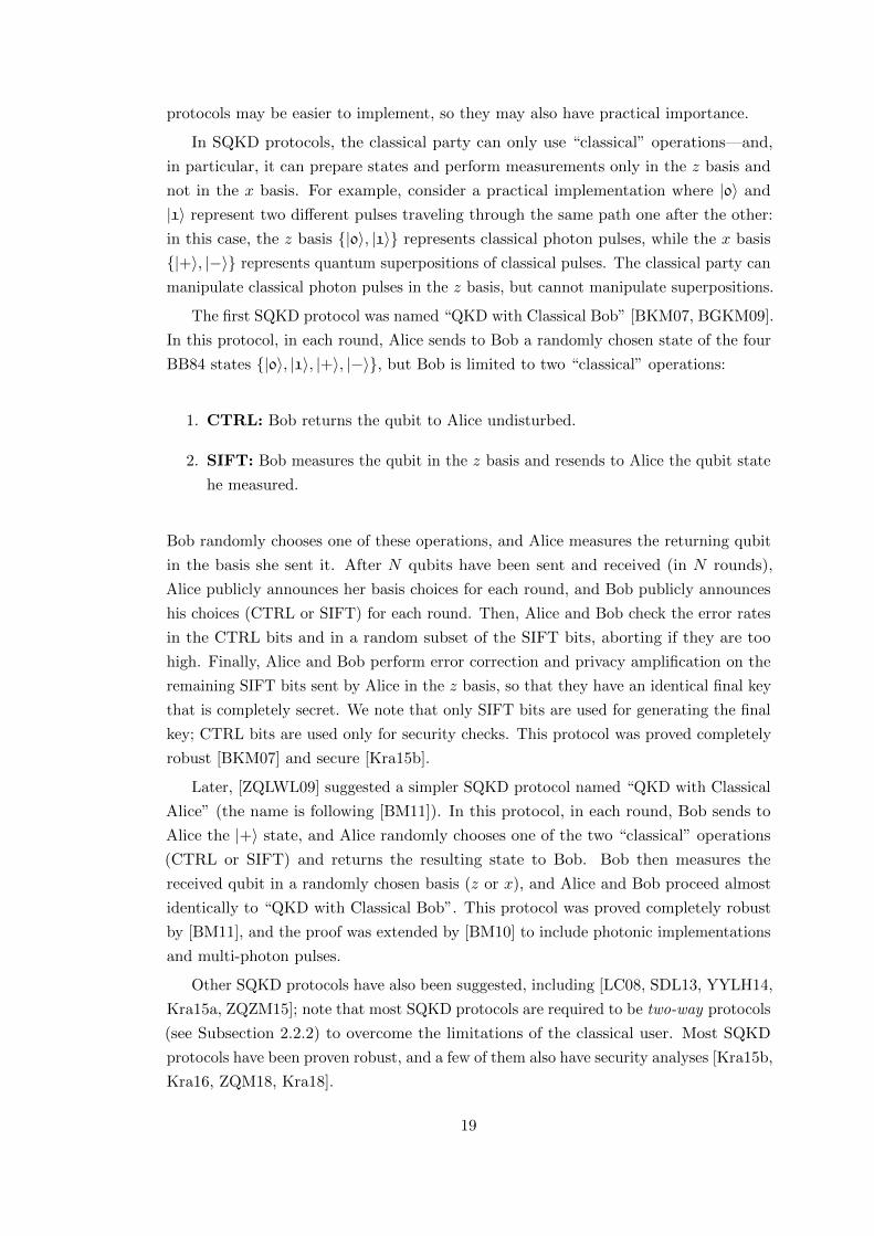
protocols may be easier to implement, so they may also have practical importance.
In SQKD protocols, the classical party can only use “classical” operations—and,
in particular, it can prepare states and perform measurements only in the z basis and
not in the x basis. For example, consider a practical implementation where |0〉 and
|1〉 represent two different pulses traveling through the same path one after the other:
in this case, the z basis {|0〉, |1〉} represents classical photon pulses, while the x basis
{|+〉, |−〉} represents quantum superpositions of classical pulses. The classical party can
manipulate classical photon pulses in the z basis, but cannot manipulate superpositions.
The first SQKD protocol was named “QKD with Classical Bob” [BKM07, BGKM09].
In this protocol, in each round, Alice sends to Bob a randomly chosen state of the four
BB84 states {|0〉, |1〉, |+〉, |−〉}, but Bob is limited to two “classical” operations:
1. CTRL: Bob returns the qubit to Alice undisturbed.
2. SIFT: Bob measures the qubit in the z basis and resends to Alice the qubit state
he measured.
Bob randomly chooses one of these operations, and Alice measures the returning qubit
in the basis she sent it. After N qubits have been sent and received (in N rounds),
Alice publicly announces her basis choices for each round, and Bob publicly announces
his choices (CTRL or SIFT) for each round. Then, Alice and Bob check the error rates
in the CTRL bits and in a random subset of the SIFT bits, aborting if they are too
high. Finally, Alice and Bob perform error correction and privacy amplification on the
remaining SIFT bits sent by Alice in the z basis, so that they have an identical final key
that is completely secret. We note that only SIFT bits are used for generating the final
key; CTRL bits are used only for security checks. This protocol was proved completely
robust [BKM07] and secure [Kra15b].
Later, [ZQLWL09] suggested a simpler SQKD protocol named “QKD with Classical
Alice” (the name is following [BM11]). In this protocol, in each round, Bob sends to
Alice the |+〉 state, and Alice randomly chooses one of the two “classical” operations
(CTRL or SIFT) and returns the resulting state to Bob. Bob then measures the
received qubit in a randomly chosen basis (z or x), and Alice and Bob proceed almost
identically to “QKD with Classical Bob”. This protocol was proved completely robust
by [BM11], and the proof was extended by [BM10] to include photonic implementations
and multi-photon pulses.
Other SQKD protocols have also been suggested, including [LC08, SDL13, YYLH14,
Kra15a, ZQZM15]; note that most SQKD protocols are required to be two-way protocols
(see Subsection 2.2.2) to overcome the limitations of the classical user. Most SQKD
protocols have been proven robust, and a few of them also have security analyses [Kra15b,
Kra16, ZQM18, Kra18].
19

2.5 Practical Implementations of QKD Protocols
2.5.1 The Fock Space Notations
Quantum cryptographic protocols are usually implemented with photons. However,
standard qubit notations do not describe all possible photon operations and do not
properly represent the actual operations of Alice and Bob; as a result, qubit notations
do not cover all possible attacks. To correct notations, we must replace the qubit Hilbert
space H2 , Span{|0〉, |1〉} by an extended Hilbert space—the “Fock space” F :
• In the simplest case, there are m ≥ 0 photons, all of them belonging to one
photonic mode. Here, the Fock state |m〉 represents m photons in this single mode:
|0〉 is the vacuum state, representing no photons in that mode; |1〉 represents one
photon in that mode; |2〉 represents two photons in that mode; and so on.
• For describing several different pulses of photons (for example, photons traveling
through different paths or at different times, or any other external degree of free-
dom), we need several photonic modes. For example, a single photon in one of two
pulses (and, thus, in one of two modes) describes one qubit, and the z basis states
of this qubit are {|0〉 = |0〉 ⊗ |1〉 ≡ |0〉|1〉 , |1〉 = |1〉 ⊗ |0〉 ≡ |1〉|0〉}. (These two
states are mathematically described as tensor products, but we omit the ⊗ sign for
brevity.) A linear combination describes one photon in a superposition of the two
pulses: for example, the x basis states are{|+〉 = |0〉|1〉+|1〉|0〉√
2, |−〉 = |0〉|1〉−|1〉|0〉√
2
}.
• More generally, for describing m = m1 +m0 photons in two different pulses (two
modes), where m1 photons are in one pulse and m0 photons are in the other pulse,
we write |m1〉|m0〉. We add subscripts to specify the type of pulse—for example,
|m1〉t1 |m0〉t0 for the two times t1, t0, or |m1〉A|m0〉B for the two paths A,B.
• For describing more than two pulses (more than two modes), we use generalized
notations: for example, m = m2 +m1 +m0 photons traveling at times t2, t1, t0 are
denoted |m2〉t2 |m1〉t1 |m0〉t0 . In particular, the vacuum state (absence of photons)
is denoted |0〉 for one mode, |0〉|0〉 for two modes, |0〉|0〉|0〉 for three modes, etc.
All the above notations assume identical photon polarizations (which are an internal
degree of freedom) for all m photons. However, a single photon in a single pulse generally
has two orthogonal polarizations: horizontal ↔ and vertical l. The two polarizations
are described as two modes for each pulse, so k pulses mean 2k modes.
In this thesis (except Chapters 3–5, for the reasons explained in Section 3.2),
polarization modes of m = m1+m0 photons are denoted |m1,m0〉 without any subscript,
while pulse modes are denoted |m1〉|m0〉 with subscripts. Thus:
• If there is exactly one photon in a single pulse, its two polarization modes represent
one qubit. The z basis states of this qubit are |0〉 = |0, 1〉 (representing one photon
20

in the horizontal polarization mode and zero photons in the vertical polarization
mode) and |1〉 = |1, 0〉 (where the single photon is in the vertical mode).
• A linear combination describes one photon in a superposition of those two polariza-
tion modes: for example, the x basis states are{|+〉 = |0,1〉+|1,0〉√
2, |−〉 = |0,1〉−|1,0〉√
2
}.
• The |m1,m0〉 state represents m = m1 + m0 photons in those two polarization
modes: m1 photons in the vertical mode and m0 photons in the horizontal mode.
In particular, the vacuum state |0, 0〉 represents an absence of any photon.
Formally, for two polarization modes, the entire 2-mode Fock space is:
F , Span{|m1,m0〉 | m1 ≥ 0 , m0 ≥ 0}, (2.3)
where the |m1,m0〉 state represents m1 indistinguishable photons in the |1〉 mode and
m0 indistinguishable photons in the |0〉 mode.
Similarly, a single photon in the |+〉 mode may be written as |0, 1〉x, and a single
photon in the |−〉 mode may be written as |1, 0〉x. The entire 2-mode Fock space can
be represented as
F = Span{|m−,m+〉x | m− ≥ 0 , m+ ≥ 0}, (2.4)
where the |m−,m+〉x state represents m− indistinguishable photons in the |−〉 mode
and m+ indistinguishable photons in the |+〉 mode.
2.5.2 Experimental Implementations of Polarization-Based QKD
The BB84 protocol may be experimentally implemented in a “polarization-based” im-
plementation, that we can model as follows: the quantum particles sent by Alice to Bob
are single photons whose polarizations encode the quantum states. The four possible
states sent by Alice are |0〉, |1〉, |+〉, and |−〉, where |0〉 = |↔〉 (a single photon in the
horizontal polarization) and |1〉 = |l〉 (a single photon in the vertical polarization). The
|+〉 = |↗↙〉 and |−〉 = |↖↘〉 states correspond to orthogonal diagonal polarizations.
For measuring the incoming photons, Bob uses a polarizing beam splitter (PBS) and
two detectors. Bob actively configures the PBS for choosing his random measurement
basis (z or x). If the PBS is configured for measurement in the z basis, it sends any
horizontally polarized photon to one path and any vertically polarized photon to the
other path. At the end of each path we place a detector, which clicks whenever it detects
a photon. Therefore, the detector at the first path clicks only if the |0〉 mode is detected,
and the detector at the second path clicks only if the |1〉 mode is detected; a diagonally
polarized photon (|+〉 = |↗↙〉 or |−〉 = |↖↘〉) would cause exactly one of the detectors
(uniformly random) to click. Similarly, if the PBS is configured for measurement in the
x basis, it distinguishes |+〉 from |−〉. This implementation (using an “active” basis
21

choice) may be slow, because Bob needs to randomly choose a basis for each arriving
photon.
A variant of this implementation uses a “passive” basis choice (e.g., [KZH+02]). This
variant uses one polarization-independent beam splitter, two PBSs, and four detectors.
The polarization-independent beam splitter is placed in the front, and it randomly
sends each photon to one path or to another. A photon going to the first path is then
measured (as described above) in the z basis, while a photon going to the second path
is measured (as described above) in the x basis. We note that in this “passive” variant,
the basis is chosen “randomly” by the polarization-independent beam splitter, and Bob
does not have to actively choose it; however, it is exposed to the “Fixed Apparatus”
attack [BGM14] (see Example 3 of Section 8.4).
The above implementations of QKD are further discussed in Chapter 8.
2.5.3 Practical Attacks
The security promises of QKD are true in theory, but its practical security is far
from being guaranteed: practical implementations of QKD use realistic photons, so
they deviate from the theoretical protocols based on ideal qubits. These deviations
make possible various attacks (see [LCT14, SBPCDLP09]), similarly to the idea of
“side-channel attacks” in classical computer security.
For example, in the “Photon-Number Splitting” attack [BLMS00] (which assumes the
QKD system is implemented using photons, and assumes the quantum state sent by Alice
should be a single photon), Eve exploits two facts: (a) in most implementations, Alice
sometimes sends to Bob more than one photon (e.g., two photons); and (b) Bob usually
cannot count the number of photons he measures. Thus, for any pulse consisting of two
or more photons, Eve “steals” one of the photons and keeps it in her quantum memory
for a later measurement (after Alice and Bob expose the correct bases), obtaining full
information without being noticed; and she blocks all single-photon pulses.
Another example is the “Bright Illumination” practical attack [LWWESM10]: this
attack uses a weakness of Bob’s measurement devices, allowing Eve to “blind” them
and fully control Bob’s measurement results (full description is available in Section 8.3).
Eve can then get full information on the secret key without inducing any error. An
extensive discussion of this attack is available in Chapter 8.
Possible solutions to these problems include: (a) a much more careful analysis of
practical devices and practical implementations; (b) “Measurement-Device Independent”
QKD protocols [BHM96, Ina02, LCQ12, BP12], which may be secure even if the
measurement devices are controlled by Eve; and (c) “Fully Device Independent” QKD
protocols [MY98, MAP11, VV14], which may be secure even if all quantum devices are
untrusted (under certain assumptions).
22

2.6 Hoeffding’s Theorem
The final stages of our security proofs in Chapters 6 and 7 consist mainly of applications
of the following Theorem, proven by Hoeffding in [Hoe63, Section 6]:
Theorem 2.1 (Hoeffding’s Theorem). Let X1, . . . , Xn be a random sample without
replacement taken from a population c1, . . . , cN such that a ≤ cj ≤ b for all 1 ≤ j ≤ N .
(That is, each Xi gets the value of a random cj, such that the same j is never chosen
for two different variables Xi, Xi′.) If X , X1+...+Xnn and µ , E[X] is the expected
value of X, then:
1. For any ε > 0,
Pr[X − µ ≥ ε
]≤ e−
2nε2
(b−a)2 . (2.5)
2. µ = 1N
∑Ni=1 ci. Namely, the expected value of X is the average value of the
population.
The following Corollary of Hoeffding’s theorem is useful for proving security:
Corollary 2.2. Let us be given an (n + n′)-bit string c = c1 . . . cn+n′, and assume
that we randomly and uniformly choose a partition of c into two substrings, cA of
length n and cB of length n′. (Formally, this is a random partition of the index set
{1, . . . , n + n′} into two disjoint sets, A and B, satisfying |A| = n, |B| = n′, and
A ∪B = {1, . . . , n+ n′}.) Then, for any p > 0 and ε > 0,
Pr
[(|CA|n
> p+ ε
)∧(|CB|n′≤ p)]≤ e−2
(n′
n+n′
)2nε2, (2.6)
where CA and CB are random variables whose values equal to cA and cB, respectively.
Proof. The random and uniform partition of c into two substrings, cA of length n and
cB of length n′, is actually a sample of size n without replacement from the population
c1, . . . , cn+n′ ∈ {0, 1}. (The sampled n bits are the bits of cA, while the other n′ bits
are the bits of cB.) Therefore, we can apply Hoeffding’s theorem (Theorem 2.1) to this
sampling.
Let X be the average of the sample, and let µ be the expected value of X (so,
according to Theorem 2.1, µ is the average value of the population), then
X =|CA|n
, (2.7)
µ =|CA|+ |CB|n+ n′
. (2.8)
Then |CB|n′ ≤ p is equivalent to (n+ n′)µ− nX ≤ n′ · p, and, therefore, to n · (X − µ) ≥
23

n′ · (µ− p). This means that the conditions(|CA|n > p+ ε
)and
(|CB|n′ ≤ p
)rewrite to
(X − µ > ε+ p− µ
)∧( nn′· (X − µ) ≥ µ− p
), (2.9)
which implies(1 + n
n′
)(X − µ) > ε, which is equivalent to X − µ > n′
n+n′ ε. Using
Hoeffding’s theorem (Theorem 2.1), we get
Pr
[(|CA|n
> p+ ε
)∧(|CB|n′≤ p)]≤ Pr
[X − µ > n′
n+ n′ε
]≤ e−2
(n′
n+n′
)2nε2.
(2.10)
Using Corollary 2.2 for comparing the error rates in different sets of qubits (e.g.,
INFO and TEST bits) is allowed, on the condition that the random and uniform
sampling occurs only after the qubits are sent by Alice and measured by Bob. In other
words, the sampling cannot affect the bases in which the qubits are sent and measured,
and it cannot affect Eve’s attack.
Similar uses of Hoeffding’s theorem for proving security of QKD are available
in [BBBMR06, BGM09].
We also use another Theorem, proven by Hoeffding in [Hoe63, Section 2, Theorem 1]:
Theorem 2.3. Let X1, . . . , XN be independent random variables with finite first and
second moments, such that 0 ≤ Xi ≤ 1 for all 1 ≤ i ≤ N . If X , X1+...+XNN and
µ , E[X] is the expected value of X, then for any ε > 0,
Pr[X − µ ≥ ε
]≤ e−2Nε2 , (2.11)
and, in a similar way (see [Hoe63, Section 1]),
Pr[µ−X ≥ ε
]≤ e−2Nε2 . (2.12)
We will use the following Corollary of Theorem 2.3 for proving security of the
“efficient BB84” protocol in Subsection 7.3.3:
Corollary 2.4. Let 0 ≤ p ≤ 1 be a parameter, and let b = b1 . . . bN be an N-bit
string, such that each bi is chosen probabilistically and independently out of {0, 1}, with
Pr(bi = 0) = p and Pr(bi = 1) = 1− p. Then:
Pr
(|b| ≤ (1− p)N
2
)≤ e−
12N(1−p)2 , (2.13)
Pr
(|b| ≤ pN
2
)≤ e−
12Np2 . (2.14)
Proof. Let us define Xi = bi for all 1 ≤ i ≤ N . Then Xi are independent random
variables with finite first and second moments, such that 0 ≤ Xi ≤ 1 for all 1 ≤ i ≤ N
24

and µ , E[X] = 1− p. Therefore, using Theorem 2.3, we get the two following results:
Pr
[(1− p)−X ≥ 1− p
2
]≤ e−
12N(1−p)2 , (2.15)
Pr[X − (1− p) ≥ p
2
]≤ e−
12Np2 . (2.16)
We notice that X = |b|N = 1− |b|N . Substituting this result, we get
Pr
[−|b|N≥ −1− p
2
]≤ e−
12N(1−p)2 , (2.17)
Pr
[1− |b|
N− 1 ≥ −p
2
]≤ e−
12Np2 , (2.18)
and, therefore,
Pr
[|b| ≤ (1− p)N
2
]≤ e−
12N(1−p)2 , (2.19)
Pr
[|b| ≤ pN
2
]≤ e−
12Np2 . (2.20)
2.7 Notation for Bit Strings
In this thesis, we denote bit strings (of t bits, where t ≥ 0 is some integer) by a bold
letter (e.g., i = i1 . . . it, where i1, . . . , it ∈ {0, 1}); and we refer to these bit strings
as elements of Ft2—that is, as elements of a t-dimensional vector space over the field
F2 = {0, 1}, where addition of two vectors corresponds to a XOR operation between
them. The number of 1-bits in a bit string s is denoted by |s|, and the Hamming
distance between two strings s and s′ is dH(s, s′) , |s⊕ s′|.
2.8 Structure of this Thesis
First, we discuss a new semiquantum key distribution protocol (the “Mirror protocol”)
that solves a practical security problem:
• In Chapter 3, we present the Mirror protocol and prove it completely robust.
This chapter is based on a 2017 paper we published in Physical Review A [BKLM17].
• In Chapter 4, we discuss a simplified variant of the Mirror protocol and present
several attacks against it, proving this variant to be non-robust.
This chapter is based on a 2018 paper we published in Entropy [BLM18].
• In Chapter 5, we prove security of the Mirror protocol against “uniform collective”
attacks (defined in Subsection 2.3.2).
This chapter is based on a 2020 preprint we posted to the arXiv [KLM20].
25

Then, we discuss composable security of generalized BB84 protocols:
• In Chapter 6, we extend [BBBGM02, BGM09] to prove fully composable security
of a variant of BB84 (named “BB84-INFO-z”) against collective attacks.
This chapter is based on a 2020 paper we published in Theoretical Computer
Science [BLM20].
• In Chapter 7, we extend [BBBMR06] to prove fully composable security of several
variants of BB84 against the most general attacks.
Finally, in Chapter 8, we explain how the practical “Bright Illumination” attack [LWWESM10]
can be described as a theoretical “Reversed-Space” attack.
This chapter is based on a 2020 paper we published in the TPNC conference [LM20].
26

Chapter 3
The Mirror Protocol and
Robustness Proof
In this chapter, we present an experimental security problem of the currently existing
SQKD protocols. To solve this problem, we suggest a new SQKD protocol (the “Mirror
protocol”) and prove it completely robust.
This chapter is based on a paper published in Physical Review A in 2017 by Michel
Boyer, Matty Katz, Rotem Liss, and Tal Mor [BKLM17].
3.1 Experimental Infeasibility of the SIFT Operation in
SQKD Protocols
In the currently existing SQKD protocols (see Section 2.4), one of the “classical”
operations is SIFT: measuring in the z basis {|0〉, |1〉} and then resending. In practical
(photonic) implementations, and especially if limited to the existing technology, the
SIFT operation is very hard to securely implement, because the generated photon
will probably be at a different timing or frequency, thus leaking information to the
eavesdropper; see details in [TLC09] (which is a comment on [BKM07]) and in the
reply [BKM09].
For example, let us look at the “QKD with classical Alice” protocol implemented
with two classical modes, |0〉 and |1〉, describing two pulses (two distinct time-bins) on a
single arm. The photon can be either in one pulse, in the other, or in a superposition (a
non-classical state). In this case, the SIFT operation requires Alice to measure the two
pulses, generate a single photon in a state depending on the measurement outcome, and
resend it to Bob; on the other hand, Alice can implement the CTRL operation simply by
using a mirror (reflecting both pulses). In this case, it is indeed very difficult for Alice
to regenerate the SIFT photon exactly at the right timing, so that it is indistinguishable
from a CTRL photon.
Furthermore, in [TLC09] it was shown that even if Alice could (somehow) have the
27

machinery to perform SIFT with perfect timing, Eve would still be able to attack the
protocol by taking advantage of the fact that Alice’s detectors are imperfect: Eve’s
attack is modifying the frequency of the photon generated by Bob. Alice does not notice
the change in frequency. If Alice performs SIFT, the photon she generates is in the
original frequency; if she performs CTRL, the photon she reflects is in the frequency
modified by Eve. Therefore, if Eve is powerful enough, she can measure the frequency
and tell whether Alice used SIFT or CTRL. If Eve finds out that Alice used SIFT, she
can copy the bit sent by Alice in the z basis; if she finds out that Alice used CTRL, she
shifts the frequency back to the original frequency. (A very similar attack works for other
implementations, too—e.g., for polarization-based or phase-based implementations.)
This “tagging” attack makes it possible for Eve to get full information on the key
without inducing noise.
3.2 The Mirror Protocol
We suggest a new SQKD protocol, similar to “QKD with classical Alice”, that is
experimentally feasible: in the original protocol of “QKD with classical Alice”, Alice
could choose only between two operations (CTRL and SIFT); in our new protocol, that
we name the “Mirror protocol”, Alice may choose between four operations (CTRL,
SWAP-10, SWAP-01, and SWAP-ALL). This protocol avoids the need of using the
infeasible operation SIFT. The two operations SWAP-10 and SWAP-01 correspond to
two possible reflections of pulses by using a controllable mirror; these operations cannot
be described by qubit notations, so below we use 4-level system notations. Our new
protocol is based on the Fock space notations, where the |m1,m0〉 state represents m1
indistinguishable photons in the |1〉 mode and m0 indistinguishable photons in the |0〉mode1; more details about the Fock space notations are given in Subsection 2.5.1.
This protocol is experimentally feasible and is safe against the “tagging” attack
described in [TLC09]. Moreover, in this chapter we prove the protocol to be completely
robust against an attacker Eve that can do anything allowed by the laws of quantum
physics, including the possibility of sending multi-photon pulses (namely, assuming Eve
may use any quantum state consisting of the two modes |0〉 and |1〉—or, equivalently,
any superposition of the Fock states |m1,m0〉). In Chapter 5 we also prove it secure
against “uniform collective” attacks. An illustration of the protocol is available as
Figure 3.1.
We can describe the new protocol in terms of photon pulses that correspond to
two distinct time-bins, and of a controllable mirror operated by Alice: in this case, the
CTRL operation corresponds to operating the mirror on both pulses (reflecting both
pulses back to the originator, Bob); the SWAP-10 operation corresponds to operating
1In the three “Mirror” chapters of this thesis (Chapters 3–5), we use the |m1,m0〉 notation to denotetwo photon pulses (to make notations simpler in case we analyze two or three subsystems, each consistingof several modes), in contrast to the |m1〉|m0〉 notation used for this purpose in Subsection 2.5.1.
28

Figure 3.1: A schematic diagram of the Mirror protocol described inSection 3.2. This figure was generated by Walter O. Krawec for [KLM20] (Chapter 5).
the mirror only on the |0〉 pulse while measuring the other pulse (and similarly for the
SWAP-01 operation and the |1〉 pulse); and the SWAP-ALL operation corresponds to
measuring all pulses, without reflecting any of them.
For the experimental implementation, we note that a (very slow) mechanically-moved
mirror is trivial to implement; a much faster device can be electronically implemented by
using standard optical elements (that are commonly used in QKD): a Pockels cell (that
can change the polarization of the photon(s) in one of the pulses) and a polarizing beam
splitter (that makes it possible to split the two different pulses into two paths, because
they are now differently polarized). Like other (fast) QKD experimental settings,
implementation is feasible but is not trivial. More details about the experimental
implementation of this protocol are available in [Gur13, Tam14].
Let Alice’s initial probe be in the vacuum state |0, 0〉Aanc , and let us assume that a
single photon is arriving from Bob; thus, the system as a whole can be described as a
4-level system (a single photon in four modes). Alice’s operations are as follows:
I (CTRL) Do nothing:
I|0, 0〉Aanc |m1,m0〉B = |0, 0〉Aanc |m1,m0〉B. (3.1)
S1 (SWAP-10) Swap half of Alice’s probe (the left mode) with the |m1〉B half of
Bob’s state:
S1|0, 0〉Aanc |m1,m0〉B = |m1, 0〉Aanc |0,m0〉B. (3.2)
S0 (SWAP-01) Swap half of Alice’s probe (the right mode) with the |m0〉B half of
29

Bob’s state:
S0|0, 0〉Aanc |m1,m0〉B = |0,m0〉Aanc |m1, 0〉B. (3.3)
S (SWAP-ALL) Swap the entire probe of Alice with the entire state |m1,m0〉B of
Bob:
S|0, 0〉Aanc |m1,m0〉B = |m1,m0〉Aanc |0, 0〉B. (3.4)
After each of the three SWAP operations, Alice measures her probe (the |·〉Aanc state)
in the z basis and sends to Bob the |·〉B state. If there is no noise and no eavesdropping,
and if we analyze the “ideal case” (in which exactly one photon is arriving from Bob to
Alice), then each round is described by the four-dimensional Hilbert space
Span{|0, 0〉Aanc |0, 1〉B , |0, 0〉Aanc |1, 0〉B , |0, 1〉Aanc |0, 0〉B , |1, 0〉Aanc |0, 0〉B}, (3.5)
namely, by a four-level system; for our protocol, we use this four-level system instead
of the qubit system used by BB84 and by many other QKD schemes. In the most
general “theoretical attack” (the attack analyzed by standard QKD security proofs),
Eve attacks Alice’s and Bob’s states using any probe of her choice, but she cannot
modify the four-dimensional Hilbert space of the protocol: she can only use these four
levels. However, in practical attacks (as analyzed in our robustness analysis), Eve may
use an extended Hilbert space (the entire Fock space).
While Eve is fully powerful, it is common to assume that Alice and Bob are limited
to use only current technology. In particular, Alice and Bob are limited in the sense that
they cannot count the number of photons in each mode, but can only check whether
a detector corresponding to a specific mode clicks (detects at least one photon in this
mode) or not (detects an empty mode). For our protocol to be practical (and for our
robustness analysis to be stronger), we assume Alice and Bob are indeed limited in that
sense: therefore, when Alice and Bob measure in the z basis, their measurement results
are denoted as k1k0, where k0, k1 ∈ {0, 1}. Similarly, when Bob measures in the x basis,
his measurement result is k−k+, where k+, k− ∈ {0, 1}.This limitation leads to the definition of “sum”, as follows: let us look at a measure-
ment result of Alice or Bob (that is 00, 01, 10, or 11). The “sum” of this measurement
result is the number of distinct modes detected to be non-empty during the measurement
(namely, the sum of digits in the measurement result). This definition is summarized in
Table 3.1.
The protocol consists of the following steps:
1. In each of the N rounds, Bob sends to Alice the |+〉B state; Alice randomly chooses
one of her four classical operations (CTRL, SWAP-10, SWAP-01, or SWAP-ALL)
and sends the result back to Bob; and Bob measures the state he receives, choosing
randomly whether to measure in the z basis or the x basis.
2. Alice reveals her operation choices (CTRL, SWAP-x (x ∈ {01, 10}), or SWAP-ALL;
30
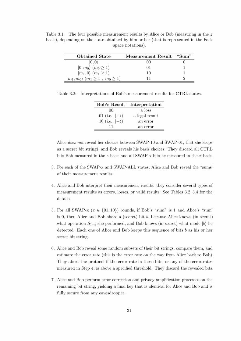
Table 3.1: The four possible measurement results by Alice or Bob (measuring in the zbasis), depending on the state obtained by him or her (that is represented in the Fock
space notations).
Obtained State Measurement Result “Sum”
|0, 0〉 00 0|0,m0〉 (m0 ≥ 1) 01 1|m1, 0〉 (m1 ≥ 1) 10 1
|m1,m0〉 (m1 ≥ 1 , m0 ≥ 1) 11 2
Table 3.2: Interpretations of Bob’s measurement results for CTRL states.
Bob’s Result Interpretation
00 a loss01 (i.e., |+〉) a legal result10 (i.e., |−〉) an error
11 an error
Alice does not reveal her choices between SWAP-10 and SWAP-01, that she keeps
as a secret bit string), and Bob reveals his basis choices. They discard all CTRL
bits Bob measured in the z basis and all SWAP-x bits he measured in the x basis.
3. For each of the SWAP-x and SWAP-ALL states, Alice and Bob reveal the “sums”
of their measurement results.
4. Alice and Bob interpret their measurement results: they consider several types of
measurement results as errors, losses, or valid results. See Tables 3.2–3.4 for the
details.
5. For all SWAP-x (x ∈ {01, 10}) rounds, if Bob’s “sum” is 1 and Alice’s “sum”
is 0, then Alice and Bob share a (secret) bit b, because Alice knows (in secret)
what operation S1−b she performed, and Bob knows (in secret) what mode |b〉 he
detected. Each one of Alice and Bob keeps this sequence of bits b as his or her
secret bit string.
6. Alice and Bob reveal some random subsets of their bit strings, compare them, and
estimate the error rate (this is the error rate on the way from Alice back to Bob).
They abort the protocol if the error rate in these bits, or any of the error rates
measured in Step 4, is above a specified threshold. They discard the revealed bits.
7. Alice and Bob perform error correction and privacy amplification processes on the
remaining bit string, yielding a final key that is identical for Alice and Bob and is
fully secure from any eavesdropper.
31

Table 3.3: Interpretations of Alice’s and Bob’s measurement results for SWAP-x states.
Alice’s “Sum” Bob’s “Sum” Interpretation
0 0 a loss0 1 Alice and Bob share a bit1 0 Alice and Bob do not share a bit1 1 an error
0 or 1 2 an error2 impossible
Table 3.4: Interpretations of Alice’s and Bob’s measurement results for SWAP-ALLstates.
Alice’s Result Bob’s Result Interpretation
00 00 a loss01 or 10 00 a legal result
11 00 an errorany 01, 10, or 11 an error
Notice that Bob does not have a special role in the beginning: he always generates
the same state, |+〉. It is even possible that the adversary Eve generates this state
instead of him.
3.3 Robustness Analysis
To prove robustness, we will prove that for Eve’s attack to be undetectable by Alice
and Bob (namely, for Eve’s attack not to cause any errors), it must not give Eve any
information.
Eve’s attack on a state can be performed in both directions: from the source (Bob)
to Alice, Eve applies U ; from Alice back to Bob, Eve applies V . We may assume,
without limiting generality, that Eve uses a fixed probe space HE for her attacks.
According to the definition of robustness, we will prove that if, during a run of the
protocol, no error can be detected by Alice and Bob, then Eve gets no information on
the raw key. According to Tables 3.2–3.4, if Alice and Bob cannot find any error, the
following conditions must be true for all measurement results that were not discarded
due to basis mismatch:
1. For all CTRL rounds, Bob’s measurement result (in the x basis) must not be 10
or 11: namely, Bob must never detect any photon in the |−〉 mode.
2. For all SWAP-x rounds, Alice’s “sum” and Bob’s “sum” (in the z basis) must not
be both 1.
3. For all SWAP-x rounds, Bob’s “sum” (in the z basis) must not be 2: namely,
Bob’s measurement result must not be 11.
32

4. For all SWAP-x rounds, no error (that may be detected during the protocol) can
exist. In other words:
(a) For all SWAP-10 rounds, Bob’s measurement result (in the z basis) must not
be 10.
(b) For all SWAP-01 rounds, Bob’s measurement result (in the z basis) must not
be 01.
5. For all SWAP-ALL rounds, Alice’s measurement result must not be 11.
6. For all SWAP-ALL rounds, Bob’s measurement result must not be 01, 10, or 11.
We now analyze each round of the protocol. After the round begins, the source
(Bob) sends to Alice the state |0, 1〉x,B ∈ HB. Eve can now interfere: she attaches her
own probe state (in the Hilbert space HE) and applies the unitary transformation U .
The resulting Bob+Eve state (including Eve’s probe) is of the form
|ψinit〉 ,∑m1≥0m0≥0
|m1,m0〉B|Em1,m0〉E, (3.6)
where |Ei,j〉E are non-normalized vectors in HE.
Condition 5 means that |Em1,m0〉E = 0 for all m1,m0 satisfying m1 ≥ 1 and m0 ≥ 1.
Therefore,
|ψinit〉 = |φ1,0〉+ |φ0,1〉+ |φ0,0〉, (3.7)
where
|φ1,0〉 ,∑m1≥1
|m1, 0〉B|Em1,0〉E, (3.8)
|φ0,1〉 ,∑m0≥1
|0,m0〉B|E0,m0〉E, (3.9)
|φ0,0〉 , |0, 0〉B|E0,0〉E. (3.10)
Alice now applies one of the four possible operations (CTRL = I, SWAP-10 = S1,
SWAP-01 = S0, or SWAP-ALL = S) and destructively measures her probe state. The
(non-normalized) state of the Bob+Eve system after Alice’s operation and measurement
is written in Table 3.5.
Then, Eve applies a second unitary transformation V on the state sent from Alice
to Bob (and on her own probe state). According to conditions 2, 3, and 6, the density
matrices V ρ(1)S-10V
†, V ρ(1)S-01V
†, and V ρS-ALLV† must only overlap with |0, 0〉B. It follows
that there exists |H0,0〉E ∈ HE such that
V |φ0,0〉 = |0, 0〉B|H0,0〉E. (3.11)
Let us denote V |φ1,0〉 =∑
m1≥0m0≥0
|m1,m0〉B|Fm1,m0〉E. Let us look at a SWAP-01
33

Table 3.5: The (non-normalized) state of the Bob+Eve system after Alice’s operation,given Alice’s “sum”. Note that |φ1,0〉, |φ0,1〉, and |φ0,0〉 are defined in
Equations (3.8)–(3.10).
Alice’s Operation Alice’s “Sum” Bob+Eve State
CTRL |ψCTRL〉 , |φ1,0〉+ |φ0,1〉+ |φ0,0〉SWAP-10 0 |ψ(0)
S-10〉 , |φ0,1〉+ |φ0,0〉SWAP-01 0 |ψ(0)
S-01〉 , |φ1,0〉+ |φ0,0〉SWAP-10 1 ρ
(1)S-10 ,
∑m1≥1
|0, 0〉B〈0, 0|B ⊗ |Em1,0〉E〈Em1,0|E
SWAP-01 1 ρ(1)S-01 ,
∑m0≥1
|0, 0〉B〈0, 0|B ⊗ |E0,m0〉E〈E0,m0 |E
SWAP-ALL ρS-ALL , ρ(1)S-10 + ρ
(1)S-01 + |φ0,0〉〈φ0,0|
round for which Alice’s “sum” is 0: in this round, the state of Bob+Eve after Eve’s
attack is
V |ψ(0)S-01〉 = V |φ1,0〉+ V |φ0,0〉
=∑m1≥0m0≥0
|m1,m0〉B|Fm1,m0〉E + |0, 0〉B|H0,0〉E, (3.12)
and following conditions 4b and 3, Bob must not detect a photon in the |0〉 mode
(otherwise, the error may be detected during the protocol). Therefore, |Fm1,m0〉E = 0
for all m0 ≥ 1. It follows that
V |φ1,0〉 =∑m1≥1
|m1, 0〉B|Fm1,0〉E + |0, 0〉B|F0,0〉E. (3.13)
Similarly (following conditions 4a and 3),
V |φ0,1〉 =∑m0≥1
|0,m0〉B|G0,m0〉E + |0, 0〉B|G0,0〉E. (3.14)
Now, Equations (3.11), (3.13), and (3.14) imply that if Alice applies CTRL, the
state of Bob+Eve after Eve’s attack is
V |ψCTRL〉 = V |φ1,0〉+ V |φ0,1〉+ V |φ0,0〉
=∑m≥1
[|m, 0〉B|Fm,0〉E + |0,m〉B|G0,m〉E] + |0, 0〉B|H〉E, (3.15)
where |H〉E , |F0,0〉E + |G0,0〉E + |H0,0〉E. Following condition 1, the probability of Bob
detecting a photon in the |−〉 mode must be 0.
We now use the following Lemma:
Lemma 3.1. If |ψ′〉 =∑
m≥1 [|m, 0〉B|Fm,0〉E + |0,m〉B|G0,m〉E] + |0, 0〉B|H〉E is a bi-
34
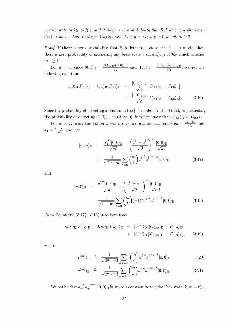
partite state in HB ⊗HE, and if there is zero probability that Bob detects a photon in
the |−〉 mode, then |F1,0〉E = |G0,1〉E, and |Fm,0〉E = |G0,m〉E = 0 for all m ≥ 2.
Proof. If there is zero probability that Bob detects a photon in the |−〉 mode, then
there is zero probability of measuring any basis state |m−,m+〉x,B of HB which satisfies
m− ≥ 1.
For m = 1, since |0, 1〉B =|0,1〉x,B+|1,0〉x,B√
2and |1, 0〉B =
|0,1〉x,B−|1,0〉x,B√2
, we get the
following equation:
|1, 0〉B|F1,0〉E + |0, 1〉B|G0,1〉E =|0, 1〉x,B√
2[|G0,1〉E + |F1,0〉E]
+|1, 0〉x,B√
2[|G0,1〉E − |F1,0〉E] . (3.16)
Since the probability of detecting a photon in the |−〉 mode must be 0 (and, in particular,
the probability of detecting |1, 0〉x,B must be 0), it is necessary that |F1,0〉E = |G0,1〉E.
For m ≥ 2, using the ladder operators a0, a1, a+, and a−, since a0 = a++a−√2
and
a1 = a+−a−√2
, we get
|0,m〉B =a†0m|0, 0〉B√m!
=
(a†+ + a†−√
2
)m|0, 0〉B√m!
=1√
2m ·m!
m∑k=0
(m
k
)a†−
ka†+
m−k|0, 0〉B (3.17)
and
|m, 0〉B =a†1m|0, 0〉B√m!
=
(a†+ − a
†−√
2
)m|0, 0〉B√m!
=1√
2m ·m!
m∑k=0
(m
k
)(−1)ka†−
ka†+
m−k|0, 0〉B. (3.18)
From Equations (3.17)–(3.18) it follows that
|m, 0〉B|Fm,0〉E + |0,m〉B|G0,m〉E = |e(m)〉B [|G0,m〉E + |Fm,0〉E]
+ |o(m)〉B [|G0,m〉E − |Fm,0〉E] , (3.19)
where
|e(m)〉B ,1√
2m ·m!
∑k even
(m
k
)a†−
ka†+
m−k|0, 0〉B, (3.20)
|o(m)〉B ,1√
2m ·m!
∑k odd
(m
k
)a†−
ka†+
m−k|0, 0〉B. (3.21)
We notice that a†−ka†+
m−k|0, 0〉B is, up to a constant factor, the Fock state |k,m− k〉x,B.
35

Because the probability of finding a photon in the |−〉 mode must be zero, it means
that the coefficient of a†−ka†+
m−k|0, 0〉B must be zero for all k ≥ 1.
Substituting |e(m)〉B and |o(m)〉B by their values in Equation (3.19), the coefficient of
a†−ka†+
m−k|0, 0〉B (up to a non-zero constant factor) is |G0,m〉E + |Fm,0〉E for even values
of k and |G0,m〉E − |Fm,0〉E for odd values of k. Since k = m ≥ 1 and k = m − 1 ≥ 1
have different parities, this implies both |G0,m〉E + |Fm,0〉E and |G0,m〉E − |Fm,0〉E must
be 0, and thus |Fm,0〉E = |G0,m〉E = 0.
Applying Lemma 3.1, we deduce that |Fm,0〉E = |G0,m〉E = 0 for all m ≥ 2, and that
|F1,0〉E = |G0,1〉E , |F 〉E.
It follows that the joint states of Bob+Eve after Eve’s attack, when Alice performed
SWAP-x and her “sum” was 0 (these are the only rounds in which Alice and Bob may
share a secret bit), are: (using Table 3.5 and Equations (3.11), (3.13), and (3.14))
V |ψ(0)S-10〉 = V |φ0,1〉+ V |φ0,0〉 = |0, 1〉B|F 〉E + |0, 0〉B [|G0,0〉E + |H0,0〉E] , (3.22)
V |ψ(0)S-01〉 = V |φ1,0〉+ V |φ0,0〉 = |1, 0〉B|F 〉E + |0, 0〉B [|F0,0〉E + |H0,0〉E] .(3.23)
Therefore, the state of Eve’s probe is independent of all Alice’s and Bob’s shared
bits, and is equal to |F 〉E whenever Alice and Bob share a bit. Eve can thus get no
information on the bits shared by Alice and Bob without causing errors that may be
noticed by Alice and Bob.
3.4 Conclusion
In this chapter, we have suggested a solution for a practical security problem of SQKD
protocols, that was discussed in Section 3.1 and [TLC09]: we have presented a new
semiquantum key distribution protocol and proved it robust (see Chapter 5 for full
security analysis against “uniform collective” attacks). Unlike all previous SQKD
protocols, our new protocol can be experimentally implemented in a secure way.
36

Chapter 4
Attacks Against a Simplified
Variant of the Mirror Protocol
In this chapter, we present a simpler variant of the Mirror protocol (the “simplified
Mirror protocol”) which is easier to implement. Our variant allows the classical party,
Alice, to choose one of three operations, while the Mirror protocol allows her to choose
one of four operations. We then present two attacks against this variant, proving it
non-robust. Our results show the four classical operations allowed by the Mirror protocol
are probably necessary for robustness.
This chapter is based on a paper published in Entropy in 2018 by Michel Boyer,
Rotem Liss, and Tal Mor [BLM18].
4.1 The Simplified Mirror Protocol
The simplified Mirror protocol we present in this chapter is identical to the Mirror
protocol described in Section 3.2, except that it does not include the SWAP-ALL
operation. In other words, in the simplified protocol, Alice chooses at random one of
the three classical operations CTRL, SWAP-10, and SWAP-01.
The simplified protocol is easier to implement, because the SWAP-ALL operation
poses some experimental challenges to the electronic implementation discussed in
Section 3.2: for implementing SWAP-ALL, the Pockels cell should either remain working
for a long time (changing polarization for both pulses) or be operated twice (changing
polarization for each pulse separately). In more details, for the two pulses representing
the |0〉 mode and the |1〉 mode: if we assume the duration of each pulse is t and the time
difference between the two pulses is T (where t� T ), the first solution means keeping
the Pockels cell operating during the time period [0, T + 2t], and the second solution
means operating the Pockels cell during the two time periods [0, t] and [T + t, T + 2t].
The first solution may be problematic for some models of the Pockels cell, and the
second solution may be problematic because of the recovery time needed for the Pockels
cell. Therefore, at least in some implementations, the simplified Mirror protocol is much
37

easier to implement than the standard Mirror protocol.
Moreover, analyzing the simplified protocol gives a better understanding of the
properties required for an SQKD protocol to be robust. In particular, this analysis
explains why the structure and complexity of the Mirror protocol are necessary for
robustness.
For completeness, we provide below the full description of the simplified Mirror
protocol. We emphasize, however, that this protocol is almost identical to the Mirror
protocol described in Section 3.2, and the only difference is removing the SWAP-ALL
operation.
In the simplified Mirror protocol, in each round, Bob sends to Alice the initial state
|+〉B, which is equivalent to |0, 1〉x,B , |0,1〉B+|1,0〉B√2
. Then, Alice prepares an ancillary
state in the initial vacuum state |0, 0〉Aanc and chooses at random one of the following
three classical operations (defined on any Fock state she may possibly get, due to Eve’s
attack):
I (CTRL) Reflect all photons towards Bob, without measuring any photon. The
mathematical description is:
I|0, 0〉Aanc |m1,m0〉B = |0, 0〉Aanc |m1,m0〉B. (4.1)
S1 (SWAP-10) Reflect all photons in the |0〉 mode towards Bob, and measure all
photons in the |1〉 mode. The mathematical description is:
S1|0, 0〉Aanc |m1,m0〉B = |m1, 0〉Aanc |0,m0〉B. (4.2)
S0 (SWAP-01) Reflect all photons in the |1〉 mode towards Bob, and measure all
photons in the |0〉 mode. The mathematical description is:
S0|0, 0〉Aanc |m1,m0〉B = |0,m0〉Aanc |m1, 0〉B. (4.3)
We note that in the above mathematical description, Alice measures her ancillary
state |·〉Aanc in the z basis and sends back to Bob the |·〉B state. The states sent from
Alice to Bob (without any error, loss, or eavesdropping) are detailed in Table 4.1. Then,
Bob measures the incoming state in a random basis (either the z basis or the x basis).
After completing all rounds, Alice sends over the classical channel her operation
choices (CTRL or SWAP-x; she keeps x ∈ {01, 10} in secret), Bob sends over the
classical channel his basis choices, and both of them reveal some non-secret information
on their measurement results (as elaborated in Section 3.2). Then, Alice and Bob reveal
and compute the error rate on test bits for which Alice used SWAP-10 or SWAP-01
and Bob measured in the z basis, and the error rate on test bits for which Alice used
CTRL and Bob measured in the x basis. They also check whether other errors exist
(for example, it must never happen that both Alice and Bob detect a photon). Alice
38

Table 4.1: The state sent from Alice to Bob in the simplified Mirror protocol withouterrors or losses, depending on Alice’s classical operation and on whether Alice detected
a photon or not.
Alice’s Operation Did Alice Detect a Photon? State Sent from Alice to Bob
CTRL no (happens with certainty) |0, 1〉x,B = 1√2
[|0, 1〉B + |1, 0〉B]
SWAP-10 no (happens with probability 12) |0, 1〉B
SWAP-10 yes (happens with probability 12) |0, 0〉B
SWAP-01 no (happens with probability 12) |1, 0〉B
SWAP-01 yes (happens with probability 12) |0, 0〉B
and Bob also discard mismatched rounds, such as rounds in which Alice used SWAP-10
and Bob used the x basis.
In the non-testing rounds, Alice and Bob share the secret bit 0 if Alice uses SWAP-10
and detects no photon while Bob measures in the z basis and detects a photon in the
|0〉 mode; similarly, they share the secret bit 1 if Alice uses SWAP-01 and detects no
photon while Bob measures in the z basis and detects a photon in the |1〉 mode.
Finally, Alice and Bob verify that the error rates are below some thresholds, and
they perform error correction and privacy amplification in the standard way for QKD
protocols. At the end of the protocol, Alice and Bob hold an identical final key that is
supposed to be completely secure against any eavesdropper.
4.2 Attacks Against the Simplified Mirror Protocol
We prove the simplified protocol to be non-robust by presenting two attacks: a “full
attack” described in Subsection 4.2.1, which gives Eve full information but causes full
loss of the CTRL bits, and a “weaker attack” described in Subsection 4.2.2, which gives
Eve less information but causes fewer losses of CTRL bits.
4.2.1 A Full Attack on the Simplified Protocol
In this attack, Eve gets full information of all secret bits: namely, she gets full information
on the SWAP-10 and SWAP-01 bits that were measured by Bob in the z basis.
Eve applies her attack in two stages: the first stage is on the way from Bob to Alice,
and the second stage is on the way from Alice to Bob. In both stages she uses her
own probe space (namely, ancillary space) HE = H3 spanned by the orthonormal basis
{|0〉E, |1〉E, |2〉E}. We assume that Eve fully controls the environment, the errors, and
the losses (this is a standard assumption when analyzing the security of QKD): namely,
no losses and no errors exist between Bob and Eve or between Alice and Eve.
In the first stage of the attack (on the way from Bob to Alice), Eve intercepts the
39

Table 4.2: The state of Bob+Eve after Alice’s classical operation for the attacksdescribed in Subsections 4.2.1 and 4.2.2, depending on Alice’s classical operation and
on whether Alice detected a photon or not.
Alice’s Operation Did Alice Detect a Photon? Bob+Eve State
CTRL no (happens with certainty) 1√3
[|0, 1〉B|1〉E + |1, 0〉B|1〉E+|0, 0〉B|0〉E]
SWAP-10 no (happens with probability 23) 1√
2[|0, 1〉B|1〉E + |0, 0〉B|0〉E]
SWAP-10 yes (happens with probability 13) |0, 0〉B|1〉E
SWAP-01 no (happens with probability 23) 1√
2[|1, 0〉B|1〉E + |0, 0〉B|0〉E]
SWAP-01 yes (happens with probability 13) |0, 0〉B|1〉E
state |+〉B = |0, 1〉x,B sent by Bob, generates instead the state
1√3
[|0, 1〉B|1〉E + |1, 0〉B|1〉E + |0, 0〉B|0〉E] =
√2
3|0, 1〉x,B|1〉E +
√1
3|0, 0〉B|0〉E, (4.4)
and sends to Alice the B part of the state. This state causes Alice to get no photons with
probability 13 and get the expected |+〉B state with probability 2
3 . Alice then performs
at random one of the three classical operations CTRL, SWAP-10, or SWAP-01; the
resulting possible states of Bob+Eve are described in Table 4.2.
In the second stage of the attack (on the way from Alice to Bob), Eve applies the
unitary operator V on the joint Bob+Eve state, where V is defined as follows:
V |0, 1〉B|1〉E = −√
1
3|1, 0〉B|1〉E +
√2
3|0, 0〉B|0〉E, (4.5)
V |1, 0〉B|1〉E = −√
1
3|0, 1〉B|0〉E +
√2
3|0, 0〉B|1〉E, (4.6)
V |0, 0〉B|0〉E =
√1
3|0, 1〉B|0〉E +
√1
3|1, 0〉B|1〉E +
√1
3|0, 0〉B|+〉E, (4.7)
V |0, 0〉B|1〉E = |0, 0〉B|2〉E. (4.8)
V is indeed a unitary operator, because we can prove the right-hand sides to be
orthonormal: all right-hand sides are normalized vectors; the first two vectors are clearly
orthogonal; the third vector is orthogonal to the first two, because 〈0|+〉E = 〈1|+〉E = 1√2;
and the fourth vector is orthogonal to the three others. Thus, V defines (or, more
precisely, can be extended to) a unitary operator on HB ⊗HE.
Applying the unitary operator V to Table 4.2 gives the states listed in Table 4.3.
Comparing it with Table 4.1, we conclude that this attack never causes Alice and Bob
to detect an error. Moreover, Eve detects the entire secret key: Eve measures “0” in
her probe if Alice and Bob agree on the “secret” bit 0, and she measures “1” in her
probe if Alice and Bob agree on the “secret” bit 1. However, Eve causes several kinds
of losses; in particular, all CTRL bits are lost.
40

Table 4.3: The state of Bob+Eve after completing Eve’s attack described inSubsection 4.2.1, depending on Alice’s classical operation and on whether Alice
detected a photon or not.
Alice’s Operation Did Alice Detect a Photon? Bob+Eve State
CTRL no (happens with certainty) |0, 0〉B|+〉ESWAP-10 no (happens with probability 2
3)1√6|0, 1〉B|0〉E + |0, 0〉B
3|0〉E + |1〉E√12
SWAP-10 yes (happens with probability 13) |0, 0〉B|2〉E
SWAP-01 no (happens with probability 23)
1√6|1, 0〉B|1〉E + |0, 0〉B
|0〉E + 3|1〉E√12
SWAP-01 yes (happens with probability 13) |0, 0〉B|2〉E
Therefore, this attack makes it possible for Eve to get full information without
inducing any error. However, Eve causes many losses, including full loss of the CTRL
bits.
4.2.2 A Weaker Attack on the Simplified Protocol
The full attack described in Subsection 4.2.1 makes it impossible for Bob to ever detect
a CTRL bit, which may look suspicious. We now present a weaker attack that lets Bob
detect some CTRL bits but gives Eve less information.
The first stage of the attack (on the way from Bob to Alice) remains the same:
that is, the state Eve sends to Alice is still given by Equation (4.4), and the resulting
Bob+Eve state after Alice’s classical operation is still shown in Table 4.2. Eve’s probe
space is, too, the same as before: HE = H3 , Span{|0〉E, |1〉E, |2〉E}.This attack is characterized by the parameter 0 ≤ ε ≤ 1. We will see that ε = 0
gives the full attack described in Subsection 4.2.1, while ε = 1 gives Eve no information
at all.
Another important parameter used by the attack is
κ ,
√1− ε23− 2ε2
. (4.9)
We notice that for small values of ε, the value of κ is close to√
13 . Moreover, for all
0 ≤ ε ≤ 1, it holds that 0 < ε2 + κ2 ≤ 1 and 2κ2 < 1.
In the second stage of the attack (on the way from Alice to Bob), Eve applies the
unitary operator V on the joint Bob+Eve state, where V is defined as follows:
V |0, 1〉B|1〉E = ε|0, 1〉B|2〉E − κ|1, 0〉B|1〉E +√
1− κ2 − ε2|0, 0〉B|0〉E, (4.10)
V |1, 0〉B|1〉E = −κ|0, 1〉B|0〉E + ε|1, 0〉B|2〉E +√
1− κ2 − ε2|0, 0〉B|1〉E, (4.11)
V |0, 0〉B|0〉E = κ|0, 1〉B|0〉E + κ|1, 0〉B|1〉E +√
1− 2κ2|0, 0〉B|+〉E, (4.12)
V |0, 0〉B|1〉E = |0, 0〉B|2〉E. (4.13)
41

Table 4.4: The state of Bob+Eve after completing Eve’s attack described inSubsection 4.2.2, depending on Alice’s classical operation and on whether Alice detected
a photon or not. The parameters a and b are defined in Equations (4.16)–(4.17).
Alice’s Operation Did Alice Detect a Photon? Bob+Eve State
CTRL no (happens with certainty)
√2ε2
3|0, 1〉x,B|2〉E
+
√1− 2ε2
3|0, 0〉B|+〉E
SWAP-10 no (happens with probability 23)
1√2
[|0, 1〉B (ε|2〉E + κ|0〉E)
+|0, 0〉B (a|0〉E + b|1〉E)]
SWAP-10 yes (happens with probability 13) |0, 0〉B|2〉E
SWAP-01 no (happens with probability 23)
1√2
[|1, 0〉B (ε|2〉E + κ|1〉E)
+|0, 0〉B (b|0〉E + a|1〉E)]
SWAP-01 yes (happens with probability 13) |0, 0〉B|2〉E
V is indeed a unitary operator, because we can prove the right-hand sides to be
orthonormal: all right-hand sides are clearly normalized; the first two vectors are
orthogonal; the fourth vector is orthogonal to the three others; and the third vector is
orthogonal to the first and to the second, because
1− 2κ2 =3− 2ε2 − 2(1− ε2)
3− 2ε2=
1
3− 2ε2, (4.14)
1− κ2 − ε2 =(3− 2ε2)− (1− ε2)− (3ε2 − 2ε4)
3− 2ε2=
2(1− ε2)2
3− 2ε2, (4.15)
and thus√1−κ2−ε2
√1−2κ2√
2= κ2. Therefore, V extends to a unitary operator on HB⊗HE.
The final global state after Eve’s attack is described in Table 4.4 (computed by
applying the operator V to Table 4.2), given the following definitions:
a ,√
1− κ2 − ε2 +
√1− 2κ2√
2, (4.16)
b ,
√1− 2κ2√
2. (4.17)
We notice that for ε = 0, the attack is the same as in Subsection 4.2.1. If ε = 1, the
loss rate of CTRL bits is 13 , and Eve gets no information at all on the information bits
(because κ = 0).
In general, if Alice and Bob share a “secret” bit b ∈ {0, 1}, Eve’s probe state is in
the (normalized) stateε|2〉E + κ|b〉E√
ε2 + κ2. (4.18)
When Eve measures her probe state in the computational basis {|0〉E, |1〉E, |2〉E},
42

Table 4.5: The probability p of Eve obtaining an information bit, and the loss ratesRCTRL and RSWAP-x of CTRL and SWAP-x bits (where x ∈ {01, 10}), respectively, for
several values of the attack’s parameter ε.
ε 0 0.1 0.2 0.3 0.4 0.5 0.6 0.7 0.8 0.9 1
p 1 0.97 0.89 0.78 0.66 0.55 0.44 0.34 0.25 0.15 0RCTRL 1 0.99 0.97 0.94 0.89 0.83 0.76 0.67 0.57 0.46 0.33
RSWAP-x 0.83 0.83 0.82 0.79 0.76 0.73 0.68 0.63 0.58 0.53 0.5
she gets the information bit b with probability
p =κ2
ε2 + κ2=
1− ε2
1 + 2ε2 − 2ε4, (4.19)
and the loss rates of CTRL and SWAP-x bits (where x ∈ {01, 10}) are
RCTRL = 1− 2ε2
3, (4.20)
RSWAP-x = 1− ε2 + κ2
2, (4.21)
respectively.
Table 4.5 shows the probabilities p and the loss rates RCTRL, RSWAP-x for various
values of ε. For example, for ε = 0.5, Eve still gets the information bit with probability
p ≈ 0.55, Bob’s loss rate for the CTRL bits is RCTRL ≈ 0.83, and his loss rate for the
SWAP-x bits is RSWAP-x ≈ 0.73.
For all values of ε, the attack causes no errors. However, in principle, it can be
detected because it causes different loss rates to different types of bits: the loss rate
experienced by Bob in the CTRL bits, RCTRL, is usually different from the loss rate
in the SWAP-x bits, RSWAP-x (see Table 4.5 for details). Therefore, in principle, the
attack can be detected by a statistical test for most values of ε.
The loss rates become equal only for the value ε = ε0 ,√
3−√3
2 ≈ 0.796 (which gives
κ2 = ε2
3 ). It seems that this specific attack cannot be detected, even in principle: it
causes no errors, and it causes the same loss rate for all qubits. For this attack, Eve gets
the information bit with probability p = 14 , and the loss rates are RCTRL = RSWAP-x =
1√3≈ 0.577. Therefore, this attack gives Eve a reasonable amount of information, and it
is not detectable by looking at errors or comparing loss rates. (We can slightly modify
the attack to make the loss rates identical in both directions of the quantum channel,
too.)
We conclude that this weaker attack gives Eve partial information, causes no errors,
and causes several loss rates. We also conclude that since the loss rates caused by the
attack are usually different for different types of bits, the attack can be detected, in
principle, for any value of ε except ε0. However, for ε = ε0, the attack seems undetectable.
43
4.3 Conclusion
We have discussed a simpler and natural variant of the Mirror protocol (the “simplified
Mirror protocol”) which is easier to implement. We have found the simplified Mirror
protocol to be completely non-robust, actually making it an “over-simplified” Mirror
protocol. We have presented in Subsection 4.2.1 an attack giving Eve full information
without causing any error; in addition, since this attack also causes full loss of the
CTRL bits, we have presented in Subsection 4.2.2 weaker attacks giving Eve partial
information, causing no errors, and causing fewer losses. In particular, we have presented
a specific attack (characterized by the parameter ε = ε0 ,√
3−√3
2 ≈ 0.796) that seems
undetectable and gives Eve one quarter (14) of all information bits.
These attacks prove the simplified Mirror protocol, which allows Alice to use
only three classical operations (CTRL, SWAP-10, and SWAP-01), to be completely
non-robust. On the other hand, the Mirror protocol is proved completely robust (see
Section 3.3). As explained in Section 4.1, the only difference between the simplified Mirror
protocol and the Mirror protocol is that the Mirror protocol allows a fourth classical
operation, SWAP-ALL; therefore, allowing the SWAP-ALL operation is necessary for
robustness. More generally, the Mirror protocol probably cannot be made much simpler
while keeping it robust: its complexity is crucial for robustness. Therefore, we have seen
that if we need an SQKD protocol that is experimentally feasible in a secure way, we
may have to use a relatively complicated protocol.
In this chapter, we have not checked the experimental feasibility of Eve’s attacks,
because Eve is usually assumed to be all-powerful. Nonetheless, it can be interesting to
check in the future the experimental feasibility of those attacks and discover whether
the simplified Mirror protocol is flawed also in practice and not “only” in theory. Other
interesting directions for future research include trying to find experimentally feasible
SQKD protocols that are simpler than the Mirror protocol, and trying to find similar
attacks against other QKD and SQKD protocols that have not been proved completely
robust.
44

Chapter 5
Security of the Mirror Protocol
Against Uniform Collective
Attacks
In this chapter, we prove security of the Mirror protocol against “uniform collective”
attacks (defined in Subsection 2.3.2) and evaluate the resulting key rate.
This chapter is based on a preprint posted to the arXiv in 2020 by Walter O. Krawec,
Rotem Liss, and Tal Mor [KLM20].
5.1 Introduction
This chapter proves security of the Mirror protocol under a large class of uniform
collective attacks. The class of the “uniform collective attacks” is an important and
powerful subclass of possible attacks (see Subsection 2.3.2 for details); some existing
security proofs of SQKD protocols against general attacks may in fact be limited to
uniform collective attacks, because they use de Finetti’s theorem and similar techniques
(see [Ren08, CKR09]) that can directly be applied only to entanglement-based protocols1.
Therefore, in this chapter we restrict our analysis to uniform collective attacks.
The uniform collective attacks analyzed in this chapter allow Eve to inject multiple
photons into the classical user’s lab, but not into the quantum user’s lab (attacks of the
later kind are left for future analysis, but we briefly discuss them in the beginning of
Section 5.3). In addition, we limit our analysis to two-mode quantum communication,
leaving more complicated attacks for future research. We assume Alice’s and Bob’s
devices precisely implement the needed operations (most notably, Alice’s classical
operations described in Equations (5.1)–(5.4)), and without loss of generality, we
assume an all-powerful Eve controlling all errors and losses in the quantum channel.
1Applying de Finetti’s theorem and similar techniques to prepare-and-measure protocols (includingSQKD protocols) is usually easy for one-way QKD protocols, but it does not necessarily work fortwo-way protocols. See Subsection 2.2.2 for details about the different types of QKD protocols.
45

We derive an information-theoretic proof of security against these attacks and
simulate the performance of the protocol in a variety of realistic scenarios, including
lossy quantum channels, compared to the BB84 protocol. Ultimately, this chapter shows
that SQKD protocols hold the potential to be secure and feasible in practice, and not
just “secure in ideal conditions”. The methods and techniques we present in this work
may also be applicable to security proofs of other SQKD protocols or even other two-way
QKD protocols where users are limited in some manner in their quantum capabilities.
5.2 The Mirror Protocol: a Concise Description
In this section we present a concise description of the Mirror protocol, which should be
useful for the security proof. A full description of the protocol is available in Section 3.2;
In the Mirror protocol, in each round, Bob sends to Alice the initial state |+〉B, which
is equivalent to |0, 1〉x,B , |0,1〉B+|1,0〉B√2
. Then, Alice prepares an ancillary state in the
initial vacuum state |0, 0〉Aanc and chooses at random one of the following four classical
operations (defined on any Fock state she may possibly get, due to Eve’s attack):
I (CTRL) Reflect all photons towards Bob, without measuring any photon. The
mathematical description is:
I|0, 0〉Aanc |m1,m0〉B = |0, 0〉Aanc |m1,m0〉B. (5.1)
S1 (SWAP-10) Reflect all photons in the |0〉 mode towards Bob, and measure all
photons in the |1〉 mode. The mathematical description is:
S1|0, 0〉Aanc |m1,m0〉B = |m1, 0〉Aanc |0,m0〉B. (5.2)
S0 (SWAP-01) Reflect all photons in the |1〉 mode towards Bob, and measure all
photons in the |0〉 mode. The mathematical description is:
S0|0, 0〉Aanc |m1,m0〉B = |0,m0〉Aanc |m1, 0〉B. (5.3)
S (SWAP-ALL) Measure all photons, without reflecting any photon towards Bob.
The mathematical description is:
S|0, 0〉Aanc |m1,m0〉B = |m1,m0〉Aanc |0, 0〉B. (5.4)
We note that in the above mathematical description, Alice measures her ancillary
state |·〉Aanc in the z basis and sends back to Bob the |·〉B state.
The states sent from Alice to Bob (without any error, loss, or eavesdropping) and
their interpretations, depending on Alice’s random choice of a classical operation and
on whether Alice detected a photon or not, are detailed in Table 5.1.
46

Table 5.1: The state sent from Alice to Bob in the Mirror protocol without errors orlosses, and its interpretation, depending on Alice’s random choice of a classical
operation and on whether Alice detected a photon or not.
Alice’s Op. Did Alice Detect a Photon? State to Bob Round Type Raw Key
CTRL no (happens with certainty) |0, 1〉x,B “test” none
SWAP-10 no (happens with probability 12) |0, 1〉B “raw key” 0
SWAP-10 yes (happens with probability 12) |0, 0〉B “raw key” none
SWAP-01 no (happens with probability 12) |1, 0〉B “raw key” 1
SWAP-01 yes (happens with probability 12) |0, 0〉B “raw key” none
SWAP-ALL yes (happens with certainty) |0, 0〉B “SWAP-ALL” none
Then, Bob measures the incoming state in a random basis (either the z basis or
the x basis). We assume here, as is true in most experimental setups, that Alice and
Bob use detectors and not counters: namely, their detectors cannot count the number
of incoming photons. Therefore, when a detector clicks, Alice and Bob cannot know
whether it detected a single-photon pulse (a single photon in its measured mode) or a
multi-photon pulse (more than one photon in its measured mode).
After completing all rounds, Alice and Bob perform classical post-processing : Alice
sends over the classical channel her operation choices (CTRL, SWAP-x, or SWAP-ALL;
she keeps x ∈ {01, 10} in secret); Bob sends over the classical channel his basis choices;
and both of them reveal all rounds where they got a loss, and all measurement results
each of them got in all testing rounds (CTRL, SWAP-ALL, and a random subset of
the SWAP-x rounds, for which Alice also reveals her values of x ∈ {01, 10}) and in all
mismatched rounds (such as rounds in which Alice used SWAP-10 and Bob used the x
basis). In the non-testing rounds, as detailed in Table 5.1, Alice and Bob share the raw
key bit 0 if Alice uses SWAP-10 and detects no photon while Bob measures in the z
basis and detects a photon (or photons) in the |0〉 mode; similarly, they share the raw
key bit 1 if Alice uses SWAP-01 and detects no photon while Bob measures in the z
basis and detects a photon (or photons) in the |1〉 mode.
Now, Alice and Bob have enough information for computing all the probabilities
they need for finding the key rate (that are detailed later, in Table 5.3), so they compute
all these probabilities and deduce the final key rate according to the algorithm in
Subsection 5.3.7. If the final key rate is negative, they abort the protocol; otherwise,
they perform error correction and privacy amplification in the standard way for QKD
protocols. At the end of the protocol, Alice and Bob hold an identical final key that is
completely secure against any eavesdropper.
47

5.3 Security Proof of the Mirror Protocol Against Uni-
form Collective Attacks
We now prove security of the Mirror protocol. For our security proof, we assume that
the adversary Eve is restricted to uniform collective attacks—namely, that Eve attacks
each round in an independent and identical manner, but she is allowed to postpone the
measurement of her private quantum ancilla until any future point in time. Beyond this,
we will also assume in our security analysis that Eve is allowed to inject any signal into
the forward channel (linking quantum Bob to classical Alice); in the reverse channel,
she is free to perform any quantum unitary probe, but we will assume that the number
of photons returning to Bob is at most one. That is, Eve is allowed to inject multiple
photons into the channel going to Alice, but on the way back, only a single photon or
no photons at all will be returned to Bob. This assumption means that Eve may need
to remove photons on the way from Alice to Bob, if she sent multiple photons towards
Alice; in Subsection 5.3.1 we explain how Eve can perform this attack.
The above assumption (that at most one photon is sent towards Bob) is made to
simplify the analysis of the return channel. We point out that in Chapter 3 we proved
the Mirror protocol to be completely robust even without this assumption—namely,
proved it robust against all multi-photon attacks and all kinds of losses and dark counts
(see Section 3.3); however, full security analysis of the multi-photon case, including
both losses and dark counts, is very difficult even in the simplest one-way standard
QKD, and even more so in any standard two-way QKD protocol such as “Plug &
Play” [MHHTZG97], “Ping Pong” [BF02], and LM05 [LM05] (see also [BLMR13]).
Furthermore, this case has not been analyzed in security proofs of many other SQKD
protocols (e.g., [Kra15b, Kra16, ZQM18, Kra18]. Therefore, we do not aim to solve this
major issue here in the specific case of the Mirror protocol: extending the full security
proof to this most general case is left for future research.
5.3.1 Eve’s Attacks
Eve’s first attack: We first analyze the forward-channel attack—namely, the attack
on the way from Bob to Alice. Here, we note that it is to Eve’s advantage to simply
discard the signal coming from Bob (which should be the same each round and carries
no information at this point) and inject a signal of her own, possibly consisting of
multiple photons and entangled with her private quantum ancilla.
Specifically, in each round, Bob sends to Alice the same quantum state: |0, 1〉x,B ,|0,1〉B+|1,0〉B√
2. At this point, Eve performs her first attack: she replaces Bob’s original
state by her own state. Without loss of generality, Eve’s state is of the form:
|ψ0〉 ,∑m1≥0m0≥0
|m1,m0〉B|em1,m0〉E. (5.5)
48

Eve’s second attack: Then, Alice performs her classical operation (CTRL, SWAP-
10, SWAP-01, or SWAP-ALL) and sends the resulting state back to Bob. Now, Eve
performs her second attack, described as the unitary operator UR. As explained above,
for the second attack we make the simplifying assumption that Eve always sends at
most one photon—namely, she sends a superposition of |0, 1〉B, |1, 0〉B, and |0, 0〉B with
her corresponding ancillary states |g0,1m1,m0〉E, |g1,0m1,m0〉E, and |g0,0m1,m0〉E. We emphasize
that this simplifying assumption applies only to the second attack, and not to the first
attack.
Thus, Eve’s second attack is of the form:
UR|m′1,m′0〉B|em1,m0〉E = |0, 1〉B|f0,1m′1,m′0,m1,m0〉E + |1, 0〉B|f1,0m′1,m′0,m1,m0
〉E
+ |0, 0〉B|f0,0m′1,m′0,m1,m0〉E. (5.6)
However, in our security proof we use terms of the following simplified notations:
UR|m1,m0〉B|em1,m0〉E = |0, 1〉B|g0,1m1,m0〉E + |1, 0〉B|g1,0m1,m0
〉E + |0, 0〉B|g0,0m1,m0〉E. (5.7)
where we denote |gj,km1,m0〉E , |f j,km1,m0,m1,m0〉E. We note that the operation of UR
on states |m′1,m′0〉B|em1,m0〉E where m′1 6= m1 or m′0 6= m0 will not appear in our
security proof, because these states do not give us meaningful statistics2 and thus do
not contribute to the probabilities in Table 5.3. We also note that since Eve is all-
powerful, she will have no trouble performing any unitary operation, even if it includes
a complicated operation for reducing the number of photons.
In both attacks, subsystem B is sent to a legitimate user, while subsystem E is kept
as Eve’s ancilla.
5.3.2 Analyzing all Types of Rounds
In Table 5.2 we classify all rounds into six types, that Alice and Bob need to analyze.
The rounds are classified according to Alice’s random choice of a classical operation and
Bob’s random choice of a measurement basis.
Notice the use of basis-mismatched rounds. Technically, we could have used only
the “standard” (basis-matching) rounds for completing the security proof, by using
the Cauchy-Schwarz inequality for finding worst-case bounds. However, using the
technique of analyzing “mismatched measurements” [BHP93, WMU08], we can derive
a significantly improved formula for the final key rate.
Alice and Bob have to find relevant statistics for each type of round and compute all
2States of the form UR|0,m0〉B|em1,m0〉E and UR|m1, 0〉B|em1,m0〉E may appear in “raw key” roundsanalyzed in Subsection 5.3.3, but we analyze only rounds which contribute to the raw key, whereAlice detects no photon—namely, m1 = 0 or m0 = 0, respectively. In addition, states of the formUR|0, 0〉B|em1,m0〉E may appear in “SWAP-ALL” rounds analyzed in Subsection 5.3.5, but we analyzeonly “double-clicks” of Alice (where Eve’s attack UR is irrelevant, although we use it algebraically toprove Lemma 5.1) and “creation” events (where Alice detects no photon, so m1 = m0 = 0).
49

Table 5.2: All types of rounds, according to Alice’s random choice of a classicaloperation [CTRL, SWAP-x (x ∈ {01, 10}), or SWAP-ALL] and Bob’s random choice of
a measurement basis (z or x).
Round Type Alice’s Operation Bob’s Basis
“raw key” SWAP-x computational (z)mismatched “raw key” SWAP-x Hadamard (x)
“test” CTRL Hadamard (x)mismatched “test” CTRL computational (z)
“SWAP-ALL” SWAP-ALL computational (z)mismatched “SWAP-ALL” SWAP-ALL Hadamard (x)
probabilities listed in Table 5.3. In Subsections 5.3.3–5.3.5 we relate these probabilities
to the quantum states appearing in our security proof, and in Subsection 5.3.6 we derive
the resulting final key rate formula.
Table 5.3: All the probabilities Alice and Bob need to compute, and the formulasrelating them to quantum states in our security proof. All formulas are proved in
Subsections 5.3.3–5.3.5.
Prob. Round Definition Formula
〈E0|E0〉E “raw key” Alice, Bob get raw key bits 0, 0, respectively〈E1|E1〉E “raw key” Alice, Bob get raw key bits 0, 1, respectively〈E2|E2〉E “raw key” Alice, Bob get raw key bits 1, 0, respectively〈E3|E3〉E “raw key” Alice, Bob get raw key bits 1, 1, respectively
M “raw key” both Alice and Bob get raw key bits =∑3
i=0〈Ei|Ei〉Ep0,+ mismatched Alice gets raw key bit 0; Bob observes |+〉 2<〈E0|E1〉E = 2p0,+
“raw key” − (〈E0|E0〉E + 〈E1|E1〉E)p1,+ mismatched Alice gets raw key bit 1; Bob observes |+〉 2<〈E2|E3〉E = 2p1,+
“raw key” − (〈E2|E2〉E + 〈E3|E3〉E)
p+,+ “test” Bob observes |+〉 =∣∣∣∑3
i=0 |Ei〉E
−∑1
j=0 (|gj〉E − |hj〉E)∣∣∣2
pCTRL:0 mismatched Bob observes |0, 1〉 = 2 ||E0〉E + |E2〉E“test” −|g0〉E + |h0〉E|2
pCTRL:1 mismatched Bob observes |1, 0〉 = 2 ||E1〉E + |E3〉E“test” −|g1〉E + |h1〉E|2
pdouble “SWAP-ALL” Alice observes a “double-click” event (|1, 1〉) 〈h0|h0〉E + 〈h1|h1〉E ≤ 12pdouble
pcreate:0 “SWAP-ALL” Alice observes |0, 0〉; Bob observes |0, 1〉 = 2〈g0|g0〉Epcreate:1 “SWAP-ALL” Alice observes |0, 0〉; Bob observes |1, 0〉 = 2〈g1|g1〉E
In all types of rounds, Bob begins by sending |0, 1〉x,B , |0,1〉B+|1,0〉B√2
, which Eve
immediately replaces by her own state |ψ0〉 ,∑
m1≥0m0≥0
|m1,m0〉B|em1,m0〉E (see Equa-
tion (5.5)). Then, Alice chooses her classical operation, as detailed below.
50

5.3.3 “Raw Key” Rounds: Alice Chooses the SWAP-x Operation
In “raw key” rounds, Alice chooses either SWAP-10 or SWAP-01 (each with probability12), that are defined in Equations (5.2)–(5.3). Then, the non-normalized state of the
joint system, conditioning on Alice detecting no photon3, is:
ρ(after Alice)ABE =
1
2|0〉〈0|A⊗P
∑m0≥0
|0,m0〉B|e0,m0〉E
+1
2|1〉〈1|A⊗P
∑m1≥0
|m1, 0〉B|em1,0〉E
,
(5.8)
where we define:
P (|ψ〉) , |ψ〉〈ψ|. (5.9)
We note that |0〉A and |1〉A denote the raw key bit of Alice: Alice deduces it from her
own choice of SWAP-10 (which corresponds to |0〉A) or SWAP-01 (which corresponds
to |1〉A), as explained in Table 5.1.
After Eve’s second attack (namely, after Eve applies the UR operator defined in
Equation (5.7)), the joint non-normalized state becomes:
URρ(after Alice)ABE U †R
=1
2|0〉〈0|A ⊗ P
|0, 1〉B ∑m0≥0
|g0,10,m0〉E + |1, 0〉B
∑m0≥0
|g1,00,m0〉E + |0, 0〉B
∑m0≥0
|g0,00,m0〉E
+
1
2|1〉〈1|A ⊗ P
|0, 1〉B ∑m1≥0
|g0,1m1,0〉E + |1, 0〉B
∑m1≥0
|g1,0m1,0〉E + |0, 0〉B
∑m1≥0
|g0,0m1,0〉E
.
(5.10)
To simplify notation, we define the following states in subsystem E:
|E0〉E ,1√2
∑m0≥0
|g0,10,m0〉E,
|E1〉E ,1√2
∑m0≥0
|g1,00,m0〉E,
|E2〉E ,1√2
∑m1≥0
|g0,1m1,0〉E,
|E3〉E ,1√2
∑m1≥0
|g1,0m1,0〉E, (5.11)
3Notice that according to Table 5.1, raw key bits are shared by Alice and Bob only in “raw key”rounds where Alice detects no photon and Bob does detect a photon.
51

so Equation (5.10) becomes:
URρ(after Alice)ABE U †R
= |0〉〈0|A ⊗ P
|0, 1〉B|E0〉E + |1, 0〉B|E1〉E + |0, 0〉B1√2
∑m0≥0
|g0,00,m0〉E
+ |1〉〈1|A ⊗ P
|0, 1〉B|E2〉E + |1, 0〉B|E3〉E + |0, 0〉B1√2
∑m1≥0
|g0,0m1,0〉E
. (5.12)
(a) Standard “Raw Key” Rounds: Bob Chooses the z Basis
Now, Bob measures his subsystem in the z basis, and his raw key bit is simply his
measurement result (“0” or “1”). Conditioning on Bob detecting a photon (namely,
measuring |0, 1〉B or |1, 0〉B), the final normalized state of the joint system after Bob’s
measurement is:
ρABE =1
M(|00〉〈00|AB ⊗ |E0〉〈E0|E + |01〉〈01|AB ⊗ |E1〉〈E1|E
+|10〉〈10|AB ⊗ |E2〉〈E2|E + |11〉〈11|AB ⊗ |E3〉〈E3|E), (5.13)
where M is a normalization term (which will be computed soon).
Equation (5.13) confirms that, as written in Table 5.3:
〈E0|E0〉E = Pr (Alice gets raw key bit 0, and Bob gets raw key bit 0) , (5.14)
〈E1|E1〉E = Pr (Alice gets raw key bit 0, and Bob gets raw key bit 1) , (5.15)
〈E2|E2〉E = Pr (Alice gets raw key bit 1, and Bob gets raw key bit 0) , (5.16)
〈E3|E3〉E = Pr (Alice gets raw key bit 1, and Bob gets raw key bit 1) . (5.17)
In addition, we can compute the normalization term M :
M =3∑i=0
〈Ei|Ei〉E = Pr(both Alice and Bob get raw key bits) (5.18)
= Pr (Alice observes no photon, and Bob observes a photon) .
Notice that all these probabilities are observable quantities: Alice and Bob estimate
〈E0|E0〉E, 〈E1|E1〉E, 〈E2|E2〉E, 〈E3|E3〉E, and M during the classical post-processing
stage by testing a random subset of raw key bits.
(b) Mismatched “Raw Key” Rounds: Bob Chooses the x Basis
In this case, Bob measures his subsystem in the x basis. Let us rewrite the state
he measures, provided in Equation (5.12), by substituting |0, 1〉B = |+〉B+|−〉B√2
and
52

|1, 0〉B = |+〉B−|−〉B√2
. We get:
URρ(after Alice)ABE U †R
= |0〉〈0|A ⊗ P
|0, 1〉B|E0〉E + |1, 0〉B|E1〉E + |0, 0〉B1√2
∑m0≥0
|g0,00,m0〉E
+ |1〉〈1|A ⊗ P
|0, 1〉B|E2〉E + |1, 0〉B|E3〉E + |0, 0〉B1√2
∑m1≥0
|g0,0m1,0〉E
= |0〉〈0|A ⊗ P
(|+〉B√
2(|E0〉E + |E1〉E) + · · ·
)+ |1〉〈1|A ⊗ P
(|+〉B√
2(|E2〉E + |E3〉E) + · · ·
), (5.19)
where the remainders of the above terms (the “· · · ”) are irrelevant to our discussion.
We denote by p0,+ the probability that Alice gets the raw key bit 0 and Bob observes
|+〉B (see Table 5.3). Similarly, we denote by p1,+ the probability that Alice gets the
raw key bit 1 and Bob observes |+〉B. These probabilities are:
p0,+ =
∣∣∣∣ |E0〉E + |E1〉E√2
∣∣∣∣2 =1
2(〈E0|E0〉E + 〈E1|E1〉E + 2<〈E0|E1〉E) , (5.20)
p1,+ =
∣∣∣∣ |E2〉E + |E3〉E√2
∣∣∣∣2 =1
2(〈E2|E2〉E + 〈E3|E3〉E + 2<〈E2|E3〉E) . (5.21)
Therefore, we find:
2<〈E0|E1〉E = 2p0,+ − (〈E0|E0〉E + 〈E1|E1〉E) , (5.22)
2<〈E2|E3〉E = 2p1,+ − (〈E2|E2〉E + 〈E3|E3〉E) . (5.23)
5.3.4 “Test” Rounds: Alice Chooses the CTRL Operation
In “test” rounds, Eve sends to Alice her state |ψ0〉 ,∑
m1≥0m0≥0
|m1,m0〉B|em1,m0〉E (see
Equation (5.5)), and Alice chooses the CTRL operation—namely, Alice does nothing
(see Equation (5.1)). Then, Eve applies her second attack UR (see Equation (5.7)), and
the resulting quantum state is:
UR|ψ0〉 = |0, 1〉B∑m1≥0m0≥0
|g0,1m1,m0〉E+|1, 0〉B
∑m1≥0m0≥0
|g1,0m1,m0〉E+|0, 0〉B
∑m1≥0m0≥0
|g0,0m1,m0〉E. (5.24)
53

(a) Standard “Test” Rounds: Bob Chooses the x Basis
Changing basis, whereby |0, 1〉B = |+〉B+|−〉B√2
and |1, 0〉B = |+〉B−|−〉B√2
, we find:
UR|ψ0〉 =|+〉B√
2
∑m1≥0m0≥0
|g0,1m1,m0〉E +
∑m1≥0m0≥0
|g1,0m1,m0〉E
+ · · · , (5.25)
where the extra · · · term is irrelevant to our discussion.
Let p+,+ be the probability that Bob observes |+〉B (see Table 5.3). From Equa-
tion (5.25) we deduce:
p+,+ =
∣∣∣∣∣∣∣∣1√2
∑m1≥0m0≥0
|g0,1m1,m0〉E +
1√2
∑m1≥0m0≥0
|g1,0m1,m0〉E
∣∣∣∣∣∣∣∣2
(5.26)
= |(|E0〉E + |E2〉E − |g0〉E + |h0〉E) + (|E1〉E + |E3〉E − |g1〉E + |h1〉E)|2
= ||E0〉E + |E2〉E − |g0〉E + |h0〉E|2 + ||E1〉E + |E3〉E − |g1〉E + |h1〉E|2
+ 2< [(〈E0|E + 〈E2|E − 〈g0|E + 〈h0|E) · (|E1〉E + |E3〉E − |g1〉E + |h1〉E)] ,
where we define:
|g0〉E ,1√2|g0,10,0〉E,
|g1〉E ,1√2|g1,00,0〉E,
|h0〉E ,1√2
∑m1≥1m0≥1
|g0,1m1,m0〉E,
|h1〉E ,1√2
∑m1≥1m0≥1
|g1,0m1,m0〉E, (5.27)
and we remember from Equation (5.11) that:
|E0〉E ,1√2
∑m0≥0
|g0,10,m0〉E,
|E1〉E ,1√2
∑m0≥0
|g1,00,m0〉E,
|E2〉E ,1√2
∑m1≥0
|g0,1m1,0〉E,
|E3〉E ,1√2
∑m1≥0
|g1,0m1,0〉E. (5.28)
54

(b) Mismatched “Test” Rounds: Bob Chooses the z Basis
In this case, we denote by pCTRL:0 the probability of Bob observing |0, 1〉B (see Table 5.3).
From Equation (5.24), we find (similarly to the computation of p+,+):
pCTRL:0 =
∣∣∣∣∣∣∣∣∑m1≥0m0≥0
|g0,1m1,m0〉E
∣∣∣∣∣∣∣∣2
= 2 ||E0〉E + |E2〉E − |g0〉E + |h0〉E|2 . (5.29)
Similarly, denoting by pCTRL:1 the probability of Bob observing |1, 0〉B, we find:
pCTRL:1 =
∣∣∣∣∣∣∣∣∑m1≥0m0≥0
|g1,0m1,m0〉E
∣∣∣∣∣∣∣∣2
= 2 ||E1〉E + |E3〉E − |g1〉E + |h1〉E|2 . (5.30)
5.3.5 “SWAP-ALL” Rounds: Alice Chooses the SWAP-ALL Opera-
tion, and Bob Chooses the z Basis
(a) The Probability of a “Double-Click” Event: Used for Upper-Bounding
〈h0|h0〉E and 〈h1|h1〉E
In “SWAP-ALL” rounds, Eve sends to Alice the initial state |ψ0〉 ,∑
m1≥0m0≥0
|m1,m0〉B|em1,m0〉Edescribed in Equation (5.5), and Alice chooses the SWAP-ALL operation defined in
Equation (5.4), which essentially means that Alice measures subsystem B and sends a
vacuum state towards Bob.
Let us denote by pdouble the probability that Alice observes a “double-click” event
(detecting a photon in both modes |0〉 and |1〉)—namely, that she measures a state
|m1,m0〉Aanc where m1,m0 ≥ 1 (see Table 5.3). This probability is easily found to be:
pdouble =∑m1≥1m0≥1
〈em1,m0 |em1,m0〉E. (5.31)
We can thus prove the following Lemma:
Lemma 5.1. 〈h0|h0〉E ≤ 12pdouble and 〈h1|h1〉E ≤ 1
2pdouble, where |h0〉E, |h1〉E were
defined in Equation (5.27).
Proof. Let us define the non-normalized state |ζ〉 as:
|ζ〉 , 1√2
∑m1≥1m0≥1
|m1,m0〉B|em1,m0〉E. (5.32)
(We use the state |ζ〉 only for this algebraic proof; it does not appear in the protocol.)
55

Clearly:
〈ζ|ζ〉 =1
2
∑m1≥1m0≥1
〈em1,m0 |em1,m0〉E =1
2pdouble. (5.33)
Applying UR (see Equation (5.7)), the state |ζ〉 evolves to:
UR|ζ〉 =1√2
∑m1≥1m0≥1
(|0, 1〉B|g0,1m1,m0
〉E + |1, 0〉B|g1,0m1,m0〉E + |0, 0〉B|g0,0m1,m0
〉E)
= |0, 1〉B|h0〉E + |1, 0〉B|h1〉E + |0, 0〉B|hvac〉E (5.34)
(where |h0〉E, |h1〉E were defined in Equation (5.27), and |hvac〉E , 1√2
∑m1≥1m0≥1
|g0,0m1,m0〉E).
By unitarity of UR, we have:
1
2pdouble = 〈ζ|ζ〉 = 〈h0|h0〉E + 〈h1|h1〉E + 〈hvac|hvac〉E, (5.35)
which implies that 〈h0|h0〉E+〈h1|h1〉E ≤ 12pdouble. Since both 〈h0|h0〉E and 〈h1|h1〉E are
non-negative, this implies 〈h0|h0〉E ≤ 12pdouble and 〈h1|h1〉E ≤ 1
2pdouble, as we wanted.
(b) The Probability of a “Creation” Event: Used for Computing 〈g0|g0〉Eand 〈g1|g1〉E
Let pcreate:0 denote the probability that Alice observes |0, 0〉Aanc (namely, a vacuum
state) and Bob observes |0, 1〉B (see Table 5.3). In this event, Eve “creates” (on the
way from Alice to Bob) a photon in the |0〉 mode that should not have existed. (See
Section 4.2 for examples of such attacks.) Similarly, let pcreate:1 denote the probability
that Alice observes |0, 0〉Aanc and Bob observes |1, 0〉B.
After Eve sends the initial state |ψ0〉 ,∑
m1≥0m0≥0
|m1,m0〉B|em1,m0〉E described in
Equation (5.5), and after Alice applies the SWAP-ALL operation defined in Equa-
tion (5.4), the resulting state is:∑m1≥0m0≥0
|m1,m0〉Aanc |0, 0〉B|em1,m0〉E. (5.36)
For computing the probabilities pcreate:0 and pcreate:1, we need to analyze the term
where Alice observes |0, 0〉Aanc—namely, the term |0, 0〉Aanc |0, 0〉B|e0,0〉E. Now, Eve’s
second attack applies the unitary operator UR (described in Equation (5.7)) to this
non-normalized term, which gives the following final result:
|0, 0〉Aanc⊗UR|0, 0〉B|e0,0〉E = |0, 0〉Aanc⊗[|0, 1〉B|g0,10,0〉E + |1, 0〉B|g1,00,0〉E + |0, 0〉B|g0,00,0〉E
].
(5.37)
Since pcreate:0 is the probability that Alice observes |0, 0〉Aanc and Bob observes |0, 1〉B(and similarly for pcreate:1), we get, according to the definitions of |g0〉E, |g1〉E in
56

Equation (5.27):
pcreate:0 = 〈g0,10,0|g0,10,0〉E = 2〈g0|g0〉E, (5.38)
pcreate:1 = 〈g1,00,0|g1,00,0〉E = 2〈g1|g1〉E. (5.39)
5.3.6 Deriving the Final Key Rate
We remember that the final normalized state of the joint system after Bob’s measurement,
in standard “raw key” rounds where raw key bits are generated, is, according to
Equation (5.13):
ρABE =1
M(|00〉〈00|AB ⊗ |E0〉〈E0|E + |01〉〈01|AB ⊗ |E1〉〈E1|E
+|10〉〈10|AB ⊗ |E2〉〈E2|E + |11〉〈11|AB ⊗ |E3〉〈E3|E). (5.40)
Theorem 1 from [Kra17] allows us to mathematically compute a bound on the
conditional von Neumann entropy S(A|E) of ρABE, as follows:
S(A|E) ≥ 〈E0|E0〉E + 〈E3|E3〉EM
·[H2
(〈E0|E0〉E
〈E0|E0〉E + 〈E3|E3〉E
)−H2(λ1)
](5.41)
+〈E1|E1〉E + 〈E2|E2〉E
M·[H2
(〈E1|E1〉E
〈E1|E1〉E + 〈E2|E2〉E
)−H2(λ2)
],
where:
λ1 ,1
2+
√(〈E0|E0〉E − 〈E3|E3〉E)2 + 4<2〈E0|E3〉E
2 (〈E0|E0〉E + 〈E3|E3〉E), (5.42)
λ2 ,1
2+
√(〈E1|E1〉E − 〈E2|E2〉E)2 + 4<2〈E1|E2〉E
2 (〈E1|E1〉E + 〈E2|E2〉E), (5.43)
H2(x) , −x log2(x)− (1− x) log2(1− x). (5.44)
Thus, to complete our proof of security, we only need bounds on the quantities
<〈E0|E3〉E and <〈E1|E2〉E; all the other parameters in the above expressions (〈E0|E0〉E,
〈E1|E1〉E, 〈E2|E2〉E, 〈E3|E3〉E, and M) are observable probabilities that appear in
Table 5.3 and can be directly computed by Alice and Bob.
We thus expand Equation (5.26) and substitute Equations (5.22)–(5.23) and (5.29)–
(5.30) (all appearing in Table 5.3):
p+,+ = ||E0〉E + |E2〉E − |g0〉E + |h0〉E|2 + ||E1〉E + |E3〉E − |g1〉E + |h1〉E|2
+ 2< [(〈E0|E + 〈E2|E − 〈g0|E + 〈h0|E) · (|E1〉E + |E3〉E − |g1〉E + |h1〉E)]
=1
2(pCTRL:0 + pCTRL:1)
+ 2< (〈E0|E + 〈E2|E) (|E1〉E + |E3〉E)− 2< (〈E0|E + 〈E2|E) (|g1〉E − |h1〉E)
− 2< (〈g0|E − 〈h0|E) (|E1〉E + |E3〉E) + 2< (〈g0|E − 〈h0|E) (|g1〉E − |h1〉E)
57

=1
2(pCTRL:0 + pCTRL:1)
+ 2p0,+ − (〈E0|E0〉E + 〈E1|E1〉E) + 2<〈E0|E3〉E+ 2p1,+ − (〈E2|E2〉E + 〈E3|E3〉E) + 2<〈E1|E2〉E− 2< (〈E0|E + 〈E2|E) (|g1〉E − |h1〉E)− 2< (〈g0|E − 〈h0|E) (|E1〉E + |E3〉E)
+ 2< (〈g0|E − 〈h0|E) (|g1〉E − |h1〉E) . (5.45)
The resulting equation is: (substituting Equation (5.18), which appears in Table 5.3)
< (〈E0|E3〉E + 〈E1|E2〉E) =1
2p+,+ − p0,+ − p1,+ −
1
4(pCTRL:0 + pCTRL:1) +
1
2M
+ < (〈g1|E − 〈h1|E) (|E0〉E + |E2〉E)
+ < (〈g0|E − 〈h0|E) (|E1〉E + |E3〉E)
− < (〈g0|E − 〈h0|E) (|g1〉E − |h1〉E) . (5.46)
By the Cauchy-Schwarz inequality, Lemma 5.1, and Equations (5.38)–(5.39) (all appear-
ing in Table 5.3), we determine the following bound:
< (〈E0|E3〉E + 〈E1|E2〉E) ≥ 1
2p+,+ − p0,+ − p1,+ −
1
4(pCTRL:0 + pCTRL:1) +
1
2M
− 1√2
(√pcreate:1 +
√pdouble)
(√〈E0|E0〉E +
√〈E2|E2〉E
)− 1√
2(√pcreate:0 +
√pdouble)
(√〈E1|E1〉E +
√〈E3|E3〉E
)− 1
2(√pcreate:0 +
√pdouble) (
√pcreate:1 +
√pdouble) .(5.47)
To compute S(A|E), we will simply minimize Equation (5.41) with respect to the
condition outlined above and the following conditions (resulting from the Cauchy-
Schwarz inequality):
|<〈E0|E3〉E| ≤√〈E0|E0〉E · 〈E3|E3〉E, (5.48)
|<〈E1|E2〉E| ≤√〈E1|E1〉E · 〈E2|E2〉E. (5.49)
In addition, we need to compute the expression H(A|B):
H(A|B) = H(AB)−H(B), (5.50)
where:
H(AB) = H
(〈E0|E0〉E
M,〈E1|E1〉E
M,〈E2|E2〉E
M,〈E3|E3〉E
M
), (5.51)
H(B) = H
(〈E0|E0〉E + 〈E2|E2〉E
M,〈E1|E1〉E + 〈E3|E3〉E
M
). (5.52)
58

The final key rate expression is given by the Devetak-Winter key rate formula [DW05]:
r = S(A|E)−H(A|B), (5.53)
using S(A|E) and H(A|B) computed above.
5.3.7 Algorithm for Computing the Key Rate
The following algorithm allows us to compute the key rate for any noise model and
experimental data:
1. Estimate all probabilities and inner products listed in Table 5.3. (All these
probabilities can be computed by Alice and Bob in the classical post-processing
stage.)
2. Compute the minimal value of the lower bound for S(A|E) presented in Equa-
tion (5.41), which is copied here:
S(A|E) ≥ 〈E0|E0〉E + 〈E3|E3〉EM
·[H2
(〈E0|E0〉E
〈E0|E0〉E + 〈E3|E3〉E
)−H2(λ1)
]+〈E1|E1〉E + 〈E2|E2〉E
M·[H2
(〈E1|E1〉E
〈E1|E1〉E + 〈E2|E2〉E
)−H2(λ2)
],
(5.54)
where
λ1 ,1
2+
√(〈E0|E0〉E − 〈E3|E3〉E)2 + 4<2〈E0|E3〉E
2 (〈E0|E0〉E + 〈E3|E3〉E), (5.55)
λ2 ,1
2+
√(〈E1|E1〉E − 〈E2|E2〉E)2 + 4<2〈E1|E2〉E
2 (〈E1|E1〉E + 〈E2|E2〉E), (5.56)
H2(x) , −x log2(x)− (1− x) log2(1− x), (5.57)
where the minimum is taken over <〈E0|E3〉E and <〈E1|E2〉E, subject to the three
following constraints:
< (〈E0|E3〉E + 〈E1|E2〉E) ≥ 1
2p+,+ − p0,+ − p1,+ −
1
4(pCTRL:0 + pCTRL:1) +
1
2M
− 1√2
(√pcreate:1 +
√pdouble)
(√〈E0|E0〉E +
√〈E2|E2〉E
)− 1√
2(√pcreate:0 +
√pdouble)
(√〈E1|E1〉E +
√〈E3|E3〉E
)− 1
2(√pcreate:0 +
√pdouble) (
√pcreate:1 +
√pdouble) , (5.58)
|<〈E0|E3〉E| ≤√〈E0|E0〉E · 〈E3|E3〉E, (5.59)
|<〈E1|E2〉E| ≤√〈E1|E1〉E · 〈E2|E2〉E. (5.60)
59

Note that we evaluate the minimum because we assume the worst-case scenario—
namely, that Eve chooses her attack so as to minimize S(A|E) (and, thus, minimize
the key rate r).
In practice, we can minimize over a single parameter (say, <〈E1|E2〉E), and take
the other one (<〈E0|E3〉E) as the right-hand-side of Equation (5.58), minus the
free parameter <〈E1|E2〉E (but not less than 0). This will give us the minimum,
because for any given value of <〈E1|E2〉E, it is beneficial for Eve to have the
smallest possible (non-negative) value of <〈E0|E3〉E.
3. Compute H(A|B) using the observed parameters:
H(A|B) = H(AB)−H(B)
= H
(〈E0|E0〉E
M,〈E1|E1〉E
M,〈E2|E2〉E
M,〈E3|E3〉E
M
)− H
(〈E0|E0〉E + 〈E2|E2〉E
M,〈E1|E1〉E + 〈E3|E3〉E
M
). (5.61)
4. Find the final key rate expression, using the Devetak-Winter key rate formula [DW05]:
r = S(A|E)−H(A|B). (5.62)
5.4 Examples
The key rate bounds we found in Section 5.3 work in a wide range of scenarios, and they
can be evaluated for all the possible values of all probabilities in Table 5.3. We would
now like to evaluate our bounds for two concrete scenarios, that are easily comparable
with attacks on other QKD and SQKD protocols.
5.4.1 First Scenario: Single-Photon Attacks without Losses
In the first scenario, let us assume that Bob has a perfect qubit source (no multi-photon
pulses) and there are no photon losses. Furthermore, let us assume that Eve does not
perform a multi-qubit attack at all (not even in her first attack). In this scenario, the
only free parameters are the noises QZ, QX in the channel: QZ is the probability that a
|0, 1〉B state is flipped into |1, 0〉B (and vice versa) in “raw key” rounds, and QX is the
probability that a |+〉B state is flipped into |−〉B in “test” rounds.
We consider the following noise model:
• In the “raw key” rounds, we consider that both the forward channel (from Bob to
Alice) and the reverse channel (from Alice to Bob) are depolarizing channels with
error QZ, as follows:
EQZ(ρ) = (1− 2QZ)ρ+ 2QZ ·
I22. (5.63)
60

• In the “test” rounds, we consider that the whole channel (from Bob to Alice and
back to Bob; notice that Alice does nothing in such rounds) is a depolarizing
channel with error QX, as follows:
EQX(ρ) = (1− 2QX)ρ+ 2QX ·
I22. (5.64)
Here, in the forward attack, Eve always replaces Bob’s original state |0, 1〉x,B ,|0,1〉B+|1,0〉B√
2by the following state (a special case of Equation (5.5)):
|ψ0〉 = |0, 1〉B|e0,1〉E + |1, 0〉B|e1,0〉E, (5.65)
with 〈e0,1|e0,1〉E = 〈e1,0|e1,0〉E = 12 .
5.4.2 Second Scenario: Single-Photon Attacks with Losses
In the second scenario, our noise model remains identical to the first scenario, except
two modifications:
• In the forward channel (from Bob to Alice), a loss occurs with probability pF` ; if it
does not occur, the original noise model is applied.
• In the reverse channel (from Alice to Bob), a loss occurs with probability pR` ; if it
does not occur, the original noise model is applied.
We assume, in particular, that a loss is final : if a loss occurs in the forward channel, no
photon will ever be observed in this round by either Alice or Bob.
5.4.3 Evaluation Results
In Table 5.4 we evaluate all probabilities in both scenarios.
Table 5.4: Computing all probabilities in Table 5.3 for both examples (both scenarios).
Probability Single-Photon; no Losses Single-Photon + Losses
〈E0|E0〉E = 〈E3|E3〉E = 14(1−QZ) 1
4(1− pF` )(1− pR` )(1−QZ)〈E1|E1〉E = 〈E2|E2〉E = 1
4QZ14(1− pF` )(1− pR` )QZ
M = 12
12(1− pF` )(1− pR` )
p0,+ = p1,+ = 18
18(1− pF` )(1− pR` )
p+,+ = 1−QX (1− pF` )(1− pR` )(1−QX)
pCTRL:0 = pCTRL:1 = 12
12(1− pF` )(1− pR` )
pdouble = 0 0
pcreate:0 = pcreate:1 = 0 0
61

First scenario—single-photon attacks without losses: Substituting the prob-
abilities from Table 5.4 in Equations (5.58)–(5.60), we find the three constraints to
be:
< (〈E0|E3〉E + 〈E1|E2〉E) ≥ 1
4− 1
2QX, (5.66)
|<〈E0|E3〉E| ≤1
4(1−QZ), (5.67)
|<〈E1|E2〉E| ≤1
4QZ. (5.68)
As explained in Subsection 5.3.7, we numerically find the minimal value of the key-rate
expression r = S(A|E)−H(A|B) for various values of QZ,X by using the lower bound
on S(A|E) presented in Equation (5.54), which is evaluated under the three above
constraints on the values of <〈E0|E3〉E and <〈E1|E2〉E. This numerical optimization
yields the graph shown in Figure 5.1, presenting two cases:
• In the dependent noise model, where the error rates QX and QZ are identical
(namely, QX = QZ), we recover the asymptotic BB84 noise tolerance of 11%.
• In the independent noise model, where the two-way channel is modeled as two
independent depolarizing channels (namely, QX = 2QZ(1 − QZ)), the maximal
(asymptotic) noise tolerance is 7.9%.
Interestingly, both values agree with the values found in [Kra17] for the original “QKD
with Classical Bob” SQKD protocol [BKM07].
In both scenarios, because the Mirror protocol is two-way, we compare it to two
copies of BB84 performed from Alice to Bob; this is a common comparison for two-
way protocols (see, for example, [BLMR13]). The key rate of two copies of BB84 is
2(1− 2H2(p))—namely, twice the original key rate of BB84.
Second scenario—single-photon attacks with losses: Substituting the proba-
bilities from Table 5.4 in Equations (5.58)–(5.60), we find the three constraints to
be:
< (〈E0|E3〉E + 〈E1|E2〉E) ≥ (1− pF` )(1− pR` )
(1
4− 1
2QX
), (5.69)
|<〈E0|E3〉E| ≤1
4(1− pF` )(1− pR` )(1−QZ), (5.70)
|<〈E1|E2〉E| ≤1
4(1− pF` )(1− pR` )QZ. (5.71)
The numerical analysis for this scenario is similar to the previous one. However, here
we must also model the loss rates, so we consider a fiber channel with loss rates
pF,R` = 1 − 10−α` (where α = 0.15 dBkm is the loss coefficient, and ` is measured in
kilometers). We consider two examples of fiber lengths: ` = 10km and ` = 50km.
Results are presented in Figure 5.2.
62

Figure 5.1: A graph of the final key rate versus the noise level of the Mirrorprotocol in the first scenario (single-photon attacks without losses), for dependent
(QX = QZ) and independent (QX = 2QZ(1−QZ)) noise models, compared to twocopies of BB84.
63

Figure 5.2: A graph of the final key rate versus the noise level of the Mirrorprotocol in the second scenario (single-photon attacks with losses), compared to
two copies of BB84, for two possible lengths of fiber channels (` = 10km and ` = 50km).
64

5.5 Conclusion
We have proved security of the Mirror protocol against uniform collective attacks,
including attacks where the adversary Eve sends multiple photons towards the classical
user (Alice). Our analysis shows that the asymptotic noise tolerance of the Mirror
protocol is comparable, in the single-photon scenario, to the “QKD with Classical Bob”
protocol [BKM07, Kra17] and even to the BB84 protocol. Moreover, we have suggested
a general framework for analyzing multi-photon attacks; this framework may be useful
for other QKD and SQKD protocols, too.
We conclude the Mirror protocol is theoretically secure against uniform collective
attacks, and we suspect similar security results can be achieved for general attacks.
Extensions of our results, such as security against general attacks, security against
multi-photon attacks on both channels, and evaluation of our key-rate formula in the
multi-photon case, are left for future research. Our extension to multi-photon attacks
also suggests the intriguing possibility of analyzing SQKD protocols employing decoy
states and similar counter-measures against practical attacks.
Our results show that SQKD protocols can potentially be implemented in a secure
way, overcoming the practical attacks suggested by [TLC09, BKM09]. They therefore
hold the potential to transform the SQKD protocols, making them not only theoretically
fascinating, but also practically secure.
65

66

Chapter 6
Composable Security of the
“BB84-INFO-z” Protocol Against
Collective Attacks
In this chapter, we present a fully composable security proof of a new QKD protocol,
that we name “BB84-INFO-z”, against collective attacks (described in Subsection 2.3.2).
The proof uses BBBMR’s security approach, that is described in Subsection 2.3.3.
This chapter is based on a paper published in Theoretical Computer Science in 2020
by Michel Boyer, Rotem Liss, and Tal Mor [BLM20].
This is an extended (journal) version; the conference version was presented in the
COMPLEXIS conference in 2017 by the same authors [BLM17] and was part of my M.Sc.
thesis [Lis17], but its security proof was not fully composable. This journal version is
extended to make the security proof (against collective attacks) fully composable.
6.1 Introduction
In this chapter, we extend the security proof of BB84 against collective attacks given
in [BGM09], and we prove security of a QKD protocol we shall name “BB84-INFO-z”
against collective attacks. This protocol is almost identical to BB84, except that all
its INFO bits are in the z basis; in other words, the x basis is used only for testing.
The bits are thus partitioned into three disjoint sets: INFO, TEST-Z, and TEST-X, of
arbitrary sizes (n INFO bits, nz TEST-Z bits, and nx TEST-X bits).
Unlike the other papers that discussed BBBMR’s security approach [BM97b, BM97a,
BBBGM02, BBBMR06, BGM09] (see Subsection 2.3.3 for details), here we prove
fully composable security of BB84-INFO-z against collective attacks. The method
implemented in this chapter also directly applies to the BB84 security proof of [BGM09]
against collective attacks, proving the fully composable security of BB84 against collective
attacks. In Chapter 7 we further extend this method to show that the BB84 security
proof of [BBBMR06] proves the fully composable security of BB84 (and, furthermore, of
67

many BB84-like protocols) against joint attacks. (We note that in the conference version
of this chapter [BLM17], we used a weaker security definition: it was not sufficient for
proving fully composable security, but it was more composable than in previous papers.)
6.2 Full Definition of the “BB84-INFO-z” Protocol
Below we formally define all steps of the BB84-INFO-z protocol, as used in this chapter.
See Section 2.7 for an explanation of the notation of bit strings (s, b, etc.), and see
Section 1.1 for an explanation of the notations |00〉, |10〉, |01〉, |11〉.
1. Before the protocol, Alice and Bob choose some shared (and public) parameters:
numbers n, nz, and nx (we denote N , n+ nz + nx), error thresholds pa,z and
pa,x, an r × n parity check matrix PC (corresponding to a linear error-correcting
code C), and an m × n privacy amplification matrix PK (representing a linear
key-generation function). It is required that all r +m rows of the matrices PC
and PK put together are linearly independent.
2. Alice randomly chooses a partition P = (s, z,b) of the N bits by randomly
choosing three N -bit strings s, z,b ∈ FN2 that satisfy |s| = n, |z| = nz, |b| = nx,
and |s + z + b| = N . Thus, P partitions the set of indexes {1, 2, ..., N} into three
disjoint sets:
• I (INFO bits, where sj = 1) of size n;
• TZ (TEST-Z bits, where zj = 1) of size nz; and
• TX (TEST-X bits, where bj = 1) of size nx.
3. Alice randomly chooses an N -bit string i ∈ FN2 and sends the N qubit states
|ib11 〉, |ib22 〉, . . . , |i
bNN 〉, one after the other, to Bob using the quantum channel. Notice
that Alice uses the z basis for sending the INFO and TEST-Z bits, and that she
uses the x basis for sending the TEST-X bits. Bob keeps each received qubit in
quantum memory, not measuring it yet1.
4. Alice sends to Bob over the classical channel the bit string b = b1 . . . bN . Bob
measures each of the qubits he saved in the correct basis (namely, when measuring
the i-th qubit, he measures it in the z basis if bi = 0, and he measures it in the x
basis if bi = 1).
The bit string measured by Bob is denoted by iB. If there is no noise and no
eavesdropping, then iB = i.
1 Here we assume that Bob has a quantum memory and can delay his measurement. In practicalimplementations, Bob usually cannot do that, but is assumed to measure in a randomly-chosen basis (zor x), so that Alice and Bob later discard the qubits measured in the wrong basis. In that case, weneed to assume that Alice sends more than N qubits, so that N qubits are finally detected by Bob andmeasured in the correct basis. In the original scheme, the probability of choosing each basis (z or x)was 1
2, which caused half of the sent qubits to be lost; in the improved scheme suggested by [LCA05],
the probability of choosing the z basis can be much higher, which means that fewer qubits get lost.
68

5. Alice sends to Bob over the classical channel the bit string s. The INFO bits
(that will be used for creating the final key) are the n bits with sj = 1, while the
TEST-Z and TEST-X bits (that will be used for testing) are the nz +nx bits with
sj = 0. We denote the substrings of i,b that correspond to the INFO bits by is
and bs, respectively.
6. Alice and Bob both publish the bit values they have for all the TEST-Z and
TEST-X bits, and they compare the bit values. If more than nz · pa,z TEST-Z
bits are different between Alice and Bob or more than nx · pa,x TEST-X bits are
different between them, they abort the protocol. We note that pa,z and pa,x (the
pre-agreed error thresholds) are the maximal allowed error rates on the TEST-Z
and TEST-X bits, respectively—namely, in each basis (z and x) separately.
7. The values of the remaining n bits (the INFO bits, with sj =1) are kept in secret
by Alice and Bob. The bit string of Alice is denoted x = is, and the bit string of
Bob is denoted xB.
8. Alice sends to Bob the syndrome of x (with respect to the error-correcting code C
and to its corresponding parity check matrix PC), that consists of r bits and is
defined as ξ = xPTC . By using ξ, Bob corrects the errors in his xB string (so that
it is the same as x).
9. The final key consists of m bits and is defined as k = xPTK . Both Alice and Bob
compute it.
The protocol is defined similarly to BB84 (and to its description in [BGM09]), except
that it uses the generalized bit numbers n, nz, and nx (numbers of INFO, TEST-Z,
and TEST-X bits, respectively); that it uses the partition P = (s, z,b) for dividing the
N -bit string i into three disjoint sets of indexes (I, TZ, and TX); and that it uses two
separate thresholds (pa,z and pa,x) instead of one (pa).
6.3 Security Proof for the BB84-INFO-z Protocol Against
Collective Attacks
6.3.1 The General Collective Attack of Eve
Before the beginning of the QKD protocol (and, thus, independently of i and P), Eve
chooses some collective attack to perform. A collective attack is bitwise: it attacks
each qubit separately, by using a separate probe (ancillary state). Each probe is
attached by Eve to the quantum state, and Eve saves it in a quantum memory. Eve
can keep her quantum probes indefinitely, even after the final key is used by Alice and
Bob; and she can perform, at any time of her choice, an optimal measurement of all
her probes together, chosen based on all the information she has at the time of the
69

measurement (including the classical information sent during the protocol, and including
the information she acquires when Alice and Bob use the key).
Given the j-th qubit |ibjj 〉Tj sent from Alice to Bob (1 ≤ j ≤ N), Eve attaches a
probe state |0E〉Ej and applies some unitary operator Uj of her choice to the compound
system |0E〉Ej |ibjj 〉Tj . Then, Eve keeps to herself (in a quantum memory) the subsystem
Ej , which is her probe state; and sends to Bob the subsystem Tj , which is the qubit
sent from Alice to Bob (which may have been modified by her attack Uj).
The most general collective attack Uj of Eve on the j-th qubit, represented in the
orthonormal basis {|0bj 〉Tj , |1bj 〉Tj}, is
Uj |0E〉Ej |0bj 〉Tj = |Ebj00〉Ej |0bj 〉Tj + |Ebj01〉Ej |1
bj 〉Tj , (6.1)
Uj |0E〉Ej |1bj 〉Tj = |Ebj10〉Ej |0bj 〉Tj + |Ebj11〉Ej |1
bj 〉Tj , (6.2)
where |Ebj00〉Ej , |Ebj01〉Ej , |E
bj10〉Ej , and |Ebj11〉Ej are non-normalized states in Eve’s probe
system Ej attached to the j-th qubit.
We thus notice that Eve can modify the original product state of the compound
system, |0E〉Ej |ibjj 〉Tj , into an entangled state (e.g., |Ebj00〉Ej |0bj 〉Tj + |Ebj01〉Ej |1bj 〉Tj ).
Eve’s attack may thus cause Bob’s state to become entangled with her probe. On
the one hand, this may give Eve some information on Bob’s state; on the other hand,
this causes disturbance that may be detected by Bob. Our security proof shows that
the information obtained by Eve and the disturbance caused by Eve are inherently
correlated: this correlation is the basic reason QKD protocols are secure.
6.3.2 Results from [BGM09]
The security proof of BB84-INFO-z against collective attacks is very similar to the
security proof of BB84 itself against collective attacks, that was detailed in [BGM09].
Most parts of the proof are not affected at all by the changes made to BB84 to get the
BB84-INFO-z protocol (changes detailed in Section 6.2 of this chapter), because these
parts assume fixed strings s and b, and because the attack is collective (so the analysis
is restricted to the INFO bits).
Therefore, the reader is referred to the proof in Section 2 and Subsections 3.1–3.5
of [BGM09], that applies to BB84-INFO-z without any changes (except changing the
total number of bits, 2n, to N , which does not affect the proof at all), and that will not
be repeated here.
We denote the rows of the error-correction parity check matrix PC as the vectors
v1, . . . , vr in Fn2 , and the rows of the privacy amplification matrix PK as the vectors
vr+1, . . . , vr+m. We also define, for every r′, Vr′ , Span{v1, ..., vr′}; and we define
dr,m , minr≤r′<r+m
dH(vr′+1, Vr′) = minr≤r′<r+m
dr′,1. (6.3)
For a 1-bit final key k ∈ {0, 1}, we define ρk to be the state of Eve corresponding to
70

the final key k, given that she knows ξ. Thus,
ρk =1
2n−r−1
∑x∣∣ xPT
C = ξ
x · vr+1 = k
ρb′
x , (6.4)
where ρb′
x is Eve’s state after the attack, given that Alice sent the INFO bit string x
encoded in the bases b′ = bs. In [BGM09], the state ρk was also defined: it is a lift-up
of ρk (which means that ρk is a partial trace of ρk), in which the states ρb′
x appearing in
ρk are replaced by their purifications (see full definition in Subsection 3.4 of [BGM09]).
In the end of Subsection 3.5 of [BGM09], it was found that (in the case of a 1-bit
final key, i.e., m = 1)
1
2tr |ρ0 − ρ1| ≤ 2
√Pr
[|CI| ≥
dr,12| BI = b′, s
], (6.5)
where CI is a random variable whose value is the n-bit string of errors on the n INFO
bits; BI is a random variable whose value is the n-bit string of bases of the n INFO bits;
b′ is the bit-flipped string of b′ = bs; and dr,1 (and, in general, dr,m) was defined above.
Now, according to [NC00, Theorem 9.2 and page 407], and using the fact that ρk is
a partial trace of ρk, we find that 12 tr |ρ0 − ρ1| ≤ 1
2 tr |ρ0 − ρ1|. From this result and
from inequality (6.5) we deduce that
1
2tr |ρ0 − ρ1| ≤ 2
√Pr
[|CI| ≥
dr,12| BI = b′, s
]. (6.6)
6.3.3 Bounding the Differences Between Eve’s States
We define c , i + iB: namely, c is the XOR of the N -bit string i sent by Alice and of
the N -bit string iB measured by Bob. For all indexes 1 ≤ ` ≤ N , c` = 1 if and only if
Bob’s `-th bit value is different from the `-th bit sent by Alice. The partition P divides
the N bits into n INFO bits, nz TEST-Z bits, and nx TEST-X bits. The corresponding
substrings of the error string c are cs (the string of errors on the INFO bits), cz (the
string of errors on the TEST-Z bits), and cb (the string of errors on the TEST-X bits).
The random variables that correspond to cs, cz, and cb are denoted by CI, CTZ, and
CTX, respectively.
We define CI to be a random variable whose value is the string of errors on the
INFO bits if Alice had encoded and sent the INFO bits in the x basis (instead of the z
basis dictated by the protocol). In these notations, Equation (6.6) reads as
1
2tr |ρ0 − ρ1| ≤ 2
√Pr
[|CI| ≥
dr,12| P
]= 2
√Pr
[|CI| ≥
dr,12| cz, cb,P
], (6.7)
using the fact that Eve’s attack is collective, so the qubits are attacked independently,
71

and, therefore, the errors on the INFO bits are independent of the errors on the TEST-Z
and TEST-X bits (namely, of cz and cb).
As explained in [BGM09], Equation (6.7) was not derived for the actual attack
U = U1 ⊗ . . .⊗UN applied by Eve, but for a virtual flat attack (that depends on b and
therefore could not have been applied by Eve). That flat attack gives the same states
ρ0 and ρ1 as given by the original attack U , and it gives a lower (or the same) error rate
in the conjugate basis. Therefore, Equation (6.7) holds for the original attack U , too.
This means that, starting from this point, all our results apply to the original attack U
rather than to the flat attack.
So far, we have discussed a 1-bit key. We will now discuss a general m-bit key k.
We define ρk to be the state of Eve corresponding to the final key k, given that she
knows ξ:
ρk =1
2n−r−m
∑x∣∣xPT
C = ξ
xPTK = k
ρb′
x . (6.8)
Proposition 6.1. For any two keys k,k′ of m bits,
1
2tr |ρk − ρk′ | ≤ 2m
√Pr
[|CI| ≥
dr,m2| cz, cb,P
]. (6.9)
Proof. We define the key kj , for 0 ≤ j ≤ m, to consist of the first j bits of k′ and the
last m − j bits of k. This means that k0 = k, km = k′, and kj−1 differs from kj at
most on a single bit (the j-th bit).
First, we find a bound on 12 tr |ρkj−1
− ρkj |: since kj−1 differs from kj at most on
a single bit (the j-th bit, given by the formula x · vr+j), we can use the same proof
that gave us Equation (6.7), attaching the other (identical) key bits to ξ of the original
proof; and we find that
1
2tr |ρkj−1
− ρkj | ≤ 2
√Pr
[|CI| ≥
dj2| cz, cb,P
], (6.10)
where we define dj as dH(vr+j , V′j ), and V ′j , Span{v1, v2, . . . , vr+j−1, vr+j+1, . . . , vr+m}.
Now we notice that dj is the Hamming distance between vr+j and some vector in
V ′j , which means that dj =∣∣∑r+m
i=1 aivi∣∣ with ai ∈ F2 and ar+j 6= 0. The properties of
Hamming distance assure us that dj is at least dH(vr′+1, Vr′) for some r ≤ r′ < r +m.
Therefore, we find that dr,m = minr≤r′<r+m dH(vr′+1, Vr′) ≤ dj .
The result dr,m ≤ dj implies that if |CI| ≥ dj2 then |CI| ≥ dr,m
2 . Therefore, Equa-
tion (6.10) implies
1
2tr |ρkj−1
− ρkj | ≤ 2
√Pr
[|CI| ≥
dr,m2| cz, cb,P
]. (6.11)
72

Now we use the triangle inequality for norms to find
1
2tr |ρk − ρk′ | =
1
2tr |ρk0 − ρkm | ≤
m∑j=1
1
2tr |ρkj−1
− ρkj |
≤ 2m
√Pr
[|CI| ≥
dr,m2| cz, cb,P
], (6.12)
as we wanted.
We would now like to bound the expected value (namely, the average value) of the
trace distance between two states of Eve corresponding to two final keys. However, we
should take into account that if the test fails, no final key is generated, in which case
we define the distance to be 0. We thus define the random variable ∆(pa,z ,pa,x)Eve (k,k′) for
any two final keys k,k′:
∆(pa,z ,pa,x)Eve (k,k′|P, ξ, cz, cb) ,
12 tr |ρk − ρk′ | if
|cz|nz≤ pa,z and
|cb|nx≤ pa,x
0 otherwise.
(6.13)
We need to bound the expected value 〈∆(pa,z ,pa,x)Eve (k,k′)〉, that is given by:
〈∆(pa,z ,pa,x)Eve (k,k′)〉 =
∑P,ξ,cz,cb
∆(pa,z ,pa,x)Eve (k,k′|P, ξ, cz, cb) · Pr(P, ξ, cz, cb). (6.14)
(In Subsection 6.3.6 we prove that this expected value is indeed the quantity we need to
bound for proving fully composable security, defined in Subsection 2.3.1.)
Theorem 6.2.
〈∆(pa,z ,pa,x)Eve (k,k′)〉 ≤ 2m
√Pr[(|CI|n ≥
dr,m2n
)∧( |CTZ
|nz≤ pa,z
)∧( |CTX
|nx≤ pa,x
)],
(6.15)
where |CI|n is a random variable whose value is the error rate on the INFO bits if they
had been encoded in the x basis,|CTZ
|nz
is a random variable whose value is the error rate
on the TEST-Z bits, and|CTX
|nx
is a random variable whose value is the error rate on
the TEST-X bits.
Proof. We use the convexity of x2, namely, the fact that for all {pi}i satisfying pi ≥ 0
and∑
i pi = 1, it holds that (∑
i pixi)2 ≤
∑i pix
2i . We find that:
〈∆(pa,z ,pa,x)Eve (k,k′)〉2
=
∑P,ξ,cz,cb
∆(pa,z ,pa,x)Eve (k,k′|P, ξ, cz, cb) · Pr(P, ξ, cz, cb)
2
(by (6.14))
73

≤∑
P,ξ,cz,cb
(∆
(pa,z ,pa,x)Eve (k,k′|P, ξ, cz, cb)
)2· Pr(P, ξ, cz, cb) (by convexity of x2)
=∑
P,ξ, |cz|nz≤pa,z ,
|cb|nx≤pa,x
(12 tr |ρk − ρk′ |
)2 · Pr(P, ξ, cz, cb) (by (6.13))
≤ 4m2 ·∑
P,ξ, |cz|nz≤pa,z ,
|cb|nx≤pa,x
Pr[|CI| ≥ dr,m
2 | cz, cb,P]· Pr(P, ξ, cz, cb) (by (6.9))
= 4m2 ·∑
P, |cz|nz≤pa,z ,
|cb|nx≤pa,x
Pr[|CI| ≥ dr,m
2 | cz, cb,P]· Pr(P, cz, cb)
= 4m2 ·∑P
Pr[(|CI| ≥ dr,m
2
)∧( |CTZ
|nz≤ pa,z
)∧( |CTX
|nx≤ pa,x
)| P]· Pr(P)
= 4m2 · Pr[(|CI| ≥ dr,m
2
)∧( |CTZ
|nz≤ pa,z
)∧( |CTX
|nx≤ pa,x
)], (6.16)
as we wanted.
6.3.4 Proof of Security
Following [BGM09] and [BBBMR06], we choose matrices PC and PK such that the
inequalitydr,m2n > pa,x + ε is satisfied for some ε (we will explain in Subsection 6.3.7 why
this is possible). This means that
Pr[(|CI|n ≥
dr,m2n
)∧( |CTZ
|nz≤ pa,z
)∧( |CTX
|nx≤ pa,x
)]≤ Pr
[(|CI|n > pa,x + ε
)∧( |CTX
|nx≤ pa,x
)]. (6.17)
We will now prove the right-hand-side of (6.17) to be exponentially small in n.
As said earlier, the random variable CI corresponds to the bit string of errors on the
INFO bits if they had been encoded in the x basis. The TEST-X bits are also encoded
in the x basis, and the random variable CTXcorresponds to the bit string of errors on
these bits. Therefore, we can treat the selection of the indexes of the n INFO bits and
the nx TEST-X bits as a random sampling (after the numbers n, nz, and nx and the
indexes of the TEST-Z bits have all already been chosen) and use Hoeffding’s theorem
and Corollary 2.2 (that are described in Section 2.6).
Applying Corollary 2.2, we get:
Pr
[(|CI|n
> pa,x + ε
)∧(|CTX
|nx
≤ pa,x)]≤ e−2
(nx
n+nx
)2nε2. (6.18)
In the above discussion, we have actually proved the following Theorem:
Theorem 6.3. Let us be given δ > 0, R > 0, and, for infinitely many values of n,
a family {vn1 , . . . , vnrn+mn} of linearly independent vectors in Fn2 such that δ <
drn,mnn
and mnn ≤ R. Then for any pa,z, pa,x > 0 and εsec > 0 such that pa,x + εsec ≤ δ
2 , and
for any n, nz, nx > 0 and two mn-bit final keys k,k′, the distance between Eve’s states
74
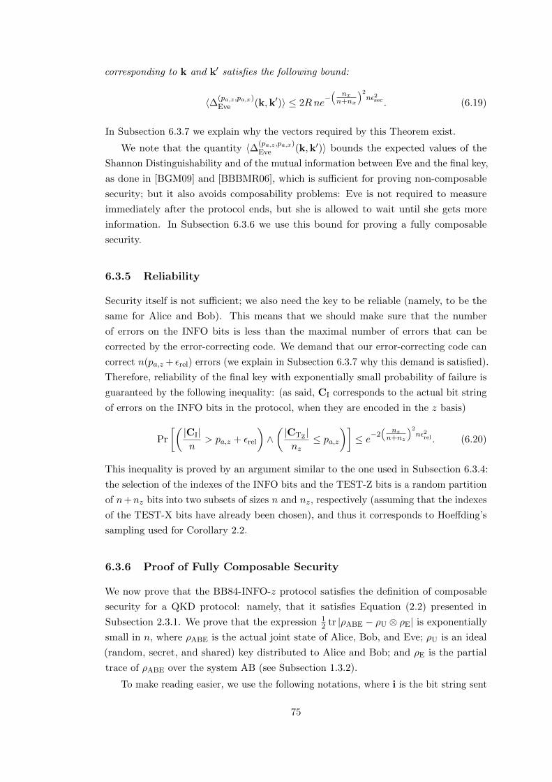
corresponding to k and k′ satisfies the following bound:
〈∆(pa,z ,pa,x)Eve (k,k′)〉 ≤ 2Rne
−(
nxn+nx
)2nε2sec . (6.19)
In Subsection 6.3.7 we explain why the vectors required by this Theorem exist.
We note that the quantity 〈∆(pa,z ,pa,x)Eve (k,k′)〉 bounds the expected values of the
Shannon Distinguishability and of the mutual information between Eve and the final key,
as done in [BGM09] and [BBBMR06], which is sufficient for proving non-composable
security; but it also avoids composability problems: Eve is not required to measure
immediately after the protocol ends, but she is allowed to wait until she gets more
information. In Subsection 6.3.6 we use this bound for proving a fully composable
security.
6.3.5 Reliability
Security itself is not sufficient; we also need the key to be reliable (namely, to be the
same for Alice and Bob). This means that we should make sure that the number
of errors on the INFO bits is less than the maximal number of errors that can be
corrected by the error-correcting code. We demand that our error-correcting code can
correct n(pa,z + εrel) errors (we explain in Subsection 6.3.7 why this demand is satisfied).
Therefore, reliability of the final key with exponentially small probability of failure is
guaranteed by the following inequality: (as said, CI corresponds to the actual bit string
of errors on the INFO bits in the protocol, when they are encoded in the z basis)
Pr
[(|CI|n
> pa,z + εrel
)∧(|CTZ
|nz
≤ pa,z)]≤ e−2
(nz
n+nz
)2nε2rel . (6.20)
This inequality is proved by an argument similar to the one used in Subsection 6.3.4:
the selection of the indexes of the INFO bits and the TEST-Z bits is a random partition
of n+nz bits into two subsets of sizes n and nz, respectively (assuming that the indexes
of the TEST-X bits have already been chosen), and thus it corresponds to Hoeffding’s
sampling used for Corollary 2.2.
6.3.6 Proof of Fully Composable Security
We now prove that the BB84-INFO-z protocol satisfies the definition of composable
security for a QKD protocol: namely, that it satisfies Equation (2.2) presented in
Subsection 2.3.1. We prove that the expression 12 tr |ρABE − ρU ⊗ ρE| is exponentially
small in n, where ρABE is the actual joint state of Alice, Bob, and Eve; ρU is an ideal
(random, secret, and shared) key distributed to Alice and Bob; and ρE is the partial
trace of ρABE over the system AB (see Subsection 1.3.2).
To make reading easier, we use the following notations, where i is the bit string sent
75

by Alice, iB is the bit string received by Bob, and c = i⊕ iB is the string of errors:
iABT ,
(iz, ib, i
Bz , i
Bb
), (6.21)
T ,
1 if |cz|nz ≤ pa,z and |cb|nx≤ pa,x
0 otherwise. (6.22)
In other words, iABT consists of all TEST-Z and TEST-X bits of Alice and Bob; and T
is the random variable representing the result of the test.
According to the above definitions, the states ρABE and ρU are
ρABE =∑
i,iB,P|T=1
Pr(i, iB,P
)· |k〉A〈k|A ⊗ |k
′〉B〈k′|B
⊗(ρb′
x,xB
)E⊗ |iAB
T ,P, ξ〉C〈iABT ,P, ξ|C, (6.23)
ρU =1
2m
∑k
|k〉A〈k|A ⊗ |k〉B〈k|B, (6.24)
where(ρb′
x,xB
)E
is defined to be Eve’s quantum state if Alice sends the INFO string
x = is in the bases b′ = bs and Bob gets the INFO string xB = iBs . All the other states
actually represent classical information: subsystems A and B represent the final keys
held by Alice (k = xPTK ) and Bob (k′, that is obtained from xB, ξ = xPT
C , and PK), and
subsystem C represents the information published in the unjammable classical channel
during the protocol (this information is known to Alice, Bob, and Eve)—namely, iABT
(all the test bits), P (the partition), and ξ = xPTC (the syndrome).
We note that in the definition of ρABE, we sum only over events in which the test is
passed (namely, in which the protocol is not aborted by Alice and Bob): in such cases,
an m-bit key is generated. The cases in which the protocol aborts do not exist in the
sum—namely, they are represented by the zero operator, as required by the definition of
composable security (see Subsection 2.3.1 and [Ren08, Subsection 6.1.2]). Thus, ρABE
is a non-normalized state, and tr(ρABE) is the probability that the test is passed.
To help us bound the trace distance, we define the following intermediate state:
ρ′ABE ,∑
i,iB,P|T=1
Pr(i, iB,P
)· |k〉A〈k|A ⊗ |k〉B〈k|B
⊗(ρb′
x,xB
)E⊗ |iAB
T ,P, ξ〉C〈iABT ,P, ξ|C. (6.25)
This state is identical to ρABE, except that Bob holds the Alice’s final key (k) instead of
his own calculated final key (k′). In particular, the similarity between ρABE and ρ′ABE
means, by definition, that ρE , trAB (ρABE) and ρ′E , trAB (ρ′ABE) are the same state:
namely, ρE = ρ′E.
76

Proposition 6.4. Under the same conditions as Theorem 6.3, it holds that
1
2tr∣∣ρ′ABE − ρU ⊗ ρE
∣∣ ≤ 2Rne−(
nxn+nx
)2nε2sec , (6.26)
for ρ′ABE and ρU defined above and for the partial trace ρE , trAB (ρABE).
Proof. We notice that in ρ′ABE, the only factors depending directly on x and xB (and
not only on k and ξ) are the probability Pr(i, iB,P
)and Eve’s state
(ρb′
x,xB
)E
. The
probability can be reformulated as:
Pr(i, iB,P
)= Pr
(iABT ,P, ξ
)· Pr
(k | iAB
T ,P, ξ)
· Pr(x | k, iAB
T ,P, ξ)· Pr
(xB | x,k, iAB
T ,P, ξ)
= Pr(iABT ,P, ξ
)· 1
2m· 1
2n−r−m
· Pr(xB | x,k, iAB
T ,P, ξ). (6.27)
(Because all the possible n-bit values of x have the same probability, 12n ; and because
all the r + m rows of the matrices PC and PK are linearly independent, so there are
exactly 2n−r−m values of x corresponding to each specific pair (ξ,k).)
Therefore, the state ρ′ABE takes the following form:
ρ′ABE =1
2m
∑k,iABT ,P,ξ|T=1
Pr(iABT ,P, ξ
)· |k〉A〈k|A ⊗ |k〉B〈k|B
⊗
1
2n−r−m
∑x,xB
∣∣xPTC = ξ
xPTK = k
Pr(xB | x,k, iAB
T ,P, ξ)·(ρb′
x,xB
)E
⊗ |iAB
T ,P, ξ〉C〈iABT ,P, ξ|C
=1
2m
∑k,iABT ,P,ξ|T=1
Pr(iABT ,P, ξ
)· |k〉A〈k|A ⊗ |k〉B〈k|B
⊗ (ρk)E ⊗ |iABT ,P, ξ〉C〈iAB
T ,P, ξ|C. (6.28)
(ρk was defined in Equation (6.8).)
The partial trace ρ′E = trAB (ρ′ABE), that (as proved above) is the same as ρE, is
ρE = ρ′E =1
2m
∑k,iABT ,P,ξ|T=1
Pr(iABT ,P, ξ
)· (ρk)E ⊗ |i
ABT ,P, ξ〉C〈iAB
T ,P, ξ|C, (6.29)
and the state ρU ⊗ ρE is
ρU ⊗ ρE =1
22m
∑k,k′′,iAB
T ,P,ξ|T=1
Pr(iABT ,P, ξ
)· |k〉A〈k|A ⊗ |k〉B〈k|B
77

⊗ (ρk′′)E ⊗ |iABT ,P, ξ〉C〈iAB
T ,P, ξ|C.
By using the triangle inequality for norms, since ρ′ABE and ρU⊗ ρE are the same (except
the difference between Eve’s states, (ρk)E and (ρk′′)E), we get, by using the definition
of 〈∆(pa,z ,pa,x)Eve (k,k′′)〉 (Equation (6.14)) and Theorem 6.3:
1
2tr∣∣ρ′ABE − ρU ⊗ ρE
∣∣ ≤ 1
22m
∑k,k′′,iAB
T ,P,ξ|T=1
Pr(iABT ,P, ξ
)· 1
2tr |(ρk)E − (ρk′′)E|
=1
22m
∑k,k′′
〈∆(pa,z ,pa,x)Eve (k,k′′)〉
≤ 2Rne−(
nxn+nx
)2nε2sec , (6.30)
as we wanted.
We still have to bound the following difference:
ρABE − ρ′ABE =∑
i,iB,P|T=1
Pr(i, iB,P
)· |k〉A〈k|A ⊗
[|k′〉B〈k′|B − |k〉B〈k|B
]⊗
(ρb′
x,xB
)E⊗ |iAB
T ,P, ξ〉C〈iABT ,P, ξ|C
= Pr((
k 6= k′)∧ (T = 1)
)·
∑i,iB,P
Pr(i, iB,P |
(k 6= k′
)∧ (T = 1)
)· |k〉A〈k|A ⊗
[|k′〉B〈k′|B − |k〉B〈k|B
]⊗
(ρb′
x,xB
)E⊗ |iAB
T ,P, ξ〉C〈iABT ,P, ξ|C. (6.31)
Because the trace distance between every two normalized states is bounded by 1, and
because of the reliability proof in Subsection 6.3.5, we get:
1
2tr∣∣ρABE − ρ′ABE
∣∣ ≤ Pr((
k 6= k′)∧ (T = 1)
)≤ e−2
(nz
n+nz
)2nε2rel . (6.32)
(Because if k 6= k′, Alice and Bob have different final keys, and this means that the
error correction stage did not succeed. According to the discussion in Subsection 6.3.5,
this can happen only if there are too many errors in the information string—namely, if|CI|n > pa,z + εrel.)
To sum up, we get the following bound:
1
2tr |ρABE − ρU ⊗ ρE| ≤
1
2tr∣∣ρABE − ρ′ABE
∣∣+1
2tr∣∣ρ′ABE − ρU ⊗ ρE
∣∣≤ e
−2(
nzn+nz
)2nε2rel + 2Rne
−(
nxn+nx
)2nε2sec . (6.33)
This bound is exponentially small in n. Thus, we have proved composable security of
78

BB84-INFO-z.
6.3.7 Security, Reliability, and Error Rate Threshold
According to Theorem 6.3 and to the discussion in Subsection 6.3.5, to get both security
and reliability we only need vectors {vn1 , . . . , vnrn+mn} satisfying both the conditions
of the Theorem (distancedrn,mn
2n > δ2 ≥ pa,x + εsec) and the reliability condition (the
ability to correct n(pa,z + εrel) errors). Such families were proven to exist in Appendix E
of [BBBMR06], giving the following upper bound on the bit-rate:
Rsecret ,m
n< 1−H2(2pa,x + 2εsec)−H2
(pa,z + εrel +
1
n
), (6.34)
where H2(x) , −x log2(x)− (1− x) log2(1− x).
Note that we use here the error thresholds pa,x for security and pa,z for reliability.
This is possible, because in [BBBMR06] these conditions (security and reliability) on
the codes are discussed separately.
To get the asymptotic error rate thresholds, we require Rsecret > 0, and we get the
condition:
H2(2pa,x + 2εsec) +H2
(pa,z + εrel +
1
n
)< 1. (6.35)
The secure asymptotic error rate thresholds zone is shown in Figure 6.1 (it is below
the curve), assuming that 1n is negligible. Note the trade-off between the error rates
pa,z and pa,x. Also note that in the case pa,z = pa,x, we get the same threshold as BB84
([BBBMR06] and [BGM09]), which is 7.56%.
6.4 Conclusion
In this chapter, we have proved the BB84-INFO-z protocol to be fully secure against
collective attacks. We have discovered that the results of BB84 hold very similarly for
BB84-INFO-z, with only two exceptions:
1. The error rates must be separately checked to be below the thresholds pa,z and
pa,x for the TEST-Z and TEST-X bits, respectively, while in BB84 the error rate
threshold pa applies to all the TEST bits together.
2. The exponents of Eve’s information (security) and of the failure probability of the
error-correcting code (reliability) are different than in [BGM09], because different
numbers of test bits are now allowed (nz and nx are arbitrary). This implies that
the exponents may decrease more slowly (or more quickly) as a function of n.
However, if we choose nz = nx = n (thus sending N = 3n qubits from Alice to
Bob), then we get exactly the same exponents as in [BGM09].
The asymptotic error rate thresholds found in this chapter allow us to tolerate a
higher threshold for a specific basis (say, the x basis) if we demand a lower threshold
79
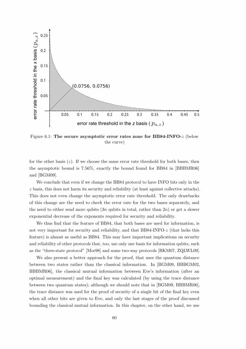
(0.0756, 0.0756)
Figure 6.1: The secure asymptotic error rates zone for BB84-INFO-z (belowthe curve)
for the other basis (z). If we choose the same error rate threshold for both bases, then
the asymptotic bound is 7.56%, exactly the bound found for BB84 in [BBBMR06]
and [BGM09].
We conclude that even if we change the BB84 protocol to have INFO bits only in the
z basis, this does not harm its security and reliability (at least against collective attacks).
This does not even change the asymptotic error rate threshold. The only drawbacks
of this change are the need to check the error rate for the two bases separately, and
the need to either send more qubits (3n qubits in total, rather than 2n) or get a slower
exponential decrease of the exponents required for security and reliability.
We thus find that the feature of BB84, that both bases are used for information, is
not very important for security and reliability, and that BB84-INFO-z (that lacks this
feature) is almost as useful as BB84. This may have important implications on security
and reliability of other protocols that, too, use only one basis for information qubits, such
as the “three-state protocol” [Mor98] and some two-way protocols [BKM07, ZQLWL09].
We also present a better approach for the proof, that uses the quantum distance
between two states rather than the classical information. In [BGM09, BBBGM02,
BBBMR06], the classical mutual information between Eve’s information (after an
optimal measurement) and the final key was calculated (by using the trace distance
between two quantum states); although we should note that in [BGM09, BBBMR06],
the trace distance was used for the proof of security of a single bit of the final key even
when all other bits are given to Eve, and only the last stages of the proof discussed
bounding the classical mutual information. In this chapter, on the other hand, we use
80

the trace distance between the two quantum states until the end of the proof, which
allows us to prove fully composable security.
Therefore, our proof shows the fully composable security of BB84-INFO-z against
collective attacks (and, in particular, security even if Eve keeps her quantum states until
she gets more information when Alice and Bob use the key, rather than measuring them
at the end of the protocol); and a very similar approach can be applied to [BGM09],
immediately proving the composable security of BB84 against collective attacks. Our
proof also makes a step towards making the security proof in [BBBMR06] (security
proof of BB84 against joint attacks) prove the composable security of BB84 against
joint attacks, a proof fully achieved in Chapter 7.
Our results show that the BB84-INFO-z protocol can securely be used for distributing
a secret key; the security is of an ideal implementation and against an adversary limited
to collective attacks (a generalization to the most general attacks (joint attacks), by
using the methods of [BBBMR06], is proposed in Chapter 7). Moreover, security of
the final key is universally composable, which means that the key may be used for any
cryptographic purpose without harming security, even if Eve keeps her quantum states
and makes optimal use of any information she gets in the future.
The techniques described in our proof may be applied in the future for proving
security of other protocols by using similar methods, and, in particular, for proving
security of other QKD protocols that use only one basis for the information bits, such
as [Mor98, BKM07, ZQLWL09] mentioned above.
81

82

Chapter 7
Composable Security of
Generalized BB84 Protocols
Against General (Joint) Attacks
In this chapter, we present a fully composable security proof of “generalized BB84” QKD
protocols against joint attacks (namely, against the most general theoretical attacks, as
described in Subsection 2.3.2). The protocols for which we prove security are the BB84-
INFO-z protocol (Subsection 7.3.1), the standard BB84 protocol (Subsection 7.3.2), the
“efficient BB84” protocol (Subsection 7.3.3), and the “modified efficient BB84” protocol
(Subsection 7.3.4). The proof uses BBBMR’s security approach, that is described in
Subsection 2.3.3.
This chapter is based on a paper being prepared by Michel Boyer and Rotem Liss1.
7.1 Full Definition of the Generalized BB84 Protocols
The protocols for which we prove security in this chapter belong to a generalized class
of BB84-like protocols. Below we formally define this general class of protocols. Some
of the details in this definition are decided by each specific protocol, but most of the
details are shared by all the protocols. See Section 2.7 for an explanation of the notation
of bit strings (s, b, etc.), and see Section 1.1 for an explanation of the notations
|0〉0, |1〉0, |0〉1, |1〉1.
1. Before the protocol begins, Alice and Bob choose some shared (and public)
parameters: the numbers N and n, the sets B and {Sb}b∈B and probability
distributions over them (decided by the specific protocol) that will control the
choice of the bit strings b, s ∈ FN2 , the testing function T (decided by the specific
protocol), the r × n parity check matrix PC (corresponding to a linear error-
correcting code C), and the m×n privacy amplification matrix PK (representing a
1This paper is in preparation.
83

linear key-generation function). It is required that all r +m rows of the matrices
PC and PK put together are linearly independent.
Formally, for choosing the sets B and {Sb}b∈B and the corresponding probability
distributions, Alice and Bob should choose the set B ⊆ FN2 of basis strings, the
probabilities Pr(b) for all b ∈ B, the sets Sb ⊆ FN2 of s strings for all b ∈ B,
and the probabilities Pr(s | b) for all b ∈ B and s ∈ Sb. We require that |s| = n
for all s ∈ Sb. The testing function T : FN−n2 × FN−n
2 × FN2 → {0, 1} must get
(iT ⊕ jT,bT, s) as inputs and give 0 or 1 as an output. In Section 7.3 we give
examples of protocols and their formal definitions using these notations.
2. Alice randomly chooses an N -bit string i ∈ FN2 , an N -bit string b ∈ B, and an
N -bit string s ∈ Sb (that must satisfy |s| = n), and sends the N qubit states
|i1〉b1 , |i2〉b2 , . . . , |iN 〉bN , one after the other, to Bob using the quantum channel.
Bob keeps each received qubit in a quantum memory, not measuring it yet2.
3. Alice sends to Bob over the classical channel the bit string b = b1 . . . bN . Bob
measures each of the qubits he saved in the correct basis (namely, when measuring
the i-th qubit, he measures it in the z basis if bi = 0, and he measures it in the x
basis if bi = 1).
The bit string measured by Bob is denoted by j. The XOR of i and j is denoted
c , i⊕ j. If there is no noise and no eavesdropping, then i = j (that is, c = 0).
4. Alice sends s to Bob over the classical channel. The INFO bits (that will be used
for creating the final key) are the n bits with sj = 1, while the TEST bits (that
will be used for testing) are the N − n bits with sj = 0. We denote the substrings
of i, j, c,b that correspond to the INFO bits by iI, jI, cI, and bI, respectively; and
we denote the substrings of i, j, c,b that correspond to the TEST bits by iT, jT,
cT, and bT, respectively.
5. Alice and Bob both publish the bit values they have for all the TEST bits (iT
and jT, respectively), and they compute their XOR cT = iT ⊕ jT. They compute
T (cT,bT, s): if it is 0, they abort the protocol; if it is 1, they continue the run of
the protocol.
6. The values of the remaining n bits (the INFO bits, with sj =1) are kept in secret
by Alice and Bob. The bit string of Alice is iI, the bit string of Bob is jI, and
their XOR is cI.
2 Here we assume that Bob has a quantum memory and can delay his measurement. In practicalimplementations, Bob usually cannot do that, but he is assumed to choose his own random basis stringb′′ ∈ B and measure in the bases it dictates. Later, Alice and Bob discard the qubits measured in thewrong basis. In that case, we need to assume that Alice sends more than N qubits, so that N qubitsare finally detected by Bob and measured in the correct basis. In Appendix A of [BBBMR06] it isexplained why this change of the protocol does not hurt security.
84
7. Alice sends to Bob the syndrome of iI (with respect to the error-correcting code
C and to its corresponding parity check matrix PC), that consists of r bits and is
defined as ξ , iIPTC . By using ξ, Bob corrects the errors in his jI string (so that
it is the same as iI).
8. The final key consists of m bits and is defined as k , iIPTK . Both Alice and Bob
compute it.
7.2 Bound on the Security Definition for the Generalized
BB84 Protocols
7.2.1 The Hypothetical “Inverted-INFO-Basis” Protocol
For the security proof, we use an alternative, hypothetical protocol, in which Alice
sends to Bob the qubits after inverting the bases of the INFO bits (without changing
the bases of the TEST bits). We call this protocol “hypothetical” because it is never
actually used by Alice and Bob, and we do not perform any reduction to it (or from it),
but we compute probabilities of certain events in the hypothetical protocol for use in
our security bound. In particular, we use the error rate in the hypothetical protocol for
bounding the trace distance in the security definition of the real protocol.
In the hypothetical protocol, Alice, Bob, and Eve do everything exactly as they
would do in the real protocol, except that Alice and Bob use (and publish) the basis
string b0 , b⊕ s instead of b: namely, they use the basis string bT for the TEST bits
and the basis string bI (the bitwise NOT of bI) for the INFO bits.
Formally, this hypothetical protocol is defined by replacing Steps 2–3 of the original
protocol (as described in Section 7.1) by the following steps:
2. Alice randomly chooses an N -bit string i ∈ FN2 , an N -bit string b ∈ B, and an
N -bit string s ∈ Sb (that must satisfy |s| = n). Then, she computes the N -bit
string b0 , b⊕ s, and sends the N qubit states |i1〉b01 , |i2〉b02 , . . . , |iN 〉b0N , one after
the other, to Bob using the quantum channel. Bob keeps each received qubit in a
quantum memory, not measuring it yet.
3. Alice sends to Bob over the classical channel the bit string b0 = b01 . . . b0N . Bob
measures each of the qubits he saved in the correct basis (namely, when measuring
the i-th qubit, he measures it in the z basis if b0i = 0, and he measures it in the x
basis if b0i = 1).
We notice that in this protocol, Alice chooses b and s in the same way as she would
choose them in the real protocol, but uses (and sends to Bob for his use) b0 and s
instead.
In the security proof, we will use the notation of Prinverted-INFO-basis for calculating the
probability of a certain event assuming that Alice and Bob use the hypothetical protocol.
85

In particular, we note that Prinverted-INFO-basis(· | b, s) is a conditional probability on
Alice choosing the bit strings b, s (while she actually uses the basis string b0).
It should be noted that Prinverted-INFO-basis(· | b, s) is usually the same as Pr(· | b0, s):
namely, the hypothetical protocol given that Alice chooses b, s (and thus uses b0, s)
is the same as the real protocol given that Alice chooses b0, s. However, the second
notation is not always well-defined, because it may be the case that b ∈ B while b0 /∈ B,
or that s ∈ Sb while s /∈ Sb0 ; therefore, it may be the case that b0 is not an allowed basis
string for the real protocol. In the standard BB84 protocol (see Subsection 7.3.2), such
problems are impossible, and this is why [BBBMR06] uses the notation of Pr(· | b0, s)
instead of Prinverted-INFO-basis(· | b, s). However, in our chapter, we discuss generalized
BB84 protocols, and we must use the notation of Prinverted-INFO-basis(· | b, s).3
7.2.2 The General Joint Attack of Eve
Before the beginning of the QKD protocol (and, thus, independently of i, b, and s),
Eve chooses some joint attack to perform. In a joint attack, all the qubits are attacked
by using a shared giant probe (ancillary state) kept by Eve. Eve saves her probe in a
quantum memory and can keep it indefinitely, even after the final key is used by Alice
and Bob; and she can perform, at any time of her choice, an optimal measurement
of her giant probe, chosen based on all the information she has at the time of the
measurement (including the classical information sent during the protocol, and including
the information she acquires when Alice and Bob use the key).
Given that Alice sends to Bob the state |i〉b , ⊗Nj=1|ij〉bj (namely, the N -bit string
is i and the N -bit basis string is b), Eve attaches a probe state |0〉E and applies some
unitary operator U of her choice to the compound system |0〉E|i〉b. Then, Eve keeps
to herself (in a quantum memory) her probe state, and she sends to Bob the N -qubit
quantum state sent from Alice to Bob (which may have been modified due to her attack
U).
The most general joint attack U of Eve is
U |0〉E|i〉b =∑j∈FN2
|E′i,j〉b|j〉b, (7.1)
where |E′i,j〉b are non-normalized states in Eve’s probe system. We note that
〈E′i,j|E′i,j〉b = Pr(j | i,b, s). (7.2)
Writing the INFO and TEST bits of Alice and Bob separately (iT, iI instead of i, and
jT, jI instead of j), we can denote |E′i,j〉b by |E′iT,iI,jT,jI〉b.
In Subsection 3.4 of [BBBMR06], the notation of |EiI,jI〉b,s is introduced. This
notation is useful, because it treats iT and jT as constants (since they are ultimately
3 It is also possible that Pr(b, s) 6= Pr(b0, s), in which case the use of b0, s in the real protocol doesnot happen with the same probability as the use of b0, s in the hypothetical protocol.
86

published by Alice and Bob, and then they are known to Eve), assuming their values to
be known. It is defined as
|EiI,jI〉b,s ,1√
Pr(jT | iT, iI,b, s)|E′iT,iI,jT,jI〉b. (7.3)
We note that |EiI,jI〉b,s also depends on the constants iT, jT (and not only on iI, jI,b, s).
According to Equations (3.22)–(3.23) of [BBBMR06], given that Alice sends iI, iT,b, s
and that Bob measures jT, the normalized state of Eve and Bob is
|ψiI〉 =∑jI∈Fn2
|EiI,jI〉b,s|jI〉b, (7.4)
and it also holds that
〈EiI,jI |EiI,jI〉b,s = Pr(jI | iI, iT, jT,b, s). (7.5)
Let us define ρb,siI,jI(which also depends on iT, jT) to be the normalized state of Eve
if Alice sends iI, iT,b, s and Bob measures jI, jT. That is, ρb,siI,jIis the normalization of
|E′i,j〉b and of |EiI,jI〉b,s, so
ρb,siI,jI,
|EiI,jI〉b,s〈EiI,jI |Pr(jI | iI, iT, jT,b, s)
=|E′i,j〉b〈E′i,j|Pr(j | i,b, s)
. (7.6)
The state of Eve after her attack (tracing out Bob) is
ρiI , trBob(|ψiI〉〈ψiI |) =∑jI∈Fn2
|EiI,jI〉b,s〈EiI,jI | =∑jI∈Fn2
Pr(jI | iI, iT, jT,b, s)ρb,siI,jI, (7.7)
and we define its purification |ϕiI〉 (so that ρiI is a partial trace of |ϕiI〉) as
|ϕiI〉 ,∑jI∈Fn2
|EiI,jI〉b,s|iI ⊕ jI〉. (7.8)
7.2.3 The Symmetrized Attack of Eve
In [BBBMR06], the most general joint attack is not directly analyzed: for simplicity, it
is assumed that Eve applies a process called symmetrization, resulting in a symmetrized
attack. The process of symmetrization is always beneficial for Eve (it does not change the
error rate, and we prove in Proposition 7.4 that it does not decrease Eve’s information),
so a security proof against all symmetrized attacks implies a security proof against all
the possible joint attacks.
In Eve’s original attack, she has her own probe subsystem E. In the symmetriza-
tion process, Eve adds another probe subsystem M, in the initial state of |0x〉M ,1√2N
∑m∈FN2
|m〉M. Given the original attack U (applied to Alice’s qubits and to the
probe E), the symmetrized attack U sym (applied to Alice’s qubits and to both probes E
87

and M) is defined by
U sym , (IE ⊗ S†)(U ⊗ IM)(IE ⊗ S), (7.9)
where S is a unitary operation applied to Alice’s qubits and to the probe M, and it
operates as follows:
S|i〉b|m〉M = (−1)(i⊕b)·m|i⊕m〉b|m〉M. (7.10)
Intuitively, Eve first XORs Alice’s bit values with a random string m (kept by her); then
she applies her original attack; and then she reverses the XOR with m. Full definition
and explanations are available in Subsection 3.1 of [BBBMR06].
In this chapter, we use several properties of the symmetrized attack. First of all, the
“Basic Lemma of Symmetrization” (Lemma 3.1 of [BBBMR06]) gives the expression for
|Esymi,j′〉b (of the symmetrized attack) as a function of |E′i,j〉b (of the original attack):
|Esymi,j′〉b =
1√2N
∑m∈FN2
(−1)(i⊕j)·m|E′i⊕m,j⊕m〉b|m〉M. (7.11)
The second property we use, proved in Corollary 3.3 of [BBBMR06], is the fact that
the probabilities of the error strings cI and cT (if not conditioning on i) are not affected
by the symmetrization. Namely,
Prsym(cI, cT | b, s) = Pr(cI, cT | b, s). (7.12)
This is true for all the basis strings b; in particular, this is true for the basis string b0 ,
b⊕s used in the hypothetical “inverted-INFO-basis” protocol defined in Subsection 7.2.1,
so
Prsyminverted-INFO-basis(cI, cT | b, s) = Prinverted-INFO-basis(cI, cT | b, s). (7.13)
The third property we use, proved in Lemma 3.8 of [BBBMR06], is the fact that
the probabilities for errors in the TEST bits are not affected by the bases used for the
INFO bits:
Prsym(jT | iT,b, s) = Prsym(jT | iT,bT, s). (7.14)
In particular, since the only difference between the hypothetical “inverted-INFO-basis”
protocol and the real protocol is the basis string used for the INFO bits (bI and bI,
respectively), this means that the probabilities of errors in the TEST bits are the same
for both of these protocols:
Prsyminverted-INFO-basis(jT | iT,b, s) = Prsym(jT | iT,b, s). (7.15)
The fourth property we use, proved in Corollary 3.6 of [BBBMR06], is the fact
that the probability of any string of INFO bits iI is uniform (that is, 12n ) even when
88

conditioning on the four parameters iT, jT,b, s, that are ultimately known to Eve (we
note that jT is affected by Eve’s attack). Namely,
Prsym(iI | iT, jT,b, s) =1
2n. (7.16)
7.2.4 Results from [BBBMR06]
The security proof of the generalized BB84 protocols is very similar to the security
proof of BB84 itself, that was detailed in [BBBMR06]. Most parts of the proof are not
affected at all by the changes made to BB84 to get the generalized BB84 protocols
(changes detailed in Section 7.1 of this chapter), because these parts assume fixed strings
s and b.
Therefore, the reader is referred to the proof in Section 3 (except Subsection 3.3.2)
and Subsections 4.1–4.4 of [BBBMR06], that applies to all the generalizations of BB84
without any changes (except changing the total number of bits, 2n, to N , which does
not affect the proof at all), and that will not be repeated here.
We denote the rows of the error-correction parity check matrix PC as the vectors
v1, . . . , vr in Fn2 , and the rows of the privacy amplification matrix PK as the vectors
vr+1, . . . , vr+m. We also denote, for any 1 ≤ r′ ≤ r +m,
V excr′ , Span{v1, . . . , vr′−1, vr′+1, . . . , vr+m}, (7.17)
namely, V excr′ is the (r + m − 1)-dimensional vector space that spans all the error
correction and privacy amplification vectors, except vr′ ; and we also define
v , minr+1≤r′≤r+m
dH(vr′ , Vexcr′ ). (7.18)
For a 1-bit final key k ∈ {0, 1} (that is, for m = 1), and given a symmetrized attack
of Eve, we define ρsymk to be the state of Eve corresponding to the final key k, given
that she knows ξ. Thus,
ρsymk =1
2n−r−1
∑iI
∣∣ iIPTC = ξ
iI · vr+1 = k
(ρiI)sym, (7.19)
where (ρiI)sym, as defined in Equation (7.7), is Eve’s state after the (symmetrized)
attack, given that Alice sent the INFO bit string iI (and given the bit strings iT, jT,b, s,
that are ultimately known to Eve).
In addition, we define the state ρsymk , that is a lift-up of ρsymk (which means that
ρsymk is a partial trace of ρsymk ), by assuming that Eve knows the purification |ϕsymiI〉
89

defined in Equation (7.8):
ρsymk =1
2n−r−1
∑iI
∣∣ iIPTC = ξ
iI · vr+1 = k
|ϕsymiI〉〈ϕsym
iI|. (7.20)
(This state was defined in Equation (4.10) of [BBBMR06], but was denoted there as
ρk(vr+1, ξ).)
In the end of Subsection 4.4 of [BBBMR06] (in its Proposition 4.6, and according to
the proof of Lemma 4.5, which appears in Appendix D.2 of [BBBMR06]), it was found
that (in the case of a 1-bit final key, i.e., m = 1), for any symmetrized attack,
1
2tr |ρsym0 − ρsym1 | ≤ 2
√Prsyminverted-INFO-basis
[|CI| ≥
v
2| iT, jT,b, s
], (7.21)
where CI is the random variable whose value equals to cI , iI⊕jI, and Prsyminverted-INFO-basis
means that the probability is taken over the hypothetical “inverted-INFO-basis” protocol
defined in Subsection 7.2.1 (to which Eve applies the same symmetrized attack that
she applies to the real protocol). We also note that v was defined above, and that in
the current case (m = 1), its definition is simplified to v = dH(vr+1, Vexcr+1) (and V exc
r+1 is
simply Span{v1, . . . , vr}).
Now, according to [NC00, Theorem 9.2 and page 407], and using the fact that ρsymkis a partial trace of ρsymk , we find out that
1
2tr |ρsym0 − ρsym1 | ≤ 1
2tr |ρsym0 − ρsym1 |. (7.22)
From this result and from Equation (7.21) we deduce that
1
2tr |ρsym0 − ρsym1 | ≤ 2
√Prsyminverted-INFO-basis
[|CI| ≥
v
2| iT, jT,b, s
]. (7.23)
7.2.5 Bounding the Differences Between Eve’s States
So far, we have discussed a 1-bit key. We will now discuss a general m-bit key k. We
define ρsymk to be the state of Eve corresponding to the final key k, given that she knows
ξ:
ρsymk =1
2n−r−m
∑iI
∣∣iIPTC = ξ
iIPTK = k
(ρiI)sym. (7.24)
90

We note (for use in Subsection 7.2.6) that if we substitute (ρiI)sym from Equation (7.7),
we get
ρsymk =1
2n−r−m
∑iI,jI
∣∣iIPTC = ξ
iIPTK = k
Prsym(jI | iI, iT, jT,b, s) ·(ρb,siI,jI
)sym. (7.25)
Proposition 7.1. For any two keys k,k′ of m bits, and for any symmetrized attack,
1
2tr |ρsymk − ρsymk′ | ≤ 2m
√Prsyminverted-INFO-basis
[|CI| ≥
v
2| iT, jT,b, s
], (7.26)
where CI is the random variable whose value equals to cI , iI ⊕ jI, and, in addition,
v , minr+1≤r′≤r+m dH(vr′ , Vexcr′ ).
Proof. We define the key kj , for 0 ≤ j ≤ m, to consist of the first j bits of k′ and the
last m − j bits of k. This means that k0 = k, km = k′, and kj−1 differs from kj at
most on a single bit (the j-th bit).
First, we find a bound on 12 tr |ρsymkj−1
− ρsymkj|: since kj−1 differs from kj at most on
a single bit (the j-th bit, given by the formula iI · vr+j), we can use the same proof that
gave us Equation (7.23), attaching the other (identical) key bits to ξ of the original
proof; and we find out that
1
2tr |ρsymkj−1
− ρsymkj| ≤ 2
√Prsyminverted-INFO-basis
[|CI| ≥
vj2| iT, jT,b, s
], (7.27)
where we define vj to be dH(vr+j , Vexcr+j), and, therefore, v = min1≤j′≤m vj′ .
In particular, v ≤ vj . Therefore, if |CI| ≥ vj2 , then |CI| ≥ v
2 . Therefore, Equa-
tion (7.27) implies
1
2tr |ρsymkj−1
− ρsymkj| ≤ 2
√Prsyminverted-INFO-basis
[|CI| ≥
v
2| iT, jT,b, s
]. (7.28)
Now we use the triangle inequality for norms to find
1
2tr |ρsymk − ρsymk′ | =
1
2tr |ρsymk0
− ρsymkm| ≤
m∑j=1
1
2tr |ρsymkj−1
− ρsymkj|
≤ 2m
√Prsyminverted-INFO-basis
[|CI| ≥
v
2| iT, jT,b, s
]. (7.29)
We would now like to bound the expected value (namely, the average value) of the
trace distance between two states of Eve corresponding to two final keys. However, we
should take into account that if the test fails, no final key is generated, in which case
we define the distance to be 0. We thus define the random variable ∆symEve (k,k′) for any
91

two final keys k,k′:
∆symEve (k,k′ | iT, jT,b, s, ξ) ,
12 tr |ρsymk − ρsymk′ | if T (iT ⊕ jT,bT, s) = 1
0 otherwise. (7.30)
We need to bound the expected value 〈∆symEve (k,k′)〉, that is given by:
〈∆symEve (k,k′)〉 =
∑iT, jT ∈ FN−n2 ,
b ∈ B, s ∈ Sb, ξ ∈ Fn2
∆symEve (k,k′ | iT, jT,b, s, ξ) · Prsym(iT, jT,b, s, ξ).
(7.31)
(In Subsection 7.2.6 we prove that this expected value is indeed the quantity we need to
bound for proving fully composable security, defined in Subsection 2.3.1.)
Theorem 7.2. For any two final keys k,k′,
〈∆symEve (k,k′)〉 ≤ 2m
√Prinverted-INFO-basis
[(|CI|n≥ v
2n
)∧ (T = 1)
], (7.32)
where |CI|n is a random variable whose value is the error rate on the INFO bits, and
T is a random variable whose value is 1 if the test passes and 0 otherwise. We note
that the protocol considered for the probability in the right-hand-side is the hypothetical
“inverted-INFO-basis” protocol defined in Subsection 7.2.1, in which Alice and Bob use the
basis string b0 , b⊕ s instead of b. We note that the probability in the right-hand-side
is the probability for the original (non-symmetrized) attack.
Proof. We use the convexity of x2, namely, the fact that for all {pi}i satisfying pi ≥ 0
and∑
i pi = 1, it holds that (∑
i pixi)2 ≤
∑i pix
2i . We also use the fact that
Prsyminverted-INFO-basis(iT, jT,b, s)
= Prsyminverted-INFO-basis(iT,b, s) · Prsyminverted-INFO-basis(jT | iT,b, s)
= Prsym(iT,b, s) · Prsym(jT | iT,b, s)
= Prsym(iT, jT,b, s), (7.33)
which is correct because iT,b, s are all chosen in the same way both in the hypothetical
“inverted-INFO-basis” protocol and in the real protocol (even though different basis
strings are used in these protocols), and because according to the third property of
the symmetrized attack (Equation (7.15)), Prsyminverted-INFO-basis(jT | iT,b, s) = Prsym(jT |iT,b, s).
92

In addition, we use the result
Prsyminverted-INFO-basis
[(|CI| ≥
v
2
)∧ (T = 1) | b, s
]= Prinverted-INFO-basis
[(|CI| ≥
v
2
)∧ (T = 1) | b, s
], (7.34)
which is correct because according to the second property of the symmetrized attack
(Equation (7.13)), Prsyminverted-INFO-basis(cI, cT | b, s) = Prinverted-INFO-basis(cI, cT | b, s),
and because the random variable T depends only on the random variable CT and on
the parameters bT, s.
We also use the result
Prsyminverted-INFO-basis(b, s) = Prinverted-INFO-basis(b, s), (7.35)
which is correct because Alice’s random choice of b, s is independent of Eve’s attack.
We find out that:
〈∆symEve (k,k′)〉2
=
∑iT,jT,b,s,ξ
∆symEve (k,k′ | iT, jT,b, s, ξ) · Prsym(iT, jT,b, s, ξ)
2
(by (7.31))
≤∑
iT,jT,b,s,ξ
(∆sym
Eve (k,k′ | iT, jT,b, s, ξ))2 · Prsym(iT, jT,b, s, ξ) (by convexity of x2)
=∑
iT,jT,b,s,ξ|T=1
(12 tr |ρsymk − ρsymk′ |
)2 · Prsym(iT, jT,b, s, ξ) (by (7.30))
≤ 4m2 ·∑
iT,jT,b,s,ξ|T=1
Prsyminverted-INFO-basis
[|CI| ≥ v
2 | iT, jT,b, s]
· Prsym(iT, jT,b, s, ξ) (by (7.26))
= 4m2 ·∑
iT,jT,b,s|T=1
Prsyminverted-INFO-basis
[|CI| ≥ v
2 | iT, jT,b, s]
· Prsym(iT, jT,b, s)
= 4m2 ·∑
iT,jT,b,s
Prsyminverted-INFO-basis
[(|CI| ≥ v
2
)∧ (T = 1) | iT, jT,b, s
]· Prsym(iT, jT,b, s)
= 4m2 ·∑
iT,jT,b,s
Prsyminverted-INFO-basis
[(|CI| ≥ v
2
)∧ (T = 1) | iT, jT,b, s
]· Prsyminverted-INFO-basis(iT, jT,b, s) (by (7.33))
= 4m2 ·∑b,s
Prsyminverted-INFO-basis
[(|CI| ≥ v
2
)∧ (T = 1) | b, s
]· Prsyminverted-INFO-basis(b, s)
93

= 4m2 ·∑b,s
Prinverted-INFO-basis
[(|CI| ≥ v
2
)∧ (T = 1) | b, s
]· Prinverted-INFO-basis(b, s) (by (7.34)–(7.35))
= 4m2 · Prinverted-INFO-basis
[(|CI| ≥ v
2
)∧ (T = 1)
](7.36)
7.2.6 Bound for Fully Composable Security
We now prove a crucial part of the claim that generalized BB84 protocols satisfy
the definition of composable security for a QKD protocol: namely, that they satisfy
Equation (2.2) presented in Subsection 2.3.1. We derive an upper bound for the
expression 12 tr |ρABE − ρU ⊗ ρE|, where ρABE is the actual joint state of Alice, Bob,
and Eve at the end of the protocol; ρU is an ideal (random, secret, and shared) key
distributed to Alice and Bob; and ρE is the partial trace of ρABE over the system AB
(see Subsection 1.3.2). In other words, we upper-bound the trace distance between
the system after the real QKD protocol and the system after an ideal key distribution
protocol (which first performs the real QKD protocol and then magically distributes to
Alice and Bob a random, secret, and shared key).
The states ρABE and ρU are
ρABE =∑
i,j,b,s|T=1
Pr (i, j,b, s) · |k〉A〈k| ⊗ |kB〉B〈kB|
⊗(ρb,siI,jI
)E⊗ |iT, jT,b, s, ξ〉C〈iT, jT,b, s, ξ|, (7.37)
ρU =1
2m
∑k
|k〉A〈k| ⊗ |k〉B〈k|, (7.38)
where(ρb,siI,jI
)E
is defined in Equation (7.6) to be Eve’s quantum normalized state if
Alice sends the bit strings iI, iT,b, s and Bob measures the bit strings jI, jT. All the
other states actually represent classical information: subsystems A and B represent the
final keys held by Alice (k , iIPTK ) and Bob (his key kB is obtained from jI, ξ , iIP
TC ,
and PK), and subsystem C represents the information published in the unjammable
classical channel during the protocol (this information is known to Alice, Bob, and
Eve)—namely, iT, jT (all the TEST bits), b (the basis string), s (the string representing
the partition into INFO and TEST bits), and ξ , iIPTC (the syndrome).
We note that in the definition of ρABE, we sum only over the events in which the test
is passed (namely, in which the protocol is not aborted by Alice and Bob): in such cases,
an m-bit key is generated. The cases in which the protocol aborts do not exist in the
sum—namely, they are represented by the zero operator, as required by the definition
of composable security (see [Ren08, Subsection 6.1.2]). Thus, ρABE is a non-normalized
state, and tr(ρABE) is the probability that the test is passed.
94

To help us bound the trace distance, we define the following intermediate state:
σABE ,∑
i,j,b,s|T=1
Pr (i, j,b, s) · |k〉A〈k| ⊗ |k〉B〈k|
⊗(ρb,siI,jI
)E⊗ |iT, jT,b, s, ξ〉C〈iT, jT,b, s, ξ|. (7.39)
This state is identical to ρABE, except that Bob holds Alice’s final key (k) instead of
his own calculated final key (kB). In particular, the similarity between ρABE and σABE
means, by definition, that ρE , trAB (ρABE) and σE , trAB (σABE) are the same state:
that is, ρE = σE.
Proposition 7.3. For any symmetrized attack, it holds that
1
2tr∣∣σsymABE − ρU ⊗ σ
symE
∣∣≤ 2m
√Prinverted-INFO-basis
[(|CI|n≥ v
2n
)∧ (T = 1)
], (7.40)
for σsymABE and ρU defined above (but for the symmetrized attack) and for the partial
trace σsymE , trAB
(σsymABE
). We note that the probability in the right-hand-side is the
probability for the original (non-symmetrized) attack.
Proof. We notice that in σsymABE, the only factors depending directly on iI and jI (and not
only on k and ξ) are the probability Prsym (i, j,b, s) and Eve’s state(ρb,siI,jI
)symE
. The
probability can be reformulated as
Prsym (i, j,b, s) = Prsym (iT, jT,b, s, ξ) · Prsym (k | iT, jT,b, s, ξ)
· Prsym (iI | k, iT, jT,b, s, ξ) · Prsym (jI | iI,k, iT, jT,b, s, ξ)
= Prsym (iT, jT,b, s, ξ) · 1
2m· 1
2n−r−m
· Prsym (jI | iI, iT, jT,b, s) . (7.41)
(This is correct because all the possible n-bit values of iI have the same probability, 12n ,
conditioned on iT, jT,b, s, according to the fourth property of the symmetrized attack
(Equation (7.16)); and because all the r+m rows of the matrices PC and PK are linearly
independent, so there are exactly 2n−r−m values of iI corresponding to each specific pair
(ξ,k).)
Therefore, the state σsymABE takes the following form:
σsymABE =1
2m
∑k,iT,jT,b,s,ξ|T=1
Prsym (iT, jT,b, s, ξ) · |k〉A〈k| ⊗ |k〉B〈k|
95

⊗
1
2n−r−m
∑iI,jI
∣∣iIPTC = ξ
iIPTK = k
Prsym (jI | iI, iT, jT,b, s) ·(ρb,siI,jI
)symE
⊗ |iT, jT,b, s, ξ〉C〈iT, jT,b, s, ξ|
=1
2m
∑k,iT,jT,b,s,ξ|T=1
Prsym (iT, jT,b, s, ξ) · |k〉A〈k| ⊗ |k〉B〈k|
⊗(ρsymk
)E⊗ |iT, jT,b, s, ξ〉C〈iT, jT,b, s, ξ|. (7.42)
(This expression for ρsymk was found in Equation (7.25).)
The partial trace σsymE , trAB
(σsymABE
)is
σsymE =1
2m
∑k,iT,jT,b,s,ξ|T=1
Prsym (iT, jT,b, s, ξ) ·(ρsymk
)E⊗|iT, jT,b, s, ξ〉C〈iT, jT,b, s, ξ|,
(7.43)
and the state ρU ⊗ σsymE is
ρU ⊗ σsymE =1
22m
∑k,k′,iT,jT,b,s,ξ|T=1
Prsym (iT, jT,b, s, ξ) · |k〉A〈k| ⊗ |k〉B〈k|
⊗(ρsymk′
)E⊗ |iT, jT,b, s, ξ〉C〈iT, jT,b, s, ξ|. (7.44)
Since σsymABE and ρU ⊗ σsymE are the same (except the difference between Eve’s states,(ρsymk
)E
and(ρsymk′
)E
), we get, by using the triangle inequality for norms, the definition
of 〈∆symEve (k,k′)〉 (Equation (7.31)), and Theorem 7.2:
1
2tr∣∣σsymABE − ρU ⊗ σ
symE
∣∣≤ 1
22m
∑k,k′,iT,jT,b,s,ξ|T=1
Prsym (iT, jT,b, s, ξ) · 1
2tr∣∣(ρsymk
)E−(ρsymk′
)E
∣∣=
1
22m
∑k,k′
〈∆symEve (k,k′)〉
≤ 2m
√Prinverted-INFO-basis
[(|CI|n≥ v
2n
)∧ (T = 1)
]. (7.45)
Proposition 7.4. For any attack, it holds that
1
2tr |σABE − ρU ⊗ σE| ≤
1
2tr∣∣σsymABE − ρU ⊗ σ
symE
∣∣ , (7.46)
for σABE, σsymABE, and ρU defined above and for the partial traces σE , trAB (σABE) and
σsymE , trAB
(σsymABE
).
Proof. First, we have to find an expression for(ρb,siI,jI
)symE
. According to Equation (7.6),
96

(ρb,siI,jI
)symE
=
[|Esym
i,j′〉b〈Esym
i,j′|]E
Prsym(j | i,b, s), (7.47)
and according to the “Basic Lemma of Symmetrization” (see Equation (7.11)),
|Esymi,j′〉b =
1√2N
∑m∈FN2
(−1)(i⊕j)·m|E′i⊕m,j⊕m〉b|m〉M. (7.48)
Therefore,
(ρb,siI,jI
)symE
=1
2N
∑m,m′∈FN2
(−1)(i⊕j)·(m⊕m′)[|E′i⊕m,j⊕m〉b〈E′i⊕m′,j⊕m′ | ⊗ |m〉M〈m′|
]E
Prsym(j | i,b, s).
(7.49)
The state σsymABE now takes the following form:
σsymABE =1
2N
∑i,j,b,s,m,m′|T=1
Prsym (i, j,b, s) · |k〉A〈k| ⊗ |k〉B〈k|
⊗(−1)(i⊕j)·(m⊕m
′)[|E′i⊕m,j⊕m〉b〈E′i⊕m′,j⊕m′ | ⊗ |m〉M〈m′|
]E
Prsym(j | i,b, s)
⊗ |iT, jT,b, s, ξ〉C〈iT, jT,b, s, ξ|
=1
2N
∑i,j,b,s,m,m′|T=1
Prsym (i,b, s) · |k〉A〈k| ⊗ |k〉B〈k|
⊗ (−1)(i⊕j)·(m⊕m′)[|E′i⊕m,j⊕m〉b〈E′i⊕m′,j⊕m′ | ⊗ |m〉M〈m′|
]E
⊗ |iT, jT,b, s, ξ〉C〈iT, jT,b, s, ξ|. (7.50)
We define a unitary operator V : given the state |m〉M (held by Eve), the unitary
operator V takes a XOR of all the states in the subsystems A, B, and C with the
relevant parts of m. Namely, if we define mI and mT as the INFO bits and the TEST
bits (respectively) of m (of course, they depend on s), and if we define km , mIPTK
and ξm , mIPTC , then
V |k〉A|k〉B [|E〉|m〉M]E |iT, jT,b, s, ξ〉C= |k⊕ km〉A|k⊕ km〉B [|E〉|m〉M]E
|iT ⊕mT, jT ⊕mT,b, s, ξ ⊕ ξm〉C. (7.51)
Therefore (also using the fact that Prsym (i,b, s) = Pr (i,b, s) = Pr (i⊕m,b, s)),
V σsymABEV† =
1
2N
∑i,j,b,s,m,m′|T=1
Pr (i⊕m,b, s) · |k⊕ km〉A〈k⊕ km′ | ⊗ |k⊕ km〉B〈k⊕ km′ |
⊗ (−1)(i⊕j)·(m⊕m′)[|E′i⊕m,j⊕m〉b〈E′i⊕m′,j⊕m′ | ⊗ |m〉M〈m′|
]E
⊗ |iT ⊕mT, jT ⊕mT,b, s, ξ ⊕ ξm〉C〈iT ⊕m′T, jT ⊕m′T,b, s, ξ ⊕ ξm′ |. (7.52)
97

Tracing out the subsystem M (which is a part of Eve’s probe), we get
trM
[V σsymABEV
†]
=1
2N
∑i,j,b,s,m|T=1
Pr (i⊕m,b, s) · |k⊕ km〉A〈k⊕ km| ⊗ |k⊕ km〉B〈k⊕ km|
⊗[|E′i⊕m,j⊕m〉b〈E′i⊕m,j⊕m|
]E
⊗ |iT ⊕mT, jT ⊕mT,b, s, ξ ⊕ ξm〉C〈iT ⊕mT, jT ⊕mT,b, s, ξ ⊕ ξm|.(7.53)
Now we can change the indexes of the sum, in the following way: we denote i′ , i⊕m
and j′ , j⊕m (for a fixed m), and we immediately get, according to the definitions,
the results i′T = iT ⊕mT, j′T = jT ⊕mT, k′ , i′IPTK = (iI ⊕mI)P
TK = k ⊕ km, and
similarly ξ′ , i′IPTC = ξ⊕ ξm. We also notice that T gets (iT⊕ jT,bT, s) as inputs, and
that they all stay the same (because i′T ⊕ j′T = (iT ⊕mT)⊕ (jT ⊕mT) = iT ⊕ jT), and
therefore the change of indexes does not impact the condition T = 1. Therefore,
trM
[V σsymABEV
†]
=1
2N
∑i′,j′,b,s,m|T=1
Pr(i′,b, s
)· |k′〉A〈k′| ⊗ |k′〉B〈k′|
⊗[|E′i′,j′〉b〈E′i′,j′ |
]E
⊗ |i′T, j′T,b, s, ξ′〉C〈i′T, j′T,b, s, ξ′|. (7.54)
Using the relation(ρb,siI,jI
)E
=[|E′i,j〉b〈E
′i,j|]E
Pr(j|i,b,s) from Equation (7.6), we get
trM
[V σsymABEV
†]
=∑
i′,j′,b,s|T=1
Pr(i′,b, s
)· |k′〉A〈k′| ⊗ |k′〉B〈k′|
⊗ Pr(j′ | i′,b, s)(ρb,si′I,j′I
)E
⊗ |i′T, j′T,b, s, ξ′〉C〈i′T, j′T,b, s, ξ′|
=∑
i′,j′,b,s|T=1
Pr(i′, j′,b, s
)· |k′〉A〈k′| ⊗ |k′〉B〈k′|
⊗(ρb,si′I,j′I
)E⊗ |i′T, j′T,b, s, ξ′〉C〈i′T, j′T,b, s, ξ′|
= σABE. (7.55)
To sum up, we get the result σABE = trM[V σsymABEV
†]. A very similar proof gives
us the result ρU ⊗ σE = trM[V(ρU ⊗ σsymE
)V †]. Since the trace distance is preserved
under unitary operators and does not increase under partial trace, we get
1
2tr |σABE − ρU ⊗ σE| =
1
2tr∣∣∣trM [V (σsymABE − ρU ⊗ σ
symE
)V †]∣∣∣
≤ 1
2tr∣∣∣V (σsymABE − ρU ⊗ σ
symE
)V †∣∣∣
=1
2tr∣∣σsymABE − ρU ⊗ σ
symE
∣∣ . (7.56)
98

Proposition 7.5. For any attack,
1
2tr |ρABE − σABE| ≤ Pr
[(k 6= kB
)∧ (T = 1)
], (7.57)
for ρABE and σABE defined above, and for k being the final key computed by Alice and
kB being the final key computed by Bob.
Proof.
ρABE − σABE =∑
i,j,b,s|T=1
Pr (i, j,b, s)
· |k〉A〈k| ⊗[|kB〉B〈kB| − |k〉B〈k|
]⊗
(ρb,siI,jI
)E⊗ |iT, jT,b, s, ξ〉C〈iT, jT,b, s, ξ|
= Pr[(
k 6= kB)∧ (T = 1)
]·
∑i,j,b,s
Pr[i, j,b, s |
(k 6= kB
)∧ (T = 1)
]· |k〉A〈k| ⊗
[|kB〉B〈kB| − |k〉B〈k|
]⊗
(ρb,siI,jI
)E⊗ |iT, jT,b, s, ξ〉C〈iT, jT,b, s, ξ|. (7.58)
The trace distance between any two normalized states is bounded by 1. Therefore,
1
2tr |ρABE − σABE| ≤ Pr
[(k 6= kB
)∧ (T = 1)
]. (7.59)
Corollary 7.6. For any attack,
1
2tr |ρABE − ρU ⊗ ρE|
≤ Pr[(
k 6= kB)∧ (T = 1)
]+ 2m
√Prinverted-INFO-basis
[(|CI|n ≥
v2n
)∧ (T = 1)
], (7.60)
for ρABE and ρU defined above and for the partial trace ρE , trAB (ρABE).
Proof. Using Propositions 7.3, 7.4, and 7.5, and also the fact that ρE = σE, we get:
1
2tr |ρABE − ρU ⊗ ρE|
≤ 1
2tr |ρABE − σABE|+
1
2tr |σABE − ρU ⊗ σE|
≤ 1
2tr |ρABE − σABE|+
1
2tr∣∣σsymABE − ρU ⊗ σ
symE
∣∣≤ Pr
[(k 6= kB
)∧ (T = 1)
]+ 2m
√Prinverted-INFO-basis
[(|CI|n ≥
v2n
)∧ (T = 1)
]. (7.61)
99

We have thus found an upper bound for the expression 12 tr |ρABE − ρU ⊗ ρE|. In
Section 7.3 we prove this upper bound to be exponentially small in n for specific
protocols.
7.3 Full Security Proofs for Specific Protocols
Below we prove full security for specific important examples of generalized BB84
protocols.
In this section we use Hoeffding’s theorem, as described in Section 2.6; in particular,
we use Corollary 2.2.
7.3.1 The BB84-INFO-z Protocol
In the BB84-INFO-z protocol, all the INFO bits are sent by Alice in the z basis, while
the TEST bits are sent in both the z and the x bases. This means that b and s together
define a random partition of the set of indexes {1, 2, . . . , N} into three disjoint sets:
• I (INFO bits, where sj = 1 and bj = 0) of size n;
• TZ (TEST-Z bits, where sj = 0 and bj = 0) of size nz; and
• TX (TEST-X bits, where sj = 0 and bj = 1) of size nx.
Formally, Alice and Bob agree on parameters n, nz, nx (such that N = n+ nz + nx),
and we choose B = {b ∈ FN2 | |b| = nx} and Sb = {s ∈ FN
2 | (|s| = n) ∧ (|s ⊕ b| =
n + nx)} (namely, s ∈ Sb if it consists of n 1-bits that do not overlap with the nx
1-bits of b) for all b ∈ B. The probability distributions Pr(b) and Pr(s | b) are all
uniform—namely, Pr(b, s) is identical for all b ∈ B and s ∈ Sb.
Alice and Bob also agree on error rate thresholds, pa,z and pa,x (for the TEST-Z
and TEST-X bits, respectively). The testing function T is defined as follows:
T (iT ⊕ jT,bT, s) = 1 ⇔ (|iTZ⊕ jTZ
| ≤ nz · pa,z) ∧ (|iTX⊕ jTX
| ≤ nx · pa,x) . (7.62)
Namely, the test passes if and only if the error rate on the TEST-Z bits is at most pa,z
and the error rate on the TEST-X bits is at most pa,x.
Following Corollary 7.6, we know the following bound:
1
2tr |ρABE − ρU ⊗ ρE|
≤ Pr[(
k 6= kB)∧ (T = 1)
]+ 2m
√Prinverted-INFO-basis
[(|CI|n ≥
v2n
)∧ (T = 1)
]. (7.63)
Below we prove the two probabilities in the right-hand-side to be exponentially small in
n:
100

Theorem 7.7. Let us be given δsec > 0, and, for infinitely many values of n, a family
{vn1 , . . . , vnrn+mn} of linearly independent vectors in Fn2 such that δsec <
vn . Then for
any pa,z, pa,x > 0 and εsec > 0 such that pa,x + εsec ≤ δsec2 , and for any nz, nx > 0, it
holds for the BB84-INFO-z protocol that
Prinverted-INFO-basis
[(|CI|n≥ v
2n
)∧ (T = 1)
]≤ e−2
(nx
n+nx
)2nε2sec . (7.64)
Proof. Because v2n >
δsec2 ≥ pa,x + εsec, it holds that
Prinverted-INFO-basis
[(|CI|n≥ v
2n
)∧ (T = 1)
]= Prinverted-INFO-basis
[(|CI|n≥ v
2n
)∧(|CTZ
|nz
≤ pa,z)∧(|CTX
|nx
≤ pa,x)]
≤ Prinverted-INFO-basis
[(|CI|n
> pa,x + εsec
)∧(|CTX
|nx
≤ pa,x)]
. (7.65)
In the hypothetical “inverted-INFO-basis” protocol, the INFO and TEST-X bits
are sent and measured in the x basis, while the TEST-Z bits are sent and measured in
the z basis. Therefore, the random and uniform sampling of the n INFO bits out of
the n+ nx bits sent in the x basis (assuming that the TEST-Z bits have already been
chosen) does not affect the bases in the hypothetical protocol. This means that we can
apply Corollary 2.2 to this sampling, and we get
Prinverted-INFO-basis
[(|CI|n
> pa,x + εsec
)∧(|CTX
|nx
≤ pa,x)]≤ e−2
(nx
n+nx
)2nε2sec .
(7.66)
Theorem 7.8. Let us be given δrel > 0, and, for infinitely many values of n, a family
{vn1 , . . . , vnrn+mn} of linearly independent vectors in Fn2 such that the parity-check matrix
PC, whose rows are {vn1 , . . . , vnrn}, defines an error-correcting code that can correct up
to n · δrel errors on an n-bit string. Then for any pa,z, pa,x > 0 and εrel > 0 such that
pa,z + εrel ≤ δrel, and for any nz, nx > 0, it holds for the BB84-INFO-z protocol that
Pr[(
k 6= kB)∧ (T = 1)
]≤ e−2
(nz
n+nz
)2nε2rel . (7.67)
Proof. If k 6= kB, Alice and Bob have different final keys, and this means that the error
correction stage did not succeed. The error-correcting code can correct up to n · δrelerrors, and, therefore, it can correct up to n · (pa,z + εrel) errors (since pa,z + εrel ≤ δrel).Therefore, a failure of the error correction stage must mean that there are more than
n·(pa,z+εrel) errors in the INFO bits: namely, if k 6= kB, then necessarily |CI|n > pa,z+εrel.
101

Therefore,
Pr[(
k 6= kB)∧ (T = 1)
]= Pr
[(k 6= kB
)∧(|CTZ
|nz
≤ pa,z)∧(|CTX
|nx
≤ pa,x)]
≤ Pr
[(|CI|n
> pa,z + εrel
)∧(|CTZ
|nz
≤ pa,z)]
. (7.68)
In the real protocol, the INFO and TEST-Z bits are sent and measured in the z
basis, while the TEST-X bits are sent and measured in the x basis. Therefore, the
random and uniform sampling of the n INFO bits out of the n+ nz bits sent in the z
basis (assuming that the TEST-X bits have already been chosen) does not affect the
bases in the real protocol. This means that we can apply Corollary 2.2 to this sampling,
and we get
Pr
[(|CI|n
> pa,z + εrel
)∧(|CTZ
|nz
≤ pa,z)]≤ e−2
(nz
n+nz
)2nε2rel . (7.69)
If we combine the conditions and the results of Corollary 7.6, Theorem 7.7, and
Theorem 7.8, we get the following result:
Corollary 7.9. Let us be given δsec > 0, δrel > 0, and, for infinitely many values of
n, a family {vn1 , . . . , vnrn+mn} of linearly independent vectors in Fn2 such that δsec <
vn
and such that the parity-check matrix PC, whose rows are {vn1 , . . . , vnrn}, defines an
error-correcting code that can correct up to n · δrel errors on an n-bit string. Then for
any pa,z, pa,x > 0 and εsec, εrel > 0 such that pa,x + εsec ≤ δsec2 and pa,z + εrel ≤ δrel, and
for any nz, nx > 0, it holds for the BB84-INFO-z protocol that
1
2tr |ρABE − ρU ⊗ ρE| ≤ e
−2(
nzn+nz
)2nε2rel + 2mne
−(
nxn+nx
)2nε2sec . (7.70)
This bound is exponentially small in n.
All that is left to be explained is why the vectors required by Corollary 7.9 exist.
We need a family of vectors {vn1 , . . . , vnrn+mn} satisfying both the condition v2n >
δsec2 ≥
pa,x+ εsec and the ability to correct up to n(pa,z + εrel) errors. Such families were proven
to exist in Appendix E of [BBBMR06], giving the following upper bound on the bit-rate:
Rsecret ,mn
n< 1−H2(2pa,x + 2εsec)−H2
(pa,z + εrel +
1
n
), (7.71)
where H2(x) , −x log2(x)− (1− x) log2(1− x).
Note that we use here the error thresholds pa,x for the condition on v and pa,z for
error correction. This is possible, because in [BBBMR06] these conditions on the codes
are discussed separately.
102

(0.0756, 0.0756)
Figure 7.1: The secure asymptotic error rates zone for BB84-INFO-z (belowthe curve)
To get the asymptotic error rate thresholds, we require Rsecret > 0, and we get the
condition
H2(2pa,x + 2εsec) +H2
(pa,z + εrel +
1
n
)< 1. (7.72)
The secure asymptotic error rate thresholds zone is shown in Figure 7.1 (it is below
the curve), assuming that 1n is negligible. Note the trade-off between the error rate
thresholds pa,z and pa,x. Also note that in the case of pa,z = pa,x, we get the same
threshold as in similar security proofs of BB84 [BBBMR06, BGM09], which is 7.56%.
7.3.2 The Standard BB84 Protocol
In the standard BB84 protocol, the strings b and s are chosen randomly (except that
we demand |s| = n) and independently, and N = 2n. In other words, there are n INFO
bits and n TEST bits (chosen randomly), and for each one of them, the basis (z or x)
is chosen randomly and independently.
Formally, in BB84, we choose N = 2n, B = FN2 , and Sb = {s ∈ FN
2 | |s| = n}for all b ∈ B. The probability distributions Pr(b) and Pr(s | b) = Pr(s) are all
uniform—namely, Pr(b, s) is identical for all b ∈ B and s ∈ Sb.
Given the parameter pa agreed by Alice and Bob, the testing function T is
T (iT ⊕ jT,bT, s) = 1 ⇔ |iT ⊕ jT| ≤ n · pa. (7.73)
Namely, the test passes if and only if the error rate on the TEST bits is at most pa.
103
Proposition 7.10. In the standard BB84 protocol,
Prinverted-INFO-basis
[(|CI|n≥ v
2n
)∧ (T = 1)
]= Pr
[(|CI|n≥ v
2n
)∧ (T = 1)
].
(7.74)
Proof.
Prinverted-INFO-basis
[(|CI|n≥ v
2n
)∧ (T = 1)
]=
∑b,s
Prinverted-INFO-basis
[(|CI|n≥ v
2n
)∧ (T = 1) | b, s
]· Pr(b, s)
=∑b,s
Pr
[(|CI|n≥ v
2n
)∧ (T = 1) | b0, s
]· Pr(b0, s)
= Pr
[(|CI|n≥ v
2n
)∧ (T = 1)
](7.75)
(where b0 , b⊕ s).
The security of the standard BB84 protocol is now easily obtained:
Theorem 7.11. Let us be given δsec > 0, δrel > 0, and, for infinitely many values of
n, a family {vn1 , . . . , vnrn+mn} of linearly independent vectors in Fn2 such that δsec <
vn
and such that the parity-check matrix PC, whose rows are {vn1 , . . . , vnrn}, defines an
error-correcting code that can correct up to n · δrel errors on an n-bit string. Then for
any pa > 0 and εsec, εrel > 0 such that pa + εsec ≤ δsec2 and pa + εrel ≤ δrel, it holds for
the standard BB84 protocol that
1
2tr |ρABE − ρU ⊗ ρE| ≤ e−
12nε2rel + 2mne
− 14nε2sec . (7.76)
Proof. By using Corollary 7.6 and Proposition 7.10, we get the following bound for
BB84:
1
2tr |ρABE − ρU ⊗ ρE|
≤ Pr[(
k 6= kB)∧ (T = 1)
]+ 2mn
√Pr
[(|CI|n≥ v
2n
)∧ (T = 1)
]= Pr
[(k 6= kB
)∧(|CT|n≤ pa
)]+ 2mn
√Pr
[(|CI|n≥ v
2n
)∧(|CT|n≤ pa
)]. (7.77)
Because v2n >
δsec2 ≥ pa + εsec, and also because the event k 6= kB implies that the
104

error rate on the INFO bits is higher than δrel ≥ pa + εrel, we get:
Pr
[(k 6= kB
)∧(|CT|n≤ pa
)]+ 2mn
√Pr
[(|CI|n≥ v
2n
)∧(|CT|n≤ pa
)]≤ Pr
[(|CI|n
> pa + εrel
)∧(|CT|n≤ pa
)]+ 2mn
√Pr
[(|CI|n
> pa + εsec
)∧(|CT|n≤ pa
)]. (7.78)
All the bits in the protocol are sent in random and independent bases. Therefore,
the random and uniform sampling of the n INFO bits out of the N = 2n bits does not
affect the bases (in the real protocol). This means that we can apply Corollary 2.2 to
this sampling, and we get
Pr
[(|CI|n
> pa + εrel
)∧(|CT|n≤ pa
)]≤ e−
12nε2rel , (7.79)
Pr
[(|CI|n
> pa + εsec
)∧(|CT|n≤ pa
)]≤ e−
12nε2sec . (7.80)
Combining Equations (7.77)–(7.80), we get
1
2tr |ρABE − ρU ⊗ ρE| ≤ e−
12nε2rel + 2mne
− 14nε2sec . (7.81)
In Appendix E of [BBBMR06] we get the following results on vector families satisfying
the requirements of Theorem 7.11: the bit-rate satisfies
Rsecret ,mn
n< 1−H2(2pa + 2εsec)−H2
(pa + εrel +
1
n
), (7.82)
and the condition on the asymptotic error rate threshold is
H2(2pa + 2εsec) +H2
(pa + εrel +
1
n
)< 1. (7.83)
This gives an asymptotic error rate threshold of 7.56%.
7.3.3 The “Efficient BB84” Protocol
In the “efficient BB84” protocol (suggested by [LCA05]), the bit string b is chosen
probabilistically, but not uniformly : each qubit is sent in the z basis with probability p
(and in the x basis with probability 1− p), where 0 < p ≤ 12 . Then, the bit string s is
chosen such that there are nz TEST-Z bits and nx TEST-X bits. In other words, as
in BB84-INFO-z, the strings b and s together define a random partition of the set of
105

indexes {1, 2, . . . , N} into three disjoint sets:
• I (INFO bits, where sj = 1) of size n. However, unlike BB84-INFO-z, this set
consists of both z qubits and x qubits; therefore, it can be divided to two disjoint
subsets:
– IZ (INFO-Z bits, where sj = 1 and bj = 0); and
– IX (INFO-X bits, where sj = 1 and bj = 1).
• TZ (TEST-Z bits, where sj = 0 and bj = 0) of size nz; and
• TX (TEST-X bits, where sj = 0 and bj = 1) of size nx.
Formally, in “efficient BB84”, Alice and Bob agree on parameters n, nz, nx (such
that N = n + nz + nx) and on a parameter 0 < p ≤ 12 , and we choose B = FN
2 and
Sb = {s ∈ FN2 | (|s| = n)∧ (|s∧b| = nx)} for all b ∈ B (namely, it is required that there
are n INFO bits, nz TEST-Z bits, and nx TEST-X bits). This time, the probability
distribution Pr(b) is not uniform: it holds that Pr(b) = (1− p)|b| · pN−|b|, because the
probability of each bit to be in the x basis is 1− p. On the other hand, the probability
distribution Pr(s | b) is uniform.
Remark. A subtle point is that for some values b ∈ FN2 (for example, for b = 00 . . . 0),
the set Sb is empty: no s can be agreed by Alice and Bob for such values of b. In that
case, as assumed in [LCA05, Section 4.3], the protocol aborts, and other values of b
and s are randomly chosen; this is equivalent to assuming Alice is not allowed to choose
these values of b. Therefore, to be more precise, we must re-define
B = {b ∈ FN2 | Sb 6= ∅} = {b ∈ FN
2 | (|b| ≥ nx) ∧ (|b| ≥ nz)}, (7.84)
and we must normalize the probabilities by defining Pr0(b) , (1 − p)|b| · pN−|b| (the
original probability of each b), Np ,∑
b∈B Pr0(b) (the sum of all the original probabil-
ities for all the allowed values of b ∈ B), and then the real probability of each b ∈ B is
Pr(b) =Pr0(b)
Np=
(1− p)|b| · pN−|b|
Np. (7.85)
This guarantees that the sum of probabilities of all the allowed values b ∈ B is 1.
Alice and Bob also agree on an error rate threshold, pa (applied both to the TEST-Z
bits and to the TEST-X bits). The testing function T is defined as follows:
T (iT ⊕ jT,bT, s) = 1 ⇔ (|iTZ⊕ jTZ
| ≤ nz · pa) ∧ (|iTX⊕ jTX
| ≤ nx · pa) . (7.86)
Namely, the test passes if and only if the error rate on the TEST-Z bits is at most pa
and the error rate on the TEST-X bits is at most pa.
In this security proof, instead of analyzing all the INFO bits together, we analyze
the INFO-Z and the INFO-X bits separately. We define the following random variables:
106
• CIZ and CIX are the random variables corresponding to the error strings on the
INFO-Z bits and on the INFO-X bits, respectively.
• NIZ and NIX are random variables equal to the numbers of INFO-Z and INFO-X
bits, respectively. (We note that the parameters n, nz, nx are deterministically
chosen by Alice and Bob, while NIZ and NIX are determined by the probabilistic
choice of b. We also note that, necessarily, n = NIZ +NIX .)
Proposition 7.12. For any ε > 0,
Pr
[(|CI|n
> pa + ε
)∧ (T = 1)
]≤ Pr
[(|CIZ |NIZ
> pa + ε
)∧ (T = 1)
]+ Pr
[(|CIX |NIX
> pa + ε
)∧ (T = 1)
]. (7.87)
Equation (7.87) similarly applies to the hypothetical “inverted-INFO-basis” protocol,
too (namely, it applies even if Pr is replaced by Prinverted-INFO-basis).
Proof. We observe that if the error rate on all the INFO bits together is larger than
pa + ε, then at least one of the error rates (on the INFO-Z bits or on the INFO-X bits)
must be larger than pa + ε. (Equivalently, if both error rates on the INFO-Z bits and
on the INFO-X bits are less than pa + ε, then the error rate on the INFO bits is less
than pa + ε.) Namely,(|CI|n
> pa + ε
)⇒
(|CIZ |NIZ
> pa + ε
)∨(|CIX |NIX
> pa + ε
). (7.88)
In particular, the corresponding probabilities satisfy
Pr
[(|CI|n
> pa + ε
)∧ (T = 1)
]≤ Pr
[(|CIZ |NIZ
> pa + ε
)∧ (T = 1)
]+ Pr
[(|CIX |NIX
> pa + ε
)∧ (T = 1)
]. (7.89)
This result applies both to the real protocol and to the hypothetical “inverted-INFO-basis”
protocol.
Proposition 7.13. For any ε > 0 and δ > 0,
Pr
[(|CIZ |NIZ
> pa + ε
)∧ (T = 1)
]≤ Pr (NIZ ≤ δ)
+ maxδ≤tz≤n
Pr
[(|CIZ |tz
> pa + ε
)∧ (T = 1) | NIZ = tz
], (7.90)
107

and
Pr
[(|CIX |NIX
> pa + ε
)∧ (T = 1)
]≤ Pr (NIX ≤ δ)
+ maxδ≤tx≤n
Pr
[(|CIX |tx
> pa + ε
)∧ (T = 1) | NIX = tx
]. (7.91)
Equations (7.90)–(7.91) similarly apply to the hypothetical “inverted-INFO-basis”
protocol, too (namely, they apply even if Pr is replaced by Prinverted-INFO-basis).
Proof. First, we prove Equation (7.90):
Pr
[(|CIZ |NIZ
> pa + ε
)∧ (T = 1)
]=
∑tz
Pr
[(|CIZ |tz
> pa + ε
)∧ (T = 1) | NIZ = tz
]· Pr (NIZ = tz)
=∑tz<δ
Pr
[(|CIZ |tz
> pa + ε
)∧ (T = 1) | NIZ = tz
]· Pr (NIZ = tz)
+∑
δ≤tz≤nPr
[(|CIZ |tz
> pa + ε
)∧ (T = 1) | NIZ = tz
]· Pr (NIZ = tz)
≤∑tz≤δ
Pr (NIZ = tz)
+ maxδ≤tz≤n
Pr
[(|CIZ |tz
> pa + ε
)∧ (T = 1) | NIZ = tz
]·∑
δ≤tz≤nPr (NIZ = tz)
≤ Pr (NIZ ≤ δ) + maxδ≤tz≤n
Pr
[(|CIZ |tz
> pa + ε
)∧ (T = 1) | NIZ = tz
]. (7.92)
The proof of Equation (7.91) is similar. Both proofs apply both to the real protocol
and to the “inverted-INFO-basis” protocol.
Theorem 7.14. Let us be given δsec > 0, δrel > 0, and, for infinitely many values of
n, a family {vn1 , . . . , vnrn+mn} of linearly independent vectors in Fn2 such that δsec <
vn
and such that the parity-check matrix PC, whose rows are {vn1 , . . . , vnrn}, defines an
error-correcting code that can correct up to n · δrel errors on an n-bit string. Then for
any pa > 0 and εsec, εrel > 0 such that pa + εsec ≤ δsec2 and pa + εrel ≤ δrel, for any
0 < p ≤ 12 , and for any 0 < nz <
pN2 and 0 < nx <
(1−p)N2 , it holds for the “efficient
BB84” protocol that
1
2tr |ρABE − ρU ⊗ ρE| ≤ e−
12Np2 + e
−2(
nzn+nz
)2( pN2 −nz)ε
2rel
+ e−12N(1−p)2 + e
−2(
nxn+nx
)2( (1−p)N2−nx
)ε2rel
108

+ 2mn
√e−
12Np2 + e
−2(
nxn+nx
)2( pN2 −nz)ε2sec+
e−12N(1−p)2 + e
−2(
nzn+nz
)2( (1−p)N2−nx
)ε2sec . (7.93)
Proof. By using Corollary 7.6 and Proposition 7.12, we get the following bound:
1
2tr |ρABE − ρU ⊗ ρE|
≤ Pr[(
k 6= kB)∧ (T = 1)
]+ 2mn
√Prinverted-INFO-basis
[(|CI|n≥ v
2n
)∧ (T = 1)
]≤ Pr
[(|CI|n
> pa + εrel
)∧ (T = 1)
]+ 2mn
√Prinverted-INFO-basis
[(|CI|n
> pa + εsec
)∧ (T = 1)
]≤ Pr
[(|CIZ |NIZ
> pa + εrel
)∧ (T = 1)
]+ Pr
[(|CIX |NIX
> pa + εrel
)∧ (T = 1)
]+ 2mn
√Prinverted-INFO-basis
[(|CIZ |NIZ
> pa + εsec
)∧ (T = 1)
]+
Prinverted-INFO-basis
[(|CIX |NIX
> pa + εsec
)∧ (T = 1)
]. (7.94)
Proposition 7.13 and the definition of T give us the following bounds:
Pr
[(|CIZ |NIZ
> pa + εrel
)∧ (T = 1)
]≤ Pr
(NIZ ≤
pN
2− nz
)+ max
pN2−nz≤tz≤n
Pr[( |CIZ
|tz
>pa + εrel
)∧( |CTZ
|nz≤pa
)|NIZ= tz
], (7.95)
Pr
[(|CIX |NIX
> pa + εrel
)∧ (T = 1)
]≤ Pr
(NIX ≤
(1− p)N2
− nx)
+ max(1−p)N
2−nx≤tx≤n
Pr[( |CIX
|tx
>pa + εrel
)∧( |CTX
|nx≤pa
)|NIX= tx
], (7.96)
Prinverted-INFO-basis
[(|CIZ |NIZ
> pa + εsec
)∧ (T = 1)
]≤ Prinverted-INFO-basis
(NIZ ≤
pN
2− nz
)+ max
pN2−nz≤tz≤n
Prinverted-INFO-basis
[( |CIZ|
tz>pa + εsec
)∧( |CTX
|nx≤pa
)|NIZ= tz
], (7.97)
Prinverted-INFO-basis
[(|CIX |NIX
> pa + εsec
)∧ (T = 1)
]109
≤ Prinverted-INFO-basis
(NIX ≤
(1− p)N2
− nx)
+ max(1−p)N
2−nx≤tx≤n
Prinverted-INFO-basis
[( |CIX|
tx>pa + εsec
)∧( |CTZ
|nz≤pa
)|NIX= tx
]. (7.98)
For each one of Equations (7.95)–(7.98), we need to upper-bound two probabilities.
For bounding the first set of probabilities, we use the results of Corollary 2.4:
Pr
(|b| ≤ (1− p)N
2
)≤ e−
12N(1−p)2 , (7.99)
Pr
(|b| ≤ pN
2
)≤ e−
12Np2 . (7.100)
We notice that |b| = NIX + nx and |b| = NIZ + nz; therefore,
Pr
(NIX ≤
(1− p)N2
− nx)≤ e−
12N(1−p)2 , (7.101)
Pr
(NIZ ≤
pN
2− nz
)≤ e−
12Np2 , (7.102)
Prinverted-INFO-basis
(NIX ≤
(1− p)N2
− nx)≤ e−
12N(1−p)2 , (7.103)
Prinverted-INFO-basis
(NIZ ≤
pN
2− nz
)≤ e−
12Np2 . (7.104)
For bounding the second set of probabilities, given specific values of NIZ = tz and
NIX = tx, we use Corollary 2.2:
In the real protocol, the INFO-Z and TEST-Z bits are sent and measured in the
z basis, while the INFO-X and TEST-X bits are sent and measured in the x basis.
Therefore, the random and uniform sampling of the tz INFO-Z bits out of the tz + nz
bits sent in the z basis (assuming that the INFO-X and TEST-X bits have already been
chosen) does not affect the bases in the real protocol; similarly, the random and uniform
sampling of the tx INFO-X bits out of the tx + nx bits sent in the x basis (assuming
that the INFO-Z and TEST-Z bits have already been chosen) does not affect the bases
in the real protocol. We note that these samplings are uniform, because the probability
Pr(s | b) is uniform for all the allowed values of b and s. This means that we can apply
Corollary 2.2 to both of these samplings, and we get
Pr
[(|CIZ |tz
> pa + εrel
)∧(|CTZ
|nz
≤ pa)| NIZ = tz
]≤ e
−2(
nztz+nz
)2tzε2rel , (7.105)
Pr
[(|CIX |tx
> pa + εrel
)∧(|CTX
|nx
≤ pa)| NIX = tx
]≤ e
−2(
nxtx+nx
)2txε2rel . (7.106)
110

Maximizing over tz and tx, we get:
maxpN2−nz≤tz≤n
Pr
[(|CIZ |tz
> pa + εrel
)∧(|CTZ
|nz
≤ pa)| NIZ = tz
]≤ e
−2(
nzn+nz
)2( pN2 −nz)ε
2rel , (7.107)
max(1−p)N
2−nx≤tx≤n
Pr
[(|CIX |tx
> pa + εrel
)∧(|CTX
|nx
≤ pa)| NIX = tx
]≤ e
−2(
nxn+nx
)2( (1−p)N2−nx
)ε2rel . (7.108)
In the hypothetical “inverted-INFO-basis” protocol, the INFO-X and TEST-Z bits
are sent and measured in the z basis, while the INFO-Z and TEST-X bits are sent
and measured in the x basis. Therefore, the random and uniform sampling of the tx
INFO-X bits out of the tx + nz bits sent in the z basis (assuming that the INFO-Z and
TEST-X bits have already been chosen) does not affect the bases in the hypothetical
protocol; similarly, the random and uniform sampling of the tz INFO-Z bits out of the
tz + nx bits sent in the x basis (assuming that the INFO-X and TEST-Z bits have
already been chosen) does not affect the bases in the hypothetical protocol. We note
that these samplings are uniform, because the probability Pr(b) depends only on |b|and is invariant to permutations. This means that we can apply Corollary 2.2 to both
of these samplings, and we get
Prinverted-INFO-basis
[(|CIZ |tz
> pa + εsec
)∧(|CTX
|nx
≤ pa)| NIZ = tz
]≤ e
−2(
nxtz+nx
)2tzε2sec , (7.109)
Prinverted-INFO-basis
[(|CIX |tx
> pa + εsec
)∧(|CTZ
|nz
≤ pa)| NIX = tx
]≤ e
−2(
nztx+nz
)2txε2sec . (7.110)
Maximizing over tz and tx, we get:
maxpN2−nz≤tz≤n
Prinverted-INFO-basis
[(|CIZ |tz
> pa + εsec
)∧(|CTX
|nx
≤ pa)| NIZ = tz
]≤ e
−2(
nxn+nx
)2( pN2 −nz)ε
2sec , (7.111)
max(1−p)N
2−nx≤tx≤n
Prinverted-INFO-basis
[(|CIX |tx
> pa + εsec
)∧(|CTZ
|nz
≤ pa)| NIX = tx
]≤ e
−2(
nzn+nz
)2( (1−p)N2−nx
)ε2sec . (7.112)
To sum up, we get the following bound:
1
2tr |ρABE − ρU ⊗ ρE|
111
≤ e−12Np2 + e
−2(
nzn+nz
)2( pN2 −nz)ε
2rel
+ e−12N(1−p)2 + e
−2(
nxn+nx
)2( (1−p)N2−nx
)ε2rel
+ 2mn
√e−
12Np2 + e
−2(
nxn+nx
)2( pN2 −nz)ε2sec+
e−12N(1−p)2 + e
−2(
nzn+nz
)2( (1−p)N2−nx
)ε2sec . (7.113)
Similarly to the standard BB84, we get the following results on vector families
satisfying the requirements of Theorem 7.14: the bit-rate satisfies
Rsecret ,mn
n< 1−H2(2pa + 2εsec)−H2
(pa + εrel +
1
n
), (7.114)
and the condition on the asymptotic error rate threshold is
H2(2pa + 2εsec) +H2
(pa + εrel +
1
n
)< 1. (7.115)
This gives an asymptotic error rate threshold of 7.56%.
7.3.4 The “Modified Efficient BB84” Protocol
A relatively minor property of the definition of the “efficient BB84” protocol in [LCA05]
(and in Subsection 7.3.3) makes both the security bound and the security proof pretty
complicated. In this subsection, we describe a modified protocol that has an easier
security proof. The only modification in this protocol is setting the number of INFO-Z
and INFO-X bits to be fixed, rather than letting them vary probabilistically. This
change simplifies the description of the protocol, because it is no longer needed to set the
probability p and to treat illegal choices of b, s (see Remark 1); and it also simplifies the
security proof, because it is no longer needed to probabilistically analyze the numbers
of INFO-Z and INFO-X bits (as done in Subsection 7.3.3).
In the “modified efficient BB84” protocol, the strings b and s together define a
random partition of the set of indexes {1, 2, . . . , N} into four disjoint sets:
• IZ (INFO-Z bits, where sj = 1 and bj = 0) of size tz;
• IX (INFO-X bits, where sj = 1 and bj = 1) of size tx;
• TZ (TEST-Z bits, where sj = 0 and bj = 0) of size nz; and
• TX (TEST-X bits, where sj = 0 and bj = 1) of size nx.
Formally, in “modified efficient BB84”, Alice and Bob agree on parameters tz, tx, nz, nx
(such that N = n+nz+nx and n = tz+tx), and we choose B = {b ∈ FN2 | |b| = tx+nx}
and Sb = {s ∈ FN2 | (|s| = n)∧ (|s∧ b| = nx)} for all b ∈ B (namely, it is required that
there are tz INFO-Z bits, tx INFO-X bits, nz TEST-Z bits, and nx TEST-X bits). The
112

probability distributions Pr(b) and Pr(s | b) are uniform (because |b|, which is the only
parameter that affects Pr(b) in Subsection 7.3.3, is fixed in the modified protocol).
Alice and Bob also agree on an error rate threshold, pa (applied both to the TEST-Z
bits and to the TEST-X bits). The testing function T is defined as follows:
T (iT ⊕ jT,bT, s) = 1 ⇔ (|iTZ⊕ jTZ
| ≤ nz · pa) ∧ (|iTX⊕ jTX
| ≤ nx · pa) . (7.116)
Namely, the test passes if and only if the error rate on the TEST-Z bits is at most pa
and the error rate on the TEST-X bits is at most pa.
Proposition 7.15. For any ε > 0,
Pr
[(|CI|n
> pa + ε
)∧ (T = 1)
]≤ Pr
[(|CIZ |tz
> pa + ε
)∧ (T = 1)
]+ Pr
[(|CIX |tx
> pa + ε
)∧ (T = 1)
]. (7.117)
Equation (7.117) similarly applies to the hypothetical “inverted-INFO-basis” protocol,
too (namely, it applies even if Pr is replaced by Prinverted-INFO-basis).
Proof. The same proof as Proposition 7.12.
Theorem 7.16. Let us be given δsec > 0, δrel > 0, and, for infinitely many values of
n, a family {vn1 , . . . , vnrn+mn} of linearly independent vectors in Fn2 such that δsec <
vn
and such that the parity-check matrix PC, whose rows are {vn1 , . . . , vnrn}, defines an
error-correcting code that can correct up to n · δrel errors on an n-bit string. Then for
any pa > 0 and εsec, εrel > 0 such that pa + εsec ≤ δsec2 and pa + εrel ≤ δrel, and for any
tz, tx, nz, nx > 0 such that n = tz + tx, it holds for the “modified efficient BB84” protocol
that
1
2tr |ρABE − ρU ⊗ ρE|
≤ e−2(
nztz+nz
)2tzε2rel + e
−2(
nxtx+nx
)2txε2rel
+ 2mn
√e−2(
nxtz+nx
)2tzε2sec + e
−2(
nztx+nz
)2txε2sec . (7.118)
Proof. By using Corollary 7.6 and Proposition 7.15, we get the following bound:
1
2tr |ρABE − ρU ⊗ ρE|
≤ Pr[(
k 6= kB)∧ (T = 1)
]+ 2mn
√Prinverted-INFO-basis
[(|CI|n≥ v
2n
)∧ (T = 1)
]
113

≤ Pr
[(|CI|n
> pa + εrel
)∧ (T = 1)
]+ 2mn
√Prinverted-INFO-basis
[(|CI|n
> pa + εsec
)∧ (T = 1)
]≤ Pr
[(|CIZ |tz
> pa + εrel
)∧ (T = 1)
]+ Pr
[(|CIX |tx
> pa + εrel
)∧ (T = 1)
]+ 2mn
√Prinverted-INFO-basis
[(|CIZ |tz
> pa + εsec
)∧ (T = 1)
]+
Prinverted-INFO-basis
[(|CIX |tx
> pa + εsec
)∧ (T = 1)
]≤ Pr
[(|CIZ |tz
> pa + εrel
)∧(|CTZ
|nz
≤ pa)]
+ Pr
[(|CIX |tx
> pa + εrel
)∧(|CTX
|nx
≤ pa)]
+ 2mn
√Prinverted-INFO-basis
[(|CIZ |tz
> pa + εsec
)∧(|CTX
|nx
≤ pa)]
+
Prinverted-INFO-basis
[(|CIX |tx
> pa + εsec
)∧(|CTZ
|nz
≤ pa)]. (7.119)
For bounding these probabilities, we use Corollary 2.2:
In the real protocol, the INFO-Z and TEST-Z bits are sent and measured in the
z basis, while the INFO-X and TEST-X bits are sent and measured in the x basis.
Therefore, the random and uniform sampling of the tz INFO-Z bits out of the tz + nz
bits sent in the z basis (assuming that the INFO-X and TEST-X bits have already been
chosen) does not affect the bases in the real protocol; similarly, the random and uniform
sampling of the tx INFO-X bits out of the tx+nx bits sent in the x basis (assuming that
the INFO-Z and TEST-Z bits have already been chosen) does not affect the bases in the
real protocol. This means that we can apply Corollary 2.2 to both of these samplings,
and we get
Pr
[(|CIZ |tz
> pa + εrel
)∧(|CTZ
|nz
≤ pa)]
≤ e−2(
nztz+nz
)2tzε2rel , (7.120)
Pr
[(|CIX |tx
> pa + εrel
)∧(|CTX
|nx
≤ pa)]
≤ e−2(
nxtx+nx
)2txε2rel . (7.121)
In the hypothetical “inverted-INFO-basis” protocol, the INFO-X and TEST-Z bits
are sent and measured in the z basis, while the INFO-Z and TEST-X bits are sent and
114

measured in the x basis. Therefore, the random and uniform sampling of the tx INFO-X
bits out of the tx + nz bits sent in the z basis (assuming that the INFO-Z and TEST-X
bits have already been chosen) does not affect the bases in the hypothetical protocol;
similarly, the random and uniform sampling of the tz INFO-Z bits out of the tz + nx
bits sent in the x basis (assuming that the INFO-X and TEST-Z bits have already been
chosen) does not affect the bases in the hypothetical protocol. This means that we can
apply Corollary 2.2 to both of these samplings, and we get
Prinverted-INFO-basis
[(|CIZ |tz
> pa + εsec
)∧(|CTX
|nx
≤ pa)]
≤ e−2(
nxtz+nx
)2tzε2sec , (7.122)
Prinverted-INFO-basis
[(|CIX |tx
> pa + εsec
)∧(|CTZ
|nz
≤ pa)]
≤ e−2(
nztx+nz
)2txε2sec . (7.123)
To sum up, we get the following bound:
1
2tr |ρABE − ρU ⊗ ρE|
≤ e−2(
nztz+nz
)2tzε2rel + e
−2(
nxtx+nx
)2txε2rel
+ 2mn
√e−2(
nxtz+nx
)2tzε2sec + e
−2(
nztx+nz
)2txε2sec . (7.124)
Similarly to the standard BB84 and to the “efficient BB84” protocols, we get the
following results on vector families satisfying the requirements of Theorem 7.16: the
bit-rate satisfies
Rsecret ,mn
n< 1−H2(2pa + 2εsec)−H2
(pa + εrel +
1
n
), (7.125)
and the condition on the asymptotic error rate threshold is
H2(2pa + 2εsec) +H2
(pa + εrel +
1
n
)< 1. (7.126)
This gives an asymptotic error rate threshold of 7.56%.
115

116

Chapter 8
From Practice to Theory: the
“Bright Illumination” Attack on
Quantum Key Distribution
Systems
In this chapter, we explain how the practical “Bright Illumination” attack on QKD
systems can be described as a theoretical “Reversed-Space” attack.
This chapter is based on a paper published in the 9th International Conference on
the Theory and Practice of Natural Computing (TPNC) in 2020 by Rotem Liss and Tal
Mor [LM20].
8.1 Introduction
In the area of quantum information processing, theory usually precedes experiment.
For example, the BB84 protocol was suggested in 1984 [BB84], five years before it
was implemented [BBBSS92], and it still cannot be implemented in a perfectly se-
cure way even today [LCT14, SK14]. The “Photon-Number Splitting” attack was
suggested in 2000 [BLMS00], but it is not implementable today. Quantum comput-
ing was suggested in the 1980s [Deu85, Fey82, Ben80], but no useful and universal
quantum computer (with a large number of clean qubits) has been implemented un-
til today [Pre18]. The same applies to Shor’s factorization algorithm [Sho94, Sho99],
quantum teleportation [BBCJPW93] (at least to some extent; see also [PHB+14]), and
many other examples.
In contrast to the above examples, the “Bright Illumination” attack against practical
QKD systems was presented and fully implemented in 2010 [LWWESM10], prior to
any theoretical prediction of the possibility of such an attack.
In this chapter, we ask the question: could the “Bright Illumination” attack have
117

been theoretically predicted? How can the “Bright Illumination” attack be theoretically
modeled (even approximately) by using the Fock space notations? We show that the
“Bright Illumination” attack can be modeled as a “Reversed-Space” attack [GM12] (or,
more generally, as a “Quantum Space” attack [GM07, Gel08, GM12]) and that this
attack and similar attacks could and should have been suggested by theoreticians.
8.2 Imperfections in Experimental Implementation of QKD
In this chapter, we usually consider the polarization-based implementations of BB84
discussed in Subsection 2.5.2, in which |0〉 = |↔〉, |1〉 = |l〉, |+〉 = |↗↙〉, and |−〉 = |↖↘〉.For describing the practical system, we use the Fock space notations described in
Subsection 2.5.1, in which the |m1,m0〉 state represents m1 indistinguishable photons
in the |1〉 mode and m0 indistinguishable photons in the |0〉 mode.
Two important examples of imperfections (see [GM16]) are highly relevant to various
“Reversed-Space” attacks. As we show in this chapter, these two imperfections must be
combined for understanding the “Bright Illumination” attack.
Imperfection 1: Our realistic assumption, which is true for standard detectors in
QKD implementations, is that Bob’s detectors cannot count the number of photons in a
pulse. Thus, they cannot distinguish all Fock states |m〉 from one another, but can only
distinguish the Fock state |0〉 (a lack of photons) from the Fock states {|m〉 : m ≥ 1}.Namely, standard detectors can only decide whether the mode is empty (m = 0) or
has at least one photon (m > 0). In contrast, we assume that Eve can (in principle)
do anything allowed by the laws of quantum physics; in particular, Eve may have such
“photon counters”.
In particular, let us assume that there are two pulses, each of them consisting of a
single mode. Bob cannot know whether a pulse contains one photon or two photons;
therefore, he cannot distinguish between |1〉|0〉 and |2〉|0〉 (and, similarly, he cannot
distinguish between |0〉|1〉 and |0〉|2〉). For example, assume that Alice sends the |1〉|0〉state (a qubit) to Bob, and Eve replaces Alice’s state by |2〉|0〉 and sends it to Bob
instead (or, similarly, assume that Eve replaces |0〉|1〉 by |0〉|2〉). In this case, Bob cannot
notice the change, and no error can occur; still, Bob got a state he had not expected to
get. It may be possible for Eve to take advantage of this fact in a fully-designed attack.
Imperfection 2: Our realistic assumption is that Bob cannot know exactly when the
photon he measured arrived. For example (in a polarization-based implementation):
• Alice’s ideal qubit arrives at time t (states denoted |0, 1〉t|0, 0〉t+δ , |1, 0〉t|0, 0〉t+δ).
• Eve’s photon may arrive at time t+δ (states denoted |0, 0〉t|0, 1〉t+δ , |0, 0〉t|1, 0〉t+δ).
Again, Eve may take advantage of this fact in a fully-designed attack.
118

Similar imperfections can be found if Bob cannot know exactly what the wavelength
of the photon is, or where the photon arrives.
The conceptual difference between the two imperfections is in whether Bob
can (ideally) avoid measuring the extra states sent by Eve, or not:
• In Imperfection 1, Eve may send more than one photon, and Bob must measure
the state (while he cannot count the number of photons using current technology).
• In Imperfection 2, Eve sends states in two separate subsystems. Bob can, in
principle, ignore the “wrong” subsystem in case he knows for sure it has not been
sent by Alice.
8.3 The “Bright Illumination” Attack
The “Bright Illumination” blinding attack [LWWESM10] works against QKD systems
that use Avalanche Photodiodes (APDs) as Bob’s detectors. As an example, we describe
below the implementation of this attack against a system implementing the BB84
protocol in a polarization-based scheme, but it is important to note that the attack can
be adapted to most QKD protocols and implementations that use APDs [LWWESM10].
The APDs can be operated in two “modes of operation”: the “linear mode” that
detects only a light beam above a specific power threshold, and “Geiger mode” that
detects even a single photon (but cannot count the number of photons). In this attack,
the adversary Eve sends a continuous strong light beam towards Bob’s detectors, causing
them to operate only in the linear mode (thus “blinding” the detectors).
After Bob’s detectors have been blinded (and in parallel to sending the continuous
strong beam, making sure they are kept blind), Eve performs a “measure-resend” attack:
she detects the qubit (single photon) sent by Alice, measures it in one of the two bases
(exactly as Bob would do), and sends to Bob a strong light beam depending on the
state she measured, a little above the power threshold of the detectors. For example,
if Eve measures the state |1, 0〉, she sends to Bob the state |m, 0〉 for m� 1. Now, if
Bob chooses the same basis as Eve, he will measure the same result as Eve; and if Bob
chooses a different basis, he will measure nothing, because the strong light beam will
get split between the two detectors. This means that Bob will always either measure
the same result as Eve or lose the bit.
In the end, Bob and Eve have exactly the same information, so Eve can copy Bob’s
classical post-processing and get the same final key as Alice and Bob do. Moreover,
Eve’s attack causes no detectable disturbance, because Bob does not know that his
detectors have operated in the wrong mode of operation; the only effect is a loss rate
of 50% (that is not problematic: the loss rate for the single photons sent by Alice is
usually much higher, so Eve can cause Bob to get the same loss rate he expects to get).
119

This attack was both developed and experimentally demonstrated against commercial
QKD systems by [LWWESM10]. See [LWWESM10] for more details and for diagrams.
8.4 “Reversed-Space” Attacks
The “Reversed-Space” methodology, described in [Gel08, GM16, GM12], is a theo-
retical framework of attacks exploiting the imperfections of Bob. This methodology
is a special case (easier to analyze) of the more general methodology of “Quantum
Space” attacks [GM07, Gel08], that exploits the imperfections of both Alice and Bob;
the “Reversed-Space” methodology assumes Alice to be ideal and only exploits Bob’s
imperfections [Gel08, GM12, BGM14, GM16]. (Another special case of a “Quantum
Space” attack is the “Photon-Number Splitting” attack described in Subsection 2.5.3.)
In the ideal QKD protocol, Bob expects to get from Alice a state in the Hilbert
space HA; however, in the “Reversed-Space” attack, Bob gets from Eve an unexpected
state, residing in a larger Hilbert space called the “space of the protocol” and denoted
by HP. In principle, Eve could have used a huge space H′ such that HA ⊆ HP ⊆ H′:the huge Hilbert space H′ consists of all the quantum states that Eve can possibly send
to Bob, but it is too large, and most of it is irrelevant.
Because “Reversed-Space” attacks assume a “perfect Alice” (sending prefect qubits),
it is usually easy to find the relevant subspace HP, as we demonstrate by three examples
below; HP is only enlarged (relative to the ideal space HA) by Bob’s imperfections.
Therefore, HP is the space that includes all the states that may be useful for Eve to
send to Bob. The space HP is defined by taking all the possible measurement results of
Bob and reversing them in time; more precisely, it is the span of all the states in HA
and all the states that Eve can send to Bob so that he gets the measurement results she
desires.
Whether Bob is aware of it or not, his experimental setting treats not only the states
in HA, but all the possible inputs in the “space of the protocol” HP. Bob then classifies
them into three classes: (1) valid states from Alice, (2) losses, and (3) invalid states.
Valid states are always treated in conventional security analysis: a random subset is
compared with Alice for estimating the error rate, and then the final key is obtained
using the error correction and privacy amplification processes. Losses are expected, and
they are not counted as noise. Invalid states are usually counted as errors (noise), but
they do not appear in ideal analyses of ideal protocols. We note that loss rate and error
rate are computed separately: the error rate must be small (e.g., around 10%) for the
protocol not to be aborted by Alice and Bob, while the loss rate can be much higher
(even higher than 99%). Any “Reversed-Space” attack takes advantage of the possibility
that Bob treats some states in HP in the wrong way, because he does not expect to get
these states.
Eve’s attack is called “Reversed-Space” because Eve can devise her attack by looking
at Bob’s possible measurement results: Eve finds a measurement result she wants to
120

be obtained by Bob (because he interprets it in a way desired by her) and reverses the
measurement result in time for finding the state in HP she should send to Bob. In
particular, if Bob applies the unitary operation UB on his state prior to his measurement,
Eve should apply the inverted operation U−1B = U†B to each state corresponding to each
possible measurement outcome of Bob.
We present three examples of “Reversed-Space” attacks. For simplicity, we only con-
sider BB84 implemented in a polarization-based scheme (as described in Subsection 2.5.2
and Section 8.2), but the attacks may be generalized to other implementations, too. We
emphasize that all three examples have been chosen to satisfy two conditions, also satis-
fied by the “Bright Illumination” attack: (a) Eve performs a “measure-resend” attack
in a basis she chooses randomly, and (b) it is possible for Eve to get full information
without inducing noise.
Example 1 (a special case of the “Trojan Pony” attack [GLLP04]): This
example exploits Imperfection 1 described in Section 8.2, and it assumes Bob uses an
“active” basis choice (see Subsection 2.5.2).
In this attack, Eve performs a “measure-resend” attack—namely, she measures each
qubit state sent from Alice to Bob in a random basis, and resends “it” towards Bob.
However, instead of resending it as a single photon, she resends a huge number of
photons towards Bob: she sends many identical photons, all with the same polarization
as the state she measured (|0〉, |1〉, |+〉, or |−〉). If Bob chooses the same basis as Eve,
he will get the same result as her, because Imperfection 1 causes his system to treat
the incoming states |0,m〉 and |m, 0〉 (for any m ≥ 1) as if they were |0, 1〉 and |1, 0〉,respectively; but if he chooses a different basis from Eve, both of his detectors will
(almost surely) click. If Bob decides to treat this invalid event (a two-detector click) as
an “error”, the error rate will be around 50%, so Alice and Bob will abort the protocol;
but if he naively decides to treat this event as a “loss”, Eve can get full information
without inducing errors.
Alice sends an ideal qubit (a single photon), while Eve may send any number of
photons. Therefore, using the Fock space notations, HA = H2 , Span{|0, 1〉, |1, 0〉} and
HP = Span{|m1,m0〉 : m1,m0 ≥ 0}.
Example 2 (a special case of the “Faked States” attack [MH05, MAS06,
Gel08]): This attack exploits Imperfection 2 described in Section 8.2. We assume
that Bob has four detectors (namely, that he uses the “passive” basis choice variant
of the polarization-based encoding: see Subsection 2.5.2), and that his detectors have
different (but overlapping) time gates during which they are sensitive: given the three
different times t0 < t1/2 < t1, the detectors for the computational basis are sensitive
only to pulses sent at t0 or t1/2 (or in between), and the detectors for the Hadamard
basis are sensitive only to pulses sent at t1/2 or t1 (or in between). Alice normally sends
her pulses at t1/2 (when both detectors are sensitive), but Eve may send her pulses at
121

t0, t1/2, or t1.
Eve performs a “measure-resend” attack by measuring Alice’s state in a random
basis, and resending it towards Bob as follows: if Eve measures in the computational
basis, she resends the state at time t0; and if she measures in the Hadamard basis, she
resends the state at time t1. Therefore, Bob gets the same result as Eve if he measures
in the same basis as hers, but he gets a loss otherwise (because Bob’s detectors for the
other basis are not sensitive at that timing). This means that Eve gets full information
without inducing any error.
Using the same notations as in Imperfection 2, the state |m1,m0〉t0 |n1, n0〉t1/2 |o1, o0〉t1consists of the Fock states |m1,m0〉 sent at time t0, |n1, n0〉 sent at time t1/2, and |o1, o0〉sent at time t1. Alice sends an ideal qubit (a single photon at time t1/2), while Eve may
send a single photon at any of the times t0, t1/2, or t1, or a superposition.
Therefore, HA = H2 , Span{|0, 0〉t0 |0, 1〉t1/2 |0, 0〉t1 , |0, 0〉t0 |1, 0〉t1/2 |0, 0〉t1} and
HP = Span{|0, 1〉t0 |0, 0〉t1/2 |0, 0〉t1 , |1, 0〉t0 |0, 0〉t1/2 |0, 0〉t1 , |0, 0〉t0 |0, 1〉t1/2 |0, 0〉t1 ,
|0, 0〉t0 |1, 0〉t1/2 |0, 0〉t1 , |0, 0〉t0 |0, 0〉t1/2 |0, 1〉t1 , |0, 0〉t0 |0, 0〉t1/2 |1, 0〉t1}.
Example 3 (the “Fixed Apparatus” attack [BGM14]) can be applied by Eve
if Bob uses a “passive” basis choice (see Subsection 2.5.2). In this attack, Eve sends to
Bob an unexpected state, and this state “forces” Bob to obtain the basis Eve wants.
This attack makes it possible for Eve to force Bob choose the same basis as her (and,
therefore, get the same outcome as her), thus stealing the whole key without inducing
any errors or losses. The attack is only possible if Eve has a one-time access to Bob’s
laboratory, because it requires Eve to first compromise Bob’s device (otherwise, she
cannot send him that unexpected state).
Assume that Bob uses a polarization-independent beam splitter that splits the
incoming beam into two different output arms (as described in Subsection 2.5.2). This
beam splitter has two input arms: a regular arm, through which the standard incoming
beam comes, and a blocked arm, where the incoming state is always assumed to be
the zero-photon beam |0, 0〉 (the vacuum state of two polarizations). If Eve can drill
a small hole in Bob’s device, exactly where the blocked arm gets its input from, then
she can send a beam to the blocked arm and not only to the standard arm. It is
proved [BGM14] that Eve can then cause the beam splitter to choose an output arm to
her desire, instead of choosing a “random” arm. The state |m1,m0〉r|n1, n0〉b consists of
the Fock state |m1,m0〉 sent through the regular arm of the beam splitter and the Fock
state |n1, n0〉 sent through the blocked arm. Alice sends an ideal qubit (a single photon
through the regular arm), while Eve may send a single photon through any of the two
arms or a superposition. Therefore, HA = H2 , Span{|0, 1〉r|0, 0〉b , |1, 0〉r|0, 0〉b} and
HP = Span{|0, 1〉r|0, 0〉b , |1, 0〉r|0, 0〉b , |0, 0〉r|0, 1〉b , |0, 0〉r|1, 0〉b}.
122

8.5 Quantum Side-Channel Attacks
Shamir’s “Quantum Side-Channel Attack” on Polarization-Based QKD: The
following attack was proposed by Adi Shamir in a meeting with Tal Mor (one of the
authors of [LM20], on which this chapter is based) around 1996–1999 [Sha], and it may
have never been published (but see similar attacks below). Shamir’s attack only applies
to QKD implementations that use “active” basis choice (as opposed to the “passive”
basis choice, which leads to the “Fixed Apparatus” attack described in Example 3 of
Section 8.4). The attack is related to Imperfection 2 described in Section 8.2: Bob’s
apparatus must be fully or partially ready to receive Alice’s photon before it arrives.
For example, if the photon is supposed to arrive at time t, then Bob’s setup is already
partially ready at time t− δ; in particular, Bob decides the basis choice and configures
the polarizing beam splitter accordingly before time t− δ. The attack also assumes that
the detectors themselves are still inactive (blocked) at time t− δ, and are activated just
before time t. Therefore, at time t− δ, the polarizing beam splitter is already configured
to match the required basis (the computational basis or the Hadamard basis), while the
detectors are still blocked.
Eve’s attack is sending a strong pulse at time t− δ, that hits the polarizing beam
splitter (but not the blocked detectors) and gets reflected back to Eve, containing full
or partial information on the direction of the polarizing beam splitter—and, thus, on
the basis choice. Assuming Eve gets the information on Bob’s basis choice before she
receives Alice’s pulse, Eve could employ the following full attack: Eve measures the
photon coming from Alice in the same basis chosen by Bob, learns the qubit’s value,
and resends to Bob the resulting state (in the same basis), obtaining full information
while inducing no errors and no losses.
One can suggest two ways to possibly prevent the attack: (a) opening the detection
window (activating the detectors) shortly after the polarizing beam splitter is configured
according to the basis choice (if the time difference is sufficiently short, Eve cannot find
Bob’s basis choice on time for employing the full attack); or (b) blocking access to the
polarizing beam splitter until the detectors are activated (although this solution may
be hard to implement).
As we explain in Section 8.6, the “Bright Illumination” attack could have been
predicted by adding Imperfection 1 described in Section 8.2 (namely, detection of
multi-photon pulses) to the above idea of a strong pulse sent at time t− δ towards Bob
(i.e., Imperfection 2, as already discussed here) and using the Fock space notations.
“Conventional Optical Eavesdropping” and “Quantum Side-Channel At-
tacks”: Other attacks, similar to Shamir’s attack, have been independently developed—
for example, the “Large Pulse” attack [VMH01], which attacks both Alice’s and Bob’s
set-ups. As written in [VMH01]: “This [large pulse] attack is one of the possible methods
of conventional optical eavesdropping, a new strategy of eavesdropping on quantum
123

cryptosystems, which eliminates the need of immediate interaction with transmitted
quantum states. It allows the eavesdropper to avoid inducing transmission errors that
disclose her presence to the legal users.”
Instead of restricting ourselves to “conventional optical eavesdropping on quantum
cryptosystems”, we make use of a different sentence from [VMH01]—“eavesdropping
on quantum cryptosystems which eliminates the need of immediate interaction with
transmitted quantum states”—and we define “quantum side-channel attacks” as follows:
A quantum side-channel attack is any eavesdropping strategy which eliminates the
need of any immediate interaction with the transmitted quantum states.
According to the above definition, both Shamir’s attack and the “Large Pulse”
attack are “quantum side-channel attacks”, because they attack the devices and not
the quantum states themselves. On the other hand, the “Reversed-Space” attacks and
the “Quantum Space” attacks (see Section 8.4) can be fully described using a proper
description of the QKD protocol, which uses the Fock space notations; therefore, they
should not be considered as “quantum side-channel attacks”. In fact, we can say they are
complementary to “quantum side-channel attacks”, and we name them “state-channel
attacks”.
In a classical communication world, the notion of “side-channel attacks” makes
use of any information leaked by the physical execution of the algorithm (see, for
example, [KB07]). Accordingly, other researchers (e.g., [SBPCDLP09]) have chosen to
adopt a wide definition of “quantum side-channels”, which also includes the “Photon-
Number Splitting” attack and many other practical attacks. However, we prefer to take
a narrower view of “quantum side-channel attacks”, as explained above.
8.6 From Practice to Theory: The Possibility of Predict-
ing the “Bright Illumination” Attack
The “Bright Illumination” attack could have been predicted, because it simply combines
Imperfections 1 and 2 that were described in Section 8.2: namely, detecting many
photons at time t − δ, while the single “information” photon should have arrived at
time t. In some sense, it seems to merge a “Reversed-Space” attack and a “quantum
side-channel attack”, because it attacks both the transmitted quantum states and the
detectors themselves. However, because Bob’s detectors are fully exposed to Eve at
both times t and t− δ (unlike the “Large Pulse” attack [VMH01], where the detectors
are not exposed at time t − δ), we see the “Bright Illumination” attack as a special
(and fascinating) case of “Reversed-Space” attack, and not as a “quantum side-channel
attack”.
The “Bright Illumination” attack is made possible by a lack of information on the
“space of the protocol” HP: Eve sends many photons (as in Imperfection 1) at time t− δ
124

(as in Imperfection 2), and Bob does not notice her disruption because he cannot count
the number of photons and cannot block the detectors at time t− δ.
For preventing all the possible attacks and proving full security, it must be known
how Bob’s detectors treat any number m of photons sent to him by Eve, and it must
also be known how Bob’s detectors treat multiple pulses. In particular, a detector
definitely cannot operate properly in the hypothetical scenario where an infinite number
of photons (with infinite energy) arrives as its input. A potentially secure system must
have an estimated threshold N , such that if m . N photons arrive, they are correctly
measured by the detectors (treated as one photon), and if m & N photons arrive, the
measurement result is clearly invalid and is known to Bob (for example, smoke comes
out of the detectors, or the detectors are burned). N is estimated, so there is a small
unknown range near it.
Prior to the “Bright Illumination” attack, it seems that no systematic effort has been
invested in finding or approximating the threshold N and characterizing the detectors’
behavior on all possible inputs (any number of photons m). A proper “Reversed-Space”
analysis would have suggested that experimentalists must check what N is and fully
analyze the behavior of Bob’s detectors on each quantum state; such an analysis would
then have found the “space of the protocol” HP which is available for Eve’s attack.
A careful “Reversed-Space” analysis—if it had been carried out—would then have
found that instead of one estimated threshold N (with some small unknown range
around it), there are two estimated thresholds N1, N2, such that N1 < N2, with a
some small unknown range around each of them, and a large difference between them.
Therefore, there are three main ranges of the numbers of photons m: (a) for m . N1
photons, Bob’s detectors work well (and click if at least one photon arrives); (b) for
N1 . m . N2 photons, it would have become known that some strange phenomena
happen—for example, that Bob’s detectors switch to the “linear mode”; and (c) for
m & N2 photons, Bob’s detectors malfunction (e.g., the detectors are burned).
Thus, surprisingly, even if the experimentalist had not known about the two modes
of operation (“Geiger mode” and the “linear mode”) existing for each detector, he or she
could still have discovered the two different thresholds N1, N2 and then investigated the
detectors’ behavior in the middle range N1 . m . N2. This would have allowed him or
her to discover the “linear mode” and realize that there is also a need to check multiple
pulses for finding the correct “space of the protocol” and for analyzing the security
against “Reversed-Space” attacks. Namely, the “Reversed-Space” approach makes it
possible to discover attacks even if the detectors are treated as a black box whose
internal behavior is unknown. By theoretically trying to prove security against any
theoretical “Reversed-Space” attack, it would have been possible to find the practical
“Bright Illumination” attack; it would have even been possible to study the operation of a
“black-box” detector and discover, for example, that it has a “linear mode” of operation
(even if this mode of operation had not been already known for realistic detectors).
125

8.7 Conclusion
We have seen a rare example (in quantum information processing) where experiment
preceded theory. We can see now that this experimental attack could have been
theoretically predicted: for a system to be secure, Bob must be sure that Eve cannot
attack by sending an unexpected number of photons, and he must know what happens
to his detectors for any number of photons. Otherwise—Eve can attack; and we could
have known that this may be possible.
We have also defined the general notion of “quantum side-channel attacks”: we
have distinguished “state-channel attacks” (including “Reversed-Space” and “Quantum
Space” attacks) that interact with the transmitted (prepared or measured) quantum
states, from “quantum side-channel attacks” that do not interact with the transmitted
quantum states.
126

Chapter 9
Summary
In this research, we have answered several important questions about security of QKD:
1. In Chapters 3, 4, and 5, we have discussed practical security of semiquantum
key distribution (SQKD) protocols. Unlike previous SQKD protocols, our newly
suggested “Mirror protocol” is experimentally feasible, and we have proved it
secure against “uniform collective” attacks.
Notice that these chapters analyze security of a two-way protocol (see Subsec-
tion 2.2.2) which is harder to analyze than one-way protocols; thus, as explained
in Section 5.1, its security analysis is limited to uniform collective attacks.
2. In Chapters 6 and 7, we have improved and generalized the security approach
of [BBBMR06] to prove fully composable security of the BB84 protocol and many
of its variants against the most general attacks.
3. In Chapter 8, we have shown how a practical attack (the “Bright Illumination”
attack) can be theoretically modeled as a “Reversed-Space” attack.
All three directions share the motivation of bridging the gap between theory and
practice, and all of them are aimed (in different ways) to answer one ultimate question:
can we experimentally implement a QKD protocol with full and unconditional security
against any possible attack (including all attacks that use practical imperfections)? This
general question is one of the most important open problems in the field of QKD.
More specific open problems include: analyzing experimental implementations of
the Mirror protocol; proving unconditional security of SQKD protocols against the most
general attacks (and not only collective or “uniform collective” attacks) and against
all multi-photon attacks; generalizing [BBBMR06]’s security approach to various QKD
protocols that are not similar to BB84; and systematically mapping practical attacks to
theoretical models.
Much work remains to be done on the general problem of obtaining full security proofs
for realistic QKD systems, but we believe our research has improved the understanding
of practical security in a variety of important sub-fields of QKD.
127

128

Bibliography
[BB84] Charles H. Bennett and Gilles Brassard. Quantum cryptography:
Public key distribution and coin tossing. In International Con-
ference on Computers, Systems & Signal Processing, IEEE, 1984,
pages 175–179, Dec 1984.
[BBBGM02] Eli Biham, Michel Boyer, Gilles Brassard, Jeroen van de Graaf,
and Tal Mor. Security of quantum key distribution against all
collective attacks. Algorithmica, 34(4):372–388, Nov 2002. doi:
10.1007/s00453-002-0973-6.
[BBBMR06] Eli Biham, Michel Boyer, Oscar P. Boykin, Tal Mor, and Vwani
Roychowdhury. A proof of the security of quantum key distribution.
Journal of Cryptology, 19(4):381–439, Apr 2006. doi:10.1007/
s00145-005-0011-3.
[BBBSS92] Charles H. Bennett, Francois Bessette, Gilles Brassard, Louis Sal-
vail, and John Smolin. Experimental quantum cryptography. Jour-
nal of Cryptology, 5(1):3–28, Jan 1992. doi:10.1007/BF00191318.
[BBCJPW93] Charles H. Bennett, Gilles Brassard, Claude Crepeau, Richard
Jozsa, Asher Peres, and William K. Wootters. Teleporting an
unknown quantum state via dual classical and Einstein-Podolsky-
Rosen channels. Physical Review Letters, 70:1895–1899, Mar 1993.
doi:10.1103/PhysRevLett.70.1895.
[BBCM95] Charles H. Bennett, Gilles Brassard, Claude Crepeau, and Ueli M.
Maurer. Generalized privacy amplification. IEEE Transactions on
Information Theory, 41(6):1915–1923, Nov 1995. doi:10.1109/
18.476316.
[BBM92] Charles H. Bennett, Gilles Brassard, and N. David Mermin. Quan-
tum cryptography without Bell’s theorem. Physical Review Letters,
68:557–559, Feb 1992. doi:10.1103/PhysRevLett.68.557.
[Ben80] Paul Benioff. The computer as a physical system: A micro-
scopic quantum mechanical Hamiltonian model of computers as
129

represented by Turing machines. Journal of Statistical Physics,
22(5):563–591, May 1980. doi:10.1007/BF01011339.
[BF02] Kim Bostrom and Timo Felbinger. Deterministic secure direct
communication using entanglement. Physical Review Letters,
89:187902, Oct 2002. doi:10.1103/PhysRevLett.89.187902.
[BGKM09] Michel Boyer, Ran Gelles, Dan Kenigsberg, and Tal Mor. Semi-
quantum key distribution. Physical Review A, 79:032341, Mar
2009. doi:10.1103/PhysRevA.79.032341.
[BGM09] Michel Boyer, Ran Gelles, and Tal Mor. Security of the Bennett-
Brassard quantum key distribution protocol against collective
attacks. Algorithms, 2(2):790–807, Jun 2009. doi:10.3390/
a2020790.
[BGM14] Michel Boyer, Ran Gelles, and Tal Mor. Attacks on fixed-apparatus
quantum-key-distribution schemes. Physical Review A, 90:012329,
Jul 2014. doi:10.1103/PhysRevA.90.012329.
[BHM96] Eli Biham, Bruno Huttner, and Tal Mor. Quantum cryptographic
network based on quantum memories. Physical Review A, 54:2651–
2658, Oct 1996. doi:10.1103/PhysRevA.54.2651.
[BHP93] Stephen M. Barnett, Bruno Huttner, and Simon J.D. Phoenix.
Eavesdropping strategies and rejected-data protocols in quantum
cryptography. Journal of Modern Optics, 40(12):2501–2513, 1993.
doi:10.1080/09500349314552491.
[BKLM17] Michel Boyer, Matty Katz, Rotem Liss, and Tal Mor. Experimen-
tally feasible protocol for semiquantum key distribution. Physi-
cal Review A, 96:062335, Dec 2017. doi:10.1103/PhysRevA.96.
062335.
[BKM07] Michel Boyer, Dan Kenigsberg, and Tal Mor. Quantum key dis-
tribution with classical Bob. Physical Review Letters, 99:140501,
Oct 2007. doi:10.1103/PhysRevLett.99.140501.
[BKM09] Michel Boyer, Dan Kenigsberg, and Tal Mor. Boyer, Kenigsberg,
and Mor reply:. Physical Review Letters, 102:098902, Mar 2009.
doi:10.1103/PhysRevLett.102.098902.
[BLM17] Michel Boyer, Rotem Liss, and Tal Mor. Security against collective
attacks of a modified BB84 QKD protocol with information only
in one basis. In Proceedings of the 2nd International Conference on
130

Complexity, Future Information Systems and Risk—COMPLEXIS,
24–26 April, 2017, Porto, Portugal, pages 23–29. INSTICC, Apr
2017. doi:10.5220/0006241000230029.
[BLM18] Michel Boyer, Rotem Liss, and Tal Mor. Attacks against a simpli-
fied experimentally feasible semiquantum key distribution protocol.
Entropy, 20(7):536, Jul 2018. doi:10.3390/e20070536.
[BLM20] Michel Boyer, Rotem Liss, and Tal Mor. Composable security
against collective attacks of a modified BB84 QKD protocol with
information only in one basis. Theoretical Computer Science,
801:96–109, Jan 2020. doi:10.1016/j.tcs.2019.08.014.
[BLMR13] Normand J. Beaudry, Marco Lucamarini, Stefano Mancini, and
Renato Renner. Security of two-way quantum key distribution.
Physical Review A, 88:062302, Dec 2013. doi:10.1103/PhysRevA.
88.062302.
[BLMS00] Gilles Brassard, Norbert Lutkenhaus, Tal Mor, and Barry C.
Sanders. Limitations on practical quantum cryptography. Phys-
ical Review Letters, 85:1330–1333, Aug 2000. doi:10.1103/
PhysRevLett.85.1330.
[BM97a] Eli Biham and Tal Mor. Bounds on information and the security
of quantum cryptography. Physical Review Letters, 79:4034–4037,
Nov 1997. doi:10.1103/PhysRevLett.79.4034.
[BM97b] Eli Biham and Tal Mor. Security of quantum cryptography against
collective attacks. Physical Review Letters, 78:2256–2259, Mar
1997. doi:10.1103/PhysRevLett.78.2256.
[BM10] Michel Boyer and Tal Mor. On the robustness of (photonic)
quantum key distribution with classical Alice. arXiv preprint
arXiv:1012.2418, Dec 2010. URL: https://arxiv.org/abs/1012.
2418.
[BM11] Michel Boyer and Tal Mor. Comment on “semiquantum-key dis-
tribution using less than four quantum states”. Physical Review
A, 83:046301, Apr 2011. doi:10.1103/PhysRevA.83.046301.
[BMS96] Charles H. Bennett, Tal Mor, and John A. Smolin. Parity bit in
quantum cryptography. Physical Review A, 54:2675–2684, Oct
1996. doi:10.1103/PhysRevA.54.2675.
[BOHLMO05] Michael Ben-Or, Micha l Horodecki, Debbie W. Leung, Dominic
Mayers, and Jonathan Oppenheim. The universal composable
131

security of quantum key distribution. In Joe Kilian, editor, The-
ory of Cryptography: Second Theory of Cryptography Conference,
TCC 2005, Cambridge, MA, USA, February 10-12, 2005. Proceed-
ings, pages 386–406, Berlin, Heidelberg, Feb 2005. Springer Berlin
Heidelberg. doi:10.1007/978-3-540-30576-7_21.
[BP12] Samuel L. Braunstein and Stefano Pirandola. Side-channel-free
quantum key distribution. Physical Review Letters, 108:130502,
Mar 2012. doi:10.1103/PhysRevLett.108.130502.
[Can01] Ran Canetti. Universally composable security: a new paradigm for
cryptographic protocols. In Proceedings 42nd IEEE Symposium
on Foundations of Computer Science, pages 136–145, Oct 2001.
doi:10.1109/SFCS.2001.959888.
[CKR09] Matthias Christandl, Robert Konig, and Renato Renner. Post-
selection technique for quantum channels with applications to
quantum cryptography. Physical Review Letters, 102:020504, Jan
2009. doi:10.1103/PhysRevLett.102.020504.
[Deu85] David Deutsch. Quantum theory, the Church-Turing principle and
the universal quantum computer. Proceedings of the Royal Society
of London A: Mathematical and Physical Sciences, 400(1818):97–
117, Jul 1985. doi:10.1098/rspa.1985.0070.
[DH76] Whitfield Diffie and Martin Hellman. New directions in cryptogra-
phy. IEEE Transactions on Information Theory, 22(6):644–654,
Nov 1976. doi:10.1109/TIT.1976.1055638.
[DR13] Joan Daemen and Vincent Rijmen. The design of Rijndael: AES—
the advanced encryption standard. Springer Science & Business
Media, 2013.
[DW05] Igor Devetak and Andreas Winter. Distillation of secret key
and entanglement from quantum states. Proceedings of the Royal
Society A, 461(2053):207–235, Jan 2005. doi:10.1098/rspa.2004.
1372.
[Eke91] Artur K. Ekert. Quantum cryptography based on Bell’s theorem.
Physical Review Letters, 67:661–663, Aug 1991. doi:10.1103/
PhysRevLett.67.661.
[Fey82] Richard P. Feynman. Simulating physics with computers. Inter-
national Journal of Theoretical Physics, 21(6):467–488, Jun 1982.
doi:10.1007/BF02650179.
132

[FvdG99] Christopher A. Fuchs and Jeroen van de Graaf. Cryptographic
distinguishability measures for quantum-mechanical states. IEEE
Transactions on Information Theory, 45(4):1216–1227, May 1999.
doi:10.1109/18.761271.
[Gel08] Ran Gelles. On the security of theoretical and realistic quantum key
distribution schemes. Master’s thesis, Technion—Israel Institute
of Technology, Haifa, Sep 2008. URL: https://www.graduate.
technion.ac.il/theses/Abstracts.asp?Id=24946.
[GLLP04] Daniel Gottesman, Hoi-Kwong Lo, Norbert Lutkenhaus, and
John Preskill. Security of quantum key distribution with im-
perfect devices. Quantum Information & Computation, 4(5):325–
360, Sep 2004. URL: http://www.rintonpress.com/journals/
qiconline.html#v4n5.
[GM07] Ran Gelles and Tal Mor. Quantum-space attacks. arXiv preprint
arXiv:0711.3019, Nov 2007. URL: https://arxiv.org/abs/0711.
3019.
[GM12] Ran Gelles and Tal Mor. On the security of interferometric quan-
tum key distribution. In Adrian-Horia Dediu, Carlos Martın-
Vide, and Bianca Truthe, editors, Theory and Practice of Nat-
ural Computing: First International Conference, TPNC 2012,
Tarragona, Spain, October 2-4, 2012. Proceedings, pages 133–
146, Berlin, Heidelberg, Oct 2012. Springer Berlin Heidelberg.
doi:10.1007/978-3-642-33860-1_12.
[GM16] Ran Gelles and Tal Mor. Reversed space attacks. arXiv preprint
arXiv:1110.6573, May 2016. URL: https://arxiv.org/abs/
1110.6573.
[GMD02] A. Galindo and M. A. Martın-Delgado. Information and computa-
tion: Classical and quantum aspects. Reviews of Modern Physics,
74:347–423, May 2002. doi:10.1103/RevModPhys.74.347.
[Gru99] Jozef Gruska. Quantum computing. McGraw-Hill London, 1999.
[Gur13] Pavel Gurevich. Experimental quantum key distribution with clas-
sical Alice. Master’s thesis, Technion—Israel Institute of Technol-
ogy, Haifa, May 2013. URL: https://www.graduate.technion.
ac.il/Theses/Abstracts.asp?Id=26105.
[Hoe63] Wassily Hoeffding. Probability inequalities for sums of bounded
random variables. Journal of the American Statistical Associ-
133

ation, 58(301):13–30, Mar 1963. doi:10.1080/01621459.1963.
10500830.
[Ina02] Hitoshi Inamori. Security of practical time-reversed EPR quantum
key distribution. Algorithmica, 34(4):340–365, Nov 2002. doi:
10.1007/s00453-002-0983-4.
[KB07] Boris Kopf and David Basin. An information-theoretic model for
adaptive side-channel attacks. In Proceedings of the 14th ACM
Conference on Computer and Communications Security, CCS ’07,
pages 286–296, New York, NY, USA, Oct 2007. Association for
Computing Machinery. doi:10.1145/1315245.1315282.
[KLM20] Walter O. Krawec, Rotem Liss, and Tal Mor. Security proof against
collective attacks for an experimentally feasible semi-quantum key
distribution protocol. arXiv preprint arXiv:2012.02127, Dec 2020.
URL: https://arxiv.org/abs/2012.02127.
[Kra15a] Walter O. Krawec. Mediated semiquantum key distribution. Phys-
ical Review A, 91:032323, Mar 2015. doi:10.1103/PhysRevA.91.
032323.
[Kra15b] Walter O. Krawec. Security proof of a semi-quantum key dis-
tribution protocol. In 2015 IEEE International Symposium on
Information Theory (ISIT), pages 686–690. IEEE, Jun 2015.
doi:10.1109/ISIT.2015.7282542.
[Kra16] Walter O. Krawec. Security of a semi-quantum protocol where
reflections contribute to the secret key. Quantum Informa-
tion Processing, 15(5):2067–2090, Feb 2016. doi:10.1007/
s11128-016-1266-3.
[Kra17] Walter O. Krawec. Quantum key distribution with mismatched
measurements over arbitrary channels. Quantum Information &
Computation, 17(3&4):209–241, Mar 2017. doi:10.26421/QIC17.
3-4-2.
[Kra18] Walter O. Krawec. Practical security of semi-quantum key distri-
bution. In Eric Donkor, editor, Proceedings of SPIE, Quantum
Information Science, Sensing, and Computation X, volume 10660,
page 1066009, May 2018. doi:10.1117/12.2303759.
[KRBM07] Robert Konig, Renato Renner, Andor Bariska, and Ueli Maurer.
Small accessible quantum information does not imply security.
Physical Review Letters, 98:140502, Apr 2007. doi:10.1103/
PhysRevLett.98.140502.
134

[KZH+02] C. Kurtsiefer, P. Zarda, M. Halder, H. Weinfurter, P. M. Gor-
man, P. R. Tapster, and J. G. Rarity. A step towards global
key distribution. Nature, 419(6906):450–450, Oct 2002. doi:
10.1038/419450a.
[LC99] Hoi-Kwong Lo and H. F. Chau. Unconditional security of
quantum key distribution over arbitrarily long distances. Sci-
ence, 283(5410):2050–2056, Mar 1999. doi:10.1126/science.
283.5410.2050.
[LC08] Hua Lu and Qing-Yu Cai. Quantum key distribution with classical
Alice. International Journal of Quantum Information, 06(06):1195–
1202, Dec 2008. doi:10.1142/S0219749908004353.
[LCA05] Hoi-Kwong Lo, H.F. Chau, and M. Ardehali. Efficient quantum
key distribution scheme and a proof of its unconditional security.
Journal of Cryptology, 18(2):133–165, Apr 2005. doi:10.1007/
s00145-004-0142-y.
[LCQ12] Hoi-Kwong Lo, Marcos Curty, and Bing Qi. Measurement-device-
independent quantum key distribution. Physical Review Letters,
108:130503, Mar 2012. doi:10.1103/PhysRevLett.108.130503.
[LCT14] Hoi-Kwong Lo, Marcos Curty, and Kiyoshi Tamaki. Secure quan-
tum key distribution. Nature Photonics, 8(8):595–604, Jul 2014.
doi:10.1038/nphoton.2014.149.
[Lis17] Rotem Liss. Entanglement and geometrical distances in
quantum information and quantum cryptography. Master’s
thesis, Technion—Israel Institute of Technology, Haifa, May
2017. URL: https://www.graduate.technion.ac.il/Theses/
Abstracts.asp?Id=30246.
[LM05] Marco Lucamarini and Stefano Mancini. Secure deterministic
communication without entanglement. Physical Review Letters,
94:140501, Apr 2005. doi:10.1103/PhysRevLett.94.140501.
[LM20] Rotem Liss and Tal Mor. From practice to theory: The “Bright
Illumination” attack on quantum key distribution systems. In
Carlos Martın-Vide, Miguel A. Vega-Rodrıguez, and Miin-Shen
Yang, editors, Theory and Practice of Natural Computing, pages
82–94, Cham, Dec 2020. Springer International Publishing. doi:
10.1007/978-3-030-63000-3_7.
135

[LWWESM10] Lars Lydersen, Carlos Wiechers, Christoffer Wittmann, Dominique
Elser, Johannes Skaar, and Vadim Makarov. Hacking com-
mercial quantum cryptography systems by tailored bright illu-
mination. Nature Photonics, 4(10):686–689, Aug 2010. doi:
10.1038/nphoton.2010.214.
[MAP11] Lluıs Masanes, Antonio Acın, and Stefano Pironio. Secure device-
independent quantum key distribution with causally independent
measurement devices. Nature Communications, 2(238):1–7, Mar
2011. doi:10.1038/ncomms1244.
[MAS06] Vadim Makarov, Andrey Anisimov, and Johannes Skaar. Effects of
detector efficiency mismatch on security of quantum cryptosystems.
Physical Review A, 74:022313, Aug 2006. doi:10.1103/PhysRevA.
74.022313.
[May01] Dominic Mayers. Unconditional security in quantum cryptography.
Journal of the ACM, 48(3):351–406, May 2001. doi:10.1145/
382780.382781.
[MH05] Vadim Makarov and Dag R. Hjelme. Faked states attack on
quantum cryptosystems. Journal of Modern Optics, 52(5):691–705,
Mar 2005. doi:10.1080/09500340410001730986.
[MHHTZG97] A. Muller, T. Herzog, B. Huttner, W. Tittel, H. Zbinden, and
N. Gisin. “plug and play” systems for quantum cryptography.
Applied Physics Letters, 70(7):793–795, Feb 1997. doi:10.1063/
1.118224.
[Mor98] Tal Mor. No cloning of orthogonal states in composite systems.
Physical Review Letters, 80:3137–3140, Apr 1998. doi:10.1103/
PhysRevLett.80.3137.
[MY98] Dominic Mayers and Andrew Yao. Quantum cryptography with
imperfect apparatus. In Proceedings 39th Annual Symposium
on Foundations of Computer Science, pages 503–509, Nov 1998.
doi:10.1109/SFCS.1998.743501.
[NC00] Michael A. Nielsen and Isaac L. Chuang. Quantum computa-
tion and quantum information. Cambridge university press (10th
anniversary edition, 2010), 2000.
[PAB+20] S. Pirandola, U. L. Andersen, L. Banchi, M. Berta, D. Bunandar,
R. Colbeck, D. Englund, T. Gehring, C. Lupo, C. Ottaviani,
J. L. Pereira, M. Razavi, J. Shamsul Shaari, M. Tomamichel,
136

V. C. Usenko, G. Vallone, P. Villoresi, and P. Wallden. Advances
in quantum cryptography. Advances in Optics and Photonics,
12(4):1012–1236, Dec 2020. doi:10.1364/AOP.361502.
[PHB+14] W. Pfaff, B. J. Hensen, H. Bernien, S. B. van Dam, M. S. Blok, T. H.
Taminiau, M. J. Tiggelman, R. N. Schouten, M. Markham, D. J.
Twitchen, and R. Hanson. Unconditional quantum teleportation
between distant solid-state quantum bits. Science, 345(6196):532–
535, Aug 2014. doi:10.1126/science.1253512.
[Pre18] John Preskill. Quantum computing in the NISQ era and beyond.
Quantum, 2:79, Aug 2018. doi:10.22331/q-2018-08-06-79.
[PW00] Birgit Pfitzmann and Michael Waidner. Composition and integrity
preservation of secure reactive systems. In Proceedings of the
7th ACM Conference on Computer and Communications Security,
CCS ’00, pages 245–254, New York, NY, USA, Nov 2000. ACM.
doi:10.1145/352600.352639.
[Ren07] Renato Renner. Symmetry of large physical systems implies inde-
pendence of subsystems. Nature Physics, 3(9):645–649, Jul 2007.
doi:10.1038/nphys684.
[Ren08] Renato Renner. Security of quantum key distribution. Interna-
tional Journal of Quantum Information, 6(01):1–127, Feb 2008.
doi:10.1142/S0219749908003256.
[RGK05] Renato Renner, Nicolas Gisin, and Barbara Kraus. Information-
theoretic security proof for quantum-key-distribution protocols.
Physical Review A, 72:012332, Jul 2005. doi:10.1103/PhysRevA.
72.012332.
[RP00] Eleanor Rieffel and Wolfgang Polak. An introduction to quantum
computing for non-physicists. ACM Computing Surveys, 32(3):300–
335, Sep 2000. doi:10.1145/367701.367709.
[RSA78] Ronald L. Rivest, Adi Shamir, and Leonard Adleman. A method
for obtaining digital signatures and public-key cryptosystems.
Communications of the ACM, 21(2):120–126, Feb 1978. doi:
10.1145/359340.359342.
[SBPCDLP09] Valerio Scarani, Helle Bechmann-Pasquinucci, Nicolas J. Cerf,
Miloslav Dusek, Norbert Lutkenhaus, and Momtchil Peev. The
security of practical quantum key distribution. Reviews of Modern
Physics, 81:1301–1350, Sep 2009. doi:10.1103/RevModPhys.81.
1301.
137

[SDL13] Zhi-Wei Sun, Rui-Gang Du, and Dong-Yang Long. Quantum key
distribution with limited classical Bob. International Journal of
Quantum Information, 11(01):1350005, Apr 2013. doi:10.1142/
S0219749913500056.
[Sha] Adi Shamir. personal communication.
[Sha49] Claude E. Shannon. Communication theory of secrecy systems.
The Bell System Technical Journal, 28(4):656–715, Oct 1949. doi:
10.1002/j.1538-7305.1949.tb00928.x.
[Sho94] Peter W. Shor. Algorithms for quantum computation: discrete
logarithms and factoring. In Proceedings 35th Annual Symposium
on Foundations of Computer Science, pages 124–134, Nov 1994.
doi:10.1109/SFCS.1994.365700.
[Sho99] Peter W. Shor. Polynomial-time algorithms for prime factorization
and discrete logarithms on a quantum computer. SIAM Review,
41(2):303–332, Apr 1999. doi:10.1137/S0036144598347011.
[SK14] Valerio Scarani and Christian Kurtsiefer. The black paper of
quantum cryptography: Real implementation problems. Theo-
retical Computer Science, 560:27–32, Dec 2014. Theoretical As-
pects of Quantum Cryptography—celebrating 30 years of BB84.
doi:10.1016/j.tcs.2014.09.015.
[SML10] Douglas Stebila, Michele Mosca, and Norbert Lutkenhaus. The
case for quantum key distribution. In Alexander Sergienko, Save-
rio Pascazio, and Paolo Villoresi, editors, Quantum Communica-
tion and Quantum Networking: First International Conference,
QuantumComm 2009, Naples, Italy, October 26-30, 2009, Revised
Selected Papers, pages 283–296, Berlin, Heidelberg, 2010. Springer
Berlin Heidelberg. doi:10.1007/978-3-642-11731-2_35.
[SP00] Peter W. Shor and John Preskill. Simple proof of security of the
BB84 quantum key distribution protocol. Physical Review Letters,
85:441–444, Jul 2000. doi:10.1103/PhysRevLett.85.441.
[SR08] Valerio Scarani and Renato Renner. Quantum cryptography with
finite resources: Unconditional security bound for discrete-variable
protocols with one-way postprocessing. Physical Review Letters,
100:200501, May 2008. doi:10.1103/PhysRevLett.100.200501.
[Tam14] Natan Tamari. Experimental semiquantum key distribution: Clas-
sical Alice with mirror. Master’s thesis, Technion—Israel Institute
138

of Technology, Haifa, Nov 2014. URL: https://www.graduate.
technion.ac.il/Theses/Abstracts.asp?Id=28660.
[TLC09] Yong-gang Tan, Hua Lu, and Qing-yu Cai. Comment on “quantum
key distribution with classical Bob”. Physical Review Letters,
102:098901, Mar 2009. doi:10.1103/PhysRevLett.102.098901.
[TLGR12] Marco Tomamichel, Charles Ci Wen Lim, Nicolas Gisin, and
Renato Renner. Tight finite-key analysis for quantum cryptography.
Nature Communications, 3(634):1–6, Jan 2012. doi:10.1038/
ncomms1631.
[VMH01] Artem Vakhitov, Vadim Makarov, and Dag R. Hjelme. Large
pulse attack as a method of conventional optical eavesdropping in
quantum cryptography. Journal of Modern Optics, 48(13):2023–
2038, 2001. doi:10.1080/09500340108240904.
[VV14] Umesh Vazirani and Thomas Vidick. Fully device-independent
quantum key distribution. Physical Review Letters, 113:140501,
Sep 2014. doi:10.1103/PhysRevLett.113.140501.
[WMU08] Shun Watanabe, Ryutaroh Matsumoto, and Tomohiko Uyematsu.
Tomography increases key rates of quantum-key-distribution pro-
tocols. Physical Review A, 78:042316, Oct 2008. doi:10.1103/
PhysRevA.78.042316.
[XMZLP20] Feihu Xu, Xiongfeng Ma, Qiang Zhang, Hoi-Kwong Lo, and Jian-
Wei Pan. Secure quantum key distribution with realistic devices.
Reviews of Modern Physics, 92:025002, May 2020. doi:10.1103/
RevModPhys.92.025002.
[YYLH14] Kun-Fei Yu, Chun-Wei Yang, Ci-Hong Liao, and Tzonelih Hwang.
Authenticated semi-quantum key distribution protocol using Bell
states. Quantum Information Processing, 13(6):1457–1465, Mar
2014. doi:10.1007/s11128-014-0740-z.
[ZQLWL09] Xiangfu Zou, Daowen Qiu, Lvzhou Li, Lihua Wu, and Lvjun Li.
Semiquantum-key distribution using less than four quantum states.
Physical Review A, 79:052312, May 2009. doi:10.1103/PhysRevA.
79.052312.
[ZQM18] Wei Zhang, Daowen Qiu, and Paulo Mateus. Security of a
single-state semi-quantum key distribution protocol. Quantum
Information Processing, 17(6):135, Apr 2018. doi:10.1007/
s11128-018-1904-z.
139

[ZQZM15] Xiangfu Zou, Daowen Qiu, Shengyu Zhang, and Paulo Mateus.
Semiquantum key distribution without invoking the classical
party’s measurement capability. Quantum Information Processing,
14(8):2981–2996, Aug 2015. doi:10.1007/s11128-015-1015-z.
140

פרקטי למימוש ובטוח יעיל חדש, SQKD פרוטוקול היא התוצאה .(uniform collective attacks או
התקפות. של רחב מגוון כנגד
הקרוי ביותר, והחשוב הראשון QKDה־ פרוטוקול של להרכבה'' ה''ניתנת הבטיחות את חקרנו שנית,
כמו ,BB84 לפרוטוקול .(1984 בשנת אותו ופרסמו אותו שהמציאו וברסר בנט שם (על BB84
בהתקפות המשתמשים מאוד חזקים יריבים נגד בטיחות הוכחות קיימות נוספים, רבים לפרוטוקולים
מההוכחות חלק זאת, עם יחד הפרוטוקול; של (אידאלי) תאורטי מימוש על האפשריות ביותר הכלליות
כאשר גם סודי נשאר שהמפתח מוכיחות אינן הן כלומר, – להרכבה'' ''ניתנת בטיחות מראות אינן
6 בפרק הצפנה). לצורך (למשל, קריפטוגרפי מפרוטוקול כחלק בפועל בו משתמשים ובוב אליס
כנגד להרכבה'' ה''ניתנת בטיחותו את והוכחנו ,''BB84-INFO-z'' הקרוי שונה, מעט בפרוטוקול דנו
מסוימת אלגברית בטיחות גישת הרחבנו 7 בפרק קודם. שהזכרנו הקיבוציות'' ה''התקפות מחלקת
שהיא הראינו ,BB84 עבור להרכבה'') ''ניתנת (שאינה בטיחות להוכיח כדי בה השתמשו שבעבר
וכן ,BB84-INFO-z עצמו, BB84 היתר: (בין BB84 על המבוססים פרוטוקולים מגוון עבור עובדת
''ניתנת בטיחות תוכיח שהיא כדי אותה ושינינו יותר), יעיל מימוש המאפשרים BB84 של וריאנטים
יכולה שהיא והראינו הזו הבטיחות גישת את שיפרנו כלומר, האפשריות: ההתקפות כל כנגד להרכבה''
יותר. ומורכבות אחרות בגישות שהושגו לתוצאות הדומות טובות תוצאות להשיג
,QKD מערכות על ''Bright Illumination'' הנקראת חשובה פרקטית התקפה חקרנו 8 בפרק לבסוף,
.(''Reversed-Space Attacks'') התקפות של תאורטי מודל באמצעות אותה למדל שניתן והראינו
תאורטי. ניתוח בעזרת זה מסוג פרקטיות התקפות לחזות ניתן עקרוני, שבאופן מראה זו תוצאה
עשויות והן ,QKDה־ בתחום לניסוי תאוריה בין הקיים הפער על לגשר מיועדות שמצאנו התוצאות כל
QKD של ויעיל פרקטי מימוש לבנות כיצד זה: בתחום החשובות הפתוחות הבעיות אחת בפתרון לעזור
האפשריות. ההתקפות כל כנגד לחלוטין בטוח שהוא סייגים) (ללא להוכיח שניתן האמיתי, בעולם
ii

תקציר
לחשוב היה שניתן לאינטואיציה מנוגדים פיסיקליים מצבים ליצור מאפשרים הקוונטית הפיסיקה חוקי
כמה של – הפרש או סכום כגון – בסופרפוזיציה להיות עשוי חלקיק למשל, אפשריים: בלתי שהם
אינפורמציה עיבוד הנקרא המחקר תחום שונים. מצבים כמה או שונים, זמנים כמה שונים, מיקומים
לנו מאפשר הוא ולכן ועיבודה, אינפורמציה ייצוג לצורך האלה החוקים את לנצל דרכים חוקר קוונטית
קלאסיים תקשורת ולמכשירי למחשבים קשות) שהן (או אפשריות שאינן משימות ולבצע בעיות לפתור
ולא־קוונטיים. סטנדרטיים כלומר, –
המפתחות הפצת שיטת פיתוח הוא הקוונטית האינפורמציה בתחום שהושגו הראשונים ההישגים אחד
לשני לאפשר נועדו QKD פרוטוקולי .(QKD בקיצור או ,Quantum Key Distribution) הקוונטית
לשניהם. ומשותף אקראי לחלוטין, סודי מפתח ליצור ו''בוב'') ''אליס'' כלל בדרך (המכונים משתמשים
מהיריבה למנוע דרך שום אין שבו (לא־קוונטי), קלאסי בעולם אפשרית בלתי היא כזו מלאה סודיות
נשמרת הסודיות הקוונטי בעולם זאת, לעומת לבוב; אליס בין המשודר המידע כל את להעתיק ''איב''
מנוגדת שאינה פעולה כל לבצע יכולה היא אם ואפילו מוגבל, בלתי חישוב כוח יש לאיב אם אפילו
יכולה איב מאומת: קלאסי ובערוץ לא־בטוח קוונטי בערוץ משתמשים ובוב אליס הפיסיקה. לחוקי
להאזין רק לה מותר אבל הקוונטי, בערוץ הנשלחים הקוונטיים המצבים כל את כרצונה ולשנות ליירט
לשנותו). יכולה אינה (היא הקלאסי בערוץ הנשלח הקלאסי המידע לכל
בעיות של רחב מגוון קיים בתאוריה: רק נכונה QKD של המושלמת'' ה''בטיחות הבטחת הצער, למרבה
התאורטיים הפרוטוקולים את במדויק מממשים אינם הם כי האמיתי, בעולם QKD במימושי בטיחות
כלל בדרך מניחים תאורטיים QKD פרוטוקולי (למשל, אמיתיים. קוונטיים ברכיבים משתמשים אלא
או פוטונים שני לפעמים שולחת היא במציאות אבל בודד, (פוטון) אור חלקיק לבוב שולחת שאליס
שונות: פרקטיות סביבות בכמה QKD פרוטוקולי מגוון של בטיחותם את חקרנו לכן יותר.)
Semiquantum Key) קוונטית־למחצה מפתחות הפצת פרוטוקולי של הבטיחות את בדקנו ראשית,
יכולים אינם כלומר, – ''קלאסיים'' הם בוב או אליס שבהם ,(SQKD בקיצור או ,Distribution
קיימים, SQKD בפרוטוקולי פרקטיות בטיחות בעיות ניתחנו 3 בפרק קוונטיות. פעולות לבצע
במראה שימוש על המבוסס ,''Mirror (''פרוטוקול יותר מורכב ומעט חדש SQKD פרוטוקול הצענו
שהפרוטוקול והראינו מאובטח, פרקטי למימוש וניתן הנ''ל הבטיחות בעיות את שפותר מתכווננת)
מעט מפשטים שאם הוכחנו 4 בפרק .(complete robustness) בסיסיות בטיחות דרישות מקיים החדש
Mirror פרוטוקול של שמורכבותו והסקנו בטוח, שאינו פרוטוקול מקבלים ,Mirror פרוטוקול את
כנגד Mirror פרוטוקול של הבטיחות את הוכחנו 5 בפרק לבסוף, חיונית. כנראה היא המקורי
דיוק, ליתר ;collective attacks או קיבוציות'', ''התקפות (הקרויות התקפות של נרחבת מחלקה
אחידות'' קיבוציות ''התקפות שנקראות אלה, התקפות של חשובה תת־קבוצה כנגד בטיחות הוכחנו
i

המחשב. למדעי בפקולטה מור, טל חבר פרופ' בהנחיית נעשה המחקר
ובכנסים: בכתבי־עת למחקר ושותפיו המחבר מאת כמאמרים פורסמו זה בחיבור התוצאות רוב
1. Michel Boyer, Matty Katz, Rotem Liss, and Tal Mor. Experimentally feasible protocolfor semiquantum key distribution. Physical Review A, 96:062335, Dec 2017. doi:10.1103/
PhysRevA.96.062335. (Chapter 3)
2. Michel Boyer, Rotem Liss, and Tal Mor. Attacks against a simplified experimentallyfeasible semiquantum key distribution protocol. Entropy, 20(7):536, Jul 2018. doi:10.3390/
e20070536. (Chapter 4)
3. Walter O. Krawec, Rotem Liss, and Tal Mor. Security proof against collective attacksfor an experimentally feasible semi-quantum key distribution protocol. arXiv preprintarXiv:2012.02127, Dec 2020. URL: https://arxiv.org/abs/2012.02127. (Chapter 5)
4. Michel Boyer, Rotem Liss, and Tal Mor. Composable security against collective attacks ofa modified BB84 QKD protocol with information only in one basis. Theoretical ComputerScience, 801:96–109, Jan 2020. doi:10.1016/j.tcs.2019.08.014. (Chapter 6)
5. Rotem Liss and Tal Mor. From practice to theory: The “Bright Illumination” attack onquantum key distribution systems. In Carlos Martın-Vide, Miguel A. Vega-Rodrıguez, andMiin-Shen Yang, editors, Theory and Practice of Natural Computing, pages 82–94, Cham, Dec2020. Springer International Publishing. doi:10.1007/978-3-030-63000-3_7. (Chapter 8)
תודות
והעצות הרעיונות הדיונים, ועל המועילה הדרכתו על מור, טל חבר פרופ' שלי, למנחה להודות ברצוני
ברצוני מתקדמים. לתארים לימודיי אורך לכל לי שנתן והתמיכה העזרה על ובמיוחד המחקר, במהלך
במחקר פורה פעולה שיתוף על קראווק וולטר משנה ולפרופ' בואייה מישל חבר לפרופ' גם להודות
משותפים. ופרסומים תוצאות למגוון שהובילו רבים מחקריים דיונים ועל
לאנדריאס ארנון־פרידמן, לרותם רנר, לרנאטו אורוס, לרומן ברסר, לז'יל גם להודות ברצוני
ליוסי ביהם, לאלי סלביי, ללואי גסטיאני, לצ'יצ'ה דיווינצנזו, לדיוויד בנט, לצ'רלס סמולין, לג'ון ווינטר,
פיירוורקר. ולאיתי רזק, ליאיר שפירא, לרומן וינשטיין,
למשפחתי. מגיעה מיוחדת תודה
בהשתלמותי. הנדיבה הכספית התמיכה על ולטכניון ג'ייקובס לקרן דניאל, לקרן מודה אני


פרוטוקולי של הבטיחותקוונטית מפתחות הפצת
מחקר על חיבור
התואר לקבלת הדרישות של חלקי מילוי לשם
לפילוסופיה דוקטור
ליס רותם
לישראל טכנולוגי מכון – הטכניון לסנט הוגש
2021 מאי חיפה התשפ"א סיוון


פרוטוקולי של הבטיחותקוונטית מפתחות הפצת
ליס רותם