Sede Amministrativa: Università degli Studi di Padova

Dipartimento di Ingegneria Meccanica

SCUOLA DI DOTTORATO DI RICERCA IN: Ingegneria Industriale

INDIRIZZO: Energetica

CICLO: XXIII

ANALYSIS AND DEVELOPMENT OF INNOVATIVE

BINARY CYCLE POWER PLANTS FOR GEOTHERMAL

AND COMBINED GEO-SOLAR THERMAL RESOURCES

Direttore della Scuola: Ch.mo Prof. Paolo Bariani

Coordinatore d’indirizzo: Ch.mo Prof. Alberto Mirandola

Supervisore: Ch.mo Prof. Andrea Lazzaretto

Dottorando: Giovanni Manente

2

Contents

Abstract ...............................................................................................................................................5 Introduction ........................................................................................................................................6 1. Geothermal Energy and Enhanced Geothermal Systems (EGS) ...............................................11

1.1 Characterization of geothermal resource types ..................................................................11 1.2 Natural hydrothermal systems .............................................................................................12 1.3 Enhanced geothermal systems..............................................................................................13 1.4 Design issues in EGS reservoir stimulation..........................................................................16 1.5 Availability diagram for water ..............................................................................................17 1.6 Recoverable EGS resource .....................................................................................................18 1.7 Status of EGS technology .......................................................................................................22 1.8 Generalizations from EGS field testing .................................................................................24 1.9 Subsurface system design issues and approaches ..............................................................25 1.10 Environmental impacts .......................................................................................................27 1.11 Economic feasibility issues for EGS ....................................................................................31 Conclusions ...................................................................................................................................33

2. Organic Rankine Cycles: Applications, Working Fluid Selection and Optimization Studies

Performed in the Scientific Literature ............................................................................................35 2.1 Thermal efficiency and total heat-recovery efficiency........................................................36 2.2 Optimization of the cycle parameters for different working fluids ...................................40 2.3 Slope of the saturated vapor curve .......................................................................................43 2.4 Additional selection criteria: volumetric flow rates and expander diameter...................45 2.5 Supercritical ORCs..................................................................................................................48 2.6 Heat transfer area in ORCs ....................................................................................................51 2.7 High temperature applications: biomass combustion ........................................................53 2.8 Expanders in ORCs .................................................................................................................55 2.9 Environmental aspects and chemical stability ....................................................................58 Conclusions ...................................................................................................................................59

3. Kalina Cycle Power Plants ...........................................................................................................62 3.1 The use of mixtures in Organic Rankine Cycles...................................................................62 3.2 The Kalina cycle power plant for medium temperature heat sources ..............................64 3.3 The Kalina cycle power plant for low temperature heat sources ......................................72 Conclusions ...................................................................................................................................76

4. Synthesis/Design Optimization of Organic Rankine Cycles for Low Temperature Geothermal

Sources with the HEATSEP Method................................................................................................78 4.1. The application of the HEATSEP method ............................................................................78 4.2. Description of the optimization problem ............................................................................80 4.3 Results of the optimization problem ....................................................................................82 4.4 Variation of the exergy recovery efficiency near the optimum solution: sub-optimal

points.............................................................................................................................................86 Conclusions ...................................................................................................................................92

5. Boiling Heat Transfer in Organic Rankine Cycle Vaporizers ....................................................94 5.1 Pool boiling curve...................................................................................................................94 5.2 Correlations for nucleate boiling ..........................................................................................95 5.3 Critical heat flux......................................................................................................................98 5.4 Flow boiling ............................................................................................................................99

3

5.4.1 The Chen method ..........................................................................................................100 5.4.2 The Shah model .............................................................................................................101 5.4.3 Gungor and Winterton correlation ..............................................................................102 5.4.4 Kandlikar correlation....................................................................................................103 5.4.5 The asymptotic model used by Steiner and Taborek .................................................107

5.5 Critical evaluation of flow boiling methods .......................................................................112 5.6 New flow boiling methods based on flow pattern maps...................................................114 5.7 Heat transfer under supercritical pressures......................................................................121 Conclusions .................................................................................................................................124

6. Economic Analysis of Binary Power Plants..............................................................................126 6.1 Estimation of capital investment in industrial plants .......................................................126 6.2 Cost factors in capital investment.......................................................................................128

6.2.1 Direct costs ....................................................................................................................128 6.2.2 Indirect costs .................................................................................................................130

6.3 Methods for estimating capital investment .......................................................................130 6.4 Estimation of operating costs..............................................................................................133 6.5 Calculation of capital costs ..................................................................................................134 6.6 Calculation of operating costs .............................................................................................139 6.7 Economic evaluation of binary cycle power plants...........................................................140 Conclusions .................................................................................................................................145

7. Off-Design Model of Stillwater Geothermal Binary Power Plant............................................147 7.1. Stillwater design basis ........................................................................................................148 7.2 Stillwater simulation basis: modeling of the power plant components ..........................151

7.2.1 Expander-generator modeling .....................................................................................151 7.2.2 Feed pumps modeling...................................................................................................154 7.2.3 Shell and tube heat exchangers modeling: preheater and vaporizer .......................156 7.2.4 Air-Cooled Condenser Modeling ..................................................................................164

7.3. Validation of the Aspen model against plant data ............................................................173 7.3.1 Validation for brine flow rates close to the design value (3,627.5 klb/hr) ..............174 7.3.2 Validation of the Aspen model for brine flow rates close to 2,575 klb/hr ...............176

7.4 Stillwater brine distribution strategy and annual energy production ............................179 7.4.1 Brine distribution strategy ...........................................................................................179 7.4.2 Aspen simulation results: comparison between configuration B and C...................180 7.4.3 Summary comparison: configuration B vs. configuration C ......................................192

7.5 Geothermal-only annual energy production......................................................................196 Conclusions .................................................................................................................................199

8. Exergy of solar radiation............................................................................................................201 8.1 The exergy of a field matter.................................................................................................201 8.2 Definition applicable for the exergy of solar radiation .....................................................202 8.3 The first derivation of the thermal radiation exergy formula ..........................................203 8.4 Efficiency of radiation processes ........................................................................................204

8.4.1 Radiation to work conversion ......................................................................................204 8.4.2 Thermal radiation to heat conversion.........................................................................204 8.4.3 Irreversibility of the emission and the absorption of radiation................................206

8.5 Solar radiation to heat conversion......................................................................................207 8.6 Difference between the exergy relations derived by Spanner, Jeter and Petela.............210 8.7 Exergy balance equations involving radiative heat transfer ............................................212 8.8 Reversible conversion of black radiation fluxes................................................................213 8.9 Difference between Petela and Carnot efficiency..............................................................217 8.10 Thermodynamical engines ................................................................................................218

4

8.10.1 Curzon-Ahlborn engine ..............................................................................................218 8.10.2 Stefan-Boltzmann engine ...........................................................................................221

8.11 Photothermal conversion ..................................................................................................223 8.12 Solar energy efficiency.......................................................................................................225 8.13 Concentrators .....................................................................................................................227 8.14 Selective black bodies ........................................................................................................228 Conclusions .................................................................................................................................230

9. Solar Power Plants .....................................................................................................................232 9.1 Design aspects ......................................................................................................................232 9.2 Thermal receivers ................................................................................................................235 9.3 Thermal storage for solar power plants.............................................................................238

9.3.1 Storage capacity and solar multiple.............................................................................238 9.3.2 Media for thermal storage ............................................................................................241

9.4 Thermal solar power plants ................................................................................................242 9.4.1 Farm solar power plants with line-focussing collectors............................................242 9.4.2 Central Receiver Solar Power Plants with Heliostat Fields .......................................247

Conclusions .................................................................................................................................250 10. Hybrid Solar-Geothermal Power Generation to Increase the Energy Production from

Binary Geothermal Plants..............................................................................................................253 10.1 Hybrid geo-solar power plant configuration ...................................................................253 10.2 Solar collector field: main assumptions and calculation of the useful solar heat.........255 10.3 Aspen simulation results for the hybrid cycle .................................................................258 10.4 Geothermal-solar hybrid annual energy production ......................................................267 10.5 Hybrid cycle with increased solar collectors area, regenerative configuration and

thermal storage ..........................................................................................................................271 10.5.1 Stillwater regenerative configuration .......................................................................271 10.5.2 Simulation results and annual energy production...................................................277

10.6 Economic analysis ..................................................................................................................290 10.6.1 Stillwater hybrid 200,000 m2 land area ....................................................................290 10.6.2 Stillwater hybrid 400,000 m2 land area ....................................................................290

Conclusions .................................................................................................................................292 Appendix A. Working fluid properties..........................................................................................294 Appendix B. Expanders isentropic efficiencies ............................................................................301 Appendix C. Shell and tube heat exchangers: heat transfer and pressure drop correlations..305 Appendix D. Fan velocity triangles ...............................................................................................310 Appendix E. Brine distribution strategy: results for configuration A ........................................312 Appendix F. Hybrid Geo-Solar Cycle Simulation Results for 30°F and 0°F ...............................318 Conclusions .....................................................................................................................................324

5

Abstract This thesis analyzes binary cycle power plants (Organic Rankine Cycles) for electricity generation from low enthalpy geothermal resources. The objective is the maximization of the net power output by means of the proper selection of the working fluid and cycle parameters. A critical review of many studies on ORCs in the scientific literature is carried out to provide a basis for an optimization study having the exergy recovery efficiency as objective function. Two working fluids (isobutane and R134a) are analyzed taking into account both supercritical and subcritical pressures and different temperatures of the geothermal fluid. The application of advanced techniques derived from Pinch Analysis (HEATSEP method) allowed finding also sub-optimal solutions, corresponding to small deviations of the cycle parameters from the optimal design values. These solutions, although sub-optimal from a thermodynamic point of view, may be selected when different aspects related to the technology, economics, flexibility or safety of the system are considered. The costs of the optimal thermodynamic solutions are estimated using the module costing technique that relates all capital and operating costs to the purchased cost of equipment evaluated for some base conditions. The economic results show the impact of the geothermal fluid temperature and working fluid selection on the economics of the system. The results of this study are applied to the Stillwater real binary cycle power plant that started operating in 2009 in Nevada (USA). The power plant operates at subcritical pressures with isobutane as working fluid and uses a dry cooling system as heat rejection system. Due to the limited geothermal resource the plant net power output is much lower than expected (33.5 MW). A detailed off-design model of the power plant is developed using the software Aspen. The model is tested and adjusted against the plant data collected during the first year of operation. After validation, the model is run to evaluate the operating parameters that maximize the annual energy production. The simulation results show that an equal distribution of the geothermal fluid to the two plant’s units with utilization of all four turbines can provide more power than the current operation where the geothermal fluid is fed asymmetrically to the two units and only three turbines operate. A study is then performed to increase the performance of Stillwater geothermal binary power plant with the addition of the solar source. The combination of the high exergy solar resource with the low exergy geothermal resource could provide many benefits such as the improvement of the thermal efficiency and the increase of the power output during the day and especially during the warm season, a time when the energy production of air-cooled geothermal power plants is markedly reduced. The addition of the solar heat in the Stillwater geothermal plant restores operating conditions close to design point also in presence of reduced geothermal flow rate and temperature. The detailed off-design model of Stillwater power plant is used to carry out this hybridization study. Cycle parameters are optimized for different values of the ambient temperature and solar irradiation in order to maximize the annual energy production. Two different designs of hybrid geo-solar plants, with and without storage, are compared, and the levelized cost of electricity (LCOE) of the incremental generation from solar energy is calculated. As expected, this LCOE is quite high due to the high costs of the solar collectors and could be competitive only in presence of appropriate incentives.

6

Introduction This thesis is about the analysis and development of innovative power plants for the generation of electricity from low temperature geothermal resources and the evaluation of the synergies resulting from the integration with the solar resource. These plants operate using the binary cycle technology: the geothermal fluid heats and vaporizes the working fluid that expands in the turbine producing power. The working fluid is then condensed and pumped to the heat exchangers repeating the cycle whereas the cooled geothermal fluid is reinjected into the reservoir. The optimal utilization of low temperature heat sources is important in the geothermal sector since low temperature reservoirs are more widespread than high grade hydrothermal resources and moreover they can be created artificially with the development of Enhanced (or engineered) Geothermal Systems (EGS). The basic concept is simple: drill a well to sufficient depth to reach a useful temperature, create large heat transfer surface areas by hydraulically fracturing the rock and intercept the fracture with a second well. By circulating water from one well to the other through the fractured region, heat can be extracted from the rock. Tester et al. (2006) analyzed the significant potential that the geothermal energy and the EGS systems could offer to provide base load power. The combination of these technologies are allowing a growing and diversified collection of countries to actively pursue geothermal development in areas previously assumed to have little exploitable resource. The organic fluids (hydrocarbons and refrigerants) present thermophysical properties that make them particularly suitable as working fluids in these plants: a low boiling point, a low critical temperature and a positive slope of the saturated vapor curve. All these characteristics imply thermodynamic and techno-economic advantages such as a better match with the cooling thermal profile of the sensible heat source and a simplified expander design and operation. An optimization of the project of these systems can provide a substantial improvement compared to conventional solutions: the main decision variables are the configuration of the thermodynamic cycle, the working fluid and the cycle parameters in relation to the temperature of the heat source. The first studies performed in scientific literature (Badr et al., Hung et al., Maizza and Maizza) used the thermal efficiency as objective function without considering the problem of the coupling with the sensible heat source. More recent studies showed that the maximization of the power output implies both a high thermal efficiency and an effective cooling of the heat source (Liu et al., Invernizzi et al.). The result is that the best working fluids present critical temperatures similar or lower than the temperature of the heat source (Dai et al., Tester et al.). Other researchers introduced new metrics to evaluate different working fluids that are related to the size, and thus costs, of the main plant’s components such as the volumetric flow rate at the inlet and outlet of the expanders (Saleh et al., Tchanche et al., Wang and Zhao, Zyhowski et al.) and the heat transfer coefficients in the preheating-vaporization process (Hettiarachchi et al., Kontoleontos et al.). The highest exergy loss in the system occurs in the heat transfer process between the heat source and the working fluid (Wei et al.) therefore different solutions have been proposed in order to obtain a better match between the two thermal profiles such as the utilization of supercritical pressures (Schuster et al.) or the use of mixtures (Angelino and Colonna di Paliano, Wang and Zhao), also varying the composition in the different parts of the cycle as in the Kalina cycle (Kalina, Ogriseck). The analysis of the projects of the Enel binary cycle power plants (Stillwater and Salt Wells) led to definition of the optimization problem of these plants using advanced techniques for the optimal integration of heat fluxes that proceed from the Pinch Analysis method (Kemp). The HEATSEP method (Lazzaretto and Toffolo) is applied to the synthesis/design optimization of the Organic Rankine Cycle, so that the design of the heat transfer section within the plant is considered

7

separately from the design optimization of the basic plant components. The range of temperatures examined for the geothermal resource is from 130 to 180°C, two working fluids are compared: isobutane and R134a both at subcritical and supercritical pressures. The objective function that is maximized is the exergy recovery efficiency defined as the ratio of the net power output to the exergy of the heat source. The HEATSEP method is also used to show sub-optimal solutions, that is the variation of the exergy recovery efficiency for deviations from the optimal turbine inlet temperature and pressure. These points become of high interest when economic evaluations are performed which may suggest minor thermodynamic penalties at the advantage of important economic savings. An economic evaluation of the optimal thermodynamic solutions is carried out using the equipment module costing technique (Turton et al.) that relates all costs back to the purchased cost of equipment evaluated for some base conditions. The latter costs are dependent on the size or capacity of the plant’s components. Therefore the heat exchangers preheaters, vaporizers and air cooled condensers are designed using the Aspen Exchanger Design&Rating software that implements advanced heat transfer correlations. A research was performed on the boiling heat transfer that occurs in the vaporizer where local heat transfer coefficients are calculated due to the marked variation of the heat transfer coefficient with the quality. It is presented the evolution from the first additive methods (Chen) up to most recent asymptotic models (Steiner and Taborek, Kattan et al.) to combine the nucleate boiling and the convective boiling mechanisms that contribute to the heat transfer. The aim in a binary power plant is the maximization of the annual energy production rather than the maximization of the power output at the design conditions. A detailed off-design model of “Stillwater” power plant was built, using the software Aspen, in order to find the best cycle parameters to maximize the power output for variations of the boundary conditions from the design values: namely the ambient temperature, the geothermal fluid flow rate and inlet temperature. The specifications for the main plant’s components provided from the manufacturers and the plant’s data collected during 2009, the first year of operation, provided a good source of information to adjust and validate the model. An additional degree of freedom is given by the modularity of the Stillwater power plant composed by two identical units with two expanders in each unit. A proper distribution of the available limited geothermal fluid between the two units may improve the performance of the whole plant. Stillwater power plant uses air cooled condensers as heat rejection system due to the scarcity of water in the site. The dry cooling system implies a strong reduction of the power output when the ambient temperature rises during the warm season and in the central hours of a day. The integration with the solar resource can boost the performance in those same periods characterized by high solar irradiation levels. In addition the solar heat at a higher temperature could improve the conversion efficiency of low enthalpy geothermal fields. The evaluation of the performance of hybrid geo-solar power plants using a metric based on the second law efficiency must use a proper definition for the exergy of the solar radiation. Any matter, which could be either a substance or a field matter, can be evaluated by means of its exergy value that expresses the maximum ability of this matter for carrying out work in relation to the given human environment. Although many papers on the exergy of the solar radiation have been published it appears that some uncertainty still exists in the scientific community therefore a section is here included to summarize the results achieved from Petela and the following researchers showing the common basis of different approaches. In the last years there has been an increased interest in standalone solar power plants based on either farm or tower systems where high temperatures and thus high conversion efficiencies can be achieved. The introduction of the solar resource in geothermal power plants could avoid many issues associated with the design and operation of standalone solar thermal power plants and mitigate the high cost of solar projects with

8

the lower cost of geothermal projects: there is the potential for both energy sources to share common equipment, such as expander-generators, air cooled condenser and heat exchangers allowing more equipment to run full time even though the sun is intermittent. The solar resource can be used also as a strategic tool for repowering existing geothermal power plants in order to face reductions in the geothermal flow rate and temperature restoring the conditions close to the design point. This is the idea underlying the study of hybridization of Stillwater power plant. Starting from the detailed off-design model for the geothermal only power plant a proper hybrid geo-solar configuration is selected. The cycle parameters are optimized in relation to variations of the ambient temperature and the solar irradiation in order to maximize the power output for each ambient condition and consequently the annual energy production. Two hybrid geo-solar solutions are compared calculating the incremental levelized cost of electricity.

Acknowledgements

I thank all the people that supported me in developing this activity, especially:

Andrea Lazzaretto, Andrea Toffolo, Department of Mechanical Engineering, University of Padova.

Irene Fastelli, Marco Paci, Nicola Rossi, Enel Research Centre, Pisa.

Jefferson W. Tester, Ronald DiPippo, Randall Field, Massachusetts Institute of Technology, Boston.

9

References Angelino G. and Colonna di Paliano P., Multicomponent working fluids for Organic Rankine Cycles (ORCs), Energy 1998. Badr O., Probert S.D. and O’Callaghan P.W., Selecting a Working Fluid for a Rankine-Cycle Engine, Applied Energy, 1985. Dai Y., Wang J. and Gao L., Parametric optimization and comparative study of organic Rankine cycle (ORC) for low grade waste heat recovery, Energy Conversion and Management 2009. Hettiarachchi H.D.M., Golubovic M., Worek W.M. and Ikegami Y., Optimum design criteria for an Organic Rankine cycle using low-temperature geothermal heat sources, Energy 2007. Hung T.C., Shai T.Y. and Wang S.K., A review of organic Rankine cycles (ORCs) for the recovery of low-grade waste heat, Energy 1997. Kalina A.I., Combined-cycle system with novel bottoming cycle, Journal of Engineering for Gas Turbines and Power, October 1984. Kattan N., Thome J.R. and Favrat D., Flow Boiling in Horizontal Tubes: Part 3 – Development of a new heat transfer model based on flow pattern, Journal of Heat Transfer, Vol. 120, 1998. Kemp I.C., Pinch analysis and process integration (2nd ed.), Butterworth-Heinemann, London 2007. Kontoleontos E., Mendrinos D. and Karytsas C., Optimized Geothermal Binary Power Cycles, Centre for Renewable Energy Sources, Greece. Invernizzi C., Iora P. and Silva P., Bottoming micro-Rankine cycles for micro-gas turbines, Applied Thermal Engineering 2007. Lazzaretto A. and Toffolo A., A Method to Separate the Problem of Heat Transfer Interactions in the Synthesis of Thermal System, Energy, 33, 2008. Liu B.T., Chen K.H. and Wang C.C, Effect of working fluids on organic Rankine cycle for waste heat recovery, Energy 2004. Maizza V. and Maizza A., Unconventional working fluids in organic Rankine-cycles for waste energy recovery systems, Applied Thermal Engineering 2001. Ogriseck S., Integration of Kalina cycle in a combined heat and power plant, a case study, Applied Thermal Engineering 2009. Petela R., Exergy of undiluted thermal radiation, Solar Energy 2003. Saleh B., Koglbauer G., Wendland M. and Fischer J., Working fluids for low-temperature organic Rankine cycles, Energy 2007. Schuster A., Karellas S. and Aumann R., Efficiency optimization potential in supercritical Organic Rankine Cycles, Energy 2010.

10

Steiner D. and Taborek J., Flow Boiling Heat Transfer in Vertical Tubes Correlated by an Asymptotic Model, Heat transfer engineering, Vol. 13, 1992. Tchanche B.F., Papadakis G., Lambrinos G. and Frangoudakis A., Fluid selection for a low-temperature solar organic Rankine cycle, Applied Thermal Engineering 2009. Tester J.W. et al., The Future of Geothermal Energy: Impact of Enhanced Geothermal Systems (EGS) on the United States in the 21st Century. Massachusetts Institute of Technology, Cambridge, MA, USA, 2006. Tester et al., Utilization of low-enthalpy geothermal fluids to produce electric power, Geothermal Energy Research Group MIT, 2008. Turton R., Bailie R.C., Whiting W.B. and Shaeiwitz J.A., Analysis, Synthesis and Design of Chemical Processes (2a

ed.), Prentice Hall, 2009.

Wang X.D. and Zhao L., Analysis of zeotropic mixtures used in low-temperature solar Rankine cycles for power generation, Solar Energy 2009. Wei D., Lu X., Lu Z. and Gu J., Performance analysis and optimization of organic Rankine cycle (ORC) for waste heat recovery, Energy Conversion and Management 2007. Zyhowski G.J., Brown A.P. and Achaichia A., HFC-245fa Working Fluid in Organic Rankine Cycle - A Safe and Economic Way to Generate Electricity from Waste Heat, ECOS 2010 Lausanne Switzerland.

11

1. Geothermal Energy and Enhanced

Geothermal Systems (EGS)

1.1 Characterization of geothermal resource types Geothermal energy consists of the thermal energy stored in the earth’s crust. Thermal energy in the earth is distributed between the constituent host rock and the natural fluid that is contained in its fractures and pores at temperatures above ambient levels. These fluids are mostly water with varying amounts of dissolved salts. Typically, in their natural in situ state, they are present as a liquid or supercritical fluid phase but sometimes may consist of a saturated or superheated steam vapor phase. Most geothermal resources presently usable for electrical power generation result from the intrusion of magma (molten rock) from great depths (> 30 km) into the earth’s crust. These intrusions typically reach depths of 0 to 10 km. Geothermal fluids of natural origin have been used for cooking and bathing since before the beginning of recorded history, but it was not until the early 20th century that geothermal energy was harnessed for industrial and commercial purposes. In 1904, electricity was first produced using geothermal steam at the vapor-dominated field in Larderello, Italy. Since that time, other hydrothermal developments, such as the steam field at The Geysers, California, and the hot-water systems at Wairakei, New Zealand; Cerro Prieto, Mexico; and Reykjavik, Iceland; and in Indonesia and the Philippines, have led in 2010 to an installed world electrical generating capacity of more than 11,000 MWe and a direct-use, nonelectric capacity of more than 100,000 MWth (thermal megawatts of power). Heat flows through the crust of the earth at an average rate of almost 59 mW/m2. The heat flow is due to two primary processes: the upward convection and conduction of heat from the earth’s mantle and core, and the heat generated by the decay of radioactive elements in the crust, particularly isotopes of uranium, thorium, and potassium. The geothermal gradient expresses the increase in temperature with depth in the earth’s crust. Down to depths accessible by drilling (just over 10,000 m) the average geothermal gradient is about 2.5-3°C/100 m but there are areas where the gradient is much higher than the average value. Local and regional geologic and tectonic phenomena play a major role in determining the location (depth and position) and quality (fluid chemistry and temperature) of a particular resource. For example, regions of higher than normal heat flow are associated with tectonic plate boundaries and with areas of geologically recent igneous activity and/or volcanic events. This is why people frequently associate geothermal energy only with places where such conditions are found and they neglect to consider geothermal energy opportunities in other regions. A geothermal system is made up of three main elements: a heat source, a reservoir and a fluid which is the carrier that transfers the heat. Figure 1 shows the typical features of a natural geothermal system. Two conditions must be met before one has a viable geothermal resource: accessibility and sufficient reservoir productivity. Accessibility is usually achieved by drilling to depths of interest, frequently using conventional methods similar to those used to extract oil and gas from underground reservoirs. A sufficient reservoir productivity is needed , that is large amounts of hot, natural fluids contained in a confined aquifer with high natural rock permeability and porosity to ensure long-term production at economically acceptable levels. When sufficient natural recharge to the hydrothermal system does not occur, which is often the case, a reinjection scheme is necessary to ensure production rates will be maintained. High grade geothermal resources are

12

characterized by hot fluids contained in high permeability and porosity host rock and at relatively shallow depths (less than 3 km). Commercial utilization of the resources requires that the process be economically competitive. Consequently, the commercial geothermal systems developed to date have been limited to a relatively few, accessible, high-grade deposits scattered throughout the world. Improvements in extraction technology to lower production costs or increases in the prices for conventional fuels would make lower-grade geothermal resources commercially feasible.

Figure 1. Typical features of a natural hydrothermal geothermal reservoir system.

1.2 Natural hydrothermal systems Systems that spontaneously produce hot fluids are easier to exploit and are called hydrothermal or convection-dominated systems. Hydrothermal systems require a source of heat (usually a magmatic intrusion), formations with enough permeability to allow fluid mobility, an adequate supply of water, sufficient contact surface, time for the fluid to be heated and a return path to the surface (Figure 1). Water or steam in hydrothermal systems is usually of meteoric origin, typically located at depths of 1-4 km at temperatures up to 350°C. Water falls as rain or snow and percolates downward through sediments or fissures until it comes to a heat source. There, it is heated and buoyantly rises toward the surface. If the pressure on the fluid in the reservoir is insufficient to prevent boiling, a vapor phase forms in the upper portion of the reservoir. This vapor phase consists of steam (often superheated or dry) and noncondensable gases that separate from the liquid phase. Hydrothermal systems that produce superheated steam are called vapor-dominated and occur rarely. The major ones are The Geysers field in California, the Larderello field in Italy and the Matsukawa field in Japan. Systems that are pressurized above the vapor pressure do not form a vapor cap, and production from these types of field consists of hot water or a mixture of hot water and steam. Such liquid-dominated resources are common and widely distributed. Usually the fluid in liquid-dominated systems is flashed (that is subjected to a pressure drop that allows a separate vapor phase to form) and separated so that the vapor phase can be piped directly to the turbine generator. The liquid may be flashed more than once (multistage flashing). High quality liquid dominated fields containing relatively low-salinity water under pressure at temperatures up to 350°C have been identified in many regions including the western US, New Zealand, Iceland, Indonesia, the Philippines, Italy, Turkey and several countries in eastern Africa.

13

Extraction of heat from hydrothermal systems is straightforward. Because the reservoirs are pressurized the fluid passes directly to the surface under artesian flow when the reservoir is penetrated. Productivity of the wells may be enhanced by stimulation at the wellbore or downhole pumping, but this is often unnecessary. When the pressure of a such a field drops to the point where it is insufficient to produce hot fluid, stimulation techniques are used such as injecting water to repressurize the system and force fluid to move through the porous rock to be heated as it flows toward the production well. The current cost of electricity from hydrothermal resources is around 7-10 c$/kWh. Electricity is produced by geothermal energy in 24 countries shown in Table 1.

Table 1. Countries generating geothermal power in 2010.

1.3 Enhanced geothermal systems High-grade hydrothermal resources have high average thermal gradients, high rock permeability and porosity, sufficient fluids in place, and an adequate reservoir recharge of fluids – all Enhanced Geothermal Systems resources lack at least one of these. For example, reservoir rock may be hot enough but not produce sufficient fluid for viable heat extraction, either because of low formation permeability/connectivity and insufficient reservoir volume, and/or the absence of naturally contained fluids. The Enhanced (or engineered) Geothermal Systems (EGS) are broadly defined as engineered reservoirs that have been created to extract economical amounts of heat from low permeability and/or porosity geothermal resources. This definition can be adapted to include all geothermal resources that are currently not in commercial production and require stimulation or enhancement. In principle EGS systems (or hot dry rock, HDR) are available everywhere just by drilling to depths sufficiently deep to produce rock temperature useful for heat extraction. For power generation in low-grade, low-gradient regions (20-40°C/km) depths of 4-8 km are required, while for high grade, high-gradient systems (60°C/km), 2-5 km are sufficient. Techniques for the extraction of heat from

14

low permeability HDR have been under investigation in a number of laboratories worldwide. For low permeability formations, the basic concept is simple: drill a well to sufficient depth to reach a useful temperature, create large heat transfer surface areas by hydraulically fracturing the rock and intercept the fracture with a second well (Figure 2). By circulating water from one well to the other through the fractured region, heat can be extracted from the rock. The idea itself is a simple extrapolation that emulates naturally occurring hydrothermal circulation systems.

Figure 2. Enhanced Geothermal System reservoir concept

for low-permeability formations. Creating an Enhanced Geothermal System requires improving the natural permeability of hot rock. Rocks are naturally porous by virtue of minute fractures and pore spaces between mineral grains. When some of this porosity is interconnected so that fluids (water, steam, natural gas, crude oil) can flow through the rock, such interconnected porosity is called permeability. Rock permeability extends from rocks that are highly permeable and whose contained fluids can be produced by merely drilling wells (e.g., oil and gas wells, water wells, hydrothermal systems), to those that are almost completely impermeable (e.g., tight gas sands, hot dry rock). Extensive drilling for petroleum, geothermal, and mineral resources during the past century has demonstrated that the largest heat resource in the Earth’s crust, by far, is contained in rocks of low natural permeability. Recovery of heat from such rocks at commercial rates and competitive costs is the objective of the EGS program. To extract thermal energy economically, one must drill to depths where the rock temperatures are sufficiently high to justify investment in the heat-mining project. For generating electricity, this will normally mean drilling to rock temperatures in excess of 150°C to 200°C; for many space or process heating applications, much lower temperatures would be acceptable, such as 100°C to 150°C. Today’s hydrothermal systems rarely require drilling deeper than 3 km (10,000 ft), while EGS systems would require drilling at deeper depths up to the technical limit for today’s drilling technology that is around 10 km (30,000 ft). Thus the temperatures found between depths 3 to 10 km are of interest for EGS systems. With reference to the United States Figures 3-5 illustrate this by showing temperatures at depths of 3.5, 6.5, and 10 km, respectively.

15

Figure 3. Temperatures at a depth of 3.5 km.

Figure 4. Temperatures at a depth of 6.5 km.

Figure 5. Temperatures at a depth of 10 km. In the short term, it makes sense to develop high-grade EGS resources. For example, high thermal gradients often exist at the margins of hydrothermal fields. Because wells there would be shallower (< 4km) and hotter (>200°C) with infrastructure for power generation and transmission often in place, such high-grade regions could easily be viewed as initial targets of opportunity. Drilling and completing wells for geothermal energy applications involve methods similar to those used in drilling for oil and gas, but are generally more difficult and expensive because formation temperatures are higher and the rock itself is harder to drill. Well costs are a significant economic component of any geothermal development project. For lower grade EGS, the cost of the well field can account for 60% or more of the total capital investment. Average costs for drilling tend to scale exponentially with depth whether they are conventional oil and gas wells or geothermal wells but all hydrothermal and HDR well costs are higher than a typical oil or gas well drilled to the same depth. Well diameters for geothermal wells range from 20 to 30 cm which is somewhat larger than found for oil and gas wells. Larger diameters increase costs, as do the slower penetration rates often encountered in geothermal drilling. Emerging technologies, which have yet to be demonstrated in

16

geothermal applications and are still going through development and commercialization, can be expected to significantly reduce the cost of deep wells. To justify the cost of developing a geothermal field, estimates of the total amount of extractable energy and the production rate must be made. Computer models are used to simulate performance for a given set of reservoir properties. Different models apply to high permeability hydrothermal formations and to fractured low permeability media common in HDR reservoirs.

1.4 Design issues in EGS reservoir stimulation Since the 1970s, research projects aimed at developing techniques for the creation of geothermal reservoirs in areas that are considered noncommercial for conventional hydrothermal power generation have been – and are being – conducted around the world. These include the following: United States: Fenton Hill, Coso, Desert Peak, Glass Mountain, and The Geysers/Clear Lake; United Kingdom: Rosemanowes; France: Soultz, Le Mayet de Montagne; Japan: Hijiori and Ogachi; Australia: Cooper Basin, Hunter Valley, and others; Sweden: Fjallbacka; Germany: Falkenberg, Horstberg, and Bad Urach; Switzerland: Basel and Geneva. Techniques for extracting heat from low-permeability, hot dry rock (HDR) began at the Los Alamos National Laboratory in 1974. For low-permeability formations, the initial concept is quite straightforward: drill a well to sufficient depth to reach a useful temperature, create a large heat-transfer surface area by hydraulically fracturing the rock, and intercept those fractures with a second well. By circulating water from one well to the other through the stimulated region, heat can be extracted from the rock. Fundamentally, this early approach – as well as all later refined methods – requires that good hydraulic conductivity be created between injection and production wells through a large enough volume of rock to sustain economically acceptable energy-extraction rates and reservoir lifetimes. Ultimately, field testing will need to produce a commercial-sized reservoir that can support electricity generation or cogeneration of electrical power and heat for a variety of applications such as heat for industrial processes and local district heating. The initial concept of producing discrete hydraulic fractures has largely been replaced by stimulating the natural fracture system. Although the goal of operating a commercial-sized EGS reservoir has not been achieved yet field testing has successfully demonstrated that reservoirs of sufficient size with nearly sufficient connectivity to produce fluids at commercial rates can be established. Through field tests in low-permeability crystalline rock, researchers have made significant progress in understanding reservoir characteristics, including fracture initiation, dilation and propagation, thermal drawdown, water loss rates, flow impedance, fluid mixing, and fluid geochemistry. Included among the milestones that have been achieved are drilling deep directionally oriented wells to specific targets; creation of contained fracture systems in large volumes of rock of 1 km3 or more; improved understanding of the thermal-hydraulic mechanisms controlling the opening of fracture apertures; improved methods for sequencing the drilling of wells, stimulating reservoirs, and managing fluid flow and other hydraulic characteristics; circulation of fluid at well-flow rates of up to 25 kg/s on a continuous basis; methods to monitor and manage induced microseismicity during stimulation and circulation; extraction of heat from well-defined regions of hot fractured rock without excessive thermal drawdown; generation of electrical power in small pilot plants. Nonetheless, there are some issues that must be resolved before EGS can be considered commercial. In general, these are all connected to enhancing the connectivity of the stimulated reservoir to the injection and production well network. The remaining priority issue is demonstrating commercial levels of fluid production from several engineered EGS reservoirs over acceptable production periods. The primary goals for commercial feasibility are to develop and validate methods to achieve a twofold to fourfold increase in

17

production well-flow rate from current levels, while maintaining sufficient contact with the rock within the reservoir and ensuring sufficient reservoir lifetime and to validate long-term operability of achieving commercial rates of heat production from EGS reservoirs for sustained periods of time at several sites. The secondary goals connected to EGS technology improvement are to develop better methods of determining the distribution, density, and orientation of pre-existing and stimulated fractures to optimize overall hydraulic connectivity within the stimulated reservoir; improve methods to repair or remedy any flow short circuits that may develop; understand the role of major, pre-existing faults in constraining or facilitating the flow in the reservoir; develop robust downhole tools to measure temperature, pressure, flow rate, and natural gamma emissions, capable of surviving in a well at temperatures of 200°C or higher for long-term monitoring; predict scaling or deposition through better understanding of the rock-fluid geochemistry.

1.5 Availability diagram for water There are inherent limitations on converting geothermal energy to electricity, because of the lower temperature of geothermal fluids in comparison to much higher combustion temperatures for fossil fuels. Lower energy source temperatures result in lower maximum work-producing potential in terms of the fluid’s availability or exergy; and in lower heat-to-power efficiencies as a consequence of the second law of thermodynamics. The value of the availability determines the maximum amount of electrical power that could be produced for a given flow rate of produced geofluid, given a specified temperature and density or pressure. Figure 6 illustrates how the availability of the geofluid (taken as pure water) varies as a function of temperature and pressure. It shows that increasing pressure and increasing temperature have a nonlinear effect on the maximum work-producing potential. For example, an aqueous geofluid at supercritical conditions with a temperature of 400°C and pressure of 250 bar has more than five times the power-producing potential than a hydrothermal liquid water geofluid at 225°C. Ultimately, this performance enhancement provides an incentive for developing supercritical EGS reservoirs. The Iceland Deep Drilling Project (IDDP) is a program aimed to improve the efficiency and economics of geothermal power generation by harnessing deep natural supercritical fluids obtained at drillable depths. This requires drilling down to 4 to 5 km, and sampling hydrothermal fluids at temperatures of 450 to 600°C (Krafla geothermal field in northern Iceland and the Hengill and the Reykjanes geothermal fields in south western Iceland).

18

Figure 6. Availability diagram for water.

1.6 Recoverable EGS resource The heat flow varies from less than 20 mW/m2 in areas of low heat flow to more than 150 mW/m2 in areas of high heat flow. The value of surface heat flow is the building block for the temperature-at-depth calculation. Individual sites have thermal conductivity that varies with depth and, thus, the average thermal gradient depends on the depth interval studied. Contours of measured heat flow are combined with regionally specific, depth-averaged thermal conductivity models to more accurately represent the larger-scale thermal regime (i.e., average gradients and temperatures as a function of depth). The heat flow at the surface is composed of two main components that are the heat generated by radioactive elements in the crust and the tectonic component of heat flow that comes from the interior of the Earth. The radioactive component varies from 0 to more than 100 mW/m2, with a typical value of about 25 mW/m2. The characteristic depth of the radioelements (U, Th, and K) in the crust averages about 10 km. Although the EGS resource base is huge, it is not evenly distributed. With reference to the United States temperatures of more than 150°C at depths of less than 6 km are more common in the active tectonic regions of the west and are confined to those areas. The highest temperature regions represent areas of favorable configurations of high heat flow, low thermal conductivity, plus favorable local situations. The most favorable resource areas (e.g., in the U.S. the Southern Rocky Mountains) have a high tectonic component of heat flow, high crustal radioactivity, low thermal conductivity, and other favorable circumstances such as young volcanic activity. There are areas identified in the resource maps where high temperatures are routinely being encountered in sedimentary rock during drilling for hydrocarbons. These temperatures typically reach 150°C (330°F) to more than 200°C (400°F). In some of these areas, significant porosity and permeability exists at depths of 3 to 6 km, and there is potential for large amounts of hot water either with or without stimulation of the reservoirs. In some of these cases, there may be the opportunity to stimulate fluid flows high enough to produce significant quantities of geothermal energy without having to create a new reservoir, or with relatively minor modifications of an existing oil or gas reservoir. So the distinction between an EGS system and a natural hydrothermal system are somewhat blurred. In these areas, there is also a developed infrastructure and an existing energy industry presence. Therefore, it seems possible that EGS or hybrid geothermal systems

19

might be developed before the transition is made to pure, “start-from-scratch” EGS systems. These situations are divided into two categories: Coproduced Fluids and Geopressured Fluids. The first might be considered “conventional” hydrothermal development, in that high volumes of water are produced in some fields as a byproduct of hydrocarbon production. Collecting and passing the fluid through a binary system electrical power plant could be a relatively straightforward process; because, in some cases, the produced fluid already is passed to a central collection facility for hydrocarbon separation and water disposal. The second category of systems in sedimentary rock is represented by the geopressured areas of deep basins where wells produce at pressures much higher than hydrostatic. Geothermal is often classified as a renewable resource, but the time scale for its renewability is certainly longer than for solar, wind, or biomass energy, which have daily and annual cycles. For instance, a fractured EGS reservoir is cooled significantly during heat-mining operations over its normal project life of about 20 to 30 years, as a result of heat-mining operations. If the reservoir was abandoned at that point, the rock would recover to its initial temperature in about 100 years. There are several factors that control the amount of the resource that can be recovered as heat or converted into electricity. These include the initial rock temperature and the maximum temperature drop that can be tolerated by the heat/power plant (i.e., the reservoir abandonment temperature), the volume of rock that can be accessed and stimulated, the active or effective heat-exchange area (controlled by the length, width, and spacing of the existing and stimulated fractures), and the flow rate of the water through the connected fractures (controlled by the permeability and the pattern of the injectors and producers). It is helpful to review the way reserves are treated by the oil and gas industry before addressing this subject for EGS. In the energy industry, the estimated amount of oil or gas available with current technology at today’s energy prices is often referred to as the reserve. Reserves clearly are much smaller than the resource base; but, in general, reserve estimates will increase as extractive technology improves and/or energy prices increase. Oil and gas reserves correspond to economically extractable resources. Reserve estimates made by the oil and gas industry are further categorized as proven, probable, and possible. Proven reserves exist where there is a sufficient body of supporting data from geology, geophysics, well tests, and field production to estimate the extent of the oil or gas contained in the body of rock. They are deemed commercially recoverable under current economic conditions, operating methods, and government regulations. Probable reserves are unproven reserves, but geological and engineering data suggest that they are more likely than not to be recoverable. Probable reserves can be in areas adjoining proven or developed fields or isolated from developed fields, but with drilling and testing data that indicates they are economic with current technology. Possible reserves are unproved reserves that are less likely to be recoverable than probable reserves, based on geological and engineering data analysis. Possible reserves have few, if any, wells drilled; and the reservoir has not been produced, or even tested. However, the reservoir displays favorable geology and geophysics, and its size is estimated by statistical analysis. With regard to hydrothermal geothermal resources, some fields have been drilled and produced, so there are supporting data to make assessments of proven, probable, and possible reserves. EGS is an emerging technology that has not been produced commercially so the level of speculation and uncertainty is too high to regard any of the EGS resource base as economic reserves at this time. There are no commercial EGS reservoirs and no past production history on which to base recovery calculations. EGS should to be classified as a possible future reserve. The volume of rock that can be fractured and the average spacing between the fractures, along with their length and width, will control the effective heat-exchange area of the reservoir. These, in turn, will determine the rate of energy output and the life of the reservoir. Reservoir volume and the effective surface area available for heat transfer will also affect the fraction of the thermal energy stored in the reservoir that can be extracted over time. The rate at which water – the heat transfer medium – is circulated through the system is a critical parameter. The flow pattern of water between injection and production wells controls how much of the fractured volume is actually

20

swept by the circulating fluid. The permeability and porosity of the fractured volume determine the amount of water stored in the rock, as well as how fast it can move through the rock and with what amount of pressure drop. The circulating water exists at a representative temperature that is taken to be the average temperature of the rock. Also important, the actual flow pattern of fluid in the reservoir is influenced by the spatial distribution of permeability and porosity, as well as the relative positions of the production and injection wells. � Geofluid Temperature The rate of heat extraction from the rock depends on the difference between the temperature of the rock and the temperature of the circulating water at any point within the reservoir. The larger this difference, the more quickly heat will move from the rock into the water and, in the end, the more heat that can be extracted from the rock. Ideally, we want to maximize the total amount of useful energy extracted from the reservoir. The total energy extracted is given by the time integral over the production period of the instantaneous rate of heat extraction from the rock. For an EGS reservoir, the heat extraction rate is equal to the product of the mass flow rate and the specific enthalpy difference between the produced and reinjected fluid. If we increase the mass flow rate too much, the produced fluid temperature and its specific enthalpy will both decline, offsetting a potential increase in heat extraction rate. At some mass flow rate, an optimal balance is achieved between heat extraction rate and thermal drawdown rate. In addition, there are issues concerning the efficiency of converting the extracted thermal energy to electrical energy. If we had a completely flexible power-conversion system that could use any temperature of fluid to generate electric power or extract usable heat (although at varying efficiency) we could cool the rock significantly and continue to use the same surface equipment. However real electric generating power plants, heat pumps, or heat exchangers are designed for a specific set of conditions. The larger the difference between design conditions and actual operating conditions, the less efficient the equipment will become. This places a practical lower limit on the circulating fluid temperature, and consequently a lower limit on the average temperature of the rock in contact with the fluid. This latter temperature is called the “reservoir abandonment temperature”. The approach for restoring plant output when the thermal drawdown becomes too large is drilling new infill wells into parts of the field that have not been exploited. This strategy has worked for hydrothermal systems and should work for EGS as well. An abandonment temperature of only 10°C lower than the initial rock temperature was specified by a MIT study to estimate the recoverable energy fraction. � Fractured rock volume While solid rock is excellent for storing heat, the rate of heat removal by conduction is slow, as a result of its low thermal conductivity. Only that fraction of the rock volume made accessible by the stimulation process can be considered part of the active reservoir where heat extraction occurs. The basic idea is to create permeability and porosity by hydraulic stimulation to open up channels for fluid to circulate through the rock, thereby shortening the rock conduction path. The transfer of heat in such a porous/fractured rock reservoir is a complex process that is not easy to model analytically. Studies have evaluated the impact of various reservoir properties such as fractured volume, fracture spacing, permeability, porosity, and well configuration on the recovery fraction of heat and the fractured volume was found the single most important parameter affecting how much of the thermal energy that could be recovered. Based on early field testing of EGS concepts, the geometric arrangement of the production and injection wells, to a large degree, influences the amount of rock that can be stimulated, and the accessible volume of rock that the circulating fluid contacts. EGS wells could be configured in a variety of ways: e.g., with one producer for every injector (a doublet), two producers to each injector (a triplet), or four producers to each injector (the classic five-spot pattern used in enhanced

21

oil recovery operations). Having more than one producer for each injector reduces the amount of “dead” fractured volume, in which the rock is fractured but the fluid doesn’t circulate. � Fracture spacing Earlier researchers cited the importance of reservoir geometric structure on heat-removal effectiveness. While the fractured volume had the largest effect on recovery factor, fracture spacing also had a measurable impact because it is part of determining the active reservoir volume. They investigated fracture spacings between 3 and 300 m. For reasonable fracture spacings of 3 to 30 m that might be realistically accomplished, the fracture spacing is largely irrelevant compared to the total fractured volume in determining how much of the heat-in-place will be recovered. Many researchers identify fractured rock volume as the single most important parameter affecting thermal recovery. To reach this conclusion, they have implicitly assumed that the rock mass has been homogeneously fractured, which will certainly not be the case in practice. While large surface area and fractured volumes are needed to ensure long-term heat extraction at acceptable rates, their mere existence alone does not guarantee performance. Sufficient fracture density and size are needed. � Fracture surface area The geothermal reservoir operates like an underground heat exchanger. Injected water is circulated through the reservoir and is exposed to the surfaces of hot rock allowing it to remove heat. The rate of heat transfer – and, consequently, the final temperature that the fluid achieves – is related to the mass flow rate of fluid and the surface area the fluid contacts. The heat-transfer system can be thought of as similar to a series of flat plates with gaps (the fractures) between them and a semi-infinite conduction heat source surrounding each fracture. Heat is transferred by conduction through the rock, perpendicular to the surfaces of the fractures. Then heat is transferred by convection at the rock-fluid interface to the fluid contained in the fracture. The larger that surface area is relative to the flow rate, the faster heat can be transferred to the fluid and still have its outlet temperature approach the original rock temperature with minimal thermal drawdown. There are several parameters that affect this heat-transfer area: - Well spacing: this is the distance between the wells in the active part of the reservoir. The well

spacing controls the length of the fracture that is actively involved with fluid circulation. - Fracture spacing: the average distance between fractures that are open and accepting fluid. These

are assumed to be connected to the production wells through the fractured rock volume. In reality, these may not act as separate discrete fractures, but as an overall fractured rock mass.

- Fracture length and width: the fracture length is related to, but not necessarily the same as, the well spacing between producer and injector. The fracture is not likely to be a flat plate, but will take a tortuous path through the rock. The path length will, thus, be longer than the well spacing in most cases. The fracture width is the lateral distance that the fracture extends and has active circulation.

- Well configuration: the arrangement of the production wells in relation to the injector. The actively circulated fracture width is controlled, to some extent, by the geometry of the well configuration.

It has been shown that for a variety of fracture spacings, well geometries, and fracture permeabilities, the percentage of heat recoverable from a stimulated volume of at least 1 x 108 m3 under economic production conditions is nearly constant at about 40%, with a range between 34% and 47%. This roughly corresponds to a block of rock approximately 500 m x 500 m x 500 m. MIT used recovery factors from 2% to 40% in the calculation of potentially recoverable resources for its study. With a recovery factor and an abandonment temperature specified, the recoverable heat can be determined from the total energy in place, i.e., the resource-base amount:

( )0, TTCVFQ irrrrec −= ρ (Eq. 1)

22

where: ρ : rock density; V : total reservoir volume; Cr : rock specific heat; Tr,i : mean initial reservoir rock temperature; T0 : mean ambient surface temperature. The ability to create large stimulated rock volumes has certainly improved dramatically. It is possible now stimulate volumes of 1 km3 or more. Once the amount of recoverable heat from the reservoir has been estimated, it needs to be converted to electricity. Field experience with EGS testing led us to believe that heat can be extracted from the rock for extended periods, with minimal thermal drawdown, if the system is designed and operated carefully. Therefore as a first approximation, it is assumed that the production temperature of the fluid at the surface is the average temperature of the rock volume. The power cycle employed, and the ambient surface temperatures along with the fluid temperature, determine the energy conversion efficiency. MIT used the thermal efficiencies shown in the following Table 2 assuming binary plants at resource temperatures under 200°C and flash plants at temperatures above 200°C:

Temperature [°C] Thermal efficiency % 150 11 200 14 250 16 300 18 350 22

Table 2. Cycle thermal efficiencies used for energy conversion. To relate electrical energy to a potential electric-generating capacity, this energy will need to be converted to electric power therefore we need to consider the time over which the energy will be produced. A project life of 20 or 30 years is usually assumed and divided the recoverable energy reserves by the number of seconds in 20 or 30 years. The average MWe of capacity that results is :

t

QMW recth

e

η= (Eq. 2)

where: Qrec : recoverable thermal energy; ηth : net cycle thermal efficiency; t : seconds in 30 years. Specifying a recovery factor is arbitrary – however, by assuming a range that spans an order of magnitude and is always lower than the estimates by Sanyal and Butler, the inherent uncertainty in this prediction was captured. This additional reduction was implemented by specifying a mean temperature of the reservoir at the end of production. This is the abandonment temperature Tr,a and had a value of 10°C below the initial rock temperature, Tr,i. A study from MIT estimated that the total recoverable energy in U.S. with 2% recoverable fraction of thermal energy from the reservoir is around 154 GWe considering a slice between 5 and 6 km or 72 GWe from a slice between 4 and 5 km.

1.7 Status of EGS technology Several major international Enhanced Geothermal Systems (EGS) R&D field projects have focused on demonstrating the feasibility of mining heat by stimulating and operating an engineered reservoir. The major projects include: Fenton Hill, in the United States; Rosemanowes, in the United Kingdom; Soultz, in France; Cooper Basin, in Australia; and Hijiori and Ogachi, in Japan.

23

Field efforts began with the pioneering work of scientists at Los Alamos National Laboratory in the early 1970s at the Fenton Hill, New Mexico, site. In the early years, the program was referred to as the Hot Dry Rock or HDR project. Later, this was replaced by Enhanced/Engineered Geothermal Systems (EGS) to more correctly reflect the continuum of grade (or quality of resource) that exists among today’s commercial hydrothermal systems, the unproductive margins of hydrothermal regions, and mid- to low-geothermal gradient regions throughout the United States. The history of the worldwide effort to extract the Earth’s heat from rocks that do not have pre-existing high permeability began with the Fenton Hill hot dry rock experiments. The objective of the project was to develop a heat-extraction system in a high-temperature-gradient area with a large volume of uniform, low-permeability, crystalline basement rock on the margin of a hydrothermal system in the Valles Caldera region of New Mexico. Building on the experience and data from the Fenton Hill project, the Rosemanowes, Hijiori, Ogachi, and Soultz projects attempted to develop further the concept of creating a reservoir in crystalline rock in other geological settings. These EGS/HDR field experiments were carried out starting about 1975 in the United Kingdom, and somewhat later in Japan, France, Sweden, and the Federal Republic of Germany. While the Fenton Hill experience demonstrated the technical feasibility of the HDR concept by 1980, none of the testing carried out at Fenton Hill yielded all the performance characteristics required for a commercial-sized system. Three major issues remained at the end of the project as constraints to commercialization: (i) the demonstration of sufficient reservoir productivity with high-productivity fracture systems of sufficient size and thermal lifetime to maintain economic fluid production rates (50 to 100 kg/s per well pair at wellhead temperatures above 150°C); (ii) the maintenance of these flow rates with sufficiently low pumping pressures; (iii) the relatively high cost of drilling deep (> 3 km) wells in hard rock. Drilling costs become the dominant economic component in low-grade, low gradient EGS resources. In certain geologic situations, controlling water losses will be important, as it can have negative economic and environmental impacts. After several years of active field work, some researchers recognized that EGS reservoirs consisted of three-dimensional networks of hydraulically activated joints and fractures. These fissure systems contribute to the connection between injection and production boreholes, rather than just one – or even a series of – artificially created hydraulic fractures. By the early 1980s, research at various sites confirmed that the creation of new hydraulic fractures was not the dominant process; but that the shearing of natural joints was a more important mechanism. These joints could be completely or partly sealed in their natural state. They fail in shear due to the fluid injected under pressure. The shearing mechanism allows frictional slippage to occur before tensile failure. The realization that shearing on existing joints constitutes the main mechanism of reservoir growth (creation of new hydraulic fractures) has been one of the most significant outcomes of the international research projects. This has led to a basic change in how researchers interpret the evolution of the structure of an EGS reservoir, as a result of hydraulic pressurization. It has led to a departure from conventional oil field reservoir development techniques (which emphasize discrete hydraulic fracturing as a means of stimulation) toward a new technology related to the properties of any jointed rock mass that is subjected to a particular anisotropic stress regime. The most important conclusion from all this prior work regarding the development of EGS as a power-producing technology is that we can probably form an EGS reservoir at any depth and anywhere in the world that has both a temperature high enough for energy conversion and sufficient far-field connectivity through existing natural fractures. Nonetheless, uncertainties still exist, for example, regarding the natural state of stress and rock properties, even within well-characterized geologic regions. The major shortcoming of the field testing, so far, is that circulation rates through the stimulated regions have been below commercially viable rates. Recent progress at Soultz and Cooper Basin suggests that the ability to reach commercial levels is reasonably close.

24

Taking all uncertainties collectively, we have not yet seen any “show stoppers” to making EGS work technically. While a given stimulation method may not provide for efficient, cost-effective heat mining at today’s energy prices, it still extracts net energy. Field efforts have repeatedly demonstrated that EGS wells can be drilled; pre-existing, sealed fractures at depth can be stimulated; and a connection can be made between wells. Fluid can be circulated through the network and heated to economic temperatures; and we can maintain the circulation, and use the heat from the produced fluid directly – or use it to generate electricity.

1.8 Generalizations from EGS field testing The basic EGS techniques of permeability enhancement, heat mining, and injection augmentation already work. They are regularly used in regions where the natural fractures support flow and connectivity, but where recharge is limited. � High flow rates with long path lengths are needed. By looking at natural hydrothermal systems, we know that we need to have production of about 5 MWe per production well, which requires flow rates ranging from 30 to 100 kg/s, depending on the fluid temperature. At the same time, we need a large heat-exchange area or long residence time for water to reheat to production temperatures; this could imply large pressure drops. Better understanding of successful natural systems (in comparable geological settings) should lead to improved methods of generating artificially enhanced geothermal systems. � Stimulation is through shearing of pre-existing fractures. In strong crystalline rock, hydraulic properties are determined by the natural fracture system and the stresses on that fracture system. The expectation of scientists planning the early experiments in enhancing geothermal reservoirs was that fracturing would be tensile. While it may be possible to create tensile fractures, it appears to be much more effective to stimulate pre-existing natural fractures and cause them to fail in shear. Understanding the orientation of the stress field is crucial to designing a successful stimulation. Shearing of natural fractures increases hydraulic apertures, and this improvement remains after pressures are reduced. Fortunately, stress fields in strong rocks are anisotropic, so critically aligned natural joints and fractures shear at relatively low overpressures (2-10 MPa). � The first well needs to be drilled and stimulated in order to design the entire system. Early efforts to create reservoirs through stimulation relied on drilling two wells, oriented such that there appeared to be a good chance of connecting them, given the stress fields observed in the wellbore and the regional stress patterns. However, at Fenton Hill, Rosemanowes, Hijiori, and Ogachi, this method did not yield a connected reservoir. It seems much easier to drill the first well, then stimulate it to create as large a volume as possible of fractured rock, then drill into what we think is the most likely place, and stimulate again. Careful scientific exploration is needed to characterize the region as to the stress field, pre-existing fractures, rock lithology, etc. � Rock-fluid interactions may have a long-term effect on reservoir operation. While studies of the interaction of the reservoir rock with the injected fluid have been made at most of the sites where EGS has been tested, there is still a good deal to learn about how the injected fluid will interact with the rock over the long term. The field tests have seen some evidence for dissolution of rock leading to development of preferred pathways and short circuits. The use of carbon dioxide (CO2) as the circulating heat transfer fluid in an EGS reservoir has been proposed. A conceptual model for such a system has been developed, based on the Fenton Hill Hot Dry Rock reservoir. The argument is made that supercritical CO2 holds certain thermodynamic advantages over water in EGS applications and could be used to sequester this important greenhouse gas.

25

� Pumping the production well to get the high-pressure drops needed for high flow rates without increasing overall reservoir pressure seems to reduce the risk of short circuiting while producing at high rates.

High pressures on the injection well during long-term circulation can result in short circuits. Circulating the fluid by injecting at high pressures was found to consume energy while, at the same time, tending to develop shorter pathways through the system from the injector to the producer. High pressure injection during circulation also may cause the reservoir to continue to extend and grow, which may be useful for a portion of the time the field is operating – but may not create fractures that are in active heat exchange, given the system of wells that are in place. High-pressure injection can also result in fluid losses to those parts of the reservoir that are not accessed by the production wells. However, by pumping the production wells in conjunction with moderate pressurization of the injection well, the circulating fluid is drawn to the producers from throughout the stimulated volume of fractured rock, minimizing fluid loss to the far field. � Models are available for characterizing fractures and for managing the reservoir. Numerical simulation can model fluid flow in discrete fractures, flow with heat exchange in simple to complex fractures, in porous media and in fractured, porous media. Changes in permeability, temperature changes, and pressure changes in fractures can be fit to data to provide predictive methods. However, because long-term tests have not been carried out in the larger, commercial-sized reservoirs, it is not yet known whether the models will adequately predict the behavior of such reservoirs. � Induced seismicity concerns. In EGS tests at the Soultz site, microseismic events generated in the reservoir during stimulation and circulation were large enough to be felt on the surface. Efforts to understand how microearthquakes are produced by stimulation are ongoing, and new practices for controlling the generation of detectable microseismic events are developing. A predictive model that connects reservoir properties and operating parameters such as flow rate, volume injected, and pressure which might affect the generation of detectable microearthquakes is important to realizing the potential of EGS. Such a model has not been quantitatively established.

1.9 Subsurface system design issues and approaches Typically, 50 to 150 kg/s or more of water per production well, depending on its temperature, are required to make a geothermal project economical. Resource temperature and flow per well are the primary factors in defining the economics of a geothermal resource. The increasing cost of drilling deeper wells trades off against the increased thermodynamic efficiency of higher temperature. Eventually, an Enhanced Geothermal System (EGS) will reach an optimum depth after which drilling deeper wells will not be more economical. However, studies have shown that the optimal depth for minimum costs is on a fairly flat cost-versus-depth surface for most geothermal gradients. The insensitivity of project cost to depth, in the neighborhood of the optimal point, permits a range of economically acceptable depths. Hydrothermal projects are based on resources with naturally high well productivity and high temperatures. They rely on having high flow per well to compensate for the capital cost of drilling and completing the system at depth, and they need very high permeability to meet required production and injection flow rates. Typically, in a successful hydrothermal reservoir, wells produce 5 MW or more of net electric power through a combination of temperature and flow rate. For instance, a well in a shallow hydrothermal reservoir producing water at 150°C would need to flow at about 125 kg/s (2,000 gpm) to generate about 4.7 MW of net electric power to the grid. A number of resource-related properties (temperature gradient, natural porosity and permeability of the rock, rock physical properties, stresses in the rock, water stored in the rock, and susceptibility to

26

seismicity) control the amount of the heat resource in the earth’s crust that can be extracted. These factors play a major role in determining the economics of producing energy. While it is clear that the flow rate of the fluid and its temperature control the rate of energy produced, it is not evident what controls the reservoir production rate. In a natural system, wells flow due to pressure drop at the well, caused either by density changes due to boiling or by downhole pumping. The amount of possible pressure drop is controlled by the natural permeability. The permeability, or ability to conduct water to the well, may result from cracks in the rock or from connected pore spaces; but, from whatever cause, in a hydrothermal system the permeability is high. In an EGS system, the natural permeability is enhanced (or created when none exists) through stimulation. Stimulation can be hydraulic, through injecting fluids at higher or lower rates and pressures; or chemical, by injecting acids or other chemicals that will remove the rock or the material filling the fractures. The fracture system not only needs to be connected and have high transmissivity, but it also must allow injected cool water to have sufficient residence time to contact the hot rock, so that it will be produced from the production wells at or close to the formation temperature. If there is too much pre-existing permeability or if the stimulation produces a preferred pathway of very open cracks that the injected fluid can take to the production wells, the created or enhanced fractures may allow water to move too quickly, or short circuit, from the injection wells to the production wells without heating up enough. While permeability of a fractured reservoir can be improved by increasing the injection pressure, there are negative effects of increasing the throughput in this way. At Fenton Hill, high-injection pressures were used to maintain open fractures and improve permeability, however, the fractured volume continued to grow, water was lost from the circulating system, and new fractured volume was created that was not accessed by the wells. At Rosemanowes, trying to improve fracture permeability by increasing injection pressures resulted in growth of the fracture system but away from the inter-well region, exacerbating the water loss without improving the connectivity. One of the big risk areas in the long-term operation of an EGS system is the potential change in the permeability and connectivity of the stimulated reservoir with time. The fluid injected may be a combination of water from surface or shallow ground water and water naturally occurring in the geothermal reservoir. It will be cooled by the energy conversion system. As a result, the circulated water will not be in equilibrium with the minerals in the rock. With time, these minerals may dissolve or minerals dissolved in the water may precipitate, changing the permeability of the rock over time. Well-field cost in hydrothermal power projects generally accounts for about 25%-50% of the total project capital cost. EGS projects are associated with somewhat lower flow rates, lower conversion efficiencies (because of lower temperatures), and greater depths (required to encounter economic temperatures). These factors often bring the well-field cost up to more than 50% of the total cost of the project, at least in the early stages of project development. Rock, in general, does not make a very good heat exchanger. While rocks have a high heat capacity and can, therefore, store a large amount of thermal energy per unit of volume, they do not have very high thermal conductivities. This means that water we inject into our enhanced or created reservoir must reside in the fractures or pore spaces long enough to heat up, and that only the rock surface area close to the fluid flow path will give up its heat to the fluid. There are two ways to increase the residence time of the water in the rock: (i) increase the path length and (ii) slow the flow rate. The second method seems in direct contrast to our goal of having very high flow rates per well. However, we can slow the flow rate in a given fracture or part of the porous system by exposing the fluid to more fractures or a larger porous matrix contact area. This conforms to our other option of increasing the path length, because a longer path length will also allow more contact area. A larger number of fractures in combination with larger well spacing and a more complex fracture or porous pathway should accomplish the goal of a longer residence time for the fluid, and should also result in higher transmissivity. To accomplish the two goals of long residence time and high

27

transmissivity, a large number of complex fractures (none of them with very large apertures) would work the best. Creation and operation of an EGS require that water be available at the site for a reasonable cost. During creation of an extensive and connected fractured system, large quantities of water are needed for stimulation and growth of the reservoir. While most systems probably can be maintained without adding much water through management of pressure in the reservoir, some water will need to be replaced in the reservoir. The size of the reservoir may need to be expanded periodically to maintain the heat-exchange area, requiring the addition of more water. A site with water available in large quantities, in close proximity, will improve project economics. At the best potential EGS sites, rocks are critically stressed for shear failure, so there is always the potential for induced seismicity that may be sufficiently intense to be felt on the surface. With current technology, it appears feasible that the number and magnitude of these induced events can be managed. In fact, based on substantial evidence collected so far, the probability of a damaging seismic event is low, and the issue – though real – is often one more of public perception. Nonetheless, there is some risk that, particularly in seismically quiet areas, operation of an EGS reservoir under pressure for sustained periods may trigger a felt earthquake. As a result, the potential for seismicity becomes an environmental factor for determining the economics of EGS project development. The previous analysis indicated that the heat stored in the earth to depths that are accessible with today’s technology is truly vast. However, the fraction of this resource base that can be economically recovered is dependent on increased understanding of reservoir behavior and, therefore, is directly connected to current research and testing of EGS. The pressing needs to advance the state of the art in EGS reservoir technology are: - Assessing the size of the stimulated volume and heat-transfer area; - Development of high-temperature downhole instruments; - Better understanding of rock/water interactions; - Methods for coping with flow short circuits; - Strategy for dealing with formation temperature decline; - Methods to control growth of fractured volume; - Improved reservoir modeling.

1.10 Environmental impacts

When examining the full life cycle of geothermal energy developments, their overall environmental impacts are markedly lower than conventional fossil-fired and nuclear power plants. With geothermal energy, there is no need to physically mine materials from a subsurface resource, or to modify the earth’s surface to a significant degree as, for example, in strip mining of coal or uranium. Unlike fossil and biomass fuels, geothermal energy is not processed and transported over great distances (an energy-consuming and potentially environmentally damaging process), there are minimal discharges of nitrogen or sulfur oxides or particulate matter resulting from its use, and there is no need to dispose of radioactive materials. However, there still are impacts that must be considered and managed if this energy resource is to be developed as part of a more environmentally sound, sustainable energy portfolio for the future. The major environmental issues for EGS are associated with ground-water use and contamination, with related concerns about induced seismicity or subsidence as a result of water injection and production. Issues of noise, safety, visual impacts, and land use associated with drilling and production operations are also important but fully manageable. As geothermal technology moves away from hydrothermal and more toward larger EGS developments, it is likely that environmental impacts and risks will be further reduced relative to those associated with hydrothermal systems.

28

For example, EGS plants should only rarely have a need for abatement of hydrogen sulfide (H2S), ammonia (NH3), and other chemical emissions. � Gaseous emissions Gaseous emissions result from the discharge of noncondensable gases (NCGs) that are carried in the source stream to the power plant. For hydrothermal installations, the most common NCGs are carbon dioxide (CO2) and hydrogen sulfide (H2S), although species such as methane, hydrogen, sulfur dioxide, and ammonia are often encountered in low concentrations. We expect that for most EGS installations, there will be lower amounts of dissolved gases than are commonly found in hydrothermal fluids. Consequently, impacts would be lower and may not even require active treatment and control. In hydrothermal plants emissions are managed through process design. In steam and flash plants, naturally occurring NCGs in the production fluid must be removed to avoid the buildup of pressure in the condenser and the resultant loss in power from the steam turbine. The vent stream of NCGs can be chemically treated and/or scrubbed to remove H2S, or the NCGs can be recompressed and injected back into the subsurface with the spent liquid stream from the power plant. Both of these solutions require power, thereby increasing the parasitic load and reducing the plant output and efficiency. Binary plants avoid this problem because such plants only recover heat from the source fluid stream by means of a secondary working fluid stream. The source geofluid stream is reinjected without releasing any of the noncondensables. The selection of a particular H2S cleanup process from many commercially available ones will depend on the specific amounts of contaminants in the geofluid stream and on the established gaseous emissions standards at the plant site. Geothermal steam and flash plants emit much less CO2 on an electrical generation basis (per megawatt-hour) than fossil-fueled power plants, and binary plants emit essentially none. In addition the concentrations of nitrogen oxide (NOx) and sulfur dioxide (SO2 ) in the gaseous discharge streams from geothermal steam and flash plants are extremely minute. The NOx could come from the combustion process used to abate H2S in some of the plants, however, most geothermal steam plants do not rely on combustion for H2S abatement and therefore emit no NOx at all. � Water pollution Liquid streams from well drilling, stimulation, and production may contain a variety of dissolved minerals, especially for high-temperature reservoirs ( >230°C). The amount of dissolved solids increases significantly with temperature. Some of these dissolved minerals (e.g., boron and arsenic) could poison surface or ground waters and also harm local vegetation. � Noise pollution The highest noise levels are usually produced during the well drilling, stimulation, and testing phases when noise levels ranging from about 80 to 115 decibels A-weighted (dBA) may occur at the plant fence boundary. During normal operations of a geothermal power plant, noise levels are in the 71 to 83 decibel range at a distance of 900 m. During normal operations, there are three main sources of noise: the transformer, the power house, and the cooling tower’s fans. Air cooled condensers employ numerous cells, each fitted with a fan, and are worse from a noise perspective than water cooling towers. � Land Use Land footprints for hydrothermal power plants vary considerably by site because the properties of the geothermal reservoir fluid and the best options for waste stream discharge (usually reinjection) are highly site-specific. Typically, the power plant is built at or near the geothermal reservoir because long transmission lines degrade the pressure and temperature of the geofluid. Although well fields can cover a considerable area, typically 5 to 10 km2 or more, the well pads themselves will only cover about 2% of the area. With directional-drilling techniques, multiple wells can be drilled from a single pad to minimize the total wellhead area. The footprint of the power plant, cooling towers, and auxiliary buildings and substation is relatively modest. The land use for a geothermal binary plant (excluding wells) is around 1400 m2/MW and the land use for a geothermal

29

flash plant (including wells, pipes, etc.) is about 7500 m2/MW. For comparison the land use of a solar thermal power plant is much higher, around 28000 m2/MW. Also coal plants (including strip mining) and nuclear plants involve a higher land use compared to geothermal power plants. � Land subsidence If geothermal fluid production rates are much greater than recharge rates, the formation may experience consolidation, which will manifest itself as a lowering of the surface elevation, i.e., this may lead to surface subsidence. This was observed early in the history of geothermal power at the Wairakei field in New Zealand where reinjection was not used. Subsidence rates in one part of the field were as high as 0.45 m per year. Wairakei used shallow wells in a sedimentary basin. Subsidence in this case is very similar to mining activities at shallow depths where raw minerals are extracted, leaving a void that can manifest itself as subsidence on the surface. After this experience, other geothermal developments adopted actively planned reservoir management to avoid this risk. Most of EGS geothermal developments are likely to be in granitic-type rock formations at great depth, which may contain some water-filled fractures within the local stress regime at this depth. After a geothermal well is drilled, the reservoir is stimulated by pumping high-pressure water down the well to open up existing fractures (joints) and keep them open by relying on the rough surface of the fractures. Because the reservoir is kept under pressure continuously, and the amount of fluid in the formation is maintained essentially constant during the operation of the plant, the usual mechanism causing subsidence in hydrothermal systems is absent and, therefore, subsidence impacts are not expected for EGS systems. � Induced seismicity Induced seismicity in normal hydrothermal settings has not been a problem because the injection of waste fluids does not require very high pressures. However, the situation in the case of many EGS reservoirs is different and requires serious attention. The process of opening fractures can occur in a sliding manner by shear failure or in extensional manner by tensile failure. In either case, acoustic noise is generated during this process. This acoustic noise is referred to as microseismic noise or events. The acoustic noise is monitored during the stimulation process as an EGS reservoir management tool to see how far the stimulation has opened the reservoir in three dimensions. Typically, natural fractures vary in length on a scale of 1 to 10 meters. Seismic energy radiated during the shearing process depends on the length of the fracture or the stress release from the constraining natural forces. A majority of the observed data from existing EGS projects suggest that the higher energy radiated from the shearing is caused by a high stress release from relatively small joint lengths. This would suggest that if there were some perceived events on the surface, the frequency content would be too high to generate any seismic risk, but minor events may still raise concerns among local inhabitants. Sound geological and tectonic investigations must be carried out prior to the selection of the site to avoid the inadvertent lubrication of a major fault that could cause a significant seismic event. � Water use Geothermal projects, in general, require access to water during several stages of development and operation. Water is required during well drilling to provide bit cooling and rock chip removal. This water (actually a mixture of water and chemicals) is recirculated after being cooled and strained. Makeup water is required to compensate for evaporation losses during cooling. In EGS applications, surface water will be needed to both stimulate and operate the reservoir (i.e., the underground heat exchanger) and produce the circulation patterns needed. The quantity of hydrothermal fluids naturally contained in the formation is likely to be very limited, particularly in formations with low natural permeability and porosity. In the places where water resources are in high demand, water use for geothermal applications will require careful management and conservation practice. It is necessary to coordinate water use during field development with other local water demands for agricultural or other purposes. In principle, EGS systems may be approximated as “closed-loop” systems whereby energy is extracted from the hot fluid produced by production wells (namely, a heat exchanger for binary

30

plants) and cooled fluid is reinjected through injection wells. However, the circulation system is not exactly closed because water is lost to the formation; this lost water must be made up from surface water supplies. Cooling water is generally used for condensation of the plant working fluid. The waste heat can be dissipated to the atmosphere through cooling towers if makeup water is available. Water from a nearby river or other water supply can also serve as a heat sink. An alternative to water-cooling is the technique of air-cooling using electric motor-driven fans and heat exchangers. This approach is particularly useful where the supply of fresh water is limited, and is currently used mainly for binary power plants. While air-cooled condensers eliminate the need for fresh makeup water that would be required for wet cooling towers, they occupy large tracts of land owing to the poor heat transfer properties of air vs. water. This greatly increases the land area needed for heat rejection compared to a plant of the same power rating that uses a wet cooling tower. � Catastrophic events Accidents can occur during various phases of geothermal activity including well blowouts, ruptured steam pipes, turbine failures, fires, etc. This is no different from any other power generation facility where industrial accidents unfortunately can and do happen. The ones that are unique to geothermal power plants involve well drilling and testing. In the early days of geothermal energy exploitation, well blowouts were a fairly common occurrence; but, nowadays, the use of sophisticated and fast-acting blowout preventers have practically eliminated this potentially life-threatening problem. � Thermal pollution Although thermal pollution is currently not a specifically regulated quantity, it does represent an environmental impact for all power plants that rely on a heat source for their motive force. Heat rejection from geothermal plants is higher per unit of electricity production than for fossil fuel plants or nuclear plants, because the temperature of the geothermal stream that supplies the input thermal energy is much lower for geothermal power plants. Considering only thermal discharges at the plant site, a geothermal plant is two to three times worse than a nuclear power plant with respect to thermal pollution, and the size of the waste heat rejection system for a 100 MW geothermal plant will be about the same as for a 500 MW gas turbine combined cycle. Therefore, cooling towers or air-cooled condensers are much larger than those in conventional power plants of the same electric power rating. Geothermal energy from EGS represents a large, indigenous resource that can provide base-load electric power and heat while incurring minimal environmental impacts. The MIT study estimated that with a reasonable investment in R&D, EGS could provide in the U.S. 100 GWe or more of cost-competitive generating capacity in the next 50 years. Most of the key technical requirements to make EGS work economically are in effect, with remaining goals easily within reach. For example, at Soultz, a connected reservoir-well system with an active volume of more than 2 km3 at depths from 4 to 5 km has been created and tested at fluid production rates within a factor of 2 to 3 of initial commercial goals. These are the specific findings: 1) EGS is one of the few renewable energy resources that can provide continuous base-load power with minimal visual and other environmental impacts. Geothermal systems have a small footprint and virtually no emissions, including carbon dioxide. Geothermal energy has significant base-load potential, requires no storage, and, thus, it complements other renewables – solar (CSP and PV), wind, hydropower – in a lower-carbon energy future. 2) The accessible geothermal resource, based on existing extractive technology, is large and contained in a continuum of grades ranging from today’s hydrothermal, convective systems through high- and mid-grade EGS resources to the very large, conduction-dominated contributions in the deep basement and sedimentary rock formations.

31

3) Ongoing work on both hydrothermal and EGS resource development complement each other. Improvements to drilling and power conversion technologies, as well as better understanding of fractured rock structure and flow properties, benefit all geothermal energy development scenarios. 4) EGS technology has advanced since its infancy in the 1970s at Fenton Hill. Field studies conducted worldwide for more than 30 years have shown that EGS is technically feasible in terms of producing net thermal energy by circulating water through stimulated regions of rock at depths ranging from 3 to 5 km. We can now stimulate large rock volumes (more than 2 km3), drill into these stimulated regions to establish connected reservoirs, generate connectivity in a controlled way if needed, circulate fluid without large pressure losses at near commercial rates, and generate power using the thermal energy produced at the surface from the created EGS system. Initial concerns regarding five key issues (flow short circuiting, a need for high injection pressures, water losses, geochemical impacts, and induced seismicity) appear to be either fully resolved or manageable with proper monitoring and operational changes. 5) The main constraint is creating sufficient connectivity within the injection and production well system in the stimulated region of the EGS reservoir to allow for high per-well production rates without reducing reservoir life by rapid cooling. 6) Research, Development, and Demonstration (RD&D) in certain critical areas could greatly enhance the overall competitiveness of geothermal in two ways. First, it would lead to generally lower development costs for all grade systems, which would increase the attractiveness of EGS projects for private investment. Second, it could substantially lower power plant, drilling, and stimulation costs, which increases accessibility to lower-grade EGS areas at depths of 6 km or more. In a manner similar to the technologies developed for oil and gas and mineral extraction, the investments made in research to develop extractive technology for EGS would follow a natural learning curve that lowers development costs and increases reserves along a continuum of geothermal resource grades. The impacts that would result from research-driven improvements are in drilling technology, power conversion technology and reservoir technology areas. 7) EGS systems are versatile, inherently modular, and scalable from 1 to 50 MWe for distributed applications to large “power parks,” which could provide thousands of MWe of base-load capacity.

1.11 Economic feasibility issues for EGS Geothermal energy, which is transformed into delivered energy (electricity or direct heat), is an extremely capital-intensive and technology-dependent industry. Capital investment can be divided into three distinct phases: 1) Exploration, and drilling of test and production wells; 2) Construction of power conversion facilities; 3) Discounted future redrilling and well stimulation. Given the high initial capital cost, most EGS facilities will deliver base-load power to grid operations under a long-term power purchase agreement (typically greater than 10 years) in order to acquire funding for the capital investment. The plant’s life is typically 30 years with periodic (approximately seven to 10 years) redrilling, fracturing, and hydraulic stimulation during that period. Estimated levelized costs were used as a basis for comparing EGS projections to existing and new energy-supply technologies. Starting with specified base-case values that represent financial parameters (debt interest, equity rate of return, etc.), system performance (thermal drawdown rate or reservoir lifetime, well flow rate, number of production and injection wells, etc.), capital costs (site exploration, drilling and redrilling, reservoir stimulation, and surface plant facilities), and operating and maintenance costs, the predicted costs for EGS at targeted, representative sites were calculated and the effects of sensitivity to uncertain parameters explored. The reservoir fluid flow rate has a

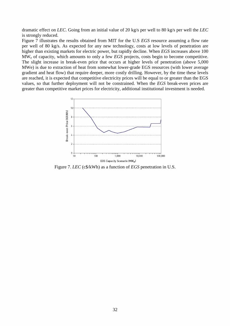
32

dramatic effect on LEC. Going from an initial value of 20 kg/s per well to 80 kg/s per well the LEC is strongly reduced. Figure 7 illustrates the results obtained from MIT for the U.S EGS resource assuming a flow rate per well of 80 kg/s. As expected for any new technology, costs at low levels of penetration are higher than existing markets for electric power, but rapidly decline. When EGS increases above 100 MWe of capacity, which amounts to only a few EGS projects, costs begin to become competitive. The slight increase in break-even price that occurs at higher levels of penetration (above 5,000 MWe) is due to extraction of heat from somewhat lower-grade EGS resources (with lower average gradient and heat flow) that require deeper, more costly drilling. However, by the time these levels are reached, it is expected that competitive electricity prices will be equal to or greater than the EGS values, so that further deployment will not be constrained. When the EGS break-even prices are greater than competitive market prices for electricity, additional institutional investment is needed.

Figure 7. LEC (c$/kWh) as a function of EGS penetration in U.S.

33

Conclusions

Geothermal energy from EGS represents a large, indigenous resource that can provide base-load electric power, requires no storage, and, thus, it complements other renewables – solar (CSP and PV), wind, hydropower – in a lower-carbon energy future. Most of the key technical requirements to make EGS work economically have been achieved, as shown by the significant progress achieved in recent tests carried out at Soultz (France), and the remaining objectives can be reached with field testing and applied geoscience and engineering research. Field studies conducted worldwide for more than 30 years have shown that EGS is technically feasible in terms of producing net thermal energy by circulating water through stimulated regions of rock at depths ranging from 3 to 5 km. Now there are engineering techniques and tools to stimulate large rock volumes (more than 2 km3), drill into these stimulated regions to establish connected reservoirs, generate connectivity in a controlled way if needed, circulate fluid without large pressure losses at near commercial rates, and generate power using the thermal energy produced at the surface from the created EGS system. Initial concerns regarding five key issues – flow short circuiting, a need for high injection pressures, water losses, geochemical impacts, and induced seismicity – appear to be either fully resolved or manageable with proper monitoring and operational changes. The main constraint is still creating sufficient connectivity within the injection and production well system in the stimulated region of the EGS reservoir to allow for high per-well production rates without reducing reservoir life by rapid cooling.

34

References Bertani R., Geothermal Energy: an overview on resources and potential, International Geothermal Days, Slovakia 2009. Dickson M.H. and Fanelli M., Geothermal Energy. Utilization and Technology, CNR Pisa, Institute of Geosciences and Earth Resources, Earthscan 2005. Guðmundur Ó. Friðleifsson, Albert Albertsson, and Wilfred A. Elders, Iceland Deep Drilling Project (IDDP) - 10 Years Later –Still an Opportunity for International Collaboration, Proceedings World geothermal Congress 2010, Bali, Indonesia, 25-29 April 2010 Holm A., Blodgett L., Jennejohn D. and Gawell K., Geothermal Energy: International Market Update, Geothermal Energy Association, May 2010 Tester J.W. et al., The Future of Geothermal Energy: Impact of Enhanced Geothermal Systems (EGS) on the United States in the 21st Century. Massachusetts Institute of Technology, Cambridge, MA, USA, 2006. Tester J.W. et al., Sustainable Energy. Choosing Among Options, MIT Press 2005.

35

2. Organic Rankine Cycles: Applications,

Working Fluid Selection and Optimization

Studies Performed in the Scientific Literature The conversion of thermal energy at low temperatures is a widely studied issue in the field of energy systems. Such kind of heat is made available by many industrial processes, and valuable efforts have been devoted to recover it internally although in most cases it is rejected to the environment as is. The renewable energy field also deals with this kind of heat when natural or artificial low temperature geothermal resources are exploited and when solar energy is collected by means of low-to-medium temperature devices. Power generation from low temperature heat is affected by the low thermal efficiency dictated by Carnot limit. Organic Rankine cycles (ORCs) are a suitable way to perform this energy conversion, as they provide the highest thermal efficiencies in that temperature range. The maximization of the performance of these cycles has been investigated in the literature from the thermodynamic point of view, but technological and economical aspects are involved as well. The choice of the organic fluid operating the cycle also plays a key role. Thermal efficiency has been initially considered as the pure thermodynamic objective to be maximized at different heat source temperatures. Badr, Probert and O’Callaghan (1985) present some thermo-physical requirements that the fluid should fulfil. Hung, Shai and Wang (1997) distinguish among three categories of fluids (dry, wet and isentropic) according to the slope of the saturated vapor curve in the T-s diagram and show that isentropic fluids are the most suitable. Maizza and Maizza (2001) underline the relationship among the critical temperature of the operating fluids, the evaporating temperature and cycle efficiency. In these early studies the nature of the available heat source in terms of both mass flow rate and temperature is not considered. A sensitivity analysis on vaporization temperature is made for a single pressure level saturated vapor cycle, superheating being allowed only when the critical temperature of the operating fluid is too low. This approach is sound when the heat source has an infinite heat capacity or when it is continuously regenerated in a closed loop, as it happens in thermodynamic solar systems. However, in many cases the low temperature heat source consists of sensible heat and must be cooled as much as possible in order to completely exploit its thermal energy. Thus, power rather than efficiency has to be considered as an objective. Liu, Chen and Wang (2004) explain the difference between maximum cycle efficiency and maximum exploitation of the heat source as objectives. Thermal efficiency is not able to describe the best coupling between the heat source and the cycle operated by the organic fluid, because the ultimate aim is obtaining the maximum power output from a given heat source. Consequently, the choice of cycle design parameters and of the organic fluid should be based on “total heat recovery efficiency”, which is the ratio between cycle power and the overall available heat (and not only the fraction that is actually exploited). As pointed out by Wei et al. (2007), the energy conversion is strongly affected by the exergy destruction in the evaporator. The methods proposed to decrease the irreversibilities in the evaporation phase are: ▪ the use of supercritical pressures (but the higher the pressure, the higher the power absorbed by the feed pumps) ▪ the use of mixtures, the glide of which reduces the distance between the two temperature profiles in the evaporator. However, the benefits are not so high, because the temperature profile in the condensation is not horizontal as well, and this forces the increase of turbine discharge pressure. Other options involve

36

more complex cycles, in which the evaporation is split into two pressure levels, or in which the compositions of the operating fluid in the evaporator and in the condenser are kept different by means of a distillation column as in Kalina cycles. Component technology also affects the choice of cycle design parameters and of the organic fluid: ▪ Expander. On one hand, the use of steam would require multi-stage turbines, as the enthalpy drops across the expander are high even with moderate temperature differences, and erosion of turbine blades may occur if a sufficient level of superheating cannot be obtained. On the other hand, the organic fluids with molecular weights higher than water can be expanded in single stage turbines and erosion problems are avoided because of the different slope of the saturated vapour curve. In addition, the higher operating fluid mass flow rate makes the full admission condition possible at turbine inlet for small power outputs as well. ▪ Pumps. In general, operating fluids having a high density of the liquid phase are preferred to reduce the load absorbed by feed pumps, which is a relatively high percentage of the expander power output. ▪ Heat exchangers. Fluids with too low pressures in the condenser and/or too high pressures in the evaporator are usually avoided. Fluids are searched with thermophysical properties yielding high heat transfer coefficients both in the evaporator and condenser in order to reduce heat transfer areas and costs. A special attention is to be addressed also to the thermal stability of the organic working fluid, as it could limit the maximum temperature of the cycle. These considerations show the strong correlation existing among thermodynamic, economic and technological issues and justify the increased interest towards ORCs even for higher temperature levels, e.g. biomass applications and other small-scale integrated plants.

2.1 Thermal efficiency and total heat-recovery efficiency The organic Rankine cycle (ORC) is a process for conversion of low and medium temperature heat to electricity. The ORC process works like a Rankine steam power plant but uses an organic working fluid instead of water. The sizes of ORCs cover a wide range, from few kW to many MW however, in almost all the studies performed on ORCs, the cycle configuration is kept simple with a single high pressure level. The working fluid is pumped to the high pressure, it is evaporated using the heat source and then it is expanded in the turbine producing power. The applications of ORCs can be classified in three temperature intervals at which the heat source is available (Siddiqi and Atakan, 2010): a) below 200°C: e.g. geothermal resources; b) 200-500°C: e.g. waste heat from industries, exhaust from engines; c) above 500°C: e.g. biomass combustion. The research on ORCs has mainly focused on finding the best working fluid for a given application. The selection involves many criteria. One of the first survey of the working fluids suitable for ORCs (Badr et al., 1985) found thirteen criteria that a fluid should satisfy. These criteria are related with the thermophysical properties; the chemical stability; safety, health and environmental aspects; availability and costs. It is difficult to find a working fluid which exhibits all the desirable properties and the final choice is a compromise between different metrics: for example isobutane is a working fluid used in many ORCs and it is flammable. The thermodynamic criteria that a fluid should satisfy depend on the application: 1) In most cases the heat carrier is a sensible heat source (pressurized water, exhaust gas) that is

discharged into the environment or fed back into the underground after its utilization. In this case the objective is getting the maximum power output from the available mass flow rate of the heat carrier fluid. Both a high cycle thermal efficiency and a low outlet temperature of the heat carrier are needed.

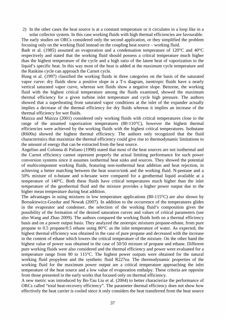
37

2) In the other cases the heat source is at a constant temperature or it circulates in a loop like in a solar collector system. In this case working fluids with high thermal efficiencies are favourable.

The early studies on ORCs considered only the second application, or they simplified the problem focusing only on the working fluid instead on the coupling heat source – working fluid. Badr et al. (1985) assumed an evaporation and a condensation temperature of 120°C and 40°C respectively and stated that the working fluid should possess a critical temperature much higher than the highest temperature of the cycle and a high ratio of the latent heat of vaporization to the liquid’s specific heat. In this way most of the heat is added at the maximum cycle temperature and the Rankine cycle can approach the Carnot cycle. Hung et al. (1997) classified the working fluids in three categories on the basis of the saturated vapor curve: dry fluids show a positive slope in a T-s diagram, isentropic fluids have a nearly vertical saturated vapor curve, whereas wet fluids show a negative slope. Benzene, the working fluid with the highest critical temperature among the fluids examined, showed the maximum thermal efficiency for a given turbine inlet temperature and cycle high pressure. The authors showed that a superheating from saturated vapor conditions at the inlet of the expander actually implies a decrease of the thermal efficiency for dry fluids whereas it implies an increase of the thermal efficiency for wet fluids. Maizza and Maizza (2001) considered only working fluids with critical temperatures close to the range of the assumed vaporization temperatures (80-110°C), however the highest thermal efficiencies were achieved by the working fluids with the highest critical temperatures. Isobutane (R600a) showed the highest thermal efficiency. The authors only recognized that the fluid characteristics that maximize the thermal efficiency could give rise to thermodynamic limitations to the amount of energy that can be extracted from the heat source. Angelino and Colonna di Paliano (1998) stated that most of the heat sources are not isothermal and the Carnot efficiency cannot represent properly the actual limiting performance for such power conversion systems since it assumes isothermal heat sinks and sources. They showed the potential of multicomponent working fluids, featuring non-isothermal heat addition and heat rejection, in achieving a better matching between the heat source/sink and the working fluid. N-pentane and a 50% mixture of n-butane and n-hexane were compared for a geothermal liquid available at a temperature of 140°C. Both these fluids have critical temperatures much higher than the inlet temperature of the geothermal fluid and the mixture provides a higher power output due to the higher mean temperature during heat addition. The advantages in using mixtures in low temperature applications (80-115°C) are also shown by Borsukiewicz-Gozdur and Nowak (2007). In addition to the occurrence of the temperatures glides in the evaporator and condenser, the selection of the working fluid’s composition gives the possibility of the formation of the desired saturation curves and values of critical parameters (see also Wang and Zhao 2009). The authors compared the working fluids both on a thermal efficiency basis and on a power output basis. They analyzed the zeotropic mixtures propane-ethane, from pure propane to 0.5 propane/0.5 ethane using 80°C as the inlet temperature of water. As expected, the highest thermal efficiency was obtained in the case of pure propane and decreased with the increase in the content of ethane which lowers the critical temperature of the mixture. On the other hand the highest value of power was obtained in the case of 50/50 mixture of propane and ethane. Different pure working fluids were also considered and the thermal efficiency and power were evaluated for a temperature range from 90 to 115°C. The highest power outputs were obtained for the natural working fluid propylene and the synthetic fluid R227ea. The thermodynamic properties of the working fluid for the maximum power output are a critical temperature approaching the inlet temperature of the heat source and a low value of evaporation enthalpy. These criteria are opposite from those presented in the early works that focused only on thermal efficiency. A new metric was introduced by Bo-Tau Liu et al. (2004) to better characterize the performance of ORCs called “total heat-recovery efficiency”. The parameter thermal efficiency does not show how effectively the heat carrier is cooled since it only considers the heat transferred from the heat source

38

to the working fluid. Instead the total heat-recovery efficiency (ηT) takes into account the whole thermal energy of the heat carrier and it is defined by the following equation:

avT

Q

W&

&=η (Eq. 1)

where W& is the power output and avQ& is the available thermal power in the heat carrier.

The thermal efficiency (ηTH) is the ratio between the power output and the input thermal power to the thermodynamic cycle:

inTH

Q

W&

&=η (Eq. 2)

The heat recovery efficiency (φ) is defined as the ratio between the heat transferred to the cycle and the heat available from the heat carrier:

av

in

Q

Q&

&=φ (Eq. 3)

Hence the total heat-recovery efficiency is the product of the thermal efficiency and the heat recovery efficiency:

φηη ⋅= THT (Eq. 4) Bo-Tau Liu et al. (2004) examined the variation of the total heat-recovery efficiency with the evaporating temperature TH. As TH increases the thermal efficiency increases whereas the heat recovery efficiency decreases, which means that the outlet temperature of the heat carrier increases. An optimum is found for TH that maximizes the total heat-recovery efficiency. Figure 1 shows the variation of thermal efficiency (dashed line), heat recovery efficiency (dotted line) and total heat-recovery efficiency (full line) as a function of the evaporating temperature. The critical temperature of the working fluid is 600 K and the curves “a” and “b” refer respectively to an inlet temperature of the heat source of 473 K and 573 K. Figure 2 shows the variation of the same parameters for a working fluid with a lower critical temperature, TC = 450 K, assuming the two same inlet temperatures for the heat carrier.

Figure 1. Variation of thermal efficiency, heat recovery efficiency and total

heat-recovery efficiency. TC = 600 K, TIN = 473 K (a), TIN = 573 K (b).

39

Figure 2. Variation of thermal efficiency, heat recovery efficiency and total

heat-recovery efficiency. TC = 450 K, TIN = 473 K (a), TIN = 573 K (b). The previous Figures show that a proper selection of the evaporating temperature (and pressure) is important in order to maximize the power output from a given heat source. An other degree of freedom is represented by the selection of the working fluid. In the previous Figures the maximum value of the total heat recovery efficiency for a temperature of the heat source of 473 K is higher when the critical temperature is lower. This effect is shown in Figure 3 that compares the thermal and total heat-recovery efficiencies of toluene and R123 for an inlet temperature of the heat source of 473 K. Toluene has a critical temperature much higher than R123 and, as expected, it shows a higher thermal efficiency. However this implies a worse cooling of the heat source and, overall, R123 shows a higher total heat recovery efficiency.

Figure 3. Variation of total heat recovery efficiency and thermal efficiency as a function

of evaporating temperature for the cases Toluene and R123. (a) R123; (b) Toluene. The analysis of total heat-recovery efficiency is very different from the conventional analysis which focused on thermal efficiency. When TH is increased, the outlet temperature of waste heat is also increased. Therefore, although ηTH increases with the increase of TH, the heat availability

40

φ decreases thereby showing a maximum value of ηT. It leads to significant difference between design of the ORC system from the viewpoints of the thermal efficiency and that based on the “total heat-recovery efficiency”. Analysis using a constant waste heat temperature or based on thermal efficiency may result in considerable deviation for system design relative to the varying temperature conditions of the actual waste heat recovery.

2.2 Optimization of the cycle parameters for different working fluids Invernizzi et al. (2007) studied the application of ORCs to recover the thermal power of the exhaust gases of micro-gas turbines at temperatures 250-350°C. They considered different classes of pure working fluids with critical temperatures from about 180°C to about 320°C. They found that the evaporating temperatures that maximize the total heat-recovery efficiency are close to the fluid critical temperature when the inlet temperature of the heat source is much higher than the critical temperature of the working fluid. However these optimal evaporating temperatures differ considerably from the critical temperature when the inlet temperature of the heat source approaches the critical temperature of the working fluid. This result is shown in Figure 4 and it is consistent with the results of Bo-Tau Liu et al. (2004) shown in the previous Figures:

Figure 4. Optimal evaporation temperatures (for saturated cycles)

that maximize the total heat recovery efficiency. The x-axis shows the difference between the inlet temperature of the heat source and the critical temperature of the working fluid. The y-axis shows the difference between the inlet temperature of the heat source (the micro gas turbine exhaust gases) and the evaporating temperature which maximizes the power output. Results are shown with reference to three different values of the exhaust temperature (250°C, 300°C and 350°C) as indicated in the diagram. Once selected the optimal evaporation temperature in relation to the gas temperature, different working fluids can be compared under their optimized conditions to select the best working fluid. For example a comparison was performed between pentane (TCR = 193.85°C) and MD2M (TCR = 326.5°C) assuming the micro gas turbine exhaust available at 300°C. The optimized evaporating temperature of pentane is close to its critical temperature whereas the optimized evaporating temperature of MD2M is 170°C yielding TrE = 0.74 (reduced evaporating temperature). The thermodynamic efficiency is higher in case of MD2M with respect to pentane. The lower value of

41

TrE of MD2M allows to achieve a higher amount of recovered heat during the evaporation phase compared to the preheating phase thus resulting in a larger amount of heat introduced at higher temperature. On the other hand the cycle with pentane can accomplish a more effective cooling of the hot gas source, resulting in a lower gas exit temperature. Overall the power output is higher with pentane than with MD2M (46 kW vs. 41 kW). Dai et al. (2009) examined the effects of the thermodynamic parameters on the ORC performance for different working fluids. They used the “exergy recovery efficiency” as objective function that is defined by the following equation:

INRECEX

E

W&

&=,η (Eq. 5)

where the exergy INE& of heat source is used that is defined by:

( ) ( )( )000 ssThhmE INININ −−−= && (Eq. 6) The meaning is similar to the total heat-recovery efficiency, previously defined, but the low quality of the heat source is taken into account. For a given heat source the maximization of the exergy recovery efficiency implies the maximization of the power output. A genetic algorithm was employed to optimize the thermodynamic parameters of the ORC systems. The genetic algorithm, which was presented firstly by Professor Holland in America, is a stochastic global search method that simulates natural biological evolution. Based on the Darwinian survival of the fittest principle, the genetic algorithm operates on a population of potential solutions to produce better and better approximations to the optimal solution. The genetic algorithm differs from the traditional optimization techniques because it involves a search from a population of solutions and not from a single point, and it prevents convergence to sub-optimal solutions in the process of searching for the optimum. The authors assumed a temperature of the heat source of 145°C. Figure 5 shows the power output variation with the turbine inlet temperature for each working fluid. The cycle high pressure is optimized for each turbine inlet temperature, as shown in Figure 6 with reference to a turbine inlet temperature of 135°C. Figure 5 shows that only water and ammonia benefit from an increase of the turbine inlet temperature whereas the power outputs for all the organic fluids considered decrease with the increase of the turbine inlet temperature. The results show that the cycles with organic working fluids are much better than the cycle with water in converting low grade waste heat to useful work. R236ea shows the highest power output followed by isobutane and, among the organic fluids considered, R236ea and isobutane have the lowest critical temperatures that are 5-10°C lower than the inlet temperature of the heat source. The other organic fluids have critical temperatures between 150°C and 215°C and show lower power outputs. Despite the large difference in critical temperatures the optimal turbine inlet temperature is within a narrow range between 80 and 90°C for all the organic fluids considered. This is consistent with the findings of Invernizzi et al. shown in Figure 4 where almost horizontal lines are drawn in the left part of the graph where the gas temperature is lower than the critical temperature.

42

Figure 5. Variations of net power output with various turbine

inlet temperatures under the respective optimal pressure.

Figure 6. Variations of net power outputs with various turbine

inlet pressures for a turbine inlet temperature of 135°C. Franco and Casarosa (2008) pointed the importance of the working fluid selection to maximize the power output from a given heat source. Analyzing the h-s diagram of an organic fluid they showed that for a fixed maximum temperature and condensation pressure the enthalpy drop increases with the cycle high pressure. For a subcritical cycle the maximum enthalpy drops are obtained at pressures close to the critical pressure. The mass flow rate of the working fluid is given by the heat balance with the heat source. If the inlet temperature of the heat source is enough higher than the critical temperature of the working fluid then the cooling of the heat source is not limited by pinch point problems at the beginning of the vaporization. There is also a secondary advantage in operating at pressures close to the critical pressure: for a given turbine inlet temperature the enthalpy rise from the pump outlet conditions to the turbine inlet conditions decreases with the cycle high pressure and thus more working fluid can be evaporated from a given heat source. Tester et al. (2008) evaluated the performance of different working fluids for low temperature geothermal applications using the exergy recovery efficiency (called utilization efficiency) as objective function. The working fluids examined were propane, isobutane, n-pentane, isopentane,

43

cyclopentane, ammonia, toluene, R32, R134a and R245fa. They found that the best working fluids for subcritical operation are: - R134a for inlet temperatures of the heat source between 110 and 130°C; - Isobutane for inlet temperatures of the heat source between 140 and 170°C; - R245fa for inlet temperatures of the heat source between 180 and 190°C. If a general optimization criterion can be drawn from these findings the best working fluids for subcritical operation have critical temperatures 5-35°C lower than the inlet temperature of the heat source.

2.3 Slope of the saturated vapor curve An other important thermodynamic property of the working fluids, in addition to the critical temperature, is the shape of the saturated vapor curve. The classification in dry, isentropic and wet fluids was extended by Bo-Tau Liu et al. (2004) that expressed analytically the slope of the saturated vapor curve. They used the thermodynamic relation of entropy described by:

dPT

VdT

T

cdS

P

P

∂∂−= (Eq. 7)

The reference state (S = 0) is at T = Tref and P = Pref which is a subcooled liquid state. The entropy of the saturated vapor can be expressed as:

high

highhighPhighT

highPrefT

P

P

highPrefT

refPrefTT

HdT

T

cdP

T

VS

∆++

∂∂−= ∫∫

,

,

,

,

(Eq. 8)

where ∆Hhigh, Thigh and Phigh denote the enthalpy of vaporization, the evaporating temperature and the evaporating pressure respectively. Differentiating with respect to Thigh yields the following:

( )( ) 22

2high

high

high

high

high

P

high T

H

Td

Hd

T

c

dT

dS ∆−

∆+≈ (Eq. 9)

By exploitation of the Watson relation between ∆Hhigh and Thigh: n

iihighr

ihighriihighihigh T

THH

−−

∆=∆__

____ 1

1 (Eq. 10)

where Tr denote the reduced evaporating temperatures. The exponent n is suggested to be 0.375 or 0.38. Substituting Eq. 10 into Eq. 9 yields:

highhigh

highr

highr

high

P HT

T

Tn

T

c ∆+

−⋅

−=2

_

_ 11

ξ (Eq. 11)

where highdT

dS=ξ is the slope of the saturated vapor curve on the T-s diagram.

Types of working fluids can be predicted by the above expression. That is ξ > 0: dry fluid; ξ ̴ 0: isentropic fluid; ξ < 0: wet fluid. Not all the organic working fluids belong to dry or isentropic type. For example, ethanol is a wet fluid. The cause is related to the chemical structure of the working fluids. For working fluids, such as water, showing strong attraction among molecules (hydrogen bonds), ∆Hhigh is comparatively large. Hence, molecules having hydrogen bonds interactions like water, ammonia, and ethanol give rise to large ∆Hhigh and become wet types.

44

Invernizzi et al. (2007) introduced a parameter of “molecular complexity” (σ) to classify the working fluids defined as:

7.0, =

∂∂=

TrSV

CR

T

S

R

Tσ (Eq. 12)

where the derivative is calculated for the saturated vapor conditions at a reduced temperature (Tr) of 0.7. The parameter σ is computable by an equation of state through numerical derivative or through a direct calculation, as the previous equation is equivalent to:

7.0, =

∂∂+

∂∂=

TrSVPSVT

CR

T

S

dT

dp

p

S

R

Tσ (Eq. 13)

The σ coefficient is a function of the heat capacity of the vapor and thus it is directly related to the molecular structure of the fluid. The qualitative effects of the molecular structure on the value of σ are highlighted in case of the saturated vapor is comparable to an ideal gas. In this case:

7.0,

1

1

1

=

−+

−=

TrSVrSVr

r

R TdT

dp

p γγσ (Eq. 14)

For simple molecules the first term on the right-hand side of Eq. 14 prevails on the positive term and the slope of the saturated vapour line in the T-S diagram is negative. If the molecular complexity increases, the heat capacity ratio γ decreases, tending to one, and the slope of the saturated vapor line becomes positive: the more positive, the more complex is the molecular structure. The temperature drop in the turbine decreases as σ increases: in fact, for an ideal gas,

p

p

T

T ∂−=∂γ

γ 1 (Eq. 15)

and T

T∂ vanish as γ tends to the unity.

Invernizzi et al. (2007) correlated the thermal efficiency ( )THWF ηη = and the total heat-recovery efficiency ( )Trec ηη = with the parameter of molecular complexity. The correlations are shown in Figure 7. They found that the thermal efficiency increases with the molecular complexity because the increase of σ implies an increase of the fluid critical temperature and makes more significant the effect of the regeneration. The large deviation of ηWF fixed σ is due to the variation of the fluid critical temperature (fixed σ, fluids with higher TCR have higher ηWF). As a counterpart,

recη decreases with σ, owing to the presence of the regenerator and to the significant amount of heat exchanged through the evaporation of the working fluid, in comparison with that of the preheating phase that implies a reduction of the heat recovery efficiency ( )φτ =rec . High molecular complexities result in a decrease of the power output of the recovery cycle. An other aspect related to σ is that a high value of molecular complexity, implies a high recuperator heat load. For example in case of the cycle with n-pentane (σ = 6.95) a thermal power of 0.86 kW is transferred within the regenerator per each kW delivered by the turbine that is much lower than the value of 2.0 obtained with MM (σ = 29.2). So from this point of view n-pentane is better.

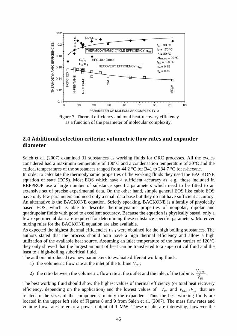
45

Figure 7. Thermal efficiency and total heat-recovery efficiency

as a function of the parameter of molecular complexity.

2.4 Additional selection criteria: volumetric flow rates and expander

diameter

Saleh et al. (2007) examined 31 substances as working fluids for ORC processes. All the cycles considered had a maximum temperature of 100°C and a condensation temperature of 30°C and the critical temperatures of the substances ranged from 44.2 °C for R41 to 234.7 °C for n-hexane. In order to calculate the thermodynamic properties of the working fluids they used the BACKONE equation of state (EOS). Most EOS which have a sufficient accuracy as, e.g., those included in REFPROP use a large number of substance specific parameters which need to be fitted to an extensive set of precise experimental data. On the other hand, simple general EOS like cubic EOS have only few parameters and need only a small data base but they do not have sufficient accuracy. An alternative is the BACKONE equation. Strictly speaking, BACKONE is a family of physically based EOS, which is able to describe thermodynamic properties of nonpolar, dipolar and quadrupolar fluids with good to excellent accuracy. Because the equation is physically based, only a few experimental data are required for determining these substance specific parameters. Moreover mixing rules for the BACKONE equation are also available. As expected the highest thermal efficiencies ηΤΗ were obtained for the high boiling substances. The authors stated that the process should both have a high thermal efficiency and allow a high utilization of the available heat source. Assuming an inlet temperature of the heat carrier of 120°C they only showed that the largest amount of heat can be transferred to a supercritical fluid and the least to a high-boiling subcritical fluid. The authors introduced two new parameters to evaluate different working fluids:

1) the volumetric flow rate at the inlet of the turbine INV& ;

2) the ratio between the volumetric flow rate at the outlet and the inlet of the turbine: IN

OUT

V

V&

&.

The best working fluid should show the highest values of thermal efficiency (or total heat recovery efficiency, depending on the application) and the lowest values of INV& and INOUT VV && / that are related to the sizes of the components, mainly the expanders. Thus the best working fluids are located in the upper left side of Figures 8 and 9 from Saleh et al. (2007). The mass flow rates and volume flow rates refer to a power output of 1 MW. These results are interesting, however the

46

authors used the thermal efficiency in y-axis. The total heat recovery efficiency is more appropriate when applications like geothermal resources are considered and, as previously seen, fluids with high thermal efficiency generally show poor heat recovery efficiency and thus low power outputs.

Figure 8. Thermal efficiency vs. volumetric flow rate at the inlet of the turbine for different working fluids.

Figure 9. Thermal efficiency vs. turbine outlet/inlet

flow ratio for different working fluids. A similar approach was used by Tchanche et al. (2009) to comparatively assess the performance of working fluids for use in low-temperature solar organic Rankine cycle systems. Twenty working fluids with critical temperatures above 75°C were considered. An evaporating temperature of 75°C and a condensing temperature of 35°C were assumed for all fluids and the power output was fixed at 2 kW. The authors calculated the thermal efficiency, the volumetric flow rate at the outlet of the turbine OUTV& and the ratio INOUT VV && / . As expected the highest thermal efficiency (4.89%) was achieved by water, the fluid with the highest critical temperature, whereas R32, the fluid with the lowest critical temperature, yielded the lowest thermal efficiency (2.61%). N-Pentane, cyclohexane, water, ethanol, methanol, R123 and R141b exhibited high volume flow rates. These working fluids

47

had the highest critical temperatures (above 180°C) among the fluids considered. Fluids with low volume flow rate are R32, ammonia, R407C, R290, R134a and R152a. The screening of the working fluids was also based on the evaporating and condensing pressure. According to Badr et al. (1985) the saturation pressure at the maximum temperature of the cycle should not be excessive (< 25 bar). Very high pressures lead to mechanical stress problems and therefore expensive components may be required. The saturation pressure at the minimum temperature of the cycle should not be so low as to lead to problems of sealing against infiltration of the atmospheric air into the system. Badr et al. (1985) limited the minimum condenser pressure to 0.5 bar whereas Tchanche et al. (2009) used 1 bar. Using these limits Tchanche et al. (2009) found that cyclohexane, methanol, water and ethanol present low condenser pressures whereas R407C (mixture), R32 and ammonia have pressures above 30 bar in the evaporator. The fluids with low condenser pressures have pressure ratios across the expander higher than 3.5, value fixed by the authors as a limit. The working fluids found good from a pressure point of view were the isentropic fluids: R134a, R123, R141b and the dry fluids: RC318, R600a (isobutane), R600 (n-butane), R601 (n-pentane) and the wet fluid: R152a. The fluids that exhibit high thermal efficiencies, low turbine outlet volume flow rates and reasonable pressures for low-temperature applications driven by heat source temperature below 90°C are R134a, followed by R152a, R290 (propane), R600 and R600a. The early work of Angelino et al. (1984) considered the class of linear hydrocarbons from C4H10 to C10H22 for selecting the best working fluid for a 100°C-40°C evaporation-condensation temperature. The increase in molecular complexity has the effect of rising the fluid critical temperature (while reducing its critical pressure) so that the same 40-100°C temperature span corresponds to regions of the state diagram of lower reduced temperatures as the number of atoms in the molecule is increased. The condensation pressure ranges from 377 kPa for n-butane to 0.49 kPa for n-decane. As a consequence volume flows at condenser inlet exhibit wide variation which affect the turbine dimensions: the optimal turbine diameter for n-decane is many times higher than that for n-butane. The cycle pressure ratio increases from about 4 for butane to about 20 for decane. Wang and Zhao (2009) studied the performance of a mixture of a dry fluid R245fa and a wet fluid R152a. Three mass fractions 0.9/0.1 (MA) 0.65/0.35 (MB), 0.45/0.55 (MC) of R245fa/R152a were chosen. Under these mass fraction conditions, the zeotropic mixtures are respectively dry (MA), isentropic (MB) and wet (MC) as shown in Figure 10.

Figure 10. T-s diagram for three zeotropic mixtures of R245fa/R152a.

They found that none of the fluids considered possessed the highest thermal efficiency, the lowest volumetric flow rate at the inlet of the turbine and the lowest volume flow ratio between the outlet and the inlet of the turbine at the same time. Assuming an evaporating temperature of 85°C they

48

found that the highest thermal efficiency is achieved using pure R245fa, the lowest volumetric flow rate is possessed by MC while MB possesses the lowest volume flow ratio. Zyhowski et al. (2010) compared a 245fa ORC system against an isopentane ORC system for two temperatures of the heat source: 90°C and 120°C. They assumed a specific diameter (dS) of 4 for the turbine (from the Balje diagram) and they calculated the turbine diameter (D) from the volumetric flow rate at the outlet of the turbine and the isentropic enthalpy drop using the following equation:

25.0

5.0

IS

OUTS

h

VdD

∆=

& (Eq. 16)

The isopentane turbine diameter would be 11-12% larger than the 245fa turbine diameter whereas the electrical output is only 0.5% more for isopentane with the 90°C source and 4.0% more with the 120°C source. Therefore the authors chose to compare the two fluids for a given turbine size and they found that using isopentane instead of HFC-245fa would result in an estimated 19% reduction in electrical output for a 90°C source and nearly an 18% reduction for a 120°C source, thus overall R245fa is better. Marcuccilli and Thiolet (2009) performed an extensive survey of different working fluids to determine the best thermal efficiency achievable and to evaluate which fluids are the most suitable for radial turbine operation. They examined both subcritical and supercritical cycles but they adopted the following simplifications: - only the configuration without regenerator was considered; - a maximum pressure ratio of 4 was assumed that leads to radial inflow turbines with only one stage; - the inlet temperature of the heat source was 450 K and a temperature difference of 5°C was applied between the inlet of the hot source and the inlet of the turbine. They selected the best working fluids using a performance factor (PF) that is proportional to the thermal efficiency and inversely proportional to the square of the turbine diameter (D):

2DPF THη= (Eq. 17)

Based on this performance metric propane at supercritical pressures was selected as the best working fluid for applications in the range of temperatures between 403 and 443 K.

2.5 Supercritical ORCs Schuster et al. (2010) evaluated the performance of ORCs operating at supercritical pressures. They compared different fluids using both the thermal efficiency and the total heat-recovery efficiency (called system efficiency). They showed that the advantage in adopting a supercritical pressure compared to a subcritical operation is due to two main reasons, as shown in Figures 11a and b:

1) lower exergy destruction in the evaporator; 2) lower exergy losses in the exhausts.

49

Figure 11a. Exergy Losses and Destruction in

subcritical ORC.

Figure 11b. Exergy Losses and Destruction in supercritical ORC.

Figure 12 shows the variation of the total heat-recovery efficiency Tη (system efficiency) in subcritical conditions with the temperature at the inlet of the turbine (live vapour temperature), assuming an inlet temperature of the heat source of 210°C. The subcritical conditions were calculated with a constant superheating of 2 K. A fluid was regarded suitable for the use as working fluid, when the vapour content of the exhaust vapour after the turbine was > 0.90 in order to avoid droplet erosion (as a consequence of this condition the curves for water end at moderate live vapour temperatures). The highest system efficiency (13.3%) is reached by R245fa at evaporating conditions close to its critical temperature (TCR=154.1°C). Fluids with higher or lower critical temperatures show lower system efficiencies.

Figure 12. Total heat-recovery efficiency in subcritical conditions. Inlet temperature of the heat source: 210°C.

50

Figure 13 shows the system efficiency variation with the temperature at the inlet of the turbine for supercritical cycles assuming a cycle high pressure close to the critical pressure (1.03 pCR). The maximum system efficiency is 14.4%, that is 1.1 percentage points more than the maximum in subcritical conditions. Also the peak system efficiency of R245fa is higher than that achieved in the subcritical operation and an optimized cycle high pressure could give even a higher improvement of system efficiency.

Figure 13. Total heat-recovery efficiency in supercritical conditions. Inlet temperature of the heat source: 210°C. The authors concluded that the supercritical operation provides some advantages compared to subcritical ORCs, however lower mean temperature differences between the heat source and the working fluid also require larger U·A values for the heat exchangers. According to Tester et al. (2008) the working fluids that provide the highest exergy recovery efficiency (called utilization efficiency) at supercritical pressures are: - R32 for inlet temperatures of the heat source between 100 and 130°C; - R134a for inlet temperatures of the heat source between 140 and 170°C; - isobutane for an inlet temperature of the heat source of 180°C; - R245fa for inlet temperatures of the heat source between 190 and 200°C. Figure 14 shows the results obtained from their study:

Figure 14. Exergy recovery efficiency for supercritical cycles as a function

of geofluid temperature for seven candidate working fluids.

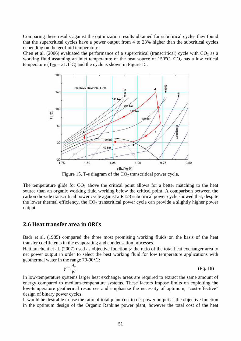
51

Comparing these results against the optimization results obtained for subcritical cycles they found that the supercritical cycles have a power output from 4 to 23% higher than the subcritical cycles depending on the geofluid temperature. Chen et al. (2006) evaluated the performance of a supercritical (transcritical) cycle with CO2 as a working fluid assuming an inlet temperature of the heat source of 150°C. CO2 has a low critical temperature (TCR = 31.1°C) and the cycle is shown in Figure 15:

Figure 15. T-s diagram of the CO2 transcritical power cycle.

The temperature glide for CO2 above the critical point allows for a better matching to the heat source than an organic working fluid working below the critical point. A comparison between the carbon dioxide transcritical power cycle against a R123 subcritical power cycle showed that, despite the lower thermal efficiency, the CO2 transcritical power cycle can provide a slightly higher power output.

2.6 Heat transfer area in ORCs

Badr et al. (1985) compared the three most promising working fluids on the basis of the heat transfer coefficients in the evaporating and condensation processes. Hettiarachchi et al. (2007) used as objective function γ the ratio of the total heat exchanger area to net power output in order to select the best working fluid for low temperature applications with geothermal water in the range 70-90°C:

W

AT

&=γ (Eq. 18)

In low-temperature systems larger heat exchanger areas are required to extract the same amount of energy compared to medium-temperature systems. These factors impose limits on exploiting the low-temperature geothermal resources and emphasize the necessity of optimum, “cost-effective” design of binary power cycles. It would be desirable to use the ratio of total plant cost to net power output as the objective function in the optimum design of the Organic Rankine power plant, however the total cost of the heat

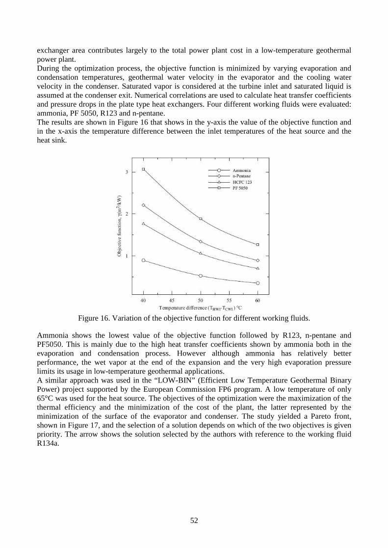
52

exchanger area contributes largely to the total power plant cost in a low-temperature geothermal power plant. During the optimization process, the objective function is minimized by varying evaporation and condensation temperatures, geothermal water velocity in the evaporator and the cooling water velocity in the condenser. Saturated vapor is considered at the turbine inlet and saturated liquid is assumed at the condenser exit. Numerical correlations are used to calculate heat transfer coefficients and pressure drops in the plate type heat exchangers. Four different working fluids were evaluated: ammonia, PF 5050, R123 and n-pentane. The results are shown in Figure 16 that shows in the y-axis the value of the objective function and in the x-axis the temperature difference between the inlet temperatures of the heat source and the heat sink.

Figure 16. Variation of the objective function for different working fluids.

Ammonia shows the lowest value of the objective function followed by R123, n-pentane and PF5050. This is mainly due to the high heat transfer coefficients shown by ammonia both in the evaporation and condensation process. However although ammonia has relatively better performance, the wet vapor at the end of the expansion and the very high evaporation pressure limits its usage in low-temperature geothermal applications. A similar approach was used in the “LOW-BIN” (Efficient Low Temperature Geothermal Binary Power) project supported by the European Commission FP6 program. A low temperature of only 65°C was used for the heat source. The objectives of the optimization were the maximization of the thermal efficiency and the minimization of the cost of the plant, the latter represented by the minimization of the surface of the evaporator and condenser. The study yielded a Pareto front, shown in Figure 17, and the selection of a solution depends on which of the two objectives is given priority. The arrow shows the solution selected by the authors with reference to the working fluid R134a.

53

Figure 17. Optimal solutions for R134a.

Figure 18. Optimal solutions for Isobutane.

The study found that the surface area required by R134a is less than that required by isobutane for the same thermal efficiency (Figure 17 vs Figure 18). However the authors underlined that other aspects could determine the selection of the working fluid, for example the turbine dimensions that are lower for R134a due to its high density.

2.7 High temperature applications: biomass combustion ORCs are also used for high temperature applications in small biomass power plants. In these applications the flame temperature is around 1200 K but the maximum process temperature must be limited to about 600 K because at higher temperatures the organic fluids would become chemically unstable. Drescher and Bruggemann (2007) studied alternatives to octamethyltrisiloxane (OMTS), the working fluid that, despite its low thermal as well as low total heat-recovery efficiency, is

54

commonly adopted in biomass applications. The working fluid is coupled to the flue gas by thermal oil to avoid local overheating and to operate the heat exchanger in the flue gas at atmospheric pressure. The temperature-enthalpy diagram of the process is shown in Figure 19. The use of the thermal oil leads to a pinch point similar to low grade heat applications at the beginning of vaporization of the working fluid and introduces an additional pinch point between thermal oil and flue gas.

Figure 19. Temperature-enthalpy diagram for the standard plant design.

However in comparison to low grade heat applications, the thermal oil mass flow can be adjusted to a certain extent and the heat can be transferred by more than one “thermal oil cycle”. The authors proposed an improved plant design with two thermal oil boilers in order to avoid the constriction of the pinch point at the beginning of vaporization (Figure 20). This design allows to consider also fluids with high vaporization enthalpy at maximum process temperature and thus with a higher thermal efficiency.

Figure 20. Temperature-enthalpy diagram for the improved plant design.

For these applications thermal efficiency can be used for fluid evaluation and Figure 21 shows that the highest thermal efficiency is achieved by Butylbenzene, the fluid with the highest critical temperature among the fluids considered (family of alkylbenzenes). OMTS is also shown and it yields the lowest thermal efficiency. The maximum process pressure was limited to 2 MPa to reduce safety measures and material expenses. If the vapor pressure at maximum process temperature was lower than 2 MPa, the fluid was expanded directly from dew line. Otherwise, the fluid was superheated.

55

Figure 21. Variation of thermal efficiency with evaporating temperature

for selected working fluids for biomass applications. Siddiqi et Atakan (2010) compared the performance of n-heptane, R245fa and SES36 (mixture) against water for an inlet temperature of the heat source of 500°C. They fixed 16 bar as the upper limit for the evaporating pressure assumed a reasonable value for single stage turbines. The found that water shows the highest total heat recovery efficiency followed closely by n-heptane, whereas R245fa and SES36 show much lower total heat-recovery efficiencies. The mean temperature of heat addition for water is similar to that of n-heptane but water shows a much lower temperature of heat rejection than the other fluids leading to higher efficiencies. This effect more than compensates the fact that the exhaust gases leave the heat exchanger at a higher temperature for water than for the organic fluids: the pinch point for the organic liquids is found at the inlet of the preheater (outlet of the pump) whereas for water it is found at the beginning of the vaporization. The authors also found that the heat exchanger area could be reduced using water compared to the organic fluids. Karellas and Schuster (2008) quoted many examples of ORC applications that use the waste heat from biomass combustion. They stated that ORC is the only proven technology for the production of power up to 1 MWe from solid fuels like biomass. Even if the efficiency of the ORC is low due to the maximum temperature limit for the working fluids the use of organic fluids has some advantages compared to water mainly related to the expanders’ design and operation, as explained in the following paragraph.

2.8 Expanders in ORCs Badr et al. (1985) pointed that for low power systems, with moderate temperature differences across the expander, the corresponding enthalpy drops of the steam are relatively high. If all the energy were to be extracted in a single-stage impulse turbine the efflux velocity through the nozzle would be over 1000 m/s, which requires the blades to travel at a velocity of about 500 m/s. (For maximum efficiency the blade travelling velocity to nozzle efflux velocity ratio of an impulse turbine should be ≈ 0,45). This speed is over twice the practical limit, dictated by the allowable stresses for most common turbine-wheel materials and constructional techniques. So single-stage impulse turbines must operate with lower than the optimal velocity ratio, resulting in poorer efficiencies. The use of multi-stage turbines may overcome this difficulty, but would lead to higher cost, complicated small turbines. Furthermore, the frictional losses in small-sized turbines are relatively high.

56

In addition when using steam the necessary degree of superheat (required to avoid exhausting wet steam of low quality) may not be obtainable. So erosion of the turbine blades is more likely to occur. “Two-phase flow” could be experienced in the turbine bearings, leading, possibly, to erratic operation. According to Badr et al. (1985) if a heavy organic-fluid vapour is used instead of steam, the velocity of the efflux is reduced approximately as the ratio of the inverse square roots of the molecular weights of the fluids. Thus a vapour which is 5-6 times as dense as steam would make a single-stage turbine with the proper velocity ratio, a feasible prospect. Moreover because the enthalpy drop is less for heavy vapours than for steam (i.e. approximately in the inverse proportion of their molecular weights), more vapour must flow through the turbine for the same power output. This is a great advantage in small turbines because it allows the blades to be larger and makes satisfying the full-admission condition of the turbine possible, even for small power outputs. Angelino et al. (1984) stated that the efficiency of an axial flow turbine stage of good aerodynamic design is mostly determined by the following parameters based on the similarity rules: a) The “isentropic head coefficient” kis, defined by:

∆=

2

2u

hk is

is (Eq. 19)

where u[m/s] is the peripheral speed at the turbine mean radius and ∆his [J/kg] is the isentropic enthalpy drop. b) The “specific speed” Ns, defined by:

4/3/ isouts hVnN ∆= & (Eq. 20)

where “n” is the speed of rotation (revolutions/s) and outV& (m3/s) is the volumetric flow rate at the

stage exit. c) The “size parameter” defined by:

4/1/ isout hVVH ∆= & (Eq. 21)

The physical significance is its proportionality to actual turbine dimensions. d) The volumetric expansion ratio, defined by:

in

out

V

VVR

&

&= (Eq. 22)

Where inV& is the volumetric flow rate at stage inlet. VR accounts for the “compressibility effects” in

a more generalized way than other equivalent parameters (pressure ratio, Mach numbers). Two of these parameters, VH and VR, can be regarded as thermodynamic data. The other two, Ns and kis, are to be selected by the turbine designer. As far as kis is concerned, it is generally possible to adopt optimum kis values with organic fluids. In fact they are compatible with conservative levels of peripheral speeds, (a feature far to be achieved in single stage steam turbines, for which high kis are a major cause of poor efficiency). A similar statement cannot be drawn for Ns since it depends on the particular application. For the optimum values for Ns and kis the authors represented the achievable efficiency in the VH-VR plane (Figure 22). As obvious highest efficiency are found for large turbines and low expansion ratios. An increase of the volumetric flow ratio implies a much larger increase of the size parameter to get the same efficiency. When high “VR” become unavoidable, as in engines operating under large temperature spans, a two or multistage solution is chosen.

57

Figure 22. Constant efficiency lines for turbine stages at optimum values of kis and Ns.

Invernizzi et al. (2007) correlated the volumetric expansion ratio with the product “Critical Temperature X Acentric Factor”. They found that fluids with high values of “TCR·ω” show high volumetric expansion ratios (Figure 23). Higher volume flow ratios and thus higher volume flow rates at the outlet imply larger sizes for the turbine for a fixed power output.

Figure 23. Turbine volume flow ratio

It has been shown that efficiencies higher than 80%, in case of single stage axial turbines, can only be achieved with volumetric flow ratios less than about 50. Therefore from the point of view of the

58

volumetric expansion ratio only fluids with ω×CRt less than about 70 can provide an acceptable efficiency (higher than 80%) of the turbine. This was used as fluid selection criterion. Gambarotta and Vaja (2008) studied the application of ORCs coupled to internal combustion engines. They found that evaporating pressures lower than the optimal could lead only to a slight decrease of the power output but to a high reduction of the turbine outlet/inlet volume flow ratios, as they found for benzene. The ORCs parameters vary in off-design conditions. For low temperature applications the main variable that affects the power output is the ambient temperature. According to Wei et al. (2007) and Marcuccilli and Thiolet (2009) a proper nominal condition is important to improve the system performance throughout the whole year and maximize the annual energy production. This choice involves a proper selection of the working fluid and its cycle parameters and a proper selection of the design point for the plant’s components.

2.9 Environmental aspects and chemical stability The selection of the working fluid is also based on environmental and safety aspects. Environmental aspects are the ozone depletion potential (ODP), the global warming potential (GWP) and the atmospheric lifetime (ALT). There are few substances with low ODP or/and low GWP and these fluids used at present, will be phased-out in a near future. Among these are: R141b, R123, R407, R134a, R407C and R32. Water and alkanes families are environmentally friendly substances. Regarding the safety aspects, the flammability and the auto ignition have to be mentioned. ASHRAE 34 provides a safety classification for fluids. For example alkanes that are non-toxic but flammable are class A3. They require safety devices. R152a is classified A2 (lower flammability and non-toxic). R134a is of class A1 (non-flammable and non-toxic). R123 is B1 (non-flammable but toxic). Ammonia classified B2 (toxic and lower flammability) could be used in an open space with lesser precaution compared with alkanes. An other important aspect is the chemical stability The fluid should be chemically stable over the whole temperature range employed and in the presence of lubricants and container materials. The temperature limit for thermal stability is around 300°C for many organic fluids, however for some fluids it is much lower: R134a has a maximum stability temperature of only about 180°C. Therefore this limit must be carefully checked for medium and high temperature applications of ORCs. Once the most appropriate working fluid is selected, thermal stability tests of the fluid when in extended contact for many hours with the used lubricant and the constructional materials of the proposed system, up to the highest expected operating temperature of the cycle should be carried out. The substance should be of low cost and available in large quantities since it constitutes an important cost item in the overall capital cost of an ORC.

59

Conclusions

The technology based on the binary cycle power plants using an organic fluid as working fluid is particularly suitable for the conversion of low temperature heat and can provide thermodynamic, technical, economic and environmental advantages. The studies performed in the scientific literature have underlined that both the choice of the working fluid and the selection of the optimal cycle parameters are essential to maximize either the thermal efficiency or the power output from a given heat source. The maximization of the power output needs both an effective cooling of the heat source and a high thermal efficiency, and the best fluids show a critical temperature similar or slightly lower than the temperature of the sensible heat source. Thus, there are different optimal fluids for different temperature ranges of the heat source. In addition, in each temperature range, more than one fluid can perform well, therefore additional metrics are introduced for the final selection, these being mainly related to the thermophysical properties that affect size and costs of the main plant’s components. For example isobutane and R236EA provide the highest power outputs among different selected fluids when the geothermal fluid inlet temperature is around 150°C. Further evaluations of the volumetric flow rate at the inlet of the turbine, turbine outlet/inlet volume flow ratio, isentropic enthalpy drop in the expander, heat transfer coefficients in the preheater, evaporator and condenser and additional metrics lead to a good final choice both from a thermo-economic and technical point of view. No comprehensive study was found in the literature that compare several different working fluids on all these aspects for different temperatures of the heat source (e.g. from 100 to 200°C at intervals of 10°C). In addition studies of different authors use different assumptions and fluids making the results not directly comparable. Even if many papers have been considered, only the most recent take into account other metrics in addition to either efficiency or power output. Focusing on the maximization of the power output from a given heat source at temperatures from 100 to 200°C we can broadly state that the best fluid in the lower part of the range is R134a, in the mid-range it is isobutane or R236EA and in the upper part of the range it is R245fa. According to the studies performed in the literature the operation at supercritical pressures improves the performance compared to a subcritical operation and the best fluids that maximize the power output show a critical temperature quite lower than the temperature of the heat source. For example in the mid temperature range considered for the heat source R134a generates more power than isobutane while the latter is more suitable in the upper part of the range.

60

References Angelino G., Gaia M. and Macchi E., A review of Italian activity in the field of ORCs, Proceedings of the International VDI Seminar, Zurich 1984. Angelino G. and Colonna di Paliano P., Multicomponent working fluids for Organic Rankine Cycles (ORCs), Energy 1998. Badr O., Probert S.D. and O’Callaghan P.W., Selecting a Working Fluid for a Rankine-Cycle Engine, Applied Energy, 1985. Borsukiewicz-Gozdur A. and Nowak W., Comparative analysis of natural and synthetic refrigerants in application to low temperature Clausius–Rankine cycle, Energy 2007. Chen Y., Lundqvist P., Johansson A. and Platell P., A comparative study of the carbon dioxide transcritical power cycle compared with an organic rankine cycle with R123 as working fluid in waste heat recovery, Applied Thermal Engineering 2006. Dai Y., Wang J. and Gao L., Parametric optimization and comparative study of organic Rankine cycle (ORC) for low grade waste heat recovery, Energy Conversion and Management 2009. Drescher U. and Bruggemann D., Fluid selection for the Organic Rankine Cycle (ORC) in biomass power and heat plants, Applied Thermal Engineering 2007. Gambarotta A. and Vaja I., Internal Combustion Engines bottoming with ORCs. A thermodynamic analysis, ECOS 2008. Hung T.C., Shai T.Y. and Wang S.K., A review of organic Rankine cycles (ORCs) for the recovery of low-grade waste heat, Energy 1997. Invernizzi C., Iora P. and Silva P., Bottoming micro-Rankine cycles for micro-gas turbines, Applied Thermal Engineering 2007. Karellas S. and Schuster A., Supercritical Fluid Parameters in Organic Rankine Cycle Applications, International Journal of Thermodynamics, 2008. Kontoleontos E., Mendrinos D. and Karytsas C., Optimized Geothermal Binary Power Cycles, Centre for Renewable Energy Sources, Greece. Liu B.T., Chen K.H. and Wang C.C, Effect of working fluids on organic Rankine cycle for waste heat recovery, Energy 2004. Madhawa Hettiarachchi H.D., Golubovic M., Worek W.M. and Ikegami Y., Optimum design criteria for an Organic Rankine cycle using low-temperature geothermal heat sources, Energy 2007. Maizza V. and Maizza A., Unconventional working fluids in organic Rankine-cycles for waste energy recovery systems, Applied Thermal Engineering 2001. Marcuccilli F. and Thiolet D., Optimizing Binary Cycles in Radial Inflow Turbines, GRC Transactions 2009.

61

Saleh B., Koglbauer G., Wendland M. and Fischer J., Working fluids for low-temperature organic Rankine cycles, Energy 2007. Schuster A., Karellas S., Kakaras E. and Spliethoff H., Energetic and economic investigation of Organic Rankine Cycle applications, Applied Thermal Engineering 2009. Schuster A., Karellas S. and Aumann R., Efficiency optimization potential in supercritical Organic Rankine Cycles, Energy 2010. Siddiqi M.A. and Atakan B., Investigation of the criteria for fluid selection in Rankine cycles for waste heat recovery, ECOS 2010 Lausanne Switzerland. Tchanche B.F., Papadakis G., Lambrinos G. and Frangoudakis A., Fluid selection for a low-temperature solar organic Rankine cycle, Applied Thermal Engineering 2009. Wang X.D. and Zhao L., Analysis of zeotropic mixtures used in low-temperature solar Rankine cycles for power generation, Solar Energy 2009. Wei D., Lu X., Lu Z. and Gu J., Performance analysis and optimization of organic Rankine cycle (ORC) for waste heat recovery, Energy Conversion and Management 2007. Zyhowski G.J., Brown A.P. and Achaichia A., HFC-245fa Working Fluid in Organic Rankine Cycle - A Safe and Economic Way to Generate Electricity from Waste Heat, ECOS 2010 Lausanne Switzerland.

62

3. Kalina Cycle Power Plants The Kalina cycle was patented by Kalina in the early 1980s to replace the Rankine cycle as a bottoming cycle for a combined-cycle energy system as well as for generating electricity using low temperature heat sources. The cycle uses a water-ammonia mixture as the working fluid and the composition is varied in the various parts of the cycle by using distillation and mixing processes. The variable composition leads to two main thermodynamic advantages: � a better match between the heat source thermal profile and the working fluid heating curve; � the possibility to reach lower expander outlet pressures thanks to the reduction of the

temperature glide in the condensation process. After a brief description of the peculiar advantages arising from the use of mixtures in Organic Rankine Cycles the Kalina cycle is analyzed summarizing the main findings of studies in the scientific literature.

3.1 The use of mixtures in Organic Rankine Cycles

The use of zeotropic mixtures as working fluids in binary power plants involves a temperature glide in the vaporization process improving the match between the temperature profiles of the heat source and the working fluid. Ibrahim (1996) quoted studies both on hydrocarbon mixtures and ammonia-water mixtures as working fluids. He applied a heat-exchanger synthesis method (the transshipment model) to find the optimal plant configuration that maximizes the power output from a given geothermal resource at a temperature of 180°C using a ammonia-water mixture. The optimum heat exchanger network utilizes the turbine exhaust for both preheating and partial boiling (Figure 1). The cycle with the optimum heat-exchanger network, provides up to 30% more power than the power obtained from the simple Rankine cycle. Using these techniques, it is possible to study and predict the performance of different configurations of complicated thermodynamics cycles without going through extensive computer modeling. The results also show that the design of the heat-exchanger network can have significant impact on the performance of power cycles.

Figure 1. Optimum heat-exchanger design which utilizes the

turbine exhaust for preheating and partial boiling.

63

Angelino and Colonna di Paliano (1998) described the use of multi-component working media in saturated, superheated and supercritical cycles. Besides the peculiar character of vaporisation, the other main difference between pure and mixed fluids lies in non-isothermal condensation. The overall temperature drop and the shape of the temperature-enthalpy curve (i.e. the apparent heat capacity) depend on the nature, number and difference in critical temperatures of mixture constituents and on the mixture composition. The authors considered the possibility to include in the cycle a condensing regenerator to recover a fraction of the heat of condensation of the vapor (Figure 2).

Figure 2. Saturated cycle configuration in the T-s plane for mixtures of complex molecules (siloxanes) with the corresponding regenerator temperature profile.

They compared n-pentane against a mixture of n-butane and n-hexane with similar critical temperatures and pressures. For each fluid they found the optimal cycle parameters that maximize the power output for a geothermal liquid stream available at a temperature of 140°C. The hydrocarbon mixture yields about 7% more electricity than the pure component due to the raised mean heat addition temperature. When a dry cooling system is used there is an additional advantage in using mixtures: for a given mean temperature difference in the air cooled condenser a higher temperature increase can be applied for the cooling air so less air is used with potential benefits in both cooler frontal area and fan power consumption.

Figure 3. T-s diagrams for n-pentane (left) and for a mixture 50% n-butane plus 50% n-hexane (right).

64

In more recent studies Wang and Zhao (2009) studied a mixture of a dry fluid R245fa and a wet fluid R152a. They showed how the critical temperature and the shape of the saturated vapor curve vary by changing the mass fractions of the two components in the mixture. These two variables greatly affect the performance of ORCs so the best mixture and composition can be selected for a given application extending the range of available working fluids for low-temperature Rankine cycles.

3.2 The Kalina cycle power plant for medium temperature heat sources

The only way to increase the efficiency of a cycle with fixed temperature heat source and coolant is to reduce its irreversibilities. Irreversibilities may be classified in three categories: 1) Thermo-economic : deliberately introduced in a cycle to reduce capital cost. For example a larger heat exchanger may reduce the irreversibilities of heat transfer but would increase the cost of electricity. It involves a direct tradeoff between capital investment and cycle efficiency. 2) Technological : caused by component performance. If the state-of-the-art of turbine design puts a limit on the efficiency of available turbines, the irreversibility may be reduced only by an advance in the technology of turbine design. The tradeoff between cost and efficiency is indirect. It involves the cost of engineering and research, not materials. 3) Structural : the structure of the system may introduce irreversibilities. For example a single pressure Rankine cycle using water as the working substance has an inherent irreversibility. To reduce the temperature difference between the water and the heat source the structure of Rankine cycles is often modified to utilize two or even three pressure levels. The plateau in temperature may also be removed by operating at supercritical pressures. Structural changes may be introduced at much lower cost than technological improvements. In the Kalina cycle the efficiency improvement is obtained by means of an effective structural change. The ideal cycle to convert sources of a sensible heat into mechanical and electrical energy is not the Carnot cycle which has a rectangular shape in coordinates enthalpy versus temperature or entropy versus temperature but the Lorentz cycle, which has in such coordinates the shape of a triangle. There are mainly three ways for increasing the efficiency of the Rankine Cycle utilizing variable-temperature heat sources: 1) the use of a multipressure boiler; 2) the implementation of a supercritical cycle; 3) the use of a multicomponent mixture as a working fluid. As seen in the previous section the use of a mixture in a Rankine cycle arrangement implies not only a variable temperature boiling but also a variable temperature condensation. The back pressure on the turbine must be high enough to assure complete condensation, and as a result there are only small improvements in efficiency. To circumvent this limitation, the composition of the fluid entering the condenser must somehow be made leaner than the composition in the boiler and turbine. The leaner mixture will condense at a lower pressure at the given coolant temperature. The idea underlying the Kalina cycle is achieving a high “exergy utilization efficiency”, i.e. the ratio of the net power output to the available exergy of a source, designing a cycle with the following features: � A low-boiling working fluid, circulating through the evaporator and the turbine, that has a

variable – within a wide range - boiling temperature. � Effective utilization of the heat that can be extracted from a turbine-outlet flow before

condensation. � A high-boiling fluid circulating through the condenser that has a constant – or variable within a

narrow range – condensation temperature.

65

The system uses a water-ammonia solution as a working fluid however other multicomponent solutions can be used as well. The original configuration of the Kalina cycle is shown in Figure 4:

Figure 4. Flow diagram of the original Kalina cycle (1984).

A completely condensed working fluid (1) of a so-called “basic composition” is pumped to a first intermediate pressure (point 2 is at 2.3 bar in Kalina 1984). This flow is heated in an economizer (2-3) and in a heater (3-4) and as a result it is partially evaporated. The released vapour is significantly enriched by the light component of the mixture, i.e., ammonia. The vapour is separated from the liquid in a flashtank and then mixed with part of the remaining liquid to produce a so-called “working composition” (8). This newly created flow, as well as the remaining liquid, is sent to a counterflow economizer to preheat the incoming flow and to recuperate heat. After precooling in the economizer (8-10), the working solution is completely condensed by the cooling water (10-13). Then the working solution is pumped to a high pressure and sent into the “evaporator-boiler”, where it is completely evaporated and superheated (14-15) in a counterflow heat exchange with the heat source, in this case exhaust gases from a gas turbine. The thermodynamical losses in the process of a heat transfer from the heat source to the working fluid are minimized by the proper selection of the composition and parameters of the working fluid. In Kalina (1984) the working composition is 0.5 kg NH3 / kg mixture and the turbine inlet pressure and temperature are respectively 83bar and 530°C. The vapour of the working solution is expanded in a multistage turbine producing mechanical work. It is an essential distinguishing feature of this process that the vapour is expanded in the turbine to such a low pressure (0.6 bar in Kalina 1984) that it cannot be condensed at the given ambient temperature. As a result of such expansion a significantly large work output is provided. Hot vapour (at around 70°C) which exits the turbine is cooled consecutively in the heater and in the economizer, thus providing the necessary energy for a working fluid distillation. Then the working solution is combined with the liquid from the flashtank previously cooled in the economizer and then throttled to a pressure equal to the pressure of the working solution. As a result of such

66

combining, the basic solution is reinstalled at point 24 (the concentration is 0.3 kg NH3/kg mixture. Then the basic solution is sent to a condenser where it completely condenses by means of cooling water (1). The whole cycle is then repeated. Kalina showed that the application of his cycle as a bottoming cycle in a combined-cycle energy system can provide a power 1.6 to 1.9 times higher than a Rankine cycle at the same border conditions. He also quoted that the Kalina cycle entails lower specific costs because: � The working fluid starts to boil almost immediately after entering the evaporator, which

increases the heat transfer coefficients; � The quantity of heat rejected in the condenser is smaller than in the Rankine cycle system, thus

reducing the surface and thereby the cost of the condenser; � Higher efficiency of the presented new cycle system results in a lower quantity of heat being

transferred in the evaporator per unit of power output, and thus in a lower specific cost of the evaporator.

Wall et al. (1989) analyzed the plant configuration shown in Figure 5 that presents some differences compared to the original Kalina plant configuration:

Figure 5. Schematic diagram of the Kalina cycle.

The ammonia rich solution (23) is mixed with the basic solution (24) to produce the desired working composition (25) whereas in the original design it was mixed with the poor liquid mixture from the flashtank. In addition a regenerative preheater is included in this new design before the evaporator-boiler. The authors underline that by circulating the mixture at different compositions in different parts of the cycle, condensation (absorption) can be done at slightly above atmospheric pressure with a low concentration of ammonia, while heat input is at a higher concentration, about 70%, for optimum cycle performance. The mass flow circulating between the separator and the absorber is about four times that of the turbine, thus, causing some additional condensate pump work. However, this loop makes possible the changes in composition between initial condensation in the absorber and heat addition in the boiler. The basic plant configuration of this system is shown in Figure 6.

67

Figure 6. Basic plant configuration of the Kalina cycle for medium temperature heat sources.

Nag and Gupta (1998) analyzed the latter basic plant configuration but with a simplified heat exchanger network compared to Wall et al.. They set the separator temperature (T4) equal to 70°C, the turbine inlet pressure equal to 100 bar and they varied the turbine inlet temperature (T9) in the range 475°C-525°C. From a second law analysis they found that the turbine inlet composition that maximize the efficiency is between 0.7 and 0.75 kg of NH3/kg of mixture (Figure 7).

Figure 7. Effect of composition on second law efficiency for different values

of turbine inlet temperature at a separator temperature of 70°C.

T S E P

P1

P2

ThV

COND 1

COND 2

MIX 1

MIX 2 SPL

basic composition

working composition

68

Olsson et al. (1994) studied the application of the Kalina cycle for the utilization of industrial waste heat from the iron and steel industry of moderate temperature (300-400°C). These temperatures are low for the normal steam Rankine cycle and too high for the organic Rankine cycle. A hot process gas at either of two moderate temperatures 400°C or 300°C is used as the heat source and the minimum outlet temperature of the gas is varied between 80°C and 175°C. The authors considered four cycle configurations with the same basic plant configuration and different heat exchanger networks. In the simplest configuration I, the distillation/condensation subsystem consists of a reheater, a separator, an absorber and a condenser. In Configuration II a regenerative feed water heater is included, Configurations III is the same as Figure 5 and Configuration IV includes an additional feed water heater. A fixed maximum pressure of 115 bar and maximum temperature of 500°C were assumed. For each case the working composition and the basic composition were varied in order to find the best efficiencies. For each working composition, the best basic composition was determined. Then different working compositions are tried until the composition giving the best cycle efficiency is found. Olsson et al., defining the first law cycle efficiency as the ratio between the net power output and the available heat from the heat source (i.e. the heat transferred in the vapour generator when the gas outlet temperature is the lowest acceptable), found that there are only slight improvements in the first law efficiency by making the configuration more complex. The Kalina cycle provides up to 20-30% more power from a given heat source compared with a Rankine cycle. This is a result of the much better ability of the Kalina cycle to extract heat at low temperatures so the improvement over the steam Rankine cycle is the highest for the cases which accept a lower minimum gas temperature. The steam Rankine cycle produces no more work when the minimum gas temperature is lowered from 130°C to 80°C. In addition in the Kalina cycle a proper design of the distillation/condensation subsystem allows the working fluid to enter the boiler at a temperature around 70-80°C, which is higher than the corrosion dew point temperature. The optimal ammonia mass fraction in the working solution is around 70% when the inlet temperature of the exhausts is 400°C and it increases up to 90% when the inlet temperature of the exhausts is 300°C. The results of this study show that configurations III and IV are better for the highest temperatures of the exhausts (400°C). When the exhausts inlet temperature is 300°C the simpler Kalina configurations (I and II) have the highest efficiencies. The best heat exchanger network also depends on the constraint on minimum temperature of the exhausts. Kalina and Tribus (1992) listed twelve embodiments of the Kalina cycles. They considered each system as made up of two highly interactive subsystems. The first subsystem, described by the symbol KCS, contains the heat acquisition process plus the power producing device. The second subsystem is the distillation/condensation subsystem and it is denoted by the symbol D. A combination is described by KCSxDy where x and y are numbers that denote the subsystems. The system KCS1D2 has the same basic plant configuration of the systems described previously but it presents a much more complex heat exchanger network in the distillation/condensation subsystem (Figure 8) to better match the temperature profiles.

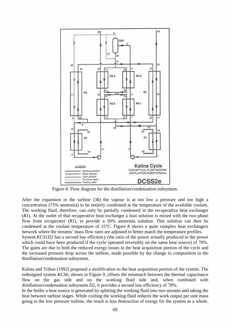
69

Figure 8. Flow diagram for the distillation/condensation subsystem.

After the expansion in the turbine (38) the vapour is at too low a pressure and too high a concentration (75% ammonia) to be entirely condensed at the temperature of the available coolant. The working fluid, therefore, can only be partially condensed in the recuperative heat exchanger (R1). At the outlet of that recuperative heat exchanger a lean solution is mixed with the two phase flow from recuperator (R1), to provide a 50% ammonia solution. This solution can then be condensed at the coolant temperature of 15°C. Figure 8 shows a quite complex heat exchangers network where the streams’ mass flow rates are adjusted to better match the temperature profiles. System KCS1D2 has a second law efficiency (the ratio of the power actually produced to the power which could have been produced if the cycle operated reversibly on the same heat source) of 70%. The gains are due to both the reduced exergy losses in the heat acquisition portion of the cycle and the increased pressure drop across the turbine, made possible by the change in composition in the distillation/condensation subsystem. Kalina and Tribus (1992) proposed a modification to the heat acquisition portion of the system. The redesigned system KCS6, shown in Figure 9, offsets the mismatch between the thermal capacitance flow on the gas side and on the working fluid side and, when combined with distillation/condensation subsystem D2, it provides a second law efficiency of 78%. In the boiler a heat source is generated by splitting the working fluid into two streams and taking the heat between turbine stages. While cooling the working fluid reduces the work output per unit mass going to the low pressure turbine, the result is less destruction of exergy for the system as a whole.

70

In the superheater an additional heat sink is provided by adding a reheating between the HP and the IP turbines to better use the high thermal capacity flux in the hot gases.

Figure 9. Heat acquisition portion of system KCS6D2.

Figure 10 shows the improvement deriving from this modification. On the left (Figure 10a) the temperature profiles in the waste heat boiler of system KCS1 and on the right (Figure 10b) the temperature profiles for system KCS6. The “exergetic temperature” is used in the y-axis, thus the space between the two curves is proportional to the exergy losses. This is briefly explained here below. The maximum work which may be obtained from a heat engine occurs when each increment of heat taken from the heat source is converted to work with the Carnot efficiency:

( ) sourceksourceC TTT /sin−=η (Eq. 1)

We call ηC the “exergetic temperature”. Representing each element of heat taken from the source by dQ, the maximum work which may be obtained from the heat source is:

dQT

TTW

source

ksource∫−

= sinmax (Eq. 2)

According to Equation 2 the area under a graph of exergetic temperature versus Q represents the maximum work which can be obtained from any heat engine which utilizes a source having temperature distribution Tsource. This maximum work potential is called the exergy of the stream. The space between the curves therefore is proportional to the loss of the exergy which might have been obtained from the source of heat.

71

Figure 10. Exergetic temperature distributions in the waste heat boiler of system KCS1 (left) and KCS6 (right). A study of the temperature profiles in subsystem D2 shows opportunities for further improvement. More can be done by not only rebalancing the flows, but also by tailoring the thermal properties (changing the composition). The result is less exergy destruction in the distillation and condensation processes that implies a lower back pressure on the vapour turbine, producing an increased efficiency of the cycle. Kalina and Leibowitz (1989) analyzed the off-design performance for a Kalina system 6. Two major factors affect the off-design, non ISO operation in conventional combined cycle systems: � A reduction in the gas turbine’s firing rate decreases the steam flow and pressure entering the

bottoming cycle turbine, thus reducing thermodynamic availability and the steam turbine’s expansion efficiency, both of which lower cycle efficiency.

� Winter operation limits bottoming cycle output, below that where thermodynamic laws allow, because of high levels of vacuum in the condenser. At cooling source temperatures below 50°F (10°C) there are no more gains to be made in the bottoming cycle.

The results of many studies presented in the previous sections showed the improvement in performance of the Kalina cycle over a Rankine cycle at the design conditions: this is about 20-25% against a double-pressure steam cycle. During off-design operation the improvement is even greater due to the following reasons:

� The ammonia/water working fluid allows for substantial pressure in the condenser, typically 25 psia (1.7 bars). During winter operation, the output of the bottoming cycle continues to rise without having to contend with any vacuum.

� Freeze-up is not an issue either. A 70/30 ammonia/water mixture freezes at -73°C. � The cycle’s variable composition maintains higher volume flows during reduced load

operation. Turbine efficiency is kept closer to design levels, and bottoming cycle output is improved.

Figure 11 shows that as the cooling source temperature decreases from 11°C to -11°C the Kalina cycle output increases by 9% (from 91.7 to 99.9 MW). During this temperature change the condenser pressure decreases from 1.7 bar to 1.1 bar. When the condenser pressure characteristic reaches 1.1 bar at 0°C the mixture of the working fluid is enriched to 0.75 (from 0.7) to prevent the onset of a vacuum. At lower temperatures the mixture is increased further to keep the condenser

72

pressure at 1.1 bar. Changing composition permits the operator to set any desired condenser pressure. In large steam plants there is an increase in output of only 1% from 11°C to -11°C. Reducing the cooling temperature the volume flow through the condensing stages became so large that the leaving losses (kinetic energy of steam not recovered in condenser) decreases the gains made by reaching a deeper vacuum in the condenser. At 5°C and below the steam plant’s output remains flat.

Figure 11. Comparison between Kalina system 6 and large steam plants

as the cooling source temperature decreases. The Kalina cycle performance is 27% better than the two-pressure reference steam cycle during non-winter operation and then improves still further during winter operation. At -11°C the improvement is 37%. During non-winter operation the performance of the Kalina cycle and the steam bottoming cycle fall off together, i.e, the margin of improvement remains constant.

3.3 The Kalina cycle power plant for low temperature heat sources

A simpler basic plant configuration is proposed for low temperature heat sources where the rich ammonia solution from the separator flows to the turbine. Ogriseck analyzed the system shown in Figure 12.

73

Figure 12. Schematic diagram of Kalina cycle for low temperature heat sources. A lower cycle high pressure is used compared to the higher temperature applications (e.g. 30 bar against 100 bar). Figure 13 shows the temperature-enthalpy diagram for a mixture with an ammonia content of 70%. The temperature of evaporation increases with an increase of the evaporator pressure.

Figure 13. Temperature-enthalpy diagram for a mixture with an ammonia content of 70%.

Figure 14 shows the boiling profiles at variable temperatures of different ammonia–water mixtures against the isothermal evaporation of pure water at a pressure of 30 bar. The higher the fraction of ammonia in the mixture, the lower is its boiling temperature. With the increasing ammonia concentration, the specific enthalpy of steam decreases.

74

Figure 14. Comparison between boiling of pure water and different ammonia-water mixtures at 30 bar. Figure 15 shows the boiling curves and the dew point curves at different ammonia contents and at different pressures of the binary mixture.

Figure 15. Ammonia-water phase diagram.

Worldwide, there are only a few plants made on the basis of the Kalina principle. The most common are given in Table 1.

Table 1. Kalina projects worldwide. The authors developed a model of the Kalina power plant in Husavik, Iceland. The cycle parameters are a ammonia composition of 82%, a turbine inlet pressure of 32 bar and a turbine outlet pressure of 6.6 bar. The following basic plant configuration, shown in Figure 16, can be identified for the Kalina cycle for low temperature applications:

75

Figure 16. Basic plant configuration of the Kalina cycle power plant for low temperature heat sources In the system proposed by Lolos and Rogdakis (2009) the working medium is partially vaporized using solar energy. The NH3-H2O vapour, which is separated from the two-phase mixture, is superheated by an external heat source and then expanded in the turbine. Flat solar collectors (an optimal choice regarding the ratio heat gain/cost for low temperature applications up to 80°C) are used for the vaporization of the mixture which cover up to 95% of the unit overall heat demand. Figure 17 shows the schematic diagram of the proposed cycle.

T

S E P

P

ThV

COND 1

MIX basic

composition

NH3 rich vapor

NH3 lean solution

76

Figure 17. Schematic arrangement of a solar Kalina power cycle.

The ammonia-strong-saturated solution of a mass fraction Xr (0) which leaves the absorber is pumped to a high pressure by the feed pump (1r). It is then preheated in the low-temperature (2r) and high temperature (3r) recuperators. In the evaporator the mixture is heated (by using flat plate solar collectors) to a temperature TH (4r) (e.g. 70°C) where it is partially vaporized. This mixed-phase fluid is separated to a saturated-rich ammonia-water vapor of mass fraction Xv (4) and a weak ammonia-water liquid solution of mass fraction Xw (4w). The high pressure saturated vapor is superheated to a temperature Tmax (e.g. 130°C) at the superheater (5) by means of an external heat source (e.g. solar or geothermal) and then expanded. Then the expanded stream is cooled. The saturated liquid solution (4w) after recuperating some of the heat at the high temperature recuperator is throttled down to a low pressure (2w) and then mixed with the vapor leaving the vapor cooler (1). Both streams are fed to the counter-current absorber to produce the ammonia strong saturated solution (state 0).

Conclusions

The use of a mixture as working fluid in an Organic Rankine Cycle implies not only a variable temperature boiling, with the resulting good thermal match with the sensible heat source, but also a variable temperature condensation. The back pressure of the turbine must be high enough to assure complete condensation, resulting only in small improvements in efficiency. In the Kalina cycle this limitation is circumvented by making the (basic) composition of the fluid entering the condenser leaner than the (working) composition in the boiler and the turbine. This occurs in the distillation subsystem where the mixture is heated and partially evaporated by the turbine exhaust to generate an ammonia rich vapour that is then mixed to generate the proper working composition that minimize the exergy losses in the evaporator-boiler. Many Kalina cycle systems have been proposed that present the same basic plant configuration and mainly differ with regard to the heat exchanger network both in the heat acquisition subsystem and the distillation/condensation subsystem. A simpler basic plant configuration is used for low temperature applications (e.g. Husavik power plant, Iceland) where the separated enriched ammonia vapour is actually the working solution in the turbine and the fluid composition is unchanged between the condenser and the evaporator.

77

References Angelino G. and Colonna di Paliano P., Multicomponent working fluids for Organic Rankine Cycles (ORCs), Energy 1998 Ibrahim O.M., Design Considerations for Ammonia-Water Rankine Cycle, Energy 1996 Kalina A.I., Combined-cycle system with novel bottoming cycle, Journal of Engineering for Gas Turbines and Power, October 1984 Kalina A.I. and Tribus M., Advances in Kalina cycle technology (1980-1991): Part I development of a practical cycle, Flowers ‘92 Kalina A.I. and Tribus M., Advances in Kalina cycle technology (1980-1991): Part II iterative improvements, Flowers ‘92 Kalina A.I. and Leibowitz H.M., Off-design performance, equipment considerations, and material selection for a Kalina system 6 bottoming cycle, ASME Cogen-Turbo 1989 Lolos P.A. and Rogdakis E.D., A Kalina power cycle driven by renewable energy sources, Energy 2009 Nag P.K. and Gupta A.V.S.S.K.S., Exergy Analysis of the Kalina Cycle, Applied Thermal Engineering 1998 Ogriseck S., Integration of Kalina cycle in a combined heat and power plant, a case study, Applied Thermal Engineering 2009 Olsson E.K., Thorin E.B., Dejfors C.A.S., Svedberg G., Kalina cycles for power generation from industrial waste heat, Flowers ‘94 Wall G., Chuang C.-C. and Masaru Ishida, Exergy study of the Kalina cycle, AES-Vol. 10-3, pp. 73-77, ASME. Wang X.D. and Zhao L., Analysis of zeotropic mixtures used in low-temperature solar Rankine cycles for power generation, Solar Energy 2009.

78

4. Synthesis/Design Optimization of Organic

Rankine Cycles for Low Temperature

Geothermal Sources with the HEATSEP Method This section shows the optimization study of a binary cycle power plant performed working with Prof. A. Toffolo and Prof. A. Lazzaretto at the University of Padova. This work starts from the optimization studies on Organic Rankine Cycles performed in the scientific literature and, using advanced techniques for improving the integration between the heat fluxes inside a system, achieves new interesting results. The heat source is a low temperature geothermal source (pressurized hot water, the socalled “brine”) having a finite mass flow rate (100 kg/s) and a given input temperature. Six inlet temperatures are considered for the brine (130°C to 180°C at steps of 10°C) and two working fluids are analyzed: isobutane and R134a. The brine must not be cooled below 70°C to avoid silica precipitation and the resulting scaling problems. The energy conversion is performed by a plant based on a single pressure level ORC, the structure and the parameters of which have to be optimized. The thermodynamic objective to be maximized is the exergy recovery efficiency or, equivalently, the net electrical power generated by the plant. The HEATSEP method (Lazzaretto and Toffolo, 2008) is applied to the synthesis/design optimization of the ORC cycle, so that the design of the heat transfer section within the plant is considered separately from the design optimization of the basic plant components, and different options about its configuration can then be defined for the same temperatures and mass flow rates of the thermal streams involved. The use of R134a results in higher exergy recovery coefficients for all the brine input temperatures considered in this analysis (130°C-180°C). R134a optimal cycles are all supercritical except for the lowest brine input temperature (130°C), while most of the isobutane ones are saturated vapour subcritical cycles. The method allowed us to obtain the variation of the exergy recovery efficiency with the turbine inlet temperature and pressure that shows not only the optima but also sub-optimal points. These points become of high interest when economic evaluations are performed which may suggest minor thermodynamic penalties at the advantage of important economic savings.

4.1. The application of the HEATSEP method

The HEATSEP method simplifies the problem of the synthesis/design optimization of complex energy systems by separating the choices about the configurations of the heat transfer section from those about the rest of the system. The main problem is therefore divided into two subproblems: ▪ The first is about the configuration and the design parameters of the “basic” components of the system, i.e. those components that are not involved in the heat transfer. They are called “basic” considering that they are strictly needed to realize “the concept” behind the plant. In order to simplify the definition of this “basic” system configuration, basic components can be organized according to elementary thermodynamic cycles as shown by Lazzaretto and Toffolo (2008) and Lazzaretto and Manente (2009). In this subproblem, the section of the system in which heat transfers occur is seen as an undefined “black-box”.

79

▪ The second is about the configuration of the heat transfer section only, that is the configuration of the heat exchanger network inside the black-box. The thermodynamic conditions at the boundary of this black-box are those of the thermal streams involved in the heat transfer and have already been evaluated in the previous subproblem. So, the preliminary concept about the energy conversion system is first translated into a basic plant configuration, which is defined by the essential components and their links. These links are then cut from the thermal point of view only, that is the temperature at the inlet of a basic component is made independent from that at the outlet of the preceding component. In this way, the heat transfer section of the system is isolated from the basic plant configuration, and the potential thermal streams (hot and cold) that interact within the black-box are generated. Of course, the additional degrees of freedom introduced by these thermal cuts correspond to new decision variables in the design optimization of the basic plant configuration. In this work, the considered single pressure level ORC has a very simple basic plant configuration (Figure 1), and is made of two basic components only (the feed pump and the turbine) and three thermal cuts. In the first thermal cut the brine is cooled from its initial temperature down to 70°C (both these temperatures are given, so no additional degree of freedom is generated by this cut), in the second one the operating fluid is heated from pump outlet temperature up to turbine inlet temperature (i.e. cycle maximum temperature, which has to be considered as a the decision variables of the design optimization problem), and, finally, in the third one the operating fluid is cooled from turbine outlet temperature down to pump inlet temperature (this temperature is strictly related to condensation pressure, so the latter quantity is included in the set of the decision variables instead of the former).

Figure 1. Basic plant configuration of the single pressure level ORC.

The configuration of the heat transfer section is not included in the basic plant configuration, so that the search space of the possible basic plant configurations and the associated design variables can be explored more freely, provided that the feasibility of the heat transfer within the black-box has to be checked. This is one of the main advantages of the HEATSEP method: the design optimization of the basic plant configuration is not performed using a model that takes into account all the possible configurations of the heat transfer section, or embeds them in a superstructure (this would then require mixed-integer programming techniques to select the units to be included in the plant configuration). In the considered single pressure level ORC, significant alternatives must be considered in the definition of the heat transfer section although the black-box encloses three thermal streams only: ▪ The heat transfer between the brine and the organic fluid can be operated by means of one, two or three devices according to cycle maximum pressure and temperature (just one heat exchanger if the cycle is supercritical, two or three if the cycle is subcritical and saturated or superheated vapor enters the turbine, respectively);

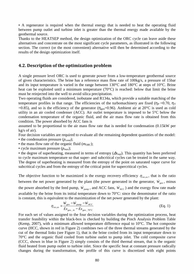
80

▪ A regenerator is required when the thermal energy that is needed to heat the operating fluid between pump outlet and turbine inlet is greater than the thermal energy made available by the geothermal source. Thanks to the HEATSEP method, the design optimization of the ORC cycle can leave aside these alternatives and concentrate on the most significant cycle parameters, as illustrated in the following section. The correct (or the most convenient) alternative will then be determined according to the results of the design optimization itself.

4.2. Description of the optimization problem

A single pressure level ORC is used to generate power from a low-temperature geothermal source of given characteristics. The brine has a reference mass flow rate of 100kg/s, a pressure of 15bar and its input temperature is varied in the range between 130°C and 180°C at steps of 10°C. Brine heat can be exploited until a minimum temperature (70°C) is reached: below that limit the brine must be reinjected into the well to avoid silica precipitation. Two operating fluids are considered, isobutane and R134a, which provide a suitable matching of the temperature profiles in that range. The efficiencies of the turbomachinery are fixed (ηP =0.70, ηT

=0.85), and so is the efficiency of the generator (ηgen=0.96). Ambient air at 20°C is used as cold utility in an air cooled condenser (ACC). Air outlet temperature is imposed to be 5°C below the condensation temperature of the organic fluid, and the air mass flow rate is obtained from this condition. The power absorbed by ACC fans is assumed to be proportional to the air mass flow rate that is needed for condensation (0.15kW per kg/s of air). Four decision variables are required to evaluate all the remaining dependent quantities of the model: ▪ the condensation pressure (pcond); ▪ the mass flow rate of the organic fluid (mORC); ▪ cycle maximum pressure (pmax); ▪ the degree of superheating, measured in terms of entropy (∆ssup). This quantity has been preferred to cycle maximum temperature so that super- and subcritical cycles can be treated in the same way. The degree of superheating is measured from the entropy of the point on saturated vapor curve for subcritical cycles and from the entropy of the critical point for supercritical cycles. The objective function to be maximized is the exergy recovery efficiency exrec,η , that is the ratio

between the net power generated by the plant (the power generated in the generator, genW& , minus

the power absorbed by the feed pump, pumpW& , and ACC fans, ACCW& ) and the exergy flow rate made

available by the brine from its initial temperature down to 70°C: since the denominator of the ratio is constant, this is equivalent to the maximization of the net power generated by the plant:

Cgeoingeo

ACCpumpgenexrec xExE

WWW

°−−−

=70__

, &&

&&&η (Eq. 1)

For each set of values assigned to the four decision variables during the optimization process, heat transfer feasibility within the black-box is checked by building the Pinch Analysis Problem Table (Kemp, 2007), with a minimum allowed temperature difference equal to 10°C. The hot composite curve (HCC, shown in red in Figure 2) combines two of the three thermal streams generated by the cut of the thermal links (see Figure 1), that is the brine cooled from its input temperature down to 70°C and the organic fluid cooled from turbine outlet to pump inlet. The cold composite curve (CCC, shown in blue in Figure 2) simply consists of the third thermal stream, that is the organic fluid heated from pump outlet to turbine inlet. Since the specific heat at constant pressure radically changes during the transformation, the profile of this curve is discretized with eight points

81

connected by linear segments (if the cycle is subcritical the 4th and the 5th point represent the beginning and the end of the evaporation, respectively). The HCC comprises the only heat source in the system (brine), and other external hot utilities are not available: the HCC starts from the abscissa corresponding to the maximum temperature of the CCC in the temperature-thermal power diagram (Figure 2) and must cover the entire load required by the CCC. The thermal power in excess is released to a cold utility (the air flow in the ACC). The heat transfer feasibility constraint (HTFC) requires that the cumulated balance of thermal power has no deficit at any temperature level, that is the heat made available by the hot streams is always larger that the heat requested by the cold streams. The possible pinch points of the heat transfer process (i.e. the points in which the cumulated heat made available is strictly equal to the heat requested) are indicated in Figure 2 with numbers from 1 to 8: note that these are also the points that are used to discretize the heating process of the organic fluid.

Figure 2. Composite curve and discretization of the organic fluid heating in the supercritical (left) and subcritical (right) case. In addition to the optimal solution, we consider here also the suboptimal solutions in the neighbourhood in order to investigate how the heat transfer feasibility constraint acts on the objective function and see what happens to the composite curves when departing from the optimum. The model of the basic plant configuration was built in the MATLAB/Simulink environment (Figure 3). The block diagram of the Simulink model is a straightforward translation of the scheme given in Figure 1: the blocks named “pump” and “turbine” represent the basic components, whereas those named “brine cooler”, “ORC heater” and “ORC cooler” represent the three thermal cuts. The blocks of the latter group can be considered as cold or hot sides of heat exchangers, but the source of the absorbed heat or the destination of the released heat remains undefined. Organic fluid properties are evaluated by custom routines that interpolate the thermodynamic data provided by the NIST database. Since the temperature profile of the organic fluid heating is discretized in linear segments, the model is able to deal with both super- and subcritical cycles.

82

Figure. 3. The Simulink model of the basic plant configuration. The optimization problem is solved with the sequential quadratic programming routines implemented in the MATLAB Optimization Toolbox. The optimization algorithm actually operates on pcond, pmax and ∆ssup, while the fourth decision variable (mORC) is evaluated in order to maximize

exrec,η while satisfying the heat transfer feasibility constraint. This strategy avoids the evaluation of

non-feasible solutions, because mORC is a variable that acts a linear transformation of the abscissas of the whole CCC in the temperature-heat load diagram.

4.3 Results of the optimization problem

The optimal design parameters obtained at different brine inlet temperatures are summarized in Tables 1 and 2 for isobutane and R134a, respectively. The mass flow rate of the geothermal fluid is 100 kg/s.

T_in geofluid [°C] 130 140 150 160 (I caso) 160 (II caso) 170 180

m_ORC [kg/s] 62.4 76.0 81.8 99.6 91.6 105.6 114.5

p_max [bar] 14.27 15.16 18.85 36.00 23.11 35.24 44.19

T_in_turb [°C] 84.4 87.4 98.5 134.0 109.4 135.1 152.0

T_sat_p_max [°C] 83.0 86.0 97.2 134.0 108.3 132.7 /

superh_turb_in [°C] 1.4 1.4 1.3 0.0 1.1 2.4 /

p_cond [bar] 4.375 4.345 4.376 4.348 4.376 4.396 4.381

T_sat_p_cond [°C] 32.8 32.6 32.8 32.6 32.8 33.0 32.9

T_out_turb [°C] 46.5 47.0 49.2 34.3 50.2 49.1 54.3

superh_turb_out [°C] 13.7 14.4 16.3 1.7 17.4 16.1 21.4

m_air_ACC [kg/s] 2790.4 3490.9 3710.7 4298.2 4176.5 4520.6 4994.6

T_air_out_ACC [°C] 27.8 27.6 27.8 27.6 27.8 28.0 27.9

Q_heating [kW] 24266.7 29848.9 32940.7 38020.9 37552.6 43809.0 49358.1

Q_recup [kW] 0 286 0 0 0 1288.6 2454.3

Q_ACC [kW] 21885.3 26502.0 29134.5 32726.7 32796.3 36232.4 39418.4

Q_geofluid [kW] 24266.7 29563.4 32940.7 38020.9 37552.6 42520.4 46903.8

W_gen [kW] 2395.1 3083.9 3863.1 5637.6 4868.9 6610.4 7988.1

W_pump [kW] 162.2 215.9 311.2 826.0 450.7 854.1 1193.7

W_ACC [kW] 418.6 523.6 556.6 644.7 626.5 678.1 749.2

W_net [kW] 1814.4 2344.4 2995.3 4166.8 3791.7 5078.2 6045.3

ηηηη_rec_ex 0.3370 0.3559 0.3806 0.4514 0.4108 0.4759 0.4961

ηηηη_thermal 0.0748 0.0793 0.0909 0.1096 0.1010 0.1194 0.1289

Working Fluid: Isobutane

Table 1. Optimal design parameters of the basic plant configuration using isobutane as ORC fluid.

83

T_in geofluid [°C] 130 140 150 160 170 180

m_ORC [kg/s] 138.2 145.0 159.5 177.4 195.0 212.1

p_max [bar] 40.47 45.21 47.97 52.57 58.64 66.70

T_in_turb [°C] 104.4 118.5 129.4 139.4 149.3 159.3

T_sat_p_max [°C] 100.9 / / / / /

superh_turb_in [°C] 3.5 / / / / /

p_cond [bar] 8.475 8.454 8.323 8.319 8.308 8.286

T_sat_p_cond [°C] 33.4 33.3 32.7 32.7 32.7 32.6

T_out_turb [°C] 33.4 39.4 50.8 57.7 63.0 67.0

superh_turb_out [°C] (titolo = 94%) 6.1 18.0 25.0 30.4 34.4

m_air_ACC [kg/s] 2679.8 3128.5 3785.5 4226.4 4681.1 5170.6

T_air_out_ACC [°C] 28.4 28.3 27.7 27.7 27.7 27.6

Q_heating [kW] 25295.0 29563.4 35149.2 40844.5 46453.3 51963.7

Q_recup [kW] 0 0 1294.6 2672.4 3933.0 5059.9

Q_ACC [kW] 22518.1 26004.1 29360.6 32701.7 36008.1 39275.3

Q_geofluid [kW] 25295.0 29563.4 33854.5 38172.2 42520.4 46903.8

W_gen [kW] 3022.7 3846.7 4822.9 5882.9 7039.9 8316.8

W_pump [kW] 531.1 639.6 757.0 939.3 1172.8 1478.3

W_ACC [kW] 402.0 469.3 567.8 634.0 702.2 775.6

W_net [kW] 2089.6 2737.8 3498.1 4309.6 5165.0 6062.9

ηηηη_rec_ex 0.3881 0.4156 0.4445 0.4669 0.4841 0.4975

ηηηη_thermal 0.0826 0.0926 0.1033 0.1129 0.1215 0.1293

Working Fluid: R134a

Table 2. Optimal design parameters of the basic plant configuration using R134a as ORC fluid.

R134a cycles are all supercritical (except for the case with 130°C brine) while most of the isobutane ones are saturated vapour subcritical cycles (in the case with 170°C brine the subcritical vapour is superheated and the cycle with 180°C brine is supercritical). The optimal thermodynamic cycles for isobutane are shown in Figure 4 in a T-s diagram and in Figure 5 in a p-h diagram. The optimal thermodynamic cycles for R134a are shown in Figure 6 in a T-s diagram and in Figure 7 in a p-h diagram.

Figure 4. Optimal thermodynamic cycles of isobutane in a T-s diagram

for different geothermal fluid inlet temperatures (130-180°C).

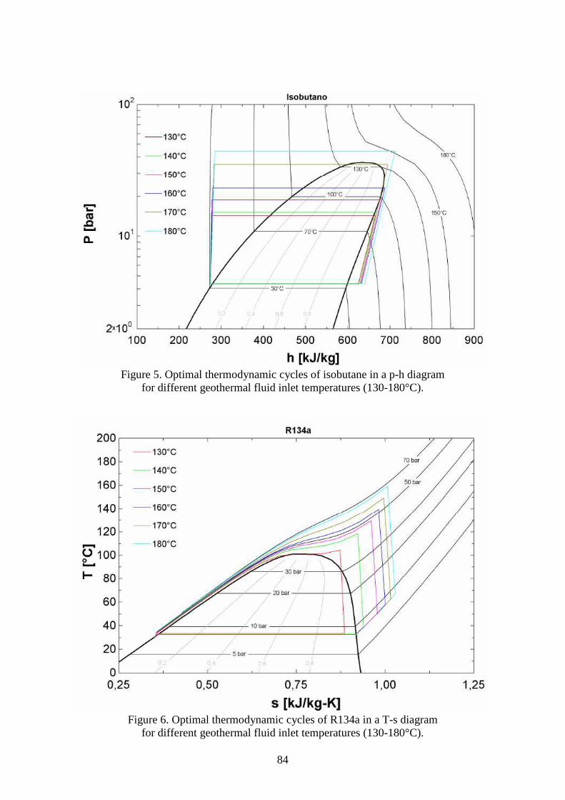
84

Figure 5. Optimal thermodynamic cycles of isobutane in a p-h diagram

for different geothermal fluid inlet temperatures (130-180°C).

Figure 6. Optimal thermodynamic cycles of R134a in a T-s diagram

for different geothermal fluid inlet temperatures (130-180°C).

85

Figure 7. Optimal thermodynamic cycles of R134a in a p-h diagram

for different geothermal fluid inlet temperatures (130-180°C). Comparing the results obtained with the two different organic fluids it appears that the exergy recovery efficiency is always higher in R134a cycles, in particular at the lowest temperature of the geothermal source (Figure 8).

Exergy recovery efficiency

Isobutane vs R134a

0

10

20

30

40

50

60

130 140 150 160 170 180

Geofluid Inlet Temperature [°C]

ηη ηη rec,ex

Isobutane

R134a

Figure 8. Comparison Isobutane-R134a for different geothermal fluid inlet

temperatures (130-180°C).

86

Thanks to the thermophysical properties of the R134a and the better coupling of the thermal streams, in the supercritical cycles the higher power absorbed by the pump is largely compensated by the higher power generation, as shown in Figure 9 for a geothermal fluid inlet temperature of 150°C.

Comparison Isobutane - R134a

Geofluid inlet temperature = 150°C

0

1000

2000

3000

4000

5000

Exp-Generator Feed Pump ACC Net

Power [kW]

Isobutane

R134a

Figure 9. Comparison Isobutane-R134a for a brine inlet temperature of 150°C.

Generator power and parasitic loads.

4.4 Variation of the exergy recovery efficiency near the optimum solution:

sub-optimal points The Heatsep method is also used to display the variation of the exergy recovery efficiency for deviations from the optimal turbine inlet conditions. For generic (not optimal) pressures and temperatures at the inlet of the turbine the working fluid mass flow rate is varied in order to maximize the exergy recovery efficiency. The heat transfer feasibility is checked by building the Pinch Analysis Problem Table (Kemp, 2007), with a minimum allowed temperature difference equal to 10°C. The minimum distance between the hot composite curve and the cold composite curve occurs in correspondence to one or more points used to discretize the heating process of the organic fluid. An optimum response surface (ORS) of the optimization problem is obtained, that is the surface that results from the mapping from a selected set of significant degrees of freedom (in this case, cycle maximum pressure and temperature) to the corresponding optimal objective function values. The following figures show the variation of the exergy recovery efficiency as a function of pressure and specific enthalpy of the organic fluid at turbine inlet for isobutane and R134a for a geothermal fluid inlet temperature of 150°C. In these figures, the maximum of the exergy recovery efficiency, that is the result of the optimization process, is shown as a white circle, the saturation curves that enclose the two-phase zone are represented with a thick red curve. A thick black isothermal curve at base of diagram indicates the upper limit to the heating of the organic fluid (if this line were passed, the difference between brine inlet temperature and organic fluid maximum temperature would be less than 10°C, violating the heat transfer feasibility constraint). The diagrams also show in which portions of the ORS the possible pinch points related to the heat transfer feasibility constraint are active: the numbers that identify ORS portions refer to the points used to discretize the cold composite curve (see Figure 2).

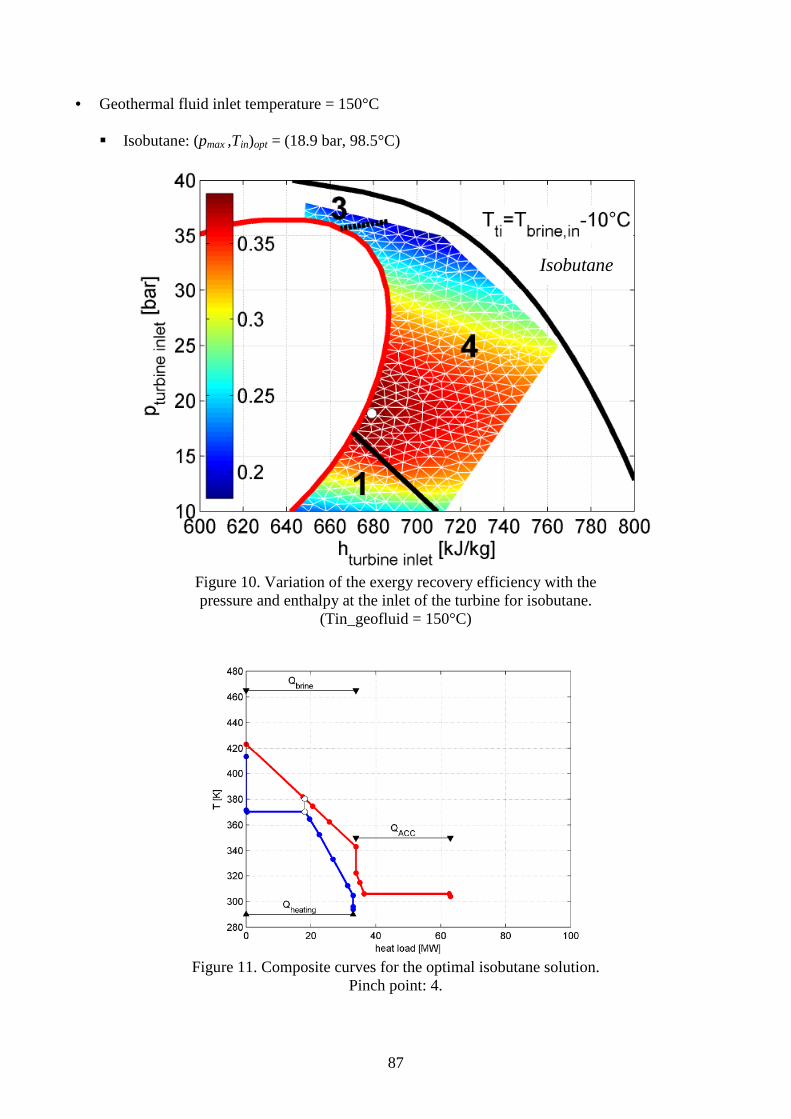
87

• Geothermal fluid inlet temperature = 150°C

� Isobutane: (pmax ,Tin)opt = (18.9 bar, 98.5°C)

Figure 10. Variation of the exergy recovery efficiency with the pressure and enthalpy at the inlet of the turbine for isobutane.

(Tin_geofluid = 150°C)

Figure 11. Composite curves for the optimal isobutane solution.

Pinch point: 4.

Isobutane

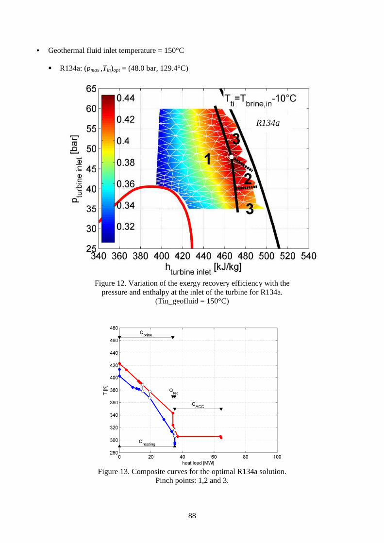
88

• Geothermal fluid inlet temperature = 150°C

� R134a: (pmax ,Tin)opt = (48.0 bar, 129.4°C)

Figure 12. Variation of the exergy recovery efficiency with the

pressure and enthalpy at the inlet of the turbine for R134a. (Tin_geofluid = 150°C)

Figure 13. Composite curves for the optimal R134a solution.

Pinch points: 1,2 and 3.

R134a

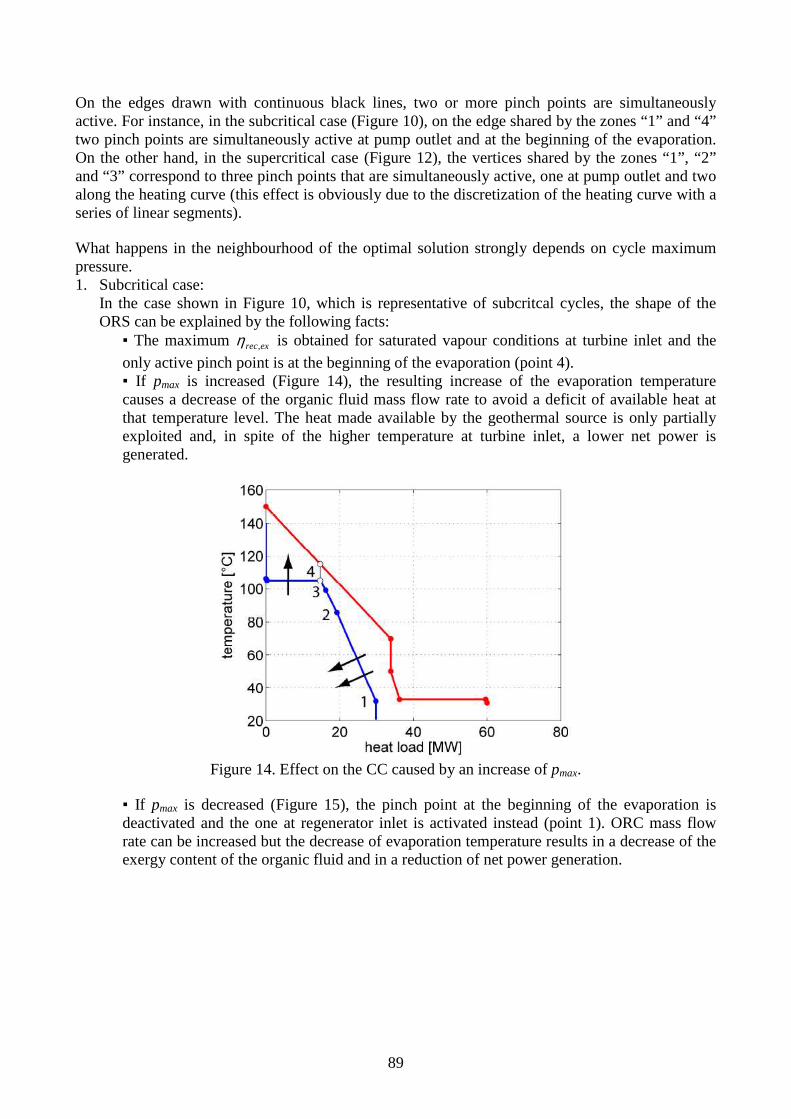
89

On the edges drawn with continuous black lines, two or more pinch points are simultaneously active. For instance, in the subcritical case (Figure 10), on the edge shared by the zones “1” and “4” two pinch points are simultaneously active at pump outlet and at the beginning of the evaporation. On the other hand, in the supercritical case (Figure 12), the vertices shared by the zones “1”, “2” and “3” correspond to three pinch points that are simultaneously active, one at pump outlet and two along the heating curve (this effect is obviously due to the discretization of the heating curve with a series of linear segments). What happens in the neighbourhood of the optimal solution strongly depends on cycle maximum pressure. 1. Subcritical case:

In the case shown in Figure 10, which is representative of subcritcal cycles, the shape of the ORS can be explained by the following facts: ▪ The maximum exrec,η is obtained for saturated vapour conditions at turbine inlet and the

only active pinch point is at the beginning of the evaporation (point 4). ▪ If pmax is increased (Figure 14), the resulting increase of the evaporation temperature causes a decrease of the organic fluid mass flow rate to avoid a deficit of available heat at that temperature level. The heat made available by the geothermal source is only partially exploited and, in spite of the higher temperature at turbine inlet, a lower net power is generated.

Figure 14. Effect on the CC caused by an increase of pmax.

▪ If pmax is decreased (Figure 15), the pinch point at the beginning of the evaporation is deactivated and the one at regenerator inlet is activated instead (point 1). ORC mass flow rate can be increased but the decrease of evaporation temperature results in a decrease of the exergy content of the organic fluid and in a reduction of net power generation.

90

Figure 15. Effect on the CC caused by a decrease of pmax.

▪ In case of superheating (Figure 16), the specific exergy of the organic fluid at turbine inlet increases, but the shift of the isothermal segment of the CCC towards the HCC imposes a reduction of ORC mass flow rate, which in turn results in a partial usage of the geothermal source and a consequent reduction of the exergy recovery efficiency.

Figure 16. Effect on the CC caused by an increase of the superheating.

2. Supercritical case:

In the case shown in Fig. 12, which is representative of supercritcal cycles, the shape of the ORS can be explained by the following facts: ▪ If cycle maximum temperature is lowered while pmax is kept constant (Figure 17), the CCC “rotates” counter-clockwise in the temperature heat load diagram so that ORC mass flow rate can be increased, the active pinch point being still at pump outlet (point 1). Although the heat transferred to organic fluid increases, the exergy content of the organic fluid at turbine inlet diminishes because of the lower temperature, and the exergy recovery coefficient is lower.

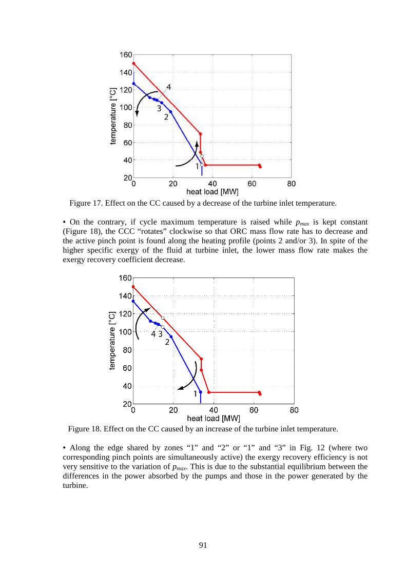
91

Figure 17. Effect on the CC caused by a decrease of the turbine inlet temperature.

▪ On the contrary, if cycle maximum temperature is raised while pmax is kept constant (Figure 18), the CCC “rotates” clockwise so that ORC mass flow rate has to decrease and the active pinch point is found along the heating profile (points 2 and/or 3). In spite of the higher specific exergy of the fluid at turbine inlet, the lower mass flow rate makes the exergy recovery coefficient decrease.

Figure 18. Effect on the CC caused by an increase of the turbine inlet temperature.

▪ Along the edge shared by zones “1” and “2” or “1” and “3” in Fig. 12 (where two corresponding pinch points are simultaneously active) the exergy recovery efficiency is not very sensitive to the variation of pmax. This is due to the substantial equilibrium between the differences in the power absorbed by the pumps and those in the power generated by the turbine.

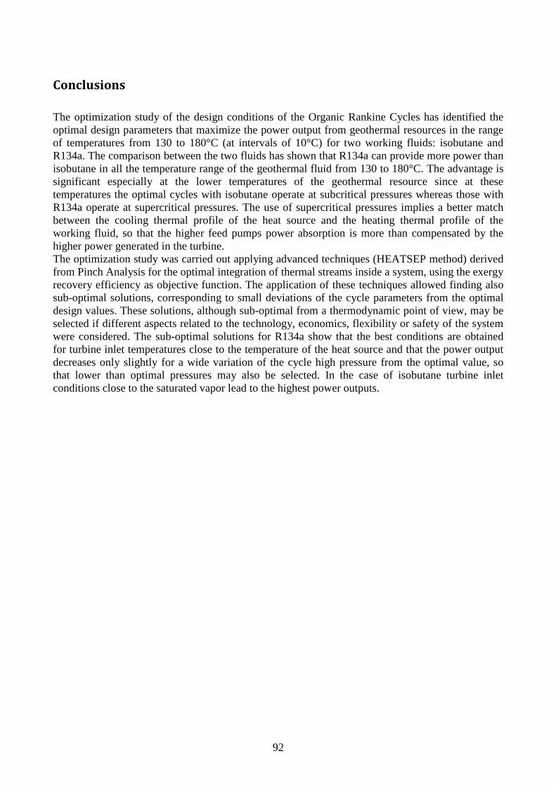
92

Conclusions

The optimization study of the design conditions of the Organic Rankine Cycles has identified the optimal design parameters that maximize the power output from geothermal resources in the range of temperatures from 130 to 180°C (at intervals of 10°C) for two working fluids: isobutane and R134a. The comparison between the two fluids has shown that R134a can provide more power than isobutane in all the temperature range of the geothermal fluid from 130 to 180°C. The advantage is significant especially at the lower temperatures of the geothermal resource since at these temperatures the optimal cycles with isobutane operate at subcritical pressures whereas those with R134a operate at supercritical pressures. The use of supercritical pressures implies a better match between the cooling thermal profile of the heat source and the heating thermal profile of the working fluid, so that the higher feed pumps power absorption is more than compensated by the higher power generated in the turbine. The optimization study was carried out applying advanced techniques (HEATSEP method) derived from Pinch Analysis for the optimal integration of thermal streams inside a system, using the exergy recovery efficiency as objective function. The application of these techniques allowed finding also sub-optimal solutions, corresponding to small deviations of the cycle parameters from the optimal design values. These solutions, although sub-optimal from a thermodynamic point of view, may be selected if different aspects related to the technology, economics, flexibility or safety of the system were considered. The sub-optimal solutions for R134a show that the best conditions are obtained for turbine inlet temperatures close to the temperature of the heat source and that the power output decreases only slightly for a wide variation of the cycle high pressure from the optimal value, so that lower than optimal pressures may also be selected. In the case of isobutane turbine inlet conditions close to the saturated vapor lead to the highest power outputs.

93

References Lazzaretto A. and Toffolo A., A Method to Separate the Problem of Heat Transfer Interactions in the Synthesis of Thermal System, Energy, 33, 2008. Lazzaretto A. and Manente, G., Analysis of Superimposed Elementary Thermodynamic Cycles: from the Brayton-Joule to Advanced Mixed (Auto-Combined) Cycles, International Journal of Thermodynamics, 2009. Kemp I.C., Pinch analysis and process integration (2nd ed.), Butterworth-Heinemann, London 2007. Toffolo A., Lazzaretto A., Manente G. and Rossi N., Synthesis/Design Optimization of Organic Rankine Cycles for Low Temperature Geothermal Sources with the HEATSEP Method, ECOS 2010, Lausanne.

94

5. Boiling Heat Transfer in Organic Rankine

Cycle Vaporizers

In binary cycle power plants the working fluid is vaporized by heat exchange with the heat source. A boiling fluid consists of a two phase mixture of vapor and liquid. When such a fluid flows a number of distinct flow regimes can occur depending on the flow rate and the relative amounts of vapor and liquid present. Two-phase flow is thus more complex than single-phase flow and special methods are needed to calculate the heat transfer coefficients in boiling systems. In the calculation of the two-phase heat transfer coefficient both the nucleate boiling and the forced convection contribute to the heat transfer. This section describes firstly the heat transfer correlations proposed in the literature for the nucleate pool boiling regime and then presents the methods used for calculating the heat transfer coefficient in flow boiling. An accurate prediction of the heat transfer coefficients is important for a proper design of the vaporizers.

5.1 Pool boiling curve

Pool boiling refers to vaporization that takes place at a solid surface submerged in a quiescent liquid. When the temperature Ts of the solid surface exceeds the saturation temperature Tsat of the liquid, vapor bubbles form at nucleation sites on the surface, grow and subsequently detach from the surface. The driving force for heat transfer is ∆Te = Ts – Tsat called the excess temperature. The boiling curve is a plot of surface heat flux (W/m2) versus excess temperature and is shown in Figure 1. Point A on the curve marks the onset of nucleate boiling (ONB). At lower excess temperatures, heat transfer occurs by natural convection alone. Nucleate boiling exists between points A and C on the curve where two different boiling regimes can be distinguished: A-B : Boiling characterized by the formation of isolated vapor bubbles at nucleation sites dispersed on the solid surface. Bubble growth and detachment result in significant fluid mixing near the solid surface that greatly increases the rate of heat transfer. B-C : As the heat flux increases beyond point B, the number of active nucleation sites and the rate of vapor formation become so great that bubble interference and coalescence occur. The vapor leaves the solid surface in jets or columns that subsequently merge and form large slugs of vapor. The high rate of vapor formation begins to inhibit the flow of liquid across the solid surface, causing the slope of the boiling curve to decrease. The heat flux continues to increase since the increase in temperature driving force more than compensates for the decreasing heat transfer coefficient. C : The heat flux attains a maximum, called the “critical heat flux”, at point C. At this point, the rate of vapor formation is so great that some parts of the surface are covered by a continuous vapor film. C-D : Transition region: the heat flux decreases as ∆Te increases. The fraction of the solid surface covered by vapor continues to increase and the heat transfer rates for gases are generally much lower than for liquids. D : The heat flux has reached a minimum (Liedenfrost point) where the entire solid surface is covered by a vapor blanket. Beyond this point heat is transferred from the solid surface across the vapor film to the liquid. Hence this regime is called “film boiling”. Most reboilers and vaporizers are designed to operate in the nucleate boiling regime. The transition region, with its unusual characteristic of decreasing heat flux with increasing driving force, is

95

always avoided in equipment design. Film boiling implies a much higher temperature driving force corresponding to much lower heat transfer coefficients. The pool boiling curve is influenced by: - the roughness of the solid surface (mirror finished surfaces require higher excess temperatures to achieve a given heat flux since they present less cavities acting as nucleation sites); - an increase of the system pressure shifts the pool boiling curve toward lower excess temperatures.

Figure 1. Pool boiling curve for water at one atmosphere pressure.

5.2 Correlations for nucleate boiling

In the nucleate boiling region the temperature of the solid surface Ts increases only slightly for wide variations of the heat flux. This can be expressed as:

m

sats A

qTT

=− ψ (Eq. 1)

Where ψ and m are constants that depend on the physical properties of the liquid and vapor and the surface nucleation properties. The exponent m assumes values between 0.2 and 0.5 and especially around 0.3. The heat transfer coefficient is thus a function of the heat flux:

( )( )

( ) nm

satsnb A

qC

A

q

TT

Aqh

=

=−

=−

−1

1/ ψ (Eq. 2)

where 7.0≅n . The early correlations of Rohsenow and Forster-Zuber show the fluid properties included in the coefficients ψ and C. � Rohsenow (1952) presented the following equation:

96

( )( )

s

L

LL

n

GLLsf

Lsats c

gr

AqC

r

cTT

−=

−λµ

ρρσ

µ

'/

(Eq. 3)

where n’ = 0.33 and s = 1 for water; n’ = 0.33 and s = 1.7 for the other fluids. Csf is a constant that accounts for the nucleation properties of different combinations liquid-surface. As a first approximation Csf = 0.013.

� The Forster-Zuber correlation (1955) is:

( )24.024.029.05.0

75.024.049.045.079.0

00122.0GL

satsatsLLLnb

r

PTTch

ρµσρλ ∆−

= (Eq. 4)

where )()( satsatssatsat TPTPP −=∆ . Other researchers simplified the above expressions by considering the pressure dependence of the fluid properties. � Stephan and Abdelsalam (1980) considered experimental data concerning pool boiling on

horizontal surfaces in the range of fully established nucleate boiling in a wide pressure range

between 97.00001.0 ≤≤Cp

p. They classified the substances in four groups:

1) water; 2) hydrocarbons (benzene, ethanol, n-pentane, n-heptane, n-hexane, n-butanol); 3) cryogenic liquids (helium, hydrogen, nitrogen, oxygen, neon); 4) refrigerants (R12, R114, R113, R11, R22, propane, n-butane, CO2) Using the regression analysis they found four equations for the four groups of substances and one equation, with a higher error, valid for all the substances. The equations were of the type:

( ),..., 21 XXfNu = (Eq. 5) and the linear regression analysis allowed to select those dimensionless numbers Xi which exerted the most significant influence on the dependent variable Nu. In order to facilitate the application of these heat transfer equations the authors introduced a significant simplification: they included the thermophysical properties of the substance in a fluid specific parameter c :

n

nb A

qch

⋅= (Eq. 6)

They expressed c as a function of pressure and they used a different value of the exponent n for each group of substances:

Water: 673.0

1

⋅=A

qchnb (Eq. 7)

Hydrocarbons: 670.0

2

⋅=A

qchnb (Eq.8)

Refrigerants: 745.0

4

⋅=A

qchnb (Eq. 9)

The pressure dependent values c4 are plotted in Figure 2 and show a marked increase with pressure.

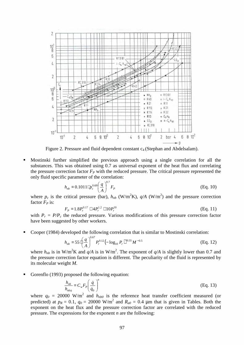
97

Figure 2. Pressure and fluid dependent constant c4 (Stephan and Abdelsalam).

� Mostinski further simplified the previous approach using a single correlation for all the

substances. This was obtained using 0.7 as universal exponent of the heat flux and correlating the pressure correction factor FP with the reduced pressure. The critical pressure represented the only fluid specific parameter of the correlation:

Pcnb FA

qph

7.069.01011.0

⋅= (Eq. 10)

where pc is the critical pressure (bar), hnb (W/m2K), q/A (W/m2) and the pressure correction factor FP is:

102.117.0 1048.1 rrrP PPPF ++= (Eq. 11) with Pr = P/Pc the reduced pressure. Various modifications of this pressure correction factor have been suggested by other workers.

� Cooper (1984) developed the following correlation that is similar to Mostinski correlation:

( ) 5.055.010

12.067.0

log55 −−−

⋅= MPPA

qh rrnb (Eq. 12)

where hnb is in W/m2K and q/A is in W/m2. The exponent of q/A is slightly lower than 0.7 and the pressure correction factor equation is different. The peculiarity of the fluid is represented by its molecular weight M.

� Gorenflo (1993) proposed the following equation:

n

Pwnb

nb

q

qFC

h

h

=

00&

& (Eq. 13)

where q0 = 20000 W/m2 and hnb0 is the reference heat transfer coefficient measured (or predicted) at pR = 0.1, q0 = 20000 W/m2 and Ra0 = 0.4 µm that is given in Tables. Both the exponent on the heat flux and the pressure correction factor are correlated with the reduced pressure. The expressions for the exponent n are the following:

98

- water: 15.03.09.0 rpn ⋅−= (Eq. 14)

- other fluids: 3.03.09.0 rpn ⋅−= (Eq. 15) The pressure correction factor is for all fluids except water:

rr

rP pp

pF

−++=

1

15.22.1 27.0 (Eq. 16)

The correlation accounts for the surface roughness effects according to 133.0

0

=

a

aw R

RC .

The predictions of the various correlations differ by a huge amount (one order of magnitude). One reason for the wide variation is that nucleate boiling is very sensitive to the precise condition of the surface on which boiling occurs. It is not practical to specify the detailed surface characteristics required to rigorously model the phenomenon. Even if this could be done it would be of dubious utility in equipment design because the surface characteristics change over time due to aging, corrosion, fouling, cleaning procedures. As a result the variability exhibited by the calculated values actually reflects the variability observed among the sets of experimental data upon which the various correlations are based. Therefore significant conservatism is adopted in equipment design due to the uncertainty inherent in boiling correlations. The rate of heat transfer for nucleate boiling of mixtures is lower than for pure substances. The reason is that the more volatile components accumulate preferentially in the vapor bubbles, leaving the surrounding liquid enriched in the less volatile (higher boiling) components. As a result, the temperature of the liquid in the immediate vicinity of the heating surface increases and the effective driving force for heat transfer is reduced. Furthermore the concentration gradient generates a mass transfer resistance in addition to the thermal resistance. Palen presented a simple empirical method that involves a multiplicative mixture correction factor that is applied to the heat transfer coefficient calculated from the Mostinski correlation. The correction factor Fm is given by the following equation:

1

75.015.0

023.01

−

+= BRA

qFm (Eq. 17)

where BR is the boiling range BR = TDew - TBubble (K) and q/A (W/m2). In conjunction with this equation for Pr > 0.2 the pressure correction factor is: 17.08.1 rP PF = Heat transfer coefficients for boiling on tube bundles are generally higher than for boiling on single tubes under the same conditions. The enhancement in heat-transfer rate is due to the convective circulation that is set up within and around the tube bundle. The circulation is driven by the density difference between the liquid surrounding the bundle and the two-phase mixture within the bundle. Palen presented an approximate method for calculating convective effects. The average boiling heat transfer coefficient hb is expressed as follows:

ncbnbb hFhh += (Eq. 18) where hnc is a heat-transfer coefficient for liquid-phase natural convection and Fb is a factor that is correlated in terms of bundle geometry.

5.3 Critical heat flux

At high heat fluxes the vapor bubbles leave the heated surface in columns or jets. When the velocity of the vapor jets reaches a sufficiently large value the jets become unstable and collapse. The

99

resultant accumulation of vapor at the heated surface prevents an adequate supply of liquid from reaching the surface and the heat flux begins to decrease. Zuber proposed the following equation for the critical heat flux in nucleate pool boiling on a large flat upward facing surface:

( )( ) 25.05.0149.0 GLGc

grA

q ρρσρ −=

(Eq. 19)

For other geometries, such as boiling on a horizontal cylinder, the coefficient assumes different values. The critical heat flux is a strong function pressure through its effect on r, ρG and σ. This is clearly shown by the correlation derived from Mostinski for boiling on a horizontal tube:

( ) 9.035.0 1367 rrcc

PPPA

q −=

(Eq. 20)

Where q/A (W/m2) and Pc (kPa). The critical heat flux increases up to a maximum value and then decreases and is zero at the critical pressure. For tube bundles Palen presented the following correlation:

btubecbundlec A

q

A

q φ,,

=

(Eq. 21)

where φb is a bundle correction factor equal or less than one depending on the bundle geometry parameter. The critical heat flux for a mixture may be higher or lower than for a pure component under similar conditions. Although a higher value is usually found as would be expected from the effect of boiling point elevation and mass transfer resistance in mixture boiling the variation of surface tension with composition can cause the mixture critical heat flux to be lower than the pure component value in some cases. In any event the mixture effect is generally neglected in design work since it cannot be reliably predicted. Thus the above correlations are used with the mixture physical properties replacing the pure component properties.

5.4 Flow boiling

Figure 3 depicts the variation in flow regime and heat transfer coefficient for convective boiling in a vertical tube. The fluid enters the tube as a subcooled liquid and initially heat is transferred by convection alone. With the onset of boiling and the establishment of the bubbly flow regime the heat transfer coefficient starts to rise sharply as the nucleate boiling mechanism contributes to the heat transfer. As the vapor fraction increases the flow regime changes from bubbly to slug flow and then to annular flow while the heat transfer coefficient continues to increase. Eventually the amount of liquid is reduced to the point where dry spots begin to appear on the tube wall, and the heat transfer coefficient begins to decrease. It continues to decrease until the tube wall is completely dry and all remaining liquid is in the form of droplets entrained in the vapor phase (mist flow regime). The heat transfer coefficient remains relatively constant as the droplets are gradually vaporized and the vapor becomes superheated. In the final stages heat is transferred solely by gas-phase convection. Thus the rate of heat transfer varies greatly over the length of the tube and an incremental analysis is required to accurately predict performance.

100

Figure 3. Convective boiling in a vertical tube.

It was recognized in the early stages of boiling research that the heat transfer coefficient in flow boiling is an interaction of nucleate and convective boiling. The following sections explain the main methods proposed in the literature for the calculation of the heat transfer coefficients in flow boiling.

5.4.1 The Chen method

The first correlational model for flow boiling coefficient was proposed by Rohsenow in 1952 as a simple addition of the nucleate and convective coefficients:

cbnbfb hhh += (Eq. 22)

This model was used in principle by Chen, who in 1963 formulated the first cohesive flow boiling method which became very popular. The Chen correlation is:

FhShh Lnbfb += (Eq. 23)

where: hfb : flow boiling heat transfer coefficient; hL : convective heat-transfer coefficient for liquid phase; hnb : nucleate boiling coefficient for the same wall superheat; F : boiling enhancement factor that accounts for the increase in velocity of the fluid; S : suppression factor that accounts for the decrease in bubble activity. a) Convective boiling By using experimental data from different sources Chen determined experimental values of the convective boiling enhancement factor F and based it on the Martinelli parameter, Xtt :

101

1.05.09.01

−=G

L

L

Gtt x

xX

µµ

ρρ

(Eq. 24)

The liquid heat transfer coefficient hL is: dh LLLL /PrRe023.0 4.08.0 λ= (Eq. 25)

where:

LL

dxG

µ)1(

Re−= (Eq. 26)

L

LLL

c

λµ

=Pr (Eq. 27)

The enhancement factor F can be determined by the following equation to fit the curve proposed by Chen: For 1/Xtt ≤ 0.1, F = 1; For 1/Xtt > 0.1, ( ) 736.0/1213.035.2 ttXF += (Eq. 28) hcb can then be found by multiplying the liquid heat transfer coefficient hL by the enhancement factor F . b) Nucleate boiling Chen method for obtaining hnb is based on the analysis of Forster and Zuber, however Chen found it necessary to introduce a nucleate boiling suppression factor S in order to account for diminished contribution of nucleate boiling at higher vapour fractions. Thus hnb is given by Eq. 4 and the suppression factor S is dependent on the two-phase flow Reynolds number according to the following equation:

( ) 17.125.16 Re1053.21

1

FS

L ⋅⋅+=

− (Eq. 29)

The wall temperature is assumed at first to calculate an initial hnb, then later checked. A reiterative process is used until the assumed wall superheat agrees with the final value.

5.4.2 The Shah model

The other class of correlation for mixed nucleation and convection boiling uses the Boiling number that was first introduced by Davidson in 1943 in a first attempt to relate the effects of heat flux and mass velocity in the flow boiling process:

rG

qBo

⋅=

& (Eq. 30)

where q& is the heat flux, G is the mass flux of the fluid and r is the latent heat of vaporization. This dimensionless ratio may be interpreted as a measure of the nucleate boiling contribution: as heat flux increases, nucleation is increased, and so is the nucleate heat transfer coefficient hnb; increased mass velocity results in higher convective coefficient hcb, lower wall temperature, and hence decreased activation of nucleation cavities. In 1976 Shah proposed a correlation to calculate the heat transfer coefficient of boiling flow through pipes based on the following dimensionless parameters: a) Froude number ( FrL ):

iLL

gd

GFr

2

2

ρ= (Eq. 31)

determines whether stratification effects are important or not. A Froude number greater than 0.04 signifies that stratification effects are negligible and inertial forces are dominant compared with gravitational forces. For low Froude numbers the Shah method is recommended because it allows for effects of stratification that occurs in horizontal tubes.

102

b) Convection numbers (Co e N):

5.08.01

−=L

G

x

xCo

ρρ

(Eq. 32)

( ) 3.038.0 −= LFrCoN with a horizontal tube and FrL < 0.04 CoN = with a vertical tube or horizontal tube with FrL > 0.04

c) Boiling number (Bo):

rG

qBo

⋅=

& (Eq. 33)

determines the enhancement due to nucleate boiling. A boiling number less than 5109.1 −× signifies that there is no enhancement due to nucleation. Shah identified the chart correlation in which two regions are defined: 1) a nucleate boiling region, Co > 1.0, where heat transfer is determined by the boiling number only; 2) a region of convection boiling, Co < 1.0 where nucleation bubbles are completely suppressed. For the purpose of simplifying the use of the Chart correlation, Shah’s method was traduced in equation form. The flow boiling heat transfer coefficient on the tube perimeter is the greater of the convective and nucleate boiling component:

Lcb hNh 8.08.1 −= (Eq. 34)

Lnb hBoh 5.0230= when N>1 and Bo > 0.00003 (Eq. 35)

( ) Lnb hBoh 5.0461+= when N>1 and Bo < 0.00003 (Eq. 36)

( ) Lnb hNCBoh 1.05.0 74.2exp −= when 0.1<N<1 (Eq. 37)

( ) Lnb hNCBoh 15.05.0 74.2exp −= when N<0.1 (Eq. 38) where C = 14.7 when Bo > 0.0011, C = 15.43 when Bo < 0.0011 and hL is given by Eq. 25. Shah’s correlation is applicable for a wide range of reduced pressures (between 0.004 and 0.89). Shah’s method is applicable for saturated boiling inside pipes of all Newtonian fluids (except metallic fluids). A comparative study of Shah’s correlations to data points for 11 refrigerants revealed a mean deviation of ±14%.

5.4.3 Gungor and Winterton correlation

A correlation was proposed by Gungor and Winterton (1986) that applies to tubes and annuli for both vertical and horizontal flow and that extends to subcooled as well as saturated boiling. The data points taken from the literature consisted of the experimentally measured values of heat transfer coefficient and wall temperature as a function of pressure (or saturation temperature), mass flux, heat flux and quality. For subcooled boiling the bulk temperature (or subcooling) is recorded in place of the quality. The basic form of the correlation used is:

nbLfb ShEhh += (Eq. 39)

Lh has been given by the Dittus-Boelter equation for liquid only flowing in the duct:

dh L

LLL

λ4.08.0 PrRe023.0= (Eq. 40)

In two-phase flow the heat transfer is increased by an enhancement factor E well above the level for a single-phase liquid flow. This effect depends on the quality x and on the vapor to liquid density ratio ρG/ρL (that is on the Martinelli parameter Xtt) as in the previous correlations. According to the

103

authors also the generation of vapor in the boiling process, that results in significant disturbance of the boundary layer, improves the heat transfer. A dimensionless measure of how important this

effect may be is given by the boiling number: rG

qBo

⋅=

&. Consequently ( )BoXfE tt ,= and was

calculated from experimental data. The expression found for E is: 86.0

16.1 137.1240001

++=

ttXBoE (Eq. 41)

A number of literature expressions for hnb were investigated, the best being that proposed by Cooper, here recalled:

( ) 5.055.010

12.067.0

log55 −−−

⋅= MPPA

qh rrnb (Eq. 12)

The suppression factor S takes account of the fact that the boundary layer of superheated liquid in which the vapor bubble grows is thinner in forced convection. The expressions found for S is:

17.126 Re1015.11

1

LES −⋅+

= (Eq. 42)

If the tube is horizontal and the Froude number is less than 0.05 then E and S should be multiplied respectively by:

( )FrFrE 21.02

−= (Eq. 43)

FrS =2 (Eq. 44) As the equations stand it is assumed that the heat flux q& is known. If Tw (wall temperature) is known then, as with many other correlations, a degree of iteration is required. For saturated boiling this correlation is similar in accuracy to the Shah correlation (but requires slightly fewer equations). For subcooled boiling it is nearly as good as the best of the correlations developed specifically for this boiling regime.

5.4.4 Kandlikar correlation

Collier presented the flow boiling map (1981) depicting the basic relationship between the heat transfer coefficient and the quality with the heat flux as a parameter. Collier’s map (Figure 4) was plotted for a single value of mass flux and was specific to water at low pressures.

104

Figure 4. Collier’s flow boiling map.

The objective of Kandlikar’s work (1991) was to develop a flow boiling map to represent the heat transfer coefficient as a function of three major parameters: quality, heat flux and mass flux. The entire range from the onset of nucleate boiling in the subcooled region up to a quality of 0.8 in the saturated boiling region is covered. The location of critical heat flux is not shown on the map. The final flow boiling map is shown in Figure 5.

Figure 5. Kandlikar’s flow boiling map.

The quantitative representation given in the saturated region may be directly applied to practical situations. In the subcooled region only a qualitative representation is provided since specific fluid properties are needed in various equations for subcooled boiling.

105

In order to represent a number of different fluids on the same map it is essential to nondimensionalize the heat transfer coefficient: hTP/hL where hL0 is the single-phase heat transfer coefficient with total flow as liquid. The Petukhov-Popov (1963) and Gnielinski (1976) correlations for hL0 are better able to account for the Prandtl number effect for different fluids compared to the Dittus-Boelter correlation. Only the saturated boiling region is here considered. The Kandlikar correlation is given by the maximum of (hTP/hL0)NBD and (hTP/hL0)CBD where the subscripts NBD and CBD refer to the nucleate boiling dominant and convective boiling dominant regions given by: a) Nucleate boiling dominant (NBD) region:

( ) ( ) ( )4444 34444 21

444444 3444444 21 termNucleate

fl

termConvective

LG

L

NBDL

TP xFBoFrfxxh

h 8.07.02

64.016.0

1.0

0

10.105816683.0 −+−

=

ρρ

(Eq. 45)

b) Convective boiling dominant (CBD) region:

( ) ( )4444 34444 21

4444444 34444444 21 termNucleate

fl

termConvective

lG

L

CBDL

TP xFBoFrfxxh

h 8.07.02

08.072.0

45.0

0

12.667)(11360.1 −+−

=

ρρ

(Eq. 46)

where: ( ) ( ) 3.0

2 25 LL FrFrf = for FrL < 0.04 for horizontal tubes; ( ) 12 =LFrf for FrL > 0.04 for horizontal tubes and for vertical tubes.

In the region x<0.02 hTP values corresponding to x = 0.02 are employed. This adjustment is needed due to the form of the correlation. Ffl is a fluid dependent parameter set equal to 1.0 for water. Kandlikar obtained Ffl values for refrigerants R-11, R-12, R-22, R-113, R-114 and R-152a that are listed in Table 1.

Fluid Ffl Water 1.00 R-11 1.30 R-12 1.50

R-13B1 1.31 R-22 2.20 R-113 1.30 R-114 1.24 R-152a 1.10

Table 1. Fluid-dependent parameter Ffl in the Kandlikar correlation. To represent the equation on the flow boiling map three parameters are needed: ρL/ρG, Bo, and Ffl. A modified boiling number Bo* is introduced to include the effect of Bo and Ffl. Bo* is defined by:

7.0/1*flFBoBo = (Eq. 47)

The variation of hTP/hL0 with x is plotted in the flow boiling map for three values of ρL/ρG and two values of Bo* covering the ranges of parameters commonly employed in the refrigeration, power and process industries. a) Nucleate Boiling Dominant (NBD) Region The nucleate boiling dominant region exists at lower values of x in the saturated boiling region in Figure 5. Here Bo* is seen as the major influencing parameter. As Bo* increases the contribution due to nucleate boiling increases and consequently hTP/hL0 increases. The trend in hTP/hL0 versus x is also influenced by the magnitude of Bo*. At higher values of Bo* the convective contribution is small compared to the nucleate boiling component. As ρL/ρG decreases,

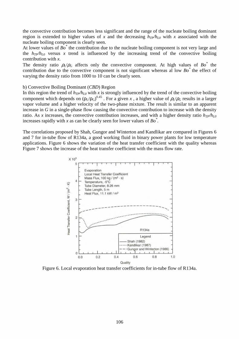
106

the convective contribution becomes less significant and the range of the nucleate boiling dominant region is extended to higher values of x and the decreasing hTP/hL0 with x associated with the nucleate boiling component is clearly seen. At lower values of Bo* the contribution due to the nucleate boiling component is not very large and the hTP/hL0 versus x trend is influenced by the increasing trend of the convective boiling contribution with x. The density ratio ρL/ρG affects only the convective component. At high values of Bo* the contribution due to the convective component is not significant whereas al low Bo* the effect of varying the density ratio from 1000 to 10 can be clearly seen. b) Convective Boiling Dominant (CBD) Region In this region the trend of hTP/hL0 with x is strongly influenced by the trend of the convective boiling component which depends on (ρL/ρG)0.45 . For a given x , a higher value of ρL/ρG results in a larger vapor volume and a higher velocity of the two-phase mixture. The result is similar to an apparent increase in G in a single-phase flow causing the convective contribution to increase with the density ratio. As x increases, the convective contribution increases, and with a higher density ratio hTP/hL0 increases rapidly with x as can be clearly seen for lower values of Bo*. The correlations proposed by Shah, Gungor and Winterton and Kandlikar are compared in Figures 6 and 7 for in-tube flow of R134a, a good working fluid in binary power plants for low temperature applications. Figure 6 shows the variation of the heat transfer coefficient with the quality whereas Figure 7 shows the increase of the heat transfer coefficient with the mass flow rate.

Figure 6. Local evaporation heat transfer coefficients for in-tube flow of R134a.

107

Figure 7. Average evaporation heat transfer coefficients for in-tube flow of R134a.

5.4.5 The asymptotic model used by Steiner and Taborek

Kutateladze proposed in the early ‘60 a power type addition model for the two boiling components using n = 2 :

( ) ( )( ) nncb

nnbfb

/1ααα += (Eq. 48)

This model is best termed “asymptotic”, as the value of ( ),...,, xmqffb &&=α approaches the larger of

the two components. This assures a smooth transition as the boiling mechanism changes from nucleate to convective dominated with increasing q& . This model has the advantage that the two boiling components are independent of each other, their interaction being governed by the above equation. Equation 45 is general with ∞<≤ n1 , n = 1 representing the additive model (Chen) and

∞→n is the case of larger of the two. Steiner and Taborek (1992) used this asymptotic method and placed main emphasis on a sound mechanistic model which would respect all the established principles of pool and convective boiling and the fundamental characteristics of flow boiling: � For heat fluxes below the onset of nucleate boiling, only convective flow boiling is present and

the coefficient is largely independent of heat flux over a wide range of mass velocity and vapor fraction;

� In fully developed nucleate boiling, the flow boiling coefficient is virtually independent of mass velocity and vapor fraction, both being measures of the effective flow velocity.

The interaction between nucleate and convective boiling as a function of vapor fraction x is shown in Figure 8 with reference to ethanol at saturated conditions for a wide range of heat fluxes and two mass velocities. The single-phase liquid coefficient before the onset of nucleate boiling is shown in the Figures for comparison, demonstrating the rapid rise of the heat transfer coefficient with the

108

start of nucleation. At low heat fluxes, convective boiling is a significant component and with increasing x values rapidly becomes the dominant component. At intermediate and high heat fluxes the heat transfer coefficient markedly increases due to the nucleate boiling contribution.

Figure 8. Flow boiling heat transfer coefficient as a function

of vapor fraction at two mass velocities. Figure 9 shows the schematic model of the flow boiling process derived by the authors: � Region A-B Approaching point A, the liquid is subcooled and single-phase convective heat transfer takes place at a rate of αLO (liquid only). If in the region A-B the heat flux (wall superheat) reaches a minimum value, subcooled nucleate boiling takes place and the heat transfer coefficient increases substantially. The bubbles collapse in the core of the stream, which had not yet reached saturation temperature. � Region B-D The saturation temperature is reached at point B and the rapidly increased velocity of the two-phase flow mixture results in a corresponding increase of the heat transfer coefficient. In most industrial cases conditions for the onset of nucleate boiling are satisfied at point B and nucleate and convective boiling coefficients are superimposed, according to their relative magnitudes. The full lines in Figure 9 represent the asymptotic addition of the nucleate and convective components. With increasing vapor fraction, the flow regime progresses from bubbly to churn flow (point D). � Region D-E-F-G At still higher vapor fraction x, the flow becomes annular (D-E), with a thin layer on the tube wall and eventually with mist particles entrained in the stream core (E-F). With further increase of vapor fraction x and hence flow velocity, the liquid annular film cannot be sustained and the “dryout” point F is reached at x-critical. At this point the remaining liquid is sheared off the wall and keeps flowing as “mist” in the tube core.

109

The heat transfer coefficient decreases drastically as the dry wall condition is reached and the tube wall temperature raises accordingly if the wall is heated with constant heat flux. Beyond the dryout point, region F-G, the complete evaporation of the droplets in the mist occurs at low heat transfer rates and may persist over substantial tube length. Finally, at point G, the evaporation is completed with x = 1, and the coefficient drops to the value αG0 based on gas only conditions.

Figure 9. Schematic representation of the vertical flow boiling process.

Steiner and Taborek (1992) used the asymptotic model assuming n = 3 . The local flow boiling heat transfer coefficient is given by the following equation:

( ) ( )( ) 3/133cbnbffb ααα += (Eq. 49)

( ) ( )( ) 3/130

3, tpLnbfonbfb FF ααα += (Eq. 50)

where:

onb,α : nucleate pool boiling coefficient, based on normalized conditions of heat flux and reduced

pressure. The coefficient can originate from any predictive method or data.

nbfF : correction factor which compensates for differences between pool and flow condition. The

parameters include pressure, heat flux, tube diameter and surface roughness, and a residual correction expressed as a function of molecular weight.

110

0Lα : local convective heat transfer coefficient, based on the total (liquid plus vapor) mass velocity assumed as liquid (LO). Ftp : two-phase flow multiplier accounting for enhancement of the coefficient in the liquid-vapor mixture. It is a function of the vapor fraction x and ratio of liquid/vapor densities. � Ftp was derived as a function of the vapor fraction x and the ρL/ρG ratio (instead of using the

Martinelli parameter). For x < xcr (usually xcr < 0.5) the correlation is given by the following equation:

( )1.135.0

6.05.1 9.11

+−=

G

Ltp xxF

ρρ

(Eq. 51)

The curves exhibit a steep slope al very low x values, corresponding to data, and correctly converge to Ftp → 1 as x → 0, which is not the case in many literature methods.

� The coefficient onb,α is supplied at normalized values (subscript “o”) of the parameters

involved: - reduced pressure: 1.0, =orp ;

- wall roughness: mR oa µ1, = ;

- heat flux 2/20 mkWq =& (for hydrocarbons, refrigerant and organics). For determination of onb,α any predictive method can be used and the procedures developed by

Gorenflo are recommended. Table 2 shows precalculated values of onb,α for some fluids:

Fluid Formula onb,α [W/m2K] Propane C3H8 4000 n-Butane C4H10 3300 n-Pentane C5H12 3070 Isopentane C5H12 2940

R134a C2H2F4 3500 R227 C3HF7 3800

Table 2. Nucleate flow boiling heat transfer coefficients at normalized conditions. � The correction factor nbfF is:

( )

)(

133.0

,

4.0

MFR

R

d

d

q

qFF

oa

a

o

prnf

opfnbf

=

−

&

& (Eq. 52)

Special attention was paid to the possible effects of mass velocity m& and vapor fraction x on flow nucleate boiling. Extensive data show no effect of either parameter within wide ranges of heat flux and reduced pressure. Thus in vertical flow nucleate boiling ( ) 1, =xmf & . These observations also pose some question as to the validity of the nucleate boiling suppression factor. The pressure correction factor is (for pr < 0.95):

7.37

45.0

1

7.14.3816.2 r

rrpf p

ppF

−++= (Eq. 53)

In the literature the exponent on q& in nucleate boiling is usually expressed as a constant between about 0.67 and 0.8. However it is documented by experimental data that the slope of the data plotted as α versus q& decreases with pressure. The expressions derived are:

)75.1exp(1.08.0)( rpprnf −= for all fluids except cryogenics (Eq. 54)

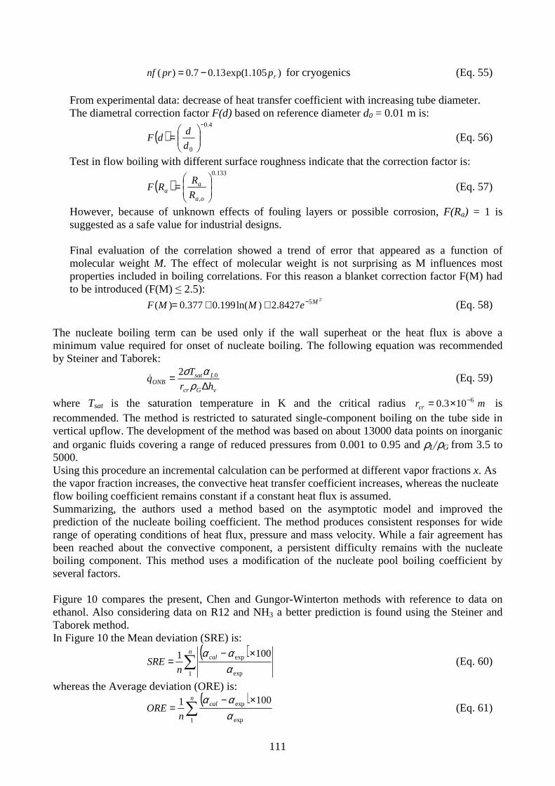
111

)105.1exp(13.07.0)( rpprnf −= for cryogenics (Eq. 55)

From experimental data: decrease of heat transfer coefficient with increasing tube diameter. The diametral correction factor F(d) based on reference diameter d0 = 0.01 m is:

( )4.0

0

−

=

d

ddF (Eq. 56)

Test in flow boiling with different surface roughness indicate that the correction factor is:

( )133.0

,

=

oa

aa R

RRF (Eq. 57)

However, because of unknown effects of fouling layers or possible corrosion, F(Ra) = 1 is suggested as a safe value for industrial designs.

Final evaluation of the correlation showed a trend of error that appeared as a function of molecular weight M. The effect of molecular weight is not surprising as M influences most properties included in boiling correlations. For this reason a blanket correction factor F(M) had to be introduced (F(M) ≤ 2.5):

258427.2)ln(199.0377.0)( MeMMF −++= (Eq. 58) The nucleate boiling term can be used only if the wall superheat or the heat flux is above a minimum value required for onset of nucleate boiling. The following equation was recommended by Steiner and Taborek:

vGcr

LsatONB hr

Tq

∆=

ρασ 02

& (Eq. 59)

where Tsat is the saturation temperature in K and the critical radius mrcr6103.0 −×= is

recommended. The method is restricted to saturated single-component boiling on the tube side in vertical upflow. The development of the method was based on about 13000 data points on inorganic and organic fluids covering a range of reduced pressures from 0.001 to 0.95 and ρL/ρG from 3.5 to 5000. Using this procedure an incremental calculation can be performed at different vapor fractions x. As the vapor fraction increases, the convective heat transfer coefficient increases, whereas the nucleate flow boiling coefficient remains constant if a constant heat flux is assumed. Summarizing, the authors used a method based on the asymptotic model and improved the prediction of the nucleate boiling coefficient. The method produces consistent responses for wide range of operating conditions of heat flux, pressure and mass velocity. While a fair agreement has been reached about the convective component, a persistent difficulty remains with the nucleate boiling component. This method uses a modification of the nucleate pool boiling coefficient by several factors. Figure 10 compares the present, Chen and Gungor-Winterton methods with reference to data on ethanol. Also considering data on R12 and NH3 a better prediction is found using the Steiner and Taborek method. In Figure 10 the Mean deviation (SRE) is:

( )∑

×−=

ncal

nSRE

1 exp

exp 1001

ααα

(Eq. 60)

whereas the Average deviation (ORE) is: ( )

∑×−

=n

cal

nORE

1 exp

exp 1001

ααα

(Eq. 61)

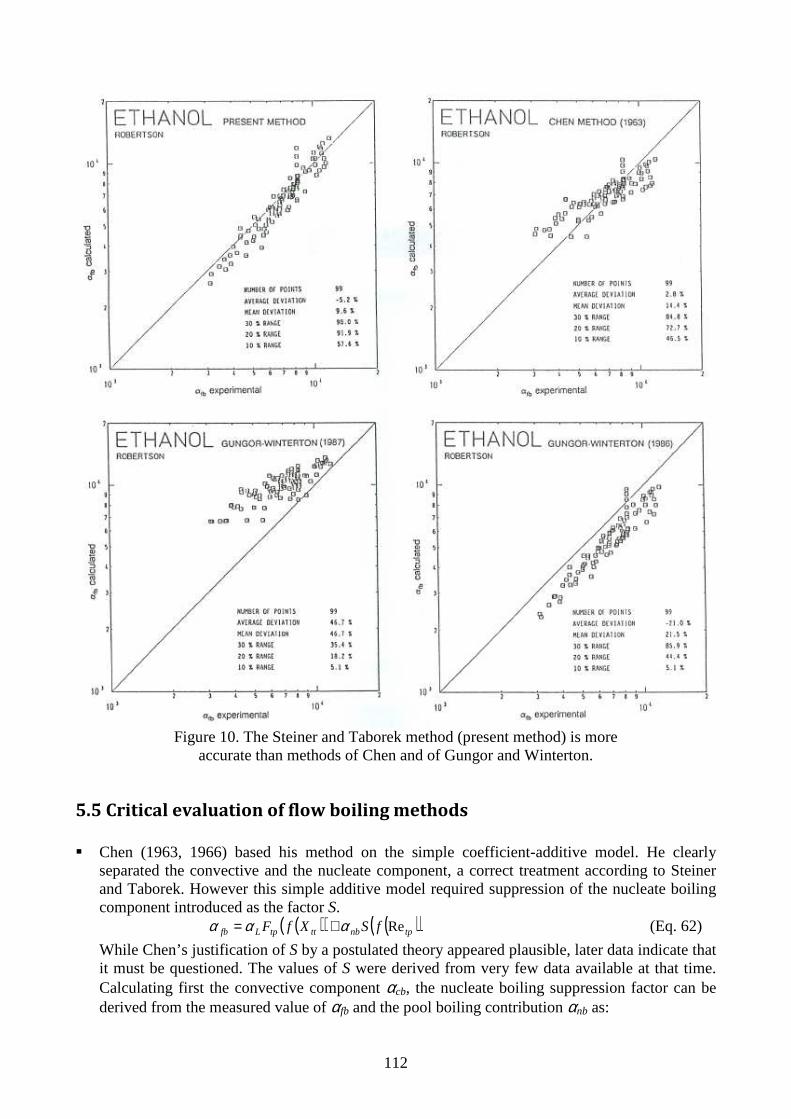
112

Figure 10. The Steiner and Taborek method (present method) is more

accurate than methods of Chen and of Gungor and Winterton.

5.5 Critical evaluation of flow boiling methods

� Chen (1963, 1966) based his method on the simple coefficient-additive model. He clearly

separated the convective and the nucleate component, a correct treatment according to Steiner and Taborek. However this simple additive model required suppression of the nucleate boiling component introduced as the factor S.

( )( ) ( )( )tpnbtttpLfb fSXfF Reααα += (Eq. 62)

While Chen’s justification of S by a postulated theory appeared plausible, later data indicate that it must be questioned. The values of S were derived from very few data available at that time. Calculating first the convective component αcb, the nucleate boiling suppression factor can be derived from the measured value of αfb and the pool boiling contribution αnb as:

113

nb

cbfbSα

αα −= (Eq. 63)

Recalculation of the data from Chen’s data base shows that effects of q& and m& were not taken into consideration. No evidence of a suppression factor can be seen by inspection of experimental data. Thus the nucleate boiling suppression hypothesis must be questioned or revised. In addition the Forster-Zuber equation used by Chen for αnb is now obsolete. Nevertheless the pool boiling process undergoes some change by the flow effects as attested to by consistent need for corrections to αnb.

� The Shah method (1976, 1982) is based on a simple graphical model, essentially a plot of the

ratio αfb/αL (local values) over a convection number Co, with the boiling number in parameter. The Co number is merely a modified Martinelli Xtt factor, representing the convective enhancement, while the nucleate pool boiling is represented solely by the Bo number. At large Co numbers (low x) the nucleate Bo-based solutions are accepted, while at low Co (high x), the convective model is valid. In essence this emulates the asymptotic model with n → ∞:

)(BofLfb αα = or )(CofLα (Eq. 64)

Both the convective and nucleate terms are ( )Lf α , contrary to analysis, causing incorrect effect of x in the nucleate-dominated region. The use of the Bo number to represent the complex nucleate boiling processes is only a useful simplification, however it cannot replace the sophistication of newer pool boiling methods.

� Gungor and Winterton’s method (1986) is a modification of the Chen method defined as:

( )( ) ( ))Re,(, LnbttLfb EfSXBofE ααα += (Eq. 65)

The αnb term is calculated by the Cooper correlation. The enhancement factor E now includes the Bo number and the suppression factor S is a function of the E factor itself. This complex combination of parameters was arrived at not as a mechanistic model, but by repeated regression analysis. This violation of many principles of boiling processes was later noted by Winterton himself. The method was later superseded by a completely different formulation by the same authors in 1987:

++=

G

LLfb xfBo

ρραα ,30001 86.0 (Eq. 66)

The ease of calculation was emphasized by the authors (apparently by replacing αnb by the Bo number). By multiplying both the Bo and the convective term with αL, the effects of nucleate boiling and two-phase flow convection are again intermixed.

� In Liu and Winterton’s method (1988), the authors correctly point out the deficiencies of the

previous methods and returned to the essence of the Chen method by abandoning the αL multiplier and using the asymptotic model with n = 2:

( ) ( )( ) 2/122nbLfb SE ααα += (Eq. 67)

35.0

1Pr1

−+=

G

LLxE

ρρ

(Eq. 68)

( ) 116.01.0 Re055.01−

+= LES (Eq. 69)

114

The Cooper pool boiling method is used for αnb. The E and S factors are still not a product of a model but only a result of regression analysis, and S is again ( )Ef . The use of the asymptotic addition may help to predict better extreme cases. As to the use of the suppression factor S the same comments as above apply.

� In 1987 Kandlikar proposed a method that is an expansion of the Shah model:

( )fCC

Lfb FBoCCoC ⋅⋅+⋅= 4231αα (Eq. 70)

This equation must be evaluated with a set of the constants C1 to C4 for each, the convective and the nucleate dominated regions, and the larger value of αfb is used. The set of constants C1 to C4 was established using Kandlikar’s own data bank on water. However, when tested on refrigerants data, the Bo term was inadequately represented and a fluid specific correction factor Ff was added. Critical evaluation of the method’s structure yields the following: In the purely convective dominated region Bo → 0, the equation contracts but as x → 0 the convective term does not approach 0Lfb αα = as required by theory.

In the pool boiling dominated region the fbα value decreases with x. Such behaviour while

common for horizontal flow with partial dryout is contrary to observations for vertical flow. The effect of pressure on nucleate boiling is represented only by the heat of vaporization term from the Bo number (and if used in connection with αL, the physical properties group). This effect of properties is too weak and this is common to all Bo-number based methods and a serious objection against their use for extreme conditions being too optimistic at low pressures. The use of Ff factor improves the method’s accuracy but obliterates its claim for generality. Also the values of Ff follow no logical pattern (as f (M, or similar)). Finally one must question the reasons for making sophisticated additions to the Shah method, which was intended for simplicity. The essential limitations of the Bo number will remain, regardless of how many corrections are used.

5.6 New flow boiling methods based on flow pattern maps

Most of the flow boiling correlations for horizontal flows are vertical tube methods with some correction to try to account for flow stratification at low flow rates. In vertical upflow dryout in annular flow tends to occur at vapor qualities in the range from 50-75% and hence few test data are taken above this threshold; consequently these vertical tube methods are not particularly suitable for predicting local coefficients in horizontal tubes where complete evaporation of the fluid has to be modeled. The major deficiencies identified on in-tube flow boiling correlations are that the predicted variations and peak in heat transfer coefficient versus vapor quality at a fixed mass velocity and heat flux often provide a poor match to experimental data; the rapid falloff in the heat transfer coefficient at high vapor quality is not predicted well and most correlations do not go to the natural limits of single-phase heat transfer at a vapor quality of 100%. Kattan et al. (1998) retained in the new model the following positive aspects in the existing methods: � The asymptotic approach used successfully by Steiner and Taborek (1992) for vertical upflow

boiling. No nucleate boiling suppression factor is used since the asymptotic model already, by itself, reduces the nucleate boiling contribution as the convective boiling contribution becomes dominant, i.e., using a boiling suppression factor would be redundant.

� The Cooper (1984) pool boiling correlation used in the correlations of Gungor and Winterton. This correlation was shown to accurately predict the nucleate boiling coefficient.

115

The objective was to develop a physically based model, albeit empirical, that incorporates three important features:

1) turbulent film flow heat transfer based on the liquid film velocity; 2) flow pattern type; 3) partial wetting of the tube circumference by the evaporating liquid.

Figure 11 shows the local heat transfer coefficient of R134a plotted versus vapor quality at fixed mass velocity, heat flux and saturation temperature with the flow pattern boundaries depicted as thick vertical lines. In the annular A flow regime the heat transfer coefficient rises rapidly as its evaporating liquid film thins. In the intermittent I flow regime the trend in heat transfer coefficient versus vapor quality is an extension to that for annular flow. At the transition to stratified-wavy flow at the onset of partial dryout of the annular film, the heat transfer falls off very rapidly towards the data point for the vapor phase heat transfer coefficient at x = 1. Therefore it is very clear that the peak in heat transfer coefficient is determined by the point of onset of partial dryout at the top of the tube. The vapor quality at which the peak occurs is thus a function of fluid properties, local heat flux and mass velocity.

Figure 11. R134a heat transfer coefficient at G = 300 kg/(s·m2) and Tsat = 4.4°C (D=10.92 mm).

I: intermittent flow regime; A: annular flow regime; SW: stratified-wavy flow regime. As a first step in the heat transfer model of Kattan-Thome-Favrat, flow regime transition curves are calculated. After determination of the flow pattern map, the actual local flow regime is determined for the specified combination of x and G. In the heat transfer model Kattan et al. (1998) took into account the fact that in stratified, stratified-wavy and annular flow with partial dryout, heat is transferred partially to the vapor phase on the dry upper perimeter of the tube. Therefore they proposed to calculate the heat transfer coefficient for the wet and dry perimeter separately as:

( )π

θπθ2

2 wetdryvdrytp

hhh

−+= (Eq. 71)

where θdry is the dry angle, hv is the heat transfer coefficient for the dry perimeter:

Dh v

vvv

λ4.08.0 PrRe023.0= (Eq. 72)

and hwet is the heat transfer coefficient for the wet perimeter calculated from the asymptotic model with n =3 :

116

( ) 3/133nbcbwet hhh += (Eq. 73)

The convective boiling heat transfer coefficient hcb is calculated from the liquid film thickness δ as follows:

δλ

δL

Lcbh 4.069.0 PrRe0133.0= (Eq. 74)

( )( )

( )( )

( )drydrydry

L D

R

A

R

A

θπεπ

θπε

θπδ

−−=

−−=

−=

22

1

2

1

2 (Eq. 75)

In the above equation the void fraction ε is calculated by using the Rouhani-Axelsson void fraction correlation and the dry angle θdry is calculated iteratively assuming that θdry=θstrat from:

( ) ( )( )stratstratL RA θπθπ −−−= 2sin25.0 2 (Eq. 76) The nucleate boiling heat transfer coefficient is determined from the correlation of Cooper (Eq. 12). The parameter that takes into account the existence of different flow patterns is the dry angle shown in Figure 12:

Figure 12. Annular flow with partial dryout configuration.

The dry angle θdry defines the flow structure and the ratio of the tube perimeter in contact with liquid and vapor. In stratified flow θdry equals the stratified angle θstrat and was calculated iteratively by Kattan. For annular and intermittent flows where the tube perimeter is continuously wet θdry = 0. A more complicated approach is used to predict θdry for stratified wavy flows. The correlation was compared with five different existing correlations, being particularly more accurate for the flow regimes with partially wetted tube walls compared to the earlier methods. The model proposed by the authors is based on turbulent liquid film flow rather than on tubular flow as in past correlations. In all previous correlations hcb was based on the inside tube diameter and multiplied by an empirical enhancement factor usually related to the Martinelli number, an approach that does not explicitly model the liquid velocity in two-phase flow and is thus inconsistent with the use of the Dittus-Boelter correlation. Instead in the present model the void fraction is used to determine the thin liquid film thickness and the vapor and liquid velocities without the need of any additional physically meaningless empirical enhancement factor. The input values are the mass velocity, the saturation temperature, the heat flux, the vapor quality and the fluid properties. The transition boundary curves on the flow pattern map are determined first, and then the flow pattern for the input conditions is determined. After that, the dry angle θdry is calculated using the void fraction correlation. Once the dry angle is known the heat transfer coefficients for the wet wall and the dry wall are determined using the void fraction and the asymptotic model. Finally the two-phase flow heat transfer coefficient htp is calculated proportional to the liquid and vapor heat transfer coefficients depending on the dry angle. The objective is to improve the heat transfer coefficient prediction at high vapor quality (from 85% to 100%) where few data tend to be found in flow boiling databanks. This zone is very important in thermal design because the falloff in the heat transfer coefficient in the partial dryout region has a significant effect on the tube length of evaporators.

117

Kattan et al. (1998) used three criteria to analyze and compare the accuracy of different correlations for horizontal flow boiling: - the standard deviation:

2

1

21 εεσ −

= ∑

=

n

iin

(Eq. 77)

- the mean deviation:

∑=

=n

iin 1

1 εε (Eq. 78)

- the average deviation:

∑=

=n

iin 1

1 εε (Eq. 79)

where the relative error for each data point is calculated as: ( )

exp

exp

h

hhcali

−=ε (Eq. 80)

The mean deviation for all the existing correlations tested for different fluids for all flow regimes varies from 20.9 % to 26.7 %. The mean deviation is 13.3% for the present correlation. The standard deviation for all the existing correlations varies from 25.7% to 42.6%, while for the present correlation the standard deviation is 16.8%. The average deviation is quite small for all correlations, i.e., the test data tend to be centered by the correlational predictions and not skewed. The larger standard standard deviations of the existing correlations therefore represent poor modeling of:

i) the slope of the heat transfer coefficient as a function of the vapor quality; ii) the peak in the heat transfer coefficient; iii) the fall-off in the heat transfer coefficient with partial tube wetting after the peak; iv) the adverse effects of flow stratification.

Intermittent and annular flow regime are predicted reasonably well by all methods. The present model based on turbulent film flow of the annular liquid ring (rather than tubular flow) requires only the void fraction to be calculated to model the effect of liquid velocity. In contrast the existing correlations do not model this process mechanistically and utilize empirical factors but do not really predict the effect of two-phase flow on liquid velocity. In the stratified-wavy flow regime the present model predicts the flow boiling data much better compared to the existing correlations. The new flow boiling model predicts the heat transfer coefficients well at high vapor quality, while all the other correlations tested have very large errors or are incapable of modeling this data since they do not recognize the onset of dryout. In this region the heat transfer coefficient decreases rapidly with increasing vapor quality and a small change in vapor quality leads to a large variation in the heat transfer coefficient. Figure 13 shows a comparison of the new correlation to the Gungor and Winterton (1986), Jung et al., and Steiner correlations evaluated against the R134a experimental data. Only the new correlation predicts the sharp peak and dropoff of the heat transfer coefficient at high vapor quality and high mass velocity.

118

Figure 13. Comparison of the new correlation with R134a experimental

data at G = 198 kg/s·m2 and with three existing correlations. Figure 14 shows the influence of the heat flux and mass velocities on the R134a heat transfer coefficient. As expected the influence of the heat flux is more important at low vapor quality when the pool boiling contribution is dominant. The shape of the curve of heat transfer coefficient versus vapor quality is shown to change appropriately as a function of mass velocity, heat flux and flow pattern similar to experimental data. In Figure 14 the predicted effect of the heat flux and mass velocity on the location and magnitude of the peak in heat transfer coefficient versus vapor quality is also clearly shown. After the peak the fall off in the heat transfer coefficient is sharper with a higher slope at higher mass velocity.

Figure 14. Influence of the heat flux on the predicted heat transfer coefficient.

The flow pattern oriented model of Kattan-Thome-Favrat (1998) was a major improvement over previous methods for flow boiling heat transfer predictions however the heat transfer coefficients predicted for stratified wavy flow were not as accurate as for annular flow. The new flow pattern map developed by Wojtan et al. (2005) was utilized to improve the stratified-wavy heat transfer model of Kattan et al (1998). Based on the analysis of experimental results at different heat fluxes a nucleate boiling suppression factor S has been proposed. It has been observed that the method of Kattan et al. (1998)

119

overpredicts the heat transfer coefficient in the annular flow regime with increasing heat flux. As the deviation increases with increasing heat flux it can be concluded that the nucleate boiling contribution is too high. Based on analysis of the experimental data, it has been estimated that the nucleate boiling heat transfer contribution calculated from the pool boiling correlation of Cooper should be reduced by 20% to obtain good agreement with experimental values. This is not surprising in view of the reduced thermal boundary layer in flow boiling: bubble growth is inhibited compared to nucleate pool boiling. Moreover, the flow boiling heat transfer model of Kattan et al. covers neither dryout nor mist flow heat transfer, so new prediction methods for these flow regimes are also developed. Figure 15 shows the rapid decrease of the heat transfer coefficient with increasing vapor quality that indicates the inception of dryout. The end of this decrease of heat transfer coefficient marks the end of dryout and the beginning of mist flow. At the inception point the dryout occurs at the top of the horizontal tube, where locally the heat transfer begins to fall as the annular film dries out. At the completion quality dryout is complete around the tube perimeter, and the deterioration of the heat transfer ends. The qualities at the respective points are denoted xdi and xde. The distinction of these two points is caused by the shift of the dryout position from the top to the bottom around and along the tube perimeter with increasing quality. As depicted in Figure 16, dryout occurs at the top of the tube first (cross section A–A), where the liquid film is thinner, and then progresses downward around the perimeter (cross section B–B) until reaching the bottom (cross section C–C). The process of dryout thus takes place over a range of vapor qualities and ends at the bottom of the tube when the fully developed mist flow regime is reached. This regime between xdi and xde will be called dryout. For the dryout region the heat transfer coefficient can be calculated from the following linear interpolating equation:

( ) ( ))()( demistditpdide

diditpdryout xhxh

xx

xxxhh −

−−

−= (Eq. 81)

where )( ditp xh is the two phase flow heat transfer coefficient calculated at the dryout inception

quality xdi and )( demist xh is the mist flow heat transfer coefficient calculated at the dryout completion quality xde.

Figure 15. Experimental heat transfer coefficients for R-22 at Tsat = 5°C at two mass velocities: (a) 300 kg/m2s (c) 500 kg/m2s.

120

Figure 16. Dryout zone during evaporation in a horizontal tube.

121

5.7 Heat transfer under supercritical pressures

The special characteristic of fluids near the thermodynamic critical point is that their thermodynamic properties vary rapidly with temperature and pressure. A similar large variation in the fluid properties exists at a certain fluid temperature in the supercritical pressure region. The fluid temperature at which the specific heat reaches its peak value for a given pressure is known as a pseudo-critical point. Figure 17 shows the thermophysical property variations according to the temperatures for supercritical pressure water at 25.0 MPa. All thermophysical properties undergo significant changes near the pseudo-critical point as shown in Figure 17.

Figure 17. Thermophysical property variations with temperatures for

supercritical pressure water at 25.0 MPa.

The specific heat rises sharply to a peak value and then falls steeply. Density and dynamic viscosity undergo a significant drop within a very narrow temperature range in the vicinity of the pseudo-critical temperature. Other fluids such as CO2 and HFC-134a follow similar trends. In general, as pressure is increased, the pseudo-critical temperature increase and the maximum value of the specific heat decreases and the variations of the other properties with temperature become less severe. This strong dependence of thermodynamic properties on temperature and pressure leads to different heat transfer regime according to a small change of fluid temperature. At supercritical pressure, despite non-existence of tangible phase change, the working fluid undergoes a transition form liquid-like substance to gas-like one without any of discontinuities associated with two phases being present when the fluid temperature rises up and passes the pseudo-critical temperature. Depending on the applied heat flux and the mass flux of flow, the heat transfer regime can be categorized into three types of enhanced, normal and deteriorated heat transfer at supercritical pressure. In general, deviations from normal heat transfer have been found to occur when the wall temperature is greater than the pseudo-critical temperature and the bulk fluid temperature is less than the pseudo-critical temperature, i.e., Tw > Tpc > Tb. This criterion indicates the condition of large property variations occurring within the near wall region. Radial variations of the thermophysical properties near the wall with the temperatures result in the complexities of the heat transfer behavior at the supercritical pressure fluid. Therefore, a convective heat transfer correlation for a constant property fluid such as the well-known Dittus–Boelter correlation is no longer applicable to the supercritical pressure fluid.

122

Various correlations have been developed for the normal heat transfer, based on the experimental data of water, carbon dioxide, and the Freon. Most of these correlations are expressed in the form of a constant properties heat transfer correlation multiplied by the ratios of properties between the bulk fluid temperature and the wall temperature. Kang and Chang (2009) performed experiments in a vertical tube using the Freon R134a as working fluid medium to provide a reliable heat transfer database and investigate the heat transfer characteristics during both the steady state and the pressure transient conditions. The steady-state heat transfer experiments were performed with various heat and mass fluxes at a fixed pressure. The mass flux was in the range between 600 and 2000 kg/m2·s and the maximum heat flux was 160 kW/m2. The selected pressures were 4.1, 4.3 and 4.5 MPa which correspond to 1.01, 1.06 and 1.11 times the critical pressure (critical pressure of the Freon, HFC-134a is 4.059 MPa), respectively. To develop the heat transfer correlation, heat transfer rates from the inner wall of the test section to the fluid should be evaluated from the measured parameters in the steady-state heat transfer experiment. The local heat transfer coefficient can be defined as follows:

( )zbzw TT

qh

,, −=

& (Eq. 82)

where Tw is the wall temperature, Tb is the bulk temperature and z is a generic location along the test section. In the steady-state heat transfer experiments, major experimental parameters are heat flux, mass flux, inlet fluid temperature and inlet system pressure. Figure 18 shows the variation of the wall temperatures and the heat transfer coefficients against the bulk fluid enthalpy with a parameter of heat flux at the mass flux of 600 kg/m2·s. The wall temperature is the temperature at the inner wall of the tube.

Figure 18. Variation of wall temperature and heat transfer coefficient for R134a:

P = 4300 kPa, G = 600 kg/m2·s.

123

The black solid line is the calculated bulk fluid temperature and the enthalpy at the pseudo-critical temperature is denoted as a red dotted line in each figure. According to Figure 18, thermal behavior of the tube is determined mainly by the applied heat flux and the mass flux of fluid, which shows a general agreement with findings of previous studies and understandings. In case of a low heat flux, wall temperature profile is parallel to bulk fluid temperature line, and the heat transfer coefficient has the maximum value at slightly lower than a pseudo-critical enthalpy. The wall temperature, however, shows abrupt increase with increase of a heat flux, which clearly indicates the occurrence of heat transfer deterioration. As a heat flux is increased, starting time for heat transfer deterioration has a tendency to be earlier. Experimental data on forced convection of the steady-state heat transfer are correlated in terms of dimensionless parameters for the purpose of design calculations. Heat transfer correlations can be expressed in the form of a constant properties heat transfer correlation multiplied by the ratios of properties between the bulk fluid temperature and the wall temperature. Among the various properties, specific heat is the most influencing parameter in heat transfer rate under the supercritical pressure. In order to take account of abrupt variation of specific heat with temperatures, an integrated specific heat ( Pc ) and Prandtl number (rP ) are employed assuming constant pressure as follows:

( )( )bw

bw

T

T

Pbw

P TT

HHdTc

TTc

w

b−−=

−= ∫

1 (Eq. 83)

b

bPc

λµ

=rP (Eq. 84)

The heat transfer correlation developed by the authors is:

( ) 0293.0552.0762.0 /rPRe0224.0 bwbbNu ρρ= (Eq. 85) where the subscripts b and w refer respectively to the bulk and wall conditions. The proposed heat transfer correlation was tested against the experimental data of open literature and the comparison showed that the heat transfer coefficient is plausibly applicable to the different experimental conditions and different working fluids at supercritical pressures.

124

Conclusions

In flow boiling the nucleate and convective components are superimposed by a very complex mechanism, which so far is not well understood. The first correlation for flow boiling coefficient was proposed as a simple addition of the nucleate and convective coefficients and was used in principle by Chen in the early 1960s. In the mid 1970s Shah proposed a method where the nucleate boiling mechanism is dominant at low qualities whereas at high qualities only the convective mechanism is valid. The asymptotic model or power type addition model assures a smooth transition as the boiling mechanism changes from nucleate to convective dominated. The method proposed by Steiner and Taborek in the early 1990s used the asymptotic model and placed main emphasis on a sound mechanistic model whereas other methods were only obtained by repeated regression analysis violating many principles of boiling processes. The variation with quality of the heat transfer coefficient should be taken into account for a proper design of the evaporators in Organic Rankine Cycles. With increasing vapor fraction, the flow regime progresses from bubbly to annular flow with a thin layer on the tube wall. With further increase of vapor fraction and hence flow velocity, the liquid annular film cannot be sustained and the dryout point is reached. At this point the remaining liquid is sheared off the wall and keeps flowing as mist in the tube core. The heat transfer coefficient decreases drastically as the dry wall condition is reached and beyond the dryout point the complete evaporation of the droplets in the mist occurs at low heat transfer rates and may persist over substantial tube length. The newest heat transfer models proposed by Kattan-Thome-Favrat (1998 and 2005) take into account the fact that in annular flow with partial dryout heat is transferred partially to the vapor phase on the dry upper perimeter of the tube. Therefore they proposed to calculate the heat transfer coefficient for the wet and dry perimeter separately so the flow boiling data at high vapor qualities and in the dryout region are predicted much better compared to the existing correlations. At supercritical pressures the heat transfer mechanism is different and the correlations are more similar to those applied for single-phase forced convection but take into account the marked variation of the fluid properties with temperature near the pseudo-critical point.

125

References Bonacina C., Cavallini A. and Mattarolo L., Trasmissione del calore, Cleup 1992. Dipartimento di Fisica Tecnica, Vaporizzazione, Padova. Fraas A.P., Heat exchanger design, Wiley 1989. Gungor K.E. and Winterton R.H.S., A general correlation for flow boiling in tubes and annuli, Int. J. Heat Mass Transfer, Vol. 29, 1986. Kakaç S. and Liu H., Heat exchangers. Selection, Rating and Thermal Design, CRC Press 2002. Kandlikar S.G., Development of a Flow Boiling Map for Subcooled and Saturated Flow Boiling of Different Fluids Inside Circular Tubes, Journal of Heat Transfer, Vol. 113, 1991. Kang K.-H. and Chang S.-H., Experimental study on the heat transfer characteristics during the pressure transients under supercritical pressures, Int. J. of Heat and Mass Transfer 52(21-22), pp. 4946-4955, 2009. Kattan N., Thome J.R. and Favrat D., Flow Boiling in Horizontal Tubes: Part 1 – Development of a diabatic two-phase flow pattern map, Journal of Heat Transfer, Vol. 120, 1998. Kattan N., Thome J.R. and Favrat D., Flow Boiling in Horizontal Tubes: Part 2 – New Heat Transfer Data for Five Refrigerants, Journal of Heat Transfer, Vol. 120, 1998. Kattan N., Thome J.R. and Favrat D., Flow Boiling in Horizontal Tubes: Part 3 – Development of a new heat transfer model based on flow pattern, Journal of Heat Transfer, Vol. 120, 1998. Kuppan T., Heat Exchanger Design Handbook, Dekker 2000. Serth R.W., Process heat transfer: principles and applications, Elsevier Academic Press 2007. Shah R.K. and Sekulic D.P., Fundamentals of Heat Exchanger Design, Wiley 2003. Steiner D. and Taborek J., Flow Boiling Heat Transfer in Vertical Tubes Correlated by an Asymptotic Model, Heat transfer engineering, Vol. 13, 1992. Stephan K. and Abdelsalam M., Heat-transfer correlations for natural convection boiling, Int. J. Heat Mass Transfer, Vol. 23, pp. 73-87, 1980. Wojtan L., Ursenbacher T. and Thome J. R., Investigation of flow boiling in horizontal tubes: Part I—A new diabatic two-phase flow pattern map, International Journal of Heat and Mass Transfer 48 (2005). Wojtan L., Ursenbacher T. and Thome J. R., Investigation of flow boiling in horizontal tubes: Part II—Development of a new heat transfer model for stratified-wavy, dryout and mist flow regimes, International Journal of Heat and Mass Transfer 48 (2005).

126

6. Economic Analysis of Binary Power Plants In this section an economic analysis of the binary cycle power plants is performed. The techniques commonly used to calculate the economics of chemical processes are described first. Then these are applied to the economic evaluation of Organic Rankine Cycles. The optimal thermodynamic solutions found in Chapter 4 for isobutane and R134a are economically evaluated using the “equipment module costing technique”. This costing technique relates all costs back to the purchased cost of equipment evaluated for some base conditions. The results show that the levelized cost of electricity (LCOE) decreases, as expected, with the increase of the geothermal fluid inlet temperature. The operation with isobutane is convenient in the upper part of the temperature range considered for the geothermal fluid whereas in the lower part the fluid R134a keeps both a thermodynamic and an economic advantage.

6.1 Estimation of capital investment in industrial plants

An industrial plant design must present a process that yields a profit. The net profit equals total income minus all expenses. The capital needed to supply the necessary plant facilities is called the “fixed-capital investment”, while that required to start up the plant and finance the first few months of operation of the plant is called the “working capital”. Typical values for the working capital are between 15 and 20% of the fixed capital investment. The sum of the fixed-capital investment and the working capital is known as the “total capital investment”. “Manufacturing fixed-capital investment” represents the capital necessary for the installed process equipment with all auxiliaries that are needed for complete process operation. “Nonmanufacturing fixed-capital investment” includes the fixed capital required for construction overhead and for all plant components not directly related to the process operation. These include the land, processing buildings, administrative and other offices. A check list of items covering a new facility is useful in making a complete estimation of the fixed-capital investment. Usually the primary reason that capital costs are underestimated stems from the failure to include all of the equipment needed in the process. Capital must be allocated for direct plant expenses as well as for indirect expenses. The following Table 1 shows the main cost items and the typical percentages of fixed-capital investment values for chemical plants.

Component Range % Direct costs

Purchased equipment 15-40 Purchased-equipment installation 6-14

Instrumentation and controls 2-8 Piping 3-20

Electrical equipment and materials 2-10 Buildings (including services) 3-18

Yard improvements 2-5 Service facilities 8-20

Land 1-2 Indirect costs

Engineering and supervision 4-21 Construction expense 4-16

127

Contractor’s fee 2-6 Contingency 5-15

Table 1. Typical percentages of fixed-capital investment values for direct and indirect cost segments.

� Types of capital cost estimates An estimate of the capital investment for a process may vary from a predesign estimate based on little information except the size of the proposed project to a detailed or firm estimate prepared from complete drawing and specifications. There are five main categories of capital-investment estimates: a) “Order-of-magnitude estimate” (or “ratio estimate”): based on similar previous cost data; it relies on cost information from previously built plants. This information is adjusted using appropriate scaling factors for capacity. b) “Study estimate” (“factored estimate”): based on knowledge of major items of equipment; each piece of equipment is roughly sized and the approximate cost determined. The total cost of equipment is then factored to give the estimated capital cost. c) “Preliminary estimate” (“budget authorization estimate”; “scope estimate”): based on sufficient data to permit the estimate to be budgeted (accuracy of estimate within ±20%). This estimate requires more accurate sizing of equipment than used in the study estimate. In addition, approximate layout of equipment is made along with estimates of piping, instrumentation and electrical requirements. Utilities are also estimated. d) “Definitive estimate” (“project control estimate”) based on almost complete data but before completion of drawings and specifications (accuracy of estimate within ±10 %). It requires preliminary specifications for all the equipment, utilities, instrumentation, electrical etc. e) “Detailed estimate” (“contractor’s estimate”) based on complete engineering drawings, specifications and site surveys (accuracy of estimate within ±5 %). Vendor quotes will have been obtained. The plant is ready to go to the construction stage. The focus of many authors (e.g. Peters and Timmerhaus, 1991 and Turton et al., 2009) is on predesign cost estimates (defined here as order of magnitude, study and preliminary estimates) since these are cheaper than detailed estimates and extremely important for determining if a proposed project should be given further consideration and to compare alternative designs. The predesign estimates may be used to provide a basis for requesting and obtaining a capital appropriation from company management. Later estimates may indicate that the project will cost more or less than the amount appropriated. Management is then asked to approve a variance which may be positive or negative. � Cost indexes The “cost indexes” are used for updating available cost data applicable at a past date to costs that are representative of conditions at a later time. If the cost at some time in the past is known (C1), the equivalent cost at the present time (C2) can be determined by multiplying the original cost by the ratio of the “present index value” (I2) to the “index value” applicable when the original cost was obtained (I1):

=

1

212 I

ICC (Eq. 1)

Many different types of cost indexes are published regularly. Some of these can be used for estimating equipment costs; others apply specifically to labor, construction, materials, or other specialized fields. For use with process-equipment estimates and chemical-plant investment estimates, the “Marshall and Swift equipment cost indexes” and the “Chemical Engineering” plant cost indexes are recommended:

128

a) The “Marshall and Swift” equipment cost indexes are divided into two categories: - “all-industry” equipment index: arithmetic average of individual indexes for many (tens)

different types of industrial, commercial and housing equipment; - “process-industry” equipment index: weighted average of eight of these. They are based on an “index value” of 100 for the year 1926.

b) The “Chemical Engineering Plant Cost Index (CEPCI)” is a weighted average of machinery, erection, buildings, engineering. It is based on a value of 100 for the years 1957-1959. The CEPCI is used by Turton et al. (2009) to account for inflation.

� Estimating equipment costs by scaling It is often necessary to estimate the cost of a piece of equipment when no cost data are available for the particular size of operational capacity involved. Good results can be obtained by using the “logarithmic relationship” (known as the “six-tenths-factor rule”), if the new piece of equipment is similar to one of another capacity for which cost data are available. According to this rule, if the cost of a given unit at one capacity is known, the cost of a similar unit with X times the capacity of the first is approximately ( ) 6.0X times the cost of the initial unit.

6.0

..

..

=

bequipcapac

aequipcapacCC ba (Eq. 2)

The preceding equation indicates that a “log-log plot” of capacity versus equipment cost for a given type of equipment should be a straight line with a slope equal to 0.6. The application of the 0.6 rule of thumb for most purchased equipment is an oversimplification since the actual values of the “cost capacity factor” vary from less than 0.2 to greater than 1.0. Table 2 shows the exponents for some equipment of binary cycle power plants. The cost-capacity concept should not be used beyond a tenfold range of capacity, and care must be taken to make certain the two pieces of equipment are similar with regard to type of construction, materials of constructions, temperature and pressure operating range.

Equipment Size range Exponent Heat exchanger, shell and tube, floating head

100 - 400 ft2 0.60

Pump, centrifugal, horizontal, cast steel (includes motor)

104 – 105 gpm * psi 0.33

Fan, centrifugal 2*104 – 7*104 ft3/min 1.17 Table 2. Typical exponents for equipment cost vs. capacity (from Peters and Timmerhaus).

This rule illustrates a concept referred to as the “economy of scale”: the larger the equipment, the lower the cost of equipment per unit of capacity. It is necessary to have cost information on the equipment at some “base case” in order to be able to determine the cost of other similar equipment. This base-case cost information may be obtained from a current bid provided by a manufacturer for the needed equipment or from company records of prices paid for similar equipment.

6.2 Cost factors in capital investment

6.2.1 Direct costs

� Purchased equipment The cost of purchased equipment is the basis of several predesign methods for estimating capital investment. The most accurate method for determining process equipment costs is to obtain firm bids from fabricators or suppliers or quick estimates made by fabricators. Second best in reliability

129

are cost values from the file of past purchase orders that must be corrected to the current cost index. Limited information has also been published in various journals. Peters and Timmerhaus (1991) and Turton et al. (2009) provided costs for a large number of different types and capacities of equipment. � Purchased-Equipment Installation The installation of equipment involves costs for labor, foundations, supports, platforms, construction expenses directly related to the erection of purchased equipment. Table 3 presents the range of installation cost as a percentage of the purchased-equipment cost for components of binary cycle power plants. Installation costs for equipment are estimated to vary from 25 to 55 % of the purchased equipment cost. The installation labor cost is also a function of equipment size.

Type of equipment Installation cost % Heat exchangers 30-60

Pumps 25-60 Table 3. Installation cost for equipment as a percentage of the purchased equipment cost.

� Instrumentation and controls This cost item includes instrument costs, installation-labor costs, expenses for auxiliary equipment and materials. Total instrumentation cost depends on the amount of control required and may amount to 6 to 30% of the purchased cost for all equipment. Computers are commonly used with controls. � Piping The cost for piping covers labor, valves, fittings, pipe, supports, and other items involved in the complete erection of all piping used in the process. Since process-plant piping can run as high as 80% of purchased-equipment cost or 20% of fixed-capital investment an accurate estimate is needed. Piping estimation methods involve either some degree of piping “take-off” from detailed drawings and flow sheets or using a “factor technique” when neither detailed drawings nor flow sheets are available. Labor for installation is estimated as approximately 40 to 50% of the total installed cost of piping. � Electrical Installations The cost for electrical installations consists primarily of installation labor and materials for power and lighting. In chemical plants electrical-installations cost amounts to 10-15% of the value of all purchased equipment. The electrical installation consists of four major components: power wiring; lighting; transformation and service; instrument and control wiring. � Buildings Including Services This cost consists of expenses for labor, materials and supplies involved in the erection of all buildings connected with the plant. Costs for plumbing, heating, lighting, ventilation and similar building services are included. � Yard Improvements Costs for fencing, grading, roads, sidewalks, railroad sidings, landscaping and similar items. This cost approximates 10 to 20 % of the purchased-equipment cost. This is equivalent to approx. 2 to 5 % of the fixed-capital investment. � Service facilities Utilities for supplying steam, water, power, compressed air, and fuel are part of the service facilities of an industrial plant. These include waste disposal, fire protection and miscellaneous service items

130

(shop, first aid and cafeteria equipment). The total cost for service facilities in chemical plants generally ranges from 30 to 80% of the purchased-equipment cost. � Land The cost for land depends on the location of the property. As a rough average land costs for industrial plants amount to 4 to 8 % of the purchased-equipment cost or 1 to 2 % of the total capital investment.

6.2.2 Indirect costs

� Engineering and Supervision The costs for construction design and engineering, drafting, procuring, expediting, travel, communications constitute the capital investment for engineering and supervision. This cost, since it cannot be directly charged to equipment, materials, or labor is considered an indirect cost in fixed-capital investment and is approximately 30% of the purchased equipment cost or 8% of the total direct costs of the process plant. � Construction Expense It includes temporary construction and operation, construction tools and rentals, home office personnel located at the construction site, construction payroll, travel and living, taxes and insurance. For ordinary chemical-process plants the construction expenses average roughly 10% of the total direct costs for the plant. � Contractor’s Fee It varies for different situations, but it can be estimated to be about 2 to 8 percent of the direct plant cost or 1.5 to 6 % of the fixed-capital investment. � Contingencies A contingency factor is usually included in an estimate of capital investment to compensate for unpredictable events, such as storms, floods, strikes, price changes. Contingency factors ranging from 5 to 15 % of the direct and indirect plant costs are commonly used. Startup Expense After plant construction there are changes that have to be made before the plant can operate at maximum design conditions. These changes involve expenditures for materials and equipment and result in loss of income while the plant is shut down or is operating at only partial capacity. These expenses may be as high as 12% of the fixed-capital investment.

6.3 Methods for estimating capital investment

If an estimate of the capital cost for a process plant is needed and access to a previous estimate for a similar plant with a different capacity is available, then the principles already introduced for the scaling of purchased costs of equipment can be used: the six-tenths rule (n= 0.6 is more accurate in this application than it is for estimating the cost of a single piece of equipment) and the cost indexes to update the capital costs (changes that result from inflation). But in most situations cost information will not be available for the same process configuration; therefore other estimating techniques must be used. Seven methods are here outlined and the degree of accuracy decreases with each succeeding method. 1) “Detailed-item” estimate

131

It requires careful determination of each fixed-capital investment item by using drawings and specifications. The equipment is priced from current cost data or from firm delivered quotations. Estimates of installation costs are determined from accurate labor rates, efficiencies and employee-hour calculations. Accurate estimates of engineering, drafting, field supervision employee-hours must be detailed in the same manner. 2) “Unit-cost” estimate This method needs accurate records of previous cost experience. It requires detailed estimates of purchased price obtained either from quotations or index-corrected cost records and published data. Equipment installation labor is evaluated as a fraction of the delivered-equipment cost. Costs for concrete, steel, pipe are obtained by “take-offs” from the drawings and applying unit costs to the material and labor needs. A unit cost is also applied to engineering employee-hours, number of drawings and specifications. A factor for construction expense, contractor’s fee and contingency is estimated from previously completed projects. A cost equation summarizing this method can be given as:

( ) ( )[ ]( )FndeeLyxxLn fdfHfMfMfEEC ∑ ∑ ∑∑ +++++= ' (Eq. 3)

Cn = new capital investment E = purchased-equipment cost EL = purchased-equipment labor cost fx = specific material unit cost, e.g., fp = unit cost of pipe Mx = specific material quantity fy = specific material labor unit cost per employee-hour M’L = labor employee-hours for specific material fe = unit cost for engineering He = engineering employee-hours fd = unit cost per drawing or specification dn = number of drawings or specifications fF = construction or field expense factor always > 1 3) “Percentage of delivered-equipment cost” This method requires determination of the delivered-equipment cost. The other items included in the “total direct plant cost” are then estimated as percentages of the equipment cost. The cost equation that summarizes this method is:

( )[ ]( )In fEfEfEfEC ∑ ∑ ++++= ...321 (Eq. 4)

E = purchased-equipment cost f1, f2… = multiplying factors for piping, electrical, instrumentation … fI = indirect cost factor > 1 The percentages should be determined on the basis of the type of process involved, design complexity, materials, location, past experience. This method is commonly used for preliminary and study estimates. It yields most accurate results when applied to projects similar in configuration to recently constructed plants. 4) “Lang factors” for approximation of capital investment This technique, proposed originally by Lang, and used to obtain order of magnitude cost estimates, recognizes that the cost of a process plant may be obtained by multiplying the basic equipment cost by some factor to approximate the capital investment. These factors vary depending upon the type of process plant being considered. The major items of equipment are those shown in the process flow diagram.

132

Type of plant Fixed-capital investment Total capital investment Solid-processing plant 3.9 4.6 Solid-fluid-processing plant 4.1 4.9 Fluid-processing plant 4.8 5.7

Table 4. Lang multiplication factors. Plants processing only fluids have the largest Lang factor. The greater the Lang Factor the lower the purchased costs contribute to the plant costs. For all cases, the purchased cost of the equipment is less than a third of the capital cost of the plant. This estimating technique is insensitive to changes in process configuration. It cannot account for the common problems of special materials of construction and high-operating pressures. 5) “Power factor” applied to plant-capacity ratio This method relates the fixed-capital investment of a new process plant to the fixed-capital investment of similar previously constructed plants by an exponential power ratio.

( )xn RCC = (Eq. 5)

Cn : fixed capital investment of the new facility; C : fixed capital investment of the constructed facility; R : ratio: capacity of the new facility divided by the capacity of the old; x : capacity power factor. This power has been found to average between 0.6 and 0.7 for many process facilities and Peters Timmerhaus show the capacity power factors for various kinds of processing plants. The value of x approaches unity when the capacity of a process facility is increased by adding identical process units instead of increasing the size of the process equipment. More accurate estimates by this method are obtained by subdividing the process plant into various process units and applying the best available data from similar previously installed “process units” separately to each subdivision. Results obtained using this procedure have shown high correlation with “fixed-capital investment estimates” that have been obtained with more detailed techniques. 6) “Investment cost per unit of capacity” Many data have been published giving the fixed-capital investment required for various processes per unit of annual production capacity. Although these values depend on the capacity of the individual plants it is possible to take average conditions. The fixed-capital investment is then obtained by multiplying the “investment cost per unit of capacity” by the annual production capacity of the proposed plant. 7) “Turnover ratios” Turnover ratio is defined as the ratio of gross annual sales to the fixed-capital investment, where the product of the annual production rate and the average selling price of the commodities is the numerator. The reciprocal of the turnover ratio is defined as the capital ratio or the “investment ratio”. A considerable improvement in the application of these methods can be obtained by considering the fixed-capital investment requirement by parts. Each part is treated as a separate unit to obtain the total investment cost directly related to it. Various forms of compartmentalization have been proposed: a) “Modular estimate”: the basis is to consider individual modules in the total system with each consisting of a group of similar items. For example, all heat exchangers might be included in one module. The module would include the basic delivered cost of the piece of equipment with Lang factors for supplemental items (piping, insulation, paint, labor, auxiliaries, indirect costs and contingencies).

133

b) “Unit operations estimate”: the modules can be based on combinations of equipment that involve similar types of operations requiring related types of auxiliaries. An example would be a “distillation operation” requiring the distillation column with the necessary auxiliaries of reboiler, condenser, pumps, holdup tanks and supports. c) “Functional-unit estimate”: it is based on the grouping of equipment by function.

6.4 Estimation of operating costs

Methods for estimating the “total capital investment” required for a given plant are presented in the previous section. Another important part is the estimation of costs for operating the plant and selling the products. These costs can be grouped under the heading of “total product cost”. The latter is divided into the categories of “manufacturing costs” and “general expenses”. Manufacturing costs are also known as “operating or production costs”.

Total product cost Manufacturing costs General expenses Direct production costs Administrative expenses

Fixed charges Distribution and marketing expenses Plant overhead costs Research and development

Table 5. Total product cost. Total product costs are expressed in $ per unit time and are usually calculated on one of 3 bases: daily basis, unit of product basis or annual basis. The best source of information for use in “total-product-cost estimates” is data from similar or identical projects. Adjustments for increased costs as a result of inflation must be made. � Manufacturing costs Manufacturing costs are directly connected with the manufacturing operation or the physical equipment of a process plant itself and can be divided in three groups: a) Direct production costs These costs represent operating expenses that vary with production rate. They involve: - Expenditures for raw materials (including freight transportation, unloading...).

The flowrates of chemical feed stocks required by the process are obtained from the PFD. For preliminary cost analyses, market prices are often used for estimating raw-material costs. In chemical plants, raw-material costs are usually in the range of 10 to 50 % of the total product cost.

- Costs of waste treatment to protect environment. - Cost for utilities, such as steam, electricity, process and cooling water, compressed air, natural

gas, and fuel oil varies widely. Utility costs for ordinary chemical processes amount to 10 to 20 % of the total product cost. The flowrates for utilities are found on the PFD.

- Direct operating labor: costs of personnel required for plant operations. Operating labor may be divided into skilled and unskilled labor. Hourly “wage rates” for operating labor in different industries at various locations can be obtained. For chemical processes operating labor usually amounts to about 15% of the total product cost. In preliminary cost analyses the quantity of operating labor can be estimated from company experience (or from published information) with similar processes. The relationship between labor requirements and production rate is not linear, so a 0.2 to 0.25 power of the capacity ratio when plant capacities are scaled up or down is often used.

134

- Supervisory and clerical labor directly connected with the manufacturing operation: cost of administrative/engineering and support personnel. It is related to product quality standards.

- Plant maintenance and repairs: to keep the plant in efficient operating condition. These expenses include the cost for labor, materials and supervision. In the process industries the total plant cost per year for maintenance and repairs is about 6 % of the fixed-capital investment.

- Operating supplies: items such as chart paper, lubricants, test chemicals, custodial supplies cannot be considered as raw materials.

- Laboratory charges: the cost of laboratory tests for control of operations and for product-quality control.

- Patents and Royalties: cost of using patented or licensed technology. Many manufacturing processes are covered by patents and it may be necessary to pay a set amount for patent rights or a royalty based on the amount of material produced. A rough approximation of patent and royalty costs for patented processes is 0 to 6 % of the total product cost.

b) Fixed costs Expenses which remain constant from year to year and do not vary widely with changes in production rate. Depreciation, property taxes, insurance and rent. These charges amount to about 10 to 20% of the total product cost. These costs are charged at constant rates even when the plant is not in operation. - Depreciation: equipment, buildings and other material objects comprising a manufacturing plant require an initial investment which must be written off as a manufacturing expense. In order to write off this cost a decrease in value is assumed to occur throughout the usual life of the plant. This decrease in value is designated as depreciation. A straight line method is usually assumed for determining the rate of depreciation. In applying this method a useful-life period and a salvage value at the end of the useful life are assumed. The difference between initial cost and the salvage value divided by the total years of useful life gives the annual cost due to depreciation. The annual depreciation rate for machinery and equipment is usually about 10% of the fixed-capital investment. c) Plant-overhead costs For hospital and medical services; safety services; restaurant and recreation facilities, fire protection. These charges are closely related to the costs for all labor directly connected with the production operation so the plant-overhead cost for chemical plants is about 50 to 70% of the total expense for operating labor, supervision and maintenance. � General Expenses These are costs associated with management level and administrative activities not directly related to the manufacturing process. These may be classified as:

a) Administrative expenses; b) Distribution and marketing expenses: costs of sales and marketing required to sell chemical

products; c) Research and development expenses; d) Financing expenses: interest on borrowed money; e) Gross-earnings expenses: are based on income-tax laws.

6.5 Calculation of capital costs

Turton et al. (2009) adopted the equipment module costing technique to estimate the cost of a new plant. This approach was introduced by Guthrie in the late 1960s and early 1970s and relates all costs back to the purchased cost of equipment evaluated for some base conditions. Deviations from

135

these base conditions are handled by using multiplying factors that depend on the equipment type, the system pressure and the materials of construction. All the data for the purchased cost of equipment were obtained from a survey of equipment manufacturers during the period May to September of 2001. The data for the purchased cost of the equipment at ambient operating pressure and using carbon steel construction, opC , was fitted to the

following equation: ( ) ( )( )2

103102110 logloglog AKAKKCop ++= (Eq. 6)

where A is the capacity or size parameter for the equipment. The capacity can be shaft power, heat duty, gas flowrate, area, volume etc. The data for K1, K2, K3 along with the maximum and minimum values used in the correlation are given in Table 6 for components of binary cycle power plants. The full list is in Appendix A.1 Turton et al. (2009).

Equipment Type Equipment Description

K 1 K2 K3 Capacity, Units Min Size

Max Size

Fixed tube 4.3247 -0.3030 0.1634 area, m2 10 1000 Heat exchangers Air cooler 4.0336 0.2341 0.0497 area, m2 10 10000

Pumps Centrifugal 3.3892 0.0536 0.1538 shaft power, kW 1 300 Fans Axial vane 3.1761 -0.1373 0.3414 gas flowrate,

m3/s 1 100

Turbines Radial 2.2476 1.4965 -0.1618 fluid power, kW 100 1500 Electric drives Explosion

proof 2.4604 1.4191 -0.1798 shaft power, kW 75 2600

Table 6. Equipment cost data. These data are also presented in the form of graphs in Turton et al. (2009). For instance Figure 1 shows the purchased costs for heat exchangers plotted as ACo

p / as a function of size attribute A.

This form of graph clearly illustrates the decreasing cost per unit of capacity as the size of the equipment increases.

136

Figure 1. Purchased costs for heat exchangers.

For equipment made from other materials of construction and/or operating at nonambient pressure, the cost of equipment is given by:

MPopp FFCC = (Eq. 7)

FP is the pressure factor given by: ( )2

103102110 logloglog PCPCCFp ++= (Eq. 8)

The units of pressure, P, are bar gauge (barg). The pressure factors are always greater than unity. The values of constants for different equipment used in binary cycle power plants are given in Table 7 and also shown are the ranges of pressures over which the correlations are valid. Some equipment does not have pressure ratings and therefore has values of C1-C3 equal to zero.

Equipment Type Equipment Description

C1 C2 C3 Pressure Range (barg)

Heat exchangers Fixed tube sheet, floating

head

0.03881

-0.11272 0.08183 5 < P < 140

Heat exchangers Air cooler 0 0 0 P < 10 Pumps Centrifugal -0.3935 0.3957 -0.00226 10 < P < 100 Fans Axial vane 0 0 0 ∆P < 1 kPa

Turbines Radial 0 0 0 / Electric Drive Explosion

proof 0 0 0 /

Table 7. Pressure factors for process equipment.

137

To account for the cost of different materials of construction it is necessary to use the appropriate material factor FM as shown in Table 8. This material factor is not simply the relative cost of the material of interest to that of carbon steel. The reason is that the cost to produce a piece of equipment is not directly proportional to the cost of the raw materials since there are additional costs such as the machining costs and the labor costs.

Equipment Type Material of Construction FM CS-shell/CS-tube 1 CS-shell/Cu-tube 1.35 Cu-shell/Cu-tube 1.7 CS-shell/SS-tube 1.8 CS-shell/Ti-tube 4.6

Heat exchanger: fixed tube sheet, floating head

Ti-shell/Ti-tube 11.4 Cast iron 1

Carbon steel 1.55 SS 2.3

Pumps centrifugal

Ni alloy 4.35 Table 8. Material factors.

The “bare module cost” for each piece of equipment (CBM ) is the sum of the direct and indirect costs shown in Table 9.

Factor Basic equation Multiplying factor to be used with purchased cost Cp

0

1. Direct ( CDE ) a) Equipment 00

pp CC = 1.0

b) Materials for installation 0pMM CC α= Mα

c) Labor for installation ( )MpLL CCC += 0α ( ) LM αα+0.1

2. Indirect ( CIDE ) a) Freight, insurance and taxes

( )MpFITFIT CCC += 0α ( ) FITM αα+0.1

b) Construction overhead LOO CC α= ( ) OLM ααα+0.1 c) Engineering expenses ( )MpEE CCC += 0α ( ) EM αα+0.1

Bare Module ( CBM ) DEIDEBM CCC +=0

Table 9. Equations for evaluating direct and indirect costs. Turton et al. (2009) proposed the following equation for the calculation of the bare module cost:

BMopBM FCC = (Eq. 9)

where FBM , called “bare module cost factor”, is a multiplication factor to account for the items in Table 9 plus the specific materials of construction and operating pressure. For the base conditions (carbon steel and ambient pressure) a superscript “0” is added to the bare module cost factor and the bare module equipment cost. Thus 0

BMC and 0BMF refer to the base conditions.

From Table 9 we see that the bare module factor for the base conditions is given by: ( )( )EOLFITLMBMF αααααα +++++= 110 (Eq. 10)

The bare module cost can be quickly calculated using the following expression:

( )MPopBM FFBBCC 21 += (Eq. 11)

where the values of the constants B1 and B2 are given in Table 10.

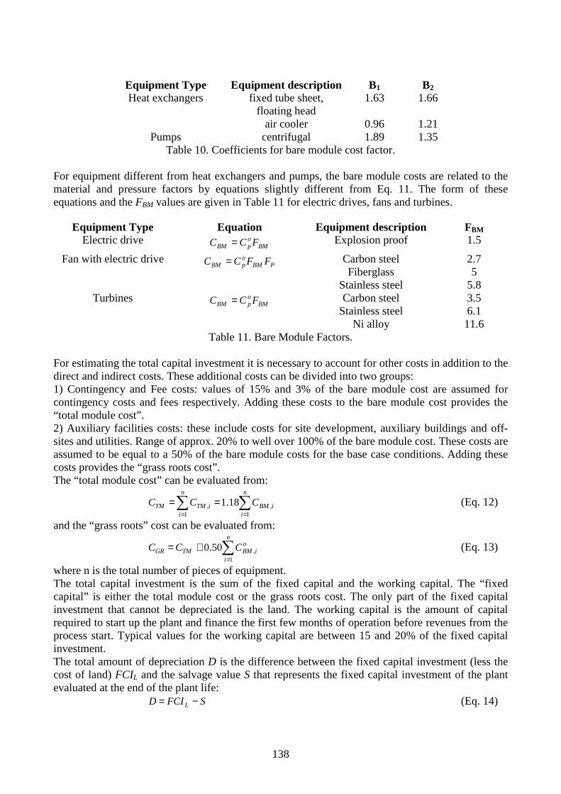
138

Equipment Type Equipment description B1 B2

fixed tube sheet, floating head

1.63 1.66 Heat exchangers

air cooler 0.96 1.21 Pumps centrifugal 1.89 1.35

Table 10. Coefficients for bare module cost factor. For equipment different from heat exchangers and pumps, the bare module costs are related to the material and pressure factors by equations slightly different from Eq. 11. The form of these equations and the FBM values are given in Table 11 for electric drives, fans and turbines.

Equipment Type Equation Equipment description FBM Electric drive

BMopBM FCC = Explosion proof 1.5

Carbon steel 2.7 Fiberglass 5

Fan with electric drive PBM

opBM FFCC =

Stainless steel 5.8 Carbon steel 3.5

Stainless steel 6.1 Turbines

BMopBM FCC =

Ni alloy 11.6 Table 11. Bare Module Factors.

For estimating the total capital investment it is necessary to account for other costs in addition to the direct and indirect costs. These additional costs can be divided into two groups: 1) Contingency and Fee costs: values of 15% and 3% of the bare module cost are assumed for contingency costs and fees respectively. Adding these costs to the bare module cost provides the “total module cost”. 2) Auxiliary facilities costs: these include costs for site development, auxiliary buildings and off-sites and utilities. Range of approx. 20% to well over 100% of the bare module cost. These costs are assumed to be equal to a 50% of the bare module costs for the base case conditions. Adding these costs provides the “grass roots cost”. The “total module cost” can be evaluated from:

∑∑==

==n

iiBM

n

iiTMTM CCC

1,

1, 18.1 (Eq. 12)

and the “grass roots” cost can be evaluated from:

∑=

+=n

i

oiBMTMGR CCC

1,50.0 (Eq. 13)

where n is the total number of pieces of equipment. The total capital investment is the sum of the fixed capital and the working capital. The “fixed capital” is either the total module cost or the grass roots cost. The only part of the fixed capital investment that cannot be depreciated is the land. The working capital is the amount of capital required to start up the plant and finance the first few months of operation before revenues from the process start. Typical values for the working capital are between 15 and 20% of the fixed capital investment. The total amount of depreciation D is the difference between the fixed capital investment (less the cost of land) FCIL and the salvage value S that represents the fixed capital investment of the plant evaluated at the end of the plant life:

SFCID L −= (Eq. 14)

139

6.6 Calculation of operating costs In order to estimate the manufacturing cost we need process information provided on the PFD, an estimate of the fixed capital investment FCI ( total module cost CTM or the grass roots cost CGR ), and an estimate of the number of operators required to operate the plant. The equation used to evaluate the cost of manufacture is:

Cost of Manufacture (COM) = Direct Manufacturing Costs (DMC) + Fixed Manufacturing Costs (FMC) + General Expenses (GE)

The cost of manufacturing, COM, can be determined when the following costs are known: 1) Fixed capital investment (FCI): (CTM or CGR)

This cost is determined using the method shown in the previous section. 2) Cost of operating labor (COL)

For chemical processing plants the operating labor requirement (number of operators) can be obtained from the number of steps required by the process; the average hourly wage can be obtained from the Bureau of Labor and Statistics.

3) Cost of utilities (CUT) The costs of utilities are directly influenced by the cost of fuel that directly impact the price of electricity, steam and thermal fluids. Usually the equipment necessary to produce the various utility streams are not shown on the PFD and only the utility streams are shown or can be found by doing a simple heat balance. These streams, termed “utilities”, are necessary for the control of stream temperatures as required by the process. These utilities can be purchased from a public or private utility or self-generated by the company. The capital investment required to build facilities that supply utilities is taken into account when a grass-roots cost is used for the fixed capital investment. The costs associated with supplying a given utility are then obtained by calculating the operating costs to generate the utility. These costs are presented by Turton et al. (2009) for the following major utilities: air supply; steam from boilers; cooling tower water; high purity water; electrical substation; fuels; refrigeration.

4) Cost of waste treatment (CWT) Waste disposal costs of hazardous or non-hazardous solid and liquid are reported by Turton et al. (2009) as well as the waste water treatment costs.

5) Cost of raw materials (CRM) The cost of raw materials ($/kg) can be estimated by using the current price listed in publications. In most cases the cost of raw materials is the biggest cost in chemical plants. The other cost items can be estimated using the equations in Table 12.

Cost item Typical range of multiplying

factors Value used in text

(or midpoint value) 1. Direct manufacturing costs (DMC)

a) Raw materials CRM b) Waste treatment CWT c) Utilities CUT d) Operating labor COL COL e) Direct supervisory and clerical labor

(0.1 – 0.25)COL 0.18COL

f) Maintenance and repairs (0.02 – 0.1)FCI 0.06FCI g) Operating supplies (0.1 – 0.2) * (line 1.f) 0.009FCI h) Laboratory charges (0.1 – 0.2)COL 0.15COL i) Patents and royalties (0 – 0.06)COM 0.03COM

140

2. Fixed manufacturing costs (FMC)

a) Depreciation 0.1FCI 0.1FCI b) Local taxes and insurance (0.014-0.05)FCI 0.032FCI c) Plant overhead costs (0.50-0.7) * (line 1.d +line 1.e +

line 1.f) 0.708COL+0.036FCI

3. General manufacturing expenses (GE)

a) Administration costs 0.15*(line 1.d + line 1.e + line 1.f) 0.177COL+0.009FCI b) Distribution and selling costs (0.02 – 0.2)COM 0.11COM c) Research and development 0.05COM 0.05COM

Table 12. Multiplication factors for estimating manufacturing cost.

6.7 Economic evaluation of binary cycle power plants The following Table 13 summarizes the coefficients used for the evaluation of the capital costs of binary cycle power plants:

Component A K1 K2 K3

B1 B2

FM C1 C2 C3

FBM

Feed pump (1) P [kW] 3.3892 0.0536 0.1538

1.89 1.35

2 -0.3935 0.3957

-0.00226

Electrical motor pump (2) P [kW] 2.4604 1.4191 -0.1798

1.5

Expander P [kW] 2.2476 1.4965 -0.1618

12

Electrical generator (3) P [kW] ( ) 94.011800/1850000PCop = 1.5

ACC heat exchanger A [m2] 4.0336 0.2341 0.0497

0.96 1.21

1

ACC fans (4) Q [m3/s] 3.1761 -0.1373 0.3414

2.7

Electrical motors fans (4) P [kW] 1.9560 1.7142 -0.2282

2.7

Shell&Tube heat exchangers A [m2] 4.3247 -0.3030 0.1634

1.63 1.66

1 0.03881 -0.11272 0.08183

Table 13. Coefficients used for the evaluation of the capital costs of binary cycle power plants. (1) Number of pumps calculated in order that Pmax ≤ 300 kW. (2) Electrical motors and generators oversized of 20% to the respective pumps and turbines. (3) Electrical generator cost functions not found and a different procedure is used (Lazzaretto and Macor, 1993) estimating the cost of a new generator by scaling the cost of a known generator. (4) The number of ACC fans is calculated assuming a volumetric flow rate for each fan equal to 65 m3/s.

141

The cost of the working fluid should also be included since it can be similar to the cost of the main components. Basing on the data provided by Enel on Stillwater and Salt Wells power plants, about 760 kg of working fluid are needed for each kg/s of working fluid mass flow rate. The purchased cost of the working fluid is: 0.96 $/kg for isobutane and 4.62 $/kg for R134a. The assumed bare module cost factor Fbm that accounts for installation costs is 1.25. The estimation of the operating costs is shown in the following Table 14:

Operating labor 1.00 COL Direct supervisory and clerical labor 0.15 COL

Maintenance and repairs 0.03 CGR Laboratory charges 0.07 COL

Local taxes and insurance 0.02 CGR General expenses 0.03 CGR + 0.50 COL

Administration costs 0.08 COL Table 14. Manufacturing costs.

where CGR is the grass roots cost of the binary power plant and COL is the operating labor cost. It is assumed that eight workers are needed for operating the plant giving a COL = 63,000 $/year (35 $/hour and 1800 hours/year). The costs of raw materials, waste treatment and utilities are assumed null. The cost of electricity is simply calculated using the following equation:

fP

CCOE

NET

annual

⋅⋅=

8760 (Eq. 15)

where Cannual is the annual cost that comprise capital and operating costs and “f ” is the availability of the geothermal power plant assumed 0.96. Assuming a depreciation of the capital investment of 0.1·CGR the cost of electricity is:

96.08760

80.118.0

⋅⋅+

=NET

OLGR

P

CCCOE (Eq. 16)

The numerator is composed by two terms: the first depends on the plant’s characteristics whereas the second is a constant. The results obtained are shown in the following Tables 15 and 16 respectively for R134a and isobutane:

R134a R134a R134a Geofluid temperature °C 130 140 150

Working fluid $ 606,512 636,398 699,843 Feed pumps $ 465,718 (2) 606,730 (3) 703,983 (3)

Electrical motors pumps $ 312,214 (2) 416,285 (3) 455,966 (3) Expanders $ 5,087,084 5,539,310 5,955,722

Electrical generators $ 936,508 1,174,676 1,452,948 ACC $ 1,010,760 1,090,161 1,192,563

ACC fans $ 1,686,501 (42) 1,968,860 (49) 2,382,396 (59) ACC fans electrical

motors $ 506,336 (42) 591,108 (49) 715,264 (59)

Recuperator $ - - 170,427 Preheater $ 276,422 - - Vaporizer $ 101,047 - -

Superheater $ 276,422 - -

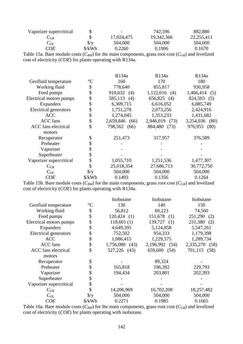
142

Vaporizer supercritical $ - 742,596 882,880 CGR $ 17,024,475 19,342,366 22,255,411 COL $/y 504,000 504,000 504,000 COE $/kWh 0.2260 0.1906 0.1670

Table 15a. Bare module costs (CBM) for the main components, grass root cost (CGR) and levelized cost of electricity (COE) for plants operating with R134a.

R134a R134a R134a Geofluid temperature °C 160 170 180

Working fluid $ 778,640 855,817 930,958 Feed pumps $ 910,632 (4) 1,122,016 (4) 1,466,414 (5)

Electrical motors pumps $ 585,113 (4) 656,825 (4) 824,503 (5) Expanders $ 6,309,715 6,616,052 6,885,749

Electrical generators $ 1,751,278 2,073,256 2,424,916 ACC $ 1,274,045 1,353,233 1,431,682

ACC fans $ 2,659,846 (66) 2,946,019 (73) 3,254,036 (80) ACC fans electrical

motors $ 798,562 (66) 884,480 (73) 976,955 (80)

Recuperator $ 251,473 317,957 376,589 Preheater $ - - - Vaporizer $ - - -

Superheater $ - - - Vaporizer supercritical $ 1,055,710 1,251,536 1,477,307

CGR $ 25,018,354 27,686,713 30,772,750 COL $/y 504,000 504,000 504,000 COE $/kWh 0.1493 0.1356 0.1264

Table 15b. Bare module costs (CBM) for the main components, grass root cost (CGR) and levelized cost of electricity (COE) for plants operating with R134a.

Isobutane Isobutane Isobutane Geofluid temperature °C 130 140 150

Working fluid $ 56,812 69,223 74,560 Feed pumps $ 120,424 (1) 151,678 (1) 251,290 (2)

Electrical motors pumps $ 118,601 (1) 139,727 (1) 231,380 (2) Expanders $ 4,649,395 5,124,858 5,547,261

Electrical generators $ 752,502 954,333 1,179,398 ACC $ 1,086,415 1,229,575 1,289,734

ACC fans $ 1,756,080 (43) 2,196,992 (54) 2,335,270 (58) ACC fans electrical

motors $ 527,226 (43) 659,600 (54) 701,115 (58)

Recuperator $ - 89,324 - Preheater $ 165,818 196,392 229,793 Vaporizer $ 194,434 203,801 202,393

Superheater $ - - - Vaporizer supercritical $ - - -

CGR $ 14,206,969 16,702,208 18,257,482 COL $/y 504,000 504,000 504,000 COE $/kWh 0.2271 0.1985 0.1665

Table 16a. Bare module costs (CBM) for the main components, grass root cost (CGR) and levelized cost of electricity (COE) for plants operating with isobutane.

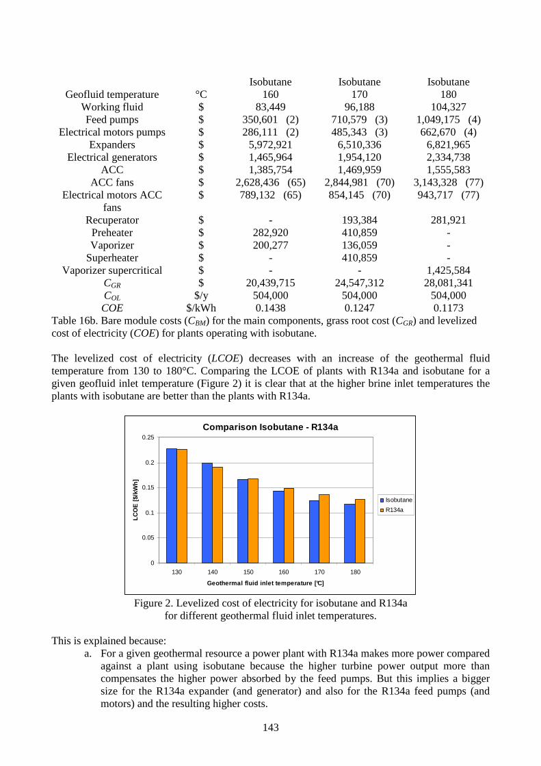
143

Isobutane Isobutane Isobutane

Geofluid temperature °C 160 170 180 Working fluid $ 83,449 96,188 104,327 Feed pumps $ 350,601 (2) 710,579 (3) 1,049,175 (4)

Electrical motors pumps $ 286,111 (2) 485,343 (3) 662,670 (4) Expanders $ 5,972,921 6,510,336 6,821,965

Electrical generators $ 1,465,964 1,954,120 2,334,738 ACC $ 1,385,754 1,469,959 1,555,583

ACC fans $ 2,628,436 (65) 2,844,981 (70) 3,143,328 (77) Electrical motors ACC

fans $ 789,132 (65) 854,145 (70) 943,717 (77)

Recuperator $ - 193,384 281,921 Preheater $ 282,920 410,859 - Vaporizer $ 200,277 136,059 -

Superheater $ - 410,859 - Vaporizer supercritical $ - - 1,425,584

CGR $ 20,439,715 24,547,312 28,081,341 COL $/y 504,000 504,000 504,000 COE $/kWh 0.1438 0.1247 0.1173

Table 16b. Bare module costs (CBM) for the main components, grass root cost (CGR) and levelized cost of electricity (COE) for plants operating with isobutane. The levelized cost of electricity (LCOE) decreases with an increase of the geothermal fluid temperature from 130 to 180°C. Comparing the LCOE of plants with R134a and isobutane for a given geofluid inlet temperature (Figure 2) it is clear that at the higher brine inlet temperatures the plants with isobutane are better than the plants with R134a.

Comparison Isobutane - R134a

0

0.05

0.1

0.15

0.2

0.25

130 140 150 160 170 180

Geothermal fluid inlet temperature [°C]

LCO

E [$

/kW

h]

Isobutane

R134a

Figure 2. Levelized cost of electricity for isobutane and R134a

for different geothermal fluid inlet temperatures. This is explained because:

a. For a given geothermal resource a power plant with R134a makes more power compared against a plant using isobutane because the higher turbine power output more than compensates the higher power absorbed by the feed pumps. But this implies a bigger size for the R134a expander (and generator) and also for the R134a feed pumps (and motors) and the resulting higher costs.

144

b. Operating the R134a at supercritical pressures a better approach is obtained between the geothermal fluid and the working fluid compared to the subcritical operation of isobutane. But this implies, for a given minimum temperature difference (∆Tmin = 10°C), a closer approach between the two thermal profiles and smaller mean temperature differences (∆tml). Assuming the same overall heat transfer coefficients the area of the heat exchanger between the geothermal fluid and the working fluid must be bigger resulting in higher costs.

c. For a given geothermal resource the thermodynamic cycle with R134a needs a working fluid mass flow rate almost double than isobutane. Assuming a proportionality between the mass flow rate and the quantity of working fluid in the plant the quantity of R134a should be almost double than the quantity of isobutane. In addition the unit cost of R134a is about five times higher than the cost of isobutane. The result is that the cost for the working fluid R134a is about one order of magnitude higher than the cost of isobutane.

145

Conclusions

This chapter presented the various cost factors involved in capital investment and operation of industrial plants and the main techniques used for estimating these costs. The equipment module costing technique is applied for estimating the cost of binary cycle power plants. This approach relates all costs to the purchased cost of equipment evaluated for some base conditions. The cost functions were taken from Turton et al. (2009) for different type of equipment and construction as a function of a size or capacity parameter and, when possible, were compared against other literature sources. The optimal thermodynamic solutions found in Chapter 4 for isobutane and R134a were evaluated from an economic point of view calculating the costs of the main components namely the expander/generators, air cooled condenser with fans, shell and tube heat exchangers and feed pumps with electrical motors. The results show that the levelized cost of the electricity roughly halves from 0.22 c$/kWh to 0.12 c$/kWh when the temperature of the geothermal fluid is increased from 130 to 180°C. The plants operating with isobutane are more convenient in the upper part of the range considered for the temperature of the geothermal fluid (150÷180°C) whereas at lower temperatures (130÷150°C) R134a is more convenient both from the thermodynamic and economic point of view. This can be explained by the following reasons, as already seen in the last section: � When operating at supercritical pressures with R134a the higher expander power output more

than compensates the higher feed pumps power absorption, but this implies larger sizes and costs for both expanders-generators and pumps-motors compared to a subcritical power plant.

� At supercritical pressures a better temperature matching is obtained between geothermal and working fluid compared to the subcritical operation of isobutane. However, these closer thermal profiles and smaller mean temperature differences (∆tml) result in bigger heat transfer surfaces and higher costs for a given minimum temperature difference (∆Tmin = 10°C).

� The unit cost of R134a is higher than the cost of isobutane.

146

References Lazzaretto A. and Macor A., Analisi sperimentale e statistica di funzioni di costo per componenti di impianti combinati, Atti del VII Convegno Nazionale: Gruppi Combinati Prospettive Tecniche ed Economiche, SGEditoriali Padova, 1993. Peters M.S. and Timmerhaus K.D., Plant Design and Economics for Chemical Engineers, McGraw-Hill, 1991. Turton R., Bailie R.C., Whiting W.B. and Shaeiwitz J.A., Analysis, Synthesis and Design of Chemical Processes (2a

ed.), Prentice Hall, 2009.

147

7. Off-Design Model of Stillwater Geothermal

Binary Power Plant This section describes the activity carried out at MIT (Boston) on the innovative geothermal binary power plant of Stillwater (Nevada, USA) started in 2009. A detailed off-design model of the power plant was developed in order to maximize the power output from the available geothermal resource that is lower than expected. The Stillwater plant is composed by two identical units. Each unit has the configuration shown in Figure 1. The geothermal fluid heats and vaporizes the working fluid, isobutane, that flows through the expanders and generates power. A dry cooling system is used as the heat rejection system. Using the manufacturers’ data and performance sheets for the main components an Aspen Plus model for Stillwater power plant was built. The power plant parameters measured during the operation in 2009 have provided a good source of information to test and adjust the model. Figure 1. Stillwater power plant configuration: one unit.

148

7.1. Stillwater design basis The geothermal fluid design flow rate is 7,255,000 lb/hr and the geothermal fluid design inlet temperature is 310°F. The brine flow is equally distributed between the two identical Units. The overall power plant can be studied modeling a single unit fed with a brine flow of 3,627,500 lb/hr at 310°F. The ambient temperature in the design conditions is 53.7°F, the annual average ambient temperature of Fallon. Enel provided a flowsheet (here not shown) of the geothermal power plant in design conditions made by an engineering firm. The flowsheet shows the main plant components of one unit and the flow rates, temperatures and pressures of the power plant’s streams in design conditions. A table shows the gross power output, the main parasitic loads and the net power output for these design conditions. A model of one unit of the Stillwater Power Plant in design conditions was built using the Aspen Plus platform. The provided flowsheet was taken as the reference to set the pump outlet pressure (495 psia), the working fluid flow rate (3,113,250 lb/hr), the expander inlet temperature (260.9°F), the expander outlet pressure (65.05 psia) and the pressure drops in the heat exchangers. The working fluid composition on a mole basis is: isobutane 96%, n-butane 3.7%, propane 0.3%. The property method used is RefProp (Reference Fluid Properties), developed by NIST (National Institute of Standards and Technology) that has been incorporated into the Aspen Plus V7.1. RefProp provides accurate thermophysical properties for hydrocarbons and refrigerants, both pure fluids and mixtures. SteamNBS property method is used for the properties of the geothermal fluid modeled as pure water. The expander isentropic efficiency is calculated using the Performance Calculator provided by the manufacturer (Mafi-Trench) based on the expander inlet conditions and the expander outlet pressure. Figure 2 shows the Aspen Plus flowsheet of one unit of the Stillwater Power Plant and the streams’ temperatures (°F) and pressures (psia) in design conditions to compare with the reference flowsheet.

Figure 2. Aspen Plus Flowsheet of one Unit of Stillwater Power Plant and stream results to compare with the reference design.

149

Some of the stream temperatures are a bit different from the reference design flowsheet temperatures, and these differences can mainly be ascribed to the different property methods used by the reference and Aspen Plus. With the expander isentropic efficiency determined using the performance calculator, the gross power output produced by one unit is 23.0 MW. This value is about 0.6 MW lower than the gross power output shown in the reference flowsheet for one unit. The minimum temperature difference (pinch-point temperature difference, ∆Tpp) between the brine and the working fluid is only 3.3°F when calculated using RefProp in the Aspen Plus model. This low value implies low LMTDs (logarithmic mean temperature differences) both for the preheater and the vaporizer. In Figures 3a and 3b the expander performance correlations provided by the manufacturer are shown. The expander isentropic efficiency is correlated with two parameters: the isentropic enthalpy drop and the volumetric flow rate at the outlet. When these two parameters are at their optimal values, respectively 24.43 Btu/lb and 40,000 ft3/min, the expander isentropic efficiency is 86.9%. In Stillwater design conditions, the expanders do not operate at their design point. The black lines in Figures 3a and 3b show the design condition and this design condition is far from the optimum for the turbine. Consequently the calculated turbine isentropic efficiency based on the Mafi-Trench performance curve is 84.4%, well below the reference assumed efficiency. The reference, using a higher expander isentropic efficiency (about 86.5%), calculated a higher gross power output.

Expander efficiency correction factor due to Isentropic Enthalpy drop

0.840.860.880.900.920.940.960.981.00

0.7 0.8 0.9 1 1.1 1.2 1.3

(∆∆∆∆his_offd/ ∆∆∆∆his_d)^0,5

Effi

cien

cy C

orre

ctio

n F

acto

r

Figure 3a. Expander efficiency correction factor for deviation from optimal isentropic enthalpy drop.

Expander efficiency correction factordue to Outlet Volumetric Flow Rate

0.60

0.70

0.80

0.90

1.00

0.5 1 1.5 2

Vout_offd/Vout_d

Effi

cien

cy C

orre

ctio

n F

acto

r

Figure 3b. Expander efficiency correction factor for deviation from optimal outlet volumetric flow rate.

In Figure 4 the heat of vaporization (kJ/kg) of the working fluid as a function of pressure (up to 32 bar,a) is calculated using RefProp and compared against the value provided using Peng-Robinson property method. RefProp property method yields a higher heat of vaporization, the difference being about 10% compared to Peng-Robinson for the design vaporization pressure of Stillwater.

150

Impure Isobutane - Heat of Vaporization vs PressureDifference between RefProp and Peng-Robinson

80

100

120

140

160

180

200

220

240

260

1.6E+06 2.0E+06 2.4E+06 2.8E+06 3.2E+06

Pressure [Pa]

Hea

t of V

apor

izat

ion

[kJ/

kg]

Peng Robinson Refprop Figure 4. Isobutane heat of vaporization.

The engineering firm that made the reference flowsheet and the heat exchangers’ manufacturer, using a property method with a lower heat of vaporization than RefProp, found a higher minimum temperature difference between the brine and the working fluid (∆Tpp > 3.3°F) and, consequently, higher LMTDs for both the preheater and the vaporizer. The design condition of Stillwater was therefore modified from the design basis provided. Using the existing heat exchangers (“U” and “A” values provided by the manufacturers) the cycle high pressure was reduced relax the heat exchanger pinch. The new design working fluid flow rate (3.19 million lb/hr) is found from the heat balance with the brine assuming 5°F of superheating at the outlet of the vaporizer. The optimal pressure that maximizes the net power output is 410 psia. In these new design conditions the gross power output produced by one unit is 22.5 MW (< 23 MW). Summarizing, using RefProp property method (guaranteeing 5°F of superheating at the inlet of the expanders) and using the actual expander isentropic efficiency, the gross power output produced by one unit is 1.1 MW lower than the value provided by the engineering firm (22.5 vs 23.6 MW). Figure 5 shows the Aspen flowsheet with the stream results for this new design condition.

Figure 5. Revised design basis for Stillwater Power Plant.

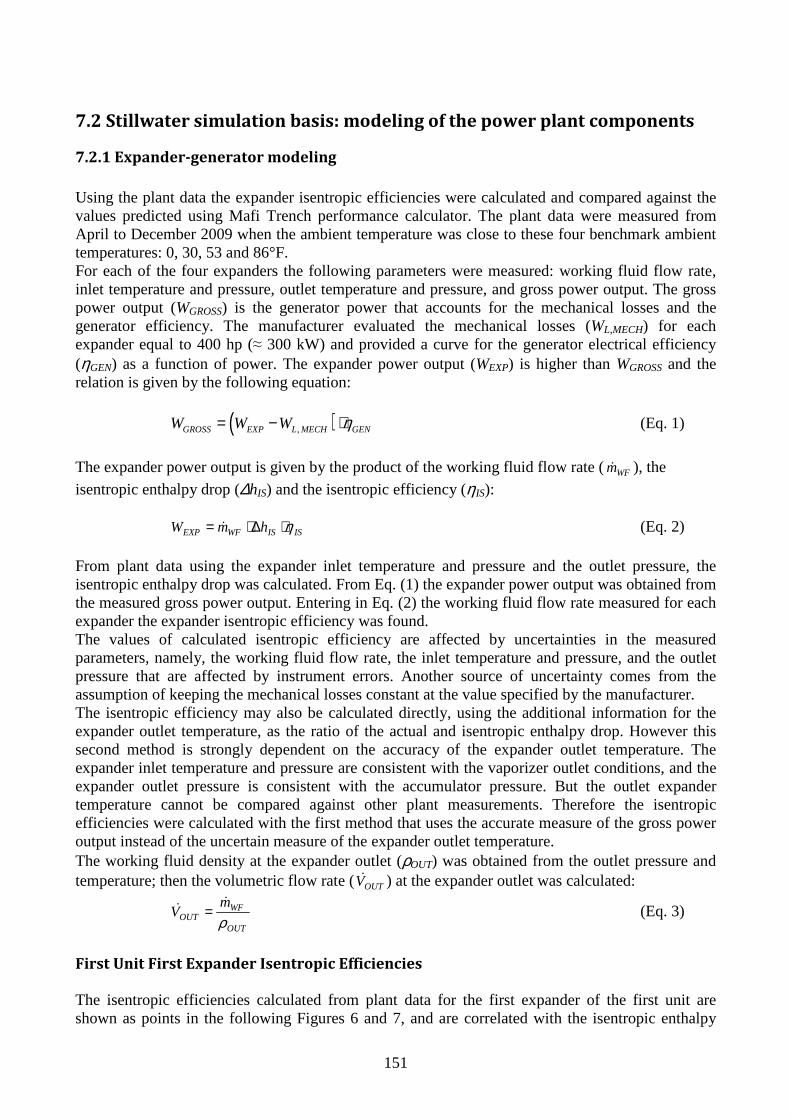
151

7.2 Stillwater simulation basis: modeling of the power plant components

7.2.1 Expander-generator modeling

Using the plant data the expander isentropic efficiencies were calculated and compared against the values predicted using Mafi Trench performance calculator. The plant data were measured from April to December 2009 when the ambient temperature was close to these four benchmark ambient temperatures: 0, 30, 53 and 86°F. For each of the four expanders the following parameters were measured: working fluid flow rate, inlet temperature and pressure, outlet temperature and pressure, and gross power output. The gross power output (WGROSS) is the generator power that accounts for the mechanical losses and the generator efficiency. The manufacturer evaluated the mechanical losses (WL,MECH) for each expander equal to 400 hp (≈ 300 kW) and provided a curve for the generator electrical efficiency (ηGEN) as a function of power. The expander power output (WEXP) is higher than WGROSS and the relation is given by the following equation:

( ),GROSS EXP L MECH GENW W W η= − ⋅ (Eq. 1)

The expander power output is given by the product of the working fluid flow rate ( WFm& ), the

isentropic enthalpy drop (∆hIS) and the isentropic efficiency (ηIS):

ISISWFEXP hmW η⋅∆⋅= & (Eq. 2) From plant data using the expander inlet temperature and pressure and the outlet pressure, the isentropic enthalpy drop was calculated. From Eq. (1) the expander power output was obtained from the measured gross power output. Entering in Eq. (2) the working fluid flow rate measured for each expander the expander isentropic efficiency was found. The values of calculated isentropic efficiency are affected by uncertainties in the measured parameters, namely, the working fluid flow rate, the inlet temperature and pressure, and the outlet pressure that are affected by instrument errors. Another source of uncertainty comes from the assumption of keeping the mechanical losses constant at the value specified by the manufacturer. The isentropic efficiency may also be calculated directly, using the additional information for the expander outlet temperature, as the ratio of the actual and isentropic enthalpy drop. However this second method is strongly dependent on the accuracy of the expander outlet temperature. The expander inlet temperature and pressure are consistent with the vaporizer outlet conditions, and the expander outlet pressure is consistent with the accumulator pressure. But the outlet expander temperature cannot be compared against other plant measurements. Therefore the isentropic efficiencies were calculated with the first method that uses the accurate measure of the gross power output instead of the uncertain measure of the expander outlet temperature. The working fluid density at the expander outlet (ρOUT) was obtained from the outlet pressure and temperature; then the volumetric flow rate (OUTV& ) at the expander outlet was calculated:

OUT

WFOUT

mV

ρ&& = (Eq. 3)

First Unit First Expander Isentropic Efficiencies The isentropic efficiencies calculated from plant data for the first expander of the first unit are shown as points in the following Figures 6 and 7, and are correlated with the isentropic enthalpy

152

drop and the volumetric flow rate at the outlet. The variation of the isentropic efficiency predicted by Mafi Trench correlation is superimposed as a black line on the same figures. When the variation of the efficiency with the first variable (on the x-axis) is shown, the second variable (hidden) is kept at its design value, and vice versa.

1st Unit, 1 st Expander Isentropic Efficiencies

0.00

0.10

0.20

0.30

0.40

0.50

0.60

0.70

0.80

0.90

1.00

10.0 15.0 20.0 25.0 30.0 35.0 40.0 45.0

Isentropic Enthalpy Drop [Btu/lb]

Isen

tropi

c E

ffici

ency 53°F

86°F

30°F

0°F

MTC

Figure 6. Expander isentropic efficiencies calculated from Stillwater plant data for the first

expander of the first unit. Variation with the isentropic enthalpy drop.

1st Unit, 1 st Expander Isentropic Efficiencies

0.00

0.10

0.20

0.30

0.40

0.50

0.60

0.70

0.80

0.90

1.00

0 10000 20000 30000 40000 50000 60000

Volumetric Flow Rate at the Outlet [ft3/min]

Isen

tropi

c E

ffici

ency 53°F

86°F

30°F

0°F

MTC

Figure 7. Expander isentropic efficiencies calculated from Stillwater plant data for the first

expander of the first unit. Variation with the volumetric flow rate at the outlet. To compare the efficiencies calculated from plant data against the curve representing Mafi Trench correlation, the points were filtered in Figures 8 and 9 to take into account only points with the outlet volumetric flow rate and the isentropic enthalpy drop, respectively, close to the design value.

153

The figures show that the efficiencies predicted using Mafi Trench correlation represent the isentropic efficiencies calculated from plant data quite well.

1st Unit, 1 st Expander Isentropic Efficiencies

( Only Data with 35,000<V out <48,000 ft3/min )

0.00

0.10

0.20

0.30

0.40

0.50

0.60

0.70

0.80

0.90

1.00

10.0 15.0 20.0 25.0 30.0 35.0 40.0 45.0

Isentropic Enthalpy Drop [Btu/lb]

Isen

tropi

c E

ffici

ency

53°F

30°F

0°F

MTC

Figure 8. Expander isentropic efficiencies calculated from Stillwater plant data for the first

expander of the first unit. Data filtered to compare against MTC performance curve.

1st Unit, 1 st Expander Isentropic Efficiencies( Only Data with 21< ∆∆∆∆h is <28 Btu/lb )

0.00

0.10

0.20

0.30

0.40

0.50

0.60

0.70

0.80

0.90

1.00

0 5000 10000 15000 20000 25000 30000 35000 40000 45000

Volumetric Flow Rate at the Outlet [ft3/min]

Isen

tropi

c E

ffici

ency

86°F

MTC

Figure 9. Expander isentropic efficiencies calculated from Stillwater plant data for the first

expander of the first unit. Data filtered to compare against MTC performance curve. The points are referred to four ambient conditions: 0, 30, 53 and 86°F ambient temperature and are shown using dots with different colors. The expander outlet pressure is kept at the minimum value of 40 psia during the coldest days of the year, and it is increased when the air temperature is warmer to be able to condense the working fluid. The isentropic enthalpy drop, ∆hIS, is related to the expander pressure ratio; therefore higher values for ∆hIS are found in the winter conditions and lower values are found in summer conditions. Also the volumetric flow rate at the outlet is related to the expander outlet pressure by means of the density. Higher expander outlet pressures imply higher densities and lower volumetric flow rates.

154

Looking at the 53°F ambient temperature points, most of the isentropic efficiencies are higher than 80% with some points showing efficiencies even higher than 85%. The volumetric flow rate at the outlet of the expander is about 15% lower than the design flow rate (40,000 ft3/min). The isentropic enthalpy drop is on average about 25% higher than the design value (24.43 Btu/lb). Even though there is much scatter, the points show higher isentropic efficiencies as the values of the two variables get closer to their optimal values. Mafi Trench efficiency curves are drawn assuming a design value for the second independent variable, being the first variable shown on the x-axis. Many points are below the Mafi Trench black curve that correlates with ∆hIS (Figure 6) due to the non-optimal VOUT; most of the points are below the Mafi Trench black curve that correlates with VOUT (Figure 7) due to the non-optimal ∆hIS. In the 30 and 0°F ambient temperature cases, the expanders experience the highest isentropic enthalpy drops and the highest volumetric flow rate due to the low expander outlet pressure. Since Stillwater working fluid mass flow rate is usually lower than the design value, these conditions make the outlet volumetric flow rate similar to the design value. Figure 8, with the filtered points, shows that for the 30°F case Mafi Trench correlation seems too conservative, overestimating the penalties associated with higher ∆hIS. In the 86°F case the points cluster around the optimal ∆hIS but show isentropic efficiencies much lower than the design value due to the low outlet volumetric flow rates. Figure 9 with the filtered points clearly shows that Mafi Trench correlation predicts the decrease of the isentropic efficiency for low flow rates quite well. The objective of this activity is maximizing the net power output of the Stillwater Power Plant using the available geothermal fluid. Simplifying the operational condition with the highest expander power output is similar to the condition with the highest net power output since the parasitic loads have a smaller magnitude. Eq. (2) shows the three components that define the expander power output and the expander isentropic efficiency is one of these. Looking through the figures some interesting findings can be drawn. For the 0 and 30°F cases the optimal outlet volumetric flow rate can be obtained with a working fluid mass flow rate lower than the design value (i.e., 1560 klb/hr for one expander). The low outlet volumetric flow rate in the 86°F case implies poor isentropic efficiencies and increasing the working fluid mass flow rate might be beneficial even if this may cause a further increase of the expander outlet pressure. The 53°F isentropic efficiencies could be improved by operating with lower expander pressure ratios and with a higher working fluid mass flow rate. Appendix B shows the isentropic efficiencies calculated for the second expander of the first unit and the two expanders of the second unit. The expanders of the second unit, especially the second expander, show that isentropic efficiencies calculated from plant data are lower than the efficiencies predicted using Mafi Trench correlation.

7.2.2 Feed pumps modeling

Each unit of the Stillwater Power Plant is equipped with three feed pumps in parallel. One of these three pumps is driven by a variable frequency drive and the performance curves provided by the manufacturer are shown in Figure 10.

155

Figure 10. Stillwater feed pumps performance curves.

The x-axis variable in all the three graphs is the working fluid volumetric flow rate through one pump in US gallons per minute (GPM). The y-axis variable in the upper graph is the pump absorbed power in horsepower. The central graph shows the head and efficiency curves drawn for different speeds of rotation. The y-axis variable in the lower graph is the Net Positive Suction Head Required (NPSHr) to prevent cavitation, in feet. The Feed Pumps Performance curves “Head” and “Efficiency” were included in the Aspen Model using the simplifying assumption that all the three feed pumps are equipped with VFDs. The power absorbed by the feed pumps is given by:

driver

VPUMPSFEED

hgQP

ηηρ 1

_ ⋅⋅⋅⋅

= (Eq. 4)

where ρ is the WF density, QV is the WF volumetric flow rate, h is the head and η is the pump efficiency. A value of 97% was assumed for the driver efficiency ηdriver.

156

7.2.3 Shell and tube heat exchangers modeling: preheater and vaporizer

� Heat exchangers data sheets The manufacturer’s heat exchangers specification sheets show the geometric and performance data of Stillwater preheaters and vaporizers. The preheater and the vaporizer are shell and tube heat exchangers with the brine flowing inside the tubes and the working fluid in the shell. Each unit of the Stillwater plant has two preheater shells in series followed by one vaporizer shell. Table 1 below summarizes the main characteristics: Parameter Preheater (1 Shell) Vaporizer (1 Shell) Area [ft2] 154,740 54,854 Tube outside diameter [in] 0.625 0.625 Tube length [ft] 58 40 Tube number 6,650 3,427 Fins density [No./in] 19 19 Tube thickness [in] 0.065 0.065 Tube pitch [in] 0.8125 0.8125 Tube Layout 30° Triangular 30° Triangular Shell inside diameter [in] 84 65 Baffle Spacing [ft] 5.2 4.9 U design service [Btu/hr-ft2-°F] 84.0 128.2

Table 1. Preheater and vaporizer data from the manufacturer specification sheets. The shell and tube heat exchangers employ low-finned tubes to increase the surface area on the shell side since the isobutane thermophysical properties make its heat transfer coefficient low compared to the water (brine) heat transfer coefficient. The effective finned surface area is 2.45 times the bare tube area. Table 2 below compares isobutane and water thermophysical properties at 70°C: Parameter Isobutane (70°C; 25 bar) Water (70°C; 10 bar) Thermal Conductivity [W/m-K] 0.0761 0.6636 Density [kg/m3] 493.2 978.2 Specific Heat [kJ/kg-K] 2.754 4.188 Dynamic Viscosity [Pa· s] 0.0000993 0.000404 Table 2. Comparison between the thermophysical properties of pure isobutane and water at 70°C.

The thermal conductivity of isobutane is almost one order of magnitude lower than that of water, the density is about half and the specific heat is 0.66 times the specific heat of water. The lower dynamic viscosity of isobutane is not sufficient to compensate for the differences in the other properties and, overall, the heat transfer characteristics of isobutane are poorer than those of water. With a proper design and using finned tubes, the heat exchanger manufacturer tries to balance the heat transfer resistances on the tube side and shell side. � Heat exchangers heat transfer correlation found using “Aspen Shell&Tube” The detailed geometries of Stillwater preheater and vaporizer from the manufacturer data sheets were entered into “Aspen Exchanger Design & Rating”. The brine flow rate and working fluid flow rate were varied from their design values in order to find the variation of the tube-side and shell-

157

side heat transfer coefficients and pressure drops with the flow rate. Also the working fluid pressure was varied from its design value in order to find any dependence of the heat transfer coefficients on pressure. In actual operation of the preheater-vaporizer subsystem, some of the working fluid could vaporize inside the preheater, or the preheating phase could be completed inside the vaporizer. Specific heat transfer correlations were found to take into account both of these possible cases. The following correlations were found for the preheater:

( ) ( )GEOPGEO mfh &=

( ) ( )WFPLWF mfh &=,

( ) ( )WFPBWF mfh &=,

and the following correlations were found for the vaporizer:

( ) ( )GEOVGEO mfh &=

( ) ( )WFVLWF mfh &=,

( ) ( )WFWFVBWF pmfh ,, &=

( ) ( )WFWFVSWF pmfh ,, &=

where h is the film coefficient, WFm& is the mass flow rate, p is the pressure; the subscripts refer to

the following: GEO: geothermal fluid, WF: working fluid, L: liquid, B: boiling, S: superheating, P: preheater, and V: vaporizer. In the Figures 11 to 14 some of the correlations found are shown. The remaining correlations are shown in Appendix C. The geothermal fluid heat transfer coefficients (hGEO) are referred to the tube inside area whereas the working fluid heat transfer coefficients (hWF) are based on the outside finned area. The ratio between the outside finned area and the tube inside area is Ae/Ai = 3.94 for both the preheater and the vaporizer.

Preheater - Variation of tube side heat transfer co efficient with Brine Flow Rate (Basis: tube inside diameter)

0

200

400

600

800

1000

1200

1400

1600

1800 2000 2200 2400 2600 2800 3000 3200 3400 3600 3800 4000

Brine Flow Rate [klb/hr]

Hea

t tra

nsfe

r co

effic

ient

[Btu

/hr-

ft2-°F

]

Figure 11. Variation of the geothermal fluid heat transfer coefficient

with the flow rate in the preheater: ( ) ( )GEOPGEO mfh &= .

158

Vaporizer - Variation of tube side heat transfer co efficient with Brine Flow Rate (Basis: tube inside diameter)

0

500

1000

1500

2000

2500

3000

1500 2000 2500 3000 3500 4000Brine Flow Rate [klb/hr]

Hea

t tra

nsfe

r co

effic

ient

[B

tu/h

r-ft2

-°F]

Figure 12. Variation of the geothermal fluid heat transfer coefficient

with the flow rate in the vaporizer: ( ) ( )GEOVGEO mfh &= .

Preheater - Variation of shell side Liquid heat tra nsfer coefficient with Working Fluid Flow Rate (Basis: outside finned area)

0

50

100

150

200

250

300

350

400

1000 1500 2000 2500 3000 3500

Working Fluid Flow Rate [klb/hr]

Hea

t tra

nsfe

r co

effic

ient

[B

tu/h

r-ft2

-°F]

Figure 13. Variation of the working fluid heat transfer coefficient with the flow rate in the preheater for the liquid phase: ( ) ( )WFPLWF mfh &=, .

159

Vaporizer - Variation of shell side Boiling heat tr ansfer coefficient with Working Fluid pressure - Parameter WF Flow Rat e

( Basis: outside finned area )

600

800

1000

1200

1400

1600

1800

2000

2200

320 340 360 380 400 420 440 460 480

Working Fluid vaporizer inlet pressure [psia]

Hea

t tra

nsfe

r co

effic

ient

[B

tu/h

r-ft2

-°F]

2500 klb/hr

2400

2300

2200

2100

2000

1900

1800

Poli. (2000)

Figure 14. Variation of the working fluid heat transfer coefficient with the flow rate and

pressure in the vaporizer for the boiling process: ( ) ( )WFWFVBWF pmfh ,, &= .

The comparison between Figure 13 and Figure 14 shows that the working fluid heat transfer coefficient in the boiling process is much higher than the heat transfer coefficient in the preheating process. This occurs because in the boiling process the convective heat transfer is combined with a nucleate boiling mechanism. Another finding is that the boiling heat transfer coefficient shows a strong variation with the isobutane pressure for pressures above about 400 psia. The passage area for the geothermal fluid in the vaporizer is about half the passage area in the preheater, and the higher fluid velocity implies that the brine heat transfer coefficient in the vaporizer is almost twice the heat transfer coefficient in the preheater as Figure 11 and Figure 12 show. Comparing the tube side and shell side heat transfer coefficients taking into account the ratio between the outside finned area and the tube inside area (i.e., ~4), it turns out that the two thermal resistances are similar in the preheater whereas in the vaporizer the working fluid thermal resistance is lower. The decrease of the heat transfer coefficient with the reduction of the flow rate is more marked for the tube side flow than for the shell side flow in the preheater, this being consistent with the heat transfer correlations available in the open literature for forced convection. � Phase specific overall heat transfer coefficients included in Aspen Plus The applicable heat transfer correlations were included in the equation of the overall heat transfer coefficient. The overall heat transfer coefficient referred to the outside finned area, Ue, is given by the following equation:

i

e

ii

eif

eb

ew

eb

eebf

ee A

A

hA

Ar

A

Ar

A

Ar

hU

111,, ++++= , (Eq. 5)

where:

he: shell side heat transfer coefficient based on the outside finned area; hi: tube side heat transfer coefficient based on the tube inside area; Ae: outside finned area; Ai: tube inside area;

160

Aeb: outside bare area; r f,i: tube side fouling resistance referred to the tube inside area; r f,eb: shell side fouling resistance referred to the outside bare area; rw: wall resistance referred to the outside bare area.

The fouling resistance values reported in the manufacturer’s heat exchanger data sheets were used. These are for both the preheater and the vaporizer:

BtuFfthrr if /001.0 2, °⋅⋅=

BtuFfthrr ebf /0001.0 2, °⋅⋅= .

The wall resistance is: BtuFfthrrw /000174.0 2 °⋅⋅= .

The main thermal resistances are the tube-side fouling resistance and the working fluid and brine thermal resistances. For an assumed brine flow of 3,000 klb/hr and a working fluid flow of 2,500 klb/hr, Table 3 shows the relative proportion between these main thermal resistances for the preheater and the vaporizer. Thermal resistance [hr-ft2-°F/Btu] Preheater Vaporizer Shell side (working fluid) 0.00306 0.00075 Tube side (geothermal fluid) 0.00372 0.00201 Tube side fouling 0.00394 0.00394

Table 3: Comparison between the three main thermal resistances for both the preheater and the vaporizer. In the preheater the brine fouling resistance is similar to the shell side and tube side thermal resistances. In the vaporizer the brine fouling resistance is the main thermal resistance since the boiling process for the working fluid and the higher velocity for the geothermal fluid imply an enhancement of the heat transfer coefficients. Taking into account also the values of the minor thermal resistances, the overall heat transfer coefficients found for the preheater and the vaporizer with the flow rates of this example are, respectively: UP = 87.5 Btu/hr-ft2-°F

UV = 134.9 Btu/hr-ft2-°F. The overall heat transfer coefficient in the vaporizer is higher than it is in the preheater, and the values found are a bit higher than the values reported in the manufacturer data sheets (see Table 1), considering that the design flow rates in the data sheets are higher than this example. The following phase specific overall heat transfer coefficients were specified in Aspen Plus entering in Calculator Blocks Eq. (1) with the proper film heat transfer coefficients correlations.

Preheater overall heat transfer coefficients: ( ) ( )WFGEOPL mmfU && ,=

( ) ( )WFWFGEOPB pmmfU ,, &&= .

Vaporizer overall heat transfer coefficients: ( ) ( )WFGEOVL mmfU && ,=

( ) ( )WFWFGEOVB pmmfU ,, &&=

( ) ( )WFWFGEOVS pmmfU ,, &&= .

where the subscripts on U refer to the phase (or the process) of the working fluid, namely: L: liquid phase, B: boiling process (two-phase) and S: superheating process (vapor phase).

161

Using “Aspen Exchanger Design & Rating” the following pressure drop correlations were found and implemented in Calculator blocks:

( ) ( )GEOPGEO mfp &=∆

( ) ( )WFPWF mfp &=∆

( ) ( )GEOVGEO mfp &=∆

( ) ( )WFWFVWF pmfp ,&=∆ .

� Validation of the model “preheater-vaporizer” sub-system against plant data This model for the power plant subsystem “preheater-vaporizer” was at first simulated separately in order to compare its predictions with the plant data. The power plant data available and used for this analysis are shown in Figure 15; they are:

• geothermal fluid (GEO) flow rate, plant inlet and outlet temperatures; • working fluid (WF) flow rate; • WF temperature and pressure at the inlet of the preheater; • WF temperature and pressure at the outlet of the vaporizer.

Figure 15. Plant data available for the preheater-vaporizer subsystem.

There are not enough plant data available to analyze separately the preheater model and the vaporizer model. The aim is therefore to compare the whole plant subsystem model against the plant data. The input data (in blue) are the geothermal fluid flow rate, temperature and pressure at the inlet of vaporizer and the working fluid flow rate, temperature and pressure at the inlet of the preheater. The working fluid is used as the basis for the heat duty and the working vaporizer outlet conditions predicted by the model are compared against the plant data (in red). The plant data measured for the 86°F ambient temperature in the first unit of the Stillwater plant were used as test case and Figures 16 and 17 show the geothermal fluid flow rate, the working fluid flow rate, and the working fluid pressure at the inlet of the preheater for these points. The figures show large variations for these parameters: the geothermal fluid flow ranges from 4,000 klb/hr to below 1,500 klb/hr; the working fluid flow ranges from 3,100 klb/hr to below 1,200 klb/hr; the working fluid pressure at the inlet of the preheater ranges from 480 to 320 psia. These values show that Stillwater Power Plant is fed with a brine flow much lower than the design (that was 3,627.5 klb/hr for one unit). The presence of the few points with a higher geofluid flow rate can be explained with a different distribution of the brine between the two units. Consequently, the isobutane flow rate is much lower than the design value (about 3,100 klb/hr), the working fluid pressure is lower than the design value, and the range of variation is higher than 150 psia. These three plant parameters are the three predictor variables used for the heat transfer and pressure drop correlations. The heat transfer correlations were obtained for a large range of variations of the

Preheater (2 Shells)

Vaporizer (1 Shell)

mGEO TGEO_IN pGEO_IN

TGEO_OUT

mWF TWF_IN pWF_IN

TWF_OUT pWF_OUT

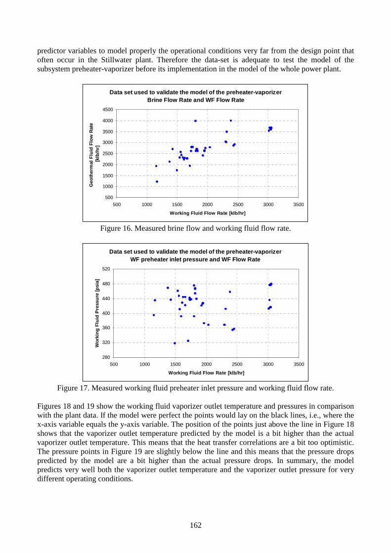
162

predictor variables to model properly the operational conditions very far from the design point that often occur in the Stillwater plant. Therefore the data-set is adequate to test the model of the subsystem preheater-vaporizer before its implementation in the model of the whole power plant.

Data set used to validate the model of the preheate r-vaporizer Brine Flow Rate and WF Flow Rate

500

1000

1500

2000

2500

3000

3500

4000

4500

500 1000 1500 2000 2500 3000 3500

Working Fluid Flow Rate [klb/hr]

Geo

ther

mal

Flu

id F

low

Rat

e [k

lb/h

r]

Figure 16. Measured brine flow and working fluid flow rate.

Data set used to validate the model of the preheate r-vaporizer WF preheater inlet pressure and WF Flow Rate

280

320

360

400

440

480

520

500 1000 1500 2000 2500 3000 3500

Working Fluid Flow Rate [klb/hr]

Wor

king

Flu

id P

ress

ure

[psi

a]

Figure 17. Measured working fluid preheater inlet pressure and working fluid flow rate.

Figures 18 and 19 show the working fluid vaporizer outlet temperature and pressures in comparison with the plant data. If the model were perfect the points would lay on the black lines, i.e., where the x-axis variable equals the y-axis variable. The position of the points just above the line in Figure 18 shows that the vaporizer outlet temperature predicted by the model is a bit higher than the actual vaporizer outlet temperature. This means that the heat transfer correlations are a bit too optimistic. The pressure points in Figure 19 are slightly below the line and this means that the pressure drops predicted by the model are a bit higher than the actual pressure drops. In summary, the model predicts very well both the vaporizer outlet temperature and the vaporizer outlet pressure for very different operating conditions.

163

Working Fluid Temperature at the Outlet of the Vapo rizer Comparison between Plant Data and Simulation Result s

1st Unit, 86°F Ambient Temperature

220

230

240

250

260

270

280

290

300

220 230 240 250 260 270 280 290 300

WF Temperature Outlet Vaporizer [°F]

Plant Data

WF

Tem

pera

ture

Out

let V

apor

izer

[°F

]

Asp

en M

odel

Res

ults

Figure 18: Comparison between the vaporizer outlet temperature predicted by the model and the vaporizer outlet temperature measured in the power plant.

Working Fluid Pressure at the Outlet of the Vaporiz er Comparison between Plant Data and Simulation Result s

1st Unit, 86°F Ambient Temperature

280

300

320

340

360

380

400

420

440

460

480

280 300 320 340 360 380 400 420 440 460 480

WF Pressure Outlet Vaporizer [°F]

Plant Data

WF

Pre

ssur

e O

utle

t Vap

oriz

er [°

F]

Asp

en M

odel

Res

ults

Figure 19: Comparison between the vaporizer outlet pressure predicted by the model and the vaporizer outlet pressure measured in the power plant.

164

7.2.4 Air-Cooled Condenser Modeling

� Air-Cooled Condenser Configuration Stillwater geothermal binary power plant uses a dry cooling system as its heat rejection system. The air cooled condenser (ACC) is composed of 84 bays, i.e., 21 bays for each expander. Each bay has three fans for a total of 63 fan cells serving each expander-generator. The fans, located above the tube bundles, draw air up and across the tubes. This arrangement is called “induced-draft” configuration and offers some advantages against the “forced-draft” configuration. For the latter case, the fans are located below the tube bundle and blow air upwards. Induced-draft operation gives more uniform air flow over the tube bundle and the exit air velocity is several times higher than in forced-draft operation, thereby reducing the potential for hot air to be recirculated back to the intake of the unit or other nearby units. The induced-draft configuration also protects the upper rows of the tube bundle from sun which helps to stabilize the operation of the unit. The plenum chamber above the bundle also acts as a chimney and when the fans are turned off there is a larger air flow compared to a forced draft unit. High-fin tubing is used to compensate for the low air-side heat-transfer coefficient. The fins are embedded and made of aluminum. The main geometric and performance data provided by the manufacturer are shown in Table 4 for one unit of the Stillwater plant (42 bays). Parameter Air Cooled Condenser Finned area [ft2] 5,959,876 Bare area [ft2] 272,140 No. bays (Bundles) per Unit 42 Tube outside diameter [in] 1.25 Tube length [ft] 60 Tube number per Bundle 330 Tube thickness [in] 0.083 Tube pitch [in] 2.75 Tube layout 30° Triangular Tube rows 5 Tube passes 2 Fins outer diameter [in] 2.5 Fins density [No./in] 11 U finned design [Btu/hr-ft2-°F] 3.89 U bare design [Btu/hr-ft2-°F] 85.1

Table 4: Air Cooled Condenser Data from the Manufacturer Specification Sheets. The axial-flow fans employed in the ACC have 4 blades and a diameter of 14 ft. Speed reducers decrease the electric motor rotational speed from 1,750 rpm to a nominal fan speed of 242 rpm. The electric motor power rating is 15 hp. Two-thirds of the fans are equipped with variable frequency drives (VFDs) to vary the speed of the fans. Each VFD powers 21 fans. The design blade pitch angle is 5° and it can be adjusted only manually. The main data provided for the fans and the drivers are shown in Table 5.

165

Parameter ACC Fans and drivers Fans per bay 3 Fan diameter [ft] 14 No. of blades 4 Blade pitch angle 5° Pitch adjustment Manual Fan speed of rotation [rpm] 242 Fan tip speed [ft/min] 10,600 Electric motor speed of rotation [rpm] 1,750 Variable frequency drive Yes ( 2/3 of the Fans ) Electric motor power size [hp] 15

Table 5: Air Cooled Condenser Fans and Drivers Data from the Manufacturer Specification Sheets. � Fan performance curves The fan performance curves provided by the manufacturer, shown in Figure 20, provide more insights into the operation of the fans.

Figure 20. Fan performance curves.

The curves are drawn for the nominal speed of rotation 242 rpm and are referred to an air density of 0.0629 lb/ft3. The x-axis variable is, in both graphs, the air volumetric flow rate drawn by the fan in [ft 3/min]. The upper graph shows the fan shaft power (FSP) in hp, and the lower graph shows the fan total pressure (FTP) in in H2O. The different lines in the graphs refer to different blade pitch angles, from 2° to 22°. Appendix D explains, by means of the velocity triangles, the impact of the blade pitch angle setting on the fan performance curves.

166

The fan total pressure (pT) is defined as the air total pressure increase from the inlet (subscript 1) to the outlet (subscript 2):

12 TTT ppp −= (Eq. 6) The fan shaft power (PFAN) is the power absorbed by the fan measured at the fan shaft and is related to the air volumetric flow rate (qV) and the total pressure by means of the fan total efficiency (ηT):

FAN

TVT P

pq ⋅=η (Eq. 7)

The black dot in both graphs is the design operating point that lies on the 5°-design blade pitch angle line, not drawn in these graphs. At the design point the air flow rate is 138.8 kft3/min, the total pressure is about 0.34 in H2O, and the shaft power is 9.0 hp. The stable operation region is characterized by a negative slope of the total pressure curves; at low flow rates flow instability phenomena occur (stall and surge). In the stable zone the fan shaft power decreases when the air flow increases. Figure 21 shows the fan total efficiencies found for each blade pitch angle using Eq. (7). The total pressure curves are drawn again to show that the total efficiency maximum occurs at flow rates higher than those for the maximum total pressure. The total efficiency peak is higher for low blade pitch angles.

Variation of "Fan Total Efficiency" and "Fan Total Pressure" with Volumetric flow rate - Parameter: Blade Pitch Angle

0.00

0.10

0.20

0.30

0.40

0.50

0.60

0.70

0.80

0.90

1.00

80,000 130,000 180,000 230,000 280,000 330,000 380,000 430,000

Volumetric Flow Rate [ft3/min]

Fan

Tot

al E

ffici

ency

and

F

an T

otal

Pre

ssur

e [in

w]

22° Eff

18° Eff

22° press

18° press

14° Eff

14° press

10° Eff

10° press

6° Eff

6° press

2° Eff

2° press

Op_Point_pr

Op_Point_Eff

Figure 21. Fan total efficiency and fan total pressure.

The design operation point is at a safe distance from the low flow instability region (stall and surge) and it has a quite high total efficiency (about 82%). The upper and lower black dots in Figure 21 show, respectively, the fan total efficiency and the fan total pressure at the design point. The operating strategy is to run the fans at the design speed (242 rpm) during most of the year, and when the ambient temperature is low, to reduce the speed of rotation of the fans equipped with VFD to

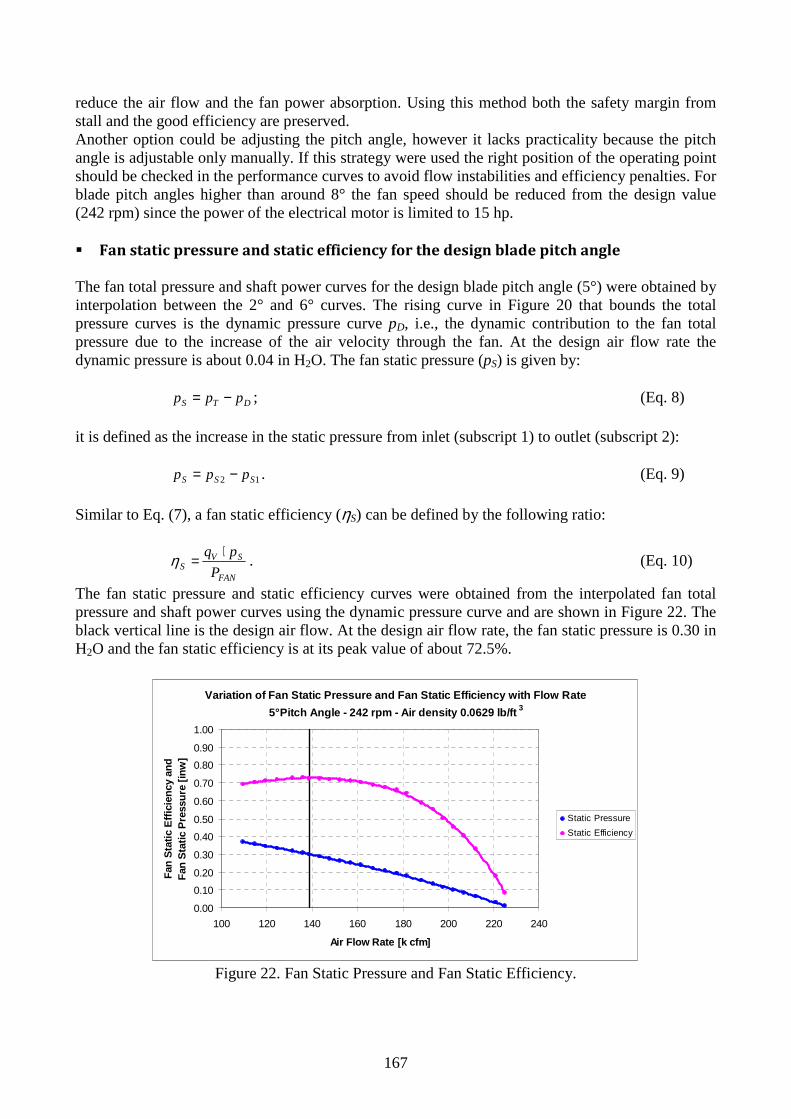
167

reduce the air flow and the fan power absorption. Using this method both the safety margin from stall and the good efficiency are preserved. Another option could be adjusting the pitch angle, however it lacks practicality because the pitch angle is adjustable only manually. If this strategy were used the right position of the operating point should be checked in the performance curves to avoid flow instabilities and efficiency penalties. For blade pitch angles higher than around 8° the fan speed should be reduced from the design value (242 rpm) since the power of the electrical motor is limited to 15 hp. � Fan static pressure and static efficiency for the design blade pitch angle The fan total pressure and shaft power curves for the design blade pitch angle (5°) were obtained by interpolation between the 2° and 6° curves. The rising curve in Figure 20 that bounds the total pressure curves is the dynamic pressure curve pD, i.e., the dynamic contribution to the fan total pressure due to the increase of the air velocity through the fan. At the design air flow rate the dynamic pressure is about 0.04 in H2O. The fan static pressure (pS) is given by:

DTS ppp −= ; (Eq. 8) it is defined as the increase in the static pressure from inlet (subscript 1) to outlet (subscript 2):

12 SSS ppp −= . (Eq. 9) Similar to Eq. (7), a fan static efficiency (ηS) can be defined by the following ratio:

FAN

SVS P

pq ⋅=η . (Eq. 10)

The fan static pressure and static efficiency curves were obtained from the interpolated fan total pressure and shaft power curves using the dynamic pressure curve and are shown in Figure 22. The black vertical line is the design air flow. At the design air flow rate, the fan static pressure is 0.30 in H2O and the fan static efficiency is at its peak value of about 72.5%.

Variation of Fan Static Pressure and Fan Static Eff iciency with Flow Rate

5° Pitch Angle - 242 rpm - Air density 0.0629 lb/ft 3

0.00

0.10

0.20

0.30

0.40

0.50

0.60

0.70

0.80

0.90

1.00

100 120 140 160 180 200 220 240

Air Flow Rate [k cfm]

Fan

Sta

tic E

ffici

ency

and

F

an S

tatic

Pre

ssur

e [in

w]

Static Pressure

Static Efficiency

Figure 22. Fan Static Pressure and Fan Static Efficiency.

168

� Air Flow Resistance Curve found using “Aspen AirCooled” At the operating point the fan static pressure must be equal to the air pressure drop across the bundle of high-finned tubes. In the manufacturer’s ACC data sheet a pressure drop of 0.285 in H2O is reported for the 53°F annual conditions. This value is a bit lower but consistent with the static pressure provided by the fan. In order to obtain the air flow resistance curve, the detailed geometry of the ACC was entered in “Aspen Exchanger Design & Rating” and several simulations were run with different air and working fluid flow rates. The air pressure drop values found were correlated against the air mass flow rate and the air mean density, Figure 23, using the following equation:

AIRm

AIRAIR

mKp

,

2

ρ&

⋅=∆ (11)

with

+⋅=

outinAIRm ρρρ11

2

11

,

. (12)

The air pressure drop found for the design air flow rate was 0.32 in H2O; this value is consistent with but a bit higher than the fan static pressure so the air flow resistance curve was scaled down to match the fan static pressure in correspondence to the design air flow rate.

Air Cooled Condenser - Variation of Air Pressure Dr op with Air mass flow Rate and Air mean density

0.000

0.005

0.010

0.015

0.020

0.025

0.000 0.100 0.200 0.300 0.400 0.500 0.600

Air Mass Flow per Fan [M lb/hr]

∆∆ ∆∆p

* ρρ ρρ

m [i

nw *

lb/ft

3]

Figure 23. Air flow resistance curve.

The manufacturer’s data sheets show three operating conditions for the ACC: the 53.7°F ambient temperature (design condition), the 30°F (winter condition) and the 86°F (summer condition). The air temperature increase across the bundle is in all the three cases around 31°F. The air pressure drop is almost equal in all the three ambient conditions which implies an almost equal air volumetric flow rate given by the intersection with the fan static pressure curve. The air mass flow rate in winter conditions is higher than the air mass flow rate in summer conditions due to the higher air density at lower temperatures. This is shown in the manufacturer’s data sheets using the volumetric air flow rate based on standard conditions (1 atm, 70°F, for which the density is 0.075 lb/ft3). If a pressure drop correlation based only on the air mass flow rate were used, an

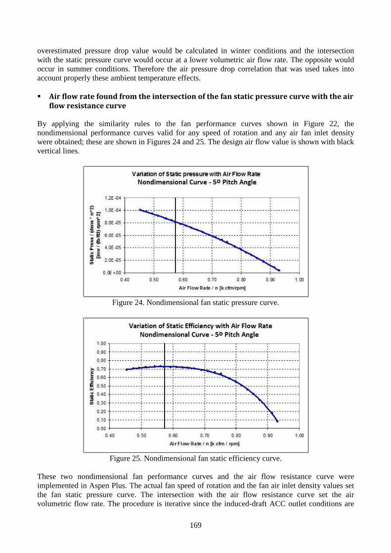
169

overestimated pressure drop value would be calculated in winter conditions and the intersection with the static pressure curve would occur at a lower volumetric air flow rate. The opposite would occur in summer conditions. Therefore the air pressure drop correlation that was used takes into account properly these ambient temperature effects. � Air flow rate found from the intersection of the fan static pressure curve with the air

flow resistance curve By applying the similarity rules to the fan performance curves shown in Figure 22, the nondimensional performance curves valid for any speed of rotation and any air fan inlet density were obtained; these are shown in Figures 24 and 25. The design air flow value is shown with black vertical lines.

Figure 24. Nondimensional fan static pressure curve.

Figure 25. Nondimensional fan static efficiency curve.

These two nondimensional fan performance curves and the air flow resistance curve were implemented in Aspen Plus. The actual fan speed of rotation and the fan air inlet density values set the fan static pressure curve. The intersection with the air flow resistance curve set the air volumetric flow rate. The procedure is iterative since the induced-draft ACC outlet conditions are

170

unknown at the beginning and the air density at the inlet of the fans is required to calculate both the fan static pressure curve and the air flow resistance curve. The fan design air inlet density is 0.0629 lb/ft3, this being the air density value for the design ACC outlet temperature (84.6°F) and the Stillwater site ambient pressure (12.7 psia). Assuming this design fan air inlet density, Figure 26 shows the fan static pressure curves for different speeds of rotation and the intersections with the air flow resistance curve. The blade pitch angle is 5°. Table 6 shows the values of the air flow rate and static pressure at the intersections and the correspondent fan static efficiencies.

Fan Static Pressure and Static Efficiency for diffe rent speeds of rotation

( Air Density = 0.0629 lb/ft 3 - Blade Pitch Angle = 5° )

0.00

0.10

0.20

0.30

0.40

0.50

0.60

0.70

0.80

0 25 50 75 100 125 150 175 200 225 250

Air Flow Rate [k cfm]

Fan

Sta

tic E

ffic

ienc

y an

dF

an S

tatic

Pre

ssur

e [in

w] St Pr 242 rpm

St Pr 210 rpm

St Pr 180 rpm

St Pr 150 rpm

St Pr 120 rpm

St Eff 242 rpm

St Eff 210 rpm

St Eff 180 rpm

St Eff 150 rpm

St Eff 120 rpm

Flow Res Charact

Figure 26. Fan static pressure and static efficiency curves drawn for different speeds of rotation. Intersections with the air flow resistance curve.

Fan Speed Flow Rate Pressure Static Fan Power[rpm] [ft3/min] [inwc] Efficiency [kW]242 138589 0.3014 0.7266 7.49210 118525 0.2307 0.7262 4.91180 99842 0.1728 0.7254 3.10150 81349 0.1228 0.7239 1.80120 63170 0.0809 0.7210 0.92

Table 6. Intersection points between the fan static pressure curves at different speed of rotation and the air flow resistance curve.

The power absorbed by the fan is calculated using the following equation:

motorelredspS

SVFAN

pqP

__

1

ηηη ⋅⋅= (Eq. 13)

where ηsp_red is the efficiency of the speed reducer assumed to be 95% and ηel_motor is the electric motor efficiency, also assumed 95%. The table shows clearly that a reduction of the air flow rate for a factor “x” implies a reduction of the fan absorbed power for a factor of almost “x” raised to the third power as predicted by the similitude rules. Also, the fan static efficiency keeps its good design value for air flow rates very far from the design air flow rates. This power saving is only possible using fans with VFDs.

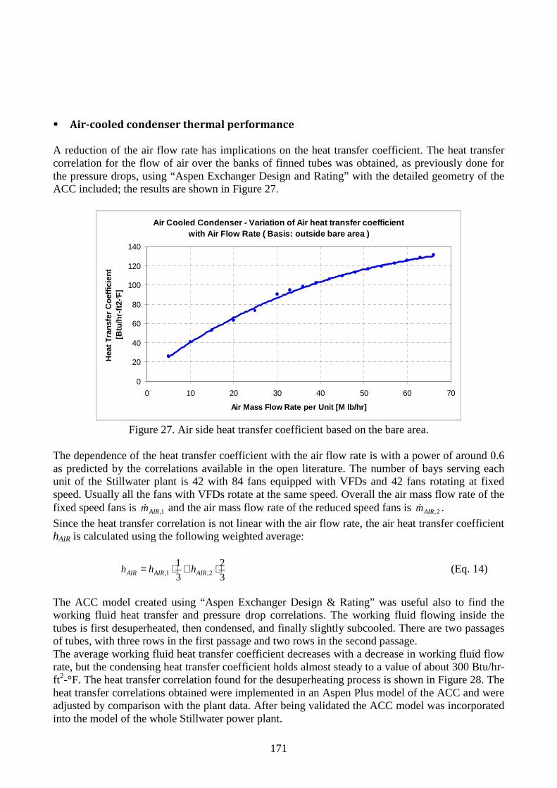
171

� Air-cooled condenser thermal performance A reduction of the air flow rate has implications on the heat transfer coefficient. The heat transfer correlation for the flow of air over the banks of finned tubes was obtained, as previously done for the pressure drops, using “Aspen Exchanger Design and Rating” with the detailed geometry of the ACC included; the results are shown in Figure 27.

Air Cooled Condenser - Variation of Air heat transf er coefficient with Air Flow Rate ( Basis: outside bare area )

0

20

40

60

80

100

120

140

0 10 20 30 40 50 60 70

Air Mass Flow Rate per Unit [M lb/hr]

Hea

t Tra

nsfe

r C

oeffi

cien

t [B

tu/h

r-ft2

-°F]

Figure 27. Air side heat transfer coefficient based on the bare area.

The dependence of the heat transfer coefficient with the air flow rate is with a power of around 0.6 as predicted by the correlations available in the open literature. The number of bays serving each unit of the Stillwater plant is 42 with 84 fans equipped with VFDs and 42 fans rotating at fixed speed. Usually all the fans with VFDs rotate at the same speed. Overall the air mass flow rate of the fixed speed fans is 1,AIRm& and the air mass flow rate of the reduced speed fans is 2,AIRm& .

Since the heat transfer correlation is not linear with the air flow rate, the air heat transfer coefficient hAIR is calculated using the following weighted average:

3

2

3

12,1, ⋅+⋅= AIRAIRAIR hhh (Eq. 14)

The ACC model created using “Aspen Exchanger Design & Rating” was useful also to find the working fluid heat transfer and pressure drop correlations. The working fluid flowing inside the tubes is first desuperheated, then condensed, and finally slightly subcooled. There are two passages of tubes, with three rows in the first passage and two rows in the second passage. The average working fluid heat transfer coefficient decreases with a decrease in working fluid flow rate, but the condensing heat transfer coefficient holds almost steady to a value of about 300 Btu/hr-ft2-°F. The heat transfer correlation found for the desuperheating process is shown in Figure 28. The heat transfer correlations obtained were implemented in an Aspen Plus model of the ACC and were adjusted by comparison with the plant data. After being validated the ACC model was incorporated into the model of the whole Stillwater power plant.

172

Air Cooled Condenser - Variation of the WF vapor he at transfer coefficient with the WF Flow Rate in the desuperhea ting process

0

20

40

60

80

100

120

140

0 500,000 1,000,000 1,500,000 2,000,000 2,500,000 3,000,000 3,500,000

WF Flow Rate [lb/hr]

Hea

t tra

nsfe

r coe

ffic

ient

[B

tu/h

r-ft

2-°F

]

Figure 28: Working fluid desuperheating heat transfer coefficient in the air cooled condenser.

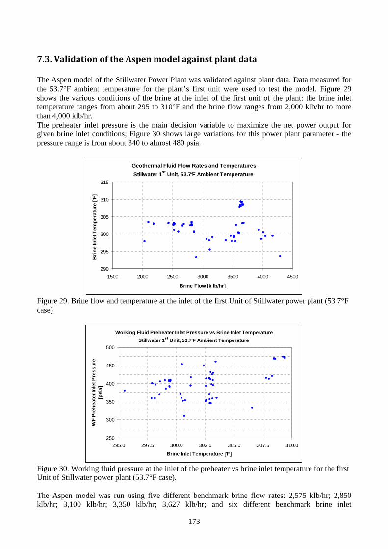
173

7.3. Validation of the Aspen model against plant data

The Aspen model of the Stillwater Power Plant was validated against plant data. Data measured for the 53.7°F ambient temperature for the plant’s first unit were used to test the model. Figure 29 shows the various conditions of the brine at the inlet of the first unit of the plant: the brine inlet temperature ranges from about 295 to 310°F and the brine flow ranges from 2,000 klb/hr to more than 4,000 klb/hr. The preheater inlet pressure is the main decision variable to maximize the net power output for given brine inlet conditions; Figure 30 shows large variations for this power plant parameter - the pressure range is from about 340 to almost 480 psia.

Geothermal Fluid Flow Rates and Temperatures

Stillwater 1 st Unit, 53.7°F Ambient Temperature

290

295

300

305

310

315

1500 2000 2500 3000 3500 4000 4500

Brine Flow [k lb/hr]

Brin

e In

let T

empe

ratu

re [°

F]

Figure 29. Brine flow and temperature at the inlet of the first Unit of Stillwater power plant (53.7°F case)

Working Fluid Preheater Inlet Pressure vs Brine Inl et Temperature

Stillwater 1 st Unit, 53.7°F Ambient Temperature

250

300

350

400

450

500

295.0 297.5 300.0 302.5 305.0 307.5 310.0

Brine Inlet Temperature [°F]

WF

Pre

heat

er In

let P

ress

ure

[psi

a]

Figure 30. Working fluid pressure at the inlet of the preheater vs brine inlet temperature for the first Unit of Stillwater power plant (53.7°F case). The Aspen model was run using five different benchmark brine flow rates: 2,575 klb/hr; 2,850 klb/hr; 3,100 klb/hr; 3,350 klb/hr; 3,627 klb/hr; and six different benchmark brine inlet

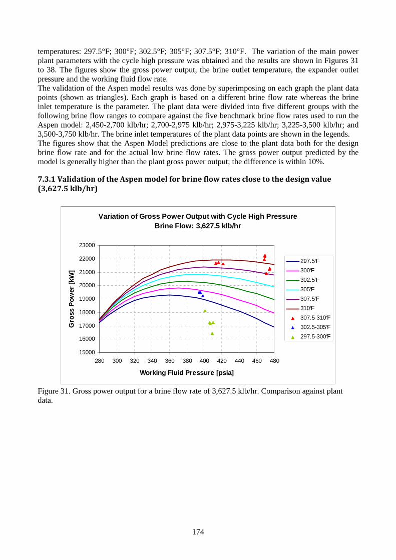
174

temperatures: 297.5°F; 300°F; 302.5°F; 305°F; 307.5°F; 310°F. The variation of the main power plant parameters with the cycle high pressure was obtained and the results are shown in Figures 31 to 38. The figures show the gross power output, the brine outlet temperature, the expander outlet pressure and the working fluid flow rate. The validation of the Aspen model results was done by superimposing on each graph the plant data points (shown as triangles). Each graph is based on a different brine flow rate whereas the brine inlet temperature is the parameter. The plant data were divided into five different groups with the following brine flow ranges to compare against the five benchmark brine flow rates used to run the Aspen model: 2,450-2,700 klb/hr; 2,700-2,975 klb/hr; 2,975-3,225 klb/hr; 3,225-3,500 klb/hr; and 3,500-3,750 klb/hr. The brine inlet temperatures of the plant data points are shown in the legends. The figures show that the Aspen Model predictions are close to the plant data both for the design brine flow rate and for the actual low brine flow rates. The gross power output predicted by the model is generally higher than the plant gross power output; the difference is within 10%.

7.3.1 Validation of the Aspen model for brine flow rates close to the design value

(3,627.5 klb/hr)

Variation of Gross Power Output with Cycle High Pre ssureBrine Flow: 3,627.5 klb/hr

15000

16000

17000

18000

19000

20000

21000

22000

23000

280 300 320 340 360 380 400 420 440 460 480

Working Fluid Pressure [psia]

Gro

ss P

ower

[kW

]

297.5°F

300°F

302.5°F

305°F

307.5°F

310°F

307.5-310°F

302.5-305°F

297.5-300°F

Figure 31. Gross power output for a brine flow rate of 3,627.5 klb/hr. Comparison against plant data.

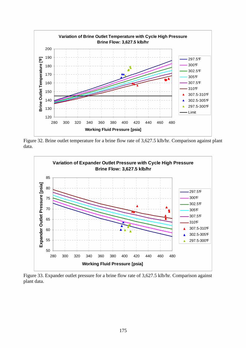
175

Variation of Brine Outlet Temperature with Cycle Hi gh PressureBrine Flow: 3,627.5 klb/hr

120

130

140

150

160

170

180

190

200

280 300 320 340 360 380 400 420 440 460 480

Working Fluid Pressure [psia]

Brin

e O

utle

t Tem

pera

ture

[°F]

297.5°F

300°F

302.5°F

305°F

307.5°F

310°F

307.5-310°F

302.5-305°F

297.5-300°F

Limit

Figure 32. Brine outlet temperature for a brine flow rate of 3,627.5 klb/hr. Comparison against plant data.

Variation of Expander Outlet Pressure with Cycle Hi gh Pressure Brine Flow: 3,627.5 klb/hr

50

55

60

65

70

75

80

85

280 300 320 340 360 380 400 420 440 460 480

Working Fluid Pressure [psia]

Exp

ande

r O

utle

t Pre

ssur

e [p

sia]

297.5°F

300°F

302.5°F

305°F

307.5°F

310°F

307.5-310°F

302.5-305°F

297.5-300°F

Figure 33. Expander outlet pressure for a brine flow rate of 3,627.5 klb/hr. Comparison against plant data.

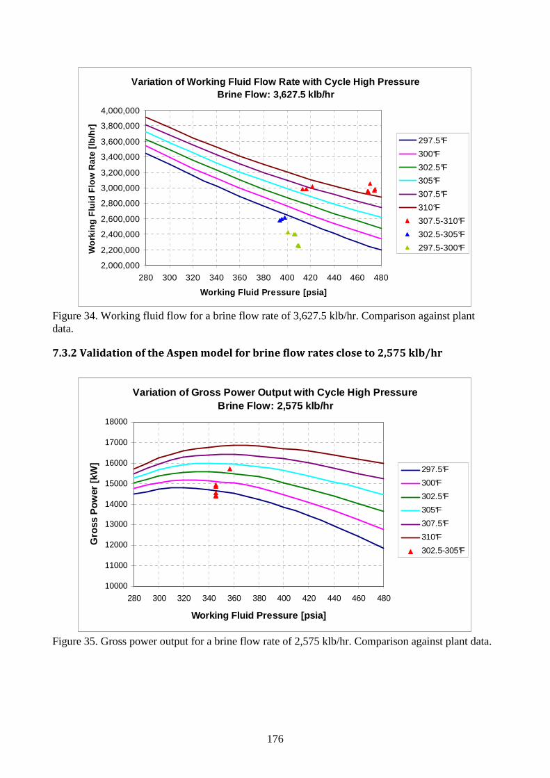
176

Variation of Working Fluid Flow Rate with Cycle Hig h PressureBrine Flow: 3,627.5 klb/hr

2,000,000

2,200,000

2,400,000

2,600,000

2,800,000

3,000,000

3,200,000

3,400,000

3,600,000

3,800,000

4,000,000

280 300 320 340 360 380 400 420 440 460 480

Working Fluid Pressure [psia]

Wor

king

Flu

id F

low

Rat

e [lb

/hr] 297.5°F

300°F

302.5°F

305°F

307.5°F

310°F

307.5-310°F

302.5-305°F

297.5-300°F

Figure 34. Working fluid flow for a brine flow rate of 3,627.5 klb/hr. Comparison against plant data.

7.3.2 Validation of the Aspen model for brine flow rates close to 2,575 klb/hr

Variation of Gross Power Output with Cycle High Pre ssureBrine Flow: 2,575 klb/hr

10000

11000

12000

13000

14000

15000

16000

17000

18000

280 300 320 340 360 380 400 420 440 460 480

Working Fluid Pressure [psia]

Gro

ss P

ower

[kW

] 297.5°F

300°F

302.5°F

305°F

307.5°F

310°F

302.5-305°F

Figure 35. Gross power output for a brine flow rate of 2,575 klb/hr. Comparison against plant data.

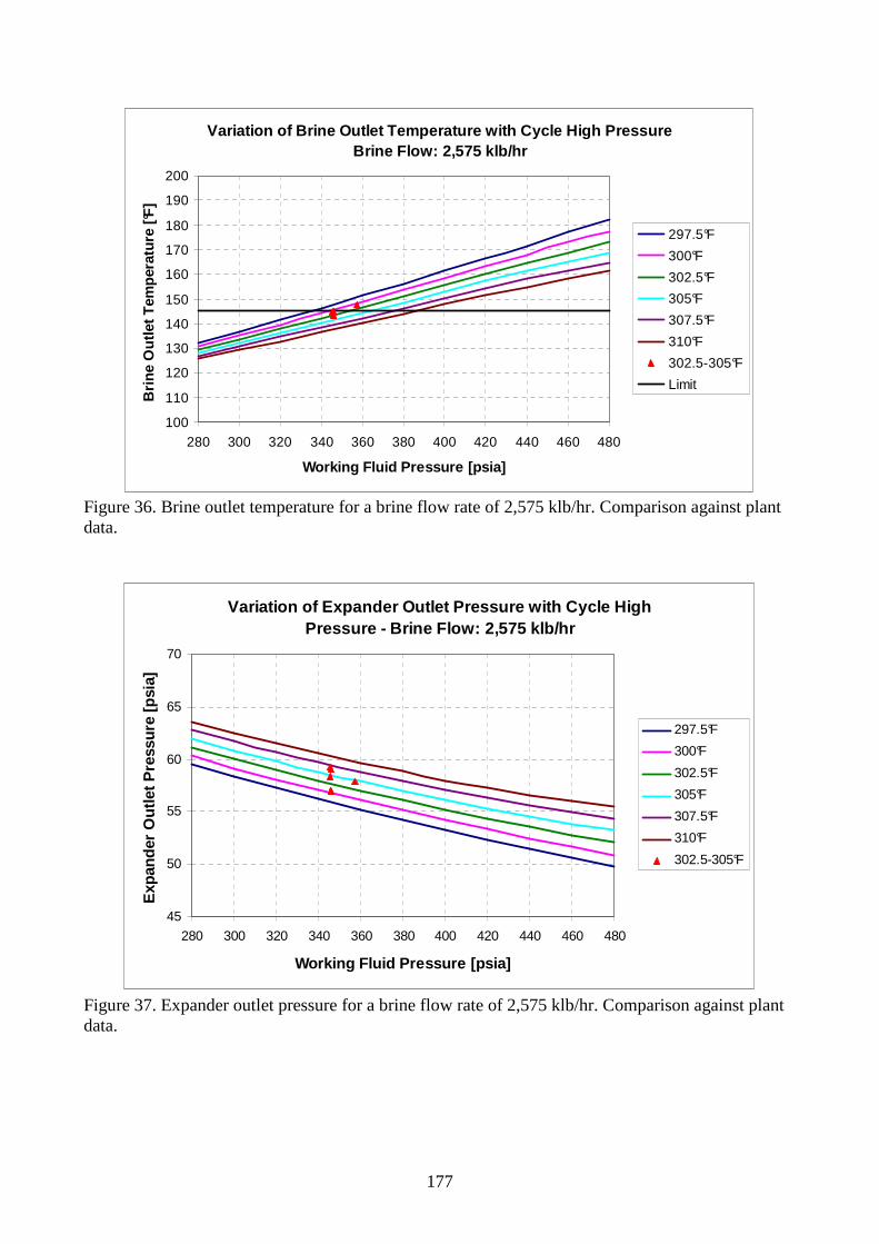
177

Variation of Brine Outlet Temperature with Cycle Hi gh PressureBrine Flow: 2,575 klb/hr

100

110

120

130

140

150

160

170

180

190

200

280 300 320 340 360 380 400 420 440 460 480

Working Fluid Pressure [psia]

Brin

e O

utle

t Tem

pera

ture

[°F

]

297.5°F

300°F

302.5°F

305°F

307.5°F

310°F

302.5-305°F

Limit

Figure 36. Brine outlet temperature for a brine flow rate of 2,575 klb/hr. Comparison against plant data.

Variation of Expander Outlet Pressure with Cycle Hi gh Pressure - Brine Flow: 2,575 klb/hr

45

50

55

60

65

70

280 300 320 340 360 380 400 420 440 460 480

Working Fluid Pressure [psia]

Exp

ande

r O

utle

t Pre

ssur

e [p

sia]

297.5°F

300°F

302.5°F

305°F

307.5°F

310°F

302.5-305°F

Figure 37. Expander outlet pressure for a brine flow rate of 2,575 klb/hr. Comparison against plant data.

178

Variation of Working Fluid Flow Rate with Cycle High PressureBrine Flow: 2,575 klb/hr

1,000,000

1,200,000

1,400,000

1,600,000

1,800,000

2,000,000

2,200,000

2,400,000

2,600,000

2,800,000

3,000,000

280 300 320 340 360 380 400 420 440 460 480

Working Fluid Pressure [psia]

Wor

king

Flu

id F

low

Rat

e [lb

/hr]

297.5°F

300°F

302.5°F

305°F

307.5°F

310°F

302.5-305°F

Figure 38. Working fluid flow for a brine flow rate of 2,575 klb/hr. Comparison against plant data.

179

7.4 Stillwater brine distribution strategy and annual energy production

7.4.1 Brine distribution strategy

The design geothermal fluid flow rate for Stillwater is 7,255 klb/hr. At the design conditions each unit receives a brine flow of 3,627.5 klb/hr at a temperature of 310°F. The actual conditions for the geothermal resources in Stillwater are much different: on average the brine flow is only 5,150 klb/hr (that is 71% of the design value) at a temperature of 297.5°F (12.5°F lower than the design brine inlet temperature). The working fluid flow rate that can be evaporated using these limited geothermal resources is lower than the design value, and the thermodynamic cycle parameters, mainly the cycle high pressure, are different. There is also an additional effect related to plant components’ performance. The expander isentropic efficiency is dependent on the working fluid flow rate and other cycle parameters, and the heat exchangers’ overall heat transfer coefficients decrease with a decrease of the flow rates. For these reasons the net power produced by the power plant is much lower than the design value of 33.6 MW predicted by Power Engineers for the design conditions. Using the Aspen Model of the Stillwater Power Plant, the net power output produced can be maximized by finding the optimal cycle parameters to harness the available geothermal resources. The expanders’ isentropic efficiency values are important in this analysis since the expanders are operating far from their design conditions. Thanks to the modular design of the Stillwater plant, there is an additional degree of freedom: by turning off one of the four expanders, the remaining three expanders can operate with working fluid flow rates closer to the design flow rates. This can be done by dividing the brine flow asymmetrically between the two units; See Figures 39-40.

Figure 39. The brine flow distribution between the two units of the Stillwater Power Plant.

Three benchmark brine flow distribution strategies were selected: A) Configuration A: Unit 1 receives 3,627.5 klb/hr to be consistent with the original design flow. Both turbines are used in Unit 1. Unit 2 receives the remaining 1,522.5 klb/hr and uses only one turbine. B) Configuration B: Unit 1 receives 3,433 klb/hr which is two-thirds of the total brine flow. Both turbines are used in Unit 1. Unit 2 receives the remaining 1,717 klb/hr of brine and uses only one turbine.

Brine Flow Total

Brine Flow Unit 1

Brine Flow Unit 2

WF Flow 1

T1 T2

WF Flow 2

T3 T4

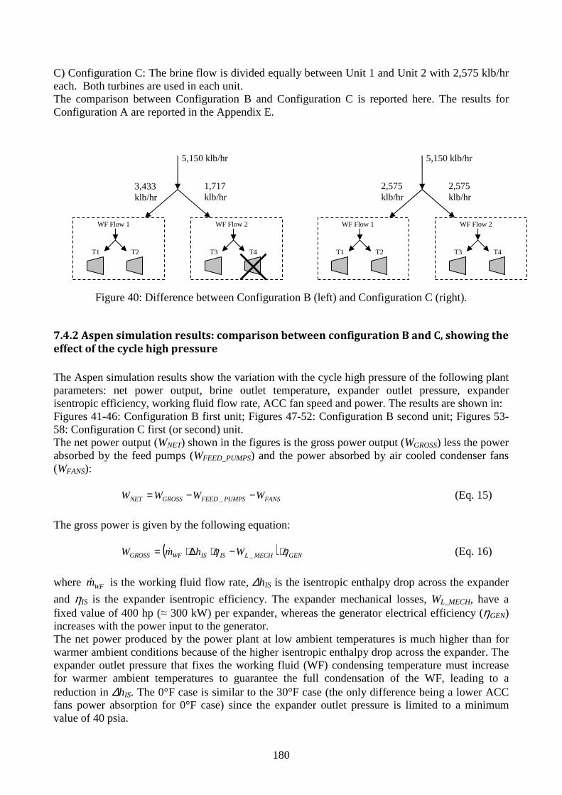
180

C) Configuration C: The brine flow is divided equally between Unit 1 and Unit 2 with 2,575 klb/hr each. Both turbines are used in each unit. The comparison between Configuration B and Configuration C is reported here. The results for Configuration A are reported in the Appendix E.

Figure 40: Difference between Configuration B (left) and Configuration C (right).

7.4.2 Aspen simulation results: comparison between configuration B and C, showing the

effect of the cycle high pressure

The Aspen simulation results show the variation with the cycle high pressure of the following plant parameters: net power output, brine outlet temperature, expander outlet pressure, expander isentropic efficiency, working fluid flow rate, ACC fan speed and power. The results are shown in: Figures 41-46: Configuration B first unit; Figures 47-52: Configuration B second unit; Figures 53-58: Configuration C first (or second) unit. The net power output (WNET) shown in the figures is the gross power output (WGROSS) less the power absorbed by the feed pumps (WFEED_PUMPS) and the power absorbed by air cooled condenser fans (WFANS):

FANSPUMPSFEEDGROSSNET WWWW −−= _ (Eq. 15)

The gross power is given by the following equation:

( ) GENMECHLISISWFGROSS WhmW ηη ⋅−⋅∆⋅= _& (Eq. 16)

where WFm& is the working fluid flow rate, ∆hIS is the isentropic enthalpy drop across the expander

and ηIS is the expander isentropic efficiency. The expander mechanical losses, WL_MECH, have a fixed value of 400 hp (≈ 300 kW) per expander, whereas the generator electrical efficiency (ηGEN) increases with the power input to the generator. The net power produced by the power plant at low ambient temperatures is much higher than for warmer ambient conditions because of the higher isentropic enthalpy drop across the expander. The expander outlet pressure that fixes the working fluid (WF) condensing temperature must increase for warmer ambient temperatures to guarantee the full condensation of the WF, leading to a reduction in ∆hIS. The 0°F case is similar to the 30°F case (the only difference being a lower ACC fans power absorption for 0°F case) since the expander outlet pressure is limited to a minimum value of 40 psia.

5,150 klb/hr

2,575 klb/hr

2,575 klb/hr

WF Flow 1

T1 T2

WF Flow 2

T3 T4

5,150 klb/hr

3,433 klb/hr

1,717 klb/hr

WF Flow 1

T1 T2

WF Flow 2

T3 T4

181

For each ambient temperature the net power output maximum corresponds to an optimal preheater inlet pressure. Since the two parasitic loads in the definition of the net power have values much lower than the gross power output, the effect of the cycle high pressure on the working fluid flow rate, expander isentropic enthalpy drop and isentropic efficiency are sufficient to explain the variation of the net power with the cycle high pressure. 1) Working Fluid Flow Rate For each cycle high pressure the WF flow rate is the same for all the ambient temperature cases since, with the assumed operational strategy of 5°F of superheat at the outlet of the vaporizer, the WF flow rate is determined by the heat available from the brine above the pinch point. When the WF cycle high pressure (and saturation temperature) decreases, the heat available from the brine above the pinch point increases, and despite the increase of the WF heat of vaporization at lower pressures, more working fluid can be evaporated. This is summarized as:

WFWF cycle high pressure m↓⇒ ↑&

2) Isentropic Enthalpy Drop By reducing the WF pressure, the resulting higher WF flow rate implies a higher condensing heat load on the ACC and, even if the overall heat transfer coefficient U in the ACC may increase slightly, the mean temperature difference between the air and the condensing WF must increase, i.e., the expander outlet pressure must rise. This effect combined with the decrease of the cycle high pressure implies that:

ISWF cycle high pressure h↓⇒ ∆ ↓

3) Expander Isentropic Efficiency The expander isentropic efficiency is correlated with both the ∆hIS and the volumetric flow rate at the expander outlet OUTV& using the following equation:

( ) ( )OUTISdesignISactualIS Vfhf &21,, ⋅∆⋅=ηη

- The design value of ∆hIS (24.4 Btu/lb) is low compared to the isentropic enthalpy drops found during the year for Stillwater expanders and it is close to the values found for the 86°F ambient temperature case. This means that a reduction of the cycle high pressure implies, for all the cases except the 86°F case, an increase of the efficiency correction factor f1 due to enthalpy:

( )1 ISWF cycle high pressure f h↓⇒ ∆ ↑

- The WF volumetric flow rate at the expander outlet is defined by the following equation:

OUT

WFOUT

mV

ρ&& =

The expander outlet pressure and density are higher for the warmer ambient temperatures and this implies that, for the same WF mass flow rate WFm& , OUTV& is higher when the ambient temperature is

low. The design value of OUTV& (40,000 ft3/min per expander) is obtained for the design WF mass flow rate (around 3,100 klb/hr per unit) and the design expander outlet pressure. The WF mass flow rates

182

of Scenario B are a bit lower than the design value but the WF mass flow rates of Scenario C are much lower than the design value. This means that the reduction of the cycle high pressure with the resulting increase of the WF mass flow rate is always beneficial to the increase of ηIS for Scenario C, but could be detrimental for Scenario B with low ambient temperatures, as shown below:

The resultant ηIS is given by the product of the two correction factors f1 and f2 but there is a clear result for Scenario C in that for almost all the ambient temperatures (except the highest annual temperatures):

ISWF cycle high pressure η↓⇒ ↑

Summarizing, a decrease of the cycle high pressure on the one hand is beneficial because it increases WFm& but on the other hand is detrimental because it lowers ∆hIS. The low expander design

value for ∆hIS promotes low ∆hIS and the relatively high expander design value of OUTV& promotes

higher WFm& . That is, the use of the expander performance calculator combined with the presence of

lower than design WF flow rates moves the maximum net power output to lower cycle high pressures. Lower cycle high pressures (associated with higher WF mass flow rates) involve lower brine outlet temperatures and a fuller utilization of the heat available from the brine. However the brine outlet temperature must be held above 145°F to avoid silica scaling problems. For low and moderate ambient temperatures the cycle high pressure must be raised from its optimal value (the value that maximizes the net power output) to keep the brine outlet temperature above 145°F. In the figures that follow, large dots show the selected cycle high pressures. At 86°F the selected cycle high pressures are the pressures that correspond to the net power output peak. At 53.7°F the selected operating points are very close to the net power output peak, but at lower ambient temperatures, 30°F and 0°F, the selected pressures are quite far from the optimal values. The net power output curves are flatter when the WF mass flow rate is higher; this implies that the reduction of net power output in moving from the “unconstrained” optimal pressure to the “constrained” optimal pressure is higher for Scenario C than for Scenario B.

High WFm&

(Scenario B)

f2 ( OUTV& ) ↑ when Tamb is warm

f2 ( OUTV& ) ↓ when Tamb is low

f2 ( OUTV& ) ↑ always

Low WFm&

(Scenario C)

WF cycle high pressure ↓

183

� Aspen Simulation Results: Configuration B, First Unit

Variation of Net Power with Cycle High Pressure - S c. B 1 st UnitBrine Flow: 3,433 klb/hr, Brine Temperature: 297.5° F

0

2000

4000

6000

8000

10000

12000

14000

16000

18000

20000

22000

280 300 320 340 360 380 400 420 440 460 480

Working Fluid Pressure [psia]

Net

Pow

er [k

W]

53.7°F

86°F

30°F

0°F

Figure 41. Net Power Output for the First Unit of Configuration B.

Variation of Brine Outlet Temperature with Cycle Hi gh Pressure

Sc. B 1 st Unit - Brine Flow: 3,433 klb/hr, Brine Temperature : 297.5°F

100

120

140

160

180

200

220

280 300 320 340 360 380 400 420 440 460 480

Working Fluid Pressure [psia]

Brin

e O

utle

t Tem

pera

ture

[°F]

53.7°F

86°F

30°F

0°F

Limit

Figure 42. Brine Outlet Temperature for the First Unit of Configuration B.

184

Variation of Expander Outlet Pressure with Cycle Hi gh Pressure

Sc. B 1 st Unit - Brine Flow: 3,433 klb/hr, Brine Temperature : 297.5°F

30

40

50

60

70

80

90

100

110

120

280 300 320 340 360 380 400 420 440 460 480

Working Fluid Pressure [psia]

Exp

ande

r Out

let P

ress

ure

[psi

a]

53.7°F

86°F

30°F

0°F

Figure 43. Expander Outlet Pressure for the First Unit of Configuration B.

Variation of Expander Isentropic Efficiency with Cy cle High Pressure

Sc. B 1 st Unit - Brine Flow: 3,433 klb/hr, Brine Temperature : 297.5°F

0.60

0.64

0.68

0.72

0.76

0.80

0.84

0.88

280 300 320 340 360 380 400 420 440 460 480

Working Fluid Pressure [psia]

Isen

trop

ic E

ffic

ienc

y

53.7°F

86°F

30°F

0°F

Figure 44. Expander Isentropic Efficiency for the First Unit of Configuration B.

185

Variation of Working Fluid Flow Rate with Cycle Hig h Pressure

Sc. B 1 st Unit - Brine Flow: 3,433 klb/hr, Brine Temperature : 297.5°F

1,400,000

1,600,000

1,800,000

2,000,000

2,200,000

2,400,000

2,600,000

2,800,000

3,000,000

3,200,000

3,400,000

280 300 320 340 360 380 400 420 440 460 480

Working Fluid Pressure [psia]

Wor

king

Flu

id F

low

Rat

e [lb

/hr]

53.7°F

86°F

30°F

0°F

Figure 45. Working fluid flow rate for the First Unit of Configuration B.

Variation of Fan Speed and Fan Power with WF Pressu re

Sc. B 1 st Unit Brine Flow: 3,433 klb/hr, Brine Temperature: 297.5° F

( 0°F Only Fans with VFDs )

0

100

200

300

400

500

600

700

800

900

1000

1100

1200

280 300 320 340 360 380 400 420 440 460 480

Working Fluid Pressure [psia]

Fan

Spe

ed [r

pm] a

nd

Fan

Pow

er [k

W] 30°F Speed

30°F Power

0°F Speed

0°F Power

Figure 46. Fans Speed and Fans Power for the First Unit of Configuration B.

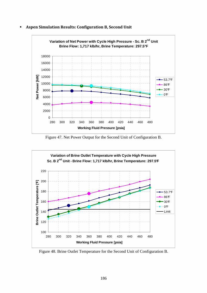
186

� Aspen Simulation Results: Configuration B, Second Unit

Variation of Net Power with Cycle High Pressure - S c. B 2 nd UnitBrine Flow: 1,717 klb/hr, Brine Temperature: 297.5° F

0

2000

4000

6000

8000

10000

12000

14000

16000

18000

280 300 320 340 360 380 400 420 440 460 480

Working Fluid Pressure [psia]

Net

Pow

er [k

W]

53.7°F

86°F

30°F

0°F

Figure 47. Net Power Output for the Second Unit of Configuration B.

Variation of Brine Outlet Temperature with Cycle High Pr essure

Sc. B 2nd Unit - Brine Flow: 1,717 klb/hr, Brine Temperature: 29 7.5°F

100

120

140

160

180

200

220

280 300 320 340 360 380 400 420 440 460 480

Working Fluid Pressure [psia]

Brin

e O

utle

t Tem

pera

ture

[°F

]

53.7°F

86°F

30°F

0°F

Limit

Figure 48. Brine Outlet Temperature for the Second Unit of Configuration B.

187

Variation of Expander Outlet Pressure with Cycle Hi gh Pressure

Sc. B 2nd Unit - Brine Flow: 1,717 klb/hr, Brine Temperature : 297.5°F

30

40

50

60

70

80

90

100

110

120

280 300 320 340 360 380 400 420 440 460 480

Working Fluid Pressure [psia]

Exp

ande

r Out

let P

ress

ure

[psi

a]

53.7°F

86°F

30°F

0°F

Figure 49. Expander Outlet Pressure for the Second Unit of Configuration B.

Variation of Expander Isentropic Efficiency with Cy cle High Pressure

Sc. B 2 nd Unit - Brine Flow: 1,717 klb/hr, Brine Temperature : 297.5°F

0.60

0.64

0.68

0.72

0.76

0.80

0.84

0.88

280 300 320 340 360 380 400 420 440 460 480

Working Fluid Pressure [psia]

Isen

tro

pic

Eff

icie

ncy

53.7°F

86°F

30°F

0°F

Figure 50. Expander Isentropic Efficiency for the Second Unit of Configuration B.

188

Variation of Working Fluid Flow Rate with Cycle Hig h Pressure

Sc. B 2 nd Unit - Brine Flow: 1,717 klb/hr, Brine Temperature : 297.5°F

800,000

1,000,000

1,200,000

1,400,000

1,600,000

1,800,000

2,000,000

2,200,000

2,400,000

2,600,000

280 300 320 340 360 380 400 420 440 460 480

Working Fluid Pressure [psia]

Wor

king

Flu

id F

low

Rat

e [lb

/hr]

53.7°F

86°F

30°F

0°F

Figure 51. Working fluid flow rate for the Second Unit of Configuration B.

Variation of Fan Speed and Fan Power with WF Pressu reBrine Flow: 1,717 klb/hr, Brine Temperature: 297.5° F

Sc. B 2nd Unit( 0°F Only Fans with VFDs )

0

100

200

300

400

500

600

700

800

900

1000

1100

280 300 320 340 360 380 400 420 440 460 480

Working Fluid Pressure [psia]

Fan

Spe

ed [r

pm] a

nd

Fan

Pow

er [k

W] 30°F Speed

30°F Power

0°F Speed

0°F Power

Figure 52. Fans Speed and Fans Power for the Second Unit of Configuration B.

189

� Aspen Simulation Results: Configuration C, First Unit (or Second Unit)

Variation of Net Power with Cycle High Pressure - S c. C 1st UnitBrine Flow: 2,575 klb/hr, Brine Temperature: 297.5° F

0

2000

4000

6000

8000

10000

12000

14000

16000

18000

20000

22000

280 300 320 340 360 380 400 420 440 460 480

Working Fluid Pressure [psia]

Net

Pow

er [k

W]

53.7°F

86°F

30°F

0°F

Figure 53. Net Power Output for one Unit of Configuration C.

Variation of Brine Outlet Temperature with Cycle Hi gh Pressure

Sc. C 1st Unit - Brine Flow: 2,575 klb/hr, Brine Temperature : 297.5°F

100

120

140

160

180

200

220

280 300 320 340 360 380 400 420 440 460 480

Working Fluid Pressure [psia]

Brin

e O

utle

t Tem

pera

ture

[°F

]

53.7°F

86°F

30°F

0°F

Limit

Figure 54. Brine Outlet Temperature for one Unit of Configuration C.

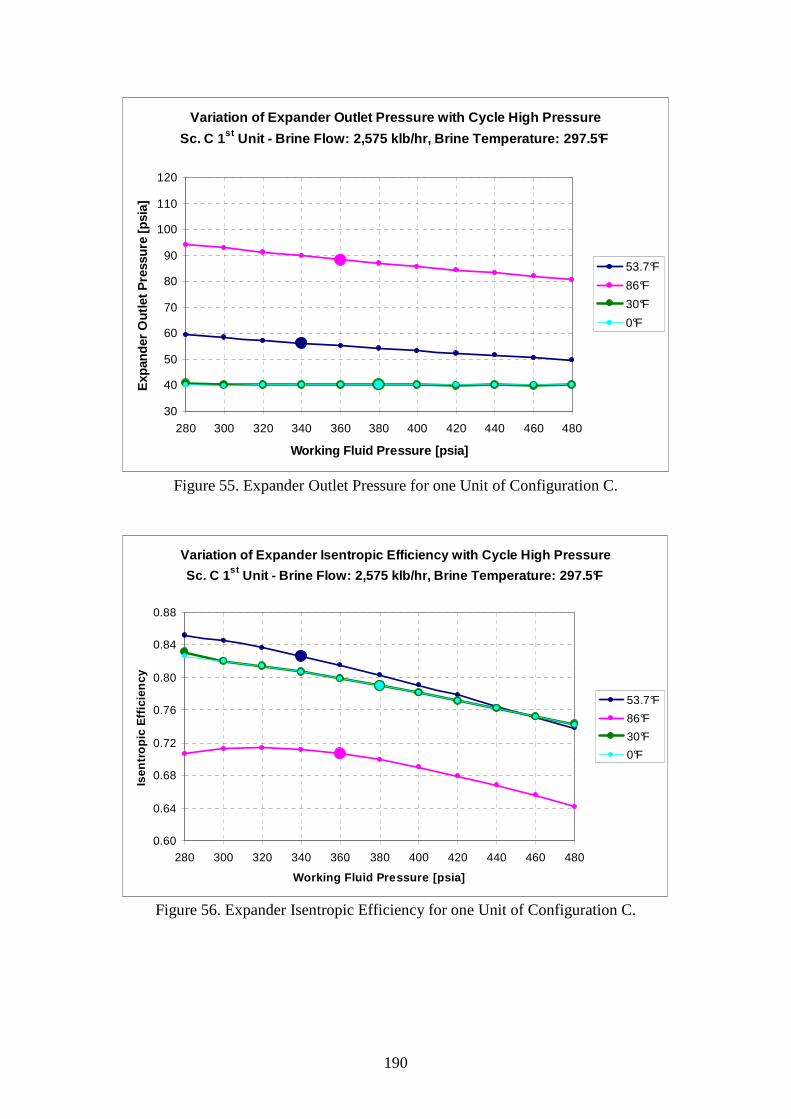
190

Variation of Expander Outlet Pressure with Cycle Hi gh Pressure

Sc. C 1st Unit - Brine Flow: 2,575 klb/hr, Brine Temperature : 297.5°F

30

40

50

60

70

80

90

100

110

120

280 300 320 340 360 380 400 420 440 460 480

Working Fluid Pressure [psia]

Exp

ande

r O

utle

t Pre

ssur

e [p

sia]

53.7°F

86°F

30°F

0°F

Figure 55. Expander Outlet Pressure for one Unit of Configuration C.

Variation of Expander Isentropic Efficiency with Cy cle High Pressure

Sc. C 1st Unit - Brine Flow: 2,575 klb/hr, Brine Temperature : 297.5°F

0.60

0.64

0.68

0.72

0.76

0.80

0.84

0.88

280 300 320 340 360 380 400 420 440 460 480

Working Fluid Pressure [psia]

Isen

trop

ic E

ffic

ienc

y

53.7°F

86°F

30°F

0°F

Figure 56. Expander Isentropic Efficiency for one Unit of Configuration C.

191

Variation of Working Fluid Flow Rate with Cycle Hig h Pressure

Sc. C 1st Unit - Brine Flow: 2,575 klb/hr, Brine Temperature : 297.5°F

1,400,000

1,600,000

1,800,000

2,000,000

2,200,000

2,400,000

2,600,000

2,800,000

3,000,000

3,200,000

3,400,000

280 300 320 340 360 380 400 420 440 460 480

Working Fluid Pressure [psia]

Wor

king

Flu

id F

low

Rat

e [lb

/hr]

53.7°F

86°F

30°F

0°F

Figure 57. Working fluid flow rate for one Unit of Configuration C.

Variation of Fan Speed and Fan Power with WF Pressure

Sc. C 1st UnitBrine Flow: 2,575 klb/hr, Brine Temperature: 297.5°F

( 0°F Only Fans with VFDs )

0

100

200

300

400

500

600

700

800

900

1000

1100

1200

280 300 320 340 360 380 400 420 440 460 480

Working Fluid Pressure [psia]

Fan

Spe

ed [r

pm] a

nd

Fan

Pow

er [k

W] 30°F Speed

30°F Power

0°F Speed

0°F Power

Figure 58. Fans Speed and Fans Power for one Unit of Configuration C.

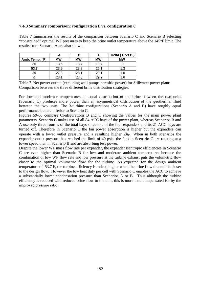
192

7.4.3 Summary comparison: configuration B vs. configuration C

Table 7 summarizes the results of the comparison between Scenario C and Scenario B selecting “constrained” optimal WF pressures to keep the brine outlet temperature above the 145°F limit. The results from Scenario A are also shown. Table 7. Net power output (excluding well pumps parasitic power) for Stillwater power plant: Comparison between the three different brine distribution strategies. For low and moderate temperatures an equal distribution of the brine between the two units (Scenario C) produces more power than an asymmetrical distribution of the geothermal fluid between the two units. The 3-turbine configurations (Scenario A and B) have roughly equal performance but are inferior to Scenario C. Figures 59-66 compare Configurations B and C showing the values for the main power plant parameters. Scenario C makes use of all 84 ACC bays of the power plant, whereas Scenarios B and A use only three-fourths of the total bays since one of the four expanders and its 21 ACC bays are turned off. Therefore in Scenario C the fan power absorption is higher but the expanders can operate with a lower outlet pressure and a resulting higher ∆hIS. When in both scenarios the expander outlet pressure has reached the limit of 40 psia, the fans in Scenario C are rotating at a lower speed than in Scenario B and are absorbing less power. Despite the lower WF mass flow rate per expander, the expander isentropic efficiencies in Scenario C are even higher than Scenario B for low and moderate ambient temperatures because the combination of low WF flow rate and low pressure at the turbine exhaust puts the volumetric flow closer to the optimal volumetric flow for the turbine. As expected for the design ambient temperature of 53.7 F, the turbine efficiency is indeed higher when the brine flow to a unit is closer to the design flow. However the low heat duty per cell with Scenario C enables the ACC to achieve a substantially lower condensation pressure than Scenarios A or B. Thus although the turbine efficiency is reduced with reduced brine flow to the unit, this is more than compensated for by the improved pressure ratio.

A B C Delta ( C vs B )Amb. Temp. [°F] MW MW MW MW

86 13.6 13.7 13.7 053.7 23.9 23.8 25.1 1.330 27.8 28.1 29.1 1.00 28.1 28.3 29.9 1.6

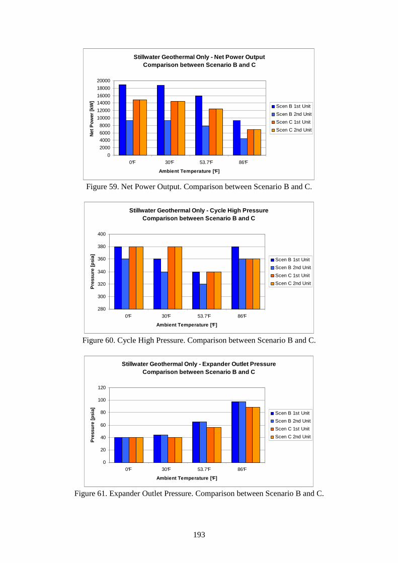
193

Stillwater Geothermal Only - Net Power Output Comparison between Scenario B and C

0

2000

4000

6000

8000

10000

12000

14000

16000

18000

20000

0°F 30°F 53.7°F 86°F

Ambient Temperature [°F]

Net

Pow

er [k

W]

Scen B 1st Unit

Scen B 2nd Unit

Scen C 1st Unit

Scen C 2nd Unit

Figure 59. Net Power Output. Comparison between Scenario B and C.

Stillwater Geothermal Only - Cycle High Pressure Comparison between Scenario B and C

280

300

320

340

360

380

400

0°F 30°F 53.7°F 86°F

Ambient Temperature [°F]

Pre

ssur

e [p

sia] Scen B 1st Unit

Scen B 2nd Unit

Scen C 1st Unit

Scen C 2nd Unit

Figure 60. Cycle High Pressure. Comparison between Scenario B and C.

Stillwater Geothermal Only - Expander Outlet Pressu re Comparison between Scenario B and C

0

20

40

60

80

100

120

0°F 30°F 53.7°F 86°F

Ambient Temperature [°F]

Pre

ssur

e [p

sia] Scen B 1st Unit

Scen B 2nd Unit

Scen C 1st Unit

Scen C 2nd Unit

Figure 61. Expander Outlet Pressure. Comparison between Scenario B and C.

194

Stillwater Geothermal Only - Expander Isentropic Ef ficiency Comparison between Scenario B and C

0.50

0.55

0.60

0.65

0.70

0.75

0.80

0.85

0.90

0°F 30°F 53.7°F 86°F

Ambient Temperature [°F]

Isen

trop

ic E

ffici

ency

Scen B 1st Unit

Scen B 2nd Unit

Scen C 1st Unit

Scen C 2nd Unit

Figure 62. Expander Isentropic Efficiency. Comparison between Scenario B and C.

Stillwater Geothermal Only - Working Fluid FlowComparison between Scenario B and C

0

500,000

1,000,000

1,500,000

2,000,000

2,500,000

3,000,000

3,500,000

0°F 30°F 53.7°F 86°F

Ambient Temperature [°F]

WF

Flo

w [l

b/hr

]

Scen B 1st Unit

Scen B 2nd Unit

Scen C 1st Unit

Scen C 2nd Unit

Figure 63. Working Fluid Flow Rate. Comparison between Scenario B and C.

Stillwater Geothermal Only - Feed Pumps Power Absor ptionComparison between Scenario B and C

0

200

400

600

800

1000

1200

1400

1600

1800

2000

0°F 30°F 53.7°F 86°F

Ambient Temperature [°F]

Pow

er [k

W] Scen B 1st Unit

Scen B 2nd Unit

Scen C 1st Unit

Scen C 2nd Unit

Figure 64. Feed Pumps Power Absorbed. Comparison between Scenario B and C.

195

Stillwater Geothermal Only - ACC VFD Fans Speed Comparison between Scenario B and C

( 0°F using only VFD Fans )

0

40

80

120

160

200

240

280

0°F 30°F 53.7°F 86°F

Ambient Temperature [°F]

Spe

ed [r

pm] Scen B 1st Unit

Scen B 2nd Unit

Scen C 1st Unit

Scen C 2nd Unit

Figure 65. Fans speed of rotation. Comparison between Scenario B and C.

Stillwater Geothermal Only - ACC Fans Power Absorpt ionComparison between Scenario B and C

0

200

400

600

800

1000

1200

0°F 30°F 53.7°F 86°F

Ambient Temperature [°F]

Pow

er [k

W] Scen B 1st Unit

Scen B 2nd Unit

Scen C 1st Unit

Scen C 2nd Unit

Figure 66. Fans power absorbed. Comparison between Scenario B and C.

196

7.5 Geothermal-only annual energy production

The results of the Aspen Model for the Stillwater plant have shown that an equal distribution of the brine between the two units with utilization of all four turbines (Configuration C) can provide a higher net power output than other configurations. Using this operational strategy the Aspen Model was run for ambient temperatures from 0 to 105°F in intervals of 5°F. The total brine flow is 5,150 klb/hr and the brine inlet temperature is 297.5°F. For each case the cycle high pressure was varied, in intervals of 20 psia, in order to find the optimal working fluid pressure that maximizes the net power output. For low and moderate ambient temperatures (< 50-60°F) the power peaked for brine return temperatures lower than 145°F, so in these cases the WF pressure was increased to the first value with brine return temperature > 145°F. The results are shown in Table 8. For each ambient temperature the second column shows the optimal WF pressure, the third column shows the net cycle power output per unit that accounts only for the feed pumps and ACC fans power consumption, whereas the last column shows the net plant power output produced by the whole power plant after subtracting the power to run the well pumps.

Ambient Optimal Preheater Net Power 1 Unit without WP Net Power 2 Units with WP

Temperature Inlet Pressure ( Pgross - Pfeedp - PACC ) (Well Pumps Abs. = 4.2 MW)[°F] [psia] [kW] [kW]

0 380 14943 256865 380 14909 25619

10 380 14835 2547015 380 14743 2528620 380 14708 2521725 380 14670 2513930 380 14546 2489235 380 14063 2392740 360 14079 2395845 360 13510 2282050 360 12850 2150055 340 12338 2047760 340 11499 1879865 320 10649 1709770 340 9724 1524875 340 8819 1343780 340 7918 1163785 360 7044 988890 360 6216 823295 360 5417 6633100 380 4652 5105105 380 3954 3708

Table 8. Maximum net power output and optimal WF pressures: ambient temperatures 0 to 105°F. The well pumps power consumption was obtained from Stillwater plant data for a brine flow of 5,150 klb/hr. The plant data show the power in MW absorbed by the north and south/east well production pumps and the current A and voltage V for the reinjection pumps. The total power consumption for all well pumps (both production and reinjection) is 4.2 MW. Figure 67 shows the net power output profile (column 4 in Table 8) as a function of the ambient temperature.

197

Stillwater - Variation of Net Power Output with Amb ient Temperature Brine Flow = 5,150 klb/hr , Brine Temperature = 297 .5°F - Scenario C

Overall Net Power Output from both Units (Well Pump s Abs. = 4.2 MW)

0

5000

10000

15000

20000

25000

30000

0 10 20 30 40 50 60 70 80 90 100

Ambient Temperature [°F]

Net

Pow

er [k

W]

Figure 67. Net power output variation vs. ambient temperature for the overall power plant.

The power output profile can be divided in three zones:

1) Warm ambient temperatures (Tamb > 60°F): The power output is low due to the high expander outlet pressures needed to condense the WF, and due to the low expander isentropic efficiencies. The improvement of both these parameters with the reduction of the ambient temperature implies a steep power output increase with the reduction of the ambient temperature.

2) Moderate and annual average ambient temperatures (35°F < Tamb < 60°F): As the ambient temperature drops, the power curve rises but the slope of the power curve decreases since the expander isentropic efficiency has reached good values and the power output starts to be constrained by the minimum brine return temperature (145°F).

3) Low ambient temperatures (Tamb < 30°F): The power output is almost constant since the minimum expander outlet pressure is limited to 40 psia. The slight increase of power with a drop in ambient temperature is due to the lower ACC fans power absorption.

The monthly and annual energy production was calculated using detailed historic weather data giving the hourly ambient temperature variation for Fallon, Nevada, the Stillwater site; the results are shown in Table 9 and Figure 68. The monthly energy production profile shows a valley from May to September, as expected, due to the high ambient temperatures. Assuming a 100% availability, the annual energy production using the geothermal-only resource is 169.09 GWh. This value is much lower than the contractual energy production of 230 GWh for the Stillwater plant. This is mainly caused by the limited geothermal resource available: brine flow 5,150 klb/hr at a temperature of 297.5°F.

198

EnergyMonth Production

[MWh]January 18171February 15946March 16138April 15045May 13173June 10273July 8999August 9987September 11926October 14865November 16716December 17846Total 169085

Table 9. Stillwater geothermal-only monthly and annual energy production. Brine flow = 5,150 klb/hr and brine temperature = 297.5°F.

Stillwater - Monthly Energy Production (Scenario C)Brine Flow 5,150 klb/hr, Brine Temperature 297.5°F

02000400060008000

100001200014000160001800020000

Janu

ary

Febru

ary

Mar

chApr

ilM

ayJu

ne July

Augus

t

Septe

mber

Octobe

r

Novem

ber

Decem

ber

Month

Ene

rgy

Pro

duct

ion

[MW

h]

Figure 68. Stillwater geothermal-only monthly energy production. Brine flow = 5,150 klb/hr and brine temperature = 297.5°F.

199

Conclusions

A detailed off-design model of Stillwater power plant, a subcritical binary power plant that uses isobutane as working fluid was built using the software Aspen. This plant started the operation in Nevada (USA) in 2009 but is generating much less power than the design net power output (about 33.5 MW) due to the limited geothermal resource. Accurate models were built for the main components of the system using equipment specifications and performance correlations. When possible the results of the separate subsystems’ models were compared against the plant’s data finding in general good agreement. This can be seen for example in the comparison between the correlation for the expanders’ isentropic efficiency provided by the manufacturer and the efficiencies calculated from the real plant’s data. The air cooled condenser model involved dealing on the one hand with the poor heat transfer coefficients of air and, on the other hand, with the high power absorptions of the axial flow fans. The variations of the film coefficients with flow rate and pressure were included in the definition of phase-specific overall heat transfer coefficients in the preheater and vaporizer. Everything was integrated into a comprehensive plant model that well represents the operating strategy of the real power plant. The simulation results include the optimal cycle parameters that maximize the power output for deviations of the boundary conditions, namely the geothermal fluid flow rate, geothermal fluid temperature and ambient temperature, from the design values. Particularly interesting is the highly non-linear power output profile found with respect to the ambient temperature where the nonlinearities result from equipment performance relationships, the return brine temperature constraint, and the minimum condensing pressure constraint. Using this model, the study on the distribution of the limited geothermal resource to the two units of the power plant showed that an equal distribution of the geothermal fluid to the two units with utilization of all four turbines can provide more power than the current operation where the geothermal fluid is fed asymmetrically to the two units and only three turbines operate. The increase in power output deriving from this change in the geofluid feeding strategy is about 5% for moderate and low ambient temperatures. The trade-off analysis between three and four turbines is an excellent example in which the non-linearity of the system produced non-intuitive results. The annual energy production was maximized by the proper selection of the optimal cycle parameters and geofluid feeding strategy in order to improve the performance of this geothermal binary power plant using the limited geothermal resource available.

200

References Jefferson W. Tester, Ronald DiPippo and Randall Field, Personal communications, MIT, 2010. Nicola Rossi, Marco Paci and Irene Fastelli, Personal communications, Enel Centro Ricerche, 2008-2010.

201

8. Exergy of solar radiation The following part of the thesis deals with the solar resource and the integration with the geothermal resource in a plant with a higher performance. In the thermodynamic evaluation of energy systems that use solar energy, the exergy of the heat transfer fluid (HTF) in the solar collectors is often considered without considering the process of degradation of the exergy of radiation at the level fixed by the temperature of this heat. This section shows that the limiting efficiency for the radiation to work conversion is very high (>90%), due to the high temperature of the sun, however this is only a theoretical limit because of technical constraints that limit the maximum temperature in real devices. High concentration ratios involve high temperatures of the heat transfer fluid and small exergy losses in the conversion of the thermal radiation into heat. However they also imply higher costs. A clear example is the comparison between a farm solar system with parabolic trough collectors and a tower system where much higher temperatures are reached. The evaluation of both thermodynamic and economic aspects leads to the final design. The focus in this chapter is the correct evaluation of the exergy of the solar radiation, i.e. the theoretical limit, whereas the following chapter describes design and operating issues associated with real solar power plants.

8.1 The exergy of a field matter

The exergy analysis is extensively used to evaluate the performance of power generation systems that use solar energy. This second law approach is especially useful when different types of primary energies are used in the same system or when the system produces different kinds of energy (e.g. power, heating and cooling) since it introduces a qualitative criterion in the energy conversion process. The tricky aspect is the correct evaluation of the exergy of the solar radiation. Although many papers on this subject have been published since 1960 the results proposed by different authors are often divergent. Thus it appears that some uncertainty exists in the scientific community and this is clearly shown by the definitions used for solar exergy even in the most recent studies performing exergetic analyses. For example Zhai et al. (2008), Chow et al. (2009) and Farahat et al. (2009) used, in their works, three different definitions for the exergy of solar radiation. The aim of this section is to clarify this question from a theoretical standpoint summarizing the results achieved from Petela, and the next researchers and showing the common basis of different approaches. In usual engineering practice the characteristic formula for exergy (B) derived for a substance matter is: ( )000 SSTHHB −−−= (Eq. 1)

where H and S are, respectively, the enthalpy and entropy of considered matter, H0 and S0 are, respectively, the enthalpy and entropy of this matter in an equilibrium state with environment of temperature T0.Any matter, which could be either a substance or a field matter, can be evaluated by means of its exergy value that expresses the maximum ability of this matter for carrying out work in relation to the given human environment. The radiation is the matter of the electromagnetic field and it is the subject of this study, however there are still a lot of field matters left for which the exergy formula has not been derived, for example the terrestrial magnetic field or the acoustic field.

202

Any process, or phenomenon, can be analyzed based on the “exergy conservation equation” (completed by the exergy loss due to irreversibility). Using this equation the exergy efficiency of a process can be defined as the ratio of the process output and the process input, both expressed in terms of exergy. The next section gives a brief summary about the proper definition for the exergy of solar radiation. The following sections demonstrate these expressions from a theoretical standpoint.

8.2 Definition applicable for the exergy of solar radiation The exergy of thermal radiation is the maximum work that can be obtained from radiation energy. For a black surface at temperature T and an environment at temperature T0 the exergy of thermal radiation emitted by the surface is:

+

−=4

004

3

1

3

41

T

T

T

TTb σ (Eq. 2)

that can be expressed also in the following form that recalls the exergy of a substance:

( ) ( )30

30

40

4

3

4TTTTTb −−−= σσ (Eq. 3)

The exergetic efficiency of a process that converts thermal radiation into work is:

b

WWRex =→,η (Eq. 4)

The exergetic efficiency of a process that converts the thermal radiation into heat is:

b

bqQRex =→,η (Eq. 5)

In this process the useful effect is the exergy of the heat bq and the exergy loss is caused by the irreversibility that characterizes the process of radiation absorption with simultaneous emission from the surface at temperature Ta. Thus there is a process of degradation of the exergy of radiation at the level fixed by the temperature of this heat. The exergetic efficiency can be maximized finding the optimal temperature of the surface Ta. Considering the sun-earth configuration the exergy of solar radiation is:

2

2

L

Rbb ⋅=ω (Eq. 6)

Where R is the sun radius, L is the earth-sun distance and b is exergy defined above where T is now the temperature of the sun (5762 K). The exergetic efficiency is:

ω

ηb

bqQRex =→, (Eq. 7)

where a

aq T

TTqb 0−

⋅= and Ta is the temperature of the absorbing surface.

The exergy efficiency of a process that uses the solar radiation is the ratio between the product (work or heat) and the exergy of radiation taking into account the specific characteristics of radiation. Thus the Petela factor (“Landsberg-Petela-Press efficiency”) can be applied:

400

3

1

3

41

+

−=T

T

T

Tψ (Eq. 8)

(that for a sun temperature of 5762K and an ambient temperature of 300K is 0.93) in combination with the effective irradiance existing in a given site at a given time to account for the attenuation through the atmosphere.

203

In concentrating systems only the DNI must be considered and the expression for the exergy of thermal radiation is:

+

−⋅=4

00

3

1

3

41

T

T

T

TDNIbω (Eq. 9)

(In systems with low concentration also the diffuse component of solar radiation is used. So the global radiation should be used in place of the DNI and also the expression in the parenthesis should be substituted using the Press factor to take into account that the maximum efficiency from a global radiation is lower than the maximum conversion efficiency from a concentrated radiation). However it is technologically impossible to reach the high temperatures required for the reversible conversion of solar radiation. According to the model of the Müser engine using single stage solar collectors without concentration the maximum work is about 12.8% of the thermal input; if a selective absorption coating is added the maximum work is about 53.6 % of the thermal input; at the maximum concentration ratio (46,300) that implies very high receiver temperatures the maximum work is about 85.4% of the thermal input. In real applications the efficiency is much lower because additional loss mechanisms occur and these are not considered in the Müser engine model.

8.3 The first derivation of the thermal radiation exergy formula In 1961 Petela approached, first, the problem of the exergy of thermal radiation. At that time the author was unaware of already available formulae for the entropy of radiation emission (flux) derived by Planck in 1914 and he utilized the formulae presented by Guggenheim in 1957, for the entropy S (kJ/K) of radiation of temperature T, fulfilling an enclosed space of volume V and for the internal energy U (kJ) of such radiation:

VaTS 3

3

4= (Eq.10)

VaTU 4= (Eq. 11) where a is the universal constant ( 4319 /10561.7 KmkJa ⋅⋅= − ). For a surface of emissivity ε the energy emission e (kW/m2) according to the Stefan-Boltzmann equation is:

44

4TT

ace ⋅⋅=⋅⋅= σεε (Eq. 12)

where c is the light speed in vacuum ( smc /10998.2 8⋅= ) and σ is the Stefan-Boltzmann constant

( 428 /1067.5 KmW ⋅⋅= −σ ). Petela obtained the entropy s (kW/m2·K) of emitted black radiation from the following proportion:

S

s

U

e = (Eq. 13)

from which, assuming a black surface (1=ε ): 3

3T

acs ⋅= (Eq. 14)

This is consistent with the Planck’s expression. Using this expression Petela (1961) derived the first fundamental formula on the exergy b (kW/m2) of black radiation emission flux:

( )

+

−⋅=−+⋅=4

00430

40

4

3

1

3

4143

12 T

T

T

TTTTTT

acb σ (Eq. 15)

204

The exergy of radiation does not depend on the temperatures of surrounding surfaces. Also the shape and the emissivity of the environment do not influence the exergy of heat radiation of the considered surface. For a perfectly grey surface with emissivity ε Petela (1964) showed that the exergy (kW/m2) of the radiation emission flux is blackb⋅ε . The exergy value b represents the property of the radiation flux traveling in space.

8.4 Efficiency of radiation processes

8.4.1 Radiation to work conversion

The energy conversion efficiency eη of thermal radiation into work can be defined as the ratio of the work W, performed due to utilization of the radiation, to the energy e [W/m2] of this radiation:

e

We =η (Eq. 16)

In an ideal (reversible) process the maximum work Wmax can be obtained from radiation energy. Then, such work is the exergy of the radiation, bW =max , and the efficiency eη becomes the maximum conversion efficiency ψ :

ψη == max,ee

b (Eq. 17)

where:

1

0

4

1

0

3

4

3

11

T

T

T

T−

⋅+=ψ (Eq. 18)

This limiting efficiency (ψ ), has significance similar to that of the Carnot efficiency for the heat engines. The exergy conversion efficiency of thermal radiation into work can be defined as the ratio of the work W, performed due to utilization of the radiation, to the exergy b of this radiation:

b

Wex =η (Eq. 19)

8.4.2 Thermal radiation to heat conversion

The radiation to heat conversion can be considered based on the scheme reported in Figure 1 that shows schematically the fluxes of energy, exergy and entropy exchanged between two parallel and infinite surfaces.

Figure 1. Scheme of emission and adsorption by the surface at temperature Ta.

205

To simplify the considerations it is assumed that the surface at temperature T is black ( 1=ε ) and the emission e of this surface arrives in the absorbing surface characterized by the emissivity aε

and temperature aT . The heat receiver at temperature aT absorbs the radiation heat q exchanged

between the surfaces:

aaa eeeq εε −−−= )1( (Eq. 20) )( aa eeq −⋅= ε (Eq. 21)

where e and ae is the radiation energy calculated for the respective black surfaces.

The energy conversion efficiency is given by the ratio q/e (output/input):

−⋅==4

1T

T

e

q aae εη (Eq. 22)

This expression shows that: - the energy efficiency does not depend on the environment temperature T0; - the higher the emissivity aε of the absorbing surface, the higher the efficiency; - the smaller the surface temperature Ta, the higher the efficiency. In the limiting case Ta = T0 the efficiency is high but the heat absorbed is zero. The conversion of radiation energy into heat implies exergy losses since the value of the radiation matter is degraded to the level marked by the temperature of heat. With reference to Figure 1 the exergy balance equation is:

( ) bbbbb aaaq δεε −−−−= 1 (Eq. 23)

The effectiveness of conversion of the incident radiation into heat q, can be evaluated by the exergy conversion efficiency exη :

b

bqex =η (Eq. 24)

where exergy qb of the heat receiver is:

a

aq T

TTqb 0−⋅= (Eq. 25)

Substituting in Eq. 24 the exergy conversion efficiency becomes:

30

40

4

440

4313

TTTT

TT

T

T a

aaex −+

−⋅

−⋅= εη (Eq. 26)

The exergy efficiency: - depends on the environment temperature 0T : the lower T0 the higher the efficiency.

- depends on the temperature Ta of the absorbing surface. Temperature Ta can be controlled by a proper arranging of the withdrawn heat q, and it can be shown that the efficiency has its maximum. The condition:

0=∂∂

a

ex

T

η (Eq. 27)

yields: 034 0

440

5 =−− TTTTT aa (Eq. 28) For T = 6000 K and T0 = 300 K the optimal temperature of the absorbing surface is Ta = 2544 K. The occurrence of this maximum can be explained since with the growing temperature Ta of the absorbing surface, the exergy ba of emission of this surface increases, whereas the exergy losses

bδ decrease. This means that the heat extraction should be arranged in such a way that the

206

temperature of this surface is maintained at the level of the optimal temperature Ta . However the optimal temperature of Ta is too high for an actual solar collector system.

8.4.3 Irreversibility of the emission and the absorption of radiation

In the exergy balance equation the exergy losses δb are caused by the irreversibilities associated with the processes of emission or absorption of radiation. The exergy losses can be calculated, according to the Gouy–Stodola theorem, as the product of the overall entropy growth Π and the environment temperature T0:

0Tb Π=δ (Eq. 29) (The exergy of radiation ba emitted by the absorbing surface is an additional and different term in the exergy balance equation). The processes of alone emission and the simultaneous emission and absorption are here below presented. Alone emission

During alone emission of the surface at temperature Ta ( e = b = s = 0 ): aeq = . The entropy as of

this emission is: 3

3 aaa Tac

s ⋅⋅= ε . The overall entropy growth for the considered emission process

consists of the entropy drop (-) of the heat source and of the entropy of the produced (+) emission:

aa

sT

q +−=Π (Eq. 30)

Substituting, the expression for Π becomes:

012

3 >⋅⋅=Π aa Tacε (Eq. 31)

and this proves that the emission alone (not accompanied by any absorption) is irreversible. An approximate example of the emission without absorption could be the radiation of the sun where Ta = TS. The conversion of heat from the sun to its radiative emission occurs at exergy loss determined by Eq. (29). In percentage values:

43

13

0

0

−

+⋅

=

S

SSun

T

T

T

Tb

bδ (Eq. 32)

Assuming TS = 6000 K and an earth viewpoint (T0 = 300 K), Eq. (32) gives %786.1=b

bδ and this

shows that the conversion of the heat from the sun to its radiative energy is relatively very effective because it occurs at high temperature. Simultaneous emission and absorption Absorption alone, without accompanying emission of the considered surface is impossible. Thus the simultaneous emission and absorption process is here considered. An emission e of a black radiation ( 1=ε ) from a surface of temperature T arrives in the considered surface of emissivity (aε ) and temperature Ta . Between the two surfaces the heat q is exchanged:

( )44

4 aa TTac

q −⋅⋅= ε (Eq. 33)

The overall entropy growth in such a case consists of the: a) entropy increase (+) of the heat receiver; b) of disappearing (-) entropy of the absorbed radiation; c) the entropy produced (+) due to emission of the considered surface:

207

aaa

ssT

q +−=Π ε (Eq. 34)

Substituting, one obtains:

014312

34

3 ≥

+

−

⋅⋅=Π

aaaa T

T

T

TT

acε (Eq. 35)

The expression in the quadratic brackets is always non-negative, except for T = Ta when there is a minimum which amounts zero. If T = Ta the process is reversible but there is no heat exchange.

8.5 Solar radiation to heat conversion

Figure 2 is an adequate model for the earth-sun configuration and depicts any absorbing surface on the earth in relation to the sun in zenith.

Figure 2. Scheme of radiation exchange between the sun and the absorbing surface on earth.

From the sun, the black radiation of exergy ωb , energy ωe , and entropy ωs , within the solid angle

ω, arrives in the absorbing surface on the earth that simultaneously emits its own radiation fluxes in the solid angle π2 : exergy ab , energy ae , entropy as . The absorbing surface also obtains in the solid angle ωπ −2 the radiation fluxes of exergy 0b , energy 0e and entropy 0s from the environment at temperature T0. 1) Sun to absorbing surface Assuming the solar radiation as unpolarized, uniform and black at temperature T=6000 K the exergy ωb of such radiation can be calculated as follows:

∫∫=ω

ω ϕϑϑϑπ

ddb

b sincos (Eq. 36)

where ω (srd) is the solid angle in which the sun is visible from the earth, ϑ and φ (rd) are the angle coordinates (azimuth and declension) of directions included within the range of the solid angle ω in which from any point of the absorbing surface the sun surface is visible. After calculation of the both integrals in Eq. (36), one obtains:

208

2

2

L

Rbb ⋅=ω (Eq. 37)

where R is the sun radius, L is the distance from the earth to the sun and the exergy b of the black radiation emitted by the sun (within the solid angle of π2 ) is calculated according to Eq. (15), here below recalled:

( )

+

−⋅=−+⋅=4

00430

40

4

3

1

3

4143

12 T

T

T

TTTTTT

acb σ (Eq. 15)

The energy emission ωe arriving from the sun to the absorbing surface within the solid angle ω ,

is:

2

2

L

Ree ⋅=ω (Eq. 38)

where the sun emission e (in the whole solid angle π2 ) is: 4

4T

ace ⋅= (Eq. 39)

2) Environment to absorbing surface The absorbing surface obtains also the black radiation energy 0e from the environment at temperature T0 within the solid angle ωπ −2 and the portion absorbed is:

−⋅⋅=

2

24

00 14 L

RT

ace aε (Eq. 40)

According to the definition, the exergy of the environment radiation is zero: 00 =b . 3) Absorbing surface emission The absorbing surface, of emissivity aε and temperature Ta , radiates its own emission ae in the whole solid angle π2 :

4

4 aaa Tac

e ⋅⋅= ε (Eq. 41)

The exergy ba of the radiation emitted by the absorbing surface is:

( )30

40

4 4312 aaaa TTTTac

b −+⋅⋅= ε (Eq. 42)

Energy equation The temperature Ta of the absorbing surface remains constant by extracting the heat q determined by the following energy conservation equation:

( ) qeeee aa +=+−− 01 ωω ε (Eq. 43) The energy efficiency eη is defined by:

⋅

−⋅−

−⋅==

2

24

2

24

04 1

1

L

RT

L

RTT

e

qa

ae εηω

(Eq. 44)

Exergy equation The exergy balance equation is:

( ) bbbbbb qaa δε ωω ++=+⋅−− 01 (Eq. 45)

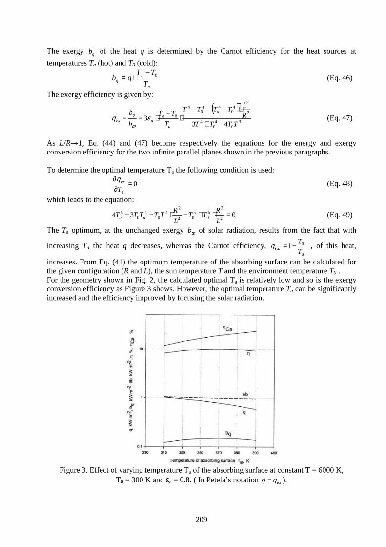
209

The exergy qb of the heat q is determined by the Carnot efficiency for the heat sources at

temperatures Ta (hot) and T0 (cold):

a

aq T

TTqb 0−

⋅= (Eq. 46)

The exergy efficiency is given by:

( )3

04

04

2

24

044

04

0

433

TTTTR

LTTTT

T

TT

b

b a

a

aa

qex −+

⋅−−−⋅−⋅== εη

ω (Eq. 47)

As L/R→1, Eq. (44) and (47) become respectively the equations for the energy and exergy conversion efficiency for the two infinite parallel planes shown in the previous paragraphs. To determine the optimal temperature Ta the following condition is used:

0=∂∂

a

ex

T

η (Eq. 48)

which leads to the equation:

0342

25

05

02

24

04

05 =⋅+−⋅−−

L

RTT

L

RTTTTT aa (Eq. 49)

The Ta optimum, at the unchanged exergy ωb of solar radiation, results from the fact that with

increasing Ta the heat q decreases, whereas the Carnot efficiency, a

Ca T

T01−=η , of this heat,

increases. From Eq. (41) the optimum temperature of the absorbing surface can be calculated for the given configuration (R and L), the sun temperature T and the environment temperature T0 . For the geometry shown in Fig. 2, the calculated optimal Ta is relatively low and so is the exergy conversion efficiency as Figure 3 shows. However, the optimal temperature Ta can be significantly increased and the efficiency improved by focusing the solar radiation.

Figure 3. Effect of varying temperature Ta of the absorbing surface at constant T = 6000 K,

T0 = 300 K and εa = 0.8. ( In Petela’s notation exηη = ).

210

8.6 Difference between the exergy relations derived by Spanner, Jeter and

Petela

The First Law of Thermodynamics, applied to any medium undergoing the process within an enclosed system, leads to the known equation of energy conservation for the beginning medium state, 1, and end state, 2. The heat 21−Q delivered to the medium from the external sources is spent

on the raising the internal energy of the medium from 1U to 2U , and on the performing absolute

work 21−W :

211221 −− +−= WUUQ (Eq. 50)

A radiation matter can be assumed to be the processed medium. The absolute work 21−W consists

of the useful work uW and of the work eW spent for the compression of the environment:

eu WWW +=−21 (Eq. 51)

where:

∫ ⋅−=2

1

0)( dVppWu (Eq. 52)

and: ( )010 VVpWe −⋅= (Eq. 53)

where p is the current radiation pressure and p0 is the radiation pressure at the environment temperature. Work eW is unavailable, whereas work uW represents the exergy b of the medium at

the state 1, bWu = , whenever this work uW is maximum.

In 1964 Spanner introduced his “maximum economic efficiency” Sη in which, instead of using the

useful work uW , he used absolute work 21−W related to the initial internal energy U1 of the

radiation arriving to the considered surface:

1

2

1

21

3

41

T

T

U

WS ⋅−== −η (Eq. 54)

where 1T and 2T are the absolute temperatures of the radiation matter at the beginning and at the end of the process, respectively. However, if instead of the Spanner’s efficiency Sη , one introduces a rather more justified efficiency η ′ defined with use of the useful work as:

1U

Wu=′η (Eq. 55)

then the efficiency η ′ becomes just the ratio ψ where 1

1

U

b=ψ , and is in agreement with Petela:

ψη =

⋅−

⋅+=′

1

0

4

1

0

34

31

1T

T

T

T (Eq. 56)

The values of the radiation exergy resulting from Petela’s and Spanner’s formulae can be compared. For the high values of the radiation temperature T, both exergy values approach each other, however, for the lower values of temperature T, they differ significantly. The three theoretical ideas of the solar energy utilization are schematically shown in Figure 4.

211

Figure 4. Three models for utilization of solar energy.

1) The sun surface and the environment are in direct contact with an ideal heat engine which

consumes heat SQ , rejects heat 01Q and performs work 1W at the Carnot efficiency of S

C T

T01 1−=η

with no exergy loss. 2) The solar radiation, by its radiation pressure, generates work 2W with the use of any ideal mechanical engine. The exergy loss appears during emission of the solar radiation. 3) The solar radiation is absorbed at the surface of temperature Ta. An ideal heat engine, by direct contact with this surface consumes heat Qa , by direct contact with environment rejects Q03 , and

performs work 3W at the Carnot efficiency of a

C T

T03 1−=η . The exergy losses appear during

emission and absorption of the solar radiation. Jeter (1981) came to the result corresponding to the first idea discussed above. The efficiency 1Cη proposed by Jeter for estimation of the solar radiation exergy is unfair because this efficiency expresses the exergy not of the solar radiation but of the heat originated from the sun. In addition, the idea of direct contact of the heat engine with the sun and earth is not realistic. To obtain heat from solar radiation one has to first absorb the radiation and this absorption is not considered in Jeter’s case. The appropriate situation is the third configuration that corresponds to Petela’s idea. The following Table 1 summarizes the different approached used by the three authors to define the exergy of thermal radiation. Table 1. Output and input of the limiting energy efficiency of radiation utilization by three different researchers.

Researcher

Input Output Maximum efficiency

Spanner Radiation energy Absolute work

T

T0

3

41−

Jeter Heat Net work of a heat engine

T

T01−

Petela Radiation energy Useful work = radiation exergy 4

00

3

1

3

41

+−T

T

T

T

212

The numerical illustration of the three limiting energy efficiencies, as a function of radiation temperature T, is shown in Figure 5 for comparison.

Figure 5. Comparison of three limiting energy efficiencies.

8.7 Exergy balance equations involving radiative heat transfer The expressions given in much of the literature for the entropy and exergy flux of heat transfer do not apply to radiative heat transfer. Heat transfer is introduced as having three forms: conduction, convection, and radiative transfer, and the entropy and exergy fluxes are given by Tq and

( )TTq 01− , respectively, where q is the heat flux and T0 is the environmental temperature. However, these relations for the entropy and exergy flux of heat transfer do not apply to radiative transfer. For BR emission the entropy flux is given by ( )Tq /3/4 ⋅ and the entropy flux of radiation emission with an arbitrary spectrum is given by ( )Tqn /⋅ where n ≥ 4/3. The general exergy balance equation for a control volume (CV) is:

( ) ( )[ ] CViii

i

CVboundary

CVCV

b

CV IssThhmdt

dVPWdA

T

Tq

dt

d &&& −−−−+

−−

−=

Ξ∑∫ 0000

01 (Eq. 57)

for a non-steady-state flow process where potential and kinetic energy effects have not been included and where: - P0 is the environmental pressure, - T0 is the environmental temperature, - ΞCV is the exergy in the CV, - VCV is the volume of the CV and - Tb is the temperature at the boundary where heat flux q occurs. In this general exergy balance equation the exergy flux of heat transfer is given in the form

( )TTq 01− that does not apply to radiative heat transfer. Correct evaluation of the exergy flux of thermal radiation allows the thermal-mechanical exergy balance equation to be restated so that it correctly applies to thermal radiation heat transfer:

( ) CViii

i

boundaryCV

CVCVNet

bcc

CV IsThmdt

dVPWdAM

T

Tq

dt

d &&& −−+

−−

+

−=

Ξ∑∫ 00

01 (Eq. 58)

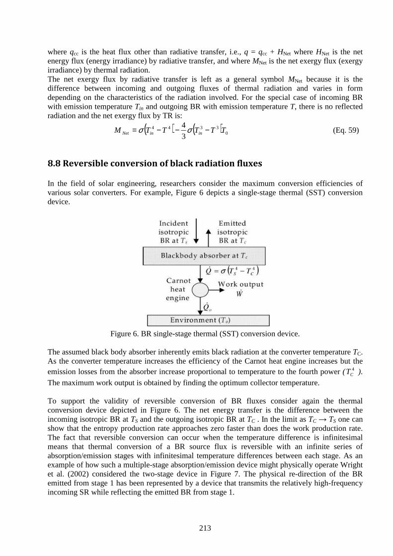
213

where qcc is the heat flux other than radiative transfer, i.e., q = qcc + HNet where HNet is the net energy flux (energy irradiance) by radiative transfer, and where MNet is the net exergy flux (exergy irradiance) by thermal radiation. The net exergy flux by radiative transfer is left as a general symbol MNet because it is the difference between incoming and outgoing fluxes of thermal radiation and varies in form depending on the characteristics of the radiation involved. For the special case of incoming BR with emission temperature Tin and outgoing BR with emission temperature T, there is no reflected radiation and the net exergy flux by TR is:

( ) ( ) 03344

3

4TTTTTM ininNet −−−= σσ (Eq. 59)

8.8 Reversible conversion of black radiation fluxes In the field of solar engineering, researchers consider the maximum conversion efficiencies of various solar converters. For example, Figure 6 depicts a single-stage thermal (SST) conversion device.

Figure 6. BR single-stage thermal (SST) conversion device.

The assumed black body absorber inherently emits black radiation at the converter temperature TC. As the converter temperature increases the efficiency of the Carnot heat engine increases but the emission losses from the absorber increase proportional to temperature to the fourth power ( 4

CT ).

The maximum work output is obtained by finding the optimum collector temperature. To support the validity of reversible conversion of BR fluxes consider again the thermal conversion device depicted in Figure 6. The net energy transfer is the difference between the incoming isotropic BR at TS and the outgoing isotropic BR at TC . In the limit as TC → TS one can show that the entropy production rate approaches zero faster than does the work production rate. The fact that reversible conversion can occur when the temperature difference is infinitesimal means that thermal conversion of a BR source flux is reversible with an infinite series of absorption/emission stages with infinitesimal temperature differences between each stage. As an example of how such a multiple-stage absorption/emission device might physically operate Wright et al. (2002) considered the two-stage device in Figure 7. The physical re-direction of the BR emitted from stage 1 has been represented by a device that transmits the relatively high-frequency incoming SR while reflecting the emitted BR from stage 1.

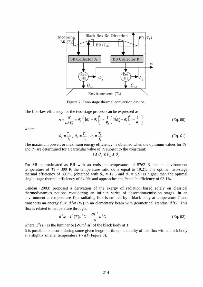
214

Figure 7. Two-stage thermal conversion device.

The first-law efficiency for the two-stage process can be expressed as:

( ) ( )

−−+

−−== −

BBA

AASS

SAT

W

θθθ

θθθθ

ση 1

11

1 444444

(Eq. 60)

where:

0T

TAA =θ ,

0T

TBB =θ ,

0T

TSS =θ (Eq. 61)

The maximum power, or maximum energy efficiency, is obtained when the optimum values for θA and θB are determined for a particular value of θS subject to the constraint:

SAB θθθ ≤≤≤1

For SR approximated as BR with an emission temperature of 5762 K and an environment temperature of T0 = 300 K the temperature ratio θS is equal to 19.21. The optimal two-stage thermal efficiency of 89.7% (obtained with θA = 12.5 and θB = 5.9) is higher than the optimal single-stage thermal efficiency of 84.9% and approaches the Petela’s efficiency of 93.1%. Candau (2003) proposed a derivation of the exergy of radiation based solely on classical thermodynamics notions considering an infinite series of absorption/emission stages. In an environment at temperature T0 a radiating flux is emitted by a black body at temperature T and transports an energy flux φ2d (W) in an elementary beam with geometrical etendue Gd 2 . This flux is related to temperature through:

GdT

GdTLd 24

202 )(π

σφ == (Eq. 62)

where )(0 TL is the luminance [W/m2·sr] of the black body at T. It is possible to absorb, during some given length of time, the totality of this flux with a black body at a slightly smaller temperature T - dT (Figure 8):

215

Figure 8. First step of the reversible transformation of radiation into work.

This black body then necessarily emits in the same etendue and over the same period an energy flux:

GddTTL 20 )( − (Eq. 63)

The net gain of energy per second is proportional to )()( 00 dTTLTL −− :

GdTdTQd 233 4

πσ= (Eq. 64)

or per unit etendue:

dTTGd

QddQ 3

2

3 4

πσ== (Eq. 65)

dQ (W/m2·sr) can be optimally converted into work by a perfectly reversible thermal machine

operating between T – dT and T0 (Figure 9), with an efficiency of dTT

T

−− 01 (Carnot efficiency).

The work thus produced is, per unit time and unit etendue (W/m2·sr):

dTTT

T

dTT

TdQdW 300 1

41

−=

−−=

πσ

(Eq. 66)

The flux reemitted by the thermostat can in turn be absorbed by a second thermostat at temperature T - 2dT, and the process is repeated until the temperature of the thermostat, and thus of the radiation, reaches T0, the limit at which dQ can no longer be converted into work (Figure 9).

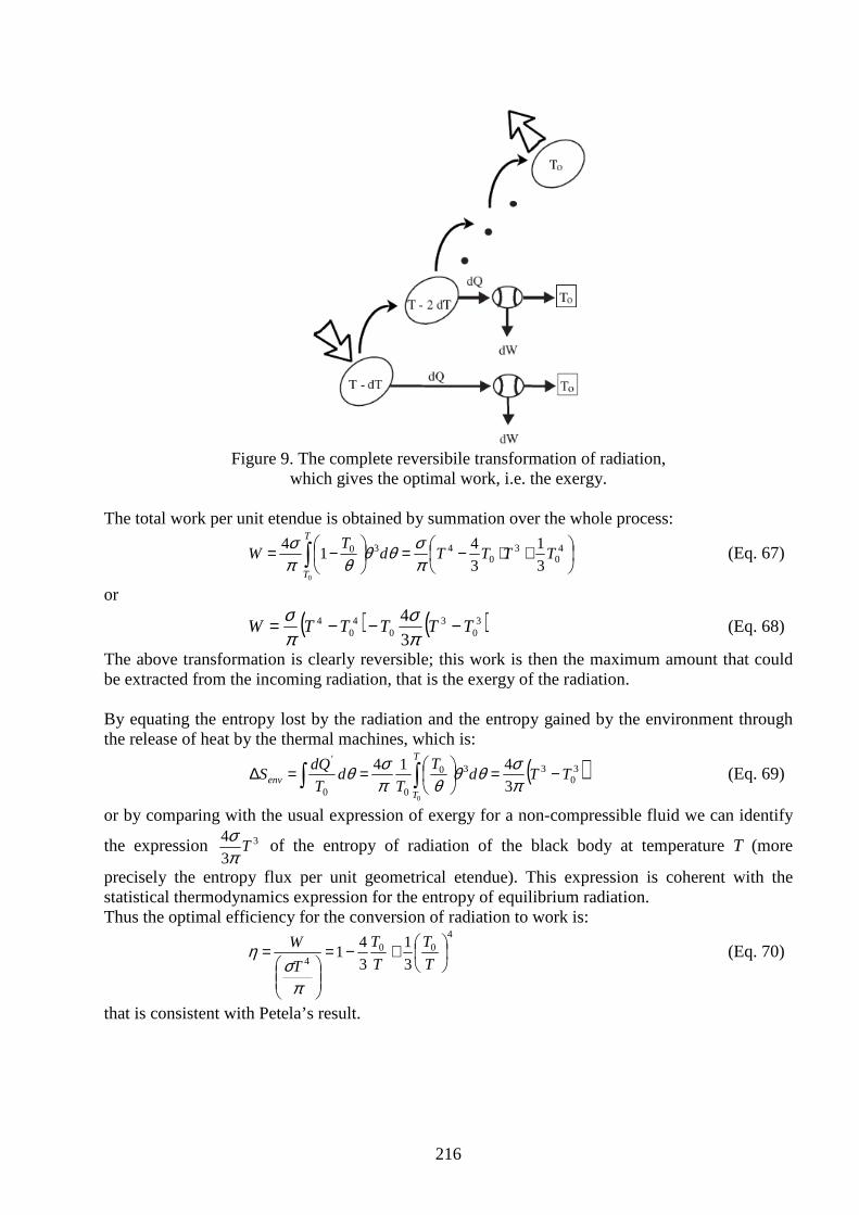
216

Figure 9. The complete reversibile transformation of radiation,

which gives the optimal work, i.e. the exergy. The total work per unit etendue is obtained by summation over the whole process:

+⋅−=

−= ∫4

03

0430

3

1

3

41

4

0

TTTTdT

WT

Tπσθθ

θπσ

(Eq. 67)

or

( ) ( )30

30

40

4

3

4TTTTTW −−−=

πσ

πσ

(Eq. 68)

The above transformation is clearly reversible; this work is then the maximum amount that could be extracted from the incoming radiation, that is the exergy of the radiation. By equating the entropy lost by the radiation and the entropy gained by the environment through the release of heat by the thermal machines, which is:

( )30

330

00

'

3

414

0

TTdT

Td

T

dQS

T

T

env −=

==∆ ∫∫ πσθθ

θπσθ (Eq. 69)

or by comparing with the usual expression of exergy for a non-compressible fluid we can identify

the expression 3

3

4T

πσ

of the entropy of radiation of the black body at temperature T (more

precisely the entropy flux per unit geometrical etendue). This expression is coherent with the statistical thermodynamics expression for the entropy of equilibrium radiation. Thus the optimal efficiency for the conversion of radiation to work is:

400

4 3

1

3

41

+−=

=

T

T

T

T

T

W

πσ

η (Eq. 70)

that is consistent with Petela’s result.

217

8.9 Difference between Petela and Carnot efficiency All material that absorb TR must also inherently emit TR as was illustrated by the single-stage thermal device. The viewpoint of many researchers (e.g. Landsberg) is that inherent emission can be ignored in determining the maximum work output for TR conversion and also the analysis of Petela’s parallel-plate approach gives the impression that the exergy irradiance of BR is with no inherent emission term. However, this is a misunderstanding that arises because the Guoy–Stodola theorem, used in Petela’s approach, can only give the net exergy flux of TR between the parallel surfaces. Inherent emission by a non-ideal thermal conversion device reduces work output because the energy flux of the TR emitted by the converter is generally high (emission temperature well above T0). Also, inherent emission results in substantial irreversibility. Consequently, researchers have erroneously stated that inherent emission has a negative effect on ideal conversion as well. However, in contrast to non-ideal conversion, inherent emission has a beneficial effect on ideal conversion. The reason for this reversal in the effect of inherent emission can be seen by considering the reversible black-box conversion device shown in Figure 10. The device absorbs the incoming isotropic BR with emission temperature T and emits BR at T0 with zero exergy flux.

Figure 10. Black-box model for ideal BR conversion.

There is no entropy flow with work transfer so the entropy of the source radiation can leave the device by only two paths; BR at T0 and heat conduction at T0, whereas for a Carnot heat engine there is only one path by which entropy leaves the device, by heat conduction at T0. The entropy-to-energy ratio of heat conduction at T0 is equal to 1/T0 while that of BR at T0 is equal to (4/3)/To. BR at T0 is a better means of rejecting entropy to the environment than heat conduction at T0 because the required energy flow rate to the environment is lower. As a result, inherent emission results in an additive term (x4/3) in the exergy expression:

+−=Ξ 44

3

1

3

41 xxATσ& (Eq. 71)

where x = T0/T . The reason that the Petela efficiency (Wout/σAT 4) is less than the Carnot efficiency (1 − T0/T) is not due to inherent emission. Rather it is due to the fact that the source flux has a high ratio of entropy to energy resulting in the 4/3 factor in the second term of Eq. (70). That is, the entropy flux of BR at T is a factor of 4/3 higher than that of heat conduction at T with the same energy flux.

218

8.10 Thermodynamical engines

De Vos (2008) described two thermodynamic models of “endoreversible engines”: irreversible engines where all irreversibilities are restricted to the coupling of the engine to the external world, that is in the heat exchange between the Carnot engine and the two external heat reservoirs. These models are the Curzon-Ahlborn engine that contains linear conductors and the Stefan-Boltzmann engine that contains nonlinear conductors. In the following sections Q and W are respectively heat flows and work flows per unit of time.

8.10.1 Curzon-Ahlborn engine

In the Curzon-Ahlborn engine, as in the Carnot engine, there are two heat reservoirs: one at the high temperature T1, the other at the low temperature T2 but there are also two irreversible components: thermal resistors which limit the heat flows Q1 and Q2 and they cause: a temperature drop from T1 to an intermediate temperature T3 and a temperature drop from an intermediate temperature T4 to T2. A reversible Carnot engine operates between the intermediate heat reservoir at temperature T3 and the intermediate reservoir at temperature T4. The configuration is shown in Figure 11.

Figure 11. Curzon-Ahlborn engine configuration.

Applying the conservation of energy:

21 QWQ += (Eq. 72) Applying the conservation of entropy to a surface containing only the reversible parts of the engine:

4

2

3

1

T

Q

T

Q= (Eq. 73)

Using the definition for the conversion efficiency:

1QW η= (Eq. 74) we obtain:

3

41T

T−=η (Eq. 75)

219

which is none other than Carnot’s formula, however for a reversible engine working between the temperatures T3 and T4 (instead of T1 and T2). Linear constitutive laws are introduced for the thermal conductors:

( )3111 TTgQ −= (Eq. 76)

)( 2422 TTgQ −= (Eq. 77) (after Fourier’s law for the diffusion of heat: TQ ∇−= λ ). The proportionality coefficients g1 and g2 are called the thermal conductances or heat conductances. Substitution of Eqs. (76) and (77) into Eq. (73) yields:

( ) ( )4

242

3

311

T

TTg

T

TTg −=

− (Eq. 78)

Solving the set of two Eqs. (75) and (78) for T3 and T4 gives:

221

21

21

13 1

1T

gg

gT

gg

gT

η−++

+= (Eq. 79)

( ) 221

21

21

14 1 T

gg

gT

gg

gT

++−

+= η (Eq. 80)

Substitution of the T3 result into Eq. 76 finally yields:

ηη

−−−=

1121

1TTT

gQ (Eq. 81)

where:

21

21

gg

ggg

+= (Eq. 82)

This relationship between 1Q and η , called the “current-efficiency” characteristic is depicted in Figure 12. The intersection with the abscissa axis is the Carnot efficiency Cη of a reversible engine working

between the temperatures T1 and T2 : 1

21T

TC −=η .

Multiplication of Eq. (81) by η gives the “work-efficiency” characteristic ( )ηW : ( )

ηηη

−−−=

1121 TTT

gW (Eq. 83)

The intersection with the ordinate axis and the intersection with the abscissa axis divide the ( )η1Q and ( )ηW characteristics into 3 parts: left: refrigerator; middle: heat engine; right: heat pump.

To demonstrate that the Curzon-Ahlborn engine is not reversible, the ΣS can be calculated for a closed surface containing the whole engine, i.e., both the Carnot engine and the two heat conductors. We have:

2

2

1

1

T

Q

T

QS +−=∑ (Eq. 84)

Thus: ( ) ( )

2

1

1

1

2

1

2

1

1

1

2

1

1

1

2

2

T

Q

T

Q

T

Q

T

Q

T

Q

T

WQ

T

Q

T

QS C ηηη −=−−=−−=−=∑ (Eq. 85)

Substitution of Eq. (81) into Eq. (85) yields: ( )

( )ηη

−−−=Σ

121

2121

TT

TTTgS (Eq. 86)

220

Figure 12 shows the quantity ( )∑ ηS , together with the ( )η1Q and ( )ηW characteristics.

Figure 12. Thermodynamic quantities as a function of the conversion efficiency of a Curzon-Ahlborn engine: heat consumption, work production, entropy creation rate.

We see that under reversible conditions, (i.e., 3

41T

T−=η equal to its Carnot value), both 1Q and W

are zero. This expresses the general principle that under reversible conditions conversion happens infinitely slowly. We see further that, for this same value of η , the entropy creation rate ∑S is both minimum and

zero. The produced work W displays a maximum at an η value between 0 and Cη . This value is found

by applying: 0=ηd

dW to Eq. 83, yielding:

02 2112

1 =−+− TTTT ηη (Eq. 87) Solving for η gives:

1

21T

T−=η (Eq. 88)

Thus we have derived the Curzon-Ahlborn formula, which expresses the efficiency of the engine in maximum power condition. This important formula was discovered by Novikov in 1957, for the special case ∞=2g , and proven to be true also in the general case (arbitrary g1 and arbitrary g2) by Curzon and Ahlborn in 1975. Under this maximum-power condition, the quantities Q1, W, and ∑S take nonzero values:

( )2111 TTTgQ −= (Eq. 89)

( )2

21 TTgW −= (Eq. 90)

( ) 21

2

21 / TTTTgS −=Σ (Eq. 91)

221

Figure 13 shows the relation between η and the temperature ratio 1

2

T

T. We see that the Curzon-

Ahlborn curve lies substantially below the straight line 1

21T

T−=η . This confirms the general rule:

efficiency under irreversible conditions is lower than under reversible conditions.

Figure 13. Energy conversion efficiency as a function of temperature ratio

according to Carnot and according to Curzon-Ahlborn.

8.10.2 Stefan-Boltzmann engine

The Curzon-Ahlborn model is not immediately applicable to solar energy, as the transport of solar heat does not satisfy the linear law:

( )3111 TTgQ −= (Eq. 76)

but instead a Stefan-Boltzmann law: ( )4

34

111 TTgQ −= (Eq. 92)

Therefore it is necessary to transform the Curzon-Ahlborn engine into an endoreversible engine where transports obey the Stefan-Boltzmann law. We will call such engines Stefan-Boltzmann engines. If heat is delivered to and drained from the Carnot engine by means of radiation instead of by conduction, then the transport equations have to be replaced by the corresponding Stefan-Boltzmann laws:

( )43

4111 TTgQ −= (Eq. 92)

( )42

4422 TTgQ −= (Eq. 93)

Proceeding exactly as above: ( ) ( )

4

42

442

3

43

411

T

TTg

T

TTg −=

− (Eq. 94)

3

41T

T−=η (Eq. 95)

and solving for T3 and T4 gives:

( ) ( )4

2321

2413

21

143 1

1

11T

gg

gT

gg

gT

ηηη −−++

−+= (Eq. 96)

( )( )

( )( ) 4

23

321

241

4

321

144 1

11

1T

gg

gT

gg

gT η

ηη

η−

−++−

−+= (Eq. 97)

222

Substitution of the T3 result into the equation for Q1 yields:

( )( ) ( )4

21

42

41

4

21111

1

ηηη

−+−−−=

gg

TTggQ (Eq. 98)

By solving ( ) 01 =ηQ for η , we find again the Carnot efficiency: 1

21T

TC −=η .

The curves of Figure 14 are very similar to the corresponding curves on Fig. 12 for the Curzon-Ahlborn model. But we see that the curve ( )η1Q is more “rectangular” in the Stefan-Boltzmann

case than in the Curzon-Ahlborn case. Whereas the curve ( )η1Q is a simple hyperbola in the Curzon-Ahlborn case, it is a fifth degree curve in the present case. It is therefore no surprise that the values of η and 1Q corresponding to the maximum power cannot be expressed in closed form. Multiplying ( )η1Q by η yields ( )ηW , the work-efficiency characteristic:

( ) ( )( ) ( )4

21

42

41

4

2111

1

ηηηηη

−+−−−=

gg

TTggW (Eq. 99)

The curve displays a maximum for 0=ηd

dW, i.e., for the η value satisfying:

( ) ( ) ( )( ) ( ) 01413141 421

3422

4411

422

5411

8412 =−−−−−+−+− TgTgTgTgTgTg ηηηη (Eq. 100)

The solution η of this “eight-degree equation” should yield a Stefan-Boltzmann equivalent of the Curzon-Ahlborn formula, however in contrast to the Curzon-Ahlborn case the solution cannot be analytical and it is dependent of the conductance ratio g1/g2. Even in the following three peculiar cases the mathematics cannot be performed analytically: a) 21 gg << , i.e., g1/g2 → 0;

b) 21 gg >> , i.e., g1/g2 → ∞

c) 21 gg = , i.e., g1/g2 = 1, and Indeed: a) for g1 = 0 Eq. 100 yields a fifth-degree equation:

( ) ( ) 04131 42

42

541 =−−+− TTT ηη (Eq. 101)

b) for g2 = 0 it also yields a fifth degree equation: ( ) ( ) 01314 4

244

154

1 =−−−− TTT ηη (Eq. 102) c) for g2 = g1 the equation remains of eighth degree. The total entropy production rate ∑S is:

( )[ ] ( )[ ]( ) ( )4

21

42

41

421

21

21

11

11

ηηηη

−+−−−−−

=∑gg

TTTT

TT

ggS (Eq. 103)

Figure 14 shows the quantity ( )∑ ηS , together with the ( )η1Q and ( )ηW characteristics. All three

quantities become zero at η = ηC.

223

Figure 14. Thermodynamic quantities as a function of the conversion efficiency of a

Stefan-Boltzmann engine: heat consumption, work production and entropy creation rate.

8.11 Photothermal conversion

The peculiar case in which +∞=2g corresponds to the model introduced by Müser in 1957. In this case T2 = T4 and the resulting configuration is shown in Figure 15.

Figure 15. Müser engine.

The solar converter is assumed to be oriented optimally, i.e., perpendicular to the Sun’s rays. Therefore the incident radiation is equal to the solar constant 4

STfS σ= (1353 W/m2).

From all directions, not covered by the solar disk, the converter receives black-body radiation at temperature TP: from the ground, from the surrounding buildings and/or trees and from the clouds

224

and/or atmosphere. The converter itself radiates a black-body radiation of temperature T3, called the converter temperature (Figure 16). Per unit of surface area it emits a power 4

3Tσ .

Figure 16. Muser engine.

(We assume for simplicity that only the upper surface emits radiation. The bottom side of the device has a zero emissivity ε , which can be realized by applying a mirror-like metal coating. If the bottom were not metallized, the body would emit 4

32 Tσ , as a 1 m2 flat radiator has 2 m2 surface

area). The net total incident energy is given by:

( ) ( )[ ]43

4443

441 11 TTffTTTfTfQ PSPS −−+=−−+= σσσσ (Eq. 104)

Equation (104) and Fig. 16 can be interpreted as follows. The converter radiates the full Stefan-Boltzmann flux 4

3Tσ toward the hemisphere above it. It receives 4ST radiation only from a small

solid angle ω . The incident solar radiation is therefore only a fraction f of the Stefan-Boltzmann

flux 4STσ . The “aperture factor f ” is given by:

∫∫

∫∫=

π

ω

ωϑ

ωϑ

2

cos

cos

d

d

f (Eq. 105)

The denominator of this expression equals π ; the numerator equals approximately ω , if the solar disc is small, as then the cosine of ϑ is almost unity in the whole solid angle ω . Thus

πω≈f (Eq. 106)

(The exact calculation of Eq. 105 yields:

−=π

ωπω

41f )

Because ω equals 2

SRπ divided by r2, we finally get:

2

2

r

Rf S≈ (Eq. 107)

i.e., the “dilution factor”. Note that f was introduced from a “solar” point of view, whereas here f is deduced from a “planetary” point of view. Both approaches give the same result.

225

The rest of the hemisphere sends to the converter a Stefan-Boltzmann radiation 4PTσ with

“aperture factor”:

∫∫

∫∫−

π

ωπ

ωϑ

ωϑ

2

2

cos

cos

d

d

(Eq. 108)

i.e., f−1 . We now compare the energy flow (104) with the general transport equation of the Stefan-Boltzmann machine, i.e., with ( )4

34

11 TTg − . We have:

σ=1g (Eq. 109)

( )[ ] 4/1441 1 PS TffTT −+= (Eq. 110)

The latter equation can be interpreted as follow. The solar absorber sees a hemisphere with nonuniform temperature. For the Stefan-Boltzmann engine however, this situation is equivalent to the case where the solar absorber is irradiated by a “sky” at uniform temperature T1. This temperature is some weighted average of TS and TP.

It can be shown that the planet temperature TP can be approximated by: SP Tf

T2

4/1

= . Substitution

into Eq. 110 gives:

STff

T4/12

1 44

5

−= (Eq. 111)

Because for any planet 1<<f , we can approximate T1 as follows:

STf

T4/1

1 4

5

≈ (Eq. 112)

or

PTT 4/11 5≈ (Eq. 113)

Thus the effective sky temperature T1 equals 1.495 times the planet temperature. For the Earth we have KTP 288= and thus KT 4311 = .

8.12 Solar energy efficiency

The photothermal converter produces an amount W of power per unit of time and per unit of surface area. We introduce a solar energy conversion efficiency:

4STf

Ww

σ= (Eq. 114)

This quantity should not be confused with the engine efficiency η , which is given by:

( ) 43

44 1 TTfTf

W

PS σσση

−−+= (Eq. 115)

From:

1QW η= (Eq. 116)

( ) 43

441 1 TTfTfQ PS σσσ −−+= (Eq. 117)

η−=

14

3T

T (Eq. 118)

226

PTT =4 (Eq. 119) we can deduce immediately that:

( )

−−−+= 4

44

1

11 PS TfTfW σ

ηση (Eq. 120)

and thus:

( )( )( )

⋅

−−−−+=

4

4

4

4

1

1111

S

P

fT

Tfw

ηηη (Eq. 121)

With the approximation:

SP Tf

T2

4/1

= (Eq. 122)

this eventually leads to the relationship between w and η , we were searching for:

( )( )( )4

4

14

115

ηηη

−−−−= f

w (Eq. 123)

With very good accuracy this can be approximated by: ( )

( )4

4

14

115

ηηη−

−−≈w (Eq. 124)

Figure 17 shows this function ( )ηw :

Figure 17. Solar energy conversion efficiency w as a function

of engine efficiency η of Müser engine. Between its two zeros, i.e., between 0=η and 33126.051 4/1 =−= −η , the function displays a

maximum. The coordinates of this extremum are determined by solving 0=ηd

dw, i.e., by solving:

( ) ( ) 041315 5 =−−+− ηη (Eq. 125) This equation can be related to the general theory of the Stefan-Boltzmann engines. We have to appeal to numerical methods for solving Eq. 125. This yields:

20292.0=η Subsequent substitution into Eq. 124 gives:

12797.0=w Thus a Müser engine has a maximum efficiency of 12.8%.

227

8.13 Concentrators

We assume that the incident radiation can be artificially augmented by a factor C (larger than unity), called the concentration factor. This is realized by use of optical devices, i.e., either by lenses (refractive devices) or by mirrors (reflective devices) or by a combination of both. Human technology cannot make C infinitely large. The highest concentration is realized by capturing all rays leaving a unit of Sun surface area and making an optical image of it on a unit of surface area on the planet. This would require a huge elliptic mirror with the sun at one focal point and the planet at the other focal point. The resulting power incident on the solar energy converter would equal the solar energy radiation density at the Sun’s surface, i.e., 4

STσ .

Thus: 44

max SS TTfC σσ = (Eq. 126)

Therefore the highest concentration maxC is f/1 that equals 46300 for the earth.

When C = Cmax, the solar absorber sees the solar disc in a π2 solid angle instead of in a limited solid angle.

For an arbitrary C, the incident solar radiation is 4STCfσ with

fC

11 ≤≤ .

From all directions, expect those covered by the lenses and/or mirrors, the converter still receives radiation from the surroundings at temperature TP. The black-body radiator still emits a power 43Tσ per unit of surface area. The net total incident energy is now given by:

( ) ( )[ ]43

4443

441 11 TTCfCfTTTCfTCfQ PSPS −−+=−−+= σσσσ (Eq. 127)

such that:

( )[ ] 4/1441 1 PS TCfCfTT −+= (Eq. 128)

This effective “sky” temperature is higher than the value PT4/15 of the Muser engine without concentrator. Depending on the concentration factor C, the effective temperature T1 ranges from 1.495 times the planet temperature to the Sun temperature. We again have to define a solar energy efficiency:

4STCf

Ww

σ= (Eq. 129)

After some calculations, we find the generalization of Eq. 123: ( )( )

( )4

4

14

1114

ηηη

−−−−+=

C

CfCw (Eq. 130)

For fully concentrated sunlight (i.e., C=1/f):

( )

−−=

4141

ηη f

w (Eq. 131)

This function is zero for 0=η and for 2/1 4/1f−=η .

In between, it has a maximum for η satisfying 0=ηd

dw, i.e., satisfying

( ) ( ) 014

31 5 =−−+− ff ηη (Eq. 132)

In contrast with the Muser engine with C = 1, the theory of the Muser engine with C >> 1 can take advantage of the fact that T2 << T1. This leads to an approximate analytical solution yielding:

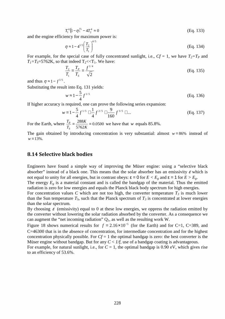
228

( ) 041 42

541 ≈−− TT η (Eq. 133)

and the engine efficiency for maximum power is: 5/4

1

25/141

−≈

T

Tη (Eq. 134)

For example, for the special case of fully concentrated sunlight, i.e., Cf = 1, we have T2=TP and T1=TS=5762K, so that indeed T2<<T1. We have:

2

4/1

1

2 f

T

T

T

T

S

P == (Eq. 135)

and thus 5/11 f−≈η . Substituting the result into Eq. 131 yields:

5/1

4

51 fw −≈ (Eq. 136)

If higher accuracy is required, one can prove the following series expansion:

...160

9

4

1

4

51 5/35/25/1 +++−= fffw (Eq. 137)

For the Earth, where 0500.05762

288 ==K

K

T

T

S

P we have that w equals 85.8%.

The gain obtained by introducing concentration is very substantial: almost %86=w instead of %.13=w

8.14 Selective black bodies

Engineers have found a simple way of improving the Müser engine: using a “selective black absorber” instead of a black one. This means that the solar absorber has an emissivity ε which is not equal to unity for all energies, but in contrast obeys: ε = 0 for E < Eg and ε = 1 for E > Eg. The energy Eg is a material constant and is called the bandgap of the material. Thus the emitted radiation is zero for low energies and equals the Planck black body spectrum for high energies. For concentration values C which are not too high, the converter temperature T3 is much lower than the Sun temperature TS, such that the Planck spectrum of T3 is concentrated at lower energies than the solar spectrum. By choosing ε (emissivity) equal to 0 at these low energies, we oppress the radiation emitted by the converter without lowering the solar radiation absorbed by the converter. As a consequence we can augment the “net incoming radiation” Q1, as well as the resulting work W. Figure 18 shows numerical results for 51016.2 −×=f (for the Earth) and for C=1, C=389, and C=46300 that is in the absence of concentration, for intermediate concentration and for the highest concentration physically possible. For Cf = 1 the optimal bandgap is zero: the best converter is the Müser engine without bandgap. But for any C < 1/f, use of a bandgap coating is advantageous. For example, for natural sunlight, i.e., for C = 1, the optimal bandgap is 0.90 eV, which gives rise to an efficiency of 53.6%.

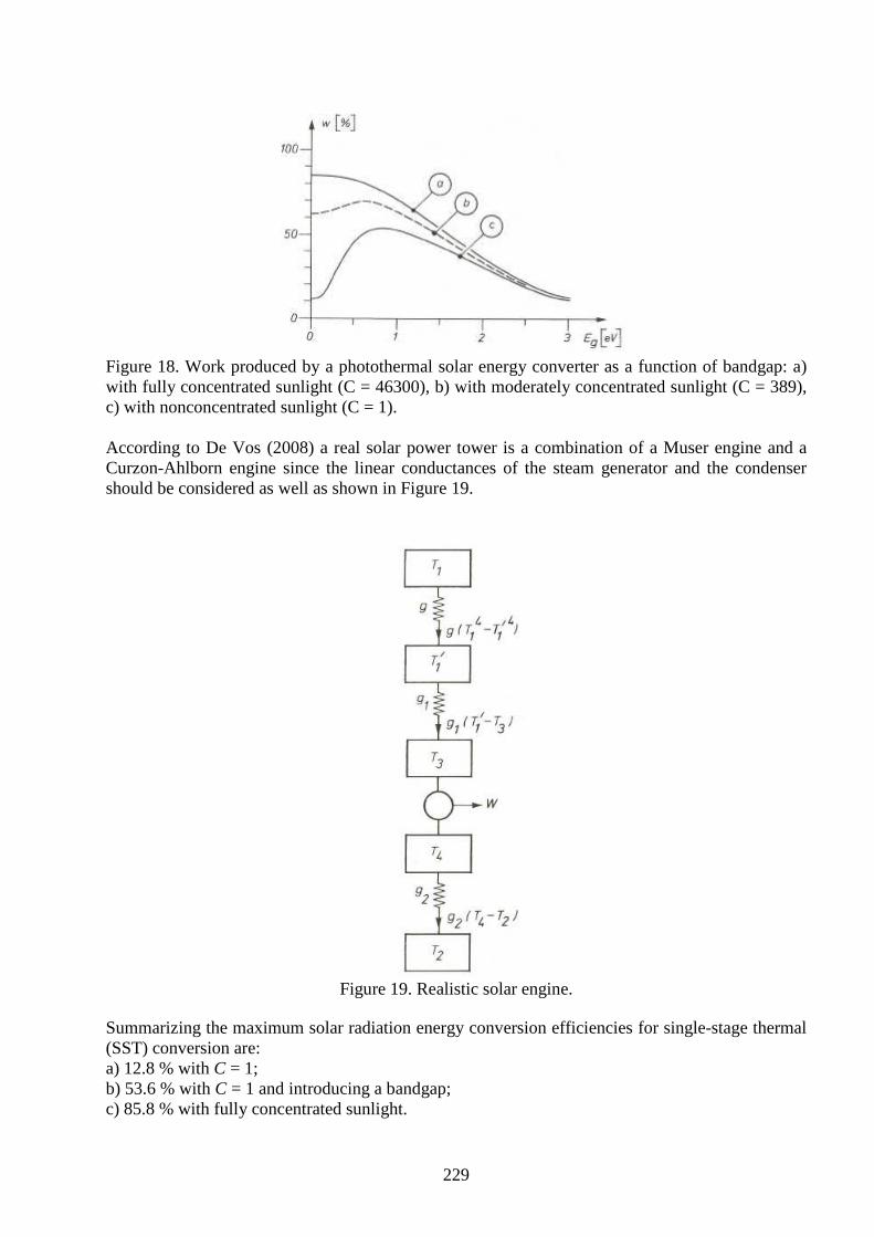
229

Figure 18. Work produced by a photothermal solar energy converter as a function of bandgap: a) with fully concentrated sunlight (C = 46300), b) with moderately concentrated sunlight (C = 389), c) with nonconcentrated sunlight (C = 1). According to De Vos (2008) a real solar power tower is a combination of a Muser engine and a Curzon-Ahlborn engine since the linear conductances of the steam generator and the condenser should be considered as well as shown in Figure 19.

Figure 19. Realistic solar engine.

Summarizing the maximum solar radiation energy conversion efficiencies for single-stage thermal (SST) conversion are: a) 12.8 % with C = 1; b) 53.6 % with C = 1 and introducing a bandgap; c) 85.8 % with fully concentrated sunlight.

230

Higher efficiency values can be achieved using multiple stage thermal systems. With an infinite number of stages the exergy of the BR source, that is, the maximum work available from the BR source flux is reached. Petela’s result (93.3%) represents the upper limit to the conversion of solar radiation (SR) approximated as BR. So second-law (exergetic) efficiencies can be evaluated. The second-law efficiency of a particular conversion process is simply the ratio of the work output for that process to the exergy of the available SR accounting for its characteristics (e.g., isotropic or unconcentrated or attenuated by the atmosphere). Identifying the upper limit to BR conversion is of fundamental thermodynamic importance as it allows second-law efficiencies to be defined and provides insight by identifying sources of non-ideal behavior in known conversion processes.

Conclusions

The definition proposed by Petela for the exergy of the solar radiation is now accepted by most researchers. The limiting efficiency for the radiation to work conversion is given by:

1

0

4

1

0

3

4

3

11

T

T

T

T−

⋅+=ψ

This expression is different from the Carnot efficiency for the heat engines due to the different definition for the entropy flux of radiation emission compared to the entropy flux of conductive or convective heat transfer. Assuming a sun temperature equal to 5760K and an environmental temperature of 300K the maximum efficiency ψ is about 93%. Wright et al. and Candau supported the validity of the reversible conversion of black radiation fluxes considering devices with an infinite series of absorption/emission stages. But such kind of system is only theoretically conceivable due to the high temperatures required in the conversion system approaching the sun temperature. Even single-stage devices operating at their optimal temperature would involve a temperature close to 2000°C and in this case the maximum efficiency would be about 85%. In the definition of the exergy of the solar radiation some authors may be oriented to use the optimal single-stage thermal efficiency since generally dealing with single stage systems. For example the thermodynamic model of endoreversible engine studied by De Vos is a single stage system and the limiting efficiency increases with the concentration ratio and using a selective absorber. However only the Petela’s result represents the upper limit to the conversion of solar radiation approximated as black radiation and can be used to evaluate second-law efficiencies.

231

References Candau Y., On the exergy of radiation, Solar Energy 2003. Chen K. and Chun W., Radiation energy transfer and maximum conversion efficiency, Applied Energy 2008. Chow T.T., Pei G., Fong K.F., Lin Z., Chan A.L.S. and Ji J., Energy and exergy analysis of photovoltaic–thermal collector with and without glass cover, Applied Energy 2009. De Vos A., Thermodynamics of Solar Energy Conversion, Wiley 2008. Farahat S., Sarhaddi F. and Ajam H., Exergetic optimization of flat plate solar collectors, Renewable Energy 2009. Petela R., Exergy of undiluted thermal radiation, Solar Energy 2003. Press W.H., Theoretical maximum for energy from direct and diffuse sunlight, Nature 1976. Winter C.-J., Sizmann R. L. and Vant-Hull L.L., Solar Power Plants, Springer-Verlag, 1990. Wright S.E., Rosen M.A., Scott D.S. and Haddow J.B., The exergy flux of radiative heat transfer for the special case of blackbody radiation, Exergy 2002. Wright S.E., Rosen M.A., Scott D.S. and Haddow J.B., The exergy flux of radiative heat transfer with an arbitrary spectrum, Exergy 2002. Zhai H., Dai Y.J., Wu J.Y. and Wang R.Z., Energy and exergy analyses on a novel hybrid solar heating, cooling and power generation system for remote areas, Applied Energy 2008.

232

9. Solar Power Plants This section presents the design aspects and the technology of solar power plants (SPPs). These plants are unique in their dependence upon the availability of the solar resource and its quality. A proper integration with the geothermal resource may alleviate some of the issues of standalone solar power plants such as the need of a storage system, the irradiation threshold and the high costs. After a brief characterization of SPPs the principal types of systems for the collection and conversion of solar radiation into heat are described also showing some practical realizations.

9.1 Design aspects

The output of a solar power plant SPP may be thermal energy for direct use in heat processes (food, textile or chemical industry) or it may be electricity. Electricity may be generated directly from solar radiation (photovoltaic SPPs) or via intermediate thermomechanical conversion (thermal SPPs). The nature, quality and availability of input energy to a SPP differ significantly from those of conventional power plants. Solar radiation is dilute and is terrestrially accessible only during daylight hours. Its availability hinges on latitude, season, time of day, morphology of the location and momentary meteorological conditions. The repercussions on SPPs technology and operation are several. Several methods for the collection and conversion of solar radiation into heat are feasible. Concentrating configurations with liquids (oil, molten salts/metals) or water/steam as primary heat transfer fluids HTF have been adopted in most of the thermal SPPs which exist today. The high temperature heat achievable with radiation concentration makes efficient thermodynamic conversion feasible. Nonetheless the potential of lower investment costs may make non- or low- concentrating configurations, such as “solar pond” or “vacuum tube collector”, attractive thermal SPP concepts. The assembly of collectors, consisting of either point-focussing parabolic dishes, line-focussing parabolic troughs, vacuum tube or non-concentrating flat plate collectors constitute a “collector field”. Thermal SPPs using such fields of collectors are referred to as “distributed collector or farm systems”. Another solar thermal concept is the “central receiver or tower SPPs” where a field of mirrors (heliostats) concentrate irradiation on a centrally located receiver. In a thermal SPP electricity is usually generated centrally by one power conversion unit. Several thermodynamic conversion processes exist: the Rankine cycle with water/steam as phase-change medium, the Brayton cycle, the organic Rankine cycle and the closed loop Stirling cycle with gas as a working medium. The main function of storage in thermal SPPs is to shift utilization of solar energy into off-sunshine time periods. It provides an essential second function in steadying plant output under fluctuating radiation input conditions. In this way the thermodynamic cycle operation is shielded from fluctuations in solar energy input, thus stabilizing operating conditions and improving conversion efficiency. In addition the thermal inventory provided by storage can serve as a ready reservoir for covering parasitic thermal needs (for instance for thermal SPP start up). Several factors influence the performance of a SPP : � Inoperability because irradiance stays below a certain threshold needed for operation. � Restrictions or losses incurred for physical or technical reasons:

- ability to utilize only direct irradiation in concentrating thermal SPPs; - optical losses, atmospheric losses or spillage losses;

233

- thermal reradiation and convective losses at receivers-absorbers; - heat dissipation in the heat transport and storage subsystem; - cosine losses in fixed-collector or 1-axis tracking SPPs; - thermodynamic conversion losses.

� Thermal and electrical parasitic needs. The definition of efficiency implies, and efficiency measurements require, steady boundary conditions. Energies are used in the definition of efficiency and under steady-state conditions ratios of energy and ratios of power become the same, thus it is established practice in engineering to define and to interpret efficiency as the ratio of output power to input power (power ratios). However under transient regimes, efficiency in terms of energy (energy efficiency) may differ significantly from power ratio. Technical factors such as energy inventories and storage, thermal inertia and the time period all influence the numerical value of the energy input-output ratio. Four bases for calculating input/output relationships are in use: 1) “Gross or net power efficiency”:

Ratio of output power, divided by the active collector area (kWt/m2; kWe/m

2), at a given instant in time, to the total or direct irradiation (kW/m2) incident on the collector surface at the same instant in time.

2) “Operating hours energy efficiency”: Ratio of energy output, divided by the active collector area (kWht/m

2; kWhe/m2), over a given

time span during which the SPP is in operation, to the total or direct irradiation incident on the collector surface (kWh/m2) over the same time span.

3) “24-hours energy efficiency”: Ratio of 24-hour energy output, divided by the active collector area (kWht/m

2; kWhe/m2), to

the total or direct irradiation (kWh/m2) incident on the collector surface area from sunrise to sunset.

4) “Annual energy efficiency”: Ratio of the total of output generated over the year (kWht/m

2a; kWhe/m2a), to the aggregate

yearly total or direct irradiation (kWh/m2a) incident on the collector surface. In detailed design, annual output performance is predicted by computational simulation, using a model of the SPP dynamic characteristics and irradiation data representative of the plant location. Measured long-term irradiation data, averaged over appropriate small time increments (minutes, hours), are the best basis for such a numerical analysis. Design procedures for SPPs are still being refined and are not yet standardized. A key decision is whether energy storage and/or auxiliary (fossil) energy sources must be incorporated to satisfy output requirements. � Design point: The design of a SPP must start by specifying energy input conditions, i.e.

assuming a specific irradiance. This design point along with a specification of the output power capacity under rated conditions provides the basis for sizing a SPP, its subsystems and elements. The design point irradiation (800 W/m2 for example) is frequently chosen at 10.00 a.m. or at noon at equinox, but sometimes at noon of summer solstice. Rated (nameplate) power capacity of SPPs is usually stated in terms of design point operating conditions. Comparison of power capacity between SPP alternatives on the basis of nominal performance is only of limited significance as design points may be not identical.

� Performance: Actual SPP energy output performance must be calculated by adding up average energy output over incremental time intervals (e.g. minutes, hours). Key factors are the irradiation determined by the meteorological situation, the SPP operating strategies, the

234

readiness of a SPP to operate whenever solar input is available. Plant output performance may be improved significantly if thermal storage can be used as a thermal buffer or as a tool for time-shifting solar energy input.

� Solar multiple: To obtain better SPP performance on average irradiation days and over the year, a larger than nominal collector subsystem may be desirable, even if energy storage capacities are small or if power conversion unit output possibilities are exceeded under (short-term) favorable input conditions. Furthermore with thermal storage, the collector subsystem must be oversized relative to that needed for rated (design point) output. The solar multiple (SM) is the ratio of collector subsystem output thermal power at design point conditions, to that needed by the power conversion unit for generating nominal output (i.e. the rated turbine gross power). With SM > 1, the excess of energy collected by the collector subsystem can be used to charge the thermal storage.

� Capacity factor: For reasons of maintenance, service or cost, power plants are never operated 8760 h/y at rated capacity. The average of output power of SPPs over multi-day time periods is affected by irradiation conditions and plant availability and therefore is lower than the rated capacity at design point. The ratio of yearly output to the hypothetical yearly output if operating continuously at nameplate rating is defined as the capacity factor (CF). The higher the “CF”, the better the utilization of the plant. Three factors mainly affect the CF: the location-specific irradiation conditions, the SPP type and system configuration and the SPP operating reliability. A typical CF of SPPs is around 25-30%.

The objective in SPP system design is to maximize (at minimum cost) the collection of solar energy and the benefit which is derived from energy output (electricity, heat or both). These are the key factors that are of influence for such an objective: 1) Irradiation conditions: reliable information about local insolation conditions (in quantity and quality) is crucial. Insolation is given usually in terms of yearly distribution of hourly averages of global, direct and/or direct normal (DNI) irradiance values (kW/m2) or in terms of yearly distribution of daily averages of global or direct irradiation (kWh/m2d). Both representations are useful for rationally setting the SPP design point, considering that power and energy thresholds are specific for SPP configurations. Global irradiance measurements are routinely carried out for meteorological surveys whereas direct normal irradiance measurements of high reliability are carried out in far fewer locations; hence the amount of DNI data available is correspondingly smaller. In addition DNI tends to be very location-specific due to local cloud interference and air quality. 2) Energy storage size: storage capacity large enough to ensure 24 hours of SPP output generation is feasible but not practical. For cost reasons the CF of SPPs will not exceed 30-50% and the size of storage must be matched with the size of the collector subsystem. 3) Energy inventory, operating flexibility and thresholds: in thermal SPPs energy inventory and thermal capacity are important issues. Thermal inventory is associated with any thermal SPP element heated above ambient temperature during operation. This thermal inventory can be helpful to bridge short interruptions in solar energy input caused by passing clouds but, on the other hand, is detrimental to the capability of adjusting to changing input conditions. The parasitic power and energy needs are characteristic for each SPP. Low parasitic needs and low operating thresholds are key design objectives for every SPP. 4) Maturity and reliability: a high operational availability of SPPs is needed during every irradiation period. Availability hinges on technical reliability of subsystems, with reliability again closely connected with technical maturity. The objective in a SPP design is to generate output at the least possible unit cost. There are several models and techniques for judging the attractiveness of investment propositions. The cost/benefit

235

approach compares the cost for capital investment plus present value of recurrent costs over plant lifetime (operations, maintenance and consumables) with the present value of lifetime revenues from the sale of plant output. The preferred indicator for the relative ranking between power plant alternatives is the levelized energy cost (LEC) defined as the average annual cost divided by the average expected yearly energy output. LEC may also be viewed as the constant amount of revenue per unit of energy output which is necessary to recover the full cost of the system over its lifetime. A techno-economic optimization is required with the objective functions either of: � least LEC: if SPP energy output can be utilized whenever it is produced, tacitly assuming that

revenue produced per unit of energy output is fixed; � least cost/benefit ratio: when SPP energy output can be controlled (by storage of solar energy

or by fossil energy input) and shifted to the time of day when highest revenue per unit of energy output can be achieved.

The two objectives may not necessarily result in the same design solution because of different time-of-day and/or time-of-year energy value variations. Assumptions about technical reliability, operational availability and lifetime, as well as amount of O&M over lifetime, influence the calculated energy unit cost. The energy value strongly depends on the economic environment and on future energy price expectations. For example, expectation of a low escalation of fossil fuel cost may favour hybrid SPPs with minimal SM and minimal storage capacity, while high future fuel cost expectations may lead to quite opposite SPP solutions. The conceptual design process usually involves distinct stages: 1) Plant definition: basic plant configuration and nominal performance at design point; 2) Energy collection optimization: sizing of the collector field with particular regard to output temperature, receiver and HTF characteristics; 3) Energy utilization optimization: selecting the optimal turbine-generator power block, thermal storage capacity and/or auxiliary energy input.

9.2 Thermal receivers

The optical system collects and concentrates direct (beam) solar radiation and delivers it to the receiver. The receiver must be designed to intercept the energy effectively, absorb it efficiently and convert it to thermal energy at the temperature required by the conversion process. The efficiency of mechanical conversion cycles is proportional to the driving temperature, chemical reaction rates increase exponentially with temperature but receiver radiation losses increase with the fourth power of temperature. Thus the receiver area should be minimized to reduce heat losses and also the cost of the receiver. The receiver is subject to many of the following requirements: � Nominal operating temperature is set by application needs; material degradation rates (and

costs) increase with temperature. � The choice of HTF (steam, Na, air, He, KNO3/NaNO3, oil, “sand”, process chemicals, etc.)

affects the general design, the corrosion of receiver containment, heat transfer rates (and thus the allowable flux density).

� Receiver thermal losses increase with effective receiver area and receiver temperature; spillage caused by mirror surface errors or tracking errors is avoidable with more costly collectors or increased receiver size (the latter however implies increased cost and thermal loss).

� Allowable maximum flux density ranges from 2.5 MW/m2 (for liquid sodium receivers) to 0.2 MW/m2 for an air-cooled tube receiver. For a high temperature receiver thermal losses per m2 can be very high, so the receiver must be carefully configured to maintain a small effective

236

area and to enhance the effective allowable flux density. Cavity receivers may be more efficient in some cases.

� Medium temperature parabolic trough receivers achieve lower concentrations so they require protective devices against convection losses. This requirement is usually met by applying a cylindrical glass enclosure with the special property of transmitting incoming radiation and absorbing most of the infrared back radiation.

Usually the application (defining the operating temperature) and the selection of the HTF (defining allowable flux levels) are the main independent choices. The radiative-to-thermal heat exchange process in the receiver may involve one of three possibilities: 1) Tube receiver: use of tubes that receive the radiation on the outside, conduct the energy trough the wall and exchange it to the HTF carried on the inside. The tube materials may be metallic or ceramic depending on the temperature range. In a high temperature application the tubes may be protected from thermal radiation loss by placing them in a cavity. In a medium temperature environment the tubes can be placed inside of infrared reflecting glass envelopes. 2) Volumetric receiver: use of wires, foam or shaped walls within a volume to enhance the absorptive surface area which receives the radiation, converts it to heat and transfer thermal energy by convection to air passing by. The advantage is the absence of bending stress limitations which determine low cycle fatigue and lifetime for tubes. 3) Direct absorption receiver: use of fluids or particle streams which receive the direct radiation and immediately absorb it in their volume or on their surfaces with or without chemical reactions taking place within the fluid or the particles. The average ratio of transferrable heat flow to absorbing surface or volume could be a cost criterion. For volumetric and direct absorbing receivers, these ratios are expected to be very favourable in comparison to tube receivers. However the volumetric and direct absorption receivers are still at the R&D level. The following paragraph describes the interaction between incoming radiation and heat transferring mechanism with the simplifying assumption that losses from reflection, natural convection or conduction are not considered. The flux entering a system is defined by:

4)( TTACAQin σεφα −=& (Eq. 1)

with A the heat transfer area, α the absorptance, C the ratio of concentration, φ the solar radiation, )(Tε the temperature dependent emissivity and T any relevant temperature. Clearly, the energy (or

power) transferred into a system decreases with increasing temperature. The process of utilizing

thermal energy in a subsequent ideal system is described by the Carnot efficiency T

TT aCarnot

−=η

with Ta being the ambient temperature. This efficiency increases with increasing temperature. Combining both effects then gives the maximum power as inCarnotQW && η= .

Assuming 4sTC σφ = with Ts as the temperature on the Sun’s surface:

T

TTTTTAW a

s

−−= ))(( 44 εασ& (Eq. 2)

With the simplification of εα = , the optimum temperature follows from:

0=∂∂

T

W& (Eq. 3)

Resulting in Topt = 2462K when assuming Ts = 5760K and Ta = 300K.

237

In reality the maximum concentration factor Cmax = 46000, corresponding to the maximum solar flux density of 62 MW/m2 is only an upper bound value. So realistic values of φC should be used

instead of 4sTσ . A concentration of 1000 is achievable for tower SPP and it is a very small fraction

(2%) of the limiting theoretical value. Selectivity could also be used ( 1/ >εα ) although selectivity is difficult to achieve at higher temperatures. Thus the optimum temperature depends critically on the ratio: εφα /C as shown in Table 1. C αααα/εεεε φφφφS [W/m2] εφα /C [MW/m 2] Topt [K] Ideal 46000 1 1353 62.64 2462 Terrestrial 1000 1 700 0.7 1033 Improved 1000 2 700 1.4 1180

Table 1. Optimum temperature of the converter. Receivers’ design depends on the application, the kind of heat transfer medium, the range of working fluid temperatures, the material used and the method of energy transfer. In tower SPP highly concentrated radiation is directed onto tubes configured as an external vertical cylinder, a flat vertical plate or arranged within a protected cavity. In all cases the HTF is heated through metal or ceramic tubes, either within one state of phase (liquid or gaseous) or phase changed (water into steam). Tube receivers entail pressure losses associated with HTF flow. The pressure losses depend on the length of the loops. Trade-off considerations are the cost for many low-flow/short loops and the parasitic power needs for few high-flow/long loops. Usually, the tube sizes are selected to achieve high flow rates with resultant high heat flux transfer. Present conventional tube receivers (with steam, sodium or salt fluids) are suitable for temperatures up to 500-600°C. Using gases as HTF, metallic materials can tolerate maximum temperatures in the range of 800-900°C. The only way to overcome this limit is to use ceramic materials. Trough concentrators reflect sunlight off a linear, parabolic mirror surface and focus it onto an absorber tube that is located along the focal line of the trough. A heat transfer fluid, usually water or oil, is pumped through the receiver tube to heat it to temperatures ranging from 100°C to about 400°C. Parabolic troughs have concentrating factors between 10 and 100 and usually employ a one-dimensional tracking system. Each parabolic trough unit is modular and can be coupled to another for either series or parallel operation. In series, this increases the operating temperature, and, in parallel, this achieves higher energy flows to feed a process or power plant. The receiver is designed to maximize temperature while minimizing heat losses. Typically, an evacuated glass tube with a high transmittance surrounds a metal absorber tube that has been selectively coated with a high-absorptivity, low-emissivity material. With the best available technologies today absorptivities of 0.92-0.96 and emissivities of 0.14 or less are possible. Other losses occur in capturing solar energy with trough systems. These include reflectivity losses in the trough mirrors, tracking errors and shading losses, losses in storing heat. For low temperature process heat (up to about 400°C), oil-cooled parabolic troughs have been operated in power ranges from 200 kWe to 80 MWe. The parabolic trough development was fostered by building large scale plants in the US (Barstow and Kramer Junction in California). Concerning parabolic trough collector SPP the progress will be using very large units (aperture width more than 10 m) that also indicates receiver enlargements. Research items are the direct use of steam within the receiver tubes (direct steam generation) and improvement of the selective absorber surface to achieve both stability and higher values of εα / at higher temperatures.

238

9.3 Thermal storage for solar power plants

9.3.1 Storage capacity and solar multiple

SPP output must satisfy the demands of the utility market. However solar plant input is limited by diurnal, seasonal and weather-related insolation changes. In order to cope with these fluctuations, the solar plant input may be backed up by fossil fuels, or the solar changes may be mitigated by a buffering storage system. Thermal storage and/or fossil backup act as: 1) an output management tool to prolong operation after sunset, to shift energy sales from low revenue off-peak hours to high revenue peak demand hours, and to contribute to guaranteed output; 2) an internal plant buffer, smoothing out insolation changes for steadying cycle operation, and for operational requirements (component preheating and freeze protection). A “storage hour” is defined as the storage capacity necessary to run a process at “rated output power” Pout for one hour. Figure 1 shows the operating sequence of a SPP with storage on a cloudless day. Between sunrise at t1 and receiver start-up at t2, incoming radiation is too low for receiver operation. During τR, receiver thermal output is still insufficient to run the conversion at cycle rated value. During τC, receiver output exceeds the required nominal input power, and surplus energy EC charges the storage system with a charging utilization factor γc. During τD, the energy difference required to keep the conversion cycle running at rated power is retrieved from storage with a discharge utilization factor γd. From sunset at t5 through τO, the process runs at its rated power from storage only.

Figure 1. Qualitative daily operating sequence of a thermal solar power plant with storage.

Thus with storage, only the receiver needs to be designed for peak load PRe, and the cycle may be designed for PCy. Since charge and discharge utilization factors are < 1 due to storage and heat exchanger losses, the SPP transfers over the year less energy to the cycle via the storage system than it could transfer, if feasible, from the receiver directly.

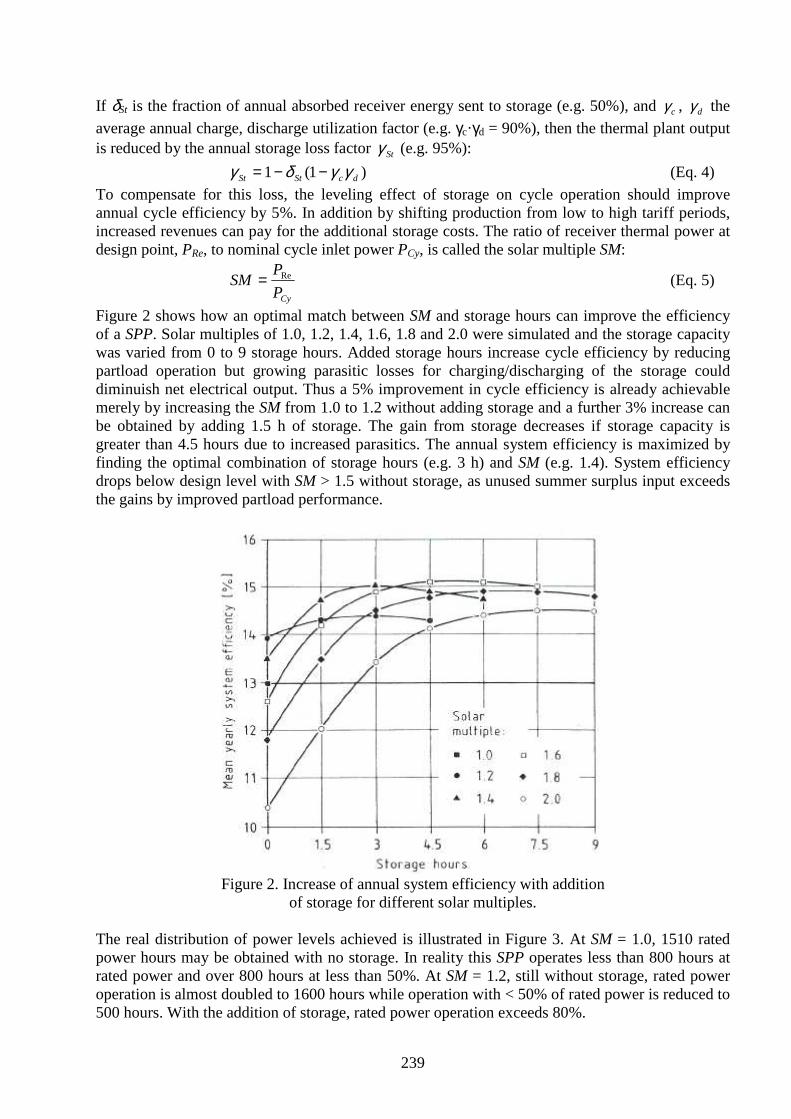
239

If δSt is the fraction of annual absorbed receiver energy sent to storage (e.g. 50%), and cγ , dγ the

average annual charge, discharge utilization factor (e.g. γc·γd = 90%), then the thermal plant output is reduced by the annual storage loss factor Stγ (e.g. 95%):

)1(1 dcStSt γγδγ −−= (Eq. 4)

To compensate for this loss, the leveling effect of storage on cycle operation should improve annual cycle efficiency by 5%. In addition by shifting production from low to high tariff periods, increased revenues can pay for the additional storage costs. The ratio of receiver thermal power at design point, PRe, to nominal cycle inlet power PCy, is called the solar multiple SM:

CyP

PSM Re= (Eq. 5)

Figure 2 shows how an optimal match between SM and storage hours can improve the efficiency of a SPP. Solar multiples of 1.0, 1.2, 1.4, 1.6, 1.8 and 2.0 were simulated and the storage capacity was varied from 0 to 9 storage hours. Added storage hours increase cycle efficiency by reducing partload operation but growing parasitic losses for charging/discharging of the storage could diminuish net electrical output. Thus a 5% improvement in cycle efficiency is already achievable merely by increasing the SM from 1.0 to 1.2 without adding storage and a further 3% increase can be obtained by adding 1.5 h of storage. The gain from storage decreases if storage capacity is greater than 4.5 hours due to increased parasitics. The annual system efficiency is maximized by finding the optimal combination of storage hours (e.g. 3 h) and SM (e.g. 1.4). System efficiency drops below design level with SM > 1.5 without storage, as unused summer surplus input exceeds the gains by improved partload performance.

Figure 2. Increase of annual system efficiency with addition

of storage for different solar multiples. The real distribution of power levels achieved is illustrated in Figure 3. At SM = 1.0, 1510 rated power hours may be obtained with no storage. In reality this SPP operates less than 800 hours at rated power and over 800 hours at less than 50%. At SM = 1.2, still without storage, rated power operation is almost doubled to 1600 hours while operation with < 50% of rated power is reduced to 500 hours. With the addition of storage, rated power operation exceeds 80%.

240

Figure 3. Real distribution of power levels achieved. 1) SM = 1.0; 2) SM = 1.2; 3) SM = 1.4,

Storage hours = 1.5; 4) SM = 1.6, Storage hours = 3.0; 5) SM = 2.0, Storage hours = 4.5. Relative to the base case with the SM =1.0 and no storage, cost analyses showed that the specific electricity cost can be reduced by up to 15% if SM is increased to 1.4, even without adding storage. With storage, a specific cost decrease of up to 25% is possible. In Figure 4 the results from an other study are reported showing the levelized cost of energy (in 2004 dollars) for near-term parabolic trough plants with different sizes of solar field and amounts of thermal storage. The minimum cost of energy from a plant with no thermal energy storage occurs with a solar multiple of about 1.5. The lowest cost of energy for a plant with thermal storage occurs with 12 hours of thermal energy storage and a solar multiple of about 2.5-3.0.

Figure 4. Levelized cost of energy as a function of solar field size and thermal storage capacity.

241

9.3.2 Media for thermal storage

The storage media can be solid, liquid or phase-change media. The energetic densities of the main thermal energy storage liquid media are shown in Table 2.

Storage medium Temperature [°C] Average heat capacity [kJ/kg-K]

Volume specific heat capacity [kWht/m

3] Liquid media

Mineral oil 200 - 300 2.6 55 Synthetic oil 250 - 350 2.3 57 Silicone oil 300 - 400 2.1 52 Nitrite salts 250 – 450 1.5 152 Nitrate salts 265 - 565 1.6 250 Carbonate salts 450 - 850 1.8 430 Liquid sodium 270 - 530 1.3 80

Table 2. Thermal data of storage media considered for SPPs. For temperatures of up to 300°C thermal mineral oil can be stored at ambient pressure and is the most economical and practical solution. Synthetic and silicone oils, available for up to 410°C, have to be pressurized and are expensive. Molten salts and sodium can be used between 300 and 550°C at ambient pressure but require parasitic energy to keep them liquid. In a “single medium storage” system, the HTF is at the same time the storage medium. The advantage is that no internal heat exchange between HTF and storage medium is necessary. If the liquid has low thermal conductivity and permits good thermal stratification (such as water and thermal oil) the one-tank “thermocline” concept requires the least tank volume since the hot and cold medium are contained in a single vessel. When thermal conductivity is higher (molten salts or sodium) a rapid balancing of the temperatures in the hot and cold regions takes place, making separate hot and cold tanks necessary. “Dual medium storage” employ a storage medium that is different from the HTF because the storage medium, usually solid, is cheaper than the transfer fluid. The HTF exchanges its heat in direct or indirect contact with the storage medium. The main disadvantage is a drop in temperature between charging and discharging due to the intermediate heat exchange. Storage concepts can be classified in terms of the primary HTF : � Oil-cooled solar plants: Thermal, synthetic and silicone oils with operating temperatures from

300°C to over 400°C are interesting as HTF for SPP. Unlike water/steam, oils do not require high pressure piping and they do not have freezing problems as with sodium or molten salt. Thermal oil as a storage medium has been tested in both the single tank thermocline and in the two tanks configurations. Only the first of the SEGS plants used mineral oil as both HTF and storage medium. The use of synthetic and silicone oils made oil storage concepts prohibitively expensive and dual medium concepts were studied. In Solar One a 180 MWht capacity dual medium thermocline storage system, operating between 218°C and 304°C was adopted. Its cylindrical steel tank was filled with a compacted bed of rock and sand impregnated with heat transfer oil. In the IEA-SSPS project the volume of the vessel was filled with cast iron plates that implied no oil degradation but it was too expensive.

� Steam-cooled solar plants: At Solar One water/steam was used as HTF for the central receiver allowing direct feeding of a steam-driven turbine. However steam generated at 500°C and 100 bar cannot be stored directly and economically. Therefore, a separate oil loop transfer heat to and from rock/sand storage. The problem is that while steam is produced at about 500°C/100 bar in the receiver system, steam from storage reached only 277°C/27 bar at Solar One. Thus

242

the cycle efficiency was reduced by nearly 50%. The problem is related with the heat exchange between the liquid heat storage medium and the phase-changing HTF, i.e. condensing steam at charging and evaporating steam at discharging.

� Molten salt-cooled solar plants: Molten salts are favoured central receiver coolants because of their high volume heat capacity, low vapor pressure, good heat transfer and low cost, which makes them economical enough to be used as a large bulk storage medium while their thermodynamic properties permit compact and efficient receivers. However the storage tanks must be hydraulically separated from the receiver loop by an intermediate heat exchanger in order to store storage medium at ambient pressure.

� Sodium-cooled solar plants: Due to its excellent thermodynamic properties, sodium has been found to be an efficient receiver coolant. A 5 MWht 280°C to 560°C sodium storage system operated for four years at the IEA-SSPS project. Although sodium cost is higher than molten salt, total system costs do not differ so much because the sodium tank is cheaper.

9.4 Thermal solar power plants

Several solar thermal facilities were built. The early facilities were designed as modest-size experimental or prototype solar power plants SPP. Of all solar thermal technologies, SPPs using parabolic trough concentrators were the first to reach sufficient maturity to be constructed on a commercial basis in a favourable regulatory environment. Since 2007 many new large solar power plant have been built, or are in a construction phase, mainly in US and Spain based on the parabolic trough and tower technology. Some of the early SPP experiences, as well as the more recent SPPs, are here below briefly described.

9.4.1 Farm solar power plants with line-focussing collectors (parabolic trough and

linear Fresnel)

In Egypt a solar thermal power facility of 35 kWmech capacity using line-focussing parabolic troughs was demonstrated as early as 1913. The facility was designed for pumping water. The advent of the oil economy stymied any subsequent development efforts and development activities started again in the mid 1970s in response to the sudden oil price increase. Some typical aspects of parabolic troughs SPPs can be highlighted: � Each collector field consists of parallel loops of individual parabolic trough collectors in series.

HTF is usually thermo-oil (suitable up to 300°C) or synthetic oil (stable up to 400°C). The advantage of oil as primary HTF is a low vapor pressure, resulting in operating pressures < 5 bar. The disadvantage of oil is the viscosity at low temperatures, which is critical at start-up after the plant has cooled down. By temperature stratification, oil offers the advantage of one-tank thermal energy storage (thermocline principle).

� Small collector fields need some amount of storage to allow operation of the power conversion unit independent from changes in oil temperature as a consequence of irradiation transients. The oil inventory of large collector fields provides sufficient operational flexibility without buffer storage.

� For maximizing annual generation, yet minimizing size and cost of collector fields, thermodynamic conversion must be as efficient as possible for the solar-induced broad range of operating conditions. Taking advantage of off-the-shelf PCUs for cost reasons, early designs tended to be not well adapted to variable operating conditions. Wet cooling is essential for best possible cycle efficiency but in sunny and arid regions scarcity of water may necessitate that dry cooling be used affecting annual plant performance.

243

1) IEA-SSPS. The experimental parabolic trough IEA-SSPS (International Energy Agency – Small Solar Power System) farm plant in Almeria, Spain (1981) was designed for 500 kWe net generation at 920 W/m2 irradiation at equinox noon. For performance comparison two different collector types were installed: one collector field consisted of one-axis tracking collectors, the other was made up of two-axes tracking modules. For the same reason two thermocline storage vessels, one with dual media, were incorporated. A steam turbine generator was selected in preference to an ORC-based power conversion subsystem. Compensating for a low solar multiple SM, the plant routinely was operated in storage charging mode for several hours before the steam generator and PCU were started. This operating strategy provided for a maximum of full-rated power production. The energy production was curtailed by lower than expected local irradiation and low PCU efficiency and by high thermal inertia and high irradiation threshold (> 350 W/m2) for net generation. Significant findings were that the expected performance advantage of a two-axes tracking trough collector field could not be demonstrated because the additional collected energy was compensated for by higher piping losses. Furthermore the maintenance of the one axis tracking collector is considerably easier than for the two axes. An other finding was that plant performance decreased sharply as compared to rated performance when the irradiation was less than assumed for the design point. 2) SEGS I-IX. The nine Solar Electric Generating Systems or SEGS, located in the California Mojave Desert are the world’s largest solar power plants. These plants, developed between 1984 and 1990, range in size from 14–80 MW and comprise 354 MW of installed electric generating capacity and more than 2 million m2 of parabolic trough collectors. The trough solar collectors (LS-1, LS-2, LS-3) progressed to larger trough apertures (from 2.5 to 5.7 m), higher concentration ratios (from 61 to 82) and improved absorber emissivities (from 0.30 to 0.15). Routine hybrid operation (solar + natural gas) of the SEGS plants renders it difficult to determine their performance in solar-only operating mode from output statistics. In a program that ran from 1992 to 1997 work was carried out to reduce operation and maintenance (O&M) costs, improve plant efficiency, and reduce the cost of energy produced. Cost-reduction strategies were developed for O&M planning optimization, subsystem automation, collector alignment and cleaning, reliability improvement of components subjected to cyclic operation, and subsystem efficiency improvement. The current state-of-the-art in parabolic trough plant design is an outgrowth of the Luz SEGS power-plant technology. In general, a parabolic trough solar power plant in a good solar resource region requires approximately 5 acres (20,000 m2) per MW of plant capacity. Plants with thermal storage and higher capacity factors will require proportionally more land per MWe. The system diagram of SEGS VIII is shown in Figure 5.

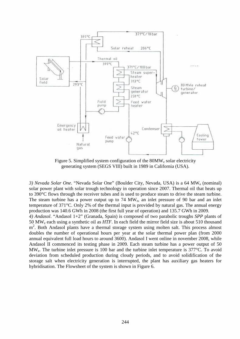
244

Figure 5. Simplified system configuration of the 80MWe solar electricity

generating system (SEGS VIII) built in 1989 in California (USA). 3) Nevada Solar One. “Nevada Solar One” (Boulder City, Nevada, USA) is a 64 MWe (nominal) solar power plant with solar trough technology in operation since 2007. Thermal oil that heats up to 390°C flows through the receiver tubes and is used to produce steam to drive the steam turbine. The steam turbine has a power output up to 74 MWe, an inlet pressure of 90 bar and an inlet temperature of 371°C. Only 2% of the thermal input is provided by natural gas. The annual energy production was 140.6 GWh in 2008 (the first full year of operation) and 135.7 GWh in 2009. 4) Andasol. “Andasol 1+2” (Granada, Spain) is composed of two parabolic troughs SPP plants of 50 MWe each using a synthetic oil as HTF. In each field the mirror field size is about 510 thousand m2. Both Andasol plants have a thermal storage system using molten salt. This process almost doubles the number of operational hours per year at the solar thermal power plan (from 2000 annual equivalent full load hours to around 3600). Andasol I went online in november 2008, while Andasol II commenced its testing phase in 2009. Each steam turbine has a power output of 50 MWe. The turbine inlet pressure is 100 bar and the turbine inlet temperature is 377°C. To avoid deviation from scheduled production during cloudy periods, and to avoid solidification of the storage salt when electricity generation is interrupted, the plant has auxiliary gas heaters for hybridisation. The Flowsheet of the system is shown in Figure 6.

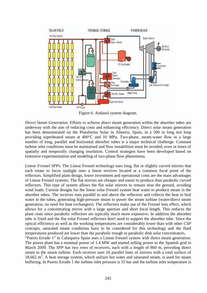
245

Figure 6. Andasol system diagram.

Direct Steam Generation. Efforts to achieve direct steam generation within the absorber tubes are underway with the aim of reducing costs and enhancing efficiency. Direct solar steam generation has been demonstrated on the Plataforma Solar in Almeria, Spain, in a 500 m long test loop providing superheated steam at 400°C and 10 MPa. Two-phase, steam-water flow in a large number of long, parallel and horizontal absorber tubes is a major technical challenge. Constant turbine inlet conditions must be maintained and flow instabilities must be avoided, even in times of spatially and temporally changing insolation. Control strategies have been developed based on extensive experimentation and modeling of two-phase flow phenomena. Linear Fresnel SPPs. The Linear Fresnel technology uses long, flat or slightly curved mirrors that each rotate to focus sunlight onto a linear receiver located at a common focal point of the reflectors. Simplified plant design, lower investment and operational costs are the main advantages of Linear Fresnel systems. The flat mirrors are cheaper and easier to produce than parabolic curved reflectors. This type of system allows the flat solar mirrors to remain near the ground, avoiding wind loads. Current designs for the linear solar Fresnel system heat water to produce steam in the absorber tubes. The receiver runs parallel to and above the reflectors and collects the heat to boil water in the tubes, generating high-pressure steam to power the steam turbine (water/direct steam generation, no need for heat exchangers). The reflectors make use of the Fresnel lens effect, which allows for a concentrating mirror with a large aperture and short focal length. This reduces the plant costs since parabolic reflectors are typically much more expensive. In addition the absorber tube is fixed and the flat solar Fresnel reflectors don't need to support the absorber tube. Since the optical efficiency as well as the working temperatures are considerably lower than with other CSP concepts, saturated steam conditions have to be considered for this technology and the fluid temperatures produced are lower than the parabolic trough or parabolic dish solar concentrators. “Puerto Errado 1” in Calasparra Spain uses a Linear Fresnel system with direct steam generation. The power plant has a nominal power of 1.4 MW and started selling power to the Spanish grid in March 2009. The SPP has two rows of receivers, each with a length of 860 m, providing direct steam to the steam turbine. Each receiver uses 16 parallel lines of mirrors with a total surface of 18,662 m2. A heat storage system, which utilizes hot water and saturated steam, is used for steam buffering. In Puerto Errado 1 the turbine inlet pressure is 55 bar and the turbine inlet temperature is

246

270°C (saturated steam). Construction of the utility-scale Linear Fresnel CSP plant Puerto Errado 2 (30 MW) started in April 2010 and is scheduled for completion in 2012.

Figure 7. SPP with Fresnel technology.

Integrated Solar Combined Cycle System. The Archimede Project is the first integration, worldwide, of a gas combined cycle and a solar thermodynamic power plant. The project is based on a strongly innovative technology elaborated by Enea. It was built in Enel's power station in Priolo Gargallo (Siracusa, Sicily), which was chosen for its high insulation levels and its morphological characteristics. The solar concentration power plant, completely integrated with the thermodynamic cycle and the other facilities and services of the plant, increase the plant's power by about 5 MW. The key innovative features that distinguish Archimede from other similar projects making use of linear parabolic trough solar collectors are the development of a tube with a selective coating, specifically designed for high temperatures, with high absorption levels and high selectivity in terms of thermal re-emission. This allows to use molten salts both as the HTF and storage medium making it possible to operate at higher temperatures (550 °C) as compared to other technologies. Thus a better integration of the solar plant with the combined cycle is obtained, with significant synergies and greater solar conversion efficiency. The Integrated Solar Combined Cycle System (ISCCS) configuration, shown in Figure 8, integrates a trough solar plant into the bottoming cycle of a combined cycle plant. The primary advantage is that the incremental cost of increasing the bottoming cycle is less than the cost of a stand alone steam power plant. The disadvantage is the added complexity of integrating the solar and the gas. Solar energy is used to generate steam and the waste heat from the gas turbine is used for preheating and superheating the steam.

247

Figure 8. Process Flow Diagram for Integrated Solar Combined Cycle System (ISCCS).

9.4.2 Central Receiver Solar Power Plants with Heliostat Fields

The main advantage of solar power towers in comparison to line-focusing systems is the ability to provide high-temperature superheated steam, leading to higher power generation efficiencies. The advantage over the parabolic trough or Fresnel collector concept is that the sunlight on the central receiver is focused to a smaller area, and the heat transfer medium does not have to be piped around the large solar field. This means that higher working fluid temperatures in the receiver (up to 1000°C) and better steam parameters are feasible. Development of solar tower systems began in the early sixties with work by G. Francia (Italy): he operated a small facility with 135 m2 of mechanically controlled mirrors and about 130 kWt capacity (but without thermodynamic cycle conversion) at San Ilario-Nervi near Genoa. In the early seventies, the 1500 kWt French solar furnace at Odeillo, Pyrenees became operational and was used in the mid seventies to demonstrate operational feasibility of an electricity producing cycle. Subsequently many solar tower facilities were built. 1) Solar One and Two. The 10 MWe Solar One at Barstow/CA (USA) was of “single-loop” design and employing water/superheated steam as the primary heat transfer medium and as working fluid in the power conversion cycle. Solar One was operated from early 1982 to late 1988. Water was preheated in two steps, evaporated and superheated in a once-through external receiver. A dual medium (oil/rocks) thermal storage could be charged/discharged via steam/oil heat exchangers. Heat supply for the steam turbine could come from the receiver directly, or from storage via a steam generator (at degraded steam conditions), or both simultaneously. In place of the once-through steam system of Solar One, a mixture of potassium and sodium nitrate salts was used as the prime mover fluid in the Solar Two demonstration. The change reduced the pressure of the receiver chamber because water was no longer used and allowed for thermal storage to be achieved at high temperatures (>500°C).

248

Figure 9. System diagram of the Solar One 10 MWe tower SPP in California (USA).

2) Themis and IEA-SSPS. Other two experimental tower SPPs employed “dual loop” heat transport concepts using a liquid as primary coolant. Primary HTF was eutectic salt in the 2.3 MWe Themis plant at Targasonne (France) and sodium in the IEA-SSPS 500 kWe tower plant in Almeria (Spain). The “dual loop” concept allows higher receiver heat fluxes yet reduces cycle fatigue stress of the receiver material, (subjecting it to lower internal pressure and avoiding quenching effects by oscillating water columns). In Themis SPP a steam generator linked the secondary conversion cycle loop to the primary salt loop. This decoupled solar energy input and storage charging from power output generation, made plant operation more flexible. Thus temporary drops in the collection of solar energy in the primary circuit hardly affected operation of the PCU at nominal cycle conditions. Energy was accumulated in the storage tanks until enough salt at sufficiently high temperature was available to sustain a rated output generation for 2-3 hours. Only at this point the turbine was started and power generated. In the IEA-SSPS a sodium/steam generator decoupled the secondary water/steam loop from the primary sodium circuit and the power circuit was operated with hot storage sufficiently charged. 3) Eurelios. “Eurelios” was a 1.0 MWe full system experiment located in Adrano, Italy. Its objective was to demonstrate the grid-connected operation of a tower SPP and to gain data. Eurelios was the first tower SPP ever to be operated, being connected to the grid in the spring of 1981. The plant design incorporated a once-through water/steam receiver and a short-time buffer storage, using molten salt and a water/steam accumulator. A minimum irradiation of 450 W/m2 of direct normal irradiation was specified. Due primarily to the extreme pipe length of the receiver, total start-up of the plant required about 2 hours. The operation showed that excellent direct irradiation conditions and minimal thermal losses and parasitics both during operation and stand-by were key design criteria for good net energy performance from solar input. Peak power performance, although of considerable technical interest, is an inadequate indicator for judging real system performance. 4) PS10 and PS20. PS10 solar thermal power plant in southern Spain, just west of Seville, was inaugurated in March 2007 and it has a nominal power of 11 MWe. The plant concentrates the sun’s rays onto the top of a tower 115 m high and the solar receiver on top of the tower produces saturated steam and circulates it to a conventional steam turbine that generates the electricity. The

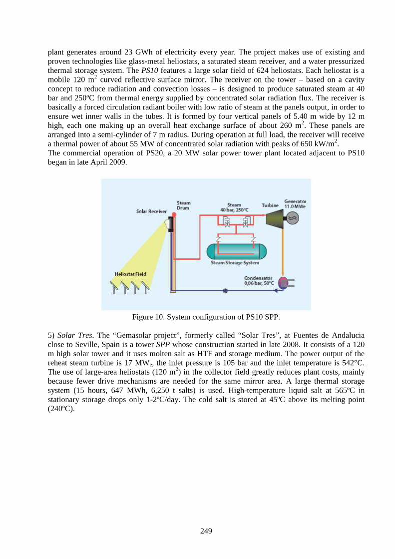
249

plant generates around 23 GWh of electricity every year. The project makes use of existing and proven technologies like glass-metal heliostats, a saturated steam receiver, and a water pressurized thermal storage system. The PS10 features a large solar field of 624 heliostats. Each heliostat is a mobile 120 m2 curved reflective surface mirror. The receiver on the tower – based on a cavity concept to reduce radiation and convection losses – is designed to produce saturated steam at 40 bar and 250ºC from thermal energy supplied by concentrated solar radiation flux. The receiver is basically a forced circulation radiant boiler with low ratio of steam at the panels output, in order to ensure wet inner walls in the tubes. It is formed by four vertical panels of 5.40 m wide by 12 m high, each one making up an overall heat exchange surface of about 260 m2. These panels are arranged into a semi-cylinder of 7 m radius. During operation at full load, the receiver will receive a thermal power of about 55 MW of concentrated solar radiation with peaks of 650 kW/m2. The commercial operation of PS20, a 20 MW solar power tower plant located adjacent to PS10 began in late April 2009.

Figure 10. System configuration of PS10 SPP.

5) Solar Tres. The “Gemasolar project”, formerly called “Solar Tres”, at Fuentes de Andalucia close to Seville, Spain is a tower SPP whose construction started in late 2008. It consists of a 120 m high solar tower and it uses molten salt as HTF and storage medium. The power output of the reheat steam turbine is 17 MWe, the inlet pressure is 105 bar and the inlet temperature is 542°C. The use of large-area heliostats (120 m2) in the collector field greatly reduces plant costs, mainly because fewer drive mechanisms are needed for the same mirror area. A large thermal storage system (15 hours, 647 MWh, 6,250 t salts) is used. High-temperature liquid salt at 565ºC in stationary storage drops only 1-2ºC/day. The cold salt is stored at 45ºC above its melting point (240ºC).

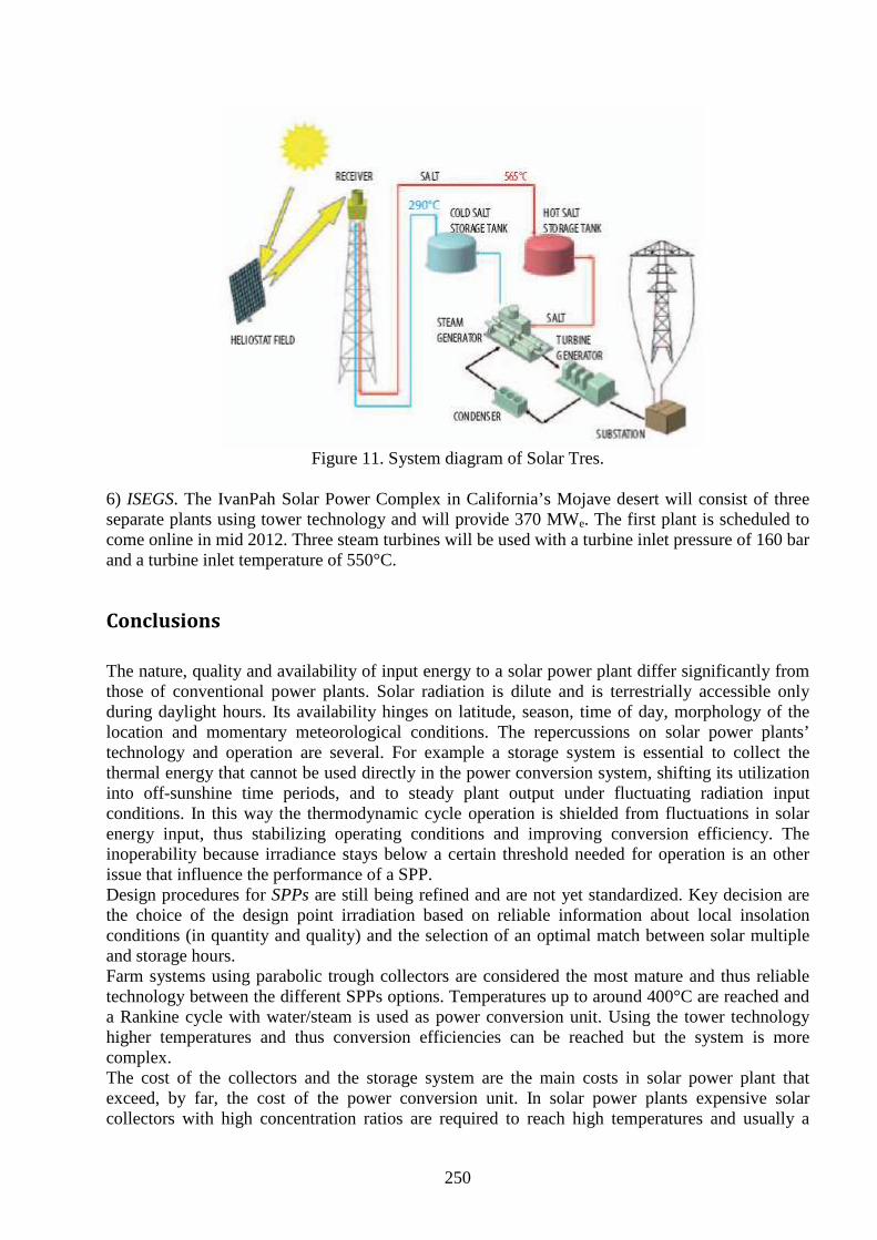
250

Figure 11. System diagram of Solar Tres.

6) ISEGS. The IvanPah Solar Power Complex in California’s Mojave desert will consist of three separate plants using tower technology and will provide 370 MWe. The first plant is scheduled to come online in mid 2012. Three steam turbines will be used with a turbine inlet pressure of 160 bar and a turbine inlet temperature of 550°C.

Conclusions

The nature, quality and availability of input energy to a solar power plant differ significantly from those of conventional power plants. Solar radiation is dilute and is terrestrially accessible only during daylight hours. Its availability hinges on latitude, season, time of day, morphology of the location and momentary meteorological conditions. The repercussions on solar power plants’ technology and operation are several. For example a storage system is essential to collect the thermal energy that cannot be used directly in the power conversion system, shifting its utilization into off-sunshine time periods, and to steady plant output under fluctuating radiation input conditions. In this way the thermodynamic cycle operation is shielded from fluctuations in solar energy input, thus stabilizing operating conditions and improving conversion efficiency. The inoperability because irradiance stays below a certain threshold needed for operation is an other issue that influence the performance of a SPP. Design procedures for SPPs are still being refined and are not yet standardized. Key decision are the choice of the design point irradiation based on reliable information about local insolation conditions (in quantity and quality) and the selection of an optimal match between solar multiple and storage hours. Farm systems using parabolic trough collectors are considered the most mature and thus reliable technology between the different SPPs options. Temperatures up to around 400°C are reached and a Rankine cycle with water/steam is used as power conversion unit. Using the tower technology higher temperatures and thus conversion efficiencies can be reached but the system is more complex. The cost of the collectors and the storage system are the main costs in solar power plant that exceed, by far, the cost of the power conversion unit. In solar power plants expensive solar collectors with high concentration ratios are required to reach high temperatures and usually a

251

storage system is needed. The integration of the solar resource with the geothermal resource in a binary power plant may solve many issues that affect the operation and the economics of solar power plants. Although the temperature level is reduced, cheaper solar collectors could be used, the storage system could be eliminated or scaled down and the power conversion unit would work with a higher capacity factor. In addition, as shown in the following chapter, there are many synergies between the solar and the geothermal resource that could be fruitfully used.

252

References Duffie J.A. and Beckman W.A., Solar Engineering of Thermal Processes, Wiley, 2006. Winter C.-J., Sizmann R. L. and Vant-Hull L.L., Solar Power Plants, Springer-Verlag, 1990. Concentrating Solar Power. From Research to Implementation, European Communities, 2007. Turboden Solar Thermal Power Applications, PowerPoint presentation, 2010. Cohen G.E., Nevada Solar One – Case Study, CSP Today Conference, San Francisco, June 2010. Muller-Steinhagen H. and Trieb F., Concentrating Solar Power, A review of the technology, 2004. Steam Turbines for CSP plants, Siemens, 2010. Solar Trough Power Plants, U.S. Department of Energy, 2000. Solar Thermal – Concentrated Solar Power, NREL Report, 2005.

253

10. Hybrid Solar-Geothermal Power Generation

to Increase the Energy Production from Binary

Geothermal Plants A study was performed to increase the performance of Stillwater geothermal binary power plant with the addition of the solar source. The detailed off-design model of the Stillwater geothermal binary power plant was used as the basis for this hybridization study. The addition of the solar thermal heat in geothermal power plants could provide many advantages: � the medium temperature solar heat can be combined with the low enthalpy geothermal resource

in a power plant with a higher efficiency; � an increase of the power output during the day and especially during the warm season, a time

when the energy production of air-cooled geothermal power plants is markedly reduced (as seen in Chapter 7) and the power demand is greatest;

� alleviation or removal of issues associated with standalone solar power plants (described in Chapter 9) such as the need of a storage system, the irradiation threshold, the deviation from the design conditions, the low capacity factor and the resulting high costs;

� the repowering of existing geothermal power plants in order to face reductions in the geothermal flow rate and temperature restoring conditions close to the design point and boosting the plant performance;

� potential for both energy sources to share common equipment, such as expander-generators, air cooled condenser and heat exchangers; this allows more equipment to run full time even though the sun is intermittent;

In addition the combination is facilitated since in many locations there exists an overlap of good geothermal and solar resources and there are financial supports for solar projects. A proper choice of the hybrid plant configuration is essential to maximize the efficiency in the utilization of the solar resource. The cycle parameters are optimized in relation to variations of the ambient temperature and the solar irradiation in order to maximize the power output for each ambient condition and thus the annual energy production. Two hybrid geo-solar solutions are compared calculating the incremental levelized cost of electricity.

10.1 Hybrid geo-solar power plant configuration

Stillwater geothermal resources are limited: the brine flow is only 71% of the design value and the brine inlet temperature is 12.5°F lower than the design value. The power plant net power output predicted by the Aspen model for the 53.7°F ambient temperature is 20.9 MW. This value is about 60% of the value predicted by Power Engineers for the design conditions. The power plant is operating at part-load conditions, far from the design conditions; it could produce much more power with an adequate heat source since the gross power capacity for each of its four expanders is 12 MW. The results from the geothermal only analysis and the detailed modeling of the main Stillwater power plant components provide a good starting point for the hybrid geothermal-solar analysis.

254

The gross power output is given by:

( ) GENMECHLISISWFGROSS WhmW ηη ⋅−⋅∆⋅= _& (Eq. 1)

The addition of solar heat increases the gross power output by increasing one or more of the following parameters: working fluid flow rate WFm& , isentropic enthalpy drop ∆hIS and turbine

isentropic efficiency ηIS. The geothermal-only analysis showed that these three parameters are closely related and the maximum power output occurs in correspondence to the cycle high pressure that maximizes the product of these three parameters. The solar heat should be used to increase both WFm& and ∆hIS without lowering ηIS. This aspect is important to define both the hybrid power plant configuration and the required size of the solar field. The expander isentropic efficiency has its maximum for ∆hIS,DES = 24.4 Btu/lb and DESOUTV ,

& =

40,000 ft3/min. Using only the available geothermal resource: - ∆hIS is higher than ∆hIS,DES (except for the highest ambient temperatures) due to the high pressure ratios across the expander; - OUTV& is lower than DESOUTV ,

& (except for the lowest ambient temperatures) due to the low working

fluid mass flow rates. Figures 1a and b show respectively the ∆hIS and OUTV& for four ambient temperature cases compared to the expanders design values (black horizontal lines).

Expander Isentropic Enthalpy Drops

0

5

10

15

20

25

30

35

40

0 30 60 90

Ambient Temperature [°F]

∆∆ ∆∆h

IS [B

tu/lb

]

Expander Outlet Volumetric Flow Rates

0

10000

20000

30000

40000

50000

0 30 60 90

Ambient Temperature [°F]

VO

UT

[ft3 /m

in]

Figure 1a. Isentropic enthalpy drops. Figure 1b. VOUT expander.

Figure 1a shows that a further increase of ∆hIS is detrimental to the isentropic efficiency for low and moderate ambient temperatures. Figure 1b shows that an increase of the working fluid flow rate for moderate and warm ambient temperatures could be useful to increase the expander isentropic efficiency. On the basis of these results the hybrid geo-solar power plant configuration shown in Figure 2 was selected:

255

Figure 2. Hybrid Geothermal-Solar Stillwater Power Plant.

The solar heater is placed between the vaporizer and the demister. The solar heater is used to complete the vaporization of the working fluid and to provide 5°F of superheating at the inlet of the expanders. Currently, at the outlet of the vaporizer there is still a consistent working fluid liquid fraction (about 20-30% by mass); the solar heater fully vaporizes and superheats the WF. Using this power plant configuration and operational strategy both the WF flow rate and pressure are increased compared to the geothermal-only case. On the one hand, the expander isentropic efficiency increases, compared to the geo-only case, due to the higher working fluid flow rate; on the other hand, it decreases due to the higher ∆hIS. The WF pressure increase, and the resulting ∆hIS increase, is important to increase the gross power output, and in many cases it is necessary for increasing the brine outlet temperature above the lower limit of 145°F.

10.2 Solar collector field: main assumptions and calculation of the useful

solar heat

The land area available for the solar field is 200,000 m2. Parabolic trough collectors are used as a concentrating system using a sun tracking system with a rotation about a north-south axis. The last table in Figure 3 that refers to the direct beam solar radiation shows that a N-S axis orientation collects more solar energy in a year compared to an E-W axis orientation. Figure 3 is taken from the “NREL Renewable Resource Data Center” and shows the solar radiation data for Reno (NV) that is relatively close to Fallon, the Stillwater site.

256

Figure 3. Reno (NV) solar radiation data.

The incident solar radiation I is calculated from the direct normal irradiation DNI and the angle of incidence θ:

θcos⋅= DNII (Eq. 2) The cosine of the incidence angle is calculated for each month using the last table in Figure 3 by comparing the solar radiation collected using a two-axis tracking system against that collected by a horizontal N-S axis tracking system. The values are shown in Table 1.

Jan Feb Mar Apr May Jun Jul Aug Sep Oct Nov Dec 2-axis 3.7 4.4 5.3 6.3 7.3 8.2 9.1 8.3 7.6 6.2 4.0 3.6

N-S axis 2.3 3.2 4.5 5.8 7.0 8.0 8.8 7.9 6.8 4.9 2.7 2.2 cos θθθθ 0.6216 0.7273 0.8491 0.9206 0.9589 0.9756 0.9670 0.9518 0.8947 0.7903 0.6750 0.6111

Table 1. Direct beam solar radiation (kWh/m2-day) collected by a 2-axis system compared to that collected by a single N-S horizontal axis tracking system; calculation of the angle of incidence.

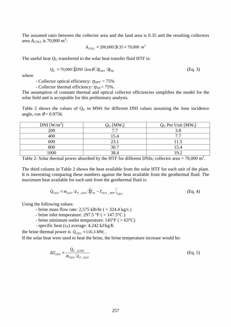
257

The assumed ratio between the collector area and the land area is 0.35 and the resulting collectors area ACOLL is 70,000 m2:

2000,7035.0000,200 mACOLL =⋅= The useful heat QU transferred to the solar heat transfer fluid HTF is:

( ) THOPTU DNIQ ηηθ ⋅⋅⋅⋅= cos000,70 (Eq. 3) where

- Collector optical efficiency: ηOPT = 75% - Collector thermal efficiency: ηTH = 75%.

The assumption of constant thermal and optical collector efficiencies simplifies the model for the solar field and is acceptable for this preliminary analysis. Table 2 shows the values of QU in MWt for different DNI values assuming the June incidence angle, cos θ = 0.9756.

DNI [W/m2] QU [MW t] QU Per Unit [MWt] 200 7.7 3.8 400 15.4 7.7 600 23.1 11.5 800 30.7 15.4 1000 38.4 19.2

Table 2: Solar thermal power absorbed by the HTF for different DNIs; collector area = 70,000 m2. The third column in Table 2 shows the heat available from the solar HTF for each unit of the plant. It is interesting comparing these numbers against the heat available from the geothermal fluid. The maximum heat available for each unit from the geothermal fluid is:

( )GEOMINOUTINGEOPGEOGEO TTcmQ __ −⋅⋅= && (Eq. 4)

Using the following values:

- brine mass flow rate: 2,575 klb/hr ( = 324.4 kg/s ) - brine inlet temperature: 297.5 °F ( = 147.5°C ) - brine minimum outlet temperature: 145°F ( ≈ 63°C) - specific heat (cP) average: 4.242 kJ/kg.K

the brine thermal power is tGEO MWQ 3.116=& . If the solar heat were used to heat the brine, the brine temperature increase would be:

GEOPGEO

UNITUGEO cm

QT

_

1_

⋅=∆

&

& (Eq. 5)

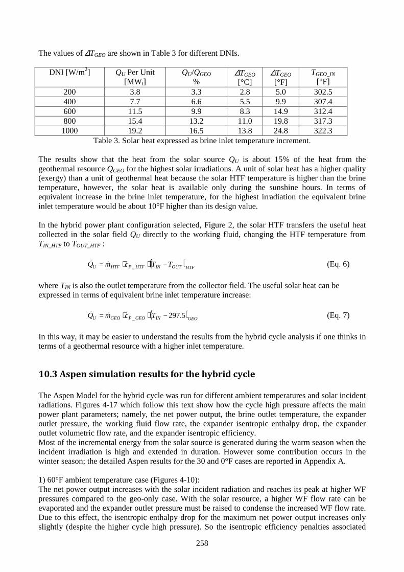
258

The values of ∆TGEO are shown in Table 3 for different DNIs.

DNI [W/m2] QU Per Unit [MW t]

QU/QGEO

% ∆TGEO [°C]

∆TGEO [°F]

TGEO_IN [°F]

200 3.8 3.3 2.8 5.0 302.5 400 7.7 6.6 5.5 9.9 307.4 600 11.5 9.9 8.3 14.9 312.4 800 15.4 13.2 11.0 19.8 317.3 1000 19.2 16.5 13.8 24.8 322.3

Table 3. Solar heat expressed as brine inlet temperature increment. The results show that the heat from the solar source QU is about 15% of the heat from the geothermal resource QGEO for the highest solar irradiations. A unit of solar heat has a higher quality (exergy) than a unit of geothermal heat because the solar HTF temperature is higher than the brine temperature, however, the solar heat is available only during the sunshine hours. In terms of equivalent increase in the brine inlet temperature, for the highest irradiation the equivalent brine inlet temperature would be about 10°F higher than its design value. In the hybrid power plant configuration selected, Figure 2, the solar HTF transfers the useful heat collected in the solar field QU directly to the working fluid, changing the HTF temperature from TIN_HTF to TOUT_HTF :

( )HTFOUTINHTFPHTFU TTcmQ −⋅⋅= _&& (Eq. 6)

where TIN is also the outlet temperature from the collector field. The useful solar heat can be expressed in terms of equivalent brine inlet temperature increase:

( )GEOINGEOPGEOU TcmQ 5.297_ −⋅⋅= && (Eq. 7)

In this way, it may be easier to understand the results from the hybrid cycle analysis if one thinks in terms of a geothermal resource with a higher inlet temperature.

10.3 Aspen simulation results for the hybrid cycle

The Aspen Model for the hybrid cycle was run for different ambient temperatures and solar incident radiations. Figures 4-17 which follow this text show how the cycle high pressure affects the main power plant parameters; namely, the net power output, the brine outlet temperature, the expander outlet pressure, the working fluid flow rate, the expander isentropic enthalpy drop, the expander outlet volumetric flow rate, and the expander isentropic efficiency. Most of the incremental energy from the solar source is generated during the warm season when the incident irradiation is high and extended in duration. However some contribution occurs in the winter season; the detailed Aspen results for the 30 and 0°F cases are reported in Appendix A. 1) 60°F ambient temperature case (Figures 4-10): The net power output increases with the solar incident radiation and reaches its peak at higher WF pressures compared to the geo-only case. With the solar resource, a higher WF flow rate can be evaporated and the expander outlet pressure must be raised to condense the increased WF flow rate. Due to this effect, the isentropic enthalpy drop for the maximum net power output increases only slightly (despite the higher cycle high pressure). So the isentropic efficiency penalties associated

259

with the further departure from the expander design ∆hIS are reduced; overall, ηIS slightly increases with the solar radiation due to the higher expander outlet volumetric flow rate. The higher WF flow rate in the hybrid operation lowers the brine outlet temperature compared to the geo-only case, but the optimal WF pressures are higher than in the geo-only case which leads to higher brine return temperatures. For the 60°F case the selected WF pressures, shown with larger dots, are very close to pressures that maximize the net power output. 2) 90°F ambient temperature case (Figures 11-17): The brine outlet temperature is always higher than 145°F and the WF optimal pressure increases with the incident radiation. The expander outlet pressure is further increased to condense the increased WF flow rate, brushing against values around 100 psia. Thus, despite the increase of the working fluid flow rate, the WF outlet volumetric flow rate per expander stays close 20,000 ft3/min, or about half of the expander design value. The isentropic efficiency slightly increases with the incident radiation due to the increase of ∆hIS that approaches the expander design isentropic enthalpy drop value. 3) 30 and 0°F ambient temperature cases (Appendix F, Figures F1-F12): The net power output maximum is constrained by the minimum brine return temperature. So the selected pressures, shown with larger dots, are higher than the peak net power pressures. However with the increase of the solar radiation the net power output curves becomes flatter with the WF pressure so the difference in net power output between the constrained and unconstrained case is reduced. The expander outlet pressure is often at its minimum value of 40 psia. The increase of the cycle high pressure and WF mass flow rate with higher incident solar radiation imply, respectively, higher ∆hIS and VOUT. These two parameters are already above their design value with the geo-only resource, so their increase implies a further reduction of ηIS. Thus for low ambient temperatures, the increase in gross power output with the solar radiation comes only from the increase in the WF mass flow rate and ∆hIS across the expander, while it is hampered by the reduction in ηIS.

260

� Aspen simulation results: ambient temperature 60°F

Stillwater - Variation of Net Power Output with cyc le high pressure for different solar incident radiations

Ambient Temperature = 60°F

0

2000

4000

6000

8000

10000

12000

14000

16000

280 300 320 340 360 380 400 420 440 460 480

Preheater Inlet Pressure [psia]

Net

Pow

er [k

W] Geo-only

Inc_Rad = 200 W/m2

Inc_Rad = 400 W/m2

Inc_Rad = 600 W/m2

Inc_Rad = 800 W/m2

Figure 4. Variation of net power output with cycle high pressure and incident solar

radiation for 60°F ambient temperature.

Stillwater - Variation of Brine Outlet Temperature with cycle high pressure for different solar incident radiatio ns

Ambient Temperature = 60°F

100

120

140

160

180

200

220

280 300 320 340 360 380 400 420 440 460 480

Preheater Inlet Pressure [psia]

Tem

pera

ture

[°F

] Geo-only

Inc_Rad = 200 W/m2

Inc_Rad = 400 W/m2

Inc_Rad = 600 W/m2

Inc_Rad = 800 W/m2

Limit

Figure 5. Variation of brine outlet temperature with cycle high pressure and incident solar

radiation for 60°F ambient temperature.

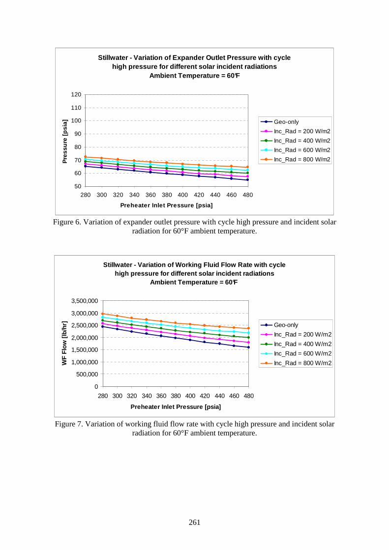
261

Stillwater - Variation of Expander Outlet Pressure with cycle high pressure for different solar incident radiatio ns

Ambient Temperature = 60°F

50

60

70

80

90

100

110

120

280 300 320 340 360 380 400 420 440 460 480

Preheater Inlet Pressure [psia]

Pre

ssur

e [p

sia]

Geo-only

Inc_Rad = 200 W/m2

Inc_Rad = 400 W/m2

Inc_Rad = 600 W/m2

Inc_Rad = 800 W/m2

Figure 6. Variation of expander outlet pressure with cycle high pressure and incident solar

radiation for 60°F ambient temperature.

Stillwater - Variation of Working Fluid Flow Rate w ith cycle high pressure for different solar incident radiatio ns

Ambient Temperature = 60°F

0

500,000

1,000,000

1,500,000

2,000,000

2,500,000

3,000,000

3,500,000

280 300 320 340 360 380 400 420 440 460 480

Preheater Inlet Pressure [psia]

WF

Flo

w [l

b/hr

] Geo-only

Inc_Rad = 200 W/m2

Inc_Rad = 400 W/m2

Inc_Rad = 600 W/m2

Inc_Rad = 800 W/m2

Figure 7. Variation of working fluid flow rate with cycle high pressure and incident solar

radiation for 60°F ambient temperature.

262

Stillwater - Variation of Isentropic Enthalpy Drop with cycle high pressure for different solar incident radiatio ns

Ambient Temperature = 60°F

10

15

20

25

30

35

40

45

280 300 320 340 360 380 400 420 440 460 480

Preheater Inlet Pressure [psia]

∆∆ ∆∆hi

s [B

tu/lb

]

Geo-only

Inc_Rad = 200 W/m2

Inc_Rad = 400 W/m2

Inc_Rad = 600 W/m2

Inc_Rad = 800 W/m2

Expander_Design

Figure 8. Variation of isentropic enthalpy drop with cycle high pressure and incident solar

radiation for 60°F ambient temperature.

Stillwater - Variation of WF Volumetric Flow Rate a t the outlet of each Expander with cycle high pressure for different sol ar incident radiations

Ambient Temperature = 60°F

20,000

25,000

30,000

35,000

40,000

45,000

280 300 320 340 360 380 400 420 440 460 480

Preheater Inlet Pressure [psia]

VO

UT [

ft3/m

in]

Geo-only

Inc_Rad = 200 W/m2

Inc_Rad = 400 W/m2

Inc_Rad = 600 W/m2

Inc_Rad = 800 W/m2

Expander_Design

Figure 9. Variation of volumetric flow rate at the outlet of each Expander with cycle high pressure

and incident solar radiation for 60°F ambient temperature.

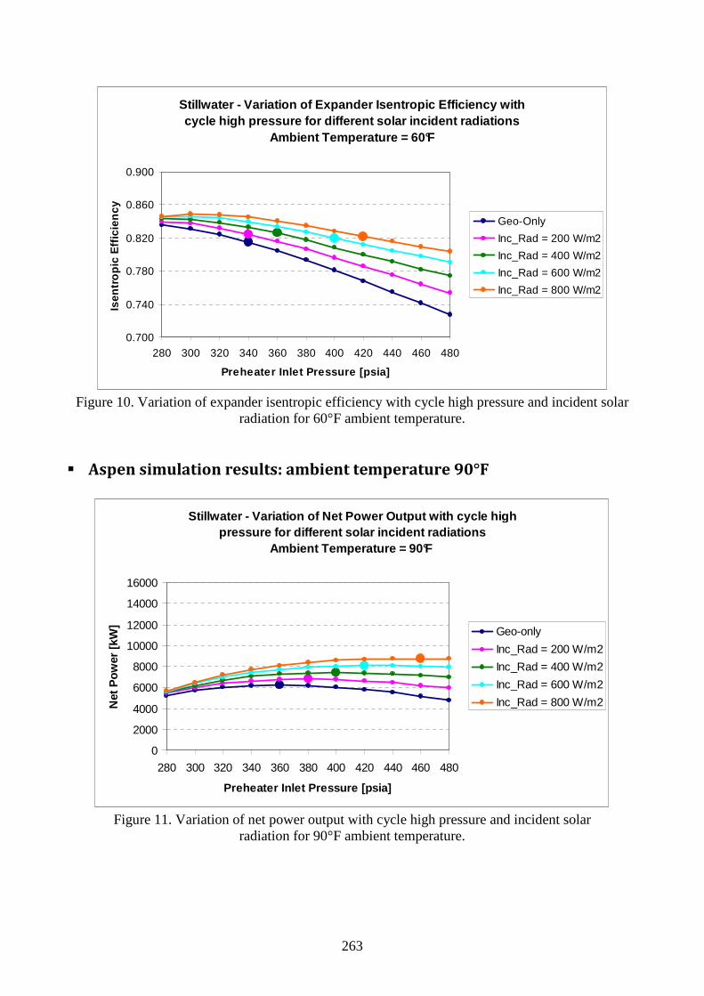
263

Stillwater - Variation of Expander Isentropic Effic iency with cycle high pressure for different solar incident ra diations

Ambient Temperature = 60°F

0.700

0.740

0.780

0.820

0.860

0.900

280 300 320 340 360 380 400 420 440 460 480

Preheater Inlet Pressure [psia]

Isen

tro

pic

Eff

icie

ncy Geo-Only

Inc_Rad = 200 W/m2

Inc_Rad = 400 W/m2

Inc_Rad = 600 W/m2

Inc_Rad = 800 W/m2

Figure 10. Variation of expander isentropic efficiency with cycle high pressure and incident solar

radiation for 60°F ambient temperature. � Aspen simulation results: ambient temperature 90°F

Stillwater - Variation of Net Power Output with cyc le high pressure for different solar incident radiations

Ambient Temperature = 90°F

0

2000

4000

6000

8000

10000

12000

14000

16000

280 300 320 340 360 380 400 420 440 460 480

Preheater Inlet Pressure [psia]

Net

Pow

er [k

W] Geo-only

Inc_Rad = 200 W/m2

Inc_Rad = 400 W/m2

Inc_Rad = 600 W/m2

Inc_Rad = 800 W/m2

Figure 11. Variation of net power output with cycle high pressure and incident solar

radiation for 90°F ambient temperature.

264

Stillwater - Variation of Brine Outlet Temperature with cycle high pressure for different solar incident radiatio ns

Ambient Temperature = 90°F

100

120

140

160

180

200

220

280 300 320 340 360 380 400 420 440 460 480

Preheater Inlet Pressure [psia]

Tem

pera

ture

[°F]

Geo-only

Inc_Rad = 200 W/m2

Inc_Rad = 400 W/m2

Inc_Rad = 600 W/m2

Inc_Rad = 800 W/m2

Limit

Figure 12. Variation of brine outlet temperature with cycle high pressure and incident solar

radiation for 90°F ambient temperature.

Stillwater - Variation of Expander Outlet Pressure with cycle high pressure for different solar incident radiatio ns

Ambient Temperature = 90°F

50

60

70

80

90

100

110

120

280 300 320 340 360 380 400 420 440 460 480

Preheater Inlet Pressure [psia]

Pre

ssur

e [p

sia]

Geo-only

Inc_Rad = 200 W/m2

Inc_Rad = 400 W/m2

Inc_Rad = 600 W/m2

Inc_Rad = 800 W/m2

Figure 13. Variation of expander outlet pressure with cycle high pressure and incident solar

radiation for 90°F ambient temperature.

265

Stillwater - Variation of Working Fluid Flow Rate w ith cycle high pressure for different solar incident radiatio ns

Ambient Temperature = 90°F

0

500,000

1,000,000

1,500,000

2,000,000

2,500,000

3,000,000

3,500,000

280 300 320 340 360 380 400 420 440 460 480

Preheater Inlet Pressure [psia]

WF

Flo

w [l

b/hr

] Geo-only

Inc_Rad = 200 W/m2

Inc_Rad = 400 W/m2

Inc_Rad = 600 W/m2

Inc_Rad = 800 W/m2

Figure 14. Variation of working fluid flow rate with cycle high pressure and incident solar

radiation for 90°F ambient temperature.

Stillwater - Variation of Isentropic Enthalpy Drop with cycle high pressure for different solar incident radiatio ns

Ambient Temperature = 90°F

10

15

20

25

30

35

40

45

280 300 320 340 360 380 400 420 440 460 480

Preheater Inlet Pressure [psia]

∆∆ ∆∆hi

s [B

tu/lb

]

Geo-only

Inc_Rad = 200 W/m2

Inc_Rad = 400 W/m2

Inc_Rad = 600 W/m2

Inc_Rad = 800 W/m2

Expander_Design

Figure 15. Variation of isentropic enthalpy drop with cycle high pressure and incident solar

radiation for 90°F ambient temperature.

266

Stillwater - Variation of WF Volumetric Flow Rate a t the outlet of each Expander with cycle high pressure for different sol ar incident radiations

Ambient Temperature = 90°F

10,000

15,000

20,000

25,000

30,000

35,000

40,000

45,000

280 300 320 340 360 380 400 420 440 460 480

Preheater Inlet Pressure [psia]

VO

UT [

ft3/m

in]

Geo-only

Inc_Rad = 200 W/m2

Inc_Rad = 400 W/m2

Inc_Rad = 600 W/m2

Inc_Rad = 800 W/m2

Expander_Design

Figure 16. Variation of volumetric flow rate at the outlet of each Expander with cycle high pressure

and incident solar radiation for 90°F ambient temperature.

Stillwater - Variation of Expander Isentropic Effic iency with cycle high pressure for different solar incident ra diations

Ambient Temperature = 90°F

0.600

0.650

0.700

0.750

0.800

0.850

280 300 320 340 360 380 400 420 440 460 480

Preheater Inlet Pressure [psia]

Isen

tro

pic

Eff

icie

ncy

Geo-Only

Inc_Rad = 200 W/m2

Inc_Rad = 400 W/m2

Inc_Rad = 600 W/m2

Inc_Rad = 800 W/m2

Figure 17. Variation of expander isentropic efficiency with cycle high pressure and incident solar

radiation for 90°F ambient temperature.

267

10.4 Geothermal-solar hybrid annual energy production

The Aspen results for the hybrid geo-solar power plant have shown that there is an optimal cycle high pressure that maximizes the net power output for each combination ambient temperature and incident radiation. The Aspen model was run for ambient temperatures from 0 to 100°F in intervals of 10°F and for incident solar radiations from 0 to 1000 W/m2 in intervals of 50 W/m2. For each case the cycle high pressure was varied in intervals of 20 psia to find the optimal working fluid pressure that maximizes the net power output with the constraint of a brine return temperature higher than 145°F. These maximum net cycle power output values (in kW) for one unit of the plant are shown in Table 4. The net cycle power output accounts only for the feed pumps and ACC fans power consumption. The respective optimal high pressures (in psia) are shown in Table 5. When the ambient temperature is below 60°F, the pressures are determined by the constraint on the brine minimum return temperature.

Incident Irradiation [W/m2] 0 10 20 30 40 50 60 70 80 90 100

0 14942 14824 14707 14520 14087 12846 11505 9728 7922 6218 465350 15269 15131 15030 14826 13931 13094 11705 9901 8068 6358 4787100 15045 14926 14803 14626 14208 13337 11903 10072 8235 6498 4916150 15364 15221 15134 14931 14485 13584 12090 10239 8405 6642 5045200 15683 15543 15451 15221 14360 13539 12275 10405 8564 6793 5170250 15525 15402 15303 15091 14648 13792 12394 10580 8712 6946 5308300 15863 15701 15639 15393 14922 14046 12609 10769 8881 7097 5448350 16179 16005 15963 15675 14841 14294 12811 10946 9054 7250 5583400 16110 15941 15885 15608 15167 14296 13000 11112 9223 7406 5727450 16435 16248 16208 15898 15454 14562 13134 11301 9392 7568 5877500 16415 16224 16204 15887 15433 14823 13347 11482 9569 7732 6021550 16729 16541 16526 16160 15739 14864 13559 11671 9757 7901 6174600 16708 16522 16493 16149 15733 15135 13705 11861 9937 8067 6327650 16531 16351 16309 16002 16021 15205 13914 12062 10120 8244 6476700 16838 16633 16626 16249 16089 15484 14139 12246 10305 8412 6629750 16722 16542 16507 16159 16393 15712 14286 12437 10488 8577 6788800 17037 16840 16828 16418 16187 15811 14507 12633 10680 8755 6951850 16488 16078 14729 12832 10858 8933 7110900 16483 16224 14887 13022 11070 9117 7262950 16774 16036 15098 13229 11274 9300 7416

1000 16302 15280 13424 11445 9478 7561

Ambient Temperature [°F]

Table 4. Maximum net cycle power output for combinations of ambient temperature and incident irradiation.

Incident Irradiation [W/m2] 0 10 20 30 40 50 60 70 80 90 100

0 380 380 380 380 360 360 340 340 340 360 38050 380 380 380 380 380 360 340 340 340 360 380100 400 400 400 400 380 360 340 340 360 360 380150 400 400 400 400 380 360 340 340 360 380 380200 400 400 400 400 400 380 340 360 360 380 380250 420 420 420 420 400 380 360 360 360 380 400300 420 420 420 420 400 380 360 360 380 380 400350 420 420 420 420 420 380 360 360 380 400 400400 440 440 440 440 420 400 360 360 380 400 420450 440 440 440 440 420 400 380 380 400 400 420500 460 460 460 460 440 400 380 380 400 420 420550 460 460 460 460 440 420 380 380 400 420 440600 480 480 480 480 460 420 400 400 400 420 440650 460 460 460 460 460 440 400 400 420 440 440700 460 460 460 460 480 440 400 400 420 440 460750 480 480 480 480 480 440 420 420 440 440 460800 480 480 480 480 460 460 420 420 460 460 480850 460 460 420 420 460 480 480900 480 480 440 440 460 480 480950 480 460 440 440 460 480 480

1000 460 460 440 480 480 480

Ambient Temperature [°F]

Table 5. Optimal high pressure for combinations of ambient temperature and incident irradiation.

268

The values in blue refer to the geothermal-only production. The red values were found using a different operating strategy, that is, assuming 10°F of superheating at the inlet of the expander (instead of 5°F). This operational strategy change was required to keep the brine outlet temperature above 145°F. The maximum net power output values were fitted by a 3-D surface using a multiple linear regression technique. A fourth order polynomial in the form ),( ITfW AMB= in the variables ambient temperature TAMB and incident irradiation I provides a good fit to the points. The net power output surface is shown in Figure 18:

Figure 18. Net power output variation with ambient temperature and incident radiation. Intersecting the power surface with “Net power-Ambient temperature” planes results in curve profiles similar to the already shown for the geothermal-only production in which I = 0 W/m2). Intersecting the power surface with “Net power-Incident radiation” planes yields curve profiles that show different slopes with the incident radiation depending on the ambient temperature. This means that the utilization of the solar energy is more or less effective to increase the power output depending on the ambient temperature and also that the efficacy in the utilization of the solar energy depends on the solar energy input to the power plant. Figure 19 shows the partial derivative of the net power output with respect to the solar radiation for four different ambient temperatures: 0, 30, 60 and 90°F. High values of the derivative indicate a good utilization of the solar heat.

269

∂ (Net Power) / ∂ (Solar Energy) for different Ambient Temperatures and

different Solar Radiations

0

1000

2000

3000

4000

5000

0 200 400 600 800 1000

Solar Energy (Incident Radiation [W/m 2])

Der

ivat

ive 0°F

30°F

60°F

90°F

Figure 19. Slopes of the net power surface for different ambient temperature-incident radiation combinations.

Figure 19 shows that the increase in net power output from using solar energy available with irradiations higher than 300 W/m2 is greater when the ambient temperature is high. The increase in the solar contribution to the plant heat input leads in all cases to a higher net power output. However, only when the ambient temperature is high does it lead to a better utilization of the solar heat. These findings are consistent with the Aspen results for the hybrid cycle where the brine minimum return temperature and the expander isentropic efficiency play an important role. The Fallon historic weather data were used to calculate the annual energy production from the geo-only hybrid cycle. The net power output for the overall hybrid power plant is given by twice the net power output from one unit, less the parasitic power to run the well pumps calculated for a brine flow of 5,150 klb/hr (found equal to 4.2 MW). Table 6 and Figure 20 show the monthly energy production from the hybrid power plant and the incremental energy compared to the geothermal-only power plant. The valley in the monthly energy production profile during the warm season that is evident in the geo-only operation remains also in the hybrid operation. Assuming a 100% availability the annual energy production from the hybrid cycle is 184.05 GWh. The annual energy increase deriving from the use of the solar energy is about 15 GWh compared to the geothermal-only power plant. This result is obtained using a solar collector area of 70,000 m2 that corresponds to the available land area of 200,000 m2.

270

Energy Prod. Energy Prod. DifferenceMonth Geo-Only Hybrid Geo-Solar Hybrid vs Geo

[MWh] [MWh] [MWh]

January 18171 18740 569February 15946 16668 722March 16138 17266 1129April 15045 16420 1374May 13173 14815 1641June 10273 12319 2046July 8999 10851 1852August 9987 11663 1675September 11926 13485 1559October 14865 16010 1145November 16716 17461 745December 17846 18354 508

Total 169085 184050 14965 Table 6. Monthly and annual energy production from the hybrid geo-solar power plant.

Comparison against the geothermal-only energy production.

Stillwater - Monthly increase in energy production using SolarBrine Flow = 5,150 klb/hr, Brine Temperature = 297. 5°F

Land Area = 200,000 m 2

0

2000

4000

6000

8000

10000

12000

14000

16000

18000

20000

Janu

ary

Febru

ary

Mar

chApr

ilM

ayJu

ne July

Augus

t

Septe

mbe

r

Octobe

r

Novem

ber

Decem

ber

Month

Ene

rgy

Pro

duct

ion

[MW

h]

Geo-only

Hybrid Geo-Solar

Incremental

Figure 20: Monthly energy production from the hybrid geo-solar power plant and incremental energy production compared to the geothermal-only power plant.

271

10.5 Hybrid cycle with increased solar collectors area, regenerative

configuration and thermal storage

10.5.1 Stillwater regenerative configuration

The results from the studies on the Stillwater geothermal and hybrid geo-solar power plant showed that for low and moderate ambient temperatures the net power output is limited by the minimum brine outlet temperature constraint (145°F). The addition of a recuperator between the expander and the air cooled condenser alleviates this constraint increasing the streams’ temperatures at the cold end of the preheater. The regenerative configuration of Stillwater hybrid power plant is shown in Figure 21.

Figure 21. Stillwater hybrid geo-solar regenerative power plant configuration. The recuperator was designed, with reference to the actual parameters of the Stillwater geothermal only power plant, to provide a minimum temperature difference of 15°F between the hot and the cold stream. The working fluid cycle high pressure selected for the design of the recuperator was 340 psia: at this pressure the working fluid flow rate is about 2,170 klb/hr.

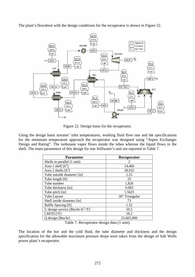
272

The plant’s flowsheet with the design conditions for the recuperator is shown in Figure 22.

Figure 22. Design basis for the recuperator. Using the design basis streams’ inlet temperatures, working fluid flow rate and the specifications for the minimum temperature approach the recuperator was designed using “Aspen Exchanger Design and Rating”. The isobutane vapor flows inside the tubes whereas the liquid flows in the shell. The main parameters of this design for one Stillwater’s unit are reported in Table 7.

Parameter Recuperator Shells in parallel (1 unit) 2 Area 1 shell [ft2] 14,466 Area 2 shells [ft2] 28,932 Tube outside diameter [in] 1.25 Tube length [ft] 25 Tube number 1,826 Tube thickness [in] 0.083 Tube pitch [in] 1.5625 Tube Layout 30° Triangular Shell inside diameter [in] 73 Baffle Spacing [ft] 1.52 U design service [Btu/hr-ft2-°F] 50.5 LMTD [°F] 18.2 Q design [Btu/hr] 25,665,000

Table 7. Recuperator design data (1 unit). The location of the hot and the cold fluid, the tube diameter and thickness and the design specification for the allowable maximum pressure drops were taken from the design of Salt Wells power plant’s recuperator.

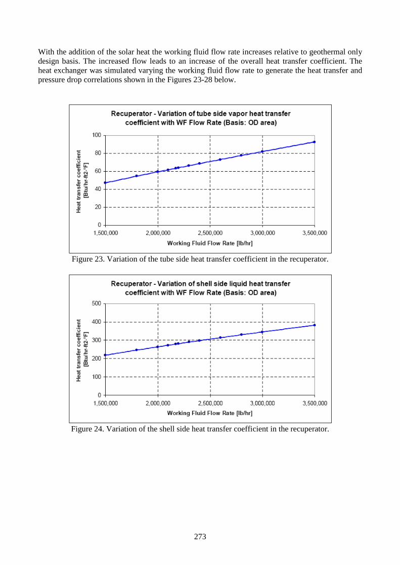
273

With the addition of the solar heat the working fluid flow rate increases relative to geothermal only design basis. The increased flow leads to an increase of the overall heat transfer coefficient. The heat exchanger was simulated varying the working fluid flow rate to generate the heat transfer and pressure drop correlations shown in the Figures 23-28 below.

Figure 23. Variation of the tube side heat transfer coefficient in the recuperator.

Figure 24. Variation of the shell side heat transfer coefficient in the recuperator.

274

Figure 25. Variation of the overall heat transfer coefficient in the recuperator.

Figure 26. Variation of the tube side vapor pressure drops in the recuperator.

275

Figure 27. Variation of the shell side liquid pressure drops in the recuperator.

The heat transfer correlations show that the main thermal resistance is due to the isobutane vapor flow inside the tubes. The heat transfer coefficient of the liquid isobutane in the shell is about four times higher than the heat transfer coefficient of the vapor isobutane inside the tubes. The velocity inside the tubes cannot be increased too much because this would imply higher pressure drops, as Figure 26 shows. The pressure drops between the expander and the air cooled condenser must be kept at a minimum value to get low expander outlet pressures and high power outputs. The recuperator pressure drop lowers the condensation temperature and the mean temperature difference in the air cooled condenser. On the other hand, the air cooled condenser heat duty is reduced because most of the desuperheating process occurs in the recuperator. The recuperator heat transfer and pressure drop correlations were implemented in the Aspen model and simulations were run to compare against the non-regenerative configuration results. The results show that, using the regenerative configuration, the benefits deriving from the reduced ACC heat load almost balance the penalties deriving from the recuperator pressure drops. Therefore the expander outlet pressure is increased only slightly. Figures 28-30 show a comparison between the two configuration with reference to three different ambient temperatures. The solar irradiation used for this comparison is 600 W/m2 incident on a collector area of 35,000 m2 (that is a useful solar heat of 40,305,900 Btu/hr). Figure 28 shows that the net power output from a regenerative configuration is almost identical to that from a non-regenerative configuration due to the resulting almost unchanged expander outlet pressure (Figure 30). The main effect of the recuperator is the increase of the brine outlet temperature (Figure 29). If the working fluid flow rate is fixed by the heat available from the brine above the pinch point (warm ambient temperature cases), then the brine simply comes out warmer in the regenerative configuration and the net power output is almost the same. However if the working fluid flow rate is adjusted within the brine temperature constraint, the regenerative configuration can provide particular advantages compared to the non-regenerative configuration. This is shown in Figures 28 and 29 for the 30°F case: the two large green dots show the operating points for both configurations: using a regenerative configuration the operating pressure can be closer to the optimum resulting in a net power output increase of about 0.9 MW for one plant unit in this specific case.

276

Figure 28. Net power output: comparison between the regenerative and

the non-regenerative configuration.

Figure 29. Brine outlet temperature: comparison between the regenerative and

the non-regenerative configuration.

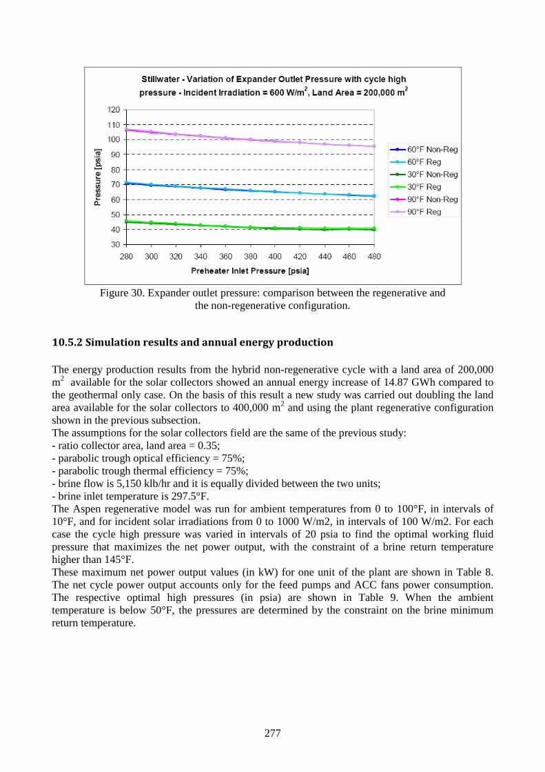
277

Figure 30. Expander outlet pressure: comparison between the regenerative and

the non-regenerative configuration.

10.5.2 Simulation results and annual energy production

The energy production results from the hybrid non-regenerative cycle with a land area of 200,000 m2 available for the solar collectors showed an annual energy increase of 14.87 GWh compared to the geothermal only case. On the basis of this result a new study was carried out doubling the land area available for the solar collectors to 400,000 m2 and using the plant regenerative configuration shown in the previous subsection. The assumptions for the solar collectors field are the same of the previous study: - ratio collector area, land area = 0.35; - parabolic trough optical efficiency = 75%; - parabolic trough thermal efficiency = 75%; - brine flow is 5,150 klb/hr and it is equally divided between the two units; - brine inlet temperature is 297.5°F. The Aspen regenerative model was run for ambient temperatures from 0 to 100°F, in intervals of 10°F, and for incident solar irradiations from 0 to 1000 W/m2, in intervals of 100 W/m2. For each case the cycle high pressure was varied in intervals of 20 psia to find the optimal working fluid pressure that maximizes the net power output, with the constraint of a brine return temperature higher than 145°F. These maximum net power output values (in kW) for one unit of the plant are shown in Table 8. The net cycle power output accounts only for the feed pumps and ACC fans power consumption. The respective optimal high pressures (in psia) are shown in Table 9. When the ambient temperature is below 50°F, the pressures are determined by the constraint on the brine minimum return temperature.

278

Table 8. Maximum net cycle power output for combinations of ambient temperature and incident irradiation.

Table 9. Optimal high pressure for combinations of ambient temperature and incident irradiation.

Geothermal only energy production using the recuperator The values in blue refer to the geothermal only production using the regenerative configuration. These values can be compared with the values obtained for the geo-only case using the non-regenerative configuration. The comparison is shown in Table 10 and Figure 31.

Table 10. Increase in geothermal only net power output using the recuperator.

279

Figure 31. Overall plant net power output increase using the regenerative configuration.

With the regenerative configuration, the power output starts to be limited by the brine minimum outlet temperature constraint (145°F) at ambient temperatures below 50°F, whereas without the recuperator it was already limited at 60°F. At low ambient temperatures the regenerative configuration can operate at cycle high pressures closer to the optimum and the overall plant net power output increase is about 2.0 MW. Using the net power output profiles, shown in Figure 31, the overall plant annual energy production was calculated using the hourly ambient temperature variation for Fallon (NV). Assuming 100% availability, the energy production from the regenerative configuration is 175.2 GWh. Thus the increase in annual energy production using the recuperator is 6.1 GWh (Figure 32).

Figure 32. Increase in annual geo-only energy production using a regenerative configuration.

280

Hybrid geothermal-solar energy production Tables 8 and 9 show that the net power output and the corresponding optimal cycle high pressure increase with the incident radiation. At low ambient temperatures the working fluid pressure is limited by the brine minimum temperature constraint. In these cases at high incident irradiations, and with the assumed operational strategy of 5°F of superheating at the inlet of the expanders, the solar heat input to the power plant must be limited to guarantee the minimum brine return temperature (145°F). A storage system can store the excess thermal energy and make it available during the low irradiation hours. Storage can also be harnessed to time-shift the solar energy for use when it is more effective. The maximum net power output values shown in Table 8 were fitted by a 3-D surface using a multiple linear regression technique. A sixth order polynomial in the form ( )ITfW AMB ,= in the variables ambient temperature TAMB and incident irradiation I provides a good fit to the points. Figure 33 shows the partial derivative of the net power output with respect to the solar radiation for different ambient temperatures. High values of the derivative indicate a good utilization of the solar heat.

Figure 33. Slopes of the net power surface for different ambient temperature-incident radiation combinations. Figure 33 shows an optimum in the efficiency of utilization of the solar heat for incident irradiations at around 300-400 W/m2. The maximum values of the derivatives are found for ambient temperatures between 50 and 80°F, and the optimal incident irradiation (solar heat) that maximizes the derivative is shown in Figure 34 for each ambient temperature.

281

Figure 34. Incident Irradiations that maximize the efficiency in the utilization of the solar heat. Although the optimum efficiency may be in the 200 to 400 W/m2 range, it is not practical to store a majority of the solar irradiation. At low ambient temperatures the derivative curves, shown in Figure 33, are almost flat up to their upper incident radiation limit. At higher ambient temperatures the derivative curves are relatively flat up to 600 W/m2. On the basis of these results, we examined the effect of different solar incident irradiation thresholds from 450 to 700 W/m2 in intervals of 50 W/m2. The storage strategy employed was: • When the incident irradiation is lower than the threshold and thermal storage has been depleted,

the plant is operated using the incoming solar heat. • When the incident irradiation is higher than the threshold, the plant is operated using the solar

heat corresponding to the threshold irradiation, and the excess solar heat is stored. • At low and moderate ambient temperatures, the irradiation might be limited by the maximum

incident irradiation (Table 8) rather than the threshold if the maximum is less than the threshold value.

• The storage is discharged to maintain the threshold (or maximum) irradiation when the incident irradiation is low and zero.

Using this storage strategy, the Fallon historic weather data were used to calculate the annual energy production from the geo-solar hybrid cycle. The net power output for the overall hybrid power plant is given by twice the net power output from one unit, less the parasitic power to run the well pumps calculated for a brine flow of 5,150 klb/hr. Table 11 and Figure 35 show the annual energy production from the hybrid cycle assuming different storage thresholds. The corresponding storage capacity required is shown in Table 11 and Figure 36.

Threshold Storage Energy Production[W/m 2] [kWht] [GWh]

450 501,521 205.12500 348,438 205.10550 301,188 205.02600 253,938 204.89650 206,688 204.74700 176,019 204.56

Table 11. Hybrid geo-solar energy production.

282

Figure 35. Impact of storage threshold on the hybrid geo-solar energy production.

Figure 36. Impact of storage threshold on the storage capacity.

Figures 35 and 36 show that as the storage threshold increases, the annual energy production decreases only slightly whereas the storage capacity undergoes a strong decrease. The 600 W/m2 threshold case is a potential compromise between the two metrics. For this case, the annual energy production is 204.89 GWh. Thus the annual energy increase is 35.8 GWh compared to the geothermal-only power plant and 20.9 GWh compared to the hybrid non-regenerative cycle that uses half as much solar collector area. This result is obtained using a solar collector area of 140,000 m2 that corresponds to a land area of 400,000 m2. The energy increase using solar is more than double compared to the 200,000 m2 land area case mainly due to the addition of the

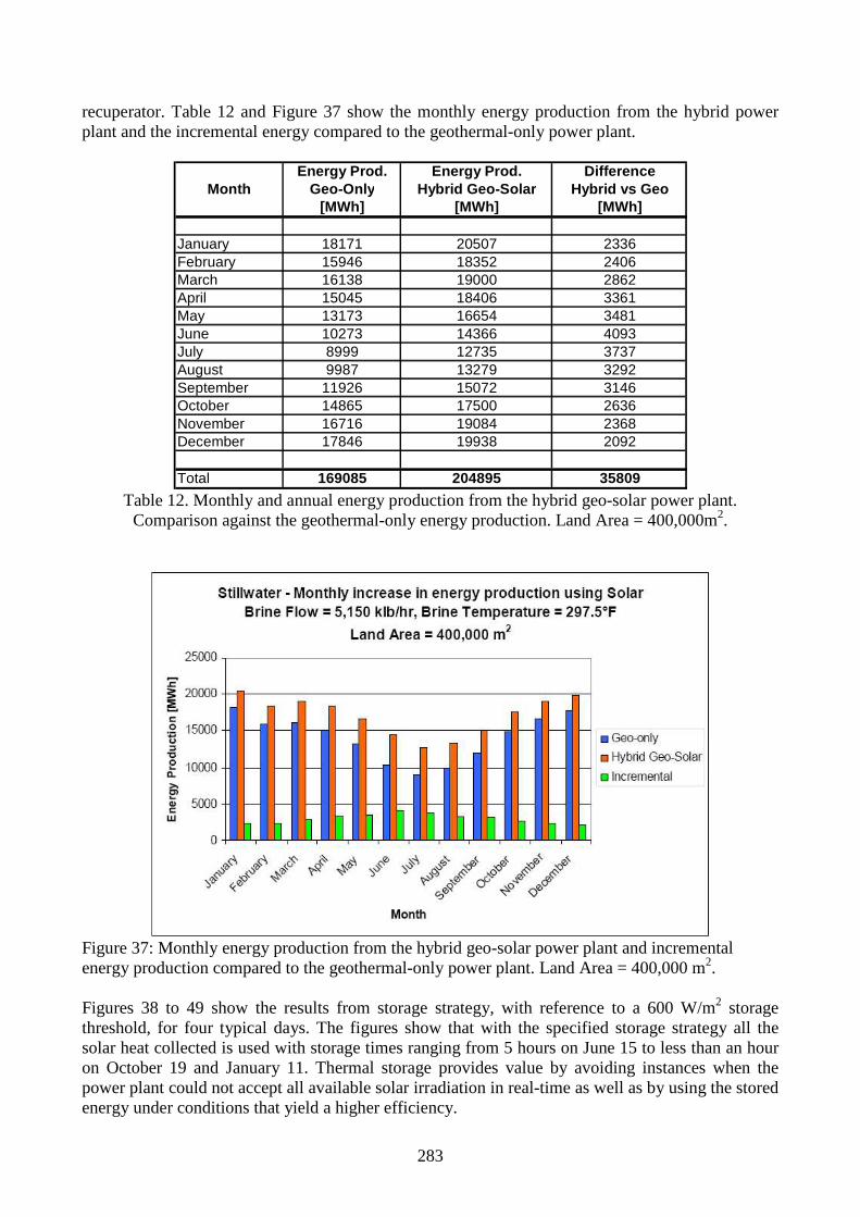
283

recuperator. Table 12 and Figure 37 show the monthly energy production from the hybrid power plant and the incremental energy compared to the geothermal-only power plant.

Energy Prod. Energy Prod. DifferenceMonth Geo-Only Hybrid Geo-Solar Hybrid vs Geo

[MWh] [MWh] [MWh]

January 18171 20507 2336February 15946 18352 2406March 16138 19000 2862April 15045 18406 3361May 13173 16654 3481June 10273 14366 4093July 8999 12735 3737August 9987 13279 3292September 11926 15072 3146October 14865 17500 2636November 16716 19084 2368December 17846 19938 2092

Total 169085 204895 35809 Table 12. Monthly and annual energy production from the hybrid geo-solar power plant. Comparison against the geothermal-only energy production. Land Area = 400,000m2.

Figure 37: Monthly energy production from the hybrid geo-solar power plant and incremental energy production compared to the geothermal-only power plant. Land Area = 400,000 m2. Figures 38 to 49 show the results from storage strategy, with reference to a 600 W/m2 storage threshold, for four typical days. The figures show that with the specified storage strategy all the solar heat collected is used with storage times ranging from 5 hours on June 15 to less than an hour on October 19 and January 11. Thermal storage provides value by avoiding instances when the power plant could not accept all available solar irradiation in real-time as well as by using the stored energy under conditions that yield a higher efficiency.

284

Figure 38. Hourly variation of ambient temperature during June 15.

Figure 39. Hourly variation of incident and used irradiation during June 15.

285

Figure 40. Hourly variation of overall plant net power output during June 15.

Variation of ambient temperature - April 15

0

10

20

30

40

50

60

70

80

90

100

1 2 3 4 5 6 7 8 9 10 11 12 13 14 15 16 17 18 19 20 21 22 23 24

Hour

Tem

pera

ture

[°F

]

Figure 41. Hourly variation of ambient temperature during April 15.

286

Variation of incident irradiation and used irradiat ion - April 15

0

0.1

0.2

0.3

0.4

0.5

0.6

0.7

0.8

0.9

1

1 2 3 4 5 6 7 8 9 10 11 12 13 14 15 16 17 18 19 20 21 22 23 24

Hour

Irrad

iatio

n [k

W/m

2 ]

Incident Used

Figure 42. Hourly variation of incident and used irradiation during April 15.

Overall plant net power output - April 15

0

5,000

10,000

15,000

20,000

25,000

30,000

35,000

1 2 3 4 5 6 7 8 9 10 11 12 13 14 15 16 17 18 19 20 21 22 23 24

Hour

Net

Pow

er [k

W]

Figure 43. Hourly variation of overall plant net power output during April 15.

287

Variation of ambient temperature - October 19

0

10

20

30

40

50

60

70

80

90

100

1 2 3 4 5 6 7 8 9 10 11 12 13 14 15 16 17 18 19 20 21 22 23 24

Hour

Tem

pera

ture

[°F

]

Figure 44. Hourly variation of ambient temperature during October 19.

Variation of incident irradiation and used irradiat ion - October 19

0

0.1

0.2

0.3

0.4

0.5

0.6

0.7

0.8

0.9

1

1 2 3 4 5 6 7 8 9 10 11 12 13 14 15 16 17 18 19 20 21 22 23 24

Hour

Irrad

iatio

n [k

W/m

2 ]

Incident Used

Figure 45. Hourly variation of incident and used irradiation during October 19.

288

Overall plant net power output - October 19

0

5,000

10,000

15,000

20,000

25,000

30,000

35,000

1 2 3 4 5 6 7 8 9 10 11 12 13 14 15 16 17 18 19 20 21 22 23 24

Hour

Net

Pow

er [k

W]

Figure 46. Hourly variation of overall plant net power output during October 19.

Variation of ambient temperature - January 11

0

10

20

30

40

50

60

70

80

90

100

1 2 3 4 5 6 7 8 9 10 11 12 13 14 15 16 17 18 19 20 21 22 23 24

Hour

Tem

pera

ture

[°F

]

Figure 47. Hourly variation of ambient temperature during January 11.

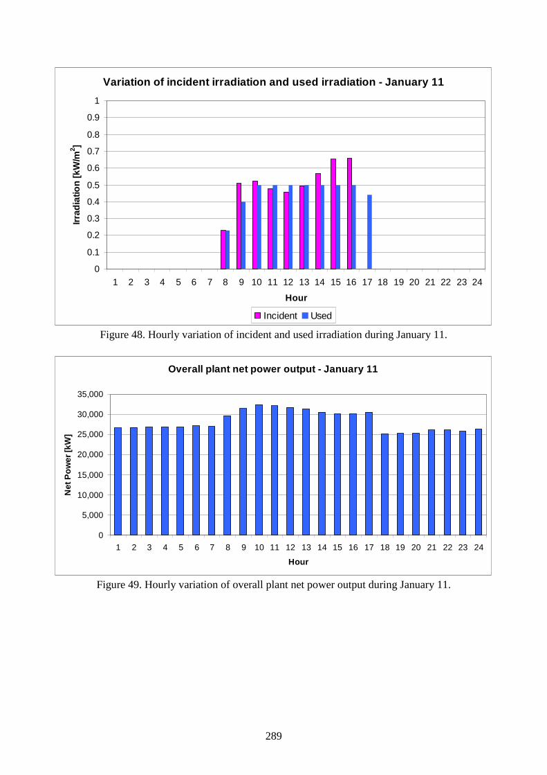
289

Variation of incident irradiation and used irradiat ion - January 11

0

0.1

0.2

0.3

0.4

0.5

0.6

0.7

0.8

0.9

1

1 2 3 4 5 6 7 8 9 10 11 12 13 14 15 16 17 18 19 20 21 22 23 24

Hour

Irrad

iatio

n [k

W/m

2 ]

Incident Used

Figure 48. Hourly variation of incident and used irradiation during January 11.

Overall plant net power output - January 11

0

5,000

10,000

15,000

20,000

25,000

30,000

35,000

1 2 3 4 5 6 7 8 9 10 11 12 13 14 15 16 17 18 19 20 21 22 23 24

Hour

Net

Pow

er [k

W]

Figure 49. Hourly variation of overall plant net power output during January 11.

290

10.6 Economic analysis

10.6.1 Stillwater hybrid 200,000 m2 land area

The annual energy production from the hybrid geo-solar non-regenerative configuration with a solar collector area of 70,000 m2 is 183.96 GWh. The geothermal only production is 169.09 GWh, so the incremental energy using solar is 14.87 GWh. The main costs for hybridizing the existing plant with solar thermal energy include the solar collectors, the heat transfer fluid (HTF) and the storage system (when present). The “NREL’s solar advisor model” provides costing equations for these main solar plant’s subsystems:

• solar collector costs (including the collectors, drives and electronics): $ 300/m2; • HTF costs (including fluid and pumps): $ 150/kWe based on the incremental peak hybrid

power output compared to the geothermal only case; • storage costs: $ 40/kWht.

All these three cost functions are linear with the capacity or size parameter and the costs for the system analyzed are shown in Table 13: Item Capacity or size Cost Collectors 70,000 m2 $ 21,000,000 HTF 7,000 kW $ 1,050,000 Total $ 22,050,000

Table 13. Direct capital costs. The assumed indirect cost for the solar field’s components is 20% of the direct costs. The total capital cost is thus $ 26,460,000. The assumed O&M cost is 2% of the direct capital costs, that is, $441,000 for each year of plant’s operation. Assuming an interest rate of 7% and a plant’s life of operation of 25 years the levelized cost of the incremental electricity (LCOE) generated by the power plant using solar is 18.2 c$/kWh. The incremental LCOE considers only the incremental costs of the solar field and the incremental electricity generated from the hybrid cycle compared to the geothermal-only production. Lost production of the existing plant during hybridization construction is not considered in these LCOE results.

10.6.2 Stillwater hybrid 400,000 m2 land area

The annual energy production from the hybrid geo-solar regenerative configuration with a solar collector area of 140,000 m2 is 204.89 GWh. The geothermal only production is 169.09 GWh, so the incremental energy using solar is 35.81 GWh. Table 14 shows the direct capital cost evaluations for the plant’s components added to the geothermal power plant. “NREL’s solar advisor model” was used to calculate the costs for the main solar plant’s subsystems. The cost equations provided by Turton et al. (2009) were used to evaluate the costs for the recuperator. Using an incident irradiation threshold of 600 W/m2 the thermal storage capacity required is 253,940 kWht. Item Capacity or size Cost Collectors 140,000 m2 $ 42,000,000 HTF 14,000 kW $ 2,100,000 Storage 253,940 kWht $ 10,158,000 Recuperator 4 shells $ 1,296,000 Total $ 55,554,000

Table 14. Direct capital costs.

291

The assumed indirect cost for the solar field’s components is 20% of the direct costs. The indirect costs for the recuperator are $ 524,000. Thus the total indirect costs are $ 11,376,000 and the total capital cost is $ 66,930,000. The assumed O&M cost is 2% of the direct capital costs, that is $ 1,111,000 for each year of plant’s operation. Assuming an interest rate of 7% and a plant’s life of operation of 25 years the levelized cost of the incremental electricity (LCOE) generated by the power plant using solar is 19.1 c$/kWh. Table 15 and Figure 50 show the variation of the LCOE with the incident irradiation storage threshold. The results show that the highest threshold gives the lowest LCOE. The LCOE becomes almost identical to the value found for the 200,000 m2 land area when the storage irradiation threshold is set around 700 W/m2.

Storage LCOEThreshold

[W/m 2] [c$/kWh]450 22.5500 20.4550 19.8600 19.1650 18.5700 18.1

Table 15. Variation of the incremental LCOE with the storage threshold.

Figure 50. Variation of the incremental LCOE with the storage threshold.

292

Conclusions

In a geothermal power plant equipped with a dry cooling system the net power output profile shows a marked decrease of the power output with the ambient temperature, as seen in Chapter 7 for Stillwater power plant. At warm ambient temperatures (>25°C) the power generated is less than half the power generated at low ambient temperatures (around 0°C). The integration of the solar resource with the geothermal resource boosts the power output during the warm season and the central hours of a day, times characterized by high levels of solar irradiation. In addition, in a hybrid geo-solar power plant issues related to the intermittent nature of the solar energy, which affect the design and operation of standalone solar power plants, can be avoided. An analysis of the hybridization of the Stillwater power plant with the solar resource was performed using the off-design model built in Aspen. The hybrid cycle configuration was selected in order to approach, with the addition of the solar source, the plant’s original design conditions. The results show the optimal cycle parameters that maximize the net power output for each combination ambient temperature – incident irradiation. The increase in the annual energy production due to the solar source is compared to the geothermal energy production using historical hour-by-hour weather data for the plant’s site. A second hybrid geothermal-solar system is analyzed with a doubled land area for the solar collectors, a regenerative plant configuration to alleviate the constraint on the minimum brine outlet temperature and a storage system. Thermal storage provides value by avoiding instances when the power plant could not accept all available solar irradiation in real-time as well as by using the stored energy under conditions that yield a higher efficiency. The levelized cost of electricity for the incremental energy generated by solar resource is quite high (around 18 c$/kWh) compared to the geothermal one (around 8 c$/kWh) for both the hybrid systems considered. So, only local tax incentives for solar power could make the economics attractive.

293

References Jefferson W. Tester, Ronald DiPippo and Randall Field, Personal communications, MIT, 2010. Nicola Rossi, Marco Paci and Irene Fastelli, Personal communications, Enel Centro Ricerche, 2008-2010.

294

Appendix A. Working fluid properties The working fluid is impure isobutane with the following composition on a mole basis: 96% isobutane, 3.7% n-butane and 0.3% propane. This Appendix is divided into three sections: the first shows the differences between RefProp and Peng-Robinson property methods, based on some parameters of interest; the second shows the differences between pure and impure isobutane using Refprop as property method; and the third shows the differences between the two methods in the expansion zone. RefProp property method and the actual composition for isobutane were used in Aspen simulations. Both assumptions lead to a higher heat of vaporization for the working fluid and a higher saturated liquid temperature for a given pressure than using Peng-Robinson and/or using pure isobutane. This property method selection implies that to vaporize one unit of working fluid flow rate, the geothermal fluid is cooled more in the vaporizer (than using Peng-Robinson and/or pure isobutane), and the two temperature profiles get closer resulting in smaller pinch point temperature differences. The results, shown in Appendices A.1 and A.2, and additional results found for the expanders, shown in Appendix A.3, indicate that both Power Engineers (PE) and the heat exchanger manufacturers used a property method closer to Peng-Robinson than to RefProp. The RefProp property method is considered the standard and is widely accepted for system simulations. A.1 RefProp vs. Peng-Robinson in the preheating-vaporizing zone The heat of vaporization from saturated liquid conditions to saturated vapor conditions for a given vaporization pressure is lower using Peng-Robinson than using RefProp. This difference increases as the pressure increases, as shown in Table A1 and Figure A1. At Stillwater vaporization pressures, this difference is about 10%.

PressurePeng Robinson REFPROP Difference

[Pa] [kJ/kg] [kJ/kg] %2000000 209,8 211,5 0,792200000 195,2 198,2 1,502400000 180,1 184,5 2,402600000 164,1 170,1 3,562800000 146,9 154,7 5,083000000 127,9 137,8 7,203100000 117,4 128,5 8,613190000 107,3 119,4 10,09

Impure Isobutane - Vaporization Heat

Table A1. Heat of vaporization for Peng-Robinson and RefProp property methods.

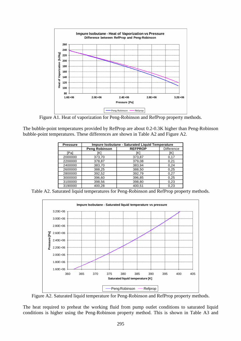
295

80

100

120

140

160

180

200

220

240

260

1.6E+06 2.0E+06 2.4E+06 2.8E+06 3.2E+06

Hea

t of

Vap

oriz

atio

n [k

J/kg

]

Pressure [Pa]

Impure Isobutane - Heat of Vaporization vs PressureDifference between RefProp and Peng-Robinson

Peng Robinson Refprop

Figure A1. Heat of vaporization for Peng-Robinson and RefProp property methods. The bubble-point temperatures provided by RefProp are about 0.2-0.3K higher than Peng-Robinson bubble-point temperatures. These differences are shown in Table A2 and Figure A2.

PressurePeng Robinson REFPROP Difference

[Pa] [K] [K] [K]2000000 373,70 373,87 0,172200000 378,87 379,08 0,212400000 383,70 383,94 0,242600000 388,25 388,50 0,252800000 392,52 392,79 0,273000000 396,60 396,85 0,253100000 398,56 398,80 0,233190000 400,28 400,51 0,23

Impure Isobutane - Saturated Liquid Temperature

Table A2. Saturated liquid temperatures for Peng-Robinson and RefProp property methods.

1.60E+06

1.80E+06

2.00E+06

2.20E+06

2.40E+06

2.60E+06

2.80E+06

3.00E+06

3.20E+06

360 365 370 375 380 385 390 395 400 405

Pre

ssur

e [P

a]

Saturated liquid temperature [K]

Impure Isobutane - Saturated liquid temperature vs p ressure

Peng Robinson Refprop

Figure A2. Saturated liquid temperature for Peng-Robinson and RefProp property methods. The heat required to preheat the working fluid from pump outlet conditions to saturated liquid conditions is higher using the Peng-Robinson property method. This is shown in Table A3 and

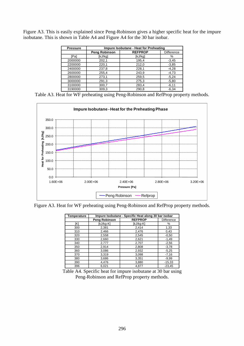
296

Figure A3. This is easily explained since Peng-Robinson gives a higher specific heat for the impure isobutane. This is shown in Table A4 and Figure A4 for the 30 bar isobar.

PressurePeng Robinson REFPROP Difference

[Pa] [kJ/kg] [kJ/kg] %2000000 202,1 195,4 -3,452200000 220,1 212,0 -3,852400000 237,8 228,1 -4,282600000 255,4 243,9 -4,732800000 273,1 259,5 -5,243000000 291,3 275,3 -5,803100000 300,7 283,4 -6,113190000 309,3 290,8 -6,34

Impure Isobutane - Heat for Preheating

Table A3. Heat for WF preheating using Peng-Robinson and RefProp property methods.

0.0

50.0

100.0

150.0

200.0

250.0

300.0

350.0

1.60E+06 2.00E+06 2.40E+06 2.80E+06 3.20E+06

Hea

t fo

r P

rehe

atin

g [k

J/kg

]

Pressure [Pa]

Impure Isobutane - Heat for the Preheating Phase

Peng Robinson Refprop

Figure A3. Heat for WF preheating using Peng-Robinson and RefProp property methods.

TemperaturePeng Robinson REFPROP Difference

[K] [kJ/kg-K] [kJ/kg-K] %300 2,381 2,414 1,33310 2,466 2,476 0,43320 2,558 2,545 -0,50330 2,660 2,621 -1,49340 2,777 2,707 -2,56350 2,914 2,808 -3,78360 3,086 2,932 -5,25370 3,319 3,098 -7,16380 3,686 3,351 -9,99390 4,476 3,880 -15,33396 6,021 4,877 -23,45

Impure Isobutane - Specific Heat along 30 bar isoba r

Table A4. Specific heat for impure isobutane at 30 bar using

Peng-Robinson and RefProp property methods.

297

2

2.5

3

3.5

4

4.5

5

5.5

6

6.5

300 310 320 330 340 350 360 370 380 390 400

Spe

cific

Hea

t [k

J/kg

-K]

Temperature [K]

Impure Isobutane specific heat vs Temperature along the 30 bar isobar

RefProp Peng Robinson

Figure A4. Specific heat for impure isobutane at 30 bar using Peng-Robinson and RefProp property methods. A.2 Pure vs. impure isobutane Impure isobutane requires a higher heat of vaporization and shows a higher saturated liquid temperature at a given pressure, relative to pure isobutane. These differences increase with high pressures. The difference between the heat of vaporization for pure and impure isobutane at Stillwater vaporization pressures is about 1.5%, whereas the difference in the saturated liquid temperature is about 0.4K. The results are shown in Table A5-Figure A5, and Table A6–Figure A6 using RefProp property method; Peng-Robinson shows the same trend.

PressurePure Isobutane Impure Isobutane Difference

[Pa] [kJ/kg] [kJ/kg] %2000000 210,15 211,46 0,622200000 196,87 198,21 0,682400000 183,13 184,51 0,752600000 168,68 170,13 0,852800000 153,19 154,73 1,003000000 136,08 137,79 1,243100000 126,63 128,47 1,433200000 116,30 118,32 1,703300000 104,72 107,01 2,143400000 91,13 93,90 2,953500000 73,74 77,58 4,94

Vaporization Heat

Table A5. Heat of vaporization for pure and impure isobutane.

298

60

80

100

120

140

160

180

200

220

240

260

1.50E+06 2.00E+06 2.50E+06 3.00E+06 3.50E+06

Hea

t of

Vap

oriz

atio

n [k

J/kg

]

Pressure [Pa]

Heat of Vaporization vs Pressure

Impure Isobutane Pure Isobutane

Figure A5. Heat of vaporization for pure and impure isobutane.

PressurePure Isobutane Impure Isobutane Difference

[Pa] [K] [K] [K]2000000 373,51 373,87 0,362200000 378,71 379,08 0,372400000 383,56 383,94 0,382600000 388,11 388,50 0,392800000 392,39 392,79 0,403000000 396,44 396,85 0,413100000 398,38 398,80 0,423200000 400,27 400,70 0,433300000 402,11 402,54 0,433400000 403,90 404,34 0,443500000 405,64 406,09 0,45

Saturated Liquid Temperature

Table A6. Saturated liquid temperature for pure and impure isobutane.

1.50E+06

2.00E+06

2.50E+06

3.00E+06

3.50E+06

350 360 370 380 390 400 410

Pre

ssur

e [P

a]

Liquid Saturation Temperature [K]

Saturated Liquid Temperature vs Pressure

Impure Isobutane Pure Isobutane

Figure A6. Saturated liquid temperature for pure and impure isobutane.

299

A.3 RefProp vs. Peng-Robinson in the expander zone RefProp was compared to Peng-Robinson in the expander zone referring to PE design conditions. The enthalpy at the expander inlet was calculated using the design temperature and pressure values from PE flowsheet. The outlet pressure was set to the design conditions (65.05 psia) and the isentropic efficiencies that matched PE turbine outlet temperature (124.2°F) were found using both methods (see Table A7). Only the Peng-Robinson equation of state matched the power output quite well (in addition to the imposed inlet/outlet temperatures and pressures) with the values provided by PE. The isentropic enthalpy drop is quite similar for the two property methods but the isentropic outlet temperature is about 4°F lower using RefProp. Therefore, using RefProp, the expander efficiency to match the PE expander outlet temperature must be much lower than using Peng-Robinson. The T-s diagram in Figure A7 shows the saturated vapor curve for both methods, along with the isobars for the high pressure (455 psia) and the low pressure (65.05 psia). Figure A7 also shows that Peng-Robinson is not reliable for high pressures.

ParametersPeng Robinson RefProp

Inlet Turbine Temperature [°F] 260,9 260,9Inlet Turbine Pressure [psia] 455 455Inlet Turbine Enthalpy [Btu/lb] -955,05 -957,98Inlet Turbine Entropy [Btu/lb-°R] -1,5861 -1,5911Outlet Turbine Pressure [psia] 65,05 65,05Outlet Isoentropic Enthalpy [Btu/lb] -986,36 -989,22Outlet Isoentropic Temperature [°F] 114,3 110,2Isoentropic Enthalpy Drop [Btu/lb] 31,32 31,25Specified Outlet Temperature [°F] 124,2 124,2Outlet Turbine Enthalpy [Btu/lb] -981,991 -982,866Outlet Turbine Entropy [Btu/lb-°R] -1,5786 -1,5801Enthalpy Drop [Btu/lb] 26,94 24,89Entropy Increase [Btu/lb-°R] 0,0076 0,0110Calculated Efficiency % 86,03 79,66Mass Flow Rate [lb/hr] 3113250 3113250Expanders Power [kW] 24583 22710Mechanical Losses [kW] 600 600Generator Efficiency % 0,979 0,979Gross Power [kW] 23479 21646

Property Method

Table A7. Expander calculations to match the inlet/outlet temperatures and pressures reported in PE flowsheet using Peng-Robinson and RefProp property methods.

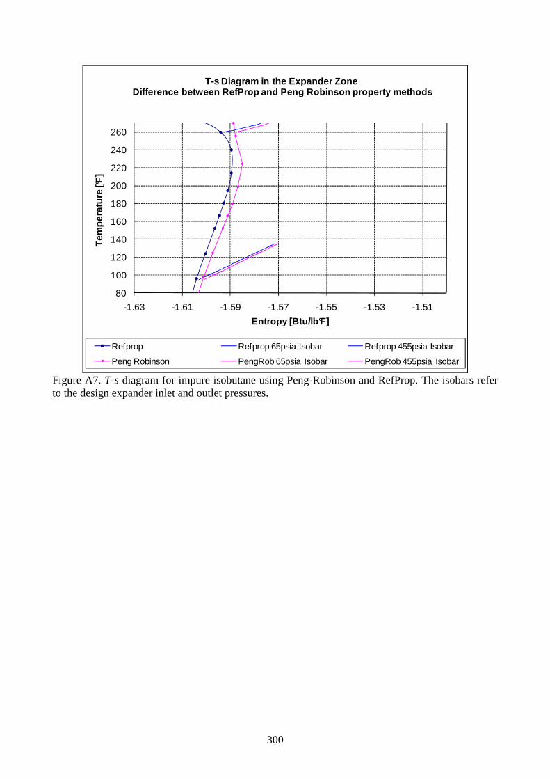
300

80

100

120

140

160

180

200

220

240

260

-1.63 -1.61 -1.59 -1.57 -1.55 -1.53 -1.51

Tem

pera

ture

[°F

]

Entropy [Btu/lb°F]

T-s Diagram in the Expander ZoneDifference between RefProp and Peng Robinson proper ty methods

Refprop Refprop 65psia Isobar Refprop 455psia Isobar

Peng Robinson PengRob 65psia Isobar PengRob 455psia Isobar

Figure A7. T-s diagram for impure isobutane using Peng-Robinson and RefProp. The isobars refer to the design expander inlet and outlet pressures.

301

Appendix B. Expanders isentropic efficiencies Isentropic efficiencies calculated from plant data for the remaining three expanders. B.1 Second expander of the first unit

1st Unit, 2 nd Expander Isentropic Efficiencies

0.00

0.10

0.20

0.30

0.40

0.50

0.60

0.70

0.80

0.90

1.00

10.0 15.0 20.0 25.0 30.0 35.0 40.0 45.0

Isentropic Enthalpy Drop [Btu/lb]

Isen

tropi

c E

ffici

ency 53°F

86°F

30°F

0°F

MTC

Figure B1. Expander isentropic efficiencies calculated from Stillwater plant data for the second expander of the first unit. Variation with the isentropic enthalpy drop.

1st Unit, 2 nd Expander Isentropic Efficiencies

0.00

0.10

0.20

0.30

0.40

0.50

0.60

0.70

0.80

0.90

1.00

10000 20000 30000 40000 50000 60000

Volumetric Flow Rate at the Outlet [ft3/min]

Isen

tropi

c E

ffici

ency 53°F

86°F

30°F

0°F

MTC

Figure B2. Expander isentropic efficiencies calculated from Stillwater plant data for the second expander of the first unit. Variation with the volumetric flow rate at the outlet.

302

1st Unit, 2 nd Expander Isentropic Efficiencies

( Only Data with 35000<V out <48000 ft3/min )

0.00

0.10

0.20

0.30

0.40

0.50

0.60

0.70

0.80

0.90

1.00

10.0 15.0 20.0 25.0 30.0 35.0 40.0 45.0

Isentropic Enthalpy Drop [Btu/lb]

Isen

tropi

c E

ffici

ency 53°F

86°F

30°F

0°F

MTC

Figure B3. Expander isentropic efficiencies calculated from Stillwater plant data for the second expander of the first unit. Data filtered to compare against MTC performance curve.

1st Unit, 2 nd Expander Isentropic Efficiencies ( Only Data with 21< ∆∆∆∆h is <28 )

0.00

0.10

0.20

0.30

0.40

0.50

0.60

0.70

0.80

0.90

1.00

0 10000 20000 30000 40000 50000

Volumetric Flow Rate at the Outlet [ft3/min]

Isen

tropi

c E

ffici

ency

86°F

MTC

Figure B4. Expander isentropic efficiencies calculated from Stillwater plant data for the second expander of the first unit. Data filtered to compare against MTC performance curve.

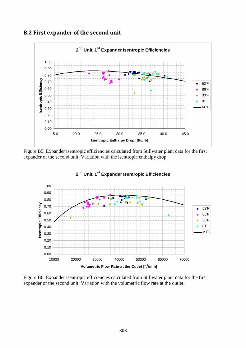
303

B.2 First expander of the second unit

2nd Unit, 1 st Expander Isentropic Efficiencies

0.00

0.10

0.20

0.30

0.40

0.50

0.60

0.70

0.80

0.90

1.00

15.0 20.0 25.0 30.0 35.0 40.0 45.0

Isentropic Enthalpy Drop [Btu/lb]

Isen

tropi

c E

ffici

ency 53°F

86°F

30°F

0°F

MTC

Figure B5. Expander isentropic efficiencies calculated from Stillwater plant data for the first expander of the second unit. Variation with the isentropic enthalpy drop.

2nd Unit, 1 st Expander Isentropic Efficiencies

0.00

0.10

0.20

0.30

0.40

0.50

0.60

0.70

0.80

0.90

1.00

10000 20000 30000 40000 50000 60000 70000

Volumetric Flow Rate at the Outlet [ft 3/min]

Isen

tropi

c E

ffici

ency 53°F

86°F

30°F

0°F

MTC

Figure B6. Expander isentropic efficiencies calculated from Stillwater plant data for the first expander of the second unit. Variation with the volumetric flow rate at the outlet.

304

B.3 Second expander of the second unit

2nd Unit, 2 nd Expander Isentropic Efficiencies

0.00

0.10

0.20

0.30

0.40

0.50

0.60

0.70

0.80

0.90

1.00

15.0 20.0 25.0 30.0 35.0 40.0 45.0

Isentropic Enthalpy Drop [Btu/lb]

Isen

tropi

c E

ffici

ency 53°F

86°F

30°F

0°F

MTC

Figure B7. Expander isentropic efficiencies calculated from Stillwater plant data for the second expander of the second unit. Variation with the isentropic enthalpy drop.

2nd Unit, 2 nd Expander Isentropic Efficiencies

0.00

0.10

0.20

0.30

0.40

0.50

0.60

0.70

0.80

0.90

1.00

10000 20000 30000 40000 50000 60000

Volumetric Flow Rate at the Outlet [ft 3/min]

Isen

tropi

c E

ffici

ency 53°F

86°F

30°F

0°F

MTC

Figure B8. Expander isentropic efficiencies calculated from Stillwater plant data for the second expander of the second unit. Variation with the volumetric flow rate at the outlet.

305

Appendix C. Shell and tube heat exchangers: heat transfer

and pressure drops correlations The remaining heat transfer correlations and pressure drop correlations found for the preheater and vaporizer are shown in this Appendix C. C.1 Heat transfer correlations for the preheater

0

200

400

600

800

1000

1200

1000 1500 2000 2500 3000 3500

Hea

t T

rans

fer

Coe

ffici

ent

[Btu

/hr-

ft2-°F

]

Working Fluid Flow Rate [klb/hr]

Preheater - Variation of shell side Boiling heat tra nsfer coefficient with WF Flow Rate - p in = 480 psia - (Basis: outside finned area)

Figure C1. Variation of the working fluid heat transfer coefficient with the flow rate in the preheater for the boiling phase: ( ) ( )WFPBWF mfh &=, .

C.2 Heat transfer correlations for the vaporizer

300

340

380

420

460

500

1800 1900 2000 2100 2200 2300 2400 2500

Hea

t tra

nsfe

r coe

ffic

ient

[B

tu/h

r-ft

2-°F

]

Working Fluid Flow Rate [klb/hr]

Vaporizer - Variation of shell side vapor heat trans fer coefficient with WF Flow Rate - Parameter WF inlet pressure - (Basis: out side finned area)

440psia

460psia

400psia

480psia

Figure C2. Variation of the working fluid heat transfer coefficient with WF flow rate and pressure in the vaporizer for the vapor phase (superheating process): ( ) ( )WFWFVSWF pmfh ,, &= .

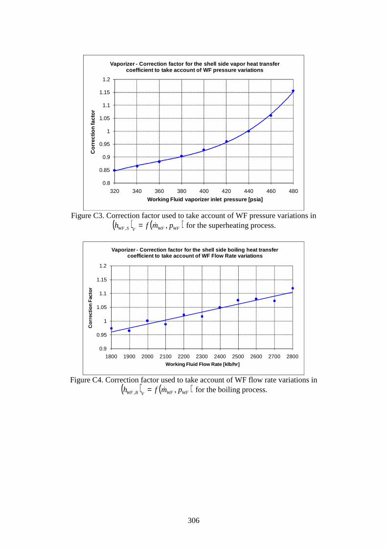
306

0.8

0.85

0.9

0.95

1

1.05

1.1

1.15

1.2

320 340 360 380 400 420 440 460 480

Cor

rect

ion

fact

or

Working Fluid vaporizer inlet pressure [psia]

Vaporizer - Correction factor for the shell side vap or heat transfer coefficient to take account of WF pressure variatio ns

Figure C3. Correction factor used to take account of WF pressure variations in

( ) ( )WFWFVSWF pmfh ,, &= for the superheating process.

0.9

0.95

1

1.05

1.1

1.15

1.2

1800 1900 2000 2100 2200 2300 2400 2500 2600 2700 2800

Cor

rect

ion

Fac

tor

Working Fluid Flow Rate [klb/hr]

Vaporizer - Correction factor for the shell side boi ling heat transfer coefficient to take account of WF Flow Rate variati ons

Figure C4. Correction factor used to take account of WF flow rate variations in

( ) ( )WFWFVBWF pmfh ,, &= for the boiling process.

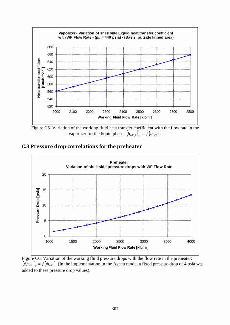
307

520

540

560

580

600

620

640

660

680

2000 2100 2200 2300 2400 2500 2600 2700 2800

Hea

t tra

nsfe

r co

effic

ient

[Btu

/h-f

t2-°F

]

Working Fluid Flow Rate [klb/hr]

Vaporizer - Variation of shell side Liquid heat tran sfer coefficient with WF Flow Rate - (p in = 440 psia) - (Basis: outside finned area)

Figure C5. Variation of the working fluid heat transfer coefficient with the flow rate in the

vaporizer for the liquid phase: ( ) ( )WFVLWF mfh &=, .

C.3 Pressure drop correlations for the preheater

0

5

10

15

20

1000 1500 2000 2500 3000 3500 4000

Pre

ssur

e D

rop

[psi

a]

Working Fluid Flow Rate [klb/hr]

PreheaterVariation of shell side pressure drops with WF Flow Rate

Figure C6. Variation of the working fluid pressure drops with the flow rate in the preheater: ( ) ( )WFPWF mfp &=∆ . (In the implementation in the Aspen model a fixed pressure drop of 4 psia was

added to these pressure drop values).

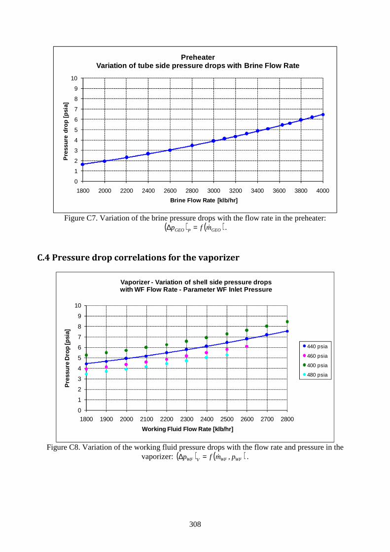
308

0

1

2

3

4

5

6

7

8

9

10

1800 2000 2200 2400 2600 2800 3000 3200 3400 3600 3800 4000

Pre

ssur

e dr

op [p

sia]

Brine Flow Rate [klb/hr]

PreheaterVariation of tube side pressure drops with Brine Fl ow Rate

Figure C7. Variation of the brine pressure drops with the flow rate in the preheater:

( ) ( )GEOPGEO mfp &=∆ .

C.4 Pressure drop correlations for the vaporizer

0

1

2

3

4

5

6

7

8

9

10

1800 1900 2000 2100 2200 2300 2400 2500 2600 2700 2800

Pre

ssur

e D

rop

[psi

a]

Working Fluid Flow Rate [klb/hr]

Vaporizer - Variation of shell side pressure drops with WF Flow Rate - Parameter WF Inlet Pressure

440 psia

460 psia

400 psia

480 psia

Figure C8. Variation of the working fluid pressure drops with the flow rate and pressure in the

vaporizer: ( ) ( )WFWFVWF pmfp ,&=∆ .

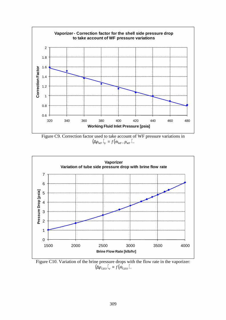
309

0.6

0.8

1

1.2

1.4

1.6

1.8

2

320 340 360 380 400 420 440 460 480

Cor

rect

ion

Fac

tor

Working Fluid Inlet Pressure [psia]

Vaporizer - Correction factor for the shell side pre ssure dropto take account of WF pressure variations

Figure C9. Correction factor used to take account of WF pressure variations in

( ) ( )WFWFVWF pmfp ,&=∆ .

0

1

2

3

4

5

6

7

1500 2000 2500 3000 3500 4000

Pre

ssur

e D

rop

[psi

a]

Brine Flow Rate [klb/hr]

Vaporizer Variation of tube side pressure drop with brine flo w rate

Figure C10. Variation of the brine pressure drops with the flow rate in the vaporizer:

( ) ( )GEOVGEO mfp &=∆ .

310

Appendix D. Fan velocity triangles: impact on fan

performance curves and blade pitch angle setting An examination of the velocity triangles at the inlet and outlet of a fan blade section is useful to understanding the axial fan performance curves and the impact on the blade pitch angle. Figure D1 shows the two velocity triangles at the inlet and the outlet.

Figure D1. Fan velocity triangles: u: blade peripheral speed; c: absolute air velocity; w: air velocity relative to blade; γ: blade pitch angle; subscripts: 1=inlet; 2=outlet. The air enters the fan with an absolute velocity c1. The axial velocity is cm:

( )22

4 HG

vm

dd

qc

−= π , (Eq. D1)

where dG is the fan diameter and dH is the hub diameter. The total pressure conveyed to the air is:

( ) ( )21

2212

211

22212 2

1

2

1

2

1ccppcpcpppp tt −+−=

⋅+−

⋅+=−= ρρρ (Eq. D2)

Where ρ is the air density. The total pressure can be expressed using the variation of momentum equation:

( ) ( )1212 uuuu ccucucup −⋅=⋅−⋅⋅= ρρ (Eq. D3) Assuming an axial inlet velocity (cu1=0), as shown in the figure, the expression of the total pressure becomes:

2ucup ⋅⋅= ρ (Eq. D4) The tangential component of the absolute velocity can be expressed as a function of β2:

(Eq. D5)

and substituting:

22 cotβρρ mcuup ⋅⋅−⋅= (Eq. D6)

With the increase of the angle β2 the cotangent decreases and the total pressure increases.

c1 w1

u

β1

γ

u

c2 w2 β2

α1

α2

Blade speed

Air

22 cotβmu cuc −=

311

The total pressure conveyed to the air can also be written as:

−+−=22

22

21

21

22 wwcc

p ρ (Eq. D7)

where the first term is the dynamic contribution and the second is the static contribution. For a given air flow rate when the blade pitch angle is increased, the relative outlet angle β2 increases and the tangential component of the absolute velocity increases. This implies a higher fan total pressure.

312

Appendix E. Brine distribution strategy: results for

configuration A

E.1 Aspen simulation results: configuration A, first unit

0

2000

4000

6000

8000

10000

12000

14000

16000

18000

20000

22000

280 300 320 340 360 380 400 420 440 460 480

Net

Pow

er [k

W]

Working Fluid Pressure [psia]

Variation of Net Power with Cycle High PressureSc. A 1 st Unit - Brine Flow: 3,627.5 klb/hr, Brine Temperature : 297.5°F

53.7°F

86°F

30°F

0°F

Figure E1. Net Power Output for the First Unit of Configuration A.

110

120

130

140

150

160

170

180

190

200

210

280 300 320 340 360 380 400 420 440 460 480

Brin

e O

utle

t Tem

pera

ture

[°F

]

Working Fluid Pressure [psia]

Variation of Brine Outlet Temperature with Cycle Hi gh PressureSc. A 1 st Unit - Brine Flow: 3,627.5 klb/hr, Brine Temperature : 297.5°F

53.7°F

86°F

30°F

0°F

Limit

Figure E2. Brine Outlet Temperature for the First Unit of Configuration A.

313

30

40

50

60

70

80

90

100

110

120

280 300 320 340 360 380 400 420 440 460 480

Exp

ande

r Out

let P

ress

ure

[psi

a]

Working Fluid Pressure [psia]

Variation of Expander Outlet Pressure with Cycle Hi gh Pressure Sc. A 1 st Unit - Brine Flow: 3,627.5 klb/hr, Brine Temperature : 297.5°F

53.7°F

86°F

30°F

0°F

Figure E3. Expander Outlet Pressure for the First Unit of Configuration A.

0.60

0.64

0.68

0.72

0.76

0.80

0.84

0.88

280 300 320 340 360 380 400 420 440 460 480

Isen

trop

ic E

ffici

ency

Working Fluid Pressure [psia]

Variation of Expander Isentropic Efficiency with Cy cle High PressureSc. A 1 st Unit - Brine Flow: 3,627.5 klb/hr, Brine Temperature : 297.5°F

53.7°F

86°F

30°F

0°F

Figure E4. Expander Isentropic Efficiency for the First Unit of Configuration A.

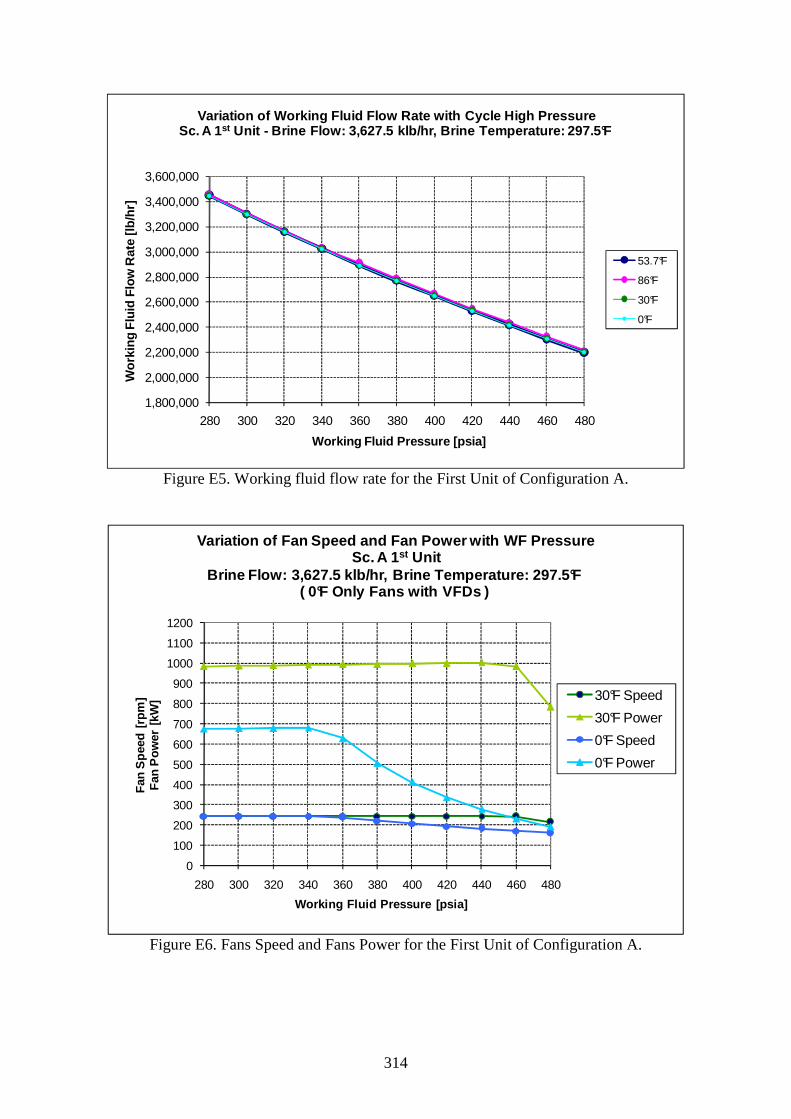
314

1,800,000

2,000,000

2,200,000

2,400,000

2,600,000

2,800,000

3,000,000

3,200,000

3,400,000

3,600,000

280 300 320 340 360 380 400 420 440 460 480

Wor

king

Flu

id F

low

Rat

e [lb

/hr]

Working Fluid Pressure [psia]

Variation of Working Fluid Flow Rate with Cycle Hig h PressureSc. A 1 st Unit - Brine Flow: 3,627.5 klb/hr, Brine Temperature : 297.5°F

53.7°F

86°F

30°F

0°F

Figure E5. Working fluid flow rate for the First Unit of Configuration A.

0

100

200

300

400

500

600

700

800

900

1000

1100

1200

280 300 320 340 360 380 400 420 440 460 480

Fan

Spe

ed [

rpm

]

Fan

Pow

er [

kW]

Working Fluid Pressure [psia]

Variation of Fan Speed and Fan Power with WF Pressu reSc. A 1 st Unit

Brine Flow: 3,627.5 klb/hr, Brine Temperature: 297. 5°F( 0°F Only Fans with VFDs )

30°F Speed

30°F Power

0°F Speed

0°F Power

Figure E6. Fans Speed and Fans Power for the First Unit of Configuration A.

315

E.2 Aspen simulation results: configuration A, second unit

0

1000

2000

3000

4000

5000

6000

7000

8000

9000

10000

11000

280 300 320 340 360 380 400 420 440 460 480

Net

Pow

er [k

W]

Working Fluid Pressure [psia]

Variation of Net Power with Cycle High PressureSc. A 2nd Unit - Brine Flow: 1,522.5 klb/hr, Brine Temperature : 297.5°F

53.7°F

86°F

30°F

0°F

Figure E7. Net Power Output for the Second Unit of Configuration A.

100

110

120

130

140

150

160

170

180

190

200

210

220

280 300 320 340 360 380 400 420 440 460 480

Brin

e O

utle

t T

empe

ratu

re [

°F]

Working Fluid Pressure [psia]

Variation of Brine Outlet Temperature with Cycle Hi gh PressureSc. A 2 nd Unit - Brine Flow: 1,522.5 klb/hr, Brine Temperature : 297.5°F

53.7°F

86°F

30°F

0°F

Limit

Figure E8. Brine Outlet Temperature for the Second Unit of Configuration A.

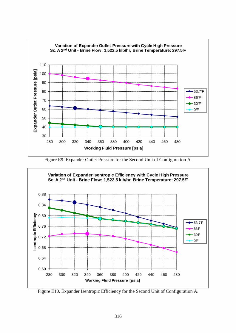
316

30

40

50

60

70

80

90

100

110

280 300 320 340 360 380 400 420 440 460 480

Exp

ande

r Out

let P

ress

ure

[psi

a]

Working Fluid Pressure [psia]

Variation of Expander Outlet Pressure with Cycle Hi gh Pressure Sc. A 2 nd Unit - Brine Flow: 1,522.5 klb/hr, Brine Temperature : 297.5°F

53.7°F

86°F

30°F

0°F

Figure E9. Expander Outlet Pressure for the Second Unit of Configuration A.

0.60

0.64

0.68

0.72

0.76

0.80

0.84

0.88

280 300 320 340 360 380 400 420 440 460 480

Isen

tropi

c E

ffic

ienc

y

Working Fluid Pressure [psia]

Variation of Expander Isentropic Efficiency with Cy cle High PressureSc. A 2 nd Unit - Brine Flow: 1,522.5 klb/hr, Brine Temperature : 297.5°F

53.7°F

86°F

30°F

0°F

Figure E10. Expander Isentropic Efficiency for the Second Unit of Configuration A.

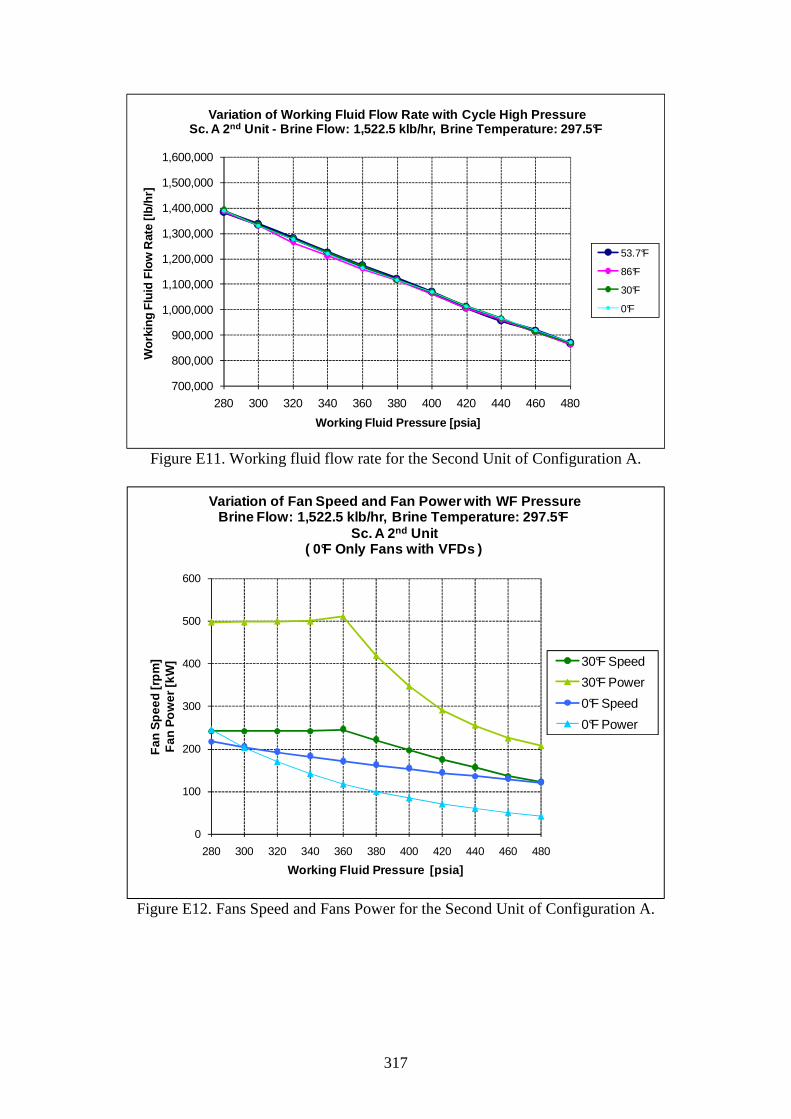
317

700,000

800,000

900,000

1,000,000

1,100,000

1,200,000

1,300,000

1,400,000

1,500,000

1,600,000

280 300 320 340 360 380 400 420 440 460 480

Wor

king

Flu

id F

low

Rat

e [lb

/hr]

Working Fluid Pressure [psia]

Variation of Working Fluid Flow Rate with Cycle Hig h PressureSc. A 2 nd Unit - Brine Flow: 1,522.5 klb/hr, Brine Temperature : 297.5°F

53.7°F

86°F

30°F

0°F

Figure E11. Working fluid flow rate for the Second Unit of Configuration A.

0

100

200

300

400

500

600

280 300 320 340 360 380 400 420 440 460 480

Fan

Spe

ed [r

pm]

F

an P

ower

[kW

]

Working Fluid Pressure [psia]

Variation of Fan Speed and Fan Power with WF Pressu reBrine Flow: 1,522.5 klb/hr, Brine Temperature: 297. 5°F

Sc. A 2 nd Unit( 0°F Only Fans with VFDs )

30°F Speed

30°F Power

0°F Speed

0°F Power

Figure E12. Fans Speed and Fans Power for the Second Unit of Configuration A.

318

Appendix F. Hybrid Geo-Solar Cycle Simulation Results for

30°F and 0°F ambient temperatures � F.1 Aspen Simulation Results: Ambient Temperature 30°F

Stillwater - Variation of Net Power Output with cyc le high pressure for different solar incident radiations

Ambient Temperature = 30°F

0

2000

40006000

8000

10000

12000

1400016000

18000

20000

280 300 320 340 360 380 400 420 440 460 480

Preheater Inlet Pressure [psia]

Net

Pow

er [k

W] Geo-only

Inc_Rad = 200 W/m2

Inc_Rad = 400 W/m2

Inc_Rad = 600 W/m2

Inc_Rad = 800 W/m2

Figure F1. Variation of net power output with cycle high pressure and incident solar

radiation for 30°F ambient temperature.

Stillwater - Variation of Brine Outlet Temperature with cycle high pressure for different solar incident radiatio ns

Ambient Temperature = 30°F

80

100

120

140

160

180

200

280 300 320 340 360 380 400 420 440 460 480

Preheater Inlet Pressure [psia]

Tem

pera

ture

[°F

] Geo-only

Inc_Rad = 200 W/m2

Inc_Rad = 400 W/m2

Inc_Rad = 600 W/m2

Inc_Rad = 800 W/m2

Limit

Figure F2. Variation of brine outlet temperature with cycle high pressure and incident solar

radiation for 30°F ambient temperature.

319

Stillwater - Variation of Expander Outlet Pressure with cycle high pressure for different solar incident radiatio ns

Ambient Temperature = 30°F

30

40

50

60

70

280 300 320 340 360 380 400 420 440 460 480

Preheater Inlet Pressure [psia]

Pre

ssur

e [p

sia]

Geo-only

Inc_Rad = 200 W/m2

Inc_Rad = 400 W/m2

Inc_Rad = 600 W/m2

Inc_Rad = 800 W/m2

Figure F3. Variation of expander outlet pressure with cycle high pressure and incident solar

radiation for 30°F ambient temperature.

Stillwater - Variation of Working Fluid Flow Rate w ith cycle high pressure for different solar incident radiatio ns

Ambient Temperature = 30°F

0

500,000

1,000,000

1,500,000

2,000,000

2,500,000

3,000,000

3,500,000

280 300 320 340 360 380 400 420 440 460 480

Preheater Inlet Pressure [psia]

WF

Flo

w [l

b/hr

] Geo-only

Inc_Rad = 200 W/m2

Inc_Rad = 400 W/m2

Inc_Rad = 600 W/m2

Inc_Rad = 800 W/m2

Figure F4. Variation of working fluid flow rate with cycle high pressure and incident solar

radiation for 30°F ambient temperature.

320

Stillwater - Variation of Isentropic Enthalpy Drop with cycle high pressure for different solar incident radiatio ns

Ambient Temperature = 30°F

10

15

20

25

30

35

40

45

280 300 320 340 360 380 400 420 440 460 480

Preheater Inlet Pressure [psia]

∆∆ ∆∆hi

s [B

tu/lb

]

Geo-only

Inc_Rad = 200 W/m2

Inc_Rad = 400 W/m2

Inc_Rad = 600 W/m2

Inc_Rad = 800 W/m2

Expander_Design

Figure F5. Variation of isentropic enthalpy drop with cycle high pressure and incident solar

radiation for 30°F ambient temperature.

Stillwater - Variation of Expander Isentropic Effic iency with cycle high pressure for different solar incident ra diations

Ambient Temperature = 30°F

0.700

0.740

0.780

0.820

0.860

0.900

280 300 320 340 360 380 400 420 440 460 480

Preheater Inlet Pressure [psia]

Isen

trop

ic E

ffici

ency Geo-Only

Inc_Rad = 200 W/m2

Inc_Rad = 400 W/m2

Inc_Rad = 600 W/m2

Inc_Rad = 800 W/m2

Figure F6. Variation of expander isentropic efficiency with cycle high pressure and incident

solar radiation for 30°F ambient temperature.

321

� F.2 Aspen Simulation Results: Ambient Temperature 0°F

Stillwater - Variation of Net Power Output with cyc le high pressure for different solar incident radiations

Ambient Temperature = 0°F

0

2000

4000

6000

8000

1000012000

14000

16000

18000

20000

280 300 320 340 360 380 400 420 440 460 480

Preheater Inlet Pressure [psia]

Net

Pow

er [k

W] Geo-only

Inc_Rad = 200 W/m2

Inc_Rad = 400 W/m2

Inc_Rad = 600 W/m2

Inc_Rad = 800 W/m2

Figure F7. Variation of net power output with cycle high pressure and incident solar

radiation for 0°F ambient temperature.

Stillwater - Variation of Brine Outlet Temperature with cycle high pressure for different solar incident radiatio ns

Ambient Temperature = 0°F

80

100

120

140

160

180

200

280 300 320 340 360 380 400 420 440 460 480

Preheater Inlet Pressure [psia]

Tem

pera

ture

[°F

] Geo-only

Inc_Rad = 200 W/m2

Inc_Rad = 400 W/m2

Inc_Rad = 600 W/m2

Inc_Rad = 800 W/m2

Limit

Figure F8. Variation of brine outlet temperature with cycle high pressure and incident solar

radiation for 0°F ambient temperature.

322

Stillwater - Variation of Expander Outlet Pressure with cycle high pressure for different solar incident radiatio ns

Ambient Temperature = 0°F

30

40

50

60

70

280 300 320 340 360 380 400 420 440 460 480

Preheater Inlet Pressure [psia]

Pre

ssur

e [p

sia]

Geo-only

Inc_Rad = 200 W/m2

Inc_Rad = 400 W/m2

Inc_Rad = 600 W/m2

Inc_Rad = 800 W/m2

Figure F9. Variation of expander outlet pressure with cycle high pressure and incident solar

radiation for 0°F ambient temperature.

Stillwater - Variation of Working Fluid Flow Rate w ith cycle high pressure for different solar incident radiatio ns

Ambient Temperature = 0°F

0

500,000

1,000,000

1,500,000

2,000,000

2,500,000

3,000,000

3,500,000

280 300 320 340 360 380 400 420 440 460 480

Preheater Inlet Pressure [psia]

WF

Flo

w [l

b/hr

] Geo-only

Inc_Rad = 200 W/m2

Inc_Rad = 400 W/m2

Inc_Rad = 600 W/m2

Inc_Rad = 800 W/m2

Figure F10. Variation of working fluid flow rate with cycle high pressure and incident solar

radiation for 0°F ambient temperature.

323

Stillwater - Variation of Isentropic Enthalpy Drop with cycle high pressure for different solar incident radiatio ns

Ambient Temperature = 0°F

10

15

20

25

30

35

40

45

280 300 320 340 360 380 400 420 440 460 480

Preheater Inlet Pressure [psia]

∆∆ ∆∆hi

s [B

tu/lb

]

Geo-only

Inc_Rad = 200 W/m2

Inc_Rad = 400 W/m2

Inc_Rad = 600 W/m2

Inc_Rad = 800 W/m2

Expander_Design

Figure F11. Variation of isentropic enthalpy drop with cycle high pressure and incident solar

radiation for 0°F ambient temperature.

Stillwater - Variation of Expander Isentropic Effic iency with cycle high pressure for different solar incident radiati ons

Ambient Temperature = 0°F

0.700

0.740

0.780

0.820

0.860

0.900

280 300 320 340 360 380 400 420 440 460 480

Preheater Inlet Pressure [psia]

Isen

trop

ic E

ffici

ency Geo-Only

Inc_Rad = 200 W/m2

Inc_Rad = 400 W/m2

Inc_Rad = 600 W/m2

Inc_Rad = 800 W/m2

Figure F12. Variation of expander isentropic efficiency with cycle high pressure and incident solar

radiation for 0°F ambient temperature.

324

Conclusions This thesis analyzed the Organic Rankine cycle system for the conversion of low temperature heat into electricity. A huge amount of heat resides as stored thermal energy in the Earth's hard rock crust and there are basically three things that are needed to make a geothermal system work: sufficiently hot rock close enough to the surface, reasonable permeability or porosity of the rock itself and a sufficient quantity of water or steam. In the high-grade hydrothermal systems, all three of these ingredients are naturally provided in a high-grade form. In other areas one or more of these ingredients is missing. That’s where enhanced geothermal systems, or EGS, would have to come into play. Existing plants have focused on the high-grade geothermal systems however there is potential for much larger-scale deployment using the EGS technology that has already been proven to work in few areas where underground heat has been successfully extracted. The technology based on the binary cycle power plants using an organic fluid as working fluid is particularly suitable for the conversion of low temperature heat and can provide many advantages that are thermodynamic, technical, economic and environmental. The studies performed in the scientific literature have underlined that both the choice of the working fluid and the selection of the optimal cycle parameters are essential in order to maximize either the thermal efficiency or the power output from a given heat source. The maximization of the power output needs both an effective cooling of the heat source and a high thermal efficiency and the best fluids present a critical temperature similar or slightly lower than the temperature of the sensible heat source. Thus there are different optimal fluids for different temperature ranges of the heat source. In addition, in each temperature range, more than one fluid can perform well, therefore additional metrics are introduced for the final selection, these being mainly related to the thermophysical properties that affect the size and thus costs of the main plant’s components. Structural changes such as the Kalina cycle may improve the performance but they imply a more complex plant configuration as well. However the basic plant configuration of the Kalina system identified for low temperature heat sources is simpler than that proposed for medium temperature applications. The optimization study of the design conditions of the Organic Rankine Cycles has identified the optimal design parameters that maximize the power output from geothermal resources in the range of temperatures from 130 to 180°C (at intervals of 10°C) for two working fluids: isobutane and R134a. The comparison between the two fluids has shown that R134a can provide more power than isobutane in all the temperature range of the geothermal fluid from 130 to 180°C. The advantage is significant especially at the lower temperatures of the geothermal resource since at these temperatures the optimal cycles with isobutane operate at subcritical pressures whereas those with R134a operate at supercritical pressures. The use of supercritical pressures implies a better match between the cooling thermal profile of the heat source and the heating thermal profile of the working fluid, thus the higher feed pumps power absorption is more than compensated by the higher power generated in the turbine. The optimization study was carried out applying advances techniques (HEATSEP method) derived from Pinch Analysis for the optimal integration of thermal streams inside a system. The application of these techniques allowed finding also sub-optimal solutions, that is the variation of the objective function (the exergy recovery efficiency) for deviations of the cycle parameters from the optimal design values. These solutions, although sub-optimal from a thermodynamic point of view, may be selected if different aspects related to the technology, economics, flexibility or safety of the system were considered. The sub-optimal solutions for R134a show that the best conditions are obtained

325

for turbine inlet temperatures close to the temperature of the heat source and that the power output decreases only slightly for a wide variation of the cycle high pressure from the optimal value, therefore lower than optimal pressures may also be selected. In the case of isobutane turbine inlet conditions close to the saturated vapor lead to the highest power outputs. The optimal thermodynamic solutions were evaluated from an economic point of view using accurate cost functions for the main components of the system and calculating the levelized cost of electricity. The results show that the plants operating with isobutane are more convenient in the upper part of the range considered for the temperature of the geothermal fluid (150÷180°C) whereas at lower temperatures (130÷150°C) the fluid R134a holds both an economic and a thermodynamic advantage. Operating at supercritical pressures the higher expander power output more than compensates the higher feed pumps power absorption but this implies larger sizes, and thus costs, for both the expanders-generators and the pumps-motors compared to a subcritical power plant. A detailed off-design model of Stillwater power plant, a subcritical binary power plant that uses isobutane as working fluid was built using the software Aspen. This plant started the operation in Nevada (USA) in 2009 but is generating much less power than the design net power output (about 33.5 MW) due to the limited geothermal resource. The results show the optimal cycle parameters that maximize the power output for variations of the geothermal fluid flow rate, geothermal fluid temperature and ambient temperature. Using this model, the study on the distribution of the limited geothermal resource to the two units of the power plant showed that an equal distribution of the geothermal fluid to the two units with utilization of all four turbines can provide more power than the current operation where the geothermal fluid is fed asymmetrically to the two units and only three turbines operate. The increase in power output deriving from this change in the geofluid feeding strategy is about 5% for moderate and low ambient temperatures. The net power output profile shows a marked decrease of the power output with the ambient temperature. At warm ambient temperatures the power generated is less than half the power generated at low ambient temperatures. The integration of the solar resource with the geothermal resource may boost the power output during the warm season and the central hours of a day, times characterized by high levels of solar irradiation. In a hybrid geo-solar power plant issues related to the intermittent nature of the solar energy, that affect the design and operation of standalone solar power plants, could be avoided such as the need of a storage system. An analysis of the hybridization of the Stillwater power plant with the solar resource was performed using the off-design model built in Aspen. The hybrid cycle configuration was selected in order to approach, with the addition of the solar source, the plant’s original design conditions. The results show the optimal cycle parameters that maximize the net power output for each combination ambient temperature – incident irradiation. The increase in the annual energy production is calculated compared to the geothermal only energy production using the historical weather data for the plant’s site. A second hybrid geothermal-solar system is analyzed with a doubled land area for the solar collectors, a regenerative plant configuration to alleviate the constraint on the minimum brine outlet temperature and a storage system. Thermal storage provides value by avoiding instances when the power plant could not accept all available solar irradiation in real-time as well as by using the stored energy under conditions that yield a higher efficiency. The levelized cost of electricity for the incremental energy generated by solar resource is quite high (around 18 c$/kWh) compared to the geothermal one (around 8 c$/kWh) for both the hybrid systems considered, however local tax incentives for solar power could make the economics attractive.