sediment resuspension and seabed scour induced · pdf filepianc world congress san francisco...

PIANC World Congress San Francisco USA 2014

1

SEDIMENT RESUSPENSION AND SEABED SCOUR INDUCED BY SHIP-PROPELLER WASH

by

O. Stoschek1, Elimar Precht

1, Ole Larsen

2, Mamta Jain

2, Lars Yde

2, Nino Ohle

3, Thomas

Strotmann3

ABSTRACT

Vessels cause hydrodynamic effects through their motion and propulsion system. In shallow areas, these effects may have an influence on the seabed. Today, knowledge about the influence of the ship traffic on the seabed stability is scarce. Some effects which have to be considered are the currents, the effects of extrusion, waves and the propeller wash. The critical shear stress of the sediments may be exceeded especially by high acceleration rates or by navigation through shallow waters which causes erosion of the bed material and suspended matter in the water column. Additional sedimentation in low current areas can occur. These effects are most pronounced in ports and harbours and shallow navigation channels.

To assess the impact of sediment resuspension by ship propellers on larger scales, like, e.g. harbours, or whole rivers, a research programme was defined by HPA (Hamburg Port Authority), MPA (Marine Port Authority, Singapore) and DHI.

Hydrodynamic simulations using a programme like MIKE by DHI can be used to simulate the effects of many ships in larger areas. However, an approach like this needs a description of how much a ship is re-suspending throughout its passage of an area. The impact of ship propellers on the resuspension of sediments can be studied theoretically, in physical model tests, or in CFD simulations, all of which have been tested within this project.

Two different CFD simulation methods were tested to evaluate the most efficient way of modelling a larger matrix of parameter influencing the bottom shear stress. The MRF method was validated and finally chosen to perform the numerical sensitivity test. It turned out that the number of propeller revolutions per minute is the most important factor for increasing the bottom shear stress and therefore the suspended sediment concentration. Additionally significant suspended sediment concentrations were measured during manoeuvring inside the restricted areas in the ports of Hamburg and Singapore.

1. INTRODUCTION

Prerequisite for a balanced sediment management is, among other topics, the knowledge of ship induced sediment transport and its interaction with the morphology. The ship-induced sediment transport results directly out of the propeller current (figure 1) and indirectly from back current and ship waves. Detailed information to indirect forces can be found in ULICZKA UND KONDZIELLA (2006).

Empirical approaches are known for the determination of erosion due to propeller currents (e.g.. LAM et al. 2011). In general they need further validation from measurements in nature or laboratory.

To assess the impact of sediment resuspension by ship propellers on larger scales, like, e.g. harbours, or whole rivers, a different approach is required. Hydrodynamic simulations using a programme like MIKE by DHI can be used to simulate the effects of many ships in larger areas. However, an approach like this needs a description of how much a single ship is re-suspending throughout its passage of an area. To test this, three different approaches have been tested for their feasibility:

Empirical approaches

Physical model tests

CFD modelling

1 DHI-WASY GmbH, Max-Planck-Straße 6, 28857 Syke, Germany

2 DHI Water & Environment (S) Pte. Ltd. 1 Cleantech Loop #03-05 CleanTech One Singapore 637141

3 HPA Hamburg Port Authority AöR, Neuer Wandrahm 4, 20457 Hamburg


2

Some effects of the propeller forces on the sea bed, which have to be considered in the three approaches, are the current, the effects of extrusion, waves and the propeller wash. The critical shear stress of the sediments may be exceeded especially by high acceleration rates or by navigation through shallow waters which causes erosion of the bed material and suspended matter in the water column. These effects are most pronounced in ports and harbours and shallow navigation channels.

Figure 1: Propeller jet in restricted water depth

2. EMPIRICAL APPROACH

This chapter provides an overview of the research on empirical approaches for the propeller wash. Furthermore, sensitivity analyses including a selection of those approaches were carried out.

2.1 Hydraulics of the propeller jet

Ship propellers have complex geometries. This is the reason for the non-uniform velocity field at the stern region of a ship. By rotating the propeller, water is drawn in, accelerated and discharged downstream propelling the vessel forward. The discharge of water contains high kinetics energy, a turbulent flow and is referred to as propeller jet. It is a complex phenomenon with three components of velocity: axial, tangential, and radial.

Figure 2 shows an unconfined propeller jet with the swirl component behind the propeller blades. This swirl component is a highly turbulent phenomenon and will not be considered in most of the empirical approaches due to their complexity.

Figure 2: Rotation in a propeller jet (B. MUTLU, SUMER, J. FREDSOE, 2002)

The power of a propeller is defined by the following parameters (STEWART 1992):

The generated thrust

The torque

The advance velocity (of the vessel)


3

2.2 Efflux velocity

The decisive parameter for the jet induction is the initial axial velocity or efflux velocity. This is the current velocity with which the water leaves the propeller. It determines the speed throughout the entire propeller jet.

The efflux velocity vo is the maximum velocity at the face of the propeller (FUEHRER AND ROEMISCH, 1977) and it is located in the axial direction at a distance of Dp/2 behind the propeller axis (see Figure 3).

Figure 3: Image of the constricted jet cross section D0

The radial position of the maximum efflux velocity Rmo can be estimated with the following equation proposed by LAM and HAMIL (2011).

(1)

Rp propeller radius [m] Rh radius of propeller hub [m]

For a moving ship, the advanced coefficient J has to be considered.

(2)

vs ship velocity [ms-1] w coefficient to convert the advance velocity into the ship velocity [-]

According to BAW (2005) this result for the efflux velocity voJ in:

√

√

(3)

2.3 Velocity field distribution

According to the axial momentum theory by ALBERTSON ET AL. (1950), the propeller jet can generally be divided into two apparent zones:

Zone of flow establishment

Zone of established flow

The zone of flow establishment accrues in the moment when the propeller begins to rotate. The location of the hub in the centre of the propeller influences the velocity progress. The propeller jet has a low velocity core in this zone along the axis of rotation. Therefore, the lateral velocity profiles show two peaks. With increasing distance from the propeller axis the influence of the hub diminishes. The two peak velocities form a profile with only one peak located at the axis of rotation. This is the zone of established flow. The diffusion of the jet is inclined at an angle of 13° to 15° (KEE et al., 2006). Figure 4 shows the velocity distribution and the turbulence.


4

Figure 4: Schematic view of propeller jet (Hamill, 1987)

Without any influence of the outer part of the propeller along the x-axis (rotation axis), the propeller jet has developed. The maximum velocity in the core zone with x < x0 (see Figure 4) is assumed to be constant and can be calculated to:

(4)

HAMILL ET AL. (2004) proposed another approach in which the maximum velocity is not constant in the core zone:

(

) (5)

Velocity distribution in the zone of established flow

The radial velocity vx,r at any point in the jet can be calculated using equation (6) according to (Albertson et. al, 1950). “This equation was agreed by most of the researchers involved in propeller jet investigation including FUEHRER AND ROEMISCH (1977), HAMILL (1987), STEWART (1992) and HAMILL and MCGARVEY, 1996),” (LAM AND HAMIL, 2011).

[ (

) ] (6)

In this zone the position of the maximum axial velocity is found along the jet centreline and the positions of the maximum rotational and radial velocities are found at distances greater than the propeller radius (LAM AND HAMILL, 2010)

Consideration of moving ships

For moving ships, the downstream flow has to be calculated and superimposed with the velocity distribution of the propeller jet. According to VERHEY (1983) the velocity distribution in the zone of established flow can be estimated to:

(

)

(

) (

)

(7)

and applied with the efflux velocity v0:

(

)

(8)

with


5

(9)

and C = 0.18. With modification C and b can be calculated to:

(10)

with

hp vertical distance between the propeller axis and the sea bed [m]

and

(11)

This modification considers the vertical limitation due the seabed. Another approach to estimate the velocity distribution in this zone was proposed by OEBIUS (1984):

(

)

(

)

(12)

with

(13)

2.4 Rudder influence on propeller jet

Most research dealing with the velocity distribution behind a ship's propeller neglect the influence of a rudder. However, the rudder and the propeller are the main navigational components of a vessel and cannot be neglected for the navigation through an estuary or into a port. For that reason, it is of importance to understand the influence of a rudder on a propeller jet.

Effect of a rudder

Different studies e.g. (HAMILL and MCGARVEY, 1996) and observations showed that the propeller jet will be split into two streams in the presence of a rudder, one directed upwards to the surface and the other directed downwards to the seabed (see Figure 6).

Figure 6: Sketch of the splitting of the propeller jet in the presence of a rudder (B. MUTLU, SUMER, J. FREDSOE, 2002)

In the experiments of HAMILL and MCGARVEY (1998), the rudder angle, θ was changed in the range -35° < θ < +35° (see Figure 7Figure ). The rudder angle of 35° is the practical limit in which a rudder is an effective steering device (B. MUTLU, SUMER, J. FREDSOE, 2002). A change of the rudder angle turned the rudder into the bottom jet or into the surface jet. For that, in studies and experiments of


6

HAMILL and MCGARVEY (1998), the bottom jet is induced by negative angles and the surface jet by positive angles for right rotating propellers.

Figure 7: Sketch of the rudder angle, (θ = α) (B. MUTLU, SUMER, J. FREDSOE, 2002)

Bed velocities without a rudder

The bed velocity downstream of a propeller without a rudder can be calculated using equation 2.14 (BERGER, 1981). This equation is valid for small water depths and a distance between propeller axis and bottom similar to the propeller diameter, Dp.

(

)

(14)

Bed velocities with a rudder

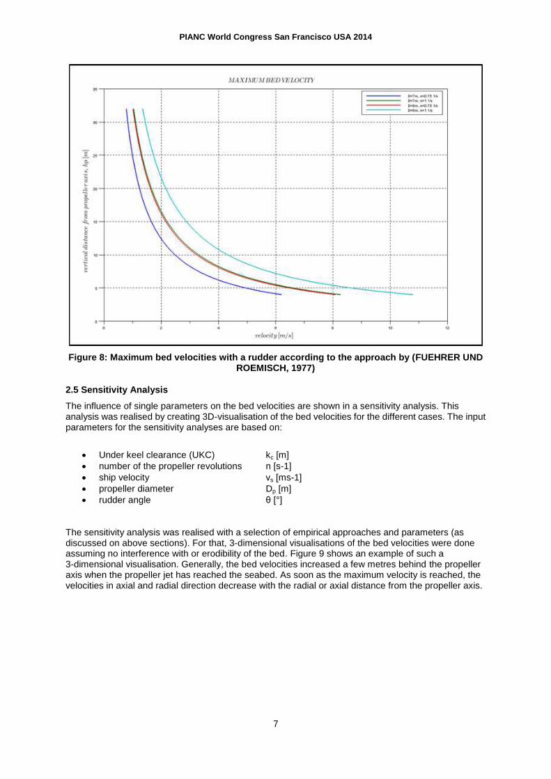
The maximum bed velocity considering the vertical distance from the propeller axis to the seabed can be estimated (FUEHRER AND ROEMISCH, 1977):

(

)

(15)

with

E coefficient [-]

Including the coefficient, E, equation (15) considers three specific configurations:

A propeller without a rudder, E = 0.42

A propeller with a rudder in central position ( θ = 0° ), E = 0.71

A ducted propeller, E = 0.25

Using the above equation the maximum bed velocity is estimated and presented in Figure 8.


7

Figure 8: Maximum bed velocities with a rudder according to the approach by (FUEHRER UND ROEMISCH, 1977)

2.5 Sensitivity Analysis

The influence of single parameters on the bed velocities are shown in a sensitivity analysis. This analysis was realised by creating 3D-visualisation of the bed velocities for the different cases. The input parameters for the sensitivity analyses are based on:

Under keel clearance (UKC) kc [m]

number of the propeller revolutions n [s-1]

ship velocity vs [ms-1]

propeller diameter Dp [m]

rudder angle θ [°]

The sensitivity analysis was realised with a selection of empirical approaches and parameters (as discussed on above sections). For that, 3-dimensional visualisations of the bed velocities were done assuming no interference with or erodibility of the bed. Figure 9 shows an example of such a 3-dimensional visualisation. Generally, the bed velocities increased a few metres behind the propeller axis when the propeller jet has reached the seabed. As soon as the maximum velocity is reached, the velocities in axial and radial direction decrease with the radial or axial distance from the propeller axis.


8

Figure 9: Example of 3D-bed velocity distribution

Example: Keel clearance

In the example only the keel clearance kc was varied from 0.5 to 3 metres. The efflux velocity for all cases is about 4 ms-1. The bed velocities decrease with increased keel clearance from 0.58 ms-1 down to 0.12 ms-1. The reduction of the efflux velocity ranges from 85 % to 97 %. Furthermore the area influenced by higher bed velocities decrease with an increase of the under keel clearance. At a keel clearance of 0.5 metres, the sea bed area influenced by the propeller jet lies from about 9 metres (0.85Dp) up to 29 metres (4Dp) behind the propeller axis. With a keel clearance of 3 metres, the influenced area is situated from about 16 metres (2.3Dp) up to 27 (3Dp) metres behind the propeller axis. The general look of the bed velocity distributions is similar for all cases. The results are listed in Table Table 1 and visualized in Figure 10.

Case 1 vo vb,max vred Propeller Jet Influence (x0 – x1)

[m]

Max rad Jet

Influence

[m/s] [m/s] [%] x0 x1 x1-x0 [m]

a 4.069 0.58 85.75 9 29 20 3.6

b 4.069 0.47 88.45 10 29 19 3.3

c 4.069 0.28 93.12 12.5 28 15.5 3

d 4.069 0.12 97.05 16 27 11 2.5

Table 1 Results of the bed velocities and their locations on the seabed for Case 1 (kc)


9

Figure 10: Case 1 (kc) of 2D-projection of the bed velocities

2.6 Summary empirical method

The propeller jet is a very complex phenomenon due the different physical effects like the turbulence, the cavitation and the different velocity components. Furthermore, many propeller specific variables characterize the propeller jet. The majority of researchers has concentrated on the velocity distribution behind the propeller axis and have neglected the turbulence and the cavitation. All the presented empirical approaches and investigations of the velocities distributions are based on the axial momentum theory of ALBERTSON ET AL.(1950) for a plain water jet. The main differences between approaches are their range of validity, and the consideration of parameters like the ship velocity or the presence of a rudder. Based on a selection of the empirical approaches, a sensitivity analysis was conducted. Within this routine the bed velocities were visualised in 3D-projection for different cases. In these cases the main parameters (under keel clearance, propeller diameter, number of revolutions, ship velocity and the rudder angle) were varied and the impacts of each variation of each parameter were easily presented.

The sensitivity analysis has shown that each parameter has different impacts on the bed velocity and the sea bed area potentially influenced by propeller. The largest impacts on the bed velocities were shown to occur with changes of the ship velocity. The bed velocities are highest in the case that the ship has a velocity of zero (accelerating) and also the influence area of the bed is widest. If the vessel is moving, the bed velocities would be lower. Another large influence on the bed velocities could be shown with the presence of a rudder. In the case of negative rudder angle the downwards stream are enhanced and caused higher bed velocities instead of positive rudder angles. An increasing of the number of revolutions caused higher bed velocities and a longer influence area of the bed velocities. An increasing of the keel clearance caused lower bed velocities. Least impacts are shown with the variation of the propeller diameter.


10

3. CFD-MODELLING

Comprehensive simulations using CFD models on real scale were conducted. The software that was used to conduct the CFD simulations was OpenFOAM. The numerical background can be found at http://www.openfoam.com.

Two different model setups were tested for their validity. One of the purposes is to construct a model that can accurately calculate the flow field due to the propeller. Thus the propeller is closely investigated by the use of a General Grid Interface (GGI) model, where the rotation of the propeller is resolved, whereby the direct impact of the propeller is modelled.

Because the numerical modelling of a moving propeller requires a resolution of several time steps per propeller revolution and a propeller in general demands a very dense grid in order to adequately resolve the surfaces, the sliding mesh model is computationally expensive, and not very well-suited for longer transient runs. For that reason, a Multiple Reference Model (MRF) was set up and tested.

3.1 Numerical description

General Grid Interface (GGI) model

In the general grid interface model, the flow problem is divided into two regions involving two domains. The inner rotating domain includes the region with the propeller, whereas the outer domain is a stationary frame including the bulk fluid. The inner grid rotates with the propeller while the outer grid remains stationary; hence the inner grid slides past the outer grid at a cylindrical interface. Values of flow variables are transferred across the interface through a general grid interface (see Figure 11).

Figure 11: Computational mesh for sliding mesh model where the rotor part is separated with stator part by overlapping GGI interface.

This approach is numerically extremely costly; therefore alternatives were tested to make scenario analyses feasible

Multiple Reference Frame Model (MRF)

The Multiple Reference Model (MRM) solver used in this project for the 3D steady-state simulations was MRFSimpleFoam, which is a finite volume steady-state solver for incompressible, turbulent flows of non-Newtonian fluids, using the SIMPLE algorithm for pressure-velocity coupling. The solver uses the Multiple Reference Frame (MRF) approach, which requires no relative mesh motion of the rotating and the stationary parts (also referred to as the Frozen Rotor approach). The momentum equations are solved by a mix of inertial and relative velocities in the relative frame together with the additional Coriolis term for the rotating part. The MRFSimpleFoam solver is fast but does not predict the full transient behaviour of the flow.


11

3.2 Model Validation

To validate the CFD approach, a study of the propeller wake in an open water set-up (no seafloor) was conducted. This is to validate the models and compare with experimental data mostly done under similar conditions in laboratories. Data on propellers is scarce, and no measurements of the flow fields behind propellers could be retrieved, the trust and torque were compared.

Test runs using a “Wageningen B” propeller with five blades and diameter of 150mm and a rotation speed of 600rpm were conducted. These B-series propellers were designed and tested at the Netherlands Ship Model basin in Wageningen. In the model setup, the propeller is placed in a channel of width and height of 3D (D is the diameter of the propeller) The length of the domain L = Di +Dw varies from 6D to 20D where Di and Dw are the distance to the inlet and wake area (outlet) as presented in Figure 12.

Figure 12: Computational domain for open water test with Wagenigen B5 propeller.

Simulations of flows over the propeller with various advance ratios (vessel speeds) were conducted using both the sliding mesh model and the multiple reference frame to firstly validate the approach, and secondly predict the propeller's performance and investigate the wake structure.

The performance of the Wageningen propeller was in a first step investigated using CFD simulations. The sliding mesh approach (GGI) was employed for simulations of flows in the presence of the rotating propeller. The propeller is placed in an open water set up of with Di = 2D and Dw = 4D with different operating conditions of rotation speeds and incoming water velocity. To characterize the performance of the propeller, the advanced coefficient J is defined as:

J = Va/nD (3.1)

where n is the rotating speed in revolutions per second, D is the propeller diameter and Va is the inlet velocity. Simulations were conducted for a range of advance coefficients J = 0.1; 0.2; 0.4; 0.6; 0.88; 1.0 with a fixed rotation speed of the propeller of 90 RPM (=1.5 rounds per second).

The sensitivity of the model to the grid resolution was tested using the B5 Wagenigen propeller at J = 0:88. The results showed convergence of thrust and torque coefficients when the mesh was refined from a coarse mesh of 1 million elements to the finest mesh of 5 million elements. Based on the results, an intermediate resolution of cells in the order of hb = 0.1m and hw = 0.2m, was chosen for all the simulations.

Results for propeller thrust, torque coefficients and efficiency are displayed in Figure 13 for the range of advance coefficients.


12

Figure 13: Comparison of thrust, torque coefficient and efficiency between simulations and experiment for the 5-blade Wageningen propeller.

The simulated results compare very well with experiments at a reasonable mesh resolution which shows that our model approach is able to capture the propeller jet correctly.

Comparison of the velocity profiles from the GGI and MRF models shows that the difference between the two models increases with distance from the propeller and that the MRF model has the tendency to under predict the velocity peak by about 10-20% (Figure 14). However, this has been deemed acceptable in the light of computational savings that the use of the MRF yields, which could be invested in additional scenarios.

Figure 14: Velocity profile downstream in the wake of the B5 Wageningen propeller at (a) J=0.88 and (b) J=0.2.

3.3 Results for a real world case (Container Vessel)

Based on the validation, it was decided to use the MRF model to conduct a large series of numerical simulations. To assess the influence of the identified variables on the propeller jet at the seafloor, a number of simulations were conducted, with changing variables as summarized in the following Table 2. The data provided by Maersk A/S and was taken from container vessel Susanne Maersk, length 347m, width: 42m and draught 13.7m, the propeller has six blades and a diameter of 9m.


13

Parameter Abbreviation Unit Variation

Under keel clearance UKC m 1 3 5 infinite

Propeller revolutions RPM Rounds/

min 30 60 90

Vessel speed V knot 0 6 12

Rudder Angle θ ° -20 0 20

Ship - - yes no

Propeller diameter D m Fixed: 9

Propeller type Fixed: Maersk S-Class

Table 2: Variables and constants in the numerical experiments

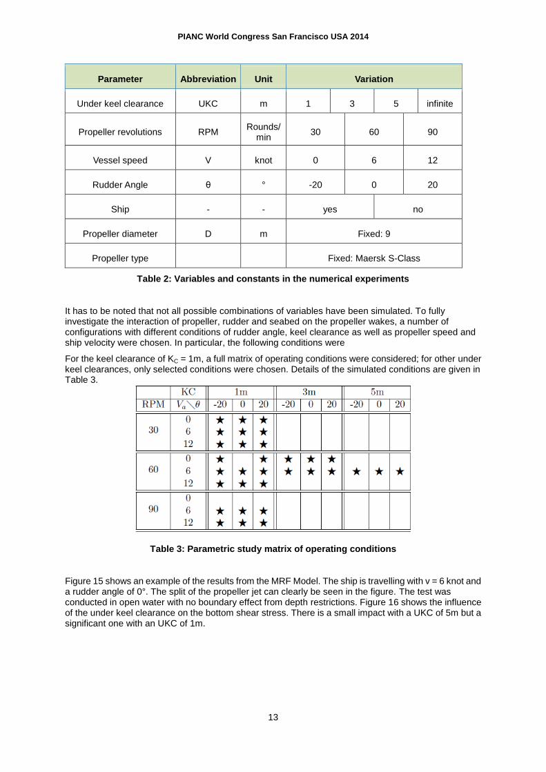
It has to be noted that not all possible combinations of variables have been simulated. To fully investigate the interaction of propeller, rudder and seabed on the propeller wakes, a number of configurations with different conditions of rudder angle, keel clearance as well as propeller speed and ship velocity were chosen. In particular, the following conditions were

For the keel clearance of KC = 1m, a full matrix of operating conditions were considered; for other under keel clearances, only selected conditions were chosen. Details of the simulated conditions are given in Table 3.

Table 3: Parametric study matrix of operating conditions

Figure 15 shows an example of the results from the MRF Model. The ship is travelling with v = 6 knot and a rudder angle of 0°. The split of the propeller jet can clearly be seen in the figure. The test was conducted in open water with no boundary effect from depth restrictions. Figure 16 shows the influence of the under keel clearance on the bottom shear stress. There is a small impact with a UKC of 5m but a significant one with an UKC of 1m.


14

Figure 15: Multiple Reference Model - RPM=60, V=6knot and rudder angle (theta)=0°

Figure 16: Results from the CFD Modell: Impact of the under keel clearance. Upper: 1 m UKC, Middle: 3 m UKC, Bottom: 5 m UKC. Tests at 60 rpm, ship speed 6kn, Rudder angle θ=0°. Wall

shear stress in hPa.

3.4 Summary CFD Modelling:

From the simulation results, the main findings are the following:

In the presence of the seabed, it obstructs the development of the flow jets thus changing the

wake structure and inducing more stress on the seabed.

At identical keel clearance, ship velocity and rudder angle and increase of rotation speed

increases wall shear stress level on the seabed

Increase in advance ratio (J) induces more wall shear stress on the seabed.


15

At identical keel clearance, ship velocity and advance ratio, a ship turning left (clockwise turning

propeller) results in minimal shear stress to the seabed.

The effect of keel clearance is straightforward: reduced UKC increases shear stress

In this study, the seabed is modelled as a rough surface which uniform roughness. As the

roughness decreases, the wall shear stress level is reduced on the seabed.

Additionally a sensitivity analysis was conducted by varying each of the parameters (RPM, Rudder angle, ship speed, UKC) independently by 5% and noting the corresponding change in resuspension (increased shear stress). The RPM is the most sensitive parameter. A 5% increase lead to 20% increased resuspension. The UKC has the least effect on maximum shear stress. A linear relationship can be possibly derived between maximum shear stress and UKC, in which the gradient varies with the rudder angle.

All these findings are to be expected from the empirical solutions. However, the CFD results yield also quantitative results. These are evaluated in the following chapters.

4. FIELD MEASUREMENTS

Measurements close to moving vessels are a challenge with respect to the safety of the boat and the crew. Nevertheless several ADCP profiles are taken in Hamburg and Singapore. These ADCP profiles were used to display suspended sediment concentrations. The calibration was performed by using water samples.

Figure 17 shows the 3-dimensional plotted suspended sediment concentration (SSC) behind a container vessel entering the Tanjong Pagar Terminal in Singapore. High SSC can be found. Figure 18 shows results from a campaign in Hamburg performed by HPA (Hamburg Port Authority). This case shows a departing vessel in a very restricted fairway. The SSC reaches up to 500 mg/l in this case. Further measurements with maneuvering vessels show concentration up to 1500 mg/l.

Figure 17: Suspended sediment concentration behind a container vessel in Singapore, Tanjong Pagar Terminal.


16

Figure 18: Suspended sediment concentrations close to a container vessel leaving the Hamburg Port. Left: SSC, Right: Profile, Bottom: Departing Ship.

5. LARGE SCALE DESCRIPTION

A CFD model is only able to model detailed parts of a ship passage. A large scale description of the impact of moving vessels on the sediment transport requires different model techniques. A 3-dimensional MIKE3 Model was set up for the Elbe River between Hamburg and Cuxhaven (Germany). Several scenarios with ship tracks between Cuxhaven and Hamburg at different tidal situations and additionally maneuver situations were evaluated.

The MIKE3 transport module (MT) and the dredging module were used. The dredging module includes erosion and spill along ship tracks. The amount of sediment was evaluated using the field measurements and a scenario module. The module includes the propeller diameter (Dp), the RPM, the UKC and the vessel speed. The SSC for maneuvering scenarios was directly taken from the measurements.

The scenarios include different starting positions inside Hamburg Port, vessels entering and leaving the port, different tidal situations and variable suspended sediment concentrations. An accumulation of the single events on propeller-induced sediment transport was done for the Elbe River. Figure 19 shows the results of a simulation of sediment movement during an un-berthing maneuver in the Süderelbe in Hamburg (Terminal Altenwerder). The measured suspended sediment concentrations during the departing maneuver were about 1500 mg/l. This was included in the model until the ship started moving. Afterwards the suspended sediment concentration was reduced to 15 mg/l during its travel to the North Sea. Initially during the maneuver, significant erosion occurs. Sediment is re-suspended and deposits in the center of the basin. This effect has been documented also in echo soundings by HPA, however, no direct relation to specific ships can be inferred.


17

Figure 19: calculated sediment movement after a departing maneuver at the container terminal in Altenwerder (Track 4, 1500 mg/l reduced to 15 mg/)

Further investigations on sediment transport along the Elbe River show in general low impact from a single ship on the overall sediment transport. Summarizing the annual ship traffic the impact cannot be neglected any more.

6. CONCLUSION

The presented study combines field measurements, physical test in the laboratory and different numerical methods for modelling currents and sediment transport to assess ship induced sediment transport. The study is performed in the ports of Singapore and Hamburg and the Elbe River (connection between Hamburg and the North Sea). In this paper a general overview of the complex study was given. Different methods and results were presented.

The most significant effect from propeller induced current can be found during maneuvering situation in restricted waters. Nevertheless the ships sailing along the Elbe River to the North Sea can be an additional source for fine sediment transport into nature reserve areas along the River. Especially in areas with very low Under Keel Clearance.

REFERENCES

Albertson M.L., Dai Y.B., Jensen R.A., and Rouse H. (1950). Diffusion of a submerged jet. Transcript of the ASCE (Paper No. 2409), (115), 639 – 697.

BAW, Federal Waterways Engineering and Research Institute (2005). Principles for the design of bank and bottom protection for inland waterways. Bulletin No. 88, Karlsruhe.

Fuehrer M. and Romisch K. (1987). Propeller jet erosion and stability criteria for bottom protection of various constructions. PIANC, Bulletin No. 58.

Hamill, G.A. (1987). Characteristics of the screw wash of a manoeuvring ship and the resulting bed scour. PhD Thesis, Queen's University of Belfast.

Hamill G.A. and McGarvey J.A. (1996). Designing for propeller action in harbours. Proceedings of the International Conference on Coastal Engineering, No 25, pp. 4451-4463.

Hamill G.A., McGarvey J.A., and Hughes D.A.B. (2004). Determination of the efflux velocity from a ship’s propeller. Proceedings of the Institution of Civil Engineers, Maritime Engineering, 157(2), pp 83-91.


18

Kee C., Hamill G.A., Lam W.H., and Wilson P.W. (2006). Investigation of the velocity distributions within a ship’s propeller wash. Proceedings of the 16th International Offshore and Polar Engineering Conference, San Francisco, California, USA, The International Society of Offshore and Polar Engineers, pp 451-456.

Lam W.H., Hamill G., Robinson D., and Raghunathan S. (2010). Observations of the initial 3D flow from a ship’s propeller. China Ocean Engineering, Ocean Engineering, Elsevier, (37), pp 1380-1388.

Lam W., Hamil G.A., Song Y.C., Robinson D.J., and Raghunathan S. (2011a). A review of the equations used to predict the velocity distribution within a ship’s propeller jet. Ocean Engineering, Elsevier, (38), pp 1-10.

Lam W., Hamill G.A., Song Y.C., Robinson D.J., and Raghunathan S. (2011b). Experimental Investigation of the Decay from A Ship’s Propeller. China Ocean Engineering, Chinese Ocean Engineering Society and Springer-Verlag Berlin Heidelberg, 25(2), pp 265-284.

Stewart D.P.J. (1992). Characteristics of a ship screw wash and the influence of quay wall proximity. PhD thesis, Queen's University of Belfast.

Uliczka, K. and Kondziella, B (2006). Dynamic response of very large containerships in extremly shallow water. Proceedings of the 31st PIANC Congress, Estoril, Spain.

Verhij H. (2006). Hydraulic aspects of the Montgomery Canal Restoration. Report, WL| Delft Hydraulics.

sediment resuspension and seabed scour induced · pdf filepianc world congress san francisco...

Documents