1

SEGMENTAL CONVOLUTIONAL NEURAL NETWORKSFOR DETECTION OF CARDIAC ABNORMALITYWITH NOISY HEART SOUND RECORDINGS∗

YUHAO ZHANG1, SANDEEP AYYAR1, LONG-HUEI CHEN2, ETHAN J. LI2,3

1Biomedical Informatics Training Program, Stanford University School of Medicine2Department of Computer Science, 3Department of Bioengineering, Stanford University

Stanford, CA 94305, USAEmail: yuhaozhang@stanford.edu, ayyars@stanford.edu, longhuei@stanford.edu, ethanli@stanford.edu

Heart diseases constitute a global health burden, and the problem is exacerbated by the error-pronenature of listening to and interpreting heart sounds. This motivates the development of automatedclassification to screen for abnormal heart sounds. Existing machine learning-based systems achieveaccurate classification of heart sound recordings but rely on expert features that have not beenthoroughly evaluated on noisy recordings. Here we propose a segmental convolutional neural net-work architecture that achieves automatic feature learning from noisy heart sound recordings. Ourexperiments show that our best model, trained on noisy recording segments acquired with an ex-isting hidden semi-markov model-based approach, attains a classification accuracy of 87.5% on the2016 PhysioNet/CinC Challenge dataset, compared to the 84.6% accuracy of the state-of-the-artstatistical classifier trained and evaluated on the same dataset. Our results indicate the potential ofusing neural network-based methods to increase the accuracy of automated classification of heartsound recordings for improved screening of heart diseases.

1. Introduction

Heart diseases constitute a significant global health burden. Just one subset of these dis-eases, valvular heart disease (VHD) resulting from rheumatic fever, causes 300,000-500,000preventable deaths each year globally, primarily in developing countries.1,2 Early detectionof many heart diseases is crucial for optimal treatment management to prevent disease pro-gression.3,4 In developing countries, the standard practice for screening of heart diseases suchas VHD and cardiac arrhythmia is cardiac auscultation to listen for abnormal heart sounds.Patients found to have suspicious abnormalities are then referred to specialists for properdiagnosis by a much more expensive echocardiographic procedure.3 Although cardiac auscul-tation has been replaced by echocardiography for screening in industrialized countries, thecost-effectiveness and procedural simplicity of auscultation make it an important screeningtool for primary care providers and clinicians in under-resourced communities.5,6

The main challenge in cardiac auscultation is the difficulty of detecting and interpretingsubtle acoustic features associated with heart sound abnormalities. Manual classification ofheart sounds suffers from high intra-observer variability,?,7–13 causing false positive and falsenegative results. Much work has been done in trying to improve screening accuracy, includingefforts to design devices to record heart sounds and automatically classify them. However,the biggest challenge for this task remains in developing an accurate classifier for heart sound

∗This work was finished in May 2016, and remains unpublished until December 2016 due to a request fromthe data provider.

2

recordings, which are often obtained in noisy environments. Here, we propose a novel approachbased on segmental convolutional neural networks to classification of heart sound recordings.Our approach achieves automatic feature learning together with accurate prediction of theabnormality. On noisy recordings, this approach outperforms prior classifiers using a state-of-the-art feature set developed for noiseless recordings.

The rest of this paper is organized as follows. In Section 2, we discuss related previousresearch. In Section 3, we introduce the methods that we used to classify noisy heart soundrecordings, including preprocessing of data, the use of traditional classifiers, and our segmentalconvolutional neural network models. Next, in Section 4, we present the performance of ourclassifiers, along with our analysis of these results. We discuss the limitations of our work andfuture directions in Section 5 and conclude our work in Section 6.

2. Related Work

The first step in automatic classification of heart sounds is segmentation of the recordingsalong heartbeat cycle boundaries. Segmentation divides the heart sound signal into cyclesof four parts: the first heart sound (S1), systole, the second heart sound (S2), and diastole.Past efforts in the field include the use of envelope-based methods14,15 and machine learningtechniques.16,17 A recent segmentation algorithm proposed by Schmidt et al has been shownto work well on a large dataset of 10,172 heart sound recordings, and achieved an averageof 95.63% F1 score, easily outstripping all other methods evaluated with the same set ofrecordings in the literature.18,19 This hidden semi-Markov model (HSMM)-based model wastested on noisy, real-world recordings and considered state-of-the-art. Therefore, we employedthe algorithm as-is to acquire the segmentation of input recordings.

Previous work in heart sound recordings classification follows the traditional paradigm ofusing hand-crafted feature sets as input to automatic classification based on machine learning.Features are typically a mixture of time domain properties, frequency domain properties,statistical properties, and transform domain properties such as from the discrete wavelettransform (DWT) or empirical mode decomposition (EMD).20 The extracted features are thenfed to different machine learning methods, which are then trained to recognize abnormal heartsounds, or in some cases to classify the recordings into the specific heart diseases. The mostcommon methods are artificial neural networks (ANNs),21 support vector machines (SVMs),22

Hidden Markov models (HMM),23 and k-nearest neighbors (kNN).24 However, prior resultshave been restricted by the use of small or otherwise limited data sets, including exclusion ofnoisy recordings or manual curation of recordings. While classifiers have been reported withaccuracies over 90%,? there is insufficient evidence to conclude whether the expert featuresused with these classifiers are fully applicable to noisy heart sound recordings. We address thisissue by training and testing traditional classifiers on a newly published set of noisy recordings.

In addition, our work is inspired by numerous recent work on the application of neuralnetworks to the processing of sensory-type data, such as visual?,25,26 and speech recognition.?

However, our segmental convolutional neural network approach is substantially different fromthese work in its use of heart sound segments during training and test time. Meanwhile, wealso empirically evaluated two different types of network architectures and tried to explain

3

their effectiveness via visualizations of learned filters and hidden layers.

3. Methods

The heard sound recordings used in our experiments were obtained from a publicly hosteddataset? for the 2016 PhysioNet/Computing in Cardiology Challengeb. This dataset consistsof approximately 3000 recordings obtained with a variety of durations, noise characteristics,and acoustic features. Cardiac conditions featured in the recordings include valvular heartdiseases, benign murmurs, aortic disease, and arrhythmias. Recordings in the dataset werecollected from different locations on the body of both children and adults. Given the uncon-trolled environment, many recordings are corrupted by various noise sources, such as talking,stethoscope motion, breathing and intestinal sounds, which comprise the challenge of learningfeatures and classifying the signals. As the dataset is intended to support the developmentof classification systems for initial screening of heart diseases, recordings were only labeled asnormal or abnormal, depending on whether follow-up for further diagnosis was recommendedfrom the recording. At the time of our work, recordings excessively corrupted by noise hadnot yet been relabeled as unclassifiable by challenge organizers, therefore our experimentswere focused on binary classification between normal and abnormal noisy recordings, whichrespectively constituted 80% and 20% of the public dataset.

We split the dataset into a 90% training set for classification model development and a 10%testing set for model evaluation. In the absence of prior probabilities for disease prevalence, weconstructed the test set to be balanced between normal and abnormal recordings for clearerinterpretability of performance metrics. As a result, 17% of the recordings in the trainingset were abnormal and the remaining 83% were normal. We preprocessed the recordings andthen used them for two independent branches of investigation: traditional classification withfeature selection, and the use of a new segmental convolutional neural network architecture.We compared the test set performance of the results of these two investigations by calculatingsensitivity, specificity, and accuracy, as these metrics are standard in prior work on heartsound classification. For completeness, we also compared area under the Receiver-OperatingCharacteristic (ROC) curve and positive predictive value.

3.1. Preprocessing

As a first step, we preprocess the recordings to handle noise and segment individual heart-beats. As stated in the related work section, we employ a recent HSMM-based segmentationalgorithm developed for noisy heard sound recordings, which has been reported to achieve anaccuracy of 95% on a benchmark dataset.

Since the signals were recorded from multiple sources and differ widely in levels of back-ground noise, we identify the handling of noise within the data crucial for the success ofdownstream components. We explore a few common venues for denoising in the heart soundrecordings and general signal processing, including techniques based on discrete wavelet trans-form (DWT)27 and empirical mode decomposition (EMD). In wavelet-based denoising, the

bThe data was obtained from the website: https://physionet.org/challenge/2016/

4

signal is reconstructed from thresholded components produced with DWT using multi-levelwavelet coefficients. This approach is finally used in our experiments, given its ease of imple-mentation.

As the noise selection and reduction can vary widely across the multiple data sources andindividual cases, we also integrate the denoising results as a feature in traditional classificationmethods by calculating the signal-to-noise (SNR) of the individual recordings.

3.2. Traditional Machine Learning-based Classifiers

We investigated the performance of various machine learning-based classifiers with hand-designed features on noisy heart sound recordings. Through this investigation, we would liketo understand: 1) the contribution of different hand-designed features for the classificationof noisy heart records; and 2) the overall performance of traditional approaches on this newdataset.

3.2.1. Features

We attempt to implement features from a published study for classifying minimal-noise record-ings as either normal or abnormal with extraction of 23 features and subsequent selectionof 5 features.28 Per recording, we extract a set of 58 time-domain, frequency-domain, andtransform-domain features which together constituted a superset of the 23 published features,as shown in Table 1. All features are represented by the mean and standard deviation over allheart beat cycles in the recording. To achieve better results, we transform and combine somefeatures as ratios. Some frequency domain features have missing values due to anomalousrecording content.

Table 1. Features extracted for traditional classification.

Overall Feature Type Feature Type Number of Features

Time Domain

Interval Length 16Absolute Amplitude 5

Total Power 5Zero Crossing Rate 1

Amplitude at Peak Frequency 5

FrequencyDomain

Peak Frequency 5Bandwidth 9Q-Factor 9

Total Harmonic Distortion 1TransformDomain

Cepstrum Peak Amplitude 1Signal-to-Noise Ratio from DWT 1

3.2.2. Models

We employ different statistical models to perform supervised learning from the dataset. Beforetraining, we impute all the missing data using median values across all training examples.We perform 10-fold cross validation to evaluate model performance on our 90% imbalanced

5

training data set. To alleviate classifier bias in learning one class over the other, we followthe standard procedure to increase the weights of classification errors of abnormal recordings.We also use 10-fold cross validation for tuning classifier hyperparameters to improve modelperformance. Our models and corresponding hyperparameters are shown in Table 2.

Table 2. Hyperparameters tuned for the investigated classification models.

Classification Model Tuning Parameters

Logistic Regression -Lasso, Ridge Based Methods regularizing/penalizing term

Support Vector Machine kernel function, cost, gammaDecision Trees number of trees

Random Forests number of estimators, number of featuresK-Nearest Neighbours number of neighbours

We use forward stepwise, backward stepwise, and Lasso regression methods for featureselection. We use features selected by the forward stepwise and Lasso methods for training thelogistic regression classifier and Lasso-selected features for training the remaining classifiers.For the Lasso method, we optimize the regularization/tuning parameter lambda and selectfeatures using the lambda value that minimizes the misclassification error rate.

3.3. Segmental Convolutional Neural Networks for Heart SoundClassification

Traditional classifiers are simple to employ and fast to train, but rely on hand-designed featuresthat do not necessarily capture useful signals in the recordings. An alternative to traditionalclassifiers is models that can automatically learn useful features that are not limited by humandesign. Among these models, convolutional neural network (CNN) provides a flexible filter-based architecture to capture the patterns in the sensory-type data. However, heart soundsignals vary in length significantly, and often contain noise that makes a certain snippet ofsignal unclassifiable. These make the adoption of CNN models less straightforward.

…

InputSignal

CNN Unit

Training Time Test Time

…1 0 1

…0 / 1

Fig. 1. Training and evaluation of the segmental convolutional neural networks.

We propose a segmental convolutional neural network architecture to solve these problems.

6

As shown in Fig. 1, our method takes raw heart sound recordings as input, and acquiresrecording segments by using the hidden semi-markov model described in Section 3.1. Then weonly keep segments with lengths from 400 to 1200 and zero-pad all signals into a 1200-elementvector. During training time, this preprocessing step keeps 98% of all segments and leavesus with 76509 training segments. We then cast these training segments as a new trainingset to train our CNN units. During test time, we first split each test signal into segmentsand then classify each segment using our trained CNN unit. Then we combine the segmentclassifications and classify a recording as abnormal only when the proportion of segmentsclassified as abnormal is over a threshold. We treat this threshold value as a hyperparameter.

This approach has three key advantages. First, since standard CNN requires fixed-lengthinput, this naturally solves the input length normalization issue. Second, expanding signalsinto segments substantially increases the number of training instances, which has been provedto be critical in the success of other applications of neural networks. Third, global classificationof a recording is more robust against accidental noise in the data, as accidental noise can onlyinfluence the classification of a small portion of local segments.

Filter configuration and depth are two major factors that influence the performance ofa CNN model. It remains unclear which type of architecture is more suitable to this task.Therefore, we now discuss the use of two different architectures for CNN units, which wename Filter-focused CNNs and Depth-focused CNNs respectively. These two architecture typesdiffer mainly in their configuration of filters, the way max-pooling is conducted, and the waydifferent layers are stacked.

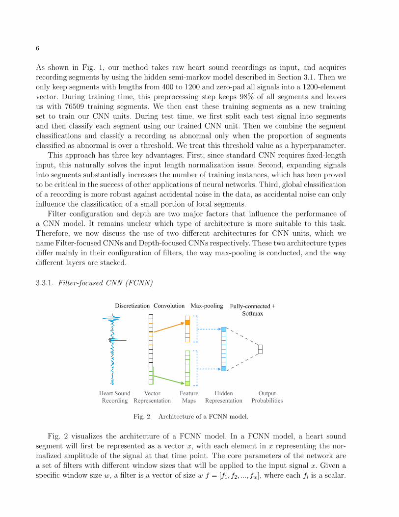
3.3.1. Filter-focused CNN (FCNN)

Heart Sound Recording

Vector Representation

Feature Maps

Hidden Representation

Output Probabilities

Discretization Convolution Max-pooling Fully-connected + Softmax

Fig. 2. Architecture of a FCNN model.

Fig. 2 visualizes the architecture of a FCNN model. In a FCNN model, a heart soundsegment will first be represented as a vector x, with each element in x representing the nor-malized amplitude of the signal at that time point. The core parameters of the network area set of filters with different window sizes that will be applied to the input signal x. Given aspecific window size w, a filter is a vector of size w f = [f1, f2, ..., fw], where each fi is a scalar.

7

A feature map m of this filter can be obtained from the application of a 1D-convolutionaloperator on f and x to produce an output sequence m = [m1,m2, ...,mn−w+1] where n is thelength of input signal x:

mi = g(

w−1∑j=0

fj+1xj+i + b)

where b is a bias term and g is a non-linear function. This convolution process is repeated formany filters of different window sizes w. After the convolution layer, a max-over-time poolingoperation is applied to each feature map mk to generate a single scalar activation hk:

hk = max([mk1,m

k2, ...,m

kn−w+1])

And then all activations hk are concatenated to form a size-N hidden representation of theoriginal signal h = [h1, h2, ..., hN ]. The idea behind the max-over-time pooling operation is toonly keep the most obvious activation that are generated by the convolution, and use that tocharacterize the signal for the downstream classification.

Finally, the hidden representation h is fed into a fully-connected with softmax layer togenerate the class probabilities y. We use cross entropy between predicted labels and groundtruth labels as loss function. The intuition behind the use of many filters of various windowsizes is that the model should be able to learn through back-propagation common patternsthat it has seen in the training signals that are useful for the classification, and these patternscould potentially be numerous and of different scales.

3.3.2. Depth-focused CNN (DCNN)

Heart Sound Recording

Vector Representation

Final Representation

OutputProbabilities

Discretization Convolution Max-pooling Softmax

…..

Condensed Representation

Repeated Layers

Hidden Representation

Fully-connected

Fig. 3. Architecture of a DCNN model.

While large filters of various sizes can help to capture useful patterns of different scales, itmay also be useful to have a model with only small filters at each layer but focuses on stackingmany layers together to form a deep architecture, as has been found in visual recognitiontasks.26 Fig. 3 visualizes the architecture of a Depth-focused CNN model. There are threemajor differences between DCNNs and FCNNs. First, the filter sizes in DCNNs are much

8

smaller than in FCNNs. Typically, the size of DCNN filters are approximately 10, while thesize of FCNN filters can range from 10 to 500. The use of very small filters in DCNNs reducesthe computational cost to perform convolutional operations and thus enables us to exploredeeper models while still capturing useful patterns in the signals. Second, in DCNNs, themotif of a convolution layer followed by a max-pooling layer is repeated several times toform a hidden representation of the original signal. Then this hidden representation is fedinto multiple stacked fully-connected layers to reduce the representation size, after which thesoftmax layer generates the output probabilities.

Finally, the way convolution and max pooling are conducted is different. In a DCNNconvolution layer, the output of convolution operation is a feature matrix m = [m1,m2, ...,mn],where each column mi is the feature map vector obtained from filter fi convolved with signalx, and can be viewed as a “channel” in the output signal. Then at the pooling layer, insteadof doing a max-over-time pooling, a max pooling over the local time region is performed, andchannels are kept. For example, a max-pooling operation with window 2 is:

mci = max(mc

2i,mc2i+1)

where mc represents the pooling output column in channel c, and mc represents the channel ccolumn in the feature matrix. Here, the max pooling serves as a sub-sampling over the signaland preserves more information compared to the max-over-time pooling operation in FCNN.

3.3.3. Network Configurations

We design experiments to evaluate our segmental convolutional neural network approach.Table 3 shows the CNN architectures that we report results on. We explored a lot differentarchitectures and included results for these models because: First, these models demonstrateprogressively increasing filter sizes and network depths, enabling comparison of the effectsof different network configurations on final performance; Second, the training times of thesemodels are tolerable given the resources we have. In the table, “Conv” represents a convolutionlayer, “MP” a max-pooling layer, and “FC” a fully-connected layer. For instance, for FCNNs,“Conv([50-500,50]*20)” represents a convolution layer with window size ranging from 50 to500 with a step of 50, and each window size corresponds to 20 different filters. For DCNNs,“Conv([10*25])” represents a convolution layer with 25 filters and window size 10.

Table 3. CNN network configurations.

CNN Model Architecture Configuration # Layers # Filters

FCNN-Small Conv([50-500,50]*20), MP, FC 3 200FCNN-Medium Conv([25-500,25]*30), MP, FC 3 600

FCNN-Large Conv([20-600, 20]*50), MP, FC 3 1500DCNN-Shallow Conv([10]*25), MP, Conv([10]*50), MP, FC(256), FC 6 75

DCNN-Deep Conv([10]*25), MP, Conv([10]*50), MP, Conv([10]*50), MP, FC(256), FC 8 125

For all CNN configurations, we use L2 regularization on the weights and dropout29 beforethe last softmax layer to regularize the model. We use AdaGrad30 to train the models with errorbackpropagation. We train each model on a 90% subset of our training set for 50 epochs, and

9

after each epoch we evaluate the model on the remaining 10% validation subset of our trainingset. For each CNN configuration, we save the model that generates the best accuracy on thevalidation set as the final model. This allows us to prevent the final model from overfittingon the training data. We then evaluate the best model from each CNN configuration on thesame test set as used by the traditional classifiers.

4. Results

4.1. Traditional Classifiers

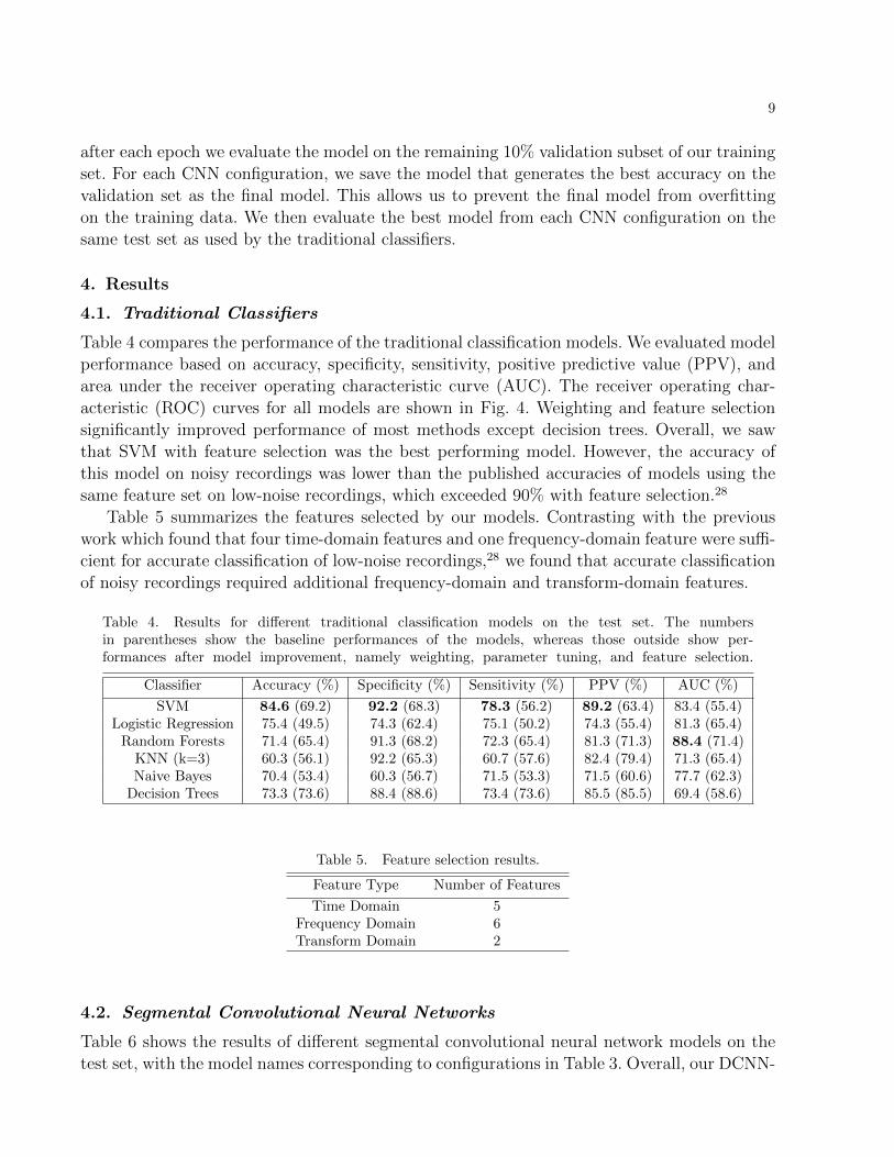
Table 4 compares the performance of the traditional classification models. We evaluated modelperformance based on accuracy, specificity, sensitivity, positive predictive value (PPV), andarea under the receiver operating characteristic curve (AUC). The receiver operating char-acteristic (ROC) curves for all models are shown in Fig. 4. Weighting and feature selectionsignificantly improved performance of most methods except decision trees. Overall, we sawthat SVM with feature selection was the best performing model. However, the accuracy ofthis model on noisy recordings was lower than the published accuracies of models using thesame feature set on low-noise recordings, which exceeded 90% with feature selection.28

Table 5 summarizes the features selected by our models. Contrasting with the previouswork which found that four time-domain features and one frequency-domain feature were suffi-cient for accurate classification of low-noise recordings,28 we found that accurate classificationof noisy recordings required additional frequency-domain and transform-domain features.

Table 4. Results for different traditional classification models on the test set. The numbersin parentheses show the baseline performances of the models, whereas those outside show per-formances after model improvement, namely weighting, parameter tuning, and feature selection.

Classifier Accuracy (%) Specificity (%) Sensitivity (%) PPV (%) AUC (%)

SVM 84.6 (69.2) 92.2 (68.3) 78.3 (56.2) 89.2 (63.4) 83.4 (55.4)Logistic Regression 75.4 (49.5) 74.3 (62.4) 75.1 (50.2) 74.3 (55.4) 81.3 (65.4)

Random Forests 71.4 (65.4) 91.3 (68.2) 72.3 (65.4) 81.3 (71.3) 88.4 (71.4)KNN (k=3) 60.3 (56.1) 92.2 (65.3) 60.7 (57.6) 82.4 (79.4) 71.3 (65.4)Naive Bayes 70.4 (53.4) 60.3 (56.7) 71.5 (53.3) 71.5 (60.6) 77.7 (62.3)

Decision Trees 73.3 (73.6) 88.4 (88.6) 73.4 (73.6) 85.5 (85.5) 69.4 (58.6)

Table 5. Feature selection results.

Feature Type Number of Features

Time Domain 5Frequency Domain 6Transform Domain 2

4.2. Segmental Convolutional Neural Networks

Table 6 shows the results of different segmental convolutional neural network models on thetest set, with the model names corresponding to configurations in Table 3. Overall, our DCNN-

10

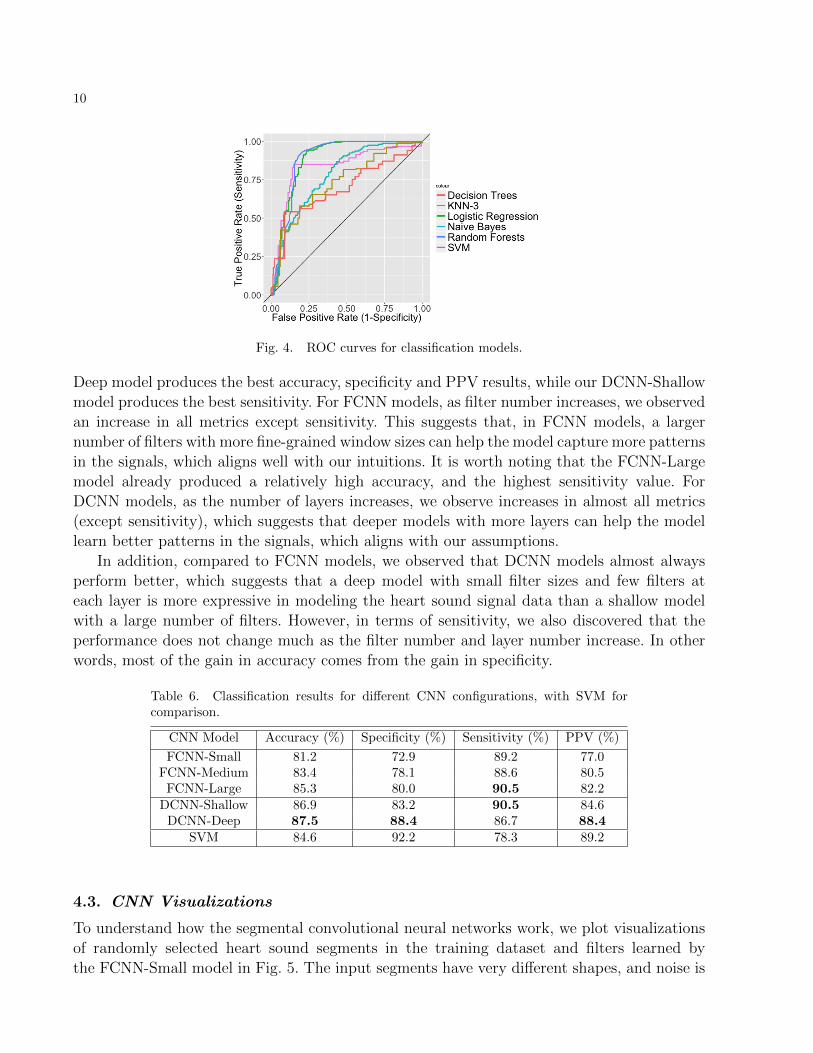
Fig. 4. ROC curves for classification models.

Deep model produces the best accuracy, specificity and PPV results, while our DCNN-Shallowmodel produces the best sensitivity. For FCNN models, as filter number increases, we observedan increase in all metrics except sensitivity. This suggests that, in FCNN models, a largernumber of filters with more fine-grained window sizes can help the model capture more patternsin the signals, which aligns well with our intuitions. It is worth noting that the FCNN-Largemodel already produced a relatively high accuracy, and the highest sensitivity value. ForDCNN models, as the number of layers increases, we observe increases in almost all metrics(except sensitivity), which suggests that deeper models with more layers can help the modellearn better patterns in the signals, which aligns with our assumptions.

In addition, compared to FCNN models, we observed that DCNN models almost alwaysperform better, which suggests that a deep model with small filter sizes and few filters ateach layer is more expressive in modeling the heart sound signal data than a shallow modelwith a large number of filters. However, in terms of sensitivity, we also discovered that theperformance does not change much as the filter number and layer number increase. In otherwords, most of the gain in accuracy comes from the gain in specificity.

Table 6. Classification results for different CNN configurations, with SVM forcomparison.

CNN Model Accuracy (%) Specificity (%) Sensitivity (%) PPV (%)

FCNN-Small 81.2 72.9 89.2 77.0FCNN-Medium 83.4 78.1 88.6 80.5

FCNN-Large 85.3 80.0 90.5 82.2DCNN-Shallow 86.9 83.2 90.5 84.6

DCNN-Deep 87.5 88.4 86.7 88.4SVM 84.6 92.2 78.3 89.2

4.3. CNN Visualizations

To understand how the segmental convolutional neural networks work, we plot visualizationsof randomly selected heart sound segments in the training dataset and filters learned bythe FCNN-Small model in Fig. 5. The input segments have very different shapes, and noise is

11

observable in some segments. This suggests the difficulty of the classification task. In addition,the visualization of filters shows that the network learned very good waveform-like patternsfrom the training data. This is even more convincing, considering the fact that all filterswere randomly initialized prior to training. This qualitative result aligns very well with ourintuitions about why CNN models are suitable for heart sound classification.

(a) (b)

Fig. 5. (a) Visualization of randomly chosen segments in the training data; (b) Visualization of learned filters(window size 200) by FCNN-Small model.

Fig. 6 shows the network activations for normal and abnormal input segments. We findthat, given the input segment, some of the output neurons in convolution layers activate,which indicates a pattern matched strongly with the signal at that local region, while othersdo not activate. Moreover, we find that more neurons in both the convolution layers andhidden layer are activated by abnormal segments compared to normal segments, indicatingthat many learned filters in the network are patterns of abnormal signals.

conv1activations

finalrepresentation

inputsegment

(a)

conv1activations

finalrepresentation

inputsegment

(b)

Fig. 6. Visualization of network activations for (a) a normal heart sound segment and (b) an abnormalsegment. All activations are from DCNN-Deep model, and only activations in the first convolution layer andthe final hidden layer are shown. Red color represents an activation value of 1, while blue color represents anactivation value of 0.

12

4.4. Comparison

We compared the performance of the best performing CNN architectures, namely DCNN-Large and FCNN-Deep, to SVM, which was the best performing model among the traditionalclassifiers (Table 6). We see that CNNs outperform SVM significantly for accuracy and sen-sitivity. While FCNN-Deep has marginally better specificity, DCNN-Large has better perfor-mance in terms of accuracy and sensitivity. Our results show that application of CNNs tonoisy heart sound recordings can produce better classification as compared to applying tra-ditional classification techniques. Due to time limits, we were not able to fully explore thearchitecture space of the CNN models. Therefore, we believe that our segmental convolutionalneural network approach has even more potential in classifying heart sound recordings thanwe have found.

5. Discussion

Our investigation of the applicability of previously published work in traditional classificationto noisy heart sound recordings suggests that further evaluation is needed. We found significantdifferences from feature extraction and classifier performance results reported from one suchstudy, which justifies more rigorous scrutiny of previous work. Specifically, it would be usefulto verify that feature extraction and traditional classification does indeed perform better ona dataset of clean heart sound recordings.

Due to limits of computing resources, we have not yet fully realized the potential of ourCNN models. We believe that better-performing models with more filters and more layerscan be achieved by doing a more thorough hyperparameter search. Another clear avenue ofexploration is to decompose the signals further with EMD, which has been shown to delineatesignals and noises of different origins in heart sound recordings.19 We would like to examinehow splitting a recording into EMD components for use as separate input channels to oursegmental CNNs may increase classification accuracy.

Limited by the annotation in the training data, our work is focused on the binary clas-sification of heart sound recordings into normal and abnormal categories. However, it is alsopractically useful to predict a third “unclassifiable” category, especially when noise is domi-nant in the heard sound recordings. For example, in real world applications, this third labelcan serve as a signal for human intervention. Therefore another direction for future work is toexplore the combination of supervised and unsupervised approaches to produce this “unclas-sifiable” label accurately.

6. Conclusion

We propose a segmental convolutional neural network approach to accurately classify noisyheart sound recordings. We studies the effectiveness of two different types of convolutionalneural network architectures, and compare their results with the application of traditionalstatistical classifiers on a set of manually curated features. Our results suggest that: First,traditional statistical classifiers using feature sets developed for low-noise recordings mayperform worse on noisy recordings. Second, segmental convolutional neural networks with

13

deep architectures and small filters can achieve higher accuracy in classifying noisy heartsound recordings without relying on manually-curated feature sets.

7. Acknowledgements

The authors would like to acknowledge Dr. Russ Altman, Dr. Steven Bagley and Dr. DavidStark at Stanford University for their helpful suggestions to improve this work. We also wantto thank Dr. Victor Froelicher for a helpful discussion on valvular heart diseases.

References

1. W. H. O. E. Consultation, Rheumatic Fever and Rheumatic Heart Disease, tech. rep., WorldHealth Organization (2001).

2. J. R. Carapetis, Circulation 118, 2748 (2008).3. E. Marijon, P. Ou, D. S. Celermajer, B. Ferreira, A. O. Mocumbi, D. Sidi and X. Jouven, Bulletin

of the World Health Organization 86, 84 (2008).4. B. J. Gersh, Auscultation of cardiac murmurs in adults. In: UpToDate, (2015).5. J. M. Sztajzel, M. Picard-Kossovsky, R. Lerch, C. Vuille and F. P. Sarasin, International journal

of cardiology 138, 308 (2010).6. I. Maglogiannis, E. Loukis, E. Zafiropoulos and A. Stasis, Computer methods and programs in

biomedicine 95, 47 (2009).7. C. E. Lok, C. D. Morgan and N. Ranganathan, CHEST Journal 114, 1283 (1998).8. A. A. Ishmail, S. Wing, J. Ferguson, T. A. Hutchinson, S. Magder and K. M. Flegel, CHEST

Journal 91, 870 (1987).9. M. D. Jordan, C. R. Taylor, A. W. Nyhuis and M. E. Tavel, Archives of internal medicine 147,

721 (1987).10. J. M. Vukanovic-Criley, S. Criley, C. M. Warde, J. R. Boker, L. Guevara-Matheus, W. H.

Churchill, W. P. Nelson and J. M. Criley, Archives of internal medicine 166, 610 (2006).11. S. K. March, J. L. Bedynek and M. A. Chizner, Teaching cardiac auscultation: effectiveness of

a patient-centered teaching conference on improving cardiac auscultatory skills, in Mayo ClinicProceedings, (11)2005.

12. J. M. Vukanovic-Criley, A. Hovanesyan, S. R. Criley, T. J. Ryan, G. Plotnick, K. Mankowitz,C. R. Conti and J. M. Criley, Clinical cardiology 33, 738 (2010).

13. S. Mangione and L. Z. Nieman, Jama 278, 717 (1997).14. M. E. Tavel, Circulation 93, 1250 (1996).15. H. Liang, S. Lukkarinen and I. Hartimo, Heart sound segmentation algorithm based on heart

sound envelogram, in Computers in Cardiology 1997 , 1997.16. S. Sun, Z. Jiang, H. Wang and Y. Fang, Computer methods and programs in biomedicine 114,

219 (2014).17. T. Oskiper and R. Watrous, Detection of the first heart sound using a time-delay neural network,

in Computers in Cardiology, 2002 , 2002.18. T. Chen, K. Kuan, L. A. Celi and G. D. Clifford, Intelligent heartsound diagnostics on a cellphone

using a hands-free kit., in AAAI Spring Symposium: Artificial Intelligence for Development , 2010.19. S. Schmidt, C. Holst-Hansen, C. Graff, E. Toft and J. J. Struijk, Physiological Measurement 31,

p. 513 (2010).20. C. D. Papadaniil and L. J. Hadjileontiadis, IEEE journal of biomedical and health informatics

18, 1138 (2014).21. S. Leng, R. San Tan, K. T. C. Chai, C. Wang, D. Ghista and L. Zhong, Biomedical engineering

online 14, p. 1 (2015).

14

22. H. Uguz, Journal of medical systems 36, 61 (2012).23. A. Gharehbaghi, I. Ekman, P. Ask, E. Nylander and B. Janerot-Sjoberg, International journal

of cardiology 198, p. 58 (2015).24. R. SaracOgLu, Engineering Applications of Artificial Intelligence 25, 1523 (2012).25. L. Avendano-Valencia, J. Godino-Llorente, M. Blanco-Velasco and G. Castellanos-Dominguez,

Annals of Biomedical Engineering 38, 2716 (2010).26. C. Liu, D. Springer, Q. Li, B. Moody, R. A. Juan, F. J. Chorro, F. Castells, J. M. Roig, I. Silva,

A. E. Johnson et al., Physiological Measurement 37, p. 2181 (2016).27. A. Krizhevsky, I. Sutskever and G. E. Hinton, Imagenet classification with deep convolutional

neural networks, in Advances in neural information processing systems, 2012.28. K. Simonyan and A. Zisserman, arXiv preprint arXiv:1409.1556 (2014).29. T. Wang, D. J. Wu, A. Coates and A. Y. Ng, End-to-end text recognition with convolutional

neural networks, in Pattern Recognition (ICPR), 2012 21st International Conference on, 2012.30. Y. LeCun and Y. Bengio, The handbook of brain theory and neural networks 3361, p. 1995

(1995).31. D. Gradolewski and G. Redlarski, Computers in biology and medicine 52, 119 (2014).32. M. Singh and A. Cheema, International Journal of Computer Applications 77 (2013).33. N. Srivastava, G. Hinton, A. Krizhevsky, I. Sutskever and R. Salakhutdinov, The Journal of

Machine Learning Research 15, 1929 (2014).34. J. Duchi, E. Hazan and Y. Singer, The Journal of Machine Learning Research 12, 2121 (2011).