segmentation course web page: vision.cis.udel.edu/~cv may 2, 2003 lecture 29
TRANSCRIPT
Segmentation
Course web page:vision.cis.udel.edu/~cv
May 2, 2003 Lecture 29

Announcements
• Read Forsyth & Ponce Chapter 14.4 and Chapter 25 on clustering and digital libraries, respectively

Outline
• Definition of segmentation• Grouping strategies• Segmentation applications
– Detecting shot boundaries– Background subtraction

What is Segmentation?
• Clustering image elements that “belong together” – Partitioning
• Divide into regions/sequences with coherent internal properties
– Grouping • Identify sets of coherent tokens in image
• Tokens: Whatever we need to group – Pixels – Features (corners, lines, etc.) – Larger regions (e.g., arms, legs, torso)– Discrete objects (e.g., people in a crowd)– Etc.

Example: Partitioning by Texture
courtesy of University of Bonn

Fitting
• Associate model(s) with tokens– Estimation: What are parameters of
model for a given set of tokens?• Least-squares, etc.
– Correspondence: Which token belongs to which model?• RANSAC, etc.

Approaches to Grouping
• Bottom up segmentation– Tokens belong together because they are
locally coherent• Top down segmentation
– Tokens belong together because they lie on the same object—must recognize object first
– RANSAC implements this in a very basic form• Not clear how to apply to higher-level concepts (i.e.,
objects for which we lack analytic models)
• Not mutually exclusive—successful algorithms generally require both

Gestalt Theory of Grouping
• Psychological basis for why/how things are grouped• Figure-ground discrimination
– Grouping can be seen in terms of allocating tokens to figure or ground
• Factors affecting token coherence– Proximity– Similarity: Based on color, texture, orientation (aka parallelism), etc.– Common fate: Parallel motion (i.e., segmentation of optical flow by
similarity)– Common region: Tokens that lie inside the same closed region tend
to be grouped together.– Closure: Tokens or curves that tend to lead to closed curves tend to
be grouped together.– Symmetry: Curves that lead to symmetric groups are grouped
together– Continuity: Tokens that lead to “continuous” — as in “joining up
nicely,” rather than in the formal sense — curves tend to be grouped– Familiar Configuration: Tokens that, when grouped, lead to a
familiar object—e.g., the top-down recognition that allows us to see the dalmation from Forsyth & Ponce

Gestalt Grouping Factors
from Forsyth & Ponce

Example: Bottom-Up Segmentation
Segmenting cheese curds by texture(note importance of scale!)

Example: Top-Down Segmentation
from Forsyth & Ponce
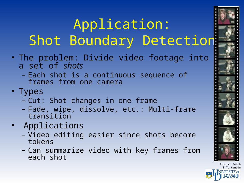
Application:Shot Boundary Detection
• The problem: Divide video footage into a set of shots– Each shot is a continuous sequence of frames
from one camera• Types
– Cut: Shot changes in one frame– Fade, wipe, dissolve, etc.: Multi-frame
transition• Applications
– Video editing easier since shots become tokens– Can summarize video with key frames from
each shotfrom M. Smith
& T. Kanade

Shot Boundary Detection
• Basic approach: Threshold inter-frame difference
• Possible metrics – Raw: SSD, correlation, etc.
• More sensitive to camera motion– Histogram– Edge comparison– Break into blocks
• Use hysteresis to handle gradual transitions
from M. Smith & T. Kanade
Graph of frame-to-frame histogram difference

Application: Background Subtraction
• The problem: Assuming static camera, discrimin-ate moving foreground objects from background
• Applications– Traffic monitoring– Surveillance/security– User interaction
Current imagefrom C. Stauffer and W. Grimson
Background image Foreground pixels
courtesy of C. Wren
Pfinder
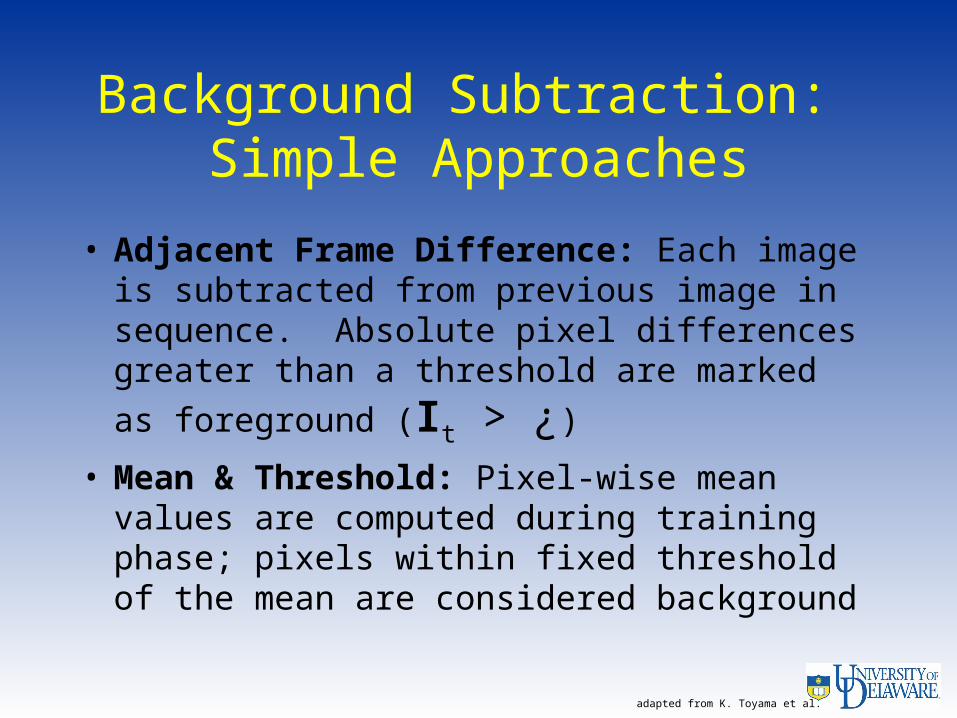
Background Subtraction: Simple Approaches
• Adjacent Frame Difference: Each image is subtracted from previous image in sequence. Absolute pixel differences greater than a threshold are
marked as foreground (It > ¿)
• Mean & Threshold: Pixel-wise mean values are computed during training phase; pixels within fixed threshold of the mean are considered background
adapted from K. Toyama et al.

Results & Problems for Simple Approaches
from K. Toyama et al.

Background Subtraction: Issues
• Noise models– Unimodal: Pixel values vary over time even for
static scenes– Multimodal: Features in background can “oscillate”,
requiring models which can represent disjoint sets of pixel values (e.g., waving trees against sky)
• Gross illumination changes– Continuous: Gradual illumination changes alter the
appearance of the background (e.g., time of day)– Discontinuous: Sudden changes in illumination and
other scene parameters alter the appearance of the background (e.g., flipping a light switch)
• Bootstrapping– Is a training phase with “no foreground” necessary,
or can the system learn what’s static vs. dynamic online?

Pixel RGB Distributions over time
Perceived color values of solid objects (e.g., tree trunk) have roughly Gaussian distributions due to CCD noise, etc. Leaf & monitor pixels
have bimodal distributions because of waving & flickering, respectively
courtesy of J. Buhmann

Improved Approaches to Background Subtraction
• Mean & Covariance: Mean and covariance of pixel values are updated continuously: – Moving average is used to adapt to slowly
changing illumination (low-pass temporal filter)
Foreground pixels are determined using a threshold on the Mahalanobis distance
• Mixture of Gaussians: A pixel-wise mixture of multiple Gaussians models the background adapted from K. Toyama et al.

Ellipsoids of Constant Probability for Gaussian
Distributions
from Duda et al.
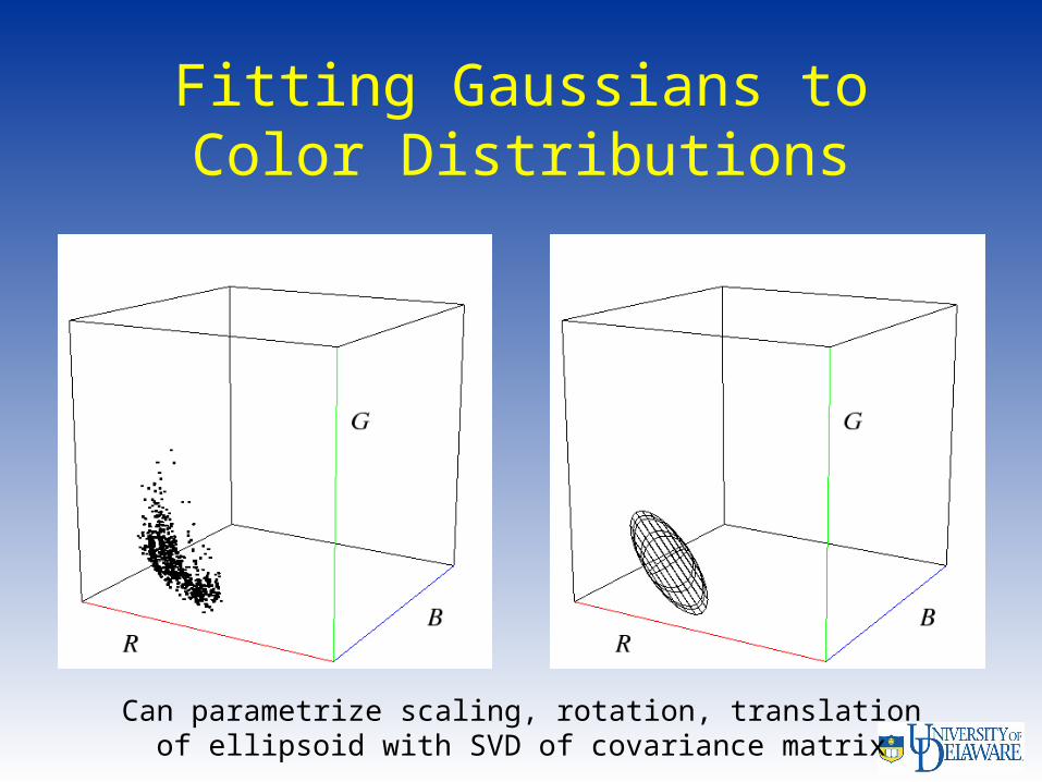
Fitting Gaussians to Color Distributions
Can parametrize scaling, rotation, translationof ellipsoid with SVD of covariance matrix

Mahalanobis Distance
• Distance of point from Gaussian distribution– Along axes of fitted
ellipsoid– In units of standard
deviations (i.e., scaled)
covariance matrix
X(2, 2)
adapted from Duda & Hart

Example: Background Subtraction for Surveillance
courtesy of Elgammal et al.