segmentation of bone structures in x-ray imagesleowwk/thesis/dingfeng-proposal.pdf · segmentation...
TRANSCRIPT

Segmentation of Bone Structures in
X-ray Images
Thesis ProposalSubmitted to School of Computing
by
Ding Feng (HT040297J)
under guidance of
Dr. Leow Wee Kheng (Associate Professor)
School of ComputingNational University of Singapore
July 2006

Thesis Proposal ABSTRACT
Abstract
Medical image segmentation, as an application of image segmentation, is to extract
anatomical structures from medical images. In this thesis proposal, existing methods
for medical image segmentation are reviewed. According to the review, segmentation of
multiple bone structures in complex x-ray images is not well studied. This leads to the
proposed research topic: segmentation of bone structures in x-ray images. Atlas-based
segmentation is a promising approach for solving such a complex segmentation problem.
Preliminary work on atlas-based segmentation of CT and x-ray images suggests that this
approach can provide a robust and accurate method for automatic segmentation of x-ray
images.
i

Thesis Proposal ACKNOWLEDGEMENT
Acknowledgement
I want to thank my supervisor, A/Professor Leow Wee Kheng, who gave me invaluable
advice for writing this term paper.
I also thank Ruixuan Wang, Piyush Kanti Bhunre Dennis Lim Shere, Ying Chen,
Xiaoping Miao and Sheng Zhang for their precious comments and suggestions.
ii

List of Figures
1.1 Hip replacement. . . . . . . . . . . . . . . . . . . . . . . . . . . . . . . . 2
2.1 Thresholding of image with bimodal intensity distribution. . . . . . . . . 5
2.2 Thresholding of image with multi-modal intensity distribution. . . . . . . 6
2.3 Adaptive thresholding. . . . . . . . . . . . . . . . . . . . . . . . . . . . . 6
2.4 Canny edge detection result. . . . . . . . . . . . . . . . . . . . . . . . . . 7
2.5 Seeded region growing segmentation. . . . . . . . . . . . . . . . . . . . . 9
2.6 Model of the watershed algorithm. . . . . . . . . . . . . . . . . . . . . . . 10
2.7 Sample result of the watershed algorithm. . . . . . . . . . . . . . . . . . 10
2.8 Bone removal in a CT image. . . . . . . . . . . . . . . . . . . . . . . . . 12
2.9 Fuzzy membership functions. . . . . . . . . . . . . . . . . . . . . . . . . . 13
2.10 Snake segmentation of bone. . . . . . . . . . . . . . . . . . . . . . . . . . 14
2.11 Gradient vector flow. . . . . . . . . . . . . . . . . . . . . . . . . . . . . . 15
2.12 Merging of contours. . . . . . . . . . . . . . . . . . . . . . . . . . . . . . 16
2.13 Level set segmentation of heart image. . . . . . . . . . . . . . . . . . . . 17
2.14 Segmentation of cartilage by active shape model. . . . . . . . . . . . . . 18
2.15 Iterative corresponding point. . . . . . . . . . . . . . . . . . . . . . . . . 22
2.16 Attraction vs. diffusion methods. . . . . . . . . . . . . . . . . . . . . . . 24
2.17 PASHA vs. demons algorithm. . . . . . . . . . . . . . . . . . . . . . . . . 25
iii

Thesis Proposal LIST OF FIGURES
2.18 Level set algorithm applied to neck axial slice. . . . . . . . . . . . . . . . 25
2.19 Pixel classification. . . . . . . . . . . . . . . . . . . . . . . . . . . . . . . 26
2.20 Heart intensity distribution. . . . . . . . . . . . . . . . . . . . . . . . . . 27
2.21 Region-based wrist x-ray image segmentation. . . . . . . . . . . . . . . . 28
2.22 Thresholding based on fuzzy index measure. . . . . . . . . . . . . . . . . 29
2.23 Initialization of tooth contour extraction. . . . . . . . . . . . . . . . . . . 30
2.24 Segmentation result of femur. . . . . . . . . . . . . . . . . . . . . . . . . 31
2.25 Geometrical model. . . . . . . . . . . . . . . . . . . . . . . . . . . . . . . 33
2.26 Geometric model based lung segmentation. . . . . . . . . . . . . . . . . . 34
2.27 Active shape model-based segmentation of hip images. . . . . . . . . . . 35
2.28 Shape context. . . . . . . . . . . . . . . . . . . . . . . . . . . . . . . . . 36
3.1 Characteristics of x-ray images. . . . . . . . . . . . . . . . . . . . . . . . 38
3.2 Representation of the pelvis bone. . . . . . . . . . . . . . . . . . . . . . . 39
3.3 Sample pelvis x-ray images. . . . . . . . . . . . . . . . . . . . . . . . . . 40
4.1 Atlas contours. . . . . . . . . . . . . . . . . . . . . . . . . . . . . . . . . 43
4.2 Iterative local transformation. . . . . . . . . . . . . . . . . . . . . . . . . 45
4.3 Sample results after refinement. . . . . . . . . . . . . . . . . . . . . . . . 46
4.4 Test results. . . . . . . . . . . . . . . . . . . . . . . . . . . . . . . . . . . 47
4.5 Pelvis x-ray images. . . . . . . . . . . . . . . . . . . . . . . . . . . . . . . 48
4.6 Edge extraction. . . . . . . . . . . . . . . . . . . . . . . . . . . . . . . . . 49
4.7 Global alignment algorithm. . . . . . . . . . . . . . . . . . . . . . . . . . 50
4.8 Registration of atlas contour to different edge segments in an input image. 52
4.9 Sample good results of global alignment. . . . . . . . . . . . . . . . . . . 53
4.10 Sample poorer results of global alignment. . . . . . . . . . . . . . . . . . 54
iv

Contents
ABSTRACT i
ACKNOWLEDGEMENT ii
LIST OF FIGURES iii
1 Introduction 1
1.1 Motivation . . . . . . . . . . . . . . . . . . . . . . . . . . . . . . . . . . . 1
1.2 Organization of the Paper . . . . . . . . . . . . . . . . . . . . . . . . . . 3
2 Literature Review 4
2.1 General Medical Image Segmentation Methods . . . . . . . . . . . . . . . 4
2.1.1 Thresholding . . . . . . . . . . . . . . . . . . . . . . . . . . . . . 4
2.1.2 Edge-based . . . . . . . . . . . . . . . . . . . . . . . . . . . . . . 6
2.1.3 Region-based . . . . . . . . . . . . . . . . . . . . . . . . . . . . . 7
2.1.4 Graph-based . . . . . . . . . . . . . . . . . . . . . . . . . . . . . . 9
2.1.5 Classification-based . . . . . . . . . . . . . . . . . . . . . . . . . . 12
2.1.6 Deformable Model . . . . . . . . . . . . . . . . . . . . . . . . . . 13
2.1.7 Summary . . . . . . . . . . . . . . . . . . . . . . . . . . . . . . . 19
2.2 Atlas-based Segmentation Methods . . . . . . . . . . . . . . . . . . . . . 20
2.2.1 Global Alignment . . . . . . . . . . . . . . . . . . . . . . . . . . . 20
v

Thesis Proposal CONTENTS
2.2.2 Local Refinement . . . . . . . . . . . . . . . . . . . . . . . . . . . 22
2.2.3 Summary . . . . . . . . . . . . . . . . . . . . . . . . . . . . . . . 27
2.3 Segmentation of X-ray Images . . . . . . . . . . . . . . . . . . . . . . . . 28
2.3.1 Region-based . . . . . . . . . . . . . . . . . . . . . . . . . . . . . 29
2.3.2 Classification-based . . . . . . . . . . . . . . . . . . . . . . . . . . 29
2.3.3 Deformable Model . . . . . . . . . . . . . . . . . . . . . . . . . . 30
2.3.4 Geometric Model . . . . . . . . . . . . . . . . . . . . . . . . . . . 32
2.3.5 Atlas-based Method . . . . . . . . . . . . . . . . . . . . . . . . . 33
2.3.6 Summary . . . . . . . . . . . . . . . . . . . . . . . . . . . . . . . 34
3 Proposed Research Topic 37
3.1 Problem Analysis . . . . . . . . . . . . . . . . . . . . . . . . . . . . . . . 37
3.2 Problem Formulation . . . . . . . . . . . . . . . . . . . . . . . . . . . . . 39
3.3 Research Plan . . . . . . . . . . . . . . . . . . . . . . . . . . . . . . . . . 41
4 Preliminary Work 42
4.1 Segmentation of Soft Tissues in Abdominal CT Images . . . . . . . . . . 42
4.1.1 Global Alignment . . . . . . . . . . . . . . . . . . . . . . . . . . . 42
4.1.2 Iterative Local Deformation . . . . . . . . . . . . . . . . . . . . . 43
4.1.3 Local Refinement . . . . . . . . . . . . . . . . . . . . . . . . . . . 45
4.1.4 Experiments and Discussion . . . . . . . . . . . . . . . . . . . . . 45
4.2 Global Alignment of Bone Structures in Pelvis X-ray Images . . . . . . . 47
4.2.1 Segmentation Algorithm . . . . . . . . . . . . . . . . . . . . . . . 47
4.2.2 Experiments and Discussion . . . . . . . . . . . . . . . . . . . . . 50
5 Conclusions 55
vi

Thesis Proposal CONTENTS
BIBLIOGRAPHY 57
vii

Chapter 1
Introduction
1.1 Motivation
There exist many types of x-ray images, such as normal x-ray images, angiograms, x-ray
microscopic images, mammography images and fluroscopic images, etc. Certain types
of x-ray images, such as angiograms, are obtained by inserting contrast agent into the
patient’s blood to enhance the contrast between the blood vessels and their neighboring
tissues. Normal x-ray images of the bone are the most commonly used imaging modality
for doctors to diagnose and treat bone diseases. Some examples of the use of x-ray images
are as follows:
• Fracture diagnosis and treatment. X-ray images are most frequently used in fracture
diagnosis because it is the fastest and easiest way for the doctors to study the injuries
of bones and joints. Doctors usually use x-ray images to determine whether a
fracture exists, and the location of the fracture. In the recovery process, doctors also
use x-ray images to determine whether the injured bones and joints have recovered.
• Evaluation of skeletal maturation. X-ray images are used to determine the physio-
logical age and growth potential, and to predict adult stature.
• Bone densitometry. Bone densitometry measures the calcium content in the bones.
In general, people with bone mineral densities significantly lower than the normal
level are more likely to break a bone. Bone densitometry does not indicate whether
bone fractures exist or not, but can predict the risk of fracture occurrence.
1

Thesis Proposal CHAPTER 1.
Figure 1.1: Hip replacement. The patient’s right hip (on the left in the photograph) hasbeen replaced by a metal implant (http://en.wikipedia.org/wiki/Hip_replacement).
• Hip replacement. Hip replacement is a medical procedure in which the hip joint is
replaced with a metal implant, and the hip socket is replaced with a plastic or a
metal and plastic cup. Hip replacement surgery requires x-ray images of the hip.
In all the medical applications highlighted above, segmentation of bones in x-ray images
is an important step in computer-aided diagnosis, surgery and treatment.
There are three general approaches for medical image segmentation, namely, man-
ual segmentation, semi-automatic segmentation and automatic segmentation. They all
have their pros and cons. Manual segmentation by domain experts is the most accu-
rate but time-consuming. Semi-automatic segmentation requires the user to provide a
small amount of inputs to facilitate accurate segmentation. Automatic segmentation does
not require any user input and, thus, is much more difficult to obtain accurate results.
Nevertheless, in many applications that involve a large number of images, it is the only
practically feasible approach. Therefore, the main focus of this research is on automatic
segmentation.
2

Thesis Proposal CHAPTER 1.
1.2 Organization of the Paper
The rest of this paper is organized as follows. Chapter 2 includes a literature review
covering some existing medical image segmentation algorithms and their strengths and
weaknesses. Based on the literature review, the research topic is proposed in Chapter 3.
Some preliminary research and the experimental results are described in Chapter 4 and
Chapter 5 concludes the paper.
3

Chapter 2
Literature Review
This review begins with general medical image segmentation methods (Section 2.1), which
usually cannot be used alone to segment complex medical images. Next, a more advanced
approach called the atlas-based approach that can incorporate domain knowledge is re-
viewed (Section 2.2). Finally, existing methods for the segmentation of x-ray images are
reviewed (Section 2.3).
2.1 General Medical Image Segmentation Methods
General medical image segmentation methods can be classified into the following cate-
gories [1, 2]: thresholding, edge-based, region-based, classification-based, graph-based and
deformable model.
2.1.1 Thresholding
Thresholding [3] is one of the basic segmentation techniques. Given an image I, thresh-
olding method tries to find a threshold t such that pixels with intensity values greater
than or equal to t are categorized into group 1, and the rest of the pixels into group 2.
Thresholding requires that the intensity of the image has a bimodal distribution. The
algorithm can perform well on simple images with bimodal intensity distribution (Figure
2.1). However, most of the medical images do not have bimodal distribution of inten-
sity. In this case, thresholding result cannot correctly partition the images into various
4

Thesis Proposal CHAPTER 2.
Figure 2.1: Thresholding of image with bimodal intensity distribution, (A) Input image.(B) Intensity histogram of (A). (C) Result of thresholding at t = 127. (D) Outlines ofthe white cells after applying a 3 × 3 Laplacian to (C) (from [2]).
anatomical structures (Figure 2.2).
Uneven illumination is another factor that affects the performance of thresholding.
Adaptive thresholding [4] handles this problem by subdividing an image into multiple
sub-images, and applying different thresholds on the sub-images (Figure 2.3). The prob-
lem with adaptive thresholding is how to subdivide the image and how to estimate the
threshold for each sub-image.
In general, thresholding algorithms do not consider the spatial relationship between
pixels. Moreover, the segmentation result is quite sensitive to noise. Thresholding alone
is seldom used for medical image segmentation. Instead, it usually functions as an image
processing step as in [5].
5

Thesis Proposal CHAPTER 2.
(a) (b) (c)
Figure 2.2: Thresholding of image with multi-modal intensity distribution. (a) Inputimage. (b) Intensity histogram of (a). (c) Result of thresholding at t = 127.
(a) (b) (c)
Figure 2.3: Adaptive thresholding. (a) Input image with strong illumination gradient.(b) Result of global thresholding at t = 80. (c) Adaptive thresholding using 140 × 140window (from http://homepages.inf.ed.ac.uk/rbf/HIPR2/adpthrsh.htm).
2.1.2 Edge-based
Edge-based segmentation algorithms use edge detectors to find edges in the image. Tradi-
tional Sobel edge detector [4] uses a pair of 3-by-3 convolution kernels to compute the first
order derivatives (gradients) along the x- and y-directions of the 2-D image. Instead of
computing first order derivatives, the Laplacian computes the second order derivatives of
the image. Usually, the Laplacian is not applied directly on the image since it is sensitive
to noise. It is often combined with a Gaussian smoothing kernel, which is referred to as
the Laplacian of Gaussian function. Bomans et al. [6] used a 3-D extension of Laplacian
of Gaussian (LoG) for the segmentation of brain structures in 3-D MR images. Gosh-
tasby and Turner [5] used this operator to extract the ventricular endocardial boundary
in cardiac MR images.
6

Thesis Proposal CHAPTER 2.
(a) (b)
Figure 2.4: Canny edge detection result. (a) Input image. (b) Edge map obtained byCanny edge detector.
More advanced edge detectors have been proposed in the computer vision literature.
Canny edge detector [7] uses a double-thresholding technique. A higher threshold t1 is
used to detect edges with strict criterion, and a lower threshold t2 is used to generate a
map that helps to link the edges detected in the former step (Figure 2.4). Harris proposed
a combined corner and edge detector known as the Harris detector [8], which finds the
edges based on the eigenvalues of the Hessian matrix.
Edge-based image segmentation algorithms are sensitive to noise and tend to find
edges that are irrelevant to the real boundary of the object. Moreover, the edges extracted
by edge-based algorithms are disjoint and cannot completely represent the boundary of
an object. Additional processing is needed to connect them to form closed and connected
object regions.
2.1.3 Region-based
Typical region-based segmentation algorithms include region growing and watershed.
7

Thesis Proposal CHAPTER 2.
A. Region Growing
Region growing algorithm begins with selecting n seed pixels. The seed pixel can be
selected either manually or by certain automatic procedures, e.g., converging square al-
gorithm [9] applied in [10]. Converging square algorithm recursively decomposes an n×n
square image into four (n−1)×(n−1) square images and chooses the one with maximum
intensity density. This procedure is repeated until a single point remains. Each seed pixel
i is regarded as a region Ai, i ∈ {1, 2, . . . , n}. The algorithm then adds neighboring pixels
to the regions with similar image features, thereby growing the regions. The choice of
homogeneity criterion is crucial for the success of the algorithm.
A homogeneity criterion proposed by Adams and Bischof [10] is the difference between
the pixel intensity and the mean intensity of the region. Yu et al. [11] proposed to use
the weighted sum of gradient information and the contrast between the region and the
pixel as the homogeneity criterion. Pohle and Toennies [12] proposed an adaptive region
growing algorithm that incorporated a homogeneity learning process instead of using a
fixed criterion.
Region growing algorithms are fast, but may produce undesired segments if the images
contain much noise (Figure 2.5). Furthermore, region-based algorithms will segment ob-
jects with inhomogeneous region into multiple sub-regions, resulting in over-segmentation.
B. Watershed
The watershed algorithm [13] is another region-based image segmentation approach orig-
inally proposed by Beucher and Lantuejoul. It is a popular segmentation method coming
from the field of mathematical morphology. According to Serra [14], the watershed algo-
rithm can be intuitively thought of as a landscape or topographic relief that is flooded
by water. The height of the landscape at each point represents the pixel’s intensity.
Watersheds are the dividing lines of the catchment basins of rain falling over the regions
(Figure 2.6). The input of the watershed transform is the gradient of the image, so that
the catchment basin boundaries are located at high gradient points [15].
The watershed transform has good properties that make it useful for many image
segmentation applications. It is simple and intuitive. It can also be parallelized [15],
8

Thesis Proposal CHAPTER 2.
(a) (b)
Figure 2.5: Seeded region growing segmentation. (a) A good kidney segmentation result.(b) A bad segmentation result. Some regions are incorrectly merged together (fromhttp://www.via.cornell.edu/ece547/projects/g3/results.htm).
and always produces a complete division of the image. However, it has several major
drawbacks. It can result in over-segmentation (Figure 2.7) because each local minimum,
regardless of the size of the region, will form its own catchment basin. It is also sensi-
tivity to noise. Moreover, watershed algorithm is poor at detecting thin structures and
structures with low signal-to-noise ratio [16].
To improve the algorithm, Najman and Schmitt proposed to use morphological oper-
ations to reduce over-segmentation [17]. Grau et al. [16] encoded prior information into
the algorithm. Part of its cost function is changed from the gradient between two pix-
els to the difference of posterior probabilities of having an edge between two pixels given
their intensities as the prior information. Wegner et al. [18] proposed to perform a second
watershed transform on the mosaic image generated by the first watershed transform to
reduce over-segmentation.
2.1.4 Graph-based
Graph-based approach is relatively new in the area of image segmentation. The common
theme underlying this approach is the formation of a weighted graph, where each vertex
9

Thesis Proposal CHAPTER 2.
(a) (b)
Figure 2.6: Model of the watershed algorithm. (a) The input image and (b) the topo-logical illustration. Regions with low intensities in (a) correspond to the catchmentbasins in (b), and the region with high intensity is the watershed line (from http:
//www.mathworks.com/company/newsletters/newsnotes/win02/watershed.html).
(a) (b)
Figure 2.7: Sample result of the watershed algorithm. Over-segmentation is clearly vis-ible. (a) The input image. (b) The segmentation result (from http://www.itk.org/
HTML/WatershedSegmentationExample.html).
corresponds to an image pixel or region and each edge is weighted with respect to the
similarity between pixels or regions. A graph G = (V, E) can be partitioned into two
disjoint sets A and B, where A ∪ B = V and A ∩ B = ∅, by removing edges between
them. Graph-based algorithms try to minimize certain cost functions, such as a cut,
cut(A, B) =∑
u∈A,v∈B
w(u, v) (2.1.1)
where w(u, v) is the edge weight between u and v.
Wu and Leahy proposed the minimum cut in [19]. A graph is partitioned into k
10

Thesis Proposal CHAPTER 2.
sub-graphs such that the maximum cut across the subgroups is minimized. However,
based on this cutting criterion, their algorithm tends to cut the graph into small sets of
nodes because the value of Eqn. (2.1.1) is, to some extent, proportional to the size of the
sub-graphs. To avoid this bias, Shi and Malik [20] proposed the normalized cut with a
new cost function Ncut,
Ncut(A, B) =cut(A, B)
assoc(A, V )+
cut(A, B)
assoc(B, V )(2.1.2)
where assoc(X, V ) =∑
u∈X,t∈V w(u, t) is the total connection from nodes in X to all
nodes in the graph. In [21], Wang and Siskind further improved the graph cut algorithm,
and proposed a new cost function for general image segmentation, namely Ratio Cut.
This scheme finds the minimal ratio of the corresponding sums of two different weights
associated with edges along the cut boundary in an undirected graph:
Rcut(A, B) =c1(A, B)
c2(A, B)(2.1.3)
where c1(A, B) is the first boundary cost that measures the homogeneity of A and B,
and c2(A, B) is the second boundary cost that measures the number of links between A
and B. A polynomial-time algorithm is also proposed.
Boykov and Jolly [22] used graph cuts for interactive organ segmentation, e.g., bone
removal from abdominal CT images. Their segmentation is initialized with some manual
“clicks” and “strokes” on object regions and backgrounds (Figure 2.8). These clicks and
strokes are regarded as seed points, which provide information such as hard constraints
for the segmentation, and intensity distributions for object and background. The infor-
mation is later integrated into the proposed graph cut cost function, and the cost function
is minimized when segmentation is done. Compared to region-based segmentation algo-
rithms, graph-based segmentation algorithms tend to find the global optimal solutions,
while region-based algorithms are based on greedy search. Since graph-based algorithms
try to find the global optimum, it is computationally expensive. Over-segmentation is
also one of the problems since it uses low-level features such as intensity and edges, which
are often corrupted by noise.
11

Thesis Proposal CHAPTER 2.
Figure 2.8: Bone removal in a CT image using interactive graph cut [22]. The regionsmarked by “O” and “B” are manually initialized as object and background respectively.Bone segments are marked by horizontal lines.
2.1.5 Classification-based
Ren and Malik proposed to train a classifier to classify “good segmentation” and “bad
segmentation” [23]. The criteria used for the classification include texture similarity,
brightness similarity, contour energy, curvilinear continuity, etc. A preprocessing step
which groups pixels into “superpixels” is used to reduce the size of the image. This
step is actually done by applying the normalized cut algorithm [20]. Human segmented
natural images are used as positive examples, while negative examples are constructed
by randomly matching human segmentations and the images.
Fuzzy reasoning methods are proposed to detect the cardiac boundary automatically
[24, 25]. These methods begin with the application of the Laplacian-of-Gaussian to
obtain the zero-crossing areas of the image. High-level knowledge is usually represented in
linguistic form. For example, intensities are described as “dark”, “dim”, “medium bright”
or “bright”. Fuzzy sets are developed based on the fuzzy membership functions of these
linguistic categories (Figure 2.9). The fuzzy membership function is set empirically to
describe the range of possible intensity values. A rough boundary region is then obtained
12

Thesis Proposal CHAPTER 2.
Figure 2.9: Fuzzy membership functions for linguistic descriptions dark, dim, medium-bright and bright [25], c1–c4 are the intensity values at which the respective membershipfunction reaches its maximum.
from fuzzy reasoning, where a search operation is employed to obtain the final boundary.
Toulson and Boyce proposed to use a Back-Propagation neural network in image
segmentation [26]. The neural network is trained on the set of manually segmented
samples. Segmentation is performed pixel by pixel. The inputs to the neural network are
the class membership probabilities of the pixels from a neighborhood around the pixel
being classified. Therefore, contextual rules can be learned and spatial consistency of the
segmentation can be improved.
Classification-based segmentation algorithm requires training. The training param-
eters are usually set in a trial-and-error manner, which is subjective. The accuracy of
this algorithm largely depends on the selected training samples. Also, classification-based
segmentation algorithm is more tedious to use.
2.1.6 Deformable Model
Numerous deformable models have been proposed, and the most important ones are
discussed below.
13

Thesis Proposal CHAPTER 2.
(a) (b)
Figure 2.10: Snake segmentation of bone [28]. (a) The initial contour (black curve). (b)Segmentation result (black curve) (from http://www.cvc.uab.es/~petia/dmcourse.
htm).
A. Active Contour Models (Snake)
The snake model was first proposed by Kass et al. [27]. It is a controlled continuity spline
which can deform to match any shape under the influence of two kinds of forces. The
internal spline forces serve to impose a piecewise smoothness constraint. The external
forces (image features) attract the snake to the salient image features such as lines,
edges and terminations. The snake algorithm iteratively deforms the model and finds the
configuration with the minimum total energy, which hopefully corresponds to the best fit
of the snake to the object contour in the image (Figure 2.10).
Atkins and Mackiewich [28] used the active contour for brain segmentation. The input
image is first smoothed. Then, an initial mask that determines the brain boundary is
obtained by thresholding. Finally, segmentation is performed by the snake model.
Snake is a good model for many applications, including edge detection, shape model-
ing, segmentation and motion tracking, since it forms a smooth contour that corresponds
to the region boundary. However, it has some intrinsic problems. Firstly, the result of the
snake algorithm is sensitive to the initial configuration of the snake. Secondly, it cannot
converge well to concave parts of the regions.
14

Thesis Proposal CHAPTER 2.
Figure 2.11: Gradient vector flow [29]. Left: deformation of snake with GVF forces.Middle: GVF external forces. Right: close-up within the boundary concavity.
An analysis of the snake model shows that its image force, usually composed of image
intensity gradient, exists in a narrow region near the convex part of the object boundary.
A snake that falls in a region without image forces cannot be pulled towards the object
boundary. Snake with Gradient Vector Flow (GVF), proposed by Xu and Prince [29],
partially solved this problem by pre-computing the diffusion of the gradient vectors (gra-
dient vector flow) on the edge map (Figure 2.11). As a result, image forces exist even
near concave regions, which can pull the snake toward the desired object boundary. GVF
is less sensitive to the initial configuration of the contour than the original snake model.
However, it still requires a good initialization and can still be attracted to undesired
locations by noise.
B. Level Set
Snake-based deformable model cannot handle evolving object contours that require topo-
logical changes. For example, when two evolving contours merge into one contour (Figure
2.12), an algorithm that represents the contours by connected points needs to remove the
points inside the merged region. This is computationally expensive, especially for the
3-D case.
Sethian proposed a level set [30] approach to solve the above problem by embedding
the contour in a higher dimensional surface called the level set function. The contour is
15

Thesis Proposal CHAPTER 2.
(a) (b)
Figure 2.12: Merging of contours [31]. (a) Two initially separate contours. (b) Twocontours are merged together.
exactly the intersection between the level set function and the x-y plane, and corresponds
to the boundary of the object to be segmented. For 2-D contour, the level set function
z = φ(x, y, t = 0) is represented as a 3-D surface, of which the height is the signed
distance from a point (x, y) to the contour in the x-y plane. This constructs an initial
configuration of the level set function φ. The contour is the zero level set of the level set
function, i.e., φ(x, y, t = 0) = 0.
The evolution of the contour is propelled by some force F . F may depend on many
factors, such as local geometric information and global properties of the contour. Once
the level set function is constructed, the evolution of the interface can be easily computed.
The level set function actually represents all possible states of the evolution of the contour,
which cannot be constructed in advance. To solve this chicken-and-egg problem, instead
of constructing the whole level set function directly, the evolving zero level set is computed
iteratively based on the force F .
The iterative algorithm needs to update only the level set function values near the
current object boundary. This leads to the narrow band method [30]. If the contour
propagates only in one direction, the fast marching algorithm [30] can be used.
The major advantage of the level set approach is that the level set function remains a
single function while the zero level set may change topology, break, merge and form sharp
corners [32]. However, it generally cannot maintain shape information, and is sensitive
to noise.
16

Thesis Proposal CHAPTER 2.
(a) (b) (c)
Figure 2.13: Level set segmentation of heart image [34]. (a) Initial contour (blue curve).(b) Evolving contour. (c) Final contour.
Level set is quite popular in the literature of medical image segmentation, and quite
a number of improvements have been proposed. To deal with the noise problem, Droske
et al. proposed to incorporate curvature terms in the velocity function [33]. They also
proposed an adaptive grid to speed up the fast marching algorithm. To restrict the
evolution of the zero level set, Yang et al. proposed a Level Set Distribution model
(LSDM) [34], which is similar to the Point Distribution Model described in the next
section. The segmentation process is shown in Figure 2.13.
C. Active Shape/Appearance Model
Many objects in medical images, such as organs, cells, and other biological structures,
have a tendency towards some average shape. When a collection of shapes of the same
organ is available, standard statistical analysis can be applied. The active shape model
(ASM) [35] and the active appearance model (AAM) [36], proposed by Cootes et al., are
widely used when a set of training samples are available.
In ASM, a training shape is usually represented by a 2n-dimensional vector (x1, y1, x2,
y2, . . . , xn, yn) containing coordinates of points on the shape. The shape vector corre-
sponds to a point in a high-dimensional (2n-D) space called the eigen space. Thus,
ASM is also known as Point Distribution Model (PDM). Therefore, all the training sam-
ples form a point cloud in the eigen space. ASM applies Principal Component Analysis
17

Thesis Proposal CHAPTER 2.
(a) (b)
Figure 2.14: Segmentation of cartilage by active shape model [38]. (a) Initial contour(white curve). (b) Resultant contour after 14 iterations.
(PCA) on this point cloud to identify the eigenvectors (eigenshapes) that describe the
point cloud. An arbitrary shape can be represented by the linear combination of these
eigenshapes with different coefficients. A model can be deformed by changing these co-
efficients. An initial guess can be randomly generated as proposed by Hill [37]. Then, an
optimization algorithm such as genetic algorithm or direct searching in the eigen space
can be used to find the optimal solution. Segmentation of cartilage on MR images are
shown in Figure 2.14. In comparison, AAM incorporates not only shape information but
also gray level information, and improves the robustness of ASM.
Based on Cootes’ model, Wang and Staib [39] applied smoothness covariance matrix
to make the neighboring points on the shape correlated, i.e. the neighboring points on
the shape are more likely to move together. To bias the search process in a certain range,
a Bayesian formulation based on prior knowledge is proposed. The prior of shape and
pose parameters is modeled as a zero-mean Gaussian distribution. Similar work was done
by Gleason et al. [40] in detecting kidney disease in CT images.
The advantage of ASM and AAM is that the shape can be deformed in a more
controllable way compared to snake and level set method. One of the disadvantages of
these algorithms is that they require a lot of training samples to build a point distribution
in the high-dimensional eigen space. An eigen space with a small number of eigenshapes
may not be able to generate the desired shape, while an eigen space with a large number
18

Thesis Proposal CHAPTER 2.
of eigenshapes may incur high complexity in finding the optimal solution.
2.1.7 Summary
General medical image segmentation algorithms can be evaluated according to the in-
formation used, performance, computational complexity, sensitivity to noise, manual
initialization, and training requirement. Thresholding algorithm uses the information
based on single pixel and does not take spatial information into account, whereas other
algorithms mainly use information based on a local patch or global information. The
segmentation result of thresholding algorithm highly depends on the intensity distribu-
tion of the images. Edge-based algorithm tend to produce disjoint edges. Region-based
algorithms require that the target objects to be segmented have homogeneous features.
Thresholding, region-based and graph-based algorithms generally have over-segmentation
tendency.
The computational complexities of thresholding, region-based and edge-based algo-
rithms are roughly linear, while those of the other two algorithms are higher, especially
for algorithms based on deformable models. Quite a number of numerical algorithms
have been proposed to speed up the deformable models, such as narrow band method
and fast marching method for level set.
All the algorithms are sensitive to noise, but deformable models include constraints
that make them less sensitive to noise. Region-based algorithm and deformable models
usually require manual initialization. Classification-based algorithm and active shape
and appearance models require training samples.
In general, thresholding, region/edge-based, graph-based and classification-based al-
gorithms can solve simple medical image segmentation problems. The target image is
usually noise free and of high contrast, and features of the target structures are quite
homogeneous. For complex medical image segmentation problems, deformable models
have more potentials.
19

Thesis Proposal CHAPTER 2.
2.2 Atlas-based Segmentation Methods
An atlas is a model that contains domain information of anatomical parts. In practice,
an atlas is usually obtained by manually segmenting and labeling one or a set of n-
dimensional images containing the same anatomical parts. The basic idea of atlas-based
segmentation is to register the atlas to the input images and label the input images
according to the atlas.
Broadly speaking, existing methods use either a non-probabilistic atlas [41, 42, 43,
44, 45, 46, 47, 48, 49, 50, 51, 52, 53, 54, 55, 56, 57, 58, 59, 60] or a probabilistic atlas
[16, 61, 62, 63, 64, 65, 66, 67]. In the probabilistic case, the probability of a voxel belonging
to certain tissue type [16, 64] or probabilistic shape in active shape model are used. The
representations of probability are often Gaussian [16, 64].
Atlas-based segmentation methods consist of two major stages, namely global align-
ment and local refinement. These two stages are discussed in more detail in the following
sections.
2.2.1 Global Alignment
The purpose of global alignment is to align the position, scale and rotation of the atlas
to the input image. “Global” means that each part of the atlas undergoes exactly the
same transformation, which includes scaling, rotation and translation.
Several transformation types, such as similarity transformation and affine transforma-
tion, are frequently applied. Affine transformation [42, 46, 47, 49, 50, 53, 54, 60, 62, 63]
has the highest Degrees of Freedom (DoF). It captures rotation, scaling, translation
and shearing. Similarity transformation [44, 48, 52, 68] includes rotation, scaling and
translation. These transformations are all linear transformations and have very low com-
putational complexity. Non-linear transformations (usually low-order polynomial) may
also be used [50], since they can capture more variation of the atlas, thus making the
global alignment more accurate. At the same time, their computational complexity is
relatively low. Rigid transformation is seldom used since it only captures rotation and
translation.
The transformation can be performed either manually or automatically. Semi-automatic
20

Thesis Proposal CHAPTER 2.
methods are also proposed. Gansor et al. applied a manual approach which manipulates a
grid to match the atlas and input images [51]. Semi-automatic schemes normally include
a common procedure, which is manually selecting landmark points, and thus, establishing
correspondence between the atlas and the input images. The rest of this section reviews
the automatic methods.
Aboutanos et al. [41] applied morphological operations to segment the surface of
brains. Their algorithm erodes an initial model with a 2-D circular disk, which has 11
pixels in diameter. The algorithm is claimed to guarantee the placement of the model
inside the cortical area. However, this algorithm assumes that the organ in the atlas and
in the target image are very similar in position. It is very specific and cannot be easily
generalized. Especially when the initial model and the organ in the target image are
quite different, this algorithm will fail inevitably.
For the rest of the automatic methods, we further classify them into two groups.
One group actively searches for correspondence, and the other group does not search for
correspondence explicitly.
Iterative Closest Point (ICP) and optical flow-based algorithms belong to the first
group. When performing registration, for each (sampled) point on the atlas, ICP iter-
atively searches for the nearest point on the target as a possible correspondence, solves
a transformation matrix, and updates, i.e., transforms the atlas, until the sum-squared
difference between the atlas and the target is minimized. ICP can be regarded as a
geometric method. Optical flow-based algorithm, on the other hand, is a photometric
method. It borrows the idea from tracking, and treats the atlas and target image as
neighboring frames in a temporal motion sequence. In each iteration, the algorithm uses
optical flow to search for the correspondence between the atlas image and the target
image, and computes the displacement of each point in the image. A Gaussian filtering
step is often applied to smooth the displacements.
Optimization-based algorithms belong to the second group. The main framework
of optimization-based algorithms is to formulate a similarity or dissimilarity function
between the atlas and the target, and apply optimization algorithm to maximize or
minimize that function. The similarity or dissimilarity functions proposed can be sum of
squared differences between the intensities of corresponding voxels [44, 60, 68], chamfer
21

Thesis Proposal CHAPTER 2.
Figure 2.15: Iterative corresponding point [49]. The white contours iteratively convergeto the actual boundary of the soft tissues. In each iteration, the algorithm searches forcorresponding points with most similar features.
distance [46, 47], correlation ratio [42, 54], or mutual information [48, 50, 52, 53, 62,
63]. The optimization algorithms applied include gradient descent, Levenberg-Marquardt,
simulated annealing, etc.
2.2.2 Local Refinement
The purpose of the local refinement is to align the atlas and the target as accurately as
possible. “Local” means that different parts of the atlas may undergo different transfor-
mations. Since accuracy is the main objective, the methods used in this stage have to
focus on the details of the atlas and the target image. Therefore, they are highly complex.
Local deformation and pixel classification are two major approaches used for the local
refinement stage.
22

Thesis Proposal CHAPTER 2.
A. Local Deformation
Local deformation deforms the atlas locally and fits it to the target image accurately. A
number of methods have been proposed to solve the local deformation problem. Some
methods actively search for or guess the corresponding points in the target image. Thirion
[69] named such methods as attraction models, since the model is attracted by image
features and deformed to match the target image.
Ding et al. proposed an Iterative Corresponding Point algorithm [49], which belongs
to the attraction model. The proposed method is similar to the original ICP. Apart from
that, it uses intensity difference distribution (IDD) along the contour to find possible
correspondence. It computes IDD of each point along the contours in the atlas, and
searches for corresponding point in a small neighborhood in the target image that has
the most similar IDD. Once the correspondence is established, an affine transformation
matrix is computed to transform the atlas contours. The process discussed above is
repeated until convergence (Figure 2.15). Finally, the GVF snake is applied to extract
accurate object boundaries.
Diffusion-based algorithms such as demons algorithm [69] is very popular, and it is
used in [16, 42, 44, 46, 47, 48, 52, 68]. In the demons algorithm, the deformable model or
image diffuses through the fixed target image by the action of the effectors called demons
located on the object boundaries in the target image. Demons act locally to pull the
deformable models towards the target image.
Figure 2.16 shows a comparison between the attraction method and the diffusion
method during a registration process. For the attraction method, the points located on
the model contour are attracted by the closest points on the target contour. On the other
hand, for the diffusion method, the model is pulled into the target by the action of the
demons located on the target contour.
Demons algorithm has several variations based on the selection of the demons’ po-
sitions, the types of deformations, and the forces of the demons. In the most popular
variation, all pixels in the target image are selected as the demons. For each demon, a
displacement is computed by the optical flow algorithm. A Gaussian filter is then ap-
plied to obtain a smooth displacement field. The above process is iterated until the final
displacement field is obtained, which represents the deformation of the model.
23

Thesis Proposal CHAPTER 2.
(a) (b)
Figure 2.16: Attraction vs. diffusion methods. The model is represented by a white disk,and the target by a gray disk. (a) In the attraction method, the point (black dot) on themodel contour is attracted by the closest point on the target contour. (b) In the diffusionmethod, the demon (black dot) on the target contour pulls the model towards itself.
PASHA [70] proposed by Cachier et al. is used in [54]. PASHA algorithm incorporates
both geometric features and intensity features. The energy function of PASHA contains
three components: intensity similarity, geometric distance, and a regularization term.
The intensity similarity term measures the local correlation between the points in the
source image and those in the target image. The geometric distance measures the dis-
agreement between the estimated point correspondence and the computed deformation.
The regularization term imposes smoothness constraints. A gradient descent algorithm
is used to optimize the energy function and, in the process, estimate the point corre-
spondence, and compute the deformation. Large displacement vectors are not favored.
A comparison between the results of demons algorithm and PASHA is shown in Figure
2.17. The displacement field produced by PASHA is smoother than that produced by the
demons algorithm.
Some local deformation methods are based on the standard optimization algorithm.
Aboutanos et al. [41] proposed a cost function that combines intensity, morphology, gra-
dient, deviation from previous contour and smoothness. They used an optimization
algorithm to minimize the cost function and transform the initial contour to fit the brain.
Standard deformable models are also used in the local refinement stage such as snake
and its modified versions [49, 56, 61], level set [50, 60]. For example, Ding et al. [49]
24

Thesis Proposal CHAPTER 2.
(a) (b) (c) (d)
Figure 2.17: PASHA vs. demons algorithm [54]. (a) Deformable template. (b) Fixedtarget image. (c) Displacement field produced by demons algorithm on a grid. (d) Dis-placement field produced by PASHA on a grid. The results suggest that the displacementfield produced by PASHA is smoother than that produced by the demons algorithm.
(a) (b) (c)
Figure 2.18: Level set algorithm applied to neck axial slice [50]. (a) Initial contour (whitecurves). (b) Intermediate deformation step. (c) Segmentation result.
applied snake with GVF algorithm for final contour refinement. Duay et al. [50] applied
level set algorithm to perform local deformation after global alignment (Figure 2.18).
B. Pixel Classification
Pixel classification method separates the pixels into several groups, and each corresponds
to an anatomical part. It is usually performed in probabilistic atlas-based segmentation.
Classification is based on maximizing a posterior probability of a pixel belonging to a
particular anatomical part. The features used in pixel classification is usually intensity
25

Thesis Proposal CHAPTER 2.
(a) (b)
(c) (d)
Figure 2.19: Pixel classification [64]. (a) One slice of CT image. (b) Atlas information.(c) Segmentation result without atlas information. (d) Segmentation result with atlasinformation.
and position information of the pixel. Park et al. [64] proposed to classify pixels using a
Bayesian framework. Pixels are classified into 5 groups: liver, right kidney, left kidney,
spinal cord and “none of the above”. The atlas is constructed from manually segmented
organs from 32 registered CT slices. The intensity value of each pixel in the atlas image
corresponds to the probability that it belongs to certain organ. The cost function to
be maximized contains a Maximum A Posteriori (MAP) formulation that estimates the
classes of the pixels that best explain the given input image. It also includes a Markov
Random Field (MRF) regularization term, which penalizes dissimilar adjacent labels
(Figure 2.19).
26
Thesis Proposal CHAPTER 2.
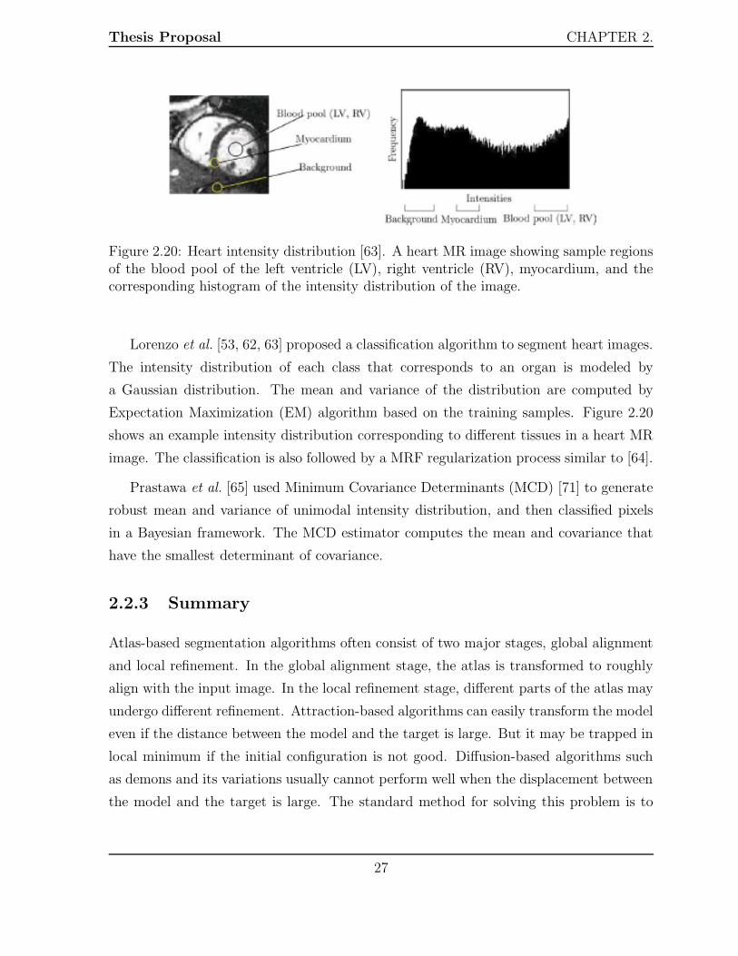
Figure 2.20: Heart intensity distribution [63]. A heart MR image showing sample regionsof the blood pool of the left ventricle (LV), right ventricle (RV), myocardium, and thecorresponding histogram of the intensity distribution of the image.
Lorenzo et al. [53, 62, 63] proposed a classification algorithm to segment heart images.
The intensity distribution of each class that corresponds to an organ is modeled by
a Gaussian distribution. The mean and variance of the distribution are computed by
Expectation Maximization (EM) algorithm based on the training samples. Figure 2.20
shows an example intensity distribution corresponding to different tissues in a heart MR
image. The classification is also followed by a MRF regularization process similar to [64].
Prastawa et al. [65] used Minimum Covariance Determinants (MCD) [71] to generate
robust mean and variance of unimodal intensity distribution, and then classified pixels
in a Bayesian framework. The MCD estimator computes the mean and covariance that
have the smallest determinant of covariance.
2.2.3 Summary
Atlas-based segmentation algorithms often consist of two major stages, global alignment
and local refinement. In the global alignment stage, the atlas is transformed to roughly
align with the input image. In the local refinement stage, different parts of the atlas may
undergo different refinement. Attraction-based algorithms can easily transform the model
even if the distance between the model and the target is large. But it may be trapped in
local minimum if the initial configuration is not good. Diffusion-based algorithms such
as demons and its variations usually cannot perform well when the displacement between
the model and the target is large. The standard method for solving this problem is to
27

Thesis Proposal CHAPTER 2.
(a) (b) (c) (d)
Figure 2.21: Region-based wrist x-ray image segmentation [72]. (a) Input image. (b)Result obtained by region growing. (c) Result obtained by region merging. (d) Finalresult.
apply the algorithm in an image pyramid.
Snake model is good in the sense that it is a connected contour and is quite flexible
for representing a region boundary. However, it is sensitive to noise in the image and
its initial configuration. Moreover, its parameters need to be set in a trial-and-error
manner. Level set has the ability to handle topology changes of contours, and efficient
numerical algorithms have been proposed. However, it is sensitive to image noise. Pixel
classification can utilize domain knowledge encapsulated in the probability distribution,
but it requires training. The features used are usually intensity and position of the pixel,
which are not so reliable in the x-ray images. Moreover, the boundaries of the target
organs produced by pixel classification are usually not precise.
Atlas-based segmentation methods use prior knowledge to guide the segmentation
process. It is ideal for segmenting complex medical images, which cannot be handled
robustly by general segmentation methods.
2.3 Segmentation of X-ray Images
In comparison to the segmentation of images in other modalities, less research has been
performed on the segmentation of ordinary x-ray images. Existing algorithms for the
segmentation of x-ray images often rely on some general medical image segmentation
methods.
28

Thesis Proposal CHAPTER 2.
Figure 2.22: Thresholding based on fuzzy index measure [73]. The white part is bone,the gray part is skin and the black part is background. The region of bones are disjoint.
2.3.1 Region-based
Manos et al. applied a region-based algorithm [72] to segment hand and wrist bones.
The algorithm starts with a region growing stage. Region growing will produce an over-
segmented image (Figure 2.21(b)). This is followed by a region merging stage, which
incorporates region similarity, size, connectivity and edge information (Figure 2.21(c)).
The final segmentation result (Figure 2.21(d)) is obtained by region labeling according
to some heuristic rules based on gray-level information.
2.3.2 Classification-based
El-Feghi et al. [73] applied a fuzzy set algorithm to segment lateral skull images. Three
crisp subsets, namely background, skin and bones are determined by minimizing a fuzzy
index function. The fuzzy index function decreases as the similarity between two pixels
increases. As no spatial information is considered, the segmented bone regions are disjoint
(Figure 2.22).
McNitt-Gray et al. [74] proposed to segment chest radiographs into anatomical regions
using neural networks. 59 features including the gray level information, local difference
measures and local texture measures are used as the input of the neural network. Spatial
information is also used to correct mis-classified pixels.
29

Thesis Proposal CHAPTER 2.
Figure 2.23: Initialization of tooth contour extraction [78].
Classification-based algorithms are generally not effective for x-ray image segmenta-
tion due to the intrinsic properties of x-ray images, i.e., images of different body parts
overlap.
2.3.3 Deformable Model
Most of the x-ray image segmentation work is based on deformable models, especially
active contour model. In order to locate the rib border in chest radiographs, Yue et
al. [75] first determined the thoracic cage boundary to restrict the search space. Hough
transform was then used to find approximate rib borders. The snake model was finally
applied to refine the rib borders.
Jiang et al. used geodesic active contour [76] to segment forearm bones [77]. Geodesic
active contour is based on the traditional snake model, and evolves over time according
to geometric measures (curvatures) of the image. The initial snake contour is manually
segmented from the x-ray image of the patient at the initial visit to the hospital.
Chen and Jain [78] applied snake model to extract the contours of teeth. To get the
initial configuration of the snake model, they detected the gap between upper and lower
teeth and the gap between neighboring teeth (Figure 2.23).
30

Thesis Proposal CHAPTER 2.
Figure 2.24: Segmentation result of femur [79].
Chen et al. proposed an incremental approach to segment femur bones [79] (Figure
2.24). Salient features in the x-ray images including parallel lines in the shaft area, circles
in the femoral heads are first detected. Then, a 2-D femur model is fitted onto the input
x-ray images to match the features. The final femur contours are refined by a snake
algorithm with curvature constraints. To achieve this, a spring force which describes
the difference between the actual curvature of the snake and the reference curvature of
the model is introduced. Chen’s work only considered femur bones in the x-ray image
without exploiting the spatial relationship between pelvis and femur bones.
Similar work (femur segmentation) has been done by Behiels et al. [80]. The proposed
algorithm is based on active shape model. The major contribution is that a regularization
term representing the smoothness of shape change in each iteration is incorporated.
In [81], Ballerini and Bocchi added an internal energy term to the snake framework to
model the spatial relationships between adjacent bones to segment the hand bones. This
energy term is represented by an elastic force that connects appropriate points of adjacent
snakes. The snake model is represented in polar coordinates. The polar representation
31

Thesis Proposal CHAPTER 2.
has the advantage that it introduces ordering of the contour points and prevents the snake
elements from crossing each other during evolution. However, it may run into problem
when representing a concave shape. In snake optimization stage, the snake configuration
is coded into chromosomes, and genetic algorithm (GA) is applied to minimize the energy
of the snake. This may alleviate the sensitivity to the initial contour placement, which is
chosen randomly.
A semi-automatic approach was proposed by Bernard et al. [82], which incorporated
an articulated model to segment the cervical spine. Articulated structures normally ex-
hibit two kinds of shape variations, i.e., variations in shapes of individual parts and
variations in spatial relationships between the parts. A hierarchical PCA was proposed
to deal with this problem. The hierarchical PCA consists of a topological PCA describing
topological variations of an articulated structure, i.e., the spatial organization of anatom-
ical structures, and a shape PCA describing the shape and pose variations of individual
structures.
2.3.4 Geometric Model
In [83], Vinhais and Campilho created a geometrical model of lungs (Figure 2.25) by
computing a mean shape from the training images. They applied a Laplacian of Gaus-
sian (LoG) filter with high standard deviation on the image to extract some anatomical
landmarks (Figure 2.26(a)) for an initial rough registration. They used genetic algorithm
(GA) to find the coefficients of the geometric model in the free-form deformation stage.
Each chromosome of GA contains an ordered list of the control points of a free-form
deformation grid [84]. Segmentation result is shown in Figure 2.26(c).
The major problem of this algorithm is that the anatomical landmarks may not be
reliably extracted because LoG filter is easily affected by noise. This will cause the free-
form deformation to fail. Moreover, GA usually takes a large amount of computation
time to produce a reasonable solution.
32

Thesis Proposal CHAPTER 2.
(a) (b) (c)
Figure 2.25: Geometrical model [83]. (a) Chest x-ray image. (b) Geometrical model. (c)Deformation of (b) using free-form deformation grid.
2.3.5 Atlas-based Method
Boukala et al. [85] applied atlas-based segmentation method to segment pelvis and femur
images. First, an atlas is built from a set of 24 manually landmarked training images.
The landmarks consist of 20 easily located anatomical features along the boundary of
the bones (Figure 2.27(a)). To increase the number of points, boundaries between these
landmarks are subdivided regularly. The femurs are rotated around the femoral head
center to make all the angles in different training images the same (Figure 2.27(b)). Next,
corresponding points between the training images are obtained. Active shape models are
constructed based on these corresponding points for the femurs and the pelvis separately.
In the global alignment stage, the pelvis and the femur are registered independently.
The average model shape is first registered to the input image. To do this, the shape
context descriptor [86] is used to find the correspondence between the points on the
model contour and those on the edges in the input image. For each point on both the
model contour and the edges in the image, the shape context computes the distribution
of neighboring points located in a log-polar coordinate system (Figure 2.28). This gives a
histogram-like descriptor for each point. For each model point, correspondence is found
by searching for the edge point with the most similar shape context descriptor. Due to
the presence of noise in the image, shape context method is not robust enough to find
the correct correspondence.
In the local refinement stage, active shape model is used to search for the boundaries
33

Thesis Proposal CHAPTER 2.
(a) (b) (c)
Figure 2.26: Geometric model-based lung segmentation [83]. (a) Extracted landmarks.(b) Displaced grid and corresponding deformed model. (c) Segmentation result.
of the bones. The boundaries of the femurs and the pelvis are extracted independently
using different active shape models (ASM). The shortcoming of ASM is that the extracted
boundaries may not be accurate because a large number of sample points is required to
represent a complex shape. As shown in Figure 3.2, the pelvis has a very complex shape.
Although articulations are used in constructing the atlas, they are not employed explicitly
in the segmentation process. The segmentation results of this algorithm are not clearly
presented in [85].
2.3.6 Summary
The computational complexities of region-based and classification-based segmentation
algorithms for x-ray images are low. However, region-based algorithms are easily affected
by noise. They are prone to over-segment the images. Classification-based algorithms are
not suitable for segmenting x-ray images because images of different tissues may overlap.
The other algorithms are more promising for x-ray image segmentation.
Among the existing methods for segmenting x-ray images, those presented in [79,
80, 83, 85] are most related to the proposed research topic. [79] and [80] focus on the
segmentation of a single femur bone. Chen et al. [79] use domain knowledge of the
femur, such as the width of the shaft and the radius of the femoral head, to aid in the
34

Thesis Proposal CHAPTER 2.
(a) (b)
Figure 2.27: Active shape model-based segmentation of hip images [85]. (a) 20 expert-labeled landmarks. (b) The femur is rotated around the femoral head center to adjustthe angle between the drawn lines.
segmentation. Behiels et al. [80] apply the snake algorithm to segment femur bones.
In [83], genetic algorithm (GA) is used to obtain an optimal deformation of the free-
form grid, but it has a high computational complexity. The anatomical landmarks used
to initialize GA are extracted by LoG filter. But, LoG filter is not immune to noise.
Therefore, the anatomical landmarks obtained using this method may not be reliable.
In [85], segmentation of pelvis and femurs is performed using atlas-based method.
Articulation is used in atlas construction to remove the difference in the orientations of
the femurs in different images. But, it is not used directly in the segmentation algorithm.
Shape context descriptors are used to search for correspondence between the points on
the atlas contour and the edge points in the input image. Shape descriptor is affected
by noise in the image, which incurs error in global alignment. Active shape models are
used in the local refinement stage to extract the boundaries of the femurs and the pelvis
separately. As discussed in the previous section, the boundaries extracted may not be
accurate.
In conclusion, the problem of segmentation of bone structures in x-ray images is not
well studied, and there is a lot of room for significant improvements.
35

Thesis Proposal CHAPTER 2.
���������
��������
���
(a)
(b)
Figure 2.28: Shape context. (a) Log-polar histogram of point distribution counts thenumber of points inside each bin. (b) Shape context descriptor (from http://www.eecs.
berkeley.edu/Research/Projects/CS/vision/shape/sc_digits.html).
36

Chapter 3
Proposed Research Topic
Segmentation of bones in x-ray images is an important step in medical diagnosis, surgery,
and treatment. The review in Chapter 2 shows that this problem has not been well
studied. Algorithms for segmentation of a single bone in x-ray images may not be robust
enough, and the quantitative segmentation results are seldom reported. This leads to the
proposed research topic: segmentation of bone structures in x-ray images.
3.1 Problem Analysis
In order to study the problem of bone segmentation in x-ray images, some characteristics
of this problem are analyzed.
• Unlike other medical imaging modalities, bone regions in x-ray images often overlap
with other organs, such as flesh, soft tissues and other bones (Figure 3.1). Pelvis
region in x-ray images can also be “corrupted” by gas inside the ascending and
descending colons or bowel (Figure 3.1).
• Bones are connected with other bones by joints. When the entire bone structure is
being segmented, articulation of the bones needs to be considered.
• Bones are 3-D in nature. A simple 2-D closed curve may not be accurate enough
to represent the boundaries of bones in x-ray images. For example, the pelvis bone
may need to be represented by its outer boundaries as well as inner contours (Figure
3.2).
37

Thesis Proposal CHAPTER 3.
(a) (b)
Figure 3.1: Characteristics of x-ray images. (a) Bone regions in x-ray images oftenoverlap with other organs, such as flesh, soft tissues and other bones. (b) Pelvis regionis corrupted by gas in the ascending and descending colons.
Segmentation of bone structures in x-ray images is both intrinsically and extrinsically
difficult. Intrinsic difficulties refer to those caused by the intrinsic properties of x-ray
imaging systems:
• Noise. Noise in x-ray images has a number of origins, but the most fundamental
is from the x-ray source itself. This type of noise is called “quantum noise”, in
reference to the discrete nature of the x-ray photons producing it (http://www.
lxi.leeds.ac.uk/learning/iq/noise/).
• Overlapping. As discussed in the characteristics of the problem.
Extrinsic difficulties are usually due to the patients:
• Ambiguity. Neighboring tissues inside human body may have similar x-ray absorp-
tion rates. As a result, the boundaries of the organs may be ambiguous. That is,
in the image, there is sometimes no clear edge between two neighboring organs.
• Bone density variability. Different patients may have different bone densities, which
result in significantly different intensities in the bone regions between their x-ray
images. A normal patient usually has dense bones and the x-ray image of bones
are bright, whereas a patient who suffers from osteoporosis has low-density bones,
38

Thesis Proposal CHAPTER 3.
(a) (b)
Figure 3.2: Representation of the pelvis bone. (a) 3-D pelvis bone (from http://www.
bartleby.com/107/illus241.html). (b) 2-D contour representation of the left pelvisbone.
which results in much darker bone images. Moreover, other body tissues may also
affect the intensities of bone images.
• Inter-patient shape variability. The shapes of the bones of different patients can
differ quite significantly. In particular, the shape of the pelvis bone of a female
patient is quite different from that of a male patient. This is due to the fact that
females usually have much wider pelvis bones (Figure 3.3).
• Imaging pose variability. The bones may be located in different parts of different
images due to different imaging pose (Figure 3.3).
3.2 Problem Formulation
The problem of automatic segmentation of bone structures in x-ray image can be formu-
lated as non-rigid registration of the atlas to the target x-ray image.
• The inputs of the problem:
Let M = {mi} represent the whole reference bone structure in the atlas, mi =
39

Thesis Proposal CHAPTER 3.
(a) (b)
Figure 3.3: Sample pelvis x-ray images. The shape of the pelvis of (a) a male patientdiffers from that of (b) a female patient mainly because the female has a wider pelvisthan the male.
{pij} represent the individual bones in the whole structure connected by joints, pij
represent the control points located on bone mi. 2-D joint angle between bone mu
and bone mv is represented by ωuv. S is the shape (e.g., curvature) information of
pij. C = {qj} denotes the set of edge points in the image, which include edge points
along the contour of the bones and other noise points, such as edge points along the
contours of other body tissues and noise edges, etc. Some points on the contour of
the bone structure may not be in C because they are not prominent edge points in
the image.
• The output of the problem:
M ′ = {m′
i} is the extracted contour of bone structure in the target image, which is
represented by a deformed version of M . m′
i = {p′ij} represents the control points
on the deformed contours.
We assume that the input x-ray images always contain the full frontal view of of the
pelvis. The imaging positions for different patients may be different, but the femur bones
are shown in the input images.
Let T denote similarity transformation, A denote articulation that can rotate mu with
respect to the joint connected to mv, D denote a deformation function that can move pi
40

Thesis Proposal CHAPTER 3.
to a new position, and f denote a correspondence function from M to C. The aim is to
find T , A, D and f such that the total error E is minimized:
E = (1 − α)∑
pi
||D(A(T (pi))) − f(pi)||2 + α
∑
pi
||S(D(A(T (pi)))) − S(pi)||2 (3.2.1)
where α ∈ [0, 1] is a parameter. The error E balances the registration error Ep and shape
difference Es to ensure that the deformation D does not severely distort the shape of the
bones:
Ep =∑
i
||D(A(T (pi))) − f(pi)||2 (3.2.2)
Es =∑
i
||S(D(A(T (pi)))) − S(pi)||2 (3.2.3)
3.3 Research Plan
The complex problem of segmenting bone structures in x-ray images can be decomposed
into several sub-problems as follows.
1. Feature Selection In this step, stable features should be selected to obtain correct
correspondence between the points in the atlas and the points in the target image.
This is an important first step that will affect the result of the following steps.
2. Global Alignment Based on the features found in the above step, global alignment
is to determine a rough alignment between the atlas and the image in terms of
scaling, rotation and translation. This step is performed with respect to the whole
bone structure. In addition, articulations between connected bones should be taken
into account.
3. Local Refinement Local refinement is to accurately register the atlas contours to
the boundaries of the bones. It needs to take into account the articulation and
shapes of the bones.
The research plan is to solve each of these sub-problems and then integrate the algorithms
into a complete solution.
41

Chapter 4
Preliminary Work
Two pieces of related preliminary work have been done, i.e., segmentation of soft tissues
in abdominal CT images [49] and global alignment of bone structures in pelvis x-ray
images. Although the former has different target organs and imaging modality, the main
ideas underneath are similar.
4.1 Segmentation of Soft Tissues in Abdominal CT
Images
Automatic segmentation of soft tissues in abdominal CT images is carried out by non-
rigid registration of 2-D atlas to target images. The atlas consists of a set of closed
contours of the human body, liver, stomach, and spleen, which are manually segmented
from a reference CT image given in [87]. As shown in Figure 4.1, the reference image
is significantly different from the target image in terms of shapes and intensities of the
body parts. Such differences are common in practical applications.
The segmentation algorithm consists of three stages: (1) Global alignment, (2) itera-
tive local deformation, and (3) local refinement.
4.1.1 Global Alignment
This stage performs registration of the atlas to the target input image with unknown
correspondence. First, the outer body contour of the target image (target contour) is
42

Thesis Proposal CHAPTER 4.
(a) (b)
Figure 4.1: (a) Atlas contours (white curves) superimposed on the reference CT imagetaken from [87]. (b) Atlas registered onto a target image after global transformation.
extracted by straightforward contour tracing. Next, the outer body contour of the atlas
(reference contour) is registered under affine transformation to the target contour using
Iterative Closest Point algorithm. After registration, the correspondence between the
reference and target contour points is known. Then, the affine transformation matrix
between the reference and target contours is easily computed from the known corre-
spondence by solving a system of over-constrained linear equations. This transformation
matrix is then applied to the entire atlas to map the contours of the inner body parts to
the target image.
4.1.2 Iterative Local Deformation
This stage iteratively applies local transformations to the individual body parts to bring
their reference contours closer to the target contours. The idea is to search the local
neighborhoods of reference contour points to find possible corresponding target contour
points. To achieve this goal, it is necessary to use features that are invariant to image
intensity because the reference and target images can have different intensities (as shown
in Figure 4.1).
43

Thesis Proposal CHAPTER 4.
Let N(p) denote the normal to the reference contour at point p, and L(p) denote
an ordered list of points {pi}, i = −n, . . . , 0, . . . , n, lying on N(p), with p0 = p. Let
I(pi) denote the intensity of point pi. Then, the ordered list D(p) = {I(pi) − I(pi+1)},
i = −n, . . . , n − 1, is the intensity difference distribution (IDD) at p along N(p). IDD
depends only on the local intensity difference, which does not differ as much as intensity
across images. Thus, IDD is better than intensity for determining corresponding points
between the images. In the same way, we can compute the IDD D′(p′) of an image point
p′ along a normal N(p) of the reference contour and with respect to the target image
intensities I ′(p′i). In the current implementation, n = 5, i.e., the length of IDD is 10.
The local search for possible corresponding points is performed as follows. After
coarse registration of the atlas and the reference image to the target image by global
alignment. For each reference contour point p, a search is performed within a small
neighborhood U(p) centered at p and along the normal N(p) for a target image point
p′ whose IDD D′(p′) is most similar to D(p). The difference between D(p) and D′(p′)
is measured in terms of the Euclidean distance between them. The neighborhood U(p)
decreases quadratically over time so that the search process will converge. In the current
implementation, the width of the search neighborhood is 100 at the first iteration.
After finding the best matching target image point p′ of a reference contour point p, a
verification procedure is performed. Shoot a ray from the centroid of the closed reference
contour of p to p′. If the number of “white” pixels or “black” pixels along the ray in the
target image exceeds a predefined threshold, then the point p′ is discarded because the
intensity of the desired body parts are gray. Otherwise, p′ is regarded as a corresponding
point of p.
Given the reference contour points pi whose corresponding points p′
i are found, com-
pute the affine transformation matrix that maps pi to p′i. Then, the matrix is applied to
all reference contour points, including those whose corresponding points are not found.
The above local deformation is repeated iteratively for each closed contour of the body
parts individually until the reference contours converge. Therefore, the reference contours
of different body parts can be mapped to the corresponding target image contours through
different affine transformation matrices that are appropriate for them.
44

Thesis Proposal CHAPTER 4.
(a) (b)
Figure 4.2: Iterative local transformation. (a) The white reference contours are iterativelytransformed. (b) The result of iterative local transformation after convergence.
4.1.3 Local Refinement
The last stage performs local refinement of the atlas contour using active contour, i.e.,
snake algorithm [88] with Gradient Vector Flow (GVF) [29]. The original snake algorithm
has the shortcoming of not being able to move into concave parts of the objects to be
segmented. This is because there is no image forces outside the concave parts to attract
the snake. GVF diffuses the gradient vectors of the edges outward, and uses the gradient
vectors as the image forces to attract the snake into concave parts. Sample results are
shown in Figure 4.3.
4.1.4 Experiments and Discussion
40 abdominal CT images (from slice 41 to 80) of 1mm thickness of a patient were used
in the test. The accuracy of the segmentation result was measured in terms of the
area of intersection between the target body part (that was obtained manually) and the
segmented regions. This performance measure, called similarity index S, was proposed
45

Thesis Proposal CHAPTER 4.
(a) (b)
Figure 4.3: Sample results after refinement. (a) Good result. (b) Result affected by theair pocket inside the stomach.
by Zijdenbos et al. [89]:
S = 2|A ∩ B|
|A| + |B|(4.1.1)
where A is the set of pixels of the body part in the target image and B that of the
segmented region. When the segmented region coincide exactly with the target body
part, S = 1.
Detailed segmentation performance of the algorithm is shown in Figure 4.4. The liver
is well segmented and the algorithm’s performance on liver is very stable (Figure 4.4(a)).
The similarity indices are greater than 0.95 for slices 41 to 76 (Figure 4.4a). From slice
77 onward, the liver is split into two lobes, which is greatly different from that in the
atlas image.
Figure 4.4(b) illustrates the average performance of the algorithm on segmenting the
liver, spleen, and stomach. The similarity index is above 0.9 for slices 43 to 76. That is,
with a single 2D atlas, the algorithm can successfully and accurately segment 34 slices of
the abdominal CT volume.
46

Thesis Proposal CHAPTER 4.
40 45 50 55 60 65 70 75 80 0.75
0.8
0.85
0.9
0.95
1
liver spleen stomach
slice number
similarity index
40 45 50 55 60 65 70 75 80 0.75
0.8
0.85
0.9
0.95
1 average similarity index
slice number
(a) (b)
Figure 4.4: Test results. (a) Similarity indices of liver, spleen, and stomach. (b) Averagesimilarity index.
4.2 Global Alignment of Bone Structures in Pelvis
X-ray Images
In this preliminary work, the objective is to globally align an atlas of bone structure to
pelvis x-ray images (Figure 4.5). The atlas image is randomly selected from a set of x-ray
pelvis images. The contours of the bone structure, which consists of a pelvis bone and
two femur bones, are manually delineated (white curves in Figure 4.5(a)).
The main idea of the algorithm is to locate the two femur bones first because they are
often much clearer than the pelvis bone in the image, thus more likely to be detected.
The pelvis bone is then translated, scaled and rotated according to the positions of the
two femoral heads. The details of the algorithm are described below.
4.2.1 Segmentation Algorithm
The algorithm begins with a histogram equalization operation on the target images.
Histogram equalization extends the gray levels of the image and boosts its contrast. This
pre-processing step partially eliminates the intensity variations between images.
Next, the algorithm extracts low-level features in the equalized image. The low-level
features used include edges, gradients and gradient directions because intensity alone is
47

Thesis Proposal CHAPTER 4.
(a) (b)
Figure 4.5: Pelvis x-ray images. (a) Atlas x-ray image. The model contours are shownin white. (b) Target image.
not reliable as discussed in Chapter 3. The edge information is obtained by a combination
of the Canny edge detector [7] and the Sobel edge operator. The Canny edge detector
can produce edges with single pixel width. These edges are then filtered by the edge map
produced by the Sobel edge operator so that weak edges are removed (Figure 4.6). From
the resulting edge map (Figure 4.6(d)), a list of edge segments ei are obtained by a simple
edge tracing algorithm.
A normal global alignment technique is to transform the atlas contours to fit the
edges in the target edge image. However, in this case, there exist many noise edges in
the edge image. Registration of atlas contours to the target edge image is bound to be
corrupted by the noise edges. The proposed algorithm performs the registration in the
other direction, i.e., register the edge segments in the edge image to the atlas contours.
This is based on the assumption that at least one edge segment in the edge map is very
close to the the ideal boundary of the target femur. The assumption is reasonable due
to the fact that the ideal boundaries of femurs, especially the shafts, are always clearly
visible in the input image. Thus, they can be detected by an edge detection algorithm.
Each edge segment ei is registered to a part of the atlas contour of the femur bone. The
registration is performed using Iterative Closest Point (ICP) algorithm (Figure 4.7(b)).
The distance function used in ICP incorporates both geometrical distance and gradient
48

Thesis Proposal CHAPTER 4.
(a) (b)
(c) (d)
Figure 4.6: Edge extraction. (a) Input image. (b) Edges obtained by Canny edge detec-tor. (c) Edges obtained by Sobel edge detector. (d) Edges in (b) filtered by (c) accordingto the edge strength.
direction information. The transformation used is rigid, which is to ensure that the
scale of ei remains fixed. After ICP, a rigid transformation Ti is obtained for each ei.
The atlas contour is then registered to the edge segment ei based on the inverse of
the transformation Ti, i.e., T−1
i (Figure 4.7(c), 4.8). After registration to all the edge
segments, a set of candidate transformations T−1
i is obtained. Among these candidates,
the optimal transformation To is selected based on minimizing a cost function describing
the closest distance between the transformed atlas contour and the edge points in the
Sobel edge map.
49
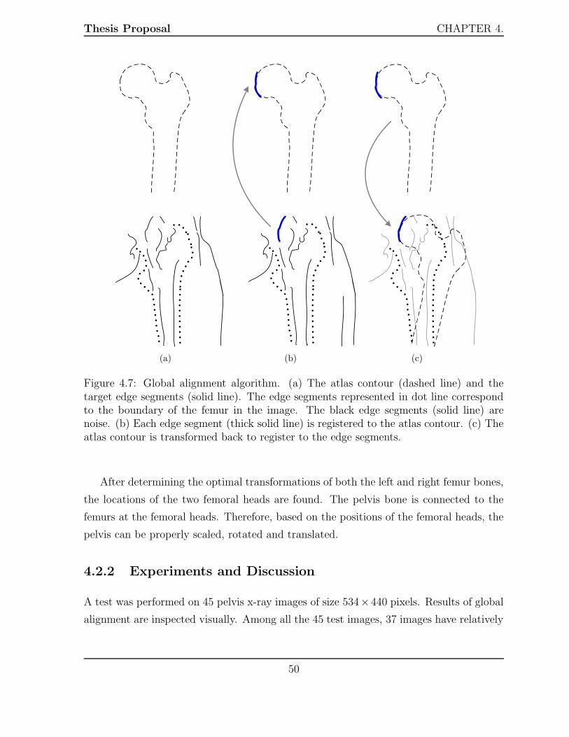
Thesis Proposal CHAPTER 4.
(a) (b) (c)
Figure 4.7: Global alignment algorithm. (a) The atlas contour (dashed line) and thetarget edge segments (solid line). The edge segments represented in dot line correspondto the boundary of the femur in the image. The black edge segments (solid line) arenoise. (b) Each edge segment (thick solid line) is registered to the atlas contour. (c) Theatlas contour is transformed back to register to the edge segments.
After determining the optimal transformations of both the left and right femur bones,
the locations of the two femoral heads are found. The pelvis bone is connected to the
femurs at the femoral heads. Therefore, based on the positions of the femoral heads, the
pelvis can be properly scaled, rotated and translated.
4.2.2 Experiments and Discussion
A test was performed on 45 pelvis x-ray images of size 534× 440 pixels. Results of global
alignment are inspected visually. Among all the 45 test images, 37 images have relatively
50

Thesis Proposal CHAPTER 4.
good results (Figure 4.9). The remaining 8 images have poorer results, in which the worst
cases are shown in Figure 4.10. The poorer results may be due to the noise edges in the
image that corrupt the computation of the optimal transformation To.
51

Thesis Proposal CHAPTER 4.
Figure 4.8: Registration of atlas contour to different edge segments in an input image.Atlas contours are marked in green. Edges in the image are marked in blue. Transformedatlas contours are marked in red.
52

Thesis Proposal CHAPTER 4.
Figure 4.9: Sample good results of global alignment. Registered atlas contours are shownin red.
53

Thesis Proposal CHAPTER 4.
Figure 4.10: Sample poorer results of global alignment. Registered atlas contours areshown in red.
54

Chapter 5
Conclusions
In this thesis proposal, a thorough review of the general medical image segmentation
algorithms, particularly atlas-based medical image segmentation algorithms and x-ray
image segmentation algorithms, is presented. General segmentation algorithms are cat-
egorized into six classes, namely thresholding, region-based, edge-based, graph-based,
classification-based and deformable models. Apart from deformable models, they usually
work on either individual pixels or local image patches, and are very sensitive to noise.
In comparison, deformable models perform segmentation by fitting a connected contour
to the features (usually edges) in the image. Therefore, they are less sensitive to noise.
Atlas-based segmentation algorithms consist of two major steps, namely global align-
ment and local refinement. Global alignment globally registers the atlas to the target
image to determine an approximation of the position, scale and orientation of the atlas.
Local refinement registers the atlas contours to the object boundaries in the target image
as accurately as possible. Since the atlas contains domain knowledge, it is more promising
for solving the complex problem of segmenting bone structures in x-ray images.
Currently, most x-ray image segmentation methods rely on general algorithms. Atlas-
based segmentation of x-ray images is proposed in [85]. However, their global alignment
algorithm using shape context as the feature is not robust against noise. The use of
active shape model for local refinement may not extract the bone boundaries accurately.
In addition, articulation is not considered explicitly in the segmentation process. In
conclusion, segmentation of bone structures in x-ray images is not well studied.
The research plan decomposes the complex segmentation problem into three parts:
55

Thesis Proposal CHAPTER 5.
feature selection, global alignment and local refinement. Two pieces of preliminary work
have been accomplished: segmentation of soft tissues in CT images and global alignment
of bone structures in x-ray images. According to the preliminary work, the feature se-
lection part is almost completed. The global alignment results show that the algorithm
is promising but needs to be improved so that it can perform reliably on all test images.
Moreover, articulation of bones needs to be incorporated into the global alignment pro-
cess. Local refinement remains to be done. The algorithm proposed for segmenting soft
tissues in CT images is promising, and can provide ideas for local refinement.
56

Bibliography
[1] D. L. Pham, C. Xu, and J. L. Prince, “A survey of current methods in medical
image segmentation,” Department of Electrical and Computer Engineering, The
Johns Hopkins University, Tech. Rep., 1998.
[2] J. Rogowska, “Overview and fundamentals of medical image segmentation,” in Hand-
book of Medical Imaging, Processing and Analysis, I. N. Bankman, Ed. Academic
Press, 2000, ch. 5, pp. 69–85.
[3] M. Sezgin and B. Sankur, “Survey over image thresholding techniques and quanti-
tative performance evaluation,” Journal of Electronic Imaging, vol. 13, no. 1, pp.
146–165, January 2004.
[4] R. C. Gonzalez and R. E. Woods, Digital Image Processing. Prentice Hall, 2001.
[5] A. Goshtasby and D. A. Turner, “Segmentation of cardiac cine MR images for extrac-
tion of right and left ventricular chambers,” IEEE Transactions on Medical Imaging,
vol. 14, no. 1, pp. 56–64, March 1995.
[6] M. Bomans, K.-H. Hohne, U. Tiede, and M. Riemer, “3-D segmentation of MR
images of the head for 3-D display,” IEEE Transactions on Medical Imaging, vol. 9,
no. 2, pp. 177–183, June 1990.
[7] J. Canny, “A computational approach to edge detection,” IEEE Transactions on
Pattern Analysis and Machine Intelligence, vol. 8, no. 6, pp. 679–698, November
1986.
[8] C. Harris and M. Stephens, “A combined corner and edge detector,” in Proceedings
of the 4th ALVEY Vision Conference, 1988, pp. 147–151.
57

Thesis Proposal BIBLIOGRAPHY
[9] L. O’Gorman and A. C. Sanderson, “The converging squares algorithm: An efficient
multidimensional peak picking method,” in International Conference on Acoustics,
Speech, and Signal Processing, vol. 8, April 1983, pp. 112–115.
[10] R. Adams and L. Bischof, “Seeded region growing,” IEEE Transaction on Pattern
Analysis and Machine Intelligence, vol. 16, no. 6, pp. 641–647, June 1994.
[11] X. Yu, J. Yla-Jaaski, O. Huttunen, T. Vehkomaki, O. Sipila, and T. Katila, “Image
segmentation combining region growing and edge detection,” in Pattern Recognition,
International Conference on, vol. III, April 1992, pp. 481–484.
[12] R. Pohle and K. Toennies, “Segmentation of medical images using adaptive region
growing,” in Proc. SPIE (Medical Imaging 2001), 2001.
[13] S. Beucher and C. Lantuejoul, “Use of watersheds in contour detection,” in Proc.
International Workshop on Image Processing, Real-Time Edge and Motion Detec-
tion/Estimation, September 1979.
[14] J. Serra, Image Analysis and Mathematical Morphology. Academic Press, 1982.
[15] J. B. Roerdink and A. Meijster, “The watershed transform: Definitions, algorithms
and parallelization strategies,” Fundamenta Informaticae, vol. 41, 2001.
[16] V. Grau, A. Mewes, M. Alcaniz, R. Kikinis, and S. Warfield, “Improved watershed
transform for medical image segmentation using prior information,” IEEE Transac-
tion on Medical Imaging, vol. 23, no. 4, pp. 447–458, 2004.
[17] L. Najman and M. Schmitt, “Geodesic saliency of watershed contours and hierarchi-
cal segmentation,” Pattern Analysis and Machine Intelligence, IEEE Transactions
on, vol. 18, Dec 1996.
[18] S. Wegner, T. Harms, H. Oswald, and E. Fleck, “The watershed transformation on
graphs for the segmentation of CT images,” in Proceedings of the 13th International
Conference on Pattern Recognition, August 1996, pp. 498–502.
[19] Z. Wu and R. Leahy, “An optimal graph theoretic approach to data clustering:
Thoery and its application to image segmentation,” IEEE Transactions on Pattern
Analysis and Machine Intelligence, vol. 15, no. 11, pp. 1101–1113, November 1993.
58

Thesis Proposal BIBLIOGRAPHY
[20] J. Shi and J. Malik, “Normalized cuts and image segmentation,” IEEE Transactions
on Pattern Analysis and Machine Intelligence, vol. 22, no. 8, pp. 888–905, August
2000.
[21] S. Wang and J. M. Siskind, “Image segmentation with ratio cut,” IEEE Transcations
on Pattern Analysis and Machine Intelligence, vol. 25, no. 6, pp. 675–690, June 2003.
[22] Y. Boykov and M.-P. Jolly, “Interactive graph cuts for optimal boundary & region
segmentation of ojbects in N-D images,” in Proceedings of International Conference
on Computer Vision, 2001, pp. 105–112.
[23] X. Ren and J. Malik, “Learning a classification model for segmentation,” in Inter-
national Conference on Computer Visioin, Nice, France, October 2003.
[24] M. S. Brown, M. F. Mcnitt-Gray, J. G. G. Nicholas J. Mankovich, J. Hiller, L. S.
Wilson, and D. R. Aberle, “Method for segmenting chest CT image data using an
anatomical model: Preliminary results,” IEEE Transactions on Medical Imaging,
vol. 16, no. 6, pp. 828–839, 1997.
[25] J. Feng, W.-C. Lin, and C.-T. Chen, “Epicardial boundary detection using fuzzy
reasoning,” Medical Imaging, IEEE Transactions on, vol. 10, no. 2, pp. 187–199,
June 1991.
[26] D. L. Toulson and J. F. Boyce, “Segmentation of MR image using neural nets,” in
Image and Vision Computing, vol. 10, 1992, pp. 324–328.
[27] M. Kass, A. Witkin, and D. Terzopoulos, “Snakes: Active contour models,” Int’l J.
Computer Vision, pp. 321–331, 1987.
[28] M. S. Atkins and B. T. Mackiewich, “Fully automated hybird segmentation of the
brain,” in Handbook of Medical Imaging, Processing and Analysis, I. N. Bankman,
Ed. Academic Press, 2000, ch. 11, pp. 171–183.
[29] C. Xu and J. L. Prince, “Snakes, shapes, and gradient vector flow,” IEEE Transac-
tion on Image Processing, vol. 7, no. 3, March 1998.
59

Thesis Proposal BIBLIOGRAPHY
[30] J. A. Sethian, Level Set Methods and Fast Marching Methods. Evolving Interfaces
in Computational Geometry, Fluid Mechanics, Computer Vision, and Materials Sci-
ence. Cambridge University Press, 1999.
[31] ——, “Tracking interfaces with level sets,” American Scientist, May–June 1997.
[32] R. Malladi, J. A. Sethian, and B. C. Vemuri, “Shape modeling with front propaga-
tion: A level set approach,” IEEE Transactions on Pattern Analysis and Machine
Intelligence, vol. 17, no. 2, pp. 158–175, February 1995.
[33] M. Droske, B. Meyer, M. Rumpf, and K. Schaller, “An adaptive level set method
for medical image segmentation,” in Proc. of the Annual Symposium on Information
Processing in Medical Imaging, 2001.
[34] J. Yang, L. H. Staib, and J. S. Duncan, “Neighbor-constrained segmentation with
level set based 3-d deformable models,” IEEE Transactions on Medical Imaging,
2004.
[35] T. F. Cootes, A. Hill, C. J. Taylor, and J.Haslam, “The use of active shape models
for locating structures in medical images,” Image and Vision Computing, vol. 12,
no. 6, pp. 355–366, July 1994.
[36] T. F. Cootes, G. J. Edwards, and C. J. Taylor, “Active appearance models,” in Proc.
European Conference on Computer Vision, vol. 2, 1998, pp. 484–498.
[37] A. Hill, C. J. Taylor, and T. Cootes, “Object recognition by flexible template match-
ing using genetic algorithms,” in European Conference on Computer Vision, May
1992, pp. 852–856.
[38] T. F. Cootes and C. J. Taylor, “Statistical models of appearance for computer vi-
sion,” Imaging Science and Biomedical Engineering, Manchester M13 9PT, U.K.,
Tech. Rep., March 2004.
[39] Y. Wang and L. H. Staib, “Boundary finding with correspondence using statistical
shape models,” in Computer Vision and Pattern Recognition, June 1998, pp. 338–
345.
60

Thesis Proposal BIBLIOGRAPHY
[40] S. S. Gleason, H. Sari-Sarraf, M. A. Abidi, O. Karakashian, and F. Morandi, “A new
deformable model for analysis of X-Ray CT images in preclinical studies of mice for
polycystic kidney disease,” IEEE Transactions on Medical Imaging, vol. 21, no. 10,
pp. 1302–1309, October 2002.
[41] G. B. Aboutanos, J. Nikanne, N. Watkins, and B. M. Dawant, “Model creation
and deformation for the automatic segmentation of the brain in MR images,” IEEE
Transaction on Biomedical Engineering, vol. 46, no. 11, pp. 1346–1356, 1999.
[42] P.-Y. Bondiau, G. Malandain, S. Chanalet, P.-Y. Marcy, J.-L. Habrand, F. Fau-
chon, P. Paquis, A. Courdi, O. Commowick, I. Rutten, and N. Ayache, “Atlas-based
automatic segmentation of mr images: Validation study on the brainstem in ra-
diotherapy context,” International Journal of Radiation Oncology Biology Physics,
vol. 61, no. 1, pp. 289–298, January 2005.
[43] P. Cachier and X. Pennec, “3D non-rigid registration by gradient descent on a
gaussian-windowed similarity measure using convolutions,” in Mathematical Methods
in Biomedical Image Analysis, June 2000, pp. 182–189.
[44] M. Chen, T. Kanade, H. A. Rowley, and D. Pomerleau, “Quantitative study of brain
anatomy,” in Mathematical Methods in Biomedical Image Analysis, June 1998, pp.
84–92.
[45] F. S. Cohen and C. Pintavirooj, “Invariant surface alignment in the presence of
affine and some nonlinear transformations,” Medical Image Analysis, vol. 8, no. 2,
pp. 151–164, June 2004.
[46] M. B. Cuadra, O. Cuisenaire, R. Meuli, and J. P. Thiran, “Automatic segmentation
of internal structures of the brain in mr images using a tandem of affine and non-
rigid registration of an anatomical brain atlas,” in Image Processing, Oct. 2001, pp.
1083–1086.
[47] M. B. Cuadra, C. Pollo, A. Bardera, O. Cuisenaire, J.-G. Villemure, and J.-P. Thiran,
“Atlas-based segmentation of pathological MR brain images using a model of lesion
growth,” IEEE Transaction on Medical Imaging, vol. 23, no. 10, pp. 1301–1314,
2004.
61

Thesis Proposal BIBLIOGRAPHY
[48] B. M. Dawant, S. L. Hartmann, J. P. Thirion, F. Maes, D. Vandermeulen, and
P. Demaerel, “Automatic 3-D segmentation of internal structures of head in MR
images using a combination of similarity and free-form transformations: Part I,
methodology and validation on normal subjects,” IEEE Trans. on Medical Imaging,
vol. 18, no. 10, pp. 909–916, 1999.
[49] F. Ding, W. K. Leow, and S.-C. Wang, “Segmentation of 3D CT volume images
using a single 2D atlas,” in Proc. First International Workshop on Computer Vision
for Biomedical Image Applications (CVBIA 2005), 2005, pp. 459–468.
[50] V. Duay, N. Houhou, and J.-P. Thiran, “Atlas-based segmentation of medical images
locally constrained by level sets,” Signal Processing Institute (ITS), Ecole Polytech-
nique Federale de Lausanne (EPFL), Tech. Rep., 2005.
[51] K. A. Ganser, H. Dickhaus, R. Metzner, and C. R. Wirtz, “A deformable digital
brain atlas system according to talairach and tournoux,” Medical Image Analysis,
vol. 8, no. 1, pp. 3–22, March 2004.
[52] S. L. Hartmann, M. H. Parks, P. R. Martin, and B. M. Dawant, “Automatic 3-D
segmentation of internal structures of head in MR images using a combination of
similarity and free-form transformations: Part II, validation on severely atrophied
brains,” IEEE Trans. on Medical Imaging, vol. 18, no. 10, pp. 917–926, 1999.
[53] M. Lorenzo-Valdes, G. I. Sanchez-Ortiz, R. Mohiaddin, and D. Rueckert, “Atlas-
based segmentation and tracking of 3D cardiac MR images using non-rigid regis-
tration,” in International Conference on Medical Image Computing and Computer-
Assisted Intervention, 2002, pp. 642–650.
[54] M. G. Linguraru, M. Angel Gonzalez Ballester, and N. Ayache, “Deformable atlases
for the segmentation of internal brain nuclei in magnetic resonance imaging,” Acta
Universitatis Cibiniensis, Technical Series, 2005, to appear.
[55] D. Rueckert, G. I. Sanchez-Ortiz, M. Lorenzo-Valdes, R. Chandrashekara, and
R. Mohiaddin, “Non-rigid registration of cardiac MR: Application to motion mod-
elling and atlas-based segmentation,” in IEEE International Symposium on Biomed-
ical Imaging, 2002.
62

Thesis Proposal BIBLIOGRAPHY
[56] S. Sandor and R. Leahy, “Surface-based labeling of cortical anatomy using a de-
formable atlas,” IEEE Transactions on Medical Imaging, vol. 16, no. 1, pp. 41–54,
February 1997.
[57] D. Shen and C. Davatzikos, “An adaptive-focus deformable model using statistical
and geometric information,” IEEE Transactions on Pattern Analysis and Machine
Intelligence, vol. 22, no. 8, pp. 906–913, August 2000.
[58] D. Shen, E. H. Herskovits, and C. Davatzikos, “An adaptive-focus statistical shape
model for segmentation and shape modeling of 3-D brain structures,” IEEE Trans-
actions on Medical Imaging, vol. 20, no. 4, pp. 257–270, April 2001.
[59] D. Shen, Z. Lao, J. Zeng, W. Zhang, I. A. Sesterhenn, L. Sun, J. W. Moul, E. H.
Herskovits, G. Fichtinger, and C. Davatzikos, “Optimized prostate biopsy via a
statistical atlas of cancer spatial distribution,” Medical Image Analysis, vol. 8, no. 2,
pp. 139–150, June 2004.
[60] B. C. Vemuri, Y. C. J. Ye, and C. M. Leonard, “Image registration via level-set
motion: Applications to atlas-based segmentation,” Medical Image Analysis, vol. 7,
no. 1, pp. 1–20, March 2003.
[61] Y. Chen, F. Huang, H. D. Tagare, M. Rao, D. Wilson, and E. A. Geiser, “Using
prior shape and intensity profile in medical image segmentation,” in Proceedings of
Ninth IEEE International Conference on Computer Vision, 2003.
[62] M. Lorenzo-Valdes, D. Rueckert, R. Mohiaddin, and G. I. Sanchez-Ortiz, “Segmen-
tation of cardiac MR images using the em algorithm with 4D probabilistic atlas and
a global connectivity filter,” in International Conference of the IEEE Engineering
in Medicine and Biology Society, 2003.
[63] M. Lorenzo-Valdes, G. I. Sanchez-Ortiz, A. G. Elkington, R. H. Mohiaddin, and
D. Rueckert, “Segmentation of 4D cardiac MR images using a probabilistic atlas
and the EM algorithm,” Medical Image Analysis, vol. 8, pp. 255–265, 2004.
[64] H. Park, P. H. Bland, and C. R. Meyer, “Construction of an abdominal probabilistic
atlas and its application in segmentation,” IEEE Trans. on Medical Imaging, vol. 22,
no. 4, pp. 483–492, 2003.
63

Thesis Proposal BIBLIOGRAPHY
[65] M. Prastawa, J. H. Gilmore, W. Lin, and G. Gerig, “Automatic segmentation of MR
images of the developing newborn brain,” Medical Image Analysis, 2005.
[66] I. Sluimer, M. Prokop, and B. van Ginneken, “toward automated segmentation of
the pathological lung in CT,” IEEE Transactions on Medical Imaging, vol. 24, no. 8,
pp. 1025–1038, August 2005.
[67] M. Straka, A. L. Cruz, A. Kochl, M. Sramek, M. E. Groller, and
D. Fleischmann, “3d watershed transform combined with a probabilistic
atlas for medical image segmentation,” in MIT 2003, 2003, pp. http:
//www.cg.tuwien.ac.at/research/publications/2003/Straka-2003-3DW/
[68] S. L. Hartmann, M. H. Parks, H. Schlack, W. Riddle, R. R. Price, P. R. Martin,
and B. M. Dawant, “Automatic computation of brain and cerebellum volumes in
normal subjects and chronic alcoholics,” in IPMI, A. Kuba, M. Samal, and A. Todd-
Pokropek, Eds., vol. 1613. Springer, 1999, pp. 430–435.
[69] J. P. Thirion, “Image matching as a diffusion process: An analogy with maxwell’s
demons,” Medical Image Analysis, vol. 2, no. 3, pp. 243–260, 1998.
[70] P. Cachier, E. Bardinet, D. Dormont, X. Pennec, and N. Ayache, “Iconic feature
based nonrigid registration: The PASHA algorithm,” CVIU — Special Issue on
Nonrigid Registration, vol. 89, no. 2-3, pp. 272–298, Feb.-march 2003.
[71] P. J. Rousseeuw and K. V. Driessen, “A fast algorithm for the minimum covariance
determinant estimator,” Technometrics, vol. 41, no. 3, pp. 212–223, August 1999.
[72] G. K. Manos, A. Y. Cairns, I. W. Rickets, and D. Sinclair, “Segmenting radiographs
of the hand and wrist,” Computer Methods and Programs in Biomedicine, vol. 43,
no. 3-4, pp. 227–237, June 1993.
[73] S. S.-A. El-Feghi, I.and Huang, M.A., and M. Ahmadi, “X-ray image segmentation
using auto adaptive fuzzy index measure,” in MWSCAS ’04. The 2004 47th Midwest
Symposium on Circuits and Systems, vol. 3, 2004, pp. 499–502.
[74] M. F. McNitt-Gray, H. K. Huang, and J. W. Sayre, “Feature selection in the pattern
classification problem of digital chest radiograph segmentation,” IEEE Transactions
on Medical Imaging, vol. 14, no. 3, pp. 537–547, September 1995.
64

Thesis Proposal BIBLIOGRAPHY
[75] Z. Yue, A. Goshtasby, and L. V. Ackerman, “Automatic detection of rib borders
in chest radiographs,” IEEE Transactions on Medical Imaging, vol. 14, no. 3, pp.
525–536, September 1995.
[76] V. Caselles, R. Kimmel, and G. Sapiro, “Geodesic active contours,” in ICCV, 1995,
pp. 694–699.
[77] Y. Jiang and P. Babyn, “X-ray bone fracture segmentation by incorporating global
shape model priors into geodesic active contours,” in Proceedings of the 18th Inter-
national Congress and Exhibition, vol. 1268, June 2004, pp. 219–224.
[78] H. Chen and A. K. Jain, “Tooth contour extraction for matching dental radiographs,”
in Proc. International Conference on Pattern Recognition, 2004, pp. 522–525.
[79] Y. Chen, X. Ee, W. K. Leow, and T. S. Howe, “Automatic extraction of femur
contours from hip x-ray images,” in Proc. First International Workshop on Computer
Vision for Biomedical Image Applications (CVBIA 2005, 2005, pp. 200–209.
[80] G. Behiels, D. Vandermeulen, F. Maes, P. Suetens, and P. Dewaele, “Active shape
model-based segmentation of digital x-ray images,” in Proceedings of the Second
International Conference on Medical Image Computing and Computer-Assisted In-
tervention, 1999, pp. 128–137.
[81] L. Ballerini and L. Bocchi, “Bone segmentation using multiple communicating
snakes,” in SPIE International Symposium Medical Imaging, 2003.
[82] R. Bernard, B. Likar, and F. Pernus, “Segmenting articulated structures by hier-
archical statistical modeling of shape, appearance and topology,” in Medical Image
Computing and Computer Assisted Intervention - 4th MICCAI, 2001, pp. 499–506.
[83] C. Vinhais and A. Campilho, “Genetic model-based segmentation of chest x-ray
images using free form deformations,” in Image Analysis and Recognition: Second
International Conference, ICIAR 2005, 2005.
[84] T. W. Sederberg and S. R. Parry, “Free-form deformation of solid geometric models,”
in ACM SIGGRAPH Computer Graphics, vol. 20, 1986, pp. 151–160.
65

Thesis Proposal BIBLIOGRAPHY
[85] N. Boukala, E. Favier, B. Laget, and P. Radeva, “Active shape model based segmen-
tation of bone structures in hip radiographs,” in Proceedings of IEEE International
Conference on Industrial Technology, 2004, pp. 1682–1687.
[86] S. Belongie, J. Malik, and J. Puzicha, “Shape context: A new descriptor for shape
matching and object recognition,” in NIPS, 2000, pp. 831–837.
[87] P. Fleckenstein and J. T. Jensen, Anatomy in Diagnostic Imaging. Munksgaard,
1993.
[88] M. Kass, A. Witkin, and D. Terzopoulos, “Snakes: active contour models,” Int. J.
of Computer Vision, vol. 1, no. 4, pp. 321–331, 1987.
[89] A. P. Zijdenbos, B. M. Dawant, R. A. Margolin, and A. C. Palmer, “Morphometric
analysis of white matter lesions in MR images: Method and validation,” IEEE Trans.
on Medical Imaging, vol. 13, no. 4, pp. 716–724, 1994.
66