segmentation of color images for interactive 3d object...
TRANSCRIPT

Segmentation of color images
for interactive 3D object retrieval
Von der Fakultat fur Elektrotechnik und Informationstechnik
der Rheinisch-Westfalischen Technischen Hochschule Aachen
zur Erlangung des akademischen Grades eines
Doktors der Ingenieurwissenschaften genehmigte Dissertation
vorgelegt von
Diplom-Ingenieur
Jose Pablo Alvarado Moya
aus San Jose, Costa Rica
Berichter: Universitatsprofessor Dr.-Ing. Karl-Friedrich Kraiss
Universitatsprofessor Dr.-Ing. Dietrich Meyer-Ebrecht
Tag der mundlichen Prufung: 02. Juli 2004
Diese Dissertation ist auf den Internetseiten der Hochschulbibliothek online verfugbar


a mis queridos padres
(to my parents)


Acknowledgments
I extend the most sincere appreciation to all people and organizations who made this
thesis possible. My deepest gratitude goes to my advisor Prof. Dr.-Ing. K.-F. Kraiss,
who offered me the invaluable opportunity of working as a research assistant at his Chair
and gave me the freedom to explore the fascinating world of image analysis. His support
and guidance have been fundamentally important for the successful completion of this
dissertation. I am also indebted to my second examiner Prof. Dr.-Ing. D. Meyer-Ebrecht
for his interest in my work.
To the Heinz-Nixdorf Foundation for supporting the projects Axon2 and Axiom, in which
scope the current research work took place, and to Steiff GmbH for providing such nice
object sets.
To the DAAD for providing the financial support for the first stage of my studies in
Germany: they made it possible to obtain my Dipl.-Ing., which undeniably lead me into
the next stage as a research assistant. To the ITCR for ensuring me a job after all these
years in Germany.
I want to thank my colleagues Dr. Peter Walter and Dr. Ingo Elsen who helped me
with my first steps in the world of computer vision, and especially to my project col-
leagues Jochen Wickel, Dr. Thomas Kruger and Peter Dorfler for providing such a rich
and fruitful environment for developing new ideas. To all my colleagues at the Chair
of Technical Computer Science for the healthy, symbiotic collaboration creating and
maintaining the LTI-Lib, which is becoming a great contribution to the research world
in image understanding.
To my student researchers Stefan Syberichs, Thomas Rusert, Bastian Ibach, Markus
Radermacher, Jens Rietzschel, Guy Wafo Moudhe, Xinghan Yu, Helmuth Euler for
their collaborative work in the image processing part of our projects, and specially to
Axel Berner, Christian Harte, and Frederik Lange for their excellent work and valuable
support.
Many a thanks are due to all my proofreaders Suat Akyol, Rodrigo Batista, Manuel
Castillo, Michael Hahnel, Lars Libuda, who reviewed some of the chapters, but especially
to Peter Dorfler, who patiently reviewed the whole thesis. I also want to thank Lars,
Michael and Peter for the “proof-listening” in the preparation of the public presentation.

I am especially indebted to my dear friends Suat, Rodrigo, Jana, Manuel and Martha,
and to my family in Costa Rica for their huge support during the hard times while
preparing this thesis.
This work is dedicated to my mother and to the memory of my father. They always
encouraged me to give my best and infused me with boundless curiosity and persistence.
Thank you for your absolute confidence in me and for your understanding and support
for my pursuits.
Jose Pablo Alvarado Moya
Aachen, 02.07.2004

Contents
List of Figures v
List of Tables ix
Glossary xi
List of symbols and abbreviations xiii
1 Introduction 1
1.1 Motivation and Problem Statement . . . . . . . . . . . . . . . . . . . . . 4
1.2 Analysis Approach . . . . . . . . . . . . . . . . . . . . . . . . . . . . . . 5
1.2.1 Marr’s Metatheory . . . . . . . . . . . . . . . . . . . . . . . . . . 6
1.2.2 Computational Level of Vision Systems . . . . . . . . . . . . . . . 7
1.3 Goal and Structure of this Work . . . . . . . . . . . . . . . . . . . . . . . 8
2 Visual Object Retrieval 11
2.1 Task of Object Retrieval Systems . . . . . . . . . . . . . . . . . . . . . . 12
2.2 Taxonomy of Object Retrieval Systems . . . . . . . . . . . . . . . . . . . 13
2.2.1 Architecture of Object Retrieval Systems . . . . . . . . . . . . . . 14
2.2.2 Object Set . . . . . . . . . . . . . . . . . . . . . . . . . . . . . . . 16
2.2.3 Nature of Images . . . . . . . . . . . . . . . . . . . . . . . . . . . 18
2.2.4 Scene Composition . . . . . . . . . . . . . . . . . . . . . . . . . . 20
2.2.5 Knowledge Type . . . . . . . . . . . . . . . . . . . . . . . . . . . 22
2.3 Assessment of Object Retrieval Systems . . . . . . . . . . . . . . . . . . 24
2.4 Experimental Set-up . . . . . . . . . . . . . . . . . . . . . . . . . . . . . 25
i

Contents
3 Foundations of Image Segmentation 29
3.1 Definition of Segmentation . . . . . . . . . . . . . . . . . . . . . . . . . . 29
3.2 Image-based Segmentation . . . . . . . . . . . . . . . . . . . . . . . . . . 34
3.2.1 Feature-space Approaches . . . . . . . . . . . . . . . . . . . . . . 36
3.2.2 Image-domain-based Approaches . . . . . . . . . . . . . . . . . . 38
3.2.3 Hybrid Methods . . . . . . . . . . . . . . . . . . . . . . . . . . . . 41
3.2.4 Discussion . . . . . . . . . . . . . . . . . . . . . . . . . . . . . . . 43
3.3 Surface-based Segmentation . . . . . . . . . . . . . . . . . . . . . . . . . 44
3.4 Object-based Segmentation . . . . . . . . . . . . . . . . . . . . . . . . . 47
3.5 Segmentation in Current Object Recognition Systems . . . . . . . . . . . 49
3.6 Framework for Segmentation in Object Retrieval Applications . . . . . . 52
3.7 Evaluation of Segmentation Algorithms . . . . . . . . . . . . . . . . . . . 53
3.7.1 Evaluation Using the Pareto Front . . . . . . . . . . . . . . . . . 55
3.7.2 Fitness Functions . . . . . . . . . . . . . . . . . . . . . . . . . . . 57
4 Image-based Segmentation 61
4.1 Mean-Shift Segmentation . . . . . . . . . . . . . . . . . . . . . . . . . . . 62
4.2 Watershed-based Segmentation . . . . . . . . . . . . . . . . . . . . . . . 65
4.2.1 Color Edgeness . . . . . . . . . . . . . . . . . . . . . . . . . . . . 66
4.2.2 Reducing Over-Segmentation . . . . . . . . . . . . . . . . . . . . 68
4.3 k-Means-based Segmentation . . . . . . . . . . . . . . . . . . . . . . . . . 74
4.4 Adaptive Clustering Algorithm . . . . . . . . . . . . . . . . . . . . . . . 76
4.5 Discussion . . . . . . . . . . . . . . . . . . . . . . . . . . . . . . . . . . . 78
5 Surface-Based Segmentation 87
5.1 Physical Assumptions . . . . . . . . . . . . . . . . . . . . . . . . . . . . . 87
5.2 Perceptual Organization . . . . . . . . . . . . . . . . . . . . . . . . . . . 88
5.3 Application Dependent Cues . . . . . . . . . . . . . . . . . . . . . . . . . 90
5.3.1 Encoding Color Information . . . . . . . . . . . . . . . . . . . . . 91
5.3.2 Encoding Positional Information . . . . . . . . . . . . . . . . . . . 92
5.3.3 Combining Cues with Bayesian Belief Networks . . . . . . . . . . 93
ii

Contents
5.3.4 Example: Detection of an Homogeneous Background . . . . . . . 95
5.4 Example: Separation of Hand Surfaces and Skin-Colored Objects . . . . 100
5.4.1 Selection of the Skin-Color Model . . . . . . . . . . . . . . . . . . 101
5.4.2 Color Zooming . . . . . . . . . . . . . . . . . . . . . . . . . . . . 101
5.4.3 Probabilities for Color Labels . . . . . . . . . . . . . . . . . . . . 103
5.4.4 Positional Information . . . . . . . . . . . . . . . . . . . . . . . . 104
5.4.5 Combining All Information Cues . . . . . . . . . . . . . . . . . . 105
5.4.6 Seed Selection and Growing Stages . . . . . . . . . . . . . . . . . 106
6 Object-Based Segmentation 109
6.1 Recognition Based on Global Descriptors . . . . . . . . . . . . . . . . . . 110
6.1.1 Global Descriptors . . . . . . . . . . . . . . . . . . . . . . . . . . 110
6.1.2 Classification . . . . . . . . . . . . . . . . . . . . . . . . . . . . . 115
6.1.3 Recognition Experiments with Global Descriptors . . . . . . . . . 117
6.2 Recognition Based on Local Descriptors . . . . . . . . . . . . . . . . . . 119
6.2.1 Location Detection . . . . . . . . . . . . . . . . . . . . . . . . . . 120
6.2.2 Descriptor Extraction . . . . . . . . . . . . . . . . . . . . . . . . . 125
6.2.3 Classification of Local Descriptors . . . . . . . . . . . . . . . . . . 127
6.2.4 Assignment of Object Labels to Regions . . . . . . . . . . . . . . 131
6.3 Object-based Segmentation Module . . . . . . . . . . . . . . . . . . . . . 132
6.4 Recognition Experiments with Multiple Objects . . . . . . . . . . . . . . 135
7 Conclusion and Outlook 139
7.1 Summary of the Work . . . . . . . . . . . . . . . . . . . . . . . . . . . . 139
7.2 Outlook . . . . . . . . . . . . . . . . . . . . . . . . . . . . . . . . . . . . 143
Bibliography 145
A Pareto Envelope-based Selection Algorithm 161
B Optimal region pair selection 165
C Fast Relabeling 169
iii

Contents
D Images for Evaluation of Image-Based Segmentation 173
E Test-set P17 175
F Test-sets S25 and S200 177
G Computation of the Hessian Matrix 179
Index 185
iv

List of Figures
1.1 Scene of objects as raw-data. . . . . . . . . . . . . . . . . . . . . . . . . . 2
1.2 Original scene for Figure 1.1. . . . . . . . . . . . . . . . . . . . . . . . . . 3
1.3 Interactive object retrieval concept. . . . . . . . . . . . . . . . . . . . . . 4
1.4 Four stages of visual processing according to Marr and Palmer. . . . . . . 7
1.5 Three stages of visual processing usually found in artificial systems. . . . 7
1.6 Dalmatian. . . . . . . . . . . . . . . . . . . . . . . . . . . . . . . . . . . 8
2.1 Image formation. . . . . . . . . . . . . . . . . . . . . . . . . . . . . . . . 11
2.2 Levels of abstraction. . . . . . . . . . . . . . . . . . . . . . . . . . . . . . 13
2.3 Task of an object retrieval system. . . . . . . . . . . . . . . . . . . . . . 13
2.4 Aspects to consider in the taxonomy of object retrieval systems. . . . . . 14
2.5 General structure of an object retrieval system. . . . . . . . . . . . . . . 14
2.6 Architectures for object retrieval systems. . . . . . . . . . . . . . . . . . 16
2.7 Examples for the composition of objects. . . . . . . . . . . . . . . . . . . 17
2.8 Shape properties for objects and their parts. . . . . . . . . . . . . . . . . 18
2.9 Five criteria to describe the objects in a set. . . . . . . . . . . . . . . . . 18
2.10 Two possibilities for object acquisition. . . . . . . . . . . . . . . . . . . . 19
2.11 Multiple views in object retrieval. . . . . . . . . . . . . . . . . . . . . . . 20
2.12 Nature of images. . . . . . . . . . . . . . . . . . . . . . . . . . . . . . . . 20
2.13 Background homogeneity. . . . . . . . . . . . . . . . . . . . . . . . . . . 21
2.14 Scene transformations. . . . . . . . . . . . . . . . . . . . . . . . . . . . . 21
2.15 Knowledge Type. . . . . . . . . . . . . . . . . . . . . . . . . . . . . . . . 24
2.16 Acquisition systems . . . . . . . . . . . . . . . . . . . . . . . . . . . . . . 26
v

List of Figures
3.1 Ideal segmentation results in Marr-Palmer’s vision model. . . . . . . . . . 30
3.2 Segmentation algorithms at the image-based processing level. . . . . . . . 36
3.3 Feature-space-based segmentation. . . . . . . . . . . . . . . . . . . . . . . 37
3.4 Example of region growing segmentation. . . . . . . . . . . . . . . . . . . 39
3.5 Example of split-and-merge segmentation. . . . . . . . . . . . . . . . . . 39
3.6 Examples of edge detection. . . . . . . . . . . . . . . . . . . . . . . . . . 40
3.7 Example of watershed segmentation. . . . . . . . . . . . . . . . . . . . . 41
3.8 Example of Guy-Medioni saliency computation. . . . . . . . . . . . . . . 47
3.9 Segmentation framework within the object retrieval concept. . . . . . . . 52
3.10 Evaluation approaches for segmentation algorithms. . . . . . . . . . . . . 54
3.11 Pareto Front . . . . . . . . . . . . . . . . . . . . . . . . . . . . . . . . . . 56
4.1 Mean-Shift Procedure. . . . . . . . . . . . . . . . . . . . . . . . . . . . . 63
4.2 Example of mean-shift segmentation. . . . . . . . . . . . . . . . . . . . . 64
4.3 Watershed detection with immersion simulation. . . . . . . . . . . . . . . 65
4.4 Watershed detection with a rain-falling algorithm. . . . . . . . . . . . . . 66
4.5 Topographical map from color image. . . . . . . . . . . . . . . . . . . . . 66
4.6 Color Contrast vs. Gradient Maximum. . . . . . . . . . . . . . . . . . . . 68
4.7 Watershed-based segmentation concept. . . . . . . . . . . . . . . . . . . . 68
4.8 Suppression of over-segmentation with initial flood level. . . . . . . . . . 69
4.9 Reducing the over-segmentation of watersheds. . . . . . . . . . . . . . . . 70
4.10 Algorithm for stepwise partition optimization. . . . . . . . . . . . . . . . 72
4.11 Example of stepwise optimization. . . . . . . . . . . . . . . . . . . . . . . 73
4.12 Segmentation concept based on k-means clustering. . . . . . . . . . . . . 74
4.13 k-Means Algorithm. . . . . . . . . . . . . . . . . . . . . . . . . . . . . . . 75
4.14 Example of k-means based concept. . . . . . . . . . . . . . . . . . . . . . 76
4.15 ACA mean value update. . . . . . . . . . . . . . . . . . . . . . . . . . . . 77
4.16 Example for ACA Segmentation. . . . . . . . . . . . . . . . . . . . . . . 78
4.17 Pixel-wise potential accuracy vs. region-wise information content. . . . . 81
4.18 Example of parameterization results. . . . . . . . . . . . . . . . . . . . . 82
4.19 Throughput (ft) and region integrity (fi) . . . . . . . . . . . . . . . . . . 82
vi

List of Figures
4.20 Color space selection. . . . . . . . . . . . . . . . . . . . . . . . . . . . . . 83
4.21 Update strategy for region merge. . . . . . . . . . . . . . . . . . . . . . . 83
4.22 Optimized watershed parameters. . . . . . . . . . . . . . . . . . . . . . . 84
5.1 Material edge detection. . . . . . . . . . . . . . . . . . . . . . . . . . . . 88
5.2 Gestalt Principles for Grouping. . . . . . . . . . . . . . . . . . . . . . . . 89
5.3 Edge Saliency Examples. . . . . . . . . . . . . . . . . . . . . . . . . . . . 90
5.4 Example for surface detection with color models. . . . . . . . . . . . . . . 92
5.5 Positional probability map. . . . . . . . . . . . . . . . . . . . . . . . . . . 94
5.6 Example of Bayesian Belief Network. . . . . . . . . . . . . . . . . . . . . 94
5.7 Figure/Ground organization principles. . . . . . . . . . . . . . . . . . . . 96
5.8 Detection of background surface. . . . . . . . . . . . . . . . . . . . . . . 96
5.9 Rough background probability. . . . . . . . . . . . . . . . . . . . . . . . . 97
5.10 Probabilities with estimated color models. . . . . . . . . . . . . . . . . . 98
5.11 Background detection. . . . . . . . . . . . . . . . . . . . . . . . . . . . . 98
5.12 Final background surface. . . . . . . . . . . . . . . . . . . . . . . . . . . 99
5.13 Optimization of Figure/Ground segmentation. . . . . . . . . . . . . . . . 99
5.14 CPTs for background detection. . . . . . . . . . . . . . . . . . . . . . . . 100
5.15 Detection of skin surface. . . . . . . . . . . . . . . . . . . . . . . . . . . . 101
5.16 Probability maps for different skin color models. . . . . . . . . . . . . . . 102
5.17 Skin-color zoomed images. . . . . . . . . . . . . . . . . . . . . . . . . . . 103
5.18 Probabilities for color labels. . . . . . . . . . . . . . . . . . . . . . . . . . 104
5.19 Positional cues for the hand detection. . . . . . . . . . . . . . . . . . . . 105
5.20 BBN used to compute the hand probability. . . . . . . . . . . . . . . . . 105
5.21 Partial and final results for the BBN depicted in 5.20. . . . . . . . . . . . 105
5.22 CPTs for hand surface detection. . . . . . . . . . . . . . . . . . . . . . . 106
5.23 Seeds and result after growing. . . . . . . . . . . . . . . . . . . . . . . . . 106
6.1 Architecture for the global descriptor classification. . . . . . . . . . . . . 111
6.2 Generation of an opponent color OGD. . . . . . . . . . . . . . . . . . . . 115
6.3 RBF Network. . . . . . . . . . . . . . . . . . . . . . . . . . . . . . . . . . 116
vii

List of Figures
6.4 Some elements of S25. . . . . . . . . . . . . . . . . . . . . . . . . . . . . 118
6.5 Some elements of P17. . . . . . . . . . . . . . . . . . . . . . . . . . . . . 119
6.6 Location Detection. . . . . . . . . . . . . . . . . . . . . . . . . . . . . . . 120
6.7 Multi-scale image representations. . . . . . . . . . . . . . . . . . . . . . . 121
6.8 Detection of Locations. . . . . . . . . . . . . . . . . . . . . . . . . . . . . 121
6.9 Multi-scale pyramidal image representation. . . . . . . . . . . . . . . . . 122
6.10 DoG-based saliency measure for each level in the pyramid. . . . . . . . . 122
6.11 Example of local saliency threshold. . . . . . . . . . . . . . . . . . . . . . 124
6.12 Pareto Fronts for Location Detectors. . . . . . . . . . . . . . . . . . . . . 126
6.13 Masks for a local color feature. . . . . . . . . . . . . . . . . . . . . . . . . 127
6.14 Location-Region Voting. . . . . . . . . . . . . . . . . . . . . . . . . . . . 131
6.15 Recognition and object-based segmentation stages. . . . . . . . . . . . . 132
6.16 First Hypothesis . . . . . . . . . . . . . . . . . . . . . . . . . . . . . . . 133
6.17 Further Hypotheses. . . . . . . . . . . . . . . . . . . . . . . . . . . . . . 134
6.18 Combination and final masks. . . . . . . . . . . . . . . . . . . . . . . . . 135
6.19 Examples of multiple objects. . . . . . . . . . . . . . . . . . . . . . . . . 136
6.20 Final segmentations of multiple objects. . . . . . . . . . . . . . . . . . . 136
A.1 Pareto Envelope-based Selection Algorithm . . . . . . . . . . . . . . . . . 162
C.1 Example for relabeling. . . . . . . . . . . . . . . . . . . . . . . . . . . . . 170
C.2 Relevant neighbors for the label computation. . . . . . . . . . . . . . . . 170
C.3 Preliminary relabeling. . . . . . . . . . . . . . . . . . . . . . . . . . . . . 171
C.4 Final relabeling. . . . . . . . . . . . . . . . . . . . . . . . . . . . . . . . . 172
G.1 Classic linear Hessian kernels. . . . . . . . . . . . . . . . . . . . . . . . . 180
G.2 Kernels derived from (G.6). . . . . . . . . . . . . . . . . . . . . . . . . . 182
G.3 Gradient kernels derived from (G.9). . . . . . . . . . . . . . . . . . . . . 182
G.4 Kernels derived from (G.11). . . . . . . . . . . . . . . . . . . . . . . . . . 183
viii

List of Tables
3.1 Definitions for segmentation. . . . . . . . . . . . . . . . . . . . . . . . . . 31
3.2 Classification of image-based segmentation techniques. . . . . . . . . . . 35
3.3 Comparison of image-based segmentation techniques . . . . . . . . . . . 45
3.4 Segmentation in available object recognition systems . . . . . . . . . . . 50
4.1 Parameters of the Mean-Shift Segmentation . . . . . . . . . . . . . . . . 78
4.2 Parameters of the Watershed-based Segmentation . . . . . . . . . . . . . 79
4.3 Parameters of the k-Means-based Segmentation . . . . . . . . . . . . . . 80
6.1 Coefficients for the total energy with 1st OGD . . . . . . . . . . . . . . . 114
6.2 Coefficients for the total energy with 2nd OGD . . . . . . . . . . . . . . 114
6.3 Recognition Results with Global Descriptors and Object Set S25 . . . . . 118
6.4 Recognition Results with Global Descriptors for Object Set P17 . . . . . 119
6.5 Parameters for the Location Detector . . . . . . . . . . . . . . . . . . . . 126
6.6 Recognition Results with Local Descriptors for Object Set S25 . . . . . . 129
6.7 Recognition Results with Local Descriptors for Object Set P17 . . . . . . 130
6.8 Recognition Results with Local Color Descriptors for Object Set S25 . . 130
6.9 Recognition Results for Object Set S200 . . . . . . . . . . . . . . . . . . 130
6.10 Combined recognition results . . . . . . . . . . . . . . . . . . . . . . . . 136
A.1 PESA Parameters and Typical Values . . . . . . . . . . . . . . . . . . . . 163
ix

List of Tables
x

Glossary
Acquisition
All steps taken to capture an image using a digital camera.
Ceteris Paribus
“All other things being equal”. A prediction is qualified by ceteris paribus if the
causal relationship that it describes can be ruled out by other factors, in case these
are not explicitely suppressed. Gestalt and Figure/Ground organization principles
are examples of ceteris paribus rules.
Clique
Term in graph theory used to denote a set of nodes with the property that between
any pair of nodes in the clique there exists an edge. The cardinality of this set is
usually denoted as its order or size. Hence, a first order clique contains isolated
nodes, a second order clique contains pairs of adjacent nodes, etc.
Gestalt Theory
Psychological theory of visual perception, particularly interested in the way in
which the structure of a whole figure organizes its subparts.
Image Analysis
Transformation of an image by an algorithm where the output is not an image, but
some other information representation. Segmentation and descriptor extraction
are examples of image analysis tasks.
Image Processing
Manipulation of an image by an algorithm where the output is also an image.
Image filtering is an example of an image processing task.
Object Retrieval
Method to search in a database of three-dimensional objects for elements similar
to those depicted in a query image (or a sequence of images).
xi

Glossary
Object Recognition
Object retrieval task in which only the most similar object to the query is of
interest.
Segmentation
Image Analysis task that partitions an image into regions defined by some homo-
geneity predicate or correlated with real-world objects.
xii

List of symbols and abbreviations
General NotationA Matrix.
A =
a11 a12 · · · a1m
a21 a22 · · · a2m
......
. . ....
an1 an2 · · · anm
P (·) Probability.
P (· | ·) Conditional probability.
p(·) Probability density.
S Set
| S | Cardinality of the set Sy Scalar.
x Vector.
x = [x1 x2 . . . xn]T =
x1
x2
...
xn
Segmentationc Feature vector of an image element e.
e Image element as a 2-tuple 〈p, c〉.G2 Two-dimensional image grid G2 = [0 . . . (a1−1)]× [0 . . . (a2−1)] for ai ∈ IN.
P Image partition P = Ri; i = 1 . . . n.p Position vector of an image element e.
Ri Image region.
S Image segmentation.
EvaluationAu Algorithm A parameterized with u.
P Pareto front.
F (Au,G) Aggregate fitness function of algorithm A considering the reference data G.
fce(Au,G) Pixel-wise certainty.
fra(Au,G) Region integrity.
fpa(Au,G) Pixel-wise potential accuracy.
xiii

List of symbols and abbreviations
fr(Au,GI) Mean normalized region size.
fra(Au,G) Region-wise potential accuracy.
fri(Au,G) Region-wise information content.
ft(Au,GI) Throughput of the algorithm Au for the reference image set GI .
G Set of reference data 〈I i,S i〉 | i = 1 . . . n.I i Reference image used in the evaluation.
S i Ideal segmentation of the reference image I i.
Image-based segmentationSI Image partition corresponding to the image-based segmentation.
A(·, ·) Adjacency predicate.
HI(·) Homogeneity predicate for image-based segmentation.
Surface-based segmentationSS Image partition corresponding to the surface-based segmentation.
HS(·) Homogeneity predicate for surface-based segmentation.
Object-based segmentationDu Algorithm for location detection parameterized with u
E Descriptor extraction algorithm: xj = E(lj, I)
L Object recognition operator.
l Location. l = 〈p, r, θ〉L Set of locations detected in an image
Ω Object set defined by the application.
oi Object identification label.
p Position of a location or pixel in the image
R Number of levels in the multi-scale image representation
r Radius of a location
s Scale factor between levels of a multi-scale image representation
fsig(x) Sigmoid function. fsig(x) = 1/(1 + exp(−x)).
θ Orientation of a location
W(l) Weight matrix at the l-th layer
wi(·)(l) i-th row vector of the weight matrix W at the l-th layer
x Descriptor vector in a d-dimensional feature space
AbbreviationsACA Adaptive Clustering Algorithm
BBN Bayesian Belief Network
CPT Conditional Probability Table
DoG Difference of Gaussians
EDT Euclidean Distance Transform
kNN k-Nearest Neighbors
MAP Maximum a-posteriori
MDD Maximal Directional Derivative
xiv

List of symbols and abbreviations
MRF Markov Random Field
OGD Oriented Gaussian Derivative
ORS Object Retrieval System
PCA Principal Components Analysis
PESA Pareto Envelope-based Selection Algorithm
QMF Quadrature Mirror Filter
RAG Region Adjacency Graph
RBF Radial Basis Function
RGB Three-dimensional color space Red, Green and Blue.
SIFT Scale Invariance Feature Transform
SVD Singular value decomposition (M = USVT )
xv

List of symbols and abbreviations
xvi

Chapter 1
Introduction
The amount of available computational resources has increased significantly in the last
years. Furthermore, technological advances have lead to a continuous reduction of the
cost for storage space and processing capacity. This development has made it possible
to handle much more than only textual information in the data being used. Not surpris-
ingly, a large part of these new data forms describes visually perceivable information,
as visual stimuli constitute the primary information source for its users. Visual data
(e. g. images or videos) and other generative forms of visualization (e. g. CAD data) are
prominent examples of these data forms.
Databases containing visual information grow steadily and are often coupled with intra-
net or Internet-based software systems like production management tools, electronic
catalogs, online-shops, or other e-commerce applications. The expanding volume of the
data makes it necessary to conceive novel efficient ways to query information.
A straightforward search method presupposes the annotation of all data items with
keywords, which are consequently used for retrieval. This annotation process cannot
be performed automatically and the manual labeling of all images and related visual
data is a tedious and expensive task. If the query lacks a valid keyword description this
approach even fails completely.
A more convenient way to access visual data is the so-called content-based retrieval ,
in which stored documents are recovered by a query that, in some way, resembles the
content of the searched document. A special case is the query-by-example: a retrieval
system finds the most similar documents to a so-called query document . For instance,
an image depicting an object of interest can be shown to the system and serve as key
in the search for comparable items.
Image retrieval approaches return images in a database closely akin to a query one,
using some predefined similarity criteria. This approach is unsuitable for a content-
based query of three-dimensional objects, since the matter of interest is not the image
as a whole, but the objects depicted therein. As a consequence, retrieval systems for
three-dimensional objects have to include methods to cope, among other issues, with
1

1 Introduction
pose variations of the objects in the analyzed scene and with changes in the image
acquisition conditions. For example, if the images of a scene are taken with a digital
camera, the retrieval results have to be insensitive to variations in the illumination and
independent of the exact position of the objects within the scene.
The segmentation task plays an important role within this context. It tries to split an
image into semantically meaningful parts, which are thereafter identified by appropriate
recognition methods. The design of efficient segmentation algorithms has been an active
research topic in the field of computer vision for at least three decades. As ultimate
goal it is aspired to attain a performance comparable to the capabilities of the human
visual system. However, no standard solution to the segmentation problem has been yet
devised.
A major impediment in the attainment of this goal is the fact that biological vision,
the paragon of most algorithms, has not been fully understood. There is no general
segmentation theory from which the algorithms could be formally derived. The following
example illustrates the complexity of the problem: an image of a three-dimensional scene
has been depicted using a human “unfriendly” format in Figure 1.1. Each hexadecimal
1 1 6 AAAAAAAAAAA6 6 6 AAAAAAAAA7 7 7 7 7 BBBBBBB7 7 7 7 7 77 BBBBB7 7 7 7 7 7 7 7 7 BBB7 7 7 7 7 7 7 7 7 7 7 B7 7 7 7 7 76 6 6 6 6 6 AAAA6 6 6 6 6 6 6 7 7 7 AAA7 7 7 7 7 7 7 7 7 7 7 7 7 7 7 7 7 7 7 7 77 7 7 BB7 7 7 7 7 7 7 7 7 7 7 BBBB7 7 7 7 7 7 7 7 BBBBBBB76 6 6 6 6 6 6 AA6 6 6 7 7 7 7 7 7 7 ABBBB7 7 7 7 7 7 7 7 BBBBBBB7 7 7 7 77 CCCCCCCCC7 7 7 CCCCCCCCCCCC7 CCCCCCCCCB6 6 6 AAAAAAAA7 7 7 7 7 BBBBBBBBBBB7 7 BBBBBBBBCCCCCCCCCCCCCCCCCC7 7 7 CCCCCCCCCC7 7 7 7 7 CCCCCCCAAAAAAAAAAABB7 BBBBBBBBBBBB7 7 7 7 BCCCCCCCCC7 7 7 77 7 CCCCCCC8 8 8 8 8 8 8 8 8 CCCCC8 8 8 8 8 8 8 7 7 7 7 CC7 AAAAAABB7 7 7 7 7 7 7 7 BBBBBB7 7 7 7 7 7 7 7 7 7 CCCC7 7 7 7 7 7 78 8 8 8 8 8 C8 8 8 8 8 8 8 8 8 8 8 8 8 8 D8 8 8 8 8 8 8 8 8 8 8 8 8 C7 7 7 ABB7 7 7 7 7 7 7 7 7 7 7 7 7 7 7 7 7 7 7 7 7 7 7 7 7 7 7 7 7 CC7 8 8 8 8 8 88 8 8 8 8 DDDD8 8 8 8 8 8 8 8 8 8 DDDDDDD8 8 8 8 8 8 8 DDD7 7 7 BB7 7 7 7 7 7 7 7 7 7 7 7 BBCCCC7 7 7 7 7 7 7 7 7 CCCCCCCC8 8 8 88 8 8 DDDDDDDDDD8 8 8 8DDDDDDDDDDDDD88 DDDDBBBBBBBB7 7 7 7 7 7 BBCCCCCCCCC7 7 7 7 CCCCCCCDDDDDDD8DDDDDDDDDDDDDDD8 8DDDDDDDDDDDDD88 8 8 DDBBBBBBBBBB7 7 BCCCCCCCCCCCCCC8 CCCCDDDDDDDDDD8 88 8 DDDDDDDDDDDD8 8 8 8 8 8 DDDDDDDDD8 8 8 8 8 8 8BBBBBBBBB7 7 7 CCCCCCCCCCCC8 8 8 8 8 8 8 DDDDDDDDD8 8 8 88 5 3 4 4 5 5 5 DDEE8 8 8 8 8 8 8 8 8 8 8 8 EEEE8 8 8 8 8 8 8 8BBBBBB7 7 7 7 7 7 7 7 7 CCCCCCC8 8 8 8 8 8 8 8 8 8 8 8 DDEEE8 8 8 8 83 4 4 3 3 4 4 5 5 5 5 5 8 8 8 8 8 8 8 8 8 8 8 8 8 8 EE8 8 8 8 8 8 8 8BBB7 7 7 7 7 7 7 7 7 7 7 7 7 7 CC8 8 8 8 8 8 8 8 8 8 8 8 8 8 8 DEEEEEE8 8 83 4 6 6 6 4 4 4 4 4 5 5 5 5 5 8 8 8 8 8 8 8 8 8 8 EEEEEE8 8 8 8 87 7 7 7 7 7 7 7 7 7 7 7 7 7 7 8 8 CC8 8 8 8 8 8 8 8 8 8 8 8 8 DEEEEEEEEEEE8 5 3 3 4 6 6 6 4 4 4 4 5 5 5 5 6 5 8 8 8 8 8 EEEEEEEEEEEE8C7 7 7 7 7 7 7 7 7 7 7 7 8 CCCCDDDD8 8 8 8 8 8 8 DDDEEEEEEEEEEEE8 8 8 3 2 2 3 4 4 6 7 4 4 4 4 5 5 5 6 6 6 9 EEEEEEEEEEEEEECCC7 7 7 7 7 7 7 7 8 CCCCDDDDDDDD8 8 8 DDDDEEEEEEEEEEEEEE8 8 8 8 8 5 5 3 3 4 5 5 5 4 4 4 5 5 5 5 6 6 EEEEEEEEEEEEECCCCC7 7 7 8 CCCCCDDDDDDDDDDDDDDDDEEEEEEEEEEEEEEEE8 8 8 8 8 8 E5 3 3 3 4 6 5 5 4 4 4 5 5 5 6 6 6 EEEEEEEEEECCCCCC8 CCCCCDDDDDDDDDDDDDDDDEEEEEEEEEEEEEEEEEEE8 8 8 8 7 8 3 5 4 2 3 6 4 6 5 7 6 4 4 4 5 5 5 5 5 EEEEEEEECCCC8 8 8 8 8 DDDDDDDDDDDDDD7 DDDEEEEEEEEEEEEEEEEEEEEEE8 7 7 8 AA2 5 4 4 3 6 6 4 4 5 6 7 4 4 5 5 5 5 5 9 EEEE9C7 8 8 8 8 8 8 8 8 8 DDDDDDDDDD8 8 7 7 7 7 EEEEEEEEEEEEEEEEEEEEE8 7 7 7 8 6 6 6 A2 5 5 3 2 3 6 3 5 5 7 7 6 4 4 5 5 5 5 9 9 F98 8 8 8 8 8 8 8 8 8 8 8 8 DDDDD8 8 8 8 8 7 7 7 7 7 7 EEEEEEEEEEEEEEEEEE8 8 7 7 8 8 6 6 6 7 7 A7 2 5 5 3 9 7 6 4 5 5 7 7 5 4 4 5 5 6 FF8 8 8 8 8 8 8 8 8 8 8 8 8 8 DD8 8 8 8 8 8 8 7 7 7 7 7 7 7 7 EEEEEEEEEEEEEE8 8 8 7 7 7 8 8 5 5 2 3 AAAA7 4 7 9 9 3 3 3 4 4 7 5 7 6 4 4 4 5 F8 8 8 8 8 8 8 8 8 8 8 8 8 8 DD8 8 8 8 8 8 8 7 7 7 7 7 7 7 7 7 7 EEEEEEEEEE98 8 8 8 7 7 8 8 8 5 5 8 8 3 3 3 3 3 6 8 1 9 5 4 5 2 3 3 4 6 5 5 5 5 4 58 8 8 8 8 8 8 8 8 8 8 8 DDDDDD8 8 8 8 8 7 7 7 7 7 7 7 7 7 7 7 8 EEEEEEE9 88 8 8 8 7 7 8 8 9 FFFFFFF3 7 8 9 1 9 7 7 2 5 5 4 3 3 3 6 6 6 6 48 8 8 8 8 8 8 8 8 8 DDDDDDDDDE8 8 8 7 7 7 7 7 7 7 7 7 7 7 8 8 8 8 EE9 9 8 88 8 8 7 7 7 8 8 FFFFFFFFF7 8 9 1 9 8 3 AA7 2 3 5 5 2 3 4 6 68 8 8 8 8 8 8 8 DDDDDDDDDFFDEDFF7 7 7 7 7 7 7 7 7 7 7 8 8 8 8 9 9 8 8 88 8 8 7 7 8 8 8 FFFFFFFF7 8 9 9 1 9 8 3 3 3 AA7 A3 2 3 3 4 48 8 8 8 8 DDDDDDDDDDBBCCDDEEEFF7 7 7 7 7 7 7 7 7 7 8 8 8 9 9 8 8 88 8 7 7 7 8 8 8 FFFFFFF7 8 8 9 9 1 9 8 7 8 8 3 2 7 7 7AAAFF8 8 8 DDDDDDDDDDFABCCDEEFFFFFFF7 7 7 7 7 7 7 7 8 8 8 9 8 8 8 88 8 7 7 7 8 8 8 FFFFFF7 7 8 9 9 1 9 9 8 7 F8 5 5 5 9 7 7 7 7 FFDDDDDDDDDDDDAABCCCDEEFFFFFFFF7 7 7 7 7 7 7 7 8 8 8 8 8 8 88 8 7 7 8 8 8 8 9 9 FFF7 7 8 8 9 9 1 9 9 9 8 6 9 9 5 5 5 9 9 9 9 9 98 8 DDDDDDDDDDABBBCCDEFFFFFFFFFF7 7 7 7 7 7 7 7 8 8 8 8 8 88 7 7 7 8 8 8 8 9 9 9 9 7 7 8 8 9 9 9 1 9 9 9 8 7 9 9 5 5 5 5 9 9 9 9 98 8 8 8 DDDDDDF1 AABBCDDEFFFFFFFFFFF7 7 7 7 7 7 7 7 8 8 8 8 88 7 7 8 8 8 8 8 9 9 9 6 7 7 8 8 9 9 9 1 9 9 9 8 7 9 9 9 5 5 5 5 9 9 9 98 8 8 8 8 DDDDC9 AAABBCDEFFFFFFFFFFFF7 7 7 7 7 7 7 7 8 8 8 8 87 7 7 8 8 8 8 8 9 9 9 7 7 8 8 9 9 9 9 9 9 9 9 8 8 6 9 9 9 5 5 5 5 9 9 98 8 8 8 8 8 8 DEB9 1 1 ABCCDFFFFFFFFFFFFFB7 7 7 7 7 7 7 8 8 8 8 87 7 7 8 8 8 8 8 9 9 7 7 7 8 8 9 9 9 9 9 9 9 9 8 8 7 9 9 9 5 5 5 5 9 9 98 8 8 8 8 8 8 8 CB9 1 1 ABCDEFFFFFFFFFFEDFF7 7 7 7 7 7 7 8 8 8 8 87 7 8 8 8 8 8 9 9 7 7 7 8 8 8 9 9 9 9 9 9 9 9 8 8 7 9 9 9 5 5 5 5 9 9 98 8 8 8 8 8 8 8 FC9 1 AABCDEFFFFFFFFFEEFDF7 7 7 7 7 7 7 8 8 8 8 77 7 8 8 8 8 9 9 7 7 7 8 8 8 9 9 9 9 9 9 9 9 9 8 8 7 7 9 9 5 5 5 5 9 9 98 8 8 8 8 8 8 8 FD9 1 1 ABBDFFFFFFFFFEDDEFFA7 7 7 7 7 7 8 8 8 8 77 7 8 8 8 9 9 9 7 7 7 8 8 8 9 9 9 9 9 9 9 9 9 8 8 8 7 9 9 5 5 5 5 5 9 98 8 8 8 8 8 8 8 CB9 1 1 AABDFFFFFFFFEDCCFFFA7 7 7 7 7 7 8 8 8 7 77 8 8 8 9 9 9 2 7 7 8 8 8 9 9 9 9 9 9 9 9 9 9 9 8 8 7 6 9 5 5 5 5 9 9 98 8 8 8 8 8 8 8 FC9 1 1 AABDFFFFFFFEDCCDFFDA7 7 7 7 7 7 8 8 8 7 77 8 8 9 9 9 9 2 7 7 8 8 8 9 9 9 9 9 9 9 9 9 9 9 8 8 7 7 9 9 9 5 5 9 9 98 8 8 8 8 8 EEFFE1 1 AABCEFFFFFEECBDFFFFA7 7 7 7 7 7 8 8 8 7 78 F9 9 9 9 9 5 7 8 8 8 8 9 9 9 9 9 9 9 9 9 9 9 8 8 7 7 9 9 9 9 9 F9 98 8 8 8 EE9 9 DFDB1 AAACCEEEEEDCBEFFFDF7 7 7 7 7 7 7 8 8 7 7 7FFFF9 9 9 5 2 8 8 8 9 9 9 9 9 9 9 9 9 9 9 9 8 8 8 7 9 9 9 9 FFFF8 8 EEEEE9 FFEDC1 AABBCCCCCCEFFFFFFD9 9 7 7 7 7 7 8 8 7 7 99 9 FFFF9 9 6 8 8 8 9 9 9 9 9 9 9 9 9 9 9 9 8 8 8 7 9 9 9 FFFFFEEEEEEEEFDEFEEEEBBBBCEFFFFFFFFFD9 9 9 9 7 7 7 8 7 7 9 99 9 9 9 9 FFF6 6 2 8 9 9 9 9 9 9 9 9 9 9 9 9 8 8 8 7 9 9 FFFFFFEEEEEEEE1 EDEFFFFFFFFFFFFFFFFFFF3 1 1 1 1 1 7 7 8 7 1 1 11 1 1 1 1 1 1 1 1 1 1 1 9 9 9 9 9 9 9 9 9 9 9 9 8 8 8 9 9 FFFFFFFEEEEE1 1 1 1 DEBEEFFFFFFFFFFFFFFFFC1 1 1 1 1 1 1 1 FF1 1 11 1 1 1 1 1 1 1 1 6 6 6 1 1 9 9 9 9 9 9 9 9 9 9 9 9 9 9 FFFFFFFFEEE1 1 1 1 1 1 1 DEBBFFFFFFFFFFFEEEFF1 1 1 1 1 1 1 1 FFFFF11 1 1 1 1 1 1 1 6 6 6 6 6 6 1 1 1 1 3 3 3 3 1 1 1 1 FFFFFFFFFFE1 1 1 1 1 1 1 1 1 1 EEBFFFFFFFFFEEEEDF3 1 1 1 1 1 1 FFFFFFFFFF1 1 1 1 1 6 6 6 6 6 6 6 6 6 1 1 1 1 1 1 1 FFFFFFFFFFFFF1 1 1 1 1 1 1 1 1 1 1 1 EEBBBEEEEEEEEDDC3 1 1 1 1 1 FFFFFFFFFFFFFFFF6 6 6 6 6 6 6 6 6 6 6 1 1 FFFFFFFFFFFFFFFFF1 1 1 1 1 1 1 1 1 1 1 1 1 DEBBBBBEEDDDC9 6 1 1 1 1 FFFFFFFFFFFFFFFFF9 9 9 9 9 9 9 9 9 9 9 9 9 9 FFFFFFFFFFFFFFFF91 1 1 1 1 1 1 1 1 1 1 1 1 1 3 DAAAAAAA1 9 2 6 6 6 6 FFFFFFFFFFFFFFFFFF9 9 9 9 9 9 9 9 9 9 9 9 9 9 9 9 9 FFFFFFFFFFFFFF91 1 1 1 1 1 1 1 1 1 1 1 1 1 1 1 1 2 2 2 2 2 2 6 6 6 6 6 6 9 9 FFFFFFFFFFFFFFFF9 9 9 9 9 9 9 9 9 9 9 9 9 9 9 9 9 9 9 9 FFFFFFFFFFF9 91 1 1 1 1 1 1 1 1 1 1 1 1 1 1 6 6 6 6 6 6 6 6 6 6 6 6 9 9 9 9 9 FFFFFFFFFFFFFF9 9 9 9 9 9 9 9 9 9 9 9 9 9 9 9 9 9 9 9 9 9 9 FFFFFFFF9 9 91 1 1 1 1 1 1 1 1 1 1 1 1 1 6 6 6 6 6 6 6 6 6 6 6 6 9 9 9 9 9 9 9 9 FFFFFFFFFFF9 9 9 9 9 9 9 9 9 9 9 9 9 9 9 9 9 9 9 9 9 9 9 9 9 9 FFFFFF9 9 91 1 1 1 1 1 1 1 1 1 1 1 6 6 6 6 6 6 6 6 6 6 6 6 6 9 9 9 9 9 9 9 9 9 9 FFFFFFFFF9 9 9 9 9 9 9 9 9 9 9 9 9 9 9 9 9 9 9 9 9 9 9 9 9 9 9 9 9 FFF9 9 9 91 1 1 1 1 1 1 1 1 1 1 6 6 6 6 6 6 6 6 6 6 6 6 6 6 9 9 9 9 9 9 9 9 9 9 9 9 FFFFFF99 9 9 9 9 9 9 9 9 9 9 9 9 9 9 9 9 9 9 9 9 9 9 9 9 9 9 9 9 9 9 9 9 9 9 91 1 1 1 1 1 1 1 1 1 6 6 6 6 6 6 6 6 6 6 6 6 6 6 9 9 9 9 9 9 9 9 9 9 9 9 9 9 FFFF9 99 9 9 9 9 9 9 9 9 9 9 9 9 9 9 9 9 9 9 9 9 9 9 9 9 9 9 9 9 9 9 F9 9 9 96 1 1 1 1 1 1 1 6 6 6 6 6 6 6 6 6 6 6 6 6 6 6 9 9 9 9 9 9 9 9 9 9 9 9 9 9 9 9 9 F9 9 99 9 9 9 9 9 9 9 9 9 9 9 9 9 9 9 9 9 9 9 9 9 9 9 9 9 9 9 9 9 FFFF9 96 6 1 1 1 1 1 6 6 6 6 6 6 6 6 6 6 6 6 6 6 9 9 9 9 9 9 9 9 9 9 9 9 9 9 9 9 9 9 9 F9 9 99 9 9 9 9 9 9 9 9 9 9 9 9 9 9 9 9 9 9 9 9 9 9 9 9 9 9 9 9 FFFFFFF6 6 6 1 1 6 6 6 6 6 6 6 6 6 6 6 6 6 6 6 9 9 9 9 9 9 9 9 9 9 9 9 9 9 9 9 9 9 9 FFF9 99 9 9 9 9 9 9 9 9 9 9 9 9 9 9 9 9 9 9 9 9 9 9 9 9 9 9 9 9 FFFFFFF6 6 6 6 6 6 6 6 6 6 6 6 6 6 6 6 6 6 9 9 9 9 9 9 9 9 9 9 9 9 9 9 9 9 9 9 9 9 FFFFFF9 9 9 9 9 9 9 9 9 9 9 9 9 9 9 9 9 9 9 9 9 9 9 9 9 9 9 9 FFFFFFFF6 6 6 1 1 6 6 6 6 6 6 6 6 6 6 6 6 9 9 9 9 9 9 9 9 9 9 9 9 9 9 9 9 9 9 9 9 FFFFFFFF9 9 9 9 9 9 9 9 9 9 9 9 9 9 9 9 9 9 9 9 9 9 9 9 9 9 FFFFFFFFF
Figure 1.1: Scene of objects as raw-data. Is it possible to detect the boundaries betweenobjects using only this information?
2
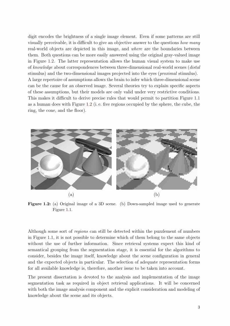
digit encodes the brightness of a single image element. Even if some patterns are still
visually perceivable, it is difficult to give an objective answer to the questions how many
real-world objects are depicted in this image, and where are the boundaries between
them. Both questions can be more easily answered using the original gray-valued image
in Figure 1.2. The latter representation allows the human visual system to make use
of knowledge about correspondences between three-dimensional real-world scenes (distal
stimulus) and the two-dimensional images projected into the eyes (proximal stimulus).
A large repertoire of assumptions allows the brain to infer which three-dimensional scene
can be the cause for an observed image. Several theories try to explain specific aspects
of these assumptions, but their models are only valid under very restrictive conditions.
This makes it difficult to derive precise rules that would permit to partition Figure 1.1
as a human does with Figure 1.2 (i. e. five regions occupied by the sphere, the cube, the
ring, the cone, and the floor).
(a) (b)
Figure 1.2: (a) Original image of a 3D scene. (b) Down-sampled image used to generateFigure 1.1.
Although some sort of regions can still be detected within the puzzlement of numbers
in Figure 1.1, it is not possible to determine which of them belong to the same objects
without the use of further information. Since retrieval systems expect this kind of
semantical grouping from the segmentation stage, it is essential for the algorithms to
consider, besides the image itself, knowledge about the scene configuration in general
and the expected objects in particular. The selection of adequate representation forms
for all available knowledge is, therefore, another issue to be taken into account.
The present dissertation is devoted to the analysis and implementation of the image
segmentation task as required in object retrieval applications. It will be concerned
with both the image analysis component and the explicit consideration and modeling of
knowledge about the scene and its objects.
3

1 Introduction
1.1 Motivation and Problem Statement
The previous considerations indicate that the first step in the selection or design of a
segmentation algorithm has to be the accurate specification of the context where the
segmentation processes will operate, since only this context can provide the additional
knowledge necessary to assign a meaning to the result. If, for instance, an industrial
environment permits a special acquisition set-up (e. g. back-light illumination), all infor-
mation derived from this restricted scene configuration could be employed in simplifying
the object detection and reducing the problem into a two-dimensional template match-
ing task. For image and video coding the segmentation not necessarily leads to regions
corresponding to real 3D objects in a scene, but merely to an image partition that can be
efficiently or effectively coded. Medical applications often require interactive segmenta-
tion approaches, to allow the incorporation of the operator’s specialized knowledge into
the process. For comfortable use, object retrieval systems need unsupervised segmen-
tation algorithms that automatically detect the correspondence between image regions
and real objects.
This work deals with retrieval systems following the concept depicted in Figure 1.3.
A user queries for information by presenting one or more objects to a digital camera
attached to the system. This scheme is appropriate in fields where human users have to
plough through large object databases in order to identify products without additional
automatic identification resources like bar-codes or transceivers. It helps to speed up
queries and supersedes manual browsing of printed catalogs. Typical applications can
be found in spare part retrieval, product remittance or in hardware stores, where the
retrieval system delivers for the shown object additional information like part number,
equivalent or similar products, or just its physical location in the store.
Cogweel Part Nr. 11252Material: PlasticColor: WhiteWeight: 2gCost: 45ct
Camera
Result
CAM 289c
PROGRESSIVE SCAN CAMERA
IntelligentElectronicCatalogue
Figure 1.3: Interactive object retrieval concept. The user makes a query for informationabout an object presenting it under a camera.
The recognition approach can also be extended to production lines as a verification
mechanism. The reliable recognition of several objects in a scene can help determining,
for instance, if a packaging process is functioning correctly, or if some objects have been
left out or have been incorrectly included in an assortment.
4

1.2 Analysis Approach
These application contexts permit the use of a homogeneous background. However,
camera and illumination parameters can change in a form that makes it difficult to
predict the final background values. In those cases where a single user interacts with
the retrieval system for a long period of time, it can be expected from him or her to
wear a glove of the same color as the background. Depending on the nature of the
object set, wearing a glove could even be mandatory to protect the user’s hand, the
objects, or both. In applications where the retrieval system is going to be operated by
occasional users (e. g. hardware store), hygienic issues and more comfort make a non-
intrusive approach necessary. Here, the user will present the object by holding it in his
or her bare hand. The segmentation must separate the hand from the object, which can
be a difficult task, especially if the objects have skin colored surfaces.
The following requirements are additionally imposed by the current object retrieval
context:
• The segmentation must be able to deal with color images taken from standard
industrial CCD cameras.
• The whole recognition process, from image acquisition to object identification,
must occur within a time interval tolerable for an interactive application. No
more than a few seconds should be required.
• The algorithms must run on general purpose computer systems. Even if many
state-of-the-art techniques could run fast in massively parallel computers, their
applicability to real world contexts is limited, since this kind of hardware makes
the retrieval system unaffordable.
• Real applications demand the identification of object sets containing groups of
similar items. The segmentation task has to detect the boundaries of objects
reliably enough to make a robust recognition possible.
• The recognition of several objects in one image must be possible, even if some
objects overlap.
1.2 Analysis Approach
Biological systems have proven to be an ideal model to be imitated when solving tasks
that entail some degree of environmental interaction. In the computer vision literature,
for example, the similarity of an algorithm with a biological process is often implicitly or
explicitely used as an informal proof of correctness. However, fundamental processing
differences between computer-based and biological vision systems impede a straightfor-
ward transfer of possible concepts between both domains.
The computational strength of biological systems is given by the cooperation of millions
of simple processing units: the neurons. The computational performance of the brain
5

1 Introduction
is achieved through the high interconnectivity between neurons and their learning ca-
pabilities [Pal99]. Current all-purpose digital computers, on the other hand, are based
on just a few complex processing units, much faster than single neurons, but incapable
to process high amounts of information concurrently. Thus, visual processes that occur
in parallel in the human visual path have to be simulated in a sequential manner. Spe-
cialized hardware providing some degree of parallelization tries to compensate for this
intrinsic weakness of sequential architectures, but it is still far away from reaching the
levels of concurrence found in biological brains. These facts have steered the develop-
ment of algorithms in computer vision to deviate from available biological models, even
if general concepts and goals remain the same.
1.2.1 Marr’s Metatheory
Despite these intrinsic processing differences, it is still desirable to transfer ideas inspired
by biological processes into the solution of artificial vision tasks. Marr [Mar82] proposes
a metatheory for the analysis of complex information processing systems, that allows to
isolate possible “transferable” concepts in a systematic way. He suggests three levels of
abstraction for the analysis of complex information processing systems: computational,
algorithmic and implementational.
The computational level has a more abstract nature than the next two levels and specifies
all informational constraints necessary to map the input data into the desired output.
It describes which computations need to be performed and the types of information
representation the computational stages expect, without being specific about how the
task has to be accomplished.
The algorithmic level states how the computation is executed in terms of information
processing operations. It is related with the specification of algorithms and the data
structures and representations on which they operate.
In the implementational level it is described how an algorithm is embodied as a “phys-
ical” process. It has the lowest description level.
Characteristic for this analysis approach is the increment of the number of solutions
while going down in the abstraction level. For example, there are several algorithms
to solve the computational task “edge detection”, and there are many possible ways to
implement each one of them.
Marr’s methodology is adopted here for the analysis of the segmentation task, focusing
on the computational and algorithmic levels of the problem. The implementational level
required for the evaluation of proposed concepts can be found, for instance, in the open
source software library LTI-Lib [LfTI03], which was partially developed in the context
of this work.
6

1.2 Analysis Approach
1.2.2 Computational Level of Vision Systems
Human visual perception can be described at the computational level using for example
Marr-Palmer’s computational vision framework (Figure 1.4) [Pal99]. Four stages extract
RetinalImage
Image−basedProcessing Processing
Surface−based Object−basedProcessing
Category−basedProcessing
Figure 1.4: Four stages of visual processing according to Marr and Palmer.
the relevant information found in the retinal image. The image-based processing detects
simple features like edges or corners in the image. Regions in the image corresponding to
surfaces of real objects are found in the surface-based processing. The detected surfaces
are assigned to objects in the object-based stage. Their role and relationship with other
objects within a scene is determined in the last category-based processing block. This
will be referred to henceforth as the general vision model, or Marr-Palmer’s model.
Most existing artificial visual recognition systems follow the paradigm depicted in Fig-
ure 1.5. An image is first preprocessed in order to eliminate information which is unim-
ImageCamera Image
Preprocessing ExtractionDescriptor
and AnalysisRecognition
Figure 1.5: Three stages of visual processing usually found in artificial systems.
portant for the next stages. The descriptor extraction module encodes the remaining
data in a form more appropriate for the recognition and analysis stage, which finally
identifies the image content. This concept better suits the sequential processing nature
of modern computers, and it is also more adequate for the design of systems working in
controlled environments, where each module has a well-defined task to solve.
The major difference between both models is the meaning of the information passed
from one module to the next. Marr-Palmer’s model produces image tokens, surfaces,
objects or object categories, all having a physical or real-world related meaning. The
model for artificial systems, on the other hand, uses data representations that do not
necessarily make sense for humans. Descriptors, for example, are usually designed to
encode information about a specific visual property, like color or shape, but a human
could not discern between two objects using those descriptors exclusively.
Feedback between different processing steps is also a major divergence between biological
and most current artificial systems. In human vision it is well known that knowledge
influences the perception (a classical example for this is the dalmatian image, Figure 1.6).
The perception process is therefore not unidirectional but recurrent, in the sense that
7

1 Introduction
Figure 1.6: Even if the image consists only of some white and black patches, knowing that itrepresents a dalmatian dog helps in its perception. (Photograph by R. C. James.)
the output of a block just serves as a preliminary hypothesis to be verified or improved
considering the feedback from later stages. A great advantage of this approach is its
robustness against errors in earlier processing stages, which can be fixed as soon as more
knowledge is available.
With the sequential architecture of Figure 1.5 errors in the first stages will be further
propagated into later stages, degrading the quality of the whole system. Hence, feed-
back has to be incorporated into the computational analysis of artificial vision systems
if higher degrees of robustness are aspired. For the particular case of segmentation, feed-
back from the recognition modules is necessary to detect the correspondences between
image regions and real objects, which are still unknown at the initial processing stages.
Marr-Palmer’s model provides an adequate foundation for the design of a segmentation
framework, and will be reviewed in more detail in the next chapters.
1.3 Goal and Structure of this Work
The main goal of this work is to develop a framework for unsupervised image segmen-
tation as required in the context of interactive object retrieval applications. Besides the
mandatory image analysis component, this framework must also provide methods to
explicitely include high-level information into the segmentation process, without which
it would not be possible to partition the image into semantically meaningful regions.
Hence, a detailed contextual analysis of object retrieval applications is necessary in order
to clearly state both the requirements for the segmentation task and the assumptions
that can be made. This is the aim of Chapter 2.
In the computational model for artificial vision (Figure 1.5) the segmentation task is
part of the image preprocessing module. Since this sequential architecture is prone to
8

1.3 Goal and Structure of this Work
errors in early processing stages, the quality of the segmentation results will play a
significant role in the robustness of the entire retrieval system. The consideration of
additional knowledge and the use of feedback from later stages are therefore necessary.
Marr-Palmer’s computational model provides a mechanism to incorporate knowledge
related with the application into different abstraction levels of the segmentation task.
Furthermore, it also helps to define feedback mechanisms from later stages. In accor-
dance to this model the segmentation task is divided into three stages, corresponding
to the first three processing levels, i. e. image-based, surface-based, and object-based.
After an extensive review of existing segmentation concepts and their relevance to the
current application field, Chapter 3 introduces the proposed three-staged segmentation
framework and its role within the object retrieval system. It concludes with a descrip-
tion of the evaluation approach used to measure the performance of the segmentation
algorithms. Chapters 4 to 6 present the details of each segmentation stage, including
their evaluation in the current application context. Concluding remarks and suggestions
for future work are discussed in Chapter 7.
9

1 Introduction
10

Chapter 2
Visual Object Retrieval
In the image formation process, light emitted from a given number of sources interacts
with different object surfaces in a scene. Part of the reflected light reaches an acquisition
sensor (e. g. the human eyes or a CCD camera), which transforms the incoming light into
another representation more suitable for further analysis. An image is therefore a two-
dimensional representation of a three-dimensional scene created through the projection
of light reflected by the objects onto a two-dimensional surface (Figure 2.1).
Light source
z
x y
2D Image3D Object
y’
x’
Figure 2.1: A two-dimensional image is the result of projecting the light reflected by thesurfaces in a scene onto a surface.
Vision can be understood as the inverse problem of inferring from a two-dimensional
image the contents of the three-dimensional scene depicted therein. From a mathemat-
ical point of view, the 2D images produced can be the result of an infinite number of
3D scenes. This lack of uniqueness makes vision an ill-posed problem in the sense of
Hadamard [MLT00]. Additionally, it suggests that, in principle, under exclusive use of
image information, the vision task cannot be solved. But, how is it then possible for
humans and animals to visually perceive their environment with such effectiveness? The
only possible way is restoring the well-posedness of the problem. A problem is called
well-posed if it fulfills three necessary conditions: a solution (1) exists, (2) is unique
and (3) depends continuously on the initial data (some authors interpret the latter as
robustness against noise [MLT00]).
11

2 Visual Object Retrieval
Well-posedness is restored by means of regularization of the problem, i. e. additional
constraints derived from a-priori knowledge are included in order to restrict the number
of possible solutions to exactly one. Regularization in vision involves the use of physical
properties of the environment on the one hand, and high-level knowledge about the con-
tents of the scene on the other hand. Only through the consideration of this additional
information it is possible for the human visual system to perceive only one scene from
a theoretical infinite number of interpretations.
Visual retrieval systems expect from the segmentation task to deliver image regions
belonging to real world objects. This is a general vision problem also affected by the
ill-posedness and thus requires for its solution the inclusion of contextual information.
This chapter presents in detail the characteristics of visual object retrieval systems from
which high-level conditions will be derived for inclusion in the introduced segmentation
approach.
2.1 Task of Object Retrieval Systems
In the context of visual retrieval the term object denotes a real-world entity that can be
identified by means of an unambiguous object label . The meaning of “entity” depends
on the application: it either denotes an individual object or “token”, distinguished by
an identification number, or it refers to a class or type of objects, for example “a screw”.
Two problems arise: first, an object may consist of different parts that could also be
treated as objects (for example, the parts of a screw are its head and a thread), second,
an object can belong to different classes, defined at different levels of abstraction: “a
spare part”, “a screw”, “a Phillips screw”, “a screw with left handed thread”, “a Phillips
screw with left handed thread” (Figure 2.2).
The main task of an object retrieval system is to determine the labels of all objects
depicted in an image (or images) of a scene, within predefined constraints in the com-
position of the objects and the levels of abstraction. The design of a retrieval system
highly depends on these last conditions. The recognition of the exact part number of
a screw is, for example, a different task than identifying it as “a screw” or as “a spare
part”, or detecting the two blades of a pair of scissors is another task than recognizing
the scissors as one object. Revealing the exact part number of an object is usually de-
noted as identification and the deduction of its type or class is known as categorization
[Pal99].
A distinction between systems for object recognition and object retrieval can be made.
In the first case, the system delivers one identification label for each object detected in
the image. In the second case, the system will additionally search for similar objects,
i. e. many possible candidates will be retrieved per detected object (Figure 2.3). In
other words, object recognition is a special case of object retrieval, where only the most
similar object is located.
12

2.2 Taxonomy of Object Retrieval Systems
Screw 1
Screw Part 5123
Left Thread
Phillips Screw Slotted Screw
Right Thread
Screw Part 3231
Screw 2
Screw
Spare Part
Leve
l of A
bstra
ctio
n
High
Low
Figure 2.2: An object can be identified at different levels of abstraction.
The exact specification of the objects to be recognized has a direct effect on the expec-
tations for the segmentation task. For example, the query “find a brick” should produce
a different partition of the same image than “find a wall”.
2.2 Taxonomy of Object Retrieval Systems
Five main criteria define the taxonomy of object retrieval systems (ORS ): first, the
architecture of the computational system itself, second, the restrictions on and properties
of the objects that are to be recognized, third, the nature of the images or visual input
being used, fourth, the conditions imposed on the scene settings for the recognition and
ObjectData
Images
Retrieval
Recognition"octahedron"
"octahedron""cube""pyramid"...
ORS
Figure 2.3: The task of an object recognition or retrieval system (ORS). A recognition systemdelivers just the labels of the objects found in the presented images. A retrievalsystem’s output is a list of similar or possible objects.
13

2 Visual Object Retrieval
fifth, the type of knowledge used to achieve the recognition (Figure 2.4).
Object Set
System Architecture
Scene Composition
Nature of Images
Knowledge Type
Object Retrieval System
Figure 2.4: Aspects to consider in the taxonomy of object retrieval systems.
2.2.1 Architecture of Object Retrieval Systems
The process of retrieving visually similar objects can be decomposed into several mod-
ules, each performing a distinct part of the complete task. A general framework em-
bracing the modules and their interactions is shown in Figure 2.5. The purpose of each
module is described below.
Data flow
Control flow
Images
Classification
ExtractionDescriptor
Preprocessing
VerificationUser Interface
Acquisition
InternalDataData
Object
Figure 2.5: The general structure of an object retrieval system. Depending on the actualimplementation, some of the blocks and links may be combined or omitted.
• Acquisition: This module contains all functionality related to the acquisition of
object images: directly from a camera system, by loading previously stored images,
or from an image generator, like a scene rendering engine. The latter approach is
useful for automatic generation of training data from CAD models stored in the
database, circumventing manual acquisition of training images.
• Preprocessing: The task of this module is to eliminate all information that is
irrelevant for the application from the images. A subtask is, for example, color
normalization, which tries to remove dependencies on the illumination. An im-
portant and complex subproblem is the image segmentation: only those regions
belonging to objects need further analysis.
14

2.2 Taxonomy of Object Retrieval Systems
• Extraction of descriptors: The preprocessed images are passed to the descriptor
extraction module, which computes a set of vectors describing different image
properties (for example, color histograms, shape moments, etc.). These descriptors
are typically shorter representation forms for the information contained in the
images. Their shorter size is advantageous for the next classification stages and
for storage purposes.
• Classification: The extracted descriptors are received by the classification mod-
ule, which usually provide two operating phases. In the training phase, the classi-
fiers are adapted to the training data. In the recall (also test or recognition) phase,
it either assigns an object identification to each extracted descriptor or suggests a
list of candidate labels. The available techniques vary considerably depending on
the task at hand. Most systems use either a neural network or a classifier based
on statistical principles.
• Verification: Most of the time, it is not sufficient to rely on a classifier’s per-
formance. Therefore, it is advisable to submit the results to a verification stage
which determines the plausibility of the result or assesses the classifier’s credibil-
ity. This module can also incorporate additional non-visual knowledge provided
by the user.
• User Interface: The user interface presents the retrieval result to the user and
accepts user inputs, such as the query itself, additional information to aid the
retrieval, or commands to the acquisition hardware.
• Data Storage: There are two major data repositories that are required: first, an
interface to a database containing non-visual data describing the object set, like
weight, materials, price, etc. This database may also be external to the retrieval
engine. The second repository is an internal storage area which contains the con-
figuration of the system, like the adapted classifiers.
It lies at hand to implement this architecture accordingly to its inherent structure.
This is done by providing a set of modules, each performing one or more of the subtasks
outlined above. Depending on the way these modules interact, three subclasses of object
retrieval systems can be highlighted: monolithic, sequential and recurrent structures.
Monolithic systems consist of a single large algorithm which takes an image or image
sequence as input and returns the object’s identification label. The key issue is that it is
not possible to differentiate among image analysis and classification components. The
image is usually just preprocessed and passed on to the identification module, which
determines the label of the shown objects directly. As single processing blocks, they are
usually difficult to adapt to different applications.
Sequential structures provide separate modules for descriptor extraction and classifica-
tion. They follow the general paradigm already introduced in Figure 1.5. The main ad-
vantage of this approach, when compared with the monolithic structure, is its improved
flexibility. Different kinds of object sets may also require different kinds of descriptors,
15

2 Visual Object Retrieval
classifiers or acquisition methods. Therefore, if a system is supposed to be adapted to
more than one task, it is easier to exchange some modules than to develop a complete
new system. Most available object retrieval systems follow this strictly sequential design
approach.
Recurrent or iterative structures refine or modify the behavior of the acquisition, pre-
processing, and descriptor extraction modules using feedback from the classification
and verification stages. If the general recognition process is considered as shown in Fig-
ure 2.5, the feedback can be modeled by control signals that modify a module’s behavior
either by changing parameters or simply by iterating a process. In the most simple case,
this may consist of determining the next most interesting region of an image, extracting
descriptors for it, classifying them and verifying if a meaningful result can be achieved.
If that is the case, the loop terminates, otherwise it reiterates.
Recurrent structures are still rare, but their robustness against errors in early process-
ing stages is an important advantage that will encourage their use in future systems.
However, the interactions between modules have an impact in the time requirements for
a recognition task, that makes the strict sequential structure more attractive in many
industrial applications with restricted scene configurations.
Figure 2.6 summarizes the three architecture types for object retrieval systems.
Monolithic Sequential Recurrent
RECOGNITIONMODULE
UI
ACQ ACQ
CLASSIFVERIFUI
PREPR DSCEXT ACQ PREPR
CLASSIFVERIFUI
DSCEXT
OD ID OD ID OD ID
Object Retrieval System Architectures
Figure 2.6: Three architectures found in object retrieval systems derived from the generalstructure in Figure 2.5. The acquisition (ACQ), user interface (UI), object data(OD) and internal data (ID) are present in all cases. The modules preprocessing(PREPR), descriptor extraction (DSCEXT), classification (CLASSIF) and veri-fication (VERIF) are integrated into a single block in the monolithic approach.The highest interaction between modules occurs in the recurrent architecture.
2.2.2 Object Set
As stated previously, the definition of an object depends strongly on the desired abstrac-
tion level of the recognizer. The object set an ORS deals with is usually constrained
to elements of one specific class at predefined abstraction levels (like spare parts, tools,
mechanical components, toys, plush animals, etc.) or the combination of a few of them.
16

2.2 Taxonomy of Object Retrieval Systems
With respect to the composition of the objects, they can be regarded as atoms if they
consist of just one component, or as an assembly or aggregate if they comprise two
or more objects. In assemblies, the joints between the different parts can have differ-
ent degrees of freedom, varying from rigid joints (zero degrees of freedom) to several
translational and/or rotational degrees of freedom. Scissors are an example of an ob-
ject composed of two parts, kept together by a junction with one rotational degree of
freedom (Figure 2.7). A segmentation algorithm must be able to detect at least object
parts, which can then be merged at later stages using additional information.
(a) (b) (c)
Figure 2.7: Examples for the composition of objects: (a) an atomic object; (b) assembly oftwo parts with one rotational degree of freedom; (c) assembly of many parts,some of them fixed, others with one translatory degree of freedom.
Another important criterion to take into account is the shape variability of objects
and their parts. They can for instance be rigid, flexible (like a cord) or deformable
(like a stuffed animal) (Figure 2.8). This aspect is of fundamental importance for the
segmentation: for rigid objects it is usually possible to employ additional algorithms to
detect specific shapes (e. g. template matching or generic Hough transform). For flexible
or deformable objects special techniques like active contours or shape models are more
appropriate.
The complexity of three-dimensional shapes is also relevant for the design of an ORS. In
some industrial fields, sets of “flat” objects that can be recognized by their characteristic
two-dimensional shapes are frequent. The limited number of degrees of freedom in
the presentation of these objects simplifies not only the segmentation and recognition
algorithms, but also the image acquisition techniques. Other applications require the
recognition of three-dimensional objects from arbitrary view points, fact that forces the
use of more complex approaches that are able to cope with the possible variations in
the position and appearance of the objects.
All visual properties of the objects impose constraints on the acquisition module. For
this reason, attention must be payed on how attributes like color, material, transparency,
reflectance, etc. can affect the recognition process. For example, if an application deals
17

2 Visual Object Retrieval
rigid flexible deformable
Figure 2.8: Shape properties for objects and their parts.
with metal parts, special illumination techniques are required in order to suppress un-
desired reflections. Knowledge about these properties is also important for the segmen-
tation: the metal parts demand algorithms to assign regions caused by highlights to the
corresponding object parts. Figure 2.9 summarizes the previously mentioned criteria to
categorize an object set.
Shape Variability
Composition Shape Complexity
=?Abstraction Level
Visual Properties
Object Set
Figure 2.9: Five criteria to describe the objects in a set.
2.2.3 Nature of Images
The nature of the images to be used affects especially the design of the acquisition
module of the system. Different kinds of image acquisition techniques exploit particular
physical principles in order to capture those visual details that are of interest for the
application. Medical systems, for instance, employ a wide range of imaging possibilities,
18

2.2 Taxonomy of Object Retrieval Systems
including ultrasonic or magnetic resonance acquisition methods. In microscopy, elec-
tronic or nuclear magnetic resonance principles can be found. This work concentrates
on systems operating in the same visual environment as humans. Exclusively industrial
and consumer color cameras based on CCD or CMOS sensors are used.
Each application imposes specific requirements on the spectral information encoded in
the captured images. If, for example, all objects show the same color it is obvious that a
chromatic visual feature will not be able to support the recognition, and thus monochro-
matic cameras can be used. In other environments, cameras sensible to infrared light
could simplify the detection of objects radiating heat.
Camera 1 Camera 2 Camera 1
Figure 2.10: Two possibilities to acquire different views of an object. On the left side,multiple cameras acquire different perspectives at the same time. On the rightside, one camera acquires different perspectives at different points in time, whilethe object is being rotated.
To analyze a scene, the ORS can use one or multiple images. In the latter case, the im-
ages can be taken with one or more cameras at one or many points in time (Figure 2.10).
This is often necessary to recognize three-dimensional objects with similar views, where
one image alone might not contain all information necessary for the recognition. Fig-
ure 2.11 shows a simple example for this case: if just one picture of an object is taken
from its bottom or side view, it would not be possible to determine the proper object,
because one aspect alone is ambiguous. Both views are necessary in order to achieve a
correct recognition.
Independently of the utilization of one or more cameras, image sequences can be em-
ployed to capture information about the motion of objects and their parts, or just to
acquire several distinct images from different perspectives. Additionally, the use of se-
quences can support the recognition process, under the assumption that the image n+1
will probably contain the same objects that were present in the image n, captured from
a relatively similar point of view. This fact is relevant for the result verification, since
the recognition system should detect the same objects at similar positions in subsequent
images.
In any case it is important to consider the quality of the images when designing an ORS.
Aspects like noise, optical distortions and quantization will influence the choice of an
algorithm. Figure 2.12 summarizes all previously mentioned criteria for the classification
of the different image types.
19

2 Visual Object Retrieval
botto
m−v
iew
side
−vie
w
Workaround for a wrong turn with epstopdf
A B C D
Figure 2.11: Requirement of multiple views for object retrieval. The objects A and B areidentical if considered from the side. The objects A and D look alike from thebottom. Both views are required in order to make a correct recognition.
Acquisition Technique
Single/Multiple Images
Spectral Coding
Picture Quality
Number of CamerasImage Sequences
NoiseOptical Distortion
Nature of Images
Figure 2.12: Four criteria of the nature of images to take into account in the design of anORS.
2.2.4 Scene Composition
The organization of objects in a scene and all constraints imposed on them affect the
complexity of the algorithms for image processing and recognition. A single object in
front of a homogeneous background simplifies not only the preprocessing and segmen-
tation of the images, but also the recognition, under the assumption that exactly one
object will be found. Detection and localization of several objects in cluttered scenes
(Figure 2.13) is a challenging task even for modern object recognition systems. A solu-
tion to this problem could, for example, help mobile autonomous vehicles to navigate
freely in their environment. In object retrieval systems that follow a query-by-example
approach, scenes can be found containing three objects: a usually homogeneous back-
ground, the presented object and the hand of the user. Keeping these objects apart is
not always an easy task, particularly if their colors are similar. In order to cope with this
problem, some knowledge of the scene needs to be incorporated into the image analysis
process.
The different ways in which an object can be found in the images is also part of the scene
composition: can it be recognized independently of the illumination, pose or distance
to the camera? These transformations of the scene can be grouped into three classes
20

2.2 Taxonomy of Object Retrieval Systems
Figure 2.13: Finding and recognizing the object in the scene on the left side is much easierthan finding it in the scene on the right side, where a non-homogeneous back-ground, shadows and other objects impose additional demands on the system.
(Figure 2.14):
(a) (b) (c) (d) (e)
Figure 2.14: Different object transformations in a scene: (a) the original object; (b) scaled,translated or rotated in the image plane; (c) rotated on the axes parallel tothe image plane; (d) taken using a different illumination set-up; (e) partiallyoccluded by another object. Even if the images of the object differ, the objectretrieval system has to identify the same object in all images.
• Similarity transformations: These two-dimensional transformations are caused
by shifts of the object in the image plane, a rotation around the camera axis, or a
change in scale (shift along the camera axis). If the loss of information caused by
quantization is neglected, diffuse illumination is assumed and the optical projection
is approximately orthogonal, these kinds of transformations do not change the
amount of information about an object.
• Three-dimensional transformations: These are caused by a rotation of the object
in the axes parallel to the image plane. They significantly change the information
content about an object’s view. For this reason, several pictures of different object
poses are required in order to capture enough information about the entire object’s
appearance.
• Scene formation changes: Illumination changes, partial occlusion, and background
changes can be classified into this group of transformations. Their effects disturb
21
2 Visual Object Retrieval
the recognition process and have to be suppressed, a goal which is usually difficult
to be reached.
2.2.5 Knowledge Type
An ORS will identify only those objects it already knows. In order to gain all required
information about the appearance of the objects, modern retrieval systems are capable of
learning different aspects and properties of the object set in a training phase. However,
the set of appearance features to be utilized is selected beforehand. Visual and non-
visual properties can support the recognition process. Visual features include shape,
color, texture, motion and location of the objects in the image. Non-visual information
comprises knowledge about classes of objects, the context in which they are found,
their role within a scene, or further non-visual physical data like weight, temperature
or material.
Two representation schemes can be followed in order to encode visual information:
object-centered or viewer-centered [Pop94]. The former relies on models that describe
properties of an object as a whole. A 3D CAD model, for instance, can be used to
represent the entire shape of an object. These models are independent of the observer.
Recognition processes for this kind of representations try to find a match between de-
scriptors extracted from the models and from the acquired images. Some approaches,
for example, attempt to reconstruct a 3D-model from the images in order to provide a
basis for the comparison.
Viewer-centered approaches rely on a representation form composed of a set of images
taken from different viewpoints. Hence, the recognition compares information gained
from the same image space. In contrast to the object-centered techniques, viewer-
centered approaches have lower computational costs, since it is not necessary to recre-
ate complex models of the objects, and the extraction and comparison of descriptors
is relatively simple compared to the task of implicitly or explicitly matching an ob-
ject model with a 2D image. Additionally, the recognition rates achieved with viewer-
centered systems are usually better. Nonetheless, 3D object models can still be used in
viewer-centered approaches to generate images from different perspectives, employing
for example ray tracing techniques.
The viewer-centered approach can again be subdivided into two categories [Els99]: pixel-
based and descriptor-based retrieval. The first one tries to match images directly, mod-
ifying them slightly in order to cope with certain variations in the object’s appearance
(like translation or rotation). A disadvantage of this approach is the comparatively large
size of an image necessary to represent a single view of an object. Another drawback
is its high sensitivity to small scene changes. Pixel-based representations are employed
in retrieval systems where the object’s position and orientation within the scene can
be reliably detected. Monolithic architectures are typically used, since the objects are
directly identified from the acquired images. A prominent example here is the face
22
2.2 Taxonomy of Object Retrieval Systems
recognition with eigen-faces [TP91].
The descriptor-based approach tries to extract more compact representations that gen-
erally cope with just one type of information, like shape, color or texture, and are often
invariant against some scene transformations, especially rotation, translation, scaling
and illumination changes. These representation forms can describe one object’s view as
a whole, or just small parts of it. The former are known as global descriptors, the latter
as local descriptors.
Some evidence exists that the holistic analysis of the object’s appearance and the at-
tention to details are both present in the human visual system [Pal99]. This suggests
that an object retrieval system should also employ both approaches in order to solve
complex visual tasks. A way to feed information from the recognition process back into
the segmentation will be introduced later, and is based on the local descriptor paradigm.
If global descriptors are used, the preprocessing module has to provide a relatively robust
segmentation in order to ensure that all descriptors will exclusively contain information
about the objects of interest. Due to the complexity of this task special interest has
been focused on recognition approaches based on local descriptors, as they can cope
with inaccurate segmentation results or even work without a segmentation stage [SP99,
Low03]. However, with current systems based on local descriptors this seems to hold only
if the object set contains elements with clearly different appearances. The higher the
number of local descriptors, the greater the probability that similar ones are obtained
from different objects. This increases the ambiguity of the classification results and
imposes higher demands on the verification modules, which have to decide which results
are relevant and which not. Furthermore, the huge amount of generated descriptors
severely restricts the cardinality of the object set a recognition system can cope with.
The next issue to consider about the knowledge type is the way it is used during the
recognition process [AGNT96]. In a bottom-up approach, a comparison between data
taken from the presented image and those previously learned is done at a low-level
first, and with the results of these comparisons higher level relationships can be de-
duced. The appropriate methods for performing these deductions are classification or
nearest-neighbor approaches. These methods assign labels to images or image parts, but
usually do not incorporate a-priori knowledge about the task at hand. The sequential
architecture implements strictly bottom-up systems.
In contrast, top-down approaches work exclusively on the basis of prior hypotheses
which are iteratively refined. First, it is determined whether two objects match on the
highest level of abstraction. Subsequently, the comparison is refined and verified on
lower levels. The methods applied for implementing a top-down approach are usually
rule-based systems or semantic networks. These methods were used as sole recognition
approaches in the early period of computer vision. Nowadays, top-down systems are
used as a second layer of inference on top of a bottom-up module, forming a hybrid
system. Recurrent architectures are necessary if these kind of concepts for information
23

2 Visual Object Retrieval
processing are followed.
Figure 2.15 summarizes all aspects of the knowledge type used in object retrieval sys-
tems.
Knowledge Type
3D−Reconstruction2D−3D Comparison
...
GlobalLocal
Pixel BasedDescriptor Based
Object Centered
Viewer Centered
Object Representation
Expert SystemsSemantic Networks
Logic Systems
Neural NetworksStatistical
IndexingClassification
Recognition Approach
Bottom−Up
Top−Down
ShapeColor
TextureMotion
Location
...MaterialWeight
Object class
Non−Visual
Data type
Visual
Figure 2.15: Three criteria and their subtopics to consider about the knowledge used for therecognition.
2.3 Assessment of Object Retrieval Systems
The quality of an ORS depends on three factors: robustness, efficiency and correctness.
Robustness denotes the tolerance of the system against changes in the scene configu-
ration or in image quality (like modification of the illumination, partial occlusion of
the objects, or noise). It is considerably affected by the knowledge types used. The
complexity of the algorithms necessary to achieve robustness can be kept within limits
by imposing constraints on the possible variations of the scenes. For example, an envi-
ronment with controlled illumination in an industrial optical measuring system renders
the robustness against illuminant changes unnecessary.
Efficiency is related to the demands on computational resources (like memory) and the
time an ORS requires to achieve its task. A trade-off between both issues is usually
necessary, since an ideal configuration using short times and low resources is difficult
or even impossible to obtain. For example, simple indexing algorithms are fast, but if
the object set is too large, the storage demands can become prohibitive. On the other
hand, some neural network approaches do not make use of huge amounts of space, but
they are computationally expensive.
Correctness expresses the fulfillment of several recognition criteria, which are usually
imposed by each specific application. For example, an object recognition system for
24

2.4 Experimental Set-up
industrial quality control delivers a “correct” result only if it recognizes the proper
object. Even small changes in its appearance have to be detected. In contrast, for
search engines a recognition result is valid if the detected objects are similar to the
presented one.
Interdependencies between these three factors will always be present. To fulfill strict
recognition criteria, complex algorithms (usually slow ones) are required. Acquisition
constraints are also necessary in order to compensate for the lack of robustness against
some transformations which could make different objects look very similar (for example,
the exact detection of colors without constraints on the illumination is not easy to
achieve).
2.4 Experimental Set-up
As experimental set-up, used to verify the proposed segmentation concepts, an object
retrieval system will be used that has, according to the previously described taxonomy,
following properties:
1. System architecture
Recurrent system architecture.
2. Object set
The object sets contain from 10 to 200 objects. The size of individual objects varies
between a few millimeters and 30 cm. Three object classes will be considered: P17,
P25 and P200, which are sets of soft toys (see Appendices D, E).
(a) Abstraction level
Individual objects, and not categories, will be recognized. Each object has a
unique identification number.
(b) Shape variability
The objects can be rigid or deformable. However, the descriptors employed
here are not appropriate for the recognition of flexible objects.
(c) Composition
Atomic objects or simple aggregates with rotatory degrees of freedom can be
expected.
(d) Shape complexity
Complex three-dimensional objects can be expected.
(e) Visual properties
The objects are all opaque with non-metallic surfaces.
3. Nature of images
(a) Acquisition technique
Fixed CCD industrial camera in an acquisition place with diffuse illumination.
(b) Spectral coding
Color images in RGB color space.
25

2 Visual Object Retrieval
(c) Multiple images
Recognition uses only one camera but it can use one or more images of the
object taken at different points in time.
(d) Picture quality
Since modern industrial cameras provide a good signal to noise ratio, the
algorithms do not require strong robustness against noise. Minimal optical
distortions can be neglected.
4. Scene composition
A homogeneous background (dark-blue or black) will be used. An image can
contain only the object of interest, or additionally the hand of the user holding
it. It is pertinent to note that the objects can be skin colored. Scenes with more
than one object can also be expected. Figure 2.16 present some examples of the
acquisition places used and the images acquired with them.
Camera
Object Hand
Background
Figure 2.16: Acquisition systems (left) and images delivered to the recognition system(right).
26

2.4 Experimental Set-up
5. Knowledge type(a) Data type
Only color and texture information will be used, since the shape informa-
tion is unreliable considering that the objects can be deformable and partial
occlusion is expected.
(b) Object representation
Only viewer-centered, descriptor-based methods will be used, but both local
and global.
(c) Recognition approach
Bottom-up, with a top-down verification stage.
27

2 Visual Object Retrieval
28

Chapter 3
Foundations of Image Segmentation
3.1 Definition of Segmentation
Great attention has been directed to the problem of segmentation. Hundreds of publi-
cations in this field appear every year, each trying to find an optimal solution for one
specific application. However, a unified, generally accepted definition of this term does
not yet exist. Most authors agree on the following facts about segmentation:
• its task is to partition the image into several segments or regions.
• it is an early processing stage in computer vision systems. Within the compu-
tational model for computer vision (Figure 1.5) it belongs to the preprocessing
module.
• it is one of the most critical tasks in automatic image analysis. This issue is
strongly related with the sequential processing approach habitually followed: an
error in the segmentation, which is one of the first processing steps, will affect
later stages.
What kind of segments this task has to find is not clearly specified. Sonka et al. define
the goal of segmentation as “to divide an image into parts that have a strong corre-
lation with objects or areas of the real world contained in the image” [SHB99]. In
Marr-Palmer’s computational model (Figure 1.4), this definition implies that segmen-
tation covers all three stages between image-based and object-based processing. They
also identify two types of segmentation: partial and complete, where the difference lies
in the degree of concordance between the regions found and real world objects. Par-
tial segmentation finds regions in the image that correspond to surfaces in the real
world, without grouping them into objects, i. e. it ends at the surface-based level of the
computational model. Complete segmentation detects real objects, covering also the
object-based stage. This kind of definition is well-suited for the processing model of
computer-based vision systems, as later stages require meaningful regions to work with.
29

3 Foundations of Image Segmentation
As previously mentioned, the meaning of real-world object depends on each specific re-
trieval application. For this reason other authors (e. g. Jain [Jai89], Gonzalez and Woods
[GW92]) refer to segmentation as the task of decomposing an image into its components,
where the term component has to be understood as a compact representation of an im-
age part more appropriate for the contextual dependent processing [FP03]. Thus, this
definition also involves the first three stages of the computational model. Moreover,
Forsyth [For99] states that segmentation and recognition of objects should not be re-
garded as different problems; segmentation is not a preprocessing step but a side effect
of the recognition process.
Other authors [PP93, SK94, LM01] define segmentation in terms of a homogeneity crite-
rion between low-level features that must be fulfilled within each region but violated as
soon as two adjacent regions merge. This resembles the principle of region segmentation
encountered in biological vision contexts [Pal99]. In contrast to the previous definitions,
a homogeneity-based segmentation has to be exclusively localized in the image-based
processing level, since the homogeneity criterion is neither always necessary nor suffi-
cient to ensure a correspondence between regions and real-world objects. For example,
Figure 3.1 depicts possible segmentation results at each level of Marr-Palmer’s compu-
tational model. At the image-based level a simple feature describing the pixel’s position
and its gray-value has been used. The background object is composed of several patches,
for which neither the position nor the gray value of the pixels are necessarily similar.
Additionally, the shadow of the ring cast at the base of the cone has an extremely similar
gray tone to the cone itself, even if these regions belong to different objects.
(a) (b) (c) (d)
Figure 3.1: Ideal segmentation results at different levels of Marr-Palmer’s vision computa-tional model. (a) Original image, (b) image-based level, (c) surface-based leveland (d) object-based level. At the image-based level pixels are grouped accordingto their feature values (e. g. their gray value). The surface-based level detectssurfaces, but not objects; for example, the background keeps its patches. Theobject-based level detects a region per object.
For many authors segmentation is a synonym for low-level processing algorithms. For
example in [Par97, Dav97] gray-level segmentation is used as another term for thresh-
olding, a task where each pixel in the image is assigned to one of two classes depending
on its gray-value and a threshold parameter. Medioni et al. [MLT00] limit their seg-
mentation definition to a more restricted surface-based level concept. They assume a
previous detection of image-based primitives like points and edges and try to find the
most salient boundaries of surfaces using a general framework based on tensor voting
30

3.1 Definition of Segmentation
and the Gestalt principle of continuity (see Chapter 5 for more details).
Techniques following these last definitions produce only partial results, in which the de-
tected image parts are not correlated with real-world objects (see Figure 3.1). Therefore,
they cannot be directly applied in the context of object recognition. A summary of the
relationship between the different definitions mentioned above and the corresponding
three stages of Marr-Palmer’s computational model is shown in Table 3.1.
Table 3.1: Relationship between different definitions of segmentation and the three
stages of the computational model of vision.
Author Goal of Segmentation I S O
Palmer [Pal99] Find regions with uniform image features. XPal & Pal [PP93] Find homogeneous regions. X
Skarbek & Koschan [SK94] Find regions with homogeneous colors. XLucchese & Mitra [LM01] Find homogeneous regions. X
Sonka et al. [SHB99] Partial segmentation finds regions corre-
sponding to surfaces.
X ×
Medioni et al. [MLT00] Find salient region boundaries that de-
limit object surfaces.
X
Sonka et al. [SHB99] Complete segmentation finds regions cor-
responding to real objects.
X × ×
Jain [Jai89] Decompose an image into application de-
fined components.
X × ×
Gonzalez & Woods [GW92] Subdivide an image into parts or objects
defined by the application.
X × ×
Forsyth & Ponce [FP03] Generate a compact representation of an
image, better suited for the application.
X × ×
I: Image-based stage. S: Surface-based stage. O: Object-based stage.X Suggested. × Suggested but not treated.
Interestingly, all authors who demand a semantic correlation between real-world objects
and image segments, introduce in their works image-based approaches only. They do not
provide any general concepts to incorporate high-level knowledge into the segmentation
process, without which this correspondence cannot be achieved.
Here, a definition for segmentation has been chosen that is both well-suited for object
retrieval applications and also allows the task to be analyzed under consideration of the
general vision computational model. Before it can be properly stated, some fundamental
concepts have to be specified.
Definition 1 (Image element) An image element e or pixel, is a 2-tuple e = 〈p, c〉containing a position vector p and a feature vector c.
31

3 Foundations of Image Segmentation
The d-dimensional feature vector c ∈ IRd describes different low-level aspects like color,
texture, edgeness, etc. The position vector p is assumed two-dimensional and discrete in
this work, i. e. p ∈ G2 ⊂ IN2. G2 denotes a two-dimensional finite, discrete and compact
grid G2 = [0 . . . a1 − 1]× [0 . . . a2 − 1], with ai ∈ IN.
Definition 2 (Image) An image I is a finite, non-empty set of image elements with
the following three properties: 1. for ei = 〈pi, ci〉 ∈ I and ej = 〈pj, cj〉 ∈ I, pi = pj ⇒ci = cj; 2. pi ∈ G2; and 3. |I| = |G2|.
The first condition ensures that each pixel in the image has a unique position, i. e.
two different image elements cannot share the same position. The second condition
constraints the used image definition to two-dimensional discrete images, as provided
by industrial CCD or CMOS cameras. The third condition ensures the connectedness
of the image and its size to be a1 × a2.
The treatment of an image I as a mathematical set is appropriate for many analysis is-
sues of the segmentation task but is disadvantageous in other image processing contexts,
where a functional representation fI is more appropriate:
Definition 3 (Image as a function) The functional representation of the image I is
fI : G2 → IRd, such that ei ∈ I ⇐⇒ ei = 〈pi, fI(pi)〉.
Hence, the vectorial function fI maps the pixel position pi ∈ G2 into its d-dimensional
feature vector ci ∈ IRd. Let fI(p) = [f1(p), . . . , fd(p)]T . The scalar functions fi(p)
define the channels of the image I.
Definition 4 (Image region) An image region R is a non-empty subset of the image
I, i. e. R ⊆ I, R 6= ∅.
A region does not need to be topologically connected. Therefore, under this definition,
two visible independent parts of a partially occluded object can be assigned to one single
region.
Definition 5 (Image partition) An image partition P of the image I is a set of n
regions Ri; i = 1 . . . n such that⋃n
i=1Ri = I and Ri ∩Rj = ∅ for i 6= j.
Note that this definition corresponds to the mathematical concept of a set partition, with
the difference that in the general mathematical context the regions are called blocks. One
partition is said to be finer than another if it splits the image into smaller regions.
Definition 6 (Object and Object set) An object is a real-world entity with specific
meaning in the context of the application. It is uniquely identified by a label oi. The set
of all objects defined by the application is denoted with Ω.
32

3.1 Definition of Segmentation
In other words, an object in the context of segmentation is a real-world entity with
a unique label oi that can be used to unequivocally identify the object. For this rea-
son,objects and labels will be used here as synonyms. The restriction of the object def-
inition to an application context allows, for example, to assign one unique background
label to all uninteresting real entities in a cluttered scene.
Definition 7 (Recognition operator) The recognition operator L assigns to an im-
age region Ri the subset Oi ⊆ Ω of labels belonging to all objects depicted or partially
depicted in it.
Taking all these terms into account, a definition for segmentation in the context of object
retrieval applications can be given:
Definition 8 (Segmentation) The segmentation S of the image I is a partition of
the image I which satisfies 1. |L(Ri)| = 1 for Ri ∈ S, i = 1 . . . nopt and 2. nopt = |S| is
minimal.
The first condition ensures the correspondence of each region to exactly one object. This
avoids to consider as valid segmentations, those image partitions whose regions cover
more than one object. The second condition ensures that no object is assigned to more
than one region. Without the latter condition, finer partitions with one pixel per region
would also be valid segmentations. The paradox of the task at hand becomes clear:
the segmentation is required to implement the operator L, which at the same time is
required by the segmentation.
An algorithm produces an over-segmentation of an image if it finds a partition So such
that |So| > nopt. In this case, the condition |L(Ri)| = 1 can still hold. An under-
segmentation Su typically contains less regions than the optimal (i. e. |Su| < nopt);
hence, there is at least one region Rk for which |L(Rk)| > 1.
To solve the segmentation problem a three-staged framework based on the general vision
computational model is proposed. The three segmentation steps correspond to the first
three stages of Marr-Palmer’s model:
• Image-based segmentation uses only the information contained in the camera im-
age to find regions defined by low-level homogeneity criteria.
• Surface-based segmentation tries to find regions that correspond to real-world
surfaces.
• Object-based segmentation detects real-world objects, by grouping regions of the
surface-based segmentation using high-level knowledge.
Image-based segmentation follows the definition of the first four authors in Table 3.1. It
is at this level where major research efforts are currently made. For most applications,
however, image-based segmentation alone is insufficient to provide satisfactory results.
33

3 Foundations of Image Segmentation
Hence, several proposals have been made to additionally include knowledge about phys-
ical properties of materials and illumination. This can be regarded as a surface-based
segmentation approach. Definition 8 can be directly applied to object-based segmenta-
tion only, since all information required by the recognition operator L is absent in the
first two stages.
Each stage provides partial results to the next one and obtains feedback from later
modules to correct wrong hypotheses. Thus, algorithms need to be found that allow
the incorporation of feedback and provide adequate representations for the next stages.
The next sections evaluate the state-of-the-art of segmentation algorithms at each of
these three processing stages. After that, an overview of segmentation in the context of
object recognition will be given, followed by a discussion of evaluation methods for image
segmentation. This chapter concludes with a summary of the proposed framework.
3.2 Image-based Segmentation
At the image-based level there is still no concept for the term object. Instead, a uni-
formity or homogeneity criterion for a given image feature is used. This criterion relies
on the fundamental assumption that real objects will be commonly composed of piece-
wise homogeneous surfaces. Image-based segmentation is therefore defined in terms of
a region homogeneity predicate HI and a region adjacency predicate A as follows:
Definition 9 (Image-based segmentation) The image-based segmentation SI of an
image I is a partition of I that satisfies for each region Ri ∈ SI , HI(Ri) = true, and
HI(Ri ∪Rj) = false for A(Ri,Rj) = true.
The condition H(Ri ∪ Rj) = false prevents to partition the image in too many regions
(over-segmentation): if the result of merging any pair of adjacent regions is inhomo-
geneous, then it implies that the segmentation already contained the largest possible
regions for which the homogeneity predicate still held. All available approaches at this
processing level can be regarded as a specialized implementation of the predicate H.
They add additional restrictions to Definition 4 allowing more precise constraints on
the validity of a region. For instance, a condition usually imposed on H is the connect-
edness of the regions.
Several surveys of segmentation techniques have been published. Three of them [PP93,
SK94, LM01] review about 300 of the latest publications giving a fair overview of the
current state-of-the-art in segmentation at the image-based processing level. Pal and Pal
[PP93] mainly evaluate algorithms for gray-valued images and introduce three of the first
attempts to exploit color information. Since for the current context of object retrieval
the use of color images as input data is assumed, all gray-value-based approaches would
discard valuable information and are therefore not further evaluated.
34

3.2 Image-based Segmentation
Skarbek and Koschan [SK94] concentrate their survey on color image segmentation.
They classify the algorithms according to the underlying concepts of the homogene-
ity predicate H and identify four categories: pixel-based, area-based, edge-based and
physics-based approaches. Pixel-based approaches consider a region as homogeneous,
if the features ci of its elements belong to the same cluster in the feature-space. Area-
based techniques define a region as a set of connected pixels obtained for instance by
growing from seeds, by joining smaller pixel blocks or by splitting non-uniform regions.
The third, edge-based group, defines regions as those sets of pixels delimited by inhomo-
geneities or discontinuities. This is the complementary concept to area-based segmenta-
tion. Physics-based methods include knowledge about physical properties of the image
formation process to improve the detection of regions corresponding to object surfaces.
Physics-based methods are categorized in the current work as surface-based techniques.
They do not belong to the image-based stage, since all additional knowledge about phys-
ical properties of object surfaces cannot be regarded as part of a low-level homogeneity
predicate, but rather as external higher level information about the analyzed scene.
Lucchese and Mitra [LM01] also review exclusively color segmentation approaches and
use a similar categorization: feature-space-based, image-domain-based and physics-
based techniques. The combination of area and edge-based methods into one image-
domain class makes more sense nowadays, since many modern approaches try to satisfy
both concepts simultaneously.
Medioni et al. [MLT00] follow a different categorization for segmentation approaches
based on computational techniques rather than on the homogeneity criterion. However,
all methods analyzed in their work employ exclusively low-level information and can,
therefore, be categorized as approaches at the image-based processing level. They iden-
tify four classes: regularization, consistent labeling, clustering and robust methods, and
artificial neural networks. Clustering methods play a central role in feature-based seg-
mentation; regularization and consistent labeling are found in image-domain algorithms;
artificial neural networks can be used in both feature-space and image-domain analysis.
The huge number of available algorithms and the lack of objective, generally accepted
techniques to evaluate segmentation algorithms, make a comparison of already existent
methods impossible [PP93]. As a matter of fact, the only way to determine the per-
formance of an algorithm for a particular set of images is through empirical evaluation,
Table 3.2: Classification of image-based segmentation techniques.
Sonka et al. Skarbek & Koschan Lucchese & Mitra Medioni et al.
[SHB99] [SK94] [LM01] [MLT00]
Global knowledge Pixel-based Feature-space-based Clustering
Region-based Area-basedImage-domain-based
(Cst. Labeling
Edge-based Edge-based Regularization)
35
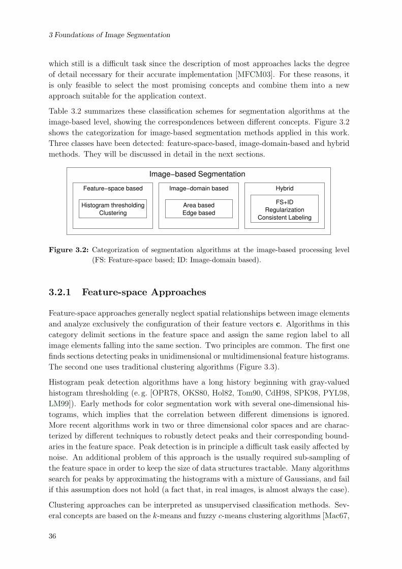
3 Foundations of Image Segmentation
which still is a difficult task since the description of most approaches lacks the degree
of detail necessary for their accurate implementation [MFCM03]. For these reasons, it
is only feasible to select the most promising concepts and combine them into a new
approach suitable for the application context.
Table 3.2 summarizes these classification schemes for segmentation algorithms at the
image-based level, showing the correspondences between different concepts. Figure 3.2
shows the categorization for image-based segmentation methods applied in this work.
Three classes have been detected: feature-space-based, image-domain-based and hybrid
methods. They will be discussed in detail in the next sections.
HybridImage−domain basedFeature−space based
Histogram thresholdingClustering
Area basedEdge based
Consistent LabelingRegularization
Image−based Segmentation
FS+ID
Figure 3.2: Categorization of segmentation algorithms at the image-based processing level(FS: Feature-space based; ID: Image-domain based).
3.2.1 Feature-space Approaches
Feature-space approaches generally neglect spatial relationships between image elements
and analyze exclusively the configuration of their feature vectors c. Algorithms in this
category delimit sections in the feature space and assign the same region label to all
image elements falling into the same section. Two principles are common. The first one
finds sections detecting peaks in unidimensional or multidimensional feature histograms.
The second one uses traditional clustering algorithms (Figure 3.3).
Histogram peak detection algorithms have a long history beginning with gray-valued
histogram thresholding (e. g. [OPR78, OKS80, Hol82, Tom90, CdH98, SPK98, PYL98,
LM99]). Early methods for color segmentation work with several one-dimensional his-
tograms, which implies that the correlation between different dimensions is ignored.
More recent algorithms work in two or three dimensional color spaces and are charac-
terized by different techniques to robustly detect peaks and their corresponding bound-
aries in the feature space. Peak detection is in principle a difficult task easily affected by
noise. An additional problem of this approach is the usually required sub-sampling of
the feature space in order to keep the size of data structures tractable. Many algorithms
search for peaks by approximating the histograms with a mixture of Gaussians, and fail
if this assumption does not hold (a fact that, in real images, is almost always the case).
Clustering approaches can be interpreted as unsupervised classification methods. Sev-
eral concepts are based on the k-means and fuzzy c-means clustering algorithms [Mac67,
36

3.2 Image-based Segmentation
(a)
0
2000
4000
6000
8000
10000
0 0.2 0.4 0.6 0.8 1
Num
ber o
f Pix
els
Intensity
Intensity Histogram
0
2000
4000
6000
8000
10000
R Y G C B M
Num
ber o
f Pix
els
Hue
Hue Histogram
(b) (c)
RY
GC
BM
0 0.2 0.4 0.6 0.8 1
Hue
Intensity
Histogram Cells
RY
GC
BM
0 0.2 0.4 0.6 0.8 1
Hue
Intensity
Clusters
RY
GC
BM
0 0.2 0.4 0.6 0.8 1
Hue
Intensity
Clusters
(d) (e)
(f) (g) (h)
Figure 3.3: Feature-space-based segmentation. (a) Original image. Histogram-based meth-ods usually compute one dimensional histograms (b,c) and detect peaks and theirregions, making a regular partition of the feature space (d). Clustering algorithmsdetect clusters in the feature space (e). The results for histogram-based (f) andclustering-based (g) segmentation differ. Details are better retained with cluster-ing algorithms but a “noisy” mask is produced that needs some post-processing.The result using a mean-shift based segmentation is shown in (h).
37

3 Foundations of Image Segmentation
DHS01] applied on different color and texture spaces [MG93, RTT95, WH97, LGL97,
ZW00, YK01]. One of the major drawbacks of the original clustering methods is that
the number of clusters (k or c) must be known a-priori. Several heuristics have been sug-
gested to compute k automatically based on some image statistics (e. g. [RT99, YK01]).
To achieve illumination invariance, a modification to the k-means algorithm is suggested
in [WTD01] to use an angular distance in a zero-mean color space instead of the classical
euclidean distance.
Special attention deserves the work of Comaniciu and Meer [CM02] (Figure 3.3h). They
use a mean-shift procedure to detect clusters in the feature space. The only required
parameter is the desired bandwidth of the kernel used to compute the modes of the
unknown underlying probability density distribution. In [Com03], the author also in-
troduces a method to automatically detect different bandwidths from the data for each
section of the feature space. The major drawback of this concept is its computational
cost. Even if it is relatively fast compared with some statistical relaxation methods, it
is much slower than simpler k-means clustering-based approaches. More details about
this concept are presented in Chapter 4.
3.2.2 Image-domain-based Approaches
Another way to cope with the image-based segmentation problem is to compare the
feature values of each pixel in the image-domain, i. e. pixels are compared within prede-
fined spatial neighborhoods. Two major groups of algorithms can be identified: the first
one defines regions through the feature similarity between their elements (area-based
approaches). The second one identifies feature discontinuities as boundaries between
homogeneous regions (edge-based approaches). Many modern segmentation strategies
try to satisfy both concepts simultaneously [MFCM03].
Area-based Approaches
Traditional area-based techniques utilize one of two principles: region growing or split-
and-merge. Region growing methods assume the existence of some seed -points, to which
adjacent pixels will be added if they fulfill a homogeneity criterion [AK88, Jai89, GW92,
BP97, TB97, SHB99]. The main advantage of these methods is the creation of spatially
connected and compact regions, which contrast with the usually noisy image partition
obtained with pure feature-based segmentation approaches. They are frequently applied
to separate one single homogeneous object (e. g. background, Figure 3.4) from the rest
of the image, but using several seeds positioned at different objects it is also possible
to perform more sophisticated segmentations [BP97]. The required seed selection is a
subtask of this approach, which can be solved by taking advantage of clustering methods
or morphological operations, among others [LM01, FYEA01].
Split-and-merge algorithms first over-partition an image into small regions, followed by
38

3.2 Image-based Segmentation
(a) (b)
Figure 3.4: Example for a simple region growing segmentation result. Four seeds at thecorners of the original image (a) served as starting point for the growing, whichdetects background only (b).
a merging stage that joins adjacent regions still fulfilling the homogeneity predicate
(Figure 3.5). Quad-trees, Delauney triangulation or Voronoi diagrams belong to the
tessellation techniques habitually employed to split the image [PH95, GS97a, SHB99,
LM01]. The comparison between adjacent regions can use simple statistics or can be
based on more elaborated mathematical models, like Markov Random Fields (MRF),
which also permit merging regions of similar texture [PH95].
(a) (b) (c)
Figure 3.5: Example of a split-and-merge segmentation method. The original image (a) issplit using a quad-tree technique (b) followed by a merge-stage, where similarregions melt (c).
Other area-based methods employ a graph-representation of the image, where pixel sim-
ilarities are coded as weights of the edges between the graph nodes (image pixels). For
example Shi and Malik [SM00] introduce a technique called normalized cuts to opti-
mally split the image into two sub-graphs that maximize the intra-subgraph similarity
and simultaneously maximize the inter-subgraph dissimilarity. Yu [Yu03] enhanced the
method to optimally split an image into k regions. Barbu and Zhu [BZ03] suggest the
use of the Swendsen-Wang cuts instead. The opposite approach is followed by Haris et
al. [HEMK98], who utilize a graph structure to decide which regions need to be merged,
instead of how the image should be split.
39

3 Foundations of Image Segmentation
Edge-based Approaches
Edges are discontinuities in the feature characteristics (e. g. intensity) of adjacent pixels.
Their detection is just the first stage of any edge-based segmentation approach. Further
processing is necessary in order to provide a valid segmentation as stated by Definition 9.
Since standard detectors like Marr and Hildreth’s [MH80], Canny’s [Can86] or SUSAN
[SB95] usually leave some gaps between object boundaries, some mechanisms are re-
quired to fill them appropriately (Figure 3.6). This task can be solved combining the
(a) (b) (c)
Figure 3.6: Examples of edge detection. The original image (a) has been analyzed with (b)the Canny algorithm and (c) the SUSAN algorithm. Some gaps remaining in thedetected edges have been marked with circles.
edge detection with an area-based or a feature-space-based approach [ZL98]. Recently
a new generation of edge detectors based on the Earth Mover’s Distance have been pro-
posed [MR98, RT01]. They show a better performance due to their capability to detect
junctions and corners. However, since the computational load required to analyze a
single pixel is relatively high, their throughput is very low compared with traditional
techniques.
Morphological watershed segmentation [VS91, SP00, RM00] can also be categorized as
an edge-based approach (Figure 3.7). They work on a topographical edgeness map,
where the probability of a pixel to be an edge is modeled by its altitude. A “flooding”
step begins which fills the valleys with water. The watershed lines are detected when
the water of two different valleys encounters. Relatively efficient algorithms exist to
compute the watershed lines and catchment basins, but they are sensitive to noise and
tend to over-partition the images. The available techniques work on gray-valued images
obtained usually as the gradient of the intensity. Chapter 4 presents more details in
these respects.
Another family of edge-based algorithms are the active contours (also known as snakes)
[KWT88, Ron94, CTCG95, GL97, XP98, CRB99, IV00]. They are frequently used in
medical applications, where, due to the imaging techniques employed, noise is not neg-
ligible. A parametrical curve model for the boundary of an object is assumed to be
known, leaving the algorithms with the task of determining its parameters. This is
accomplished by minimizing a functional, which depends on both an external image
40

3.2 Image-based Segmentation
(a) (b) (c)
Figure 3.7: Example of watershed segmentation. The gradient of the original image (a) hasbeen depicted in (b). It is used as a topological map to find basins and watersheds(c).
energy that tries to attract the active contour and an internal contour energy that hin-
ders contour deformation. The convergence of the curves to one specific object depends
on the initialization and makes them suitable for interactive segmentation applications.
Active contours are not suitable for object retrieval applications, as they have been con-
ceived to detect single objects projected into one connected region. Thus, the detection
of several (maybe overlapping) objects in complex scenes is, with them, a difficult task.
3.2.3 Hybrid Methods
All previous methods have intrinsic disadvantages that can be partially compensated
by combining different techniques. For instance, clustering methods detect homoge-
neous regions in the feature space. However, since spatial relationships are ignored,
the region boundaries in the image-domain are highly irregular. The incorporation of
image-domain concepts can provide a solution to this problem [GG91]. Further ex-
amples for this family of hybrid strategies include the combination of active contours,
region growing and a Bayesian probabilistic framework [ZY96], the use of both edge
detection and region growing stages [STB96, Sin97, ZL98], a combination of watersheds
and region growing [HEMK98], and the interaction of an adaptive clustering algorithm
with a Markov Random Field which provides some spatial constraints [Pap92, Che03].
A detailed review of techniques to combine area-based and edge-based approaches can
be found in [MFCM03].
Besides these rather classical edge and area-based techniques, another group of algo-
rithms exists based on a more theoretical statement. They try to find edges and ho-
mogeneous regions simultaneously. Two groups can be distinguished: regularization
methods and consistent labeling methods [MLT00].
As already stated in Chapter 2, regularization means to restore the well-posedness of
an ill-posed problem by constraining the number of possible solutions. Let the image Ibe the result of a two-dimensional projection operation F of a scene S, i. e. I = F (S).
41
3 Foundations of Image Segmentation
The general vision task is the inverse function F−1 that infers which scene S can be the
causal stimulus for a given image I: S = F−1(I). The regularization theory restricts
the space of acceptable solutions by choosing the scene S that minimizes an appropriate
functional G(S). The constrains are given through the functional G(S) and a norm ‖·‖.The solution can be found using one of following three methods [MLT00]:
• find S such that the constraint ‖G(S)‖ < C is satisfied and S best approximates
the data, i. e. min ‖F (S)− I‖, or
• find S such that it is close enough to the data and is the most “regular”, i. e.
‖F (S)− I‖ ≤ C, min ‖G(S)‖, or
• find S that minimizes a weighted sum of the closeness to the data and the degree
of regularization, i. e. min(‖F (S)− I‖2 + λ‖G(S)‖2).
A stochastic formulation of the regularization problem uses the Bayesian rule, and states
the problem as the selection of the most likely model of the scene S given the image I:
P (S|I) =P (I|S)P (S)
P (I)
The likelihood P (I|S) corresponds to the term ‖F (S)−I‖ and the a-priori probability
P (S) corresponds to the regularization term ‖G(S)‖.
The same framework is used for segmentation replacing the scene S by a segmenta-
tion model S, i. e. a regularization-based segmentation method tries to find the most
probable segmentation for a given image. Searching for the optimal model requires
relatively expensive algorithms, like simulated annealing [GG84] or expectation maxi-
mization [BS94]. Even if these algorithms find an optimal or almost optimal solution of
the functional minimization task, this fact does not ensure that the result is better suited
for an application than a partition obtained with more simple and faster approaches.
Regularization methods can incorporate some contextual knowledge in the specification
of the functional G(S) to improve their results. However, the possible degrees of freedom
are relatively limited in order to keep the algorithmic complexity tractable.
Consistent labeling algorithms try to assign a discrete or continuous set of labels to a
set of regions under consideration of a compatibility criterion. Markov Random Fields
are frequently used for a stochastic labeling approach [GG84, PH95, DM01] together
with a maximum a-posteriori (MAP) optimization approach, similar to the previously
mentioned stochastic regularization formulation. Other optimization methods besides
the maximum a-posteriori estimation are possible. For example, maximization of the
posterior marginals [MMP87] or sequential maximum a-posteriori [BS94] are suggested
to cope with different unfavorable issues of the MAP estimation. This kind of algo-
rithms are employed in the segmentation of textured images [PH95], due to their ability
to stochastically model the content of non-homogeneous regions. For the current ap-
plication context these methods are rather unsuitable as a consequence of their high
computational costs.
42

3.2 Image-based Segmentation
3.2.4 Discussion
Skarbek and Koschan [SK94] conclude their survey with several important remarks. The
most relevant for the current context follow:
1. Color images allow more reliable image segmentation than gray scale images.
2. General purpose algorithms are not robust and usually not algorithmically effi-
cient.
3. As a rule, authors ignore comparing their novel ideas with existing ones.
4. As a rule, authors do not estimate the algorithmic complexity of their methods.
5. Most clearly specified, algorithmically efficient, and robust are methods designed
for the particular small applications assuming well specified knowledge about the
scene.
6. It seems that separating processes for region segmentation and for object recog-
nition is the reason of failure of general purpose segmentation algorithms. This is
in agreement with the previously mentioned thesis of D. Forsyth [For99].
7. All techniques are dependent on parameters, constants and thresholds which are
usually fixed on the basis of few experiments. Tuning and adapting of parameters
is rarely performed.
Many of these conclusions are interrelated. General purpose algorithms completely ig-
nore contextual information, and strongly depend on the choice of a proper parameter
set. Small modifications in these parameters can substantially change the results. Al-
gorithms developed for specific applications have a better behavior, since the additional
knowledge can be used to force the desired results focusing on relevant information only.
The limited number of scene configurations can also be exploited to design faster algo-
rithms. It is pertinent to remark that the contextual knowledge is often only used in
the selection of an algorithm or its parameters [Che03]. This implicit embedment of
knowledge in the algorithms can not replace the explicit use of information gained from
the scene itself during the recognition process.
The problem pointed out by Conclusion 3 persists. Most authors only compare their
work with strongly related algorithms, ignoring the capabilities of other segmentation
classes. It is frequently unclear, if the results presented for an algorithm A could also be
provided with another parameter choice of algorithm B. The lack of direct comparison
possibilities, like the availability of source code or standard testbeds, makes the problem
even worse. It seems there is no short term solution to these problems.
Not only the theoretical complexity of the algorithms is neglected, but also their effi-
ciency: how large are the constants in the complexity analysis really? For the current
retrieval application this issue is of great importance, since the segmentation task usu-
ally determines how long a user has to wait for a result and how long it takes to train the
retrieval system. Some authors mention as advantage of their algorithms the efficient
implementation for parallel computers, however, since common computer architectures
still use just a few processors, such concepts would be too slow for real applications.
43

3 Foundations of Image Segmentation
Others stress the advantages of non-iterative algorithms neglecting the fact that iterative
ones are not necessarily slower. Table 3.3 summarizes advantages and disadvantages of
the discussed image-based segmentation categories.
Within the current three-staged segmentation framework, the image-based subtask does
not need to provide a complete solution to be useful for the subsequent recognition
modules. Instead, only a partial result is necessary, which will be further processed,
taking into account additional knowledge. From an algorithmic perspective it is easier
to merge smaller regions than to split an existent one, since for the second case it is
necessary to decide where the region could be properly split. For this reason, the image-
based segmentation level has to produce an over-segmentation, i. e. a partition of the
image for which |L(Ri)| is still 1 but n = |S| is not necessarily minimal.
Under the assumption that surfaces of real objects are described by piecewise homoge-
neous regions, any of the above mentioned algorithms could be used in the implementa-
tion of an image-based segmentation stage, with a few exceptions: Active contours are
unsuitable in all those cases, where more than one object per image can be expected and
the manual supervision of the segmentation process is not affordable. Both conditions
are present in the context of object retrieval. Techniques based on Markov Random
Fields and related stochastic principles are computationally expensive. Furthermore,
controlling the degree of over-segmentation with these algorithms is a difficult task,
since they inherently search for a global optimal solution in a more or less unpredictable
way (e. g. simulated annealing). The possibility to obtain a slightly better segmentation
does not compensate for the difficulties in parameter selection and the time complexity
issues of these algorithms. Chapter 4 compares in detail the most promising techniques
for the current context and describes the proposed approach for the image-based seg-
mentation stage.
3.3 Surface-based Segmentation
Even though recognition approaches based on local descriptors claim to work without
the need of any segmentation, they usually fail in the recognition of objects with similar
local structures. Consequently, a hybrid recognition system relying on both local and
holistic concepts is a preferable approach. In order to train a retrieval system, all images
still need to be segmented to make the extraction of global descriptors possible. This
has to be achieved without knowledge about each object in particular, since at the
training stage the objects are still unknown. However, all information available about
the scene setting can be taken into account. Surface-based segmentation algorithms
must be designed to fulfill this requirements. For the recognition stage, it has to find
homogeneous surfaces of objects, employing knowledge about physical properties of
materials, perceptual grouping concepts, and all available information about possible
scene configurations.
44

3.3 Surface-based Segmentation
Table 3.3: Comparison of image-based segmentation techniques
Feat
ure-
Spac
e
+ Detection of homogeneity in a global context.− Spatial relationship between pixels is ignored.
Clu
ster
ing
+ Simultaneous consideration of all dimensions of the feature space.+ Clustering-based on density estimation detects clusters of arbitrary shape.+ Relatively efficient algorithms exist.− Size or number of clusters must be known a-priori.− Density estimators require a bandwidth or a complex algorithm to compute
it from the data.
His
togr
am
+ Multiple 1D histogram methods are computationally inexpensive.− Noise sensitive.− 1D approaches ignore correlation between different feature space dimensions.− Models used to detect histogram peaks (e. g. Gaussians) usually do not cor-
rectly match the real distributions.
Imag
edo
mai
n
Are
a-ba
sed
Reg
.gr
owin
g + Creation of connected compact regions.+ Fast algorithms available.+ Suitable for figure/ground segmentation of convex compact objects.− Selection of seeds can be a complex problem.− Inappropriate for segmentation of multiple objects.
Sp.&
Mer
ge + Fast algorithms available.+ Suitable for texture segmentation.− Traditional tessellation mechanisms produce too coarse spatial quanti-
zation artifacts.
Gra
ph
+ Provide mechanisms to maximize intra-graph similarity and minimizeinter-graph dissimilarity.
− Computational expensive, especially if only one pixel per node is used.
Edg
e-ba
sed
+ Borders between regions are usually smoother and more accurate than theborders detected with feature-space-based methods.
− Edge detectors usually leave gaps in region borders, making the detection ofclosed regions difficult.
Wat
ersh
ed + Detection of closed contours.+ Relatively efficient algorithms available.− Highly sensitive to noise and parameter changes.− Image is easily over-segmented.
A.C
onto
urs + Robust to noise (especially appropriate for medical applications).
− Applicable for only one object in a homogeneous background.− Difficult automatic initialization of the contour.− Not suitable for unsupervised segmentation.
Hyb
rid
+ Combination of several methods can be appropriately adapted to the needsof each application.
+ Complex models allow segmentation of textures.− High computational cost of stochastic modeling methods.
45

3 Foundations of Image Segmentation
The image-based stage detected homogeneous regions with the help of a homogeneity
predicate HI , which exclusively took into account the feature vector c of each image
element and its spatial configuration p. Surface-based segmentation follows a similar
definition (Definition 10), but with a different homogeneity predicate HS that integrates
knowledge about the physical world in general and the application in particular.
Definition 10 (Surface-based segmentation) The surface-based segmentation SS of
an image I is a partition of I that satisfies for each region Ri ∈ SS, HS(Ri) = true,
and HS(Ri ∪Rj) = false for A(Ri,Rj) = true.
Knowledge about the physical image formation process has proven to be helpful for the
segmentation of object surfaces, and all approaches explicitely incorporating such knowl-
edge have been categorized in several surveys as physics-based approaches [SK94, LM01].
The severe and unrealistic restrictions imposed on object materials and illumination
conditions (usually Lambertian surfaces and diffuse illumination) constitute the major
drawback of most existent physics-based algorithms. A further problem has been the
relatively high complexity of the algorithms necessary to manage multiple hypotheses.
Nevertheless, this class of techniques has provided useful hints to cope, at least partially,
with shadows and highlights detection [GS97b, MS97, BF00, SCE01].
Methods to include additional application knowledge into the segmentation process are
very specific for each problem. For example, a typical solution for figure/ground segmen-
tation, i. e. the problem of separating one region of interest from the rest of the image, is
to assume color models for the objects as a-priori information (see for example [BC91]
for lichens analysis, [LC91] for road segmentation and [JR99] for skin segmentation).
Applications with a fixed camera use that fact to detect as background all motionless
regions and as objects only those pixels deviating from the background model generated
in the process [EHD99]. The incorporation of more sophisticated knowledge is also pos-
sible. In [ABA02] the authors introduce a segmentation approach to separate the user’s
hand, background and object by combining several high-level cues in a probabilistic
framework. The basic idea has been integrated into the current framework.
Research in the field of perceptual grouping tries to reconstruct salient shapes from
primitive low-level features like edges or line segments [WB86, AMP+97, AL98, DMM00,
FR00, DMM03, ES03, Fel03]. Since its final goal is to detect perceptually relevant visual
entities, it is somewhat associated with the general segmentation task. Forsyth and
Ponce [FP03] even regard perceptual grouping as another form of segmentation.
Medioni et al. [MLT00] introduce a segmentation concept that can also be regarded as
a perceptual grouping approach. A tensor voting mechanism allows the detection of
surface boundaries using a saliency measure, which states how conspicuous an edge is in
the global context of the image. This method requires as input an edge map from the
image-based module. It relies on the perceptual grouping principle of continuity [Pal99]
to detect the most salient edges and to fill the gaps between them in a perceptually
consistent manner. Even if the algorithm is non-iterative, the tensor voting is a relatively
46

3.4 Object-based Segmentation
time consuming operation. Similar to edge-based segmentation approaches, a region
detection stage has to be appended to the saliency analysis. Figure 3.8 shows an example
of saliency and junction maps computed with this approach. The darker a pixel the more
conspicuous it is as edge or as junction, respectively. The general segmentation method is
similar to edge-based approaches at the image-based processing level, with the difference
that a fundamental concept in the algorithm is the physics-based supposition that all
edges belonging to object surfaces have to be continuous. Edge-based approaches just
search for discontinuities in the feature vector of adjacent pixels.
(a) (b) (c)
Figure 3.8: Example of edge and junction saliency as proposed by Medioni et al. . (a) Edgemap used as input. (b) Edge saliency map. (c) Junction saliency map.
In this work, perceptual grouping and segmentation are considered as independent tasks,
since the results of a perceptual grouping operation are not necessarily an image parti-
tion.
3.4 Object-based Segmentation
One of the oldest approaches to object-based segmentation is template matching [SHB99],
where an a-priori known object view (the template) is searched within the image. The
simplest methods, based on correlation or comparable matching operators, can only de-
termine the position of the template. A recent development in this area is presented in
[BU02]. Partial templates are used to detect object parts of a given class (e. g. horses),
even though the global appearance of the objects in the test images differs from the
learned material. The methods become more complex and time consuming if further
parameters like orientation or scale need to be estimated. Strongly related to this
approach are the object-centered three-dimensional object recognition techniques (see
Section 2.2.5). Many of them are the natural extension of two-dimensional template
matching techniques to the three-dimensional space. Since the number of objects and
their orientation in an image are unknown in the current application, the search space
for matching approaches becomes intractable.
Only in recent years interest has been shown in exploring the possible interaction be-
tween recognition and segmentation beyond the direct use of shape or image templates.
47

3 Foundations of Image Segmentation
One of the first works to combine segmentation with knowledge about the objects is
[LS97]. The image-based stage executes an over-segmentation using a feature-space-
based approach. Shape models of fruits are then used to select the best region grouping
among different hypotheses. This method is however not well suited for object retrieval
applications, since it is only efficient if all objects in the image are a-priori known,
making a preliminar object detection stage necessary.
Peng and Bhanu [PB98] introduce a concept to adjust the segmentation parameters
based on final recognition results. Here, the behavior of the image-based segmentation
task is modified following a reinforcement-learning concept: the success or failure of
the recognition has an effect on how the segmentation parameters have to be modified.
The lack of explicit surface-based or object-based stages makes the segmentation results
relatively unstable.
Chella et al. [CGI+99] use a symmetry measure to detect salient points in an image.
These allow to find contours of relevant objects in the scene by means of a snake. The
detected objects are compared with a set of prototypes employing also a symmetry-
based measure. The approach suffers from all inconveniences of active contours, i. e. the
risk to stay at a local minimum and the difficulty to detect several close-lying objects.
The main advantage of the snakes in this context resides in their properties to track
already detected objects.
A proposal for integration of object recognition, segmentation, localization and tracking
within a probabilistic framework gives von Wichert [vW01]. The idea is very similar
to local-feature recognition methods extended to the temporal dimension to accomplish
also a tracking task. This is achieved with the condensation algorithm of Isard and Blake
[IB98]. Their method cannot model object rotations. Its capabilities were demonstrated
with a single object and its applicability to much larger object sets is yet unclear. Rather
than an image segmentation, in the sense adopted here, they perform a detection task,
where only a rectangular bounding box around the object is found. This coarse detection
is inappropriate for the generation of global object descriptors.
Yu introduces in her work [Yu03] an extension of the normalized cuts concept [SM97,
SM00] to detect not two, but k parts in an image, optionally involving the general
perceptual grouping concepts of repulsion and attraction, or even specific knowledge
about the object appearances. This approach is promising as it finds in polynomial
time a nearly optimal solution for a known NP complete problem [Coo98]. However,
some drawbacks make the general idea inappropriate for the current application: it
requires the number k of regions for the segmentation as input parameter, the extensions
for object-based segmentation allow only one object in the image at a time, and the
eigenvector-based computation takes from half a minute (image-based stage) to several
minutes (object-based stage) in a 1GHz PC, which lie beyond tolerable times for an
interactive system.
Tu et al. [TCYZ03] also use a probabilistic framework to determine which models of
48

3.5 Segmentation in Current Object Recognition Systems
faces, text and generic regions can generate a given image with maximum a-posteriori
probability. The approach becomes prohibitive for a greater number of objects. Another
detection algorithm based on knowledge of face and car appearances is given in [SK00].
3.5 Segmentation in Current Object Recognition Sys-
tems
In the literature of object recognition it is frequently assumed that training material
is somehow pre-segmented. Even if not much information is given about the utilized
segmentation technique, an informed assumption can be taken based on the image sets
used. The COIL Image Database [NNM96] (or part of it) is employed in many ex-
periments. Additional images showing similar scene configurations are also commonly
included in the object sets: i. e. a single object on a black background. Depending on
the recognition approach, either the objects can be isolated using simple image-based
techniques or the descriptors extracted for recognition can be designed to ignore back-
ground information (for example, in a color histogram the bins corresponding to “black”
can be set to zero).
In Pope’s Oliver system [Pop95, PL96] one appearance model is computed for each
object, taking into account different training images. The model is based on local
descriptors constructed from line and curve segments. It also administrates additional
spatial information to allow the recognition stage to match image features and object
models. Since all descriptors are based on edges, segmentation can become unnecessary if
the training images exhibit an edgeless background. The introduced concept is specially
designed to cope with cluttered scenes. Even though object models cluster similar
descriptors from different views, it is unclear how much space would be required to
recognize a larger set of objects, since the author only presents experiments with one
single object at a time. Training one object model took more than 19 hours 1995,
where 30 seconds were required to extract the features from one image. Considering the
drastic improvements in computational performance of the last years and optimistically
supposing a factor of twenty between the execution times, the training for a set of 200
elements would nowadays take about one week!
Dypers at MIT [SC97] is a recognition system designed to be a component of wearable
computers. The recognition approach is fast (the authors report ten recognitions per
second). Multidimensional histograms model viewpoints and scalings of one object. This
method is not appropriate to distinguish between several similar items, but it has already
been applied to discern between 100 different objects. The detection of more than one
object in an image is achieved with help of a probabilistic voting mechanism. It estimates
the probability that a given object is present in the image, but not exactly where (this
is called recognition without correspondence). No information is given about how it is
ensured, for the training stage, that exclusively the object in an image is considered
49

3 Foundations of Image Segmentation
Table 3.4: Segmentation in available object recognition systems
Pope [Pop95] Schiele&Crowley
[SC97]
Lowe [Low03]
System Oliver Dypers —
Descriptor local local local
Object set size 1 or 2 103 varied 2 or 4
Background (train) homogeneous suppressed homogeneous
Segmentation (train) not required pre-segmented not required
Background (test) cluttered cluttered cluttered
Segmentation (test) not required not required not required
Objects/image 1 object several objects several objects
Localization yes no yes
to compute the histograms. From the images it can be guessed that a homogeneous
background is assumed for the training material, which will have no effect in the gradient-
based descriptors. Additionally, many other training images do not need to be segmented
as they are entirely occupied with a part of the whole object.
Lowe’s recognition approach [Low03] is a further development of the system in [PL96].
Each object is modeled as a set of images and each image is described by a set of many
local descriptors. These descriptors are computed for salient locations, i. e. conspicu-
ous image parts that can be robustly detected even if the object is rotated, scaled or
translated in the image plane. The recognition is achieved through a voting mechanism
that considers all local descriptors detected in the test image and a nearest neighbor
classifier. The result is improved in a verification stage, where all descriptors found are
used to compute the affine transformation that best maps the winner training image
onto the current test one. The shown experiments, involving two or three objects in a
scene, exhibit the usual configuration of works dealing with local descriptors: all objects
are relatively easy to be distinguished from each other and from the background, but
work well in cluttered scenes. This approach will be improved in Chapter 6 to control
part of the object-based segmentation.
The recognition technique followed by Yu [Yu03] is integrated within the segmentation
task. Salient locations are detected with a technique explained in [Mah02]. An optimal
distance measure is used to compute a matching score between those locations and the
training data. Finally, a graph representation is computed from these scores together
with a similarity measure between pixel features. The normalized cuts technique is then
employed to produce a figure/ground segmentation.
Seemore [Mel97] was one of the first systems combining different types of global features.
It was able to recognize a set of more than 100 objects. The segmentation problem is
however ignored. It is assumed that training and test images show a black background.
50

3.5 Segmentation in Current Object Recognition Systems
Table 3.4: cont.
Yu [Yu03] Mel [Mel97] Kummert et
al. [KFSB98]
Alvarado et al.
[ADW01]
Wickel et al.
[WAD+02]
— Seemore — Axon2 Axiom
local global global global global
15 varied 100 varied ∼15 blocks 202 toys 202 toys,
47 blocks
suppressed black homogeneous black black
pre-segmented pre-segmented region growing region growing hybrid
cluttered black homogeneous black black
graph cuts not required region growing region growing hybrid
1 object† 1 object several objects 1 object 1 object†
yes no yes yes yes
† More objects can be recognized if they do not overlap.
Kummert et al. [KFSB98] introduce a region growing segmentation for their recognition
system. Training and test images are taken under the same scene configuration: a ho-
mogeneous background holds the object set consisting of colored blocks of a construction
kit. Each block type has a different color, a fact that simplifies the detection of the re-
quired seeds for the growing algorithm. This scene setting permits the robust detection
of all present objects, making their recognition possible. The authors concentrate their
research in the recognition of aggregates, i. e. of complex objects constructed with the
basic building units detected in the segmentation.
Axon2 [ADW01] recognizes 202 plush animals using global color and texture descriptors.
The major achievement of this system is its ability to distinguish many similar objects,
even if some of them are deformable and/or articulated (see Section 2.2.2). This task
can only be accomplished with a robust segmentation and the use of global descriptors.
Here, a black background was also assumed. The system users can hold the objects
with their hands, but wearing a black glove; their fingers, therefore, occlude the objects
partially. This configuration permits to easily isolate an object by means of a region
growing approach. Axiom [WAD+02] is a further development of the latter project.
It is also capable of recognizing real objects learned from computer generated images.
The background of the scenes is still black, but the user is allowed to hold the objects
with his bare hand. A hybrid segmentation algorithm was designed to separate hand,
background, and object, even if the latter is also skin-colored [ABA02]. This kind
of segmentation is only possible by incorporating specific knowledge about the scene
configuration (e. g. the hand will be found at the bottom of the image).
Table 3.4 summarizes the information available for the eight previously described ob-
ject recognition systems, with focus on the role of segmentation. The time taken for a
recognition task is not given, since differences in the hardware platforms make a fair com-
51

3 Foundations of Image Segmentation
parison impossible. The recognition approaches are extremely different and concentrate
on different issues of the recognition problem. Local-based approaches pay attention to
the recognition of objects in cluttered scenes (e. g. [Pop95, Low03]). Analysis of larger
object sets, or sets with similar elements is rare. Global-based approaches concentrate
on the recognition of larger and more complex sets, but, as a rule, they require a re-
stricted scene setting to allow a robust segmentation. These fundamental differences
together with the substantial divergences between object sets hinder the comparison of
the recognition performances of all systems.
3.6 Framework for Segmentation in Object Retrieval
Applications
For practical retrieval applications it is desirable for a system to cope with both large
object sets and scenes containing one or more objects. All revised concepts focus on only
one of these issues: projects working with local features report successful recognition in
cluttered scenes, but only for very small object sets. On the other hand, research groups
using global features can already recognize one object from hundreds, but only in scene
settings with a single object. In order to exploit the advantages of both approaches,
the system architecture depicted in Figure 3.9 is proposed, which adopts the recurrent
structure described in Section 2.2.1.
SceneSetting
Knowledge
Knowledge ofObjects’ LocalAppearance
Knowledge ofObjects’ GlobalAppearance
Global DescriptorExtraction
Acquisition
Preprocessing
ClassificationLocal
Verification
ClassificationGlobal
Image−based
Object−basedSegmentation
ExtractionLocal Descriptor
Result
Surface−based
Figure 3.9: Segmentation framework within the object retrieval concept.
The main difference between previous recognition systems and this concept resides in
the interaction between recognition and segmentation modules. In contrast to the work
of Yu [Yu03], where segmentation and recognition are done in a single step, here a
52
3.7 Evaluation of Segmentation Algorithms
wrong initial assumption can be corrected as soon as more information is available. It is
this recurrent process what allows the implementation of the “paradoxical” recognition
operator L introduced in Definition 7.
An image taken from the camera is first preprocessed to obtain a minimal invariance
against scene transformations (like illumination) and reduce possible noise effects. Two
processing branches follow. The left branch of Figure 3.9 corresponds to a recognition
process based on global descriptors: segmentation, extraction of global descriptors and
classification. The right branch is a typical local-descriptor recognition system: local
descriptor extraction followed by the classification and verification. For simple scenes
and object sets it is still possible to ignore the interactions between both branches and
make use of the framework in a classical manner. For applications with several similar
objects in a scene, the proposed interaction is mandatory. The segmentation module
plays an intermediary role between both recognition approaches.
As previously mentioned, the segmentation task is split in three stages. In the first
one, the image is over-segmented considering only low-level information. This image-
based stage attempts to detect regions belonging to only one object. Since without any
additional knowledge it is impossible to ensure this condition, requests are accepted
to further split a region in case higher processing levels detect inconsistencies. The
surface-based stage uses knowledge about the specific scene settings to synthesize re-
gions encompassing object surfaces. The information is used to decide which regions
detected in the previous stage can be merged. After these initial processes, the object
identification labels still need to be assigned.
The local recognition approach generates several hypotheses in the classification of the
location descriptors. These hypotheses have to transfered to the regions detected in
the surface-based staged. The best hypotheses for region classification are given to the
object-based stage, which generates the segmentation results necessary for a verification
based on global descriptors. Inconsistencies detected in the process can be fed back into
the earlier modules.
The current concept keeps a modular structure, which allows to treat each problem
separately. Promising results from many research groups in the last quarter century can
be meaningfully employed at each corresponding level.
3.7 Evaluation of Segmentation Algorithms
No segmentation algorithm is generally applicable to all images and different algorithms
are not equally suitable for a particular application [PP93]. It is therefore necessary to
have objective mechanisms to evaluate a promising set of techniques in the context of
interest. Zhang [Zha96] proposed the categorization for evaluation methods depicted in
Figure 3.10.
53
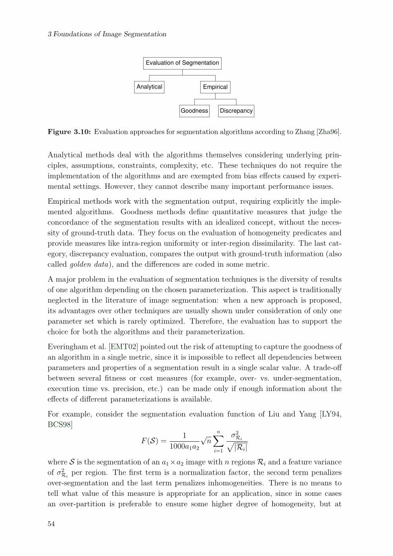
3 Foundations of Image Segmentation
Evaluation of Segmentation
Analytical Empirical
Goodness Discrepancy
Figure 3.10: Evaluation approaches for segmentation algorithms according to Zhang [Zha96].
Analytical methods deal with the algorithms themselves considering underlying prin-
ciples, assumptions, constraints, complexity, etc. These techniques do not require the
implementation of the algorithms and are exempted from bias effects caused by experi-
mental settings. However, they cannot describe many important performance issues.
Empirical methods work with the segmentation output, requiring explicitly the imple-
mented algorithms. Goodness methods define quantitative measures that judge the
concordance of the segmentation results with an idealized concept, without the neces-
sity of ground-truth data. They focus on the evaluation of homogeneity predicates and
provide measures like intra-region uniformity or inter-region dissimilarity. The last cat-
egory, discrepancy evaluation, compares the output with ground-truth information (also
called golden data), and the differences are coded in some metric.
A major problem in the evaluation of segmentation techniques is the diversity of results
of one algorithm depending on the chosen parameterization. This aspect is traditionally
neglected in the literature of image segmentation: when a new approach is proposed,
its advantages over other techniques are usually shown under consideration of only one
parameter set which is rarely optimized. Therefore, the evaluation has to support the
choice for both the algorithms and their parameterization.
Everingham et al. [EMT02] pointed out the risk of attempting to capture the goodness of
an algorithm in a single metric, since it is impossible to reflect all dependencies between
parameters and properties of a segmentation result in a single scalar value. A trade-off
between several fitness or cost measures (for example, over- vs. under-segmentation,
execution time vs. precision, etc.) can be made only if enough information about the
effects of different parameterizations is available.
For example, consider the segmentation evaluation function of Liu and Yang [LY94,
BCS98]
F (S) =1
1000a1a2
√n
n∑i=1
σ2Ri√|Ri|
where S is the segmentation of an a1×a2 image with n regions Ri and a feature variance
of σ2Ri
per region. The first term is a normalization factor, the second term penalizes
over-segmentation and the last term penalizes inhomogeneities. There is no means to
tell what value of this measure is appropriate for an application, since in some cases
an over-partition is preferable to ensure some higher degree of homogeneity, but at
54

3.7 Evaluation of Segmentation Algorithms
other times the opposite could be the better choice. A minimization of this function
finds only a more or less arbitrary balance between over-segmentation and homogeneity.
Furthermore, exactly the same metric value can be produced with different ratios of both
properties. In other words, it is possible to check that F (S1) < F (S2), but this does not
tell anything about the suitability of a specific parameterization of an algorithm for a
given application.
Evaluation through empirical discrepancy is associated with the generation of a reference
data set, including images and their ideal segmentation. The generation of such a golden
set is, depending on the application, a difficult and expensive task, since the evaluation
is significant only if the reference set is representative enough for the context. For this
reason, many authors opt to simply show one or two (more or less arbitrarily chosen)
examples, using only one set of parameters, and let the reader assess the quality of
the algorithm. Another related problem is the common expectation for semantically
meaningful results using an image-based algorithm. This is in part a consequence of
the unclear definition of the term segmentation (see Section 3.1): a task defined at a
low-level is expected to have the ability of guessing what objects look like. As already
stated, this is a hopeless venture, unless additional scene configuration restrictions and
object appearance knowledge are exploited.
In the context of object retrieval, the choice of a segmentation technique and its param-
eters will influence the final recognition results. For this reason, the recognition rate
seems to be a suitable empirical measure of the appropriateness of a segmentation tech-
nique in this context. However, it can only evaluate the whole segmentation concept,
making it difficult to assess the quality of the image-based and surface-based stages
separately.
In this work, the empirical evaluation approach suggested by Everingham et al. [EMT02]
has been chosen, which is based on multi-objective performance optimization. The
result of such an evaluation mechanism is a front, describing the “best” configurations
in a multi-dimensional fitness space. For a given trade-off between the single fitness
measures, this approach permits to objectively select not only the best algorithm, but
also the parameterization that produces the desired operating point.
3.7.1 Evaluation Using the Pareto Front
The aggregate fitness function F for an algorithm A with the parameterization u, eval-
uated using as reference the ground-truth data G is defined as
F (Au,G) = Φ(f1(Au,G), . . . , fn(Au,G)) (3.1)
with the individual fitness functions fi(Au,G) defined to increase monotonically with
the fitness of some particular aspect of the algorithm’s behavior. The functions fi span
a multidimensional fitness space, where each point represents the performance of an
algorithm parameterized with one point u in a parameter space. The general form of
55

3 Foundations of Image Segmentation
Φ is assumed unknown, but it has to increase monotonically with increasing values of
all fitness functions fi. This condition ensures that a point in the fitness space can
be considered fitter than all other points with smaller values in all dimensions. In
Figure 3.11, for example, the point q1 is fitter than the point q4 and all other elements
within the gray rectangle. In this context, the point q1 is said to dominate q4. All
non-dominated points in a set define the Pareto front of that set. In the example of
Figure 3.11 this front is defined by the points q1, q2 and q3. Choosing a parameterization
that is not in the Pareto front is always a bad choice, since there is another point on
the front with a better aggregate fitness.
PSfrag replacements
f1
f2
q1
q2
q3
q4
Figure 3.11: Pareto Front. The point q1 dominates the region highlighted with a gray rect-angle. Dashed lines delimit the dominated regions of the points q2, q3 and q4.The thick solid line represents the Pareto front for the four points.
The previous concepts can be expressed mathematically using the following equation:
P = 〈u ∈ PA, f(Au,G)〉 | ¬∃v ∈ PA : f(Av,G) f(Au,G) (3.2)
where P is the Pareto front, f is the vector of fitness functions [f1, . . . , fn]T and PA is
the parameter space of algorithm A. The partial ordering relation “” on f describes
the domination property and is defined as:
f(Av,G) f(Au,G) ⇔ ∀i : fi(Av,G) ≥ fi(Au,G) ∧ ∃i : fi(Av,G) > fi(Au,G) (3.3)
Any algorithm that finds the Pareto front for a set of fitness points implements equations
(3.2) and (3.3). Since the parameter space PA usually contains an infinite number of
parameterizations, the next problem consists in choosing a representative set of samples
from PA, such that their Pareto front can be assumed to be a reliable approximation of
the exact front extracted for the complete space.
A naive approach would be to regularly sample the values of each parameter, since
the number of necessary evaluations would increase exponentially with the number of
parameters. For example, an algorithm with seven parameters, each sampled five times,
would require 57 = 78125 evaluations. Since a single evaluation comprises computations
56

3.7 Evaluation of Segmentation Algorithms
for a complete data set, the time requirements for this naive approach are enormous,
even for such a coarse sampling of the parameter space.
Here, the proposal of Everingham et al. [EMT02] is followed and the multi-objective
evolutionary algorithm PESA (Pareto Envelope-based Selection Algorithm [CKO00]) is
used. This genetic approach suppresses the computation of useless parameterizations
and concentrates the analysis on those regions of the parameter space that provide
promising results. Even if this algorithm also samples the parameter space, the resolu-
tion used for each parameter is much higher (e. g. 256 or 1024 samples per parameter).
The number of evaluations required is then proportional to the number of bits used to
represent a parameterization. Appendix A describes PESA in detail.
All multi-objective optimization algorithms (including PESA) try to find the front con-
taining parameterizations best optimized for the reference data set G. Hence, it is
important in the evaluation to use representative data taken from the application con-
text.
3.7.2 Fitness Functions
For multi-objective evaluation algorithms several fitness functions have to be chosen. It
is possible to use both goodness and discrepancy measures. Independently of the final
selection, a reference data set G has to be chosen. In the case of image segmentation,
this set is defined as
G = 〈I i,S i〉 | i = 1 . . . n (3.4)
where S i is the ideal segmentation result for the reference image I i. The set GI =
I i | i = 1 . . . n contains all reference images. GS = S i | i = 1 . . . n is the set of all
reference segmentations.
Let Si be the segmentation result of an algorithm A parameterized with u for the
reference image I i:
Si = Au(I i). (3.5)
The goal is to find functions that evaluate the difference between Si and S i.
Seven fitness measures are used here to evaluate different aspects of the algorithms:
throughput, mean normalized region size, pixel-wise potential accuracy, region-wise po-
tential accuracy, region-wise information content, region integrity, and pixel-wise cer-
tainty. The first five have been originally proposed in [EMT02]. The last two have been
introduced in this work to cope with special properties of the different segmentation
stages. For the next definitions it is always assumed Rj ∈ Si and Rk ∈ S i. In accor-
dance to (3.5), the expression |Au(I i)| is used to represent the number of regions in the
partition found by the algorithm Au.
57

3 Foundations of Image Segmentation
Throughput Throughput for the segmentation is defined as the number of images
per second processed by an algorithm. Let t(Au(I i)) be the time required to compute
the segmentation for the image I i. Thus, the throughput is a goodness measure defined
as
ft(Au,GI) =|GI |∑
Ii∈GIt(Au(I i))
(3.6)
Mean Normalized Region Size The more regions in a partition the more processing
is necessary for its further analysis. Therefore, the number of regions found by a segmen-
tation algorithm is a simple cost function related with the degree of over-segmentation.
The reciprocal is used here as a fitness function. This goodness measure can also be
interpreted as the mean region size as a fraction of the entire image:
fr(Au,GI) =1
|GI |∑Ii∈GI
1
|Au(I i)|(3.7)
Pixel-wise Potential Accuracy This fitness function measures to what extent it
is possible to assign each region of the evaluated segmentation Si to a region of the
reference segmentation S i under the assumption of a perfect classifier. Therefore, the
pixel-wise potential accuracy is a good indicator for the appropriateness of an algorithm
for the image-based segmentation stage: if its value is too low, the next stages of the
segmentation framework, which play the role of real classifiers, will not be able to
produce correct segmentations.
The pixel-wise potential accuracy fpa is defined as
fpa(Au,G) =∑
〈Ii,Si〉∈G
∑Rj∈Si
∣∣P(Rj, Au(I i))∣∣
∑Rj∈Si
|Rj|(3.8)
where P(Rj,Si) denotes the set of pixels in Rj that also belong to the regions of Si that
most overlap with Rj:
P(Rj,Si) =
p | 〈p, ·〉 ∈ Rj ∧ 〈p, ·〉 ∈ Rk,Rk ∈ Si, j = arg max
l|Rk ∩
pRl|
(3.9)
The p-intersection of two regions Rk ∩pRl is defined as:
Rk ∩pRl = p | 〈p, ·〉 ∈ Rk ∩ q | 〈q, ·〉 ∈ Rl (3.10)
58

3.7 Evaluation of Segmentation Algorithms
Region-wise Potential Accuracy If the distribution of region sizes in the reference
data has a large variance, the pixel-wise potential accuracy will neglect the relevance of
small regions belonging probably to small objects. The region-wise potential accuracy
considers each reference region as equally important:
fra(Au,G) =
∑〈Ii,Si〉∈G
∑Rj∈Si
wra(Rj)
|Rj|∣∣P(Rj, Au(I i))
∣∣∑
〈Ii,Si〉∈G
∑Rj∈Si
wra(Rj)(3.11)
with the set P as defined above and the weighting function
wra(Rj) =
PRk∈Si
|Rk||Rj |
if |Rj| ≥ r
0 otherwise .(3.12)
The constant r removes very small regions from the analysis and is set here to 0.05%
of the image size. This discrepancy measure can be interpreted as the proportion of
each reference region that can be correctly identified given the segmentation result
Si = Au(I i). Everingham et al. called an equivalent function “object-wise potential
accuracy”. Their weighting function wra involves the reciprocal of a-priori probabilities
for the reference regions. Here, the reciprocal of the image percentage is used instead.
Since the reference segmentation not necessarily has to partition the image in regions
belonging to objects, the name “region-wise potential accuracy” is here preferred.
Region-wise Information Content Assuming that the information about a refer-
ence region is uniformly distributed among its pixels, this discrepancy function measures
the proportion of information of the reference region available within a single detected
region. It is defined as:
fri(Au,G) =
∑〈Ii,Si〉∈G
∑Rj∈Au(Ii)
wri(Rj)
|Rk=arg maxl |Rj∩pRl||
|Q(Rj,S i)|∑〈Ii,Si〉∈G
∑Rj∈Au(Ii)
wri(Rj)(3.13)
with the set Q representing the pixels of region Rj that also belong to the reference
region Rk most overlapped by Rj, i. e.
Q(Rj,S i) =
p | 〈p, ·〉 ∈ Rj ∧ 〈p, ·〉 ∈ Rk,Rk ∈ S i, k = arg max
l|Rj ∩
pRl|
(3.14)
and the weighting function
wri(Rj) =
1 if |Rk| ≥ r, k = arg maxl |Rj ∩pRl|
0 otherwise .(3.15)
59

3 Foundations of Image Segmentation
As in the previous fitness function, r suppresses the consideration of very small reference
regions.
The more regions are detected for a reference region, the smaller the fitness. This
function punishes over-segmentation, but it accepts under-segmentation. Therefore, fra
should not be used to evaluate partitions with a reduced number of regions: it even
assigns the best fitness to segmentations with a single region.
Region integrity The region integrity function is used here to measure the degree of
over- or under-segmentation of the reference regions:
fi(Au,G) =1
|G|∑
〈Ii,Si〉∈G
h
1
|S i|∑Rj∈Si
∣∣∣∣Rk | Rk ∈ Au(I i), j =arg maxl|Rk ∩
pRl|∣∣∣∣
(3.16)
with the weighting function h(x) = xe−x/e−1 chosen to be maximal at x = 1. The
argument of h in (3.16) is the mean value of the number of detected regions per reference
region. Under-segmentations lie below and over-segmentation above the optimal value of
one. The fitness function fi ignores, however, the exact position of the region boundaries.
Pixel-wise certainty The surface-based and object-based stages of the segmentation
always produce partitions of low cardinality. Many of the previous measures have a
discrete nature that cannot properly distinguish between small differences of the pa-
rameterizations. However, these later stages can also produce additional information
that describe the certainty with which each pixel has been assigned to its label or class.
If this information is available, it can also be employed as a goodness measure in the
parameter optimization. Let p(pk|Au(I i)) denote the certainty with which the segmen-
tation algorithm Au assigns the pixel at pk to its label. The pixel certainty is then
defined as
fce(Au,GI) =
∑Ii∈GI
∑Ri∈Au(Ii)
∑〈pk,·〉∈Ri
p(pk|Au(I i))∑Ii∈GI
|Au(I i)|, (3.17)
which is the mean value of the certainty for all pixels in the reference set.
These seven fitness functions are used in the next chapters to evaluate the proposed
concepts in the context of object retrieval.
60

Chapter 4
Image-based Segmentation
The goal of the image-based segmentation stage is to partition the image in regions
that belong exclusively to one object. Since at this early processing stage there is still
no information available about the objects or the scene, it can only be assumed that
the surfaces of the objects are homogeneous or piecewise homogeneous and that the
boundaries between them can be detected using low-level features.
The homogeneity predicate HI(Ri) used in Definition 9 has to be chosen to reject every
small variation in the image space that can be caused by boundaries between objects
or surfaces. In the current framework, the final goal of the image-based stage is to
efficiently find a partition SI that maximizes the probability for |L(Ri)| = 1. The
resulting over-segmentation is given to the next stages, which merge the small regions
into meaningful segments under consideration of application dependent knowledge.
There are two fundamental reasons to justify the use of an image-based segmentation
level. First, the low-level information content in each small homogeneous region is more
robust than the information of a single pixel, which can, for instance, be easily affected
by noise. Second, even though the algorithms produce an over-segmentation, the total
number of regions is always smaller than the original number of pixels, implying a con-
siderable reduction of the computational burden to be carried by the next segmentation
stages.
The following sections discuss four algorithms considered as possible candidates to solve
the task at hand. They have been chosen to represent different segmentation categories
(Figure 3.2) and are compared using the Pareto front strategy discussed in the previous
chapter. The mean-shift algorithm is a good representative for the class of feature-
space-based techniques. A watershed-based concept characterizes the image-domain-
based concepts. A simple hybrid method is also evaluated, consisting of a k-means
based color clustering combined with a graph-based merge stage in the image-domain.
The Adaptive Clustering Algorithm (ACA) stands for the consistent labeling class.
61

4 Image-based Segmentation
4.1 Mean-Shift Segmentation
D. Comaniciu and P. Meer [CM02] propose a segmentation algorithm based on mean-
shift clustering, a concept that relies on the mean-shift procedure to detect the modes
of highest density in a multidimensional feature space and their corresponding basins of
attraction.
Given n feature points c1 . . . cn in a d-dimensional space IRd, the kernel density esti-
mation at the point c, with a kernel K(c) and a bandwidth parameter h, is given by
f(c) =1
nhd
n∑i=1
K
(c− ci
h
). (4.1)
Clusters in the feature space can be detected by searching for maxima in the density
function f(c). In other words, the modes of the density can be found at those feature
points c for which the gradient ∇f(c) becomes zero. The so-called mean-shift procedure
allows to find these points without requiring the explicit computation of f or its gradient.
Only the derivatives of the kernel K(c) are necessary. The class of kernels with the
form K(c) = αk(‖c‖2), with α a normalization constant and k(x) a profile function are
especially adequate. The Epanechnikov profile
kE(x) =
1− x 0 ≤ 1
0 x > 1(4.2)
minimizes the mean square error between the real density and its estimate asymptoti-
cally, i. e. if the number of data points n →∞. The profile
kN(x) = exp
(−1
2x
)(4.3)
yields the normal kernel
KN(c) = (2π)−d/2 exp
(−1
2‖c‖2
). (4.4)
which is often preferred as it is differentiable for all x.
The computation of the density relies on a function g(x) = −k′(x), with which a new
kernel G(c) can be defined:
G(c) = βg(‖c‖2) (4.5)
where β is also a normalization constant. From the Epanechnikov profile the d-dimen-
sional unit sphere is obtained, while GN(c) = −βk′N(‖c‖2) keeps the form of KN(c).
The mean value of the feature points within a window delimited by the kernel G(c) and
centered at the point c is
µh,G(c) =
∑ni=1 cig
(∥∥c−ci
h
∥∥2)
∑ni=1 g
(∥∥c−ci
h
∥∥2) . (4.6)
62

4.1 Mean-Shift Segmentation
The mean-shift vector is then defined as
mh,G(c) = µh,G(c)− c . (4.7)
This vector points always toward the direction of maximum increase in the density.
The localization of the modes is finally achieved with an iterative process: first, the
kernel is placed at an arbitrary point c of the feature space; then, the mean-shift vector
mh,G(c) is computed and used to translate the kernel window G(c). At the new position
the mean-shift vector is re-computed followed by the corresponding kernel shift, and so
on. Hence, the path traced from c to the density mode can be expressed as a sequence
of points st:
s0 = c
st+1 = µh,G(st)(4.8)
For convex and monotonically decreasing profiles k(x) this iterative mean-shift procedure
converges to one mode of the estimated density function f(c) [CM02]. Figure 4.1 shows
a simple example in a two-dimensional feature space.
0
0.2
0.4
0.6
0.8
1
0 0.2 0.4 0.6 0.8 1
Feat
ure
2
Feature 1
0
0.2
0.4
0.6
0.8
1
0 0.2 0.4 0.6 0.8 1
Feat
ure
2
Feature 1
0
0.2
0.4
0.6
0.8
1
0 0.2 0.4 0.6 0.8 1
Feat
ure
2
Feature 1
(a) (b) (c)
Figure 4.1: The mean-shift clustering in a two-dimensional feature space. (a) 56 featurepoints. (b) Density estimated with (4.1), a bandwidth h = 0.1 and a normalkernel. The density is proportional to the darkness of the picture. (c) Threedetected clusters and the respective paths of the mean-shift procedure for eachpoint. Approximately six iterations per point were required.
A cluster in the feature space is detected by grouping all those locations with paths
converging to the same mode (Figure 4.1c). Since an image generally consists of several
thousand pixels, finding the paths for each single one is a computationally expensive
task. Therefore, the feature space is usually quantized to reduce the data volume the al-
gorithm needs to deal with. Additionally, techniques for multidimensional range search-
ing are necessary in order to efficiently find the points falling in the window specified
by the kernel.
Comaniciu and Meer choose as feature space a joint domain combining spatial and color
information. Since both subspaces are different in nature, a kernel has been selected
63

4 Image-based Segmentation
that allows a separate consideration of both components:
Khp,hc(p, c) =C
h2ph
dc
k
(∥∥∥∥ p
hp
∥∥∥∥2)
k
(∥∥∥∥ c
hc
∥∥∥∥2)
(4.9)
where p represents the pixel position and c its d-dimensional feature value (a scalar
gray value or a three-dimensional vector in the CIE L∗u∗v∗ color space).
The first stage of the mean-shift segmentation is a discontinuity preserving smoothing.
It reduces noise and suppresses fine textures that are irrelevant for the segmentation
task. Let ei = 〈pi, ci〉 denote the convergence point of a mean-shift procedure started
at ei = 〈pi, ci〉 in the joint domain. The mean-shift filtering replaces on each pixel the
feature component ci with ci.
The second stage seeks clusters among all convergent points ei = 〈pi, ci〉 that are closer
than the bandwidth hp in the spatial domain and hc in the color space. Each pixel ei
is assigned to the cluster detected for its corresponding convergent point ei. The image
partitioning is finished grouping all connected pixels with the same cluster label into
one region.
The most important parameters of this algorithm are the spatial and color band-
widths, that have to be adapted to each application. Large bandwidths force an under-
segmentation and small bandwidths an over-segmentation. Comaniciu and Meer suggest
that the ideal values should be a function of the location in the feature space and their
computation should be controlled by high-level knowledge. In the current three-staged
concept, the surface-based segmentation could, for example, signalize to increase or
reduce the bandwidth as a feedback mechanism to request fewer or more regions.
The problem of the mean-shift concept is its computational cost: applying the mean-
shift procedure to each single pixel is a relatively expensive task when it is compared
to the approach described in the next section. For this reason, Meer et al. propose to
Original Mean-shift filter Segmentation
Figure 4.2: Example of mean-shift segmentation. With bandwidths hp = 15 pixels and hc =5 color units the algorithm takes 240 seconds on an Intel Pentium 4 (2.8 GHz)PC.
replace parts of the exact algorithm with approximations that increase the speed at cost
64

4.2 Watershed-based Segmentation
of a fair decrease in the segmentation quality. For example, the kernel is approximated
with a hyper-box instead of a more adequate hyper-sphere. Further details on these
optimizations can be found in [Lab02]. Figure 4.2 shows a segmentation example for an
image of size 442× 424, computed with the exact algorithm.
4.2 Watershed-based Segmentation
Watersheds have a long history in the field of image processing, beginning with the
introduction of the watershed transformation as a morphological tool by Digabel and
Lantuejoul 1977. It was not until 1991 that watersheds found their way into practical
applications, with the proposal of an efficient algorithm by Vincent and Soille [VS91].
The term watershed denotes in topography the region of land that drains into a par-
ticular body of water (e. g. river, lake or ocean). Hence, rain that falls anywhere in
the watershed will end at its corresponding body of water. Another meaning, which is
the one of interest in image processing, is the topographical dividing line between these
drainage basins. Watersheds, therefore, usually run along mountain ridges.
Two efficient algorithms for the computation of watersheds deserve special attention.
The immersion simulation of Vincent and Soille [VS91] is optimized for images with
integer-valued pixels. It detects the catchment basins by piercing the minima of the
image and then slowly immersing it into water. The watersheds are detected in those
locations where water coming from different basins (or minima) meets. (Figure 4.3).
Figure 4.3: Watershed detection with immersion simulation. The image is pierced at itsminima and then immersed into water. Watersheds are found at the meetinglocations of water coming from different catchment basins.
The De Smet and Piret [SP00] rain-falling algorithm is more appropriate for images with
a floating-point representation of their gray values. It groups pixels that lie in the path
of a rain drop towards a local minimum and assigns all convergent paths to the same
catchment basin (Figure 4.4). The rain-falling algorithm is faster in the detection of
catchment basins than the immersion simulation, which has been optimized to identify
the watershed lines. Hence, the rain-falling concept is more adequate for the current
65

4 Image-based Segmentation
level of segmentation, as the catchment basins are direct representations of homogeneous
regions.
Figure 4.4: Watershed detection with a rain-falling algorithm. All pixels in the path of arain-drop toward a basin’s minimum are assigned to that catchment basin
4.2.1 Color Edgeness
The first step for a watershed-based image analysis is the generation of a topographical
map, where region dissimilarities are encoded in higher altitudes (Figure 4.5). In this
context, the magnitude of the gradient of a gray valued image has been typically em-
ployed, since it is a relatively robust edgeness representation form. Its approximation for
discrete digital images has been analyzed in detail in the past. Most methods involve
the use of well known convolution kernels, like the operators by Roberts, Robinson,
Prewitt, Kirsch, or Sobel [Rob65, SHB99]. Ando [And00] proposes a design strategy
for consistent gradient operators, which minimize the inconsistency between continuous
and discrete gradient implementations.
(a) (b) (c) (d) (e)x
y
x
y
Hei
ght
Hei
ght
Figure 4.5: Topographical map from color image. (a) Original Image. (b) Detail from orig-inal. (c) Two-dimensional representation of a topographical map for (b), wherethe blackness represents the height of a pixel. (d) Three-dimensional topograph-ical representation. (e) Some valleys flooded.
On the other hand, not much attention has been payed to the computation of gradient
equivalents in the multi-spectral case. It has been often suggested to decompose the
problem into several mono-spectral instances that are somehow combined. For example,
Sonka et al. [SHB99] suggest the use of the maximum among all gradient magnitudes
of the red, green, and blue components. Other possibilities involve the computation of
66
4.2 Watershed-based Segmentation
the mean or the median of all spectral channels. This sort of combinations ignores the
interrelationships among all spectral bands (Figure 4.6).
In this work, color contrast measures based on the maximal directional derivative (MDD)
[Cum91, Gre99] have been chosen as representations of the pixel edgeness. The direc-
tional derivative of the functional image representation fI in the direction u ∈ IR2 at
the image position p is given by
d
dtfI(p + tu)|t=0 (4.10)
With the Jacobian of fI(p) = [f1(p), . . . , fd(p)]T defined as
DfI(p) =
∂f1
∂p1
∂f1
∂p2
......
∂fd
∂p1
∂fd
∂p2
(4.11)
it can be proven that the directional derivative equals the scalar product between the
Jacobian and the unit directional vector [Gre99]:
d
dtfI(p + tu)|t=0 = DfI(p) · u . (4.12)
The maximal directional derivative (MDD) is the set of two-dimensional vectors ζjlying in the direction of a unit vector u that maximizes ‖DfI(p) · u‖m, with the Lm
norm ‖x‖m = m√|x1|m + |x2|m:
ζj
=
uo | ‖DfI(p) · uo‖m = max
‖u‖=1‖DfI(p) · u‖m
. (4.13)
For m = 2 (Euclidean metric) the vectors ζi can be found via the eigensolution of the
square of the Jacobian: [DfI(p)TDfI(p)
]ej = λjej . (4.14)
The vector uo is ei/‖ei‖, for i = arg maxj λj. Since the square of the Jacobian is a 2× 2
matrix, the eigensolution can be efficiently computed for each pixel.
The color contrast is defined as the vector in the direction of the maximal directional
derivative with a magnitude equal to the difference between the largest and smallest
eigenvalues of the squared Jacobian DfI(p)TDfI(p).
Both the MDD and the color contrast can be used as color edgeness representations.
Figure 4.6 shows an example, where the maximum among the channel gradients fails,
while the color contrast still detects all available edges. The MDD result is in this case
identical to the color contrast, since in this case there is only one eigenvector in the
horizontal position.
67

4 Image-based Segmentation
(a)
PSfrag replacements
R
x
PSfrag replacements
G,B
x
(b) (c)
(d) (e)
Figure 4.6: Color Contrast vs. Gradient Maximum. The image in (a) has the monochromaticprofiles depicted in (b) for the red channel and in (c) for the green and bluechannels. The maximum among all gradients is dominated by the red component,which suppresses the activities in all other channels (d). The color contrast canstill detect such variations (e).
4.2.2 Reducing Over-Segmentation
The major problem of watersheds is the resulting over-segmentation. Several measures
have to be taken in order to find an image partition with fewer regions. The concept
followed here is depicted in Figure 4.7. It is an extension of the segmentation approach
Edge−preserving smoothing
Watershed Transform
Region Merging
Color Contrast Gradient
Adaptive Flood Level
Figure 4.7: Watershed-based segmentation concept.
for gray valued images introduced by Haris et al. [HEMK98]: the color edgeness com-
68

4.2 Watershed-based Segmentation
putation replaces the scalar gradient, and an adaptive computation of the initial flood
level has been added.
The first stage for edge-preserving smoothing suppresses the effects of noise and small
irrelevant image structures. It relies on operators like the median filter, the mean-shift
filter discussed in the previous section, or any other form of image diffusion. Here, the
former has been chosen, since it is considerably faster than the other methods and still
generates acceptable results.
The second method to control the degree of over-segmentation makes use of a pre-defined
flood level l, that drowns catchment basins formed by small edgeness hills (Figure 4.8).
However, finding appropriate values for l is a difficult task, since the optimal value
FloodLevel
Figure 4.8: Elevating the initial flood level l reduces the number of detected regions. Witha low level (left) five regions are detected. Less conspicuous edges are removedincreasing l (right). In the latter case only three regions are detected.
range strongly depends on the analyzed image. Figure 4.9 shows the sensitiveness of
the region number against small variations of the initial flood level. Setting l to zero
and without pre-smoothing, more than 22000 regions are detected in each image (an
average of just 9 pixels per region), making the results of a “pure” watershed transform
impractical. A median filter of size 5 × 5 helps to reduce this number of regions by
one order of magnitude. The flood level used to generate the middle column seems to
be more appropriate to segment the darker object, but for the brighter one this setting
doubles the cardinality of a better partition obtained with l = 3.14%. On the other
hand, selecting the higher flood level forces an under-segmentation of the first object.
Hence, in this work an adaptive selection of the flood level l is proposed, based on the
observation that only a small percentage of all pixels in an image can be part of the
edges between semantically meaningful regions. Let ‖∇fI(p)‖ denote the edgeness at
the image position p, and let (1 − δ) be the fraction of the image expected to contain
edge candidates. The level l is selected such that
|pj | ‖∇fI(pj)‖ ≥ l| = (1− δ)|I| . (4.15)
This choice of δ maintains the semantic of the flood level l: a value of zero means to leave
the result of the watersheds untouched, while δ = 1 floods the complete topological map,
generating a segmentation with only one region. The parameter δ = 67.5% reproduces
the best partitions in Figure 4.9 automatically.
69

4 Image-based Segmentation
l = 1.56% l = 3.14%
572 Regions 275 Regions
1973 Regions 898 Regions
Figure 4.9: Reducing the over-segmentation of watersheds. A median-filter of size 5 × 5smoothes each color channel. The initial flood levels are set to 1.6% and 3.1% ofthe maximum value of the gradient magnitude.
Graph Merging Strategy for an Approximative Optimal Solution
The number of regions in the watershed partition has been reduced using the edge-
preserving smoothing and the adaptive flood level computation. However, the whole
procedure has only considered information about image discontinuities. A last region
merging stage is appended to incorporate information about the region content. This
can be efficiently achieved with a graph representation of the image partition. The
concept developed by Haris et al. [HEMK98] for region adjacency graphs (RAG) can be
applied to the current color segmentation as well, if the scalar dissimilarity measures
are adequately modified to evaluate color features.
The merging strategy is based on the assumption that given an image-based homogeneity
predicate HI and the regions of the watershed partitionR∗i ∈ Sw, it always holds HI(R∗
i )
(i. e. the regions of the watershed partition are homogeneous according to HI), and for
some adjacent region pairs R∗i ,R∗
j ∈ Sw HI(R∗i ∪ R∗
j) is also true. Therefore, the goal
of the region merging process is to transform the partition Sw into a partition SI that
fulfills Definition 9, i. e. for any two adjacent regions Ri,Rj ∈ SI , HI(Ri ∪Rj) is false.
Assuming the existence of an objective function F (S) that evaluates the error of a
70
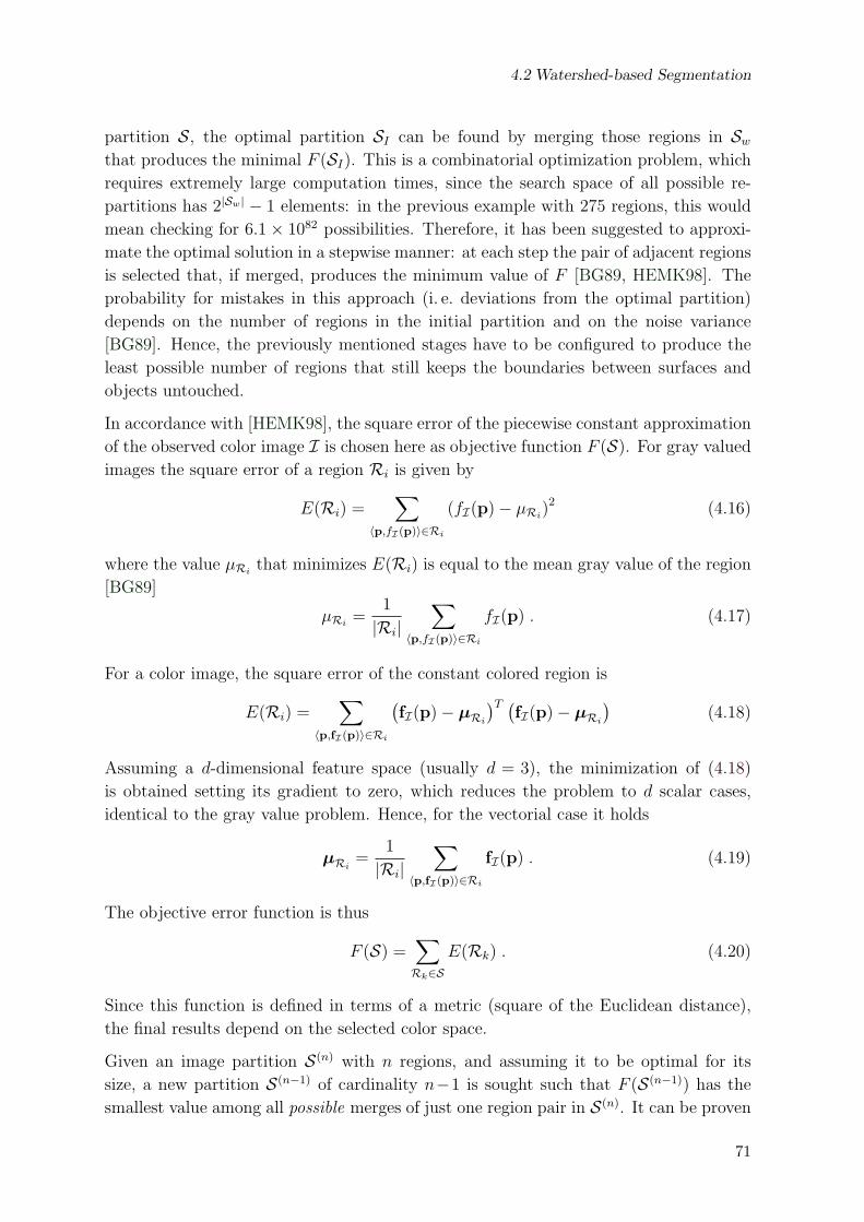
4.2 Watershed-based Segmentation
partition S, the optimal partition SI can be found by merging those regions in Sw
that produces the minimal F (SI). This is a combinatorial optimization problem, which
requires extremely large computation times, since the search space of all possible re-
partitions has 2|Sw| − 1 elements: in the previous example with 275 regions, this would
mean checking for 6.1× 1082 possibilities. Therefore, it has been suggested to approxi-
mate the optimal solution in a stepwise manner: at each step the pair of adjacent regions
is selected that, if merged, produces the minimum value of F [BG89, HEMK98]. The
probability for mistakes in this approach (i. e. deviations from the optimal partition)
depends on the number of regions in the initial partition and on the noise variance
[BG89]. Hence, the previously mentioned stages have to be configured to produce the
least possible number of regions that still keeps the boundaries between surfaces and
objects untouched.
In accordance with [HEMK98], the square error of the piecewise constant approximation
of the observed color image I is chosen here as objective function F (S). For gray valued
images the square error of a region Ri is given by
E(Ri) =∑
〈p,fI(p)〉∈Ri
(fI(p)− µRi)2 (4.16)
where the value µRithat minimizes E(Ri) is equal to the mean gray value of the region
[BG89]
µRi=
1
|Ri|∑
〈p,fI(p)〉∈Ri
fI(p) . (4.17)
For a color image, the square error of the constant colored region is
E(Ri) =∑
〈p,fI(p)〉∈Ri
(fI(p)− µRi
)T (fI(p)− µRi
)(4.18)
Assuming a d-dimensional feature space (usually d = 3), the minimization of (4.18)
is obtained setting its gradient to zero, which reduces the problem to d scalar cases,
identical to the gray value problem. Hence, for the vectorial case it holds
µRi=
1
|Ri|∑
〈p,fI(p)〉∈Ri
fI(p) . (4.19)
The objective error function is thus
F (S) =∑Rk∈S
E(Rk) . (4.20)
Since this function is defined in terms of a metric (square of the Euclidean distance),
the final results depend on the selected color space.
Given an image partition S(n) with n regions, and assuming it to be optimal for its
size, a new partition S(n−1) of cardinality n−1 is sought such that F (S(n−1)) has the
smallest value among all possible merges of just one region pair in S(n). It can be proven
71

4 Image-based Segmentation
(Appendix B) that the best n−1 partition in the context of F is obtained by merging
the region pair that minimizes the function
γ(Ri,Rj) =
|Ri|·|Rj ||Ri|+|Rj |(µRi
− µRj)T (µRi
− µRj) for A(Ri,Rj) = true
+∞ otherwise(4.21)
with the adjacency predicate A introduced in Definition 9 (p. 34).
For the merge algorithm, it is adequate to interpret the image partition as part of an
adjacency graph G = 〈S, E〉, where the regions in S represent the nodes of the graph,
and the edge set E is defined as
E = 〈Ri,Rj〉 | 〈Ri,Rj〉 ∈ S × S, A(Ri,Rj) = true . (4.22)
To each edge 〈Ri,Rj〉 a dissimilarity weight is assigned, calculated with (4.21). The
region merging algorithm for stepwise optimization is summarized in Figure 4.10, where
G(i) denotes the adjacency graph with nodes in the partition S(i) of cardinality i. The
choice among different stop criteria allows to adjust the final number of regions.
The simplest stop criterion is to specify the desired number of regions in the final
partition, and to stop when that number is reached. A second possibility is to stop
when the smallest value of γ(Ri,Rj) surpasses a dissimilarity threshold. Both criteria
rely on a simple adjacency predicate: two regions Ri and Rj are adjacent, if at least
one pixel eRiin Ri is neighbor of another pixel eRj
in Rj. The pixel neighborhood
predicates used in this work are N4 and N8 defined in terms of the L1 and L∞ norms:
N4(ea, eb) ⇔ ‖pa − pb‖1 = 1
N8(ea, eb) ⇔ ‖pa − pb‖∞ = 1(4.23)
with the image elements ek = 〈pk, ck〉, k ∈ a, b. Thus, the adjacency predicate can
be formulated as
A(Ri,Rj) ⇔ i 6= j ∧ ∃eRi∈ Ri , eRj
∈ Rj : Nz(eRi, eRj
) (4.24)
Algorithm: Stepwise Partition Optimization [BG89, HEMK98]
1: i = |S(n)|2: while stop condition not fulfilled do
3: find edge 〈Ri,Rj〉 in G(i) with the smallest weight γ(Ri,Rj)
4: merge the regions Ri and Rj to produce S(i−1) and G(i−1)
5: update the edge data
6: i := i− 1
7: end while
Figure 4.10: Algorithm for stepwise partition optimization.
72

4.2 Watershed-based Segmentation
with z ∈ 4, 8.
A third method provides an improved mechanism for region growing. Even though it
is not employed within the watershed-based concept, it can be conveniently introduced
here, in the context of stop criteria for graph-based merging techniques. The surface-
based segmentation (Chapter 5) and the k-means based approach (Section 4.3) make
use of it. Some nodes of the graph are marked at the beginning of the algorithm as
seeds of specific classes. The stepwise optimization algorithm remains unchanged, but
the adjacency predicate is modified, such that at least one of the regions has to be no
seed:
A′(Ri,Rj) ⇔ A(Ri,Rj) ∧ (¬Seed(Ri) ∨ ¬Seed(Rj)) (4.25)
If one of the regions merged was a seed, the new graph node becomes also a seed.
The additional condition in the adjacency predicate ensures that two regions already
assigned to different classes will never merge. Traditional growing methods always assign
a region to an adjacent seed. In contrast, this concept merges the most similar regions
first, independently if they are adjacent or not to one of the seeds. With this third
merging strategy, the resulting number of regions in the partition equals the number of
classes used in the seeds.
Original 500 Regions 250 Regions 50 Regions
Figure 4.11: Reduction of the over-segmentation with a region-based stepwise optimizationstage.
Figure 4.11 depicts the results of merging the second partition of the second object in
Figure 4.9. The stop criterion was set to 500, 250 and 50 regions respectively. The
merge stage can be efficiently computed with the help of priority queues that find the
most similar pair of regions in constant time, and an efficient graph implementation
that allows to merge two nodes and update the priority queue in logarithmic time on
the number of nodes of the graph [LfTI03]. The segmentation of the third image in
Figure 4.11 (442× 424) takes for the whole watershed process about 0.3 seconds, using
an Intel Pentium 4 (2.8GHz) PC.
73
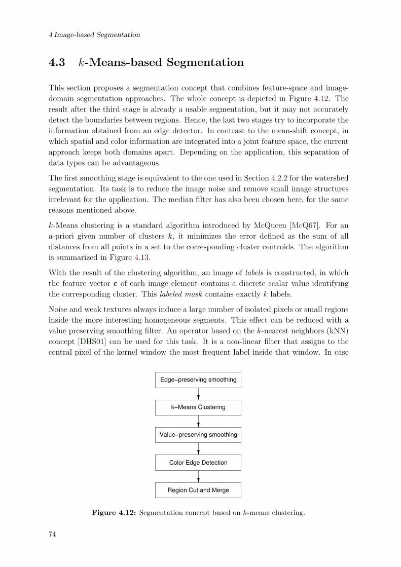
4 Image-based Segmentation
4.3 k-Means-based Segmentation
This section proposes a segmentation concept that combines feature-space and image-
domain segmentation approaches. The whole concept is depicted in Figure 4.12. The
result after the third stage is already a usable segmentation, but it may not accurately
detect the boundaries between regions. Hence, the last two stages try to incorporate the
information obtained from an edge detector. In contrast to the mean-shift concept, in
which spatial and color information are integrated into a joint feature space, the current
approach keeps both domains apart. Depending on the application, this separation of
data types can be advantageous.
The first smoothing stage is equivalent to the one used in Section 4.2.2 for the watershed
segmentation. Its task is to reduce the image noise and remove small image structures
irrelevant for the application. The median filter has also been chosen here, for the same
reasons mentioned above.
k-Means clustering is a standard algorithm introduced by McQueen [McQ67]. For an
a-priori given number of clusters k, it minimizes the error defined as the sum of all
distances from all points in a set to the corresponding cluster centroids. The algorithm
is summarized in Figure 4.13.
With the result of the clustering algorithm, an image of labels is constructed, in which
the feature vector c of each image element contains a discrete scalar value identifying
the corresponding cluster. This labeled mask contains exactly k labels.
Noise and weak textures always induce a large number of isolated pixels or small regions
inside the more interesting homogeneous segments. This effect can be reduced with a
value preserving smoothing filter. An operator based on the k-nearest neighbors (kNN)
concept [DHS01] can be used for this task. It is a non-linear filter that assigns to the
central pixel of the kernel window the most frequent label inside that window. In case
Edge−preserving smoothing
k−Means Clustering
Color Edge Detection
Region Cut and Merge
Value−preserving smoothing
Figure 4.12: Segmentation concept based on k-means clustering.
74
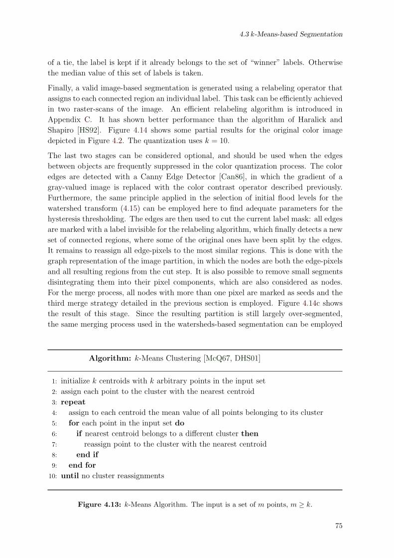
4.3 k-Means-based Segmentation
of a tie, the label is kept if it already belongs to the set of “winner” labels. Otherwise
the median value of this set of labels is taken.
Finally, a valid image-based segmentation is generated using a relabeling operator that
assigns to each connected region an individual label. This task can be efficiently achieved
in two raster-scans of the image. An efficient relabeling algorithm is introduced in
Appendix C. It has shown better performance than the algorithm of Haralick and
Shapiro [HS92]. Figure 4.14 shows some partial results for the original color image
depicted in Figure 4.2. The quantization uses k = 10.
The last two stages can be considered optional, and should be used when the edges
between objects are frequently suppressed in the color quantization process. The color
edges are detected with a Canny Edge Detector [Can86], in which the gradient of a
gray-valued image is replaced with the color contrast operator described previously.
Furthermore, the same principle applied in the selection of initial flood levels for the
watershed transform (4.15) can be employed here to find adequate parameters for the
hysteresis thresholding. The edges are then used to cut the current label mask: all edges
are marked with a label invisible for the relabeling algorithm, which finally detects a new
set of connected regions, where some of the original ones have been split by the edges.
It remains to reassign all edge-pixels to the most similar regions. This is done with the
graph representation of the image partition, in which the nodes are both the edge-pixels
and all resulting regions from the cut step. It is also possible to remove small segments
disintegrating them into their pixel components, which are also considered as nodes.
For the merge process, all nodes with more than one pixel are marked as seeds and the
third merge strategy detailed in the previous section is employed. Figure 4.14c shows
the result of this stage. Since the resulting partition is still largely over-segmented,
the same merging process used in the watersheds-based segmentation can be employed
Algorithm: k-Means Clustering [McQ67, DHS01]
1: initialize k centroids with k arbitrary points in the input set
2: assign each point to the cluster with the nearest centroid
3: repeat
4: assign to each centroid the mean value of all points belonging to its cluster
5: for each point in the input set do
6: if nearest centroid belongs to a different cluster then
7: reassign point to the cluster with the nearest centroid
8: end if
9: end for
10: until no cluster reassignments
Figure 4.13: k-Means Algorithm. The input is a set of m points, m ≥ k.
75

4 Image-based Segmentation
2770 Regions 468 Regions 258 Regions 25 Regions(a) (b) (c) (d)
Figure 4.14: Example of k-means based concept. The images depict the boundaries foundafter (a) color quantization with k-means for k = 10, (b) kNN filtering, (c) edgecut and small region suppression, (d) region merge.
(Figure 4.14d).
4.4 Adaptive Clustering Algorithm
Pappas [Pap92] proposed for the segmentation task the Adaptive Clustering Algorithm
(ACA), which also uses the k-means clustering as a first step in a framework that
combines feature-space with image-domain information. The consideration of the latter
is made, however, within a consistent labeling framework. His algorithm, developed
originally for gray-valued images but easily extendable to color images (e. g. [Che03]),
formulates segmentation as a maximum a posteriori (MAP) optimization problem. The
image is assumed to be formed by a set of uniform or slowly varying regions, such that
sharp transitions can only occur at the boundaries between them.
The probability that the segmentation S is valid for a given image I is
p(S | I) ∝ p(I | S)p(S) . (4.26)
where p(I | S) denotes the conditional density of the observed image given the distri-
bution of regions, and p(S) is the a-priori density of the region process. The former is
modeled for each pixel as a white Gaussian process
p(I | S) ∝ exp
− ∑〈pk,ck〉∈I
(ck − µRi(pk))
T (ck − µRi(pk))
2σ2
(4.27)
where µRi(pk) denotes the expected value for the pixel at the position pk within the
image region Ri. This term constrains the expected colors in a region to the data.
The a-priori density is modeled with a Markov Random Field (MRF), i. e. the conditional
probability of an image element ek = 〈pk, ck〉 only depends on its direct neighbors:
p(ek|ej | k 6= j) = p(ek|ej | Nz(ek, ej)), with the neighborhood predicates defined
76

4.4 Adaptive Clustering Algorithm
in (4.23). The Hammersley-Clifford theorem [Bes74] states that if the density p(S) is a
MRF then it is described by a Gibbs density with the clique potentials VC(S):
p(S) =1
Zexp
(−∑
C
VC(S)
)(4.28)
with a normalization constant Z, and the sum over all cliques C. A clique is a set of
neighbor points, and in this special case, any pair of two adjacent pixels (second order
cliques). The clique potentials VC(S) are chosen such that there is a higher probability
for two neighbor pixels to belong to the same region than to different regions. Thus,
the region density p(S) imposes spatial continuity:
VC(S) =
−β if C = 〈ek, ej〉, ek, ej ∈ Ri ∈ S, Nz(ek, ej)
+β if C = 〈ek, ej〉, ek ∈ Ra ∈ S, ej ∈ Rb ∈ S, a 6= b, Nz(ek, ej)(4.29)
The combined probability for the segmentation S is given by
p(S | I) ∝ exp
− ∑〈pk,ck〉∈I
(ck − µRi(pk))
T (ck − µRi(pk))
2σ2−∑
C
VC(S)
(4.30)
If the mean values for the regions µRi(pk) are assumed constant and β = 0 then (4.30)
is equivalent to the k-means algorithm. Hence, this probabilistic framework can be
regarded as a generalization of k-means clustering.
ACA uses the centroids detected by the k-means algorithm as initialization for µRi(pk).
The next step is to update these mean values using a window and the current labeled
mask (Figure 4.15): for each pixel position pk and a new hypothesized label i, the new
pk
i
ii
j
Figure 4.15: ACA mean value update.
mean value for the pixel is estimated from all image elements with label i that lie within
the window centered at pk. The probability (4.30) can be computed for all labels, and
the one with the highest probability is assigned to the pixel. Several iterations for mean
estimation and relabeling are repeated, until the number of label changes lie below a
given threshold. The window size is then reduced and the whole process is repeated
until a minimum window size is reached. At the end of the process, the mean value
77

4 Image-based Segmentation
within a region changes slowly, allowing one label to represent very different colors at
different locations in the image. If the smallest window size is kept large enough, the
resulting means-image can also be considered as an edge-preserving smoothing filter.
An example for the computed mean values and the obtained segmentation is depicted
in Figure 4.16. The computation took 38 seconds on an Intel Pentium 4 (2.8GHz) PC
and it found 764 regions. Increasing β from 0.75 to 5.75 reduced the number of regions
to 436, but the algorithm required almost six minutes to converge.
(a) (b) (c)
Figure 4.16: Example for ACA Segmentation. (a) Original, (b) computed means, (c) bound-aries between regions. 764 regions were detected
The unpredictable time requirements of this approach make its evaluation in a Pareto
front optimization very expensive. Furthermore, five minutes is definitively too much
time for a user to wait for a recognition result. For these reasons, the ACA segmentation
will be no further considered for the image-based segmentation level.
4.5 Discussion
The first three methods have been compared using the Pareto Front strategy (Sec-
tion 3.7.1). The parameter ranges used in each algorithm are listed in Tables 4.1 to 4.3,
with the corresponding number of bits used for their representation. The evolutionary
search tries to optimize the parameter values to reach the highest non-dominated fitness
values.
Table 4.1: Parameters of the Mean-Shift Segmentation
Parameter Value Range
hp 1 – 32 (8 bits)
hc 1 – 32 (8 bits)
max. neighbor color distance 0 – 255 (8 bits)
speed-up medium, high
Mean-shift segmentation has a relatively small number of parameters (Table 4.1). The
78

4.5 Discussion
bandwidths for the spatial (hp) and color (hc) components of the kernel have been limited
to a maximum of 32 pixels and 32 color component units, respectively. Higher values
increase the computation times without any hope for improvement, since greater kernels
smooth the images strongly. Since the exact computation of the algorithm requires long
times (60-240 seconds, depending on the image), only the optimized versions proposed
by the authors [Lab02] have been analyzed.
Table 4.2: Parameters of the Watershed-based Segmentation
Parameter Value Range
Median Filter Kernel Size 1, 3, 5, 7
Color Space RGB, XYZ, xyY, L∗u∗v∗, rgI, OCP, YIQ
Color Edgeness Operator Maximum, Color Contrast, MDD
Gradient Kernel Ando, OGD, Difference, Roberts, Sobel, Prewitt, Kirsch
δ 0 – 1 (8 bits)
Neighborhood N4, N8
Region Merge Mode Updated, Fixed
Merge Threshold 0 – 100 (12 bits)
Min. Region Number 1 – 25
The parameters for the watershed segmentation (Table 4.2) can be grouped according to
the processing stages in Figure 4.7. The median sizes for the edge-preserving smoothing
stage have been restricted to odd sizes between 1 and 7.
Seven standard color spaces have been used in the optimizations: the well known color
spaces RGB, XYZ, xyY, and L∗u∗v∗ [GW92], the chromaticity space rgI [DWL97a],
an opponent color space OCP computed as R-G,B-Y,I and the luminance-inphase-
quadrature space YIQ from the NTSC television standard. Color spaces with angu-
lar hue components, like HSI or HSV, are not appropriate to be directly employed in
any form of edge computation based on scalar gradients, since the angular values can
abruptly change between 0 and 2π causing the spurious detection of strong edges in red
colored areas. For the edgeness computation two factors have been studied: the edge
operator itself (MDD, contrast or maximum among the gradient of all color channels)
and the underlying gradient approximation kernel.
The δ term in (4.15) is also sought by the genetic algorithm. A neighborhood predicate
is used in the watershed transform to decide, among other things, when two different
water fronts met. The PESA algorithm (Appendix A) can also choose between the
neighborhood predicates defined in (4.23).
The fixed region merge mode allows to deactivate the update stage of the mean values
when two regions merge (steps 4 and 5, Figure 4.10). In this case, the edge weights
are computed once at the beginning of the algorithm and the merge process uses them
for the rest of the process. Two stop criteria for the merge process can be combined:
the threshold specifies the maximum allowed distance between the mean colors of two
79
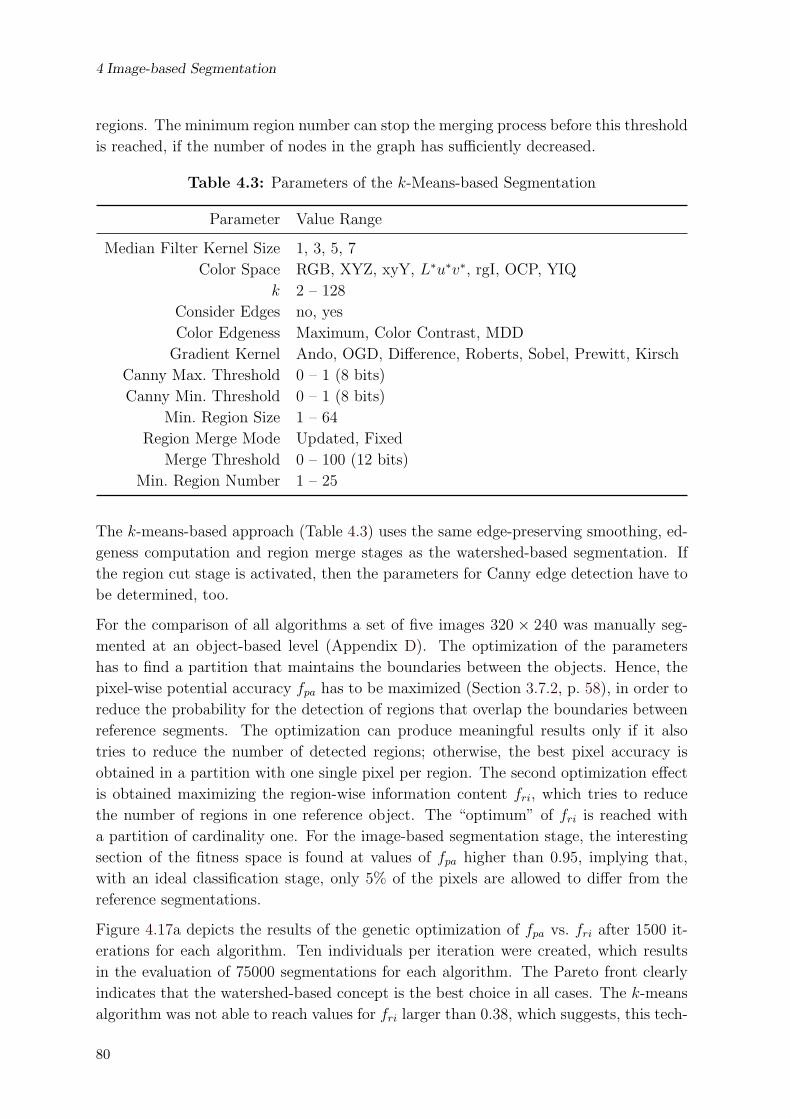
4 Image-based Segmentation
regions. The minimum region number can stop the merging process before this threshold
is reached, if the number of nodes in the graph has sufficiently decreased.
Table 4.3: Parameters of the k-Means-based Segmentation
Parameter Value Range
Median Filter Kernel Size 1, 3, 5, 7
Color Space RGB, XYZ, xyY, L∗u∗v∗, rgI, OCP, YIQ
k 2 – 128
Consider Edges no, yes
Color Edgeness Maximum, Color Contrast, MDD
Gradient Kernel Ando, OGD, Difference, Roberts, Sobel, Prewitt, Kirsch
Canny Max. Threshold 0 – 1 (8 bits)
Canny Min. Threshold 0 – 1 (8 bits)
Min. Region Size 1 – 64
Region Merge Mode Updated, Fixed
Merge Threshold 0 – 100 (12 bits)
Min. Region Number 1 – 25
The k-means-based approach (Table 4.3) uses the same edge-preserving smoothing, ed-
geness computation and region merge stages as the watershed-based segmentation. If
the region cut stage is activated, then the parameters for Canny edge detection have to
be determined, too.
For the comparison of all algorithms a set of five images 320 × 240 was manually seg-
mented at an object-based level (Appendix D). The optimization of the parameters
has to find a partition that maintains the boundaries between the objects. Hence, the
pixel-wise potential accuracy fpa has to be maximized (Section 3.7.2, p. 58), in order to
reduce the probability for the detection of regions that overlap the boundaries between
reference segments. The optimization can produce meaningful results only if it also
tries to reduce the number of detected regions; otherwise, the best pixel accuracy is
obtained in a partition with one single pixel per region. The second optimization effect
is obtained maximizing the region-wise information content fri, which tries to reduce
the number of regions in one reference object. The “optimum” of fri is reached with
a partition of cardinality one. For the image-based segmentation stage, the interesting
section of the fitness space is found at values of fpa higher than 0.95, implying that,
with an ideal classification stage, only 5% of the pixels are allowed to differ from the
reference segmentations.
Figure 4.17a depicts the results of the genetic optimization of fpa vs. fri after 1500 it-
erations for each algorithm. Ten individuals per iteration were created, which results
in the evaluation of 75000 segmentations for each algorithm. The Pareto front clearly
indicates that the watershed-based concept is the best choice in all cases. The k-means
algorithm was not able to reach values for fri larger than 0.38, which suggests, this tech-
80

4.5 Discussion
nique always finds partitions that split the reference regions. The mean-shift algorithm
can be parameterized to achieve the same pixel accuracy levels, but it produces a higher
number of regions (lower values of fri). Figure 4.17b depicts the area of interest in the
fitness space and Figure 4.18 shows three images generated with the parameterizations
found for fpa = 0.98.
Figure 4.19 depicts the values for the throughput (in a Pentium 4, 2.8GHz PC) and
region integrity functions, plotted against the pixel-wise potential accuracy component
of the fitness points in the previously generated Pareto front. These curves show that
even though these fitness measures were not considered in the optimization, they are
also best for the watershed-based concept. At the highest pixel-wise potential accura-
cies, the watershed approach segments about 5 images per second, the k-means concept
4, while the mean-shift requires 5 seconds per image. The region integrity curve shows a
predicted behavior: the optimization of the region information content fri finds param-
eterizations that strongly under-partition the images, which is reflected in lower values
of the region integrity. The peak of the mean-shift algorithm at lower values of the
pixel-wise accuracy indicates its tendency to over-segmentation.
A disadvantage of the k-means and mean-shift approaches is that both have a random
component in the detection of clusters in the feature space. This causes that the re-
sults of found parameterizations may not be reliable. The deterministic nature of the
watershed-transform is, in this sense, more adequate, since the contents of the Pareto
front produce always reproducible results.
For the watershed-based approach, a deeper look into the found parameters is pertinent.
Several experiments have been performed to test the effects of one parameter by fixing its
value while all others are allowed to be modified in the optimization process. This novel
0
0.1
0.2
0.3
0.4
0.5
0.6
0.7
0.8
0.9
1
0.3 0.4 0.5 0.6 0.7 0.8 0.9 1
Reg
ion−
wis
e In
form
atio
n C
onte
nt
Watershed−based
Mean−Shiftk−Means−based
Pixel−wise Potential Accuracy
0
0.05
0.1
0.15
0.2
0.25
0.3
0.95 0.96 0.97 0.98 0.99 1
Reg
ion−
wis
e In
form
atio
n C
onte
nt
Pixel−wise Potential Accuracy
Watershed−based
Mean−Shiftk−Means−based
(a) (b)
Figure 4.17: Pixel-wise potential accuracy (fpa) vs. region-wise information content (fri).(a) Pareto Fronts. (b) Zoomed area for the potential accuracy between 0.95and 1.0.
81

4 Image-based Segmentation
(a) (b) (c) (d)
Figure 4.18: For the test image (a) the parameterizations found for fpa = 0.98 produced(b) 47 regions with the watershed-based approach, (c) 96 regions with the k-means approach, and (d) 270 regions with the mean-shift segmentation.
Mean−Shiftk−Means−based
Watershed−based
0
1
2
3
4
5
6
7
8
9
0.3 0.4 0.5 0.6 0.7 0.8 0.9 1
Thr
ough
put
Pixel−wise Potential Accuracy
Mean−Shiftk−Means−based
Watershed−based
0
0.1
0.2
0.3
0.4
0.5
0.6
0.7
0.8
0.9
1
0.3 0.4 0.5 0.6 0.7 0.8 0.9 1
Reg
ion
Inte
grity
Pixel−wise Potential Accuracy
(a) (b)
Figure 4.19: Throughput (ft) and region integrity (fi)
test approach reveals some interesting effects that cannot be obtained with conventional
subjective evaluation methods.
The experiments proved that for pixel-wise accuracies above 0.95 a slightly better per-
formance is obtained with a median kernel of size 5. Smaller values cause an increase
in the number of detected regions. Greater kernels smooth the corners of the relatively
small regions, causing more pixel misclassifications.
The choice for a specific color space has always played a fundamental role in the seg-
mentation literature. The tests summarized in Figure 4.20 indicate that in the entire
value range of fpa the color spaces rgI and OCP are more frequently in the front. The
curves for xyY, XYZ and L∗u∗v∗ have been left out to improve the legibility of the chart.
Their performances are similar to the RGB color space. The CIE L∗u∗v∗ color space
was never used in any of the parameterizations in the front. For fpa ≥ 0.95 all color
spaces provide similar results. The RGB and OCP reach the highest values of pixel-wise
potential accuracy.
The selection of a specific color edgeness operator has not shown considerable effects
82

4.5 Discussion
RGBrgI
YIQOCP
0
0.1
0.2
0.3
0.4
0.5
0.6
0.7
0.8
0.9
1
0.3 0.4 0.5 0.6 0.7 0.8 0.9 1
Reg
ion−
wis
e In
form
atio
n C
onte
nt
Pixel−wise Potential Accuracy
rgIYIQ
0
0.05
0.1
0.15
0.2
0.25
0.3
0.35
0.95 0.96 0.97 0.98 0.99 1
Reg
ion−
wis
e In
form
atio
n C
onte
nt
Pixel−wise Potential Accuracy
RGB
RGB
OCP
OCP
(a) (b)
Figure 4.20: Color space selection.
on the fitness results. The optimization process always finds a combination of all other
parameters to provide similar fitness measures. However, in the Pareto front the max-
imal directional derivative was used more frequently with an underlying Ando [And00]
gradient kernel.
For the region merge stage, updating the node values has proven to be necessary (Fig-
ure 4.21) if the pixel accuracy is the matter of interest. For long merging processes,
however, the number of wrong merges increases if the mean values for the regions are
updated after each merge. The reason for this behavior is, that for larger regions the
piecewise constant model for the image no longer holds.
0
0.1
0.2
0.3
0.4
0.5
0.6
0.7
0.8
0.9
1
0.3 0.4 0.5 0.6 0.7 0.8 0.9 1
Reg
ion−
wis
e In
form
atio
n C
onte
nt
Pixel−wise Potential Accuracy
UpdatedFixed
0
0.05
0.1
0.15
0.2
0.25
0.95 0.96 0.97 0.98 0.99 1
Reg
ion−
wis
e In
form
atio
n C
onte
nt
Pixel−wise Potential Accuracy
UpdatedFixed
(a) (b)
Figure 4.21: Update strategy for region merge. (a) Complete range for pixel-wise poten-tial accuracy (fpa) vs. region-wise information content (fri). (b) Highest pixelaccuracies.
83

4 Image-based Segmentation
The greatest adaption of the parameters is found in the configuration of the watershed
transformation. Figure 4.22 shows the points found in the parameter subspace spanned
by the adaptive flood factor δ, the merge threshold and the minimum number of regions.
The maximization of the pixel-wise potential accuracy is reached with small flood fac-
0 0.1 0.2 0.3 0.4 0.5 0.6 0.7 0.8 0.9 1 020
4060
80100
0
5
10
15
20
25
Min. regions
Flood factor
Merge threshold
Figure 4.22: Optimized watershed parameters. Low flood factors and merge thresholds areused in parameterizations with the highest pixel potential accuracies. Highflood factors and merge thresholds are employed in the optimizations of theregion-wise information content. The cluster around the flood factor δ = 0.5was obtained with the rest of the front.
tors, which allow to generate partitions with many regions. The region information
fitness is maximized with segmentations of low cardinality. These can be generated
using large flood factors, or high color distance thresholds to stop the merging process,
and not restricting the number of regions. The genetic optimization suggests to use all
three conditions simultaneously. On the middle range of the optimizations all possible
combinations of the merge threshold and the minimum number of regions have been
found, while the flood factor concentrates around the value 0.5± 0.1.
It remains the question how to manage requests from later stages to split a region. Since
the watershed transform (the fourth stage in Figure 4.7) always detects the slightest dis-
continuities, the regions it finds can be assumed to be indivisible atoms. A split request
from later stages “reactivates” the corresponding components of the region which were
available before the merging stage took place. Such an request is usually accompanied
with a desired number of parts, in which the given region has to be split. This goal can be
easily achieved creating a subgraph with the found components as nodes and re-merging
them until the desired number of parts is reached. However, choosing parameterization
with high levels of pixel-wise potential accuracy renders the region parsing (i. e. region
split) unnecessary, since the later stages only need to provide merging strategies.
Summarizing, the use of the watershed concept is adequate for the image-based stage
of the current application context, not only because it was the most efficient of all four
analyzed approaches, but also because it reached the best levels of pixel-wise potential
84

4.5 Discussion
accuracy and region-wise information content. Using a representative reference set of
images and segmentations, it is also possible to gain the optimal parameterizations from
the evaluation process.
85

4 Image-based Segmentation
86

Chapter 5
Surface-Based Segmentation
The image-based stage has provided an over-segmentation of the image. The next task
is to merge some of the detected regions, such that the new partition exhibits some
correspondence with real world surfaces. For this task, additional knowledge has to
be incorporated into the process that cannot be gained from the images, but is still
unrelated to the particular appearance of each object. Three information sources can
be identified:
1. the physical processes involved in the image formation,
2. theories and studies on perceptual organization of visual stimuli, and
3. knowledge about the scene configuration expected in an application.
5.1 Physical Assumptions
The family of physics-based segmentation algorithms surveyed in [SK94] and [LM01]
detect object surfaces relying on knowledge about physical properties of materials and
light. The proposed algorithms are not applicable to the current test scenarios for two
reasons: first, the object sets studied in this work do not fulfill the conditions imposed
by those algorithms, as the textures of the materials and the non-Lambertian surfaces
ensure neither stable nor valid results; second, the required computational times are not
tolerable for interactive applications. Additionally, quantities supporting the detection
of material borders, like reflectance ratio, gradient direction, or intensity profile analysis
[MS97] are not discriminative enough to allow a reliable detection of the surfaces in the
current object sets, and are easily disturbed by surface textures.
The detection of shadows and highlights has also proven to be unreliable for the current
object sets and illumination conditions. The reason is that most efficient approaches
rely exclusively on spectral information. Special color spaces designed to detect material
changes, shadows or highlights are the only source of information. In the images of
the current application the necessary conditions for material, highlight, and shadow
edges are often fulfilled at arbitrarily distributed locations, activated by different object
87
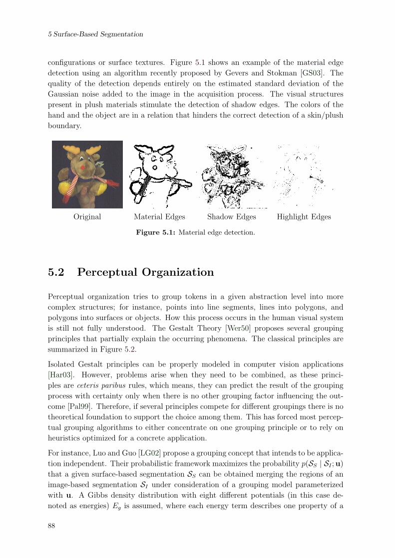
5 Surface-Based Segmentation
configurations or surface textures. Figure 5.1 shows an example of the material edge
detection using an algorithm recently proposed by Gevers and Stokman [GS03]. The
quality of the detection depends entirely on the estimated standard deviation of the
Gaussian noise added to the image in the acquisition process. The visual structures
present in plush materials stimulate the detection of shadow edges. The colors of the
hand and the object are in a relation that hinders the correct detection of a skin/plush
boundary.
Original Material Edges Shadow Edges Highlight Edges
Figure 5.1: Material edge detection.
5.2 Perceptual Organization
Perceptual organization tries to group tokens in a given abstraction level into more
complex structures; for instance, points into line segments, lines into polygons, and
polygons into surfaces or objects. How this process occurs in the human visual system
is still not fully understood. The Gestalt Theory [Wer50] proposes several grouping
principles that partially explain the occurring phenomena. The classical principles are
summarized in Figure 5.2.
Isolated Gestalt principles can be properly modeled in computer vision applications
[Har03]. However, problems arise when they need to be combined, as these princi-
ples are ceteris paribus rules, which means, they can predict the result of the grouping
process with certainty only when there is no other grouping factor influencing the out-
come [Pal99]. Therefore, if several principles compete for different groupings there is no
theoretical foundation to support the choice among them. This has forced most percep-
tual grouping algorithms to either concentrate on one grouping principle or to rely on
heuristics optimized for a concrete application.
For instance, Luo and Guo [LG02] propose a grouping concept that intends to be applica-
tion independent. Their probabilistic framework maximizes the probability p(SS | SI ;u)
that a given surface-based segmentation SS can be obtained merging the regions of an
image-based segmentation SI under consideration of a grouping model parameterized
with u. A Gibbs density distribution with eight different potentials (in this case de-
noted as energies) Eg is assumed, where each energy term describes one property of a
88
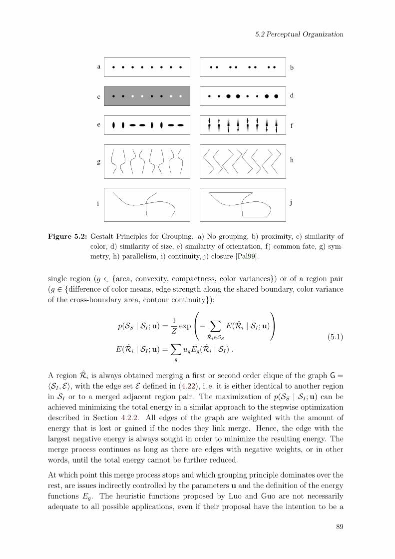
5.2 Perceptual Organization
b
d
f
h
j
a
c
e
g
i
Figure 5.2: Gestalt Principles for Grouping. a) No grouping, b) proximity, c) similarity ofcolor, d) similarity of size, e) similarity of orientation, f) common fate, g) sym-metry, h) parallelism, i) continuity, j) closure [Pal99].
single region (g ∈ area, convexity, compactness, color variances) or of a region pair
(g ∈ difference of color means, edge strength along the shared boundary, color variance
of the cross-boundary area, contour continuity):
p(SS | SI ;u) =1
Zexp
− ∑Ri∈SS
E(Ri | SI ;u)
E(Ri | SI ;u) =
∑g
ugEg(Ri | SI) .
(5.1)
A region Ri is always obtained merging a first or second order clique of the graph G =
〈SI , E〉, with the edge set E defined in (4.22), i. e. it is either identical to another region
in SI or to a merged adjacent region pair. The maximization of p(SS | SI ;u) can be
achieved minimizing the total energy in a similar approach to the stepwise optimization
described in Section 4.2.2. All edges of the graph are weighted with the amount of
energy that is lost or gained if the nodes they link merge. Hence, the edge with the
largest negative energy is always sought in order to minimize the resulting energy. The
merge process continues as long as there are edges with negative weights, or in other
words, until the total energy cannot be further reduced.
At which point this merge process stops and which grouping principle dominates over the
rest, are issues indirectly controlled by the parameters u and the definition of the energy
functions Eg. The heuristic functions proposed by Luo and Guo are not necessarily
adequate to all possible applications, even if their proposal have the intention to be a
89

5 Surface-Based Segmentation
“non-purposive” grouping algorithm.
This concept can be regarded as an extension of a split-and-merge image-based segmen-
tation process, that combines color, edgeness and shape criteria to decide which regions
have to be merged. With the test sets employed in this work this kind of approaches
tend to produce under-segmentations, and are therefore not further considered.
An important property of biological perceptual grouping processes is the capability to
detect emerging properties. For example, in Figure 5.2a most people perceive a “line”
of dots, even if there is no such line. According to the Gestalt theory, this capability is
possible only under a holistic analysis of the image. Algorithms like the previous one,
which only inspect the direct neighborhood of a region, are not able to detect this kind
of configurations.
A second family of perceptual grouping concepts tries to detect emerging structures in
edges and points. They rely on the Gestalt principle of continuity, i. e. elements that can
be seen as smooth continuations of each other tend to be grouped together (Figure 5.2i).
Two prominent examples in this category are Shashua and Ullman’s structural saliency
[SU88] and Guy and Medioni’s tensor voting approach [MLT00]. Figure 5.3 depicts the
grouping results for edges extracted with a Canny detector from the original image in
Figure 5.1. Both approaches are computationally intensive (especially the algorithm
for structural saliency). Moreover, further processing is necessary in order to map the
edgeness saliency into the region oriented concept followed in this work. For these
reasons, their use in the current application is not recommended.
(a) (b) (c) (d)
Figure 5.3: Examples for saliency extraction from edges. (a) Color contrast edgeness.(b) Canny Edges. (c) Guy-Medioni Saliency. (d) Shashua-Ullman Saliency.
5.3 Application Dependent Cues
In object retrieval applications, the data sets are usually composed by objects of the
same category (e. g. soft toys, building blocks, screws, jewels, etc.). Hence, only a
few number of materials can be expected, which implies that the surfaces of different
objects can be extremely similar. For this reason, merging all regions that have the
similar surface properties inevitably produces under-segmentations. The object-based
90

5.3 Application Dependent Cues
stage can use additional information about each particular object to avoid this effect.
The detection of surfaces that belong to the general scene configuration is however
still desirable, in order to suppress information that is irrelevant for the recognition
process. This task can only be accomplished considering all available information about
the specific application context [SK94]. The next paragraphs present some general
principles to encode common information hints in a form that can be incorporated into
the segmentation process. These hints are combined using Bayesian Belief Networks
(BBN) which can be easily configured and parameterized to fulfill the application needs
[Cha91, RN95, Nil98].
In the next paragraphs the term probability is used in a subjectivist sense [RN95], i. e. the
values denote the belief , that an event occurs or a condition holds, under consideration
of some evidence, without the need of verification with a statistical experiment.
5.3.1 Encoding Color Information
In color segmentation and object recognition the color property has proven to be discrim-
inative enough to robustly support classification processes [Ber01, SB91]. Depending
on the scene setting, several common surfaces can be described using probabilistic color
models. The basic idea is to determine the probability P (Rs|c) that a pixel belongs to
a region Rs of a surface s given its color vector c.
In the simplest case this belief can be assumed to follow a parametric model. For a
homogeneous surface, for instance, this can be a multivariate Gaussian:
P (Rs|c) = κ exp
−1
2(c− µ)TΣ−1(c− µ)
(5.2)
with the mean color µ and the covariance matrix Σ. The maximal value κ is obtained
when c = µ. It is usually set to one.
A second possibility relies on the Bayes Theorem, with which P (Rs|c) can be rewritten
as
P (Rs|c) =p(c|Rs)P (Rs)
P (c)=
p(c|Rs)P (Rs)
p(c|Rs)P (Rs) + p(c|R¬s)P (R¬s)(5.3)
Non-parametric likelihood models p(c|Rs) (e. g. histograms) are able to reflect the prop-
erties of more complex surfaces. Jones and Rehg [JR99], for example, propose a general
skin color model for an all-purpose skin detection in images.
Besides the surface color model, the computation of (5.3) requires an additional model
p(c|R¬s) that indicates which colors are not expected to be found in the surface. It
is represented in a similar form as p(c|Rs). The third term in (5.3) is the a-priori
probability P (Rs) that a pixel belongs to the surface s. The latter is here assumed to
be described by a Markov process, i. e. its value depends on the pixel itself and on its
direct neighbors. The probability P (Rs) for each pixel is computed iteratively, with an
91

5 Surface-Based Segmentation
initial supposition of P0(Rs) = 0.5. Pt+1(Rs) is then computed as a weighted sum of all
previous beliefs Pt(Rs|c) within a neighborhood of the pixel. This neighborhood and
the weights are specified through a bandwidth h and a profile function w(x), which is
non-negative (w(x) ≥ 0) and has a unit area (∫∞−∞ w(x)dx = 1):
Pt+1(Rs)|pi=
∑〈pk,ck〉∈I
w
(‖pi − pk‖2
h
)Pt(Rs|ck) . (5.4)
Here, a normal profile (4.3) is used [AA01]. Hence, the new a-priori probabilities can be
efficiently computed with the convolution of the previous a posteriori probability with
a two-dimensional Gaussian kernel. Usually, two or three iterations are sufficient to
obtain a satisfactory result.
The output of this iterative process is a pixel-wise probability map, which contains for
each pixel the belief P (Rs|c) that it belongs to the surface s under consideration of its
color and the color of its neighbors. The region-wise probability is computed as the
mean of all pixel-wise probabilities within the region. Figure 5.4 depicts an example for
the hand probability using a skin color model. The contrast in the probability image is
considerably improved in the second iteration.
(a) (b) (c) (d)
Figure 5.4: Example for surface detection with color models. A skin color model has beenused to detect the skin surfaces in the image (a). The pixel-wise probabilitiesare depicted for the first and second iterations in (b) and (c), respectively. Theregion-wise probability for (c) is shown in (d). The darker a pixel, the higher itsprobability to belong to a skin surface.
5.3.2 Encoding Positional Information
In retrieval applications with a fixed acquisition place there are several properties of the
scene configuration that can be exploited. For example, the user’s hand can be expected
at one specific side of the image, the background always surrounds the object, or, if the
objects have no holes, the hand of the user can be expected to be adjacent to the object.
Positional probability maps can encode this information.
The simplest case are linear positional maps. For instance, if there is a higher probability
to find a specific surface at the bottom of the image, then the pixel-wise probability can
92

5.3 Application Dependent Cues
be modeled as p(Rs|p) = y/a2, with p = [x, y], the image size a1×a2, and a left-handed
coordinate system (the origin at the upper-left corner of the image).
A generalization of this concept is provided by means of the distance transform. This
morphological operator manipulates binary images (i. e. the pixel’s feature values can be
zero or one). It assigns to each one-valued pixel (figure pixel) the distance to the closest
pixel with value zero (ground pixel). Distance transforms based on the L1 and L∞ norms
can be efficiently computed, since both are special cases of chamfer norms, with which
the shortest distance between a figure pixel and the ground can always be obtained from
the distances of its neighbors to the ground. The Euclidean distance transform (EDT)
does not obey the chamfer principle, making its computation more expensive. Recently
an algorithm has been introduced to generate the exact EDT [MQR03] in linear time
on the total number of image pixels.
Positional probabilities can be computed as follows: those pixels expected to belong
to the surface are set to zero and the rest of the image is set to one. The distance
transform is then computed. A linear function is used to map the shortest distances
into the highest beliefs, with the distance zero always mapped into the belief 1. Let lkbe the distance value assigned to the pixel at position pk, the corresponding positional
belief is obtained as
P (Rs|pk) =
0 if νlk > max
ili
1− νlkmax
ili
otherwise(5.5)
with ν a positional decay factor. If ν is 1, then the largest distance is mapped to zero.
If it is greater than one then the beliefs will be concentrated into the a-priori reference
positions, and with ν < 1 a positional probability of zero is never reached.
Region-wise expectations can be generated combining the probabilities of all elements
in a region by means of an operator like median, maximum or minimum. Figure 5.5
depicts an example with the maximum operator on a L∞-based distance transform for
ν = 1 and ν = 3.6.
5.3.3 Combining Cues with Bayesian Belief Networks
The previous cues encode knowledge about different, independent issues of the scene
composition. A mechanism has to be chosen to combine them into a single belief, on
which the final decision can rely whether to assign the region to the modeled surface
or not. Here, the framework of Bayesian Belief Networks (BBN) is employed. A belief
network is a directed, acyclic graph with random variables as nodes and with edges
modeling the direct influence between two variables. Each node has a conditional prob-
ability table (CPT) that quantifies the effects the parent nodes have on it. Thus, the
topology of the graph describes qualitative issues of the complete probabilistic model,
while the CPTs represent the quantitative aspects [RN95, Nil98]. Figure 5.6 presents a
93

5 Surface-Based Segmentation
(a) (b) (c) (d)
Figure 5.5: Positional probability map. The boundary of the image except its bottom isassumed background. The linear mapping of the distance transform (based onL∞) is depicted in (a) for ν = 1 and in (c) for ν = 3.6. The region-wise positionalmaps for these transformations are depicted in (b) and (d), respectively. Theywere generated with a maximum operator on all region pixels. In all images blackdenotes a belief of 1 and white a belief of 0.
simple example with three nodes. The random variable B depends on the variables C
and L, which can, for instance, denote the surface color and surface positional processes,
respectively.
B
C L
PSfrag replacements
CPT: P (B|¬C,¬L)P (B|¬C, L)P (B| C,¬L)P (B| C, L)
Figure 5.6: Example of Bayesian Belief Network. B depends on C and L. The quantitativedependencies are encoded in the CPT.
Let P (C) and P (L) denote the beliefs that the conditions C and L are present. The
probability for B is now sought. It can be rewritten as
P (B) = P (B,¬C,¬L) + P (B,¬C, L) + P (B, C,¬L) + P (B, C, L) (5.6)
With the chain rule it follows for the fourth term
P (B, C, L) = P (B|C, L) · P (C|L) · P (L) (5.7)
and since C and L are independent variables
P (B, C, L) = P (B|C, L) · P (C) · P (L) (5.8)
The same is valid for the remaining three terms in (5.6). Hence
P (B) = P (B|¬C,¬L) · P (¬C)P (¬L) +
P (B|¬C, L) · P (¬C)P ( L) +
P (B| C,¬L) · P ( C)P (¬L) +
P (B| C, L) · P ( C)P ( L)
(5.9)
94

5.3 Application Dependent Cues
The conditional probabilities in the CPTs can encode the belief of experts that the event
B occurs under the assumption that the two conditions L and C are met, or not. These
values can also be generated from a representative training set.
The following paragraphs present two examples for cue extraction and combination in
the context of object retrieval. The first one, the detection of the surface of a homoge-
neous background, is a simple task that delivers relatively robust results. Its output is
used in the second example, in which regions belonging to the hand of the user have to
be detected.
5.3.4 Example: Detection of an Homogeneous Background
The detection of the background is an unavoidable task in the training stage of a recog-
nition system if the selected approach relies on global descriptors. Moreover, the robust
detection of the background is sufficient for the recall stage in the recognition of isolated
objects.
The separation of an image into the background and the object of interest is denoted
in biological visual systems as the figure/ground organization process. The figure is
usually closer to the observer and is bounded by a contour that defines its shape. The
ground is assumed to extend behind the figure and outside the image boundaries, so
that no contour or shape can be attributed to it. Usually, its contents are of less interest
[Pal99].
Similarly to the Gestalt grouping principles, there exists a set of ceteris paribus rules to
describe the figure/ground organization. The most important are surroundedness, size,
orientation, contrast, symmetry, convexity and parallelism (Figure 5.7).
For the current application, the most relevant principle is the surroundedness. The
boundary areas of the acquired images (Figure 2.16) are covered in major part by the
background, which can be assumed to be dark and homogeneous. The actual color
may vary according to the shutter speed and other camera settings, which are in some
cases continuously adapted to optimally exploit the dynamic range of the CCD or CMOS
sensors. The choice of a black surface is made to reduce the contrast of shadows cast onto
the background, which otherwise could easily be confused with object parts. Additional
precautions have to be taken to avoid merging lateral regions of the figure with the
ground, especially if self-shadows make their appearance similar.
The background detection follows the steps enumerated in Figure 5.8. A Gaussian
model is used to roughly describe the belief that a pixel has a background color. This
step can be interpreted as a generalization of the thresholding segmentation of gray-
valued images: the one-dimensional interval in an axis of gray-values is replaced with
an ellipsoid in the color space. All components of the colors have to be considered, since
the intensity of pixels belonging to the background and the objects can be identical.
The mean and covariance of the model are chosen to incorporate the possible variations
95
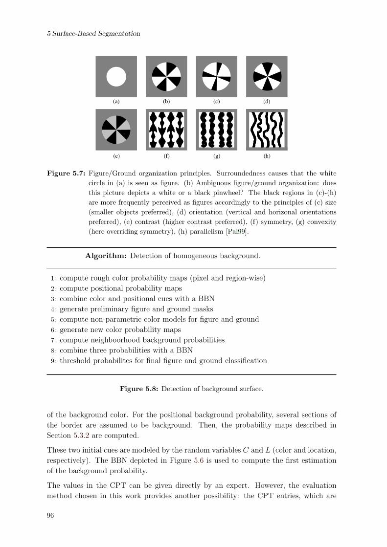
5 Surface-Based Segmentation
(a) (b) (c) (d)
(e) (f) (g) (h)
Figure 5.7: Figure/Ground organization principles. Surroundedness causes that the whitecircle in (a) is seen as figure. (b) Ambiguous figure/ground organization: doesthis picture depicts a white or a black pinwheel? The black regions in (c)-(h)are more frequently perceived as figures accordingly to the principles of (c) size(smaller objects preferred), (d) orientation (vertical and horizonal orientationspreferred), (e) contrast (higher contrast preferred), (f) symmetry, (g) convexity(here overriding symmetry), (h) parallelism [Pal99].
Algorithm: Detection of homogeneous background.
1: compute rough color probability maps (pixel and region-wise)
2: compute positional probability maps
3: combine color and positional cues with a BBN
4: generate preliminary figure and ground masks
5: compute non-parametric color models for figure and ground
6: generate new color probability maps
7: compute neighboorhood background probabilities
8: combine three probabilities with a BBN
9: threshold probabilites for final figure and ground classification
Figure 5.8: Detection of background surface.
of the background color. For the positional background probability, several sections of
the border are assumed to be background. Then, the probability maps described in
Section 5.3.2 are computed.
These two initial cues are modeled by the random variables C and L (color and location,
respectively). The BBN depicted in Figure 5.6 is used to compute the first estimation
of the background probability.
The values in the CPT can be given directly by an expert. However, the evaluation
method chosen in this work provides another possibility: the CPT entries, which are
96

5.3 Application Dependent Cues
part of the parameterization of the algorithm, can be automatically adjusted in the
evolutionary optimization of the algorithm’s fitness. In other words, the BBNs can be
trained using the PESA approach (Appendix A), under consideration of a representative
reference data set. All images presented in this chapter have been produced using such
genetically optimized parameterizations.
Figure 5.9 shows two examples for the three probability maps obtained for P (C), P (L)
and P (B). This preliminary result is not always robust enough to support a final
background detection. Hence, a second stage is appended which exploits the information
contained in the map for P (B).
Original P (C) P (L) P (B)
Figure 5.9: Rough background probability. Black denotes a belief 1 and white 0
Preliminary masks for ground and figure are computed from P (B) using two threshold
values. All pixels with probabilities above Pg are assigned to the ground, and only
those pixels with beliefs below Pf are considered as part of the figure, with Pg ≥ Pf .
Non-parametric density color models are then computed for both masks, i. e. all pixels
in the original image whose corresponding mask value is set to one are collected into
a color histogram. Both models are then used to compute the new color probability
P (C ′) with (5.3). It has to be noted that the ground color classification considers not
only a background color model, but the figure information as well. This helps improving
the robustness of the detection. Figure 5.10 depicts the figure/ground masks and the
pixel-wise and region-wise color probability maps. Shadows within the objects can also
reach high confidence values to be part of the background. For this reason it is necessary
to incorporate spatial information cues as well.
From the background mask an additional background belief value P (N) can be derived,
which considers for each region the number of neighbors that have been classified as
background in the preliminary mask. Since the thresholds Pg and Pf leave a gap in the
probability interval, there are also neighbors with an undefined membership. P (N) is
97

5 Surface-Based Segmentation
Background Mask Figure Mask pixel-wise P (C ′) region-wise P (C ′)
Figure 5.10: Probabilities with estimated color models.
here defined as the percentage of the boundary of a region that is adjacent to background
regions. Undefined regions are considered in the computations weighted with 0.5.
B’
S
CPTB
CPTS
N L
C’
N : Neighborhood
L: Location
C ′: Adapted Color Model
S: Spatial Information
B′: Background
Figure 5.11: BBN for the computation of the final background probabilities.
Three cues are now available: P (C ′), P (N) and P (L). These are combined with the
BBN depicted in Figure 5.11. Examples for the partial and final probability maps are
depicted in Figure 5.12. The final background segmentation is obtained with a simple
thresholding operation on P (B′).
The Pareto-based evaluation concept has been employed to optimize the fitness functions
fpa (pixel-wise potential accuracy) vs. fce (pixel-wise certainty). The certainty measure
required by the latter function is here computed as the normalized distance between
the final probabilities P (B′) and the threshold value. For the next results, the set with
seven images included in Appendix E has served as reference data.
The parameters of this algorithm are partially redundant. For example, the final thresh-
old and the CPT entries of the final node B′ can be shifted by a constant factor without
changing the final result. Therefore, the optimization process can always find alternative
parameterizations. Some of them may appear confusing. For instance, configurations of
98

5.3 Application Dependent Cues
P (N) P (S) P (B′) Final
Figure 5.12: Final background surface.
the upper nodes in the BBN can be found that invert the result (they produce the prob-
ability for a region not to belong to the background), however, the optimization process
can compensate this “confusion” at later stages, generating the correct results in the
end. To steer the parameterization into more “meaningful” values, the optimization has
been split into two stages. The attention is first directed to the preliminary background
detection: the four conditional probabilities in the CPT of node B, the coefficient ν in
(5.5), and the Gaussian color model are the parameters of interest. The second stage
optimizes the adaptive part of the algorithm, looking for appropriate thresholds Pg and
Pf , the CPTs for the BBN in Figure 5.11, and the final decision threshold. Figure 5.13
depicts the Pareto fronts found in both stages. The parameterization with the highest
0.55
0.6
0.65
0.7
0.75
0.8
0.85
0.9
0.95
1
0.98 0.982 0.984 0.986 0.988 0.99
Pixe
l−w
ise
Cer
tain
ty
Pixel−wise Potential Accuracy
Stage 2Stage 1
Figure 5.13: Optimization of Figure/Ground segmentation for the reference set in Ap-pendix E.
99

5 Surface-Based Segmentation
accuracy in the first stage has been employed in the second optimization. The front
clearly indicates the advantage of the adaptive stage.
The found CPTs are listed in Figure 5.14. The CPT for node B (the first stage) strongly
suppresses the information obtained from the positional beliefs, which were generated
with a decay factor of ν = 3.67. For the second stage, the combination of the positional
and neighborhood cues is accepted if only one of the information cues supports the
hypothesis. If both L and N are present, the result is uncertain. This is caused by
the large number of small regions at the boundary of the object, which in this case
have the highest neighborhood values, as they are uniformly distributed between the
figure and the ground. The CPT for the final node B′ is similar to an AND operation:
only the regions that according to their spatial and color characteristics are part of the
background will be assigned to it. The final threshold was found to be 0.341.
P (B|¬C,¬L) 0.000
P (B|¬C, L) 0.043
P (B| C,¬L) 0.800
P (B| C, L) 0.998
(a)
P (S|¬N,¬L) 0.002
P (S|¬N, L) 0.800
P (S| N,¬L) 0.992
P (S| N, L) 0.561
(b)
P (B′|¬C ′,¬S) 0.006
P (B′|¬C ′, S) 0.027
P (B′| C ′,¬S) 0.247
P (B′| C ′, S) 0.973
(c)
Figure 5.14: Conditional Probability Tables for background detection. (a) Node B. (b)Node S. (c) Node B′.
5.4 Example: Separation of Hand Surfaces and Skin-
Colored Objects
Literature on the detection of skin surfaces concentrates on applications for hand-gesture
recognition, where additional information sources can support the segmentation process;
for example, the structure of the face [JV01], characteristic motion patterns [BD01], or
enough contrast between skin and non-skin objects [JR99]. Appendix E presents some
example images from an object retrieval application, where the only hints available are
the skin color and the scene composition. In those cases where only one object and
the user’s hand are expected in an image, it is more efficient to employ the current
surface-based method for background/hand/object segmentation than the more expen-
sive multiple object segmentation approaches introduced in the next chapter.
For the current algorithm it is assumed that the hand of the user is present at the bottom
of the image and that the object of interest occupies the middle region, surrounded
mostly by the background and maybe some parts of the users’ hand. The algorithm
for the separation of background and hand regions from the object is summarized in
Figure 5.15. The detection of the background was already discussed in the last section.
100

5.4 Example: Separation of Hand Surfaces and Skin-Colored Objects
Algorithm: Detection of skin surface.
1: find the homogeneous background
2: select skin-color model
3: compute skin-color probability map
4: zoom the skin colors of the image
5: generate positional probability maps
6: combine all information cues with a BBN
7: compute object and skin surface seeds
8: repeat
9: grow seeds using original image
10: grow seeds using color zoomed image
11: mark inconsistencies as free
12: until converged or maximum number of iterations reached
13: if still some free regions then
14: grow seeds using original image
15: end if
Figure 5.15: Detection of skin surface.
5.4.1 Selection of the Skin-Color Model
The skin color model selection is a fundamental step of the current approach. A generic
color model cannot be used, since it is not able to distinguish between object surfaces and
hand (Figure 5.16a). Therefore, a database of skin color models pi(c|Rs) is necessary,
where each model describes one specific skin color type. Since it is known that the hand
is found at the bottom of the image, a selection mechanism based on the maximum
likelihood principle can be used, i. e. the model that maximizes the skin probability at
the bottom of the image is chosen:
p(c|Rs) = pi(c|Rs), i = arg maxi
∑〈ck,pk〉∈W
pi(ck|Rs)P (Rs)
P (ck)
(5.10)
with W the set of image elements at the bottom of the image. The winner color model
is then used to compute a skin probability map (Figure 5.16b). The statistical process
describing the colors of hand regions is denoted henceforth with the random variable C.
5.4.2 Color Zooming
For some object sets, differences between skin colors and object colors can be very
small. However, these differences can still support the surface classification if they are
101

5 Surface-Based Segmentation
(a) (b) (c)
Figure 5.16: Probability maps for different skin color models: (a) Jones and Regh [JR99]generic skin color model, (b) model of skin appropriate to the image, (c) darkerskin model.
appropriately enhanced. Selecting among different standard color representations does
not provide the desired effect, since, as already indicated by Jones and Regh [JR99],
color points that lie near each other in one color space, will always be close together
in any other representation. Instead of just transforming the color information into
another chromatic coordinate system, a “zooming” operation is necessary, which maps
the section of the color space containing the colors of interest into the whole available
representation range (for instance, the RGB color cube). Not many alternatives have
been proposed for this task. One possibility is the color histogram equalization proposed
in [PNS03]. However, the computational requirements to adapt a three-dimensional
mesh to the color space are not acceptable for the current task. The separated histogram
equalization for each color channel is also unsuitable since it breaks the interdependencies
among the color components. Since the skin colors are concentrated in one connected
region of the color space, the whitening transformation of the corresponding color model
is a possible solution.
For each non-parametric skin color model pi(c|Rs) an approximative parametric Gaus-
sian model pi(c|Rs) can be computed:
pi(c|Rs) =1
(2π)d2 |Σi|
exp
−1
2(c− µi)
TΣ−1i (c− µi)
µi =
∑c
pi(c|Rs)c
Σi =∑c
pi(c|Rs)(c− µi)(c− µi)T
(5.11)
The whitening transformation of any color point c is then defined in terms of the co-
variance matrix Σi and mean vector µi of the approximated model:
c′i = Λ− 1
2i UT
i (c− µi)
Σi = UΛiUT
(5.12)
102

5.4 Example: Separation of Hand Surfaces and Skin-Colored Objects
with c′i the transformed point, Λi the diagonal matrix containing the eigenvalues of Σi,
and U the matrix with the column eigenvectors of Σi. Similarly to the Principal Com-
ponent Analysis (PCA), this linear transformation decorrelates the color components
of the model but, additionally, it maps the data into the unit sphere centered at the
origin of the transformed space. The color zooming is finally obtained by translating
this sphere to the center of the color space and clipping the uninteresting color points
to the boundaries of that space. Since the axes are decorrelated, this operation can be
achieved applying a sigmoid function to each component of c′i = [c′1, c′2, . . . , c
′d]
T :
ci = [fsig(c′1), fsig(c
′2), . . . , fsig(c
′d)]
T
fsig(x) =1
1 + exp(−x
θ
) (5.13)
The parameter θ determines how strong the zoom around the point µi will be. Fig-
ure 5.17 depicts the result of this operation on the example image (θ = 1.45). Since the
zoom operation also amplifies noise, the mean color for the regions of the image-based
segmentation is computed (Figure 5.17b).
(a) (b) (c)
Figure 5.17: Skin-color zoomed images. (a) Original image. (b) Whitened image. (c) Region-wise whitened colors, with suppressed background.
5.4.3 Probabilities for Color Labels
Now that the small skin color differences have been enhanced, an independent classifica-
tion for each tonality of skin color can be done. For this task, the region-wise whitened
image is color quantized with the k-Means algorithm, in order to find the most salient
clusters in the newly zoomed space. The number of clusters k is part of the parame-
terization and can be optimally determined in the evaluation process. For the following
examples a value of k = 83 has been employed. The probability of each cluster to belong
to the hand is now sought. The only information sources available are still the skin color
and the expected hand position. A preliminary probability map is computed, which as-
sumes that a region can only be part of a skin surface if it lies at the bottom of the
103

5 Surface-Based Segmentation
image and if it also has a high probability in the skin map. Furthermore, the positional
information is restricted to the window used in the selection of the color model: at the
bottom of the image there is a belief of one, but a the top of the window the belief has
already decayed to zero. The “AND” operation is computed with the product of both
beliefs, which is equivalent to the use of a simple BBN with two parent nodes (position
and skin), in which all entries of the CPT have the value zero, except the conditional
probability expecting both evidences, which is set to one. This preliminary “skeptical”
map is shown in Figure 5.18. The skin probability of each color cluster is computed
as the maximal belief value found in the preliminary map among all pixels that belong
to the cluster. The resulting probability map is depicted in Figure 5.18b. The random
variable W is used to denote this information cue.
Additionally, a piece-wise constant approximation of the original image is computed,
in which the color of all pixels in a region are replaced by the mean color value in
that region. This image is also color quantized and, using the same strategy as for W ,
probabilities are assigned to each color cluster. This new information queue is denoted
with Q. An example is depicted in Figure 5.18c. Q is useful for detecting regions that
do not belong to the hand.
(a) (b) (c)
Figure 5.18: Probabilities for color labels. (a) Positional and skin color map. (b) Whitenedcolor probabilities. (c) Normal color probabilities.
5.4.4 Positional Information
Two positional hints are available to support the belief for a region to be part of the
hand. First, the vertical location. Here, a less discriminative map is generated with a
belief of 1 at the bottom and 0 at the uppermost pixel in the figure (Figure 5.19a). The
random variable describing this process is denoted with Y . The second cue B encodes
the belief that the hand can be found at the border of the object. It is computed using
the distance transform on the figure mask (Figures 5.19c).
104

5.4 Example: Separation of Hand Surfaces and Skin-Colored Objects
(a) (b) (c) (d)
Figure 5.19: Positional cues for the hand detection. (a) Pixel-wise vertical probability po-sition map. (b) Region-wise vertical probability position map. (c) Pixel-wiseborder probability map. (d) Region-wise border probability map.
5.4.5 Combining All Information Cues
Five belief measures are now available to support the hand surface detection: skin color
C, vertical position Y , border probability B, whitened label probability W , and color
label probability Q. The BBN depicted in Figure 5.20 is used to combine them all. First,
a total location probability P (L) is computed from Y and B, and a total label-based
probability E is generated from Q and W . Finally, L, C and E are combined into the
hand probability H (Figure 5.21).
L
CPTL
Y B
E CPTE
Q W
C
HCPTH
Y : Vertical Position
B: Figure Border
Q: Quantization Label
W : Whitened Label
L: Location
C: Color
E: Combined Color Label
H: Hand
Figure 5.20: BBN used to compute the hand probability.
(a) (b) (c) (d)
Figure 5.21: Partial and final results for the BBN depicted in 5.20. (a) P (L). (b) P (C).(c) P (E). (d) P (H).
The evolutionary optimization process is used to train the entries of the CPTs. The
105

5 Surface-Based Segmentation
values found in an optimization for the example image are listed in Figure 5.22. The
CPT for L suppresses the effect of B, which in the example image is not required. The
CPTs for E and H represent AND rules: the hand hypothesis will be accepted only if
all evidences support it.
P (L|¬Y,¬B) 0.229
P (L|¬Y, B) 0.035
P (L| Y,¬B) 0.784
P (L| Y, B) 0.935
(a)
P (E|¬Q,¬W ) 0.004
P (E|¬Q, W ) 0.020
P (E| Q,¬W ) 0.282
P (E| Q, W ) 0.925
(b)
P (H|¬C,¬E,¬L) 0.004
P (H|¬C,¬E, L) 0.024
P (H|¬C, E,¬L) 0.024
P (H|¬C, E, L) 0.082
P (H| C,¬E,¬L) 0.016
P (H| C,¬E, L) 0.004
P (H| C, E,¬L) 0.278
P (H| C, E, L) 0.953
(c)
Figure 5.22: Conditional Probability Tables for hand surface detection. (a) Node L. (b)Node E. (c) Node H.
5.4.6 Seed Selection and Growing Stages
The probability value P (H) discussed in the previous section provides a reliable result
only for the highest and lowest belief values. These are then used to select several seeds
for a region growing algorithm (Figure 5.23a). All regions with a probability higher
than the threshold Ph are assigned to the hand and all region with a probability lower
than Po are assigned to the object. The remaining regions are marked as free.
(a) (b) (c)
Figure 5.23: Seeds and result after growing. (a) Original image. (b) Seeds detected with thethresholds Ph and Po: black regions are still free, bright gray are object regionsand dark gray, hand regions. (c) Result after growing.
A region growing stage generates the final hand surface segmentation. It is based on the
seeded graph merging strategy discussed in the last chapter (Section 4.2.2). However,
106

5.4 Example: Separation of Hand Surfaces and Skin-Colored Objects
since the colors used for the merging process are very similar, some precautions have to
be taken.
Here, a simple iterative algorithm has been chosen. The merging operation is executed
twice, using both the whitened image and the original one. The labels of those regions
for which both results diverge are reverted to their previous free status, providing a
new initialization for a further growing iteration. This process is repeated until both
growing processes provide the same result, a maximal number of iterations is reached,
or the conflicting regions are always the same. If the process does not converge to a
complete segmentation (i. e. there are still some regions marked as free) the last growing
result generated with the original image is taken. Figure 5.23b depicts an final example.
Both merge operations were consistent in this case.
107

5 Surface-Based Segmentation
108

Chapter 6
Object-Based Segmentation
The previous segmentation stages found an image partition composed of homogeneous
regions. Some of them correspond to real surfaces, like the background, but the major
part does not have a semantic meaning yet. In retrieval applications that expect a single
object in a controlled scene configuration, the result of the surface-based segmentation
is sufficient for the recognition modules, as all regions that do not belong to any a-priory
expected surface can be assumed to be part of the object of interest. Retrieval systems
that try to identify several objects in an image necessitate an object-based segmentation
stage capable to distinguish the objects known to the application. This is the topic of
the current chapter.
The assignment of object identification labels to the surface-based regions is only possible
if enough information about the appearance of the objects is available. This information
is obtained interacting with object recognition processes. As stated in Chapter 2, the
current work deals with viewer-centered recognition systems that rely on feature descrip-
tors. In a training stage, several views of different object poses are acquired and utilized
to extract descriptor vectors that quantitatively characterize specific visual properties
of the objects, like texture, shape, or color. These vectors are then employed to train
the classification module, which makes use of artificial neural networks or statistical
classifiers to generalize the acquired knowledge. The descriptors can be categorized ac-
cording to six different criteria [Wal99, SC97]: information type, locality, compactness,
specificity, sensitivity and complexity.
The information type specifies which image property is described (e. g. color, texture,
or shape). According to the locality , a descriptor can be global if it encodes information
about the whole image, or local if it only considers small image regions. The compactness
is related to the dimensionality of the feature space. Low compactness (high dimension-
ality) usually leads to long training and recognition times. Specificity is the property
of the descriptors to build clusters in the feature space that can be uniquely classified,
i. e. it indicates how discriminant the descriptors are. The influence that certain image
transformations have on the descriptors is characterized by their sensitivity . There are
three possibilities: invariance (if a transformation is completely ignored), equivariance
109

6 Object-Based Segmentation
(if the vector change can be described as a function of the image transformation) and
robustness (if an image transformation produces small changes on the descriptor). Com-
plexity is related to the computational costs necessary to extract a descriptor vector from
the image data. Usually, trade-offs among these criteria have to be made. For example,
the invariance against certain image transformations should be limited in order to avoid
discarding too much information that could affect the specificity of the descriptors.
The selection of the descriptors depends on properties of the object set with which the
retrieval application has to deal with. For instance, if all objects have the same color,
only shape an texture can be used in the recognition, or, if all objects are identical except
for their size, choosing descriptors that are invariant to the scaling could negatively
affect the recognition results. The object retrieval applications in this work expect the
descriptors to be invariant against translation and rotation, as the objects are presented
to the system in arbitrary positions and orientations. Robustness against scale changes
is also necessary, since the distance from the object to the camera may vary within some
predefined levels. The object sets used in the current experimental settings consist of
items with similar, non-rigid shapes. Furthermore, the scene configuration allows partial
occlusion with other objects and with the user’s hand. The use of shape descriptors is
therefore unsuitable, since under these circumstances their specificity is very low.
This chapter introduces a concept in which the advantages of two different recognition
approaches are combined using the object-based segmentation stage as mediator. Recog-
nition processes based on global-descriptors can be used to reliably identify objects in
sets with hundreds of elements, under the condition that only one object is present in
the image and only marginal occlusion is expected. On the other hand, the identifi-
cation of objects with local descriptors is more flexible dealing with cluttered scenes,
but they have limitations distinguishing objects with similar local structures. The fol-
lowing sections introduce the global and local recognition sub-systems, as employed in
this work. Thereafter, the object-based segmentation stage and its interactions with the
recognition modules are discussed. A few recognition/segmentation examples conclude
this chapter.
6.1 Recognition Based on Global Descriptors
The isolated path for the recognition of objects relying on global descriptors has a
sequential nature (Figure 6.1). After the preprocessing and segmentation stages, several
descriptors are extracted and classified in a module mainly composed of Radial Basis
Function (RBF) Networks.
6.1.1 Global Descriptors
Five global descriptors have been employed in the current work. Chromaticity his-
tograms [DWL97b, DWL97a] and an aggregate of one-dimensional color histograms
110

6.1 Recognition Based on Global Descriptors
Descriptor 3Descriptor 1 Descriptor 2 Descriptor 5Descriptor 4
RBFNetworks
Combiner
Segmentation
Preprocessing
ExtractorExtractor Extractor ExtractorExtractor
Figure 6.1: Architecture for the global descriptor classification.
encode the color information. A wavelet-based energy descriptor, and two multi-reso-
lutional descriptors based on steerable filters [Alv98] have been employed to describe
the textural appearance of the objects. Implementations for all descriptor extraction
modules can be found in [LfTI03].
Before the descriptors are extracted, it is assumed that the segmentation stages have
suppressed all image regions except the ones belonging to the object of interest. This is
done by setting the color value of all uninteresting pixels to ideal black c = [0, 0, 0]T .
Chromaticity Histograms
The chromaticity histogram contains information about the colors in an image, ignoring
the intensity component [DWL97b, Hon97]. Their major advantage is, that with an
appropriate normalization they tend to be invariant against changes in the illumination
geometry. The chromaticity values r and g are defined as r = R/(R + G + B) and
g = G/(R + G + B), with R, G, and B the red, green and blue components of a pixel.
The two-dimensional chromaticity histogram employed here quantizes the chromaticity
space into 16× 16 bins.
Noise robustness is improved by convolving the histogram with a 3 × 3 low-pass filter
kernel ([1/4, 1/2, 1/4][1/4, 1/2, 1/4]T ). Considering that valid chromaticity values can
only occupy a subset of the histogram bins (r + g ≤ 1), the resulting descriptor vector
requires 136 dimensions.
Scale invariance is achieved by normalizing the histogram with the sum of its entries.
In other words, the chromaticity descriptor encodes the probability density of the chro-
maticity values in an object. In order to discard the background information, the his-
111

6 Object-Based Segmentation
togram generation ignores all ideal black pixels.
Color Histograms
Humans can recognize objects without problems in gray-valued images. Hence, discard-
ing the intensity channel in the chromaticity descriptor implies that valuable information
for the recognition is being ignored. On the other hand, color histograms that include an
intensity component tend to be sensitive to changes in the illumination. Preprocessing
algorithms for color constancy or color normalization can be used to circumvent this
problem. Here, a gray-world color normalization has been employed [Alv98, BCF02].
Four histograms with 32 bins each are generated for the red, green, blue and luminance
channels, where luminance is defined as L = (min(R,G,B) + max(R,G,B))/2. Noise
effects are again reduced by convolving the resulting vector with a 1× 3 low-pass filter
kernel ([1/4, 1/2, 1/4]T ). The four histograms are concatenated into a 128-dimensional
vector.
Multi-resolutional Energy Descriptor
Using the concepts for texture channels presented in [Smi97], a texture-energy image is
generated. The algorithm used is similar to the generation of a conspicuity map for the
intensity channel in the saliency analysis of Itti et al. [IKN00] except that fast QMF
wavelets replace the more time-consuming Gabor filter banks.
A color channel is first transformed into its wavelet representation (with four levels),
using a 9-tap symmetric kernel H9 = [0.0281, −0.0609, −0.0734, 0.4147, 0.7974, 0.4147,
−0.0734, −0.0609, 0.0281]T . The low-pass band is ignored, which means that only three
bands are considered (nine texture channels in total). The energy bands are calculated
computing the square value for each pixel. The total energy is computed with the
multi-scaled addition defined in [IKN98].
Energy images are generated for the color channels R, G and B. Finally, histograms for
each channel with 32 bins are concatenated into a 96 dimensional descriptor. The same
measures against noise are taken as for the color descriptors.
Multi-resolutional Oriented Gaussian Derivative
The information contained at each spectral band of a multi-resolutional image decom-
position has been successfully applied in image retrieval tasks [MM96, JH98]. However,
these descriptors have a limited applicability in three-dimensional object recognition
tasks, due to their lack of invariance against scaling and rotation. Less sensitive descrip-
tors can be generated exploiting the steerability property [FA91] of Oriented Gaussian
Derivatives (OGD) [Alv98].
112

6.1 Recognition Based on Global Descriptors
Let cθ(p) = f(p) ∗ gθ(p) be a spectral component of a channel f(p) extracted by
convolution with a steerable filter gθ(p) given by
gθ(p) =J∑
j=1
kj(θ)gθj (p) , (6.1)
with kj(θ) the interpolation functions, gθj (p) the basis filters, and J the total number of
basis filters. Let pθ(p) be the power channel of cθ(p), defined as
pθ(p) =(cθ(p)
)2=
(J∑
j=1
kj(θ)cθj(p)
)2
=J∑
i,j=1
ki,j(θ)pθi,j(p) (6.2)
withki,j(θ) = ki(θ)kj(θ)
pθi,j(p) = cθi (p)cθ
j(p)
cθj(p) = f(p) ∗ gθ
j (p)
(6.3)
The power is therefore steerable with the interpolation functions ki,j(θ) and the basis
power channels pθi,j(p).
Let EθR be the energy for a region R ⊆ If , where If is the set representation of the
channel f(p).
EθR =
∑〈p,f(p)〉∈R
pθ(p) =J∑
i,j=1
ki,j(θ)εi,j (6.4)
with εi,j =∑
〈p,f(p)∈R〉 pθi,j(p). The total energy Eθ
R is therefore also steerable. With
εi,j = εj,i it follows:
EθR =
J∑i=1
ki,i(θ)εi,i + 2∑
1≤i<j≤J
ki,j(θ)εi,j (6.5)
For an n-th order OGD-Filter, (6.5) can be rewritten as [Alv98]:
EθR = A0 +
n∑i=1
Ai cos(2iθ −Θi) . (6.6)
The terms Ai do not depend on the steering angle θ, i. e. the descriptors Ai are rotation
invariant. Tables 6.1 and 6.2 list their values for the first and second order Oriented
Gaussian Derivatives.
The original channel is analyzed extracting the terms for the total energy at different
resolutions of a dyadic pyramid, in which the resolution between different levels changes
by a factor of 2. This way, the information at different frequency bands is incorporated
into the final descriptor.
For the current application, the multi-resolutional texture descriptor is based on a 2nd
OGD energy decomposition and a dyadic pyramid with four levels. Following [Alv98],
113

6 Object-Based Segmentation
Table 6.1: Coefficients for the total energy with 1st OGD
Eθ = A0 + A1 cos(2θ + Θ1)
A0ε1,1 + ε2,2
2
A11
2
√(ε1,1 − ε2,2)2 + (2ε1,2)2
Θ1 arctan
(2ε1,2
ε1,1 − ε2,2
)
Table 6.2: Coefficients for the total energy with 2nd OGD
Eθ = A0 + A1 cos(2θ + Θ1) + A2 cos(4θ + Θ2)
A03(ε1,1 + ε2,2) + 4ε3,3 + 2ε1,2
8
A1
√(ε1,1 − ε2,2
2
)2
+ (ε1,3 + ε2,3)2
A2
√(ε1,1 + ε2,2
8− 2ε3,3 + ε1,2
4
)2
+
(ε1,3 − ε2,3
2
)2
Θ1 arctan
(2ε1,3 + ε2,3
ε1,1 − ε2,2
)Θ2 arctan
(4(ε1,3 − ε2,3)
(ε1,1 + ε2,2 − 4ε3,3 − 2ε1,2)
)
a 13 × 13 OGD filter kernel with variance σ20 = 2 is employed to extract the terms
Ai. In order to enhance the resolution axis, a second pyramid with σ′0 =√
2σ0 is also
created. The coefficients Ai in Table 6.2 are computed for each level of both pyramids.
The final vector contains all terms Ai first sorted by σm = 2m/2σ0 and then by the term
index i. Thus, the generated vector for one channel has 24 dimensions. A color texture
descriptor is constructed by concatenating the scalar descriptors for the R, G and B
channels, leading to the final descriptor of dimensionality 72.
Opponent-Color-Based Multi-Resolutional Texture Descriptor
The previous descriptor incorporates color information using a trichromatic approach:
each color channel is analyzed separately. A second alternative for the color analysis can
be found in the opponent color theory of human vision [Pal99]. Here, receptive fields
organized in a center-surround fashion compare the stimulus of the center (e. g. red) with
the stimulus in the surrounding (e. g. green). The concept is extended to an opponent
color OGD as depicted in Figure 6.2. The oriented derivatives of two opponent color
channels (e. g. red and green) are compared at different resolutions: the lowest resolution
114

6.1 Recognition Based on Global Descriptors
corresponding to the surround and the highest to the center.
OGD 2
OGD
ColorChannel
ColorSpace
2
OpponentColorOGD
Center
Surround
Figure 6.2: Generation of an opponent color OGD.
If the energy Eθa−b for the opponent color channel is computed with (6.5), it follows
[Alv98]:
Eθa−b = Eθ
a + Eθb − Eθ
a↔b (6.7)
Hence, besides the energies for each single color channel, the comparison of the filter
responses at different resolutions generates a new descriptor term: the opponent color
energy Eθa↔b. For the OGD, it can be expressed as
Eθa↔b = Aab
0 +n∑
i=1
Aabi cos(2iθ −Θi) (6.8)
with a and b any two opponent color channels. For the 1st OGD the new terms are:
Aab0 = ε0
ab + ε90
ab
Aab1 =
√(ε0
ab − ε90ab )2 + (ε0,90
ab )2
Θab1 = arctan
(ε0,90
ab
ε0ab − ε90
ab
)with
ε0
ab =∑
(p)∈R
c0
a (p)c0
b (p)
ε90
ab =∑
(p)∈R
c90
a (p)c90
b (p)
ε0,90
ab =∑
(p)∈R
c0
a (p)c90
b (p) + c0
b (p)c90
a (p)
Combining the terms A0 and A1 for all resolutions in the pyramids of both input channels
(center R and surround G) and those of the new opponent color OGD, a descriptor vector
with 48 dimensions is generated.
6.1.2 Classification
The classification of the descriptors follows the hierarchical approach depicted in Fig-
ure 6.1. In the first layer, one Radial Basis Function Network [Bis95] per descriptor type
115

6 Object-Based Segmentation
is used. The second layer combines the outputs of all networks into a final classification
result.
RBF Networks
Radial Basis Function networks (RBF) consist of two fully connected layers (Figure 6.3).
Each hidden unit represents a radial basis function, and its weight vector wi(·)(1) =
[w(1)i,1 , . . . , w
(1)i,d ]T indicates the center (or prototype) of such function in the input feature
space.
...
...
...
PSfrag replacements
W(1)
W(2)
y(2)1 y
(2)2 y
(2)n
y(1)1
y(1)m
x1 x2 x3 xd
w(2)11
w(2)n2
w(2)1m
w(l)m1
Figure 6.3: RBF Network.
The activation of the i-th hidden unit is given by
y(1)i = hi(‖x−wi(·)
(1)‖) (6.9)
with x the input vector, ‖ · ‖ a distance norm (usually the L2 norm), and h(·) a radial
basis function, which is here chosen to be a Gaussian with different standard deviations
σi for each unit.
hi(x) =1√2πσi
exp
(− x2
2σ2i
)(6.10)
The excitation of the output layer is obtained as the product of the weights W(2) with
the hidden unit’s activations y(1) = [y(1)1 · · · y(1)
m ]T . The sigmoid function fsig is used as
activation function of the output layer. Thus, the activation of the j-th output unit is
y(2)j = fsig
(n∑
i=1
w(2)ji hi(‖x−wi(·)
(1)‖)
)(6.11)
The training stage estimates the weight matrices W(1) and W(2), as well as the standard
deviations of the radial-basis functions. The first layer uses a Linear Vector Quantization
(LVQ) training algorithm [Vog93, Koh95] to find the centers of the prototypes. The
116

6.1 Recognition Based on Global Descriptors
distance from those centers to the nearest training pattern of another class is used to
compute the standard deviations. The second matrix is determined with the Moore-
Penrose pseudo-inverse [Bis95]. More details on the exact algorithm are presented in
[Dor99] and its implementation in [LfTI03].
It is necessary to configure the classifiers such that enough information about the ap-
pearance of the objects is stored. Choosing a large number of hidden units would
hinder the generalization of the acquired knowledge: patterns slightly different to the
ones used in the training stage could not be recognized. On the other hand, a small
number of prototypes would merge clusters belonging to different classes, making their
robust recognition impossible. The total number of hidden units can be set assuming
that the activation of each output unit will depend on a number of prototypes equal to
the number of characteristic views of an object, each of which can be expected to build
a cluster in the feature space.
Combiner
The combination of the results is done by a simple averaging combiner which has been
shown to reduce the classification error [TG96]. The final probabilities P (oi|x1, . . . ,xK)
that the given descriptors belong to a class oi are estimated as the average of the
probabilites Pk(oi|xk) obtained from each classifier:
P (oi|x1, . . . ,xK) =1
K
K∑k=1
Pk(oi|xk) (6.12)
where K is the number of classifiers used (in this case K = 5). This approach provides
good results despite its computational simplicity.
6.1.3 Recognition Experiments with Global Descriptors
With the test set S25 shown in Appendix F (some elements depicted in Figure 6.4) sev-
eral recognition experiments based on global descriptors have been done. The training
set contains 40 images taken at regularly distributed view points of the upper hemi-
sphere. The test set contains 35 images of the objects held with a glove at arbitrary
positions, including views from the lower hemisphere, that in principle are unknown to
the system. Table 6.3 lists the recognition results for each isolated descriptor and some
combinations. The first two rows represent color descriptors and the next three rows
texture descriptors. The recognition rates denote the percentage of correct classifica-
tions considering the rank . For example, for chromaticity histograms in 99.54% of all
test cases the correct objects occupied the best or second best places of all generated
probabilities. The mean computation times required for the extraction of descriptors
and the classification of one object are listed in the last column. They were generated
on an Intel Pentium4-2.8MHz PC. The first combination exclusively considers the best
117
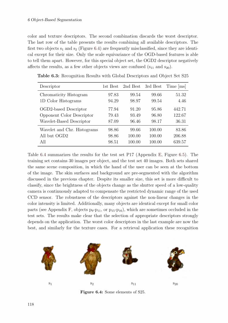
6 Object-Based Segmentation
color and texture descriptors. The second combination discards the worst descriptor.
The last row of the table presents the results combining all available descriptors. The
first two objects s1 and s2 (Figure 6.4) are frequently misclassified, since they are identi-
cal except for their size. Only the scale equivariance of the OGD-based features is able
to tell them apart. However, for this special object set, the OGD2 descriptor negatively
affects the results, as a few other objects views are confused (s11 and s20).
Table 6.3: Recognition Results with Global Descriptors and Object Set S25
Descriptor 1st Best 2nd Best 3rd Best Time [ms]
Chromaticity Histogram 97.83 99.54 99.66 51.32
1D Color Histograms 94.29 98.97 99.54 4.46
OGD2-based Descriptor 77.94 91.20 95.86 442.71
Opponent Color Descriptor 79.43 93.49 96.80 122.67
Wavelet-Based Descriptor 87.09 96.46 98.17 36.31
Wavelet and Chr. Histograms 98.86 99.66 100.00 83.86
All but OGD2 98.86 100.00 100.00 206.88
All 98.51 100.00 100.00 639.57
Table 6.4 summarizes the results for the test set P17 (Appendix E, Figure 6.5). The
training set contains 30 images per object, and the test set 40 images. Both sets shared
the same scene composition, in which the hand of the user can be seen at the bottom
of the image. The skin surfaces and background are pre-segmented with the algorithm
discussed in the previous chapter. Despite its smaller size, this set is more difficult to
classify, since the brightness of the objects change as the shutter speed of a low-quality
camera is continuously adapted to compensate the restricted dynamic range of the used
CCD sensor. The robustness of the descriptors against the non-linear changes in the
color intensity is limited. Additionally, many objects are identical except for small color
parts (see Appendix F, objects p9-p11, or p15-p16), which are sometimes occluded in the
test sets. The results make clear that the selection of appropriate descriptors strongly
depends on the application. The worst color descriptors in the last example are now the
best, and similarly for the texture cases. For a retrieval application these recognition
s1 s2 s11 s20
Figure 6.4: Some elements of S25.
118

6.2 Recognition Based on Local Descriptors
rates are sufficient, as the correct object is always within the best three candidates with
a 99.56% probability. The time requirements are smaller than in the previous example,
since the acquisition system delivers smaller images.
Table 6.4: Recognition Results with Global Descriptors for Object Set P17
Descriptor 1st Best 2nd Best 3rd Best Time [ms]
Chromaticity Histogram 75.29 91.03 94.71 15.29
1D Color Histograms 87.94 97.65 99.85 3.21
OGD2-based Descriptor 65.00 82.35 90.74 251.72
Opponent Color Descriptor 63.09 83.68 90.15 73.21
Wavelet-Based Descriptor 61.76 82.06 91.03 21.70
1D Hist. and OGD2 88.38 96.03 98.97 253.27
All but Wavelet Descriptor 89.56 97.35 99.56 337.32
All 89.71 97.79 99.56 358.50
The pyramid computations for the multi-resolutional analysis and the computation of
basis channels for the steerable filters required in the OGD-based descriptors take the
longest computation times. Nevertheless, the global based recognition is fast enough for
an interactive application.
6.2 Recognition Based on Local Descriptors
The processing path for object recognition using local descriptors (depicted on the right
side of Figure 3.9, p. 52) can also be used in a sequential manner. However, the results are
reliable only after a verification stage. The amount of information that this recognition
concept manipulates is usually considerably larger than global descriptor approaches.
Therefore, their computation times and memory requirements are traditionally higher.
Nonetheless, the recognition of several connected objects in an image is only possible
under consideration of local information.
Local descriptor extraction consists of two stages. First, salient locations in the images
p5 p8 p14 p15
Figure 6.5: Some elements of P17.
119

6 Object-Based Segmentation
are detected. Second, descriptors for the locations are computed. These descriptors are
then classified and verified.
6.2.1 Location Detection
Salient locations, are conspicuous image regions, identified by their position in the image,
their size, and a principal orientation. The detection of these interest points is an active
research field in computer vision. Besides object recognition, they play an important
role in three-dimensional reconstruction and in pose estimation [Bau00, MS02]. In all
three fields of application robust locations are sought that are always detected at the
same relative object positions, independently of the exact object localization, scaling,
or orientation within the image (Figure 6.6).
(a) (b) (c)
Figure 6.6: Location Detection. (a) Example image used throughout the current chapter(contrast has been enhanced). (b) A few locations detected in the image, repre-sented through white squares. (c) Locations detected for the rotated image. Thelocation at the eye of the bear is stable, while some locations in the head of theturtle are not.
Most principles rely on the multi-resolutional analysis, which decomposes an image into
several levels of detail, each containing information at one specific scale or resolution of
the image. Several representations are possible. Figure 6.7 depicts three of them. The
rectangles at the bottom of each structure stand for the original image. Each successive
level discards more and more detail, until the lowest resolution is reached at the top of
the decomposition. Details are removed at each level by means of a low-pass filtering
operation, for which a Gaussian kernel has to be used. A detailed theoretical discussion
for the necessity of the Gaussian kernel is given in [Lin94]. The m-th level in a multi-
scale representation is thus identified by the standard deviation σm of the kernel used
in its generation.
The pyramid representation (Figure 6.7a) only utilizes as much memory as necessary.
Interest points in a given level can be more efficiently detected than employing other
multi-scale representations, since the search algorithm has to deal with fewer pixels.
120

6.2 Recognition Based on Local Descriptors
(a) (b) (c)
σ
Figure 6.7: Multi-scale image representations. (a) Multi-scale pyramid. (b) Lowe’s multi-scale representation. (c) Scale-space representation.
The disadvantage of the pyramid is that the access to the same pixel at several scales
is relatively expensive, since it has to be interpolated. Lowe’s approach (Figure 6.7b)
sacrifices some memory in order to gain speed while accessing the values of a pixel at
different scales within an octave. The scale-space representation (Figure 6.7c) is highly
redundant, and is only used if high precision for the pixel values at different scales is
necessary, and if there is a large number of accesses to the same pixel at several scales.
The pyramid representation has been chosen in this work, since the number of inter-level
accesses is limited, and the search of maxima within each level is the most frequent task.
The location search operates on gray-valued images. The steps involved are summarized
in Figure 6.8. After the computation of a multi-scale representation, saliency maps are
extracted for each level. All local maxima in these maps are possible interest points,
but only a limited number of them can be accepted in order to reduce the processing
times of the next stages. Once the location’s position and scale has been determined,
its orientation is estimated. To deal with color images, the locations are independently
detected for the intensity channel and two opponent color channels R−G, B − Y .
Algorithm: Detection of Locations.
1: compute multi-scale representation of the image
2: compute saliency maps for each level
3: search for scale-space maxima
4: restrict maximal number of locations
5: compute location orientation
Figure 6.8: Detection of Locations.
For the multi-scale representation, two main parameters have to be determined: the
number of levels L, and the scale factor s between two adjacent levels. The latter is
traditionally chosen such that an octave contains an integer number of levels (s = 2−1/k,
k ∈ IN). Figure 6.9 shows an example with k = 2 and L = 6. Lower values of s
produce more precise scale-space representations, but they also considerably increase
121

6 Object-Based Segmentation
Figure 6.9: Multi-scale pyramidal image representation. Six levels with a scale factor betweenthem of s = 2−1/2 (contrast has been enhanced).
the memory requirements and computation times. Lowe [Low03] suggests s = 2−1/3.
The next step generates a conspicuity or saliency measure for each pixel at each level
(Figure 6.10). There are many possibilities for this task. They rely on the gradient mag-
nitude, differences of Gaussians (DoG), the Laplacian operator, or different cornerness
measures, among others [MS02]. The appropriateness of these operators depends on the
image content and is usually empirically determined for each concrete application.
Figure 6.10: DoG-based saliency measure for each level in the pyramid.
Three conditions have to be met in order to consider a point of the multi-scale represen-
tation as a valid salient location. First, its saliency value must be a maximum within
a local neighborhood. Second, in order to avoid the detection of an extremely large
number of locations, the saliency must be greater than a threshold value, which is level
dependent and computed as a predefined fraction of the maximal saliency value found
in that level. The third condition ensures that the locations do not lie at image edges.
The reason for this last condition is that edges are always salient, but they cannot be
robustly localized at a single point. In contrast to the salient points, which are null-
dimensional and are detected as two-dimensional maxima in the saliency image, edges
are one-dimensional salient features, and in the ideal case represent one-dimensional
maxima. A small amount of noise in the images suffices to generate two-dimensional
maxima at arbitrary positions of the edge. The edgeness at a point p = [x, y]T of
the scalar image fI(p) can be computed as the ratio between the largest and smallest
122

6.2 Recognition Based on Local Descriptors
eigenvalues of the Hessian matrix H at p [HS88]:
H(x, y) =
[∂2fI(x,y)
∂x2
∂2fI(x,y)∂x∂y
∂2fI(x,y)∂x∂y
∂2fI(x,y)∂y2
](6.13)
Lowe [Low03] uses the approximation of the derivatives taking differences of neigh-
boring sample points. For the images used in the current work, the kernels derived
in Appendix G have provided more stable approximations. Let λmax and λmin repre-
sent the largest and smallest eigenvalues of H, respectively. Following [HS88], the ratio
r = λmax/λmin can be indirectly used without an explicit computation of the eigenvalues,
since
Tr(H) =∂2fI(x, y)
∂x2+
∂2fI(x, y)
∂y2= λmax + λmin ,
Det(H) =∂2fI(x, y)
∂x2
∂2fI(x, y)
∂y2−(
∂2fI(x, y)
∂x∂y
)2
= λmaxλmin
andTr(H)2
Det(H)=
(r + 1)2
r
which is a monotonically increasing function of r. Only those locations with an edgeness
value smaller than a given threshold are accepted as valid interest points.
In the current application, images can contain objects with very different brightness
values. Since the maximal contrast of an object is proportional to its brightness, reject-
ing locations that have a value smaller than a fraction of the maximal image saliency
inevitably suppresses more locations found in darker regions. In Figure 6.11, for exam-
ple, the white object has always larger saliency values than the darker objects. For the
recognition it is important that a representative number of locations is still available
for each object. The choice of a small saliency threshold provides the desired result
for dark objects, but has as side effect the detection of an excessive large number of
locations in the brighter regions. The number of locations can be reduced employing
local saliency thresholds at each level of the pyramid. The maximal saliency in a circular
neighborhood around each location is computed. If the location saliency is higher than
a predefined fraction of the local maximum, the location is kept.
The previous steps have allowed to detect the position of the locations. Their size
is now given through a location radius, proportional to the level of the multi-scale
representation at which each location has been found. The last step is the estimation
of the orientation. Lowe [Low03] proposes to use an orientation histogram, computed
using the gradient orientations in a neighborhood of the location at the corresponding
pyramid level. Here, additional experiments have been done with the weighted average
orientation within a Gaussian window centered at the location.
An optimal location detection depends on many parameters. Their optimization is usu-
ally done fixing all parameters but one, which obviously strongly restricts the search
for optimal points in the parameter space. The evolutionary multi-objective evalua-
tion concept employed in previous chapters can now be extended to the evaluation of
123

6 Object-Based Segmentation
(a) (b) (c)
(d) (e)
Figure 6.11: Example of local saliency threshold. (a) Original image. (b) DoG-basedsaliency. (c) Corresponding neighboring maxima for a window of radius 10.(d) 120 locations detected without local thresholding. (e) 117 locations foundwith local thresholding
the location detection, providing at the same time optimal parameterizations for each
concrete application.
Two properties are of main interest: the number of locations detected, and the robust-
ness of those locations against image transformations like rotation and scaling. Ideal
translation invariance in the image plane is assumed, since that is one of the prop-
erties ensured with the use of a Gaussian kernel in the generation of the multi-scale
representation [Lin94].
Let the locations be represented by 3-tuples l = 〈p, r, θ〉 describing the position p, the
radius r, and the angle θ of the interest point. The algorithm Du for location detection
is parameterized with u, and is used to find the set of locations Li corresponding to a
reference image I i in a reference set GI :
Li = Du(I i) (6.14)
If the image I i is modified using a transformation Ts,α
Ts,α =
[s cos α −s sin α
s sin α s cos α
](6.15)
that rotates the image with an angle α and scales it with a factor s
I ′i = Ts,α(I i) =〈p′j, cj〉 | p′j = Ts,αpj, 〈pj, cj〉 ∈ Ij
(6.16)
124

6.2 Recognition Based on Local Descriptors
then it can be expected for each robust location l ∈ Li that an equivalent location
l′ ∈ L′i = Du(I ′i) exists, such that l′ = 〈Ts,αp, rs, θ + α〉 for l = 〈p, r, θ〉
Hence, the fitness functions measure how many locations fulfill this robustness condition
for a given set of scaling factors and rotation angles. Here, the mean absolute number
of stable locations fas, the percentage of stable locations frs, and the throughput of
the algorithm have been chosen for the optimization stage. Let Ts,α(Du(I i)) denote
the set of transformed locations of the image I i, Du(Ts,α(I i)) the set of locations for
the transformed image and ∩ an approximative intersection operator that considers two
locations as the same element if their values lie within some tolerance ranges. The subset
of stable locations for a rotation α and scale s is thus
Li(s, α, I i, Du) = Ts,α(Du(I i))∩Du(Ts,α(I i)) (6.17)
with which the fitness functions can be defined as
fas(Du,GI) =
∑Ii∈GI
∑s
∑α
|Li(s, α, I i, Du)|
|GI |(6.18)
frs(Du,GI) =
∑Ii∈GI
∑s
∑α
|Li(s, α, I i, Du)|∑Ii∈GI
|Ts,α(Du(I i))|+ |Du(Ts,α(I i))| − |Li(s, α, I i, Du)|(6.19)
The throughput ft is similarly defined as in (3.6).
Table 6.5 lists the parameters of the location detector and their accepted value ranges.
The optimization with the PESA algorithm (Appendix A) for three different types of
saliency measures provides the Pareto Fronts depicted in Figure 6.12a. Here, the front
for all projections into the ft = 0 plane is shown. The Difference of Gaussians (DoG) has
in all cases the best trade-off between the number of stable locations and the percentage
of stable locations. The three-dimensional front for the DoG saliency measure is depicted
in Figure 6.12b.
For the recognition, a small number of unstable locations is desired, but sufficient lo-
cations are necessary. The absolute number of stable locations should lie between 100
and 150. The most relevant parameters for the selected configuration are: a total of
13 levels with four levels per octave, a neighborhood size for maxima detection within
a level of 3 × 3, a DoG saliency estimator with a distance of one level between the
Gaussians, using for the lower level a variance σ2 = 0.99. The saliency threshold is 0.59
and the edgeness threshold 9.78. The average orientation computation was preferred in
all points over Lowe’s orientation histogram.
6.2.2 Descriptor Extraction
The major problem of local descriptors is their low specificity, which is a consequence
of the limited size of the image region they describe. Choosing highly compact descrip-
125

6 Object-Based Segmentation
Table 6.5: Parameters for the Location Detector
Parameter Value Range
Number of Levels 6 – 20
Scaling Factor 2−1/k, k=2 – 5
Max. Detection Neighborhood 3, 5, 7
Saliency Type Gradient Magnitude, DoG, Harris Cornerness
DoG Level Distance 1 – 5
DoG Base Variance 1 – 5
Saliency Threshold 0 – 1 (8 bits)
Edgeness Threshold 1 – 10 (8 bits)
Orientation Mode Histogram, Average
Orientation Window Radius 2 – 5
σ of Orientation Window 0.5 – 6 (8 bits)
0
200
400
600
800
1000
1200
1400
1600
0.05 0.1 0.15 0.2 0.25 0.3 0.35 0.4 0.45
Abs
olut
e N
umbe
r of S
tabl
e L
ocat
ions
Percentage of Stable Locations
DoGGradient
Harris
04
812
16
0.050.15
0.250.35
0.45
0200400600800
100012001400
ThroughputRelative Stable
Abs
olut
e St
able
(a) (b)
Figure 6.12: Pareto Fronts for Location Detectors. (a) Percentage of stable locations (frs)vs. Absolute number of stable locations (fas) for all three saliency measures. (b)Three-dimensional front for the DoG-based measure including also the through-put (ft).
tors can make this problem even worse. However, since several thousands of locations
have to be manipulated and stored in the classification modules, the selection of high
dimensional feature spaces has severe consequences in the memory requirements and the
expected computation times.
In this work, two local descriptors have been studied. The first one is Lowe’s Scale
Invariance Feature Transform (SIFT) descriptor, which is a 128-dimensional vector en-
coding a histogram of weighted gradient vectors within the location’s region (see [Low03]
for details). It performed best in an experimental comparison provided in [MS03]. The
second one is an simple local color descriptor, used to exploit the color information in
126

6.2 Recognition Based on Local Descriptors
the current object sets.
The color descriptor encodes the distribution of colors around the interest point, which
can be assumed to be characteristic due the corner-like nature of the salient locations.
The descriptor is extracted by aligning two masks (Figure 6.13) with the position and
orientation of the location, and computing for each image slice the corresponding mean
color. The radius of the location determines the radius used for the masks. Two overlap-
ping masks are necessary in order to gain some robustness against errors in the detection
of the location orientation. The number of slices is a parameter to be adjusted for each
application.
245126
1089117
13
Figure 6.13: Masks for a local color feature. The final descriptor has 3 × 12 dimensions, aseach slice contributes a mean color with three components.
6.2.3 Classification of Local Descriptors
The parameterization of classifiers for local descriptors is more complex than for the
global equivalents, since it cannot be guessed how many clusters will be found in the
feature space for each object. Additionally, the low specificity of local descriptors has as
consequence that clusters belonging to different objects occupy the same regions in the
feature space. For these reasons, in local feature classification the k-Nearest-Neighbor
(kNN) classifier is employed. It stores the complete training data set, and computes the
probability P (oi|x) that a pattern x belongs to a class oi relying on
P (oi|x) =p(x|oi)P (oi)
p(x). (6.20)
Let p(x) be the probability density for the descriptor vectors x in the feature space.
The probability P that a feature vector can be found in a region A of the feature space
is then
P =
∫A
p(x)dx (6.21)
If the data set is large enough, a condition fulfilled by many local descriptors, (6.21) can
be approximated as:
P ≈ mA
m(6.22)
with mA the number of training patterns falling into the region A and m the total
number of training patterns. If the probability density p(x) can be assumed to be
127

6 Object-Based Segmentation
continuous and if it does not vary significantly over the region A, then (6.21) can also
be approximated as
P =
∫A
p(x)dx ≈ p(x)v (6.23)
with v the volume of the region A and x any point within the region. Combining (6.22)
and (6.23) it follows
p(x) ≈ mA
m· 1
v(6.24)
The probability density is then approximated determining the smallest region of volume
v (traditionally a hyper-sphere), centered at x that contains exactly mA patterns. For
the classification problem each training pattern has been labeled with its corresponding
class, such that the following probabilities can be computed
p(x|oi) =miA
mi
1
vp(x) =
mA
m
1
vP (oi) =
mi
m(6.25)
with oi the class label, miA the number of patterns of the class oi falling into A, mi the
total number of patterns belonging to the class oi. It follows with (6.20)
P (oi|x) =miA
mA. (6.26)
Since the classification maximizes P (oi|x), the pattern x probably belongs to the class
with the largest number of points in a set containing the k = mA nearest patterns to x.
In object retrieval applications, however, it can be assumed that all classes have the
same a-priori probability P (oi) = 1/|Ω|, with Ω the set of all objects to be recognized
by the system. In this case, the probability for a class given the pattern x is
P (oi|x) =miA
mA· m
mi|Ω|. (6.27)
In the training stage, interest locations are detected for each pre-segmented image of
all objects. Descriptors for those locations are extracted and stored in a kd-tree data
structure [FBF77], which makes possible an efficient retrieval of the k nearest neighbors
of a given pattern in the recall stage. Additionally, Lowe introduced in [Low99] a best-
bin-first approximative search method, that allows to find points in the kd-tree that
are probably the nearest neighbors using a limited number of comparisons only. This
accelerates the search with tolerable sacrifices in the classification quality.
A simple recognition approach relying on local descriptors is based on a voting concept.
Each location votes for all objects that have a probability greater than zero in the dis-
tributions found by the classifiers for its descriptors. The magnitude of the votes equals
the probability of each object. This resembles the combination mechanism employed in
the global classification concept, except that in this case the object probability distri-
butions are obtained from the same kind of information sources. The final classification
result is then a ranking list, where the objects with the largest number of votes are the
most probable.
128

6.2 Recognition Based on Local Descriptors
Table 6.6: Recognition Results with Local Descriptors for Object Set S25
MTpI: Mean Time per Image MTpL: Mean Time per Location
Descriptor kNN BBF 1st Best 2nd Best 3rd Best MTpI MTpL
[%] [%] [%] [ms] [ms]
Lowe’s Descriptor 1 yes 20.91 28.69 34.97 425.29 6.68
Local Color Desc. 5 no 75.20 83.66 88.00 430.62 6.77
Local Color Desc. 3 no 76.46 84.46 88.69 391.67 6.16
Local Color Desc. 1 no 78.17 84.80 88.34 316.86 4.98
Local Color Desc. 1 yes 78.40 84.57 87.66 252.14 3.96
Tables 6.6 and 6.7 present the recognition results for the sets S25 and P17, respectively,
obtained with this voting concept. The same test images were used as in the experiments
for recognition with global descriptors. The number of nearest neighbors is listed in
the second column, followed by an indication whether the best-bin-first (BBF) search
method is employed or not. The last entries in each row contain the mean times for
descriptor extraction and classification per image and per location. Lowe’s descriptor is
inappropriate for the current application context, as the reached recognition rates are
very low. Moreover, the high dimensionality of the feature space demands long searching
times. The local color descriptor, despite its simplicity, provides in this framework
results comparable to those of global descriptors. In these tables, masks with 6 slices
(i. e. a total of 12 mean colors per local descriptor) have been employed. In both cases
the locations have been detected in the intensity channel. The smaller the number of
nearest neighbors used in the probability estimation, the better the classification results.
The reason for this behavior can be sought in atypical patterns with high specificity for
certain objects. If they lie in a sparse region of the feature space, the selection of
k neighbors will force the consideration of additional patterns, which can be located
far away from the nearest neighbor and thus probably belong to other classes. The
improvement of the results with the approximative best-bin-first search is an unexpected
behavior. It indicates that the irregular quantization of the feature space done by the
kd-trees is correlated with object classes. Thus, restricting the search space to those
bins where a point is expected provides better results than searching for the absolute
nearest point which can belong to the wrong object.
Table 6.8 lists some additional classification results for different color descriptors, in
which the number of slices per mask is varied. The final feature space dimensionality
equals this number times 6, since two overlapping masks are employed and each slice
contributes the three components of its mean color. Besides the intensity channel,
locations have also been detected on the opponent color channels R − G and B − Y .
The larger number of locations improves the results considerably. For these experiments
a nearest neighbor classifier has been used (i. e. k = 1).
The performance difference between local and global approaches is more noticeable with
129

6 Object-Based Segmentation
Table 6.7: Recognition Results with Local Descriptors for Object Set P17
MTpI: Mean Time per Image MTpL: Mean Time per Location
Descriptor kNN BBF 1st Best 2nd Best 3rd Best MTpI MTpL
[%] [%] [%] [ms] [ms]
Lowe’s Descriptor 5 no 49.26 61.03 66.91 4962.78 43.36
Lowe’s Descriptor 1 yes 42.06 52.94 60.44 466.42 4.08
Local Color Desc. 5 no 81.32 91.76 93.82 506.45 4.43
Local Color Desc. 3 no 82.50 91.91 94.41 452.14 3.95
Local Color Desc. 1 no 81.91 91.62 94.85 343.84 3.00
Local Color Desc. 1 yes 82.50 91.91 95.15 295.94 2.59
Table 6.8: Recognition Results with Local Color Descriptors for Object Set S25
Slices 1st Best 2nd Best 3rd Best
[%] [%] [%]
2 93.71 97.94 99.08
3 94.17 98.06 99.66
4 94.97 98.51 99.43
5 93.71 98.51 99.43
6 94.29 98.62 99.66
7 94.29 98.51 99.43
larger object sets. Table 6.9 lists the comparison for the test set S200, from which an
excerpt has been depicted in Appendix F. It contains 200 objects, including the 25 items
of S25. The training and test sets were acquired under the same conditions of S25 (see
Section 6.1.3). The local color descriptor requires almost 30 times more memory than
all global descriptors together. The larger data set affects the computations for both
classifiers: RBF-Networks have to deal with larger weight matrices and kNN classifiers
have to search for neighbors in a data set with much more points. The global color
descriptors perform in this case better than the local equivalent. Due to the low memory
and time requirements it is feasible to merge the results of all global descriptors to obtain
an even more reliable result.
Table 6.9: Recognition Results for Object Set S200
Recognition 1st Best 2nd Best 3rd Best Time Memory
[%] [%] [%] [ms] MB
Global Chr. Histogram 77.23 86.85 91.17 61.13 2.3
Global 1D Histograms 82.06 90.71 93.80 12.98 2.7
Global Descriptors (all 5) 87.27 93.30 95.59 846 12
Local Color Descriptor 72.39 81.11 85.52 1110 345
130
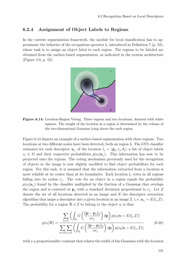
6.2 Recognition Based on Local Descriptors
6.2.4 Assignment of Object Labels to Regions
In the current segmentation framework, the module for local classification has to ap-
proximate the behavior of the recognition operator L, introduced in Definition 7 (p. 33),
whose task is to assign an object label to each region. The regions to be labeled are
obtained from the surface-based segmentation, as indicated in the system architecture
(Figure 3.9, p. 52).
Figure 6.14: Location-Region Voting. Three regions and two locations, denoted with whitesquares. The weight of the location in a region is determined by the volume ofthe two-dimensional Gaussian lying above the each region.
Figure 6.14 depicts an example of a surface-based segmentation with three regions. Two
locations at two different scales have been detected, both on region 3. The kNN classifier
estimates for each descriptor xlj of the location lj = 〈pj, rj, θj〉 a list of object labels
oi ∈ Ω and their respective probabilities p(oi|xlj). This information has now to be
projected onto the regions. The voting mechanism previously used for the recognition
of objects in the image is now slightly modified to find object probabilities for each
region. For this task, it is assumed that the information extracted from a location is
more reliable at its center than at its boundaries. Each location lj votes in all regions
falling into its radius rj. The vote for an object in a region equals the probability
p(oi|xlj) found by the classifier multiplied by the fraction of a Gaussian that overlaps
the region and is centered at pj with a standard deviation proportional to rj. Let Ldenote the set of all locations detected in an image and E the descriptor extraction
algorithm that maps a descriptor into a given location in an image I, i. e. xlj = E(lj, I).
The probability for a region R ∈ I to belong to the object oi is thus
p(oi|R) =
∑lj∈L
(∫R
G
(‖p− pj‖2
κrj
)dp
)p(oi|x = E(lj, I))
∑ok∈Ω
∑lj∈L
(∫R
G
(‖p− pj‖2
κrj
)dp
)p(ok|x = E(lj, I))
(6.28)
with κ a proportionality constant that relates the width of the Gaussian with the location
131

6 Object-Based Segmentation
radius, ‖ · ‖2 the L2-norm, and G(x) given by
G(x) =1√2π
exp
(−x2
2
). (6.29)
Even if in Figure 6.14 no locations were found for the regions 1 and 2, with this concept
they get some small votes from the locations found in region 3.
6.3 Object-based Segmentation Module
Figure 6.15 depicts the high-level modules of the object recognition framework intro-
duced in Figure 3.9 (p. 52). At this point, the local classification module has computed
for each region R of the surface-based segmentation a set of probabilities p(oi|R) that
the region belongs to the object oi in the set Ω.
SceneSetting
Knowledge
Knowledge ofObjects’ LocalAppearance
Knowledge ofObjects’ GlobalAppearance
Global DescriptorExtraction
ClassificationLocal
Verification
ClassificationGlobal
Object−basedSegmentation
Result
Surface−based
Figure 6.15: Recognition and object-based segmentation stages.
This information is passed directly to the object-based segmentation module. It then
generates a set of hypotheses to be verified using the global-based recognition method.
Any object oi with a probability greater than zero in any region is preliminarily taken
as candidate object in the image. All regions Rj for which
p(oi|Rj) > δ maxok∈Ω
p(ok|Rj) (6.30)
are assumed to belong to the object oi. They are used to construct a segmentation
mask, in which all regions fulfilling (6.30) are assigned to the figure and the rest to the
ground. The factor δ ∈ [0 . . . 1] controls the minimal accepted probabilities as a fraction
of the maximal belief available for the considered region.
A hypothesis is accepted only if the total number of pixels in its mask is greater than
a predefined threshold. This is necessary, first, because arbitrary probability values can
be expected for small isolated regions, as they can be similar to local aspects of different
objects; and second, because the recognition system based on global descriptors cannot
132

6.3 Object-based Segmentation Module
cope with high levels of occlusion. The threshold value is selected as a fraction of the
smallest expected object in the training set.
Figure 6.16 depicts an example image, the locations detected in it, and the surface-based
segmentation. The region probabilities and hypothesized mask for the object s24 (see
Appendix F) are also shown.
(a) (b) (c)
(d) (e)
Figure 6.16: First Hypothesis. (a) Original Image. (b) Locations. (c) Surface-based segmen-tation. (d) Region probabilities for object s24. (d) Hypothesis mask for objects24.
The hypothesis for one object oi is verified with the global recognition subsystem. The
mask is used to suppress the ground regions in the image before the feature extraction
and classification stages produce a “global” probability distribution. The rank of the
object oi in the distribution and its probability value are used to accept and compare the
hypotheses. If the rank value is higher than a predefined value, the global verification
fails. On the other hand, if the rank is good enough, the probability for oi is used
as goodness measure g(oi). For example, if the hypothesis corresponds to the object
o1, and the probability distribution obtained from the global classification contains the
following four object/probability tuples
〈o2, p = 0.4〉︸ ︷︷ ︸Rank 1
, 〈o1, p = 0.3〉︸ ︷︷ ︸Rank 2
, 〈o3, p = 0.2〉︸ ︷︷ ︸Rank 3
, 〈o4, p = 0.1〉︸ ︷︷ ︸Rank 4
then the hypothesis is accepted if the rank 2 is lower or equal than a predefined value.
The probability 0.3 is used as goodness measure for the o1 hypothesis (i. e. g(o1) = 0.3).
133

6 Object-Based Segmentation
This method favors those hypotheses that are consistent with the global recognition.
Figure 6.17 depicts some examples. The first three hypotheses have been accepted
while the fourth one is considered as wrong.
24
s16s13
s7
s
(a) (b) (c)
(d) (e)
Figure 6.17: Further hypotheses for the test image in (a). (b) s7. (c) s13. (d) s16. (e) s19.
The hypotheses for all objects oi in the set Ω are then evaluated. The object-based
segmentation receives the goodness measures for all hypotheses as feedback from the
verification stage. In the location classification (Section 6.2.4), probabilities p(oi|R) for
each region were estimated. Discriminant values are now computed for each region of
the form p(oi|R)g(oi). Each region is then assigned to the object ok with the maximal
discriminant:
L(R) = ok = arg maxoi
p(oi|R)g(oi) . (6.31)
The resulting mask (Figure 6.18b) can still contain some artifacts, which are removed in
a last stage. All regions with a number of pixels less than a predefined value are marked
as free, while all other regions are kept as seeds for a growing process. The freed regions
are then merged to the most similar objects. The growing mechanism has already been
discussed in the previous chapters. Figure 6.18c shows the final mask for the example
figure. As recognition result a probability distribution is generated in which the final
object labels use as probability the goodness measures computed for their corresponding
hypotheses.
134

6.4 Recognition Experiments with Multiple Objects
(a) (b) (c)
Figure 6.18: Combination and final masks. (a) Test image. (b) Combination of hypotheses.(c) Final segmentation mask.
6.4 Recognition Experiments with Multiple Objects
The previous sections have presented recognition results with global and local descriptors
for images containing a single object (test sets S25 and S200, Tables 6.3, 6.6, 6.8, and
6.9), or one object and the hand of the user (test set P17, Tables 6.4 and 6.7). In these
contexts, the surface-based segmentation is sufficient to suppress everything but the
object of interest in the images. This section provides further experiments with several
objects in the images, a task that necessitates the object-based segmentation module
and the interaction with the recognition subsystems, i. e. these experiments make used
of the complete three-staged segmentation framework.
A new test set is necessary that contains images with several objects and their cor-
responding reference segmentations. In order to avoid the acquisition of hundreds of
images and especially their manual segmentation, the test set S25 has been used to au-
tomatically generate images and their optimal segmentations, with the advantage that
the degree of overlapping between the objects can be directly controlled. It has to be
noted that the resulting images may contain objects lying partially outside the images,
and thus the occlusion factor given in the experiments has to be considered as the least
expected occlusion percentage. Figure 6.19 presents some examples for different degrees
of inter-object occlusion. 625 images for each of seven different occlusion percentages
have been generated by randomly taking two objects and rotating and translating one
of them until the desired overlapping factor is obtained.
Table 6.10 summarizes the experimental results. Since the images contain two objects,
a correct classification assigns the two largest probabilities to the expected objects. The
entries in the table represent the percentages of correct classifications for the different
experiments. The first row contains the results according to the local region classification
only (Section 6.2.4). The next rows specify the minimal rank which a hypothesized
object is allowed to have in the probability distribution found with global descriptors.
Figure 6.20 shows the resulting segmentations of the images in Figure 6.19. The use of
135

6 Object-Based Segmentation
(a) (b) (c) (d)
Figure 6.19: Examples of multiple objects. The occlusion percentages are (a) 0%, (b) 20%,(c) 30% and (d) 60%.
the first two ranks in the global-based probability distribution improves the recognition
rates in all cases.
(a) (b) (c) (d)
Figure 6.20: Final segmentations for the images Figure 6.19. The occlusion percentages are(a) 0%, (b) 20%, (c) 30% and (d) 60%.
Table 6.10: Combined recognition results
Global Occlusion Percentage
Rank 0% 10% 20% 30% 40% 50% 60%
Local 89.18 87.83 88.65 85.99 82.03 78.40 71.27
1 91.13 88.24 89.39 86.73 82.93 78.89 72.34
2 91.29 88.64 89.39 86.98 83.02 78.98 72.42
3 90.97 88.08 88.82 86.40 82.94 78.24 72.26
4 91.05 88.56 87.51 85.83 82.36 76.99 71.52
5 90.15 88.40 86.86 84.77 82.36 76.59 70.94
The reduction of the recognition rates in comparison to the values in Table 6.8 is related
to the fact that the voting is made region-wise and not for the whole image. Splitting
the locations into regions increases the chance that their information gets lost if a region
is assigned to the wrong object.
Summarizing, the proposed three-stage segmentation framework has made it possible
136

6.4 Recognition Experiments with Multiple Objects
not only to recognize several objects in an image but also to delimit the regions depicting
them. No other segmentation concept known to the author is capable of such achieve-
ment. The surface-based segmentation provides all necessary mechanisms to preprocess
the training set, when the conditions of a homogeneous background and one object per
image are fulfilled. This second segmentation stage is even sufficient for applications
that expect only one object in the image. The proposed mechanisms for the incorpo-
ration of knowledge about the scene into the segmentation process has permitted to
solve complex problems like the separation of the user’s hand from skin-colored objects.
The object-based segmentation makes use of knowledge about the appearance of each
particular object. It serves as mediator between recognition approaches based on global
and local descriptors, which, until now, had been kept apart in the object recognition
literature.
137

6 Object-Based Segmentation
138

Chapter 7
Conclusion and Outlook
Humans acquire a major part of the information about their environment through the
visual sense. It is therefore not surprising that the use and size of databases containing
visual information steadily increase. The expanding volume of data makes it necessary
to conceive efficient ways to query this kind of information. Object retrieval systems
following a query-by-example paradigm are a promising concept in applications that
retrieve data on three-dimensional objects. The user just presents the object itself to a
digital camera attached to the system. A recognition process follows that identifies the
object or objects in the image and uses the identification labels to retrieve additional
information.
This concept is applicable in contexts where human users have to recognize products
without additional automatic identification resources like bar-codes or transceivers. It
helps to speed up queries and supersedes manual browsing of printed catalogs. Concrete
applications can be found in spare part retrieval, product remittance, or in hardware
stores, where the retrieval system provides information like part numbers, equivalent or
similar products, or just the physical location of a product in the store. Additionally,
the recognition process can also be employed as a verification mechanism in production
lines. For instance, the recognition of several objects in a scene can help determining if
a packaging process is properly working.
7.1 Summary of the Work
The present dissertation is devoted to the analysis and implementation of the image
segmentation task as required by object retrieval applications. Its final goal is to find an
image partition, such that each detected region corresponds to an object known to the
retrieval system. This task is a vision problem, i. e. the segmentation has to infer, at least
partially, which three-dimensional scene is the cause for a given image. Since one image
can depict a theoretically infinite number of possible scenes, the segmentation problem
is ill-posed. The only way to reduce the possible number of scene interpretations to
139
7 Conclusion and Outlook
exactly one is by imposing additional constraints derived from a-priori knowledge about
the scene composition, the image formation process, and the expected objects in the
scene.
Hence, this work is not only concerned with image analysis and processing issues, but
also with the modeling of knowledge about the objects and the scene, and its incorpo-
ration into the segmentation process. In accordance with Marr-Palmer’s general vision
model, the segmentation task is split into three stages. The image-based segmentation
stage exclusively analyzes information contained in the image to find homogeneous re-
gions. The surface-based level incorporates knowledge of the scene composition into the
process to support the detection of expected surfaces, like the background. The object-
based stage makes use of knowledge about the appearance of expected objects to finally
produce the desired segmentation. This conceptual separation allows to concentrate at
each level on different aspects of the segmentation problem.
The three segmentation stages can be regarded as a progressive region merging task, in
which the merge decisions are taken considering information gained at different levels of
abstraction. At the image-based stage pixels merge into regions taking into account low-
level features only. The surface-based stage combines those image-based regions which
are likely to belong to the same surfaces, accordingly to some given a-priori information
about the expected surfaces. The last, object-based stage interacts with the recognition
modules to merge regions that belong to the same objects, incorporating high-level
information about the objects themselves into the process.
No standard mechanisms for the evaluation of segmentation algorithms exist, making it
difficult to objectively compare different approaches. Some scalar functions have been
proposed that provide a total goodness measure for the segmentation (e. g. [LY94]).
However, they are in general inappropriate, since scalar values cannot encode unavoid-
able conflicts between different competing aspects of a segmentation result, like the total
number of regions, throughput, or segmentation accuracy. In this work, a flexible evalu-
ation approach initially proposed by Everingham et al. in [EMT02] has been chosen. It
is based on an evolutionary multi-objective optimization concept, that not only allows
a quantitative comparison of different segmentation algorithms, but also provides the
best parameterizations to operate in optimal points of a multi-dimensional fitness space.
Most fitness functions represent discrepancy measures, which compare the results of an
algorithm with some “ground truth” data. The preparation of such a “golden set” can
be regarded as disadvantage, since in several applications it represents a tedious, diffi-
cult and expensive task. However, it provides a mechanism to optimize the performance
of an algorithm for a specific application if the reference set is chosen to represent the
commonly expected cases. In object retrieval applications with a controlled environ-
ment, preparing the reference set does not represent a major problem, as the images are
relatively similar and a small set is already representative.
In the last three decades the research efforts have concentrated on image-based seg-
mentation algorithms. Selecting among thousands of existent possibilities is, however, a
140
7.1 Summary of the Work
difficult – if not impossible – task, mainly because the source code of the algorithms is
rarely published and their descriptions frequently lack the degree of detail necessary for
an accurate reconstruction. Hence, new approaches appear with every application case.
In this work a detailed review of existing segmentation concepts provides the founda-
tions for two revised color segmentation algorithms. The first one is a watershed-based
approach, which uses information in the image-domain to detect homogeneous regions.
An initial image partition is created using the watershed transformation, followed by
a region merging stage that tries to minimize the error of a piece-wise constant image
approximation. The second concept relies on a k-Means-based cluster detection in the
color space, which, together with an edge detector, is used to find an initial image par-
tition. The same merging stage as in the previous concept can be appended to reduce
the final number of regions. These two algorithms and the mean-shift segmentation of
Comaniciu and Meer [CM02] have been compared with the multi-objective evaluation
method. The watershed-based approach is the best choice, not only due to its efficiency,
but because it provides higher levels of accuracy with a smaller number of regions.
Additionally, an extension of Pappas’ Adaptive-Clustering Algorithm [Pap92] to color
images has been tested as a representative of consistent labeling approaches. However,
the required computation times are excessively high for an interactive application.
The surface-based stage can incorporate data obtained from three information sources:
the image formation process, perceptual grouping rules, and knowledge about the scene
composition. The first two cues are context independent. Hence, they have a negative
influence on the segmentation, since surfaces of similar objects merge if they are made
of the same materials. For this reason at this stage exclusively knowledge about the
scene composition is employed. Information about colors and positional expectations
for the surfaces is encoded in random variables. The probability for a region to belong
to a surface is then obtained combining different random variables with Bayesian Belief
Networks. Knowledge of experts can be straightforwardly encoded in the Conditional
Probability Tables (CPT) of the networks. Additionally, it is possible to train their
values using a representative reference set: the entries of the CPTs are part of the
parameterization of the segmentation algorithm and therefore they are optimized in the
evolutionary evaluation process.
If the knowledge encoded in the random variables is highly reliable, then the final
membership of a region to a surface is decided with a simple thresholding operation
(e. g. homogeneous background detection). For complex surfaces, however, the used
knowledge is limited or uncertain. In this case the combined probabilities are used to
mark the regions with the highest beliefs as seeds for the surfaces. A region growing
process computes the final surface segmentation. This approach has been successfully
employed in the segmentation of the hand from objects that exhibit skin similar colors.
An additional novel idea in the current framework is the use of the object-based segmen-
tation module as mediator between two different recognition paradigms. The informa-
tion provided by a recognition subsystem based on local descriptors is used to generate
141

7 Conclusion and Outlook
several hypotheses about the belief of a region to belong to a given object. Each hy-
pothesis is then tested with a recognition module that analyzes global descriptors. All
hypotheses are combined to obtain the final segmentation mask. The recognition re-
sult is not sequentially dependent on the segmentation stage anymore. Both modules
cooperate to find the most probable segmentation for given a recognition result and
vice-versa.
The most important contributions of this work can be summarized as follows:
• Detailed analysis of the object retrieval and recognition task (Chapter 2).
• Proposal of a three-staged segmentation framework that facilitates the incorpo-
ration of additional knowledge into the segmentation process of retrieval applica-
tions. The three stages are denoted as image-based, surface-based, and object-
based segmentation (Section 3.1).
• Detailed analysis of modern approaches for segmentation within the three-staged
segmentation framework (Chapter 3).
• Introduction of an efficient and accurate image-based segmentation concept for
color images based on the watershed transform (Section 4.2).
• Proposal of a mechanism based on Bayesian Belief Networks to combine several
information cues in the segmentation of scene surfaces (Section 5.3).
• Extension of a multi-objective evaluation concept that permits to optimize the
parameterization of the segmentation algorithms to fulfill the requirements of spe-
cific applications (Section 3.7). For instance, the Conditional Probability Tables
(CPTs) used in the Bayesian Belief Networks can be learned from reference data
(Section 5.4).
• Proposal of a new concept to combine recognition processes relying on global and
local feature descriptors, using the segmentation as a mediator (Section 6.3).
• Segmentation of images containing the hand of the user and skin-colored objects
(Section 5.4, Figure 5.23).
• Segmentation of images containing several, possibly overlapping objects (Sec-
tion 6.3, Figures 6.18 and 6.20).
• Development of a novel color zooming concept, that relies on the whitening trans-
formation to enhance small color differences (Section 5.4.2, Figure 5.17).
• Objective evaluation for algorithms that detect salient points using the multi-
objective evolutionary approach. This helps improving the recognition processes
based on local descriptors (Section 6.2.1).
142

7.2 Outlook
7.2 Outlook
The introduced segmentation framework is general enough to be employed in other ap-
plications fields. Splitting the segmentation task of any application into three stages
always reduces its complexity, as each subproblem needs to deal with fewer conditions
and restrictions than the whole problem. Additionally, the framework provides a guide-
line for the integration of specific knowledge into the segmentation and recognition
processes. On the other hand, extending the introduced algorithmic concepts to other
contexts is a challenging task.
The watershed-based segmentation is applicable to other contexts without further mod-
ifications. Extensions are still possible, if the expected computation times are not re-
strictive. For example, the over-segmentation of the watershed transformation has been
reduced relying on the error minimization of a piece-wise constant image approximation.
Following [BG89], this condition can be replaced by a more general polygonal surface
approximation. The computational burden for this enhancement is especially reflected
in the region merging process, since after each merge new surfaces have to be estimated
and the error measure has to be updated.
The surface-based level can be extended to use other information queues. For instance,
if image sequences are available, the next step is to encode motion information into
additional random variables. One interesting research topic is the extension of the
evaluation concept to find not only the CPTs of the Bayesian Networks but also their
topology. This requires, however, a modification of the evolutionary algorithm: each
hypothesized topology has to be optimized some steps before it is finally accepted or
discarded. Otherwise, an arbitrary architecture with a “fortunate” random CPT ini-
tialization would be further optimized, while potentially better architectures with an
unfavorable initialization would be rejected.
The evolutionary multi-objective evaluation concept can be extended to improve other
aspects of the location detection, like area coverage, i. e. a good location detector for
object recognition should find at least one location in each surface-based region, or,
equivalently, the location density should be uniform in the whole image. This ensures
that all regions obtain sufficient information from the recognition modules. Additionally,
the Pareto fronts can serve as replacement for the ROC curves utilized in the evalua-
tion of local descriptors (e. g. [MS03]), as they encode more information about possible
parameterizations and are more flexible in the selection of fitness measures.
For the retrieval systems of rigid objects, a pose-estimation module based on local-
descriptors can be integrated into the verification stage. This would allow a more reliably
detection of the object boundaries and would make possible to distinguish between
different instances of the same object class. A challenging task in a rather theoretical line
will be to find a probabilistic framework in which the segmentation and the classification
processes can be unified. A possibility can be the integration of the consistent labeling
concepts introduced in [Fla02].
143

7 Conclusion and Outlook
The fact that the human visual system employs both local and global information sources
[Car98, Pal99] is an indicator that future research should not exclusively concentrate on
the recognition based on local descriptors. The design of global descriptors for texture,
shape, and color that are robust to occlusion and illumination changes is also an active
research field. Promising achievements in that area will automatically improve the
segmentation and recognition results using the framework introduced in this work.
144

Bibliography
[AA01] S. Akyol and P. Alvarado. Finding relevant image content for mobile sign
language recognition. In Proc. of the IASTED International Conference Sig-
nal Processing, Pattern Recognition and Applications, pages 48–52, Rhodes,
Greece, July 2001.
[ABA02] P. Alvarado, A. Berner, and S. Akyol. Combination of high-level cues in un-
supervised single image segmentation using Bayesian belief networks. In
Proc. of the International Conference on Imaging Science, Systems and
Technology, pages 235–240, Las Vegas, Nevada, June 2002.
[ADW01] P. Alvarado, P. Doerfler, and J. Wickel. Axon2 – a visual object recogni-
tion system for non-rigid objects. In Proc. of the IASTED International
Conference Signal Processing, Pattern Recognition and Applications, pages
235–240, Rhodes, Greece, July 2001.
[AGNT96] J. K. Aggarwal, J. Ghosh, D. Nair, and I. Taha. A comparative study of three
paradigms for object recognition – Bayesian statistics, neural networks, and
expert systems. In K. Bowyer and N. Ahuja, editors, Advances in Image
Understanding (a Festschrift for Azriel Rosenfeld), pages 241–262. IEEE
Computer Society Press, 1996.
[AK88] M. Amadasun and R. A. King. Low-level segmentation of multispectral
images via agglomerative clustering of uniform neighbourhoods. Pattern
Recognition, 21(3):261–268, 1988.
[AL98] A. Amir and M. Lindenbaum. A generic grouping algorithm and its quan-
titative analysis. IEEE Transactions on Pattern Analysis and Machine In-
telligence, 20(2):168–185, February 1998.
[Alv98] P. Alvarado. Farbtexturanalyse fur die Objekterkennung. Diplomarbeit,
Lehrstuhl fur Technische Informatik, RWTH-Aachen University, Aachen,
Germany, Oktober 1998.
[AMP+97] F. Ackermann, A. Maßmann, S. Posch, G. Sagerer, and D. Schluter. Percep-
tual grouping of contour segments using Markov Random Fields. Pattern
Recognition and Image Analysis, 7(1):11–17, 1997.
145

Bibliography
[And00] S. Ando. Consistent gradient operators. IEEE Transactions on Pattern
Analysis and Machine Intelligence, 22(3):252–265, March 2000.
[Bau00] A. Baumberg. Reliable feature matching across widely separated views. In
Computer Vision and Pattern Recognition (CVPR’00), volume 1, June 2000.
[BC91] L. Bonsiepen and W. Coy. Stable segmentation using color information. In
Proc. of CAIP’91, Computer Analysis of Images and Patterns, pages 77–84,
Dresden, September 1991. R. Klette.
[BCF02] K. Barnard, V. Cardei, and B Funt. A comparison of computational color
constancy algorithms – Part I. IEEE Transactions on Image Processing,
11(9):972–984, September 2002.
[BCS98] M. Borsotti, P. Campadelli, and R. Schettini. Quantitative evaluation of
color image segmentation results. Pattern Recognition Letters, 19:741–747,
1998.
[BD01] A. Bobick and J. Davis. The representation and recognition of action using
temporal templates. IEEE Transactions on Pattern Analysis and Machine
Intelligence, 23(3):257–267, 2001.
[Ber01] A. Berner. Segmentierung von Bildern und Bildsequenzen fur die 3D Ob-
jekterkennung. Diplomarbeit, Lehrstuhl fur Technische Informatik, RWTH-
Aachen University, Aachen, Germany, December 2001.
[Bes74] J. Besag. Spatial interaction and the statistical analysis of lattice systems.
Journal of the Royal Statistical Society. Series B, 26(2):192–236, 1974.
[BF00] K. Barnard and G. Finlayson. Shadow identification using colour ratios.
In Proc. of the IS&T/SID Eigth Color Imaging Conference: Color Science,
Systems and Applications, pages 97–101, 2000.
[BG89] J.-M. Beaulieu and M. Goldberg. Hierarchy in picture segmentation: A
stepwise optimization approach. IEEE Transactions on Pattern Analysis
and Machine Intelligence, 11(2):150–163, February 1989.
[Bis95] C. M. Bishop. Neural Networks for Pattern Recognition. Oxford University
Press, 1995.
[BP97] T. Bomberg and S. Posch. Regionensegmentierung von Farbbildfolgen.
In E. Paulus and F. M. Wahl, editors, Mustererkennung 97, 19. DAGM-
Symposium, Informatik-Fachberichte, Informatik Aktuell, pages 63–70,
Braunschweig, 1997. Springer.
146

Bibliography
[BS94] C. Bouman and M. Shapiro. A Multiscale Random Field Model for Bayesian
image segmentation. IEEE Transactions on Image Processing, 3(2):162–
177, March 1994. Available from World Wide Web: citeseer.nj.nec.
com/bouman96multiscale.html.
[BU02] E. Borenstein and S. Ullman. Class-specific, top-down segmentation. In
Proc. European Conference on Computer Vision, pages 109–124, 2002.
[BZ03] A. Barbu and S. C. Zhu. Graph partition by Swendsen-Wang Cuts. In Proc.
International Conference on Computer Vision, 2003.
[Can86] J. F. Canny. A computational approach to edge detection. IEEE Transac-
tions on Pattern Analysis and Machine Intelligence, 8(6):679–698, August
1986.
[Car98] R. Carter. Mapping the Mind. Phoenix, 1998.
[CdH98] M. Celenk and M Uijt de Haag. Optimal thresholding for color images.
In Proc. of the SPIE – The Int’l Soc. for Optical Eng., Nonlinear Image
Processing IX, pages 250–259, San Jose, CA, January 1998.
[CGI+99] A. Chella, V. Di Gesu, I. Infantino, D. Intravaia, and C. Valenti. A coop-
erating strategy for object recognition. In Shape, Contour and Grouping in
Computer Vision, pages 264–276, 1999. Available from World Wide Web:
citeseer.nj.nec.com/chella98cooperating.html.
[Cha91] E. Charniak. Bayesian networks without tears. AI Magazine, 4(12):50–63,
1991.
[Che03] J. Chen. Perceptually-based texture and color features for image segmenta-
tion and retrieval. PhD thesis, Northwestern University, Illinois, December
2003.
[CKO00] D. W. Corne, J. D. Knowles, and M. J. Oates. The Pareto envelope-based se-
lection algorithm for multiobjective optimization. In Proceedings of Interna-
tional Conference on Parallel Probelm Solving from Nature, pages 839–848,
2000.
[CM02] D. Comaniciu and P. Meer. Mean shift: A robust approach toward fea-
ture space analysis. IEEE Transactions on Pattern Analysis and Machine
Intelligence, 24(5):603–619, May 2002.
[Com03] D. Comaniciu. An algorithm for data-driven bandwidth selection. IEEE
Transactions on Pattern Analysis and Machine Intelligence, 25(2):281–288,
2003.
[Coo98] M. C. Cooper. The tractability of segmentation and scene analysis. Inter-
national Journal of Computer Vision, 30(1):27–42, 1998.
147

Bibliography
[CRB99] C. Chesnaud, P. Refregier, and Vlady Boulet. Statistical region snake-based
segmentation adapted to different physical noise models. IEEE Transactions
on Pattern Analysis and Machine Intelligence, 21(11):1145–1157, November
1999.
[CTCG95] T. F. Cootes, C. J. Taylor, D. H. Cooper, and J. Graham. Active shape
models — their training and application. Computer Vision and Image Un-
derstanding, 61(1):38–59, January 1995.
[Cum91] A. Cumani. Edge detection in multispectral images. CVGIP: Graphical
Models and Image Processing, 53:40–51, 1991.
[Dav97] E. R. Davies. Machine Vision: Theory, Algorithms, Practicalities. Academic
Press, 2nd edition edition, 1997.
[DHS01] R. O. Duda, P. E. Hart, and D. G. Stork. Pattern Classification. John Wiley
& Sons, 2001.
[DM01] Y. Deng and B. S. Manjunath. Unsupervised segmentation of color-texture
regions in images and video. IEEE Transactions on Pattern Analysis and
Machine Intelligence, 23(8):800–810, August 2001.
[DMM00] A. Desolneux, L. Moisan, and J. M. Morel. Meaningful alignments. Inter-
national Journal of Computer Vision, 40(1):7–23, 2000.
[DMM03] A. Desolneux, L. Moisan, and J. M. Morel. A grouping principle and four
applications. IEEE Transactions on Pattern Analysis and Machine Intelli-
gence, 25(4):508–513, April 2003.
[DWL97a] M. S. Drew, J. W. Wei, and Z. Li. Illumination-invariant color object recog-
nition via compressed chromaticity histograms of normalized images. Tech-
nical Report CMPT-TR 97–09, Simon Fraser University School of Computer
Science, 1997.
[DWL97b] M. S. Drew, J. W. Wei, and Z. Li. On illumination invariance in color object
recognition. Technical Report CMPT-TR 97-07, Simon Fraser University
School of Computer Science, 1997.
[Dor99] P. Dorfler. Implemetierung eines RBF-Netwerks fur ein 3D-Objekt-
erkennungssystem. Studienarbeit, Lehrstuhl fur Technische Informatik,
RWTH-Aachen University, May 1999.
[EHD99] A. Elgammal, D. Harwood, and L. Davis. Non-parametric model for back-
ground subtraction. In IEEE International Conference on Computer Vision,
Workshop Nr. 2, FRAME-RATE, 1999. Available from World Wide Web:
http://www.eecs.lehigh.edu/FRAME/Elgammal/bgmodel.html.
148

Bibliography
[Els99] I. Elsen. Ansichtenbasierte 3D-Objekterkennung mit erweiterten Selbstorga-
nisierenden Merkmalskarten. PhD thesis, Lehrstuhl fur Technische Infor-
matik, RWTH-Aachen University, Aachen, Germany, 1999.
[EMT02] M. R. Everingham, H. Muller, and B. T. Thomas. Evaluating image seg-
mentation algorithms using the Pareto Front. In A. Heyden, G. Sparr,
M. Nielsen, and P. Johansen, editors, Proceedings of the 7th European
Conference on Computer Vision, volume IV of LNCS 2353, pages 34–48.
Springer, June 2002.
[ES03] E. A. Engbers and A. W. M. Smeulders. Design considerations for generic
grouping in vision. IEEE Transactions on Pattern Analysis and Machine
Intelligence, 25(4):445–457, April 2003.
[FA91] W. T. Freeman and E. H. Adelson. The design and use of steerable fil-
ters. IEEE Transactions on Pattern Analysis and Machine Intelligence,
13(9):891–906, September 1991.
[FBF77] J. Friedman, J. Bentley, and R. Finkel. An algorithm for finding best matches
in logarithmic expected time. ACM Transactions on Mathematical Software,
3(3):209–226, 1977.
[Fel03] J. Feldman. Perceptual grouping by selection of a logically minimal model.
International Journal of Computer Vision, 55(1):5–25, 2003.
[Fla02] B. Flach. Strukturelle Bilderkennung. Habilitationsschift, Fakultat Infor-
matik, Technische Universitat Dresden, 2002.
[For99] D. Forsyth. An empirical-statistical agenda for recognition. In D. A. Forsyth,
J. L. Mundy, V. Gesu, and R. Cipolla, editors, Shape, Contour and Group-
ing in Computer Vision, volume 1681 of Lecture Comments in Computer
Science, pages 9–21. Springer-Verlag, 1999.
[FP03] D. A. Forsyth and J. Ponce. Computer Vision. A Modern Approach. Prentice
Hall, 2003.
[FR00] G. L. Foresti and C. Regazzoni. A hierarchical approach to feature extraction
and grouping. IEEE Transactions on Image Processing, 9(6):1056–1074,
June 2000.
[FYEA01] J. Fan, D. K. Y. Yau, A. Elmagarmid, and W. Aref. Automatic image seg-
mentation by integrating color-edge extraction and seeded region growing.
IEEE Transactions on Image Processing, 10(10):1454–1466, October 2001.
[GG84] S. Geman and D. Geman. Stochastic relaxation, Gibbs distributions, and
the Bayesian restoration of images. IEEE Transactions on Pattern Analysis
and Machine Intelligence, 6(6):721–741, November 1984.
149

Bibliography
[GG91] T. Gevers and F. C. A. Groen. Segmentation of color images. In Proc. of
7th Scandinavian Conference on Image Analysis, 1991.
[GL97] R. P. Grzeszczuk and D. N. Levin. “Brownian Strings”: Segmenting images
with stochastically deformable contours. IEEE Transactions on Pattern
Analysis and Machine Intelligence, 19(10):1100–1114, October 1997.
[Gre99] I. R. Greenshields. Coherent computation of the multispectral maximal
directional derivative. Image and Vision Computing, 18:1–7, 1999.
[GS97a] T. Gevers and A. W. M. Smeulders. Combining region splitting and edge
detection through guided Delaunay image subdivision. In Conference on
Computer Vision and Pattern Recognition, pages 1021–1028, Puerto Rico,
June 1997.
[GS97b] T. Gevers and A. W. M. Smeulders. Edge steered region segmentation by
photometric color invariant. In Proceedings of SCIA, Lappeenranta, Finland,
1997.
[GS03] T. Gevers and H. M. G. Stokman. Classifying color edges in video into
shadow-geometry, highlight or material transitions. IEEE Transactions on
Multimedia, 5(2):237–243, 2003.
[GW92] Rafael C. Gonzalez and Richard E. Woods. Digital Image Processing.
Addison-Wesley Publishing Company, Inc., 1992.
[Har03] C. Harte. Perceptual Grouping zur Unterstutzung der Segmentierung von
3D Objekten. Diplomarbeit, Lehrstuhl fur Technische Informatik, RWTH-
Aachen University, Aachen, Germany, February 2003.
[HEMK98] K. Haris, S. Efstratiadis, N. Maglaveras, and A. Katsaggelos. Hybrid image
segmentation using watersheds and fast region merging. IEEE Transactions
on Image Processing, 7(12):1684–1699, December 1998.
[Hol82] K. Holla. Opponent colors as a 2-dimensional feature within a model of the
first stages of the human visual system. In Proc. 6th Int. Conference on
Pattern Recognition, pages 561–563, Munich, Germany, October 1982.
[HS88] C. Harris and M. Stephens. A combined corner and edge detector. In Fourth
Alvey Vision Conference, pages 147–151, Manchester, UK, 1988.
[HS92] R. M. Haralick and L. G. Shapiro. Computer and Robot Vision. Addison-
Wesley Longman Publushing, 1992.
[Hon97] T. Honer. Untersuchung von Methoden zur beleuchtungsinvarianten
Farbspektralanalyse. Diplomarbeit, Lehrstuhl fur Technische Informatik,
RWTH-Aachen University, Aachen, Germany, 1997.
150

Bibliography
[IB98] M. Isard and A. Blake. Condensation – conditional density propagation for
visual tracking. International Journal of Computer Vision, 29(1):5–28, 1998.
[IKN98] L. Itti, C. Koch, and E. Niebur. A model of saliency-based visual atten-
tion for rapid scene analysis. IEEE Transactions on Pattern Analysis and
Machine Intelligence, 20(11):1254–1259, November 1998.
[IKN00] L. Itti, C. Koch, and E. Niebur. A saliency-based search mechanism for overt
and covert shifts of visual attention. Vision Research, 40(10-12):1489–1506,
2000.
[IV00] G. Iannizzotto and L. Vita. Fast and accurate edge-based segmentation
without contour smoothing in 2-d real images. IEEE Transactions on Image
Processing, 9(7):1232–1237, July 2000.
[Jai89] A. K. Jain. Fundamentals of Digital Image Processing. Information and
System Sciences Series. Prentice Hall, 1989.
[JH98] A. Jain and G. Healey. A multiscale representation including opponent color
features for texture recognition. IEEE Transactions on Image Processing,
7(1):124–128, Januar 1998.
[JR99] M. J. Jones and J. Rehg. Statistical color models with application to skin de-
tection. In Proc. IEEE Conference on Computer Vision and Pattern Recog-
nition, pages 274–280, 1999.
[JV01] M.J. Jones and P. Viola. Robust real-time object detection. Technical Report
CRL-2001-1, Compaq, Cambridge Research Laboratory, February 2001.
[KC99] J. D. Knowles and D. W. Corne. Local search, multiobjective optimisation
and the Pareto archived evolution strategy. In Proc. of the third Australia-
Japan Joint Workshop on Intelligent and Evolutionary Systems, pages 209–
216, 1999.
[KFSB98] F. Kummert, G. A. Fink, G. Sagerer, and E. Braun. Hybrid object recog-
nition in image sequences. In 14th International Conference on Pattern
Recognition, volume II, pages 1165–1170, Brisbane, Australia, 1998.
[Koh95] T. Kohonen. Self-Organizing Maps. Springer, 1995.
[KWT88] M. Kass, A. Witkin, and D. Terzopoulos. Snakes: Active contour models.
International Journal of Computer Vision, pages 321–331, 1988.
[Lab02] Robust Image Understanding Laboratory. Edge detection and image seg-
mention (edison) system [online]. 2002 [cited 10 March 2004]. Available
from World Wide Web: http://www.caip.rutgers.edu/riul/research/
code.html.
151

Bibliography
[LC91] X. Lin and S. Chen. Color image segmentation using a modified HSI system
for road following. In Proc. IEEE Conf. on Robotics and Automation, pages
1998–2003, Sacramento, California, April 1991.
[LfTI03] RWTH-Aachen University Lehrstuhl fur Technische Informatik. LTI-Lib
computer vision library [online]. 2003 [cited 14 April 2004]. Available from
World Wide Web: http://ltilib.sourceforge.net.
[LG02] J. Luo and C. Guo. Non-purposive perceptual region grouping. In IEEE
Proceedings of the International Conference on Image Processing, volume II,
pages 749–752, 2002.
[LGL97] J. Luo, R. Gray, and H. C. Lee. Towards physics-based segmentation of pho-
tographic color images. In International Conference on Image Processing,
volume 3, pages 58–61, Washington DC, October 1997.
[Lin94] T. Lindeberg. Scale-space theory: A basic tool for analysing structures at
different scales. Journal of Applied Statistics, 21(2):224–270, 1994.
[LM99] L. Lucchese and S. K. Mitra. Unsupervised low-frequency driven segmen-
tation of color images. In Proc. of 1999 Int’l Conf. on Image Processing
(ICIP’99), Kobe, Japan, October 1999.
[LM01] L. Lucchese and S. K. Mitra. Color image segmentation: A state-of-the-art
survey. In Proc. of the Indian National Science Academy (INSA-A), volume
67-2, pages 207–221, New Delhi, India, March 2001.
[Low99] D. G. Lowe. Object recognition from local scale-invariant features. In Inter-
national Conference on Computer Vision, pages 1150–1157, Corfu, Greece,
September 1999.
[Low03] D. G. Lowe. Distinctive image features from scale-invariant keypoints. In-
ternational Journal of Computer Vision, preprint, 2003. Available from
World Wide Web: http://www.cs.ubc.ca/spider/lowe/pubs.html [cited
11 August 2003].
[LS97] L. Liu and S. Sclaroff. Color region grouping and shape recognition with
deformable models. Computer Science Technical Report 97-019, Boston
University, November 1997.
[LY94] J. Liu and Y.-H. Yang. Multiresolution color image segmentation. IEEE
Transactions on Pattern Analysis and Machine Intelligence, 16(7):689–700,
July 1994.
[Mac67] J. MacQueen. Some methods for classification and analysis of multivariate
observations. In L. M. LeCam and J. Neyman, editors, Proc. Fifth Berkeley
Symposium on Math. Stat. and Prob., volume I, pages 281–297, California,
1967. University of California Press.
152
Bibliography
[Mah02] S. Mahamud. Discriminative Distance Measures for Object Detection. PhD
thesis, Computer Science Department, Carnegie Mellon University, Pitts-
burgh, PA, December 2002.
[Mar82] D. Marr. Vision. W. H. Freeman and Company, New York, 1982.
[McQ67] J. McQueen. Some methods for classification and analysis of multivariate
observations. In Proc. of the 5th Berkeley Symp. on Math. Stat. and Prob.,
volume 1, pages 281–296, 1967.
[Mel97] B. M. Mel. SEEMORE: combining color, shape, and texture histogram-
ming in a neurally-inspired approach to visual object recognition. Neural
Computation, 9:777–804, 1997.
[MFCM03] X. Munoz, J. Freixenet, X. Cufı, and J. Martı. Strategies for image segmen-
tation combining region and boundary information. Pattern Recognition
Letters, 24:375–392, 2003.
[MG93] J. L. Marroquin and F. Girosi. Some extensions of the k-means algorithm
for image segmentation and pattern classification. Technical Report AIM-
1390, Massachusetts Institute Of Technology, Artificial Intelligence Labora-
tory A.I., 1993.
[MH80] D. Marr and E. Hildreth. Theory of edge detection. In Proceedings of the
Royal Society, volume B 207, pages 187–217, 1980.
[MLT00] G. Medioni, M. S. Lee, and C. K. Tang. A Computational Framework for
Segmentation and Grouping. Elsevier, 2000.
[MM96] B. S. Manjunath and W. Y. Ma. Texture features for browsing and re-
trieval of image data. IEEE Transactions on Pattern Analysis and Machine
Intelligence, 18(8):837–842, August 1996.
[MMP87] J. Marroquin, S. Mitter, and T. Poggio. Probabilistic solution of ill-posed
problems in computational vision. Journal of the American Statistical As-
sociation, 82:76–89, March 1987.
[MQR03] C. R. Maurer, Jr., R. Qi, and V. Raghavan. A linear time algorithm for
computing exact Euclidean Distance Transforms of binary images in ar-
bitary dimensions. IEEE Transactions on Pattern Analysis and Machine
Intelligence, 25(2):265–270, February 2003.
[MR98] D. H. Marimont and Y. Rubner. A probablistic framework for edge de-
tection and scale selection. In Proceedings of the 1998 IEEE International
Conference on Computer Vision, pages 207–214, Bombay, India, January
1998.
153

Bibliography
[MS97] B. A. Maxwell and S. A. Shafer. Physics-based segmentation of complex
objects using multiple hypotheses of image formation. Computer Vision
and Image Understanding, 65(2):269–295, 1997.
[MS02] K. Mikolajczyk and C. Schmid. An affine invariant interest point detec-
tor. In European Conference on Computer Vision, pages 128–142. Springer,
2002. Available from World Wide Web: http://www.inrialpes.fr/movi/
publi/Publications/2002/MS02. Copenhagen.
[MS03] K. Mikolajczk and C. Schmid. A performance evaluation of local descriptors.
In IEEE Conference on Computer Vision and Pattern Recognition, June
2003.
[Nil98] N. J. Nilsson. Artificial Intelligence: A New Synthesis. Morgan Kaufmann
Publishers, Inc., 1998.
[NNM96] S. A. Nene, S. K. Nayar, and H. Murese. Columbia Object Image Library
(COIL-100). Technical Report CUCS-006-96, Columbia University, Depart-
ment of Computer Science, New York, 1996.
[OKS80] Y. I. Ohta, T. Kanade, and T. Sakai. Color information for region segmen-
tation. Computer Graphics and Image Processing, 13:1277–1294, 1980.
[OPR78] R. Ohlander, K. Price, and D. R. Reddy. Picture segmentation using a
recursive region splitting method. Computer Graphics and Image Processing,
8:313–333, 1978.
[Pal99] S. E. Palmer. Vision Science. Photons to Phenomenology. The MIT Press,
1999.
[Pap92] T. N. Pappas. An adaptive clustering algorithm for image segmentation.
IEEE Transactions on Signal Processing, 40(4):901–914, April 1992.
[Par97] J. R. Parker. Algorithms for Image Processing and Computer Vision. Wiley
Computer Publishing, 1997.
[PB98] J. Peng and B. Bhanu. Closed-loop object recognition using reinforcement
learning. IEEE Transactions on Pattern Analysis and Machine Intelligence,
20(2):139–154, February 1998.
[PH95] D. K. Panjwani and G. Healey. Markov Random Field models for unsuper-
vised segmentation of textured color images. IEEE Transactions on Pattern
Analysis and Machine Intelligence, 17(10):939–954, October 1995.
[PL96] A. R. Pope and D. G. Lowe. Learning appearance models for object recog-
nition. In International Workshop on Object Representation for Computer
Vision, Cambridge, UK, April 1996.
154

Bibliography
[PNS03] E. Pichon, M. Niethammer, and G. Sapiro. Color histogram equalization
through mesh deformation. In ICIP, volume 2, pages 117–120, 2003.
[Pop94] A. R. Pope. Model-based object recognition. a survey of recent research.
Technical Report 94-04, Univ. of British Columbia, January 1994.
[Pop95] A. R. Pope. Learning to Recognize Objects in Images: Acquiring and Using
Probabilistic Models of Appearance. PhD thesis, The University of British
Columbia, December 1995.
[PP93] N. R. Pal and S. K. Pal. A review on image segmentation techniques. Pattern
Recognition, 26(9):1277–1294, 1993.
[PYL98] S. H. Park, I. D. Yun, and S. U. Lee. Color image segmentation based on 3-D
clustering: Morphological approach. Pattern Recognition, 31(8):1061–1076,
August 1998.
[RM00] J. B. T. M. Roerdink and A. Meijster. The watershed transform: Definitions,
algorithms and parallelization strategies. Fundamenta Informaticae, 41:187–
228, 2000.
[RN95] S. Russell and P. Norvig. Artificial Intelligence. A Modern Approach. Pren-
tice Hall, 1995.
[Rob65] L. G. Roberts. Machine perception of three-dimensional solids. In J. T.
Trippett, editor, Optical and Electro-Optical Information Processing, pages
159–197. MIT Press, Cambridge, MA, 1965.
[Ron94] R. Ronfard. Region-based strategies for active contour models. International
Journal of Computer Vision, 13(2):229–251, 1994.
[RT99] S. Ray and R. H. Turi. Determination of number of clusters in k-means
clustering and application in colour image segmentation. In N. R. Pal, A. K.
De, and J. Das, editors, Proceedings of the 4th International Conference
on Advances in Pattern Recognition and Digital Techniques, pages 137–143,
Calcutta, India, December 1999.
[RT01] M. Ruzon and C. Tomasi. Edge, junction, and corner detection using color
distributions. IEEE Transactions on Pattern Analysis and Machine Intelli-
gence, 23(11):1281–1295, November 2001.
[RTT95] S. Ray, R. H. Turi, and P. E. Tischer. Clustering-based colour image seg-
mentation: an evaluation study. In Proc. of Digital Image Computing: Tech-
niques and Applications, pages 86–92, Australia, December 1995.
[SB91] M. J. Swain and D. H. Ballard. Color indexing. International Journal of
Computer Vision, 7(1):11–32, 1991.
155

Bibliography
[SB95] S. M. Smith and J. M. Brady. SUSAN – A new approach to low level image
processing. Technical Report TR95SMS1c, Oxford Centre for Functional
Magnetic Resonance Image of the Brain, Oxford University, Chertsey, Sur-
rey, UK, 1995. Available from World Wide Web: http://citeseer.nj.
nec.com/smith95susan.html.
[SC97] B. Schiele and L. Crowley. Recognition without correspondence using multi-
dimensional receptive field histograms. Technical Report 453, M.I.T. Media
Laboratory, 1997.
[SCE01] E. Salvador, A. Cavallaro, and T. Ebrahimi. Shadow identification and
classification using invariant color models. In Proc. of the 2001 IEEE Inter-
national Conference on Acoustics, Speech and Signal Processing, volume 3,
pages 1545–1548, 2001.
[SHB99] M. Sonka, V. Hlavac, and R. Boyle. Image Processing, Analysis, and Ma-
chine Vision. PWS Publishing, 1999.
[Sin97] D. Sinclair. Image parsing for image retrieval from large image data bases:
from coloured image to coloured regions. Technical Report 97.4, AT&T
Laboratories, Cambridge, 1997. Available from World Wide Web: http:
//www-lce.eng.cam.ac.uk/publications/files/tr.97.4.pdf.
[SK94] W. Skarbek and A. Koschan. Color image segmentation. a survey. Technical
Report 94-32, Technische Universitat Berlin, 1994.
[SK00] H. Schneiderman and T. Kanade. A statistical model for 3D object detection
applied to faces and cars. In IEEE Conference on Computer Vision and
Pattern Recognition, June 2000.
[SM97] J. Shi and J. Malik. Normalized cuts and image segmentation. In Proc. of the
IEEE Conf. on Computer Vision and Pattern Recognition, pages 731–737,
June 1997.
[SM00] J. Shi and J. Malik. Normalized cuts and image segmentation. IEEE Trans-
actions on Pattern Analysis and Machine Intelligence, 22(8):888–905, Au-
gust 2000.
[Smi97] J. R. Smith. Integrated Spatial and Feature Image Systems: Retrieval, Anal-
ysis and Compression. PhD thesis, Columbia University, 1997.
[SP99] B. Schiele and A. Pentland. Probabilistic object recognition and localization.
In ICCV 99. IEEE, 1999.
[SP00] P. De Smet and R. Pries. Implementation and analysis of an optimized
rainfalling watershed algorithm. In IS&TSPIE’s 12th Annual Symposium
Electronic Imaging 2000: Science and Technology Conference: Image and
156

Bibliography
Video Communications and Processing, pages 759–766, San Jose, California,
USA, January 2000.
[SPK98] L. Shafarenko, M. Petrou, and J. Kittler. Histogram-based segmentation in a
perceptually uniform color space. IEEE Transactions on Image Processing,
7(9):1354–1358, September 1998.
[STB96] E. Saber, A. M. Tekalp, and G. Bozdagi. Fusion of color and edge informa-
tion for improved segmentation and edge linking. In Proc. of International
Conference on Acoustics, Speech, and Signal Processing, Atlanta, Georgia,
May 1996.
[SU88] A. Shashua and S. Ullman. Structural saliency: The detection of globally
salient structures using a locally connected network. In IEEE Second Inter-
national Converence on Computer Vision, pages 321–327, Tampa, Florida,
1988. IEEE.
[TB97] A. Tremeau and N. Borel. A region growing and merging algorithm to color
segmentation. Pattern Recognition, 30(7):1191–1204, July 1997.
[TCYZ03] Z. Tu, X Chen, A. Yuille, and S.-C. Zhu. Image parsing: Segmentation,
detection, and object recognition. In 9th IEEE International Conference on
Computer Vision, October 2003.
[TG96] K. Tumer and J. Ghosh. Theoretical Foundations of Linear and Order
Statistics Combiners for Neural Pattern Classifiers. Technical Report TR-
95-02-98, Center for Imaging Science, John Hopkins University, Baltimore,
USA, 1996.
[Tom90] S. Tominaga. A color classification method for color images using a uniform
color space. In Proc. 10th Int. Conf. on Pattern Recognition, volume 1, pages
803–807, June 1990.
[TP91] M. Turk and A. Pentland. Eigen faces for recognition. Journal of Cognitive
Neuroscience, 3(1), 1991.
[Vog93] M. Vogt. Combination of radial basis function neural networks with opti-
mized learning vector quantization. In IEEE International Conference on
Neural Networks, volume 3, pages 1841–1846, San Francisco, CA, 1993.
[VS91] L. Vincent and P. Soille. Watersheds in digital spaces: An efficient algorithm
based on immersion simulations. IEEE Transactions on Pattern Analysis
and Machine Intelligence, 13(6):583–598, June 1991.
[vW01] G. von Wichert. A probabilistic approach to simultaneous segmentation,
object recognition, 3D localization and tracking using stereo. In B. Radig and
S. Florczyk, editors, Pattern Recognition, 23rd DAGM Symposium, pages
100–107, 2001.
157

Bibliography
[WAD+02] J. Wickel, P. Alvarado, P. Dorfler, T. Kruger, and K.-F. Kraiss. Axiom
– a modular visual object retrieval system. In M. Jarke, J. Koehler, and
G. Lakemeyer, editors, KI 2002: Advances in Artificial Intelligence, LNAI
2479, pages 253–267. Springer, 2002.
[Wal99] P. Walter. Verfahren der sequentiellen Merkmalsanalyse fur die Muster-
erkennung. PhD thesis, Lehrstuhl fur Technische Informatik, RWTH-Aachen
University, Aachen, Germany, 1999.
[WB86] R. Weiss and M. Boldt. Geometric grouping applied to straight lines. In
Proc. of IEEE Conference of Computer Vision and Pattern Recognition,
pages 489–495, 1986.
[Wer50] M. Wertheimer. Gestalt theory. In W. D. Ellis, editor, A source-
book of Gestalt psychology, pages 1–11. The Humanities Press, New York,
1924/1950.
[WH97] A. R. Weeks and G. E. Hague. Color segmentation in the HSI color space
using the k-means algorithm. In Proc. of the SPIE – Nonlinear Image Pro-
cessing VIII, pages 143–154, San Jose, CA, February 1997.
[WTD01] S. Wesolkowski, S. Tominaga, and R. D. Dony. Shading and highlight in-
variant color image segmentation using the MPC algorithm. In SPIE Color
Imaging: Device-Independent Color, Color Hardcopy and Graphic Arts VI,
pages 229–240, San Jose, January 2001.
[XP98] C. Xu and J. L. Prince. Snakes, shapes, and gradient vector flow. IEEE
Transactions on Image Processing, 7(3):359–369, March 1998.
[YK01] K. J. Yoon and I. S. Kweon. Color image segmentation considering of human
sensitivity for color pattern variations. In SPIE2001, pages 269–278, Newton,
USA, October 2001.
[Yu03] S. Yu. Computational Models of Perceptual Organization. PhD thesis,
Robotics Institute, Carnegie Mellon University, Pittsburgh, PA, May 2003.
[Zha96] Y. J. Zhang. A survey on evaluation methods for image segmentation. Pat-
tern Recognition, 29(8):1335–1346, 1996.
[ZL98] D. Zugaj and V. Lattuati. A new approach of color images segmentation
based on fusing region and edge segmentations outputs. Pattern Recognition,
31(2):105–113, 1998.
[ZT99] E. Zitzler and L. Thiele. Multiobjective evolutionary algorithms: A com-
parative case study and the strength Pareto approach. IEEE Transaction
on Evolutionary Computation, 3(4):257–271, November 1999.
158

Bibliography
[ZW00] C. Zhang and P. Wang. A new method of color image segmentation based on
intensity and hue clustering. In Proc. International Conference on Pattern
Recognition, volume 3, September 2000.
[ZY96] S. C. Zhu and A. Yuille. Region competition: Unifying snakes, region grow-
ing, and Bayes/MDL for multiband image segmentation. IEEE Transactions
on Pattern Analysis and Machine Intelligence, 18(9):884–900, September
1996.
159

Bibliography
160

Appendix A
Pareto Envelope-based Selection
Algorithm
The Pareto front was defined in Chapter 3 as the subset of parameterizations (or indi-
viduals) that are non-dominated in a fitness space (see equation 3.3). Several algorithms
have been proposed for its computation, for instance, SPEA (Strength Pareto Evolu-
tionary Algorithm [ZT99]) and PAES (Pareto Archived Evolution Strategy [KC99]).
The PESA algorithm (Pareto Envelope-based Selection Algorithm) by Corne et al. has
been chosen in this work to solve this task, since it has proven to perform better than
the other available techniques [CKO00].
PESA is an evolutionary algorithm. The search for the non-dominated front relies on
the principles of mutation and crossover of the currently fittest individuals. Mutation
tries to improve a parameterization through a few random changes. It searches for bet-
ter candidates in the neighborhood of previously found solutions. Crossover takes two
parent candidates and combines them in order to generate a third, possibly better indi-
vidual, where the combination makes possible to cover a larger region of the parameter
space.
In the current PESA implementation, a parameterization (also phenotype) needs a bi-
nary representation (chromosome). The mutation process inverts the value of a chromo-
some’s bit if a random number between 0 and 1, drawn from a uniform distribution, is
smaller than the desired mutation rate Pm. A uniform crossover technique is also used,
in which each bit of the child is inherited with the same probability from each parent.
The algorithm administrates two sets of phenotypes, called populations. The external
population PE represents the current approximation of the Pareto front. The internal
population PI , usually smaller, contains a set of new candidates to be eventually included
in the front. To avoid that the external front exceeds a predefined maximal size, some
old elements may have to be removed. The selection of these individuals is the main
difference between most Pareto evolutionary algorithms. PESA keeps track of the degree
of crowding at different regions of the fitness space. It selects for removal those elements
161

A Pareto Envelope-based Selection Algorithm
in the most dense sections, such that the phenotypes in the front tend to be equally
distributed. The algorithm is outlined in Figure A.1.
Algorithm: PESA [CKO00]
1: initialize the external population PE with the empty set
2: initialize the internal population PI with nI random individuals
3: repeat
4: find all individuals in PI that are not dominated by any element of PI∪PE
and incorporate them into PE
5: while |PE| > nE do
6: select and remove an individual of PE
7: end while
8: remove all remaining elements of PI
9: while |PI | < nI do
10: if probability Pc then
11: select two parents from PE and produce single child by crossover and
mutation
12: else
13: select single parent from PE and produce single child by mutation
14: end if
15: add child to PI
16: end while
17: until maximum number of iterations is reached
18: return PE
Figure A.1: Pareto Envelope-based Selection Algorithm
The incorporation of non-dominated candidates into the Pareto front at line 4 includes
the removal of all individuals that are dominated by the new incomers. This is necessary
to maintain the consistency of PE. For the required crowding measure, Corne et al. have
originally suggested to partition the fitness space in regular hyper-boxes. A “squeeze
factor” is then assigned to each box, defined as the total number of phenotypes within
the box. This histogram-based density estimation is employed at line 6: an individual
in the box with the highest squeeze factor is selected for removal. The opposite occurs
in the choice of individuals for crossover and mutation (lines 11 and 13): a binary
tournament strategy is used to direct the attention towards the least dense regions of
the front, i. e. from a randomly chosen pair of individuals, the one with the smallest
squeeze factor is always taken as parent, breaking ties randomly. Both actions help
keeping the parameterizations equally distributed in the fitness subspace spanned by
the Pareto front.
The crossover probability Pc at line 10 defines the fraction of new individuals that are
162

generated through crossover. The probability 1− Pc specifies, therefore, the number of
parameterizations obtained from mutation of a single parent.
Everingham et al. [EMT02] replace the histogram in the squeeze factor computation
with a kernel density estimator that uses Gaussian kernels with a diagonal covariance
matrix. This method has also been adopted here. The variances of the kernel at each
dimension are fixed to a fraction of the bounding box that delimits the known fitness
space.
Here, an additional extension has been “borrowed” from the simulated annealing opti-
mization techniques. The mutation rate is allowed to decrease asymptotically from an
initial value Pminitialtowards the desired final rate Pmfinal
, resembling the temperature
reduction typically found in such annealing algorithms:
Pm = (Pminitial− Pmfinal
) exp(i/τ) + Pmfinal(A.1)
with i the iteration number and τ the mutation decrease factor. The increased mutation
rates at the beginning stimulate a stronger random sampling of the parameter space. At
early iteration stages the points in the front have not suffered a long evolution, and thus
their parameter values are still relatively unstable. The random sampling accelerates
the localization of fitter candidates. As soon as several iterations have confirmed the
fitness of the points in the front, the random sampling becomes rather harmful to the
process. Lower mutation rates give more weight to the information contained in the
parents, which are at later iterations probably fitter than random candidates.
The most important parameters for the PESA algorithm and their corresponding default
values (used in the evaluation sections) are listed in Table A.1.
Table A.1: PESA Parameters and Typical Values
Symbol Parameter Value
nI Size of the internal population |PI | 10
nE Size of the external population |PE| 100-200
Pc Crossover probability 0.7
PminitialMutation rate 3/chromosome size
PmfinalMutation rate 1/chromosome size
τ Mutation decrease factor 40
Maximum number of iterations 500-1500
Kernel size as fraction of the bounding-box size 1/32
163

A Pareto Envelope-based Selection Algorithm
164

Appendix B
Optimal region pair selection
Let F be an objective function that measures the square error of the piecewise constant
approximation for a multi-spectral image fI , and let S(n) represent the optimal image
partition of cardinality n. The optimal stepwise optimization of the partition S(n) is
defined as the result of merging one pair of regions Ri,Rj ∈ S(n) such that the resulting
region set S(n−1) with n−1 elements has the smallest possible error F (S(n−1)).
The error of a region Ri is denoted with E(Ri) and is given for multi-spectral images
by (4.18)
E(Ri) =∑
〈p,fI(p)〉∈Ri
(fI(p)− µRi
)T (fI(p)− µRi
).
where the mean color of the region µRiis defined in (4.19) as
µRi=
1
|Ri|∑
〈p,fI(p)〉∈Ri
fI(p) .
The total error is given by (4.20):
F (S) =∑Rk∈S
E(Rk)
which can be rewritten as
F (S) = E(Ri) + E(Rj) +∑
Rk∈S\Ri,Rj
E(Rk) (B.1)
for an arbitrary pair of regions Ri and Rj in S, i 6= j. Let µRiand µRj
represent the
mean vectors for the regions Ri and Rj respectively. If these regions merge, the new
mean vector is
µ = µRi∪Rj=|Ri|µRi
+ |Rj|µRj
|Ri|+ |Rj|. (B.2)
165

B Optimal region pair selection
The error for the new merged region can be written as
E(Ri ∪Rj) =∑
〈p,fI(p)〉∈Ri
(fI(p)− µ)T (fI(p)− µ) +
∑〈p,fI(p)〉∈Rj
(fI(p)− µ)T (fI(p)− µ) .(B.3)
The first term can be decomposed in the following manner∑〈p,fI(p)〉∈Ri
(fI(p)− µ)T (fI(p)− µ)
=∑
〈p,fI(p)〉∈Ri
(fI(p)− µRi
+ µRi− µ
)T (fI(p)− µRi
+ µRi− µ
)=
∑〈p,fI(p)〉∈Ri
(fI(p)− µRi
)T (fI(p)− µRi
)+
∑〈p,fI(p)〉∈Ri
(fI(p)− µRi
)T (µRi
− µ)
+
∑〈p,fI(p)〉∈Ri
(µRi
− µ)T (
fI(p)− µRi
)+
∑〈p,fI(p)〉∈Ri
(µRi
− µ)T (
µRi− µ
)and with (4.18) and the commutativity of the scalar product
= E(Ri) + 2(µRi
− µ)T ∑
〈p,fI(p)〉∈Ri
(fI(p)− µRi
)+ |Ri|
(µRi
− µ)T (
µRi− µ
)(B.4)
The second term is equal to zero, since∑〈p,fI(p)〉∈Ri
(fI(p)− µRi
)=
∑〈p,fI(p)〉∈Ri
fI(p) −∑
〈p,fI(p)〉∈Ri
µRi
= |Ri|µRi− |Ri|µRi
(B.5)
and therefore∑〈p,fI(p)〉∈Ri
(fI(p)− µ)T (fI(p)− µ) = E(Ri) + |Ri|(µRi
− µ)T (
µRi− µ
)(B.6)
Substituting (B.2) in (B.6) and applying the result to (B.3), it follows:
E(Ri ∪Rj) = E(Ri) + E(Rj) +|Ri| · |Rj||Ri|+ |Rj|
(µRi
− µRj
)T (µRi
− µRj
)(B.7)
Hence, considering the total error in (B.1), if two adjacent regions Ri and Rj in the
partition S(n) merge, the objective function for the new partition S(n−1) will change
exactly by
γ(Ri,Rj) =|Ri| · |Rj||Ri|+ |Rj|
(µRi− µRj
)T (µRi− µRj
) (B.8)
Since γ(Ri,Rj) is always positive or zero, the best partition of cardinality n− 1 is
obtained selecting the pair of regions with the smallest value for γ(Ri,Rj).
166

For the special case of segmentation, the resulting partition is traditionally restricted
to contain connected regions. This is ensured by imposing the additional condition
A(Ri,Rj) = true on the choice of a region pair (see also Definition 9).
167

B Optimal region pair selection
168

Appendix C
Fast Relabeling
Many tasks in image processing require labeled masks, where each connected region
is identified by a unique label. However, color quantization algorithms and some seg-
mentation approaches based on them assign labels to disconnected regions. Efficient
relabeling mechanisms have to be found in order to detect all connected segments and
to associate them with new distinctive tags. Several algorithms have been proposed for
this task, most of them making a trade-off between efficiency and memory requirements.
For completeness, this appendix presents the algorithm developed in the context of this
work, which is especially very efficient in time, since it visits each pixel only twice: it
runs over the complete mask once to compute the labels, and a second time to assign the
computed labels to the corresponding pixels. An auxiliary vector will have in the worst
case the same number of elements as the input mask. This vector and the required
destination mask imply a total memory requirement of twice the size of the original
image. An implementation of this algorithm is provided as part of the LTI-Lib computer
vision library [LfTI03].
The basic idea of the algorithm is to check in an image scan if “past” neighboring pixels
have the same label as the current one, in which case, the label is kept. Otherwise, a
new label is assigned. Tracking the equivalences between labels is required since at some
future point of the algorithm it can turn out that different labels are in fact the same one.
The use of a data structure to keep track of the equivalences, delays the reassignment
of equivalent labels to the second image scan. Figure C.1 depicts an example of a mask
with two labels (background and object) and three connected regions. The relabeling
process begins with the label zero at the upper-right pixel of the image. The first pixel
found with a label different than zero (third row) becomes the label one. At the fourth
row two new region candidates are found, which get the labels two and three. The
process continues, until at some point it is discovered that the labels 2 and 3 are the
same. The algorithm continues assigning the label 2 to the object and keeps track that
the labels 2 and 3 are equivalent. In the second image scan the smallest equivalent label
is assigned to all pixels, so that all pixels previously labeled with 3 become also part of
169
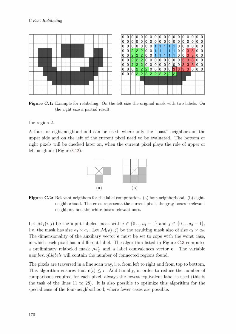
C Fast Relabeling
0 0 0 0 0 0 0 0 0 0 0 0 0 0 0 0 0 00 0 0 0 0 0 0 0 0 0 0 0 0 0 0 0 0 00 0 0 0 0 0 0 0 0 0 0 0 0 0 0 0 0 00 0 0 0 0 0 0 0 0 0 0 0 0 0 0 0 0 00 0 0 0 0 0 0 0 0 0 0 0 0 0 0 0 0 00 0 0 0 0 0 0 0 0 0 0 0 0 0 0 0 0 00 0 0 0 0 0 0 0 0 0 0 0 0 0 0 0 0 00 0 0 0 0 0 0 0 0 0 0 0 0 0 0 0 0 00 0 0 0 0 0 0 0 0 0 0 0
1 1 1 1 11 1 1 1 11 1 1 1 1
2 2 22 2 22 2 22 2 2
2 2 22 2 2 2 2 2 2 2
3 33 3
3 3 33 3 33 33 3
2
Figure C.1: Example for relabeling. On the left size the original mask with two labels. Onthe right size a partial result.
the region 2.
A four- or eight-neighborhood can be used, where only the “past” neighbors on the
upper side and on the left of the current pixel need to be evaluated. The bottom or
right pixels will be checked later on, when the current pixel plays the role of upper or
left neighbor (Figure C.2).
(a) (b)
Figure C.2: Relevant neighbors for the label computation. (a) four-neighborhood. (b) eight-neighborhood. The cross represents the current pixel, the gray boxes irrelevantneighbors, and the white boxes relevant ones.
Let MI(i, j) be the input labeled mask with i ∈ 0 . . . a1 − 1 and j ∈ 0 . . . a2 − 1,i. e. the mask has size a1 × a2. Let MO(i, j) be the resulting mask also of size a1 × a2.
The dimensionality of the auxiliary vector e must be set to cope with the worst case,
in which each pixel has a different label. The algorithm listed in Figure C.3 computes
a preliminary relabeled mask M′O and a label equivalences vector e. The variable
number of labels will contain the number of connected regions found.
The pixels are traversed in a line scan way, i. e. from left to right and from top to bottom.
This algorithm ensures that e(i) ≤ i. Additionally, in order to reduce the number of
comparisons required for each pixel, always the lowest equivalent label is used (this is
the task of the lines 11 to 28). It is also possible to optimize this algorithm for the
special case of the four-neighborhood, where fewer cases are possible.
170

Algorithm: Preliminary Relabeling
1: current label := 0
2: β := a1a2 − 1
3: initialize the auxiliary vector e of size a1a2 with β
4: for all pixels (i, j) in the mask MI do
5: if no past neighbors share the label with the pixel then
6: assign a new label: M′O(i, j) := current label
7: current label :=current label+1.
8: else if only one past neighbor pixel (k, l) shares the same label then
9: M′O(i, j) := M′
O(k, l)
10: else if n neighbor pixels (kp, lp), p = 0, 1, . . . n− 1, n ≥ 2 share the same label
then
11: let l1 := M′O(kn−1, ln−1)
12: while n ≥ 2 do
13: let l2 := M′O(kn−2, ln−2)
14: while e(l1) 6= β do
15: l1 := e(l1)
16: end while
17: while e(l2) 6= β do
18: l2 := e(l2)
19: end while
20: if l1 < l2 then
21: e(l2) := l122: else if l1 > l2 then
23: e(l1) := l224: l1 := l225: end if
26: n := n− 1
27: end while
28: M′O(i, j) := l1
29: end if
30: end for
31: number of labels := current label
Figure C.3: Efficient mask relabeling. Computation of preliminary mask and equivalencesvector
171

C Fast Relabeling
The algorithm in Figure C.4 computes the final maskMO using as input the preliminary
mask M′O and the equivalences vector e computed previously. The first for-loop ensures
that each equivalence label corresponds to the smallest possible one. The second loop
renumbers the labels to be continously assigned. At last, the third loop builds the final
relabeled mask.
Algorithm: Relabeling
1: for i from 0 to number of labels do
2: if e(i) 6= β then
3: while e(e(i)) 6= β do
4: e(i) := e(e(i))
5: end while
6: end if
7: end for
8: last label := 1
9: for i from 0 to number of labels do
10: if e(i) = β then
11: e(i) :=last label
12: last label := last label + 1
13: else
14: e(i) := e(e(i))
15: end if
16: end for
17: e(β) := 0
18: for all pixel (i, j) in MO do
19: MO(i, j) := e(M′O(i, j))
20: end for
Figure C.4: Efficient mask relabeling. Computation of the final mask
172

Appendix D
Images for Evaluation of
Image-Based Segmentation
Five images were used for the evaluation of the image-based algorithms. The original
images are depiced on the left side, and the manual reference segmentation on the right
side. Each gray-level corresponds to one object level.
173

D Images for Evaluation of Image-Based Segmentation
174

Appendix E
Test-set P17
These images belong to an object recognition system exhibited in the Heinz-Nixdorf
MuseusForum in Paderborn, Germany. The visitors take an object from the set, and
present them to the system. For several reasons, the use of a background-colored glove
is in such an application undesirable; among others, the users tend to be hesitant to
wear the glove, and prefer to continue to the next exhibit; for hygienic reasons, the
gloves have to be frequently replaced, and it has to be ensured that there is always a
black glove near the object recognition. The non-intrusive object presentation is more
comfortable.
p1 p2 p3 p4
p5 p6 p7 p8
p9 p10 p11 p12
175

E Test-set P17
p13 p14 p15 p16
p17
This test set contains images of 17 soft-toys taken with a camera Phillips ToUCam
Pro. The image quality is sufficient to allow the recognition of objects. However, the
relatively low contrast of the camera forces to adapt its parameters (shutter speed and
gain) to the brightness of each object. Otherwise, white objects would saturate the
camera while dark objects would be almost indistinguishable from the background.
The optimization of figure/ground and hand/object segmentations in Chapter 5 used
the following reference images, with their respective hand segmented reference masks.
176

Appendix F
Test-sets S25 and S200
Test-set S25
s1 s2 s3 s4 s5
s6 s7 s8 s9 s10
s11 s12 s13 s14 s15
s16 s17 s18 s19 s20
s21 s22 s23 s24 s25177

F Test-sets S25 and S200
Test-set S200 (a subset)
178

Appendix G
Computation of the Hessian Matrix
Several operations in traditional and modern image processing require the computation
of the Hessian matrix H, already defined in (6.13) as
H(x, y) =
[∂2fI(x,y)
∂x2
∂2fI(x,y)∂x∂y
∂2fI(x,y)∂x∂y
∂2fI(x,y)∂y2
]
with the pixel position p = [x, y]T and the functional image representation fI .
The Laplacian of the image, for example, is equal to the trace of this matrix. Addition-
ally, some definitions for the cornerness or edgeness of a pixel can be defined in terms
of the eigenvalues and eigenvectors of H [HS88].
Traditionally, the components of this matrix are approximated with simple differences
of neighbor pixels. For instance, if the functional representation of the image fI(x, y)
is approximated with a matrix representation I with components ix,y, then the second
derivatives can be approximated with following equations:
∂2fI(x, y)
∂x2≈ ix−1,y − 2ix,y + ix+1,y
∂2fI(x, y)
∂y2≈ ix,y−1 − 2ix,y + ix,y+1
∂2fI(x, y)
∂x∂y≈ ix−1,y−1 + ix+1,y+1 − ix−1,y+1 + ix+1,y−1
(G.1)
Using these approximations, the computation of each component of the Hessian matrix
for all pixels of a gray-valued image can be interpreted as the convolution of that image
with the kernels depicted in Figure G.1.
These computations are simple and can be performed in a fast and efficient way. How-
ever, this representation has proven to be unreliable for a stable computation of the
eigenvalues and eigenvectors. This appendix introduces a novel set of linear kernels
especially designed to be stable in the last situation.
179

G Computation of the Hessian Matrix
1 −2 1
1
−2
1
1 −1
−1 1
00 0
0
0
(a) (b) (c)
Figure G.1: Classic linear kernels used to compute the Hessian coefficients: (a) ∂2fI(x,y)∂x2 ,
(b) ∂2fI(x,y)∂y2 , (c) ∂2fI(x,y)
∂x∂y .
Let fI(x, y) be approximated at the location (x, y) with a second order Taylor polynomial
fI(x + ∆x, y + ∆y) =[∆x ∆y
]H
[∆x
∆y
]+ gT
[∆x
∆y
]+ fI(x, y) (G.2)
with H the Hessian matrix defined in (6.13) and g the gradient of the image at the
position (x, y). (G.2) can be rewritten as:
fI(x + ∆x, y + ∆y) = a(∆x)2 + b∆x∆y + c(∆y)2 + d∆x + e∆y + k (G.3)
It can be easily proven that it holds:
a =∂2fI(x, y)
∂x2
b = 2∂2fI(x, y)
∂x∂y
c =∂2fI(x, y)
∂y2
(G.4)
The basic idea is to compute the terms a, b and c relying on a quadratic approximaton
of the image that considers for each pixel the information within a 3× 3 neighborhood.
Let the polynomial have zero error at (x, y), i. e. k = fI(x, y). There are eight neighbor
values to support the computation of the remaining five coefficients. Let |∆x| = |∆y| =1. The following eight equations can be derived from (G.3):
ix−1,y−1 − k = a + b + c− d− e
ix,y−1 − k = c− e
ix+1,y−1 − k = a− b + c + d− e
ix−1,y − k = a− d
ix+1,y − k = a + d
ix−1,y+1 − k = a− b + c− d + e
ix,y+1 − k = c + e
ix+1,y+1 − k = a + b + c + d + e
(G.5)
180
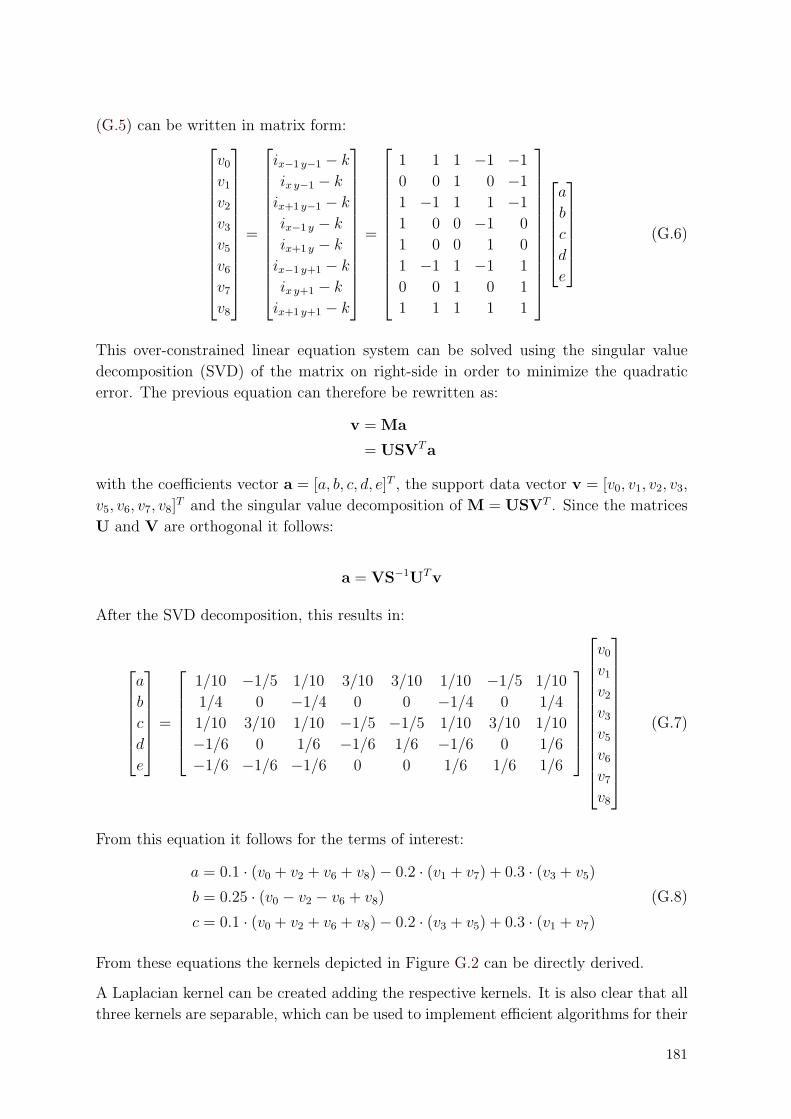
(G.5) can be written in matrix form:
v0
v1
v2
v3
v5
v6
v7
v8
=
ix−1 y−1 − k
ix y−1 − k
ix+1 y−1 − k
ix−1 y − k
ix+1 y − k
ix−1 y+1 − k
ix y+1 − k
ix+1 y+1 − k
=
1 1 1 −1 −1
0 0 1 0 −1
1 −1 1 1 −1
1 0 0 −1 0
1 0 0 1 0
1 −1 1 −1 1
0 0 1 0 1
1 1 1 1 1
a
b
c
d
e
(G.6)
This over-constrained linear equation system can be solved using the singular value
decomposition (SVD) of the matrix on right-side in order to minimize the quadratic
error. The previous equation can therefore be rewritten as:
v = Ma
= USVTa
with the coefficients vector a = [a, b, c, d, e]T , the support data vector v = [v0, v1, v2, v3,
v5, v6, v7, v8]T and the singular value decomposition of M = USVT . Since the matrices
U and V are orthogonal it follows:
a = VS−1UTv
After the SVD decomposition, this results in:
a
b
c
d
e
=
1/10 −1/5 1/10 3/10 3/10 1/10 −1/5 1/10
1/4 0 −1/4 0 0 −1/4 0 1/4
1/10 3/10 1/10 −1/5 −1/5 1/10 3/10 1/10
−1/6 0 1/6 −1/6 1/6 −1/6 0 1/6
−1/6 −1/6 −1/6 0 0 1/6 1/6 1/6
v0
v1
v2
v3
v5
v6
v7
v8
(G.7)
From this equation it follows for the terms of interest:
a = 0.1 · (v0 + v2 + v6 + v8)− 0.2 · (v1 + v7) + 0.3 · (v3 + v5)
b = 0.25 · (v0 − v2 − v6 + v8)
c = 0.1 · (v0 + v2 + v6 + v8)− 0.2 · (v3 + v5) + 0.3 · (v1 + v7)
(G.8)
From these equations the kernels depicted in Figure G.2 can be directly derived.
A Laplacian kernel can be created adding the respective kernels. It is also clear that all
three kernels are separable, which can be used to implement efficient algorithms for their
181

G Computation of the Hessian Matrix
(a) (b) (c)
0.1 0.1
0.1
−0.60.3 0.3
−0.2
0.1
−0.2 −0.2
0.3
−1/8 1/8
00 0
0
0
−0.2
0.1
0.1
0.1 0.1
−0.6
0.3
1/8 −1/8
Figure G.2: Kernels derived from (G.6). (a) ∂2fI(x,y)∂x2 , (b) ∂2fI(x,y)
∂y2 , (c) ∂2fI(x,y)∂x∂y .
computations. The separation [0.1, 0.3, 0.1][1,−2, 1]T is composed by the classic kernel
on the direction of interest, while the orthogonal component corresponds to a low-pass
filter. The classic kernel and the derived one for ∂2fI(x,y)∂x∂y
differ only in a normalization
factor.
The gradient kernels can also be derived from equations (G.2), (G.3) and (G.7):
∂fI(x, y)
∂x= d =
(v2 + v5 + v8)− (v0 + v3 + v6)
6∂fI(x, y)
∂y= e =
(v0 + v3 + v6)− (v2 + v5 + v8)
6
(G.9)
which yield the normalized Prewitt kernels depicted in Figure G.3. They are also sep-
arable and representable as the outer-product of the classic kernels with an orthogonal
low-pass component.
0−1/6 1/6
0−1/6 1/6
−1/6
0
1/6
−1/6
0
1/6
−1/6
0
1/6
(a) (b)
0−1/6 1/6
Figure G.3: Gradient kernels derived from (G.9). (a) ∂fI(x,y)∂x , (b) ∂fI(x,y)
∂y .
The same procedure can be applied if the condition of zero error for the central pixel is
relaxed. In this case, nine equations are used to seek six unknowns:
u0
u1
u2
u3
u5
u6
u7
u8
u9
=
ix−1 y−1
ix y−1
ix+1 y−1
ix−1 y
ix y
ix+1 y
ix−1 y+1
ix y+1
ix+1 y+1
=
1 1 1 −1 −1 1
0 0 1 0 −1 1
1 −1 1 1 −1 1
1 0 0 −1 0 1
0 0 0 0 0 1
1 0 0 1 0 1
1 −1 1 −1 1 1
0 0 1 0 1 1
1 1 1 1 1 1
a
b
c
d
e
k
(G.10)
182

The gradient kernels and the b term are as in (G.8) and (G.9), but the Hessian coefficients
change to
a =1
6· (u0 + u2 + u3 + u5 + u6 + u8)−
1
3· (u1 + u4 + u7)
c =1
6· (u0 + u1 + u2 + u6 + u7 + u8)−
1
3· (u3 + u4 + u5)
(G.11)
which are depicted in Figure G.4. Again, they are separable with the classical Hessian
kernels as one component, but now the low-pass component corresponds to the same
rectangular filter used in the computation of the gradients.
(a)
1/6 1/6
1/6
−1/31/6 1/6
−1/3
−1/3 −1/3
−1/3
1/6 1/6 1/6
−1/3
1/6
1/6 1/6 1/6
(b)
Figure G.4: Kernels derived from (G.11). (a) ∂2fI(x,y)∂x2 , (b) ∂2fI(x,y)
∂y2 ,
The approximated function at [∆x, ∆y] = [0, 0] is
f =5
9u4 +
2
9(u1 + u3 + u5 + u7)−
1
9(u0 + u2 + u6 + u8) (G.12)
183

G Computation of the Hessian Matrix
184
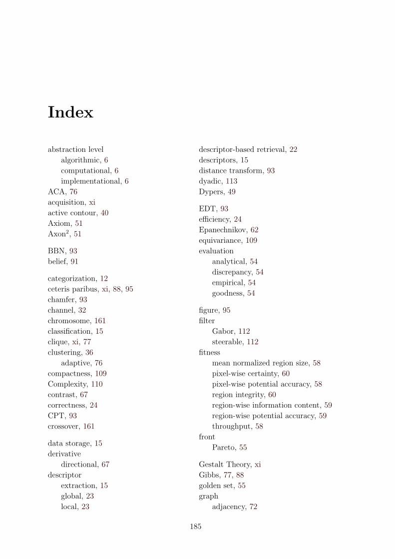
Index
abstraction level
algorithmic, 6
computational, 6
implementational, 6
ACA, 76
acquisition, xi
active contour, 40
Axiom, 51
Axon2, 51
BBN, 93
belief, 91
categorization, 12
ceteris paribus, xi, 88, 95
chamfer, 93
channel, 32
chromosome, 161
classification, 15
clique, xi, 77
clustering, 36
adaptive, 76
compactness, 109
Complexity, 110
contrast, 67
correctness, 24
CPT, 93
crossover, 161
data storage, 15
derivative
directional, 67
descriptor
extraction, 15
global, 23
local, 23
descriptor-based retrieval, 22
descriptors, 15
distance transform, 93
dyadic, 113
Dypers, 49
EDT, 93
efficiency, 24
Epanechnikov, 62
equivariance, 109
evaluation
analytical, 54
discrepancy, 54
empirical, 54
goodness, 54
figure, 95
filter
Gabor, 112
steerable, 112
fitness
mean normalized region size, 58
pixel-wise certainty, 60
pixel-wise potential accuracy, 58
region integrity, 60
region-wise information content, 59
region-wise potential accuracy, 59
throughput, 58
front
Pareto, 55
Gestalt Theory, xi
Gibbs, 77, 88
golden set, 55
graph
adjacency, 72
185
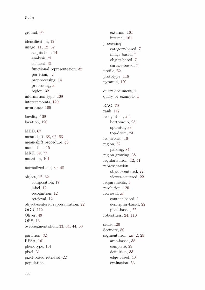
Index
ground, 95
identification, 12
image, 11, 12, 32
acquisition, 14
analysis, xi
element, 31
functional representation, 32
partition, 32
preprocessing, 14
processing, xi
region, 32
information type, 109
interest points, 120
invariance, 109
locality, 109
location, 120
MDD, 67
mean-shift, 38, 62, 63
mean-shift procedure, 63
monolithic, 15
MRF, 39, 77
mutation, 161
normalized cut, 39, 48
object, 12, 32
composition, 17
label, 12
recognition, 12
retrieval, 12
object-centered representation, 22
OGD, 112
Oliver, 49
ORS, 13
over-segmentation, 33, 34, 44, 60
partition, 32
PESA, 161
phenotype, 161
pixel, 31
pixel-based retrieval, 22
population
external, 161
internal, 161
processing
category-based, 7
image-based, 7
object-based, 7
surface-based, 7
profile, 62
prototype, 116
pyramid, 120
query document, 1
query-by-example, 1
RAG, 70
rank, 117
recognition, xii
bottom-up, 23
operator, 33
top-down, 23
recurrence, 16
region, 32
parsing, 84
region growing, 38
regularization, 12, 41
representation
object-centered, 22
viewer-centered, 22
requirements, 5
resolution, 120
retrieval, xi
content-based, 1
descriptor-based, 22
pixel-based, 22
robustness, 24, 110
scale, 120
Seemore, 50
segmentation, xii, 2, 29
area-based, 38
complete, 29
definition, 33
edge-based, 40
evaluation, 53
186

Index
feature-space-based, 36
hybrid, 41
image-based, 34
image-domain-based, 38
object recognition, 49
object-based, 47
partial, 29
surface-based, 44
sensitivity, 109
sequential, 15
Specificity, 109
split-and-merge, 38
steerability, 112
stimulus
distal, 3
proximal, 3
template matching, 47
train
BBN, 97
under-segmentation, 33, 60
user interface, 15
verification, 15
viewer-centered representation, 22
vision
ill-posed, 11
watershed, 40, 65
wavelet, 112
well-posed problem, 11
187

Index
188

Curriculum Vitae
Personal Data
Surname, name: Alvarado Moya, Jose Pablo
Date of Birth: 30.09.1969, San Jose, Costa Rica
Nationality: Costa-Rican
School
1975 – 1980 Escuela Jesus Jimenez
Cartago, Costa Rica
1981 – 1986 Colegio de San Luis Gonzaga
Cartago, Costa Rica
University studies
01/1987 – 12/1991 Bachillerato en Ingenierıa Electronica,
Instituto Tecnologico de Costa Rica
10/1994 – 10/1998 DAAD Scholarship
German Diplom-Ingenieur in Electrical Engineering,
RWTH Aachen University
Professional Experience
1992 – 1994 Data Processing Center, ITCR
1993 – 1994 Fundatec, Costa Rica
1999 – 2004 Research Assistant
Chair of Technical Computer Science,
RWTH Aachen University
Aachen, 02.07.2004
